CMCL 2013

Cognitive Modeling and Computational Linguistics

Proceedings of the Workshop

August 8, 2013Sofia, Bulgaria

Production and Manufacturing byOmnipress, Inc.2600 Anderson StreetMadison, WI 53704 USA

c©2013 The Association for Computational Linguistics

Order copies of this and other ACL proceedings from:

Association for Computational Linguistics (ACL)209 N. Eighth StreetStroudsburg, PA 18360USATel: +1-570-476-8006Fax: +1-570-476-0860acl@aclweb.org

ISBN 978-1-937284-61-9

ii

Introduction

The papers in these precedings were presented at the Fourth Annual Workshop on Cognitive Modelingand Computational Linguistics (CMCL), held in Sofia, Bulgaria on 8 August 2013, in conjunction withthe Annual Meeting of the Association for Computational Linguistics (CMCL). The CMCL workshopseries provides a unique venue for work on the interdisciplinary field of computational psycholinguistics,described by ACL Lifetime Achievement Award recipient Martin Kay as “build[ing] models of languagethat reflect in some interesting way on the ways in which people use language”. This workshop seriesbuilds on the tradition of earlier meetings, including the 1997 computational psycholinguistics meetingat the 1997 Annual Conference of the Cognitive Science Society in Berkeley, CA, and on the IncrementalParsing workshop held in 2004 at the Annual Meeting of the Association for Computational Linguistics.

We received nineteen submissions to the 2013 CMCL workshop, of which we accepted eleven for finalappearance in the conference program. The overall quality of workshop submissions was extremelystrong, reflecting the perennially increasing quality of work in this field. This year we also expandedthe workshop by including keynote talks from two invited speakers, Dr Sharon Goldwater from theUniversity of Edinburgh and Professor Rick Lewis from the University of Michigan, leading researchersin computational psycholinguistics. We would like to thank all submitting authors for allowing usto consider their work, the program committee for an outstanding job in reviewing and discussingsubmissions, and of course our invited speakers. We also gratefully acknowledge funding from theCognitive Science Society for the Best Student Paper award, and to the Cluster of Excellence on“Multimodal Computing and Interaction” for assisting with funding of our invited speakers. Many thanksto all of you for your continued support of this workshop.

Vera Demberg and Roger Levy

iii

Organizers:

Vera Demberg, Saarland UniversityRoger Levy, UC San Diego

Program Committee:

Afra Alishahi, Tilburg UniversityKlinton Bicknell, UC San DiegoMatthew Crocker, Saarland UniversityBrian Dillon, University of MassachussettsAfsaneh Fazly, University of TorontoNaomi Feldman, University of MarylandMichael C. Frank, Stanford UniversityStefan Frank, Radboud University NijmegenSharon Goldwater, Edinburgh UniversityNoah Goodman, Stanford UniversityJohn T. Hale, Cornell UniversityT. Florian Jaeger, University of RochesterFrank Keller, University of EdinburghJeffrey Heinz, University of DelawareRichard L. Lewis, University of MichiganBrian Edmond Murphy, Carnegie Mellon UniversityTimothy John O’Donnell, Massachusetts Institute of TechnologySebastian Padó, University of HeidelbergUlrike Padó, Hochschule für Technik, StuttgartSteven Piantadosi, University of RochesterDavid Reitter, Penn State UniversityWilliam Schuler, The Ohio State UniversityNathaniel Smith, University of EdinburghEd Stabler, UC Los AngelesWhitney Tabor, University of Connecticut and Haskins Laboratories

Invited Speakers:

Sharon Goldwater, University of EdinburghRick Lewis, University of Michigan

v

Table of Contents

Why is English so easy to segment?Abdellah Fourtassi, Benjamin Börschinger, Mark Johnson and Emmanuel Dupoux . . . . . . . . . . . . . 1

A model of generalization in distributional learning of phonetic categoriesBozena Pajak, Klinton Bicknell and Roger Levy . . . . . . . . . . . . . . . . . . . . . . . . . . . . . . . . . . . . . . . . . . . 11

Learning non-concatenative morphologyMichelle Fullwood and Tim O’Donnell . . . . . . . . . . . . . . . . . . . . . . . . . . . . . . . . . . . . . . . . . . . . . . . . . . . 21

Statistical Representation of Grammaticality Judgements: the Limits of N-Gram ModelsAlexander Clark, Gianluca Giorgolo and Shalom Lappin. . . . . . . . . . . . . . . . . . . . . . . . . . . . . . . . . . . .28

An Analysis of Memory-based Processing Costs using Incremental Deep Syntactic Dependency ParsingMarten van Schijndel, Luan Nguyen and William Schuler . . . . . . . . . . . . . . . . . . . . . . . . . . . . . . . . . . . 37

Computational simulations of second language construction learningYevgen Matusevych, Afra Alishahi and Ad Backus . . . . . . . . . . . . . . . . . . . . . . . . . . . . . . . . . . . . . . . . . 47

The semantic augmentation of a psycholinguistically-motivated syntactic formalismAsad Sayeed and Vera Demberg . . . . . . . . . . . . . . . . . . . . . . . . . . . . . . . . . . . . . . . . . . . . . . . . . . . . . . . . . . 57

Evaluating Neighbor Rank and Distance Measures as Predictors of Semantic PrimingGabriella Lapesa and Stefan Evert . . . . . . . . . . . . . . . . . . . . . . . . . . . . . . . . . . . . . . . . . . . . . . . . . . . . . . . . 66

Concreteness and Corpora: A Theoretical and Practical StudyFelix Hill, Douwe Kiela and Anna Korhonen . . . . . . . . . . . . . . . . . . . . . . . . . . . . . . . . . . . . . . . . . . . . . . 75

On the Information Conveyed by Discourse MarkersFatemeh Torabi Asr and Vera Demberg . . . . . . . . . . . . . . . . . . . . . . . . . . . . . . . . . . . . . . . . . . . . . . . . . . . 84

Incremental Grammar Induction from Child-Directed Dialogue UtterancesArash Eshghi, Julian Hough and Matthew Purver . . . . . . . . . . . . . . . . . . . . . . . . . . . . . . . . . . . . . . . . . . 94

vii

Workshop Program

Thursday, August 8th, 2013

8:25 Opening Remarks

8:30 Invited Talk by Sharon Goldwater

Session 1: Segmentation and Phonetics

09:30 Why is English so easy to segment?Abdellah Fourtassi, Benjamin Börschinger, Mark Johnson and Emmanuel Dupoux

10:00 A model of generalization in distributional learning of phonetic categoriesBozena Pajak, Klinton Bicknell and Roger Levy

10:30 Coffee break

Session 2: Syntax and Morphology

11:00 Learning non-concatenative morphologyMichelle Fullwood and Tim O’Donnell

11:30 Statistical Representation of Grammaticality Judgements: the Limits of N-GramModelsAlexander Clark, Gianluca Giorgolo and Shalom Lappin

12:00 An Analysis of Memory-based Processing Costs using Incremental Deep SyntacticDependency ParsingMarten van Schijndel, Luan Nguyen and William Schuler

12:30 Computational simulations of second language construction learningYevgen Matusevych, Afra Alishahi and Ad Backus

13:00 Lunch break

ix

Thursday, August 8th, 2013 (continued)

Session 3: Semantics

14:00 The semantic augmentation of a psycholinguistically-motivated syntactic formalismAsad Sayeed and Vera Demberg

14:30 Evaluating Neighbor Rank and Distance Measures as Predictors of Semantic PrimingGabriella Lapesa and Stefan Evert

15:00 Concreteness and Corpora: A Theoretical and Practical StudyFelix Hill, Douwe Kiela and Anna Korhonen

15:30 Coffee break

Session 4: Discourse and Dialog

16:00 On the Information Conveyed by Discourse MarkersFatemeh Torabi Asr and Vera Demberg

16:30 Incremental Grammar Induction from Child-Directed Dialogue UtterancesArash Eshghi, Julian Hough and Matthew Purver

17:00 Invited Talk by Rick Lewis

x

Proceedings of the Workshop on Cognitive Modeling and Computational Linguistics, pages 1–10,Sofia, Bulgaria, August 8, 2013. c©2013 Association for Computational Linguistics

Whyisenglishsoeasytosegment?

Abdellah Fourtassi1, Benjamin Borschinger2,3

Mark Johnson3 and Emmanuel Dupoux1

(1) Laboratoire de Sciences Cognitives et Psycholinguistique, ENS/EHESS/CNRS, Paris(2) Department of Computing, Macquarie University

(3) Department of Computational Linguistics, Heidelberg University{abdellah.fourtassi, emmanuel.dupoux}@gmail.com , {benjamin.borschinger, mark.johnson}@mq.edu.au

—

Abstract

Cross-linguistic studies on unsupervisedword segmentation have consistentlyshown that English is easier to segmentthan other languages. In this paper, wepropose an explanation of this findingbased on the notion of segmentationambiguity. We show that English has avery low segmentation ambiguity com-pared to Japanese and that this differencecorrelates with the segmentation perfor-mance in a unigram model. We suggestthat segmentation ambiguity is linkedto a trade-off between syllable structurecomplexity and word length distribution.

1 Introduction

During the course of language acquisition, in-fants must learn to segment words from continu-ous speech. Experimental studies show that theystart doing so from around 7.5 months of age(Jusczyk and Aslin, 1995). Further studies indi-cate that infants are sensitive to a number of wordboundary cues, like prosody (Jusczyk et al., 1999;Mattys et al., 1999), transition probabilities (Saf-fran et al., 1996; Pelucchi et al., 2009), phonotac-tics (Mattys et al., 2001), coarticulation (Johnsonand Jusczyk, 2001) and combine these cues withdifferent weights (Weiss et al., 2010).

Computational models of word segmentationhave played a major role in assessing the relevanceand reliability of different statistical cues presentin the speech input. Some of these models focusmainly on boundary detection, and assess differ-ent strategies to identify them (Christiansen et al.,1998; Xanthos, 2004; Swingley, 2005; Daland andPierrehumbert, 2011). Other models, sometimescalled lexicon-building algorithms, learn the lexi-con and the segmentation at the same time and useknowledge about the extracted lexicon to segment

novel utterances. State-of-the-art lexicon-buildingsegmentation algorithms are typically reported toyield better performance than word boundary de-tection algorithms (Brent, 1999; Venkataraman,2001; Batchelder, 2002; Goldwater, 2007; John-son, 2008b; Fleck, 2008; Blanchard et al., 2010).

As seen in Table 1, however, the performancevaries considerably across languages with Englishwinning by a high margin. This raises a general-izability issue for NLP applications, but also forthe modeling of language acquisition since, obvi-ously, it is not the case that in some languages,infants fail to acquire an adult lexicon. Are theseperformance differences only due to the fact thatthe algorithms might be optimized for English? Ordo they also reflect some intrinsic linguistic differ-ences between languages?

Lang. F-score Model ReferenceEnglish 0.89 AG Johnson (2009)Chinese 0.77 AG Johnson (2010)Spanish 0.58 DP Bigram Fleck (2008)Arabic 0.56 WordEnds Fleck (2008)Sesotho 0.55 AG Johnson (2008)Japanese 0.55 BootLex Batchelder (2002)French 0.54 NGS-u Boruta (2011)

Table 1: State-of-the-art unsupervised segmentation scoresfor eight languages.

The aim of the present work is to understandwhy English usually scores better than other lan-guages, as far as unsupervised segmentation isconcerned. As a comparison point, we choseJapanese because it is among the languages thathave given the poorest word segmentation scores.In fact, Boruta et al. (2011) found an F-scorearound 0.41 using both Brent (1999)’s MBDP-1and Venkataraman (2001)’s NGS-u models, andBatchelder (2002) found an F-score that goesfrom 0.40 to 0.55 depending on the corpus used.Japanese also differs typologically from Englishalong several phonological dimensions such as

1

number of syllabic types, phonotactic constraintsand rhythmic structure. Although most lexicon-building segmentation algorithms do not attemptto model these dimensions, they still might be rel-evant to speech segmentation and help explain theperformance difference.

The structure of the paper is as follows. First,we present the class of lexical-building segmen-tation algorithm that we use in this paper (Adap-tor Grammar), and our English and Japanese cor-pora. We then present data replicating the basicfinding that segmentation performance is better forEnglish than for Japanese. We then explore the hy-pothesis that this finding is due to an intrinsic dif-ference in segmentation ambiguity in the two lan-guages, and suggest that the source of this differ-ence rests in the structure of the phonological lexi-con in the two languages. Finally, we use these in-sights to try and reduce the gap between Japaneseand English segmentation through a modificationof the Unigram model where multiple linguisticlevels are learned jointly.

2 Computational Framework andCorpora

2.1 Adaptor GrammarIn this study, we use the Adaptor Grammar frame-work (Johnson et al., 2007) to test different mod-els of word segmentation on English and JapaneseCorpora. This framework makes it possible toexpress a class of hierarchical non-parametricBayesian models using an extension of probabilis-tic context-free grammars called Adaptor Gram-mar (AG). It allows one to easily define modelsthat incorporate different assumptions about lin-guistic structure and is therefore a useful practicaltool for exploring different hypotheses about wordsegmentation (Johnson, 2008b; Johnson, 2008a;Johnson et al., 2010; Borschinger et al., 2012).

For mathematical details and a description ofthe inference procedure for AGs, we refer thereader to Johnson et al. (2007). Briefly, AG usesthe non-parametric Pitman-Yor-Process (Pitmanand Yor, 1997) which, as in Minimum Descrip-tion lengths models, finds a compact representa-tion of the input by re-using frequent structures(here, words).

2.2 CorporaIn the present study, we used both Child Di-rected Speech (CDS) and Adult Directed Speech

(ADS) corpora. English CDS was derived fromthe Bernstein-Ratner corpus (Bernstein-Ratner,1987), which consists in transcribed verbal inter-action of parents with nine children between 1and 2 years of age. We used the 9,790 utter-ances that were phonemically transcribed by Brentand Cartwright (1996). Japanese CDS consists inthe first 10, 000 utterances of the Hamasaki cor-pus (Hamasaki, 2002). It provides a phonemictranscript of spontaneous speech to a single childcollected from when the child was 2 up to whenit was 3.5 years old. Both CDS corpora are avail-able from the CHILDES database (MacWhinney,2000).

As for English ADS, we used the first 10,000utterances of the Buckeye Speech Corpus (Pitt etal., 2007) which consists in spontaneous conver-sations with 40 speakers in American English. Tomake it comparable to the other corpora in thispaper, we only used the idealized phonemic tran-scription. Finally, for Japanese ADS, we usedthe first 10,000 utterances of a phonemic tran-scription of the Corpus of Spontaneous Japanese(Maekawa et al., 2000). It consists of recordedspontaneous conversations, or public speeches indifferent fields ranging from engineering to hu-manities. For each corpus, we present elementarystatistics in Table 2.

3 Unsupervised segmentation with theUnigram Model

3.1 SetupIn this experiment we used the Adaptor Gram-mar framework to implement a Unigram model ofword segmentation (Johnson et al., 2007). Thismodel has been shown to be equivalent to the orig-inal MBDP-1 segmentation model (see Goldwater(2007)). The model is defined as:

—Utterance→Word+

Word→ Phoneme+

—In the AG framework, an underlined non-

terminal indicates that this non-terminal isadapted, i.e. that the AG will cache (and learnprobabilities for) entire sub-trees rooted in thisnon-terminal. Here, Word is the only unit that themodel effectively learns, and there are no depen-dencies between the words to be learned. Thisgrammar states that an utterance must be analyzedin terms of one or more Words, where a Word is a

2

Corpus Child Directed Speech Adult Directed Speech

— English Japanese English JapaneseTokens— Utterances 9, 790 10, 000 10, 000 10, 000— Words 33, 399 27, 362 57, 185 87, 156— Phonemes 95, 809 108, 427 183, 196 289, 264Types— Words 1, 321 2, 389 3, 708 4, 206— Phonemes 50 30 44 25Average Lengths— Words per utterance 3.41 2.74 5.72 8.72— Phonemes per utterance 9.79 10.84 18.32 28.93— Phonemes per word 2.87 3.96 3.20 3.32

Table 2 : Characteristics of phonemically transcribed corpora

sequence of Phonemes.We ran the model twice on each corpus for

2,000 iterations with hyper-parameter samplingand we collected samples throughout the process,following the methodology of Johnson and Gold-water (2009)1. For evaluation, we performed theirMinimum Bayes Risk decoding using the col-lected samples to get a single score.

3.2 Evaluation

For the evaluation, we used the same measures asBrent (1999), Venkataraman (2001) and Goldwa-ter (2007), namely token Precision (P), Recall (R)and F-score (F). Precision is defined as the num-ber of correct word tokens found out of all tokensposited. Recall is the number of correct word to-kens found out of all tokens in the gold standard.The F-score is defined as the harmonic mean ofPrecision and Recall , F = 2∗P∗R

P+R .We will refer to these scores as the segmentation

scores. In addition, we define similar measures forword boundaries and word types in the lexicon.

3.3 Results and discussion

The results are shown in Table 3. As expected,the model yields substantially better scores in En-glish than Japanese, for both CDS and ADS. Inaddition, we found that in both languages, ADSyields slightly worse results than CDS. This is tobe expected because ADS uses between 60% and300% longer utterances than CDS, and as a resultpresents the learner with a more difficult segmen-tation problem. Moreover, ADS includes between

1We used incremental initialization

70% and 280% more word types than CDS, mak-ing it a more difficult lexical learning problem.Note, however, that despite these large differencesin corpus statistics, the difference in segmentationperformance between ADS and CDS are smallcompared to the differences between Japanese andEnglish.

An error analysis on English data shows thatmost errors come from the Unigram model mistak-ing high frequency collocations for single words(see also Goldwater (2007)). This leads to anunder-segmentation of chunks like “a boy” or “isit” 2. Yet, the model also tends to break off fre-quent morphological affixes, especially “-ing” and“-s” , leading to an over-segmentation of wordslike “talk ing” or “black s”.

Similarly, Japanese data shows both over-and under-segmentation errors. However, over-segmentation is more severe than for English, asit does not only affect affixes, but surfaces asbreaking apart multi-syllabic words. In addition,Japanese segmentation faces another kind of er-ror which acts across word boundaries. For exam-ple, “ni kashite” is segmented as “nika shite” and“nurete inakatta” as “nure tei na katta”. This leadsto an output lexicon that, on the one hand, allowsfor a more compact analysis of the corpus thanthe true lexicon: the number of word types dropsfrom 2,389 to 1,463 in CDS and from 4,206 to2,372 in ADS although the average token length –and consequently, overall number of tokens – doesnot change as dramatically, dropping from 3.96 to

2For ease of presentation, we use orthography to presentexamples although all experiments are run on phonemic tran-scripts.

3

— Child Directed Speech Adult Directed Speech

— English Japanese English Japanese

— F P R F P R F P R F P RSegmentation 0.77 0.76 0.77 0.55 0.51 0.61 0.69 0.66 0.73 0.50 0.48 0.52Boundaries 0.87 0.87 0.88 0.72 0.63 0.83 0.86 0.81 0.91 0.76 0.74 0.79Lexicon 0.62 0.65 0.59 0.33 0.43 0.26 0.41 0.48 0.36 0.30 0.42 0.23

Table 3 : Word segmentation scores of the Unigram model

3.31 for CDS and from 3.32 to 3.12 in ADS. Onthe other hand, however, most of the output lex-icon items are not valid Japanese words and thisleads to the bad lexicon F-scores. This, in turn,leads to the bad overall segmentation performance.

In brief, we have shown that, across two dif-ferent corpora, English yields consistently bettersegmentation results than Japanese for the Uni-gram model. This confirms and extends the resultsof Boruta et al. (2011) and Batchelder (2002). Itstrongly suggests that the difference is neither dueto a specific choice of model nor to particularitiesof the corpora, but reflects a fundamental propertyof these two languages.

In the following section, we introduce the no-tion of segmentation ambiguity, it to English andJapanese data, and show that it correlates with seg-mentation performance.

4 Intrinsic Segmentation Ambiguity

Lexicon-based segmentation algorithms likeMBDP-1, NGS-u and the AG Unigram modellearn the lexicon and the segmentation at thesame time. This makes it difficult, in case ofpoor performance, to see whether the problemcomes from the intrinsic segmentability of thelanguage or from the quality of the extractedlexicon. Our claim is that Japanese is intrinsicallymore difficult to segment than English, even whena good lexicon is already assumed. We explorethis hypothesis by studying segmentation alone,assuming a perfect (Gold) lexicon.

4.1 Segmentation ambiguity

Without any information, a string of N phonemescould be segmented in 2N−1 ways. When a lexi-con is provided, the set of possible segmentationsis reduced to a smaller number. To illustrate this,suppose we have to segment the input utterance:

/ay s k r iy m/ 3, and that the lexicon contains thefollowing words : /ay/ (I), /s k r iy m/ (scream),/ay s/ (ice), /k r iy m/ (cream). Only two segmen-tations are possible : /ay skriym/ (I scream) and/ays kriym/ (ice cream).

We are interested in the ambiguity generated bythe different possible parses that result from such asupervised segmentation. In order to quantify thisidea in general, we define a Normalized Segmenta-

tion Entropy. To do this, we need to assign a prob-ability to every possible segmentation. To this end,we use a unigram model where the probability of alexical item is its normalized frequency in the cor-pus and the probability of a parse is the productof the probabilities of its terms. In order to obtaina measure that does not depend on the utterancelength, we normalize by the number of possibleboundaries in the utterance. So for an utterance oflength N , the Normalized Segmentation Entropy(NSE) is computed using Shannon formula (Shan-non, 1948) as follows:

—

NSE = −�

i Pilog2(Pi)/(N − 1)—

where Pi is the probability of the parse i .For CDS data we found Normalized Segmen-

tation Entropies of 0.0021 bits for English and0.0156 bits for Japanese. In ADS data wefound similar results with 0.0032 bits for Englishand 0.0275 bits for Japanese. This means thatJapanese needs between 7 and 8 times more bitsthan English to encode segmentation information.This is a very large difference, which is of thesame magnitude in CDS and ADS. These differ-ences clearly show that intrinsically, Japanese ismore ambiguous than English with regards to seg-mentation.

One can refine this analysis by distinguishingtwo sources of ambiguity: ambiguity across word

boundaries, as in ”ice cream / [ay s] [k r iy m]”3We use ARPABET notation to represent phonemic input.

4

Figure 1 : Correlation between Normalized Segmentation Entropy (in bits) and the segmentation F-score for CDS (left) andADS (Right)

vs ”I scream / [ay] [s k r iy m]”. And ambigu-ity within the lexicon, that occurs when a lexicalitem is composed of two or more sub-words (likein “Butterfly”).

Since we are mainly investigating lexicon-building models, it is important to measure the am-biguity within the lexicon itself, in the ideal casewhere this lexicon is perfect. To this end, we com-puted the average number of segmentations for alexicon item. For example, the word “butterfly”has two possible segmentations : the original word“butterfly” and a segmentation comprising the twosub-words : “butter” and “fly”. For English to-kens, we found an average of 1.039 in CDS and1.057 in ADS. For Japanese tokens, we found anaverage of 1.811 in CDS and 1.978 in ADS. En-glish’s averages are close to 1, indicating that itdoesn’t exhibit lexicon ambiguity. Japanese, how-ever, has averages close to 2 which means that lex-ical ambiguity is quite systematic in both CDS andADS.

4.2 Segmentation ambiguity and supervisedsegmentation

The intrinsic ambiguity in Japanese only showsthat a given sentence has multiple possible seg-mentations. What remains to be demonstrated isthat these multiple segmentations result in system-atic segmentation errors. To do this we proposea supervised segmentation algorithm that enumer-ates all possible segmentations of an utterancebased on the gold lexicon, and selects the segmen-tation with the highest probability. In CDS data,this algorithm yields a segmentation F-score equalto 0.99 for English and 0.95 for Japanese. In ADSwe find an F-score of 0.96 for English and 0.93 forJapanese. These results show that lexical informa-tion alone plus word frequency eliminates almost

all segmentation errors in English, especially forCDS. As for Japanese, even if the scores remainimpressively high, the lexicon alone is not suffi-cient to eliminate all the errors. In other words,even with a gold lexicon, English remains easierto segment than Japanese.

To quantify the link between segmentation en-tropy and segmentation errors, we binned the sen-tences of our corpus in 10 bins according to theNormalized Segmentation Entropy, and correlatethis with the average segmentation F-score foreach bin. As shown Figure 1, we found significantcorrelations: (R = −0.86, p < 0.001) for CDSand (R = −0.93, p < 0.001) for ADS, showingthat segmentation ambiguity has a strong effecteven on supervised segmentation scores. The cor-relation within language was also significant butonly in the Japanese data : R = −0.70 for CDSand R = −0.62 for ADS.

—Next, we explore one possible reason for this

structural difference between Japanese and En-glish, especially at the level of the lexicon.

4.3 Syllable structure and lexicalcomposition of Japanese and English

One of the most salient differences between En-glish and Japanese phonology concerns their syl-lable structure. This is illustrated in Figure 2(above), where we plotted the frequency of the dif-ferent syllabic structures of monosyllabic tokensin English and Japanese CDS. The statistics showthat English has a very rich syllabic compositionwhere a diversity of consonant clusters is allowed,whereas Japanese syllable structure is quite simpleand mostly composed of the default CV type. Thisdifference is bound to have an effect on the struc-ture of the lexicon. Indeed, Japanese has to use

5

Figure 2 : Trade-off between the complexity of syllable structure (above) and the word token length in terms of syllables(below) for English and Japanese CDS.

multisyllabic words in order to achieve a large sizelexicon, whereas, in principle, English could usemostly monosyllables. In Figure 2 (below) we dis-play the distribution of word length as measuredin syllables in the two languages for the CDS cor-pora. The English data is indeed mostly composedof mono-syllabic words whereas the Japanese oneis made of words of more varied lengths. Overall,we have documented a trade-off between the di-versity of syllable structure on the one hand, andthe diversity of word lengths on the other (see Ta-ble 4 for a summary of this tradeoff expressed interms of entropy).

— CDS ADS

— Eng. Jap. Eng. Jap.Syllable types 2.40 1.38 2.58 1.03Token lengths 0.62 2.04 0.99 1.69

Table 4 : Entropies of syllable types and token lengths interms of syllables (in bits)

We suggest that this trade-off is responsible forthe difference in the lexicon ambiguity across thetwo languages. Specifically, the combination ofa small number of syllable types and, as a conse-quence, the tendency for multi-syllabic word typesin Japanese makes it likely that a long word willbe composed of smaller ones. This cannot happenvery often in English, since most words are mono-syllabic, and words smaller than a syllable are notallowed.

5 Improving Japanese unsupervisedsegmentation

We showed in the previous section that ambigu-ity impacts segmentation even with a gold lexicon,mainly because the lexicon itself could be ambigu-ous. In an unsupervised segmentation setting, theproblem is worse because ambiguity within andacross word boundaries leads to a bad lexicon,which in turn results in more segmentation errors.In this section, we explore the possibility of miti-gating some of these negative consequences.

In section 3, we saw that when the Unigrammodel tries to learn Japanese words, it produces anoutput lexicon composed of both over- and under-segmented words in addition to words that re-sult from a segmentation across word boundaries.One way to address this is by learning multiplekinds of units jointly, rather than just words; in-deed, previous work has shown that richer mod-els with multiple levels improve segmentation forEnglish (Johnson, 2008a; Johnson and Goldwater,2009).

5.1 Two dependency levelsAs a first step, we will allow the model to notjust learn words but to also memorize sequences ofwords. Johnson (2008a) introduced these units as“collocations” but we choose to use the more neu-tral notion of level for reasons that become clearshortly. Concretely, the grammar is:

6

— CDS ADS

— English Japanese English Japanese

— F P R F P R F P R F P RLevel 1— Segmentation 0.81 0.77 0.86 0.42 0.33 0.55 0.70 0.63 0.78 0.42 0.35 0.50— Boundaries 0.91 0.84 0.98 0.63 0.47 0.96 0.86 0.76 0.98 0.73 0.61 0.90— Lexicon 0.64 0.79 0.54 0.18 0.55 0.10 0.36 0.56 0.26 0.15 0.68 0.08Level 2— Segmentation 0.33 0.45 0.26 0.59 0.65 0.53 0.50 0.60 0.43 0.45 0.54 0.38— Boundaries 0.56 0.98 0.40 0.71 0.87 0.60 0.76 0.95 0.64 0.73 0.92 0.60— Lexicon 0.36 0.25 0.59 0.47 0.44 0.49 0.46 0.38 0.56 0.43 0.37 0.50

Table 5 : Word segmentation scores of the two levels model

—Utterance→ level2+

level2→ level1+

level1→ Phoneme+

—We run this model under the same conditions

as the Unigram model but evaluate two differentsituations. The model has no inductive bias thatwould force it to equate level1 with words, ratherthan level2. Consequently, we evaluate the seg-mentation that is the result of taking there to be aboundary between every level1 constituent (Level1 in Table 5) and between every level2 constituent(Level 2 in Table 5 ). From these results , we seethat English data has better scores when the lowerlevel represents the Word unit and when the higherlevel captures regularities above the word. How-ever, Japanese data is best segmented when thehigher level is the Word unit and the lower levelcaptures sub-word regularities.

Level 1 generally tends to over-segment utter-ances as can be seen by comparing the BoundaryRecall and Precision scores (Goldwater, 2007). Infact when the Recall is much higher than the Pre-cision, we can say that the model has a tendencyto over-segment. Conversely, we see that Level 2tends to under-segment utterances as the Bound-ary Precision is higher than the Recall.

Over-segmentation at Level 1 seems to benefitEnglish since it counteracts the tendency of theUnigram model to cluster high frequency colloca-tions. As far as segmentation is concerned, thiseffect seems to outweigh the negative effect ofbreaking words apart (especially in CDS), as En-glish words are mostly monosyllabic.

For Japanese, under-segmentation at Level 2

seems to be slightly less harmful than over-segmentation at Level 1, as it prevents, to someextent, multi-syllabic words to be split. However,the scores are not very different from the ones wehad with the Unigram model and slightly worsefor the ADS. What seems to be missing is an inter-mediate level where over- and under-segmentationwould counteract one another.

5.2 Three dependency levels

We add a third dependency level to our model asfollows :

—Utterance→ level3+

level3→ level2+

level2→ level1+

level1→ Phoneme+

—As with the previous model, we test each of the

three levels as the word unit, the results are shownin Table 6.

Except for English CDS, all the corporahave their best scores with this intermediatelevel. Level 1 tends to over-segment Japaneseutterances into syllables and English utterancesinto morphemes. Level 3, however, tends tohighly under-segment both languages. EnglishCDS seems to be already under-segmented atLevel 2, very likely caused by the large numberof word collocations like ”is-it” and ”what-is”,an observation also made by Borschinger et al.(2012) using different English CDS corpora.English ADS is quantitatively more sensitive toover-segmentation than CDS mainly because ithas a richer morphological structure and relativelylonger words in terms of syllables (Table 4).

7

— CDS ADS

— English Japanese English Japanese

— F P R F P R F P R F P RLevel 1— Segmentation 0.79 0.74 0.85 0.27 0.20 0.41 0.35 0.28 0.48 0.37 0.30 0.47— Boundaries 0.89 0.81 0.99 0.56 0.39 0.99 0.68 0.52 0.99 0.70 0.57 0.93— Lexicon 0.58 0.76 0.46 0.10 0.47 0.05 0.13 0.39 0.07 0.10 0.70 0.05Level 2— Segmentation 0.49 0.60 0.42 0.70 0.70 0.70 0.77 0.76 0.79 0.60 0.65 0.55— Boundaries 0.71 0.97 0.56 0.81 0.82 0.81 0.90 0.88 0.92 0.81 0.90 0.74— Lexicon 0.51 0.41 0.64 0.53 0.59 0.47 0.58 0.69 0.50 0.51 0.57 0.46Level 3— Segmentation 0.18 0.31 0.12 0.39 0.53 0.30 0.43 0.55 0.36 0.28 0.42 0.21— Boundaries 0.26 0.99 0.15 0.46 0.93 0.31 0.71 0.98 0.55 0.59 0.96 0.43— Lexicon 0.17 0.10 0.38 0.32 0.25 0.41 0.37 0.28 0.51 0.27 0.20 0.42

Table 6 : Word segmentation scores of the three levels model

6 Conclusion

In this paper we identified a property of lan-guage, segmentation ambiguity, which we quan-tified through Normalized Segmentation Entropy.We showed that this quantity predicts performancein a supervised segmentation task.

With this tool we found that English was in-trinsically less ambiguous than Japanese, account-ing for the systematic difference found in this pa-per. More generally, we suspect that SegmentationAmbiguity would, to some extent, explain muchof the difference observed across languages (Ta-ble 1). Further work needs to be carried out to testthe robustness of this hypothesis on a larger scale.

We showed that allowing the system to learnat multiple levels of structure generally improvesperformance, and compensates partially for thenegative effect of segmentation ambiguity on un-supervised segmentation (where a bad lexicon am-plifies the effect of segmentation ambiguity). Yet,we end up with a situation where the best level ofstructure may not be the same across corpora orlanguages, which raises the question as to how todetermine which level is the correct lexical level,i.e., the level that can sustain successful grammat-ical and semantic learning. Further research isneeded to answer this question.

Generally speaking, ambiguity is a challenge inmany speech and language processing tasks: forexample part-of-speech tagging and word sense

disambiguation tackle lexical ambiguity, proba-bilistic parsing deals with syntactic ambiguity andspeech act interpretation deals with pragmatic am-biguities. However, to our knowledge, ambiguityhas rarely been considered as a serious problem inword segmentation tasks.

As we have shown, the lexicon-based approachdoes not completely solve the segmentation am-biguity problem since the lexicon itself could bemore or less ambiguous depending on the lan-guage. Evidently, however, infants in all lan-guages manage to overcome this ambiguity. It hasto be the case, therefore, that they solve this prob-lem through the use of alternative strategies, forinstance by relying on sub-lexical cues (see Jaroszand Johnson (2013)) or by incorporating semanticor syntactic constraints (Johnson et al., 2010). Itremains a major challenge to integrate these strate-gies within a common model that can learn withcomparable performance across typologically dis-tinct languages.

Acknowledgements

The research leading to these results has received fundingfrom the European Research Council (FP/2007-2013) / ERCGrant Agreement n. ERC-2011-AdG-295810 BOOTPHON,from the Agence Nationale pour la Recherche (ANR-2010-BLAN-1901-1 BOOTLANG, ANR-11-0001-02 PSL* andANR-10-LABX-0087) and the Fondation de France. Thisresearch was also supported under the Australian ResearchCouncil’s Discovery Projects funding scheme (project num-bers DP110102506 and DP110102593).

8

ReferencesEleanor Olds Batchelder. 2002. Bootstrapping the lex-

icon: A computational model of infant speech seg-mentation. Cognition, 83(2):167–206.

N. Bernstein-Ratner. 1987. The phonology of parent-child speech. In K. Nelson and A. van Kleeck,editors, Children’s Language, volume 6. Erlbaum,Hillsdale, NJ.

Daniel Blanchard, Jeffrey Heinz, and RobertaGolinkoff. 2010. Modeling the contribution ofphonotactic cues to the problem of word segmenta-tion. Journal of Child Language, 37(3):487–511.

Benjamin Borschinger, Katherine Demuth, and MarkJohnson. 2012. Studying the effect of input sizefor Bayesian word segmentation on the Providencecorpus. In Proceedings of the 24th International

Conference on Computational Linguistics (Coling

2012), pages 325–340, Mumbai, India. Coling 2012Organizing Committee.

Luc Boruta, Sharon Peperkamp, Benoıt Crabbe, andEmmanuel Dupoux. 2011. Testing the robustnessof online word segmentation: Effects of linguisticdiversity and phonetic variation. In Proceedings of

the 2nd Workshop on Cognitive Modeling and Com-

putational Linguistics, pages 1–9, Portland, Oregon,USA, June. Association for Computational Linguis-tics.

M. Brent and T. Cartwright. 1996. Distributional regu-larity and phonotactic constraints are useful for seg-mentation. Cognition, 61:93–125.

M. Brent. 1999. An efficient, probabilistically soundalgorithm for segmentation and word discovery.Machine Learning, 34:71–105.

Morten H Christiansen, Joseph Allen, and Mark S Sei-denberg. 1998. Learning to segment speech usingmultiple cues: A connectionist model. Language

and cognitive processes, 13(2-3):221–268.

Robert Daland and Janet B Pierrehumbert. 2011.Learning diphone-based segmentation. Cognitive

Science, 35(1):119–155.

Margaret M. Fleck. 2008. Lexicalized phonotac-tic word segmentation. In Proceedings of ACL-08:

HLT, pages 130–138, Columbus, Ohio, June. Asso-ciation for Computational Linguistics.

Sharon Goldwater. 2007. Nonparametric Bayesian

Models of Lexical Acquisition. Ph.D. thesis, BrownUniversity.

Naomi Hamasaki. 2002. The timing shift of two-year-olds responses to caretakers yes/no questions. InStudies in language sciences (2)Papers from the 2nd

Annual Conference of the Japanese Society for Lan-

guage Sciences, pages 193–206.

Gaja Jarosz and J Alex Johnson. 2013. The richnessof distributional cues to word boundaries in speechto young children. Language Learning and Devel-

opment, (ahead-of-print):1–36.

Mark Johnson and Katherine Demuth. 2010. Unsuper-vised phonemic Chinese word segmentation usingAdaptor Grammars. In Proceedings of the 23rd In-

ternational Conference on Computational Linguis-

tics (Coling 2010), pages 528–536, Beijing, China,August. Coling 2010 Organizing Committee.

Mark Johnson and Sharon Goldwater. 2009. Im-proving nonparameteric Bayesian inference: exper-iments on unsupervised word segmentation withadaptor grammars. In Proceedings of Human Lan-

guage Technologies: The 2009 Annual Conference

of the North American Chapter of the Associa-

tion for Computational Linguistics, pages 317–325,Boulder, Colorado, June. Association for Computa-tional Linguistics.

Elizabeth K. Johnson and Peter W. Jusczyk. 2001.Word segmentation by 8-month-olds: When speechcues count more than statistics. Journal of Memory

and Language, 44:1–20.

Mark Johnson, Thomas Griffiths, and Sharon Gold-water. 2007. Bayesian inference for PCFGs viaMarkov chain Monte Carlo. In Human Language

Technologies 2007: The Conference of the North

American Chapter of the Association for Computa-

tional Linguistics; Proceedings of the Main Confer-

ence, pages 139–146, Rochester, New York. Associ-ation for Computational Linguistics.

Mark Johnson, Katherine Demuth, Michael Frank, andBevan Jones. 2010. Synergies in learning wordsand their referents. In J. Lafferty, C. K. I. Williams,J. Shawe-Taylor, R.S. Zemel, and A. Culotta, ed-itors, Advances in Neural Information Processing

Systems 23, pages 1018–1026.

Mark Johnson. 2008a. Unsupervised word segmen-tation for Sesotho using Adaptor Grammars. InProceedings of the Tenth Meeting of ACL Special

Interest Group on Computational Morphology and

Phonology, pages 20–27, Columbus, Ohio, June.Association for Computational Linguistics.

Mark Johnson. 2008b. Using Adaptor Grammars toidentify synergies in the unsupervised acquisition oflinguistic structure. In Proceedings of the 46th An-

nual Meeting of the Association of Computational

Linguistics, pages 398–406, Columbus, Ohio. Asso-ciation for Computational Linguistics.

Peter W Jusczyk and Richard N Aslin. 1995. Infantsdetection of the sound patterns of words in fluentspeech. Cognitive psychology, 29(1):1–23.

Peter W. Jusczyk, E. A. Hohne, and A. Bauman.1999. Infants’ sensitivity to allophonic cues forword segmentation. Perception and Psychophysics,61:1465–1476.

9

Brian MacWhinney. 2000. The CHILDES Project:

Tools for Analyzing Talk. Transcription, format and

programs, volume 1. Lawrence Erlbaum.

Kikuo Maekawa, Hanae Koiso, Sadaoki Furui, and Hi-toshi Isahara. 2000. Spontaneous speech corpus ofjapanese. In proc. LREC, volume 2, pages 947–952.

Sven L Mattys, Peter W Jusczyk, Paul A Luce, James LMorgan, et al. 1999. Phonotactic and prosodic ef-fects on word segmentation in infants. Cognitive

psychology, 38(4):465–494.

Sven L Mattys, Peter W Jusczyk, et al. 2001. Doinfants segment words or recurring contiguous pat-terns? Journal of experimental psychology, human

perception and performance, 27(3):644–655.

Bruna Pelucchi, Jessica F Hay, and Jenny R Saffran.2009. Learning in reverse: Eight-month-old infantstrack backward transitional probabilities. Cognition,113(2):244–247.

J. Pitman and M. Yor. 1997. The two-parameterPoisson-Dirichlet distribution derived from a stablesubordinator. Annals of Probability, 25:855–900.

M. A. Pitt, L. Dilley, K. Johnson, S. Kiesling, W. Ray-mond, E. Hume, and Fosler-Lussier. 2007. Buckeyecorpus of conversational speech.

J. Saffran, R. Aslin, and E. Newport. 1996. Sta-tistical learning by 8-month-old infants. Science,274:1926–1928.

Claude Shannon. 1948. A mathematical theory ofcommunication. Bell System Technical Journal,27(3):379–423.

Daniel Swingley. 2005. Statistical clustering and thecontents of the infant vocabulary. Cognitive Psy-

chology, 50:86–132.

A. Venkataraman. 2001. A statistical model for worddiscovery in transcribed speech. Computational

Linguistics, 27(3):351–372.

Daniel J Weiss, Chip Gerfen, and Aaron D Mitchel.2010. Colliding cues in word segmentation: therole of cue strength and general cognitive processes.Language and Cognitive Processes, 25(3):402–422.

Aris Xanthos. 2004. Combining utterance-boundaryand predictability approaches to speech segmenta-tion. In First Workshop on Psycho-computational

Models of Human Language Acquisition, page 93.

10

Proceedings of the Workshop on Cognitive Modeling and Computational Linguistics, pages 11–20,Sofia, Bulgaria, August 8, 2013. c©2013 Association for Computational Linguistics

A model of generalization in distributional learning of phonetic categories

Bozena PajakBrain & Cognitive Sciences

University of RochesterRochester, NY 14627-0268

bpajak@bcs.rochester.edu

Klinton BicknellPsychology

UC San DiegoLa Jolla, CA 92093-0109kbicknell@ucsd.edu

Roger LevyLinguistics

UC San DiegoLa Jolla, CA 92093-0108

rlevy@ucsd.edu

AbstractComputational work in the past decadehas produced several models accountingfor phonetic category learning from distri-butional and lexical cues. However, therehave been no computational proposals forhow people might use another powerfullearning mechanism: generalization fromlearned to analogous distinctions (e.g.,from /b/–/p/ to /g/–/k/). Here, we presenta new simple model of generalization inphonetic category learning, formalized ina hierarchical Bayesian framework. Themodel captures our proposal that linguis-tic knowledge includes the possibility thatcategory types in a language (such asvoiced and voiceless) can be shared acrosssound classes (such as labial and velar),thus naturally leading to generalization.We present two sets of simulations thatreproduce key features of human perfor-mance in behavioral experiments, and wediscuss the model’s implications and di-rections for future research.

1 Introduction

One of the central problems in language acqui-sition is how phonetic categories are learned, anunsupervised learning problem involving mappingphonetic tokens that vary along continuous di-mensions onto discrete categories. This task maybe facilitated by languages’ extensive re-use of aset of phonetic dimensions (Clements 2003), be-cause learning one distinction (e.g., /b/–/p/ vary-ing along the voice onset time (VOT) dimension)might help learn analogous distinctions (e.g., /d/–/t/, /g/–k/). Existing experimental evidence sup-ports this view: both infants and adults general-ize newly learned phonetic category distinctions tountrained sounds along the same dimension (Mc-Claskey et al. 1983, Maye et al. 2008, Perfors

& Dunbar 2010, Pajak & Levy 2011a). However,while many models have been proposed to accountfor learning of phonetic categories (de Boer &Kuhl 2003, Vallabha et al. 2007, McMurray et al.2009, Feldman et al. 2009, Toscano & McMur-ray 2010, Dillon et al. 2013), there have been nocomputational proposals for how generalizationto analogous distinctions may be accomplished.Here, we present a new simple model of gener-alization in phonetic category learning, formal-ized in a hierarchical Bayesian framework. Themodel captures our proposal that linguistic knowl-edge includes the possibility that category typesin a language (such as voiced and voiceless) canbe shared across sound classes (defined as previ-ously learned category groupings, such as vowels,consonants, nasals, fricatives, etc.), thus naturallyleading to generalization.

One difficulty for the view that learning one dis-tinction might help learn analogous distinctions isthat there is variability in how the same distinc-tion type is implemented phonetically for differ-ent sound classes. For example, VOT values areconsistently lower for labials (/b/–/p/) than for ve-lars (/g/–/k/) (Lisker & Abramson 1970), and thedurations of singleton and geminate consonantsare shorter for nasals (such as /n/–/nn/) than forvoiceless fricatives (such as /s/–/ss/) (Giovanardi& Di Benedetto 1998, Mattei & Di Benedetto2000). Improving on our basic model, we imple-ment a modification that deals with this difficultyby explicitly building in the possibility for analo-gous categories along the same dimension to havedifferent absolute phonetic values along that di-mension (e.g., shorter overall durations for nasalsthan for fricatives).

In Section 2 we discuss the relevant backgroundon phonetic category learning, including previ-ous modeling work. Section 3 describes our ba-sic computational model, and Section 4 presentssimulations demonstrating that the model can re-

11

produce the qualitative patterns shown by adultlearners in cases when there is no phonetic vari-ability between sound classes. In Section 5 wedescribe the extended model that accommodatesphonetic variability across sound classes, and inSection 6 we show that the improved model qual-itatively matches adult learner performance bothwhen the sound classes implement analogous dis-tinction types in identical ways, and when they dif-fer in the exact phonetic implementation. Section 7concludes with discussion of future research.

2 Background

One important source of information for unsuper-vised learning of phonetic categories is the shapeof the distribution of acoustic-phonetic cues. Forexample, under the assumption that each phoneticcategory has a unimodal distribution on a particu-lar cue, the number of modes in the distributionof phonetic cues can provide information aboutthe number of categories: a unimodal distributionalong some continuous acoustic dimension, suchas VOT, may indicate a single category (e.g., /p/,as in Hawaiian); a bimodal distribution may sug-gest a two-category distinction (e.g., /b/ vs. /p/, asin English); and a trimodal distribution implies athree-category distinction (e.g., /b/, /p/, and /ph/,as in Thai). Infants extract this distributional infor-mation from the speech signal (Maye et al. 2002,2008) and form category representations focusedaround the modal values of categories (Kuhl 1991,Kuhl et al. 1992, Lacerda 1995). Furthermore, in-formation about some categories bootstraps learn-ing of others: infants exposed to a novel bimodaldistribution along the VOT dimension for oneplace of articulation (e.g., alveolar) not only learnthat novel distinction, but also generalize it to ananalogous contrast for another (e.g., velar) placeof articulation (Maye et al. 2008). This ability ispreserved beyond infancy, and is potentially usedduring second language learning, as adults are alsoable to both learn from distributional cues and usethis information when making category judgmentsabout untrained sounds along the same dimensions(Maye & Gerken 2000, 2001, Perfors & Dunbar2010, Pajak & Levy 2011a,b).

The phonetic variability in how different soundclasses implement the same distinction type mightin principle hinder generalization across classes.However, there is evidence of generalization evenin cases when sound classes differ in the exact

phonetic implementation of a shared distinctiontype. For example, learning a singleton/geminatelength contrast for the class of voiceless fricatives(e.g., /s/–/ss/, /f/–/ff/) generalizes to the class ofsonorants (e.g., /n/–/nn/, /j/–/jj/) even when the ab-solute durations of sounds in the two classes aredifferent – overall longer for fricatives than forsonorants (Pajak & Levy 2011a) – indicating thatlearners are able to accomodate the variability ofphonetic cues across different sound classes.

Phonetic categorization from distributional cueshas been modeled using Gaussian mixture mod-els, where each category is represented as a Gaus-sian distribution with a mean and covariance ma-trix, and category learning involves estimatingthe parameters of each mixture component and– for some models – the number of components(de Boer & Kuhl 2003, Vallabha et al. 2007, Mc-Murray et al. 2009, Feldman et al. 2009, Toscano& McMurray 2010, Dillon et al. 2013).1 Thesemodels are successful at accounting for distribu-tional learning, but do not model generalization.We build on this previous work (specifically, themodel in Feldman et al. 2009) and implement gen-eralization of phonetic distinctions across differentsound classes.

3 Basic generalization model

The main question we are addressing here con-cerns the mechanisms underlying generalization.How do learners make use of information aboutsome phonetic categories when learning othercategories? Our proposal is that learners expectcategory types (such as singleton and geminate,or voiced and voiceless) to be shared amongsound classes (such as sonorants and fricatives).We implement this proposal with a hierarchicalDirichlet process (Teh et al. 2006), which allowsfor sharing categories across data groups (here,sound classes). We build on previous computa-tional work in this area that models phonetic cate-gories as Gaussian distributions. Furthermore, wefollow Feldman et al. (2009) in using Dirichletprocesses (Ferguson 1973), which allow the modelto learn the number of categories from the data,and implementing the process of learning fromdistributional cues via nonparametric Bayesian in-ference.

1In Dillon et al. (2013) each phoneme is modeled as amixture of Gaussians, where each component is an allophone.

12

H

G0γ

Gcα0

zic

dic i ∈ {1..nc}c ∈ C

Figure 1: The graphical representation of the basicmodel.

H : µ ∼ N (µ0,σ2

κ0)

σ2 ∼ InvChiSq(ν0,σ20 )

G0 ∼ DP(γ,H)Gc ∼ DP(α0,G0)zic ∼ Gc

dic ∼ N (µzic ,σ2zic

)

fc ∼ N (0,σ2f )

dic ∼ N (µzic ,σ2zic

)+ fc

Figure 2: Mathematical description of the model.The variables below the dotted line refer to the ex-tended model in Figure 6.

3.1 Model details

As a first approach, we consider a simplified sce-nario of a language with a set of sound classes,each of which contains an unknown number ofphonetic categories, with perceptual token definedas a value along a single phonetic dimension.The model learns the set of phonetic categoriesin each sound class, and the number of categoriesinferred for one class can inform the inferencesabout the other class. Here, we make the simpli-fying assumption that learners acquire a context-independent distribution over sounds, although themodel could be extended to use linguistic con-text (such as coarticulatory or lexical information;Feldman et al. 2009).

Figure 1 provides the graphical representationof the model, and Figure 2 gives its mathematical

Variable Explanation

Hbase distribution over means andvariances of categories

G0distribution over possiblecategories

Gcdistribution over categories inclass c

γ,α0 concentration parameterszic category for datapoint dic

dic datapoint (perceptual token)nc number of datapoints in class cC set of classesfc offset parameter

σ f standard deviation of prior on fc

Table 1: Key for the variables in Figures 1, 2,and 6. The variables below the dotted line referto the extended model in Figure 6.

description. Table 1 provides the key to the modelvariables. In the model, speech sounds are pro-duced by selecting a phonetic category zic, whichis defined as a mean µzic and variance σ2

zicalong

a single phonetic dimension,2 and then samplinga phonetic value from a Gaussian with that meanand variance. We assume a weak prior over cat-egories that does not reflect learners’ prior lan-guage knowledge (but we return to the possiblerole of prior language knowledge in the discus-sion). Learners’ beliefs about the sound inventory(distribution over categories and mean and vari-ance of each category) are encoded through a hier-archical Dirichlet process. Each category is sam-pled from the distribution Gc, which is the distri-bution over categories in a single sound class. Inorder to allow sharing of categories across classes,the Gc distribution for each class is sampled from aDirichlet process with base distribution G0, whichis shared across classes, and concentration param-eter α0 (which determines the sparsity of the dis-tribution over categories). G0, then, stores the fullset of categories realized in any class, and it issampled from a Dirichlet process with concentra-tion parameter γ and base distribution H, whichis a normal inverse chi-squared prior on category

2Although we are modeling phonetic categories as havingvalues along a single dimension, the model can be straight-forwardly extended to multiple dimensions, in which case thevariance would be replaced by a covariance matrix Σzic .

13

means and variances.3 The parameters of the nor-mal inverse chi-squared distribution are: ν0 and κ0,which can be thought of as pseudo-observations,as well as µ0 and σ2

0 , which determine the priordistribution over means and variances, as in Fig-ure 2.

3.2 Inference

The model takes as input the parameters of thebase distribution H, the concentration parametersα0 and γ , and the data, which is composed of alist of phonetic values. The model infers a poste-rior distribution over category labels for each data-point via Gibbs sampling. Each iteration of Gibbssampling resamples the assignments of each data-point to a lower-level category (in Gc) and also re-samples the assignments of lower-level categoriesto higher-level categories (in G0). We marginalizeover the category means and variances.

4 Simulations: basic model

The first set of simulations has three goals: first,to establish that our model can successfully per-form distributional learning and second, to showthat it can use information about one type of classto influence judgements about another, in the casethat there is no variability in category structurebetween classes. Finally, these simulations reveala limitation of this basic model, showing that itcannot generalize in the presence of substantialbetween-class variability in category realizations.We address this limitation in Section 5.

4.1 The data

The data we use to evaluate the model comefrom the behavioral experiments in Pajak & Levy(2011a). Adult native English speakers were ex-posed to novel words, where the middle conso-nant varied along the length dimension from short(e.g., [ama]) to long (e.g., [amma]). The distri-butional information suggested either one cate-gory along the length dimension (unimodal distri-bution) or two categories (bimodal distribution),as illustrated in Figure 3. In Experiment 1, thetraining included sounds in the sonorant class (4continua: [n]-...-[nn], [m]-...-[mm], [j]-...-[jj], [l]-...-[ll]) with the duration range of 100–205msec.In Experiment 2 the training included sounds in

3In the case of categories defined along multiple di-mensions, the base distribution would be a normal inverse-Wishart.

● ●

● ●

0

4

8

12

16

0

4

8

12

16

Expt1:sonorants

Expt2:fricatives

100 120 140 160 180 200 220 240 260 280

Stimuli length continuum (in msec)

Fam

iliar

izat

ion

freq

uenc

y

bimodal unimodal

Figure 3: Experiment 1 & 2 training (Pajak andLevy 2011a). The y axis reflects the frequencyof tokens from each training continuum. The fourpoints indicate the values of the untrained data-points.

the voiceless fricative class (4 continua: [s]-...-[ss], [f]-...-[ff], [T]-...-[TT], [S]-...-[SS]) with the du-ration range of 140–280msec. The difference induration ranges between the two classes reflectedthe natural duration distributions of sounds inthese classes: generally shorter for sonorants andlonger for fricatives (Greenberg 1996, Giovanardi& Di Benedetto 1998, Mattei & Di Benedetto2000).

Subsequently, participants’ expectations aboutthe number of categories in the trained class andanother untrained class were probed by asking forjudgments about tokens at the endpoints of thecontinua: participants were presented with pairsof words (e.g., sonorant [ama]–[amma] or frica-tive [asa]–[assa]) and asked whether these weretwo different words in this language or two rep-etitions of the same word. As illustrated in Ta-ble 2, in the test phase of Experiment 1 the du-rations of both the trained and the untrained classwere identical (100msec for any short consonantand 205msec for any long consonant), whereasin the test phase of Experiment 2 the durationswere class-specific: longer for trained fricatives(140msec for a short fricative and 280msec for along fricative) and shorter for untrained sonorants(100msec for a short sonorant and 205msec for along sonorant).

The experiment results are illustrated in Fig-ure 4. The data from the ‘trained’ condition showsthat learners were able to infer the number of cat-egories from distributional cues: they were more

14

Expt1−trained Expt1−untrained

Pro

port

ion

of 'd

iffer

ent'

resp

onse

s

0.0

0.2

0.4

0.6

0.8

1.0

BimodalUnimodal

Expt2−trained Expt2−untrained

Pro

port

ion

of 'd

iffer

ent'

resp

onse

s

0.0

0.2

0.4

0.6

0.8

1.0

BimodalUnimodal

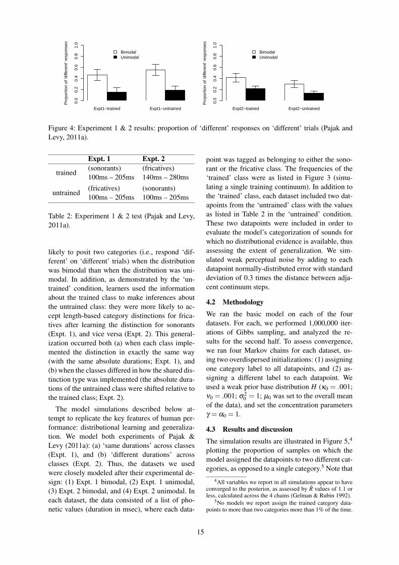
Figure 4: Experiment 1 & 2 results: proportion of ‘different’ responses on ‘different’ trials (Pajak andLevy, 2011a).

Expt. 1 Expt. 2

trained(sonorants) (fricatives)100ms – 205ms 140ms – 280ms

untrained(fricatives) (sonorants)100ms – 205ms 100ms – 205ms

Table 2: Experiment 1 & 2 test (Pajak and Levy,2011a).

likely to posit two categories (i.e., respond ‘dif-ferent’ on ‘different’ trials) when the distributionwas bimodal than when the distribution was uni-modal. In addition, as demonstrated by the ‘un-trained’ condition, learners used the informationabout the trained class to make inferences aboutthe untrained class: they were more likely to ac-cept length-based category distinctions for frica-tives after learning the distinction for sonorants(Expt. 1), and vice versa (Expt. 2). This general-ization occurred both (a) when each class imple-mented the distinction in exactly the same way(with the same absolute durations; Expt. 1), and(b) when the classes differed in how the shared dis-tinction type was implemented (the absolute dura-tions of the untrained class were shifted relative tothe trained class; Expt. 2).

The model simulations described below at-tempt to replicate the key features of human per-formance: distributional learning and generaliza-tion. We model both experiments of Pajak &Levy (2011a): (a) ‘same durations’ across classes(Expt. 1), and (b) ‘different durations’ acrossclasses (Expt. 2). Thus, the datasets we usedwere closely modeled after their experimental de-sign: (1) Expt. 1 bimodal, (2) Expt. 1 unimodal,(3) Expt. 2 bimodal, and (4) Expt. 2 unimodal. Ineach dataset, the data consisted of a list of pho-netic values (duration in msec), where each data-

point was tagged as belonging to either the sono-rant or the fricative class. The frequencies of the‘trained’ class were as listed in Figure 3 (simu-lating a single training continuum). In addition tothe ‘trained’ class, each dataset included two dat-apoints from the ‘untrained’ class with the valuesas listed in Table 2 in the ‘untrained’ condition.These two datapoints were included in order toevaluate the model’s categorization of sounds forwhich no distributional evidence is available, thusassessing the extent of generalization. We sim-ulated weak perceptual noise by adding to eachdatapoint normally-distributed error with standarddeviation of 0.3 times the distance between adja-cent continuum steps.

4.2 MethodologyWe ran the basic model on each of the fourdatasets. For each, we performed 1,000,000 iter-ations of Gibbs sampling, and analyzed the re-sults for the second half. To assess convergence,we ran four Markov chains for each dataset, us-ing two overdispersed initializations: (1) assigningone category label to all datapoints, and (2) as-signing a different label to each datapoint. Weused a weak prior base distribution H (κ0 = .001;ν0 = .001; σ2

0 = 1; µ0 was set to the overall meanof the data), and set the concentration parametersγ = α0 = 1.

4.3 Results and discussionThe simulation results are illustrated in Figure 5,4

plotting the proportion of samples on which themodel assigned the datapoints to two different cat-egories, as opposed to a single category.5 Note that

4All variables we report in all simulations appear to haveconverged to the posterior, as assessed by R values of 1.1 orless, calculated across the 4 chains (Gelman & Rubin 1992).

5No models we report assign the trained category data-points to more than two categories more than 1% of the time.

15

trained untrained

0.00

0.25

0.50

0.75

1.00

bim

odal

unim

odal

bim

odal

unim

odal

Pro

port

ion

of 2

−ca

tego

ry in

fere

nces

Basic model:Experiment 1

trained untrained

0.00

0.25

0.50

0.75

1.00

bim

odal

unim

odal

bim

odal

unim

odal

Pro

port

ion

of 2

−ca

tego

ry in

fere

nces

Basic model:Experiment 2

Figure 5: Simulation results for the basic model.Error bars give 95% binomial confidence intervals,computed using the estimated number of effec-tively independent samples in the Markov chains.

in the ‘trained’ condition, this means categoriza-tion of all datapoints along the continuum. In the‘untrained’ condition, on the other hand, it is cat-egorization of two datapoints: one from each end-point of the continuum.

The results in the ‘trained’ conditions demon-strate that the model was able to learn from thedistributional cues, thus replicating the success ofprevious phonetic category learning models.

Of most interest here are the results in the ‘un-trained’ condition. The figure on the left showsthe results modeling the ‘same-durations’ exper-iment (Expt. 1), demonstrating that the model cat-egorizes the two datapoints in the untrained soundclass in exactly the same way as it did for thetrained sound class: two categories in the bimodalcondition, and one category in the unimodal con-dition. Thus, these results suggest that we can suc-cessfully model generalization of distinction typesacross sound classes in phonetic category learningby assuming that learners have an expectation thatcategory types (such as short and long, or voice-less and voiced) may be shared across classes.

The figure on the right shows the results model-ing the ‘different-durations’ experiment (Expt. 2),revealing a limitation of the model: failure to gen-eralize when the untrained class has the same cat-egory structure but different absolute phonetic val-ues (overall shorter in the untrained class than inthe trained class). Instead, the model categorizesboth untrained datapoints as belonging to a singlecategory. This result diverges from the experimen-tal results, where learners generalize the learneddistinction type in both cases, whether the abso-

lute phonetic values of the analogous categoriesare identical or not. We address this problem inthe next section by implementing a modificationto the model that allows more flexibility in howeach class implements the same category types.

5 Extended generalization model

The goal of the extended model is to explicitly al-low for phonetic variability across sound classes.As a general approach, we could imagine func-tions that transform categories across classes sothat the same categories can be “reused” by be-ing translated around to different parts of the pho-netic space. These functions would be specific op-erations representing any intrinsic differences be-tween sound classes. Here, we use a very simplefunction that can account for one widely attestedtype of transformation: different absolute phoneticvalues for analogous categories in distinct soundclasses (Ladefoged & Maddieson 1996), such aslonger overall durations for voiceless fricativesthan for sonorants. This type of transformationhas been successfully used in prior modeling workto account for learning allophones of a singlephoneme that systematically vary in phonetic val-ues along certain dimensions (Dillon et al. 2013).

5.1 Model details

We implement the possibility for between-classvariability by allowing for one specific type ofidiosyncratic implementation of categories acrossclasses: learnable class-specific ‘offsets’ by whichthe data in a class are shifted along the phoneticdimension, as illustrated in Figure 6 (the key forthe variables is in Table 1).

5.2 Inference

Each iteration of MCMC now includes aMetropolis-Hastings step to resample the offsetparameters fc, which uses a zero-mean Gaussianproposal, with standard deviation σp = range of data

5 .

6 Simulations: extended model

This second set of simulations has two goals: (1) toestablish that the extended model can successfullyreplicate the performance of the basic model inboth distributional learning and generalization inthe no-variability case, and (2) to show that ex-plicitly allowing for variability across classes letsthe model generalize when there is between-classvariability in category realizations.

16

H

G0γ

Gcα0

zic

dic

fc

σ f

i ∈ {1..nc}c ∈ C

Figure 6: The graphical representation of the ex-tended model.

6.1 Methodology

We used the same prior as in the first set of sim-ulations, and used a Gaussian prior on the offsetparameter with standard deviation σ f = 1000. Be-cause only the relative values of offset parametersare important for category sharing across classes,we set the offset parameter for one of the classesto zero. The four Markov chains now crossed cate-gory initialization with two different initial valuesof the offset parameter.

6.2 Results and discussion

The simulation results are illustrated in Fig-ure 7. The figure on the left demonstrates thatthe extended model performs similarly to the ba-sic model in the case of no variability betweenclasses. The figure on the right, on the otherhand, shows that – unlike the basic model –the extended model succeeds in generalizing thelearned distinction type to an untrained soundclass when there is phonetic variability betweenclasses. These results suggest that allowing forvariability in category implementations acrosssound classes may be necessary to account forhuman learning. Taken together, these results areconsistent with our proposal that language learn-ers have an expectation that category types can beshared across sound classes. Furthermore, learn-ers appear to have implicit knowledge of the waysthat sound classes can vary in their exact phoneticimplementations of different category types. This

trained untrained

0.00

0.25

0.50

0.75

1.00

bim

odal

unim

odal

bim

odal

unim

odal

Pro

port

ion

of 2

−ca

tego

ry in

fere

nces

Extended model:Experiment 1

trained untrained

0.00

0.25

0.50

0.75

1.00

bim

odal

unim

odal

bim

odal

unim

odal

Pro

port

ion

of 2

−ca

tego

ry in

fere

nces

Extended model:Experiment 2

Figure 7: Simulation results for the extendedmodel. Error bars give 95% binomial confidenceintervals, computed using the estimated numberof effectively independent samples in the Markovchains.

type of knowledge may include – as in our ex-tended generalization model – the possibility thatphonetic values of categories in one class can besystematically shifted relative to another.

7 General discussion

In this paper we presented the first model of gen-eralization in phonetic category learning, in whichlearning a distinction type for one set of sounds(e.g., /m/–/mm/) immediately generalizes to an-other set of sounds (e.g., /s/–/ss/), thus reproduc-ing the key features of adult learner performancein behavioral experiments. This extends previouscomputational work in phonetic category learn-ing, which focused on modeling the process oflearning from distributional cues, and did not ad-dress the question of generalization. The basicpremise of the proposed model is that learners’knowledge of phonetic categories is representedhierarchically: individual sounds are grouped intocategories, and individual categories are groupedinto sound classes. Crucially, the category struc-ture established for one sound class can be di-rectly shared with another class, although differ-ent classes can implement the categories in id-iosyncratic ways, thus mimicking natural variabil-ity in how analogous categories (e.g., short /m/ and/s/, or long /mm/ and /ss/) are phonetically imple-mented for different sound classes.

The simulation results we presented succeedin reproducing the human pattern of generaliza-tion performance, in which the proportion of two-category inferences about the untrained class is

17

very similar to that for the trained class. Note,however, that there are clear quantitative dif-ferences between the two in learning perfor-mance: the model learns almost perfectly fromthe available distributional cues (‘trained’ condi-tion), while adult learners are overall very conser-vative in accepting two categories along the lengthdimension, as indicated by the overall low num-ber of ‘different’ responses. There are two mainreasons why the model might be showing moreextreme categorization preferences than humansin this particular task. First, humans have cogni-tive limitations that the current model does not,such as those related to memory or attention. Inparticular, imperfect memory makes it harder forhumans to integrate the distributional informationfrom all the trials in the exposure, and longer train-ing would presumably improve performance. Sec-ond, adults have strong native-language biases thataffect learning of a second language (Flege 1995).The population tested by Pajak & Levy (2011a)consisted of adult native speakers of American En-glish, a language in which length is not used con-trastively. Thus, the low number of ‘different’ re-sponses in the experiments can be attributed toparticipants’ prior bias against category distinc-tions based on length. The model, on the otherhand, has only a weak prior that was meant to beeasily overridden by data.

This last point is of direct relevance for thearea of second language (L2) acquisition, whereone of the main research foci is to investigatethe effects of native-language knowledge on L2learning. The model we proposed here can poten-tially be used to systematically investigate the roleof native-language biases when learning categorydistinctions in a new language. In particular, an L2learner, whose linguistic representations includetwo languages, could be implemented by addinga language-level node to the model’s hierarchicalstructure (through an additional Dirichlet process).This extension will allow for category structures tobe shared not just within a language for differentsound classes, but also across languages, thus ef-fectively acting as a native-language bias.

As a final note, we briefly discuss alternativeways of modeling generalization in phonetic cat-egory learning. In the model we described in thispaper, whole categories are generalized from oneclass to another. However, one might imagine an-other approach to this problem where generaliza-

tion is a byproduct of learners’ attending moreto the dimension that they find to be relevant fordistinguishing between some categories in a lan-guage. That is, learners’ knowledge would not in-clude the expectation that whole categories maybe shared across classes, as we argued here, butrather that a given phonetic dimension is likelyto be reused to distinguish between categories inmultiple sound classes.

This intuition could be implemented in differ-ent ways. In a Dirichlet process model of categorylearning, the concentration parameter α might belearned, and shared for all classes along a givenphonetic dimension, thus producing a bias to-ward having a similar number of categories acrossclasses. Alternatively, the variance of categoriesalong a given dimension might be learned, andalso shared for all classes. Under this scenario,learning category variance along a given dimen-sion would help categorize novel sounds along thatdimension. That is, two novel datapoints would belikely categorized into separate categories if the in-ferred variance along the relevant dimension wassmaller than the distance between the datapoints,but into a single category if the inferred variancewas comparable to that distance.

Finally, this model assumes that sound classesare given in advance, and that only the categorieswithin each class are learned. While this assump-tion may seem warranted for some types of per-ceptually dissimilar sound classes (e.g., conso-nants and vowels), and also may be appropriatefor L2 acquisition, it is not clear that it is true forall sound classes that allow for generalization ininfancy. It remains for future work to determinehow learners may generalize while simultaneouslylearning the sound classes.

We plan to pursue all these directions in fu-ture work with the ultimate goal of improving ourunderstanding how human learners represent theirlinguistic knowledge and how they use it when ac-quiring a new language.

Acknowledgments

We thank Gabriel Doyle and three anonymousCMCL reviewers for useful feedback. This re-search was supported by NIH Training Grant T32-DC000041 from the Center for Research in Lan-guage at UC San Diego to B.P. and NIH TrainingGrant T32-DC000035 from the Center for Lan-guage Sciences at University of Rochester to B.P.

18

References

de Boer, Bart & Patricia K. Kuhl. 2003. Inves-tigating the role of infant-directed speech witha computer model. Acoustic Research LettersOnline 4(4). 129–134.

Clements, George N. 2003. Feature economy insound systems. Phonology 20. 287–333.

Dillon, Brian, Ewan Dunbar & William Idsardi.2013. A single-stage approach to learningphonological categories: Insights from Inukti-tut. Cognitive Science 37. 344–377.

Feldman, Naomi H., Thomas L. Griffiths &James L. Morgan. 2009. Learning phonetic cat-egories by learning a lexicon. In Proceedingsof the 31st Annual Conference of the CognitiveScience Society, 2208–2213. Austin, TX: Cog-nitive Science Society.

Ferguson, Thomas S. 1973. A Bayesian analy-sis of some nonparametric problems. Annals ofStatistics 1. 209–230.

Flege, James E. 1995. Second-language speechlearning: theory, findings and problems. InWinifred Strange (ed.), Speech perception andlinguistic experience: issues in cross-languageresearch, 229–273. Timonium, MD: York Press.

Gelman, Andrew & Donald B. Rubin. 1992. In-ference from iterative simulation using multiplesequences. Statistical Science 7. 457–511.

Giovanardi, Maurizio & Maria-GabriellaDi Benedetto. 1998. Acoustic analysis ofsingleton and geminate fricatives in Italian.The European Journal of Language and Speech(EACL/ESCA/ELSNET) 1998. 1–13.

Greenberg, Steven. 1996. The Switchboard tran-scription project. Report prepared for the1996 CLSP/JHU Workshop on Innovative Tech-niques in Continuous Large Vocabulary SpeechRecognition.

Kuhl, Patricia K. 1991. Human adults and humaninfants show a “perceptual magnet effect” forthe prototypes of speech categories, monkeysdo not. Perception and Psychophysics 50(2).93–107.

Kuhl, Patricia K., Karen A. Williams, FranciscoLacerda, Kenneth N. Stevens & Bjorn Lind-blom. 1992. Linguistic experience alters pho-netic perception in infants by 6 months of age.Science 255. 606–608.

Lacerda, Francisco. 1995. The perceptual magnet-effect: An emergent consequence of exemplar-based phonetic memory. In K. Ellenius &

P. Branderud (eds.), Proceedings of the 13thInternational Congress of Phonetic Sciences,140–147. Stockholm: KTH and Stockholm Uni-versity.

Ladefoged, Peter & Ian Maddieson. 1996. Thesounds of the world’s languages. Oxford, UK;Cambridge, MA: Blackwell.

Lisker, Leigh & Arthur S. Abramson. 1970. Thevoicing dimensions: Some experiments in com-parative phonetics. In Proceedings of the SixthInternational Congress of Phonetic Sciences,Prague: Academia.

Mattei, Marco & Maria-Gabriella Di Benedetto.2000. Acoustic analysis of singleton and gemi-nate nasals in Italian. The European Journal ofLanguage and Speech (EACL/ESCA/ELSNET)2000. 1–11.

Maye, Jessica & LouAnn Gerken. 2000. Learningphonemes without minimal pairs. In S. Cather-ine Howell, Sarah A. Fish & Thea Keith-Lucas(eds.), Proceedings of the 24th Annual BostonUniversity Conference on Language Develop-ment, 522–533. Somerville, MA: CascadillaPress.

Maye, Jessica & LouAnn Gerken. 2001. Learn-ing phonemes: how far can the input take us?In A. H-J. Do, L. Domınguez & A. Johansen(eds.), Proceedings of the 25th Annual BostonUniversity Conference on Language Develop-ment, 480–490. Somerville, MA: CascadillaPress.

Maye, Jessica, Daniel J. Weiss & Richard N.Aslin. 2008. Statistical phonetic learning ininfants: facilitation and feature generalization.Developmental Science 11(1). 122–134.

Maye, Jessica, Janet F. Werker & LouAnn Gerken.2002. Infant sensitivity to distributional infor-mation can affect phonetic discrimination. Cog-nition 82. B101–B111.

McClaskey, Cynthia L., David B. Pisoni &Thomas D. Carrell. 1983. Transfer of trainingof a new linguistic contrast in voicing. Percep-tion and Psychophysics 34(4). 323–330.

McMurray, Bob, Richard N. Aslin & Joseph C.Toscano. 2009. Statistical learning of phoneticcategories: insights from a computational ap-proach. Developmental Science 12(3). 369–378.

Pajak, Bozena & Roger Levy. 2011a. How ab-stract are phonological representations? Evi-dence from distributional perceptual learning.

19

In Proceedings of the 47th Annual Meeting ofthe Chicago Linguistic Society, Chicago, IL:University of Chicago.

Pajak, Bozena & Roger Levy. 2011b. Phono-logical generalization from distributional evi-dence. In L. Carlson, C. Holscher & T. Ship-ley (eds.), Proceedings of the 33rd Annual Con-ference of the Cognitive Science Society, 2673–2678. Austin, TX: Cognitive Science Society.

Perfors, Amy & David Dunbar. 2010. Phonetictraining makes word learning easier. In S. Ohls-son & R. Catrambone (eds.), Proceedings of the32nd Annual Conference of the Cognitive Sci-ence Society, 1613–1618. Austin, TX: Cogni-tive Science Society.

Teh, Yee Whye, Michael I. Jordan, Matthew J.Beal & David M. Blei. 2006. HierarchicalDirichlet processes. Journal of the AmericanStatistical Association 101(476). 1566–1581.

Toscano, Joseph C. & Bob McMurray. 2010. Cueintegration with categories: Weighting acousticcues in speech using unsupervised learning anddistributional statistics. Cognitive Science 34.434–464.

Vallabha, Gautam K., James L. McClelland, Fer-ran Pons, Janet F. Werker & Shigeaki Amano.2007. Unsupervised learning of vowel cate-gories from infant-directed speech. Proceedingsof the National Academy of Sciences 104(33).13273–13278.

20

Proceedings of the Workshop on Cognitive Modeling and Computational Linguistics, pages 21–27,Sofia, Bulgaria, August 8, 2013. c©2013 Association for Computational Linguistics

Learning non-concatenative morphology

Michelle A. FullwoodDept. of Linguistics and Philosophy

Massachusetts Institute of Technologymaf@mit.edu

Timothy J. O’DonnellDept. of Brain and Cognitive SciencesMassachusetts Institute of Technology

timod@mit.edu

AbstractRecent work in computational psycholin-guistics shows that morpheme lexica canbe acquired in an unsupervised man-ner from a corpus of words by select-ing the lexicon that best balances pro-ductivity and reuse (e.g. Goldwater etal. (2009) and others). In this paper,we extend such work to the problem ofacquiring non-concatenative morphology,proposing a simple model of morphologythat can handle both concatenative andnon-concatenative morphology and apply-ing Bayesian inference on two datasets ofArabic and English verbs to acquire lex-ica. We show that our approach success-fully extracts the non-contiguous triliteralroot from Arabic verb stems.

1 Introduction

What are the basic structure-building operationsthat enable the creative use of language, and howdo children exposed to a language acquire the in-ventory of primitive units which are used to formnew expressions? In the case of word forma-tion, recent work in computational psycholinguis-tics has shown how an inventory of morphemescan be acquired by selecting a lexicon that bestbalances the ability of individual sound sequencesto combine productively against the reusability ofthose sequences (e.g., Brent (1999), Goldwater etal. (2009), Feldman et al. (2009), O’Donnell et al.(2011), Lee et al. (2011).) However, this workhas focused almost exclusively on one kind ofstructure-building operation: concatenation. Thelanguages of the world, however, exhibit a varietyof other, non-concatenative word-formation pro-cesses (Spencer, 1991).

Famously, the predominant mode of Semiticword formation is non-concatenative. For exam-ple, the following Arabic words, all related to

the concept of writing, share no contiguous se-quences of segments (i.e., phones), but they doshare a discontinuous subsequence

√ktb, which

has been traditionally analyzed as an independentmorpheme, termed the “root”.

kataba “he wrote”kutiba “it was written”yaktubu “he writes”ka:tib “writer”kita:b “book”kutub “books”maktab “office”

Table 1: List of Arabic words with root√

ktb

Many Arabic words appear to be constructedvia a process of interleaving segments from dif-ferent morphemes, as opposed to concatenation.

Concatenativecook

PAST

c o o k e d

Non-concatenativecook

PAST

T a b a x a

Figure 1: Schematic of concatenative vs non-concatenative morphology

Such non-concatenative morphology is perva-sive in the world’s languages. Even English,whose morphology is fundamentally concatena-tive, displays pockets of non-concatenative behav-ior, for example in the irregular past tenses (seeTable 2).

In these words, the stem vowels undergo ablautchanging between tenses. This cannot be han-dled in a purely concatenative framework unlesswe consider these words listed exceptions. How-ever, such irregulars do show limited productiv-

21

bite /bajt/ bit /bIt/sing /sIN/ sang /sæN/give /gIv/ gave /gejv/feel /fil/ felt /fElt/

Table 2: Examples of English irregular verbs

ity (see Albright and Hayes (2003), Prasada andPinker (1993), Bybee and Slobin (1982), Bybeeand Moder (1983), Ambridge (2010)), and in otherlanguages such stem changing processes are fullyproductive.

In Semitic, it is clear that non-concatenativeword formation is productive. Borrowings fromother languages are modified to fit the avail-able non-concatenative templates. This has alsobeen tested psycholinguistically: Berman (2003),for instance, shows that Hebrew-speaking pre-schoolers can productively form novel verbs outof nouns and adjectives, a process that requires theability to extract roots and apply them to existingverbal templates.

Any model of word formation, therefore, needsto be capable of generalizing to both concatenativeand non-concatenative morphological systems. Inthis paper, we propose a computational model ofword formation which is capable of capturing bothtypes of morphology, and explore its ramificationsfor morphological segmentation.

We apply Bayesian inference on a small cor-pus of Arabic and English words to learn the mor-phemes that comprise them, successfully learningthe Arabic root with great accuracy, but less suc-cessfully English verbal inflectional suffixes. Wethen examine the shortcomings of the model andpropose further directions.

2 Arabic Verbal Morphology

In this paper, we focus on Arabic verbal stem mor-phology. The Arabic verbal stem is built fromthe interleaving of a consonantal root and a vo-calism that conveys voice (active/passive) and as-pect (perfect/imperfect). The stem can then un-dergo further derivational prefixation or infixation.To this stem inflectional affixes indicating the sub-ject’s person, number and gender are then added.In the present work, we focus on stem morphol-ogy, leaving inflectional morphology to future ex-tensions of the model.

There are nine common forms of the Arabic ver-bal stem, also known by the Hebrew grammati-

cal term binyan. In Table 3,√

fQl represents thetriconsonantal root. Only the perfect forms aregiven.

Form Active PassiveI faQal fuQilII faQQal fuQQilIII faaQal fuuQilIV PafQal PufQilV tafaQQal tufuQQilVI tafaaQal tufuuQilVII PinfaQal -VIII PiftaQal PiftiQilX PistafQal PistufQil

Table 3: List of common Arabic verbal binyanim

Each of these forms has traditionally been asso-ciated with a particular semantics. For example,Form II verbs are generally causatives of Form Iverbs, as is kattab “to cause to write” (c.f. katab“to write”). However, as is commonly the casewith derivational morphology, these semantic as-sociations are not completely regular: many formshave been lexicalized with alternative or more spe-cific meanings.

2.1 Theoretical accountsThe traditional Arab grammarians’ account of theArabic verb was as follows: each form was asso-ciated with a template with slots labelled C1, C2

and C3, traditionally represented with the conso-nants

√fQl, as described above. The actual root

consonants were slotted into these gaps. Thus thetemplate of the Form VIII active perfect verb stemwas taC1aC2C2aC3. This, combined with the tri-consonantal root, made up the verbal stem.

Template t a C1 a C2 C2 a C3

Root f Q l

Figure 2: Traditional analysis of Arabic Form Vverb

The first generative linguistic treatment of Ara-bic verbal morphology (McCarthy, 1979; Mc-Carthy, 1981) adopted the notion of the rootand template, but split off the derivational pre-fixes and infixes and vocalism from the template.Borrowing from the technology of autosegmentalphonology (Goldsmith, 1976), the template was

22

now comprised of C(onsonant) and V(owel) slots.Rules governing the spreading of segments en-sured that consonants and vowels appeared in thecorrect positions within a template.

Under McCarthy’s model, the analysis for[tafaQQal] would be as follows:

CV Template C V C V C C V C

Prefixt Root

f Q l

Vocalisma

Figure 3: McCarthy analysis of Arabic Form Vverb

While increasing the number of morphemes as-sociated with each verb, the McCarthy approacheconomized on the variety of such units in the lex-icon. The inventory of CV templates was limited;there were three vocalisms corresponding to activeand passive voice intersecting with perfect and im-perfect aspect; and only four derivational prefixes(/P/,/n/,/t/,/st/), one of which became an infix viamorphophonological rule in Form VIII.1

We adopt a middle ground between the tradi-tional Arab grammarians’ description of the ver-bal stem and McCarthy’s analysis as our startingpoint. We describe this approach in the next sec-tion.

3 The Approach

Our initial model of morphology adopts Mc-Carthy’s notion of an abstract template, but coa-lesces the prefixes and infixes with the vocalisminto what we term the “residue.” Each stem isthus composed of two morphemes: the root andthe residue, and their interleaving is dictated by atemplate with slots for root and residue segments.

For example, Piktatab = - - - r - - r - r (template)+ ktb (root) + Pitaa (residue), where r indicates aroot segment and - a residue segment.

The residue may be of length 0, effectively mak-ing the word consist of a single morpheme. Con-catenative morphology may be modelled in this

1Other theories of Arabic morphology that reject the ex-istence of the root are also extant in the literature; see e.g.(Bat-El, 1994) for a stem modification and vowel overwritingapproach.

framework by grouping all the root segments to-gether, for example cooked [kukt] = r r r - (tem-plate) + kuk (root) + t (residue).

The template, root and residue are each drawnfrom a separate sub-lexicon, modeled using toolsfrom Bayesian non-parametric statistics (see Sec-tion 4). These tools put a prior distribution on thelexica that biases them in favour of reusing exist-ing frequent forms and small lexica by promotingmaximal sharing of morphemes.

When applied to data, we derive a segmentationfor each word into a root and a residue.

4 Model

Following earlier work on Bayesian lexicon learn-ing (e.g. Goldwater et al. (2009), we use a distri-bution over lexical items known as the Pitman–YorProcess (PYP) (Pitman and Yor, 1995). LetG be adistribution over primitive phonological elementsof the lexicon (e.g., words, roots, residues, tem-plates, morphemes, etc.). The behavior of PYPprocess PYP(a, b,G) with base measure G and pa-rameters a and b can be described as follows. Thefirst time we sample from PYP(a, b,G) a new lex-ical item will be sampled using G. On subsequentsamples from PYP(a, b,G), we either reuse an ex-isting lexical item i with probability ni−a

N+b , whereN is the number of lexical items sampled so far, ni

is the number of times that lexical item i has beenused in the past, and 0 ≤ a ≤ 1 and b > −a areparameters of the model. Alternatively, we samplea new lexical item with probability aK+b

N+b , whereK is the number of times a new lexical item wassampled in the past from the underlying distribu-tionG. Notice that this process induces a rich-get-richer scheme for sampling from the process. Themore a particular lexical item has been reused, themore likely it is to be reused in the future. ThePitman–Yor process also produces a bias towardssmaller, more compact lexica.

In our model, we maintain three sublexica fortemplates (LTp), roots (LRt), and residues (LRs)each drawn from a Pitman–Yor process with itsown hyperparameters.

LX ∼ PYP(aX, bX , GX) (1)

where X ∈ {Tp,Rt,Rs} Words are drawn byfirst drawing a template, then drawing a root anda residue (of the appropriate length) and insertingthe segments from the root and residue in the ap-propriate positions in the word as indicated by the

23

template. Our templates are strings in {Rt,Rs}∗indicating for each position in a word whether thatposition is part of the word’s root (Rt) or residue(Rs). These templates themselves are drawn froma base measure GTp which is defined as follows.To add a new template to the template lexicon firstdraw a length for that template, K, from a Poissondistribution.

K ∼ POISSON(5) (2)

We then sample a template of length K bydrawing a Bernoulli random variable ti for eachposition i ∈ 1..K is a root or residue position.

ti ∼ BERNOULLI(θ) (3)

The base measure over templates, GTp, is de-fined as the concatenation of the ti’s.

The base distributions over roots and residues,GRt and GRs, are drawn in the following manner.Having drawn a template, T we know the lengthsof the root, KRt, and residue KRt. For each posi-tion in the root or residue ri where i ∈ 1..KRt/Rs,we sample a phone from a uniform distributionover phones.

ri ∼ UNIFORM(|alphabet|) (4)

5 Inference

Inference was performed via Metropolis–Hastingssampling. The sampler was initialized by assign-ing a random template to each word in the trainingcorpus. The algorithm then sampled a new tem-plate, root, and residue for each word in the corpusin turn. The proposal distribution over templatesfor our sampler considered all templates currentlyin use by another word, as well as a randomly gen-erated template from the prior. Samples from thisproposal distribution were corrected into the truedistribution using the Metropolis–Hastings crite-rion.

6 Related work

The approach of this paper builds on previ-ous work on Bayesian lexicon learning start-ing with Goldwater et al. (2009). However,to our knowledge, this approach has not beenapplied to non-concatenative morphological seg-mentation. Where it has been applied to Arabic(e.g. Lee et al. (2011)), it has been applied to un-vowelled text, since standard Arabic orthography

drops short vowels. However, this has the effect ofreducing the problem mostly to one of concatena-tive morphology.

Non-concatenative morphology has been ap-proached computationally via other research,however. Kataja and Koskenniemi (1988) firstshowed that Semitic roots and patterns could bedescribed using regular languages. This insightwas subsequently computationally implementedusing finite state methods by Beesley (1991) andothers. Roark and Sproat (2007) present a modelof both concatenative and non-concatenative mor-phology based on the operation of compositionthat is similar to the one we describe above.

The narrower problem of isolating roots fromSemitic words, for instance as a precursor to in-formation retrieval, has also received much atten-tion. Existing approaches appear to be mostlyrule-based or dictionary-based (see Al-Shawakfaet al. (2010) for a recent survey).

7 Experiments

We applied the morphological model and infer-ence procedure described in Sections 4 and 5 totwo datasets of Arabic and English.

7.1 Data

The Arabic corpus for this experiment consistedof verbal stems taken from the verb concordanceof the Quranic Arabic Corpus (Dukes, 2011). Allpossible active, passive, perfect and imperfectfully-vowelled verbal stems for Forms I–X, ex-cluding the relatively rare Form IX, were gener-ated. We used this corpus rather than a lexicon asour starting point to obtain a list of relatively highfrequency verbs.

This list of stems was then filtered in two ways:first, only triconsonantal “strong” roots were con-sidered. The so-called “weak” roots of Arabic ei-ther include a vowel or semi-vowel, or a doubledconsonant. These undergo segmental changes invarious environments, which cannot be handled byour current generative model.

Secondly, the list was filtered through the Buck-walter stem lexicon (Buckwalter, 2002) to obtainonly stems that were licit according to the Buck-walter morphological analyzer.

This process yielded 1563 verbal stems, com-prising 427 unique roots, 26 residues, and 9 tem-plates. The stems were supplied to the sampler inthe Buckwalter transliteration.

24

The English corpus was constructed along sim-ilar lines. All verb forms related to the 299 mostfrequent lemmas in the Penn Treebank (Marcus etal., 1999) were used, excluding auxiliaries such asmight or should. Each lemma thus had up to fiveverbal forms associated with it: the bare form (for-get), the third person singular present (forgets), thegerund (forgetting), past tense (forgot), and pastparticiple (forgotten).

This resulted in 1549 verbal forms, compris-ing 295 unique roots, 108 residues, and 55 tem-plates. CELEX (Baayen et al., 1995) pronuncia-tions for these words were supplied to the samplerin CELEX’s DISC transliteration.

Deriving a gold standard analysis for Englishverbs was less straightforward than in the Arabiccase. The following convention was used: Theroot was any subsequence of segments shared byall the forms related to the same lemma. Thus, forthe example lemma of forget, the correct template,root and residue were deemed to be:

forget f@gEt r r r - r f@gt Eforgets f@gEts r r r - r - f@gt Esforgot f@gQt r r r - r f@gt Qforgetting f@gEtIN r r r - r - - f@gt EINforgotten f@gQtH r r r - r - f@gt QH

Table 4: Correct analyses under the root/residuemodel for the lemma forget

37 templates were concatenative, and 18 non-concatenative. The latter were necessary to ac-commodate 46 irregular lemmas associated with254 forms.

7.2 Results and Discussion

We ran 10 instances of the sampler for 200 sweepsthrough the data. For the Arabic training set, thisnumber of sweeps typically resulted in the sam-pler finding a local mode of the posterior, makingfew further changes to the state during longer runs.An identical experimental set-up was used for En-glish. Evaluation was performed on the final stateof each sampler instance.

The correctness of the sampler’s output wasmeasured in terms of the accuracy of the tem-plates it predicted for each word. The word-levelaccuracy indicates the number of words that hadtheir entire template correctly sampled, while thesegment-level accuracy metric gives partial creditby considering the average number of correct bits

r - r - r

r - - r - r

r - r - - r

r - - - r - r

- - r - r - r

- - r - r - - r

- - r - - - r - r

- - - - r - r - r

- - - - - - r - r - r0

20

40

60

80

100

Acc

urac

y

Figure 4: Unweighted accuracy with which eachtemplate was sampled

(r versus -) in each sampled template.Table 5 shows the average accuracy of the 10

samples, weighted by each sample’s joint proba-bility.

Accuracy Word-level Segment-levelArabic 92.3% 98.2%English 43.9% 85.3%

Table 5: Average weighted accuracy of samples

Arabic Analyses Figure 4 shows the averageunweighted accuracy with which each of the 9Arabic templates was sampled.

Figure 4 reveals an effect of both the rarity andthe length of each template. For instance, the per-formance on template r - - r - r (second bar fromleft) is exceptionally low, but this is the resultof there being only one instance of this templatein the training set: Euwqib, the passive form ofthe Form III verb of root Eqb, in the Buckwaltertransliteration.2 In addition, the longer the word,

2This is an artifact of Arabic orthography and the Buck-walter transliteration, which puts the active form EAqab withtemplate r - r - r in correspondence with the passive templater - - r - r.

25

the poorer the performance of the model. This islikely the result of the difficulty of searching overthe space of templates for longer forms. Since thenumber of potential templates increases exponen-tially with the length of the form, finding the cor-rect template becomes increasingly difficult. Thisproblem can likely be addressed in future mod-els by adopting an analysis similar to McCarthy’swhereby the residue is further subdivided into vo-calism, prefixes and infixes. Note that even in suchlong forms, however, the letters belonging to theroot were generally isolated in one of the two mor-phemes.

English Analyses The English experimentyielded poorer results than the Arabic dataset.The statistics of the datasets reveal the cause of thefailure of the English model: the English datasethad several times more residues and templatesthan the Arabic dataset did, thus lacking as muchuniform structure. Nevertheless, the relativelyhigh segment-level accuracy shows that the modeltended to find templates that were only incorrectin 1 or 2 positions.

The dominant pattern of errors was in the di-rection of overgeneralization of the concatenativetemplates to the irregular forms. Out of the 254words related to a lemma with an irregular pastform, 241 received incorrect templates, 232 ofwhich were concatenative, often correctly splittingoff the regular suffix where there was one. Forexample, sing and singing were parsed as sing+∅and sing+ing, while sung was parsed as a separateroot. Note that under an analysis of English ir-regulars as separate memorized lexical items, thesampler behaved correctly in such cases.

However, out of 1295 words related to perfectlyregular lemmas, the sampler determined 628 tem-plates incorrectly. Out of these, 325 were givenconcatenative templates, but with too much or toolittle segmental material allocated to the suffix.For example, the word invert was analyzed as in-ver+t, with its other forms following suit as in-ver+ted, inver+ting and inver+ts. This is likelydue to subregularities in the word corpus: withmany words ending with -t, this analysis becomesmore attractive.

The remaining 303 regular verbs were givennon-concatenative templates. For instance, iden-tify was split up into dfy and ienti. No consistentpattern could be discerned from these cases.

8 Conclusion

We have proposed a model of morpheme-lexiconlearning that is capable of handling concatena-tive and non-concatenative morphology up to thelevel of two morphemes. We have seen thatBayesian inference on this model with an Ara-bic dataset of verbal stems successfully learns thenon-contiguous root and residue as morphemes.

In future work, we intend to extend our sim-plified model of morphology to McCarthy’s com-plete model by adding concatenative prefixationand suffixation processes and segment-spreadingrules. Besides being capable of handling the in-flectional aspects of Arabic morphology, we an-ticipate that this extension will improve the per-formance of the model on Arabic verbal stemsas well, since the number of non-concatenativetemplates that have to be learned will decrease.For example, the template for the Form V verb[tafaQQal] can be reduced to that for the Form IIverb [faQQal] plus an additional prefix.

We also anticipate that the performance on En-glish will be vastly improved, since the dominantmode of word formation in English is concate-native, while the small number of irregular pasttenses and plurals that undergo ablaut can be han-dled using the non-concatenative architecture ofthe model. This would also be more in line withnative speakers’ intuitions and linguistic analysesof English morphology.

Acknowledgments

Parts of the sampler code were written by Pe-ter Graff. We would also like to thank AdamAlbright and audiences at the MIT PhonologyCircle and the Northeast Computational Phonol-ogy Workshop (NECPhon) for feedback on thisproject. This material is based upon work sup-ported by the National Science Foundation Gradu-ate Research Fellowship Program under Grant No.1122374.

ReferencesEmad Al-Shawakfa, Amer Al-Badarneh, Safwan Shat-

nawi, Khaleel Al-Rabab’ah, and Basel Bani-Ismail.2010. A comparison study of some Arabic root find-ing algorithms. Journal of the American Society forInformation Science and Technology, 61(5):1015–1024.

Adam Albright and Bruce Hayes. 2003. Rulesvs. analogy in English past tenses: A computa-

26

tional/experimental study. Cognition, 90(2):119–161.

Ben Ambridge. 2010. Children’s judgments of regularand irregular novel past–tense forms: New data onthe English past–tense debate. Developmental Psy-chology, In Press.

Harald R. Baayen, Richard Piepenbrock, and Leon Gu-likers. 1995. The CELEX Lexical Database. Re-lease 2 (CD-ROM). Linguistic Data Consortium,University of Pennsylvania, Philadelphia, Pennsyl-vania.

Outi Bat-El. 1994. Stem modification and clustertransfer in Modern Hebrew. Natural Language andLinguistic Theory, 12:571–593.

Kenneth R. Beesley. 1991. Computer analysis ofArabic morphology: A two-level approach with de-tours. In Bernard Comrie and Mushira Eid, editors,Perspectives on Arabic Linguistics III: Papers fromthe Third Annual Symposium on Arabic Linguistics,pages 155–172. John Benjamins. Read originally atthe Third Annual Symposium on Arabic Linguistics,University of Utah, Salt Lake City, Utah, 3-4 March1989.

Ruth A. Berman. 2003. Children’s lexical innova-tions. In Joseph Shimron, editor, Language Process-ing and Acquisition in Languages of Semitic, Root-based, Morphology, pages 243–292. John Ben-jamins.

Michael R. Brent. 1999. Speech segmentationand word discovery: A computational perspective.Trends in Cognitive Sciences, 3(8):294–301, Au-gust.

Tim Buckwalter. 2002. Buckwalter Arabic mor-phological analyzer version 1.0. Technical ReportLDC2002L49, Linguistic Data Consortium.

Joan L. Bybee and Carol Lynn Moder. 1983. Mor-phological classes as natural categories. Language,59(2):251–270, June.

Joan L. Bybee and Daniel I. Slobin. 1982. Rules andschemas in the development and use of the Englishpast tense. Language, 58(2):265–289.

Kais Dukes. 2011. Quranic Arabic Corpus.http://corpus.quran.com/.

Naomi H. Feldman, Thomas L. Griffiths, and James L.Morgan. 2009. Learning phonetic categories bylearning a lexicon. In Proceedings of the 31st An-nual Meeting of the Cognitive Science Society.

John Anton Goldsmith. 1976. Autosegmental Phonol-ogy. Ph.D. thesis, Massachusetts Institute of Tech-nology.

Sharon Goldwater, Thomas L. Griffiths, and MarkJohnson. 2009. A Bayesian framework for wordsegmentation: Exploring the effects of context.Cognition, 112:21–54.

Laura Kataja and Kimmo Koskenniemi. 1988. Finite-state description of Semitic morphology: a casestudy of Ancient Akkadian. In Proceedings of the12th conference on Computational linguistics - Vol-ume 1, COLING ’88, pages 313–315, Stroudsburg,PA, USA. Association for Computational Linguis-tics.

Yoong Keok Lee, Aria Haghighi, and Regina Barzi-lay. 2011. Modeling syntactic context improvesmorphological segmentation. In Proceedings of theConference on Natural Language Learning.

Mitchell P. Marcus, Beatrice Santorini, Mary AnnMarcinkiewicz, and Ann Taylor. 1999. Treebank3 technical report. Technical report, Linguistic DataConsortium, Philadelphia.

John J. McCarthy. 1979. Formal Problems in SemiticPhonology and Morphology. Ph.D. thesis, Mas-sachusetts Institute of Technology.

John J. McCarthy. 1981. A prosodic theory of noncon-catenative morphology. Linguistic Inquiry, 12:373–418.

Timothy J. O’Donnell, Jesse Snedeker, Joshua B.Tenenbaum, and Noah D. Goodman. 2011. Pro-ductivity and reuse in language. In Proceedings ofthe 33rd Annual Conference of the Cognitive ScienceSociety.

Jim Pitman and Marc Yor. 1995. The two-parameterPoisson–Dirichlet distribution derived from a sta-ble subordinator. Technical report, Department ofStatistics University of California, Berkeley.

Sandeep Prasada and Steven Pinker. 1993. Generalisa-tion of regular and irregular morphological patterns.Language and Cognitive Processes, 8(1):1–56.

Brian Roark and Richard Sproat. 2007. Computa-tional Approaches to Morphology and Syntax. Ox-ford University Press.

Andrew Spencer. 1991. Morphological Theory.Blackwell.

27

Proceedings of the Workshop on Cognitive Modeling and Computational Linguistics, pages 28–36,Sofia, Bulgaria, August 8, 2013. c©2013 Association for Computational Linguistics

Statistical Representation of Grammaticality Judgements: the Limits ofN-Gram Models

Alexander Clark, Gianluca Giorgolo, and Shalom LappinDepartment of Philosophy, King’s College London

firstname.lastname@kcl.ac.uk

Abstract

We use a set of enriched n-gram models to track

grammaticality judgements for different sorts of

passive sentences in English. We construct these

models by specifying scoring functions to map the

log probabilities (logprobs) of an n-gram model for

a test set of sentences onto scores which depend

on properties of the string related to the parame-

ters of the model. We test our models on classifica-

tion tasks for different kinds of passive sentences.

Our experiments indicate that our n-gram models

achieve high accuracy in identifying ill-formed pas-

sives in which ill-formedness depends on local rela-

tions within the n-gram frame, but they are far less

successful in detecting non-local relations that pro-

duce unacceptability in other types of passive con-

struction. We take these results to indicate some of

the strengths and the limitations of word and lexical

class n-gram models as candidate representations of

speakers’ grammatical knowledge.

1 Introduction

Most advocates (Pereira, 2000; Bod et al., 2003)and critics (Chomsky, 1957; Fong et al., 2013) of aprobabilistic view of grammatical knowledge haveassumed that this view identifies the grammaticalstatus of a sentence directly with the probability ofits occurrence. By contrast, we seek to character-ize grammatical knowledge statistically, but with-out reducing grammaticality directly to probabil-ity. Instead we specify a set of scoring proceduresfor mapping the logprob value of a sentence intoa relative grammaticality score, on the basis of theproperties of the sentence and of the logprobs thatan n-gram word model generates for the corpuscontaining the sentence. A scoring procedure inthis set generates scores in terms of which we con-struct a grammaticality classifier, using a param-eterized standard deviation from the mean value.The classifier provides a procedure for testing the

accuracy of different scoring criteria in separat-ing grammatical from ungrammatical passive sen-tences.

We evaluate this approach by applying it tothe task of distinguishing well and ill-formed sen-tences with passive constructions headed by fourdifferent sorts of verbs: intransitives (appear,last), pseudo-transitives, which take a restrictedset of notional objects (laugh a hearty laugh,weigh 10 kg), ambiguous transitives, which allowboth agentive and thematic subjects (the jeans /the tailor fitted John), and robust transitives thatpassivize freely (write, move). Intransitives andpseudo-transitives generally yield ill-formed pas-sives. Passives formed from ambiguous transitivestend to be well-formed only on the agentive read-ing. Robust transitives, for the most part, yieldacceptable passives, even if they are semantically(or pragmatically) odd.

Experimenting with several scoring proceduresand alternative values for our standard deviationparameter, we found that our classifier can distin-guish pairwise between elements of the first twoclasses of passives and those of the latter two witha high degree of accuracy. However, its perfor-mance is far less reliable in identifying the differ-ence between ambiguous and robust transitive pas-sives. The first classification task relies on locallexical patterns that can be picked up by n-grammodels, while the second requires identification ofanomalous relations between passivized verbs andby-phrases, which are not generally accessible tomeasurement within the range of an n-gram.

We also observed that as we increased the sizeof the training corpus, the performance of our en-riched models on the classification task also in-creased. This result suggests that better n-gramlanguage models are more sensitive to the sorts ofpatterns that our scoring procedures rely on to gen-erate accurate grammaticality classifications.

We note the important difference between

28

grammaticality and acceptability. Following stan-dard assumptions, we take grammaticality to bea theoretical notion, and acceptability to be anempirically testable property. Acceptability is, inpart, determined by grammaticality, but also byfactors such as sentence length, processing limi-tations, semantic acceptability and many other el-ements. Teasing apart these two concepts, and ex-plicating their precise relationship raises a host ofsubtle methodological issues that we will not ad-dress here. Oversimplifying somewhat, we are try-ing to reconstruct a gradient notion of grammati-cality which is derived from probabilistic models,that can serve as a core component of a full modelof acceptability.

We distinguish our task from the standard taskof error detection in NLP (e.g. Post (2011)),that can be used in various language processingsystems, such as machine translation (Pauls andKlein, 2012), language modeling and so on. Inerror detection, the problem is a supervised learn-ing task. Given a corpus of examples labeled asgrammatical or ungrammatical, the problem is tolearn a classifier to distinguish them. We use su-pervised learning as well, but only to measure theupper bound of an unsupervised learning method.We assume that native speakers do not, in general,have access to systematic sets of ungrammaticalsentences that they can use to calibrate their judge-ment of acceptability. Rather ungrammatical sen-tences are unusual or unlikely. However, we usesome ungrammatical sentences to set an optimalthreshold for our scoring procedures.

2 Enriched N-Gram Language Models

We assume that we have some high quality lan-guage model which defines a probability distri-bution over whole sentences. As has often beennoted, it is not possible to reduce grammatical-ity directly to a probability of this type, for sev-eral reasons. First, if one merely specifies a fixedprobability value as a threshold for grammatical-ity, where strings are deemed to be grammaticalif and only if their probability is higher than thethreshold, then one is committed to the existenceof only a finite number of grammatical sentences.The probabilities of the possible strings of wordsin a language sum to 1, and so at most 1/ε sen-tences can have a probability of at least ε. Second,probability can be affected by factors that do notinfluence grammaticality. For example, the word

’yak’ is rarer (and therefore less probable) than theword ’horse’, but this does not affect the relativegrammaticality of ’I saw a horse’ versus ’I saw ayak’. Third, a short ungrammatical sentence mayhave a higher probability than a long grammaticalsentence with many rare words.

In spite of these arguments against a naive re-duction of grammaticality, probabilistic inferencedoes play a role in linguistic judgements, as in-dicated by the fact that they are often gradient.Probabilistic inference is pervasive throughout alldomains of cognition (Chater et al., 2006), andtherefore it is plausible to assume that knowledgeof language is also probabilistic in nature. More-over language models do seem to play a crucialrole in speech recognition and sentence process-ing. Without them we would not be able to under-stand speech in a noisy environment.

We propose to accommodate these differentconsiderations by using a scoring function to mapprobabilities to grammaticality rankings. Thisfunction does not apply directly to probabilities,but rather to the parameters of the language model.The probability of a particular sentence with re-spect to a log-linear language model will be theproduct of certain parameters: in log space, thesum. We define scores that operate on this collec-tion of parameters.

2.1 Scores

We have experimented with scores of two differ-ent types that correlate with the grammaticalityof a sentence. Those of the first type are dif-ferent implementations of the idea of normaliz-ing the logprob assigned by an n-gram model toa string by eliminating the significance of factorsthat do not influence the grammatical status of asentence, such as sentence length and word fre-quency. Scores of the second type are based on theintuition that the (un)grammaticality of a sentenceis largely determined by its problematic compo-nents. These scores are functions of the lowestscoring n-grams in the sentence.

Mean logprob (ML) This score is the logprobof the entire sentence divided by the length of thesentence, or equivalently the mean of the logprobsfor the single trigrams:ML = 1

n logPTRIGRAM(〈w1, . . . , wn〉)By normalizing the logprob for the entire sentenceby its length we eliminate the effect of sentencelength on the acceptability score.

29

Weighted mean logprob (WML) This score iscalculated by dividing the logprob of the entiresentence by the sum of the unigram probabilitiesof the lexical items that compose the sentence:WML = log PTRIGRAM(〈w1,...,wn〉)

log PUNIGRAM(〈w1,...,wn〉)This score eliminates at the same time the effect ofthe length of the sentence and the lower probabil-ity assigned to sentences with rare lexical items.

Synctactic log odds ratio (SLOR) This scorewas first used by Pauls and Klein (2012) andperforms a normalization very similar to WML(we will see below that in fact the two scores arebasically equivalent):SLOR =log PTRIGRAM(〈w1,...,wn〉)−log PUNIGRAM(〈w1,...,wn〉)

n

Minimum (Min) This score is equal to the low-est logprob assigned by the model to the n-gramsof the sentence divided by the unigram logprob ofthe lexical item heading the n-gram:Min = mini

[log P (wi|wi−2wi−1)

log P (wi)

]In this way, if a single n-gram is assigned a lowprobability (normalized for the frequency of itshead lexical item), then this low score is in somesense propagated to the whole sentence.

Mean of the first quartile (MFQ) This scoreis a generalization of the Min score. We orderthe single n-gram logprobs from the lowest to thehighest, and we consider the first (lowest) quar-tile. We then normalize the logprobs for these n-grams by the unigram probability of the head lex-ical item, and we take the mean of these scores.In this way we obtain a score that is more robustthan the simple Min, as, in general, a grammaticalanomaly influences the logprob of more than onen-gram.

2.2 N-Gram ModelsWe are using n-gram models on the understand-ing that they are fundamentally inadequate for de-scribing natural languages in their full syntacticcomplexity. In spite of their limitations, they are agood starting point, as they perform well as lan-guage models across a wide range of languagemodeling tasks. They are easy to train, as theydo not require annotated training data.

We do not expect that our n-gram based gram-maticality scores will be able to idenitfy all of thecases of ungrammaticality that we encounter. Ourworking hyposthesis is that they can capture cases

of ill-formedness that depend on local factors, thatcan be identified within n-gram frames, as op-posed to those which involve non-local relations.If these models can detect local grammaticality vi-olations, then we will have a basis for thinkingthat richer, more structured language models canrecognize non-local as well as local sources of un-grammaticality.

3 Experiments with Passives

Rather than trying to test the performance of thesemodels over all types of ungrammaticality, welimit ourselves to a case study of the passive. Bytightly controlling the verb types and grammat-ical construction to which we apply our modelswe are better able to study the power and the lim-its of these models as candidate representations ofgrammatical knowledge.

3.1 Types of Passives

Our controlled experiments on passives are, inpart, inspired by speakers’ judgments discussed inAmbridge et al. (2008). Their experimental workmeasures the acceptability of various passive sen-tences.

The active-passive alternation in English is ex-emplified by the pair of sentences

• John broke the window.

• The window was broken by John.

The acceptability of the passive sentence de-pends largely on lexical properties of the verb.Some verbs do not allow the formation of the pas-sive, as in the case of pure intransitive verbs likeappear, discussed below, which permit neither theactive transitive, nor the passive.

We conducted some prelimiary experiments,not reported here, on modelling the data on pas-sives from recent work in progress that Ben Am-bridge and his colleagues are doing, and whichhe was kind enough to make available to us. Weobserved that the scores we obtained for our lan-guage models did not fully track these judgements,but we did notice that we obtained much bettercorrelation at the low end of the judgment distri-bution. In Ambridge’s current data this judgementrange corresponds to passives constructed with in-transitive verbs.

The Ambridge data indicates that the capacityof verbs to yield well-formed passive verb phrases

30

forms a continuum. Studying the judgement pat-terns in this data we identified four reasonablysalient points along this hierarchial continuum.

First, at the low end, we have intransitiveslike appear: (*John appeared the book. *Thebook was appeared). Next we have what may bedescribed as pseudo-transitives verbs like laugh,which permit only notional NP objects and do noteasily passivize (Mary laughed a hearty laugh/*ajoke. ?A hearty laugh/*A joke was laughed byMary) above them. These are followed by casesof ambiguous transitives like fit, which, in activeform, carry two distinct readings that correspondto an agentive and a thematic subject, respectively.

• The tailor fitted John for a new suit.

• The jeans fitted John

Only the agentive reading can be passivized.

• John was fitted by the tailor.

• *John was fitted by the jeans.

Finally, the most easily passivized verbs are ro-bust transitives, which take the widest selection ofNP subjects in passive form (John wrote the book.The book was written by John).

This continuum causes well-formedness in pas-sivization to be a gradient property, as the Am-bridge data illustrates. Passives tend to be moreor less acceptable along this spectrum. The gradi-ence of acceptability for passives implies the par-tial overlap of the score distributions for the differ-ent types of passives that our experiments show.

The experiments were designed to test our hy-pothesis that n-gram based language models arecapable of detecting ungrammatical patterns onlyin cases where they do not depend on relationsbetween words that cross the n-word boundaryapplied in training. Therefore we expect such amodel to be capable of detecting the ungrammati-cality of a sentence like A horrible death was diedby John, because the trigrams death was died, wasdied by and died by John are unlikely to appearin any corpus of English. On the other hand, wedo not expect a trigram model to store the infor-mation necessary to identify the relative anomalyof a sentence like Two hundred people were heldby the theater, because all the trigrams (as well asthe bigrams and the unigrams) that constitute thesentence are likely to appear with reasonable fre-quency in a large corpus of English.

The experiments generalize this observationand test the performance of n-gram models on awider range of verb types. To quantify the per-formance of the different models we derive simpleclassifiers using the scores we have defined andtesting them in a binary classification task. Thistask measures the ability of the classifier to dis-tinguish between grammatical sentences, and sen-tences containing different types of grammaticalerrors.

The models are trained in an unsupervised man-ner using only corpus data, which we assume to beuniformly grammatical. In order to evaluate thescoring methods, we use some supervised data toset the optimal value of a simple threshold. This isnot however a supervised classification task: wewant to see how well the scores could be usedto separate grammatical and ungrammatical data,and though unorthodox, this seems a more directway of measuring this conditional property thanstipulating some fixed threshold.

3.2 Training data

We used the British National Corpus (BNC) (BNCConsortium, 2007) to obtain our training data. Wetrained six different language models, using sixdifferent subcorpora of the BNC. The first modelused the entire collection of written texts anno-tated in the BNC, for a total of approximately 100million words. The other models were trained onincreasingly smaller portions of the written textscollection: 40 million words, 30 million words, 15million words, 7.6 million words, and 3.8 millionwords. We constructed these corpora by randomlysampling an appropriate number of complete sen-tences.

All models were trained on word sequences.For smoothing the n-gram probability distribu-tions we used Kneser-Ney interpolation, as de-scribed in Goodman (2001).

3.3 Test data

We constructed the test data for our hypothesis ina controlled fashion. We first compiled a list ofverbs for each of the four verb types that we con-sider (intransitives, pseudo-transitives, ambiguoustransitives, and robust transitives). We selectedverbs from the BNC that appeared at least 100times in their past participle form in the entire cor-pus in order to ensure a sufficient number of pas-

31

sive uses in the training data.1 We selected 40 in-transitive verbs, 13 pseudo transitives, 23 ambigu-ous transitives and 40 transitive verbs. To clas-sify the verbs we relied on our intuitions as nativespeakers of English.

Using these lists we automatically generatedfour corpora by selecting an agent and a patientfrom a predefined pool of NPs, randomly select-ing a determiner (if necessary) and a number (ifthe NP allows plurals). The resulting corpora areof the following sizes:

• intransitive verbs – 24480 words, 3240 sen-tences,

• pseudo transitive verbs – 7956 words, 1053sentences,

• ambiguous transitive verbs – 14076 words,1863 sentences,

• robust transitive verbs – 24480 words, 3240sentences.

Each corpus was evaluated by the six models.We computed our derived scores for each sentenceon the basis of the logprobs that the language mod-els assigns.

3.4 Binary classifiers

For each model and for each score we constructeda set of simple binary classifiers on the basis ofthe results obtained for the transitive verb corpus.We took the mean of each score assigned by themodel to the transitive sentences, and we set dif-ferent thresholds by subtracting from this valuea number of standard deviations ranging from 0to 2.75. The rationale behind these classifiers isthat, assuming the passives of the robust transi-tives to be grammatical, the scores for the othercases should be comparatively lower. Thereforeby setting a threshold “to the left” of the mean weshould be able to distinguish between grammati-cal sentences, whose score is to the right of thethreshold, and ungrammatical ones, expected to ahave a score lower than the threshold. Formallythe classifier is defined as follows:

cs(w) =

{+ if s(w) ≥ m− S · σ− otherwise

(1)

1Notice that in most cases the past participle form is thesame as the simple past form, and for this reason we set thethreshold to such a high value.

where s is one of our scores, w is the sentence tobe classified, s(w) represents the value assignedby the score to sentence w, m is the mean forthe score in the transitive condition, σ is the stan-dard deviation for the score again in the transitivecondition, and S is a factor by which we movethe threshold away from the mean. The classi-fier assigns the grammatical (+) tag only to thosesentences that are assigned values higher than thethreshold m− S · σ.

Alternatively in terms of the widely used z-score, defined as zs(w) = (s(w) −m)/σ we cansay that w is classified as grammatical iff zs(w) ≥−S.

4 Results

For reasons of space we will limit the presenta-tion of our detailed results to the 100 million wordmodel, as it offers the sharpest effects. We will,however, also report comparisons on the most im-portant metrics for the complete set of models.

In Figure 1 we show the distribution of the fivescores for the four different corpora (transitive,ambiguous, pseudo, and intransitive) obtained us-ing the 100 million word model. In all cases weobserve the same general pattern: the sentences inthe corpus generated with robust transitives are as-signed comparatively high scores, and these grad-ually decrease when we consider the ambiguous,the pseudo and the intransitive conditions. Inter-estingly, this order reflects the degree of “transi-tivity” that these verb types exhibit. Notice, how-ever, that the four conditions seem to group intotwo different macro-distributions. On the rightwe have the transitive-ambiguous sentences andon the left the pseudo-intransitive cases. This par-tially confirms our hypothesis that n-gram mod-els have problems recognizing lexical dependen-cies that determine the felicitousness of passivesconstructed using ambiguous transitive verbs, asthese are, for the most part, non-local. Neverthe-less, it is important to note that the overlap of thedistributions for these two cases is also due to thefact that many cases in the ambiguous transitivecorpus are indeed grammatical.

Figure 2 summarizes the (balanced) accuraciesobtained by our classifiers for each comparison,by each model. These results confirm our hy-pothesis that the classifiers tend to perform betterwhen distinguishing passive sentences constructedwith a robust transitive verbs from those headed by

32

Logprob ML WML

SLOR Min MFQ

0.00

0.05

0.10

0.15

0.0

0.5

1.0

1.5

2.0

0

2

4

6

0.0

0.5

1.0

1.5

2.0

0

2

4

6

0

1

2

3

4

−30 −25 −20 −15 −2.5 −2.0 −1.5 −1.0 −0.9 −0.8 −0.7 −0.6 −0.5

0.0 0.5 1.0 −1.75 −1.50 −1.25 −1.00 −0.75 −1.75 −1.50 −1.25 −1.00 −0.75

dens

ity

condition

transitive

ambiguous

pseudo

intransitive

Figure 1: Distributions of the six scores Logprob, ML, WML, SLOR, Min and MFQ for the four differ-ent conditions (robust transitive passives, ambiguous transitive passives, pseudo transitive passives andintransitive passives) for the 100 million words language model.

pseudo-transitives and intransitives.

In the comparison between transitive and am-biguous transitive sentences, the classifiers are“stuck” at around 60% accuracy. Using largertraining corpora produces only a marginal im-provement. This contrasts with what we observefor the transitive/pseudo and transitive/intransitiveclassification tasks. In the transitive/pseudo task,we already obtain reasonable accuracy with themodel trained with the smallest BNC subset.Oddly, the overall best result is achieved with 30million words, although the result obtained withthe model trained on the full BNC corpus is notmuch lower. For the transitive/intransitive classifi-cation task we observe a much steadier and largergrowth in accuracy, reaching the overall best resultof 85.1%. Table 1 reports the best results for eachcomparison by each language model. For eachcondition we report the best accuracy obtained, thecorresponding F1 score, the score that achieves thebest result, and the best accuracy obtained by justusing the logprobs. These results are obtained us-

ing different values for the S parameter. However,in general the best results are obtained when the Sparameter is set to a value in the interval [0.5, 1.5].

In comparing the performance of the individ-ual scores, we first notice that, while for the tran-sitive/ambiguous comparison all scores performpretty much at the same level, there is a clear hier-archy between scores for the other comparisons.

We observe that the baseline raw logprob as-signed by the n-grams models performs muchworse than the scores, resulting in roughly 10%less accuracy than the best performing score in ev-ery condition. ML performs slightly better, obtain-ing around 5% greater accuracy than logprob as apredictor. This shows that even though the lengthof the sentences in our test data is relatively con-stant (between 9 and 11 words), there is still animprovement if we take this structural factor intoaccount. The two scores WML and SLOR displaythe same pattern, showing that they are effectivelyequivalent. This is not surprising given that theyare designed to modify the raw logprob by tak-

33

transitiveambiguous

transitivepseudo

transitiveintransitive

● ●● ● ●

●

● ●● ● ● ●

● ● ● ●

●

●

●●

●● ● ●

●

● ● ●●

●

●

●●

●● ●

● ●●

●

●

● ●●

● ●● ●

●● ● ●

●●

●●

●●

● ●

●● ● ●

● ● ●●

●

●● ●

● ● ● ●●

●●

●●

●● ●

●●

●●

●

●●

●●

●● ●

●●

● ●●

●

●

●

●●

● ●

● ●●

●●

● ● ●

●●

● ●

●● ● ● ●

●

●

●

●●

●●

●● ●

●●

●●

●

●

●● ●

● ● ● ● ●●

●●

●●

● ●

● ● ● ●●

●●

●●

●● ●

●

● ● ●●

●

●

●

●●

● ●

●●

●●

●

● ● ●● ●

●●

●● ● ●

●●

●

●

●●

● ●

● ●● ●

●

●

●●

●● ● ●

● ● ●●

●●

●●

●●

● ●

●● ●

●●

●

●

●●

●●

●

●●

● ●●

●

●●

●

●●

●

●●

● ●●

●●

● ● ●

●●

●●

● ● ●

●

●

●

●

●●

●

●● ● ● ●

● ●

●

● ●

●

●

●● ●

● ●●

●●

●●

●●

● ● ● ● ●●

●●

●

●●

●

● ●

● ● ●

●

●●

●

●●

●

●●

●●

●●

●●

● ● ●

●

●●

●● ●

●

●

●●

●●

●

●● ●

●●

● ●●

●

● ●●

● ● ● ● ●●

●●

●●

●●

●● ●

●●

●●

●

●●

●●

●●

● ● ●

●

●

●

●●

●●

● ●● ● ● ● ●

●●

●●

●

●●

● ●●

●

●

●

●

●●

●

●● ●

● ● ● ● ●● ●

●●

●●

●●

●

●●

●

●

●

●●

● ●● ●

●

●

●

●

●

●

●●

●

●● ● ●

●

●

●

●

●

●●

●

●

●

●

●●

●

● ● ●

● ●

●

●● ●

●

●

●

●

●

●

●●

●

●●

●

●

●

●

●

● ● ● ●

●● ●

●

●

●

●

●

●

●

●●

●

● ●●

●

●

●

●

●

●

●●

●

●

● ●●

●

●

●

●

●

●

●

●

● ●

●

● ●

● ● ● ●● ●

●

●

● ●●

●

●

●

●

●

●

●

●

●

● ●

●

●

●

●

● ● ● ●

●● ● ●

●

●

●

●

●

●

●●

●●

● ●

●

●

●

●

●

●

●●

●

●● ●

●

●

●

●

●

●

●●

●

●

●

●

●

●

●●

● ●● ●

●

●

● ●●

●

●

●

●

●

●

●

●● ●

● ●

●

●

●

●

● ● ●

●●

●●

●

●

●

●

●

●

●

●

●

●● ●

●

●

●

●

●

●

●

●

●

●

● ●●

●

●

●

●

●

●

●

●

●

●

●

●

●

●

●

● ●

● ●

●

●

●● ●

●

●

●

●

●

●

●

●

●

● ● ● ●

●

●

●

●

●

●

●● ● ●

●

●

●

●

●

●

●

●

●

●● ●

●

●

●

●

●

●

●

●

●

●

● ● ●

●

●

●

●

●

●

●

●

●

●

●

●

●

●

●

●●

● ●

●

●

●●

●

●

●

●

●

●

●

●

●

●

●● ● ●

●

●

●

●

●

●

●●

● ●●

●

●

●

●

●

●

●

●

●

● ●●

●

●

●

●

●

●

●

●

●

●● ●

●

●

●

●

●

●

●

●●

●

●● ●

●

●

●

●

● ●

●

●

●● ●

●

●

●

●

●

●

●

●

●●

●● ●

●

●

●

●

●

●

● ●●

●●

●

●

●

●

●●

●

●

● ● ●

●

●

●

●

●

●●

●

●

●● ● ●

●

●

●

●

●

●●

●

●

●

●

●

●

● ● ● ● ● ●

●

●● ●

●

●

●

●

●

●

●●

●

● ●●

●

●

●

●● ● ● ●

●● ●

●●

●

●

●

●

●

●●

●

●● ●

●

●

●

●

●

●

●●

●

●

● ●●

●

●

●

●

●

●●

●

●●

●

●

●

● ●● ●

● ●

●

●

● ● ●

●

●

●

●

●

●

●

●

●●

●

●

●

●

●

●● ● ●

●●

●●

●

●

●

●

●

●

●●

●

●

● ●●

●

●

●

●

●

●●

●

●

● ● ●

●

●

●

●

●

●

●

●

●

●

●

●

●

●

●● ●

● ●

●

●

● ● ●

●

●

●

●

●

●

●

●

●

●

●

●

●

●

●

●

● ● ●

●●

●●

●

●

●

●

●

●

●

●

●

●

● ● ●

●

●

●

●

●

●

●

●

●

●● ●

●

●

●

●

●

●

●

●

●

●

● ●

●

●

●

●

●● ●

●

●

●

● ●

●

●

●

●

●

●

●

●

●

● ● ●●

●

●

●

●

● ●

●

●● ●

●●

●

●

●

●

●

●

●

●

●● ●

●

●

●

●

●

●

●

●

●

●

● ●

●

●

●

●

●

●

●

●

●

●

●●

●

●

●

●●

● ●

●

●

●

● ●

●

●

●

●

●

●

●

●

●

●

●●

●

●

●

●

●

●

●

●

●● ●

●

●

●

●

●

●

●

●

●

●

●●

●

●

●

●

●

●

●

●

●

●

●

●●

●

●

●

●

●

●

●

●

●

●

● ● ●●

●

●

●

●

●

●

●

●

●●

●

●

●

●

●

●

●

●

●

●

●● ●

●

●

●

●

●

●

0.5

0.6

0.7

0.8

0.5

0.6

0.7

0.8

0.5

0.6

0.7

0.8

0.5

0.6

0.7

0.8

0.5

0.6

0.7

0.8

0.5

0.6

0.7

0.8

3.8M7.6M

15M30M

40M100M

0.00

0.25

0.50

0.75

1.00

1.25

1.50

1.75

2.00

2.25

2.50

2.75

0.00

0.25

0.50

0.75

1.00

1.25

1.50

1.75

2.00

2.25

2.50

2.75

0.00

0.25

0.50

0.75

1.00

1.25

1.50

1.75

2.00

2.25

2.50

2.75

S

Bal

ance

d ac

cura

cy

Score

●

●

●

●

●

●

Logprob

ML

WML

SLOR

Min

MFQ

Figure 2: Accuracies for the classifiers for each model. S represents the number of standard deviations“to the left” of the mean of the transitive condition score, used to set the threshold.

ing into account exactly the same factors (lengthof the sentence and frequency of the unigrams thatcompose the sentence). These two scores performgenerally better in the transitive/ambiguous com-parison, and they achieve good performance whenthe size of the training model is small. However,for the most part, the two scores derived from thelogprobs of the least probable n-grams in the sen-tence, Min and MFQ, get the best results. Minexhibits erratic behavior (mainly due to its non-normal distribution for each condition, as shown

in figure 1), and it seems to be more stable onlyin the presence of a large training set. MFQ hasa much more robust contour, as it is significantlyless dependent on the choice of S.

5 Conclusions and Future Work

In Clark and Lappin (2011) we propose a modelof negative evidence that uses probability of oc-currence in primary linguistic data as the basis forestimating non-grammaticality through relatively

34

Model Comparison Best accuracy F1 Best performing score Logprob accuracytransitive/ambiguous 60.9% 0.7 SLOR 57.3%

3.8M transitive/pseudo 77% 0.81 MFQ 67.6%transitive/intransitive 73.8% 0.72 SLOR 65.6%transitive/ambiguous 62.9% 0.68 MFQ 57.8%

7.6M transitive/pseudo 78.5% 0.76 MFQ 69.1%transitive/intransitive 75.8% 0.72 MFQ 67.3%transitive/ambiguous 62.3% 0.66 WML 57.8%

15M transitive/pseudo 72.6% 0.78 SLOR 66.5%transitive/intransitive 79.5% 78.3 MFQ 69.5%transitive/ambiguous 63.3% 0.75 WML 58.9%

30M transitive/pseudo 83.1% 0.88 Min 71.2%transitive/intransitive 81.8% 0.82 MFQ 72.2%transitive/ambiguous 63.8% 0.75 SLOR 59.5%

40M transitive/pseudo 80.1% 0.86 Min 69.7%transitive/intransitive 83.5% 0.83 SLOR 72.6%transitive/ambiguous 63.3% 0.75 SLOR 58.4%

100M transitive/pseudo 80.3% 0.9 MFQ 71.3%transitive/intransitive 85.1% 0.85 SLOR 73.8%

Table 1: Best accuracies

low frequency in a sample of this data. Here wefollow Clark et al. (2013) in effectively invertingthis strategy.

We identify a set of scoring functions based onparameters of probabilistic models that we use todefine a grammaticality threshold, which we useto classify strings as grammatical or ill-formed.This model offers a stochastic characterisation ofgrammaticality without reducing grammaticalityto probability.

We expect enriched lexical n-gram models ofthe kind that we use here to be capable of rec-ognizing the distinction between grammatical andungrammatical sentences when it depends on localfactors within the frame of the n-grams on whichthey are trained. We further expect them not to beable to identify this distinction when it depends onnon-local relations that fall outside of the n-gramframe.

It might be thought that this hypothesis con-cerning the capacities and limitations of n-grammodels is too obvious to require experimental sup-port. In fact, this is not the case. Reali and Chris-tiansen (2005) show that n-gram models can beused to distinguish grammatical from ungrammat-ical auxiliary fronted polar questions with a highdegree of success. More recently Frank et al.(2012) argue for the view that a purely sequen-tial, non-hierarchical view of linguistic structure is

adequate to account for most aspects of linguisticknowledge and processing.

We have constructed an experiment with differ-ent (pre-identified) passive structures that providessignificant support for our hypothesis that lexicaln-gram models are very good at capturing localsyntactic relations, but cannot handle more distantdependencies.

In future work we will be experimenting withmore expressive language models that can repre-sent non-local syntactic relations. We will pro-ceed conservatively by first extending our enrichedlexical n-gram models to chunking models, andthen to dependency grammar models, using onlyas much syntactic structure as is required to iden-tify the judgement patterns that we are studying.

To the extent that this research is successful itwill provide motivation for the view that syntacticknowledge is inherently probabilistic in nature.

AcknowledgmentsThe research described in this paper was done in theframework of the Statistical Models of Grammaticality(SMOG) project at King’s College London, funded by grantES/J022969/1 from the Economic and Social Research Coun-cil of the UK. We are grateful to Ben Ambridge for providingus with the data from his experiments and for helpful dis-cussion of the issues that we address in this paper. We alsothank the three anonymous CMCL 2013 reviewers for usefulcomments and suggestions, that we have taken account of inpreparing the final version of the paper.

35

ReferencesBen Ambridge, Julian M Pine, Caroline F Rowland, and

Chris R Young. 2008. The effect of verb semanticclass and verb frequency (entrenchment) on childrens andadults graded judgements of argument-structure overgen-eralization errors. Cognition, 106(1):87–129.

BNC Consortium. 2007. The British National Corpus, ver-sion 3 (BNC XML Edition). Distributed by Oxford Uni-versity Computing Services on behalf of the BNC Consor-tium.

R. Bod, J. Hay, and S. Jannedy. 2003. Probabilistic linguis-tics. MIT Press.

N. Chater, J.B. Tenenbaum, and A. Yuille. 2006. Probabilis-tic models of cognition: Conceptual foundations. Trendsin Cognitive Sciences, 10(7):287–291.

N. Chomsky. 1957. Syntactic Structures. Mouton, TheHague.

A. Clark and S. Lappin. 2011. Linguistic Nativism and thePoverty of the Stimulus. Wiley-Blackwell, Malden, MA.

A. Clark, G. Giorgolo, and S. Lappin. 2013. Towards a sta-tistical model of grammaticality. In Proceedings of the35th Annual Conference of the Cognitive Science Society.

Sandiway Fong, Igor Malioutov, Beracah Yankama, andRobert C. Berwick. 2013. Treebank parsing andknowledge of language. In Aline Villavicencio, ThierryPoibeau, Anna Korhonen, and Afra Alishahi, editors, Cog-nitive Aspects of Computational Language Acquisition,Theory and Applications of Natural Language Processing,pages 133–172. Springer Berlin Heidelberg.

Stefan Frank, Rens Bod, and Morten Christiansen. 2012.How hierarchical is language use? In Proceedings of theRoyal Society B, number doi: 10.1098/rspb.2012.1741.

J.T. Goodman. 2001. A bit of progress in language model-ing. Computer Speech & Language, 15(4):403–434.

A. Pauls and D. Klein. 2012. Large-scale syntactic languagemodeling with treelets. In Proceedings of the 50th AnnualMeeting of the Association for Computational Linguistics,pages 959–968. Jeju, Korea.

F. Pereira. 2000. Formal grammar and information theory:together again? Philosophical Transactions of the RoyalSociety of London. Series A: Mathematical, Physical andEngineering Sciences, 358(1769):1239–1253.

M. Post. 2011. Judging grammaticality with tree substitutiongrammar derivations. In Proceedings of the 49th AnnualMeeting of the Association for Computational Linguistics:Human Language Technologies, pages 217–222.

F. Reali and M.H. Christiansen. 2005. Uncovering the rich-ness of the stimulus: Structure dependence and indirectstatistical evidence. Cognitive Science, 29(6):1007–1028.

36

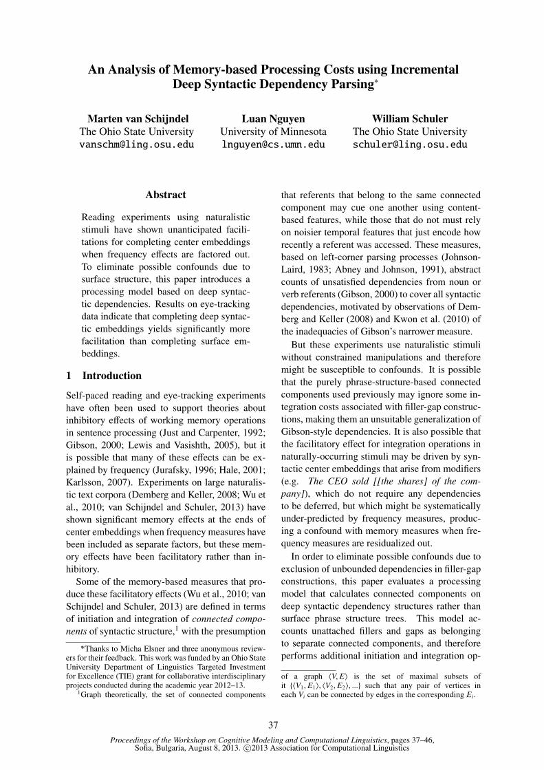
Proceedings of the Workshop on Cognitive Modeling and Computational Linguistics, pages 37–46,Sofia, Bulgaria, August 8, 2013. c©2013 Association for Computational Linguistics

An Analysis of Memory-based Processing Costs using IncrementalDeep Syntactic Dependency Parsing∗

Marten van Schijndel

The Ohio State University

vanschm@ling.osu.edu

Luan Nguyen

University of Minnesota

lnguyen@cs.umn.edu

William Schuler

The Ohio State University

schuler@ling.osu.edu

Abstract

Reading experiments using naturalistic

stimuli have shown unanticipated facili-

tations for completing center embeddings

when frequency effects are factored out.

To eliminate possible confounds due to

surface structure, this paper introduces a

processing model based on deep syntac-

tic dependencies. Results on eye-tracking

data indicate that completing deep syntac-

tic embeddings yields significantly more

facilitation than completing surface em-

beddings.

1 Introduction

Self-paced reading and eye-tracking experiments

have often been used to support theories about

inhibitory effects of working memory operations

in sentence processing (Just and Carpenter, 1992;

Gibson, 2000; Lewis and Vasishth, 2005), but it

is possible that many of these effects can be ex-

plained by frequency (Jurafsky, 1996; Hale, 2001;

Karlsson, 2007). Experiments on large naturalis-

tic text corpora (Demberg and Keller, 2008; Wu et

al., 2010; van Schijndel and Schuler, 2013) have

shown significant memory effects at the ends of

center embeddings when frequency measures have

been included as separate factors, but these mem-

ory effects have been facilitatory rather than in-

hibitory.

Some of the memory-based measures that pro-

duce these facilitatory effects (Wu et al., 2010; van

Schijndel and Schuler, 2013) are defined in terms

of initiation and integration of connected compo-

nents of syntactic structure,1 with the presumption

∗*Thanks to Micha Elsner and three anonymous review-ers for their feedback. This work was funded by an Ohio StateUniversity Department of Linguistics Targeted Investmentfor Excellence (TIE) grant for collaborative interdisciplinaryprojects conducted during the academic year 2012–13.

1Graph theoretically, the set of connected components

that referents that belong to the same connected

component may cue one another using content-

based features, while those that do not must rely

on noisier temporal features that just encode how

recently a referent was accessed. These measures,

based on left-corner parsing processes (Johnson-

Laird, 1983; Abney and Johnson, 1991), abstract

counts of unsatisfied dependencies from noun or

verb referents (Gibson, 2000) to cover all syntactic

dependencies, motivated by observations of Dem-

berg and Keller (2008) and Kwon et al. (2010) of

the inadequacies of Gibson’s narrower measure.

But these experiments use naturalistic stimuli

without constrained manipulations and therefore

might be susceptible to confounds. It is possible

that the purely phrase-structure-based connected

components used previously may ignore some in-

tegration costs associated with filler-gap construc-

tions, making them an unsuitable generalization of

Gibson-style dependencies. It is also possible that

the facilitatory effect for integration operations in

naturally-occurring stimuli may be driven by syn-

tactic center embeddings that arise from modifiers

(e.g. The CEO sold [[the shares] of the com-

pany]), which do not require any dependencies

to be deferred, but which might be systematically

under-predicted by frequency measures, produc-

ing a confound with memory measures when fre-

quency measures are residualized out.

In order to eliminate possible confounds due to

exclusion of unbounded dependencies in filler-gap

constructions, this paper evaluates a processing

model that calculates connected components on

deep syntactic dependency structures rather than

surface phrase structure trees. This model ac-

counts unattached fillers and gaps as belonging

to separate connected components, and therefore

performs additional initiation and integration op-

of a graph 〈V, E〉 is the set of maximal subsets ofit {〈V1, E1〉, 〈V2, E2〉, ...} such that any pair of vertices ineach Vi can be connected by edges in the corresponding Ei.

37

a) Noun Phrase

Relative Clause

Sentence w. Gap

Verb Phrase w. Gap

Sentence w. Gap

millionsstole

say

officials

who

Noun Phrase

personthe

b)

i1

i2 i3

i4

i5

i6

i7

1

2

1

2

1

1say

officials

stole

who

person

millionsthe0

0

0

0

0

00

Figure 1: Graphical representation of (a) a single

connected component of surface syntactic phrase

structure corresponding to (b) two connected com-

ponents of deep syntactic dependency structure for

the noun phrase the person who officials say stole

millions, prior to the word say. Connections es-

tablished prior to the word say are shown in black;

subsequent connections are shown in gray.

erations in filler-gap constructions as hypothesized

by Gibson (2000) and others. Then, in order to

control for possible confounds due to modifier-

induced center embedding, this refined model is

applied to two partitions of an eye-tracking cor-

pus (Kennedy et al., 2003): one consisting of sen-

tences containing only non-modifier center em-

beddings, in which dependencies are deferred, and

the other consisting of sentences containing no

center embeddings or containing center embed-

dings arising from attachment of final modifiers,

in which no dependencies are deferred. Processing

this partitioned corpus with deep syntactic con-

nected components reveals a significant increase

in facilitation in the non-modifier partition, which

lends credibility to the observation of negative

integration cost in processing naturally-occurring

sentences.

2 Connected Components

The experiments described in this paper evalu-

ate whether inhibition and facilitation in reading

correlate with operations in a hierarchic sequen-

tial prediction model that initiate and integrate

connected components of hypothesized syntactic

structure during incremental parsing. The model

used in these experiments refines previous con-

nected component models by allowing fillers and

gaps to occur in separate connected components

of a deep syntactic dependency graph (Mel’cuk,

1988; Kintsch, 1988), even when they belong to

the same connected component when defined on

surface structure.

For example, the surface syntactic phrase struc-

ture and deep syntactic dependency structure for

the noun phrase the person who officials say stole

millions are shown in Figure 1.2 Notice that af-

ter the word officials, there is only one connected

component of surface syntactic phrase structure

(from the root noun phrase to the verb phrase with

gap), but two disjoint connected components of

deep syntactic dependency structure (one ending

at i3, and another at i5). Only the deep syntactic

dependency structure corresponds to familiar (Just

and Carpenter, 1992; Gibson, 1998) notions of

how memory is used to store deferred dependen-

cies in filler-gap constructions. The next section

will describe a generalized categorial grammar,

which (i) can be viewed as context-free, to seed a

latent-variable probabilistic context-free grammar

to accurately derive parses of filler-gap construc-

tions, and (ii) can be viewed as a deep syntactic

dependency grammar, defining dependencies for

connected components in terms of function appli-

cations.

3 Generalized Categorial Grammar

In order to evaluate memory effects for hypothe-

sizing unbounded dependencies between referents

of fillers and referents of clauses containing gaps,

a memory-based processor must define connected

components in terms of deep syntactic dependen-

cies (including unbounded dependencies) rather

than in terms of surface syntactic phrase structure

trees. To do this, at least some phrase structure

edges must be removed from the set of connec-

tions that define a connected component.

Because these unbounded dependencies are not

represented locally in the original Treebank for-

mat, probabilities for operations on these modified

2Following Mel’cuk (1988) and Kintsch (1988),the graphical dependency structure adopted here usespositionally-defined labels (‘0’ for the predicate label, ‘1’for the first argument ahead of a predicate, ‘2’ for the lastargument behind, etc.) but includes unbounded dependen-cies between referents of fillers and referents of clausescontaining gaps. It is assumed that semantically-labeledstructures would be isomorphic to the structures definedhere, but would generalize across alternations such as activeand passive constructions, for example.

38

connected components are trained on a corpus an-

notated with generalized categorial grammar de-

pendencies for ‘gap’ arguments at all categories

that subsume a gap (Nguyen et al., 2012). This

representation is similar to the HPSG-like repre-

sentation used by Hale (2001) and Lewis and Va-

sishth (2005), but has a naturally-defined depen-

dency structure on which to calculate connected

components. This generalized categorial grammar

is then used to identify the first sign that introduces

a gap, at which point a deep syntactic connected

component containing the filler can be encoded

(stored), and a separate deep syntactic connected

component for a clause containing a gap can be

initiated.

A generalized categorial grammar (Bach, 1981)

consists of a set U of primitive category types;

a set O of type-constructing operators allowing a

recursive definition of a set of categories C =def

U ∪ (C × O × C); a set X of vocabulary items;

a mapping M from vocabulary items in X to se-

mantic functions with category types in C; and

a set R of inference rules for deriving functions

with category types in C from other functions with

category types in C. Nguyen et al. (2012) use

primitive category types for clause types (e.g. V

for finite verb-headed clause, N for noun phrase

or nominal clause, D for determiners and pos-

sessive clauses, etc.), and use the generalized set

of type-constructing operators to characterize not

only function application dependencies between

arguments immediately ahead of and behind a

functor (-a and -b, corresponding to ‘\’ and ‘/’ in

Ajdukiewicz-Bar-Hillel categorial grammars), but

also long-distance dependencies between fillers

and categories subsuming gaps (-g), dependencies

between relative pronouns and antecedent modif-

icands of relative clauses (-r), and dependencies

between interrogative pronouns and their argu-

ments (-i), which remain unsatisfied in derivations

but function to distinguish categories for content

and polar questions. A lexicon can then be de-

fined in M to introduce lexical dependencies and

obligatory pronominal dependencies using num-

bered functions for predicates and deep syntactic

arguments, for example:

the⇒ (λi (0 i)=the) : D

person⇒ (λi (0 i)=person) : N-aD

who⇒ (λk i (0 i)=who ∧ (1 i)=k) : N-rN

officials⇒ (λi (0 i)=officials) : N

the

D

person

N-aD

NAa

who

N-rN

officials

N

say

V-aN-bV

stole

V-aN-bN

millions

N

V-aNAe

V-gNGa

V-aN-gNAg

V-gNAc

V-rNFc

NR

Figure 2: Example categorization of the noun

phrase the person who officials say stole millions.

say⇒ (λi (0 i)=say) : V-aN-bV

stole⇒ (λi (0 i)=stole) : V-aN-bN

millions⇒ (λi (0 i)=millions) : N

Inference rules in R are then defined to com-

pose arguments and modifiers and propagate gaps.

Arguments g of type d ahead of functors h of

type c-ad are composed by passing non-local de-

pendencies ψ ∈ {-g, -i, -r} × C from premises to

conclusion in all combinations:

g:d h: c-ad ⇒ ( fc-ad g h): c (Aa)

g:dψ h: c-ad ⇒ λk ( fc-ad (g k) h): cψ (Ab)

g:d h: c-adψ⇒ λk ( fc-ad g (h k)): cψ (Ac)

g:dψ h: c-adψ⇒ λk ( fc-ad (g k) (h k)): cψ (Ad)

Similar rules compose arguments behind functors:

g: c-bd h:d ⇒ ( fc-bd g h): c (Ae)

g: c-bdψ h:d ⇒ λk ( fc-bd (g k) h): cψ (Af)

g: c-bd h:dψ⇒ λk ( fc-bd g (h k)): cψ (Ag)

g: c-bdψ h:dψ⇒ λk ( fc-bd (g k) (h k)): cψ (Ah)

These rules use composition functions fc-ad

and fc-bd for initial and final arguments, which de-

fine dependency edges numbered v from referents

of predicate functors i to referents of arguments j,

where v is the number of unsatisfied arguments

ϕ1...ϕv ∈ {-a, -b} ×C in a category label:

fuϕ1..v−1-acdef= λg h i ∃ j (v i)= j ∧ (g j) ∧ (h i) (1a)

fuϕ1..v−1-bcdef= λg h i ∃ j (v i)= j ∧ (g i) ∧ (h j) (1b)

R also contains inference rules to compose mod-

ifier functors g of type u-ad ahead of modifi-

cands h of type d:

g: u-ad h:c⇒ ( fIM g h):c (Ma)

g: u-adψ h:c⇒ λk ( fIM (g k) h):cψ (Mb)

g: u-ad h:cψ⇒ λk ( fIM g (h k)):cψ (Mc)

39

∃i1 j1.. iℓ jℓ ... ∧ (gℓ:c/d { jℓ} iℓ) xt

∃i1 j1.. iℓ ... ∧ ((gℓ f ):c iℓ)xt ⇒ f :d (–Fa)

∃i1 j1.. iℓ jℓ ... ∧ (gℓ:c/d { jℓ} iℓ) xt

∃i1 j1.. iℓ jℓiℓ+1 ... ∧ (gℓ:c/d { jℓ} iℓ) ∧ ( f :e iℓ+1)xt ⇒ f :e (+Fa)

∃i1 j1.. iℓ−1 jℓ−1iℓ ... ∧ (gℓ:d iℓ)

∃i1 j1.. iℓ jℓ ... ∧ (( f gℓ):c/e { jℓ} iℓ)

g:d h:e⇒ ( f g h):c or

g:d h:e⇒ λk( f (g k) h):c or

g:d h:e⇒ λk( f g (h k)):c or

g:d h:e⇒ λk( f (g k) (h k)):c

(–La)

∃i1 j1.. iℓ−1 jℓ−1iℓ ... ∧ (gℓ−1:a/c { jℓ−1} iℓ−1) ∧ (gℓ:d iℓ)

∃i1 j1.. iℓ−1 jℓ−1 ... ∧ (gℓ−1 ◦ ( f gℓ):a/e { jℓ−1} iℓ−1)

g:d h:e⇒ ( f g h):c or

g:d h:e⇒ λk( f (g k) h):c or

g:d h:e⇒ λk( f g (h k)):c or

g:d h:e⇒ λk( f (g k) (h k)):c

(+La)

Figure 3: Basic processing productions of a right-corner parser.

g: u-adψ h:cψ⇒ λk ( fIM (g k) (h k)):cψ (Md)

or for modifier functors behind a modificand:

g:c h: u-ad ⇒ ( fFM g h):c (Me)

g:cψ h: u-ad ⇒ λk ( fFM (g k) h):cψ (Mf)

g:c h: u-adψ⇒ λk ( fFM g (h k)):cψ (Mg)

g:cψ h: u-adψ⇒ λk ( fFM (g k) (h k)):cψ (Mh)

These rules use composition functions fIM and fFM

for initial and final modifiers, which define depen-

dency edges numbered ‘1’ from referents of mod-

ifier functors i to referents of modificands j:

fIMdef= λg h j ∃i (1 i)= j ∧ (g i) ∧ (h j) (2a)

fFMdef= λg h j ∃i (1 i)= j ∧ (g j) ∧ (h i) (2b)

R also contains inference rules for hypothesiz-

ing gaps -gd for arguments and modifiers:3

g: c-ad ⇒ λk ( fc-ad {k} g): c-gd (Ga)

g: c-bd ⇒ λk ( fc-ad {k} g): c-gd (Gb)

g:c⇒ λk ( fIM {k} g):c-gd (Gc)

and for attaching fillers e, d-re, d-ie as gaps -gd:

g:e h: c-gd ⇒ λi ∃ j (g i) ∧ (h i j):e (Fa)

g:d-re h: c-gd ⇒ λk j ∃i (g k i) ∧ (h i j): c-re (Fb)

g:d-ie h: c-gd ⇒ λk j ∃i (g k i) ∧ (h i j): c-ie (Fc)

3Since these unary inferences perform no explicit compo-sition, they are defined to use only initial versions composi-tion functions fc-ad and fIM.

and for attaching modificands as antecedents of

relative pronouns:

g:e h:c-rd ⇒ λi ∃ j (g i) ∧ (h i j):e (R)

An example derivation of the noun phrase the per-

son who officials say stole millions using these

rules is shown in Figure 2. The semantic expres-

sion produced by this derivation consists of a con-

junction of terms defining the edges in the graph

shown in Figure 1b.

This GCG formulation captures many of the in-

sights of the HPSG-like context-free filler-gap no-

tation used by Hale (2001) or Lewis and Vasishth

(2005): inference rules with adjacent premises can

be cast as context-free grammars and weighted us-

ing probabilities, which allow experiments to cal-

culate frequency measures for syntactic construc-

tions. Applying a latent variable PCFG trainer

(Petrov et al., 2006) to this formulation was shown

to yield state-of-the-art accuracy for recovery of

unbounded dependencies (Nguyen et al., 2012).

Moreover, the functor-argument dependencies in

a GCG define deep syntactic dependency graphs

for all derivations, which can be used in incremen-

tal parsing to calculate connected components for

memory-based measures.

4 Incremental Processing

In order to obtain measures of memory opera-

tions used in incremental processing, these GCG

inference rules are combined into a set of parser

40

∃i1 j1.. in jn.. iℓ jℓ ... ∧ (gn:y/zψ { jn} in) ∧ ... ∧ (gℓ:c/d { jℓ} iℓ) xt

∃i1 j1.. in jn.. iℓ ... ∧ (gn:y/zψ { jn} in) ∧ ... ∧ ((gℓ( f ′{ jn} f )):c iℓ)xt ⇒ λk( f ′{k} f ):d

(–Fb)

∃i1 j1.. in jn.. iℓ jℓ ... ∧ (gn:y/zψ { jn} in) ∧ ... ∧ (gℓ:c/d { jℓ} iℓ) xt

∃i1 j1.. in jn.. iℓ jℓiℓ+1 ... ∧ (gn:y/zψ { jn} in) ∧ ... ∧ (gℓ:c/d { jℓ} iℓ) ∧ (( f ′{ jn} f ):e iℓ+1)xt ⇒ λk( f ′{k} f ):e

(+Fb)

∃i1 j1.. in jn.. iℓ−1 jℓ−1iℓ ... ∧ (gn:y/zψ { jn} in) ∧ ... ∧ (gℓ:d iℓ)

∃i1 j1.. in jn.. iℓ jℓ ... ∧ (gn:y/zψ { jn} in) ∧ ... ∧ (( f gℓ) ◦ ( f ′{ jn}):cψ/e { jℓ} iℓ)

g:d h:e⇒ λk( f g ( f ′{k} h)):cψ (–Lb)

∃i1 j1.. in jn.. iℓ−1 jℓ−1iℓ ... ∧ (gn:y/zψ { jn} in) ∧ ... ∧ (gℓ−1:a/cψ { jℓ−1} iℓ−1) ∧ (gℓ:d iℓ)

∃i1 j1.. in jn.. iℓ−1 jℓ−1 ... ∧ (gn:y/zψ { jn} in) ∧ ... ∧ (gℓ−1 ◦ ( f gℓ) ◦ ( f ′{ jn}):a/e { jℓ−1} iℓ−1)

g:d h:e⇒ λk( f g ( f ′{k} h)):cψ (+Lb)

Figure 4: Additional processing productions for attaching a referent of a filler jn as the referent of a gap.

productions, similar to those of the ‘right corner’

parser of van Schijndel and Schuler (2013), ex-

cept that instead of recognizing shallow hierarchi-

cal sequences of connected components of surface

structure, the parser recognizes shallow hierarchi-

cal sequences of connected components of deep

syntactic dependencies. This parser exploits the

observation (van Schijndel et al., in press) that left-

corner parsers and their variants do not need to ini-

tiate or integrate more than one connected compo-

nent at each word. These two operations are then

augmented with rules to introduce fillers and at-

tach fillers as gaps.

This parser is defined on incomplete connected

component states which consist of an active sign

(with a semantic referent and syntactic form or

category) lacking an awaited sign (also with a ref-

erent and category) yet to come. Semantic func-

tions of active and awaited signs are simplified to

denote only sets of referents, with gap arguments

(λk) stripped off and handled by separate con-

nected components. Incomplete connected com-

ponents, therefore, always denote semantic func-

tions from sets of referents to sets of referents.

This paper will notate semantic functions of

connected components using variables g and h, in-

complete connected component categories as c/d

(consisting of an active sign of category c and an

awaited sign of category d), and associations be-

tween them as g:c/d. The semantic representa-

tion used here is simply a deep syntactic depen-

dency structure, so a connected component func-

tion is satisfied if it holds for some output ref-

erent i given input referent j. This can be no-

tated ∃i j (g:c/d { j} i), where the set { j} is equiva-

lent to (λ j′ j′= j). Connected component functions

that have a common referent j can then be com-

posed into larger connected components:4

∃i jk (g { j} i) ∧ (h {k} j) ⇔ ∃i j (g◦h {k} i) (3)

Hierarchies of ℓ connected compo-

nents can be represented as conjunctions:

∃i1 j1... iℓ jℓ (g1:c1/d1 { j1} i1) ∧ ... ∧ (gℓ:cℓ/dℓ { jℓ} iℓ).

This allows constraints such as unbounded depen-

dencies between referents of fillers and referents

of clauses containing gaps to be specified across

connected components by simply plugging vari-

ables for filler referents into argument positions

for gaps.

A nondeterministic incremental parser can now

be defined as a deductive system, given an input

sequence consisting of an initial connected com-

ponent state of category T/T, corresponding to an

existing discourse context, followed by a sequence

of observations x1, x2, . . . , processed in time order.

As each xt is encountered, it is connected to an ex-

isting connected component or it introduces a new

disjoint component using the productions shown

in Figures 3, 4, and 5.

4These are connected components of dependency struc-ture resulting from one or more composition functions beingcomposed, with each function’s output as the previous func-tion’s second argument. This uses a standard definition offunction composition: (( f ◦ g) x) = ( f (g x)).

41

∃i1 j1.. iℓ−1 jℓ−1iℓ ... ∧ (gℓ:d iℓ)

∃i1 j1.. iℓ jℓ ... ∧ (( f gℓ) ◦ (λh k i (h k)):a/eψ { jℓ} iℓ)g:d h:eψ⇒ ( f g h):c (–Lc)

∃i1 j1.. iℓ−1 jℓ−1iℓ ... ∧ (gℓ−1:a/c { jℓ−1} iℓ−1) ∧ (gℓ:d iℓ)

∃i1 j1.. iℓ−1 jℓ−1 ... ∧ (gℓ−1 ◦ ( f gℓ) ◦ (λh k i (h k)):a/eψ { jℓ−1} iℓ−1)g:d h:eψ⇒ ( f g h):c (+Lc)

∃i1 j1.. iℓ jℓ ... ∧ (gℓ−1:c/dψ { jℓ−1} iℓ−1) ∧ (gℓ:dψ/e { jℓ} iℓ)

∃i1 j1.. iℓ−1 jℓ−1 ... ∧ (gℓ−1 ◦ (λh i∃ j(h j)) ◦ gℓ:c/e { jℓ−1} iℓ−1)(+N)

Figure 5: Additional processing productions for hypothesizing filler-gap attachment.

Operations on dependencies that can be derived

from surface structure (see Figure 3) are taken

directly from van Schijndel and Schuler (2013).

First, if an observation xt can immediately fill

the awaited sign of the last connected component

gℓ:c/d, it is hypothesized to do so, turning this

incomplete connected component into a complete

connected component (gℓ f ):c (Production –Fa); or

if the observation can serve as an initial sub-sign

of this awaited sign, it is hypothesized to form a

new complete sign f :e in a new component with xt

as its first observation (Production +Fa). Then,

if either of these resulting complete signs gℓ:d

can immediately attach as an initial child of the

awaited sign of the most recent connected com-

ponent gℓ−1:a/c, it is hypothesized to merge and

extend this connected component, with xt as the

last observation of the completed connected com-

ponent (Production +La); or if it can serve as an

initial sub-sign of this awaited sign, it is hypoth-

esized to remain disjoint and form its own con-

nected component (Production –La). The side

conditions of La productions are defined to unpack

gap propagation (instances of λk that distinguish

rules Aa–h and Ma–h) from the inference rules

in Section 3, because this functionality will be re-

placed with direct substitution of referent variables

into subordinate semantic functions, below.

The Nguyen et al. (2012) GCG was defined

to pass up unbounded dependencies, but in in-

cremental deep syntactic dependency processing,

unbounded dependencies are accounted as sepa-

rate connected components. When hypothesizing

an unbounded dependency, the processing model

simply cues the active sign of a previous connected

component containing a filler without completing

the current connected component. The four +F,

–F, +L, and –L operations are therefore combined

with applications of unary rules Ga–c for hypoth-

esizing referents as fillers for gaps (providing f ′

in the equations in Figure 4). Productions –Fb

and +Fb fill gaps in initial children, and Produc-

tions –Lb and +Lb fill gaps in final children. Note

that the Fb and Lb productions apply to the same

types of antecedents as Fa and La productions re-

spectively, so members of these two sets of pro-

ductions cannot be applied together.

Applications of rules Fa–c and R for introduc-

ing fillers are applied to store fillers as existentially

quantified variable values in Lc productions (see

Figure 5). These Lc productions apply to the same

type of antecedent as La and Lb productions, so

these also cannot be applied together.

Finally, connected components separated by

gaps which are no longer hypothesized (ψ) are

reattached by a +N production. This +N pro-

duction may then be paired with a –N production

which yields its antecedent unchanged as a conse-

quent. These N productions apply to antecedents

and consequents of the same type, so they may be

applied together with one F and one L production,

but since the +N production removes in its conse-

quent a ψ argument required in its antecedent, it

may not apply more than once in succession (and

applying the –N production more than once in suc-

cession has no effect).

An incremental derivation of the noun phrase

the person who officials say stole millions, using

these productions, is shown in Figure 6.

5 Evaluation

The F, L, and N productions defined in the pre-

vious section can be made probabilistic by first

computing a probabilistic context-free grammar

(PCFG) from a tree-annotated corpus, then trans-

forming that PCFG model into a model of prob-

abilities over incremental parsing operations us-

ing a grammar transform (Schuler, 2009). This

allows the intermediate PCFG to be optimized us-

ing an existing PCFG-based latent variable trainer

42

∃i0 (.. :T/T {i0} i0) the

∃i0 i2 (.. :T/T {i0} i0) ∧ (.. :N/N-aD {i2} i2)+Fa,–La,–N

person

∃i0 i2 (.. :T/T {i0} i0) ∧ (.. :N/V-rN {i2} i2)–Fa,–La,–N

who

∃i0 i2 i3 (.. :T/T {i0} i0) ∧ (.. :N/V-gN {i3} i2)+Fa,+Lc,–N

officials

∃i0 i2 i3 i5 (.. :T/T {i0} i0) ∧ (.. :N/V-gN {i3} i2) ∧ (.. :V-gN/V-aN-gN {i5} i5)+Fa,–La,–N

say

∃i0 i2 i6 (.. :T/T {i0} i0) ∧ (.. :N/V-aN {i6} i2)+Fb,+La,+N

stole

∃i0 i2 i7 (.. :T/T {i0} i0) ∧ (.. :N/N {i7} i2)+Fa,+La,–N

millions

∃i0 (.. :T/T {i0} i0)–Fa,+La,–N

Figure 6: Derivation of the person who officials say stole millions, showing connected components with

unique referent variables (calculated according to the equations in Section 4). Semantic functions are

abbreviated to ‘..’ for readability. This derivation yields the following lexical relations: (0 i1)=the,

(0 i2)=person, (0 i3)=who, (0 i4)=officials, (0 i5)=say, (0 i6)=stole, (0 i7)=millions, and the following

argument relations: (1 i2)=i1, (1 i3)=i2, (1 i5)=i4, (2 i5)=i6, (1 i6)=i3, (2 i6)=i7.

(Petrov et al., 2006). When applied to the output

of this trainer, this transform has been shown to

produce comparable accuracy to that of the origi-

nal Petrov et al. (2006) CKY parser (van Schijn-

del et al., 2012). The transform used in these ex-

periments diverges from that of Schuler (2009), in

that the probability associated with introducing a

gap in a filler-gap construction is reallocated from

a –F–L operation to a +F–L operation (to encode

the previously most subordinate connected com-

ponent with the filler as its awaited sign and be-

gin a new disjoint connected component), and the

probability associated with resolving such a gap is

reallocated from an implicit –N operation to a +N

operation (to integrate the connected component

containing the gap with that containing the filler).

In order to verify that the modifications to the

transform correctly reallocate probability mass for

gap operations, the goodness of fit to reading

times of a model using this modified transform

is compared against the publicly-available base-

line model from van Schijndel and Schuler (2013),

which uses the original Schuler (2009) transform.5

To ensure a valid comparison, both parsers are

trained on a GCG-reannotated version of the Wall

Street Journal portion of the Penn Treebank (Mar-

cus et al., 1993) before being fit to reading times

using linear mixed-effects models (Baayen et al.,

2008).6 This evaluation focuses on the process-

ing that can be done up to a given point in a sen-

tence. In human subjects, this processing includes

both immediate lexical access and regressions that

5The models used here also use random slopes to reducetheir variance, which makes them less anticonservative.

6The models are built using lmer from the lme4 R package(Bates et al., 2011; R Development Core Team, 2010).

aid in the integration of new information, so the

reading times of interest in this evaluation are log-

transformed go-past durations.7

The first and last word of each line in the

Dundee corpus, words not observed at least 5

times in the WSJ training corpus, and fixations af-

ter long saccades (>4 words) are omitted from the

evaluation to filter out wrap-up effects, parser in-

accuracies, and inattention and track loss of the

eyetracker. The following predictors are centered

and used in each baseline model: sentence posi-

tion, word length, whether or not the previous or

next word were fixated upon, and unigram and bi-

gram probabilities.8 Then each of the following

predictors is residualized off each baseline before

being centered and added to it to help residualize

the next factor: length of the go-past region, cumu-

lative total surprisal, total surprisal (Hale, 2001),

and cumulative entropy reduction (Hale, 2003).9

All 2-way interactions between these effects are

7Go-past durations are calculated by summing all fixa-tions in a region of text, including regressions, until a newregion is fixated, which accounts for additional processingthat may take place after initial lexical access, but before thenext region is processed. For example, if one region ends atword 5 in a sentence, and the next fixation lands on word 8,then the go-past region consists of words 6-8 while go-pastduration sums all fixations until a fixation occurs after word8. Log-transforming eye movements and fixations may maketheir distributions more normal (Stephen and Mirman, 2010)and does not substantially affect the results of this paper.

8For the n-gram model, this study uses the Brown corpus(Francis and Kucera, 1979), the WSJ Sections 02-21 (Mar-cus et al., 1993), the written portion of the British NationalCorpus (BNC Consortium, 2007), and the Dundee corpus(Kennedy et al., 2003) smoothed with modified Kneser-Ney(Chen and Goodman, 1998) in SRILM (Stolcke, 2002).

9Non-cumulative metrics are calculated from the finalword of the go-past region; cumulative metrics are summedover the go-past region.

43

included as predictors along with the predictors

from the previous go-past region (to account for

spillover effects). Finally, each model has sub-

ject and item random intercepts added in addition

to by-subject random slopes (cumulative total sur-

prisal, whether the previous word was fixated, and

length of the go-past region) and is fit to centered

log-transformed go-past durations.10

The Akaike Information Criterion (AIC)

indicates that the gap-reallocating model

(AIC = 128,605) provides a better fit to reading

times than the original model (AIC = 128,619).11

As described in Section 1, previous findings of

negative integration cost may be due to a confound

whereby center-embedded constructions caused

by modifiers, which do not require deep syntac-

tic dependencies to be deferred, may be driving

the effect. Under this hypothesis, embeddings

that do not arise from final adjunction of mod-

ifiers (henceforth canonical embeddings) should

yield a positive integration cost as found by Gib-

son (2000).

To investigate this potential confound, the

Dundee corpus is partitioned into two parts. First,

the model described in this paper is used to anno-

tate the Dundee corpus. From this annotated cor-

pus, all sentences are collected that contain canon-

ical embeddings and lack modifier-induced em-

beddings.12 This produces two corpora: one con-

sisting entirely of canonical center-embeddings

such as those used in self-paced reading exper-

iments with findings of positive integration cost

(e.g. Gibson 2000), the other consisting of the

remainder of the Dundee corpus, which contains

sentences with canonical embeddings but also in-

cludes modifier-caused embeddings.

The coefficient estimates for integration oper-

ations (–F+L and +N) on each of these corpora

are then calculated using the baseline described

above. To ensure embeddings are driving any ob-

served effect rather than sentence wrap-up effects,

the first and last words of each sentence are ex-

cluded from both data sets. Integration cost is

measured by the amount of probability mass the

parser allocates to –F+L and +N operations, accu-

10Each fixed effect that has an absolute t-value greater than10 when included in a random-intercepts only model is addedas a random slope by-subject.

11The relative likelihood of the original model to the gap-sensitive model is 0.0009 (n = 151,331), which suggests theimprovement is significant.

12Modifier-induced embeddings are found by looking forembeddings that arise from inference rules Ma-h in Section 3.

Model coeff std err t-score

Canonical -0.040 0.010 -4.05

Other -0.017 0.004 -4.20

Table 1: Fixed effect estimates for integration cost

when used to fit reading times over two partitions

of the Dundee corpus: one containing only canon-

ical center embeddings and the other composed of

the rest of the sentences in the corpus.

mulated over each go-past region, and this cost is

added as a fixed effect and as a random slope by

subject to the mixed model described earlier.13

The fixed effect estimate for cumulative inte-

gration cost from fitting each corpus is shown

in Table 1. Application of Welch’s t-test shows

that the difference between the estimated distri-

butions of these two parameters is highly signif-

icant (p < 0.0001).14 The strong negative corre-

lation of integration cost to reading times in the

purely canonical corpus suggests canonical (non-

modifier) integrations contribute to the finding of

negative integration cost.

6 Conclusion

This paper has introduced an incremental parser

capable of using GCG dependencies to distinguish

between surface syntactic embeddings and deep

syntactic embeddings. This parser was shown to

obtain a better fit to reading times than a surface-

syntactic parser and was used to parse the Dundee

eye-tracking corpus in two partitions: one consist-

ing of canonical embeddings that require deferred

dependencies and the other consisting of sentences

containing no center embeddings or center em-

beddings arising from the attachment of clause-

final modifiers, in which no dependencies are de-

ferred. Using linear mixed effects models, com-

pletion (integration) of canonical center embed-

dings was found to be significantly more nega-

tively correlated with reading times than comple-

tion of non-canonical embeddings. These results

suggest that the negative integration cost observed

in eye-tracking studies is at least partially due to

deep syntactic dependencies and not due to con-

founds related to surface forms.

13Integration cost is residualized off the baseline before be-ing centered and added as a fixed effect.

14Integration cost is significant as a fixed effect (p = 0.001)in both partitions: canonical (n = 16,174 durations) andnon-canonical (n = 131,297 durations).

44

References

Steven P. Abney and Mark Johnson. 1991. Memoryrequirements and local ambiguities of parsing strate-gies. J. Psycholinguistic Research, 20(3):233–250.

R. Harald Baayen, D. J. Davidson, and Douglas M.Bates. 2008. Mixed-effects modeling with crossedrandom effects for subjects and items. Journal ofMemory and Language, 59:390–412.

Emmon Bach. 1981. Discontinuous constituents ingeneralized categorial grammars. Proceedings ofthe Annual Meeting of the Northeast Linguistic So-ciety (NELS), 11:1–12.

Douglas Bates, Martin Maechler, and Ben Bolker,2011. lme4: Linear mixed-effects models using S4classes.

BNC Consortium. 2007. The british national corpus.

Stanley F. Chen and Joshua Goodman. 1998. An em-pirical study of smoothing techniques for languagemodeling. Technical report, Harvard University.

Vera Demberg and Frank Keller. 2008. Data from eye-tracking corpora as evidence for theories of syntacticprocessing complexity. Cognition, 109(2):193–210.

W. Nelson Francis and Henry Kucera. 1979. Thebrown corpus: A standard corpus of present-dayedited american english.

Edward Gibson. 1998. Linguistic complexity: Local-ity of syntactic dependencies. Cognition, 68(1):1–76.

Edward Gibson. 2000. The dependency locality the-ory: A distance-based theory of linguistic complex-ity. In Image, language, brain: Papers from the firstmind articulation project symposium, pages 95–126,Cambridge, MA. MIT Press.

John Hale. 2001. A probabilistic earley parser as apsycholinguistic model. In Proceedings of the sec-ond meeting of the North American chapter of theAssociation for Computational Linguistics, pages159–166, Pittsburgh, PA.

John Hale. 2003. Grammar, Uncertainty and SentenceProcessing. Ph.D. thesis, Cognitive Science, TheJohns Hopkins University.

Philip N. Johnson-Laird. 1983. Mental models: to-wards a cognitive science of language, inference,and consciousness. Harvard University Press, Cam-bridge, MA, USA.

Daniel Jurafsky. 1996. A probabilistic model of lexicaland syntactic access and disambiguation. CognitiveScience: A Multidisciplinary Journal, 20(2):137–194.

Marcel Adam Just and Patricia A. Carpenter. 1992. Acapacity theory of comprehension: Individual differ-ences in working memory. Psychological Review,99:122–149.

Fred Karlsson. 2007. Constraints on multiple center-embedding of clauses. Journal of Linguistics,43:365–392.

Alan Kennedy, James Pynte, and Robin Hill. 2003.The Dundee corpus. In Proceedings of the 12th Eu-ropean conference on eye movement.

Walter Kintsch. 1988. The role of knowledge in dis-course comprehension: A construction-integrationmodel. Psychological review, 95(2):163–182.

Nayoung Kwon, Yoonhyoung Lee, Peter C. Gordon,Robert Kluender, and Maria Polinsky. 2010. Cog-nitive and linguistic factors affecting subject/objectasymmetry: An eye-tracking study of pre-nominalrelative clauses in korean. Language, 86(3):561.

Richard L. Lewis and Shravan Vasishth. 2005.An activation-based model of sentence processingas skilled memory retrieval. Cognitive Science,29(3):375–419.

Mitchell P. Marcus, Beatrice Santorini, and Mary AnnMarcinkiewicz. 1993. Building a large annotatedcorpus of English: the Penn Treebank. Computa-tional Linguistics, 19(2):313–330.

Igor Mel’cuk. 1988. Dependency syntax: theory andpractice. State University of NY Press, Albany.

Luan Nguyen, Marten van Schijndel, and WilliamSchuler. 2012. Accurate unbounded dependencyrecovery using generalized categorial grammars. InProceedings of the 24th International Conference onComputational Linguistics (COLING ’12), Mumbai,India.

Slav Petrov, Leon Barrett, Romain Thibaux, and DanKlein. 2006. Learning accurate, compact, and in-terpretable tree annotation. In Proceedings of the44th Annual Meeting of the Association for Compu-tational Linguistics (COLING/ACL’06).

R Development Core Team, 2010. R: A Language andEnvironment for Statistical Computing. R Foun-dation for Statistical Computing, Vienna, Austria.ISBN 3-900051-07-0.

William Schuler. 2009. Parsing with a bounded stackusing a model-based right-corner transform. In Pro-ceedings of NAACL/HLT 2009, NAACL ’09, pages344–352, Boulder, Colorado. Association for Com-putational Linguistics.

Damian G. Stephen and Daniel Mirman. 2010. Inter-actions dominate the dynamics of visual cognition.Cognition, 115(1):154–165.

Andreas Stolcke. 2002. Srilm – an extensible languagemodeling toolkit. In Seventh International Confer-ence on Spoken Language Processing.

Marten van Schijndel and William Schuler. 2013. Ananalysis of frequency- and recency-based processingcosts. In Proceedings of NAACL-HLT 2013. Associ-ation for Computational Linguistics.

45

Marten van Schijndel, Andy Exley, and WilliamSchuler. 2012. Connectionist-inspired incrementalPCFG parsing. In Proceedings of CMCL 2012. As-sociation for Computational Linguistics.

Marten van Schijndel, Andy Exley, and WilliamSchuler. in press. A model of language processingas hierarchic sequential prediction. Topics in Cogni-tive Science.

Stephen Wu, Asaf Bachrach, Carlos Cardenas, andWilliam Schuler. 2010. Complexity metrics in anincremental right-corner parser. In Proceedings ofthe 48th Annual Meeting of the Association for Com-putational Linguistics (ACL’10), pages 1189–1198.

46

Proceedings of the Workshop on Cognitive Modeling and Computational Linguistics, pages 47–56,Sofia, Bulgaria, August 8, 2013. c©2013 Association for Computational Linguistics

Computational simulations of second language construction learning

Yevgen Matusevych Afra Alishahi Ad BackusDepartment of Department of Communication Department ofCulture Studies and Information Sciences Culture Studies

Tilburg University, PO Box 90153, 5000 LE Tilburg, the NetherlandsY.Matusevych@uvt.nl A.Alishahi@uvt.nl A.M.Backus@uvt.nl

Abstract

There are few computational models of sec-ond language acquisition (SLA). At the sametime, many questions in the field of SLA re-main unanswered. In particular, SLA patternsare difficult to study due to the large amount ofvariation between human learners. We presenta computational model of second languageconstruction learning that allows manipulatingspecific parameters such as age of onset andamount of exposure. We use the model tostudy general developmental patterns of SLAand two specific effects sometimes found inempirical studies: construction priming and afacilitatory effect of skewed frequencies in theinput. Our simulations replicate the expectedSLA patterns as well as the two effects. Ourmodel can be used in further studies of variousSLA phenomena.

1 Introduction

Computational models have been widely used forinvestigating how humans learn and process theirnative language. Various models of child languageacquisition have been applied to studies of speechsegmentation (e.g., ten Bosch, Hamme, & Boves,2008), word learning (e.g., Frank, Goodman, &Tenenbaum, 2009; Fazly, Alishahi, & Stevenson,2010), induction of linguistic structure (e.g., El-man, 1990), etc. In comparison, the acquisition ofsecond language has received little attention fromthe modeling community. Most of the child lan-guage acquisition models cannot be directly usedfor investigating how humans process and acquireforeign languages. In order to do so, we have tomodel the existing knowledge of first language—i.e., bilingualism.

Li (2013) provides a state-of-the-art overviewof models of bilingualism. One of his claimsis that most existing models account for mature

adult speaker’s knowledge and do not explain howforeign language develops in learners. In otherwords, there are several computational models ofsecond language processing (e.g., Shook & Mar-ian, 2013; Roelofs, Dijkstra, & Gerakaki, 2013;Yang, Shu, McCandliss, & Zevin, 2013, etc.), butonly few of Second Language Acquisition (SLA).The latter mostly simulate lexis and semantics ac-quisition (e.g., Li & Farkas, 2002; Li, 2009; Cup-pini, Magosso, & Ursino, 2013, etc.), and thosethat address a higher level of language structureusually do not model the existing L1 knowledge(e.g., N. C. Ellis & Larsen-Freeman, 2009; Rap-poport & Sheinman, 2005; but see Monner, Vatz,Morini, Hwang, & DeKeyser, 2013).

At the same time, a number of theoretical SLAissues are not well explained yet, including gen-eral questions such as how existing knowledge ofthe first language influences the acquisition of sec-ond language. To give a specific example, it is notclear yet when L1 structures lead to interferenceand when they do not.

In this paper, we use an existing model ofearly acquisition of argument structure construc-tions (Alishahi & Stevenson, 2008) and adapt itto bilingual input data, which allows us to inves-tigate the acquisition process in second languagelearners. We demonstrate in a number of compu-tational simulations that our model replicates nat-ural L2 developmental patterns and two specificeffects observed in human L2 learners, thus allow-ing us to make certain predictions about the issuesunder investigation.

2 Description of the model

A usage-based approach to language claims thathumans learn abstract linguistic regularities frominstances of language use. Specifically, gen-eral argument structure constructions are predictedto emerge over time from individual verb us-ages which share syntactic and semantic proper-

47

ties. Argument structure constructions, accordingto Goldberg, Casenhiser, and White (2007), are“pairings of form and meaning that provide themeans of expressing simple propositions in a lan-guage” (p. 74). Since nearly all human utterancescontain propositions, the learner’s knowledge ofargument structure constructions must reflect thelevel of his grammatical competence.

The model of Alishahi and Stevenson (2008) isbased on this approach: the building block of themodel is an argument structure frame, a collec-tion of syntactic and semantic features which rep-resents a verb usage. Abstract constructions areformed by detecting and clustering similar frames,and various linguistic tasks are simulated by hav-ing the model predict the most suitable values forthe missing features in a frame. These componentsare described in the following sections.

2.1 Argument structure framesIn our SLA model, each frame contains the fol-lowing features:• Head verb in its infinitive form.• Number of arguments that the verb takes.• Semantic primitives of the verb represent-

ing the conceptual characteristics of the eventthat the verb describes.• Semantic properties of each argument rep-

resenting its conceptual meaning, indepen-dently of the event that it participates in.• Event-based properties of each argument

representing the characteristics each argu-ment takes on in the particular event it is par-ticipating in.• Syntactic pattern of the utterance.

A sample frame is shown in Table 1. In Section 3.3we will further explain how values for each framefeature are selected.

Table 1: An example frame extracted from a verbusage Bill went through the maze.

Head verb (V.) goNo. of arguments 2V. sem. primitives act, move, walkArg.1 sem. prop-s name, male, person, ...Arg.2 sem. prop-s system, instrumentality, ...Arg.1 event prop-s volitional, sentient, ...Arg.2 event prop-s location, path, destinationSyntactic pattern AGENT V. through LOC.

2.2 Learning ConstructionsAlishahi and Stevenson (2008) use an incrementalBayesian algorithm for clustering similar framesinto constructions. Each input frame is comparedto all the existing constructions and a potentiallynew one, and is added to the best matching con-struction:

BestConstruction(F) = argmaxk

P(k|F) (1)

where k ranges over the indices of all constructions(index 0 represents the new construction). UsingBayes rule and dropping P(F) which is constantfor all k:

P(k|F) =P(k)P(F |k)

P(F)∼ P(k)P(F |k) (2)

The prior probability P(k) indicates the degree ofentrenchment of construction k:

P(k) =Nk

N +1,P(0) =

1N +1

(3)

where Nk is the number of frames already clus-tered in construction k, and N is the total numberof frames observed so far. The posterior probabil-ity of a frame F is expressed in terms of the (sup-posedly independent) probabilities of its features:

P(F |k) = ∏i∈Features(F)

Pi( j|k) (4)

where j is the value of the ith feature of F , andPi( j|k) is the probability of displaying value j onfeature i within construction k. This probability isestimated using a smoothed maximum likelihoodformula.1

2.3 Bilingual acquisitionWe accept the view that L1 and L2 learning havemore commonalities than differences (see, e.g.,MacWhinney, 2013), thus we do not explicitly en-code the difference between the two languages. Asthe learner perceives a frame, he is not aware ofwhich language the frame belongs to. All the in-put data are processed equally, so that construc-tions are formed in the same space and can containframes from both languages. Such approach al-lows us to investigate how the existing L1 knowl-edge influences L2 acquisition.

1For single-valued features such as the head verb, likeli-hood is calculated by simply counting those members of con-struction k whose value for feature i exactly matches value j.For features with a set value such as the semantic propertiesof the verb and the arguments, the likelihood is calculated bycomparing sets.

48

2.4 Sentence productionWe use sentence production as our main evalua-tion task for SLA. Given a frame which representsan intended meaning through the semantic prop-erties of an event (or verb) and its participants (orarguments), we want to predict the most probablevalues for the syntactic pattern feature. FollowingAlishahi and Stevenson (2008), we estimate theprobability that feature i (in our case, the syntac-tic pattern) displays value j given other observedfeature values in a partial frame F as

Pi( j|F) = ∑k

Pi( j|k)P(k|F) (5)

= ∑k

Pi( j|k)P(k)P(F |k)

The probabilities P(k), P(F |k) and Pi( j|k) are esti-mated as before (see Equations 3 and 4). Rangingover the possible values j of feature i, the value ofan unobserved feature can be predicted by maxi-mizing Pi( j|F)2:

BestValuei(F) = argmaxj

Pi( j|F) (6)

3 Data

For cognitively plausible computational simula-tions we had to prepare naturalistic input basedon the suitable corpora. While there are availablecorpora that contain recordings of child-directedspeech (MacWhinney, 2000), the resources con-taining speech addressed to L2 learners appear tobe very limited. Therefore, our choice of lan-guages (German as a L1, and English as a L2) wasmotivated first of all by the data availability. Weextracted naturalistic L1 and L2 data from two dif-ferent sources.

3.1 Data sourcesL2 English data were extracted from the Flens-burg classroom corpus (Jakel, 2010) that containstranscripts of lessons of English (as a foreign lan-guage) taught to children in German schools thatcover all school age groups. We estimated the to-tal number of occurrences of different verbs in thecorpus. From 20 most frequent verbs we selected6 that represented syntactically and semanticallydifferent linguistic constructions, since construc-tional variability was one of the crucial factors for

2A non-deterministic alternative that we have to considerin the future is to sample the feature value from the estimateddistribution.

the model. The verbs are: go, come, read, show,look and put. For each verb, we extracted all itsoccurrences from the corpus.

For L1 we used German data extracted from theCHILDES database (MacWhinney, 2000), namelyfrom adults’ speech directed to three children:Caroline (age from 0;10 to 4;3; von Stutterheim,2004), Kerstin (from 1;3 to 3;4; M. Miller, 1979)and Leo (from 1;11 to 4;11; Behrens, 2006). Inthe same manner as for the English data, we se-lected six verbs—machen ‘to make’, kommen ‘tocome’, gucken ‘to look’, gehen ‘to go’, sehen ‘tosee’ and geben ‘to give’— and extracted all theiroccurrences from the three corpora. Since the cor-pora were of different size, the number of occur-rences for some verbs were incomparable betweenthe corpora, thus we balanced the size of the sam-ples used for further analysis by taking equal num-bers of random verb uses from each corpus.

3.2 Data annotation

Since the basic input unit for our computationalmodel was a frame, we manually annotated allthe verb occurrences in order to extract frames.Approximately 100 instances per verb were anno-tated using the following general guidelines.

1. Instance grouping is based on the semanticsof the main verb and its arguments as well ason the syntactic pattern.

2. We consider only arguments (both obligatoryand optional), but not adjuncts, since thereis evidence that the two are processed differ-ently (see, e.g., Kennison, 2002).

3. We discard all instances where the main verbwas represented by a compound form or byan infinitive, or appeared in a subordinateclause, since in all these cases the “core”frame of the argument structure constructionmight obtain additional structural or semanticcharacteristics.

4. We do consider imperatives and questionswhose form does not contradict the previouspoint.

5. We treat German prefixed/particle verbs (e.g.,zumachen ‘to close’) and English compoundverbs as an instance of the base verb (in thiscase, machen ‘to make’), given that the pre-fixed/particle verb meaning is compositionaland the prefix/particle is actually separated.

6. Considering the previous point, each parti-cle/prefix in our instances represents an in-

49

dependent semantic component (see, e.g.,Dewell, 2011, for detailed explanation), andwe treat them as separate arguments.

7. We discard all the instances in which the verbis used in a formulaic sequence (e.g.,, Wiegeht’s? ‘How are you?’), because formulaicsequences are believed to be processed andacquired as a whole (e.g., Wray, 2005; Ban-nard & Lieven, 2012).

8. Finally, we eliminate the case marking inGerman and use the Nominative case forall the arguments, because this feature isnot crucial for our model, and there is ev-idence that German children before the ageof 7 mostly rely on other features such asword order (Dittmar, Abbot-Smith, Lieven,& Tomasello, 2008).

3.3 Frame extraction

From the annotated data samples, for each verb weextracted frames and their respective frequenciesof occurrence. Following Alishahi and Steven-son (2010), the semantic primitives of verbs andtheir arguments were semi-automatically extractedfrom WordNet (G. A. Miller, 1995), and the event-based properties of the arguments were manuallycompiled.

The syntactic pattern of the frame not onlyshows the order of the arguments, but also im-plicitly includes information about their seman-tic roles, i.e., AGENT, THEME, LOCATION, etc.Note that these semantic labels are used only fordistinguishing between similar syntactic patternswith the verb in the same position but swappedarguments (cf. [so] schnell geht es vs. es geht[so] schnell ‘it goes [so] fast’—both patterns oc-cur rather frequently in German).3

Based on the manually extracted frames, an in-put corpus of verb uses was automatically gener-ated for each set of experiments. The frequency ofoccurrence of each frame determined the probabil-ity of selecting this frame, and the same methodwas used for selecting specific arguments.

3Although the inclusion of semantic labels into syntac-tic pattern makes the learning task easier, there is, in fact,no agreement yet on how exactly children acquire the non-canonical word order. They must rely on pragmatics, and thisphenomenon most thoroughly has been studied in the gener-ative tradition under the name of scrambling, but still vari-ous explanations were proposed (see, e.g., Mykhaylyk & Ko,2011). Due to this uncertainty, we found it acceptable to pro-vide the learner with the means to distinguish between thepatterns like in the example above, since it was highly impor-tant for German with its partially free word order.

4 Simulations and results

In this section we report on computational simu-lations that we ran using our model and the de-scribed input data. We investigate general L2 de-velopmental patterns, priming effects in SLA, andthe impact of skewed input on the learner’s L2 pro-ficiency. Although the latter two are not SLA phe-nomena per se and can be observed in L1 learnersas well, they have been discussed in SLA domainand suit well our methodological framework.

4.1 L2 general development

Despite numerous attempts to capture and de-scribe the dynamics of SLA, scholars admit thatthere is no ‘typical’ profile of general L2 develop-ment (for an overview, see Hasko, 2013). This isbecause many variables are involved, such as thelearner’s L1, the age of L2 onset, amount of input,type of instruction (if any), etc. They cause signif-icant differences between individual learners andspecific linguistic phenomena.

Generally, L2 develops gradually, and secondlanguage learners rarely achieve native-like L2proficiency. To demonstrate that our model fol-lows these patterns, we ran a number of simu-lations to compare how L1 and L2 proficiencychanges over time. In our scenario, the learnerwas first presented 500 L1 verb uses in smallsteps (25 times 20 frames). After each step hisL1 proficiency was tested in the following way.The learner was presented with 20 test frames inwhich the syntactic pattern was removed, and hadto predict the most suitable syntactic pattern, re-lying on his current knowledge. We should notethat because German has partially free word or-der, our German data contained a substantial num-ber of frame groups consisting of two or moreframes that were almost identical and differed onlyin the order of arguments in their syntactic pat-terns (i.e., AGENT verb THEME and THEME verbAGENT). These patterns are very close both lin-guistically (i.e., they carry very similar meanings)and algorithmically (i.e., the learner’s preferencefor one of them is determined only by their re-spective frequencies of occurrence in the input).Therefore, asking the learner to predict the exactpattern would not be a fair task. For this reason,during the evaluation we only checked whether thepattern produced by the learner contained exactlythe same set of arguments (and, possibly, the samepreposition) as the target pattern. Thus, AGENT

50

kommen THEME, kommen AGENT THEME, andTHEME kommen AGENT were considered equal forthe purpose of evaluation.

After the initial 25 steps of L1 training and test-ing, the learner was presented 500 more frames(25 times 20) which could be either from L1 orfrom L2 data in proportion 3 (L1) to 1 (L2). Thisway we simulated a common situation when achild starts learning a foreign language at school,thus being exposed to input from both languages,but L1 input prevails. The results averaged over10 simulations (Figure 1) demonstrate that the L2proficiency does not achieve that of L1.4

0 10 20 30 40 50 60

0.0

0.5

1.0

Steps

Acc

urac

y

L1L2

Figure 1: L1 and L2 development over time

We explain the lower L2 proficiency by two fac-tors. First, by the moment when the learner startedreceiving L2 input, L1 constructions were alreadyformed in his memory, so the L1 entrenchmentprevented L2 constructions to fully emerge. Sec-ond, even within the period of SLA the amount ofL2 input was 3 times smaller compared to that ofL1. To investigate whether both factors were in-deed important, we tried to eliminate each of themseparately, i.e., to present both L1 and L2 fromthe very beginning keeping the ratio 3:1 (Figure 2,left), or to set an equal ratio while keeping the lateage of L2 onset (Figure 2, right). As we can see, inneither case does the L2 proficiency reach that ofL1. However, when both factors are eliminated—that is, from the very beginning the learner re-ceives mixed L1/L2 input in equal proportion—he reaches comparable levels of L1 and L2 profi-ciency (Figure 3).

Additionally, we tried to separately manipulateeach of the two parameters keeping the other oneconstant. We expected that (1) the lower the L2age of onset, the higher the learner’s proficiency ateach moment of time with the L1/L2 ratio set at3:1, and (2) the smaller the L1/L2 ratio (down to1, when the amount of input is equal), the higher

4After presenting 4,000 more L2 frames to the learner thispattern was still observed, and neither L1 nor L2 proficiencyconverged to 1.

0 5 10 15 20 25 30

0.0

0.5

1.0

Steps

Acc

urac

y

L1L2

0 10 20 30 40 50 60

0.0

0.5

1.0

Steps

Acc

urac

y

L1L2

Figure 2: L1 and L2 proficiency provided equalage of onset (left) or input ratio (right)

0 5 10 15 20 25 30

0.0

0.5

1.0

Steps

Acc

urac

y

L1L2

Figure 3: L1 and L2 proficiency provided equallearning conditions

the learner’s proficiency at each moment of timewith the age of onset set at 500 frames. We foundno evidence for either effect. Part of the expla-nation might be that there was a substantial over-lap between L1 and L2 syntactic patterns (espe-cially considering we treated patterns as sets ofelements irrespective of word order). Thereforethe learner’s existing L1 knowledge may indirectlyhave contributed to the L2 proficiency, in a patternknown as “positive transfer” (see, e.g., Benson,2002). This can be demonstrated by comparingthe initial slopes of L2 development lines in Fig-ure 1 and Figure 2a. In the former case, represent-ing L2 exposure after L1 constructions have al-ready been entrenched, L2 acquisition goes fasterin its initial stages, because the learner has, in fact,already acquired a number of syntactic patternsthat are shared by the two languages. Monner et al.(2013), who computationally studied the effect ofFrench L1 entrenchment on Spanish L2 grammat-ical gender learning, explain an exception in theirresults in similar fashion. However, this requiresfurther investigation, possibly in simulations in-volving two languages that are typologically moredistant.

4.2 Priming effects in L2

Structural priming effects, when speakers tend torecreate a recently encountered linguistic structurein further language use, have been demonstratedboth in first (e.g., Bock, Dell, Chang, & Onishi,2007; Potter & Lombardi, 1998, etc.) and in sec-ond language (e.g., McDonough, 2006; Gries &

51

Wulff, 2005) as well as across the two (e.g., Loe-bell & Bock, 2003; Vasilyeva et al., 2010). Someof these effects are explained in terms of construc-tion grammar—primes can activate the respectiveconstructions (see Goldberg & Bencini, 2005).

To give a specific example, Gries and Wulff(2005) asked L1 German learners of English tocomplete sentence fragments after being exposedto a prime sentence, which contained either aprepositional dative (The racing driver showed thetorn overall to the team manager.) or a ditransitiveconstruction (The racing driver showed the helpfulmechanic the damaged tyre). The sentences pro-duced by the learners demonstrated the construc-tional priming effect in L2 acquisition, which wasalso supported by corpus and sorting evidence (seeGries & Wulff, 2005, for details).

Since in our model we explicitly assume the ex-istence of constructions in learner’s memory, weshould be able to observe constructional primingeffects in L2. To investigate this, we partially sim-ulated the experiment of Gries and Wulff (2005)computationally. First the model was presentedwith 250 L1 verb uses5, after which, like in theprevious experiment, L2 was introduced in paral-lel with L1 in small steps (25 times 10 frames).After each step, the learner was additionally pre-sented with one of two primes. Priming frames,which we took from the actual dataset, were usesof the verb show with variable arguments, and theonly difference between the two primes was thesyntactic pattern—a prepositional dative or a di-transitive (see Table 2).

Table 2: The two primes used.

Head verb (V.) showNo. of arg. 3V. sem. prim. act, cause, perceiveArg.1 sem. prop. varyArg.2 sem. prop. varyArg.3 sem. prop. varyArg.1 ev. prop. volitional, sentient, ...Arg.2 ev. prop. sentient, animate, ...Arg.3 ev. prop. perceivable, ...

Synt. patternAG. show BENEF. THEME

orAG. show THEME to BENEF.

5Since the impact of a single priming frame on the learnercould be insignificant, we used a smaller step size in thesesimulations.

In the experiment by Gries and Wulff (2005)learners, after seeing a prime, were presented witha test fragment consisting of an agent and a verb(The racing driver showed ...), and were requiredto continue the sentence. In terms of our model,the test frame consisted of the head verb (show)and its semantic primitives, total number of argu-ments, the first argument (pronoun you) and its se-mantic and event properties. The other features(i.e., syntactic patterns and all the properties ofthe other two arguments) were missing, and thelearner had to predict the best syntactic pattern forthe test frame. After the prediction was made, bothprime and test frame were discarded in order notto influence further results, and the learning con-tinued.

Since we investigated priming effects in ditran-sitive (D) and prepositional dative (P) construc-tions, in the further analysis we only looked at thetwo respective syntactic patterns in the learner’sproduction. That is, we calculated how many pat-terns of each type were produced after each prime(i.e., D-patterns after D-prime, P-patterns after D-prime, P-patterns after P-prime, and D-patternsafter P-prime). Additionally, we ran an identi-cal baseline simulation where the learner was notprimed, being presented a test frame immediatelyafter each learning step. Figure 4 shows how manyP- and D-patterns were produced in each of thethree conditions (P-prime, D-prime and no prime;the results are averaged over 100 simulations).

0 5 10 15 20 25 30

0.0

0.5

1.0

Steps

Fre

quen

cy

D−primeNo primeP−prime

0 5 10 15 20 25 30

0.0

0.5

1.0

Steps

Fre

quen

cy

P−primeNo primeD−prime

Figure 4: Frequency of prepositional (left) and di-transitive (right) pattern production

As we can see, on the initial 5-10 steps ofdevelopment both P- and D-patterns were pro-duced substantially more often after the respectivematching prime (the jump of the dotted line oneach plot) than after the non-matching prime or af-ter no prime. After some time, however, the prim-ing effect was leveled off, presumably because ofthe exposure to large amounts of training data, andthe frequency of production of each of the two pat-terns aligned with the actual frequency of occur-

52

rence of the respective pattern in the training data(31 for D-pattern, 3 for P-pattern).

On the one hand, the presence of the primingeffect in our results is in line with the findings ofGries and Wulff (2005). On the other hand, theirparticipants were advanced foreign learners of En-glish who must have achieved rather high profi-ciency in L2 by the moment of study, but they werestill sensitive to the priming effect—a result thatwe could not replicate computationally.

4.3 Skewed vs. balanced L2 input

There is an ongoing discussion in the literature onthe supposed facilitatory effect of skewed input onconstructional acquisition, summarized by Boydand Goldberg (2009). In monolingual contexts, ithas been demonstrated that children (Casenhiser& Goldberg, 2005) and adults (Goldberg, Casen-hiser, & Sethuraman, 2004) acquire a novel con-struction with artificial verbs faster if one verb hashigher token frequency in the input compared tothe other verbs, and slower in case of balanced in-put, with all the verbs having equal token frequen-cies.

As for SLA, N. C. Ellis and Ferreira-Junior (2009) showed that the distribution ofverbs/constructions in input to L2 learners is Zip-fian, and that the most frequent verb in each con-struction is acquired first. However, they do notprovide evidence for a facilitatory effect of skeweddistribution on construction learning. At the sametime, there is experimental evidence that hightype frequency facilitates the acquisition of wh-questions in L2 (McDonough & Kim, 2009).

Year and Gordon (2009) experimentally studiedthe facilitatory effect of skewed verb frequencyin the input on L2 constructional learning. Intheir study, L1 Korean learners of English werepresented with 5 English verbs in the ditransitiveconstruction, where either all the verbs appearedequally often (balanced input), or one verb ap-peared 6 times more often than the other (skewedinput). The learners’ knowledge of the construc-tion was assessed in the elicited production andacceptability judgement task. The exposure andtesting procedures were distributed over 8 weeks,or over 4 weeks, or over 4 days, depending on thegroup. Surprisingly, in no group they found theevidence for the facilitatory effect of skewed in-put. These findings contrast with those in the otherstudies that we mentioned.

In order to address this issue computationally,we ran simulations using our model. Unlike Yearand Gordon (2009) who investigated the acqui-sition of one construction only, we assessed thegeneral L2 knowledge of all constructions that thelearner was exposed to, since our model is per-fectly suited for this.

The frequency distribution of verbs in our nat-uralistic L2 input was not uniform (79-81-61-58-48-29), however the most frequent verb appearedapproximately 3 times more often than the leastfrequent, which was not comparable to the ratioof 1:6 in the study by Year and Gordon (2009).Thus, in addition to the natural data we introducedtwo more conditions. First, we estimated the dis-tribution of verbs over different constructions inour data and concluded that two verbs—go andshow—accounted for most syntactic patterns inthe input. Therefore, to prepare truly skewed inputdata, we set the frequencies for these two verbs to30 and for the other verbs to 16. Second, we pre-pared the balanced input data by setting the fre-quency of each verb to 1.

Using the three types of input, we ran the exactsame simulations as for investigating the generaldevelopmental pattern, and compared the learner’sL2 proficiency over time in the three conditions.The results are shown in Figure 5.

25 30 35 40 45 50 55

0.0

0.5

1.0

Steps

Acc

urac

y

NaturalBalancedSkewed

Figure 5: L2 proficiency over time on skewed vs.balanced input

As we can see, the learner’s proficiencies withthe natural and balanced input data do not dif-fer much. However, the facilitatory effect ofthe skewed frequencies in the input is very ev-ident. Thus, our findings constrast with the re-sults of Year and Gordon (2009), but are in linewith the general trend as summarized by Boyd and

6Although the ratio of 30:1 is much higher than that inthe experiment being simulated, we had to account for thefact that individual frames within each verb were assignedtheir own frequencies, so a high-frequency frame of a low-frequency verb could still appear more often in the input thana low-frequency frame of a high-frequency verb. We ex-cluded this possibility by setting the ratio to the high value.

53

Goldberg (2009). We agree with Year and Gor-don’s (2009) explanation that the lack of facili-tatory effect that they found can be explained bythe presentation order of the high-frequency verbs.Goldberg et al. (2007) demonstrated the effect ofthe presentation order of high- and low-frequencystimuli on the learners’ performance. We believethat due to the rather large ratio 30:1 that we setin the skewed data, the two high-frequency verbsprevailed in the L2 input from the very initial stageof L2 learning, therefore our simulations werecloser to the “skewed first” condition of Goldberget al. (2007) than to the “skewed random” condi-tion.

We have to note, however, that the facilitatoryeffect observed in our experiment could also bedue to the fact that the distribution of the verbs inthe test frames was also different for each of thethree conditions, since the test data were sampledfrom the same distribution as the training data. Wewill further investigate this issue in the future.

5 Discussion

Patterns of second language development havebeen studied for decades, starting from the mor-pheme learning studies in 1970s (e.g., Wode,1976). Although some classroom studies allowSLA theorists to make inferences about generalL2 developmental patterns (e.g., R. Ellis, 1994;VanPatten & Benati, 2010), scholars agree that atypical pattern of L2 development can hardly existdue to the inherent complexity of the SLA process.The enormous variability of L2 learning condi-tions makes it difficult to provide general conclu-sions about SLA development. Partly for this rea-son, most longitudinal studies have been focusingon the development of specific linguistic featuresin small number of individuals (see an overviewby Ortega & Iberri-Shea, 2005). DeKeyser (2013)emphasizes the methodological difficulties in thisdomain, especially when it comes to studying ageeffects in the second language of immigrant pop-ulation. The inherent problems of documentingthe individuals’ language experience and samplingthose learners who match a number of specific cri-teria make the research in this field very laboriousand time-consuming.

In contrast, a computational framework can beeffectively used for studying the complexities oflearning a second language, specifically in rela-tion to the characteristics of the first language.

We present a computational model of second lan-guage acquisition which investigates grammaticalL2 development in connection with the existing L1knowledge, a setup that has not been properly ad-dressed by the existing computational models ofSLA (but see Monner et al., 2013).

We evaluate the model’s acquired grammati-cal knowledge (in the form of emergent argumentstructure constructions) through sentence produc-tion. Our simulations replicate the expected pat-terns of L2 development, such as gradual emer-gence of constructions and increased proficiencyin sentence production. Moreover, we investigatetwo specific SLA phenomena: construction prim-ing and the facilitative effect of skewed frequen-cies in the input.

Priming effects have been demonstrated in sec-ond language learners (Gries & Wulff, 2005),although sometimes inconsistently (McDonough,2006). We replicate a priming effect at the earlystages of learning in our simulations, but this ef-fect diminishes as the model receives more in-put. Systematic manipulation of various (poten-tially relevant) factors via computational simula-tion will shed more light on the nature of primingin SLA.

The facilitative effect of skewed input on con-struction learning has been subject of much debate(Boyd & Goldberg, 2009). Our experiments showthat skewed frequencies in the input can improvethe performance of the model in sentence produc-tion, but more careful investigation of this patternis needed for a clear picture of the interaction be-tween different parameters.

Although some of our results are inconclu-sive, we believe that our preliminary experimentsclearly demonstrate the opportunities of the modelfor SLA research. In the future we plan investi-gating the described and other phenomena morethoroughly. Applying additional methods such asanalysis of the frame categorization structure un-der different conditions, or quantitative compari-son of the production data obtained in computa-tional simulations and in the natural learner cor-pora (Gries & Wulff, 2005), could help us to drawspecific implications for the SLA theory.

References

Alishahi, A., & Stevenson, S. (2008). A compu-tational model of early argument structure

54

acquisition. Cognitive Science, 32(5), 789–834.

Alishahi, A., & Stevenson, S. (2010). A com-putational model of learning semantic rolesfrom child-directed language. Languageand Cognitive Processes, 25(1), 50–93.

Bannard, C., & Lieven, E. (2012). Formulaic lan-guage in L1 acquisition. Annual Review ofApplied Linguistics, 32, 3–16.

Behrens, H. (2006). The input-output relationshipin first language acquisition. Language andCognitive Processes, 21(1-3), 2–24.

Benson, C. (2002). Transfer/cross-linguistic influ-ence. ELT Journal, 56(1), 68–70.

Bock, K., Dell, G. S., Chang, F., & Onishi, K. H.(2007). Persistent structural priming fromlanguage comprehension to language pro-duction. Cognition, 104(3), 437–458.

Boyd, J. K., & Goldberg, A. E. (2009). Inputeffects within a constructionist framework.The Modern Language Journal, 93(3), 418–429.

Casenhiser, D., & Goldberg, A. E. (2005). Fastmapping between a phrasal form and mean-ing. Developmental Science, 8(6), 500–508.

Cuppini, C., Magosso, E., & Ursino, M. (2013).Learning the lexical aspects of a second lan-guage at different proficiencies: A neuralcomputational study. Bilingualism: Lan-guage and Cognition, 16, 266–287.

DeKeyser, R. M. (2013). Age effects in secondlanguage learning: Stepping stones towardbetter understanding. Language Learning,63, 52–67.

Dewell, R. (2011). The Meaning of Particle /Prefix Constructions in German. John Ben-jamins.

Dittmar, M., Abbot-Smith, K., Lieven, E., &Tomasello, M. (2008). German chil-dren’s comprehension of word order andcase marking in causative sentences. ChildDevelopment, 79(4), 1152–1167.

Ellis, N. C., & Ferreira-Junior, F. (2009). Con-structions and their acquisition: Islands andthe distinctiveness of their occupancy. An-nual Review of Cognitive Linguistics, 7(1),187–220.

Ellis, N. C., & Larsen-Freeman, D. (2009). Con-structing a second language: Analyses andcomputational simulations of the emergence

of linguistic constructions from usage. Lan-guage Learning, 59, 90–125.

Ellis, R. (1994). The Study of Second LanguageAcquisition. Oxford University Press.

Elman, J. L. (1990). Finding structure in time.Cognitive Science, 14(2), 179–211.

Fazly, A., Alishahi, A., & Stevenson, S. (2010). Aprobabilistic computational model of cross-situational word learning. Cognitive Sci-ence, 34(6), 1017–1063.

Frank, M. C., Goodman, N. D., & Tenenbaum,J. B. (2009). Using speakers referentialintentions to model early cross-situationalword learning. Psychological Science,20(5).

Goldberg, A. E., & Bencini, G. M. L. (2005).Support from language processing for aconstructional approach to grammar. InA. Tyler (Ed.), Language in Use: Cognitiveand Discourse Perspectives on Languageand Language Learning. Georgetown Uni-versity Press.

Goldberg, A. E., Casenhiser, D., & White, T.(2007). Constructions as categories of lan-guage. New Ideas in Psychology, 25(2), 70–86.

Goldberg, A. E., Casenhiser, D. M., & Sethura-man, N. (2004). Learning argument struc-ture generalizations. Cognitive Linguistics,15(3), 289–316.

Gries, S. T., & Wulff, S. (2005). Do foreign lan-guage learners also have constructions? An-nual Review of Cognitive Linguistics, 3(1),182–200.

Hasko, V. (2013). Capturing the dynamics of sec-ond language development via learner cor-pus research: A very long engagement. TheModern Language Journal, 97(S1), 1–10.

Jakel, O. (2010). Working with authentic ELT dis-course data: The Flensburg English Class-room Corpus. In R. Vogel & S. Sahel (Eds.),NLK Proceedings 2010 (pp. 65–76). Uni-versitat Bielefeld.

Kennison, S. M. (2002). Comprehending nounphrase arguments and adjuncts. Journal ofPsycholinguistic Research, 31(1), 65–81.

Li, P. (2009). Lexical organization and competi-tion in first and second languages: compu-tational and neural mechanisms. CognitiveScience, 33(4), 629–664.

Li, P. (2013). Computational modeling of bilin-

55

gualism: How can models tell us more aboutthe bilingual mind? Bilingualism: Lan-guage and Cognition, 16, 241–245.

Li, P., & Farkas, I. (2002). A self-organizing con-nectionist model of bilingual processing. InR. R. Heredia & J. Altarriba (Eds.), Bilin-gual Sentence Processing (Vol. 134, pp. 59–85). Elsevier Science.

Loebell, H., & Bock, K. (2003). Structural prim-ing across languages. Linguistics, 41, 791–824.

MacWhinney, B. (2000). The CHILDES project:Tools for analyzing talk (3rd ed.). LawrenceErlbaum Associates.

MacWhinney, B. (2013). The logic of the unifiedmodel. In S. Gass & A. Mackey (Eds.), TheRoutledge Handbook of Second LanguageAcquisition (pp. 211–227). Taylor & Fran-cis Group.

McDonough, K. (2006). Interaction and syntacticpriming: English L2 speakers’ productionof dative constructions. Studies in SecondLanguage Acquisition, 28(2), 179–207.

McDonough, K., & Kim, Y. (2009). Syntacticpriming, type frequency, and EFL learners’production of wh-questions. The ModernLanguage Journal, 93(3), 386–398.

Miller, G. A. (1995). WordNet: A lexical databasefor English. Communications of the ACM,38(11), 39–41.

Miller, M. (1979). The Logic of Language De-velopment in Early Childhood. Springer-Verlag.

Monner, D., Vatz, K., Morini, G., Hwang, S.-O.,& DeKeyser, R. M. (2013). A neural net-work model of the effects of entrenchmentand memory development on grammaticalgender learning. Bilingualism: Languageand Cognition, 16, 246–265.

Mykhaylyk, R., & Ko, H. (2011). Optionalscrambling is not random: Evidence fromEnglish-Ukrainian acquisition. In M. An-derssen, K. Bentzen, & M. Westergaard(Eds.), Variation in the Input (Vol. 39, pp.207–240). Springer.

Ortega, L., & Iberri-Shea, G. (2005). Longitudi-nal research in second language acquisition:Recent trends and future directions. AnnualReview of Applied Linguistics, 25, 26–45.

Potter, M. C., & Lombardi, L. (1998). Syntac-tic priming in immediate recall of sentences.

Journal of Memory and Language, 38(3),265–282.

Rappoport, A., & Sheinman, V. (2005). Asecond language acquisition model usingexample generalization and concept cate-gories. In Proceedings of the Second Work-shop on Psychocomputational Models ofHuman Language Acquisition (pp. 45–52).Omnipress Inc.

Roelofs, A., Dijkstra, T., & Gerakaki, S. (2013).Modeling of word translation: Activationflow from concepts to lexical items. Bilin-gualism: Language and Cognition, 16,343–353.

Shook, A., & Marian, V. (2013). The bilingual lan-guage interaction network for comprehen-sion of speech. Bilingualism: Language andCognition, 16, 304–324.

ten Bosch, L., Hamme, H. V., & Boves, L. (2008).A computational model of language acquisi-tion: Focus on word discovery. In Proceed-ings of Interspeech 2008 (pp. 2570–2573).ISCA.

VanPatten, B., & Benati, A. (2010). Key Termsin Second Language Acquisition. Blooms-bury.

Vasilyeva, M., Waterfall, H., Gamez, P. B.,Gomez, L. E., Bowers, E., & Shimpi, P.(2010). Cross-linguistic syntactic primingin bilingual children. Journal of Child Lan-guage, 37(5), 1047–1064.

von Stutterheim, C. (2004). German CarolineCorpus [Electronic database]. Retrievedfrom http://childes.psy.cmu.edu/data-xml/Germanic/German/Caroline.zip.

Wode, H. (1976). Developmental sequences innaturalistic L2 acquisition. Working Paperson Bilingualism, 11, 1–31.

Wray, A. (2005). Formulaic Language and theLexicon. Cambridge University Press.

Yang, J., Shu, H., McCandliss, B. D., & Zevin,J. D. (2013). Orthographic influences ondivision of labor in learning to read Chi-nese and English: Insights from computa-tional modeling. Bilingualism: Languageand Cognition, 16, 354–366.

Year, J., & Gordon, P. (2009). Korean speakers’acquisition of the English ditransitive con-struction: The role of verb prototype, in-put distribution, and frequency. The ModernLanguage Journal, 93(3), 399–417.

56

Proceedings of the Workshop on Cognitive Modeling and Computational Linguistics, pages 57–65,Sofia, Bulgaria, August 8, 2013. c©2013 Association for Computational Linguistics

The semantic augmentation of a psycholinguistically-motivated syntacticformalism

Asad Sayeed and Vera DembergComputational Linguistics and Phonetics / M2CI Cluster of Excellence

Saarland University66123 Saarbrucken, Germany

{asayeed,vera}@coli.uni-saarland.de

AbstractWe augment an existing TAG-based in-cremental syntactic formalism, PLTAG,with a semantic component designed tosupport the simultaneous modeling ef-fects of thematic fit as well as syntacticand semantic predictions. PLTAG is apsycholinguistically-motivated formalismwhich extends the standard TAG opera-tions with a prediction and verificationmechanism and has experimental supportas a model of syntactic processing diffi-culty. We focus on the problem of for-mally modelling semantic role predictionin the context of an incremental parseand describe a flexible neo-Davidsonianformalism and composition procedure toaccompany a PLTAG parse. To thisend, we also provide a means of aug-menting the PLTAG lexicon with seman-tic annotation. To illustrate this, we runthrough an experimentally-relevant modelcase, wherein the resolution of semanticrole ambiguities influences the resolutionof syntactic ambiguities and vice versa.

1 Introduction

PLTAG (PsychoLinguistically-motivated TAG,Demberg and Keller, 2008; Demberg et al., 2014)is a variant of Tree-Adjoining Grammar (TAG)which is designed to allow the construction ofTAG parsers that enforce strict incrementality andfull connectedness through (1) constraints on theorder of operations, (2) a new type of unlexical-ized tree, so-called prediction trees, and (3) a veri-fication mechanism that matches up and extendspredicted structures with later evidence. Psy-cholinguistic evaluation has shown that PLTAGoperations can be used to predict data from eye-tracking experiments, lending this syntactic for-malism greater psycholinguistic support.

Syntax, however, may not just be the skeleton ofa linguistic construction that bears semantic con-tent: there is some evidence that syntactic struc-ture and semantic plausibility interact with eachother. In a strongly interactive view, we would ex-pect that semantic plausibility could directly affectthe syntactic expectations. Consider the sentences:

(1) a. The woman slid the butter to the man.b. The woman slid the man the butter.

The ditransitive verb “to slide” provides threeroles for participants in the predicate: agent, pa-tient, and recipient. In both cases, “the woman”fills the agent role, “the butter” the patient, and“the man” the recipient. However, they do not gen-erally fill all roles equally well. English-speakershave the intuition that “the butter” should neitherbe an agent nor a recipient under normal circum-stances. Likewise, “the man” is not a typical pa-tient in this situation. If there is a psycholinguis-tic effect of semantic plausibility, we would ex-pect that an incomplete sentence like “The womanslid the butter” would generate an expectation inthe listener of a PO construction (rather than DO)with preposition “to”, as well as an expectation ofa noun phrase and an expectation that that nounphrase would belong to the class of entities thatare plausible recipients for entities that are slid.

If this is the case, then there is not only a syntac-tic expectation at this point but a semantic expecta-tion that is in turn informed by the syntactic struc-ture and semantic content up to that point. Con-structing a model that is formally rich, psycholin-guistically plausible, and empirically robust re-quires making design decisions about the specificrelationship between syntax and semantics and theoverall level of formal articulation on which thestatistical model rests. For PLTAG, we are inter-ested in preserving as many of its syntactic charac-teristics as are necessary to model the phenomenathat it already does (Demberg and Keller, 2009).

57

In the rest of this paper, we therefore present asemantic augmentation of PLTAG that is based onneo-Davidsonian event semantics and is capableof supporting incrementality and prediction.

2 Psycholinguistic background

Does thematic fit dynamically influence the choiceof preferred syntactic structures, does it shape pre-dictions of upcoming semantic sorts, and can wemeasure this experimentally?

A classic study (Altmann and Kamide, 1999)about the influence of thematic fit on predictionsshowed that listeners can predict the complementof a verb based on its selectional restrictions. Par-ticipants heard sentences such as:

(2) a. The boy will eat the cake.b. The boy will move the cake.

while viewing images that depicted sets of rele-vant objects, in this example, a cake, a train set,a ball, and a model car. Altmann and Kamide(1999) monitored participants’ eye-movementswhile they heard the sentences and found an in-creased number of looks to the cake during theword eat compared the control condition, i.e., dur-ing the word move (only the cake is edible, butall depicted objects are movable). This indicatesthat selectional preference information providedby the verb is not only used as soon as it is avail-able (i.e., incremental processing takes place), butthis information also triggers the prediction of up-coming arguments of the verb. Subsequent workhas demonstrated that this is not a simple associ-ation effect of eat and the edible item cake, butthat people assign syntactic roles rapidly based oncase marking and that missing obligatory thematicrole fillers are predicted; in a German visual worldstudy, Kamide et al. (2003a) presented participantswith a scene containing a cabbage, a hare, a foxand a distractor object while they heard sentenceslike

(3) a. Der Hase frisst gleich den Kohl.(The harenom will eat soon the cabbageacc.)

b. Den Hasen frisst gleich der Fuchs.”(The hareacc will eat soon the foxnom.)

They found that, during the verb-adverb region,people looked more to the cabbage in the first con-dition and correctly anticipated the fox in the sec-ond condition. This means that they were able tocorrectly anticipate the filler of the missing the-matic role. Kamide et al. (2003b) furthermore

showed that role prediction is not only restrictedto the immediately-following grammatical object,but that goals as in The woman slid the butter tothe man are also anticipated.

Thematic fit furthermore seems to interact withsyntactic structure. Consider the sentences in (4),which are locally ambiguous with respect to amain clause interpretation or a reduced relativeclause.

(4) a. The doctor sent for the patient arrived.b. The flowers sent for the patient arrived.

Comprehenders incur decreased processing diffi-culty in sentences like (4-b) compared to (4-a),due to flowers not being a good thematic fit forthe agent role of sending (Steedman, 2000).

Taken together, the experimental evidence sug-gests that semantic information in the form ofthematic fit can influence the syntactic structuresmaintained by the comprehender and that peo-ple do generate anticipations not only based onthe syntactic requirements of a sentence, but alsoin terms of thematic roles. While there is evi-dence that both syntactic and semantic process-ing is rapid and incremental, there remain, how-ever, some open questions on how closely syn-tactic and semantic processing are integrated witheach other. The architecture suggested here mod-els the parallel, highly incremental construction ofsyntactic and semantic structure, but leaves opento exploration the question of how quickly andstrongly they interact with each other. Note thatwith the present architecture, thematic fit wouldonly be calculated for word pairs which stand ina possible syntactic relation. The syntax thus ex-erts strong constraints on which plausibilities areconsidered. Our example in section 6.2 illustrateshow even a tight form of direct interaction betweensyntax and semantics can be modelled.

3 Relation to previous work on jointsyntactic-semantic models

Previous attempts have been made to combinethe likelihood of syntactic structure and seman-tic plausibility estimates into one model for pre-dicting human processing difficulty (Pado et al.,2009; Jurafsky, 2002). Pado et al. (2009) pre-dict increased difficulty when the preferred syn-tactic analysis is incompatible with the analysisthat would have the best thematic fit. They inte-grate syntactic and semantic models as a weightedcombination of plausibility scores. The syntactic

58

and semantic models are computed to some extentindependently of one another, and then the resultis adjusted by a set of functions that take into ac-count conflicts between the models. In relation tothe approach proposed here, it is also importantto note that the semantic components in (Pado etal., 2009; Jurafsky, 2002) are limited to semanticrole information, while the architecture proposedin this paper can build complete semantic expres-sions for a sentence. Furthermore, these modelsdo not model the prediction and verification pro-cess (in particular, they do not make any seman-tic role predictions of upcoming input) which hasbeen observed in human language processing.

Mitchell et al. (2010) propose an integratedmeasure of syntactic and semantic surprisal as amodel of processing difficulty, and show that thesemantic component improves modelling resultsover a syntax-only model. However, the syntacticand semantic surprisal components are only veryloosely integrated with one another, as the seman-tic model is a distributional bag-of-words modelwhich does not take syntax into account.

Finally, the syntactic model underlying (Pado etal., 2009; Mitchell et al., 2010) is an incrementaltop-down PCFG parser (Roark, 2001), which dueto its parsing strategy fails to predict human pro-cessing difficulty that arises in certain cases, suchas for center embedding (Thompson et al., 1991;Resnik, 1992). Using the PLTAG parsing model isthus more psycholinguistically adequate.

3.1 Towards a broad-coverage integration ofsyntax and semantics

The current paper does not propose a new modelof sentence processing difficulty, but rather ex-plores the formal architecture and mechanism nec-essary to enable the future implementation of anintegrated syntactic-semantic model. A syntax-informed semantic surprisal component imple-mented using distributional semantics could usethe semantic expressions generated during thePLTAG semantics construction to determine whatwords (in which relationships to the current word)from the previous context to condition on for cal-culating semantic surprisal.

4 PLTAG syntax

PLTAG uses the standard operations of TAG: sub-stitution and adjunction. The order in which theyare applied during a parse is constrained by in-

crementality. This also implies that, in additionto the standard operations, there are reverse Upversions of these operations where the prefix treeis substituted or adjoined into a new elementarytree (see figure 4). In order to achieve strict incre-mentality and full connectedness at the same timewhile still using linguistically motivated elemen-tary trees, PLTAG has an additional type of (usu-ally) unlexicalized elementary tree called predic-tion trees. Each node in a prediction tree is markedwith upper and/or lower indices k

k to indicate itspredictive status. Examples for prediction treesare given at the right hand side of figure 5b. Theavailability of prediction trees enable a sentencestarting with “The thief quickly” to integrate boththe NP (“The thief”) and the ADVP (“quickly”)into the derivation even though neither type of el-ementary tree can be substituted or adjoined to theother—the system predicts an S tree to which bothcan be attached, but no specific verb head. Pre-diction markers can be removed from nodes viathe verification operation, which makes sure thatpredicted structure is matched against actually ob-served evidence from the input string. For the ex-ample above, the verb ran in “The thief quicklyran” verifies the predicted verb structure. In fig-ures 5c through 5e, we also provide an example ofprediction and verification as part of the demon-stration of our semantic framework. Other foun-dational work on PLTAG (Demberg-Winterfors,2010) contains more detailed description.

5 Neo-Davidsonian semantics

Davidsonian semantics organizes the representa-tion of predicates around existentially-quantifiedevent variables (e). Sentences are therefore treatedas descriptions of these events, leading to a lessrecursive representation where predicates are notdeeply embedded inside one another. Highlyrecursive representations can be incrementality-unfriendly, potentially requiring complex infer-ence rules to “undo” recursive structures if rele-vant information arrives later in the sentence.

Neo-Davidsonian semantics (Parsons, 1990;Hunter, 2009) is an extension of Davidsoniansemantics wherein the semantic roles are alsoseparated out into their own first-order predi-cates, rather than being fixed arguments of themain predicate of the verb. This enables a sin-gle verb predicate to correspond to multiple pos-sible arrangements of role predicates, also an

59

incrementality-friendly characteristic1. The Neo-Davidsonian representation allows us separate thesemantic prediction of a role from its syntactic ful-fillment, permitting the type of flexible frameworkwe are proposing in this paper.

We adopt a neo-Davidsonian approach to se-mantics by a formalism that bears similarity to ex-isting frameworks such as (R)MRS (Robust Min-imal Recursion Semantics) (Copestake, 2007).However, this paper is intended to explore whatarchitecture is minimally required to augment thePLTAG syntactic framework, so we do not adoptthese existing frameworks wholesale. Our ex-amples such as figures 4, 5d, and several othersdemonstrate how this looks in practice.

6 Semantics for PLTAG

6.1 Semantic augmentation for the lexicon

Constructing the lexicon for a semantically aug-mented PLTAG uses a process based on the onefor “purely syntactic” PLTAG. The PLTAG lex-icon is extracted automatically from the PLTAGtreebank, which has been derived from the PennTreebank using heuristics for binarizing flat struc-tures as well as additional noun phrase annotations(Vadas and Curran, 2007), PropBank (Palmer etal., 2003), and a slightly modified version ofthe head percolation table of Magerman (1994).PLTAG trees in the treebank are annotated withsyntactic headedness information as well as infor-mation that allows one to distinguish argumentsand modifiers.

Given the PLTAG treebank, we extract thecanonical lexicon using well-established ap-proaches from the LTAG literature (in particular(Xia et al., 2000): we traverse the converted treefrom each leaf up towards the root, as long as theparental node is the head child of its parent. If asubtree is not the head child of its parent, we ex-tract it as an elementary tree and proceed in thisway for each word of the converted tree. Given theargument/modifier distinction, we then create sub-stitution nodes in the parent tree for arguments ora root and foot node in the child tree for modifiers.Prediction trees are extracted automatically by cal-culating the minimal amount of structure neededto connect each word into a structure including allprevious words of the sentence2. The parts of this

1Consider the optionality of the agent role in passive sen-tences, where the “by-phrase” may or may not appear.

2The reader is referred to (Demberg-Winterfors, 2010;

S{∃e&? = e}

NP↓{Q1x1

ARG0(e, x1)}

VP{e}

Vlikes

{Like(e)}

NP↓{Q2x2

ARG1(e, x2)}

NP{∃e}

NP*{Q1x1

ARG0(e, x1)&? = x1

&? = Q1}

VP{e}

Vincluding{Include(e)}

NP↓{Q2x2

ARG1(e, x2)}

Figure 1: Verbal elementary trees extracted fromexample sentence Pete likes sugary drinks includ-ing alcoholic ones.

minimally-needed connecting syntactic structurewhich belong to heads to the right of the currentword are stored in the lexicon as prediction trees,c.f. right hand side of figure 5b.

Since Propbank is used in the construction pro-cess of the PLTAG treebank, we can straightfor-wardly display the semantic role annotation on thetree and the extracted lexicon, with the exceptionthat we display role annotations for PPs on theirNP child. For arguments, annotations are retainedon the substitution node in the parental tree, whilefor modifiers, the role annotation is displayed onthe foot node of the auxiliary tree, as shown for theverbal trees extracted from the sentence Pete likessugary drinks including alcoholic ones in Figure1. PropBank assigns two roles to the NP nodeabove sugary drinks (it is the ARG1 of likes andthe ARG0 of including), but we can correctly teaseapart these annotations in the lexical extractionprocess using the syntactic annotation and argu-ment/modifier distinction.

Using the same procedure, prediction trees areannotated with semantic roles. It can then happenthat one form of a prediction tree is annotated withdifferent syntactic roles, hence introducing someadditional ambiguity into the lexicon. For exam-ple, the NP substitution node in subject position ofthe prediction tree rooted in Sk in figure 5b couldbe an ARG0 for some verbs which can verify thistree and an ARG1 for others.

PLTAG elementary trees can contain one ormore lexemes, where the first lexeme is the el-ementary tree’s main anchor, and all further lex-emes are predicted. In earlier PLTAG extractions,elementary trees with several lexemes were usedfor particle verbs like show up and some hand-coded constructions in which the first part is pre-dictive of the second part, such as either . . . or orboth . . . and. Here we extend this set of trees with

Demberg et al., 2014) for full details of the PLTAG conver-sion and syntactic part of the lexicon extraction process.

60

more than one lexeme to verbs with subcatego-rized PPs, as shown, for example, in the secondlexicon entry of slid in figure 5a. Note the differ-ence to the lexicon entry of optional PPs in figure5b as in on Sunday. Furthermore,• All elementary trees which have a role anno-

tation in PropBank also have a correspond-ing annotation ∃e on their root node thatrepresents the existentially-quantified neo-Davidsonian event variable for that predicate,see fig. 1.• The event variables and entity variables on an

elementary tree are available for binding onthe path from the anchor3 of the elementarytree to the root node.• Every role annotation on a node is in the form

of a predicate ARGn(e, x), where e is theevent variable, and x is an entity variable towhich the role is conferred.• Every role annotation is prefixed with a vari-

able binding Qx, where Q is a higher-ordervariable that represents an unknown quanti-fier. This ensures that all variables are boundif a role appears before its filler.• Every elementary tree for an open-class word

has a head with corresponding predicate. Forexample, “butter” has a predicate Butter(x).• Prediction trees for open lexical classes (such

as NPs) have a head with a (x) predicate.• Every nominal elementary tree has a Qx at

the root node so that the entity variable thatis the argument to the predicate on the headis bound. The Qx is on the root node so thatour semantic processing procedure for substi-tutions and adjunctions (described in the nextsection) can unify the entity variable x withvariables on higher trees.

For PPs, we obtain role annotations from Prop-Bank and NomBank. Other closed-class syntactictypes such as pronouns have appropriately-selected quantifier constants and predicates(e.g. “someone” would be represented as∃xPerson(x)&? = ∃&? = x, see next paragraphfor the use of question marks). Determiners aremerely annotated with a quantifier “constant”symbol and no variables or predicates.

Then we require a type of additional annota-tion to which we refer as a “variable assignmentstatement”, which we use in our syntactic com-

3Lowest node on the path to where the anchor would bein a prediction tree which does not have a lexical anchor.

bination process. These statements are written? = v, where v is either a quantifier variable(Q) or constant (e.g. ∃) or an entity variable (x).These statements represent the possibility that anincoming tree might have a variable v that couldhave the same binding as one already in the pre-fix tree. Variable assignment statements occur onroot nodes or foot nodes, except where there is adescendent DT subsitution node, which receivesan additional ? = Q statement. The type of vari-able assignment statement (event, entity or quan-tifier) depends on the root node type (entity typelike NP or N vs. event type like S or VP), as shownin figure 1. The next section describes the use ofthese statements in semantic parsing. Note thatvariable assignment statements need not be rep-resented explicitly in an implementation, as reas-signing variables can be done via references orother data structures. We use them as a represen-tational and illustrative convenience here.

6.2 Semantic parsing procedure

We integrate semantics into the overall process ofPLTAG parsing by the rules in figures 2 and 3. Inaddition, we provide a more procedural descrip-tion here. At the highest level, a step in an incre-mental parse follows this pattern:

1. On scanning a new word or doing a predic-tion step, the PLTAG statistical model selectsa tree from the lexicon, an operation (substi-tion, adjunction, verification), and a positionin the prefix tree at which to insert the tree (ornone, if this is the first word).

2. All the nodes of the incoming tree are vis-ited by the visit operation, and their semanticcontent is appended as conjuncts to the out-put semantic expression.

3. The operation of attaching the new tree intothe derived tree is performed (pltagOp):(a) Variable assignment statements are

emitted and appended to the semanticoutput expression according to therules in figure 3, as well as to thesemantic expression at the syntacticnode at which the integration occurs.For verification, the Verify rule has tobe applied to all nodes that are verified.

(b) The syntactic integration of merging thenodes at the substitution or adjunctionsite is performed. The rules in 3 alsomake sure that the semantic expressions

61

D : {Ψ} TPltagStep

pltagOp(D, T ) : {Ψ&visit(T )}

D : {Ψ}Resolve

D : resolveEqns(Ψ)

Figure 2: Overall rules for trees (T ) and derivations (D) and overall semantic expressions (Ψ). PltagStepapplies when a new tree is chosen to be integrated with the prefix tree.

N1 ⇓: {Σ1, Q1, Σ2} N2 ⇑: {Σ3, ? = Q2, Σ4} D : {Ψ}QuantEquate

D[N1 7→ nodeMerge(N1 : {Σ1, Q1, Σ2}, N2 : {Σ3, Σ4})] : {Ψ&Q1 = Q2}

N1 ⇓: {Σ1, x1, Σ2} N2 ⇑: {Σ3, ? = x2, Σ4} D : {Ψ}VarEquate

D[N1 7→ nodeMerge(N1 : {Σ1, x1, Σ2}, N2 : {Σ3, Σ4})] : {Ψ&x1 = x2}

N1pp : {Σ1, 1, Σ2} N2 : {Σ3} anchor(N2):{Σ4, Pred(x), Σ5} D : {Ψ}

VerifyD[N1 7→ nodeMerge(N1 : {Σ1, 1, Σ2}, N2 : {Σ3})] : {Ψ& 1 = Pred}

Figure 3: Rules for combining nodes. The nodes are attached during the derivation via the nodeMergeoperation, with N1 being the node above (⇓), and N2 being the node below (⇑). These hold for substi-tution and adjunction (for both canonical and prediction trees). The underlying intuition is that the (⇓)node will contain the variable equation, and the (⇑) node will contain the mention of a variable to beequated. The Verify rule equates the variable with the predicate of the verification tree. The equationis appended to the output expression Ψ. Q2 can also be ∃ or another quantifier. VarEquate also applies toevent variables. The Σn notation represents the prefixes and suffixes of the semantic expressions relativeto the mentioned variable or statement. The rules delete the variable assignment statement from the nodeby concatenating Σ3 and Σ4.

from both nodes involved in the integra-tion are included in the semantic expres-sion of the merged node.

4. Optionally, a Resolve step is applied, whicheliminates variable assignment statements byreplacing variable mentions with their mostconcrete realization.

Regarding variable assignments at the integra-tion of two trees, the value for quantifier vari-ables can be a constant in the form of a quanti-fier. Entity variables can be equated with otherentity variables, and entity constants (e.g., propernames) are a relatively simple extension to therules4. Verification variables can only be equatedwith a constant—a predicate name.

We present an example of the processing ofa substitution step in figure 4. The S tree forsleeps with an open NP substitution node is inthe process of having the NP “someone” substi-tuted into it using the substUp operation. So wehave already done step 1 of our parsing procedure.Step 2 is visit, such that the semantic expressionof the NP is appended to the output expression

4A noun phrase like “Peter” will have the associated se-mantic expression peter&? = peter and will require an ad-ditional inference rule to remove the quantifier when it isadjoined or substituted to a node carrying a role. In otherwords, substituting peter into QxARG1(e, x) should resultin ARG1(e, peter). An analogous rule for constant verifi-cation that allows Qx (x) to be verified as peter is alsorequired.

Ψ. For step 3, the variable assignment statementsare then processed by application of QuantEquateand VarEquate. Finally in step 4, the expression issimplified with Resolve.

The Resolve operation. From an implementa-tion perspective, resolving variable assignmentstatements does not really need a separate oper-ation, as references can be maintained such thatthe assignment is automatically performed with-out any explicit substitution in the manner of aProlog inference engine’s resolution procedure.The same holds for the variable assignment state-ments. However, we include explicit mention ofthis mechanism for ease of expression of the se-mantic operations as well as to illustrate some de-gree of convergence with existing formalisms suchas (R)MRS, which also has a mechanism to assertrelationships between variables post hoc.

There is only one condition under which ap-plication of Resolve can fail, which is if there ismore than one assignment statement connectingthe same variable to different constants.

The Resolve rule is defined to be able to applyto the entire output expression. When should itapply? It is defined such that it can be applied atany time; its actual execution will be controlledby the parsing algorithm, e.g., after each parsingoperation or at the end of the parse.

There are remaining matters of quantifier scope

62

NP{∃x1Person(x1)

&? = x1&? = ∃}

PROsomeone

substUp−−−−−→ S{Ee}

NP↓{Q0x0ARG0(e, x0)}

VP

sleeps

(Syntactic view)

Ψ = ∃eQ0x0ARG0(e, x0)(Before substitution starts)

Ψ = ∃eQ0x0ARG0(e, x0)

&∃x1Person(x1)&? = x1&? = ∃(Result of visit)

Ψ = ∃eQ0x0ARG0(e, x0)

&∃x1Person(x1)&? = x1&? = ∃&Q0 = ∃&x0 = x1

(Result of QuantEquate and VarEquate)Ψ = ∃e∃x0ARG0(e, x0)&Person(x0)

(Result of Resolve)

Figure 4: An example incremental step from thesemantic perspective.

and semantic well-formedness that must be han-dled post hoc at every step. For example, univer-sal quantifiers require a distinction to be made be-tween the restrictor of the quantified variable andthe nuclear scope. It is possible within a neo-Davidsonian representation to perform such rep-resentational adjustments easily, as shown by Say-eed and Demberg (2012).

Example Now that we have described the pro-cedure, we provide an example of how this se-mantic augmentation of PLTAG can represent rolelabeling and prediction inside the syntactic pars-ing system. We perform a relevant segment of theparse of example (1-a), “The woman slid the but-ter to the man.” In this sentence, we expect that theparser will already know the expected role of theNP “the man” before it actually receives it. That is,it will know in advance that there is an upcomingNP to be predicted such that it is compatible with arecipient (ARG2) role, and this knowledge will berepresented in the incremental output expression.

The minimum lexicon required for our exampleis contained in figures 5a and 5b. For our illustra-tion, we only include the ditransitive alternation of“slide”. Both versions of slide contain all the roleson NP nodes. This parse involves only the predic-tion of noun phrases, so we only have an NP pre-diction tree. We presume for the sake of simplicitythat the determiner “the” represents the existentialquantifier ∃.

Our parse begins in figure 5c with “The womanslid”, since these are the same in both cases, andit proceeds up to figure 5e with the sentence “Thewoman slid the butter to the man”. We Resolvethe assignments at every step for brevity in the ex-amples, and we also apply it to the nodes. By fig-ure 5d, the parser already knows that the ARG2 of“slide” is what is sought. Finally, by figure 5e, theappropriate NP is expected by prediction.

7 Discussion and conclusions

We demonstrated how syntactic prediction andthematic roles can interact in our framework, butwe did so with a simple example of prediction:a single noun phrase. Our framework is, how-ever, able to accomodate more complex interac-tions. In particular, we want to draw attentionto an example which can not be modelled byother formalisms which are not fully connectedlike PLTAG. Consider sentences beginning with“The victim/criminal was violently. . . ”. Does thesemantic association between “victim” vs. “crimi-nal” and “violently” change the likelihoods of thesemantic roles that can be assigned to the subjectNP? Does it make an active or a passive voiceverb more likely after “violently”? These are thekinds of possible syntactic-semantic interactionsfor which one will need a flexible but robust for-malism such as we have described in this paper:the prediction mechanism allows dependents tojointly affect the expectation of a head even beforethe head has been encountered. Note that theseinteractions can also go beyond thematic roles.

In this paper, we have presented a procedureto augment a treebank-extracted PLTAG lexiconwith semantic annotations based in a flexible neo-Davidsonian theory of events. Then we haveprovided the way to combine these representa-tions during incremental parsing in a manner fullysynchronized with the existing PLTAG syntacticoperations. We demonstrated that we can rep-resent thematic role prediction in a case that isknown to be relevant to an on-going stream of psy-cholinguistic research. Ongoing and future workincludes the development of a joint syntactic-semantic statistical model for PLTAG and experi-mental validation of predictions made by our se-mantic augmentation. We are also consideringhigher-order semantic issues such as quantifierscope underspecification in the context of our for-malism (Koller et al., 2003).

63

S{∃e? = e}

NP↓{Q0x0ARG0(e, x0)}

VP{e}

V

slid{Slid(e)}

NP↓{Q2x2ARG2(e, x2)}

NP↓{Q1x1ARG1(e, x1)}

S{∃e? = e}

NP↓{Q0x0ARG0(e, x0)}

VP{e}

V

slid{Slid(e)}

NP↓{Q1x1ARG1(e, x1)}

PP

TOk

tokk

NP↓{Q2x2ARG2(e, x2)}

(a) Lexicon: ditransitive alternation of slid.

NP{Qx? = Q&? = x}

DT↓{? = Q}

Nwoman | man | butter{Woman(x)|Man(x)|Butter(x)}

DT{∃}

the

TO

to

VP

VP*{∃e? = e}

PP

P

on

NP↓{ARGM-TEMP(e, x)}

Sk{∃e? = e}

NPk ↓{Q1x1ARG0(x1)}

VPkk

{ (e)}

NPk{Qx? = Q&? = x}

DTk ↓{? = Q}

Nkk

{ (x)}

(b) Lexicalized trees and prediction trees.

S{∃e? = e}

NP↓{∃x0ARG0(e, x0)}

DT{∃}

the

Nwoman

{Woman(x0)}

VP{e}

V

slid{Slid(e)}

NP1{Q2x2ARG2(e, x2)}

DT1 ↓{? = Q2}

N11

{ (x2)}

NP↓{Q1x1ARG1(e, x1)}

S{∃e? = e}

NP↓{∃x0ARG0(e, x0)}

DT{∃}

the

Nwoman

{Woman(x0)}

VP{e}

V

slid{Slid(e)}

NP1{Q1x1ARG1(e, x1)}

DT1 ↓{? = Q1}

N11

{ (x1)}

PP

TOk

tokk

NP↓{Q2x2ARG2(e, x2)}

∃e? = e&∃x0ARG0(e, x0)&Woman(x0)&Slid(e) ∃e? = e&∃x0ARG0(e, x0)&Woman(x0)&Slid(e)&Q2x2ARG2(e, x2)&? = Q2& (x2)&Q1x1ARG1(e, x1) &Q1x1ARG1(e, x1)&? = Q1& (x1)&Q2x2ARG2(e, x2)

(c) Parse of “The woman slid” with respect to the ditransitive alternation, with the syntactic prediction of an NP. Two possibilitiesstill remain. The semantics are identical except for the role of the predicted nominal predicate. The ? = e variable assignmentstatement persists through the derivation, representing the possibility that this sentence is embedded in another.

S{∃e? = e}

NP↓{∃x0ARG0(e, x0)}

DT{∃}

the

Nwoman

{Woman(x0)}

VP{e}

V

slid{Slid(e)}

NP{∃x1ARG1(e, x1)}

DT{∃}

the

Nbutter

{Butter(x1)}

PP

TOk

tokk

NP↓{Q2x2ARG2(e, x2)}

∃e? = e&∃x0ARG0(e, x0)&Woman(x0)&Slid(e)&∃x1ARG1(e, x1)&Butter(x1)&Qx2ARG2(e, x2)

(d) Parse of “The woman slid the butter. . . ”. The arrival of“the butter” greatly reduces the likelihood of the recipientrole (ARG2) being the one filled at this point, effectivelyabolishing the first parse.

S{∃e? = e}

NP↓{∃x0 . . .}

DT{∃}

the

Nwoman

{Woman(x0)}

VP{e}

V

slid{Slid(e)}

NP{∃x1 . . .}

DT{∃}

the

Nbutter

{Butter(x1)}

PP

TO

to

NP2{Q2x2 . . .}

DT2 ↓{? = Q2}

N22

{ (x2)}

∃e? = e&∃x0ARG0(e, x0)&Woman(x0)&Slid(e)&∃x1ARG1(e, x1)&Butter(x1)&Qx2ARG2(e, x2)&? = Q2& (x2)

(e) Parse of “The woman slid the butter to. . . ”. to is verifiedand the last NP is expanded via prediction. This gives usthe last predicted predicate in the semantic expression. Itshares its variable with the ARG2 role, thus thematicallyrestricting its possible verifications.

Figure 5: Excerpt of our example parse.

64

References

Gerry Altmann and Yuki Kamide. 1999. Incremen-tal interpretation at verbs: Restricting the domain ofsubsequent reference. Cognition, 73(3):247–264.

Ann Copestake. 2007. Semantic composition with (ro-bust) minimal recursion semantics. In Proc. of theWorkshop on Deep Linguistic Processing.

Vera Demberg and Frank Keller. 2008. A psycholin-guistically motivated version of tag. In Proceedingsof the 9th International Workshop on Tree Adjoin-ing Grammars and Related Formalisms. Tubingen,pages 25–32.

Vera Demberg and Frank Keller. 2009. A computa-tional model of prediction in human parsing: Uni-fying locality and surprisal effects. In Proceedingsof the 29th meeting of the Cognitive Science Society(CogSci-09).

Vera Demberg, Frank Keller, and Alexander Koller.2014. Parsing with psycholinguistically motivatedtree-adjoining grammar. Computational Linguistics,40(1).

Vera Demberg-Winterfors. 2010. A Broad-CoverageModel of Prediction in Human Sentence Processing.Ph.D. thesis, University of Edinburgh.

Tim Hunter. 2009. Deriving syntactic properties of ar-guments and adjuncts from neo-davidsonian seman-tics. In Proc. of MOL 2009, Los Angeles, CA, USA.

Srini Narayanan Daniel Jurafsky. 2002. A bayesianmodel predicts human parse preference and readingtimes in sentence processing. In Advances in Neu-ral Information Processing Systems 14: Proceed-ings of the 2001 Neural Information Processing Sys-tems (NIPS) Conference, volume 1, page 59. TheMIT Press.

Yuki Kamide, Gerry Altmann, and Sarah L Haywood.2003a. The time-course of prediction in incremen-tal sentence processing: Evidence from anticipatoryeye movements. Journal of Memory and Language,49(1):133–156.

Yuki Kamide, Christoph Scheepers, and Gerry TMAltmann. 2003b. Integration of syntactic and se-mantic information in predictive processing: Cross-linguistic evidence from german and english. Jour-nal of Psycholinguistic Research, 32(1):37–55.

Alexander Koller, Joachim Niehren, and Stefan Thater.2003. Bridging the gap between underspecifica-tion formalisms: Hole semantics as dominance con-straints. In Proc. of EACL 2003, pages 367–374.

David M Magerman. 1994. Natural language pars-ing as statistical pattern recognition. Ph.D. thesis,Stanford University.

Jeff Mitchell, Mirella Lapata, Vera Demberg, andFrank Keller. 2010. Syntactic and semantic factorsin processing difficulty: An integrated measure. InProceedings of the 48th Annual Meeting of the As-sociation for Computational Linguistics, pages 196–206. Association for Computational Linguistics.

Ulrike Pado, Matthew W Crocker, and Frank Keller.2009. A probabilistic model of semantic plausi-bility in sentence processing. Cognitive Science,33(5):794–838.

Martha Palmer, Dan Gildea, and Paul Kingsbury. 2003.The proposition bank: An annotated corpus of se-mantic roles. Computational Linguistics, 31(1):71–106.

T. Parsons. 1990. Events in the semantics of English.MIT Press, Cambridge, MA, USA.

Philip Resnik. 1992. Left-corner parsing and psycho-logical plausibility. In In The Proceedings of the fif-teenth International Conference on ComputationalLinguistics, COLING-92, pages 191–197.

Brian Roark. 2001. Probabilistic top-down parsingand language modeling. Computational linguistics,27(2):249–276.

Asad Sayeed and Vera Demberg. 2012. Incremen-tal neo-davidsonian semantic construction for tag.In 11th Workshop on Tree-Adjoining Grammars andRelated Formalisms (TAG+11).

Mark Steedman. 2000. The syntactic process. MITPress.

Henry S. Thompson, Mike Dixon, and John Lamping.1991. Compose-reduce parsing. In Proceedings ofthe 29th annual meeting on Association for Compu-tational Linguistics, pages 87–97, Berkeley, Califor-nia.

David Vadas and James Curran. 2007. Adding nounphrase structure to the Penn Treebank. In Proceed-ings of the 45th Annual Meeting of the Associa-tion of Computational Linguistics, pages 240–247,Prague, Czech Republic, June. Association for Com-putational Linguistics.

Fei Xia, Martha Palmer, and Aravind Joshi. 2000. Auniform method of grammar extraction and its appli-cations. In Proceedings of the Joint SIGDAT Con-ference on Empirical Methods in Natural LanguageProcessing and Very Large Corpora, pages 53–62.

65

Proceedings of the Workshop on Cognitive Modeling and Computational Linguistics, pages 66–74,Sofia, Bulgaria, August 8, 2013. c©2013 Association for Computational Linguistics

Evaluating Neighbor Rank and Distance Measuresas Predictors of Semantic Priming

Gabriella LapesaUniversitat Osnabruck

Institut fur KognitionswissenschaftAlbrechtstr. 28, 49069 Osnabruck

glapesa@uos.de

Stefan EvertFAU Erlangen-Nurnberg

Professur fur KorpuslinguistikBismarckstr. 6, 91054 Erlangen

severt@fau.de

AbstractThis paper summarizes the results of alarge-scale evaluation study of bag-of-words distributional models on behavioraldata from three semantic priming experi-ments. The tasks at issue are (i) identifi-cation of consistent primes based on theirsemantic relatedness to the target and (ii)correlation of semantic relatedness withlatency times. We also provide an evalu-ation of the impact of specific model pa-rameters on the prediction of priming. Tothe best of our knowledge, this is the firstsystematic evaluation of a wide range ofDSM parameters in all possible combina-tions. An important result of the studyis that neighbor rank performs better thandistance measures in predicting semanticpriming.

1 Introduction

Language production and understanding make ex-tensive and immediate use of world knowledgeinformation that concerns prototypical events.Plenty of experimental evidence has been gatheredto support this claim (see McRae and Matzuki,2009, for an overview). Specifically, a number ofpriming studies have been conducted to demon-strate that event knowledge is responsible for fa-cilitation of processing of words that denote eventsand their participants (Ferretti et al., 2001; McRaeet al., 2005; Hare et al., 2009). The aim of our re-search is to investigate to which extent such eventknowledge surfaces in linguistic distribution andcan thus be captured by Distributional SemanticModels (henceforth, DSMs). In particular, we testthe capabilities of bag-of-words DSMs in simu-lating priming data from the three aforementionedstudies.

DSMs have already proven successful in sim-ulating priming effects (Pado and Lapata, 2007;

Herdagdelen et al., 2009; McDonald and Brew,2004). Therefore, in this work, we aim at a morespecific contribution to the study of distributionalmodeling of priming: to identify the indexes ofdistributional relatedness that produce the bestperformance in simulating priming data and to as-sess the impact of specific model parameters onsuch performance. In addition to distance in thesemantic space, traditionally used as an index ofdistributional relatedness in DSMs, we also intro-duce neighbor rank as a predictor of priming ef-fects. Distance and a number of rank-based mea-sures are compared with respect to their perfor-mance in two tasks: the identification of congruentprimes on the basis of distributional relatednessto the targets (we measure accuracy in picking upthe congruent prime) and the prediction of latencytimes (we measure correlation between distribu-tional relatedness and reaction times). The resultsof our experiments show that neighbor rank is abetter predictor than distance for priming data.

Our approach to DSM evaluation constitutesa methodological contribution of this study: weuse linear models with performance (accuracy orcorrelation) as a dependent variable and variousmodel parameters as independent variables, in-stead of looking for optimal parameter combina-tions. This approach is robust to overfitting andallows to analyze the influence of individual pa-rameters as well as their interactions.

The paper is structured as follows. Section2 provides an overview of the modeled datasets.Section 3 introduces model parameters and in-dexes of distributional relatedness evaluated in thispaper, describes the experimental tasks and out-lines our statistical approach to DSM evaluation.Section 4 presents results for the accuracy and cor-relation tasks and evaluates the impact of modelparameters on performance. We conclude in sec-tion 5 by sketching ongoing work and future de-velopments of our research.

66

Dataset Relation N Primec Primei Target Fac

V-N

AGENT 28 Pay Govern Customer 27*PATIENT 18 Invite Arrest Guest 32*PATIENT FEATURE 20 Comfort Hire Upset 33*INSTRUMENT 26 Cut Dust Rag 32*LOCATION 24 Confess Dance Court - 5

N-V

AGENT 30 Reporter Carpenter Interview 18*PATIENT 30 Bottle Ball Recycle 22*INSTRUMENT 32 Chainsaw Detergent Cut 16*LOCATION 24 Beach Pub Tan 18*

N-N

EVENT-PEOPLE 18 Trial War Judge 32*EVENT-THING 26 War Gun Banquet 33*LOCATION-LIVING 24 Church Gym Athlete 37*LOCATION-THING 30 Pool Garage Car 29*PEOPLE-INSTRUMENT 24 Hiker Barber Compass 45*INSTRUMENT-PEOPLE 24 Razor Compass Barber -10INSTRUMENT-THING 24 Hair Scissors Oven 58*

Table 1: Overview of datasets: thematic relations, number of triples, example stimuli, facilitation effects

2 Data

This section introduces the priming datasets whichare the object of the present study. All the experi-ments we aim to model were conducted to provideevidence for the immediate effect of event knowl-edge in language processing.

The first dataset comes from Ferretti et al.(2001), who found that verbs facilitate the process-ing of nouns denoting prototypical participants inthe depicted event and of adjectives denoting fea-tures of prototypical participants. In what follows,the dataset from this study will be referred to asV-N dataset.

The second dataset comes from McRae et al.(2005). In this experiment, nouns were found tofacilitate the processing of verbs denoting eventsin which they are prototypical participants. In thispaper, this dataset is referred to as N-V dataset.

The third dataset comes from Hare et al. (2009),who found a facilitation effect from nouns tonouns denoting events or their participants. Wewill refer to this dataset as N-N dataset.

Experimental items and behavioral data fromthese three experiments have been pooled togetherin a global dataset that contains 404 word triples(Target, Congruent Prime, Incongruent Prime).For every triple, the dataset contains mean reac-tion times for the congruent and incongruent con-ditions, and a label for the thematic relation in-volved. Table 1 provides a summary of the exper-imental data. It specifies the number of triples forevery relation in the datasets (N) and gives an ex-ample triple (Primecongruent , Primeincongruent , Tar-get). Facilitation effects and stars marking signif-icance by participants and items reported in the

original studies are also specified for every rela-tion (Fac). Relations for which the experimentsshowed no priming effect are highlighted in bold.

3 Method

3.1 Models

Building on the Distributional Hypothesis (Har-ris, 1954), DSMs are employed to produce seman-tic representations of words from patterns of co-occurrence in texts or documents (Sahlgren, 2006;Turney and Pantel, 2010). Semantic representa-tions in the form of distributional vectors are com-pared to quantify the amount of shared contexts asan empirical correlate of semantic similarity. Forthe purposes of this study, similarity is understoodin terms of topical relatedness (words connectedto a particular situation) rather than attributionalsimilarity (synonyms and near-synonyms).

DSMs evaluated in this study belong to the classof bag-of-words models: the distributional vectorof a target word consists of co-occurrence countswith other words, resulting in a word-word co-occurrence matrix. The models cover a large vo-cabulary of target words (27668 words in the un-tagged version; 31713 words in the part-of-speechtagged version). It contains the stimuli from thedatasets described in section 2 and further targetwords from state-of-the-art evaluation studies (Ba-roni and Lenci, 2010; Baroni and Lenci, 2011;Mitchell and Lapata, 2008). Contexts are fil-tered by part-of-speech (nouns, verbs, adjectives,and adverbs) and by frequency thresholds. Nei-ther syntax nor word order were taken into ac-count when gathering co-occurrence information.Distributional models were built using the UCS

67

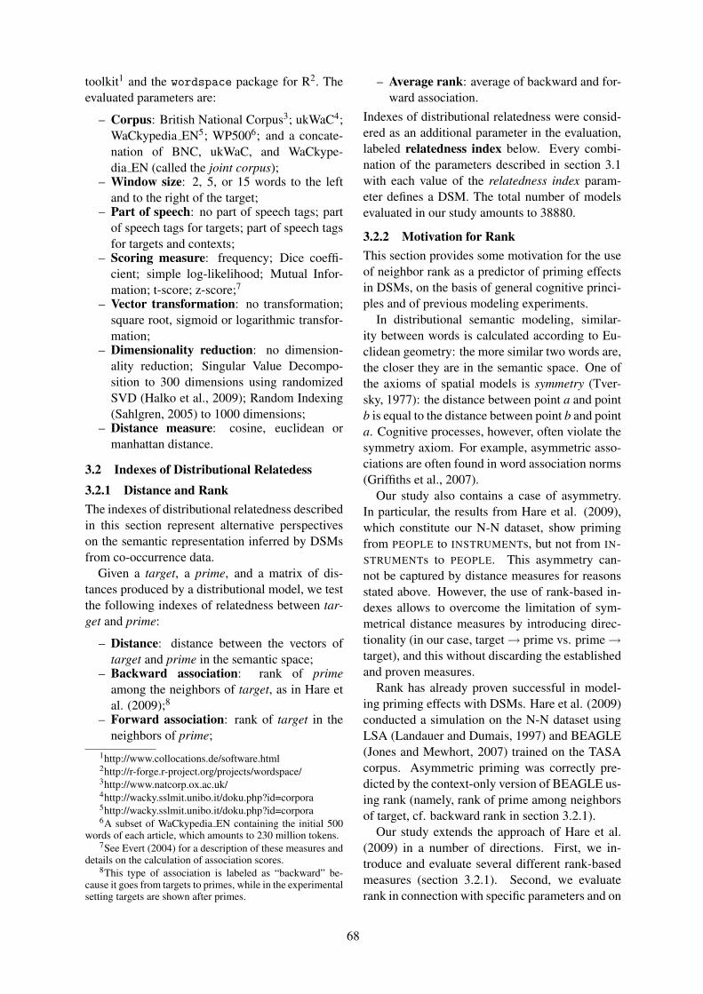
toolkit1 and the wordspace package for R2. Theevaluated parameters are:

– Corpus: British National Corpus3; ukWaC4;WaCkypedia EN5; WP5006; and a concate-nation of BNC, ukWaC, and WaCkype-dia EN (called the joint corpus);

– Window size: 2, 5, or 15 words to the leftand to the right of the target;

– Part of speech: no part of speech tags; partof speech tags for targets; part of speech tagsfor targets and contexts;

– Scoring measure: frequency; Dice coeffi-cient; simple log-likelihood; Mutual Infor-mation; t-score; z-score;7

– Vector transformation: no transformation;square root, sigmoid or logarithmic transfor-mation;

– Dimensionality reduction: no dimension-ality reduction; Singular Value Decompo-sition to 300 dimensions using randomizedSVD (Halko et al., 2009); Random Indexing(Sahlgren, 2005) to 1000 dimensions;

– Distance measure: cosine, euclidean ormanhattan distance.

3.2 Indexes of Distributional Relatedess3.2.1 Distance and RankThe indexes of distributional relatedness describedin this section represent alternative perspectiveson the semantic representation inferred by DSMsfrom co-occurrence data.

Given a target, a prime, and a matrix of dis-tances produced by a distributional model, we testthe following indexes of relatedness between tar-get and prime:

– Distance: distance between the vectors oftarget and prime in the semantic space;

– Backward association: rank of primeamong the neighbors of target, as in Hare etal. (2009);8

– Forward association: rank of target in theneighbors of prime;

1http://www.collocations.de/software.html2http://r-forge.r-project.org/projects/wordspace/3http://www.natcorp.ox.ac.uk/4http://wacky.sslmit.unibo.it/doku.php?id=corpora5http://wacky.sslmit.unibo.it/doku.php?id=corpora6A subset of WaCkypedia EN containing the initial 500

words of each article, which amounts to 230 million tokens.7See Evert (2004) for a description of these measures and

details on the calculation of association scores.8This type of association is labeled as “backward” be-

cause it goes from targets to primes, while in the experimentalsetting targets are shown after primes.

– Average rank: average of backward and for-ward association.

Indexes of distributional relatedness were consid-ered as an additional parameter in the evaluation,labeled relatedness index below. Every combi-nation of the parameters described in section 3.1with each value of the relatedness index param-eter defines a DSM. The total number of modelsevaluated in our study amounts to 38880.

3.2.2 Motivation for RankThis section provides some motivation for the useof neighbor rank as a predictor of priming effectsin DSMs, on the basis of general cognitive princi-ples and of previous modeling experiments.

In distributional semantic modeling, similar-ity between words is calculated according to Eu-clidean geometry: the more similar two words are,the closer they are in the semantic space. One ofthe axioms of spatial models is symmetry (Tver-sky, 1977): the distance between point a and pointb is equal to the distance between point b and pointa. Cognitive processes, however, often violate thesymmetry axiom. For example, asymmetric asso-ciations are often found in word association norms(Griffiths et al., 2007).

Our study also contains a case of asymmetry.In particular, the results from Hare et al. (2009),which constitute our N-N dataset, show primingfrom PEOPLE to INSTRUMENTs, but not from IN-STRUMENTs to PEOPLE. This asymmetry can-not be captured by distance measures for reasonsstated above. However, the use of rank-based in-dexes allows to overcome the limitation of sym-metrical distance measures by introducing direc-tionality (in our case, target→ prime vs. prime→target), and this without discarding the establishedand proven measures.

Rank has already proven successful in model-ing priming effects with DSMs. Hare et al. (2009)conducted a simulation on the N-N dataset usingLSA (Landauer and Dumais, 1997) and BEAGLE(Jones and Mewhort, 2007) trained on the TASAcorpus. Asymmetric priming was correctly pre-dicted by the context-only version of BEAGLE us-ing rank (namely, rank of prime among neighborsof target, cf. backward rank in section 3.2.1).

Our study extends the approach of Hare et al.(2009) in a number of directions. First, we in-troduce and evaluate several different rank-basedmeasures (section 3.2.1). Second, we evaluaterank in connection with specific parameters and on

68

larger corpora. Third, we extend the use of rank-based measures to the distributional simulation oftwo other experiments on event knowledge (Fer-retti et al., 2001; McRae et al., 2005). Note thatour simulation differs from the one by Hare et al.(2009) with respect to tasks (they test for a sig-nificant difference of mean distances between tar-get and related vs. unrelated prime) and the classof DSMs (we use term-term models, rather thanLSA; our models are not sensitive to word order,unlike BEAGLE).

3.3 Tasks and Analysis of Results

The aim of this section is to introduce the exper-imental tasks whose results will be discussed insection 4 and to describe the main features of theanalysis we applied to interpret these results.

Two experiments have been carried out:

– A classification experiment: given a targetand two primes, distributional information isused to identify the congruent prime. Perfor-mance in this task is measured by classifica-tion accuracy (section 4.1).

– A prediction experiment: the informa-tion concerning distributional relatedness be-tween targets and congruent primes is testedas a predictor for latency times. Performancein this task is quantified by Pearson correla-tion (section 4.2).

Concerning the interpretation of the evaluation re-sults, it would hardly be meaningful to look at thebest parameter combination or the average acrossall models. The best model is likely to be over-fitted tremendously (after testing 38880 param-eter settings over a dataset of 404 data points).Mean performance is largely determined by theproportions of “good” and “bad” parameter set-tings among the evaluation runs, which includemany non-optimal parameter values that were onlyincluded for completeness.

Instead, we analyze the influence of individ-ual DSM parameters and their interactions usinglinear models with performance (accuracy or cor-relation) as a dependent variable and the variousmodel parameters as independent variables. Thisapproach allows us to identify parameters thathave a significant effect on model performanceand to test for interactions between the parameters.Based on the partial effects of each parameter (andsignificant interactions) we can select a best modelin a robust way.

This statistical analysis contains some elementsof novelty with respect to the state-of-the-art DSMevaluation. Broadly speaking, approaches to DSMevaluation described in the literature fall into twoclasses. The first one can be labeled as best modelfirst, as it implies the identification of the opti-mal configuration of parameters on an initial task,considered more basic; the best performing modelon the general task is therefore evaluated on othertasks of interest. This is the approach adopted, forexample, by Pado and Lapata (2007). In the sec-ond approach, described in Bullinaria and Levy(2007; 2012), evaluation is conducted via incre-mental tuning of parameters: parameters are eval-uated sequentially to identify the best performingvalue on a number of tasks. Such approaches toDSM evaluation have specific limitations. Theformer approach does not assess which parame-ters are crucial in determining model performance,since its goal is the evaluation of performance ofthe same model on different tasks. The latter ap-proach does not allow for parameter interactions,considering parameters individually. Both limita-tions are avoided in the analysis used here.

4 Results

4.1 Identification of Congruent Prime

This section presents the results from the first taskevaluated in our study. We used the DSMs to iden-tify which of the two primes is the congruent onebased on their distributional relatedness to the tar-get. For every triple in the dataset, the different in-dexes of distributional relatedness (parameter re-latedness index) were used to compare the associ-ation between the target and the congruent primewith the association between the target and the in-congruent prime. Accuracy of DSMs in picking upthe congruent prime was calculated on the globaldataset and separately for each subset.9

Figure 1 displays the distribution of the accu-racy scores of all tested models in the task, on theglobal dataset. All accuracy values are specifiedas percentages. Minimum, maximum, mean andstandard deviation of the accuracy values for theglobal dataset and for the three subsets are dis-played in table 2.

The mean performance on N-N is lower than on

9The small number of triples for which no predictioncould be made because of missing words in the DSMs wereconsidered mistakes. The coverage of the models ranges from97.8% to 100% of the triples, with a mean of 99%.

69

0

500

1000

1500

2000

50 60 70 80 90 100

Figure 1: Identification of congruent prime: distri-bution of accuracy (%) for global dataset

Dataset Min Max Mean σ

Global 50.2 96.5 80.2 9.2V-N 45.8 95.8 80.0 8.4N-V 49.1 99.1 82.7 9.7N-N 47.6 97.6 78.7 10.0

Table 2: Identification of congruent prime: meanand range for global dataset and subsets

N-V and slightly lower than on V-N. This effectmay be interpreted as being due to mediated prim-ing, as no verb is explicitly involved in the N-Nrelationship. Yet, the relatively high accuracy onN-N and its relatively small difference from N-Vand V-N does not speak in favor of a different un-derlying mechanism responsible for this effect. In-deed, McKoon and Ratcliff (1992) suggested thateffects traditionally considered as instances of me-diated priming are not due to activation spreadingthrough a mediating node, but result from a directbut weaker relatedness between prime and targetwords. This hypothesis found computational sup-port in McDonald and Lowe (2000).10

4.1.1 Model Parameters and AccuracyThe aim of this section is to assess which param-eters have the most significant impact on the per-formance of DSMs in the task of identification ofthe congruent prime.

We trained a linear model with the eight DSMparameters as independent variables (R2 = 0.70)and a second model that also includes all two-wayinteractions (R2 = 0.89). Given the improvementin R2 as a consequence of the inclusion of two-wayinteractions in the linear model, we will focus onthe results from the model with interactions. Table3 shows results from the analysis of variance for

10The interpretation of the N-N results in terms of spread-ing activation is also rejected by Hare et al. (2009, 163).

the model with interactions. For every parameter(and interaction of parameters) we report degreesof freedom (df ), percentage of explained variance(R2), and a significance code (signif ). We onlylist significant interactions that explain at least 1%of the variance. Even though all parameters andmany interactions are highly significant due to thelarge number of DSMs that were tested, an analy-sis of their predictive power in terms of explainedvariance allows us to make distinctions betweenparameters.

Parameter df R2 signifcorpus 4 7.44 ***window 2 4.39 ***pos 2 0.92 ***score 5 7.39 ***transformation 3 3.79 ***distance 2 22.20 ***dimensionality reduction 2 10.52 ***relatedness index 3 13.67 ***score:transformation 15 4.53 ***distance:relatedness index 12 2.24 ***distance:dim.reduction 4 2.16 ***window:dim.reduction 4 1.73 ***

Table 3: Accuracy: Parameters and interactions

Results in table 3 indicate that distance, dimen-sionality reduction and relatedness index are theparameters with the strongest explanatory power,followed by corpus and score. Window and trans-formation have a weaker explanatory power, whilepos falls below the 1% threshold. There is astrong interaction between score and transforma-tion, which has more influence than one of the in-dividual parameters, namely transformation.

Figures 2 to 7 display the partial effects of dif-ferent model parameters (pos was excluded be-cause of its low explanatory power). One of themain research questions behind this work waswhether neighbor rank performs better than dis-tance in predicting priming data. The partial ef-fect of relatedness index in Figure 6 confirms ourhypothesis: forward rank achieves the best perfor-mance, distance the worst.11

Accuracy improves for models trained on big-ger corpora (parameter corpus, figure 2; corporaare ordered by size) and larger context windows(parameter window, figure 3). Cosine is the bestperforming distance measure (figure 4). Interest-ingly, dimensionality reduction is found to neg-atively affect model performance: as shown infigure 7, both random indexing (ri) and singular

11Backward rank is equivalent to distance in this task.

70

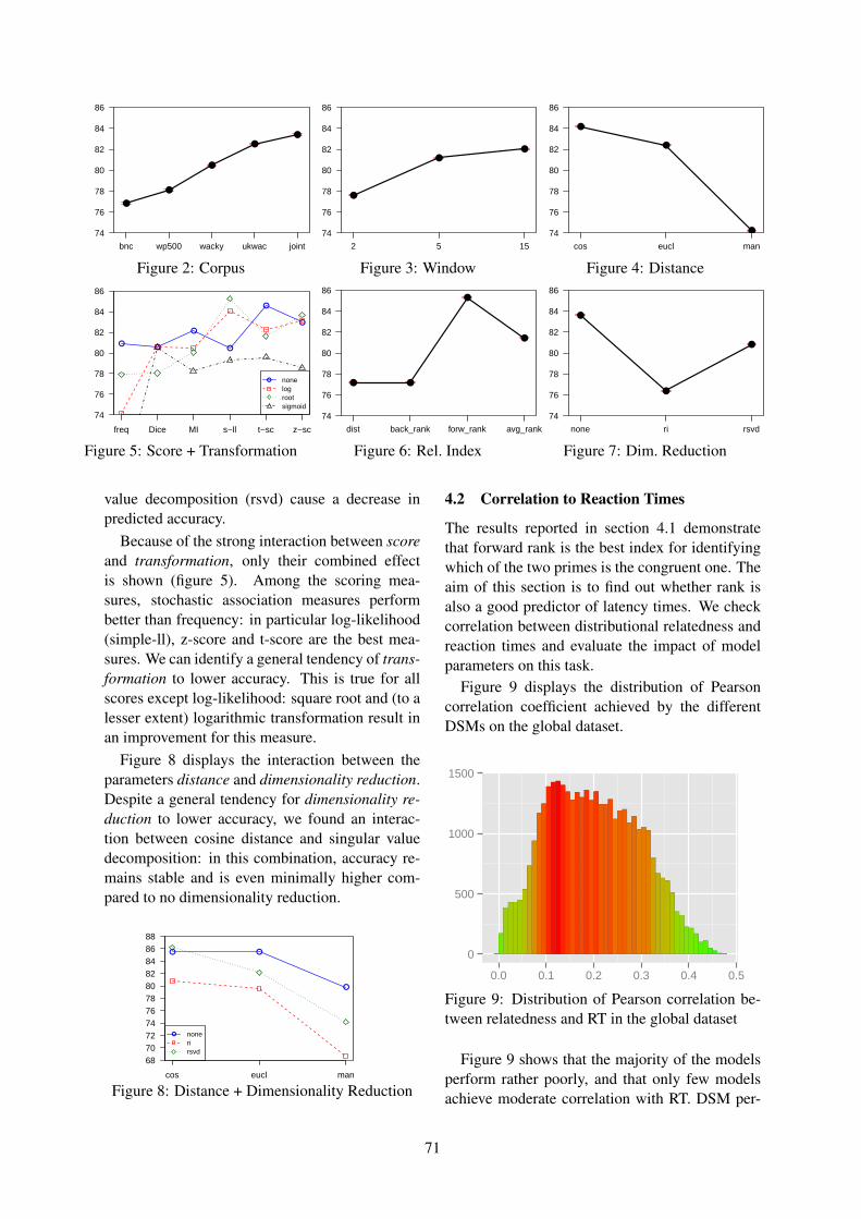
74

76

78

80

82

84

86

bnc wp500 wacky ukwac joint

●

●

●

●

●

Figure 2: Corpus

74

76

78

80

82

84

86

2 5 15

●

●

●

Figure 3: Window

74

76

78

80

82

84

86

cos eucl man

●

●

●

Figure 4: Distance

●●

●

●

●

●

none

freq Dice MI s−ll t−sc z−sc

74

76

78

80

82

84

86

● nonelogrootsigmoid

Figure 5: Score + Transformation

74

76

78

80

82

84

86

dist back_rank forw_rank avg_rank

● ●

●

●

Figure 6: Rel. Index

74

76

78

80

82

84

86

none ri rsvd

●

●

●

Figure 7: Dim. Reduction

value decomposition (rsvd) cause a decrease inpredicted accuracy.

Because of the strong interaction between scoreand transformation, only their combined effectis shown (figure 5). Among the scoring mea-sures, stochastic association measures performbetter than frequency: in particular log-likelihood(simple-ll), z-score and t-score are the best mea-sures. We can identify a general tendency of trans-formation to lower accuracy. This is true for allscores except log-likelihood: square root and (to alesser extent) logarithmic transformation result inan improvement for this measure.

Figure 8 displays the interaction between theparameters distance and dimensionality reduction.Despite a general tendency for dimensionality re-duction to lower accuracy, we found an interac-tion between cosine distance and singular valuedecomposition: in this combination, accuracy re-mains stable and is even minimally higher com-pared to no dimensionality reduction.

● ●

●

cos eucl man

6870727476788082848688

● nonerirsvd

Figure 8: Distance + Dimensionality Reduction

4.2 Correlation to Reaction Times

The results reported in section 4.1 demonstratethat forward rank is the best index for identifyingwhich of the two primes is the congruent one. Theaim of this section is to find out whether rank isalso a good predictor of latency times. We checkcorrelation between distributional relatedness andreaction times and evaluate the impact of modelparameters on this task.

Figure 9 displays the distribution of Pearsoncorrelation coefficient achieved by the differentDSMs on the global dataset.

0

500

1000

1500

0.0 0.1 0.2 0.3 0.4 0.5

Figure 9: Distribution of Pearson correlation be-tween relatedness and RT in the global dataset

Figure 9 shows that the majority of the modelsperform rather poorly, and that only few modelsachieve moderate correlation with RT. DSM per-

71

formance in the correlation task appears to be lessrobust to non-optimal parameter settings than inthe accuracy task (cf. figure 1).

Minimum, maximum, mean and standard devi-ation correlation for the global dataset and for thethree evaluation subsets are shown in table 4. In allthe cases, absolute correlation values are used soas not to distinguish between positive and negativecorrelation.

Dataset Min Max Mean σ

Global -0.26 0.47 0.19 0.10V-N -0.34 0.57 0.2 0.12N-V -0.35 0.41 0.11 0.06N-N -0.29 0.42 0.16 0.09

Table 4: Mean and range of Pearson correlationcoefficients on global dataset and subsets

4.2.1 Model Parameters and CorrelationIn this section we discuss the impact of differ-ent model parameters on correlation with reactiontimes.

We trained a linear model with absolute Pearsoncorrelation on the global dataset as dependent vari-able and the eight DSM parameters as independentvariables (R2 = 0.53), and a second model that in-cludes two-way interactions (R2 = 0.77). Table5 is based on the model with interactions; it re-ports the degrees of freedom (df ), proportion ofexplained variance (R2) and a significance code(signif ) for every parameter and every interactionof parameters (above 1% of explained variance).

Parameter df R2 signifcorpus 4 7.45 ***window 2 0.47 ***pos 2 0.20 ***score 5 3.03 ***transformation 3 3.52 ***distance 2 4.27 ***dimensionality reduction 2 10.57 ***relatedness index 3 23.40 ***dim.reduction:relatedness index 6 5.21 ***distance:dim.reduction 4 4.11 ***distance:relatedness index 6 3.77 ***score:transformation 15 3.22 ***score:relatedness index 15 1.37 ***

Table 5: Correlation: Parameters and interactions

Relatedness index is the most important param-eter, followed by dimensionality reduction andcorpus. The explanatory power of the other pa-rameters (score, transformation, distance) is lowerthan for the accuracy task, and two parameters(window and pos) explain less than 1% of the vari-ance each. By contrast, the explanatory power of

interactions is higher in this task. Table 5 showsthe five relevant interactions with an overall higherR2 compared to the accuracy task (cf. table 3).

The partial effect plot for relatedness index (fig-ure 14) confirms the findings of the accuracy task:forward rank is the best value for this parameter.The best values for the other parameters, however,show opposite tendencies with respect to the accu-racy task. Models trained on smaller corpora (fig-ure 10) perform better than those trained on big-ger ones. Cosine is still the best distance measure,but manhattan distance performs equally well inthis task (parameter distance, figure 12). Singu-lar value decomposition (parameter dimensional-ity reduction, figure 15) weakens the correlationvalues achieved by the models, but no significantdifference is found between random indexing andthe unreduced data.

Co-occurrence frequency performs better thanstatistical association measures and transforma-tion improves correlation: figure 13 displays theinteraction between these two parameters. Trans-formation has a positive effect for every score, butthe optimal transformation differs. Its impact isparticularly strong for the Dice coefficient, whichreaches the same performance as frequency whencombined with a square root transformation.

Let us conclude by discussing the interactionbetween distance and dimensionality reduction(figure 16). Based on the partial effects of the indi-vidual parameters, any combination of manhattanor cosine distance with random indexing or no di-mensionality reduction should be close to optimal.However, the interaction plot reveals that manhat-tan distance with random indexing is the best com-bination, outperforming the second best (cosinewithout dimensionality reduction) by a consider-able margin. The positive effect of random index-ing is quite surprising and will require further in-vestigation.

● ● ●

cos eucl man

0.08

0.1

0.12

0.14

0.16

0.18

0.2

0.22

0.24

0.26

● nonerirsvd

Figure 16: Distance + Dimensionality Reduction

72

0.12

0.14

0.16

0.18

0.2

0.22

0.24

0.26

bnc wp500 wacky ukwac joint

●

●● ●

●

Figure 10: Corpus

0.12

0.14

0.16

0.18

0.2

0.22

0.24

0.26

2 5 15

●●

●

Figure 11: Window

0.12

0.14

0.16

0.18

0.2

0.22

0.24

0.26

cos eucl man

●

●

●

Figure 12: Distance

●●

●

●

●

●

freq Dice MI s−ll t−sc z−sc

0.12

0.14

0.16

0.18

0.2

0.22

0.24

0.26

● nonelogrootsigmoid

Figure 13: Score + Transformation

0.12

0.14

0.16

0.18

0.2

0.22

0.24

0.26

dist back_rank forw_rank avg_rank

●

●

●

●

Figure 14: Rel. Index

0.12

0.14

0.16

0.18

0.2

0.22

0.24

0.26

none ri rsvd

● ●

●

Figure 15: Dim. Reduction

5 Conclusion

In this paper, we presented the results of a large-scale evaluation of distributional models and theirparameters on behavioral data from priming ex-periments. Our study is, to the best of our knowl-edge, the first systematic evaluation of such a widerange of DSM parameters in all possible combina-tions. Our study also provides a methodologicalcontribution to the problem of DSM evaluation.We propose to apply linear modeling to determinethe impact of different model parameters and theirinteractions on the performance of the models. Webelieve that this type of analysis is robust againstoverfitting. Moreover, effects can be tested forsignificance and various forms of interactions be-tween model parameters can be captured.

The main findings of our evaluation can be sum-marized as follows. Forward association (rank oftarget among the nearest neighbors of the prime)performs better than distance in both tasks at is-sue: identification of congruent prime and correla-tion with latency times. This finding confirms andextends the results of previous studies (Hare et al.,2009). The relevance of rank-based measures forcognitive modeling is discussed in section 3.2.2.

Identification of congruent primes on the ba-sis of distributional relatedness between prime andtarget is improved by employing bigger corporaand by using statistical association measures asscoring functions, while correlation to reactiontimes is strengthened by smaller corpora and co-

occurrence frequency or Dice coefficient. A sig-nificant interaction between transformation andscoring function is found in both tasks: consider-ing the interaction between these two parametersturned out to be vital for the identification of opti-mal parameter values.

Some preliminary analyses of individual the-matic relations showed substantial improvementsof correlations. Therefore, future work will focuson finer-grained linear models for single relationsand on further modeling of reaction times, extend-ing the study by Hutchinson et al. (2008).

Further research steps also include an evalua-tion of syntax-based models (Baroni and Lenci,2010; Pado and Lapata, 2007) and term-documentmodels on the tasks tackled in this paper, as wellas an evaluation of all models on standard tasks.

Acknowledgments

We are grateful to Ken MacRae for providing usthe priming data modeled here and to AlessandroLenci for his contribution to the development ofthis study. We would also like to thank the Com-putational Linguistics group at the University ofOsnabruck and the Corpus Linguistics group at theUniversity Erlangen for feedback. Thanks also goto three anonymous reviewers, whose commentshelped improve our analysis, and to Sascha Alex-eyenko for helpful advice. The first author’s PhDproject is funded by a Lichtenberg grant from theMinistry of Science and Culture of Lower Saxony.

73

ReferencesMarco Baroni and Alessandro Lenci. 2010. Dis-

tributional memory: A general framework forcorpus-based semantics. Computational Linguis-tics, 36(4):1–49.

Marco Baroni and Alessandro Lenci. 2011. Howwe blessed distributional semantic evaluation. InProceedings of the GEMS 2011 Workshop on GE-ometrical Models of Natural Language Semantics,GEMS ’11, pages 1–10. Association for Computa-tional Linguistics.

John A. Bullinaria and Joseph P. Levy. 2007. Ex-tracting semantic representations from word co-occurrence statistics: A computational study. Be-havior Research Methods, 39:510–526.

John A. Bullinaria and Joseph P. Levy. 2012. Ex-tracting semantic representations from word co-occurrence statistics: stop-lists, stemming and svd.Behavior Research Methods, 44:890–907.

Stefan Evert. 2004. The Statistics of Word Cooccur-rences: Word Pairs and Collocations. Ph.D. thesis,IMS, University of Stuttgart.

Todd Ferretti, Ken McRae, and Ann Hatherell. 2001.Integrating verbs, situation schemas, and thematicrole concepts. Journal of Memory and Language,44(4):516–547.

Thomas L. Griffiths, Mark Steyvers, and Joshua B.Tenenbaum. 2007. Topics in semantic representa-tion. Psychological Review, 114:211–244.

Nathan Halko, Per-Gunnar Martinsson, and Joel A.Tropp. 2009. Finding structure with randomness:Stochastic algorithms for constructing approximatematrix decompositions. Technical Report 2009-05,ACM, California Institute of Technology.

Mary Hare, Michael Jones, Caroline Thomson, SarahKelly, and Ken McRae. 2009. Activating eventknowledge. Cognition, 111(2):151–167.

Zelig Harris. 1954. Distributional structure. Word,10(23):146–162.

Amac Herdagdelen, Marco Baroni, and Katrin Erk.2009. Measuring semantic relatedness with vectorspace models and random walks. In Proceedingsof the 2009 Workshop on Graph-based Methods forNatural Language Processing, pages 50–53.

Keith A. Hutchinson, David A. Balota, Michael J.Cortese, and Jason M. Watson. 2008. Predictingsemantic priming at the item level. The QuarterlyJournal of Experimental Psychology, 61(7):1036–1066.

Michael Jones and Douglas Mewhort. 2007. Repre-senting word meaning and order information in acomposite holographic lexicon. Psychological Re-view, 114:1–37.

Thomas K. Landauer and Susan T. Dumais. 1997.A solution to Plato’s problem: The latent seman-tic analysis theory of the acquisition, induction, andrepresentation of knowledge. Psychological Review,104:211–240.

Will Lowe and Scott McDonald. 2000. The directroute: mediated priming in semantic space. Tech-nical report, Division of Informatics, University ofEdinburgh.

Scott McDonald and Chris Brew. 2004. A distribu-tional model of semantic context effects in lexicalprocessing. In Proceedings of ACL-04, pages 17–24.

Gain McKoon and Roger Ratcliff. 1992. Spreading ac-tivation versus compound cue accounts of priming:Mediated priming revisited. Journal of Experimen-tal Psychology: Learning, Memory and Cognition,18:1155–1172.

Ken McRae and Kazunaga Matzuki. 2009. People usetheir knowledge of common events to understandlanguage, and do so as quickly as possible. Lan-guage and Linguistics Compass, 3(6):1417–1429.

Ken McRae, Mary Hare, Jeffrey L. Elman, and ToddFerretti. 2005. A basis for generating expectan-cies for verbs from nouns. Memory & Cognition,33(7):1174–1184.

Jeff Mitchell and Mirella Lapata. 2008. Vector-basedmodels of semantic composition. In Proceedings ofACL-08: HLT, pages 236–244, Columbus, Ohio.

Sebastian Pado and Mirella Lapata. 2007.Dependency-based construction of semantic spacemodels. Computational Linguistics, 33(2):161–199.

Magnus Sahlgren. 2005. An introduction to randomindexing. In Proceedings of the Methods and Appli-cations of Semantic Indexing Workshop at the 7th In-ternational Conference on Terminology and Knowl-edge Engineering, TKE 2005.

Magnus Sahlgren. 2006. The Word-Space Model: Us-ing distributional analysis to represent syntagmaticand paradigmatic relations between words in high-dimensional vector spaces. Ph.D. thesis, Universityof Stockolm.

Peter D. Turney and Patrick Pantel. 2010. Fromfrequency to meaning: Vector space models of se-mantics. Journal of Artificial Intelligence Research,37:141–188.

Amos Tversky. 1977. Features of similarity. Psycho-logical Review, 84:327–352.

74

Proceedings of the Workshop on Cognitive Modeling and Computational Linguistics, pages 75–83,Sofia, Bulgaria, August 8, 2013. c©2013 Association for Computational Linguistics

Concreteness and Corpora: A Theoretical and Practical Analysis

Felix Hill

Computer Laboratory

University of Cambridge

fh295@cam.ac.uk

Douwe Kiela

Computer Laboratory

University of Cambridge

dlk427@cam.ac.uk

Anna Korhonen

Computer Laboratory

University of Cambridge

alk23@cam.ac.uk

Abstract

An increasing body of empirical evidence

suggests that concreteness is a fundamental

dimension of semantic representation. By im-

plementing both a vector space model and a

Latent Dirichlet Allocation (LDA) Model, we

explore the extent to which concreteness is re-

flected in the distributional patterns in corpora.

In one experiment, we show that that vector

space models can be tailored to better model

semantic domains of particular degrees of

concreteness. In a second experiment, we

show that the quality of the representations of

abstract words in LDA models can be im-

proved by supplementing the training data

with information on the physical properties of

concrete concepts. We conclude by discussing

the implications for computational systems

and also for how concrete and abstract con-

cepts are represented in the mind

1 Introduction

A growing body of theoretical evidence empha-

sizes the importance of concreteness to semantic

representations. This fact has not been widely

exploited in NLP systems, despite its clear theo-

retical relevance to tasks such as word-sense in-

duction and compositionality modeling. In this

paper, we take a first step towards integrating

concreteness into NLP by testing the extent to

which it is reflected by the superficial (distribu-

tional) patterns in corpora. The motivation is

both theoretical and practical: We consider the

implications for the development of computa-

tional systems and also for how concrete and ab-

stract concepts are represented in the human

mind. Experimenting with two popular methods

of extracting lexical representations from text,

we show both that these approaches are sensitive

to concreteness and that their performance can be

improved by adapting their implementation to

the concreteness of the domain of application. In

addition, our findings offer varying degrees of

support to several recent proposals about concep-

tual representation. In the following section we review recent

theoretical and practical work. In Section 3 we

explore the extent to which concreteness is re-

flected by Vector-Space Models of meaning

(VSMs), and in Section 4 we conduct a similar

analysis for (Bayesian) Latent Dirichlet Alloca-

tion (LDA) models. We conclude, in Section 5,

by discussing practical and theoretical implica-

tions.

2 Related work

2.1 Concreteness

Empirical evidence indicates important cognitive

differences between abstract concepts, such as

guilt or obesity, and concrete concepts, such as

chocolate or cheeseburger. It has been shown

that concrete concepts are more easily learned

and remembered than abstract concepts, and that

language referring to concrete concepts is more

easily processed (Schwanenflugel, 1991). There

are cases of brain damage in which either ab-

stract or concrete concepts appear to be specifi-

cally impaired (Warrington, 1975), and function-

al magnetic resonance imaging (fMRI) studies

implicate overlapping but partly distinct neural

systems in the processing of the two concept

types (Binder et al., 2005). Further, there is in-

creasing evidence that concrete concepts are

represented via intrinsic properties whereas ab-

stract representations encode extrinsic relations

to other concepts (Hill et al., in press). However,

while these studies together suggest that con-

creteness is fundamental to human conceptual

representation, much remains to be understood

about the precise cognitive basis of the ab-

stract/concrete distinction. Indeed, the majority

of theoretically motivated studies of conceptual

representation focus on concrete domains, and

75

comparatively little has been established empiri-

cally about abstract concepts.

Despite this support for the cognitive impor-

tance of concreteness, its application to computa-

tional semantics has been limited to date. One

possible reason for this is the difficulty in mea-

suring lexical concreteness using corpora alone

(Kwong, 2008). Turney et al. (2011) overcome

this hurdle by applying a semi-supervised me-

thod to quantify noun concreteness. Using this

data, they show that a disparity in the concrete-

ness between elements of a construction can faci-

litate metaphor identification. For instance, in the

expressions kill the process or black comedy, a

verb or adjective that generally occurs with a

concrete argument takes an abstract argument.

Turney et al. show that a supervised classifier

can exploit this effect to correctly identify 79%

of adjective-noun and verb-object constructions

as literal or metaphorical. Although these results

are clearly promising, to our knowledge Turney

et al.‟s paper is unique in integrating corpus-

based methods and concreteness in NLP systems.

1.2 Association / similarity

A proposed distinction between abstract and

concrete concepts that is particularly important

for the present work relates to the semantic rela-

tions association and (semantic) similarity (see

e.g. Crutch et al. 2009; Resnik, 1995). The dif-

ference between these relations is exemplified by

the concept pairs {car, petrol} and {car, van}.

Car is said to be (semantically) similar to van,

and associated with (but not similar to) petrol.

Intuitively, the basis for the similarity of car and

bike may be their common physical features

(wheels) or the fact that they fall within a clearly

definable category (modes of transport). In con-

trast, the basis for the association between car

and petrol may be that they are often found to-

gether or the clear functional relationship be-

tween them. The two relations are neither mu-

tually exclusive nor independent; bike and car

are related to some degree by both association

and similarity.

Based on fresults of behavioral experiments,

Crutch et al. (2009) make the following proposal

concerning how association and similarity inte-

ract with concreteness:

(C) The conceptual organization of abstract con-

cepts is governed by association, whereas the

organization of concrete concepts is governed by

similarity.

Crutch et al.‟s hypothesis derives from experi-

ments in which participants selected the odd-one-

out from lists of five words appearing on a

screen. The lists comprised either concrete or

abstract words (based on ratings of six infor-

mants) connected either by similarity (e.g. dog,

wolf, fox etc.; theft, robbery, stealing etc.) or

association (dog, bone, collar etc.; theft, law, vic-

tim etc.), with an unrelated odd-one-out item in

each list. Controlling for frequency and position,

subjects were both significantly faster and more

accurate if the related words were either abstract

and associated or concrete and similar. These

results support (C) on the basis that decision

times are faster when the related items form a

more coherent group, rendering the odd-one out

more salient. Hill et al. (in press) tested the same

hypothesis on a larger scale, analyzing over

18,000 concept pairs scored by human annotators

for concreteness as well as the strength of associ-

ation between them. They found a moderate in-

teraction between concreteness and the correla-

tion between association strength and similarity

(as measured using WordNet), but concluded

that the strength of the effect was not sufficiently

strong to either confirm or refute (C).

Against this backdrop, the present work ex-

amines how association, similarity and concrete-

ness are reflected in LDA models and, first,

VSMs. In both cases we test Hypothesis (C) and

related theoretical proposals, and discuss whether

these findings can lead to better performing se-

mantic models.

3 Vector Space Models

Vector space models (VSMs) are perhaps the

most common general method of extracting se-

mantic representations from corpora (Sahlgren,

2006; Turney & Pantel, 2010). Words are

represented in VSMs as points in a (geometric)

vector space. The dimensions of the space cor-

respond to the model features, which in the sim-

plest case are high frequency words from the

corpus. In such models, the position of a word

representation along a given feature dimension

depends on how often that word occurs within a

specified proximity to tokens of the feature word

in the corpus. The exact proximity required is an

important parameter for model implementation,

and is referred to as the context window. Finally,

the degree to which two word representations are

related can be calculated as some function of the

distance between the corresponding points in the

semantic space.

76

3.1 Motivation

VSMs are well established as a method of quan-

tifying relations between word concepts and have

achieved impressive performance in related NLP

tasks (Sahlgren, 2006; Turney & Pantel, 2010).

In these studies, however, it is not always clear

exactly which semantic relation is best reflected

by the implemented models. Indeed, research

has shown that by changing certain parameter

settings in the standard VSM architecture, mod-

els can be adapted to better reflect one relation

type or another. Specifically, models with

smaller context windows are reportedly better at

reflecting similarity, whereas models with larger

windows better reflect association. (Agirre et al.,

2009; Peirsman et al., 2008)

Our experiments in this section aim first to

corroborate these findings by testing how models

of varying context window sizes perform on em-

pirical data of both association and similarity.

We then test if this effect differentially affects

performance on concrete and abstract words.

3.2 Method

We employ a conventional VSM design, extract-

ing representations from the (unlemmatised)

British National Corpus (Leech et al., 1994) with

stopwords removed. In the vector representation

of each noun, our dimension features are the

50,000 most frequently occurring (non-

stopword) words in the corpus. We experiment

with window sizes of three, five and nine (one,

two and four words either side of the noun,

counting stopwords). Finally, we apply point-

wise mutual information (PMI) weighting of our

co-occurrence frequencies, and measure similari-

ty between weighted noun vectors by the cosine

of the angle between them in the vector space.

To evaluate modeling of association, we use

the University of South Florida (USF) Free-

association Norms (Nelson & McEvoy, 2012).

The USF data consist of over 5,000 words paired

with their free associates. To elicit free asso-

ciates, more than 6,000 participants were pre-

sented with cue words and asked to “write the

first word that comes to mind that is meaningful-

ly related or strongly associated to the presented

word”. For a cue word c and an associate a, the

forward association strength (association) from

c to a is the proportion of participants who pro-

duced a when presented with c. association is

thus a measure of the strength of an associate

relative to other associates of that cue. The USF

data is well suited to our purpose because many

cues and associates in the data have a concrete-

ness score, taken from either the norms of Paivio,

Yuille and Madigan (1968) or Toglia and Battig

(1978). In both cases contributors were asked to

rate words based on a scale of 1 (very abstract) to

7 (very concrete).1 We extracted the all 2,230

nouns from the USF data for which concreteness

scores were known, yielding a total of 15,195

noun-noun pairs together with concreteness and

association values.

Although some empirical word-similarity da-

tasets are publically available, they contain few if

any abstract words (Finkelstein et al., 2002; Ru-

benstein & Goodenough, 1965). Therefore to

evaluate similarity modeling, we use Wu-Palmer

Similarity (similarity) (Wu & Palmer, 1994), a

word similarity metric based on the position of

the senses of two words in the WordNet taxono-

my (Felbaum, 1998). similarity can be applied to

both abstract and concrete nouns and achieves a

high correlation, with human similarity judg-

ments (Wu & Palmer, 1994).2

3.3 Results

In line with previous studies, we observed that

VSMs with smaller window sizes were better

able to predict similarity. The model with win-

dow size 3 achieves a higher correlation with

similarity (Spearman rank rs = -0.29) than the

model with window size 9 (rs = -0.25). Howev-

er, the converse effect for association was not

observed: Model correlation with association

was approximately constant over all window siz-

es. These effects are illustrated in Fig. 1.

1Although concreteness is well understood intuitively, it

lacks a universally accepted definition. It is often described

in terms of reference to sensory experience (Paivio et al.,

1968), but also connected to specificity; rose is often consi-

dered more concrete than flora. The present work does not

address this ambiguity. 2 similarity achieves a Pearson correlation of r = .80 on

the 30 concrete word pairs in the Miller & Charles (1991)

data.

0.123 0.125 0.12

0.286 0.29

0.241

0.0

0.1

0.2

0.3

3 5 9

Window

Co

rre

latio

n

Association

Similarity

77

Figure 1: Spearman correlations between VSM out-

put and association and similarity for different win-

dow sizes.

In addressing the theoretical Hypothesis (C) we

focused on the output of our VSM of window

size five, although the same trends were ob-

served over all three models. Over all 18,195

noun-noun pairs the correlation between the

model output and association was significant (rs

= 0.13, p < 0.001) but notably lower than the cor-

relation with similarity (rs = -0.29, p < 0.001).

To investigate the effect of concreteness, we

ranked each pair in our sample by the total con-

creteness of both nouns, and restricted our analy-

sis to the 1000 most concrete and 1000 most ab-

stract pairs. The models captured association

better over the abstract pairs than concrete con-

cepts, but reflected similarity better over the con-

crete concepts. The strength of this effect is illu-

strated in Fig. 2.

Figure 2: Spearman correlation values between VSM

output and similarity and association over subsets of

concrete and abstract pairs.

Given that small window sizes are optimal for

modeling similarity, and that WSMs appear to

model similarity better over concrete concepts

than over abstract concepts, we explored whether

different window sizes were optimal for either

abstract or concrete word pairs. When comparing

the model output to association, no interaction

between window size and concreteness was ob-

served. However, there was a notable interaction

when considering performance in modeling simi-

larity. As illustrated in Fig. 3, performance on

concrete word pairs is better for smaller window

sizes, whereas with abstract word pairs a larger

window size is preferable.

Figure 3: Spearman correlation values between VSM

output and similarity and association for different

window sizes over abstract and concrete word pair

subsets

3.4 Conclusion

Our results corroborate the body of VSM re-

search that reports better performance from small

window sizes in modeling similarity. A likely

explanation for this finding is that similarity is a

paradigmatic relation: Two similar entities can

be plausibly exchanged in most linguistic con-

texts. Small context windows emphasize prox-

imity, which loosely reflects structural relation-

ships such as verb-object, ensuring that paradig-

matically related entities score highly. Models

with larger context windows cannot discern pa-

radigmatically and syntagmatically related enti-

ties in this way. The performance of our models

on the association dataset did not support the

converse conclusion that larger window sizes

perform better. Overall, each of the three models

was notably better at capturing similarity than

association. This suggests that the core architec-

ture of WSMs is not well suited to modeling as-

sociation. Indeed, „first order‟ models that di-

rectly measure word co-occurrences, rather than

connecting them via features, seem to perform

better at this task (Chaudhari et al., 2011). This

fact is consistent with the view that association is

a more basic or fundamental semantic relation

from which other more structured relations are

derived.

The fact that the USF association data re-

flects the instinctive first response of participants

when presented with a cue word is important for

interpreting the results with respect to Hypothe-

sis (C). Our findings suggest that VSMs are bet-

ter able to model this data for abstract word pairs

than for concrete word pairs. This is consistent

with the idea that language fundamentally deter-

mines which abstract concepts come to be asso-

ciated or connected in the mind. Conversely, the

0.125

0.108

0.215

0.297

0.0

0.1

0.2

0.3

Association Similarity

Relation Type

Co

rre

latio

n

Abstract

Concrete

0.202

0.272

0.223

0.254

0.14

0.086

0.1040.099

0.0

0.1

0.2

3 - Similarity 9 - Similarity 3 - Assoc. 9 - Assoc.

Window size - Relation type

Co

rre

latio

n

Abstract

Concrete

78

fact that the model reflects associations between

concrete words less well suggests that the impor-

tance of extra-linguistic information is lower for

connecting concrete concepts in this instinctive

way. Indeed, it seems plausible that the process

by which concrete concepts become associated

involves visualization or some other form of per-

ceptual reconstruction. Consistent with Hypothe-

sis (C), this reconstruction, which is not possible

for abstract concepts, would naturally reflect si-

milarity to a greater extent than linguistic context

alone.

Finally, when modeling similarity, the ad-

vantage of a small window increases as the

words become more concrete. Similarity be-

tween concrete concepts is fundamental to cogni-

tive theories involving the well studied notions

of prototype and categorization (Rosch, 1975;

Rogers & McClelland, 2003). In contrast, the

computation of abstract similarity is intuitively a

more complex cognitive operation. Although the

accurate quantification of abstract similarity may

be beyond existing corpus-based methods, our

results suggest that a larger context window

could in fact be marginally preferable should

VSMs be applied to this task.

Overall, our findings show that the design of

VSMs can be tailored to reflect particular seman-

tic relations and that this in turn can affect their

performance on different semantic domains, par-

ticularly with respect to concreteness. In the

next section, we investigate whether the same

conclusions should apply to a different class of

distributional model.

4 Latent Dirichlet Allocation Models

LDA models are trained on corpora that are di-

vided into sections (typically documents), ex-

ploiting the principle that words appearing in the

same document are likely to have similar mean-

ings. In an LDA model, the sections are viewed

as having been generated by random sampling

from unknown latent dimensions, which are

represented as probability distributions (Dirichlet

distributions) over words. Each document can

then be represented by a probability distribution

over these dimensions, and by considering the

meaning of the dimensions, the meaning of the

document can be effectively characterized. More

importantly, because each latent dimension clus-

ters words of a similar meaning, the output of

such models can be exploited to provide high

quality lexical representations (Griffiths et al.,

2007). Such a word representation encodes the

extent to which each of the latent dimensions

influences the meaning of that word, and takes

the form of a probability distribution over these

dimensions. The degree to which two words are

related can then be approximated by any function

that measures the similarity or difference be-

tween distributions.

4.1 Motivation

In recent work, Andrews et al. (2009) explore

ways in which LSA models can be modified to

improve the quality of their lexical representa-

tions. They propose that concepts are acquired

via two distinct information sources: experiential

data – the perceptible properties of objects, and

distributional data – the superficial patterns of

language. To test this hypothesis, Andrews et al.

construct three different LDA models, one

trained on experiential data, one trained in the

conventional manner on running text, and one

trained on the same text but with the experiential

data appended. They evaluate the quality of the

lexical representations in the three models by

calculating the Kulback-Leibler divergence be-

tween the representation distributions to measure

how closely related two words are (Kullback &

Leibler, 1951). When this data was compared

with the USF association data, the combined

model performed better than the corpus-based

model, which in turn performed better than the

features-only model. Andrews et al. concluded

that both experiential and distributional data are

necessary for the acquisition of good quality lex-

ical representations.

As well as suggesting a way to improve the

performance of LDA models on NLP tasks by

supplementing the training data, the approach

taken by Andrews et al. may be useful for better

understanding the nature of the abstract/concrete

distinction. In recent work, Hill et al. (in press)

present empirical evidence that concrete con-

cepts are represented in terms of intrinsic fea-

tures or properties whereas abstract concepts are

represented in terms of connections to other

(concrete and abstract) concepts. For example,

the features [legs], [tail], [fur], [barks] are all

central aspects of the concrete representation of

dog, whereas the representation of the abstract

concept love encodes connections to other con-

cepts such as heart, rose, commitment and hap-

piness etc. If a feature-based representation is

understood to be constructed from physical or

perceptible properties (which themselves may be

basic or fundamental concrete representations),

Hill et al.‟s characterization of concreteness can

be summarized as follows:

79

(H) Concreteness correlates with the degree to

which conceptual representations are feature-

based

Because such differences in representation struc-

ture would in turn entail differences in the com-

putation of similarity, (H) is closely related to a

proposal of Markman and Stilwell (2001; see

also Gentner & Markman, 2007):

(M) Computing similarity among concrete con-

cepts involves a feature-comparison operation,

whereas similarity between abstract concepts is

a structural, analogy-like, comparison.

The findings of Andrews et al. do not address

(H) or (M) directly, for two reasons. Firstly, they

evaluate their model on a set that includes no

abstract concepts. Secondly, they compare their

model output to association data without testing

how well it reflects similarity. In this section we

therefore reconstruct the Andrews models and

evaluate how well they reflect both association

and similarity across a larger set of abstract and

concrete concepts.

4.2 Method/materials

We reconstruct two of the three models devel-

oped by Andrews et al. (2009), excluding the

features-only model because of the present focus

on corpus-based approaches. However, while

the experiential data applied in the Andrews et

al. combined model was that collected by Vig-

liocco et al. (2004), we use the publicly available

McRae feature production norms (McRae et al.,

2005). The McRae data consist of 541 concrete

noun concepts together with features for each

elicited from 725 participants. In the data collec-

tion, feature was understood in a very loose

sense, so that participants were asked to list both

physical and functional properties of the nouns in

addition to encyclopedic facts. However, for the

present work, we filter out those features that

were not perceptual properties using McRae et

al.‟s feature classes, leaving a total of 1,285 fea-

ture types, such as [has_claws] and

[made_of_brass]. The importance of each fea-

ture to the representation of a given concept is

reflected by the proportion of participants who

named that feature in the elicitation experiment.

For each noun concept we therefore extract a

corresponding probability distribution over fea-

tures.

The model design and inference are identical

to those applied by Andrews et al. Our distribu-

tional model contains 250 latent dimensions and

was trained using a Gibbs Sampling algorithm on

approximately 7,500 sections of the BNC with

stopwords removed.3 The combined model con-

tains 350 latent dimensions, and was trained on

the same BNC data. However, for each instance

of one of the 541 McRae concept words, a fea-

ture is drawn at random from the probability dis-

tribution corresponding to that word and ap-

pended to the training data. The latent dimen-

sions in the combined model therefore corres-

pond to probability distributions both over words

and over features. This leads to an important dif-

ference between how words come to be related in

the distributional model and in the combined

model. Both models infer connections between

words by virtue of their occurrence either in the

same document or in pairs of documents for

which the same latent dimensions are prominent.

In the distributional model, it is the words in a

document that determines which latent dimen-

sions are ultimately prominent, whereas the in

combined model it is both the words and the fea-

tures in that document. Therefore, in the com-

bined model, two words can come to be related

because they occur not only in documents whose

words are related, but also in documents whose

features are related. For words in the McRae

data, this has the effect of strengthening the rela-

tionship between words with common features.

More interestingly, because it alters which latent

dimensions are most prominent for each docu-

ment, it should also influence the relationship

between words not in the McRae data.

We evaluate the performance of our models in

reflecting free association (association) and simi-

larity (similarity). To obtain test items we rank

the 18,195 noun-noun pairs from the USF data

by the product of the two (BNC) word frequen-

cies and select the 5,000 highest frequency pairs.

4.3 Results

As expected, the correlation of the combined

model output with association was greater than

the correlation of the distributional model output.

Notably, however, as illustrated in Fig. 4, we

observed far greater differences between the

combined and the distributional models when

comparing to similarity. Over all noun pairs, the

addition of features in the combined model im-

3 Code for model implementation was taken from Mark

Andrews : http://www.mjandrews.net/code/index.html

80

proved the correlation with similarity from

Spearman rs = 0.09 to rs = 0.15.

Figure 4: Spearman correlations between distribu-

tional and combined model outputs, similarity and

association

In order to address Hypothesis (C) (Section 2.2),

we analyzed the output of the combined model

on subsets of the 1000 most abstract and concrete

word pairs in our data as before. Perhaps surpri-

singly, as shown in Fig. 5, when comparing with

similarity, the model performed better over ab-

stract pairs, whereas when comparing with asso-

ciation the model performed better over concrete

pairs. However, when these concrete pairs were

restricted to those for which at least one of the

two words was in the McRae data, and hence to

which features had been appended in the corpus,

the ability of the model to reflect similarity in-

creased significantly.

Figure 5: Spearman correlations between combined

model output and similarity and association on differ-

ent word pair subsets

Finally, to address hypotheses (H) and (M) we

compared the previous analysis of the combined

model output to the equivalent output from the

distributional model. Surprisingly, as shown in

Fig. 6, the ability of the model to reflect associa-

tion over abstract pairs seemed to reduce with the

addition of features to the training data. Never-

theless, in all other cases the combined model

outperformed the distributional model. Interes-

tingly, the combined model advantage when

comparing with similarity was roughly the same

over both abstract and concrete pairs. However,

when these pairs contained at least one word

from the McRae data, the combined model was

indeed significantly better at modeling similarity,

consistent with Hypotheses (M) and (H).

Figure 6: Comparison between distributional

model and combined model output correlations with

similarity and association over different word pair

subsets

4.4 Conclusion

Our findings corroborate the main conclusion of

Andrews et al., that the addition of experiential

data improves the performance of the LDA mod-

el in reflecting association. However, they also

indicate that the advantage of feature-based LDA

models is far more significant when the objective

is to model similarity.

The findings are also consistent with, if

not suggestive of, the theoretical hypotheses (H)

and (M). Clearly, the property features in the

combined model training data enable it to better

model both similarity and association between

those concepts to which the features correspond.

However, this benefit is greater when modeling

similarity than when modeling association. This

suggests that the similarity operation is indeed

based on features to a greater extent than associa-

tion. Moreover, this effect is far greater for the

concrete words for which the features were add-

ed than over the other words pairs we tested.

Whilst this is not a sound test of hypothesis (H)

(no attempt was made to add „features‟ of ab-

stract concepts to the model), it is certainly con-

sistent with the idea that features or properties

are a more important aspect of concrete represen-

tations than of abstract representations.

0.13

0.09

0.14

0.15

0.00

0.05

0.10

0.15

Distributional Combined

Model type

Co

rre

latio

n

Association

Similarity

0.01

0.16

0.2

0.08

0.14

0.36

0.0

0.1

0.2

0.3

Abstract Concrete McRae

Word pair category

Co

rre

latio

n

Association

Similarity

0.03

0.093

0.15

0.018

0.11

0.025

0.01

0.16

0.2

0.08

0.14

0.36

0.0

0.1

0.2

0.3

Abstract Concrete Distributional model

McRae Abstract_ Concrete_ Combined model

McRae_

Word pair category

Co

rre

latio

n

Association

Similarity

81

Perhaps the most interesting aspect of the

combined model is how the addition of feature

information in the training data for certain words

influences performance on words for which fea-

tures were not added. In this case, our findings

suggest that the benefit when modeling similarity

is marginally greater than when modeling associ-

ation, an observation consistent with Hypothesis

(M). A less expected observation is that, be-

tween words for which features were not added,

the advantage of the combined model over the

distributional model in modeling similarity was

equal if not greater for abstract than for concrete

concepts. We hypothesize that this is because

abstract representations naturally inherit any re-

liance on feature information from the concrete

concepts with which they participate. In con-

trast, highly concrete representations do not en-

code relations to other concepts and therefore

cannot inherit relevant feature information in the

same way. Under this interpretation, the con-

crete information from the McRae words would

propagate more naturally to abstract concepts

than to other concrete concepts. As a result, the

highest quality representations in the combined

model would be those of the McRae words, fol-

lowed by those of the abstract concepts to which

they closely relate.

5 Discussion

This study has investigated how concreteness is

reflected in the distributional patterns found in

running text corpora. Our results add to the body

of evidence that abstract and concrete concepts

are represented differently in the mind. The fact

that VSMs with small windows are particularly

adept at modeling relations between concrete

concepts supports the view that similarity go-

verns the conceptual organization of concrete

concepts to a greater extent than for abstract con-

cepts. Further, the performance of our LSA

models on different tasks and across different

word pairs is consistent with the idea that con-

crete representations are built around features,

whereas abstract concepts are not.

More practically, we have demonstrated that

vector space models can be tailored to reflect

either similarity or association by adjusting the

size of the context window. This in turn indi-

cates a way in which VSMs might be optimized

to either abstract or concrete domains. Our expe-

riments with Latent Dirichlet Allocation corrobo-

rate a recent proposal that appending training

data with perceptible feature or property infor-

mation for a subset of concrete nouns can signif-

icantly improve the quality of the model‟s lexical

representations. As expected, this effect was

particularly salient for representations of words

for which features were appended to the training

data. However, the results show that this infor-

mation can propagate to words for which fea-

tures were not appended, in particular to abstract

words.

The fact that certain perceptible aspects of

meaning are not exhaustively reflected in linguis-

tic data is a potentially critical obstacle for cor-

pus-based semantic models. Our findings sug-

gest that existing machine learning techniques

may be able to overcome this by adding the re-

quired information for words that refer to con-

crete entities and allowing this information to

propagate to other elements of language. In fu-

ture work we aim to investigate specifically

whether this hypothesis holds for particular parts

of speech. For example, we would hypothesize

that verbs inherit a good degree of their meaning

from their prototypical nominal arguments.

References

Agirre, E., Alfonseca, E., Hall, K., Kravalova, J.

Pasca, K,. & Soroa,A. 2009. A Study on Similarity

and Relatedness Using Distributional and WordNet-

based Approaches. In Proceedings of NAACL-HLT

2009.

Andrews, M., Vigliocco, G. & Vinson, D. 2009.

Integrating experiential and distributional data to

learn semantic represenations. Psychological Review,

116(3), 463-498.

Barsalou, L. 1999. Perceptual symbol systems. Be-

havioral and Brain Sciences, 22, 577-609.

Binder, J., Westbury, C., McKiernan, K., Possing,

E., & Medler, D. 2005. Distinct brain systems for

processing concrete and abstract concepts. Journal of

Cognitive Neuroscience 17(6), 905-917.

Chaudhari, D., Damani, O., & Laxman, S. 2011.

Lexical Co-occurrence, Statistical Significance, and

Word Association. EMNLP 2011, 1058-1068.

Crutch, S., Connell, S., & Warrington, E. 2009.

The different representational frameworks underpin-

ning abstract and concrete knowledge: evidence from

odd-one-out judgments. Quarterly Journal of Experi-

mental Psychology, 62(7), 1377-1388.

Felbaum, C. 1998. WordNet: An Electronic Lexical

Database. Cambridge, MA: MIT Press.

Finkelstein, L., Gabrilovich, Matias, Rivlin, Solan,

Wolfman & Ruppin. 2002. Placing Search in Context:

The Concept Revisited. ACM Transactions on Infor-

mation Systems, 20(1):116-131.

Gentner, D., & Markman, A. 1997. Structure map-

ping in analogy and similarity. American Psycholo-

gist, 52. 45-56.

82

Griffiths, T., Steyvers, M., & Tenembaum, J. 2007.

Topics in semantic representation. Psychological Re-

view, 114 (2), 211-244.

Hill, F., Korhonen, A., & Bentz, C. A quantitative

empricial analysis of the abstract/concrete distinction.

Cognitive Science. In press.

Kullback, S., & Leibler, R.A. 1951. On Informa-

tion and Sufficiency. Annals of Mathematical Statis-

tics 22 (1): 79–86.

Kwong, O, Y. 2008. A Preliminary study on induc-

ing lexical concreteness from dictionary definitions.

22nd Pacific Asia Conference on Language, In-

formation and Computation, 235–244.

Leech, G., Garside, R. & Bryant, R. 1994. Claws4:

The tagging of the British National Corpus. COL-ING

94, Lancaster: UK.

Markman, A, & Stilwell, C. 2001. Role-governed

categories. Journal of Theoretical and Experimental

Artificial Intelligence, 13, 329-358.

McRae, K., Cree, G. S., Seidenberg, M. S., &

McNorgan, C. 2005. Semantic feature production

norms for a large set of living and nonliving things.

Behavior Research Methods, 37, 547-559

Miller, G., & Charles, W. 1991. Contextual corre-

lates of semantic similarity. Language and Cognitive

Processes, 6(1).

Nelson, D., & McEvoy, C. 2012. The University of

South Florida Word Association, Rhyme and Word

Fragment Norms. Retrieved online from:

http://web.usf.edu/FreeAssociation/Intro.html.

Paivio, A., Yuille, J., & Madigan, S. 1968. Con-

creteness, imagery, and meaningfulness values for

925 nouns. Journal of Experimental Psychology Mo-

nograph Supplement, 76(1, Pt. 2).

Peirsman, y., Heylen, K. & Geeraerts, D. 2008.

Size Matters. Tight and Loose Context Definitions in

English Word Space Models. In Proceedings of the

ESSLLI Workshop on Distributional Lexical Seman-

tics, Hamburg, Germany

Resnik, P. 1995. Using Information Content to

Evaluate Semantic Similarity in a Taxonomy. Pro-

ceedings of IJCAI-95.

Rogers, T., & McLelland, J. 2003. Semantic Cog-

nition. Cambridge, Mass: MIT Press.

Rosch, E. 1975. Cognitive representations of se-

mantic categories. Journal of Experimental Psycholo-

gy: General, 104(3), (September 1975), pp. 192–233.

Rubenstein, H., & Goodenough, J. 1965. Contex-

tual correlates of synonymy. Communications of the

ACM 8(10), 627-633.

Sahlgren, M. 2006. The Word-Space Model: Using

distributional analysis to represent syntagmatic and

paradigmatic relations between words in high-

dimensional vector spaces. Ph.D. dissertation, De-

partment of Linguistics, Stockholm University.

Schwanenflugel, P. 1991. Why are abstract con-

cepts hard to understand? In P. Schwanenflugel.

The psychology of word meanings (pp. 223-250).

Hillsdale, NJ: Erlbaum.

Toglia, M., & Battig, W. 1978. Handbook of se-

mantic word norms. Hillsdale, N.J: Erlbaum.

Turney, P, & Pantel, P. 2010. From frequency to

meaning: Vector space models of semantics. Journal

of Artificial Intelligence Research (JAIR), 37, 141-

188.

Turney,P., Neuman, Y., Assaf,.D, Cohen, Y. 2011.

Literal and Metaphorical Sense Identification through

Concrete and Abstract Context. EMNLP 2011: 680-

690

Vigliocco, G., Vinson, D. P., Lewis, W., & Garrett,

M. F. 2004. Reprssenting the meanings of object and

action words: The featural and unitary semantic space

hypothesis. Cognitive Psychology, 48, 422–488.

Warrington, E. (1975). The selective impairment of

semantic memory. Quarterly Journal of Experimental

Psychology 27(4), 635-657.

Wu, Z., Palmer, M. 1994. Verb semantics and lexi-

cal selection. In: Proceedings of the 32nd Annual

Meeting of the Associations for Computational Lin-

guistics. 133–138.

83

Proceedings of the Workshop on Cognitive Modeling and Computational Linguistics, pages 84–93,Sofia, Bulgaria, August 8, 2013. c©2013 Association for Computational Linguistics

On the Information Conveyed by Discourse Markers

Fatemeh Torabi AsrMMCI Cluster of Excellence

Saarland UniversityGermany

fatemeh@coli.uni-saarland.de

Vera DembergMMCI Cluster of Excellence

Saarland UniversityGermany

vera@coli.uni-saarland.de

Abstract

Discourse connectives play an impor-tant role in making a text coherentand helping humans to infer relationsbetween spans of text. Using thePenn Discourse Treebank, we investi-gate what information relevant to in-ferring discourse relations is conveyedby discourse connectives, and whetherthe specificity of discourse relations re-flects general cognitive biases for estab-lishing coherence. We also propose anapproach to measure the effect of a dis-course marker on sense identificationaccording to the different levels of a re-lation sense hierarchy. This will open away to the computational modeling ofdiscourse processing.

1 Introduction

A central question in psycholinguistic model-ing is the development of models for humansentence processing difficulty. An approachthat has received a lot of interest in recentyears is the information-theoretic measure ofsurprisal (Hale, 2001). Recent studies haveshown that surprisal can successfully accountfor a range of psycholinguistic effects (Levy,2008), as well as account for effects in nat-uralistic broad-coverage texts (Demberg andKeller, 2008; Roark et al., 2009; Frank, 2009;Mitchell et al., 2010). : what work of Roarkand Frank you mean here? Under the no-tion of the Uniform Information Density hy-pothesis (UID, Levy and Jaeger, 2007; Frankand Jaeger, 2008), surprisal has also beenused to explain choices in language produc-tion: When their language gives people theoption to choose between different linguisticencodings, people tend to choose the encod-

ing that distributes the information more uni-formly across the sentence (where the informa-tion conveyed by a word is its surprisal).

When using surprisal as a cognitive modelof processing difficulty, we hypothesize thatthe processing difficulty incurred by the hu-man when processing the word is proportionalto the update of the interpretation, i.e. the in-formation conveyed by the word (Hale, 2001;Levy, 2008). We can try to estimate partic-ular aspects of the information conveyed by aword, e.g., the information conveyed about thesyntactic structure of the sentence, the seman-tic interpretation, or about discourse relationswithin the text.

This paper does not go all the way toproposing a model of discourse relation sur-prisal, but discusses first steps towards amodel for the information conveyed by dis-course connectors about discourse relations,based on available resources like the Penn Dis-course Treebank (Prasad et al., 2008). First,we quantify how unambiguously specific dis-course relations are marked by their typicalconnectors (Section 4.1) and test whether eas-ily inferable relations are on average markedmore ambiguously than relations which areless expected according to the default assump-tion of a reader. This idea is shaped withrespect to the UID hypothesis: expected re-lations can afford to be signaled by weakermarkers and less expected ones should bemarked by strong connectors in order to keepthe discourse-level information density smooththroughout the text (Section 4.2). We theninvestigate in more detail the types of ambi-guity that a reader might face when process-ing discourse relations. While some ambigui-ties lie in discourse connectors, it also happensthat more than one relation exist at the sametime between two text spans. We show that

84

some discourse markers also signal the pres-ence of several relations (Section 5). In com-putational modeling as well as laboratory set-ups, one should therefore have a strategy todeal with the different types of ambiguities.Finally, we ask what granularity of distinctionfrom other discourse relations (with respect tothe PDTB relation sense hierarchy) each En-glish discourse connective conveys (Section 6).

2 Discourse Relations and theirMarkers

A cognitive approach to discourse process-ing emphasizes on the procedural role of theconnectives to constrain the way readers re-late the propositions in a text (Blakemore,1992; Blass, 1993). Experimental findingssuggest that these markers can facilitate theinference of specific discourse relations (De-gand and Sanders, 2002), and that discourseconnectors are processed incrementally Kohneand Demberg (2013). People can however in-fer discourse relations also in the absence ofdiscourse connecotrs, relying on the propo-sitional content of the sentences and theirworld-knowledge (Hobbs, 1979; Asher andLascarides, 1998). Asr and Demberg (2012b)point out that similar inferences are also nec-essary for discourse relations which are onlymarked with a weak connector which can beused for many relations, such as and. Further-more, we know that the inference of discourserelations is affected by a set of general cog-nitive biases. To illuminate the role of thesefactors let’s have a look at (1). While the typeof relation between the two events is clearly in-ferable in (1-a) and (1-b) due to the discourseconnectives, in (1-c), the reader would haveto access their knowledge, e.g., about Harry(from larger context) or the usual affairs be-tween bosses and employees, in order to con-struct a discourse relation.(1) a. The boss was angry because Harry skipped

the meeting (reason).b. The boss was angry, so Harry skipped the

meeting (result).c. The boss was angry and Harry skipped the

meeting.

Here, not only both reason and result inter-pretations but even an independent parallel re-lation (simple Conjunction) between the twoevents are possible to be inferred as a relatively

neutral connective, i.e., and is used. Levinson(2000) notes in his discussion on presumptivemeanings that “when events are conjoined theytend to be read as temporally successive and ifat all plausible, as causally linked”. If this istrue then the result reading is most probablefor (1-c). General preferences of this kind havebeen investigated via experimental approaches(Segal et al., 1991; Murray, 1997; Sanders,2005; Kuperberg et al., 2011). Segal et al.(1991) and Murray (1997) argue that readersexpect a sentence to be continuous with re-spect to its preceding context (the continuityhypothesis). Continuous discourse relations interms of congruency and/or temporality areconsequently easier to process than the dis-continuous ones. Sanders (2005) proposes thatcausal relatedness entails the maximum degreeof coherence in a text, therefore readers alwaysstart by attempting to find cause-consequencerelations between neighboring sentences (thecausality-by-default hypothesis). In a similarvein, Kuperberg et al. (2011) shows that read-ers face comprehension difficulty when sen-tences in short text spans cannot be put intocausal relation and no marker of other rela-tions (e.g., Concession) is available.

Taken together, these findings suggest thatworld knowledge, general cognitive biases, andlinguistic features of the sentences such as thepresence of a weak or strong marker contributeto the relational inference. With a look backto the information theoretic approach to thelinguistic patterns, one could hypothesize thatwhen one factor is strongly triggering expec-tation for a specific type of relation the otherfactors could remain silent in order to keep theinformation distribution uniform. With thisperspective, Asr and Demberg (2012a) testedwhether the predictability of discourse rela-tions due to general cognitive biases (towardscausality and continuity) can explain the pres-ence vs. absence of the discourse connectors.They found that connectors were more likelyto be dropped in the more predictable (causalor continuous) relations than in others. Ourinvestigation of the explicit relations in thispaper (the first experiment) looks into thisquestion in a stricter manner considering howmuch information a connective delivers aboutdiscourse relations. Since this information is

85

Figure 1: Hierarchy of senses in PDTB(Prasad et al., 2008)

closely related to the ambiguities a connec-tive removes (or maybe adds to the context)in the course of reading, we dedicate a sepa-rate section in this paper to illuminate differ-ent types of ambiguities. Also, a more detailquestion would be what types of informa-tion a connective can convey about one or sev-eral discourse relations. To our best of knowl-edge there has been no corpus-based study sofar about this last point which we will try tomodel in our third experiment.

3 Penn Discourse Treebank

The Penn Discourse Treebank (PDTB, Prasadet al., 2008) is a large corpus annotated withdiscourse relations, (covering the Wall StreetJournal part of the Penn Treebank). The an-notation includes sentence connectives, spansof their arguments and the sense of discourserelations implied by the connectives. The rela-tion labels are chosen according to a hierarchyof senses (Figure 1). Annotators were askedto find the Explicit discourse connectives andrespectively select a sense (as much specific aspossible) from the hierarchy. For neighboringsentences where no explicit marker existed inthe original text they were asked to first inserta suitable connective between the two argu-ments and then annotate a relation sense, inthis case categorized as Implicit. If an expres-sion — not belonging to the list of constitutedconnectives — in one of the involved sentences

is already indicative of a specific relation, theninstead they marked that expression and putthe relation into the AltLex category. In allof our experiments only the explicit relationare considered. Some connectives were anno-tated with two sense labels in the PDTB. Inour analyses below, we count these text spanstwice (i.e., once for each sense), resulting in atotal of 19,458 relation instances.

4 Are Unexpected RelationsStrongly Marked?

4.1 Markedness MeasurePoint-wise mutual information (pmi) is aninformation-theoretic measure of associationbetween two factors. For our purpose of mea-suring the markedness degree of a relation r inthe corpus, we calculate the normalized pmi ofit with any of the connectives, written as c thatit co-occurs with:

npmi(r; c) = pmi(r; c)− log p(r, c)

=log p(r,c)

p(r)p(c)− log p(r, c)

= log p(r)p(c)log p(r, c) − 1

npmi is calculated in base 2 and ranges be-tween −1 and 1. For our markedness measure,we scale it to the interval of [0, 1] and weigh itby the probability of the connector given therelation.

0 <npmi(r; c) + 1

2 < 1

markedness(r) =∑

c

p(c|r)npmi(r; c) + 12

Intuitively, the markedness measure tells uswhether a relation has very specific markers(high markedness) or whether it is usuallymarked by connectors that also mark manyother relations (low markedness).

4.2 Discourse Expectations andMarker Strength

Given the markedness measure, we are nowable to test whether those relations which aremore expected given general cognitive biases

86

0.62  

0.64  

0.66  

0.68  

0.7  

0.72  

0.74  

0.76  

Temporal  (3696)  

Con7ngency  (3741)  

Expansion  (6431)  

Comparison  (5590)  

Markedness  

Figure 2: Markedness of level-1 explicit rela-tions in the PDTB (frequencies of the relationsgiven in brackets).

(expecting continuous and causal relations)are marked less strongly than e.g. discontinu-ous relations. Figure 2 compares the marked-ness associated to the explicit relations of thePDTB when the first level relation sense dis-tinction is considered.

Figure 2 shows that COMPARISON rela-tions exhibit higher markedness than otherrelations, meaning that discontinuity ismarked with little ambiguity, i.e. markersof COMPARISON relations are only very rarelyused in other types of discourse relations.COMPARISON relations are exactly those rela-tions which were classified in Asr and Demberg(2012a) as a class of discontinuous relations.Further experimental evidence also shows thatthese relations are more likely to cause pro-cessing difficulty than others when no connec-tor is present (Murray, 1997), and that theirmarkers have a more strongly disruptive effectthan other markers when used incorrectly. Un-der the information density view, these obser-vations can be interpreted as markers for com-parison relations causing a larger context up-date. The high markedness of COMPARISON re-lations is thus in line with the hypothesis thatunpredictable relations are marked strongly.

CONTINGENCY relations, on the other hand,exhibit a lower score of markedness. Thisindeed complies with the prediction ofthe causality-by-default hypothesis (Sanders,2005) in conjunction with the UID hypothe-sis: causal relations can still be easily inferred

even in the presence of ambiguous connectivesbecause they are preferred by default.

As also discussed in Asr and Demberg(2012a), some types of EXPANSION relationsare continuous while others are discontinuous;finding that the level of markedness is near theaverage of all relations therefore comes as nosurprise.

More interesting is the case of TEMPORALrelations: these relations have low marked-ness, even though this class includes contin-uous (temporal succession) relations as well asdiscontinuous (temporal precedence) relations,and we would thus have expected a higher levelof markedness than we actually find. Evenwhen calculating markedness at the more fine-grained relation distinction level, did not finda significant difference between the marked-ness of the temporally forward vs. backwardrelations. A low level of markedness meansthat the connectors used to mark temporal re-lations are also used to mark other relations,in particular, temporal connectives are oftenused to mark CONTINGENCY relations. Thisobservation brings us to the question of gen-eral patterns of ambiguity in discourse markersand the ambiguity of discourse relations them-selves, see Section 5.

5 Ambiguous Connectivevs. Ambiguous Relation

Some discourse connectives (e.g., since, whichcan be temporal or causal, or while, which canbe temporal or contrastive) are ambiguous. Inthis section, we would like to distinguish be-tween three different types of ambiguity (allwith respect to the PDTB relation hierarchy):

1. A connector expressing different relations,where it is possible to say that one but notthe other relation holds between the textspans, for example since.

2. A connector expressing a class of relationsbut being ambiguous with respect to thesubclasses of that relation, for examplebut, which always expresses a COMPARISONrelationship but may express any subtypeof the comparison relation.

3. the ambiguity inherent in the relation be-tween two text spans, where several rela-

87

Relation pair #R1 (total) #R2 (total) #Pair χ2

T.Synchrony–CON.Cause.reason 507 (1594) 353 (1488) 187 1.08E+00T.Asynchronous.succession–CON.Cause.reason 189 (1101) 353 (1488) 159 2.43E+02 ***E.Conjunction–CON.Cause.result 352 (5320) 162 (752) 140 2.22E+02 ***T.Synchrony–EXP.Conjunction 507 (1594) 352 (5320) 123 5.43E+01 ***’T.Synchrony–CON.Condition.reneral 507 (1594) 70 (362) 52 1.67E+01 ***T.Synchrony–COM.Contrast.juxtaposition 507 (1594) 77 (1186) 45 1.97E+00T.Asynchronous.precedence–E.Conjunction 66 (986) 352 (5320) 36 1.15E+01 ***T.Synchrony–COM.Contrast 507 (1594) 37 (2380) 28 9.55E+00 ***T.Synchrony–COM.Contrast.opposition 507 (1594) 28 (362) 21 6.78E+00 **

Table 1: Most frequent co-occurring relations in the PDTB, their frequency among multi-labels(and in the entire corpus)

tions can be identified to hold at the sametime.

The first and second notion of ambiguity re-fer to what we so far have been talking about:we showed that some connectors mark canmark differnt types of relations, and that someconnectives marking a general relation typebut not marking specific subrelations.

The third type of ambiguity is also anno-tated in the PDTB. Relations which are am-biguous by nature are either labeled with acoarse-grained sense in the hierarchy (e.g.,COMPARISON.Contrast the second most fre-quent label in the corpus chosen by the anno-tators when they could not agree on a morespecific relation sense), or are labelled withtwo senses. Table 1 lists which two relationsenses were most often annotated to hold atthe same time in the PDTB, along with theindividual frequency (also frequency in theentire corpus inside brackets). Sub-types ofCause and TEMPORAL relations appear mostoften together, while TEMPORAL.Synchrony isa label that appears significantly more thanexpected among the multi-label instances,even with a higher frequency than that ofEXPANSION.Conjunction, the most frequentlabel in the corpus. Such observations confirmthe existence of the third type of ambiguity indiscourse relations.

Interestingly, these inherently ambiguousrelations also have their own specific mark-ers, such as meanwhile which occurs in about70% of its instances with two relation senses1.

1This connective is mostly labeled withTEMPORAL.Synchrony and EXPANSION.Conjunction.Interestingly these two labels appear together signif-icanly less frequently than expected (as marked inthe table with ***’) but when such a cooccurrancehappened in the corpus it has been for the connectivemeanwhile.

On the other hand, other well-known ambigu-ous connectors like since rarely mark inher-ently ambiguous relations, and most often canbe identified as one specific relation sense bylooking at the content of the arguments. Theimportance of the possibility to annotate asecond sense and hence explicitly mark theinherently ambiguous relations has also beenpointed out by Versley (2011). In fact, a con-nective like meanwhile can be thought of asdelivering information not only about the pos-sible relation senses it can express, but alsoabout the fact that two discourse relationshold simultaneously.

In conclusion, it is possible that more thanone discourse relation hold between two textspans. We believe that taking into accountthe different types of ambiguity in discourserelations can also benefit automatic discourserelation classification methods, that so far ig-nore multiple relation senses. Relations withtwo senses mostly include one temporal sense.This also (at least partially) explains the lowlevel of markedness of temporal relations inFigure 2. Of particular interest is also the find-ing that there seem to be specific connectorssuch as meanwhile which are used to mark in-herently ambiguous relations.

6 Type of Information Conveyedby a Discourse Connector

In this experiment, we focus on the differ-ences among individual connectives in reflect-ing information about discourse relations fromcoarse to fine grained granularity.

6.1 Measure of Information GainThe mutual information between two discretevariables which is indicative of the amount ofuncertainty that one removes for inference of

88

the other, can be decomposed in the followingmanner:

I(X; Y ) =∑

c

p(c)∑

r

p(r|c) log p(r|c)p(r)

The inner sum is known as Kullback-Leibler di-vergence or relative entropy of the distributionof relations p(r) independent of the connectorc and the distribution of relations p(r|c) af-ter observing c2. The relative entropy thusquantifies in how far knowing the connector cchanges the distribution of relations.

gain(c) = DKL(p(r|c)||p(r))This formulation also allows us to calculate

the change in distribution for different levels ofthe PDTB relation sense hierarchy and thus toanalyse which connectors convey informationabout which level of the hierarchy. We definethe measure of enhancement to formalize thisnotion:

enhancementxy(c) = gainy(c)− gainx(c)

The enhancementxy(c) indicates the amountof information delivered by cue c for theclassification of the instances into finer-grained relation subtypes. For exam-ple, enhancement01(because) describes howmuch information gain because providesfor distinguishing the level-1 relations itmarks from other relations. Similarly,high enhancement23(because) indicates thatthis connective is important for distinguish-ing among level 3 relations (here, distin-guishing CONTINGENCY.Cause.reason fromCONTINGENCY.Cause.result relations), whilelow enhancement23(if) indicates that if doesnot contribute almost any information fordistinguishing among the subtypes of theCONTINGENCY.Condition relation.

2Note that this formulation is closely related to sur-prisal: Levy (2008) shows that surprisal(wk+1) =− logP (wk+1|w1..wk) is equivalent to the KL diver-gence D(P (T |w1..j+1)||P (T |w1..j)) for “any stochas-tic generative process P , conditioned on some (pos-sibly null) external context, that generates completestructures T , each consisting at least partly of sur-face strings to be identified with serial linguistic in-put”. Note however that in our current formula-tion of a discourse relation, the simplification to gen-eral structure-independent surprisal does not hold(DKL(p(r|c)||p(r)) 6= − log p(c)) because our relations(as they are defined here) do not satisfy the above con-dition for T , in particular, P (r, c) 6= P (r).

6.2 Connective Help in HierarchicalClassification

Figure 3 shows the amount of enhancementfor 27 frequent (> 100 occurrences) connec-tives in the corpus in three transitions, namelyfrom no information to the first level classifi-cation, from first to the second level and fromsecond to the third. Most of the connectivescontribute most strongly at the coarsest levelof classification, i.e., their L1-Root enhance-ment is the highest. In particular, we find thatsome of the most frequent connectives such asbut, and, and also only help distinguishing dis-course relation meaning at the coarsest level ofthe PDTB relation hierarchy, but contributelittle to distinguish among e.g. different sub-types of COMPARISON or EXPANSION. An inter-esting observation is also that frequent mark-ers of comparison relations but, though, stilland however provide almost no informationabout the second or third level of the hierar-chy.

Another group of connectors, for example,instead, indeed and or contribute significantlymore information in transition from the firstto the second level. These are specific markersof some level-2 relation senses. Among these,instead and or even help more for the deepestclassification3.

Temporal and causal connectives such as be-fore, after, so, then ,when and thus have morecontribution to the deepest classification level.This reflects the distinctions employed in thedefinition of the third level senses which hasa direct correlation with the temporal order-ing, i.e., forward vs. backward transition be-tween the involved sentences. In other words,regardless of whatever high-level class of rela-tion such markers fit in, the temporal infor-mation they hold make them beneficial for the3rd level classification.

There are also a few connectives (if, indeed,for example) that convey a lot of informationabout the distinctions made at the first andsecond level of the hierarchy, but not about thethird level. The reason for this is either thatthe third level distinction can only be madebased on the propositional information in the

3Markers of EXPANSION.Alternative.conjunctionand EXPANSION.Alternative.chosen alternative re-spectively.

89

0  0.5  1  

1.5  2  

2.5  3  

enhancement  0-­‐>1  enhancement  1-­‐>2  enhancement  2-­‐>3  

4.4   4.0   3.5  

Figure 3: Enhancement through three levels of relation sense classification obtained by 27 mostfrequent connectives in the PDTB — ordered left to right by frequency.

arguments (this is the case for the sub-typesof conditionals), or that the connector usuallymarks a relation which does not have a thirdlevel (e.g., for example is a good marker ofthe EXPANSION.Instantiation relation whichdoes not have any subtypes).

It is worth noting that a sum over enhance-ments obtained in the three levels results in thetotal relative entropy the distribution of dis-course relations before vs. after encounteringthe connective. As expected, ambiguous con-nectors of the first type of ambiguity (while,since, when) convey a little bit of informationat each level of distinction, while overall in-formation gain is relatively small. Ambigu-ous connectors of the second type of ambigu-ity (e.g., but, and, if ) convey almost no infor-mation about specific sub-types of relations.Finally, markers of inherently ambiguous rela-tions (meanwhile) stand out for very low in-formation gain at all levels.

6.3 DiscussionThe notion of the information conveyed by adiscourse connector about a discourse relationcan also help to explain two previous find-ings on the relative facilitative effect of causaland adversative connectors, that at first glanceseem contradictory.

While Murray (1997) showed a generallymore salient effect for a group of adversativecues such as however, yet, nevertheless andbut compared with causal connectives there-fore, so, thus and consequently, others reporteddifferent patterns when particular pairs of con-nectives were compared: Caron et al. (1988)found greater inference activity and recall ac-curacy for because sentences than sentencesconnected with but. Also, Millis and Just(1994) found a faster reading time and bet-

ter response to the comprehension questionsin the case of because than that of althoughsentences. Interestingly, by looking at Figure3, we find that because is a more constrain-ing connective than but and even although,given that the information gain obtain by thisconnective in all levels of relation classifica-tion is greater than that of but and although.While adversative connectives are reliable sig-nals to distinguish comparison relations in ahigh-level from the other three major types ofrelations, most causal connectives deliver spe-cific information down to the finer grains. Inparticular, because is a distinguished marker ofthe reason relation; hence, it should be associ-ated with a more constraining discourse effect,while a generally used connective such as butcan serve as the marker of a variety of adver-sative relations, e.g., a simple Contrast vs. aConcession relation.

The information-theoretic view can also ac-count for the larger facilitating effect of highlyconstraining causal and adversative connec-tives on discourse comprehension comparedto additive connectives such as and, also andmoreover (Murray, 1995, 1997; Ben-Anath,2006). We also can see from the Figure 3 thatthe mentioned additive connectives show a rel-atively lower sum of enhancement.

In summary, the broad classification of a dis-course connector (Murray, 1997; Halliday andHasan, 1976) is not the only factor that deter-mines how constraining it is, or how difficult itwill be to process. Instead, one should look atits usage in different context (i.e., specificityof the connective usage in the natural text).For example, based on the measurements pre-sented in the Figure 3 we would expect a rel-atively high constraining effect of the connec-tives such as for example and instead. Note

90

however that these predictions strongly de-pend on the discourse relation sense inventoryand the discourse relation hierarchy. In partic-ular, it is important to ask in how far compu-tational linguistics resources, like the PDTB,reflect the inference processes in humans – inhow far are the sense distinction and hierar-chical classification cognitively adequate?

7 Discussion and Conclusion

Discourse Relation Hierarchy and Fea-ture Space Dimensions Psycholingusiticmodels that need to be trained on annotateddata from computational linguistics resourcesalso have to be concerned about the psycholin-guistic adequacy of the annotation. In par-ticular, for a model of discourse relation sur-prisal, we need to ask which discourse relationsare relevant to humans, and which distinctionsbetween relations are relevant to them? Forexample, it may be possible that the distinc-tion between cause and consequence (3rd levelPDTB hierarchy) is more important in the in-ference process than the distinction betweenconjunction and list (2nd level PDTB hierar-chy). Given the fact that more than one dis-course relation (or none) can hold between twotext segments, one should also ask whether ahierarchy is the right way to think about thediscourse relation senses at all – it might bemore adequate to think about discourse con-nectives conveying information about tempo-rality, causality, contrast etc, with each con-nector possibly conveying information aboutmore than one of these aspects at the sametime.

These questions are also relevant for auto-matic discourse relation identification: manyapproaches to discourse relation identificationhave simplified the task to only distinguishbetween e.g. the level-1 sense distinctions, orlevel-2 distinctions (Versley, 2011; Lin et al.,2011; Hernault et al., 2011; Park and Cardie,2012), but may be missing to differentiate as-pects that are important also for many textinterpretation tasks, such as distinguishing be-tween causes and consequences.

Towards discourse relation surprisal Acomputational model of discourse relation sur-prisal would have to take the actual local con-text into account, i.e. factors other than just

the connective, and model the interplay of dif-ferent factors in the arguments of the discourserelation. We would then be in a position toargue about the predictability of a specific in-stance of a discourse relation, as opposed toarguing based on general cognitive biases suchas the causality-by-default or continuity hy-potheses.

From the three studies in this paper, we notethat our findings so far are compatible witha surprisal account at the discourse relationlevel: The first study showed that discourserelations that seem to cause a larger contextupdate are marked by less ambiguous connec-tives than relations for which less informationneeds to be conveyed in order to be inferred.This is in line with the UID and the conti-nuity and causality-by-default hypotheses putforth by Murray (1997) and Sanders (2005).The second study then went on to show thatone can distinguish several types of ambiguityamong discourse relations, in particular, morethan one relation can hold between two propo-sitions, and there are some connectives whichexpress this inherent ambiguity. In the thirdstudy, we also showed that the effect of par-ticular discourse markers varies with respectto their contribution in different levels of re-lation classification. Some connectives such asthe majority of the adversative ones, simplyhelp to distinguish contrastive relations fromother classes, while those with a temporal di-rectionality contribute most in the deeper levelof the PDTB hierarchical classification. Theenhancement measure introduced in this pa-per can be employed for measuring the effectof any discriminative feature through the hi-erarchical classification of the relations. Thiswork is a first step towards the computationalmodeling of the discourse processing with re-spect to the linguistic markers of the abstractdiscourse relations. In future work, we wouldlike to look at the contribution of differenttypes of relational markers including sentenceconnectives, sentiment words, implicit causal-ity verbs, negation markers, event modals etc.,which in the laboratory setup have proven toaffect the expectation of the readers aboutan upcoming discourse relation (Kehler et al.,2008; Webber, 2013).

91

References

Asher, N. and Lascarides, A. (1998). Bridging.Journal of Semantics, 15(1):83–113.

Asr, F. T. and Demberg, V. (2012a). Implic-itness of discourse relations. In Proceedingsof COLING, Mumbai, India.

Asr, F. T. and Demberg, V. (2012b). Mea-suring the strength of the discourse cues.In workshop on the Advances in DiscourseAnalysis and its Computational Aspects,Mumbai, India.

Ben-Anath, D. (2006). The role of connec-tives in text comprehension. Teachers Col-lege, Columbia University Working Papersin TESOL & Applied Linguistics, 5(2).

Blakemore, D. (1992). Understanding ut-terances: An introduction to pragmatics.Blackwell Oxford.

Blass, R. (1993). Are there logical relations ina text? Lingua, 90(1-2):91–110.

Caron, J., Micko, H. C., and Thuring, M.(1988). Conjunctions and the recall of com-posite sentences. Journal of Memory andLanguage, 27(3):309–323.

Degand, L. and Sanders, T. (2002). The im-pact of relational markers on expository textcomprehension in l1 and l2. Reading andWriting, 15(7):739–757.

Demberg, V. and Keller, F. (2008). Data fromeye-tracking corpora as evidence for theoriesof syntactic processing complexity. Cogni-tion, 109(2):193–210.

Frank, A. and Jaeger, T. (2008). Speaking ra-tionally: Uniform information density as anoptimal strategy for language production.Proceedings of the 28th meeting of the Cog-nitive Science Society.

Frank, S. (2009). Surprisal-based compari-son between a symbolic and a connectionistmodel of sentence processing. In Proceedingsof the 31st annual conference of the cogni-tive science society, pages 1139–1144.

Hale, J. (2001). A probabilistic earley parseras a psycholinguistic model. In Second meet-ing of the North American Chapter of theAssociation for Computational Linguisticson Language technologies 2001, pages 1–8.

Halliday, M. and Hasan, R. (1976). Cohesionin English. Longman (London).

Hernault, H., Bollegala, D., and Ishizuka, M.(2011). Semi-supervised discourse relationclassification with structural learning. Com-putational Linguistics and Intelligent TextProcessing, pages 340–352.

Hobbs, J. R. (1979). Coherence and corefer-ence. Cognitive science, 3(1):67–90.

Kehler, A., Kertz, L., Rohde, H., and Elman,J. L. (2008). Coherence and coreference re-visited. Journal of Semantics, 25(1):1–44.

Kohne, J. and Demberg, V. (2013). The time-course of processing discourse connectives.In Proceedings of the 35th Annual Meetingof the Cognitive Science Society.

Kuperberg, G., Paczynski, M., and Ditman,T. (2011). Establishing causal coherenceacross sentences: An ERP study. Journal ofCognitive Neuroscience, 23(5):1230–1246.

Levinson, S. (2000). Presumptive Meanings:The Theory of Generalized ConversationalImplicature. The MIT Press.

Levy, R. (2008). Expectation-based syntac-tic comprehension. Cognition, 106(3):1126–1177.

Levy, R. and Jaeger, T. F. (2007). Speakersoptimize information density through syn-tactic reduction. In Advances in Neural In-formation Processing Systems.

Lin, Z., Ng, H., and Kan, M. (2011). Automat-ically evaluating text coherence using dis-course relations. In Proceedings of the 49thAnnual Meeting of the Association for Com-putational Linguistics: Human LanguageTechnologies-Volume 1, pages 997–1006.

Millis, K. and Just, M. (1994). The influenceof connectives on sentence comprehension.Journal of Memory and Language.

Mitchell, J., Lapata, M., Demberg, V., andKeller, F. (2010). Syntactic and seman-tic factors in processing difficulty: An inte-grated measure. In Proceedings of the 48thAnnual Meeting of the Association for Com-putational Linguistics, pages 196–206.

Murray, J. (1995). Logical connectives andlocal coherence. Sources of Coherence inReading, pages 107–125.

92

Murray, J. (1997). Connectives and narrativetext: The role of continuity. Memory andCognition, 25(2):227–236.

Park, J. and Cardie, C. (2012). Improving im-plicit discourse relation recognition throughfeature set optimization. In Proceedings ofthe 13th Annual Meeting of the Special In-terest Group on Discourse and Dialogue,pages 108–112. Association for Computa-tional Linguistics.

Prasad, R., Dinesh, N., Lee, A., Miltsakaki,E., Robaldo, L., Joshi, A., and Webber, B.(2008). The Penn Discourse Treebank 2.0.In Proceedings of the 6th International Con-ference on Language Resources and Evalua-tion, pages 2961–2968.

Roark, B., Bachrach, A., Cardenas, C., andPallier, C. (2009). Deriving lexical and syn-tactic expectation-based measures for psy-cholinguistic modeling via incremental top-down parsing. In Proceedings of the 2009Conference on Empirical Methods in Nat-ural Language Processing, pages 324–333,Singapore. Association for ComputationalLinguistics.

Sanders, T. (2005). Coherence, causality andcognitive complexity in discourse. In Pro-ceedings/Actes SEM-05, First InternationalSymposium on the Exploration and Mod-elling of Meaning, pages 105–114.

Segal, E., Duchan, J., and Scott, P. (1991).The role of interclausal connectives in nar-rative structuring: Evidence from adults’ in-terpretations of simple stories. DiscourseProcesses, 14(1):27–54.

Versley, Y. (2011). Towards finer-grainedtagging of discourse connectives. In Pro-ceedings of the Workshop Beyound Seman-tics: Corpus-based Investigations of Prag-matic and Discourse Phenomena.

Webber, B. (2013). What excludes an alterna-tive in coherence relations? In Proceedingsof the IWCS.

93

Proceedings of the Workshop on Cognitive Modeling and Computational Linguistics, pages 94–103,Sofia, Bulgaria, August 8, 2013. c©2013 Association for Computational Linguistics

Incremental Grammar Induction from Child-DirectedDialogue Utterances∗

Arash Eshghi

Interaction Lab

Heriot-Watt University

Edinburgh, United Kingdom

eshghi.a@gmail.com

Julian Hough and Matthew Purver

Cognitive Science Research Group

Queen Mary University of London

London, United Kingdom

{julian.hough, mpurver}@eecs.qmul.ac.uk

Abstract

We describe a method for learning an in-

cremental semantic grammar from data in

which utterances are paired with logical

forms representing their meaning. Work-

ing in an inherently incremental frame-

work, Dynamic Syntax, we show how

words can be associated with probabilistic

procedures for the incremental projection

of meaning, providing a grammar which

can be used directly in incremental prob-

abilistic parsing and generation. We test

this on child-directed utterances from the

CHILDES corpus, and show that it results

in good coverage and semantic accuracy,

without requiring annotation at the word

level or any independent notion of syntax.

1 Introduction

Human language processing has long been

thought to function incrementally, both in pars-

ing and production (Crocker et al., 2000; Fer-

reira, 1996). This incrementality gives rise to

many characteristic phenomena in conversational

dialogue, including unfinished utterances, inter-

ruptions and compound contributions constructed

by more than one participant, which pose prob-

lems for standard grammar formalisms (Howes et

al., 2012). In particular, examples such as (1) sug-

gest that a suitable formalism would be one which

defines grammaticality not in terms of licensing

strings, but in terms of constraints on the semantic

construction process, and which ensures this pro-

cess is common between parsing and generation.

(1) A: I burnt the toast.

∗ We are grateful to Ruth Kempson for her support andhelpful discussions throughout this work. We also thankthe CMCL’2013 anonymous reviewers for their constructivecriticism. This work was supported by the EPSRC, RISERproject (Ref: EP/J010383/1), and in part by the EU, FP7project, SpaceBook (Grant agreement no: 270019).

B: But did you burn . . .

A: Myself? Fortunately not.

[where “did you burn myself?” if uttered by

the same speaker is ungrammatical]

One such formalism is Dynamic Syntax (DS)

(Kempson et al., 2001; Cann et al., 2005); it

recognises no intermediate layer of syntax, but

instead reflects grammatical constraints via con-

straints on the word-by-word incremental con-

struction of meaning, underpinned by attendant

concepts of underspecification and update.

Eshghi et al. (2013) describe a method for in-

ducing a probabilistic DS lexicon from sentences

paired with DS semantic trees (see below) repre-

senting not only their meaning, but their function-

argument structure with fine-grained typing infor-

mation. They apply their method only to an ar-

tificial corpus generated using a known lexicon.

Here, we build on that work to induce a lexi-

con from real child-directed utterances paired with

less structured Logical Forms in the form of TTR

Record Types (Cooper, 2005), thus providing less

supervision. By assuming only the availability of a

small set of general compositional semantic opera-

tions, reflecting the properties of the lambda calcu-

lus and the logic of finite trees, we ensure that the

lexical entries learnt include the grammatical con-

straints and corresponding compositional seman-

tic structure of the language. Our method exhibits

incrementality in two senses: incremental learn-

ing, with the grammar being extended and refined

as each new sentence becomes available; resulting

in an inherently incremental, probabilistic gram-

mar for parsing and production, suitable for use

in state-of-the-art incremental dialogue systems

(Purver et al., 2011) and for modelling human-

human dialogue.

94

?Ty(t)

?Ty(e),♦

?Ty(e → t)

−→“john”

?Ty(t)

Ty(e),john

?Ty(e → t),♦

−→“upset”

?Ty(t)

Ty(e),john

?Ty(e → t)

?Ty(e),♦

Ty(e → (e → t)),λyλx.upset′(x)(y)

−→“mary”

Ty(t),♦,upset′(john′)(mary′)

Ty(e),john

Ty(e → t),λx.upset′(x)(mary′)

Ty(e),mary′

Ty(e → (e → t)),λyλx.upset′(x)(y)

Figure 1: Incremental parsing in DS producing semantic trees: “John upset Mary”

2 Background

2.1 Grammar Induction and Semantics

We can view existing grammar induction meth-

ods along a spectrum from supervised to unsu-

pervised. Fully supervised methods take a parsed

corpus as input, pairing sentences with syntactic

trees and words with their syntactic categories, and

generalise over the phrase structure rules to learn

a grammar which can be applied to a new set of

data. Probabilities for production rules sharing a

LHS category can be estimated, producing a gram-

mar suitable for probabilistic parsing and disam-

biguation e.g. a PCFG (Charniak, 1996). While

such methods have shown great success, they pre-

suppose detailed prior linguistic information and

are thus inadequate as human grammar learning

models. Fully unsupervised methods, on the other

hand, proceed from unannotated raw data; they

are thus closer to the human language acquisition

setting, but have seen less success. In its pure

form —positive data only, without bias— unsu-

pervised learning is computationally too complex

(‘unlearnable’) in the worst case (Gold, 1967).

Successful approaches involve some prior learning

or bias (see (Clark and Lappin, 2011)) e.g. a set

of known lexical categories, a probability distri-

bution bias (Klein and Manning, 2005) or a semi-

supervised method with shallower (e.g. POS-tag)

annotation (Pereira and Schabes, 1992).

Another point on the spectrum is lightly su-

pervised learning: providing information which

constrains learning but with little or no lexico-

syntactic detail. One possibility is the use of se-

mantic annotation, using sentence-level proposi-

tional Logical Forms (LF). It seems more cogni-

tively plausible, as the learner can be said to be

able to understand, at least in part, the meaning

of what she hears from evidence gathered from

(1) her perception of her local, immediate environ-

ment given appropriate biases on different patterns

of individuation of entities and relationships be-

tween them, and (2) helpful interaction, and joint

focus of attention with an adult (see e.g. (Saxton,

1997)). Given this, the problem she is faced with

is one of separating out the contribution of each

individual linguistic token to the overall meaning

of an uttered linguistic expression (i.e. decompo-

sition), while maintaining and generalising over

several such hypotheses acquired through time as

she is exposed to more utterances involving each

token.

This has been successfully applied in Combi-

natorial Categorial Grammar (CCG) (Steedman,

2000), as it tightly couples compositional seman-

tics with syntax (Zettlemoyer and Collins, 2007;

Kwiatkowski et al., 2010; Kwiatkowski et al.,

2012); as CCG is a lexicalist framework, grammar

learning involves inducing a lexicon assigning to

each word its syntactic and semantic contribution.

Moreover, the grammar is learnt incrementally, in

the sense that the learner collects data over time

and does the learning sentence by sentence.

Following this approach, Eshghi et al. (2013)

outline a method for inducing a DS grammar

from semantic LFs. This brings an added di-

mension of incrementality: not only is learning

sentence-by-sentence incremental, but the gram-

mar learned is inherently word-by-word incre-

mental (see section 2.2 below). However, their

method requires a higher degree of supervision

than (Kwiatkowski et al., 2012): the LFs assumed

are not simply flat semantic formulae, but full DS

semantic trees (see e.g. Fig. 1) containing infor-

mation about the function-argument structure re-

95

quired for their composition, in addition to fine

grained type and formula annotations. Further,

they test their method only on artificial data cre-

ated using a known, manually-specified DS gram-

mar. In contrast, in this paper we provide an

approach which can learn from LFs without any

compositional structure information, and test it on

real language data; thus providing the first prac-

tical learning system for an explicitly incremental

grammar that we are aware of.

2.2 Dynamic Syntax (DS)

Dynamic Syntax (Kempson et al., 2001; Cann et

al., 2005) is a parsing-directed grammar formal-

ism, which models the word-by-word incremental

processing of linguistic input. Unlike many other

formalisms, DS models the incremental building

up of interpretations without presupposing or in-

deed recognising an independent level of syntactic

processing. Thus, the output for any given string

of words is a purely semantic tree representing

its predicate-argument structure; tree nodes cor-

respond to terms in the lambda calculus, deco-

rated with labels expressing their semantic type

(e.g. Ty(e)) and formula, with beta-reduction de-

termining the type and formula at a mother node

from those at its daughters (Figure 1).

These trees can be partial, containing unsatis-

fied requirements for node labels (e.g. ?Ty(e) is a

requirement for future development to Ty(e)), and

contain a pointer ♦ labelling the node currently

under development. Grammaticality is defined as

parsability: the successful incremental construc-

tion of a tree with no outstanding requirements (a

complete tree) using all information given by the

words in a sentence. The complete sentential LF

is then the formula decorating the root node – see

Figure 1. Note that in these trees, leaf nodes do

not necessarily correspond to words, and may not

be in linear sentence order; syntactic structure is

not explicitly represented, only the structure of se-

mantic predicate-argument combination.

2.2.1 Actions in DS

The parsing process is defined in terms of condi-

tional actions: procedural specifications for mono-

tonic tree growth. These include general structure-

building principles (computational actions), puta-

tively independent of any particular natural lan-

guage, and language-specific actions associated

with particular lexical items (lexical actions). The

latter are what we learn from data here.

Computational actions These form a small,

fixed set, which we assume as given here. Some

merely encode the properties of the lambda cal-

culus and the logical tree formalism itself, LoFT

(Blackburn and Meyer-Viol, 1994) – these we

term inferential actions. Examples include THIN-

NING (removal of satisfied requirements) and

ELIMINATION (beta-reduction of daughter nodes

at the mother). These actions are language-

independent, cause no ambiguity, and add no new

information to the tree; as such, they apply non-

optionally whenever their preconditions are met.

Other computational actions reflect the fun-

damental predictivity and dynamics of the DS

framework. For example, *-ADJUNCTION in-

troduces a single unfixed node with underspec-

ified tree position (replacing feature-passing or

type-raising concepts for e.g. long-distance depen-

dency); and LINK-ADJUNCTION builds a paired

(“linked”) tree corresponding to semantic con-

junction (licensing relative clauses, apposition and

more). These actions represent possible parsing

strategies and can apply optionally whenever their

preconditions are met. While largely language-

independent, some are specific to language type

(e.g. INTRODUCTION-PREDICTION in the form

used here applies only to SVO languages).

Lexical actions The lexicon associates words

with lexical actions; like computational actions,

these are sequences of tree-update actions in an

IF..THEN..ELSE format, and composed of ex-

plicitly procedural atomic tree-building actions

such as make (creates a new daughter node),

go (moves the pointer), and put (decorates the

pointed node with a label). Figure 2 shows an ex-

ample for a proper noun, John. The action checks

whether the pointed node (marked as ♦) has a re-

quirement for type e; if so, it decorates it with type

e (thus satisfying the requirement), formula John′

and the bottom restriction 〈↓〉⊥ (meaning that the

node cannot have any daughters). Otherwise the

action aborts, i.e. the word ‘John’ cannot be parsed

in the context of the current tree.

Graph-based Parsing & Generation These ac-

tions define the parsing process. Given a sequence

of words (w1, w2, ..., wn), the parser starts from

the axiom tree T0 (a requirement to construct a

complete propositional tree, ?Ty(t)), and applies

the corresponding lexical actions (a1, a2, . . . , an),optionally interspersing computational actions.

96

Action Input tree Output tree

John

IF ?Ty(e)THEN put(Ty(e))

put(Fo(John′)put(〈↓〉⊥)

ELSE ABORT

?Ty(t)

?Ty(e),♦

?Ty(e → t)

‘John’−→

?Ty(t)

Ty(e), ?Ty(e)John′, 〈↓〉⊥,♦

?Ty(e → t)

Figure 2: Lexical action for the word ‘John’

T0

T1intro

T2pred

T3

link-adj

T4*-adj

T5

john

abort

T6

john

“john”

T7

thinT8

comp

T9

pred

T10

link-adj

T11

thinT12

comp

T13

likes

abort

abort

“likes”

Figure 3: DS parsing as a graph: actions (edges) are transitions between partial trees (nodes).

This parsing process can be modelled as a di-

rected acyclic graph (DAG) rooted at T0, with par-

tial trees as nodes, and computational and lexi-

cal actions as edges (i.e. transitions between trees)

(Sato, 2011). Figure 3 shows an example: here,

intro, pred and *adj correspond to the computa-

tional actions INTRODUCTION, PREDICTION and

*-ADJUNCTION respectively; and ‘john’ is a lex-

ical action. Different DAG paths represent dif-

ferent parsing strategies, which may succeed or

fail depending on how the utterance is continued.

Here, the path T0−T3 will succeed if ‘John’ is the

subject of an upcoming verb (“John upset Mary”);

T0 − T4 will succeed if ‘John’ turns out to be a

left-dislocated object (“John, Mary upset”).

This incrementally constructed DAG makes up

the entire parse state at any point. The right-

most nodes (i.e. partial trees) make up the current

maximal semantic information; these nodes with

their paths back to the root (tree-transition actions)

make up the linguistic context for ellipsis and

pronominal construal (Purver et al., 2011). Given

a conditional probability distribution P (a|w, T )over possible actions a given a word w and (some

set of features of) the current partial tree T , we can

parse probabilistically, constructing the DAG in a

best-first, breadth-first or beam parsing manner.

Generation uses exactly the same actions and

structures, and can be modelled on the same DAG

with the addition only of a goal tree; partial

trees are checked for subsumption of the goal

at each stage. The framework therefore inher-

ently provides both parsing and generation that

are word-by-word incremental and interchange-

able, commensurate with psycholinguistic results

(Lombardo and Sturt, 1997; Ferreira and Swets,

2002) and suitable for modelling dialogue (Howes

et al., 2012). While standard grammar formalisms

can of course also be used with incremental pars-

ing or generation algorithms (Hale, 2001; Collins

and Roark, 2004; Clark and Curran, 2007), their

string-based grammaticality and lack of inherent

parsing-generation interoperability means exam-

ples such as (1) remain problematic.

3 Method

Our task here is to learn an incremental DS gram-

mar; following Kwiatkowski et al. (2012), we

assume as input a set of sentences paired with

their semantic LFs. Eshghi et al. (2013) outline a

method for inducing DS grammars from semantic

DS trees (e.g. Fig. 1), in which possible lexical en-

tries are incrementally hypothesized, constrained

by subsumption of the target tree for the sentence.

Here, however, this structured tree information is

not available to us; our method must therefore con-

strain hypotheses via compatibility with the sen-

tential LF, represented as Record Types of Type

Theory with Records (TTR).

3.1 Type Theory with Records (TTR)

Type Theory with Records (TTR) is an exten-

sion of standard type theory shown useful in se-

mantics and dialogue modelling (Cooper, 2005;

Ginzburg, 2012). It is also used for representing

97

non-linguistic context such as the visual percep-

tion of objects (Dobnik et al., 2012), suggesting

potential for embodied learning in future work.

Some DS variants have incorporated TTR as the

semantic LF representation (Purver et al., 2011;

Hough and Purver, 2012; Eshghi et al., 2012).

Here, it can provide us with the mechanism we

need to constrain hypotheses in induction by re-

stricting them to those which lead to subtypes of

the known sentential LF.

In TTR, logical forms are specified as record

types (RTs), sequences of fields of the form [ l : T ]containing a label l and a type T . RTs can be wit-

nessed (i.e. judged true) by records of that type,

where a record is a sequence of label-value pairs

[ l = v ], and [ l = v ] is of type [ l : T ] just in case

v is of type T .

R1 :

l1 : T1

l2=a : T2

l3=p(l2) : T3

R2 :

[

l1 : T1

l2 : T2′

]

R3 : []

Figure 4: Example TTR record types

Fields can be manifest, i.e. given a singleton

type e.g. [ l : Ta ] where Ta is the type of which

only a is a member; here, we write this using the

syntactic sugar [ l=a : T ]. Fields can also be de-

pendent on fields preceding them (i.e. higher) in

the record type – see R1 in Figure 4. Importantly

for us here, the standard subtyping relation ⊑ can

be defined for record types: R1 ⊑ R2 if for all

fields [ l : T2 ] in R2, R1 contains [ l : T1 ] where

T1 ⊑ T2. In Figure 4, R1 ⊑ R2 if T2 ⊑ T2′ , and

both R1 and R2 are subtypes of R3.

Following Purver et al. (2011), we assume

that DS tree nodes are decorated not with simple

atomic formulae but with RTs, and correspond-

ing lambda abstracts representing functions from

RT to RT (e.g. λr : [ l1 : T1 ].[ l2=r.l1 : T1 ] where

r.l1 is a path expression referring to the label l1in r) – see Figure 5. The equivalent of conjunc-

tion for linked trees is now RT extension (concate-

nation modulo relabelling – see (Cooper, 2005;

Fernandez, 2006)). TTR’s subtyping relation now

allows a record type at the root node to be in-

ferred for any partial tree, and incrementally fur-

ther specified via subtyping as parsing proceeds

(Hough and Purver, 2012).

We assume a field head in all record types, with

this corresponding to the DS tree node type. We

also assume a neo-Davidsonian representation of

♦, T y(t),

x=john : ee=arrive : esp=subj(e,x) : thead=p : t

Ty(e),[

x=john : ehead=x : e

]

Ty(e → t),λr :

[

head : e]

.

x=r.head : ee=arrive : esp=subj(e,x) : thead=p : t

Figure 5: DS-TTR tree

predicates, with fields corresponding to the event

and to each semantic role; this allows all available

semantic information to be specified incrementally

via strict subtyping (e.g. providing the subj() field

when subject but not object has been parsed) – see

Figure 5 for an example.

3.2 Problem Statement

Our induction procedure now assumes as input:

• a known set of DS computational actions.

• a set of training examples of the form

〈Si, RTi〉, where Si = 〈w1 . . . wn〉 is a sen-

tence of the language and RTi– henceforth

referred to as the target RT – is the record

type representing the meaning of Si.

The output is a grammar specifying the possi-

ble lexical actions for each word in the corpus.

Given our data-driven approach, we take a prob-

abilistic view: we take this grammar as associat-

ing each word w with a probability distribution θw

over lexical actions. In principle, for use in pars-

ing, this distribution should specify the posterior

probability p(a|w, T ) of using a particular action

a to parse a word w in the context of a particular

partial tree T . However, here we make the sim-

plifying assumption that actions are conditioned

solely on one feature of a tree, the semantic type

Ty of the currently pointed node; and that actions

apply exclusively to one such type (i.e. ambiguity

of type implies multiple actions). This simplifies

our problem to specifying the probability p(a|w).In traditional DS terms, this is equivalent to as-

suming that all lexical actions have a simple IF

clause of the form IF ?Ty(X); this is true of

most lexical actions in existing DS grammars (see

Fig. 2), but not all. Our assumption may there-

fore lead to over-generation – inducing actions

which can parse some ungrammatical strings – we

must rely on the probabilities learned to make such

98

parses unlikely, and evaluate this in Section 4.

Given this, our focus here is on learning the THEN

clauses of lexical actions: sequences of DS atomic

actions such as go, make, and put (Fig. 2), but now

with attendant posterior probabilities. We will

henceforth refer to these sequences as lexical hy-

potheses. We first describe how we construct lexi-

cal hypotheses from individual training examples;

we then show how to generalise over these, while

incrementally estimating corresponding probabil-

ity distributions.

3.3 Hypothesis construction

DS is strictly monotonic: actions can only extend

the current (partial) tree Tcur, deleting nothing ex-

cept satisfied requirements. Thus, we can hypoth-

esise lexical actions by incrementally exploring

the space of all monotonic, well-formed exten-

sions T of Tcur, whose maximal semantics R is

a supertype of (extendible to) the target RT (i.e.

R ⊑ RT ). This gives a bounded space described

by a DAG equivalent to that of section 2.2.1: nodes

are trees; edges are possible extensions; paths start

from Tcur and end at any tree with LF RT . Edges

may be either known computational actions or

new lexical hypotheses. The space is further con-

strained by the properties of the lambda-calculus

and the modal tree logic LoFT (not all possible

trees and extensions are well-formed).1

Hypothesising increments In purely semantic

terms, the hypothesis space at any point is the pos-

sible set of TTR increments from the current LF

R to the target RT . We can efficiently compute

and represent these possible increments using a

type lattice (see Figure 6),2 which can be con-

structed for the whole sentence before processing

each training example. Each edge is a RT R repre-

senting an increment from one RT, Rj , to another,

Rj+1, such that Rj ∧ RI = Rj+1 (where ∧ rep-

resents record type intersection (Cooper, 2005));

possible parse DAG paths must correspond to

some path through this lattice.

Hypothesising tree structure These DAG paths

can now be hypothesised with the lattice as a con-

straint: hypothesising possible sequences of ac-

1We also prevent arbitrary type-raising by restricting thetypes allowed, taking the standard DS assumption that nounphrases have semantic type e (rather than a higher type as inGeneralized Quantifier theory) and common nouns their owntype cn, see Cann et al. (2005), chapter 3 for details.

2Clark (2011) similarly use a concept lattice relatingstrings to their contexts in syntactic grammar induction.

Ri : []

R11 :[

a : b]

R12 :[

c : d]

R12 :[

e : f]

R21 :

[

a : bc : d

]

R22 :

[

a : be : f

]

R22 :

[

c : de : f

]

RT :

a : bc : de : f

Figure 6: RT extension hypothesis lattice

tions which extend the tree to produce the required

semantic increment, while the increments them-

selves constitute a search space of their own which

we explore by traversing the lattice.

The lexical hypotheses comprising these DAG

paths are divide into two general classes: (1) tree-

building hypotheses, which hypothesise appropri-

ately typed daughters to compose a given node;

and (2) content hypotheses, which decorate leaf

nodes with appropriate formulae from Ri (non-

leaf nodes then receive their content via beta-

reduction/extension of daughters).

Tree-building can be divided into two general

options: functional decomposition (corresponding

to the addition of daughter nodes with appropri-

ate types and formulae which will form a suitable

mother node by beta-reduction); and type exten-

sion (corresponding to the adjunction of a linked

tree whose LF will extend that of the current tree,

see Sec. 3.1 above). The availability of the former

is constrained by the presence of suitable depen-

dent types in the LF (e.g. in Fig. 5, p = subj(e, x)depends on the fields with labels x and e, and

could therefore be hypothesised as the body of a

function with x and/or e as argument). The latter is

more generally available, but constrained by shar-

ing of a label between the resulting linked trees.

Figure 7 shows an example: a template for

functional decomposition hypotheses, extending a

node with some type requirement ?Ty(X) with

daughter nodes which can combine to satisfy that

requirement – here, of types Y and Y → X.

Specific instantiations are limited to a finite set of

types: e.g. X = e → t and Y = e is allowed,

but higher types for Y are not. We implement

these constraints by packaging together permitted

sequences of tree updates as macros, and using

these macros to hypothesise DAG paths commen-

surate with the lattice.

Finally, semantic content decorations (as se-

99

IF ?Ty(X)THEN make(〈↓0〉); go(〈↓0〉)

put(?Ty(Y )); go(〈↑〉)make(〈↓1〉); go(〈↓1〉)put(?Ty(Y → X)); go(↑)

ELSE ABORT

Figure 7: Tree-building hypothesis

quences of put operations) are hypothesised for

the leaf nodes of the tree thus constructed; these

are now determined entirely by the tree structure

so far hypothesised and the target LF RT .

3.4 Probabilistic Grammar Estimation

This procedure produces, for each training sen-

tence 〈w1 . . . wn〉, all possible sequences of ac-

tions that lead from the axiom tree T0 to a tree

with the target RT as its semantics. These must

now be split into n sub-sequences, hypothesising

a set of word boundaries to form discrete word hy-

potheses; and a probability distribution estimated

over this (large) word hypothesis space to provide

a grammar that can be useful in parsing. For this,

we apply the procedure of Eshghi et al. (2013).

For each training sentence S = 〈w1 . . . wn〉,we have a set HT of possible Hypothesis Tuples

(sequences of word hypotheses), each of the form

HTj = 〈hj1 . . . h

jn〉, where h

ji is the word hypoth-

esis for wi in HTj . We must estimate a prob-

ability distribution θw over hypotheses for each

word w, where θw(h) is the posterior probability

p(h|w) of a given word hypothesis h being used to

parse w. Eshghi et al. (2013) define an incremen-

tal version of Expectation-Maximisation (Demp-

ster et al., 1977) for use in this setting.

Re-estimation At any point, the Expectation

step assigns each hypothesis tuple HTj a proba-

bility based on the current estimate θ′w:

p(HTj|S) =n∏

i=1

p(hji |wi) =

n∏

i=1

θ′wi(hj

i ) (2)

The Maximisation step then re-estimatesp(h|w) as the normalised sum of the probabilitiesof all observed tuples HTj which contain h,w:

θ′′w(h) =1

Z

∑

{j|h,w∈HTj}

n∏

i=1

θ′wi(hj

i ) (3)

where Z is the appropriate normalising constant

summed over all the HTj’s.

Incremental update The estimate of θw is nowupdated incrementally at each training example:

the new estimate θNw is a weighted average of the

previous estimate θN−1w and the new value from

the current example θ′′w from equation (3):

θNw (h) =

N − 1

NθN−1w (h) +

1

Nθ′′w(h) (4)

λe.not(aux|do(v|have(pro|he, det|a(x,n|hat(x)), e), e), e)

↓

e=have : es

p3=not(e) : t

p2=do-aux(e) : t

r :

x : e

p=hat(x) : t

head=x : e

x2=ǫ(r.head,r) : e

x1=he : e

p1=object(e,x2) : t

p=subject(e,x1) : t

head=e : es

Figure 8: Conversion of LFs from FOL to TTR.

For the first training example, a uniform distribu-

tion is assumed; when subsequent examples pro-

duce new previously unseen hypotheses these are

assigned probabilities uniformly distributed over a

held-out probability mass.

4 Experimental Setup

Corpus We tested our approach on a section

of the Eve corpus within CHILDES (MacWhin-

ney, 2000), a series of English child-directed ut-

terances, annotated with LFs by Kwiatkowski et

al. (2012) following Sagae et al. (2004)’s syntactic

annotation. We convert these LFs into semanti-

cally equivalent RTs; e.g. Fig 8 shows the conver-

sion to a record type for “He doesn’t have a hat”.

Importantly, our representations remove all

part-of-speech or syntactic information; e.g. the

subject, object and indirect object predicates func-

tion as purely semantic role information express-

ing an event’s participants. This includes e.g.

do-aux(e) in (8), which is taken merely to rep-

resent temporal/aspectual information about the

event, and could be part of any word hypothesis.

From this corpus we selected 500 short

utterance-record type pairs. The minimum utter-

ance length in this set is 1 word, maximum 7,

mean 3.7; it contains 1481 word tokens of 246

types, giving a type:token ratio of 6.0). We use the

first 400 for training and 100 for testing; the test

set also has a mean utterance length of 3.7 words,

and contains only words seen in training.

Evaluation We evaluate our learner by compar-

ing the record type semantic LFs produced using

the induced lexicon against the gold standard LFs,

calculating precision, recall and f-score using a

method similar to Allen et al. (2008).

100

Coverage % Precision Recall F-Score

Top-1 59 0.548 0.549 0.548

Top-2 85 0.786 0.782 0.782

Top-3 92 0.854 0.851 0.851

Table 1: Results: parse coverage & accuracy using

the top N hypotheses induced in training.

Each field has a potential score in the range

[0,1]. A method maxMapping(R1, R2) con-

structs a mapping from fields in R1 to those in R2

to maximise alignment, with fields that map com-

pletely scoring a full 1, and partially mapped fields

receiving less, depending on the proportion of the

R1 field’s representation that subsumes its mapped

R2 field;e.g. a unary predicate field in RT2 such

as[

p=there(e) : t]

could score a maximum of

3 - 1 for correct type t, 1 for correct predicate

there and 1 for the subsumption of its argument

e; we use the total to normalise the final score.

The potential maximum for any pair is therefore

the number of fields in R1 (including those in em-

bedded record types). So, for hypothesis H and

goal record type G, with NH and NG fields re-

spectively:

(5) precision = maxMapping(H,G)/NH

recall = maxMapping(H,G)/NG

5 Results

Table 1 shows that the grammar learned achieves

both good parsing coverage and semantic accu-

racy. Using the top 3 lexical hypotheses induced

from training, 92% of test set utterances receive a

parse, and average LF f-score reaches 0.851.

We manually inspected the learned lexicon for

instances of ambiguous words to assess the sys-

tem’s ability to disambiguate (e.g. the word ‘’s’

(is) has three different senses in our corpus: (1)

auxiliary, e.g. “the coffee’s coming”; (2) verb

predicating NP identity, e.g. “that’s a girl”; and

(3) verb predicating location, e.g. “where’s the

pencil”). From these the first two were in the top

3 hypotheses (probabilities p=0.227 and p=0.068).

For example, the lexical entry learned for (2) is

shown in Fig. 9.

However, less common words fared worse: e.g.

the double object verb ‘put’, with only 3 tokens,

had no correct hypothesis in the top 5. Given suffi-

cient frequency and variation in the token distribu-

tions, our method appears successful in inducing

the correct incremental grammar. However, the

complexity of the search space also limits the pos-

sibility of learning from larger record types, as the

space of possible subtypes used for hypothesising

IF ?Ty(e → t)THEN make(〈↓0〉); go(〈↓0〉)

put(?Ty(e))go(〈↑0〉)make(〈↓1〉); go(〈↓1〉)put(Ty(e → (e → t)))put(Fo(λr1 :

[

head : e]

λr2 :[

head : e]

.

x1=r1.head : e

x2=r2.head : e

e=eq : es

p1=subj(e,x2) : t

p2=obj(e,x1) : t

head=e : t

))

put(〈↓〉⊥)ELSE ABORT

Figure 9: Action learned for second sense of ‘is’

tree structure grows exponentially with the num-

ber of fields in the type. Therefore, when learning

from longer, more complicated sentences, we may

need to bring in further sources of bias to constrain

our hypothesis process further (e.g. learning from

shorter sentences first).

6 Conclusions

We have outlined a novel method for the induc-

tion of a probabilistic grammar in an inherently in-

cremental and semantic formalism, Dynamic Syn-

tax, compatible with dialogue phenomena such

as compound contributions and with no indepen-

dent level of syntactic phrase structure. Assum-

ing only general compositional mechanisms, our

method learns from utterances paired with their

logical forms represented as TTR record types.

Evaluation on a portion of the CHILDES corpus

of child-directed dialogue utterances shows good

coverage and semantic accuracy, which lends sup-

port to viewing it as a plausible, yet idealised, lan-

guage acquisition model.

Future work planned includes refining the

method outlined above for learning from longer

utterances, and then from larger corpora e.g. the

Groningen Meaning Bank (Basile et al., 2012),

which includes more complex structures. This will

in turn enable progress towards large-scale incre-

mental semantic parsers and allow further investi-

gation into semantically driven language learning.

101

References

James F. Allen, Mary Swift, and Will de Beaumont.2008. Deep Semantic Analysis of Text. In JohanBos and Rodolfo Delmonte, editors, Semantics inText Processing. STEP 2008 Conference Proceed-ings, volume 1 of Research in Computational Se-mantics, pages 343–354. College Publications.

Valerio Basile, Johan Bos, Kilian Evang, and NoortjeVenhuizen. 2012. Developing a large semanticallyannotated corpus. In Proceedings of the Eight In-ternational Conference on Language Resources andEvaluation (LREC 2012), pages 3196–3200, Istan-bul, Turkey.

Patrick Blackburn and Wilfried Meyer-Viol. 1994.Linguistics, logic and finite trees. Logic Journalof the Interest Group of Pure and Applied Logics,2(1):3–29.

Ronnie Cann, Ruth Kempson, and Lutz Marten. 2005.The Dynamics of Language. Elsevier, Oxford.

Eugene Charniak. 1996. Statistical Language Learn-ing. MIT Press.

Stephen Clark and James Curran. 2007. Wide-coverage efficient statistical parsing with CCGand log-linear models. Computational Linguistics,33(4):493–552.

Alexander Clark and Shalom Lappin. 2011. LinguisticNativism and the Poverty of the Stimulus. Wiley-Blackwell.

Alexander Clark. 2011. A learnable representation forsyntax using residuated lattices. In Philippe Groote,Markus Egg, and Laura Kallmeyer, editors, FormalGrammar, volume 5591 of Lecture Notes in Com-puter Science, pages 183–198. Springer Berlin Hei-delberg.

Michael Collins and Brian Roark. 2004. Incrementalparsing with the perceptron algorithm. In Proceed-ings of the 42nd Meeting of the ACL, pages 111–118,Barcelona.

Robin Cooper. 2005. Records and record types in se-mantic theory. Journal of Logic and Computation,15(2):99–112.

Matthew Crocker, Martin Pickering, and CharlesClifton, editors. 2000. Architectures and Mecha-nisms in Sentence Comprehension. Cambridge Uni-versity Press.

A.P. Dempster, N.M. Laird, and D. B. Rubin. 1977.Maximum likelihood from incomplete data via theEM algorithm. Journal of the Royal Statistical So-ciety. Series B (Methodological), 39(1):1–38.

Simon Dobnik, Robin Cooper, and Staffan Larsson.2012. Modelling language, action, and perception intype theory with records. In Proceedings of the 7thInternational Workshop on Constraint Solving andLanguage Processing (CSLP12), pages 51–63.

Arash Eshghi, Julian Hough, Matthew Purver, RuthKempson, and Eleni Gregoromichelaki. 2012. Con-versational interactions: Capturing dialogue dynam-ics. In S. Larsson and L. Borin, editors, From Quan-tification to Conversation: Festschrift for RobinCooper on the occasion of his 65th birthday, vol-ume 19 of Tributes, pages 325–349. College Publi-cations, London.

Arash Eshghi, Matthew Purver, and Julian Hough.2013. Probabilistic induction for an incremental se-mantic grammar. In Proceedings of the 10th In-ternational Conference on Computational Seman-tics (IWCS 2013) – Long Papers, pages 107–118,Potsdam, Germany, March. Association for Compu-tational Linguistics.

Raquel Fernandez. 2006. Non-Sentential Utterancesin Dialogue: Classification, Resolution and Use.Ph.D. thesis, King’s College London, University ofLondon.

Fernanda Ferreira and Benjamin Swets. 2002. Howincremental is language production? evidence fromthe production of utterances requiring the compu-tation of arithmetic sums. Journal of Memory andLanguage, 46:57–84.

Victor Ferreira. 1996. Is it better to give than to do-nate? Syntactic flexibility in language production.Journal of Memory and Language, 35:724–755.

Jonathan Ginzburg. 2012. The Interactive Stance:Meaning for Conversation. Oxford UniversityPress.

E. Mark Gold. 1967. Language identification in thelimit. Information and Control, 10(5):447–474.

John Hale. 2001. A probabilistic Earley parser asa psycholinguistic model. In Proceedings of the2nd Conference of the North American Chapter ofthe Association for Computational Linguistics, Pitts-burgh, PA.

Julian Hough and Matthew Purver. 2012. Process-ing self-repairs in an incremental type-theoretic di-alogue system. In Proceedings of the 16th SemDialWorkshop on the Semantics and Pragmatics of Di-alogue (SeineDial), pages 136–144, Paris, France,September.

Christine Howes, Matthew Purver, Rose McCabe,Patrick G. T. Healey, and Mary Lavelle. 2012.Predicting adherence to treatment for schizophreniafrom dialogue transcripts. In Proceedings of the13th Annual Meeting of the Special Interest Groupon Discourse and Dialogue (SIGDIAL 2012 Confer-ence), pages 79–83, Seoul, South Korea, July. Asso-ciation for Computational Linguistics.

Ruth Kempson, Wilfried Meyer-Viol, and Dov Gabbay.2001. Dynamic Syntax: The Flow of Language Un-derstanding. Blackwell.

102

Dan Klein and Christopher D. Manning. 2005. Nat-ural language grammar induction with a genera-tive constituent-context mode. Pattern Recognition,38(9):1407–1419.

Tom Kwiatkowski, Luke Zettlemoyer, Sharon Goldwa-ter, and Mark Steedman. 2010. Inducing probabilis-tic CCG grammars from logical form with higher-order unification. In Proceedings of the 2010 Con-ference on Empirical Methods in Natural LanguageProcessing, pages 1223–1233, Cambridge, MA, Oc-tober. Association for Computational Linguistics.

Tom Kwiatkowski, Sharon Goldwater, Luke Zettle-moyer, and Mark Steedman. 2012. A proba-bilistic model of syntactic and semantic acquisitionfrom child-directed utterances and their meanings.In Proceedings of the Conference of the EuropeanChapter of the Association for Computational Lin-guistics (EACL).

Vincenzo Lombardo and Patrick Sturt. 1997. Incre-mental processing and infinite local ambiguity. InProceedings of the 1997 Cognitive Science Confer-ence.

Brian MacWhinney. 2000. The CHILDES Project:Tools for Analyzing Talk. Lawrence Erlbaum As-sociates, Mahwah, New Jersey, third edition.

Fernando Pereira and Yves Schabes. 1992. Inside-outside reestimation from partially bracketed cor-pora. In Proceedings of the 30th Annual Meetingof the Association for Computational Linguistics,pages 128–135, Newark, Delaware, USA, June. As-sociation for Computational Linguistics.

Matthew Purver, Arash Eshghi, and Julian Hough.2011. Incremental semantic construction in a di-alogue system. In J. Bos and S. Pulman, editors,Proceedings of the 9th International Conference onComputational Semantics, pages 365–369, Oxford,UK, January.

Kenji Sagae, Brian MacWhinney, and Alon Lavie.2004. Adding syntactic annotations to transcripts ofparent-child dialogs. In Proceedings of the 4th In-ternational Conference on Language Resources andEvaluation (LREC), pages 1815–1818, Lisbon.

Yo Sato. 2011. Local ambiguity, search strate-gies and parsing in Dynamic Syntax. In E. Gre-goromichelaki, R. Kempson, and C. Howes, editors,The Dynamics of Lexical Interfaces. CSLI Publica-tions.

Matthew Saxton. 1997. The contrast theory of nega-tive input. Journal of Child Language, 24(1):139–161.

Mark Steedman. 2000. The Syntactic Process. MITPress, Cambridge, MA.

Luke Zettlemoyer and Michael Collins. 2007. On-line learning of relaxed CCG grammars for parsing

to logical form. In Proceedings of the Joint Con-ference on Empirical Methods in Natural LanguageProcessing and Computational Natural LanguageLearning (EMNLP-CoNLL).

103

Author Index

Alishahi, Afra, 47

Backus, Ad, 47Bicknell, Klinton, 11Börschinger, Benjamin, 1

Clark, Alexander, 28

Demberg, Vera, 57, 84Dupoux, Emmanuel, 1

Eshghi, Arash, 94Evert, Stefan, 66

Fourtassi, Abdellah, 1Fullwood, Michelle, 21

Giorgolo, Gianluca, 28

Hill, Felix, 75Hough, Julian, 94

Johnson, Mark, 1

Kiela, Douwe, 75Korhonen, Anna, 75

Lapesa, Gabriella, 66Lappin, Shalom, 28Levy, Roger, 11

Matusevych, Yevgen, 47

Nguyen, Luan, 37

O’Donnell, Tim, 21

Pajak, Bozena, 11Purver, Matthew, 94

Sayeed, Asad, 57Schuler, William, 37

Torabi Asr, Fatemeh, 84

van Schijndel, Marten, 37

105