Does Advertising Exposure Affect Turnout?∗

Scott Ashworth† Joshua D. Clinton‡

May 24, 2006

Abstract

We identify an exogenous source of variation in exposure to campaign advertising in

the 2000 Presidential election, based on residence in battleground states. If exposure to

campaign advertising makes a potential voter significantly more likely to vote, then we

should see significantly greater turnout in battleground states. We do not. This result

is robust to several specifications and evident in a natural experiment consisting of New

Jersey residents. Conditional on existing campaign targeting strategies, campaigns do

not affect the turnout decisions of the voters we study.

∗We thank Larry Bartels, Markus Prior, an anonymous referee, and the editors for helpful comments.†Department of Politics, Princeton University. Email: sashwort@princeton.edu‡Department of Politics, Princeton University. Email: clinton@princeton.edu

1

Turnout in the United States is higher in presidential elections than in non-presidential

elections. To explain this variation, the theory of surge and decline posits that peripheral

voters participate only when stimulated, and that this occurs more frequently in presidential

elections than midterm congressional elections (Campbell 1966; Campbell 1986;1991). There

are many possible sources of possible stimulation—for example, greater media coverage or

perceptions of major consequences in presidential elections might lead more citizens to vote.

An important possibility is that actions taken by candidates themselves are the stimulation

for the surge.1 Evaluating this candidate-based explanation is important because the answer

addresses the extent to which candidates can affect election outcomes by changing the size

(and presumably the composition) of the electorate.

One of the most important mechanisms that candidates use to appeal to voters (see, for

example, West 2005; Johnston, Hagen and Jamieson 2004) is advertising. Despite the re-

sources candidates spend on advertising, a consensus has yet to emerge regarding its impact;

some argue that advertising mobilizes voters (e.g., Goldstein and Freedman 2002; Freedman,

Franz and Goldstein 2004) while others argue that the impact is ambiguous or even negative

(e.g., Lau et. al. 1999; Ansolabehere, Iyengar and Simon 1999). We reexamine this question

in the context of the 2000 presidential campaign.

Most studies of the impact of advertising on voter participation use regression-type meth-

ods to estimate models in which turnout is a function of advertising and control variables.

Although it is tempting to interpret the resulting estimates as the causal effect of campaigns

on turnout, this conclusion is premature; campaigns could target people likely to vote in

the absence of campaign activity. In other words, such regression-based work is susceptible

to the objection that the results are spurious, contaminated by campaigns targeting voters

whose behavior is independent of the campaign.2

For example, campaigns might target voters who are relatively responsive to new infor-

1Candidate behavior certainly affects and generates media coverage, but we restrict out attention to thefirst-order effect of candidate activity.

2Note that work utilizing experimental methods (e.g., Ansolabehere and Iyengar (1994); Clinton andLapinski (2005)) avoids this criticism but faces external validity concerns.

1

mation. But voters responsive to new information may also have a greater personal demand

for information and might seek out information on their own (by reading about the race in

the newspaper or watching coverage of the race) even were they not targeted. The voters

who have the most incentive to gather information and update their beliefs independent of

campaign activity may be precisely the voters whom campaigns have the greatest incentive

to target.3 Alternatively, the peripheral voters responsible for the “surge” may vote more

frequently in presidential election years because they are more willing to believe that the

stakes are higher even without advertising. In either case, if campaigns target voters likely

to change their vote intention independent candidate activity, simply comparing the voting

behavior of citizens exposed to advertisements to those who are not will overstate the impact

of campaign advertising.

Another possible source of endogeneity is correlation between turnout and the recall of

advertising (see, for example, Ansolabehere, Iyengar and Simon (1999) and Vavreck (2005)).

If the same characteristics that make a respondent indicate that they are likely to vote also

result in respondents indicating that they recall seeing an advertisement, simple comparisons

of turnout for exposed and non-exposed citizens based on these measures will overstate the

true impact of advertising.

Given these possibilities, a developing literature analyzes campaign spending and adver-

tising while addressing potential endogeneity issues (e.g., Gerber (1998); Green and Krasno

(1988); Gerber and Green (2000); Lau and Pomper (2002) and Hillygus (2005)). We con-

tribute to this important project by using the exogenous variation in campaign exposure

based on state of residence to identify the individual-level effects of advertising. Our iden-

tification strategy relies on the fact that, although battleground states are more likely to

receive presidential campaign advertisements and therefore have higher reports of exposure,

there should be no direct effect of residence on turnout holding other covariates fixed. Con-

3The front-loading of presidential primaries is consistent with this interpretation. The largest returnto candidates is in the first primaries because voters are very uncertain about their positions and thereforesusceptible to advertising (see, for example, Bartels (1988) and Ridout (2004)). However, because citizensalso have the largest return from conducting independent research early in the campaign, they are also morelikely to change their beliefs independent of campaign activity.

2

trolling for individual level characteristics such as political interest, strength of partisanship

and aspects of the political environment such as the existence of prominent statewide elec-

tions, South Dakotans (for example) should not be more likely to vote than North Dakotans.

Geographic location, by itself, should have no independent effect on turnout.

Our main empirical result is easy to state: although (self-reported) advertising exposure

is nearly 20% greater for battleground-state residents, post-campaign turnout reports are

essentially identical for battleground and non-battleground state residents. This comparison

suggests that exposure to the campaign has essentially no effect on turnout. This result is

robust to controlling for covariates in a variety of statistical models.

Data

We analyze the results of a survey administered by Knowledge Networks. The survey was

administered to 4,000 randomly selected panelists over the age of 18 from the Knowledge

Networks panel on 10/27/2000. Respondents could complete the survey until 11/7/2000 and

68% of the respondents completed the survey.

Our sample respondents closely approximate a national RDD sample because the pan-

elists we use were randomly selected using list-assisted Random Digit Dialing (RDD) sam-

pling techniques on a quarterly updated sample frame of the United States telephone popu-

lation living within the Microsoft Web TV network (87% of the United States population).

When the survey was conducted, all Knowledge Networks Panelists were given a Microsoft

WebTV and a free Internet connection in exchange for taking surveys. No evidence of panel

bias was evident (Clinton, 2001).

Knowledge Networks administered a survey collecting information relevant for assessing

political participation almost immediately after a respondent joined the panel. Because the

survey was administered prior to the start of the campaign for most respondents, it provides

a baseline to compare responses from later surveys can be compared.

We measure turnout intention using two survey questions. Initial vote intention is mea-

3

sured using responses to the question: “What are your chances of voting in the election for

President in November? Definitely WILL vote (57%); Probably WILL vote (14%); Probably

WILL NOT vote (11%); Definitely WILL NOT vote (12%); Not Sure (6%).” The post-

campaign intention to vote was collected just before the election using responses to: “Do

you plan to vote for the President next Tuesday, November 7th? Yes, definitely will vote

(63%); Probably will vote (8%); No, Probably won’t vote (8%); Definitely will not vote

(15%); Not sure (4%).” We recode responses into an indicator variable equal to 1 if a re-

spondent either definitely or probably intends to vote. Approximately 72% intend to vote

according to the recoded indicator in both instances, although 12% change their intention.

We are interested in the relationship between campaign events and turnout intention.

Given the extensive literature focused on the impact of campaign advertisements and the

amount of campaign resources devoted to their production and distribution, we focus on

the impact of advertising. (In our data, all measures of contact are highly correlated.) We

measure respondent exposure to advertising using: “Have you seen or heard any paid polit-

ical advertisements for the presidential candidates on television and the radio? Yes, many

political ads (40%); Some here and there (35%); Hardly any political ads (11%); None at all

(9%); Not sure (4%).” Responses are recoded to indicate whether the respondent reported

seeing many political advertisements or not.4 Although we acknowledge the limitations of

this measure—well documented by Ansolabehere, Iyengar and Simon (1999); Johnston, Hall,

and Jamieson (2004) and Goldstein and Ridout (2004)—we lack the data required to cal-

culate alternative measures. Theoretical results on instrumental variables estimators with

mismeasured binary endogenous variables suggest, however, that this kind of error does not

drive our substantive conclusions.

We control for individual-level heterogeneity based on: political interest, gender, strength

of partisanship, an indicator for Black respondents, an indicator for Hispanic respondents,

and age. We also use indicators for union members and respondents who attend church

4This coding decision was made for expositional purposes and permits the use of readily-available methodsof accounting for endogeneity. Keeping the categories distinct requires using more complicated IV estimatorsdue to the ordered nature of the potentially endogenous exposure variable.

4

“once or twice a month” or more to control for possible mobilization efforts undertaken

by unions and churches in the 2000 election.5 We also use an indicator variable for voters

who live in one of the 20 states identified by CNN as a battleground state for the 2000

presidential election: Washington, Oregon, Nevada, Arizona, New Mexico, Iowa, Missouri,

Arkansas, Louisiana, Wisconsin, Illinois, Tennessee, Michigan, Ohio, West Virginia, Florida,

Delaware, Pennsylvania, New Hampshire, Maine.6 Approximately 39% of our sample resides

in a battleground state. Finally, we control for the political context by indicating whether

senatorial and gubernatorial elections were held in the state.

Identification Strategy

The simplest way to estimate campaign effects is to compare the behavior of voters who are

exposed to the campaign to those who are not. In our sample, turnout was about 65% among

respondents who did not recall seeing any advertisements, and was 81% among respondents

who recall seeing advertisements. It is tempting to conclude that seeing advertisements raises

the probability of voting by about 16 percentage points.

Unfortunately, this simple procedure is biased if some of the variation in exposure to

campaign advertising is due to factors that also affect turnout. For example, voters who are

more interested in the election might seek out campaign information that others avoid (see,

for example, work by Prior (2005)). If more interested voters are also more likely to vote, the

difference in turnout rates incorrectly attributes the difference to advertising. Similarly, if

the propensity to recall advertisements is greater for voters than for non-voters, the estimates

are inflated.

To avoid this bias, we need variation in campaign exposure that is unconfounded with

voters’ participation propensities. In this paper, we exploit the variation associated with

5Table 3 summarizes the descriptive sample statistics by battleground residence.6CNN indicates that the list is based on “the states most closely watched and highly contested in the

final weeks of the campaign.” We also experimented with a complete set of state dummies as instruments,to let the data decide which states were battleground states. This lead to weak instrument problems, so wefocus on the dichotomous instrument in the text.

5

differences in the state of residence. In presidential elections, campaigns vary their treat-

ment of different states to take advantage of the Electoral College system (see, for example,

Stromberg (2002)). So two otherwise identical voters are exposed to different levels of cam-

paign activity because one lives in Pennsylvania (a battleground state) and the other in

New York (a nationally uncompetitive state). Comparing voters living in battleground and

non-battleground states therefore offers the potential to reveal the true campaign effect (An-

solabehere, Snowberg and Snyder (2006) use a similar identification strategy to examine the

impact of news on the incumbency advantage).

These considerations suggest a simple instrumental variables strategy: use residence in a

battleground state as an instrument for campaign exposure. Although battleground states

are more likely to receive campaign advertisements and therefore higher reports of exposure,

we assume that there is no independent causal effect of residence on turnout. Holding

individual level characteristics and electoral contexts fixed, whether a respondent lives a few

miles north or south of the New York and Pennsylvania border (for example) should not

affect the probability of voting.

Our estimator has a simple intuition. To highlight this intuition, we first develop the

estimator without control variables. If battleground residence is independent of the propen-

sity to vote, then we can estimate the causal effect of battleground residence on turnout by

the simple difference:

Pr(vote = 1 | BG = 1)− Pr(vote = 1 | BG = 0),

where vote and BG are indicator variables for vote intention and residence in a battleground

state. Our exclusion restriction assumes that this difference is due entirely to different levels

of advertising exposure in the two types of states. Because not all battleground state citizens

are exposed to the increased advertising activity, the estimated effect is diluted – the actual

individual level effect of advertisements must be even larger than the effect of battleground

residence. The exclusion restriction lets us factor the causal effect of battleground status on

6

turnout into the causal effect of battleground status on advertising exposure and the causal

effect of advertising exposure on turnout (β):

Pr(vote = 1 | BG = 1)− Pr(vote = 1 | BG = 0)

= β (Pr(ad = 1 | BG = 1)− Pr(ad = 1 | BG = 0)) ,

where ad is a indicator variable for advertising exposure. Expressing the causal effect of

advertising on turnout as the ratio of the two identified causal effects yields:

β =Pr(vote = 1 | BG = 1)− Pr(vote = 1 | BG = 0)

Pr(ad = 1 | BG = 1)− Pr(ad = 1 | BG = 0).

Using sample averages on the right-hand side gives the Wald estimator, the simplest case of

two-stage least squares (2SLS) and the starting point for our analysis. (See Angrist, Imbens

and Rubin (1996) for a more formal derivation in a potential outcomes framework.)

This derivation assumes that the difference in advertising exposure is the sole mechanism

by which battleground status affects turnout. This assumption could fail in several different

ways. The most obvious is that residents of battleground and non-battleground states might

differ in ways known to predict turnout. Because we extensively address this possibility

in a subsequent section, we initially focus on alternative causal paths linking residence and

turnout even when covariates are held fixed. Two such causal paths seem particularly salient.

First, other types of campaign activity, such as canvassing, are greater in battleground states

than in non-battleground states. Second, residents of battleground states might perceive a

greater probability that they are pivotal in the election. As emphasized by Bartels (1991),

such failures of the exclusion restriction lead to biased estimates.

These two possible biases work against our conclusions. Proposition 2 of Angrist, Imbens

and Rubin (1996) says, as long as the impact of advertising and alternative causal paths

such as responsiveness to the perceived pivot probability of the state and omitted campaign

channels (e.g., canvassing) are in the same direction, the estimates of advertising’s effect

7

will be biased away from zero. Intuitively, the Wald estimator will overstate the true effect

because it assumes that the only difference in turnout is due to differing levels of advertising

in battleground states. If other factors are also present in battleground states, we attribute

too much of the effect to advertising. As we find an effect of advertising that is close to zero,

these biases cannot be the cause of the findings.

Results

Table 1: Data for National Wald estimatesBattleground Non-battleground Difference

Turnout 71.7 71.7 0.00Ad exposure 53.4 32.2 21.2Sample Size 1050 1660

Our main empirical finding is readily apparent in Table 1: residents of battleground

states are no more likely to vote than residents of other states. Even if we attribute all of

the possible differences in campaign activity and news coverage between battleground and

non-battleground states to advertising—a move that surely overstates the true impact of

advertising—the effect is essentially 0.7 And this is in spite of a considerable difference in

self-reported exposure to advertising (21.2%). This represents prima facie evidence against

the claim that advertising increases turnout. (The next section addresses concerns that

covariate differences explain this pattern, but the substantive conclusion of Table 1 persists.)

To turn the percentages reported in Table 1 into estimates with valid standard errors,

we use 2SLS to estimate the probability of respondent i reporting an intention to vote using

votei = α + β adi + εi (1)

where vote is the post-campaign vote intention and ad is the indicator of recalled advertising

7All of our results are essentially identical if we use a more comprehensive measure of campaign exposurethat accounts for both advertising and personal contact by a campaign. This is not surprising, because only8% of the sample reports personal contact but not advertising exposure.

8

Table 2: National Sample Wald Estimator

Hausman testOLS Wald estimates p-value N

Full Sample .167 .007 .048 2697(.017) (.084)

vote1 = 0 .128 .005 .633 772(.035) (.263)

vote1 = 1 .044 -.055 .045 1921(.012) (.053)

exposure. 2SLS estimation of equation 1 is numerically equivalent to the ratio form of the

Wald estimator.

The estimates are presented in Table 2, along with the results of OLS estimation of

equation 1. We present the results for the full sample and for two subsets of respondents:

those who initially planned to vote, and those who did not.

The OLS results in Table 2 show substantial correlation between exposure and turnout.

In the full sample – and ignoring the potential endogeneity of advertising and initial vote

intentions – the effect of advertising sufficiently memorable so as to be recalled by the

respondent is .167 on a 0-1 scale (with a White standard error of .017). Accounting for the

endogeneity of advertising exposure dramatically changes the point estimates. In the full

sample, the effect is cut by a factor of 24, to just 0.007. The instrument is strong, with a

first-stage F statistic of 126 for the full sample.

We replicate Hillygus’s (2005) finding that the effect of advertising differs for respondents

who initially plan to vote and those who do not. Table 2 reveals a .084 (standard error of

.037) larger impact on a 0-1 scale of advertising among initial nonvoters relative to initial

voters (as difference that is statistically significant at a p-value of .02). Moreover, as is the

case in the full sample, accounting for the potential endogeneity of advertising in the initial

nonvoter and voter samples reveals a very different estimate of advertising’s magnitude:

0.005 for initial nonvoters and −0.055 for initial voters.8

8Evaluating the magnitude of the changes resulting from accounting for the endogeneity of advertisingmust be tempered by the fact that the estimates are imprecise. In the next section, we increase the precision

9

The last column of table 2 presents statistical tests of the endogeneity of advertising

exposure. We reject the null of no endogeneity at the 5% level in both the full sample and

in the sample of initial voters. Although the change in magnitude for the point estimates

for initial nonvoters is similar, the estimates are too imprecise for us to reject the null of no

endogeneity.

Robustness Checks

We have argued that the apparent impact of advertising may be an artifact of endogenous

advertising strategies. We now examine the robustness of these results by introducing in-

dividual level covariates and assuming several parametric forms for the relationship with

turnout. None of these investigations change the substantive conclusions evident in Table 1.

Are sample differences responsible for the results?

The Wald estimator attributes all of the difference in turnout between battleground and non-

battleground states to differences in advertising exposure. Although we argue above that

alternative causal paths linking battleground status and turnout cannot account for our

results, the exclusion restriction also fails if residents of battleground and non-battleground

states differ in ways known to predict turnout.

Table 3 shows that the covariates are well balanced between the two subsamples. Only

the indicators for Black, Hispanic, and a senate race in the state differ significantly. Because

Blacks and Hispanics both constitute larger parts of the sample in non-battleground states

and because they are also less likely to participate in elections (e.g., Abramson and Claggett

(1984) and Verba, Schlozman, and Brady (1995)), failing to adjust for these two covariates

should increase the estimated effect of advertising exposure. As we expect Senate races to

attract voters’ interest, the fact that more individuals in non-battleground states were also

exposed to a senate election is a more plausible threat to the Wald estimator.

of our estimates by controlling for covariates known to predict turnout.

10

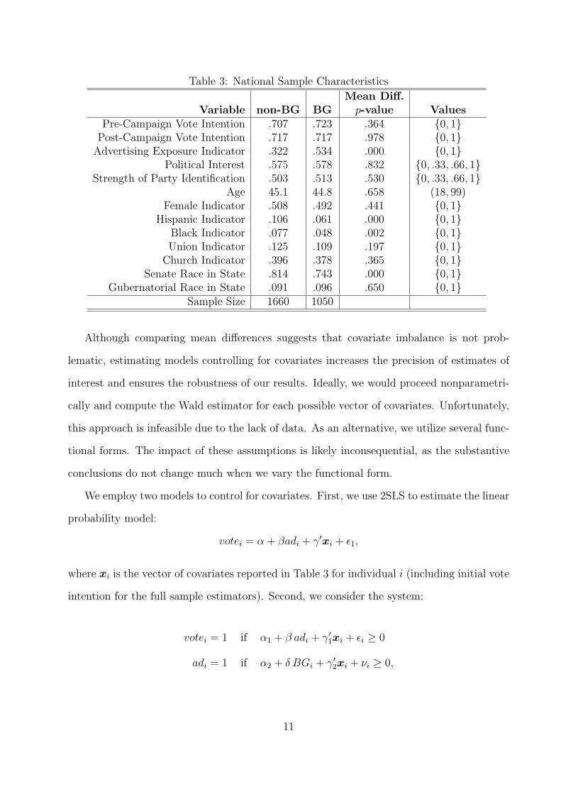
Table 3: National Sample Characteristics

Mean Diff.Variable non-BG BG p-value Values

Pre-Campaign Vote Intention .707 .723 .364 {0, 1}Post-Campaign Vote Intention .717 .717 .978 {0, 1}

Advertising Exposure Indicator .322 .534 .000 {0, 1}Political Interest .575 .578 .832 {0, .33, .66, 1}

Strength of Party Identification .503 .513 .530 {0, .33, .66, 1}Age 45.1 44.8 .658 (18, 99)

Female Indicator .508 .492 .441 {0, 1}Hispanic Indicator .106 .061 .000 {0, 1}

Black Indicator .077 .048 .002 {0, 1}Union Indicator .125 .109 .197 {0, 1}

Church Indicator .396 .378 .365 {0, 1}Senate Race in State .814 .743 .000 {0, 1}

Gubernatorial Race in State .091 .096 .650 {0, 1}Sample Size 1660 1050

Although comparing mean differences suggests that covariate imbalance is not prob-

lematic, estimating models controlling for covariates increases the precision of estimates of

interest and ensures the robustness of our results. Ideally, we would proceed nonparametri-

cally and compute the Wald estimator for each possible vector of covariates. Unfortunately,

this approach is infeasible due to the lack of data. As an alternative, we utilize several func-

tional forms. The impact of these assumptions is likely inconsequential, as the substantive

conclusions do not change much when we vary the functional form.

We employ two models to control for covariates. First, we use 2SLS to estimate the linear

probability model:

votei = α + βadi + γ′xi + ε1,

where xi is the vector of covariates reported in Table 3 for individual i (including initial vote

intention for the full sample estimators). Second, we consider the system:

votei = 1 if α1 + β adi + γ′1xi + εi ≥ 0

adi = 1 if α2 + δ BGi + γ′2xi + νi ≥ 0,

11

where (ε, ν) ∼ N (0, Σ) and

Σ =

1 ρ

ρ 1

.

This bivariate probit model is estimated using maximum likelihood.9

Table 4 presents the effects of advertising exposure in models with covariates. (The

(online) appendix presents complete tables of coefficient estimates.) All reported estimators

(except for the Wald estimator in column 3) control for the variables listed in Table 3. In

each case, we present results both for the full sample and separately for the subsamples of

initial voters and nonvoters.

Table 4: Estimates of the Effect of Advertising Exposure on Turnout

OLS Probit Wald estimates 2SLS Bivariate probit NFull Sample .033 .024 .007 −.094 −.059 2348

(.013) (.010) (.084) (.059) (.044)(−.142, .033)

vote1 = 0 .101 .076 .005 −.225 −.145 631(.039) (.030) (.263) (.273) (.166)

(−.317, .215)

vote1 = 1 .008 .005 −.055 −.074 −.062 1715(.012) (.010) (.053) (.052) (.047)

(−.180, .013)

The first two columns present the average effect of advertising exposure on turnout inten-

tion treating advertising exposure as exogenous using OLS (with heteroskedasticity-robust

standard errors) and probit. The substantive results are similar across specifications. For

initial voters, the impact of advertising is essentially zero, but for initial non-voters there

appears to be a modest and statistically significant positive impact.

The last two columns present the results from the IV estimates with covariates. Ac-

counting for the endogeneity of advertising reveals no positive relationship between turnout

and advertising. The results reported in Table 1 are robust to controlling for covariates

9Greene (2003) discusses the bivariate probit model for a recursive system in section 21.6.6. Convenientlyenough, the endogenous regressor has no impact on the form of the loglikelihood.

12

using several parametric forms for the relationship. (For ease of comparability, the table

also includes the Wald estimates from Table 2.)

To calculate the predicted impact of advertising on vote choice for the bivariate probit

case (column five in Table 4), we use the average treatment effect:

ATE =1

n

n∑

i=1

Φ(α1 + β + γ′1xi)− Φ(α1 + γ′1xi).

The ATE is the mean difference of the predicted probability for each respondent i reporting

an intention to vote given the set of covariates and assuming adi = 1 and the predicted

probability for each respondent i reporting an intention to vote given the set of covariates

and assuming adi = 0. For statistical inference, we bootstrap this average. A single bootstrap

iteration of the average treatment effect requires: sampling with replacement from the data

matrix, estimating the model on the data sample, and calculating the average treatment

effect. Because each sample yields an estimate of the average treatment effect, repeating

the process generates the bootstrap standard error and bootstrap bias corrected confidence

interval for the average treatment effect across the samples reported in Table 4.

Table 4 reveals that adding control variables fails to change the substantive conclusions

regarding the impact of advertising exposure evident in the Wald estimates. In no case

is the estimated effect statistically significantly different than zero. For initial voters, the

estimated effects are remarkably stable across models, and the 95% confidence interval rules

out substantively important positive effects in every case. In contrast to the OLS and Probit

estimates, the IV estimates allow for substantively large negative effects. For initial non-

voters, the estimates are imprecise and confidence intervals permit any reasonable value.

A Hausman test rejects exogeneity in the linear probability model at the 3% level for the

full sample and at the 11% level for the sample of initial voters. The p-value for Hausman

test for the sample of initial non-voters is only slightly higher at .212. For the bivariate probit

and the full sample our estimate of ρ is different than zero at the 4% level, so exogeneity

is rejected in this case as well. Exogeneity is rejected for the initial non-voter and voter

13

samples at 14% and 20% respectively.

Are we missing countervailing effects?

Another way our estimates of the previous section could be misleading is if advertising has

large effects on turnout in both directions: advertisements mobilize some voters at the same

time they demobilize others. Such countervailing effects are a serious possibility given that

12% of the respondents change their intention during the campaign. If these changes are

concentrated in battleground states, then they could indicate a campaign effect (whose sign

differs between the two offsetting voter groups).

This is not what happened. Although 12% of respondents in battleground states changed

their intention, about 11% of respondents in non-battleground states also changed their

intention. The t-statistic for this difference is only 0.760. These results are very similar to

those for final vote intention. Controlling for covariates does not affect these results.

Are the results due to measurement error?

Another possible objection is that the results are the consequence of using variables that

mismeasure advertising exposure because our measure is based on the respondent’s recall of

advertising exposure. It is well known that recall measures can be noisy (see, for example,

Niemi, Katz and Newman (1980); Price and Zaller (1993); Ansolabehere, Iyengar and Simon

(1999); and Vavreck (2005)). In our application, the measurement error is non-classical –

respondents not intending to vote cannot underreport their intended voting behavior (as

they are already indicate that they do not intend to vote) and respondents intending to vote

cannot overreport their intended voting behavior. When measurement error takes this form,

the OLS estimates are biased toward zero, but the IV estimates are biased away from zero

(Kane, Rouse and Staiger 1999). So, again, this bias works against our findings and cannot

account for the results we report in Tables 2 and 4.10

10Another form of measurement error in advertising exposure comes from our coding it as a dichotomousvariable. Again, this leads to bias away from zero (Angrist and Imbens, 1995). The bottom line is that

14

The New Jersey Sample

As a final robustness check, we investigate the relationship between advertising exposure and

turnout for New Jersey residents. New Jersey is worth of individual attention because the

state is divided into two non-native media markets. The northeastern half lies in the New

York media market and the southwestern half receives broadcasts from Philadelphia (Table

and Cable Television Factbook 2000). Because the Philadelphia market is in a battleground

state and the New York market is not, the natural division of New Jersey residents according

to their media market offers the opportunity to investigate the relationship among residents

from the same state. Because all of these voters have the same importance to the electoral

college outcome, face-to-face mobilization efforts should not vary by media market. To the

extent that the results for the New Jersey sample are similar to those of the national sample,

our confidence that the results are about advertising are increased.

Although the level of self-reported intended turnout among residents in the Philadelphia

and New York media market are virtually identical (75% and 76% respectively), residents of

the Philadelphia media market are 20% more likely to report being exposed to many political

advertisements. Because the observed difference is nearly identical to the difference between

battleground and non-battleground state residents reported in Table 3, our confidence in our

identification assumption is increased. Table 5 presents the marginal percentages.

Table 5: Data for the New Jersey Wald Estimator

PA market NY marketTurnout 74.7 75.8Ad exposure 66.7 47.6Sample Size 111 328

The basic results from the Wald estimator persist when we introduce respondent-level

controls and account for advertising endogeneity using a 2SLS estimator (see the (online)

appendix). There appears to be no causal relationship between advertising and turnout.

measurement error probably does affect our point estimates, but it certainly does not drive the substantiveconclusions.

15

Caveats & Conclusions

If exposure to campaign advertising makes an eligible voter significantly more likely to vote,

then we should see significantly greater turnout in battleground states. We do not. This

result is robust to different specifications for control variables and to interesting subsamples.

These results suggest that the causal effect of advertising on turnout is very small, at least

in our sample.11 This qualification is important. Any data analysis can be informative at

most about the sample that is studied. There are consequently several ways that our results

might differ from those of other samples.

The first issue concerns the representativeness of the panel we use. Although Knowledge

Networks used probability sampling to choose respondents and to choose the subsample

asked the political questions we use, there is nonresponse at both stages. Thus our sample

is not fully representative of the population at large and it is possible that people who did

not answer the questions were precisely the people for whom campaigns are effective. So it

is possible that that there are important campaign effects outside of our sample. Without

data on these individuals, we cannot know.

Suggestive evidence that this is not the case is provided by inspecting the average turnout

in battleground and non-battleground states according to the turnout statistics for the 2000

election as reported by the U.S. Census Bureau. Using the ratio of voters over the total state

population as a measure of turnout reveals a turnout of 57.83% for battleground states or

57.44% for non-battleground states (p-value of .58). Using the total number of citizens in

the state as the denominator yields an average turnout of 60.82% and 60.45% respectively

(p-value of .58).

The second issue is a more subtle econometric point. Our instrumental variables estimator

estimates the causal effect of advertising exposure only for those respondents whose exposure

status would have been different had they resided in a different kind of state (Angrist, Imbens

and Rubin 1996). A zero causal effect for this subpopulation is consistent with a nonzero

11Independently and simultaneously, Huber and Arceneaux (2006) use a similar identification strategy tothe 2000 Annenberg National Election Study and find substantially identical results.

16

effect for people who would see advertisements wherever they lived. Thus, our estimates

are conditional on the strategies that parties use to select which voters to target. Different

campaign advertising strategies might well lead to important campaign effects.12 Still, this

local average treatment effect is the relevant effect for some policy questions. For example, a

candidate who must decide to allocate her remaining budget between two states cares about

precisely this subpopulation.

These caveats aside, the results of our study clearly demonstrate that simply asserting

that advertising is exogenous is insufficient and analyses that fail to examine this possibility

are potentially severely biased. Using an exclusion restriction that makes use of the fact

that battleground state residents are significantly more likely to be exposed to advertising

but state residence likely has no independent impact on turnout, we show that advertising

does not result in increased turnout. Consequently, understanding the “surge” associated

with presidential elections as well as the purpose and implications of the massive amount of

advertising in contemporary election contests likely requires looking elsewhere.

12This observation may help to reconcile our results with the results of the observational study of Lassen(2005) and the experimental study of Horiuchi, Imai and Taniguchi (2005), both of whom find that citizenswho are randomly selected to receive information about the candidates in an election are more likely tovote than are citizens who do not get the information. In our data, citizens are targeted by candidates. Ifcandidates preferentially target citizens who are relatively unresponsive to new information, then we shouldexpect to see smaller campaign effects in our sample than in the randomly selected samples of Lassen (2005)and Horiuchi, Imai and Taniguchi (2005).

17

References

Abramson, Paul R. and William Claggett. 1984. “Race-Related Differences in Self-Reportedand Validated Turnout.” Journal of Politics 46(3):719–38.

Angrist, Joshua D. and Guido W. Imbens. 1995. “Two-Stage Least Squares Estimationof Average Causal Effects in Models with Variable Treatment Intensity.” Journal of theAmerican Statistical Association 90(430):431–42.

Angrist, Joshua D., Guido W. Imbens and Donald B. Rubin. 1996. “Identification of CausalEffecys Using Instrumental Variables.” Journal of the American Statistical Association91(434):444–55.

Ansolabehere, Stephen, Eric Snowberg and Jr. James M. Snyder. 2006. “Television and theIncumbency Advantage in U.S. Elections.” forthcoming Legislative Studies Quarterly.

Ansolabehere, Stephen and Shanto Iyengar. 1994. Going Negative: How Political Advertise-ments Shrink and Polarize the Electorate. New York, NY: Free Press.

Ansolabehere, Stephen, Shanto Iyengar and Adam Simon. 1999. “Replicating ExperimentsUsing Aggregate and Survey Data: The Case of Negative Advertising and Turnout.”American Political Science Review 93:901–9.

Bartels, Larry M. 1988. Presidential Primaries and the Dynamics of Public Choice. Prince-ton, NJ: Princeton University Press.

Bartels, Larry M. 1991. “Instrumental and “Quasi-Instrumental” Variables.” American Jour-nal of Political Science 35(3):777–800.

Campbell, Angus. 1966. Surge and Decline: A Study of Electoral Change. In Electionsand the Political Order, ed. Angus Campbell, Phillip E. Converse, Warren E. Miller andDonald E. Stokes. New York: Wiley.

Campbell, James E. 1986. “Presidential Coattails and Midterm Losses in State LegislativeElections.” American Political Science Review 80(1):45–63.

Campbell, James E. 1991. “The Presidential Surge and Its Midterm Decline in CongressionalElections, 1868-1988.” Journal of Politics 53(2):477–87.

Clinton, Joshua D. 2001. “Panel Bias from Attrition and Conditioning: A Case Study of theKnowledge Networks Panel.” Princeton University typescript.

Clinton, Joshua D. and John Lapinski. 2005. “An Experimental Study of Political Advertis-ing Effects in the 2000 Presidential Election.” Journal of Politics 66(1):67–96.

Freedman, Paul, Michael Franz and Kenneth Goldstein. 2004. “Campaign Advertising andDemocratic Citizenship.” 48(4):723–41.

Gerber, Alan. 1998. “Estimating the Effect of Campaign Spending on Senate Election Out-comes Using Instrumental Variables.” American Journal of Political Science 92:401–11.

18

Gerber, Alan S. and Donald P. Green. 2000. “The Effects of Canvassing, Telephone Calls andDirect Mail on Voter Turnout: A Field Experiment.” American Political Science Review94:653–63.

Goldstein, Kenneth and Paul Freedman. 2002. “Campaign Advertising and Voter Turnout:New Evidence for a Stimulation Effect.” 64(3):721–740.

Goldstein, Kenneth and Travis N. Ridout. 2004. “Measuring the Effects of Televised PoliticalAdvertising in the United States.” Annual Review of Political Science 7:205–26.

Green, Donald P. and Jonathan S. Krasno. 1988. “Salvation for the Spendthrift Incumbent:Reestimating the Effects of Campaign Spending in Hosue Elections.” American Journalof Political Science pp. 884–907.

Greene, William H. 2003. Econometric Analysis. Fifth ed. Upper Saddle River, NJ: PrenticeHall.

Hillygus, D. Sunshine. 2005. “The Dynamics of Turnout Intention in Election 2000.” Journalof Politics 67(1):50–68.

Horiuchi, Yusaku, Kosuke Imai and Naoko Taniguchi. 2005. “Designing and AnalysingRandomized Experiments.” Unpublished paper, Princeton University.

Huber, Gregory A. and Kevin Arceneaux. 2006. “Uncovering the Persuasive Effects ofPresidential Advertising.” Yale University Typescript.

Johnston, Richard, Michael G. Hagen and Kathleen Hall Jamieson. 2004. The 2000 Presiden-tial Election and the Foundations of Party Politics. Cambridge, MA: Cambridge UniversityPress.

Kane, Thomas J., Cecilia Elena Rouse and Douglas Staiger. 1999. “Estimating the Returnsto Schooling when Schooling is Misreported.” NBER Working Paper 7235.

Lassen, David Dreyer. 2005. “The Effect of Information on Voter Turnout: Evidence from aNatural Experiment.” American Journal of Political Science 49(1):103–118.

Lau, Richard R. and Gerald M. Pomper. 2002. “Effectiveness of Negative Campaigning inU.S. Senate Elections.” American Journal of Political Science 46(1):47–66.

Lau, Richard R., Lee Sigelman Caroline Heldman and Paul Babbitt. 1999. “The Effectsof Negative Political Advertisements: A Meta-Analytic Assessment.” American PoliticalScience Review 93(4):851–75.

Niemi, Richard, Richard S. Katz and David Newman. 1980. “Reconstructing Past Parti-sanship: The Failure of the Party Identification Recall.” American Journal of PoliticalScience 24:633–51.

Price, Vincent and John Zaller. 1993. “Who Gets the News? Alternative Measures of NewsReception and Their Implications for Research.” Public Opinion Quarterly 57:133–64.

19

Prior, Markus. 2005. “News vs. Entertainment: How Increasing Media Choice Wides Gapsin Political Knowledge and Turnout.” American Journal of Political Science 49(3):577–92.

Ridout, Travis N. 2004. “Campaign Advertising Strategies in the 2000 Presidential Nom-inations: The Case of Al, George, Bill and John.” The Medium and the Message. ed.Kenneth M. Goldstein and Patricia Starch. pp. 27-43. Upper Saddle River, NJ: PearsonPrentice-Hill.

Stromberg, David. 2002. “Optimal Campaigning in Presidential Elections: The Probabilityof Being Florida.” IIES working paper.

Television and Cable Factbook. 2000. Vol. 68 Washington D.C.: Warren CommunicationsNews.

Vavreck, Lynn. 2005. “The Dangers of Self-Reports of Political Behavior.” UCLA Typescript.

Verba, Sidney, Kay Lehman Schlozman and Henry E. Brady. 1995. Voice and Equality: CivicVoluntarism in American Politics. Cambridge, MA: Harvard University Press.

West, Darrell M. 2005. Air Wars: Television Advertising in Election Campaigns, 1952-2004.4 ed. Washington DC: CQ Press.

20