Accurate Speed and Density Measurementfor Road Traffic in India

Rijurekha Sen1∗, Andrew Cross2, Aditya Vashistha2,Venkata N. Padmanabhan2, Edward Cutrell2, and William Thies2

1IIT Bombay 2Microsoft Research Indiariju@cse.iitb.ac.in {t-across,t-avash,padmanab,cutrell,thies}@microsoft.com

ABSTRACTMonitoring traffic density and speed helps to better manage trafficflows and plan transportation infrastructure and policy. In this pa-per, we present techniques to measure traffic density and speed inunlaned traffic, prevalent in developing countries, and apply thosetechniques to better understand traffic patterns in Bengaluru, India.Our techniques, based on video processing of traffic, result in about11% average error for density and speed compared to manually-observed ground truth values. Though we started with intuitiveand straight-forward image processing tools, due to a myriad ofnon-trivial issues posed by the heterogeneous and chaotic trafficin Bengaluru, our techniques have grown to be non-obvious. Wedescribe the techniques and their evaluation, with details of whysimpler methods failed under various circumstances. We also ap-ply our techniques to quantify the congestion during peak hoursand to estimate the gains achievable by shifting a fraction of trafficto other time periods. Finally, we measure the fundamental curvesof transportation engineering, relating speed vs. density and flowvs. speed, which are integral tools for policy makers.

1. INTRODUCTIONTraffic congestion leads to long and unpredictable commute times,

environmental pollution and fuel waste. These negative effects aremore acute in developing countries like India, where infrastructuregrowth is slow because of cost and bureaucratic issues. Intelli-gent traffic management and better access to traffic information forcommuters can help alleviate congestion issues to a certain extent.Static sensors like loop detectors [2, 11, 13], video cameras [6,7] and mobile sensors like GPS in vehicles [8, 9, 26, 31, 33] areused for traffic monitoring purposes in developed contexts. Mostof these techniques, however, are only suited for lane based orderlytraffic in developed countries where the penetration of GPS devicesand smartphones is also sufficiently high.

Traffic in developing countries has significantly different charac-teristics from traffic in developed countries. High heterogeneity in∗The first author started work on this project during an internshipat Microsoft Research India.

Permission to make digital or hard copies of all or part of this work forpersonal or classroom use is granted without fee provided that copies arenot made or distributed for profit or commercial advantage and that copiesbear this notice and the full citation on the first page. To copy otherwise, torepublish, to post on servers or to redistribute to lists, requires prior specificpermission and/or a fee.DEV’13, January 11–12, 2013, Bangalore, India.Copyright 2013 ACM 978-1-4503-1856-3/13/01 ...$15.00.

vehicle sizes makes defining lanes cumbersome. On a typical roadin India, all vehicles from buses to two-wheelers pack themselvestogether to utilize the available road infrastructure. Traditional traf-fic sensors have been designed to work for laned traffic, and withoutcareful modification to sensor placement and sensor data process-ing, they are not suitable for monitoring unlaned traffic. We haveanecdotal evidence of this shortcoming, as the image processingsoftware from Bosch gives 55% median error on vehicle counts atthe Bengaluru traffic management center [24], and hence has beenreplaced by manual monitoring of the video feeds to ensure accu-racy.

There have been several efforts to design clean slate solutions forunlaned traffic monitoring. One approach is to detect congestionbased on acoustic sensing [29], since chaotic traffic is often noisy.Another system measures traffic density (the fraction of roadwayoccupied by vehicles) based on variations in an RF signal betweenwireless sensors placed on either side of the road [28]. This sys-tem infers the length of traffic queues from an array of such sensorsleading up to a traffic light. These methods are insufficient becausefirstly, they only yield a binary classification of traffic densities intotwo-states: congested or free-flowing. Secondly, both methods re-quire significant manual overhead to train the sensors for differentroad characteristics [30].

There have been several initial attempts to process images andvideos of chaotic traffic [17, 18, 20, 25]. Jain et al. give two al-gorithms [17, 18] to produce a binary classification of traffic den-sity, one algorithm for daylight conditions and the other for night-time. This research makes significant contributions as the tech-niques work on low-quality webcam images, and not traditionalhigh-quality video feeds from traffic cameras. The algorithm fornighttime is intuitive, but the algorithm for daytime processing ismore complicated, using a histogram of grayscale images to clas-sify traffic which requires manual training; ultimately, this algo-rithm is similarly limited to a binary classification of traffic. Therehas not been an empirical evaluation of the accuracy of the algo-rithm yet, which leaves uncertainty about its effectiveness in de-tecting vehicles that match the grayscale color of the road.

Some techniques [12, 19] track vehicle features to calculate ve-hicle trajectories across frames and have been thoroughly evalu-ated in lane-based orderly traffic. Similar feature-based trackingin unlaned traffic is done by Trazer [20]. It uses Haar features todetect vehicles anywhere in a given frame and classifies each ve-hicle into one of five categories: heavy vehicles, medium vehicles,small four-wheelers, auto rickshaws and two-wheelers. Searchingfor Haar features over an entire frame needs 8-core processors torun in real time, 4 GB RAM and a 650 GB hard-drive in both on-line and offline computation. Also, in high traffic density, vehicleocclusion makes feature matching challenging.

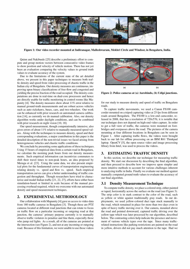
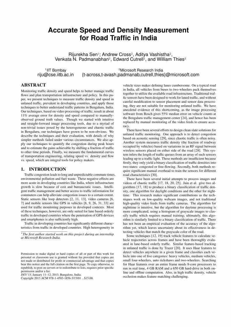
Figure 1: Our video recorder mounted at Indiranagar, Malleshwaram, Mekhri Circle and Windsor, in Bengaluru, India.

Quinn and Nakibuule [25] describe a preliminary effort to com-pute and group motion vectors between consecutive video framesto show position and velocity of vehicle motion. There has not yetbeen an evaluation comparing the velocity values to ground truthvalues to evaluate accuracy of the system.

Due to the limitations of the current state of the art detailedabove, we present in this paper techniques to measure both traf-fic density and speed from video processing of chaotic traffic in theIndian city of Bengaluru. Our density measures are continuous, im-proving upon binary classifications of free-flow and congested andyielding the precise fraction of the road occupied. The density com-putations are done in real-time on dual-core processors and henceare directly usable for traffic monitoring in control rooms like Ma-punity [4]. The density measures show about 11% error relative tomanual ground-truth measurements and are robust across vehiclessuch as auto rickshaws, buses, cars, and two-wheelers. Our workcan be enhanced with prior research on automated camera calibra-tion [14], as currently we do manual calibration. Also, our densityalgorithm works under daylight conditions, and can be combinedwith prior research on night vision [10, 18].

Our speed measurement, though computationally intensive, alsogives errors of about 11% relative to manually measured speed val-ues. Along with the techniques to measure density, speed and theircorresponding evaluations, a major contribution in this paper is thedetailed description of the non-trivial issues we faced arising fromheterogeneous vehicles and chaotic traffic conditions.

We conclude by presenting some applications of these techniques.Using 15 hours of empirical data from a certain road in Bengaluru,we calculate the morning peak hours from our density measure-ments. Such empirical information can incentivize commuters toshift their travel times to non-peak hours, an idea proposed byMerugu et al. [23]. Using the same data, we also present empir-ical plots for the fundamental curves of transportation engineeringrelating density vs. speed and flow vs. speed. Such empiricaltransportation curves can give a better understanding of traffic con-gestion and throughput. Though researchers have tried to charac-terize and model Indian traffic [21, 22, 27], efforts have either beensimulation-based or limited in scale because of the manual pro-cessing overhead required, which we overcome with our automateddensity and speed measurement techniques.

2. EXPERIMENTAL METHODOLOGYOur collaboration with Mapunity [4] gave us access to video data

from 180 traffic cameras in Bengaluru [3]. Though these are PTZcameras located at different road junctions that can rotate to focuson traffic flow on a particular incoming or outgoing road at thatjunction, the cameras’ primary purpose currently is to manuallyobserve traffic violators to penalize and fine them, especially thosewho jump red lights. As a result, all of the cameras are pointed atthe intersection (see Figure 2), and not at any incoming or outgoingroad. Because of this limitation, we were unable to use those videos

Figure 2: Police cameras at (a) Aurobindo, (b) Udipi junctions.

for our study to measure density and speed of traffic on Bengalururoads.

To capture traffic movements, we used a Canon FS100 cam-corder mounted on a tripod capturing video at 25 fps from differentroads around Bengaluru. The FS100 is a low-end camcorder, re-leased in 2008, that has a resolution of 720x576; it is notable thatour technique does not depend on high-end video capture. In orderto get a full view of traffic, the cameras were mounted on foot-bridges and overpasses above the road. The pictures of the cameramounting at four different locations in Bengaluru can be seen inFigure 1. After capturing traffic flows, the videos were broughtback to our lab for offline processing on an IBM R61 Thinkpadlaptop. OpenCV [5], the open source video and image processinglibrary from Intel, was used to process the videos.

3. ESTIMATING TRAFFIC DENSITYIn this section, we describe our technique for measuring traffic

density. We start our discussion by describing the final algorithm,and then proceed to describe how we improve upon simpler andmore intuitive methods to account for various challenges inherentto analyzing traffic in India. Finally we evaluate our method againstmanually computed ground truth values to evaluate the accuracy ofour final algorithm.

3.1 Density Measurement TechniqueTo compute traffic density, we place a colored strip, either painted

or taped, horizontally across the surface on the road (see Figure 3).The strip color is in stark contrast to the color of the road, suchas yellow or white against traditionally gray roads. In our de-ployments, we used yellow-colored duct tape stuck manually tothe road, which remained in place for more than two days even inspite of heavy traffic moving over it. Our camera, mounted abovethe road and pointed downward, captured traffic driving over theyellow tape which was later processed by our algorithm, describedbelow. The contrasting colors help indicate the presence and move-ment of various vehicle types over the tape. Since many traffic-related instructions like parking restrictions are painted on the roadin yellow, drivers did not pay much attention to the tape. Had we

Figure 3: Road (a) before and (b) after perspective correction.

used a more out-of-place color, such as fluorescent green, that mayhave caused more distraction or alteration to traffic patterns.

Our basic strategy for computing density is to calculate the frac-tion of the tape that is obscured by vehicles on every frame. Whilethis measurement reflects the density for only a one-dimensionalstrip of the frame, when averaged over time the result is propor-tional to the full two-dimensional frame density, assuming that ve-hicles cross the tape at their average speed for the frame.

To detect obfuscation of the tape, we apply two separate tests.The first test detects vehicles that have uniform coloration on theirroofs, such as buses, cars, and auto rickshaws. When such a ve-hicle passes over the tape, it obscures the color contrast betweenthe tape and the road. That is, without obfuscation there are neigh-boring pixels that have very different colors (yellow for the tape,black for the road), but with obfuscation both of these pixels arethe same color (the color of the vehicle). We detect such cases bydifferencing the pixels immediately inside and outside the tape, ateach position across the road; if the difference exceeds a threshold,we report the presence of a vehicle at the corresponding position.

The second test detects vehicles that do not have a uniform col-oration, including two-wheelers, open trucks, and the backs/sidesof other vehicles. Because there is spatial variation in the vehicle’scolor, this implies that there is temporal variation in color as the ve-hicle travels over a fixed set of pixels. Thus, we detect the presenceof the vehicle by detecting changes in coloration – for a fixed setof pixels overlapping the tape – between one frame and the next.Overall, a vehicle is reported if it is detected by either of the testsabove.

After estimating the fraction of tape that is obscured by vehi-cles, we adjust this estimate to compensate for systematic bias rel-ative to ground truth values. This adjustment is needed for tworeasons. First, our algorithm still does not detect a fraction of somevehicles, leading to a systematic under-estimate of vehicle density.Second, when we extrapolate from one-dimensional density to two-dimensional density, an adjustment is needed to normalize the mea-surement scale. We implement the adjustment using a simple linearmodel: given raw density r, the final density d = ar + b, wherea and b are learned using a training set of ground truth values. Wedescribe the details of the training and testing procedures in ourevaluation sections.

Our algorithm is formalized with pseudocode in Figure 4. Online 2, as the algorithm processes each frame of the video, it per-forms a perspective correction to make the resulting frame lookmore similar to one that is taken vertically from above (see Fig-ure 3). On line 3, the algorithm divides the tape into discrete pieces,or rectangles; the overall density reported for a frame is the frac-tion of rectangles that are obscured by a vehicle. As depicted inFigure 5, each rectangle of the tape is paired with an adjacent rect-angle of the road, in order to test the color contrast. We use thenotation {Bi,Yi} to denote these corresponding black and yellowrectangle pairs. Line 4 applies both of the tests described earlier:

1: function COMPUTE-DENSITY2: Correct perspective error of camera for frame N (shown

in Figure 3).3: Divide the rectangular yellow tape and a parallel black

rectangle of the road, adjacent to the tape, into verticalrectangle pairs {Bi,Yi} (shown in Figure 5).

4: For each {Bi, Yi} pair, consider the pair occupied if either:(i) the RGB difference between Bi and Yi is below a

threshold C, or(ii) the RGB difference between Yi in frame N and Yi

in frame N − 1 is more than a threshold T .5: Compute raw density r as ratio of occupied rectangle pairs

to total rectangle pairs.6: Compute corrected density d = ar + b, where a and b are

learned from training data.7: end function

Figure 4: Algorithm to compute density for frame N .

Figure 5: Vertical pairs of black and yellow rectangles.

(i) testing changes in color between the tape and the road, and (ii)testing changes in color from one frame to the next. Line 5 com-putes the raw frame density in terms of the fraction of rectanglesthat are obscured. Line 6 computes the corrected frame densityusing a linear model, in which the parameters are gleaned fromtraining data.

3.2 How We Arrived at this TechniqueThough the algorithm described above is complex and non-intuitive,

the complexities are necessary to accurately measure traffic densitydue to several challenges for image processing. Here we describethe simpler methods that we tried, the obstacles we encountered,and the solutions we came up with to arrive at the final algorithm.

Background subtraction does not detect busesInitially, we tried background subtraction, a well-known image pro-cessing tool. In this method, the foreground pixels in frame N arecalculated by subtracting a background frame from it. The den-sity of frame N is calculated by the ratio of foreground pixels tototal pixels in the frame. The background frame was manually se-lected as a frame containing no vehicles to serve as the template,where any pixel differences indicate a vehicle. This simple intuitivemethod gave disastrous results because of a peculiar characteristicof buses in Bengaluru.

Bengaluru buses have a gray cover on their roofs, probably as aprotection from heat and rain. Online image searches revealed sim-ilar characteristics of buses in other Indian cities. This gray color isalmost the same color as the road, and therefore using backgroundsubtraction does not detect a vehicle. In fact, when two buses standside by side occupying the entire road as shown in Figure 6, back-ground subtraction measures no density (Figure 7).

Simple yellow-tape analysis is too sensitive to lightingIn order to handle the issue of gray bus tops, we introduced thenovel idea of using a high-contrast strip of tape on the road. As de-scribed previously, we defined vertical rectangle pairs {Bi,Yi} andcomputed density as the ratio of occupied rectangle pairs to total

Figure 6: Video excerpt with two buses, achallenging case for density calculation.

0 10 20

30 40 50 60 70

80 90

100

5 10 15 20 25 30 35 40 45 50 55 60

De

nsity p

erc

en

tag

e

Time in seconds

raw30 secs avg

Figure 7: Background subtraction doesnot detect the buses in video excerpt.

0 10 20

30 40 50 60 70

80 90

100

5 10 15 20 25 30 35 40 45 50 55 60

De

nsity p

erc

en

tag

e

Time in seconds

raw30 secs avg

Figure 8: Yellow tape analysis (simple al-gorithm, not our best) detects the buses.

Figure 9: A bus with its shadow. Simple techniques are sensi-tive to lighting conditions and may count the shadow as part ofthe vehicle; our technique reports the correct density.

rectangle pairs. Our initial approach to detecting “occupied” pairswas very simple. Building on the idea of background subtraction,we manually selected a background frame without any vehicles,containing only the empty road with the tape. For a frame N , if theRGB color values of pixels in either Bi or Yi differed from corre-sponding pixels in the background frame by more than a thresholdT , the pair {Bi,Yi} was considered occupied in that frame, indicat-ing the presence of a vehicle. This approach detects gray buses dueto changes observed to the yellow rectangle Yi. It detects auto rick-shaws (which are yellow) due to changes to the black rectangle Bi.The algorithm also detects vehicles of other colors, as they changethe appearance of both rectangles.

This simple solution handled the issue of gray bus roofs, as seenfrom Figure 8 where density in a frame with two buses is mea-sured accurately. However, the shortcoming of this method is thatit is not robust to variable lighting conditions, in particular shad-ows. Surprisingly, the shadows of vehicles caused the pixel colorsto change so much that no value of the threshold T was able to filterthe shadows and detect the vehicles accurately. Depending on theangle of light, sometimes density was measured to be higher thanthe actual density because the shadow made the vehicles look big-ger than they actually were. An example of a vehicle with shadowis shown in Figure 9. Also, for both this technique and for back-ground subtraction, the manual selection of the background framewas tricky. Lighting conditions changed over time, which meant anempty frame under different lighting conditions could exhibit colordifferences relative to the background frame, leading to non-zerodensity measurement.

Our final algorithm is robust to these lighting variations by ex-amining only the difference in color between black and yellow rect-angles, as opposed to comparing either rectangle to an absolutethreshold. For example, in Figure 9, we do not mistake the shadowas being part of the vehicle.

3.3 EvaluationTo evaluate our technique, we use two levels of analysis. The

first considers individual cars and compares the fraction of the tapeobscured relative to manually-measured values. The second con-

siders a longer period of general traffic and compares to a differentground truth metric: the fraction of the entire frame that is occupiedby vehicles.

Individual vehiclesWe consider ten vehicles of each type (auto rickshaws, buses, cars,and two-wheelers), for a total of 40 vehicles. To simplify this anal-ysis, we restrict our attention to vehicles that pass through the fieldof view alone (i.e., there is no other vehicle visible in frames wherethey are visible).

Ground truth: Our ground truth in this comparison is the frac-tion of the tape that is obscured on each frame, as collected by man-ual measurements. To collect this data, we examined each frame ofthe video in which a vehicle overlapped the tape (488 frames total)and measured the number of pixels obscured (by any part of thevehicle) using a screen capture tool.

Automated algorithm: The automated algorithm worked as de-scribed in the prior section, and was applied to every frame in whichthe vehicle appeared (including frames in which the vehicle did notoverlap the tape). Where indicated below, we aggregated the per-frame density by vehicle type to obtain an average density for eachvehicle in the frame. For illustrative purposes, we did not applyany correction (line 6 of the algorithm) except in computing therelative error rates; in this case, we trained the model on the per-vehicle ground truth densities using least-squares linear regressionand leave-one-out cross validation.

Results: First we describe the raw density calculations (fromline 5 of the algorithm), in order to understand the accuracy of thebasic technique. Then we use the corrected density estimates inorder to compute the error rate of our technique.

Figure 10 illustrates the raw fraction of the tape obscured on aframe-by-frame basis, using both automated and manual measure-ments. We observe a good correlation (R2 = 0.81) between thecalculated values and the ground truth. Errors originate from twosources. First, some parts of vehicles are not detected as obscur-ing the tape, which results in points that fall below the trend line inFigure 10. Second, a handful of shadows are detected as being partof the vehicle, which results in points along the y axis in Figure 10.

To estimate the impact of these frame-level errors on the aggre-gate density measurement, we average raw density values acrossframes corresponding to a single vehicle. Results of this per-vehicledensity comparison appear in Figure 11. At the granularity of vehi-cles, we observe a much higher correlation (R2 = 0.998) betweencalculated and ground truth values.

The error rates1 of our final (corrected) density calculations areshown in Table 1. Overall, our estimates show an average error rate1Throughout this paper, the error rate e for a single calculationis defined as e = |(c − t)/t|, where c represents the calculatedvalue and t represents the true value. When averaging the error rateacross multiple predictions, we ignore the few cases where t = 0.

0.5

two-wheelers

R² = 0.815

0

0.2

0.4

0.6

0.8

0 0.2 0.4 0.6 0.8

Ca

lcu

late

d F

ract

ion

True Fraction

Fraction of Tape Obscured

(Per Frame)

Figure 10: Comparison of frame-level density calculations withground-truth values. Density estimates represent raw values(line 5 of algorithm), prior to correction.

vehicle type average error median error

auto rickshaws 9.3% 5.4%

bus 1.8% 1.2%

car 9.6% 11.4%

two-wheelers 13.8% 15.0%

all vehicles 10.9% 5.0%

Table 1: Density error rates per vehicle type. Densities rep-resent corrected values, separately trained and tested for eachrow of the table, using the vehicle type(s) in the first column.

of 10.9%, and a median error rate of 5.0%. Error rates are lowestfor buses (1-2%) and highest for two-wheelers (14-15%) due to thesize of those vehicles; for smaller vehicles, a fixed amount of errorresults in larger error rate.

General trafficIn this section we expand the evaluation to a more realistic scenario,in two respects. First, we consider general traffic, in which manyvehicles may be within the field of view at the same time. Sec-ond, we estimate the density for the full two-dimensional frame,and compare to corresponding ground truth values, rather than re-stricting our attention to the fraction of tape that is occupied.

Our analysis utilizes three video segments from Malleshwaram.In total, the videos last 130 seconds and include 122 vehicles. Con-gestion varied across the segments, but was generally medium tolight. We did not evaluate bumper-to-bumper, stand-still traffic dueto the overhead of manual data collection; stand-still traffic requiresa large window of samples in order for the one-dimensional densitymeasured at the tape to match the two-dimensional density of theframe.

Ground truth: To ascertain the ground-truth density, we man-ually analyzed each frame of the videos (about 3250 frames to-tal). After correcting the videos for perspective (as per Figure 3),we measured the width and length of each vehicle, as well as theframes in which points of interest on the vehicle (front and backedges) both entered and exited the frame. Assuming constant vehi-cle motion, this information is sufficient to calculate the fraction ofeach vehicle that is visible on each frame.

One limitation of our ground-truth data is due to the camera per-spective. Because we were not looking straight down on traffic, ourvideos include a view of the back side of vehicles (even followingperspective correction). Due to the difficulty of automatically dis-tinguishing between the top and the back of vehicles, for the sakeof this comparison we counted both the top and back of vehicles as

R² = 0.998

0

0.25

0.5

0 0.25 0.5

Ca

lcu

late

d F

ract

ion

True Fraction

Fraction of Tape Obscured

(Per-Vehicle Average over 2s Window)

autos

buses

cars

two-wheelers

Figure 11: Comparison of vehicle-level density calculationswith ground-truth values. Density estimates represent raw val-ues (line 5 of algorithm), prior to correction.

part of the ground truth density. This introduces bias in two ways:first, taller vehicles are reported to consume more space than theyactually do, and second, vehicles appear to grow as they progressacross the frame. For simplicity, we represent the vehicle size asconstant across frames; this size is calculated as the average of thesize upon entering the frame and the size upon exiting the frame.

Automated algorithm: For automatic calculation of density, westarted with the algorithm described previously to estimate the rawfraction of tape that was obscured by vehicles on each frame. Inorder to extrapolate to the density of a two-dimensional frame, wesimply average the one-dimensional densities over a window of val-ues. We also make a small adjustment to compensate for the factthat the tape was at the bottom of the frame: to estimate the fullframe density at frame N , we consider the tape values averagedover a window centered at N − 7. Also, we correct the final esti-mates by training against ground truth values for full-frame densi-ties (using linear regression and leave-one-out cross validation).

Results: Results of the comparison are illustrated in Figure 12.Our technique performs well, eliciting a good correlation betweenpredicted and true densities (R2 = 0.87). The average and medianerror rates are 18% and 15%, respectively. This comparison uti-lizes a window size of 6s, which is about the largest window that ismeaningful using our limited ground truth data.

Because our algorithm relies on averaging to extend the mea-sured one-dimensional density to the full two-dimensional frame,our results improve considerably with increasing window sizes.This trend is illustrated in Figure 13, where average error rates de-crease roughly ten-fold as the window grows from 1s to 6s. In theapplications described later, we use a window size of 30s, whichshould yield even better accuracies for our technique.

4. ESTIMATING TRAFFIC SPEEDIn this section we describe our speed estimation technique. Simi-

lar to our explanation of the density estimation technique in the pre-vious section, we start by presenting the final algorithm followed bya description of the inadequacies of simpler methods that promptedour improvements culminating in the design of the final algorithm.We conclude by evaluating the accuracy of our speed estimates rel-ative to the manually observed ground truth.

4.1 Speed Estimation TechniqueThe algorithm to compute traffic speed for a frame N is given in

Figure 14. The goal is to find the displacement or offset betweenpixels of two consecutive frames that maximizes the similarity be-tween pixels of those two frames. In other words, if all pixels in

R² = 0.87

0

0.2

0.4

0.6

0 0.2 0.4 0.6

Est

ima

ted

De

nsi

ty (

Av

g)

True Density (Avg)

Fraction of Frame

Occupied (6s Avg)

average error = 17.8%

median error = 14.6%

Figure 12: Correlation between calculated and true density val-ues for 6s windows of traffic footage.

0%

50%

100%

150%

200%

250%

1 2 3 4 5 6

Err

or

Ra

te

Window Size (secs)

Average error

Median error

Figure 13: Density errors as a function of window size.

frame N − 1 moved by that offset, then they would best match thepixels in frame N .

We first correct perspective errors in both frames N − 1 and N .Then we consider pixels PixelSet in frame N that have changedby more than a threshold from the corresponding pixels in frameN −1. This reduces the search space by ignoring stationary pixels,where no new vehicles have entered and no old vehicles have left.This also prevents mistaking the yellow tape for a car with speedzero.

Then we consider pixels PixelSet’ in frame N−1, which containpixels within a search window distance from PixelSet. This searchwindow is chosen to reduce the search space to make computationfaster while still considering pixels at far enough distance to handlehigh speed motion. With our 25 fps 720 by 576 pixels video, weempirically found that a search window of 100 pixels is more thansufficient to match vehicles moving at high speed.

The algorithm then finds the (x,y) offset between pixels PixelSetin frame N and pixels PixelSet’ in frame N − 1, that minimizesthe total RGB difference over all pixels in PixelSet. This offsetrepresents the raw estimate of speed between frames N−1 and N .Analogously to our density algorithm, we adjust the raw estimateinto a corrected value using a linear model based on training data,which is returned from the algorithm.

4.2 How We Arrived at this TechniqueLike density, our speed measurement technique also evolved from

simpler methods. Researchers previously have used motion vectorsto estimate vehicle motion [16, 25, 32]. As the embedded motionvector values in MPEG2 videos are computed over a small searchspace, for improved accuracy, we tried to compute motion vectorsbetween consecutive frames using OpenCV functions. The magni-

1: function COMPUTE-DIFF(frame 1, frame 2, pixelSet)2: for each pixel p in pixelSet do3: RGBdiff = RGBdiff + difference in RGB between p in

frame 1 and p in frame 24: end for5: return RGBdiff6: end function7: function COMPUTE-SPEED(frame N − 1, frame N )8: Correct perspective error of camera for both frames N − 1

and N (shown in Figure 3).9: Let S be the set of pixels p s.t. RGB difference

between p in frame N − 1 and p in frame N is greaterthan threshold T

10: Select the offset (i, j) within a search window, thatminimizes COMPUTE-DIFF(frame N − 1 shifted by(i, j), frame N , S). The raw speed is set to j.

11: Compute the corrected speed s = aj + b, where a and bare learned from training data.

12: return s13: end function

Figure 14: Algorithm to compute speed for frame N .

tude of the motion vectors computed for each pixel in a frame, wasconsidered as the speed for that pixel.

Though moving vehicles were detected accurately using the OpenCVmotion vectors, when we looked at actual magnitudes of speeds,and compared them to manually measured pixel movements be-tween frames, we found the correlation to be extremely low (0.07for one ground truth dataset). One challenge was that the motionvectors were being computed independently for small blocks ofpixels; thus, pixels within a homogeneous region (such as roofsof cars) might find a good match at a distance or direction differentthan the velocity of traffic. Our algorithm can be understood as avariation of MPEG2 motion estimation, but rather than consider-ing small macroblocks, we consider a large set of pixels (those thathave changed between frames), thereby averting this problem.

It may be that techniques that track flow of features [12, 19, 20,25] can give equal or better speed measurements than we presenthere. However, we are unaware of any published evaluation offeature-based techniques in unlaned traffic. The simplicity of ourtechnique may also make it more accessible to non-experts.

4.3 EvaluationSimilarly to the evaluation of density, the evaluation of our speed

algorithm proceeds in two steps: first for individual vehicles, andthen for general traffic.

Individual vehiclesWe examine the speeds of 40 vehicles (10 of each type), using thesame data set as described in the density section.

Ground truth: We assume that each vehicle travels at a constantrate, and calculate its speed based on the number of pixels traveledin a given number of frames. We consider a window of frames thatis as large as possible while keeping the vehicle in view, and mea-sure the number of pixels traveled during that time. To minimizedistortion due to perspective, we track a point on each vehicle thatis as close to the ground as possible (e.g., the lower-back edge, nearthe rear tires).

One limitation of this data is that the assumption of constant ve-hicle speed is sometimes violated, as vehicles accelerate or decel-erate in response to upcoming road conditions.

y = 1.90x - 8.68

R² = 0.970

20

40

60

80

0 10 20 30 40

Ca

lc S

pe

ed

(k

m/h

r)

True Speed (km/hr)

buses

y = 1.32x - 1.56

R² = 0.980

20

40

60

0 10 20 30 40

Ca

lc S

pe

ed

(k

m/h

r)

True Speed (km/hr)

auto rickshaws

y = 1.33x - 8.29

R² = 0.960

20

40

60

0 10 20 30 40

Ca

lc S

pe

ed

(k

m/h

r)

True Speed (km/hr)

cars

y = 1.20x - 0.91

R² = 1.000

20

40

60

0 10 20 30 40

Ca

lc S

pe

ed

(k

m/h

r)

True Speed (km/hr)

two-wheelers

y = 1.26x + 0.47

R² = 0.480

20

40

60

80

0 10 20 30 40

Ca

lcu

late

d S

pe

ed

(k

m/h

r)True Speed (km/hr)

all vehicle types

busesauto rickshawscarstwo-wheelers

Figure 15: Correlation between calculated and true speed values for individual vehicle types.

Automatic algorithm: To condense the algorithm’s per-frameestimates into a single estimate for each vehicle, we use the medianvalue out of the frames in which the vehicle is present.

Results: The raw speeds (line 10 of the algorithm) are shown foreach vehicle type in Figure 15 and for all vehicle types combinedin Figure 16. The final error rates of corrected speed values aresummarized in Table 2.

These results reveal an interesting and important trend: the rawspeed values correlate better with ground truth for individual ve-hicle types than they do for all vehicles combined. For individ-ual vehicle types, the algorithm leads to correlations of at leastR2 = 0.96. However, for all vehicles combined, the correlations islow (R2 = 0.48).

The cause of this trend is that different vehicles have differentheights, and taller vehicles appear faster to our algorithm becausethey are closer to the camera. For example, in Figure 16, the speedcalculated for buses is high relative to all of the other vehicles, be-cause buses are taller and closer to the camera.

Thus, in order for our technique to accurately measure the speedof individual vehicles, it seems necessary to detect the vehicle’sheight. Perhaps this could be done with a stereo camera that cal-culates the depth of each pixel, or an auxiliary device (such as arangefinder) that calculates distance to a target. Another approachwould be to utilize computer vision to detect the vehicle type, andconsequently infer the approximate height.

General traffic

Ground truth: We utilize the same data set as described in thedensity evaluation. Our calculation of speed values is similar to thesingle-vehicle case. However, in order to enable coding of moreground-truth data with limited human resources, we utilized a moreapproximate measurement. Instead of measuring the exact num-ber of pixels traveled by cars, we measured the number of framesneeded to traverse the full field of view (576 pixels).

If a frame contains more than one vehicle, then we calculate theoverall speed for the frame as the weighted average of those vehiclespeeds, where the weights correspond to the ground-truth densitiesfor the vehicles. For example, if a bus and two-wheeler are travel-ing at different rates in the same frame, then the overall speed willgive more weight to the speed of the bus, since it is a larger vehicle.In computing the speed for a frame, we consider all vehicles thathave any part visible (including their back) within that frame.

Our coding has limited precision, as most vehicles require about20 frames to cross the field of view. This implies an inherent impre-cision of±2.5% for all vehicles, which is significant relative to ouralgorithm’s error rate. In fact, one could argue that our algorithmis, by construction, a better estimate of the true speed. Nonetheless,we explore the correlation between both measurement techniquesas a rough validation of our technique.

Automated algorithm: We start by calculating the raw speedvalues as described on line 10 of the algorithm. In order to discarda handful of outlier values, we apply a five-point sliding median

y = 1.90x - 8.68

R² = 0.970

20

40

60

80

0 10 20 30 40

Ca

lc S

pe

ed

(k

m/h

r)

True Speed (km/hr)

buses

y = 1.32x - 1.56

R² = 0.980

20

40

60

0 10 20 30 40

Ca

lc S

pe

ed

(k

m/h

r)

True Speed (km/hr)

auto rickshaws

y = 1.33x - 8.29

R² = 0.960

20

40

60

0 10 20 30 40

Ca

lc S

pe

ed

(k

m/h

r)

True Speed (km/hr)

cars

y = 1.20x - 0.91

R² = 1.000

20

40

60

0 10 20 30 40

Ca

lc S

pe

ed

(k

m/h

r)

True Speed (km/hr)

two-wheelers

y = 1.26x + 0.47

R² = 0.480

20

40

60

80

0 10 20 30 40

Ca

lcu

late

d S

pe

ed

(k

m/h

r)

True Speed (km/hr)

all vehicle types

busesauto rickshawscarstwo-wheelers

Figure 16: Correlation between calculated and true speed val-ues for all vehicle types.

vehicle type average error median error

auto rickshaws 2.4% 2.4%

bus 1.7% 1.3%

car 1.3% 1.0%

two-wheelers 1.6% 1.7%

all vehicles 11.4% 11.2%

Table 2: Speed error rates per vehicle type. Speeds representcorrected values, separately trained and tested for each row ofthe table, using the vehicle type(s) in the first column.

across frames. Then, to compute the average speed over a window,we consider all non-zero values within that window. If there are nocars within a window, then we report the speed as zero. Finally, weadjust the windowed speed values using a linear transformation,analogous to line 11 of the algorithm. We learn the parametersby training on windows of ground-truth speed values, using leastsquares linear regression and leave-one-out cross-validation.

Results: Illustrated in Figure 17 are the results for a 6s window,the largest that is meaningfully supported by our ground truth dataset. The algorithm performs accurately, with a high correlation toground truth (R2 = 0.94), a low average error (7.7%), and a lowmedian error (5.6%). Figure 18 shows that the error rate decreasesfor larger window sizes, suggesting that the 30s window used inour applications section is even more accurate than reported here.These results are better than for the individual vehicle case becausethere is a non-uniform distribution of vehicle types (in particular,fewer buses) in real traffic.

5. APPLICATIONSHaving shown the accuracies of our density and speed measure-

ment techniques, we now present some possible applications. Thefirst application is to present current traffic conditions to commutersto potentially affect their choice of travel time. The second appli-cation is to compute the relationships between different traffic pa-rameters like density, speed and flow.

R² = 0.94

0

20

40

0 20 40

Est

ima

ted

Sp

ee

d (

km

/hr)

True Speed (km/hr)

Speed (Average over 6s)

average error = 7.7%

median error = 5.6%

Figure 17: Correlation between calculated and true speed val-ues for 6s windows of traffic footage.

0%

5%

10%

15%

20%

1 2 3 4 5 6

Err

or

Ra

te

Window Size (secs)

Average error

Median error

Figure 18: Error rates for speed calculations as a function ofwindow size.

5.1 Application 1: Shifting Travel TimesThe notion of using alternative routes to reduce travel time is a

well-known idea. In cities like Bengaluru, however, the lack of al-ternative routes renders the strategy ineffective. Instead of choosingdifferent routes, Merugu et al. [23] proposed that commuters couldchoose different travel times to reduce commute times. To furtherthe idea, this work also studied the concept of using economic in-centives to encourage employees of a certain company to come totheir office earlier than their normal schedule.

To understand the attitude of commuters towards the idea ofshifting their travel times, we conducted a small survey. Whilevehicles waited in a long queue at a red signal on Kasturba roadin Bengaluru, we polled drivers in stationary private vehicles abouttheir destination, their choice of travel time and whether they couldhave traveled at a different time to avoid traffic. We conducted thesurvey for 4.5 hours over 3 days and questioned 20 people, spend-ing a minimum of 6 minutes with each person. Half of the peopleanswered that it was not possible for them to shift their travel timebecause of several constraints at home or work, while the remaining10 people said that for them it was possible to drive at a differenttime. However, even those who were free to shift their travel timewere pessimistic about the effect of doing so. They felt that traf-fic conditions would have been bad even at that different time. Weconcluded that there is a gap between the commuters’ perceptionsof traffic patterns throughout the day and the reality, which a systemusing our algorithm could address.

To empirically evaluate these commuters’ misgivings, we col-lected 15 hours of video between 8:15am and 11:15am every dayon July 6th, 9th, 10th, 11th and 12th, 2012, on 5th Cross under-

0

20

40

60

80

100

120

0 20 40 60 80 100 120 140 160 180 0

20

40

60

80

100

120

De

nsity (

% r

oa

d o

ccu

pie

d)

Sp

ee

d (

Km

/hr)

Time in minutes

freeflow congested freeflow

densityspeed

Figure 19: Traffic density and speed (20-minute moving aver-age) from 8:15am to 11:15am on July 10.

0

4

8

12

0 20 40 60 80 100 120 140 160 180

Flu

x

Time in minutes

freeflow congested freeflow

Figure 20: Traffic flux (20-minute moving average) from8:15am to 11:15am on July 10.

pass at Malleshwaram in Bengaluru. These five dates covered everyday of the work week from Monday to Friday. The 5th Cross un-derpass is close to a major city bus stop in a commercial area, andis a busy stretch of road on weekdays. We manually noted the roadstate and processed the collected videos offline to compute densityand speed.

Moving averages of frame densities and speeds over 20 minutes,for 3 hours on July 10th, are shown in Figure 19. As the fig-ure demonstrates, traffic density is low for the first hour, increasesuntil the worst congestion is observed between about 9:55am and10:25am, and then decreases after 10:25am. The figure also demon-strates the inverse relationship between speed and density. The pat-tern of congestion was observed manually as well, and was similarover all five days of data collection, though congestion was less onJuly 9th for no observable reason.

Using Figure 19, we can revisit the question of commuter be-havior. The figure shows that there are enough windows of timewhere people, free to travel at alternate times, could travel and en-counter much less congestion for this particular road stretch. It alsoshows the empirical speed difference between free-flow and con-gested traffic on this road. Thus the pessimism that the commutersexpressed in our interviews might sometimes result from a lack ofinformation about actual traffic situation. The current manual in-spection of traffic feeds in Bengaluru, in the absence of automatedimage processing techniques, can benefit from our techniques byoffering richer data with less effort. The end result would be toprovide commuters with accurate real-time or historical statistics tohelp them make more informed decisions about their travel times.

0

10

20

30

40

50

0 10 20 30 40 50 60 70 80 90 100

Speed (

Km

/hr)

Density (% road occupied)

Figure 21: Speed vs. density (based on 30s moving averages).

5.2 Application 2: Fundamental CurvesWe next seek to analyze the relationship among the different

traffic metrics like speed and density, and also flux, which is theproduct of the previous two. From an individual commuter’s per-spective, improving his or her own speed and hence commute timematters the most. Hence he or she may choose to travel in a periodof low density. But from the perspective of traffic management, fluxor throughput is also important and higher flux enables handling ofmore traffic at a particular intersection or road stretch. Thus higherdensities, if that translates to higher flux, might be preferred.

We first plot the flux values in Figure 20 for the same three hoursof data presented in Figure 19. As we see, the flux values duringperiods of congestion (high density) are marginally lower than inperiods of free-flow (low density). Intuitively, an increase in den-sity causes such a decrease in speed that the product of the two islower, than at low densities with high speeds.

We next compute density, speed and flux values for the videodata collected at Malleshwaram on July 10, which contains bothfree-flow and congested traffic. After taking 30-second moving av-erages of both speed and density, we average the speed values overbins of 10% density values. The resulting speed vs. density plot isshown in Figure 21. Similarly, we average the flux values over binsof 10 speed values and the resulting flux vs. speed plot is shown inFigure 22. This is the first attempt to plot these curves, also knownas the fundamental curves of transportation engineering [1], usingautomated vision algorithms to collect empirical data on chaoticand unlaned traffic in India.

The main observations that we make from Figures 21 and 22 areas follows.

(1) The general shape of the curves in both figures matches thetheoretical relationships [1] as well as empirical relationships mea-sured for laned traffic in Atlanta, Georgia, and California [15].Speed decreases with increasing density in Figure 21. Flux values,the product of speed and density, are low at low speeds with highdensities on the left part of Figure 22, and also low at high speedswith low densities on the right. When both speed and density arehigh enough, flux values are high in the middle.

(2) Though the general shape of the curves matches our expec-tations, the exact nature of the curves might be interesting to studyin comparison to similar empirical graphs. For example, the maxi-mum traffic speeds we observe are lower than in [15]. It is not clearif this is an aspect of laned vs. unlaned traffic, or an artifact of ourobservation point.

(3) An increase in speed is intended by commuters and trafficmanagement authorities, while the latter might also want to in-crease flux. Density is probably not a necessary metric to optimizedirectly. To operate at higher speeds, we want to remain as far tothe left as possible in Figure 21. For higher flux, say greater than5 as shown by a horizontal line in Figure 22, speeds between 26

0

2

4

6

8

0 10 20 30 40 50

Flu

x

Speed (Km/hr)

Figure 22: Flux vs. speed (based on 30s moving averages).

and 38 km/hr are needed, as shown by vertical lines. Such speeds,as seen by dotted lines in Figure 21, will require the density to beapproximately 40% or below.

(4) Though the maximum densities in Figure 21 are seen to benear 100%, such high density values occur very infrequently. Fig-ure 23 illustrates the fraction of overall flux that appears in eachof the binned density ranges for the congested period (9:45am to10:35am) on July 10. As seen from the figure, 95% of the flux cor-responds to densities of less than 80%. Let’s consider a value of75% density as typical of highly congested scenarios; this densityis shown to be common in Figure 23, though it is not visible inFigure 19 due to the 20-minute moving average. Figure 21 showsthat decreasing the density from 75% to 55% can double the speed.This is shown by an arrow inside the region of interest marked by arectangle.

This observation is interesting for understanding how a shift oftravel times can impact congested periods. If an additional 20% ofthe total roadway is cleared by time-shifting commuters, and addi-tional vehicles do not come to take their place, then speeds for theremaining vehicles can improve considerably. This phenomenon ofa small number of extra vehicles causing congestion collapse wasalso observed by Jain et al. [18]. The feasibility of imposing suchshifts in travel times to positively impact congestion, using eitherincentives or congestion pricing, will be interesting to explore.

The final question we consider is as follows: By how much wouldspeeds improve, over a fixed period on a given day, if the totalflux or throughput during that period is re-distributed with con-stant speed and density? This question speaks to the “best casescenario” of traffic control, in which rush hours are eliminated andtraffic speeds increase while maintaining the same volume of trans-portation.

To address this question, we utilize 3 hours of data from July10. Figure 24 plots the original distribution of speeds during thistime period. Observations from 30s windows are sorted by speedand aggregated according to their flux. We find the majority (about60%) of flux during this period was at 20 to 30 km/hr. To estimatethe impact of spreading out the flux, we first calculate the averageflux for the time period: 5.04. Then, Figure 25 plots the distribu-tion of speeds observed for similar values of flux (between 4.5 and5.5). The figure shows that speeds are typically above 35 km/hr,representing a modest improvement for commuters. It remains aquestion for future work as to how flux can be regulated with suffi-cient precision to enable this benefit.

6. CONCLUSIONS AND FUTURE WORKIn this paper, we present techniques to estimate traffic density

and speed from video analysis of chaotic unlaned traffic preva-lent in developing countries. Our methods are accurate to withinabout 11% of manually measured speed and density values. We

0

10

20

30

40

40 50 60 70 80 90 100

Flu

x P

erc

en

tag

e

Density (% road occupied)

Figure 23: For 30s windows during con-gested periods on July 10, percentage offlux that exhibited given densities.

0

12

24

36

48

60

0 10 20 30 40 50

Flu

x P

erc

en

tag

e

Speed (Km/hr)

Figure 24: For 30s windows between8:15am to 11:15am on July 10, percent-age of flux that exhibited given speeds.

0

12

24

36

48

60

0 10 20 30 40 50

Flu

x P

erc

en

tag

e

Speed (Km/hr)

Figure 25: For 30s windows with fluxbetween 4.5 - 5.5 on July 10, percentageof total flux that exhibited given speeds.

also present some applications for our methods in detecting peaktraffic hours on a road and computing empirical relations betweentraffic parameters like density, speed and flow.

There are several possible extensions to our work. First, our al-gorithms were trained and tested in a single location and duringsimilar times of day. Generalization across different locations andvariable lighting conditions is an important task for future work.Second, the current method needs video transfer from the road toa lab for processing. One possible extension could be to imple-ment our algorithms on TI’s image processing platforms or GPUsto reduce the video communication costs. If that proves infeasi-ble, we could potentially reduce the overhead of wired connectionsfor video transfer and study whether wireless video transfer over3G or 4G provides sufficient quality for video analysis. Third, wehave examined temporal variations of density at a fixed location.It could be interesting to examine spatial variations of density ata fixed time, to see how different parts of a road network affecteach other. Overall our methods give sufficiently high accuracyand shows good promise to be useful in real application scenarios.

7. REFERENCES[1] http://en.wikipedia.org/wiki/Fundamental_

diagram_of_traffic_flow.[2] http://paleale.eecs.berkeley.edu/~varaiya/

transp.html.[3] http://www.btis.in/.[4] http://www.mapunity.in/.[5] http://www.opencv.org/.[6] http://www.scats.com.au/index.html.[7] http://www.visioway.com,http:

//www.traficon.com.[8] R. E. Anderson, A. Poon, C. Lustig, W. Brunette, G. Borriello, and

B. E. Kolko. Building a transportation information system using onlyGPS and basic SMS infrastructure. In ICTD, 2009.

[9] J. Biagioni, T. Gerlich, T. Merrifield, and J. Eriksson. EasyTracker:automatic transit tracking, mapping, and arrival time prediction usingsmartphones. In SenSys, 2011.

[10] Y. L. Chen, B. F. Wu, H. Y. Huang, and C. J. Fan. A real-time visionsystem for nighttime vehicle detection and traffic surveillance. IEEETransactions on Industrial Electronics, 58(5), 2011.

[11] S. Cheung, S. Coleri, B. Dundar, S. Ganesh, C. Tan, and P. Varaiya.Traffic measurement and vehicle classification with a single magneticsensor. Paper ucb-its-pwp-2004-7, CA Partners for Advanced Transit& Highways, 2004.

[12] B. Coifman, D. Beymer, P. McLauchlan, and J. Malik. A real-timecomputer vision system for vehicle tracking and traffic surveillance.Transportation Research Part C, 1998.

[13] B. Coifman and M. Cassidy. Vehicle reidentification and travel timemeasurement on congested freeways. Transportation Research PartA: Policy and Practice, 36(10):899–917, 2002.

[14] D. J. Dailey, F. W. Cathey, and S. Pumrin. An algorithm to estimate

mean traffic speed using uncalibrated cameras. IEEE Transactions onIntelligent Transportation Systems, 1(2), 2000.

[15] W. H., L. J., C. Q., and N. D. Representing the fundamental diagram:The pursuit of mathematical elegance and empirical accuracy. InTransportation Research Board 89th Annual Meeting, 2010.

[16] F. Hu, H. Sahli, X. F. Dong, and J. Wang. A High Efficient Systemfor Traffic Mean Speed Estimation from MPEG Video. In ArtificialIntelligence and Computational Intelligence, 2009.

[17] V. Jain, A. Dhananjay, A. Sharma, and L. Subramanian. Trafficdensity estimation from highly noise image sources. TransportationResearch Board Annual Summit, 2012.

[18] V. Jain, A. Sharma, and L. Subramanian. Road traffic congestion inthe developing world. In ACM DEV, 2011.

[19] N. K. Kanhere, S. T. Birchfield, W. A. Sarasua, and T. C. Whitney.Real-time detection and tracking of vehicle base fronts for measuringtraffic counts and speeds on highways. Transportation ResearchBoard Annual Meeting, 2007.

[20] C. Mallikarjuna, A. Phanindra, and K. R. Rao. Traffic data collectionunder mixed traffic conditions using video image processing. Journalof Transportation Engineering, 2009.

[21] C. Mallikarjuna and K. R. Rao. Heterogenous traffic flow modeling:a complete methodology. Transportmetrica, 2011.

[22] C. Mallikarjuna, K. R. Rao, and N. Seethepalli. Analysis ofmicroscopic data under heterogenous traffic conditions. Transport,2010.

[23] D. Merugu, B. S. Prabhakar, and N. S. Rama. An IncentiveMechanism for Decongesting the Roads: A Pilot Program inBangalore. In NetEcon, 2009.

[24] Personal communication, Mapunity, 2012.[25] A. Quinn and R. Nakibuule. Traffic flow monitoring in crowded

cities. In AAAI Spring Symposium on AI for Development, 2010.[26] R.Balan, N.Khoa, and J.Lingxiao. Real-time trip information service

for a large taxi fleet. In Mobisys, Jun 2011.[27] A. Salim, L. Vanajakshi, and S. Subramanian. Estimation of average

space headway under heterogeneous traffic conditions. InternationalJournal of Recent Trends in Engineering and Technology, 2010.

[28] R. Sen, A. Maurya, B. Raman, R.Mehta, R.Kalyanaraman, S.Roy,and P. Sharma. Kyunqueue: A sensor network system to monitorroad traffic queues. In Sensys, Nov 2012.

[29] R. Sen, B. Raman, and P. Sharma. Horn-ok-please. In Mobisys, June2010.

[30] R. Sen, P. Siriah, and B. Raman. Roadsoundsense: Acoustic sensingbased road congestion monitoring in developing regions. In IEEESECON, June 2011.

[31] A. Thiagarajan, L. Ravindranath, K. LaCurts, S. Madden,H. Balakrishnan, S. Toledo, and J. Eriksson. Vtrack: Accurate,energy-aware road traffic delay estimation using mobile phones. InSensys, November 2009.

[32] Y. Xiaodong, X. Ping, D. Lingyu, and T. Qi. An algorithm toestimate mean vehicle speed from mpeg skycam video. MultimediaTools Appl., 2007.

[33] J. Yoon, B. Noble, and M. Liu. Surface street traffic estimation. InMobiSys. ACM, 2007.