accurate and linear time pose estimation from points and lines · 2017-01-15 · accurate and...
TRANSCRIPT
Accurate and Linear Time Pose Estimationfrom Points and Lines
Alexander Vakhitov1 Jan Funke2 Francesc Moreno-Noguer2
1 Department of Mathematics and Mechanics, St. Petersburg University, Russia2 Institut de Robotica i Informatica Industrial, UPC-CSIC, Barcelona, Spain
[email protected], {jfunke,fmoreno}@iri.upc.edu
Abstract. The Perspective-n-Point (PnP) problem seeks to estimatethe pose of a calibrated camera from n 3D-to-2D point correspondences.There are situations, though, where PnP solutions are prone to fail be-cause feature point correspondences cannot be reliably estimated (e.g.scenes with repetitive patterns or with low texture). In such scenarios,one can still exploit alternative geometric entities, such as lines, yieldingthe so-called Perspective-n-Line (PnL) algorithms. Unfortunately, exist-ing PnL solutions are not as accurate and efficient as their point-basedcounterparts. In this paper we propose a novel approach to introduce3D-to-2D line correspondences into a PnP formulation, allowing to si-multaneously process points and lines. For this purpose we introducean algebraic line error that can be formulated as linear constraints onthe line endpoints, even when these are not directly observable. Theseconstraints can then be naturally integrated within the linear formula-tions of two state-of-the-art point-based algorithms, the OPnP [45] andthe EPnP [24], allowing them to indistinctly handle points, lines, or acombination of them. Exhaustive experiments show that the proposedformulation brings remarkable boost in performance compared to onlypoint or only line based solutions, with a negligible computational over-head compared to the original OPnP and EPnP.
1 Introduction
The objective of the Perspective-n-Point problem (PnP) is to estimate the pose ofa calibrated camera from n known 3D-to-2D point correspondences [34]. Earlyapproaches were focused on solving the problem for the minimal cases withn = {3, 4, 5} [7, 11, 12, 15, 19, 42]. The proliferation of feature point detectors [16,36] and descriptors [3, 26, 29, 37, 40] able to consistently retrieve many featurepoints per image, brought a series of new PnP algorithms that could efficientlyhandle arbitrarily large sets of points [9, 13, 18, 24, 25, 27, 30, 38, 45]. Amongst
This work is partly funded by the Russian MES grant RFMEFI61516X0003; bythe Spanish MINECO project RobInstruct TIN2014-58178-R and by the ERA-NetChistera project I-DRESS PCIN-2015-147.
2 ECCV-16 submission ID 1482
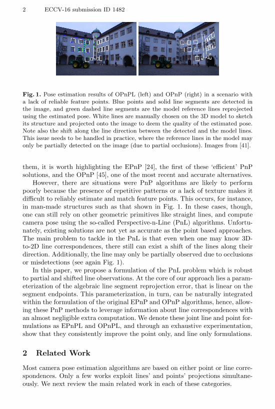
Fig. 1. Pose estimation results of OPnPL (left) and OPnP (right) in a scenario witha lack of reliable feature points. Blue points and solid line segments are detected inthe image, and green dashed line segments are the model reference lines reprojectedusing the estimated pose. White lines are manually chosen on the 3D model to sketchits structure and projected onto the image to deem the quality of the estimated pose.Note also the shift along the line direction between the detected and the model lines.This issue needs to be handled in practice, where the reference lines in the model mayonly be partially detected on the image (due to partial occlusions). Images from [41].
them, it is worth highlighting the EPnP [24], the first of these ‘efficient’ PnPsolutions, and the OPnP [45], one of the most recent and accurate alternatives.
However, there are situations were PnP algorithms are likely to performpoorly because the presence of repetitive patterns or a lack of texture makes itdifficult to reliably estimate and match feature points. This occurs, for instance,in man-made structures such as that shown in Fig. 1. In these cases, though,one can still rely on other geometric primitives like straight lines, and computecamera pose using the so-called Perspective-n-Line (PnL) algorithms. Unfortu-nately, existing solutions are not yet as accurate as the point based approaches.The main problem to tackle in the PnL is that even when one may know 3D-to-2D line correspondences, there still can exist a shift of the lines along theirdirection. Additionally, the line may only be partially observed due to occlusionsor misdetections (see again Fig. 1).
In this paper, we propose a formulation of the PnL problem which is robustto partial and shifted line observations. At the core of our approach lies a param-eterization of the algebraic line segment reprojection error, that is linear on thesegment endpoints. This parameterization, in turn, can be naturally integratedwithin the formulation of the original EPnP and OPnP algorithms, hence, allow-ing these PnP methods to leverage information about line correspondences withan almost negligible extra computation. We denote these joint line and point for-mulations as EPnPL and OPnPL, and through an exhaustive experimentation,show that they consistently improve the point only, and line only formulations.
2 Related Work
Most camera pose estimation algorithms are based on either point or line corre-spondences. Only a few works exploit lines’ and points’ projections simultane-ously. We next review the main related work in each of these categories.
ECCV-16 submission ID 1482 3
Pose from Points (PnP). The most standard approach for pose estimationconsiders 3D-to-2D point correspondences. Early PnP approaches addressed theminimal cases, with solutions for the P3P [6, 12, 14, 21], P4P [4, 11] and n ={4, 5} [42]. These solutions, however, were by construction unable to handlelarger amounts of points, or if they could, they were computationally demanding.Arbitrary number of points can be handled by the Direct Linear Transformation(DLT) [1], which however, estimates the full projection matrix without exploitingthe fact that the internal parameters of the camera are known. This knowledge isshown to improve the pose estimation in more recent PnP approaches focused onbuilding efficient solutions for the overconstrained case [2, 10, 18, 20, 24, 32, 45].Amongst these, the EPnP [24] was the first O(n) solution. Its main idea was torepresent the 3D point coordinates as a linear combination of four control points,which became the only unknowns of the problem, independently of the totalnumber of 3D coordinates. These control points were then retrieved using simplelinearization techniques. This linearization has been subsequently substituted bypolynomial solvers in the Robust PnP (RPnP) [25], the Direct Least SquaresDLS [18], and the Optimal PnP (OPnP) [45], the most accurate of all PnPsolutions. OPnP, draws inspiration on the DLS, but by-passes a degeneracysingularity of the DLS on the rotation by using a quaternion parameterizationthat allows to directly estimate the pose using a Grobner basis solver.
Pose from Lines (PnL). The number of PnL algorithms is considerably smallerthan the point-based ones. Back in the 90’s, closed-form approaches for the mini-mal case with 3 line correspondences were proposed [5, 7], together with theoret-ical studies about the multiple solutions this problem could have [31]. The DLTwas shown to be applicable to line representations in [17], although again, withpoorer results than algorithms that explicitly exploited the knowledge of theinternal parameters of the camera, like [2], also applied to lines. [28] estimatesthe camera rotation matrix by solving a polynomial system of equations usingan eigendecomposition of a so-called multiplication matrix. This method hasbeen recently extended to full pose estimation (rotation+translation) in [33], bycombining Pluecker 3D line parameterization with a DLT-like estimation algo-rithm. [44] combines the former P3L algorithms to compute pose by optimizinga cost function built from line triplets. Finally, [23] shows promising results byformulating the problem in terms of a system of symmetric polynomials.
Pose from Points and Lines (PnPL). There is a very limited numberof approaches that can simultaneously process point and line correspondences.The first of these approaches is the aforementioned DLT, initially used for pointbased pose estimation [1], and later extended to lines [17]. Both formulations canbe integrated into the same framework. [8] also claims a methodology that canpotentially handle points and lines. Unfortunately, this is not theoretically shownneither demonstrated in practice. Finally, there are a few works that tackle thecamera pose estimation from minimal number of points and lines. [35] proposessolutions for the P3L, P2L1P, P1L2P and P3L. And most recently, [22] solvesfor pose and focal length from points, directions and points with directions.
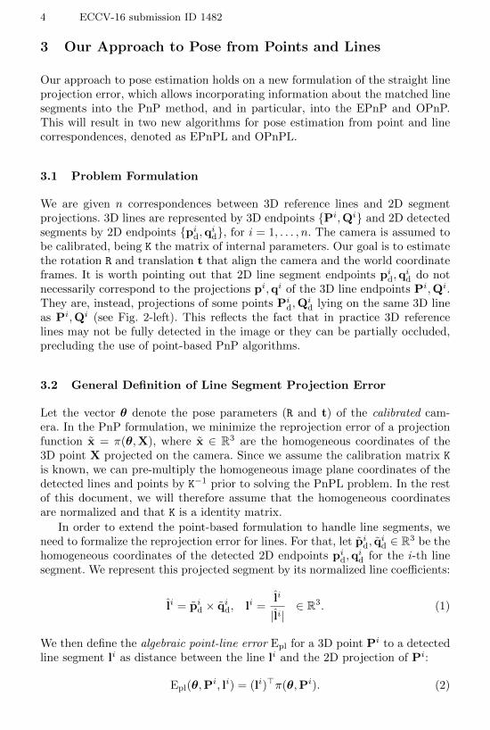
4 ECCV-16 submission ID 1482
3 Our Approach to Pose from Points and Lines
Our approach to pose estimation holds on a new formulation of the straight lineprojection error, which allows incorporating information about the matched linesegments into the PnP method, and in particular, into the EPnP and OPnP.This will result in two new algorithms for pose estimation from point and linecorrespondences, denoted as EPnPL and OPnPL.
3.1 Problem Formulation
We are given n correspondences between 3D reference lines and 2D segmentprojections. 3D lines are represented by 3D endpoints {Pi,Qi} and 2D detectedsegments by 2D endpoints {pid,qid}, for i = 1, . . . , n. The camera is assumed tobe calibrated, being K the matrix of internal parameters. Our goal is to estimatethe rotation R and translation t that align the camera and the world coordinateframes. It is worth pointing out that 2D line segment endpoints pid,q
id do not
necessarily correspond to the projections pi,qi of the 3D line endpoints Pi,Qi.They are, instead, projections of some points Pi
d,Qid lying on the same 3D line
as Pi,Qi (see Fig. 2-left). This reflects the fact that in practice 3D referencelines may not be fully detected in the image or they can be partially occluded,precluding the use of point-based PnP algorithms.
3.2 General Definition of Line Segment Projection Error
Let the vector θ denote the pose parameters (R and t) of the calibrated cam-era. In the PnP formulation, we minimize the reprojection error of a projectionfunction x = π(θ,X), where x ∈ R3 are the homogeneous coordinates of the3D point X projected on the camera. Since we assume the calibration matrix K
is known, we can pre-multiply the homogeneous image plane coordinates of thedetected lines and points by K−1 prior to solving the PnPL problem. In the restof this document, we will therefore assume that the homogeneous coordinatesare normalized and that K is a identity matrix.
In order to extend the point-based formulation to handle line segments, weneed to formalize the reprojection error for lines. For that, let pid, q
id ∈ R3 be the
homogeneous coordinates of the detected 2D endpoints pid,qid for the i-th line
segment. We represent this projected segment by its normalized line coefficients:
li = pid × qid, li =li
|li|∈ R3. (1)
We then define the algebraic point-line error Epl for a 3D point Pi to a detectedline segment li as distance between the line li and the 2D projection of Pi:
Epl(θ,Pi, li) = (li)>π(θ,Pi). (2)

ECCV-16 submission ID 1482 5
P
Pd
Qd p q
pd
l
Camera coordinate system
World coordinate system
!!
pd
qd
p
q
d1
d4 d3
d2
qd
Q
pd
qd
q
d1
d4 d3
d2
p Camera pose, θ
Fig. 2. Left: Notation and problem formulation. Given a set of 3D-to-2D line cor-respondences, we seek to estimate the pose θ that aligns the camera and the worldcoordinate systems. 3D lines are represented by 3D endpoint pairs (P,Q). 2D corre-sponding segments are represented by the detected endpoints (pd,qd) in the imageplane. Note that the 3D-to-2D line correspondence does not imply a correspondence ofthe enpdoints, preventing the use of a standard PnP algorithm. Right: Correction of3D line segments to put in correspondence the projection of the line endpoints (P,Q)with the detected segment endpoints (pd,qd). Top: before correction. Bottom: aftercorrection. Note how the projections (p,q) have been shifted along the line.
We further define the algebraic line segment error El as the sum of squares ofthe two point-line errors for the 3D line segment endpoints:
El(θ,Pi,Qi, li) = E2
pl(θ,Pi, li) + E2
pl(θ,Qi, li). (3)
The overall line segment error Elines for the whole image is the accumulatedalgebraic line segment error over all the matched line segments:
Elines(θ, {Pi}, {Qi}, {li}) =∑i
El(θ,Pi,Qi, li). (4)
Note that this error does not explicitly use the detected line segment endpoints,depending only on the line coefficients li. However, we seek to approximate withit the distance between the detected endpoints and the line projected from themodel onto the image plane. This approximation may incur in gross errors insituations such as the one depicted in Fig.2-top-right. In this scenario, the trueprojected endpoints (p,q) are relatively far from the 2D detected endpoints(pd,qd), and the algebraic point-line errors d1 and d4 are much larger thanthe gold standard errors d2, d3. This leads to preferred minimization of thealgebraic error for line matches where the detected and projected endpoints arefurther away. To handle this problem we considered a two-step approach. We firstestimate the initial camera pose with the given 3D model. We then recompute theposition of the end-points onto the 3D model such that they reduce the distancesbetween the projected and detected endpoints. Using this updated 3D model,

6 ECCV-16 submission ID 1482
we compute the final estimate of the camera pose. Fig.2-bottom-right shows howthe ground truth projected end-points have changed their position after havingupdated the 3D model. We next describe in more detail this correction process.
3.3 Putting 3D and 2D Line Endpoints in Correspondence
Let’s consider d be the length of the detected line segment and the notationdetailed in Fig. 2-right. After the first iteration of the complete PnPL algorithm(see Sections 3.4 and 3.5) we obtain an initial estimate of the camera pose. Wethen shift the endpoints of every line segment in the camera coordinate frame sothat the length of the projected line segment matches the length of the detectedsegments, and the sum of distances between corresponding endpoints is minimal.
More specifically, given an estimate for the pose R, t, we compute p,q andthe unit line direction vector v along the projected line l. We then shift theposition of p and q along this line, such that they become as close as possiblefrom pd,qd, and separated by a distance d. This can be expressed with thefollowing two equations, function of a shifting parameter γ:
pd = p + γv qd = p + (γ + d)v (5)
which yields that γ = v>(
12 (pd + qd)− p
)− d
2 . Given γ we can then take theright hand side of (5) as the new projections of p,q, and backproject the positionof the new endpoints P,Q in the camera and world coordinate frames.
To backproject a point from the image plane to a 3D line, we compute theintersection of the line of sight of the point with the 3D line as follows:
λx = αX + βD, (6)
where x are the point’s projection homogeneous coordinates, X is the 3D pointbelonging to the line and D is the 3D line direction. Both X and D are ex-pressed w.r.t. the camera coordinate frame. From this equation we see thats = [−λ, α, β]> is orthogonal to the vectors [X(j), D(j), −x(j)]>, j = 1, 2,where X(j) corresponds to the j-th component of the vector X. We employ thecross product operation to solve for s and then compute the 3D point positionas X + β
αD. This procedure turns to be very fast.
3.4 EPnPL
We next describe a necessary modification to the EPnP algorithm to simultane-ously consider np point and nl line correspondences.
In the EPnP [24] the projection of a point on the camera plane is written as
πEPnP(θ,P) = K
4∑j=1
αjCcj , (7)
where αj are point-specific coefficients computed from the model and Ccj for
j = 1, . . . , 4 are the unknown control point coordinates in the camera frame.

ECCV-16 submission ID 1482 7
Recall that we are considering normalized homogeneous coordinates, and hencewe can set the calibration matrix K to be the identity matrix. We define ourvector of unknowns as µ = [C>1 , C>2 , C>3 , C>4 ]> and then obtain, using (2), anexpression for the algebraic point-line error in case of EPnP:
Epl, EPnP(θ,Pi, li) =
4∑j=1
αj(li)>Cc
j = (mil(P
i))>µ, (8)
for mil(P
i) = ([α1, α2, α3, α4]⊗ li)>. The overall error in Eq. 4 then becomes
Elines(θ, {Pi}, {Qi}, {li}) =∑i
((mi
l(Pi))>µ
)2+((mi
l(Qi))>µ
)2. (9)
Finally, considering both point and lines correspondences, the function to beminimized by the EPnPL will be
arg minµ
{‖Mpµ‖2 + Elines(θ, {Pi}, {Qi}, {li})
}= arg min
µ
{‖Mµ‖2
}(10)
where M = [M>p , M>l ]> ∈ R2(np+nl)×12, Mp ∈ R2np×12 is the matrix of parameters
for the np point correspondences, as in [24], and Ml ∈ R2nl×12 is the matrix cor-responding to the point-line errors of the nl matched line segments. Equation 10is finally minimized by following the EPnP methodology.
3.5 OPnPL
In OPnP [45], the camera parameters are represented as R = 1λR, t = 1
λt, where
λ is an average point depth in the camera frame. To deal with points and lineswe define λ as the average depth of the points and line segments’ endpoints.Similarly, we compute the mean point Q, which can be used to write the thirdcomponent of t:
t3 = 1− r>3 Q, (11)
where r3 is the third row of R. The projection of a 3D point X onto the imageplane (assuming the calibration matrix K to be the identity) will be:
πOPnP(θ,X) = RX + t. (12)
As we did for the EPnP, we use this projection into Eq. 2 to compute thealgebraic point-line error.
Following [45], we can use Eq. 11 for t3 to compute the algebraic error for allpoints Epoints as a function of R, t1, t2:
Epoints(r, t) = ‖Gpr + Hpt12 + kp‖2 , (13)
where r is a vectorized form of R, t12 = [t1 t2]>, Gp ∈ R2np×9 and Hp ∈ R2np×2
are matrices built from the projections and 3D model coordinates of the np
points, and kp is a 2np constant vector.

8 ECCV-16 submission ID 1482
The overall line segment error Elines as defined in Eq. 4 can be expressedin the same form as in Eq. 13 with Gl, Hl, kl instead of Gp, Hp, kp, and usingalgebraic line segment error (3) with (12) as point-line projection function.
In order to compute the pose, we adapt the cost function of [45] to thefollowing one with both points and lines terms:
Etot(ρ, t) = Epoints(r(ρ), t) + Elines(r(ρ), t) , (14)
where we parameterize r with non-unit quaternions vector ρ = [a, b, c, d]>. Wenext seek to minimize this function w.r.t. the pose parameters.
Setting the derivative of Etot w.r.t. t to zero, and denoting Gtot = [G>p , G>l ]>,
Htot = [H>p , H>l ]>, ktot = [k>p , k>l ]> we can write t as a function of r:
H>tot(Gtotr + Htott + ktot) = 0 =⇒ t = Pr + u, (15)
for P = −(H>totHtot)−1(H>totGtot), u = −(H>totHtot)
−1H>totktot.The derivative of Etot w.r.t. the first quaternion parameter a is:
∂r
∂aG>tot(Gtotr + Htott + ktot) =
∂r
∂aG>tot
((Gtot + HtotP)r + Htotu + ktot
)= 0 , (16)
where in the second step we have used Eq. 15. Three more equations analogousto (16) constitute a system which the original OPnP uses to design a specificpolynomial solver [45]. In our case we can use exactly the same solver, as theequations we get for joint point and line matches, have exactly the same formas when only considering points.
4 Experiments
We evaluate the proposed approach in “points and lines” and “only lines” situa-tions, nonplanar and planar configurations, and synthetic and real experiments.
4.1 Synthetic Experiments
We will compare our approach against state-of-the-art in two situations: A jointpoint-and-line case, and a line-only case. In both scenarios we will consider non-planar and planar configurations, and will report rotation and translation errorsfor increasing amounts of 2D noise and number of correspondences. We will alsostudy the influence of the amount of shift between the lines in the 3D model,and the observed segments projected on the image.
In the synthetic experiments we assume a virtual 640× 480 pixels calibratedcamera with focal length of 500. We randomly generate np + 2nl 3D points ina box with coordinates [−2, 2] × [−2, 2] × [4, 8] in the camera frame, where np
and nl are the number of points and line segments, respectively. We then builda random rotation matrix; the translation vector is taken to be the mean vectorof all the points, as done in [45]. From the last 2nl generated points, we form nl
ECCV-16 submission ID 1482 9
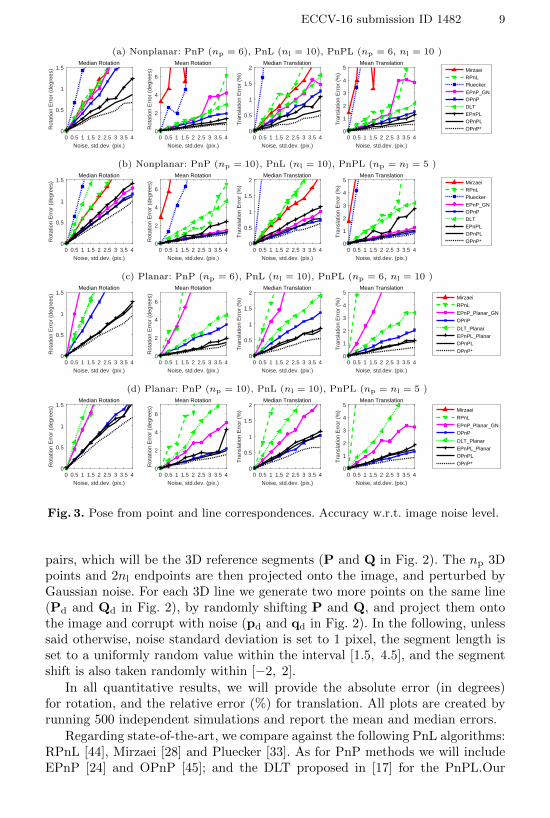
(a) Nonplanar: PnP (np = 6), PnL (nl = 10), PnPL (np = 6, nl = 10 )
0 0.5 1 1.5 2 2.5 3 3.5 4Noise, std.dev. (pix.)
0
0.5
1
1.5
Rot
atio
n E
rror
(de
gree
s)
Median Rotation
0 0.5 1 1.5 2 2.5 3 3.5 4Noise, std.dev. (pix.)
0
2
4
6
Rot
atio
n E
rror
(de
gree
s)
Mean Rotation
0 0.5 1 1.5 2 2.5 3 3.5 4Noise, std.dev. (pix.)
0
0.5
1
1.5
2
Tra
nsla
tion
Err
or (
%)
Median Translation
0 0.5 1 1.5 2 2.5 3 3.5 4Noise, std.dev. (pix.)
0
1
2
3
4
5
Tra
nsla
tion
Err
or (
%)
Mean TranslationMirzaeiRPnLPluecker
EPnP_GNOPnPDLTEPnPLOPnPLOPnP*
(b) Nonplanar: PnP (np = 10), PnL (nl = 10), PnPL (np = nl = 5 )
0 0.5 1 1.5 2 2.5 3 3.5 4Noise, std.dev. (pix.)
0
0.5
1
1.5
Rot
atio
n E
rror
(de
gree
s)
Median Rotation
0 0.5 1 1.5 2 2.5 3 3.5 4Noise, std.dev. (pix.)
0
2
4
6
Rot
atio
n E
rror
(de
gree
s)
Mean Rotation
0 0.5 1 1.5 2 2.5 3 3.5 4Noise, std.dev. (pix.)
0
0.5
1
1.5
2
Tra
nsla
tion
Err
or (
%)
Median Translation
0 0.5 1 1.5 2 2.5 3 3.5 4Noise, std.dev. (pix.)
0
1
2
3
4
5
Tra
nsla
tion
Err
or (
%)
Mean TranslationMirzaeiRPnLPluecker
EPnP_GNOPnPDLTEPnPLOPnPLOPnP*
(c) Planar: PnP (np = 6), PnL (nl = 10), PnPL (np = 6, nl = 10 )
0 0.5 1 1.5 2 2.5 3 3.5 4Noise, std.dev. (pix.)
0
0.5
1
1.5
Rot
atio
n E
rror
(de
gree
s)
Median Rotation
0 0.5 1 1.5 2 2.5 3 3.5 4Noise, std.dev. (pix.)
0
2
4
6
Rot
atio
n E
rror
(de
gree
s)
Mean Rotation
0 0.5 1 1.5 2 2.5 3 3.5 4Noise, std.dev. (pix.)
0
0.5
1
1.5
2
Tra
nsla
tion
Err
or (
%)
Median Translation
0 0.5 1 1.5 2 2.5 3 3.5 4Noise, std.dev. (pix.)
0
1
2
3
4
5
Tra
nsla
tion
Err
or (
%)
Mean Translation
Mirzaei
RPnL
EPnP_Planar_GNOPnP
DLT_Planar
EPnPL_PlanarOPnPL
OPnP*
(d) Planar: PnP (np = 10), PnL (nl = 10), PnPL (np = nl = 5 )
0 0.5 1 1.5 2 2.5 3 3.5 4Noise, std.dev. (pix.)
0
0.5
1
1.5
Rot
atio
n E
rror
(de
gree
s)
Median Rotation
0 0.5 1 1.5 2 2.5 3 3.5 4Noise, std.dev. (pix.)
0
2
4
6
Rot
atio
n E
rror
(de
gree
s)
Mean Rotation
0 0.5 1 1.5 2 2.5 3 3.5 4Noise, std.dev. (pix.)
0
0.5
1
1.5
2
Tra
nsla
tion
Err
or (
%)
Median Translation
0 0.5 1 1.5 2 2.5 3 3.5 4Noise, std.dev. (pix.)
0
1
2
3
4
5
Tra
nsla
tion
Err
or (
%)
Mean Translation
Mirzaei
RPnL
EPnP_Planar_GNOPnP
DLT_Planar
EPnPL_PlanarOPnPL
OPnP*
Fig. 3. Pose from point and line correspondences. Accuracy w.r.t. image noise level.
pairs, which will be the 3D reference segments (P and Q in Fig. 2). The np 3Dpoints and 2nl endpoints are then projected onto the image, and perturbed byGaussian noise. For each 3D line we generate two more points on the same line(Pd and Qd in Fig. 2), by randomly shifting P and Q, and project them ontothe image and corrupt with noise (pd and qd in Fig. 2). In the following, unlesssaid otherwise, noise standard deviation is set to 1 pixel, the segment length isset to a uniformly random value within the interval [1.5, 4.5], and the segmentshift is also taken randomly within [−2, 2].
In all quantitative results, we will provide the absolute error (in degrees)for rotation, and the relative error (%) for translation. All plots are created byrunning 500 independent simulations and report the mean and median errors.
Regarding state-of-the-art, we compare against the following PnL algorithms:RPnL [44], Mirzaei [28] and Pluecker [33]. As for PnP methods we will includeEPnP [24] and OPnP [45]; and the DLT proposed in [17] for the PnPL.Our

10 ECCV-16 submission ID 1482
(a) Nonplanar: PnP (np), PnL(nl), PnPL (np, nl)
6 7 8 9 10 11 12 13 14 15n
p, n
l
0
0.5
1
Rot
atio
n E
rror
(de
gree
s)
Median Rotation
6 7 8 9 10 11 12 13 14 15n
p, n
l
0
0.5
1
Rot
atio
n E
rror
(de
gree
s)
Mean Rotation
6 7 8 9 10 11 12 13 14 15n
p, n
l
0
0.5
1
1.5
Tra
nsla
tion
Err
or (
%)
Median Translation
6 7 8 9 10 11 12 13 14 15n
p, n
l
0
0.5
1
1.5
2
Tra
nsla
tion
Err
or (
%)
Mean TranslationMirzaeiRPnLPluecker
EPnP_GNOPnPDLTEPnPLOPnPLOPnP*
(b) Nonplanar: PnP (np), PnL (nl), PnPL (n′p = n′
l = 0.5np = 0.5nl )
6 7 8 9 10 11 12 13 14 15n
p,n
l
0
0.5
1
1.5
Rot
atio
n E
rror
(de
gree
s)
Median Rotation
6 7 8 9 10 11 12 13 14 15n
p,n
l
0
2
4
6
Rot
atio
n E
rror
(de
gree
s)
Mean Rotation
6 7 8 9 10 11 12 13 14 15n
p,n
l
0
0.5
1
1.5
2
Tra
nsla
tion
Err
or (
%)
Median Translation
6 7 8 9 10 11 12 13 14 15n
p,n
l
0
1
2
3
4
5
Tra
nsla
tion
Err
or (
%)
Mean TranslationMirzaeiRPnLPluecker
EPnP_GNOPnPDLTEPnPLOPnPLOPnP*
(c) Planar: PnP (np), PnL(nl), PnPL (np, nl)
6 7 8 9 10 11 12 13 14 15n
p, n
l
0
0.5
1
1.5
Rot
atio
n E
rror
(de
gree
s)
Median Rotation
6 7 8 9 10 11 12 13 14 15n
p, n
l
0
2
4
6
Rot
atio
n E
rror
(de
gree
s)
Mean Rotation
6 7 8 9 10 11 12 13 14 15n
p, n
l
0
0.5
1
1.5
2
Tra
nsla
tion
Err
or (
%)
Median Translation
6 7 8 9 10 11 12 13 14 15n
p, n
l
0
1
2
3
4
5
Tra
nsla
tion
Err
or (
%)
Mean Translation
Mirzaei
RPnL
EPnP_Planar_GNOPnP
DLT_Planar
EPnPL_PlanarOPnPL
OPnP*
(d) Planar: PnP (np), PnL (nl), PnPL (n′p = n′
l = 0.5np = 0.5nl )
7 9 11 13 15n
p,n
l
0
0.5
1
1.5
Rot
atio
n E
rror
(de
gree
s)
Median Rotation
7 9 11 13 15n
p,n
l
0
2
4
6
Rot
atio
n E
rror
(de
gree
s)
Mean Rotation
7 9 11 13 15n
p,n
l
0
0.5
1
1.5
2
Tra
nsla
tion
Err
or (
%)
Median Translation
7 9 11 13 15n
p,n
l
0
1
2
3
4
5
Tra
nsla
tion
Err
or (
%)
Mean Translation
Mirzaei
RPnL
EPnP_Planar_GNOPnP
DLT_Planar
EPnPL_PlanarOPnPL
OPnP*
Fig. 4. Pose from point and line correspondences. Accuracy w.r.t. increasing numberof point or line correspondences.
two approaches will be denoted as EPnPL and OPnPL. Additionally, we willalso consider the OPnP*, which will take as input both point and line corre-spondences. However, for the lines we will consider the true correspondences{Pi,Qi} ↔ {pi,qi} instead of the correspondences {Pi,Qi} ↔ {pid,qid} (seeagain Fig. 2), that feed our two approaches and the rest of algorithms. Note thatthis is an unrealistic situation, and OPnP* has to be interpreted as a baselineindicating the best performance one could expect.
Pose from points and lines. We consider point and line correspondencesfor two configurations, non-planar and planar. We evaluate the accuracy of theapproaches w.r.t. the image noise in Fig. 3, and w.r.t. an increasing number ofcorrespondences (either points, lines or points and lines) in Fig. 4. To ensurefairness between PnP, PnL and PnPL algorithms we analyze two situations:

ECCV-16 submission ID 1482 11
(a) Nonplanar: PnL (nl = 10), PnPL (np = 0, nl = 10 )
0 0.5 1 1.5 2 2.5 3 3.5 4Noise, std.dev. (pix.)
0
0.5
1
1.5
Rot
atio
n E
rror
(de
gree
s)
Median Rotation
0 0.5 1 1.5 2 2.5 3 3.5 4Noise, std.dev. (pix.)
0
2
4
6
Rot
atio
n E
rror
(de
gree
s)
Mean Rotation
0 0.5 1 1.5 2 2.5 3 3.5 4Noise, std.dev. (pix.)
0
0.5
1
1.5
2
Tra
nsla
tion
Err
or (
%)
Median Translation
0 0.5 1 1.5 2 2.5 3 3.5 4Noise, std.dev. (pix.)
0
1
2
3
4
5
Tra
nsla
tion
Err
or (
%)
Mean Translation
Mirzaei
RPnL
Pluecker
DLT
EPnPL
OPnPL
OPnP*
(b) Planar: PnL (nl = 10), PnPL (np = 0, nl = 10 )
0 0.5 1 1.5 2 2.5 3 3.5 4Noise, std.dev. (pix.)
0
0.5
1
1.5
2
Rot
atio
n E
rror
(de
gree
s)
Median Rotation
0 0.5 1 1.5 2 2.5 3 3.5 4Noise, std.dev. (pix.)
0
5
10
Rot
atio
n E
rror
(de
gree
s)
Mean Rotation
0 0.5 1 1.5 2 2.5 3 3.5 4Noise, std.dev. (pix.)
0
0.5
1
1.5
2
2.5
Tra
nsla
tion
Err
or (
%)
Median Translation
0 0.5 1 1.5 2 2.5 3 3.5 4Noise, std.dev. (pix.)
0
5
10
Tra
nsla
tion
Err
or (
%)
Mean Translation
Mirzaei
RPnL
DLT_Planar
EPnPL_Planar
OPnPL
OPnP*
Fig. 5. Pose from only line correspondences. Accuracy w.r.t. image noise level.
(a) Different number of constraints. When evaluating accuracy w.r.t. image noisewe consider np = 6 point correspondences for the PnP algorithms (minimumnumber required by EPnP), nl = 10 correspondences for the PnL (minimumnumber for Pluecker [33]) and the PnPL methods use np = 6 point plus nl = 10line correspondences. The results for the non-planar and planar configurationsare shown in Fig. 3-(a) and (c), respectively. As expected, the EPnPL and OP-nPL methods are more accurate than the point only versions, because theyare using additional information. Indeed, OPnPL is very close from the OPnP*baseline, indicating that line information is very well exploited. Additionally,our approaches work remarkably better than DLT (the other PnPL solution)and the rest of PnL methods. In Fig. 4-(a) and (c) we observe that the methods’accuracy w.r.t. an increasing number of points also shows that our approachesexhibit the best performances.
(b) Constant number of constraints. We also provide results of accuracy w.r.t.noise in which we limit the total number of constraints, either obtained fromline or point correspondences, to a constant value (np = 10 for PnP methods,nl = 10 for PnL methods and np = 5, nl = 5 for PnPL methods). Note that PnPalgorithms will be in this case in a clear advantage, as we are feeding them withpoint correspondences just perturbed by noise. PnL and PnPL algorithms needto deal with weaker line correspondences which besides noisy, are less spatiallyconstrained. Results in Fig. 3-(b) and (d) confirm this. EPnP and OPnP havelargely improved their performance compared to the previous scenario, but whatis very remarkable is that OPnPL is almost as good as its point-only versionOPnP. EPnPL is more clearly behind EPnP. In any event, our solutions againperform much better than DLT and the PnL algorithms. Similar performancepatterns can be observed in Fig. 4-(b) and (d) when evaluating the accuracyw.r.t. number of constraints in the non-planar case. For the planar case, our twosolutions clearly outperform all other approaches, specially in rotation error.

12 ECCV-16 submission ID 1482
80 200 320 440 560 n
p+n
l
0
0.02
0.04
0.06
0.08A
vera
ge R
untim
e (s
ec)
Time
20 220 420 620n
p+n
l
0
0.005
0.01
0.015
0.02
Tim
e, s
.
Mean processing time
20 220 420 620n
p+n
l
0
0.01
0.02
0.03
0.04
Tim
e, s
.
Mean solving time
MirzaeiRPnLPlueckerEPnP_GNOPnPDLTEPnPLOPnPL
Fig. 6. Running times for increasing number of correspondences. Left: All methods.Center: Phases of our approaches. ‘Processing’ (center-left) includes the calculation of2D line equations and the line correction from Sec. 3.3. ‘Solving’ (center-right) refersto the actual time taken to compute the pose as described in Sect. 3.4 and 3.5.
Pose from lines only. In this experiment we just compare the line-based ap-proaches, i.e, the PnL and PnPL methods (but only fed with line correspon-dences). We consider nl = 10. In Fig. 5-(a) and (b) we show the pose accuracyat increasing levels of noise, for the nonplanar and planar case. EPnPL and OP-nPL perform consistently better than all other approaches, specially OPnPL.We also observed that PnL methods are very unstable under planar configura-tions and, in particular, Pluecker [33] did not manage to work and Mirzaei [28]yielded a very large error (out of bounds in the graphs).
Scalability. We evaluate the runtime of the methods for an increasing numberof point and line correspondences. For the PnL and PnP methods we used np andnl correspondences, respectively, with np = nl. The PnPL methods receive twicethe number of correspondences, i.e, np+nl. Fig. 6-left shows the results, where allmethods are implemented in MATLAB. As expected, the runtime of OPnPL andEPnPL is about twice the runtime of their point-only counterparts, confirmingthey are still O(n) algorithms. This linear time is maintained even having toexecute the correction scheme of the line segments described in Sect. 3.3. For thisto happen, our implementations exploit efficient vectorized operations. Fig. 6-right reports the time taken by our approach at different phases.
Shift of line segments. As discussed above, to simulate real situations in whicha 3D reference line on the model may only be partially projected onto the inputimage, we enforce the detected lines to be shifted versions of the true projectedlines. In this experiment, we evaluate the robustness of the PnL and PnPLalgorithms to this shift, which is controlled by means of a parameter k ∈ [0, 1].k = 0 would correspond to a non-shift, i.e., {pi,qi} = {pid,qid}. k = 1 wouldcorrespond to a shift of 3 units between the true projected and the detected lineendpoints. Additionally, we consider another baseline, the OPnP naive, wherewe feed the OPnP algorithm with the correspondences {Pi,Qi} ↔ {pid,qid}. Theresults are shown in Fig. 7. Note that PnL methods and DLT are insensitive tothe amount of shift (Mirzaei [28] occasionally fails, but this is independent onthe amount of shift). This was expected, as these algorithms only consider theline directions in the image plane, and not the particular position of the lines.Our EPnPL and OPnPL approaches could be more sensitive, as we explicitly use

ECCV-16 submission ID 1482 13
0.1 0.3 0.5 0.7 0.9 Segment shift coeff.
0
0.5
1
1.5R
otat
ion
Err
or (
degr
ees)
Median Rotation
0.1 0.3 0.5 0.7 0.9 Segment shift coeff.
0
2
4
6
Rot
atio
n E
rror
(de
gree
s)
Mean Rotation
0.1 0.3 0.5 0.7 0.9 Segment shift coeff.
0
0.5
1
1.5
2
Tra
nsla
tion
Err
or (
%)
Median Translation
0.1 0.3 0.5 0.7 0.9 Segment shift coeff.
0
1
2
3
4
5
Tra
nsla
tion
Err
or (
%)
Mean Translation
Mirzaei
RPnL
Pluecker
DLT
OPnP_naiveEPnPL
OPnPL
OPnP*
Fig. 7. Robustness to the amount of shift between the 3D reference lines and theprojected ones. See text for details.
the position of the line in the image plane. However, the correction step we usein Sect. 3.3 gets rid of this problem. As expected OPnP naive fails completely.
4.2 Real Images
We also evaluated our approach on real images of the NYU2 [39] and EPFLCastle-P19 [41] datasets. These are datasets with structured objects (indoor andman-made scenarios) and with a large amount of straight lines and repetitivepatterns that will benefit of a joint point and line based approach. For theseexperiments we will only evaluate the point based OPnP and the OPnPL, eitherusing only lines or lines with points.
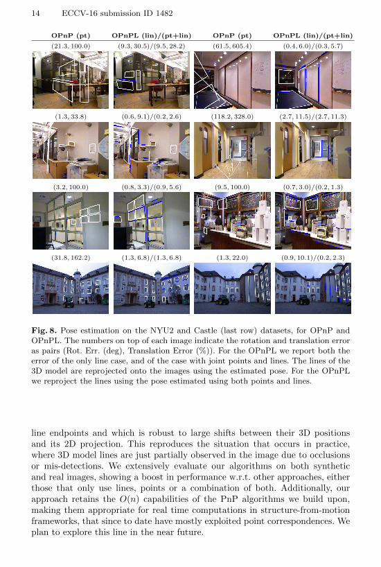
We implemented a standard structure from motion pipeline on triplets ofimages for building the 3D models. Details are provided in the supplementalmaterial. One of the images of the triplet is then taken to be the reference andanother the test image. SIFT feature points are detected in both images andline features are detected and represented using the recent scale invariant linedescriptor [43], shown to be adequate for wide baseline matching. The test imageis matched against the model, using RANSAC with P3P for the point-only case;and using RANSAC with OPnPL for a combination of four points or lines (4lines, 3 lines/1 point, etc.) The final pose is computed using the points withinthe concensus for the OPnP. For the OPnPL we consider the concensus made ofboth points and lines and the concensus made of only lines.
Figure 8 reports sample images of both datasets, including both quantita-tive and qualitative results. As can be seen, these type of scenarios (repetitivepatterns in the castle, many straight and planar surfaces, low textured areas),are situations in which the point-based approaches are prone to fail, and wherelines and lines+points methods perform more robustly.
5 Conclusion
In this paper we have proposed an approach to integrate 3D-to-2D line correspon-dences within the formulation of two state-of-the-art PnP algorithms, allowingthem to indistinctly treat points, lines or a combination of them. In order todo so, we introduce an algebraic line error that is formulated in terms of the
14 ECCV-16 submission ID 1482
OPnP (pt) OPnPL (lin)/(pt+lin) OPnP (pt) OPnPL (lin)/(pt+lin)
(21.3, 100.0) (9.3, 30.5)/(9.5, 28.2) (61.5, 605.4) (0.4, 6.0)/(0.3, 5.7)
(1.3, 33.8) (0.6, 9.1)/(0.2, 2.6) (118.2, 328.0) (2.7, 11.5)/(2.7, 11.3)
(3.2, 100.0) (0.8, 3.3)/(0.9, 5.6) (9.5, 100.0) (0.7, 3.0)/(0.2, 1.3)
(31.8, 162.2) (1.3, 6.8)/(1.3, 6.8) (1.3, 22.0) (0.9, 10.1)/(0.2, 2.3)
Fig. 8. Pose estimation on the NYU2 and Castle (last row) datasets, for OPnP andOPnPL. The numbers on top of each image indicate the rotation and translation erroras pairs (Rot. Err. (deg), Translation Error (%)). For the OPnPL we report both theerror of the only line case, and of the case with joint points and lines. The lines of the3D model are reprojected onto the images using the estimated pose. For the OPnPLwe reproject the lines using the pose estimated using both points and lines.
line endpoints and which is robust to large shifts between their 3D positionsand its 2D projection. This reproduces the situation that occurs in practice,where 3D model lines are just partially observed in the image due to occlusionsor mis-detections. We extensively evaluate our algorithms on both syntheticand real images, showing a boost in performance w.r.t. other approaches, eitherthose that only use lines, points or a combination of both. Additionally, ourapproach retains the O(n) capabilities of the PnP algorithms we build upon,making them appropriate for real time computations in structure-from-motionframeworks, that since to date have mostly exploited point correspondences. Weplan to explore this line in the near future.
ECCV-16 submission ID 1482 15
References
1. Abdel-Aziz, Y.: Direct linear transformation from comparator coordinates in close-range photogrammetry. In: ASP Symposium on Close-Range Photogrammetry inIllinois, 1971 (1971)
2. Ansar, A., Daniilidis, K.: Linear pose estimation from points or lines. PatternAnalysis and Machine Intelligence, IEEE Transactions on 25(5), 578–589 (2003)
3. Bay, H., Tuytelaars, T., Van Gool, L.: Surf: Speeded up robust features. In: Com-puter vision–ECCV 2006, pp. 404–417. Springer (2006)
4. Bujnak, M., Kukelova, Z., Pajdla, T.: A general solution to the p4p problem forcamera with unknown focal length. In: Computer Vision and Pattern Recognition,2008. CVPR 2008. IEEE Conference on. pp. 1–8. IEEE (2008)
5. Chen, H.H.: Pose determination from line-to-plane correspondences: existence con-dition and closed-form solutions. In: Computer Vision, 1990. Proceedings, ThirdInternational Conference on. pp. 374–378. IEEE (1990)
6. DeMenthon, D., Davis, L.S.: Exact and approximate solutions of the perspective-three-point problem. IEEE Transactions on Pattern Analysis & Machine Intelli-gence (11), 1100–1105 (1992)
7. Dhome, M., Richetin, M., Lapreste, J.T., Rives, G.: Determination of the atti-tude of 3d objects from a single perspective view. Pattern Analysis and MachineIntelligence, IEEE Transactions on 11(12), 1265–1278 (1989)
8. Ess, A., Neubeck, A., Van Gool, L.J.: Generalised linear pose estimation. In:BMVC. pp. 1–10 (2007)
9. Ferraz, L., Binefa, X., Moreno-Noguer, F.: Very fast solution to the pnp problemwith algebraic outlier rejection. In: Proceedings of the Conference on ComputerVision and Pattern Recognition (CVPR). pp. 501–508 (2014)
10. Fiore, P.D.: Efficient linear solution of exterior orientation. IEEE Transactions onPattern Analysis & Machine Intelligence (2), 140–148 (2001)
11. Fischler, M.A., Bolles, R.C.: Random sample consensus: a paradigm for modelfitting with applications to image analysis and automated cartography. Communi-cations of the ACM 24(6), 381–395 (1981)
12. Gao, X.S., Hou, X.R., Tang, J., Cheng, H.F.: Complete solution classification forthe perspective-three-point problem. Pattern Analysis and Machine Intelligence,IEEE Transactions on 25(8), 930–943 (2003)
13. Garro, V., Crosilla, F., Fusiello, A.: Solving the pnp problem with anisotropicorthogonal procrustes analysis. In: 2012 Second International Conference on 3DImaging, Modeling, Processing, Visualization & Transmission. pp. 262–269. IEEE(2012)
14. Grunert, J.A.: Das pothenotische problem in erweiterter gestalt nebst u ber seineanwendungen in geoda sie. In: Grunerts Archiv fu r Mathematik und Physik (1841)
15. Haralick, R.M., Lee, C.n., Ottenburg, K., Nolle, M.: Analysis and solutions of thethree point perspective pose estimation problem. In: Computer Vision and PatternRecognition, 1991. Proceedings CVPR’91., IEEE Computer Society Conference on.pp. 592–598. IEEE (1991)
16. Harris, C., Stephens, M.: A combined corner and edge detector. In: Alvey visionconference. vol. 15, p. 50. Citeseer (1988)
17. Hartley, R., Zisserman, A.: Multiple view geometry in computer vision. Cambridgeuniversity press (2003)
18. Hesch, J.A., Roumeliotis, S.I.: A direct least-squares (dls) method for pnp. In:Computer Vision (ICCV), 2011 IEEE International Conference on. pp. 383–390.IEEE (2011)
16 ECCV-16 submission ID 1482
19. Horaud, R., Conio, B., Leboulleux, O., Lacolle, L.B.: An analytic solution for theperspective 4-point problem. In: Computer Vision and Pattern Recognition, 1989.Proceedings CVPR’89., IEEE Computer Society Conference on. pp. 500–507. IEEE(1989)
20. Kneip, L., Li, H., Seo, Y.: Upnp: An optimal o (n) solution to the absolute poseproblem with universal applicability. In: Computer Vision–ECCV 2014, pp. 127–142. Springer (2014)
21. Kneip, L., Scaramuzza, D., Siegwart, R.: A novel parametrization of theperspective-three-point problem for a direct computation of absolute camera posi-tion and orientation. In: Computer Vision and Pattern Recognition (CVPR), 2011IEEE Conference on. pp. 2969–2976. IEEE (2011)
22. Kuang, Y., Astrom, K.: Pose estimation with unknown focal length using points,directions and lines. In: Proceedings of the IEEE International Conference on Com-puter Vision. pp. 529–536 (2013)
23. Kuang, Y., Zheng, Y., Astrom, K.: Partial symmetry in polynomial systems andits applications in computer vision. In: Proceedings of the IEEE Conference onComputer Vision and Pattern Recognition. pp. 438–445 (2014)
24. Lepetit, V., Moreno-Noguer, F., Fua, P.: Epnp: An accurate o(n) solution to thepnp problem. International Journal of Computer Vision 81(2), 155–166 (2009)
25. Li, S., Xu, C., Xie, M.: A robust o (n) solution to the perspective-n-point problem.Pattern Analysis and Machine Intelligence, IEEE Transactions on 34(7), 1444–1450(2012)
26. Lowe, D.G.: Distinctive image features from scale-invariant keypoints. Interna-tional journal of computer vision 60(2), 91–110 (2004)
27. Lu, C.P., Hager, G.D., Mjolsness, E.: Fast and globally convergent pose estimationfrom video images. Pattern Analysis and Machine Intelligence, IEEE Transactionson 22(6), 610–622 (2000)
28. Mirzaei, F.M., Roumeliotis, S., et al.: Globally optimal pose estimation from linecorrespondences. In: Robotics and Automation (ICRA), 2011 IEEE InternationalConference on. pp. 5581–5588. IEEE (2011)
29. Moreno-Noguer, F.: Deformation and illumination invariant feature point descrip-tor. In: Computer Vision and Pattern Recognition (CVPR), 2011 IEEE Conferenceon. pp. 1593–1600. IEEE (2011)
30. Nakano, G.: Globally optimal dls method for pnp problem with cayley param-eterization. In: British Machine Vision Conference 2015, Proceedings of. BMVA(2015)
31. Navab, N., Faugeras, O.: Monocular pose determination from lines: Critical setsand maximum number of solutions. In: Computer Vision and Pattern Recognition,1993. Proceedings CVPR’93., 1993 IEEE Computer Society Conference on. pp.254–260. IEEE (1993)
32. Penate-Sanchez, A., Andrade-Cetto, J., Moreno-Noguer, F.: Exhaustive lineariza-tion for robust camera pose and focal length estimation. IEEE Transactions onPattern Analysis & Machine Intelligence (10), 2387–2400 (2013)
33. Pribyl, B., Zemck, P., et al.: Camera pose estimation from lines using plcker coor-dinates. In: British Machine Vision Conference 2015, Proceedings of. BMVA (2015)
34. Quan, L., Lan, Z.: Linear n-point camera pose determination. Pattern Analysisand Machine Intelligence, IEEE Transactions on 21(8), 774–780 (1999)
35. Ramalingam, S., Bouaziz, S., Sturm, P.: Pose estimation using both points andlines for geo-localization. In: Robotics and Automation (ICRA), 2011 IEEE Inter-national Conference on. pp. 4716–4723. IEEE (2011)

ECCV-16 submission ID 1482 17
36. Rosten, E., Drummond, T.: Machine learning for high-speed corner detection. In:Computer Vision–ECCV 2006, pp. 430–443. Springer (2006)
37. Rublee, E., Rabaud, V., Konolige, K., Bradski, G.: Orb: an efficient alternative tosift or surf. In: Computer Vision (ICCV), 2011 IEEE International Conference on.pp. 2564–2571. IEEE (2011)
38. Schweighofer, G., Pinz, A.: Globally optimal o (n) solution to the pnp problem forgeneral camera models. In: BMVC. pp. 1–10 (2008)
39. Silberman, N., Hoiem, D., Kohli, P., Fergus, R.: Indoor segmentation and sup-port inference from rgbd images. In: Computer Vision–ECCV 2012, pp. 746–760.Springer (2012)
40. Simo-Serra, E., Trulls, E., Ferraz, L., Kokkinos, I., Fua, P., Moreno-Noguer, F.:Discriminative learning of deep convolutional feature point descriptors. In: Pro-ceedings of the International Conference on Computer Vision (ICCV) (2015)
41. Strecha, C., von Hansen, W., Gool, L.V., Fua, P., Thoennessen, U.: On bench-marking camera calibration and multi-view stereo for high resolution imagery. In:Computer Vision and Pattern Recognition, 2008. CVPR 2008. IEEE Conferenceon. pp. 1–8. IEEE (2008)
42. Triggs, B.: Camera pose and calibration from 4 or 5 known 3d points. In: ComputerVision, 1999. The Proceedings of the Seventh IEEE International Conference on.vol. 1, pp. 278–284. IEEE (1999)
43. Verhagen, B., Timofte, R., Van Gool, L.: Scale-invariant line descriptors for widebaseline matching. In: Applications of Computer Vision (WACV), 2014 IEEE Win-ter Conference on. pp. 493–500. IEEE (2014)
44. Zhang, L., Xu, C., Lee, K.M., Koch, R.: Robust and efficient pose estimation fromline correspondences. In: Computer Vision–ACCV 2012, pp. 217–230. Springer(2013)
45. Zheng, Y., Kuang, Y., Sugimoto, S., Astrom, K., Okutomi, M.: Revisiting the pnpproblem: A fast, general and optimal solution. In: Computer Vision (ICCV), 2013IEEE International Conference on. pp. 2344–2351. IEEE (2013)