Accuracy vs. Incentives:A Tradeoff for Performance Measurement

in Public Policy∗

Aaron L. Schwartz†

May 3, 2017

AbstractHealth care providers and educators are increasingly subject to measurement of noisy per-formance signals. I show that shrinkage estimation, commonly used to improve measure-ment accuracy, blunts performance incentives. A stylized model of consumers choosingagents demonstrates welfare consequences; accurate measurement promotes efficient con-sumer sorting, while responsiveness of measures to true performance promotes efficient agenteffort. I quantify the magnitude of the accuracy-incentives tradeoff in estimating hospitalheart attack mortality. Shrinkage estimation substantially dilutes incentives, particularlyfor smaller hospitals, whose measured performance increases by only 30-50% of true per-formance improvements. Alternatively, increasing the timespan of measurement improvesaccuracy without reducing incentives.

JEL Classification: D83; H11; H51; H52; I00; I11; I18; I28.

Keywords: Health Care Economics; Economics of Education; Quality Disclosure; Perfor-mance Payment; Statistical Discrimination.

∗I thank Joseph Newhouse, Thomas McGuire, Timothy Layton, Adam Sacarny, Hannah Neprash, DariaPelech, Alan Zaslavsky, Michael Chernew, J. Michael McWilliams, David Cutler and Amitabh Chandra forhelpful comments, as well as numerous seminar participants. Special thanks go to Andrew Ryan for kindlysharing code. Much-appreciated financial support came from the US National Institutes of Health (F30AG044106-01A1)†Department of Health Care Policy, Harvard Medical School, Harvard University. Address: 180

Longwood Avenue, Boston, MA 02115. Main Office: (617) 432-1909. Fax: (617) 432-0173.Aaron Schwartz@hms.harvard.edu.

1

1 Introduction

Perceptions of suboptimal quality in health care and education have spurred interest

in promoting performance accountability for hospitals, doctors, schools and teachers. Reg-

ulators and institutional purchasers have increasingly employed standardized performance

measures for this purpose. In health care, providers are scored on outcomes such as mortal-

ity, cost, and patient satisfaction, or on processes such as rates of appropriately prescribing

a medication (Institute of Medicine, 2015). In education, there is considerable interest in

value-added modeling, which assesses a teacher or school’s performance based on changes

in student test scores (Koedel et al., 2015). Several federal and state policies in the United

States have accelerated these trends, mandating public disclosure of certain performance

measures and tying substantial financial incentives to others.

The reliability of performance measures in these settings has been a persistent concern

(Hofer et al., 1999; Kane and Staiger, 2002, 2001; Chay et al., 2005). High variance of

measured outcomes and relatively small sample sizes of patients or students can result in

significant measurement error. Outstanding performers in one period often experience rever-

sion to the mean soon after, suggesting that initial performance was partially due to chance.

To address this limitation, it is common to modify estimates of observed performance by

shrinking them toward a common prior value, typically the average observed performance

of all agents. An extensive literature dating to Stein (1956) illustrates that shrinkage esti-

mation reduces measurement error, and shrinkage estimation is now employed in a variety

of specific modeling strategies referred to as mixed, hierarchical, multilevel or random ef-

fects modeling, or empirical Bayes estimation. Research on the policy applications of these

techniques has focused on their statistical properties like precision or statistical bias (Chetty

et al., 2014; Koedel et al., 2015; Normand and Shahian, 2007). It may seem innocuous to

judge these performance measures on the basis of such statistical properties. However, be-

cause these measures are intended to affect the market behavior of consumers and suppliers,

the measures should be ultimately judged on the basis of economic rather than statistical

criteria.

2

This paper explores the economic implications of applying Bayesian shrinkage techniques

to performance measurement in public policy. The study is motivated by a simple obser-

vation: shrinkage estimation reduces a measure’s responsiveness to agent behavior. When

shrinkage techniques are not employed, and performance is estimated as a mean of some

outcome (i.e. the average mortality of a surgeon’s patients), then an increase in an agent’s

true performance will coincide with an equal expected increase in measured performance.

Employing shrinkage techniques will tend to increase the measured performance of below-

average agents, and decrease the measured performance of above-average agents. In both

cases, however, the shrunken estimate will be less responsive to the agent’s observed out-

comes and to the agent’s true unobserved performance. For incentive schemes in which

agents are rewarded according to their measured performance, reducing the responsiveness

of a measure will reduce the marginal incentive for performance improvement. Thus, the

incentive properties of performance estimation techniques, which are economic properties,

are a first-order concern for designing optimal incentive schemes in public policy.

As motivating examples, consider two public programs with incentives tied to shrinkage-

derived performance estimates. The Affordable Care Act’s Hospital Readmissions Reduction

Program has levied $1.9 billion in penalties on hospitals based on shrinkage-derived esti-

mates of patients’ rates of repeat admission, conditional on patient characteristics (Boccuti

and Casillas, 2017). In the Washington DC IMPACT teacher evaluation program, whether a

teacher will be dismissed or receive a salary bonus of up to $27,000 depends on a composite

of performance metrics including a shrinkage-derived value-added measure. The incentives

employed in these programs are generally considered to be high-powered, and studies have

demonstrated some performance improvement (Dee and Wyckoff, 2015; Zuckerman et al.,

2016), which is relatively rare for performance pay initiatives (Eijkenaar et al., 2013; Fryer et

al., 2012; Fryer, 2013; Glazerman and Seifullah, 2010; Springer et al., 2012, 2010). However,

because shrinkage estimation reduces the marginal payment for improved performance, the

true incentive power of these programs is unknown, and may be substantially lower than in-

tended. In policy settings like these, improved accuracy from shrinkage estimation comes at

a cost of reducing the power of performance incentives, which may in turn reduce agent per-

formance. The purpose of this paper is to provide initial theoretical and empirical traction

3

for understanding this tradeoff, its magnitude, and how it might be avoided.

The paper’s first contribution is an assessment of the welfare implications of measure

accuracy and measure responsiveness in performance estimation. In a stylized model of

two agents with market power competing on quality, both accuracy and responsiveness of

performance signals contribute to welfare. Greater accuracy improves consumers’ sorting

to agents, thereby reducing welfare losses resulting from misinformed consumer choices.

Responsive performance estimation drives a demand response to quality, and if present,

a performance payment incentive, reducing welfare loss arising from suboptimal quality

investment by agents. The relative welfare contribution of each measurement property

depends on the policy setting. This model motivates my examination of shrinkage estimation

by demonstrating that accuracy of performance measurement and incentives for performance

improvement can be substitutes in promoting welfare.

My second contribution is a characterization of the tradeoff between accuracy improve-

ment and reduced measure responsiveness entailed by shrinkage estimation. Shrinkage esti-

mators reduce measure responsiveness according to a shrinkage factor, which is a function

of sample size, variance in true performance across agents, and variance in observed per-

formance within agents (i.e. noise). Incentives are distorted by the extent to which an

agent’s performance score is determined by other agents’ observed performance, resulting

in a free-rider problem. Greater incentive distortions are to be expected whenever observed

performance is an especially noisy signal of true performance. In particular, agents with few

available performance observations (i.e. teachers with small classrooms or hospitals with

few patients) face weaker incentives to improve performance. I also demonstrate how the

accuracy-incentives tradeoff relates to alternate definitions of a measure’s biasedness.

Third, I show that the magnitude of the accuracy-incentives tradeoff is substantial in

the context of hospital performance measurement. Using Monte Carlo simulation, I examine

measure accuracy and responsiveness in the context of measuring heart attack mortality,

which is publicly reported in the United States via a national disclosure program. I calculate

that the current Medicare preferred method for shrinking one-year performance estimates

reduces measure responsiveness by 35 percent on average, and by 65 percent for smaller

hospitals. These smaller hospitals must decrease mortality by 2.4 times more than a large

4

hospital in order to experience an equal measured mortality improvement.

Finally, I compare the accuracy and responsiveness of several alternate approaches to

estimating hospital performance. Although shrinkage estimators tend to reduce measure-

ment error substantially, similar reductions in error can be achieved without shrinkage by

increasing the number of years used to estimate performance. Scoring each estimation tech-

nique based on accuracy and responsiveness, I identify a frontier of techniques that dominate

others. I also test whether the accuracy-incentives tradeoff holds when performance mea-

surement is ordinal rather than cardinal.

This study is related most closely to the economics literature on performance measure-

ment in health care and education. In education, studies have highlighted the obstacles

introduced by imprecise performance measures (Kane and Staiger, 2002; Staiger and Rock-

off, 2010). A review of value-added modeling documents many studies of measurement

properties like bias and stability (Koedel, Mihaly, and Rockoff, 2015). Health economics is

largely devoted to understanding extensive information imperfections in health care (Arrow,

1963) which may motivate quality reporting or pay-for-performance schemes (Kolstad, 2013;

Richardson, 2013). Many of these studies of health care and education fall within a broader

economic literature on quality disclosure and certification (Dranove and Jin, 2010). There is

also an expansive statistical, medical, and policy literature on various statistical properties

of health care quality measurement, including measure reliability (e.g. Adams et al., 2010;

Dimick et al., 2004; Nyweide et al., 2009).

A broader economics literature concerns the general consequences of imprecise quality

signals in markets. In organizational economics, this topic has been a particular area of focus,

especially with regard to the optimal power of incentive contracts (Gibbons and Roberts,

2013). Precision of performance signals also plays a role in the economics of discrimination.

For example, the canonical Phelps (1972) study of statistical discrimination concludes by

illustrating how high-performing minorities may face discrimination in the labor market if

they produce a high variance performance signal. Just as this penalty for high-variance

performance may reduce human capital investment (Farmer and Terrell, 1996), I argue that

shrinkage estimation in education and health care policy may discourage quality investment.

5

The key distinction between my research and the broader literature on quality signals is

my focus on the public policy setting. For example, I do not impose labor market equilibrium

conditions equating compensation to agents’ expected marginal product of labor. Instead,

I assume that a government paying for health care or education services differs from other

employers in that the government can provide compensation that departs from a posterior

belief about workers’ productivity1. This ensures that whether to use shrinkage estimation

for performance-based pay is the government’s choice rather than a necessity. Also, following

the standard rationale for government disclosure of performance information, I assume that

consumers otherwise lack the full information necessary to construct accurate beliefs about

agent performance. In this setting of imperfect information, the government’s methods for

estimating agent performance will tend to affect consumer decision-making.

The remainder of the paper proceeds as follows. Section 2 presents a stylized model

demonstrating the contributions of measure accuracy and measure responsiveness to welfare.

Section 3 describes the accuracy-incentives tradeoff in the context of shrinkage estimation.

Section 4 details the Monte Carlo simulation and its results. Section 5 discusses implications

of the analysis for health and education policy and briefly concludes.

2 Measurement Accuracy, MeasurementResponsiveness, and Welfare: A Stylized Model

I consider a stylized model in which agents with market power choose levels of quality

and quality signals guide consumers’ choice of agents. This model could describe patients

choosing among hospitals or families choosing schools in settings where performance in-

formation is publicly disclosed. Consumers are arrayed uniformly on a line between two

agents (agent A and agent B), with z ∈ (0, 1) denoting a consumer’s distance from agent A.

Both the distance between agents and the number of consumers are normalized to one. The

model proceeds in three stages. First, each agent j simultaneously chooses a level of qual-

ity uj ∈ [0, ∞) and bears the costs of that quality investment, e (uj). Second, consumers

perceive a quality signal, uj, about each agent. Third, consumers sort between agents, who1For example, Medicare has historically paid the same service prices to all physicians within a geographic

area despite obvious variation in physician productivity.

6

receive a regulated fee, r, for each consumer they serve.

Consumer utility depends on quality of the consumer’s chosen agent, uA or uB, and

transport costs c > 0 per unit of travel. Specifically,

U(z) =

{α + uj − cz if j = A

α + uj − c(1− z) if j = B

I assume α > c/2, which ensures that the minimal utility achieved from being served by an

agent exceeds the maximum transport costs entailed by choosing the closest agent. Thus,

each consumer will choose one of the agents. The signal of quality that consumers receive,

uj, contains some error εj. By definition:

uj = uj + εj

Quality signals are received identically by all consumers, and no particular distribution of the

error is assumed. Errors are assumed i.i.d. for both agents, with error in one agent’s quality

signal unaffected by the other agent’s true quality, such that E [εj | u−j, ε−j ] = E [εj], where

–j indicates the agent who is not agent j.

Note that consumers’ perception of an agent’s quality equals the agent’s quality signal.

This is reasonable in the public policy settings I discuss, where information imperfections

are pervasive and consumers may lack alternate sources of performance information. So-

phisticated Bayesian processing of agent quality signals would require knowledge of the

distribution of agent performance and the error distribution, which consumers are assumed

not to have. Moreover, even with such information, evidence suggests consumers tend

to trust signals excessively in statistical reasoning rather than processing those signals in

a fully Bayesian manner (Tversky and Kahneman, 1971; Rabin, 2002). The difference

in the quality signals from each agent yields a relative quality signal, represented by the

notation u∆j = uj − u−j + εj − ε−j = u∆

j + ε∆j . These quality signals yield a demand for

each agent, Zj(u∆j

).

Agents are self-interested, and their utility is the difference between revenue and effort

costs. Given the regulated price per consumer r and effort costs of quality investment e (uj),

7

agent utility is

Vj = Zjr − e (uj)

For simplicity and tractability, I assume effort costs are quadratic, with e (uj) =12u2j . As-

suming a quadratic cost function conveniently ensures an interior solution for agent choice

of quality. Revenue and costs are identical for both agents, implying symmetric behavior in

equilibrium. Note also that agents are risk-neutral, a standard assumption when modeling

the behavior of firms.2

Equilibrium

Consumers maximize utility on the basis of the perceived quality of both agents, choosing

agent A if and only if u∆A > cz − c (1− z), yielding the following demand:

Zj =1

2+u∆j

2c

To ensure an interior sorting solution, I assume that max(∣∣u∆

j

∣∣) < c . In a symmetric

equilibrium with equal agent quality, this corresponds to the assumption that max(∣∣ε∆j ∣∣) <

c.

Agents maximize their utility, with the first order condition uj = dE[Zj ]

dujr describing their

choice of quality. Substituting for the derivative of demand and noting that dE[u∆j ]

duj=

dE[uj ]

duj

(which follows from the prior assumption that E [εj | u−j, ε−j ] = E [εj]), yields equilibrium

quality supply:

u∗j =dE [uj]

duj

r

2c

Given that the right hand side terms of this expression are equal for both agents, agent

quality choices are indeed identical, and therefore equilibrium demand is

Z∗j =1

2+ε∆j

2c2At this point, it bears emphasizing the stylized nature of this model. In order to consider issues of perfor-

mance signal accuracy and responsiveness in isolation, the model does not incorporate additional concernsregarding agent altruism (Kolstad, 2013; McGuire, 2000), multitasking (Holmstrom and Milgrom 1990),the insurance value of performance contracts to agents (Gibbons and Roberts 2013), or agent participationdecisions (Rothstein, 2015).

8

Welfare

Before characterizing welfare in equilibrium, it is instructive to consider a general expres-

sion describing welfare across various potential sorting and quality decisions. If consumers

choose agents such that all consumers located at z < ZA choose agent A and all located at

z > ZA choose agent B, then realized total welfare following sorting, W , can be expressed

as the sum of consumer and agent utilities:

W =

∫ ZA

0

U (z | j = A) dz +

∫ 1

ZA

U (z | j = B) dz +∑j

Vj

When agent quality is symmetric, substituting for consumer and agent utility, evaluating,

and rearranging yields

W = γ −(u− 1

2

)2

− c(ZA −

1

2

)2

where γ = r+ α+ 14(1− c), a collection of constants reflecting the maximum possible total

utility for agents and consumers. As the expression demonstrates, this first-best welfare

can only be achieved when agent quality and the consumer sorting threshold each equal

particular optimal values (in this case, both 12). There is a quadratic welfare penalty for

deviations from these values. For intuition behind these results, note that optimal quality

entails equalizing the marginal cost of quality for both agents, 2u, with the marginal benefit

for consumers, one. Because agents choose equal quality in equilibrium, it follows that

optimal sorting occurs at the midpoint between agents, which minimizes travel distance.

The expected total welfare across a range of possible error draws is simply the expectation

of this expression. Evaluating the expectation and substituting demand and quality in

equilibrium yields the following expression for expected welfare loss in equilibrium relative

to the first-best scenario:

(dE[uj]

duj

r

2c− 1

2

)2

+1

4cE[(u∆j − u∆

j

)2]

This key expression demonstrates the two components of welfare loss in equilibrium. The left

term is the square of the difference between equilibrium quality and optimal quality. Quality

will be suboptimal whenever the demand response to a quality signal is low (c > r), even if

9

signals of agent quality are fully responsive to agent quality investments(

dE[uj ]

duj= 1)

. When

quality signals are less than fully responsive(

dE[uj ]

duj< 1)

, welfare losses from suboptimal

quality will be exacerbated. The right term represents the welfare loss attributable to excess

consumer travel costs due to error in the relative quality signal. Note that E[(u∆j − u∆

j

)2]

is the mean squared error of u∆j , the relative quality signal, as an estimate of u∆

j , the true

difference in agent quality.

Thus, in equilibrium, welfare is a function of the accuracy of performance signals and the

responsiveness of the signal to agents’ quality choices. The intuition for this result follows

from the two ways in which quality information contributes to welfare. First, accurate

quality signals promote efficient sorting for marginal consumers, who may choose an agent

poorly based on an erroneous quality signal. Second, quality signals that are responsive

to agent behavior elicit a demand response, increasing agents’ incentives for investing in

quality and thereby raising quality above suboptimal levels. I define an accuracy-incentives

tradeoff as occurring when one component of this welfare expression increases while the

other component decreases.

Policy Responses and Special Cases

These equilibrium conditions suggest how quality disclosure policies and performance

payment policies may be welfare improving. A regulator can promote optimal sorting by

reducing the mean squared error of quality signals that consumers perceive. For example,

if the government were able to measure and publicly disclose a quality signal with zero

error, then optimal sorting would result. Because mean squared error is the sum of variance

and squared bias, note that an unbiased signal with large variance may produce greater

welfare loss than a biased signal with lesser variance. A regulator can induce optimal agent

effort in two ways. The regulated fee can be set so that r = c(

dE[uj ]

duj

)−1

. However, this

approach would entail extremely high fees in the event of low demand elasticity (i.e. high

transport costs). Alternatively, the regulator can introduce a bonus payment for quality

such that agents now receive payments of Zjr+buj. Agents would then choose the following

10

equilibrium quality levels:

u∗j =dE[uj]

duj

r

2c+dE[uj]

dujb

Optimal quality can be achieved by choosing a bonus payment b and regulated fee r such

that the right hand side equals the optimal quality choice. Importantly, the quality incentive

from the bonus payment is blunted by any reduction in the responsiveness of the quality

signal to agent quality. Note that this result would hold even in the extreme case in which

consumers were assumed to be fully knowledgeable of agent quality and quality signals did

not influence demand.

Although both the provision of accurate performance information and appropriate qual-

ity incentives can be welfare improving, the relative welfare contribution of these policies will

depend on the setting. In two special cases, one of these policy mechanisms contributes to

welfare. First, consider a setting in which agent quality is fixed and depends only on innate

talent, rather than effort. In this case, ui is no longer a choice variable for agents. In this

setting, equilibrium demand, 12+

u∆j +ε∆j2c

, is a function of exogenous quality differences and

signal error, and welfare losses relative to the first best equal 14cE[(u∆j − u∆

j

)2]. First-best

welfare can be achieved by providing quality signals with zero error. However, policies that

provide incentives for quality have no effect on welfare, since quality is exogenous. Second,

consider a setting in which demand is inelastic with respect to quality. This assumption can

be modeled as transport costs c approaching infinity. In this setting, consumers sort equally

between agents regardless of quality differences, and agent quality is zero. Introducing a

quality bonus payment could raise quality above zero. Indeed, first-best welfare could be

achieved by providing a quality bonus such that dE[uj ]

dujb = 1

2. However, improving measure

accuracy has no effect on welfare.

To summarize, in this stylized principal-agent model, welfare loss can be decomposed into

two sources: consumer uncertainty about quality and insufficient (or excessive) incentives for

quality improvement. This welfare decomposition and the subsequent discussion of optimal

policy responses illustrate how these two sources of welfare loss can be addressed separately

by policies such as disclosure of precise performance information or provision of performance

bonuses. Whether improving accuracy of performance signals or improving incentives for

11

performance improvement contributes more to welfare improvement depends on demand

responsiveness and the marginal costs of quality improvement. However, there will be an

accuracy-incentives tradeoff when one component of welfare loss increases and the other

decreases.

3 Shrinkage Estimation and the Accuracy-Incentives Tradeoff

Shrinkage estimation describes a broad class of estimation techniques that adjust raw

observed estimates toward a common prior value. These estimates are said to “borrow

strength” or “borrow information” across units of observation, because the parameter of

one unit is estimated using data from an independent unit. In the context of performance

estimation, this means that estimates of an agent’s performance will depend on other agents’

performance. Early motivation for such approaches was provided by Stein (1956), who

proved the paradoxical result that, when estimating the means of several independent normal

random variables, simple averages were inferior to alternative estimation approaches with

respect to mean squared error. The massive breadth of the ensuing literature precludes a

comprehensive review here. In this section, I briefly review general properties of shrinkage

estimators and demonstrate how choosing between estimators with and without shrinkage

entails an accuracy-incentivse tradeoff.

Consider estimating the performance of many educators or health care providers. Assume

a data-generating process for the health or educational outcomes of individual i who receives

services from agent j:

yij = βxij + uj + εij, i = 1, . . . , nj

where x is a vector of individual covariates, uj is the agent performance and εij is error. Agent

performance is assumed to be normally distributed with mean µu. A standard shrinkage

estimator for uj, uj can be expressed as follows: (Gelman and Hill, 2007; Koedel, Mihaly,

and Rockoff, 2015, Skrondal and Rabe-Hesketh, 2009):

uj = sjrj + (1− sj) µu

12

where rj is agent’s average residuals yj− βxj, and sj ∈ [0, 1] is the shrinkage factor, which

equals σ2u

σ2u+

σ2εnj

, where σ2u and σ2

ε are variances of uj and εij (i.e. the across-agent and

within-agent variance).3 If the model is correctly specified, then the shrinkage estimator

minimizes the estimates’ prediction error. The mean squared error of the shrinkage estimate

is sj σ2ε

nj, smaller than the prediction error of a fixed effect estimate by a factor of 1− sj.4

This approach is particularly useful in correcting for attenuation bias when performance

estimates are used as regressors (e.g. Chetty, Friedman, and Rockoff, 2014).

Several variants of such shrinkage estimation have been employed for performance mea-

surement in health care and education. In health care, because larger hospitals often ex-

hibit performance superior to smaller hospitals due to scale economies or learning-by-doing

(Gaynor, Seider, and Vogt, 2005), alternative methods shrink observed hospital outcomes

toward a volume-standardized performance mean rather than an overall mean (Dimick et

al., 2009; Silber et al., 2010). In education, some shrinkage techniques for teacher value-

added measures involve modeling multiple sources of residual within-teacher variation such

as annual classroom effects (i.e. exogenous classroom shocks) in addition to student char-

acteristics and idiosyncratic student-level error (Kane and Staiger, 2008). Other techniques

also account for drift in teacher quality over time (Chetty, Friedman, and Rockoff, 2014). De-

spite these differences, the methods all attempt to reduce mean squared error of performance

estimates by shrinking an average residual toward a common value, with the magnitude of

shrinkage depending on a decomposition of variance.

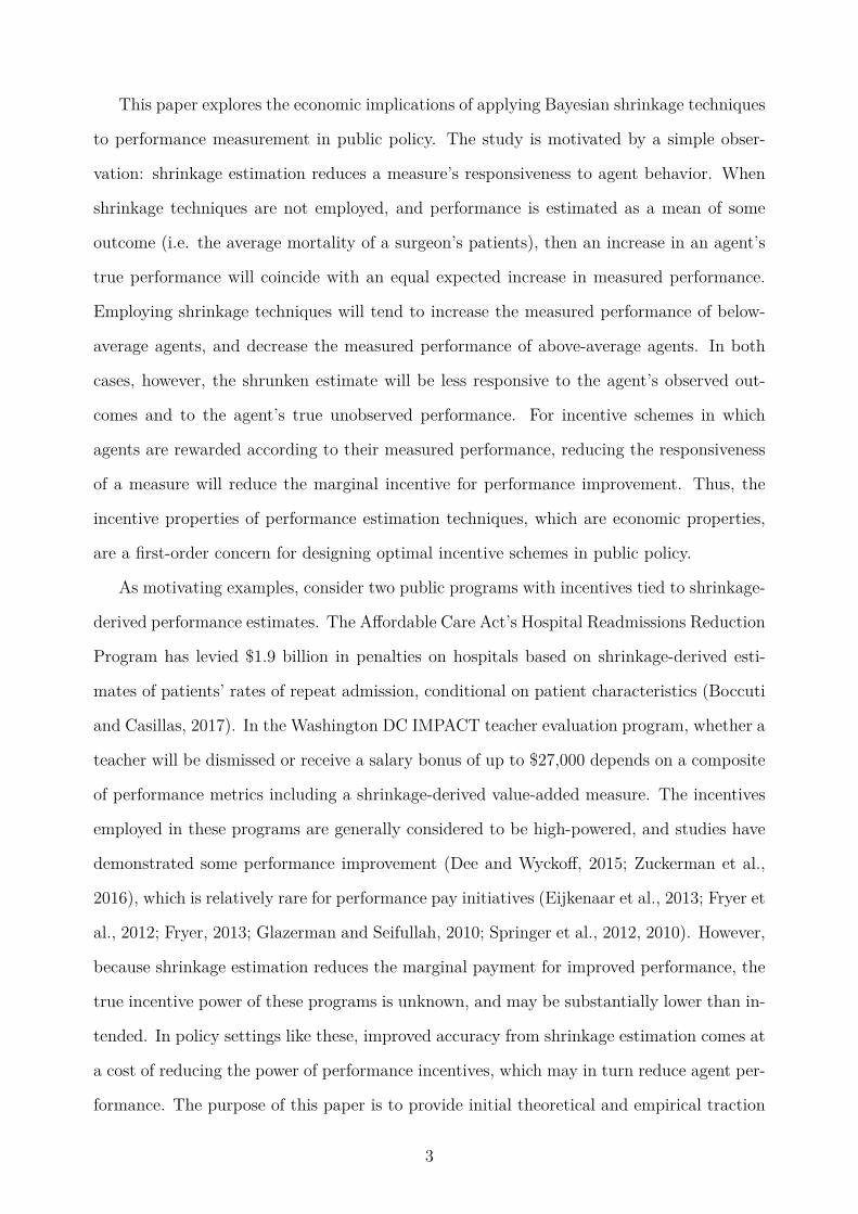
To illustrate basic properties of shrinkage estimation graphically, I briefly compare ob-

served and shrunken performance estimates (rj and uj) calculated from synthetic classroom

data. The data generating process is based on Rothstein (2015), which specifies a distri-

bution of teacher ability and measure reliability in a simulation analysis of value-added3Note that the estimate uj cannot be operationalized as written since the equation requires estimates of

the variance components and mean. This is a general property of shrinkage estimators, and there are manyways of incorporating estimates of these parameters into the calculation of uj . Fully Bayesian approachesemploy a posterior distribution of these additional parameters (estimated based on prior distributions) whileempirical Bayes approaches plug in point estimates. For details and examples, see Gelman and Hill (2009),Gelman et al. (2014), Morris (1983), Guarino et al. (2014), Chetty, Friedman, and Rockoff (2014), Dimick,Staiger, and Birkmeyer (2010).

4See McCulloch and Neuhaus (2011) for a derivation of this result. These prediction error estimates reflectan assumption that there is zero measurement error in the estimation of β, a reasonable simplification whensample sizes are large.

13

measurement. In my synthetic data, teachers serve classrooms of 27 students, true teacher

performance uj is independently distributed N(0, 0.15), and student outcome is indepen-

dently distributed N(uj, 0.95). These parameters correspond to a shrinkage factor of 0.4

for each teacher performance estimate. The mean of student outcomes within a class consti-

tutes a teacher’s observed performance, rj. Shrunken posterior performance estimates, uj,

are obtained via a random effects model. Panel A of Figure 1 shows the distribution of ob-

served and shrunken performance estimates for 100,000 teachers. Because of idiosyncratic

variation in student performance, observed performance is over-dispersed relative to true

teacher ability. Shrunken performance estimates exhibit less variance than both observed

and true teacher performance. As noted by Chandra et al. (2016), the latter property fol-

lows because true performance is the sum of the shrunken performance prediction and an

orthogonal prediction error.

Shrinkage estimators may be considered unbiased or biased depending on the criterion

for bias. Consistent with this observation are Panels B and C of Figure 1, which present

binned scatterplots of true performance vs measured performance and vice versa. First,

consider for some performance measure uj, the property E [uj|uj ] = uj, which I refer to as

prediction unbiasedness, following Chetty, Friedman, and Rockoff (2014). If a measure is

prediction unbiased, then an agent’s measured performance will equal his or her expected

true performance. As shown in Panel B, these shrunken performance measures very closely

approximate the conditional mean of true teacher performance in the synthetic data. For

this reason, linear shrinkage estimators are sometimes referred to as best linear unbiased pre-

dictors (BLUPs) (Skrondal and Rabe-Hesketh, 2009).5 Alternatively, observed performance

clearly demonstrates prediction biasedness, overestimating the performance of teachers with

relatively greater observed performance and underestimating the performance of teachers

with inferior performance. Second, consider measurement unbiasedness, defined here as

E [uj|uj ] = uj. If a measure exhibits measurement unbiasedness, then an agent’s expected

measured performance will equal their true performance. As shown in Panel C, shrink-

age estimators do poorly according to this criterion, underestimating the performance of5There has been recent interest in questioning whether assumptions required for unbiasedness hold when

consumers’ choice of agents is not exogenous. See, for example Kalbfleisch and Wolfe (2013) and Guarinoet al. (2014).

14

high performers and overestimating the performance of low performers. Alternatively, true

performance very closely approximates the conditional average of observed (unshrunken)

teacher performance.

Measurement bias relates to a key incentive property of shrinkage estimators: responsive-

ness to agent behavior. I define measure responsiveness as dE[uj ]

duj, the change in expected mea-

sured performance for a change in actual performance. If an individual agent’s performance

contributes negligibly to the average performance across agents, then dE[uj ]

duj=

dE[uj ]

duj≈ sj.

Thus, the size of the shrinkage factor faced by an agent equals the measure’s responsive-

ness to that agent’s behavior. (Note that in Panel C of Figure 1, the scatterplot slope for

shrunken estimates indeed equals the shrinkage factor 0.4.) The loss of measure respon-

siveness entailed by shrinkage estimation equals one minus the shrinkage factor. As the

shrinkage factor approaches one, the measure becomes fully responsive to agent behavior,

with dE[rj ]

duj= 1. In this case, the performance of other agents no longer affects an agent’s

performance estimate. Because measure responsiveness is increasing in nj and σ2u and de-

creasing in σ2ε , shrinkage estimates of performance will be less responsive for agents serving

a smaller number of consumers (e.g. smaller hospitals), for measured outcomes with a large

amount of residual error, and for settings in which agent performance is very similar.

Consider these shrinkage estimation properties in light of the model presented in Section

2. Recall that equilibrium welfare loss is increasing in the mean squared error of the rela-

tive performance signal and, when the marginal revenue from quality investment is low (i.e.

r < c), decreasing in the responsiveness of quality signals to true quality. Because shrinkage

estimation decreases mean squared error and reduces dE[uj ]

dujfrom 1 to sj, adopting shrinkage

estimation entails an accuracy-incentives tradeoff in this setting. For the intuition behind

this result, recall that an agent’s investment in quality increases with the responsiveness

of quality signal to agent behavior. For example, the quality bonus scheme described in

Section 2 consists of a linear schedule of reward payments for measured performance. As

measure responsiveness decreases, so does the effective marginal quality bonus for improved

performance. Consumers’ demand response to quality, another driver of agent quality invest-

ments in Section 2, will be similarly diluted if publicly disclosed quality ratings are shrunken

and consumers perceive these ratings to be measurement unbiased. Thus, although shrink-

15

age estimators may improve consumer sorting by improving measure accuracy, they reduce

measure responsiveness and may discourage quality investment.

4 Quantifying the Accuracy-Incentives Tradeoff:Hospital Quality Measurement

I use Monte Carlo simulation to assess the magnitude of the accuracy-incentives tradeoff

in the case of hospital performance measurement. Currently, CMS employs shrinkage esti-

mation to evaluate hospital mortality rates and rates of hospital readmissions for patients

with select diagnoses. These measures, constructed from Medicare claims data, are part of

broader efforts to tie Medicare payments to measures of health care value (Burwell, 2015)

and to report hospital quality ratings (Werner and Bradlow, 2006). 30-day mortality ratings

have been publicly reported since 2007 and began contributing to hospital payment adjust-

ments as part of the Medicare Hospital Value-Based Purchasing Program in the 2014 fiscal

year. 30-day readmission rates have been publicly reported since 2009 and began contribut-

ing to hospital payment penalties through the Hospital Readmissions Reduction Program

in fiscal year 2013.6 CMS methods for calculating mortality and readmissions measures are

broadly similar, involving hierarchical logistic models that include patient characteristics as

covariates (Ash et al., 2012; Krumholz et al., 2006).

I examine measurement of hospital 30-day mortality for patients with acute myocardial

infarction (AMI), commonly known as heart attack. AMI was one of the first diagnoses

used for CMS mortality measures, and is a serious complication of cardiovascular disease,

the leading cause of death in the United States. The simulation compares the performance

of alternative measurement techniques according to two properties: root mean squared error

(accuracy) and measure responsiveness (incentives). The simulation allows me to construct

true hospital performance, which is typically unobserved, and to calculate an error equal6Hospital Readmissions Reduction Program penalties take the form of reductions in Medicare payments

for all hospital admissions. The reduction is based on risk-adjusted readmissions rates for patients admittedwith a select set of diagnoses, with a maximum penalty of 3% since fiscal year 2015 (Centers for Medicareand Medicaid Services, 2017a). Payments for the Hospital Value-Based Purchasing Program payments aremore complex. In fiscal year 2017, 2% of base hospital payments were withheld from participating hospitals,and these funds were devoted to hospital incentive payments. Payments were calculated on the basis of 21performance measures, which were combined into composite scores for achievement as well as improvement(Centers for Medicare and Medicaid Services, 2017b).

16

to the difference between this value and measured performance. In addition, by taking

repeated draws of data, simulation results incorporate findings from a broad set of possible

hospital outcomes. Simulation is an especially valuable empirical tool to evaluate the effects

of measurement choices because plausibly exogenous variation in measurement techniques

is rare7

Many studies have recently used simulation to examine the properties of performance

measures in health and education (Normand et al., 2007; Thomas and Hofer, 1999; sev-

eral papers reviewed in Koedel, Mihaly, and Rockoff, 2015, including Rothstein, 2015). My

analysis closely follows that of Ryan et al. (2012), which compares the accuracy of several

alternate AMI mortality measures. I replicate and extend those simulation methods by as-

sessing measure responsiveness in addition to measurement error. The simulation methods,

briefly described here, are detailed more fully in Ryan et al. (2012).

Simulation Methods

The data generating process has been calibrated to approximate the distribution of risk-

adjusted mortality in Medicare inpatient claims data. In addition, the simulation includes a

rejection sampling condition that discards any simulation iteration in which the simulated

data differ substantially from Medicare inpatient data in more than one of several mo-

ment conditions.8 These conditions, and their values in Medicare inpatient data are: mean

mortality (0.209), within-hospital standard deviation in mortality (0.091), between-hospital

standard deviation in mortality (0.078), mean annual change in mortality (-0.007), within-

hospital standard deviation of annual mortality change (0.137), between-hospital standard

deviation of annual mortality changes (0.031), and mean hospital AMI volume (104.8).

The simulation proceeds in the following steps. For each of 3000 hospitals, an initial

volume of AMI patients and an annual growth rate in volume are drawn from a trun-

cated gamma distribution and a normal distribution, respectively (see Ryan et al. [2012]7Empirically evaluating the effect of shrinkage estimation on agent performance is challenging because

of this limitation. Exploiting variation in incentives across agents with different sample sizes within anincentive scheme would also be problematic. Even in the presence of quasi-random variation in classroom orhospital size, it would be difficult to isolate the effect of the incentive distortions due to shrinkage estimationfrom the effect of classroom or hospital size.

8Specifically, the iteration was discarded if more than one of the simulated data parameters fell outsideof a bootstrapped 95% confidence interval of the Medicare data parameter.

17

for all parameter values). Each hospital is assigned an initial raw mortality rate and an

annual growth rate in mortality improvement, drawn from normal distributions. Annual

raw mortality rates are then adjusted to reflect improved mortality in higher volume hos-

pitals. Specifically, raw mortality rates are adjusted based on annual hospital volume and

the empirical relationship between volume and risk-adjusted mortality in Medicare inpatient

claims, which was modeled using a generalized linear model (Bernoulli family, logit link) and

a of fifth degree polynomial function of hospital volume. The resulting annual mortality rate

serves as a hospital’s true mortality score and corresponds to each patient’s probability of

dying within 30 days of admission. Deaths are assigned according to a random draw for each

patient. Note that the probability of mortality is not a function of patient characteristics.

This corresponds to an assumption that risk-adjustment eliminates residual confounding in

all mortality measurement techniques I consider.

For each measurement technique that I consider, I calculate hospital mortality scores

based on one, two, or three years of observed mortality. In each simulation iteration, the

accuracy of each measure is assessed by comparing measured mortality scores uj to true mor-

tality in the following year uj. The temporal lag reflects the role of public reporting policies

in providing past hospital performance data to inform current patient decisions. Measure

accuracy is scored as root mean square error (RMSE),√

(uj − uj)2. Each measure’s respon-

siveness, dE[uj ]

dujis scored as the average shrinkage factor sj employed in the performance

estimation. Accuracy and responsiveness are assessed across all hospitals and by category of

hospital size. Hospitals are categorized as small, medium, and large, where small hospitals

have patient volume in the bottom quartile (approximately 30 AMI admissions per year or

fewer) and large hospitals have patient volume in the top quartile (approximately 143 AMI

admissions per year or higher).

I consider five alternate measures of hospital mortality, four of which are included in Ryan

et al. (2012). The first measure is observed over expected mortality (OE). OE, which is

not a shrinkage estimator, has been used to estimate cardiac surgery performance (Kolstad,

2013). It is calculated as follows:

OEj =

∑nji=1 yij∑nj

i=1 β0 + β1Xij

· y

18

where yij is an indicator for death, y is the overall average mortality rate, and X is a vector

of patient characteristics. The denominator is the expected number of patient deaths based

on prediction via linear regression. In the absence of patient covariates, this expression

simplifies to the observed mortality rate∑nj

i=1 yij/nj. I also implement a moving average

(MA) of this estimator, a simple average of OE estimates over two or three years. Since OE

and MA do not incorporate shrinkage, the responsiveness of these measures equals one.9

The second measure is risk-standardized mortality rate (RSMR), the current CMS mea-

sure for 30-day mortality and 30-day readmissions. CMS initially used one year of claims

data for its RSMR calculations, though it now uses three. The formula for RSMR is:

uRSMRj =

∑nji=1 f( β0 + θj + β1Xij)∑nj

i=1 f( β0 + β1Xij)· y

where f() is the inverse of the logistic link function. For this simulation, β0, θj, and β1 are

estimated via a multilevel logistic model with a hospital random effect. The third measure

I test is a novel variant of RSMR that I call the average best linear unbiased estimator

(ABLUP). ABLUP, also a shrinkage estimate, is calculated using the same logistic model

estimates as RSMR:

uABLUPj =

∑Ni=1 f( β0 + θj + β1Xi)

N

where N is the total number of patients across all hospitals. Thus, ABLUP can be inter-

preted as the hospital’s average of predicted mortality across all possible patients in the

sample. Although ABLUP and RSMR are derived from the same logistic model, they do

not produce identical estimates, which is apparent when assuming all patients are uniform

in their characteristics. In this case, uRSMRj = uABLUPj

y

f(β0).

The fourth and fifth measures are the Dimick-Staiger measure (DS) (Dimick et al., 2009)

and the hierarchical Poisson measure (HP) (Ryan et al., 2012). Unlike the previously de-

scribed shrinkage estimators, the DS and HP estimators do not shrink all hospitals’ observed

mortality rates toward a common mortality average. Instead, mortality rates are shrunk to-

ward values that are specific to a hospital’s patient volume. Both estimators are calculated9A moving average of t years of data dilutes the contribution of any single year’s performance to a single

performance score by a factor of 1t . However, because each performance year will contribute to t moving

average estimates, measure responsiveness remains equal to one.

19

according to the following formula:

uDS, HPj = ujsDS,HPj + wDS,HPj

(1− sDS,HPj

)

where uj is a hospital’s observed mortality, sDS,HPj is the DS or HP shrinkage factor and

wDS,HPj is the hospital’s predicted mortality based on its volume. There are several dif-

ferences between the DS and HP measures regarding how shrinkage factors and volume-

predicted mortality are calculated. Unlike for DS, HP estimates of volume-specific mortality

are derived from a nonlinear model (a negative binomial model for number of deaths), HP

is calculated from hospital-level data rather than patient-level data, and HP uses a max-

imum likelihood approach to estimate shrinkage factors.10 Shrinkage factors, which serve

as estimates of measure responsiveness, are explicitly calculated in DS and HP estimation.

For RSMR and ABLUP, each shrinkage factor is calculated as the weight by which esti-

mated mortality uj is the weighted average of a hospital’s observed mortality and the mean

estimated mortality across hospitals.

Results and Sensitivity Analysis

Figure 2 illustrates each 30-day mortality measure’s overall performance in terms of

accuracy and responsiveness. Note that the horizontal axis is reverse-coded, with greater

accuracy measures displayed farther to the right. To gauge the magnitude of measurement

error in relation to average hospital performance, recall that the average hospital 30-day

mortality rate is 20.9%. First, consider the one-year mortality measures, which tend to

perform least accurately and with the least responsiveness. OE, the one-year measure with-

out shrinkage, has a substantial amount of error, with a RMSE of roughly 0.1. Shrinkage

measures perform much more accurately, with RMSE less than 0.06. However, the loss of

measure responsiveness entailed by shrinkage estimation is also substantial. The average

shrinkage factor facing hospitals ranges from 0.62 to 0.70 for one-year shrinkage measures.

This level of measure responsiveness can be viewed as a tax of approximately 30-40 percent10For the details of how volume-predicted mortality and shrinkage factors are calculated for DS and HP,

see Dimick et al. (2009) and Ryan et al. (2012). For details on adjusting the DS estimator for patientcovariates, see Staiger et al. (2009).

20

on measure improvement. Note that a hospital facing a 0.62 shrinkage factor must reduce

mortality by 1.6 percentage points to decrease measured mortality by one percentage point.

Each measure’s accuracy and responsiveness by hospital size are presented in Table 1.

Columns (1) and (5) confirm that the shrinkage estimators have greater accuracy and lower

measure responsiveness than the estimators without shrinkage, OE and MA. Columns (2)

and (5) present RMSE and measure responsiveness for hospitals in the bottom quartile of

AMI volume. These smaller hospitals experience the greatest improvements in RMSE and

greatest reductions in responsiveness when shrinkage estimators are employed. For exam-

ple, with one year of mortality data, RMSE for the non-shrinkage measure is 0.17, and the

shrinkage measure RMSR reduces this error to 0.09. However, RSMR also decreases mea-

sure responsiveness from one to 0.35. These differences in the accuracy and responsiveness

between shrinkage and non-shrinkage estimates tend to narrow as more years of data are in-

cluded in measures. However, even with multiple years of data, responsiveness of shrinkage

estimates to the performance of small hospitals remains very low, at 0.50 for the three-year

RSMR. As shown in columns (4) and (8) of Table 1, shrinkage does not appear to reduce

error in estimating large hospitals’ performance. For larger hospitals, error is slightly greater

for measures without shrinkage, and the responsiveness of shrinkage measures ranges from

0.83 to 0.96.

Figure 3 aids in demonstrating the substantial variation in the responsiveness of shrink-

age measures by hospital size. The figure presents, from a representative simulation iter-

ation, the responsiveness of one-year shrinkage measures for each decile of hospital AMI

volume. Responsiveness increases at a decreasing rate with respect to hospital volume, with

considerable variation across hospital sizes. The responsiveness of shrinkage estimators, ap-

proximately 0.2 for hospitals in the bottom decile of AMI volume, rises to approximately

0.9 in the top decile. Since measures only approach full responsiveness asymptotically as

sample size increases, measures are not fully responsive to hospital performance for even the

largest hospitals in the sample. There is also heterogeneity across shrinkage estimators in

terms of their responsiveness.

Several estimators dominate others on the basis of both accuracy and responsiveness.

For example, the DS estimator is both more accurate and more responsive than the HP

21

estimator. Similarly, the novel measure ABLUP tends to dominate the current CMS ap-

proach, RSMR. The performance frontier of all measures is comprised of the two-year DS,

three-year ABLUP, and three-year MA. Notably, volume-adjusted shrinkage estimators DS

and HP, which shrink observed mortality toward a target that is specific to hospital volume,

do not dominate ABLUP and RSMR, which are not volume adjusted. To understand this

result, recall that shrinkage measures entail greater shrinkage when there is lesser cross-

hospital variation in performance. Volume-adjusted shrinkage estimators attribute some

hospital performance variation to hospital volume, thereby reducing residual cross-hospital

variation, increasing shrinkage, and reducing measure responsiveness.

Incorporation of additional years of data tends to improve both measure accuracy and

responsiveness. The non-shrinkage measure experiences an especially pronounced gain in

accuracy when the measurement timeframe expands. As column (1) of Table 1 shows, RMSE

for this measure falls from 0.097 to 0.061 when three years of data are used instead of one

year. The corresponding change in error for the RSMR shrinkage measure was considerably

smaller, from 0.060 to 0.052. Increasing the number of observations also improves the

responsiveness of shrinkage estimates. However, even with three-years of data, shrinkage

estimates are still approximately 20-25% less responsive than the non-shrinkage estimates,

which are fully responsive regardless of the number of observations.

Although additional years of data increased measure accuracy in the simulation, this

finding may not generalize to settings in which there is substantial drift in agent behavior

over time. If there is extensive drift, early outcomes are less informative of current perfor-

mance. To demonstrate the sensitivity of measure accuracy to the magnitude of performance

drift, I conduct two secondary simulations. In the first, a no-drift case, each hospital’s true

mortality rate is fixed over time. In the second, strong-drift case, each hospital has an annual

growth rate in mortality improvement (percent change per year) that is drawn from a nor-

mal distribution with mean zero and standard deviation of 20%. All other data-generation

parameters are the same as in the previously described simulation. In each case, I calculate

the RMSE of three measures of hospital mortality: one-year observed mortality, three-year

mortality average (unweighted), and a three-year weighted average of mortality. Rather

than selecting arbitrary weights for the weighted average, I calculate weights for years t-1,

22

t-2, and t-3 using constrained linear regression. In each simulation iteration, I regress hos-

pital observed mortality in year t-1 on observed mortality in years t-2, t-3, and t-4, with

the constraint that the sum of these coefficients equals one. The resulting coefficients serve

as the weights for mortality in years t-1, t-2 and t-3, respectively.

Table 2 presents the results from these simulations. As shown in column (1), when there is

no drift in hospital performance, a moving average has lower RMSE than a one-year estimate.

As expected, the constrained regression produces equal weights for all measurement years in

this case. As shown in column (2), in the case of substantial performance drift, a three year

unweighted average is less accurate than a one-year estimate (0.116 vs. 0.109 RMSE). The

weighted average, with average weights of 0.67, 0.31 and 0.02 for mortality data from years

t-1, t-2, and t-3, outperforms both alternate measures. Thus, even in the case of changing

hospital performance, incorporating early data into measures can increase accuracy if those

data are weighted appropriately.

Because ordinal performance measures are an alternative to the cardinal measures typ-

ically used for quality disclosure or incentive pay (Barlevy and Neal, 2012; Dimick et al.,

2010), in a final secondary analysis, I assess the accuracy and responsiveness of each mea-

sure using rank-based criteria. With vj and vj as a hospital’s true and measured mortality

ranking among J hospitals, rank accuracy is estimated as the average of |vj−vj |J

, which is the

approximate percentile difference between true and measured performance rankings. Rank

responsiveness is estimated as the average change in a hospital’s measured rank for a one

percentage point reduction in that hospital’s observed 30-day mortality rate. To facilitate

comparison among measures, each rank responsiveness estimate is normalized by dividing

by the OE rank responsiveness estimate.

Table 3 illustrates each 30-day mortality measure’s performance in terms of rank accuracy

and rank responsiveness. Though shrinkage estimation uniformly reduces rank error, its

effect on rank responsiveness varies according to estimator and hospital size. DS and HP

estimators reduce rank responsiveness across all hospital size categories. RSMR and ABLUP

tend to reduce rank responsiveness for small hospitals, but increase it for medium and large

hospitals. For intuition as to why shrinkage estimation need not always reduce rank-based

incentives, consider the case of all hospitals being equally sized. Shrinkage estimation would

23

have no effect on the magnitude of performance improvement necessary for a hospital to

surpass a higher ranked hospital, because decreased measure responsiveness would be exactly

offset by a narrowed distribution of measured performance. By moving outlier hospitals

toward the grand mean, RSMR and ABLUP tend to increase the number of hospitals that

a large hospital can overtake in rank when it improves performance.

5 Policy Implications and Conclusion

These theoretic and empirical findings highlight a substantial tradeoff involved in the

choice of performance estimation technique. Although accuracy and responsiveness to agent

behavior are both economically desirable features of performance measures, one feature

generally comes at the cost of the other. Indeed, shrinkage estimates are least responsive to

agent behavior in policy settings like health care and education, where performance outcomes

are noisy. In the case of hospital performance measurement, the magnitude of this loss in

responsiveness is economically significant and substantially dilutes performance incentives.

In addition, the magnitude of distortion varies substantially across hospitals, affecting small

hospitals to a much greater degree.

These results can inform the design of public policies involving performance measure-

ment. Given the tradeoff between accuracy and incentives, the appropriate choice of esti-

mation technique should depend on a policy’s goals. In education, a policy that identifies

inferior teachers for replacement or inferior schools for closure may be welfare improving

even if the policy does not produce a behavioral response with respect to agent effort. Since

the goal of such policies is to select superior agents rather than to incentivize agent perfor-

mance, shrinkage estimation seems appropriate. However, for performance payment schemes

in which payment is a function of a teacher’s absolute performance, shrinkage estimation

will tend to dilute incentives unless bonus payments are increased to compensate for reduced

measure responsiveness.

Shrinkage estimation may be less appropriate for health care policies, which tend to em-

phasize incentives for performance improvement. Policies aiming to retain superior agents

(i.e. by shutting down inferior hospitals or medical practices) tend to be rare. Shrinkage

24

measurement seems generally inappropriate for performance payment policies like Medi-

care’s hospital readmissions penalties because shrinkage dilutes provider incentives and it

is unclear how improved measurement accuracy would contribute to improved welfare. The

case of public disclosure of quality information is more ambiguous. Even in the absence of a

performance-based payment system, shrinkage estimation will dilute performance incentives

in settings where consumer demand response to quality signals is an important performance

incentive. While publicly disclosing a more accurate signal could improve patients’ choice of

hospital, a less responsive performance measure may reduce demand elasticity to provider

quality. Whether or not to shrink these performance estimates depends on comparing the

welfare gains from more efficient patient sorting to the welfare gains from increased provider

quality spurred by from demand elasticity to quality.

The simulation results highlight that some measurement techniques may outperform

others with respect to both accuracy and incentives. Policymakers should select measures

from this frontier, though the relative performance of each technique may vary according

to the policy setting. The results also demonstrate that incorporating more observations

into performance measures by lengthening the timespan of performance measurement is a

substitute to shrinkage estimation in improving measure accuracy. For measures without

shrinkage, the gains in accuracy from including more data were considerable. Additional

accuracy gains from applying shrinkage may not be worth the loss in measure responsiveness.

Even if agent performance varies over time, inclusion of early performance data in a weighted

average of performance can improve measure accuracy. Furthermore, choice of estimator can

depend on whether policies use cardinal or ordinal performance data. If incentives are based

on performance rank, shrinkage estimation need not always entail reduced incentives.

The analysis in this paper assumes risk-neutrality of agents, which may not hold in

all policy settings. A classic finding in the principal-agent literature is that, in determining

optimal compensation, agent risk aversion introduces a tradeoff between incentive power and

insurance for agents (Gibbons and Roberts, 2013). Although high-powered incentives can

still produce efficient agent performance, they expose agents to risk. High-powered incentives

may be inappropriate when agents are risk averse, especially if high-powered incentives do

not produce large welfare gains for consumers (i.e. reduced patient mortality). Although

25

estimating agent performance with shrinkage does provide some insurance to agents, it is

a blunt tool for this purpose. The shrinkage factors used in performance measurement are

not calculated to optimally balance agent insurance against performance incentives.11 Thus,

even if the optimal incentive power of health care or education policies is low (i.e. due to

agent risk aversion or multitasking concerns), shrinkage estimation would not produce the

optimally powered incentives.

Finally, choice of measurement technique may be affected by fairness concerns. An

agent may view noisier performance measures as less fair because ratings can vary widely

over time even as agent behavior is constant. Similarly, a policymaker may be hesitant to

employ a less accurate measurement technique that increases the probability of type I or

type II errors in rewarding or penalizing agents. However, despite their improved accuracy,

shrinkage measures may also be viewed as performing poorly with respect to fairness. For

a given agent, errors from measures without shrinkage have an expectation of zero, and will

tend to even out over time, while errors from shrinkage estimates are persistent. Shrinkage

estimates will persistently underestimate the performance of high-performing agents, and

overestimate the performance of low-performing agents. These errors are magnified for

agents with fewer observations. Thus, agents may view shrinkage estimation as an unfair

form of statistical discrimination, because their performance is consistently underestimated

or because improved performance is not rewarded fully in measured performance.

11For example, shrinkage factors are a function of variation in true performance across agents, while riskfor an agent depends only on outcome variation for that agent.

26

References

Adams, J.L., Mehrotra, A., Thomas, J.W. and E.A. McGlynn, “Physician Cost Profiling–

Reliability and Risk of Misclassification,” New England Journal of Medicine 362 (2010),

1014–21.

Adams, J.L., Mehrotra, A., Thomas, J.W. and E.A. McGlynn, “Physician Cost Profiling–

Reliability and Risk of Misclassification,” New England Journal of Medicine 362 (2010),

1014–21.

Arrow, K.J., “Uncertainty and the Welfare Economics of Medical Care,” American Eco-

nomic Review 53 (1963), 941–973.

Ash, A., Fienberg, S., Louis, T.A., Normand, S.-L.T., Stukel, T.A., and J. Utts, “Statistical

Issues in Assessing Hospital Performance,” (2012)< http://www.cms.gov/Medicare/Quality-

Initiatives-Patient-Assessment-Instruments/HospitalQualityInits/Downloads/Statistical-

Issues-in-Assessing-Hospital-Performance.pdf>.

Boccuti, C. and G. Casillas, “Aiming for Fewer Hospital U-turns: The Medicare Hospital

Readmission Reduction Program,” Kaiser Family Foundation Issue Brief (2017).

Centers for Medicare and Medicaid Services, “Readmissions Reduction Program,” (2017a)

<https://www.cms.gov/medicare/medicare-fee-for-service-payment/acuteinpatientpps

/readmissions-reduction-program.html>.

Centers for Medicare and Medicaid Services, “Hospital Value-Based Purchasing,” (2017b)

<https://www.cms.gov/Medicare/Quality-Initiatives-Patient-Assessment-Instruments

/hospital-value-based-purchasing/index.html?>.

Chandra, A., Finkelstein, A., Sacarny, A., and C. Syverson, “Health Care Exceptional-

ism? Performance and Allocation in the US Health Care Sector,” American Economic

Review 106 (2016), 2110–2144.

Chay, K., McEwan, P.J, and M. Urquiola, “The Central Role of Noise in Evaluating In-

terventions That Use Test Scores to Rank Schools,” American Economic Review 95

27

(2005), 1237-1258.

Chetty, R., Friedman, J.N., and J.E. Rockoff, “Measuring the Impacts of Teachers I:

Evaluating Bias in Teacher Value-Added Estimates,” American Economic Review 104

(2014), 2593–2632.

Dee, T.S. and J. Wyckoff, “Incentives, Selection, and Teacher Performance: Evidence from

IMPACT,” Journal of Policy Analysis and Management 34 (2015), 267–297.

Dimick, J.B., Staiger, D.O., Baser, O., and J.D. Birkmeyer, “Composite Measures for

Predicting Surgical Mortality in the Hospital,” Health Affairs 28 (2009), 1189–98.

Dimick, J.B., Staiger, D.O., J.D. Birkmeyer, “Ranking Hospitals on Surgical Mortality:

The Importance of Reliability Adjustment,” Health Services Research 45 (2010), 1614–

29.

Dimick, J.B., Welch, H.G., J.D. Birkmeyer, “Surgical Mortality as an Indicator of Hospital

Quality: the Problem with Small Sample Size,” JAMA 292 (2004), 847–51.

Dranove, D. and G.Z. Jin, “Quality Disclosure and Certification: Theory and Practice,”

Journal of Economic Literature 48 (2010), 935–963.

Eijkenaar, F., Emmert, M., Scheppach, M., and O. Schoffski, “Effects of Pay for Perfor-

mance in Health Care: A Systematic Review of Systematic Reviews,” Health Policy

110 (2013), 115–130.

Farmer, A. and D. Terrell, “Discrimination, Bayesian Updating of Employer Beliefs, and

Human Capital Accumulation,” Economic Inquiry 34 (1996), 204–219.

Fryer, R., Levitt, S., List, J. and S. Sadoff, “Enhancing the Efficacy of Teacher Incentives

through Loss Aversion: A Field Experiment,” NBER working paper 18237 (2012).

Fryer, R.G., “Teacher Incentives and Student Achievement: Evidence from New York City

Public Schools,” Journal of Labor Economics 31 (2013), 373–407.

28

Gaynor, M., Seider, H., and W.B. Vogt, “The Volume–Outcome Effect, Scale Economies,

and Learning-by-Doing,” American Economic Review: Papers and Proceedings 95

(2005), 243–247.

Gelman, A., Carlin, J., Stern, H., Dunson, D., Vehtari, A., and D. Rubin eds., Bayesian

Data Analysis, 3rd edition (Boca Raton, FL: CRC Press, 2014).

Gelman, A. and J. Hill, Data Analysis Using Regression and Multilevel / Hierarchical

Models (Cambridge, UK: Cambridge University Press, 2007), 258.

Gibbons, R. and J. Roberts, The Handbook of Organizational Economics (Princeton, NJ:

Princeton University Press, 2013).

Glazerman, S., and A. Seifullah, An Evaluation of the Teacher Advancement Program

(TAP) in Chicago: Year Two Impact Report (Washington, DC: Mathematica Policy

Research, 2010).

Guarino, C., Maxfield, M., Reckase, M.D., Thompson, P., and J.M. Wooldridge, “An Evalu-

ation of Empirical Bayes’ Estimation of Value-Added Teacher Performance Measures,”

Michigan State University Education Policy Center working paper 31 (2014).

Hofer, T.P., Hayward, R.A., Greenfield, S., Wagner, E.H., Kaplan, S.H., and W.G. Man-

ning, “The Unreliability of Individual Physician Report Cards for Assessing the Costs

and Quality of Care of a Chronic Disease,” JAMA 281 (1999), 2098–105.

Institute of Medicine, Vital Signs: Core Metrics for Health and Health Care Progress

(Washington, DC: The National Academies Press, 2015).

Kane, T.J., and D.O. Staiger, “Estimating Teacher Impacts on Student Achievement: An

Experimental Evaluation,” NBER working paper 14607 (2008).

Kane T.J., and D.O. Staiger, “Improving School Accountability Measures,” NBER working

paper 8156 (2001).

Kane T.J., and D.O. Staiger, “The Promise and Pitfalls of Using Imprecise School Ac-

countability Measures,” Journal of Economic Perspectives 16 (2002), 91–114.

29

Koedel, C., Mihaly, K., and J.E. Rockoff, “Value-Added Modeling: A Review,” Economics

of Education Review 47 (2015), 180–195.

Kolstad, J., “Information and Quality when Motivation is Intrinsic: Evidence from Surgeon

Report Cards,” American Economic Review 103 (2013), 2875–2910.

Krumholz, H.M., Wang, Yun, Mattera, J.A., Wang, Yongfei, Han, L.F., Ingber, M.J., Ro-

man, S., and S.-L.T Normand, “An Administrative Claims Model Suitable for Profiling

Hospital Performance based on 30-day Mortality Rates among Patients with an Acute

Myocardial Infarction,” Circulation 113 (2006), 1683–92.

McCulloch, C.E. and J.M. Neuhaus, “Prediction of Random Effects in Linear and Gener-

alized Linear Models under Model Misspecification,” Biometrics 67 (2011), 270–9.

McGuire, T.G., “Physician Agency”, in: Culyer. A. and J.P. Newhouse, eds., Handbook of

Health Economics (North Holland: Elsevier, 2000) 461—536.

Morris, C., “Parametric Empirical Bayes Inference: Theory and Applications,” Journal of

the American Statistical Association 78 (1983), 47–55.

Normand, S.-L.T., and D.M. Shahian, “Statistical and Clinical Aspects of Hospital Out-

comes Profiling,” Statistical Science 22 (2007), 206–226.

Normand, S.-L.T., Wolf, R.E., Ayanian, J.Z. and B.J. McNeil, “Assessing the Accuracy of

Hospital Clinical Performance Measures,” Medical Decision Making 27 (2007), 9–20.

Nyweide, D.J., Weeks, W.B., Gottlieb, D.J., Casalino, L.P., and E.S. Fisher, “Relationship

of Primary Care Physicians’ Patient Caseload with Measurement of Quality and Cost

Performance,” JAMA 302 (2009), 2444–50.

Phelps, E., “The Statistical Theory of Racism and Sexism,” American Economic Review

62 (1972), 659–661.

Rabin, M., “Inference By Believers In The Law Of Small Numbers,” Quarterly Journal of

Economics 117 (2002), 775–816.

30

Richardson, S.S. , “Integrating Pay-for-Performance into Health Care Payment Systems,”

Unpublished manuscript (2013).

Rothstein J., “Teacher Quality Policy When Supply Matters,” American Economic Review

105 (2015), 100–130.

Ryan, A., Burgess, J., Strawderman, R. and J. Dimick, “What is the Best Way to Estimate

Hospital Quality Outcomes? A Simulation Approach,” Health Services Research 27

(2012), 1699–718.

Silber, J.H., Rosenbaum, P.R., Brachet, T.J., Ross, R.N., Bressler, L.J., Even-Shoshan,

O., Lorch, S., and K.G. Volpp, “The Hospital Compare Mortality Model and the

Volume-Outcome Relationship,” Health Services Research 45 (2010), 1148–67.

Skrondal, A., and S. Rabe-Hesketh, “Prediction in Multilevel Generalized Linear Models,”

Journal of the Royal Statistical Society 172 (2009), 659–687.

Springer, M.G., Ballou, D., Hamilton, L., Le, V., Lockwood, J.R., McCaffrey, D., Pepper,

M., and B. Stecher, “Teacher Pay for Performance: Experimental Evidence from the

Project on Incentives in Teaching” Society for Research on Educational Effectiveness

(2010).

Springer, M.G., Pane, J.F., Le, V.-N., McCaffrey, D.F., Burns, S.F., Hamilton, L.S., and B.

Stecher, “Team Pay for Performance: Experimental Evidence From the Round Rock

Pilot Project on Team Incentives.” Educational Evaluation and Policy Analysis 34

(2012), 367–390.

Staiger, D.O. and Rockoff, J., “Searching for Effective Teachers with Imperfect Informa-

tion.” Journal of Economic Perspectives 24 (2010), 97–117.

Stein, C., “Inadmissibility of the Usual Estimator for the Mean of a Multivariate Normal

Distribution,” Proceedings of the Third Berkeley Symposium on Mathematical Statis-

tics and Probability, 1954–1955 1 (1956), 197–206.

Thomas, J.W. and T.P. Hofer, “Accuracy of Risk-Adjusted Mortality Rate as a Measure

of Hospital Quality of Care,” Medical Care 37 (1999), 83–92.

31

Tversky A. and D. Kahneman, “Belief in the Law of Small Numbers,” Psychological Bulletin

76 (1971), 105–110.

Werner, R.M. and E.T. Bradlow, “Relationship Between Medicare’s Hospital Compare

Performance Measures and Mortality Rates,” JAMA 296 (2006), 2694–702.

Zuckerman, R.B., Sheingold, S.H., Orav, E.J., Ruhter, J., and A.M. Epstein, “Readmis-

sions, Observation, and the Hospital Readmissions Reduction Program,” New England

Journal of Medicine 374 (2016), 1543–1551.

32

Figure 1: Bias in Observed and Shrunken Performance

(a) Distribution of True and Measured Performance

(b) Prediction Bias of Observed and ShrunkenPerformance

(c) Measurement Bias of Observed and ShrunkenPerformance

Notes: This figure compares true performance (unobservable) to observed performance andshrunken estimates of observed performance. The data are simulated to match the varianceproperties of teacher value-added measures. True performance is distributed normally withmean zero and σu of 0.15. With classrooms of 27 students and σe of 0.95, the shrinkagefactor is 0.4. Observed performance is the average outcome within in a teacher’s classroom.Shrunken performance is predicted via random effects estimation. Panel A is a kernel densityplot of true performance, observed performance, and shrunken performance estimates for100,000 teachers. Panels B and C present binned scatterplots, constructed by dividingteachers into deciles based on their horizontal axis values and plotting means within eachdecile.

33

Figure 2: 30-Day Mortality Measure Accuracy and Responsiveness

Notes: This figure plots average responsiveness and root mean square error (RMSE) of eachhospital 30-day AMI mortality measure, estimated via Monte Carlo simulation with 1000 it-erations. Measures incorporate one, two, or three years of prior hospital data (e.g. two yearsfor MA 2). Error is the difference between a measure value and true (unobserved) hospitalperformance in the following year. A one percentage point difference between a measuredand true mortality rate corresponds to an error of 0.01. Responsiveness is defined as themeasure shrinkage factor, which approximates the change in expected measure performancefor a change in true performance. Observed over expected (OE) and moving average (MA)are mortality measures without shrinkage. Shrinkage estimators are risk standardized mor-tality rate (RSMR), average best linear unbiased estimate (ABLUP), Dimick-Staiger (DS)and hierarchical Poisson (HP).

34

Table 1: 30-Day Mortality Measure Accuracy and Responsiveness, by Hospital Size

Root Mean Square Error ResponsivenessBy Hospital Size By Hospital Size

All Small Medium Large All Small Medium LargeEstimator (1) (2) (3) (4) (5) (6) (7) (8)

One

Year

OE∗ .0967 .1748 .0513 .0260 1 1 1 1RSMR .0599 .0942 .0473 .0277† .649 .351 .708 .840ABLUP∗ .0558 .0863 .0450 .0279 .698 .378 .761 .903DS∗ .0496 .0708 .0445 .0274 .642 .303 .697 .884HP .0575 .0905 .0448 .0288 .623 .339 .663 .834

Two

Year

s MA∗ .0705 .1248 .0401 .0250 1 1 1 1RSMR .0538 .0844 .0420 .0278† .717 .454 .766 .852ABLUP∗ .0483 .0740 .0386 .0272 .782 .502 .847 .942DS∗∗ .0460 .0674 .0394 .0268 .728† .412 .793 .927HP .0526 .0832 .0398 .0280 .715 .448 .764 .893

Thr

eeYe

ars MA∗∗ .0611 .1041 .0385 .0289 1 1 1 1

RSMR .0520 .0791 .0415 .0308† .728† .501 .784 .852ABLUP∗∗ .0463† .0677 .0384 .0308† .816 .562 .878 .955DS .0464† .0666 .0397 .0305 .762 .463 .828 .941HP .0521 .0805 .0401 .0315 .749 .495 .800 .911

Notes: Cells contain either the root mean squared error (RMSE) or average responsivenessof each hospital 30-day AMI mortality measure, estimated via Monte Carlo simulation with1000 iterations. Measures incorporate one, two, or three years of prior hospital data. Erroris the difference between a measure value and true (unobserved) hospital performance inthe following year. Responsiveness is defined as the measure shrinkage factor, which ap-proximates the change in expected measure performance for a change in true performance.A one percentage point difference between a measured and true mortality rate correspondsto an error of 0.01. Observed over expected (OE) and moving average (MA) are mortal-ity measures without shrinkage. Shrinkage estimators are risk standardized mortality rate(RSMR), average best linear unbiased estimate (ABLUP), Dimick-Staiger (DS) and hierar-chical Poisson (HP). Small and large hospitals have annual AMI volume in bottom or topquartile, respectively. Medium hospitals have AMI volume in the middle quartiles. Esti-mators marked by * are non-dominated on the basis of overall RMSE and responsivenessby other estimators with the same number of years of data. Estimators marked by ** arenon-dominated among all estimators regardless of the number of years of data. Withineach column, paired t-tests indicate statistically significant (p<0.05) differences between allpairwise cell comparisons except for those indicated by †.

35

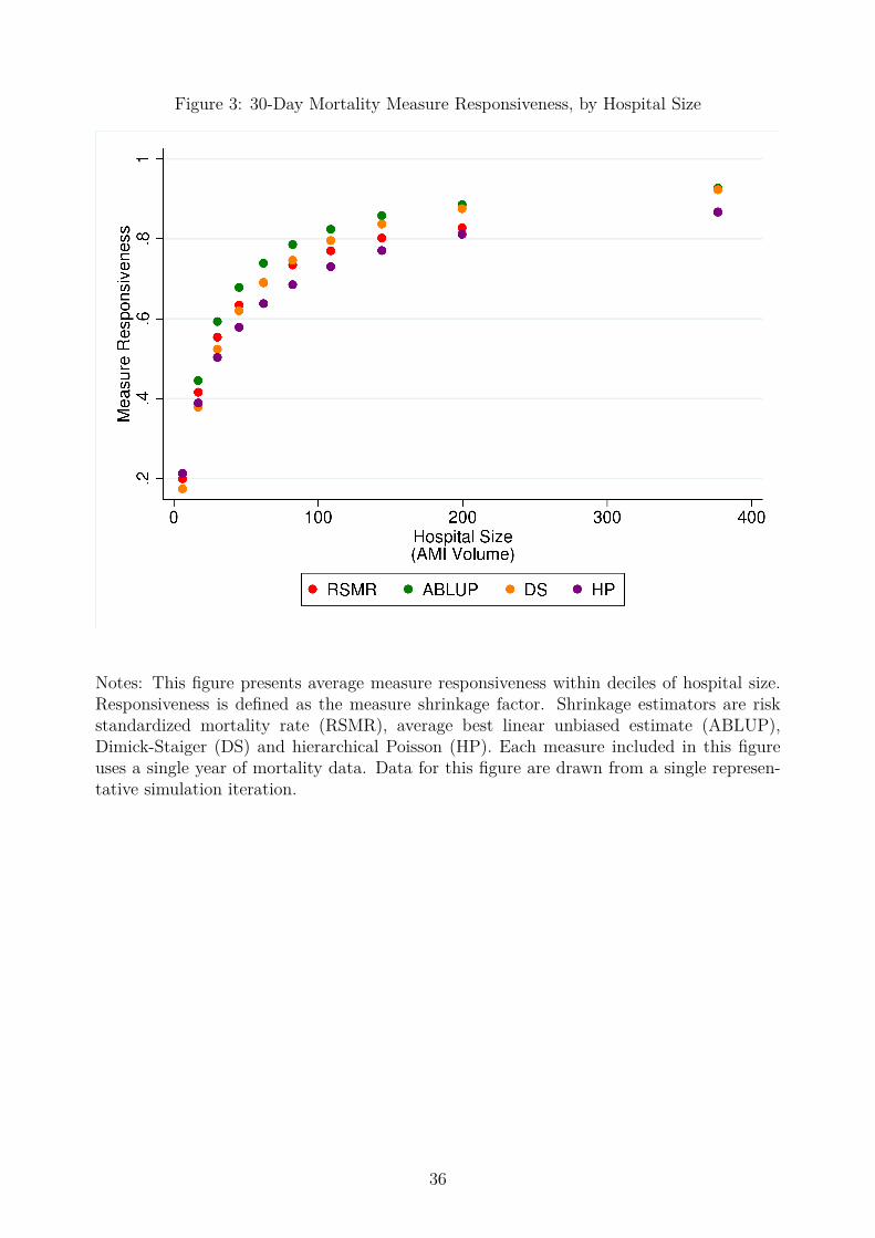
Figure 3: 30-Day Mortality Measure Responsiveness, by Hospital Size

Notes: This figure presents average measure responsiveness within deciles of hospital size.Responsiveness is defined as the measure shrinkage factor. Shrinkage estimators are riskstandardized mortality rate (RSMR), average best linear unbiased estimate (ABLUP),Dimick-Staiger (DS) and hierarchical Poisson (HP). Each measure included in this figureuses a single year of mortality data. Data for this figure are drawn from a single represen-tative simulation iteration.

36

Table 2: Comparison of Measure Accuracy for Moving Averages

Root Mean Square ErrorNo Temporal Trend in

PerformanceTemporal Trend in

PerformanceEstimator (1) (2)

One-Year Observed Mortality .101 .109Three-Year Unweighted Average .059 .116Three-Year Weighted Average .059 .100

Moving Average WeightsNo Temporal Trend in

PerformanceTemporal Trend in

PerformanceYear Before Index Year (1) (2)

t-1 0.33† .67t-2 0.33† .31t-3 0.33† .02

Notes: This table compares the accuracy of moving averages for performance measurementin two scenarios of hospital performance trajectories. In the column 1 simulation, hospitalperformance is constant over time. In the column 2 simulation, each hospital improves at anannual percent drawn from a normal distribution with mean zero and standard deviation oftwenty. The Monte Carlo simulations are iterated 1000 times. Error is the difference betweena measure value and true (unobserved) hospital performance in the following year, year t.The weights for each year of data in 3-year moving averages are determined by constrainedlinear regression of observed mortality in year t-1 on observed mortality in years t-2, t-3and t-4, with the sum of coefficients constrained to equal one. According to paired t-tests,within each simulation, all values of RMSE and all weights exhibit statistically significantpairwise differences except for those indicated by †.

37

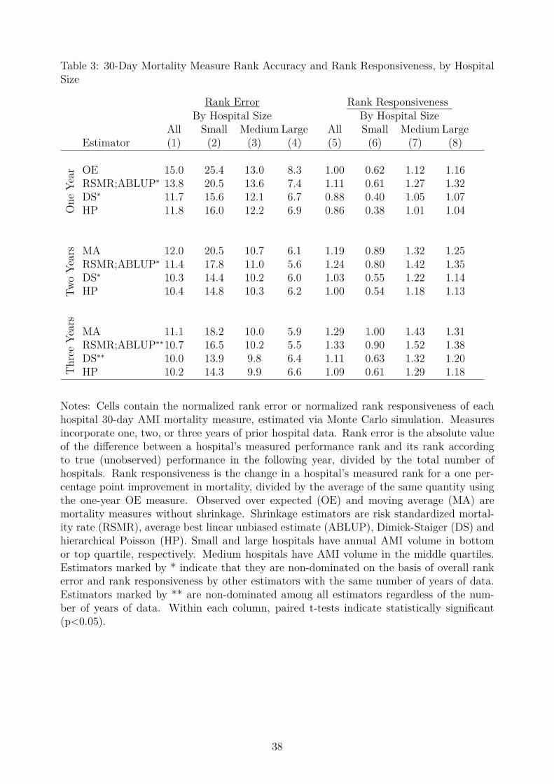
Table 3: 30-Day Mortality Measure Rank Accuracy and Rank Responsiveness, by HospitalSize

Rank Error Rank ResponsivenessBy Hospital Size By Hospital Size

All Small Medium Large All Small Medium LargeEstimator (1) (2) (3) (4) (5) (6) (7) (8)

One

Year OE 15.0 25.4 13.0 8.3 1.00 0.62 1.12 1.16

RSMR;ABLUP∗ 13.8 20.5 13.6 7.4 1.11 0.61 1.27 1.32DS∗ 11.7 15.6 12.1 6.7 0.88 0.40 1.05 1.07HP 11.8 16.0 12.2 6.9 0.86 0.38 1.01 1.04

Two

Year

s MA 12.0 20.5 10.7 6.1 1.19 0.89 1.32 1.25RSMR;ABLUP∗ 11.4 17.8 11.0 5.6 1.24 0.80 1.42 1.35DS∗ 10.3 14.4 10.2 6.0 1.03 0.55 1.22 1.14HP 10.4 14.8 10.3 6.2 1.00 0.54 1.18 1.13

Thr

eeYe

ars

MA 11.1 18.2 10.0 5.9 1.29 1.00 1.43 1.31RSMR;ABLUP∗∗10.7 16.5 10.2 5.5 1.33 0.90 1.52 1.38DS∗∗ 10.0 13.9 9.8 6.4 1.11 0.63 1.32 1.20HP 10.2 14.3 9.9 6.6 1.09 0.61 1.29 1.18

Notes: Cells contain the normalized rank error or normalized rank responsiveness of eachhospital 30-day AMI mortality measure, estimated via Monte Carlo simulation. Measuresincorporate one, two, or three years of prior hospital data. Rank error is the absolute valueof the difference between a hospital’s measured performance rank and its rank accordingto true (unobserved) performance in the following year, divided by the total number ofhospitals. Rank responsiveness is the change in a hospital’s measured rank for a one per-centage point improvement in mortality, divided by the average of the same quantity usingthe one-year OE measure. Observed over expected (OE) and moving average (MA) aremortality measures without shrinkage. Shrinkage estimators are risk standardized mortal-ity rate (RSMR), average best linear unbiased estimate (ABLUP), Dimick-Staiger (DS) andhierarchical Poisson (HP). Small and large hospitals have annual AMI volume in bottomor top quartile, respectively. Medium hospitals have AMI volume in the middle quartiles.Estimators marked by * indicate that they are non-dominated on the basis of overall rankerror and rank responsiveness by other estimators with the same number of years of data.Estimators marked by ** are non-dominated among all estimators regardless of the num-ber of years of data. Within each column, paired t-tests indicate statistically significant(p<0.05).

38