accuracy of wavelets, seismic inversion and thin bed ... 2017_accuracy of... ·...

79th EAGE Conference & Exhibition 2017 Paris, France, 12-15 June 2017

Th P2 05

Accuracy of Wavelets, Seismic Inversion and Thin Bed

Resolution

E. Zabihi Naeini* (Ikon Science), M. Sams (Ikon Science)

Summary

Broadband re-processed seismic data from the NW Shelf of Australia were inverted using a standard approach

to wavelet estimation. The inversion method applied was a facies-based deterministic inversion where the low-

frequency model is a product of the inversion process itself, constrained by facies dependent input trends, the

resultant facies distribution and the match to the seismic. The results identified the presence of a gas reservoir

that had recently been confirmed through drilling. The reservoir is thin, with up to 15 ms of maximum thickness.

The bandwidth of the seismic data is approximately 5-70 Hz and only a short well log was availabe to extract the

wavelets. As such there was little control on the lowest frequencies of the wavelet. Wavelets were then

estimated using a variety of new techniques that attempt to address the limitations of short well-log segments

and low frequency seismic. The revised inversion produced similar results but showed greater continuity and an

extension of the reservoir at one flank. These differences could be traced back to the low frequency component

of the inversion results and suggest that subtle variations in the low frequency component of wavelets can have

an impact on seismic reservoir characterisation of thin beds.


Introduction

The conventionally acquired Willem 3D seismic survey in the Carnarvon Basin of the North West Shelf of Australia was reprocessed to achieve a broader bandwidth by applying de-ghosting algorithms (Sams et al., 2016). The seismic were then inverted using a facies based inversion technology (Kemper and Gunning, 2014). One objective of the inversion was to explore the then recently discovered gas sand at the Pyxis-1 well. The inversion predicted the presence of a thin gas sand (approximately 60 ft. thick) within the Upper Jurassic, consistent with the reports from Woodside Petroleum. Despite this success, it was recognised at the time that the estimated wavelet might not be completely compatible with the seismic data given that the well data used for the inversion was only available over 400 ms and the bandwidth of the seismic was approximately 5-70 Hz. Uncertainties or errors in the representation of the lowest frequencies within the seismic data due to the lack of constraints provided by conventional wavelet estimation from limited well data might impact the detailed characterisation of the reservoir. The objective of the current study is to observe the differences in the estimated gas sand distribution of the Pyxis discovery for a range of wavelets derived with and without broadband considerations. We also show some synthetic scenarios to further assist in understanding the impact of wavelets on inversion for thin bed detection and characterisation.

Wavelet Estimation Methods

White and Zabihi Naeini (2014) proposed a practical frequency domain approach to handle the low frequency decay of the wavelet; both on the amplitude and phase spectra. Following this work, Zabihi Naeini et al. (2016) proposed new techniques for wavelet estimation for broadband seismic data namely parametric constant phase, frequency domain least-squares with multi-tapering and time domain Bayesian least-squares. Here we examine the parametric constant phase and time domain Bayesian least-squares and compare it to the traditionally derived wavelets using the Walden and White method (1998). We use a deterministic facies-based inversion to characterise the Pyxis gas reservoir. Three inversions are carried out using different wavelets: a) standard reference wavelets, b) constant phase wavelets, and c) time domain Bayesian least-squares wavelets. For full details of these techniques we refer to the above mentioned papers.

Real Data Example

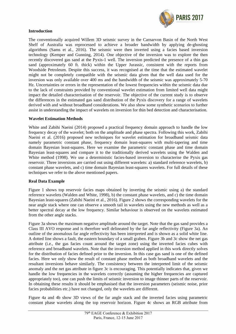
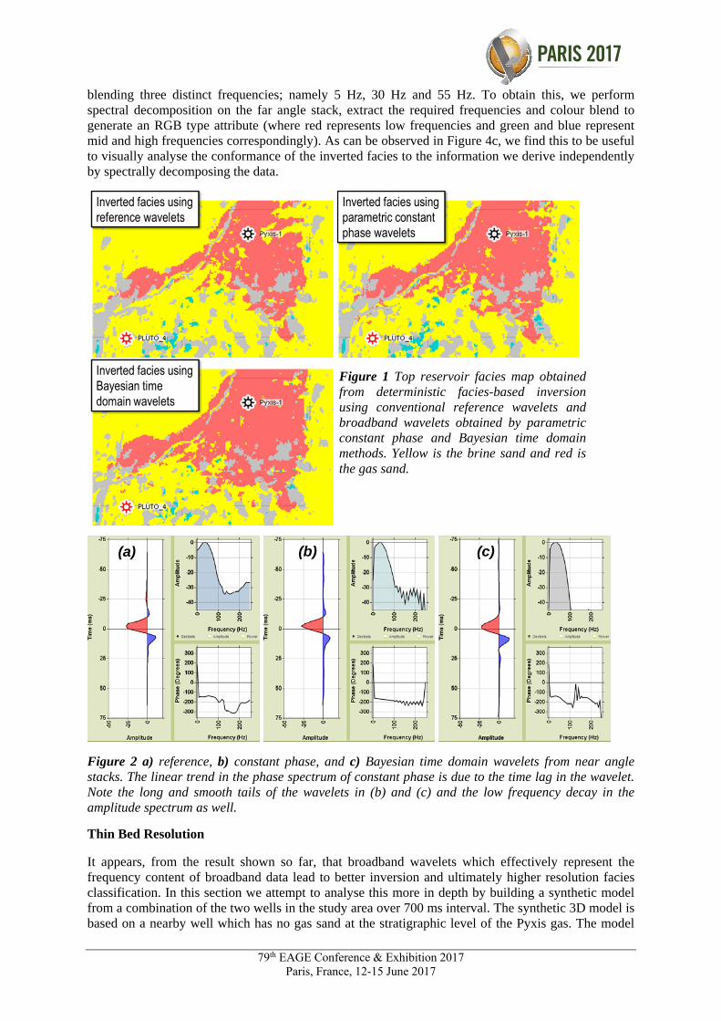
Figure 1 shows top reservoir facies maps obtained by inverting the seismic using a) the standard reference wavelets (Walden and White, 1998), b) the constant phase wavelets, and c) the time domain Bayesian least-squares (Zabihi Naeini et al., 2016). Figure 2 shows the corresponding wavelets for the near angle stack where one can observe a smooth tail in wavelets using the new methods as well as a better spectral decay at the low frequency. Similar behaviour is observed on the wavelets estimated from the other angle stacks.

Figure 3a shows the maximum negative amplitude around the target. Note that the gas sand provides a Class III AVO response and is therefore well delineated by the far angle reflectivity (Figure 3a). An outline of the anomalous far angle reflectivity has been interpreted and is shown as a solid white line. A dotted line shows a fault, the eastern boundary of a small graben. Figure 3b and 3c show the net gas attribute (i.e., the gas facies count around the target zone) using the inverted facies cubes with reference and broadband wavelets. Note that the inversion method applied in this work directly solves for the distribution of facies defined prior to the inversion. In this case gas sand is one of the defined facies. Here we only show the result of constant phase method as both broadband wavelets and the resultant inversions behave similarly. The consistency between the interpreted limit of the seismic anomaly and the net gas attribute in figure 3c is encouraging. This potentially indicates that, given we handle the low frequencies in the wavelets correctly (assuming the higher frequencies are captured appropriately too), one can push the limits of seismic inversion to image thinner parts of the reservoir. In obtaining these results it should be emphasised that the inversion parameters (seismic noise, prior facies probabilities etc.) have not changed, only the wavelets are different.

Figure 4a and 4b show 3D views of the far angle stack and the inverted facies using parametric constant phase wavelets along the top reservoir horizon. Figure 4c shows an RGB attribute from


blending three distinct frequencies; namely 5 Hz, 30 Hz and 55 Hz. To obtain this, we perform spectral decomposition on the far angle stack, extract the required frequencies and colour blend to generate an RGB type attribute (where red represents low frequencies and green and blue represent mid and high frequencies correspondingly). As can be observed in Figure 4c, we find this to be useful to visually analyse the conformance of the inverted facies to the information we derive independently by spectrally decomposing the data.

Figure 2 a) reference, b) constant phase, and c) Bayesian time domain wavelets from near angle stacks. The linear trend in the phase spectrum of constant phase is due to the time lag in the wavelet. Note the long and smooth tails of the wavelets in (b) and (c) and the low frequency decay in the amplitude spectrum as well.

Thin Bed Resolution

It appears, from the result shown so far, that broadband wavelets which effectively represent the frequency content of broadband data lead to better inversion and ultimately higher resolution facies classification. In this section we attempt to analyse this more in depth by building a synthetic model from a combination of the two wells in the study area over 700 ms interval. The synthetic 3D model is based on a nearby well which has no gas sand at the stratigraphic level of the Pyxis gas. The model

Figure 1 Top reservoir facies map obtained from deterministic facies-based inversion using conventional reference wavelets and broadband wavelets obtained by parametric constant phase and Bayesian time domain methods. Yellow is the brine sand and red is the gas sand.

(a) (b) (c)


introduces a wedge of gas sand at the level of the Pyxis discovery and four angle stacks have been created using an Ormsby wavelet with corner frequencies 4-8-30-60 Hz. Since it is a synthetic test we can easily modify the frequency content of the wavelets used for inversion without being biased by any wavelet estimation method. Therefore to fully capture the impact of wavelets and also understand the accuracy of the wavelet estimation method on the inverted facies we generate three scenarios:

1) an Ormsby wavelet with high frequency deficiency, 4-8-25-55 Hz, 2) an Ormsby wavelet with lowfrequency deficiency, 5-9-30-60 Hz, 3) an estimated wavelet using broadband Bayesian time domainmethod (Zabihi Naeini et al., 2016). These wavelets are shown in Figure 6 and as can be observed one

(a) (b)

(c) Figure 3 a) far angle stack maximum negative amplitude map, b) net gas attribute using inverted facies with reference wavelets, and c) with broadband constant phase wavelets.

(a) (b)

(c) Figure 4 a) far angle stack amplitude map, b) inverted facies with broadband wavelets, and c) RGB blended attribute from spectraldecomposition of the far stack. Note the thickblack contour in Figure 4c demonstrates theboundaries of the inverted gas sand facies (inred) in 4b.


has to look closely to spot the differences. Despite that, these minor differences, on the order of 1 to 2 Hz, will have a rather major impact on the resolution and the inverted facies. Most importantly the low frequency deficiency leads to an underestimation of the gas sand at the thinning part of the wedge. Consistent with what we observed on real data the accuracy of the low frequencies plays a key role.

Figure 6 Inverted facies from the true reference wavelet (a), the wavelet with high frequency deficiency (b), low frequency deficiency (c) and the estimated broadband wavelet (d). Arrow shows the extent of gas sand recovered with the true reference wavelet in 6a.

Conclusions

Broadband seismic data should be inverted using broadband wavelets to reveal the full benefits. Analysis of the inverted facies (and impedance properties) using broadband wavelets and the comparison with conventional wavelets showed how appropriate capturing of the low frequencies, even subtle differences as low as 1 Hz, can enhance the interpretation of the reservoir. Also in places where the low frequency content does not dominate, the proper handling of the low frequencies can have an impact on the interpretation of thin beds. Of course the complexity of the geology and seismic noise make it even harder to achieve the optimal resolution.

Acknowledgements

The authors would like to thank Searcher Seismic for access to the seismic data.

References

Kemper M. and Gunning J. [2014] Joint impedance and facies inversion – Seismic inversion redefined. First Break, 32, 89–95.

Sams, M., Westlake, S., Thorp, J. and Zadeh, E. [2016] Willem 3D: Reprocessed, inverted, revitalized. The Leading Edge, 35(1), 22–26.

Walden A. and White R. [1998] Seismic wavelet estimation: a frequency domain solution to a geophysical noisy input–output problem. IEEE Transactions on Geoscience and Remote Sensing, 36(1), 287-297.

White R.E. and Zabihi Naeini E. [2014] Broad-band well tie. 76th EAGE Conference & Exhibition, Extended Abstract, Tu EL12 10.

Zabihi Naeini E., Gunning J. and White R. [2016] Well tie for broadband seismic data. Geophysical Prospecting, doi: 10.1111/1365-2478.12433.

accuracy of wavelets, seismic inversion and thin bed ... 2017_accuracy of... ·...

Documents