accuracy assessment of georectified aerial photographs...

www.elsevier.com/locate/geomorph

Geomorphology 74

Accuracy assessment of georectified aerial photographs:

Implications for measuring lateral channel movement in a GIS

Michael L. Hughes*, Patricia F. McDowell, W. Andrew Marcus

Department of Geography, University of Oregon, Eugene, OR 97403-1251, USA

Received 3 September 2004; received in revised form 8 July 2005; accepted 11 July 2005

Abstract

Aerial photographs are commonly used to measure planform river channel change. We investigated the sources and

implications of georectification error in the measurement of lateral channel movement by testing how the number (6–30)

and type (human versus natural landscape features) of ground-control points (GCPs) and the order of the transformation

polynomial (first-, second-, and third-order) affected the spatial accuracy of a typical georectified aerial photograph. Error was

assessed using the root-mean-square error (RMSE) of the GCPs as well as error in 31 independent test points. The RMSE and

the mean and median values of test-point errors were relatively insensitive to the number of GCPs above eight, but the upper

range of test-point errors showed marked improvement (i.e., the number of extreme errors was reduced) as more GCPs were

used for georectification. Using more GCPs thus improved overall georectification accuracy, but this improvement was not

indicated by the RMSE, suggesting that independent test-points located in key areas of interest should be used in addition to

RSME to evaluate georectification error.

The order of the transformation polynomial also influenced test-point accuracy; the second-order polynomial function

yielded the best result for the terrain of the study area. GCP type exerted a less consistent influence on test-point accuracy,

suggesting that although hard-edged points (e.g., roof corners) are favored as GCPs, some soft-edged points (e.g., trees) may be

used without adding significant error. Based upon these results, we believe that aerial photos of a floodplain landscape similar to

that of our study can be consistently georectified to an accuracy of approximately F5 m, with ~10% chance of greater error.

The implications of georectification error for measuring lateral channel movement are demonstrated with a multiple buffer

analysis, which documents the inverse relationship between the size of the buffers applied to two channel centerlines and the

magnitude of change detected between them. This study demonstrates the importance of using an independent test-point

analysis in addition to the RSME to evaluate and treat locational error in channel change studies.

D 2005 Published by Elsevier B.V.

Keywords: Channel change; Channel migration; Georectification; Aerial photographs; Geospatial error; GIS

0169-555X/$ - s

doi:10.1016/j.ge

* Correspondi

E-mail addre

(2006) 1–16

ee front matter D 2005 Published by Elsevier B.V.

omorph.2005.07.001

ng author. Fax: +1 541 346 2067.

ss: [email protected] (M.L. Hughes).

M.L. Hughes et al. / Geomorphology 74 (2006) 1–162

1. Introduction

Aerial photographs are rich sources of information

on historical river conditions (Trimble, 1991; Lawler,

1993) and have been widely used to track the historical

planform evolution of river systems (e.g., Lewin and

Weir, 1977; Petts, 1989; Gurnell, 1997; Surian, 1999;

Graf, 2000; Winterbottom and Gilvear, 2000; O’Con-

nor et al., 2003; plus many others). Historical planform

channel analysis typically involves the co-registration

of aerial photos and maps from different years so

channel positions can be analyzed in overlay. Since

the 1980s, the development of desktop GIS software

and improvements in remote sensing and digital scan-

ning technology have enabled users to more efficiently

scan and co-register aerial photos; however, spatial

error in digital imagery (including scanned aerial

photos) is inevitable and can impart inaccuracies in

measurements of lateral channel movement.

While there is widespread recognition in the

GIScience community of the sources, types, and impli-

cations of locational error in geospatial data sets

(Chrisman, 1982, 1992; Goodchild and Gopal, 1989;

Unwin, 1995; Leung and Yan, 1998), fluvial geomor-

phologists have generally ignored the magnitude of

geospatial error in relation to geomorphic change or

have used only Root Mean Square Error (RMSE) as a

measure of this error (e.g., Urban and Rhoads, 2004).

Only recently have fluvial geomorphologists begun to

embrace geospatial error as an independent research

topic (e.g., Mount and Louis, 2005). Consequently,

despite the development of approaches for measuring

positional accuracy of linear features (e.g., Goodchild

and Hunter, 1997; Leung and Yan, 1998) and recogni-

tion of the inherent problems of positional error on

maps of rivers (Hooke and Redmond, 1989; Locke and

Wyckoff, 1993) and lakes (Butler, 1989), there is no

widely supported conceptual framework for evaluating

and treating positional error on digital imagery in the

measurement of lateral channel movement.

In this article, we seek to identify the magnitude

and controls of geospatial error in georectified aerial

photos and to address the implications of this error for

measuring lateral channel movement. Accordingly,

we raise the following questions:

(i) How is the locational accuracy of georectified

aerial photos affected by the number and type

of ground control points (GCPs) and the

order of polynomial transformation used in

georectification?

(ii) Is root-mean-square error (RMSE) a good proxy

of overall georectification error?

(iii) What are the implications of georectifcation

error for quantifying lateral channel movement

and how can such error be minimized?

We address these questions using repeated georec-

tification of an aerial photo showing the Umatilla

River in northeastern Oregon. The quality and scale

of this imagery is typical of those used throughout

North America and many other parts of the world to

reconstruct river histories. This article is the first

phase of a broader study to evaluate channel and

floodplain change resulting from large floods in

selected rivers of the U.S. Pacific Northwest.

2. Background

GIScience and remote sensing play an increasingly

significant role in geomorphological studies. Some

recent examples of topics that have benefited from

advances in the generation and handling of digital

geospatial data include (but are not limited to) map-

ping and modeling of: fluvial erosion (Finlayson and

Montgomery, 2003), complex terrain (Wilson and

Gallant, 2000), mass wasting (Roering et al., 2005);

mountain topography (Schroder and Bishop, 2004),

historical channel change (Leys and Werrity, 1999;

Collins et al., 2003), and river habitats (Marcus et al.,

2003) and depths (Fonstad and Marcus, 2005). While

many studies have developed methods for using digi-

tal data (e.g., aerial photos, satellite images, historical

maps, and digital elevation models) to address tradi-

tional research topics, relatively few studies have

rigorously addressed the effects of geospatial data

quality on the results of geomorphic analyses

(although see Holmes et al., 2000; Mount et al.,

2003; Mount and Louis, 2005). Therefore, geomor-

phologists currently using digital geospatial need to

better understand how the quality of geospatial data

may affect analyses of digital data sets and to under-

stand what factors control such data quality. Develop-

ment of error-sensitive change detection methods

depends on this knowledge. As GIScience continues

M.L. Hughes et al. / Geomorphology 74 (2006) 1–16 3

to better establish a theoretical basis in geography,

opportunities are emerging for geomorphologists to

undertake GIScience studies aimed at better under-

standing the applicability and limitations of digital

geospatial data in their research.

2.1. General notes and terminology

Before aerial photos can be overlaid to map chan-

nel change in a GIS, they must be scanned and co-

registered. Aerial photo co-registration refers to the

conversion of digitally scanned photos to a common

projection and coordinate system. Co-registration is

usually achieved by georegistering individual photos

to the same base layer. Digital orthophotographs

(DOQs) and topographic maps (DRGs, digital raster

graphics) are typically used as base layers.

Several techniques are available for co-registra-

tion of digital aerial photographs in a GIS, including

aerotriangulation, orthorectification, and polynomial

transformation. Each of these techniques has advan-

tages and disadvantages that make it appropriate for

specific applications. Aerotriangulation and orthor-

ectification are typically used only when polynomial

georectification fails to yield acceptable results. Dur-

ing aerotriangulation, GCPs are forced to have iden-

tical coordinates on the target (unregistered) layer

and (georeferenced) base layer, thereby causing the

image to be warped along triangulated edges rather

than at point locations. This process requires a large

number of GCPs for high accuracy and can there-

fore be difficult to apply in river change analysis

because the number and distribution of GCPs are

often limited. Moreover, error on triangulated photos

varies in a nonsystematic fashion, complicating error

analysis and application of buffers for reducing error

and uncertainty during change detection. By con-

trast, orthorectification can provide high degrees of

geospatial accuracy, but is less commonly employed

by geomorphologists because it requires sophisti-

cated software and is generally more labor- and

data-intensive.

In this article, we evaluate polynomial georectifi-

cation, which is readily applied to large sets of aerial

photos (e.g., photos from flight lines along a river),

can be performed with most commercially available

GIS software packages, and is widely used for co-

registration of aerial photos. When coupled with pixel

resampling to correct for image warping during trans-

formation, the process is called polynomial georecti-

fication. After scanning the original paper photo to

create a digital file, polynomial georectification is

performed in three steps: (i) matching of ground-con-

trol points (GCPs) on the scanned photo image and

base layer, (ii) transformation of the GCP coordinates

on the scanned image from a generic raster set to a

geographical projection and coordinate system, and

(iii) pixel resampling.

2.2. Aerial photo scanning

During the scanning procedure, the user defines the

type (color versus gray scale) and resolution (dots per

inch or d.p.i.) of the scan. Color and gray scale photos

are customarily scanned into color and gray scale

digital images, respectively. Because some data are

blostQ in this digital conversion, users tend to max-

imize the resolution of the scan to improve image

quality; however, users should consider the resolution

of the base layer to which the digital photo will be

registered before selecting a scan resolution. Scanning

to a pixel resolution of 0.1 m, for example, makes

little sense if the base-layer resolution is 2.0 m. Data

loss during photo georectification, which includes

pixel resampling (discussed below), may be mini-

mized if the resolution of the scanned photo and

georeferenced base layer are similar.

2.3. GCP selection for channel change analysis

The number, distribution, and type of GCPs can

affect the accuracy of polynomial georectification, and

researchers investigating river channel change have

offered different guidelines for GCP selection. In

examining historical planform change using scanned

maps, Leys and Werrity (1999) noted that GCPs

should be widely distributed across the image to

provide a bstable warp,Q while Richards (1986) and

Campbell (2002) advised that the majority of control

points should be located around the edge of the image

with several uniformly spaced points in its central

portion. While these suggestions may be appropriate

for satellite images that have relatively little error due

to topographic variations, or for scanned maps with

constant scale variations across their projections, they

are not necessarily well suited for historical aerial


photos, which usually have GCPs and areas of analy-

tical interest that are unevenly distributed across the

image over space and time, particularly in rural or

forested settings. Moreover, better accuracy may be

obtained by concentrating GCPs near the features of

interest rather than across the entire aerial photo. This

is particularly true with river channels, which tend to

flow through floodplains of low relief and may be

surrounded by valley walls of relatively high relief.

Selecting GCPs that are far removed from the river

channel may unnecessarily skew the transformation

toward topographically complex areas not representa-

tive of the river channel and floodplain.

In addition to GCP distribution, GCP type can

affect georectification accuracy. For the purposes of

this study, we define two types of GCPs: hard and soft

points. Hard points are features that have a sharp edge

or corner, so their locations can be pinpointed. Hard

points may include features such as building corners,

road intersections, fences, and sidewalks. Soft points

are features with irregular or fuzzy edges, such as rock

outcrops and the centers of individual trees and shrub

clusters. Because it is more difficult to pinpoint a soft

point and because soft points may change over time

(e.g., as when a tree grows larger), the choice of soft

rather than hard points can affect overall georectifica-

tion accuracy. However, in order to have enough

GCPs for polynomial georectification, particularly in

riverine environments, it is sometimes necessary to

intermix hard and soft GCPs; therefore, soft points

often cannot be categorically excluded.

Another challenging aspect of locating GCPs on

historical aerial photos is that the correspondence

between features on photos collected years or dec-

ades apart is sometimes poor. Buildings, roads,

fences, trees, and other similar features can be

moved, obliterated, or altered over time. Even in

developed areas, GCPs may be difficult to locate

and users are often faced with using a sub-optimal

number, type, or spatial distribution of GCPs.

2.4. Polynomial georectification, transformation

order, and RMSE

Polynomial transformation is applied to unregis-

tered raster images (including scanned aerial photos)

using linear and nonlinear functions. Polynomial

transformations are named by their order, or the

numerical value of the highest exponent used in

the polynomial function. Therefore, first-order, sec-

ond-order, and third-order transformations are linear,

quadratic, and cubic transformations, respectively.

When curvilinear (i.e., quadratic or higher) functions

are used, the term brubbersheetingQ is sometimes

applied, although this term may also be applied to

aerotriangulation. Transformations using curvilinear

functions are popular for aerial photos of the scale

and terrain of this study because they can correct for

some of the effects of both radial error (related to

curvature of the earth) and geometric error (related to

topography and camera lens distortion) and can

therefore lend map-like qualities to a georectified

photo without orthorectification. Remote sensing

textbooks and photogrammetry manuals tend to

emphasize the use of first-order and second-order

transformations (e.g., Campbell, 2002; Leica Geosys-

tems, 2003), because third- and higher order trans-

formations tend to excessively warp digital images.

During polynomial transformation, a least-squares

function is fit between GCP coordinates on the

scanned image and base layer. This function is then

used to assign coordinates to the entire photo. After

transformation, GCPs on the photo and base layer will

have slightly different coordinates, depending on the

degree to which the overall transformation affects the

proximal area of each GCP. The difference in location

between the GCPs on the transformed layer and base

layer is often represented by the total root-mean-

square error (RMSE), a metric based in the Pythagor-

ean Theorem and calculated for a coordinate pair by

the equation (Slama et al., 1980)

RMSE ¼ xs � xrð Þ2 þ ys � yrð Þ2h i1=2

ð1Þ

where xs and ys are geospatial coordinates of the point

on the source image; and xr and yr are coordinates of

the same point on the transformed aerial photo. The

RMSE for the whole image is the sum of the RMSE

for each coordinate divided by the square root of the

number of coordinate pairs.

2.5. Pixel resampling

Spatial transformations typically generate a differ-

ent number of pixels in the transformed image than in

the original image. Moreover second-order or higher


transformations can create pixels of variable size

across the transformed image. A resampling step is

necessary to equalize pixel size throughout the image

and to assign values from the original image to the

transformed image. There are a number of resampling

approaches; nearest neighbor, bilinear, and cubic con-

volution (Campbell, 2002) resampling schemes are

most common and are included in almost all GIS

programs. We found that cubic convolution produced

output photos best suited for interpretation of fluvial

features because it smoothes jagged edges along linear

boundaries (e.g., river banks). Nearest neighbor

resampling can create jagged feature boundaries, but

does not alter the original pixel values, a critical

element if spectral analysis of the image is planned.

Bilinear resampling provides intermediate results in

comparison to the other two techniques. If the refer-

ence and transformed images are approximately the

same resolution, variations in resampling methods

should not alter spatial location by more than approxi-

mately +0.5 pixels; however, because resampling

methods affect image interpretation, we recommend

experimentation with different resampling methods to

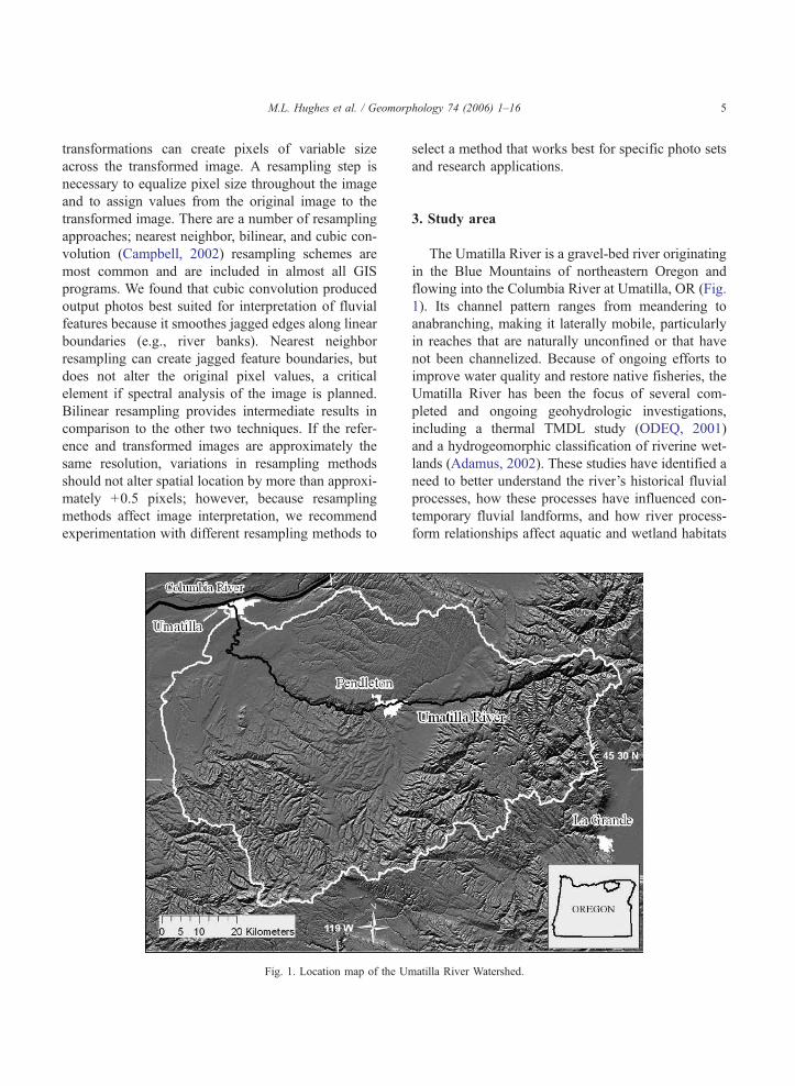
Fig. 1. Location map of the Um

select a method that works best for specific photo sets

and research applications.

3. Study area

The Umatilla River is a gravel-bed river originating

in the Blue Mountains of northeastern Oregon and

flowing into the Columbia River at Umatilla, OR (Fig.

1). Its channel pattern ranges from meandering to

anabranching, making it laterally mobile, particularly

in reaches that are naturally unconfined or that have

not been channelized. Because of ongoing efforts to

improve water quality and restore native fisheries, the

Umatilla River has been the focus of several com-

pleted and ongoing geohydrologic investigations,

including a thermal TMDL study (ODEQ, 2001)

and a hydrogeomorphic classification of riverine wet-

lands (Adamus, 2002). These studies have identified a

need to better understand the river’s historical fluvial

processes, how these processes have influenced con-

temporary fluvial landforms, and how river process-

form relationships affect aquatic and wetland habitats

atilla River Watershed.


important to native species. Channel modifications,

including levees and revetments, are believed to

degrade physical habitats and water quality by physi-

cally constraining the river channel and hampering

lateral channel movements that may otherwise benefit

habitat quality. Therefore, a detailed understanding

lateral channel movement serves a variety of river

science and management needs.

4. Study design and methods

We hypothesized that georectification accuracy

would improve when larger numbers of GCPs are

used, when hard rather than soft GCPs are selected,

and when a second-order polynomial is applied for

spatial transformation. To test these hypotheses, we

repeatedly georectified a 1964, 1 :20,000 black-and-

white aerial photo of the Umatilla River at Pendleton,

OR (ASCS, 1964), varying the hypothesized controls

to evaluate their relative effects. The quality and scale

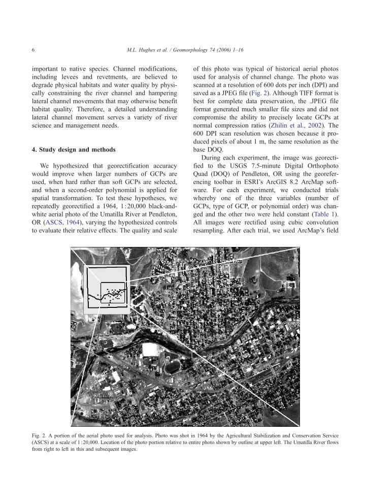
Fig. 2. A portion of the aerial photo used for analysis. Photo was shot i

(ASCS) at a scale of 1 :20,000. Location of the photo portion relative to en

from right to left in this and subsequent images.

of this photo was typical of historical aerial photos

used for analysis of channel change. The photo was

scanned at a resolution of 600 dots per inch (DPI) and

saved as a JPEG file (Fig. 2). Although TIFF format is

best for complete data preservation, the .JPEG file

format generated much smaller file sizes and did not

compromise the ability to precisely locate GCPs at

normal compression ratios (Zhilin et al., 2002). The

600 DPI scan resolution was chosen because it pro-

duced pixels of about 1 m, the same resolution as the

base DOQ.

During each experiment, the image was georecti-

fied to the USGS 7.5-minute Digital Orthophoto

Quad (DOQ) of Pendleton, OR using the georefer-

encing toolbar in ESRI’s ArcGIS 8.2 ArcMap soft-

ware. For each experiment, we conducted trials

whereby one of the three variables (number of

GCPs, type of GCP, or polynomial order) was chan-

ged and the other two were held constant (Table 1).

All images were rectified using cubic convolution

resampling. After each trial, we used ArcMap’s field

n 1964 by the Agricultural Stabilization and Conservation Service

tire photo shown by outline at upper left. The Umatilla River flows

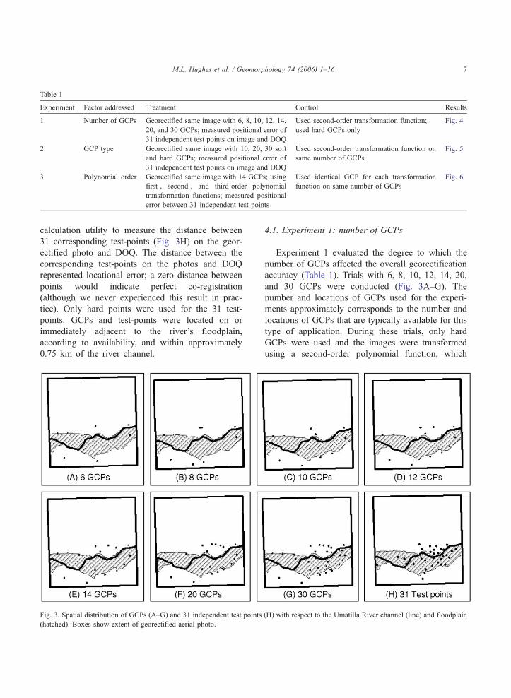
Table 1

Experiment Factor addressed Treatment Control Results

1 Number of GCPs Georectified same image with 6, 8, 10, 12, 14,

20, and 30 GCPs; measured positional error of

31 independent test points on image and DOQ

Used second-order transformation function;

used hard GCPs only

Fig. 4

2 GCP type Georectified same image with 10, 20, 30 soft

and hard GCPs; measured positional error of

31 independent test points on image and DOQ

Used second-order transformation function on

same number of GCPs

Fig. 5

3 Polynomial order Georectified same image with 14 GCPs; using

first-, second-, and third-order polynomial

transformation functions; measured positional

error between 31 independent test points

Used identical GCP for each transformation

function on same number of GCPs

Fig. 6


calculation utility to measure the distance between

31 corresponding test-points (Fig. 3H) on the geor-

ectified photo and DOQ. The distance between the

corresponding test-points on the photos and DOQ

represented locational error; a zero distance between

points would indicate perfect co-registration

(although we never experienced this result in prac-

tice). Only hard points were used for the 31 test-

points. GCPs and test-points were located on or

immediately adjacent to the river’s floodplain,

according to availability, and within approximately

0.75 km of the river channel.

Fig. 3. Spatial distribution of GCPs (A–G) and 31 independent test points

(hatched). Boxes show extent of georectified aerial photo.

4.1. Experiment 1: number of GCPs

Experiment 1 evaluated the degree to which the

number of GCPs affected the overall georectification

accuracy (Table 1). Trials with 6, 8, 10, 12, 14, 20,

and 30 GCPs were conducted (Fig. 3A–G). The

number and locations of GCPs used for the experi-

ments approximately corresponds to the number and

locations of GCPs that are typically available for this

type of application. During these trials, only hard

GCPs were used and the images were transformed

using a second-order polynomial function, which

(H) with respect to the Umatilla River channel (line) and floodplain


yielded the best results during pilot trials. We plotted

five indicators to evaluate the magnitude of and con-

trols on georectification error: the RMSE of GCPs

and the mean, median, 90th percentile cumulative

error value and maximum distances between test-

points on the georectified image and DOQ. The

degree of correspondence between the reported

RMSE and the summary statistics for the 31 test-

points provided the basis for evaluating georectifica-

tion accuracy.

4.2. Experiment 2: GCP type

Experiment 2 tested how using hard- versus soft-

edged GCPs affected georectification accuracy.

Hard-edged GCPs were defined as landscape fea-

tures with permanent, easily identified corners or

edges and mainly included building corners, but

also included fence corners and street and sidewalk

intersections. Soft-edged GCPs were defined as fea-

tures with bsoftQ or fuzzy edges; in this study we

used only isolated tree canopies for soft-edged

GCPs. Trials were conducted to compare test-point

error resulting from transformations based on 10, 20,

and 30 hard or soft point GCPs (Table 1). A second-

order polynomial transformation was used for all the

experimental trials. Differences in median and range

of test-point values from trial to trial provided the

basis for evaluating the effects of test-point type on

georectification accuracy.

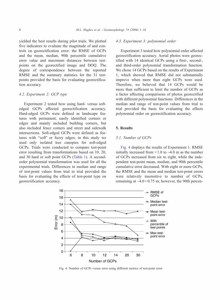
Fig. 4. Number of GCPs versus error using

4.3. Experiment 3: polynomial order

Experiment 3 tested how polynomial order affected

georectification accuracy. Aerial photos were georec-

tified with 14 identical GCPs using a first-, second-,

and third-order polynomial transformation function.

We chose 14 GCPs based on the results of Experiment

1, which showed that RMSE did not substantially

improve when more than eight GCPs were used.

Therefore, we believed that 14 GCPs would be

more than sufficient to limit the number of GCPs as

a factor affecting comparisons of photos georectified

with different polynomial functions. Differences in the

median and range of test-point values from trial to

trial provided the basis for evaluating the effects

polynomial order on georectification accuracy.

5. Results

5.1. Number of GCPs

Fig. 4 displays the results of Experiment 1. RMSE

initially increased from b1.0 to ~4.0 m as the number

of GCPs increased from six to eight, while the inde-

pendent test-point mean, median, and 90th percentile

cumulative error decreased. With eight or more GCPs,

the RMSE and the mean and median test-point errors

were relatively insensitive to number of GCPs,

remaining at ~4.0+0.75 m; however, the 90th percen-

different metrics of test-point error.

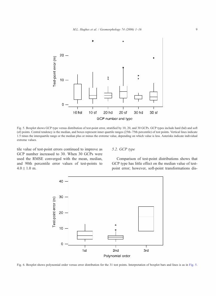
Fig. 5. Boxplot shows GCP type versus distribution of test-point error, stratified by 10, 20, and 30 GCPs. GCP types include hard (hd) and soft

(sf) points. Central tendency is the median, and boxes represent inner quartile ranges (25th–75th percentile) of test points. Vertical lines indicate

1.5 times the interquartile range or the median plus or minus the extreme value, depending on which value is less. Asterisks indicate individual

extreme values.


tile value of test-point errors continued to improve as

GCP number increased to 30. When 30 GCPs were

used the RMSE converged with the mean, median,

and 90th percentile error values of test-points to

4.0F1.0 m.

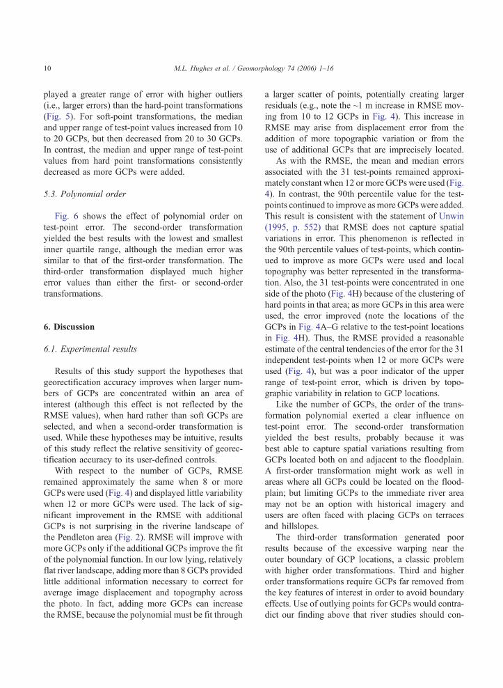
Fig. 6. Boxplot shows polynomial order versus error distribution for the 3

5.2. GCP type

Comparison of test-point distributions shows that

GCP type has little effect on the median value of test-

point error; however, soft-point transformations dis-

1 test points. Interpretation of boxplot bars and lines is as in Fig. 5.


played a greater range of error with higher outliers

(i.e., larger errors) than the hard-point transformations

(Fig. 5). For soft-point transformations, the median

and upper range of test-point values increased from 10

to 20 GCPs, but then decreased from 20 to 30 GCPs.

In contrast, the median and upper range of test-point

values from hard point transformations consistently

decreased as more GCPs were added.

5.3. Polynomial order

Fig. 6 shows the effect of polynomial order on

test-point error. The second-order transformation

yielded the best results with the lowest and smallest

inner quartile range, although the median error was

similar to that of the first-order transformation. The

third-order transformation displayed much higher

error values than either the first- or second-order

transformations.

6. Discussion

6.1. Experimental results

Results of this study support the hypotheses that

georectification accuracy improves when larger num-

bers of GCPs are concentrated within an area of

interest (although this effect is not reflected by the

RMSE values), when hard rather than soft GCPs are

selected, and when a second-order transformation is

used. While these hypotheses may be intuitive, results

of this study reflect the relative sensitivity of georec-

tification accuracy to its user-defined controls.

With respect to the number of GCPs, RMSE

remained approximately the same when 8 or more

GCPs were used (Fig. 4) and displayed little variability

when 12 or more GCPs were used. The lack of sig-

nificant improvement in the RMSE with additional

GCPs is not surprising in the riverine landscape of

the Pendleton area (Fig. 2). RMSE will improve with

more GCPs only if the additional GCPs improve the fit

of the polynomial function. In our low lying, relatively

flat river landscape, addingmore than 8 GCPs provided

little additional information necessary to correct for

average image displacement and topography across

the photo. In fact, adding more GCPs can increase

the RMSE, because the polynomial must be fit through

a larger scatter of points, potentially creating larger

residuals (e.g., note the ~1 m increase in RMSE mov-

ing from 10 to 12 GCPs in Fig. 4). This increase in

RMSE may arise from displacement error from the

addition of more topographic variation or from the

use of additional GCPs that are imprecisely located.

As with the RMSE, the mean and median errors

associated with the 31 test-points remained approxi-

mately constant when 12 or more GCPs were used (Fig.

4). In contrast, the 90th percentile value for the test-

points continued to improve as more GCPs were added.

This result is consistent with the statement of Unwin

(1995, p. 552) that RMSE does not capture spatial

variations in error. This phenomenon is reflected in

the 90th percentile values of test-points, which contin-

ued to improve as more GCPs were used and local

topography was better represented in the transforma-

tion. Also, the 31 test-points were concentrated in one

side of the photo (Fig. 4H) because of the clustering of

hard points in that area; as more GCPs in this area were

used, the error improved (note the locations of the

GCPs in Fig. 4A–G relative to the test-point locations

in Fig. 4H). Thus, the RMSE provided a reasonable

estimate of the central tendencies of the error for the 31

independent test-points when 12 or more GCPs were

used (Fig. 4), but was a poor indicator of the upper

range of test-point error, which is driven by topo-

graphic variability in relation to GCP locations.

Like the number of GCPs, the order of the trans-

formation polynomial exerted a clear influence on

test-point error. The second-order transformation

yielded the best results, probably because it was

best able to capture spatial variations resulting from

GCPs located both on and adjacent to the floodplain.

A first-order transformation might work as well in

areas where all GCPs could be located on the flood-

plain; but limiting GCPs to the immediate river area

may not be an option with historical imagery and

users are often faced with placing GCPs on terraces

and hillslopes.

The third-order transformation generated poor

results because of the excessive warping near the

outer boundary of GCP locations, a classic problem

with higher order transformations. Third and higher

order transformations require GCPs far removed from

the key features of interest in order to avoid boundary

effects. Use of outlying points for GCPs would contra-

dict our finding above that river studies should con-


strain GCPs to the area of the interest near the river. In

general, it is hard to imagine a scenario where third or

higher order transformations would be appropriate for

studies of areas with similar topography.

In comparison to the number of GCPs and transfor-

mation order, GCP type exerted a less consistent influ-

ence on georectification accuracy. The median values

of test-points derived from hard- and soft-point trans-

formations were generally similar. However, the quar-

tile ranges and outlying values were greater for the

soft-point transformations when 20 or 30 GCPs were

used. In contrast, with 10 GCPs both the median and

inner quartile range were lower for the soft-point

transformation, probably because the distribution of

soft points was more favorable with respect to the 31

independent test-points. Results suggest that hard

points should ideally serve as the basis for polynomial

georectification, but that some soft points may be used

without significantly changing the average transforma-

tion error or overall georectification accuracy.

These results have significant implications for under-

standing the positional accuracy of rivers and other

landscape features on georectified aerial photos. First,

GCPs on historical aerial photos are typically limited in

number, so transformations are often generated from a

limited number of GCPs that may or may not be repre-

sentative of key areas of interest. The baverageQ posi-tional accuracy in such cases may therefore be

acceptable, but local errors, perhaps critical to the

measurements, may be missed. Second, users tend to

remove brogueQ points to improve RMSE. Our results

suggest that, contrary to intuition, this practice may

actually diminish georectification accuracy in key

areas where the additional GCP(s) may otherwise

improve accuracy. Third, tracking the relation between

RMSE and number of GCPs may be misleading

because using more GCPs can result in better trans-

formations, even when the RMSE appears to have

stabilized. In general, increasing the spatial density

of GCPs within an area of interest (when possible)

can reduce the overall range of error for that area and

potentially for the entire image.

6.2. Implications for measuring lateral channel move-

ment in GIS

Most approaches for measuring lateral channel

movement with aerial imagery fall into one of two

categories. Leopold (1973) introduced the concept

(since used by many authors: e.g., Gurnell et al.,

1994; O’Connor et al., 2003) of measuring the

change in distance of the intersection of the channel

centerline (or margin) with a series of floodplain or

cross-valley transects. This method generates a set of

change-distance measurements, the number of which

depends on stream length and transect spacing. A

second approach treats the floodplain and channel as

rasters or polygons that can be mapped on aerial

imagery to determine migration rates over time

(e.g., Graf, 1984; Urban and Rhoads, 2004). In this

approach, channel locations from sequential images

are overlaid to calculate changes in channel area

(m2) per unit channel length (m), and therefore a

distance of migration (m2 /m=m) for each river-

length unit. Both approaches rely on image overlay,

making them sensitive to geospatial error on compo-

nent layers.

Alongside these two approaches of channel change

detection, researchers have adopted several

approaches to treat geospatial error in the measure-

ment of channel change. Two approaches are com-

mon: (i) treating error as negligible with respect to the

magnitude of geomorphic change, and (ii) applying

buffers within which any apparent bchangeQ is attrib-uted to error and therefore disregarded. Until recently,

many authors have adopted the first of these

approaches without evaluating the effects of error on

change measurements; however, the growing empha-

sis on remote sensing and GIS techniques in fluvial

geomorphology has begun to shed light on issues of

scale and error in geomorphic analyses (e.g., Gilvear

and Byant, 2003; Marcus et al., 2004), prompting

some researchers to recognize the value of error-sen-

sitive change detection methodologies. For example,

Urban and Rhoads (2004) presented an approach for

buffering channel centerlines during measurement of

lateral channel movement by applying a value of

twice the RMSE error of the georectified photo; how-

ever, because our results indicate that RMSE can be a

poor metric of georectification accuracy, we suggest

that when possible buffer size be based on an analysis

of independent test-points distributed across an area of

interest.

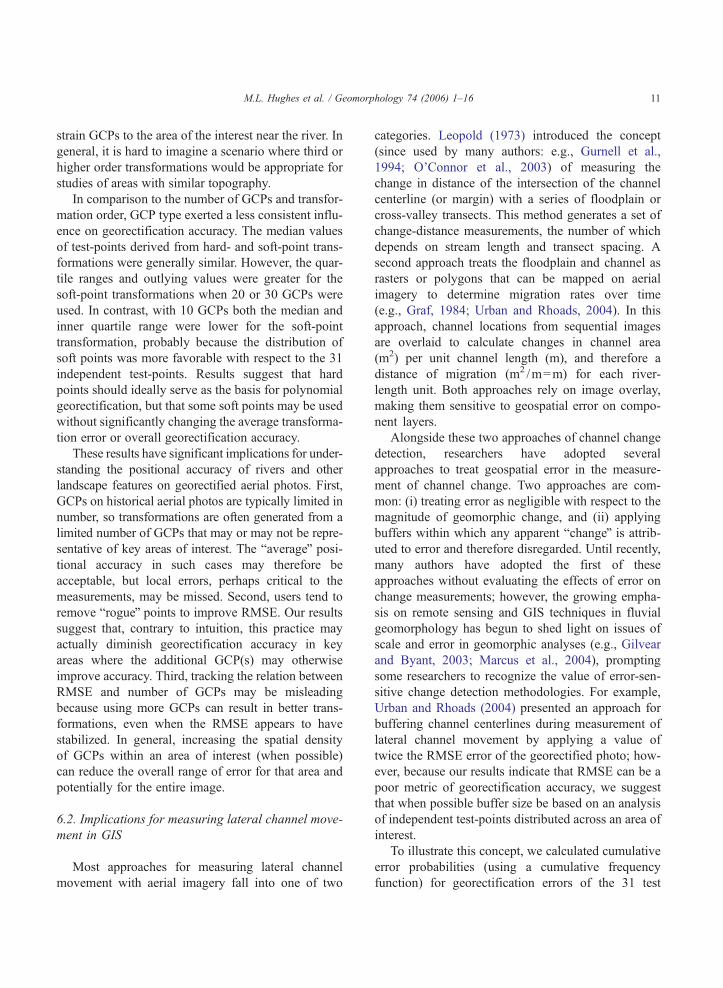
To illustrate this concept, we calculated cumulative

error probabilities (using a cumulative frequency

function) for georectification errors of the 31 test


points in Experiment 1 (Fig. 7; see description of data

in Section 5.1). These data can be used to specify

channel centerline buffers according to the briskQ oferror deemed acceptable by the user. In this case, we

believe that aerial photos similar to the test photo can

be georectified to an accuracy of approximately F5 m

of the base layer coordinates with approximately 30

GCPs and an approximate 10% chance of encounter-

ing greater error within the area of interest; however,

the relation between the optimal number and location

of GCPs will vary among photos of different scale and

regions of different topography, so the results from

our analysis should not be used to prescribe a mini-

mum number of GCPs in other studies. Rather, Fig. 7

should be viewed as one approach to defining error

probabilities and change detection thresholds. In gen-

eral, the magnitude of errors we documented in this

study is consistent with that of other channel change

studies that employed aerial photos (e.g., Lewin and

Hughes, 1976; Gurnell et al., 1994; Winterbottom and

Gilvear, 2000; Urban and Rhoads, 2004;) and digitally

georeferenced satellite imagery (Zhou and Li, 2000),

suggesting the existence of error thresholds across

remote sensing platforms.

Buffer size can strongly affect change detection

capability. Fig. 8 demonstrates the effects of buffer

size on the measurement of lateral channel movement

on a 2-km test reach of the Umatilla River. Pre- and

post-flood aerial photos dated 1964 and 1971 were

Fig. 7. Test point error versus cumulative error probability for trials with 6 t

georectified with 10, 20, 30 GCPs. Wetted channel

centerlines were then digitized from each of these

photos. Buffers corresponding to the 90th percentile

value of test-point error for 10, 20, and 30 GCPs (5-,

7.8-, and 10.8-m buffers, respectively; see Fig. 7)

were applied to each side of the corresponding cen-

terlines and a series of lateral movement polygons

were generated by extracting from the GIS areas

between the two centerline buffers. These polygons,

representing areas of lateral channel movement, were

then cut into smaller polygons along 50-m cross-

valley transects. Finally, the area of these transect

polygons was plotted versus distance downstream.

Fig. 8 demonstrates the inverse relationship

between buffer size and the magnitude of measurable

lateral movement. Where lateral channel movement is

greatest (e.g., transects 11–14), percent differences in

measured lateral movement across buffer sizes are

small. In comparison, percent differences in measured

channel change across buffer sizes are large where

channel movement is more subtle (e.g., transects 16–

20). In areas of limited channel movement, estimated

rates of channel change may be more sensitive to

buffer size than to actual channel movement.

While these results suggest that buffers based on

RSME values can lead to channel-change measure-

ments that are significant in error, the use of RMSE

for buffer delineation has another other problematic

tendency: RSME-based buffers tend to be used to

o 30 GCPs. Cumulative frequency percentile refers to the probability

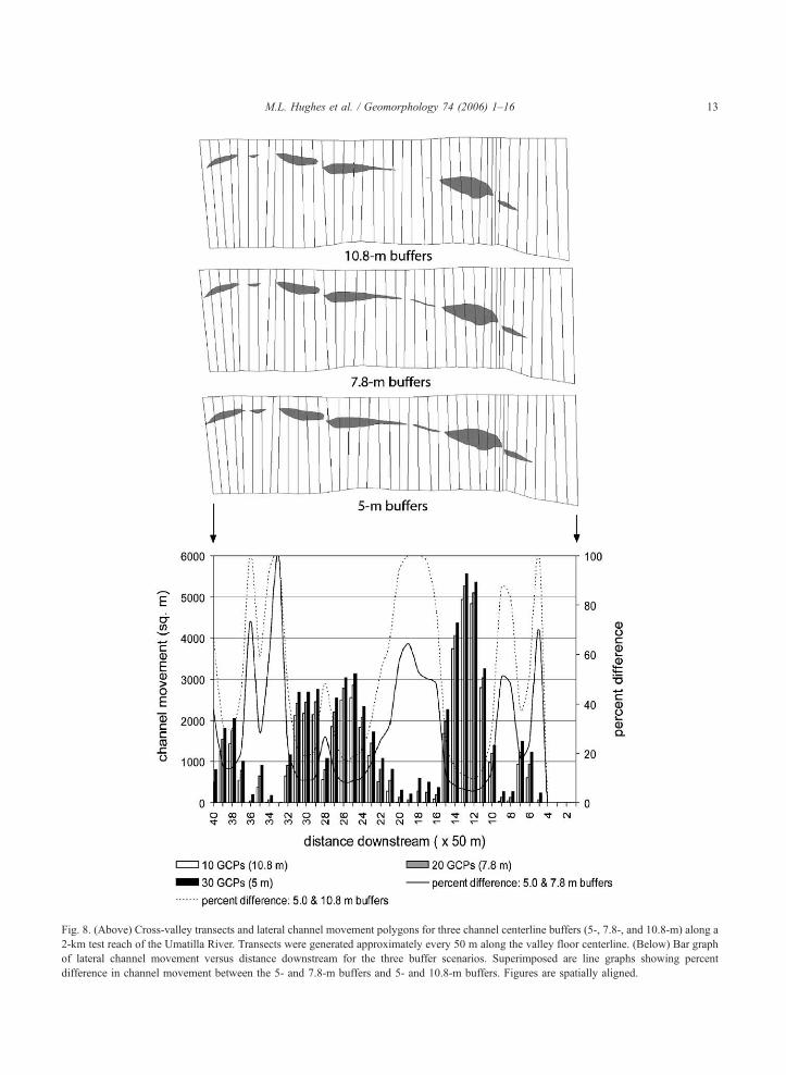
Fig. 8. (Above) Cross-valley transects and lateral channel movement polygons for three channel centerline buffers (5-, 7.8-, and 10.8-m) along a

2-km test reach of the Umatilla River. Transects were generated approximately every 50 m along the valley floor centerline. (Below) Bar graph

of lateral channel movement versus distance downstream for the three buffer scenarios. Superimposed are line graphs showing percent

difference in channel movement between the 5- and 7.8-m buffers and 5- and 10.8-m buffers. Figures are spatially aligned.



determine whether change has taken place despite the

possibilities of true channel change within the RMSE

buffer and no channel change outside it. Alterna-

tively, we suggest that change detection be viewed

in the context of the probability that measured change

is real and that error probability be based on analyses

of independent test points (Fig. 7). Termed the

bempirical probability approachQ, this approach

avoids the assumption that all channel movements

within the buffer size are not real and that all move-

ments outside the buffer are real. Alternatively,

researchers using the empirical probability approach

can specify the probability of measuring actual

change at their discretion and proceed with channel

measurements knowing the likelihood that georecti-

fication error is affecting their measurements. This

approach may be particularly useful in areas where

channels are relatively confined (e.g., transects 16–

21) and measured changes are often less than the

RSME. Also, this approach consistent with the prob-

ability-based approaches for reporting change advo-

cated by Graf (1984, 2001) and implemented in GIS

by Graf (2000) and Winterbottom and Gilvear

(2000).

Despite its shortfalls as an error indicator, RMSE is

still quite useful in reconstructing channel change

with aerial photos. In particular, because RSME is

readily calculated for each individual photo as the

image is georectified, providing a basis for varying

the buffer size from image to image if necessary. In

the case of the Umatilla River, we believe the error

probability functions we developed for the Pendleton

photo (Fig. 7) can be applied across many stream

segments in that basin because the RMSE on other

photos is similar, the topography from photo to photo

is reasonably constant, and georectification methods

have followed a consistent protocol; however, in

basins (or portions of basins) with variable topogra-

phy or inconsistent photo resolution and quality,

development of probability functions for multiple

photos would likely be necessary. In these cases,

RMSE is a useful tool to screen photos that may

require more detailed error analyses. We recognize

the time costs associated with developing multiple

probability functions and corresponding buffers must

be weighed against the benefits of their application. In

many fluvial hazard and river restoration studies, we

believe that this cost–benefit would be justified by the

improvements in information on channel movement

rates and processes allowed by the empirical prob-

ability approach.

7. Conclusions

Results of this study show that the RMSE and the

central tendency of locational error for 31 test-points

were relatively insensitive to GCP number when eight

or more GCPs were used. The 90th percentile cumu-

lative error values of test-points, however, consis-

tently decreased (i.e., improved) as more GCPs were

used (Fig. 4), indicating that the upper range of geo-

rectification error can be significantly reduced by

using more GCPs. We attribute the reduction in test-

point error to a higher spatial density of GCPs within

the area of interest and a better fit to local topography.

Using more GCPs improves georectification accuracy

only when additional points are positioned to better

incorporate the topography of the area of interest.

A second-order polynomial transformation gene-

rated the best fit (Fig. 6), providing sufficient flex-

ibility to correct for the range of topographic variation

typical of the terrace-floodplain environment of this

study. A first-order polynomial transformation gene-

rated a similar median error, but had higher outliers

from poor transformation in areas of higher elevation

near the river. First-order transformations may be

appropriate for channel change studies if GCPs

could be limited to the floodplain, but this may be

impractical with historic photos of rural or forested

settings. A third-order polynomial transformation gen-

erated poor results because of image warping at the

outer GCP locations. The need to avoid edge effects

by including GCPs far from the river suggests that

third or higher order polynomial transformations are

probably inappropriate for most river change studies.

The use of hard or soft GCP points did not drama-

tically affect median rectification errors, although the

hard points generated fewer high-error values (Fig. 5).

The similarity of results across GCP types indicates

they can be intermixed without introducing spurious

amounts of error.

Results clearly demonstrate that while RMSE may

be an acceptable proxy of average error, it is generally a

poor indicator of overall georectifcation accuracy

across a photo. Therefore, using RMSE for error esti-


mates and determination of buffer size may lead to

over- or under-estimating the amount of true change,

depending on the correspondence of the RMSE and the

upper range of true error on the photo in an area of

interest. We recommend that lateral movement mea-

surements be based on empirical probability functions

(e.g., Fig. 7), which are generated from a set of test-

point errors independent of the GCPs. According to this

study of a 1 :20,000 image transformed with 30 GCPs

and a second-order polynomial, a buffer distance of 5m

on each side of the channel centerline would remove

~90% of georectification error that may otherwise

affect measurements of lateral channel movement. A

5-m value is equivalent to 1.25 times the RMSE for the

30 GCPs. Buffers of similar magnitude are likely to be

necessary for error-sensitive photo-based studies of

lateral channel movement. Researchers using aerial

photos to measure channel change are encouraged to

conduct similar error analyses in order to assess the

magnitude of georectification error relative to the mag-

nitude of channel migration. Accordingly, error prob-

ability should be explicitly stated so that photo-based

studies of channel change may be better understood in

the context geospatial error.

Acknowledgements

Research on this project was supported by the

National Science Foundation, Geography and Regio-

nal Science award BCS 0215291 to P.F. McDowell

and W.A. Marcus.

References

Adamus, P., 2002. Umatilla River Floodplain and Wetlands: A

Quantitative Characterization, Classification, and Restoration

Concept. Adamus Resource Assessment Inc., Corvallis, OR.

Agricultural Stabilization and Conservation Service (ASCS),

1964. Vertical aerial photograph of the Umatilla River at

Pendleton, Oregon. US Department of Agriculture, Aerial

Photo Project ASCS-10-64-DC. Malcolm Aerial Surveys,

Roanoke, VA.

Butler, D.R., 1989. Geomorphic change or cartographic inaccuracy?

A case study using sequential topographic maps. Surveying and

Mapping 49 (2), 67–71.

Campbell, J.B., 2002. Introduction to Remote Sensing, 3rd edition.

The Guilford Press, New York.

Chrisman, N.R., 1982. A Theory of Cartographic Error and its

Measurement in Digital Databases. American Society of

Photogrammetry and Remote Sensing, Falls Church, VA,

pp. 159–168.

Chrisman, N.R., 1992. The error component in spatial data. In:

Maguire, D.J., Goodchild, M.F., Rhind, D.W. (Eds.), Principles

of Geographic Information Systems, vol. 1. Harlow: Longman,

White Plains, NY, pp. 165–174.

Collins, B.D., Montgomery, D.R., Sheikh, A.J., 2003. Reconstruct-

ing the historical riverine landscape of the Puget Lowland. In:

Montgomery, D.R., Bolton, S.M., Booth, D.B., Wall, L. (Eds.),

Restoration of Puget Sound Rivers. University of Washington

Press, Seattle, WA, pp. 79–128.

Finlayson, D.P., Montgomery, D.R., 2003. Modeling large-scale

fluvial erosion in geographic information systems. Geomorphol-

ogy 53, 147–164.

Fonstad, M.A., Marcus, W. A., 2005. Remote sensing of stream

depths with hydraulically assisted bathymetry (HAB) models.

Geomorphology 72, 320–339.

Gilvear, D., Byant, R., 2003. Analysis of aerial photography and

other remotely sensed data. In: Kondolf, G.M., Piegay, H.

(Eds.), Tools in Fluvial Geomorphology. Wiley, Chichester,

U.K., pp. 135–170.

Goodchild, M.F., Gopal, S. (Eds.), 1989. The Accuracy of Spatial

Databases. Taylor and Francis, London.

Goodchild, M.F., Hunter, G.J., 1997. A simple positional accuracy

measure for linear features. International Journal of Geographi-

cal Information Science 11 (3), 299–306.

Graf, W.L., 1984. A probabilistic approach to the spatial assessment

of river channel instability. Water Resources Research 20 (7),

953–962.

Graf, W.L., 2000. Locational probability for a dammed, urbanizing

stream: Salt River, Arizona, USA. Environmental Management

25 (3), 321–335.

Graf, W.L., 2001. Damage control: restoring the physical integrity

of America’s rivers. Annals of the Association of American

Geographers 91 (1), 1–27.

Gurnell, A.M., 1997. Channel change on the River Dee meanders,

1946–1992, from the analysis of air photographs. Regulated

Rivers : Research and Management 13, 13–26.

Gurnell, A.M., Downward, S.R., Jones, R., 1994. Channel planform

change on the River Dee meanders, 1876–1992. Regulated

Rivers : Research and Management 9, 187–204.

Holmes, K.W., Chadwick, O., Kyriakidis, P.C., 2000. Error in a

USGS 30-meter digital elevation model and its impact on terrain

modelling. Journal of Hydrology 233 (1–4), 154–173.

Hooke, J.M., Redmond, C.E., 1989. Use of cartographic sources for

analysing river channel change with examples from Britain. In:

Petts, G.E., Moller, H., Roux, R.L. (Eds.), Historical Change of

Large Alluvial Rivers: Western Europe. John Wiley and Sons,

New York, pp. 79–93.

Lawler, D.M., 1993. The measurement of river bank and lateral

channel change: a review. Earth Surface Processes and Land-

forms 18, 777–821.

Leica Geosystems, 2003. ERDAS Field Guidek, 7th ed. Atlanta,

Georgia.

Leopold, L.B., 1973. River channel change with time — an

example. Geological Society of America Bulletin 84,

1845–1860.


Leung, Y., Yan, J.P., 1998. A locational error model for spatial

features. International Journal of Geographical Information

Science 12 (6), 607–620.

Lewin, J., Hughes, D., 1976. Assessing channel change on Welsh

rivers. Cambria 3, 1–10.

Lewin, J., Weir, M.J.C., 1977. Monitoring river channel change. In:

van Genderen, J.L., Collins, W.G. (Eds.), Monitoring Environ-

mental Change by Remote Sensing. Remote Sensing Society

University of Reading, UK, pp. 23–27.

Leys, K.F., Werrity, A., 1999. River channel planform change:

software for historical analysis. Geomorphology 29, 107–120.

Locke, W.W., Wyckoff, W.K., 1993. A method for assessing the

planimetric accuracy of historical maps: the case of the Color-

ado–Green River system. Professional Geographer 45 (4),

416–424.

Marcus, W.A., Legleiter, C.J., Aspinall, R.J., Boardman, J.W., Crab-

tree, R.L., 2003. High spatial resolution, hyperspectral (HSRH)

mapping of in-stream habitats, depths, and woody debris in

mountain streams. Geomorphology 55 (1–4), 363–380.

Marcus, W.A., Aspinall, R.J., Marston, R.A., 2004. GIS and surface

hydrology. In: Bishop, M.P., Shroder, J.F. (Eds.), Geographic

Information Science and Mountain Geomorphology. Praxis

Scientific Publishing, Chichester, UK, pp. 343–379.

Mount, N.J., Louis, J., Teeuw, R.M., Zukowski, P.M., Stott, T.,

2003. Estimation of error i bankfull width comparisons from

temporally sequenced raw and corrected aerial photographs.

Geomorphology 56, 65–77.

Mount, N.J., Louis, J., 2005. Estimation and propagation of error in

measurements of river channel movement from aerial imagery.

Earth Surface Processes and Landforms 30, 635–643.

O’Connor, J.E., Jones, M.A., Haluska, T.L., 2003. Flood plain and

channel dynamics of the Quinault and Queets Rivers, Washing-

ton, USA. Geomorphology 51, 31–59.

Oregon Department of Environmental Quality (ODEQ), 2001.

Umatilla River Basin Total Maximum Daily Load (TMDL)

and Water Quality Management Plan (WQMP). Salem, OR.

Petts, G.E., 1989. Historical analysis of fluvial hydrosystems. In:

Petts, G.E., Muller, H., Roux, A.L. (Eds.), Historical Change of

Large Alluvial Rivers: Western Europe. Wiley, Chichester, UK,

pp. 1–18.

Richards, J.E., 1986. Remote Sensing Digital Image Processing: An

Introduction. Springer, New York.

Roering, J.J., Kirchner, J.W., Dietrich, W.E., 2005. Characterizing

structural and lithologic controls on deep-seated landsliding:

Implications for topographic relief and landscape evolution in

the Oregon Coast Range, USA. Geological Society of America

Bulletin 117, 654–668.

Schroder Jr., J.F., Bishop, M.P. (Eds.), 2004. Geographic Informa-

tion Science and Mountain Geomorphology. Praxis Scientific

Publishing, Chichester, UK.

Slama, C.C., Theurer, C., Henriksen, S.W. (Eds.), 1980. Manual of

Photogrammetry, 4th edition. American Society of Photogram-

metry, Falls Church, VA.

Surian, N., 1999. Channel changes due to river regulation. Earth

Surface Processes and Landforms 24, 1135–1151.

Trimble, S., 1991. Historical sources of information for geomor-

phological research in the United States. Professional Geogra-

pher 43 (2), 212–228.

Unwin, D.J., 1995. Geographical information systems and the

problem of derror and uncertaintyT. Progress in Human Geogra-

phy 19 (4), 549–558.

Urban, M.A., Rhoads, B.L., 2004. Catastrophic human-induced

change in stream-channel planform and geometry in an agricul-

tural watershed, Illinois, USA. Annals of the Association of

American Geographers 93 (4), 783–796.

Wilson, J.P., Gallant, J.C. (Eds.), 2000. Terrain Analysis: Principles

and Applications. John Wiley and Sons, Hoboken, New Jersey.

Winterbottom, S.J., Gilvear, D.J., 2000. A GIS-based approach to

mapping probabilities of river bank erosion: regulated river

tummel, Scotland. Regulated Rivers : Research and Manage-

ment 16, 127–140.

Zhilin, L., Xiuxia, Y., Lam, K.W.K., 2002. Effects of .JPEG com-

pression on the accuracy of photogrammetric point determina-

tion. Photogrammetric Engineering and Remote Sensing 68 (8),

847–853.

Zhou, G., Li, R., 2000. Accuracy evaluation of ground control points

form IKONOS high-resolution satellite imagery. Photogram-

metric Engineering and Remote Sensing 66 (9), 1103–1112.

accuracy assessment of georectified aerial photographs...

Documents