AccPar: Tensor Partitioning forHeterogeneous Deep Learning Accelerators

Linghao Song†, Fan Chen†, Youwei Zhuo‡, Xuehai Qian‡, Hai Li†, Yiran Chen†

†Duke University, ‡University of Southern California{linghao.song, fan.chen, hai.li, yiran.chen}@duke.edu, {youweizh, xuehai.qian}@usc.edu

ABSTRACTDeep neural network (DNN) accelerators as an example ofdomain-specific architecture have demonstrated great successin DNN inference. However, the architecture accelerationfor equally important DNN training has not yet been fullystudied. With data forward, error backward and gradient cal-culation, DNN training is a more complicated process withhigher computation and communication intensity. Becausethe recent research demonstrates a diminishing specializationreturn, namely, “accelerator wall”, we believe that a promis-ing approach is to explore coarse-grained parallelism amongmultiple performance-bounded accelerators to support DNNtraining. Distributing computations on multiple heteroge-neous accelerators to achieve high throughput and balancedexecution, however, remaining challenging.

We present ACCPAR, a principled and systematic methodof determining the tensor partition among heterogeneous ac-celerator arrays. Compared to prior empirical or unsystematicmethods, ACCPAR considers the complete tensor partitionspace and can reveal previously unknown new parallelismconfigurations. ACCPAR optimizes the performance basedon a cost model that takes into account both computationand communication costs of a heterogeneous execution en-vironment. Hence, our method can avoid the drawbacks ofexisting approaches that use communication as a proxy of theperformance. The enhanced flexibility of tensor partitioningin ACCPAR allows the flexible ratio of computations to be dis-tributed among accelerators with different performances. Theproposed search algorithm is also applicable to the emergingmulti-path patterns in modern DNNs such as ResNet. Wesimulate ACCPAR on a heterogeneous accelerator array com-posed of both TPU-v2 and TPU-v3 accelerators for the train-ing of large-scale DNN models such as Alexnet, Vgg seriesand Resnet series. The average performance improvementsof the state-of-the-art “one weird trick” (OWT) and HYPAR,and ACCPAR, normalized to the baseline data parallelismscheme where each accelerator replicates the model and pro-cesses different input data in parallel, are 2.98×, 3.78×, and6.30×, respectively.

1. INTRODUCTIONAdvances in deep learning (DL) have become the main

drivers of revolutions in various commercial and enterprise ap-

plications, such as computer vision [1–3], social network [4–6], financial data analysis [7–9], healthcare [10–12] and sci-entific computing [13–15]. Due to the high demand of com-puting power in DL applications, we have recently witnesseda phenomenal trend in which the landscape of computing hasshifted from general-purpose processors to domain-specificarchitectures [16–110]. By sacrificing some flexibility, suchdomain-specific accelerators are specialized for executingkernels of modern DL algorithms and therefore, are capableto deliver high performance with low power budget.

While the latest advances are pushing the envelope of DLacceleration for higher performance and energy efficiency,a recent study of chip specialization [111] has predicted anultimate accelerator wall. More specifically, due to the con-straints in the exploration of mapping computational prob-lems (e.g., DL) onto hardware platforms with fixed hardwareresources, the optimization space of chip specialization islimited by a theoretical roofline. Combining with recent slowCMOS technology scaling, the gains from specific acceleratordesigns will gradually diminish and the execution efficiencywill eventually hit an upper-bound. On the other hand, thecomputational demands of emerging DL applications con-tinue increasing in order to adapt to more complex modelswith deeper structures [112, 113] or more sophisticated learn-ing methods [114, 115].

To address the mismatch between the diminishing perfor-mance gains in hardware accelerators and the ever-growingcomputational demands, it is imperative to explore coarse-grained parallelism among multiple performance-boundedaccelerators to support large-scale DL applications. In gen-eral, a deep neural network (DNN) model is a parametricfunction that takes a high-dimensional input and makes use-ful predictions (i.e., inference), such as a classification la-bel. Model parameters, i.e., kernels or weights, are obtainedthrough a large number of iterations in training process in-volving data forward, error backward and gradient calculationphases. The trained model can be used to perform inferencefunction through only the data forward phase. Comparedto inference, training is much more complicated and com-putational intensive. Hence, typically training is offloadedto high-end CPUs/GPUs and then the trained models aredeployed to end/user devices. It is a natural need to havemulti-accelerator architectures specialized for DNN training.

Given the high complexity of modern DNN models, find-

ing the best distribution of computations on multiple accelera-tors is nontrivial. Moreover, due to the inherent performancedifference of accelerators and the discrepancy of the commu-nication bandwidth between them, ensuring high throughputand balanced execution is extremely challenging. The prob-lem can be formulated as partitioning the model and data ten-sors among accelerators to enable parallel processing. Thereare two approaches: data parallelism, where each acceleratorreplicates the model and processes different input data inparallel before applying the calculated gradients to update themodel; and model parallelism, where each accelerator keepspart of the model and performs a part of computation basedon the same input. The choice between the two parallelismconfigurations affects the overall performance since it incursdifferent communication patterns between the accelerators.

The current solutions to this problem are either purely em-pirical or incomplete — both lacking optimal guarantee. Forexample, for a given DNN, “One Weird Trick” (OWT) [107]empirically suggests to use data parallelism for convolutional(CONV) layers and model parallelism for fully-connected(FC) layers. HYPAR [108] proposes a principled approachto search for the optimized parallelism configuration to mini-mize data communication. Although it can achieve a muchbetter result than OWT, HYPAR suffers from several limita-tions: 1) the search is based on an incomplete design space;2) it can only handle DNN architectures with linear structure;3) it lacks a cost model and uses only communication as theproxy for performance optimization; and most importantly4) it assumes an homogeneous execution environment — theperformance of each accelerator and the bandwidth betweenthem are all the same. A truly optimal solution for this criticalproblem still does not exist yet.

The combination of model and data parallelism is exploredin deep learning accelerator architectures [60, 90] multi-GPUtraining systems [107,116–119]. Recursive methods [74,118]are proposed for tensor partitioning on multiple devices anddynamic programming methods [116, 118] are proposed fortensor partitioning layer-wisely. Inspired by those previousworks [74, 107, 116–119], we present ACCPAR — a princi-pled and systematic method of determining the tensor parti-tion among heterogeneous accelerator arrays. Our solutionis composed of several key innovations. First, we considera complete tensor partition space in all three dimensions:batch size, input data size, and output data size. Hence, oursolution is able to reveal previously unknown parallelism con-figuration. The completeness and optimality of the searchingalgorithm is also guaranteed. Second, in order to better opti-mize performance, we propose a cost model considering bothcomputation and communication cost of a heterogeneous ex-ecution environment, instead of using communication as theproxy for performance as in HYPAR. Third, ACCPAR of-fers flexible tensor partition ratio between the accelerators tomatch their unique computing power and network bandwidth.Finally, we propose a technique to handle the emerging multi-path patterns in modern DNNs such as ResNet [113]. AC-CPAR significantly outperform the state-of-the-art solutions,offering the first complete solution for tensor partitioning onheterogeneous accelerator arrays.

We simulate ACCPAR on a heterogeneous accelerator ar-ray composed of both TPU-v2 and TPU-v3 accelerators for

Notation Description

FlInput feature map to Layer l (output feature map ofLayer l−1).

El+1 Input error to Layer l (output error of Layer l +1).Wl Kernel of Layer l.4Wl Gradient of Kernel in Layer l.

B Mini-batch size.Di,l Input data size(channel number) of Layer l.Do,l Output data size(channel number) of Layer l.ci The computation density of Accelerator i.pi,l The partitioning of Accelerator i at Layer l.bi The network bandwidth of Accelerator i.

A(·) Function to return the size of a tensor.

C(·) Function to return the amount of computation to beperformed by an accelerator.

α , β Partitioning ratios.

Table 1: Notations and descriptions.

training of large-scale DNN models such as Alexnet [112],Vgg series [120] and Resnet series [113]. The average per-formance of “one weird trick” (OWT) [107], HYPAR [108]and ACCPAR, normalized to the baseline data parallelism onthe heterogeneous accelerator array is 2.98×, 3.78×, 6.30×,respectively. For Vgg series, ACCPAR can achieve a speedupup to 16.14×, while the highest speedup of OWT and HYPARare 8.24× and 9.46×, respectively. For Resnet series, ACC-PAR can achieve performance speedup from 1.92× to 2.20×,while the ranges of speedup achieved by OWT and HYPARare 1.22× to 1.38× and 1.03× to 1.04×, respectively.

2. BACKGROUND AND MOTIVATION

2.1 DNN TrainingDNN training involves three tensor computing phases at

each layer: forward, backward and gradient. The notationsand descriptions are listed in Table 1. In the forward phase,at layer l, the input feature map tensor (Fl) from a previouslayer and the kernel/weight tensor (Wl) are multiplied infully-connected (FC) layers or convolved in convolutional(CONV) layers to generate the output feature map tensor,which is used as the input feature map tensor for the next layer(Fl+1). Usually a non-linear activation f (·) is performed oneach scalar of the feature map. Thus, the forward phasecan be represented as Fl+1 = f (Fl⊗Wl), where ⊗ is eithermultiplication or convolution. In the backward phase, at layerl, the error tensor (El) is computed by El =

(El+1⊗W>

l

)�

f ′(Fl), where El+1 is the error tensor from layer l +1, � isan element-wise multiplication, and f ′(·) is the derivativefunction of f (·). In the gradient phase, the gradient to thekernel/weight is computed by4Wl = F>l ⊗El+1.

The three tensor computation phases capture the commonflow in many popular training algorithms, such as GradientDescent, Stochastic Gradient Descent, Mini-batch GradientDescent, Momentum [121] and Adaptive Moment Estimation(Adam) [122]. For example, Momentum method updates theparameter using vt = γ ·vt−1 +η ·∇θ J(θ),θ = θ −vt , whereθ is the parameter (weight), ∇θ J(θ) is the gradient of a lossfunction J(·) with respect to θ , v is the velocity to record thehistoric gradient, γ is the momentum hyper parameter and η

is the learning rate, respectively.

Segment DNN Accelerators & ArchitecturesNeuro Co-processor SpiNNaker [16], Neuromorphic Acc. [17], TrueNorth [18–20], MT-spike [21], PT-spike [22]DNN Co-processor NPU [23], DianNao-family [24–27], Cambricon [28], Cambricon-x [29], TPU [30, 31], ScaleDeep [32], Stripes [33],

Neural Cache [123, 124], Diffy [125]FPGA FPGA-DCNN [34], Embedded-FPGA-CNN [35], FPGA-Exploration [36], OpenCL-FPGA-CNN [37] [126], Caf-

feine [38], DeepBurning [39], FPGA-DPCNN [40], TABLA [41], DNNWEAVER [42], FP-DNN [43], FPGA-LSTM [44], ESE [45], FPGA-Dataflow [46], FPGA-BNN [47], FPGA-Utilization [48], FFT-CNN [49], VIBNN [50],iSwitch [127], Shortcut-Mining [128], FA3C [129], E-RNN [130]

Dataflow Neuflow [51], Eyeriss [52–54], Flexflow [55], Fused-CNN [56], CNN-Paritition [57], GANAX [58], UCNN [59],TANGRAM [131], Sparse-Systolic [132], MAERI [133]

PIM Neurocube [60], XNOR-POP [61], DRISA [62], 3DICT [63], NAND-NET [134], SCOPE [135], Promise [136]Light Models EIE [64], SC-DCNN [65], SCNN [66], Escher [67], LookNN [68], Bit-Pragmatic DNN [69], Bit Fusion [70], Cn-

vlutin [99], TIE [137], Laconic [138], ADM-NN [139], Gist [140]Co-Design DPS-CNN [71], Minerva [72], MoDNN [73], MeDNN [74], AdaLearner [75], Stitch-X [76], PIM-DNN [77],

Scalpel [78], CirCNN [79], CoSMIC [80], SnaPEA [81], OLAcce [82], Prediction-based DNN [83], PERMDNN [84],MnnFast [141], DNN Computation Reuse [142], vDNN [143], Compressing-DMA-Engine [144], AxTrain [145], Eagerpruning [146], Bit-Tactical [147], GENESYS [148]

Emerging Tech. TETRIS [85], RENO [88], PRIME [86], ISAAC [87], Memristive Boltzmann Machine [89], PipeLayer [90], Atom-layer [91], ReCom [92], ReGAN [93], ReRAM ACC. [94], EMAT [95], ReRAM-BNN [96], ZARA [97], SNrram [98],Sparse ReRAM Engine [149], RedEye [150], Quantum-SC-NN [151], FloatPIM [152], PUMA [153], FPSA [154]

Toolset/Framework Data Parallelism [106], OWT [107], NEUTRAMS [100], Perform-ML [101], Adaptive-Classifier [102],DNNBuilder [103], Group Scissor [104], FFT-CNN [105], HyPar [108], NNest [155]

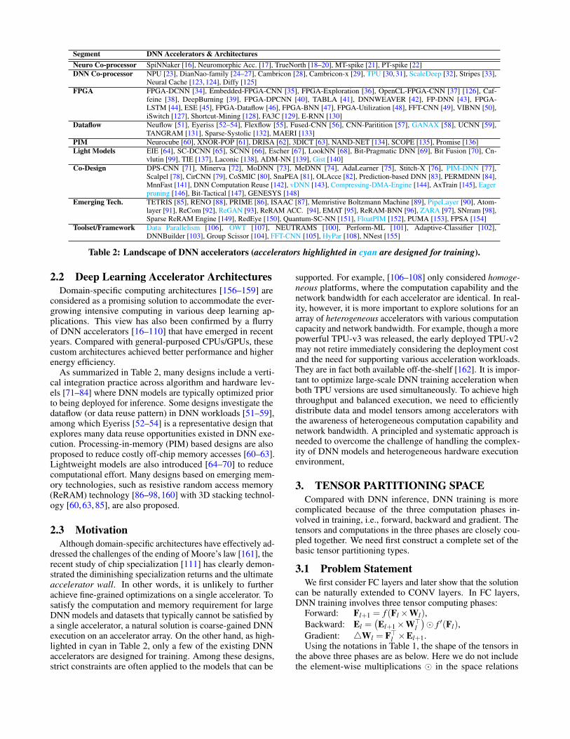
Table 2: Landscape of DNN accelerators (accelerators highlighted in cyan are designed for training).

2.2 Deep Learning Accelerator ArchitecturesDomain-specific computing architectures [156–159] are

considered as a promising solution to accommodate the ever-growing intensive computing in various deep learning ap-plications. This view has also been confirmed by a flurryof DNN accelerators [16–110] that have emerged in recentyears. Compared with general-purposed CPUs/GPUs, thesecustom architectures achieved better performance and higherenergy efficiency.

As summarized in Table 2, many designs include a verti-cal integration practice across algorithm and hardware lev-els [71–84] where DNN models are typically optimized priorto being deployed for inference. Some designs investigate thedataflow (or data reuse pattern) in DNN workloads [51–59],among which Eyeriss [52–54] is a representative design thatexplores many data reuse opportunities existed in DNN exe-cution. Processing-in-memory (PIM) based designs are alsoproposed to reduce costly off-chip memory accesses [60–63].Lightweight models are also introduced [64–70] to reducecomputational effort. Many designs based on emerging mem-ory technologies, such as resistive random access memory(ReRAM) technology [86–98, 160] with 3D stacking technol-ogy [60, 63, 85], are also proposed.

2.3 MotivationAlthough domain-specific architectures have effectively ad-

dressed the challenges of the ending of Moore’s law [161], therecent study of chip specialization [111] has clearly demon-strated the diminishing specialization returns and the ultimateaccelerator wall. In other words, it is unlikely to furtherachieve fine-grained optimizations on a single accelerator. Tosatisfy the computation and memory requirement for largeDNN models and datasets that typically cannot be satisfied bya single accelerator, a natural solution is coarse-gained DNNexecution on an accelerator array. On the other hand, as high-lighted in cyan in Table 2, only a few of the existing DNNaccelerators are designed for training. Among these designs,strict constraints are often applied to the models that can be

supported. For example, [106–108] only considered homoge-neous platforms, where the computation capability and thenetwork bandwidth for each accelerator are identical. In real-ity, however, it is more important to explore solutions for anarray of heterogeneous accelerators with various computationcapacity and network bandwidth. For example, though a morepowerful TPU-v3 was released, the early deployed TPU-v2may not retire immediately considering the deployment costand the need for supporting various acceleration workloads.They are in fact both available off-the-shelf [162]. It is impor-tant to optimize large-scale DNN training acceleration whenboth TPU versions are used simultaneously. To achieve highthroughput and balanced execution, we need to efficientlydistribute data and model tensors among accelerators withthe awareness of heterogeneous computation capability andnetwork bandwidth. A principled and systematic approach isneeded to overcome the challenge of handling the complex-ity of DNN models and heterogeneous hardware executionenvironment,

3. TENSOR PARTITIONING SPACECompared with DNN inference, DNN training is more

complicated because of the three computation phases in-volved in training, i.e., forward, backward and gradient. Thetensors and computations in the three phases are closely cou-pled together. We need first construct a complete set of thebasic tensor partitioning types.

3.1 Problem StatementWe first consider FC layers and later show that the solution

can be naturally extended to CONV layers. In FC layers,DNN training involves three tensor computing phases:

Forward: Fl+1 = f (Fl×Wl),Backward: El =

(El+1×W>

l

)� f ′(Fl),

Gradient: 4Wl = F>l ×El+1.Using the notations in Table 1, the shape of the tensors in

the above three phases are as below. Here we do not includethe element-wise multiplications � in the space relations

since they can be performed in place.Forward: (B,Do,l)← (B,Di,l)× (Di,l ,Do,l),Backward: (B,Di,l)← (B,Do,l)× (Do,l ,Di,l),Gradient: (Di,l ,Do,l)← (Di,l ,B)× (B,Do,l).For illustration purpose, this section considers a simple

case of an array with two accelerators. The problem is toexhaustively and systematically enumerate all possible parti-tions of the tensors involved in the three phases among the twoaccelerators, and understand the corresponding data commu-nication and replication requirements. This is critical becausethe partition will determine the communication between theaccelerators and affect overall training performance. We willalso explain why the current solutions [107, 108] failed toprovide a complete and comprehensive solution.

3.2 Partitioning in Three DimensionsWe note that the two matrices in each of the pairs (Fl ,El)

and (Fl+1,El+1) have the same shape. We assume that Fl andEl (also Fl+1 and El+1) are partitioned in the same manner.This constraint is intuitive since otherwise additional com-munication will be unnecessarily incurred, contradicting ourgoal of minimizing communication between the accelerators.

We see only three dimensions appear in the three tensorcomputing phases: B (batch size), Do,l (output data size oflayer l), and Di,l (input data size of layer l). Therefore, wecan naturally focus on the partition in these three dimensions.For the partitions in one dimension, we assume that the samepartition parameter is used for this dimension in every tensorto avoid additional communication.

Key observation: The dimensions are not independent. Infact, only one dimension can be “free” in a partition.

We explain observation using an example: consider theforward phase and the partition in B dimension, Since wewill have only two partitions, for (B,Di,l) (Fl), the Di,l di-mension should not be partitioned. This also determines that(Di,l ,Do,l) (Wl) should not be partitioned in Di,l dimension,otherwise the matrix multiplication cannot be performed. Theonly case left is the Do,l dimension of Wl . Suppose we par-tition that, the combination of multiplication of the localpartitions in each accelerator does not lead to a completeresult of Fl with shape (B,Di,l). Specifically, depending onthe partition, only the upper left and lower right sub-matrix,or upper right and lower left sub-matrix are computed. There-fore, Do,l dimension of Wl cannot be partitioned. In fact,the whole Wl needs to be replicated on the two accelera-tors to compute the complete Fl . The other scenarios can beconsidered similarly.

With the assumption that Fl and El (also Fl+1 and El+1)use the same partition, and the fact that only one dimensionis free in a partition, there are only three partition types. Wediscuss them one by one in the following.

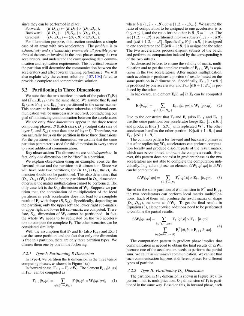
3.2.1 Type-I: Partitioning B DimensionIn Type-I, we partition the B dimension in the three tensor

computing phases, as shown in Figure 1(a).In forward phase, Fl+1 =Fl×Wl . The element Fl+1[b,qo]

in Fl+1 can be computed as

Fl+1[b,qo] = ∑qi∈{1,··· ,Di,l}

Fl [b,qi]×Wl [qi,qo], (1)

where b∈ {1,2, · · · ,B},qo∈ {1,2, · · · ,Do,l}. We assume theratio of computation to be assigned to one accelerator is α ,0≤ α ≤ 1, and the ratio for the other is β , β = 1−α . Theset {1,2, · · · ,B} is partitioned into two subsets {1,2, · · · ,αB}and {αB+1,2, · · · ,B}. Specifically, Fl [1 : αB, :] is assignedto one accelerator and Fl [αB+1 : B, :] is assigned to the other.The two accelerators process disjoint subsets of the batch,and perform the computation indexed by the corresponding bof the two subsets.

As discussed before, to ensure the validity of matrix multi-plication and to get the complete results of Fl+1, Wl is repli-cated in the two accelerators. After matrix multiplication,each accelerator produces a portion of results based on thesame partition in B dimension. Specifically, Fl+1[1 : αB, :]is produced by one accelerator and Fl+1[αB+1 : B, :] is pro-duced by the other.

In backward, an element El [b,qi] in El can be computedas

El [b,qi] = ∑qo∈{1,··· ,Do,l}

El+1[b,qo]×W>l [qo,qi]. (2)

Due to the constraint that Fl and El (also Fl+1 and El+1)use the same partition, one accelerator keeps El+1[1 : αB, :]and produces El+1[1 : αB, :] with replicated W>

l . The otheraccelerator handles the other portion: El [αB+ 1 : B, :] andEl+1[αB+1 : B, :].

The common pattern for forward and backward phases isthat after replicating Wl , accelerators can perform computa-tion locally and produce disjoint parts of the result matrix,which can be combined to obtain the complete result. How-ever, this pattern does not exist in gradient phase as the twoaccelerators are not able to complete the computation indi-vidually. In gradient phase, an element4Wl [qi,qo] in4Wlcan be computed as

4Wl [qi,qo] = ∑b∈{1,··· ,B}

F>l [qi,b]×El+1[b,qo]. (3)

Based on the same partition of B dimension in F>l and El+1,the two accelerators can perform local matrix multiplica-tions. Each of them will produce the result matrix of shape(Di,l ,Do,l), the same as 4Wl . To get the final results inEquation (3), element-wise additions need to be performedto combine the partial results:

4Wl [qi,qo] = ∑b∈{1,··· ,αB}

F>l [qi,b]×El+1[b,qo]

+ ∑b∈{αB+1,··· ,B}

F>l [qi,b]×El+1[b,qo].(4)

The computation pattern in gradient phase implies thatcommunication is needed to obtain the final results of4Wl ,because one of the accelerators needs to perform the partialsum. We call it as intra-layer communication. We can see thatsuch communication happens at different phases for differenttypes of partition.

3.2.2 Type-II: Partitioning Di,l DimensionThe partition in Di,l dimension is shown in Figure 1(b). To

perform matrix multiplication, Di,l dimension of Fl is parti-tioned in the same way. Based on this, in forward phase, each

Forw

ard

Back

war

dG

radi

ent

FlWl Fl+1

El+1

El+1

El

F>l

W>l

F>l

El+1

El+1

Fl+1Wl

W>l

El

Fl

4Wl 4Wl

↵B

↵B

↵B

↵B

↵B

↵B

Do,l

Do,l

Do,l

Do,l

Do,l

Do,l

Do,l

Do,l

Do,lDo,l

Do,l

B

B

B B

B

B

=)

=)

�

!

!=)

�=)

!=)

!

Do,l

WlFl

B =)!

!

=)

!

Fl+1

B

B

El

=) BW>

l

B

=)

El+1

!

!

B

El+1

�

(a) Type-I (b) Type-II (c) Type-III

Di,l

Di,l

Di,l

Di,l

Di,l

Di,l Di,l

Di,l

Di,l Di,l

Di,l

Di,l

↵Do,l

↵Do,l

↵Do,l

↵Do,l

↵Di,l

↵Di,l

↵Di,l

↵Di,l

↵Do,l↵Do,l

↵Di,l↵Di,l

4Wl

F>l

Figure 1: Three basic tensor partitioning types. The partitioning ratio for one accelerator is α and the partitioningratio for the other accelerator is β = 1−α . Shadow tensors are assigned to one accelerator and non-shadow tensors areassigned to the other accelerator. ⊗ denotes element-wise addition of two tensors.

accelerator will compute a result matrix of shape (B,Do,l).Similar to the case of 4Wl in Type-I, computing the com-plete Fl+1 requires element-wise addition in this partitioning:

Fl+1[b,qo] = ∑qi∈{1,··· ,αDi,l}

Fl [b,qi]×Wl [qi,qo]

+ ∑qi∈{αDi,l+1,··· ,Di,l}

Fl [b,qi]×Wl [qi,qo].(5)

Since Fl+1 and El+1 follow the same partition, in backwardphase, El+1 is replicated in the two accelerators. This allowseach of the accelerators produces a disjoint part of result ofEl . The partition and replication are similar to that used ingradient phase. A key difference between Type-I and Type-IIis that the intra-layer communication incurs at forward phase,instead of gradient phase.

3.2.3 Type-III: Partitioning Do,l DimensionThe partitioning Do,l dimension is shown in Figure 1(c). Fl

needs to be replicated to compute complete Fl+1 in forwardphase. It is the case overlooked by all previous solutions.Essentially, it means that the input feature maps of the samebatch are replicated into the two accelerators, instead ofpartitioning B. It may sound not intuitive since we wantto have accelerators process the same data. However, weshow that it is an important partition in the design space thatpresents the same trade-off in terms of communication justas in Type-I and Type-II.

Similar to gradient phase of Type-I and forward phase ofType-II, the backward phase of Type-III requires element-wise addition of partial results:

El [b,qi] = ∑qo∈{1,··· ,αDo,l}

El+1[b,qo]×W>l [qo,qi]

+ ∑qo∈{αDo,l+1,··· ,Do,l}

El+1[b,qo]×W>l [qo,qi].

(6)

3.3 Extension to CONV

In the previous sessions, we used matrix-matrix multipli-cation in FC to illustrate the three types of partitions, whichcan be conceptually visualized in Figure 1. For CONV, thethree partitioning types are still valid. However, Fl [b,qi],Fl+1[b,qo], El [b,qi] and El+1[b,qo] are no longer scalarsbut are 2-dimensional matrices. Therefore, Fl , Fl+1, El andEl+1 are 4-dimensional tensors, i.e., (batch, channel)×(width,height). Similarly, 4Wl [qi,qo] and Wl [qi,qo] are also 2-dimensional matrices rather than scalars. Thus, 4Wl andWl are 4-dimensional tensors, i.e., (input channel, outputchannel)×(kernel width, kernel height). The multiplication(×) in Equation (1), (2), (3), (4), (5), (6) then become convo-lution (⊗). The additional dimensions (4D vs. 2D) and morecomplex operations (× vs. ⊗) only imply different amountof computation but not affect the partition types based onexisting dimensions (B, Di,l , and Do,l).

3.4 CompletenessIn the three phases, only three dimensions appear and we

have shown that only one dimension can be partitioned at atime. Thus, the three types we derived constitute the completepartition space. Table 3 summarized the key features ofthe partitions. The LHS Shape and RHS Shape respectivelyindicate the shapes of the metrics on the left-hand and right-hand side of the equation for each phase. The Psum Shapeis the shape of the matrices containing partial results in twoaccelerators that need to be combined using element-wiseadditions. It happens when the matrix appear on the LHS.This is also the shape of the matrix that needs to be replicatedif it appears on the RHS. From Table 3, we can observe arotational symmetry on each column.

3.5 Problems of “One Weird Trick” & HyParTwo solutions were recently proposed to address the same

problem that is addressed by this paper, — communicationand parallelism between accelerators. However, neither ofthese two solutions is complete.

Krizhevsky [107] proposed “one weird trick” (OWT) to

Multiplication L Shape R Shape Partition Dim Psum Shape Basic TypeFl+1 = Fl×Wl (B,Do,l) (B,Di,l), (Di,l ,Do,l) Di,l (B,Do,l) Type-IIEl = El+1×W>

l (B,Di,l) (B,Do,l), (Di,l ,Do,l) Do,l (B,Di,l) Type-III4Wl = F>l ×El+1 (Di,l ,Do,l) (B,Di,l), (B,Do,l) B (Di,l ,Do,l) Type-I

Table 3: Rotational Symmetry of the Three Tensor Multiplications.

configure CONV layers with data parallelism and FC layerswith model parallelism to get a higher performance. It iscertainly better than just using data parallelism for all layers,however it does not provide any insight on why this trickworks and whether it is the best we can do. Therefore, thissolution is fundamentally empirical.

HyPar [108] is a more recent and principled approach to op-timize the parallelism configurations also by partitioning thelayers based on the intra-layer and inter-layer communication.However, it only considers the same two basic partitions inOWT, — data parallelism and model parallelism. In fact, theycorrespond to Type-I and Type-II in Figure 1, respectively.Therefore, the parallelism setting in HyPar is not complete.Even if it is based on a more systematic approach to explorethe partition space, it cannot find the optimal solution basedon incomplete basic partition types. Specifically, HyPar willmiss one intra-layer communication pattern (Type-III) andfive inter-layer communication patterns (see more details inSection 4.1). Moreover, HyPar always partitions the tensorsequally, so it cannot capture the performance heterogeneityamong accelerators.

4. ACCPAR COST MODELTo search the optimal partition of layers, we propose a cost

model for multiple accelerators. We consider the computationby individual accelerator and the communication between ac-celerators as two major affecting DNN training performance.Compared to HYPAR [108], which uses communication costas the proxy for performance, the cost model of ACCPARtakes both communication cost Ecm and computation cost Ecpinto consideration. The optimization target is to minimizeoverall cost.

4.1 Communication Cost ModelAssuming the network bandwidth for accelerator i is bi,

and T is the accessed tensor needs to be transferred from oneto the other, we define the communication cost Ecm for thetensor transfer as

Ecm =A(T)

bi. (7)

The tensor size A(T) is defined as the product of the lengthsof all dimensions. For example, the size of a 4-by-5 matrixis 20, and the size of a kernel whose input channel is 16,kernel window width is 3, kernel window length is 3 andoutput channel is 32, is 4,608 = 16×3×3×32. Next, wewill determine what the remotely-accessed tensor T is.

4.1.1 Intra-layer Communication CostAs discussed in Section 3, for each of the three basic tensor

partitioning types, there is one and only one computationphase requires remote accessing.

Basic Type Intra-layer Communication Cost

Type-I A(Wl)bi

Type-II A(Fl+1)bi

Type-III A(El)bi

Table 4: Intra-layer communication cost of the three ba-sic tensor partitioning types. Note that intra-layer com-munication cost is not dependable on the partitioning ra-tio α because intermediate results are accumulated lo-cally and partial sum tensors are accessed remotely.

In Type-I, the gradient phase requires remote accessing(Equation (4)). For the accelerator whose partitioning ratiois α , for each b ∈ {1, · · · ,αB}, the intermediate tensor sizeis A(F>l [:,b]×El+1[b, :]) = Di,l ·Do,l = A(4Wl) = A(Wl).Those intermediate tensors (∀b ∈ {1, · · · ,αB}) are accumu-lated locally (∑qi∈{1,··· ,αDi,l}(·)) by the accelerator i to reduceremote accessing by the other accelerator j. Also, the accel-erator j performs local accumulation ∑qi∈{αDi,l+1,··· ,Di,l}(·).Thus, the size of the tensor remotely accessed by acceleratori from accelerator j is A(Wl) rather than (1−α) ·B ·A(Wl).With Equation (7), we get the intra-layer communication costfor accelerator i to remotely access the partial sum tensor inaccelerator j is A(Wl)

bi.

For Type-II and Type-III, readers can follow the similaridea to get the intra-layer communication cost for the twobasic tensor partitioning types. We list the intra-layer com-munication cost of the three basic tensor partitioning types inTable 4.

4.1.2 Inter-layer Communication CostSince each layer is assigned a basic tensor partitioning

type, when switching content from one layer to the next layer,an accelerator may require remote accessing. That is the inter-layer communication. There are two tensor conversions mayrequire remote accessing, i.e., (1) the conversion of the outputfeature map tensor Fl+1 in layer l to the input feature maptensor Fl+1 in layer l+1 and (2) the conversion of the outputerror tensor El+1 in layer l +1 to the input error tensor El+1in layer l. As we have three basic tensor partitioning types,there are nine inter-layer communication patterns betweenthe basic types, as shown in Figure 2. Tensors in layer l arecolored in green and Tensors in layer l + 1 are colored inblue.

(a) Type-I to Type-I, (f) Type-II to Type-III and (h)Type-III to Type-II. In the tensor conversion of the threepatterns, since the (green) tensors in layer l and the (blue)tensors in layer l + 1 has the same partitioning, there is noconversion, and the inter-layer communication cost is 0.

(c) Type-I to Type-III, (d) Type-II to Type-I, (e) Type-

(a) Type-I to Type-I

Fl+1 Fl+1Fl+1 Fl+1

El+1El+1

(b) Type-I to Type-II

Fl+1 Fl+1

El+1

(c) Type-I to Type-III

Fl+1 Fl+1

El+1

(d) Type-II to Type-I

Fl+1 Fl+1

El+1

(e) Type-II to Type-II

Fl+1 Fl+1

El+1

(f) Type-II to Type-III

Fl+1 Fl+1

El+1

(g) Type-III to Type-I

Fl+1 Fl+1

El+1

(h) Type-III to Type-II

Fl+1 Fl+1

El+1

(i) Type-III to Type-IIII↵

�

�

�↵

↵↵

�

�

�

�

�

1

1

1

1

El+1

El+1

El+1 El+1El+1

El+1El+1

El+1El+1

Figure 2: Inter-layer communication patterns between three basic tensor partitioning types. Shadow tensors are heldby one accelerator (whose partitioning ratio is α) and non-shadow tensors are held by the other accelerator (whosepartitioning ratio is β ).

Layer l +1Type-I Type-II Type-III

Type-I 0 αβA(Fl+1)+αβA(El+1)bi

βA(Fl+1)bi

Layer l Type-II βA(El+1)bi

βA(El+1)bi

0

Type-III αβA(Fl+1)+αβA(El+1)bi

0 βA(Fl+1)bi

Table 5: Inter-layer communication cost between the three basic tensor partitioning types.

II to Type-II and (i) Type-III to Type-III. We take Figure2(c) as an example. In the tensor conversion from Type-I toType-III, in the forward phase, the accelerator i (whose parti-tioning ratio is α) holds green shadow tensor Fl+1 in layer l,but in the next layer l+1, the accelerator need the whole blueshadow tensor Fl+1. The difference is the black part, andthe black tensor incurs remote accessing to the other accel-erator j (whose partitioning ratio is β ). Thus the inter-layercommunication amount is (βB)×Do,l = βA(Fl+1), and theinter-layer communication cost by accelerator i to remotelyaccess the black tensor in accelerator j is βA(Fl+1)

bi. Reversely,

the inter-layer communication cost for the accelerator j isαA(Fl+1)

b jin this case. Note that the inter-layer communica-

tion cost for (c) Type-I to Type-III, (d) Type-II to Type-I, (e)Type-II to Type-II and (i) Type-III to Type-III are the same,but the shapes of conversion tensors are not the same.

(b) Type-I to Type-II and (g) Type-III to Type-I. Wetake Figure 2(b) as an example. In the tensor conversionfrom Type-I to Type-II, in the forward phase, the accelerator

i (whose partitioning ratio is α) holds green shadow tensorFl+1 (αB,Do,l) in layer l, but in the next layer l +1, the ac-celerator need the whole blue shadow tensor Fl+1 (B,αDo,l).The difference is the black part, and again the black tensorincurs remote accessing to the other accelerator j (whosepartitioning ratio is β ). Thus the inter-layer communica-tion amount is (βB)×αDo,l = αβA(Fl+1), and the inter-layer communication cost by accelerator i to remotely accessthe black tensor in accelerator j is αβA(Fl+1)

bi. Reversely,

the inter-layer communication cost for the accelerator j is(1−α)(1−β )A(Fl+1)

b j=

βαA(Fl+1)b j

in this case. Note that the inter-layer communication cost for (b) Type-I to Type-II and (g)Type-III to Type-I are the same, but the shapes of conversiontensors are not the same.

We list the inter-layer communication cost for the ninepatterns of the tensor conversion between the three basicpartitioning types in Table 5.

4.2 Computation Cost ModelWe assume the tensor computation density of an accel-

Multiplication # FLOPFl+1 = Fl×Wl A(Fl+1) · (Di,l +Di,l−1)El = El+1×W>

l A(El) · (Do,l +Do,l−1)4Wl = F>l ×El+1 A(Wl) · (B+B−1)

Table 6: The amount of floating point operations (FLOP)in the three multiplications.

erator i is ci and the amount of floating point operations toperform the multiplication of the multiplication of two tensorsT1×T2 is C(T1×T2). For an accelerator with a partition-ing ratio α , the effective amount floating point operationsperformed is α ·C(T1×T2). We can define the computationcost Ecp for an accelerator i to perform the computation as

Ecp =α ·C(T1×T2)

ci. (8)

The most important step to get the computation cost is tocalculate the number of floating point operations (FLOP) of atensor multiplication. In the forward phase, to get the outputtensor Fl+1, the number of FLOP is (B ·Do,l) · (Di,l +Di,l−1) = A(Fl+1) · (Di,l +Di,l − 1). The numbers of FLOP forthe three multiplications are listed in Table 6.

4.3 Discussion on ConvolutionsWe can easily expand the communication cost and compu-

tation cost from fully-connected layers to convolutional lay-ers. In convolutions, Fl , Fl+1, El and El+1 are 4-dimensionaltensors, i.e., (batch, channel, height, width). We can viewthe four dimensional tensors as three dimensional tensors,but the third and fourth dimension is a meta dimension, i.e.,(batch, channel, [height, width]). The kernel Wl are also4-dimensional tensors, i.e., (input channel, output channel,kernel height, kernel width), and we can also view it as athree dimensional tensor, and the second dimension is a metadimension, i.e., (input channel, [kernel height, kernel width],output channel). Thus, the communications costs listed inTable 4 and 5 keep the same formats.

In a matrix-matrix multiplication MC = MA×MB, assumethe shape of MC, MA, MB is (MC,NC), (MC,P), (P,NC) re-spectively. The idea to to calculate the number of floatingpoints performed is to multiply the number of output ele-ments and the the number of floating points for each element.In the matrix-matrix multiplication, the number of outputelements is MC×NC =A(MC). For each output element, thenumber of multiplications performed is P and the number ofadditions performed is P−1. So the total number of FLOP isA(MC) ·(P+P−1). To find the number of FLOP for a convo-lutional layers, we need only to find the number of FLOP forthe convolution for one element in the output tensor becausethe number of elements of a tensor Tout is always A(Tout)no matter what the dimension it is. The number of multi-plications performed is (input channel) × (kernel height) ×(kernel width) and number of additions performed is ((inputchannel) × (kernel height) × (kernel width) - 1). Note that(input channel) is Di,l , Do,l or B in the three multiplicationsrespectively, and (kernel height) × (kernel width) is actuallythe 2D feature map or kernel size, i.e., the size of the featuremap or kernel except the input and output channel. So for

Type-I

Type-II

Type-III

Li Li+1

Figure 3: Layer-wise partitioning is determined by dy-namic programming to minimize the computation costand the communication cost.

convolutional layers, the number of floating point operationsis the entries in Table 6 multiply the 2D feature map or kernelsize.

5. ACCPAR PARTITIONING ALGORITHMIn this section, we explain the ACCPAR partitioning method.

Like recent work HyPar [108], we determine the partitioningfor each layer in a DNN model by a layer-wise dynamic par-titioning scheme. However, ACCPAR is much more generalfor three reasons: 1) the algorithm considers the completesearch space discussed in Section 5; 2) it can be parameter-ized with arbitrary partitioning ratio based on heterogeneouscompute, communication cost and effective bandwidth be-tween accelerator groups; 3) it can handle multiple paths inDNNs. As a result, we will see in Section 6 that ACCPARachieves considerable speedups over HYPAR.

5.1 Layer-wise PartitioningTo find the best partitioning for each layer in a DNN to

minimize communication and improve performance, an intu-itive way is to enumerate all possible configurations by bruteforce. Unfortunately, it will result in a O(3N) complexity fora DNN with N layers — not a practical solution. Followingthe dynamic programming approaches [108, 116, 118], wereduce search complexity to O(N) by dynamic programming.

Figure 3 illustrates the layer-wise partitioning procedure.For each layer, we determine the minimum cost based onthe three basic partitioning types from the first layer till thecurrent layer. We denote the accumulative cost up to layer Liwhen it is in state (Li, t) as c(Li, t) — layer Li chooses a basicpartitioning type t ∈T ={Type-I, Type-II, Type-III}. Basedon the cost model in Section 4, the accumulative cost givenpartition choice t of the current layer Li+1 (c(Li+1, t)) can becalculated inductively with the cost of the previous layer Li(c(Li, tt)):

c(Li+1, t) = mintt∈T{c(Li, tt)+Ecp(t)+Ecm(tt, t)}. (9)

Here, Ecp(t) is the computation cost for the current layerLi+1 for a type t, and Ecm(tt, t) is the sum of the intra-layercommunication cost for a type t and the inter-layer com-munication cost when transition from state (Li, tt) to state(Li+1, t). For each basic partitioning type, during the algo-rithm execution we need to record the path to a previous layerfor backtracking after going through all layers, shown as theblack arrows in Figure 3. In this manner, after we computethe accumulative cost of the last layer, we have obtained the

(a)

P1 P2

Li

Li+1

P1

P2(b) (c)

Li Li+1

P1

P2Li Li+1

(d)

P1

P2Li Li+1

Figure 4: (a) Layer Li and Li+1 are connected by path P1 and path P2. (b) Partitioning for (Li, t = Type-I) to (Li+1, t =Type-I), (c) Partitioning for (Li, t = Type-II) to (Li+1, t = Type-I), and (d) Partitioning for (Li, t = Type-III) to (Li+1, t =Type-I).

cost state of the last layer and all previous layers with back-tracking. The algorithm starts by initializing c(L0, t) for thethree basic partitioning types in layer L0 to 0.

We employ a hierarchical (recursive) partition for multiplehierarchies similar to [74, 108, 118]. The idea is to apply thelayer-wise partitioning recursively on a partitioned hierarchyto partition on an accelerator array.

5.2 Handling Multiple PathsDifferent from HYPAR, ACCPAR is able to determine the

partition for the multi-path typologies that are common inResnet [113]. Figure 4 shows an example where there aretwo paths between layer Li and Li+1. Path P1 consists of oneweighted layer and Path P2 consists of two weighted layers.The key idea for multi-path partitioning is to (1) enumeratethe partition state of layer Li+1 (Li+1, t), t ∈T , (2) enumeratethe partition state of layer Li (Li, tt), tt ∈T , (3) perform indi-vidual layer-wise partitioning for each path between the twostates (Li, tt) and (Li+1, t) for each combination, (4) determinethe lowest cost for the state (Li+1, t).

We need to determine the lowest cost for each state, i.e.,enumerate the three colored circles in Figure 4 in Layer Li+1.For example, (Li+1, t = Type-I) is one of the three possiblestates shown as the yellow circle at Layer Li+1 in Figure4. We then enumerate the three colored circles at Layer Li.Figure 4(b) starts from (Li, t = Type-I), we search the threepaths in P1 and the three paths in P2 between the two states(Li, t = Type-I) and (Li+1, t = Type-I). We then select thelowest-cost path in P1, and the the lowest-cost path in P2to (Li+1, t = Type-I), and combine them as the lowest-costpath from (Li, t = Type-I) to (Li+1, t = Type-I). Similarly,we compute the lowest-cost path from (Li, t = Type-II) to(Li+1, t =Type-I) as shown in Figure 4(c), and the lowest-costpath from (Li, t = Type-III) to (Li+1, t = Type-I) as shown inFigure 4(d). With the three paths, i.e., the lowest-cost paths(1) from (Li, t =Type-I) to (Li+1, t =Type-I), (2) from (Li, t =Type-II) to (Li+1, t = Type-I) and (3) from (Li, t = Type-III)to (Li+1, t = Type-I), we can finally determine the lowest costto reach state (Li+1, t = Type-I) and record the lowest-costpath from Layer Li to state (Li+1, t = Type-I). Following thesimilar procedure, we can determine the lowest-cost path tostate (Li+1, t = Type-II) and state (Li+1, t = Type-III). Sincewe have searched the optimal states for Layer Li+1, the opti-mal states in the last layer of the DNN model will be satisfied.

TPU-v2 TPU-v3Cores 4×2 4×2

FLOPS 180T 420THBM Memory 64GB 128GB

Memory Bandwidth 2400GB/s 4800GB/s# Accelerators 128 128

Table 7: The specifications of the accelerators.

5.3 Partitioning RatioACCPAR allows the partition ratio to be adjusted for hetero-

geneous accelerators to balance the communication and com-putation costs of the individual accelerators For an acceleratorwith a partitioning ratio α , the computation and communica-tion cost are both a function of α and a partitioning pi,l , i.e.,Ecp(α, pi,l) and Ecm(α, pi,l). To calculate the partition ratiofor achieving the best performance, we need to find the ratioto balance the sum of computation cost and communicationcost among two accelerator groups. From Equation (7), (8)and Table 4, 5 we can see that computation and communi-cation cost are both linear with respect to the partition ratio:Ecp(α, pi,l) = α ·Ecp(pi,l) and Ecm(α, pi,l) = α ·Ecm(pi,l).For the accelerator with a partitioning ratio β and a parti-tioning p j,l , we can get β ·Ecp(p j,l) and β ·Ecm(p j,l). Todetermine the partitioning ratio, we just need solve the linearequation

α ·Ecp(pi,l)+α ·Ecm(pi,l)

= β ·Ecp(p j,l)+β ·Ecm(p j,l).(10)

6. EVALUATION

6.1 Evaluation SetupWe use nine DNNs to evaluate ACCPAR: Lenet [163],

Alexnet [112], Vgg11, Vgg13, Vgg19 [120], and Resnet18,Resnet34, Resnet50 [113]. We train Lenet on MNIST [164]dataset and other eight DNN models are trained with Ima-geNet [165].

We build a in-house simulator to model the performanceof the accelerator array in tensor processing unit TPU-v2 andTPU-v3. In the simulation, we derive the tensor accessingtraces (loading and storing) and partial sum computation(MULT and ADD) traces for the simulation and then we

calculate the time consuming for the computation and dataaccessing. The trace granularity for FC layer is element-wise(i.e., 1) and for CONV is kernel-wise (e.g., 3x3). While TPU-v1 is designed for DNN inference [31], TPU-v2 and TPU-v3target DNN training. Table 7 lists the specifications for thesetwo accelerators. An accelerator is a board that holds theprocessing units — 2 cores per chip and 4 chip per board.The peak floating point operations per second (FLOPS) are180T for TPU-v2 and 420T for TPU-v3, and the memoryfor the two accelerators are 64GB high bandwidth memory(HBM) and 128GB HBM [162]. The memory bandwidthfor TPU-v2 is 2400GB/s. Since the memory bandwidth forTPU-v3 is not available, we assume a 4800GB/s memorybandwidth for TPU-v3. For the network, the maximum datarate per core is 2Gb/s [166]. We set the network data ratefor TPU-v2 as 8Gb/s and that for TPU-v3 as 16Gb/s. Thenumber of accelerators for TPU-v2 and TPU-v3 are both 128.The data format used in the DNN training is bfloat, Google’s16-bit floating point data format for training. We also set themini batch size to be 512.

To evaluate the effectiveness of ACCPAR, we compareit against data parallelism (DP) [106], “One Weird Trick”(OWT) [107] and HYPAR [108]. In DP, each acceleratormaintains a local copy of DNN model, while training sam-ples are partitioned among these accelerators. In OWT, theCONV layers in a DNN model is configured for data paral-lelism, and the FC layers are configured for model parallelism.In HYPAR, both CONV and FC layers can be configured fordata parallelism or model parallelism to minimize overallcommunication. Data communication, operational compu-tation and hardware heterogeneity are jointly considered inACCPAR for collaborative optimization. Here we use DP asthe baseline, and the performance and training throughputof OWT, HYPAR and ACCPAR are all normalized to the DPdesign.

6.2 Heterogeneous ArrayWe fist evaluate the performance for a heterogeneous accel-

erator array using same number of accelerators with differentperformance: 128 TPU-v2 accelerators and 128 TPU-v3 ac-celerators.

The normalized performance of DP, OWT and HYPARare shown in Figure 5. The geometric mean of speedup (thethroughput improvement) in DP, OWT, HYPAR and ACCPARare 1.00×, 2.98×, 3.78×, 6.30×, respectively. For Vggseries, ACCPAR can get a speedup up to 16.14×, while thehighest speedup of OWT and HYPAR are 8.24× and 9.46×.For Resnet series, ACCPAR can get speedups from 1.92× to2.20×, while the ranges of speedup achieved by OWT andHyPar are 1.22× to 1.38× and 1.03× to 1.04×, respectively.

We see that the speedups achieved by ACCPAR is signif-icantly higher than OWT and HYPAR. In Figure 5, on thefour Vgg series, the speedups of OWT range from 5.33×to 8.25×, and the speedups of HYPAR range from 5.92×to 9.46×. However, the speedups of ACCPAR range from9.75× to 16.14×, which are significantly higher than OWTand HYPAR. The improvements of ACCPAR come from:(1) the complete partitioning type search space, which in-cludes all three types of tensor partitioning settings to reducecommunication; and (2) the communication and computa-

Lenet

Alexnet

Vgg11

Vgg13

Vgg16

Vgg19

Resnet18

Resnet34

Resnet50

Gmean

0

2

4

6

8

10

12

14

16

18

Speedup

OWTHyParAccPar

DP

Figure 5: The speedup of data parallelism (DP), “oneweird trick” (OWT) [107], HyPar [108] and AccPar ina heterogeneous accelerator array.

tion joint optimization considering heterogeneity. With thecommunication and computation by different acceleratorsbalanced by certain partitioing ratio, the idle time due toheterogeneous communication/computation capability underequal partitioning in OWT [107] and HyPar [108] are greatlyalleviated.

From Figure 5, we also notice that the the speedups ofResenet series are lower than that of Vgg series. Between thetwo series, the main difference is that the model sizes of Vggseries are larger than those of Resnet series, while the com-putation densities of Resnet series are higher than those ofVgg series. Among the three basic tensor partitioning types,Type-II and Type-III partitions the weight of layers, i.e., themodel, while Type-I partitions the feature maps, i.e., the data.In data parallelism, all layers are configured by Type-I. Thus,for DNNs with a large model size, such as Vgg series, Type-IIand Type-III are favored due to the potential greater reductionof communication when partitioning the model. On the otherside, for DNNs with higher computation density, Type-I isfavored for greater potential reduction of the communicationwhen partitioning feature maps. Moreover, because the dif-ference of mode sizes among different layers is smaller thanthe difference of feature maps, the relative benefits achievedby Type-II and Type-III are smaller than those of Type-I. Theabove analysis explains the reason why speedups of Resenetseries are lower than that of Vgg series, since DNNs in formerseries mainly benefit from Type-II and Type-III — model par-tition, the trend is true for not only ACCPAR but also HYPARand OWT. However, even for Resnet series, the speedups ofACCPAR are considerably higher than OWT and HYPAR: thehighest speedup by OWT and HyPar on the Resnet series are1.04× and 1.38× respectively, but the highest speedup byACCPAR is 2.20×. This means that ACCPAR is 112% betterthan OWT and 59% better than HYPAR.

6.3 Homogeneous ArrayWe then evaluate the performance for a homogeneous ac-

celerator array, where 128 accelerators employed are of the

OWTHyParAccPar

DP

Lenet

Alexnet

Vgg11

Vgg13

Vgg16

Vgg19

Resnet18

Resnet34

Resnet50

Gmean

012

4

6

8

10Speedup

Figure 6: The speedup of data parallelism (DP), “oneweird trick” (OWT) [107], HyPar [108] and AccPar ina homogeneous accelerator array.

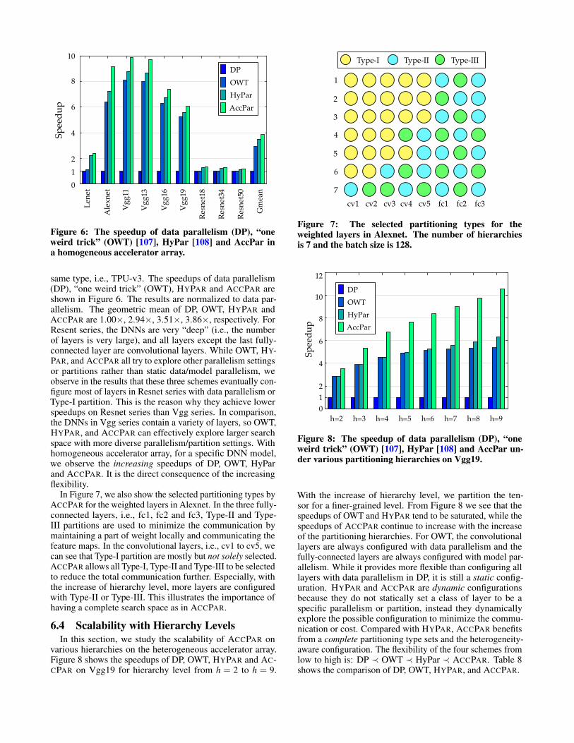
same type, i.e., TPU-v3. The speedups of data parallelism(DP), “one weird trick” (OWT), HYPAR and ACCPAR areshown in Figure 6. The results are normalized to data par-allelism. The geometric mean of DP, OWT, HYPAR andACCPAR are 1.00×, 2.94×, 3.51×, 3.86×, respectively. ForResent series, the DNNs are very “deep” (i.e., the numberof layers is very large), and all layers except the last fully-connected layer are convolutional layers. While OWT, HY-PAR, and ACCPAR all try to explore other parallelism settingsor partitions rather than static data/model parallelism, weobserve in the results that these three schemes evantually con-figure most of layers in Resnet series with data parallelism orType-I partition. This is the reason why they achieve lowerspeedups on Resnet series than Vgg series. In comparison,the DNNs in Vgg series contain a variety of layers, so OWT,HYPAR, and ACCPAR can effectively explore larger searchspace with more diverse parallelism/partition settings. Withhomogeneous accelerator array, for a specific DNN model,we observe the increasing speedups of DP, OWT, HyParand ACCPAR. It is the direct consequence of the increasingflexibility.

In Figure 7, we also show the selected partitioning types byACCPAR for the weighted layers in Alexnet. In the three fully-connected layers, i.e., fc1, fc2 and fc3, Type-II and Type-III partitions are used to minimize the communication bymaintaining a part of weight locally and communicating thefeature maps. In the convolutional layers, i.e., cv1 to cv5, wecan see that Type-I partition are mostly but not solely selected.ACCPAR allows all Type-I, Type-II and Type-III to be selectedto reduce the total communication further. Especially, withthe increase of hierarchy level, more layers are configuredwith Type-II or Type-III. This illustrates the importance ofhaving a complete search space as in ACCPAR.

6.4 Scalability with Hierarchy LevelsIn this section, we study the scalability of ACCPAR on

various hierarchies on the heterogeneous accelerator array.Figure 8 shows the speedups of DP, OWT, HYPAR and AC-CPAR on Vgg19 for hierarchy level from h = 2 to h = 9.

7

6

5

4

3

2

1

cv1 cv2 cv3 fc1 fc2 fc3cv4 cv5

Type-I Type-II Type-III

Figure 7: The selected partitioning types for theweighted layers in Alexnet. The number of hierarchiesis 7 and the batch size is 128.

Speedup

012

4

6

8

10

12

OWTHyParAccPar

DP

h=2 h=3 h=4 h=5 h=6 h=7 h=8 h=9

Figure 8: The speedup of data parallelism (DP), “oneweird trick” (OWT) [107], HyPar [108] and AccPar un-der various partitioning hierarchies on Vgg19.

With the increase of hierarchy level, we partition the ten-sor for a finer-grained level. From Figure 8 we see that thespeedups of OWT and HYPAR tend to be saturated, while thespeedups of ACCPAR continue to increase with the increaseof the partitioning hierarchies. For OWT, the convolutionallayers are always configured with data parallelism and thefully-connected layers are always configured with model par-allelism. While it provides more flexible than configuring alllayers with data parallelism in DP, it is still a static config-uration. HYPAR and ACCPAR are dynamic configurationsbecause they do not statically set a class of layer to be aspecific parallelism or partition, instead they dynamicallyexplore the possible configuration to minimize the commu-nication or cost. Compared with HYPAR, ACCPAR benefitsfrom a complete partitioning type sets and the heterogeneity-aware configuration. The flexibility of the four schemes fromlow to high is: DP ≺ OWT ≺ HyPar ≺ ACCPAR. Table 8shows the comparison of DP, OWT, HYPAR, and ACCPAR.

DP OWT HyPar ACCPAR

Static Static Dynamic DynamicLow −−−−−−−−−−−−−−−−−−−−→ High

Table 8: The caparison of flexibility of DP, OWT, HyParand ACCPAR.

7. CONCLUSIONIn this paper we present ACCPAR, a principled and sys-

tematic method to determining the tensor partition amongheterogeneous accelerator arrays for achieving optimal per-formance. ACCPAR considers the complete tensor partitionspace and reveals a new and previously unknown parallelismconfiguration. It optimizes performance based on a costmodel considering both computation and communicationcost of heterogeneous execution environment. The generalsearch algorithm is applicable for the emerging multi-pathpatterns in modern DNNs such as ResNet. We simulate ACC-PAR on a heterogeneous accelerator array composed of bothTPU-v2 and TPU-v3 accelerators for training of large-scaleDNN models such as Alexnet, Vgg series and Resnet series.The average performance of ACCPAR and previous state-of-the-art “one weird trick” (OWT) and HYPAR normalizedto data parallelism in the heterogeneous accelerator array is6.30×, 2.98×, 3.78×, respectively.

ACKNOWLEDGEMENTWe thank the anonymous reviewers for their constructiveand insightful comments. This work is supported in part byNSF CCF-1910299, NSF CSR-1717885, ARO W911NF-19-2-0107 and AFRL FA8750-18-2-0121. This work is alsosupported by the National Science Foundation grants NSFCCF-1657333, NSF CCF-1717754, NSF CNS-1717984, NSFCCF-1750656, and NSF CCF-1919289.

8. REFERENCES[1] S. Ren et al., “Faster r-cnn: Towards real-time object detection with

region proposal networks,” in NIPS, 2015.[2] W. Liu et al., “Ssd: Single shot multibox detector,” in ECCV, 2016.[3] X. Liu et al., “Dpatch: An adversarial patch attack on object

detectors,” arXiv:1806.02299, 2018.[4] B. Perozzi et al., “Deepwalk: Online learning of social

representations,” in KDD, 2014.[5] T. N. Kipf and M. Welling, “Semi-supervised classification with

graph convolutional networks,” arXiv:1609.02907, 2016.[6] A. Grover and J. Leskovec, “node2vec: Scalable feature learning for

networks,” in KDD, 2016.[7] T. Fischer and C. Krauss, “Deep learning with long short-term

memory networks for financial market predictions,” EuropeanJournal of Operational Research, 2018.

[8] X. Ding et al., “Deep learning for event-driven stock prediction,” inIJCAI, 2015.

[9] Y. Deng et al., “Deep direct reinforcement learning for financialsignal representation and trading,” IEEE TNNLS, 2016.

[10] R. Miotto et al., “Deep learning for healthcare: review, opportunitiesand challenges,” Briefings in bioinformatics, 2017.

[11] T. Ching et al., “Opportunities and obstacles for deep learning inbiology and medicine,” Journal of The Royal Society Interface, 2018.

[12] O. Faust et al., “Deep learning for healthcare applications based onphysiological signals: A review,” Computer methods and programsin biomedicine, 2018.

[13] L. Song et al., “Deep learning for vertex reconstruction ofneutrino-nucleus interaction events with combined energy and timedata,” in ICASSP, 2019.

[14] P. Baldi et al., “Searching for exotic particles in high-energy physicswith deep learning,” Nature communications, 2014.

[15] J. Wu et al., “Galileo: Perceiving physical object properties byintegrating a physics engine with deep learning,” in NIPS, 2015.

[16] S. B. Furber et al., “Overview of the spinnaker system architecture,”IEEE Transactions on Computers, 2013.

[17] Z. Du et al., “Neuromorphic accelerators: A comparison betweenneuroscience and machine-learning approaches,” in MICRO, 2015.

[18] P. A. Merolla et al., “A million spiking-neuron integrated circuit witha scalable communication network and interface,” Science, 2014.

[19] S. K. Esser et al., “Backpropagation for energy-efficientneuromorphic computing,” in NIPS, 2015.

[20] S. K. Esser et al., “Convolutional networks for fast, energy-efficientneuromorphic computing,” Proceedings of the National Academy ofSciences (PNAS), 2016.

[21] T. Liu et al., “Mt-spike: A multilayer time-based spikingneuromorphic architecture with temporal error backpropagation,” inICCAD, 2017.

[22] T. Liu et al., “Pt-spike: A precise-time-dependent single spikeneuromorphic architecture with efficient supervised learning,” inASP-DAC, 2018.

[23] H. Esmaeilzadeh et al., “Neural acceleration for general-purposeapproximate programs,” in MICRO, 2012.

[24] T. Chen et al., “Diannao: A small-footprint high-throughputaccelerator for ubiquitous machine-learning,” in ASPLOS, 2014.

[25] Y. Chen et al., “Dadiannao: A machine-learning supercomputer,” inMICRO, 2014.

[26] Z. Du et al., “Shidiannao: Shifting vision processing closer to thesensor,” in ISCA, 2015.

[27] D. Liu et al., “Pudiannao: A polyvalent machine learning accelerator,”in ASPLOS, 2015.

[28] S. Liu et al., “Cambricon: An instruction set architecture for neuralnetworks,” in ISCA, 2016.

[29] S. Zhang et al., “Cambricon-x: An accelerator for sparse neuralnetworks,” in MICRO, 2016.

[30] “Google supercharges machine learning tasks with tpu custom chip.”https://cloudplatform.googleblog.com/2016/05/Google-supercharges-machine-learning-tasks-with-custom-chip.html.

[31] N. P. Jouppi et al., “In-datacenter performance analysis of a tensorprocessing unit,” in ISCA, 2017.

[32] S. Venkataramani et al., “Scaledeep: A scalable compute architecturefor learning and evaluating deep networks,” in ISCA, 2017.

[33] P. Judd et al., “Stripes: Bit-serial deep neural network computing,” inMICRO, 2016.

[34] C. Zhang et al., “Optimizing fpga-based accelerator design for deepconvolutional neural networks,” in FPGA, 2015.

[35] J. Qiu et al., “Going deeper with embedded fpga platform forconvolutional neural network,” in FPGA, 2016.

[36] M. Motamedi et al., “Design space exploration of fpga-based deepconvolutional neural networks,” in ASP-DAC, 2016.

[37] N. Suda et al., “Throughput-optimized opencl-based fpga acceleratorfor large-scale convolutional neural networks,” in FPGA, 2016.

[38] C. Zhang et al., “Caffeine: Towards uniformed representation andacceleration for deep convolutional neural networks,” in ICCAD,2016.

[39] Y. Wang et al., “Deepburning: Automatic generation of fpga-basedlearning accelerators for the neural network family,” in DAC, 2016.

[40] C. Zhang et al., “Energy-efficient cnn implementation on a deeplypipelined fpga cluster,” in ISLPED, 2016.

[41] D. Mahajan et al., “Tabla: A unified template-based framework foraccelerating statistical machine learning,” in HPCA, 2016.

[42] H. Sharma et al., “From high-level deep neural models to fpgas,” inMICRO, 2016.

[43] Y. Guan et al., “Fp-dnn: An automated framework for mapping deepneural networks onto fpgas with rtl-hls hybrid templates,” in FCCM,2017.

[44] Y. Guan et al., “Fpga-based accelerator for long short-term memoryrecurrent neural networks,” in ASP-DAC, 2017.

[45] S. Han et al., “Ese: Efficient speech recognition engine with sparselstm on fpga,” in FPGA, 2017.

[46] Y. Ma et al., “Optimizing loop operation and dataflow in fpgaacceleration of deep convolutional neural networks,” in FPGA, 2017.

[47] R. Zhao et al., “Accelerating binarized convolutional neural networkswith software-programmable fpgas.,” in FPGA, 2017.

[48] Y. Shen et al., “Overcoming resource underutilization in spatial cnnaccelerators,” in FPL, 2016.

[49] C. Zhang and V. K. Prasanna, “Frequency domain acceleration ofconvolutional neural networks on cpu-fpga shared memory system.,”in FPGA, 2017.

[50] R. Cai et al., “Vibnn: Hardware acceleration of bayesian neuralnetworks,” in ASPLOS, 2018.

[51] C. Farabet et al., “Neuflow: A runtime reconfigurable dataflowprocessor for vision,” in CVPRW, 2011.

[52] Y.-H. Chen et al., “Eyeriss: A spatial architecture for energy-efficientdataflow for convolutional neural networks,” in ISCA, 2016.

[53] Y.-H. Chen et al., “Eyeriss: An energy-efficient reconfigurableaccelerator for deep convolutional neural networks,” IEEE JSSC,2017.

[54] Y.-H. Chen et al., “Using dataflow to optimize energy efficiency ofdeep neural network accelerators,” IEEE Micro, 2017.

[55] W. Lu et al., “Flexflow: A flexible dataflow accelerator architecturefor convolutional neural networks,” in HPCA, 2017.

[56] M. Alwani et al., “Fused-layer cnn accelerators,” in MICRO, 2016.[57] Y. Shen et al., “Maximizing cnn accelerator efficiency through

resource partitioning,” in ISCA, 2017.[58] A. Yazdanbakhsh et al., “Ganax: A unified mimd-simd acceleration

for generative adversarial networks,” in ISCA, 2018.[59] K. Hegde et al., “Ucnn: Exploiting computational reuse in deep

neural networks via weight repetition,” in ISCA, 2018.[60] D. Kim et al., “Neurocube: A programmable digital neuromorphic

architecture with high-density 3d memory,” in ISCA, 2016.[61] L. Jiang et al., “Xnor-pop: A processing-in-memory architecture for

binary convolutional neural networks in wide-io2 drams,” in ISLPED,2017.

[62] S. Li et al., “Drisa: A dram-based reconfigurable in-situ accelerator,”in MICRO, 2017.

[63] Q. Lou et al., “3dict: a reliable and qos capable mobileprocess-in-memory architecture for lookup-based cnns in 3d xpointrerams,” in ICCAD, 2018.

[64] S. Han et al., “Eie: efficient inference engine on compressed deepneural network,” in ISCA, 2016.

[65] A. Ren et al., “Sc-dcnn: Highly-scalable deep convolutional neuralnetwork using stochastic computing,” in ASPLOS, 2017.

[66] A. Parashar et al., “Scnn: An accelerator for compressed-sparseconvolutional neural networks,” in ISCA, 2017.

[67] Y. Shen et al., “Escher: A cnn accelerator with flexible buffering tominimize off-chip transfer,” in FCCM, 2017.

[68] M. S. Razlighi et al., “Looknn: Neural network with nomultiplication,” in DATE, 2017.

[69] J. Albericio et al., “Bit-pragmatic deep neural network computing,”in MICRO, 2017.

[70] H. Sharma et al., “Bit fusion: Bit-level dynamically composablearchitecture for accelerating deep neural network,” in ISCA, 2018.

[71] T. Na and S. Mukhopadhyay, “Speeding up convolutional neuralnetwork training with dynamic precision scaling and flexiblemultiplier-accumulator,” in ISLPED, 2016.

[72] B. Reagen et al., “Minerva: Enabling low-power, highly-accuratedeep neural network accelerators,” in ISCA, 2016.

[73] J. Mao et al., “Modnn: Local distributed mobile computing systemfor deep neural network,” in DATE, 2017.

[74] J. Mao et al., “Mednn: A distributed mobile system with enhancedpartition and deployment for large-scale dnns,” in ICCAD, 2017.

[75] J. Mao et al., “Adalearner: An adaptive distributed mobile learningsystem for neural networks,” in ICCAD, 2017.

[76] C.-E. Lee et al., “Stitch-x: An accelerator architecture for exploitingunstructured sparsity in deep neural networks,” in SysML, 2018.

[77] J. Liu et al., “Processing-in-memory for energy-efficient neuralnetwork training: A heterogeneous approach,” in MICRO, 2018.

[78] J. Yu et al., “Scalpel: Customizing dnn pruning to the underlyinghardware parallelism,” in ISCA, 2017.

[79] C. Ding et al., “Circnn: accelerating and compressing deep neuralnetworks using block-circulant weight matrices,” in MICRO, 2017.

[80] J. Park et al., “Scale-out acceleration for machine learning,” inMICRO, 2017.

[81] V. Akhlaghi et al., “Snapea: Predictive early activation for reducingcomputation in deep convolutional neural networks,” in ISCA, 2018.

[82] E. Park et al., “Energy-efficient neural network accelerator based onoutlier-aware low-precision computation,” in ISCA, 2018.

[83] M. Song et al., “Prediction based execution on deep neural networks,”in ISCA, 2018.

[84] C. Deng et al., “Permdnn: Efficient compressed deep neural networkarchitecture with permuted diagonal matrices,” in MICRO, 2018.

[85] M. Gao et al., “Tetris: Scalable and efficient neural networkacceleration with 3d memory,” in ASPLOS, 2017.

[86] P. Chi et al., “Prime: A novel processing-in-memory architecture forneural network computation in reram-based main memory,” in ISCA,2016.

[87] A. Shafiee et al., “Isaac: A convolutional neural network acceleratorwith in-situ analog arithmetic in crossbars,” in ISCA, 2016.

[88] X. Liu et al., “Reno: a high-efficient reconfigurable neuromorphiccomputing accelerator design,” in DAC, 2015.

[89] M. N. Bojnordi and E. Ipek, “Memristive boltzmann machine: Ahardware accelerator for combinatorial optimization and deeplearning,” in HPCA, 2016.

[90] L. Song et al., “Pipelayer: A pipelined reram-based accelerator fordeep learning,” in HPCA, 2017.

[91] X. Qiao et al., “Atomlayer: a universal reram-based cnn acceleratorwith atomic layer computation,” in DAC, 2018.

[92] H. Ji et al., “Recom: An efficient resistive accelerator for compresseddeep neural networks,” in DATE, 2018.

[93] F. Chen et al., “Regan: A pipelined reram-based accelerator forgenerative adversarial networks,” in ASP-DAC, 2018.

[94] B. Li et al., “Reram-based accelerator for deep learning,” in DATE,2018.

[95] F. Chen and H. Li, “Emat: an efficient multi-task architecture fortransfer learning using reram,” in ICCAD, 2018.

[96] T. Tang et al., “Binary convolutional neural network on rram,” inASP-DAC, 2017.

[97] F. Chen et al., “Zara: A novel zero-free dataflow accelerator forgenerative adversarial networks in 3d reram,” in DAC, 2019.

[98] P. Wang et al., “Snrram: an efficient sparse neural networkcomputation architecture based on resistive random-access memory,”in DAC, 2018.

[99] J. Albericio et al., “Cnvlutin: ineffectual-neuron-free deep neuralnetwork computing,” in ISCA, 2016.

[100] Y. Ji et al., “Neutrams: Neural network transformation and co-designunder neuromorphic hardware constraints,” in MICRO, 2016.

[101] A. Mirhoseini et al., “Perform-ml: Performance optimized machinelearning by platform and content aware customization,” in DAC,2016.

[102] Z. Takhirov et al., “Energy-efficient adaptive classifier design formobile systems,” in ISLPED, 2016.

[103] X. Zhang et al., “Dnnbuilder: an automated tool for buildinghigh-performance dnn hardware accelerators for fpgas,” in ICCAD,2018.

[104] Y. Wang et al., “Group scissor: Scaling neuromorphic computingdesign to large neural networks,” in DAC, 2017.

[105] J. H. Ko et al., “Design of an energy-efficient accelerator for trainingof convolutional neural networks using frequency-domaincomputation,” in DAC, 2017.

[106] M. Li et al., “Scaling distributed machine learning with the parameterserver,” in OSDI, 2014.

[107] A. Krizhevsky, “One weird trick for parallelizing convolutionalneural networks,” arXiv:1404.5997, 2014.

[108] L. Song et al., “Hypar: Towards hybrid parallelism for deep learningaccelerator array,” in HPCA, 2019.

[109] Y. S. Shao et al., “Simba: Scaling deep-learning inference withmulti-chip-module-based architecture,” in MICRO, 2019.

[110] M. Zhu et al., “Sparse tensor core: Algorithm and hardwareco-design for vector-wise sparse neural networks on modern gpus,”in MICRO, 2019.

[111] A. Fuchs and D. Wentzlaff, “The accelerator wall: Limits of chipspecialization,” in HPCA, 2019.

[112] A. Krizhevsky et al., “Imagenet classification with deepconvolutional neural networks,” in NIPS, 2012.

[113] K. He et al., “Deep residual learning for image recognition,” inCVPR, 2016.

[114] I. Goodfellow et al., “Generative adversarial nets,” in NIPS, 2014.[115] A. Radford et al., “Unsupervised representation learning with deep

convolutional generative adversarial networks,” arXiv:1511.06434,2015.

[116] Z. Jia et al., “Exploring hidden dimensions in parallelizingconvolutional neural networks,” in ICML, 2018.

[117] M. Wang et al., “Unifying data, model and hybrid parallelism in deeplearning via tensor tiling,” arXiv:1805.04170, 2018.

[118] M. Wang et al., “Supporting very large models using automaticdataflow graph partitioning,” in EuroSys, 2019.

[119] Z. Jia et al., “Beyond data and model parallelism for deep neuralnetworks,” in SysML, 2019.

[120] K. Simonyan and A. Zisserman, “Very deep convolutional networksfor large-scale image recognition,” arXiv:1409.1556, 2014.

[121] N. Qian, “On the momentum term in gradient descent learningalgorithms,” Neural networks, 1999.

[122] D. P. Kingma and J. Ba, “Adam: A method for stochasticoptimization,” arXiv:1412.6980, 2014.

[123] C. Eckert et al., “Neural cache: Bit-serial in-cache acceleration ofdeep neural networks,” in ISCA, 2018.

[124] X. Wang et al., “Bit prudent in-cache acceleration of deepconvolutional neural networks,” in HPCA, 2019.

[125] M. Mahmoud et al., “Diffy: a déjà vu-free differential deep neuralnetwork accelerator,” in MICRO, 2018.

[126] J. Zhang and J. Li, “Improving the performance of opencl-based fpgaaccelerator for convolutional neural network.,” in FPGA, 2017.

[127] Y. Li et al., “Accelerating distributed reinforcement learning within-switch computing,” in ISCA, 2019.

[128] A. Azizimazreah and L. Chen, “Shortcut mining: Exploitingcross-layer shortcut reuse in dcnn accelerators,” in HPCA, 2019.

[129] H. Cho et al., “Fa3c: Fpga-accelerated deep reinforcement learning,”in ASPLOS, 2019.

[130] Z. Li et al., “E-rnn: Design optimization for efficient recurrent neuralnetworks in fpgas,” in HPCA, 2019.

[131] M. Gao et al., “Tangram: Optimized coarse-grained dataflow forscalable nn accelerators,” in ASPLOS, 2019.

[132] H. Kung et al., “Packing sparse convolutional neural networks forefficient systolic array implementations: Column combining underjoint optimization,” in ASPLOS, 2019.

[133] H. Kwon et al., “Maeri: Enabling flexible dataflow mapping over dnnaccelerators via reconfigurable interconnects,” in ASPLOS, 2018.

[134] H. Kim et al., “Nand-net: Minimizing computational complexity ofin-memory processing for binary neural networks,” in HPCA, 2019.

[135] S. Li et al., “Scope: A stochastic computing engine for dram-basedin-situ accelerator,” in MICRO, 2018.

[136] P. Srivastava et al., “Promise: An end-to-end design of aprogrammable mixed-signal accelerator for machine-learningalgorithms,” in ISCA, 2018.

[137] C. Deng et al., “Tie: Energy-efficient tensor train-based inferenceengine for deep neural network,” in ISCA, 2019.

[138] S. Sharify et al., “Laconic deep learning inference acceleration,” inISCA, 2019.

[139] A. Ren et al., “Admm-nn: An algorithm-hardware co-designframework of dnns using alternating direction methods ofmultipliers,” in ASPLOS, 2019.

[140] A. Jain et al., “Gist: Efficient data encoding for deep neural networktraining,” in ISCA, 2018.

[141] H. Jang et al., “Mnnfast: A fast and scalable system architecture formemory-augmented neural networks,” in ISCA, 2019.

[142] M. Riera et al., “Computation reuse in dnns by exploiting inputsimilarity,” in ISCA, 2018.

[143] M. Rhu et al., “vdnn: Virtualized deep neural networks for scalable,memory-efficient neural network design,” in MICRO, 2016.

[144] M. Rhu et al., “Compressing dma engine: Leveraging activationsparsity for training deep neural networks,” in HPCA, 2018.

[145] X. He et al., “Joint design of training and hardware towards efficientand accuracy-scalable neural network inference,” IEEE JETCAS,2018.

[146] J. Zhang et al., “Eager pruning: algorithm and architecture supportfor fast training of deep neural networks,” in ISCA, 2019.

[147] A. Delmas Lascorz et al., “Bit-tactical: A software/hardwareapproach to exploiting value and bit sparsity in neural networks,” inASPLOS, 2019.

[148] A. Samajdar et al., “Genesys: Enabling continuous learning throughneural network evolution in hardware,” in MICRO, 2018.

[149] T.-H. Yang et al., “Sparse reram engine: Joint exploration ofactivation and weight sparsity in compressed neural networks,” inISCA, 2019.

[150] R. LiKamWa et al., “Redeye: Analog convnet image sensorarchitecture for continuous mobile vision,” in ISCA, 2016.

[151] R. Cai et al., “A stochastic-computing based deep learningframework using adiabatic quantum-flux-parametronsuperconducting technology,” in ISCA, 2019.

[152] M. Imani et al., “Floatpim: In-memory acceleration of deep neuralnetwork training with high precision,” in ISCA, 2019.

[153] A. Ankit et al., “Puma: A programmable ultra-efficientmemristor-based accelerator for machine learning inference,” inASPLOS, 2019.

[154] Y. Ji et al., “Fpsa: A full system stack solution for reconfigurablereram-based nn accelerator architecture,” in ASPLOS, 2019.

[155] L. Ke et al., “Nnest: Early-stage design space exploration tool forneural network inference accelerators,” in ISLPED, 2018.

[156] J. L. Hennessy and D. A. Patterson, “A new golden age for computerarchitecture: Domain-specific hardware/software co-design,enhanced security, open instruction sets, and agile chip development,”Turing Lecture, 2018.

[157] D. Patterson, “50 years of computer architecture: From themainframe cpu to the domain-specific tpu and the open risc-vinstruction set,” in ISSCC, 2018.

[158] J. L. Hennessy and D. A. Patterson, “A new golden age for computerarchitecture,” Communications of the ACM, 2019.

[159] J. Dean et al., “A new golden age in computer architecture:Empowering the machine-learning revolution,” IEEE Micro, 2018.

[160] Q. Yang et al., “A quantized training method to enhance accuracy ofreram-based neuromorphic systems,” in ISCAS, 2018.

[161] G. E. Moore, “Cramming more components onto integrated circuits,”Electronics, 1965.

[162] “Ai & machine learning products cloud tpu.”https://cloud.google.com/tpu/.

[163] Y. LeCun et al., “Lenet-5, convolutional neural networks,” URL:http://yann. lecun. com/exdb/lenet, 2015.

[164] Y. LeCun et al., “Gradient-based learning applied to documentrecognition,” Proceedings of the IEEE, 1998.

[165] J. Deng et al., “Imagenet: A large-scale hierarchical image database,”in CVPR, 2009.

[166] “Vpc resource quotas.”https://cloud.google.com/vpc/docs/quota.