accounting for cross-country income differences
TRANSCRIPT

Chapter 9
ACCOUNTING FOR CROSS-COUNTRY INCOME DIFFERENCES
FRANCESCO CASELLI*
LSE, CEPR, and NBERe-mail: [email protected]
Contents
Abstract 6801. Introduction 6812. The measure of our ignorance 683
2.1. Basic data 6852.2. Basic measures of success 6862.3. Alternative measures used in the literature 6882.4. Sub-samples 689
3. Robustness: basic stuff 6903.1. Depreciation rate 6903.2. Initial capital stock 6913.3. Education-wage profile 6933.4. Years of education 1 6943.5. Years of education 2 6943.6. Hours worked 6953.7. Capital share 696
4. Quality of human capital 6984.1. Quality of schooling: Inputs 698
4.1.1. Teachers’ human capital 6994.1.2. Pupil–teacher ratios 7014.1.3. Spending 702
4.2. Quality of schooling: test scores 7034.3. Experience 7064.4. Health 7084.5. Social vs. private returns to schooling and health 710
5. Quality of physical capital 7115.1. Composition 7115.2. Vintage effects 7155.3. Further problems with K 716
* A data set is posted at http://econ.lse.ac.uk/staff/caselli_francesco/.
Handbook of Economic Growth, Volume 1A. Edited by Philippe Aghion and Steven N. Durlauf© 2005 Elsevier B.V. All rights reservedDOI: 10.1016/S1574-0684(05)01009-9

680 F. Caselli
6. Sectorial differences in TFP 7176.1. Industry studies 7186.2. The role of agriculture 7196.3. Sectorial composition and development accounting 724
7. Non-neutral differences in technology 7277.1. Basic concepts and qualitative results 7277.2. Development accounting with non-neutral differences 734
8. Conclusions 737Acknowledgements 738References 738
Abstract
Why are some countries so much richer than others? Development Accounting is afirst-pass attempt at organizing the answer around two proximate determinants: factorsof production and efficiency. It answers the question “how much of the cross-countryincome variance can be attributed to differences in (physical and human) capital, andhow much to differences in the efficiency with which capital is used?” Hence, it does forthe cross-section what growth accounting does in the time series. The current consensusis that efficiency is at least as important as capital in explaining income differences.I survey the data and the basic methods that lead to this consensus, and explore severalextensions. I argue that some of these extensions may lead to a reconsideration of theevidence.
Ch. 9: Accounting for Cross-Country Income Differences 681
1. Introduction
This chapter is about development accounting. It is widely known, and will be foundagain to be true here, that cross-country differences in income per worker are enormous.Development accounting uses cross-country data on output and inputs, at one point intime, to assess the relative contribution of differences in factor quantities, and differ-ences in the efficiency with which those factors are used, to these vast differences inper-worker incomes. Hence, it is the same idea of growth accounting (illustrated by Jor-genson’s chapter in this Handbook), with cross-country differences replacing cross-timedifferences.
Conceptually, development accounting can be thought of as quantifying the relation-ship
(1)Income = F(Factors, Efficiency).
Like growth accounting, this is a potentially useful tool. If one found that Factors areable to account for most of the differences, then development economics could focuson explaining low rates of factor accumulation. There would of course be ample scopefor controversy over the policies better suited to engineering higher investment rates invarious types of capital, but there would be consensus over the fact that the intermediategoal of development policy is to engineer those higher rates. Instead, should one findthat Efficiency differences play a large role, then one would have to confront the addi-tional task of explaining why some countries extract more output than others from theirfactors of production. Experience suggests that this additional question is the hardest tocrack.
The consensus view in development accounting is that Efficiency plays a very largerole. A sentence commonly used to summarize the existing literature sounds somethinglike “differences in efficiency account for at least 50% of differences in per capita in-come”. The next section of this chapter (Section 2) will survey the existing literature,replicate its basic findings, and update them with more recent data. Looking at a cross-section of 94 countries in the year 1996, I confirm that standard procedures assign toEfficiency the role of the chief culprit.
Operationally, the key steps in development accounting are: (1) choosing a functionalform for F , and (2) accurately measuring Income and Factors. Efficiency is backed outas a residual. As for the Solow residual, this residual is a “measure of our ignorance” onthe causes of poverty and under-development. And, as in growth accounting, one poten-tially promising research strategy is to try to “chip away” at this residual by improvingon steps (1) and (2), i.e. by looking at alternative functional forms, and by attemptinga more sophisticated measurement of Income and Factors. For example, one could tryto include information on quality differences in the capital stock – instead of relyingexclusively on quantity.
682 F. Caselli
The bulk of this chapter aims at outlining strategies for such a chipping away.1 Itinvestigates the potential for different functional forms, and different ways of estimatinginputs and outputs, to reduce the measure of our ignorance. Rather than reaching firmconclusions, it tries to classify ideas into more or less promising. Its contribution is toformulate sentences such as “improvements in the measurement of x are unlikely tosignificantly reduce the unexplained component of per-capita income differences”, or“the unexplained component is somewhat sensitive to the measurement of z, so this is apotentially fruitful area for further research”.
The experiments I perform fall in five broad categories. The first is a fairly mechanicalset of robustness checks with respect to the choice of parameters in the basic model usedin the literature, as well as with respect to possible measurement errors in output, labor,and years of schooling. I conclude that none of these robustness checks seriously callsinto question the conclusions from the current consensus (Section 3).
Second, I consider extensions of the basic development-accounting framework aimedat improving the measurement of human capital. In most development-accounting ex-ercises differences in human capital stem exclusively from differences in the quantityof schooling. One set of extensions I consider exploits cross-country data on schoolresources and test scores as proxies for the quality of education, and then uses thesequality indicators to augment the quantity-based measure of human capital. I find thattaking into account schooling quality leads to trivially small reductions in the measureof our ignorance. Another extension replicates existing work that augments human cap-ital by a proxy of the health status of the labor force. There is some indication thatthis may lead to a significant reduction in the unexplained component of income, butI argue that the bulk of the variance most likely remains unexplained. All the measuresof human capital considered are built on the assumption that the private return to hu-man capital accurately describes its social return. I conclude this section with a briefdiscussion of why and how one may want to try and relax this assumption (Section 4).
Third, I turn to the measurement of physical capital. Here I review contributionsthat highlight enormous cross-country variation in the composition of the stock ofequipment. A simple model shows how to relate variation in capital composition tounobserved quality differences in the capital stock. How much of the responsibility forefficiency differences can be assigned to these differences in the quality of capital de-pends on parameters that are very hard to pin down, but the potential is extremely large.I therefore conclude that the composition of capital should be a key area of future re-search. I also glance at vintage-capital models, but argue that they hold little promisefor development accounting, as well as at the distinction between private and publicinvestment, which is instead potentially quite important (Section 5).
The most innovative contributions of the chapter are represented by the fourth andfifth sets of extensions. In the former I explore the role of the sectorial composition of
1 The analogy in spirit with Jorgenson’s monumental contribution in growth accounting – some of which iscollected in Jorgenson (1995a, 1995b) is obvious, but it stops there: the reader should expect nothing like thesame level of depth, comprehensiveness, and insight.
Ch. 9: Accounting for Cross-Country Income Differences 683
output. The large differences in overall efficiency that are found at the aggregate levelcould reflect large differences in efficiency within each sector of the economy, but theycould also be due to the fact that some countries have more of their inputs in intrinsicallyless productive sectors than others. I explore this idea by looking at an agriculture/non-agriculture decomposition (poor countries have as much as 90% of their workforce inagriculture, rich countries as little as 3%), but find that only a small fraction of theoverall variation in efficiency is due to differences in sectorial composition: Efficiencydifferences appear to be a within industry phenomenon (Section 6).
The last set of exercises explores a radical departure from the standard framework,and finds radically different answers. In the standard framework, which relies on aCobb–Douglas specification of the production function, efficiency differences are factorneutral: if a country uses physical capital efficiently, it also necessarily uses human cap-ital efficiently. I argue that this is a pretty restrictive assumption, and propose a simpleCES generalization of the basic framework where cross-country efficiency differencesare allowed to be non neutral. Stunningly, I find that, when non neutrality is allowedfor, the data say that poor countries use physical capital more efficiently than rich coun-tries (while rich countries use human capital more efficiently). Furthermore, when thedevelopment-accounting exercise is performed in a context of non-neutral efficiencydifferences the conclusions on the contribution of these differences to cross-countryincome inequality become very fragile. In particular, if the elasticity of substitutionbetween physical and human capital is low enough, observed differences in factorendowments become able to explain the bulk of the cross-country income variance.I therefore conclude that the most important outstanding question in development ac-counting may well be what this elasticity of substitution is (Section 7).
Before plunging into the data and the calculations, it is worthwhile to stress the lim-its of development accounting. Development accounting does not uncover the ultimatereasons why some countries are much richer than others: only the proximate ones. Likegrowth accounting, it has nothing to say on the causes of low factor accumulation, orlow levels of efficiency. Indeed, the most likely scenario is that the same ultimate causesexplain both. Furthermore, it has nothing to say on the way factor accumulation and ef-ficiency influence each other, as they most probably do. Instead, it should be understoodas a diagnostic tool, just as medical tests can tell one whether or not he is suffering froma certain ailment, but cannot reveal the causes of it. This does not make the test any theless useful.
2. The measure of our ignorance
The key empirical result that motivates this chapter is that in a simple framework withtwo factors of production, physical and human capital, a large fraction of the cross-country income variance remains unexplained. This result has been established by avariety of authors using a variety of techniques. Knight, Loayza and Villanueva (1993),Islam (1995), and Caselli, Esquivel and Lefort (1996), for example, used panel-data
684 F. Caselli
techniques to estimate (1). They all found that, after controlling for factor accumulation,country-specific effects played a large role in output differences, and interpreted thesefixed effects as picking up differences in efficiency. King and Levine (1994), Klenowand Rodriguez-Clare (1997), Prescott (1998), and Hall and Jones (1999), instead, useda calibration approach, and found that plausible parametrizations of (1) had limited ex-planatory power without large efficiency differences. These studies used cross-countrynational-account data on inputs and outputs, but Hendricks (2002) was able to reachsimilar conclusions by using earnings of migrants to the United States, and Aiyar andDalgaard (2002) by using a dual approach involving factor prices rather than quantities.All these papers were inspired by – and written in response to – the challenge posed bythe seminal contribution of Mankiw, Romer and Weil (1992).2
In this section I revisit the basic development-accounting finding. Because I wantto set the stage for a variety of extensions of the basic model, I adopt the calibrationapproach, which offers more flexibility in experimenting with different parameter valuesand functional forms.3
I adopt as the benchmark Hall and Jones’ production function, according to which acountry’s GDP, Y , is
(2)Y = AKα(Lh)1−α,
where K is the aggregate capital stock and Lh is the “quality adjusted” workforce,namely the number of workers L multiplied by their average human capital h. α is aconstant. Clearly this is a special case of (1), where the residual A represents the effi-ciency with which factors are used. It is also clear that A corresponds to the standardnotion of Total Factor Productivity (TFP), so until further notice I will speak of effi-ciency and TFP interchangeably.
In per-worker terms the production function can be rewritten as
(3)y = Akαh1−α,
where k is the capital labor ratio (k = K/L). We want to know how much of thevariation in y can be explained with variation in the observables, h and k, and how muchis “residual” variation, i.e. must be attributed to differences in A. Clearly to answer thisquestion we need, besides data on y, data on k and h, as well as a value for the capitalshare α.
2 However, there are some pre-1990s antecedents. In particular, the nine-country studies of Denison (1967),and Christensen, Cummings and Jorgenson (1981).3 An earlier survey of the material covered in this section is provided by McGrattan and Schmitz (1999).
See also Easterly and Levine (2001) for a review of development accounting as well as other evidence forcross-country efficiency differentials.
Ch. 9: Accounting for Cross-Country Income Differences 685
2.1. Basic data
The basic data set used in this chapter combines variables from two sources. The firstis version 6.1 of the Penn World Tables [PWT61 – Heston, Summers and Aten (2002)],i.e. the latest incarnation of the celebrated Summers and Heston (1991) data set. FromPWT61 I extract output, capital, and the number of workers. The second is Barro andLee (2001), which I use for educational attainment. Several additional data sources willbe brought to bear for specific exercises in later sections, but the data we construct herewill be crucial to everything we do.
Previous authors have mostly used version 5.6 of the Penn World Tables (PWT56).They have therefore attempted to explain the world income distribution as of the late1980s. By using version 6.1 I am able to update the basic result to the mid-90s.
I measure y from PWT61 as real GDP per worker in international dollars (i.e. in PPP– this variable is called RGDPWOK in the original data set).4
I generate estimates of the capital stock, K , using the perpetual inventory equation
Kt = It + (1 − δ)Kt−1,
where It is investment and δ is the depreciation rate. I measure It from PWT61 as realaggregate investment in PPP.5 Following standard practice, I compute the initial capitalstock K0 as I0/(g+δ), where I0 is the value of the investment series in the first year it isavailable, and g is the average geometric growth rate for the investment series betweenthe first year with available data and 1970. The rationale for this choice is tenuous:I/(g + δ) is the expression for the capital stock in the steady state of the Solow model.We will see below whether results are very sensitive to this assumption, or for thatmatter to the others I am about to make, such as the one for δ, which – following theliterature – I set to 0.06. To compute k, I divide K by the number of workers.6
To construct human capital I take from Barro and Lee (2001) the average years ofschooling in the population over 25 year old. Following Hall and Jones (1999) this isturned into a measure of h through the formula:
h = eφ(s),
where s is average years of schooling, and the function φ(s) is piecewise linear with
4 Some authors subtract from the PWT measure of GDP the value-added of the mining industry, becausenot doing so would result in some oil-rich countries being among the most productive in the world. Thisrationale is inherently dubious (then why not subtracting the value added of agriculture and forestry, that alsouse natural resources abundantly?). More importantly, since a similar correction is not feasible for the capitalstock, this procedure must result in hugely downward biased estimates of the TFP of these countries. I applyno such correction here.5 Computed as RGDPL · POP · KI, where RGDPL is real income per capita obtained with the Laspeyres
method, POP is the population, and KI is the investment share in total income.6 Obtained as RGDPCH · POP/RGDPWOK, where RGDPCH is real GDP per capita computed with the
chain method.

686 F. Caselli
slope 0.13 for s � 4, 0.10 for 4 < s � 8, and 0.07 for 8 < s.7 The rationale forthis functional form is as follows. Given our production function, perfect competitionin factor and good markets implies that the wage of a worker with s years of educationis proportional to his human capital. Since the wage–schooling relationship is widelythought to be log-linear, this calls for a log-linear relation between h and s as well,or something like h = exp(φss), with φs a constant. However, international data oneducation–wage profiles [Psacharopoulos (1994)] suggests that in Sub-Saharan Africa(which has the lowest levels of education) the return to one extra year of education isabout 13.4 percent, the World average is 10.1 percent, and the OECD average is 6.8percent. Hall and Jones’s measure tries to reconcile the log-linearity at the country levelwith the concavity across countries.
s is observed in the data every five years, most recently in 2000. Since s moves slowlyover time, a quinquennial observation can plausibly be employed for nearby dates aswell.
I treat a country as having “complete data” at date t if it has an uninterrupted invest-ment series between 1960 and t , and it has an observation for s in 1995.8 With thisdefinition, there are 94 countries with complete data in 1995, 94 in 1996, 91 in 1997,90 in 1998, 87 in 1999, and 82 in 2000 (and 0 thereafter). Hence, I focus on 1996 as themost recent year that affords the largest sample. In this sample, for more than half ofthe countries the investment series starts in 1950.9
As is well known, per-capita income differences are enormous. The richest countryin the sample (USA) has income per worker equal to 57,259 1996 international dollars,while the poorest (Zaire, today’s Democratic Republic of the Congo) has 630 – a ratioof 91. The ratio between the 90th (Canada) and the 10th percentile (Togo) of the incomedistribution, a measure of dispersion I’ll use prominently in the rest of the paper, is 21.The log-variance, another measure I’ll rely on heavily, is 1.30.
For the last ingredient required by Equation (3), α, I (implicitly) use US time-seriesdata on the capital-share, whose long-run (and roughly constant) average value is 1/3.All these data choices will be subject to scrutiny in the rest of the chapter – indeed, thisscrutiny is one of the chapter’s contributions.
2.2. Basic measures of success
With data on k, h, and y, and a choice for α, Equation (3) is one equation in the un-known A. In particular, after defining yKH = kαh1−α , we can rewrite (3) as
(4)y = AyKH,
where both y and yKH are observable. I will refer to yKH as the factor-only model.
7 Specifically we have φ(s) = 0.134 · s if s � 4, φ(s) = 0.134 · 4 + 0.101 · (s − 4) if 4 < s � 8,φ(s) = 0.134 · 4 + 0.101 · 4 + 0.068 · (s − 8) if 8 < s.8 Availability of data on income and labor force are not binding given these constraints.9 Nicaragua in 1979 has I < 0, which we deal with by re-setting it to I = 0. Haiti has missing data on I in
1966, which we deal with by imputing the average of 1965 and 1967.
Ch. 9: Accounting for Cross-Country Income Differences 687
Throughout this chapter I will pursue the following version of the development-accounting question: how successful is the factor-only model at explaining cross-country income differences? In other words, I will compare the (observed) variationin yHK to the (observed) variation in y. Clearly, this means that I am asking the follow-ing question. Suppose that all countries had the same level of efficiency A: what wouldthe world income distribution look like in that case, compared to the actual one?
To perform this assessment, I will look at two alternative measures. The first one isin the tradition of variance decompositions. From (4) we have
(5)var[log(y)
] = var[log(yKH)
] + var[log(A)
] + 2cov[log(A), log(yKH)
].
Now notice that if all countries had the same level of TFP we would have var[log(A)] =cov[log(A), log(yKH)] = 0. Hence, a first measure of success of the factor-only modelis
success1 = var[log(yKH)]var[log(y)] .
In our data the counterfactual variance, var[log(yKH)], takes the value 0.5. Since theobserved variance of log(y), var[log(y)], is 1.30 this approach leads to the conclu-sion that the fraction of the variance of income explained by observed endowmentsis success1 = 0.39.
While success1 is nicely grounded in the tradition of variance decomposition, it hasthe well-known drawback that variances are sensitive to outliers. A measure that is lesssensitive to outliers is a measure of the inter-percentile differential. Define xp the valueof the pth percentile of the distribution of x. My second measure of success of thefactor-only model is
success2 = y90KH/y10
KH
y90/y10,
i.e. it compares what the 90th-to-10th percentile ratio would be in the counterfactualworld with common technology, to the actual value. In the data the value of y90
KH/y10KH
is 7. Since y90/y10 is 21, according to the percentile ratio the fraction of the cross-country income dispersion explained by observables is success2 = 0.34.
I summarize the baseline experiment in Table 1. Clearly by both measures of successthe dispersion of yKH is much less than the dispersion of y, and this is the basic fact thatmotivates this study.10
Before proceeding, it is useful to check that these results are consistent with theslightly different data used in previous studies. Using the Hall and Jones data setsuccess1 is 0.40 (vs. 0.39 with ours), and success2 is 0.34, as with ours. As is evident,the different decade, country coverage, and methodology in assembling the PWT doesnot lead to important changes in this basic finding.
10 Of course variation in yKH – even though much less than variation in y – is economically significant andinteresting in its own right. For recent studies shedding light on the sources of variation in k and h see, e.g.,Bils and Klenow (2000), Hsieh and Klenow (2003), and Gourinchas and Jeanne (2003).

688 F. Caselli
Table 1Baseline success of the factor-only model
var[log(y)] 1.297 y90/y10 21var[log(yKH)] 0.500 y90
KH/y10KH 7
success1 0.39 success2 0.34
2.3. Alternative measures used in the literature
success1 essentially asks what would the dispersion of (log) per-capita income be if allcountries had the same level of efficiency, A, and then compares this counter-factualdispersion to the observed one. Klenow and Rodriguez-Clare (1997) propose the alter-native measure:
successKR = var[log(yKH)] + cov[log(A), log(yKH)]var[log(y)] ,
which differs from success1 for the covariance term in the numerator. In terms ofEquation (5) successKR is equivalent to a variance decomposition in which the con-tribution from the covariance term is split evenly between A and yKH . Because in thedata cov[log(A), log(yKH)] is positive (0.28) the Klenow and Rodriguez-Clare measureassigns a greater role to k and h than the simple ratio of variances: successKR is 0.60.Here I do not emphasize this measure because it does not answer the question: whatwould the dispersion of incomes be if all countries had the same A? As Klenow andRodriguez-Clare explain, it asks the different question: “when we see 1% higher y, howmuch higher is our conditional expectation of yKH?” which in my opinion is not asintuitive.
Klenow and Rodriguez-Clare (1997) and Hall and Jones (1999) also work with adifferent version of the expression for per-capita income, because they rewrite (3) as
y =(
k
y
) a1−α
hA1
1−α ,
i.e. in terms of the capital–output ratio instead of the capital–labor ratio. In other wordstheir counterfactual income estimates based on factor-differences is yKH = ( k
y)
a1−α h (in-
stead of yKH = kαh1−α). I find yKH more intuitive and cleaner, as yKH is not invariantto differences in A (since A affects y), and is therefore less appropriate for answer-ing the question: “what would the income distribution look like if all countries had thesame A?”. Indeed, it is easy to see that yKH = yKHA
αα−1 . Whether var[log(yKH)] is
greater or less than var[log(yKH)] depends on the relative magnitudes of (appropriatelyweighted) var[log(A)] and cov[log(yKH), log(A)], with log(yKH) getting less credit the(relatively) larger is the covariance. Intuitively, when A and yKH covary a lot, if thelatter is very small the former is also very small, so that yKH does not vary as much.In practice this is indeed what happens: when using yKH the factors only model looks

Ch. 9: Accounting for Cross-Country Income Differences 689
even more unsuccessful than when using yKH : success1 is as low as 0.22, and success2is 0.20. Notice that relative to Klenow and Rodriguez-Clare (1997) we have made twomethodological changes whose effects go in opposite directions: omitting the covari-ance term from success1 lowers the explanatory power of factors, while writing y interms of the capital–labor ratio increases it. This is why we end up with results that arein the same ball park.
It is worth noting that Hall and Jones’ production function, Equation (2), is substan-tially more restrictive than the one used by some of the other authors in the literature.In particular Mankiw, Romer and Weil (1992) and Klenow and Rodriguez-Clare (1997)work with Y = KαHβL1−α−β . Equation (2) is the special case where β = 1 − α.The great advantage of the Hall and Jones’ formulation is that it generates the log-linearrelation between wages and years of schooling that we exploited to calibrate h.11 Sincewage data do seem to call for log-linear wage-education profiles, Hall and Jones’ re-striction may be justified.
2.4. Sub-samples
It may be interesting to take a look at the values that the success measures take in sub-sample of countries. This is done in Table 2, where I report success1 – as well as itstwo component parts – for the sub-samples of countries below and above the medianper worker income; in and out of the OECD; and for the various continents. I also forconvenience repeat the full-sample values. I do not report success2 because the smallsample sizes make this variable hard to interpret.
Obviously the variation in log income per worker is smaller the smaller and morehomogeneous the sub-samples. Perhaps more interestingly, it is also smaller in sub-
Table 2Success in sub-samples
Sub-sample Obs. var[log(y)] var[log(yKH)] success1
Above the median 47 0.172 0.107 0.620Below the median 47 0.624 0.254 0.407
OECD 24 0.083 0.050 0.606Non-OECD 70 1.047 0.373 0.356
Africa 27 0.937 0.286 0.305Americas 25 0.383 0.179 0.468Asia and Oceania 25 0.673 0.292 0.434Europe 17 0.136 0.032 0.233
All 94 1.297 0.500 0.385
11 With the Mankiw, Romer and Weil formulation the wage of a worker with s years of schooling is w(s) =wL + wH h(s), where wL is the wage paid to “raw” labor and wH is the wage per unit of human capital.

690 F. Caselli
samples that tend to be richer on average (Above the median, OECD, Europe andAmericas). It is indeed remarkable that, within the four continental groupings, the great-est variation in living standards is observed in Africa, a continent that is often depictedas flattened out by unmitigated and universal blight.
The success of the factor-only model is higher in the above the median and in theOECD samples than in the below the median and non-OECD samples, respectively.Hence, it is easier to explain income differences among the rich than among the poor.Furthermore, as indicated by comparison with the results for the full sample, it is easierto explain income differences among the rich than between the rich and the poor –while it is roughly as easy to explain within-poor differences as rich-poor differences.At the continental level, success is highest in the Americas, with roughly 50% of the logincome variance explained, and lowest in Europe, with 23%. The latter result is entirelydriven by the inclusion of the lone eastern European country (Romania), whose veryhigh level of human capital makes it difficult to explain its very low income [Caselliand Tenreyro (2004) generalize this finding to a broader sample]. When Romania isexcluded the success of the factor-only model for Europe is virtually perfect. In sum,the factor-only model works the worst where we need it most: i.e. when poor countriesare involved.12
3. Robustness: basic stuff
The rest of this chapter is essentially about the robustness of the findings reported inTable 1. In this section I start out with a set of relatively straightforward and somewhatplodding robustness checks. In particular, I look at some of the parameters of the basicmodel as well as at some issues of measurement error. Subsequent subsections deviatefrom the benchmark increasingly aggressively.
3.1. Depreciation rate
The effect of varying the depreciation rate in the perpetual-inventory calculation is tochange the relative weight of old and new investment. A higher rate of depreciation willincrease the relative capital stock of countries that have experienced high investmentrates towards the end of the sample period. Poorer countries have in general experienceda larger increase in investment rates over the sample period, but the relative gain is verysmall, so it is unlikely that higher or lower depreciation rates will have a considerableimpact on our calculation.13 In Figure 1 I compute and plot success1 and success2 fordifferent values of δ. Clearly, the sensitivity of the factor-only model to changes in δ isminimal.
12 Results for Asia are virtually unchanged when I do not aggregate it with Oceania.13 I computed the average investment rate in the sub-periods 1969–1972 and 1993–1996. Then I subtractedthese two averages, and correlated the resulting change in investment with real GDP per worker in 1996. Theresult is a modest −0.08.

Ch. 9: Accounting for Cross-Country Income Differences 691
Figure 1. Depreciation rate and success.
3.2. Initial capital stock
The capital stocks in our calculations depend on the time series of investment (observ-able) and on assumptions on the initial capital stock, K0, which is unobservable. Doesthe initial condition for the capital stock matter? One way to approach this question isto compute the statistic
(6)(1 − δ)tK0
(1 − δ)tK0 + ∑ti=0(1 − δ)iIt−i
,
i.e. the surviving portion of the guessed initial capital stock as a fraction of the finalestimate of the capital stock. For t = 1996 the average across countries of this statisticis 0.01, with a maximum of 0.09 (Congo). This is prima facie evidence that the initialguess has very small “persistence”. However, this statistic is considerably negativelycorrelated with per capita income in 1996 (correlation coefficient −0.24), indicatingthat our estimate of the capital stock is more sensitive to the initial guess in the poorercountries in the sample. This may be troublesome because if we systematically over-estimated the initial (and hence the final) capital stocks in poor countries, we will biasdownward the measured success of the factor-only model. Furthermore, it is not implau-sible that our guess of the initial capital stock will be too high for poor countries. Whilerich countries may have roughly satisfied the steady state condition that motivates theassumption K0 = I0/(g + δ), most of the poorer countries almost certainly did not.

692 F. Caselli
Indeed it is quite plausible that their investment rates were systematically lower beforethan after date 0 (i.e., before investment data became available for these countries).14
A first check on this problem is to focus on a narrower sample with longer investmentseries. If we focus only on the 50 countries with complete investment data starting in1950, we should be fairly confident that the initial guess plays little role in the valueof the final capital stock. In this smaller, and probably more reliable, sample we getsuccess1 = 0.39, and success2 = 0.48. Hence, the ratio of log-variances is unchangedrelative to the full 94-country sample, but the inter-percentile ratio shows a considerableimprovement. Clearly, though, as the sample size declines the inter-percentile ratio be-comes less compelling as a measure of dispersion, so on balance these results – thoughinconclusive – are reasonably reassuring.15
Another strategy is to attempt to set an upper bound on the measures of success, bymaking extreme assumptions on the degree to which the capital stock in poor countriesis mismeasured. One such calculation assumes persistent growth rates in investment, I
(as opposed to persistent investment levels). For example, we can construct a counter-factual investment series from 1940 to 1950 by assuming that the growth rate of in-vestment in this period was the same as in the period 1950–1960. For countries withinvestment data starting after 1950 we can use the growth rate of investment in the firstten years of available data, and project back all the way to 1940. We can then use theperpetual inventory model on these data [always with K0 = I0/(g + δ)], and measuresuccess. On the full sample this yields success1 = 0.39 and success2 = 0.34, and onthe sub-sample with complete I data starting in 1950 it yields success1 = 0.39 andsuccess2 = 0.48, i.e. no change.16
Another experiment is to estimate the initial capital stock by assuming that the factor-only model adequately explained the data at time 0. Suppose that we trusted the estimateK0 = I0/(g + δ) for the United States (where date 0 is 1950), and consequently for allother dates. Then for any other country we could estimate K0 by solving the expression
Y0
YUS=
(K0
KUS
)α(L0h0
LUShUS
)1−α
,
where 0 is now the first year for which both this country’s and the US’ data on in-vestment, GDP, and human capital is available. Note that everything is observable inthis equation except K0 (tough this does require us to construct new estimates of thehuman-capital stock for years prior to 1996). Clearly this procedure implies enormousvariance in K0, and this variance should persist to 1996, giving the factor-only model a
14 Circumstantial evidence that this may be the case is that a regression of the growth rate of total investmentbetween 1950 and 1960 on per-capita income in 1950 yields a statistically significant negative coefficient.15 In this 50-country sample the variance of log income is 1.06, and the inter-percentile ratio is 8.5, i.e.according to both measures there is less dispersion than in the full sample (1.3 and 21), but much more so forthe inter-percentile differential.16 When this method is used only to fill-in data between 1950 and 1961 it yields success1 = 0.38 andsuccess2 = 0.34.

Ch. 9: Accounting for Cross-Country Income Differences 693
real good shot at explaining the data. On the full sample this yields success1 = 0.41 andsuccess2 = 0.34, and on the sub-sample with complete I data starting in 1950 it yieldssuccess1 = 0.45 and success2 = 0.48. Hence, even when the initial capital stock isconstructed in such a way that the factor-only model fully explained the data at time 0,the model falls far short in 1996. I conclude from this set of exercises that improvingthe initial capital stock estimates is not likely to lead to major revisions to the baselineresult.
3.3. Education-wage profile
By assuming decreasing aggregate returns to years of schooling the Hall and Jonesmethod dampens the variation across countries in human capital, thereby potentiallyincreasing the role of differences in technology. More generally, our measure of humancapital may obviously be quite sensitive to the parameters of the function φ(s).
One way of checking this is to assume a constant rate of return, or φ(s) = φss, andexperiment with various values of the (constant) return to schooling φs . Since countrieswith higher per-capita income have higher average years of education, the factor-onlymodel will be the more successful the steeper is the education–wage profile. Figure 2confirms this by plotting success1 and success2 as functions of φs .
While higher assumed returns to an extra year of education do lead to greater ex-planatory power for the factor-only model, only returns that are implausibly large lead tosubstantial successes. For success1 (success2) to be 0.75 the return to one year of school-
Figure 2. Returns to schooling and success.

694 F. Caselli
ing would have to be around 25% (26%). As already mentioned, in the Psacharopoulos(1994) survey the average return is about 10%. The highest estimated return is 28.8%(for Jamaica in 1989), but this is a clear outlier since the second-highest is 20.1% (IvoryCoast, 1986). These tend to be OLS estimates. Instrumental variable estimates on USdata are 17–20 percent at the very highest [Card (1999)] – sufficient for our measures ofsuccess to just clear the 50 percent threshold. But the IV estimates tend to be lower indeveloping countries. For example, Duflo (2001) finds instrumental-variable estimatesof the return to schooling in Indonesia in a range between 6.8% to 10.6% – and roughlysimilar to the OLS estimates. It seems, then, that independently of the return to school-ing, the variation in schooling years across countries is too limited to explain very largea fraction of the cross-country variation in incomes.17
3.4. Years of education 1
De la Fuente and Doménech (2002) survey data and methodological issues that arise inthe construction of international educational attainment data, such as the average yearsof education in the Barro and Lee data set. Their conclusion – perhaps not surprisingly –is that such series are rather noisy, and that this explains in part why human-capital basedmodels often perform rather poorly. For several OECD countries they also constructnew estimates that take into account more comprehensive information than is usuallyexploited, and find that for this restricted sample their measure substantially improvesthe empirical explanatory power of human capital.
To see if incorrect measurement of s is a likely culprit for the lack of success of thefactor-only model, I compute our success statistics for the sub-sample covered in the Dela Fuente and Doménech (2002) data set, first with our baseline data, and then with thenew figures provided by these authors (in their Appendix 1, Table A.4) for 1995. Thisdata is available for only 15 of our 94 countries. In this 15-country sample, with ourbaseline (Barro and Lee) schooling data, I obtain success1 = 0.487 and succeess2 =0.976. In the same sample with the De la Fuente and Doménech data success1 = 0.490and success2 = 0.977. The differences seem small.
This result is not particularly surprising because De la Fuente and Doménech (2002)show that the discrepancies between their measures and the ones in the literature are(1) stronger in first differences than in levels; and (2) stronger at the beginning of thesample than at the end. Indeed, for the 15-country sample in 1995 the correlation be-tween the De la Fuente and Doménech (2002), and the Barro and Lee (2001) data I usein the rest of the paper is 0.78. Incorrect measurement of s is not the reason why thefactor-only model performs poorly.
3.5. Years of education 2
So far we have used Barro and Lee’s data on years of schooling in the population over25 years old. This may be appropriate for rich countries with a large share of college
17 This discussion, of course, assumes away human-capital externalities. I return to this in Section 4.5.
Ch. 9: Accounting for Cross-Country Income Differences 695
graduates. But it is much less appropriate for the typical country in our sample. Barroand Lee (2001) also report data on years of schooling for the population over 15 yearsof age. These data can be combined with the data on the over-25 as follows.
First, note that we can write
s15 = 1
N15
[(N15 − N25)s<25 + N25s25
],
where s15 and s25 are the average years of education in the population over 15 andover 25 years of age, respectively (the data), and s<25 is the (unknown) average yearsof education in the population between 15 and 25 years of age. N15 and N25 are thesizes of the population over 15 and over 25. With data on N15 and N25, then, this is oneequation in one unknown that can easily be solved for s<25. With an estimate of s<25 athand, one could then produce a new measure of s as
s = L<25s<25 + L25s25,
where L<25 and L25 are estimates of the proportions of above and below 25 year oldsin the economically active populations.
I take data for N15, N25, L<25, and L25 from LABORSTA, the data base of the Inter-national Labor Organization (ILO).18 This alternative measure of s can be constructedfor 91 countries. With it, our success measures are 0.362 and 0.322, respectively. Hence,this potentially improved measure of human capital worsens its explanatory power. Thereason is not hard to see: poor countries experienced much faster growth in schoolingthan rich countries. This means, in particular, that the education gap is much smaller forthe cohort less than 25 years of age. Hence, bringing the education of this cohort intothe picture reduces the cross-country variation in human capital.
3.6. Hours worked
So far I have measured L as the economically active population, a measure that basicallycoincides with the labor force. Of course, the number of hours worked – the concept oflabor input we would ideally like to use in our calculations – may be far from propor-tional to this measure, both because of cross-country differences in unemployment, andbecause the average employed worker may supply different amount of hours in differentcountries, for example because of different wages or different opportunity cost of work(in terms of forgone leisure).
LABORSTA includes data on weekly hours for 41 countries in 1996, and in thissample the variance of hours worked is indeed very large: from 57 (Egypt), to 26.6(Moldova).19 However, the particular cross-country pattern of these hours does not go
18 For both the population at large and the economically active subset the data is available at 10-year intervalsfrom 1950 to 2000, with the lucky exception that there is also an observation for 1995, which I use. Thepopulation is broken down in 5-year age intervals, so it’s a no brainer to aggregate up to the numbers we need.19 For the subset of 28 countries that are both in the ILO sample and in our baseline sample the maximum isthe same, and the minimum is 31.7 (Netherlands).

696 F. Caselli
Figure 3. Hours worked around the world.
in the direction that favors the factor-only model. Figure 3, where I plot weekly hoursagainst log income per worker (for countries with data on both variables), clearly showsthat workers work fewer hours in high-income countries.20 This implies that – if any-thing – TFP differences are under-estimated!
In principle, this effect may be compensated – and possibly reversed – by higherunemployment rates in poorer countries. Figure 4 plots data from the World Bank’sWorld Development Indicators (WDI) on unemployment rates against log per capitaincome, in 1996.21 Contrary to common perceptions, unemployment rates are not higherin poorer countries. It therefore seems unlikely that further pursuing differences in hoursworked may lead to a significant improvement in the explanatory power of the factor-only model.
3.7. Capital share
The exponents on k and h act as weights: the larger the exponent on, say, k, the largerthe impact that variation in k will have on the observed variation in y. However, underconstant returns to scale these exponents sum to one, so increasing the explanatorypower of k through increases in α also means lowering the explanatory power of h.
20 The coefficient of a regression of log weekly hours on log per-worker income implies that a one percentincrease in per worker income lowers weekly hours by about 0.11% – which is sizable.21 ILO data on unemployment generate a very similar picture.

Ch. 9: Accounting for Cross-Country Income Differences 697
Figure 4. Unemployment rates around the world.
Figure 5. Capital share and success.
Because k is more variable across countries than h, in general one can increase theexplanatory power of the “factor-only” model by increasing α.
Figure 5 plots success1 and success2 as functions of the capital share α. As predicted,the fit of the factor-only model increases with the assumed value of α. Remarkably,

698 F. Caselli
our measures of success are quite sensitive to variations in α. For example, a relativelyminor increase of α to 40% is sufficient to bring success1 to 0.5, and a 50% capitalshare implies success measures in the 0.6–0.7 range. Success is almost complete witha 60% capital share. This high sensitivity of the success measure, especially aroundthe benchmark value of α = 1/3, imply that the parameter α is a “sensitive choice”in development accounting, and that our assessment of the quantitative extent of ourignorance may change non-trivially with more precise measures of the capital share.Still, as long as the capital share is below 40%, most of the variation in income is stillexplained by TFP.
4. Quality of human capital
We have seen that simple parametric deviations from the benchmark measurements inSection 2 do not alter the basic conclusion that differences in the efficiency with whichfactors are used are extremely large. Here and in the next section I subject this claimto further scrutiny, by investigating possible differences in the quality of the human andphysical capital stocks. For, the measures adopted thus far are exclusively based on thequantity of education and the quantity of investment, but do not allow, for example,one year of education in country A to generate more human capital than in country B.Similarly, they do not allow one dollar of investment in country A to purchase capitalof higher quality than in country B.
I conceptualize differences in the quality of human capital by writing
h = Aheφ(s).
Up until now, I have assumed that Ah is constant across countries. In this section Iexamine the possibility that Ah is variable.
4.1. Quality of schooling: Inputs
Klenow and Rodriguez-Clare (1997) and Bils and Klenow (2000) have proposed waysto allow the quality of education to differ across countries. Their main focus is that thehuman capital of one generation (the “students”) may depend on the human capital ofthe preceding one (the “teachers”). One can further extend their framework to allowfor differences in teacher–pupil ratios, and other resources invested in education. Forexample, one could write:
(7)Ah = pφpmφmkφk
h hφht ,
where p is the teacher–pupil ratio, m is the amount of teaching materials per student(textbooks, etc.), kh is the amount of structures per student (classrooms, gyms, labs, . . . ),and ht is the human capital of teachers: the better the teachers, the more students will getout of their years of schooling. More generally, the term ht might capture externalitiesin the process of acquiring human capital.
Ch. 9: Accounting for Cross-Country Income Differences 699
In this sub-section I will try to plug in values for the inputs p, m, kh, and ht , andcalibrate the corresponding elasticities. Unfortunately, little is known about the latter.Indeed, they are the object of intense controversy in and out of academe. Hence, I willtypically look at a fairly broad range of values.
4.1.1. Teachers’ human capital
I begin by focusing on the last of the factors in (7), ht . To isolate this particular channelfor differences in schooling quality I ignore other sources, i.e. I set φp = φm = φk = 0,which is essentially Bils and Klenow’s assumption. When we review the evidence onthese other φs, we’ll see that this assumption may actually be quite realistic. If we makethe additional “steady state” assumption that ht = h, we can write
h = eφ(s)/(1−φh),
and plugging this into (3) we get:
(8)y = Akαe(1−α)φ(s)
1−φh .
Note that this formulation magnifies the impact of differences in years of schooling, themore so the larger the elasticity of student human capital to teacher’s human capital.
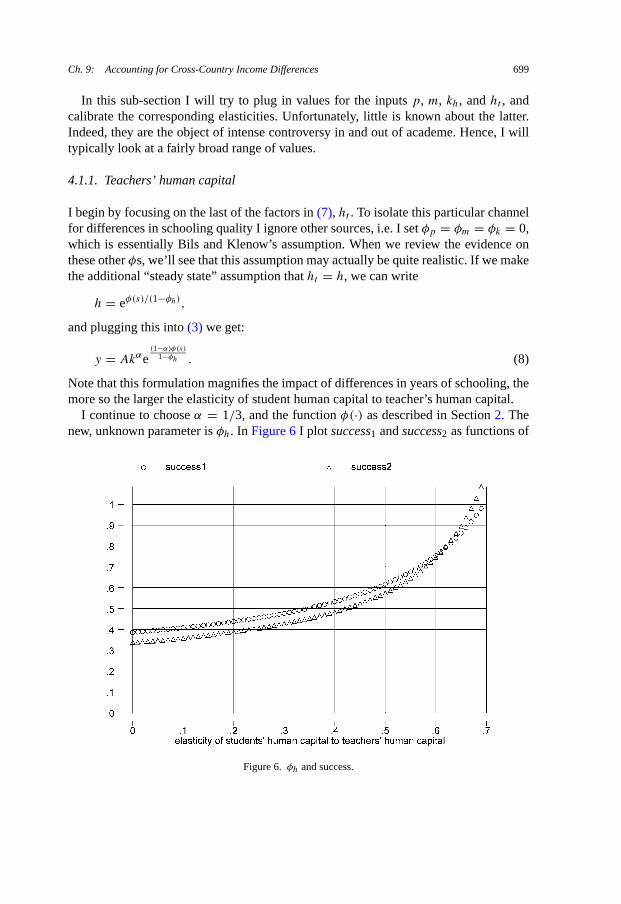
I continue to choose α = 1/3, and the function φ(·) as described in Section 2. Thenew, unknown parameter is φh. In Figure 6 I plot success1 and success2 as functions of
Figure 6. φh and success.

700 F. Caselli
this parameter. Note that φh = 0 is the baseline case of Section 2. At the low values ofφh implied by the baseline case the success measures are fairly insensitive to changes inthe elasticity of students’ to teachers’ human capital. However, the relationship betweenthe success measures and φh is sufficiently convex that when φh is 69% success iscomplete. Coincidentally, 69% is very close to the upper bound of the range of valuesBils and Klenow consider “admissible” for φh (67%), though clearly this admissibilityis purely theoretical: their preferred values are actually in the 0–20% range.22
One way to think about what is reasonable for φh is to compute by how much theteachers’ human capital effect “blows up” the Mincerian return: from Equation (8) wesee that with φh = 0.2 the “social” return to schooling is 1.2 times the private one; withφh = 0.4 it is 1.7 times larger; and with φh = 0.67 it is 3 times more. While it is hardto reach a firm conclusion, it would seem that reasonable priors on φh are inconsistentwith large improvements in the fit of the factor-only model.
Turning to possible objective estimates of φh, the first option is of course to lookfor estimates of the effect of teachers’ years of education on student achievement. Thisis because under our assumptions differences in teacher’s quality are ultimately de-termined by teachers’ years of education. However, Hanushek’s (2004) review of theliterature concludes that teachers’ measurable credentials – including years of educa-tion – have no measurable impact on schooling outcomes.23
Another way to formulate priors on the possible magnitude of φh is to look at evi-dence on the effect of parental education on wages. After all, our simple representative-agent model of human capital is not explicit about the particular way the economy’saverage level of human capital enhances the learning experience of new members ofsociety. We can legitimately re-interpret ht , therefore, as the human capital of parents.One recent set of log-wage regressions including the schooling of parents (alongsidewith an individual’s own schooling) is presented in Altonji and Dunn (1996). Depend-ing on data sources, and on whether the regression is estimated for men or women,their coefficient on father’s years of schooling ranges from −0.5% to 1%, and the co-efficient on mother’s schooling from less than 0.1% to about 0.5%. Note that given our
22 They compute this upper-bound (roughly) as follows. Given data on schooling years of different cohorts,given a Mincerian wage-years of schooling profile, and given a value for φh, it is possible to estimate thegrowth rate of h, and hence the contribution of growth in h to the growth of y. Holding the Mincerian profileconstant, the larger φh, the larger the fraction of growth explained by human capital (for reasons alreadytouched upon in the text). For Bils and Klenow the upper bound for φh is the value such that growth in humancapital explains all of growth – or the value beyond which the residual, growth in TFP, would have to benegative. When the Mincerian profile features decreasing returns, as in our baseline specification, and as inBils and Klenow’s preferred specification, this maximum value for φh is 0.19; when the Mincerian profile islinear the maximum becomes 0.67. The decreasing returns case allows for a smaller maximum φh because,towards the beginning of the sample period, many countries with very low education levels have very highMincerian returns, implying fast growth in human capital.23 This does not mean that teachers’ quality does not matter, of course. It only means that teacher quality isnot related to measurable credentials. This unmeasurable quality effect remains (appropriately) a part of themeasure of our ignorance.

Ch. 9: Accounting for Cross-Country Income Differences 701
functional form assumption the coefficient of parental education is φsφh, where φs isthe return to own years of schooling (assumed constant for simplicity). If the return toown schooling, φs , is in the ball park of 0.10 (as the evidence on Mincerian coefficientsroughly implies), and we focus on Altonji and Dunn’s upper bound of 0.01 for φsφh,we conclude that φh cannot be more than 0.1. A quick check with Figure 6 reveals thateven this upper bound does not support a meaningful boost in the explanatory power ofoverall human capital.24
4.1.2. Pupil–teacher ratios
The term hφht in Equation (7) does not appear to enhance the success of the factor-
only model. I now consider the term pφp . Lee and Barro (2001) report data on thepupil–teacher ratio in a cross-section of countries for various periods since 1960, andseparately for primary and secondary schooling. For each country, I focus on the pupil–teacher ratio in the years when the average worker attended school. To pinpoint this year,I need to start with an estimate of the age of the average worker, which I construct fromLABORSTA.25 Then I assume that children begin primary schooling at the age of 6.This implies that the relevant observation for the primary pupil–teacher ratio would befor the year 1996-age + 6. Furthermore, using unpublished panel data by Barro and Leeon the duration of primary and secondary schooling, we can determine the relevant ob-servation for the secondary pupil–teacher ratio as 1996-age + 6 + duration of primaryschool.
In order to combine the primary and secondary ratios in a unique statistic, I combinethe duration of schooling data with our basic data on the average years of schooling ofthe population over 25 years of age, s, to determine what fraction of schooling time theaverage worker spent in primary, and what fraction in secondary school. I then constructp by simply averaging the primary and secondary teacher–pupil ratio using as weightsthe time spent in these two grades, respectively. At the end of all this, I have data on p
for 87 of our 94 countries.26
24 Another way to boost the contribution of human capital to income would be to assume that parental/teacherhuman capital increases the slope and not just the intercept of the log-wage – schooling relation. This is indeedAltonji and Dunn’s main focus. However, they do not find much evidence in support of this hypothesis.25 As already mentioned, LABORSTA breaks down the economically active population in 5-year age inter-vals, from 10–14, to 60–64, plus a catch-all bracket for 65+. To get at the average age of a worker I simplyweighted the middle year of each interval by the fraction of the labor force in that interval. For the 65+ group,I arbitrarily used 68. Of my 94-country sample, this data is available for 91 countries. I imputed averageage for the two missing countries (Taiwan and Zaire) through a cross-sectional regression of average age ofworker on per-worker income and years of schooling.26 Since the pupil–teacher ratio is observed at five-year intervals in practice we “target” the observationclosest to the estimated age at which the average worker went to school. With this procedure, in the sampleof 86 countries with data on pupil–teacher ratios, the target dates for primary school attendance are 1960 fortwo countries, 1965 for 40, and 1970 for 44. For secondary school attendance the target dates are 1965 (onecountry), 1970 (25), 1975 (55), and 1980 (5).

702 F. Caselli
Figure 7. φp and success.
Figure 7 plots success1 and success2 as functions of φp. Since richer countries havehigher teacher–pupil ratios, clearly a higher elasticity of human capital to this ratioimplies a better fit, or greater success. What is a reasonable range of values for φp?At the low end of the spectrum there is the position taken by Hanushek and coauthors,who conclude that resources – including a large teacher–pupil ratio – have little if anyeffect on economic outcomes.27 At the other end of the spectrum, my own reading ofthe literature indicates that the highest published estimate of φp is a very sizable 0.5.28
However, even with this extremely high estimate it is clear that the fit of the modelimproves modestly, with our success measures barely attaining even the 50% mark.
4.1.3. Spending
I do not have direct data on materials, m and structures per student, kh. Instead, I have –always from Lee and Barro (2001) – a measure of government spending per student inPPP dollars. The bulk of this spending typically goes to teacher salaries, so variation inthese data also reflect differences in the number and possibly the quality of teachers per
27 In a cross-country context, Hanushek and Kimko (2000) find no evidence that more resources improveschooling quality, and Hanushek, Rivkin and Taylor (1996) and Hanushek (2003) reach the same conclusionupon reviewing the US-based literature.28 Card and Krueger (1996). I infer this number from their reported 5% increase in earnings associated witha 10% reduction in class size for white men.

Ch. 9: Accounting for Cross-Country Income Differences 703
Figure 8. φsp and success.
student. However, to a certain extent, they may also reflect variation in materials. Forthe purposes of using these data, it seems sensible, therefore, to replace Equation (7) byAh = spendingφsp , where the dating of the spending observation and the weights givento primary and secondary spending are determined as for the pupil–teacher ratio. Forthis exercise, I have data for 64 countries, and for this sample the measures of successare plotted in Figure 8. Again, rich countries devote more resources to education perstudent, so the fit of the model improves with φsp. However, again, there is the Hanushekposition in the papers cited above, according to which φsp should be thought of as closeto zero. At the other end of the range I have found an estimate of 0.2, which clearly isbarely sufficient to even clear the 50% threshold of explanatory power.29,30
4.2. Quality of schooling: test scores
Another way to investigate the potential of quality-of-education modifications to thebasic model is to exploit information on the performance of students on reading, science,
29 Johnson and Stafford (1973), who run a regression of log hourly wages on log state expenditure per student(and controls), obtaining a coefficient of 0.198. For the reasons discussed by Hanushek and co-authors thereis a high presumption of upward bias in this estimate.30 Lee and Barro (2001) also report information on the duration of the schooling year (in days and hours),but these variables – while highly variable – are weakly, and if anything negatively, correlated with per-capitaincome, so that they are highly unpromising from the perspective of improving the fit of the model. Similarly,teacher salaries, as a percent of per-capita GDP, are higher in poorer countries.
704 F. Caselli
and math tests in different countries. When students in one country outperform studentsof another (holding grade constant), we can assume that they have enjoyed schoolingof higher quality, whether this higher quality comes from higher teacher–pupil ratios,quality of teachers, other expenditures, or other unobservables specific to the productionof human capital. Hanushek and Kimko (2000) find that test scores enter significantlyin growth regressions.
To implement this idea I think of Ah as a function of test scores: higher test scoressignal higher human capital. Suppose, for example, that the relationship between schoolquality and test results is given by Ah = eφτ τ , where τ is the test score.31 Then, withdata on test scores, if we knew φτ we could construct a new counterfactual measure ofyKH , or the output attributable to “observable” factors of production.
I use data on test scores provided by Lee and Barro (2001), who for several countriesobserve data on multiple tests (e.g.: math, science, and reading), and for multiple grades,at different dates. Ideally I would follow the procedure outlined in the previous sub-section, i.e. to “target” the year in which the average worker is presumed to have beenin school. Because this data is very sparse, however, and mostly available in recentdates, I will focus on recent observations. This procedure is appropriate if the quality ofeducation has grown over time at roughly similar rates across countries.
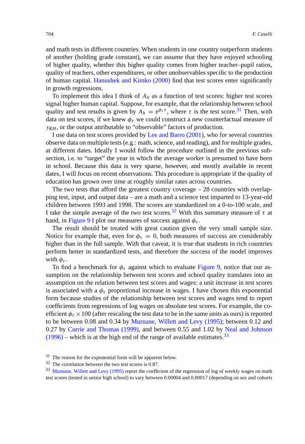
The two tests that afford the greatest country coverage – 28 countries with overlap-ping test, input, and output data – are a math and a science test imparted to 13-year-oldchildren between 1993 and 1998. The scores are standardized on a 0-to-100 scale, andI take the simple average of the two test scores.32 With this summary measure of τ athand, in Figure 9 I plot our measures of success against φτ .
The result should be treated with great caution given the very small sample size.Notice for example that, even for φτ = 0, both measures of success are considerablyhigher than in the full sample. With that caveat, it is true that students in rich countriesperform better in standardized tests, and therefore the success of the model improveswith φτ .
To find a benchmark for φτ against which to evaluate Figure 9, notice that our as-sumption on the relationship between test scores and school quality translates into anassumption on the relation between test scores and wages: a unit increase in test scoresis associated with a φτ proportional increase in wages. I have chosen this exponentialform because studies of the relationship between test scores and wages tend to reportcoefficients from regressions of log wages on absolute test scores. For example, the co-efficient φτ ×100 (after rescaling the test data to be in the same units as ours) is reportedto be between 0.08 and 0.34 by Murnane, Willett and Levy (1995); between 0.12 and0.27 by Currie and Thomas (1999), and between 0.55 and 1.02 by Neal and Johnson(1996) – which is at the high end of the range of available estimates.33
31 The reason for the exponential form will be apparent below.32 The correlation between the two test scores is 0.87.33 Murnane, Willett and Levy (1995) report the coefficient of the regression of log of weekly wages on mathtest scores (tested in senior high school) to vary between 0.00004 and 0.00017 (depending on sex and cohorts

Ch. 9: Accounting for Cross-Country Income Differences 705
Figure 9. φτ (×100) and success.
Inspection of Figure 9 given this range of values suggests that using test scoresas proxies for schooling quality cannot substantially improve the performance of thefactor-only model. The problem is that, given the drastically reduced sample size, it ishard to take a stand on the degree to which this finding generalizes.
I can attain a slight increase in sample size if I drop the requirement that the tests beimparted in roughly the same period and roughly the same subject. If I use all the test
considered, US data). Since the test results are reported to vary between 2 and 17 points, we assume that thetest is on a 0–20 scale. When translated to our 0–100 scale this implies the φs reported in the text. The Currieand Thomas (1999) results imply that “students who score in the upper quartile of the reading exam earn 20%more than students who score in the lower quartile of the exam, while students in the top quartile of the mathexam earn another 19% more. When they control for father’s occupation, father’s education, children, birthorder, mother’s age, and birth weight, the wage gap between the top and bottom quartile on the reading examis 13% for men and 18% for women, and on the math exam it is 17% for men and 9% for women” [Krueger(2003, p. 25)]. From here we can infer that φτ varies between 0.0012 and 0.0027 (dividing the percentagechange in the wage by the 75 points that separate the top from the bottom quartile). Neal and Johnson (1996)run a regression of log real yearly wages on standardized AFQT test scores, and find a coefficient between 0.17and 0.29. Introducing more controls the coefficients are between 0.12 and 0.16. Since the standard deviationof AFQT scores (as reported in the note to their Appendix A.3) is 36.65, this implies that a one-point increasein AFQT scores increases wages by between 0.33 and 0.79 percent. Given that AFQT scores range between95 and 258, this implies a φ between 0.0055 and 0.0102 (treating each of the AFQT points as 1.64 of our 100points). (Whether AFQT scores are measures of schooling outcome is somewhat controversial.) Hanushekand Kimko (2000) use essentially the same international test scores we are using here to explain the earningsof migrants to the US, and obtain φτ × 100 of approximately 0.2.
706 F. Caselli
Figure 10. φτ (×100) and success, all tests in the 90s.
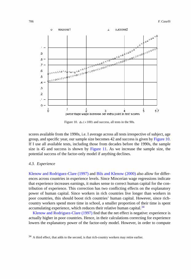
scores available from the 1990s, i.e. I average across all tests irrespective of subject, agegroup, and specific year, our sample size becomes 42 and success is given by Figure 10.If I use all available tests, including those from decades before the 1990s, the samplesize is 45 and success is shown by Figure 11. As we increase the sample size, thepotential success of the factor-only model if anything declines.
4.3. Experience
Klenow and Rodriguez-Clare (1997) and Bils and Klenow (2000) also allow for differ-ences across countries in experience levels. Since Mincerian wage regressions indicatethat experience increases earnings, it makes sense to correct human capital for the con-tribution of experience. This correction has two conflicting effects on the explanatorypower of human capital. Since workers in rich countries live longer than workers inpoor countries, this should boost rich countries’ human capital. However, since rich-country workers spend more time in school, a smaller proportion of their time is spentaccumulating experience, which reduces their relative human capital.34
Klenow and Rodriguez-Clare (1997) find that the net effect is negative: experience isactually higher in poor countries. Hence, in their calculations correcting for experiencelowers the explanatory power of the factor-only model. However, in order to compute
34 A third effect, that adds to the second, is that rich-country workers may retire earlier.

Ch. 9: Accounting for Cross-Country Income Differences 707
Figure 11. φτ (×100) and success, all available test scores.
the average age of workers they rely on UN data on the age structure of the population,while in principle it would be more accurate to look at the age structure of the laborforce. Using again the LABORSTA-based measure of the average age of the economi-cally active population in the formula
experience = age-schooling − 6,
I find that the correlation between experience and per-capita income is −0.29 in our94-country sample. Therefore, I confirm the Klenow and Rodriguez-Clare conclusionthat poor countries have less education but more experience. Adding experience to thefactor-only model, therefore, will only worsen its explanatory power.35
35 This discussion assumes implicitly that experience enters linearly in the production function for humancapital, an assumption we know not to be valid. However, for this consideration to overturn the conclusionwe just reached, it would have to be the case that poor countries are to the right of the argmax, which seemsvery unlikely: in my data, the maximum average experience is 27 years. More importantly the discussionalso abstracts from compositional issues. Feyrer (2002) uncovers an economically important and remarkablyrobust association between a country’s productivity and its share of the labor force that is between 40 and 49years of age. Extending the development accounting framework to capture this effect would be a worthwhiletask.

708 F. Caselli
4.4. Health
Weil (2001) and Shastry and Weil (2003) point out that there are very large cross-country differences in nutrition and health status, and argue that these differences mapinto substantial differences in energy and capacity for effort. They find that accountingfor health differences across countries increases by one-third the explanatory power ofhuman capital for differences in per-capita income.
Weil (2001) uses as a proxy for health the Adult Mortality Rate (AMR), which mea-sures the fraction of current 15-year-old people who will die before age 60, under theassumption that age-specific death rates in the future will stay constant at current levels.In practice, this is a measure of the probability of dying “young”, and is therefore aplausible (inverse) proxy for overall health status.
The correction of human capital for health can be implemented through the assump-tion Ah = eφamrAMR, where clearly φamr < 0: a higher adult mortality rate implies aless energetic workforce. I gather cross-country data on AMRs from the WDI, covering92 of our 94 countries, for the year 1999. I plot success for different values of −φamrin Figure 12. Since richer countries have healthier workers, the explanatory power ofhuman capital increases in −φamr.
Weil’s preferred value for −φamr(×100) is 1.68. Conditional on this value, I do con-firm his finding that the factor-only model’s explanatory power improves considerably– indeed by almost one third, taking us well above the 50 percent threshold of success.This is therefore a very important and promising contribution.
Figure 12. −φamr and success.
Ch. 9: Accounting for Cross-Country Income Differences 709
Given his choices of functional form, however, this calibration implies that a one-percentage-point reduction in the probability of dying young is associated with a 1.68percent increase in human capital, and hence in wages. Put another way, reducing theprobability of dying before the age of 60 (as of age 15) by 6 percentage points has thesame impact on wages as one extra year of schooling. This effect may seem a bit toolarge to be realistic. Given the somewhat tortuous – if ingenious – path through whichWeil comes up with this calibration, I would tend to consider this number an upperbound.36
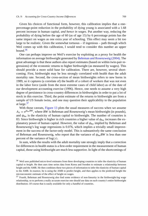
One can perhaps improve on Weil’s exercise by exploiting as a proxy for health theinformation on average birthweight generated by Behrman and Rosenzweig (2004). Thegreat advantage is that these authors also report estimates (based on within twin-pair re-gressions) of the economic returns to higher birthweight (as measured by wages). Thisshould provide a more solid base for calibration. There are, however, several short-coming. First, birthweight may be less strongly correlated with health than the adultmortality rate. Second, the cross-section of mean birthweights refers to new borns in1989, so it captures (a correlate of) the health of a cohort of workers that was not evenin the labor force (aside from the most extreme cases of child labor) as of the date ofour development accounting exercise (1996). Hence, one needs to assume a very highdegree of persistence in cross-country differences in birthweights in order to put a lot ofstock in this exercise. Third, the point estimate of the returns to birthweight are from asample of US female twins, and one may question their applicability to the populationat large.37
With those caveats, Figure 13 plots the usual measures of success when we assumeAh = eφbwBW , where BW is Behrman and Rosenzweig’s mean birthweight (in pounds),and φbw is the elasticity of human capital to birthweight. The number of countries is83. Since birthweight is higher in rich countries a higher value of φbw increases the ex-planatory power of human capital. However, the value of φbw implied by Behrman andRosenzweig’s log wage regressions is 0.076, which implies a trivially small improve-ment in the success of the factor-only model. This is substantively the same conclusionof Behrman and Rosenzweig, who report that the variance of φbwBW is less than onepercent of the variance of log(y).
In sum, while the results with the adult mortality rate strongly imply that a correctionfor differences in health status is a first-order requirement in the measurement of humancapital, those using birthweight are much less supportive. In light of the shortcomings of
36 Weil uses published micro-level estimates from three developing countries to infer the elasticity of humancapital to height. He then uses time series data from Korea and Sweden to estimate a relationship betweenheight and the AMR. He then combines these two pieces of information to infer the elasticity of human capitalto the AMR. In essence, he is using the AMR to predict height, and then applies to the predicted height themicroeconomic estimate of the effect of height on wages.37 Fourth, Behrman and Rosenzweig also find some evidence of non-linearity in the birthweight-log wagerelationship, so to perform a really accurate exercise one should use data on each country’s entire birthweightdistribution. Of course that is easily available for only a handful of countries.
710 F. Caselli
Figure 13. φbw and success.
both exercises, however, it seems highly worthwhile to try and explore the matter furtherwith more accurate indicators of health and more precisely calibrated parameters.
4.5. Social vs. private returns to schooling and health
Some additional important caveats about the nature of the calculations above is in orderbefore I “set aside” human capital. Recall that the function φ(s) that we have used tomap years of schooling into human capital was calibrated on estimates of private ratesof return. Similarly, attempts at calibrating the health-human capital relation rely onobserved private returns to health. But, as pointed out by various authors, and especiallyforcefully by Pritchett (2003), these private returns may bear little relationship to thesocial (or aggregate) return to education, which is of course what one would like to plugin our calculations.
As Pritchett points out, the social return to education may be higher or lower thanthe private one. Most growth theorists instinctively think about the former case, as theyhave in mind models with positive spillovers from human capital. However, Pritchett’sreview of the evidence is typical in finding very little empirical support for positive ex-ternalities.38 On the other hand, various versions of the education-as-signalling-devicemodel, as well as models of rent seeking, imply that the social return to education is
38 See, e.g., Heckman and Klenow (1997) and Acemoglu and Angrist (2000).

Ch. 9: Accounting for Cross-Country Income Differences 711
lower than the private return.39 This possibility is quite compelling. Note, however, thatour calculations above imply that if we uniformly lower the social rate of return to ed-ucation, cross-country schooling inequality will explain even less of income inequalitythan it does in our benchmark calculation (see Figure 2).
Pritchett, however, also convincingly argues that the extent of rent seeking, and there-fore the extent to which the social return is below the private return, is much larger inpoor countries. For example, in many poor countries the government employs an over-whelmingly large share of college graduates. This is sometimes the result of guaranteed-employment rules that commit the government to find employment to anyone with atertiary degree. In contrast, in rich countries most college graduates work in the pri-vate sector. Since standard rent-seeking arguments imply that the government sector isintrinsically likely to make less efficient use of resources, this implies that on averagethe social return to education will be lower in poor countries. This effect is of coursereinforced by the fact that poor countries are notoriously more prone to corruption andrent seeking than rich ones.
This will help. If the social rate of return to education (and health) is allowed to behigher in rich countries, then the variance of h will increase, and with it the explanatorypower of the model. How important this could be quantitatively is hard to say, but byall means it would be worth finding out. A first exploratory step may be to break downthe labor force into government-employees and private-sector workers. One may thenretain the parameterization of the benchmark case for the private sector workers, butassume lower returns for government employees.
5. Quality of physical capital
5.1. Composition
Recent research by Eaton and Kortum (2001) has shown that most of the world’s cap-ital is produced in a small number of R&D-intensive countries, while the rest of theworld generally imports its equipment. This suggests that, for most countries, (widelyavailable data on) imports of capital of a certain type are an adequate proxy for overallinvestment in that type of equipment. Caselli and Wilson (2004) exploit this observationto investigate cross-country differences in the composition of the capital stock.40
Their results – a partial summary of which is shown in Table 3 – are startling: differenttypes of equipment constitute widely varying fractions of the overall capital stock acrosscountries. For each of the nine equipment categories Caselli and Wilson work with,the share in total investment in 1995 has minima in the low single digits, and maxima
39 See, e.g., Murphy, Shleifer and Vishny (1991), or Gelb, Knight and Sabot (1988).40 This idea is also used in Caselli and Coleman (2001a). The equipment-import data are extracted from theFeenstra (2000) data set.
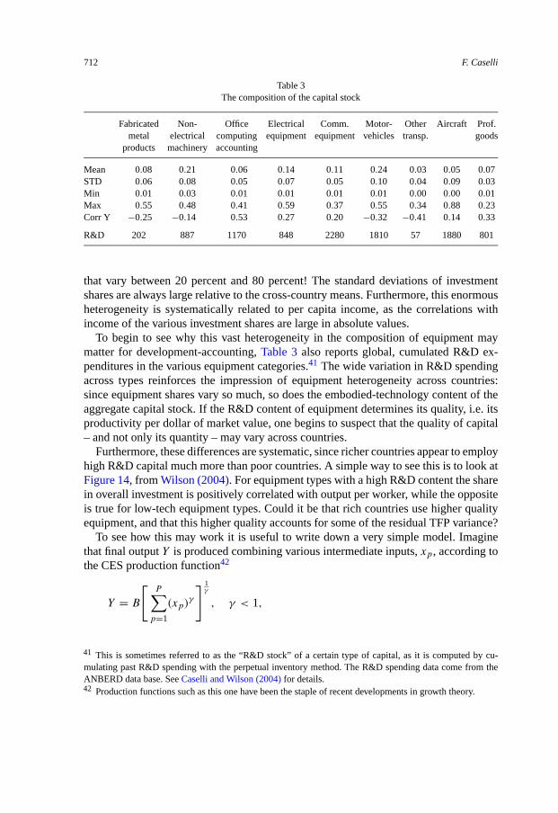
712 F. Caselli
Table 3The composition of the capital stock
Fabricated Non- Office Electrical Comm. Motor- Other Aircraft Prof.metal electrical computing equipment equipment vehicles transp. goods
products machinery accounting
Mean 0.08 0.21 0.06 0.14 0.11 0.24 0.03 0.05 0.07STD 0.06 0.08 0.05 0.07 0.05 0.10 0.04 0.09 0.03Min 0.01 0.03 0.01 0.01 0.01 0.01 0.00 0.00 0.01Max 0.55 0.48 0.41 0.59 0.37 0.55 0.34 0.88 0.23Corr Y −0.25 −0.14 0.53 0.27 0.20 −0.32 −0.41 0.14 0.33
R&D 202 887 1170 848 2280 1810 57 1880 801
that vary between 20 percent and 80 percent! The standard deviations of investmentshares are always large relative to the cross-country means. Furthermore, this enormousheterogeneity is systematically related to per capita income, as the correlations withincome of the various investment shares are large in absolute values.
To begin to see why this vast heterogeneity in the composition of equipment maymatter for development-accounting, Table 3 also reports global, cumulated R&D ex-penditures in the various equipment categories.41 The wide variation in R&D spendingacross types reinforces the impression of equipment heterogeneity across countries:since equipment shares vary so much, so does the embodied-technology content of theaggregate capital stock. If the R&D content of equipment determines its quality, i.e. itsproductivity per dollar of market value, one begins to suspect that the quality of capital– and not only its quantity – may vary across countries.
Furthermore, these differences are systematic, since richer countries appear to employhigh R&D capital much more than poor countries. A simple way to see this is to look atFigure 14, from Wilson (2004). For equipment types with a high R&D content the sharein overall investment is positively correlated with output per worker, while the oppositeis true for low-tech equipment types. Could it be that rich countries use higher qualityequipment, and that this higher quality accounts for some of the residual TFP variance?
To see how this may work it is useful to write down a very simple model. Imaginethat final output Y is produced combining various intermediate inputs, xp, according tothe CES production function42
Y = B
[P∑
p=1
(xp)γ
] 1γ
, γ < 1,
41 This is sometimes referred to as the “R&D stock” of a certain type of capital, as it is computed by cu-mulating past R&D spending with the perpetual inventory method. The R&D spending data come from theANBERD data base. See Caselli and Wilson (2004) for details.42 Production functions such as this one have been the staple of recent developments in growth theory.

Ch. 9: Accounting for Cross-Country Income Differences 713
Figure 14. Capital composition and income.
where B is a disembodied total factor productivity term. Intermediate-good p is pro-duced combining equipment and labor:
(9)xp = Ap(hpLp)1−α(Kp)α, 0 < α < 1,
where Kp measures the quantity of equipment (in current dollars) used to produceintermediate-input p, hpLp is human-capital augmented labor in sector p, and Ap isthe productivity of sector p.
The key assumption is that capital is heterogeneous: there are P distinct types ofcapital, and each type is product specific, in the sense that intermediate p can only beproduced with capital of type p. In other words, an intermediate is identified by the typeof equipment that is used in its production.43 The assumption that γ < 1 implies that –in producing aggregate output – all these activities are imperfect substitutes.
The productivity term Ap is product specific. Product variation in A allows for thepossibility that one dollar spent on equipment of type p may deliver different amountsof efficiency units if instead spent on type p′. For example, the embodied-technology
43 For example, for equipment-type “trucks”, the corresponding intermediate good x (say, “road transporta-tion”) is the one obtained by combining workers with trucks. For equipment-type “computers”, the corre-sponding intermediate good is “computing services”, etc. Hence, our intermediates do not easily map intoindustries or sectors (computers are used in most industries), but rather into the various types of activities(transport, computing, etc.) required to generate output within each sector.
714 F. Caselli
content of good p may be greater because the industry producing equipment of type p
is more R&D intensive.44
A number of simplifying assumptions allow one to write a simple formula that bringsthe idea of the “quality of capital” in sharp relief. In keeping with the representative-agent spirit of the rest of the chapter say, then, that human capital per worker is constantacross sector, i.e. hp = h, and that labor is free to flow across sectors so that the marginalproduct of labor is the same for all equipment types. Then one can show that the outputequation can be rewritten as45
(10)Y = (K)α(hL)1−αB
(P∑
p=1
(Ap)γ
1−(1−α)γ (ξp)αγ
1−(1−α)γ
) 1−(1−α)γγ
,
where of course K is the total market value of the capital stock, L is total labor, and ξp
is the share of capital of type p in the total capital stock, or ξp = Kp/K .Up until now we have been writing Y = (K)α(hL)1−αA, and we have struggled with
the fact that A seems to play an enormously important role in determining output differ-ences. The last equation neatly shows the relationship between A and the compositionof the capital stock: if different types of capital have different productivities, then theobserved wild variation in equipment shares ξ implies that the quality of capital – overand above its quantity K – can vary across countries and can account for a portion ofthe unexplained variation.
Caselli and Wilson (2004) propose a regression-based approach to make inferenceson the various Aps. Unfortunately, even with knowledge of the Aps it is virtually impos-sible to bound the amount of income variance that the ξps can explain. This is becausethe last term of Equation (10) is exceedingly sensitive to the value of γ , and there seemat the moment to exist no reliable approach to the calibration of this elasticity. If γ issufficiently low, i.e. capital types are sufficiently poor substitutes for one another, thequality of capital accounts for all of the unexplained component of income differences.However, whether such values are reasonable or not our current state of knowledge can-not say. I conclude therefore that further research on the composition of capital is animportant priority for development accounting.
44 Since, for simplicity, we have written an aggregate production function that is symmetric in the servicesprovided by different types of capital, product variation in Ap may also reflect differences in the variouscapital types’ shares in aggregate output.
Caselli and Wilson also allow the productivity term Ap to vary across countries, for a given equipmenttype p. The idea behind country variation is that equipment of type p may be more complementary with thecharacteristics of country i, an idea that is strongly supported by their empirical results.
In order to make sure that cross-country differences in Kp measure physical differences in installed capitalwe need to assume that the law of one price holds. This is plausible, since we know that most capital isimported from a few world producers. If the law of one price does not hold, however, cross-country differencesin Ap may also reflect price differences.45 See Caselli and Wilson (2004) for details.
Ch. 9: Accounting for Cross-Country Income Differences 715
5.2. Vintage effects
Solow’s (1959) paper on vintage capital formalized the idea that technological progressis embodied in capital goods. Rodriguez-Clare (1996), Jovanovic and Rob (1997),Parente (2000), Mateos-Planas (2000) have noted that this could potentially enhance theexplanatory power of cross-country differences in investment rates. The idea, of course,is that low investment rates will be associated with lower adoption of new technology.Indeed, some of these authors have argued that versions of the capital-embodied modelgreatly outperform the homogeneous-capital model in accounting for cross-country in-come differences.
Formally, the vintage-capital model could be described by the formulas:
(11)Yt = (Ltht )
1−αt∑
i=0
At−iKαt−i ,
Kt−i = (1 − δ)i It−1,
where It−1 is investment at time t −1 in terms of the consumption good. Consistent withSolow’s idea, this model has the property that capital installed by sacrificing one unitof consumption at date s yields As(1 − δ)t−s efficiency units of capital at time t , whilecapital installed by sacrificing one unit of consumption at time t yields At efficiencyunits. If As < At we have that the earlier sacrifice in consumption contributes less tooutput today not only because of physical depreciation, but also because of the oldervintage. To appreciate the potential consequences of this note that the same comparisonin a homogeneous-capital (i.e. disembodied technical change) model would be betweenAt(1 − δ)t−s and At , i.e. differences in efficiency units obtained with the same sacrificeof consumption would only be due to physical depreciation.
As explained by Greenwood, Hercowitz and Krusell (1997), under certain conditionsthe formulation above is equivalent to
Yt = (Ltht )1−α
t∑i=0
Kαt−i ,
Kt−i = (1 − δ)iqt−i It−i ,
which has the following interpretation. Instead of one unit of consumption producingequal amounts of capital of increasing quality at different dates, one unit of consump-tion produces increasing amounts of capital of the same quality. Because the aggregateimplications of growth in A are isomorphic to those of growth in q, the two formulationscan be equivalent representations of the idea of embodied technological progress.
The second version of the model suggests, however, that – at least in principle –the estimates of the physical capital stocks we have been using until now do actuallyalready reflect embodied technical change. This is because the real investment series weconstruct from PWT61 is a series for real investment in terms of the investment good,and not in terms of the consumption good. In other words, the PWT61 investment data

716 F. Caselli
that we use are data on Is = qs Is , and not on Is . Therefore, vintage effects – or atleast those vintage effects that show up in a reduced relative price of investment goods– should already be accounted for.
As a very rough check on this argument, I have run a cross-country OLS regres-sion of output per quality-adjusted worker on a distributed-lag function of depreciatedinvestments (in units of the investment good). I.e. the left hand side variable wasYt/(Ltht )
1−α , and the right hand side variables were It , (1 − δ)It−1, (1 − δ)2It−2, . . . .I experimented with 5, 10, and 20 lags of investment. The homogeneous-capital hypoth-esis – or, much more accurately, the hypothesis that all vintage effects are adequatelycaptured by investment-good prices in PWT61 – is equivalent to all the coefficients tak-ing the same value, irrespective of the vintage. The “vintage effects” hypothesis wouldpredict that coefficients on recent lags of investment would be systematically larger thanthose on older lags. The result was somewhat inconclusive, in that both hypotheses wererejected: all coefficients were not statistically the same, but neither they fell monoton-ically with the lag of investment. A possible explanation is that the price deflators inPWT work well enough to remove systematic vintage effects, but the remaining i.i.d.measurement error occasionally makes some vintages look more productive than others.In any case there is little indication that vintage-based models will significantly improveon the benchmark.
5.3. Further problems with K
The investment series I have used to estimate the capital stock is an aggregate of pri-vate and public investment expenditures. As Pritchett (2000) very convincingly argues,however, elementary logic and vast anecdotal experience suggest that many govern-ments’ investment efforts are much less productive than private ones. There is an infinitesupply of examples where government investments have not produced anything tangi-ble (non-existent highways, industrial complexes that have never been completed, etc.).Furthermore, even when public investments do materialize, the resulting structures andmachinery may be run less efficiently than under private management.46
As for Pritchett’s (2003) criticism of schooling-based measures of human capitalbased on private returns, his (2000) criticism of what he derogatorily but accuratelycalls CUDIE (cumulated depreciated investment expenditure) may help shedding lighton the puzzles we are concerned with, both because governments tend to account fora larger share of production, employment, and capital ownership in poorer countries,and because less-accountable poor-country governments are likely to be disproportion-ately less efficient (relative to the private sector) than rich country ones. Hence, thereare good reasons to expect the government to play an especially detrimental role in the
46 The 1994 World Bank’s World Development Report documents substantial cross-country differences inthe efficiency with which public infrastructure is used. Hulten (1996) uses these inefficiency indicators in agrowth-regression exercise.

Ch. 9: Accounting for Cross-Country Income Differences 717
productivity of investment in poor countries. This implies that the “effective” varianceof K is larger than in the baseline model.47
As I suggested in the previous section for the analogous problem with human capital,a first pass at investigating this issue would be to try to separate out public from privateinvestment, and apply different weights in the perpetual-inventory calculation, whichwould become
Kt = Iprivate,t + γ Ipublic,t − δKt−1.
One could then try to re-do development accounting with this modified capital measure(possibly for various values of γ ). Unfortunately, I have not been able to identify reliableand updated PPP breakdowns of the investment series into private and public capital.48
Perhaps a cleaner exercise, but also even more ambitious, would be to try to com-pletely net out the government from the development accounting exercise. I.e. subtractthe government’s share from aggregate output, capital ownership, and employment, andperform the development-accounting exercise on the residual (private) inputs and out-put. This confronts the same data limitations as the exercise described in the previousparagraph, and the additional problem of coming up with a reliable PPP governmentshare of GDP.49
6. Sectorial differences in TFP
Up to here in this chapter I have treated a country’s GDP as if it was produced in asingle sector, i.e. as if GDP measured the physical output of a homogeneous good.The basic message has been that it is impossible to explain cross-country differences inincome without admitting a large role for differences in TFP. It is tempting to jump tothe conclusion that these TFP differences signal the existence of barriers to technologyadoption in less developed countries, or other frictions that broadly make some countries“function” less well than others. But large differences in TFP could also be the resultof variation in the weights in GDP of sectors with different sectorial-level productivity– even when these sectorial productivities are identical across countries. In this case
47 While the emphasis is on the role of the government, Pritchett gives various other reasons why CUDIE isproblematic.48 However, both the WDI and the IMF’s Government Finance Statistics (GFS) have data on governmentcapital formation in domestic currency. One could therefore potentially construct a non-government invest-ment series, and – in principle – use PWT deflators to turn this series into a real investment series. Whetherone would get anything sensible out of this is another matter.49 One can of course not simply subtract G from Y , in PWT, because G is government consumption ofgoods and services, and not government production. In the NIPA government output is defined as the sum offactor payments, i.e. compensation to general-government employees plus general-government consumptionof fixed capital. Something like these categories are reported in the IMF’s Government Financial Statistics.Unfortunately, the spottiness of these data forced me to abandon this particular enterprise.

718 F. Caselli
we would want to focus on barriers to the mobility of factors across sectors, instead ofbarriers to the mobility of technology or work practices across countries.50
6.1. Industry studies
There is a tradition of productivity comparisons at the industry, or even at the firm,level. Particularly illustrative of the advantages of this approach are a series of reportspublished by the McKinsey Global Institute. These studies focus on painstaking com-parisons of the production functions (broadly construed) of narrowly defined industries(from automobile, to beer, to retail banking) in a few industrialized economies (mostlyUS, Japan, Germany, and the UK). Baily and Solow (2001) present a thoughtful surveyof the achievements, as well as the shortcomings, of these studies (as well as extensivereferences).51
Briefly, even within narrowly defined industries, and even among countries at verysimilar levels of development, total factor productivity presents remarkable variation.A similar conclusion, for somewhat more aggregated manufacturing industries (butmore countries), is reached by Harrigan (1997, 1999). Hence, industry-level studiessuggest that aggregate TFP differences are not solely due to differences in the weightsof high- and low-TFP sectors. Since these studies are often limited to industries in a fewhighly developed economies, however, one should be cautious before assuming that thesame causes drive the low TFP levels of less developed economies.
Besides confirming that TFP differences exist also at the industry level, the McKinseyresearchers are often also able to shed some tentative light on their sources. In particular,they highlight differences in working practices, and they are sometimes also able to linkinefficient practices to the regulatory environment. In general, the studies point to alink between the degree of competition domestic producers are exposed to (as affectedby the amount of regulation), and the efficiency with which they organize their laborinput. This is of course an important, and plausible, finding. Further support for thisview comes from the work of Schmitz (2001) on the North-American iron-ore industry,which shows convincingly that the efficiency of labor practices is very responsive to thedegree of product-market competition.52
50 Here we are arguing that differences in sectoral composition may account for some of the differences in thelevel of GDP. Koren and Tenreyro (2004) show that these same differences account for a substantial fractionof differences in its volatility.51 A precursor to these intra-industry cross-country productivity comparisons is the three-country study ofConrad and Jorgenson (1985). See also Wagner and van Ark (1996).52 Another wonderful industry-level comparison of cross-country productivity differences is presented byClark (1987), who examines the productivity of cotton mills around the world in the early years of the twen-tieth century. He shows that, assuming constant capital–labor ratios, the textile industries of Britain and NewEngland would have had a huge cost disadvantage relative to India, Japan, and many other countries. Yet,British cotton textiles dominated export markets. Clark shows that the various countries’ industries used iden-tical equipment, and that the expertise to organize and run the mills could not have differed too much. Rather,

Ch. 9: Accounting for Cross-Country Income Differences 719
6.2. The role of agriculture
As mentioned, existing cross-country comparisons of sectorial TFP tend to be limitedto small sets of developed countries. The goal of this section is therefore to provide arough, preliminary assessment of the sectorial-composition interpretation of TFP dif-ferences that extends to developing countries as well. In particular, I will focus on anagriculture–nonagriculture split of GDP. The main reason for looking at this particularbreakdown is easily inferred from Figure 15: in the poorest countries of the world virtu-ally everyone works in agriculture, and in the richest virtually nobody does. It is obviousthat this is the most important source of variation in the composition of GDP around theWorld. Another reason for focusing on agriculture is that I have no PPP output data forother sectors. Finally, the agriculture-nonagriculture dualism has traditionally played acentral role in the history of thought on economic development.53
The main purpose of this section, then, is to assess the hypothesis that (i) agricultureis an intrinsically low TFP sector, and (ii) poor countries’ low aggregate TFP is due
Figure 15. The importance of agriculture.
the source of the productivity differences boils down to the fact that each English worker was willing to tendto a much larger number of machines. In low-productivity countries workers were idle most of the time. Whythis was so remains a bit of a mystery, and one should be cautious in assuming that this finding would stillhold up one century later. Nevertheless, Clark’s findings reinforce the case that labor practices may be animportant source of observed differences in productivity.53 Some of the classics are Fisher (1945), Clark (1940), Rostow (1960), Nurkse (1953), Lewis (1954),Kuznets (1966), and Jorgenson (1961).

720 F. Caselli
in substantial measure to their high shares of agriculture. In this subsection, however,I start by taking a preliminary (and perhaps somewhat digressive) look at basic data onagricultural GDPs, non-agricultural GDPs, and agricultural labor shares. What we findshould provide further motivation for asking the development-accounting question withdisaggregated data.
I begin by writing per-worker GDP in PPP as
(12)y = PAyAlA + PAyAlA,
where PA (PA) is the international (PPP) price of agricultural (non-agricultural) goods,yA (yA) is the per-worker output of the agricultural (non-agricultural) sector, and lA(lA) is the agricultural (non-agricultural) share of employment. We already know thatlA varies dramatically across countries. What about PAyA and PAyA?
The Food and Agriculture Organization (FAO) has collected and published cross-country data on producer prices in agriculture for a large number of countries between1970 and 1990 [Rao (1993), see also Restuccia, Yang and Zhu (2003)]. This permitsthe construction of PPP exchange rates for agriculture, and therefore of PPP compar-isons of agricultural output. Going even further, the FAO researchers also assembledsome data on agricultural inputs for the year 1985, and this allowed them to generate across-section of PPP agricultural GDPs. Furthermore, the methodology followed in theFAO study deliberately follows the methods of Summers and Heston (1991). Hence,the estimates of PPP agricultural GDP in the FAO data set are comparable to the aggre-gate PPP numbers of PWT61. The FAO data set also obviously contains information onagricultural employment (which was used for Figure 15).
A difficulty that needs to be addressed, however, is that the FAO numbers for PPPagricultural GDP do not directly map into the quantity PAyA in Equation (12). Thereason is as follows. The FAO PPP GDPs aggregate the quantities of the various agricul-tural products by a set of “international prices”, that are essentially weighted averagesof each country’s prices. The same is done in the PWT for all goods and services. How-ever, the two systems use a different normalization for the international prices – i.e.they have the same relative prices of agricultural products but different absolute levels.Hence, the PPP agricultural value-added coming from the FAO data set cannot sim-ply be plugged into Equation (12) with PWT aggregate value added on the left handside.54
54 Formulas may help here. Suppose that there is only one agricultural good and one nonagricultural good.Call PA and P
Atheir respective prices in PWT international dollars: the PWT’s unit of account. The normal-
ization used in PWT is that PAyA,US + PA
yA,US = PA,USyA,US + P
A,USyA,US, where PA,US (P
A,US) is
the price of A (A) in the US (this is what Summers and Heston mean when they say, somewhat opaquely,that the PPP of the US is 1). Instead, the normalization in the FAO data set is PF
AyA,US = PA,USyA,US,
where PFA
is the price of the agricultural good in FAO’s international dollars. In this two-good example this
obviously implies PFA
= PA,US, so that PFA
yA = PAyA only if we have PA = PA,US, as well. But theabove-described normalization of PWT prices does not assure this at all, and indeed it would be true only bycoincidence. I guess one could put this into PWT-speak, and say that the fact that the PPP of GDP is normal-

Ch. 9: Accounting for Cross-Country Income Differences 721
I try to solve this problem as follows. It is well known that – because they arequantity-weighted – international-dollar relative prices in the PWT closely resemblerich-country, and especially US, relative prices [Hill (2000)]. Hence, for the US, weshould have
PAYA,US
YUS≈ PA,USYA,US
YDUS
,
where PA,USYA,US/YDUS is the agricultural share in GDP at domestic prices, which can
be obtained from the WDI. In these equations YUS, and PA,USYA,US/YDUS are known (the
former from PWT, and the latter from WDI). Hence, we can solve for PAYA,US. Nowrecall that the FAO estimates for PPP agricultural GDP differ from the (implicit) PWTestimates only by a constant of normalization. It should follow that if we rescale allof the FAO agricultural GDP numbers such that the US value coincides with PAYA,US(as just calculated) we have an estimate of the contribution of agriculture to PWT GDPthat we can plug into Equation (12).
As already pointed out by Restuccia, Yang and Zhu (2003), the most striking featureof the FAO data is that variation in agricultural value-added per worker (in PPP) dwarfsthe variation in aggregate value-added per worker. In the largest sample with data onboth agricultural and aggregate GDP per worker (80 countries) the inter-percentile rangein agricultural GDP is 45 and the log-variance is 2.15. The corresponding numbers foraggregate GDP are 22 and 1.18, respectively.55 Real agricultural GDP per worker isplotted in Figure 16 against real aggregate GDP per worker.
Subtracting real agricultural GDP from aggregate GDP, it is also possible to back outnon-agricultural value-added per worker.56 The (not surprising but nonetheless) veryimportant finding is that differences in labor productivity in the non-agricultural sectorare much smaller than differences in aggregate labor productivity (and, a fortiori, inagricultural labor productivity). The inter-percentile range is only 4.16 (compared with22 for aggregate GDP and 45 for agriculture) and the log-variance is 0.33 (comparedwith 1.18 and 2.15). Figure 17 plots non-agricultural value-added per worker againstaggregate value-added per-worker. Comparison of Figures 16 and 17 shows that laborproductivity is generally higher outside than inside agriculture, and this is much moretrue for developing countries, an observation previously made by Gollin, Parente andRogerson (2000).57
ized to 1 for the US, does not imply that the PPP of individual sectors (such as agriculture) is normalized to 1for the US as well.55 Due to the high persistence of the World’s income distribution these last two numbers are very close to thecorresponding numbers for our benchmark 1996 sample (21 and 1.3).56 This is where the measurement problem described before becomes important: the log-variance of agricul-tural GDP is obviously insensitive to the price-normalization adopted, but non-agricultural GDP is computedas a residual from Equation (12), so it is crucial that PAyA and y are in the same units.57 Only Australia and New Zealand have higher productivity in agriculture than in nonagriculture. The aver-age log-difference between nonagricultural and agricultural output per worker in the entire 80-country sampleis 2.18; among the poorest 20 it is 3.13; among the richest 20 it is 0.86.

722 F. Caselli
Figure 16. Labor productivity in agriculture.
Figure 17. Labor productivity outside of agriculture.
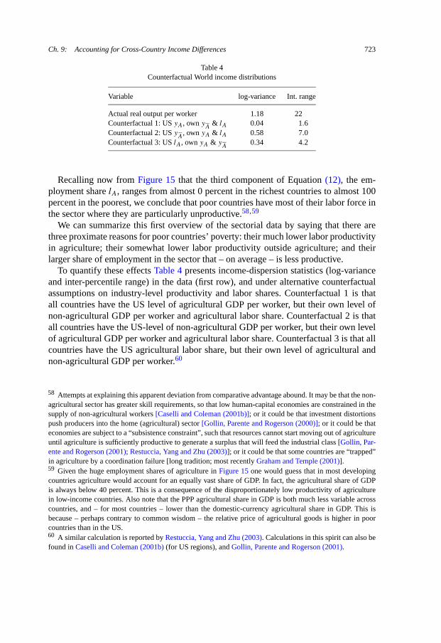
Ch. 9: Accounting for Cross-Country Income Differences 723
Table 4Counterfactual World income distributions
Variable log-variance Int. range
Actual real output per worker 1.18 22Counterfactual 1: US yA, own y
A& lA 0.04 1.6
Counterfactual 2: US yA
, own yA & lA 0.58 7.0Counterfactual 3: US lA, own yA & y
A0.34 4.2
Recalling now from Figure 15 that the third component of Equation (12), the em-ployment share lA, ranges from almost 0 percent in the richest countries to almost 100percent in the poorest, we conclude that poor countries have most of their labor force inthe sector where they are particularly unproductive.58,59
We can summarize this first overview of the sectorial data by saying that there arethree proximate reasons for poor countries’ poverty: their much lower labor productivityin agriculture; their somewhat lower labor productivity outside agriculture; and theirlarger share of employment in the sector that – on average – is less productive.
To quantify these effects Table 4 presents income-dispersion statistics (log-varianceand inter-percentile range) in the data (first row), and under alternative counterfactualassumptions on industry-level productivity and labor shares. Counterfactual 1 is thatall countries have the US level of agricultural GDP per worker, but their own level ofnon-agricultural GDP per worker and agricultural labor share. Counterfactual 2 is thatall countries have the US-level of non-agricultural GDP per worker, but their own levelof agricultural GDP per worker and agricultural labor share. Counterfactual 3 is that allcountries have the US agricultural labor share, but their own level of agricultural andnon-agricultural GDP per worker.60
58 Attempts at explaining this apparent deviation from comparative advantage abound. It may be that the non-agricultural sector has greater skill requirements, so that low human-capital economies are constrained in thesupply of non-agricultural workers [Caselli and Coleman (2001b)]; or it could be that investment distortionspush producers into the home (agricultural) sector [Gollin, Parente and Rogerson (2000)]; or it could be thateconomies are subject to a “subsistence constraint”, such that resources cannot start moving out of agricultureuntil agriculture is sufficiently productive to generate a surplus that will feed the industrial class [Gollin, Par-ente and Rogerson (2001); Restuccia, Yang and Zhu (2003)]; or it could be that some countries are “trapped”in agriculture by a coordination failure [long tradition; most recently Graham and Temple (2001)].59 Given the huge employment shares of agriculture in Figure 15 one would guess that in most developingcountries agriculture would account for an equally vast share of GDP. In fact, the agricultural share of GDPis always below 40 percent. This is a consequence of the disproportionately low productivity of agriculturein low-income countries. Also note that the PPP agricultural share in GDP is both much less variable acrosscountries, and – for most countries – lower than the domestic-currency agricultural share in GDP. This isbecause – perhaps contrary to common wisdom – the relative price of agricultural goods is higher in poorcountries than in the US.60 A similar calculation is reported by Restuccia, Yang and Zhu (2003). Calculations in this spirit can also befound in Caselli and Coleman (2001b) (for US regions), and Gollin, Parente and Rogerson (2001).

724 F. Caselli
The results are stunning. The figures in the second row imply that if poor countriesachieved the same level of agricultural labor productivity as the US, world income in-equality would virtually disappear! This is of course a reflection of the convergence ofUS agricultural incomes to US non-agricultural incomes [documented in Caselli andColeman (2001b)], as well as the huge agricultural share of employment in many ofthe poorest countries. However, the other two counterfactual experiments also gener-ate large declines in dispersion. Because agriculture is generally much less productivethan non-agriculture, reducing the agricultural employment share to US levels wouldreduce income inequality by an enormous two thirds (third row). And cross-countrynon-agricultural productivity differences, while much less than agricultural ones, arestill sufficiently large that income inequality would fall by about one half if poor coun-tries were as productive outside of agriculture as the US (second row).61
6.3. Sectorial composition and development accounting
The previous subsection establishes that there are very large within industry cross-country differences in output per worker. Indeed, the agricultural GDP differences aresubstantially larger than the aggregate GDP ones. Furthermore, these cross-countrydifferences in industry GDPs are seen to potentially “account” for a large fraction ofthe cross-country dispersion in aggregate income. We can now return to the originalquestion: are these large differences in agricultural GDP attributable to the amounts ofobservable inputs employed in agriculture by the various countries, or are they the resultof industry-level cross-country TFP differences? This is of course “the” development-accounting question.
To try to answer this question, we need assumptions on the industry production func-tions, as well as ways of measuring industry-level inputs. I will assume that each ofthe two sectors produces according to a Cobb–Douglas technology. In agriculture, thefactors of production are capital, labor, and land (T ). In non-agriculture, they are capitaland labor:
(13)YA = AA(KA)αA(LAhA)βA(TA)1−αA−βA,
(14)YA = AA(KA)αA(LAhA)1−αA.
The goal now is to construct counter-factual agricultural and non-agricultural outputdata,
yA,HK = kαA
A hβA
A t1−αA−βA
A ,
yA,HK = kαA
Ah
1−αA
A.
61 Of course, this discussion abstracts from the changes in world-wide agricultural relative prices that suchchanges would bring about.

Ch. 9: Accounting for Cross-Country Income Differences 725
These counter-factual data answer the question: what would the world distribution ofagricultural (non-agricultural) output per worker look like if all countries had the sameagricultural (non-agricultural) total factor productivity?
Assume that the rates of return on capital must be equalized across sectors – a plau-sible arbitrage condition. This is easily seen to imply
αA
P DA YA
KA
= αA
P D
AYA
KA
,
where P DA (P D
A) is the domestic producer price of agricultural (non-agricultural) goods,
which will generally differ from the PPP price, and is the price the domestic investorcares about (unless he produces for the export market). The quantities P D
A YA and P D
AYA
are, of course, agricultural and non-agricultural output in domestic prices, and they areobservable from WDI.62 Hence, combining this equation with
(15)KA + KA = K,
where K is the (observable) total capital stock, we can back out KA and KA, and hence(with labor shares calculated from FAO and PWT) kA and kA.63
It is harder to come up with numbers for hA and hA. Caselli and Coleman (2001b)show that there is a very systematic tendency for agriculture to be one of the least skillintensive sectors in the economy. For example, for each of the years between 1940 and1990 they rank the roughly 120 industries featured in the US Census of Population bypercentage of workers with an elementary degree or less, and in each of these yearsagriculture consistently ranks in the bottom 10. This suggests that it may not be unrea-sonable to set hA = 1 in all countries, i.e. that the agricultural work force is made up byworkers with no education. It is then easy to compute human capital per worker outsideof agriculture. In particular, if s is the average years of schooling in the labor force, and afraction lA has no education and works in agriculture, then the remaining fraction 1− lAmust have years of education sA = s/(1− lA). hA is then computed with the “standard”formula linking years of education to human capital by way of Mincerian returns.
For tA I simply plug in WDI data on each country’s endowment of arable land. Forthe parameters, I use essentially the same calibration as in Caselli and Coleman (2001b),which is in turn based on the work of Jorgenson and Gollop (1992). The labor share inthe USA is about 60% in both farming and non-farming. The capital share in agricultureis about 21%, and the remainder is absorbed by land.
62 In fact, we use the share of agriculture in GDP in domestic prices from the WDI. This is sufficient for the
calculation below since only the ratio YDA
/YDA
is needed.63 Instead of using a no-arbitrage condition for capital, sector specific capital inputs may be recovered usingan indifference condition for rural–urban labor flows. This condition would involve, among other things, an“urban wage premium” compensating for costs of skill acquisition [as, for example, in Caselli and Coleman(2001b)] or for the lower probability of finding a job, as in the celebrated model of Harris and Todaro (1970).See Temple (2003) for an interesting calibration of the Harris–Todaro model aiming to assess the output costsof the labor-market rigidities that lead to economic dualism.

726 F. Caselli
Table 5Success within sectors
Sector success1 success2
Agriculture 0.15 0.09Nonagriculture 0.59 0.63
For the 65 countries for which we can construct yA,HK and yA,HK and for whichwe have measures of yA and yA, the success of the factor-only model is as reportedin Table 5. Once again, the results are striking. Briefly, the factor-only model explainsvirtually nothing of the observed per-capita income variance in agriculture: it’s entirelya story of TFP differences, even more so than for aggregate GDP. Conversely, physicaland human capital inputs do a better than usual job at explaining per-worker output dif-ferences outside of agriculture. This may be plausible, as knowledge flows are probablymore effective in manufacturing or services than in agriculture. Still, the TFP scales arestill tipped against the developing countries.
While informative, this exercise does not yet answer the development accountingquestion of how much PPP income per worker variation would be observed if all coun-tries had the same technology. This counter-factual PPP income per worker would be
(16)yiHK = PAAAyi
A,KH liA + PAAAyi
A,KHliA
where PA and PA are the international-dollar prices of agricultural and non-agriculturalgoods, and AA and AA are the efficiency levels in some reference country.
Because of its additive nature, implementing Equation (16) calls for an explicit choiceof values for AA and AA to keep constant as we vary country factor endowments andsectorial composition – summarized by yi
A,KH liA and yi
A,KHliA
. (We did not have tochoose a benchmark in the purely multiplicative framework of the one-sector model,because in that framework the common level of efficiency disappears when taking thelog-variance or the inter-percentile ratio). Furthermore, the results will be sensitive towhich country (i.e. what particular choice of As) is chosen as a reference. Hence, thedevelopment accountant must decide whose country’s technology will be assigned therole of the benchmark technology in the counterfactual exercise.
A certain degree of arbitrariness is inevitable in this choice. Nevertheless, a somewhatplausible argument can be made that it makes sense to hold constant the technology ofthe richest country in the sample; in our case, the USA. This is because in a sense thisis the most successful country, so it is interesting to know how the world income dis-tribution would change if all countries shared the industry TFPs of the most successfulamong them.
For the reference country (the US) it is true by definition that
yA = PAAAyA,KH,

Ch. 9: Accounting for Cross-Country Income Differences 727
and
yA = PAAAyA,KH .
Since yA and yA are known, we can back out reference values for PAAA and PAAA andcompute the counter-factual in (16). The result of this exercise, which is also the mainresult of this section, is 0.34 for success1, and 0.32 for success2. In words, once again,this means that, if all countries had the same industry-level TFPs as the US, but theirobserved allocation of measurable factors to agriculture and non-agriculture, the worlddistribution of income would be about one third as unequal as it actually is. Given that– for this sub-sample – the corresponding success measures are 0.45 and 0.39 when thesectorial composition of GDP is not taken into account, I conclude that taking accountof differences in sectorial composition actually decreases the share of cross-countryincome inequality that we can explain with a country’s factor endowments.
This result should have been expected, by now. In the previous subsection we haveseen that the dispersion in agricultural incomes per worker is a critical “source” ofdispersion in per-capita income. Table 5 shows, however, that almost all of the variationin agricultural income comes from differences in agricultural TFP. It is not surprising,therefore, that we find that – even allowing for differences in output composition –factor endowments still do not work as the main cause of GDP differences.
One possible way to enhance the quantitative role of sectorial considerations is ex-plored in a highly innovative paper by Graham and Temple (2001). Instead of assuming,as here, that both agriculture and non-agriculture have constant returns to scale, theyfollow a long tradition in development economics in hypothesizing that the formeris characterized by decreasing returns and the latter by increasing returns. As is wellknown these assumptions tend to generate multiple equilibria, and it is therefore possi-ble to try to explain large cross-country income differences with the argument that poorcountries are in “low”, i.e. high agriculture, i.e. low returns, equilibria; while rich coun-tries are in industrialized equilibria and therefore benefit from the increasing returns.The difficulty here is to figure out in the data which countries are in the bad and whichones are in the good equilibrium. The contribution of Graham and Temple is to show avery ingenious way of solving this problem. They find that multiple equilibria explaina relatively large fraction of per capita income differences. The lingering question iswhether the significant departures from constant returns to scale required for their resultare plausible.64
7. Non-neutral differences in technology
7.1. Basic concepts and qualitative results
In all of the previous sections we have assumed that all differences in efficiency acrosscountries are TFP differences, as summarized by the multiplicative factor A. This im-
64 See also Chanda and Dalgaard (2003) for another contribution that argues for a large role of agriculture.

728 F. Caselli
plies that we view differences in efficiency as factor neutral: some countries simply useall of their inputs more efficiently than others. This is of course a restriction on the setof possible efficiency differences. Caselli and Coleman (2005) have begun exploring amore general view, that allows for the possibility that differences in technology showup as differences in the efficiency with which specific factors – as opposed to all factorsproportionally – are used, or even that some countries use some factors more efficiently,and some less efficiently, than others. In other words, a more general view of technologydifferences where such differences are not factor neutral.65
Extending the development-accounting exercise to allow for factor non neutrality inefficiency differences is the object of this section. While Caselli and Coleman considera three-factor production function (capital, skilled labor, and unskilled labor), here I willstick to the two-factor world (human and physical capital) of the rest of the chapter. Thefirst step we need to take to proceed in this direction is to replace the Cobb–Douglasrestriction – which implicitly rules out non-neutrality – with a more general productionfunction where non-neutral differences can be contemplated. The simplest such gener-alization is provided by the CES formula:
(17)Y = [α(AkK)σ + (1 − α)(AhLh)σ
]1/σ, α ∈ (0, 1), σ < 1.
In (17) Ak and Ah are the efficiency units delivered by one unit of physical capital andone unit of quality-adjusted labor, respectively. If Ak is higher in one country than inanother, we say that the former country uses capital more efficiently. If Ah is greater, thecountry uses human capital more efficiently. The parameters σ and α are constant acrosscountries. σ governs the ease of substitution between physical and human capital. Theelasticity of substitution is
η = 1/(1 − σ).
The Cobb–Douglas case of the previous sections of the paper emerges as a limit for σ
approaching 0 (η approaching 1). In this case, total factor productivity A converges toAα
k A1−αh .66
In the factor-neutral world explored so far in this chapter, making inference aboutefficiency differences across countries is a simple matter of solving one equation inone unknown. Inference on non neutral differences is a bit more challenging, as Equa-tion (17) has two unknowns: Ak and Ah. The issue, then, is to find a suitable secondequation. As in Caselli and Coleman (2005), to do so I assume that factor markets areeverywhere competitive. Then, if r is the user cost of capital, and if w is the market
65 See also Hsieh (2000) for some observations on this topic.66 Many macroeconomists are attached to the Cobb–Douglas assumption on the alleged ground that thecapital share is constant in the US. The trendlessness of the capital share in the US, however, can of course bereplicated by CES models with the “right” time series behavior of the effective supplies of capital and labor(i.e. AkK and AhhL). Furthermore, there is clear evidence of substantial fluctuations in the capital shares ofmany countries other than the US.
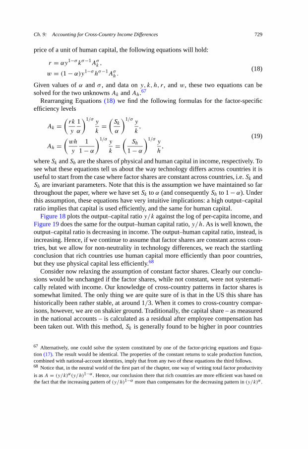
Ch. 9: Accounting for Cross-Country Income Differences 729
price of a unit of human capital, the following equations will hold:
(18)r = αy1−σ kσ−1Aσ
k ,
w = (1 − α)y1−σ hσ−1Aσh .
Given values of α and σ , and data on y, k, h, r , and w, these two equations can besolved for the two unknowns Ak and Ah.67
Rearranging Equations (18) we find the following formulas for the factor-specificefficiency levels
(19)
Ak =(
rk
y
1
α
)1/σy
k=
(Sk
α
)1/σy
k,
Ah =(
wh
y
1
1 − α
)1/σy
k=
(Sh
1 − α
)1/σy
h,
where Sk and Sh are the shares of physical and human capital in income, respectively. Tosee what these equations tell us about the way technology differs across countries it isuseful to start from the case where factor shares are constant across countries, i.e. Sk andSh are invariant parameters. Note that this is the assumption we have maintained so farthroughout the paper, where we have set Sk to α (and consequently Sh to 1 − α). Underthis assumption, these equations have very intuitive implications: a high output–capitalratio implies that capital is used efficiently, and the same for human capital.
Figure 18 plots the output–capital ratio y/k against the log of per-capita income, andFigure 19 does the same for the output–human capital ratio, y/h. As is well known, theoutput–capital ratio is decreasing in income. The output–human capital ratio, instead, isincreasing. Hence, if we continue to assume that factor shares are constant across coun-tries, but we allow for non-neutrality in technology differences, we reach the startlingconclusion that rich countries use human capital more efficiently than poor countries,but they use physical capital less efficiently.68
Consider now relaxing the assumption of constant factor shares. Clearly our conclu-sions would be unchanged if the factor shares, while not constant, were not systemati-cally related with income. Our knowledge of cross-country patterns in factor shares issomewhat limited. The only thing we are quite sure of is that in the US this share hashistorically been rather stable, at around 1/3. When it comes to cross-country compar-isons, however, we are on shakier ground. Traditionally, the capital share – as measuredin the national accounts – is calculated as a residual after employee compensation hasbeen taken out. With this method, Sk is generally found to be higher in poor countries
67 Alternatively, one could solve the system constituted by one of the factor-pricing equations and Equa-tion (17). The result would be identical. The properties of the constant returns to scale production function,combined with national-account identities, imply that from any two of these equations the third follows.68 Notice that, in the neutral world of the first part of the chapter, one way of writing total factor productivity
is as A = (y/k)α(y/h)1−α . Hence, our conclusion there that rich countries are more efficient was based onthe fact that the increasing pattern of (y/h)1−α more than compensates for the decreasing pattern in (y/k)α .

730 F. Caselli
Figure 18. Distribution of y/k.
Figure 19. Distribution of y/h.
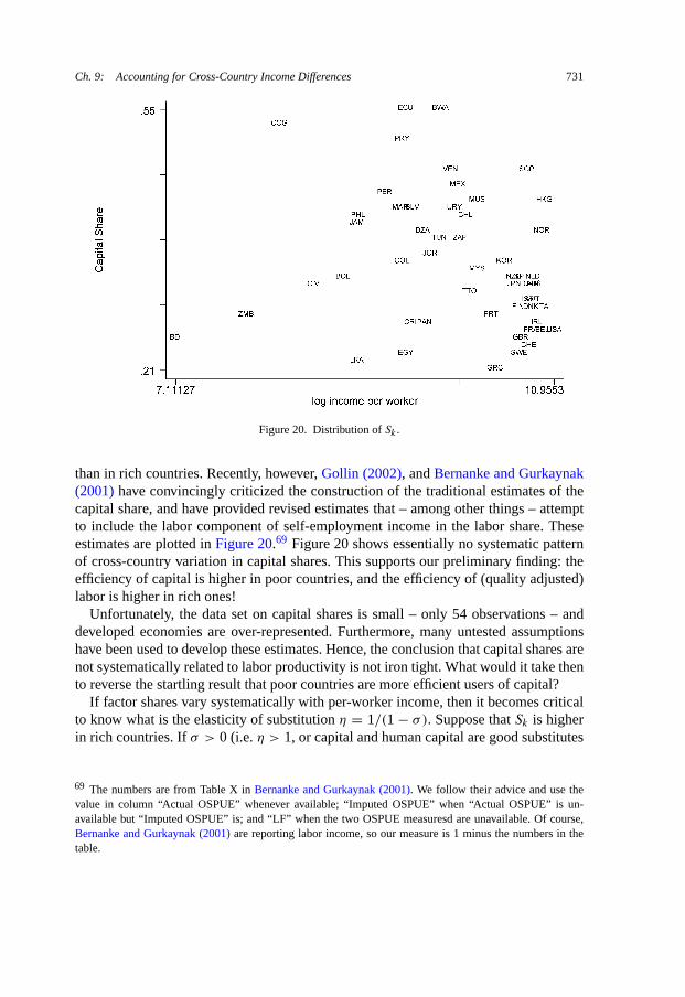
Ch. 9: Accounting for Cross-Country Income Differences 731
Figure 20. Distribution of Sk .
than in rich countries. Recently, however, Gollin (2002), and Bernanke and Gurkaynak(2001) have convincingly criticized the construction of the traditional estimates of thecapital share, and have provided revised estimates that – among other things – attemptto include the labor component of self-employment income in the labor share. Theseestimates are plotted in Figure 20.69 Figure 20 shows essentially no systematic patternof cross-country variation in capital shares. This supports our preliminary finding: theefficiency of capital is higher in poor countries, and the efficiency of (quality adjusted)labor is higher in rich ones!
Unfortunately, the data set on capital shares is small – only 54 observations – anddeveloped economies are over-represented. Furthermore, many untested assumptionshave been used to develop these estimates. Hence, the conclusion that capital shares arenot systematically related to labor productivity is not iron tight. What would it take thento reverse the startling result that poor countries are more efficient users of capital?
If factor shares vary systematically with per-worker income, then it becomes criticalto know what is the elasticity of substitution η = 1/(1 − σ). Suppose that Sk is higherin rich countries. If σ > 0 (i.e. η > 1, or capital and human capital are good substitutes
69 The numbers are from Table X in Bernanke and Gurkaynak (2001). We follow their advice and use thevalue in column “Actual OSPUE” whenever available; “Imputed OSPUE” when “Actual OSPUE” is un-available but “Imputed OSPUE” is; and “LF” when the two OSPUE measuresd are unavailable. Of course,Bernanke and Gurkaynak (2001) are reporting labor income, so our measure is 1 minus the numbers in thetable.
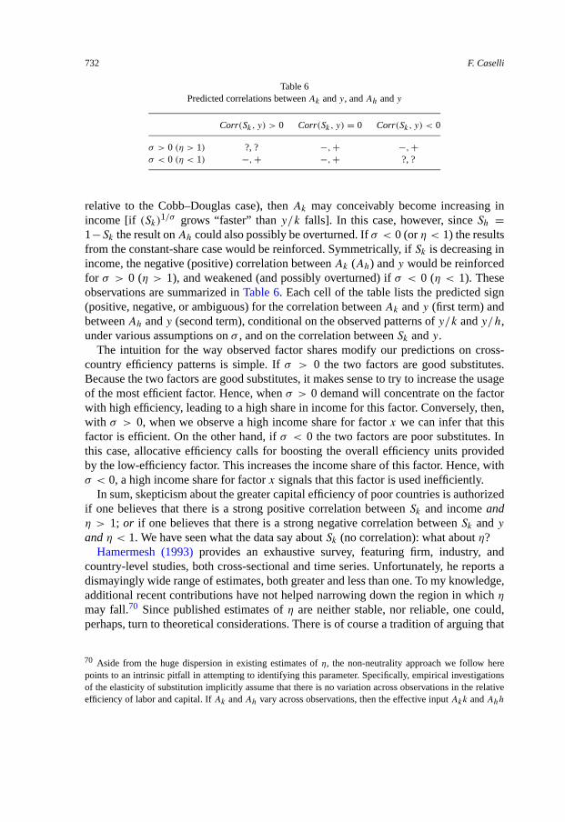
732 F. Caselli
Table 6Predicted correlations between Ak and y, and Ah and y
Corr(Sk, y) > 0 Corr(Sk, y) = 0 Corr(Sk, y) < 0
σ > 0 (η > 1) ?, ? −, + −, +σ < 0 (η < 1) −,+ −, + ?, ?
relative to the Cobb–Douglas case), then Ak may conceivably become increasing inincome [if (Sk)
1/σ grows “faster” than y/k falls]. In this case, however, since Sh =1−Sk the result on Ah could also possibly be overturned. If σ < 0 (or η < 1) the resultsfrom the constant-share case would be reinforced. Symmetrically, if Sk is decreasing inincome, the negative (positive) correlation between Ak (Ah) and y would be reinforcedfor σ > 0 (η > 1), and weakened (and possibly overturned) if σ < 0 (η < 1). Theseobservations are summarized in Table 6. Each cell of the table lists the predicted sign(positive, negative, or ambiguous) for the correlation between Ak and y (first term) andbetween Ah and y (second term), conditional on the observed patterns of y/k and y/h,under various assumptions on σ , and on the correlation between Sk and y.
The intuition for the way observed factor shares modify our predictions on cross-country efficiency patterns is simple. If σ > 0 the two factors are good substitutes.Because the two factors are good substitutes, it makes sense to try to increase the usageof the most efficient factor. Hence, when σ > 0 demand will concentrate on the factorwith high efficiency, leading to a high share in income for this factor. Conversely, then,with σ > 0, when we observe a high income share for factor x we can infer that thisfactor is efficient. On the other hand, if σ < 0 the two factors are poor substitutes. Inthis case, allocative efficiency calls for boosting the overall efficiency units providedby the low-efficiency factor. This increases the income share of this factor. Hence, withσ < 0, a high income share for factor x signals that this factor is used inefficiently.
In sum, skepticism about the greater capital efficiency of poor countries is authorizedif one believes that there is a strong positive correlation between Sk and income andη > 1; or if one believes that there is a strong negative correlation between Sk and y
and η < 1. We have seen what the data say about Sk (no correlation): what about η?Hamermesh (1993) provides an exhaustive survey, featuring firm, industry, and
country-level studies, both cross-sectional and time series. Unfortunately, he reports adismayingly wide range of estimates, both greater and less than one. To my knowledge,additional recent contributions have not helped narrowing down the region in which η
may fall.70 Since published estimates of η are neither stable, nor reliable, one could,perhaps, turn to theoretical considerations. There is of course a tradition of arguing that
70 Aside from the huge dispersion in existing estimates of η, the non-neutrality approach we follow herepoints to an intrinsic pitfall in attempting to identifying this parameter. Specifically, empirical investigationsof the elasticity of substitution implicitly assume that there is no variation across observations in the relativeefficiency of labor and capital. If Ak and Ah vary across observations, then the effective input Akk and Ahh

Ch. 9: Accounting for Cross-Country Income Differences 733
Table 7Regressions of log(Ak) and log(Ah) on log(y)
Dep. var. η = 0.1 η = 0.5 η = 0.9 η = 1.1 η = 1.5 η = 2 η = 50
log(Ak) −0.32 −0.027 0.14 −0.89 −0.48 −0.43 −0.37(6.2) (4.28) (0.39) (1.99) (3.58) (4.38) (5.59)
log(As) 0.80 0.74 0.21 1.53 1.00 0.94 0.87(28.06) (17.55) (.88) (5.36) (12.88) (17.37) (25.57)
long-run elasticities are higher than short-run ones, and macro-economic higher thanmicro-economic. Ventura (1997) is a particularly convincing recent example. For ourpurposes it clearly seems appropriate to focus on a long-run, aggregate interpretation ofthe elasticity. However, it is not clear that even in this case these arguments put a lowerbound on η: even accepting that it is higher than a microeconomic, short-run elasticity,does not necessarily imply that it is, say, greater than 1.
For the countries with available data, we can actually compute the implied values ofAk and As from Equation (19) for different values of the elasticity of substitution η.For each of these implied set of estimates, in Table 7 we report the coefficients of re-gressions of log(Ak) and log(Ah) on log(y) (t-statistics in parenthesis).71 The resultsfrom the table confirm that the available data is mostly consistent with the situation inthe middle column of Table 6: for most values of η, rich countries seem to use capitalless efficiently than poor ones. The only exception is for η = 0.9, where Ak is weaklyand insignificantly positively related to income. This is not surprising, since η = 0.9is “almost” Cobb–Douglas, and in this limiting case Ak and Ah are not independentlyidentifiable. The coefficients are also sizable, with a 10 percent increase in income perworker being associated with up to a 9 percent decline in Ak , and even larger increasesin Ah.
Everything considered, the result that poor countries use capital more efficiently thanrich ones seems surprisingly robust, particularly because very little structure is imposedon the data to reach this conclusion. Needless to say, it is also rather stunning – espe-cially if one is used to think about the world in TFP (factor neutral) terms. However, apossible theoretical explanation is readily available.
will be mis-measured, perhaps wildly. I believe this may indeed be the reason why estimates of η are sounstable. I think this point is implicit in the analysis of Diamond, McFadden and Rodriguez (1978). If theinduced measurement error is random, it seems the bias in the estimate of η should be upwards. Intuitively,observations with very different input combinations will appear to have similar output levels, something thatis consistent with a high elasticity of substitution. However, if the As vary systematically, the bias could alsobe downward. Suppose, for example, that Ax and x are positively correlated across observations. Then thedata will tend to understate the true variation in effective input, so that less substitutability will appear to berequired to explain the observed variation in output.71 In these regressions there are 53 observations for log(Ak) and 50 for log(Ah). Also notice that, from
Equations (19), the As are identified up to the common multiplicative constants α1/σ and (1 − α)1/σ .

734 F. Caselli
Caselli and Coleman (2005) find somewhat analogous evidence that poor countriesuse unskilled labor more efficiently than rich countries – while rich countries use skilledlabor more efficiently. To explain this finding they develop a simple model of appropri-ate technology, in which countries face a menu of technology choices. The choice oftechnology is not neutral, in that different technologies augment different inputs differ-ently. One key result is that which technology is chosen by each country depends on theelasticity of substitution between inputs. If the elasticity of substitution is greater than 1,the appropriate technology augments the abundant factor relatively more, while if theelasticity is less than 1, it is appropriate to choose a technology that augments the scarcefactor relatively more. Since the elasticity of substitution between skilled and unskilledworkers is commonly deemed to be in the neighborhood of 1.4, and rich countries areabundant in skilled labor, this explains why they would choose skilled-labor augmentingtechnologies, while poor countries choose unskilled-labor augmenting technologies.
Returning now to the new result here that poor countries use physical capital moreefficiently – and human capital less efficiently – than rich countries, and recalling thatpoor countries are relatively abundant in human capital, we can use the same theoreticalexplanation if we are willing to assume that the elasticity of substitution between capitaland (quality-adjusted) labor is less than 1; an assumption that – as we have seen –cannot be ruled out based on the available evidence. In sum, with a high elasticity ofsubstitution between skilled and unskilled labor, and a low elasticity of substitutionbetween capital and the labor aggregate, an appropriate technology model can explainthe joint patterns of cross-country choice of the efficiency of capital, skilled labor, andunskilled labor.72
7.2. Development accounting with non-neutral differences
Development accounting asks how the observed distribution of GDP per worker com-pares to the distribution that would obtain in the counterfactual case that all countrieshad the same technology. As is clear from Equation (17), we are again in the situationin which – unlike in the simple TFP framework – the answer to this question will not beinsensitive to which particular pair of values of Ak and Ah are plugged in. As we did inthe previous subsection, and for the same reasons, I choose as the benchmark countrythe USA. Hence, I first compute the US Ak and Ah from Equations (19), and then I plugthese numbers in Equation (17) for each country, and obtain measures of success of amodel where all countries use the same (US) technology.73
72 Other treatments of the problem studied by Caselli and Coleman (2005) – a country’s appropriate choicefrom a menu of technologies as a function of its factor endowments – are, e.g., Basu and Weil (1998)and Acemoglu and Zilibotti (2001). The problem is also closely related to the problem of induced inno-vation/directed technical change studied, e.g., in Samuelson (1965, 1966) and Acemoglu (1998, 2003).73 More precisely, I compute αAσ
k= Sk,US(yUS/kUS)σ , and (1 − α)Aσ
h= Sh,US(yUS/hUS)σ , and plug
these expressions in Equation (17).

Ch. 9: Accounting for Cross-Country Income Differences 735
Figure 21. Success with non-neutral technology differences.
Figure 21 plots the success of the factor-only model when all countries use the tech-nology of the United States. Note that our measures of success converge – as they should– to those of the factor-neutral (Cobb–Douglas) model for η converging to 1. Success ofthe factor-only model is also systematically decreasing with the value of the elasticity ofsubstitution, η. To see why this is so recall that the lower is η the closer the productionfunction becomes to the Leontief case. Also notice that Figures 18 and 19 imply thatpoor countries are relatively abundant in human capital: the ratio h/k is decreasing withper-capita income. Finally, recall that the US uses human-capital relatively efficiently.Hence, the ratio Ah,USh/Ak,USk is extremely high in poor countries, suggesting thatmuch “effective human capital” in these countries would be unproductive in the lim-iting Leontief case. This “waste” may explain the low GDP of poor countries withouthaving to invoke low As, i.e. it leads to greater success of the factor-only model. On theother side of η = 1, we tend to approach the linear production function. The closer weare to this case, the less a disproportionate Ahh/Akk ratio hurts a country’s productiv-ity, so the factor-only model performs less and less well. Something else is required toexplain why GDP is so low.
The most remarkable finding of Figure 21, however, is quantitative: namely, not onlyfor elasticities of substitution less than 1 does the model with non neutral technologyoutperforms the Cobb–Douglas one, but there is a range of elasticities such that theperformance of the model is extremely good. Indeed, an elasticity of 0.5 delivers a

736 F. Caselli
perfect fit for the factor-only model! This is remarkable because an elasticity of 0.5 –given our current state of knowledge – is not particularly implausible.74
One could object to the exercise we just reported that the counter-factual choice oftechnology – all countries using the US technology – is not sensible. For, we knowfrom the previous section that – assuming our factor share data to be dependable –countries are observed to use technologies that cannot be ranked: some technologiesboost the productivity of physical capital, some others of human capital. Therefore, onemay speculate that – given the choice – poor countries would not necessarily chooseto use the US technology. Instead, they would choose the technology most appropriategiven their factor endowments.
In order to address this point, we now treat the observed (Ak,Ah) combinations fromthe previous sub-section as a “menu” of available technologies. One could think of thismenu as a summary of the world’s technical knowledge, each observed (Ak,Ah) pairbeing a particular blueprint to generate output from physical and human capital. I thenre-interpret the counter-factual of no technology differences as one where all countrieshave access to the same menu of technologies; ask what technology from this menuwould each country choose; and compute the counter-factual world income distributionwhen all countries choose their appropriate technology (from the set of available ones).The appropriate technology is the output-maximizing one.75
The results from this alternative counter-factual experiment are plotted in Figure 22.Here, for each value of η, I have computed from Equations (19) the implied values of Ak
and Ah for each country with complete data – including data on the factor shares Sk andSh. This gave us 50 “observed” technologies. For each country in our 94-country sam-ple, then, I have “chosen” from this menu of 50 the appropriate technology, and I havecomputed success under the assumption that each country uses this output-maximizingchoice. As can be seen, the results preserve the broad qualitative features of those ofFigure 21, but quantitatively the factor-only model does much less well. In particular(almost), complete success only occurs if the technology is Leontief.
The intuition for this change in results is simple. Given the observed wide dispar-ity in factor proportions, when countries can choose their technology appropriately theywill in general choose different (Ak , Ah) combinations. In particular, few poor countrieswill find it optimal to use the technology observed in the USA. Indeed, countries withunfavorable factor endowments will be able to partially remedy by choosing technol-ogy appropriately. Hence, factor endowments do not have as much explanatory powerfor income differences as they do when all countries are forced to use the same (US)technology.
Even when countries choose technology, however, the measures of success are verysensitive to the choice of the elasticity of substitution: if the elasticity of substitution is
74 Elasticities less than 0.5 imply an income dispersion under the common-technology assumption that areeven greater than the observed ones.75 See Caselli and Coleman (2005) for a model where the technology choice is decentralized at the level offirms, and the equilibrium aggregate technology is the GDP-maximizing one.
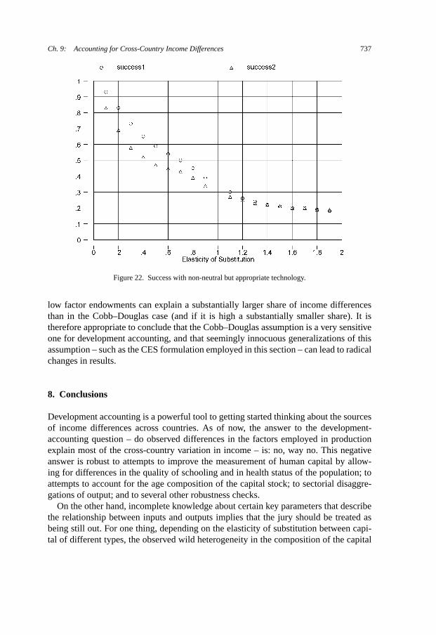
Ch. 9: Accounting for Cross-Country Income Differences 737
Figure 22. Success with non-neutral but appropriate technology.
low factor endowments can explain a substantially larger share of income differencesthan in the Cobb–Douglas case (and if it is high a substantially smaller share). It istherefore appropriate to conclude that the Cobb–Douglas assumption is a very sensitiveone for development accounting, and that seemingly innocuous generalizations of thisassumption – such as the CES formulation employed in this section – can lead to radicalchanges in results.
8. Conclusions
Development accounting is a powerful tool to getting started thinking about the sourcesof income differences across countries. As of now, the answer to the development-accounting question – do observed differences in the factors employed in productionexplain most of the cross-country variation in income – is: no, way no. This negativeanswer is robust to attempts to improve the measurement of human capital by allow-ing for differences in the quality of schooling and in health status of the population; toattempts to account for the age composition of the capital stock; to sectorial disaggre-gations of output; and to several other robustness checks.
On the other hand, incomplete knowledge about certain key parameters that describethe relationship between inputs and outputs implies that the jury should be treated asbeing still out. For one thing, depending on the elasticity of substitution between capi-tal of different types, the observed wild heterogeneity in the composition of the capital

738 F. Caselli
stock by type of equipment could turn out to be a key proximate determinant of incomedifferences. For another, depending on the elasticity of substitution between physicaland human capital, we may find that all is needed for these factors to explain a largefraction of income inequality is a departure from Cobb–Douglas. Disaggregating thegovernment sector out of the data may also potentially reduce the unexplained com-ponent of GDP. There is no deep reason why we should not be able to make progresson these three fronts, so that my assessment of the future of this research enterprise isoptimistic.
Acknowledgements
I thank John Duffy and Silvana Tenreyro for comments, and Mariana Colacelli, KalinaManova, and Andrea Szabó for research assistance.
References
Acemoglu, D. (1998). “Why do new technologies complement skills? Directed technical change and wageinequality”. Quarterly Journal of Economics 113, 1055–1089.
Acemoglu, D. (2003). “Labor- and capital-augmenting technical change”. Journal of European EconomicAssociation 1, 1–37.
Acemoglu, D., Angrist, J. (2000). “How large are human capital externalities? Evidence from compulsoryschooling laws”. In: Bernanke, B.S., Rogoff, K. (Eds.), NBER Macroeconomics Annual 2000. MIT Press,Cambridge, pp. 9–59.
Acemoglu, D., Zilibotti, F. (2001). “Productivity differences”. Quarterly Journal of Economics 116, 563–606.Aiyar, S., Dalgaard, C.-J. (2002). “Total factor productivity revisited: A dual approach to levels-accounting”.
Working Paper, Brown University.Altonji, J.G., Dunn, T.A. (1996). “The effects of family characteristics on the return to education”. The Review
of Economics and Statistics 78 (4), 692–704.Baily, M.N., Solow, R.M. (2001). “International productivity comparisons built from the firm level”. Journal
of Economic Perspectives 15 (3), 151–172.Barro, R.J., Lee, J. (2001). “International data on educational attainment: Updates and implications”. Oxford
Economic Papers 53 (3), 541–563.Basu, S., Weil, D.N. (1998). “Appropriate technology and growth”. The Quarterly Journal of Economics 113
(4), 1025–1054.Behrman, J.R., Rosenzweig, M.R. (2004). “Returns to birthweight”. Review of Economics and Statistics 86
(2), 586–601.Bernanke, B.S., Gurkaynak, R.S. (2001). “Is growth exogenous? Taking Mankiw, Romer, and Weil seriously”.
In: Bernanke, B.S., Rogoff, K. (Eds.), NBER Macroeconomics Annual 2001. MIT Press, Cambridge.Bils, M., Klenow, P.J. (2000). “Does schooling cause growth”. The American Economic Review 90 (5),
1160–1183.Card, D. (1999). “The causal effect of education on earnings”. In: Ashenfelter, O., Card, D. (Eds.), Handbook
of Labor Economics, vol. 3A. North-Holland, Amsterdam, pp. 1801–1863.Card, D., Krueger, A. (1996). “Labor market effects of school quality: Theory and evidence”. In: Burtless, G.
(Ed.), Does Money Matter? The Effect of School Resources on Student Achievement and Adult Success.Brookings Institute, Wasinghton, DC.
Ch. 9: Accounting for Cross-Country Income Differences 739
Caselli, F., Coleman, W.J. (2001a). “Cross-country technology diffusion: The case of computers”. AmericanEconomic Review 91 (2), 328–335.
Caselli, F., Coleman, W.J. (2001b). “The U.S. structural transformation and regional convergence: A reinter-pretation”. Journal of Political Economy 109 (3), 584–616.
Caselli, F., Coleman, W.J. (2005). “The world technology frontier”. Working Paper, LSE. American EconomicReview. In press.
Caselli, F., Esquivel, G., Lefort, F. (1996). “Reopening the convergence debate: A new look at cross-countrygrowth empirics”. Journal of Economic Growth 1 (3), 363–389.
Caselli, F., Tenreyro, S. (2004). “Is Poland the next Spain?”. Working Paper, LSE.Caselli, F., Wilson, D. (2004). “Importing technology”. Journal of Monetary Economics 51 (1), 1–32.Chanda, A., Dalgaard, C.-J. (2003). “Dual economies and international TFP differences”. Working Paper,
Louisiana State University.Christensen, L.R., Cummings, D., Jorgenson, D.W. (1981). “Relative productivity levels, 1947–1973: An
international comparison”. European Economic Review 16 (1), 61–94.Clark, C. (1940). “The morphology of economic growth”. In: Clark, C. (Ed.), The Conditions of Economic
Progress. Macmillan, London, pp. 337–373.Clark, G. (1987). “Why isn’t the whole world developed? Lessons from the cotton mills”. Journal of Economic
History 47, 141–173.Conrad, K., Jorgenson, D.W. (1985). “Sectoral productivity gaps between the United States, Japan and
Germany, 1960–1979”. In: Giersch, H. (Ed.), Probleme und Perspektiven der weltwirtschaftlichen En-twicklung. Duncker and Humblot, Berlin, pp. 335–347.
Currie, J., Thomas, D. (1999). “Early test scores, socioeconomic status and future outcomes”. Working PaperNo. 6943, National Bureau of Economic Research.
De la Fuente, A., Doménech, R. (2002). “Human capital in growth regressions: How much difference doesdata quality make? An update and further results”. CEPR Discussion Papers No. 3587.
Denison, E.F. (1967). Why Growth Rates Differ. The Brookings Institutions, Washington, DC.Diamond, P., McFadden, D., Rodriguez, M. (1978). “Measurement of the elasticity of factor substitution and
bias of technical change”. In: Fuss, M., McFadden, D. (Eds.), Production Economics: A Dual Approach toTheory and Applications, vol. II, Applications of the Theory of Production. North-Holland, Amsterdam.
Duflo, E. (2001). “Schooling and labor market consequences of school construction in Indonesia: Evidencefrom an unusual policy experiment”. American Economic Review 91 (4), 795–813.
Easterly, W., Levine, R. (2001). “It’s not factor accumulation: Stylized facts and growth models”. World BankEconomic Review 15 (2), 177–219.
Eaton, J., Kortum, S. (2001). “Trade in capital goods”. European Economic Review 45 (7), 1195–1235.Feenstra, R.C. (2000). ‘World trade flows, 1980–1997”. University of California.Feyrer, J. (2002). “Demographics and productivity”. Working Paper, Dartmouth College.Fisher, A. (1945). Economic Programs and Social Security. Macmillan, London.Gelb, A., Knight, J.B., Sabot, R.H. (1988). “Lewis through a looking glass: Public sector employment, rent
seeking, and economic growth”. World Bank.Gollin, D. (2002). “Getting income shares right”. Journal of Political Economy 110 (2), 458–474.Gollin, D., Parente, S.L., Rogerson, R. (2000). “Farm work, home work and international productivity differ-
ences”. Working Paper.Gollin, D., Parente, S.L., Rogerson, R. (2001). “Structural transformation and cross-country income differ-
ences”. Working Paper, University of California in Los Angeles.Gourinchas, P.-O., Jeanne, O. (2003). “The elusive gains from international financial integration”. Working
Paper No. 9684, National Bureau of Economic Research.Graham, B.S., Temple, J. (2001). “Rich nations, poor nations: How much can multiple equilibria explain?”.
Working Paper No. 76. Center for International Development, Harvard University.Greenwood, J., Hercowitz, Z., Krusell, P. (1997). “Long-run implications of investment-specific technological
change”. American Economic Review 87 (3), 342–362.Hall, R.E., Jones, C.I. (1999). “Why do some countries produce so much more output per worker than oth-
ers?”. The Quarterly Journal of Economics 114 (1), 83–116.

740 F. Caselli
Hamermesh, D.S. (1993). Labor Demand. Princeton University Press.Hanushek, E.A. (2003). “The failure of input based schooling policies”. Economic Journal 113 (485), F64–
F98.Hanushek, E.A. (2004). “Some simple analytics of school quality”. Working Paper No. 10229, National Bu-
reau of Economic Research.Hanushek, E.A., Kimko, D.D. (2000). “Schooling, labor-force quality, and the growth of nations”. The Amer-
ican Economic Review 90 (5), 1184–1208.Hanushek, E.A., Rivkin, S.G., Taylor, L.L. (1996). “Aggregation and the estimated effects of school re-
sources”. The Review of Economics and Statistics 78 (4), 611–627.Harrigan, J. (1997). “Technology, factor supplies, and international specialization: estimating the neoclassical
model”. American Economic Review 87 (4), 475–494.Harrigan, J. (1999). “Estimation of cross-country differences in aggregate production functions”. Journal of
International Economics 47, 267–293.Harris, J.R., Todaro, M. (1970). “Migration, unemployment and development: a two-sector analysis”. Amer-
ican Economic Review 60, 126–142.Heckman, J.J., Klenow, P.J. (1997). “Human capital policy”. Working Paper, University of Chicago.Hendricks, L. (2002). “How important is human capital for development? Evidence from immigrant earn-
ings”. American Economic Review 92 (1), 198–219.Heston, A., Summers, R., Aten, B. (2002). Penn World Tables Version 6.1. Downloadable Dataset. Center for
International Comparisons at the University of Pennsylvania.Hill, R. (2000). “Measuring substitution bias in international comparisons based on additive purchasing power
parity methods”. European Economic Review 44 (1), 45–162.Hsieh, C.-T. (2000). “Measuring biased technology”. Working Paper, Princeton University.Hulten, C.R. (1996). “Infrastructure capital and economic growth: How well you use it may be more important
than how much you have”. Working Paper No. 5847, National Bureau of Economic Research.Hsieh, C.-T., Klenow, P.J. (2003). “Relative prices and relative prosperity”. Working Paper No. 9701, National
Bureau of Economic Research.Islam, N. (1995). “Growth empirics: A panel data approach”. The Quarterly Journal of Economics 110, 1127–
1170.Johnson, G.E., Stafford, F.P. (1973). “Social returns to quantity and quality of schooling”. Journal of Human
Resources 8 (2), 139–155.Jorgenson, D.W. (1961). “The development of a dual economy”. Economic Journal 71, 309–334.Jorgenson, D.W. (1995a). Productivity, vol. 1: Postwar U.S. Economic Growth. MIT Press.Jorgenson, D.W. (1995b). Productivity, vol. 2: International Comparisons of Economic Growth. MIT Press.Jorgenson, D.W., Gollop, F.M. (1992). “Productivity growth in U.S. agriculture: A postwar perspective”.
American Journal of Agricultural Economics 74 (3), 745–750.Jovanovic, B., Rob, R. (1997). “Solow v. Solow: Machine prices and development”. Unpublished, New York
University.King, R.G., Levine, R. (1994). “Capital fundamentalism, economic development, and economic growth”.
Carnegie-Rochester Conference Series on Public Policy 40 (0), 259–292.Klenow, P.J., Rodriguez-Clare, A. (1997). “The neoclassical revival in growth economics: Has it gone too
far?”. In: Bernanke, B.S., Rotemberg, J.J. (Eds.), NBER Macroeconomics Annual 1997. MIT Press, Cam-bridge, pp. 73–103.
Knight, M., Loayza, N., Villanueva, D. (1993). “Testing the neoclassical theory of economic growth”. IMFStaff Papers 40 (3), 512–541.
Koren, M., Tenreyro, S. (2004). “Diversification and development”. LSF Working Paper, 3.Krueger, A.B. (2003). “Economic considerations and class size”. Economic Journal 113 (485), F34–F63.Kuznets, S. (1966). Modern Economic Growth. Yale University Press, New Haven.Lee, J.-W., Barro, R.J. (2001). “Schooling quality in a cross-section of countries”. Economica 68, 465–488.Lewis, W.A. (1954). “Economic development with unlimited supplies of labor”. Manchester School of Eco-
nomics and Social Studies 22, 139–151.
Ch. 9: Accounting for Cross-Country Income Differences 741
Mankiw, N.G., Romer, D., Weil, D.N. (1992). “A contribution to the empirics of economic growth”. TheQuarterly Journal of Economics 107 (2), 407–437.
Mateos-Planas, X. (2000). “Schooling and distortions in a vintage capital model”. University of Southampton,Department of Economics. 40 pp.
McGrattan, E.R., Schmitz, J.A. Jr. (1999). “Explaining cross-country income differences”. In: Taylor, J.B.,Woodford, M. (Eds.), Handbook of Macroeconomics, vol. 1A. North-Holland, Amsterdam, pp. 669–737.
Murnane, R.J., Willett, J.B., Levy, F. (1995). “The growing importance of cognitive skills in wage determina-tion”. The Review of Economics and Statistics 77 (2), 251–266.
Murphy, K., Shleifer, A., Vishny, R. (1991). “The allocation of talent: Implications for growth”. QuarterlyJournal of Economics 106 (2), 503–530.
Neal, D.A., Johnson, W.R. (1996). “The role of premarket factors in black–white wage differences”. Journalof Political Economy 104 (5), 869–895.
Nurkse, R. (1953). Problems of Capital Formation in Underdeveloped Countries. Oxford University Press,New York.
Parente, S.L. (2000). “Learning-by-using and the switch to better machines”. Review of Economic Dynam-ics 3 (4), 675–703.
Prescott, E.C. (1998). “Needed: A theory of total factor productivity”. International Economic Review 39 (3),525–551.
Pritchett, L. (2000). “The tyranny of concepts: CUDIE (Cumulated, Depreciated, Investment Effort) is notcapital”. Journal of Economic Growth 5 (4), 361–384.
Pritchett, L. (2003). “Does learning to add up add up? The returns to schooling in aggregate data”. Draftchapter for Handbook of Education Economics, Harvard University.
Psacharopoulos, G. (1994). “Returns to investment in education: A global update”. World Development 22(9), 1325–1343.
Rao, P.D.S. (1993). “Intercountry comparisons of agricultural output and productivity”. FAO Economic andSocial Development Paper, FAO, Rome.
Restuccia, D., Yang, D.T., Zhu, X. (2003). “Agriculture and aggregate productivity: A quantitative cross-country analysis”. Working Paper, University of Toronto, Economics Department.
Rodriguez-Clare, A. (1996). “The role of trade in technology diffusion”. Minneapolis Fed Working Paper114.
Rostow, W.W. (1960). The Stages of Economic Growth: A Non-Communist Manifesto. Cambridge UniversityPress, Cambridge, MA.
Samuelson, P. (1965). “A theory of induced innovation along Kennedy–Weiszacker lines”. Review of Eco-nomics and Statistics 47 (November).
Samuelson, P. (1966). “Rejoinder: Agreements, disagreements, doubts, and the case of induced Harrod-neutraltechnical change”. Review of Economics and Statistics 48 (November).
Schmitz, J.A., Jr. (2001). “What determines labor productivity?: Lessons from the dramatic recovery of theU.S. Canadian iron-ore industries”. Staff Report, 286, Federal Reserve Bank of Minneapolis.
Shastry, G.K., Weil, D.N. (2003). “How much of cross-country income variation is explained by health?”.Journal of the European Economic Association 1 (2–3), 387–396.
Solow, R. (1959). “Investment and technical progress”. In: Arrow, K., Karlin, S., Suppes, P. (Eds.), Mathe-matical Methods in the Social Sciences. Stanford University Press.
Summers, R., Heston, A. (1991). “The Penn World Table (Mark 5): An expanded set of international compar-isons, 1950–1988”. The Quarterly Journal of Economics 101 (2), 327–368.
Temple, J. (2003). “Dualism and aggregate productivity”. Unpublished, University of Bristol.Ventura, J. (1997). “Growth and interdependence”. The Quarterly Journal of Economics 112 (1), 57–84.Wagner, K., van Ark, B. (Eds.) (1996). International Productivity Differences: Measurement and Explana-
tions. North-Holland, Amsterdam.Weil, D.N. (2001). “Accounting for the effect of health on economic growth”. Working Paper, Brown Univer-
sity.Wilson, D.J. (2004). “Cross-country differences in capital composition”. Forthcoming in FRBSF Economic
Letter.