accelerator architectures for deep learning and graph
TRANSCRIPT

Accelerator Architectures forDeep Learning and Graph Processing
by
Linghao Song
Department of Electrical and Computer EngineeringDuke University
Date:Approved:
Yiran Chen, Advisor
Hai Li, Co-Advisor
Kenneth Brown
Benjamin Lee
Jun Yang
Dissertation submitted in partial fulfillment of therequirements for the degree of Doctor of Philosophy
in the Department of Electrical and Computer Engineeringin the Graduate School of
Duke University
2020

ABSTRACT
Accelerator Architectures forDeep Learning and Graph Processing
by
Linghao Song
Department of Electrical and Computer EngineeringDuke University
Date:Approved:
Yiran Chen, Advisor
Hai Li, Co-Advisor
Kenneth Brown
Benjamin Lee
Jun Yang
An abstract of a dissertation submitted in partial fulfillment of therequirements for the degree of Doctor of Philosophy
in the Department of Electrical and Computer Engineeringin the Graduate School of
Duke University
2020

Copyright © 2020 by Linghao SongAll rights reserved

Abstract
Deep learning and graph processing are two big-data applications and they are widely
applied in many domains. The training of deep learning is essential for inference and has not
yet been fully studied. With data forward, error backward, and gradient calculation, deep
learning training is a more complicated process with higher computation and communication
intensity. Distributing computations on multiple heterogeneous accelerators to achieve high
throughput and balanced execution, however, remaining challenging. In this dissertation, I
present AccPar, a principled and systematic method of determining the tensor partition for
multiple heterogeneous accelerators for efficient training acceleration. Emerging resistive
random access memory (ReRAM) is promising for processing in memory (PIM). For high-
throughput training acceleration in ReRAM-based PIM accelerator, I present PipeLayer,
an architecture for layer-wise pipelined parallelism. Graph processing is well-known for
poor locality and high memory bandwidth demand. In conventional architectures, graph
processing incurs a significant amount of data movements and energy consumption. I present
GraphR, the first ReRAM-based graph processing accelerator which follows the principle
of near-data processing and explores the opportunity of performing massive parallel analog
operations with low hardware and energy cost. Sparse matrix-vector multiplication (SpMV),
a subset of graph processing, is the key computation in iterative solvers for scientific
computing. The efficiently accelerating floating-point processing in ReRAM remains a
challenge. In this dissertation, I present ReFloat, a data format and a supporting accelerator
architecture, for low-cost floating-point processing in ReRAM for scientific computing.
iv

Acknowledgements
It is never easy to get a Ph.D. degree, but with the contribution and help from many people I
finally did it. Here, I mention them.
Professor Yiran Chen, my advisor, and Professor Hai Li, my co-advisor, have invaluable
advice and help to my research, professional development and life during my whole Ph.D.
program. In the first three years of Ph.D. program, I struggled because none of my work
was accepted by a conference. It was a really hard time and I even planned to quit and
find an SDE job. But my advisors never gave up on me. They always encouraged me and
believed in me. They gave me every opportunity to talk to or have a lunch with a scholar
who visited our lab or was in collaboration, let me present at a senior student’s presentation,
and made every effort to let me feel that I was not alone or forgotten. Professor Chen also
gave me many skills suggestions for social communication, career and team management.
I would like to thank my committee members – Professor Kenneth Brown, Professor
Benjamin Lee and Professor Jun Yang, and Professor Daniel Sorin in my qualify exam
committee. Their time and efforts out of their busy schedules help me improve in the
preliminary or/and final exams.
I would like to thank Professor Xuehai Qian (USC) for his insightful and valuable
feedbacks on my research.
In my two summer research interns, my mentors Catherine Schuman (ORNL), Steven
Young (ORNL) and Ang Li (PNNL) broadened my knowledge in computing systems.
I thank the efforts from my co-authors – Paul Bogdan, Nagadastagiri Challapalle, Fan
Chen, Xiang Chen, Enes Eken, Yu Hua, Houxiang Ji, Bing Li, Xin Liu, Jiachen Mao,
Vijaykrishnan Narayanan, Kent Nixon, Gabriel Perdue, Thomas Potok, Ximing Qiao,
Sahithi Rampalli, Tianqi Tang, Chengning Wang, Yandan Wang, Yitu Wang, Wei Wen,
Wujie Wen, Chunpeng Wu, Yuan Xie, Cong Xu, Huanrui Yang, Jianlei Yang, Youwei Zhuo.
v

My parents, Xuequan Song and Xiaoqin Dai, who always stand behind me.
vi

Contents
Abstract iv
Acknowledgements v
List of Figures ix
List of Tables xiii
1 Introduction 1
1.1 Tensor Partitioning for Deep Learning Accelerators . . . . . . . . . . . . 5
1.2 Layer-wise Pipelined Parallelism for Deep Learning Accelerators . . . . . 7
1.3 Accelerator Architecture for Graph Processing . . . . . . . . . . . . . . . 9
1.4 Low-Cost Floating-Point Processing in ReRAM . . . . . . . . . . . . . . 12
2 Tensor Partitioning for Deep Learning Accelerators 14
2.1 Background and Motivation . . . . . . . . . . . . . . . . . . . . . . . . 14
2.2 Tensor Partitioning Space . . . . . . . . . . . . . . . . . . . . . . . . . . 18
2.3 Cost Model . . . . . . . . . . . . . . . . . . . . . . . . . . . . . . . . . 25
2.4 Partitioning Algorithm . . . . . . . . . . . . . . . . . . . . . . . . . . . 31
2.5 Evaluation . . . . . . . . . . . . . . . . . . . . . . . . . . . . . . . . . . 34
3 Layer-wise Pipelined Parallelism for Deep Learning Accelerators 41
3.1 Background . . . . . . . . . . . . . . . . . . . . . . . . . . . . . . . . . 41
3.2 PIPELAYER Architecture . . . . . . . . . . . . . . . . . . . . . . . . . . 46
3.3 Implementation of PIPELAYER . . . . . . . . . . . . . . . . . . . . . . . 55
3.4 Discussion . . . . . . . . . . . . . . . . . . . . . . . . . . . . . . . . . . 61
3.5 Evaluation . . . . . . . . . . . . . . . . . . . . . . . . . . . . . . . . . . 63
vii

4 Accelerator Architecture for Graph Processing 70
4.1 Background and Motivation . . . . . . . . . . . . . . . . . . . . . . . . 70
4.2 GraphR Architecture . . . . . . . . . . . . . . . . . . . . . . . . . . . . 75
4.3 Mapping Algorithms in GE . . . . . . . . . . . . . . . . . . . . . . . . . 86
4.4 Evaluation . . . . . . . . . . . . . . . . . . . . . . . . . . . . . . . . . . 91
5 Low-Cost Floating-Point Processing in ReRAM 98
5.1 Background . . . . . . . . . . . . . . . . . . . . . . . . . . . . . . . . . 98
5.2 Motivation and REFLOAT Ideas . . . . . . . . . . . . . . . . . . . . . . 103
5.3 REFLOAT Data Format . . . . . . . . . . . . . . . . . . . . . . . . . . . 107
5.4 Accelerator Architecture for REFLOAT . . . . . . . . . . . . . . . . . . . 112
5.5 Evaluation . . . . . . . . . . . . . . . . . . . . . . . . . . . . . . . . . . 119
6 Conclusion 127
Bibliography 128
Biography 157
viii

List of Figures
1.1 An overview of my research. . . . . . . . . . . . . . . . . . . . . . . . . 4
2.1 Three basic tensor partitioning types. . . . . . . . . . . . . . . . . . . . . 20
2.2 Inter-layer communication patterns between three basic tensor partitioningtypes. . . . . . . . . . . . . . . . . . . . . . . . . . . . . . . . . . . . . 27
2.3 Layer-wise partitioning is determined by dynamic programming to mini-mize the computation cost and the communication cost. . . . . . . . . . . 31
2.4 Dynamic programming on multi-paths. . . . . . . . . . . . . . . . . . . 31
2.5 The speedup of data parallelism (DP), “one weird trick” (OWT) [1], HYPAR
[2] and AccPar in a heterogeneous accelerator array. . . . . . . . . . . . 36
2.6 The speedup of data parallelism (DP), “one weird trick” (OWT) [1], HYPAR
[2] and AccPar in a homogeneous accelerator array. . . . . . . . . . . . . 38
2.7 The selected partitioning types for the weighted layers in Alexnet. Thenumber of hierarchies is 7 and the batch size is 128. . . . . . . . . . . . . 39
2.8 The speedup of data parallelism (DP), “one weird trick” (OWT) [1], HYPAR
[2] and AccPar under various partitioning hierarchies on Vgg19. . . . . . 40
3.1 Convolutional neural network (CNN). . . . . . . . . . . . . . . . . . . . 41
3.2 Data flows between two adjacent layers1. . . . . . . . . . . . . . . . . . 44
3.3 Basics of ReRAM. . . . . . . . . . . . . . . . . . . . . . . . . . . . . . 45
3.4 Data flows and dependencies in layer-wise pipeline. . . . . . . . . . . . . 47
3.5 A basic scheme for data input and kernel mapping. . . . . . . . . . . . . 50
3.6 A balanced scheme for data input and kernel mapping. . . . . . . . . . . 51
3.7 Layer-wise pipeline. . . . . . . . . . . . . . . . . . . . . . . . . . . . . 52
ix

3.8 Latency of PIPELAYER architecture. . . . . . . . . . . . . . . . . . . . . 53
3.9 Memory subarray design. . . . . . . . . . . . . . . . . . . . . . . . . . . 53
3.10 Overall architecture of PIPELAYER. . . . . . . . . . . . . . . . . . . . . 55
3.11 Error backward for (a) activation function, (b) max pooling layer and (c)convolution layer. . . . . . . . . . . . . . . . . . . . . . . . . . . . . . . 58
3.12 Error backward for convolution layer by convolution of error of layer l andreordered kernels. . . . . . . . . . . . . . . . . . . . . . . . . . . . . . . 59
3.13 The computation of partial derivatives for kernels. . . . . . . . . . . . . . 60
3.14 Tradeoff between resolution and accuracy. . . . . . . . . . . . . . . . . . 61
3.15 Weight partition. . . . . . . . . . . . . . . . . . . . . . . . . . . . . . . 62
3.16 Speedups of networks in both training and inference. . . . . . . . . . . . 65
3.17 Energy savings for PIPELAYER. . . . . . . . . . . . . . . . . . . . . . . 66
3.18 Speedups vs. parallelism granularity. . . . . . . . . . . . . . . . . . . . . 68
3.19 Area vs. parallelism granularity. . . . . . . . . . . . . . . . . . . . . . . 68
4.1 Graph processing in vertex-centric programs. . . . . . . . . . . . . . . . 70
4.2 (a) Edge-centric processing and (b) dual sliding windows. . . . . . . . . . 70
4.3 (a) Sparse matrix and its compressed representations in: (b) CSC, (c) CSR,and (d) COO. . . . . . . . . . . . . . . . . . . . . . . . . . . . . . . . . 73
4.4 (a) A directed graph and its representations in (b) adjacency matrix and (c)coordinate list. . . . . . . . . . . . . . . . . . . . . . . . . . . . . . . . . 74
4.5 Vertex Programming Model . . . . . . . . . . . . . . . . . . . . . . . . 75
4.6 GRAPHR Key insight: supporting graph processing with ReRAM crossbars. 76
4.7 GRAPHR accelerator architecture. . . . . . . . . . . . . . . . . . . . . . 78
x

4.8 Workflow of GRAPHR in out-of-core setting. . . . . . . . . . . . . . . . 80
4.9 Controller operation. . . . . . . . . . . . . . . . . . . . . . . . . . . . . 80
4.10 Streaming-apply execution model. . . . . . . . . . . . . . . . . . . . . . 81
4.11 Preprocessing edge list. . . . . . . . . . . . . . . . . . . . . . . . . . . . 82
4.12 PageRank in vertex programming. . . . . . . . . . . . . . . . . . . . . . 85
4.13 SSSP in vertex programming. . . . . . . . . . . . . . . . . . . . . . . . . 85
4.14 The configuration of sALU to perform (a) add in PageRank and (b) min inSSSP. . . . . . . . . . . . . . . . . . . . . . . . . . . . . . . . . . . . . 88
4.15 The processing of (a) PageRank and (b) SSSP in GRAPHR . . . . . . . . 89
4.16 GRAPHR speedup normalized to CPU platform. . . . . . . . . . . . . . . 94
4.17 GRAPHR energy saving normalized to CPU platform. . . . . . . . . . . . 95
4.18 GRAPHR (a) performance and (b) energy saving compared to GPU platform. 96
4.19 GRAPHR (a) performance and (b) energy saving compared to PIM platform. 97
4.20 GRAPHR (a) performance and (b) energy saving v.s. dataset density. . . . 97
5.1 Fixed-point (integer) MVM in ReRAM. . . . . . . . . . . . . . . . . . . 99
5.2 The bit layout of an (a) 8-bit signed integer and (b) a 64-bit double-precisionfloating-point number. . . . . . . . . . . . . . . . . . . . . . . . . . . . . 100
5.3 The cycle number and crossbar number under various bit length. . . . . . 104
5.4 The conversion of index and value in floating-point format to REFLOAT
format. . . . . . . . . . . . . . . . . . . . . . . . . . . . . . . . . . . . 107
5.5 Comparison of a matrix block (a) in original full precision format and (b)in REFLOAT format. . . . . . . . . . . . . . . . . . . . . . . . . . . . . 109
xi
5.6 The overall accelerator architecture for scientific computing in REFLOAT
format. . . . . . . . . . . . . . . . . . . . . . . . . . . . . . . . . . . . 113
5.7 The architecture for (a) a processing engine for floating-point MVM on amatrix block and (b) a crossbar cluster for fixed-point MVM. . . . . . . . 113
5.8 The row-major layout and block-major layout of a sparse matrix. . . . . . 116
5.9 The performance of GPU(in double and single precision), ESCMA andREFLOAT for CG solver. . . . . . . . . . . . . . . . . . . . . . . . . . . 122
5.10 The performance of GPU (in double and single precision), ESCMA andREFLOAT for BiCGSTAB solver. . . . . . . . . . . . . . . . . . . . . . . 123
5.11 The convergence traces of CG solver of GPU (red line) and REFLOAT (blueline). . . . . . . . . . . . . . . . . . . . . . . . . . . . . . . . . . . . . 123
5.12 The convergence traces of BiCGSTAB solver of GPU (red line) and RE-FLOAT (blue line). . . . . . . . . . . . . . . . . . . . . . . . . . . . . . 124
5.13 Memory overhead of matrices in ESCMA and REFLOAT. . . . . . . . . . 125
xii

List of Tables
2.1 Notations and descriptions. . . . . . . . . . . . . . . . . . . . . . . . . . 14
2.2 Landscape of DNN accelerators (accelerators highlighted in cyan are de-signed for training). . . . . . . . . . . . . . . . . . . . . . . . . . . . . . 16
2.3 Rotational Symmetry of the Three Tensor Multiplications. . . . . . . . . 23
2.4 Intra-layer communication cost of the three basic tensor partitioning types. 26
2.5 Inter-layer communication cost between the three basic tensor partitioningtypes. . . . . . . . . . . . . . . . . . . . . . . . . . . . . . . . . . . . . 26
2.6 The amount of floating point operations (FLOP) in the three multiplications. 29
2.7 The specifications of the accelerators. . . . . . . . . . . . . . . . . . . . 34
2.8 The caparison of flexibility of DP, OWT, HYPAR and ACCPAR. . . . . . 40
3.1 Operations in a cycle. . . . . . . . . . . . . . . . . . . . . . . . . . . . 49
3.2 Cycles and cost in PIPELAYER architecture. . . . . . . . . . . . . . . . . 54
3.3 Hyper parameters of networks on MNIST. . . . . . . . . . . . . . . . . . 64
3.4 Configurations of the GPU platform. . . . . . . . . . . . . . . . . . . . . 64
3.5 Optimized parallelism granularity G configurations of each convolutionlayer in VGGs. . . . . . . . . . . . . . . . . . . . . . . . . . . . . . . . 67
4.1 Comparison of different architectures for graph processing. . . . . . . . . 86
4.2 Property and operations of applications in GRAPHR. . . . . . . . . . . . 90
4.3 Graph datasets. . . . . . . . . . . . . . . . . . . . . . . . . . . . . . . . 92
4.4 Specifications of the CPU platform. . . . . . . . . . . . . . . . . . . . . 93
4.5 Specifications of the GPU platform. . . . . . . . . . . . . . . . . . . . . 93
xiii

5.1 The iteration numbers for convergence under various exp(onent) and fra(ction)bit configurations for matrix crystm03. . . . . . . . . . . . . . . . . . . 107
5.2 List of symbols and descriptions. . . . . . . . . . . . . . . . . . . . . . . 108
5.3 Platform Configuration. . . . . . . . . . . . . . . . . . . . . . . . . . . . 119
5.4 Matrices in the evaluation. . . . . . . . . . . . . . . . . . . . . . . . . . 121
5.5 The bit number for exponent and fraction of matrix block and vector seg-ment in REFLOAT. . . . . . . . . . . . . . . . . . . . . . . . . . . . . . 125
5.6 The absolute number of iterations to reaching convergence. . . . . . . . . 126
xiv

Chapter 1
Introduction
Advances in deep learning (DL) have become the main drivers of revolutions in various
commercial and enterprise applications, such as computer vision [3–5], social network [6–8],
financial data analysis [9–11], healthcare [12–14] and scientific computing [15–17]. Due
to the high demand of computing power in DL applications, we have recently witnessed a
phenomenal trend in which the landscape of computing has shifted from general-purpose
processors to domain-specific architectures [1, 2, 18–117]. By sacrificing some flexibility,
such domain-specific accelerators are specialized for executing kernels of modern DL
algorithms and therefore, are capable to deliver high performance with low power budget.
While the latest advances are pushing the envelope of DL acceleration for higher
performance and energy efficiency, a recent study of chip specialization [118] has predicted
an ultimate accelerator wall. More specifically, due to the constraints in the exploration of
mapping computational problems (e.g., DL) onto hardware platforms with fixed hardware
resources, the optimization space of chip specialization is limited by a theoretical roofline.
Combining with recent slow CMOS technology scaling, the gains from specific accelerator
designs will gradually diminish and the execution efficiency will eventually hit an upper-
bound. On the other hand, the computational demands of emerging DL applications continue
increasing in order to adapt to more complex models with deeper structures [119, 120] or
more sophisticated learning methods [121,122]. Efficient training acceleration of large-scale
deep learning is a challenge.
It has been widely accepted that Moore’s Law is ending soon [123], which means that
processor performance will no longer increase at the same pace as in recent decades. On the
other side, the volume of data that computer systems process has skyrocketed over the last
1

decade. In conventional Von Neumann architecture where computation and data storage
are separated, a large amount of data movements are also incurred due to the large number
of layers and millions of weights. Such data movements quickly become a performance
bottleneck due to limited memory bandwidth and more importantly, an energy bottleneck.
A recent study [124] showed that data movements between CPUs and off-chip memory
consumes two orders of magnitude more energy than a floating point operations. In an era
of soon-ending Moore’s law and the increasing demand of deep learning, it is urgent to
reduce the data movement and computing cost.
Processing-in-memory (PIM) is an efficient technique to reduce data movements in
memory hierarchy. On the other hand, the emerging non-volatile memory, metal-oxide resis-
tive random access memory (ReRAM) [125] has been considered as a promising candidate
for future memory architecture due to its high density, fast read access and low leakage
power. ReRAM-based PIM is a particularly appealing option because ReRAM provides
both computation and storage capability. Such design incurs no increase in cost-per-bit
implied by compute logic in traditional PIM based on DRAM. Recent works [88] demon-
strated that ReRAM-based PIM offer great acceleration of the inference of Convolutional
Neural Networks (CNNs) with low energy cost. However, how to accelerate training which
is essential for deep learning inference with PIM architectures, remains challenged.
Besides deep learning, graph processing is another big-data applications. With the
explosion of data collected from massive sources, graph processing received intensive
interests due to the increasing needs to understand relationships. It has been applied in
many important domains including cyber security [126], social media [127], PageRank
citation ranking [128], natural language processing [129–131], system biology [132, 133],
recommendation systems [134–136] and machine learning [137–139]. There are several
ways to perform graph processing. The distributed systems [140–146] leverage the ample
computing resources to process large graphs. However, they inherently suffer from synchro-
2
nization and fault tolerance overhead [147–149] and load imbalance [150]. Alternatively,
disk-based single-machine graph processing systems [151–155] (a.k.a. out-of-core systems)
can largely eliminate all the challenges of distributed frameworks. The key principle of
such systems is to keep only a small portion of active graph data in memory and spill the
remainder to disks. The third approach is the in-memory graph processing. The potential
of in-memory data processing has been exemplified in a number of successful projects,
including RAMCloud [156], Pregel [157], GraphLab [158], Oracle TimesTen [159], and
SAP HANA [160].
It is well-known for the poor locality because of the random accesses in traversing the
neighborhood vertices, and high memory bandwidth requirement, because the computations
on data accesses from memory are typically simple. In addition, graph operations lead
to memory bandwidth waste because they only use a small portion of a cache block. In
conventional architecture, graph processing incurs significant amount of data movements
and energy consumption.
Scientific computing, a subset of graph processing, is a collection of tools, techniques
and theories required to solve science and engineering problems represented in mathematical
systems [161]. Different from computer science that deals with quantities that are discrete,
the underlying variables in scientific computing are continuous in nature, such as time,
temperature, distance, density, etc. One of the most important aspects of scientific computing
is obtaining solutions of the partial differential equations (PDEs) models. These solutions
have a significant impact on the understanding of natural phenomena in science [162, 163]
and the design and decision-making of engineered systems [164, 165]. Unfortunately,
most problems in continuous mathematics cannot be solved accurately. In practice, they
are converted to a linear system Ax = b and then solved through an iterative solver that
ultimately converges to a numerical solution [166, 167]. To obtain an accurate answer,
intensive computing power [168, 169] is required to perform the sparse matrix-vector
3

Figure 1.1: An overview of my research.
multiplication (SpMV). In addition, a large memory footprint [170] is also essential for
storing and retrieving the input and output data, as well as data generated during the course
of the computation.
However, we are approaching the end of the scaling of Moore’s Law [171], and general-
purpose platforms, such as CPUs and GPUs, will no longer benefit from the integration of
cores [172]. Novel architecture paradigm is to be proposed to improve performance and
efficiency on emerging application domains. Beyond conventional technology, emerging
non-volatile memory such as resistive random access memory (ReRAM) is considered
as a promising candidate for implementing processing-in-memory (PIM) accelerators
[88, 89, 91, 92] that can provide orders of magnitude improvement of computing efficiency
in the matrix-vector multiplication (MVM) operations. Note that most of these proposed
ReRAM-based accelerators are limited to machine learning applications, and in most
cases, machine learning applications can accept a low precision, e.g., less than 16-bit
fixed-point [173]. Since the high-performance floating-point solver is a norm in scientific
computing, it is an opportunity but also a challenge to leverage the power of parallel in-
4

situ processing in ReRAM to efficiently support floating-point SpMV and accelerate the
mathematical model solving process in the field of science and engineering.
In this dissertation, I address the above mentioned challenges in deep learning and
graph processing by architecture level optimizations. Related research was published
on HPCA’20 [174], HPCA’19 [2], HPCA’18 [175] and HPCA’17 [92]. Another related
work [176] is under review. Figure 1.1 shows a logical overview of my research.
1.1 Tensor Partitioning for Deep Learning Accelerators
To address the mismatch between the diminishing performance gains in hardware accelera-
tors and the ever-growing computational demands, it is imperative to explore coarse-grained
parallelism among multiple performance-bounded accelerators to support large-scale DL
applications. In general, a deep neural network (DNN) model is a parametric function that
takes a high-dimensional input and makes useful predictions (i.e., inference), such as a
classification label. Model parameters, i.e., kernels or weights, are obtained through a large
number of iterations in training process involving data forward, error backward and gradient
calculation phases. The trained model can be used to perform inference function through
only the data forward phase. Compared to inference, training is much more complicated
and computational intensive. Hence, typically training is offloaded to high-end CPUs/GPUs
and then the trained models are deployed to end/user devices. It is a natural need to have
multi-accelerator architectures specialized for DNN training.
Given the high complexity of modern DNN models, finding the best distribution of com-
putations on multiple accelerators is nontrivial. Moreover, due to the inherent performance
difference of accelerators and the discrepancy of the communication bandwidth between
them, ensuring high throughput and balanced execution is extremely challenging. The
problem can be formulated as partitioning the model and data tensors among accelerators to
enable parallel processing. There are two approaches: data parallelism, where each acceler-
5

ator replicates the model and processes different input data in parallel before applying the
calculated gradients to update the model; and model parallelism, where each accelerator
keeps part of the model and performs a part of computation based on the same input. The
choice between the two parallelism configurations affects the overall performance since it
incurs different communication patterns between the accelerators.
The current solutions to this problem are either purely empirical or incomplete — both
lacking optimal guarantee. For example, for a given DNN, “One Weird Trick” (OWT) [1]
empirically suggests to use data parallelism for convolutional (CONV) layers and model
parallelism for fully-connected (FC) layers. HYPAR [2] proposes a principled approach
to search for the optimized parallelism configuration to minimize data communication.
Although it can achieve a much better result than OWT, HYPAR suffers from several
limitations: 1) the search is based on an incomplete design space; 2) it can only handle DNN
architectures with linear structure; 3) it lacks a cost model and uses only communication as
the proxy for performance optimization; and most importantly 4) it assumes an homogeneous
execution environment — the performance of each accelerator and the bandwidth between
them are all the same. A truly optimal solution for this critical problem still does not exist
yet.
The combination of model and data parallelism is explored in deep learning accelerator
architectures [62,92] multi-GPU training systems [1,177–180]. Recursive methods [76,179]
are proposed for tensor partitioning on multiple devices and dynamic programming methods
[177, 179] are proposed for tensor partitioning layer-wisely. Inspired by those previous
works [1, 76, 177–180], we present ACCPAR— a principled and systematic method of
determining the tensor partition among heterogeneous accelerator arrays. Our solution is
composed of several key innovations. First, we consider a complete tensor partition space
in all three dimensions: batch size, input data size, and output data size. Hence, our solution
is able to reveal previously unknown parallelism configuration. The completeness and
6

optimality of the searching algorithm is also guaranteed. Second, in order to better optimize
performance, we propose a cost model considering both computation and communication
cost of a heterogeneous execution environment, instead of using communication as the proxy
for performance as in HYPAR. Third, ACCPAR offers flexible tensor partition ratio between
the accelerators to match their unique computing power and network bandwidth. Finally,
we propose a technique to handle the emerging multi-path patterns in modern DNNs such
as ResNet [120]. ACCPAR significantly outperform the state-of-the-art solutions, offering
the first complete solution for tensor partitioning on heterogeneous accelerator arrays.
We simulate ACCPAR on a heterogeneous accelerator array composed of both TPU-v2
and TPU-v3 accelerators for training of large-scale DNN models such as Alexnet [119],
Vgg series [181] and Resnet series [120]. The average performance of “one weird trick”
(OWT) [1], HYPAR [2] and ACCPAR, normalized to the baseline data parallelism on the
heterogeneous accelerator array is 2.98×, 3.78×, 6.30×, respectively. For Vgg series,
ACCPAR can achieve a speedup up to 16.14×, while the highest speedup of OWT and
HYPAR are 8.24× and 9.46×, respectively. For Resnet series, ACCPAR can achieve
performance speedup from 1.92× to 2.20×, while the ranges of speedup achieved by OWT
and HYPAR are 1.22× to 1.38× and 1.03× to 1.04×, respectively.
1.2 Layer-wise Pipelined Parallelism for Deep LearningAccelerators
Despite the recent progresses [88–90], the current schemes based on ReRAM lack important
features to efficiently execute complete deep learning applications. First, they only focus on
testing (inference) phase of CNN but do not support the more sophisticated and intensive
training (learning) phase. Second, ISAAC [89] uses a very deep pipeline to improve system
throughput. However, it is only beneficial when a large number of consecutive images can
be fed into the architecture. This is not true in training phase as only a limited number of
7

consecutive image could be processed before weight updates. Third, the deep pipeline in
ISAAC also introduces pipeline bubbles. Moreover, data organization and kernel mapping
are not clearly addressed in PRIME [88].
To close the gaps of ReRAM-based acceleration for complete deep learning, this work
proposes PIPELAYER, a ReRAM-based PIM accelerator that supports complete deep
learning applications. Compared to previous works, we make the following contributions.
(1) Accelerating both training and testing. Supporting training phase is more sophisticated
and challenging because it involves weight updates and complex data dependencies. The
previous schemes assume that the weight values are only written to ReRAM once at the
start and never change. (2) The simple intra- and inter-layer pipeline designed for training.
To ensure high throughput for CNNs of many layers with weight updates, PIPELAYER
adopts a new pipelined architecture different from [89] so that data could continuously
flow into the accelerator in consecutive cycles. It is essential to support pipelined training
phase. Various data input and kernel mapping schemes could be exploited using our design
to balance data processing parallelism and hardware cost (i.e. the number of replicated
ReRAM arrays). (3) Spike-based data input and output. To eliminate the overhead of DACs
and ADCs, PIPELAYER uses a spike-based scheme, instead of voltage-level based scheme
for data input. Such design requires more cycles to inject data, however, the drawback is
offset by the pipelined architecture for multiple layers. The data input scheme used in [89]
is similar as our spike-based input, both eliminating DACs, but our Integration and Fire
component eliminates ADCs while [89] keeps.
In the evaluation, we use ten networks. Six are popular large scale networks, AlexNet [119],
and VGG-A, VGG-B, VGG-C, VGG-D, VGG-E [181], which are based on ImageNet [182].
Four networks based on MNIST [183] are built by ourselves. To evaluate PIPELAYER, we
build a simulator based on NVSim [184]. And the baseline is a platform with the newest
released GPU, GTX 1080. The experiment results show that, PIPELAYER achieves the
8
speedup of 42.45x compared with GPU platform on average. The average energy saving of
PIPELAYER compared with GPU implementation is 7.17x.
1.3 Accelerator Architecture for Graph Processing
A graph can be naturally represented as an adjacency matrix and most graph algorithms
can be implemented by some form of matrix-vector multiplications. However, due to the
sparsity of graph, graph data are not stored in compressed sparse matrix representations,
instead of matrix form. Graph processing based on sparse data representation involves:
(1) bringing data for computation from memory based on compressed representation; (2)
performing the computations on the loaded data. Due to the sparsity, the data accesses
in (1) may be random and irregular. In essence, (2) performs simple computations that
are part of the matrix-vector multiplications but only on non-zero operands. As a result,
each computing core experiences alternative long random memory access latency and short
computations. This leads to the well-known challenges in graph processing and other issues
such as memory bandwidth waste [185].
The current graph processing accelerators mainly optimize the memory accesses. Specif-
ically, Graphicionado [185] reduces memory access latency and improves throughput by
replacing random accesses to conventional memory hierarchy with sequential accesses to
scratchpad memory optimization and pipelining. Ozdal et al. [186] improves the perfor-
mance and energy efficiency by latency tolerance and hardware supports for dependence
tracking and consistency. TESSERACT [187] applies the principle of near-data process-
ing by placing compute logics (e.g., in-order cores) close to memory to claim the high
internal bandwidth of Hybrid Memory Cube (HMC) [188]. However, all architectures do
little change on compute unit, — the simple computations are performed one at a time by
instructions or specialized units.
To perform matrix-vector multiplications, two approaches exist that reflect two ends
9
of the spectrum: (1) the dense-matrix-based methods incur regular memory accesses and
perform computations with every element in matrix/vector; (2) the sparse-matrix-based
methods incur random memory accesses but only perform computations on non-zero
operands. In this work, we adopt an approach that can be considered as the mid-point
between these two ends that could potentially achieve better performance and energy
efficiency. Specifically, we propose to perform sparse matrix-vector multiplications on data
blocks of compressed representation. The benefit is two-fold. First, the computation and
data movement ratio is increased. It means that the cost of bringing data could be naturally
hidden by the larger amount of computations on a block of data. Second, inside this data
block, computations could be performed in parallel. The downside is that certain hardware
and energy will be wasted in performing useless multiplications with zero.
This approach could in principle be applied to the current GPUs or accelerators, but with
the same amount of compute resources (e.g., SM in GPUs), it is unclear whether the gain
would outweigh the inefficiency caused by the sparsity. Clearly, a key factor is the cost of
compute logic, — with a low-cost mechanism to implement matrix-vector multiplications,
the proposed approach is likely to be beneficial.
We demonstrate that the non-volatile memory, metal-oxide resistive random access
memory (ReRAM) [125] could serve as the essential hardware building block to perform
matrix-vector multiplications in graph processing. Recent works [88, 89, 92] demonstrate
the promising applications of efficient in-situ matrix-vector multiplication of ReRAM on
neural network acceleration. The analog computation is suitable for graph processing
because: (1) The iterative algorithms could tolerate the imprecise values by nature; (2)
Both probability calculation (e.g., PageRank and Collaborative Filtering) and typical graph
algorithms involving integers (e.g., BFS/SSSP) are resilient to errors. Due to the low-cost
and energy efficiency, matrix-based computation in ReRAM would not incur significant
hardware waste due to sparsity. Such waste is only incurred inside the ReRAM crossbar
10

with moderate size (e.g., 8 × 8). Moreover, the sparsity is not completely lost, — if a small
subgraph contains all zeros, it does not need to be processed. As a result, the architecture
will mostly enjoy the benefits of more parallelism in computation and higher ratio between
computation and data movements. Performing computation in ReRAM also enables near
data processing with reduced data movements: the data do not need to go through the
memory hierarchy like in the conventional architecture or some accelerators.
Applying ReRAM in graph processing poses a few challenges: (1) Data representation.
Graph is stored in compressed format, not in adjacency matrix, to perform in-memory
computation, data needs to be converted to matrix format. (2) Large graph. The real-world
large graphs may not fit in memory. (3) Execution model. The order of subgraph processing
needs to be carefully determined because it affects the hardware cost and correctness. (4)
Algorithm mapping. It is important to map various graph algorithms to ReRAM with good
parallelism.
We propose GRAPHR, a novel ReRAM-based accelerator for graph processing. It
consists of two key components: memory ReRAM and graph engine (GE), which are both
based on ReRAM but with different functionality. The memory ReRAM stores the graph
data in compressed sparse representation. GEs (ReRAM crossbars) perform the efficient
matrix-vector multiplications on the sparse matrix representation. We propose a novel
streaming-apply model and the corresponding preprocessing algorithm to ensure correct
processing order. We propose two algorithm mapping patterns, parallel MAC and parallel
add-op, to achieve good parallelism for different type of algorithms. GRAPHR can be used
as a drop-in accelerator for out-of-core graph processing systems.
In the evaluation, we compare GRAPHR with a software framework [151] on a high-end
CPU-based platform ,GPU and PIM [187] implementations. The experiment results show
that GRAPHR achieves a 16.01× (up to 132.67×) speedup and a 33.82× energy saving on
geometric mean compared to the CPU baseline. Compared to GPU, GRAPHR achieves
11

1.69× to 2.19× speedup and consumes 4.77× to 8.91× less energy. GRAPHR gains a
speedup of 1.16× to 4.12×, and is 3.67× to 10.96× more energy efficiency compared to
PIM-based architecture.
1.4 Low-Cost Floating-Point Processing in ReRAM
Previous work [189] is arguably the first to realize scientific computing using ReRAM. For
accelerating the SpMV in an iterative solver, a whole matrix is partitioned into blocks and
the input vector is partitioned into segments. Each matrix block is mapped to a cluster of
ReRAM crossbars and the clusters process blocks of the matrix in parallel. For floating-
point (64-bit) multiplication on a matrix block, the matrix block is expanded to 118 bits
(53 bits for the fraction, 64 for the exponent padding and 1 bit for the sign) fixed-point
format and mapped to 118 crossbars [189]. The mapping cost in [189] is high for ReRAM
crossbars and leads to a low performance. Because the number of ReRAM crossbars on
an accelerator is limited [89, 175, 189], the number of available clusters that can be used in
parallel to process the matrix is also low because one cluster may include many crossbars.
At the same time, a large number of crossbars in a cluster leads to a large number of cycles
consumed by the floating-point multiplication for the matrix block with a vector segment.
In this work, we present REFLOAT, a data format and a supporting accelerator archi-
tecture, for low-cost floating-point processing in ReRAM for scientific computing. We
study the effects of lower bits in both the exponent and the fraction for both matrix block
and vector segment on (1) the number of required ReRAM crossbars to form a cluster to
perform the floating-point multiplication on a matrix block, (2) the cycle number consumed
to process the the floating-point multiplication on a matrix block and (3) the introduced
accuracy loss. Then we present the conversion scheme from default double-precision float-
ing format to REFLOAT format and the computing in REFLOAT format. The REFLOAT
accelerator architecture is presented to support the low-cost floating-point processing in
12

REFLOAT format. In the evaluation part, we show REFLOAT performs 21.88× better than a
GPU baseline and 4.30× faster than the state-of-the-art accelerator for scientific computing
in ReRAM [189].
13
Chapter 2
Tensor Partitioning for Deep LearningAccelerators
2.1 Background and Motivation
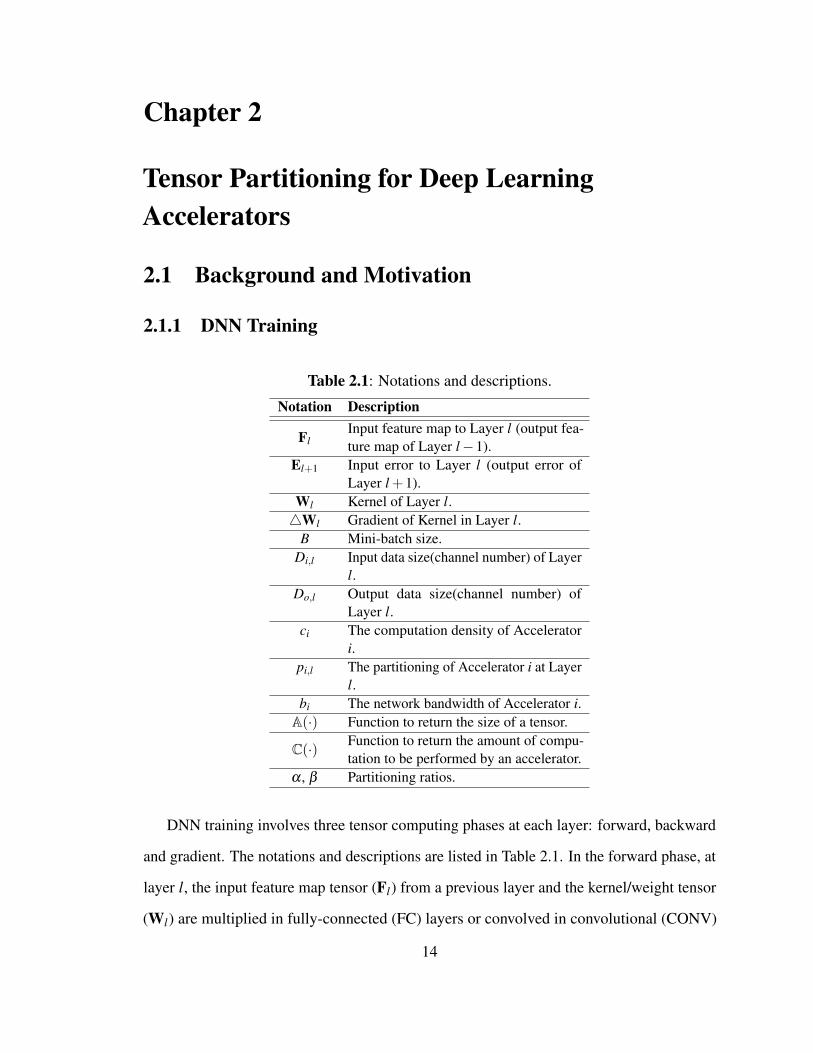
2.1.1 DNN Training
Table 2.1: Notations and descriptions.
Notation Description
FlInput feature map to Layer l (output fea-ture map of Layer l−1).
El+1 Input error to Layer l (output error ofLayer l +1).
Wl Kernel of Layer l.4Wl Gradient of Kernel in Layer l.
B Mini-batch size.Di,l Input data size(channel number) of Layer
l.Do,l Output data size(channel number) of
Layer l.ci The computation density of Accelerator
i.pi,l The partitioning of Accelerator i at Layer
l.bi The network bandwidth of Accelerator i.
A(·) Function to return the size of a tensor.
C(·) Function to return the amount of compu-tation to be performed by an accelerator.
α , β Partitioning ratios.
DNN training involves three tensor computing phases at each layer: forward, backward
and gradient. The notations and descriptions are listed in Table 2.1. In the forward phase, at
layer l, the input feature map tensor (Fl) from a previous layer and the kernel/weight tensor
(Wl) are multiplied in fully-connected (FC) layers or convolved in convolutional (CONV)
14

layers to generate the output feature map tensor, which is used as the input feature map
tensor for the next layer (Fl+1). Usually a non-linear activation f (·) is performed on each
scalar of the feature map. Thus, the forward phase can be represented as Fl+1 = f (Fl⊗Wl),
where ⊗ is either multiplication or convolution. In the backward phase, at layer l, the error
tensor (El) is computed by El =(El+1⊗W>l
) f ′(Fl), where El+1 is the error tensor from
layer l +1, is an element-wise multiplication, and f ′(·) is the derivative function of f (·).
In the gradient phase, the gradient to the kernel/weight is computed by4Wl = F>l ⊗El+1.
The three tensor computation phases capture the common flow in many popular training
algorithms, such as Gradient Descent, Stochastic Gradient Descent, Mini-batch Gradient
Descent, Momentum [190] and Adaptive Moment Estimation (Adam) [191]. For example,
Momentum method updates the parameter using vt = γ · vt−1 +η ·∇θ J(θ),θ = θ − vt ,
where θ is the parameter (weight), ∇θ J(θ) is the gradient of a loss function J(·) with
respect to θ , v is the velocity to record the historic gradient, γ is the momentum hyper
parameter and η is the learning rate, respectively.
2.1.2 Deep Learning Accelerator Architectures
Domain-specific computing architectures [225–228] are considered as a promising solution
to accommodate the ever-growing intensive computing in various deep learning applications.
This view has also been confirmed by a flurry of DNN accelerators [1, 2, 18–110] that
have emerged in recent years. Compared with general-purposed CPUs/GPUs, these custom
architectures achieved better performance and higher energy efficiency.
As summarized in Table 2.2, many designs include a vertical integration practice across
algorithm and hardware levels [73–86] where DNN models are typically optimized prior to
being deployed for inference. Some designs investigate the dataflow (or data reuse pattern)
in DNN workloads [53–61], among which Eyeriss [54–56] is a representative design that
explores many data reuse opportunities existed in DNN execution. Processing-in-memory
15

Table 2.2: Landscape of DNN accelerators (accelerators highlighted in cyan are designedfor training).
Segment DNN Accelerators & ArchitecturesNeuro Co-processor SpiNNaker [18], Neuromorphic Acc. [19], TrueNorth [20–22], MT-spike [23],
PT-spike [24]DNN Co-processor NPU [25], DianNao-family [26–29], Cambricon [30], Cambricon-x [31],
TPU [32, 33], ScaleDeep [34], Stripes [35], Neural Cache [192, 193], Diffy[194]
FPGA FPGA-DCNN [36], Embedded-FPGA-CNN [37], FPGA-Exploration [38],OpenCL-FPGA-CNN [39] [195], Caffeine [40], DeepBurning [41], FPGA-DPCNN [42], TABLA [43], DNNWEAVER [44], FP-DNN [45], FPGA-LSTM [46], ESE [47], FPGA-Dataflow [48], FPGA-BNN [49], FPGA-Utilization [50], FFT-CNN [51], VIBNN [52], iSwitch [196], Shortcut-Mining [197], FA3C [198], E-RNN [199]
Dataflow Neuflow [53], Eyeriss [54–56], Flexflow [57], Fused-CNN [58], CNN-Paritition [59], GANAX [60], UCNN [61], TANGRAM [200], Sparse-Systolic [201], MAERI [202]
PIM Neurocube [62], XNOR-POP [63], DRISA [64], 3DICT [65], NAND-NET [203], SCOPE [204], Promise [205]
Light Models EIE [66], SC-DCNN [67], SCNN [68], Escher [69], LookNN [70], Bit-Pragmatic DNN [71], Bit Fusion [72], Cnvlutin [101], TIE [206], La-conic [207], ADM-NN [208], Gist [209]
Co-Design DPS-CNN [73], Minerva [74], MoDNN [75], MeDNN [76], AdaLearner [77],Stitch-X [78], PIM-DNN [79], Scalpel [80], CirCNN [81], CoSMIC [82],SnaPEA [83], OLAcce [84], Prediction-based DNN [85], PERMDNN [86],MnnFast [210], DNN Computation Reuse [211], vDNN [212], Compressing-DMA-Engine [213], AxTrain [214], Eager pruning [215], Bit-Tactical [216],GENESYS [217]
Emerging Tech. TETRIS [87], RENO [90], PRIME [88], ISAAC [89], Memristive Boltz-mann Machine [91], PipeLayer [92], Atomlayer [93], ReCom [94], Re-GAN [95], ReRAM ACC. [96], EMAT [97], ReRAM-BNN [98], ZARA [99],SNrram [100], Sparse ReRAM Engine [218], RedEye [219], Quantum-SC-NN [220], FloatPIM [221], PUMA [222], FPSA [223]
Toolset/Framework Data Parallelism [108], OWT [1], NEUTRAMS [102], Perform-ML [103],Adaptive-Classifier [104], DNNBuilder [105], Group Scissor [106], FFT-CNN [107], HyPar [2], NNest [224]
(PIM) based designs are also proposed to reduce costly off-chip memory accesses [62–65].
Lightweight models are also introduced [66–72] to reduce computational effort. Many
designs based on emerging memory technologies, such as resistive random access memory
(ReRAM) technology [88–100, 229] with 3D stacking technology [62, 65, 87], are also
proposed.
16
2.1.3 Motivation
Although domain-specific architectures have effectively addressed the challenges of the
ending of Moore’s law [230], the recent study of chip specialization [118] has clearly
demonstrated the diminishing specialization returns and the ultimate accelerator wall. In
other words, it is unlikely to further achieve fine-grained optimizations on a single ac-
celerator. To satisfy the computation and memory requirement for large DNN models
and datasets that typically cannot be satisfied by a single accelerator, a natural solution is
coarse-gained DNN execution on an accelerator array. On the other hand, as highlighted in
cyan in Table 2.2, only a few of the existing DNN accelerators are designed for training.
Among these designs, strict constraints are often applied to the models that can be supported.
For example, [1, 2, 108] only considered homogeneous platforms, where the computation
capability and the network bandwidth for each accelerator are identical. In reality, how-
ever, it is more important to explore solutions for an array of heterogeneous accelerators
with various computation capacity and network bandwidth. For example, though a more
powerful TPU-v3 was released, the early deployed TPU-v2 may not retire immediately
considering the deployment cost and the need for supporting various acceleration workloads.
They are in fact both available off-the-shelf [231]. It is important to optimize large-scale
DNN training acceleration when both TPU versions are used simultaneously. To achieve
high throughput and balanced execution, we need to efficiently distribute data and model
tensors among accelerators with the awareness of heterogeneous computation capability
and network bandwidth. A principled and systematic approach is needed to overcome
the challenge of handling the complexity of DNN models and heterogeneous hardware
execution environment.
17

2.2 Tensor Partitioning Space
Compared with DNN inference, DNN training is more complicated because of the three
computation phases involved in training, i.e., forward, backward and gradient. The tensors
and computations in the three phases are closely coupled together. We need first construct a
complete set of the basic tensor partitioning types.
2.2.1 Problem Statement
We first consider FC layers and later show that the solution can be naturally extended to
CONV layers. In FC layers, DNN training involves three tensor computing phases:
Forward: Fl+1 = f (Fl×Wl),Backward: El =
(El+1×W>l
) f ′(Fl),
Gradient: 4Wl = F>l ×El+1.
Using the notations in Table 2.1, the shape of the tensors in the above three phases are
as below. Here we do not include the element-wise multiplications in the space relations
since they can be performed in place.
Forward: (B,Do,l)← (B,Di,l)× (Di,l,Do,l),
Backward: (B,Di,l)← (B,Do,l)× (Do,l,Di,l),
Gradient: (Di,l,Do,l)← (Di,l,B)× (B,Do,l).
For illustration purpose, this section considers a simple case of an array with two
accelerators. The problem is to exhaustively and systematically enumerate all possible
partitions of the tensors involved in the three phases among the two accelerators, and
understand the corresponding data communication and replication requirements. This is
critical because the partition will determine the communication between the accelerators
and affect overall training performance. We will also explain why the current solutions [1,2]
failed to provide a complete and comprehensive solution.
18

2.2.2 Partitioning in Three Dimensions
We note that the two matrices in each of the pairs (Fl ,El) and (Fl+1,El+1) have the same
shape. We assume that Fl and El (also Fl+1 and El+1) are partitioned in the same manner.
This constraint is intuitive since otherwise additional communication will be unnecessarily
incurred, contradicting our goal of minimizing communication between the accelerators.
We see only three dimensions appear in the three tensor computing phases: B (batch
size), Do,l (output data size of layer l), and Di,l (input data size of layer l). Therefore, we
can naturally focus on the partition in these three dimensions. For the partitions in one
dimension, we assume that the same partition parameter is used for this dimension in every
tensor to avoid additional communication.
Key observation: The dimensions are not independent. In fact, only one dimension can
be “free” in a partition.
We explain observation using an example: consider the forward phase and the partition
in B dimension, Since we will have only two partitions, for (B,Di,l) (Fl), the Di,l dimension
should not be partitioned. This also determines that (Di,l,Do,l) (Wl) should not be parti-
tioned in Di,l dimension, otherwise the matrix multiplication cannot be performed. The
only case left is the Do,l dimension of Wl . Suppose we partition that, the combination of
multiplication of the local partitions in each accelerator does not lead to a complete result
of Fl with shape (B,Di,l). Specifically, depending on the partition, only the upper left and
lower right sub-matrix, or upper right and lower left sub-matrix are computed. Therefore,
Do,l dimension of Wl cannot be partitioned. In fact, the whole Wl needs to be replicated on
the two accelerators to compute the complete Fl . The other scenarios can be considered
similarly.
With the assumption that Fl and El (also Fl+1 and El+1) use the same partition, and the
fact that only one dimension is free in a partition, there are only three partition types. We
discuss them one by one in the following.
19

Forw
ard
Back
war
dG
radi
ent
FlWl Fl+1
El+1
El+1
El
F>l
W>l
F>l
El+1
El+1
Fl+1Wl
W>l
El
Fl
4Wl 4Wl
↵B
↵B
↵B
↵B
↵B
↵B
Do,l
Do,l
Do,l
Do,l
Do,l
Do,l
Do,l
Do,l
Do,lDo,l
Do,l
B
B
B B
B
B
=)
=)
!
!=)
=)
!=)
!
Do,l
WlFl
B =)!
!
=)
!
Fl+1
B
B
El
=) BW>
l
B
=)
El+1
!
!
B
El+1
(a) Type-I (b) Type-II (c) Type-III
Di,l
Di,l
Di,l
Di,l
Di,l
Di,l Di,l
Di,l
Di,l Di,l
Di,l
Di,l
↵Do,l
↵Do,l
↵Do,l
↵Do,l
↵Di,l
↵Di,l
↵Di,l
↵Di,l
↵Do,l↵Do,l
↵Di,l↵Di,l
4Wl
F>l
The partitioning ratio for one accelerator is α and the partitioning ratio for the other accelerator is β = 1−α .Shadow tensors are assigned to one accelerator and non-shadow tensors are assigned to the other accelerator.
⊗ denotes element-wise addition of two tensors.
Figure 2.1: Three basic tensor partitioning types.
Type-I: Partitioning B Dimension
In Type-I, we partition the B dimension in the three tensor computing phases, as shown in
Figure 2.1(a).
In forward phase, Fl+1 = Fl×Wl . The element Fl+1[b,qo] in Fl+1 can be computed as
Fl+1[b,qo] = ∑qi∈1,··· ,Di,l
Fl[b,qi]×Wl[qi,qo], (2.1)
where b ∈ 1,2, · · · ,B,qo ∈ 1,2, · · · ,Do,l. We assume the ratio of computation to be
assigned to one accelerator is α , 0 ≤ α ≤ 1, and the ratio for the other is β , β = 1−α .
The set 1,2, · · · ,B is partitioned into two subsets 1,2, · · · ,αB and αB+1,2, · · · ,B.
Specifically, Fl[1 : αB, :] is assigned to one accelerator and Fl[αB+ 1 : B, :] is assigned
to the other. The two accelerators process disjoint subsets of the batch, and perform the
computation indexed by the corresponding b of the two subsets.
As discussed before, to ensure the validity of matrix multiplication and to get the com-
plete results of Fl+1, Wl is replicated in the two accelerators. After matrix multiplication,
each accelerator produces a portion of results based on the same partition in B dimen-
20
sion. Specifically, Fl+1[1 : αB, :] is produced by one accelerator and Fl+1[αB+1 : B, :] is
produced by the other.
In backward, an element El[b,qi] in El can be computed as
El[b,qi] = ∑qo∈1,··· ,Do,l
El+1[b,qo]×W>l [qo,qi]. (2.2)
Due to the constraint that Fl and El (also Fl+1 and El+1) use the same partition, one
accelerator keeps El+1[1 : αB, :] and produces El+1[1 : αB, :] with replicated W>l . The other
accelerator handles the other portion: El[αB+1 : B, :] and El+1[αB+1 : B, :].
The common pattern for forward and backward phases is that after replicating Wl ,
accelerators can perform computation locally and produce disjoint parts of the result matrix,
which can be combined to obtain the complete result. However, this pattern does not exist in
gradient phase as the two accelerators are not able to complete the computation individually.
In gradient phase, an element4Wl[qi,qo] in4Wl can be computed as
4Wl[qi,qo] = ∑b∈1,··· ,B
F>l [qi,b]×El+1[b,qo]. (2.3)
Based on the same partition of B dimension in F>l and El+1, the two accelerators can
perform local matrix multiplications. Each of them will produce the result matrix of shape
(Di,l,Do,l), the same as 4Wl . To get the final results in Equation (2.3), element-wise
additions need to be performed to combine the partial results:
4Wl[qi,qo] = ∑b∈1,··· ,αB
F>l [qi,b]×El+1[b,qo]
+ ∑b∈αB+1,··· ,B
F>l [qi,b]×El+1[b,qo].(2.4)
The computation pattern in gradient phase implies that communication is needed to
obtain the final results of4Wl , because one of the accelerators needs to perform the partial
sum. We call it as intra-layer communication. We can see that such communication happens
at different phases for different types of partition.
21

Type-II: Partitioning Di,l Dimension
The partition in Di,l dimension is shown in Figure 2.1(b). To perform matrix multiplication,
Di,l dimension of Fl is partitioned in the same way. Based on this, in forward phase, each
accelerator will compute a result matrix of shape (B,Do,l). Similar to the case of4Wl in
Type-I, computing the complete Fl+1 requires element-wise addition in this partitioning:
Fl+1[b,qo] = ∑qi∈1,··· ,αDi,l
Fl[b,qi]×Wl[qi,qo]
+ ∑qi∈αDi,l+1,··· ,Di,l
Fl[b,qi]×Wl[qi,qo].(2.5)
Since Fl+1 and El+1 follow the same partition, in backward phase, El+1 is replicated in
the two accelerators. This allows each of the accelerators produces a disjoint part of result of
El . The partition and replication are similar to that used in gradient phase. A key difference
between Type-I and Type-II is that the intra-layer communication incurs at forward phase,
instead of gradient phase.
Type-III: Partitioning Do,l Dimension
The partitioning Do,l dimension is shown in Figure 2.1(c). Fl needs to be replicated to
compute complete Fl+1 in forward phase. It is the case overlooked by all previous solutions.
Essentially, it means that the input feature maps of the same batch are replicated into the
two accelerators, instead of partitioning B. It may sound not intuitive since we want to have
accelerators process the same data. However, we show that it is an important partition in the
design space that presents the same trade-off in terms of communication just as in Type-I
and Type-II.
Similar to gradient phase of Type-I and forward phase of Type-II, the backward phase
22
of Type-III requires element-wise addition of partial results:
El[b,qi] = ∑qo∈1,··· ,αDo,l
El+1[b,qo]×W>l [qo,qi]
+ ∑qo∈αDo,l+1,··· ,Do,l
El+1[b,qo]×W>l [qo,qi].
(2.6)
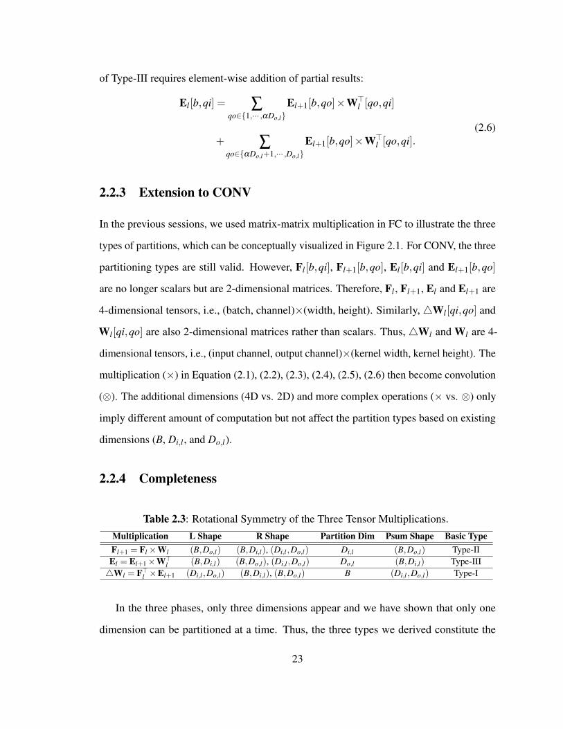
2.2.3 Extension to CONV
In the previous sessions, we used matrix-matrix multiplication in FC to illustrate the three
types of partitions, which can be conceptually visualized in Figure 2.1. For CONV, the three
partitioning types are still valid. However, Fl[b,qi], Fl+1[b,qo], El[b,qi] and El+1[b,qo]
are no longer scalars but are 2-dimensional matrices. Therefore, Fl , Fl+1, El and El+1 are
4-dimensional tensors, i.e., (batch, channel)×(width, height). Similarly,4Wl[qi,qo] and
Wl[qi,qo] are also 2-dimensional matrices rather than scalars. Thus, 4Wl and Wl are 4-
dimensional tensors, i.e., (input channel, output channel)×(kernel width, kernel height). The
multiplication (×) in Equation (2.1), (2.2), (2.3), (2.4), (2.5), (2.6) then become convolution
(⊗). The additional dimensions (4D vs. 2D) and more complex operations (× vs. ⊗) only
imply different amount of computation but not affect the partition types based on existing
dimensions (B, Di,l , and Do,l).
2.2.4 Completeness
Table 2.3: Rotational Symmetry of the Three Tensor Multiplications.
Multiplication L Shape R Shape Partition Dim Psum Shape Basic TypeFl+1 = Fl×Wl (B,Do,l) (B,Di,l), (Di,l ,Do,l) Di,l (B,Do,l) Type-IIEl = El+1×W>
l (B,Di,l) (B,Do,l), (Di,l ,Do,l) Do,l (B,Di,l) Type-III4Wl = F>l ×El+1 (Di,l ,Do,l) (B,Di,l), (B,Do,l) B (Di,l ,Do,l) Type-I
In the three phases, only three dimensions appear and we have shown that only one
dimension can be partitioned at a time. Thus, the three types we derived constitute the
23

complete partition space. Table 2.3 summarized the key features of the partitions. The LHS
Shape and RHS Shape respectively indicate the shapes of the metrics on the left-hand and
right-hand side of the equation for each phase. The Psum Shape is the shape of the matrices
containing partial results in two accelerators that need to be combined using element-wise
additions. It happens when the matrix appear on the LHS. This is also the shape of the
matrix that needs to be replicated if it appears on the RHS. From Table 2.3, we can observe
a rotational symmetry on each column.
2.2.5 Problems of “One Weird Trick” & HyPar
Two solutions were recently proposed to address the same problem that is addressed by this
work, — communication and parallelism between accelerators. However, neither of these
two solutions is complete.
Krizhevsky [1] proposed “one weird trick” (OWT) to configure CONV layers with data
parallelism and FC layers with model parallelism to get a higher performance. It is certainly
better than just using data parallelism for all layers, however it does not provide any insight
on why this trick works and whether it is the best we can do. Therefore, this solution is
fundamentally empirical.
HyPar [2] is a more recent and principled approach to optimize the parallelism configura-
tions also by partitioning the layers based on the intra-layer and inter-layer communication.
However, it only considers the same two basic partitions in OWT, — data parallelism and
model parallelism. In fact, they correspond to Type-I and Type-II in Figure 2.1, respectively.
Therefore, the parallelism setting in HyPar is not complete. Even if it is based on a more
systematic approach to explore the partition space, it cannot find the optimal solution based
on incomplete basic partition types. Specifically, HyPar will miss one intra-layer communi-
cation pattern (Type-III) and five inter-layer communication patterns (see more details in
Section 2.3.1). Moreover, HyPar always partitions the tensors equally, so it cannot capture
24

the performance heterogeneity among accelerators.
2.3 Cost Model
To search the optimal partition of layers, we propose a cost model for multiple accelerators.
We consider the computation by individual accelerator and the communication between
accelerators as two major affecting DNN training performance. Compared to HYPAR [2],
which uses communication cost as the proxy for performance, the cost model of ACCPAR
takes both communication cost Ecm and computation cost Ecp into consideration. The
optimization target is to minimize overall cost.
2.3.1 Communication Cost Model
Assuming the network bandwidth for accelerator i is bi, and T is the accessed tensor needs
to be transferred from one to the other, we define the communication cost Ecm for the tensor
transfer as
Ecm =A(T)
bi. (2.7)
The tensor size A(T) is defined as the product of the lengths of all dimensions. For
example, the size of a 4-by-5 matrix is 20, and the size of a kernel whose input channel
is 16, kernel window width is 3, kernel window length is 3 and output channel is 32, is
4,608 = 16×3×3×32. Next, we will determine what the remotely-accessed tensor T is.
Intra-layer Communication Cost
As discussed in Section 2.2, for each of the three basic tensor partitioning types, there is
one and only one computation phase requires remote accessing.
In Type-I, the gradient phase requires remote accessing (Equation (2.4)). For the ac-
celerator whose partitioning ratio is α , for each b ∈ 1, · · · ,αB, the intermediate tensor
25
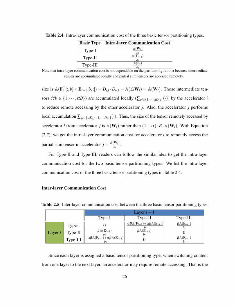
Table 2.4: Intra-layer communication cost of the three basic tensor partitioning types.
Basic Type Intra-layer Communication Cost
Type-I A(Wl)bi
Type-II A(Fl+1)bi
Type-III A(El)bi
Note that intra-layer communication cost is not dependable on the partitioning ratio α because intermediateresults are accumulated locally and partial sum tensors are accessed remotely.
size is A(F>l [:,b]×El+1[b, :]) = Di,l ·Do,l = A(4Wl) = A(Wl). Those intermediate ten-
sors (∀b ∈ 1, · · · ,αB) are accumulated locally (∑qi∈1,··· ,αDi,l(·)) by the accelerator i
to reduce remote accessing by the other accelerator j. Also, the accelerator j performs
local accumulation ∑qi∈αDi,l+1,··· ,Di,l(·). Thus, the size of the tensor remotely accessed by
accelerator i from accelerator j is A(Wl) rather than (1−α) ·B ·A(Wl). With Equation
(2.7), we get the intra-layer communication cost for accelerator i to remotely access the
partial sum tensor in accelerator j is A(Wl)bi
.
For Type-II and Type-III, readers can follow the similar idea to get the intra-layer
communication cost for the two basic tensor partitioning types. We list the intra-layer
communication cost of the three basic tensor partitioning types in Table 2.4.
Inter-layer Communication Cost
Table 2.5: Inter-layer communication cost between the three basic tensor partitioning types.
Layer l +1Type-I Type-II Type-III
Type-I 0 αβA(Fl+1)+αβA(El+1)bi
βA(Fl+1)bi
Layer l Type-II βA(El+1)bi
βA(El+1)bi
0
Type-III αβA(Fl+1)+αβA(El+1)bi
0 βA(Fl+1)bi
Since each layer is assigned a basic tensor partitioning type, when switching content
from one layer to the next layer, an accelerator may require remote accessing. That is the
26
(a) Type-I to Type-I
Fl+1 Fl+1Fl+1 Fl+1
El+1El+1
(b) Type-I to Type-II
Fl+1 Fl+1
El+1
(c) Type-I to Type-III
Fl+1 Fl+1
El+1
(d) Type-II to Type-I
Fl+1 Fl+1
El+1
(e) Type-II to Type-II
Fl+1 Fl+1
El+1
(f) Type-II to Type-III
Fl+1 Fl+1
El+1
(g) Type-III to Type-I
Fl+1 Fl+1
El+1
(h) Type-III to Type-II
Fl+1 Fl+1
El+1
(i) Type-III to Type-IIII↵
↵
↵↵
1
1
1
1
El+1
El+1
El+1 El+1El+1
El+1El+1
El+1El+1
Shadow tensors are held by one accelerator (whose partitioning ratio is α) and non-shadow tensors are heldby the other accelerator (whose partitioning ratio is β ).
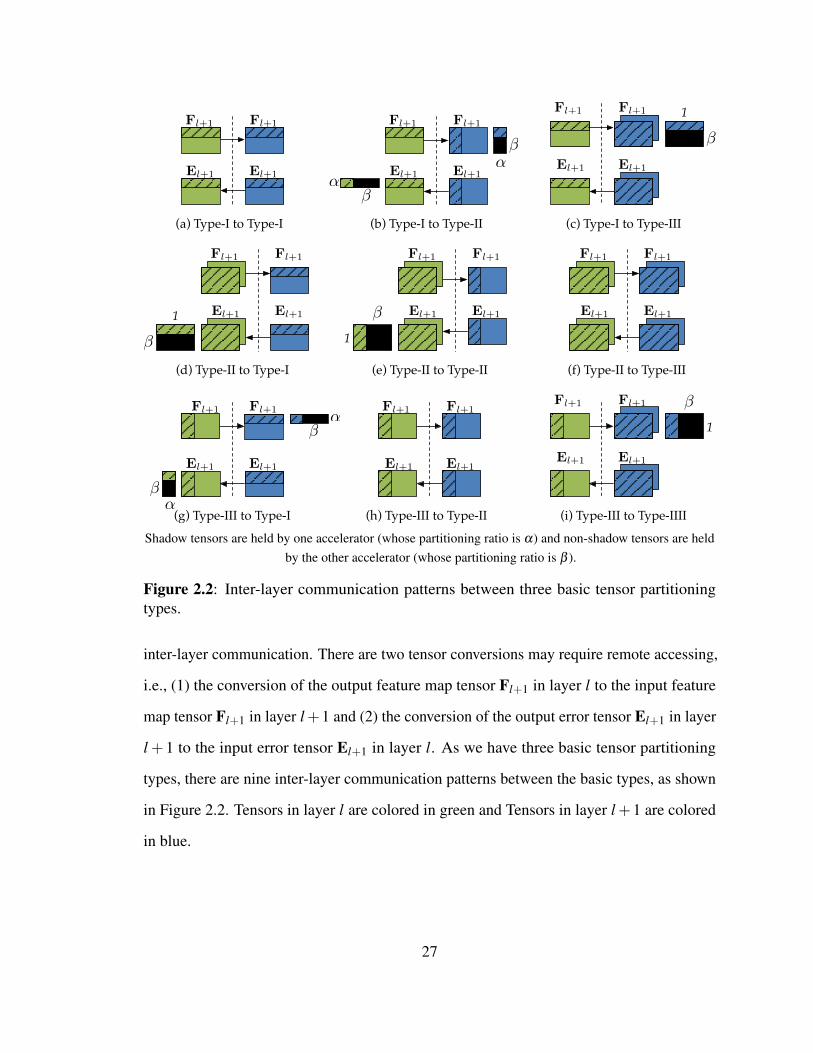
Figure 2.2: Inter-layer communication patterns between three basic tensor partitioningtypes.
inter-layer communication. There are two tensor conversions may require remote accessing,
i.e., (1) the conversion of the output feature map tensor Fl+1 in layer l to the input feature
map tensor Fl+1 in layer l+1 and (2) the conversion of the output error tensor El+1 in layer
l +1 to the input error tensor El+1 in layer l. As we have three basic tensor partitioning
types, there are nine inter-layer communication patterns between the basic types, as shown
in Figure 2.2. Tensors in layer l are colored in green and Tensors in layer l +1 are colored
in blue.
27

(a) Type-I to Type-I, (f) Type-II to Type-III and (h) Type-III to Type-II.
In the tensor conversion of the three patterns, since the (green) tensors in layer l and the
(blue) tensors in layer l + 1 has the same partitioning, there is no conversion, and the
inter-layer communication cost is 0.
(c) Type-I to Type-III, (d) Type-II to Type-I, (e) Type-II to Type-II and (i) Type-III to
Type-III.
We take Figure 2.2(c) as an example. In the tensor conversion from Type-I to Type-III,
in the forward phase, the accelerator i (whose partitioning ratio is α) holds green shadow
tensor Fl+1 in layer l, but in the next layer l+1, the accelerator need the whole blue shadow
tensor Fl+1. The difference is the black part, and the black tensor incurs remote accessing to
the other accelerator j (whose partitioning ratio is β ). Thus the inter-layer communication
amount is (βB)×Do,l = βA(Fl+1), and the inter-layer communication cost by accelerator
i to remotely access the black tensor in accelerator j is βA(Fl+1)bi
. Reversely, the inter-layer
communication cost for the accelerator j is αA(Fl+1)b j
in this case. Note that the inter-layer
communication cost for (c) Type-I to Type-III, (d) Type-II to Type-I, (e) Type-II to Type-II
and (i) Type-III to Type-III are the same, but the shapes of conversion tensors are not the
same.
(b) Type-I to Type-II and (g) Type-III to Type-I.
We take Figure 2.2(b) as an example. In the tensor conversion from Type-I to Type-II, in
the forward phase, the accelerator i (whose partitioning ratio is α) holds green shadow
tensor Fl+1 (αB,Do,l) in layer l, but in the next layer l + 1, the accelerator need the
whole blue shadow tensor Fl+1 (B,αDo,l). The difference is the black part, and again the
black tensor incurs remote accessing to the other accelerator j (whose partitioning ratio
is β ). Thus the inter-layer communication amount is (βB)×αDo,l = αβA(Fl+1), and
28

the inter-layer communication cost by accelerator i to remotely access the black tensor in
accelerator j is αβA(Fl+1)bi
. Reversely, the inter-layer communication cost for the accelerator
j is (1−α)(1−β )A(Fl+1)b j
=βαA(Fl+1)
b jin this case. Note that the inter-layer communication
cost for (b) Type-I to Type-II and (g) Type-III to Type-I are the same, but the shapes of
conversion tensors are not the same.
We list the inter-layer communication cost for the nine patterns of the tensor conversion
between the three basic partitioning types in Table 2.5.
2.3.2 Computation Cost Model
We assume the tensor computation density of an accelerator i is ci and the amount of floating
point operations to perform the multiplication of the multiplication of two tensors T1×T2
is C(T1×T2). For an accelerator with a partitioning ratio α , the effective amount floating
point operations performed is α ·C(T1×T2). We can define the computation cost Ecp for
an accelerator i to perform the computation as
Ecp =α ·C(T1×T2)
ci. (2.8)
Table 2.6: The amount of floating point operations (FLOP) in the three multiplications.
Multiplication # FLOPFl+1 = Fl×Wl A(Fl+1) · (Di,l +Di,l−1)El = El+1×W>l A(El) · (Do,l +Do,l−1)4Wl = F>l ×El+1 A(Wl) · (B+B−1)
The most important step to get the computation cost is to calculate the number of floating
point operations (FLOP) of a tensor multiplication. In the forward phase, to get the output
tensor Fl+1, the number of FLOP is (B ·Do,l) · (Di,l +Di,l−1) = A(Fl+1) · (Di,l +Di,l−1).
The numbers of FLOP for the three multiplications are listed in Table 2.6.
29

2.3.3 Discussion on Convolutions
We can easily expand the communication cost and computation cost from fully-connected
layers to convolutional layers. In convolutions, Fl , Fl+1, El and El+1 are 4-dimensional
tensors, i.e., (batch, channel, height, width). We can view the four dimensional tensors
as three dimensional tensors, but the third and fourth dimension is a meta dimension, i.e.,
(batch, channel, [height, width]). The kernel Wl are also 4-dimensional tensors, i.e., (input
channel, output channel, kernel height, kernel width), and we can also view it as a three
dimensional tensor, and the second dimension is a meta dimension, i.e., (input channel,
[kernel height, kernel width], output channel). Thus, the communications costs listed in
Table 2.4 and 2.5 keep the same formats.
In a matrix-matrix multiplication MC = MA×MB, assume the shape of MC, MA, MB
is (MC,NC), (MC,P), (P,NC) respectively. The idea to to calculate the number of floating
points performed is to multiply the number of output elements and the the number of floating
points for each element. In the matrix-matrix multiplication, the number of output elements
is MC×NC = A(MC). For each output element, the number of multiplications performed
is P and the number of additions performed is P− 1. So the total number of FLOP is
A(MC) · (P+P−1). To find the number of FLOP for a convolutional layers, we need only
to find the number of FLOP for the convolution for one element in the output tensor because
the number of elements of a tensor Tout is always A(Tout) no matter what the dimension
it is. The number of multiplications performed is (input channel) × (kernel height) ×
(kernel width) and number of additions performed is ((input channel) × (kernel height) ×
(kernel width) - 1). Note that (input channel) is Di,l , Do,l or B in the three multiplications
respectively, and (kernel height) × (kernel width) is actually the 2D feature map or kernel
size, i.e., the size of the feature map or kernel except the input and output channel. So
for convolutional layers, the number of floating point operations is the entries in Table 2.6
multiply the 2D feature map or kernel size.
30

2.4 Partitioning Algorithm
In this section, we explain the ACCPAR partitioning method. Like recent work HyPar [2],
we determine the partitioning for each layer in a DNN model by a layer-wise dynamic
partitioning scheme. However, ACCPAR is much more general for three reasons: 1) the
algorithm considers the complete search space discussed in Section 2.4; 2) it can be parame-
terized with arbitrary partitioning ratio based on heterogeneous compute, communication
cost and effective bandwidth between accelerator groups; 3) it can handle multiple paths in
DNNs. As a result, we will see in Section 2.5 that ACCPAR achieves considerable speedups
over HYPAR.
2.4.1 Layer-wise Partitioning
Type-I
Type-II
Type-III
Li Li+1
Figure 2.3: Layer-wise partitioning is determined by dynamic programming to minimizethe computation cost and the communication cost.
(a)
P1 P2
Li
Li+1
P1
P2(b) (c)
Li Li+1
P1
P2Li Li+1
(d)
P1
P2Li Li+1
(a) Layer Li and Li+1 are connected by path P1 and path P2. (b) Partitioning for (Li, t = Type-I) to(Li+1, t = Type-I), (c) Partitioning for (Li, t = Type-II) to (Li+1, t = Type-I), and (d) Partitioning for
(Li, t = Type-III) to (Li+1, t = Type-I).
Figure 2.4: Dynamic programming on multi-paths.
31

To find the best partitioning for each layer in a DNN to minimize communication and
improve performance, an intuitive way is to enumerate all possible configurations by brute
force. Unfortunately, it will result in a O(3N) complexity for a DNN with N layers — not a
practical solution. Following the dynamic programming approaches [2,177,179], we reduce
search complexity to O(N) by dynamic programming.
Figure 2.3 illustrates the layer-wise partitioning procedure. For each layer, we determine
the minimum cost based on the three basic partitioning types from the first layer till the
current layer. We denote the accumulative cost up to layer Li when it is in state (Li, t) as
c(Li, t) — layer Li chooses a basic partitioning type t ∈ T =Type-I, Type-II, Type-III.
Based on the cost model in Section 2.3, the accumulative cost given partition choice t of
the current layer Li+1 (c(Li+1, t)) can be calculated inductively with the cost of the previous
layer Li (c(Li, tt)):
c(Li+1, t) = mintt∈Tc(Li, tt)+Ecp(t)+Ecm(tt, t). (2.9)
Here, Ecp(t) is the computation cost for the current layer Li+1 for a type t, and Ecm(tt, t)
is the sum of the intra-layer communication cost for a type t and the inter-layer communi-
cation cost when transition from state (Li, tt) to state (Li+1, t). For each basic partitioning
type, during the algorithm execution we need to record the path to a previous layer for
backtracking after going through all layers, shown as the black arrows in Figure 2.3. In this
manner, after we compute the accumulative cost of the last layer, we have obtained the cost
state of the last layer and all previous layers with backtracking. The algorithm starts by
initializing c(L0, t) for the three basic partitioning types in layer L0 to 0.
We employ a hierarchical (recursive) partition for multiple hierarchies similar to [2, 76,
179]. The idea is to apply the layer-wise partitioning recursively on a partitioned hierarchy
to partition on an accelerator array.
32

2.4.2 Handling Multiple Paths
Different from HYPAR, ACCPAR is able to determine the partition for the multi-path
typologies that are common in Resnet [120]. Figure 2.4 shows an example where there are
two paths between layer Li and Li+1. Path P1 consists of one weighted layer and Path P2
consists of two weighted layers. The key idea for multi-path partitioning is to (1) enumerate
the partition state of layer Li+1 (Li+1, t), t ∈ T , (2) enumerate the partition state of layer
Li (Li, tt), tt ∈T , (3) perform individual layer-wise partitioning for each path between the
two states (Li, tt) and (Li+1, t) for each combination, (4) determine the lowest cost for the
state (Li+1, t).
We need to determine the lowest cost for each state, i.e., enumerate the three colored
circles in Figure 2.4 in Layer Li+1. For example, (Li+1, t = Type-I) is one of the three
possible states shown as the yellow circle at Layer Li+1 in Figure 2.4. We then enumerate
the three colored circles at Layer Li. Figure 2.4(b) starts from (Li, t = Type-I), we search
the three paths in P1 and the three paths in P2 between the two states (Li, t = Type-I)
and (Li+1, t = Type-I). We then select the lowest-cost path in P1, and the the lowest-
cost path in P2 to (Li+1, t = Type-I), and combine them as the lowest-cost path from
(Li, t = Type-I) to (Li+1, t = Type-I). Similarly, we compute the lowest-cost path from
(Li, t = Type-II) to (Li+1, t = Type-I) as shown in Figure 2.4(c), and the lowest-cost path
from (Li, t = Type-III) to (Li+1, t = Type-I) as shown in Figure 2.4(d). With the three
paths, i.e., the lowest-cost paths (1) from (Li, t = Type-I) to (Li+1, t = Type-I), (2) from
(Li, t = Type-II) to (Li+1, t = Type-I) and (3) from (Li, t = Type-III) to (Li+1, t = Type-I), we
can finally determine the lowest cost to reach state (Li+1, t = Type-I) and record the lowest-
cost path from Layer Li to state (Li+1, t = Type-I). Following the similar procedure, we
can determine the lowest-cost path to state (Li+1, t = Type-II) and state (Li+1, t = Type-III).
Since we have searched the optimal states for Layer Li+1, the optimal states in the last layer
of the DNN model will be satisfied.
33
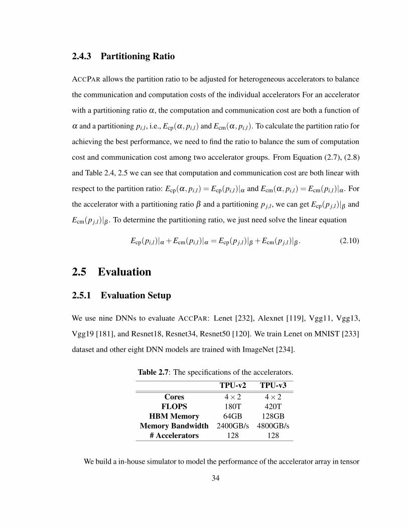
2.4.3 Partitioning Ratio
ACCPAR allows the partition ratio to be adjusted for heterogeneous accelerators to balance
the communication and computation costs of the individual accelerators For an accelerator
with a partitioning ratio α , the computation and communication cost are both a function of
α and a partitioning pi,l , i.e., Ecp(α, pi,l) and Ecm(α, pi,l). To calculate the partition ratio for
achieving the best performance, we need to find the ratio to balance the sum of computation
cost and communication cost among two accelerator groups. From Equation (2.7), (2.8)
and Table 2.4, 2.5 we can see that computation and communication cost are both linear with
respect to the partition ratio: Ecp(α, pi,l) = Ecp(pi,l)|α and Ecm(α, pi,l) = Ecm(pi,l)|α . For
the accelerator with a partitioning ratio β and a partitioning p j,l , we can get Ecp(p j,l)|β and
Ecm(p j,l)|β . To determine the partitioning ratio, we just need solve the linear equation
Ecp(pi,l)|α +Ecm(pi,l)|α = Ecp(p j,l)|β +Ecm(p j,l)|β . (2.10)
2.5 Evaluation
2.5.1 Evaluation Setup
We use nine DNNs to evaluate ACCPAR: Lenet [232], Alexnet [119], Vgg11, Vgg13,
Vgg19 [181], and Resnet18, Resnet34, Resnet50 [120]. We train Lenet on MNIST [233]
dataset and other eight DNN models are trained with ImageNet [234].
Table 2.7: The specifications of the accelerators.
TPU-v2 TPU-v3Cores 4×2 4×2
FLOPS 180T 420THBM Memory 64GB 128GB
Memory Bandwidth 2400GB/s 4800GB/s# Accelerators 128 128
We build a in-house simulator to model the performance of the accelerator array in tensor
34

processing unit TPU-v2 and TPU-v3. In the simulation, we derive the tensor accessing
traces (loading and storing) and partial sum computation (MULT and ADD) traces for
the simulation and then we calculate the time consuming for the computation and data
accessing. The trace granularity for FC layer is element-wise (i.e., 1) and for CONV is
kernel-wise (e.g., 3x3). While TPU-v1 is designed for DNN inference [33], TPU-v2 and
TPU-v3 target DNN training. Table 2.7 lists the specifications for these two accelerators.
An accelerator is a board that holds the processing units — 2 cores per chip and 4 chip
per board. The peak floating point operations per second (FLOPS) are 180T for TPU-v2
and 420T for TPU-v3, and the memory for the two accelerators are 64GB high bandwidth
memory (HBM) and 128GB HBM [231]. The memory bandwidth for TPU-v2 is 2400GB/s.
Since the memory bandwidth for TPU-v3 is not available, we assume a 4800GB/s memory
bandwidth for TPU-v3. For the network, the maximum data rate per core is 2Gb/s [235].
We set the network data rate for TPU-v2 as 8Gb/s and that for TPU-v3 as 16Gb/s. The
number of accelerators for TPU-v2 and TPU-v3 are both 128. The data format used in the
DNN training is bfloat, Google’s 16-bit floating point data format for training. We also set
the mini batch size to be 512.
To evaluate the effectiveness of ACCPAR, we compare it against data parallelism
(DP) [108], “One Weird Trick” (OWT) [1] and HYPAR [2]. In DP, each accelerator
maintains a local copy of DNN model, while training samples are partitioned among these
accelerators. In OWT, the CONV layers in a DNN model is configured for data parallelism,
and the FC layers are configured for model parallelism. In HYPAR, both CONV and FC
layers can be configured for data parallelism or model parallelism to minimize overall
communication. Data communication, operational computation and hardware heterogeneity
are jointly considered in ACCPAR for collaborative optimization. Here we use DP as the
baseline, and the performance and training throughput of OWT, HYPAR and ACCPAR are
all normalized to the DP design.
35

2.5.2 Heterogeneous Array
We fist evaluate the performance for a heterogeneous accelerator array using same number
of accelerators with different performance: 128 TPU-v2 accelerators and 128 TPU-v3
accelerators.
Lenet
Alexnet
Vgg11
Vgg13
Vgg16
Vgg19
Resnet18
Resnet34
Resnet50
Gmean
0
2
4
6
8
10
12
14
16
18Speedup
OWTHyParAccPar
DP
Figure 2.5: The speedup of data parallelism (DP), “one weird trick” (OWT) [1], HYPAR [2]and AccPar in a heterogeneous accelerator array.
The normalized performance of DP, OWT and HYPAR are shown in Figure 2.5. The
geometric mean of speedup (the throughput improvement) in DP, OWT, HYPAR and
ACCPAR are 1.00×, 2.98×, 3.78×, 6.30×, respectively. For Vgg series, ACCPAR can
get a speedup up to 16.14×, while the highest speedup of OWT and HYPAR are 8.24×
and 9.46×. For Resnet series, ACCPAR can get speedups from 1.92× to 2.20×, while the
ranges of speedup achieved by OWT and HYPAR are 1.22× to 1.38× and 1.03× to 1.04×,
respectively.
We see that the speedups achieved by ACCPAR is significantly higher than OWT
and HYPAR. In Figure 2.5, on the four Vgg series, the speedups of OWT range from
5.33× to 8.25×, and the speedups of HYPAR range from 5.92× to 9.46×. However, the
36

speedups of ACCPAR range from 9.75× to 16.14×, which are significantly higher than
OWT and HYPAR. The improvements of ACCPAR come from: (1) the complete partitioning
type search space, which includes all three types of tensor partitioning settings to reduce
communication; and (2) the communication and computation joint optimization considering
heterogeneity. With the communication and computation by different accelerators balanced
by certain partitioing ratio, the idle time due to heterogeneous communication/computation
capability under equal partitioning in OWT [1] and HYPAR [2] are greatly alleviated.
From Figure 2.5, we also notice that the the speedups of Resenet series are lower than
that of Vgg series. Between the two series, the main difference is that the model sizes
of Vgg series are larger than those of Resnet series, while the computation densities of
Resnet series are higher than those of Vgg series. Among the three basic tensor partitioning
types, Type-II and Type-III partitions the weight of layers, i.e., the model, while Type-I
partitions the feature maps, i.e., the data. In data parallelism, all layers are configured by
Type-I. Thus, for DNNs with a large model size, such as Vgg series, Type-II and Type-III
are favored due to the potential greater reduction of communication when partitioning the
model. On the other side, for DNNs with higher computation density, Type-I is favored for
greater potential reduction of the communication when partitioning feature maps. Moreover,
because the difference of mode sizes among different layers is smaller than the difference
of feature maps, the relative benefits achieved by Type-II and Type-III are smaller than
those of Type-I. The above analysis explains the reason why speedups of Resenet series are
lower than that of Vgg series, since DNNs in former series mainly benefit from Type-II and
Type-III — model partition, the trend is true for not only ACCPAR but also HYPAR and
OWT. However, even for Resnet series, the speedups of ACCPAR are considerably higher
than OWT and HYPAR: the highest speedup by OWT and HYPAR on the Resnet series are
1.04× and 1.38× respectively, but the highest speedup by ACCPAR is 2.20×. This means
that ACCPAR is 112% better than OWT and 59% better than HYPAR.
37

2.5.3 Homogeneous Array
OWTHyParAccPar
DP
Lenet
Alexnet
Vgg11
Vgg13
Vgg16
Vgg19
Resnet18
Resnet34
Resnet50
Gmean
012
4
6
8
10
Speedup
Figure 2.6: The speedup of data parallelism (DP), “one weird trick” (OWT) [1], HYPAR [2]and AccPar in a homogeneous accelerator array.
We then evaluate the performance for a homogeneous accelerator array, where 128
accelerators employed are of the same type, i.e., TPU-v3. The speedups of data parallelism
(DP), “one weird trick” (OWT), HYPAR and ACCPAR are shown in Figure 2.6. The results
are normalized to data parallelism. The geometric mean of DP, OWT, HYPAR and ACCPAR
are 1.00×, 2.94×, 3.51×, 3.86×, respectively. For Resent series, the DNNs are very “deep”
(i.e., the number of layers is very large), and all layers except the last fully-connected
layer are convolutional layers. While OWT, HYPAR, and ACCPAR all try to explore other
parallelism settings or partitions rather than static data/model parallelism, we observe in the
results that these three schemes evantually configure most of layers in Resnet series with
data parallelism or Type-I partition. This is the reason why they achieve lower speedups on
Resnet series than Vgg series. In comparison, the DNNs in Vgg series contain a variety of
layers, so OWT, HYPAR, and ACCPAR can effectively explore larger search space with more
diverse parallelism/partition settings. With homogeneous accelerator array, for a specific
38

DNN model, we observe the increasing speedups of DP, OWT, HYPAR and ACCPAR. It is
the direct consequence of the increasing flexibility.
7
6
5
4
3
2
1
cv1 cv2 cv3 fc1 fc2 fc3cv4 cv5
Type-I Type-II Type-III
Figure 2.7: The selected partitioning types for the weighted layers in Alexnet. The numberof hierarchies is 7 and the batch size is 128.
In Figure 2.7, we also show the selected partitioning types by ACCPAR for the weighted
layers in Alexnet. In the three fully-connected layers, i.e., fc1, fc2 and fc3, Type-II and
Type-III partitions are used to minimize the communication by maintaining a part of weight
locally and communicating the feature maps. In the convolutional layers, i.e., cv1 to cv5, we
can see that Type-I partition are mostly but not solely selected. ACCPAR allows all Type-I,
Type-II and Type-III to be selected to reduce the total communication further. Especially,
with the increase of hierarchy level, more layers are configured with Type-II or Type-III.
This illustrates the importance of having a complete search space as in ACCPAR.
2.5.4 Scalability with Hierarchy Levels
In this section, we study the scalability of ACCPAR on various hierarchies on the heteroge-
neous accelerator array. Figure 2.8 shows the speedups of DP, OWT, HYPAR and ACCPAR
on Vgg19 for hierarchy level from h = 2 to h = 9. With the increase of hierarchy level,
we partition the tensor for a finer-grained level. From Figure 2.8 we see that the speedups
39

Speedup
012
4
6
8
10
12
OWTHyParAccPar
DP
h=2 h=3 h=4 h=5 h=6 h=7 h=8 h=9
Figure 2.8: The speedup of data parallelism (DP), “one weird trick” (OWT) [1], HYPAR [2]and AccPar under various partitioning hierarchies on Vgg19.
of OWT and HYPAR tend to be saturated, while the speedups of ACCPAR continue to
increase with the increase of the partitioning hierarchies. For OWT, the convolutional
layers are always configured with data parallelism and the fully-connected layers are always
configured with model parallelism. While it provides more flexible than configuring all
layers with data parallelism in DP, it is still a static configuration. HYPAR and ACCPAR
are flexible configurations because they do not flexibly set a class of layer to be a specific
parallelism or partition, instead they flexibly explore the possible configuration to minimize
the communication or cost. Compared with HYPAR, ACCPAR benefits from a complete
partitioning type sets and the heterogeneity-aware configuration. The flexibility of the four
schemes from low to high is: DP ≺ OWT ≺ HYPAR ≺ ACCPAR. Table 2.8 shows the
comparison of DP, OWT, HYPAR, and ACCPAR.
Table 2.8: The caparison of flexibility of DP, OWT, HYPAR and ACCPAR.
DP OWT HYPAR ACCPAR
Static Static Flexible FlexibleLow −−−−−−−−−−−−−−−−−−−−−→ High
40

Chapter 3
Layer-wise Pipelined Parallelism for DeepLearning Accelerators
3.1 Background
3.1.1 Basics of Deep Neural Network
The core component of many deep learning applications (on computer vision [236–240],
data mining [241–244], language processing [245–249] and etc.) is convolutional neural
network (CNN).
CONV POOL IP
K
Cl+1Cl
Figure 3.1: Convolutional neural network (CNN).
Figure 3.1 illustrates the organization of an example CNN, which has three types of
layers: convolution layer, pooling layer and inner product layer. In a convolution layer, a set
of kernels are convoluted with data of channels from the previous layer (layer l) to generate
data for channels of next layer (layer l +1). dl is a cube of data in a layer. dl[x,y,c] is the
value at a point in the three dimensional data cube. We also denote the size of d in layer l as
(Xl×Yl×Cl), so 0 ≤ x ≤ Xd−1,0 ≤ y ≤ Yd−1,0 ≤ c ≤Cd−1 and Cd is the number of
channels. (xl,yl,cl) indicates a point in layer l’s data cube. K is the kernel composed of a
set of weights. Kl is the kernel used in the computation to generate data in layer l. A kernel
41

represents four dimensional data: the size of each dimension is Kx, Ky, Cl and Cl+1, where
Kx and Ky are determined by algorithm (e.g. in LeNet [233], Kx and Ky are both 5).
dl+1 is computed as:
dl+1[x,y,c] =Cl−1
∑cl=0
Kx−1
∑kx=0
Ky−1
∑ky=0
Kl[kx,ky,cl,c]×dl[x+ kx,y+ ky,cl]. (3.1)
To perform Equation (3.1), in total (Xl+1×Yl+1×Cl+1×Cl×Kx×Ky) multiplications
and (Xl+1×Yl+1×Cl+1× (Cl×Kx×Ky−1) additions are performed.
A pooling layer performs the subsampling. Taking average pooling as an example, a
window of data in l is averaged to get one data point in l +1 as follows:
dl+1[x,y,c] =1
KxKy
Kx−1
∑kx=0
Ky−1
∑ky=0
dl[Kxx+ kx,Kyy+ ky,c]. (3.2)
This average pooling operation performs (Xl+1×Yl+1×Cl+1× (Kx×Ky−1)) additions
and (Xl+1×Yl+1×Cl+1) multiplications. The multiplication could be implemented as
shift operation if (Kx×Ky) is the power of 2. Max pooling is another variance, where the
maximum value among values in a window in l is selected for l +1.
In the inner product layer, the values in data tube of l and l+1 are considered as a vector
(denoted as ~dl and ~dl+1). If the previous layer is convolution or pooling, the size of ~dl is
Xl×Yl×Cl . If the previous layer is also inner product, then the size of ~dl is the size of the
output vector from l. ~dl+1 is a n×1 vector, n is determined by the algorithm. Wl+1−l is a
weight matrix of size (n×m), m is the size of ~dl .~b is a vector of bias.
The vector of l +1 is computed as:
~dl+1 =Wl+1−l~dl +~b. (3.3)
42

This inner product operation performs (n× (m−1)) additions and (n×m) multiplica-
tions. Activation function is another important component. It is an element-wise operation
and usually a nonlinear function, such as sigmoid 11+e−x or rectified linear unit (ReLU)
max(0,x).
3.1.2 Data Forward and Backward in a Neural Network
Neural network has two phases: training (learning) phase and testing (inference) phase. In
testing phase, the weights of a neural network have been determined and the task is to use
the network on input samples, e.g. to recognize who is the person in an image. In testing
phase, input data flow through the layers consecutively in forward direction. It is shown in
Figure 3.2, dl−1 is the output of layer l−1 and the input of layer l. The forward process
can be represented as the two equations indicated above. The computation is the same as
what we discussed in Section 3.1.1.
Before a neural network for a specific application can be deployed, it needs to be trained
and generate the weights. This is done in training phase, where data not only move forward
but also backward, — to update weights based on errors. In training phase, a cost function
is defined to quantitatively evaluate how well the outputs of a neural network compare to
the standard labels. We use y and t to represent the output of a neural network and the
standard label respectively. An L2 norm loss function is defined as J(W,b) = 12 ||y− t||22 and
J(W,b) =−∑i, j
1(yi = t j)logp(yi = t j) is the softmax loss function.
The error δ for each layer is defined as: δl ,∂J∂bl
. If we use an L2 norm loss function,
for the last(output) layer L, the error is δL = f ′(uL) (y− t) where represents a Hadamard
product, i.e. element-wise multiplications. For other layers excluding the output layer, the
error is δl = (Wl+1)>δl+1 f ′(ul).
1In this chapter, we use ∇X to denote the partial derivative of a loss function J(·) with respect to a variableX , i.e., ∇X = ∂J
∂X .
43
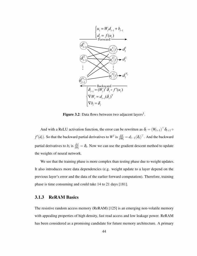
dl−11
dl−1Nl−1
ul1
f
ulNl
f
Forward
Backwardδ l−1 = (Wl )
Τδ l ! ′f (ul )
∇Wl = dl−1(δ l )Τ
∇bl = δ l
⎧
⎨⎪
⎩⎪⎪
ul =Wldl−1 + bl−1dl = f (ul )
⎧⎨⎪
⎩⎪
… …
dl1
dlNl
dl2
dl−12
ul2
f
Figure 3.2: Data flows between two adjacent layers1.
And with a ReLU activation function, the error can be rewritten as δl = (Wl+1)>δl+1
f ′(dl). So that the backward partial derivatives to W l is ∂J∂Wl
= dl−1(δl)>. And the backward
partial derivatives to bl is ∂J∂bl
= δl . Now we can use the gradient descent method to update
the weights of neural network.
We see that the training phase is more complex than testing phase due to weight updates.
It also introduces more data dependencies (e.g. weight update to a layer depend on the
previous layer’s error and the data of the earlier forward computation). Therefore, training
phase is time consuming and could take 14 to 21 days [181].
3.1.3 ReRAM Basics
The resistive random access memory (ReRAM) [125] is an emerging non-volatile memory
with appealing properties of high density, fast read access and low leakage power. ReRAM
has been considered as a promising candidate for future memory architecture. A primary
44

application of ReRAM is to be used as an alternate for main memory [250–252]. Figure 3.3
(a) demonstrates the metal-insulator-metal (MIM) structure of an ReRAM cell. It has a
top electrode, a bottom electrode and a metal-oxide layer sandwiched between electrodes.
By applying an external voltage across it, an ReRAM cell can be switched between a high
resistance state (HRS or OFF-state) and a low resistance state (LRS or On-state), which
are used to represent the logical ”0” and ”1”, respectively, as shown in Figure 3.3 (b). The
endurance of ReRAM could be up to 1012 [253, 254], alleviating the lifetime concern faced
by other non-volatile memory, such as PCM [255].
Bitline
Wordline
a1
a2
a3
b1 b2 b3
w1,1
w2,1
w3,1
w1,2
w2,2
w3,2
w1,3
w2,3
w3,3
bj = f ( ai i wij
i∑ )
Top Electrode
Metal Oxide
Bottom ElectrodeC
urrent
Voltage
SET
RESET
HRS(‘0’)
LRS(‘1’)
(a) (b) (c)
Figure 3.3: Basics of ReRAM.
The ReRAM features the capability to perform in-situ matrix-vector multiplication [256,
257] as shown in Figure 3.3 (c), which utilizes the property of bitline current summation in
ReRAM crossbars to enable computing with high performance and low energy cost. While
conventional CMOS based system showed success on neural network acceleration [27,
43, 101], recent works [88–90, 92] demonstrated that ReRAM-based architectures offer
significant performance and energy benefits for the computation and memory intensive
neural network computing.
Recent works [88–90] demonstrated that ReRAM-based architecture could accelerate
matrix-vector multiplication in neural computation. However, the current works lack
important features to efficiently execute complete deep learning applications. First, they do
not support training that involves weight update and complex data dependencies. Second,
the deep pipeline in ISAAC [89] is not beneficial to training phase where the length
45

of consecutive images that could enter the pipeline is limited by batch size. Also, it is
vulnerable to pipeline bubble.
3.2 PIPELAYER Architecture
In this section, we first analyze the general training procedure and outline the required
mechanisms to support it. Then we present the ideas of intra- and inter-layer pipeline that
explore the parallelism and support training naturally.
PIPELAYER architecture directly leverages ReRAM cells to perform computation with-
out the need for extra processing units. Resistive random access memory (ReRAM or
RRAM) is a type of non-volatile memory that stores information by changing the cell
resistances. This work focuses on a subset of resistive memories, — metal-oxide ReRAM,
which uses metal oxide layers as switching materials. More details on the technology could
be found in [88, 253–255, 258–262].
Our design partition the ReRAM-based main memory into two regions: morphable
subarrays (Morp) and memory subarrays (Mem). The morphable subarrays can perform
both computation and data (weights) storage, the two modes can be configured. In computa-
tion mode, the morphable subarrays perform matrix-vector multiplications. The memory
subarrays are similar to conventional memory and have data storage capability. Due to
space limit, readers could refer to [88] for details on the ReRAM basics.
3.2.1 Training Support
For simplicity, Figure 3.4 shows the configuration of PIPELAYER to process the training
of a 3-layer CNN. The rectangles are one layer of morphable subarrays. The circles are
memory subarrays to store intermediate results transferred between morphable subarrays
for different layers.
46

A1W
A2W
A3W
A11d
A21d
A31d T
A22(W )*
A32(W )*
d0 d1 d2 d3
δ3δ2δ1 32
1 2 3
210
W W W1 2 3∇ ∇∇
T0 T1 T2 T3
T4T5T6T7
(a) Forward
(b) Backward
Figure 3.4: Data flows and dependencies in layer-wise pipeline.
Data dependencies exist in forward and backward computations. The computation
timing and dependencies are shown in Figure 3.4. Starting from forward computation,
the initial cycle is T0, in cycle T1, the input (d0) enters A1 (morphable subarrays), which
perform the matrix-vector multiplication. At the end of T1, the results are written to a
memory subarray, d1. For clarity, we use red dashed lines to show the system state between
two consecutive cycles. Note that the cycles in Figure 3.4 (e.g. T0, T1, ...) are logical cycles,
depending on implementation, each cycle could take several physical clock cycles. We will
show in Section 3.2.2 that the number of physical cycles is determined by parallelism and
hardware resource. The term ”cycle” from this point all refer to the logical cycle. The solid
lines between rectangles (morphable subarrays) and circles (memory subarrays) indicate
the data dependencies. The following forward layers are performed similarly.
The results of forward computation are eventually stored in d3 before backward compu-
tation starts at T4. The backward computations generate errors (δl) (l is the layer) and partial
derivatives to b and W (∇bl and ∇Wl). As the first step, the error for the last (third) layer
(δ3) is computed in T4. It is stored in memory subarrays served as the input for computations
in the next cycle.
47

In T5, two computations happen in parallel: (1) partial derivatives (∇W3) is computed
by previous results in d2 and δ3; (2) errors (δ2) of the second layer is computed from δ3.
Both of the computations depend on δ3, which is computed in T4. ∇W3 is stored in memory
subarrays, which will be used to update weights in A3 and A32 later. Note that (W3)∗ is
a reordered form of W3 and will be discussed in Section 3.3.3. Finally, in T7, the partial
derivatives for the first layer (∇W1) is computed and stored in memory subarrays.
In training, batch size (denoted as B) is used to specify the number of images that can
be processed before a weight update. If B = 1, ∇W1, ∇W2 and ∇W3 are used to update the
weights in A1,A2,A3 and A22,A32. If B > 1, ∇W1, ∇W2 and ∇W3 are stored in the buffers
in a special way so that the average of all partial derivatives can be computed automatically.
Training phase is more complicated than testing phase because it involves data de-
pendencies between outputs from previous layers and the compute of partial derivatives
and errors for weight update. Memory subarrays are used as buffers to store intermediate
results, this greatly reduce data movements and energy consumption by avoiding data being
transferred across memory hierarchy. When not necessary (e.g. with only testing), some of
them can be converted to morphable subarrays.
Within a cycle, different operations could be performed depending on the phase of
computation. Table 3.1 shows the operations in four possible cases. In an implementation,
the cycle time has to allow the longest sequence of operations to fit. Note that the cycle time
is not a bottleneck, because memory is much slower than processors.
3.2.2 Intra Layer Parallelism
Data Input and Kernel Mapping
We propose a basic scheme of data input and the mapping of kernels to a ReRAM array,
illustrated in Figure 3.5. In this example, data of layer l, kernels and data of layer l+1 have
a size of 114×114×128, 3×3×128×256 and 112×112×256, respectively.
48
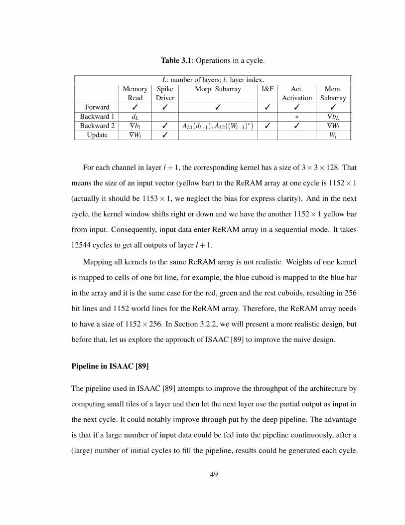
Table 3.1: Operations in a cycle.
L: number of layers; l: layer index.Memory Spike Morp. Subarray I&F Act. Mem.
Read Driver Activation SubarrayForward 3 3 3 3 3 3
Backward 1 dL ∗ ∇bL
Backward 2 ∇bl 3 AL1(dl−1); AL2((Wl−1)∗) 3 3 ∇Wl
Update ∇Wl 3 Wl
For each channel in layer l +1, the corresponding kernel has a size of 3×3×128. That
means the size of an input vector (yellow bar) to the ReRAM array at one cycle is 1152×1
(actually it should be 1153× 1, we neglect the bias for express clarity). And in the next
cycle, the kernel window shifts right or down and we have the another 1152×1 yellow bar
from input. Consequently, input data enter ReRAM array in a sequential mode. It takes
12544 cycles to get all outputs of layer l +1.
Mapping all kernels to the same ReRAM array is not realistic. Weights of one kernel
is mapped to cells of one bit line, for example, the blue cuboid is mapped to the blue bar
in the array and it is the same case for the red, green and the rest cuboids, resulting in 256
bit lines and 1152 world lines for the ReRAM array. Therefore, the ReRAM array needs
to have a size of 1152×256. In Section 3.2.2, we will present a more realistic design, but
before that, let us explore the approach of ISAAC [89] to improve the naive design.
Pipeline in ISAAC [89]
The pipeline used in ISAAC [89] attempts to improve the throughput of the architecture by
computing small tiles of a layer and then let the next layer use the partial output as input in
the next cycle. It could notably improve through put by the deep pipeline. The advantage
is that if a large number of input data could be fed into the pipeline continuously, after a
(large) number of initial cycles to fill the pipeline, results could be generated each cycle.
49

114
114
128
1283
3
112
112
256
=
…
WL_0
WL_1…
BL_0BL_1BL_2
WL_1151
… ⇒
01212543
1152
…
BL_255
(1152=3*3*128)
12544(12544=112*112)
layer l+1layer l
Figure 3.5: A basic scheme for data input and kernel mapping.
Unfortunately, this assumption is untrue for neural network training phase, where weights
are updated at the end of a batch. The new inputs in the next batch need to be processed
based on the updated weights and we cannot have a large number of consecutive input data
for the pipeline. Therefore, the pipeline design in ISAAC does not fit well for training
phase.
Another issue is the vulnerability to pipeline bubble, leading to execution stall. Consider
a network where all kernels are of size 2×2×1. One point p50 in layer l5 depends on 4,
16, 64, 256 points in layer l4, l3, l2 and l1, which means the computation of p50 is stalled
when any of the 340 (= 4+ 16+ 64+ 256) points is delayed, which could further stall
computations depending on p50. Moreover, data dependencies are complex in training
phase, layer l may not only depend on layer l−1, but also from earlier layers (e.g. δ1 in 3.4
depends on δ2 and early data d1). It further increase the chance of stalls. [89] mentioned
pipeline imbalance issue but similar issues could easily occur with more complex training
50

phase and it is extremely hard to predict and avoid all of them.
Parallelism Granularity
0
16
1…
3
17
256
1152
1152
……
…
…
…
128
128
2…
294912
49
…
G=256
(256=2*128)
(1152=9*128)
(49=12544/G)
(294912= G*1152)
Figure 3.6: A balanced scheme for data input and kernel mapping.
The ReRAM array size could be made feasible by partition. We can decompose the
1152×256 matrix to a group of 18 (=9×2) matrices and map each of them to a 128×128
ReRAM array (shown in the right part of Figure 3.6). We can get the right results by
collecting array outputs horizontally and summing them vertically.
To improve performance, we define a metric called parallelism granularity, denoted as
G, indicating the number of duplicated copies of ReRAM arrays that store the same weights.
If G = 1, the design is equivalent to the naive scheme. If G = 12544, the results of a layer
could be generated in just one cycle but the hardware cost is prohibitive.
Essentially, parallelism granularity allows explore the trade-off between hardware
resource of ReRAM array and performance. A good trade-off requires a carefully chosen G.
Figure 3.6 shows an example with G = 256.
51

3.2.3 Inter Layer Parallelism
T0A32A31
A22A21
A11ErrLA3A2A1
T1 T2 T3 T4 T5 T6 T7 T8 T9
A32A31
A22A21
A11ErrLA3A2A1
A32A31
A22A21
A11ErrLA3A2A1
Figure 3.7: Layer-wise pipeline.
In training, the input data are normally processed in batch. The inputs in the same batch
are all processed based on the same weights at the start of the batch. The weight updates due
to each input are stored and only applied to at the end of a batch. Therefore, no dependency
exists among data inputs inside a batch. We propose an architecture to support pipelined
training. The performance gain is due to the fact that B is normally much larger than 1 (e.g.
64), otherwise, each input needs to be processed sequentially.
Based on Figure 3.4, the pipelined execution is shown in Figure 3.7. The execution
with intra- and inter-layer pipeline could achieve high throughput without the drawbacks of
previous work. In the execution, a new input can enter the pipeline every cycle within a
batch. At the end of batch, a new input belonging to the next batch cannot enter the pipeline
until all inputs in previous batch are processed and weights are updated. In another word, a
new batch has to wait the ”tail” of previous batch to drain from the pipeline.
Figure 3.8 (a) shows the latency of the baseline architecture without pipeline. Assuming
the neural network has L layers, we can see that the forward computation of one input takes
L cycles, the backward computation of one input takes (L+1) cycles, at the end of a batch,
one cycle is dedicated to the weight update. Therefore, a batch takes (2L+1)B+1 cycles.
52

I1
A1 AL
I2 IB Update I1 I2… …
A2 … ErrL AL1/AL2 … A11
1 batch
Forward Backward
(a) Latency of PipeLayer without pipeline
I1
I2
IB Update
I1
I2
…… ……
2L+1B-1 1
B: batch sizeL: # of layers
(b) Latency of PipeLayer with pipeline
Figure 3.8: Latency of PIPELAYER architecture.
For a total number of N inputs, the total number of training cycles is (2L+1)N +N/B.
Now let us consider the pipelined execution, the latency is illustrated in Figure 3.8 (b).
Within a batch, a new input could enter every cycle. Similar to the baseline case, the first
weight update is generated after (2L+1) cycles. Then there will be (B−1) cycles until
the end of batch. Finally, there is one cycle to apply all weight updates within the batch.
Since the forward and backward computation are intertwined with each other, we do not
distinguish the forward and backward cycles. From the above analysis, the total number of
cycles to process N inputs with L layers is (N/B)(2L+B+1).
δ2A21
W2∇
A2A1
(2L-1) entries
Figure 3.9: Memory subarray design.
53

The major implication of pipelining is the increased requirement of memory subarrays.
The problem is illustrated in Figure 3.9. Consider the same example in Figure 3.4, since now
A1 will produce output every cycle, we need to have more buffers so that the data which
will be used later are not over written. Specifically, referring to Figure 3.4, d1 computed in
T1 will be used after 5 cycles, in T6. Therefore, between A1 and A2, 5 buffers are needed.
A1 should logically keep a pointer pointing to the current buffer that the output should
be written to. After an output, the pointer is increased by one. Logically we implement
circular buffers. When it reaches 5, it will wrap around and return to the first entry. When
the output is written again to the first entry, the useful data (d1) used to compute ∇W2 can
be safely overwritten because ∇W2 has been computed. According to this, in Figure 3.4,
A1 will write 1st-, 2nd-, 3rd-, 4th- and 5th-entry in buffer between A1 and A2 in T1, T2, T3,
T4, T5, consecutively. Since ∇W2 is computed from the data in the 1st-entry in the buffer in
T5, in the next cycle, A1 could overwrite the 1st-entry of the buffer. In general, the buffer
requirement at l-th layer (assuming the total number of layers is L) is 2(L− l)+1.
Another implication of pipelining is that at the same cycle, there will be a read and
a write on the same buffer. To support this, we need to duplicate the single buffer. This
happens for the buffer at d3, δ1, δ2, δ3. Table 3.2 compares the number of cycles and the
cost of (groups of) arrays of nonpipelined and pipelined architectures.
Table 3.2: Cycles and cost in PIPELAYER architecture.
G: parallelism granularity; L: number of layers;B: batch size; N: number of total input images.
Non-pipelined PipelinedForward Cycles LN
(N/B)(2L+B+1)Backward Cycles (L+1)N +N/BMorp Subarrays GL+G(2L−1)
GL+G(L−1)+BLMem Subarrays 2L
54

3.3 Implementation of PIPELAYER
Global IO Row Buffer Controller
Memory SubarrayConnection
Dri
ver
Glo
bal R
ow D
ecod
er
I&FMorp
Subarray Dri
ver I&F
MorpSubarray D
rive
r …Activation Activation
Dri
ver I&F
MorpSubarray D
rive
r I&FMorp
Subarray Dri
ver …
Dri
ver I&F
MorpSubarray D
rive
r I&FMorp
Subarray Dri
ver …
Activation Activation
Dri
ver I&F
MorpSubarray D
rive
r I&FMorp
Subarray Dri
ver …
Data
Add
r_C
olA
ddr_
Row
b b
a
a
c
d
e
I Vth CounterC
u+
uo
uo
u+
t
t
Timing Control
K2 Vi(t)
Di
Vprg
Vo
. . .Vo
K1
cDP
DN
-& LUT D
Configuration
D’Reg
Vo
Figure 3.10: Overall architecture of PIPELAYER.
3.3.1 Overall Architecture
Figure 3.10 shows the architecture of PIPELAYER. Our design leverages ReRAM cells to
perform computation without the need for extra processing units. The design partitions the
ReRAM-based main memory into two regions: morphable subarrays and memory subarrays.
The morphable subarrays can perform both computation and data (weights) storage, the two
modes can be configured. In computation mode, the morphable subarrays could perform
matrix-vector multiplications. The memory subarrays are the same as conventional memory
and have data storage capability. They are used to store intermediate results between layers
and keep data that will be used in Figure 3.10 only shows the morphable subarrays and
memory subarrays.
55

a. Spike Driver. To reduce the area and energy overhead of voltage-level based input scheme
in [88], we use a weighted spike coding scheme similar to ISAAC [89]. The spike driver
converts the input to a sequence of weighted spikes. In weight update, spike driver serves as
write driver to tune weights stored in the ReRAM array.
b. Integration and Fire. It is a required component of a spike-based scheme. It integrates
input current and generates output spikes. The output spikes are connected to a counter, so
essentially the analog currents are converted into digital values. The data input scheme used
in [89] is similar as our spike input, both eliminating DACs, but our integration and fire
components eliminates ADCs while [89] keeps.
c. Activation. It implements the activation function defined in a CNN algorithm. When
morphable subarrays are configured as memory, it is bypassed.
d. Connection. This component connects morphable and memory subarrays. The outputs
from morphable subarrays (when they are in computation mode) need to be written to
memory subarrays so that they are used as input for the morphable subarrays for the next
layer in next cycle.
e. Control. It offloads the computation from the host CPU and orchestrates the data transfers
between memory subarrays and morphable subarrays in training and testing with based on
the algorithm configurations (e.g. batch size).
3.3.2 Component Designs
Spike Driver
We use a weighted spike coding scheme. For a N-bit input value, we need N time slots for
potential spikes. The spike driver design is shown in Figure 3.10 (a). Inside the driver, N
levels of reference voltage, ranging from V0/2N−1 to V0/2 are generated. A timing control
component shifts key K1 to connect one of the reference voltages at one time slot. Note that
the shifting is non-decreasing: the voltage of output spike increases as time slot progresses,
56

thus the data input is of a Least Significant Bit First (LSBF) mode. K2 is controlled by the
input data to decide whether the spike output is generated or not.
Another function of spike driver is to write or program data to a subarray, where K1 is
connected to a programing voltage. K2 tunes the resistance of a ReRAM cell controlled by
input data which serve as programing control sequences. Spike divers are reused between
adjacent subarrays.
Integration and Fire
Figure 3.10 (b) shows the design of Integration and Fire circuit. A controlled current source
serves as a current follower to inject an equivalent strength current as that from a bit line to
a capacitor. As a result, the voltage on this capacitor is accumulated.
When the voltage on the capacitor increases to the threshold (Vth) of the comparator,
an output spike is generated and counted by a counter. Note that the current on the bit
line is the accumulation of products of spikes (input data) and ReRAM cell conductances
(corresponding weights). For a fixed threshold Vth, a K times stronger current will makes
the comparator to generate K times of output spikes. As a result, the number of spikes
generated by the comparator is actually the accumulation of products of input data and
corresponding weights. A group of integration and fire components are connected to bit
lines of a subarray and they can generate an vector in parallel.
Activation Function
Figure 3.10 (c) shows the design of activation component. The activation component
consists of a subtractor and a look up table (LUT). Since positive weights and negative
weights are mapped to two subarrays, we need to collect the results DP from a positive
subarray and DN from a negative subarray. Our activation component is configurable by
different LUTs to realize the activation function defined in specific algorithm. In this
57
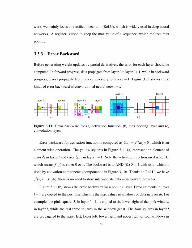
work, we mainly focus on rectified linear unit (ReLU), which is widely used in deep neural
networks. A register is used to keep the max value of a sequence, which realizes max
pooling.
3.3.3 Error Backward
Before generating weight updates by partial derivatives, the error for each layer should be
computed. In forward progress, data propagate from layer l to layer l+1, while in backward
progress, errors propagate from layer l inversely to layer l− 1. Figure 3.11 shows three
kinds of error backward in convolutional neural networks.
Act
ivat
ion 2 0 0 0
0 1 0
0 0 0 5
0 3 0 0
2 1
3 5
0
Act
ivat
ion
(b)(a) (c)
layer l-1 layer l-1
layer l-1 layer l
layer llayer l
Figure 3.11: Error backward for (a) activation function, (b) max pooling layer and (c)convolution layer.
Error backward for activation function is computed as δl−1 = f ′(ul)δl , which is an
element-wise operation. The yellow squares in Figure 3.11 (a) represent an element of
error δl in layer l and error δl−1 in layer l−1. Note the activation function used is ReLU,
which means f ′(·) is either 0 or 1. The backward is to AND (&) 0 or 1 with δl−1, which is
done by activation components (component c in Figure 3.10). Thanks to ReLU, we have
f ′(ul) = f ′(dl), there is no need to store intermediate data ul in forward progress.
Figure 3.11 (b) shows the error backward for a pooling layer. Error elements in layer
l−1 are copied to the positions which is the max values in windows of data in layer dl . For
example, the pink square, 3, in layer l−1, is copied to the lower right of the pink window
in layer l, while the rest three squares in the window get 0. The four squares in layer l
are propagated to the upper left, lower left, lower right and upper right of four windows in
58

layer l−1. Mathematically, max pooling can be viewed as one kind of activation function.
The error backward for a pooling layer is also performed in the activation component
(component c in Figure 3.10). With dl already stored in memory subarrays, the index for
the max element in a window can be found.
For error backward, we can reuse the logic in a convolution layer. In Figure 3.11 (c),
a 3× 3 kernel is used in forward progress. In the forward progress, to generate the nine
elements in the red window in layer l, all of the (light, medium and dark) blue squares in
layer l−1 are convoluted with the 3×3 kernel and the dark blue square (with red edges)
are exactly multiplied with each elements in the kernel. In the backward, to get the error for
the dark blue square, we can just convolute the nine elements in the red window in layer l
with the kernel.
114
114
128
2563
3
112+2+2
112+2+2
256
…
⇒
layer l-1 layer l
Figure 3.12: Error backward for convolution layer by convolution of error of layer l andreordered kernels.
δl−1 = conv2(δl, rot180(K), ’full’) is the computation for error backward for convolu-
tion layer. For elements at edges, zero paddings are added. Figure 3.12 shows the error
backward for the convolution layer in Figure 3.5, where error in layer l−1 are zero-padded
by 2 at each edge, so the length and width increase to 116. Also, the kernels are reordered.
In this way, we can perform convolutions by using the data input and kernel mapping
scheme discussed in Section 3.2.2.
59

3.3.4 Weight Update
Computing Partial Derivatives
The partial derivatives to bias is the sum of all related error: ∇b = ∑u,v(δl)u,v. It is
done by reading bitline with the input spikes representing 1. The partial derivative to a
weight is the sum of element-wise products of error and patches/windows of data: ∇W =
∑u,v(δl)u,v · (dl−1)u,v. It can be converted to convolution.
In Figure 3.13, the convolution of one blue channel of error in layer l−1 and the total
128 channels of data in layer l is the partial derivatives to weights of the blue kernel (size of
3×3×128). All the kernels (red, green and others) are similar. In the convolution, data in
layer l (yellow slices) can be viewed as convolution kernels while error in layer l−1 (doted
slices) can be viewed as convolution data. Therefore, the convolution is done by mapping
the yellow slices to ReRAM arrays and sending the backward error to the arrays.
114
114
128
112
112
256
128
3
3
…
dl-1 δllayer l-1 layer l
Figure 3.13: The computation of partial derivatives for kernels.
Writing New Weights to Morphable Subarrays
With the partial derivatives for weights ∇W and bias ∇b, old weights and bias that read from
morphable subarrays. The new (updated) weights and bias can be computed and written to
morphable subarrays.
In weight updating, we need to compute the average of the B (B is the batch size)
60
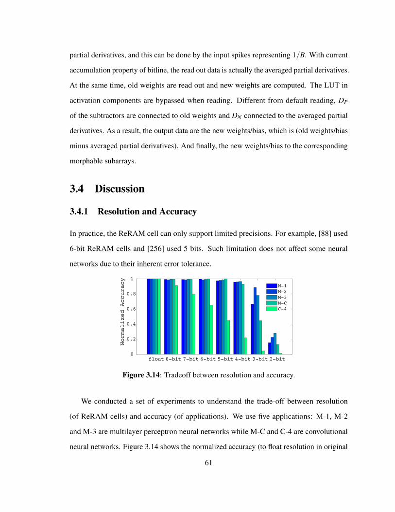
partial derivatives, and this can be done by the input spikes representing 1/B. With current
accumulation property of bitline, the read out data is actually the averaged partial derivatives.
At the same time, old weights are read out and new weights are computed. The LUT in
activation components are bypassed when reading. Different from default reading, DP
of the subtractors are connected to old weights and DN connected to the averaged partial
derivatives. As a result, the output data are the new weights/bias, which is (old weights/bias
minus averaged partial derivatives). And finally, the new weights/bias to the corresponding
morphable subarrays.
3.4 Discussion
3.4.1 Resolution and Accuracy
In practice, the ReRAM cell can only support limited precisions. For example, [88] used
6-bit ReRAM cells and [256] used 5 bits. Such limitation does not affect some neural
networks due to their inherent error tolerance.
float 8-bit 7-bit 6-bit 5-bit 4-bit 3-bit 2-bit0
0.2
0.4
0.6
0.8
1
Normalized Accuracy
M-1M-2M-3M-CC-4
Figure 3.14: Tradeoff between resolution and accuracy.
We conducted a set of experiments to understand the trade-off between resolution
(of ReRAM cells) and accuracy (of applications). We use five applications: M-1, M-2
and M-3 are multilayer perceptron neural networks while M-C and C-4 are convolutional
neural networks. Figure 3.14 shows the normalized accuracy (to float resolution in original
61

implementation) of using different number of bits. We see that for M-1, M-2, M-3, using 4-
bit just slightly decreases the accuracy. However, the accuracy is more sensitive to resolution
for convolutional neural networks, as accuracies of M-C and C-4 drop sharply from 3-bit.
Especially for C-4, even at 4-bit resolution, the normalized accuracy is only around 0.2.
When higher resolution is needed, we can use multiple arrays with lower resolution,
similar to [89]. The default resolution of PIPELAYER is 16-bit, the same as [27,89], and the
resolution of ReRAM cells used in PIPELAYER is 4-bit.
4-
0D0<<0
4-
1D1<<4
4-
2D2<<8
4-
3D3<<12
Din
D(a) Forwarding
4-
0W0
4-
1W1
4-
2W2
4-
3W3 Wold
(b) Updating
∇W+
WnewW3..0
W7..4
W11..8
W15..12
+ W3 W2 W1 W0
Figure 3.15: Weight partition.
In testing phase, we can easily get 16-bit results by adding four shifted 4-bit results, as
shown in Figure 3.15 (a). Here, the same data input four groups of 4-bit arrays. The four
groups store 4-bit weights for the the 15..12, 11..8, 7..4 and 3..0 segment respectively. We
can shift and add the results from the four groups and get the results for 16-bit resolution. In
training phase, we need to first read the old four segments of 4-bit weights then shift them
to get the old weights. With the partial derivatives, we get the new weights and write back
to the four groups to finish the update. It is shown in figure 3.15 (b).
3.4.2 Application Programming Interface
Thanks to the layer wise inter layer pipeline of PIPELAYER, the system can be config-
ured by layer interactively. Before discussing layer wise function invocation, we provide
62
two functions, Copy to PL and Copy to CPU to transfer data from CPU main memory to
PIPELAYER or inversely. For one layer configuration, a topology set function Topology set
is invoked. This function configures the connections and datapath of G groups of arrays
as shown in Figure 3.6, while G can be set by programmer or automatically optimized by
compiler. Next, the weight load function Weight load is invoked, which load pre-trianed
weights to the arrays in testing phase, or initial weights in training phase. After all layers
are configured, running with pipeline can be started by function Pipeline Set. Finally,
one of the running mode functions Train or Test starts the execution.
3.5 Evaluation
3.5.1 Benchmarks
The benchmark networks used are based on databases MNIST [183] and ImageNet [182].
MNIST is a classical database of handwritten digits for pattern recognition. It consists of a
training set of 60K images and a inference set of 10K images. And the labels for the images
range from 0 to 9. Images of MNIST are 28-by-28 gray images. ImageNet provides 14.2M
images and 21.8K indexed synsets. Most of the largest and state-of-the-art performance
neural networks are based on ImageNet.
For ImageNet, we select six popular large scale networks, i.e. AlexNet [119], and
VGG-A, VGG-B, VGG-C, VGG-D, VGG-E [181]. The topologies and hyperparameters
of these networks can be found from the references. For MNIST, we build four neural
networks as our benchmarks, the hyper parameters are shown in Table 3.3.
In Table 3.3, N1-N2 represents an inner product layer where there are N1 perceptrons in
layer l and N2 neurons in layer l+1 (e.g. 784−100 represents an inner product layer where
there are 784 neurons in the first layer and 100 neurons in the second layer). ConvKxC
represents a convolution layer where the kernel size is K by K and the number of channels
in the next layer is C.
63

Table 3.3: Hyper parameters of networks on MNIST.
Network Hyper ParametersMnist-A 784-100-10Mnist-B 784-500-250-10Mnist-C 784-1500-1000-500-10Mnist-0 conv5x10-360-10
3.5.2 Experiment Setup
In our experiments, we compare PIPELAYER with a GPU-based platform. Benchmarks
running on the platform are based on the widely used framework Caffe [263].
To run the GPU platform, we set the running mode in the Caffe prototxt to GPU. The
GPU used is the newest released GTX 1080. Table 3.4 shows the parameters of our GPU
platform. The run times for GPU platform are measured by caffe and the energy costs are
measured by the tool nvidia-smi provided by NVIDIA CUDA.
Table 3.4: Configurations of the GPU platform.
CPU: Intel Xeon E5-2630 V3, 8 cores,2.40 GHz, 8× (32+32)KB L1 Cache,8×256KB L2 Cache, 20 MB L3 Cache.Memory 128 GBStorage 1 TBGraphic Card NVIDIA Geforce GTX 1080Architecture PascalCUDA Cores 2560Base Clock 1607 MHzCompute Capability 6.1Graphic Memory 8 GB GDDR5XMemory Bandwidth 320 GB/sCUDA Version 8
To evaluate PIPELAYER, we build a simulator based on NVSim [184]. The read/write
latency, read/write energy cost used in the simulator are 29.31 ns/50.88 ns per spike, 1.08
pJ/3.91 nJ per spike, which are reported in [264]. And the area model is based on data
64

reported in [252].
3.5.3 Performance Results
Figure 3.16 shows the performance comparisons of training and inference (testing) phase.
For each application, we report the execution time comparison of GPU, non-pipelined and
pipelined PIPELAYER ( PIPELAYER). The GPU implementation is used as the baseline and
running times of benchmarks on different settings are normalized to it.
Mnist-A_train
Mnist-B_train
Mnist-C_train
Mnist-0_train
AlexNet_train
VGG-A_train
VGG-B_train
VGG-C_train
VGG-D_train
VGG-E_train
Gmean_train
Mnist-A_test
Mnist-B_test
Mnist-C_test
Mnist-0_test
AlexNet_test
VGG-A_test
VGG-B_test
VGG-C_test
VGG-D_test
VGG-E_test
Gmean_test
Gmean_all
1
10
100
Speedup
GPUPipeLayer w/o pipelinePipeLayer
Figure 3.16: Speedups of networks in both training and inference.
Compared to GPU platform, the geometric mean of overall (training + inference),
training and inference speedup achieved by pipelined PIPELAYER architecture are 33.85
x, 53.22x and 42.45x, respectively. Among all applications in both training and inference,
the highest speedup achieved by non-pipelined PIPELAYER is 20.81x, while for pipelined
PIPELAYER, the highest speedup is 146.58x.
PIPELAYER architecture archives lower speedups in training phase than in inference
phase. It is because training requires more intermediate data processing and weight updates.
The pipelined PIPELAYER achieves a geometric mean speedup of 42.45x, significantly
better than non-pipelined variants because the computations and data movements are
performed in a highly parallel manner.
Intuitively, as the depth and layers of the neural networks increase, PIPELAYER archi-
tecture will achieve higher speedups compared to conventional architecture. However, we
65

found that it is not always the case. For example, the speedup of Mnist-C is larger than
AlexNet in training. That is because Mnist-C is a mutilayer perceptron network, whose
weights are all matrixs and can be directly mapped to ReRAM arrays.
3.5.4 Energy Results
Figure 3.17 shows energy savings in GPU platform and PIPELAYER (pipelined). The higher
the bars are, the more energy efficient the corresponding architectures are. We show results
for both training and inference.
Mnist-A_train
Mnist-B_train
Mnist-C_train
Mnist-0_train
AlexNet_train
VGG-A_train
VGG-B_train
VGG-C_train
VGG-D_train
VGG-E_train
Gmean_train
Mnist-A_test
Mnist-B_test
Mnist-C_test
Mnist-0_test
AlexNet_test
VGG-A_test
VGG-B_test
VGG-C_test
VGG-D_test
VGG-E_test
Gmean_test
Gmean_all
1
10
100
Energy Saving GPU
PipeLayer
Figure 3.17: Energy savings for PIPELAYER.
The geometric mean of energy saving compared to GPU in training and inference are
6.52x and 7.88x, respectively and the overall geometric mean of energy saving is 7.17x.
The highest energy saving for training and inference are 27.03x (Mnist-C) and 70.03x
(Mnist-A), respectively. We see that energy saving of PIPELAYER in training is slightly less
than that in inference. This is due to the extra morphable and memory subarrays needed.
In summary, we see from the results that PIPELAYER architecture provides significant
performance improvement with drastic energy reduction. It comes from two sources. First,
the computation cost is reduced, the matrix-vector multiplications commonly used in CNNs
66

are performed by analog circuits, which is much more energy efficient than conventional
GPU implementation. Second, the data movements in memory hierarchy are greatly reduced.
In PIPELAYER, the data movements between different levels of memory hierarchies in
conventional architectures are replaced by data movements in memory itself through layers.
3.5.5 Sensitivity of Parallelism Granularity
This section analyzes the effect of parallelism granularity on PIPELAYER. Table 3.5 shows
the default parallelism granularity for each convolution layer of 5 VGG networks. We use a
scalar λ to enlarge or reduce the parallelism granularity of a network for λ times.
Table 3.5: Optimized parallelism granularity G configurations of each convolution layer inVGGs.
Layer VGG-A VGG-B VGG-C VGG-D VGG-Econv11 1024 1024 1024 1024 1024conv12 - 1024 1024 1024 1024conv21 256 256 256 256 256conv22 - 256 256 256 256conv31 64 64 64 64 64conv32 64 64 64 64 64conv33 - - 64 64 64conv34 - - - - 64conv41 16 16 16 16 16conv42 16 16 16 16 16conv43 - - 16 16 16conv44 - - - - 16conv51 4 4 4 4 4conv52 4 4 4 4 4conv53 - - 4 4 4conv54 - - - - 4
In Figure 3.18, λ = 0 means the parallelism granularity of all layers are G = 1 and
λ = ∞ means G is set to the maximum value for each layer. Figure 3.18 shows that the
speedup (compared with GPU) increase monotonically with λ . However, the increase
of parallelism granularity will also cause the increase in area, as shown in Figure 3.19.
Therefore, choosing the suitable parallelism granularity to explore the balance between
67
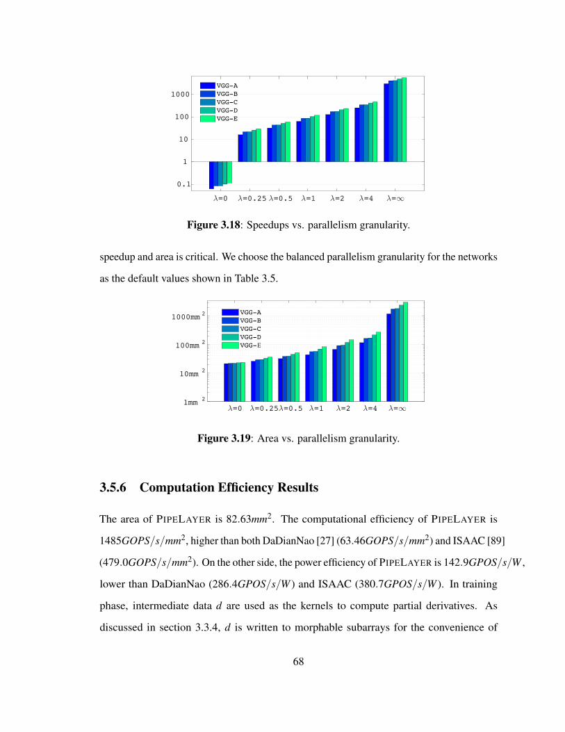
6=0 6=0.25 6=0.5 6=1 6=2 6=4 6=1
0.1
1
10
100
1000 VGG-AVGG-BVGG-CVGG-DVGG-E
Figure 3.18: Speedups vs. parallelism granularity.
speedup and area is critical. We choose the balanced parallelism granularity for the networks
as the default values shown in Table 3.5.
6=0 6=0.256=0.5 6=1 6=2 6=4 6=11mm 2
10mm 2
100mm 2
1000mm 2 VGG-AVGG-BVGG-CVGG-DVGG-DE
Figure 3.19: Area vs. parallelism granularity.
3.5.6 Computation Efficiency Results
The area of PIPELAYER is 82.63mm2. The computational efficiency of PIPELAYER is
1485GOPS/s/mm2, higher than both DaDianNao [27] (63.46GOPS/s/mm2) and ISAAC [89]
(479.0GOPS/s/mm2). On the other side, the power efficiency of PIPELAYER is 142.9GPOS/s/W ,
lower than DaDianNao (286.4GPOS/s/W ) and ISAAC (380.7GPOS/s/W ). In training
phase, intermediate data d are used as the kernels to compute partial derivatives. As
discussed in section 3.3.4, d is written to morphable subarrays for the convenience of
68

partial derivatives computing, which means the groups of ”storing” arrays are converted to
”computing” arrays. For this reason, PIPELAYER gains a higher computational efficiency.
However, the lower power efficiency is because we write all of data to ReRAM arrays, while
DaDianNao and ISAAC write to eDRAMs.
69

Chapter 4
Accelerator Architecture for Graph Processing
4.1 Background and Motivation
4.1.1 Graph Processing
…
…
Edges:
Vertices:
(b) Access pattern in vertex-centric program
…(a) Vertex and edge accesses in
graph processing
(random access)
(global random access)
(local sequential access)
Figure 4.1: Graph processing in vertex-centric programs.
……Edges:
Vertices(source):
…Updates:
1. Edge-centric scatter 2. Edge-centric gather
…Updates:
…Vertices(destination):
(a) Edge-centric processing
(sequential read)
(random access)
(sequential read)
(sequential write)
(random access)
(b) Dual sliding windows
Figure 4.2: (a) Edge-centric processing and (b) dual sliding windows.
Graph algorithms traverse vertices and edges to discover interesting graph properties
based on relationship. A graph could be naturally considered as an adjacency matrix, where
the rows correspond to the vertices and the matrix elements represent the edges. Most graph
algorithms can be mapped to matrix operations. However, in reality, the graph is sparse,
which means that there would be many zeros in the adjacency matrix. This property incurs
the waste of both storage and compute resources. Therefore, the current graph processing
systems use the format that is suitable for sparse graph data. Based on such data structures,
70

the graph processing can be essentially considered as implementing the matrix operations
on the sparse matrix representation. In this case, individual (and simple) operations in
the whole matrix computation are performed by the compute units (e.g., a core in CPU
or an SM in GPU) after data is fetched. In the following, we elaborate the challenge of
random accesses in various graph processing approaches. More details on sparse graph data
representation will be discussed in Section 4.1.3.
To provide an easy programming interface, the vertex-centric program featuring “Think
Like a Vertex (TLAV)” [157] was proposed as a natural and intuitive way for human brain
to think of the graph problems. Figure 4.1 (a) shows an example, an algorithm could first
access and process the red vertex in the center with all its neighbors through the red edges.
Then it can move to one of the neighbors, the blue vertex on the top, accessing the vertex
and the neighbors through the blue edges. After that, the algorithm can access another
vertex (the green one on the left), which is one of the neighbors of the blue vertex.
In graph processing, the vertex accesses lead to random accesses because the neighbor
vertices are not stored continuously. For edges, they incur local sequential access because
the edges related to a vertex are stored continuously but global random accesses because
algorithm needs to access the edges of different vertices. The concepts are shown in
Figure 4.1 (b). The random accesses lead to long memory latency and, more importantly,
the bandwidth waste, because only a small portion of data are accessed in a memory block.
In a conventional hierarchical memory system, this leads to the significant data movements.
Clearly, reducing random accesses is critical to improve the performance of graph
processing, this is particularly crucial for the disk-based single machine graph processing
systems (a.k.a out-of-core systems [151–154]), because the random disk I/O operations are
much more detrimental to the performance. In this context, the memory is considered small
and fast (therefore can afford random accesses) while disk is considered large and slow
(therefore should be only accessed sequentially). The edge-centric model in X-Stream [153]
71

is a notable solution for reducing random accesses. Specifically, the edges of a graph
partition are stored and accessed sequentially in disk and the related vertices are stored and
accessed randomly in memory. Such setting is feasible because typically the vertex data are
much smaller than edge data. During process, X-Stream generates Updates in scatter phase,
which incurs sequential writes, and then, applies these Updates to vertices in gather phase,
which incurs sequential reads. The concepts are shown in Figure 4.2 (a).
A notable drawback of X-stream is that the number of updates may be as large as that of
edges, GridGraph [151] proposed optimizations to further reduce the storage cost and data
movements due to updates. The solution is based on the dual sliding windows (shown in
Figure 4.2 (b)), which partitions edges into blocks and vertices into chunks. On visiting the
edge blocks, the source vertex chunk (orange) is accessed and updates are directly applied
to the destination vertex chunk (blue). This requires no temporary update storage as in
X-Stream. Edge blocks can be accessed in source oriented order (shown in Figure 4.2 (b))
or destination oriented order. Note that the dual sliding window mechanism is based on
edge-centric model.
4.1.2 Graph Processing Accelerators
Due to the wide applications of graph processing and its challenges, several hardware
accelerators were recently proposed. Ahn et al. [187] proposes TESSERACT, the first
PIM-based graph processing architecture. It defines a generic communication interface
to map graph processing to HMC. At any time, each core can Put a remote memory
access and get interrupted to receive and execute the Put calls from other cores. Ozdal
et al. [186] introduces an accelerator for asynchronous graph processing, which features
efficient hardware scheduling and dependence tracking. To use the system, programmers
have to understand its architecture and modify existing code. Graphicionado [185] is a
customized graph accelerator designed for high performance and energy efficiency based
72

on off-chip DRAM and on-chip eDRAM. It modifies the graph data structure and data path
to optimize graph access patterns and designs specialized memory subsystem for higher
bandwidth. These accelerators all optimize the memory accesses, reducing the latency or
better tolerating the random access latency. [265] and [266] focused on the data coherence in
memory which can be accessed by instructions from host CPU and the accelerator, and [266]
also considered atomic operations. Other PIM-based accelerators for graph processing
are [267, 268].
4.1.3 Graph Representation
The processing of the matrix-vector multiplications on small data blocks could increase
the ratio between computation and data movement and reduce the pressure on memory
system. With its matrix-vector multiplication capability, ReRAM could naturally perform
the low-cost parallel dense operations on the sparse sub-matrices (subgraphs), enjoying the
benefits without increasing hardware and energy cost.
The key insight of GRAPHR is to still store the majority of the graph data in the com-
pressed sparse matrix representation and process the subgraphs in uncompressed sparse
matrix representation. In the following, we review several commonly used sparse represen-
tations.
0010
0004
3700
8002
0123
0 1 2 3
(row,col,val)(0,2,3)(0,3,8)(1,2,7)(2,0,1)(3,1,4)(3,3,2)
(b) CSC
(row,val)0123
1246
colptr0
(col,val)0123
2346
rowptr0
1234
0
5(0,8)(1,7)
(3,4)
(3,2)
(2,1)
(0,3)1234
0
5
(2,3)(3,8)(2,7)(0,1)(1,4)(3,2)
(a) (c) CSR (d) COO
Figure 4.3: (a) Sparse matrix and its compressed representations in: (b) CSC, (c) CSR, and(d) COO.
The three major compressed sparse representations are compressed sparse column
73

(CSC), compressed sparse row (CSR) and coordinate list (COO). They are illustrated in
Figure 4.3. In the CSC representation, non-zeros are stored in column major order as (row
index, value) pairs in a list, the number of entries in the list is the number of non-zeros.
Another list of column starting pointers indicate the starting index of a row in the (row,val)
list. For example, in Figure 4.3 (a), 4 in the colptr indicates that the 4-th entry in (row,val)
list, i.e., (0,8) is the starting of column 3. The number of entries in colptr is the number
of columns + 1. Compressed sparse row (CSR) is similar to CSC, with row and column
alternated. For coordinate list (COO), each entry is a tuple of (row index, column index,
value) of the nonzeros.
2
00110110
00011111
11000011
11000010
00000011
00000010
00001101
00001101
(a) (b) (c)
0 20 31 21 32 03 03 1
4 15 05 16 06 17 16 26 37 2
4 64 75 65 76 46 57 47 67 7
B0-0 B0-1 B1-0 B1-1
2
10
7
34
5
6
Figure 4.4: (a) A directed graph and its representations in (b) adjacency matrix and (c)coordinate list.
In GRAPHR, we assume coordinate list (COO) representation to store a graph. Given a
graph in Figure 4.4 1 (a), its (sparse) adjacency matrix representation and COO representa-
tion (partitioned into four 4 × 4 subgraphs) are shown in Figure 4.4(b) and (c), respectively.
In this example, the coordinate list saves 61% storing space, compared with the adjacency
matrix representation. For real-world graphs with high sparsity, the saving is even high: the
coordinate list can only take 0.2% of space for WikiVote [269] compared to an adjacency
1As shown in Section 4.1.3, each entry in a coordinate list should be a three-element tuple of Source ID,Destination ID, Edge Weight. To simplify the example, we use an unweighted graph, so a two-elementtuple of Source ID, Destination ID is sufficient to represent one edge.
74

matrix.
4.2 GraphR Architecture
4.2.1 Sparse Matrix Vector Multiplication (SpMV) and Graph Pro-cessing
1 //Phase 1: compute edge values2 for each edge E(V,U) from active vertex V do3 E.value = processEdge(E.weight,V.prop)4 end for5
6 //Phase 2: reduce and apply7 for each edge E(U,V) to vertex V do8 V.prop = reduce(V.prop,E.value)9 end for
Figure 4.5: Vertex Programming Model
Figure 4.5 shows the general vertex programming model for graph processing. It follows
the principle of “Think Like The Vertex” [157]. In each iteration, the computation can
be divided into two phases. In the first phase, each edge is processed with processEdge
function, based on edge weight and active source vertex V ’s property (V.prop), it computes
a value for each edge. In the second phase, each vertex reduces values of all incoming
edges (E.value) and generates a property value, which is applied to the vertex as its updated
property.
Figure 4.6 (a) shows vertex program in graph view. V15, V7, V1 and V2 each executes a
processEdge function, the results are stored in corresponding edges to V4. After all edges
are processed, V4 executes reduce function to generate the new property and update itself.
In graph processing, the operation in processEdge function is multiplication, to generate
the new property for each vertex, what essentially needed is the Multiply-Accumulate
(MAC) operation. Moreover, the vertex program of each vertex is equivalent to a sparse
75

V4
V7
V1
V2
processEdge
reduce/apply
V4
V1 V2 V7
edges to V4value of all vertices
=
new value of V4
(a) Vertex Program in Graph View (b) Vertex Program in Matrix View
ReRAMCrossbar (CB)
perform SpMV in analog manner
(c) Ideal case: CB of |V|×|V||V| is the number of vertices in a graph
(d) Realistic case: memory ReRAM stores a block of graph; ReRAM GEs
process/scan subgraphs (sliding window)
2 Graph Engines (GEs)
All GEs “scan” the block
(sliding window)
CBCBCBCB
reduce
block
CBCBCBCB
scan
V15
Figure 4.6: GRAPHR Key insight: supporting graph processing with ReRAM crossbars.
matrix vector multiplication (SpMV) shown in Figure 4.6 (b). Assume A is the sparse
adjacency matrix, and x is a vector containing V.prop of all vertices, the vertex program of
all vertices can be computed in parallel in matrix view as ATx. As shown in Figure 3.3 (c),
ReRAM crossbar could perform matrix-vector multiplication efficiently. Therefore, as long
as a vertex program can be expressed in SpMV form, it can be accelerated by our approach.
We will discuss in Section 4.3 on the different patterns to express algorithms in SpMV.
From Figure 4.6 (b), we see that the size of the matrix and vector are |V | × |V | and
|V |, respectively, where V is the number of vertices in the graph. In ideal case, if we are
given a ReRAM crossbar (CB) of size |V |× |V |, the vertex program of each vertex can be
executed in parallel and the new value (i.e., V.prop in Figure 4.5) can be computed in one
76

cycle. More importantly, the memory to store AT can directly perform such in-memory
computation without data movement. Unfortunately, this is unrealistic, the size of CB
is quite limited (e.g., 4× 4 or 8× 8), to realize this idea, we need to use Graph Engines
(GEs) composed of small CBs to process subgraphs in certain manner. This is the ultimate
design goal of GRAPHR architecture. We face several key problems. First, as discussed in
Section 4.1.3, graph is stored in compressed format, not in adjacency matrix, to perform in-
memory computation, data needs to be converted to matrix format. Second, the real-world
large graphs may not fit in memory. Third, the order of subgraph processing needs to be
carefully determined, because this affects the hardware cost to buffer the temporary results
for reduction.
To solve these problems, Figure 4.6 (d) shows the high level processing procedure.
The GRAPHR architecture has both memory and compute module, each time, a block of
a large graph is loaded into GRAPHR’s memory module (in blue) in compressed sparse
representation. If the memory module can fit the whole graph, then there is only one block,
otherwise, a graph is partitioned into several blocks. Inside GRAPHR, a number of GEs (in
orange), each of which is composed of a number of CBs, “scan” and process (similar to a
sliding window) subgraphs in streaming-apply model (Section 4.2.3). To enable in-memory
computation, graph data are converted to matrix format by a controller. Such conversion
is straightforward with preprocessed edge list (Section 4.2.4). The intermediate results of
subgraphs are stored in buffers and simple computation logics are used to perform reduction.
GRAPHR can be used in two settings: 1) multi-node: one can connect different GRAPHR
nodes and connect them together to process large graphs. In this case, each block is
processed by a GRAPHR node. Data movements happen between GRAPHR nodes. 2)
out-of-core: one can use one GRAPHR node as an in-memory graph processing accelerator
to avoid using multiple threads and moving data through memory hierarchy. In this case, all
blocks are processed consecutively by a single GRAPHR node. Data movements happen
77
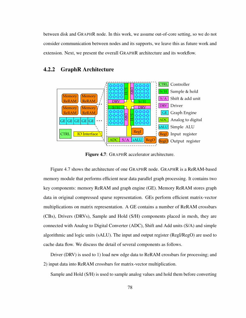
between disk and GRAPHR node. In this work, we assume out-of-core setting, so we do not
consider communication between nodes and its supports, we leave this as future work and
extension. Next, we present the overall GRAPHR architecture and its workflow.
4.2.2 GraphR Architecture
IO InterfaceCTRL
DRVS/H
S/HD
RV
S/HDRV
DRV
S/H
RegI
ADC S/A sALU RegO
MemoryReRAM
GEGE
MemoryReRAM
GE GE GE
CTRL
GE
DRV
S/H
RegO
RegI
sALU
S/A
Input registerOutput register
Simple ALU
Shift & add unitSample & hold
DriverGraph Engine
Controller
ADC Analog to digital
MemoryReRAM
MemoryReRAM
…
…
Figure 4.7: GRAPHR accelerator architecture.
Figure 4.7 shows the architecture of one GRAPHR node. GRAPHR is a ReRAM-based
memory module that performs efficient near data parallel graph processing. It contains two
key components: memory ReRAM and graph engine (GE). Memory ReRAM stores graph
data in original compressed sparse representation. GEs perform efficient matrix-vector
multiplications on matrix representation. A GE contains a number of ReRAM crossbars
(CBs), Drivers (DRVs), Sample and Hold (S/H) components placed in mesh, they are
connected with Analog to Digital Converter (ADC), Shift and Add units (S/A) and simple
algorithmic and logic units (sALU). The input and output register (RegI/RegO) are used to
cache data flow. We discuss the detail of several components as follows.
Driver (DRV) is used to 1) load new edge data to ReRAM crossbars for processing; and
2) input data into ReRAM crossbars for matrix-vector multiplication.
Sample and Hold (S/H) is used to sample analog values and hold them before converting
78

to a digital form.
Analog to Digital Converter (ADC) converts analog values to digital format. Because
ADCs have relatively higher area and power consumption, ADCs are not connected to every
bitlines of ReRAM crossbars in a GE but shared between those bitlines. If the GE cycle
is 64ns, we can have one ADC working at 1.0GSps to convert all data from eight 8-bitline
crossbars within one GE.
sALU is a simple customized algorithmic and logic unit. sALU performs operations
that cannot be efficiently performed by ReRAM crossbars, such as comparison. The actual
operation performed by sALU depends on algorithm and can be configured. We will show
more details when we discuss algorithms in Section 4.3.
Data Format is not practical for ReRAM cells to support a high resolution. Recent
work [256] reported 5-bit resolution on ReRAM programing. To alleviate the pressure
of diver, we conservatively assume the 4-bit ReRAM cell. To support higher computing
resolution, e.g., 16 bit, the Shift and Add (S/A) unit is employed. A 16-bit fixed point
number M can be represented as M = [M3,M2,M1,M0], where each segment Mi is a 4-bit
number. We can shift and add results from four 4-bit-resolution ReRAM crossbars, i.e.
D3 12+D2 8+D1 4+D0 to get a 16-bit result.
When sALU and S/A are bypassed, a graph engine could be simply considered as a
memory ReRAM mat. A similar scheme of reusing ReRAM crossbars for computing and
storing is employed in [88].
The I/O interface is used to load graph data and instructions into memory ReRAM
and controller, respectively. In GRAPHR, controller is the software/hardware interface
that could execute simple instructions to: 1) coordinate graph data movements between
memory ReRAM and GEs based on streaming-apply execution model; 2) convert edges in
preprocessed coordinate list (assumed in this work but can work with other representations
as well) in memory ReRAM to sparse matrix format in GEs; 3) perform convergence check.
79
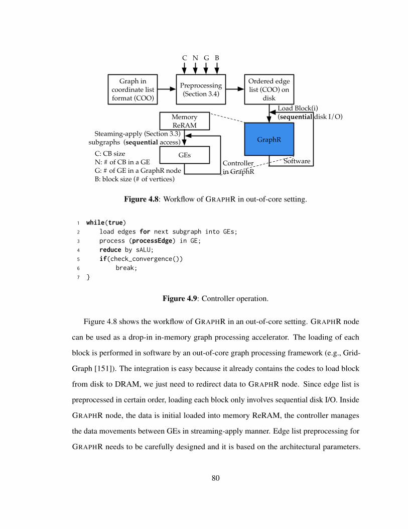
Graph in coordinate list format (COO)
Preprocessing(Section 3.4)
C N G B
Ordered edge list (COO) on
disk
GraphR
Memory ReRAM
GEs
Load Block(i)(sequential disk I/O)
Steaming-apply (Section 3.3) subgraphs (sequential access)
Controllerin GraphR
SoftwareC: CB sizeN: # of CB in a GEG: # of GE in a GraphR nodeB: block size (# of vertices)
Figure 4.8: Workflow of GRAPHR in out-of-core setting.
1 while(true)2 load edges for next subgraph into GEs;3 process (processEdge) in GE;4 reduce by sALU;5 if(check_convergence())6 break;7
Figure 4.9: Controller operation.
Figure 4.8 shows the workflow of GRAPHR in an out-of-core setting. GRAPHR node
can be used as a drop-in in-memory graph processing accelerator. The loading of each
block is performed in software by an out-of-core graph processing framework (e.g., Grid-
Graph [151]). The integration is easy because it already contains the codes to load block
from disk to DRAM, we just need to redirect data to GRAPHR node. Since edge list is
preprocessed in certain order, loading each block only involves sequential disk I/O. Inside
GRAPHR node, the data is initial loaded into memory ReRAM, the controller manages
the data movements between GEs in streaming-apply manner. Edge list preprocessing for
GRAPHR needs to be carefully designed and it is based on the architectural parameters.
80

Figure 4.9 shows the operations performed by controller.
4.2.3 Streaming-Apply Execution Model
GE
Subgraph
GEreduce (sALU)
reduce (sALU)
GE GEGE GE
Subgraph in GE (matrix)
Block in disk
(COO)
Block in GraphR (COO)
Block in disk
(COO)
Block in disk
(COO)
(a) Streaming-Apply: Column-major (GraphR)
(b) Streaming-Apply: Row-major
(c) Global processing order
RegI RegO
Figure 4.10: Streaming-apply execution model.
In GRAPHR, all GEs process a subgraph, the order of processing is important, since
it affects hardware resource requirement. We present streaming-apply execution model
shown in Figure 4.10. The key insight is that subgraphs are processed in a streaming
manner and the reductions are performed on the fly by sALU. There are two variants of
this model: column-major and row-major. During execution, RegI and RegO are used to
store source vertices and updated destination vertices. In column-major order in Figure 4.10
(a), subgraphs with same destination vertices are processed together. The required RegO
size is the same as the number of destination vertices in a subgraph. In row-major order in
Figure 4.10 (b), subgraphs with same source vertices are process together. The required
RegO size is the total number of destination vertices of all subgraphs with the same source
vertices. It is easy to see that row-major order requires larger RegO. On the other side,
row-major order incurs less read of RegI, — only one read is needed for all subgraphs
with same source vertices. In GRAPHR, we use column-major order since it requires less
registers, and in ReRAM, the write cost is higher than read cost.
Figure 4.10 (c) shows the global processing order in a complete out-of-core setting. We
81

see that the whole graph is partitioned into 4 blocks, three of them are stored in disk in COO
representation, one is stored in GraphR’s memory ReRAM also in COO representation.
Only the subgraph being processed by GEs is in sparse matrix format. Due to the sparsity
of graph data, if the subgraph is empty, then GEs can move down to the next subgraph.
Therefore, the sparsity only incurs waste inside the subgraph (e.g., when one GE has an
empty matrix but others do not).
4.2.4 Graph Preprocessing
To support streaming-apply execution model and conversion from coordination list rep-
resentation to sparse matrix format, edge list needs to be preprocessed so that edges of
consecutive subgraphs are stored together. It also ensures sequential disk and memory
access on block/subgraph loading. In the following, we explain the preprocessing procedure
in detail.
9
102
113
124
135
146
157
168
4133
4234
4335
4436
4537
4638
4739
4840
2517
2618
2719
2820
2921
3022
3123
3224
5749
5850
5951
6052
6153
6254
6355
6456
C=4
N=2G=2
GE 1
Subgraph Block
V=6431
63
31 63B=32
Figure 4.11: Preprocessing edge list.
82

Given some architectural parameters, the preprocessing is implemented in software and
performed only once. Figure 4.2.4 illustrates these parameters and the subgraph order we
should produce. This order is determined by streaming-apply model. C is the size of CB; N
is the number of CBs in a GE; G is the number of GEs in a GRAPHR node; and B is the
number of vertices in a block (i.e., block size). Also, V is the number of vertices in the
graph. Among the parameters, C, N and G specify the architecture setting of a GRAPHR
node, B is determined by the size of memory ReRAM in the node. In the example, the
graph has 64 vertices (V = 64) and each block has 32 vertices (B = 32), so the graph is
partitioned into 4 blocks, each one will be loaded from disk to GRAPHR node. Further,
C = 4,N = 2,G = 2, so the subgraph size is C× (C×N×G) = 4× (4×2×2) = 4×16.
Therefore, each block is partitioned into 16 subgraphs, the number of each is the global
subgraph order. Our goal is to produce an ordered edge list according this order so that
edges could be loaded sequentially.
Before presenting the algorithm, we assume that the original edge list is first ordered
based on source vertex and then for all edges with the same source, they are ordered by
destination. In another word, edges are stored in row-major order in matrix view. We also
assume that in the ordered edge list, edges in a subgraph is stored in column-major order.
Considering the problem in matrix view, each edge (i, j), we first compute a global order ID
(I(i, j)), so we have a 3-tuple: (i, j, I(i, j)). This global order ID takes all zeros into account, for
example, if there are k zeros between two edges in the global order, the different of global
order ID of them is still k. Then, all 3-tuples could be sorted by I(i, j). The ordered edge list
is obtained if we output them according to this order. The space and time complexity of this
procedure are O(V ) and O(V logV ), respectively, with common method. The key problem
here is to compute I(i, j) for each (i, j). Without confusion, we simply denote I(i, j) as I. We
show that I can be computed in a hierarchical manner.
Let BI denote the global block order of the block that contains (i, j). We assume that
83
blocks are also processed in column-major order: B(0,0)→ B(1,0)→ B(0,1)→ B(1,1). The
coordinates of a block B are:
Bi =
⌊iB
⌋,B j =
⌊jB
⌋(4.1)
Based on column-major order, BI is:
IB = B j +(V/B)×B j (4.2)
We assume that B can divide V , and similarly, C can divide B, C×N×B can divide B.
Otherwise, we can simply pad zeros to satisfy the conditions, it will not affect the results
since these zeros do not correspond to actual edges. The block corresponding to BI start
with the following global order ID:
start global ID(BI) = BI×B2/(C2×N×G)+1 (4.3)
Next, we compute SI, (i, j)’s global subgraph ID. The coordinates of the edge from the
start of a block BI (Bi,B j) are:
i′ = i−Bi×B, j′ = j−B j×B (4.4)
The relative coordinates of the subgraph from the start of correspond block are:
SIi′ =
⌊i′
C
⌋,SI j′ =
⌊j′
C×N×G
⌋(4.5)
Then, we can compute SI:
SI = (Si′+S j′×B/C)+ start global ID(BI)
= (Si′+S j′×B/C)+BI×B2/(C2×N×G)+1(4.6)
Finally, we compute SubI, the relative order of (i, j) from its corresponding subgraph
(SI). The coordinates are:
SubIi = i− (B×Bi)− (Si×C),
SubI j = j− (B×B j)− (S j×C)(4.7)
84
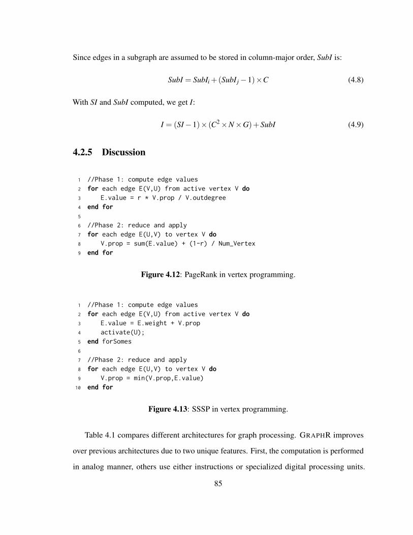
Since edges in a subgraph are assumed to be stored in column-major order, SubI is:
SubI = SubIi +(SubI j−1)×C (4.8)
With SI and SubI computed, we get I:
I = (SI−1)× (C2×N×G)+SubI (4.9)
4.2.5 Discussion
1 //Phase 1: compute edge values2 for each edge E(V,U) from active vertex V do3 E.value = r * V.prop / V.outdegree4 end for5
6 //Phase 2: reduce and apply7 for each edge E(U,V) to vertex V do8 V.prop = sum(E.value) + (1-r) / Num_Vertex9 end for
Figure 4.12: PageRank in vertex programming.
1 //Phase 1: compute edge values2 for each edge E(V,U) from active vertex V do3 E.value = E.weight + V.prop4 activate(U);5 end forSomes6
7 //Phase 2: reduce and apply8 for each edge E(U,V) to vertex V do9 V.prop = min(V.prop,E.value)10 end for
Figure 4.13: SSSP in vertex programming.
Table 4.1 compares different architectures for graph processing. GRAPHR improves
over previous architectures due to two unique features. First, the computation is performed
in analog manner, others use either instructions or specialized digital processing units.
85

Table 4.1: Comparison of different architectures for graph processing.
CPU GPU Tesseract[187]
GAA [186] Graphicionado[185]
GRAPHR
ProcessEdge
Instruction Instruction Instruction SpecializedAU
Specialized unit ReRAM cross-bar
Reduce Instruction Instruction Instructionand inter-cubecommunica-tion
SpecializedAPU/SCU
Specialized unit ReRAM cross-bar or sALU
ProcessingModel
Sync/Async Sync Sync Async Sync Sync
DataMovement
Disk to memory(out-of-core);Memory hierar-chy
Disk to mem-ory; CPU/GPUmemory; GPUmem. hierarchy
Betweencubes (in-memoryonly)
Betweenmemory andaccelerator(in-memoryonly)
Between mod-ules in memorypipeline; mem-ory to SPM;SPM to/fromprocessingunits.
Disk to memory(out-of-core)or betweenGRAPHR nodes(multi-node);Between mem-ory ReRAMand GEs (insideGRAPHR)
MemoryAccess
Random: vertex access and start of edge list of a vertex; Reduced ran-dom withSPM.
Sequential edgelist.
Sequential: edge list. Pipelined mem-ory access
Generality All algorithms Vertex program Vertex programin SpMV
This provides the excellent energy efficiency. Second, all disk and memory accesses in
GRAPHR are sequential, this is due to preprocessing and less flexibility in scheduling
vertices. It is a good trade-off because it is highly energy efficient to perform parallel
operations in ReRAM CBs. We believe that GRAPHR is the first architecture scheme using
ReRAM CBs to perform graph processing, and the work presents detailed and complete
solution to integrate it as a drop-in accelerator for out-of-core graph processing systems.
The architecture, streaming-apply execution model and the preprocessing algorithms are
all novel contributions. Also, GRAPHR is general because it could accelerate all vertex
programs that can be performed in SpMV form.
4.3 Mapping Algorithms in GE
In this section, we discuss two patterns when mapping algorithms to GEs: parallel MAC
and parallel add-op. We use a typical example for each category (i.e., PageRank and SSSP,
86
respectively) to explain the insights. More examples (but not all) of supported algorithms in
GRAPHR are listed in Table 4.2. The first two are parallel MAC pattern and the last two are
parallel add-op pattern.
4.3.1 Parallel MAC
In an algorithm, if processEdge function performs a multiplication, which can be performed
in each CB cell, we call it parallel MAC pattern. The parallelization degree is roughly
(C×C×N×G) (see parameter in Figure 4.8).
PageRank [128] is an excellent example of this pattern. Figure 4.12 shows its vertex
program. It does the following iterative computation:−→PRt+1 = rM ·−→PRt +(1− r)−→e .
−→PRt is
the PageRank at iteration t, M is a probability transfer matrix, r is the probability of random
surfing and −→e is a vector of probabilities of staying in each page.
We consider a small subgraph that could be processed by a 5×4 CB (the additional row
is to perform addition). It contains at most 16 edges represented by the intersection of 4 rows
and 4 columns in the sparse matrix (shown in Figure 4.15 (a)). Thus, the block is related to 8
vertices (i.e., i0∼ i3, j0∼ j3). The following are the parameters for the 4 × 4 block PageR-
ank shown in Figure 4.15 (b1): M = [0,1/2,1,0;1/3,0,0,1/2;1/3,0,0,1/2;1/3,1/2,0,0]
,−→e = [1/4,1/4,1/4,1/4]T, r = 4/5.
We define M0 = rM and −→e0 = (1− r)−→e , so that−→PRt+1 = M0
−→PRt +
−→e0 . In CB in
Figure 4.15 (b2, b3), the values are already scaled with r. Figure 4.15 (b3) shows the
mapping of PageRank algorithm to a CB. The additional row is used to implement the
addition of −→e0 . The sALU is configured to perform add operation in the reduce function to
add PageRank values (Figure 4.14 (a)). To check convergence, the new PageRank value is
compared with it in the previous iteration, the algorithm is converged if the difference is
less than a threshold.
87

2 4 53
7 2 31
sALU reg(old)
9 6 84reg(new)
3 9 42
5 6 47
sALU reg old)
3 6 42reg(new)(b)(a)
Figure 4.14: The configuration of sALU to perform (a) add in PageRank and (b) min inSSSP.
4.3.2 Parallel Add-Op
In an algorithm, if processEdge function performs an addition, which can be performed in
for each CB row at a time, we call it parallel add-op pattern. The op specifies the operation
in reduce that is implemented in sALU. The parallelization degree is roughly (C×N×G).
Single Source Shortest Path (SSSP) [270] is a typical example of this pattern. Figure 4.13
shows the vertex program. We see that processEdge performs an addition and reduce
performs min operation. Therefore, sALU is configured to perform min operation shown in
Figure 4.14 (b).
In SSSP, each vertex v is given a distance label dist(v) that maintains the length of the
shortest known path to vertex v from the source. The distance label is initialized to 0 at the
source and ∞ at all other nodes. Then the SSSP algorithm iteratively applies the relaxation
operator, which is defined as follows: if (u,v) is an edge and dist(u)+w(u,v) < dist(v),
the value of dist(v) is updated to dist(u)+w(u,v). An active vertex is relaxed by applying
this operator to all the edges connected to it. Each relaxation may lower the distance label
of some vertex, and when no further lowering can be performed anywhere in the graph, the
resulting vertex distance labels indicate the shortest distances from the source to the vertex,
regardless of the order in which the relaxations were performed. Breadth-first numbering of
a graph is a special case of SSSP where all edge labels are 1.
We explain the mapping of SSSP algorithm to a CB using a small 8-vertex subgraph
88

SrcDst 0000
i0i1i2i3
i0(4 i1:3 i3:2i2:11
5 31 1
j0:7 j1:6 j3:Mj2:M
Src
Dst 31-
j0:7 j1:5 j3:4j2:3Dst 2 4
(b2)
/
/
/
/
0 0 0 0
) )
) )
) ) ) )
) ) )
/
/
/
/
0 0 0 0
(c1)
Src
Dst
Src
Dst
(c2)
i0:1/4
i1:1/4
i3:1/4
i2:1/4
1/3
1/3
1/3
j0 j1 j3j2
Src
Dst
(b1)
1/2 1/2
1
1/2
1/2
1/4
9/60 13/60 25/60
1/41/4
1/41
13/60
(b3)
) )
) )
) ) ) )
) ) )
min
7 6 M M
min min min
Dst 2 4
41
7 5 9 M
M 5 9 M
) )
) )
) ) ) )
) ) )
min
7 5 9 M
min min min
31
7 5 6 4
M M 6 4
) )
) )
) ) ) )
) ) )
min
7 5 6 4
min min min
11
7 5 6 4
M M M M
) )
) )
) ) ) )
) ) )
min
7 5 6 4
min min min
21
7 5 3 4
M M 3 M
( ) t=4( ) t=3( ) t=2( ) t=1
31
2
12
2
Dst 31-
i0
i1
i2
i3Src
(RegI)
(RegO)
(a)
Figure 4.15: The processing of (a) PageRank and (b) SSSP in GRAPHR
corresponding to a 4 × 4 block in sparse matrix, as shown in Figure 4.15 (c1). It can
be represented by adjacency matrix: W = [M,1,5,M;M,M,3,1; M,M,M,M;M,M,1,M]
where M indicates no edge connected two vertices and M is set to a reserved maximum
value for a memory cell in a CB. The values are stored in the CB shown in Figure 4.15 (c2).
Given a vertex u and dist(u), the row in the adjacency matrix W for u indicates w(u,v).
We could perform the relaxation operator (i.e., addition) for u in parallel. Here, SpMV is
only used to select a row in CB by multiplying with an one-hot vector.
The relaxation operator of u involves reading: 1) dist(u): it is computed iteratively from
the source, for the source vertex, the initial value is zero; 2) The vector of the dist(v) before
the relaxation operator: it is a vector indicating the distance between source and all other
vertices and is also computed iteratively from the source. In our example, for the source
vertices (i0, i1, i2, i3), the initial value is [4,3,1,2]; 3) The vector of the w(u,v): it is the
89
distance from u to the destination vertices in the subgraph, and can be obtained by reading a
row in adjacency matrix W.
Figure 4.15 (c3) shows the process to perform SSSP in a 5 × 4 CB. The last row (green
squares) is set to a fixed value 1, which is used to add dist(u) (the input to the last wordline)
to each w(u,v) in the relaxation operator. The initial value for dist(u) for the destination
vertices ( j0, j1, j2, j3) are [7,6,M,M]. The vector of w(u,v) is obtained by activating the
wordline associated to vertex v. In the time slot (t = 1), wordline 0 (for source vertex i0) is
activated (the red square with input value 1) and a value 4 (this is the current value in dist(v)
for source i0) is input to the last wordline (the green box line). The vector of the dist(v)
for the destination vertices (( j0, j1, j2, j3)) is set as the value of the output at each bitline,
which is [7,6,M,M]. With this mapping, the current summation in bitline in Figure 4.15
(c3-1) is [1×M+4×1,1×1+4×1,1×5+4×1,1×M+4×1] = [M,5,9,M]. It is the
dist(u)+w(u,v) computed in parallel, where u is the source vertex. Then the distance
of source to each vertex v is compared with the initial dist(v) ([7,6,M,M]) by an array
of comparators, and in the final output of bitline, we get [7,5,9,M], which is the updated
dist(v) vector after time slot t = 1. The parallel comparisons are performed by vertex-related
operations in. Different algorithms may require different functions on vertices.
Table 4.2: Property and operations of applications in GRAPHR.
Applications Vertex Property processEdge()SpMV Multiplication Value E.value = V.prop / V.outdegree * E.weightPageRank Page Rank Value E.value = r * V.prop / V.outdegreeBFS Level E.value = 1 + V.propSSSP Path Length E.value = E.weight + V.prop
Applications reduce() Ative Vertex ListSpMV V.prop = sum(E.value) Not RequiredPageRank V.prop = sum(E.value) + (1-r) / Num Vertex Not RequiredBFS V.prop = min(V.prop,E.value) RequiredSSSP V.prop = min(V.prop,E.value) Required
After time slot t = 1, we move to the next vertex in Figure 4.15 (c3-2), where we i)
90

activate the second wordline; ii) change the input to the last wordline to 3 (the distance
label for source vertex i1); and iii) set the intermediate dist(v) to be the final output of
bitline in time slot t = 1, which is [7,5,9,M]. Similar as Figure 4.15 (c3-1), the the current
summation in bitline is [M,M,6,4] and it is compared with [7,5,9,M], yielding the final
output of bitline for time slot t = 2 as [7,5,6,4]. We indicate the updated distance label
using orange squares. The operations in time slot t = 3 and t = 4 can be performed in the
similar manner.
Initially, before processing the block, the active indicator for each destination vertex
is set to be FALSE. After the serial processing in CB, the active indicators for all vertices
which have been updated (marked in orange in Figure 4.15 (c3)) are set to be TRUE. This
indicates that they are active for next iteration. In our example, j1, j2, j3 are marked active.
Referring to Figure 4.15, this means that the distance labels for these vertices have been
updated. Because we are processing the block in CB, the active indicator for destination
vertex may be accessed for multiple times, but if it is set be TRUE at least one time, this
vertex is active in next iteration. Globally, after all active source vertices and corresponding
edges are processed in an iteration, source vertex properties (values and active indicators)
that hold the old values are updated by the properties of the same vertices in destination.
The new source vertex properties are used in the next iteration. We can check if there are
still active vertices to determine the convergence.
4.4 Evaluation
4.4.1 Graph Datasets and Applications
Table 4.3 shows the datasets used in our evaluation. We use seven real-world graphs. For
WikiVote(WV), Slashdot(SD), Amazon(AZ), WebGoogle(WG), LiveJournal(LJ), Orkut(OK)
and Netflix(NF). We run pagerank(PR), breadth first search(BFS), single source shortest
path (SSSP) and sparse matrix-vector multiplication (SpMV) on the first six datasets. On
91

Table 4.3: Graph datasets.
Dataset # Vertices #EdgesWikiVote(WV) [269] 7.0K 103KSlashdot(SD) [269] 82K 948KAmazon(AZ) [269] 262K 1.2M
WebGoogle(WG) [269] 0.88M 5.1MLiveJournal(LJ) [269] 4.8M 69M
Orkut(OK) [271] 3.0M 106MNetflix(NF) [272] 480K users, 17.8K movies 99M
Netflix(NF), we run collaborative filtering(CF), and the feature length used is 32.
4.4.2 Experiment Setup
In our experiments, we compare GRAPHR with a CPU baseline platform, a GPU platform
and PIM-based architecture [187]. PR, BFS, SSSP and SpMV running on the CPU platform
are based on the software framework GridGraph [151], while collaborative filtering is
based on GraphChi [152]. PR, BFS, SSSP and SpMV running on GPU platform are based
on Gunrock [273], while CuMF SGD [274] is the GPU framework for CF. We evaluate
PIM-based architecture on zSim [275], a scalable x86-64 multicore simulator. We modified
zSim with HMC memory and interconnection model, heterogeneous compute units, on-chip
network and other hardware features. The results are validated results with NDP [276],
which also extends zSim for HMC simulation. In all experiments, graph data could fit in
memory. We also exclude the disk I/O time from the execution time of the CPU/GPU-based
platform.
Specifications of the CPU and GPU platforms are shown in Table 4.4 and Table 4.5.
The CPU energy consumption is estimated by Intel Product Specifications [277] while
NVIDIA System Management Interface (nvidia-smi) is used to estimate energy consump-
tion by GPU. The execution times for CPU/GPU platform are measured in the computing
frameworks.
92

Table 4.4: Specifications of the CPU platform.
CPU Intel Xeon E5-2630 V3,8 cores, 2.40 GHz8× (32+32)KB L1 Cache8×256KB L2 Cache20 MB L3 Cache
Memory 128 GBStorage 1 TB2 CPUs, a total number of 32 threads.
Table 4.5: Specifications of the GPU platform.
Graphic Card NVIDIA Tesla K40cArchitecture Kepler# CUDA Cores 2880Base Clock 745 MHzGraphic Memory 12 GB GDDR5Memory Bandwidth 288 GB/sCUDA Version 7.5
To evaluate GRAPHR, for the ReRAM part, we use NVSim [184] to estimate time and
energy consumption. The HRS/LRS resistance are 25M/50K Ω, read voltage (Vr) and
write voltage (Vw) are 0.7V and 2V respectively, and current of LRS/HRS are 40 uA and
2 uA respectively. The read/write latency and read/write energy cost used are 29.31ns /
50.88ns, 1.08 pJ / 3.91nJ respectively from data reported in [264]. The programming of
a bipolar ReRAM cell is to change (from High to Low) or inverse. For multi-level cell,
the programming is to change the resistance to a middle state between High and Low, and
the middle state is determined by the programming voltage pulse length. Actually, the
difference between High and Low is the worse case. Note that [256,262] describe a ReRAM
programming prototype, which includes: 1) writing circuitry; 2) ReRAM cell/array; and 3)
conversion circuitry. They demonstrated the possibility of 1% accuracy for multi-level cell.
However, in a real production system, only “writing circuitr” and “ReRAM cell/array” are
needed, there is no need to consider the conversion, as we just need to “acquiesce” a writing
precision. Therefore, this energy cost estimation for 4-bit cell programming is reasonable
93

and more conservative than two recent ReRAM-based accelerators [88, 89].
For on-chip registers, we use CACTI 6.5 [278] at 32nm to model. For Analog/Digital
converters, we use data from [279]. The system performance is modeled by code instrumen-
tation. The ReRAM crossbar size S, number of ReRAM crossbars per graph engine C and
number of graph engines is 8, 32, 64 respectively.
4.4.3 Performance Results
Figure 4.16 compares the performance of GRAPHR and CPU platform. The CPU implemen-
tation is used as the baseline and execution times of applications of GRAPHR are normalized
to it. Compared to CPU platform, the geometric mean of speedups with GRAPHR archi-
tecture on all 25 executions is 16.01×. Among all applications on the datasets, the highest
speedup achieved by GRAPHR is 132.67×, and it happens on SpMV on WikiVote dataset.
The lowest speedup GRAPHR achieved is 2.40×, on SSSP using OK dataset. PageRank and
SpMV are parallel MAC pattern and have higher speedup compared to CPU-based platform.
For BFS and SSSP which are parallel add-op pattern, GRAPHR achieves lower speedups
only due to parallel addition.
PageRank BFS SSSP SpMVWV SD AZ WG LJOK WV SD AZ WG LJOK WV SD AZ WG LJOK WV SD AZ WG LJOK CF Gm
1
10
100140
CPUGraphR
Figure 4.16: GRAPHR speedup normalized to CPU platform.
94

PageRank BFS SSSP SpMVWV SD AZWG LJOK WV SD AZWG LJOK WV SD AZWG LJOK WV SD AZWG LJOK CFGm
1
10
100
230CPUGraphR
Figure 4.17: GRAPHR energy saving normalized to CPU platform.
4.4.4 Energy Results
Figure 4.17 shows the energy savings in GRAPHR architecture over CPU platform. The
geometric mean of energy savings of all applications compared to CPU is 33.82×. The
highest energy achieved by GRAPHR is 217.88×, which is on sparse matrix-vector multipli-
cation on SD dataset. The lowest energy saving achieved by GRAPHR happens on SSSP on
OK dataset, which is 4.50×. GRAPHR gets the high energy efficiency from the non-volatile
property of ReRAM and the in-situ computation capability.
4.4.5 Comparison to GPU Platform
GPUs take advantage of a large amount of threads (CUDA cores) for high parallelism.
The GPU used in the comparison has 2880 CUDA cores, while in GRAPHR we have a
comparable number (2048= 32×64) of crossbars. To compare with GPU, we run PageRank
and SSSP on LiveJournal dataset, and collaborative filtering(CF) on Netflix dataset.
The performance and energy saving normalized to CPU are shown in Figure 4.18 (a)
and (b). Overall, the performance of GRAPHR is higher than GPU with considering the
data transfer time between CPU memory and GPU memory, — an overhead GRAPHR
does not incur. GRAPHR has performance gains ranging from 1.69× to 2.19× compared
to GPU. More importantly, GRAPHR consumes 4.77× to 8.91× less energy than GPU.
95

PR SSSP CF
1
10
60CPUGPUGraphR
PR SSSP CF
1
10
30CPUGPUGraphR
(a) Performance (b) Energy Saving
Figure 4.18: GRAPHR (a) performance and (b) energy saving compared to GPU platform.
Figure 4.18 (a) shows that, GRAPHR achieves higher speedups on PageRank and CF, where
MACs dominate the computation and are fully supported by GRAPHR and GPU. For SSSP,
the vertex-related traversing in GRAPHR requires accessing to main memory and storage.
In GPU, a cache based memory hierarchy better supports the random accessing. So the
speedup of GRAPHR is lower. The reason why GRAPHR still has gain in SSSP is due to
sequential access pattern. For energy saving, GRAPHR is better than GPU. Besides energy
saving by in-situ computation in GEs and the in-memory processing system design, from
Fig 17 in [185] we see that in conventional CMOS system, static energy consumption by
eDRAM (memory) incurs the majority of energy consumption. As the technology node
scales down, leakage power dominates in CMOS system. In contrast, ReRAM has almost 0
static energy leakage, so GRAPHR has higher energy saving.
4.4.6 Comparison to PIM Platform
We compare GRAPHR with a PIM-based architecture (i.e., Tesseract [187]). The perfor-
mance and energy saving normalized to CPU are shown in Figure 4.19 (a) and (b). GRAPHR
gains a speedup of 1.16× to 4.12×, and is 3.67× to 10.96× more energy efficiency com-
pared to PIM-based architecture.
96

WV AZ LJ WV AZ LJ
1
10
50
Performance
CPUPIMGraphR
WV AZ LJ WV AZ LJ
1
10
100200
Energy Saving CPU
PIMGraphR
PageRank PageRankSSSP SSSP
(a) Performance (b) Energy Saving
Figure 4.19: GRAPHR (a) performance and (b) energy saving compared to PIM platform.
4.4.7 Sensitivity to Sparsity
We use #Edge/(#Vertex)2 to represent the density of a dataset, and with the density decreases,
the sparsity increases. Figure 4.20 (a) and (b) shows the performance and energy saving of
GRAPHR (compared to the CPU platform) with the density of datasets. With the sparsity
increases, the performance and energy saving slightly decreases. Because with the sparsity
increases, the number of edge blocks to be traversed will increase, which slows down the
edge accessing time and consumes more energy.
WV SD AZ WG LJ
1
10
100200
Energy Saving
PRSSSP
10-3
10-2
10-1
100
Sparsity
WV SD AZ WG LJ
1
10
50
Performance
PRSSSP
10-3
10-2
10-1
100
Sparsity
(a) Performance (b) Energy Saving
Den
sity
Den
sity
Figure 4.20: GRAPHR (a) performance and (b) energy saving v.s. dataset density.
97
Chapter 5
Low-Cost Floating-Point Processing in ReRAM
5.1 Background
5.1.1 MVM Acceleration in ReRAM
Resistive Random Access Memory (ReRAM) [125, 280] has recently demonstrated tremen-
dous potential to efficiently accelerate the computing kernel, i.e., MVM, in machine learning
models. Conceptually, each element in a matrix M is mapped to the conductance state of
an ReRAM cell, while the input vector x is encoded as voltage levels that are applied on
the wordlines of the ReRAM crossbar. In this way, the current accumulation on bitlines
is proportional to the dot-product of the stored conductance and voltages on the word-
lines, representing the result y = M×x. Such in-situ computation significantly reduces the
costly memory access in MVM processing engines [256], and mostly importantly, provides
massive opportunities to exploit the inherent parallelism in an N×N ReRAM crossbar.
ReRAM-based MVM processing engines are fixed-point hardware in nature due to the
fact that the matrix and the vector are respectively represented in discrete conductance states
and voltage levels [125]. If ReRAM is used to support floating-point MVM operation, a
large number of crossbars will be provisioned for mantissa alignment, resulting in very high
hardware cost. Fortunately, the fixed-point precision requirement is acceptable for machine
learning applications thanks to the low-precision and quantized neural network algorithms
[173, 281–285]. Many fixed-point based accelerators [88, 89, 91, 92, 218, 222, 223, 286] are
built with the ReRAM MVM processing engine and achieve reasonably good classification
accuracy.
98

0 1 0 11 1 0 11 0 0 01 0 1 1
0 1 1 00 1 0 00 1 0 11 1 0 1
0101
M-b3 M-b2
V-b3
0 0 1 11 1 1 00 0 1 01 1 0 1
M-b10 1 1 11 0 1 01 1 0 10 0 1 1
M-b0
2 1 1 2O0 1 2 0 1 2 2 1 1 1 0 2 1
1111
V-b2
1010
V-b1
0001
V-b0
C1
2 1 1 2S1 1 2 0 1 2 2 1 1 1 0 2 1+<<
3 2 1 3 1 4 1 2 2 2 3 2 2 2 3 3O1
0 0 0 0 0 0 0 0 0 0 0 0 0 0 0 0S0
7 4 3 7 3 8 1 4 6 6 5 4 4 2 7 5S2+<<
+<<
C2
C31 1 0 1 0 2 1 1 0 0 2 1 1 2 1 2O2
S3 6 18 3 9 12 12 12 9 9 6 15 12
+<<
C41 0 1 1 1 1 0 1 1 1 0 1 0 0 1 1O3
S4 31 18 13 31 13 37 6 19 25 25 24 19 18 12 31 25 C5+<<
75 73 32 81+<<
C6
C7
S 368 354 207 387
175171 88 181+<<
15 9 6 15
Figure 5.1: Fixed-point (integer) MVM in ReRAM.
368354207387
d
=
0 13 7 1111 14 3 89 5 2 514 6 9 15
T
d
×
612613
d
=
0000 1101 0111 10111011 1110 0011 10001001 0101 0010 01011110 0110 1001 1111
T
b
×
0110110001101101
b
, (5.1)
Figure 5.1 shows an example of computing fixed-point MVM in Eq. (5.1) by utilizing
ReRAM-based MVM engine with single-bit precision. Before computation, decimal
99

integers in both the matrix and the vector are converted to binary bits, where we set the
precision for the matrix and input vector are 4-bit. The matrix is bit-sliced into 4 one-bit
matrices and then mapped to four crossbars, i.e., M-b3, M-b2, M-b1 and M-b0 in Figure
and the input vector is bit-sliced into 4 one-bit vectors, i.e., V-b3, V-b2, V-b1 and V-b0.
The multiplication is performed in pipeline. The multiplication results in each crossbars
are initiated by a zero vector S0. In the first cycle C1, the most significant bit (MSB)
vector V-b3 is applied on wordlines of the four crossbars, and the multiplication results,
denoted by O0, of V-b3 with M-b3, M-b2, M-b1 and M-b0 are obtained in parallel. In
cycle C2, S0 is right-shifted by 1 bit to get S1, and V-b2 is input to the crossbars to get the
multiplication results O1. Similar operations are performed in C3 and C4. After C4, we get
S4, the multiplication results of the input vector with four bit-slices if the matrix. In the
following threes cycles C5 to C7, we shift and add S4 from the four crossbars to get the
final multiplication result. For the fixed-point multiplication of an NM-bit matrix with an
Nv-bit vector, the processing cycle count is Cint = Nv +(NM−1).
5.1.2 Fixed-Point and Floating-Point
…63 52 0
sign exp (11 bits) frac (52 bits)
(a) (b)
7 0
sign
Figure 5.2: The bit layout of an (a) 8-bit signed integer and (b) a 64-bit double-precisionfloating-point number.
We use an 8-bit signed integer and an IEEE 754-2008 standard [287] 64-bit double-
precision floating-point number as an example to compare the difference between fixed-point
and floating-point numbers. Typically, these designs refer to the format used to store and
manipulate the digital representation of the data. As demonstrated in Figure 5.2 (a), fixed-
100
point numbers represent integers – positive and negative whole numbers – via a sign bit
followed by multiple (e.g., i-bit) value bits, yielding a data range of −2i to 2i−1. IEEE 754
double-precision floating-point numbers shown in Figure 5.2 (b) are designed to represent
and manipulate rational numbers, where a number is represented with one sign bit (s), 11-bit
exponent (e), and 52-bit fraction (b51b50...b0). The value of a double-precision floating-
point is interpreted as (−1)s× (1.b51b50...b0)×2(e−1023), yielding a dynamic data range
from ±2.2×10−308 to ±1.8×10308.
Different data formats have different computational performance, and hence resulting
in different final precision. From data storage perspective, the storage characteristic and
space required for fixed-point and floating-point numbers are also significantly different.
The choice of appropriate data format is influenced by both the application’s computational
accuracy requirements and the available hardware storage resources. However, in general,
floating-point is a norm for high-precision computations because it can support a wider
range of data values with the ability to precisely represent very small or very large numbers.
5.1.3 Scientific Computing
1 initiate x = x02 while (not converge) do3 //Step 1: compute the residual4 r = b - A * x5 //Step 2: compute the correction6 compute p7 //Step 3: update the current solution8 x = x + p9 end while
Code 5.1: The iterative solver.
Scientific computing is an interdisciplinary science that solves computational problems
in a wide range of disciplines including physics, mathematics, chemistry, biology, engineer-
ing, and other natural sciences subjects [288–290]. Those complex computing problems are
101

normally modeled by systems of large-scale Partial Differential Equations (PDEs). Since
it is almost impossible to directly solve the analytical solution of those PDEs, a common
practice is to discretize continuous PDEs into a linear model Ax = b [166, 167] to be solved
by numerical methods. The numerical solution of this linear system is usually obtained by
an iterative solver [291–293]. Code 5.1 illustrates a typical computing process in iterative
methods. The vector x that needs to be solved is firstly initialized usually to an all-zero
vector x0, followed by three steps in the main body: (1) the residual (error) of the current
solution vector is calculated as r = b−Ax; (2) to improve the performance of the estimated
solution, a correction vector p is computed based on the current residual r; (3) the current
solution vector is improved by adding the correction vector as x = x+p, aiming to reduce
the possible residuals produced in the next calculation iteration. The iterative solver stops
when a defined convergence criteria is satisfied. Two widely used convergence criteria
are (1) that the iteration index is less than a preset threshold K or (2) that the L-2 norm
of the residual (res = ||b−Ax||2) is less than a preset threshold τ . Notably, all the values
involved in Code 5.1 are implemented as double-precision floating-point numbers to meet
the high-precision requirement of mainstream scientific applications.
The various iterative methods follow the above computational steps and differ only in
the calculation of the correction vectors. Among all candidate solutions, Krylov subspace
approach is the standard method today. In this work, we focus on two representative Krylov
subspace solvers – Conjugate Gradient (CG) [294] and Stabilized BiConjugate Gradient
(BiCGSTAB) [295]. The computational kernels of these two methods are large-scale sparse
floating-point matrix-vector multiplication y = Ax as aforementioned, which requires the
support of floating-point precision computation, imposing significant challenges to the
underlying computing hardware.
102
5.2 Motivation and REFLOAT Ideas
5.2.1 Motivation
Given the huge success of ReRAM-based high-parallel MVM engines in machine learn-
ing [88, 89, 91, 92, 221, 286], it is naturally attractive to design accelerators that extend
ReRAM-based computing support to floating-point SpMV in scientific computing. Un-
fortunately, existing ReRAM-based accelerators are limited to models that have inherent
tolerance for low-precision fixed-point approximation (e.g., machine learning) and are rarely
explored to support floating-point processing in scientific computing. To bridge this gap, the
most relevant work along this direction is proposed in [189]. In this work, the sparse matrix
in scientific computing is first partitioned into multiple blocks. Each floating-point element
in the block is converted to a fixed-point number by adding approximately the same number
of padding bits as the effective data bit. The fixed-point number with extended bits are then
deployed onto the fixed-point ReRAM crossbars [189] for processing. In order to facilitate
the quantitative assessment of system performance and hardware overhead, we carefully
selected the cycle number T and the crossbar number C as two metrics for measurement: (1)
T is directly related to the performance because a smaller T indicates higher performance
and vice versa, and (2) C directly reflects the ability to execute floating-point MVMs in
parallel under a limited number of on-chip ReRAMs [89,175,189]. Specifically, the smaller
C, the stronger the parallelism. The primary goal of this work focuses on techniques that
reduce the cost for floating-point processing in ReRAM.
Crossbar number. Supposing we are computing the multiplication of a matrix block M
with a vector segment v. In the matrix block M, the number of fraction bits is fM and the
number of exponent bits is eM. In the vector segment v, the number of fraction bits is fv
and the number of exponent bits is ev. To map the matrix fraction to ReRAM crossbars,
we need ( fM + 1) ReRAM crossbars because the fraction is normalized to a value with
a leading 1. For example, (52+1) crossbars are needed to represent the 52-bit fraction in
103

double floating-point precision in [189]. To map the matrix exponent to ReRAM crossbars,
we need 2eM ReRAM crossbars for eM-bit exponent states, which is called padding in [189]
where 64-bit paddings are needed for an eM = 6. Thus, C is calculated as
C = 4× (2eM + fM +1), (5.2)
where the leading multiplier 4 is contributed from sign bits of the matrix block and the
vector segment.
Cycle number. Supposing the precision of digital-analog converters is 1-bit as that in
[89, 189]. The number of value states in the vector segment is (2ev + fv +1).For each input
state, we need (2eM + fM +1) to perform the shift-and-add to reduce the partial results from
the ReRAM crossbars. For a higher computation efficiency, a pipelined input and reduce
scheme [89] is used. Thus, T is calculated as
T = (2ev + fv +1)+(2eM + fM +1)−1. (5.3)
Cycle/crossbar number vs. accuracy loss. The bit number (of exponents and fractions in
matrix blocks and vector segments) bridges the connection between the hardware cost and
the processing accuracy. A better configuration of bit numbers may lead to low hardware
cost, i.e., fewer cycles and crossbars, with an acceptable accuracy.
Cyc
les
Exponent Bit Number for Vector Exponent Bit Number
for Matrix
Cro
ssba
r N
umbe
r
Fraction Bit Number Exponent Bit Number
Cyc
les
Fraction Bit Number
for Matrix
Fraction Bit Number for Vector
(a) (b) (c)
108642002
46
8
3000
0
1000
2000
105040302010001020304050
500
550
600
650
5040302010002
46
80
10002000300040005000
10
The cycle number for (a) various configurations of exponent bit number for vector segment and matrix blockand (b) various configurations of fraction bit number for vector segment and matrix block and (c) the crossbar
number for various configurations of fraction and fraction bit number for matrix block.
Figure 5.3: The cycle number and crossbar number under various bit length.
104
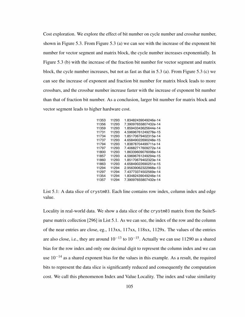
Cost exploration. We explore the effect of bit number on cycle number and crossbar number,
shown in Figure 5.3. From Figure 5.3 (a) we can see with the increase of the exponent bit
number for vector segment and matrix block, the cycle number increases exponentially. In
Figure 5.3 (b) with the increase of the fraction bit number for vector segment and matrix
block, the cycle number increases, but not as fast as that in 5.3 (a). From Figure 5.3 (c) we
can see the increase of exponent and fraction bit number for matrix block leads to more
crossbars, and the crossbar number increase faster with the increase of exponent bit number
than that of fraction bit number. As a conclusion, larger bit number for matrix block and
vector segment leads to higher hardware cost.
11353 11293 1.83482439049246e-1411356 11293 7.39097655807432e-1411359 11293 1.85943343625644e-1411731 11293 4.59696761249278e-1511734 11293 1.85170679402315e-1411737 11293 4.65849022690248e-1511794 11293 1.83878704499711e-1411797 11293 7.40682717609272e-1411800 11293 1.86339609076098e-1411857 11293 4.59696761249294e-1511860 11293 1.85170679402323e-1411863 11293 4.65849022690251e-1511294 11294 2.95639062322968e-1311297 11294 7.43773374502569e-1411354 11294 1.83482439049246e-1411357 11294 7.39097655807432e-14
List 5.1: A data slice of crystm03. Each line contains row index, column index and edgevalue.
Locality in real-world data. We show a data slice of the crystm03 matrix from the SuiteS-
parse matrix collection [296] in List 5.1. As we can see, the index of the row and the column
of the near entries are close, eg., 113xx, 117xx, 118xx, 1129x. The values of the entries
are also close, i.e., they are around 10−13 to 10−15. Actually we can use 11290 as a shared
bias for the row index and only one decimal digit to represent the column index and we can
use 10−14 as a shared exponent bias for the values in this example. As a result, the required
bits to represent the data slice is significantly reduced and consequently the computation
cost. We call this phenomenon Index and Value Locality. The index and value similarity
105

commonly exists because the sparse matrices are collocated from real-word scenarios. Thus
the elements in the matrix have spatial similarity with the nearby elements. The index and
value similarity also provide use the opportunity for low cost floating-point computing and
reduced memory size for the matrix.
5.2.2 Discussion
The bit numbers for exponent and fraction in matrix block contribute to the the number
C of crossbars required for one floating-point multiplication on a matrix block and the
processing cycle number T . The bit numbers for exponent and fraction in vector segment
contribute to the processing cycle number T . Lower bits lead to lower cost for floating-point
multiplication in ReRAM, thus a naive approach is to truncate bits for low computing
latency and resource demand. However, bit truncation may lead to significantly slower
convergence and, more importantly, nonvonvergence. We show the iteration numbers for
convergence under various exponent and fraction bit configurations in Table 5.1. In default
double-precision, it takes 80 iterations to convergence. If we fix the exponent bits and
truncate fraction bits, a 21-bit fraction takes 27 additional iterations and a fraction less
than 21 bits leads to nonconvergence. If we fix the fraction bits and truncate exponent
bits, 7-bit exponent increases the iteration number from 80 to 20620, and a exponent less
than 7 bits leads to nonconvergence. In state-of-the-art ReRAM accelerator for scientific
computing [189], to reduce the processing cost, Feinberg et al. assumed 6 bits for the
exponent (64-bit padding). The fatal problem in [189] is that the solvers are not functional
correct because of nonconvergence.
It is a challenge to reduce bit numbers for low-cost processing but maintain convergence
at the same time. To tackle this challenge, in this work, for low-cost floating-point processing
in ReRAM, we propose a data format rather than the default double-precision floating-point
format and an accelerator architecture to support the proposed data format.
106

Table 5.1: The iteration numbers for convergence under various exp(onent) and fra(ction)bit configurations for matrix crystm03.
exp 11 11 11 11 11 11frac 52 30 29 28 27 26#ite 80 82(+2) 82(+2) 83(+3) 83(+3) 84(+4)exp 11 11 11 11 11 11frac 25 24 23 22 21 20#ite 90(+10) 93(+13) 93(+13) 95(+15) 107(+27) NC
exp 10 9 8 7 6frac 52 52 52 52 52#ite 80 80 80 20620(+256×) NC
NC indicates nonconvergence.
5.3 REFLOAT Data Format
In this section, we introduce the REFLOAT data format and illustrate the conversion between
a coordinate (COO) format and REFLOAT. We also discuss how to perform computation on
REFLOAT format to achieve high performance with minimal hardware overhead.
5.3.1 ReFloat Overview
1 2 0 30 4 5 06 0 7 00 0 0 8 eb
1 2 0 30 4 5 06 0 7 00 0 0 8
1028
1029
1030
1031
15401542
15411543
0123
0 1 2 31028,1540)
(a) A block in full precision. (b) A block in ReFloat.
Figure 5.4: The conversion of index and value in floating-point format to REFLOAT format.
In general, we use ReFloat(b,e, f ) to represent the REFLOAT format, where b denotes
107

Table 5.2: List of symbols and descriptions.
Symbol DescriptionReFloat(b,e, f ) : ReFloat format notation.
2b The size of a square block.e The number of exponent bits for a matrix block.f The number of fraction bits for a matrix block.A A sparse matrix.b The bias vector for a linear system.x The solution vector for a linear system.r The residual vector for a linear system.a A scalar of A.
(a)e The exponent of a, (a)e ∈ 0,1,2, ....(a) f The fraction of a, (a) f ∈ (1,2).
Ac A block of the sparse matrix A.(i, j) The index for the block Ac.
(ii, j j) The index for the scalar a in the block Ac.(iii, j j j) The index for the scalar a in the matrix A.
ebThe number of bias bits for the exponents ofscalars in the block Ac.
ev The number of exponent bits for a vector segment.fv The number of fraction bits for a vector segment.
the matrix block size (the length and width of a square matrix block) is 2b, e and f
respectively denote the number of bits for the exponent and the fraction. The symbols and
corresponding descriptions related to REFLOAT are listed in Table 5.2.
We use Figure 5.4 to illustrate the idea of REFLOAT. As shown in Figure 5.4 (a), each
scalar is in 64-bit floating-point format. It requires a 32-bit integer for row index and a
32-bit integer for column index to locate each element in the matrix block. Therefore, we
will use 8× (32+ 32+ 64) = 1024 bits for storage of the eight scalars. In this example,
assuming we use the ReFloat(2,2,3) format as depicted in Figure 5.4 (b). Alternatively,
(1) each scalar in the block can be indexed by two 2-bit integers; (2) the element value is
represented by a 1+ 2+ 3 = 6-bit floating point; (3) the block is indexed by two 30-bit
integers and (4) a 11-bit exponent bias eb is also recorded. Therefore, we only use 8× (2+
2+6)+2×30+11 = 151 bits to store the entire matrix block, which reduces the memory
requirement by approximately 10× (151 vs. 1024). This reduction in bit representation is
108

also beneficial for reducing the number of ReRAM crossbars for computation in hardware
implementation. More specifically, the full precision format consumes 118 crossbars as
illustrated in previous work [189], while only 16 crossbars are needed in our design with
REFLOAT reformatting. Hence, within the limits of the same chip area, our design can
process more matrix blocks at a time.
5.3.2 Conversion to ReFloat
…63
52 0
sign
exp (11 bits) frac (52 bits)
double
ReFloat
b51 b50 b49sign
05010
eb
(b) The conversion of a floating-point value.
(a) The conversion of row index and column index.
…(iii,jjj) …( ),
31 310 0
(ii,jj) ( ),
1 0 1 0
…(i,i) …( ),
29 290 0
b31 - b2 b31 - b2
Figure 5.5: Comparison of a matrix block (a) in original full precision format and (b) inREFLOAT format.
In order to configure the original matrix with a ReFloat(b,e, f ) format, three parameters
need to be determined in advance. b defines how the indices of input data are converted,
while the size of b is determined by the physical size of ReRAM crossbars, i.e., a crossbar
with 2b wordlines and 2b bitlines. Assuming the crossbar size is 4× 4, which indicates
109

b = 2. As demonstrated in Figure 5.5 (a), the leading 30 bits, i.e., b31 to b2 of the index
(iii, j j j) for a scalar in the matrix A are copied to the same bits in the index (i, j) for the
block Ac. For each scalar in the block Ac, the index (ii, j j) for that scalar inside the block Ac
are copied from the last two bits of the index (iii, j j j). The block index (ii, j j) are shared
by the scalars in the same block, and each scalar uses less bits for index inside that block.
Thus, we saved memory space for indexing.
The hyper parameters e and f compress the floating-point values. Essentially, a floating-
point number consists of three parts, (1) the sign bit, (2) the exponent bits, and (3) the
fraction bits. In the conversion to REFLOAT, we first keep the sign bit. For the fraction, we
only keep the leading f bits from the original fraction bits and remove the rest bits in the
fraction, as shown in Figure 5.5 (b). For the exponent bits, we need first determine the bias
value eb for the exponent. As e means the number of bits for the “swing” range, we need
to find an optimal bias value eb to fully utilize the e bits. We formalize the problem as an
optimization for find the e to minimize a loss target L, defined as,
mineb
L, L = ∑a∈Ac
(log2
(a
(a) f×2eb
))2= ∑
a∈Ac
((a)e− eb)2 . (5.4)
Let ∂L∂eb
= 0, we can get
eb =
[1|Ac| ∑
a∈Ac
(a)e
]. (5.5)
Thus, in the conversion, we use the original exponent to minus the optimal eb to get an e-bit
signed integer. The e-bit signed integer is the exponent in REFLOAT.
[(−1)×1.1111×27 1.0101×28
(−1)×1.0000×29 1.0001×27
]=
[−248.0 336.0−512.0 136.0
]. (5.6)
28×[(−1)×1.11×2−1 1.01×20
(−1)×1.00×21 1.00×2−1
]=
[−224.0 320.0−512.0 128.0
]. (5.7)
110

We use an example to intuitively illustrate the format conversion. The original floating-
point values in Eq. 5.6 are converted to ReFloat(x,2,2) format in Eq. 5.7, where eb = 8.
From this example we can see, REFLOAT incurs conversion loss for the conversion of
floating-point values from the original. However, as we have mentioned in Sec. 5.2.1,
REFLOAT is application-specific for scientific computing, and the errors in the iterative
solver are gradually corrected. Thus, the errors introduced by the conversion will also
be corrected in the iteration. More importantly, with REFLOAT, we can achieve high
performance computation because the low computation cost in REFLOAT format. We will
show the performance and convergence of the iterative solver in REFLOAT format in Sec.
5.5.
5.3.3 Computation with ReFloat
The whole matrix A is partitioned into blocks. To compute the matrix-vector multiplication
y = Ax, the input vector x and the output vector y are partitioned correspondingly into
vector segments xc and yc. The size of the vector segments is (2b×1).
For the p-th output vector segment yc(p), the computation will be,
yc(p) = ∑i
Ac(i, p)xc(i), (5.8)
where Ac(i, p) is the matrix block indexed by (i, p) and xc(i) is the input vector segment
index by i. The matrix blocks at the p-th block column are multiplied with the input vector
segments for partial sums and then they are accumulated. In the computation for each matrix
block, because the original matrix block Ac(i, p) is converted to
Ac(i, p) = 2eb(i,p)Ac(i, p), (5.9)
and the original vector segment xc(i) is converted to
xc(i) = 2ev(i)xc(i), (5.10)
111

thus, the matrix-vector multiplication for the matrix block Ac(i, p) and the vector segment
xc(i) is computed as
Ac(i, p)xc(i) = 2eb(i,p)+ev(i)Ac(i, p)xc(i). (5.11)
The matrix-vector multiplication for the p-th output vector segment in Eq. 5.8 is then
computed as
yc(p) = ∑i
2eb(i,p)+ev(i)Ac(i, p)xc(i). (5.12)
Here we can see, with REFLOAT format, the block matrix multiplication in Eq. 5.8 is
preserved. The original high-cost multiplication in full precision Acxc is replaced by a
low-cost multiplication Acxc. The architecture for high performance scientific computing in
REFLOAT will be presented in Sec. 5.4.
5.4 Accelerator Architecture for REFLOAT
In this section, we will present an accelerator architecture for efficient processing of scientific
computing in ReRAM in REFLOAT format. We will present the architecture for floating-
point SpMV engine, the data streaming of the sparse matrix into the accelerator, the
format conversion between REFLOAT and the 64-bit double-precision floating-point and
the mapping of the Krylov subspace solvers to the proposed accelerator.
5.4.1 Accelerator Overview
Figure 5.6 shows the overall architecture of the proposed accelerator for scientific computing
in ReRAM with REFLOAT. The accelerator is organized by bank architecture. Within each
bank, ReRAM crossbars are deployed for the processing of floating-point MVM on matrix
blocks. The Input Vector (IV) and Output Vector (OV) buffer are used for buffering the
input and output vectors respectively. A commit buffer collects the partial SpMV results
112

OV Buffer
Commit Buffer
…
Sche
dule
r
IV B
uffe
r
MACsIO Buffer
Figure 5.6: The overall accelerator architecture for scientific computing in REFLOAT
format.
from the ReRAM crossbars and the Multiply-and-Accumulate (MAC) units are used to
update the vectors. The scheduler is responsible for the coordination of the processing.
The Input and Output (IO) buffer is used for the matrix data movement from the IO to the
accelerator.
5.4.2 Processing Engine
S/H+ADC
4
Shift & Add
OutBuffer
…
1f 0
b0b1
Driv
er
Driv
er
Driv
er
fg-1 0
InBuffer0
S/H+ADC S/H+ADC
4
fg-1 0
4
fg-1 0
5
fg 0
…63 52 0
6
7 eb
8 ev
…63 52 0
9
(a) A processing engine. (b) A crossbar cluster.
1 1fv 0 2e+f2ev+fv
2
fx-1 0
3
fc-1 0
Figure 5.7: The architecture for (a) a processing engine for floating-point MVM on a matrixblock and (b) a crossbar cluster for fixed-point MVM.
The most important component in the accelerator is the processing engine for floating-
point matrix-vector multiplication in REFLOAT format. A processing engine is a logical
unit for the processing of floating-point SpMV in REFLOAT format. The processing
113
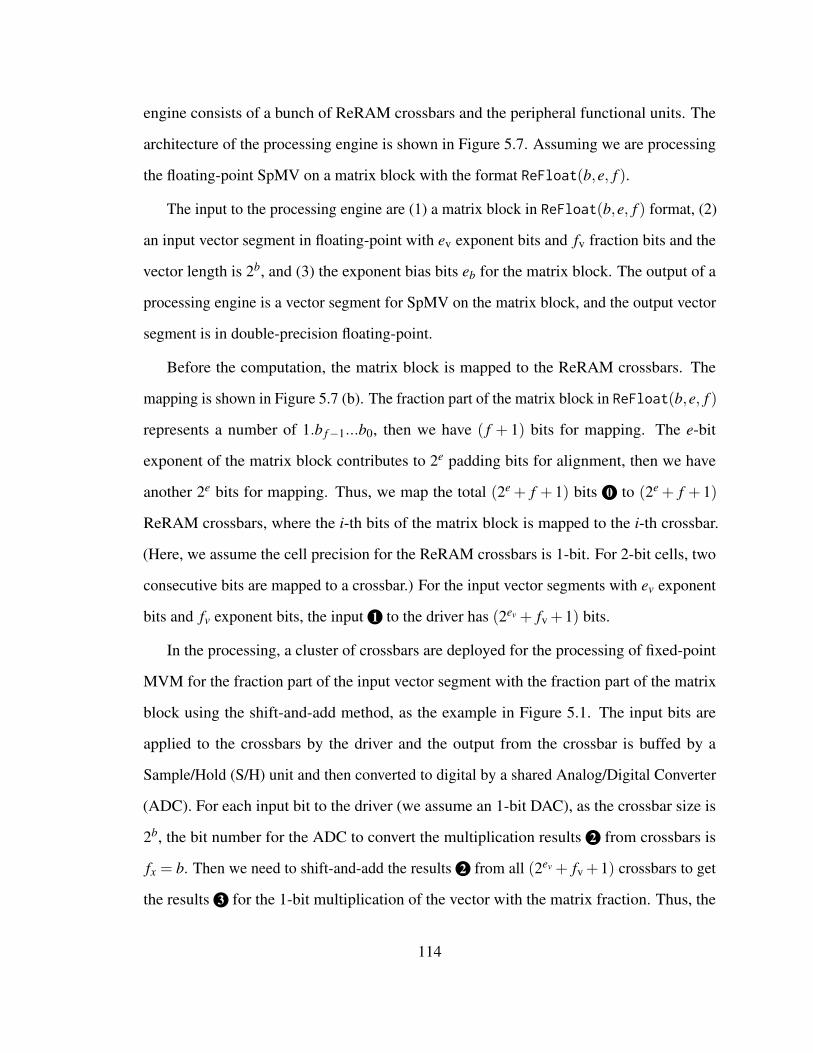
engine consists of a bunch of ReRAM crossbars and the peripheral functional units. The
architecture of the processing engine is shown in Figure 5.7. Assuming we are processing
the floating-point SpMV on a matrix block with the format ReFloat(b,e, f ).
The input to the processing engine are (1) a matrix block in ReFloat(b,e, f ) format, (2)
an input vector segment in floating-point with ev exponent bits and fv fraction bits and the
vector length is 2b, and (3) the exponent bias bits eb for the matrix block. The output of a
processing engine is a vector segment for SpMV on the matrix block, and the output vector
segment is in double-precision floating-point.
Before the computation, the matrix block is mapped to the ReRAM crossbars. The
mapping is shown in Figure 5.7 (b). The fraction part of the matrix block in ReFloat(b,e, f )
represents a number of 1.b f−1...b0, then we have ( f + 1) bits for mapping. The e-bit
exponent of the matrix block contributes to 2e padding bits for alignment, then we have
another 2e bits for mapping. Thus, we map the total (2e + f + 1) bits 0 to (2e + f + 1)
ReRAM crossbars, where the i-th bits of the matrix block is mapped to the i-th crossbar.
(Here, we assume the cell precision for the ReRAM crossbars is 1-bit. For 2-bit cells, two
consecutive bits are mapped to a crossbar.) For the input vector segments with ev exponent
bits and fv exponent bits, the input 1 to the driver has (2ev + fv +1) bits.
In the processing, a cluster of crossbars are deployed for the processing of fixed-point
MVM for the fraction part of the input vector segment with the fraction part of the matrix
block using the shift-and-add method, as the example in Figure 5.1. The input bits are
applied to the crossbars by the driver and the output from the crossbar is buffed by a
Sample/Hold (S/H) unit and then converted to digital by a shared Analog/Digital Converter
(ADC). For each input bit to the driver (we assume an 1-bit DAC), as the crossbar size is
2b, the bit number for the ADC to convert the multiplication results 2 from crossbars is
fx = b. Then we need to shift-and-add the results 2 from all (2ev + fv +1) crossbars to get
the results 3 for the 1-bit multiplication of the vector with the matrix fraction. Thus, the
114

number of bits for the 3 is
fc = 2e + f +1+b. (5.13)
Next, we consequentially input the bits in 1 to the crossbars and shift-and-add the col-
lected 3 for each of the (2ev + fv+1) bits to get 4 , which is the result for the multiplication
of the matrix block with the input 1 . The number of bits for 4 is
fg = fc +2ev + fv +1+b. (5.14)
In a processing engine, as shown in Figure 5.7 (a), there is a sign bit for the matrix
block, thus we need two crossbar cluster for the signed multiplication. The elements in the
input vector segment also have a sign bits. Thus, we need four 4 to subtract them to get 5 ,
which is the results for the multiplication of the matrix block with the vector segment. The
number of bits for 5 is ( fg +1). We also note that 5 is a signed number because of the
subtraction.
In next step, we convert the 5 to a double-precision floating-point 6 . eb 7 is the
exponent bias for the matrix block and ev 8 is exponent for the vector segment. Thus
we add 7 and 8 to the exponent of 9 to get the 9 , which is the final results for the
multiplication of the matrix block with the vector segment. 9 is in 64-bit double-precision
floating-point format.
5.4.3 Streaming & Scheduling
The processing engine is designed for the computation of MVM on a matrix block. For the
whole SpMV, the computation is partitioned to the block MVM. However, because of the
sparsity in the real-word large-scale matrix, the streaming on the matrix and the scheduling
for the block matrix MVMs need careful consideration.
Matrix Market File Format [297] (MMFF) is the matrix format used in scientific com-
puting. In MMFF, a line of entry contains the row index, the column index and the value
115
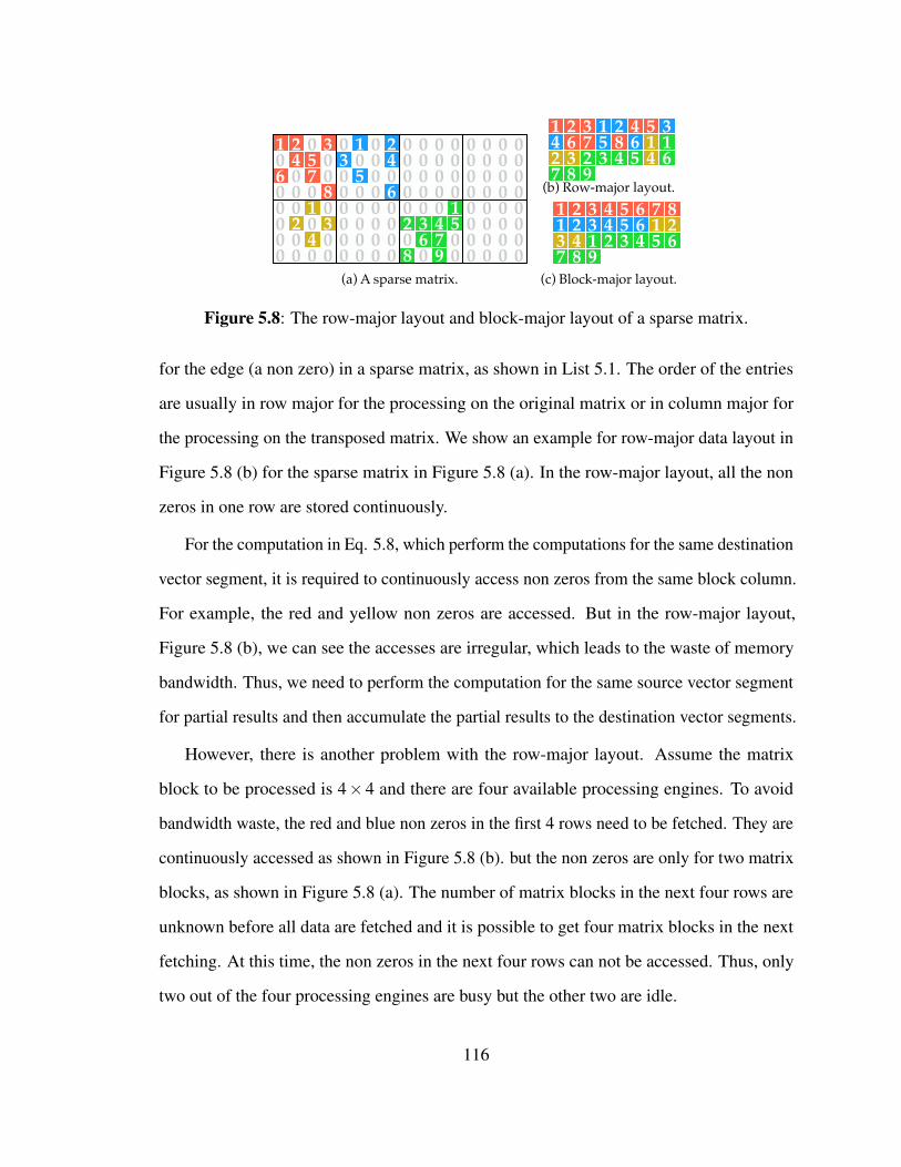
1 2 0 30
1 20
10
2
00 0 04 5
003 4 0
3
0
4
00 0 0
000
0 0 01
20
30 00 0
0 0 0
00 0
0 0 00 000
000
000
0 0 0
0 0 00 000
0
600
00
000
0 0 0
0 0 00 000
0
00
000
0 0 0
0 0 00 000
078
05
60
0 0400
56 7
8 9 00
00
1 2 3 1 21
24 5 3
43 4
12 36 7 85 6
45 67 8 9
1 2 31 2
1 24 5
3 43 4
1 23
6 7 85 6
4 5 67 8 9
(a) A sparse matrix.
(b) Row-major layout.
(c) Block-major layout.
Figure 5.8: The row-major layout and block-major layout of a sparse matrix.
for the edge (a non zero) in a sparse matrix, as shown in List 5.1. The order of the entries
are usually in row major for the processing on the original matrix or in column major for
the processing on the transposed matrix. We show an example for row-major data layout in
Figure 5.8 (b) for the sparse matrix in Figure 5.8 (a). In the row-major layout, all the non
zeros in one row are stored continuously.
For the computation in Eq. 5.8, which perform the computations for the same destination
vector segment, it is required to continuously access non zeros from the same block column.
For example, the red and yellow non zeros are accessed. But in the row-major layout,
Figure 5.8 (b), we can see the accesses are irregular, which leads to the waste of memory
bandwidth. Thus, we need to perform the computation for the same source vector segment
for partial results and then accumulate the partial results to the destination vector segments.
However, there is another problem with the row-major layout. Assume the matrix
block to be processed is 4× 4 and there are four available processing engines. To avoid
bandwidth waste, the red and blue non zeros in the first 4 rows need to be fetched. They are
continuously accessed as shown in Figure 5.8 (b). but the non zeros are only for two matrix
blocks, as shown in Figure 5.8 (a). The number of matrix blocks in the next four rows are
unknown before all data are fetched and it is possible to get four matrix blocks in the next
fetching. At this time, the non zeros in the next four rows can not be accessed. Thus, only
two out of the four processing engines are busy but the other two are idle.
116

For full utilization of the processing engines, we propose a block-major layout, as shown
in Figure 5.8 (c). Within a matrix block, the non zeros are stored in row-major order, and
the data for the blocks are continuously stored. With the block-major layout, we fetch the
non zeros to the accelerator until we exhaust all available processing engines. To avoid
conflict on writing to the same vector segment, we use a commit buffer, as shown in Figure
5.6, to collect the partial results from the processing engines and then update the output
vector with the MAC units.
5.4.4 Accelerator Programming
Conjugate Gradient (CG) [294] and Stabilized BiConjugate Gradient (BiCGSTAB) [295]
are the two Krylov subspace methods used as the iterative solver in this work. We use CG
as an example to illustrate how we program the accelerator for the solver. The pseudo code
for the CG solver is listed in Code 5.2. In the code, We use double to indicate a variable
in 64-bit(double) floating-point precision, and refloat to indicate a variable in REFLOAT.
The variable name with a mat suffix indicates a matrix, the variable name with a vec suffix
indicates a vector, and others are scalars.
At the beginning, the exponent number for the matrix block e, the fraction number
for the matrix block f , the exponent number for the vector segment ev and the fraction
number for the vector segment f v in refloat is set. Within the accelerator, the crossbars in
a bank(subbank) will be configured with the parameter as clusters for processing SpMV
in refloat. Then the sparse matrix A mat is converted to refloat Ar mat and stored in
the block-major layout (Sec. 5.4.3) at Line 2 and 3. The bias vector b vec for the linear
system and the initial solution x vec is loaded to the accelerator at Line 4 and 5. At Line
6, the SpMV of Ar mat and xr vec is processed, where the matrix blocks of Ar mat are
streamed to the accelerator and partial results are accumulated to an double vector Ax. At
Line 7 the error vector r vec is computed by the MACs. At Line 8, a precision correction
117

1 refloat: e, f, ev, ef2 double A_mat3 refloat Ar_mat = (refloat) A_mat4 double b_vec5 double x_vec = x0_vec6 double Ax = Ar_mat * x_vec7 double r_vec = b_vec - Ax8 double p_vec = r_vec9 while (not converge) do10 double Ap_vec = Ar_mat * (refloat) p_vec11 double rr = r_vec.T * r_vec12 double pAp = p_vec.T * Ap_vec13 double alpha = rr / pAp14 x_vec = x_vec + alpha * p_vec15 r_vec = r_vec - alpha * Ap_vec16 double rrnew = r_vec.T * r_vec17 double beta = rrnew / rr18 p_vec = r_vec + beta * p_vec19 end while
Code 5.2: The pseudo code for the CG solver.
vector p vec is created. Line 9 to Line 19 are the main body for the CG solver. The SpMV
is processed on the matrix and the precision correction vector p vec which is converted
into refloat before processing at Line 10. From Line 11 to Line 13, a coefficient alpha
is calculated. The doc product of two vector is performed by the MACs. At Line 14 and
Line 15, the coefficient alpha is used to update the solution vector x vec and the error
vector vector r vec element-wisely. From Line 16 to Line 18, an other coefficient beta is
calculated to update the precision correction vector. The main body continue to run until a
desired stop condition (such as that the number of the iterations is larger than a threshold or
that the residual rr is smaller than a threshold) is reached.
118
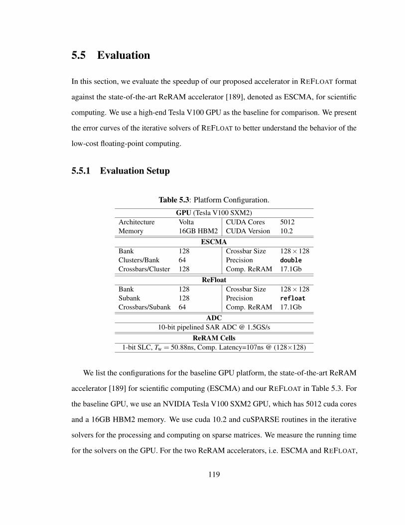
5.5 Evaluation
In this section, we evaluate the speedup of our proposed accelerator in REFLOAT format
against the state-of-the-art ReRAM accelerator [189], denoted as ESCMA, for scientific
computing. We use a high-end Tesla V100 GPU as the baseline for comparison. We present
the error curves of the iterative solvers of REFLOAT to better understand the behavior of the
low-cost floating-point computing.
5.5.1 Evaluation Setup
Table 5.3: Platform Configuration.
GPU (Tesla V100 SXM2)Architecture Volta CUDA Cores 5012Memory 16GB HBM2 CUDA Version 10.2
ESCMABank 128 Crossbar Size 128×128Clusters/Bank 64 Precision doubleCrossbars/Cluster 128 Comp. ReRAM 17.1Gb
ReFloatBank 128 Crossbar Size 128×128Subank 128 Precision refloatCrossbars/Subank 64 Comp. ReRAM 17.1Gb
ADC10-bit pipelined SAR ADC @ 1.5GS/s
ReRAM Cells1-bit SLC, Tw = 50.88ns, Comp. Latency=107ns @ (128×128)
We list the configurations for the baseline GPU platform, the state-of-the-art ReRAM
accelerator [189] for scientific computing (ESCMA) and our REFLOAT in Table 5.3. For
the baseline GPU, we use an NVIDIA Tesla V100 SXM2 GPU, which has 5012 cuda cores
and a 16GB HBM2 memory. We use cuda 10.2 and cuSPARSE routines in the iterative
solvers for the processing and computing on sparse matrices. We measure the running time
for the solvers on the GPU. For the two ReRAM accelerators, i.e. ESCMA and REFLOAT,
119

we simulate with the parameters in Table 5.3. Both the two ReRAM accelerators have
128 Banks and the crossbar size is 128× 128. In ESCMA, we configure 64 clusters for
each bank, which is slightly larger than that (56) in the original work [189]. There are 128
crossbars in each cluster. The precision in ESCMA is double floating-point. In REFLOAT,
we configure 128 banks, 128 subbanks per bank, and 64 crossbars per subbank. The
precision in REFLOAT is refloat with a default setting that e = 3, f = 3, ev = 3 and fv = 8.
For the two ReRAM accelerators, the equivalent computing ReRAM is 17.1Gb. The ADC
and ReRAM cells for the two accelerators are of the same configurations. We use a 1.5GS/s
10-bit pipelined SAR ADC [298] for conversion. The DAC is 1-bit, which is implemented
by wordline activation. We use 1-bit SLC [264] and the write latency is 50.88ns. The
computing latency for one crossbar including the ADC conversion is 107ns [189]. In the two
ReRAM accelerators, each bank has a 16MB memory for buffering and 128 floating-point
MACs for vector related processing.
The matrices used in the evaluation are listed in Table 5.4. We evaluate on 12 solvable
matrices from the SuiteSparse Matrix Collection (formerly formerly the University of
Florida Sparse Matrix Collection) [296]. The size, i.e., the number of rows, of the matrices
ranges from 4,875 to 204,316 and the Number of Non-Zero entries (NNZ) of the matrices
ranges from 105,339 for 1,660,579. NNZ/Row is a metric for sparsity. A smaller NNZ/Row
indicates a sparser matrix. NNZ/Row ranges from 4.0 to 27.7. We also visualize the matrices
in Table 5.4.
We apply the iterative solvers CG and BiCGSTAB on the matrices. The convergence
criteria for the solvers is that the L-2 norm of the residual vector (we use the term “residual”
(denoted by R2) for simplicity to call it in this section) is less than 10−8. The error
(ei = xi− xi) of any scalar in the solution vector is bonded by the residual, because |ei|2 ≤
∑i |ei|2 = |x− x|2 = |r|2/|A|2 = 1|A|2 R2, where |A| is a constant.
120

Table 5.4: Matrices in the evaluation.ID Name #Rows NNZ NNZ/R κ
353 crystm01 4875 105339 21.6 4.21e+21313 minsurfo 40806 203622 5.0 8.11e+1354 crystm02 13965 322905 23.1 4.49e+22261 shallow water1 81920 327680 4.0 3.63e+01288 wathen100 30401 471601 15.5 8.24e+31311 gridgena 48962 512084 10.5 5.74e+51289 wathen120 36441 565761 15.5 4.05e+3355 crystm03 24696 583770 23.6 4.68e+22257 thermomech TC 102158 711558 6.9 1.23e+21848 Dubcova2 65025 1030225 15.84 1.04e+42259 thermomech dM 204316 1423116 6.9 1.24e+2845 qa8fm 66127 1660579 25.1 1.10e+2
353 1313 354 2261 1288 1311
1289 355 2257 1848 2259 845
5.5.2 Performance
CG Solver
We show the performance of GPU in double and single precision floating-point, ES-
CMA [189] and REFLOAT for CG solver in Figure 5.9. The performance p is defined
as p = tx/tGPU(double), x = GPU(single), ESCMA or REFLOAT. t is the processing time
for the iterative solver to satisfy that the residual is less than 10−8. Overall, the geometric-
mean(GMN) performance of GPU(single), ESCMA and REFLOAT are 0.78×, 6.07× and
18.71× respectively, resulting in a 3.08× for REFLOAT against ESCMA. GPU(single)
benefits from faster SpMV on lower bits, but the iteration number is increased. The highest
121

performance of GPU(single) 1.22× for Matrix 2261 and for most matrices the performance
gain for switching double to single is less than 1.2×. For Matrix 1311, the GPU(single)
performance is 0.015×, because it takes 1468 additional iterations. Less bits, such as
FP16 in a straightforward way, will not converge. For most of the matrices, ESCMA and
REFLOAT performs better than the baseline GPU. However, for matrix 2257 and 2259, the
performance of REFLOAT is 3.97× and 2.68× respectively. The performance of ESCMA
is even lower on the matrix 2257 and 2259, it is 0.72× and 0.51× respectively.
353 1313 354 2261 1288 1311 1289 355 2257 1848 2259 845 GMN10-210-110010150
ESCMA ReFloat GPU(f) GPU(d)
Figure 5.9: The performance of GPU(in double and single precision), ESCMA and RE-FLOAT for CG solver.
BiCGSTAB Solver
We show the performance of GPU double and single precision floating-point, ESCMA [189]
and REFLOAT for BiCGSTAB solver in Figure 5.10. The geometric-mean(GMN) perfor-
mance of GPU(single), ESCMA and REFLOAT are 1.15×, 5.09× and 21.88× respectively,
resulting in a 4.30× for REFLOAT against ESCMA. Notice that matrix 1311 does not
converge in GPU(single), and the 1.15× geomean excludes this matrix. The trend for the
three platforms on the evaluated matrices are similar to that for CG solver. In each iteration,
for CiCGSTAB solver, there are two SpMV on the whole matrix, while for CG solver,
there is one SpMV on the whole matrix. For ESCMA, more time is consumed for the
processing of two SpMVs, leading to a slightly lower performance than that of CG solver
(5.09× v.s. 6.07×) compared with the baseline GPU. From Table 5.6 we can see, the gap
(the difference of number of iterations to get converge) in BiCGSTAB solver is smaller
122

than the gap in CG solver for most matrices. For matrix 355, 2257, 2259 and 845, the
gap is negative, which means it takes fewer iterations in refloat compared with that in
double. For REFLOAT, although more time is consumed for the processing of two SpMVs
in BiCGSTAB, which is the same scenarios as that in ESCMA, because the gap is smaller,
the performance of REFLOAT for BiCGSTAB solver is higher compared with CG solver,
i.e., 21.88× v.s. 18.71×.
353 1313 354 2261 1288 1311 1289 355 2257 1848 2259 845 GMN10-1
100
10160 ESCMA ReFloat GPU(f) GPU(d)
Figure 5.10: The performance of GPU (in double and single precision), ESCMA andREFLOAT for BiCGSTAB solver.
5.5.3 Accuracy
100 101 10210-10
10-5
100
105353
100 101 10210-10
10-5
100
1051313
100 101 10210-10
10-5
100
105354
100 101 10210-10
10-5
100
1052261
100 102 10410-10
10-5
100
1051288
1 1.5 210-20
10-10
100
10101311
100 102 10410-10
10-5
100
1051289
100 101 10210-10
10-5
100
105355
100 101 10210-10
100
10102257
100 102 10410-10
100
10101848
100 101 10210-10
100
10102259
100 101 10210-10
10-5
100
105845
The Y axis is the residual and the X axis is the normalized iteration number.
Figure 5.11: The convergence traces of CG solver of GPU (red line) and REFLOAT (blueline).
We show the convergence traces (the residual over each iteration) of the evaluated
matrices in double and in refloat for CG solver in Figure 5.11 and the convergence traces
123
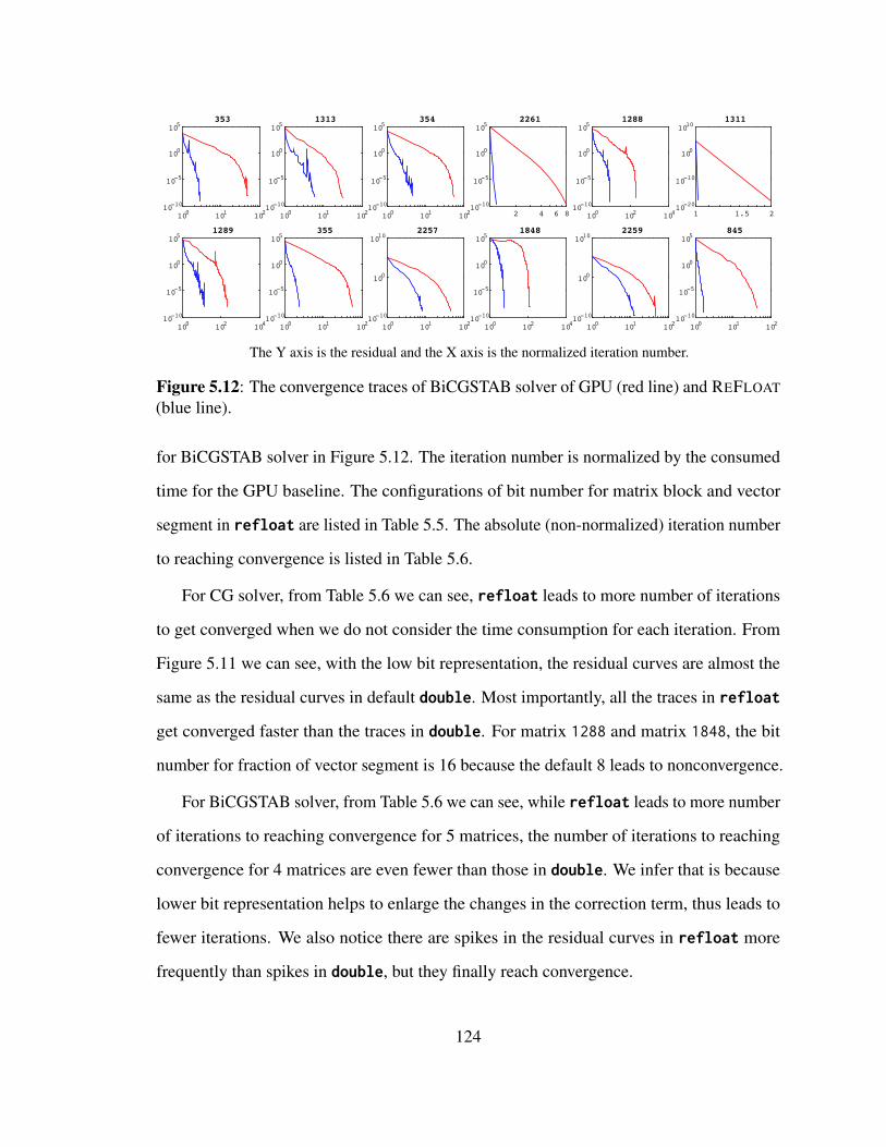
100 101 10210-10
10-5
100
105353
100 101 10210-10
10-5
100
1051313
100 101 10210-10
10-5
100
105354
2 4 6 810-10
10-5
100
1052261
100 102 10410-10
10-5
100
1051288
1 1.5 210-20
10-10
100
10101311
100 102 10410-10
10-5
100
1051289
100 101 10210-10
10-5
100
105355
100 101 10210-10
100
10102257
100 102 10410-10
10-5
100
1051848
100 101 10210-10
100
10102259
100 101 10210-10
10-5
100
105845
The Y axis is the residual and the X axis is the normalized iteration number.
Figure 5.12: The convergence traces of BiCGSTAB solver of GPU (red line) and REFLOAT
(blue line).
for BiCGSTAB solver in Figure 5.12. The iteration number is normalized by the consumed
time for the GPU baseline. The configurations of bit number for matrix block and vector
segment in refloat are listed in Table 5.5. The absolute (non-normalized) iteration number
to reaching convergence is listed in Table 5.6.
For CG solver, from Table 5.6 we can see, refloat leads to more number of iterations
to get converged when we do not consider the time consumption for each iteration. From
Figure 5.11 we can see, with the low bit representation, the residual curves are almost the
same as the residual curves in default double. Most importantly, all the traces in refloat
get converged faster than the traces in double. For matrix 1288 and matrix 1848, the bit
number for fraction of vector segment is 16 because the default 8 leads to nonconvergence.
For BiCGSTAB solver, from Table 5.6 we can see, while refloat leads to more number
of iterations to reaching convergence for 5 matrices, the number of iterations to reaching
convergence for 4 matrices are even fewer than those in double. We infer that is because
lower bit representation helps to enlarge the changes in the correction term, thus leads to
fewer iterations. We also notice there are spikes in the residual curves in refloat more
frequently than spikes in double, but they finally reach convergence.
124

Table 5.5: The bit number for exponent and fraction of matrix block and vector segment inREFLOAT.
ID CG BiCGSTABe f ev fv e f ev fv
353 3 3 3 8 3 3 3 81313 3 3 3 8 3 3 3 8354 3 3 3 8 3 3 3 82261 3 3 3 8 3 3 3 81288 3 3 3 16 3 3 3 161311 3 3 3 8 3 3 3 81289 3 3 3 8 3 3 3 8355 3 3 3 8 3 3 3 82257 3 3 3 8 3 3 3 81848 3 3 3 16 3 3 3 162259 3 3 3 8 3 3 3 8845 3 3 3 8 3 3 3 8
5.5.4 Memory Overhead
3531313 35
42261128813111289 35
5225718482259 84
5
GMEAN
0.1
0.2 0.3
0.5
1.0
ESCMA ReFloat
Figure 5.13: Memory overhead of matrices in ESCMA and REFLOAT.
In Figure 5.13, we compare the memory overhead for the matrix in refloat with
that in double (used in ESCMA [189]). On average, refloat consumes 0.21× memory
compared with double. For matrices except 2257 and 2259, refloat consumes less than
0.2× memory compared with double, which is 0.47× and 0.44× respectively. For matrix
2257 and matrix 2259, the average density within a matrix is relatively lower, thus more
memory is consumed for the matrix block index and the exponent bias as discussed in Sec.
5.3.1.
125

Table 5.6: The absolute number of iterations to reaching convergence.
ID CG BiCGSTABdouble refloat gap double refloat gap
353 68 85 +17 48 51 +31313 52 55 +3 30 69 +39354 54 95 +41 52 79 +272261 11 11 0 7 7 01288 262 305 +43 195 205 +101311 1 1 0 1 1 01289 294 401 +107 216 317 +101355 80 95 +15 55 52 -32257 55 56 +1 43 36 -71848 162 214 +52 117 145 +282259 57 58 +1 43 36 -7845 53 54 +1 41 45 -4
126
Chapter 6
Conclusion
In this dissertation, I study the architecture-level optimizations for efficient acceleration
of training in deep learning and efficient acceleration of graph processing. I present
ACCPAR, a principled and systematic method to determining the tensor partition among
heterogeneous accelerator arrays for achieving optimal performance. ACCPAR considers
the complete tensor partition space and reveals a new and previously unknown parallelism
configuration. It optimizes performance based on a cost model considering both computation
and communication cost of heterogeneous execution environment. I present PIPELAYER,
a ReRAM-based PIM accelerator architecture for high-throughput deep learning training
acceleration . I propose efficient layer-wise pipeline pipeline to exploit intra- and inter-layer
parallelism. PIPELAYER enables the highly pipelined execution of both training and testing.
I present GRAPHR, the first ReRAM-based graph processing accelerator. The key insight of
GRAPHR is that if a vertex program of a graph algorithm can be expressed in sparse matrix
vector multiplication (SpMV), it can be efficiently performed by ReRAM crossbar. The
core graph computations are performed in sparse matrix format in graph engines (ReRAM
crossbars) and edges are partitioned and sequentially fetched to the graph engines. I present
REFLOAT, a data format and a corresponding accelerator architecture to support low-cost
floating-point SpMV in ReRAM. REFLOAT is tailored for processing on ReRAM crossbars
where the number of effective bits is greatly reduced to reduce the crossbar cost and cycle
cost for the floating-point multiplication on a matrix block, thus the overall floating-point
SpMV processing is boosted.
127

Bibliography
[1] A. Krizhevsky, “One weird trick for parallelizing convolutional neural networks,”arXiv preprint arXiv:1404.5997, 2014.
[2] L. Song, J. Mao, Y. Zhuo, X. Qian, H. Li, and Y. Chen, “Hypar: Towards hybrid par-allelism for deep learning accelerator array,” in 2019 IEEE International Symposiumon High Performance Computer Architecture (HPCA), IEEE, 2019.
[3] S. Ren, K. He, R. Girshick, and J. Sun, “Faster r-cnn: Towards real-time object detec-tion with region proposal networks,” in Advances in neural information processingsystems, pp. 91–99, 2015.
[4] W. Liu, D. Anguelov, D. Erhan, C. Szegedy, S. Reed, C.-Y. Fu, and A. C. Berg,“Ssd: Single shot multibox detector,” in European conference on computer vision,pp. 21–37, Springer, 2016.
[5] X. Liu, H. Yang, Z. Liu, L. Song, H. Li, and Y. Chen, “Dpatch: An adversarial patchattack on object detectors,” arXiv preprint arXiv:1806.02299, 2018.
[6] B. Perozzi, R. Al-Rfou, and S. Skiena, “Deepwalk: Online learning of social repre-sentations,” in Proceedings of the 20th ACM SIGKDD international conference onKnowledge discovery and data mining, pp. 701–710, ACM, 2014.
[7] T. N. Kipf and M. Welling, “Semi-supervised classification with graph convolutionalnetworks,” arXiv preprint arXiv:1609.02907, 2016.
[8] A. Grover and J. Leskovec, “node2vec: Scalable feature learning for networks,” inProceedings of the 22nd ACM SIGKDD international conference on Knowledgediscovery and data mining, pp. 855–864, ACM, 2016.
[9] T. Fischer and C. Krauss, “Deep learning with long short-term memory networks forfinancial market predictions,” European Journal of Operational Research, vol. 270,no. 2, pp. 654–669, 2018.
[10] X. Ding, Y. Zhang, T. Liu, and J. Duan, “Deep learning for event-driven stockprediction,” in Twenty-fourth international joint conference on artificial intelligence,2015.
[11] Y. Deng, F. Bao, Y. Kong, Z. Ren, and Q. Dai, “Deep direct reinforcement learningfor financial signal representation and trading,” IEEE transactions on neural networksand learning systems, vol. 28, no. 3, pp. 653–664, 2016.
[12] R. Miotto, F. Wang, S. Wang, X. Jiang, and J. T. Dudley, “Deep learning for health-care: review, opportunities and challenges,” Briefings in bioinformatics, vol. 19, no. 6,pp. 1236–1246, 2017.
128
[13] T. Ching, D. S. Himmelstein, B. K. Beaulieu-Jones, A. A. Kalinin, B. T. Do, G. P.Way, E. Ferrero, P.-M. Agapow, M. Zietz, M. M. Hoffman, W. Xie, G. L. Rosen, B. J.Lengerich, J. Israeli, J. Lanchantin, S. Woloszynek, A. E. Carpenter, A. Shrikumar,J. Xu, E. M. Cofer, C. A. Lavender, S. C. Turaga, A. M. Alexandari, Z. Lu, D. J.Harris, D. DeCaprio, Y. Qi, A. Kundaje, Y. Peng, L. K. Wiley, M. H. S. Segler, S. M.Boca, S. J. Swamidass, A. Huang, A. Gitter, and C. S. Greene, “Opportunities andobstacles for deep learning in biology and medicine,” Journal of The Royal SocietyInterface, vol. 15, no. 141, p. 20170387, 2018.
[14] O. Faust, Y. Hagiwara, T. J. Hong, O. S. Lih, and U. R. Acharya, “Deep learningfor healthcare applications based on physiological signals: A review,” Computermethods and programs in biomedicine, vol. 161, pp. 1–13, 2018.
[15] L. Song, F. Chen, S. R. Young, C. D. Schuman, G. Perdue, and T. E. Potok, “Deeplearning for vertex reconstruction of neutrino-nucleus interaction events with com-bined energy and time data,” in ICASSP 2019-2019 IEEE International Conferenceon Acoustics, Speech and Signal Processing (ICASSP), pp. 3882–3886, IEEE, 2019.
[16] P. Baldi, P. Sadowski, and D. Whiteson, “Searching for exotic particles in high-energyphysics with deep learning,” Nature communications, vol. 5, p. 4308, 2014.
[17] J. Wu, I. Yildirim, J. J. Lim, B. Freeman, and J. Tenenbaum, “Galileo: Perceivingphysical object properties by integrating a physics engine with deep learning,” inAdvances in neural information processing systems, pp. 127–135, 2015.
[18] S. B. Furber, D. R. Lester, L. A. Plana, J. D. Garside, E. Painkras, S. Temple, andA. D. Brown, “Overview of the spinnaker system architecture,” IEEE Transactionson Computers, vol. 62, no. 12, pp. 2454–2467, 2013.
[19] Z. Du, D. D. Ben-Dayan Rubin, Y. Chen, L. He, T. Chen, L. Zhang, C. Wu, andO. Temam, “Neuromorphic accelerators: A comparison between neuroscience andmachine-learning approaches,” in Proceedings of the 48th International Symposiumon Microarchitecture, pp. 494–507, ACM, 2015.
[20] P. A. Merolla, J. V. Arthur, R. Alvarez-Icaza, A. S. Cassidy, J. Sawada, F. Akopyan,B. L. Jackson, N. Imam, C. Guo, Y. Nakamura, B. Brezzo, I. Vo, S. K. Esser,R. Appuswamy, B. Taba, A. Amir, M. D. Flickner, W. P. Risk, R. Manohar, and D. S.Modha, “A million spiking-neuron integrated circuit with a scalable communicationnetwork and interface,” Science, vol. 345, no. 6197, pp. 668–673, 2014.
[21] S. K. Esser, R. Appuswamy, P. Merolla, J. V. Arthur, and D. S. Modha, “Back-propagation for energy-efficient neuromorphic computing,” in Advances in NeuralInformation Processing Systems, pp. 1117–1125, 2015.
[22] S. K. Esser, P. A. Merolla, J. V. Arthur, A. S. Cassidy, R. Appuswamy, A. Andreopou-los, D. J. Berg, J. L. McKinstry, T. Melano, D. R. Barch, C. d. Nolfo, P. Datta,
129

A. Amir, B. Taba, M. D. Flickner, and D. S. Modha, “Convolutional networks for fast,energy-efficient neuromorphic computing,” Proceedings of the National Academy ofSciences (PNAS), p. 201604850, 2016.
[23] T. Liu, Z. Liu, F. Lin, Y. Jin, G. Quan, and W. Wen, “Mt-spike: A multilayer time-based spiking neuromorphic architecture with temporal error backpropagation,” inComputer-Aided Design (ICCAD), 2017 IEEE/ACM International Conference on,pp. 450–457, IEEE, 2017.
[24] T. Liu, L. Jiang, Y. Jin, G. Quan, and W. Wen, “Pt-spike: A precise-time-dependentsingle spike neuromorphic architecture with efficient supervised learning,” in DesignAutomation Conference (ASP-DAC), 2018 23rd Asia and South Pacific, pp. 568–573,IEEE, 2018.
[25] H. Esmaeilzadeh, A. Sampson, L. Ceze, and D. Burger, “Neural acceleration forgeneral-purpose approximate programs,” in Proceedings of the 2012 45th AnnualIEEE/ACM International Symposium on Microarchitecture, pp. 449–460, IEEEComputer Society, 2012.
[26] T. Chen, Z. Du, N. Sun, J. Wang, C. Wu, Y. Chen, and O. Temam, “Diannao: Asmall-footprint high-throughput accelerator for ubiquitous machine-learning,” inACM Sigplan Notices, pp. 269–284, ACM, 2014.
[27] Y. Chen, T. Luo, S. Liu, S. Zhang, L. He, J. Wang, L. Li, T. Chen, Z. Xu, N. Sun, andO. Temam, “Dadiannao: A machine-learning supercomputer,” in Proceedings of the47th Annual IEEE/ACM International Symposium on Microarchitecture, pp. 609–622,IEEE Computer Society, 2014.
[28] Z. Du, R. Fasthuber, T. Chen, P. Ienne, L. Li, T. Luo, X. Feng, Y. Chen, and O. Temam,“Shidiannao: Shifting vision processing closer to the sensor,” in ACM SIGARCHComputer Architecture News, vol. 43, pp. 92–104, ACM, 2015.
[29] D. Liu, T. Chen, S. Liu, J. Zhou, S. Zhou, O. Teman, X. Feng, X. Zhou, andY. Chen, “Pudiannao: A polyvalent machine learning accelerator,” in ACM SIGARCHComputer Architecture News, vol. 43, pp. 369–381, ACM, 2015.
[30] S. Liu, Z. Du, J. Tao, D. Han, T. Luo, Y. Xie, Y. Chen, and T. Chen, “Cambricon: Aninstruction set architecture for neural networks,” in 2016 ACM/IEEE 43rd AnnualInternational Symposium on Computer Architecture (ISCA), pp. 393–405, IEEE,2016.
[31] S. Zhang, Z. Du, L. Zhang, H. Lan, S. Liu, L. Li, Q. Guo, T. Chen, and Y. Chen,“Cambricon-x: An accelerator for sparse neural networks,” in 2016 49th AnnualIEEE/ACM International Symposium on Microarchitecture (MICRO), pp. 1–12,IEEE, 2016.
130

[32] “Google supercharges machine learning tasks with tpu custom chip.”https://cloudplatform.googleblog.com/2016/05/Google-supercharges-machine-learning-tasks-with-custom-chip.html.
[33] N. P. Jouppi, C. Young, N. Patil, D. Patterson, G. Agrawal, R. Bajwa, S. Bates,S. Bhatia, N. Boden, A. Borchers, R. Boyle, P.-l. Cantin, C. Chao, C. Clark, J. Coriell,M. Daley, M. Dau, J. Dean, B. Gelb, T. V. Ghaemmaghami, R. Gottipati, W. Gulland,R. Hagmann, C. R. Ho, D. Hogberg, J. Hu, R. Hundt, D. Hurt, J. Ibarz, A. Jaffey,A. Jaworski, A. Kaplan, H. Khaitan, D. Killebrew, A. Koch, N. Kumar, S. Lacy,J. Laudon, J. Law, D. Le, C. Leary, Z. Liu, K. Lucke, A. Lundin, G. MacKean,A. Maggiore, M. Mahony, K. Miller, R. Nagarajan, R. Narayanaswami, R. Ni, K. Nix,T. Norrie, M. Omernick, N. Penukonda, A. Phelps, J. Ross, M. Ross, A. Salek,E. Samadiani, C. Severn, G. Sizikov, M. Snelham, J. Souter, D. Steinberg, A. Swing,M. Tan, G. Thorson, B. Tian, H. Toma, E. Tuttle, V. Vasudevan, R. Walter, W. Wang,E. Wilcox, and D. H. Yoon, “In-datacenter performance analysis of a tensor process-ing unit,” in Proceedings of the 44th Annual International Symposium on ComputerArchitecture, ISCA ’17, (New York, NY, USA), pp. 1–12, ACM, 2017.
[34] S. Venkataramani, A. Ranjan, S. Banerjee, D. Das, S. Avancha, A. Jagannathan,A. Durg, D. Nagaraj, B. Kaul, P. Dubey, and A. Raghunathan, “Scaledeep: A scalablecompute architecture for learning and evaluating deep networks,” in Proceedingsof the 44th Annual International Symposium on Computer Architecture, pp. 13–26,ACM, 2017.
[35] P. Judd, J. Albericio, T. Hetherington, T. M. Aamodt, and A. Moshovos, “Stripes:Bit-serial deep neural network computing,” in Microarchitecture (MICRO), 201649th Annual IEEE/ACM International Symposium on, pp. 1–12, IEEE, 2016.
[36] C. Zhang, P. Li, G. Sun, Y. Guan, B. Xiao, and J. Cong, “Optimizing fpga-basedaccelerator design for deep convolutional neural networks,” in Proceedings of the2015 ACM/SIGDA international symposium on field-programmable gate arrays,pp. 161–170, 2015.
[37] J. Qiu, J. Wang, S. Yao, K. Guo, B. Li, E. Zhou, J. Yu, T. Tang, N. Xu, S. Song,Y. Wang, and H. Yang, “Going deeper with embedded fpga platform for convolutionalneural network,” in Proceedings of the 2016 ACM/SIGDA International Symposiumon Field-Programmable Gate Arrays, pp. 26–35, ACM, 2016.
[38] M. Motamedi, P. Gysel, V. Akella, and S. Ghiasi, “Design space exploration offpga-based deep convolutional neural networks,” in 2016 21st Asia and South PacificDesign Automation Conference (ASP-DAC), pp. 575–580, IEEE, 2016.
[39] N. Suda, V. Chandra, G. Dasika, A. Mohanty, Y. Ma, S. Vrudhula, J.-s. Seo, andY. Cao, “Throughput-optimized opencl-based fpga accelerator for large-scale con-volutional neural networks,” in Proceedings of the 2016 ACM/SIGDA InternationalSymposium on Field-Programmable Gate Arrays, pp. 16–25, ACM, 2016.
131
[40] C. Zhang, Z. Fang, P. Zhou, P. Pan, and J. Cong, “Caffeine: Towards uniformedrepresentation and acceleration for deep convolutional neural networks,” in Computer-Aided Design (ICCAD), 2016 IEEE/ACM International Conference on, pp. 1–8, IEEE,2016.
[41] Y. Wang, J. Xu, Y. Han, H. Li, and X. Li, “Deepburning: automatic generationof fpga-based learning accelerators for the neural network family,” in 2016 53ndACM/EDAC/IEEE Design Automation Conference (DAC), pp. 1–6, IEEE, 2016.
[42] C. Zhang, D. Wu, J. Sun, G. Sun, G. Luo, and J. Cong, “Energy-efficient cnnimplementation on a deeply pipelined fpga cluster,” in Proceedings of the 2016International Symposium on Low Power Electronics and Design, pp. 326–331, 2016.
[43] D. Mahajan, J. Park, E. Amaro, H. Sharma, A. Yazdanbakhsh, J. K. Kim, andH. Esmaeilzadeh, “Tabla: A unified template-based framework for acceleratingstatistical machine learning,” in High Performance Computer Architecture (HPCA),2016 IEEE International Symposium on, pp. 14–26, IEEE, 2016.
[44] H. Sharma, J. Park, D. Mahajan, E. Amaro, J. K. Kim, C. Shao, A. Mishra, andH. Esmaeilzadeh, “From high-level deep neural models to fpgas,” in Microarchitec-ture (MICRO), 2016 49th Annual IEEE/ACM International Symposium on, pp. 1–12,IEEE, 2016.
[45] Y. Guan, H. Liang, N. Xu, W. Wang, S. Shi, X. Chen, G. Sun, W. Zhang, and J. Cong,“Fp-dnn: An automated framework for mapping deep neural networks onto fpgaswith rtl-hls hybrid templates,” in 2017 IEEE 25th Annual International Symposiumon Field-Programmable Custom Computing Machines (FCCM), pp. 152–159, IEEE,2017.
[46] Y. Guan, Z. Yuan, G. Sun, and J. Cong, “Fpga-based accelerator for long short-termmemory recurrent neural networks,” in 2017 22nd Asia and South Pacific DesignAutomation Conference (ASP-DAC), pp. 629–634, IEEE, 2017.
[47] S. Han, J. Kang, H. Mao, Y. Hu, X. Li, Y. Li, D. Xie, H. Luo, S. Yao, Y. Wang,H. Yang, and W. J. Dally, “Ese: Efficient speech recognition engine with sparselstm on fpga,” in Proceedings of the 2017 ACM/SIGDA International Symposium onField-Programmable Gate Arrays, pp. 75–84, 2017.
[48] Y. Ma, Y. Cao, S. Vrudhula, and J.-s. Seo, “Optimizing loop operation and dataflowin fpga acceleration of deep convolutional neural networks,” in Proceedings of the2017 ACM/SIGDA International Symposium on Field-Programmable Gate Arrays,pp. 45–54, ACM, 2017.
[49] R. Zhao, W. Song, W. Zhang, T. Xing, J.-H. Lin, M. Srivastava, R. Gupta, andZ. Zhang, “Accelerating binarized convolutional neural networks with software-
132

programmable fpgas,” in Proceedings of the 2017 ACM/SIGDA International Sympo-sium on Field-Programmable Gate Arrays, pp. 15–24, 2017.
[50] Y. Shen, M. Ferdman, and P. Milder, “Overcoming resource underutilization in spatialcnn accelerators,” in Field Programmable Logic and Applications (FPL), 2016 26thInternational Conference on, pp. 1–4, IEEE, 2016.
[51] C. Zhang and V. Prasanna, “Frequency domain acceleration of convolutional neu-ral networks on cpu-fpga shared memory system,” in Proceedings of the 2017ACM/SIGDA International Symposium on Field-Programmable Gate Arrays, pp. 35–44, 2017.
[52] R. Cai, A. Ren, N. Liu, C. Ding, L. Wang, X. Qian, M. Pedram, and Y. Wang,“Vibnn: Hardware acceleration of bayesian neural networks,” in Proceedings of theTwenty-Third International Conference on Architectural Support for ProgrammingLanguages and Operating Systems, pp. 476–488, ACM, 2018.
[53] C. Farabet, B. Martini, B. Corda, P. Akselrod, E. Culurciello, and Y. LeCun, “Neuflow:A runtime reconfigurable dataflow processor for vision,” in Computer Vision andPattern Recognition Workshops (CVPRW), 2011 IEEE Computer Society Conferenceon, pp. 109–116, IEEE, 2011.
[54] Y. Chen, J. Emer, and V. Sze, “Eyeriss: A spatial architecture for energy-efficientdataflow for convolutional neural networks,” in 2016 ACM/IEEE 43rd Annual Inter-national Symposium on Computer Architecture (ISCA), pp. 367–379, 2016.
[55] Y.-H. Chen, T. Krishna, J. S. Emer, and V. Sze, “Eyeriss: An energy-efficientreconfigurable accelerator for deep convolutional neural networks,” IEEE Journal ofSolid-State Circuits, vol. 52, no. 1, pp. 127–138, 2017.
[56] Y.-H. Chen, J. Emer, and V. Sze, “Using dataflow to optimize energy efficiency ofdeep neural network accelerators,” IEEE Micro, vol. 37, no. 3, pp. 12–21, 2017.
[57] W. Lu, G. Yan, J. Li, S. Gong, Y. Han, and X. Li, “Flexflow: A flexible dataflowaccelerator architecture for convolutional neural networks,” in High PerformanceComputer Architecture (HPCA), 2017 IEEE International Symposium on, pp. 553–564, IEEE, 2017.
[58] M. Alwani, H. Chen, M. Ferdman, and P. Milder, “Fused-layer cnn accelerators,” inMicroarchitecture (MICRO), 2016 49th Annual IEEE/ACM International Symposiumon, pp. 1–12, IEEE, 2016.
[59] Y. Shen, M. Ferdman, and M. Peter, “Maximizing cnn accelerator efficiency throughresource partitioning,” in Proceedings of the 44th Annual International Symposiumon Computer Architecture, pp. 535–547, ACM, 2017.
133

[60] A. Yazdanbakhsh, K. Samadi, N. S. Kim, and H. Esmaeilzadeh, “Ganax: A unifiedmimd-simd acceleration for generative adversarial networks,” in 2018 ACM/IEEE45th Annual International Symposium on Computer Architecture (ISCA), pp. 650–661, IEEE, 2018.
[61] K. Hegde, J. Yu, R. Agrawal, M. Yan, M. Pellauer, and C. Fletcher, “Ucnn: Ex-ploiting computational reuse in deep neural networks via weight repetition,” in 2018ACM/IEEE 45th Annual International Symposium on Computer Architecture (ISCA),pp. 674–687, IEEE, 2018.
[62] D. Kim, J. Kung, S. Chai, S. Yalamanchili, and S. Mukhopadhyay, “Neurocube: Aprogrammable digital neuromorphic architecture with high-density 3d memory,” inComputer Architecture (ISCA), 2016 ACM/IEEE 43rd Annual International Sympo-sium on, pp. 380–392, IEEE, 2016.
[63] L. Jiang, M. Kim, W. Wen, and D. Wang, “Xnor-pop: A processing-in-memoryarchitecture for binary convolutional neural networks in wide-io2 drams,” in LowPower Electronics and Design (ISLPED, 2017 IEEE/ACM International Symposiumon, pp. 1–6, IEEE, 2017.
[64] S. Li, D. Niu, K. T. Malladi, H. Zheng, B. Brennan, and Y. Xie, “Drisa: A dram-basedreconfigurable in-situ accelerator,” in Proceedings of the 50th Annual IEEE/ACMInternational Symposium on Microarchitecture, pp. 288–301, ACM, 2017.
[65] Q. Lou, W. Wen, and L. Jiang, “3dict: a reliable and qos capable mobile process-in-memory architecture for lookup-based cnns in 3d xpoint rerams,” in Proceedings ofthe International Conference on Computer-Aided Design, p. 53, ACM, 2018.
[66] S. Han, X. Liu, H. Mao, J. Pu, A. Pedram, M. A. Horowitz, and W. J. Dally, “Eie:efficient inference engine on compressed deep neural network,” in Proceedings of the43rd International Symposium on Computer Architecture, pp. 243–254, IEEE Press,2016.
[67] A. Ren, Z. Li, C. Ding, Q. Qiu, Y. Wang, J. Li, X. Qian, and B. Yuan, “Sc-dcnn:Highly-scalable deep convolutional neural network using stochastic computing,” inProceedings of the Twenty-Second International Conference on Architectural Supportfor Programming Languages and Operating Systems, pp. 405–418, ACM, 2017.
[68] A. Parashar, M. Rhu, A. Mukkara, A. Puglielli, R. Venkatesan, B. Khailany, J. Emer,S. W. Keckler, and W. J. Dally, “Scnn: An accelerator for compressed-sparse convolu-tional neural networks,” in Proceedings of the 44th Annual International Symposiumon Computer Architecture, pp. 27–40, ACM, 2017.
[69] Y. Shen, M. Ferdman, and P. Milder, “Escher: A cnn accelerator with flexiblebuffering to minimize off-chip transfer,” in Field-Programmable Custom Computing
134

Machines (FCCM), 2017 IEEE 25th Annual International Symposium on, pp. 93–100,IEEE, 2017.
[70] M. S. Razlighi, M. Imani, F. Koushanfar, and T. Rosing, “Looknn: Neural networkwith no multiplication,” in 2017 Design, Automation & Test in Europe Conference &Exhibition (DATE), pp. 1775–1780, IEEE, 2017.
[71] J. Albericio, A. Delmas, P. Judd, S. Sharify, G. O’Leary, R. Genov, and A. Moshovos,“Bit-pragmatic deep neural network computing,” in Proceedings of the 50th AnnualIEEE/ACM International Symposium on Microarchitecture, pp. 382–394, ACM,2017.
[72] H. Sharma, J. Park, N. Suda, L. Lai, B. Chau, V. Chandra, and H. Esmaeilzadeh, “Bitfusion: Bit-level dynamically composable architecture for accelerating deep neuralnetwork,” in 2018 ACM/IEEE 45th Annual International Symposium on ComputerArchitecture (ISCA), pp. 764–775, IEEE, 2018.
[73] T. Na and S. Mukhopadhyay, “Speeding up convolutional neural network trainingwith dynamic precision scaling and flexible multiplier-accumulator,” in Proceedingsof the 2016 International Symposium on Low Power Electronics and Design, pp. 58–63, ACM, 2016.
[74] B. Reagen, P. Whatmough, R. Adolf, S. Rama, H. Lee, S. K. Lee, J. M. Hernandez-Lobato, G.-Y. Wei, and D. Brooks, “Minerva: Enabling low-power, highly-accuratedeep neural network accelerators,” in 2016 ACM/IEEE 43rd Annual InternationalSymposium on Computer Architecture (ISCA), pp. 267–278, IEEE, 2016.
[75] J. Mao, X. Chen, K. W. Nixon, C. Krieger, and Y. Chen, “Modnn: Local distributedmobile computing system for deep neural network,” in 2017 Design, Automation &Test in Europe Conference & Exhibition (DATE), pp. 1396–1401, IEEE, 2017.
[76] J. Mao, Z. Yang, W. Wen, C. Wu, L. Song, K. W. Nixon, X. Chen, H. Li, and Y. Chen,“Mednn: A distributed mobile system with enhanced partition and deployment forlarge-scale dnns,” in Proceedings of the 36th International Conference on Computer-Aided Design, pp. 751–756, IEEE Press, 2017.
[77] J. Mao, Z. Qin, Z. Xu, K. W. Nixon, X. Chen, H. Li, and Y. Chen, “Adalearner: Anadaptive distributed mobile learning system for neural networks,” in Computer-AidedDesign (ICCAD), 2017 IEEE/ACM International Conference on, pp. 291–296, IEEE,2017.
[78] C.-E. Lee, Y. S. Shao, J.-F. Zhang, A. Parashar, J. Emer, S. W. Keckler, and Z. Zhang,“Stitch-x: An accelerator architecture for exploiting unstructured sparsity in deepneural networks,” in SysML, 2018.
135

[79] J. Liu, H. Zhao, M. A. Ogleari, D. Li, and J. Zhao, “Processing-in-memory forenergy-efficient neural network training: A heterogeneous approach,” in MICRO,2018.
[80] J. Yu, A. Lukefahr, D. Palframan, G. Dasika, R. Das, and S. Mahlke, “Scalpel:Customizing dnn pruning to the underlying hardware parallelism,” in Proceedings ofthe 44th Annual International Symposium on Computer Architecture, pp. 548–560,ACM, 2017.
[81] C. Ding, S. Liao, Y. Wang, Z. Li, N. Liu, Y. Zhuo, C. Wang, X. Qian, Y. Bai, G. Yuan,X. Ma, Y. Zhang, J. Tang, Q. Qiu, X. Lin, and B. Yuan, “Circnn: acceleratingand compressing deep neural networks using block-circulant weight matrices,” inProceedings of the 50th Annual IEEE/ACM International Symposium on Microarchi-tecture, pp. 395–408, ACM, 2017.
[82] J. Park, H. Sharma, D. Mahajan, J. K. Kim, P. Olds, and H. Esmaeilzadeh, “Scale-outacceleration for machine learning,” in Proceedings of the 50th Annual IEEE/ACMInternational Symposium on Microarchitecture, pp. 367–381, ACM, 2017.
[83] V. Akhlaghi, A. Yazdanbakhsh, K. Samadi, R. K. Gupta, and H. Esmaeilzadeh,“Snapea: Predictive early activation for reducing computation in deep convolutionalneural networks,” in 2018 ACM/IEEE 45th Annual International Symposium onComputer Architecture (ISCA), 2018.
[84] E. Park, D. Kim, and S. Yoo, “Energy-efficient neural network accelerator based onoutlier-aware low-precision computation,” in 2018 ACM/IEEE 45th Annual Interna-tional Symposium on Computer Architecture (ISCA), pp. 688–698, IEEE, 2018.
[85] M. Song, J. Zhao, Y. Hu, J. Zhang, and T. Li, “Prediction based execution on deepneural networks,” in 2018 ACM/IEEE 45th Annual International Symposium onComputer Architecture (ISCA), pp. 752–763, IEEE, 2018.
[86] C. Deng, S. Liao, Y. Xie, K. K. Parhi, X. Qian, and B. Yuan, “Permdnn: Efficientcompressed dnn architecture with permuted diagonal matrices,” in 2018 51st AnnualIEEE/ACM International Symposium on Microarchitecture (MICRO), pp. 189–202,IEEE, 2018.
[87] M. Gao, J. Pu, X. Yang, M. Horowitz, and C. Kozyrakis, “Tetris: Scalable andefficient neural network acceleration with 3d memory,” in Proceedings of the Twenty-Second International Conference on Architectural Support for Programming Lan-guages and Operating Systems, pp. 751–764, ACM, 2017.
[88] P. Chi, S. Li, C. Xu, T. Zhang, J. Zhao, Y. Liu, Y. Wang, and Y. Xie, “Prime: A novelprocessing-in-memory architecture for neural network computation in reram-basedmain memory,” in Proceedings of the 43rd International Symposium on ComputerArchitecture, ISCA ’16, pp. 27–39, 2016.
136
[89] A. Shafiee, A. Nag, N. Muralimanohar, R. Balasubramonian, J. P. Strachan, M. Hu,R. S. Williams, and V. Srikumar, “Isaac: A convolutional neural network acceleratorwith in-situ analog arithmetic in crossbars,” in Proceedings of the 43rd InternationalSymposium on Computer Architecture, pp. 14–26, IEEE Press, 2016.
[90] X. Liu, M. Mao, B. Liu, H. Li, Y. Chen, B. Li, Y. Wang, H. Jiang, M. Barnell, Q. Wu,and J. Yang, “Reno: a high-efficient reconfigurable neuromorphic computing acceler-ator design,” in Design Automation Conference (DAC), 2015 52nd ACM/EDAC/IEEE,pp. 1–6, IEEE, 2015.
[91] M. N. Bojnordi and E. Ipek, “Memristive boltzmann machine: A hardware acceleratorfor combinatorial optimization and deep learning,” in High Performance ComputerArchitecture (HPCA), 2016 IEEE International Symposium on, pp. 1–13, IEEE, 2016.
[92] L. Song, X. Qian, H. Li, and Y. Chen, “Pipelayer: A pipelined reram-based acceleratorfor deep learning,” in 2017 IEEE International Symposium on High PerformanceComputer Architecture (HPCA), pp. 541–552, IEEE, 2017.
[93] X. Qiao, X. Cao, H. Yang, L. Song, and H. Li, “Atomlayer: a universal reram-basedcnn accelerator with atomic layer computation,” in Proceedings of the 55th AnnualDesign Automation Conference, p. 103, ACM, 2018.
[94] H. Ji, L. Song, L. Jiang, H. H. Li, and Y. Chen, “Recom: An efficient resistiveaccelerator for compressed deep neural networks,” in Design, Automation & Test inEurope Conference & Exhibition (DATE), 2018, pp. 237–240, IEEE, 2018.
[95] F. Chen, L. Song, and Y. Chen, “Regan: A pipelined reram-based accelerator forgenerative adversarial networks,” in Design Automation Conference (ASP-DAC),2018 23rd Asia and South Pacific, pp. 178–183, IEEE, 2018.
[96] B. Li, L. Song, F. Chen, X. Qian, Y. Chen, and H. H. Li, “Reram-based acceleratorfor deep learning,” in Design, Automation & Test in Europe Conference & Exhibition(DATE), 2018, pp. 815–820, IEEE, 2018.
[97] F. Chen and H. Li, “Emat: an efficient multi-task architecture for transfer learningusing reram,” in Proceedings of the International Conference on Computer-AidedDesign, p. 33, ACM, 2018.
[98] T. Tang, L. Xia, B. Li, Y. Wang, and H. Yang, “Binary convolutional neural networkon rram,” in Design Automation Conference (ASP-DAC), 2017 22nd Asia and SouthPacific, pp. 782–787, IEEE, 2017.
[99] F. Chen, L. Song, H. H. Li, and Y. Chen, “Zara: A novel zero-free dataflow acceleratorfor generative adversarial networks in 3d reram,” in Proceedings of the 56th AnnualDesign Automation Conference 2019, pp. 1–6, 2019.
137
[100] P. Wang, Y. Ji, C. Hong, Y. Lyu, D. Wang, and Y. Xie, “Snrram: an efficient sparseneural network computation architecture based on resistive random-access memory,”in Proceedings of the 55th Annual Design Automation Conference, p. 106, ACM,2018.
[101] J. Albericio, P. Judd, T. Hetherington, T. Aamodt, N. E. Jerger, and A. Moshovos,“Cnvlutin: ineffectual-neuron-free deep neural network computing,” in Proceedingsof the 43rd International Symposium on Computer Architecture, pp. 1–13, 2016.
[102] Y. Ji, Y. Zhang, S. Li, P. Chi, C. Jiang, P. Qu, Y. Xie, and W. Chen, “Neutrams: Neuralnetwork transformation and co-design under neuromorphic hardware constraints,” inMicroarchitecture (MICRO), 2016 49th Annual IEEE/ACM International Symposiumon, pp. 1–13, IEEE, 2016.
[103] A. Mirhoseini, B. D. Rouhani, E. M. Songhori, and F. Koushanfar, “Perform-ml: Per-formance optimized machine learning by platform and content aware customization,”in Proceedings of the 53rd Annual Design Automation Conference, p. 20, ACM,2016.
[104] Z. Takhirov, J. Wang, V. Saligrama, and A. Joshi, “Energy-efficient adaptive classifierdesign for mobile systems,” in Proceedings of the 2016 International Symposium onLow Power Electronics and Design, pp. 52–57, ACM, 2016.
[105] X. Zhang, J. Wang, C. Zhu, Y. Lin, J. Xiong, W.-m. Hwu, and D. Chen, “Dnnbuilder:an automated tool for building high-performance dnn hardware accelerators for fpgas,”in Proceedings of the International Conference on Computer-Aided Design, p. 56,ACM, 2018.
[106] Y. Wang, W. Wen, B. Liu, D. Chiarulli, and H. Li, “Group scissor: Scaling neuromor-phic computing design to large neural networks,” in 2017 54th ACM/EDAC/IEEEDesign Automation Conference (DAC), pp. 1–6, IEEE, 2017.
[107] J. H. Ko, B. Mudassar, T. Na, and S. Mukhopadhyay, “Design of an energy-efficientaccelerator for training of convolutional neural networks using frequency-domaincomputation,” in Proceedings of the 54th Annual Design Automation Conference2017, p. 59, ACM, 2017.
[108] M. Li, D. G. Andersen, J. W. Park, A. J. Smola, A. Ahmed, V. Josifovski, J. Long,E. J. Shekita, and B.-Y. Su, “Scaling distributed machine learning with the parameterserver,” in 11th USENIX Symposium on Operating Systems Design and Implemen-tation (OSDI 14), pp. 583–598, 2014.
[109] Y. S. Shao, J. Clemons, R. Venkatesan, B. Zimmer, M. Fojtik, N. Jiang, B. Keller,A. Klinefelter, N. Pinckney, P. Raina, S. G. Tell, Y. Zhang, W. J. Dally, J. Emer,C. T. Gray, B. Khailany, and S. W. Keckler, “Simba: Scaling deep-learning inference
138

with multi-chip-module-based architecture,” in Proceedings of the 52nd AnnualIEEE/ACM International Symposium on Microarchitecture, pp. 14–27, 2019.
[110] M. Zhu, T. Zhang, Z. Gu, and Y. Xie, “Sparse tensor core: Algorithm and hardwareco-design for vector-wise sparse neural networks on modern gpus,” in Proceedings ofthe 52nd Annual IEEE/ACM International Symposium on Microarchitecture, pp. 359–371, 2019.
[111] Q. Luo, J. Lin, Y. Zhuo, and X. Qian, “Hop: Heterogeneity-aware decentralized train-ing,” in Proceedings of the Twenty-Fourth International Conference on ArchitecturalSupport for Programming Languages and Operating Systems, pp. 893–907, 2019.
[112] W. Niu, X. Ma, S. Lin, S. Wang, X. Qian, X. Lin, Y. Wang, and B. Ren, “Patdnn:Achieving real-time dnn execution on mobile devices with pattern-based weight prun-ing,” in Proceedings of the Twenty-Fifth International Conference on ArchitecturalSupport for Programming Languages and Operating Systems, pp. 907–922, 2020.
[113] X. Peng, X. Shi, H. Dai, H. Jin, W. Ma, Q. Xiong, F. Yang, and X. Qian, “Capuchin:Tensor-based gpu memory management for deep learning,” in Proceedings of theTwenty-Fifth International Conference on Architectural Support for ProgrammingLanguages and Operating Systems, pp. 891–905, 2020.
[114] Q. Luo, J. He, Y. Zhuo, and X. Qian, “Prague: High-performance heterogeneity-aware asynchronous decentralized training,” in Proceedings of the Twenty-FifthInternational Conference on Architectural Support for Programming Languages andOperating Systems, pp. 401–416, 2020.
[115] X. Wang, R. Hou, B. Zhao, F. Yuan, J. Zhang, D. Meng, and X. Qian, “Dnnguard:An elastic heterogeneous dnn accelerator architecture against adversarial attacks,” inProceedings of the Twenty-Fifth International Conference on Architectural Supportfor Programming Languages and Operating Systems, pp. 19–34, 2020.
[116] A. Li, T. Geng, T. Wang, M. Herbordt, S. L. Song, and K. Barker, “Bstc: a novelbinarized-soft-tensor-core design for accelerating bit-based approximated neural nets,”in Proceedings of the International Conference for High Performance Computing,Networking, Storage and Analysis, pp. 1–30, 2019.
[117] X. Zhang, S. L. Song, C. Xie, J. Wang, W. Zhang, and X. Fu, “Enabling highlyefficient capsule networks processing through a pim-based architecture design,” in2020 IEEE International Symposium on High Performance Computer Architecture(HPCA), pp. 542–555, IEEE, 2020.
[118] A. Fuchs and D. Wentzlaff, “The accelerator wall: Limits of chip specialization,” in2019 IEEE International Symposium on High Performance Computer Architecture(HPCA), pp. 1–14, IEEE, 2019.
139

[119] A. Krizhevsky, I. Sutskever, and G. E. Hinton, “Imagenet classification with deep con-volutional neural networks,” in Advances in neural information processing systems,pp. 1097–1105, 2012.
[120] K. He, X. Zhang, S. Ren, and J. Sun, “Deep residual learning for image recognition,”in Proceedings of the IEEE conference on computer vision and pattern recognition,pp. 770–778, 2016.
[121] I. Goodfellow, J. Pouget-Abadie, M. Mirza, B. Xu, D. Warde-Farley, S. Ozair,A. Courville, and Y. Bengio, “Generative adversarial nets,” in Advances in neuralinformation processing systems, pp. 2672–2680, 2014.
[122] A. Radford, L. Metz, and S. Chintala, “Unsupervised Representation Learn-ing with Deep Convolutional Generative Adversarial Networks,” arXiv e-prints,p. arXiv:1511.06434, Nov 2015.
[123] M. M. Waldrop, “The chips are down for moore’s law,” Nature News, vol. 530,no. 7589, p. 144, 2016.
[124] A. Farmahini-Farahani, J. H. Ahn, K. Morrow, and N. S. Kim, “Nda: Near-dramacceleration architecture leveraging commodity dram devices and standard memorymodules,” in High Performance Computer Architecture (HPCA), 2015 IEEE 21stInternational Symposium on, pp. 283–295, IEEE, 2015.
[125] H.-S. P. Wong, H.-Y. Lee, S. Yu, Y.-S. Chen, Y. Wu, P.-S. Chen, B. Lee, F. T.Chen, and M.-J. Tsai, “Metal–oxide rram,” Proceedings of the IEEE, vol. 100, no. 6,pp. 1951–1970, 2012.
[126] G. Vigna and R. A. Kemmerer, “Netstat: A network-based intrusion detectionapproach,” in Computer Security Applications Conference, 1998. Proceedings. 14thAnnual, pp. 25–34, IEEE, 1998.
[127] E. Agichtein, C. Castillo, D. Donato, A. Gionis, and G. Mishne, “Finding high-qualitycontent in social media,” in Proceedings of the 2008 international conference on websearch and data mining, pp. 183–194, ACM, 2008.
[128] L. Page, S. Brin, R. Motwani, and T. Winograd, “The pagerank citation ranking:bringing order to the web.,” 1999.
[129] C. Biemann, “Chinese whispers: an efficient graph clustering algorithm and itsapplication to natural language processing problems,” in Proceedings of the firstworkshop on graph based methods for natural language processing, pp. 73–80,Association for Computational Linguistics, 2006.
[130] S. H. Corston, W. B. Dolan, L. H. Vanderwende, and L. Braden-Harder, “Systemfor processing textual inputs using natural language processing techniques,” May 312005. US Patent 6,901,399.
140

[131] R. Mihalcea and D. Radev, Graph-based natural language processing and informa-tion retrieval. Cambridge University Press, 2011.
[132] E. J. Chesler, L. Lu, S. Shou, Y. Qu, J. Gu, J. Wang, H. C. Hsu, J. D. Mountz, N. E.Baldwin, M. A. Langston, D. W. Threadgill, K. F. Manly, and R. W. Williams, “Com-plex trait analysis of gene expression uncovers polygenic and pleiotropic networksthat modulate nervous system function,” Nature genetics, vol. 37, no. 3, pp. 233–242,2005.
[133] A. Conesa, S. Gotz, J. M. Garcıa-Gomez, J. Terol, M. Talon, and M. Robles,“Blast2go: a universal tool for annotation, visualization and analysis in functionalgenomics research,” Bioinformatics, vol. 21, no. 18, pp. 3674–3676, 2005.
[134] G. Linden, B. Smith, and J. York, “Amazon. com recommendations: Item-to-itemcollaborative filtering,” IEEE Internet computing, vol. 7, no. 1, pp. 76–80, 2003.
[135] J. B. Schafer, D. Frankowski, J. Herlocker, and S. Sen, “Collaborative filteringrecommender systems,” in The adaptive web, pp. 291–324, Springer, 2007.
[136] F. E. Walter, S. Battiston, and F. Schweitzer, “A model of a trust-based recommen-dation system on a social network,” Autonomous Agents and Multi-Agent Systems,vol. 16, no. 1, pp. 57–74, 2008.
[137] B. J. Frey, Graphical models for machine learning and digital communication. MITpress, 1998.
[138] M. J. Wainwright and M. I. Jordan, Graphical models, exponential families, andvariational inference. Now Publishers Inc, 2008.
[139] K. P. Murphy, Machine learning: a probabilistic perspective. MIT press, 2012.
[140] Y. Low, D. Bickson, J. Gonzalez, C. Guestrin, A. Kyrola, and J. M. Hellerstein,“Distributed graphlab: a framework for machine learning and data mining in thecloud,” Proceedings of the VLDB Endowment, vol. 5, no. 8, pp. 716–727, 2012.
[141] J. E. Gonzalez, Y. Low, H. Gu, D. Bickson, and C. Guestrin, “Powergraph: Dis-tributed graph-parallel computation on natural graphs,” in Presented as part of the10th USENIX Symposium on Operating Systems Design and Implementation (OSDI12), pp. 17–30, 2012.
[142] R. S. Xin, J. E. Gonzalez, M. J. Franklin, and I. Stoica, “Graphx: A resilientdistributed graph system on spark,” in First International Workshop on Graph DataManagement Experiences and Systems, p. 2, ACM, 2013.
[143] R. Chen, J. Shi, Y. Chen, and H. Chen, “Powerlyra: Differentiated graph computationand partitioning on skewed graphs,” in Proceedings of the Tenth European Conferenceon Computer Systems, p. 1, ACM, 2015.
141

[144] M. LeBeane, S. Song, R. Panda, J. H. Ryoo, and L. K. John, “Data partitioningstrategies for graph workloads on heterogeneous clusters,” in SC15: InternationalConference for High Performance Computing, Networking, Storage and Analysis,pp. 1–12, Nov 2015.
[145] S. Song, M. Li, X. Zheng, M. LeBeane, J. H. Ryoo, R. Panda, A. Gerstlauer, and L. K.John, “Proxy-guided load balancing of graph processing workloads on heterogeneousclusters,” in 2016 45th International Conference on Parallel Processing (ICPP),pp. 77–86, Aug 2016.
[146] Y. Zhuo, J. Chen, Q. Luo, Y. Wang, H. Yang, D. Qian, and X. Qian, “Symplegraph:distributed graph processing with precise loop-carried dependency guarantee,” inProceedings of the 41st ACM SIGPLAN Conference on Programming LanguageDesign and Implementation, pp. 592–607, 2020.
[147] Z. Khayyat, K. Awara, A. Alonazi, H. Jamjoom, D. Williams, and P. Kalnis, “Mizan:a system for dynamic load balancing in large-scale graph processing,” in Proceedingsof the 8th ACM European Conference on Computer Systems, pp. 169–182, ACM,2013.
[148] M. Randles, D. Lamb, and A. Taleb-Bendiab, “A comparative study into distributedload balancing algorithms for cloud computing,” in Advanced Information Network-ing and Applications Workshops (WAINA), 2010 IEEE 24th International Conferenceon, pp. 551–556, IEEE, 2010.
[149] Y. Zhao, K. Yoshigoe, M. Xie, S. Zhou, R. Seker, and J. Bian, “Lightgraph: Lightencommunication in distributed graph-parallel processing,” in 2014 IEEE InternationalCongress on Big Data, pp. 717–724, IEEE, 2014.
[150] P. Wang, K. Zhang, R. Chen, H. Chen, and H. Guan, “Replication-based fault-tolerance for large-scale graph processing,” in 2014 44th Annual IEEE/IFIP Inter-national Conference on Dependable Systems and Networks, pp. 562–573, IEEE,2014.
[151] X. Zhu, W. Han, and W. Chen, “Gridgraph: Large-scale graph processing on a singlemachine using 2-level hierarchical partitioning,” in 2015 USENIX Annual TechnicalConference (USENIX ATC 15), pp. 375–386, 2015.
[152] A. Kyrola, G. Blelloch, and C. Guestrin, “Graphchi: large-scale graph computationon just a pc,” in Presented as part of the 10th USENIX Symposium on OperatingSystems Design and Implementation (OSDI 12), pp. 31–46, 2012.
[153] A. Roy, I. Mihailovic, and W. Zwaenepoel, “X-stream: edge-centric graph processingusing streaming partitions,” in Proceedings of the Twenty-Fourth ACM Symposiumon Operating Systems Principles, pp. 472–488, ACM, 2013.
142

[154] K. Vora, G. Xu, and R. Gupta, “Load the edges you need: A generic i/o optimizationfor disk-based graph processing,” in 2016 USENIX Annual Technical Conference(USENIX ATC 16), 2016.
[155] S. Song, X. Zheng, A. Gerstlauer, and L. K. John, “Fine-grained power analysis ofemerging graph processing workloads for cloud operations management,” in 2016IEEE International Conference on Big Data (Big Data), pp. 2121–2126, Dec 2016.
[156] D. Ongaro, S. M. Rumble, R. Stutsman, J. Ousterhout, and M. Rosenblum, “Fastcrash recovery in ramcloud,” in Proceedings of the Twenty-Third ACM Symposiumon Operating Systems Principles, pp. 29–41, ACM, 2011.
[157] G. Malewicz, M. H. Austern, A. J. Bik, J. C. Dehnert, I. Horn, N. Leiser, andG. Czajkowski, “Pregel: a system for large-scale graph processing,” in Proceedings ofthe 2010 ACM SIGMOD International Conference on Management of data, pp. 135–146, ACM, 2010.
[158] Y. Low, J. E. Gonzalez, A. Kyrola, D. Bickson, C. E. Guestrin, and J. Heller-stein, “Graphlab: A new framework for parallel machine learning,” arXiv preprintarXiv:1408.2041, 2014.
[159] T. Lahiri, M.-A. Neimat, and S. Folkman, “Oracle timesten: An in-memory databasefor enterprise applications.,” IEEE Data Eng. Bull., vol. 36, no. 2, pp. 6–13, 2013.
[160] F. Farber, S. K. Cha, J. Primsch, C. Bornhovd, S. Sigg, and W. Lehner, “Sap hanadatabase: data management for modern business applications,” ACM Sigmod Record,vol. 40, no. 4, pp. 45–51, 2012.
[161] G. H. Golub and J. M. Ortega, Scientific computing: an introduction with parallelcomputing. Elsevier, 2014.
[162] P. Harrison and A. Valavanis, Quantum wells, wires and dots: theoretical andcomputational physics of semiconductor nanostructures. John Wiley & Sons, 2016.
[163] F. Jensen, Introduction to computational chemistry. John wiley & sons, 2017.
[164] T. Chapman, P. Avery, P. Collins, and C. Farhat, “Accelerated mesh sampling forthe hyper reduction of nonlinear computational models,” International Journal forNumerical Methods in Engineering, vol. 109, no. 12, pp. 1623–1654, 2017.
[165] M. S. Nobile, P. Cazzaniga, A. Tangherloni, and D. Besozzi, “Graphics processingunits in bioinformatics, computational biology and systems biology,” Briefings inbioinformatics, vol. 18, no. 5, pp. 870–885, 2017.
[166] M. Arioli, J. W. Demmel, and I. S. Duff, “Solving sparse linear systems with sparsebackward error,” SIAM Journal on Matrix Analysis and Applications, vol. 10, no. 2,pp. 165–190, 1989.
143

[167] Y. Saad, Iterative methods for sparse linear systems, vol. 82. siam, 2003.
[168] Z. Fan, F. Qiu, A. Kaufman, and S. Yoakum-Stover, “Gpu cluster for high perfor-mance computing,” in Proceedings of the 2004 ACM/IEEE Conference on Supercom-puting, (USA), p. 47, IEEE Computer Society, 2004.
[169] F. Song, S. Tomov, and J. Dongarra, “Enabling and scaling matrix computationson heterogeneous multi-core and multi-gpu systems,” in Proceedings of the 26thACM International Conference on Supercomputing, ICS ’12, (New York, NY, USA),p. 365–376, Association for Computing Machinery, 2012.
[170] D. Luebke, “Cuda: Scalable parallel programming for high-performance scientificcomputing,” in 2008 5th IEEE international symposium on biomedical imaging: fromnano to macro, pp. 836–838, IEEE, 2008.
[171] M. M. Waldrop, “The chips are down for moore’s law,” Nature News, vol. 530,no. 7589, p. 144, 2016.
[172] H. Esmaeilzadeh, E. Blem, R. S. Amant, K. Sankaralingam, and D. Burger, “Dark sil-icon and the end of multicore scaling,” in 2011 38th Annual International Symposiumon Computer Architecture (ISCA), pp. 365–376, 2011.
[173] S. Gupta, A. Agrawal, K. Gopalakrishnan, and P. Narayanan, “Deep learning withlimited numerical precision,” in International Conference on Machine Learning,pp. 1737–1746, 2015.
[174] L. Song, F. Chen, Y. Zhuo, X. Qian, H. Li, and Y. Chen, “Accpar: Tensor partitioningfor heterogeneous deep learning accelerators,” in 2020 IEEE International Sympo-sium on High Performance Computer Architecture (HPCA), pp. 342–355, IEEE,2020.
[175] L. Song, Y. Zhuo, X. Qian, H. Li, and Y. Chen, “Graphr: Accelerating graph pro-cessing using reram,” in 2018 IEEE International Symposium on High PerformanceComputer Architecture (HPCA), pp. 531–543, IEEE, 2018.
[176] L. Song, F. Chen, X. Qian, H. Li, and Y. Chen, “Refloat: Low-cost floating-pointprocessing in reram,” in Under Review, 2020.
[177] Z. Jia, S. Lin, C. R. Qi, and A. Aiken, “Exploring hidden dimensions in parallelizingconvolutional neural networks,” arXiv preprint arXiv:1802.04924, 2018.
[178] M. Wang, C.-c. Huang, and J. Li, “Unifying data, model and hybrid parallelism indeep learning via tensor tiling,” arXiv preprint arXiv:1805.04170, 2018.
[179] M. Wang, C.-c. Huang, and J. Li, “Supporting very large models using automaticdataflow graph partitioning,” in Proceedings of the Fourteenth EuroSys Conference2019, pp. 1–17, 2019.
144

[180] Z. Jia, M. Zaharia, and A. Aiken, “Beyond data and model parallelism for deepneural networks,” arXiv preprint arXiv:1807.05358, 2018.
[181] K. Simonyan and A. Zisserman, “Very deep convolutional networks for large-scaleimage recognition,” ArXiv Preprint arXiv:1409.1556, 2014.
[182] O. Russakovsky, J. Deng, H. Su, J. Krause, S. Satheesh, S. Ma, Z. Huang, A. Karpathy,A. Khosla, M. Bernstein, A. C. Berg, and L. Fei-Fei, “ImageNet Large Scale VisualRecognition Challenge,” International Journal of Computer Vision (IJCV), vol. 115,no. 3, pp. 211–252, 2015.
[183] Y. LeCun, C. Cortes, and C. J. Burges, “The mnist database of handwritten digits,”1998.
[184] X. Dong, C. Xu, Y. Xie, and N. P. Jouppi, “Nvsim: A circuit-level performance,energy, and area model for emerging nonvolatile memory,” IEEE Transactions onComputer-Aided Design of Integrated Circuits and Systems, vol. 31, no. 7, pp. 994–1007, 2012.
[185] T. J. Ham, L. Wu, N. Sundaram, N. Satish, and M. Martonosi, “Graphicionado: Ahigh-performance and energy-efficient accelerator for graph analytics,” in Proceed-ings of the 49th International Symposium on Microarchitecture, ACM, 2016.
[186] M. M. Ozdal, S. Yesil, T. Kim, A. Ayupov, J. Greth, S. Burns, and O. Ozturk, “Energyefficient architecture for graph analytics accelerators,” in Computer Architecture(ISCA), 2016 ACM/IEEE 43rd Annual International Symposium on, pp. 166–177,IEEE, 2016.
[187] J. Ahn, S. Hong, S. Yoo, O. Mutlu, and K. Choi, “A scalable processing-in-memoryaccelerator for parallel graph processing,” in ACM SIGARCH Computer ArchitectureNews, vol. 43, pp. 105–117, ACM, 2015.
[188] J. T. Pawlowski, “Hybrid memory cube (hmc),” in Hot Chips, vol. 23, 2011.
[189] B. Feinberg, U. K. R. Vengalam, N. Whitehair, S. Wang, and E. Ipek, “Enablingscientific computing on memristive accelerators,” in 2018 ACM/IEEE 45th AnnualInternational Symposium on Computer Architecture (ISCA), pp. 367–382, IEEE,2018.
[190] N. Qian, “On the momentum term in gradient descent learning algorithms,” Neuralnetworks, vol. 12, no. 1, pp. 145–151, 1999.
[191] D. P. Kingma and J. Ba, “Adam: A method for stochastic optimization,” arXivpreprint arXiv:1412.6980, 2014.
145

[192] C. Eckert, X. Wang, J. Wang, A. Subramaniyan, R. Iyer, D. Sylvester, D. Blaauw, andR. Das, “Neural cache: Bit-serial in-cache acceleration of deep neural networks,” inProceedings of the 45th Annual International Symposium on Computer Architecture,pp. 383–396, IEEE Press, 2018.
[193] X. Wang, J. Yu, C. Augustine, R. Iyer, and R. Das, “Bit prudent in-cache accelerationof deep convolutional neural networks,” in 2019 IEEE International Symposium onHigh Performance Computer Architecture (HPCA), pp. 81–93, IEEE, 2019.
[194] M. Mahmoud, K. Siu, and A. Moshovos, “Diffy: a deja vu-free differential deep neu-ral network accelerator,” in 2018 51st Annual IEEE/ACM International Symposiumon Microarchitecture (MICRO), pp. 134–147, IEEE, 2018.
[195] J. Zhang and J. Li, “Improving the performance of opencl-based fpga accelerator forconvolutional neural network,” in Proceedings of the 2017 ACM/SIGDA InternationalSymposium on Field-Programmable Gate Arrays, pp. 25–34, 2017.
[196] Y. Li, I.-J. Liu, Y. Yuan, D. Chen, A. Schwing, and J. Huang, “Accelerating distributedreinforcement learning with in-switch computing,” in 2019 ACM/IEEE 46th AnnualInternational Symposium on Computer Architecture (ISCA), pp. 279–291, IEEE,2019.
[197] A. Azizimazreah and L. Chen, “Shortcut mining: Exploiting cross-layer shortcutreuse in dcnn accelerators,” in 2019 IEEE International Symposium on High Perfor-mance Computer Architecture (HPCA), pp. 94–105, IEEE, 2019.
[198] H. Cho, P. Oh, J. Park, W. Jung, and J. Lee, “Fa3c: Fpga-accelerated deep reinforce-ment learning,” in Proceedings of the Twenty-Fourth International Conference onArchitectural Support for Programming Languages and Operating Systems, pp. 499–513, ACM, 2019.
[199] Z. Li, C. Ding, S. Wang, W. Wen, Y. Zhuo, C. Liu, Q. Qiu, W. Xu, X. Lin, X. Qian,and Y. Wang, “E-rnn: Design optimization for efficient recurrent neural networksin fpgas,” in 2019 IEEE International Symposium on High Performance ComputerArchitecture (HPCA), pp. 69–80, IEEE, 2019.
[200] M. Gao, X. Yang, J. Pu, M. Horowitz, and C. Kozyrakis, “Tangram: Optimized coarse-grained dataflow for scalable nn accelerators,” in Proceedings of the Twenty-FourthInternational Conference on Architectural Support for Programming Languages andOperating Systems, pp. 807–820, ACM, 2019.
[201] H. Kung, B. McDanel, and S. Q. Zhang, “Packing sparse convolutional neuralnetworks for efficient systolic array implementations: Column combining under jointoptimization,” in Proceedings of the Twenty-Fourth International Conference onArchitectural Support for Programming Languages and Operating Systems, pp. 821–834, ACM, 2019.
146

[202] H. Kwon, A. Samajdar, and T. Krishna, “Maeri: Enabling flexible dataflow map-ping over dnn accelerators via reconfigurable interconnects,” in Proceedings of theTwenty-Third International Conference on Architectural Support for ProgrammingLanguages and Operating Systems, pp. 461–475, 2018.
[203] H. Kim, J. Sim, Y. Choi, and L.-S. Kim, “Nand-net: Minimizing computationalcomplexity of in-memory processing for binary neural networks,” in 2019 IEEEInternational Symposium on High Performance Computer Architecture (HPCA),pp. 661–673, IEEE, 2019.
[204] S. Li, A. O. Glova, X. Hu, P. Gu, D. Niu, K. T. Malladi, H. Zheng, B. Brennan, andY. Xie, “Scope: A stochastic computing engine for dram-based in-situ accelerator,”in 2018 51st Annual IEEE/ACM International Symposium on Microarchitecture(MICRO), pp. 696–709, IEEE, 2018.
[205] P. Srivastava, M. Kang, S. K. Gonugondla, S. Lim, J. Choi, V. Adve, N. S. Kim,and N. Shanbhag, “Promise: An end-to-end design of a programmable mixed-signalaccelerator for machine-learning algorithms,” in Proceedings of the 45th AnnualInternational Symposium on Computer Architecture, pp. 43–56, IEEE Press, 2018.
[206] C. Deng, F. Sun, X. Qian, J. Lin, Z. Wang, and B. Yuan, “Tie: energy-efficient tensortrain-based inference engine for deep neural network,” in Proceedings of the 46thInternational Symposium on Computer Architecture, pp. 264–278, 2019.
[207] S. Sharify, A. D. Lascorz, M. Mahmoud, M. Nikolic, K. Siu, D. M. Stuart, Z. Poulos,and A. Moshovos, “Laconic deep learning inference acceleration,” in Proceedings ofthe 46th International Symposium on Computer Architecture, pp. 304–317, ACM,2019.
[208] A. Ren, T. Zhang, S. Ye, J. Li, W. Xu, X. Qian, X. Lin, and Y. Wang, “Admm-nn: Analgorithm-hardware co-design framework of dnns using alternating direction methodsof multipliers,” in Proceedings of the Twenty-Fourth International Conference onArchitectural Support for Programming Languages and Operating Systems, pp. 925–938, ACM, 2019.
[209] A. Jain, A. Phanishayee, J. Mars, L. Tang, and G. Pekhimenko, “Gist: Efficientdata encoding for deep neural network training,” in 2018 ACM/IEEE 45th AnnualInternational Symposium on Computer Architecture (ISCA), pp. 776–789, IEEE,2018.
[210] H. Jang, J. Kim, J.-E. Jo, J. Lee, and J. Kim, “Mnnfast: A fast and scalable systemarchitecture for memory-augmented neural networks,” in Proceedings of the 46thInternational Symposium on Computer Architecture, pp. 250–263, 2019.
147

[211] M. Riera, J.-M. Arnau, and A. Gonzalez, “Computation reuse in dnns by exploitinginput similarity,” in Proceedings of the 45th Annual International Symposium onComputer Architecture, pp. 57–68, IEEE Press, 2018.
[212] M. Rhu, N. Gimelshein, J. Clemons, A. Zulfiqar, and S. W. Keckler, “vdnn: Virtual-ized deep neural networks for scalable, memory-efficient neural network design,” inThe 49th Annual IEEE/ACM International Symposium on Microarchitecture, p. 18,IEEE Press, 2016.
[213] M. Rhu, M. O’Connor, N. Chatterjee, J. Pool, Y. Kwon, and S. W. Keckler, “Com-pressing dma engine: Leveraging activation sparsity for training deep neural net-works,” in 2018 IEEE International Symposium on High Performance ComputerArchitecture (HPCA), pp. 78–91, IEEE, 2018.
[214] X. He, W. Lu, G. Yan, and X. Zhang, “Joint design of training and hardware towardsefficient and accuracy-scalable neural network inference,” IEEE Journal on Emergingand Selected Topics in Circuits and Systems, vol. 8, no. 4, pp. 810–821, 2018.
[215] J. Zhang, X. Chen, M. Song, and T. Li, “Eager pruning: algorithm and architec-ture support for fast training of deep neural networks,” in Proceedings of the 46thInternational Symposium on Computer Architecture, pp. 292–303, ACM, 2019.
[216] A. Delmas Lascorz, P. Judd, D. M. Stuart, Z. Poulos, M. Mahmoud, S. Sharify,M. Nikolic, K. Siu, and A. Moshovos, “Bit-tactical: A software/hardware approachto exploiting value and bit sparsity in neural networks,” in Proceedings of the Twenty-Fourth International Conference on Architectural Support for Programming Lan-guages and Operating Systems, pp. 749–763, ACM, 2019.
[217] A. Samajdar, P. Mannan, K. Garg, and T. Krishna, “Genesys: Enabling continu-ous learning through neural network evolution in hardware,” in 2018 51st AnnualIEEE/ACM International Symposium on Microarchitecture (MICRO), pp. 855–866,IEEE, 2018.
[218] T.-H. Yang, H.-Y. Cheng, C.-L. Yang, I. Tseng, H.-W. Hu, H.-S. Chang, and H.-P.Li, “Sparse reram engine: joint exploration of activation and weight sparsity incompressed neural networks,” in Proceedings of the 46th International Symposiumon Computer Architecture, pp. 236–249, ACM, 2019.
[219] R. LiKamWa, Y. Hou, Y. Gao, M. Polansky, and L. Zhong, “Redeye: Analog convnetimage sensor architecture for continuous mobile vision,” in 43rd International Sym-posium on Computer Architecture, ISCA 2016, pp. 255–266, Institute of Electricaland Electronics Engineers Inc., 2016.
[220] R. Cai, A. Ren, O. Chen, N. Liu, C. Ding, X. Qian, J. Han, W. Luo, N. Yoshikawa, andY. Wang, “A stochastic-computing based deep learning framework using adiabatic
148

quantum-flux-parametron superconducting technology,” in Proceedings of the 46thInternational Symposium on Computer Architecture, pp. 567–578, ACM, 2019.
[221] M. Imani, S. Gupta, Y. Kim, and T. Rosing, “Floatpim: In-memory accelerationof deep neural network training with high precision,” in Proceedings of the 46thInternational Symposium on Computer Architecture, pp. 802–815, ACM, 2019.
[222] A. Ankit, I. E. Hajj, S. R. Chalamalasetti, G. Ndu, M. Foltin, R. S. Williams, P. Fara-boschi, W.-m. W. Hwu, J. P. Strachan, K. Roy, and D. S. Milojicic, “Puma: Aprogrammable ultra-efficient memristor-based accelerator for machine learning infer-ence,” in Proceedings of the Twenty-Fourth International Conference on ArchitecturalSupport for Programming Languages and Operating Systems, pp. 715–731, ACM,2019.
[223] Y. Ji, Y. Zhang, X. Xie, S. Li, P. Wang, X. Hu, Y. Zhang, and Y. Xie, “Fpsa: A fullsystem stack solution for reconfigurable reram-based nn accelerator architecture,” inProceedings of the Twenty-Fourth International Conference on Architectural Supportfor Programming Languages and Operating Systems, pp. 733–747, ACM, 2019.
[224] L. Ke, X. He, and X. Zhang, “Nnest: Early-stage design space exploration tool forneural network inference accelerators,” in Proceedings of the International Sympo-sium on Low Power Electronics and Design, p. 4, ACM, 2018.
[225] J. L. Hennessy and D. A. Patterson, “A new golden age for computer architecture:Domain-specific hardware/software co-design, enhanced security, open instructionsets, and agile chip development,” Turing Lecture, 2018.
[226] D. Patterson, “50 years of computer architecture: From the mainframe cpu to thedomain-specific tpu and the open risc-v instruction set,” in 2018 IEEE InternationalSolid-State Circuits Conference-(ISSCC), pp. 27–31, IEEE, 2018.
[227] J. L. Hennessy and D. A. Patterson, “A new golden age for computer architecture,”Communications of the ACM, vol. 62, no. 2, pp. 48–60, 2019.
[228] J. Dean, D. Patterson, and C. Young, “A new golden age in computer architecture:Empowering the machine-learning revolution,” IEEE Micro, vol. 38, no. 2, pp. 21–29,2018.
[229] Q. Yang, H. Li, and Q. Wu, “A quantized training method to enhance accuracy ofreram-based neuromorphic systems,” in Circuits and Systems (ISCAS), 2018 IEEEInternational Symposium on, pp. 1–5, IEEE, 2018.
[230] G. E. Moore, “Cramming more components onto integrated circuits,” IEEE Solid-State Circuits Society Newsletter, 2006.
[231] “Ai & machine learning products cloud tpu.” https://cloud.google.com/tpu/.
149

[232] Y. LeCun et al., “Lenet-5, convolutional neural networks,” URL: http://yann. lecun.com/exdb/lenet, 2015.
[233] Y. LeCun, L. Bottou, Y. Bengio, and P. Haffner, “Gradient-based learning appliedto document recognition,” Proceedings of the IEEE, vol. 86, no. 11, pp. 2278–2324,1998.
[234] J. Deng, W. Dong, R. Socher, L.-J. Li, K. Li, and L. Fei-Fei, “Imagenet: A large-scalehierarchical image database,” in Computer Vision and Pattern Recognition, 2009.CVPR 2009. IEEE Conference on, pp. 248–255, IEEE, 2009.
[235] “Vpc resource quotas.” https://cloud.google.com/vpc/docs/quota.
[236] H. Lee, R. Grosse, R. Ranganath, and A. Y. Ng, “Convolutional deep belief networksfor scalable unsupervised learning of hierarchical representations,” in Proceedings ofthe 26th Annual International Conference on Machine Learning, pp. 609–616, ACM,2009.
[237] D. Ciresan, U. Meier, and J. Schmidhuber, “Multi-column deep neural networks forimage classification,” in Computer Vision and Pattern Recognition (CVPR), 2012IEEE Conference on, pp. 3642–3649, IEEE, 2012.
[238] D. C. Ciresan, U. Meier, J. Masci, L. Maria Gambardella, and J. Schmidhuber, “Flex-ible, high performance convolutional neural networks for image classification,” inIJCAI Proceedings-International Joint Conference on Artificial Intelligence, vol. 22,p. 1237, 2011.
[239] P. Sermanet, S. Chintala, and Y. LeCun, “Convolutional neural networks appliedto house numbers digit classification,” in Pattern Recognition (ICPR), 2012 21stInternational Conference on, pp. 3288–3291, IEEE, 2012.
[240] M. Oquab, L. Bottou, I. Laptev, and J. Sivic, “Learning and transferring mid-levelimage representations using convolutional neural networks,” in Proceedings of theIEEE Conference on Computer Vision and Pattern Recognition, pp. 1717–1724,2014.
[241] Y. LeCun, B. Boser, J. S. Denker, D. Henderson, R. E. Howard, W. Hubbard, andL. D. Jackel, “Backpropagation applied to handwritten zip code recognition,” Neuralcomputation, vol. 1, no. 4, pp. 541–551, 1989.
[242] Y. Kim, “Convolutional neural networks for sentence classification,” arXiv preprintarXiv:1408.5882, 2014.
[243] A. G. Howard, “Some improvements on deep convolutional neural network basedimage classification,” arXiv preprint arXiv:1312.5402, 2013.
150

[244] Y. Gong, Y. Jia, T. Leung, A. Toshev, and S. Ioffe, “Deep convolutional ranking formultilabel image annotation,” arXiv preprint arXiv:1312.4894, 2013.
[245] R. Collobert and J. Weston, “A unified architecture for natural language process-ing: Deep neural networks with multitask learning,” in Proceedings of the 25thinternational conference on Machine learning, pp. 160–167, ACM, 2008.
[246] O. Abdel-Hamid, A.-r. Mohamed, H. Jiang, and G. Penn, “Applying convolutionalneural networks concepts to hybrid nn-hmm model for speech recognition,” in Acous-tics, Speech and Signal Processing (ICASSP), 2012 IEEE International Conferenceon, pp. 4277–4280, IEEE, 2012.
[247] N. Kalchbrenner, E. Grefenstette, and P. Blunsom, “A convolutional neural networkfor modelling sentences,” arXiv preprint arXiv:1404.2188, 2014.
[248] L. Deng, G. Hinton, and B. Kingsbury, “New types of deep neural network learningfor speech recognition and related applications: An overview,” in Acoustics, Speechand Signal Processing (ICASSP), 2013 IEEE International Conference on, pp. 8599–8603, IEEE, 2013.
[249] A. Graves, A.-r. Mohamed, and G. Hinton, “Speech recognition with deep recurrentneural networks,” in Acoustics, Speech and Signal Processing (ICASSP), 2013 IEEEInternational Conference on, pp. 6645–6649, IEEE, 2013.
[250] C. Xu, D. Niu, N. Muralimanohar, R. Balasubramonian, T. Zhang, S. Yu, andY. Xie, “Overcoming the challenges of crossbar resistive memory architectures,” inHigh Performance Computer Architecture (HPCA), 2015 IEEE 21st InternationalSymposium on, pp. 476–488, IEEE, 2015.
[251] T. y. Liu, T. H. Yan, R. Scheuerlein, Y. Chen, J. K. Lee, G. Balakrishnan, G. Yee,H. Zhang, A. Yap, J. Ouyang, T. Sasaki, A. Al-Shamma, C. Chen, M. Gupta,G. Hilton, A. Kathuria, V. Lai, M. Matsumoto, A. Nigam, A. Pai, J. Pakhale, C. H.Siau, X. Wu, Y. Yin, N. Nagel, Y. Tanaka, M. Higashitani, T. Minvielle, C. Gorla,T. Tsukamoto, T. Yamaguchi, M. Okajima, T. Okamura, S. Takase, H. Inoue, andL. Fasoli, “A 130.7-mm2 2-layer 32-gb reram memory device in 24-nm technology,”IEEE Journal of Solid-State Circuits, vol. 49, no. 1, pp. 140–153, 2014.
[252] R. Fackenthal, M. Kitagawa, W. Otsuka, K. Prall, D. Mills, K. Tsutsui, J. Javanifard,K. Tedrow, T. Tsushima, Y. Shibahara, and G. Hush, “19.7 a 16gb reram with 200mb/swrite and 1gb/s read in 27nm technology,” in 2014 IEEE International Solid-StateCircuits Conference Digest of Technical Papers (ISSCC), pp. 338–339, IEEE, 2014.
[253] M.-J. Lee, C. B. Lee, D. Lee, S. R. Lee, M. Chang, J. H. Hur, Y.-B. Kim, C.-J. Kim,D. H. Seo, S. Seo, U.-I. Chung, I.-K. Yoo, and K. Kim, “A fast, high-endurance andscalable non-volatile memory device made from asymmetric ta2o5- x/tao2- x bilayerstructures,” Nature materials, vol. 10, no. 8, pp. 625–630, 2011.
151

[254] C. Hsu, I. Wang, C. Lo, M. Chiang, W. Jang, C. Lin, and T. Hou, “Self-rectifyingbipolar taox/tio2 rram with superior endurance over 1012 cycles for 3d high-densitystorage-class memory vlsi tech,” in 2013 Symposium on, pp. T166–T167, 2013.
[255] M. K. Qureshi, J. Karidis, M. Franceschini, V. Srinivasan, L. Lastras, and B. Abali,“Enhancing lifetime and security of pcm-based main memory with start-gap wearleveling,” in Proceedings of the 42nd Annual IEEE/ACM International Symposiumon Microarchitecture, pp. 14–23, ACM, 2009.
[256] M. Hu, J. P. Strachan, Z. Li, E. M. Grafals, N. Davila, C. Graves, S. Lam, N. Ge,R. S. Williams, and J. Yang, “Dot-product engine for neuromorphic computing:programming 1t1m crossbar to accelerate matrix-vector multiplication,” in 201653nd ACM/EDAC/IEEE Design Automation Conference (DAC), pp. 1–6, IEEE, 2016.
[257] M. Hu, H. Li, Q. Wu, and G. S. Rose, “Hardware realization of bsb recall func-tion using memristor crossbar arrays,” in Proceedings of the 49th Annual DesignAutomation Conference, pp. 498–503, ACM, 2012.
[258] S. Yu, H.-Y. Chen, Y. Deng, B. Gao, Z. Jiang, J. Kang, and H.-S. P. Wong, “3dvertical rram-scaling limit analysis and demonstration of 3d array operation,” in VLSITechnology (VLSIT), 2013 Symposium on, pp. T158–T159, IEEE, 2013.
[259] C. Xu, P.-Y. Chen, D. Niu, Y. Zheng, S. Yu, and Y. Xie, “Architecting 3d verticalresistive memory for next-generation storage systems,” in Proceedings of the 2014IEEE/ACM International Conference on Computer-Aided Design, pp. 55–62, IEEEPress, 2014.
[260] S. Yu, Y. Wu, and H.-S. P. Wong, “Investigating the switching dynamics and multi-level capability of bipolar metal oxide resistive switching memory,” Applied PhysicsLetters, vol. 98, no. 10, p. 103514, 2011.
[261] M.-C. Wu, W.-Y. Jang, C.-H. Lin, and T.-Y. Tseng, “A study on low-power, nanosec-ond operation and multilevel bipolar resistance switching in ti/zro2/pt nonvolatilememory with 1t1r architecture,” Semiconductor Science and Technology, vol. 27,no. 6, p. 065010, 2012.
[262] F. Alibart, L. Gao, B. D. Hoskins, and D. B. Strukov, “High precision tuning of statefor memristive devices by adaptable variation-tolerant algorithm,” Nanotechnology,vol. 23, no. 7, p. 075201, 2012.
[263] Y. Jia, E. Shelhamer, J. Donahue, S. Karayev, J. Long, R. Girshick, S. Guadarrama,and T. Darrell, “Caffe: Convolutional architecture for fast feature embedding,” inProceedings of the ACM International Conference on Multimedia, pp. 675–678,ACM, 2014.
152

[264] D. Niu, C. Xu, N. Muralimanohar, N. P. Jouppi, and Y. Xie, “Design trade-offs forhigh density cross-point resistive memory,” in Proceedings of the 2012 ACM/IEEEinternational symposium on Low power electronics and design, pp. 209–214, ACM,2012.
[265] J. Ahn, S. Yoo, O. Mutlu, and K. Choi, “Pim-enabled instructions: A low-overhead,locality-aware processing-in-memory architecture,” in Computer Architecture (ISCA),2015 ACM/IEEE 42nd Annual International Symposium on, pp. 336–348, IEEE,2015.
[266] L. Nai, R. Hadidi, J. Sim, H. Kim, P. Kumar, and H. Kim, “Graphpim: Enablinginstruction-level pim offloading in graph computing frameworks,” in High Perfor-mance Computer Architecture (HPCA), 2017 IEEE International Symposium on,pp. 457–468, IEEE, 2017.
[267] Y. Zhuo, C. Wang, M. Zhang, R. Wang, D. Niu, Y. Wang, and X. Qian, “Graphq:Scalable pim-based graph processing,” in Proceedings of the 52nd Annual IEEE/ACMInternational Symposium on Microarchitecture, pp. 712–725, 2019.
[268] M. Zhang, Y. Zhuo, C. Wang, M. Gao, Y. Wu, K. Chen, C. Kozyrakis, and X. Qian,“Graphp: Reducing communication for pim-based graph processing with efficient datapartition,” in 2018 IEEE International Symposium on High Performance ComputerArchitecture (HPCA), pp. 544–557, IEEE, 2018.
[269] J. Leskovec and A. Krevl, “SNAP Datasets: Stanford large network dataset collection.”http://snap.stanford.edu/data, June 2014.
[270] T. H. Cormen, Introduction to algorithms. MIT press, 2009.
[271] R. A. Rossi and N. K. Ahmed, “The network data repository with interactive graphanalytics and visualization,” in Proceedings of the Twenty-Ninth AAAI Conference onArtificial Intelligence, 2015.
[272] J. Bennett and S. Lanning, “The netflix prize,” in Proceedings of KDD cup andworkshop, vol. 2007, p. 35, 2007.
[273] Y. Wang, A. Davidson, Y. Pan, Y. Wu, A. Riffel, and J. D. Owens, “Gunrock: Ahigh-performance graph processing library on the gpu,” in Proceedings of the 21stACM SIGPLAN Symposium on Principles and Practice of Parallel Programming,p. 11, ACM, 2016.
[274] X. Xie, W. Tan, L. L. Fong, and Y. Liang, “Cumf sgd: Fast and scalable matrixfactorization,” arXiv preprint arXiv:1610.05838, 2016.
[275] D. Sanchez and C. Kozyrakis, “Zsim: fast and accurate microarchitectural simulationof thousand-core systems,” in ACM SIGARCH Computer Architecture News, vol. 41,pp. 475–486, ACM, 2013.
153

[276] M. Gao, G. Ayers, and C. Kozyrakis, “Practical near-data processing for in-memoryanalytics frameworks,” in Parallel Architecture and Compilation (PACT), 2015International Conference on, pp. 113–124, IEEE, 2015.
[277] “Intel xeon processor e5-2630 v3 (20m cache, 2.40 ghz).” http://ark.intel.com/products/83356/Intel-Xeon-Processor-E5-2630-v3-20M-Cache-2 40-GHz.
[278] http://quid.hpl.hp.com:9081/cacti/.
[279] B. Murmann, “Adc performance survey 1997-2016.” http://web.stanford.edu/∼murmann/adcsurvey.html.
[280] H. Akinaga and H. Shima, “Resistive random access memory (reram) based on metaloxides,” Proceedings of the IEEE, vol. 98, no. 12, pp. 2237–2251, 2010.
[281] Y.-D. Kim, E. Park, S. Yoo, T. Choi, L. Yang, and D. Shin, “Compression of deepconvolutional neural networks for fast and low power mobile applications,” arXivpreprint arXiv:1511.06530, 2015.
[282] B. Jacob, S. Kligys, B. Chen, M. Zhu, M. Tang, A. Howard, H. Adam, andD. Kalenichenko, “Quantization and training of neural networks for efficient integer-arithmetic-only inference,” in 2018 IEEE/CVF Conference on Computer Vision andPattern Recognition, pp. 2704–2713, IEEE, 2018.
[283] I. Hubara, M. Courbariaux, D. Soudry, R. El-Yaniv, and Y. Bengio, “Quantized neuralnetworks: Training neural networks with low precision weights and activations,” TheJournal of Machine Learning Research, vol. 18, no. 1, pp. 6869–6898, 2017.
[284] M. Courbariaux, I. Hubara, D. Soudry, R. El-Yaniv, and Y. Bengio, “Binarized neuralnetworks: Training deep neural networks with weights and activations constrainedto+ 1 or-1,” arXiv preprint arXiv:1602.02830, 2016.
[285] A. Zhou, A. Yao, Y. Guo, L. Xu, and Y. Chen, “Incremental network quantization:Towards lossless cnns with low-precision weights,” arXiv preprint arXiv:1702.03044,2017.
[286] D. Fujiki, S. Mahlke, and R. Das, “In-memory data parallel processor,” in Pro-ceedings of the Twenty-Third International Conference on Architectural Support forProgramming Languages and Operating Systems, ASPLOS ’18, pp. 1–14, ACM,2018.
[287] I. S. Committee et al., “754-2008 ieee standard for floating-point arithmetic,” IEEEComputer Society Std, vol. 2008, p. 517, 2008.
[288] J. H. Ferziger and M. Peric, Computational methods for fluid dynamics, vol. 3.Springer, 2002.
154

[289] A. Griewank and A. Walther, Evaluating derivatives: principles and techniques ofalgorithmic differentiation, vol. 105. Siam, 2008.
[290] A. C. Antoulas, Approximation of large-scale dynamical systems, vol. 6. Siam, 2005.
[291] J. H. Wilkinson, Rounding errors in algebraic processes. Courier Corporation, 1994.
[292] C. B. Moler, “Iterative refinement in floating point,” Journal of the ACM (JACM),vol. 14, no. 2, pp. 316–321, 1967.
[293] J. W. Demmel, Applied numerical linear algebra, vol. 56. Siam, 1997.
[294] M. R. Hestenes and E. Stiefel, Methods of conjugate gradients for solving linearsystems, vol. 49. NBS Washington, DC, 1952.
[295] H. A. Van der Vorst, “Bi-cgstab: A fast and smoothly converging variant of bi-cgfor the solution of nonsymmetric linear systems,” SIAM Journal on scientific andStatistical Computing, vol. 13, no. 2, pp. 631–644, 1992.
[296] T. A. Davis and Y. Hu, “The university of florida sparse matrix collection,” ACMTransactions on Mathematical Software (TOMS), vol. 38, no. 1, p. 1, 2011.
[297] R. F. Boisvert, R. Pozo, K. Remington, R. F. Barrett, and J. J. Dongarra, “Matrixmarket: a web resource for test matrix collections,” in Quality of Numerical Software,pp. 125–137, Springer, 1997.
[298] L. Kull, D. Luu, C. Menolfi, M. Braendli, P. A. Francese, T. Morf, M. Kossel,H. Yueksel, A. Cevrero, I. Ozkaya, and T. Toifl, “28.5 a 10b 1.5 gs/s pipelined-saradc with background second-stage common-mode regulation and offset calibrationin 14nm cmos finfet,” in 2017 IEEE International Solid-State Circuits Conference(ISSCC), pp. 474–475, IEEE, 2017.
[299] L. Song, Y. Wu, X. Qian, H. Li, and Y. Chen, “Rebnn: in-situ acceleration of binarizedneural networks in reram using complementary resistive cell,” CCF Transactions onHigh Performance Computing, vol. 1, no. 3, pp. 196–208, 2019.
[300] Y. Chen, Y. Xie, L. Song, F. Chen, and T. Tang, “A survey of accelerator architecturesfor deep neural networks,” Engineering, vol. 6, no. 3, pp. 264–274, 2020.
[301] L. Song, F. Chen, Y. Chen, and H. Li, “Parallelism in deep learning accelerators,”in 2020 25th Asia and South Pacific Design Automation Conference (ASP-DAC),pp. 645–650, IEEE, 2020.
[302] Y. Wang, F. Chen, L. Song, C.-J. R. Shi, H. H. Li, and Y. Chen, “Reboc: Acceleratingblock-circulant neural networks in reram,” in 2020 Design, Automation & Test inEurope Conference & Exhibition (DATE), pp. 1472–1477, IEEE, 2020.
155

[303] N. Challapalle, S. Rampalli, L. Song, N. Chandramoorthy, K. Swaminathan, J. Samp-son, Y. Chen, and V. Narayanan, “Gaas-x: Graph analytics accelerator supportingsparse data representation using crossbar architectures,” in Proceedings of the 47thInternational Symposium on Computer Architecture, 2020.
[304] Y. Wang, W. Wen, L. Song, and H. H. Li, “Classification accuracy improvement forneuromorphic computing systems with one-level precision synapses,” in 2017 22ndAsia and South Pacific Design Automation Conference (ASP-DAC), pp. 776–781,IEEE, 2017.
[305] C. Wang, D. Feng, W. Tong, Y. Hua, J. Liu, B. Wu, W. Zhao, L. Song, Y. Zhang, J. Xu,X. Wei, and Y. Chen, “Improving multilevel writes on vertical 3d cross-point resistivememory,” IEEE Transactions on Computer-Aided Design of Integrated Circuits andSystems, 2020.
[306] P. Dai, J. Yang, X. Ye, X. Cheng, J. Luo, L. Song, Y. Chen, and W. Zhao, “Sparsetrain:Exploiting dataflow sparsity for efficient convolutional neural networks training,” inProceedings of the 57th Annual Design Automation Conference 2020, pp. 1–6, 2020.
[307] F. Chen, L. Song, H. Li, and Y. Chen, “Parc: A processing-in-cam architecture forgenomic long read pairwise alignment using reram,” in 2020 25th Asia and SouthPacific Design Automation Conference (ASP-DAC), pp. 175–180, IEEE, 2020.
[308] F. Chen, W. Wen, L. Song, J. Zhang, H. H. Li, and Y. Chen, “How to obtain andrun light and efficient deep learning networks,” in 2019 IEEE/ACM InternationalConference on Computer-Aided Design (ICCAD), pp. 1–5, IEEE, 2019.
[309] P. Bogdan, F. Chen, A. Deshwal, J. R. Doppa, B. K. Joardar, H. Li, S. Nazarian,L. Song, and Y. Xiao, “Taming extreme heterogeneity via machine learning baseddesign of autonomous manycore systems,” in Proceedings of the International Con-ference on Hardware/Software Codesign and System Synthesis Companion, pp. 1–10,2019.
[310] F. Chen, L. Song, and H. Li, “Efficient process-in-memory architecture design forunsupervised gan-based deep learning using reram,” in Proceedings of the 2019 onGreat Lakes Symposium on VLSI, pp. 423–428, 2019.
[311] E. Eken, L. Song, I. Bayram, C. Xu, W. Wen, Y. Xie, and Y. Chen, “Nvsim-vx s: an im-proved nvsim for variation aware stt-ram simulation,” in 2016 53nd ACM/EDAC/IEEEDesign Automation Conference (DAC), pp. 1–6, IEEE, 2016.
[312] C. Liu, B. Yan, C. Yang, L. Song, Z. Li, B. Liu, Y. Chen, H. Li, Q. Wu, and H. Jiang,“A spiking neuromorphic design with resistive crossbar,” in Design AutomationConference (DAC), 2015 52nd ACM/EDAC/IEEE, pp. 1–6, IEEE, 2015.
156

Biography
Linghao Song is a Ph.D. candidate in the Department of Electrical and Computer Engi-
neering at Duke University. His research interests lie in the field of computer architecture,
deep learning accelerators, ReRAM-based accelerators and deep learning applications. He
received M.S. in Electrical Engineering from University of Pittsburgh in 2017 and B.S.E.
in Information Engineering from Shanghai Jiao Tong University in 2014. He worked as a
Research Intern at Oak Ridge National Laboratory (ORNL) in Summer 2018 and a Research
Intern at Pacific Northwest National Laboratory (PNNL) in Summer 2019.
Linghao’s works on computer architecture and accelerators are published on major
computer architecture conferences, including HPCA’20 [174], HPCA’19 [2], HPCA’18
[175] and HPCA’17 [92], and a journal CCF THPC [299]. His leading work on a survey
of deep learning accelerators is published on Elsevier Engineering [300]. His work on
high-energy physics data analysis is published on ICASSP’19 [15]. He leads an invited
work on parallelism in deep learning accelerators on ASP-DAC’20 [301]. He has mentored
several junior or undergraduate students and their works are published on DAC’18 [93],
DATE’18 [94], SafeAI@AAAI’19 [5] and DATE’20 [302]. He also has collaborative works
published on ISCA’20 [303], ASP-DAC’17(Best Paper Award) [304], ASP-DAC’18(Best
Paper Nomination) [95], IEEE TCAD [305], DAC’20 [306], ASP-DAC’20 [307], DAC’19
[99], ICCAD’19(Invited) [308], ESWEEK’19(Invited) [309], GLVLSI’19(Invited) [310],
DATE’18 (Invited) [96], ICCAD’17 [76], DAC’16 [311] and DAC’15 [312].
Linghao served on Artifact Evaluation Committee (AEC) of ASPLOS’20, External
Review Committee of DAC’20, Shadow Program Committee of EuroSys’20, AEC of
LCTES’19, and Program Committee of ICONS’18. He also served as a reviewer for ACM
JETC, Elsevier Neurocomputing, IEEE CAL, IEEE ESL, IEEE IoT Journal, IEEE Micro,
IEEE TC, IEEE TCAD, IEEE TIE, IEEE TNNLS, IEEE TPDS and IEEE TVLSI.
157