acceleration of heavy trucks woodrow m. poplin, p.e.attraction. a convenient unit of acceleration...

W Poplin Engineering LLC Post Office Box 210 Wadmalaw Island, SC 29487 (843) 559-8801 Fax (843) 559-8802 wpoplin.com

ACCELERATION OF HEAVY TRUCKS

Woodrow M. Poplin, P.E.

Woodrow M. Poplin, P.E. is a consulting engineer specializing in the evaluation of vehicle and transportation accidents. Over the past 23 years he has evaluated approximately 2500 vehicle accidents.

ABSTRACT The relationships of time, distance, speed and acceleration are important to the reconstruction of most accidents involving a moving heavy truck. In order to take advantage of the data available with limited testing, it is important to understand the relationships of the equations of motion. These can then be applied to the development of test data and reconstructions of heavy truck accidents. INTRODUCTION Reconstruction of accidents involves analysis using fundamental equations of motion. As typically used in reconstruction, the parameters involve time, position, velocity, and acceleration. Concepts of time and position are well understood. Velocity and acceleration are not as easily grasped. In the English measurement system, time, length and force are the three fundamental units of measure. All other units of measure are derived from these three. Therefore, when we discuss time or length, a single value and unit will suffice. We refer to 10 seconds (sec or s) or 5 feet (ft). These are scalar quantities, that is, they need only a single value to be completely defined. Force, position, velocity, and acceleration are vector quantities. Vectors require two values, a magnitude and a direction, to be fully described. The magnitude of the velocity and acceleration are combinations of the fundamental units of measurement. We define these as:

velocity = position/time ( 1 ) acceleration = velocity/time ( 2 )

Woodrow M. Poplin, M.S.E., P.E.

We can express a velocity in any convenient combination of position (length) units and time units. Therefore, velocities are given values of 10 feet per second (ft/s) or 50 miles per hour (mph). Accelerations are similarly expressed as velocities per unit of time. Typical values are 5 feet per second per second (5 ft/s2 ) or 5 meters/sec/sec. We can even use such combinations as 15 mph/sec.

There is also a gravitational acceleration produced by the mass of two objects. For reconstruction purposes, this is limited to the earth and all objects on or near its surface. The actual attraction is influenced by the mass of the objects and their distance from one another. However, for our purposes, the mass of the earth is so much larger than the other objects that we evaluate, that we take the gravitational acceleration as a constant. It is always directed toward the center of the earth and to three significant digits, its value is 32.2 ft/s2. It is interesting to note that there is no way to distinguish between the acceleration caused by a change in motion from the acceleration caused by a gravitational attraction. A convenient unit of acceleration measurement is obtained by comparing the acceleration to that produced by the gravitational attraction between an object and the earth. This acceleration is given the symbol of “g”. Accelerations are referred to as fractions or multiples of a g. Accelerations of 16.1 ft/s2 or 64.4 ft/s2 would be called ½ g and 2 g’s respectively.

As an object moves, it changes position with time. The change in position with time is the velocity. Note that because the velocity is defined by both a magnitude and a direction, the velocity is changing if the direction or the magnitude is changing. A vehicle traveling around a curve has a changing velocity even if the magnitude or “speed” remains constant. Similarly, acceleration is the rate of change of the velocity. Most equations developed for accident reconstruction assume that the acceleration is constant. If we plot a typical movement of an automobile from a stopped position to highway speed, we might get a curve like the following:

DISTANCE vs. TIME

0102030405060708090

100110120130140

0.0 2.0 4.0 6.0 8.0 10.0

Time (Sec)

Dis

tanc

e (F

t)


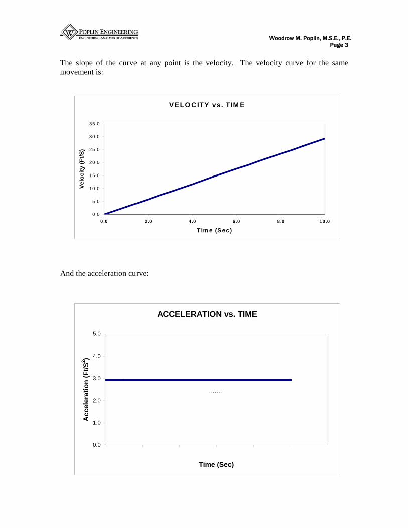
The slope of the curve at any point is the velocity. The velocity curve for the same movement is:

And the acceleration curve:

VELO CITY vs. TIM E

0.0

5.0

10.0

15.0

20.0

25.0

30.0

35.0

0.0 2.0 4.0 6.0 8.0 10.0

Tim e (Sec)

Velo

city

(Ft/S

)

ACCELERATION vs. TIME

0.0

1.0

2.0

3.0

4.0

5.0

0.00 2.00 4.00 6.00 8.00 10.00 12.00

Time (Sec)

Acc

eler

atio

n (F

t/S2 )

```````


If we can define the movement with an equation, then we can obtain the slope of the equation by taking the mathematical derivative of that equation. For example, the equation for the first graph (distance vs. time) is:

s = s0 + v0 + 1/2 at2 where s, s0, v0, a, and t are the position at time t, original position, original velocity, acceleration and time. ( 3 )

v = v0 + at is the derivative of the first equation and the

plotted curve. ( 4 ) a = constant is the derivative of equation 4 and the second

derivative of equation 3. ( 5 )

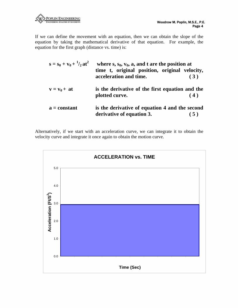
Alternatively, if we start with an acceleration curve, we can integrate it to obtain the velocity curve and integrate it once again to obtain the motion curve.

ACCELERATION vs. TIME

0.0

1.0

2.0

3.0

4.0

5.0

0.00 1.00 2.00 3.00 4.00 5.00 6.00 7.00 8.00 9.00 10.00

Time (Sec)

Acc

eler

atio

n (F

t/S2 )


Integration is a mathematical concept which calculates the area under the curve. For example, in the example above, the acceleration is 3 ft/s2. To calculate the velocity after 4 seconds, it is simply 3 ft/s2 times 4 seconds or 12 ft/s.

To obtain the distance we find the area under the velocity curve. For the triangular velocity curve, the area is half of the equivalent rectangle. For 4 seconds, this is 0.5 times 4 seconds times 12 ft/s or 24 ft.

DISTANCE vs. TIME

0102030405060708090

100110120130140

0.0 1.0 2.0 3.0 4.0 5.0 6.0 7.0 8.0 9.0 10.0

Time (Sec)

Dis

tanc

e (F

t)

VELOCITY vs. TIME

0

5

10

15

20

25

30

35

0.0 1.0 2.0 3.0 4.0 5.0 6.0 7.0 8.0 9.0 10.0

Time (Sec)

Velo

city

(Ft/S

)


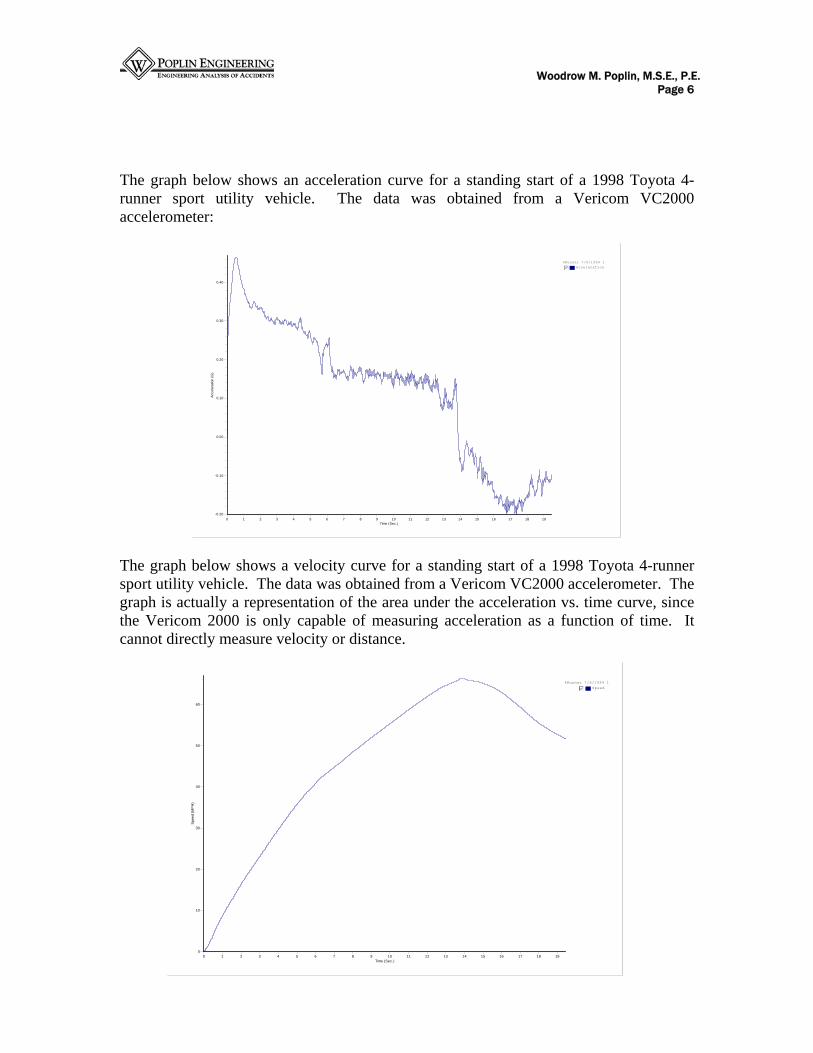
The graph below shows an acceleration curve for a standing start of a 1998 Toyota 4-runner sport utility vehicle. The data was obtained from a Vericom VC2000 accelerometer:

4Runner 7/6/1999 1

Acceleration

Time (Sec.)191817161514131211109876543210

Acce

lera

tion

(G)

0.40

0.30

0.20

0.10

0.00

-0.10

-0.20

The graph below shows a velocity curve for a standing start of a 1998 Toyota 4-runner sport utility vehicle. The data was obtained from a Vericom VC2000 accelerometer. The graph is actually a representation of the area under the acceleration vs. time curve, since the Vericom 2000 is only capable of measuring acceleration as a function of time. It cannot directly measure velocity or distance.

4Runner 7/6/1999 1

Speed

Time (Sec.)191817161514131211109876543210

Spee

d (M

PH)

60

50

40

30

20

10

0


The graph below shows a distance curve for a standing start of a 1998 Toyota 4-runner sport utility vehicle. The data was obtained from a Vericom VC2000 accelerometer. The graph represents the area under the velocity curve.

4Runner 7/6/1999 1

Distance

Time (Sec.)191817161514131211109876543210

Dis

tanc

e (F

eet)

1300

1200

1100

1000

900

800

700

600

500

400

300

200

100

0

The curve below is an acceleration curve produced by a tractor trailer:


So far we have discussed acceleration as a concept of straight line motion. However, these equations can be calculated independently for each axis of interest. For example, the ballistic equations used for falls, vaults, etc. are developed using a horizontal and vertical axis. The rise and fall times associated with a gravitational acceleration are independent of the horizontal motion. The concepts are also not limited to linear movement. The equations for angular rotation are identical if the following substitutions are used: Linear Rotation Mass Moment of inertia Distance angular displacement Velocity angular velocity Acceleration angular acceleration The rotational equations of motion for a constant angular acceleration are therefore given by:

θ = θ0 + ω0 + 1/2α t2 where θ, θ0, ω0 , α, and t are the position at time t, original angle, original rotational velocity, angular acceleration and time. ( 6 )

ω = ω0 + αt is the angular velocity at time t ( 7 )

α = constant is a constant angular acceleration ( 8 )

ACCELERATION TESTING A series of tests were conducted at a South Carolina weigh station to evaluate the acceleration characteristics of large trucks. The tests were arranged with the cooperation of The Coastal MAIT unit of the South Carolina Highway Patrol. A flat lot adjacent to the weigh station terminal provided a straight flat acceleration lane. The trucks were stopped as part of the normal inspection procedure. A Stalker radar was positioned adjacent to the exit route from the terminal. Once released, the truck drivers accelerated along the straight path to the exit. The operators were free to conduct an exit in any manner in which they desired. The truck weights were obtained from the weigh station scales. The weights were recorded along with the data from the Stalker radar. The objective was to obtain acceleration data from a variety of trucks of known weight. As would be expected, the accelerations varied significantly based on not only the capabilities and weight of the truck but the desires of the driver as well. The radar and


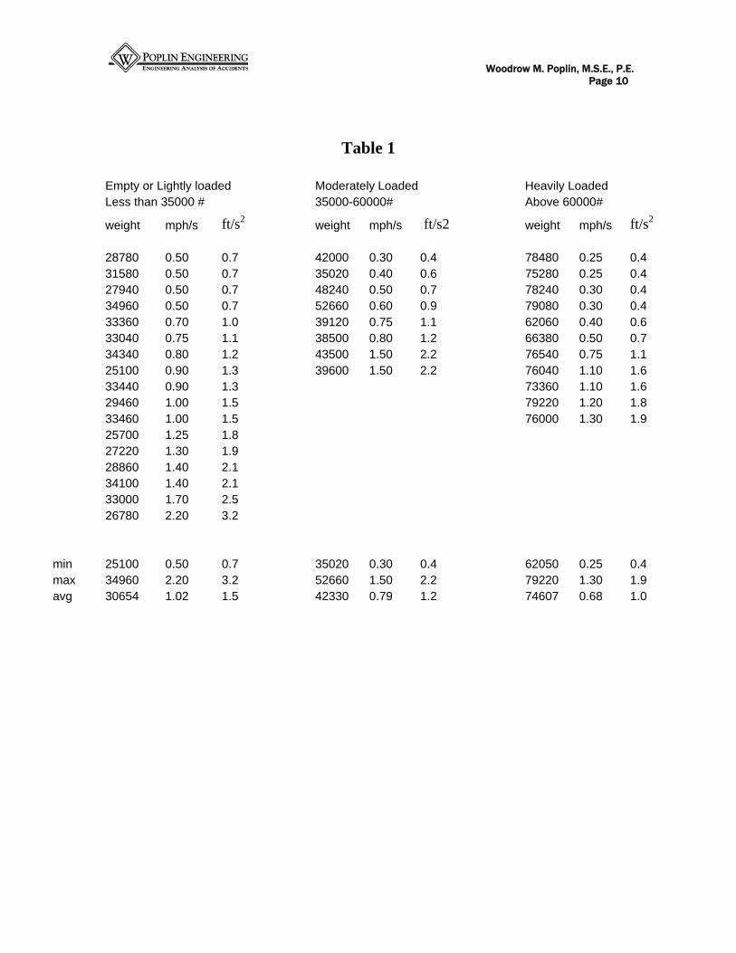
radar operator were visible to the truck drivers. This clearly offered some distraction. However, even with these limitations, the accelerations fell in a relatively narrow range. The accelerations of a total of 40 trucks were tested. All except one were tractor trailers or large straight trucks. Of the 40, the data from 4 were rejected. Of the four, one was a small straight truck. The others either stopped or were slowed by preceding traffic. The remaining 36 trucks were divided into three categories. A truck weighing 35000 pounds or less was considered either empty or lightly loaded. There were a total of 17 trucks in this category. Trucks weighing more than 35000 pounds but less than 60000 pounds were considered moderately loaded. Eight trucks fell in this category. The remaining 11 trucks weighed more than 60000 pounds and were categorized as heavily loaded. The measurements were taken over a distance of approximately 300 feet. The trucks all reached speeds between 9 and 23 mph. The Stalker radar has very limited capability at speeds below 6 mph. The instrument reading jumps from 0 to 6 mph. The Stalker software plots the data assuming a constant acceleration from 0 to 6 mph. This introduces some error at very low speeds, but with any appreciable acceleration, there is little effect on the movement over that derived from the linear acceleration extrapolation. Another source of difficulty with the radar is the sensitivity to other signal sources. Once a truck begins to accelerate, the radar correctly identifies the target of interest. However, prior to movement, weaker return signals from roadway or other weigh station traffic was often recorded in the data. Typically, the extraneous signals reflected speeds outside of the range under consideration and could therefore be readily recognized and filtered from the test data. The data was examined and evaluated as a constant acceleration. For the lightly loaded trucks, weights ranged from 25100 pounds to 34960 pounds with an average of 30654 pounds. The accelerations varied from a low of 0.7 ft/s2 to 3.2 ft/s2. The moderately loaded trucks were slower with a range of 0.4 to 2.2 ft/s2. The moderately loaded trucks

averaged 42330 pounds with the lightest at 35020 pounds. The heaviest weighed 52660 pounds. The heavily loaded trucks averaged 74607 pounds with the lightest at 62050 ponds and the heaviest at 79220 pounds. As expected, the heaviest trucks had the lowest accelerations which ranged from 0.4 to 1.9 ft/s2. A summary of the data is provided in Table 1.


Table 1

Empty or Lightly loaded Moderately Loaded Heavily Loaded Less than 35000 # 35000-60000# Above 60000#

weight mph/s ft/s2 weight mph/s ft/s2 weight mph/s ft/s2 28780 0.50 0.7 42000 0.30 0.4 78480 0.25 0.4 31580 0.50 0.7 35020 0.40 0.6 75280 0.25 0.4 27940 0.50 0.7 48240 0.50 0.7 78240 0.30 0.4 34960 0.50 0.7 52660 0.60 0.9 79080 0.30 0.4 33360 0.70 1.0 39120 0.75 1.1 62060 0.40 0.6 33040 0.75 1.1 38500 0.80 1.2 66380 0.50 0.7 34340 0.80 1.2 43500 1.50 2.2 76540 0.75 1.1 25100 0.90 1.3 39600 1.50 2.2 76040 1.10 1.6 33440 0.90 1.3 73360 1.10 1.6 29460 1.00 1.5 79220 1.20 1.8 33460 1.00 1.5 76000 1.30 1.9 25700 1.25 1.8 27220 1.30 1.9 28860 1.40 2.1 34100 1.40 2.1 33000 1.70 2.5 26780 2.20 3.2 min 25100 0.50 0.7 35020 0.30 0.4 62050 0.25 0.4 max 34960 2.20 3.2 52660 1.50 2.2 79220 1.30 1.9 avg 30654 1.02 1.5 42330 0.79 1.2 74607 0.68 1.0


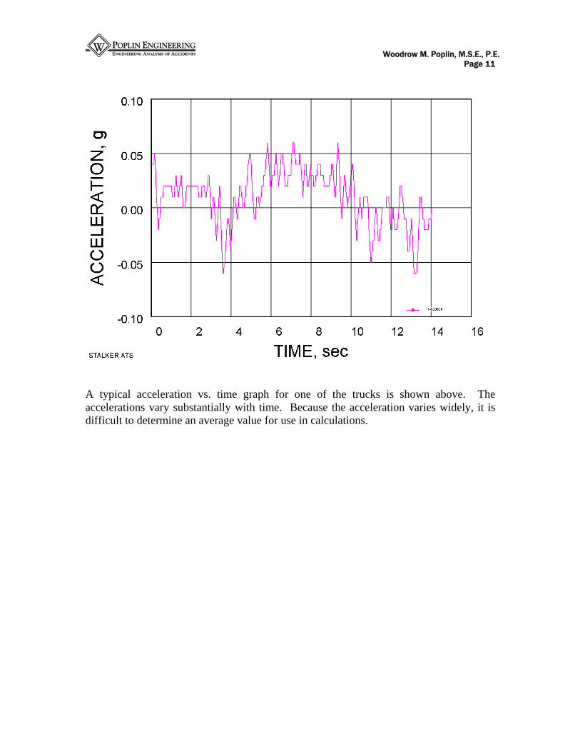
A typical acceleration vs. time graph for one of the trucks is shown above. The accelerations vary substantially with time. Because the acceleration varies widely, it is difficult to determine an average value for use in calculations.


It is much easier to examine the velocity vs. time curves and evaluate the accelerations as the slope of the curve. The velocity vs. time curves for the lightly loaded trucks are shown in the next two graphs.


The graphs for the moderately loaded trucks are shown above and for the heavily loaded trucks below.


SUMMARY The basic relationships of time, distance, velocity and acceleration have been developed and used to evaluate data produced by heavy trucks accelerating from a South Carolina weigh station. The exit path was straight and level. There were no external urgencies for the drivers. The vehicles accelerated from a stop on the basis of the equipment limitations and operator desires. All of the trucks reached speeds between 9 and 23 mph. Trucks 35000 pounds and under were considered empty or lightly loaded. Their accelerations varied from a low of 0.7 ft/s2 to 3.2 ft/s2. The moderately loaded trucks were slower with a range of 0.4 to 2.2 ft/s2. Their weight varied from 35020 pounds to the heaviest at 52660 pounds. The heavily loaded trucks averaged 74607 pounds with the lightest at 62050 ponds and the heaviest at 79220 pounds. They had the lowest accelerations which ranged from 0.4 to 1.9 ft/s2. ACKNOWLEDGEMENT The author wishes to thank the South Carolina Coastal MAIT unit for their assistance and participation in the testing procedure. Special thanks are extended to Sergeant Ricky Dixon, who undertook the effort to coordinate with the South Carolina Transport Police for the use of the weigh station and the recording of the vehicle weights.


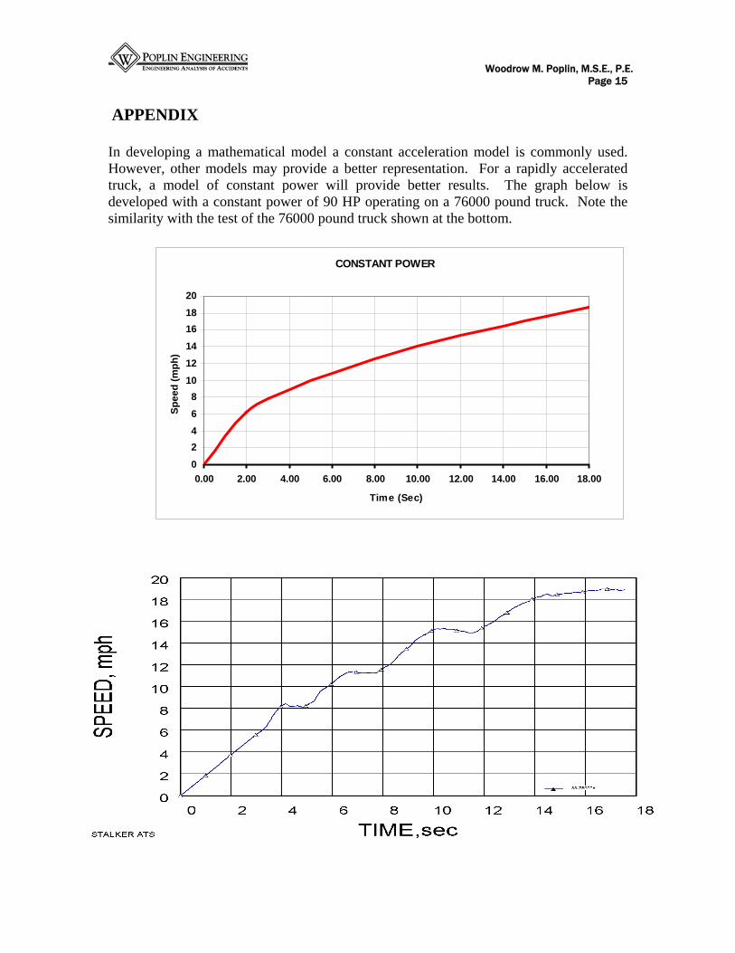
APPENDIX In developing a mathematical model a constant acceleration model is commonly used. However, other models may provide a better representation. For a rapidly accelerated truck, a model of constant power will provide better results. The graph below is developed with a constant power of 90 HP operating on a 76000 pound truck. Note the similarity with the test of the 76000 pound truck shown at the bottom.

CONSTANT POWER

02468

101214161820

0.00 2.00 4.00 6.00 8.00 10.00 12.00 14.00 16.00 18.00

Time (Sec)

Spee

d (m

ph)


CONS TANT P OW ER

0.00

5.00

10.00

15.00

20.00

25.00

0.00 2.00 4.00 6.00 8.00 10.00 12.00 14.00 16.00

T im e (Se c)

Spee

d (m

ph)

The graph above is developed with a constant power of 70 HP operating on a 39600 pound truck. Note the similarity with the test of the 39600 pound truck shown below.

acceleration of heavy trucks woodrow m. poplin, p.e.attraction. a convenient unit of acceleration...

Documents