acceleration-energy filter and bias compensation for...

공학박사학위논문

Acceleration-Energy Filter and Bias Compensation for

Stabilizing Equation Error Estimator in

Inverse Analysis Using Dynamic Displacement

동적 변위를 사용하는 역해석 문제에서

Equation Error Estimator 안정화를 위한

가속도-에너지 필터 및 편향성 보정 기법

2015년 8월

서울대학교 대학원

건설환경공학부

박 광 연

III

Abstract

New stabilization schemes which correct the equation error estimator (EEE) in the

inverse analysis using dynamic responses of linear elastic continua are presented.

The goal of the inverse analysis run in these cases is the proper identification of

material properties. Stabilization schemes consist of the acceleration-energy filter

and the bias compensation.

The acceleration-energy filter stabilizes the ill-posedness of the inverse

analysis. The acceleration-energy filter replaces the techniques known as

truncated singular value decomposition (TSVD), L1-norm regularization and L2-

norm regularization (or Tikhonov regularization). Existing regularization

techniques do not work properly for cases involving hard inclusions, i.e., tumors of

organ and suspensions of vehicles. The Acceleration-energy filter, however, work

properly for cases involving both hard and soft inclusions. The acceleration-

energy filter is separated into the acceleration filter and the energy filter. Dividing

them in this manner simplifies a filtering process.

The acceleration filter imposes finiteness condition of accelerations, the

second derivatives of the measured displacements. Accelerations can be

considered as finite functions when impact loads do not exist. The acceleration

filter requires two initial and two final values, but the overlapping moving time

window technique is employed so that the initial and final values can be ignored.

IV

The final form of the acceleration filter is a low-pass finite impulse response (FIR)

filter. However, the acceleration filter differs from typical low-pass FIR filters

because it has physical meaning which guarantees consistency with the energy

regularization.

The energy filter imposes finiteness of strain energy, which is internal energy

of linear elastic continua. The final form of the energy filter is very similar to

low-pass spatial filters used with image processing, but the energy filter has three

advantages. The first of these are the boundary conditions. The boundary

conditions of the energy filter are identical to these of an equilibrium equation for

the continuum, and are always satisfied by all continuum examples. The second is

the available meshes. The energy filter involves the connectivity information of

nodes and can handle complicatedly meshed FEM models, whereas typical low-

pass spatial filters can handle only rectangular meshes. The third advantage is the

physical meaning which guarantees consistency with the acceleration filter.

The acceleration filter and the energy filter must satisfy consistency of the

elastic waves and the temporal wave. The solution of the inverse analysis without

the consistency is not trustable because the strain and the acceleration do not have

equivalent information. The physical meaning of two filters gives consistency

between two filter.

The biases of the solutions are ignored in existing studies. However, the

inverse analysis using EEE for linear elastic continua must consider the biases. If

the noise variances are known, the biases of the solution could be perfectly

V

eliminated by means of bias compensation.

Aluminum plate and medical imaging examples are demonstrated to show the

effectiveness of the schemes described above.

Key words : Equation Error Estimation (EEE), System Identification,

Inverse Analysis, Identifying Material Properties, Acceleration-Energy Filter,

Temporal-Spatial Filter, Bias-compensation, Linear Elastic Continua,

Medical Imaging

Student Number : 2010-30239

VII

Contents

Abstract…………………………………………………………………………..III

List of Figures…………………………………………………………………......XI

List of Tables……………………………………………………………………..XV

1. Introduction………………………………………………………………………1

2. Equation Error Estimator in Inverse Analysis Using Dynamic Displacement…...7

2.1 Definition of Inverse Problem using Minimization………………………….7

2.2 FEM for discretizing EEE…………………………………………………..11

2.3 Effects of Noise in Displacement…………………………………………...15

2.3.1 Noise Amplification by Differentiation………………………………..15

2.3.2 Decomposition of Noise Effects………………………………………..20

2.4 Bias Compensation………………………………………………………….26

Bias Compensation under Unknown Noise Variance…………………….......29

2.5 Regularization………………………………………………………………30

3. Acceleration-Energy Filter……………………………………………………..37

3.1 Noise Filter Using Regularity Conditions of Displacement…………….......37

3.2 Characteristics of acceleration-Energy Filter……………………………….41

3.2.1 Characteristics in Frequency Domain……………………………….....41

3.2.2 Separation of Regularity Conditions…………………………………...43

3.2.3 Characteristics and Regularization Factors of Acceleration Filter……..45

VIII

3.2.3 Characteristics and Regularization Factors of Energy Filter…………...48

3.2.4 Characteristics of Acceleration-Energy Filter………………………….53

3.3 Discretization of Filters……………………………………………………..60

3.3.1 Discretization of Acceleration Filter…………………………………...60

3.3.2 Discretization of Energy Filter………………………………………....70

3.4 Acceleration-Energy Filter as Signal Processing…………………………...73

3.4.1 Acceleration filter as a signal processing………………………………73

3.4.2 Energy filter as a Signal Processing……………………………………74

3.5 Bias Compensation for EEE Using Filtered Displacement………………....76

4. Example & Application…………………………………………………………79

4.1 Example: Aluminum Plate…………………………………………………..79

4.1.1 Ideal Example…………………………………………………………..81

4.1.2 Verification 1: window size…………………………………………….86

4.1.3 Verification 2: Measuring Time…………………………………….......88

4.1.4 Verification 3: Damping……………………………………………......89

4.1.5 Verification 4: Noise Level……………………………………………..91

4.1.6 Verification 5: Target Frequency……………………………………….93

4.1.7 Verification 6: Bias Compensation without Noise Variance Information..94

4.1.8 Verification 7: Noise of Specific Frequency…………………………...96

4.2 Application to Medical Imaging: Ultrasonic Elastography…………………98

4.2.1 Introduction…………………………………………………………….98

4.2.2 Inverse Analysis for Helmholtz Equation…………………………….100

IX

4.2.3 Human Skin Tissue Example…………………………………………103

5. Conclusion……………………………………………………………………..111

Reference…………………………………………………………………………115

초록………………………………………………………………………………125

XI

List of Figures

Figure 2.1 Concept of OEE……………..……………..............................................9

Figure 2.2 Concept of EEE………………………………………………………...10

Figure 2.3 Transfer function of the second differentiation (absolute value)……....17

Figure 2.4 Noise free and noised differentiation of harmonic function combination..19

Figure 2.5 Human skin tissue example…………………..………………………..23

Figure 2.6 Biases from different error rates……...………………………………..24

Figure 2.7 Biases from different error seeds (same variance)…………...………...24

Figure 2.8 Ill-posedness of the solution (bias-compensation is applied)……...…..25

Figure 2.9 L2-norm regularization result of the soft inclusion case………...……..35

Figure 2.10 L2-norm regularization result of the hard inclusion case…..…...…….35

Figure 2.11 Mechanism of regularizations…………………………………...…....36

Figure 3.1 Normalized transfer function of the acceleration filter……..……….....49

Figure 3.2 Normalized transfer function of the energy filter…………..………….54

Figure 3.3 Normalized transfer function of the acceleration-energy filter……..….56

Figure 3.4 Normalized transfer function of acceleration-energy filter for Ht=9.7...57



Figure 3.7 Relationship between tH , oritH , and approxtH , ……………...……...60

Figure 3.8 Normalized coefficients of the CFIR acceleration filter………..……...63

XII

Figure 3.9 Transfer function of CFIR acceleration filter 97.0target =H …………64

Figure 3.10 Concept of overwrapping time window technique…………………...68

Figure 3.11 coefficients of FDM-FIR and CFIR filters……………………………68

Figure 3.12 transfer function of FDM-FIR acceleration filter 97.0target =H …....71

Figure 4.1 The aluminum plate example…………………………………………..80

Figure 4.2 Measured displacement on the point ‘A’………...…………………….82

Figure 4.3 Frequency spectrum and the transfer function of acceleration filter…..82

Figure 4.4 Result of the aluminum example…….………………………………...84

Figure 4.5 Results of aluminum example on the line (B-B’)……………………...85

Figure 4.6 Effect of energy filter on the stiffness discontinuous surface………….86

Figure 4.7 Results with various window sizes…………………………………….87

Figure 4.8 Results with various measuring times………………………………….88

Figure 4.9 Selection of target frequency in damping case………………………...90

Figure 4.10 Results with various damping………………………………………...90

Figure 4.11 Results with various noise levels……………………………………..92

Figure 4.12 Results using various target frequencies……………………………...92

Figure 4.13 Results when noise variance is unknown……………………………..95

Figure 4.14 Results with specific frequency noise………………………………...97

Figure 4.15 Ultrasonic measuring equipments…………………………………….99

Figure 4.16 The human skin tissue example……………………………………..106

Figure 4.17 Measured displacement on the point (A)……………………………107

XIII

Figure 4.18 Frequency spectrum and the transfer function of acceleration filter...107

Figure 4.19 Result of the human skin example…………………………………..108

Figure 4.20 Results of human skin example on the line (B-B’)…………….109, 110

XV

List of Tables

Table 4.1 Specification of the aluminum example………………………………...81

Table 4.2 Relationship between proportional error and signal to noise ratio……...91

Table 4.3 Specification of the human skin tissue example……………………….104

1

1. Introduction

Currently, system identification (SI) is an important issue in many fields, including

the civil engineering, mechanics, signal processing, shipbuilding, medical

engineering and other fields. SI reconstructs material properties and provides

important information for the maintenance and safety of structures. SI is also

known as inverse analysis.

Inverse analysis is known to be able to identify unknown system parameters

and to reconstruct inputs for producing desired outputs. The inverse analysis for

unknown system parameters detects damage in engineering structures and/or

tumors in human bodies. The identified stiffness, mass or damping can take the

form of damage indexes. The inverse analysis for the reconstruction of the input

is used for control and signal processing, but these areas are outside the scope of

this thesis.

Error minimization schemes are employed to define the inverse analysis.

Two types of error estimators, output error estimation (OEE) and equation error

estimation (EEE), are typically used. EEE estimates errors in the governing

equation or the weak form of it. The inverse analysis using EEE is suitable for

real-time processes because it is a quadratic optimization problem and a

parallelizable algorithm when the governing equation of the structure is linear

[Hjelmstad 1995]. Medical imaging, feedback control and structural safety

2

management require the real-time inverse analysis. OEE estimates errors between

responses from unknown models and measured responses. The inverse analysis

using OEE is an iterative scheme and not a parallelizable algorithm [Hjelmstad

1995, Banan 1995, Huang 2001]. Since quadratic problems have a lot of

advantages, EEE is utilized in this thesis.

The target structures are described by the linear elastic continua because the

continuum explain mosts of engineering solid structures. To solve the inverse

analysis numerically, the target continuum must be discretized by a numerical

model. In this thesis, the finite element method (FEM) is used as a numerical

model. The FEM is the best model with regard to forward analysis for continua;

however, the FEM amplifies noise in measurement when it is employed to solve the

inverse analysis. The relationship between strain and displacement amplifies the

noise.

The inverse analysis using minimization schemes leads to ill-posedness when

modeling errors and measurements noise exist [Bui 1994, Hansen 1998]. The

regularization has been proposed to reduce ill-posedness [Vogel 1986, Park 2007,

Lee 1999, Park 2001]. The regularization schemes work well for cases involving

soft inclusions. However, these efforts do not apply to cases involving hard

inclusions. Soft inclusion cases are the most common type of engineering damage,

but there are a number of hard inclusion cases, such as impurities of concrete

structures, tumors in human bodies and suspension stiffening of vehicles. The

acceleration-energy filter is proposed to stabilize the ill-posedness which arises in

3

cases involving both soft and hard inclusions. It imposes the physical laws which

the measurements must satisfy. The measurements must satisfy two laws of the

continuum, the finiteness of the strain energy and acceleration. The acceleration-

energy filter is separated into the acceleration filter and the energy filter. Dividing

them in this manner simplifies a filtering process. Both filters function as low-

pass filters to suppress noise amplification from differentiations. The effects of

the acceleration filter are similar to those of existing noise suppression filters.

However, the physical meaning of the acceleration filter is related to the physical

meaning of the energy filter, thus provides consistency between the two filters.

The energy filter is similar to low-pass spatial filters, which is used for image

processing. However, the modeling information of the target continuum is

included in the energy filter. While image filters consider only nodes arranged in

a rectangular, the modeling information allows for the energy filter to consider

nodes in more complicated connection. Moreover, the energy filter can consider

nodes around boundaries properly, as the boundary condition used in the energy

filter is identical to that of the continuum. The acceleration filter and the energy

filter must satisfy consistency of the elastic waves and the temporal wave. The

solution of the inverse analysis without the consistency is not trustable because the

strain and the acceleration do not have equivalent information. The physical

meaning of two filters gives consistency between two filter.

Solutions of the inverse analysis using EEE have not only ill-posedness but

also bias in the solution. When the measurement is polluted by noise, the EEE

4

includes squared error terms, which are directly proportional to the variance of the

noise. In most inverse analyses using EEE, the bias is negligible or easy to

remove [Nguyen 1993, Hjelmstad 1995, Haykin 2008, Ikenoue 2009, Zhang 2011].

However, the bias inherent in the inverse analysis using EEE for the linear elastic

continua cannot be ignored, as the noise is amplified twice during the inverse

analysis process and is complexly involved in the FEM model. The squared error

terms lead to fixed direction errors of the solutions, i.e., the biases, and cannot be

eliminated by an infinite measuring time. The bias compensation can reconstruct

the bias terms and remove the biases of the solutions when the variance of the noise

is known. A case of unknown variance is also introduced in this thesis.

A time-domain analysis using dynamic displacement is employed rather than a

frequency-domain analysis. A time-domain analysis is more sensitive to local

inclusion than a frequency-domain analysis. A frequency-domain analysis has

advantages which simplify problems, but is not sensitive to local inclusion

[Raghavendrachar 1992]. Laser displacement measures are commonly used [Park

2013, Choi 2013]. This equipment is more expensive than accelerometers and

requires reference points. However, laser displacement measures are more

accurate than accelerometers. Moreover, LIDAR, a laser scanning technique,

provides a high spatial resolution. Recently, there have been numerous studies

which have attempted to reduce cost of the displacement measure. Several studies

have focused on a vision-based displacement measurement technique [Kim 2012,

Kim 2013a, Kim 2013b]. It requires only a small number of video cameras to

5

measure the displacement of large structures. A light emitting diode (LED) can be

applied to improve the vision-based displacement measurement technique [Wahbeh

2003]. Kinect, an input device developed by Microsoft as part of their XBOX 360,

is applied as displacement measure to reduce costs [Qi 2014]. Specifically, a

ultrasonic elastography device provides displacement measurements [Bercoff 2003,

Bercoff 2004, Park 2006, Park 2009]. Ultrasonic elastography devices incur low

costs and provide high-quality information for diagnosis.

An example and an application are introduced to assess the acceleration-

energy filter and the bias compensation. The first example is an aluminum plate

which is under a plane stress condition. It shows how the inverse analysis using

EEE and stabilization schemes work. The second example is a human skin tissue.

It uses the Helmholtz equation, which is an equation for incompressible continuum.

The inverse analysis and stabilization schemes are slightly different from those of

the inverse analysis for the original continuum. The example shows an algorithm

for medical imaging using ultrasonic equipment.

7

2. Equation Error Estimator in Inverse Analysis Using Dynamic Displacement

2.1 Definition of Inverse Problem Using Minimization

There are numerous engineering demands to identify unknown system

parameters of continua, especially stiffness parameters. These identifying

schemes are known as system identification (SI) and/or inverse analysis. Inverse

analysis typically uses various types of measurements, including the displacement,

velocity, acceleration, and strain. With regard to the types of measurements,

displacement includes the lowest frequency information. It works well with

massive structures such as civil structures, aircraft, and ships. For wave problems

such as those in ultrasonic medical imaging, only displacement is valid because it

includes the information pertaining to frequencies around 0Hz. Acceleration and

velocity do not include this type of information.

Unknown stiffness parameters are estimated by inverse analysis for linear

elastic continua. The governing equation of the continuum is a function of the

displacement, system parameters and external forces.

02

22

=∂∂

ρ−+∂∂

∂tub

xxuC i

ilj

kijkl (2.1)

where ijklC , ix , iu , t , ib , ρ and ∂ are the elasticity tensor, the Cartesian

8

tensor, the displacement tensor, the time dimension, the body force tensor, the mass

density and the symbol of partial differentiation, respectively. The displacement

can be calculated via the system parameters and the external forces.

Error minimization schemes are employed for identifying the stiffness

parameters, which are parts of the system parameters. Output error estimation

(OEE) and equation error estimation (EEE) are typical error estimators.

OEE estimates errors between responses from unknown models and measured

responses. The next equation represents inverse analysis using OEE which uses

the L2-norm [Hjelmstad 1996, Ge 1998, Huang 2001, Kang 2005].

∫ ∫ −=ΠT V ijkl dtdVuCu

t

2

2)(min (2.2)

Here, T , tV , ijklC , u and u are the total measuring time, the whole domain

of the continuum, the unknown stiffness parameter, the calculated displacement

from the governing equation (or from a numerical model of the equation) and the

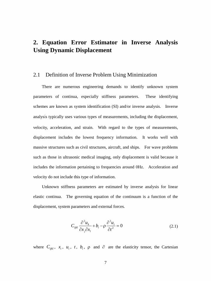
measured displacement, respectively. Fig. (2.1) shows the basic concept of

inverse analysis using OEE. Eq. (2.2) is a non-linear minimization problem

because )( ijklCu is calculated by solving forward problems, including a matrix

inversion calculation. Accordingly, inverse analysis using OEE requires a

considerable amount of computational effort and is not suitable for real-time SI.

9

Figure 2.1 Concept of OEE

However, responses of all degrees of freedom (DOF) do not have to be measured.

This is one advantage for selecting measurement points. Also, inverse analysis

using OEE does not have biases in its solutions.

EEE estimates errors in the governing equation or the weak form of it. The

inverse analysis using EEE with the L2-norm is in the next.

∫ ∫ ∂∂

ρ−∂∂

∂=Π

t Vi

lj

kijkl dVdt

tu

xxuC

t

2

22

22

min (2.3)

In this equation, T , tV , ijklC , u and ρ are the total measurement time, the

whole domain of the continuum, the unknown stiffness parameters, the measured

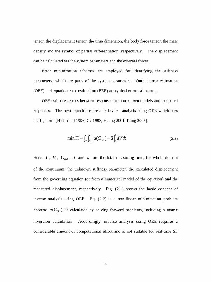
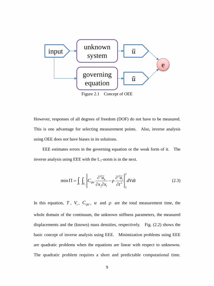
displacements and the (known) mass densities, respectively. Fig. (2.2) shows the

basic concept of inverse analysis using EEE. Minimization problems using EEE

are quadratic problems when the equations are linear with respect to unknowns.

The quadratic problem requires a short and predictable computational time.

unknown system

governing equation

input

e

10

Figure 2.2 Concept of EEE

Inverse analysis of linear elastic continua using EEE is a parallelizable algorithm,

because each time step and each of the terms are perfectly independent from each

other. The quadratic object function and the parallelizable algorithm make inverse

analysis using EEE suitable for real-time or semi-real-time processes. However,

the solutions from the inverse analysis using EEE contain biases. The biases must

be handled by a bias compensation scheme, as introduced in section 2.4. Another

disadvantage is that all displacements, velocities and accelerations on the all DOF

are required. If only one of these responses is measured, the other responses must

be derived by differentiation or integration. The noise sources in the measurement

are amplified during the differentiation and integration process. The amplified

noise amplifies the ill-posedness and the bias of the solutions. This amplification

must be handled by the acceleration-energy filter, which is introduced in chapter 3.

unknown system

governing equation

input

e

11

As introduced in chapter 1, inverse analysis using EEE is feasible for real-time

processes and thus the acceleration-energy filter in this paper focus on EEE. The

filter here can be applied to inverse analysis using OEE, but this is outside the

scope of this thesis.

Several assumptions are necessary to simplify the problems. The first is that

the external forces and the body forces are ignored because forces from outside of

the continua are difficult to measure. Transient loads, which are released

immediately before the measurement processes start, satisfy the first assumption.

When this assumption is valid, the body force term ib in Eq. (2.1) becomes zero.

A second assumption is that damping can be ignored. A short measurement time

makes damping ignorable. This assumption is satisfied when relatively few

vibrations are included in the measurement time. A third assumption is that the

mass density and the Poisson ratio are known. The final assumption here is the

assumption of isotropy continuum.

2.2 FEM for Discretizing EEE

Eq. (2.3) must be discretized, as measured displacements are usually

discretized in both temporal and spatial dimensions. The finite element method

(FEM), the rectangle method and the central finite difference method (FDM) are

utilized for discretizing the spatial domain, the temporal integration and the

temporal differentiation, respectively.

12

Originally, Eq. (2.3) is discretized but cannot be. The weak form of the

governing equation is employed for replacing the governing equation in the Eq.

(2.3). Spatial discretization starts with the variation of Eq. (2.1), without the body

force ib .

∫∫ ∂∂

ρδ−∂∂

∂δ

Vi

iVlj

kijkli dV

tuudV

xxuCu 2

22

(2.4)

Here, iu is the measured displacement. The equation above is integrated by

parts and discretized by FEM.

0

2

2

=

+

ρδ≈

∂∂

δ−∂∂

∂δ∂

+∂∂

ρδ

∑ ∫∑ ∫

∫∫∫

UDBBUNNUe V

Te

e V

Te

s jl

kijkliV

l

kijkl

j

iV

ii

ee

dVEdV

dSnxuCudV

xuC

xudV

tuu

(2.5a)

(2.5b)

where N , B , D , U and eE are the shape function matrix, the first

derivatives of the shape function matrix, the constitutive matrix with the unit

Young’s modulus, the measured displacement vector and the Young’s modulus of

each element, respectively. The superscript e refers to each element. ∑e

)(

represents a structural compatibility summation. The last term in Eq. (2.5a) is a

boundary condition and is eliminated on the fixed and free boundaries. The

sufficient condition of Eq. (2.5b) is the next.

13

02 =+=

+

ρ

∑∑

∑ ∫∑ ∫UqULm

UDBBUNN

e

ee

e

e

e V

Te

e V

Te

E

dVEdVee

(2.6a)

(2.6b)

em and eq are defined below

∫ρ=eV

Te dVNNm (2.7a)

∫=eV

Te dVDBBq (2.7b)

Since solutions of Eq. (2.6b) are the optimal solutions of the equilibrium

equation (Eq. 2.1), Eq. (2.6b) replaces the equilibrium equation in Eq. (2.3).

∫ ∑∑ +=Πt

e

ee

e

e dtE2

2

min UqUm (2.8)

The rectangle method and the central FDM are employed for descretizing the

temporal integration and the displacement-acceleration relationship, respectively.

∑ ∑∑

∑ ∑∑

∆+≈

∆+≈Π

tt

e

eet

e

e

tt

e

eet

e

e

tE

tE

2

22

2

2

min

UqULm

UqUm

(2.9a)

(2.9b)

14

The subscript t indicates each time step. The central FDM matrix for second

order derivatives using second order accuracy 2L is defined below.

−

−−

∆=

121

121121

122

tL (2.10)

Since t∆ in Eq. (2.9b) does not effect to result of the minimization problem,

the discretized object function of inverse analysis using EEE is given below.

∑ ∑∑ +=Πt

te

eet

e

e E2

22min UqULm (2.11)

The solution of the quadratic minimization problem is given below.

0)()( 2 =

+

=

∂Π∂ ∑ ∑∑ ∑

tt

e

eTieTt

tt

e

eTiTti E

EUqqUULmqU (2.12)

The number of these equations is identical to the number of elements. A

matrix form of the equation above is in the next.

0QEM =+ (2.13a)

MQE 1−−= (2.13b)

M , Q and E are defined below.

15

( )( )

( )∑=

+++

+++

+++

=n

t

teTeT

t

teTT

t

teTT

t

1

221

2212

2211

ULmmmqU

ULmmmqUULmmmqU

M

(2.14a)

∑=

=n

t

teTeT

ttTeT

ttTeT

t

teTT

ttTT

ttTT

t

teTT

ttTT

ttTT

t

1

21

22212

12111

UqqUUqqUUqqU

UqqUUqqUUqqUUqqUUqqUUqqU

Q

(2.14b)

=

eE

EE

2

1

E (2.14c)

It is important to note that the measured displacement vector U is squared.

The squared terms cause bias in the solutions. This is discussed in the next

section.

2.3 Effect of Noise in Displacement

2.3.1 Noise Amplification by Differentiation

The measured displacement always includes noise. The noise is amplified by

displacement-acceleration and displacement-strain relationships, which are the

second and the first order differentiations, respectively. To understand the noise

amplification of differentiations, a frequency-domain analysis is useful. The

Fourier transform and the transfer function provide information on the frequency

16

domain. [Bracewell 2000]

The Fourier transform (Eq. 2.15) provides frequency domain information from

a function or signal of the original domain.

)(ˆ)(21)]([ ω=π

= ∫∞

∞−

ω− fdxexfxf xiF (2.15)

Here, F , )(xf and )(ˆ ωf denote the Fourier transform, a function/signal of

the original domain and a function/signal of the frequency domain, respectively.

The original domain is a temporal or spatial domain in this paper, and the frequency

domain is a temporal or spatial frequency domain as well.

A function of the frequency domain is a transfer function. The definition if

the transfer function is the linear mapping of the input and the output in the

frequency domain.

)()()( ωω=ω XHY (2.16)

Where ω , )(ωH , )(ωY and )(ωX are the frequency in radian, the transfer

function, the Fourier transform of the output and the Fourier Transform of the input,

respectively. The Fourier transform of the differentiation is the next equation.

)(ˆ)i()(ωω=

f

dxxfd n

n

n

F (2.17)

17

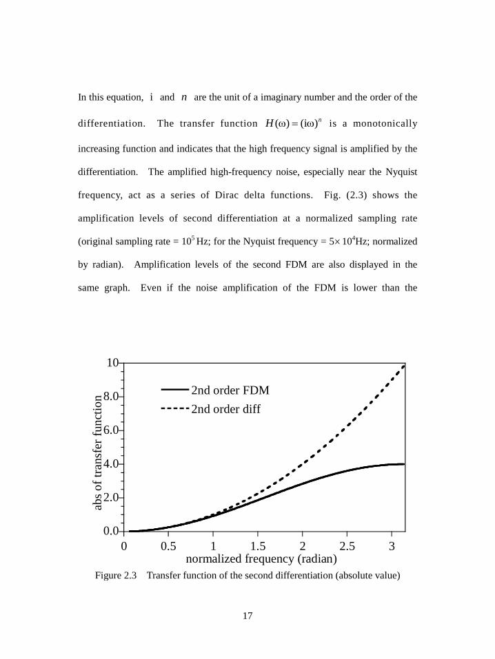
In this equation, i and n are the unit of a imaginary number and the order of the

differentiation. The transfer function nH )i()( ω=ω is a monotonically

increasing function and indicates that the high frequency signal is amplified by the

differentiation. The amplified high-frequency noise, especially near the Nyquist

frequency, act as a series of Dirac delta functions. Fig. (2.3) shows the

amplification levels of second differentiation at a normalized sampling rate

(original sampling rate = 105 Hz; for the Nyquist frequency = 5×104Hz; normalized

by radian). Amplification levels of the second FDM are also displayed in the

same graph. Even if the noise amplification of the FDM is lower than the

0.0

2.0

4.0

6.0

8.0

10

0 0.5 1 1.5 2 2.5 3

2nd order FDM2nd order diff

abs o

f tra

nsfe

r fun

ctio

n

normalized frequency (radian)

Figure 2.3 Transfer function of the second differentiation (absolute value)

18

amplification of exact differentiation, it remains critical. Figs. (2.4a, b and c)

show the noise-free and noisy differentiation of the harmonic function combination.

Fig. (2.4a) is displacement u(t) = sin(300×2πt) + cos(250×2πt) and the noised

displacement. Fig. (2.4b and c) are the accelerations, the second derivatives of the

exact/noisy displacements and the large scale of (b), respectively. As shown in the

Fig. (2.4b), the amplified high-frequency noise acts as a series of Dirac delta

functions. This breaks physical laws, the finiteness of the strain energy and

acceleration, for the dynamic response of the continuum and causes error in the

solutions of the inverse analyses.

19

-3 100

-2 100

-1 100

0 100

1 100

2 100

0 100 5 10-3 1 10-2 1.5 10-2 2 10-2

disp.disp. + noisedi

spla

cem

ent(m

m)

time(seconds)

a

-4 109-3 109-2 109-1 1090 1001 1092 1093 1094 109

0 100 5 10-3 1 10-2 1.5 10-2 2 10-2

exact acc.FDM of disp. with noise

2nd d

iff o

f dis

plac

emen

t

time(seconds)

b

-6 106

-4 106

-2 106

0 100

2 106

4 106

6 106

0 100 5 10-3 1 10-2 1.5 10-2 2 10-2

exact acc.

2nd d

iff o

f dis

plac

emen

t

time(seconds)

c

Figure 2.4 Noise free and noised differentiation of harmonic function combination

(a)original harmonic function (b)second derivatives (c)large scale of derivatives

20

2.3.2 Decomposition of Noise Effects

The amplified noise in the measured displacement effects to the solutions of

EEE. To analyze effects of noise in the measured displacements, tU in Eqs.

(2.14a and b) is replaced by )( ne UU + . eU and nU represent the exact

displacement and the noise in the measured displacement, respectively.

COVbiasexact

1 11

111111

1 1

111

1 1

111

1 1

111

QQQ

UqqUUqqUUqqUUqqU

UqqUUqqUUqqUUqqU

UqqUUqqU

UqqUUqqU

UqqUUqqU

UqqUUqqU

UqqUUqqU

UqqUUqqUQ

++=

++

+++

+

=

=

∑

∑

∑

∑

=

=

=

=

n

te

eTeTnn

eTeTee

TeTnn

TeTe

eeTT

nneTT

eeTT

nnTT

e

n

tn

eTeTnn

TeTn

neTT

nnTT

n

n

te

eTeTee

TeTe

eeTT

eeTT

e

n

tt

eTeTtt

TeTt

teTT

ttTT

t

(2.18a)

21

( )

( )( )

( )( )

( )( ) ( )

( ) ( )COVbiasexact

12

12

1

211

211

12

1

211

12

1

211

12

1

211

MMM

ULmmqUULmmqU

ULmmqUULmmqU

ULmmqU

ULmmqU

ULmmqU

ULmmqU

ULmmqU

ULmmqUM

++=

+++++

++++++

++

+++

++

++=

++

++=

∑

∑

∑

∑

=

=

=

=

n

te

eTeTnn

eTeTe

eeTT

nneTT

e

n

tn

eTeTn

neTT

n

n

te

eTeTe

eeTT

e

n

tt

eTeTt

teTT

t

(2.18b)

Where exactQ , biasQ , COVQ , exactM , biasM and COVM are the exact term of

Q , the bias term of Q , the covariance term of Q , the exact term of M , the bias

term of M and the covariance term of M , respectively. Eq. (2.13a) is

decomposed into the next form by Eq. (2.18a and b).

0)( COVbiasexactCOVbiasexact =+++++ EQQQMMM (2.19)

exactQ and exactM are exact terms which are determined by the noise-free

displacements. These terms include noise-free information and give exact

solutions.

22

exact1

exactexact MQE −= (2.20)

Here, exactE is the vector of the exact solution for the unknown Young’s

modulus vector E .

biasQ and biasM in Eq. (2.19) are bias terms which are created by the

squared noise. Bias terms have the characteristic of variance because the

summations of the squared noise are directly proportional to variance of the noise.

These terms create biases in solutions because the noise is squared before the

summation in each case. The terms do not disappear, even when the measurement

times are infinite, and they converge to specific matrixes. The matrixes are

proportional to the variance of the noise. Error seeds do not effect to the bias of

the solutions. If the bias terms are known, the bias of the solution can be

eliminated by the next equation.

EQQMM )(0 biasbias −+−= (2.21)

The terms in Eq. (2.21) are defined in Eqs. (2.14a,b) and (2.18a,b).

To demonstrate the bias of the solution, a human skin tissue example is

employed (Fig. 2.5). The example is modeled by 100×100 Q4 plane strain

elements and Helmholtz equation for analyzing both forward and backward

problems. Exact shear modulus of normal and inclusion elements are kPa36

and kPa72 , respectively. Shear modulus of each elements are estimated by

23

Figure 2.5 Human skin tissue example

Eq. (2.13b). Figs. (2.6) ~ (2.8) show the results on the line (A-A’) of Fig. (2.5).

Fig. (2.6) shows the biases from different error rates. A greater error rate results

in greater bias. Fig. (2.7) shows that the bias is not affected by the noise sets.

Even when the noise seeds are different, the same variance results in the same bias.

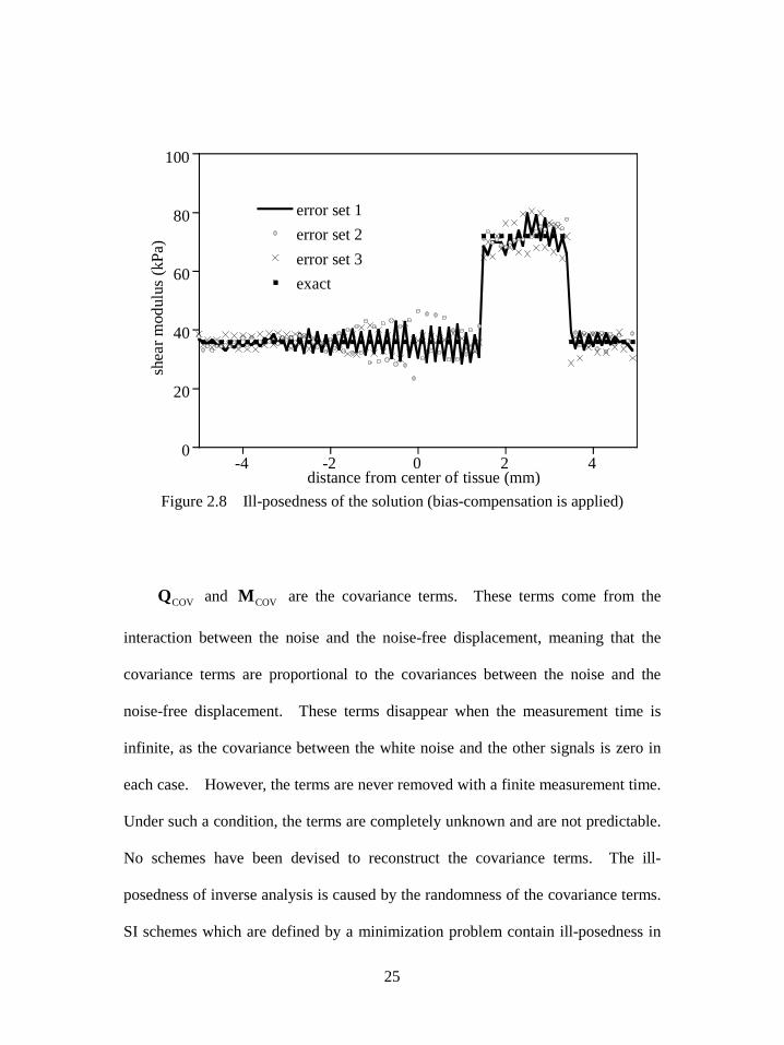
Fig. (2.8) shows the solutions using Eq. (2.21). The biases are removed, but ill-

posedness remains in the solutions. This ill-posedness occurs from the covariance

terms.

Inclusion

A

2mm 1.5mm

10mm10

mm

3mm

3.5mm

A’

24

0

500

1000

1500

2000

-4 -2 0 2 4

error: 0.10%error: 0.05%error: 0.01%exact

shea

r mod

ulus

(kPa

)

distance from center of tissue (mm) Figure 2.6 Biases from different error rates

0

100

200

300

400

500

600

700

800

-4 -2 0 2 4

error set 1error set 2error set 3exact

shea

r mod

ulus

(kPa

)

distance from center of tissue (mm) Figure 2.7 Biases from different error seeds (same variance)

25

0

20

40

60

80

100

-4 -2 0 2 4

error set 1error set 2error set 3exact

shea

r mod

ulus

(kPa

)

distance from center of tissue (mm) Figure 2.8 Ill-posedness of the solution (bias-compensation is applied)

COVQ and COVM are the covariance terms. These terms come from the

interaction between the noise and the noise-free displacement, meaning that the

covariance terms are proportional to the covariances between the noise and the

noise-free displacement. These terms disappear when the measurement time is

infinite, as the covariance between the white noise and the other signals is zero in

each case. However, the terms are never removed with a finite measurement time.

Under such a condition, the terms are completely unknown and are not predictable.

No schemes have been devised to reconstruct the covariance terms. The ill-

posedness of inverse analysis is caused by the randomness of the covariance terms.

SI schemes which are defined by a minimization problem contain ill-posedness in

26

their solutions [Bui 1994, Hansen 1998]. Fig. (2.8), which is a solution using the

bias compensation, shows the randomness of solutions containing ill-posedness.

The instability of the solution can be explained by the lack of information. Noise

in the measurement and modeling errors always exist with inverse analysis, and

they cause information losses. The non-uniqueness and discontinuity of the

solution are caused by a lack of information and cause instability in the solution.

Regularization schemes are existing for stabilizing the solutions. The

regularization schemes impose prior information to handle the lack of information.

This issue is minutely discussed in section 2.5.

2.4 Bias Compensation

The inverse analysis using EEE is disturbed not only by ill-posedness but also

by biases [Hjelmstad 1995]. The biases of the solutions are caused by error terms

in Eq. (2.19). The biases are not eliminated even when the measurement time is

long enough. Biases in solutions exist in all types of inverse analysis using EEE,

not only in the inverse analysis for linear elastic continuum using dynamic

displacement. However, the biases of the solutions are not seriously considered in

many studies. The adaptive filters employ the inverse analysis using EEE for real-

time processes [Haykin 2008]. Although the reference does not use ‘EEE’ as the

name of the error estimator, the process for estimating error of the target system is

identical to EEE. The result of the process has bias, but it is very small and

negligible when the noise is properly taken into account by noise suppression filters.

27

Additionally, it is easy to remove the bias from the solutions, since only the noise

variances have relationship with the bias in each case. The extraction of the flutter

derivatives uses the inverse analysis using EEE [Hong 2012, Cha 2015]. This

method includes the bias of the solutions as well, but it is ignorable for the same

reason given with the adaptive filter [Cha 2015].

However, the bias of EEE for the inverse analyses of linear elastic continuum

is not ignorable because the noise is amplified twice in the spatial and temporal

differentiation processes. The bias of the solution is eliminated by Eq. (2.21). If

the noise values are known, the bias terms are also known by Eq. (2.12a and b).

However, the noise values are always unknown and the bias terms are unknown as

well.

Bias compensation is suggested to handle the bias with reconstructed bias

terms. The bias compensation reconstructs the bias terms by the variances instead

of with the noise values themselves. The bias compensation requires three

assumptions. The first is that the noise is white noise. The second is that

correlation between colored noise from different white noise is zero. The final is

that the measured data is long enough and the bias terms are converged enough.

The bias terms in Eqs. (2.18a and b) consist of the colored noise vectors inu or

inuL2 , and the square matrixes eTi qq or eTi mq . The colored noise vectors are

represented by c , and the square matrix is represented by A .

28

( ) ( )

= ∑∑

==

nn t

t

Tlk

t

tl

Tk sum

11ccAAcc (2.22a)

( )

= ∑

=

nt

t

Tlksum

1ccA (2.22b)

σσσ

σσσσσσ

=

),()2,()1,(

),2()2,2()1,2(),1()2,1()1,1(

2,

2,

2,

2,

2,

2,

2,

2,

2,

mnnn

mm

tsum

lklklk

lklklk

lklklk

n

A (2.22c)

Here, and ][⋅sum denote the element multiplication of the matrixes and the

summation of all elements in a matrix, respectively. ),(2, mnlkσ is the covariance

between the nth element of the colored noise vector kc and the mth element of the

colored noise vector lc . nt is the number of time steps.

When the noise is white noise, biasQ and biasM in Eqs. (2.18a and b) are

reconstructed as biasQ and biasM by Eq. (2.22c).

σσσ

σσσ

σσσ

=

∑∑∑

∑∑∑∑∑∑

m

eemmm

m

emmm

m

emmm

m

emmm

mmmm

mmmm

m

emmm

mmmm

mmmm

n

qqq

qqq

qqq

t

,,

22,,

21,,

2

,2,

22,2,

21,2,

2

,1,

22,1,

21,1,

2

bias

Q (2.23a)

29

σ++σ+σ

σ++σ+σ

σ++σ+σ

∆−

=

∑∑∑

∑∑∑∑∑∑

m

eemmm

m

emmm

m

emmm

m

emmm

mmmm

mmmm

m

emmm

mmmm

mmmm

n

mmm

mmm

mmm

tt

,,

22,,

21,,

2

,2,

22,2,

21,2,

2

,1,

22,1,

21,1,

2

2bias2

M (2.23b)

In this equations, 2mσ , ji

nmq ,, and ji

nmm ,, are the variance values of white noise in

the mth measuring point, the ),( nm element of the matrix jTi qq and the ),( nm

element of the matrix jTi mq , respectively. 22 −∆− t of Eq. (2.23b) represents

the middle coefficient of the central FDM for second order derivatives using second

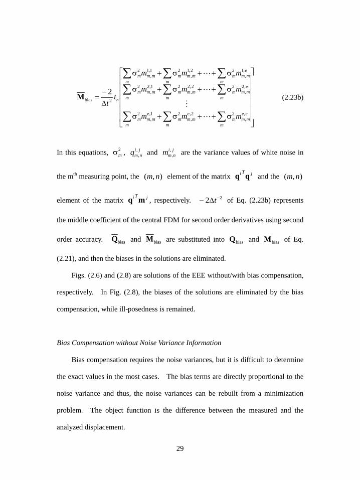
order accuracy. biasQ and biasM are substituted into biasQ and biasM of Eq.

(2.21), and then the biases in the solutions are eliminated.

Figs. (2.6) and (2.8) are solutions of the EEE without/with bias compensation,

respectively. In Fig. (2.8), the biases of the solutions are eliminated by the bias

compensation, while ill-posedness is remained.

Bias Compensation without Noise Variance Information

Bias compensation requires the noise variances, but it is difficult to determine

the exact values in the most cases. The bias terms are directly proportional to the

noise variance and thus, the noise variances can be rebuilt from a minimization

problem. The object function is the difference between the measured and the

analyzed displacement.

30

2

2

22 ))(()(min σσ btt Euu −=Π (2.24)

Where 2σ and tu are the unknown noise variance vector and the measured

displacement, respectively. ))(( 2σbt Eu is the analyzed displacement which is

calculated by the bias compensated elastic modulus using 2σ . 2

2⋅ indicates the

L2-norm minimization. Since the number of noise variance is identical to the

number of nodes, Eq. (2.24) has too much unknowns. Thus, additional

information is required for reducing the number of the unknown. A proportional

noise assumption or an absolute noise assumption can be the additional information.

2.5 Regularization

To remove the ill-posedness of the inverse analysis, missed information must

be complemented. Regularization schemes have been used for stabilizing the ill-

posedness of the inverse analyses. Unstable information is replaced by prior

information, which is imposed by regularity conditions. Material property

conditions are the most commonly used information in many studies.

Regularizations impose the condition in which the material property functions of

the continuum must be in the L2-function space.

Three types of regularization are typically used in many fields. The first is

known as truncated singular value decomposition (TSVD) [Vogel 1986]. TSVD is

not a regularization scheme, but it has the basic concept of regularization. Q in

31

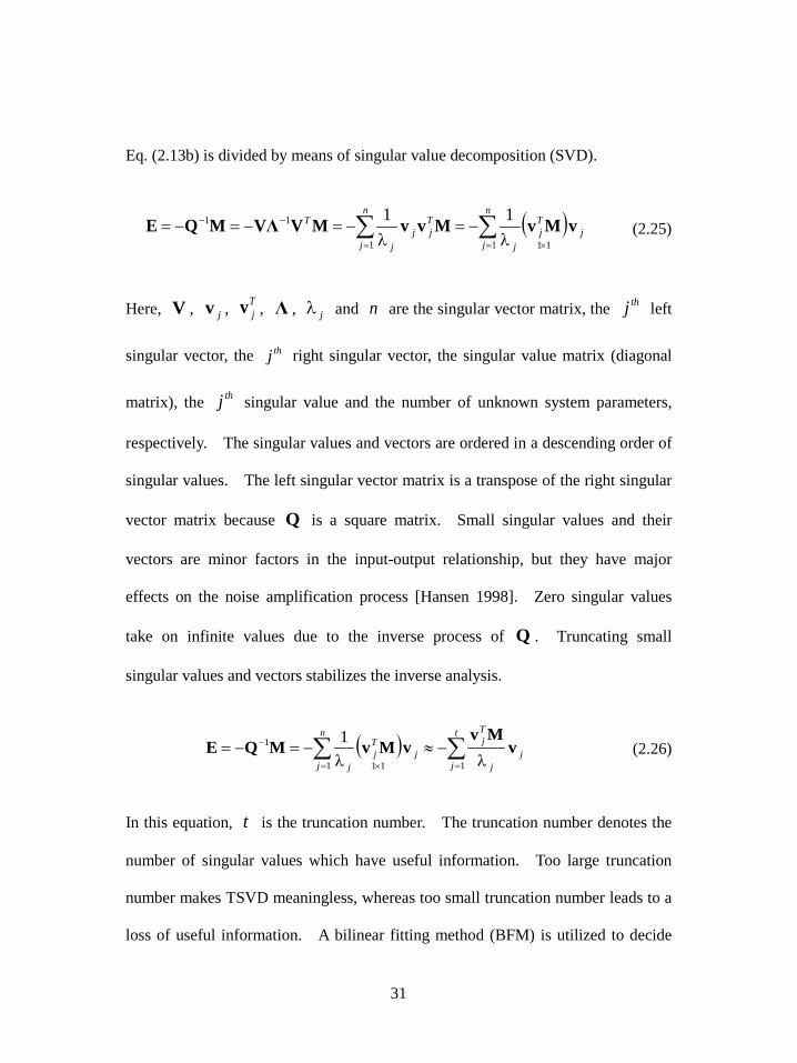
Eq. (2.13b) is divided by means of singular value decomposition (SVD).

( )∑∑= ×=

−−

λ−=

λ−=−=−=

n

jj

Tj

j

n

j

Tjj

j

T

1 111

11 11 vMvMvvMVVΛMQE (2.25)

Here, V , jv , Tjv , Λ , jλ and n are the singular vector matrix, the thj left

singular vector, the thj right singular vector, the singular value matrix (diagonal

matrix), the thj singular value and the number of unknown system parameters,

respectively. The singular values and vectors are ordered in a descending order of

singular values. The left singular vector matrix is a transpose of the right singular

vector matrix because Q is a square matrix. Small singular values and their

vectors are minor factors in the input-output relationship, but they have major

effects on the noise amplification process [Hansen 1998]. Zero singular values

take on infinite values due to the inverse process of Q . Truncating small

singular values and vectors stabilizes the inverse analysis.

( ) ∑∑== ×

−

λ−≈

λ−=−=

t

jj

j

Tj

n

jj

Tj

j 11 11

1 1 vMv

vMvMQE (2.26)

In this equation, t is the truncation number. The truncation number denotes the

number of singular values which have useful information. Too large truncation

number makes TSVD meaningless, whereas too small truncation number leads to a

loss of useful information. A bilinear fitting method (BFM) is utilized to decide

32

the truncation number [Park 2007]. Truncated singulars contain part of the

information, even if it is polluted. The truncated information is another source of

noise in the solution. This noise is related to the uniqueness of the solution.

Solutions from SI using TSVD may be not precise solutions but may instead be

another set of solutions from the same input-output values. This indicates that

even if the solution itself is incorrect, the input-output relationships from the

solution is exact. Thus, TSVD is usually used with adaptive filters, signal

processes and control fields. These fields focus on the input-output relationships

of target systems, not systems overall.

L1-norm regularization has been proposed to correct the non-uniqueness of

TSVD [Park 2007]. Prior information replaces the truncated singular parts of

TSVD.

rt

n

tjjj

t

jj

i

Tj EEvvMv

MQE +=γ+λ

−≈−= ∑∑+==

−

11

1

Subject to 0=rTt EV and trt EEEEE −≤≤− upperlower

(2.27)

Here, jv and jγ , which satisfy the condition of tj > , are the rebuilt singular

vectors and the undetermined constants of the rebuilt vectors, respectively. tE ,

rE , lowerE and upperE denote the solution by TSVD, the linear combination of

the truncated singular vectors, the lower bound of the solution and the upper bound

of the solution, respectively. rE is determined by prior information which is that

33

the stiffness functions of the continua in the spatial domain must be in the L2-norm

function space [Park 2007]. The prior condition is imposed by the L1-norm form

of the L2-norm function space condition.

)]([)(min priorprior1 tr

r

EEEEEE

−−∇=−∇=Ψ

Subjected to 0=rTt EV and trt EEEEE −≤≤− upperlower

(2.28)

Since the optimization problem defined in Eq. (2.28) is a linear programming

with respect to rE , L1-norm regularization is an iterative scheme which requires a

considerable amount of computational time.

L2-norm regularization is suggested to build a quadratic problem. The prior

and measured information are mixed at the rate of the regularization factor and the

singular values. The prior information used with L1-norm regularization is also

used in this case, but the prior information is imposed in a L2-norm form. The

prior information is imposed by means of Tikhonov regularization [Lee 1999, Park

2001].

2

2prior1

2

2EEE EEqm −β++=Π ∑ ∑∑

=

m

k e

ek

e

e

ek E (2.29)

Eq. (2.29) is a quadratic problem when the equilibrium equation is linear with

respect to E . It is not an iterative problem, and it requires low computational

efficiency.

34

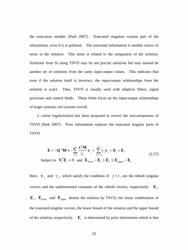
The three regularization schemes above have been used in many fields. Most

cases are soft inclusion cases, for which the above regularization schemes work

well. However, regularization does not work properly in cases involving hard

inclusion. Tumors in human bodies, suspensions of vehicles and other such

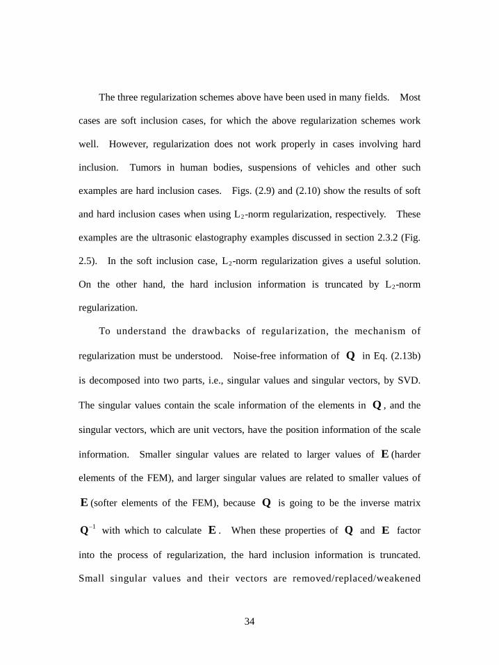
examples are hard inclusion cases. Figs. (2.9) and (2.10) show the results of soft

and hard inclusion cases when using L2-norm regularization, respectively. These

examples are the ultrasonic elastography examples discussed in section 2.3.2 (Fig.

2.5). In the soft inclusion case, L2-norm regularization gives a useful solution.

On the other hand, the hard inclusion information is truncated by L2-norm

regularization.

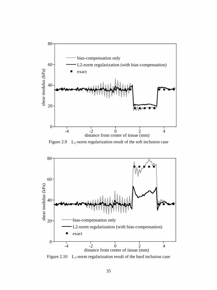
To understand the drawbacks of regularization, the mechanism of

regularization must be understood. Noise-free information of Q in Eq. (2.13b)

is decomposed into two parts, i.e., singular values and singular vectors, by SVD.

The singular values contain the scale information of the elements in Q , and the

singular vectors, which are unit vectors, have the position information of the scale

information. Smaller singular values are related to larger values of E (harder

elements of the FEM), and larger singular values are related to smaller values of

E (softer elements of the FEM), because Q is going to be the inverse matrix

1−Q with which to calculate E . When these properties of Q and E factor

into the process of regularization, the hard inclusion information is truncated.

Small singular values and their vectors are removed/replaced/weakened

35

0

20

40

60

80

-4 -2 0 2 4

bias-compensation onlyL2-norm regularization (with bias-compensation)exact

shea

r mod

ulus

(kPa

)

distance from center of tissue (mm) Figure 2.9 L2-norm regularization result of the soft inclusion case

0

20

40

60

80

-4 -2 0 2 4

bias-compensation onlyL2-norm regularization (with bias-compensation)exact

shea

r mod

ulus

(kPa

)

distance from center of tissue (mm) Figure 2.10 L2-norm regularization result of the hard inclusion case

36

Figure 2.11 Mechanism of regularizations

(TSVD/L1/L2, respectively) by regularization and amplified noise is

removed/replaced/weakened. During this process, information about hard

elements, which is included in the small singular value parts, is also

removed/replaced/weakened. It indicate that regularization is not valid for cases

involving hard inclusion. The procedure above is concluded in Fig. (2.11).

The regularizations are valid in typical cases because most damage cases

involve soft inclusion. In some cases, however, involving hard inclusion, the

regularizations are not valid. In the next section, a new stabilization schemes are

proposed to prevent the side effects associated with regularization.

Singular number

Singular value (log scale)

MQE =

Regularization

Noise effect

Normal elementInfo.Soft elementInfo.

Hard elementInfo.

37

3. Acceleration-Energy Filter

Noise filters using regularity conditions uses physical laws on the measurements as

a prior condition. The physical laws of equilibrium equation (Eq. 2.4) must be

satisfied, but noise in the measured displacement breaks the physical laws. This

situation is caused by differentiation sequences in the inverse analysis of the

continua, which amplify high-frequency noise. Amplified high-frequency noise

acts like a series of Dirac delta functions and breaks the physical laws. The

measured displacements without the physical laws effect the ill-posedness of

inverse analyses. The physical laws of Eq. (2.4) must be guaranteed to avoid ill-

posedness.

3.1 Noise Filter Using Regularity Conditions of Displacement

To prevent ill-posedness of the inverse analysis, the measured displacements

must satisfy the physical laws of the equilibrium equation. Eq. (2.4) in terms of

measured displacement u is given below.

02

22

=∂∂

ρ−∂∂

∂tu

xxuC i

lj

kijkl (3.1)

The measured displacement u have to satisfy two physical laws, the

finiteness of the strain energy and the acceleration, to satisfy the equilibrium

38

equation (Eq. 3.1).

The next equation represents the first law, the finiteness of the strain energy.

∞<∫Vl

kijkl

j

i dVdxudC

dxud

(3.2)

The equation describes that total internal energy of continuum must be finite.

The next equation represents the second law, the finiteness of the acceleration.

∞<∫Ti dt

dtud

2

22

2

(3.3)

The equation describes that the second derivative of the measured

displacement must be finite. In fact, acceleration functions are not finite functions,

because the Dirac delta functions can be included in the acceleration functions.

Except for the Dirac delta functions, however, acceleration functions exist in the

finite function space. While the impact loads are negligible, it is a valid

assumption that acceleration functions exist in the finite function space.

The measured displacement with noise, however, cannot satisfy above two

physical laws. Because the amplified high-frequency noise sources, which are

amplified by differentiations, act as a series of Dirac delta functions (section 2.3.1).

A series of Dirac delta functions breaks the physical laws, and causes ill-posedness

of the inverse analysis.

Noise filtering using regularity conditions can prevent the dissatisfaction of

39

the physical laws. Filtered displacement u~ is defined by three conditions. The

first condition is that the filtered displacement must sticks around the measured

displacement.

∫ ∫ −=ΠT V ii dtdVuu 2)~(

21min , (3.4)

where u~ and u denote the filtered displacement and the measured displacement,

respectively. The second and the third conditions are regularity conditions using

the physical laws of the displacement.

∞<=Π ∫ ∫t Vl

kijkl

j

ie dtdV

dxudC

dxud ~~

, (3.5)

∞<=Π ∫ ∫T Vi

a dtdVdt

ud2

22

2~ (3.6)

Eqs. (3.5) and (3.6) represent the regularity conditions using the finiteness of

the strain energy and the accelerations, respectively. The regularity conditions are

enforced to Eq. (3.4) as penalty functions.

∫ ∫∫ ∫

∫ ∫λ

+λ

+

−=Π

T Vl

kijkl

j

ieT V

ia

T V iiu

dtdVdxudC

dxuddtdV

dtud

dtdVuui

~~

2

~

2

)~(21min

2

22

2

2

(3.7)

Here, aλ and eλ are regularization factors which define the ratio between the

40

regularity and measured information. Since The object function is designed to

suppress noise which break the physical laws, the minimization problem is

considered as a noise filter. A governing equation and boundary conditions help

to figure out characteristics of the acceleration-energy filter. The variational

principle and the integration by parts are applied to Eq. (3.7) for deriving the

governing equation and the boundary conditions.

∫ ∫

δλ+

δλ+−δ=Πδ

T Vl

kijkl

j

ie

iiaiii dtdV

dxudC

dxud

dtud

dtuduuu

~~~~)~(~

2

2

2

2

(3.8a)

f

i

f

i

t

tV

iia

t

tV

iia

T S jl

kijklie

T Vlj

kijkleaiii

dVdtda

dtududVa

dtud

dtud

dtdSndxudCu

dtdVdxdxudC

dtuduuu

−δλ−

−

δλ+

δλ+

λ−λ+−δ=Πδ

∫∫

∫ ∫

∫ ∫

3

3

2

2

2

4

4

~~~~

~~

~~~~

(3.8b)

0~~~

2

4

4

=λ−λ+−lj

kijklstii dxdx

udCdt

uduu (3.8c)

0~~ =δ

Sj

l

kijkli n

dxudCu (3.8d)

,~3

3

dtda

dtud ii = i

i adt

ud=2

2~ fi ttt ,at = (3.8e)

Where δ , jn , it and ft are a variation, a nominal vector, an initial measuring

time and a final measuring time, respectively. Eqs. (3.8a and b) are the sequence

of the variational principle and the integration by parts, respectively. Eq. (3.8b)

41

gives the governing equation (Eq. 3.8c), the boundary condition of the spatial

domain (Eq. 3.8d) and the initial/final value conditions of the temporal domain (Eq.

3.8e). The spatial boundary condition is eliminated at the free and fixed

boundaries, because it is identical to the boundary condition of the continua. The

temporal boundary condition is not eliminated and must be considered.

3.2 Characteristics of Acceleration-Energy Filter

3.2.1 Characteristics in Frequency Domain

A transfer function is useful for identifying the characteristics of the filtering

process [Hamming 1989]. The transfer function, which shows the input-output

relationship in the frequency domain, is defined as the output divided by the input

in the frequency domain (Eq. 2.16). The transfer function for the acceleration-

energy filter is derived from the Fourier transformed governing equation of the

filter (Eq. 3.8c). However, the filter is a four-dimensional filter and hard to be

analyzed. To simplifying Eq. (3.8c) the equilibrium equation for the continuum

(Eq. 2.1) is substituted into the last term of Eq. (3.8c). The body force ib is

banished by the first assumption of Section 2.1. The equation below is a

simplified governing equation.

0~~~~~2

2

4

42

4

4

=ρλ−λ+−=λ−λ+−dt

uddt

uduudxdxudC

dtuduu eaii

lj

kijkleaii (3.9)

42

The Fourier transform and the transfer function of the above equation is

shown below.

)~()1()( 24 uu teta FF ρωλ+ωλ+= (3.10)

224424 41611

11

)()~()(

ffuuH

eatetat ρπλ+πλ+

=ρωλ+ωλ+

==ωFF

(3.11)

Here, )(uF , )~(uF , )( tH ω , tω and f are the Fourier transform of the

measured displacement, the Fourier transform of the filtered displacement, the

transfer function, the temporal frequency in radians and the temporal frequency in

Hz, respectively. It is a monotonically decreasing function from 1)0( =H to

0)( =∞H . The transfer function of the acceleration- energy filter consists of the

pass band, the cut-off band and the transient which are a signal-conserving range, a

signal-eliminating range and a transient between the above two ranges, respectively.

The transfer function in the pass band has value of near one, while the transfer

function in the cut-off band has value of near zero. The acceleration-energy filter

in this case is a low-pass filter, which is typically used to stabilize numerical

differentiations. This is feasible because amplified high-frequency noise is the

greatest problem, and a low-pass transfer function suppresses high-frequency noise.

However, this instance of the filter has strong physical meaning and is thus

optimized for the inverse analysis of the continuum.

A normalized transfer function with respect to a target frequency tf is

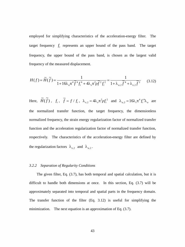
43

employed for simplifying characteristics of the acceleration-energy filter. The

target frequency tf represents an upper bound of the pass band. The target

frequency, the upper bound of the pass band, is chosen as the largest valid

frequency of the measured displacement.

22,

42,

222444 ~~11

~4~1611)~(~)(

fffffffHfH

eateta λ+λ+=

ρπλ+πλ+== (3.12)

Here, )~(~ fH , tf , tfff /~= , 22

2, 4 tee fρπλ=λ and atta f λπλ=λ 442, 16 are

the normalized transfer function, the target frequency, the dimensionless

normalized frequency, the strain energy regularization factor of normalized transfer

function and the acceleration regularization factor of normalized transfer function,

respectively. The characteristics of the acceleration-energy filter are defined by

the regularization factors 2,eλ and 2,aλ .

3.2.2 Separation of Regularity Conditions

The given filter, Eq. (3.7), has both temporal and spatial calculation, but it is

difficult to handle both dimensions at once. In this section, Eq. (3.7) will be

approximately separated into temporal and spatial parts in the frequency domain.

The transfer function of the filter (Eq. 3.12) is useful for simplifying the

minimization. The next equation is an approximation of Eq. (3.7).

44

22,

42,

62,2,

22,

42,

22,

42,

~11

~11

~~~11

~~11)(

)()~(

ff

fff

fffH

uu

ea

eaea

ea

λ+λ+=

λλ+λ+λ+≈

λ+λ+==

FF

(3.13)

The term 62,2,~fea λλ is added to the denominator of the transfer function.

The transfer function shows that the filter is a low-pass filter, which consists of a

pass band, a cut-off band and a transient. In the pass band, the added term is

nearly zero. In the transient and the cut-off band, the added term accelerates the

convergence of the transfer function. It means that the approximated transfer

function can replace the original one. Because the regularization factors 2,eλ

and 2,aλ are not defined yet, accuracy of approximated transfer function will be

analytically discussed in Section 3.2.4.

The series of ensuing equations separates the approximated equation into two

regularizations.

)()~()~1)(~1( 2

2,4

2, uuff ea FF =λ+λ+ (3.14a)

)()()~1(&)()~()~1( 22,

42, uufuuf ea FFFF =λ+=λ+ (3.14b,c)

)()()1(&)()~()1( 24 uuuu teta FFFF =ρωλ+=ωλ+ (3.14d,e)

2

2

4

4

0&~~0

dtuduu

dtuduu eiiaii

ρλ−−=λ+−= (3.14f,g)

45

lj

kijkleiiaii dxdx

udCuudt

uduu

2

4

4

0&~~0 λ−−=λ+−= (3.14h,i)

Where u , u and u~ are the measured displacements, the filtered displacements

by the strain energy regularity condition and the filtered displacement by both the

strain energy/acceleration condition. The commutative law of both conditions is

valid since multiplication of the two transfer function in Eq. (3.14a) satisfies the

commutative law. The inverse processes of the integration by parts of Eqs. (3.14h

and i) give the object function of the equations.

∫∫λ

+−=ΠT

iaT ii dt

dtuddtuuu

2

22

22

~

2)~(

21)(min (3.15a)

∫∫λ

+−=ΠV

l

kijkl

j

ieV ii dV

dxudC

dxuddVuu

2)(

21min 2 (3.15b)

The noise filter is separated into the temporal and the spatial filters, or the

acceleration and the energy filters. The integral dimensions are also separated into

their temporal and spatial dimensions. Doing this is easier than the original four-

dimension integration.

3.2.3 Characteristics and Regularization Factors of Acceleration Filter

Since Eqs. (3.15a and b) satisfy the commutative law, the acceleration filter is

independent from the energy filter. The acceleration filter has own input and

output displacement, and the object function (Eq. 3.15a) changes into the next

46

equation.

∫∫λ

+−=ΠT

iaT ii dt

dtuddtuuu

2

22

22

~

2)~(

21)(min (3.16)

Here, iu~ and iu are the output (filtered) displacement and the input (measured or

output from the energy filter) displacement, respectively. A transfer function of

the acceleration filter is derived from a variation of Eq. (3.16)

∫ ∫

δλ+−δ=Πδ

T Vii

aiii dtdVdt

uddt

uduuu 2

2

2

2 ~~)~(~ (3.17a)

f

i

f

i

t

tV

iia

t

tV

iia

T V aiii

dVdtda

dtududVa

dtud

dtud

dtVdt

uduuu

−δλ−

−

δλ+

λ+−δ=

∫∫

∫ ∫

3

3

2

2

4

4

~~~~

~~~

(3.17b)

Here, iu~ , iu , it and ft are the filtered displacement, the input displacement, an

initial measuring time and a final measuring time, respectively. The inner

equation in the first term of Eq. (3.17b) is the governing equation of the

acceleration filter and the other terms are the boundary conditions.

4

4~~0dt

uduu aλ+−= (3.18a)

,~3

3

dtda

dtud ii = i

i adt

ud=2

2~ fi ttt ,at = (3.18b)

47

Eqs. (3.18a and b) are the governing equation and the boundary conditions,

respectively. The transfer function of the acceleration filter is derived from the

transfer function of Eq. (3.18a).

ffH

aa 4161

1)(πλ+

= (3.19a)

42,~1

1)~(~f

fHa

a λ+= (3.19b)

Here, )( fHa , )~(~ fHa , tf , tfff /~= and 44

2, 16 taa fπλ=λ are the original

transfer function of the acceleration filter, the normalized transfer function of the

acceleration filter, the target frequency, the dimensionless normalized frequency

and the regularization factor of normalized transfer function, respectively. It is a

monotonically decreasing function from 1)0( =aH to 0)( =∞aH . The

acceleration filter in this case is a low-pass filter, which is typically used to stabilize

numerical differentiations. This is feasible by same reason of the acceleration-

energy filter. However, this instance of the filter has strong physical meaning and

is thus linked to the energy filter (Eq. 3.15b). The low-pass filter consists of the

pass band, the cut-off band and the transient which are a signal-conserving range, a

signal-eliminating range and a transient between the above two ranges, respectively.

Eq. (3.20b) is a normalized transfer function with respect to the target

frequency tf . The normalized transfer function is employed for simplifying

characteristics of the acceleration filter. As mentioned in Section 3.2.1, The target

48

frequency tf represents upper bound frequency of the pass band and is chosen as

the largest valid frequency of the measured displacement.

The regularization factor is defined by a target accuracy tHH =)1(~ , which is

the desired accuracy for the target frequency 1~=f .

112, −=λ

tt H

10when << tH (3.20)

Since the target frequency cannot be 0 nor an infinite value, the target

accuracy must be in 10 << tH . The target accuracy must be pre-defined by an

engineering sense to determined the regularization factor. Here, the values of 0.97,

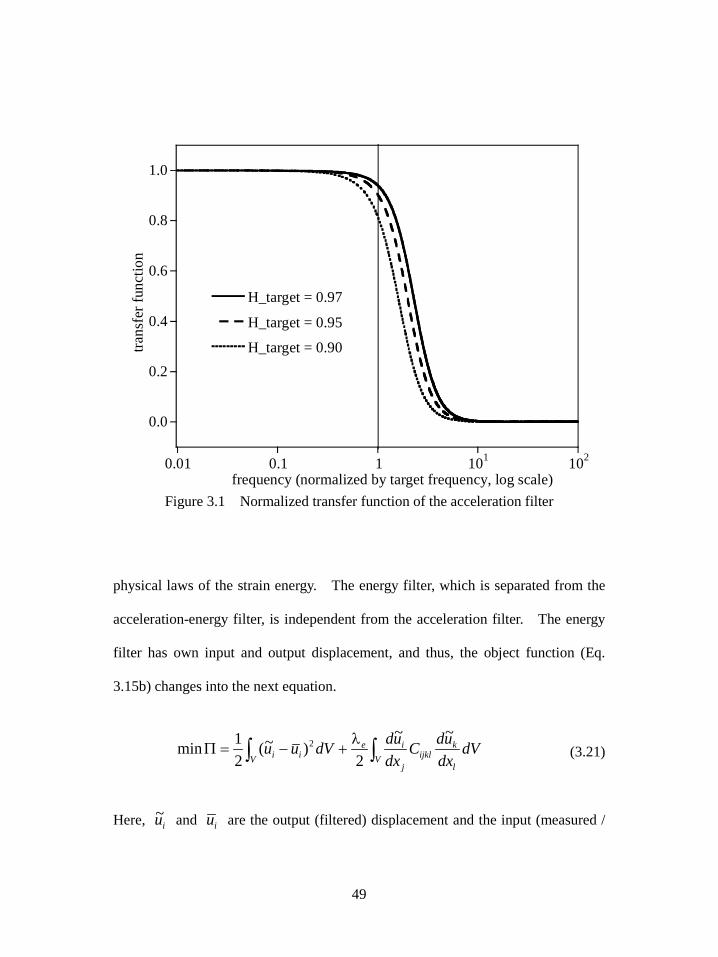
0.95 and 0.90 are recommended. Fig.(3.1) shows the normalized transfer

functions of the acceleration filter for various levels of the target accuracy. The

higher target accuracy gives the better pass band and the worse cut-off band, and

vise versa.

3.2.3 Characteristics and Regularization Factors of Energy Filter

Most noise sources are suppressed by the acceleration regularization, but the

noise associated with the pass band remains. The remaining noise is white noise

in the spatial direction. These sources are amplified by the strain-displacement

relationship and render the signals such that they are not satisfying the physical

laws of continuum. The energy filter (Eq. 3.15b) is employed to guarantee the

49

0.0

0.2

0.4

0.6

0.8

1.0

0.01 0.1 1 101 102

H_target = 0.97

H_target = 0.95

H_target = 0.90trans

fer f

unct

ion

frequency (normalized by target frequency, log scale) Figure 3.1 Normalized transfer function of the acceleration filter

physical laws of the strain energy. The energy filter, which is separated from the

acceleration-energy filter, is independent from the acceleration filter. The energy

filter has own input and output displacement, and thus, the object function (Eq.

3.15b) changes into the next equation.

∫∫λ

+−=ΠV

l

kijkl

j

ieV ii dV

dxudC

dxuddVuu

~~

2)~(

21min 2 (3.21)

Here, iu~ and iu are the output (filtered) displacement and the input (measured /

50

output from the acceleration filter) displacement, respectively. A transfer function

of the energy filter is derived from a variation of Eq. (3.21).

∫

δλ+−δ=Πδ

Vl

kijkl

j

ieiii dV

dxudC

dxuduuu

~~)~(~ (3.22a)

∫∫ δλ+

λ−−δ=

S jl

kijklieV

lj

kijkleiii dSn

dxudCudV

dxdxudCuuu

~~~~~2

(3.22b)

The inner equation in the first term of Eq. (3.22b) is the governing equation of the

energy filter and the second term is the boundary condition.

0~~

2

=λ−−lj

kijkleii dxdx

udCuu (3.23a)

0~~ =δ

Sj

l

kijkli n

dxudCu (3.23b)

Eqs. (3.23a and b) are the governing equation and the boundary condition,

respectively. The boundary condition is identical to the boundary condition of the

continua; it is zero on fixed and traction-free boundaries. The governing equation

is similar to that during acceleration regularization, i.e., functioning as a low-pass

and high-cut filter. However, it is too complex to analyze the energy filter in the

spatial frequency domain, since the elastic waves (the s-wave, the p-wave, etc.)

have physical relationships. Moreover, the elastic waves have relationship with

the temporal frequency. The next equations show relation between the spatial

frequencies of the elastic waves and the temporal frequency.

51

µρ

ω=ω tswave (3.24a)

µ+λρ

ω=ω2pwave t (3.24b)

Where swaveω , pwaveω , tω , ρ , λ and µ are the spatial frequency of the s-

wave, the spatial frequency of the p-wave, the temporal frequency, the mass density

of the medium, the Lame’s first parameter of the medium and the Lame’s second

parameter of the medium. The Lame’s second parameter µ represents the shear

modulus when the medium is a continuum.

To simplify frequency characteristics of the energy filter, the equilibrium

equation for the continuum (Eq. 2.1) is substituted into the last term of Eq. (3.23a).

The equilibrium equation for the continuum includes information of the

relationship between the elastic waves and the temporal wave, due to the fact that

Eqs. (3.24a and b) are come from the equilibrium equation. The body force ib is

banished by the first assumption of Section 2.1. It is the same sequence to section

3.2.1. The equation below is a simplified governing equation.

0~2

2

=ρλ−−dt

uduu eii (3.25)

The Fourier transform and the transfer functions of above equation are below.

52

)~()1()( 2 uu te FF ρωλ+= (3.26)

222 411

11

)()~()(

fuuH

etete ρπλ+

=ρωλ+

==ωFF

(3.27)

Here, )(uF , )~(uF , )(ωeH , tω and f are the Fourier transform of the

measured displacement, the Fourier transform of the filtered displacement, the

transfer function of the energy filter, the frequency in radians and the frequency in

Hz, respectively. It is also a monotonically decreasing function from 1)0( =H

to 0)( =∞H .

Since the elastic waves and the temporal wave are closely related by the

equilibrium equation (or Eqs. 3.24a and b), valid frequency ranges of the energy

filter and the acceleration filter must be identical. It means that two filters must

have the consistent pass band. The solution of the inverse analysis is not precise

without consistency between the acceleration filter and the energy filter, because

the temporal and spatial derivatives contain different information when the

consistency requirement is not satisfied. Since the pass band is defined by the

target frequency and the target accuracy, the consistency between two filters is

guaranteed by the same target frequency and accuracy. A normalized transfer

function of the energy filter with respect to the tf is in the next

22,~1

1)~(~f

fHe

e λ+= (3.28)

53

Here, 222, 4 tee fρπλ=λ is a normalized regularization factor of the energy filter.

The normalized regularization factor is defined by a target accuracy tHH =)1(~ ,

which is the desired accuracy for the target frequency 1~=f , and is identical to the

normalized regularization factor of the acceleration filter 2,aλ .

112, −=λ

te H

10when << tH (3.29)

A normalized regularization factor 2λ is employed for representing both

regularization factors of the acceleration and energy filters.

112,2,2 −=λ=λ=λ

tea H

10when << tH (3.30)

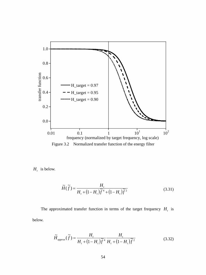
Fig.(3.2) shows the normalized transfer functions of the energy filter for

various levels of the target accuracy. The higher target accuracy gives the better

pass band and the worse cut-off band, and vise versa.

3.2.4 Characteristics of Acceleration-Energy Filter

The regularization factors 2,aλ and 2,eλ in the transfer function of the

acceleration-energy filter (Eq. 3.13) are determined by Eq. (3.30). The original

transfer function of the acceleration-energy filter in terms of the target accuracy

54

0.0

0.2

0.4

0.6

0.8

1.0

0.01 0.1 1 101 102

H_target = 0.97

H_target = 0.95H_target = 0.90tra

nsfe

r fun

ctio

n

frequency (normalized by target frequency, log scale) Figure 3.2 Normalized transfer function of the energy filter

tH is below.

( ) ( ) 24 ~1~1)~(~

fHfHHHfH

ttt

t

−+−+= (3.31)

The approximated transfer function in terms of the target frequency tH is

below.

( ) ( ) 24 ~1~1)~(~

fHHH

fHHHfH

tt

t

tt

tapprox −+−+

= (3.32)

55

)~(~ fHapprox is the approximation of the normalized transfer function for the

acceleration-energy filter. Figs. (3.3a and b) shows shapes of the original and

approximated transfer functions for various target accuracies, 97.0=tH ,

95.0=tH and 90.0=tH . As target accuracy increases, accuracy of pass band

also increases, while noise suppression effect decrease.

Figs. (3.4, 3.5 and 3.6) compare the original and approximated transfer

functions for 97.0=tH , 95.0=tH and 90.0=tH , respectively. The figures

show that difference between the both transfer functions is acceptable for the

recommended target accuracies.

In Figs. (3.3~3.6), the target accuracies of the original and approximated

acceleration-energy filters ( oritH , and approxtH , , respectively) are different from

the target accuracy of the acceleration filter and the energy filter tH .

Relationship between oritH , or approxtH , , and tH is derived from Eqs. (3.31 and

3.32) for 1~=f .

t

torit H

HH−

=2, (3.33)

2, tapproxt HH = (3.34)

Fig. (3.7) shows the relationship between the target accuracies of the separated

filters, the original filter, and the approximated filter. Difference between the

target accuracies are acceptable when tH is near to one.

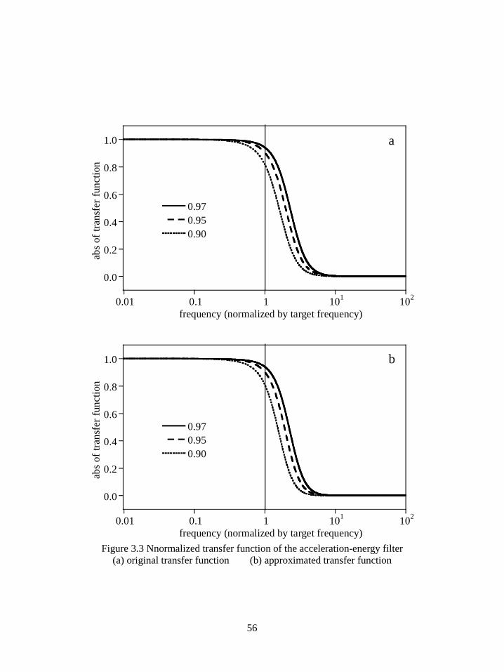
56

0.0

0.2

0.4

0.6

0.8

1.0

0.01 0.1 1 101 102

0.970.950.90

abs o

f tra

nsfe

r fun

ctio

n

frequency (normalized by target frequency)

a

0.0

0.2

0.4

0.6

0.8

1.0

0.01 0.1 1 101 102

0.970.950.90

abs o

f tra

nsfe

r fun

ctio

n


b

Figure 3.3 Nnormalized transfer function of the acceleration-energy filter

(a) original transfer function (b) approximated transfer function

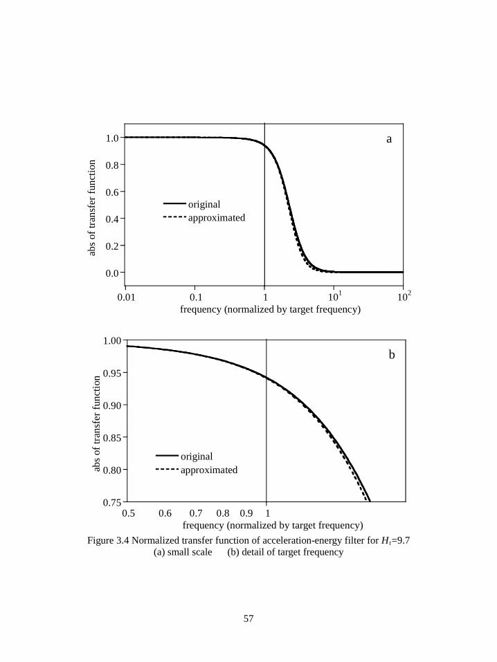
57

0.0

0.2

0.4

0.6

0.8

1.0

0.01 0.1 1 101 102

originalapproximated

abs o

f tra

nsfe

r fun

ctio

n


a

0.75

0.80

0.85

0.90

0.95

1.00

0.5 0.6 0.7 0.8 0.9 1

originalapproximatedab

s of t

rans

fer f

unct

ion


b

Figure 3.4 Normalized transfer function of acceleration-energy filter for Ht=9.7

(a) small scale (b) detail of target frequency

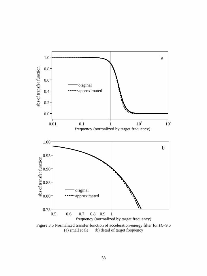
58

0.0

0.2

0.4

0.6

0.8

1.0

0.01 0.1 1 101 102


abs o

f tra

nsfe

r fun

ctio

n


a

0.75

0.80

0.85

0.90

0.95

1.00

0.5 0.6 0.7 0.8 0.9 1

originalapproximatedab

s of t

rans

fer f

unct

ion


b



59

0.0

0.2

0.4

0.6

0.8

1.0

0.01 0.1 1 101 102


abs o

f tra

nsfe

r fun

ctio

n


a

0.75

0.80

0.85

0.90

0.95

1.00

0.5 0.6 0.7 0.8 0.9 1


abs o

f tra

nsfe

r fun

ctio

n


b



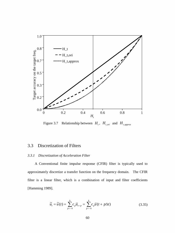
60

0.0

0.2

0.3

0.5

0.7

0.8

1.0

0 0.2 0.4 0.6 0.8 1

H_t

H_t,ori

H_t,approx

Targ

et a

ccur

acy

on th

e ta

rget

freq

.

Ht Figure 3.7 Relationship between tH , oritH , and approxtH ,

3.3 Discretization of Filters

3.3.1 Discretization of Acceleration Filter

A Conventional finite impulse response (CFIR) filter is typically used to

approximately discretize a transfer function on the frequency domain. The CFIR

filter is a linear filter, which is a combination of input and filter coefficients

[Hamming 1989].

∑∑−=−=

+ ∆+===k

kpp

k

kpptpt tptucuctuu )()(~~ (3.35)

61

Where k , pc , tu~ and tu are the truncation number, the coefficients of CFIR

filter, the output (filtered) displacement on the discretized time t and the input

(measured / output from the energy filter) displacement on the discretized time t ,

respectively. The transfer function of the CFIR filter is derived by the Fourier

transform of Eq. (3.35).

∑−=

∆π=≈k

kp

tfppCFIRt cfHfH 2ie)()( (3.36)

Here, )( fHCFIR is the transfer function of the CFIR filter. Since the coefficients

of the CFIR filter are symmetric, pp cc −= , )( fHCFIR is an even and real

function. An even and real transfer function does not cause phase shifts in the

input-output relationship. pc in Eq. (3.36) are the coefficients of the truncated

Fourier series for )( fHt and thus defined by the next equation.

∫−∆π∆=

2/

2/

2i

s

e)(sf

f

tfptp dffHtc (3.37a)

∫− ∆π∆=)~2/(1

)~2/(1

~)~2cos()~(~t

t

f

f tt fdtpfffHft (3.37b)

∫− πλ+

=)~2/(1

)~2/(1 42

~)~2cos(~11t

t

f

fs

t

s

t fdpfff

fff

(3.37c)

∫ πλ+

=)~2/(1

0 42

~)~~2cos(~11~2 tf

tt fdpfff

f (3.37d)

Where 1−∆= tfs and stt fff /~= are the sampling frequency and the normalized

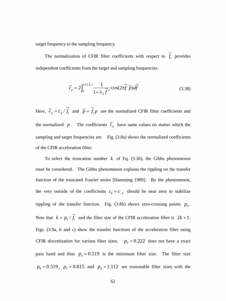
62

target frequency to the sampling frequency.

The normalization of CFIR filter coefficients with respect to tf~

provides

independent coefficients from the target and sampling frequencies.

∫ πλ+

=)~2/(1

0 42

~)~~2cos(~112~ tf

p fdpff

c (3.38)

Here, tpp fcc ~/~ = and pfp t~~ = are the normalized CFIR filter coefficients and

the normalized p . The coefficients pc~ have same values no matter which the

sampling and target frequencies are. Fig. (3.8a) shows the normalized coefficients

of the CFIR acceleration filter.

To select the truncation number k of Eq. (3.36), the Gibbs phenomenon

must be considered. The Gibbs phenomenon explains the rippling on the transfer

function of the truncated Fourier series [Hamming 1989]. By the phenomenon,

the very outside of the coefficients kk cc −= should be near zero to stabilize

rippling of the transfer function. Fig. (3.8b) shows zero-crossing points 0p .

Note that tfpk ~/0= and the filter size of the CFIR acceleration filter is 12 +k .

Figs. (3.9a, b and c) show the transfer functions of the acceleration filter using

CFIR discretization for various filter sizes. 222.00 =p does not have a exact

pass band and thus 519.00 =p is the minimum filter size. The filter size

519.00 =p , 815.00 =p and 112.10 =p are reasonable filter sizes with the

63

-1.0

0.0

1.0

2.0

3.0

4.0

5.0

6.0

0.0 0.20 0.40 0.60 0.80 1.0 1.2 1.4 1.6

normalized cefficientszero

p = p ft

c p = c

p /

f t~

~~

~

a

-1.0 10-3

-5.0 10-4

0.0 100

5.0 10-4

1.0 10-3

1.5 10-3

2.0 10-3

0.0 0.20 0.40 0.60 0.80 1.0 1.2 1.4

normalized coefficientszero

p = p ft

c p = c

p /

f t~

~~

~

0.5185850.2223410.815342

1.1115440

b

Figure 3.8 Normalized coefficients of the CFIR acceleration filter

(a) small scale (b) detail in a large scale

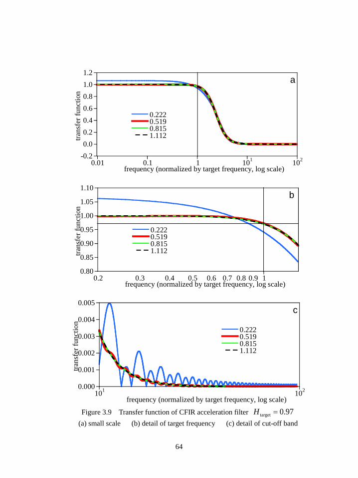
64

-0.20.00.20.40.60.81.01.2

0.01 0.1 1 101 102

0.2220.5190.8151.112tra

nsfe

r fun

ctio

n

frequency (normalized by target frequency, log scale)

a

0.80

0.85

0.90

0.95

1.00

1.05

1.10

0.2 0.3 0.4 0.5 0.6 0.7 0.8 0.9 1

0.2220.5190.8151.112tra

nsfe

r fun

ctio

n


b

0.000

0.001

0.002

0.003

0.004

0.005

101 102

0.2220.5190.8151.112

trans

fer f

unct

ion


c

Figure 3.9 Transfer function of CFIR acceleration filter 97.0target =H

(a) small scale (b) detail of target frequency (c) detail of cut-off band

65

acceptable pass bands and cut-off bands. Since the error of the pass band and the

rippling of the cut-off band are reduced as the filter size increases, 519.00 =p ,

815.00 =p and 112.10 =p are recommended as the short, standard and long

filter sizes, respectively.

The filtered displacement on the discretized time is defined as the next

equation.

∑=

∆+=t

t

fp

fppptt tptucfu

~

~

0

0

)(~~~ (3.39)

If the truncation number of the Fourier series tfpk ~0= is not a natural number,

the nearest natural number is the truncation number.

The acceleration filter is also realized by the discretization of the governing

equation (Eq. 3.18a) using FDM. The scheme is named by the FDM-FIR filter

because the final form of the discretization is an FIR filter. The FDM-FIR filter is

totally handled on the time domain, while the CFIR filter is designed on the

frequency domain. The CFIR filter design has the forward and inverse Fourier

transform processes, which cause lots of numerical error. The FDM-FIR filter,

however, does not include any domain shift processes, and gives a more stable and

accurate filter than the CFIR filter.

A fourth-order FDM matrix, 4L , is utilized during the discretization of the

governing equation of the acceleration filter (Eq. 3.18a).

66

−−

−−−−

∆=

14641

1464114641

144

tL (3.40)

Note that 4L is not a square matrix; thus, the discretized governing equation

requires two initial values and two final values.

[ ]

λ+=f

i

fsit

uuu

LLLuu~~~

~444 (3.41)

In this equation, i4L , f

4L , s4L , u , u~ , iu~ and fu~ are the first two column of

4L , the last two column of 4L , the square part of 4L , the measured

displacements, the filtered displacements, the two initial values of the regularized

displacement and two final values of the filtered displacement, respectively. Two

initial and two final values are required to solve Eq. (3.41).

uuLuLuLI ~)~~()( 44

14 =λ−λ−λ+ − ff

tii

ts

t (3.42)

The above equation gives filtered displacements using the acceleration filter.

The filtered displacements are not disturbed by the noise amplification of the

relationship between the displacements and the accelerations.

Eq. (3.42) requires two initial and two final values, but the boundaries of the

67

time series data are usually unknown. When the boundary information is not

exact, effects of the boundary value errors are derived from Eq. (3.42).

errorbounderyerror4error41

4~)~~()( uuLuLLI =+λ+λ− − ffiis

tt (3.43)

The center element of errorbounderyu is nearly zero when the data length is long

enough. Because )~~( 44f

errorfi

errori uLuL + is a zero vector except for the first and

last two elements, and 14 )( −λ+ s

tLI is a almost banded matrix. The time

window technique has been used to solve this type of boundary problem [Hong

2010, Hong 2013]. With the time window technique, Eq. (3.42) is applied to

pieces of data, and the center value is picked up in each piece (Fig. 3.10). The

window refers to an individual piece. Boundary error effects are negligible when

the time window size is long enough, as the center value of the errorboundery~u is

nearly zero. The time window technique serves as a finite impulse response (FIR)

filter formed by the center row of 14 )( −λ+ s

tLI . The FIR filter is applied in the

next equation.

∑∑−=−=

+ ∆+===k

kpp

k

kpptpt tptucuctuu )()(~~ (3.44)

Here, nu~ , nu , nc and k are the nth step of the output (filtered) displacements,

the nth step of the input (measured / output from the energy filter) displacements,

68

Figure 3.10 Concept of overwrapping time window technique

0

1

2

3

4

5

6

-1 -0.5 0 0.5 1

0.222 FDM-FIR0.519 FDM-FIR0.519 CFIR0.815 FDM-FIR0.815 CFIR1.112 FDM-FIR1.112 CFIR0.288 FDM-FIR0.587 FDM-FIR0.886 FDM-FIR

p/k

c p = c

p /

f t~

~

Figure 3.11 coefficients of FDM-FIR and CFIR filters

69

the FDM-FIR filter coefficients (the center row of 14 )( −λ+ s

tLI ) and the window

size coefficient, respectively. The window size wN is defined by the window

size coefficient k .

12 += kNw (3.45)

Since the very outside of the coefficients pc is always near zero, the window

size (or the size of the FDM-FIR filter) can be chosen by any values, while the size

of the CFIR filter must have specific values. However, it is figured out

empirically that the FDM-FIR filter converges on the analytic transfer function

faster when the window size is identical to the filter size of the CFIR filter.

Accordingly, the truncation number of CFIR filter tfpk ~/0= can be referred as

the window size of FDM-FIR filter.

1~212 +=+=t

w fpkN (3.46)

112.1≥p , 815.0≥p and 519.0≥p are suggested for the recommended,

standard and minimum window sizes. The values 1.112, 0.815 and 0.519 are

recommended 0p of CFIR filter. The coefficients of FDM-FIR and CFIR filters

is mostly same to each other when 0pp = (Fig. 3.11). The transfer functions of

the FDM-FIR filters, however, are more stable than the transfer functions of the

70

CFIR filters (Figs. 3.12a, b and c).

wN of Eq. (3.46) is the window size in the number of steps, but the window

size in the time dimension is easier to understand than wN

tt

ww TpfpNtT 0

0 22)1( ==−∆= (3.46)

Where wT and tt fT /1= are the window size on the time dimension and the

target period. tw TT 2.2> , tw TT 6.1> and tw TT 2.1> are suggested for the

recommended, standard and minimum window sized wT .

3.3.2 Discretization of Energy Filter

The variation of the object function for the energy filter (Eq. 3.21) is easily

discretized by the FEM because it is similar to the variation of the equilibrium

equation for the linear elastic continuum.

UDBBUNNUNN ~~ ∑∫∑∫∑∫ λ+=e

V

eTs

eV

eT

eV

eTeee

dVdVdV (3.47)

Here, N , B , U , U~ , eV and ∑e

)( are the shape function matrix, the first

derivation of the shape function, the global vector of the input (measured / output

from the acceleration filter) displacements, the global vector of the output (filtered)

71

-0.20.00.20.40.60.81.01.2

0.01 0.1 1 101 102

0.2220.5190.8151.112tra

nsfe

r fun

ctio

n


a

0.80

0.85

0.90

0.95

1.00

1.05

1.10

0.2 0.3 0.4 0.5 0.6 0.7 0.8 0.9 1

0.2220.5190.8151.112tra

nsfe

r fun

ctio

n


b

0.000

0.001

0.002

0.003

0.004

0.005

101 102

0.2220.5190.8151.112

trans

fer f

unct

ion


c

Figure 3.12 transfer function of FDM-FIR acceleration filter 97.0target =H

(a) small scale (b) detail of target frequency (c) detail of cut-off band

72

displacements (unknown), the domain of each element and the structural

compatibility summation, respectively. The left term and the first term on the

right are identical to the mass matrix of the FEM for the target continuum with the

unit mass density. The second term on the right is identical to the stiffness matrix

of the target continuum.

UKUMUM ~~

unitunit sλ+= (3.48)

In this equation, unitM and K are the mass matrix of the target continuum with

unit mass density and the stiffness matrix of the target continuum, respectively.

The matrixes are identical to the matrixes used in forward analyses, except for the

mass density. The filtered displacement is determined by solving Eq. (3.48).

UUMKM ~)( unit

1unit =λ+ −

s (3.49)

The stiffness matrix K includes the elastic modulus of each element, i.e., the

unknown parameters of the EEE. To solve Eq. (3.49), the unknown values must

be sourced from prior information. This prior information does not have to be

highly accurate because it has low sensitivity with regard to the final solution of the

inverse analysis (Eq. 2.13). If the prior is wholly unknown, a preliminary trial

solution of the inverse analysis can serve as the prior.

73

3.4 Acceleration-Energy Filter as Signal Processing

3.4.1 Acceleration filter as a signal processing

The acceleration filter is designed by the regularity condition and is realized

by a low-pass FIR filter. This is feasible because the object function of the

acceleration filter (Eq. 3.16) is designed for suppressing the noise amplification of

the second differentiation since it is known that differentiation amplifies high-

frequency noises. The acceleration filter is a type of the noise suppression filter to

stabilize the second derivatives of noisy measured displacements. Usual noise

suppression filters may be available for solving the inverse analysis using EEE.

However, the acceleration filter has two advantages: consistency with the energy

filter and optimality of the inverse analysis for the continuum. The acceleration

filter and the energy filter are applied together for solving inverse analysis of the

linear elastic continuum, and these process require consistency of the relationship

between the elastic waves and the temporal wave. Without the consistency, the

temporal and spatial derivatives have different information. These differences are

present serious noise. The acceleration filter contains the physical meaning of the

equilibrium equation and its FIR form has the same physical meaning as well.

The physical meaning is the media of the consistency between the acceleration and

energy filters.

74

3.4.2 Energy filter as a Signal Processing

The final form of the energy filter is a spatial filter in three-dimensional space.

For the rectangular-meshed FEM, the energy filter takes precisely the same form as

a spatial low-pass FIR filter, which is usually used in image processes. A low-

pass FIR filter may work for the inverse analysis for the continuum if it is designed

properly. However, the energy regularization has certain specialties which make it

capable of solving the inverse analysis of the linear elastic continuum.

The first advantage is the boundary conditions. The boundary conditions of

the energy filter is identical to the boundary conditions of the equilibrium equation

of the continuum. This makes the solutions around the boundaries trustable while

the other spatial filters do not give proper solutions around the boundaries. For

example, the spatial filter using a L2-norm spatial derivative regularity condition

exists, as commonly used by other researchers [Park 2006, Park 2009]. The L2-

norm type spatial filter employs the spatial derivatives of the displacement with a

L2-norm error function.

∫∫ ∇λ

+−=ΠV

sVu

dVudVuu 2

22

~~

2)~(

21min (3.50)

The governing equation (Eq. 3.51a) and the boundary condition (Eq. 3.51b)

are derived by the same procedure used for acceleration filter.

uuu s~~0 2∇λ−−= (3.51a)

0~~ =∇δS

nuu (3.51b)

75

The boundary condition of the L2-norm spatial derivative filter is not zero on

the traction-free boundaries of the continuum. A difference between the boundary

condition of the continuum and the L2-norm spatial derivative filter has detrimental

effects on solutions around the traction-free boundaries. On the other hand, The

boundary conditions of the energy filter is identical to the boundary conditions of

the continuum, and the energy filter works properly on any type of boundary.

The second is information about connectivity between nodes. The FIR form

of the spatial filters can consider only well-arranged nodes, rectangular FEM

elements. However, FEM can employ complicated elements to discretize the

continuum and cannot be handled by FIR spatial filters. However, the energy

filter contains information about the connectivity between nodes, as is the case with

the discretized continuum. For this reason, the energy filter can handle any type

of meshes.

The final advantage is the physical meaning for consistency. This was

discussed in section 3.4.1.

76

3.5 Bias Compensation for EEE Using Filtered Displacement

The reconstruction of the bias terms, Eqs. (2.23a and b), are based on the

white noise assumption. Noise in the filtered displacement, however, is not white

noise but colored noise, because filtered white noise changes into colored noise.

Moreover, since the noise undergoes the energy filter, the colored noise is not

independent from each other. Thus, covariances between colored noise must be

considered for the bias compensation.

The sequence below concerns the covariances of the filtered noise by four-

dimensional filters, which are the synthesized filters of the acceleration filter and

the energy filters. This step gives the covariances of Eq. (2.22c). White noise

),,,( tzyxw has the position of ),,( zyx with variance ),,(2 zyxσ . The white

noise after undergoing four-dimensional filtering ),,,( tzyxhk or ),,,( tzyxhl

becomes the colored noise kc or lc , respectively.

∑∑∑∑ξ ψ ζ τ

τ−ζ−ψ−ξ−τζψξ= ),,,(),,,(),,,( tzyxwhtzyxc kk (3.52a)

∑∑∑∑ξ ψ ζ τ

τ−ζ−ψ−ξ−τζψξ= ),,,(),,,(),,,( tzyxwhtzyxc ll (3.52b)

The covariance of the two types of colored noise is then lk ,σ and is derived

by the equation below. The colored noise ),,,( tzyxc iiik is on the ith node and

undergoes kh . The colored noise ),,,( tzyxc jjjl is on the jth node and

undergoes lh . Orthogonality between each instance of white noise is assumed.

77

∑ ×=σt

jjjliiikt

jjjiiilk tzyxctzyxcn

zyxzyx )],,,(),,,([1),,,,,(2, (3.53a)

∑∑∑∑∑

∑∑∑∑

τ−ζ−ψ−ξ−τζψξ×

τ−ζ−ψ−ξ−τζψξ

=

ξ ψ ζ τ

ξ ψ ζ τ

tjjjl

iiik

t tzyxwh

tzyxwh

n),,,(),,,(

),,,(),,,(1

(3.53b)

∑∑∑∑∑

∑∑∑∑

τ−ζψξτζ−ψ−ξ−×

τ−ζψξτζ−ψ−ξ−

=

ξ ψ ζ τ

ξ ψ ζ τ

tjjjl

iiik

t twzyxh

twzyxh

n),,,(),,,(

),,,(),,,(1

(3.53c)

∑ ∑∑∑∑

τ−ζψξτζ−ψ−ξ−×

τ−ζψξτζ−ψ−ξ−=

ξ ψ ζ τt jjjl

iiik

t twzyxhtwzyxh

n ),,,(),,,(),,,(),,,(1

(3.53d)

∑∑∑∑ ∑ξ ψ ζ τ

τ−ζψξτ−ζψξ×

τζ−ψ−ξ−τζ−ψ−ξ−

=

tt

jjjliiik

twtwn

zyxhzyxh

),,,(),,,(1

),.,(),,,(

(3.53e)

∑∑∑∑ξ ψ ζ τ

ζψξστζ−ψ−ξ−×

τζ−ψ−ξ−=

),,(),,,(

),,,(2

jjjl

iiik

zyxhzyxh

(3.53f)

∑∑∑ ∑ξ ψ ζ τ

τζ−ψ−ξ−τζ−ψ−ξ−

ζψξσ=),,,(

),,,(),,(2

jjjl

iiik

zyxhzyxh

(3.53g)

The orthogonality between each white noise instance is used for Eq. (3.53c).

With the Eqs. (2.22c) and (3.53g), the bias terms of Eq. (2.21) are reconstructed

with the variances of the noise, the four-dimensional acceleration-energy filters,

78

and the FEM models of the continuum.

τζ−ψ−ξ−×

τζ−ψ−ξ−ζψξσ

=

∑∑ ∑∑∑ ∑ξ ψ ζ τn m ijjdisp

iiidispijnmt zyxh

zyxhqn

ji

),,,(

),,,(),,(

),(

2

biasQ

(3.54a)

τζ−ψ−ξ−×


=

∑∑∑ ∑∑∑ ∑ξ ψ ζ τj n m ijjacc

iiidispijnmt zyxh

zyxhmn

i

),,,(

),,,(),,(

)(

2

biasM

(3.54b)

Here, ),,(2 zyxσ , jinmq ,

, , jinmm ,

, , disph and acch are the covariance values of

white noise for the measuring point on the ),,( zyx , the ),( nm element of the

matrix jTi qq , the ),( nm element of the matrix jTi mq , the filter for the

displacement of EEE and the filter for the acceleration of EEE, respectively. In

the other words, disph is the synthesized filter of the acceleration and the energy

filter. acch can be understood as the synthesized filter of the acceleration filter,

the energy filter and the central FDM for second order derivatives using second

order accuracy, as well.

biasQ and biasM are substituted into biasQ and biasM of Eq. (2.21), and

the biases in the solutions are eliminated.

79

4. Example and Application

An example and an application are introduced in this chapter. The example is a

linear elastic continuum problem using dynamic displacements under the plane

stress condition. The example uses the schemes in chapter 3. The application is

medical imaging with ultrasound equipment. Human tissues are under an

incompressible condition in this case and are governed by the Helmholtz equation.

The Helmholtz equation is a continuum in the incompressible condition. The

inverse analysis for the Helmholtz equation is slightly different from the inverse

analysis for the continuum. This is introduced in this chapter.

4.1 Example: Aluminum Plate

A thin aluminum plate model (Fig. 4.1) is employed to demonstrate the

efficiency of the acceleration-energy filter and the bias compensation. Aluminum

plates are used in many fields, especially with regard to machines and vehicles. In

this case, the plate is modeled by a plane stress FEM model. Newmark’s method

is applied to a dynamic analysis. The numerical calculations are done by

MATLAB.

In the first, the efficiency of the schemes is assessed in the ideal condition,

which is satisfies the assumptions in Section 2.1 with assumptions of a long enough

measuring time and a perfect choice of the target frequency. After that, some

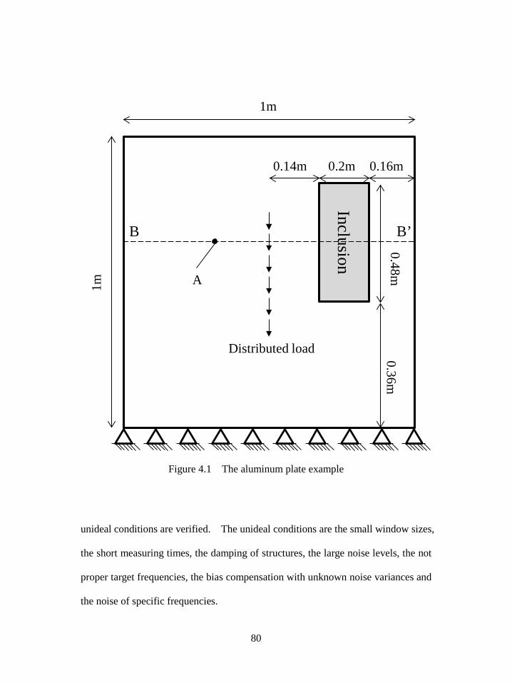
80

Figure 4.1 The aluminum plate example

unideal conditions are verified. The unideal conditions are the small window sizes,

the short measuring times, the damping of structures, the large noise levels, the not

proper target frequencies, the bias compensation with unknown noise variances and

the noise of specific frequencies.

Inclusion

Distributed load

B

0.14m 0.2m 0.16m

1m1m

0.48m0.36m

A

B’

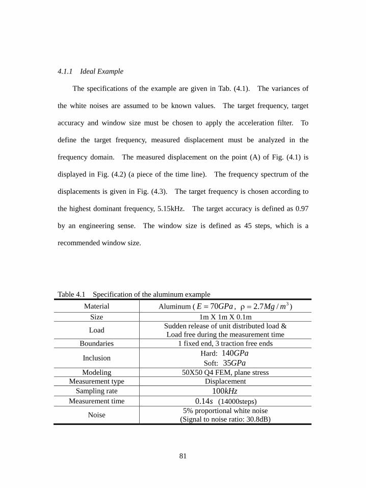
81

4.1.1 Ideal Example

The specifications of the example are given in Tab. (4.1). The variances of

the white noises are assumed to be known values. The target frequency, target

accuracy and window size must be chosen to apply the acceleration filter. To

define the target frequency, measured displacement must be analyzed in the

frequency domain. The measured displacement on the point (A) of Fig. (4.1) is

displayed in Fig. (4.2) (a piece of the time line). The frequency spectrum of the

displacements is given in Fig. (4.3). The target frequency is chosen according to

the highest dominant frequency, 5.15kHz. The target accuracy is defined as 0.97

by an engineering sense. The window size is defined as 45 steps, which is a

recommended window size.

Table 4.1 Specification of the aluminum example Material Aluminum ( GPaE 70= , 3/7.2 mMg=ρ )

Size 1m X 1m X 0.1m

Load Sudden release of unit distributed load & Load free during the measurement time

Boundaries 1 fixed end, 3 traction free ends

Inclusion Hard: GPa140 Soft: GPa35

Modeling 50X50 Q4 FEM, plane stress Measurement type Displacement

Sampling rate kHz100 Measurement time s14.0 (14000steps)

Noise 5% proportional white noise (Signal to noise ratio: 30.8dB)

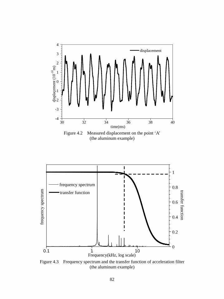
82

-4

-3

-2

-1

0

1

2

3

4

30 32 34 36 38 40

displacementdi

spla

cem

ent (

10-1

0 m)

time(ms) Figure 4.2 Measured displacement on the point ‘A’

(the aluminum example)

0

0.2

0.4

0.6

0.8

1

0.1 1 10

frequency spectrum

transfer function

freq

uenc

y sp

ectru

m transfer function

Frequency(kHz, log scale) Figure 4.3 Frequency spectrum and the transfer function of acceleration filter

(the aluminum example)

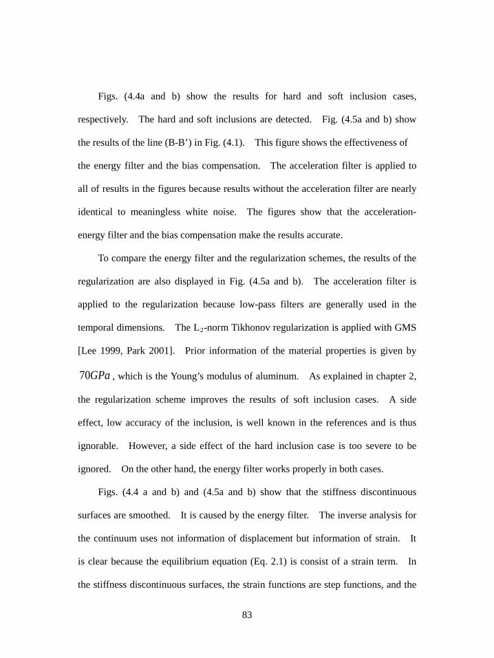
83

Figs. (4.4a and b) show the results for hard and soft inclusion cases,

respectively. The hard and soft inclusions are detected. Fig. (4.5a and b) show

the results of the line (B-B’) in Fig. (4.1). This figure shows the effectiveness of

the energy filter and the bias compensation. The acceleration filter is applied to

all of results in the figures because results without the acceleration filter are nearly

identical to meaningless white noise. The figures show that the acceleration-

energy filter and the bias compensation make the results accurate.

To compare the energy filter and the regularization schemes, the results of the

regularization are also displayed in Fig. (4.5a and b). The acceleration filter is

applied to the regularization because low-pass filters are generally used in the

temporal dimensions. The L2-norm Tikhonov regularization is applied with GMS

[Lee 1999, Park 2001]. Prior information of the material properties is given by

GPa70 , which is the Young’s modulus of aluminum. As explained in chapter 2,

the regularization scheme improves the results of soft inclusion cases. A side

effect, low accuracy of the inclusion, is well known in the references and is thus

ignorable. However, a side effect of the hard inclusion case is too severe to be

ignored. On the other hand, the energy filter works properly in both cases.

Figs. (4.4 a and b) and (4.5a and b) show that the stiffness discontinuous

surfaces are smoothed. It is caused by the energy filter. The inverse analysis for

the continuum uses not information of displacement but information of strain. It

is clear because the equilibrium equation (Eq. 2.1) is consist of a strain term. In

the stiffness discontinuous surfaces, the strain functions are step functions, and the

84

Figure 4.4 Result of the aluminum example

(a) the hard inclusion case (b) the soft inclusion case

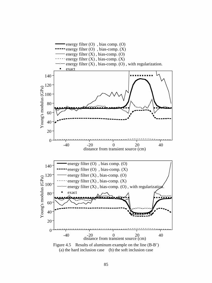
85

0

20

40

60

80

100

120

140

-40 -20 0 20 40

energy filter (O) , bias comp. (O)energy filter (O) , bias-comp. (X)energy filter (X) , bias-comp. (O)energy filter (X) , bias-comp. (X)energy filter (X) , bias-comp. (O) , with regularization.exact

You

ng's

mod

ulus

(GPa

)

distance from transient source (cm)

0

20

40

60

80

100

120

140

-40 -20 0 20 40

energy filter (O) , bias comp. (O)energy filter (O) , bias-comp. (X)energy filter (X) , bias-comp. (O)energy filter (X) , bias-comp. (X)energy filter (X) , bias-comp. (O) , with regularization.exact

You

ng's

mod

ulus

(GPa

)

distance from transient source (cm) Figure 4.5 Results of aluminum example on the line (B-B’)


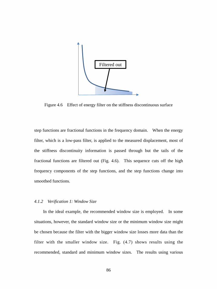
86

Figure 4.6 Effect of energy filter on the stiffness discontinuous surface

step functions are fractional functions in the frequency domain. When the energy

filter, which is a low-pass filter, is applied to the measured displacement, most of

the stiffness discontinuity information is passed through but the tails of the

fractional functions are filtered out (Fig. 4.6). This sequence cuts off the high

frequency components of the step functions, and the step functions change into

smoothed functions.

4.1.2 Verification 1: Window Size

In the ideal example, the recommended window size is employed. In some

situations, however, the standard window size or the minimum window size might

be chosen because the filter with the bigger window size losses more data than the

filter with the smaller window size. Fig. (4.7) shows results using the

recommended, standard and minimum window sizes. The results using various

Filtered out

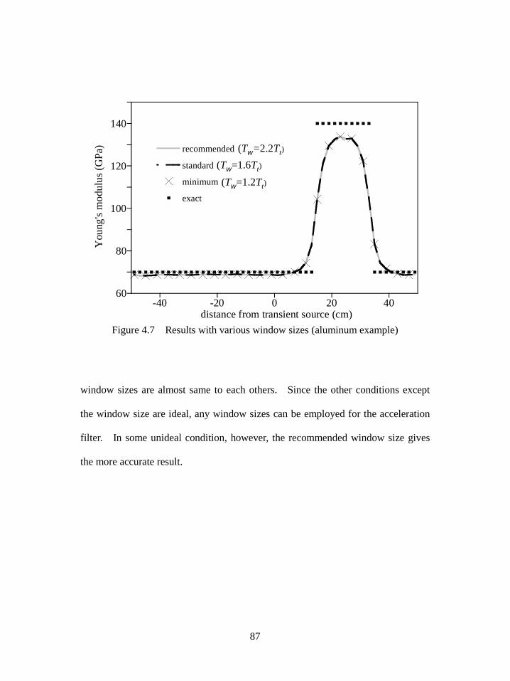
87

60

80

100

120

140

-40 -20 0 20 40

recommended

standard

minimum

exact

You

ng's

mod

ulus

(GPa

)


(Tw=1.2Tt)

(Tw=1.6Tt)

(Tw=2.2Tt)

Figure 4.7 Results with various window sizes (aluminum example)

window sizes are almost same to each others. Since the other conditions except

the window size are ideal, any window sizes can be employed for the acceleration

filter. In some unideal condition, however, the recommended window size gives

the more accurate result.

88

4.1.3 Verification 2: Measuring Time

The ideal case uses very long enough measuring time, which provides high

quality information. However, the long enough measuring time is not allowed in

some applications, especially applications with damping. The inverse analysis

using EEE in this thesis uses an assumption that damping can be ignored. The

damping is ignorable since relatively few vibrations are included in the measuring

time (Section 2.1). To verify effects of the short measuring time, 2.2waves,

0.9waves and 0.4waves of the longest wave length is applied for the measuring

time. The minimum window size is applied for reducing loss of data. Fig. (4.8)

shows the results. Results of the inclusion is less accurate than the ideal case

since lot s of information is truncated by the short measuring time. however, the

results are acceptable because the inclusion is well detected in the all cases.

60

80

100

120

140

-40 -20 0 20 40

1000 steps (ideal)200 steps (2.2waves)100 steps (0.9waves)75 steps (0.4waves)exact

You

ng's

mod

ulus

(GPa

)

distance from transient source (cm) Figure 4.8 Results with various measuring times (aluminum example)

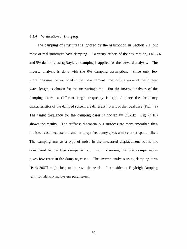
89

4.1.4 Verification 3: Damping

The damping of structures is ignored by the assumption in Section 2.1, but

most of real structures have damping. To verify effects of the assumption, 1%, 5%

and 9% damping using Rayleigh damping is applied for the forward analysis. The

inverse analysis is done with the 0% damping assumption. Since only few

vibrations must be included in the measurement time, only a wave of the longest

wave length is chosen for the measuring time. For the inverse analyses of the

damping cases, a different target frequency is applied since the frequency

characteristics of the damped system are different from it of the ideal case (Fig. 4.9).

The target frequency for the damping cases is chosen by 2.3kHz. Fig. (4.10)

shows the results. The stiffness discontinuous surfaces are more smoothed than

the ideal case because the smaller target frequency gives a more strict spatial filter.

The damping acts as a type of noise in the measured displacement but is not

considered by the bias compensation. For this reason, the bias compensation

gives few error in the damping cases. The inverse analysis using damping term

[Park 2007] might help to improve the result. It considers a Rayleigh damping

term for identifying system parameters.

90

0.0 0.1 1.0 10.0

damping 5%

damping 0%

-0.

0

0.

0.

1

1

1

1no

rmal

ized

freq

uenc

y sp

ectru

m

frequency (kHz, log scale)

target frequency

target frequency

Figure 4.9 Selection of target frequency in damping case (aluminum example)

60

80

100

120

140

-40 -20 0 20 40

0%1%5%9%exact

You

ng's

mod

ulus

(GPa

)

distance from transient source (cm) Figure 4.10 Results with various damping (aluminum example)

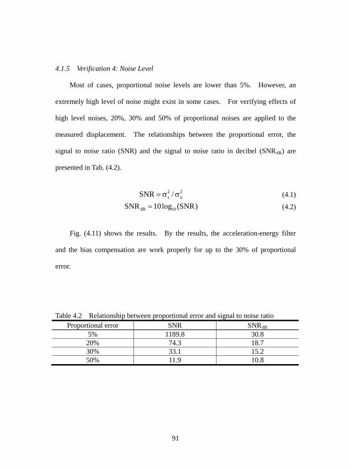
91

4.1.5 Verification 4: Noise Level

Most of cases, proportional noise levels are lower than 5%. However, an

extremely high level of noise might exist in some cases. For verifying effects of

high level noises, 20%, 30% and 50% of proportional noises are applied to the

measured displacement. The relationships between the proportional error, the

signal to noise ratio (SNR) and the signal to noise ratio in decibel (SNRdB) are

presented in Tab. (4.2).

22 /SNR ns σσ= (4.1)

)SNR(log10SNR 10dB = (4.2)

Fig. (4.11) shows the results. By the results, the acceleration-energy filter

and the bias compensation are work properly for up to the 30% of proportional

error.

Table 4.2 Relationship between proportional error and signal to noise ratio Proportional error SNR SNRdB

5% 1189.8 30.8 20% 74.3 18.7 30% 33.1 15.2 50% 11.9 10.8

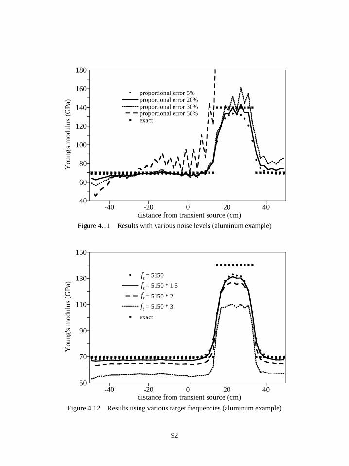
92

40

60

80

100

120

140

160

180

-40 -20 0 20 40

proportional error 5%proportional error 20%proportional error 30%proportional error 50%exact

You

ng's

mod

ulus

(GPa

)

distance from transient source (cm) Figure 4.11 Results with various noise levels (aluminum example)

50

70

90

110

130

150

-40 -20 0 20 40

= 5150

= 5150 * 1.5

= 5150 * 2 = 5150 * 3

exact

You

ng's

mod

ulus

(GPa

)


ftftft

ft

Figure 4.12 Results using various target frequencies (aluminum example)

93

4.1.6 Verification 5: Target Frequency

Since the target frequency of the acceleration-energy filter is pre-defined by an

engineering sense, a not proper target frequency might be chosen by an incorrect

engineering sense. For verifying the effects of unideal target frequency, the target

frequencies kHzft )5.115.5( ×= , Hzft )215.5( ×= and Hzft )315.5( ×= is

applied to the acceleration-energy filter of the aluminum plate example. The ideal

example uses the target frequency kHzft 15.5= . Fig. (4.12) shows results using

the various target frequencies. Even though the target frequency is not the best,

the inclusion is identified by the inverse analysis using the acceleration-energy

filter and the bias compensation. The bias of the solution is not perfectly

eliminated by bias compensation because the third assumption of the bias

compensation is not satisfied. The third assumption of the bias compensation is

that the measured data is long enough and the bias terms are converged enough.

The signal undergoing the filter using a bigger target frequency have more noise

than the signal undergoing the filter using the ideal target frequency. The bias

terms of the signal with more noise is converged slower than it of the ideal one.

94

4.1.7 Verification 6:Bias Compensation without Noise Variance Information

The bias compensation using Eqs. (3.54 a and b) and Eq. (2.21) requires the

variance of the noise in the measured displacement. However, the variance of the

noise is usually unknown. To remove the bias of the solution without the noise

variance, Eq. (2.24) must be employed. As mentioned in Section 2.4, Eq. (2.24)

has too much unknowns and additional information can reduce the number of the

unknown. A proportional noise assumption is employed for reducing the number

of the unknown and then, Eq. (2.24) changes into the function of a noise level.

2

2))nl(()nl(min btt Euu −=Π (4.3)

Where nl is the noise level in %. Fig. (4.13a) shows the normalized means

square errors of Eq. (4.3) which is normalized by the square of the maximum

displacement. ))nl(( bt Eu using 3%nl < or 7%nl > cannot be analyzed

because the solutions the inverse analyses )nl(bE using 3%nl < or 7%nl >

are not reasonable (negative or too big values). By Fig. (4.13a), 5.5% of noise

level is the optimal solution of Eq. (4.3). Note that the exact noise level is 5%.

The solutions using the exact noise level (5%) and the estimated noise level (5.5%)

are represented in Fig. (4.13b). The solution using the estimated noise level is

acceptable.

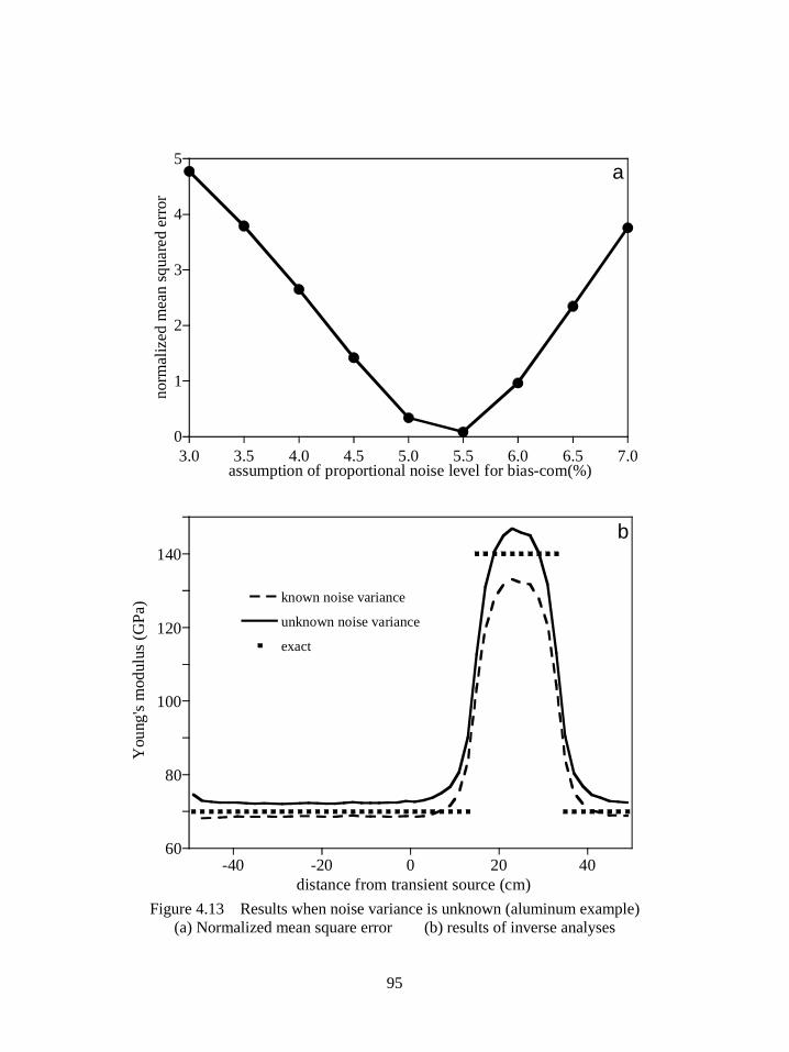
95

0

1

2

3

4

5

3.0 3.5 4.0 4.5 5.0 5.5 6.0 6.5 7.0

norm

aliz

ed m

ean

squa

red

erro

r

assumption of proportional noise level for bias-com(%)

a

60

80

100

120

140

-40 -20 0 20 40

known noise variance

unknown noise variance

exact

You

ng's

mod

ulus

(GPa

)


b

Figure 4.13 Results when noise variance is unknown (aluminum example)

(a) Normalized mean square error (b) results of inverse analyses

96

4.1.8 Verification 7: Noise of Specific Frequency

Specific frequency noise can be included in the measured displacement.

Four types of the specific frequency noise is employed to verify the noise. The

first noise is a single wave noise. The noise has 20kHz frequency, which is higher

than the target frequency, and an amplitude of the maximum displacement. The

second noise is a single wave noise with a frequency which is lower than the target

frequency. The noise has 2kHz frequency and the same amplitude to the first one.

The third noise is static noise which is constant for all nodes. The constant value

is the maximum of the displacement. The final one is static noise which is

different values for all nodes. The static noise is generated by the random value

which is uniformly distributed between the maximum displacement and the

negative value of it. Fig. (4.14a) shows the solution without additional denoising

schemes. The case of the 20kHz noise find out the inclusion since the 20kHz

noise, which is higher than the target frequency, is filtered out by the acceleration

filter. The bias compensation, however, does not work properly because the white

noise assumption is not satisfied. The case of the constant static noise also find

out the inclusion since the constant static noise does not effect to the strain, which

is actually used by the inverse analysis. The bias compensation, however, does not

work properly by the same reason of the 20kHz noise case. The solutions of the

other cases are meaningless.

For these cases, denoising schemes for the specific noise must be employed.

The static noise is a kind of the single frequency noise with 0Hz. In this example,

97

0

20

40

60

80

100

120

140

-40 -20 0 20 40

single wave noise 20kHz


static noise - constant

static noise - random

exact

You

ng's

mod

ulus

(GPa

)


a

60

80

100

120

140

-40 -20 0 20 40



static noise - constant

static noise - random

exact

You

ng's

mod

ulus

(GPa

)


b

Figure 4.14 Results with specific frequency noise (aluminum example)

(a) W/O proper denoising (b) with proper denoising

98

the adaptive line enhancer (ALE) is employed because ALE is very effective to

remove the single frequency noise [Haykin 2002]. The solutions using ALE are

shown in Fig. (4.14b). the results are almost identical to the solution of the ideal

example.

4.2 Application to Medical Imaging: Ultrasonic Elastography

The inverse analysis using EEE can be applied to medical imaging to find

tumors and cancers in human bodies. The inverse analysis using EEE works well

with medical imaging because the real-time processes make diagnoses exact and

reduce the costs. The acceleration-energy filter and the bias-compensation must

also be applied with the inverse analysis. Both civil structures and human bodies

can be modeled by continua, showing the same behaviors apart from the material

properties. In this section, ultrasonic elastography is introduced. The inverse

analysis using the Helmholtz equation related to this process are also introduced.

4.2.1 Introduction

Ultrasonic elastography is a type of medical imaging which reconstructs and

visualizes the material properties of human organs. The elasticity of

tumors/cancers differs from that in normal tissue samples. Ultrasonic

elastography has fewer side effects than other tests used to find tumors, such as

MRI, radiation tests and biopsies. The inverse analysis using EEE is a real-time

or near-real-time scheme. The inverse analysis using EEE has higher accuracy

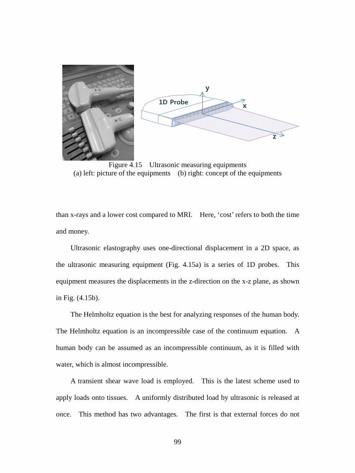
99

Figure 4.15 Ultrasonic measuring equipments (a) left: picture of the equipments (b) right: concept of the equipments

than x-rays and a lower cost compared to MRI. Here, ‘cost’ refers to both the time

and money.

Ultrasonic elastography uses one-directional displacement in a 2D space, as

the ultrasonic measuring equipment (Fig. 4.15a) is a series of 1D probes. This

equipment measures the displacements in the z-direction on the x-z plane, as shown

in Fig. (4.15b).

The Helmholtz equation is the best for analyzing responses of the human body.

The Helmholtz equation is an incompressible case of the continuum equation. A

human body can be assumed as an incompressible continuum, as it is filled with

water, which is almost incompressible.

A transient shear wave load is employed. This is the latest scheme used to

apply loads onto tissues. A uniformly distributed load by ultrasonic is released at

once. This method has two advantages. The first is that external forces do not

1D Probe

z

x

y

100

exist during the measurement. The second advantage is that concentrated loads

can be generated deep inside of bodies by the ultrasonic equipment, allowing

tumors deep inside the body to be detected.

The boundaries are assumed to be infinite boundaries, as the boundary

conditions of the bodies are unknown. This assumption is realized by a short

measuring time which is shorter than that for the wave to reach the boundary.

4.2.2 Inverse Analysis for Helmholtz Equation

The Helmholtz equation is an equation to analyze the incompressible

continuum. It is derived from the Navier’s equation.

2

22)()(

t∂∂

ρ=+∇µ+⋅∇∇µ+λubuu (4.4)

according to the incompressible condition, u⋅∇ is eliminated.

2

22

t∂∂

ρ=+∇µubu (4.5)

The displacement components are independent from each other and then, the

equation can be treated as a one dimensional problem.

2

22

tubu i

ii ∂∂

ρ=+∇µ (4.6)

101

The equation above is the Helmholtz equation. The equation below is the

variation of the Helmholtz equation.

0)( 2 =ρ−+∇µδ∫

Viiii dVubuu (4.7)

Integration by parts of the above equation leads to the subsequent equation.

0=ρδ−δ+⋅∇µδ+∇µ∇δ− ∫∫∫∫

Vii

Vii

Sii

Vii dVuudVbudSuudVuu n (4.8)

The second term is a boundary condition and is satisfied on the fixed and

traction-free boundaries. The third term is the body force term; it is eliminated by

the assumption outlined in chapter 2. The equation above is discretized by FEM

and applied to the inverse analysis using EEE.

∑ ∑∑ +µ=Πt e

ee

e

eee2

22uLmuq (4.9)

Here, eu is the local measured displacement vector. The unknown parameters

are not the Young’s modulus but the shear modulus µ in the inverse analysis for

the Helmholtz equation. In addition, eq and em are defined by the equations

below.

102

∫=eV

Te dVBBq (4.10a)

∫ρ=eV

Te dVNNm (4.10b)

Eqs. (4.10a and b) are identical to Eqs. (2.7a and b), which is the inverse analysis

for the continuum, and the next sequences are identical to those of the inverse

analysis for the continuum. The solutions of Eq. (4.9) are shown next.

0)()(11

2=+µ=

µ∂Π∂ ∑∑∑∑

==

n

t e

eeTein

t e

eeTeiei uLmuququq (4.11)

The matrix form of the above equation is the equation below.

0QμM =+ (4.12a)

( )( )

( )∑=

+++

++++++

=n

t

ettt

Tet

T

ettt

Tt

T

ettt

Tt

T

1

21

212

211

UmmmqU

UmmmqUUmmmqU

M

(4.12b)

∑=

=n

t

et

Tet

Tt

Tet

Tt

Tet

T

et

Tt

Tt

Tt

Tt

Tt

T

et

Tt

Tt

Tt

Tt

Tt

T

1

21

22212

12111

UqqUUqqUUqqU

UqqUUqqUUqqUUqqUUqqUUqqU

Q

(4.12c)

The acceleration filter for the Helmholtz equation is identical to that of the

acceleration filter for the continuum.

uuLuLuLI =λ−λ−λ+ − )()( 44

14

fft

iit

st (4.13)

103

The energy filter is identical to it of the continuum, except for D . D in Eq.

(3.47) is replaced by an identity matrix for the Helmholtz equation. The equations

next are the energy filter and its matrix form.

∑∫∑∫∑∫ µλ+=e

A

eTe

eA

eT

eA

eTeee

tdAtdAtdA UBBUNNUNN ~~ (4.14a)

UKUMUM ~~unitunit sλ+= (4.14b)

The reconstructed bias terms of the inverse analysis for the Helmholtz

equation are the equation below.

τζ−ψ−ξ−×


=

∑∑ ∑∑∑ ∑ξ ψ ζ τn m ijjdisp

iiidispijnmt zyxh

zyxhqn

ji

),,,(

),,,(),,(

),(

2

biasQ

(6.12a)

τζ−ψ−ξ−×


=

∑∑∑ ∑∑∑ ∑ξ ψ ζ τj n m ijjacc

iiidispijnmt zyxh

zyxhmn

i

),,,(

),,,(),,(

)(

2

biasM

(6.12b)

Above equations are identical to Eqs. (4.54a and b).

4.2.3 Human Skin Tissue Example

The example of ultrasonic elastography here is a model of human skin tissue.

This model is based on several references [Fink 2004, Park 2006, Park 2009]. The

shape of the example is shown in Fig. (4.16), and the specifications are given in Tab.

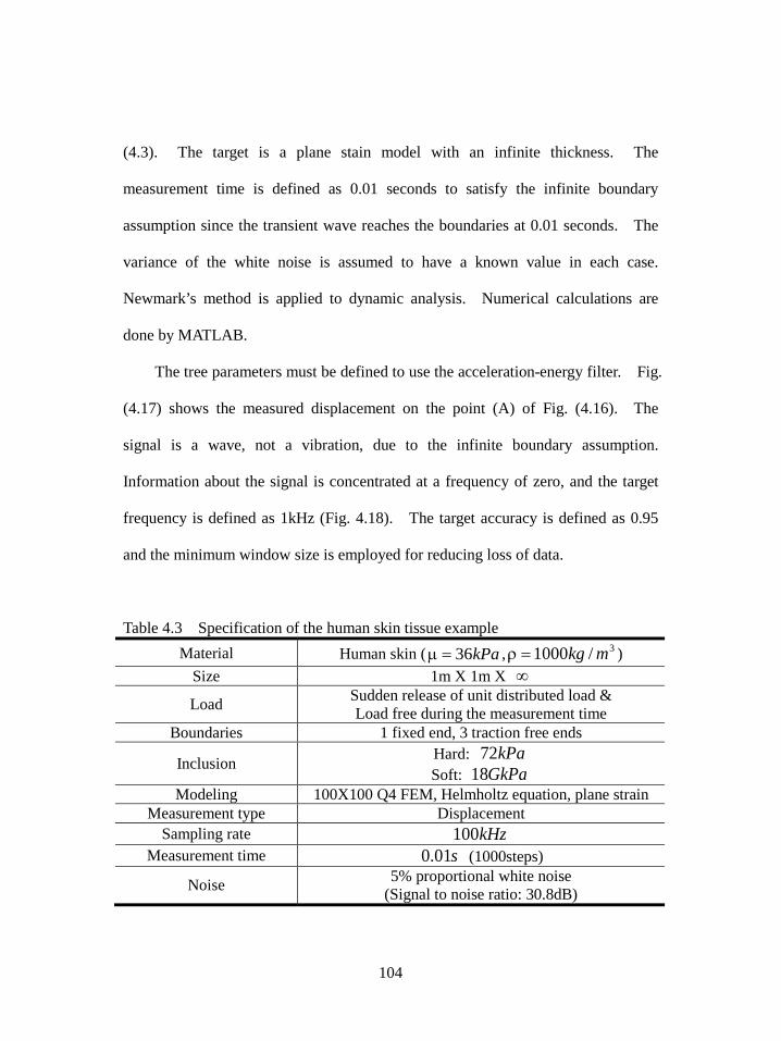
104

(4.3). The target is a plane stain model with an infinite thickness. The

measurement time is defined as 0.01 seconds to satisfy the infinite boundary

assumption since the transient wave reaches the boundaries at 0.01 seconds. The

variance of the white noise is assumed to have a known value in each case.

Newmark’s method is applied to dynamic analysis. Numerical calculations are

done by MATLAB.

The tree parameters must be defined to use the acceleration-energy filter. Fig.

(4.17) shows the measured displacement on the point (A) of Fig. (4.16). The

signal is a wave, not a vibration, due to the infinite boundary assumption.

Information about the signal is concentrated at a frequency of zero, and the target

frequency is defined as 1kHz (Fig. 4.18). The target accuracy is defined as 0.95

and the minimum window size is employed for reducing loss of data.

Table 4.3 Specification of the human skin tissue example Material Human skin ( kPa36=µ , 3/1000 mkg=ρ )

Size 1m X 1m X ∞

Load Sudden release of unit distributed load & Load free during the measurement time

Boundaries 1 fixed end, 3 traction free ends

Inclusion Hard: kPa72 Soft: GkPa18

Modeling 100X100 Q4 FEM, Helmholtz equation, plane strain Measurement type Displacement

Sampling rate kHz100 Measurement time s01.0 (1000steps)

Noise 5% proportional white noise (Signal to noise ratio: 30.8dB)

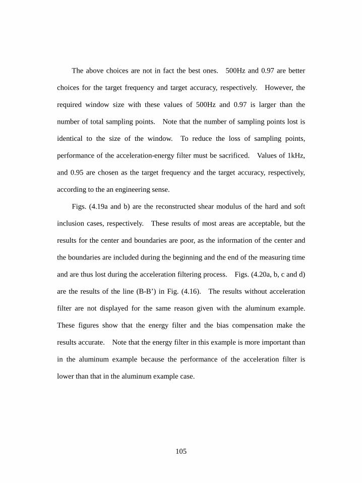
105

The above choices are not in fact the best ones. 500Hz and 0.97 are better

choices for the target frequency and target accuracy, respectively. However, the

required window size with these values of 500Hz and 0.97 is larger than the

number of total sampling points. Note that the number of sampling points lost is

identical to the size of the window. To reduce the loss of sampling points,

performance of the acceleration-energy filter must be sacrificed. Values of 1kHz,

and 0.95 are chosen as the target frequency and the target accuracy, respectively,

according to the an engineering sense.

Figs. (4.19a and b) are the reconstructed shear modulus of the hard and soft

inclusion cases, respectively. These results of most areas are acceptable, but the

results for the center and boundaries are poor, as the information of the center and

the boundaries are included during the beginning and the end of the measuring time

and are thus lost during the acceleration filtering process. Figs. (4.20a, b, c and d)

are the results of the line (B-B’) in Fig. (4.16). The results without acceleration

filter are not displayed for the same reason given with the aluminum example.

These figures show that the energy filter and the bias compensation make the

results accurate. Note that the energy filter in this example is more important than

in the aluminum example because the performance of the acceleration filter is

lower than that in the aluminum example case.

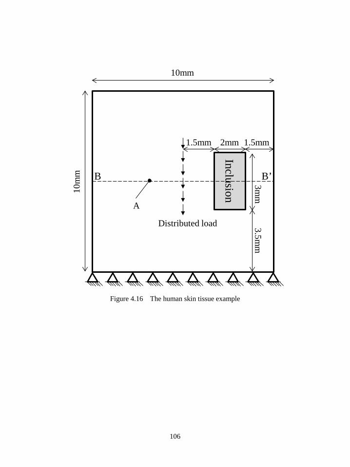
106

Figure 4.16 The human skin tissue example

Inclusion

Distributed load

B

1.5mm 2mm 1.5mm

10mm10

mm

3mm

3.5mm

B’

A

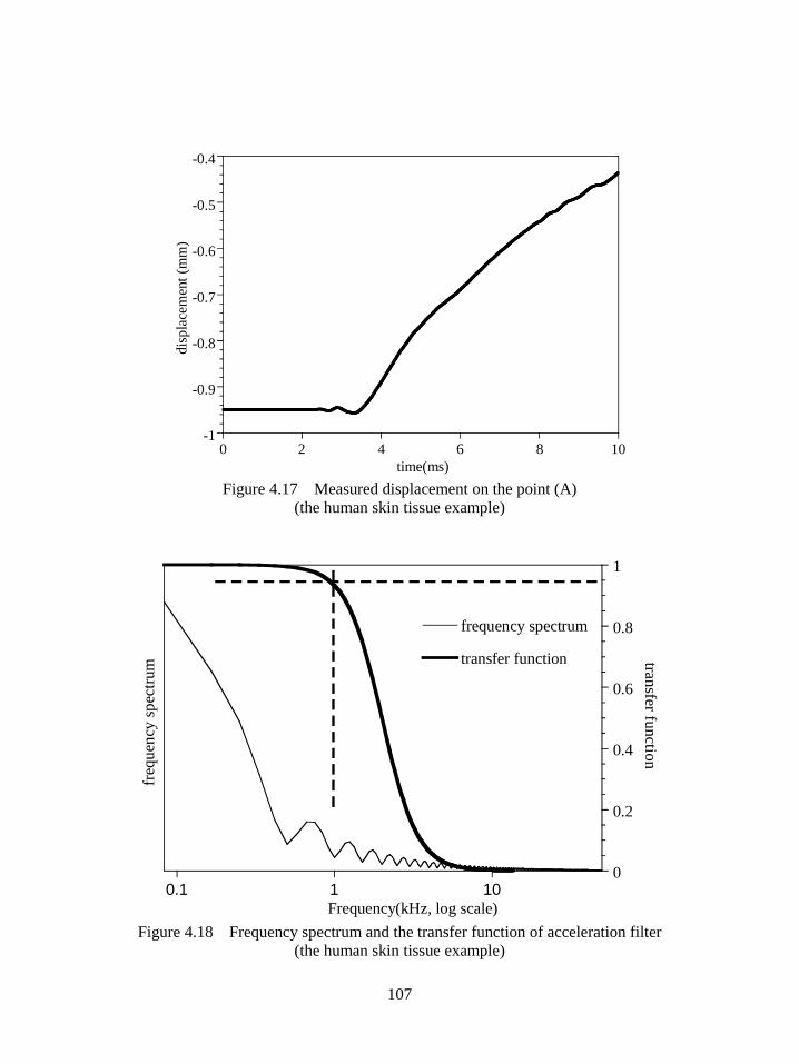
107

-1

-0.9

-0.8

-0.7

-0.6

-0.5

-0.4

0 2 4 6 8 10

disp

lace

men

t (m

m)

time(ms) Figure 4.17 Measured displacement on the point (A)

(the human skin tissue example)

0

0.2

0.4

0.6

0.8

1

0.1 1 10

frequency spectrum

transfer function

freq

uenc

y sp

ectru

m transfer function

Frequency(kHz, log scale) Figure 4.18 Frequency spectrum and the transfer function of acceleration filter

(the human skin tissue example)

108

Figure 4.19 Result of the human skin example


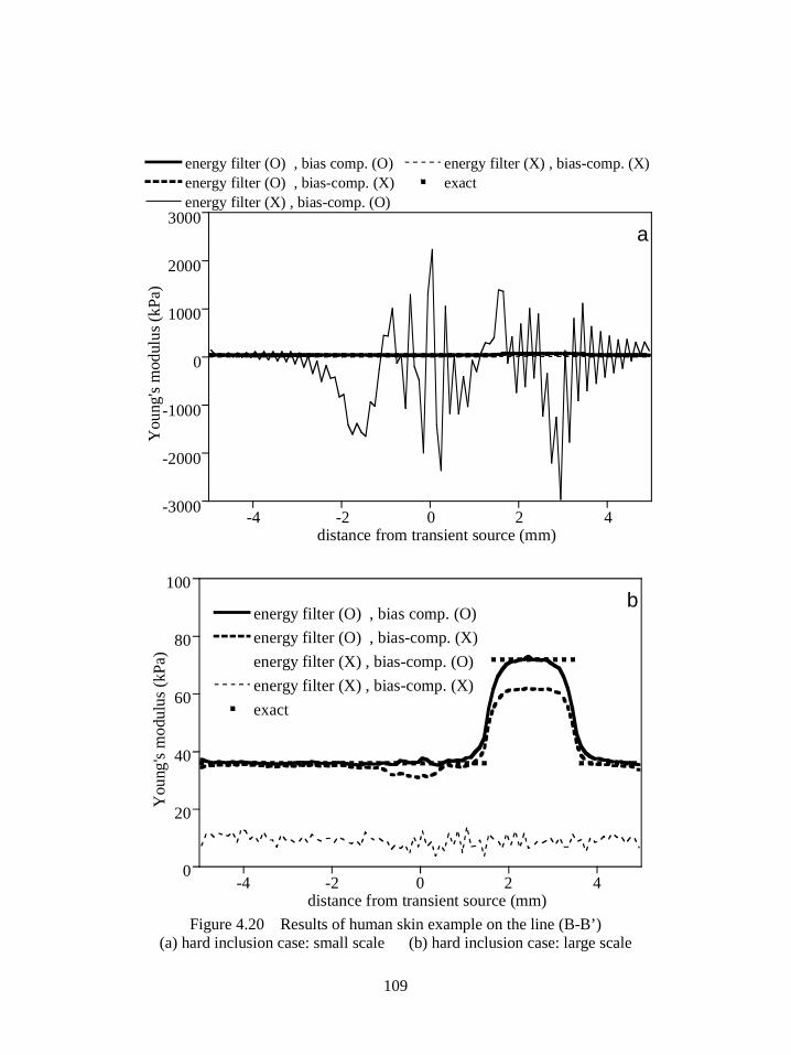
109

-3000

-2000

-1000

0

1000

2000

3000

-4 -2 0 2 4

energy filter (O) , bias comp. (O)energy filter (O) , bias-comp. (X)energy filter (X) , bias-comp. (O)

energy filter (X) , bias-comp. (X)exact

You

ng's

mod

ulus

(kPa

)

distance from transient source (mm)

a

0

20

40

60

80

100

-4 -2 0 2 4

energy filter (O) , bias comp. (O)energy filter (O) , bias-comp. (X)energy filter (X) , bias-comp. (O)energy filter (X) , bias-comp. (X)exact

You

ng's

mod

ulus

(kPa

)


b

Figure 4.20 Results of human skin example on the line (B-B’)

(a) hard inclusion case: small scale (b) hard inclusion case: large scale

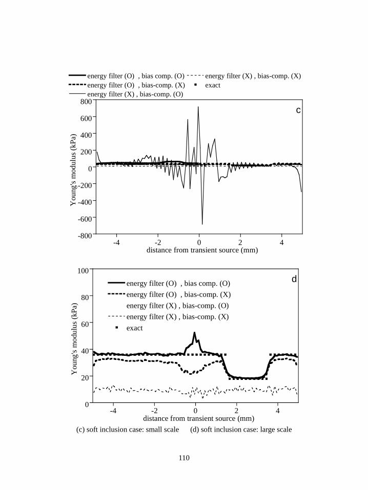
110

-800

-600

-400

-200

0

200

400

600

800

-4 -2 0 2 4

energy filter (O) , bias comp. (O)energy filter (O) , bias-comp. (X)energy filter (X) , bias-comp. (O)

energy filter (X) , bias-comp. (X)exact

You

ng's

mod

ulus

(kPa

)


c

0

20

40

60

80

100

-4 -2 0 2 4

energy filter (O) , bias comp. (O)energy filter (O) , bias-comp. (X)energy filter (X) , bias-comp. (O)energy filter (X) , bias-comp. (X)exact

You

ng's

mod

ulus

(kPa

)


d

(c) soft inclusion case: small scale (d) soft inclusion case: large scale

111

5. Conclusion

Solution stabilizers for the inverse analysis using EEE, the acceleration-energy

filter and the bias compensation are introduced in this thesis. EEE for the inverse

analysis using measured displacement has two types of solution errors: ill-

posedness and bias.

Ill-posedness is a well-known problem of the inverse analysis, and the

regularization schemes have been used to reduce the ill-posedness. The

regularization schemes work well for cases involving soft inclusions. However,

efforts of the regularization schemes are not work properly in cases involving hard

inclusions. The acceleration-energy filter has been proposed as an alternative.

The filter imposes physical conditions of the continuum to the measured

displacement. The physical conditions are the finiteness of the strain energy and

acceleration. If the measured displacement does not satisfy the physical laws, the

solution of the inverse analysis cannot be trusted, as the noise which does not

satisfy the physical laws is amplified by the displacement-acceleration relationship

and the displacement-strain relationship. The acceleration-energy filter ensures

the physical laws of continuum and makes the inverse analysis trustable. The

acceleration-energy filter is a temporal-spatial filter with three spatial dimensions

and one temporal dimension. The temporal-spatial filter has complicated

characteristics and requires much computational effort. To solve this problem, the

112

acceleration-energy filter is separated into the acceleration filter and the energy

filter.

The acceleration filter functions as a low-pass filter. Low-pass filters are

generally used to stabilize numerical differentiations. However, acceleration filter

has strong physical meaning which satisfies consistency between the acceleration

filter and the energy filter. The acceleration filter requires two initial values and

two final values, which are difficult to determine. The overwrapping time

window technique is employed so that the boundary conditions can be ignored.

The regularization factor is defined by the target frequency and the target accuracy.

The energy filter is a low-pass filter as well. This is reasonable because the

displacement-strain energy relationship amplifies high frequency noise, since the

strain is the first derivative of the displacement. The boundary condition is

identical to that of the continuum and is always satisfied. The regularization

factor is defined by the target temporal frequency and the target accuracy, which

define the regularization factor of the acceleration filter. Consistency between the

two filters is satisfied by the relationship between the regularization factors.

The bias compensation is served to remove the bias from the solutions. The

inverse analysis using EEE has been used with the adaptive filters and the flutter

derivative extraction scheme. The biases of the fields are ignorable and are easy

to remove. However, the bias of the inverse analysis using EEE for the continuum

is not ignorable because the noise is amplified by the inverse analyzing process.

The bias compensation is realized by reconstruction of the bias terms. The

113

reconstructed bias terms are functions of the noise variances, the FEM model and

the characteristics of the filters. When the variances of the noise sources are

precisely known, the bias of the solution is perfectly eliminated. Even if the noise

variance is unknown, the bias compensation can approximately reconstruct the bias

terms.

The aluminum plate example demonstrates the acceleration-energy filter and

the bias compensation. This example shows that the two schemes improve the

solution of the inverse analysis using EEE. The window size, the measuring time,

the damping of structures, the various noise levels, the target frequency and the

noise of specific frequency are verified by the aluminum example.

The schemes are applied to a medical imaging application using ultrasonic

equipment. Ultrasonic elastography helps to find tumors and cancers. The

Helmholtz equation is used to analyze tissues of human bodies, which is the

incompressible continuum. The inverse analysis and the solution stabilizers for

the Helmholtz equation are derived and are found to be nearly identical to these of

the general continuum. the acceleration-energy filter and the bias compensation

were shown to work properly for the inverse analysis of the Helmholtz equation.

115

Reference [Al-Alaoui 2007]

Al-Alaoui M A, “Linear phase low-pass IIR digital differentiators”, Signal Processing, vol. 55, no. 2, 697-706, 2007

[Banan 1995]

Banan M R, Hjelmstad K D, “Time-domain parameter estimation algorithm for structures II: numerical simulation studies”, Journal of Engineering Mechanics, 121(3), pp. 435-447, 1995

[Bercoff 2003]

Bercoff J, Chaffai S, Tanter M, Sandrin L, Catheline S, Fink M, Gennison J L, Meunier M, “In vivo breast tumor detection using transient elastography”, Ultrasound in Med. & Biol., vol. 29, no. 10, pp. 1387-1396, 2003.

[Bercoff 2004]

Bercoff J, Tanter M, Fink M, “Supersonic shear imaging: a new technique for soft tissue elasticity mapping”, IEEE Trans. Ultrason. Ferroelectr. Freq. Control, vol. 51, pp. 396-409, 2004.

[Bracewell 2000]

Bracewell R N, “The Fourier transform and its application”, Third Edition, WBC/McGraw Hill, Boston, 2000

[Bui 1994]

Bui H D, “Inverse problems in the mechanics of materials: An introduction”, CRC Press: Boca Raton, 1994.

[Choi 2013]

Choi S W, Kim B R, Lee H M, Kim Y, Park H S, “A deformed shape monitoring model for building structures based on a 2D laser scanner”, Sensors, vol. 13, pp. 6746-6758, 2013

[Chopra 2007]

Chopra A K, “Dynamics of Structures - Theory and Application to Earthquake Engineering”, Third Edition, Pearson Education Inc. Upper Saddle River, New Jersey, 2007

116

[Ding 2011] Ding J, Ding F, “Bias compensation-based parameter estimation for output error moving average system”, International Journal of Adaptive Control and Signal Processing, vol. 25, pp. 1100-1111, 2011

[Doebling 1996]

Doebling S W, Farrar C R, “Damage identification and health monitoring of structural and mechanical systems from change in their vibration characteristics: a literature review”, Los Alamos National Laboratory Report, LA-13070-MS, 1996

[Doyley 2012]

Doyley M M, “Model-based elastography: a survey of approaches to the inverse elasticity problem”, Physics in Medicine and Biology, vol. 57, R35, 2012.

[Fung 1994]

Fung Y C, “A First Course in Continuum Mechanics”, PRENTICE HALL, Englewood Cliffs, Yew Jersey, 1994

[Ge 1998a]

Ge L, Soong T T, “Damage identification through regularization method I: theory”, Journal of Engineering Mechanics, vol. 124, no. 1, pp. 103-108, 1998

[Gear 2009]

Gear J M, Goodno B J, “Mechanics of Materials”, Seventh Edition (SI Edition), Cengage Learning, Stanford, USA, 2009

[Ge 1998b]

Ge L, Soong T T, “Damage identification through regularization method II: applications”, Journal of Engineering Mechanics, vol. 124, no. 1, pp. 109-116, 1998

[Goodwin 1984]

Goodwin G C, Sin K S, “Adaptive filtering prediction and control”, Prentice Hall, Inc., NewSouth Wales, 1984

[Graff 1991]

Graff K F, “Wave Motion in Elastic Solids”, Dover Publications, 1991. [Groetsch 1984]

Groetsch C W, “The theory of Tikhonov regularization for Fredholm equations of the first kind”, Pitman Advanced Publishing: Boston, 1984.

117

[Hamming 1989] Hamming R W, “Digital filters”, Third Edition, Prentice-Hall, Englewood Cliffs, NJ, 1989

[Hansen 1992a]

Hansen P C, “Analysis of discrete ill-posed problems by means of the L-curve”, SIAM review, vol. 34, no. 4, pp. 561-580, 1992.

[Hansen 1992b]

Hansen P C, Sekii T, Shibahashi H, “The modified truncated SVD method for regularization in general form”, SIAM J. Sci. Stat. Comput., vol. 13, pp. 1142-1150, 1992

[Hansen 1997]

Hjelmstad K D, Shin S, “Damage detection and assessment of structures from static response”, Journal of Engineering Mechanics, 123(6), pp. 568-576, 1997

[Hansen 1998]

Hansen P C, “Rank-deficient and discrete ill-posed problems: numerical aspects of linear inversion”, SIAM, Philadelphia, 1998

[Haykin 2002]

Haykin S, “Adaptive filter theory”, Forth Edition, Pearson Education, Inc., 2002 [Hjelmstad 1995]

Hjelmstad K D, Banan M R, and Banan M R, “Time-domain parameter estimation algorithm for structures. I: computational aspects“, Journal of Engineering Mechanics, vol. 121, no. 3, pp. 424-434, 1995.

[Hjelmstad 1996]

Hjelmstad K D, “On the uniqueness of modal parameter estimation”, Journal of Sound and Vibration, vol. 192, no 2, pp. 581-598, 1996.

[Ho 1966]

Ho B L, Kalman R E, “Effective construction of linear state-variable models from input/output functions”, Regelungstechnik, vol. 14, no. 12, pp. 545-548, 1966

[Hong 2010]

Hong Y H, Kim H K, Lee H S, "Reconstruction of dynamic displacement and velocity from measured accelerations using the variational statement of an inverse problem", Journal of Sound and Vibration, 329 (2010) pp. 4980-5003, 2010.

118

[Hong 2012] Hong Y H, “Reconstruction of Dynamic Displacement and Velocity based on the Variation Statement of an Inverse Problem from Measured Acceleration with Special Application to the Extraction of Flutter Derivatives”, Ph. D thesis, Seoul National University, Korea, 2012.

[Hong 2013]

Hong Y H, Lee S G, Lee H S, "Design of the FEM-FIR filter for displacement reconstruction using accelerations and displacements measured at different sampling rates", Mechanial Systems and Signal Processing, Vol. 38, No. 2, pp. 460-481, 2013.7.

[Hughes 1987]

Hughes T J R, “the finite element method: linear static and dynamic finite element analysis”, Prentice-Hall, Englewood Cliff, NJ, 1987

[Ikenoue 2009]

Ikenoue M, Kanae S, Yang Z J, Wada K, “Identification of errors-in-variables model via bias-compensated instrumental variables type method”, International Journal of Onnovative Computing, Information and Control, vol. 5, pp. 29-40, 2009

[Johnson 1987]

Johnson C, “Numerical solution of partial differential equations by the finite element methods”, Cambridge University Press: New York, 1987.

[Kang 2005]

Kang J S, Park S K, Shin S, Lee H S, “Structural System Identification in Time Domain using Measured Acceleration”, Journal of Sound and Vibration, vol. 288, pp. 215-234, 2005.11.

[Kim 2011]

Kim J, “System identification of civil engineering structures though wireless structureal monitoring and subspace system identification methods”, Ph. D Thesis, University of Michigan, 2011

[Kreyszig 2006]

Kreyszig E, “Advanced Engineering Mathematics”, Ninth Edition, John Wiley & Sons, Inc., New Jersey, 2006

119

[Kumar 1996] Kumar B, Choudhury D R, Kumar A, “On the design of linear phase, FIR integrators for midband frequencoes”, IEEE, Transacation of signal processing, vol. 44(10), pp. 2391-2395, 1996

[Lawler 2006]

Lawler G F, “Introduction to Stochastic Processes”, Second Edition, Chapman & Hall/CRC, New York, 2006

[Lee 1999]

Lee H S, Kim Y H, Park C J, Park H W, “A new spatial regularization scheme for the identification of geometric shapes of inclusions in finite bodies”, International Journal for Numerical Methods in Engineering, vol. 46, no. 7, pp. 973-992, 1999.

[Lee 2000]

Lee H S, Park C J, Park H W, “Identification of geometric shapes and material properties of inclusions in two-dimensional finite bodies by boundary parameterization”, Computer Methods in Applied Mechanics and Engineering, vol. 181, no. 1-2, pp. 1-20, 2000.1.

[Lee 2010]

Lee H S, Hong Y H, Park H W, “Design of an FIR Filter for the Displacement Reconstruction Using Measured Acceleration in Low-frequency Dominant Structures”, International Journal for Numerical Methods in Engineering, vol. 82, pp. 403-434, 2010.

[Lubinski 1996]

Lubinski M A, Emelianov S Y, Raghavan K R, Yagle A E, Skovoroda A R, O’Donnell M, “Lateral displacement estimation using tissue incompressibility”, IEEE Trans. Ultrason. Ferroelectr. Freq. Control, vol. 43, pp. 247-255, 1996.

[Luengberger 1979]

Luengberger D G, “Introduction to Dynamic Systems: Theory, Models & Applications”, John Wiley & Son, Inc., New York, 1979

[Mashreghi 2014]

Mashreghi A, Yazdi H S, “A recursive algorithm for optimizing differentiation”, Journal of Computational and Applied Mathematics, vol. 263, pp. 1-13, 2014

120

[McGuiare 2000] McGuire W, Gallagher R H, Ziemian R D, “Matrix Structural Analysis”, Second Edition, John Wiley & Sons, Inc., New York, 2000

[Nguyen 1993]

Nguyen H L, Sibille P, Garnier H, “A new bias compensating least-squares method for identification of stochastic linear system in presence of colored noise”, Proceedings of 32nd conference of decision and control, San Antonio, Texas, 1993

[Ophir 1991]

Ophir J, Cespedes I, Ponnekanti H, Yazdi Y, Li X, “Elastography: a quantitative method for imaging the elasticity of biological tissues”, Ultrason. Imaging, vol. 13, pp. 111-134, 1991.

[Oppenheim 1999]

Oppenheim A V, Schafer R W, Buck J R, “Discrete-time signal processing”, Second Edition, Prentice-Hall, upper Saddle River, NJ, 1999

[Park 2001]

Park H W, Shin S B, Lee H S, “Determination of an optimal regularization factor in system identification with Tikhonov function for linear elastic continua”, International Journal for Numerical Methods in Engineering, vol. 51, no. 10, pp. 1211-1230, 2001.

[Park 2002]

Park H W, “Regularization techniques in system identification for damage assessment of structures”, PhD Thesis, Seoul National University, Seoul Korea, 2002.

[Park 2006a]

Park Y C, “A stabilizaing sheme for the dynamic analysis of slack cables”, Master Thesis, Seoul National University, 2006

[Park 2006b] Park E Y, Maniatty A M, “Shear modulus reconstruction in dynamic elastography: time harmonic case”, Phys. Med. Biol., vol. 51, pp. 3697-3721, 2006.

[Park 2007]

Park H W, Park M W, Ahn B K, Lee H S, “1-norm based regularization scheme for system identification of structures with discontinuous system parameters”, International Journal for Numerical Methods in Engineering, vol. 69, no. 3, pp. 504-523, 2007.

121

[Park 2008] Park S K, Park H W, Shin S, Lee H S, “Detection of Abrupt Structural Damage Induced by an Earthquake Using a Moving Time-Window Technique”, Computers and Structures, vol. 86, no. 11-12, pp. 1253-1265, 2008.

[Park 2009]

Park E Y, Maniatty A M, “Finite element formulation for shear modulus reconstruction in transient elastography”, Inverse Problems in Science and Engineering, vol. 17, pp. 605-626, 2009.

[Park 2012]

Park S K, “Time domain SI scheme for time-invariant and time-variant structural system”, Ph. D thesis, Seoul National University, Korea, 2012.

[Park 2013]

Park H S, Kim J M, Choi S W, Kim Y, “A wireless laser displacement sensor node for structural health monitoring”, Sensores, vol. 13, pp. 13204-13216, 2013

[Parker 1990]

Parker K J, Huang S R, Musulin R A, Lerner R M, “Tissue-response tomechanical vibrations for sonoelasticity imaging”, Ultrasound Med. Biol., vol. 16, pp. 241-246, 1990.

[Ponnekanti 1994]

Ponnekanti H, Ophir J, Cespedes I, “Ultrasonic-imaging of the stress-distribution in elastic media due to an external compressor”, Ultrasound Med. Biol., vol. 20, pp. 27-33, 1994.

[Qi 2014]

Qi X, Lichti D, El-Badry M, Chow J, Ang K, “Vertical dynamic deflection measurement in concrete beams with Microsoft Kinect”, Sensors, vol. 14, pp. 3293-3307, 2014

[Rabiner 1975]

Rabiner L R, Gold B, “Theory and application of digital signal processing”, Prentice-Hall, Englewood Cliffs, NJ, 1975

[Raghavan 1994]

Raghavan K R, Yagle A E, “Forward and inverse problems in elasticity imaging of soft-tissues”, IEEE Trans. Nucl. Sci., vol. 41, pp. 1639-1648, 1994.

122

[Rao 1996] Rao S S, “Engineering Optimization: Theory and Practice”, Third Edition, John Wiley & Son, Inc., New York, 1996

[Reddy 1990]

Reddy M R R, Kumar B, Dutta Roy S C, “Design of efficient second and higher order FIR digital differentiators for low frequencies”, Signal Processing, vol. 20, pp. 219-225, 1990

[Richards 2009]

Richards M S, Barbone P E, Oberai A A, “Quantitative three-dimensional elasticity imaging from quasi-static deformation: a phantom study”, Phys. Med. Biol., vol. 54, pp. 757-779, 2009.

[Sarvazyan 1998]

Sarvazyan A, Rudenko O, Swanson S, “Shear wave elasticity imaging: a new ultrasonic technology of medical diagnostics”, Ultrasound Med. Biol., vol. 24, pp. 1419-1435, 1998.

[Skovoroda 1995]

Skovoroda A R,Aglyamov S R, “Reconstruction of elastic properties of soft biological tissues exposed to low-frequencies disruption”, Biofizika, vol. 40, pp. 1329-1334, 1995.

[Sohn 2004]

Sohn H, Farrar C R, Hemez F M, Shunk D D, Stinemates S W, Nadler B R, Czarnecki J J, “A review of structural health monitoring literature: 1996-2001”, Los Alamos National Laboratory report, LA-13976-MS, 2004Vertroni F, Capecchi D, “Damage detection in beam structures based on frequency measurements”, Journal of Engineering Mechanics, 126(7), pp. 761-768, 2000

[Timoshenco 1959]

Timoshenco S P, Woinowsky-Krieger S, “Theory of Plates and Shell”, Second Edition, McGraw-Hill, New York, 1959

[Timoshenco 1970]

Timoshenco S P, Goodier J N, “Theory of Elasticity”, Third Edition, McGraw-Hill, New York, 1970

[Vertroni 2000]

Vertroni F, Capecchi D, “Damage detection in beam structures based on frequency measurements”, Journal of Engineering Mechanics, 126(7), pp. 761-768, 2000

123

[Wahbeh 2003] Wahbeh A M, Carffrey J P Masri S F, “A vision-based approach for the direct measurement of displacements in vibrating system”, Smart Materials and Structures, vol. 12, pp. 758-794, 2003

[Yeo 2000]

Yeo I H, Shin S, Lee H S, Chang S P, “Statistical damage assessment of framed structures from static responses”, Journal of Engineering Mechanics, ASCE, vol. 126, no. 4, pp. 414-421, 2000.

[Yoshitomi 2009]

Yoshitomi S, Takewaki I, “Noise-bias compensation in physical-parameter system identification under microtremor input”, Engineering Structures, vol. 31, pp. 580-590, 2009

[Zhang 2011]

Zhang Y, Cui G, “Bias compensation methods for stochastic system with colored noise”, Applied Mathematical Modeling, vol. 35, pp. 1709-1716, 2011

125

초록

동적 변위를 사용하는 역해석 문제에서

Equation Error Estimator 안정화를 위한

가속도-에너지 필터 및 편향성 보정 기법

서울대학교 대학원

건설환경공학부

박 광 연

본 학위 논문은 동적 변위를 이용해 선형탄성 연속체를 역해석하는 방법

중 Equation Error Estimator (EEE)를 이용한 기법을 안정화 시키기 위한 이

론을 제시한다. 여기서 역해석은 미지의 강성을 추정하는 기법을 말한

다. 안정화 기법은 가속도-에너지 필터와 편향성보정으로 이루어져 있다.

가속도-에너지 필터는 측정 변위가 가져야 할 물리적 조건을 이용해

역해석에서 발생하는 해의 부적합성(Ill-posedness)을 안정화 한다. 여기

서 사용한 물리적 조건은 가속도 유한 조건과 변형 에너지 유한 조건이

다. 이 기법들은 해의 부적합성을 안정화 시키기 위해 기존에 널리 쓰

이고 있는 특이치분해 절단법 (truncated singular value decomposition; TSVD),

126

L1-norm 정규화, L2-norm 정규화 (Tilhonov 정규화) 등의 단점을 보완하기

위해 개발 되었다. 정규화 기법들은 연속체 내부에 강성이 작은 부분이

포함 된 경우 이를 효과적으로 탐지할 수 있다. 하지만 연속체 내부에

강성이 큰 부분이 포함 된 경우 정상적으로 작동하지 않는 것을 확인 하

였다. 인체 조직의 암이나 차량 서스펜션의 경화현상, 콘크리트 내부에

이물일지 포함 된 경우 등과 같은 것들이 이에 해당한다. 이에 반해 가

속도-에너지 필터는 연속체 내부의 강성 분포에 상관없이 언제나 정상적

으로 작동한다. 가속도-에너지 필터는 가속도 필터와 에너지 필터로 분

리할 수 있다.

가속도 필터는 측정 변위의 2계 미분이 부분연속 함수공간 안에 있

다는 정보를 정규조건으로 만들어진 필터다. 2계 미분한 변위, 즉 가속

도는 실제로 부분연속 함수가 아니지만 충격하중이 없다고 가정하면 부

분연속 함수로 볼 수 있다. FDM-FIR (Finite impulse response using finite

difference method) 을 이용해 이산화된 가속도 필터는 가속도의 초기값과

최종값을 알아야 풀 수 있는 문제이다. 하지만 대부분의 경우 가속도의

초기값과 최종값은 알기 어려우며 이를 해결하기 위해 이동 시간창 기법

을 도입해 경계조건이 필요 없는 문제로 바꾼다. FDM-FIR로 이산화된

가속도 필터는 고주파 잡음을 걸러내는 일반적인 잡음제거 필터의 형태

를 갖는다. 하지만 가속도 필터는 에너지 필터와 일관성(consistency)을

127

유지할 수 있도록 하는 물리적 의미를 가지고 있다. 이는 다른 디지털

필터가 갖지 못한 장점이다.

에너지 필터는 연속체의 내부변형 에너지가 유한해야 한다는 조건을

정규조건으로 만들어진 필터다. FEM을 이용해 이산화 된 에너지 필터

는 영상처리분야에서 많이 사용하는 공간 디지털 필터와 흡사한 형태를

갖지만 몇 가지 차별성이 있다. 첫째는 필터의 경계조건이 연속체 방정

식의 경계조건과 같다는 점이다. 이로 인해 에너지 필터의 경계조건은

연속체가 가질 수 있는 모든 종류의 경계조건에 대해 유효하다. 둘째는

FEM 요소의 형태적 측면이 있다. 공간 디지털 필터는 측정점이 사각형

형태로 분포하지 않으면 사용하기 어렵다. 하지만 에너지 필터는 FEM

모형이 가지고 있는 절점 연결 정보를 함께 포함하기 때문에 복잡한 측

정점 분포에도 적용 가능하다. 셋째는 에너지 필터가 가진 물리적 의미

를 통해 가속도 정규화와의 일관성을 유지할 수 있는 점이다.

가속도 필터와 에너지 필터는 연속체의 시-공간 주파수의 관계에 의

한 일관성을 유지하도록 설계 되어야 한다. 시-공간 주파수의 관계를 무

시하고 만들어진 필터는 역해석의 정확도를 감소 시킨다. 가속도 필터

와 에너지 필터가 가지고 있는 물리적 의미는 일관성을 유지 할 수 있는

매개체 역할을 하며 이는 다른 잡음제거 필터가 갖지 못한 장점이다.

EEE를 이용한 역해석 기법은 해의 불안정성과 동시에 해의 편향성

128

(bias of solution) 문제를 가지고 있다. 기존 연구들은 대부분 편향성을 무

시하였는데 이는 무시할 수 있을 만큼 작은 경우가 많기 때문이다. 하

지만 선형 탄성 연속체의 역해석을 위한 EEE에 발생하는 해의 편향성은

무시할 수 없을 정도로 크다. 편향성 보정 기법은 이러한 해의 편향성

을 제거 하는 기법으로 측정잡음의 분산을 알면 편향성을 완벽하게 제거

할 수 있다. 잡음의 분산을 모르는 경우에는 잡음 분산을 추정하여 편

향성을 제거 할 수도 있다.

기법의 효과를 확인하기 위해 알루미늄 판 예제와 초음파 영상의학

예제를 도입한다. 이 예제를 통해 가속도-에너지 필터와 편향성 보정 기

법을 실제 적용하는 방법을 제시하고 그 유효성을 증명한다.

주요어: Equation Error Estimation (EEE), 시스템 확인 기법, 역해석,

물성치 추정, 가속도-에너지 필터, 시공간 필터, 편향성보정기법,

선형탄성 연속체, 영상의학

학번: 2010-30239

acceleration-energy filter and bias compensation for...

Documents