abstractions and paradigms for programming - …ranade/152/noteset.pdf1.1 the paradigms usually,...
TRANSCRIPT

Abstractions and Paradigms for Programming
Abhiram Ranade
Notes for CS 152, Spring 2001

Contents
1 Abstractions and Paradigms: Course Overview 51.1 The Paradigms . . . . . . . . . . . . . . . . . . . . . . . . . . . . . . . . . . 61.2 Course Overview . . . . . . . . . . . . . . . . . . . . . . . . . . . . . . . . . 7
2 Introduction to Scheme 82.1 Simple Scheme Session . . . . . . . . . . . . . . . . . . . . . . . . . . . . . . 82.2 Names and values . . . . . . . . . . . . . . . . . . . . . . . . . . . . . . . . . 102.3 Commands and values . . . . . . . . . . . . . . . . . . . . . . . . . . . . . . 10
2.3.1 Arithmetic and Logic commands . . . . . . . . . . . . . . . . . . . . 102.3.2 Graphics Commands . . . . . . . . . . . . . . . . . . . . . . . . . . . 102.3.3 The if command . . . . . . . . . . . . . . . . . . . . . . . . . . . . . 112.3.4 Examples . . . . . . . . . . . . . . . . . . . . . . . . . . . . . . . . . 122.3.5 Nesting of commands: . . . . . . . . . . . . . . . . . . . . . . . . . . 12
2.4 General Remarks on the Scheme Interpreter . . . . . . . . . . . . . . . . . . 132.5 Exercises . . . . . . . . . . . . . . . . . . . . . . . . . . . . . . . . . . . . . . 14
3 Functional Programming 15
4 Recursion 174.1 Classical Examples of Recursion . . . . . . . . . . . . . . . . . . . . . . . . . 184.2 More Examples . . . . . . . . . . . . . . . . . . . . . . . . . . . . . . . . . . 184.3 Recursion vs. loops . . . . . . . . . . . . . . . . . . . . . . . . . . . . . . . . 184.4 Recursion in Graphics . . . . . . . . . . . . . . . . . . . . . . . . . . . . . . 194.5 Clever Recursion . . . . . . . . . . . . . . . . . . . . . . . . . . . . . . . . . 194.6 Tracing Scheme procedures . . . . . . . . . . . . . . . . . . . . . . . . . . . . 204.7 Exercises . . . . . . . . . . . . . . . . . . . . . . . . . . . . . . . . . . . . . . 20
5 Proving Program Correctness 225.1 Basic ideas in program proving . . . . . . . . . . . . . . . . . . . . . . . . . 22
5.1.1 Form of the proof . . . . . . . . . . . . . . . . . . . . . . . . . . . . . 235.2 Proving correctness of functional programs . . . . . . . . . . . . . . . . . . . 235.3 Summary of the argument . . . . . . . . . . . . . . . . . . . . . . . . . . . . 24
5.3.1 Euclid’s Algorithm . . . . . . . . . . . . . . . . . . . . . . . . . . . . 245.4 Proof Strategy for Imperative programs . . . . . . . . . . . . . . . . . . . . . 25
5.4.1 Structure of proofs of Imperative Programs: . . . . . . . . . . . . . . 275.4.2 Euclid’s algorithm for computing GCD . . . . . . . . . . . . . . . . . 27
1

5.5 Proving programs involving several functions . . . . . . . . . . . . . . . . . . 285.6 Conclusions . . . . . . . . . . . . . . . . . . . . . . . . . . . . . . . . . . . . 295.7 Exercises . . . . . . . . . . . . . . . . . . . . . . . . . . . . . . . . . . . . . . 29
6 More on Scheme Statements 316.1 The “begin” Statement . . . . . . . . . . . . . . . . . . . . . . . . . . . . . . 316.2 The “cond” statement . . . . . . . . . . . . . . . . . . . . . . . . . . . . . . 316.3 The “let” stetement . . . . . . . . . . . . . . . . . . . . . . . . . . . . . . . . 32
7 Higher Order Functions 347.1 Functions as parameters to other functions . . . . . . . . . . . . . . . . . . . 34
7.1.1 Generalized Root Finder . . . . . . . . . . . . . . . . . . . . . . . . . 347.1.2 Animation . . . . . . . . . . . . . . . . . . . . . . . . . . . . . . . . . 35
7.2 Function Expressions . . . . . . . . . . . . . . . . . . . . . . . . . . . . . . . 377.2.1 Unnamed Functions . . . . . . . . . . . . . . . . . . . . . . . . . . . 37
7.3 Functions returning functions . . . . . . . . . . . . . . . . . . . . . . . . . . 387.3.1 Simulation of Data Structures . . . . . . . . . . . . . . . . . . . . . . 387.3.2 Simulating let command using functions . . . . . . . . . . . . . . . . 397.3.3 Simulating do commands using functions . . . . . . . . . . . . . . . . 39
7.4 Unnamed recursive functions . . . . . . . . . . . . . . . . . . . . . . . . . . . 407.4.1 Exercise . . . . . . . . . . . . . . . . . . . . . . . . . . . . . . . . . . 41
8 Lists 428.1 Program Example . . . . . . . . . . . . . . . . . . . . . . . . . . . . . . . . . 438.2 Proving correctness of programs involving lists . . . . . . . . . . . . . . . . . 448.3 More List Operations . . . . . . . . . . . . . . . . . . . . . . . . . . . . . . . 448.4 Applications of Lists: . . . . . . . . . . . . . . . . . . . . . . . . . . . . . . . 468.5 Procedures with variable number of arguments . . . . . . . . . . . . . . . . . 46
9 Trees 499.1 Trees and Program execution . . . . . . . . . . . . . . . . . . . . . . . . . . 499.2 Drawing Complete Binary Trees . . . . . . . . . . . . . . . . . . . . . . . . . 50
10 Built-in High Order Functions for lists 5210.1 Map . . . . . . . . . . . . . . . . . . . . . . . . . . . . . . . . . . . . . . . . 5210.2 Reduce: . . . . . . . . . . . . . . . . . . . . . . . . . . . . . . . . . . . . . . 5210.3 Filters . . . . . . . . . . . . . . . . . . . . . . . . . . . . . . . . . . . . . . . 5310.4 Application of Filters: Quicksort . . . . . . . . . . . . . . . . . . . . . . . . . 54
10.4.1 Applications of Map and Reduce . . . . . . . . . . . . . . . . . . . . 54
11 Analysis of Algorithms 5611.1 Selection sort . . . . . . . . . . . . . . . . . . . . . . . . . . . . . . . . . . . 5611.2 Analysis of smallest . . . . . . . . . . . . . . . . . . . . . . . . . . . . . . . . 5711.3 Analysis of remove . . . . . . . . . . . . . . . . . . . . . . . . . . . . . . . . 57
11.3.1 Analysis of selsort . . . . . . . . . . . . . . . . . . . . . . . . . . . . . 5811.4 Exercises . . . . . . . . . . . . . . . . . . . . . . . . . . . . . . . . . . . . . . 58
2

12 Matrices And Shortest Path Problems 59
13 Symbolic Computing 6213.1 Uses of s-expressions . . . . . . . . . . . . . . . . . . . . . . . . . . . . . . . 62
13.1.1 Symbolic Differentiation . . . . . . . . . . . . . . . . . . . . . . . . . 6313.1.2 Processing Programs . . . . . . . . . . . . . . . . . . . . . . . . . . . 64
14 Relations 6514.1 Selection . . . . . . . . . . . . . . . . . . . . . . . . . . . . . . . . . . . . . . 6514.2 Projection . . . . . . . . . . . . . . . . . . . . . . . . . . . . . . . . . . . . . 6514.3 Count . . . . . . . . . . . . . . . . . . . . . . . . . . . . . . . . . . . . . . . 6614.4 Cross Product . . . . . . . . . . . . . . . . . . . . . . . . . . . . . . . . . . . 66
14.4.1 Applications of the cross-product . . . . . . . . . . . . . . . . . . . . 6614.5 The JOIN function . . . . . . . . . . . . . . . . . . . . . . . . . . . . . . . . 6714.6 Examples . . . . . . . . . . . . . . . . . . . . . . . . . . . . . . . . . . . . . 67
15 Memoization 68
16 Embedded Languages 7016.1 Macros . . . . . . . . . . . . . . . . . . . . . . . . . . . . . . . . . . . . . . . 71
16.1.1 Convenient notation for writing macros . . . . . . . . . . . . . . . . . 7116.1.2 Nesting and recursion . . . . . . . . . . . . . . . . . . . . . . . . . . . 73
17 Embedding Advanced Graphics into Scheme 7617.1 Algorithmic Issues . . . . . . . . . . . . . . . . . . . . . . . . . . . . . . . . 7617.2 User Interface . . . . . . . . . . . . . . . . . . . . . . . . . . . . . . . . . . . 77
17.2.1 User Interface 1 . . . . . . . . . . . . . . . . . . . . . . . . . . . . . . 7817.2.2 User Interface 2 . . . . . . . . . . . . . . . . . . . . . . . . . . . . . . 7917.2.3 User Interface 3 . . . . . . . . . . . . . . . . . . . . . . . . . . . . . . 80
18 Object Oriented Programming 8118.1 Motivating examples . . . . . . . . . . . . . . . . . . . . . . . . . . . . . . . 81
18.1.1 Example 1: Library information system . . . . . . . . . . . . . . . . . 8118.1.2 Example 2: Symmetric Matrices . . . . . . . . . . . . . . . . . . . . . 82
18.2 Example 3: Extensions to Deriv . . . . . . . . . . . . . . . . . . . . . . . . . 8218.3 Basics of OOP . . . . . . . . . . . . . . . . . . . . . . . . . . . . . . . . . . . 82
18.3.1 Classes . . . . . . . . . . . . . . . . . . . . . . . . . . . . . . . . . . . 8318.3.2 Inheritance . . . . . . . . . . . . . . . . . . . . . . . . . . . . . . . . 8318.3.3 Defining Classes . . . . . . . . . . . . . . . . . . . . . . . . . . . . . . 8418.3.4 Creating Instances . . . . . . . . . . . . . . . . . . . . . . . . . . . . 8418.3.5 Defining Methods . . . . . . . . . . . . . . . . . . . . . . . . . . . . . 8518.3.6 Remark: Incremental specification of functions . . . . . . . . . . . . . 86
18.4 Utility Functions . . . . . . . . . . . . . . . . . . . . . . . . . . . . . . . . . 8718.5 Object Oriented Design . . . . . . . . . . . . . . . . . . . . . . . . . . . . . . 8718.6 Exercises . . . . . . . . . . . . . . . . . . . . . . . . . . . . . . . . . . . . . . 88
3

19 Containment Heirarchies 8919.1 Logic Circuit Simulation . . . . . . . . . . . . . . . . . . . . . . . . . . . . . 8919.2 Exercises . . . . . . . . . . . . . . . . . . . . . . . . . . . . . . . . . . . . . . 89
20 Constraint Logic Programming (CLP) 9120.1 Finite Domain CLP . . . . . . . . . . . . . . . . . . . . . . . . . . . . . . . . 9220.2 Initializing the CLP Solver . . . . . . . . . . . . . . . . . . . . . . . . . . . . 9320.3 Definition of domain variables . . . . . . . . . . . . . . . . . . . . . . . . . . 93
20.3.1 Quadratic Equation Problem: . . . . . . . . . . . . . . . . . . . . . . 9320.3.2 Magic Square Problem: . . . . . . . . . . . . . . . . . . . . . . . . . . 93
20.4 Specification of constraints . . . . . . . . . . . . . . . . . . . . . . . . . . . . 9420.4.1 Quadratic Equation Problem: . . . . . . . . . . . . . . . . . . . . . . 9420.4.2 Magic Square Problem: . . . . . . . . . . . . . . . . . . . . . . . . . . 94
20.5 Invoking the solver . . . . . . . . . . . . . . . . . . . . . . . . . . . . . . . . 9520.5.1 Printing the solutions: . . . . . . . . . . . . . . . . . . . . . . . . . . 9620.5.2 Quadratic Equation Problem: . . . . . . . . . . . . . . . . . . . . . . 9620.5.3 Magic Square Problem: . . . . . . . . . . . . . . . . . . . . . . . . . . 96
20.6 Exercises . . . . . . . . . . . . . . . . . . . . . . . . . . . . . . . . . . . . . . 97
21 Implementation of Our CLP Solver 9921.1 Brute Force Approach . . . . . . . . . . . . . . . . . . . . . . . . . . . . . . 10021.2 Refinements . . . . . . . . . . . . . . . . . . . . . . . . . . . . . . . . . . . . 10021.3 General Case . . . . . . . . . . . . . . . . . . . . . . . . . . . . . . . . . . . 10221.4 Implications . . . . . . . . . . . . . . . . . . . . . . . . . . . . . . . . . . . . 102
21.4.1 Summary . . . . . . . . . . . . . . . . . . . . . . . . . . . . . . . . . 10221.5 Finding a solution vs. finding an optimal solution . . . . . . . . . . . . . . . 10321.6 Exercises . . . . . . . . . . . . . . . . . . . . . . . . . . . . . . . . . . . . . . 103
22 Modelling with CLP 10522.1 Knapsack Problem . . . . . . . . . . . . . . . . . . . . . . . . . . . . . . . . 105
22.1.1 Solving for a fixed V . . . . . . . . . . . . . . . . . . . . . . . . . . . 106
4

Chapter 1
Abstractions and Paradigms: CourseOverview
The goal of this course is to take the first steps towards becoming a professional programmer.Professional programmers write programs for use by other people – this means they mustbe more reliable and able to serve the needs and tastes of many people, i.e. they shouldhave good user interfaces. And these programs will typically be very complex; else theusers may themselves write them. Examples of such programs are compilers, editors (e.g.text, graphics, sound ...), simulators (e.g. circuit simulator, railway system simulator, flightsimulator), programming environments (including specialized environments such as thosefor accessing databases or for modelling and solving complex mathematical and engineeringproblems).
Although we will develop toy examples of some of these programs during the course, ourgoal will of course be to study techniques which can be used for reliably developing programsthat do complex jobs. Many paradigms1 have evolved for this purpose, and we will studythem.
The process of developing programs has evolved substantially over the years. Fifty yearsago, when computers were very expensive and very slow, it was important to write programsthat executed as fast as possible. Today, the circumstances are very different: computersare very fast and very cheap. Further, computers are pervasive – millions of people usethem for a very wide range of purposes. Thus, the program development process of todaygives less importance to speed of execution and more importance to reliability and ease ofuse of programs. Since programmer effort has become more expensive (in relative terms), aprogramming process that improves programmer productivity (possibly at a cost of executionspeed) is becoming more important.
How do we write programs that are more reliable, easier to understand, easier to modify,easier to extend? Can we develop programming systems in which programs can be writtenwith minimal effort? These are some of the questions to be studied in the course.
1We use this term in the sense of “school of thought”, or a “system of beliefs/philosophies”.
5

1.1 The Paradigms
Usually, there is no single obvious method for doing any complex job, including that ofwriting a program, or writing a book, painting a picture, designing a building and so on.Typically, there are a number of different approaches, or schools of thought, or paradigmswhich contain words of wisdom as to how the job can be done. So for example there can bean Impressionist paradigm in Painting2 or a Magical Realism paradigm in Literature3.
We use the word paradigm in the sense of “school of thought”, or “set of beliefs”.We will study four programming paradigms, or approaches to developing programs, in
this course. These are Imperative Programming, Functional Programming, Object OrientedProgramming, and Logic Programming. We will mostly concentrate on the last three (sincethe first is fairly familiar through earlier courses), and even in these we will focus onlyon some of the major ideas. Many, many details (even some important ones) will be leftundiscussed.
Imperative Programming:
In this, a program is thought of as a sequence of instructions to be given to the computer. Thisparadigm inspired the development of languages such as Fortran and C, although more recentversions of these languages support non-imperative programming styles to some extent. Themain virtue of the paradigm is speed. Since the programmer more directly influences theactions of the computer (as compared to the other paradigms), a good programmer can writeprograms that execute fast. This is also a disadvantage – the programmer is expected toworry a lot about managing the computer in addition to modelling the application that isbeing programmed.
Functional Programming:
In this style program execution is thought of as function application in mathematics. Aprogram is simply a map (in the sense of a mathematical function) from the set of possibleinput instance to the desired output values. The task of programming is simply to definethese functions, and this is accomplished by defining functions from scratch or composingpredefined functions into new functions. Typically, programs written in a functional pro-gramming style are slower for the same job than their imperative counterparts; howeverthey are often immensely more readable, elegant and easier to understand. The improvedunderstandability is very important today.
Object-oriented programming:
This is really a sub-paradigm of the Imperative paradigm. One of the major ideas in itconcerns program organization. In conventional programming languages it is customary tothink of a program as consisting of data structure declarations and code. The OO paradigmencourages programmers to treat each data structure together with code for accessing it asa separate unit. Each such unit is called an object, and hence the name. OO programs are
2Popularized in the works of artists such as Claude Monet3Popularized in the work of Gabriel Garcia Marquez or Salman Rushdie.
6

considered easier to modify and extend; this is because typically a modification will needchanges to only one-two objects in the entire program. It is believed that OO programs areeasier to design because the objects constituting a program usually have a natural corre-spondence with the objects constituting the real-life system that is being modelled in theprogram. For example, in a program concerned with circuits, there may be an object foreach transistor.
Logic Programming:
This style is becoming popular for solving problems in Artificial Intelligence, or optimizationproblems. It is perhaps the easiest style for the programmer! It only requires the programmerto state formally and to full detail the (optimization) problem to be solved. The LogicProgramming system (which is some kind of an expert system) attempts to find a solutionthe problem using general techniques. A logic programming system may attempt to reducethe user specified problem to problems from some class that it knows how to solve; or itmight use brute force methods (e.g. trial and error) to solve the problem. With advances intheoretical computer science, more and more powerful logic programming systems are beingdeveloped. For the foreseeable future, it is expected that programs written in this style willbe substantially slower in execution than those in the other styles. However, it will also bemuch easier for the programmer to write programs in this style.
1.2 Course Overview
This course will study the paradigms described above. Each paradigm is the basis for severalprogramming languages, e.g. the language ML is said to be based on the functional paradigm,the language Prolog on the logic programming paradigm, the languages C++ and Java onthe Object Oriented Paradigm, and languages such as Fortran and C on the Imperative (nonobject oriented) paradigm. The most natural way to study the paradigms is to study theselanguages.
Instead, in this course we will study the Scheme language in which all the four paradigmscan be embedded. This is because Scheme is an unusually flexible language which can takeon the features of different paradigms as needed. Scheme also has several other advantagesincluding its ability to easily process non-numerical data. Learning the Scheme language(and how it can be extended as needed) will also be a part of the course.
During the course we will use examples from a variety of subfields in Computer Sciencesuch as Computer Graphics, Databases, Compilers, Circuit Design, Symbolic Algebra, Op-timization and Artificial Intelligence. In other words, the course will also be a mini-surveyof Computer Science.
7

Chapter 2
Introduction to Scheme
Scheme is a dialect of the programming language LISP–(1955)(LISt Processing language).Scheme has been chosen for our course because of a number of reasons. You can embedother languages into it quite easily. It allows easy symbol manipulation. Scheme and Lispare interpreted languages (ie. there is no intermediate object file).
This chapter will provide a brief introduction to scheme. We will begin with a verysimple session with the scheme interpreter. Then we will describe the general structure ofthe scheme commands. Finally we will describe some commonly used scheme commands.
2.1 Simple Scheme Session
The scheme interpreter can be started by typeing “scheme” to the unix command shell.After that you can typein commands, which are executed by the interpreter. You can endthe session by typeing CTRL-d.
After the scheme interpreter is invoked, the user must type commands through the key-board which the interpreter then executes. The most common command is an expressionwhich has the form “(command-name argument . . . )”. Simplest expressions are formed usingthe arithmetic operators. Thus you may type
(+ 10 35)
To which scheme will reply by printing out 45, which is the result of adding 10 to 35. Schemeuses prefix notation for expressions eg 10+35 is written as (+ 10 35). Commands can benested. For example, you may type
(+ 35 (* 2 10))
which scheme will interprete as “add the 35 to the result of multiplying 2 and 10. Trigono-metric functions can also serve as command names. As in most languages, trigonometricfunctions expect the arguments in radians. Thus here is a scheme expression to compute thetrigonometric sine of 30 degrees:
(sin (/ (* 30 3.14 ) 180 ))
You can define names as follows:
8

(define pi 3.14159 )
This tells the Scheme interpreter to use 3.14 whenever pi is encountered subsequently. Sofollowing this definition we could just write
(sin (/ (* 30 pi) 180 ))
for computing the sine of 30 degrees. Thus pi could be used in place of 3.14 in previousexpression. Previously defined names can be used to define new names, e.g.
(define twopi (* pi 2 ) )
You can also define new commands. Here is a command to calculate the volume of a cylinder:
(define (cylinder-volume r h) ;; procedure definition
(* pi r r h) ;; procedure body
) ;; end of procedure definition
The text following a ; is a comment, and is ignored by the Scheme interpreter. It is assumedin the above definition that pi has been defined earlier. The above procedure could beinvoked as follows:
(cylinder-volume 10 20) ;; procedure invocation
The numbers 10, 20 in the invocation are called the arguments, and the corresponding namesr and h in the definition of the procedure cylinder-volume are called formal parameters ofthe procedure. When the invocation is executed, the values of r and h are set to respectively10 and 20, and the procedure body is executed. The body will cause the multiplication3.14 × 10 × 10 × 20, and the result, 6280, will be returned. This is what Scheme will printas the value of the invocation. Scheme procedures can invoke other procedures, or eventhemselves, i.e. procedures can be recursive.
Besides expressions, scheme commands can be just references to a name: it is possible totype a name to the scheme interpreter, in this case the interpreter simply returns its value.So for example if you type
pi
then the scheme interpreter would respond by typing 3.14. If you type
cylinder-volume
most scheme interpreters would respond with a message saying that cylinder-volume is aprocedure.
9

2.2 Names and values
In Scheme, names do not have an associated type as in Fortran or C; so there are no typedeclaration statements. A name can be associated with any kind of data. This is doneusing define statements. For example, the statement (define pi 3.14) causes pi to beassociated with the number 3.14. It is also customary to say that the value of pi is 3.14.
Names can also be associated with procedures, for example, cylinder-volume as definedearlier is a name associated with the procedure for computing the volume of a cylinder, asdefined using (define (cylinder-volume r h) (* pi r r h)). In fact it is acceptableto ask what the value of cylinder-volume is– in Scheme it is appropriate to say that theprocedure to compute the cylinder volume is the value of cylinder-volume1
Scheme does have a command that changes the value of a name; we will look at thiscommand later.
2.3 Commands and values
The term command suggests a phrase that causes some action to happen. Scheme commandscan cause actions to happen, but in addition, many Scheme commands also represent values.For example, a command such as (* 3.14 10 10) not only causes the numbers 3.14, 10, 10to be multiplied, but it also represents the resulting value, i.e. the number 314. This meansthat the entire command can be nested inside another command, in any place where a valueis allowed. For example we may write (+ 1 (* 3.14 10 10)). The value of this command,of course, is 315.
Nesting one command inside another is allowed in most languages. However, Schemeallows much more interesting kinds of nesting. This is because almost every statement inScheme has a value (see for example, the if statement described below), hence it can bewritten wherever a value is allowed.
We describe some selected commands below.
2.3.1 Arithmetic and Logic commands
Scheme has built-in commands for addition, subtraction, multiplication, division, and a hostof other operations. The syntax is prefix, i.e. to compute 35/47, we would write (/ 35 47).Prefix syntax is also used for comparisons. For example (> a b) would return true if a > band false otherwise. This will typically be used while writing an if statement as discussedbelow.
2.3.2 Graphics Commands
Scheme offers users a graphical interface to create and draw pictures. For this you need toexecute the following command which loads the necessary file:
(load "~ranade/public/graphics.scm")
1Do not mistake this with the value of the expression (cylinder-volume 10 20) – the value of this isthe number 6280 assuming pi is defined as 3.14.
10

A window containing a screen for graphics should come up after this.The following commands are available:
1. (gr:reset) : Clears the graphics screen and resets the graphics system.
2. (gr:write x y "string") : Writes the given string at position (x,y)
3. (line x1y1x2y2) : Draws the line between the specified points.
4. (point x1y1) : Plots the specified point.
5. (trans dx dy <commands>) : Translates the origin to (dx,dy) and evaluates the com-mands.
6. (rotate cos(x) sin(x) <commands>) : Rotates axes by an angle x and evaluates thecommands.
7. (scale sx sy <commands>) : Multiplies scale of axes by sx, sy respectively.
None of the graphics commands returns a value.
2.3.3 The if command
The general form is:
(if condition-expression
then-command
else-command)
The condition-expression is first evaluated. If this evaluates to true, then the then-command
is evaluated and its value (if any) is returned as the result of the if statement. Otherwise,the else-command is evaluated and its value (if any) is returned as the result. Suppose wewish to set y to have the absolute value of x then we could write:
(define y (if (> x 0)
x
(- x))
)
This should not be read as “If x>0 then set y to x, else set y to -x”. Instead, it should beread as “Set y to the value returned by the if statement; the if statement evaluates to x ifx>0, else it evaluates to -x.”. The difference between the two should become more obvious ifyou consider the following statement:
(define z (* 2 (if (> x 0)
x
(- x)))
)
11
You will see that it is not possible to nest IF statements of FORTRAN inside arithmeticexpressions. Scheme is very flexible in comparison. Other statements e.g. the do statementwhich is analogous to the FORTRAN DO statement also is associated with a value, and canhence be nested in contexts where values are expected.
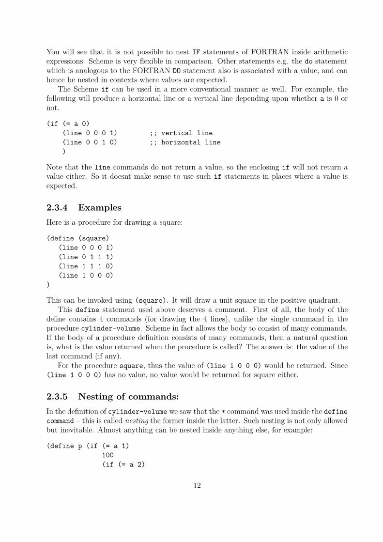
The Scheme if can be used in a more conventional manner as well. For example, thefollowing will produce a horizontal line or a vertical line depending upon whether a is 0 ornot.
(if (= a 0)
(line 0 0 0 1) ;; vertical line
(line 0 0 1 0) ;; horizontal line
)
Note that the line commands do not return a value, so the enclosing if will not return avalue either. So it doesnt make sense to use such if statements in places where a value isexpected.
2.3.4 Examples
Here is a procedure for drawing a square:
(define (square)
(line 0 0 0 1)
(line 0 1 1 1)
(line 1 1 1 0)
(line 1 0 0 0)
)
This can be invoked using (square). It will draw a unit square in the positive quadrant.This define statement used above deserves a comment. First of all, the body of the
define contains 4 commands (for drawing the 4 lines), unlike the single command in theprocedure cylinder-volume. Scheme in fact allows the body to consist of many commands.If the body of a procedure definition consists of many commands, then a natural questionis, what is the value returned when the procedure is called? The answer is: the value of thelast command (if any).
For the procedure square, thus the value of (line 1 0 0 0) would be returned. Since(line 1 0 0 0) has no value, no value would be returned for square either.
2.3.5 Nesting of commands:
In the definition of cylinder-volume we saw that the * command was used inside the define
command – this is called nesting the former inside the latter. Such nesting is not only allowedbut inevitable. Almost anything can be nested inside anything else, for example:
(define p (if (= a 1)
100
(if (= a 2)
12

150
(+ b c))))
This shows one if command nested inside another. The meaning of the definition should beclear: p is set to 100 if a is 1; to 150 if a is 2, and to the sum of b and c if a is neither 1 nor2.
Here is a case where nesting is not allowed in Scheme:
(define q (define p 100))
This is illegal because the define special form expects to evaluate its second argument anddiscover a value. But a command such as (define p 100) does not have a value and is thusinappropriate in this place.
2.4 General Remarks on the Scheme Interpreter
The Scheme Interpreter takes commands typed by the user, executes them, and prints thevalue returned by the command on the screen.
The simplest kind of Scheme command is a name. The name represents the value asso-ciated with it by preceding statements. If you type a name to the intepreter, then it simplyreturns its value.
The more complex command is an expression, i.e. anything enclosed in parentheses, say(f a1 ... an). In this, a1 through an could themselves be commands (which are said tonest inside the outer command). For expressions, the evaluation process is more complicated.It depends upon whether f is a procedure (such as cylinder-volume), or a special-form suchas define.
If f is a procedure, then Scheme evaluates the commands a1 through an and then f iscalled with these values as arguments. The result of applying f to the values of the argumentsis the value of the entire expression (f a1 ... an). Notice that the values evaluated forcommands a1 through an are not printed on the screen, but are simply used as arguments tothe function f. Only the final value of the command typed in by the user to the interpreteris printed on the screen.
If f is not a procedure, then it is said to be a special form. A special form shouldbe thought of as a built-in language construct, e.g. like the DO keyword in Fortran. Thecommands define and if are examples of special forms. For special forms the arguments a1
through an may or may not be evaluated depending upon the definition of f. Furthermore,the entire command (f a1 ... an) may or may not be associated with a value. Forexample, if the command is (define a1 a2) then a1 is not evaluated; in fact it is thepurpose of the define command to associate a value with a1. Further, the expression(define a1 a2) itself has no value. Another example is if which is also a special form.When the command (if c e1 e2) is evaluated, c is first evaluated and then only one outof e1 and e2 are evaluated depending upon whether c evaluates to true or false. In this case,a value is returned; the value of (if c e1 e2) is the value of e2 if c evaluated false and thevalue of e1 otherwise.2
2This assumes that e1 or e2 respectively do have a value. If not then no value is returned by (if c e1
e2) as well.
13

What makes Scheme exciting is that it provides facilities so that new special forms canalso be defined by the user. This is like allowing a user to add new kinds of statements toFORTRAN or C. It is this flexibility that makes it easy to support many programming styleswithin Scheme.
2.5 Exercises
1. Write a procedure that returns computes the square of a number.
2. Write a procedure that returns a 1 if the given number is positive, 0 if the number is0, and -1 if the number is negative.
3. Write a procedure that returns temperature in Centigrade given it in Fahrenheit.
4. Get practice using emacs by doing the emacs tutorial and running scheme from insideemacs. Emacs has a scheme mode which eases the task of editing scheme files. Thismode is automatically invoked when you edit a file which has a “.scm” extension.Inside this mode, the TAB key will take you to the correct indentation. Further thecommand ctrl-meta-q when typed at the beginning of a function definition will indentthe function properly. It is extremely important to be conversant with these indentingfeatures. Your programs will be expected to be indented well.
Get familiar with the commands “ctrl-c ctrl-e” with allow text from the file you areediting in emacs to be submitted to the scheme buffer in emacs. Also the other com-mands in the scheme mode.
14

Chapter 3
Functional Programming
In some ways Functional Programming is the simplest paradigm of the ones we are goingto study. One may consider it to be minimalist;1 indeed, it is possible to write interestingfunctional programs using only two kinds of language statements, e.g. define and if. Thissimplicity is very useful, it often leads to programs that are easy to reason about.
In the first part of our study of functional programming, we will define it by what itlacks rather than what it posseses. Functional programming does not have an assignmentstatement using which the value of a variable can be changed. It does have variables – butthe values, once assigned, cannot be changed. Indeed, the term variable is misleading infunctional programming; it is much more appropriate to think in terms of names that aregiven to values that arise during the course of program execution.
In a language such as FORTRAN or C, most of program execution happens using loops,of which there are various varieties. In Functional Programming, we use recursion to doall the tasks which are done using loops. This might seem complicated, however, you willsoon see that often this makes for shorter and more understandable programs. Recursionwill be an important topic in our study. It should be mentioned that the importance ofrecursion goes beyond functional programming; recursion is a very important tool in designof algorithms. We will also see use of recursion in graphics, this will form an instructive andpleasant diversion.
In the second part of our study we will take up the question of reasoning about programs.In fact we will present a strategy for proving the correctness of functional programs as wellas imperative programs. By applying the strategy to programs in the two paradigms solvingthe same problem, we will hope to pursuade you that functional programs can indeed bemuch easier to reason about.
In the third part we will consider the notion of higher level functions. A higher levelfunction is simply a function that operates on functions; in programming terms, a high levelfunction is one that takes another function as argument, or returns a function as result.Many conventional languages such as FORTRAN and C support some of these features;however in functional programming it is especially convenient to program using high levelfunctions.
Our study will not include an important feature of functional programming: lazy evalu-
1Minimalism is a paradigm in Art that stresses simplicity, use of the fewest and barest essentials orelements be it in painting, music, literature, or design.
15

ation. This is a very useful feature, which among other advantages, makes it very easy towrite programs dealing (implicitly) with infinite structures. Lazy evaluation is not supportedin common programming languages such as FORTRAN, C, C++, Java.
In addition, we will also study the list data structure, and consider several problems insymbolic computing. It will be seen that all this is programmed elegantly in the functionalstyle.
Although our examples will use the Scheme language, most of the ideas we develop willbe useful while programming in other languages as well. For example, it should become clearthat in the interest of understandablility, it is better to write programs in which the valueof a variable does not change, especially that of a global variable. A clear understanding ofrecursion is of course, central to all of Computer Science. Finally, the use of high level func-tions is an important abstraction which can be, and is often, used in standard programminglanguages.
16

Chapter 4
Recursion
A fundamental idea in design of programs is problem reduction. We say that a problem Acan be reduced to a problem B, if given the solution to problem B we can (easily) extract(from the solution to problem B) the solution to problem A. This notion is very common inMathematics, where we might say “using the substitution y = x2 + x the quartic equation(x2 + x + 5)(x2 + x + 9) + 7 = 0 reduces to the quadratic (y + 5)(y + 9) + 7 = 0”. Implicitin the notion of reduction is that the problem being reduced to be simpler than the problemwhich is being reduced. This idea appear in many places: consider the following rules fordifferentiation:
d
dx(u + v) =
d
dxu +
d
dxv
d
dx(uv) = v
d
dxu + u
d
dxv
The first rule, for example, states that the problem of differentiating the expression u + vis the same as that of first differentiating u and v separately, and taking their sum. Hereis an example where the problems that we ended up with after the reduction were of thesame kind as the one we started with (that of differentiating an expression). Such a problemreduction procedure is said to be recursive.
Of course, a recursive procedure is not of much use if it only specifies how to reduceproblems. Eventually, we must get to problems that can be solved directly, without applyingany additional reduction. These problems that are expected to be solved directly are said tobe the base cases of the recursive procedure. Suppose we wish to compute:
d
dx(x sin x + x)
Then using the first rule we would ask to compute
d
dxx sin x +
d
dxx
Now, the computation of ddx
x is not done by further reduction, i.e. this is a base case for theprocedure. So in this case we directly write that d
dxx = 1. To compute d
dxx sin x we could
use the product rule given above, and we would need to know the base case ddx
sin x = cos x.
17

4.1 Classical Examples of Recursion
Computing factorial.Computing GCD by Euclid’s algorithm.
4.2 More Examples
1. Computation of sines. Use the identity:
sin(3x) = 3 sin(x) − 4 sin3(x)
and the observation that sin(x) can be approximated by x, for small values of x, say ifx < 0.001.
Solution:
(define (polynomial t)
(- (* 3 t) (* 4 t t t) ) )
(define (sin x)
(if (< (abs x) 0.001)
x
(polynomial (sin (/ x 3) ) ) ) ) }
2. Write a function that computes the square root of x using the following idea : Supposeyi denotes the estimate of
√x. Then a better estimate is given by yi+1 = (yi + x/yi)/2.
(define (internalsqrt x y)
(if (> 0.001 (abs (- (* y y ) x) ) )
y
(intsqrt x (/ (+ y (/ x y)) 2) ) ))
(define (sqrt x)
(internalsqrt x 1.0) )
4.3 Recursion vs. loops
Recursion can be used to effectively accomplish the same thing as loops. Suppose you wishto print the squares of the numbers 1 through n on the screen. Here is how you could do it:
(define (print-square n)
(if (> n 0)
(begin (pp (* n n))
(print-square (- n 1)))))
18

This program uses the command pp which stands for “pretty-print”. In general, executing(pp x) will cause x to be printed in as nice a form as the Scheme Interpreter knows.1
In this procedure we have used the if statement without specifying the else-part. Insuch cases, if the condition happens to be false, the value returned will be undefined.
4.4 Recursion in Graphics
Recursion is not limited only to computing; we can use it for drawing pictures as well.Suppose we wish to draw a tree. Fancifully, we may think of a tree as made up of two
branches, each with a small tree on top. Thus we might write the code for drawing trees asfollows:
(define (tree n)
(if (> n 0)
(begin (line 0 0 0.5 0.5)
(line 0 0 -0.5 0.5)
(trans 0.5 0.5 (scale 0.5 0.5 (tree (- n 1))))
(trans -0.5 0.5 (scale 0.5 0.5 (tree (- n 1))))
)))
The (begin a1 ... an) statement is used for grouping statements together. It simply causesthe commands a1 through an to be evaluated. The value of an is returned as the value ofthe begin statement. In the present case, note that the last command inside the begin
command shown, (trans -0.5 ...) does not have a value. Hence the begin statementitself will not have a value. As a result, the if also will not return a value.
4.5 Clever Recursion
We will now give an example of recursion as an algorithm design technique. This will bedifferent from the preceding examples in which the algorithm to solve the problem is obviousand we were only attempting to express it recursively. In this case, the algorithm to solvethe problem is not obvious by any means, and you will see that recursive thinking helps usdiscover the algorithm.
The problem we wish to solve is: Given an integer M determine the minimum numberof coins needed to make up M paise, assuming you have an infinite supply of coins of all thedenominations 1, 2, 5, 10, 20, 25 and 50 (i.e. those available for Indian currency). At firstglance you may think that the solution is obvious: keep using the largest possible coin untilthe amount drops down to 0. For M = 40 this idea would suggest coins of 25, 10 and 5; thebest solution uses just 2 coins of 20.
How then, can we find the minimum number? The recursive idea is to start by assumingthat we can solve the problem for all integers between 1 and M . Given this assumption, canwe solve the problem for M + 1? This is where we need some cleverness.
1For now, you may wonder whether there can be different ways of printing numbers, but later when x
might be a more complex Scheme structue, this prettiness will be seen to be extremely useful.
19
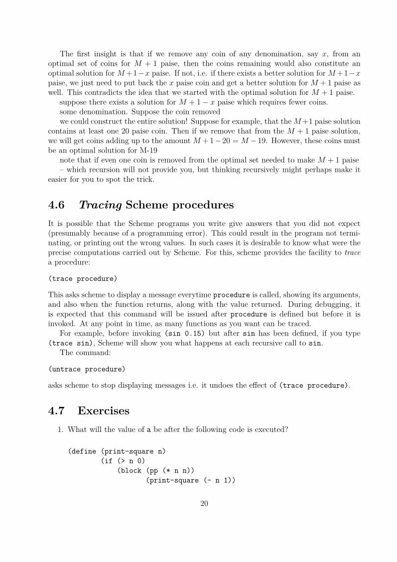
The first insight is that if we remove any coin of any denomination, say x, from anoptimal set of coins for M + 1 paise, then the coins remaining would also constitute anoptimal solution for M +1−x paise. If not, i.e. if there exists a better solution for M +1−xpaise, we just need to put back the x paise coin and get a better solution for M + 1 paise aswell. This contradicts the idea that we started with the optimal solution for M + 1 paise.
suppose there exists a solution for M + 1 − x paise which requires fewer coins.some denomination. Suppose the coin removedwe could construct the entire solution! Suppose for example, that the M +1 paise solution
contains at least one 20 paise coin. Then if we remove that from the M + 1 paise solution,we will get coins adding up to the amount M + 1 − 20 = M − 19. However, these coins mustbe an optimal solution for M-19
note that if even one coin is removed from the optimal set needed to make M + 1 paise– which recursion will not provide you, but thinking recursively might perhaps make it
easier for you to spot the trick.
4.6 Tracing Scheme procedures
It is possible that the Scheme programs you write give answers that you did not expect(presumably because of a programming error). This could result in the program not termi-nating, or printing out the wrong values. In such cases it is desirable to know what were theprecise computations carried out by Scheme. For this, scheme provides the facility to tracea procedure:
(trace procedure)
This asks scheme to display a message everytime procedure is called, showing its arguments,and also when the function returns, along with the value returned. During debugging, itis expected that this command will be issued after procedure is defined but before it isinvoked. At any point in time, as many functions as you want can be traced.
For example, before invoking (sin 0.15) but after sin has been defined, if you type(trace sin), Scheme will show you what happens at each recursive call to sin.
The command:
(untrace procedure)
asks scheme to stop displaying messages i.e. it undoes the effect of (trace procedure).
4.7 Exercises
1. What will the value of a be after the following code is executed?
(define (print-square n)
(if (> n 0)
(block (pp (* n n))
(print-square (- n 1))
20
n)
))
(define a (print-square 10))
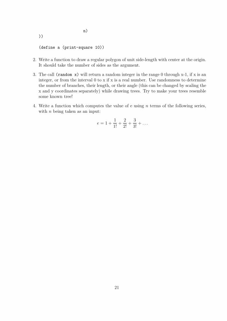
2. Write a function to draw a regular polygon of unit side-length with center at the origin.It should take the number of sides as the argument.
3. The call (random x) will return a random integer in the range 0 through x-1, if x is aninteger, or from the interval 0 to x if x is a real number. Use randomness to determinethe number of branches, their length, or their angle (this can be changed by scaling thex and y coordinates separately) while drawing trees. Try to make your trees resemblesome known tree!
4. Write a function which computes the value of e using n terms of the following series,with n being taken as an input:
e = 1 +1
1!+
2
2!+
3
3!+ . . .
21

Chapter 5
Proving Program Correctness
Programming errors, or bugs, can cause and already have caused many, many disasters, suchas failures in satellite launches, and car accidents (bugs in the program that performs carcontrol functions). We are all familiar with operating system or other program releases that“fix bugs”, and which keep appearing from time to time. If we could some how ensure thata program will function correctly, before it is released for use, we will avoid much expense,much wasted effort, and many accidents.
How can we be sure that a program is correct? One way is to test it on several examples:this is obviously insufficient; however much testing we do we still cannot be sure that theprogram will not fail on some instance that we have not tested. A better way is to provethe program to be correct. A proof of the correctness of a program is in spirit similar to theproof of a theorem in Euclidean Geometry. In both cases, the proofs consist of a sequenceof assertions, where the assertions must either be postulates, or be implied by precedingassertions using the so called inference rules. For example, if you know that “A implies B”and that “A is true”, then you can conclude that “B is true”. By properly employing suchrules of inference if you prove that “The bisectors of the angles of a triangle meet in a point”,then most people accept this as true. Proofs of correctness of programs are expected to havesimilar credibility.
The proof process is substantially different for imperative and functional programmingstyles. It will be seen in many examples that the proof of correctness is much easier to writefor functional programs than imperative style programs. The rest of the chapter describesthe proof process with examples.
5.1 Basic ideas in program proving
The first step in proving the correctness of a program is to formulate the problem precisely.We need to precisely characterize the input to the program, and the output required fromthe program. For example, for a program computing the greatest common divisor, the inputcharacterization would say that the inputs must be positive integers (otherwise the gcd isundefined), and the output is the largest integer that divides them both without leaving aremainder. Another example is a sorting program. For this the input could be an arrayA of numbers, and the output would be another array B of the same length containing apermutation of the input such that B[i]≤B[j] if i < j.
22

Given that the input to the program satisfies the input characterization (also calledpreconditions) the proof must establish (explicitly or implicitly) the following progressivelyharder claims:
1. The program terminates, e.g. does not go into any infinite loop.
2. The program terminates but not because of an erroneous operation, e.g. division byzero, or accessing an array using a subscript that is larger than the length of an array.
3. The value returned by the program is the correct value.
5.1.1 Form of the proof
In general, a proof consists of a sequence of statements, with a justification for each statementstating how that statement is deduced. Proofs of programs are similar. The statements insuch a proof must however characterize the behaviour of the program. This characterizationwill be of the form:
When control arrives at point P in the program, the variable V has value v.
If there are no loops or function calls from the beginning of the program to point P , thenwe can reason about the effect of every statement from the beginning to point P and derivea characterization of the value of V in terms of the values of the program variables at thebeginning. We will call this hand execution, or symbolic execution. Note however, that sucha justification is reliable if we hand execute only over a small number of statements. Forlarge number of statements, we are likely to make mistakes as we trace the execution.
Thus it would seem at first glance that the idea of hand execution would be useless whenthere are loops or function calls between the beginning of the program and the point P ,or when P is itself inside a loop. However, as will be seen below, with some additionalmachinery (induction) we will be able to use hand execution in our proofs.
5.2 Proving correctness of functional programs
We begin with an example. Consider the program for evaluating the factorial of number.
(define (fac n)
(if (= n 0)
1
(* n (fac (- n 1)))
)
)
Program Specification: The function correctly returns n! for all non-negative integers n.
Proof of correctness: The proof is by induction. The induction hypothesis is:
IH(n) : The call (fac n) returns n! provided n is a non-negative integer.
23

The base case is n=0, i.e. we are required to prove : IH(0) is true. We do this by hand-executing the program. When n has the value 0 then the conditional test (= n 0) succeeds,and the procedure returns 1, which in fact is the correct value 0!
Next we establish the induction. We will assume IH(n-1), i.e. that the program correctlycomputes n-1! if n-1 is supplied as the argument. We are then required to prove IH(n), withn > 0. Again we employ hand-execution. Now in the execution the first check (= n 0) fails,since we know n > 0. Thus the program now computes (fac (- n 1)) and returns the resultafter multiplying it by n. Now, (- n 1) is just n-1, and this must be at least 0 since n > 0.But IH(n-1) guarantees that factorial of n-1 is correctly computed if n-1 is a nonnegativeinteger. Thus the call (fac (- n 1)) returns n-1! – but then the value returned is n * n-1!which is n! by definition. Thus the correct value is returned, establishing the induction.
It should be noted that in all cases, we hand executed the program only for a smallnumber of steps.
5.3 Summary of the argument
Proving the correctness of functional programs consists of the following:
Write down the specifications. These consists of preconditions which the inputs to theprogram must satisfy, and a claim regarding the output that will be produced. In thefactorial example, the precondition was that the input n being supplied was a nonnegativeinteger. The claim then was that the value of n! would be correctly returned. Notice thatthe specifications may leave unsaid what happens if the program is executed without theinput specifying the preconditions.
Use induction to prove the specifications. For this, it is necessary to precisely writedown an induction hypothesis (this is usually nothing else but the specifications themselves)and identifying a variable or variables for the induction. This variable over which the in-duction is supposed to be is usually the something representative of the size of the problembeing solved. In the case of factorial, the variable was the input n.
1. Identify and prove the base case. The base case is often the smallest problem sizepossible. In case of factorial, we used the base case n=0. The base case is establishedby “hand executing” the program with the input fixed to the base case.
2. Establish the induction. For this we assume that the induction hypothesis holds fora certain problem size n and prove it holds for the next larger problem size n+1. Wemay in fact assume that the induction hypothesis actually holds for all problem sizesno larger than n, and then prove it holds for problem size n+1. The induction isestablished by hand execution as well.
5.3.1 Euclid’s Algorithm
Theorem 1 If u, v > 0 and u, v are integers then if v divides u then gcd(u, v) = v, elsegcd(u, v) = gcd(v, u mod v)
24

Our program is based on the above theorem and is as follows:
(define (gcd u v)
(if (= (remainder u v) 0)
v
(gcd v (remainder u v))
)
)
We will use gcd(u, v) to denote the gcd of u and v, and (gcd u v) the value returned byprogram.
Specification: Precondition: inputs u,v must be positive integers. Claim: (gcd u v) =gcd(u,v).
Inductive Hypothesis: The input size can be thought of as the magnitudes of the inputnumbers. The program can be proved correct by considering an induction over the valuestaken by either u or v; it is more convenient to use the values taken by v, and so we use thathere. The inductive hypothesis is:
IH(n) : (gcd u v) = gcd(u, v) for u having any positive integer as value and v having thevalue n.
Base Case: n = 1. Thus v takes the value 1. By hand execution of the program, (gcd u 1)= 1 = gcd(u,1) for all u.
Induction: We will assume IH(1),IH(2),...,IH(n-1) and prove IH(n). So consider an execu-tion in which v takes the value n. Let x = (remainder u n). Clearly x < n. There are twocases to consider.
CASE 1: x = 0. In this case the function returns n, which is in fact gcd(u, n) for any u.CASE 2: x > 0. Then the function calls (gcd n x). Since x > 0, the precondition of
IH(x) is satisfied. Since x < n, IH(x) is a part of what we have assumed. Thus we knowthat this call will return gcd(n,x) = gcd(n, (remainder u n)). But by the theorem above weknow gcd(n, (remainder u n)) = gcd(u,n). But this is in fact what we want to return. Henceproved.
5.4 Proof Strategy for Imperative programs
We again begin with the example of computing factorials. Here is a simple program
1. integer function fac(n)
2. fac = 1
3. do i=1,n
4. fac = fac*i
5. end do
6. return fac
25

The specification for this program is the same as that for the functional version. Thestructure of the proof is very different, however. For imperative programs, the proof proceedsby characterizing the values taken by the program variables as the program executes. If theprogram does not have loops, then this is very easy. In case of programs with loops, we needto characterize what happens to the variables in each iteration. For this we need the notionof a loop invariant. This is simply an assertion that holds for every iteration of the loop.The assertion is proved by induction over the number of iterations of the loop. An exampleis given below. Let xk denote the value of any variable x after statement 4 has been executedin the kth iteration.
Loop invariant: fack = k!, ik = kWe could have written that fac=i! instead of the bringing in k; however we do this in
order to keep a distinction between variables and the values they take.
Proof of invariant: We use induction over k. The base case is k = 1, i.e. the first timestatement 4 is encountered. At the beginning of the first iteration the variable fac has thevalue 1, since that is what it was initialized to in statement 2. In the first iteration thevariable i has the value 1. Thus i1 = 1, which is part of what is claimed in the invariant.Further, statement 4 multiplies the current value of i (which is 1) and the current value offac (which is 1) and sets fac to that. Thus fac1 = 1 × 1 = 1 = 1! establishing the base case.
The induction step is as follows. We will assume that fack−1 = k − 1!, ik−1 = k − 1 andthen prove that fack = k!, ik = k. Clearly, in the kth iteration ik = k. At the beginning ofthe kth iteration, fac must have the same value as it did at the end of the k − 1th iteration,i.e. fack−1 = k − 1!. But in statement 4, we set fac to be its current value (i.e. k-1!) timesthe value of i (i.e. k). Thus after statement 4 of kth iteration, fac must have the valuek − 1! × k = k!. Thus fack = k!, completing the proof.
Proof of correctness: Given the invariant proved above, the function is easily proved tobe correct. First, we should observe that the function must terminate. This is because theloop will execute only n times if n is a positive integer, or once if n is zero.1 Note thatwe dont need to consider the case of n having a negative value because of the preconditionin the specification. Note that since we do not have any operations such as division thatcan cause erroneous termination, so we can be assured that there are no runtime errors. Insummary we know that after a finite number of iterations the program will terminate. Thevalue returned by the program is the value of the variable fac. There are 2 cases dependingupon the value of n:
n = 0 Loop is executed once, the value of fac at the end is 1, which is returned. This iscorrect since 0!=1.
n > 0 In this case the loop is executed n times, and the value of the fac at the end of the nth iteration, i.e. facn is returned. But we know from the invariant that facn = n!.Thus the current value is returned in this case too.
1Here we are not making the distinction between the variable n and its value, because n doesnt changeduring the program.
26

5.4.1 Structure of proofs of Imperative Programs:
Let us assume for simplicity that our programs have only a single loop. In this case, thegeneral strategy is to write down a loop invariant that characterizes how the values evolve asthe loop executes. The loop invariant is proved by induction over the number of iterationsof the loop. To establish the inductive step, we assume that the invariant holds during somek − 1th iteration, then hand execute the program and keep track of what happens to thevariables and show that the values taken by the variables will be such that the invariant issatisfied even in the kth iteration. The base case is established by hand execution from thebeginning of the program to the first iteration of the loop.2
Proving the invariant is the key step. After this, we need to establish first that the loopexecutes only a finite number of steps, and there are no errors during execution. In the aboveprogram this was easy since the loop executed n times by the definition of the DO statementin Fortran. In other cases, more ingenuinity might be necessary. Given that the programdoes not go into an “infinite loop” and there are no errors we need to characterize the valuethat will be returned. This can be done using the invariant for the last loop iteration.
5.4.2 Euclid’s algorithm for computing GCD
An imperative style program for computing the gcd is as follows.
1. integer function fgcd(u, v)
2. integer u,v,temp
3. while( mod(u,v) != 0)
4. do
5. temp = u
6. u = v
7. v = mod(temp,v)
8. end do
9. return v
We will use the expression gcd(u,v) to denote the greatest common divisor of u and v;in contrast fgcd(u,v) is the value (if any) returned by the function above.
The specification is the same as that for the functional program. We will also need thetheorem stated there.
Invariant: Let uk, vk denote the values of the variables u, v when control reaches statement3 for the k th time. Then the claims are:
1. uk, vk > 0
2. gcd(uk, vk) = gcd(u1, v1) i.e. the gcd of the values in u and v is the same as that whenthe program started execution.
2In every case, we hand execute only for 1 iteration, i.e. a small number of steps.
27

Proof of the invariant: The proof is by induction over k. The base case is k = 1. Whenstatement 3 is visited for k = 1st time, the values of u,v are u1, v1. But because of theprecondition we know that u1, v1 > 0. Since k = 1 clearly gcd(uk, vk) = gcd(u1, v1). Thusthe base case is established.
Assume that the invariant holds at the time of the k − 1th visit to statement 3, i.e.uk−1, vk−1 > 0, gcd(uk−1, vk−1) = gcd(u1, v1). Now do a hand execution of the k − 1thiteration. Since we know that statement 3 is reached for the kth time, the test in statement3 must have succeeded, i.e. it must be that uk−1 mod vk−1 > 0. Continuing the executionwe see that when statement 5 is executed, temp gets the value uk−1. When statement 6 isexecuted variable u gets the value vk−1. Finally in statement 7 the variable v gets the valueuk−1 mod vk−1. For this operation to be legal we need that vk−1 > 0, but we have that fromthe inductive hypothesis. After this, the control returns to statement 3 for the kth time.The values of u, v at this time are vk−1, uk−1 mod vk−1, and we have established that both ofthese are positive earlier. Thus uk = vk−1 > 0 and vk = uk−1 mod vk−1 > 0. Finally, usingthe theorem stated earlier gcd(uk−1, vk−1) = gcd(vk−1, uk−1 mod vk−1) = gcd(uk, vk). Butfrom the inductive hypothesis we know that gcd(uk−1, vk−1) = gcd(u1, v1). Thus we havegcd(uk, vk) = gcd(u1, v1). This completes the proof of the invariant.
Proof Of Proper Termination: Note that because of the invariant, when control reachesstatement 3 the variable v is guaranteed to be positive. Thus the mod operation is legal, andso there are no abnormal terminations. Next note that the value of the variable v strictlydecreases in each iteration, and the invariant above ensures that it is always positive. Thusthe loop must only execute a finite number of steps.
Proof that correct value is returned: Suppose the control reaches the return statement(and we know this happens because of the proof of correctness) after visiting statement 3 ktimes. At this visit the test in statement 3 must have failed (otherwise the loop must haveexecuted at least one more time). Thus we know that uk mod vk = 0. Thus vk = gcd(uk, vk).But by the invariant gcd(uk, vk) = gcd(u1, v1). Thus the value vk returned is indeed thecorrect value.
5.5 Proving programs involving several functions
Consider the following alternative code for computing the factorial of a number:
(define (fact n)
(fact2 n 1))
(define (fact2 n f)
(if (>= n 1)
f
(fact2 (- n 1) (* f n))))
In this case the function fact is very simple; clearly, its correctness depends upon whatfact2 does. We must prove that the factorial of n is returned for the call (fact2 n 1). If
28

we can prove this (see Exercises), then that is adequate. Then we can conclude that (fact
n) must return n! since (fact n) returns (fact2 n 1) which we proved is n!.In general, once we write down and prove the specifications for a given procedure f, we
can use these specifications in proofs of other procedures which call f.
5.6 Conclusions
It should be obvious that the recursive versions are far easier to prove correct. One of thereasons for this simplicity is that each variable has only one value in a functional program.Thus we dont have to worry about “value of variable at time t”, or “how the variabledecreases”. Second, the functional programs are also more compact and pretty much followthe statement of the mathematical ideas on which they are based; notice that the functionalprogram for gcd is very similar to the statement of Theorem 1. There is a reason for this:induction is a very fundamental mathematical proof techniue, and because recursion is veryrelated to induction, it turns out that recursive programs are usually easier to write andprove correct.
On the debit side, functional (recursive) programs often require more memory and runslightly slower than their imperative counterparts.
In these days when program readability and correctness are very important, it is recom-mended that functional programming (recursion, no reassignment to values of variables) beused wherever possible.
5.7 Exercises
1. Write a function (digits n) which returns the number of digits in a number n. Writea proof of correctness. Clearly write down the mathematical property on which yourprogram is based.
2. Write the invariant necessary to prove the correctness of the following gcd program.
integer function gcd1(u, v)
integer u,v,w;
w=mod(u,v)
while(w > 0)
u=v
v=w
w=mod(u,v)
end do
return v
Prove the program correct.
3. Consider the code given below computing nCk:
29

integer function choose(n,k)
integer n,k,c,i
c=1
do i=1,k
c=c*(n-i+1)/i
end do
return c
Write an invariant for the do loop, i.e. state what you know about the different variablesat the end of the jth iteration of the loop.
4. Write down the specifications for the function fact2 of Section 5.5.
Verify that the specification implies that (fact2 n 1) correctly computes n!. Provethat the call (fact2 n 1) correctly computes n!. (Hint: Although the first call willalways have the second argument to be 1, this may not be the case in the subsequentrecursive calls. Hence the proof will actually involve proving the entire specification,i.e. for arbitrary value of the second argument as well.)
5. Write a scheme function (isqrt n) that returns ⌈√n⌉. Use a simple algorithms such
as trying out the numbers 1, 2, . . . as candidate square roots and checking until theright conditions are satisfied. You may use additional functions if necessary. State themathematical property on which your program is based. Write a proof of correctness(include a proof for the additional functions you used, if any).
30

Chapter 6
More on Scheme Statements
6.1 The “begin” Statement
If a number of statements have to be grouped together then they are put in a block. Thisfeature is usually used to group statements causing side-effects. A block is constructed usingthe “begin” statement.
Syntax:
(begin
(stmt 1)
(stmt 2)
.
.
.
(stmt n)
)
Example:
(if (< n 1)
(begin
(line 0 0 0.5 0.5)
(line 0 0 0 0.5)
(line 0 0 0.5 0)
)
)
The begin statement returns the value of the last statement in the block.
6.2 The “cond” statement
The if statement is basically a two way branch. To implement multi-way branching one canuse nested if statements but Scheme provides a more elegant way of doing the same - the“cond” statement.
Syntax:
31

(cond (t1 stmt-11 stmt-12 stmt-13 ....)
(t2 stmt-21 stmt-22 stmt-23 ....)
.
.
.
(tn stmt-n1 stmt-n2 stmt-n3 ....)
(else stmt-e1 stmt-e2 stmt-e3 ....)
)
The evaluation proceeds stepwise:- First t1 is evaluated, and if true stmt11....stmt1m areevaluated, and if false , only then t2 is evaluated and so on. The else statement is a catch-allwhich is true even if t1....tn are false. Note that the else statement must be provided whenthe cond statement is used to return a value but it may be omitted when side-effects are tobe caused.
6.3 The “let” stetement
Consider the sine function:-
(define (sine x)
(if (< x 0.0001)
x
(- (* 3 (sine (/ x 3))) (* 4 (sine (/ x 3)) (sine (/ x 3)) (sine (/ x 3))))
)
)
Notice that not only is the expression clumsy but is also wasteful, since the same statement(sine (/ x 3)) is evaluated 4 times. To deal with such situations Scheme provides the “let”statement.
Syntax:
(let ((v1 value exp.)
(v2 value exp.)
.
.
.
(vn value exp.)
)
(stmt 1)
(stmt 2)
.
.
.
(stmt m)
)
32

The value expressions are evaluated only once and the names v1....vn are associated withthe value expressions. Now these names can be used in stmt1....stmtm. For example, thesine program can be modified to
(define (sine x)
(if (< x 0.0001)
x
(let ((s (sine (/ x 3))))
(- (* 3 s) (* 4 s s s))
)
)
)
As is usual in Scheme, the value of the last statement evaluated in the block is returned asthe value returned by let. A point to be noted is that v1....vn are available only in the letblock. They are undefined outside.
33

Chapter 7
Higher Order Functions
One of the most powerful ideas in functional programming is that programmers should beallowed to manipulate functions just as they manipulate data. For example, functionalprogramming languages allow functions to be passed to other functions as arguments, or bereturned as arguments. A function which manipulates other functions in this manner is saidto be a higher order function.
Higher order functions turn out to be extremely powerful in many ways:
• Help in writing programs in a modular manner. An important question in programmingis how to develop pieces of a program as independent parts or modules which can thenbe combined conveniently to make full programs.
• Make programs more intuitive and concise.
• Can be used to build data structures. This may sound strange, but is actually true!Read on.
7.1 Functions as parameters to other functions
The ability to pass functions as parameters to other functions can be used to make programsmodular. We will describe two examples of this.
7.1.1 Generalized Root Finder
Consider first, a program that finds the square root of 2. This parameters xneg and xpos
denote the upper and lower ends of an interval in which the square root of two must beguaranteed to lie. Then the program finds the midpoint xmid of the interval [xneg, xpos]
and simply determines in which of the two subintervals [xneg, xmid] and [xmid, xpos]
the square root must lie. Then the program recurses with that interval. The recursion stopswhen the size of the interval becomes small enough (smaller than 0.01 in particular).
(define (sqrt2 xneg xpos)
(if (< (abs (- xneg xpos)) 0.01)
xneg
34

(let ((xmid (/ (+ xneg xpos) 2)))
(if (< (* xmid xmid) 2)
(sqrt2 xmid xpos)
(sqrt2 xneg xmid)))))
This program will yield the square root of 2 for the call (sqrt2 1.0 2.0), for example.You may observe, that the basic logic of bisecting the interval and recursing on the
appropriate subinterval is useful for many other calculations. In particular, for writing ageneral program for finding the roots of any function f. By passing f as a parameter, wemay write a general root finder as follows.
(define (root f xneg xpos)
(if (< (abs (- xneg xpos)) 0.01)
xneg
(let ((xmid (/ (+ xneg xpos) 2)))
(if (> 0 (f xmid))
(root f xmid xpos)
(root f xneg xmid)))))
Once we have such a function root defined, we may use it to find the square root of 2 bywriting:
(define (f x) (- (* x x) 2.0))
(root f 1.0 2.0)
Of course, we can use it to get an approximate root of any function provided we know aninterval in which a root lies. For example, the function g(x) = x − cos(x) has g(0) = −1 andg(1) > 0. Thus we can find its root by writing:
(define (g x) (- x (cos x)))
(root g 0.0 1.0)
Exercise
Our condition for the error being small enough was |f(x)| < 0.01. Some users might wantthe constant to be something other than 0.01, or might want to ensure for example that|f(x)2| < 0.01. Extend root so that it takes an additional function close-enough whichcan be used to determine whether the approximation is good-enough, i.e. assume that(close-enough x) is true only when x is close enough to the root.
7.1.2 Animation
Even in our primitive graphics system, it is possible to make objects move. Well, they dontactually move, but we can create this illusion by first drawing them in one position, erasingthem, and then drawing them in the next position. Erasing does not need anything special– we simply draw the object in the same colour as the background.
There are 3 basic tasks in doing our simple animation:
35

1. Definition of the shape of the object.
2. The basic operation of drawing and erasing the object.
3. Movement of the object, i.e. the description of the trajectory.
It is desirable that the code for each of the tasks above is written as independently as possible,and be combined only when needed. That way, it would be easy to do the animation formany shapes, or along many trajectories. We can do so by using a function for each task,and by using higher order functions to combine the functions. Here is how it might be done.The main procedure is move-shape shown below. It does the work of drawing and erasingthe shape; the precise shape to be drawn is passed to it using the function parameter shape.The trajectory along which to move the shape is specified parametrically using the functionparameters x and y.
(define (move-shape t dt tf shape x y)
(if (< t tf)
(begin (trans (x t) (y t) (shape)
(colour "white" (shape)))
(move-shape (+ t dt) dt tf shape x y))
(trans (x t) (y t) (shape))))
To use procedure move-shape we must define the functions for the shape and the trajec-tory, and pass them as parameters. So we could write:
(define (square)
(line -0.02 -0.02 -0.02 0.02)
(line -0.02 -0.02 0.02 -0.02)
(line 0.02 0.02 -0.02 0.02)
(line 0.02 0.02 0.02 -0.02))
(define (xcirc t) (* 0.5 (cos t)))
(define (ycirc t) (* 0.5 (sin t)))
(move-shape -3.14 0.01 1.57 square xcirc ycirc)
Exercises
Extend the move-shape code to handle the following cases.
1. Suppose the shape must not only move, but must also rotate so that it is always atthe same angle with its trajectory. This will look nice if the shape is an aeroplane, forexample.
2. Suppose the shape internally consists of several shapes, e.g. a moon circling the earth.
3. Suppose there are several independent shapes to be moved.
36

4. Suppose it is better to erase the shape at (x(t), y(t)) only after the drawing the nextone, i.e. at (x(t + dt), y(t + dt)).
Other extensions are also possible, e.g. the shape should move in response to a field thatcould be defined by the user. Or the shape should bounce of walls in the picture.
7.2 Function Expressions
So far we have seen only identifiers in the first position of any expression, Scheme actuallyallows expressions to be present here too — it is necessary, however, that these expressionsevaluate to functions, and then these functions are applied to the remaining arguments. Forexample, we can write:
((if (= x y)
+
*)
10 20)
which will either add the numbers 10 and 20 or multiply them depending upon whether ornot x was equal to y.
7.2.1 Unnamed Functions
It is convenient to be able to construct functions without having to give them names. Thisis done using the general form
(lambda arguement-list body)
Thus the expression
(lambda (x) (* x x ))
returns a function that takes a single argument and returns its square. We can use suchexpressions1 in any place wherever a function can be used, e.g.
(define g (lambda (x) (* x x)))
((lambda (x) (* x x)) 5) ;; returns 25.
(root (lambda (x) (- x (cos x))) 0.0 1.0) ;; root defined earlier
(move-shape -3.14 0.01 1.57 ;; move-shape defined earlier
(lambda () ;; square drawing function
(line -0.02 -0.02 -0.02 0.02)
(line -0.02 -0.02 0.02 -0.02)
(line 0.02 0.02 -0.02 0.02)
(line 0.02 0.02 0.02 -0.02))
(lambda (t) (* 0.5 (cos t))) ;; xcirc equivalent
(lambda (t) (* 0.5 (sin t))) ;; ycirc equivalent
)
1The body argument can be several commands, the value of the function is the value of the last command.
37
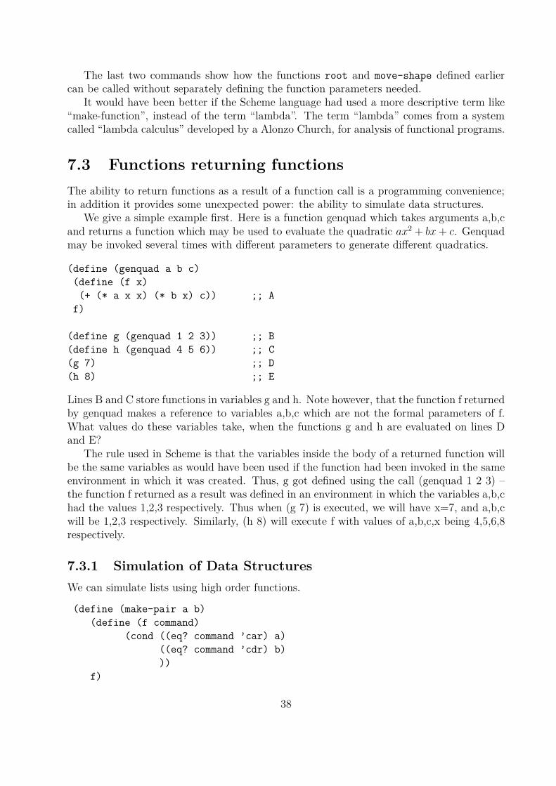
The last two commands show how the functions root and move-shape defined earliercan be called without separately defining the function parameters needed.
It would have been better if the Scheme language had used a more descriptive term like“make-function”, instead of the term “lambda”. The term “lambda” comes from a systemcalled “lambda calculus” developed by a Alonzo Church, for analysis of functional programs.
7.3 Functions returning functions
The ability to return functions as a result of a function call is a programming convenience;in addition it provides some unexpected power: the ability to simulate data structures.
We give a simple example first. Here is a function genquad which takes arguments a,b,cand returns a function which may be used to evaluate the quadratic ax2 + bx + c. Genquadmay be invoked several times with different parameters to generate different quadratics.
(define (genquad a b c)
(define (f x)
(+ (* a x x) (* b x) c)) ;; A
f)
(define g (genquad 1 2 3)) ;; B
(define h (genquad 4 5 6)) ;; C
(g 7) ;; D
(h 8) ;; E
Lines B and C store functions in variables g and h. Note however, that the function f returnedby genquad makes a reference to variables a,b,c which are not the formal parameters of f.What values do these variables take, when the functions g and h are evaluated on lines Dand E?
The rule used in Scheme is that the variables inside the body of a returned function willbe the same variables as would have been used if the function had been invoked in the sameenvironment in which it was created. Thus, g got defined using the call (genquad 1 2 3) –the function f returned as a result was defined in an environment in which the variables a,b,chad the values 1,2,3 respectively. Thus when (g 7) is executed, we will have x=7, and a,b,cwill be 1,2,3 respectively. Similarly, (h 8) will execute f with values of a,b,c,x being 4,5,6,8respectively.
7.3.1 Simulation of Data Structures
We can simulate lists using high order functions.
(define (make-pair a b)
(define (f command)
(cond ((eq? command ’car) a)
((eq? command ’cdr) b)
))
f)
38

Now consider the two statements:
(define x (make-pair 6
(make-pair 7 (make-pair 8 (make-pair 9 ’empty-list)))))
(define y (cons 6 (cons 7 (cons 8 (cons 9 ’())))))
Both the statements could be thought of as creating a list of the numbers 6,7,8,9. The meansof accessing the lists are not the same, but we can surely access the elements from x just aswell as we can from them. So to access the third element we would write
(car (cdr (cdr y)))
(((x ’cdr) ’cdr) ’car)
As you can see, both will yield the value 8 of the third element of the list. The above coderepresents the empty list by the symbol ’empty-list, but this is not necessary; ’() could havebeen used as well. In any case, the conclusion is:
Given Higher Order Functions, the language need not separately provide data structure;data structures can be constructed out of higher order functions!!
7.3.2 Simulating let command using functions
Suppose we have a let statement:
(let ((a 1)
(b (* c d)))
body
)
It can be verified that its effect is the same as the following statement which instead uses alambda.
((lambda (a b)
body)
1 (* c d))
Since the lambda form is called with arguments 1 and (* c d), the formal parameters a andb acquire these values, and the body gets executed. The value of the form is the value ofthe last line of the body. But this is in fact exactly what would happen if we used a let asabove!
7.3.3 Simulating do commands using functions
Implementation of DO LOOPS using lambda is done as a lab exercise.
39

7.4 Unnamed recursive functions
The question considered here is: can we use lambda expressions to define unnamed recursivefunctions? Note that named recursive functions are easily defined using lambda. For example,it is perfectly acceptable to write
(define fact (lambda (n)
(if (= n 0)
1
(* n (fact (- n 1))))))
This definition is equivalent to the standard one. However, it does define the name fact.Can this be avoided? At first glance, it would seem impossible, because in the body of thelambda when we make the recursive call, we would need to name the function. So we wouldneed to define the name explicitly.
It turns out however, that lambda expressions can be used to define unnamed recursivefunctions as well; how to do it is slightly complex, but very elegant. It also exposes somehidden power of the lambda form. Hence we will discuss it. It is good to understandthis section if you wish to make certain that you really understand the lambda command.However be warned that some mental gymnastics are involved.
Here is how the fact function must be expressed:
(lambda (n f)
(if (= n 0)
1
(* n (f (- n 1) f))))
The first important idea is already in the expression above: the function contains an extraargument f in addition to n. Thus this lambda expression is a higher order function. Nowcomes the second idea. When we wish to apply this function to a number, e.g. 5 (to compute5!) we need to supply the second argument as well. So in this case we supply itself! Thiscompletes the construction. More precisely, 5! could be computed by writing:
((lambda (n f)
(if (= n 0)
1
(* n (f (- n 1) f))))
5
(lambda (n f)
(if (= n 0)
1
(* n (f (- n 1) f)))))
This is only slightly different from how we call an ordinary unnamed function. For exampleif we wish to evaluate the polynomial x2 + 3x + 10 and x = 5 we would write
((lambda (x)
(+ (* x x) (* 3 x) 10))
5
)
40

This story has two morals. First, if you allow functions to take other functions as param-eters, then you dont need to explicitly allow functions to be recursive. The second moral isthat with the above construction it is possible to entirely eliminate define statements fromany program!
7.4.1 Exercise
1. What is the result of executing the following?
((lambda (n f)
(f n f))
5
(lambda (n f)
(if (= n 0)
1
(* n (f (- n 1) f)))))
2. Show how an unnamed function could be constructed for constructing gcd. Here is thestandard gcd for reference.
(define (gcd x y)
(if (= (remainder x y) 0)
y
(gcd y (remainder x y))))
Show how you would use your unnamed function to compute the gcd of 119 and 34.
41

Chapter 8
Lists
A lists is an ordered collection of objects. You can construct a list by using the function listthat takes the objects you want put into the list. For example, (list 1 2 3 4 5) will returnthe a list of the numbers 1,2,3,4 and 5 in that order. This list can be assigned to a variable,as in:
(define a (list 1 2 3 4 5))
list is a function, and it can be given more complicated arguments. For example, thefollowing code will make a list of the first 3 multiples of pi:
(define pi 3.14)
(define b (list pi (* 2 pi) (* 3 pi)))
This would cause b to become the list containing 3.14, 6.28 and 9.42 in that order.The various elements of the list can be accessed using the functions car and cdr (pro-
nounced “could er”). Car of a list gives the first element of the list, while cdr gives the wholelist except the first element.
(car a) => 1
(cdr a) => (list 2 3 4 5)
Scheme allows us to write cadr which means the car of the cdr, and so on. Thus
(cadr a )
=>2
(caddr a)
=>3
The function cons (short for “construct”) takes an element and inserts it at the frontof the list, and returns the list thus formed. The function append appends the given liststogether. Thus
(cons 0 a) => (list 0 1 2 3 4 5) ;; a is not changed however.
(append a a) => (list 1 2 3 4 5 1 2 3 4 5)
(define c (append b a))
42

The last command would set c to be the list with the first 3 elements being the multiples ofpi, and the remaining 5 being the numbers 1 through 5. In any case, the values of a and bwill not change.
(list? expr) returns true if expr evaluates to a list, and false otherwise.(null? expr) returns true if expr evaluates to the empty list (written as ’()), and true
otherwise.
Quote notation
A shortform has been provided for constructing lists out of constants. Thus the definitionof a could be written as:
(define a ’(1 2 3 4 5))
This has the same effect as the earlier definition. Scheme recognizes the character (’) tomean that the expression following it should not be evaluated, but be treated as a list. It isacceptable to write
(define d ’(1 (2 3) 4))
This is equivalent to saying (define d (list 1 (list 2 3) 4)). When using the quoted form notethat the single quote at the beginning is sufficient, while the corresponding expression usingthe list function needs the function to be specified more often as above.
There is another important difference between using quotes and the function list. Forexample, if we write
(define pi 3.14)
(define e ’(pi (* 2 pi) (* 3 pi)))
This would not set e to be a list containing 3.14, 6.28 and 9.42; instead e would become alist containing symbols; this will be explained in the chapter on symbols.
Note of course that a command such as
(define f (1 2 3 4 5))
is erroneous – scheme expects the first term after a “(” to be a function, and it will give anerror because 1 is not a function.
8.1 Program Example
(define (length l)
(if (null? l)
0
(+ 1 (length (cdr l)))))
The above program gives the length of the list l.The program below takes two lists of numbers as the input and returns a list whose ith
element is the sum of the ith elements of the input lists. It is necessary that the input listsbe of the same length.
43

(define (sum a b)
(if (null? a )
’() ;; the empty list.
(cons (+ (car a) (car b))
(sum (cdr a) (cdr b)))))
It will be seen that both the programs are based on the idea that a list is recursivelystructured. Thus a list may be thought of as the first element followed by a list of theremaining elements. Thus procedures operating on lists are often recursive; they explicitlyoperate on the first element and recurse on the remaining elements (the cdr of the list). Thebase case for the recursion is the empty list.
8.2 Proving correctness of programs involving lists
As an example, we will give a proof of correctness of the function sum.
Specification: Let a, b be two lists of numbers, both having the same length n. Let theelements be denoted by a1, . . . , an and b1, . . . , bn. Then the call (sum a b) returns a listwith elements a1 + b1, . . . , an + bn. If n = 0 then the result should be the empty list.
Note that the specification includes the preconditions that the lists have the same lengthand contain only numbers. No claims are made if sum is called with unequally long lists.
Inductive Hypothesis IH(n): (sum a b) works correctly for lists of length n, assumingthe preconditions are satisfied.
Proof of base case IH(0): If the lists are empty, then by hand execution it is clear thatthe empty list is returned. But this is what is expected, hence proved.
Proof of IH(n+1) assuming IH(n): Consider a and b of length n + 1. Then handexecution shows that the value returned is (cons (+ (car a) (car b)) (sum (cdr a)
(cdr b))). Now if a is a1, . . . , an+1 and similarly b, then (+ (car a) (car b)) is justa1 + b1. Also (cdr a) and (cdr b) must have length n since a,b had length n + 1, andmust respectively contain a2, . . . , an+1 and b2, . . . , bn+1. Thus the call (sum (cdr a) (cdr
b)) satisfies IH(n) and the preconditions in the specification, and hence a list containinga2 + b2, . . . , an+1 + bn+1 is returned. Thus what is returned is the cons of a1 + b1 with thislist, i.e. the list a1 +b1, . . . , an+1 +bn+1. But this is precisely what is expected, hence proved.
8.3 More List Operations
With the basic operations car, cdr and cons defined on lists, we can now implement morecomplex list manipulations. Some of these are predefined in Scheme.
1. Write a function to access the ith element of a list.
Solution :
44

(define (list-ref list i)
(if (null? list)
()
(if (= i 0)
(car list)
(list-ref (cdr list) (- i 1)))))
2. Write a function to return only the even-indexed elements of a list.
Solution :-
(define (even-list list)
(if (or (null? list) (null? (cdr list)))
list
(cons (car list) (even-list (cddr list)))))
3. Write a function to return the sum of the elements of a list
Solution :-
(define (list-sum list)
(if (null? list)
0
(+ (car list) (list-sum (cdr list)))))
4. Write a function to filter out an element i from a list, if it exists. Here, the objectiveis to return a list identical to the original in all respects except that all occurences ofthe element i will be missing.
Solution :-
(define (filter list i)
(if (= (car list) i)
(filter (cdr list) i)
(cons (car list) (filter (cdr list) i))))
5. Write a function to merge two lists, given that the two lists are arranged in ascendingorder.
Solution :-
(define (merge list1 list2)
(cond ((null? list1) list2)
((null? list2) list1)
((> (car list1) (car list2))
(cons (car list1) (merge (cdr list1) list2)))
(else
(cons (car list2) (merge list1 (cdr list2))))))
45

8.4 Applications of Lists:
1. Lists can represent sets of objects. Thus, we can use lists to represent a set of numbers,or the students of a class.
2. Lists can be used to represent vectors, with the ith element of the list representing theith element of the vector. By making lists of lists, you can represent multidimensionalvectors also.
3. Lists can be used to represent mathematical and symbolic expressions. eg The expres-sion ’(+ b c (* d e)) can be represented as a list containing the elements ’+ ’b ’c andthe list ’(* d e). See the chapter on symbols.
8.5 Procedures with variable number of arguments
Scheme allows procedures to take a variable number of arguments. Here is an example ofsuch a procedure and how it can be called:
(define (print a . args)
(pp a)
(pp args))
(print 1 2 3)
(print 4 5 6 7)
In general, the procedure definition must have a fixed number of parameters, except thatthe last parameter can be declared as a list parameter, by putting a . before it. Suppose wedefine a function with n formal parameters, of which the last is a list parameter. Then thecall to such a procedure must contain at least n arguments. The first n − 1 arguments willbe bound to the first n − 1 parameters in the usual manner. All the remaining argumentswill be put into a list and the list will be bound to the last parameter. So in the above theparameters a and args will have the values 1 and (2 3) when called as (print 1 2 3) andthe values 4 and (5 6 7) when called as (print 4 5 6 7).
Exercises
The first few problems deal with matrices, which are represented as a list of lists, the ith liststoring the ith row of the matrix. For example a matrix
(
a b cd e f
)
will be stored as a list ((a b c)(d e f)).
1. Write a function (firstcol mat) which returns the first column of mat, stored in thematrix representation. Thus if mat is the matrix given above, ((a) (d)) should bereturned.
46

2. Write a function (lastcols mat) which returns a matrix which has all columns of matexcept the first column. For the matrix above the result should be ((b c) (e f)).
3. Write a function (matappend mat1 mat2) which takes two matrices having the samenumber of rows and returns a matrix in which each row is the concatenation of thecorresponding rows of mat1 and mat2. Thus if mat1 and mat2 are both the matrixgiven above, we should get ((a b c a b c) (d e f d e f)).
4. Write a function (mmult mat1 mat2) which returns a matrix that is the multiplicationof mat1 and mat2. Use the functions defined above if appropriate.
5. Write a function to return the transpose of a given matrix. For example (transpose’((1 2 3) (4 5 6))) should return ’((1 4) (2 5) (3 6)). Use the functions given above asappropriate.
6. The cross product of sets {s1, . . . , sn} and {t1, . . . , tm} is defined as the set of allordered pairs (si, tj). Write a program that takes as input two lists representing sets,and returns a list representing their cross-product. For example (cross ’(1 2 3) ’(4 5))should return the list ((1 4) (1 5) (2 4) (2 5) (3 4) (3 5)). Since the outer list representsa set, note that the elements in it may be present in any order; the inner lists representordered pairs, these must be present in the order shown.
7. Write a function DEL that takes a number and a sorted list and returns the result ofdeleting the number from the list. If the number is absent then the original list shouldbe returned. For example, the call (DEL 5 ’(1 2 5 7 8 9)) should return ’(1 2 7 8 9).Your function should exploit the fact that the list is sorted.
Argue as carefully as you can that your function is correct. Your argument mustinclude a precisely written induction hypothesis, including a statement of what theinduction is over.
8. A scheme object X is said to be a search tree if either (1) X is a number, or (2) Xis a list ’(A B C) where B is a number and A and C are search trees such that B islarger than the largest number in A (or A itself if A is a number) and smaller than thesmallest number in C (or C itself if C is a number). Examples of search trees: 5, ’(1 23), ’((1 2 (3 4 5)) 7 (8 9 100)). The following are not search trees: ’(1 2 3 4), ’(1 5 (23 4)), ’((1 2 3)).
Write a function CHECK that determines whether a list is a search tree. For example(CHECK ’(1 2 (3 7 9))) should return #t.
9. Write an imperative style function that returns the smallest number from an array ofnumbers. Prove its correctness.
10. Consider the following program for reversing a list.
(define (reverse L answer)
(if (null? L)
answer
(reverse (cdr L) (cons (car L) answer))))
47

To reverse a list L, the call required is (reverse L ’()). Thus (reverse ’(1 2 3)
’()) returns ’(3 2 1).
(a) Write a precise specification for the function. Write it as formally as possible.
(b) To prove correctness, what induction hypothesis will you use? The complete proofis not expected; though you should clearly state what the induction is over.
11. Write a function to sort a list of numbers, i.e. rearrange the numbers within the listso that they are in non-decreasing order. For this use the following idea: split thelist into its even part (use the function even-list defined earlier) and the odd part,recursively sort the two parts, and then merge them together using the merge functiondefined earlier.
48

Chapter 9
Trees
In this lecture we study binary trees, how to draw them, and some of their uses.A tree is a special kind of a mathematical object called a graph. A graph is defined by
two sets, V and E. V is any set, but E is required to be a set of unordered pairs of elementsfrom V . For example, V = {1, 2, 3, 4, 5, 6}, E = {{1, 4}, {2, 4}, {3, 4}, {4, 5}, {5, 6}}. Theelements of V are said to be nodes or vertices, the elements of E are called edges. An edge{u, v} is said to connect vertices u and v. While refering to edges, it is more customary touse the notation (u, v) rather than {u, v}, and we will use that in the rest of this chapter.Pictorially, a vertices may be represented by points in the plane and edges by lines connectingthe corresponding points. The above graph is pictured below.
A cycle is a sequence of edges (u1, u2), (u2, u3), . . . , (uk−1, uk), (uk, u1). A graph in whichthere are no cycles is said to be a tree.
Any vertex in a tree may be designated as the root; the vertices that are connected to theroot are said to be the children of the root. The root is said to be the parent of the children.The vertices connected to a child u (except for its parent) are called its children, and so on.Here is an example. 5 is the root; 4, 6 are the children of 5; 1,2,3 are the children of 4.
5
/ \
4 6
/ | \
1 2 3
A rooted tree in which every vertex has 0, 1, or 2 children is a binary tree.Height The height of a binary tree is the length (number of edges) of the longest root
leaf path.
9.1 Trees and Program execution
Consider the scheme program for calculating the nth fibonacci number
(define (fib n)
(if (<= n 2)
1
49

(+ (fib (- n 1) ) (fib (- n 2 )))
)
)
The execution of this program for the call (fib 5) can be represented by the following tree:
(fib 5)
/ \
(fib 4) (fib 3)
/ \ / \
(fib 3) (fib 2) (fib 2) (fib 1)
/ \
(fib 2) (fib 1)
Here, the vertices represent function calls; if during execution of one function call anotherfunction is invoked, we draw an edge between the corresponding calls. Since (fib 1) and (fib2) return values and do not call any function hence they represent leaves.
The leave return 1 and at each node, the incoming values are added till the root is reachedand the value is output.
Note: This program is not very efficient as the (fib) of the same number is calculatedmany times over.
9.2 Drawing Complete Binary Trees
In this section we develop a program to draw binary trees in scheme graphics. For this weneed to get familiar with the following commands:
1. (trans x y stm1 stm2 ..) This command shifts the origin of scheme graphics to coordi-nate x y and executes stm1 stm2 .. in this system.
2. (scale sx sy stm1 stm2 .) This command sets a scale of (X axis : 1 to sx) and (Y axis: 1 to sy) and executes statements stm1 stm2 .. under this scale.
A possible program for drawing a tree of height h is given below
(define (tree h)
(point 0 0)
(if (> h 0)
(begin
(line 0 0 -0.1 -0.1)
(line 0 0 0.1 -0.1)
)
50

(begin
(trans -0.5 -0.5 (scale 0.5 0.5 (tree (- h 1))))
(trans 0.5 -0.5 (scale 0.5 0.5 (tree (- h 1))))
)
)
)
Exercises
1. Add drawing commands to the procedure fib discussed earlier so that it draws theexecution tree. In other words, the call (fib 5) should cause the picture shown to bedrawn, as well as it should evaluate to 120.
51
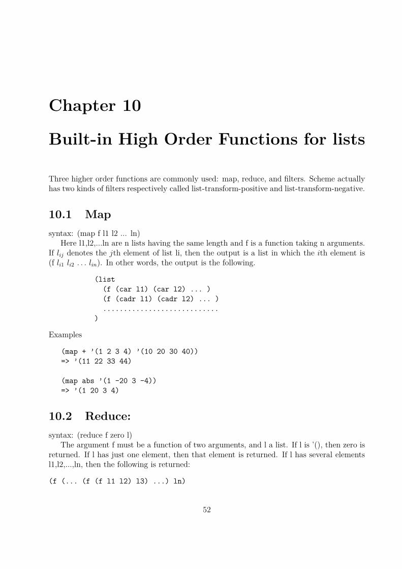
Chapter 10
Built-in High Order Functions for lists
Three higher order functions are commonly used: map, reduce, and filters. Scheme actuallyhas two kinds of filters respectively called list-transform-positive and list-transform-negative.
10.1 Map
syntax: (map f l1 l2 ... ln)Here l1,l2,...ln are n lists having the same length and f is a function taking n arguments.
If lij denotes the jth element of list li, then the output is a list in which the ith element is(f li1 li2 . . . lin). In other words, the output is the following.
(list
(f (car l1) (car l2) ... )
(f (cadr l1) (cadr l2) ... )
............................
)
Examples
(map + ’(1 2 3 4) ’(10 20 30 40))
=> ’(11 22 33 44)
(map abs ’(1 -20 3 -4))
=> ’(1 20 3 4)
10.2 Reduce:
syntax: (reduce f zero l)The argument f must be a function of two arguments, and l a list. If l is ’(), then zero is
returned. If l has just one element, then that element is returned. If l has several elementsl1,l2,...,ln, then the following is returned:
(f (... (f (f l1 l2) l3) ...) ln)
52
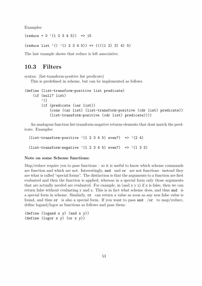
Examples:
(reduce + 0 ’(1 2 3 4 5)) => 15
(reduce list ’() ’(1 2 3 4 5)) => ((((1 2) 3) 4) 5)
The last example shows that reduce is left associative.
10.3 Filters
syntax: (list-transform-positive list predicate)This is predefined in scheme, but can be implemented as follows.
(define (list-transform-positive list predicate)
(if (null? list)
’()
(if (predicate (car list))
(cons (car list) (list-transform-positive (cdr list) predicate))
(list-transform-positive (cdr list) predicate))))
An analogous function list-transform-negative returns elements that dont match the pred-icate. Examples:
(list-transform-positive ’(1 2 3 4 5) even?) => ’(2 4)
(list-transform-negative ’(1 2 3 4 5) even?) => ’(1 3 5)
Note on some Scheme functions:
Map/reduce require you to pass functions – so it is useful to know which scheme commandsare function and which are not. Interestingly, and and or are not functions– instead theyare what is called “special forms”. The distinction is that the arguments to a function are firstevaluated and then the function is applied; whereas in a special form only those argumentsthat are actually needed are evaluated. For example, in (and x y z) if x is false, then we canreturn false without evaluating y and z. This is in fact what scheme does, and thus and isa special form in scheme. Similarly, or can return a value as soon as any non false value isfound, and thus or is also a special form. If you want to pass and /or to map/reduce,define logand/logor as functions as follows and pass them:
(define (logand x y) (and x y))
(define (logor x y) (or x y))
53

10.4 Application of Filters: Quicksort
This is a famous sorting algorithm developed by C. A. R. Hoare. First we pick an element ofthe list (in the program below it happens to be the car), which we call splitter – this elementis used to split the input list into three smaller lists consisting respectively of elementssmaller than, equal to, and greater than the spliter. Now we apply quicksort function tothe first and third lists separately and the results are appended. The lists are created usinglist-transform-positive.
(define (quicksort list )
(if (null? list )
’()
(let ((splitter (car list )))
(append
(quicksort (list-transform-positive list
(lambda (x) (< x splitter ))))
(list-transform-positive list
(lambda (x) (= x splitter )))
(quicksort (list-transform-positive list
(lambda (x) (> x splitter ))))))))
This algorithm has been found to be very efficient in practice. The number of stepsrequired to sort any list mainly depends on the splitter value. It is possible to prove that ifthe spliter is median of list then we shall require least number of steps to sort the list.
Exercise
Find how many comparisons take place if you are sorting a list of 1023 distinct elements andif at each step the splitter happens to be the median of the list. Do the same for the case inwhich the splitter happens to be the smallest element of the list.
10.4.1 Applications of Map and Reduce
1. Matrix multiplication
2. Matrix transpose and many more...
Exercises
1. Write a function that compares two lists containing numbers and determines if theyare identical.
2. Using the above function or otherwise, write a function that takes two matrices (eacha list of lists of numbers) and determines if they are identical. You are expected to usemap and reduce in both parts (less credit for writing code which does not use these).
54

You may note that logand, logor are binary functions that compute logical and, logicalor, respectively. For example (logand #t #f) evaluates to #f. Also remember that(= x y) evaluates #t or #f depending upon whether the numbers x and y are equal.
3. Suppose you are given a list M containing elements which are themselves lists and havethe form (rollno marks1 marks2 marks3 ...) where marksi are the marks in the ith labassignment. The goal is to be able to sort this in ascending order of marks obtainedin any specified assignment. So for example (sortlab M 5) should return the list Mbut sorted in ascending order of the marks in the 5th lab. Write the function sortlab.(Hint: modify any sorting function, say quicksort so that it can be passed a functionthat compares two lists. )
55

Chapter 11
Analysis of Algorithms
Most of this course is about programming style; our concern is readability, extensibility anduser friendliness of programs. Our focus is not on the speed of programs, or on developingfast algorithms. However, the speed of programs is important. It is important that we knowhow to analyze the speed of our programs. Analysis of algorithms is a vast and deep topic.Our goal here is to get a very brief flavour of it.
Usually in analyzing any algorithm it is customary to decide that a certain operation is themost dominant one, and then attempt to estimate how many times the algorithm performsthat operation. The number of times that operation is performed will vary depending uponthe size of the input given to the program, and even the precise input itself. So it is customaryto ask: for a given input size, how many operations does the program perform over allpossible input instances of that size? For example, if we are considering sorting programs, itis customary to count the number of comparisons performed by the algorithm. So we couldask, for input size n, what is the maximum number of comparisons needed to sort any inputwith n keys? This is typically called the worst case complexity. In a similar manner it ispossible to define the average case complexity, which is the number of operations needed bythe algorithm averaged over all input instances of the given size n.
In this lecture we evaluate the worst case complexity of a selection sort algorithm.
11.1 Selection sort
The basic step of selection sort is to remove the smallest element in the input that is yet tobe sorted and appending that element to the output. This may be expressed in scheme asfollows:
(define (selsort l)
(if (null? l)
’()
(let ((s (smallest l)))
(cons s (selsort (remove s l))))))
(define (smallest l)
(define (smallestwithc candidate l)
56

(if (null? l)
candidate
(if (<= candidate (car l))
(smallestwithc candidate (cdr l))
(smallestwithc (car l) (cdr l)))))
(smallestwithc (car l) (cdr l))
)
(define (remove e l) ;; assuming e occurs in l
(if (= e (car l))
(cdr l)
(cons (car l) (remove e (cdr l)))))
We will estimate the number of comparisons performed by selsort. To do this we need toestimate the number of comparisons performed by smallest and also by remove. This doneby writing recurrence equations.
11.2 Analysis of smallest
Smallest called on a list of length n simply calls smallestwithc (i.e. short for “smallestwith candidate”) with a list of length n-1 and a candidate which is just the first elementof the initial list. So we should simply analyze the number of comparisons performed bysmallestwithc.
Suppose xi denotes the number of comparisons performed by smallestwithc when it iscalled on a list of length i. Now, for the empty list (length = 0) the function simply returnsthe candidate without doing any comparisons. Thus x0 = 0. If it is called on any list oflength i > 0, then it does one comparison, and then calls itself on a list of length i − 1. Thenumber of comparisons done in the recursive call is xi−1 by definition. Thus we have:
xi = 1 + xi−1
where the equation holds for all i > 1. In other words, we have the entire family of equationsx1 = 1 + x0, x2 = 1 + x1, and so on. Such a collection of equations is called a recurrence.The simplest way to solve a recurrence is to substitute the equations into one another:
xi = 1 + xi−1 = 1 + 1 + xi−2 = 1 + 1 + 1 + xi − 3 = . . . = 1 + · · · + 1 + x0
where the number of 1s in the last expression is clearly i. But since x1 = 0, we get xi = i.Thus when smallest is called with a list of length n it must be the case that xn−1 = n − 1
comparisons are performed by smallestwithc which gets called.
11.3 Analysis of remove
We will leave it to the reader to verify similarly as above that the number of comparisonsneeded to remove an element from a list of length n in the worst case is n.
57

11.3.1 Analysis of selsort
Let yi denote the number of comparisons needed to sort a list of length i in the worst case(i.e. for that input of length i for which the maximum number of comparisons are needed).
When called on an empty list, the function returns directly, so clearly y0 = 0. If calledon a list of length i > 0, it first calls smallest on the input list, then calls remove on theinput list, and then finally recursively calls itself on a list of length one less, i.e. length i − 1.Thus we have:
yi = i − 1 + i + yi−1 = 2i − 1 + yi−1
We can solve this recurrence by substitution as before. So we get:
yi = 2i − 1 + yi−1 = 2i − 1 + 2(i − 1) − 1 + yi−2 = 2i − 1 + 2(i − 1) − 1 + · · · + 3 + 1 + y0
The last expression is simply an arithmetic series of odd numbers from 1 to 2i − 1 to whichis added y0 = 0. But the arithmetic series sums up 2i(i/2) = i2.
Thus selsort takes n2 comparisons to sort any list of length n in the worst case.
11.4 Exercises
1. Estimate the number of comparisons needed by other sorting algorithms.
2. Write a scheme program to compute xn where n is an integer, using the following idea(to be used recursively):
(a) If n is even, then xn =(
xn/2)2
.
(b) If n is odd, then xn =(
x(n−1)/2)2 × x.
How many multiplications does your program need for computing 217? You are ex-pected to estimate this as follows. Let Mn denote the number of multiplications neededto compute xn. Can you relate M17 to other Mi and so on?
58

Chapter 12
Matrices And Shortest Path Problems
We will see an unusual kinds of matrix multiplication in this lecture. This will enable usto compute shortest path in a map. It will also provide a good example of higher orderfunctions.
Suppose we are given a matrix A such that aij gives the distance between cities i and j,if they are connected by road directly. If cities i and j are not connected directly, then wewill have aij = ∞. Further, aii = 0 for all i, of course. For example consider the road mapshown in Figure 12.1.
We could represent it as the following matrix (with 1=Mumbai, 2=Pune, 3=Nashik,4=Kolhapur, 5=Nagpur):
0 160 200 450 ∞160 0 220 350 ∞200 220 0 ∞ 500450 350 ∞ 0 ∞∞ ∞ 500 ∞ 0
The usual matrix multiplication C = AB of matrices A, B is defined as consisting ofelements cij =
∑
k aik ∗ bkj . Suppose we define cij using addition in place of multiplicationand taking the minimum instead of summing, i.e. let us define:
cij = min{ai1 + b1j , ai2 + b2j , . . . , ain + bnj}
assuming n is the number of rows in A. Now consider what happens we compute A2 usingthis definition, i.e. If D = A2 we have
dij = min{ai1 + a1j , ai2 + a2j , . . . , ain + anj}
But now note that aik + bkj is simply the length of the path if we go from city i to city j,passing only through city k on the way. But we take the minimum value of aik + akj overall all possible k (including k = i, j as well). Thus dij as calculated above is nothing butthe length of the shortest path from i to j passing through any single city along the way,however the single intermediate city could be i or j itself. Let us say that a path has k hopsif it passes through k − 1 cities (excluding the origin and the destination). Thus it follows:
The ijth entry of A2 give the length of the shortest path having at most 2hops from city i to city j.
59

Kolhapur
Pune
Mumbai
Nashik
Nagpur
220
160
200
450
350
500
Figure 12.1: Schematic Map
We could continue this process! Thus by squaring the matrix A2 we will obtain the matrixA4 which can be seen as giving the lengths of all paths with at most 4 hops (i.e. which haveat most 3 other cities on the way). So squaring ⌈log n − 1⌉ times, we will obtain a matrixAm where m = 2⌈log n−1⌉ ≥ n − 1. But the entries of this matrix will denote the length ofshortest paths having at most m ≥ n − 1 hops. But no shortest path need have more thann − 1 hops (else a city would be repeated, and we can remove these circuitous paths). ThusAm will give the lengths of the shortest paths.
Exercises
1. Compute A2, A3, A4 for the matrix given earlier. Verify that A4 = A5 = A6 = . . ..
2. Write a matrix multiplication function that takes as parameters the two matrices, afunction add, a function mult and a value zero (which is the identity for the addfunction, i.e. (add zero x) => x.). It should be possible to get ordinary matrixmultiplication by specifying +, *, 0 for the parameters add, mult and 0.
3. Write binary functions imin and i+ that normally require the arguments to be numbers,but can also allow the arguments to be the symbol ’infinity. i+ should return ’infinityif either argument is ’infinity, otherwise the sum. imin should return the min if botharguments are numbers, ’infinity if both arguments are ’infinity, and the number if oneof the argument is a number and the other is ’infinity.
60

4. Write a function which uses the matrix multiplication routine of the first problem andthe functions defined in the second problem to find the length of the shortest paths ina map. Assume the input is a matrix giving distance between cities as discussed. Usethe symbol ’infinity to represent ∞. The output of the function will be a matrix, inwhich the ij entry will give the length of the shortest path between i and j. In essenceyou will be computing the n-1th power of the input matrix.
5. Write binary functions pmin and p+, which take as input some representation of apath, e.g. (length-of-the-path list-of-cities-on-the-path). pmin simply returns the pathhaving the smaller length, while p+ returns the path obtained by concatenating thegiven two paths. You are to decide on the precise representation of the path as peryour convenience.
6. Write a function which uses the matrix multiply routine of problem 1 and the functionspmin and p+ to generate the shortest paths themselves (not just the length of theshortest path). In particular, the output should be a matrix, in which the ij entrygives the length of the shortest path as well as the path itself (specified as a list ofcities along the path). The input should be the same as the input for problem 3, i.e. amatrix whose ij element gives the distance from city i to city j. From this you shouldgenerate a matrix whose ij element describes the path from city i to city j. Then youshould simply compute the n-1th power of this matrix.
61

Chapter 13
Symbolic Computing
In addition to the numeric data, scheme allows processing of symbolic data. A symbol isalmost the same as a character string – but while a character string may contain spaces, asymbol is any string that satisfies the rules of being an identifier in Scheme. We will thinkof symbols in this manner as being simple kinds of strings, we will not consider some of themore complicated aspects of symbols that the Scheme interpreter allows.
A symbol s is represented as ’s. In Scheme, the quote is used to prevent the evaluationof what follows, i.e. whatever follows is to be taken literally rather than thought of asrepresenting its value. Thus if you type s the Scheme interpreter will assume you mean thevalue of s, if you type ’s the Scheme interpreter assume you mean s itself, i.e. the symbol s.The quote has been used with lists earlier for the same purpose, we similarly allow symbolsto be inside lists as well.
(define r ’a) ; r has the value symbol a
(define r a) ; r has the same value as the value of
; assuming a has been defined earlier.
(define p ’(a b c)) ; list of symbols a b and c.
(define q (list a b c)) ; list of the values of a b c.
A list containing symbols is called a symbolic expression or an s-expression. The usual listoperations work on s-expressions, of course. For example in the above example (car p)
would return ’a.
13.1 Uses of s-expressions
S-expressions are a general way of representing symbolic data are mathematical expressions,programs, rules. For example:
(define a ’(* x (sin x)))
(define b ’(define (square x) (* x x)))
Such symbolic data can be processed as if it is a list, using the usual list operations. Wegive some examples of such processing.
62

13.1.1 Symbolic Differentiation
You have probably seen how a function could be numerically differentiated, i.e. evaluatingthe formula f ′(x) ≈ (f(x + h) − f(x))/h for some small h. However, if a function is given tous symbolically, we can find its derivative symbolically, using the usual rules of differentiatione.g.
d
dx(u + v) =
d
dxu +
d
dxv
d
dx(uv) = v
d
dxu + u
d
dxv
d
dxsin x = cos x
d
dxg(u) =
d
dxg(x)
d
dxu
These rules are recursive! Thus they can easily be encoded in Scheme. Here is the code forthe first 2 rules and the simple rules that the derivative of x itself is 1, and that of any otherconstant is 0.
(define (deriv s)
(cond ((null? s) ’())
((not (list? s)) (if (eq? s ’x)
1
0))
(else (let ((op (car s))
(args (cdr s)))
(cond ((eq? op ’+) (cons ’+ (map deriv args)))
((eq? op ’*) (list ’+ (list ’* (car args)
(deriv (cadr args)))
(list ’* (cadr args)
(deriv (car args)))))
)))))
If you now execute (deriv ’(* x x)) Scheme will return (+ (* x 1) (* x 1)) which infact can be simplified to 2x, which is indeed the derivative of x2 as required.
Exercises
1. Extend the deriv function given above to handle, trigonometric functions, exponenti-ation and natural log.
2. Write a function (simplify s) which will simplify an arbitrary algebraic expressions. The idea is to use this to simplify the output of deriv. So if you write (simplify
(deriv ’(* x x))) you should get (* 2 x).
Be warned that simplification is hard! The program will need to know about propertiesof 0 and 1 vis-a-vis addition and multiplication, as well as commutativity, distributionof addition over multiplication, and possibly other things. Write the program in stages,incorporating different rules progressively.
63

3. Write a program for doing symbolic integration. This is also hard.
13.1.2 Processing Programs
An s-expression can very well be representing a program, and so we could process it toaugment the program, or find out its properties. Or we could translate the program fromone language to another. These are processes that happen in compilers, for example.
We will consider a very simple example as an illustration: translating a program fromScheme to Lisp. These languages are very similar, though there still are many differences.We will pretend that there is only one difference– the way in which functions are definedin Lisp. The form is (defun function-name (arg1 arg2 ...) function-body). So thesquare function would be written as
(defun square (x) (* x x))
Here is a program which will do this translation. It does not handle all the cases though.
(define (trans def)
(let ((name (caadr def))
(args (cdadr def))
(body (cddr def)))
(append (list ’defun name args) body)))
Exercises
1. Extend the translator to translate nested definitions as well.
2. Scheme has a construct trace which can be used to print the arguments of a functioneverytime it is called, and the result returned by the function as it exits. Write afunction (trans s) which transforms a function definition to produce this effect. Givenbelow is an example input:
(trans ’(define (f x y z) body))
which should evaluate to
(define (f x y z)
(print x y z)
(let ((result body))
(print result)
result))
Here the function print simply prints its arguments on the screen (assume this functionis given).
64

Chapter 14
Relations
A relation is a set of k-tuples, for some fixed k. Each k-tuple in the relation is often calleda row of the relation. The set of all the ith elements of all the k-tuples is called a columnof the relation. These names are based on the pictorial interpretation of writing down arelation so that each tuple is written out horizontally, one tuple in each line. Rememberthat the tuples are unordered within the relation, whereas the elements of each tuple areordered within each tuple.
Relations are commonly used in building databases. For example, information aboutstudent roll numbers and hostels could be stored in a relation in which there is a columneach for storing roll number, name, and hostel number, and there is a row for each student.
Relations can be manipulated by performing predefined operations on them such as select,project, count, cross-product and join.
14.1 Selection
The select operation has the format
(select relation predicate)
The predicate specified must take as argument any row of the specified relation. The valueof a select operation is a new relation consisting only of the rows in the specified relationthat match the specified predicate.
You should realize that select is simply a special case of list-transform-positive.
14.2 Projection
The format is:
(project relation list-of-columns)
The value of this operation is a new relation in which only the specified columns are present,in the order they are named in list-of-columns. Note that we cannot implement this relationsimply by dropping columns – this could cause two rows to become identical in which casewe need to remove duplicates.
65

14.3 Count
This is simply the number of rows in the relation, i.e. can be implemented in scheme byusing the length built-in function for lists.
14.4 Cross Product
We define the cross product of two relations A = (a1,a2,a3..,an) and B = (b1,b2,b3...,bm)as the set of all possible rows obtained by concatenating any row of A with any row of B.The cross product has as many rows as the product of the number of rows in A and B, andas many columns as the sum of the columns in A and B. Here is an example:
A = |1 | 10| B = |5 | 55|
|2 | 20| |4 | 30|
|3 | 33|
A X B = |1 10 5 55|
|1 10 4 30|
|2 20 5 55|
|2 20 4 30|
|3 33 5 55|
|3 33 4 30|
14.4.1 Applications of the cross-product
The concept of cross product is employed in many applications -Consider a relation representing the son-father relationship - the first field name specifies
the son and the second field name the father.
Let R = |A B|
|B C|
|D B|
Taking the cross product of R with itself -
R X R = |A B A B|
|A B B C|
|A B D B|
|B C A B|
|B C B C|
|B C D B|
|D B A B|
|D B B C|
|D B D B|
Selecting those elements which have column2 = column 3 -
66

|A B B C|
|D B B C|
This represents those combinations in which the entry specifies the grandfather-father-sonof a family.
14.5 The JOIN function
SYNTAX : join(r1,field1,r2,field2)The function returns a relation which has the con-catenation of all elements of r1 and r2
in which the field1 and field 2 respectively match.eg. join(r1,2,r2,1)
when r1 = |e f| and r2 = |f g|
|d f| |b h|
returns |e f f g|
|d f f g|
14.6 Examples
Consider a relation R1 consisting of two columns, the first one naming the father, and thesecond a son. For example:
R1 = {(Dashrath,Ram), (Dashrath,Laxman), (Ram,Lava), (Ram,Kusha)}Consider a relation R2 of two columns in which the first column names the husband and
second the wife.R2 = {(Dashrath,Kousalya), (Dashrath,Kaikeyi), (Dashrath,Sumitra), (Ram,Sita), (Lax-
man,Urmila)}Now if we want to find the number of sons of Dashrath, we could useCount(Select(R1, column 1=”Dashrath”))Or to construct a relation between father-in-law and daughter-in-law we could write:Project(Join(R1,2,R2,1),’(1,4))
Exercises
1. Write code for all the primitives. Make sure that you remove duplicates while imple-menting the project operation.
2. How will you construct a relation in which each row names (two) brothers?
3. Express the join relation in terms of the other relations.
67

Chapter 15
Memoization
Memoization is a very powerful idea for making many recursive algorithms fast. Here wewill describe it for the fibonacci program.
PROBLEM: Write a function that calculates the n’th Fibonacci number.The simple minded solution to this is:
(define (fib i)
(if (< i 2)
1
(+ (fib (- i 1)) (fib (- i 2)))))
The above solution is wasteful. For example, (fib 5) will call (fib 3) and (fib 4); butfibonacci(4) will itself call (fib 3) again. Clearly, we dont need to repeat this call again – allwe need is to save a result once we calculate it.
Here is how:
(define (memofib n)
(define memo (make-vector (+ n 1))) ;; vector of n+1 nulls.
(define (init-memo)
(vector-set! memo 0 1) ;; vector indexing starts at 0
(vector-set! memo 1 1))
(define (fib n )
(if (number? (vector-ref memo n)) ;; nth number already calculated?
(vector-ref memo n)
(begin
(vector-set! memo n (+ (fib (- n 1)) (fib (- n 2))))
(vector-ref memo n))))
(init-memo)
(fib n))
This program is very similar to the simple fibonacci program – it just checks to see if thework has already been done, otherwise it does the work. After doing the work, the result issaved in a vector so that it can be used later if necessary.
68

Exercises
1. Run the original program as well as the optimized program for a large value of n. Thedifference should be immediately apparent.
2. How many recursive calls does a call to the original program result in? You mayexpress your answer in terms of the Fibonacci numbers themselves.
3. COIN CHANGING PROBLEM. Given an unlimited supply of coins of certain denom-ination, find the minimum number of coins needed to give change for any specifiedamount. The denominations should be taken as an input to the program in a list, i.e.the function should look like
(change amount list-of-coins)
For example (change 40 ’(1 2 5 10 20 25 50)) should return 2.
Hint: Suppose Change(n) denote the smallest number of coins needed to give changeof n paise. If P is one of the allowed denomination, then clearly Change(n) ≤ 1 +Change(n − P ). This is because I can add a P paise coin to the optimal way to givechange for n-P paise and get change for n paise which may not necessarily the optimalway. But the above inequality must be true for some denomination and hence we get
Change(n) = 1 + minP
Change(n − P )
For example, if the denominations are 1,2,5,10, then this condition means that
Change(n) = 1+min{Change(n−1), Change(n−2), Change(n−5), Change(n−10)}
Use this inequality to write a recursive program. Use memoization to make the programefficient.
4. We implemented memoization by using the set! primitive. This is not strictly neces-sary, as it turns out. See if you can discover why. Invent a scheme to do this. Yourscheme should work in general; but to explain it you should give the code for comput-ing Fibonacci numbers in this manner. Your code should be in the functional style.However be warned that it will probably be more complex to understand as comparedto the code that uses set! given in the text.
(Hint: Pass a list of the previously computed results to each recursive call, and haveeach call return not only the solution but also the list of all results computed tillthat point. Utilize the new list for subsequent computation. You need not write thefunction to lookup from the list, but you should carefully state what such a functionwould have to do.)
69

Chapter 16
Embedded Languages
The most interesting programs that you see around you are programming environments.These do not take an input and produce an output in the conventional sense, they allowyou to develop programs which in turn take inputs and produce outputs. The schemeinterpreter is one such program; but there are others. For example there are simulationenvironments in which you can write programs that describe complicated machines (saycircuits or chemical reactors) and then you need to describe the inputs that are to be givento these machines and the simulation environments will tell you the output produced by yourcircuits or reactors. Another example of a programming environment is MATLAB, whichis a language for manipulating matrices. So the MATLAB program allows you to write aprogram in the MATLAB language and helps you to execute that program.
The Scheme interpreter is interesting in that it can be adapted to behave like a specializedprogramming environment. This is typically done by two mechanisms. The first mechanismis of course the development of libraries of procedures which do the required collection ofspecialized tasks (e.g. matrix manipulation, simulation of circuits etc.). But in additionto procedures, the Scheme language also has special forms – these are expressions whichevaluate the arguments passed to them in some special manner. Scheme provides facilitiesviz. macros for effectively defining new special forms. In some sense it is the special formsthat give a language its character (the procedure mechanism is the same in most languages)– thus the facility to define special forms is akin to the ability to define your own language.
In fact, it is this facility that makes Scheme an ideal language in which to design specialpurpose programming systems. For example, by suitably designing libraries of proceduresand designing a few special forms, Scheme can be made to work like an Object Oriented,or a Logic Programming Language. This is often referred to as embedding new languageprimitives (e.g. object-oriented or logic programming primitives) into an existing language(e.g. Scheme).
In the next chapter, we will see a very simple example of this embedding. Althoughthe example is very simple, it is actually very useful, and it illustrates the basic issues inembedding primitives from one language into another.
Here we discuss the macro facility in scheme.
70

16.1 Macros
The syntax for defining a macro is as follows:
(define-global-macro (macro-name macro-parameters)
body
)
For example:
(define-global-macro (increment a) ;; macro definition
(list ’set! a (list ’+ a 1))
)
(define b 100)
(increment b) ;; macro invocation
A macro invocation is processed in 2 phases, an expansion phase and an evaluation phase. Inthe expansion phase, the macro invocation is textually replaced by the expansion result. Inthe evaluation phase, the expansion result is treated as ordinary Scheme code and evaluated.
The expansion phase is as follows: (1) The arguments of the macro invocation are notevaluated, but are bound as such to the formal parameters of the macro. In case of theinvocation (increment b), the formal parameter a is bound to the symbol ’b. (2) Themacro definition is then evaluated. This is basically the same as the evaluation of anyScheme procedure. For our example, the result is (list ’set! ’b (list ’+ ’b 1)), i.e.’(set! b (+ b 1)).
This result is evaluated in the expansion phase. Thus the invocation (increment b) isexpanded to (set! b (+ b 1)), which is then evaluated. The overall effect is to set b tothe value 101.
Macro expansions may contain further invocations of macros. Macros may in fact berecursive; however this must be done carefully. This is described further in Section 16.1.2.
Note that other languages such as C also provide macros (using the so called preprocessorfacility), and these are in spirit similar to Scheme macros.
16.1.1 Convenient notation for writing macros
The following notation is often used while writing macros. There are 3 command:
1. The backquote command denoted by the character ‘ having the same name
2. The unquote command denoted by the character comma ,
3. The splice-unquote command denoted by the characters ,@
The backquote command is a genaralization of an ordinary quote ’. Like an ordinary quote,it may be followed by a symbol, in which case the effect is identical. Like an ordinary quoteit may be followed by a list which does not contain the unquote or splice-unquote commands,in which case again it behaves like an ordinary quote.
If an unquote command appears inside a backquoted list, then the value of whatever isunquoted is used. For example, we might have:
71

(define a 100)
’(a)
‘(,a)
The commands ’(a) and ‘(a) will both evaluate to a list consisting of the symbol ’a, asusual. The command ‘(,a) however will evaluate to a list containing the value of a, i.e. thelist ’(100).
The unquote-splice command causes the value to be used, but the value is spliced intothe list. So suppose we have:
(define a ’(10 20 30))
Then ’(1 a 2) will denote a list consisting of the number 1, the symbol ’a and the number2; the command ‘(1 ,a 2) will denote the list ’(1 (10 20 30) 2), and the command ‘(1 ,@a
2) will denote the list ’(1 10 20 30 2).Using the above notation, the increment macro could be written as:
(define-global-macro (increment a)
‘(set! ,a (+ ,a 1))
)
Notice that this is much more readable and compact.As another example, consider the following macro which will mimic the trace facility of
Scheme.
(define-global-macro (tdefine template body)
(pp template) ;; only for debugging,
(pp body) ;; maybe omitted.
‘(define ,template
(pp (list ,@(cdr template)))
(let ((result ,body))
(pp result)
result)))
So if you now type
(tdefine (sum x y z) (+ x y z))
the macro will translate this to:
(define (sum x y z)
(pp (list x y z))
(let ((result (+ x y z)))
(pp result)
result))
Relationship between quote and backquote: At first, it might seem that every forminvolving a backquote and the unquote/splice-unquote operators can be naturally convertedto one involving only the usual quote. For example, ‘(a ,b ,@c d) can also be writtenas (append (list ’a b) c (list ’d)). However, a backquoted expression can contain aquote, for example consider the code:
72

(define c ’d)
‘(set! a ’,c)
The second line will now evaluate to ’(set! a ’d). There is no easy way to produce thisresult without using backquotes.
16.1.2 Nesting and recursion
We may use all usual Scheme features such as nesting and recursion. Here is an example.
(define-global-macro (incrementmany L) ;; increment many variables
(if (null? L)
’()
‘(begin
(set! ,(car L) (+ ,(car L) 1))
(incrementmany ,(cdr L)))))
(define x 1)
(define y 2)
(incrementmany (x y)) ;; invocation.
The invocation will cause L to be bound to the list (x y). Since this list is not null, the firstexpansion will return the result
(begin
(set! x (+ x 1))
(incrementmany (y)))
But this result itself contains a (recursive) invocation. For this invocation the parameter L
will be bound to the list (y). The result of this will be
(begin
(set! y (+ y 1))
(incrementmany ()))
This also contains an invocation of incrementmany, this time with parameter L bound to anempty list. Thus this will return the result ’(). Thus, the overall expansion will be:
(begin
(set! x (+ x 1))
(begin
(set! y (+ y 1))
’()))
When this code is executed, the effect will be to increment both x and y.It is important to be careful while using recursion in macros, however. Here is an (erro-
neous) recursive implementation of the foreach macro of Exercise 5.
73

(define-global-macro (foreach x L command) ;; Does not work!
‘(if (null? ,L)
’()
(begin
(let ((,x (car ,L)))
,command)
(foreach ,x (cdr ,L) ,command))))
(foreach i ’(1 2 3) (pp i)) ;; invocation
The result of expanding the above invocation is:
(if (null? ’(1 2 3))
’()
(begin
(let ((i (car ’(1 2 3))))
,(pp i)
(foreach i (cdr ’(1 2 3)) (pp i)))))
It is now easy to see why this wont work. The expansion will contain the recursive call(foreach i (cdr ’(1 2 3)) (pp i)). This is not the same as (foreach i ’(2 3) (pp
i))! This is because the arguments to a macro are not evaluated before expansion. So therecursive macro expansion will be called with parameter L set to ’(cdr ’(1 2 3)). In otherwords, the recursion will not terminate! Constrast this with the proper use of recursion givenabove.
Exercises
1. Write the following without using the backquote ‘(a ,b (c ,@d) e).
2. Write the following using the backquote (list ’a ’b c ’d).
3. Write a macro such that (dotimes i n body) will expand to
(do ((i 0 (+ i 1)))
((= i n))
body)
i.e. the idea is that the body should be executed n-1 times with i taking values from0 to n-1.
4. Modify the tdefine macro given above so that it prints the arguments with an explana-tory message, i.e. if we invoke (sum 1 2 3) currently the message printed would justbe (1 2 3). Instead get it to print (Calling (sum 1 2 3)).
5. Write a macro (foreach varname List command) that will execute the specified com-mand for every element of the given list. The variable specified as varname can be usedin the command, and it will take as values successive elements of List. For example:
74

(define L ’(1 3 5 7))
(foreach x L (pp x))
This should cause pp to be invoked on every element of L, i.e. it should print out 1, 3, 5,7. (foreach ...) is not expected to have a value. While writing the macro, you mayneed to use temporary variables– you may use variable names of the form foreach00,
foreach01, ..., and you may assume that these names will never be used in the userprogram. (Using the temporary variables is not necessary, the problem can also besolved without any temporary variables; but you are free to use them if you wish.)
75

Chapter 17
Embedding Advanced Graphics intoScheme
Scheme provides fairly low level primitives for graphics. The main drawing proceduresare graphics-draw-point and graphics-draw-line. These procedures take as argumentscoordinates of points (and line endpoints) with respect to the screen. The primitives that wehave used in this course nicer in that they allow alternate frames of reference to be defined(implicitly). For example, in the code
(line 0 0 0.1 0.1) ;; line 1
(trans 0.5 0.5 (line 0 0 0.1 0.1)) ;; line 2
although line 1 and line 2 appear to have identical endpoints, in reality they will be drawndifferently, because line 2 is drawn after translating the origin to (0.5,0.5). Such a facilitymakes it very convenient to abstract pictures as procedures; suppose (window) causes awindow to be drawn, then invoking (trans dx dy (window)) will cause a window to bedrawn shifted by (dx,dy).
In this chapter we will study how these primitives trans, scale etc. have been provided.There are two aspects:
1. Algorithm and data structures. The main question is how can we keep track of thecurrent frame of reference. Specifically, we should always be in a position to determinewhere to draw a line on the screen when a user requests a line to be drawn after aseries of translation, scaling and other commands. This is discussed in Section 17.1.
2. User Interface Issues. What are the different ways in which the basic functionalityrelating to translation/scaling etc. be offered to the user? Our definition of trans,
scale, rotate, line, point is only one possible interface. There could be severalother possible ways. This is discussed in Section 17.2.
17.1 Algorithmic Issues
The surface on which the drawing appears will be called the screen. In the case of Scheme,it is a window that appears on the monitor in addition to the shell window. The screen is
76

associated with a frame of reference; in case of the Scheme graphics screen, the origin is at thecenter of the screen and the four corners of the screen have coordinates ±1. The commandsgraphics-draw-point and graphics-draw-line take as arguments the coordinates in thescreen frame of reference.
The frame of reference in which the user operates is initially the same as the screen frame.However, by using translate, scale and rotate the user can define new frames of referenceand draw with respect to these frames. If the user draws a point (x, y) in a certain frameof reference, then where it will be drawn on the screen is determined by the frame changesthe user has executed before. In the rest of this section, we will only consider the questionof plotting points. Drawing of lines and more complex figures can be done in an analogousmanner.
The basic idea is to use a matrix F to represent the current frame of reference. F is a3 × 3 matrix with a special structure (f31 = f32 = 0, f33 = 1), and given a point havingcoordinates (x, y) in the current frame, its coordinates (x’,y’) in the screen frame are obtainedby performing a matrix multiplication with F :
x′
y′
1
=
f11 f12 f13
f21 f22 f23
0 0 1
xy1
Initially, F is simply the identity matrix. Clearly, in this case the matrix multiplicationabove gives x′ = x and y′ = y which is exactly what we want.
Suppose we now want have a frame which is centered at (dx, dy) in the screen frame, i.e.obtained by doing a translation of (dx, dy). A point (x, y) in such a frame must be plottedat point (x + dx, y + dy) on the screen. The effect of this frame is modelled if we set
F =
1 0 dx0 1 dy0 0 1
Now F (x, y, 1)T = (x + dx, y + dy, 1)T as we want. Scaling can be represented by setting:
F =
sx 0 00 sy 00 0 1
Composition of frame changes The important feature is that frame changes can be com-posed very easily. Suppose, F1 is a matrix that models a certain translation, and F2 modelssome scaling. Then the matrix modelling the translation followed by the scale change is sim-ply the matrix product F1F2. In fact this is true for any number of transformations of anykind: the new matrix is obtained from the old simply by performing a matrix multiplicationcorresponding to the new transformation.
17.2 User Interface
There are a number of different ways in which graphics facilities can be provided to the user.The set of primitives we have provided is only one such way.
77

Here, for example, is a completely different way in which graphics facilities could be given.Instead of having the notion of “the current frame of reference” in which points and linesare drawn, one could consider the notion of a “current pen position”, with respect to whichall drawing is done. For example, the command (point) would be invoked without givingany arguments and it would mean that the point would have to be drawn at the current penposition. (line x y) would mean draw a line from the current position to the point (x,y).We would have to provide a command (move x y) which would cause the pen to move to(x,y) without drawing.
In the rest of this chapter, we will discuss 2 user interfaces which are similar to the onewe have used in this book. These are simpler to implement. After discussing these we willdiscuss how the our actual interface is implemented.
In what follows we will only discuss translation and plotting points; other transformations(scaling, rotation) and drawing other figures (lines) are similar.
We will also assume that we are given functions matrixmultiply and matrixvectormultiply
that do these operations. Finally we will use the following definition for constructing a matrixrepresenting transformations:
(define (trans-matrix dx dy)
‘((1 0 ,dx)
(0 1 ,dy)
(0 0 1))))
17.2.1 User Interface 1
We provide the following interface to users:
1. (trans! dx dy): This causes the reference frame to be translated by (dx,dy).
2. (point x y) This asks a point to be plotted at (x,y) of the current frame of reference.The command for drawing lines is similar.
Implementation: We maintain a global variable F which represents the transformationmatrix corresponding to the current frame of reference. The trans! command is imple-mented simply by multiplying F by a suitable matrix as defined above. Similarly we definescale!, rotate!. The implementation of trans! is very simple:
(define (trans! dx dy)
(let ((ftrans (trans-matrix dx dy)))
(set! F (matrixmultiply F ftrans))))
Given that the current matrix is always available, the point command only needs to performthe required matrix multiplication. This is done as follows:
(define (point x y)
(let ((screencoord (matrixvectormultiply F (list x y 1))))
;; screencoord is the result vector represented as a list
(graphics-draw-point (car screencoord) (cadr screencoord))))
78

Criticism: This interface is not very convenient for users. Typically a user will want towrite “Draw picture P1 with origin at (x1, y1), then picture P2 with origin at (x2, y2), ...”,where the points (xi, yi) are all with respect to the current frame. These actions would berepresented using above primitives as:
(trans! x1 y1) (Picture1) (trans! (- x1) (- y1))
(trans! x2 y2) (Picture1) (trans! (- x2) (- y2))
...
The reverse translations (trans! (- xi) (- yi)) are necessary to bring the frame backto original to get ready to draw the next pictures. This code is more verbose than what ouractual interface needs:
(trans x1 y1 (Picture1))
(trans x2 y2 (Picture2))
...
Not requiring the users to write the code for reversing the translations improves compactness,and further reduces the chances of errors (say the user forgets to write the reversals).
17.2.2 User Interface 2
The problem we need to solve is: how to suppress the evaluation of some of the argumentsbeing passed to a procedure. Lambda expressions can easily accomplish this, i.e. lambdaexpressions can be used to delay evaluation.
We do require a different interface, but it is almost the same as our ideal interface:
1. (lambdatrans dx dy g): Here g is a function that contains the drawing commands,dx and dy are numbers. This primitive causes the drawing commands to be executedafter translating the origin by (dx,dy). As an example, to plot a point at (0.1,0.1) aftertranslating the origin to (0.5,0.5) we would write (lambdatrans 0.1 0.1 (lambda ()
(point 0.5 0.5))).
2. (point x y): This is the same as before.
The crucial difference between trans and lambdatrans is that the arguments to former arethe drawing commands themselves, while to the latter, they must be contained in a functionwhich is passed as an argument. Here is how lambdatrans is implemented:
(define (lambdatrans dx dy g)
(set! F (matmul F (trans-matrix dx dy)))
(g)
(set! F (matmul F (trans-matrix (- dx) (- dy))))
)
Notice that this implementation correctly does what we want. When we call the functionusing say (lambdatrans 0.1 0.1 (lambda () (point 0.5 0.5))), the arguments are in-deed evaluated – but the result of evaluating the lambda expression is a function – which iswhat get passed. The passed function is actually called only inside lambdatrans itself – andthis happens after the matrix F has been changed to reflect the translation.
79

17.2.3 User Interface 3
The trans command is actually implemented as a macro. The implementation of the othercommands is similar.
(define-global-macro (trans dx dy . body)
(let ((forwardtrans (list ’trans! dx dy))
(one-line-body (cons ’begin body))
(backwardtrans (list ’trans! (list ’- dx) (list ’- dy))))
(list ’begin forwardtrans one-line-body backwardtrans)
))
Now suppose we invoke the above with (trans 0.5 0.5 (line 0 0 0.1 0.1) (line 0.1
0.1 0.1 0.2)), the code that will result from the above will be:
’(begin (trans! 0.5 0.5)
(begin (line 0 0 0.1 0.1) (line 0.1 0.1 0.1 0.2))
(trans! (- 0.5) (- 0.5)))
which is exactly what we want.We give another definition using the notation discussed in the previous chapter.
(define-global-macro (trans dx dy . body)
‘(begin (trans! ,dx ,dy)
,@body
(trans! (- ,dx) (- ,dy))))
Now suppose we invoke the above with (trans 0.5 0.5 (line 0 0 0.1 0.1) (line 0.1
0.1 0.1 0.2)), the code that will result from the above will be:
’(begin (trans! 0.5 0.5)
(line 0 0 0.1 0.1) (line 0.1 0.1 0.1 0.2)
(trans! (- 0.5) (- 0.5)))
which is also what we want.
Exercises
1. The implementation of trans given above uses two matrix multiplications – the firstfor the forward translation and the second for the backward. To save arithmetic andalso roundoff errors, it will be better to save the original value (say by generating alet statement). Write a macro that does this.
2. Currently none of the graphics commands return any interesting value. Suppose youwould like to return a description of the bounding box generated for the drawing doneinside each command.1 Adapt all the drawing commands so that the user can do thiseasily. Show your modifications for trans, line, point, and explain what the userwill have to do in addition, if anything.
1The bounding box is the smallest axis parallel rectangle containing the drawing, and it can be representedby its bottom left and top right corners, i.e. 4 numbers.
80

Chapter 18
Object Oriented Programming
Object oriented programming is often regarded as an appropriate style for writing largeprograms. The development of such large programs typically happens over long periods oftime, and as a cooperative effort of several programmers. Further, every program inevitablyhas bugs, and inevitably needs to be extended as the demands of the users evolve. Soany paradigm for development of large, professional quality programs needs to address thefollowing issues:
Cooperative development: How to divide the development work among available program-mers so that different people can work indepedently with minimal dependence on eachother. This is typically done by fixing the specification of the part assigned to eachprogrammer, and hiding the implementation of each part from other programmers.
Re-use and extensibility of code: Since programmers are expensive, it is useful if codeonce developed can be used as many times as possible (within the same program, orin other programs). To facilitate such reuse, code that has been developed must bepackaged appropriately so that it can be passed on to the new users as a module, witha convenient interface. Further, it might be that a previously developed piece of codealmost solves the current problem – in such cases it should be possible to extend itsfunctionality to handle the current problem with minimal effort, and with minimalpossibility of introducing bugs.
18.1 Motivating examples
These all deal with extending existing software.
18.1.1 Example 1: Library information system
Suppose a library information system currently supports the following operations.
(make-patron name address)
; Enroll a new patorn.
(issue-book patron-record bookno)
; Issues a book to the patron with the given record.
81

(accept-book-return patron-record book)
; Removes the book from the record.
(print-ith-issued patron-record i)
; returns the booknumber of the ith book issued to this patron.
Suppose the library starts a category of donor-patrons, who might get more facilities.How should the information system change?
• Need to store patron category along with each patron.
• Issue-book may change – donors may be able to borrow more books.
Challenge: Can new features be added without changing old code at all.
18.1.2 Example 2: Symmetric Matrices
Suppose we possess implementation for matrices (vector-of-vectors).
(make-matrix m n)
(matrix-ref mat i j)
(matrix-set! mat i j val)
Extension needed: Can we devise a scheme for storing symmetric matrices compactly?Natural Solution: Store only the lower triangular portion. But now all the functions aboveshould be redefined in order to be consistent with this format.Problem: What if I need both symmetric and non symmetric matrices in my program.What does matrix-ref refer to?
18.2 Example 3: Extensions to Deriv
Add the operator **, or ln or tan.Can this be done without modifying the existing code at all?
18.3 Basics of OOP
In functional programming, a program may be thought of as a map (i.e. a function) fromthe set of all possible inputs to the set of desired outputs. Likewise, it is useful to viewprogramming in a certain manner to understand the object oriented paradigm.
In this view, a program is developed for modelling some real life phenomenon or a math-ematical process. The real life phenomenon or the mathematical process concerns someobjects which may be concrete or abstract, e.g. circuit components, salary records, matrices.The goal is to trace how objects evolve as certain operations (e.g. changing the value of thesignal fed to the input of a component, or calculating the effect of income tax, or inverting amatrix) are performed upon them. How to represent these objects on a computer and how
82
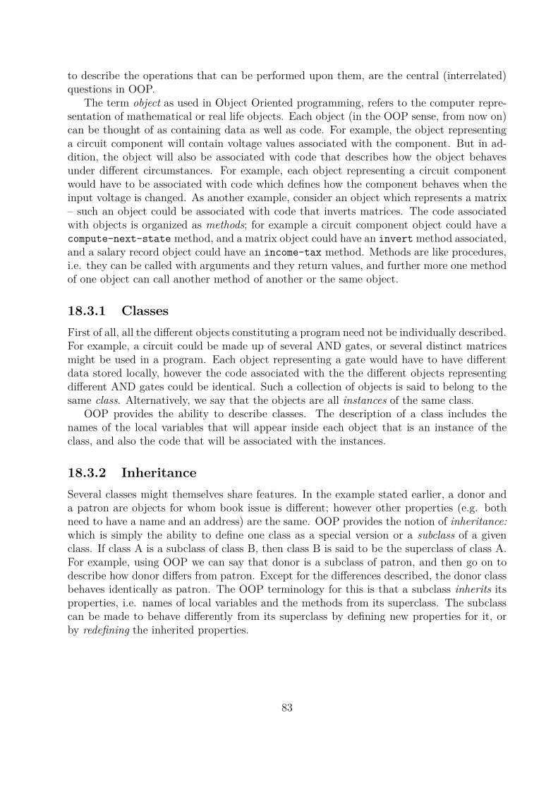
to describe the operations that can be performed upon them, are the central (interrelated)questions in OOP.
The term object as used in Object Oriented programming, refers to the computer repre-sentation of mathematical or real life objects. Each object (in the OOP sense, from now on)can be thought of as containing data as well as code. For example, the object representinga circuit component will contain voltage values associated with the component. But in ad-dition, the object will also be associated with code that describes how the object behavesunder different circumstances. For example, each object representing a circuit componentwould have to be associated with code which defines how the component behaves when theinput voltage is changed. As another example, consider an object which represents a matrix– such an object could be associated with code that inverts matrices. The code associatedwith objects is organized as methods; for example a circuit component object could have acompute-next-state method, and a matrix object could have an invert method associated,and a salary record object could have an income-tax method. Methods are like procedures,i.e. they can be called with arguments and they return values, and further more one methodof one object can call another method of another or the same object.
18.3.1 Classes
First of all, all the different objects constituting a program need not be individually described.For example, a circuit could be made up of several AND gates, or several distinct matricesmight be used in a program. Each object representing a gate would have to have differentdata stored locally, however the code associated with the the different objects representingdifferent AND gates could be identical. Such a collection of objects is said to belong to thesame class. Alternatively, we say that the objects are all instances of the same class.
OOP provides the ability to describe classes. The description of a class includes thenames of the local variables that will appear inside each object that is an instance of theclass, and also the code that will be associated with the instances.
18.3.2 Inheritance
Several classes might themselves share features. In the example stated earlier, a donor anda patron are objects for whom book issue is different; however other properties (e.g. bothneed to have a name and an address) are the same. OOP provides the notion of inheritance:which is simply the ability to define one class as a special version or a subclass of a givenclass. If class A is a subclass of class B, then class B is said to be the superclass of class A.For example, using OOP we can say that donor is a subclass of patron, and then go on todescribe how donor differs from patron. Except for the differences described, the donor classbehaves identically as patron. The OOP terminology for this is that a subclass inherits itsproperties, i.e. names of local variables and the methods from its superclass. The subclasscan be made to behave differently from its superclass by defining new properties for it, orby redefining the inherited properties.
83

18.3.3 Defining Classes
We describe OOP primitives embedded into Scheme. This is based on the work of Bryan OSullivan. More commonly, OOP is supported by languages such as C++, Java, Smalltalkand others.
A class definition has the following form:
(define-class class-name
(superclass)
list-of-additional-fields)
In this book, class names will have enclosing angled brackets as a convention; this is onlyfor readability. Here are two examples of class definitions:
(define-class <patron>
(<root>)
(name address books))
(define-class <donor>
(<patron>)
(locker-number))
A class is always defined as a subclass of some class. To enable this process to get started,Scheme OOP contains the definition of a predefined class <root> from which other classescan be derived. The <root> class does not have any local variables (also called fields orslots) associated with it; nor does it have any methods.
As mentioned earlier, when a class is defined as a subclass of another class, all theproperites (i.e. fields and methods) are inherited. The class definition mentions the addi-tions field that objects of the class are to have. Thus class <patron> is defined to have fieldsname, address, books in addition to whatever fields that <root> has. But there is nothingin <root>, so the definition causes <patron> to have just the fields name, address, books.The class <donor> is defined to be a subclass of <patron> and is deemed to have an ad-ditional field locker-number. Thus the fields in <donor> will be name, address, books,
locker-number.
18.3.4 Creating Instances
Given the above definitions we can create instances using the make-object form having thefollowing syntax.
(make-object class-name initial-values-of-fields)
This creates an instance of the specified class, with field values as specified. The initialvalues should be specified in the same order that appears in the definition of the class andits superclasses. Here are some examples:
(define x (make-object <patron> "Ranade" "IITB" ’()))
(define y (make-object <donor> "Dhamdhere" "IITB" ’() 569))
84

This will cause x to be an object of class <patron> with its fields name, address, books
set to values “Ranade”, “IITB” and the empty list respectively. y will be set to be anobject of class <donor> with its fields name, address, books, locker-number set to values“Ranade”, “IITB”, the empty list and the number 569 respectively.
18.3.5 Defining Methods
Methods must be declared, and then defined for different classes, then they may be invokedon objects of those classes. The general syntax is:
(define-generic name-of-the-method) ;; declaration
(define-method method-name class-on-which-to-be-defined arguments
code) ;; how to define
(method-name object-name arguments) ;; how to invoke
We will start with an example for the <patron> class defined above.
(define-generic issue-book)
(define-method issue-book <patron> (bookno)
(cond ((< (length (self: books)) 4)
(self:set! books
(cons bookno (self: books)))
#t)
(else ’())))
(issue-book x 123) ;; invocation
In the above code, assume x is as defined earlier, i.e. instances of <patron>.In any method invocation of any method, the first argument must be the object on which
the method is to be invoked. The subsequent arguments are bound to the arguments inthe arguments listed in the method-definition. In the above example, 123 is thus bound tobookno. The code in the method definition can be any scheme code, and it must return avalue which is the value of the method invocation. However, in addition to ordinary schemecode, two OOP commands can also be used. These are for accessing and modifying the localvariables of the object, respectively:
(self: local-variable-name)
(self:set! local-variable-name new-value)
:self:
Thus (self: books) in the code above would refer to the books field of x for the invocation(issue-book x 123); while (self:set! books ...) would set the same field as specified.Within a method, the object on which is the method is being executed can itself be referredto as :self:.Encapsulation: Local variables, or the field in an object cannot be accessed/modifieddirectly. They can only be accessed/modified inside methods defined for the class. The
85

rational for this is encapsulation, i.e. the local variables are hidden from the external world,and can be accessed by users only in a controlled manner, through the methods.Inheritance: Although issue-book is explicitly defined only for class <patron> it willapply to class <donor> as well due to inheritance. So we could write (issue-book y 456)
– this would be legal; but the above code would be used and it would check for the lendinglimit of 4 for both x and y.
However, we can redefine the issue-book method for the subclass <donor> as follows:
(define-method issue-book <donor> (bookno)
(self:set! books
(cons bookno (self: books)))
#t)
(issue-book x 123) ; at most 4 books
(issue-book y 345) ; unconditional issue
The general logic that is used to decide which code is to be used when a method is invokedon a certain object z of class Z is as follows. If the method has been defined explicitly for Z,then that definition is used. If the method is not defined for Z, then the OOP system checksif the method is defined in the immediate superclass of Z. If the superclass has the method,then that definition is used; if not, the superclass of the superclass is checked, and so on. Ifneither Z nor any of the superclasses has a definition for the method, then the system signalsan error.
18.3.6 Remark: Incremental specification of functions
In conventional programming languages, a function definition is a single define form:
(define (issue-book patron book) ...)
In OOP, the function definition may be scattered.
(define-method issue-book <patron> (bookno)
...issue only if limit not exceeded...)
(define-method issue-book <donor> (bookno)
...issue unconditionally...)
(issue-book person1 book5)
The define-method forms can be spread out over several files. They dont have to be specifiedtogether. It is this flexibility that makes OOP programs easier to extend. In conventionalprogramming, including the special case for donors would require modification to the functionissue-book. While making such modifications, there is always the danger that a bug getsintroduced in a part of the code that has already been extensively tested. In OOP, the newcode gets added as a separate method, without the need to alter the existing code
in any way.This is applicable to the other examples as well. For example, the conventional definition
of deriv is:
86

(define (deriv exp) ...)
In OOP, we could have different classes to represent different types of symbolic expressions.The deriv method for each such class would be defined separately and independently, as andwhen the class is added to the code.
(define-method deriv <sine-expression> ()
(cos ...))
(define-method deriv <cos-expression> ()
(sin ...))
18.4 Utility Functions
(class-of object) : returns the class of the object
(class-of x) ==> <patron>
(object? x) : is x an object?
(object? x) ==> #t
(is-a? object class) : is object of an instance of class (direct instance), or a subclass ofclass, or a subclass of subclass of class ... (general instance)?
(is-a? y <donor>) ==> #t
(is-a? y <root>) ==> #t
(is-a? x <donor>) ==> ’()
18.5 Object Oriented Design
The first important issue in designing object oriented programs is to define a proper inher-itance heirarchy (i.e. which class should inherit from which class). Further, you need todecide where the fields and methods should be defined. The general rule is: if a field or amethod is useful for all the subclasses of a class A then it should be defined in A. In fact amethod should be defined in A even if it is useful for most of the subclasses; if subclasses B,C need to define the method differently then it can always be redefined in B and C.
It is worth noting that there might be design decision to be made in deciding what shouldbe a method and what should be a local variable. The general rule here is: If all instancesshare the same constant value for a local variable then use a method that simply returns thatfixed value, rather than keeping a variable in every object. Keep this rule in mind while doingthe biology-tutor exercise below.
87

18.6 Exercises
1. Add a method to handle the operation (issue-many patron-object list-of-books),which should cause all the specified books to be issued if possible. (Hint: Use :self:
to repeatedly call the issue-book method of the same object. You can even use theScheme function map.)
2. You are to design a dictionary program that provides information about nouns andverbs of English. It must support the following queries: (1) (plural w) : If w is a nounreturn its plural; else return the message “Not a noun”. (2) (past w) : If w is a verbthen return its past tense, else return the message “Not a verb”.
Design a set of classes which will make it easy to store words. You may assume thatEnglish has 3 kinds of nouns: those whose plural is obtained by appending s (e.g.boy, girl), appending es (e.g. bus), or whose plural is irregular (e.g. ox, life). Youmay similarly assume that there are only two kinds of verbs, those whose past tenseis obtained by adding ed (e.g. play, jump) or irregular (e.g. study, run, go). Give thecode that builds a dictionary storing boy, ox (plural oxen), jump, go. It should be easyto add new words.
You may want to use the symbol-append function which concatenates symbols, e.g.(symbol-append ’boy ’s) => ’boys
3. A biology-tutor program is to be developed for answering questions about animals.The program is expected to take questions such as (no-of-limbs cat) and return theappropriate response, i.e. 4 in this case. The following questions are to be supported:(1) no-of-legs (2) colour-of-blood (3) blood-temperature, (4) life-span. The followinganimals should be in the database: cat, spider, housefly, cockroach, chimpanzee. Thelifespans of these animals may be assumed to be 5, .1, .05, .1, 30 years respectively.The answers to the other questions should be given as per the following passage.
The animal kingdom may be divided into vertebrates and non-vertebrates.Vertebrates have red blood while non vertebrates have colourless blood.Within vertebrates, mammal (e.g. gorilla, cat) and bird families are warmblooded, while non-vertebrates and other vertebrate families such as reptiles,amphibians and fish are cold-blooded. Within non-vertebrates are the fami-lies insecta (e.g. housefly, cockroach) and arachnida (e.g. spiders). Membersof these families have respectively 6 and 8 limbs. Mammals have 4 limbs.
Write the program. Your program should be easy to extend.
4. Write a set of classes that will help in doing animations. This is an open ended problem;however here we will consider a simple version. Create a system which allows to (i)define shapes, (ii) Assign velocities and initial positions to the shapes (iii) Show theevolution of the system as time goes on.
Specifically you should build a “screensaver” showing 2-3 kinds of aeroplanes (i.e.polygonal shapes) objects moving across the screen. The aeroplanes should disappearand reappear so as to create a pleasing, natural (to the extent possible!) effect.
88

Chapter 19
Containment Heirarchies
A common programming pattern in Object Oriented Programming is to describe large sys-tems as a nested collection of objects, also termed as containment heirarchies. In this chapterwe will see some examples.
19.1 Logic Circuit Simulation
Yet to be written.
19.2 Exercises
1. The goal of this exercise is to develop a simulation of an Economic System so as toexplore the effects of globalization. Real economists will of course cringe at our modelof an economic system – it is doubtless extremely simplicstic – but then we wont showthis to real economists. Or we can show it to them and ask them to help us improveit.
Basically our system will consist of certain number of buyers and sellers. Each buyeror seller will be located in a village. Several villages will comprise a taluka, and severaltalukas a district. Our model will be just for one district.
For concreteness, let us assume that our district consists of 8 talukas, each of whichconsists of 8 villages. Each village has 4 buyers and one seller. Each seller S will startoff with a working capital of Rs. 10, and will have to pay a rent of Re. 1 every day.There is a single commodity being traded, say chapatis. Each seller will produce asmany chapatis as there is demand. The cost of each chapati to each seller S will be afixed number C(S). For each seller S, we will fix C(S) as a random number1 uniformlydistributed in the interval (rupees) 0.9 to 1.1. C(S) will be fixed for each S for the entirecourse of the simulation. Who sells what to whom gets decided every day separatelyas follows.
1(random x) will return a random number in the interval 0 to x (non-inclusive). The number returnedis real if x is real, and integer if x is integer.
89

Each day starts off with the each seller announcing the price at which he will sellchapatis. Each buyer needs one chapati every day, however he can buy this from anyseller. If the chapati is bought from the seller in the same village, then there is nooverhead. If it is bought from a seller in the same taluka, then there is an overhead of10 paise. If it is bought from another taluka, there is an overhead of 20 paise. Eachbuyer buys his chapati such that price+overhead is smallest. The sellers collect themoney (the overhead goes for transport) from the buyers and pay the rent. The dailyprofit/loss gets added/subtracted from the working capital. If the working capital fallsbelow zero, the seller goes out of business.
Here is how the seller fixes his price. Define the BE4 price for a seller S as C(S)+0.25,i.e. the price at which he will break even (i.e. no profit no loss including the rent) if hesells 4 chapatis. On day 1, every seller fixes his price at his BE4 price. On subsequentdays his rule is very simple: he raises his price by 10 % if he made did not make a lossthe previous day, else he lowers the price by 10 %, but never below his BE4 price.
(a) Evolve the system for 30 days and report the total receipts of the sellers and thetotal money paid out by the buyers.
(b) Incorporate the effect of increased globalization as follows. Set to 0 the overheadfor buying from outside your village or your taluka. Now evolve the system for30 days.
2. The goal of this exercise is to design a program that will be able to draw faces on thescreen. Faces can be round, tall, wide. Noses can have different shapes, let us call themordinary, and parrot-beak-shaped. Eyes can have different colours, and can either beset close or wide (i.e. distance between the eyes can be small or large) and can havedifferent colours. The mouth can be large or small. This list can go on, but let us stophere.
How will you design a program that can take user requirements and draw a face? Inparticular, you should provide facilities for the user to say something like “Draw a facewhich is round, with blue eyes that are set close, and a parrot-beak nose”. Say whatclasses you will use, including the heirarchy. What will the methods and the localvariables be? How will a user specify the face that is to be drawn?
A high level answer is expected with some details. You could spend the entire hourwriting out an answer to this problem – but remember it only has 20 marks; so spendonly 20 minutes on it. More only if you have finished solving the other problems.
90

Chapter 20
Constraint Logic Programming (CLP)
It is useful to think of programming as consisting of two activities
1. Writing down the specifications precisely and exhaustively. Identifying what is theinput and what is the output and specifying what are the constraints that the outputmust satisfy for correctness.
2. Writing a program that constructs the required output.
In the Constraint Logic Programming paradigm, we only do the first step! A programmerwrites down all the constraints that the output must satisfy, and then a constraint solverwhich is at the heart of the CLP system processes the constraints and attempts to find theoutput values that satisfy the given constraints.
Consider the problem of constructing a 3 × 3 magic square using the digits 1 through 9exactly once. A magic square is simply a square array of numbers such that all row sumsand column sums are identical. Suppose a, b, c, d, e, f, g, h, i are the numbers in the array asshown in Figure 20.1. Here is how we could then specify this problem.
Find a, b, c, d, e, f, g, h, i such that
1. 1 ≤ a, b, c, d, e, f, g, h, i ≤ 9
2. a, b, c, d, e, f, g, h, i are distinct integers.
3. a + b + c = d + e + f = g + h + i = a + d + g = b + e + h = c + f + i.
It is clear that any assignment of values satisfying the above constraints will give a magicsquare. In the CLP paradigm, we would simply assert the above constraints (using suitablesyntax) and ask the system to find us a solution.
Will a solution always be found if it exists? Will a message be printed if no solutionexists? Suffice to say for now, that a whole range of solvers are available, and they work by
a b cd e fg h i
Figure 20.1: Magic Square
91

using very sophisticated ideas as well as very obvious ones (e.g. try all possible assignmentsuntil the right one is found). How quickly a solver completes its work (or even whetherit completes in finite time at all) depends upon the problem being solved as well as thesophistication of the solver. In fact it depends also upon how the problem is specified1
It is safe to say that the time taken by the CLP solver (which is a general purposeprogram) will in general be more than a program written precisely to implement the givenspecifications. However, writing the specifications alone is always much easier, and as aresult CLP systems are becoming very popular for solving certain kinds of problems. Infact many CLP systems are available commercially and in the public domain. These includeCHIP, ILOG, ECLIPSE
20.1 Finite Domain CLP
In this book we will consider a relatively simple variant of CLP called finite domain CLP. Thisbasically means that our problem must be specified using a finite number of variables, andthat each variable can take values from a finite domain. We will call such variables domainvariables. The magic square problem belongs to this category with 9 domain variables, eachvariable taking values from the finite domain 1,2,3,4,5,6,7,8,9.
Our CLP system is embedded in Scheme. It contains commands for constructing domainvariables, specifying constraints, and a very simple solver. Note that a CLP program in oursystem may freely use scheme commands and additional Scheme variables as needed. Schemevariables behave in the usual manner, i.e. their value is explicitly set by the program. Domainvariables, which must be explicitly constructed will have their values set by the ConstraintSolver when it is called.
A CLP program is in 4 parts:
1. Initialization of the CLP solver.
2. Definitions of domain variables.
3. Specification of constraints.
4. Invocation of the CLP solver.
These 4 parts are discussed below. We will use two examples to illustrate the ideas. Thefirst is a trivial problem described only because it is exceedingly simple:
Quadratic Equation Problem: Find positive integers x, y such that x+y = 7and xy = 12.
The second problem is the magic square problem described earlier.
1For the magic square, we could note that each of the rows/columns must sum to 15 since the numbers1 through 9 which must all appear sum to 45. Thus, we could have specified the third condition as 15 =a + b + c = . . .. This will almost certainly ease the work for the solver, leading to a solution faster.
92

20.2 Initializing the CLP Solver
This is done by the command:
(clp-init)
This performs some of the book-keeping functions needed by the solver. If the command isissued in the middle of a session, it causes the solver to start afresh, discarding the constraintsthat might have been added earlier. This plays a similar role as gr:reset played in graphics(i.e. clearing the screen, discarding the transformation commands issued till then).
Every CLP program must begin with this command.
20.3 Definition of domain variables
Here is how a domain variable can be constructed
(dvar domain-specified-as-a-list)
This returns a domain variable. This is simply a scheme object which can be stored in anordinary scheme variable so that it can be referred to later. For example:
(define v1 (dvar ’(1 2 3 4 5 6)))
(define v2 (dvar ’(red blue green)))
(define v3 (dvar ’(10 20 30)))
(define v4 (list (dvar ’(1 2 3)) (dvar ’(4 5 6))))
The above declares that v1 must take an integer value between 1 and 6, v2 must take asvalue a symbol ’red, ’blue, or ’green, and v3 one of the values 10, 20, 30. v4 is a list of twodomain variables; these must respectively take values in [1,3] and [4,6].
20.3.1 Quadratic Equation Problem:
We are given that x, y are positive integers whose sum is 7. So we may conclude that bothof them are in the range [1,6]. So we would write:
(define x (dvar ’(1 2 3 4 5 6)))
(define y (dvar ’(1 2 3 4 5 6)))
20.3.2 Magic Square Problem:
Each of our variables are known to be positive integers in the range [1,9]. Thus we maywrite:
93

(define 1to9 ’(1 2 3 4 5 6 7 8 9))
(define a (dvar 1to9))
(define b (dvar 1to9))
(define c (dvar 1to9))
(define d (dvar 1to9))
(define e (dvar 1to9))
(define f (dvar 1to9))
(define g (dvar 1to9))
(define h (dvar 1to9))
(define i (dvar 1to9))
We could of course have written ’(1 2 3 4 5 6 7 8 9) several times instead of defining thevariable 1to9. Note that 1to9 is just an ordinary Scheme variable and not a domain variable.
20.4 Specification of constraints
Any number of constraints may be specified, using the following syntax for each constraint:
(add-rule predicate-of-n-arguments dvar1 dvar2 .... dvarn)
The predicate must be specified as a Scheme procedure. Remember that a Predicate is afunction which returns #t or (). Here are some examples:
(add-rule (lambda (x y) (= 15 (+ x y))) v1 v3)
;; assuming v1 and v3 are as declared above.
(add-rule (lambda (x y) (not (= x y))) (car v4) (cadr v4))
;; assuming v4 is as declared above.
The first command says that the values assigned to v1 and v3 must sum to 15. The secondsays that the domain variables in the list v4 should not take the same value.
20.4.1 Quadratic Equation Problem:
In this case we need to describe the rules for the sum and the product. This may be doneas:
(add-rule (lambda (p q) (= (* p q) 12)) x y)
(add-rule (lambda (p q) (= (+ p q) 7)) x y)
20.4.2 Magic Square Problem:
There are two kinds of rules, the first kind constraining the sums of rows, columns anddiagonals, and the second kind asserting that the variables must take distinct values. Thefirst kind are easy to write down:
94

;; row sums
(add-rule (lambda (x y z) (= 15 (+ x y z))) a b c)
(add-rule (lambda (x y z) (= 15 (+ x y z))) d e f)
(add-rule (lambda (x y z) (= 15 (+ x y z))) g h i)
;; column sums
(add-rule (lambda (x y z) (= 15 (+ x y z))) a d g)
(add-rule (lambda (x y z) (= 15 (+ x y z))) b e h)
(add-rule (lambda (x y z) (= 15 (+ x y z))) c f i)
;; diagonal sums
(add-rule (lambda (x y z) (= 15 (+ x y z))) a e i)
(add-rule (lambda (x y z) (= 15 (+ x y z))) c e g)
Next we need to enforce the distinctness constraints. Since there are 9 variables that mustbe distinct, there will be
(
92
)
= 36 constraints. All these need not be written out separately;we can use a set of nested loops containing one add-rule command that is called 36 times.
(do ((i 0 (+ i 1))
(alldvars (list a b c d e f g h i))
)
((= i 8))
(do ((j (+ i 1) (+ j 1)))
((= j 9))
(add-rule (lambda (x y) (not (= x y)))
(list-ref alldvars i)
(list-ref alldvars j))))
As will be seen add-rule will be called 36 times to assert the distinctness of the ith and jthelements in the list of domain variables alldvars, for each of the 36 unordered pairs i, j.
20.5 Invoking the solver
The Solver may be called as follows
(clp-solve solution-handler)
where solution-handler is a procedure with no arguments that gets called whenever theSolver finds a solution. This procedure may print the solutions on the screen (as describedbelow), just count the solutions, or do anything else. The solver will in generall attemptto find all the solutions, and call solution-handler everytime this happens. However,solution-handler can contain the command (restart 1) which if executed stops execu-tion and returns control to the Scheme interpreter.
95

"New solution"
((3) (4))
"New solution"
((4) (3)) -- done
;Value: ()
Figure 20.2: Output for the Quadratic Equation Problem
20.5.1 Printing the solutions:
The solutions can be obtained by applying the function domain to each domain variableof interest. The function returns a list of values which the domain variable can take inthe particular solution found by the solver. Usually, when the solver finds a solution, thelist returned will have length 1. We will call such solutions simple solutions. Occasionallythe solver might group solutions together. Suppose for example that for a certain probleminvolving domain variables v1 and v3 there are 2 solutions in the first of which v1 has thevalue 1 and v3 the value 10 and in the second of which v1 has the value 2 and v3 the value10. In this case the solver might present the two solutions together as a group solution. Thisis done by the solver returning ’(1 2) in response to (domain v1) and ’(10) in response to(domain v3). In general, a group solution may be thought of as a compact representationof many simple solutions2.
Note that it is possible that the problem has no solution; in this case the procedurespecified alongwith clp-solve will not be called at all. So if the solver returns withoutcalling the specified procedure, then it means there are no solutions.
20.5.2 Quadratic Equation Problem:
In this case we could write:
(clp-solve (lambda ()
(pp "New solution")
(pp (list (domain x) (domain y)))))
The above invocation will result in printing out the two solutions as shown in Figure 20.2.
20.5.3 Magic Square Problem:
We could write:
(clp-solve (lambda ()
(pp "New solution")
(pp (append (domain a) (domain b) (domain c)))
(pp (append (domain d) (domain e) (domain f)))
(pp (append (domain g) (domain h) (domain i)))))
2Given a group solution, a simple solution can be constructed by picking one element from each of thelists returned. Thus the number of simple solutions is the product of the list lengths.
96

"New solution"
(2 7 6)
(9 5 1)
(4 3 8)
"New solution"
(2 9 4)
(7 5 3)
(6 1 8)
"New solution"
(4 3 8)
(9 5 1)
(2 7 6)
...
Figure 20.3: Fragment of the output for Magic Squares
The above invocation will print out all the solutions. A fragment of the output from theabove invocation is shown in Figure 20.3.
20.6 Exercises
The following problems should be solved using CLP.
1. Find all 3 digit numbers which equal the sum of the cubes of their digits. One exampleis 370 = 33 + 73 + 03.
2. Suppose I am building a house. This involves activities (i) Foundation-laying, (ii)Building-ground-floor (iii) building-first-floor (iv) ground-floor-plumbing (v) ground-floor-wiring (vi) first-floor-plumbing (vii) first-floor-wiring (viii) clearing-the-plot (ix)buying-construction-material. Each activity takes 1 day, and several activities may goon simultaneously, subject to the following rules:
(a) Foundation-laying can only be done after clearing-the-plot.
(b) Any of the activities involving building, plumbing and wiring can only be doneafter foundation-laying and buying-construction-material.
(c) Building-ground-floor must happen before building-first-floor.
(d) Wiring and plumbing of any floor can happen only after the floor is built.
(e) Both the floors must be plumbed on the same day.
The question to be answered is whether all the activities can together finish in 5 days.Write a CLP program to answer the question. Your program should print which dayeach activity happens.
97

(Although this problem is trivial, you should organize your program so that it is clearthat the ideas you use will be able to handle other similar, possibly more intricateproblems.)
3. Write a program to solve the n queens problem. The problem is to place n queens onan n × n chessboard so that no two queens are in the same row, column or diagonal.You should print all the solutions, along with a serial number for each solution. (Hint:Use n domain variables, the ith representing the position of a queen in the ith column.)
98
Chapter 21
Implementation of Our CLP Solver
Building a CLP system has 2 parts: developing a language using which the user can specifythe domain variables and the constraints, and developing a Solver. In this chapter we willpresent a brief high level description of th Solver used in our CLP system. The strategiesused in the solver could range from the simplest to the most sophisticated.
Here is the simplest strategy possible. Since our CLP programs only have a finite numberof domain variables, each with a finite domain, then there are only a finite number ofcandidates which need be considered. In particular, if the domain variables are x1, . . . , xn
and each variable xi has a domain of size di, then we only need to examine if any of the Πdi
ways of setting the domain variables satisfies all the specified rules. If Πdi is large, then thisstrategy will require high execution time.
At the other end of the spectrum are strategies that attempt to understand the specifiedconstraints rules. For example, if all constraints in a program happened to be linear simulta-neous equations, then we can use GAUSS ELIMINATION or CRAMER’S RULE1 This willcertainly be faster than considering all possible ways of assigning the variables and seeingwhich ones satisfied the equations. Another idea is to see if the given set of constraintscan be transformed into an equivalent set of linear simultaneous equations. If this can bedone, even then the solution could be obtained rapidly. Unfortunately, even the simplest setsof constraints arising in practice cannot be transformed into linear simultaneous equations.However, there are other class of constraints, more richer than the class of linear simulta-neous equations using which many constraint satisfaction problems can be expressed. Onesuch class is that of Integer Linear Programs. Here, the domain variables xi are integers,and the constraints are of the form
∑
aijxj ≤ bi, where aij , bi are constants. Unfortunately,finding solutions to integer linear programs is not easy; the algorithms are complex and canstill have long execution times. However, this approach is certainly better than the bruteforce approach of trying all solutions.
Our CLP solver uses the brute force approach, but with some refinements. In this chapterwe will discuss the brute force approach as well as the refinements.
1Gaussian Elimination would be strongly preferred, if the number of equations and unknowns was large.
99

21.1 Brute Force Approach
In this, we consider all possible ways for assigning values to the domain variables, and fromthose print out those assignments which satisfy all the rules.Example: Suppose we have 3 domain variables x, y, z, with domains [1,5], [1,5], [5,7] re-spectively, and two rules: (i) x = y, and (ii) z + y = 6.
In this case, if we were to use the brute force strategy we would make a table showingall possible ways in which values can be assigned to x, y, z.
x y z ;; Table 1
1 1 5
1 1 6
1 1 7
1 2 5
1 2 6
1 2 7
....all the way till
5 5 6
5 5 7
Since there are 5 possibilities each for x, y and 3 for z, table 1 will have 5 × 5 × 3 = 75entries. Next we will examine each entry of the table and retain the entry if the rules aresatisfied, and throw out the entry if any of the rules was not satisfied.
21.2 Refinements
The basic question is, can we get away without examining all the possible assignments to allthe variables? We will describe a simple strategy that does this.
Consider our example again. Rather than write down all the assignments first and thenexamine them, suppose we begin with writing down the ways of assigning values only to thevariables x, y which are named in the first rule. Since x, y both lie in [1,5], we will writedown 25 different possible assignments:
x y ;; table 2
1 1
1 2
1 3
...
5 5
Now, we right away PRUNE this list by throwing out all the assignments in which thefirst rule is not satisfied. Since the first rule says x = y, we are left with 5 assignments
x y ;; table 3
1 1
2 2
100

3 3
4 4
5 5
This procedure is justified because we know that in no solution is any of the discardedpossibilities (e.g. x=1, y=2) going to arise– all the possible values that the pair of variablesx,y will have in any solution are included in the 5 assignments above in table 3.
Next we consider rule 2. Rule 2 refers to variables y, z. Although we have written downthe possibilities for y, we have done nothing yet with z. So we next how to augment each ofthe assignments to x, y allowed by table 3 to include z as well. For each assignment given,we can have 3 ways of assigning z (without worrying yet whether rule 2 applies). So we writedown all such assignments.
x y z ;; table 4
1 1 5
1 1 6
1 1 7
2 2 5
2 2 6
...
5 5 7
Table 4 has 3 entries for every entry in table 3, and thus a total of 15 entries.Now we apply rule 2 to the entries in table 4, and throw out all the entries that do not
satisfy the rule. This gives us table 5.
x y z ;; table 5
1 1 5
We can confidently claim that this is the only solution to our problem. The proof is bycontradiction. Suppose some other solution (i,j,k) exists other than (1,1,5) which we found.Now, (i,j) is simply a possible way to assign values to x, y, and hence this must have appearedin table 2. But (i,j) also satisfies rule 1, hence this entry must have survived to table 3. Butevery entry in table 3 is appended with every possible value of z to generate table 4. Sincek is one of the possible values of z, the entry (i,j,k) must be present in table 4. But now wekept all the entries in table 4 that satisfied rule 2; hence we must have kept entry (i,j,k).Thus (i,j,k)=(1,1,5), completing the proof.Reduction in work: Table 2 only had 25 entries, table 3 had 5, table 4 had 15 and table 5had 1. Thus the total number of entries we handled during the process is 25+5+15+1=41.The number of times we applied rule 1 was 25 (to entries of table 2). The number of timeswe applied rule 2 was 15 (to entries of table 2).
Contrast this with the brute force approach mentioned earlier. We needed to examinethe 75 entries of table 1 (each was at least as large as any of the entries of the other tables).Further, we applied rule 1 to each entry, i.e. 75 times. Rule 2 was applied to all those entriesthat survived the first rule, it can easily be seen that this number is 15.
So overall we have substantial reduction in the amount of work needed, in the number oftable entries that needed to be created, as well as the number of applications of the rules.
101

21.3 General Case
The idea described above can be stated in general as follows.
1. Let R1, R2, . . . , Rn denote the rules. Then for i = 1, . . . , n do:
(a) Let X denote the set of variables which were named in rules R1, . . . , Ri−1, and Ythe set of variables which are named in Ri but not in the preceding rules.
(b) Extend the assignments generated for the variables in X to include the the vari-ables in Y .
(c) Throw out any of the generated assignments that do not satisfy rule Ri.
2. Print out all the assignments that survive to this point. These are the solutions.
21.4 Implications
The order in which rules are given is important.For example, if we had given the rule z+y=6 first, then we would have 15 entries in table
2. Keeping only the entries that satisfied this rule we would get only 1 entry in table 3.Then to apply the rule x = y we would augment table 3 with all possible ways of assigningvalues to variable x. This would produce table 4 with 5 entries. Keeping only those entriesthat satisfy rule x = y, we would get table 5 with 1 entry as before. Notice, however, thatthe work done with this order is even less!
The second issue is how do we formulate the rules. We could encode the above rulesusing our add-rule command as either:
(add-rule (lambda (a b) (= a b)) x y)
(add-rule (lambda (a b) (= 6 (+ a b)) y z))
or as a single rule:
(add-rule (lambda (a b c) (and (= a b) (= 6 (+ b c)))) x y z)
There is a clear difference in the amount of work needed in the two formulations. The secondformulation will require the enumeration of all possible ways to instantiate the variablesnamed in the rule, i.e. x, y, z. So if we use this formulation, we will right away start with 75possibilities.
21.4.1 Summary
The manner in which rules are formulated as well as the order in which they are specifiedcan make a substantial difference in the amount of work needed to find solutions.
Here are some heuristics which should be used in formulating rules in CLP programs.The basic idea behind the heuristics is to keep the size of the tables small at all time duringexecution.
1. Break a rule involving several variables into many rules, each involving fewer variablesif possible. An example of this is discussed above.
102

2. Rules which are stricter should be considered before less strict rules. The intuition isto keep the size of the tables small at all times. A stricter rule is likely to result insmaller tables.
3. Rules involving fewer variables should be considered first.
4. Rules involving smaller domains should be considered first. Again the idea is to keepthe size of the current table of possible assignments small.
Note that rules 2 and 3 should be considered in a relative sense. For example, suppose alreadyrules R1, R2 which refer to variables x, y, z have been applied. There are two additional rules,R which refers to variables x, y, z and R′ which refers to variables x, w. Which should beapplied next? Based on a naive reading of our heuristics you would say R′ since it onlyinvolves two variables as opposed to 3 involved by R. However, R involves variables whichhave already been instantiated, hence considering R would only reduce the size of the table,whereas R′ would increase the size potentially.
Note finally, that the above heuristics are not foolproof – it is possible that a differentorder than the one suggested above will produce smaller tables. It seems though that theabove heuristics will be helpful most of the time.
21.5 Finding a solution vs. finding an optimal solution
In many problems the need is to find an optimal solution, e.g. maximize the value that canbe carried in a given bag (exercise 2 below). Our CLP system does not handle such problemsdirectly, but it can be made to do so indirectly.
Our CLP system basically answers the question “Is there an assignment of variablessatisfying the given constraints?”. If f(x, y, z) is some function that we want maximized(e.g. the value of the items accomodated in the given bag), the we can certainly add aconstraint which reads “f(x,y,z)>100”. If this has a solution, then you increase the bound100 to 110 for example and try again. If no solution is reported by the system for 110, thenyou know that the maximum weight that can be carried must be between 100 and 110. Thusyou can try 105 and so on.
21.6 Exercises
1. Suppose you are given data about which countries in a map are adjacent to one another.This could be given as a list, for example, ’((india pakistan) (iran afghanistan)
(india nepal) (india china) (china nepal)(afghanistan pakistan)) The goalis to find a colour for each country such that adjacent countries get different colours.The famous four colour map theorem asserts that any map (drawn on a sphere) canbe coloured in 4 colours. Can you write a CLP program that does this? Examine thedifferent orders in which you might specify the constraints and see the effect it has onthe size of the tables constructed during the execution.
2. Suppose you are given the value vi and weight wi for each of n items, i = 1, . . . , n.Your can carry a total weight W (given). Can you pick a set that has the value at
103

least What subset should you pick so that it is as valuable as possible? Suppose theitems have values 50,20,35 and weights 10,5,8 respectively, and W=14. Then the lasttwo items should be picked.2
Can you formulate the problem as a set of rules rather than as a single rule?
3. Substitute a unique digit for each of the letters in the following so that it becomes avalid arithmetic expression.
S E N D+ M O R E
M O N E Y
2This example should pursuade you that the problem is difficult; simple strategies such as always pickthe most valuable item or the item with highest ratio value/weight do not work.
104

Chapter 22
Modelling with CLP
In this chapter we will consider how problems can be expressed using CLP.
22.1 Knapsack Problem
Alibaba has just entered his famous cave and is dazzled by all the wealth lying there. Heneeds to decide how to carry back the most valuable objects such that his knapsack does notbreak. Suppose his knapsack can carry at most W kg weight. He sees n objects lying in thecave and can instantly judge that the ith object has weight Wi and value Vi. Which objectsshould he carry?
Alibaba basically needs to make a decision about each object: whether to take it ornot. These decisions are what we need to help him with. It is customary to model the ithdecision by an indicator variable xi, with xi = 1 indicating that the ith item is selected, andxi = 0 indicating that the ith item is not selected. These variables must satisfy the followingconstraint:
n∑
i=1
xiWi ≤ W
Note that this is simply saying that the weights of the selected objects must be at mostW kg, which is indeed the condition for the knapsack not breaking. The value that is pickedup by Alibaba is given as:
n∑
i=1
xiVi
Our goal is to maximize this value. So following the discussion in the last chapter, we willformulate our problem as:
Find xi, i = 1, . . . , n and the largest V such that
1. Each xi is either 0 or 1.
2.∑n
i=1 xiWi ≤ W
3.∑n
i=1 xiVi = V
To find the maximum we will simply adopt trial and error (or binary search). In other words,we will solve the above problem for different values of V , and see which is the largest valueof V for which a solution is obtained.
105

22.1.1 Solving for a fixed V
For any fixed V , we can indeed formulate the conditions given earlier in the language of ourCLP solver. However this may not be the best formulation. The reason is that we onlyhave two conditions, each of which refer to all the n variables. We had remarked earlier thatinstead of having one condition that refers to many variables, it is better to have severalconditions each of which refer to a few variables. This can be done using the followingobservations:
∑ni=1 xiWi ≤ W
⇒ ∑ji=1 xiWi ≤ W −∑n
i=j+1 xiWi
⇒ ∑ji=1 xiWi ≤ W (22.1)
We can also argue similarly for the condition on V
∑ni=1 xiVi ≥ V
⇒ ∑ji=1 xiVi ≥ V −∑n
i=j+1 xiVi
⇒ ∑ji=1 xiVi ≥ V −∑n
i=j+1 Vi (22.2)
The last inequality follows since∑n
i=j+1 xiVi ≤ ∑ni=j+1 Vi.
Hence we can use rules of the form (22.1) and (22.2).
106