abstract - universiteit leiden
TRANSCRIPT


Abstract
Many systems in nature and the synthetic world involve ordered arrange-
ments of units on two-dimensional surfaces. In this thesis I discuss the
fundamental role payed by both the topology of the underlying surface
and its detailed curvature. Topology dictates certain broad features of
the defect structure of the ground state but curvature-driven energetics
controls the detailed structured of ordered phases. Among the surprises
are the appearance in the ground state of structures that would normally
be thermal excitations and thus prohibited at zero temperature. Exam-
ples include excess dislocations in the form of grain boundary scars for
spherical crystals above a minimal system size, dislocation unbinding for
toroidal hexatics, interstitial fractionalization in spherical crystals and the
appearance of well-separated disclinations for toroidal crystals. Much of
the analysis leads to universal predictions that do not depend on the de-
tails of the microscopic interactions that lead to order in the first place.
These predictions are subject to test by the many experimental soft and
hard matter systems that lead to curved ordered structures such as col-
loidal particles self-assembling on droplets of one liquid in a second liquid.
The defects themselves may be functionalized to create ligands with di-
rectional bonding. Thus nano to meso scale superatoms may be designed
with specific valency for use in building supermolecules and novel bulk
materials. Parameters such as particle number, geometrical aspect ra-
tios and anisotropy of elastic moduli permit the tuning of the precise
architecture of the superatoms and associated supermolecules. Thus the
field has tremendous potential from both a fundamental and materials
science/supramolecular chemistry viewpoint.

Unordinary Order
A theoretical, computational and experimental investigation
of crystalline order in curved space
by
Luca Giomi
Laurea in Fisica, Universita degli Studi di Roma La Sapienza, 2004
DISSERTATION
Submitted in partial fulfillment of the requirements for the
degree of Doctor of Philosophy in Physics
in the Graduate School of Syracuse University
April 2009
Approved
Prof. Mark J. Bowick
Date

Copyright 2009 Luca Giomi
All rights Reserved

Committee Approval Page

Contents
1 Order and geometry in condensed matter 1
1.1 Introduction . . . . . . . . . . . . . . . . . . . . . . . . . . . . . . . . 1
1.2 Ordered structures in two-dimensional matter . . . . . . . . . . . . . 4
1.2.1 Amphiphilic Membranes . . . . . . . . . . . . . . . . . . . . . 4
1.2.2 Colloidosomes . . . . . . . . . . . . . . . . . . . . . . . . . . . 6
1.2.3 Viral capsids . . . . . . . . . . . . . . . . . . . . . . . . . . . 9
1.2.4 Carbon nanotubes and related materials . . . . . . . . . . . . 12
2 Interacting topological defects in curved media 15
2.1 Geometrical frustration . . . . . . . . . . . . . . . . . . . . . . . . . . 15
2.2 Mathematical preliminaries and notation . . . . . . . . . . . . . . . . 18
2.3 Elasticity of defects on the plane . . . . . . . . . . . . . . . . . . . . 23
2.4 Coupling mechanisms between curvature and defects . . . . . . . . . 30
2.5 Order on the sphere . . . . . . . . . . . . . . . . . . . . . . . . . . . . 35
3 Crystalline order on surfaces with variable Gaussian curvature and
boundary 43
3.1 Introduction . . . . . . . . . . . . . . . . . . . . . . . . . . . . . . . . 43
3.2 Surfaces of revolution and conformal mapping . . . . . . . . . . . . . 45
3.3 Crystalline order on the Gaussian bump . . . . . . . . . . . . . . . . 49
3.4 Paraboloidal crystals . . . . . . . . . . . . . . . . . . . . . . . . . . . 59

CONTENTS vii
3.4.1 Elastic energy of disclinations on the paraboloid . . . . . . . . 59
3.4.2 Large core energies: pyramidal lattices . . . . . . . . . . . . . 62
3.4.3 Small core energies: scars and coexistence . . . . . . . . . . . 66
3.4.4 Paraboloidal Coulomb crystals . . . . . . . . . . . . . . . . . . 69
3.5 Experimental realization of paraboloidal crystals . . . . . . . . . . . . 74
Appendix 3.A Optimization via Parallel Differential Evolution . . . . . . 80
Appendix 3.B The function Γs(x) on the paraboloid . . . . . . . . . . . . 83
4 Crystalline and p−atic order in toroidal geometries 85
4.1 Introduction . . . . . . . . . . . . . . . . . . . . . . . . . . . . . . . . 85
4.2 Geometry of the torus . . . . . . . . . . . . . . . . . . . . . . . . . . 88
4.3 Defect-free p−atic textures and genera transition . . . . . . . . . . . 92
4.4 Defective ground states in hexatics . . . . . . . . . . . . . . . . . . . 99
4.5 Toroidal crystals . . . . . . . . . . . . . . . . . . . . . . . . . . . . . 104
4.5.1 Geometry of toroidal polyhedra . . . . . . . . . . . . . . . . . 105
4.5.2 Elasticity of defects on the torus . . . . . . . . . . . . . . . . . 117
4.5.3 Numerical simulation of toroidal crystals . . . . . . . . . . . . 126
4.5.4 The Fat Torus Limit . . . . . . . . . . . . . . . . . . . . . . . 133
Appendix 4.A Cluster optimization via Tapping . . . . . . . . . . . . . . 142
Appendix 4.B The doubly periodic Green function . . . . . . . . . . . . . 145
Appendix 4.C The stress function Γs(x) . . . . . . . . . . . . . . . . . . . 149
Appendix 4.D The function 〈G0(x, ·)〉 . . . . . . . . . . . . . . . . . . . . 154
Appendix 4.E The stress function Γ(x) . . . . . . . . . . . . . . . . . . . 157
5 Conclusion and discussion 158
Bibliography 160

To Angelo Giomi: granfather and carpenter.

Chapter 1
Order and geometry in condensed
matter
1.1 Introduction
More than 200 years ago, on his treatise on the resistance of fluids d’Alembert wrote:
“Geometry, which should only obey physics, when united with it sometimes com-
mands it” [1]. Since then the physics community has explored the power of geometry
not only to describe, but also the explain structures and their properties. In the
past 20 years soft condensed matter physics has provided many examples of how
the geometry of matter is not a quiescent background for some microscopic degrees
of freedom, but instead plays a major role in determining structural and mechani-
cal properties and designing the phase diagram of materials such as colloids, liquid
crystals, membranes, glasses and carbon nanostructure.
Geometric models of condensed matter systems have been developed for a wide
class of materials since the pioneering work of Bernal and Finney [2–6]. In a series
of classic papers they suggested that several properties of liquids have their geomet-
rical counterpart in randomly packed arrays of spheres. The difference in density
between the solid and the liquid phase of a simple monoatomic substance, for in-

1.1 Introduction 2
stance, is approximately the same between periodically and randomly packed hard
spheres (roughly 15% − 16%). Also the radial distribution function of randomly
packed spheres corresponds well with that determined by X-ray and neutron diffrac-
tion for rare-gas liquids. After Bernal, a significant amount of work has been done on
random close packing and, even though the legitimacy of the notion of random close
packing itself has been frequently questioned in recent years [7], it is now established
that many features of the liquid state have in fact a purely geometrical nature.
After the discovery of icosahedral order in metallic glasses [8, 9] the idea of geo-
metrical frustration (the geometric impossibility of establishing a preferred local order
everywhere in space, see Sec. 2), became a fundamental concept for the characteri-
zation of amorphous solids. Farges and coworkers [10–12] were the first to show, by
electron diffraction experiments and computer simulations, that the first atoms of
small aggregates of rare gasses condensed in ultra-high vacum form regular tetrahe-
dra, which later organize in the form of small icosahedral clusters. Since icosahedra
don’t fill three-dimensional Euclidean space R3, the structure resulting from the ag-
gregation of these icosahedral building blocks doesn’t exhibit long range translational
order. The lack of crystallization in covalent glasses is also rooted in the geometrical
frustration associated with the constant coordination number of their constituents.
Tetravalent monoatomic materials, for instance, cannot form a constant angle be-
tween bonds incident at the same atom and organize in a regular network at the
same time. In multiatomic glass-forming material the situation is more involved and
the route to the formation of amorphous structures is related to the fact that crys-
tallization would require complex activated phenomena and too large a decrease in
entropy.
A breakthrough in the geometrical description of amorphous solids came in 1979
when Sadoc and Kleman first observed that a number of continuous random lattices
can be classified as specific mappings of ordered lattices in spaces of constant cur-
vature onto R3 [13]. This idea was inspired by the remark that, whereas regular

1.1 Introduction 3
tetrahedra don’t fill the three-dimensional Euclidean space, they regularly tile the
three-dimensional sphere S3 (the manifold described by the equation
∑4i=1 x
4i = R2
in R4) on which they build a regular polytope (Schafli symbol 3, 3, 5) with 120
vertices of coordination number 12. This idea, later developed by several others (see
Sadoc and Mosseri [14], Steinhardt et al. [15], Nelson [16], Kleman [17]), paved the
way for a new approach to spatial disorder based on the interplay between order and
geometry on three-dimensional manifolds of constant Gaussian curvature.
In-plane order on two-dimensional manifolds has been subject of intensive research
since the discovery of the ordered phases Lβ and Pβ of phospholipidic membranes and
is now a rich and mature chapter of condensed matter physics [18]. After the seminal
work of Nelson and Peliti [19] on shape fluctuations in membranes with crystalline
and hexatic order, much work has been done in elucidating the intimate relation
between in-plane order and the geometry of the underlying substrate with many
striking results and even more open questions. The fundamental role of topological
defects in two-dimensional systems, first elucidated in a series of pioneeristic papers
by Berezinskii [20], Kosterlitz and Thouless [21–23], becomes even more crucial in
presence of a non-zero Gaussian curvature in the underlying medium, causing the
appearance in the ground state of structures that would normally by suppressed in
flat systems. The goal of this article is to review the most recent developments in the
study of the ground state properties of two-dimensional order on curved media; that
is the structure and the mechanics of ordered phases on two-dimensional substrates
equipped with a non-zero Gaussian curvature, in a regime where thermal fluctuations
are negligible in comparison with other energy scales of the system. While focusing
on ground states we must remind the reader that finite temperature physics on curved
spaces is not at all a subject devoid of charm or open problems. On the contrary,
the extension of the statistical mechanics of two-dimensional systems to spaces with
intrinsic curvature remains a challenge for the future.
The thesis is organized as it follows. In §2, I discuss the concept of geometrical

1.2 Ordered structures in two-dimensional matter 4
frustration and we review some fundamentals of the elasticity of topological defects in
flat and curved spaces. §3 is dedicated to crystalline order on surfaces with variable
Gaussian curvature and boundary. The existence of defective ground states in toroidal
monolayers, with intrinsic crystalline or hexatic order, represents one of the most
recent achievements in the study of order on curved surfaces and will be review in §4.
Conclusions as well as some current and potential applications of defective structures
to material science and nano-engineering will be discissed in §5.
1.2 Ordered structures in two-dimensional matter
Before discussing more technical aspects of the physics of ordered structures on curved
surfaces we want to recall some salient features of physical systems with in-pane order
and spatial curvature.
1.2.1 Amphiphilic Membranes
Amphiphilic membranes are thin sheets (50 − 100 A) of amphiphilic molecules im-
mersed in a fluid and organized in the form of a bilayer (see Fig. 1.2). The most
common constituents of biological membranes are phospholipids consisting of a polar
head group and a hydrophobic tail made up of two fatty acyl chains (see Fig. 1.1).
Tails have typical length 14 − 20 carbon atoms and regulate the thickness and the
stability of the bilaryer. The polar head group contains one or more phosphate groups
-POOH-O-R. Most phospholipid head groups belong to the phosphoglycerides, which
contain glycerol joining the head and the tail. Examples of phosphoglycerides include
phosphatidylcholine (PC), phosphatidylethanolamine (PE), phosphatidylserine (PS).
These are distinguished by the residue R carried by the phosphate group (i.e. choline
R=-CH2-CH2-N+-(CH3)3, ethanolamine R=-CH2-CH2-NH2). The fatty acyl chain
in biomembranes usually contains an even number of carbon atoms. They may be
saturated (neighboring C atoms are all connected by single bonds) or unsaturated

1.2 Ordered structures in two-dimensional matter 5
(some neighboring C atoms are connected by double bonds).
Figure 1.1: The structure of phosphatidylcholine.
At low temperature pure phospholipids crystallize and form a bilayer with all
the tails in the trans configuration and the heads parallel to the bilayer surface and
firmly linked into a lattice (mostly by hydrogen bonds). At higher temperature the
order is disrupted first among the tails (premelting or chain melting) and later among
the hydrophilic heads. The temperatures corresponding to these two transitions are
known as transition (Tt) and melting (Tm) temperatures respectively. While Tm is
relatively high for most phospholipids (∼ 200 C), the transition temperature Tt is
closer to room temperature and increases with the length of the hydrocarbon tails.
Most pure phospholipids are therefore in a phase where a fluid hydrocarbon layer is
confined between two solid planes.
In solutions the bilayer can be found in a number of phases with differing degrees
of order among the hydrocarbon chains. For phospholipids in the PC family these
phases are usually called Lα, Lβ and Pβ. In the Lα phase, the tails are liquid and
disordered. Lβ is a solid-like phase in which hydrocarbon chains are ordered and
the molecules don’t diffuse freely. The order of the hydrocarbon chains also implies
a larger thickness of the bilayer. The two lamellar phases can be separated by an
intermediate “rippled” phase Pβ in which the bilayer exhibits an undulated structure
and almost solid-like diffusion properties. Hydrocarbon chains can also appear tilted
with respect to the bilayer plane. Tilted phases are generally denoted as L′β and P ′
β.

1.2 Ordered structures in two-dimensional matter 6
There are in fact several Lβ phases characterized by different amounts of tilt and
in-plane orientational order [24].
Upon changing their concentration, amphiphiles in solutions aggregate in a large
variety of structures other than bilayers. Above the critical micelle concentration
(which is of the order of 10−3 mol/ℓ) spherical micelles appear (see Fig. 1.2). Their
formation occurs more readily for single-chain amphiphiles (e.g. monoglycerids) and
is favored by the presence of large head groups. At higher amphiphile concentra-
tions spherical micelles are replaced by non-spherical ones and eventually by cylindri-
cal rods. Spherical and cylindrical micelles can themselves organize in higher order
structures such as cubic lattices or hexagonally packed rod piles. More exotic phases
can be obtained by adding oil to the solution. Once the oil is dispersed in water,
amphiphiles can form a monolayer across the water-oil interface and self-assemble in
complex tubular structures known under the common name of plumber‘s nightmare
[25].
1.2.2 Colloidosomes
The name colloidosome was coined by Dinsmore et al. to indicate microcapsules
consisting of a shell of coagulated or partially fused colloidal particles surrounding a
liquid core [26]. Because of their controllable size, elasticity and permeability, col-
loidosomes have been recognized to form a promising class of “soft devices” for the
encapsulation and delivery of active ingredients with a variety of potential applica-
tions for development of novel drug and vaccine delivery vehicles and for the slow
release of cosmetic and food supplements. Their major advantage relies on the fact
that the permeability of the shell depends mainly on the size of the gaps between
neighboring colloidal particles which can be tuned by controlling their size, interac-
tions and degree of fusion. Velev et al. [27–29] were the first to report a method
for the preparation of colloidosomes by templating octanol-in-water emulsions stabi-
lized by latex particles and subsequently removing the octanol core by dissolution in

1.2 Ordered structures in two-dimensional matter 7
Figure 1.2: Example of structures formed form self-assembly of amphiphilic molecules. (a) a
vesicle, (b) a micelle and (c) a bilayer. [Courtesy of Mariana Ruiz Villarreal].
ethanol. Structures of similar architecture have been obtained by templating water-in-
oil emulsions [30, 31]. Multilayer shells consisting of alternating positive and negative
polyelectrolytes and/or nanoparticles have also been prepared by using layer-by-layer
assembly techniques, with the final hollow shells being obtained by removal of the
central, sacrificial colloidal particles [32, 33]. Loxley and Vincent [34] developed a
new way of preparing polymeric capsules with liquid cores based on a phase sepa-
ration of the polymer within the templated emulsion. The colloidosomes produced
by Dinsmore et al. [26] were obtained by the assembly of latex particles into shells
around water-in-oil emulsion drops, followed by thermal fusion of the particles in the
shell and centrifugal transfer into water through a planar oil-water interface.
The coverage of emulsified droplets by colloidal particles takes place by self-
assembly. The particles dispersed in the fluid spontaneously adsorb on the interface
provided the surface energy between the fluid on the inside and the outside of the

1.2 Ordered structures in two-dimensional matter 8
Figure 1.3: Scanning electron microscope image of a colloidosome from Dinsmore et al. [26]. The
colloidosome is composed of 0.9 µm diameter polystyrene spheres sintered at 105 C. The close-up
on the left shows the effect of sintering at the contact points of neighboring spheres.
droplet (σi,o) is larger than the difference of those between the particles and the inter-
nal fluid (σp,i) and the particles and the external fluid (σp,o). Thus σi,o > |σp,i−σp,o|.A similar mechanism is used in Pickering emulsions, which are stabilized by surface
adsorption of colloidal particles. Once adsorbed at the interface, interacting particles
distribute evenly, assuring a full and uniform coverage of the droplet. The interactions
depend on the type of colloidal particles used as well as the liquids. Coated poly-
methylmethacrylate (PMMA) or polystyrene spheres, for instance, acquire a perma-
nent electric dipole moment at the interface between the two fluids, possibly because
of the dissociation of charges on the hydrated surface similar to what happens at a
water-air interface [35]. The resultant dipolar interaction stabilizes the particles and
allows full coverage of the droplet.
The colloidal particles comprising the shell are then locked together to achieve
the desired permeability and robustness of the colloidosome. Several techniques are
available to achieve this. By sintering polystyrene particles at a temperature slightly
above the glass transition (Tg ≈ 100 C), it is possible to achieve a partial fusion of
neighboring particles at the contact points. This process also allows one to control
precisely the size of the gaps between particles and therefore the permeability of the
colloidosome. Another method consists of binding the particles with a polyelectrolyte

1.2 Ordered structures in two-dimensional matter 9
of opposite charge which can bridge neighboring particles and immobilize them at the
interface. Particles locking clearly enhances the toughness of the colloidal shell and
increases its rupture stress. For sintered polystyrene particles, the latter can be tuned
in the range 1− 100 MPa. Colloidosomes locked with polyelectrolytes are even more
deformable and can withstand strains of order 50 % before rupturing.
The crystalline arrangement of charged colloids on a hemispherical droplet has
been recently studied by Irvine and Chaikin who fabricated colloidal suspensions
of PMMA spheres at the interface between water and cyclohexyl bromide (CHB)
[36]. Because of the large difference in dielectric constants, ions from the oil strongly
partition into the water phase [37]. When nearly 100% PMMA particles are dispersed
into the oil phase they form a Wigner crystal and a monolayer near the interface
separated by a zone depleted of particles. These last two features are due the ion
partitioning that provides the water phase with mobile charges. The net charge of
water can be controlled through the pH, shifting the hydrolysis and ion partitioning
equilibria. An electrically neutral water droplets acts as a conductor and attracts
PMMA particles at the interface through an image charge mechanism. As a result,
particles are almost non-wet by the water phase and organize in a perfect monolayer
at (and not across) the interface.
1.2.3 Viral capsids
Viral capsids are protein shells that enclose the genetic material of a virus and protect
it from enzymatic digestion. Capsid proteins are expressed from the DNA or RNA
genome of the virus and in physiological conditions self-assemble in a very efficient
structure which can withstand high forces (their Young modulus is ∼ 2 MPa) and
at the same time effectively disassemble to allow the viral genome to be released in
the host cell. Most viral capsids have spherical or rod-like shape, but less standard
shapes, such as conical or toroidal, also occur.
The crystallographic structure of spherical viruses has been object of intense in-

1.2 Ordered structures in two-dimensional matter 10
Figure 1.4: PMMA colloids sitting at the hemispherical interface between water and cyclohexyl
bromide. The particles are positively charged and interact via a screened Coulomb interaction with
Debye screening length proportional to the concentration of ions in the solvent. [Courtesy of W.
Irvine and P. M. Chaikin, New York University, New York, NY].
vestigation and, thanks to the modern techniques of X-ray spectroscopy and cryo-
transmission electron microscopy, is now part of the core knowledge of modern virol-
ogy. In most of cases the capsid proteins are grouped in subunits called capsomers,
oligomers made of either five (pentamer) or six (hexamer) proteins. Spherical viruses
typically posses icosahedral symmetry with twelve pentamers located as the vertices
of a regular icosahedron. The number of hexamers that complete the capsids is given
by 10(T − 1), where T , the triangulation number, takes values from a sequence of
“magic numbers” (i.e. T = 1, 3, 4, 7 . . .) associated with the lattice structure of
the capsid, as brilliantly explained by Caspar and Klug (CK) in a seminal paper of
1962 [38] (the CK construction of icosahedral lattices will be reviewed in §3). The
diameters of spherical viruses span the range 10 to 100 nm. While small capsids are
almost perfectly spherical, large viruses, such as the bacteriophage HK97 or the phy-
codnavirus, typical exhibit a faceted geometry with nearly flat portions separated by
ridges and sharp corners corresponding to the twelve pentamers. This morphological

1.2 Ordered structures in two-dimensional matter 11
Figure 1.5: Two examples of viral capsids. The L-A virus (on the left) and the cowpea mosaic
virus (CPMV) (on the right). Both have 60 capsomer, but the latter as a marked faceted geometry.
From VIPERdb [45].
difference was explained by Lindmar et al [39] as a buckling transition resulting from
the balance between the stretching energy associated with the pentamers in capsomer
lattice and the bending elasticity of the viral capsid.
Nonicosahedral capsids of spherocylindrical shape are common among bacterio-
phages such as some T -even phages as well as the φCBK and the φ29. In this case
the capsid appears as a cylindrical tube composed of a ring of hexamers closed at the
ends by two half-icosahedral caps. This structure is also found in a variant of the
T = 7 papovavirus and can be induced in other icosahedral viruses by point mutation
in the capsid proteins [40, 41]. Of special interest are polymorphic viruses, which
can appear in either spherical or spherocylindrical conformation. Polymorphism has
been observed in the polyoma/SV40 animal virus [42] and the cowpea chlorotic mot-
tle virus (CCMV) [43] and, for the latter case, appears to be related to the pH and
salt concentration of the environment. The human immunodeficency virus (HIV)
also shows broad polymorphism in its capsid shape, including cone-like structures in
addition to tubular and spherical ones and has been subject of intense investigation
in recent years [44].

1.2 Ordered structures in two-dimensional matter 12
1.2.4 Carbon nanotubes and related materials
The science of carbon nano-materials has experienced a period of phenomenal growth
since carbon nanotubes (CNT) were found by Iijima in 1991 [46] and, since then, a
large number of similar structures, including helix-shaped graphitic nanotubes [47],
nanotori [48], carphitic nanocones [49] and nanoflowers [50] have been reported in the
literature. The great enthusiasm surrounding this field has its origin in the exceptional
properties that make CNT potentially useful in many applications in nanotechnology,
electronics, optics and other fields of materials science. They exhibit extraordinary
strength, unique electrical properties and are efficient conductors of heat. To date,
several methods including laser pyrolysis, arc discharge, and electron irradiation,
for preparation of graphitic nanomaterials, have been developed. Recently, metal-
catalyzed methods have been used to synthesize carbon nanomaterials.
Most single wall nanotubes (SWNT) have diameter of about 1 nm, while the length
is often of the order of microns. The lattice structure of a SWNT can be obtained
from that of a graphene plane by assigning a pair of indices (n,m) which specify
how the graphene lattice is rolled up into a seamless cylinder (see Sec. 4). n = 0
nanotubes are referred to as “zigzag”, while n = m tubules are called “armchair”.
The generic name “chiral” is used otherwise [51]. In terms of tensile deformations,
SWNT are the stiffest materials known with a Young modulus in the range 1-5 TPa
and a tensile strength of 13-53 GPa. This strength results from the covalent sp2 bonds
formed between the individual carbon atoms.
Because of the interplay between the unique electronic structure of graphene and
tubular geometry, the lattice structure of a nanotube strongly affects its electrical
properties. For a given (n,m) nanotube, a nanotube can be a conductor (if n = m),
a small-gap semiconductors (if n−m is a multiple of 3) or a standard semiconductor
(otherwise). Thus all armchair (n = m) nanotubes are metallic, and nanotubes with
(n,m) equal (5,0), (6,4), (9,1), etc. are semiconducting.
Topological defects may occur on the side-wall of carbon nanotubes and related

1.2 Ordered structures in two-dimensional matter 13
materials in the form of atomic vacancies, 5− 7 dislocations and Stone-Wales defects
[52] (i.e. quadrupoles consisting in two pairs of 5-membered and 7-membered rings)
and are believed to deeply change the mechanical and transport properties of carbon
nanotubes. The latter, in particular, were suggested to serve as possible nucleation
centers for the formation of dislocations in the original ideal graphene network and
constitute the onset of possible plastic deformations [53]. Electronic transport is af-
fected by the presence of defects by lowering in the conductivity through the defective
region of the tube. Some defect formation in armchair-type tubes (which can conduct
electricity) can cause the region surrounding that defect to become semiconducting.
Furthermore single monoatomic vacancies induce magnetic properties. Phonons scat-
tering by defective regions heavily affects the thermal properties of carbon nanotube
and leads to an overall reduction of the thermal conductivity. Phonon transport sim-
ulations indicate that substitutional defects such as nitrogen or boron will primarily
lead to scattering of high frequency optical phonons. However, larger scale defects
such as Stone Wales defects cause phonon scattering over a wide range of frequencies,
leading to a greater reduction in thermal conductivity [54]. On the other hand, de-
fective regions appear to be natural places for chemical functionalization. Numerical
simulations have shown how the presence of Stone-Wales defects considerably en-
hances the adsorption of carboxyl groups (COOH) which can then bind to molecules
with amide and ester bonds [55].

1.2 Ordered structures in two-dimensional matter 14
Figure 1.6: Examples of single wall carbon nanotubes. The chirality of the cylindrical lattice is
determined by a pair of integer indices (n,m) which specify how a graphene plane is rolled up. From
Wikipedia (http://en.wikipedia.org/wiki/Carbon nanotube.)

Chapter 2
Interacting topological defects in
curved media
2.1 Geometrical frustration
The notion of geometrical frustration was introduced to describe situations where cer-
tain types of local order, favoured by physical interactions, cannot propagate through-
out a system [56]. The expression was used for the first time by Toulouse in 1977 [57]
to describe certain particular magnetic systems with nearest-neighbours interactions
which cannot be all satisfied simultaneously. A textbook example of frustration in
magnetic models is represented by a system of Ising spins on a triangular lattice with
antiferromagnetic bonds: while a perfect antiferromagnetic alignment would minimize
all terms in the Ising Hamiltonian, such an alignment is not allowed by the topology of
the underlying lattice so that for any triangular plaquette there is always at least one
unsatisfied bond (see Fig. 2.1). This concept can be extended naturally to any system
where interactions impose a local order, but the most favoured local configuration is
geometrically incompatible with the structure of the embedding space.
Two-dimensional manifolds equipped with some microscopic field for which a no-
tion of local order can be defined unambiguously provide a paradigm for systems
2.1 Geometrical frustration 16
exhibiting geometrical frustration. Consider for instance an assembly of identical
particles interacting with a spherically symmetric pair potential Vij = V (|xi − xj|),with xi the position vector of the ith particle in a suitable coordinate system. In
flat two-dimensional space, particles almost always pack in triangular lattices, unless
the interaction potential is carefully tuned to select some some other lattice topology.
Endowing the medium with a non-planar topology introduces frustration in the sense
that the energetically favoured 6−fold orientational order can no longer be established
everywhere in the system. Such geometrical frustration arises at the microscopic level
from the celebrated Euler theorem of topology which relates the number of vertices
V , edges E and faces F of any tessellation of a 2−manifold M :
V − E + F = χ , (2.1)
where χ is the Euler characteristic of M . If M is an orientable closed surface, one can
show that χ is determined uniquely by an integer g ≥ 0, called the genus of M , which
represents the number of “handles” of M ; namely χ = 2(1−g). Two orientable closed
surfaces with the same genus (thus the same Euler characteristic) are homeomorphic:
they can be mapped into one another without changing their topological properties.
In a surface with boundary, the Euler characteristic is given by χ = 2(1 − g) − h,
where h is the number of boundaries or “holes” of M . Thus a sphere, which has no
handles nor boundary (g = h = 0) has χ = 2, while the embedded torus (g = 1 and
h = 0) has χ = 0. A disk, on the other hand, has χ = 1 (g = 0 and h = 1) and
is topologically equivalent to a sphere with one hole. In §2-4 we we discuss ordered
structures on three important topologies: the sphere, the disk and the torus.
In the case of two-dimensional crystals with 6−fold local order Eq. (2.1) can be
rephrased in a form that is particularly useful in describing the presence of defects
in the lowest energy state by defining a topological charge as the departure from the
ideal coordination number of a planar triangular lattice: qi = 6 − ci with ci the
coordination number of the ith vertex. Now, consider a tessellation in which each
face is an n−sided polygon and let k faces meet at each vertex. Since each edge is

2.1 Geometrical frustration 17
Figure 2.1: Examples of geometrical frustration. (Left) Ising antiferromagnet on a triangular
lattice. Because of the topology of the underlying lattice, no arrangement of the three spins can
minimize the Hamiltonian H = −J∑〈ij〉 SiSj . (Center) Vector field of a sphere. As a consequence
of the Poincare-Hopf theorem, a vector field must vanish at leat in two points, corresponding to
the north and south pole of the sphere in this example. (Right) Triangulation of the sphere. As
prescribed by the Euler theorem, any triangulation of the sphere must features a number of vertices
of coordination number different than six (i.e. twelve 5−fold vertices in this case).
shared between two faces and links two vertices it follows that:
nF = 2E =∑
k
kVk ,
where Vk is the number of vertices of degree k. For a triangulation n = 3. From Eq.
(2.1) it follows then:
Q =V∑
i=1
qi = 6χ . (2.2)
In the case of a sphere, with χ = 2, Eq. (2.2) implies any triangulation contains a
number of defective sites such that the total topological charge of the lattice is Q = 12.
This can be achieved, for example, by incorporating twelve 5−fold disclinations (with
q = 1) in a network of 6−fold coordinated sites like in a common soccer ball. These
twelve disclinations, whose existence would be suppressed in the lowest energy state
of a planar crystal, are the consequence of the geometrical frustration associated with
the topology of the sphere.
Eq. (2.2) is a special case of geometrical frustration on 2-manifolds where local
orientations are defined modulo π/3. More generally one can consider a p−atic direc-
tor field for which local orientations are defined modulo 2π/p. The topological charge
of a disclination is in this case as q = ∆θ/2πp
, where ∆θ is the angle the director

2.2 Mathematical preliminaries and notation 18
rotates in one counter-clockwise circuit of any closed contour enclosing the defect.
Eq. (2.2) becomes then:
Q =
N∑
i=1
qi = pχ (2.3)
where N is the total number of defects. The ratio k = q/p is commonly referred to
as the winding number of the disclination. In the case of a simple vector field, for
instance, p = 1 and Eq. (2.3) corresponds to the well known Poincare-Hopf theorem
according to which the sum of the indices of all the isolated zeros of a vector field on a
oriented differentiable manifold M is equal to the Euler characteristic χ of M . Thus
for a sphere a vector field must have at least one sink and one source, each having
topological charge one, while on a torus (χ = 0) a vector field can be defect free. A
nematic director n, on the other hand, has p = 2 (i.e. physical configurations are
invariant under inversions n → −n). Thus disclinations with ±1 topological charge
correspond to configurations where the director rotates ±π in one circuit enclosing the
defect. These elementary disclinations have semi-integer winding number k = ±1/2.
As a consequence of Eq. (2.3) the total topological charge of a nematic texture on the
sphere is Q = 4, corresponding for instance to the typical baseball texture consisting
of four q = 1 (k = 1/2) disclinations located at the vertices of a regular tetrahedron
[58, 59].
2.2 Mathematical preliminaries and notation
The equilibrium structure of two-dimensional locally ordered systems on curved sub-
strates depends crucially on the existence and arrangement of the defects. Since the
seminal works of Kosterlitz, Thouless, Halperin, Nelson and Young (KTHNY) on
defect mediated melting in two dimensions it has become conventional to adopt a
theoretical framework where the fundamental objects in the system are the defects
themselves and treat the microscopic constituents within a continuum elastic the-
ory. This approach has the advantage of far fewer degrees of freedom than a direct

2.2 Mathematical preliminaries and notation 19
Figure 2.2: Example of 5−fold (right) and 7−fold (left) disclinations on a triangular lattice on a
region of positive and negative Gaussian curvature rispectively.
treatment of the microscopic interactions and allows one the explore the origin of
the emergent symmetry observed in non-Euclidean ordered structures as the result
of the interplay between defects and geometry. The latter is one of the fundamental
hallmarks of order on two-dimensional manifolds and leads to the universal features
observed in systems as different as viral capsids and carbon macromolecules. In this
section we will briefly review some concepts of differential geometry, mostly to estab-
lish notation. In the next section we will review some fundamentals of the elasticity
of defects in two dimensions. The coupling mechanism between curvature and defects
will be introduced in §2.4.
Points on a two-dimensional surface S embedded in R3 are specified by a three-
dimensional vector R(x) as a function of a two-dimensional parameter x = (x1, x2).
For each point of S we define three vectors:
gi = ∂iR i = 1, 2 (2.4)
and n =g1 × g2
|g1 × g2|, (2.5)
where ∂i = ∂/∂xi. The vectors gi belongs to TRS, the tangent space of S at R while
n is a normal vector. Note that while n is a unit vector, gi are generally not of unit
length. The metric, or first fundamental form, of S is defined as:
ds2 = gijdxidxj (2.6)

2.2 Mathematical preliminaries and notation 20
where gij is the metric tensor:
gij = gi · gj (2.7)
The dual tensor is denoted as gij and is such that:
gikgjk = δji ,
with δji the Kronecker symbol. This allows us to introduce contravariant tangent-
plane vectors gi = gijgj , satisfying gi · gj = δji . Any vector v on the tangent plane
can be expressed as a linear combination of basis vectors gi and gi: v = vigi = vigi,
where vi = gijvj . The extrinsic curvature of the surface S is encoded in the tensor of
the second fundamental form bij (also known as the extrinsic curvature tensor):
bij = −gi · ∂jn = n · ∂jgi . (2.8)
The eigendirections of bij at a given point correspond to the principal curvature
directions of S at that point and the associated eigenvalues κ1 and κ2 are the extremal
(or principal) curvatures. The mean curvature H and the Gaussian curvature K are
defined as the sum and the product of the principal curvatures:
2H = κ1 + κ2 = gijbij (2.9)
K = κ1κ2 = 12ǫikǫjlbijbkl (2.10)
where ǫij is the dual of the Levi-Civita tensor, whose components are given by:
ǫ11 = ǫ22 = 0
ǫ12 = −ǫ21 =√g
where g = det gij. The contravariant form is ǫij = ǫij/g and satisfies ǫikǫjk = δji .
Since ǫijvivj = 0, where vi is any contravariant vector, it follows that the vector ǫijv
i
is perpendicular to vj. Thus inner multiplication by ǫij rotates a vector by π/2. The
covariant derivative of a vector field v in the ith coordinate direction is defined as

2.2 Mathematical preliminaries and notation 21
usual by:
∇ivk = ∂iv
k + Γkijvj (2.11a)
∇ivk = ∂ivk − Γjikvj (2.11b)
where Γkij is the Christoffel symbol:
Γkij = 12gkl(∂jgil + ∂iglj − ∂lgij) . (2.12)
Both the metric and the Levi-Civita tensor are invariant under parallel transport.
This translates into:
∇kgij = ∇kgij = 0 ∇kǫij = ∇kǫ
ij = 0 .
Much of the elastic theory of defects, either in flat or curved systems, relies on the
calculation of the Green function of the Laplace operator. On a generic 2−manifold
the latter obeys:
∆GL(x,y) = δ(x,y) , (2.13)
where ∆ is the Laplace-Beltrami operator:
∆ =1√g∂i√g gij∂j (2.14)
and δ the delta-function:
δ(x,y) =δ(x1 − y1)δ(x2 − y2)√
g. (2.15)
The Stokes theorem is frequently invoked when calculating elastic energies of defects.
In covariant form it can be stated as follows: given a vector field v on a 2−manifold
M with boundary ∂M , the following identity holds:
∮
∂M
dxk vk =
∫
M
d2x ǫij∇ivj . (2.16)
For sake of consistency we will adopt covariant notation throughout this paper. When
discussing planar systems, in particular, we have: bij = H = K = 0 and the elements

2.2 Mathematical preliminaries and notation 22
of the metric tensor are given in Cartesian coordinates by gxx = gyy = 1, gxy = gyx = 0
and in polar coordinates by grr = 1, gφφ = r2, grφ = gφr = 0.
The definition of orientational order on a surface clearly requires a non-ambiguous
notion of angular distance between vectors on the same tangent plane. This is tra-
ditionally achieved by introducing a pair of orthonormal vectors eα (α = 1, 2) called
vielbin (note that the canonical coordinate vectors gi are generally neither orthonor-
mal nor orthogonal) so that:
eα · eβ = (eα)i(eβ)i = δαβ , (eα)i(eα)j = gij , (2.17)
where δαβ is the usual Kronecker symbol in the indices α and β. A vector field
v = vigi can be expressed alternatively in the basis eα:
v = vαeα vα = vi(eα)i .
Clearly, since the coordinates vα are locally Cartesian, δαβ = δαβ and there is no
distinction between upper and lower Greek indices: vα = vα. Vielbin are constructed
to be invariant under parallel transport, thus ∇i(eα)j = 0 and:
∇ivα = (eα)j∇ivj = ∂ivα + Ωiαβvβ ,
where Ωiαβ is the so called spin connection, and is given by:
Ωiαβ = eα · ∂ieβ = Γkij(eα)j(eβ)k − (eβ)k∂i(eα)
k .
Taking the derivative of the left equation in (2.17) one immediately sees:
(eα)k∂i(eβ)k = −(eβ)
k∂i(eα)k ,
from which it follows Ωiαβ = −Ωiβα. In two-dimensions this makes possible the
parametrization of the spin-connection Ωiαβ by a single covariant vector Ω (i.e.
because of the antisymmetry under exchange of the Greek indices one has only
d2(d− 1)/2 = 2 independent components in d = 2 dimensions). Namely:
Ωiαβ = ǫαβΩi , (2.18)

2.3 Elasticity of defects on the plane 23
with ǫαβ = δ1αδ
2β − δ1
βδ2α the antisymmetric symbol.
It is well known how the curvature of a manifold manifests itself when a vector
is parallel transported around a closed path. Taking an infinitesimal square loop of
sides dx and dy, the parallel transported vector v′ differs from the original vector v
by an amount:
v′k − vk = Rklijv
ldxidyj , (2.19)
where Rklij is the Riemann tensor given in two-dimensions by:
Rlijk = Kǫliǫjk . (2.20)
In the orthonormal basis eα, Eq. (2.19) reads:
v′α − vα = Rijαβvβdxidyj ,
where Rijαβ is the curvature tensor associated with the spin-connection Ωiαβ :
Rijαβ = ∂iΩjαβ − ∂jΩiαβ + ΩiαγΩjγβ − ΩjαγΩiγβ . (2.21)
In two dimensions, using Eq. (2.20), one can write:
Rijαβ = (eα)k(eβ)
lRijkl = (eα)k(eβ)
lǫijǫklK = ǫαβǫijK ,
which combined with Eqs. (2.21) and (2.18), can be used to obtain:
Rijαβ = ǫαβ(∂iΩj − ∂jΩi) = ǫαβǫijK , (2.22)
which also implies:
∇× Ω = ǫij∇iΩj = K . (2.23)
2.3 Elasticity of defects on the plane
The XY−model is the simplest setting where particle-like objects emerges form a
purely continuum theory [21–23]. The order parameter is the angular field θ ∈ [0, 2π]

2.3 Elasticity of defects on the plane 24
Figure 2.3: Example of topological defects in a vector field. (a), (b) and (c) have topological charge
q = 1, (d) q = −1 and (e) and (f) have charge q = 3 and q = −3 rispectively.
which may represent the orientation of two-dimensional vectors S = S(cos θ, sin θ) or
the phase of a complex field ψ = |ψ|eiθ. The interaction that tends to minimize the
spatial variations of the order parameter results from the continuum free energy:
Fel =1
2KA
∫
d2x |∇θ(x)|2 . (2.24)
Despite its simplicity this model successfully describes several aspects of the physics
of vortices in superfluid 4He or thin superconducting films, where the angle θ is
identified with the phase of the collective wave function. Eq. (2.24) also describes
nematic liquid crystals under the assumption of equal spay and bending stiffness. This
approximation, however, favors q = ±2 (k = ±1) disclinations rather than the more
natural q = ±1 (k = ±1/2) disclinations of nematics and is not particularly suitable
to describe the ground state. At T > 0, thermal fluctuations drive the two elastic
constants to the same value at long wavelengths, so that there is a unique Kosterlitz-
Thouless transition temperature [60]. As discussed by Deem [61], the essential effect
of unequal elastic constants is to create a distinct long-range contribution to the core

2.3 Elasticity of defects on the plane 25
energy of each defect. More generally Eq. (2.24) can be considered as the simplest
phenomenological free energy describing p−atic order (assuming θ defined modulo
2π/p). Calling v = ∇θ, the minimization of the free energy (2.24) leads to the
equilibrium condition:
∆θ = ∇ivi = 0 . (2.25)
In the presence of a number of disclinations of topological charge qα, θ changes of an
amount (2π/p)∑
α qα in one circuit along any contour enclosing a total topological
charge∑
α qα:∮
dθ =
∮
dxi vi =2π
p
∑
α
qα . (2.26)
Using the Stokes theorem, Eq. (2.26) can be translated into the requirement:
ǫij∇ivj = ǫij∇i∇jθ = η(x) , (2.27)
where:
η(x) =2π
p
∑
α
qαδ(x,xα)
is the topological charge density. Using standard manipulations (see for example [62])
a vector field v satisfying Eq. (2.25) with the constraint (2.26) can be found in the
form:
vi(x) = −ǫji∇j
∫
d2y GL(x,y)η(y) (2.28)
where GL(x,y) is the Laplacian Green function. Using Eq. (2.28) in Eq. (2.24) leads
to the well known expression:
Fel = −1
2KA
∫
d2x d2y GL(x,y)η(x)η(y) . (2.29)
Like charged particles, disclinations interact via a Coulomb potential, which in two
dimensions is proportional to the logarithm of the distance in the plane. As we noted,
this framework is valid for both nematic liquid crystals in the one elastic constant
approximation and superfluids. An important difference between these two systems
lies in the choice of the boundary condition for the field θ. Nematogens are typically

2.3 Elasticity of defects on the plane 26
forced to be normal to boundary of the substrate and this implies a constraint for θ,
while such a constraint doesn’t exist in the case of 4He films, since the wave function
is defined in a different space from that to which superfuild is confined. This difference
is crucial on a curved substrate (see Ref. [63] for a detailed review of the topic).
Eq. (2.29) represents the elastic energy associated with the distortion introduced
by defects in the far field, where the elastic variables change slowly in space. This
expression breaks down in the neighborhood (or core) of a defect, where the order
parameter is destroyed and the actual energetic contribution depends on microscopic
details. In order to describe a defective system at any length scale, Eq. (2.29) must be
corrected by adding a core energy Fc representing the energetic contribution within
the core of a defect, where standard elasticity breaks down. A detailed calculation
of the core energy requires some microscopic model and is usually quite complicated.
Nonetheless its order of magnitude can be estimated by writing:
Fc = πa2fc , (2.30)
where a is the core radius, corresponding to the short distance cut-off of the elastic
theory, and fc is some unknown energy density independent on a. fc can then be
estimated by minimizing the total energy of the system with respect to a. For a
planar system with a single disclination of winding numer k, the total energy can be
easily calculated form Eqs. (2.29) and (2.30) in the form:
F = πKAk2 log
(
R
a
)
+ πa2fc . (2.31)
Minimizing Eq. (2.31) with respect to a, one finds fc = KAk2/(2a2) from which:
Fc =1
2πKAk
2 = ǫck2 . (2.32)
The quantity ǫc is the energy needed to increase the number of defects of one unit,
independently on its position.
The elasticity of dislocations and disclinations in solids resembles in many aspects
that of vortex lines in the XY−model. In two dimensional elasticity a pure in-plane

2.3 Elasticity of defects on the plane 27
deformation is encoded in a displacement field ui, i = 1, 2, which maps any point in
the system x to:
x′ = x + uigi (2.33)
where gi is a suitable basis in the coordinates of the undeformed system. If there
are no defects, the displacement field is a single-valued mapping of the plane into
itself. Topological defects introduce an incompatibility in the displacement field, in
the sense that ui is not a single-valued mapping anymore. The elastic stress in the
region surrounding a defect appears at the macroscopic level from the Hooke’s law of
elasticity:
uij =1 + ν
Yσij −
ν
Ygijσ
kk (2.34)
where Y and ν are the two-dimensional Young modulus and Poisson ratio respectively
and σij is the stress tensor. Eq. (2.34) can obtained, for example, by minimizing the
elastic energy:
F =
∫
d2x(
12λui 2i + µuiju
ij)
(2.35)
where λ and µ are the Lame coefficients in two dimensions:
λ =Y ν
1 − ν, µ =
Y
2(1 + ν).
In absence of body forces, the force balance equation requires σij to be divergence
free:
∇jσij = 0 . (2.36)
The strain tensor uij represents the variation in the first fundamental form of the
surface due to the deformation field (2.33), namely:
2uij = gij(x + u) − gij(x) = ∇iuj + ∇jui +O(u2) . (2.37)
In the presence of a dislocation line L the function u becomes multivalued so that,
while traversing any closed counterclockwise loop C containing L:
∮
C
du = b , (2.38)

2.3 Elasticity of defects on the plane 28
where b is the Burgers vector representing the amount by which the image of a closed
loop under the mapping (2.33) fails to close in presence of a dislocation line [64, 65].
If L is an isolated straight dislocation with origin at the point x0, Eq. (2.38) implies:
ǫij∇i∇juk = bkδ(x,x0) . (2.39)
Generally speaking, maps such as that of Eq. (2.33), induce variations in both
the length and the orientation of an infinitesimal distance vector dx in the deformed
medium. This statement can be clarified by writing:
dx′i − dxi = (∇jui) dxj = (uij − ωij) dx
j
where:
ωij = 12(∇iuj −∇jui) (2.40)
is the infinitesimal rotation tensor induced by the deformation Eq. (2.33). In two
dimensions the latter can be conveniently written in the form:
ωij = ǫij Θ (2.41)
with:
Θ = 12ǫik∇iuk . (2.42)
Since the application of ǫij to a vector rotates the vector by π/2 clockwise, the coef-
ficient Θ in Eq. (2.42) can be interpreted as the average rotation of an infinitesimal
line element under a distortion of the form Eq. (2.33). In presence of an isolated
disclination the field Θ becomes multi-valued. If s is the angular deficit associated
with the disclination, integrating along a circuit enclosing the disclination core yields:
∮
C
dΘ = s (2.43)
which again can be rephrased as a statement about commutativity of partial deriva-
tives:
ǫij∇i∇jΘ = s δ(x,x0) , (2.44)

2.3 Elasticity of defects on the plane 29
where x0 the position of the disclination core. In a lattice with n−fold rotational
symmetry, s = (2π/n)q, where q is the topological charge introduced above. A
comparison between Eq. (2.27) and Eq. (2.44) clarifies the common identification of
Θ with the bond angle field of a crystal [66].
Eqs. (2.39) and (2.44) provide a set of relations between the fundamental features
of topological defects in crystals (i.e. the Burgers vector b and the topological charge
q) and the partial derivatives of the displacement field u. Those relations can be now
used to derive an equation for the elastic stress arising in a system as a consequence
of the defects. A simple and elegant way to achieve this task in the context of planar
elasticity relies on the parametrization of the stress tensor via a single scalar field χ
known as the Airy stress function (see for example [67]). Taking advantage of the
commutativity of partial derivatives in Euclidean space, one can write
σij = ǫikǫjl∇k∇lχ (2.45)
so that the force balance condition (2.36) is automatically satisfied. Then, applying
the operator ǫikǫjl∇k∇l to both sides of Eq. (2.34) and using Eq. (2.45) one finds
the following fourth order Poisson-like problem:
∆2χ(x) = Y η(x) , (2.46)
where ∆2 is the biharmonic operator and η is the defect charge density:
η(x) =2π
n
∑
α
qαδ(x − xα) +∑
β
ǫijbβi ∇jδ(x − xβ) ,
where sα denotes the topological charge of a disclination at xα and bβ the Burgers
vector of a dislocation at xβ.
Let’s now turn our attention to the case of a planar crystal with local 6−fold
orientational symmetry populated with N disclinations of density:
η(x) =π
3
N∑
α=1
qαδ(x,xα) . (2.47)

2.4 Coupling mechanisms between curvature and defects 30
Assuming a free boundary (i.e. all the components of the stress tensor are zero along
the boundary and thus χ = ∇χ = 0), the stress function χ can be expressed in the
Green form:χ(x)
Y=
∫
d2y G2L(x,y)η(y) , (2.48)
where G2L(x,y) is the biharmonic Green function. The elastic energy of the system
is given by Eq. (2.35) and (2.48) in the form:
Fel =1
2Y
∫
d2x d2y G2L(x,y)η(x)η(y) , (2.49)
Eq. (2.24) and (2.49) are the fundamental equations in the elastic theory of defects
in two-dimensional planar p−atics and crystals. In the next section we will see how
a non-zero Gaussian curvature in the underlying medium affects these energies by
effectively screening the topological charge of the defects.
2.4 Coupling mechanisms between curvature and
defects
The elasticity of topological defects on curved substrates equipped with local ori-
entational order was first considered by Nelson and Peliti in the context of hexatic
membranes [19]. It is now part of the core knowledge in the statistical mechanics of
membranes that long range forces appearing as the consequence of a local orientational
order crucially affect the behavior of membranes at finite temperature. The stiffness
associated with orientational correlations leads to an enhancement of the bending
rigidity that counteracts the thermal softening that occurs in fluid membranes. Fur-
thermore, for planar membranes, the stabilizing effect induced by the orientational
stiffness opposes the entropy-driven tendency to crumple, causing a transition be-
tween a flat and crumpled phase at T > 0. In this article we focus on the ground
state properties of ordered structures on curved surfaces and we remind the reader
the specialized literature for a discussion on finite temperature physics [18].

2.4 Coupling mechanisms between curvature and defects 31
In this section we will show how an underlying non-zero Gaussian curvature cou-
ples with the defects by screening their topological charge. As a result, topological
defects, whose existence would be energetically suppressed if the same system was
lying on a flat substrate, instead proliferate. The universality of such a curvature
screening mechanism is remarkable in the sense that it occurs in a conceptually iden-
tical fashion in both p−atics and solids, although the kernel of the elastic interactions
between defects differs. As a consequence of curvature screening topological defects
organize themselves on a rigid surface so as to match the Gaussian curvature of the
substrate. On the other hand, if the geometry of the substrate is allowed to change
(for instance by lowering the bending rigidity) the system eventually enters a regime
where the substrate itself changes shape in order to accommodate some preferential
in-plane order. The latter is the fundamental mechanisms behind the buckling of crys-
talline membranes [68] and is believed to be the origin of the polyhedral geometry of
large spherical viruses such as bacteriophages [69].
In the case of manifolds equipped with a pure rotational degree of freedom like
p−atics, the curvature affects the elastic energy through the connection which deter-
mine how vectors change when parallel transported. This statement can be clarified
by rewriting the elastic energy (2.24) in the form:
Fel =1
2KA
∫
d2x∇imj∇imj (2.50)
where m is a p−atic director field which can be conveniently expressed in a local
orthonormal frame eα (α = 1 2):
m = cos θ e1 + sin θ e2 ,
where θ is defined modulo 2π/p. Since ∂imα = −ǫαβmβ∂iθ, using the properties of
vielbin outlined in §2.2, we have:
∇imj = (eα)j(∂imα + Ωiαβmβ) = −ǫαβmβ(eα)j(∂iθ − Ωi) (2.51)

2.4 Coupling mechanisms between curvature and defects 32
The elastic energy (2.50) becomes thus:
Fel =1
2KA
∫
d2x gij(∂iθ − Ωi)(∂jθ − Ωj) (2.52)
Using Eq. (2.23), the vector field Ω can be expressed as:
Ωi = −ǫji∇j
∫
d2xGL(x,y)K(y) , (2.53)
where GL(x,y) is again the Green function of the Laplace-Beltrami operator (2.14).
Replacing Eq. (2.53) and (2.28) in the expression for the elastic energy (2.52) we
obtain:
Fel = −1
2KA
∫
d2x d2y GL(x,y)[η(x)−K(x)][η(y) −K(y)] . (2.54)
As anticipated, the Gaussian curvature of the underlying substrate couples with the
defects by screening their topological charge. Eq (2.54) is identical to the Coulomb
energy of a multi-component plasma of charge density η in a background of charge
density −K. Like particles in a plasma, we can expect defects to screen each other’s
charge, thus forming clusters of zero net charge, and matching the charge distribution
of the surrounding background. This implies that disclinations will be attracted by
regions of like-sign Gaussian curvature.
Crystalline surfaces (i.e. non-Euclidean crystals) differs from manifolds equipped
with a p−atic director field because bonds, whose local orientation is encoded in the
field θ in p−atics, can now be compressed and sheared to relieve part of the elastic
stress due to the geometrical frustration provided by the embedding manifold. A first
attempt at describing the elasticity of defects on a two-dimensional curved crystal was
made by Dodgson [70], who studied the ground state of the Abrikosov fulx lattice
in a model thin-film superconductor on a sphere (subject to a field radiating from a
magnetic monopole at the center) and found evidence for twelve 5−fold disclinations
at the vertices of an icosahedron in a otherwise 6−fold coordinated environment (see
§2.5 for a review of spherical crystals). Later, Dodgson and Moore [71] proposed
adding dislocations to the ground state of a sufficiently large spherical vortex crystal

2.4 Coupling mechanisms between curvature and defects 33
to screen out the strain introduced by the twelve, topologically required, disclinations.
A general framework to describe the elasticity of defects in non-Euclidean crystals
was proposed by Bowick, Nelson and Travesset (BNT) in 2000 [72]. The BNT model,
obtained from the covariantization of the elastic energy (2.49), relies on the following
expression for the elastic energy of a collection of disclinations in a triangular lattice
of underlying Gaussian curvature K:
Fel =1
2Y
∫
d2x d2y G2L(x,y)[η(x)−K(x)][η(y) −K(y)] , (2.55)
where η(x) is the topological charge density (2.47) and G2L(x,y) the Green function
of the covariant biharmonic operator on the manifold. The origin of the coupling
between topological charge and curvature, in this case, is rooted in a profound result
of discrete geometry originally due to Descartes which can be considered the oldest
ancestor of the Gauss-Bonnet theorem of differential geometry. Let P be a convex
polyhedron and define the angular deficit of a vertex v of P as:
k(v) = 2π −c(v)∑
i=1
αi(v) , (2.56)
where αi(v) with i ∈ [1, c(v)] are the angles formed by all the faces meeting at v.
Descartes’ theorem states that the sum of the angular deficits of a convex polyhedron
is equal to 4π. More generally:
∑
v∈Pk(v) = 2πχ (2.57)
which is exactly the Gauss-Bonnet theorem for the case in which the Gaussian cur-
vature is concentrated in a finite number of points (vertices) rather than smoothly
distributed across the whole surface. The deficit angle k(v) is thus the discrete ana-
log of the Gaussian curvature. This analogy is not limited exclusively to Eq. (2.56).
Consider, for example, the corner of a cube and imagine to parallel transporting a
vector v along a close loop surrounding the corner (see Fig. 2.4). After parallel trans-
port, the vector has rotated by k(v) = π/2 with respect to its original orientation.

2.4 Coupling mechanisms between curvature and defects 34
Figure 2.4: Parallel transport of a vector around a corner of a cube. As a consequence of the
discrete Gaussian curvature, the vector rotate by π/2 after parallel transport.
Analogously, a parallel transported vector along a closed loop on a surface rotates by
an angle
δ =
∫
d2xK(x)
where the integral is extended to the portion of surface enclosed by the loop. Now,
on a triangulated surface α(v) ≈ π/3 and:
k(v) = 2π − π
3c(v) =
π
3[6 − c(v)] .
Thus the source term η − K figuring in Eq. (2.55) corresponds to the difference
between the pre-existing Gaussian curvature of the manifold with local 6−fold ori-
entational order and the additional Gaussian curvature induced by a disclination of
topological charge q. A more formal discussion can be found in Ref. [73]. As in the
case of a purely rotational degree of freedom, disclinations in non-Euclidean crystal
arrange in the lattice in such a way to match the Gaussian curvature of the underlying
medium while maximizing their reciprocal distance as a consequence of the repulsive
interaction between like-sign defects. In the next three sections we will see how the
formalism outlined here applies to three physically relevant examples of manifolds:
the sphere, the topological disk and the torus.

2.5 Order on the sphere 35
2.5 Order on the sphere
The two-dimensional sphere S2 is the simplest example of curved surface. A sphere
of radius R centered at the origin of a three-dimensional Cartesian frame can be
parametrized in the standard form:
x = R sin θ cos φ
y = R sin θ sinφ
z = R cos θ
, (2.58)
where θ ∈ [0, π] and φ ∈ [0, φ). The coefficient of the metric tensor are given by:
gθθ = R2 , gθφ = 0 , gφφ = R2 sin2 θ .
Both mean and Gaussian curvature are constant and equal to K = H2 = R−2. Be-
cause its exceptional simplicity and, at the same time, its ubiquitous presence in
natural systems, the 2-sphere has played a special role in the study of geometrical
frustration and represented historically the natural play-ground for the development
of most of our knowledge of order in curved space. With no intention of being exhaus-
tive, we review in this section some of the most fundamental concepts of crystalline
and orientational order on the sphere, mostly to give a practical example of the ideas
and mathematical tools previously described in this chapter.
Orientational order on the sphere was initially investigated by MacKintosh, Luben-
sky [74] and Prost [58] in the context of smectic vesicles. As we mention in §1.2.1,
the Lβ phase of phospholipidic membranes is characterized by the fact that the di-
rector N , specifying the average direction of the hydrocarbon tails, is parallel to the
unit normal n to the membrane. At lower temperatures, membranes can undergo a
transition into the L′β phase, in which molecules tilt relative to the surface normal,
or the hexatic phase, in which the directions between neighboring molecules form a
six-fold rotationally invariant director field with quasi long-range correlation. Both
these liquid crystalline phases can be suitably described by a p−atic free energy of

2.5 Order on the sphere 36
the form (2.50) in which the director m plays the role of the normalized projection
of the molecular axis N on the tangent plane of the vesicle:
m =N − (n · N)n
|N − (n · N)n| , (2.59)
in the case of L′β vesicles, or a hexatic director field. Thus L′
β and hexatic vesicles can
be described as p−atic phases with p = 1 and p = 6 respectively. Nematic shells (i.e.
p = 2) have also drawn considerable attention recently [59, 75, 76]. Nematic spheres
might be made by coating a droplet with gemini lipids, ABA triblock copolymers or
nanorods. Microfluidic techniques for creating a thin spherical shell of liquid crystal
in a double emulsion have been explored in [77].
As prescribed by Eq. (2.3) the total topological charge of a p−atic director field
on the sphere is given by Q = 2p. Furthermore the energy of an isolated disclination,
both on flat and curved surfaces, is proportional to the square of its topological
charge. It is, therefore, always favorable to form disclinations with the lowest possible
topological charge: q = ±1. In addition, like-sign disclinations repel each other.
These considerations imply that the ground state of a p−atic phase on a sphere
will likely have 2p maximally separated disclinations of topological charge q = 1 or
winding number k = q/p. For p = 1, there will be a source and a sink at the north
and south pole (see Fig. 2.1 center). For p = 2 one expects four k = 1/2 disclinations
at the vertices of a tetrahedron. In the case of hexatics (p = 6) the most suitable
candidate configuration for the ground state will feature twelve k = 1/6 disclinations
at the vertices of a icosahedron.
The elastic energy (2.50) corresponding to these symmetric configurations of a
spherical veiscle with p−atic order, was calculated by Lubensky and Prost with the
result:
Fel = 2πKA
[
1
plog
(
2R
rc
)
− fp
]
, (2.60)
with rc the core radius and fp a number given by:
fp = 1 +1
2p2
∑
i6=jlog(sin βij) , (2.61)

2.5 Order on the sphere 37
where βij is the distance between the ith and jth disclination and the sum is carried
over all the defects.
Experimental realizations of spherical crystals, on the other hand, are found in
colloidosomes (see §1.2.2), viral capsids (see §1.2.3) or the C60 Buckmister fullerene.
Historically, the first attempt of understanding the structure of a spherical crystal
consisting of V point-like particles interacting with a Coulomb potential on the surface
of a unit sphere, was performed in 1904 by J. J. Thomson as part of the development
of the plum pudding model of the atom [78] and is now considered a classic and still
unsolved problem of mathematical physics [79, 80]. An almost literal realization of the
Thomson problem is provided by multi-electron bubbles [81, 82]. Electrons trapped
on the surface of liquid helium have long been used to investigate two dimensional
melting [83, 84]. Multi-electron bubbles result when a large number of electrons
(105−107) at the helium interface subduct in response to an increase in the anode
potential and coat the inside wall of a helium vapor sphere of radius 10−100µm.
Typical electron spacings, both at the interface and on the sphere, are of order 2000
A, so the physics is entirely classical, in contrast to the quantum problem of electron
shells which originally motivated Thomson. Information about electron configurations
on these bubbles can, in principle, be inferred from studying capillary wave excitations
[85, 86]. Similar electron configurations should arise on the surface of liquid metal
drops confined in Paul traps [87].
As already mentioned, at least twelve 5−fold coordinated vertices are topologically
required in any triangulation of the sphere. Using the same argument outlined for
p−atics, one might expect these twelve +1 disclinations to be arranged approximately
at the vertices of a regular icosahedron. Spherical lattices with icosahedral symmetry
(i.e. icosadeltahedral lattices) have been originally investigated and classified by
Caspar and Klug in a classic paper of 1962 [38] (see Fig. 2.1 right). According to the
Caspar-Klug (CK) construction, triangular lattices on the sphere with an icosahedral
defect pattern are classified by a pair of integers (n,m) which specify the distance

2.5 Order on the sphere 38
Figure 2.5: Example of (n,m) icosadeltahedra triangulations of the sphere. 5−fold coordinated
vertices are circled in red and the path between neighboring disclinations is marked by a blue dashed
line. From [93].
between neighboring disclinations in units of the lattice spacing a. The path from
one disclination to a neighboring disclination for an (n,m) icosadeltahedral lattice
consists of n straight steps, a subsequent 60 turn, and m final straight steps. The
geodesic distance between nearest neighbor disclinations on a sphere of radius R is
d = R cos−1(1/√
5). The total number of vertices V on the sphere described by this
(n,m)-lattice is given by:
V = 10(n2 +m2 + nm) + 2 . (2.62)
In the case of the Thomson problem, such (n,m) configurations are believed to be
ground states for relatively small numbers (V ≤ 300, say) of particles interacting
through a Coulomb potential [88–92].
The ground state structure of a spherical crystal was studied by Bowick, Nelson
and Travesset by mean of the elastic free energy (2.55). For the case of the sphere,

2.5 Order on the sphere 39
Eq. (2.55) can be recasted in the form:
F =π
36Y R2
1,N∑
i,j
qiqjχ(βij) + ǫc
N∑
i=1
q2i , (2.63)
where N is the number of disclinations and
χ(βij) = 1 +
∫ (1−cos βij)/2
0
dzlog z
1 − z, (2.64)
with βij the angular distance between two disclinations at the points (θi, φi) and
(θj , φj) and is such that:
cosβij = cos θi cos θj + sin θi sin θj cos(φi − φj) . (2.65)
A plot of the function χ is shown in Fig. For large core energies (i.e. small particle
number) defects proliferation is generally expensive and one can assume the crystal
to contain only the smallest number of defects compatible with the topology of the
sphere, namely twelve. In this case the energy in Eq. (2.63) is minimized when
the twelve +1 disclinations are located at the vertices of a regular icosahedron. The
elastic energy of such icosahedral configuration is given by:
F = 0.604( π
36R2Y
)
+ 12ǫc . (2.66)
When the density of the system is increased icosahedral lattice becomes unstable and
additional defects develop from the initially isolated 5−fold disclinations to lower
the elastic energy. Since the total topological charge must be constant, new defects
generally appear in the form of one or more 5−7 dislocation (of zero total topological
charge) bound to the original 5−fold dislocations, which therefore serve as a “seed”
for the proliferation and growth of more complex defective structures. The number
of excess dislocations radiating from a single seed disclination increases with the
number of vertices V (see later). At the onset of such a structural transition each
seed disclination is bound to a single dislocation, or in other words each isolated
5−fold disclination is replace by a 5−7−5 disclination array. These one-dimensional

2.5 Order on the sphere 40
defect clusters have been named “scars” by Bowick et al. [72, 94–96] and represent
now a hallmark of spherical crystallography.
Scars in spherical non-Euclidean crystals are closely related to grain boundaries
in traditional planar systems. Unlike grain boundaries, however, scars generally ter-
minate terminate within the system. This property is due to the fact that local
crystallographic directions rotate when parallel transported on a curved surface. In
planar systems, on the other hand, crystallographic directions are fixed within a grain.
Thus, if somewhere in the system two adjacent regions (grains) have non-parallel crys-
tallographic directions, such a mismatch will necessarily propagate throughout the
system causing a grain boundary line that spans the entire length of the crystal. On
a curved surface, on the other hand, crystallographic directions rotate when parallel
transported along a line and the mismatch is eventually adjusted.
The proliferation of scars in dense non-Euclidean crystals can be understood in
the following way. In §2.4 we explained how the strain field generated by an isolated
disclination is compensated by a non-zero Gaussian curvature in the underlying sub-
strate and viceversa. In dense lattices, however, the region of space surrounding a
defect becomes nearly flat at the length scale of a lattice spacing and the mutual
screening between the strain introduced by a defect and that associated with the
curvature decreases with a consequent growth in the elastic energy. A mechanism to
restore an optimal screening is then to delocalize the topological charge of a discli-
nation on a larger portion of space, thus replacing an isolated disclination with a
one-dimensional defect cluster having the same net topological charge: a scar. On a
surface with constant positive Gaussian curvature, the appearance of scars obviously
occurs simultaneously at the location of each seed disclination once a critical density
is reached. Such a critical density can be estimated by comparing the elastic energy
(2.66) with that of a configuration obtained by replacing every seed disclination with
a 5 − 7 − 5 scar. Such a comparison yields to (a/R)critical ∼ 0.2 corresponding to
V = 305 vertices on a unit sphere [72].

2.5 Order on the sphere 41
As we mentioned, the number of excess dislocation Nd within a same scar increases
with the number of vertices V in the lattice. The relation between nd and V can
be determined using the following simple argument [97, 98]. Consider the region
surrounding one of the twelve disclinations, with deficit angle s = 2π/6, centered on
the north pole. As discussed in Ref. [72], we expect the stresses and strains at a
fixed geodesic distance r from the pole on a sphere of radius R to be controlled by
an effective disclination charge
seff(r) = s−∫ 2π
0
dφ
∫ r
0
dr′√g K
=π
3− 4π sin2
( r
2R
)
. (2.67)
Here the Gaussian curvature is K = 1/R2 and the metric tensor associated with
spherical polar coordinates (r, φ), with distance element ds2 = d2r+R2 sin2(r/R)d2φ,
gives√g = R sin(r/R). Suppose m grain boundaries radiate from the disclination at
the north pole. Then, in an approximation which neglects interactions between the
individual arms, the spacing between the dislocations in these grains is [72]
l(r) =am
seff(r), (2.68)
which implies an effective dislocation density
nd(r) =1
l(r)=
1
ma
[
π
3− 4π sin2
( r
2R
)
]
=2π
ma
[
cos( r
R
)
− 5
6
]
. (2.69)
This density vanishes when r → rc, where
rc = R arccos
(
5
6
)
≈ 33.56R , (2.70)
which is the distance at which the m grain boundaries terminate. The total number

2.5 Order on the sphere 42
of dislocations residing within this radius is thus
Nd = m
∫ rc
0
dr nd(r)
=π
3arc −
4π
a
∫ rc
0
dr sin2( r
2R
)
=π
3
[√11 − 5 arccos
(
5
6
)](
R
a
)
≈ 0.408
(
R
a
)
. (2.71)
The simple geometrical argument outlined above predicts a linear dependence between
the number of excess dislocations per scar and the ratio R/a between the radius of
the sphere and the lattice spacing a, with angular coefficient approximately equal
to 0.41. Such a prediction has been brilliantly confirmed by Bausch et al. in a
beautiful experiment of 2003 [95]. In this experiment spherical crystals were obtained
from the self-assembly of 1-µm-diameter cross-linked polystyrene beads adsorbed on
the surface of spherical water droplets, themselves suspended in a density-matched
toluene-chlorobenzene mixture (20). By changing the radius of the water droplet as
well as the number of polystyrene beads on the surface, the authors of Ref. [95]
imaged the formation of scars and counted the number of excess dislocations per scar
(see Fig.) finding Nd ∼ 0.41R/a.

Chapter 3
Crystalline order on surfaces with
variable Gaussian curvature and
boundary
3.1 Introduction
Under specific experimental conditions amphiphilic molecules in solution, such as
lipids or amphiphilic block copolymers self-assemble in a spectacular variety of shapes
including spherical and cylindrical micelles, vesicles and lamellae, together with more
complex geometries such as uni- and multilamellar vesicles, onion vesicles, toroidal
and cage-shaped micelles. The exact shape and size of these structures has been
observed to depend on both molecular (i.e. molecular size, hydrophilic/hydrophobic
ratio, molecular stiffness) and collective parameters such as the concentration or the
ability of the molecules to diffuse through the solvent.
As noted previously, amphiphilic membranes can exist in different thermodynamic
states according to the amount of orientational and positional order or their molecular
constituents. The L′β and Pβ phases, which occur in lipid membranes featuring the
phosphatidylcholine (PC) group, have been found, in particular, to exhibit in-plane

3.1 Introduction 44
orientational correlations extending over 200 A, one order of magnitude larger than
the typical spacing between PC groups [24, 99]. Because of thermal fluctuations,
such membranes generally appear in a corrugated conformation with non-constant
Gaussian and mean curvature. Furthermore it is likely for lipid membranes to have
pores providing a passage from the exterior to the interior of a vesicle. It is therefore
natural to ask how variable Gaussian curvature and the presence of one or more
boundaries affects the phenomenology reviewed in the previous section in the case of
the sphere.
In this chapter we discuss crystalline order in two important cases of surfaces with
variable Gaussian curvature and (possibly) boundary, namely the bumpy surface that
is obtained by revolving the graph of a Gaussian function around its symmetry axis
(i.e. a Gaussian bump) and the paraboloid of revolution. The former can be thought
as a gentle deformation of a plane and thus can serve as a playground to analyze
the onset of behavior not occurring in planar systems; the latter is possibly the sim-
plest two-dimensional Riemannian surface having variable Gaussian curvature and
boundary and provides a setting that is simple enough to carry out a full analytical
treatment and analyze also large curvature regimes. Furthermore, since paraboloidal
shapes naturally occur across the air/liquid interface of a fluid placed in a rotating
cylindrical vessel, a direct physical realization of paraboloidal crystals can be con-
structed by assembling monodisperse objects on the surface of a rotating liquid. In
§3.5 we review a simple experiment done in cooperation with H. Shin and C. Thomas
[100] in which such a macroscopic model for a paraboloidal crystal is constructed
by assembling a two-dimensional soap bubble “raft” on the air/liquid interface of
a water-soap solution, thus extending the classic work of Bragg and Nye on planar
bubble rafts. Purely orientational order on the Gaussian bump has been recently
reviewed by Turner et al [63] and won’t be discussed here.

3.2 Surfaces of revolution and conformal mapping 45
3.2 Surfaces of revolution and conformal mapping
Before analyzing the ground state structure of a crystalline paraboloid and Gaussian
bump, it is useful to refresh some general concepts in the geometry of surfaces of
revolution. The notion of conformal mapping of Riemannian surfaces will be also
frequently employed in the following and will be briefly reviewed in this section with
special attention on its application to the calculation of Green functions on simply
connected 2−manifolds.
A surface of revolution M is a surface obtained by revolving a two-dimensional
curve around an axis. The resulting surface therefore always has azimuthal symmetry.
The standard parametrization of a surface of revolution is:
x = ξ(r) cosφ
y = ξ(r) sinφ
z = η(r)
(3.1)
where r ∈ [0, R] (with R possibly infinite) and φ = [0, 2π). The metric of the surface
(3.1) is given by:
ds2 = [(ξ′)2 + (η′)2]dr2 + ξ2dφ2 , (3.2)
where the prime indicate a partial derivative with respect to r. The Gaussian curva-
ture is a function of r only and is given by:
K =η′(ξ′η′′ − ξ′′η′)
ξ(ξ′2 + η′2)2(3.3)
In the presence of a boundary ∂M the condition (2.2) for the total topological charge
of any triangulation on M reads:
Q =
V∂M∑
i=1
(4 − ci) +
VM∑
i=1
(6 − ci) = 6χ (3.4)
where V∂M and VM are the number of vertices on the boundary and the interior of the
manifold respectively (with V = V∂M+VM the total number of vertices). qi,∂M = 4−ci

3.2 Surfaces of revolution and conformal mapping 46
is the topological charge of a vertex of coordination number ci located on the bound-
ary, where the coordination number of a perfect triangular lattice is four rather than
six. A surface of revolution with boundary ∂M = r = R× [0, 2π] is homeomorphic
to a disk (g = 0 and h = 1) and has therefore χ = 1 and total topological charge
Q = 6. Such a topological requirement can be fulfilled for instance by placing six iso-
lated 3−fold disclinations along the boundary and keeping the interior of the surface
defect-free or, on the other hand, by placing a 5−fold disclination in the interior and
the remaining five 3−fold disclinations along the boundary.
Let us consider now a generic Riemannian surface M and two curves on S in-
tersecting at some point x0. The angle between the two intersecting curves is, by
definition, the angle between the tangents to these curves at x0. A mapping of a
portion S of a surface onto a portion S∗ is called conformal (or angle-preserving) if
the angle of intersection of every arbitrary pair of intersecting arcs on S∗ is the same
as that of the corresponding inverse images on S at the corresponding point (see for
example [101]). It is not difficult to prove that a mapping from a portion S of a
surface onto a portion S∗ is conformal if and only if, when on S and S∗ the same
coordinate systems have been introduced, the coefficients g∗ij and gij of the metric
tensor of S∗ and S are related by:
g∗ij = w(x)gij , (3.5)
with w a positive function of the coordinates x = (x1, x2). Eq. (3.5) implies indeed
that the angle between any pair of intersecting curves is the same in S∗ and S.
Isometries are a special case of conformal mappings where w = 1 and the mapping
is both distance and angle-preserving.
A special type of conformal mapping is that of a portion S of a surface into a
plane. This may be accomplished by introducing a set of coordinates u = (u1, u2)
such that:
ds2 = w(u)[(du1)2 + (du2)2] . (3.6)

3.2 Surfaces of revolution and conformal mapping 47
Coordinates (u1, u2) satisfying Eq. (3.6) are called isothermal (or conformal). In
general, any simply connected Riemannian manifold with a C∞−smooth metric ds2
can be equipped with a set of local isothermal coordinates. This important result can
be stated by saying that any simply connected Riemannian manifold is locally con-
formally equivalent to a planar domain in two-dimensions. In conformal coordinates,
the Gaussian curvature reads:
K = −2∆[logw(u)]
w(u)(3.7)
Conformal mapping is the fundamental tool behind the celebrated uniformization the-
orem according to which, every simply connected Riemannian surface is conformally
equivalent to the unit disk, the complex plane or the Riemann sphere. This theorem,
first proved by Koebe and Poincare independently in 1907, extends the Riemann
mapping theorem for simply connected domains in the complex plane to all simply
connected Riemannian surfaces and provides an insightful classification scheme. Its
formidable power lies in the fact that the mapping that allows one to transform a
generic surface into a simpler “irreducible” one is not an arbitrary homeomorphism
but is conformal, and thus preserves part of the geometrical structure of the original
manifold. In the following we will see how this feature has important consequences
in the elastic theory of defects on curved surfaces. The uniformization of Riemannian
surfaces is historically the first example of geometrization. In the case of manifolds
of higher Hausdorff dimension, and 3-manifolds in particular, the latter program has
become, following Thurston, one of the most challenging and fascinating chapters of
modern geometry.
A bounded Gaussian bump and a paraboloid of revolution are both conformally
equivalent to the unit disk D of the complex plane. Calling z = eiφ, the new metric
will be:
ds2 = w(z)(d2 + 2dφ2) (3.8)
The conformal factor w can be found by equating the metrics (3.2) and (3.8). This

3.2 Surfaces of revolution and conformal mapping 48
yields:
w(ρ) =
[
ξ(r)
]2
(3.9)
with and r related by the differential equation:
d
dr±√
(ξ′)2 + (η′)2
ξ2 = 0 (3.10)
whose solution is given by:
= exp
±∫
dr
√
(ξ′)2 + (η′)2
ξ2
(3.11)
The sign of the exponent and the integration constant in Eq. (3.11) can be tuned to
obtain the desired scale and direction of the conformal map.
The calculation of the Green function of the Laplace and biharmonic operator is
considerably simplified once a surface of revolution has been endowed with a local
system of isothermal coordinates. In this case it is easy to show the Laplace-Beltrami
operator ∆g takes the form:
∆g = w−1∆ (3.12)
where ∆ is now the Laplacian in the Euclidean metric tensor:
γ = 1, γφ = 0, γφφ = 2, (3.13)
with determinant γ. Since the determinant of the metric tensor undergoes the trans-
formation√g → w
√γ under conformal mapping, the Laplace and biharmonic equa-
tion for the Green function become:
∆GL(z, ζ) = δ(z, ζ) (3.14a)
∆w−1∆G2L(z, ζ) = δ(z, ζ) (3.14b)
where δ(z, ζ) is the standard delta function at the point z = ζ of the unit disk. Eq.
(3.14a) is now the standard Laplace-Green equation. Its associated Dirichlet problem
has the familiar solution:
GL(z, ζ) =1
2πlog
∣
∣
∣
∣
z − ζ
1 − zζ
∣
∣
∣
∣
(3.15)

3.3 Crystalline order on the Gaussian bump 49
Eq. (3.14b) is known as the weighted biharmonic Green equation. The uniqueness of
its solution requires imposing both Dirichlet and Neumann boundary conditions:
G2L(z, ζ) = 0 z ∈ ∂D
∂n(z)G2L(z, ζ) = 0 z ∈ ∂D
(3.16)
where ∂n(z) denotes the derivative with respect to the variable z along the normal
direction at ∂D. Its solution can be expressed in integral form as:
G2L(z, ζ) =
∫
dσ2GL(z, σ)[GL(σ, ζ) −H(σ, ζ)] (3.17)
where H(σ, ζ) is a harmonic kernel that enforces the Neumann condition. Such a
function depends on the form of the conformal weight w. For radial weights w =
w0(|z|2), such as those obtained by conformally mapping a surface of revolution,
H(σ, ζ) has been calculated explicitly by Shimorin [102]:
H(σ, ζ) = −2
∫ 1
|ζ|
dt
t
∫ t2
0
dsw0(s)k( s
t2ζ σ)
(3.18)
where:
k(z ζ) =∑
n≥0
(z ζ)n
cn+∑
n<0
(z ζ)|n|
c|n|(3.19)
and the coefficients cn are given by:
cn = 2
∫ 1
0
dt tnw0(t) . (3.20)
3.3 Crystalline order on the Gaussian bump
The most natural way of introducing a non-vanishing Gaussian curvature on an ini-
tially flat medium is to gently deform the medium at one point in such a way that
the curvature introduced by this deformation dies off at infinity. If the initial pla-
nar domain is the entire Euclidean plane R2, the Euler characteristic is zero and,
independently of the value of the Gaussian curvature, an ordered phase embedded
on it is not topologically required to contain defects. Such a construction is clearly

3.3 Crystalline order on the Gaussian bump 50
ideal to detect the onset of structural behavior not occurring in the ground state of
a planar system such as the appearance of dislocations and disclinations. Vitelli et al
[103, 104] analyzed crystalline and p−atic order on the bumpy surface obtained by
revolving the graph of a Gaussian function about its symmetry axis. The resulting
Gaussian bump has parametrization:
x = r cos φ
y = r sin φ
z = h exp(
− r2
2r20
)
(3.21)
with r ∈ [0, R] and φ ∈ [0, 2π). In this parametrization the metric tensor gij (with
determinant g) and the Gaussian curvature are given by:
grr = ℓ(r), grφ = 0, gφφ = r2, (3.22a)
K =α2e
− r2
r20
r20 ℓ
2(r)
(
1 − r2
r20
)
, (3.22b)
where α = h/r0 is the aspect ratio of the bump and ℓ(r) is given by:
ℓ(r) = 1 +α2r2
r20
e− r2
r20 (3.23)
It is an instructive exercise to verify that the Euler characteristic χ vanishes when
the boundary radius R is set to infinity. Employing the Gauss-Bonnet theorem one
has:
χ =
∫ R
0
dr√g K +
1
2π
∮
CR
ds κg (3.24)
where κg, the geodesics curvature of the circular boundary CR of radius R, is given
by:
κg =1
R√
ℓ(R)(3.25)
If the bump is unbounded the second term in Eq. (3.24) disappears and, on taking
R → ∞, one has:∫ ∞
0
dr√g K = 0

3.3 Crystalline order on the Gaussian bump 51
which implies χ = 0. For finite values of R, on the other hand, the first integral in
Eq. (3.24) gives:∫ R
0
dr√g K = 1 − 1
√
ℓ(R)
so that the terms proportional to 1/√
ℓ(R) cancel each other, yielding χ = 1. Because
the infinite bump has χ = 0 disclinations must appear in pairs and dislocations must
have total Burgers vector zero:
∑
i
qi =∑
i
bi = 0
Vitelli et al showed that topological defects appear in the ground state when the
aspect ratio α exceeds a critical value αc. Because of the topological constraint,
defects appears initially in the form of a pair of unbound dislocations, roughly located
in the region where K = 0. Upon increasing the aspect ratio, more dislocations
appear. This mechanism clearly resembles the defect proliferation that occurs in
two-dimensional melting and suggests an interpretation of the curvature as a local
effective temperature.
At the onset of defect proliferation, inter-defect interactions are negligible with
respect to the interactions with the “smeared out” topological charge associated with
the curvature of the underlying medium. The dislocation unbinding mechanism is
then described by a non-local function of the Gaussian curvature representing the
defect-curvature interaction part of the elastic energy of Eq. (2.54):
Fint = Y
∫
d2x η(x)
∫
d2y G2L(x,y)K(y) = Y
∫
d2x η(x)ϕ(x) , (3.26)
where Fint is the curvature-defect interaction part of the elastic energy and ϕ(x) can
be interpreted as a geometric potential associated with the Gaussian curvature of the
embedding manifold:
∆2ϕ(x) = K(x) . (3.27)
Thus
ϕ(x) =
∫
d2z d2y GL(x,y)[GL(y, z)K(z) + U(y)] , (3.28)

3.3 Crystalline order on the Gaussian bump 52
Figure 3.1: (Color online) Curvature-defect interaction energy of an isolated disclination for a
Gaussian bump of aspect ratio α = 0.5. Open symbols represent the data from a numerical mini-
mization of a fixed connectivity harmonic model. The lower and upper branch are obtained from
Eq. (3.30) by setting θ = ±π/2 and letting Λ equal 4 (blue curve) and 8 (red curve). [Courtesy of
V. Vitelli, University of Pennsylvania, Philadelphia, PA].
where U(y) is a harmonic function which enforces the boundary conditions. The
Laplacian Green function has the form (3.15) with the conformal distance ρ = |z|given here by:
=r
Rexp
−∫ R
r
dr′√
ℓ(r′) − 1
r′
(3.29)
For a single dislocation of Burgers vector b, Fint has the form [103]:
Fint =1
8hbα2Y sinφ
(
e−λ2 − 1
λ+
λ
Λ2
)
, (3.30)
where λ = r/r0 and Λ = R/r0. The first term in Eq. (3.30) corresponds to the
R → ∞ geometric potential, while the second is a finite size correction arising from a
circular boundary of radius R. A plot of the function (3.30) is shown in Fig. 3.1. The
profile of the function Fint can be elucidated by regarding a dislocation as bound pair
of disclinations of opposite topological charge. Each one of the disclinations interacts
with a potential of the form (3.27). For small r, positive (negative) disclinations

3.3 Crystalline order on the Gaussian bump 53
Figure 3.2: (Color online) Dislocation unbinding. (a) Critical aspect ratio αc as a function of r0/b.
The theoretical estimate (3.31) is plotted versus r0/b for core energies Ed = 0 (dashed line) and
Ec = 0.1B2Y (solid line). Circles are obtained from a numerical minimization of a fixed connectivity
harmonic model. On right the logarithm of the numerically calculated strain energy for a (c) defect-
free configuration on a bump of r0 = 10b and α = 0.7 > αc and (d) the defective configuration
shown in the inset. [Courtesy of V. Vitelli, University of Pennsylvania, Philadelphia, PA].
are attracted (repelled) by the center of the bump. As a consequence disclinations
experience a force which increases linearly with r. Thus if the positive disclination in
the dipole is closer to the top, it will experience a force that is opposite and slightly
less than that acting on the negative disclination that is further away from the top.
As a result an effective “tidal” force will push the dislocation downhill. For large r,
however, the geometric potential saturates and the attractive force exerted on the
positive disclination takes over and drags the dislocation toward the center of the
bump. The minimum of the elastic energy corresponding to the equilibrium between
these two competing forces is obtained for λ ≈ 1.1. The origin of these forces is the
Peach-Koehler force fk = ǫkjbiσij acting on a dislocation of Burgers vector bi in an
external stress field σij . In the case of a two-dimensional crystal on a substrate with
preexisting Gaussian curvature, dislocations couple with the internal stress due to the
curvature of the medium producing a similar effect.
Unbound dislocations occur in the ground state of a crystalline Gaussian bump
3.3 Crystalline order on the Gaussian bump 54
when the aspect ratio α exceeds a critical value. For nearly flat landscapes, indeed, the
energetic cost of a pair of unbound dislocations is larger than that due to the distortion
of the medium and the system is favoured to be defect free. Upon increasing the aspect
ratio, however, the resulting elastic strain can be partially relieved by introducing a
pair of dislocations with equal and opposite Burgers vector. The transition occurs
when the energy gain from placing each dislocation in the minimum of the potential
energy Fint outweights the total work needed to tear them apart plus the core energies
2Ed. The resulting critical aspect ratio is given by:
α2c ≈
b
2r0log(r0b′
)
, (3.31)
where b′ = (b/2)e−8πEc/(Y b2) . Upon increasing the aspect ratio, the number of un-
bound dislocations increases and elementary 5−7 dislocations start clustering in more
complicated structures of zero net Burgers vector. Fig. 3.2 shows a plot of the critical
aspect ratio αc as the function of the dimensionless parameter r0/b from Ref. [103],
as well as density plots of the strain energy corresponding to a defect-free bump (c)
and a configuration featuring two unbound dislocations (b).
The interaction between defects and curvature also has some remarkable stabi-
lizing effects on defect dynamics. Dislocation dynamics consists of two distinct pro-
cesses: glide and climb. The former is motion along the direction of the Burgers
vector and it implies only local rearrangement of atoms and thus requires a very low
activation energy which makes it dominant at low temperatures. The latter consists
of motion in the direction perpendicular to the Burgers vector, it requires diffusion
of vacancies and interstitials and is usually suppressed relative to glide. As a con-
sequence of the underlying curvature, however, a gliding dislocation experiences a
“recalling” force frecall ≈ kd|y|, where y is the transverse displacement and kd is a
position-dependent effective spring constant. At leading order in y and α, the latter
is given by:
kd(r) =bα2Y
4r0
[
1 − (1 + λ2)e−λ2
λ3
]
. (3.32)

3.3 Crystalline order on the Gaussian bump 55
Figure 3.3: (Color online) Dislocation glide. (a) Recalling potential 1
2kdy
2 acting on dislocations
gliding in the direction y (expressed in units of the lattice spacing a) for r0/a = 10, λ = 0.5 (at
y = 0), Λ = 8 and α = 0.1 (dark blue), 0.3 (blue), 0.5 (orange) and 0.7 (red). The energy is
scaled by 10−4. Effective spring constant for r0 = 10a and α = 0.5. The ordinate axis is scaled by
10−2. Filled and empty circles represent numerical data obtained from a fixed connectivity harmonic
model. [Courtesy of V. Vitelli, University of Pennsylvania, Philadelphia, PA].
This effective recaling force is not due to any external field nor to the interaction of dis-
locations with other defects, but exclusively to the coupling of the gliding dislocation
with the curvature of the substrate. As expected the effective spring constant (3.32)
vanishes for planar crystals (i.e. α→ 0). Since Y b2 can be hundreds of kBT , at finite
temperature the harmonic potential 12kdy
2 associated with the recalling force raises
the activation energy of thermally induced dislocation glide. The harmonic recalling
potential and the effective spring constant (3.32) are ploted in Fig. 3.3, together with
numerical data obtained from a fixed connectivity harmonic model [103].
Spatial curvature also provides an effective potential in the thermal diffusion of
interstitials and vacancies. These can be constructed by grouping three dislocation
dipoles. The elastic energy associated with a single interstitial/vacancy can be derived
from Eq. (3.26) in the form
Fint(x) ≈ 1
2Y ΩV (x) , (3.33)
where V = ∆ϕ and Ω is the area excess or deficit associated with the defects. As a

3.3 Crystalline order on the Gaussian bump 56
result, interstitials tend to climb to the top of the bump while vacancies are pushed
into the flat regions. Like a disclination of positive topological charge, an interstitial
is attracted to regions of positive Gaussian curvature while a vacancy is attracted to
regions of negative Gaussian curvature.
Figure 3.4: (Color online) Delaunay triangulation of 780 particles on a Gaussian bump. (a) and (b)
Top view of the lattice containing two dislocations of opposite Burgers vector on a bump of aspect
ratio α = 0.82. (c) and (d) Three dislocations arranged around a bump of aspect ratio α = 0.95. (e)
and (f) A more complex arrangements of dislocations on a bump of aspect ratio α = 1.58. [Courtesy
of Alexander Hexemer, UC Santa Barbara, Santa Barbara, CA. Currently at Lawrence Berkeley
National Lab., Berkeley, CA].
3.3 Crystalline order on the Gaussian bump 57
The crystalline structure arising on a Gaussian bump has been investigated nu-
merically by Hexemer et al [105]. By means of smart Monte Carlo (SMC) simulations,
the authors analyzed the ground state configuration of a system of N point-like parti-
cles (with N up to 780) interacting on a Gaussian bump of variable aspect ratio with
a Yukawa potential of the form U(r) = exp(−κr)/r with r the Euclidean distance
between two particles in R3. In the first approximation such a potential describes
the interaction between charged particles in solution with counter-ions and κ−1 is
the Deybe-Huckel screening length. Starting from an initially defect-free lattice and
relaxing it with order 105 SMC iterations, Hexemer et al observed the appearance of
defects for increasing aspect ratio. Fig. 3.4 shows the arrangement of 780 particles
for increasing aspect ratios. As predicted by the elastic theory, the proliferation of
defects starts with the appearance of a pair of isolated dislocations (Figs. 3.4a and
b). They are sitting at λ = 1.46 from the center and are rotated by 180, giving rise
to a configuration with total Burgers vector close to zero. Upon increasing the aspect
ratio, a third dislocation is observed (Fig. 3.4c and d). The three dislocations are
rotated by 120 with respect to each other. The green and blue circles in Fig. 3.4c
and d mark the region of zero Gaussian curvature and the minimum of the geometric
potential at 1.1 r0. As shown in the figure, for α = 0.95 two of the three dislocation
are not sitting at 1.1 r0 as one might expect. One is deep inside the area of positive
Gaussian curvature while the other is in the region of negative Gaussian curvature.
Hexemer et al excluded this discrepancy was due to a misconvergence of the algorithm
and argued it is to be attributed to the finite size of the system.
Fig. 3.4e and f show the lowest energy state on a bump of aspect ratio α = 1.58.
In this situation dislocations appear arranged in the form of grain boundaries. This
phenomenon has a simple interpretation. The total elastic energy of a collection of
defects on a curved surface consists of three parts: the curvature-defect interaction
discussed above, that tends to localize the defects where the geometric potential is
minimal, a defect-defect interaction which is repulsive for like-sign defects and attrac-

3.3 Crystalline order on the Gaussian bump 58
Figure 3.5: Total number of disclinations in the ground state as a function of the aspect ratio α.
[Courtesy of Alexander Hexemer, UC Santa Barbara, Santa Barbara, CA. Currently at Lawrence
Berkeley National Lab., Berkeley, CA].
tive for defects of opposite sign and an additional contribution due to the curvature
alone. For a small number of dislocations, inter-defect interactions are negligible if
compared with curvature-defect interactions and dislocations tend to gather where
Fint is minimal. As shown from the data in Fig. 3.5, however, the total number
of dislocations in the bump is linearly proportional to the aspect ratio. When the
total number of dislocations on the bump exceeds some threshold value the repulsive
interaction takes over and dislocations start spreading. Dislocations with parallel (an-
tiparallel) Burgers vector are organized in such a way as to maximize (minimize) their
reciprocal distance while still taking advantage of the Gaussian curvature screening.
The final result of this competition are the Y−shaped grain boundaries shown in Fig.
3.4. The branching allows the dislocations to lower their potential energy by keeping
a large number of dislocations close to the 1.1 r0 circle.

3.4 Paraboloidal crystals 59
3.4 Paraboloidal crystals
3.4.1 Elastic energy of disclinations on the paraboloid
A paraboloid of revolution is possibly the simplest surface with both variable Gaussian
curvature and boundary. Its standard parametrization is given by:
x = r cosφ
y = r sin φ
z = hR2 r
2
(3.34)
with r ∈ [0, R] and φ = [0, 2π]. Here h is the height of the paraboloid and R the
maximum radius. In the following we will call κ = 2h/R2 the normal curvature of
the paraboloid at the origin. The metric tensor gij and the Gaussian curvature are
given respectively by:
grr = 1 + κ2r2, grφ = 0, gφφ = r2 , (3.35a)
K =κ2
(1 + κ2r2)2(3.35b)
The problem of finding the optimal arrangement of disclinations in the ground state
of paraboloidal crystals has been considered by the authors of this review article
[106, 107]. As in the case of a Gaussian bump, when the maximal Gaussian curvature
exceeds some critical value (depending on κ and R) defects proliferate in an initially
defect-free configuration. Unlike the Gaussian bump, however, the Gaussian curva-
ture on a paraboloid is strictly positive and only vanishes at infinity. Positive isolated
disclinations are thus energetically preferred to dislocation dipoles and the defect pro-
liferation mechanism consists of a “migration” of one of the six topologically required
+1-disclinations from the boundary to the origin of the paraboloid. Dislocations, on
the other hand, appear in the system clustered in the form of grain boundary scars in
the high density regime as in spherical crystals. Since the Gaussian curvature is not
constant throughout the manifold, however, this transition is preceded by a regime
in which isolated disclinations and scars coexist in the crystal.

3.4 Paraboloidal crystals 60
Let ρ(x) be the effective topological charge density of a system of N disclinations
on a background of Gaussian curvature K(x):
ρ(x) =π
3
N∑
i=1
qiδ(x,xi) −K(x) (3.36)
If free boundary conditions are choosen, the elastic energy (2.55) can be written as:
Fel =1
2Y
∫
d2xΓ2(x) (3.37)
where Γ(x) = ∆χ(x), and χ(x) satisfies the inhomogeneous biharmonic equation:
∆2χ(x) = Y ρ(x) (3.38)
with boundary conditions:
χ(x) = 0 x ∈ ∂M
νi∇iχ(x) x ∈ ∂M(3.39)
where νi is the ith component of the tangent vector ν perpendicular to the boundary.
In the parametrization (3.34), the normal vector ν is simply given by gr/|gr| with gr
the basis vector associated with the coordinate r. The stress function Γ(x) can thus
be expressed as:Γ(x)
Y=
∫
d2y GL(x,y)ρ(y) + U(x) . (3.40)
GL(x,y) is given in (3.15) and U(x) is a harmonic function on the paraboloid that
enforces the Neumann boundary conditions in Eq. (3.39). The conformal distance
on the paraboloid is given by:
(r) = λre
√1+κ2r2
1 +√
1 + κ2r2. (3.41)
with λ a scale factor which ensures that (R) = 1. The Green’s function GL(x,y),
and hence the entire elastic free energy, depends only on the coefficients of the first
fundamental form of the surface (i.e. the metric tensor gij). Thus the elastic energy
associated with the defect interactions and thus the crystalline order is an intrinsic

3.4 Paraboloidal crystals 61
Figure 3.6: (Color online) The function Γs(r) and Uκ,R for different values of κ.
property of the manifold and so is invariant under local isometries. This observation,
which might appear obvious in the case of isometric surfaces such the Euclidean plane
and the cylinder, is quite remarkable when applied to more sophisticated isometric
manifolds such as the catenoid and the helicoid or Scherk surfaces.
Using Eq. (3.41) and (3.15) in Eq. (3.37), the elastic energy Fel of a collection of
N disclinations in a paraboloidal crystal can be expressed as:
Γ(x)
Y=π
3
N∑
i=1
qiGL(x,xi) − Γs(|x|) + U(x) , (3.42)
where the first term represents the bare contribution of the defects to the energy
density and the second corresponds to the screening effect of the Gaussian curvature.
Explicitly:
Γs(|x|) = log
(
αe√
1+κ2r2
1 +√
1 + κ2r2
)
, (3.43)
where r = |x| and
α =1 +
√1 + κ2R2
exp(√
1 + κ2R2) (3.44)
is a normalization constant depending on boundary radius R and the ratio κ. Fig.
3.6a shows a plot of the screening function Γs(r) for different values of κ ∈ [1, 2]. As
expected, the contribution due to Gaussian curvature is maximum at the origin of
the paraboloid and drops to zero at the boundary.

3.4 Paraboloidal crystals 62
The calculation of the harmonic function U(x) requires a little more effort. If the
crystal was defect-free (or populated by a perfectly isotropic distribution of defects)
the function U(x) would be azimuthally symmetric and constant on the boundary.
By the maximum principle of harmonic functions, U(x) would then be constant on
the whole manifold and depend only on κ and the radius R: U(x) = Uκ,R. This
constant can be determined by integrating ∆χ(x) = Γ(x) and imposing the second
boundary condition in Eq. (3.39). This gives:
Uκ,R =2π
A
∫ R
0
dr√g Γs(r), (3.45)
where A is the area of the paraboloid:
A =2π
3κ2
[
(
1 + κ2R2)
3
2 − 1]
. (3.46)
As shown in Figure 3.6b, the value of Uκ,R quickly approaches the linear regime as
the size of the radius increases:
Uκ,R ≈ −1
4κR+
1
3· (3.47)
Then, for a defect-free configuration, the contribution of the boundary to the en-
ergy density is a constant offset that persists even for large radii. In the presence of
disclinations, on the other hand, the function χ(x) is no longer expected to be az-
imuthally symmetric and the harmonic function U(x) will not be constant throughout
the paraboloid. In this case U(x) can be expressed in the integral form:
U(x) = −∫
d2y H(x,y)ρ(y), (3.48)
where H(x,y) is the harmonic kernel (3.18).
3.4.2 Large core energies: pyramidal lattices
In the regime of large core energies Fc ≫ Fel, the creation of defects is strongly
penalized and the lattice necessarily has the minimum number of disclinations allowed

3.4 Paraboloidal crystals 63
by the topology of the paraboloidal substrate. From symmetry considerations, we
might expect the optimal distribution of defects to consist of b +1−disclinations
arranged along the boundary at the base vertices of a b-gonal pyramid and a b-fold
apex (of topological charge q0 = 6 − b) at the origin. The homogeneous boundary
conditions adopted require the first term in Eq. (3.42) to vanish at the boundary. In
the minimal energy configuration then, the system has the freedom to tune the total
number of defects along the boundary to minimize the elastic energy Eq. (3.37) for
any given value of the ratio κ. This behavior is exclusive to manifolds with boundary
and doesn’t have any counterpart in crystals on compact surfaces like the sphere and
the torus. In the following, we will see how this minimization leads to properties
which we believe to hold, in the most general sense, on any surface with boundary.
We will label a pyramidal configuration by Yb, where b denotes the number of base
+1−disclinations. The coordinates (r, φ) of the vertices are given by:
Yb :
(0, any),
(
R,2πk
b
)
1≤k≤b
. (3.49)
Using the Euler theorem one can show that it is possible to construct infinite families
of polyhedra with the symmetry group Cbv from the pyramidal backbone Yb. The
number of vertices is given by:
V = 12bn(n + 1) + 1, (3.50)
where n is a positive integer which represents the number of edges (not necessarily of
the same length) of the polyhedron which separates two neighboring disclinations. In
the following we will refer to these polyhedra with the symbol Yb,n. Fig. 3.7 illustrates
two Yb,n lattices for the cases b = 4 and n = 7 (with V = 113), and b = 5 and n = 10
(V = 276). By a numerical minimization of the energy Eq. (3.37) one can establish
that the Yb are indeed equilibrium configurations for b ∈ [3, 5], for some range of the
parameters κ and R. The cases of b = 5, 6 are particularly significant because they
are characterized by an equal number of defects (N = 6) of the same topological

3.4 Paraboloidal crystals 64
Figure 3.7: (Color online) Two examples of Yb,n triangulations of the paraboloid (Y4,7 on the top
and Y5,10 on the bottom). Plaquettes with disclinations are highlighted in red, for +1−disclinations,
and green for +2−disclinations.
charge (q = 1). The two configurations will be associated therefore with the same
core energy Fc and this introduces the possibility of a structural transition between
Y5 and Y6 governed by the curvature ratio κ and the boundary radius R. For fixed R
and small values of κ the 6−fold symmetric configuration Y6 is the global minimum
of the free energy Eq. (3.37). For κ larger than some critical value κc(R), however,
the Y6 crystal becomes unstable with respect to the 5−fold symmetric configuration

3.4 Paraboloidal crystals 65
Y5. A numerical calculation of the intersection point between the elastic energies of
Y5 and Y6 for different values of κ and R allow us to construct the phase diagram
shown in Fig. 3.8. The word “phase” in this context refers to the symmetry of the
ground state configuration as a function of the geometrical system parameters κ and
R. In principle, if we keep increasing the curvature we might expect the crystal to
undergo a further transition to the Y4 phase. In this case, however, the core energy
will also increase by a factor 4/3 and so this is not generally possible in the regime
in which Fc ≫ Fel. For intermediate regimes (i.e. Fc ∼ Fel), Y5 → Y4 and Y4 → Y3
transitions are also possible. The critical value of the parameters κ and R, however, is
not universal and will depend on the precise values of the core energy and the Young
modulus.
Figure 3.8: (Color online) Phase diagram in the large core energy regime. For small κ the lattice
preserves the 6−fold rotational symmetry of the flat case. As the curvature at the origin increases
the system undergoes a transition to the Y5 phase.
The scenario depicted in Fig. 3.8 can be understood heuristically by imagining
a system of spherically symmetric equally sized subunits initially arranged on the
surface of a planar disk (κ = 0). The most efficient packing of this system is clearly
the one in which the subunits are arranged in a triangular lattice with six 3−fold

3.4 Paraboloidal crystals 66
sites on the boundary at the vertices of a hexagon. If now we slightly deform the disk
into a low-curvature paraboloid (κ > 0) we might expect the hexagonal configuration
to persist for small values of κ. When the deformation is more pronounced, however,
the curvature at the origin will be enough to support the existence of a 5−fold vertex
and the system will undergo a structural transition from the Y6 to the Y5 phase. In
principle, if we keep increasing the curvature we might expect the crystal to undergo
a further transition to the Y4 phase. In this case, however, the core energy will also
increase by a factor 4/3 and so this is not generally possible in the regime in which
Fc ≫ Fel. For intermediate regimes (i.e. Fc ∼ Fel), Y5 → Y4 and Y4 → Y3 transitions
are also possible. The critical value of the parameters κ and R, however, is not
universal and will depend in detail on the values of the core energy and the Young
modulus.
3.4.3 Small core energies: scars and coexistence
When the core energy Fc is small, the elastic energy Eq. (3.37) can be lowered by
creating additional defects. Let us assume that a fivefold disclination is sitting at
the point x0 = (r0, φ0). We can introduce a notion of distance on the paraboloid by
setting up a system of geodesic polar coordinates (s, ϕ) with origin at x0. We expect
that the stress introduced by the defect is controlled by an effective disclination charge
inside a circular domain CL of geodesic radius L:
qeff = q −∫ 2π
0
dϕ
∫ L
0
ds√gK(s, ϕ), (3.51)
where q = π/3 is the charge of the isolated defect and the integral measures the
screening due to the total Gaussian curvature within the domain. The metric tensor
and the Gaussian curvature of a generic Riemannian manifold can be expressed in

3.4 Paraboloidal crystals 67
geodesic polar coordinates in the form (see for example Do Carmo [108]):
gss = 1, gsϕ = 0, gϕϕ = G, (3.52a)
K(s, ϕ) = −∂2s
√G√G
, (3.52b)
where G = gϕ · gϕ. Furthermore, an expansion of the metric around the origin (0, ϕ)
yields:√G = s− 1
6K0s
3 + o(s5).
For small distance from the origin, Eq. (3.51) becomes:
qeff = q +
∫ 2π
0
dϕ
∫ L
0
ds ∂2s
√G (3.53)
= q − πK0L2 + o(L4). (3.54)
The right hand side of Eq. (3.54) is a very general expression for the effective discli-
nation charge at small distance and doesn’t depend on the embedding manifold. If
a grain boundary is radiating from the original disclination, we expect the spacing
between consecutive dislocations to scale like a/qeff, with a the lattice spacing [72].
When qeff → 0+ the dislocation spacing diverges and the grain boundary terminates.
Since the Gaussian curvature is not constant, the choice of the origin (i.e. the po-
sition of the central disclination along the grain boundary) affects the evaluation of
qeff. One can identify upper and lower bounds by observing that:
maxrK(r) = K(0) = κ2, (3.55a)
minrK(r) = K(R) =
κ2
(1 + κ2R2)2· (3.55b)
Unlike the case of surfaces of constant Gaussian curvature, the phase diagram for
paraboloidal crystals consists of three regions separated by the curves:
K0L2 =
1
3K0 = Kmin, Kmax. (3.56)

3.4 Paraboloidal crystals 68
Figure 3.9: (Color online) Defect phase diagram for a paraboloidal crystal of radius R = 1.
The two phase boundaries that separate the isolated disclinations (ID) regime from the coexistence
regime and the coexistence regime from the scar phase correspond to the solutions of Eq. (3.57) for
K0 = Kmin and K0 = Kmax, respectively.
When L−L(Kmin) → 0+ the effective disclination charge goes to zero and the distance
between two consecutive dislocations diverges at any point. On the other hand if
L−L(Kmax) → 0−, the disclination charge will prefer to be delocalized in the form of
grain boundary scars. For L(Kmax) < L < L(Kmin) the paraboloid will be equipped
with regions where the Gaussian curvature is high enough to support the existence
of isolated disclinations as well as regions where the screening due to the curvature
is no longer sufficient and the proliferation of grain boundary scars is energetically
favored. This leads to a three region phase diagram in which the regime of isolated
disclinations is separated from the delocalized regime of scars by a novel phase in
which both isolated disclinations and scars coexist in different parts of the paraboloid
according to the magnitude of the Gaussian curvature.
It is useful to measure the distance Lc in terms of the lattice spacing a and rephrase
Eq. (3.56) as a condition on a (or equivalently on the number of vertices V ). To do
this we note that in order for the domain CL to completely screen the topological

3.4 Paraboloidal crystals 69
charge of the shortest scar possible (i.e. 5 − 7 − 5), the geodesic radius L has to be
large enough to enclose the entire length of the scar. Calling ℓ the geodesic distance
associated with a single lattice spacing a, we will then approximate L ∼ 3ℓ. This leads
to the following expression for the lattice spacing a at the onset of scar formation:
a2 ≈ 2
K0
(
1 − cos1
3√
3
)
. (3.57)
The lattice spacing a can be approximately expressed as a function of the number of
vertices of the crystal by dividing the area A of the paraboloid by the area of a hexag-
onal Voronoi cell of radius a/2 with a2 ≈ A/√
32V . The phase diagram arising from
the solution of Eq. (3.57) is sketched in Fig. 3.9 for the case R = 1. The two phase
boundaries that separate the isolated defects (ID in the plot) regime from the coexis-
tence regime and this one from the grain boundaries phase correspond, respectively,
to the solutions for K0 = Kmin and K0 = Kmax . The simplicity of the criteria used
to derive Eqs. (3.56) doesn’t allow us to predict the regions surrounding the phase
boundaries with high numerical accuracy, but does provide a semi-quantitative pic-
ture of the novel phenomenology of defects in non-Euclidean crystals that is generally
supported by the numerical results presented in §3.4.4.
3.4.4 Paraboloidal Coulomb crystals
In the following section I report the results of a numerical minimization of a system of
V classical particles interacting via a Coulomb potential E =∑
i<j 1/|xi−xj | on the
surface of a paraboloid. The equilibrium configuration arising from this optimization
problem can be viewed as a direct realization of a paraboloidal crystal and thus
provides a testing ground for our analytical results.
The determination of the equilibrium properties of complex systems is complicated
by the rich topography of the energy landscape, with its many, often deep, local
minima (valleys) separated by high barriers (passes). The number of local minima
grows rapidly with system size, making it increasingly difficult, or impossible, to find

3.4 Paraboloidal crystals 70
Figure 3.10: (Color online) Voronoi lattice and Delaunay triangulations for ten selected systems
from numerical simulations with R = 1. The first row corresponds to V = 200 and κ = 1.6, while the
second row is for V = 200 and κ = 0.8. In the bottom four rows V = 150 , 100 , 80 , 60 , 50 , 30 , 20 , 16
and κ = 1.6. From [107].

3.4 Paraboloidal crystals 71
the global minimum. The effort in solving a given global optimization problem is
described by computational complexity theory. Locating the global minimum for a
potential energy surface belongs to the class of problems known as NP-hard, for which
there is no known algorithm that is certain to solve the problem within a time that
scales as a power of the system size.
The Thomson problem [78–80, 89–92, 109] of finding the optimal configuration of
V interacting charges on a 2-sphere represents, in this context, a celebrated example
of a hard optimization problem. The existence of novel arrays of topological defects
in minimal energy configurations provides further insight into the structure of the
energy landscape. Computer experiments on the Thomson problem indicate that,
in the range 70 ≤ V ≤ 112, the number of local minima for each value of V grows
exponentially: N ≃ 0.382 exp(0.0497V ) [90]. This trend is believed to continue for
larger values of V , making the determination of the global minimum a formidable
computational challenge. In the case of the paraboloid we believe the prefactor in
this scaling law is larger due to the additional constraint of the boundary.
To construct equilibrium lattice configurations we adopted a parallel implementa-
tion of Differential Evolution (DE) [106, 110] (see Appendix 3.A for an introductory
description of the algorithm together with the parallelization strategy). The ini-
tial pool of candidate solutions is generated at the beginning of the simulation by
randomly creating NP = 20V configurations uniformly distributed over the whole
search space r ∈ [0, R] ⊗ φ ∈ [0, 2π]. The population is then evolved by 3 · 105
DE iterations on ten processors working in parallel.
In Fig. 3.10 we show the Voronoi lattice and the Delaunay triangulations for
five selected systems up to V = 200 particles. The lowest energy seen, together
with the number of n−fold vertices, for each one of these lattices is reported in Table
3.4.4. In all the systems observed disclinations always appear clustered in either grain
boundary scars or dislocations with the exception of isolated +1−disclinations which
appearing in the bulk as expected from the curvature screening argument discussed

3.4 Paraboloidal crystals 72
V V−2 V−1 V0 V1 Energy
10 0 0 4 6 36.94485696974016
20 0 4 6 10 179.5291483377297
30 0 6 12 12 439.0497473530407
40 2 5 18 15 818.8300625504069
50 4 4 24 18 1321.878894548272
60 2 10 28 20 1949.230291403783
70 2 16 26 26 2701.959660541221
80 3 17 31 29 3581.110585181344
90 2 16 46 26 4588.364706108566
100 3 15 55 27 5722.503370970009
150 1 30 81 38 13323.70617345018
200 3 35 115 47 24173.21580330549
Table 3.1: Numerical data for twelve selected lattices. The quantities Vq represent the number of
vertices in the crystal with topological charge q.

3.4 Paraboloidal crystals 73
in §3.4.1. The complex aggregation of defects along the boundary together with the
presence of negatively charged clusters indicates that the effect of the boundary, in the
case of relatively small systems like the ones simulated, is more drastic than predicted
by the homogeneous boundary conditions Eq. (3.39). Even in the computationally
expensive case of V = 100, the distance between the origin and the boundary of the
paraboloid is only four lattice spacings. In this situation we expect the distribution
of particles along the boundary to play a major role in driving the order in the bulk.
For larger systems, such as V = 200 (top of Fig. 3.10), the behavior of the particles
in the bulk is less affected by the boundary and the crystalline order reflects more
closely the free-boundary problem discussed in §3.4.1. A comparison of the lattices
in the first two rows of Fig. 3.10, in particular, reveals substantial agreement with
the scenario described in Sec. 3.4.2. For κ = 0.8 and V = 200, the defects are all
localized along the boundary with the exception of one length-3 scar in the bulk at
distance r ≈ 0.63 from the center. For κ = 1.6, the pattern of defects in the bulk is
characterized by the coexistence of an isolated +1−disclination at the origin and a
length-5 W−shaped scar displaced along a parallel one lattice spacing away from the
central disclination. Apart from the evident difficulty in comparing the structures of
small systems with those predicted from continuum elasticity theory, this behavior
is consistent with the simple picture sketched in the phase-diagram of Fig. 3.9. The
local 5−fold symmetry at the origin of the κ = 1.6 configuration, compared with
6−fold symmetry for κ = 0.8, suggests, as in the case of spherical crystals [111], that
the complicated structure of defect clusters appearing in large systems is the result
of the instability of the simpler Yb,n configurations from which they partially inherit
their overall symmetry. A more accurate numerical verification of our theory remains
a challenge for the future.
The symmetry of the configurations presented in Fig. 3.10 deserves special atten-
tion. As for any surface of revolution, the circular paraboloid belongs possesses the
symmetry group O(2) of all rotations about a fixed point and reflections in any axis

3.5 Experimental realization of paraboloidal crystals 74
through that fixed point. Any given triangulation of the paraboloid may destroy the
full rotational symmetry completely or just partially, leaving the system in one of the
following two subgroups: the pyramidal group Cnv or the reflection symmetry group
Cs. In general we found the latter symmetry group for system sizes up to V = 200
particles. The symmetry for larger system sizes is under investigation.
3.5 Experimental realization of paraboloidal crys-
tals
Some sixty years ago Bragg and Nye used bubble rafts to model metallic crystalline
structures [112]. A carefully made assemblage of bubbles, floating on the surface of a
soap solution and held together by capillary forces, forms an excellent two-dimensional
replica of a crystalline solid, in which the regular triangular arrangement of bubbles
is analogous to the close packed structure of atoms in a metal. Feynman considered
this technique to be important enough that the famous Feynman lectures in physics
include a reproduction of the original Bragg-Nye paper in its entirety [113]. Bubble
rafts can be made easily and inexpensively, equilibrate quickly, exhibit topological
defects such as disclinations, dislocations and grain boundaries, and provide vivid
images of the structure of defects. Bubble raft models have been used to study
two-dimensional polycrystalline and amorphous arrays [114], nanoindentation of an
initially defect-free crystal [115], and the dynamic behavior of crystals under shear
[116]. In this section we review the experimental realization of a bubble-raft model
for a paraboloidal crystal done in collaboration with H. Shin and C. Thomas [100] by
assembling a single layer of millimeter-sized soap bubbles on the surface of a rotating
liquid, thus extending the classic work of Bragg and Nye on planar soap bubble rafts.
As we mentioned in the introduction, paraboloidal shapes naturally occur across
the air/liquid interface of a fluid placed in a rotating cylindrical vessel. It is simple
to verify that the height z of such an interface above the xy−plane of a system of

3.5 Experimental realization of paraboloidal crystals 75
Figure 3.11: (Color online) Lateral and top view of a computer reconstruction of two paraboloidal
rafts with κ1 ≈ 0.15 cm−1 (a, b) and κ2 ≈ 0.32 cm−1 (c, d). The number of bubbles is N1 = 3813 and
N2 = 3299 respectively. The color scheme highlights the 5−fold (red) and 7−fold (blue) disclinations
over 6−fold coordinated bubbles (yellow). From Ref. [100].
Cartesian coordinates is given by:
z =ω2
2gr2 + C , (3.58)
where ω is the angular velocity and g the gravitational acceleration and C = D −ω2R2/4g is an integration constant following from the requirement that the volume
of the liquid during rotation be equal to the volume of the liquid at rest (D is its
height) [117]. Thus the normal curvature at the origin is given by κ = ω2/g.
To make the bubble rafts, we pump air through a needle into soapy water. Because
the larger bubble sizes we prefer are most easily made when the vessel is still, we first
make the bubbles and only later spin the vessel to make the paraboloid (cf. Bragg and
Nye [112], who spun their system in order to generate smaller bubbles but stopped
the spinning to look at the bubbles on a flat surface). To image the bubbles, we
mount a CCD digital camera on the top of the vessel, with lighting from a ring

3.5 Experimental realization of paraboloidal crystals 76
around the (clear) vessel to eliminate glare. The camera rotates along with the whole
system so that the shutter speed is unimportant in imaging the bubbles. We use a
second camera to find the aspect ratio of the paraboloid. We equilibrate the system
and eliminate stacking of bubbles by imposing small perturbations of the angular
frequency to mimic the role of thermal noise. The vessel has radius R = 5 cm; the
height of paraboloids varies from h = 0–4 cm. The bubble diameter, extracted from
the Delaunay triangulation of our images, is a = 0.84(1) mm with monodispersity
∆a/a ≈ 0.003. The normal curvature κ of the paraboloid at the origin varies from
0–0.32 cm−1. In addition to the flat disk, we observe two different curvature regimes:
small curvature κ1 ≈ 0.15 cm−1 and large curvature κ2 ≈ 0.32 cm−1. In each curvature
class we collected several data sets with qualitatively similar results.
Fig. 3.11 shows a computer reconstruction of two bubble rafts with κ = κ1 and κ2
respectively. We extract two dimensional coordinates from the images with a bright-
ness based particle location algorithm through the IDL platform [118]. Data sets
are then processed to correct possible imprecisions and finally Delaunay triangulated.
The adjacency list obtained from the Delaunay triangulation is then used to deter-
mine the valency and the position of disclination defects. We choose to exclude from
the triangulation the first 3–4 bubble rings formed along the boundary of the cylin-
drical vessel, where the sharp concave meniscus due to the surface tension combined
with the native curvature of the paraboloid was observed to produce a stacking of
bubbles in a narrow double layer surrounding the perimeter of the vessel. This is the
only significant boundary effect we observe in our system and does not hamper the
identification of disclinations in the bulk.
To characterize the order of the crystalline raft, we measure the translational and
orientational correlation functions g(r) and g6(r) [119]. The former gives the proba-
bility of finding a particle at distance r from a second particle located at the origin.
The function is normalized with the density of an equivalent homogeneous system
in order to ensure g(r) = 1 for a system with no structure. Interactions between

3.5 Experimental realization of paraboloidal crystals 77
Figure 3.12: (Color online) Translational and orientational correlation functions (g and g6, re-
spectively) for rafts with (a,b) κ ≈ 0.32 cm−1, a = (0.8410± 0.0025) mm, and (c,d) κ ≈ 0.15 cm−1,
a = (0.9071 ± 0.0037) mm. All the curves are plotted as functions of r/a, where r is the planar
distance from the center and a is the bubble radius. The envelope for the crystalline solid decays al-
gebraically (dashed line), while the orientational correlation function approaches the constant value
0.8. From Ref. [100].
particles build up correlations in their position and g(r) exhibits decaying oscilla-
tions, asymptotically approaching one. For a two-dimensional solid with a triangular
lattice structure the radial correlation function is expected to exhibit sharp peaks in
correspondence with the sequence r/a =√n2 + nm+m2 = 1,
√3, 2, 2
√3 . . . while
the amplitude of the peaks decays algebraically as r−η with η = 1/3 (dashed line in
Fig. 3.12). Within the precision of our data, the positional order of the paraboloidal
crystals assembled with the bubble raft model reflects this behavior, although with
more accurate measurements, one might see dependence of the exponent η on the
curvature (because of the proliferation of defects with curvature).
The orientational correlation function g6(r) is calculated as the average of the

3.5 Experimental realization of paraboloidal crystals 78
product 〈ψ(0)ψ∗(r)〉 of the hexatic order parameter over the whole sample. For each
bubble (labeled j) that has two or more neighbors, ψj(r) = (1/Zj)∑Zj
k=1 exp(6iθjk),
where Zj is the number neighbors of i and θjk is the angle between the j − k bonds
and a reference axis. One expects g6(r) to decay exponentially in a disordered phase,
algebraically in a hexatic phase and to approach a non zero value in the case of a
crystalline solid. In the systems studied g6(r) approaches value 0.8 in the distance of
5–6 lattice spacings.
Of particular interest is the structure of the grain boundaries appearing in the
paraboloidal lattice for different values of the curvature parameter κ. Grain bound-
aries form in the bubble array during the growing process as a consequence of geo-
metrical frustration. As noted, any triangular lattice confined in a simply connected
region with the topology of the disk is required to have a net disclination charge
Q = 6. In absence of curvature, however, the elastic stress due to an isolated discli-
nation is extremely high and defects are energetically favored to cluster in the form
of a grain boundary consisting of one-dimensional arrays of tightly bound (5, 7)−fold
disclinations pairs. In a planar confined system, grain boundaries typically span the
entire length of the crystal, but if a non-zero Gaussian curvature is added to the
medium, they can appear in the form of scars carrying a net +1 topological charge
and terminating in the bulk of the crystal.
Prominent examples of grain boundaries are visible in the two lattices shown in
Fig. 3.11. For a gently curved paraboloid (with κ ≈ 0.15 cm−1), grain boundaries
form long (possibly branched) chains running from one side to the other and passing
through the center. As the curvature of the paraboloid is increased, however, this
long grain boundary is observed to terminate in the center (see Fig. 3.11d; a close-
up version of this image is seen in Fig. 3.13). For R = 5 cm, the elastic theory of
defects predicts a structural transition at κc = 0.27 cm−1 in the limit of large core
energies. In this limit the creation of defects is strongly penalized and the lattice
has the minimum number of disclinations required by the topology of the embedding
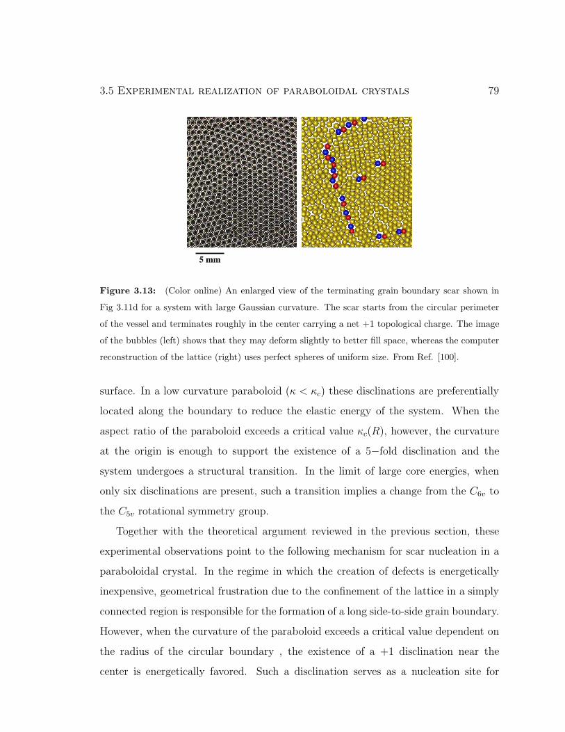
3.5 Experimental realization of paraboloidal crystals 79
Figure 3.13: (Color online) An enlarged view of the terminating grain boundary scar shown in
Fig 3.11d for a system with large Gaussian curvature. The scar starts from the circular perimeter
of the vessel and terminates roughly in the center carrying a net +1 topological charge. The image
of the bubbles (left) shows that they may deform slightly to better fill space, whereas the computer
reconstruction of the lattice (right) uses perfect spheres of uniform size. From Ref. [100].
surface. In a low curvature paraboloid (κ < κc) these disclinations are preferentially
located along the boundary to reduce the elastic energy of the system. When the
aspect ratio of the paraboloid exceeds a critical value κc(R), however, the curvature
at the origin is enough to support the existence of a 5−fold disclination and the
system undergoes a structural transition. In the limit of large core energies, when
only six disclinations are present, such a transition implies a change from the C6v to
the C5v rotational symmetry group.
Together with the theoretical argument reviewed in the previous section, these
experimental observations point to the following mechanism for scar nucleation in a
paraboloidal crystal. In the regime in which the creation of defects is energetically
inexpensive, geometrical frustration due to the confinement of the lattice in a simply
connected region is responsible for the formation of a long side-to-side grain boundary.
However, when the curvature of the paraboloid exceeds a critical value dependent on
the radius of the circular boundary , the existence of a +1 disclination near the
center is energetically favored. Such a disclination serves as a nucleation site for
3.A Optimization via Parallel Differential Evolution 80
5 7 dislocations and the side-to-side grain boundary is replaced by a terminating
center-to-side scar. Above the critical curvature the elastic theory outlined in §3.4
also predicts a regime of coexistence of isolated disclinations and scars due to the
variable Gaussian curvature. For dense systems (i.e. number of subunits larger than
a few hundred for our geometry), the coexistence is suppressed because the embedding
surface will appear nearly flat at the length scale of a lattice spacing. The bulk of the
system is thus populated uniquely by scars. This is consistent with our experimental
observation.
Away from the center of the paraboloid, we have compared the crystalline direc-
tions with the geodesics starting from a given reference point (see Fig. 3.14). Near the
boundary, the directions of both first and second neighbors (in red and blue respec-
tively), are reasonably aligned with the geodesics. The alignment becomes decorre-
lated after roughly five lattice spacings with the decorrelation more pronounced in the
radial direction (maximal principal curvature) where the normal curvature is largest.
As one gets closer to the center, the geodesic correlation becomes weaker and almost
completely vanishes along the radial direction. Along the angular direction (minimal
principal curvature), on the other hand, the crystalline axes appear aligned with the
geodesic directions.
Appendix 3.A Optimization via Parallel Differen-
tial Evolution
Many of the techniques proposed to determine the crystalline structure of systems
of interacting particles, as in the Thomson problem, are based on local optimiza-
tion procedures such as steepest descent, conjugate gradient and the quasi-Newton
method. Such methods belong to the class of line-search algorithms for multidimen-
sional non-linear programming problems. They can be described, in general, as a
sequence of line minimizations of an objective function along a set of directions that

3.A Optimization via Parallel Differential Evolution 81
Figure 3.14: (color online) Delaunay triangulation of a portion of the paraboloidal lattice with
κ ≈ 0.32 cm−1 near the center (top) and the boundary (bottom). Red (lighter) and blue (darker)
lines represent the geodesics directed toward first and second neighbors, respectively.
are generated differently in different algorithms. Besides the well known local con-
vergence properties of these methods, they are generally unable to locate the global
minimum since they inherently approach the closest local minimum for a given set of
initial conditions.
To avoid the misconvergence problem described we adopt the Differential Evolu-
tion (DE) algorithm of Storn and Price [110]. This algorithm, which has been suc-
cessfully applied to several optimization problems in engineering [120], belongs to the
family of evolutionary algorithms which are considerably faster than other stochas-

3.A Optimization via Parallel Differential Evolution 82
Figure 3.15: (Color online) CPU-Time and speedup (i.e. the time employed by n processors to
accomplished a given number of iterations divided by the time employed by a single machine to
achieve the same task).
tic optimization methods, such as simulated annealing and genetic algorithms, and
more likely to find the correct global minimum. These methods heuristically mimic
biological evolution by implementing natural selection and the principle of “survival
of the fittest”. An adaptive search procedure based on a population of candidate
solutions is used. Iterations involve a competitive selection that drops the poorer
solutions. The remaining pool of candidates are perturbed (or mutated) in order to
generate trial individuals and then recombined with other solutions by a swap of the
components. The recombination and mutation moves are applied sequentially; their
aim is to generate new solutions that are biased towards subsets of the search space
in which good, although not necessarily globally optimized, solutions have already
been found.
An essential feature of Differential Evolution is the establishment of genetic diver-
sity, which helps to maximize the probability of finding the true global minimum and
to avoid misconvergence. One begins with a large population of individuals uniformly
distributed in the search space. A good choice, in practice, is to choose the number
of individuals to be an order of magnitude more than the number of variables in the

3.B The function Γs(x) on the paraboloid 83
problem. The price one pays is a dramatic slowing down of the algorithm when ap-
plied to large scale optimization. Considerable effort has therefore been made in the
past ten years to develop parallel implementations of evolutionary algorithms aimed
at reducing the overall time to completion of the task by distributing the work on
different processors working in parallel. More recently some researchers have conjec-
tured that some parallelizations of a task improve the quality of the solution obtained
for a given overall amount of work (e.g. emergent computation).
The Island Model is a popular choice among parallelization strategies and is imple-
mented within a message passing model. It consists of dividing the initial population
into several sub-populations and letting each of them evolve independently on a single
machine for a predetermined number of iterations (called the epoch). The exchange
of genetic information is promoted by swapping individuals between different sub-
populations at the end of each epoch. In the present work the migration strategy
consists in swapping the best individual of each sub-population with a randomly se-
lected individual on another island with the ring topology chosen for the connectivity
between islands. This choice allowed us to achieve a substantial reduction of the CPU
time and a linear speedup (see Fig. 3.15).
Appendix 3.B The function Γs(x) on the paraboloid
To obtain the expression for Γ(x) given in Eq. (3.43) one has to calculate the integral:
Γs(x) =
∫
d2y GL(x,y)K(|y|) = Γs,1(x) − Γs,2(x), (3.59)
having called:
Γs,1(x) =1
2π
∫
dφ′ dr′√g K(r′) log |z − ζ |, (3.60a)
Γs,2(x) =1
2π
∫
dφ′ dr′√g K(r′) log |1 − zζ |. (3.60b)

3.B The function Γs(x) on the paraboloid 84
For this purpose one can use the expansion:
log |z − ζ | = log > −∞∑
n=1
1
n
(
<>
)n
cosnδφ, (3.61)
where > (<) represents the largest (smallest) modulus between z and ζ , while
δφ = φ− φ′. The factorization of the angular variables in Eq. (3.61), together with
the pure radial dependence of the Gaussian curvature and√g, makes the angular
dependence of Γs,1 vanish, so that we have:
Γs,1(x) = log (r)
∫ r
0
dr′κ2r′
(1 + κ2r′2)32
+
∫ R
r
dr′κ2r′
(1 + κ2r′2)32
log (r′), (3.62)
which integrated by parts gives:
Γs,1(x) = log
(
αe√
1+κ2r2
1 +√
1 + κ2r2
)
. (3.63)
Using an expansion similar to (3.61) it is also possible to prove that
log |1 − zζ | = −∞∑
n=1
1
n(′)n cos δφ, (3.64)
which integrated over the surface of the paraboloid gives Γs,2 = 0. This last conclu-
sion, combined with Eq. (3.63), yields Eq. (3.43).

Chapter 4
Crystalline and p−atic order in
toroidal geometries
4.1 Introduction
Circa twenty years afer their first observation in partially polymerized diacetylenic
phospholipid membranes by Mutz and Bensimon [121], self-assembled toroidal ag-
gregates are now considered the progenitors of a magnificent cornucopia of complex
structures, also featuring branched network and micellar surfaces of high genus. The
existence of such complex structures has become an experimental fact thanks to the
enormous work in the past decade on the study of self-assembly of amphiphilic com-
pounds such as lipids, surfactants and amphiphilic block copolymers. After the work
of Eisenberg and coworkers [122–124] it became clear that block copolymer in partic-
ular afford access to a variety of complex structures spanning an unexpectedly vast
range of topologies and geometries. More recently, several experimental studies have
been performed on di- and triblock copolymers with the intent of unraveling the origin
of morphological complexity in copolymer surfactants and some possible pathways for
micelle and vesicle formation have been proposed.
Jain and Bates, for instance, reported the formation of several non-simply-connected

4.1 Introduction 86
micellar structures from the self-assembly of diblock copolymer poly(1,2-butadiene-
b-ethylene oxide) (PB-PEO) [125] (see Fig. 4.1). These polymers self-assemble in
Y−shaped junctions and these form the building blocks for more complex micel-
lar structures via re-assembly. Later, Pochan et al. [126] found that almost all
of the microstructures assembled from poly(acrylic acid-b-methyl acrylate-b-styrene)
(PAA99-PMA73-PS66) triblock copolymers are ringlike or toroidal micelles. The
route to toroidal micelles in block copolymers, however, is believed to be different
from that to more complex network structures suggested by Jain and Bates, since
residual Y−shaped aggregates are very rarely found in the sample. According to the
authors of Ref. [126], the formation of toroidal micelles has to be attributed primarly
to the collapse of cylindrical micelles. On the other hand, mere end-to-end connection
of cylindrical micelles doesn’t appear to be the exclusive ring-forming mechanism in
triblock systems since the average circumference of the self-assembled tori appears
smaller than the contour length of the average cylindrical micelles. It seems some
more complicated process, possibly involving interactions and exchange of matter
between neighboring cylinders.
Toroidal micelles have also been observed in recent experiments by Kim et al [127]
from the self-assembly of amphiphilic dumbbell molecules based on a aromatic rod
segment that is grafted by hydrophilic polyether dendrons at one end and hydrophobic
branches at the other end. Molecular dumbbells dissolved in a selective solvent self-
assemble in an aggregate structure due to their amphiphilic character. This process
has been observed to yield coexisting spherical and open-ended cylindrical micelles.
These structures, however, change slowly over the course of a week to toroidal micelles
which thus appear more stable. The formation of ring-like structures was explained
in this case as result of the coalescence of spherical micelles occurring to reduce the
contact between hydrophobic segments and water molecules.
An alternative pathway for the self-assembly of toroidal structures in copolymer
solutions has been proposed and numerically tested by He and Schimd [128]. In this

4.1 Introduction 87
Figure 4.1: Complex non-simply connected structures from self-assembly of diblock copolymer
poly(1,2-butadiene-b-ethylene oxide) (PB-PEO). From Ref. [125].
pathway, the micelles do not coalesce, but simply grow by attracting copolymers from
the solution. Once a critical micelle size is exceeded, copolymers start to flip-flop in
such a way that the micelle core becomes itself solvent-philic (semi-vesicle state).
Finally the solvent diffuses inside the core and the semi-vesicle swells into a vesicle.
The existence of toroidal aggregates in amphiphilic compounds was suggested the-
oretically for smectic-C (SmC) membranes, based on the argument that orientational
order is not frustrated on a surface with zero Euler characteristic and thus a toroidal
topology may be energetically favoured in p−atic membranes with large order param-
eter coupling compared with the bending rigidity [58, 129]. This hypothesis was tested
by Evans in 1995 with the result that a toroidal topology is indeed prefered over the
spherical one for wide range of geometrical and mechanical parameters in defect-free
p−atic tori. The role of disclinations in p−atic tori was investigated systematically
by Bowick, Nelson and Travesset nine years after the original work of Evans with the
conclusion that, even if not required by topological constraints, unbound disclinations
can be energetically convenient even in very dense systems [130]. The precise number
of unbound disclinations is controlled primarly by the aspect ratio of the torus. The
existence of defects in the ground state of an ordered phase on the torus becomes

4.2 Geometry of the torus 88
Figure 4.2: (Color online) The standard parametrization of a circular torus of radii R1 and R2.
crucial for toroidal crystals where it leads to some unique structural features as well
as a spectacular example of a curvature-driven transition to a disordered, liquid-like,
state in the limit the aspect ratio approaches to one [131, 132]. In the remainder of
this section we will review these three examples of order on embedded tori.
4.2 Geometry of the torus
The standard two-dimensional axisymmetric torus embedded in R3 is obtained by
revolving a circle of radius R2 about a coplanar axis located at distance R1 ≥ R2
from its center. Choosing the symmetry axis as the z direction of a Cartesian frame,
a convenient parametrization can be found in terms of the polar angle ψ along the
revolving circle and the azimuthal angle φ on the xy−plane:
x = (R1 +R2 cosψ) cosφ
y = (R1 +R2 cosψ) sinφ
z = R2 sinψ
, (4.1)
where ψ , φ ∈ [−π, π). These coordinates satisfy the Cartesian equation:
(
R1 −√
x2 + y2)2
+ z2 = R22 (4.2)

4.2 Geometry of the torus 89
In this parametrization the metric tensor gij and Gaussian curvature K are given by:
gψψ = R22 , gψφ = 0 , gφφ = (R1 +R2 cosψ)2 , (4.3)
K =cosψ
R2(R1 +R2 cosψ). (4.4)
The Gaussian curvature is therefore positive on the outside of the torus, negative
on the inside and zero along the two circles of radius R1 at ψ = ±π/2 (see Fig.
4.2). Moreover K is maximally positive along the external equator at ψ = 0 and
maximally negative on the internal equator at ψ = ±π. The Gauss-Bonnet theorem
requires the total topological charge and the integrated Gaussian curvature to be zero
on the torus:N∑
k=1
qk =
∫
d2xK(x) = 0 (4.5)
A global measure of the curvature of the embedded torus is provided by the aspect
ratio r = R1/R2. Our discussion will be limited to the case r ≥ 1. A “fat” torus
with r = 1 is obtained by taking R1 = R2 and is characterized by a singularity
in the Gaussian curvature along the internal equator at ψ = ±π. The case r < 0
corresponds to a self-intersecting torus whose symmetry axis lies in the interior of
the revolving circle. The “skinny” torus limit, r → ∞, can be obtained either by
taking R2 → 0 with finite R1 or by letting R2 stay finite and taking R1 → ∞. The
Gaussian curvature diverges in the first case and goes to zero in the second. Neither
case, however, reflects a real physical situation since the area A = (2π)2R1R2 of the
torus becomes zero or infinite rispectivelly.
Non-axisymmetric tori can be generated in various ways by deforming the surface
of revolution (4.1). A special and physically relevant transformation consists in an
inversion at the unit sphere, a translation about a vector β and a second inversion.
Thus a point R on the surface is mapped onto:
R′ =R
R2 + β
| R
R2 + β|2 (4.6)

4.2 Geometry of the torus 90
This map is conformal and transforms an axisymmetric shape to a non-axisymmetric
one if the vector β is not parallel to the symmetry axis [133]. As β is increased in
magnitude, the asymmetry increases until, in the limit, the torus becomes a perfect
sphere with an infinitesimal handle. The physical importance of mapping (4.6) relies
on the fact that it leaves the bending energy κ∫
d2xH2 invariant with significant
consequences for the equilibrium shape and stability of fluid toroidal membranes.
As in any closed manifold the traditional Green-Laplace equation doesn’t have
a solution on the torus. An alternative Green function, can be obtained from the
modified equation:
∆gGL(x,y) = δg(x,y) −A−1 (4.7)
As usual the calculation of the Green function can be simplified considerably by con-
formally mapping the torus to a domain of the Euclidean plane via a suitable system
of isothermal coordinates. Intuitively the torus is conformally equivalent to a rectan-
gular domain described by a system of Cartesian coordinates. To make this explicit,
one can equate the metric of the torus in the coordinates (ψ, φ) to a conformally
Euclidean metric in the coordinates (ξ, η):
ds2 = R22dψ
2 + (R1 +R2 cosψ)2dφ2 = w (dξ2 + dη2) ,
where w is a positive conformal factor. Taking η = φ and w = (R1 + R2 cosψ)2, the
coordinate ξ is determined by the differential equation:
dξ
dψ= ± 1
r + cosψ, (4.8)
where r = R1/R2, the aspect ratio of the torus, may be taken greater or equal to
one without loss of generality. Choosing the plus sign and integrating both sides of
Eq. (4.8) we find:
ξ =
∫ ψ
0
dψ′
r + cosψ′ . (4.9)
Taking ψ ∈ [−π, π), the integral (4.9) yields:
ξ = κ arctan
(
ω tanψ
2
)
,

4.2 Geometry of the torus 91
where
κ =2√r2 − 1
, ω =
√
r − 1
r + 1. (4.10)
In the transformed coordinate system (ξ, η) the modified Green-Laplace equation
reads:
∆GL(x,y) = δ(x,y) − w
A, (4.11)
where ∆ and δ are now the Euclidean Laplacian and delta function. The function
GL(x,y) can be expressed in the form:
GL(x,y) = G0(x,y) − 〈G0(x, · )〉 − 〈G0(· ,y)〉+ 〈G0(· , · )〉 ,
where G0(x,y) is the Laplacian Green function on a periodic rectangle and the an-
gular brackets stand for the normalized integral of the function G0(x,y) with respect
to the dotted variable:
〈G0(x, · )〉 =
∫
d2y
AG0(x,y) . (4.12)
Analogously the function 〈G0(· , · )〉 is given by
〈G0(· , · )〉 =
∫
d2x d2y
A2G0(x,y)
and ensures the neutrality property:
∫
d2xGL(x,y) =
∫
d2y GL(x,y) = 0 . (4.13)
The modified Laplacian Green function on a periodic rectangle of edges p1 and p2 can
be conveniently calculated in the form:
G0(x,y) =∑
λ6=0
uλ(x)uλ(y)
λ, (4.14)
where uλ is the eigenfunction of the Laplace operator with periodic boundary condi-
tions:
∆uλ(x) = λuλ(x) , (4.15)

4.3 Defect-free p−atic textures and genera transition 92
such that:
uλ(0, η) = uλ(p1, η)
uλ(ξ, 0) = uλ(ξ, p2)
.
In Cartesian coordinates the eigenfunctions are simple plane waves of the form:
uλ(ξ, η) =ei(λnξ+µmη)
√p1p2
, (4.16)
where λn and µm are given by:
λn =2πn
p1
µm =2πm
p2
n, m = 0, ±1, ±2 . . .
and the eigenvalue λ is given by:
λ = −λ2n − µ2
m . (4.17)
Calling for simplicity x = (x, y) and y = (ξ, η), the function G0 is given by:
G0(x,y) = − 1
p1p2
∑
(n,m)6=(0,0)
eiλn(x−ξ)eiµm(y−η)
λ2n + µ2
m
. (4.18)
Summing this series eventually leads to [132]:
G0(x,y) =log 2
6π− 1
2 p1p2
|y − η|2 +1
2πlog
∣
∣
∣
∣
∣
∣
ϑ1(z−ζp1/π
| ip2p1
)
ϑ′ 13
1 (0| ip2p1
)
∣
∣
∣
∣
∣
∣
, (4.19)
where ϑ1(u|τ) is the Jacobi theta function [134, 135] defined as:
ϑ1(u|τ) = 2q14 sin u
∞∏
n=1
(
1 − 2q2n cos 2u+ q4n) (
1 − q2n)
, (4.20)
with q = exp(iπτ), z = x+ iy and ζ = ξ+ iη. A step-by-step derivation of Eq. (4.19)
is reported in Appendix 4.B.
4.3 Defect-free p−atic textures and genera transi-
tion
There has been much effort in recent years to shed light on possible pathways in
the self-assembly of toroidal micelles and vesicles from block copolymer solutions and

4.3 Defect-free p−atic textures and genera transition 93
other amphiphilic compounds. In particular, the spontaneous formation of structure
of genus g ≥ 1 from preexisting spherical objects, a mechanism which is in common
to several different scenarios proposed in the literature, has attracted the most atten-
tion and debate because of its exotic character. The simplest question one can ask in
this context is whether a vesicle can be energetically favored to change its topology
from spherical to toroidal once, the total surface area and therefore the number of
constituent molecules in the vesicle, is specified. Evans addressed this problem in
1995 [129] and showed how such a transition between genera is indeed possible in
fluid membranes and is even enhanced if the membrane is endowed with in-plane
orientational order. Although oversimplified if compared to the great complexity of
the real self-assembly mechanism, Evans’ calculation provides insight into the deli-
cate problem of stability of toroidal vesicles as well as a good starting point for our
discussion of order on the torus.
Let θ be the local orientation of a p−atic director field on a surface as defined in
Sec. 2. A standard orientational order parameter is given by scalar field:
ψ(x) = 〈eipθ(x)〉 , (4.21)
where 〈·〉 deontes a thermal average. The total elastic energy of the vesicle consists of
a pure bending term Fb, describing the elasticity of the membrane in the liquid state,
and a term Fp associated with the internal p−atic order. Thus F = Fp + Fb, with:
Fp =
∫
d2x(
τ |ψ|2 +u
2|ψ|4 + C|(∇− ipΩ)ψ|2
)
(4.22a)
Fb =
∫
d2x(
2κH2 + κgK)
(4.22b)
where κ and κg are the bending and Gaussian rigidity respectively1 and the operator
∇− ipΩ is obtained from the covariant derivative of a p−atic tensor order parameter
1The expression of the bending energy used in Eq. (4.22b) is that originally gave by Helfrich for
a membrane with zero pre-existing curvature [136]. Often the equivalent expression∫
d2x (1
2κH2 +
κgK) is found in the literature. In this case, however, the mean curvature H is defined as the sum
of the principal curvatures rather than their average.

4.3 Defect-free p−atic textures and genera transition 94
expressed in a local orthonormal frame as described in Sec. 2.4, with Ω the covariant
vector of Eq. (2.53) that parametrizes the spin-connection. The free energy (4.22a)
is invariant under rotations of the local reference frame by an arbitrary angle χ:
ψ → ψ eipχ (4.23a)
Ωi → Ωi − ∂iχ , (4.23b)
which is a typical gauge transformation. The gradient term in Eq. (4.22a) is the same
of Eq. 2.52, upon identifying KA = p2C. As observed by Park et al. [137], Eq. (4.22a)
and (4.22b) closely resemble the Landau-Ginzburg Hamiltonian of a superconductor
in an external magnetic field:
H =
∫
d3x
∣
∣
∣
∣
(
∇− 2ie
~cA
)
ψ
∣
∣
∣
∣
2
+ τ |ψ|2 +u
2|ψ|4 +
1
8π|∇ × A − H|2
. (4.24)
When exposed to an external magnetic field, a super-conducting material can undergo
a second order mean-field transition from a metal to a super-conductor characterized
by an Abrikosov lattice of vortices whose density is determined by the temperature
and the applied magnetic field H . The magnetic field, in particular, is conjugate to
the vortex number Nv since:
∫
d3x∇× A = φ0LNv , (4.25)
where L is the length of the sample in the direction of H and φ0 = hc/2e is the flux
quantum. In this context the vector potential associated with the applied magnetic
field is replaced by the covariant vector Ω whose curl is the Gaussian curvature.
Morover, on a closed surface:
∫
d2x∇× Ω =
∫
d2xK =2π
p
N∑
i=1
qi .
Thus a p−atic phase on a closed 2−manifold is analogous to an Abrikosov phase with
a fixed total vorticity rather than a fixed applied magnetic field.

4.3 Defect-free p−atic textures and genera transition 95
The transition to an ordered phase in controlled by the parameter τ in Eq. (4.22a).
For τ above a critical value τc (τc = 0 on a flat surface), ψ = 0 and the system is in
the isotropic phase. In this regime the only contribution to the energy is determined
by the shape of the vesicle as expressed by the bending term (4.22b). For τ < τc,
on the other hand, the gauge symmetry is spontaneously broken and ψ 6= 0, with
the exception of a number of isolated defective points. Within a meanfield approach,
thermal fluctuations can be neglected and the preferred configuration of the system
corresponds to the minimum of the free energy. A ground state configuration for the
p−atic order parameter can be found by rewriting the gradient energy term in Eq.
(4.22a) as:
∫
d2x |(∇− ipΩ)ψ|2 =
∫
dx1 dx2√g DkψD∗kψ
∗
= −∫
dx1 dx2 ψ∗ (Dk√g Dk
)
ψ ,
with Dk = ∂k − ipΩk, and expressing ψ in the basis of eigenfunctions of the operator
in parentheses:
ψ =∑
n
anϕn (4.26)
with ϕn satisfying the Hermitean equation:
− 1√gDk (
√g Dk)ϕn =
4πλ
Aϕn (4.27)
with the normalization condition:
∫
d2xϕ∗nϕm =
A
4πδnm (4.28)
The complex coefficients ak are then determined by minimization of the free energy
F . The eigenfunctions are sometimes referred to as “Landau levels” and are typically
degenerate. If ψ is expandend in this complete set of eigenfunctions then, in meanfield,
the partition function is dominated by configurations involving only Landau levels
with the lowest eigenvalue λ0. Taking lowest levels only, the p−atic free energy

4.3 Defect-free p−atic textures and genera transition 96
(4.22a) becomes:
Fp =
∫
d2x
[(
τ +4πλ0C
A
)
|ψ|2 +u
2|ψ|4
]
(4.29)
To find the lowest energy configuration of the field ψ one now has to solve the eigen-
value problem (4.27) to determine the lowest eigenvalue λ0 and minimize the free
energy with respect to the parameters of the linear combination (4.26). Notice that
the mean field transition has been lowered form τc = 0 to τc = −4πλ0C/A. On flat
surface λ0 = 0, but is finite and positive-definite on a surface with finite Gaussian
curvature [129].
For a sphere of unit radius parametrized in standard spherical coordinates (θ, φ),
the eigenvalue problem (4.27) is solved by λ0 = p and ϕn of the form [138]:
ϕn =
√
2p+ 1
4π(p+ n)!(p− n)!sinp+n
(
θ
2
)
cosp−n(
θ
2
)
einφ (4.30)
for integer values of n between −p and p. These functions have 2p zeros, corresponding
to topological defects of unitary charge and winding number 1/p. Because of the
lowest Landau level approximation used to derive Eq. (4.29), eigenfunctions (4.30)
are degenerate to quadratic order in ψ. This implies the freedom to place defects
anywhere on the sphere with no additional energy cost of order ψ2. The ψ4 term, on
the other hand, lifts this degeneracy and make the defects repel.
For axisymmetric, tori the eigenvalue problem (4.27) was solved numerically by
Evans with the result shown in Fig. 4.3. Eigenvalues are plotted as a function of
the aspect ratio r of the torus for various p−atic textures labelled pn with 0 ≤ n ≤p. Eigenfunctions ϕn have 4n zeros corresponding to 2n disclinations of topological
charge q = 1 (winding number 1/n) and 2n disclinations of topological charge q = −1
(winding number −1/n). Except for vector order (p = 1), defective configurations
are energetically favored for small aspect ratios and the number of disclination pairs
increases with r as a consequence of the larger (in magnitude) Gaussian curvature.
Carrying out the integrals in Eq. (4.22a) and (4.22b) in the lowest Landau level
approximation, the total elastic free energy of spherical and toroidal vesicles can be

4.3 Defect-free p−atic textures and genera transition 97
Figure 4.3: (Color online) Eigenvalues λ versus the aspect ratio r for varius p−atic configurations
(labelled pn) on the axisymmetric torus. The number of disclination pairs for each configuration is
2n. Data are taken from [129].
written as:
Fsphere = 4π(2κ+ κg) − 2π
(
C2
uA
)
[
τA4πC
+ p]2
Jsphere(p)(4.31a)
Ftorus = κ2π2r2
√r2 − 1
− 2π
(
C2
uA
)
[
τA4πC
+ λ0(r)]2
Jtorus(p, r)(4.31b)
where J is the minimal value of the integral of |ψMF|4 and
ψMF =
∑pn=−p anϕn sphere
a+ϕp + a−ϕ−n torus
is the linear combination of eigenfuctions that are degenerate to quadratic order
in ψ. The second term in Eqs. (4.31a) and (4.31b) disappears in the isotropic
phase when τ > −4πλ0C/A due to the intrinsic orientational order on the manifold.
Even in this case, Eqs. (4.31a) and (4.31b) reveal the existence of a transition line

4.3 Defect-free p−atic textures and genera transition 98
Figure 4.4: (Color online) Phase diagram for vesicles of constant area of genus zero and one with
intrinsic vector (top left), nematic (top right), tetradic (bottom left) and hexatic (bottom right)
order. The position of the transition line depends on the value of κg/κ. Toroidal vesicles that exist
in the shaded region are non-axisymmetric. Data are taken from [129].
between spherical and toroidal shape. In the absence of in-plane orientational order
the bending energy term in Eq. (4.31b) is minimized by the so called Clifford torus
with r =√
2. In this case Ftorus = 4π2κ, which is smaller than Fsphere = 4π(2κ+ κg)
when κg/κ > π− 2. Toroidal vesicles with r =√
2 are therefore energetically favored
in the fluid phase for large values of κg/κ. This argument cannot be invoked to
explain the complex self-assembly of toroidal structures from homogeneous solutions
mentioned in the introduction, but does provide a simple (but non-trivial) example
of a situation where a toroidal shape is energetically preferred to a spherical one.
The critical value of κg/κ of the genera transition is lowered for vesicles equipped

4.4 Defective ground states in hexatics 99
with in-plane p−atic order. This is displayed in the phase diagrams of Fig. 4.4 for
the case of vector (p = 1), nematic (p = 2), tetradic (p = 4) and hexatic (p = 6)
order. The lines, whose position depends on κg/κ, separate spheres (above the line)
from tori (below the line). Even for simple vector order, stable toroidal vesicles
exist as well for κg/κ < π − 2. For κg/κ > π − 2, furthermore, transition lines are
closed, with spheres on the inside and tori on the outside. In the shaded regions
non axisymmetric tori are favored over symmetric ones. The hexatic phase diagram
(bottom right corner of Fig. 4.4) deserves special attention. The shaded region is split
in two parts. That on the right contains spheres if κg/κ < π−2 and non-axisymmetric
tori otherwise, while that on the left contains spheres above the transition line and
non-axisymmetric tori below. The white region of the phase diagram is also divided in
two parts. The part in the top left of the diagram behaves as described above, while
the other part is characterized by closed lines separating spheres (outside) and small
tori (inside). These last class of tori exhibit ten pairs of q = ±1 disclinations with
positive disclinations distributed on the external equator of the torus and negative
disclinations along the internal equator. This last feature is an important property
sheared by toroidal objects with in-plane order and will be clarified in the following
sections. The results reviewed here are valid within the mean-field approach and the
lowest Landau level approximation, which both hold deep in the ordered phase that
we are most interested in. At higher temperatures Evans proved the approximations
are still valid away from the transition line and for C/A ≫ κ/kBT ≫ 1 [129]. The
latter condition is generally fulfilled by several systems (i.e. κ/kBT = 1− 10 for lipid
bilayers).
4.4 Defective ground states in hexatics
Evans’ analysis, summarized in the previous section, indicates that disclinations, even
if not required by topological constraints, can nonetheless appear in the ground state

4.4 Defective ground states in hexatics 100
of p−atic tori as a consequence of the coupling between in-plane orientational order
and spatial curvature. The occurrence of defects in the ground state of toroidal hexatic
vesicles was systematically investigated by Bowick, Nelson and Travesset based on the
formalism outlined in Sec. 2 [130]. Before embarking on a detailed analysis of the
elasticity of defects in hexatic tori, it is instructive to obtain a rough estimate of
how many pairs of ±1-disclinations would be required to achieve a perfect screening
of the background topological charge associated with the Gaussian curvature of the
torus. Consider a wedge of angular width ∆φ on the outside wall of positive Gaussian
curvature. The net curvature charge associated with this region is:
seff =
∫ φ0+∆φ2
φ0−∆φ2
dφ
∫ π2
−π2
dψ√g K = 2∆φ . (4.32)
Upon equating seff to 2π/6, the charge of a single disclination, one finds that ∆φ =
2π/12, independently of R1 and R2. Thus, 2π/∆φ = 12 positive disclinations would
be required to completely compensate the negative curvature of the inner wall. This
simple argument neglects core energies and interactions between disclinations, effects
which will cause the preferred number of defect pairs to be less than twelve.
The total elastic energy of a toroidal hexatic vesicle containing N disclinations of
topological charge qi (i = 1 . . . N) takes the form:
F
KA
=π2
9
1,N∑
i<j
qiqjQ(xi,xj) −π
3
N∑
i=1
qiL(xi)
+2π2
r +√r2 − 1
+κ
KA
2π2r2
√r2 − 1
+ǫcKA
N∑
i=1
q2i (4.33)
where the first two terms represent the contributions due to the pair interaction
between defects and the interaction of defects with the topological charge of the
substrate associated with the Gaussian curvature. The third term in Eq. (4.33) is the
spin-wave part of the frustrated hexatic energy while the last two terms represents the
bending energy and the defect core energy respectively. The defect-defect interaction
4.4 Defective ground states in hexatics 101
potential has been calculated in Ref. [130]:
Q(xi,xj) = − 1
4πlog
∣
∣
∣ϑ1
(
φi−φj
2π+ i
2π
αi−αj√r2−1
∣
∣
∣
i√r2−1
)∣
∣
∣
2
4π2
∣
∣
∣η(
i√r2−1
)∣
∣
∣
6
+1
2√r2 − 1
(
αi − αj2π
)2
(4.34)
where α is related to the polar angle ψ on a cross-section of the torus by:
cosψ =r cosα− 1
r − cosα(4.35)
and η is the Dedekind eta function:
η(τ) = e2πiτ24
∞∏
n=1
(1 − e2πinτ ) . (4.36)
The one-body interaction between defects and curvature, on the other hand, is ex-
pressed via the potential energy:
L(xi) = log
(
1
r − cosαi
)
. (4.37)
For opposite sign disclinations, the defect-defect interaction, determined by the
function Q(xi,xj), is attractive for all separations at contrast φ. If only this term
was present, the attraction would bring both charges as close as possible, binding all
dislcinations into dipoles which have a higher energy than a defect-free configuration.
Thus if no other terms were present, the ground state configuration would be defect
free. The defect-curvature interaction term L(xi), however, favors the appearance of
additional defects. This term acts like an electric field pulling the positive (negative)
disclinations into regions of positive (negative) Gaussian curvature.
The elastic energy (4.33) was analyzed numerically in Ref. [130] for various aspect
ratios and defect core energies. A plot of the energy of configurations obtained by
placing a ring of (N/2) +1-disclinations equally spaced along the same parallel on
the outside of the torus and a second ring of (N/2) −1-disclinations on the inside, is

4.4 Defective ground states in hexatics 102
Figure 4.5: (Color online) The total energy (in units of KA/2 of hexatic tori of aspect ratio r =√
2
(left) and r = 2.6926) for varying number of defects. The bending energy at fixed r is subtracted
off. The disclination core energy is set to 0.1KA, which is 0.2 in the above units.
shown in Fig. 4.5 for variousN and variable angular separation ∆ψ between the rings.
The disclination core energy is taken to be ǫc = cKA, with c a numerical constant
taken equal to 0.1 in the plots. The energy at the maximum separation (∆ψ = π)
first decreases and then increases with N . The optimal number of defect pairs N/2
is 6 and 7 (the latter curve is not shown in the plot) for r =√
2 and r = 2.6926
respectively.
The existence of defects in the ground state of a toroidal vesicle with hexatic
order is also affected by the total number of molecules N forming the hexatic phase.
In Ref. [130] it was found that defects disappear in the limit N → ∞, but are
present for numbers of molecules as large as N = 1010. This number is several
orders of magnitude larger than the typical number of molecules of biological vesicles
such as red-blood cells (i.e. N ∼ 108). To make this estimate, one considers a pair of
opposite sign disclinations that have been pulled apart from the circle of zero Gaussian
curvature to the equators in the regions of like sign Gaussian curvature; thus ψ+ = 0
and ψ− = π. Upon approximating the defect-pair energy by its flat space value, the

4.4 Defective ground states in hexatics 103
total energy reads:
F = −π3KA log
(
r + 1
r − 1
)
+π
18KA log
(
R2
a0
)
+ 2ǫc , (4.38)
where a0 is the lattice spacing. Eq. (4.38) changes sign when
R2
a0
= e− 36ǫc
KA
(
r + 1
r − 1
)6
. (4.39)
Taking
N ≈ A√
32a2
0
=8π2
√3 r(
R2
a0
)2
leads to the conclusion that defects are favored for:
N <8π2
√3e− 72ǫc
πKA
[
r
(
r + 1
r − 1
)12]
≈ 4.6 r
(
r + 1
r − 1
)12
(4.40)
where the last identity has been obtained by taking ǫc/KA = 0.1. This result estab-
lishes that defects are present in the ground state of a hexatic tours for any fixed
number of molecules provided the torus is sufficiently fat. For the energetically fa-
vored Clifford torus with r =√
2, Eq. (4.40) predicts a critical number of molecules
to be order N ∼ 1010.
In absence of defects the ratio between the hexatic stiffness KA and the bending
rigidity κ dictates the optimal shape of the toroidal vesicle. Taking qi = 0 in Eq.
(4.33) one obtains in this case:
F =2π2KA
r +√r2 − 1
+ κ2π2r2
r2 − 1. (4.41)
The first term represents the energetic cost associated with the distortion of the
hexatic director field due to the Gaussian curvature alone. In the limit of large and
small hexatic stiffness Eq. (4.41) is minimized by:
r =√
2 KA ≪ κ
r =√
KA
2κKA ≫ κ

4.5 Toroidal crystals 104
which provides a compelling example of the interplay between order and geometry:
if the stiffness associated with the intrinsic hexatic order is much smaller than the
bending rigidity, the Clifford torus is the optimal geometry; if on the other hand, the
hexatic stiffness dominates, then a thin torus, similar to a bicycle tire, is optimal.
4.5 Toroidal crystals
Crystalline assemblages of identical sub-units packed together and elastically bent in
the form of a torus have been found in the past ten years in a variety of systems
of surprisingly different nature, such as viral capsids, self-assembled monolayers and
carbon nanomaterials. In the introduction we mentioned the self-assembly of toroidal
micelles and vesicles from homogeneous solutions of amphiphilic molecules such as
oligomers of aromatic compounds or block copolymers. Toroidal geometries also
occur in microbiology in the viral capsid of the coronavirus torovirus [139]. The
torovirus is an RNA viral package of maximal diameter between 120 and 140 nm and
is surrounded, as other coronaviridae, by a double wreath/ring of cladding proteins.
Carbon nanotori form another fascinating and technologically promising class of
toroidal crystals [48] with remarkable magnetic and electronic properties. The inter-
play between the ballistic motion of the π electrons and the geometry of the embedding
torus leads to a rich variety of quantum mechanical properties including Pauli para-
magnetism [140] and Aharonov-Bohm oscillations in the magnetization [141]. Ring
closure of carbon nanotubes by chemical methods [142] suggest that nanotubes may
be more flexible than at first thought and provides another technique of constructing
carbon tori. In this section we review some recent developments in the study of the
geometry and the elasticity of toroidal crystals. Additional details can be found in
Refs. [131, 132].

4.5 Toroidal crystals 105
4.5.1 Geometry of toroidal polyhedra
Before analyzing the defect distribution arising from the elastic theory, it is neces-
sary to understand the geometry of triangulated tori. Reconciling the predictions of
a continuum elastic theory with the intrinsically discrete nature of crystallography
requires an understanding of the possible lattices that can be embedded on the torus
and the associated defects. The problem of classifying the possible triangulations
of the 2−torus has received considerable attention from mathematicians, physicists
and chemists over the past twenty years. Lavrenchenko [143] proved in 1984 that all
the triangulations of the torus can be generated from 21 irreducible triangulations
by certain sequences of operations called vertex splitting2. After the discovery of
carbon nanotubes in 1991 and the subsequent theoretical construction (later followed
by the experimental observation) of graphitic tori, many possible tessellations of the
circular torus have been proposed by the community [144–153]. In this section we
review the construction of a defect-free triangulated torus and we show how the most
symmetric defective triangulations can be generally grouped into two fundamental
classes corresponding to symmetry groups Dnh and Dnd respectively.
For the sake of consistency with the existing literature we adopt here the language
developed to describe the structure of carbon nanotubes. The structure of a triangu-
lated cylinder can be specified by a pair of triangular lattice vectors c and t, called
the chiral and translation vector respectively, which together define how the planar
lattice is rolled up. In the canonical basis a1 = (1, 0) and a2 = (12,√
32
), the vector c
has the form:
c = na1 +ma2 n, m ∈ Z . (4.42)
The translation vector t, on the other hand, can be expressed as an integer multiple
t = let l ∈ Z (4.43)
2Analogously it can be proved that the number of irreducible triangulations is one for the sphere
and two for the projective plane. The extraordinary larger value obtained for the torus should be
indicative of the high structural complexity of a crystalline torus.

4.5 Toroidal crystals 106
Figure 4.6: (Color online) Construction of a defect-free triangulation of the torus. On top planar
map of the triangulated torus corresponding to the (n,m, l) configuration (6, 3, 1). On the bottom
(6, 3, 6) chiral torus. The edges of each one of the six tubular segments has been highlighted in red.

4.5 Toroidal crystals 107
of the shortest lattice vector et perpendicular to c. The vector et is readily found to
be of the form:
et =(n + 2m)a1 − (2n+m)a2
(n+ 2m : 2n +m),
where (a : b) denotes the greatest common divisor of a and b and enforces the minimal
length. The three-dimensional structure of the torus is obtained by connecting the
edge OT of the rectangle in Fig. 4.6 (top) to O′C and OC to O′T . The edge OT is
then mapped to the external equator of the torus while the edge OC to the φ = 0
meridian. The resultant toroidal lattice has characteristic chirality related to the
initial choice of the vector c. In the nanotubes literature armchair referes to the
lattice obtained by choosing n = m, zigzag to that obtained for m = 0 and chiral to
all other lattices. An example of a (n,m, l) chiral torus is shown in Fig. 4.6 (bottom)
for the case n = 6, m = 3 and l = 6. The chirality is extremely important in graphitic
carbon nanotube or nanotori, where it determines whether the electronic behavior of
the system is metallic or semiconducting.
By Euler’s theorem one can prove that the number of triangular faces F and the
number of vertices V of a triangular toroidal lattice is given by:
V = 12F .
Denoting AR the area of the rectangle with edges c and t and AT the area of a
fundamental equilateral triangle, the number of vertices of a defect-free toroidal tri-
angulation is then:
V =AR2AT
=2l (n2 + nm+m2)
(n + 2m : 2n+m). (4.44)
The planar construction reviewed above allows only lattices with an even number of
vertices. Defect-free toroidal deltahedra with an odd number of vertices are also pos-
sible and their construction is generally achieved by assembling congruent octahedral
building blocks. An example of this scheme will be briefly discussed in Sec. 4 for the
case V = 87 and r = 6. We refer the reader to Ref. [154] for an comprehensive review
of the topic.

4.5 Toroidal crystals 108
The embedding of an equal number of pentagonal and heptagonal disclinations
in the hexagonal network was first proposed by Dunlap in 1992 as a possible way to
incorporate positive and negative Gaussian curvature into the cylindrical geometry of
carbon tubules [144]. According to the Dunlap construction the necessary curvature
is incorporated by the insertion of “knees” (straight cylindrical sections of the same
diameter joined with a kink) in correspondence with each pentagon-heptagon pair
arising from the junction of tubular segments of different chirality (see Fig. 4.8). In
Figure 4.7: (Color online) Voronoi lattices of a TPn prismatic (top) and TAn antiprismatic (bot-
tom) toroids with R1 = 1 and R2 = 0.3.
particular, a junction between a (n, 0) and a (m,m) tube can be obtained by placing a
7−fold disclination along the internal equator of the torus and a 5−fold disclination
along the external equator. Since the radii of the two segments of a junction are
different by construction, the values of n and m are commonly chosen to minimize
the ratio |c(n,0)|/|c(m,m)| = n/√
3m. By repeating the 5 − 7 construction periodically
it is possible to construct an infinite number of toroidal lattices with an even number
of disclinations pairs and dihedral symmetry group Dnh (where 2n is the total number
of 5 − 7 pairs, Fig 4.9). The structure of the lattice is described by the alternation
of two motifs with crystalline axes mutually rotated by 30 as a consequence of the
connecting disclination. One of the fundamental aspects of Dunlap’s construction is
that all the disclinations are aligned along the two equators of the torus where the

4.5 Toroidal crystals 109
like-sign Gaussian curvature is maximal. As we will see below, this feature makes
these arrangements optimal in releasing the elastic stress due to curvature.
Figure 4.8: (Color online) Dunlap knees obtained by joining two straight tubular segments with
(n, 0) and (m,m) chirality. [Courtesy of A. A. Lucas and A. Fonseca, Facultes Universitaries Notre-
Dame de la Paix, Namur, Belgium].
Figure 4.9: (Color online) Five-fold polygonal torus obtained by joining (5, 5) and (9, 0) tubular
segments via ten pairs of 5 − 7 rings. This structure was originally proposed by the authors of
Ref. [155] as a possible low-strain configuration for carbon nanotori. [Courtesy of A. A. Lucas and
A. Fonseca, Facultes Universitaries Notre-Dame de la Paix, Namur, Belgium].

4.5 Toroidal crystals 110
Another class of crystalline tori with dihedral antiprismatic symmetry Dnd was
initially proposed by Itoh et al [145, 151, 152] shortly after Dunlap. Aimed at repro-
ducing a structure similar to the C60 fullerene, Itoh’s original construction implied ten
disclination pairs and the point group D5d. In contrast to Dunlap tori, disclinations
are never aligned along the equators in antiprismatic tori, instead being staggered at
some angular distance δψ from the equatorial plane. Hereafter we will use the sym-
bol TAn to refer to toroidal deltahedra with 2n disclination pairs and Dnd symmetry
group.
A systematic construction of defected triangulations of the torus can be achieved
in the context of planar graphs [143, 156, 157]. A topological embedding of a graph
in a two-dimensional manifold corresponds to a triangulation of the manifold if each
region of the graph is bounded by exactly three vertices and three edges, and any two
regions have either one common vertex or one common edge or no common elements
of the graph. The simplest example of toroidal polyhedra with Dnd symmetry group,
featuring only 5−fold and 7−fold vertices, can be constructed by repeating n times
the unit cell of Fig. 4.11a. These toroidal antiprisms 3 have V = 4n vertices and can
be obtained equivalently from the edge skeleton of a n−fold antiprism by attaching
at each of the base edges a pentagonal pyramid and by closing the upper part of
the polyhedron with n additional triangles. By counting the faces one finds F =
5n + 2n + n = 8n from which V = 4n. The simplest polyhedron of this family has
V = 12 and D3d symmetry group (see top left of Fig. 4.10) and corresponds to the
“drilled icosahedron” obtained by removing two parallel faces of an icosahedron and
connecting the corresponding edges with the six lateral faces of an antiprism with
triangular base (i.e. a prolate octahedron). Starting from this family of toroidal
antiprisms a number of associated triangulations having the same defect structure
can be obtained by geometrical transformations such as the Goldberg inclusion [38,
3Although we presume this class of toroidal polyhedra is not discussed here for the first time, we
couldn’t find any previous reference in the literature.

4.5 Toroidal crystals 111
Figure 4.10: (Color online) First six toroidal antiprisms obtained by repeating the unit cell of
Fig. 4.11. The first polyhedron on the left is the “drilled icosahedron”.
158, 159]. Such transformations, popularized by Caspar and Klug for the construction
of the icosadeltahedral structure of spherical viruses [38], consist in partitioning each
triangular face of the original graph into smaller triangular faces in such a way that
old vertices preserve their valence and new vertices have valence six. The partition
is obtained by specifying two integer numbers (L,M) which define how the original
vertices of each triangle are connected by the new edges so that the total number of
vertices is increased by a factor T = L2 + LM +M2.
A general classification scheme for Dnd symmetric tori was provided by Berger
and Avron [156, 157] in 1995. Their scheme is based on the construction of unit
graphs comprising triangular tiles of different generations. In each generation, tiles
are scaled in length by a factor 1/√
2 with respect to the previous generation. This
rescaling approximates the non-uniformity of the metric of a circular torus.
Dunlap toroids can be obtained from unit cells such as those shown in Fig. 4.12.

4.5 Toroidal crystals 112
Figure 4.11: (a) Unit cell for toroidal antiprisms. 5−fold vertices are circled and 7−fold vertices
are boxed. (b) Unit cell of a Dnd torus in the Berger-Avron construction. The graph consists of four
generation of tiles and the internal equator of the torus is mapped into the horizontal line passing
to the mid-point between the 6th and the 7th vertex.
Figure 4.12: (Color online) Unit cells for Dunlap toroids of type (2, 1, 3, 1) and (3, 1, 3, 1) according
to the classification scheme given here. Highlighted regions correspond to the central polygon.
The geometrical properties of these graphs can be described in different ways. A
particularly intuitive way, in the spirit of this work, consists in specifying the distances

4.5 Toroidal crystals 113
between 5− and 7−fold pairs. One starts by drawing the smallest convex loop passing
through defective sites. This identifies a central polygon whose upper vertices (v1 and
v2 in Fig.4.13) have degree five and lower vertices (v5 and v6 in Fig. 4.13) have degree
seven. Then calling a the distance between 5−fold vertices v1 and v2, b that between
7−fold vertices v5 and v6 and c the length of the segment v3v4 (d = a for a trapezoid),
we can express the total number of triangles enclosed by the central polygon as:
f = 2c2 − a2 − b2 .
Each 7−fold vertex sits at the apex of a diamond-shaped complex of f ′ = 7 triangles.
Each 5−fold vertex, on the other hand, is at the apex of a triangular region of
f ′′ = (c− a+ 1)2 triangles. The graph is completed by a rectangle of height c− a+ 4
and base of arbitrary length 2d containing:
f ′′′ = 4d(c− a + 4)
triangles. The total number of vertices is
Vg = f + f ′ + f ′′ + f ′′′/2
= c2 − b2 + 2(c− a)(c+ d+ 1) + 8(d+ 1) . (4.45)
The final triangulation of the torus is obtained by repeating the prismatic unit cell l
times and therefore has V = lVg vertices. This scheme provides direct information on
the arrangement of defective sites. Thus for instance an (a, b, c, d) = (2, 1, 3, 1) unit
cell (see top of Fig. 4.12) has 5−fold vertices separated by two lattice spacings and
7−fold vertices by one lattice spacing. On the other hand the integers n and m giving
the chirality of the two segments of the junction (n, 0)/(m,m) are given directly by
as:
n = c− a+ 4
m = 2c− a− b .
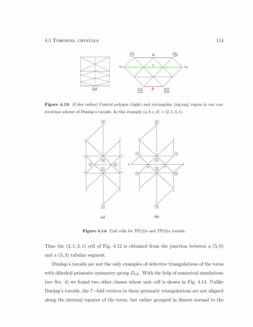
4.5 Toroidal crystals 114
Figure 4.13: (Color online) Central polygon (right) and rectangular (zig-zag) region in our con-
struction scheme of Dunlap’s toroids. In this example (a, b, c, d) = (2, 1, 3, 1).
Figure 4.14: Unit cells for TP(2)n and TP(3)n toroids.
Thus the (2, 1, 3, 1) cell of Fig. 4.12 is obtained from the junction between a (5, 0)
and a (3, 3) tubular segment.
Dunlap’s toroids are not the only examples of defective triangulations of the torus
with dihedral prismatic symmetry group Dnh. With the help of numerical simulations
(see Sec. 4) we found two other classes whose unit cell is shown in Fig. 4.14. Unlike
Dunlap’s toroids, the 7−fold vertices in these prismatic triangulations are not aligned
along the internal equator of the torus, but rather grouped in dimers normal to the

4.5 Toroidal crystals 115
Figure 4.15: (Color online) (a) TP5a and (b) TP7b toroids with V = 35 and 49 obtained by
repeating the unit cells of Fig. 4.14. 7−fold vertices form dimers normal to the equatorial plane
while 5−fold vertices are (a) distributed along the external equator or (b) form a double ring above
and below the equatorial plane.
equatorial plane. 5−fold vertices are distributed along the external equator in the
graph of Fig. 4.14a or form a double ring above and below it in the case of the
graph Fig. 4.14b. Toroidal deltahedra obtained by embedding the prismatic graphs
of Fig. 4.14 on a circular torus are shown in Fig. 4.15 for the case of a 5−fold symmetric
toroid with V = 35 and a 7−fold symmetric toroid with V = 49. In the rest of the
paper we will reserve the symbol TPn for Dunalp’s toroids and refer with TPna and
TPnb to the other two classes of toroids with symmetry group Dnh and unit cell of
as shown in Fig. 4.14a and Fig. 4.14b respectively.
All defective triangulations presented so far are characterized by an even number
of disclination pairs. Regular tessellations of the torus comprising an odd number of
defects pairs are also possible. Such tessellations are obtained by combining segments

4.5 Toroidal crystals 116
Figure 4.16: (Color online) Voronoi diagram of a toroidal lattice with r = 10/3 and V = 200
vertices. The lattice exhibits 11 disclination pairs and has Cs symmetry group.
of prismatic and antiprismatic lattices with a consequent loss of dihedral symmetry.
Fig. 4.16 shows the Voronoi diagram of a toroidal lattice, with r = 10/3 and V = 200
vertices, containing 11 disclination pairs. For an angular length of approximately
∆φ = 7/5 π the lattice is a prismatic D5d toroid while in the remaining 3/5 π the
local structure is that of an antiprismatic toroid. The global structure has only
bilateral symmetry about a sagittal plane dividing the lattice in two mirror halves
and thus point group Cs.
In the past few years, alternative constructions of triangulated tori have been
proposed as well as novel geometrical and graph-theoretical methods to express the
coordinates of their three-dimensional structures (see for example Kirby [146], Laszlo

4.5 Toroidal crystals 117
at al [147, 153, 160], Diudea et al [148, 161]). Here we choose to focus on the defect
structure associated with the two most important class TPn and TAn with groups
Dnh and Dnd.
4.5.2 Elasticity of defects on the torus
Isolated defects regime
The total free energy of a toroidal crystal with N disclinations can be expressed as
usual as:
F =1
2Y
∫
d2xΓ2(x) + ǫc
N∑
i=1
q2i + F0 (4.46)
where Y is the two dimensional Young modulus and:
Γ(x) =π
3
N∑
k=1
qkΓd(x,xk) − Γs(x) , (4.47)
The defect part of the stress function Γ(x) can be found by integrating the Green
function (4.19) and takes the form:
Γd(x,xk)
Y=
κ
16π2
(
ψk −2
κξk
)2
− 1
4π2κ(φ− φk)
2 +1
4π2rlog(r + cosψk)
− κ
4π2ReLi2(αe
iψk) +1
2πlog
∣
∣
∣
∣
ϑ1
(
z − zkκ
∣
∣
∣
∣
2i
κ
)∣
∣
∣
∣
, (4.48)
where Li2 is the usual Eulerian dilogarithm and
α =√r2 − 1 − r . (4.49)
The function Γs(x) representing the stress field due to the Gaussian curvature of the
torus, on the other hand, is given by:
Γs(x)
Y= log
[
r +√r2 − 1
2(r + cosψ)
]
+r −
√r2 − 1
r. (4.50)
A derivation of the functions Γd(x,xk) and Γs(x) will be given in Appendices 4.C,
4.D and 4.E.

4.5 Toroidal crystals 118
To analyze the elastic free energy (4.46) we start by considering the energies of two
opposite sign disclinations constrained to lie on the same meridian. The elastic free
energy of this system is shown in Fig. 4.17 as a function of the angular separation
between the two disclinations. The energy is minimized for the positive (5−fold)
disclination on the external equator (maximally positive Gaussian curvature) and the
negative (7−fold) disclination on the internal equator (maximally negative Gaussian
curvature). The picture emerging from this simple test case suggests that a good
ansatz for an optimal defect pattern is a certain number p of equally spaced +1
disclinations on the external equator matched by the same number of equally spaced
−1 disclinations on the internal equator. We name this configuration with the symbol
Tp, where p stands for the total number of disclination pairs.
Tp :
(
0,2πk
p
)
1≤k≤p;
(
π,2πk
p
)
1≤k≤p
, (4.51)
where the two pairs of numbers specify the (ψ, φ) coordinates of the positive and
negative disclinations respectively. A comparison of the energy of different Tp config-
urations, as a function of aspect ratio and disclination core energy, is summarized in
the phase diagram of Fig. 4.18. We stress here that only Tp configurations with p even
have an embedding on the torus corresponding to lattices of the TPp2
class. Neverthe-
less a comparison with p−odd configurations can provide additional information on
the stability of p−even lattices. For small core energies, moreover, thermally excited
configurations with a large number of defects and similar p−polar distributions of
topological charge are expected to exhibit an elastic energy comparable in magnitude
with that of these minimal constructions. The defect core energy has been expressed
here in the form:
Fc = ǫc
2p∑
i=1
q2i = 2pǫc . (4.52)
The core energy ǫc of a single disclination depends on the details of the crystal-forming
material and the corresponding microscopic interactions. A simple phenomenological

4.5 Toroidal crystals 119
Figure 4.17: (Color online) Elastic energy of a 5 − 7 disclination dipole constrained to lie on the
same meridian, as a function of the angular separation. In the inset, illustration of a circular torus
of radii R1 > R2. Regions of positive and negative Gaussian curvature have been shaded in red and
blue respectively.
argument (see for example Ref. [162]) gives
ǫcY
∼ a2
32π,
where a the lattice spacing. Taking a2 = A/√
32V , with A the area of the torus, yields:
ǫcAY
∼ 1
16√
3πV∼ 10−2
V. (4.53)
For a system of order V = 103 subunits, then, the dimensionless core energy on the
left hand side of Eq. (4.53) is of order 10−5. This estimate motivates our choice of
the scale for ǫc/(AY ) in Fig. 4.18.
For dimensionless core energies below 4 · 10−5 and aspect ratios r between 3.68
and 10.12 the ground state structure is the TP5 lattice corresponding to a double ring
of +1 and −1 disclinations distributed on the external and internal equators of the
torus as the vertices of a regular decagon (the T10 configuration). The TP5 lattice
has dihedral symmetry group D5h. That this structure might represent a stable
configuration for polygonal carbon toroids has been conjectured by the authors of

4.5 Toroidal crystals 120
Figure 4.18: (Color online) Phase diagram for Tp configurations in the plane (r, ǫc/AY ). For
r ∈ [3.68, 10.12] and ǫc ∼ 0 the structure is given by a T10 configuration with symmetry group D5h.
Ref. [155], based on the argument that the 36 angle arising from the insertion of
ten pentagonal-heptagonal pairs into the lattice would optimize the geometry of a
nanotorus consistently with the structure of the sp2 bonds of the carbon network
(unlike the 30 angle of the 6−fold symmetric configuration originally proposed by
Dunlap). In later molecular dynamics simulations, Han [163, 164] found that a 5−fold
symmetric lattice, such as the one obtained from a (9,0)/(5,5) junction (see Fig. 4.9),
is in fact stable for toroids with aspect ratio less then r ∼ 10. The stability, in this
case, results from the strain energy per atom being smaller than the binding energy of
carbon atoms. Irrespective of the direct experimental observation of such disclinated
toroidal crystals, which is still open, we show here how continuum elasticity predicts
that a 5−fold symmetric lattice indeed constitutes a minimum of the elastic energy
for a broad range of aspect ratios and defect core energies.
For small aspect ratios the 5−fold symmetric configuration becomes unstable and
is replaced by the 9−fold symmetric phase T9. As we mentioned, however, this
configuration doesn’t correspond to a possible triangulation of the torus. It is likely

4.5 Toroidal crystals 121
that the ground sate in this regime consists of ten skew disclination pairs as in the
antiprismatic TAn lattice. The latter can be described by introducing a further degree
of freedom δψ representing the angular displacement of defects from the equatorial
plane:
TAn :
(
(−1)2kδψ,2πk
n
)
1≤k≤n;
(
(−1)2k(π − δψ),2πk
n
)
1≤k≤n
(4.54)
A comparison of the TP5 configuration and the TA5 configuration is shown in Fig. 4.19
for different values of δψ. The intersection points of the boundary curves with the
δψ−axis has been calculated by extrapolating the (r, δψ) data points in the range
δ ∈ [0.07, 0.8] with ∆(δψ) = 2.5π ·10−3. For small δψ and r ∈ [3.3, 7.5] the prismatic
TP5 configuration is energetically favored. For r < 3.3, however, the lattice under-
goes a structural transition to the TA5 phase. For r > 7.5 the prismatic symmetry
of the TP5 configuration breaks down again. In this regime, however, the elastic
energy of both configurations rapidly rises because of the lower curvature and defects
disappear.
Defect free tori
For aspect ratio r & 11 the TP5 phase is replaced by a defect free configuration (T0
in Fig. 4.18) so that configurations with defects are no longer energy minima. Any
toroidal crystal with aspect ratio larger than ∼ 11 is than energetically favored to
be defect-free. In the thin torus limit the ground state structure is directly related
to the simple problem of finding the most efficient packing of congruent equilateral
triangles on the torus of a given aspect ratio. Given V subunits (vertices) one seeks
the densest packing of equilateral triangles of edge-length a = (A/√
32V )1/2 on the
torus with aspect ratio r, such that each vertex has valence six. Using the planar
construction described in §4.5.1, the optimal choice of the indices (n,m, l), can be
translated into the minimization of the following quantity:
∆n,m(r, V ) = n2 + nm+m2 −√
32r−1V , (4.55)

4.5 Toroidal crystals 122
Figure 4.19: (Color online) Phase diagram of a 5−fold symmetric lattice in the plane (r, δψ). For
small δψ and r in the range [3.3, 7.5] the prismatic TP5 configuration is energetically favored. For
r < 3.3 the system undergoes a structural transition to the antiprismatic phase TA5.
obtained by equating the magnitude of the chiral vector c with that of the sectional
circumference of the embedding torus, under the constraints:
l = V2
(n+2m:2n+m)n2+nm+m2
n, m, l ∈ Z
. (4.56)
This construction successfully predicts the structure of the lattices of Fig. 4.20.
So far we have studied the elasticity of toroidal crystals exclusively in terms of
interacting topological defects on a rigid toroidal substrate. Thus the elastic strain
due to defects and curvature takes the form of pure stretching on the tangent plane
of the torus and no out-of-plane deformation takes place. In a more realistic scenario,
a crystalline torus would undergo both in-plane stretching and out-of-plane bending.
The latter implies an energy cost:
Fb =κb2
∫
d2xH2(x) = κb2π2r2
√r2 − 1
, (4.57)

4.5 Toroidal crystals 123
Figure 4.20: (Color online) Two examples of defect free “crop circle” toroids with r = 20 and
V = 180 (left) and 220 (right).
with H the mean curvature (see Ref. [130]). The case of defect-free tori is simple
enough to incorporate bending in the problem and see what the optimal aspect ratio
of a defect-free torus would be as a function of the Foppl-von Karman number γ =
AY/κb representing the ratio of the stretching energy scale to the bending rigidity.
In absence of defects the only source of stress is given by the curvature. Thus
Fs =1
2Y
∫
d2xΓ2s(x) = AY
1 + 4r(r2 − 1)12 [1 − log(2 + 2rα)]
2r2+ Li2(α
2) − 2
.
Summing Eq. (4.57) and (4.58) and taking the derivative with respect to r (assuming
constant area), one obtains the following equation for the optimal value of r:
2π2 r(r2 − 2)
(r2 − 1)32
− γ
r3
[
1 + 2rα− 2r(r2 − 1)12 log(2 + 2rα)
]
= 0 . (4.58)
The optimal aspect ratio r as obtained form Eq. (4.58) is shown in Fig. 4.21 as a
function of γ. For γ ∼ 0, when the major contribution to the elastic energy is given

4.5 Toroidal crystals 124
Figure 4.21: (Color online) Optimal value of the aspect ratio r as function of the Foppl-von
Karman number γ = AY/κb. For γ ∼ 0 the Clifford torus with r =√
2 is optimal. Larger values of
γ favour instead a “skinnier” torus.
by the bending, the optimal geometry is given by the Clifford torus (r =√
2). If,
on the other hand, the in-plane stretching dominates, a “skinny” torus (large r) is
energetically favoured.
Scars and coexistence
In the regime of large particle numbers, the amount of curvature required to screen
the stress field of an isolated disclination in units of lattice spacing becomes too large
and disclinations are unstable to grain boundary “scars” consisting of a linear array
of tightly bound 5 − 7 pairs radiating from an unpaired disclination [72, 106]. In a
manifold with variable Gaussian curvature this effects leads to a regime of coexistence
of isolated disclinations (in regions of large curvature) and scars. In the case of the
torus the Gaussian curvature inside (|ψ| > π/2) is always larger in magnitude than
that outside (|ψ| < π/2) for any aspect ratio and so we may expect a regime in
which the negative internal curvature is still large enough to support the existence
of isolated 7−fold disclinations, while on the exterior of the torus disclinations are
delocalized in the form of positively charged grain boundary scars.

4.5 Toroidal crystals 125
Figure 4.22: (Color online) Isolated defects and scar phases in the (r, V ) plane. When the number
of vertices V increases the range of the screening curvature becomes smaller than one lattice spacing
and disclinations appear delocalized in the form of a 5 − 7 − 5 grain boundary mini-scar.
This hypothesis can be checked by comparing the energy of the TP5 lattice pre-
viously described with that of “scarred” configurations obtained by decorating the
original toroid in such a way that each +1 disclination on the external equator is
replaced by a 5− 7− 5 mini-scar. The result of this comparison is summarized in the
phase diagram of Fig. 4.22 in terms of r and the number of vertices of the triangular
lattice V (the corresponding hexagonal lattice has twice the number of vertices, i.e.
Vhex = 2V ). V can be derived from the angular separation of neighboring discli-
nations in the same scar by approximating V ≈ A/AV , with AV =√
32a2 the area
of a hexagonal Voronoi cell and a the lattice spacing. When the aspect ratio is in-
creased from 1 to 6.8 the range of the curvature screening becomes shorter and the
number of subunits required to destroy the stability of the TP5 lattice decreases.
For r > 6.8, however, the geodesic distance between the two equators of the torus
becomes too small and the repulsion between like-sign defects takes over. Thus the

4.5 Toroidal crystals 126
trend is inverted.
4.5.3 Numerical simulation of toroidal crystals
In this section we report the result of a numerical minimization of a system of V point-
like particles constrained to lie on the surface of a torus and interacting via a pair
potential of the form Uij = 1/|xi−xj |3 where |·| denotes the Euclidean distance in R3.
The problem of finding the minimal energy configuration of repulsively interacting
points on a 2-manifold has become a standard problem of potential theory and has
its paradigm in the classical Thomson problem on the sphere. The choice of the cubic
potential is motivated here by the so called “poppy seed bagel theorem” [80], according
to which the configuration of points that minimizes the Riesz energy E =∑
i<j 1/|xi−xj|s on a rectifiable manifold of Hausdorff dimension d is uniformly distributed on
the manifold for s ≥ d. In the case of a torus of revolution this implies that for small
s the points are mostly distributed on the exterior of the torus (the interior becomes
completely empty in the limit V → ∞). As s is increased, however, the points cover
a progressively larger portion of the surface. The distribution becomes uniform for
s ≥ 2. On the other hand, since the number of local minima of the Riesz energy
increases with s, it is practical to choose a value not much larger than two. The
choice s = 3 has the further advantage of modelling a real physical system of neutral
colloidal particles assembled at an interface [35] and is therefore suitable for direct
comparison with experiments on colloidal suspensions.
To construct low energy configurations we adopt an carefully designed hybrid op-
timization algorithm named Tapping (TA). Like other hybrid algorithms, TA consists
in a combination of fast local optimizations and global stochastic moves designed to
release the system from the local minimum to which it is confined at the end of a
local minimization step. A more detailed description of our algorithm is reported in
Appendix 4.A We study four different aspect ratios: r = 3 , 4 , 6 and 20. For each
aspect ratio we consider several different particle numbers up to V = 1000 and each

4.5 Toroidal crystals 127
simulation is performed for 105 to 106 TA iterations.
The lowest energies configurations found are shown in Fig. 4.23. Additional in-
formations, including energies and defect structures of the lattices shown here, are
available as electronic-only material. The complete set of data produced in our sim-
ulations together with a collection of interactive 3D graphics for each low energy
configuration studied can be found on-line [165].
The lattices are best presented using a Voronoi construction corresponding to the
dual lattice of the Delaunay triangulation. Here pentagonal faces are colored in red
while heptagonal faces are colored in blue. For fewer than V ∼ 180 particles the
results of our numerical minimization are in good agreement with the continuum
elastic theory. In particular for 180 < V < 500 and r = 3, 4 and 6, we always find
minimal energy configurations consisting of ten 5−fold disclinations on the outside of
the torus and ten 7−fold disclinations in the inside as predicted by the elastic theory
in the regime of ǫc/(AY ) ∼ 0. For r = 20 and V > 110 we also find the lowest energy
configurations to be defect free.
For small numbers of particles we don’t expect the continuum approximation to
accurately describe the lowest energy structure of the toroidal clusters presented in
Fig. 4.23. Loosely speaking the limit of validity of the elastic theory can be quantified
by requiring the average lattice spacing a = 2π[R1R2/(√
32V )]1/2 to be much smaller
than the radius R2 of the torus. This condition requires V to be of order 500 particles
for a torus with aspect ratio r = 3. Remarkably, good agreement between the theory
and simulations is found starting from much smaller values of V and in some cases
(see the following discussion on the configuration with r = 3 and V = 130), we
already observe the onset of the ideal behavior predicted by theory for a ∼ R2.
The occurrence of a ground state configuration with exact prismatic or antiprismatic
symmetry, in particular, is only possible when the number of particles V belongs to
a specific sequence of “magic numbers” described in §4.4. Nevertheless for V outside
such a sequence it is still possible to observe in the ground state a predominant

4.5 Toroidal crystals 128
prismatic or antiprismatic character depending on the aspect ratio.
V rmin ± 0.05 rmax ± 0.05
16 1.0 1.6
20 1.4 2.6
24 1.8 3.4
28 2.4 4.0
32 2.9 4.6
Table 4.1: Maximum and minimum aspect ratio for which the toroidal antiprisms are a global
minimum.
Some configurations deserve special attention. For V = 16, 20, 24, 28 and 32 and
r within a specific range (see Table 4.1) the global minima are represented by the
second to sixth toroidal antiprims discussed in §4.5.1. The drilled icosahedron, on
the other hand, would require the aspect ratio be less than one, as can be understood
from Table 4.1, and is therefore never a minimum for V = 12. We next describe the
salient features of the four aspect ratios simulated.
r = 3
The smallest minimal energy state with D5h symmetry is obtained for V = 35. It
features ten disclination pairs and belongs to the class of TP5a graphs. For V = 42,
a TP6b lattice is obtained with no defects along the two equators. Two 6−fold chiral
configurations are obtained for V = 60 and 126. The global minimum obtained for
V = 130 displays a fascinating example of 5−fold antiprismatic symmetry with the
ten isolated negative disclinations in the interior of the torus replaced by a simplicial
complex consisting of five triangles with a common 5−fold apex and four 7−fold
coordinated vertices along the base. A peculiar example is also represented by the
minimum obtained for V = 180. The lattice exhibits the typical pattern of a TPn
graph with (3, 1, 4, 7)−type unit cell. The angular distance between neighboring

4.5 Toroidal crystals 129
disclinations is δφ ∼ 2π/9. Since a prismatic graph cannot have an odd number
of disclination pairs the toroidal lattice is closed by a simplicial complex consisting
of two positive disclinations on the exterior of the torus at the opposite sides of the
external equator and two negative disclinations in the interior arranged similarly. The
total number of disclination pairs is therefore ten. The typical pattern of the 5−fold
antiprismatic toroid can be found in all configurations with V > 200. A single 5−7−5
scar appears in the r = 3 configurations at V = 420, while larger lattices (i.e V = 460
and 500) also feature 4−fold disclinations in the interior of the torus. It is not clear,
however, whether the presence of disclinations with topological charge |q| > 1 is a
genuine property of the ground state or rather an artifact due to a misconvergence of
our algorithm.
r = 4
An interesting feature is observed at V = 42. As in the case of r = 3 we also
find a minimum with D6h symmetry group, but unlike the latter configuration, it
belongs to the TP6a class and has 5−fold disclinations along the external equator.
A TP7b configuration is obtained again for V = 49. For V = 66 and V = 104
the global minimum is achieved by two spectacular antiprismatic configurations with
D11d and D13d symmetry group respectively. These toroids can be obtained from the
toroidal antiprisms discussed in §4.5.1 by splitting 4 one or more times the initial
set of 5−fold vertices. Thus starting from a 11−fold toroidal antiprism with V =
4×11 = 44 vertices and splitting all 22 5−fold vertices one obtains V = 44+22 = 66
vertices. Splitting twice all 26 5−fold vertices of a 13−fold toroidal antiprism with
V = 4 × 13 = 52, on the other hand, we have V = 52 + 2 × 26 = 104. For V = 120
the global minimum is represented by a fascinating lattice of TP5a type. Lattices
4Vertex splitting is a standard operation to generate larger triangulations from an irreducible one.
It consists in dividing an existing vertex v in two such that the total number of vertices is increased
by one. The two newly created vertices have coordination number c− 1, with c is the coordination
number v, while two of the c neighbors of v gain a bond.

4.5 Toroidal crystals 130
with V = 121 , 125 and 126 resemble very closely the structure of a TP5 graph while
for V = 260 the lattice has a more antiprismatic character with ten defect pairs.
r = 6
Three defect-free configurations are found at V = 87, 112 and 116. The case V = 87
is a particular example of a defect-free lattice that cannot be obtained form the planar
construction reviewed in §4.5.1. It consists of 29 octahedra connected in the form of a
chain. Since each octahedron is attached to other two, it contributes with six faces to
the total face count. Thus F = 6×29 = 174 and V = 174/2 = 87. For 180 ≤ V < 460
we always find configurations with ten disclination pairs as expected from continuum
elasticity. For V > 460 the regime of coexistence between isolated disclinations and
scars described in §4.5.2 is observed. The delocalization of isolated disclinations into
scars, however, doesn’t take place at each defective site simultaneously and the regime
of coexistence between positively charged scars and isolated 7−fold disclinations is
preceded by a phase with isolated 5− and 7−fold disclinations and scars. For tori
with aspect ratio as large as r = 20 we find defect-free ground states every time it
is possible to construct a purely 6−valent toroidal graph with the same number of
vertices V .

4.5 Toroidal crystals 131
Figure 4.23: (Color online) Selected low energy configurations for toroidal lattices of aspect ratio
r = 3, 4, 6 and 20. Lattices are labeled by (r, V ), with V the number of particles.

4.5 Toroidal crystals 132
Table 4.2: Low energy configuration for a selected number of toroidal lattices with aspect ratios
r = 3, 4, 6 and 20. For each aspect ratio the table displays the number of particles V , the lowest
energy found and the number of k−fold vertices Vk with k = 4–8.
r V V4 V5 V6 V7 V8 Energy
3
32 0 16 0 16 0 505.086593
35 0 10 15 10 0 637.633663
42 0 12 18 12 0 1020.466912
120 0 14 92 14 0 14671.476332
121 0 20 81 20 0 14981.224344
125 0 19 87 19 0 16255.583992
126 0 12 102 12 0 16586.793347
130 0 20 90 20 0 17930.955152
180 0 10 160 10 0 40623.325218
220 0 10 200 10 0 67176.585493
260 2 16 222 20 0 102100.926892
300 1 10 277 12 0 146139.605664
340 0 10 320 10 0 199812.441922
420 0 11 398 11 0 339147.966681
460 2 14 426 18 0 425754.968401
500 2 16 462 20 0 524508.172150
1000 1 17 963 19 0 2965940.674307
4
66 0 22 22 22 0 4905.964854
104 0 26 52 26 0 15598.534409
105 0 15 75 15 0 15984.990289
113 0 19 75 19 0 19237.981548
117 0 22 73 22 0 21007.172188
119 0 12 95 12 0 21914.283713
120 0 10 100 10 0 22371.402771
121 0 12 97 12 0 22859.735385
125 0 10 105 10 0 24816.591295
126 0 10 106 10 0 25311.298095
180 0 10 160 10 0 62142.129092
220 0 10 200 10 0 102919.127703
260 0 10 240 10 0 156499.285669
300 0 10 280 10 0 223997.341297
340 0 10 320 10 0 306568.539431
420 0 13 394 13 0 520431.653442
460 0 11 438 11 0 653485.181907
500 0 14 472 14 0 805206.972227
Continue to the next page . . .

4.5 Toroidal crystals 133
r V V4 V5 V6 V7 V8 Energy
6
87 0 0 87 0 0 17765.124942
108 0 12 84 12 0 30894.374674
112 0 0 112 0 0 33902.717714
115 0 0 115 0 0 36254.709031
116 0 0 116 0 0 37074.949162
180 0 10 160 10 0 112810.451302
220 0 10 200 10 0 187146.462245
260 0 10 240 10 0 284907.016076
340 0 10 320 10 0 559161.546358
420 0 10 400 10 0 950488.931696
500 0 13 474 13 0 1471923.063515
1000 0 30 940 30 0 8351619.696538
20
160 0 0 160 0 0 463967.242489
170 0 0 160 0 0 543799.839326
180 0 0 180 0 0 631751.371902
220 0 0 220 0 0 1065625.748639
260 0 0 260 0 0 1636942.532923
300 0 0 300 0 0 2370110.403872
4.5.4 The Fat Torus Limit
We have seen that disclination defects, forbidden in the lowest energy state of a
planar crystal, may be energetically favored on a substrate of non-vanishing Gaus-
sian curvature. It is therefore natural to ask whether large curvature can completely
destroy crystalline order by driving the proliferation of a sufficiently high density
of defects. The resulting state would be amorphous. The problem of generating
amorphous structures by tiling a two-dimensional curved space with identical rigid
subunits has drawn attention over the years, particularly through the connection to
the structure of such disordered materials as supercooled liquids and metallic glasses.
Since the work of Frank [166] the notion of geometrical frustration arises frequently
in investigations of supercooled liquids and the glass transition. A paradigmatic ex-
ample is represented by the icosahedral order in metallic liquids and glasses which,
although locally favored, cannot propagate throughout all of three-dimensional Eu-
clidean space. A two-dimensional analog, consisting of a liquid of monodisperse hard

4.5 Toroidal crystals 134
disks in a 2-manifold of constant negative Gaussian curvature (the hyperbolic plane)
was first proposed by Nelson and coworkers in 1983 [16]. In such a system the impos-
sibility of covering the entire manifold with a 6-fold coordinated array of disks mimics
many aspects of the geometrical frustration of icosahedral order in three dimensions.
In all these models of geometrical frustration, however, the origin of the disorder is
primarily due to the short-range nature of the potential between the subunits. In a
more realistic setting, part of the frustration is relieved by the fact that hexagonal
unit cells can compress in order to match the underlying geometry.
The embedding of a triangular lattice on an axisymmetric torus, provides a par-
ticularly suitable playground to study curvature-driven disorder. When r → 1 the
Gaussian curvature on the inside of the torus grows like 1/(r−1) and diverges on the
internal equator at ψ = π. We thus expect a high density of defects in the vicinity of
the curvature singularity and a resultant loss of the local 6−fold bond orientational
order. In this regime the system will have crystalline regions on the outside of the
torus and amorphous regions near the curvature singularity.
In this section we substantiate this claim analytically based on the elastic theory
of continuous distributions of edge dislocations on a “fat” torus. Our argument is
based on the following construction. As a consequence of the curvature singularity
the surface area of an arbitrary wedge of angular width ∆φ becomes smaller and
smaller as the sectional angle ψ increases and vanishes at ψ = π. If a defect-free
lattice is embedded on such a wedge, Bragg rows will become closer and closer as the
singularity is approached with a consequent rise in the elastic energy (see Fig. 4.24).
An intuitive way to reduce the distortion of the lattice is to recursively remove Bragg
rows as one approaches the point ψ = π (see Fig. 4.25). This is equivalent to
introducing a growing density of edge dislocations. This dislocation “cloud” will
ultimately disorder the system by destroying the local 6−fold bond orientational
order. One might therefore view the curvature as playing the role of a local effective
temperature which can drive “melting” by liberating disclinations and dislocations.

4.5 Toroidal crystals 135
Figure 4.24: (Color online) Top view of a defect free triangulation of a fat torus with (n,m, l) =
(10, 10, 20) and V = 400. The corresponding elastic energy becomes very high in the interior of the
torus where the triangles are more compressed to match the reduction of surface area.
In two-dimensional non-Euclidean crystals at T = 0, however, the mechanism for
dislocation proliferation is fundamentally different from the usual thermal melting.
While the latter is governed by an entropy gain due to unbinding of dislocation pairs,
the amorphization at T = 0 is due to the adjustment of the lattice to the geometry
of the embedding manifold via the proliferation of defects and the consequent release
of elastic stress. A similar phenomenon occurs in the disorder-driven amorphization
of vortex lattices in type-II and high-Tc superconductors [167].
Since the shrinking area per plaquette on the inside of the torus necessitates a high
density of dislocations we may approximate the dislocation cloud in this region by
a continuous distribution of Burgers vector density b. Minimizing the elastic energy
with respect to b yields a variational equation from which the optimal dislocation
density can be calculated as a function of the ratio ǫd/(Y R2) between the dislocation
core energy ǫd and elastic energy scale Y R2 with R = R1 = R2.
As a starting point, we calculate the Green function GL(x,y) in the fat torus limit
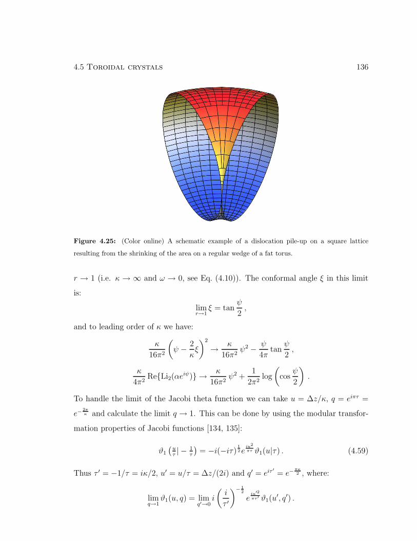
4.5 Toroidal crystals 136
Figure 4.25: (Color online) A schematic example of a dislocation pile-up on a square lattice
resulting from the shrinking of the area on a regular wedge of a fat torus.
r → 1 (i.e. κ → ∞ and ω → 0, see Eq. (4.10)). The conformal angle ξ in this limit
is:
limr→1
ξ = tanψ
2,
and to leading order of κ we have:
κ
16π2
(
ψ − 2
κξ
)2
→ κ
16π2ψ2 − ψ
4πtan
ψ
2,
κ
4π2ReLi2(αe
iψ) → κ
16π2ψ2 +
1
2π2log
(
cosψ
2
)
.
To handle the limit of the Jacobi theta function we can take u = ∆z/κ, q = eiπτ =
e−2πκ and calculate the limit q → 1. This can be done by using the modular transfor-
mation properties of Jacobi functions [134, 135]:
ϑ1
(
uτ| − 1
τ
)
= −i(−iτ) 12e
iu2
πτ ϑ1(u|τ) . (4.59)
Thus τ ′ = −1/τ = iκ/2, u′ = u/τ = ∆z/(2i) and q′ = eiτ′
= e−πκ2 , where:
limq→1
ϑ1(u, q) = limq′→0
i
(
i
τ ′
)− 12
eiu′2
πτ ′ ϑ1(u′, q′) .

4.5 Toroidal crystals 137
This is easily evaluated by means of the expansion:
ϑ1(u, q) = 2q14 sin u+ o
(
q94
)
.
Taking the logarithm and neglecting irrelevant constant terms, we obtain:
log
∣
∣
∣
∣
∣
ϑ1
(
z − z′
κ
∣
∣
∣
∣
∣
2i
κ
)∣
∣
∣
∣
∣
∼ log
∣
∣
∣
∣
sinh
(
z − z′
2
)∣
∣
∣
∣
,
which finally leads to:
GL(ψ, φ, ψ′, φ′) ∼ − ψ′
4π2tan
ψ′
2+
1
2πlog
∣
∣
∣
∣
sinh
(
z − z′
2
)∣
∣
∣
∣
(4.60)
with z = tan(ψ/2)+ iφ. With the Green function in hand, we can calculate the effect
of the curvature singularity at ψ = π on the distribution of defects. Let b be the
Burgers vector density of the dislocation cloud. Hereafter we work in a local frame,
so that:
b = bψgψ + bφgφ , (4.61)
with gi = ∂iR a basis vector in the tangent plane of the torus. R is a three-
dimensional surface vector parameterizing the torus and its Cartesian components
are given in Eq. (4.1). The quantity b has to be such that:
∫
D
d2x b(x) = bD ,
with bD the total Burger’s vector in a generic domainD. Because on a closed manifold
dislocation lines cannot terminate on the boundary, extending the integration to the
whole torus we have:∫
d2x b(x) = 0 . (4.62)
Since the basis vectors gi in Eq. (4.61) have the dimension of length, contravariant
coordinates bi have dimensions of an inverse area. Assuming all defects to be paired
in the form of dislocations (i.e. qi = 0 everywhere), the total energy of the crystal
reads:
F =1
2Y
∫
d2xΓ2(x) + ǫd
∫
d2x |b(x)|2 , (4.63)

4.5 Toroidal crystals 138
where ǫd is the dislocation core energy and
|b|2 = gijbibj = gψψ(b
ψ)2 + gφφ(bφ)2 .
The function Γ(x) encoding the elastic stress due to the curvature and the screening
contribution of the dislocation cloud obeys
1
Y∆gΓ(x) = ǫik∇ib
k(x) −K(x) , (4.64)
where ∇i is the usual covariant derivative along the coordinate-direction i and ǫik is
the Levi-Civita antisymmetric tensor on the torus:
ǫψφ = −ǫφψ =√g , ǫji = gikǫ
jk .
The stress function Γ(x) can be expressed in the form Γ(x) = Γd(ψ, φ) − Γs(ψ) with
Γs(ψ)
Y= log
[
1
2(1 + cosψ)
]
+ 1 , (4.65a)
Γs(ψ, φ)
Y=
∫
d2y ǫik∇ibk(y)GL(x,y) . (4.65b)
Taking advantage of the closeness of the torus we can integrate Eq. (4.65b) by parts
so that:Γd(ψ, φ)
Y= −
∫
d2y ǫikbk(y)∂iGL(x,y) . (4.66)
Now we want reduce the integral term in Eq. (4.66) to a more friendly functional
of b, suitable for a variational approach. Given the azimuthal symmetry we assume
that all dislocations are aligned along b = bφgφ. Even though not necessarily true,
we argue this to be a reasonable work hypothesis as well as a solid starting point to
capture the essential physics of the fat limit. In this case Γd(ψ, φ) = Γd(ψ) can be
recast in the form
Γd(ψ)
Y=
1
2π
∫ π
−πdψ′√g bφ(ψ′) [ψ′ + sinψ′ + π sgn(ψ − ψ′)] . (4.67)

4.5 Toroidal crystals 139
Substituting Eq. (4.67) and (4.65a) in Eq. (4.63) and minimizing with respect to bφ
we can now write the variational equation:
4ǫdR2(1 + cosψ)2bφ(ψ) +
∫ π
−πdψ
√g Γd(ψ
′) sgn(ψ − ψ′)
=
∫ π
−πdψ
√g Γs(ψ
′) sgn(ψ − ψ′) . (4.68)
By inverting the order of integration in the integral on the right hand side, Eq (4.68)
can be expressed in the form of a Fredholm equation of the second kind:
λB(ψ) −∫ π
−πdψ′B(ψ′)K(ψ, ψ′) = f(ψ) , (4.69)
where λ = ǫd/(Y R2), B(ψ) = R2(1 + cosψ)2bφ(ψ) and the kernel K(ψ, ψ′) is given
by:
K(ψ, ψ′) =1
4(1 + cosψ′)
π−1(ψ′ + sinψ′)(ψ + sinψ)
+ |ψ − ψ′| + 2 cosψ + ψ′
2sin
|ψ − ψ′|2
. (4.70)
The function f(ψ) on the right hand side of Eq. (4.69) is given by:
f(ψ) = −1
4
∫ ψ
−ψdψ′ (1 + cosψ′) Γs(ψ
′)
=1
2
[log 2(1 + cosψ) − 2] sinψ − 2 Cl2(ψ + π)
(4.71)
where Cl2 is the Clausen function (see Ref. [168], pp. 1005-1006) defined as:
Cl2(x) = −∫ x
0
dx log
(
2 sint
2
)
=∞∑
k=1
sin kx
k2.
As previously noted the dislocation core energy is ǫd is much smaller than the
elastic energy scale Y R2. Eq (4.69) is then suitable to be solved in powers of the
dimensionless number λ:
B(ψ) = B0(ψ) + λB1(ψ) + λ2B2(ψ) + · · ·

4.5 Toroidal crystals 140
Figure 4.26: (Color online) The Burgers vector component b(ψ) for different choices of λ.
The corrections to the zero-order term B0(ψ) can be calculated recursively by solving
a set of Fredholm equations of the first kind:
Bk−1(ψ) =
∫ π
−πdψ′Bk(ψ)K(ψ, ψ′) k ≥ 1 .
The function B0(ψ) associated with the Burgers vector density of the dislocation cloud
in the limit λ → 0, on the other hand, can be calculated directly from Eq. (4.64) by
setting the effective topological charge density on the right hand side to zero:
ǫik∇ibk(x) −K(x) = 0 . (4.72)
For a torus of revolution the only nonzero Christoffel symbols are
Γφφψ = Γφψφ = − R2 sinψ
R1 +R2 cosψ,
Γψφφ = R−12 sinψ(R1 +R2 cosψ) .
Since bψ = 0 by assumption, the first term in Eq. (4.72) can be expressed as:
ǫik∇ibk = ǫψφ(∂ψb
φ + Γφψφbφ) + ǫφψΓψφφb
φ
= (1 + cosψ)∂ψbφ − 2 sinψ bφ ,

4.5 Toroidal crystals 141
and Eq. (4.72) becomes an ordinary differential equation
∂ψbφ − 2 sinψ
1 + cosψbφ =
cosψ
R2(1 + cosψ)2, (4.73)
whose solution is given by
bφ =sinψ
R2(1 + cosψ)2, (4.74)
so that B0(ψ) = sinψ. The Burgers vector density bφ obtained by a numerical solution
of Eq. (4.69) is shown in Fig. 4.26 for different values of λ. The Burgers vector density
is measured in units of R−2. The function bφ has cubic singularities at ψ = ±π and
is approximately zero on the outside of the torus. The solid blue curve in Fig. 4.26
represents the zeroth order solution of Eq.(4.74).
Now, in the theory of dislocation mediated melting a system at the solid liquid
phase boundary is described as a crystalline solid saturated with dislocations. In
three-dimensions, in particular, there is a strong experimental evidence of the exis-
tence of a critical dislocation density at the melting point ρ(Tm) ≈ 0.6b−2 where b is
the length of the length of the smallest perfect-dislocation Burgers vector [169]. Sev-
eral theoretical works have motivated this evidence both for three-dimensional solids
and vortex lattices in super conductors [167]. On the other hand, given the existence
of such a critical density, its value can be empirically used to determine whether a
system is in a solid or liquid-like phase in the same spirit as the Lindemann criterion.
With this goal in mind we can calculate the dislocation density by requiring |b| = ρa
with ρ the density of single lattice spacing dislocations. This yields:
ρ(ψ, V )a2 = 2π
(√3
2V
)− 12∣
∣
∣
∣
tanψ
2
∣
∣
∣
∣
+ o(λ) (4.75)
Solving ρ(ψ, V )a2 = 0.6 as a function of ψ and V we obtain the diagram of Fig. 4.27.
As expected the inside of the torus contains an amorphous region whose angular size
decreases with the number of vertices V as a consequence of the reduction of the
lattice spacing.

4.A Cluster optimization via Tapping 142
Figure 4.27: (Color online) Phase diagram for curvature driven amorphization. The inside of the
torus contains an amorphous region whose angular size decreases with the number of vertices V as
a consequence of the reduction of the lattice spacing.
Appendix 4.A Cluster optimization via Tapping
The Tapping Algorithm (TA) is a hybrid algorithm designed to find the optimal
crystalline structure of particle systems constrained to lie on a curved surface and in-
teracting with a long range potential of the form Uij = 1/|ri−rj|s. Hybrid algorithms,
such as Basin-Hopping [170] and Minima-Hopping [171], have been successfully em-
ployed throughout the years to predict the crystalline structure of molecular clusters
and proteins. In general they combine fast local minimizations with global moves
whose goal is to release the system from the local minimum it is confined at the end
of a local minimization step.
A typical hybrid optimization routine can be summarized in the following two
steps: 1 ) after all the independent variables have been randomly initialized, a local
optimization is performed and a local minimum x is determined; 2 ) from x a new
configuration y is constructed by applying a global (generally stochastic) move. The
new configuration y is then used as starting point for a new local optimization step.
The two steps are iterated until a stopping criterion is satisfied. The goal is thus

4.A Cluster optimization via Tapping 143
to explore the largest possible number of local minima and avoid visiting the same
minimum too often.
The crucial point in designing an effective hybrid algorithm is clearly the choice of
the global move. There is no general rule to identify a successful global transformation
x→ y and physical intuition and prior experience are typically the only guidelines. In
the case of Basin-Hopping, for instance, the global transformation consists in a Monte
Carlo move in which all the particles of the system are randomly displaced in order
to construct a new initial configuration from which a new trial minimum is obtained.
The step is accepted with probability exp(−β∆V ), where ∆V is the energy difference
between the new and previous minimum and β is an inverse temperature adjusted
to obtain a 50% acceptance ratio. In the case of Minima-Hopping the escape step
is performed by a short Molecular Dynamics simulation by assigning the particles a
fixed kinetic energy.
The global move adopted in TA is inspired by the process of close packing of spher-
ical objects by tapping and is motivated by the well established role of topological
defects in determining the order of two-dimensional non-Euclidean crystals as well as
the picture of the potential energy surface (PES) of such systems as a multi-funnel
landscape. Consider a system of say spherical objects confined in a two-dimensional
box with an initial disordered configuration. A common way to bias the system to-
ward a close-packed configuration is to provide it kinetic energy by gently tapping
the box. If the system is populated by locally ordered regions (i.e. grains) separated
by clusters of defects, the primary effect of tapping is to produce a glide of defects
inside the crystals with a subsequent rearrangement of grains. This mechanism can
be reproduced numerically in the following way. The algorithm starts with a random
distribution of particles and rapidly quenches the system by performing a fast local
minimization. Once particles are trapped in a local minimum, defects are identified
by a Delaunay triangulation of the lattice. Then the system is tapped by adding to
the defect positions a random displacement. The magnitude of the displacement is

4.A Cluster optimization via Tapping 144
given by the typical spacing associated with the particles number times a factor λ
which represents the tapping strength. This factor is initially set to 10−3. After de-
fects have been moved a new local minimization is performed in order to construct the
trial configuration y. The energy of this configuration is compared with the energy of
the previous minimum and the move is accepted if their difference is larger than some
tolerance factor ǫE . If, on the other hand, the energy difference is smaller than ǫE ,
the system has relaxed again to the same minimum. In this case the tapping strength
is increased of a factor 10 and the process is repeated until the system successfully
hops to a new minimum. The tapping strength λ is then set to its initial value. The
process is iterated until the rate of discovery of new global minima drops below some
threshold value or a maximum number of iterations is reached.
In the current implementation of the algorithm, the local minimization step is
performed using the Fletcher-Reeves conjugate gradient algorithm [172]. Analytic
expressions for the energy gradient and the Hessian matrix are coded in the program
in order to reduce the number of evaluations of the objective function during the
relaxation step to one single event. The Delaunay triangulation is calculated via
the Dwyer’s divide and conquer algorithm with alternate cuts [173], which runs in
O(N log logN) time, making the identification of the defects particularly fast.
The main difference between TA and other hybrid algorithms (including Basin-
Hopping) is that the escape move consists of adaptive displacements of defects only,
rather than of the entire system. In the case of non-Euclidean crystals, where the con-
formation of the energy landscape is subtly related to the arrangement of topological
defects, this mechanism is believed to explore the PES more accurately. In systems
as Lennard-Jones clusters or spin-glasses, the PES is characterized by an exponential
number of local minima separated by energy barriers. For this reason the majority
of the algorithms are specifically designed to allow the system to overcome a barrier
by providing it a significant amount of energy. If the energy landscape, however, is
characterized by the presence of multiple narrow funnels, as believed in this case, the

4.B The doubly periodic Green function 145
Figure 4.28: Possible pathways is a funneled landscape.
previous methods become ineffective. A funnel represents the basin of attraction of a
given local minimum. If the global minimum is also located at the bottom of a fun-
nel, an algorithm that is attempting to locate it via a sequence of local minimization
steps has a chance to find it exclusively by starting from a configuration already at
the muzzle of the funnel. Such possibility, however, is ruled out if all the particles are
displaced simultaneously during the escape move and the system is abruptly moved
to a completely different place in the energy landscape. On the other hand, by adap-
tively tapping the defects it is possible to achieve a much finer inspection of the PES
and possibly locate the funnel associated with the global minimum.
Appendix 4.B The doubly periodic Green func-
tion
In this Appendix I provide a step-by-step proof of Eq. (4.19). Starting from Eq.
(4.18) we can notice that all sinusoidal terms cancel when the summation is carried

4.B The doubly periodic Green function 146
out. Eq. (4.18) becomes then:
G0(x,y) = − 1
p1p2
∑
(n,m)6=(0,0)
cosλn(x− ξ) cosµm(y − η)
λ2n + µ2
m
= − 2
p1p2
∞∑
m=1
cos 2πmp2
(y − η)(
2πmp2
)2 +∞∑
n=1
∞∑
m=−∞
cos 2πnp1
(x− ξ) cos 2πmp2
(y − η)(
2πnp1
)2
+(
2πmp2
)2
. (4.76)
An equivalent expression can be obtained by isolating the m = 0 contribution in the
sum rather then the n = 0 one. The first sum in Eq. (4.76) can be evaluated easily
by using:∞∑
k=1
cos kx
k2=π2
6− π|x|
2+x2
4(4.77)
Thus we have:
H(y−η) = − 2
p1p2
∞∑
m=1
cos 2πmp2
(y − η)
(2πmp2
)2= − 1
2 p1p2
(
p22
6− p2|y − η| + |y − η|2
)
(4.78)
The second sum in Eq. (4.76) can be evaluated with the help of the Poisson summa-
tion formula in the form:
∞∑
m=−∞f(m) cos pm =
∞∑
k=−∞
∫ ∞
−∞dt f(t) cos(2kπ + p) t (4.79)
In particular if we choose:
f(m) =1
(
2πnp1
)2
+(
2πmp2
)2 p =2π
p2
(y − η)
we can write the second sum in the (4.76) as:
K(x− ξ, y − η) = − 2
p1p2
∞∑
n=1
cos2πn
p1(x− ξ)
∞∑
m=−∞
cos 2πmp2
(y − η)(
2πnp1
)2
+(
2πmp2
)2
= − 2
p1p2
∞∑
n=1
cos2πn
p1(x− ξ)
∞∑
k=−∞
∫ ∞
−∞dt
cos(2πk + p) t(
2πnp1
)2
+(
2πtp2
)2 (4.80)

4.B The doubly periodic Green function 147
The integral can be easily done by remembering:
∫ ∞
0
dxcosωx
a2 + x2=
π
2ae−ωa
and then:
∫ ∞
−∞dt
cos(2πk + p) t(
2πnp1
)2
+(
2πtp2
)2 =p1p2
4πnexp
[
−(
2πn
p1
)
|p2k + y − η|]
Therefore, Eq. (4.80) becomes:
K(x− ξ, y − η) = − 1
2π
∞∑
k=−∞
∞∑
n=1
e− 2πn
p1|p2k+y−η|
ncos
2πn
p1(x− ξ) (4.81)
The sum in n can be calculated by taking into account:
∞∑
n=1
e−2πnx
ncos(2πny) = − log |1 − e−z| (4.82)
where z is the complex number:
z = 2π(x± iy)
with x > 0 and an arbitrary choice of the sign. To use Eq. (4.82) is convenient to
separate positive and negative k in Eq. (4.81):
−2πK(x− ξ, y − η) =
∞∑
n=1
e− 2πn
p1|y−η|
ncos
2πn
p1(x− ξ)
+
∞∑
k=1
∞∑
n=1
e− 2πn
p1|p2k+y−η|
ncos
2πn
p1(x− ξ)
+∞∑
k=1
∞∑
n=1
e− 2πn
p1|−p2k+y−η|
ncos
2πn
p1(x− ξ) (4.83)
Now, because y, η ∈ [0, p2] we have y − η ∈ [−p2, p2] which allow us the write the
modulus in the following way:
|p2k + (y − η)| = p2k + (y − η)
| − p2k + (y − η)| = p2k − (y − η)
∀k ≥ 1

4.B The doubly periodic Green function 148
Introducing the complex variable:
σ±k = 2π(a±k ∓ ibk)
with:
a±k =p2k ± (y − η)
p1bk =
x− ξ
p1
and using Eq. (4.82), we can rewrite Eq. (4.83) as:
2πK(x− ξ, y − η) = log∣
∣1 − e−σ0∣
∣ +
∞∑
k=1
log∣
∣
∣1 − e−σ
+k − e−σ
−
k + e−(σ+k
+σ−k
)∣
∣
∣
= log∣
∣
∣1 − e
2πip1
(z−ζ)∣
∣
∣+
∞∑
k=1
log
∣
∣
∣
∣
1 − 2q2k cos2π
p1(z − ζ) + q4k
∣
∣
∣
∣
(4.84)
having called:
z = x+ iy
ζ = ξ + iηand q = e
−πp2p1
The second term in Eq. (4.83) can be expressed in terms of the Jacobi theta function
ϑ1(u, q) defined as:
ϑ1(u, q) = 2q14 sin u
∞∏
n=1
(
1 − 2q2n cos 2u+ q4n) (
1 − q2n)
Another useful relation can be obtain by taking the derivative of ϑ1(u, q) with respect
to u:
limu→0
ϑ1(u, q)
sin u= lim
u→0
ϑ′1(u, q)
cosu= ϑ′1(0, q)
So it is easy to evaluate:
ϑ′1(0, q) = limu→0
ϑ(u, q)
sin u= 2q
1
4
∞∏
k=1
(
1 − 2q2k + q4k) (
1 − q2k)
= 2q1
4
∞∏
k=1
(
1 − q2k)3
(4.85)
In this way we can express:
∞∏
k=1
(1 − 2q2k cos 2u+ q4k) =1
(2q14 )
23 sin u
[
ϑ1(u, q)
ϑ′ 13
1 (0, q)
]

4.C The stress function Γs(x) 149
Taking:
u =π
p1(z − ζ)
and replacing in Eq. (4.84) we obtain:
2πK(x− ξ, y − η) = log |1 − e2iu| + log
∣
∣
∣
∣
∣
ϑ1(u, q)
ϑ′ 13
1 (0, q)
∣
∣
∣
∣
∣
− log∣
∣
∣(2q
14 )
23 sin u
∣
∣
∣
=log 2
3+π
6
p2
p1
− π
p1
|y − η| + log
∣
∣
∣
∣
∣
ϑ1(u, q)
ϑ′ 13
1 (0, q)
∣
∣
∣
∣
∣
(4.86)
having used the fact that:
log∣
∣1 − e2iu∣
∣ = log |eiu| + log |2i sinu|
log∣
∣
∣(2q
14 )
23 sin u
∣
∣
∣=
2
3log 2 − π
6
p2
p1+ log | sin u|
Combining Eq. (4.86) with Eq. (4.78) we finally obtain:
G0(x,y) = H(y − η) +K(x− ξ, y − η)
=log 2
6π− 1
2 p1p2|y − η|2 +
1
2πlog
∣
∣
∣
∣
∣
ϑ1(u, q)
ϑ′ 13
1 (0, q)
∣
∣
∣
∣
∣
(4.87)
An alternative notation frequently used for the Jacobi theta function is:
ϑ1(u|τ) = ϑ(u, q) q = eiπτ
adopting this choice we can write the Green function in the final form:
G0(x,y) =log 2
6π− 1
2 p1p2|y − η|2 +
1
2πlog
∣
∣
∣
∣
∣
∣
ϑ1(z−ζp1/π
| ip2p1
)
ϑ′ 13
1 (0| ip2p1
)
∣
∣
∣
∣
∣
∣
(4.88)
Appendix 4.C The stress function Γs(x)
To calculate the stress function Γs(x), it is convenient to start from:
Γs(x) =
∫
d2y K(y)[G0(x,y) − 〈G0(· ,y)〉] = Γs,1(x) − Γs,2

4.C The stress function Γs(x) 150
where we called:
Γs,1(x) =
∫
d2y K(y)G0(x,y) Γs,2 =
∫
d2y K(y) 〈G0(· ,y)〉
The calculation of these integrals can be made more straightforward by keeping the
Green function in the form (4.76). We have then:
Γs,1 = − 1
p1p2
∑
(n,m)6=(0,0)
1
λ2n + µ2
m
∫ π
−πdψ′ cosψ′ cosλn(ξ − ξ′)
∫ π
−πdφ′ cosµm(φ− φ′)
The integral in φ′ is non-zero only for m = 0:∫ π
−πdφ′ cosµm(φ− φ′) =
∫ π
−πdφ′ cosm(φ− φ′) = 2πδm,0 m = 0, ±1, ±2 . . .
Then we have:
Γs,1(x) = − 2π
p1p2
∑
n 6=0
λ−2n
∫ π
−πdψ′ cosψ′ cosλn(ξ − ξ′)
= − 2
p1
( p1
2π
)2∫ π
−πdψ′ cosψ′
∞∑
n=1
cos 2πnp1
(ξ − ξ′)
n2
Using Eq. (4.77) we can rewrite:
Γs,1(x) = −p1
12
∫ π
−πdψ′ cosψ′
+1
2
∫ π
−πdψ′ cosψ′ |ξ − ξ′| − 1
2p1
∫ π
−πdψ′ cosψ′ |ξ − ξ|2 (4.89)
The first integral is zero. Two calculate the second integral we can take
|ξ − ξ′| =
ξ − ξ′ if ξ′ < ξ → ψ′ < ψ
ξ′ − ξ if ξ′ > ξ → ψ′ > ψ
Thus:
Γs,11 =
∫ π
−πdψ′ cosψ′ |ξ − ξ′| = ξ
∫ ψ
−ψdψ′ cosψ′ + 2
∫ π
ψ
dψ′ cosψ′ξ′
= ξ(ψ)[
sinψ′]ψ
−ψ+ 2[
ξ(ψ′) sinψ′ + log(r + cosψ′)]π
ψ
= 2 log
(
r − 1
r + cosψ
)
4.C The stress function Γs(x) 151
where the second line has been obtained by a simple integration by parts:∫
dψ cosψ ξ = ξ sinψ −∫
dψsinψ
r + cosψ= ξ sinψ + log(r + cosψ)
To calculate the third integral in Eq. (4.89) we can expand the square and use the
fact that the function ξ is odd in ψ. Then:∫ π
−πdψ′ cosψ′ |ξ − ξ′|2 =
∫ π
−πdψ′ cosψ′ξ′2
The integral on the right hand side can be now calculated by parts:
Γs,12 =
∫ π
−πdψ′ cosψ′ ξ′2
=[
sinψ′ ξ2]π
−π− 2
∫ π
−πdψ′ sinψ′ ξ′
dξ′
dψ′
= −2
∫ 12πκ
− 1
2πκ
dξ′ sinψ′ ξ′
having considered:
ξ(π) = −ξ(−π) =
∫ π
0
dψ
r + cosψ=
1
2πκ
We need now to express the quantity sin φ figuring in the integral as a function of ξ.
Inverting Eq. (4.9) we obtain:
tanψ
2=
1
ωtan
ξ
κ
Then:
sinψ =2 tan ψ
2
1 + tan2 ψ2
=2ω tan ξ
κ
ω2 + tan2 ξκ
Replacing, the integral will become:
Γs,12 = −2
∫ 1
2πκ
− 12πκ
dξ′2ωξ′ tan ξ′
κ
ω2 + tan2 ξ′
κ
= −4ωκ2
∫ π2
−π2
dyy tan y
ω2 + tan2 y
having called y = ξ/κ ∈ [−π/2, π/2]. The integrand can be simplified furtherly by
considering:
tan y
ω2 + tan2 y=
sin y cos y
sin2 y + ω2 cos2 y=
sin y cos y
1 + (ω2 − 1) cos2 y

4.C The stress function Γs(x) 152
which taking:
sin y cos y =1
2sin 2y cos2 y =
1
2(1 + cos 2y)
allows us to write:
Γs,12 = −4ωκ2
∫ π2
−π2
dyy sin 2y
(ω2 + 1) + (ω2 − 1) cos 2y= −ωκ2
∫ π
−πdx
x sin x
α + β cos x
where we called x = 2π ∈ [−π, π], α = ω2 + 1 and β = ω2 − 1. The right hand side
can be now easily integrated by parts:
Γs,12 = −ωκ2
β
[
−x log
(
1 +β
αcosx
)]π
−π− ωκ2
β
∫ π
−πdx log
(
1 +β
αcosx
)
=2πωκ2
βlog
(
1 − β
α
)
− 2πωκ2
βlog
1 +√
1 − β2
α2
2
=2πωκ2
βlog
2(1 − βα)
1 +√
1 − β2
α2
which expressing all the parameters in term of the aspect ratio r gives finally:
Γs,12 = −2πκ log
[
2(r + 1)
r +√r2 − 1
]
Combining Γs,11 and Γs,12 we obtain:
Γs,1 =1
2Γs,11 −
1
2p1
Γs,12 = log
[
2(r2 − 1)
(r + cosψ)(r +√r2 − 1)
]
To complete the calculation of Γs we need now to calculate:
Γs,2 =
∫
d2y 〈G(· ,y)〉K(y) (4.90)
Rather then calculate the function 〈G(· ,y)〉 and integrate it, it is more convenient
to invert the order of the two integrals and using the result we just obtained for the
Γs,1. Explicitly:
AΓs,2 =
∫
d2xK(x)
∫
d2y G0(x,y)
=
∫
d2y
∫
d2xK(x)G0(x,y) =
∫
d2y Γs,1(y)

4.C The stress function Γs(x) 153
Now, calling:
f(r) =2(r2 − 1)
r +√r2 − 1
the Γs,2 integral becomes:
AΓs,2 = log f(r)
∫
d2y −∫
dψ′ dφ′√g′ log(r + cosφ′)
= A log f(r) − 2πR1R2
∫ π
−πdψ′ log(r + cosφ′)
−2πR22
∫ π
−πdψ′ cosψ′ log(r + cosψ′)
The first integral is of the form:∫ π
−πdx log(1 + a cosx) = 2π log
(
1 +√
1 − a2
2
)
|a|2 < 1
and can thus immediately calculated by choosing a = r−1:
Γs,21 =
∫ π
−πdψ′ log(r + cosψ′) = 2π log
(
r +√r2 − 1
2
)
The second integral can be related to an integral of the form:∫ π
0
dx cosnx log(1 − 2a cosx+ a2) = −πan
n|a|2 < 1
by choosing n = 1 and a = −r +√r2 − 1. Thus we have:
Γs,22 = 2π(
r −√r2 − 1
)
Combining Γs,21 and Γs,22 we find:
Γs,2 = log f(r) − 2π
A
(
R1R2Γs,21 +R22Γs,22
)
= log
[
4(r2 − 1)
(r +√r2 − 1)2
]
− r −√r2 − 1
r
Merging the two main contributions Γs,1 and Γs,2 we can finally write the screening
function Γs in the form:
Γs(ψ) = log
[
r +√r2 − 1
2(r + cosψ)
]
+r −
√r2 − 1
r(4.91)

4.D The function 〈G0(x, ·)〉 154
Appendix 4.D The function 〈G0(x, ·)〉
We proceed now to the calculation of the function 〈G0(x, · )〉 figuring in the expression
of the elastic free energy.Again it is convenient to express the Green function G0 in
the form of a series rather than in the more compact form (4.88):
A 〈G0(x, · )〉 = − 1
p1p2
∑
(n,m)6=(0,0)
1
λ2n + λ2
m
∫ π
−πdψ′√g′ cosλm(ξ − ξ′)
∫ π
−πdφ′ cosµm(φ− φ′)
As in the previous section, the only non-zero contribution from the sum in m is given
by m = 0. Summing over n we have then:
A 〈G0(x, · )〉 = −π6R1R2 +
1
2
∫ π
−πdψ′√g′ |ξ − ξ′| − 1
2p1
∫ π
−πdψ′√g′ |ξ − ξ′|2
The expanding the absolute value as in the previous section, we can write the first
integral in the form:
I1 =
∫ π
−πdψ′√g′ |ξ − ξ′|
= ξ
∫ ψ
−ψdψ′√g′ + 2
∫ π
ψ
dψ′√g′ ξ′
= 2R1R2ψξ + 2R22ξ sinψ + 2
∫ π
ψ
dψ′√g′ ξ′ (4.92)
The integral last integral can be simplified integrating by parts:
I11 =
∫ π
ψ
dψ′√g′ ξ′
= R1R2
∫ π
ψ
dψ′ ξ′ +R22
∫ π
ψ
dψ′ cosψ′ξ′
= R22 log
(
r − 1
r + cosψ
)
− R22ξ sinψ +R1R2
∫ π
ψ
dψ′ ξ′
The last integral can be easily calculated by expanding the ξ function in Fourier
harmonics. The conformal angle ξ is an odd function of ξ of period 2π, thus admit a

4.D The function 〈G0(x, ·)〉 155
Fourier series in the canonical form:
ξ(ψ) =
∞∑
n=1
bn sin(nψ) (4.93)
The Fourier coefficient bn is given by:
πbn =
∫ π
−πdψ sinnψ ξ(ψ) = −
[
ξ(ψ)
ncosnψ
]π
−π+
1
n
∫ π
−πdψ
cosnψ
r + cosψ
= −κn
cosnπ +1
n
∫ π
−πdψ
cos nψ
r + cosψ
The last integral can be reconducted to the form:∫ ψ
0
dxcos nx
1 + a cosx=
π√1 − a2
(√
1 − a2 − 1
a
)n
|a|2 < 1
by taking a = r−1. Then:∫ π
−πdψ
cosnψ
r + cosψ=
2√r2 − 1
(√r2 − 1 − r
)n
having called α =√r2 − 1 − r. The Fourier coefficient bn is then given by:
bn =κ
n(αn − cos nπ) =
κ
n[αn − (−1)n] (4.94)
Integrating the Fourier harmonics term by term we have:
I12 =
∫ π
ψ
dψ′ ξ(ψ′) =
∞∑
n=1
bn
∫ π
ψ
dψ′ sinnψ′ =
∞∑
n=1
bnn
(cosnψ − cosnπ)
= κ
∞∑
n=1
αn
n2cosnψ − κ
∞∑
n=1
(−1)n
n2αn − κ
∞∑
n=1
(−1)n
n2cosnψ + κ
∞∑
n=1
1
n2
=1
4κ(π2 − ψ2) − κLi2(−α) + κReLi2(αe
iψ)
where Re · stands for the real part. For the last step, we used:
∞∑
n=1
(−1)n
n2cosnx =
∞∑
n=1
cosnπ cosnx
n2
=1
2
∞∑
n=1
cosn|π + x|n2
+1
2
∞∑
n=1
cosn|π − x|n2
=1
4x2 − 1
12π2

4.D The function 〈G0(x, ·)〉 156
together with the notorious Euler identity:
ζ(2) =
∞∑
n=1
1
n2=π2
6
and the definition of dilogarithm:
Li2(z) =∞∑
n=1
zn
n2
Replacing I11 and I12 in (4.92) we can write:
I1 = 2R1R2ψξ + 2R22 log
(
r − 1
r + cosψ
)
+1
2κR1R2(π
2 − ψ2)
− 2κR1R2 Li2(−α) + 2κR1R2 ReLi2(αeiψ) (4.95)
To accomplish the calculation of the 〈G0(· ,x)〉 we are left with the integral:
I2 =
∫ π
−πdψ′√g′ |ξ − ξ′|2
= R1R2
∫ π
−πdψ′ |ξ − ξ′|2 +R2
2
∫ π
−πdψ′ cosψ′ |ξ − ξ′|2
The second integral in I2 has already been calculated in the previous section and is:
I22 = Γs,12 = −2πκ log
[
2(r2 + 1)
r +√r2 − 1
]
To calculate the first integral we can write:
I21 =
∫ π
−πdψ′ |ξ − ξ′|2 = 2πξ2 +
∫ π
−πdψ′ ξ′2
To calculate the integral of ξ2 we can recall that, letting f(x) being a square-integrable
function with Fourier series:
f(x) =a0
2+
∞∑
n=1
(an cosnx+ bn sin nx)
the Parseval’s identity requires:
1
π
∫ π
−πdx f 2(x) =
a20
2+
∞∑
n=1
(a2n + b2n)

4.E The stress function Γ(x) 157
which in our case reads:
∫ π
−πdψ′ ξ′2 = π
∞∑
n=1
b2n = πκ2
[ ∞∑
n=1
α2n
n2+
∞∑
n=1
1
n2− 2
∞∑
n=1
(−1)n
n2αn
]
= πκ2
[
Li2(α2) +
π2
6− 2 Li2(−α)
]
= πκ2
[
2 Li2(α2) +
π2
6
]
where for the last step we used the Euler dilogarithmic ladder:
Li2(z) + Li2(−z) =1
2Li2(z
2) (4.96)
Recombining the integrals I1 and I2 and we obtain finally:
〈G0(x, · )〉 = − κ
16π2
(
ψ − 2
κξ
)2
− κ
8π2Li2(α
2)
+κ
4π2ReLi2(αe
iψ) +1
4π2rlog
[
2(r2 − 1)
(r + cosψ)(r +√r2 − 1)
]
(4.97)
Appendix 4.E The stress function Γ(x)
We are finally ready to combine the results of the previous two sections and write the
complete expression of the energy density Γ. Using (4.88), (4.97) in (4.47) we have:
Γ(x)
Y=π
3
N∑
k=1
qkΓd(x,xk) − Γs(x) (4.98)
Calling z = ξ + iφ the defects contribution Γd to the energy is given by:
Γd(x,xk) =κ
16π2
(
ψk −2
κξk
)2
− 1
4π2κ(φ− φk)
2
+1
4π2rlog (r + cosψk) −
κ
4π2ReLi2(αe
iψk)
+1
2πlog
∣
∣
∣
∣
ϑ1
(
z − zkκ
∣
∣
∣
∣
2i
κ
)∣
∣
∣
∣
(4.99)
where all the constants figuring in (4.97) and (4.88) are canceled in virtue of the
charge neutrality condition.

Chapter 5
Conclusion and discussion
In this article we reviewed some of the most recent progresses toward understanding
the ground state properties of two-dimensional ordered phases on substrate of non-
zero Gaussian curvature. The latter represents a broad class of systems comprising
materials as different as viral capsids and carbon nanotori. The geometry of the sub-
strate give arise to novel defective structures that would be energetically prohibitive
in the ground state of conventional flat systems. Defects might appear in curved space
either because required by the topology of the underlying substrate (as in the case
of spherical crystals and nematics) or because favored by the curvature itself. The
latter has indeed the property of coupling with the topological charge of the defects
leading to an overall reduction of the elastic stress.
On the material science side, non-Euclidean systems provides a promising route
to constructing arrays of nanoparticles is via the chemical functionalization of topo-
logical defects created on the surface of the particles by coating them with an ordered
monolayer. Candidates for such coatings include triblock coplymers, gemini lipids,
metallic or semiconducting nanorods and conventional liquid crystal compounds. If
the induced order is vector-like or striped then there must necessarily be two defec-
tive regions corresponding to the bald spots exhibited by a combed sphere or the
source and sink of fluid flow confined to a sphere. Not only are the defects physically

159
Figure 5.1: (Color online) (Left) Idealized drawing of a side and top view and of a rippled gold
nanoparticle showing the two polar defects that must exist to allow the alternation of concentric
rings. (Right) TEM images of a chain obtained when 11-mercaptoundecanoic acid functionalized
nanoparticles are reacted with a water phase containing divalent 1,6-diaminohexane in a two-phase
reaction. Scale bar 50 nm. From [174].
and mathematically distinguished, since the condensed matter order vanishes there,
but it also turns out that chemical processes can detect the defects and insert linker
molecules at the precise defect locations. This creates the possibility of efficiently
making functionalized nanoparticles with a precise valence and corresponding direc-
tional bonding. The nanoparticles themselves can then be linked into well-defined
two and three dimensional arrays. Control over the valence and the geometry of the
directional bonding can be achieved by varying the nature of the ordered monolayer.
This scheme has been demonstrated recently in the work of DeVries et al. [174]
in which gold nanoparticles are coated with two species of naturally phase separating
ligands (see Fig. 5.1). Phase separation on the spherical gold surface translates to a
striped arrangement of alternating ligands. Such a spherical smectic has topological
defects at the north and south pole of the nanopartcle. These may be functionalized
by attaching thiol-based linker molecules at the defects via place-exchange reactions.
This creates a divalent gold nanoparticle with directional bonds 180 degrees apart.
These in turn can be linked to create polymers and free-standing films.

Bibliography
[1] J. D’Alembert, Essai d’une nouvelle theorie de la resistance des fluides (1752).
[2] J. D. Bernal, Nature 185, 68 (1960).
[3] J. D. Bernal, Proc. R. Soc. A 280, 299 (1964).
[4] J. D. Bernal and J. L. Finney, Discuss. Faraday Soc. 43, 62 (1967).
[5] J. L. Finney and J. D. Bernal, Nature 213, 1079 (1967).
[6] J. L. Finney, Proc. R. Soc. A 319, 479 (1970).
[7] S. Torquato, T. M. Truskett, and P. G. Debenedetti, Phys. Rev. Lett. 84, 2064
(2000).
[8] D. Shechtman, I. Blech, D. Gratias, and J. W. Cahn, Phys. Rev. Lett. 53, 1951
(1984).
[9] D. Levine and P. J. Steinhardt, Phys. Rev. Lett. 53, 2477 (1984).
[10] J. Farges, M. F. de Feraudy, B. Raoult, and G. Torchet, J. Phys. (Paris) 36,
C2 (1975).
[11] J. Farges, M. F. de Feraudy, B. Raoult, and G. Torchet, J. Phys. (Paris) 38,
C2 (1977).
[12] J. Farges, M. F. de Feraudy, B. Raoult, and G. Torchet, Surf. Sci. 106, 95
(1981).

Bibliography 161
[13] M. Kleman and J. F. Sadoc, J. Phys. Lett. (Paris) 40, 569 (1979).
[14] J. F. Sadoc and R. Mosseri, Philos. Mag. B 45, 467 (1982).
[15] P. J. Steinhardt, D. R. Nelson, and M. Ronchetti, Phys. Rev. Lett. 47, 1297
(1981).
[16] D. R. Nelson, Phys. Rev. Lett. 50, 982 (1983).
[17] M. Kleman, Adv. Phys. 38, 605 (1989).
[18] D. R. Nelson, T. Piran, and S. Weinberg, eds., Statistical Mechanics of Mem-
branes and Surfaces (World Scientific, Singapore, 2004), 2nd ed.
[19] D. R. Nelson and L. Peliti, J. Phys. France 48, 1085 (1987).
[20] V. Berezinskii, Zh. Eksp. Teor. Fiz. 59, 907 (1970), [Sov. Phys., JETP 32 (1971),
p. 493].
[21] J. M. Kosterlitz and D. J. Thouless, J. Phys. C 5, L124 (1972).
[22] J. M. Kosterlitz and D. J. Thouless, J. Phys. C 6, 1181 (1973).
[23] J. M. Kosterlitz, J. Phys. C 7, 1046 (1974).
[24] G. S. Smith, E. B. Sirota, C. R. Safinya, and N. A. Clark, Phys. Rev. Lett. 60,
813 (1988).
[25] J. Meunier, D. Langevin, and N. Boccara, Physics of amphiphilic layers
(Springer, Berlin, 1987).
[26] A. D. Dinsmore, M. F. Hsu, M. G. Nikolaides, M. Marquez, A. R. Bausch, and
D. A. Weitz, Science 298, 1006 (2002).
[27] O. D. Velev, K. Furusawa, and K. Nagayama, Langmuir 12, 2374 (1996).
[28] O. D. Velev, K. Furusawa, and K. Nagayama, Langmuir 12, 2385 (1996).

Bibliography 162
[29] O. D. Velev and K. Nagayama, Langmuir 13, 1856 (1997).
[30] G. R. Yi, V. N. Manoharan, S. Klein, K. R. Brzezinska, D. J. Pine, F. F. Lange,
and S. M. Yang, Adv. Mater. 14, 1137 (2002).
[31] D. Y. Wang and F. Caruso, Chem. Mater. 14, 1909 (2002).
[32] G. Kumaraswamy, A. M. Dibaj, and F. Caruso, Langmuir 18, 4150 (2002).
[33] M. Fang, P. Grant, M. McShane, G. Sukhorukov, V. Golub, and Y. Lvov,
Langmuir 18, 6338 (2002).
[34] A. Loxley and B. Vincent, J. Colloid Interface Sci. 208, 49 (1998).
[35] P. Pieranski, Phys. Rev. Lett. 45, 569 (1980).
[36] W. Irvine and P. M. Chaikin, In preparation (2009).
[37] M. E. Leunissen, A. van Blaaderen, A. D. Hollingsworth, M. T. Sullivan, and
P. M. Chaikin, Proc. Natl. Acad. Sci. USA 104, 2582 (2007).
[38] D. L. D. Caspar and A. Klug, Cold Spring Harbor Symp. Quant. Bio. 27, 1
(1962).
[39] J. Lindmar, L. Minry, and D. R. Nelson, Phys. Rev. E 68, 051910 (2003).
[40] N. A. Kiselev and A. Klug, J. Mol. Biol. 40, 155 (1969).
[41] X. F. Dong, P. Natarajan, M. Tihova, J. E. Johnson, and A. Schneemann, J.
Virol. 72, 6024 (1998).
[42] D. M. Salunke, D. L. D. Caspar, and R. L. Garcea, Biophys. J. 56, 887 (1989).
[43] J. B. Bancroft, Adv. Virus Res. 16, 99 (1970).
[44] T. T. Nguyen, R. F. Bruinsma, and W. M. Gelbart, Phys. Rev. E 72, 051923
(2005).

Bibliography 163
[45] M. Carrillo-Tripp, C. M. Shepherd, I. A. Borelli, S. Venkataraman, G. Lander,
P. Natarajan, J. E. Johnson, C. L. B. III, and V. S. Reddy, Viperdb2: an
enhanced and web api enabled relational database for structural virology (2008),
URL http://viperdb.scripps.edu/.
[46] S. Iijima, Nature 354, 56 (1991).
[47] S. Amelinckx, X. B. Zhang, D. Bernaerts, X. Zhang, V. Ivanov, and J. Nagy,
Science 265, 635 (1994).
[48] J. Liu, H. Dai, J. H. Hafner, D. T. Colbert, R. E. Smalley, S. J. Tans, and
C. Dekker, Nature 385, 780 (1997).
[49] A. Krishnan, E. Dujardin, M. M. J. Treacy, J. Hugdahl, S. Lynum, and T. Ebbe-
sen, Nature 388, 451 (1997).
[50] J. Du, Z. Liu, Z. Li, B. Han, Z. Sun, and Y. Huang, Materials Lett. 59, 456
(2005).
[51] R. Saito, G. Dresselhaus, and M. S. Dresselhaus, Physical properties of carbon
nanotubes (Imperial College Press, London, 1998).
[52] A. J. Stone and D. J. Wales, Chem. Phys. Lett. 128, 501 (1986).
[53] M. B. Nardelli, B. I. Yakobson, and J. Bernholc, Phys. Rev. B 57, R4277 (1998).
[54] N. Mingo, D. A. Stewart, D. A. Broido, and D. Srivasta, Phys. Rev. B 77,
033418 (2008).
[55] F. OuYang, B. Huang, Z. Li, J. Xiao, H. Wang, and H. Xu, J. Phys. Chem. C
112, 12003 (2008).
[56] J. F. Sadoc and R. Mosseri, Geometrical Frustration (Cambridge Univ. Press,
Cambridge, 1999).

Bibliography 164
[57] G. Toulouse, Commun. Phys. 2, 115 (1977).
[58] T. C. Lubensky and J. Prost, J. Phys. II France 2, 371 (1992).
[59] V. Vitelli and D. R. Nelson, Phys. Rev. E 74, 021711 (2006).
[60] D. R. Nelson and R. A. Pelcovits, Phys. Rev. B 16, 2191 (1977).
[61] M. W. Deem, Phys. Rev. E 54, 6441 (1996).
[62] P. M. Chaikin and T. C. Lubensky, Principle of Condensed Matter Physics
(Cambridge Univ. Press, Cambridge, 1995).
[63] A. M. Turner, V. Vitelli, and D. R. Nelson (2008), arXiv:0807.0413.
[64] F. R. N. Nabarro, Theory of Crystal Dislocations (Oxford University Press,
Oxford, 1967).
[65] J. P. Hirth and J. Lothe, Theory of Dislocations (McGraw-Hill, New York,
1968).
[66] D. R. Nelson and B. I. Halperin, Phys. Rev. B 19, 2457 (1979).
[67] A. E. Green and W. Zerna, Theoretical Elasticity (Oxford University Press,
Oxford, 1954).
[68] H. S. Seung and D. R. Nelson, Phys. Rev. A 38, 1005 (1988).
[69] J. Lidmar, L. Mirny, and D. R. Nelson, Phys. Rev. E 68, 051910 (2003),
cond-mat/0306741.
[70] M. J. W. Dodgson, J. Phys. A 29, 2499 (1996).
[71] M. J. W. Dodgson and M. A. Moore, Phys. Rev. B 55, 3816 (1997).
[72] M. J. Bowick, D. R. Nelson, and A. Travesset, Phys. Rev. B 62, 8738 (2000),
cond-mat/9911379.

Bibliography 165
[73] M. J. Bowick and A. Travesset, J. Phys. A 34, 1535 (2001), cond-mat/0005356.
[74] F. C. MacKinotsh and T. C. Lubensky, Phys. Rev. Lett. 67, 1169 (1991).
[75] D. R. Nelson, Nano Lett. 2, 1125 (2002).
[76] A. Fernandez-Nieves, D. Link, D. Rudhardt, and D. Weitz, Phys. Rev. Lett.
92, 105503 (2004).
[77] A. Fernandez-Nieves, V. Vitelli, A. S. Utada, D. R. Link, M. Marquez, D. R.
Nelson, and D. A. Weitz, Phys. Rev. Lett. 99, 157801 (2007).
[78] J. J. Thomson, Philos. Mag. 7, 237 (1904).
[79] E. B. Saff and A. B. J. Kuijlaars, Math. Intelligencer 19, 5 (1997).
[80] D. P. Hardin and E. B. Saff, Notices of the Am. Math. Soc. 51, 1186 (2005).
[81] U. Albrecht and P. Leiderer, J. Low Temp. Phys. 86, 131 (1992).
[82] P. Leiderer, Z. Phys. B 98, 303 (1995).
[83] C. Grimes and G. Adams, Phys. Rev. Lett. 42, 795 (1979).
[84] D. C. Glattli, E. Y. Andrei, and F. I. B. Williams, Phys. Rev. Lett. 60, 420
(1998).
[85] P. Lenz and D. R. Nelson, Phys. Rev. Lett. 87, 125703 (2001).
[86] P. Lenz and D. R. Nelson, Phys. Rev. E 67, 031502 (2003).
[87] E. J. Davis, Aerosol Sci. Techn. 26, 212 (1997).
[88] E. L. Altschuler, T. J. Williams, E. R. Ratner, F. Dowla, and F. Wooten, Phys.
Rev. Lett. 72, 2671 (1994).
[89] E. L. Altschuler, T. J. Williams, E. R. Ratner, R. Tipton, R. Stong, F. Dowla,
and F. Woote, Phys. Rev. Lett. 78, 2681 (1997).

Bibliography 166
[90] T. Erber and M. G. Hockney, Phys. Rev. Lett. 74, 1482 (1995).
[91] J. R. Morris, D. M. Deaven, and K. M. Ho, Phys. Rev. B 54, R1740 (1996).
[92] E. L. Altschuler and A. P. Garrido, Phys. Rev. E 71, 047703 (2005).
[93] A. Siber (2007), arXiv:0711.3527.
[94] M. J. Bowick, A. Cacciuto, D. R. Nelson, and A. Travesset, Phys. Rev. Lett.
89, 185502 (2002), cond-mat/0206144.
[95] A. R. Bausch, M. J. Bowick, A. Cacciuto, A. D. Dinsmore, M. F. Hsu, D. R.
Nelson, M. G. Nikolaides, A. Travesset, and D. A. Weitz, Science 299, 1716
(2003), cond-mat/0303289.
[96] P. Lipowsky, M. J. Bowick, J. H. Meinke, D. R. Nelson, and A. B. Bausch,
Nature Materials 4, 407 (2005).
[97] M. J. Bowick, A. Cacciuto, D. R. Nelson, and A. Travesset, Phys. Rev. B 73,
024115 (2006), cond-mat/0509777.
[98] M. J. Bowick and L. Giomi, Adv. Phys. (in press) (2009), arXiv:0812.3064.
[99] V. A. Raghunathan and J. Katsaras, Phys. Rev. E 54, 4446 (1996).
[100] M. J. Bowick, L. Giomi, C. K. Thomas, and H. Shin, Phys. Rev. E 77, 021602
(2008).
[101] E. Kreyszig, Differential Geometry (University of Toronto Press, Toronto,
1959).
[102] S. Shimorin, J. Math. Sci. 92, 4404 (1998).
[103] V. Vitelli, J. B. Lucks, and D. R. Nelson, Proc. Natl. Acad. Sci. USA 103,
12323 (2006).

Bibliography 167
[104] V. Vitelli and D. R. Nelson, Phys. Rev. E 70, 051105 (2004).
[105] A. Hexemer, V. Vitelli, E. J. Kramer, and G. H. Fredrickson, Phys. Rev. E 76,
051604 (2007).
[106] L. Giomi and M. J. Bowick, Phys. Rev. B 76, 054106 (2007).
[107] L. Giomi and M. J. Bowick, Chaos 17, 041104 (2007).
[108] M. D. Carmo, Differential geometry of curves and surfaces (Prentice-Hall,
1976).
[109] D. J. Wales and S. Ulker, Phys. Rev. B 74, 212101 (2006).
[110] R. Storn and K. Price, J. Glob. Opt. 11, 341 (1997).
[111] T. Einert, P. Lipowsky, J. Schilling, M. J. Bowick, and A. Bausch, Langmuir
21, 12076 (2005), cond-mat/0506741.
[112] L. Bragg and J. F. Nye, 1947 A190, 474 (Proc. Roy. Soc.).
[113] R. P. Feynamn, R. B. Leighton, and M. Sands, Feynman Lectures on Physics,
vol. 2 (Addison-Wesley, Reading, MA, 1963).
[114] A. W. Simpson and P. H. Hodkinson, Nature 237, 320 (1972).
[115] A. Gouldstone, K. J. V. Vliet, and S. Suresh, Nature 411, 656 (2001).
[116] Y. Wang, K. Krishan, and M. Denin, Phys. Rev. E 73, 031401 (2006).
[117] M. P. Spiegel, Applied Differential Equations (Prentice-Hall, Englewood Cliffs,
NJ, 1958).
[118] J. C. Crocker and D. G. Grier, J. Colloid Interface Sci. 179, 298 (1996).
[119] D. R. Nelson, Defects and Geometry in Condensed Matter Physics (Cambridge
Univ. Press, Cambridge, 2000).

Bibliography 168
[120] G. C. Onwubolu and B. Babu, New Optimization Techniques in Engineering
(Studies in Fuzziness and Soft Computing) (Springer, 2004).
[121] M. Mutz and D. Bensimon, Phys. Rev. A 43, 4525 (1991).
[122] L. Zhang and A. Eisenberg, Science 268, 1728 (1995).
[123] K. Yu, L. Zhang, and A. Eisenberg, Langmuir 12, 5980 (1996).
[124] S. Burke and A. Eisenberg, High Perform. Polym. 12, 535 (2000).
[125] S. Jain and F. S. Bates, Science 300, 460 (2003).
[126] D. J. Pochan, Z. Y. Chen, H. G. Cui, K. Hales, K. Qi, and K. L. Wooley, Science
306, 94 (2004).
[127] J. K. Kim, E. Lee, Z. Huang, and M. Lee, J. Am. Chem. Soc. 128, 14022 (2006).
[128] X. He and F. Schmid, Phys. Rev. Lett. 100, 137802 (2008).
[129] R. M. L. Evans, J. Phys. II France 5, 507 (1995).
[130] M. J. Bowick, D. R. Nelson, and A. Travesset, Phys. Rev. E 69, 041102 (2004).
[131] L. Giomi and M. J. Bowick, Phys. Rev. E 78, 010601(R) (2008).
[132] L. Giomi and M. J. Bowick, Eur. Phys. J. E 27, 275 (2008).
[133] U. Seifert, Phys. Rev. Lett. 66, 2404 (1991).
[134] D. Mumford, Tata Lectures on Theta I (Birkhauser, Boston, MA, 1983).
[135] J. Polchinski, String Theory (Cambridge University Press, Cambridge, 1998).
[136] W. Helfrich, Z. Naturforsch. 28c, 693 (1973).
[137] J. Park, T. C. Lubensky, and F. C. MacKinotsh, Europhys. Lett. 20, 279 (1992).
Bibliography 169
[138] R. M. L. Evans, Phys. Rev. E 53, 935 (1996).
[139] E. J. Snijder and M. C. Horzinek, The Coronaviridae (Plenum Press, New York,
1995), chap. 11, p. 219.
[140] V. Meunier, P. Lambin, and A. A. Lucas, Phys. Rev. B 57, 14886 (1998).
[141] C. P. Liu, H. B. Chen, and J. W. Ding, J. Phys.: Condens. Matter 20, 015206
(2008).
[142] M. Sano, A. Kamino, J. Okamura, and S. Shinkai, Science 293, 1299 (2001).
[143] S. A. Lavrenchenko, J. Math. Sci 51, 2537 (1990).
[144] B. I. Dunlap, Phys. Rev. B 46, 1933 (1992).
[145] S. Itoh, S. Ihara, and J. Kitakami, Phys. Rev. B 47, 1703 (1993).
[146] E. C. Kirby, Fullerene Sci. Tech. 2, 395 (1994).
[147] I. Laszlo and A. Rassat, Int. J. Quantum Chem. 84, 136 (2001).
[148] M. V. Diudea, A. Graovac, and A. Kerber, Commun. Math. Comput. Chem.
93, 102 (2001).
[149] B. I. Dunlap, Phys. Rev. B 49, 5643 (1994).
[150] B. I. Dunlap, Phys. Rev. B 50, 8134 (1994).
[151] S. Itoh, S. Ihara, and J. Kitakami, Phys. Rev. B 47, 12908 (1993).
[152] S. Itoh and S. Ihara, Phys. Rev. B 48, 8323 (1993).
[153] I. Laszlo, A. Rassat, P. W. Fowler, and A. Graovac, Chem. Phys. Lett. 342,
369 (2001).
[154] W. T. Webber, Geometriae Dedicata 67, 31 (1997).

Bibliography 170
[155] P. Lambin, A. Fonseca, J. P. Vigneron, J. B. Nagy, and A. A. Lucas, Chem.
Phys. Lett. 245, 85 (1995).
[156] J. Berger and J. E. Avron, Phys. Rev. A 51, 1146 (1995).
[157] J. Berger and J. E. Avron, J. Chem. Soc. Faraday. Trans. 91, 4037 (1995).
[158] M. Goldberg, Tohoku Math. J. 43, 104 (1937).
[159] H. S. M. Coxeter, A Spectrum of Mathematics (essay presented to H. G. Forder)
(Aukland University Press, Aukland, 1971), p. 98.
[160] I. Laszlo and A. Rassat, J. Chem. Inf. Comput. Sci. 43, 519 (2003).
[161] M. V. Diudea, Phys. Chem. Chem. Phys. 4, 4740 (2002).
[162] M. Kleman and O. D. Lavrentovich, Soft Matter Physics, an Introduction
(Springer, New York, NY, 2003).
[163] J. Han, Tech. Rep., NAS (1997).
[164] J. Han, Chem. Phys. Lett. 282, 187 (1998).
[165] L. Giomi and D. Giuliani, Toroidal lattices database,
http://physics.syr.edu/∼lgiomi/torus/database/.
[166] F. C. Frank, Proc. R. Soc. London Ser. A 215, 43 (1952).
[167] J. Kierfeld and V. Vinokur, Phys. Rev. B 61, R14928 (2000).
[168] M. Abramowitz and I. A. Stegun, Handbook of Mathematical Functions with
Formulas, Graphs, and Mathematical Tables (Dover, New York, NY, 1964),
URL http://www.math.sfu.ca/∼cbm/aands/.
[169] L. Burakovsky, D. L. Preston, and R. S. Silbar, Phys. Rev. B 61, 15011 (2000).
[170] D. J. Wales and J. P. K. Doye, J. Phys. Chem. A 101, 5111 (1997).

Bibliography 171
[171] S. Goedecker, J. Chem. Phys. 120, 9911 (2004).
[172] W. H. Press, S. A. Teukolsky, W. T. Vetterling, and B. P. Flannery, Numerical
Recipes in C (Cambridge University Press, Cambridge, 1992), 2nd ed.
[173] R. A. Dwyer, Algorithmica 2, 137 (1987).
[174] G. A. DeVries, M. Brunnbauer, Y. Hu, A. M. Jackson, B. Long, B. T. Neltner,
O. Uzun, B. H. Wunsch, and F. Stellacci, Science 315, 358 (2007).