abstract the little push: role of incentives in
TRANSCRIPT
ABSTRACT
Title of dissertation: THE LITTLE PUSH:ROLE OF INCENTIVES IN DETERMININGHOUSEHOLD BEHAVIOUR IN INDIA
Uttara BalakrishnanDoctor of Philosophy, 2018
Dissertation directed by: Professor Pamela JakielaProfessor Kenneth Leonard
A substantial proportion of households in India suffer from multiple depriva-
tions - low income, poor health, low education levels and poor housing conditions.
Additionally, gender biases arising out of cultural norms disadvantage women even
more. Programs that transfer cash to households are one way of attempting to break
the cycle of poverty and gender bias.
In my dissertation I study the impacts of three different cash transfer pro-
grams in India that specifically target the rural poor and attempt to either change
behaviours directly or impact education and health as unintended consequences. In
my first chapter, I hypothesize that a crucial determinant of son preference in Indian
households is the high future costs of raising girls which arise from cultural tradi-
tions such as dowry payments at the time of marriage and impost a huge economic
burden on households. I explore the role of future costs in determining son prefer-
ence through the evaluation of a government program that was implemented in one
state in India which gave incentives to couples to give birth to girls. I empirically

show that an exogenous change in these future costs can have dramatic positive
implications for fertility and sex-selective abortion behavior on the one hand, as
well as positively impacting differential investment allocation within the household
on the other. In my second essay, I examine whether provision of free rural health
insurance in a developing country enables households to cope with health shocks by
examining impacts on labour supply of individual household members. I find that,
while men and women, both are increasingly likely to spend more hours per week
on the labour market, the increase in labour supply for women is much steeper. I
provide evidence that the program acts through two channels: a reduction in time
spent at home for women in caregiving tasks and a reduction in time spent being
unable to work due to major morbidities. Finally, in my third chapter, I examine if
a public works program in India, that guaranteed employment to rural households,
helps ameliorate the impacts of a negative agricultural productivity shock on child
health.
THE LITTLE PUSH: ROLE OF INCENTIVES INDETERMINING HOUSEHOLD BEHAVIOUR IN INDIA
by
Uttara Balakrishnan
Dissertation submitted to the Faculty of the Graduate School of theUniversity of Maryland, College Park in partial fulfillment
of the requirements for the degree ofDoctor of Philosophy
2018
Advisory Committee:Professor Pamela Jakiela, Co-chairProfessor Kenneth Leonard, Co-chairProfessor Anna AlberiniProfessor Jing CaiProfessor Sergio Urzua

c© Copyright byUttara Balakrishnan
2018

Dedication
To my beloved parents, Lakshmi and Balakrishnan Srinivasan,
for teaching me about hard work, love and kindness,
and to my husband and best friend, Kartik Misra,
for giving me courage, support and companionship.
ii

Acknowledgments
I owe my gratitude to all the people who have made this thesis possible and
because of whom my graduate experience has been one that I will cherish forever.
I would like to especially thank all of my dissertation committee who provided
me with thoughtful advice and patient guidance throughout my graduate studies. I
have learnt a lot from you. I am so grateful for having had the opportunity to work
with you, Dr. Jakiela, Dr. Leonard, Dr. Alberini, Dr. Cai and Dr. Urzua.
I would like to thank my advisor, Professor Pamela Jakiela for giving me
invaluable opportunities to work on challenging and extremely interesting projects
over the past five years. She introduced me to field work in Kenya which remains
one of my most treasured experiences in graduate school. Thank you, Pam, for
pushing me to pursue excellence and rigor, for always being willing to give advice,
and for inspiring me to be a better researcher.
I would also like to thank my co-chair, Professor Kenneth Leonard for always
making me think hard about why my research matters and for pushing me to do
meaningful research. Thank you, Ken, for always having your door open and giving
me time and for showing me how to be an academic researcher who cares deeply,
both, about his work and his students.
Finally, I would like to give special thanks to Magda Tsaneva for her friendship,
help and guidance and for teaching me how to be better person.
iii

Table of Contents
Dedication ii
Acknowledgements iii
List of Tables vii
List of Figures ix
1 Incentives for Girls and Gender Bias in India 11.1 Introduction . . . . . . . . . . . . . . . . . . . . . . . . . . . . . . . . 11.2 Conceptual Framework . . . . . . . . . . . . . . . . . . . . . . . . . . 12
1.2.1 Basic Model . . . . . . . . . . . . . . . . . . . . . . . . . . . . 131.3 Context . . . . . . . . . . . . . . . . . . . . . . . . . . . . . . . . . . 19
1.3.1 The Bhagyalakshmi Program in Karnataka . . . . . . . . . . . 191.3.2 Program Scope and Take Up . . . . . . . . . . . . . . . . . . . 221.3.3 Control States . . . . . . . . . . . . . . . . . . . . . . . . . . . 24
1.4 Data and Descriptive Evidence . . . . . . . . . . . . . . . . . . . . . 241.4.1 Census of India . . . . . . . . . . . . . . . . . . . . . . . . . . 251.4.2 District Level Household Survey . . . . . . . . . . . . . . . . . 26
1.5 Bhagyalakshmi and Child Sex Ratio . . . . . . . . . . . . . . . . . . . 291.5.1 Identification Strategy . . . . . . . . . . . . . . . . . . . . . . 291.5.2 Bhagyalakshmi and Child Sex Ratio Results . . . . . . . . . . 31
1.6 Decomposing the Impact on Child Sex Ratio: Fertility and Sex Ratioat Birth . . . . . . . . . . . . . . . . . . . . . . . . . . . . . . . . . . 331.6.1 Identification Strategy . . . . . . . . . . . . . . . . . . . . . . 331.6.2 Effect on Fertility and Sex Ratio at Birth . . . . . . . . . . . . 361.6.3 Effect on Son-Biased Fertility Stopping Behaviour . . . . . . . 401.6.4 Did The Desired Fertility Change? . . . . . . . . . . . . . . . 421.6.5 Robustness . . . . . . . . . . . . . . . . . . . . . . . . . . . . 44
1.7 Decomposing the Impact on Child Sex Ratio: Excess Female Mortal-ity and Health Investments . . . . . . . . . . . . . . . . . . . . . . . 441.7.1 Empirical Strategy . . . . . . . . . . . . . . . . . . . . . . . . 45
iv

1.7.2 Compositional vs. Causal Effects . . . . . . . . . . . . . . . . 471.7.3 Impacts on Infant Mortality and Health Investments: Triple
Difference Estimator . . . . . . . . . . . . . . . . . . . . . . . 471.7.4 Compositional vs. Causal Effects: Are Girls Born into Better
Endowed Families? . . . . . . . . . . . . . . . . . . . . . . . . 491.8 Heterogeneity . . . . . . . . . . . . . . . . . . . . . . . . . . . . . . . 501.9 Do Girls Do Better in the Long Run? . . . . . . . . . . . . . . . . . . 521.10 Quantifying the Impact and Cost Effectiveness . . . . . . . . . . . . . 561.11 Conclusion and Policy Implications . . . . . . . . . . . . . . . . . . . 57
2 Is She Free to Work? Impact of Rural Health Insurance on Labour Supplyin India 702.1 Introduction . . . . . . . . . . . . . . . . . . . . . . . . . . . . . . . . 702.2 Context . . . . . . . . . . . . . . . . . . . . . . . . . . . . . . . . . . 78
2.2.1 Background of Health Insurance in India . . . . . . . . . . . . 782.2.2 Overview of the Rashtriya Swasthya Bima Yojana . . . . . . . 802.2.3 Enrolment and Utilization of RSBY . . . . . . . . . . . . . . . 812.2.4 Rollout of RSBY . . . . . . . . . . . . . . . . . . . . . . . . . 82
2.3 Theoretical Framework . . . . . . . . . . . . . . . . . . . . . . . . . . 832.4 Intent-to-Treat Effect . . . . . . . . . . . . . . . . . . . . . . . . . . . 85
2.4.1 Program Rollout Data . . . . . . . . . . . . . . . . . . . . . . 852.4.2 Household Survey Data . . . . . . . . . . . . . . . . . . . . . . 852.4.3 Outcomes of Interest . . . . . . . . . . . . . . . . . . . . . . . 862.4.4 District Level Information . . . . . . . . . . . . . . . . . . . . 872.4.5 Empirical Framework . . . . . . . . . . . . . . . . . . . . . . . 872.4.6 Results: Intent-to-Treat Estimates . . . . . . . . . . . . . . . 922.4.7 Female Labour Supply Heterogeneity . . . . . . . . . . . . . . 942.4.8 Intensity of Treatment . . . . . . . . . . . . . . . . . . . . . . 972.4.9 Labour Force Participation of Children Aged 6-17 years . . . . 99
2.5 Average Treatment Effect on the Treated . . . . . . . . . . . . . . . . 1002.5.1 Data . . . . . . . . . . . . . . . . . . . . . . . . . . . . . . . . 1012.5.2 Empirical Framework . . . . . . . . . . . . . . . . . . . . . . . 1022.5.3 Matching . . . . . . . . . . . . . . . . . . . . . . . . . . . . . 1052.5.4 Results: ATT Estimates . . . . . . . . . . . . . . . . . . . . . 107
2.6 Impact on Health and Health Care Utilization . . . . . . . . . . . . . 1072.7 Conclusion . . . . . . . . . . . . . . . . . . . . . . . . . . . . . . . . . 111
3 Income Shocks, Public Works and Child Nutrition 1203.1 Introduction . . . . . . . . . . . . . . . . . . . . . . . . . . . . . . . . 1203.2 Background . . . . . . . . . . . . . . . . . . . . . . . . . . . . . . . . 123
3.2.1 Previous Work . . . . . . . . . . . . . . . . . . . . . . . . . . 1233.2.2 The National Rural Employment Guarantee Scheme . . . . . . 125
3.3 Theoretical Framework . . . . . . . . . . . . . . . . . . . . . . . . . . 1263.3.1 Basics . . . . . . . . . . . . . . . . . . . . . . . . . . . . . . . 1263.3.2 Wage Implications of a Transitory Shock . . . . . . . . . . . . 127
v

3.3.3 Implications of NREGS Access for Child Health . . . . . . . . 1303.4 Data . . . . . . . . . . . . . . . . . . . . . . . . . . . . . . . . . . . . 132
3.4.1 Data . . . . . . . . . . . . . . . . . . . . . . . . . . . . . . . . 1323.4.2 Variables of interest . . . . . . . . . . . . . . . . . . . . . . . . 1343.4.3 Descriptive Statistics . . . . . . . . . . . . . . . . . . . . . . . 135
3.5 Empirical Strategy . . . . . . . . . . . . . . . . . . . . . . . . . . . . 1373.5.1 Measuring overall impact . . . . . . . . . . . . . . . . . . . . . 1383.5.2 Measuring multi-year impacts . . . . . . . . . . . . . . . . . . 1383.5.3 Challenges . . . . . . . . . . . . . . . . . . . . . . . . . . . . . 140
3.6 Results . . . . . . . . . . . . . . . . . . . . . . . . . . . . . . . . . . . 1413.6.1 Overall impact on child nutrition . . . . . . . . . . . . . . . . 1413.6.2 Multi-year program impacts . . . . . . . . . . . . . . . . . . . 1423.6.3 Heterogeneous impacts —By wealth quartiles, land ownership
and gender . . . . . . . . . . . . . . . . . . . . . . . . . . . . 1453.6.4 Accounting for lagged height . . . . . . . . . . . . . . . . . . . 1483.6.5 Robustness Checks . . . . . . . . . . . . . . . . . . . . . . . . 1483.6.6 Testing Parallel Trends . . . . . . . . . . . . . . . . . . . . . . 149
3.7 Policy Implications . . . . . . . . . . . . . . . . . . . . . . . . . . . . 150
A Appendix for Chapter 1 161A.1 Additional Figures and Tables . . . . . . . . . . . . . . . . . . . . . . 162A.2 Quantitative Estimates of the Impact of the Bhagyalakshmi Program 174
A.2.1 Quantification of Impact on Child Sex Ratio . . . . . . . . . . 174A.2.2 Quantification of Impact on Sex-Selective Abortions . . . . . . 175A.2.3 Quantification of Impact on Excess Female Mortality . . . . . 175
A.3 Discussion . . . . . . . . . . . . . . . . . . . . . . . . . . . . . . . . . 176A.3.1 Cost Effectiveness Analysis . . . . . . . . . . . . . . . . . . . . 176
A.4 Proofs . . . . . . . . . . . . . . . . . . . . . . . . . . . . . . . . . . . 178A.4.1 Proposition 1: Part (a) . . . . . . . . . . . . . . . . . . . . . 178A.4.2 Proposition 1: Part (b) . . . . . . . . . . . . . . . . . . . . . 179A.4.3 Proposition 2: Part (a) . . . . . . . . . . . . . . . . . . . . . . 180A.4.4 Proposition 2: Part (b) . . . . . . . . . . . . . . . . . . . . . . 181A.4.5 Proposition 3 . . . . . . . . . . . . . . . . . . . . . . . . . . . 182A.4.6 Proposition 4 . . . . . . . . . . . . . . . . . . . . . . . . . . . 184
B Appendix for Chapter 2 186
vi
List of Tables
1.1 Difference-in-differences estimates: Effect of Bhagyalakshmi on ChildSex Ratio . . . . . . . . . . . . . . . . . . . . . . . . . . . . . . . . . 63
1.2 Difference-in-Difference Estimates: Effect of Bhagyalakshmi on Fer-tility (all outcomes multiplied by 100) . . . . . . . . . . . . . . . . . . 64
1.3 Difference-in-Difference Estimates: Effect of Bhagyalakshmi on SexRatio at Birth (all outcomes multiplied by 100) . . . . . . . . . . . . 65
1.4 Difference-in-Difference Estimates: Effect of Bhagyalakshmi on Son-Biased Fertility Stopping Behaviour (all outcomes multiplied by 100) 66
1.5 Difference-in-Difference Estimates: Effect of Bhagyalakshmi on De-sired Fertility . . . . . . . . . . . . . . . . . . . . . . . . . . . . . . . 67
1.6 Triple difference estimates: Mortality and Health Investments (alloutcomes multiplied by 100) . . . . . . . . . . . . . . . . . . . . . . . 68
1.7 Triple difference estimates: Long Run Nutritional Outcomes . . . . . 69
2.1 Health in Past Four Weeks . . . . . . . . . . . . . . . . . . . . . . . . 1132.2 Pre-program tests using NSS 61st and 64th Rounds . . . . . . . . . . 1142.3 Difference-in-differences - Individual Level Results . . . . . . . . . . . 1152.4 Difference-in-difference for Women - by Working Age Members and
Dependents . . . . . . . . . . . . . . . . . . . . . . . . . . . . . . . . 1162.5 Difference-in-differences - Treatment Intensity . . . . . . . . . . . . . 1172.6 Difference-in-differences - Child Level Results . . . . . . . . . . . . . 1172.7 Difference-in-difference - Health and Healthcare Utilization . . . . . 118
3.1 NREGS Implementation Framework . . . . . . . . . . . . . . . . . . . 1403.2 Summary statistics . . . . . . . . . . . . . . . . . . . . . . . . . . . . 1533.3 Summary statistics contd. . . . . . . . . . . . . . . . . . . . . . . . . 1543.4 Regression Results: Specification I - Dependent Variable: Height-for-
age z-score . . . . . . . . . . . . . . . . . . . . . . . . . . . . . . . . . 1553.5 Regression Results: Specification II - Dependent Variable: Height-
for-age z-score . . . . . . . . . . . . . . . . . . . . . . . . . . . . . . . 1563.6 Regression Results: Specification I (by Wealth Quartiles and Gender)
- Dependent Variable: Height-for-age z-score . . . . . . . . . . . . . . 157
vii

3.7 Regression Results: Specification II (by Wealth Quartiles and Gen-der) - Dependent Variable: Height-for-age z-score . . . . . . . . . . . 158
3.8 Regression Results (by Land Ownership) - Dependent Variable: Height-for-age z-score . . . . . . . . . . . . . . . . . . . . . . . . . . . . . . . 159
3.9 Regression Results: Robustness Check - Dependent Variable: Height-for-age z-score . . . . . . . . . . . . . . . . . . . . . . . . . . . . . . . 160
A.1 Census Data: Pre-Period Descriptive Statistics . . . . . . . . . . . . . 163A.2 District Level Household Survey: Pre-Period Descriptive Statistics of
Woman Level Analysis . . . . . . . . . . . . . . . . . . . . . . . . . . 165A.3 District Level Household Survey: Pre-Period Descriptive Statistics of
Child Level Analysis . . . . . . . . . . . . . . . . . . . . . . . . . . . 166A.4 Effect of Hypothetical Bhagyalakshmi on Child Sex Ratio . . . . . . 167A.5 Ideal Number of Children: Pre-Program Trends . . . . . . . . . . . . 167A.6 Difference-in-Difference Estimates: Effect of Hypothetical Programs
on Fertility . . . . . . . . . . . . . . . . . . . . . . . . . . . . . . . . 168A.7 Difference-in-Difference Estimates: Effect of Bhagyalakshmi on Fer-
tility Excluding One State at a Time . . . . . . . . . . . . . . . . . . 169A.8 Effect of Bhagyalakshmi on Mortality and Breastfeeding: Family
Characteristics . . . . . . . . . . . . . . . . . . . . . . . . . . . . . . 169A.9 Heterogeneity: Fertility - Coefficients on Karnataka*Post . . . . . . . 170A.10 Heterogeneity: Infant Mortality and Breastfeeding - Coefficients on
Karnataka*Female*Post and Karnataka*Female . . . . . . . . . . . . 171A.11 Indian Human Development Survey: Pre-Period Descriptive Statis-
tics for Analysis of Nutritional Outcomes . . . . . . . . . . . . . . . . 172A.12 Quantification of Program Impacts . . . . . . . . . . . . . . . . . . . 173A.13 Cost-Effectiveness of the Incentive . . . . . . . . . . . . . . . . . . . . 173
B.1 State-wise number of beneficiaries enrolled to avail the benefit underRSBY (2012 - 2015) . . . . . . . . . . . . . . . . . . . . . . . . . . . 187
B.2 Total number of districts covered under the RSBY up to March 2010and June 2012 . . . . . . . . . . . . . . . . . . . . . . . . . . . . . . . 188
B.3 Summary Statistics for Outcomes for 2004-05 . . . . . . . . . . . . . 189B.4 Sample II Difference-in-difference - Individual Level Results . . . . . 190B.5 Summary Statistics for Outcomes (ATT Analysis) . . . . . . . . . . . 191B.6 Baseline Household Variables Before Matching (ATT analysis) . . . . 192B.7 Probit Estimates: Dependent Variable - HH has RSBY in 2011 (ATT
analysis) . . . . . . . . . . . . . . . . . . . . . . . . . . . . . . . . . . 193B.8 Matching Difference-in-Differences Estimates (ATT analysis) . . . . . 194
viii
List of Figures
1.1 Child Sex Ratio: Decadal Census Data 1981-2011 . . . . . . . . . . . 601.2 Sex Ratio at Birth: District Level Household Survey 1999-2012 . . . . 611.3 Annual Probability of Birth: District Level Household Survey 1999-2012 621.4 Trends in Excess Female Infant Mortality and Exclusive Breastfeed-
ing Duration: District Level Household Survey 1995-2012 . . . . . . . 62
2.1 Pre-Program Trends for ITT analysis - Early vs. Control Districts . . 1142.2 Pre-Program Trends for ITT analysis - Late vs. Control Districts . . 1152.3 Density of Households in each Propensity Score Bin higher than 0.4
for ATT analysis . . . . . . . . . . . . . . . . . . . . . . . . . . . . . 1182.4 Standardized Bias in Unmatched and Matched Samples . . . . . . . . 119
3.1 Pre-intervention (2004) Height in cms by Age in Years . . . . . . . . 1523.2 Pre-intervention (2002) Height-for-age by Age in months . . . . . . . 152
A.1 Percentage of Pregnancies Aborted . . . . . . . . . . . . . . . . . . . 162A.2 Annual Probability of Birth for Control States: Survey Round Wise . 163A.3 Average Number of Children Desired at Different Family Sizes: Mother’s
Age 25-34 years . . . . . . . . . . . . . . . . . . . . . . . . . . . . . . 164
ix

Chapter 1: Incentives for Girls and Gender Bias in India
1.1 Introduction
Over 35 million women are estimated to be ‘missing’ in India (Bongaarts and
Guilmoto, 2015).1 This is much starker between the ages of 0-6 years. In the Indian
Census of 2011, the female-to-male child sex ratio was 919 girls for every 1000 boys.2
If one were to expect equal populations of the two sexes then this would indicate an
8 percent deficit of girls; but, in countries where girls and boys receive similar care,
girls outnumber boys, implying that the actual deficit of young girls in India is much
larger.3 Rising male-biased child sex ratios have been attributed to an increase in
the deficit of girls at birth due to sex-selective abortions (Bhalotra and Cochrane,
2010, Anukriti et al., 2016, Jha et al., 2006) and a deficit of girls post-birth due to
excess female mortality at early ages (Sen, 1990, Sen, 1992, Gupta, 1987). However,
a more fundamental question that has not received enough attention is, what are the
underlying motives that generate a preference for sons in the first place? On the one
hand, economists have argued that poverty and deprivation are important determi-
1The term “missing girls” was first coined by Sen [1992]. Sen calculated that there were ap-proximately 100 million missing women as a result of unequal health and nutrition inputs.
2Child sex ratio is defined as the female-to-male sex ratio in the 0-6 age group. Throughoutthe paper, I define the sex ratio as females to males.
3At birth, boys outnumber girls biologically with the biological sex ratio being 964 girls forevery 1000 boys. However, in early childhood in countries where girls and boys receive equal care,biology favors women with the normal sex ratio being 1050 girls to 1000 boys (Sen, 1992).
1
nants of this behaviour. While there is some evidence for this (see e.g. Rosenzweig
and Schultz, 1982), overall, this has been called into question. It is precisely during
the period that India witnessed high economic growth (i.e. since the late 1980s),
that the problem of sex-selective abortions has worsened (Sen, 2003, Sekher, 2012,
Bhat, 2002).4 On the other hand, there have been arguments made that there are
intrinsic cultural factors like patriarchy and religious roles performed by sons, may
be responsible for India’s gender imbalance (Das Gupta et al., 2003, Jayachandran
and Pande, 2015). But this also appears to be an incomplete explanation since there
is enough evidence from representation of women in higher education and at higher
levels of government in India to challenge the claim that ‘only culture matters’ (Sen,
1990). In this paper, I argue that the determinant of behaviours such as sex-selective
abortions and neglect of girls lies at the confluence of these two extremes. High fu-
ture costs of girls, which stem from cultural traditions, and impose a large economic
strain on households are a crucial driving force of discrimination. I hypothesize that
the high future costs of female children in India may be an important determinant
of whether a girl is born and the (differential) allocation she receives within the
household.
In India, sons are viewed as future benefits and daughters are viewed as future
costs. Parents in India may prefer boys because the labour market returns to invest-
ments in girls may be lower than those for boys (Kingdon, 1998, Rosenzweig and
Schultz, 1982). They may also prefer boys because culturally, sons stay with their
parents and are expected to give a portion of their labour income to their parents
4Rosenzweig and Schultz [1982] and Qian [2008] show that households selectively allocate re-sources to children in response to changes in sex-specific earnings for adults in India and Chinarespectively.
2
as opposed to daughters who leave their natal home after marriage. Finally, in In-
dia incentives for discrimination arise from a third, more ubiquitous, source: dowry
payments for girls. Anderson [2003] finds that dowry payments are ubiquitous with
more than 90 percent of marriages in India including such a payment. She also finds
that these payments can be a huge strain on household finances with the average
dowry payment ranging from 200 to 500 percent of median annual household in-
come. Moreover, unlike differences in adult labour income which narrow over time,
dowry costs actually increase with modernization in caste-based societies like India
(Anderson, 2003).5 Consequently, if the high future cost of girls are the predomi-
nant reason for son preference and the resultant male-biased child sex ratios, and if
these costs are likely to rise with modernization; then it is unlikely that the gender
imbalance will resolve itself without active policy intervention.
High future costs of girls are likely to have large impacts on excess female
mortality through two mechanisms. First, son based fertility leads to higher fer-
tility rates because, in the absence of state led social support for retirement, sons
are expected to contribute their labour income to their parents. This is the house-
hold size effect, wherein even in the absence of active discrimination, girls are worse
off because they grow up in larger families.6 There is a large literature which dis-
5According to Anderson [2003], modernization leads to increases in both average wealth in asociety and wealth dispersion within social groups. Increases in wealth dispersion within castegroups in India leads to dowry inflation. This is because, say high caste grooms witness anincrease in the spread of their incomes. Then, a high caste groom who is low-ranked because ofthis dispersion, will be less valued by a bride from his own caste. However, a bride from his owncaste will not reduce the amount of dowry she’s willing to pay because she faces competition fromother low caste brides. Thus, even though this groom has a lower income and is therefore lessvalued by brides in his caste, his caste status remains, and competition from lower caste bridespartially insulates him from his lower earning power. This creates a floor for dowry payments forthis particular caste. Other higher ranked grooms, thus receive even higher dowry payments sincetheir higher income makes them more valuable. Thus, average dowry payments increase in such acaste-based society when wealth becomes more heterogeneous within groups.
6Son-biased stopping behaviour implies that couples are more likely to continue having children
3
cusses son-biased fertility stopping behavior (Jensen, 2012; Clark, 2000; Bhalotra
and Van Soest, 2008;Rosenblum, 2013; Alfano, 2017). Second, high future costs of
girls also lead to lower investments in their health and human capital, because of
the sex-composition effect. That is, human capital investments in a girl are less if
she grows up in a household with a higher proportion of girls. This is because from
a life-cycle perspective, the higher the proportion of daughters in the household, the
costlier it is for parents to keep those daughters alive, and hence, they invest less in
all of them (Pande et al., 2006, Rosenblum, 2013).
High future costs of girls also potentially impact the use of sex-selective abor-
tions. Couples with low desired fertility and easy access to sex detection technology
use sex-selective abortions as a means to achieve their desired sex ratio with a smaller
number of children.7 That is, high future costs of girls could lead couples to defray
these costs by choosing to not have girls altogether. In the long run, sex-selective
abortions are expected to lead to girls less likely to be born and conditional on being
born, increasingly growing up in larger families, thus indirectly also contributing to
their higher mortality.8 Moreover, the decline in fertility is expected to exacerbate
this problem.9,10
if they have a higher proportion of girls in the hope of conceiving a son.7See Hu and Schlosser [2015] and Anukriti et al. [2016] for information about ultrasound tech-
nology in India. Ultrasound scans are inexpensive and consequently their demand has seen a steepincrease. The number of abortions in India has seen a steep increase since the late 1980s (seeFigure 2 in Anukriti et al., 2016).
8A shift in the distribution of girls towards poorer families implies that in the long run girlsare expected to be on a lower steady-state than boys because of the types of families girls areincreasingly born into.
9Bhalotra and Cochrane [2010] show that ultrasound technology was mainly used by richer,more literate women. Thus poorer women continued to engage in the first mechanism, son-biasedfertility stopping behaviour, in order to change the gender composition of their children.
10In a cross-sectional study using primary data collected from Haryana in northern India, Jay-achandran [2017] shows that the desired male to female sex ratio increases sharply as fertility falls.More specifically, she finds that when the family size specified to the respondent is 3 children,the desired male to female sex ratio is 1.12, while with 2 children, it rises to 1.20. When thehypothetical family size falls to 1, the vast majority of people want a son, and the desired male to
4
This paper examines whether a decrease in the future costs of girls affects
their deficit at young ages. I study the Bhagyalakshmi program introduced in the
state of Karnataka in 2006. Under the program, couples who give birth to daughters
after March 2006, receive a long-term savings bond in the name of the girl, which is
redeemable once the girl turns 18 and is unmarried. The present discounted value of
the incentives received is about Rs. 35,042 ($543) which is large given that average
annual per capita expenditure in Karnataka in 2004-05 was about Rs. 16,800 ($240)
in rural areas (National Sample Survey, 2004-05). I estimate the causal impact of
the Bhagyalakshmi program on the overall child sex ratio. I then decompose this
into impacts on girl deficit at birth on the one hand and impacts on girl deficit
post-birth, on the other.
There are four primary contributions of this paper. First, I present evidence
that the high future cost of girls is an important driver of their observed deficit at
birth, by demonstrating the impact of the program on fertility choices and sex-
selective abortion decisions of couples. Second, I show that the deficit of girls
post-birth, measured through excess female infant mortality and differential health
investments, is also a function of their actual future costs as opposed to these being
the result of an inherent dislike for girls. Third, I provide evidence of substantial
forward-looking behaviour by demonstrating that the expectation of a payment 18
years in the future can lead to improvements in long-term nutritional indicators.
Finally, I provide the first quantitative estimates of the number of girls who were
‘saved’ because of a policy instrument that recognized the complex economic and
cultural determinants of fertility and investment choices of couples.
female sex ratio rises to 5.6.
5
I start by first modeling some aspects of the high future costs of girls within
the household and to investigate how changes in these costs might impact a couple’s
fertility, selective abortion and health investment decisions. Couples have children
both for old age income support and because they gain intrinsic utility from children.
I argue that boys always increase future parental consumption and girls, due to their
high future costs, reduce future consumption. I then demonstrate that an exogenous
decrease in the future costs of girls leads to an increase in fertility. This increase in
fertility is a result of both more women choosing to conceive and less women choosing
to selectively abort female fetuses. However, there is an ambiguous impact on girl
mortality because investments in the health of girls can either increase or decrease
when future costs change. The impact on investments is a combination of an indirect
effect through changes in fertility and the direct effect through changes in income.
For households for whom the former effect dominates, health investments in girls are
predicted to decrease while households for whom the income effect dominates, health
investments in girls increase. Finally, I show that if the decrease in future costs of
girls is large, then girls are no longer disadvantaged by having a higher proportion
of girl siblings. This in turn, reduces incentives for son-biased fertility stopping
behavior. Thus, reductions in the future cost of girls is seen to be a potentially
important factor in reversing the trend of missing women in India.
To empirically test these predictions, I first identify the impact of the Bhagyalak-
shmi program on child sex ratios at the most disaggregated level possible: villages
and towns, I use the Indian Census data. My identification of causal impacts in this
setting exploits temporal and regional variation in the introduction of the program.
Regional variation arises because the program was only available in the state of
6

Karnataka and temporal variation stems from the timing of the program: the pro-
gram was applicable to all births after March 2006. I use these sources of variation
to measure the impact of Bhagyalakshmi on child sex ratios using a difference-in-
differences framework. My estimates indicate that Bhagyalakshmi led to a large
increase in the female to male child sex ratio by about 19 points. That is, there
were 19 to 25 additional girls per 1000 boys in the 0-6 age group after the program.
The observed impact on child sex ratio could stem from two sources: changes in
sex ratio at birth and changes in differential girl mortality after birth. As predicted
by the theoretical framework, it is possible that girl fetuses not aborted at birth
could grow up with fewer resources. Decomposing the source of the impact on child
sex ratio is important in understanding if there was a substitution of sex-selective
abortions towards post-birth girl neglect after the introduction of the Bhagyalakshmi
program.
I analyze if the impact on child sex ratio is the result of changes in fertility and
selective abortion decisions before birth or a result of changes in excess female infant
mortality and differential treatment of girls after birth or a combination of both.
I use retrospective birth history data from three repeated cross sectional rounds of
the District Level Household Survey (DLHS) to decompose the impacts on child sex
ratio. First, in order to examine impacts on fertility and selective abortion decisions
before birth, I construct a woman-year panel and examine impacts in a difference-in-
differences framework similar to the one described above. My results suggest that
decreasing the future costs of girls causes a large increase in the probability of a
birth in Karnataka by 6%. This increase in fertility stems from both an increase in
the unconditional probability of a female birth and an increase in the unconditional
7
probability of a male birth. However, the increase in the unconditional probability
of a female birth is larger, suggesting that not only were there new pregnancies, but
there were also fewer selective abortions of existing pregnancies. Specifically, the
unconditional probability of a female birth increased by 9%, about half of which is
due to fewer sex-selective abortions and half is attributable to an increase in new
pregnancies. This decline in the willingness to selectively abort female fetuses led
to an increase in the sex ratio at birth of about 13 additional girls at birth for
every 1000 boys. I also find that the probability of desiring the next child to be a
girl increases by 22%. While self-reported desired fertility is subject to bias, this
nevertheless indicates that future costs do drive son preference, since a reduction in
these costs significantly changed the desired number of girls, even at smaller family
sizes. Finally, there is also suggestive evidence that the program decreased fertility
for couples with first born girls when compared to couples with first born boys, thus
indicating a reduction in son-biased fertility stopping behaviour.
In order to examine the impact on excess female infant mortality and health
investments, I perform the analysis at the child level and employ regional and cohort-
specific variation in addition to gender specific variation. I compare outcomes of
children born after March 2006 in Karnataka to outcomes of children born before
2006 and to children in control states. Additionally, since the program was only
available for girls, I use boys as a third control group. In order to account for
selection into conception and disentangle compositional and causal effects, I examine
selection directly by examining if observable family characteristics of girls changed in
Karnataka after the introduction of the program. I find that the introduction of the
Bhagyalakshmi program led to a reduction in excess female infant mortality by 0.13
8
percentage points and led to a reduction of the baseline mortality gap by 81 percent.
With respect to health investments which are proxied by exclusive breastfeeding in
this study, I find that while there is only a small impact at the intensive margin
(months of exclusive breastfeeding); there is large and significant impact at the
extensive margin (probability of being exclusively breastfed for 6 months). A simple
accounting exercise shows that this explained about 37.14 percent of the excess
female infant mortality decline. Finally, I also document an improvement in the
long-run nutritional outcomes of girls in Karnataka. I find a complete elimination
of the baseline gap in the height-for-age z-scores of girls relative to boys and relative
to children in control states. An important caveat is that the improvements in
investments reflect the average impact, indicating that the proportion of households
for whom the income effect dominates is large. Girls in households in which the
household size dominates, could potentially be worse off.
My estimates imply that the Bhagyalakshmi program led to 28,124 additional
girls surviving up to age 6, annually. Further, reductions in the number of sex-
selective abortions and female infant deaths led to 17,368 additional girls. Thus,
improvements in the sex-ratio at birth and reductions in excess female infant mor-
tality contribute about 62 percent to the total increase in the number of girls in the
0-6 age group. These results imply that there was no substitution from sex-selective
abortions towards post-birth girl neglect. Overall child sex ratio improved both be-
cause couples aborted fewer female fetuses and because they increased investments
in girls.
By relating a long-term conditional cash transfer for giving birth to girls to
fertility and investment decisions of couples, my paper shows that policies that alter
9

the relative costs of raising boys and girls can be effective at reducing son-biased
fertility stopping, sex-selective abortions and post-birth girl neglect. Many previous
explanations for these behaviours attribute them to either cultural factors wherein
parents have a a ‘preference’ for boys in the economic sense or to a symptom of
underdevelopment and poverty. The results in this paper, by contrast, argue that
the high cost of raising girls, which stem from cultural traditions, impose a huge
economic burden on households, and thus create incentives to discriminate.
This study contributes to several literatures. First, I contribute to the litera-
ture which examines the manifestations of son preference such as son biased fertility
stopping (Bhalotra and Van Soest, 2008; Rosenblum, 2013) and unequal human cap-
ital investments in girls versus boys (Jayachandran and Kuziemko, 2009; Bharadwaj
and Lakdawala, 2013; Oster, 2005). While there is emerging acknowledgment of the
role of income and costs in leading to such behaviours, there is limited evidence to
support the same, barring two studies. Alfano [2017] examines the impact of Dowry
Prohibition Rules on son-biased fertility stopping behaviour and Bhalotra et al.
[2016] study the impact of gold price shocks on differential girl mortality. However,
neither of these studies examine changes in actual monetary costs of girls. My esti-
mates provide the first evidence that actual future economic costs of daughters are
important determinants of the trend in missing women.
I also provide new evidence on the impact of conditional cash transfers on child
mortality, health investments and long run nutritional outcomes in the South Asian
context. CCT programs aim to reduce poverty in the short-term and improve human
capital in the longer-term by encouraging behaviors related to health and education.
These programs have been shown to improve a broad range of child health outcomes
10
in many countries - Mexico (Gertler, 2000), Nicaragua (Maluccio and Flores, 2005),
Brazil (Gilligan and Fruttero, 2011) and El Salvador (De Brauw et al., 2011). The
impact of a CCT program with a payment in the long-term as opposed to regular
payments in the present is not known. Additionally, the literature examining CCTs
and their gender differentiated impacts on children in South Asia is sparse and I
contribute to this limited literature.
Finally, I contribute to the more limited literature which provides evidence
of forward-looking behaviour amongst the poor in developing countries. For in-
stance, Jayachandran and Lleras-Muney [2009] show that if women have higher life
expectancy then there are positive spillovers on girls’ human capital outcomes as a
result of adjusted expectations about mortality risk. Similarly, Beaman et al. [2012]
show that the future expectation of female leadership positions in village councils in
India increases human capital investments in girls in the present. Jensen [2012] and
Khanna [2016] show that the expectation of a high wage job in the future increases
educational attainment of younger cohorts. I contribute to this literature by pro-
viding evidence of the impact of the expectation of a long-term future payment on
decreasing the selective abortion of girls and increasing health investments in them
in the short to medium run.
The rest of the paper is structured as follows: Section 1.2 provides a theoretical
motivation for the study and Section 1.3 provides details about the program. Section
1.4 introduces the data and provides descriptive evidence. Sections 1.5, 1.6 and 1.7
examine the impact of the program on the child sex ratio, girl deficit at birth and
girl deficit after birth respectively. Section 1.8 examines heterogeneous impacts and
Section 1.9 examines the long run nutritional impact of the program. Section 1.10
11
quantifies the impact of the program into the number of girls ‘saved’ and Section
1.11 concludes.
1.2 Conceptual Framework
I motivate the analysis using a model of fertility behaviour adapted from
Rosenblum [2013] and Eswaran [2002]. The model presents conditions under which
a reduction in the future cost of daughters can affect gender bias through its impact
on fertility and selective abortion choices on the one hand and through changes in
healthcare investments in girls, on the other.
Parents make decisions in two periods. In period one they decide how many
children to have and also decide the amount of investment in each child in terms
of health inputs. There are two types of costs the household faces: a fixed cost per
child, and a gender specific health input for each child. The higher the investment in
children in the first period, the greater their likelihood of surviving until the second
period. In period two, parents derive the returns of investing in their children. One
can think of the future benefits of sons as their labour income in the joint household
as well as the labour income of their future wives. The future net costs of daughters
are the costs of getting them married minus any labor income they may send back
to their natal homes.11
The major difference between the following framework and traditional models
of fertility is that in my model I assume that investing in a daughter reduces fu-
ture income. In the model by Garg and Morduch [1998] who examine the impact
11In India, where joint households are common, married sons usually remain with and supporttheir parents. By contrast, married daughters leave their parental home and are not expected toprovide financial support to their parents.
12

of sex composition of siblings on child health in Ghana, the authors assume that
investments in girls always increases future income, albeit at a lower rate than boys.
In my model, I examine the Indian context, wherein, the more you invest in your
daughter, the more expensive she becomes in the future since she is more likely to
survive to the point, where costs are faced. While this might not be true for all
households, the model represents the incentives faced by the average household in
India.
1.2.1 Basic Model
Parental consumption in each period is cj (where j = 1, 2). I follow Cigno
[1998] and Eswaran [2002] and assume that there are N children, in a household
with θ of them being boys and 1 − θ being girls where θ < 1. Parents also derive
survival utility from their children. They can increase the number of children who
survive by investing in child health in period 1. Health investments in child i are
given by ki. Following Rosenblum [2013], I define the fraction of children of gender
i surviving as, p(ki).
The lifetime utility of parents is a sum of their utilities from periods 1 and 2
(U1(c1) and U2(c2)) and utility from having children survive, US. It is given by:
UT (N, kg, kb) = U1(c1) + U2(c2) + US[p(kb)θN + p(kg)(1− θ)N ] (1.1)
The model assumes that there are no intrinsic reasons that lead to parents caring
more about sons. That is, parents derive equal utility from the survival of girls as
they do from the survival of boys.
13

Parents face a budget constraint in each period. In the first period their
exogenous income is Y1 and they incur fixed and variable costs per child. In this
model, variable costs include investments in health for child i, ki. In the second
period parents consume leftover income Y2. Let the future net benefit from each
surviving boy be B and the future net cost for each surviving girl be G. I assume
that households cannot borrow, save or accumulate assets. All decisions are taken
in period 1. The budget constraints for period 1 and period 2 respectively, are:
c1 + kbθN + kg(1− θ)N ≤ Y1
c2 ≤ Y2 + θNp(kb)B − (1− θ)Np(kg)G
In this basic model, I assume that sex-selective abortion is not a fertility op-
tion. I will introduce it explicitly in Proposition 4. Thus, utility is maximized by
only choosing, N and the investments in each child, kb, kg. Human capital invest-
ments are determined by N and θ. Parents will keep girls alive if the survival utility
of girls exceeds their consumption utility cost. I assume that there is always an
interior allocation i.e. parents always invest a positive amount in girls.
From the model, the following propositions hold. All proofs are in Appendix A.4:
Proposition 1:
(a) Household Size Effect: At the optimum of parents, fertility and investments in
girls are perceived as substitutes i.e.∂k∗g(N,θ)
∂N< 0
(b) Sex-Composition Effect: At the optimum of parents, if the future costs of girls, G
14

are large enough, then girls do better in terms of health investments, in households
with a higher fraction of boys
(a) The intuition for this is as follows: assuming an interior allocation, i.e.
the survival utility of girls outweighs the consumption utility cost. An increase
in fertility at current levels of health investment per girl will increase the couple’s
future consumption by increasing the expected number of surviving girls, thereby
lowering the marginal utility of future consumption. Parents view fertility and health
investments per girl as substitutes in the provision of a more secure future: if one
is parametrically increased, the other decreases.12 (b) A household with a higher
proportion of sons will invest more in each girl or conversely, a household with more
daughters will invest less in each additional daughter if the costs of girls are large
enough. This is the ‘sex-composition effect’. This is because, in a household with a
larger fraction of girls the combined future dowry payments is large and is not offset
by concomitant dowry receipts. Thus a girl with many brothers will be better off
since her future costs are ameliorated by the presence of her brothers. Thus, a girl
with many sisters will be worse off than a girl with many brothers.
Proposition 2:
(a) An exogenous decrease in the future costs of girls, G, will lead to an increase in
a couples’ fertility and,
(b) Ambiguous changes in the health investments in girls. Health investments will
decrease if the indirect effect through changes in fertility dominates, while invest-
12While increasing health investments in girls results in higher future utility if an interior allo-cation is assumed, increases in health investments of boys will always result in even higher futureutility in this model, thereby generating unequal resource allocations between girls and boys.
15

ments will increase if the direct effect through changes in income dominates
(a) The introduction of the Bhagyalakshmi program will reduce the future net
cost of each surviving daughter G and thus increase period 2 utility. Intuitively,
a decrease in G implies that period 2 marginal utility of consumption must rise.
Thus, the willingness to conceive in this simple framework will increase.
(b) A decrease in the future costs of girls because of Bhagyalakshmi will cause
health investments in girls to change because of two competing effects. First, the
direct income effect of the program will lead to an increase in period 2 utility and
thus increase the willingness to invest in girls. Second, there will be an indirect
effect through the effect of Bhagyalakshmi on total fertility. From part (a) of this
proposition, Bhagyalakshmi increases total fertility, however, from proposition 1 we
also know that fertility and investments in girls are viewed as substitutes. Thus, the
fertility increase under Bhagyalakshmi will indirectly reduce investments in girls.
Thus, a reduction in the actual future costs of girls can increase health investments
in girls if the direct income effect dominates, but will decrease investments if the
indirect effect dominates. It is useful to think about the types of households for
which these effects dominate. For households for whom the decline in future costs
is very large, the direct income effect is expected to dominate over the indirect ef-
fect and therefore there would be an increase in health investments in girls in these
households. For wealthier households, the indirect effect is expected to dominate.
Then, if the poor are a sufficiently large part of the population, average investments
in girls will increase.
Proposition 3: Given a fixed total number of children (i.e. fixed N); if the exoge-
16
nous decrease in future costs of girls is large enough then, the incentive to engage in
son-biased fertility stopping behaviour falls. An exogenous decrease in G will lead to
parents with relatively more girls having similar incentives to continue having more
children as those with relatively more boys. That is,∂EUT,HH1
∂N≈ ∂EUT,HH2
∂Nafter the
introduction of the Bhagyalakshmi program
Before the introduction of the Bhagyalakshmi program, couples with more
girls had an incentive to continue having more children (see Rosenblum [2013] for
more details). After the introduction of the Bhagyalakshmi program, for a house-
hold with a higher proportion of daughters, an additional daughter is no longer
costly and they might invest equally in the extra girl or the extra boy. While high-
daughter-proportioned households might still value an extra son since they still have
to ameliorate the future costs of daughters born before the program; those girls born
after the introduction of the program might also be valued. Thus, high-daughter-
proportioned households now have a weaker incentive to continue having children
apart from those households that have zero boys since they would want at least one
boy to reduce the future burden from girls born before the program. More generally,
if the future costs of girls goes down, then the relationship between the number of
children one has and the choice of having another child is no longer dependent on
the existing proportion of children of a particular gender. It then reduces to a simple
quantity-quality trade-off independent of gender.
Proposition 4: If the household size effect dominates, then an exogenous decrease
in the future costs of girls will unambiguously lead to a decline in sex-selective abor-
17

tions. If the income effect dominates, selective abortions will decline iff the reduction
in G is large enough
After the introduction of the Bhagyalakshmi program, if couples decide to
have a girl then, a decrease in future costs of girls, G because of the Bhagyalakshmi
program will lead to an increase in period 2 marginal utility from consumption.
Period 1 marginal utility can increase or decrease. It will increase if the health
investments in girls, kg decrease when G decreases. However, if health investments
increase when G decreases then period 1 marginal utility will also decrease. On
average then, the direction of change in period 1 marginal utility depends on the
direction of the change in kg for each household.
For households for whom the indirect effect through changes in fertility dom-
inates, kg will decrease leading to an increase in period 1 marginal utility. These
households will thus choose pregnancy without sex determination after the intro-
duction of the program i.e. the willingness to abort a female fetus should decline.
This is because for such households a decrease in G leads to an increase in period
1 and an increase in period 2 utility. For households for whom the income effect
dominates, kg will increase leading to a decrease in period 1 marginal utility. If
the reduction in G is large enough and the increase in period 2 marginal utility
compensates for the reduction in period 1 utility, then these households should also
see a decrease in the willingness to abort after the program.
18
1.3 Context
1.3.1 The Bhagyalakshmi Program in Karnataka
The Bhagyalakshmi program, which is the focus of this study, was introduced
by the Government of Karnataka in March, 2006.13 Karnataka is one of the richest
states in India, with a GDP per capita of Rs. 143,305 ($2223) compared to a national
average of Rs. 104,820 ($1626) in 2015-16. However, girls face discrimination both at
birth and during early childhood. Infant mortality rates for Karnataka are higher
on average than the control states in this study. More specifically, in 2005 the
female infant mortality rate in Karnataka was 50 deaths per 1000 live births while
the corresponding figure for the control states was 37 (Sample Registration System,
2014).14 Further, child marriage rates in Karnataka are among the highest in the
country. According to the National Family Health Survey (NFHS) 2005-06, 45% of
women are married before the age of 18 years.15 Son preference is also high with
only 3-5% women wanting more daughters than sons (NFHS 2005-06). High son
preference is also reflected in the increasing trend in the number of sex-selective and
other abortions between the late 1990s and early 2000s in Figure A.1.16
In this context, the Bhagyalakshmi program was introduced to promote the
13In the 2015-2016 budget, the program was allocated about 0.3% of the state budget or about$73 million.
14Tamilnadu, Kerala, Maharashtra, Andhra Pradesh, and West Bengal are used as control statesin this study. Section 1.3.3 provides more details about the control states.
15This is comparable to rates in other ‘high’ son preference states such as Bihar (60%), Rajasthan(50%), Uttar Pradesh (53%) and Madhya Pradesh (48%).
16While the southern states in the country fare better than the north both in terms of sex ratiosat birth and child mortality, son preference is a massive problem even in the south. Early work onregional variation in sex ratios in India has tended to focus on the divide between the north andthe south (see e.g. Sopher, 1980; Miller, 1981; Dyson and Moore, 1983). However more recent workbased on Census data and state level surveys has revealed that this divide is no longer valid, withsouthern states like Tamilnadu and Karnataka witnessing declining sex ratios (see e.g. Agnihotri,2003 and Srinivasan and Bedi, 2008).
19

birth of girl children. Couples are given a long-term savings bond at the birth of
a girl. The bond is in the name of the child and is redeemable by the unmarried
daughter once she turns 18. Enrollment is allowed up to one year after the birth of
the child. In addition, interim payments such as scholarship and insurance benefits
are made available to the beneficiary on continued fulfillment of the eligibility criteria
outlined in the scheme.17 Scholarship payments increase by grade level with Rs. 300
($5) being paid for enrolling in grade 3 to Rs. 1000 ($15) for enrolling in grade 10.
If the girl child falls sick, medical insurance up to a maximum of Rs. 25,000 ($375)
is also provided. If a natural death or an accident of the insured person takes place,
the family receives an insurance amount but does not receive the benefits of the
program.
The program benefits are only applicable for births after March 2006. Incen-
tives are restricted to two girls per family and couples can have a maximum of 3
children, including the beneficiary child. For couples who have three children at
the time of enrollment, the benefit can be availed only if the couple has adopted
a terminal method of family planning, so that, the total number of children per
family does not exceed three. For couples with less than three children at the time
of enrollment, a family planning certificate is not mandatory with the application.
However, in order to obtain the maturity value of the bond after 18 years, couples
will be required to furnish a family planning certificate at that time. An audit by the
Department of Women and Child Development in 2013 found that in about 95% of
17These include (a) the child should be immunized as per the program of the Health Department(b) the child should be enrolled in the Anganwadi centre (c) the child should take admission ina school recognized by the Education Department (d) the child should not to become a childlabourer (e) the child should not to marry until the age of 18 years, and (f) couples with less thanthree children at the time of enrollment should produce a family planning certificate at the timeof maturity of the bond.
20
three-child couples submitted family planning certificates with the application. This
implies that verification of this condition is high for three-child couples at the time
of enrollment and is thus, likely to be high for other couples who have to furnish this
certificate at the end of 18 years. Additionally, since 2010 the application process
is completely online which automatically rejects an application if all the required
certificates are not produced.18
The present discounted value of the incentive received for the first beneficiary
girl is Rs. 35,042 ($543) and for the second beneficiary girl is Rs. 34,832 ($540).19
For comparison, the average annual per capita expenditure in Karnataka in 2004-05
was about Rs. 16,800 ($240) in rural areas and Rs. 33,600 ($550) in urban areas
(National Sample Survey, NSS estimates).
The Bhagyalakshmi program differs from traditional programs in two impor-
tant ways. First, the amount of the long-term savings bond is large and is enough
to cover almost all of average schooling expenses over the course of a girl’s lifetime.
According to the National Sample Survey (NSS 2007-08) rural households spend an
average of Rs. 6000 ($90) per child on all levels of education in a year. Averaging
over the entire schooling period of 12 years and taking the present discounted value
implies that the PDV of education expenditure for a family is about Rs. 35,000
18One could argue that three-child couples could conceal the total number of children theyhave at the time of enrollment in order to avoid having to furnish the family planning certificate.However, it is difficult for couples to conceal the total number of children they have since the statedepartment verifies the number of surviving children in a family during enrollment. Allotment ofthe bond to eligible children is made after due verification of fulfillment of the eligibility conditionsby the concerned government department. In this sense, couples with more than three childrenare unlikely to be able to fool government officials into believing that they are eligible and haveless than three children. In any case, couples who claim to have less than 3 children at enrollmentwill need to submit a family planning certificate in the future to obtain the bond value.
19After enrollment and due verification by the concerned government department, an amount ofRs. 100,052 ($1500) is available at the end of 18 years for the first girl beneficiary in the familyand Rs. 100,037 ($1490) is available for the second girl beneficiary. These are the revised amountsfrom 2008 onwards. In 2006-07, the amounts were Rs. 34,751 ($532) for the first girl beneficiaryand Rs. 40,918 ($628) for the second girl beneficiary.
21
($545). The present discounted value of the bond of $543 is almost equal to this
amount. Alternatively, total benefits received under the program at the end of 18
years of Rs. 100,052 ($1500) are enough to cover average marital and dowry expen-
ditures as well.20 Interestingly, anecdotal evidence and newspaper reports suggest
that some parents plan on using the final bond value to help their girl children study
further and finish post-graduate education, as opposed to using the money for dowry
payments.
The second way in which the Bhagyalakshmi program is different from other
programs is that benefits accrued under the scheme do not go to the parents at
regular intervals like other cash transfers, but are essentially a lump sum at the end
of 18 years. Since the benefits are only available once the child turns 18, this is a
more suitable program to study health investments in children since the intended
beneficiary is the girl child as opposed to the parents. Any program that directly
gives payments to parents is unlikely to be spent on the intended girl beneficiary.21
1.3.2 Program Scope and Take Up
The main feature of the Bhagyalakshmi program is the long-term nature of
the bearer security. In order for families to change their behaviours because of
the program they must first believe that the government will follow-through on
the payment of the bond value in the future. There are at least three pieces of
20According to the Indian Human Development Survey (IHDS), in 2004-05 average weddingexpenditures were about Rs. 90,000 ($1360) for the bride’s family. Even among households in thelowest income quintile, the expenditure for the bride’s family was about Rs. 64,000 ($1100). Inaddition to wedding expenses, gifts of large consumer durables in dowry seem to be quite prevalent.Average cash equivalent of dowry is about Rs. 25,000 ($380).
21There is a vast literature on the how cash transfers targeted to men are spent differentlythan transfers given to women. A number of papers test whether children in households wherethe recipient of the transfer is a woman have better outcomes (see e.g. Duflo, 2003; Case, 2004;Paxson and Schady, 2007; Gertler, 2004; Rivera et al., 2004).
22

evidence that show that this might indeed be the case. First, according to data
from the Ministry of Women and Child Development in Karnataka, from 2006-07
to 2010-11 an amount of Rs. 13.78 billion (roughly $215 million) has been incurred
in the distribution of the bonds to about 13,18,000 beneficiary girls. Total girl
births in this 4-year period in the state were approximately 2 million. Assuming
all the girls born during this period were eligible, this implies a 60 percent take-
up rate.22 Moreover, the budgetary allocation to the program has increased over
the years from about $50 million in 2010-11 to about $73 million in 2015-16, once
again indicating high take-up.23 Second, the bond certificate is issued to parents
by the Life Insurance Corporation (LIC) of India after verification of eligibility
conditions.24 In this sense, the bond cannot be revoked irrespective of changes in the
state government. Additionally, LIC is one of the most trusted insurance companies
in India. Finally, as long as the girl for whom the bond has been issued meets all
her eligibility conditions such as immunization, school enrollment, being unmarried
until 18 years and production of family planning certificate after 3 children, parents
are guaranteed to receive the bond value at the end of 18 years.
22This is obtained by dividing the total number of births by the number of beneficiaries i.e.13,18,0002,000,000 .
23While one could argue that if parents have very high discount rates, then a payment of anamount eighteen years in the future may be worth little when the child is young. However, theextent to which parents discount the future depends on the certainty with which they believethey’ll receive the benefits. Given the increasing outlay of expenditure towards the program andthe high take up rate, it appears that there is a fair amount of trust amongst families about thebond.
24Life Insurance Corporation of India is an Indian central government-owned insurance groupand investment company. It is the largest insurance company in India with an estimated assetvalue of $2500 trillion.
23
1.3.3 Control States
The Bhagyalakshmi program was introduced across the state of Karnataka in
2006. Hence, there is no intra-state variation that I can exploit while estimating the
impact of the program on the outcomes of interest. Since Karnataka is a state in the
southern part of the country I use other southern and central states as control states.
Thus, the control states in this study are: Tamilnadu, Kerala, Andhra Pradesh,
West Bengal and Maharashtra. Indian states are very heterogeneous with respect to
geography, demography, socio-economic characteristics and son preference. These
differences manifest in differential fertility preference and differential investment
behaviour.25 For instance, states in the northern and western part of the country
witnessed a rapid decline in the female-to-male sex ratio from 1991 onwards after the
advent of the ultrasound technology in India.26 Figure 1.1 plots child sex ratio using
data from the decadal Census. Karnataka and the control states seem to follow a
similar pattern for both indicators. Recent literature examining programs at the
state level in India have adopted a similar approach (see e.g. Nandi and Deolalikar,
2013; Anukriti, 2014 and Stopnitzky, 2012).
1.4 Data and Descriptive Evidence
In this study, I examine the impact of changes in the actual future costs of
girls on fertility and investment choices in the present, by using the introduction
25Inter-state heterogeneity in India is well documented. For instance, Carranza [2014] finds thatsoil texture explains a large part of the variation in women’s relative participation in agricultureand in infant sex ratios across districts in India. Other literature documenting heterogeneity acrossstates includes: Rahman and Rao [2004]; Dyson and Moore [1983]; Chaudhuri [2012]; Bhaskar andGupta [2007]; Sudha and Rajan [1999].
26The worsening of the child sex ratio after 1991, especially in northern India, is mostly due tothe diffusion of prenatal sex-selection techniques (Sekher, 2012; Bhat, 2002).
24
of the Bhagyalakshmi program in a difference-in-differences and triple difference
framework. I will compare geographic units within Karnataka to their counterparts
in the control states, before and after 2006. I first start by examining the impact on
child sex ratio at the most disaggregated level using the Census dataset and then
decompose these impacts into impacts on girl deficit at birth and girl deficit post-
birth using data at the individual level. More specifically, this paper uses two main
sources of data: the Decennial Indian Census (3 rounds in 1991, 2001 and 2011)
and the District Level Household Survey (DLHS: 3 rounds in 2002-04, 2007-08 and
2012-13).
1.4.1 Census of India
I begin my analysis by studying the impact of the Bhagyalakshmi program
on child sex ratio using the census data. This is the highest level of disaggregation
available in any data set in India. India has decennial census data dating back
to 1951. In this study I use data from the 1991, 2001 and 2011 Censuses.27 The
census data is representative at the primary sampling unit (PSU) level, where the
PSU in a rural area is a village and the PSU in an urban area is a town. More
specifically, urban areas (i.e. towns) and rural areas (i.e. villages) partition the
space of sampling units within a district in the census dataset.
There are two sources of the census data. The first is the Primary Census
Abstract (PCA). The PCA in each census year provides demographic information
at the PSU level. The second source is the Census Directory (CD) which provides
village level infrastructure information. In each census year, the PCA data are
27These data are available at http://www.censusindia.gov.in.
25
merged with the Census Directory (CD). PSUs from the three census years, 1991,
2001 and 2011 are then matched, creating a three wave PSU-level panel dataset.28
In the analysis that employs the Census data, I analyze two different subsam-
ples. In Subsample I, all PSUs in Karnataka and control states are included in the
analysis. This subsample consists of 25,044 PSUs and 104,641 PSUs. In Subsample
II, only PSUs in the districts of Karnataka that share a common border with dis-
tricts in the control states are included in the analysis. This subsample consists of
13,590 PSUs and 9625 PSUs.29,30 Descriptive statistics (pre-period means in 1991
and 2001) for the combined sample (Subsample I) are presented in Table A.1 for
PSUs in Karnataka and the control states. There is a declining trend in the mean
PSU level child sex ratio for both Karnataka and control states from the 1991 to
2001 census years. Finally, PSUs in Karnataka and control states seem to be similar
with respect to other demographic characteristics in 1991 and 2001.
1.4.2 District Level Household Survey
In the second part of my analysis I decompose the estimated effects on child
sex ratio into impacts on girl deficit at birth which I measure through the sex ratio
at birth and impacts on girl deficit after birth which I examine through impacts on
infant mortality and post-natal health investments measured by exclusive breast-
28The total number of PSUs in 1991 is smaller than in 2001 since many PSUs split between 1991and 2001. Of the total PSUs in 1991, 96.1% PSUs are matched across all census years.
29Focusing on districts of Karnataka that share a common border (i.e. geographical neighbours)with districts in control states in Subsample II has the advantage that PSUs in these districts aremost likely to be very similar to each other with respect to demographics and other characteristics.It is expected that there would be fewer differences in omitted variables, if any, in this sample ofgeographic neighbors than in Subsample I.
30Inter-state migration in India is low ranging from 0.1% (rural to rural migration) to 0.11%(rural to urban migration). See e.g. Munshi and Rosenzweig, 2009. Thus, concerns of spillovereffects while analyzing border districts, are unlikely.
26
feeding.
For this purpose, I use three rounds of the District Level Household Survey
(DLHS) conducted in 2002-04 (DLHS-2), 2007-08 (DLHS-3) and 2012-13 (DLHS-
4).31 These surveys are representative at the district level and are modeled on
the Demographic Health Surveys (DHS) and collect limited fertility histories from
women of reproductive ages (15-49 years). The DLHS-2, 3, 4 surveys include demo-
graphic questions about the woman and also include information on child health.32
For examining the impact of the Bhagyalakshmi program on girl deficit at
birth, I use a woman level panel and I restrict my sample to women between the
ages 15-44 years for comparability across surveys.33 For the fertility analysis the
pre-treatment period includes data from 1999-2006 and post-treatment data from
2007 to 2012.34 Despite the program being applicable for all births after 31st March,
2006 I do not include births in 2006 as part of the post-program period for analyzing
outcomes in the woman level analysis. This is because births in this time period
were conceived before the program was announced and hence decisions regarding
these births were made by couples in the pre-program period.
For examining the impact of the Bhagyalakshmi program on girl deficit after
31The second round of the DLHS (DLHS-2) interviewed 620,107 households (about 1000 in eachof 593 districts) in India between 2002 and 2004 using multistage stratified sampling. The thirdround of the DLHS (DLHS-3) interviewed 720,320 households (1000 to 1500 from each of 611districts) between late 2007 and early 2008 following a multistage stratified sampling method. Thefourth round of the DLHS (DLHS-4) interviewed 391,772 households (100-1750 from each of 336districts) between 2012 and 2013.
32Two rounds of the DLHS, DLHS-3 (2007-08) and DLHS-4 (2012-13), do not collect completefertility histories. The survey in 2007-08 only collects information for all births after January 1,2004 and the survey in 2012-13 collects information for all births after January 1, 2008.
33The DLHS-3, 4 were administered to women in the 15-49 age group while the DLHS-2 wasadministered to married women between the ages of 15-44 years.
34I exclude births from 2013 since 2013 has incomplete annual birth history data. Therefore,the annual birth history of most interviewed women during 2013 is incomplete. In particular, thelowest number of births reported in DLHS-4 data was from 2013. To avoid idiosyncrasies due toincomplete birth history reporting, all births from 2013 are excluded from the analysis.
27
birth I use a child level analysis which pools births across the three cross sections.
I exclude twins or multiple births since it is difficult to assign birth order to such
births.35 I also include only children of birth orders 1, 2 and 3 since the Bhagyalak-
shmi program was only applicable to girls of these birth orders. My sample period
for the child level analysis comprises of the pre-treatment period which includes data
from 1995-2005 and post-treatment data which includes data from 2006 to 2012.36
I present pre-period descriptive statistics for the woman and child level samples
in Tables A.2 and A.3, by Karnataka and control states. For both the samples,
individuals seem to be similar with respect to demographic characteristics in the
pre-program period. In Table A.3, in the pre-program period girls in Karnataka
were 0.12 percentage points more likely to die in the first year of life than boys.
Additionally, the gap in exclusive breastfeeding duration between girls and boys
in Karnataka in the pre-program period is about 0.2 months. The final sample
of mothers for the fertility analysis consists of 280,896 mothers in Karnataka and
control states combined; while the final sample of children for the child level analysis
consists of 201,230 children of birth order 1, 2 and 3 born over the entire pre and
post program periods.
Finally, in order to ensure that there are no idiosyncrasies in the outcome
variables due to sampling differences generated by pooling three different repeated
cross-sectional datasets, I examine the trends in one of the outcome variables of
interest, by survey round. In Figure A.2, I examine the annual probability of birth
(only for control states) for each survey round separately and find no significant
35The percentage of the sample which has twins or multiple births is as follows: DLHS 2 (1.39%);DLHS 3 (1.40%); DLHS 4 (1.65%).
36For the child level analysis, I include all births after 31st March, 2006 as part of the post periodsince children born after this date are impacted by the program in terms of health investmentsbefore their first birthday.
28
jumps between survey rounds in the outcome variable.
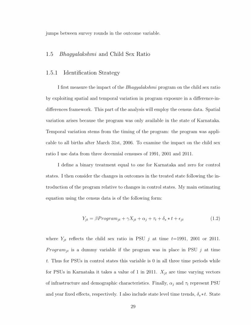
1.5 Bhagyalakshmi and Child Sex Ratio
1.5.1 Identification Strategy
I first measure the impact of the Bhagyalakshmi program on the child sex ratio
by exploiting spatial and temporal variation in program exposure in a difference-in-
differences framework. This part of the analysis will employ the census data. Spatial
variation arises because the program was only available in the state of Karnataka.
Temporal variation stems from the timing of the program: the program was appli-
cable to all births after March 31st, 2006. To examine the impact on the child sex
ratio I use data from three decennial censuses of 1991, 2001 and 2011.
I define a binary treatment equal to one for Karnataka and zero for control
states. I then consider the changes in outcomes in the treated state following the in-
troduction of the program relative to changes in control states. My main estimating
equation using the census data is of the following form:
Yjt = βProgramjt + γXjt + αj + τt + δs ∗ t+ εjt (1.2)
where Yjt reflects the child sex ratio in PSU j at time t=1991, 2001 or 2011.
Programjt is a dummy variable if the program was in place in PSU j at time
t. Thus for PSUs in control states this variable is 0 in all three time periods while
for PSUs in Karnataka it takes a value of 1 in 2011. Xjt are time varying vectors
of infrastructure and demographic characteristics. Finally, αj and τt represent PSU
and year fixed effects, respectively. I also include state level time trends, δs∗t. State
29
specific trends control for potentially heterogeneous pre-program trends. I cluster
my standard errors by state since the program being analyzed was at the state level.
To account for the small number of clusters and associated asymptotic inconsis-
tency, I use wild bootstrapping to correct for this as proposed by Cameron et al.
[2008]. The results are qualitatively identical. For simplicity, therefore, I use the
cluster-robust standard errors in all estimations, while also reporting the p-values
with Wild-t small-bootstrapping cluster procedure. Results are also robust to clus-
tering at the district level. The coefficient β is the estimate of the Bhagyalakshmi
program on child sex ratio. Finally, specifications with infrastructure and demo-
graphic controls only serve as robustness checks to the parsimonious specifications
without controls.
The fundamental identifying assumption in this framework is that the time
trends in the pre-program period in the child sex ratio across Karnataka and control
states should be the same. Figure 1.1 demonstrates common trends in child sex
ratios going back to 1981.
Even with the above assumption, the estimated impact may be due to other
state level programs that are correlated to the introduction of the program. To this
end, I follow Nandi and Deolalikar [2013] and control for a range of time varying
infrastructure and demographic characteristics. Infrastructure characteristics, in-
clude the availability of: either a primary health centre or sub-centre; tap water; all
weather road; power supply; primary school; middle school and secondary school. I
also include male and female literacy and labour force participation rates.
30
1.5.2 Bhagyalakshmi and Child Sex Ratio Results
Table 1.1 column (1) presents the standard difference-in-differences estimates
from equation 1.2 and includes only year and PSU fixed effects. Each coefficient
represents the marginal impact of the Bhagyalakshmi program on the female-to-male
child sex ratio. Results are presented for both subsamples: Panel A is the pooled
sample which includes all PSUs in Karnataka and the control states while Panel B
includes only PSUs in the border districts of Karnataka and control states. Column
(2) includes state specific trends. In the last column I include time fixed effects,
PSU fixed effects, state specific linear trends and PSU level controls.
The results suggest that, for the pooled sample in panel A, villages and towns
in Karnataka show a significant improvement in the child sex ratio between 19.33 and
25.64 points. That is, there were about 19 to 26 additional girls in the 0-6 age group
for every 1000 boys in Karnataka in the post-program period. For specifications in
columns (2)-(3), the improvement is significant at the 1% level. The estimates are
robust to including state specific linear trends. In panel B, a similar story holds for
the subsample that includes only PSUs in the border districts. One would expect
that PSUs in border districts should have fewer differences in omitted variables.
I find that, even when the sample is restricted to the small set of geographically
neighbouring PSUs there is still a positive impact of the program in Karnataka. In
particular, the improvement in panel B ranges from 18.37 points to 31 points in the
child sex ratio across different specifications. These estimates are larger than the
estimates in my base specification in panel A which is to be expected since PSUs in
border districts are likely to be more similar to each other. Thus, these results serve
31

to confirm that my original results are not caused primarily by some unobserved
characteristics. Finally, I present wild-bootstrap p-values in square brackets under
each estimate in column (3) in Table 1.1.
Using the most conservative estimate of an improvement of 20 points in column
(3) of Table 1.1 (i.e. 20 additional girls in the 0-6 age group for every 1000 boys)
in the child sex ratio, my calculations imply that the Bhagyalakshmi program led
to an annual additional 28,124 girls aged 0-6 years in Karnataka.37 Total girls in
the 0-6 age group in 2011 in Karnataka were approximately 3 million. This implies
that, annually, the program led to about about 1-2 percent fewer girls, dying either
due to sex-selective abortions or due to post-birth girl neglect, and thus surviving
up to age 6.
The improvement in the child sex ratio is similar in magnitude to the changes
in child sex ratio estimated by Nandi and Deolalikar [2013] for the implementation
of the Pre-Conception and Pre-Natal Diagnostics Techniques Act (PNDT) of 1994.
The authors estimate that child sex ratio improved by about 13-20 points as a
result of the PNDT Act in states that implemented the Act. While the PNDT was
implemented in several states and thus had a wider reach, the results in this study
imply that even state level programs can have far reaching consequences.
Finally, I conduct a placebo regression of the following nature. In Table A.4
I evaluate the impact of a hypothetical policy which was introduced in 1996: 10
years before the program was actually implemented. I then use the 1991 and 2001
census datasets in a difference-in-differences framework, treating the 2001 census as
37I use the total population sizes in the age group 0-6 years for 2011 in Karnataka to convertthe difference-in-differences estimate of 20 into a number of annual additional female children.Detailed calculations are in Appendix A.2.
32

the hypothetical ‘post ’ period. The coefficients for this hypothetical policy are small
and insignificant.
These results suggest that the Bhagyalakshmi program led to large and signif-
icant improvements in the child sex ratio of approximately 20 girls for every 1000
boys. Next, I examine whether these changes came from changes in girl deficit at
birth or changes in girl deficit after birth.
1.6 Decomposing the Impact on Child Sex Ratio: Fertility and Sex
Ratio at Birth
In this section, I examine whether the relationship between the Bhagyalakshmi
program and child sex ratio established in Section 1.5.2 stems from changes in
fertility and sex ratio at birth.
1.6.1 Identification Strategy
The empirical specification analyzing the impact on fertility and sex ratio at
birth investigates two questions: First, does the probability of a birth change as a
result of a financial incentive? Second, what is the probability of a female birth?
The first question examines the fertility response to the program while the second
question examines the impact on the sex ratio at birth.
In order to answer the first question and examine the fertility response of the
program, I examine if a woman’s fertility is impacted as a result of introduction
of the Bhagyalakshmi program. Additionally, I also examine two other dependent
variables: the unconditional probability of a male birth and the unconditional prob-
33

ability of a female birth.
For the analysis, I use the retrospective birth histories drawn from the DLHS-
2, DLHS-3 and DLHS-4 and construct a woman year panel.38 Each woman enters
the panel 5 years before the survey took place and exits the panel in the year of the
survey. So for instance, for the DLHS-4 women enter the panel in 2008 and exit in
2012; for the DLHS-3 women enter the panel in 2004 and exit in 2007 and finally, for
the DLHS-2 women enter the panel in 1999 and exit in 2003.39 Thus the pre-policy
period is 1999-2006 and the post-policy period is 2007-2012. The dependent variable
is an indicator for giving birth for woman i living in state s in year t ; gives birth to
a girl in year t or gives birth to a boy in year t :
Yist = α + βKars ∗ Postt + γXist + νs + τt + δs ∗ t+ εist (1.3)
where Postt=1 for t > 2006; Xist is a vector of time varying covariates that in-
cludes woman’s years of schooling, indicators for woman’s birth cohort, indicator
for household religion, indicator for residence in a rural area, dummy for belonging
to scheduled caste and a household standard of living (SLI) index. I also include
state and year fixed effects, νs and τt respectively, and state level linear trends, δs∗t.
The reference group consists of women in control states. In this specification, β cap-
tures the effect on the probability of a birth (and the unconditional probabilities of
girl and boy births) in Karnataka relative to control states, after the introduction
38This is similar to the approach adopted by Alfano [2017] who examines the introduction of theDowry Prevention Act in India on fertility choices.
39Since the DLHS-2 was conducted in 2002-2004, the annual birth history of most interviewedwomen during 2004 is incomplete. To avoid any idiosyncrasies due to incomplete birth reportingI exclude this year from the DLHS-2. Further, for the DLHS-3 women enter the panel four yearsbefore the survey; so from 2004-2007. This is because, for this survey round birth histories wereonly collected starting in 2004. Additionally, for the DLHS-4 women also enter the panel for fiveyears, 2018-2012 since the birth history reporting is incomplete for 2013.
34
of the Bhagyalakshmi program. Standard errors are clustered by state and I also
show the p-values with a Wild-t small-cluster bootstrapping procedure. Like be-
fore, specifications with individual level controls serve as robustness checks to the
parsimonious specifications without controls.
In order to answer the second question and examine the impact on sex ratios
at birth I perform the analysis at a more aggregated level. I perform a district-by-
year analysis of the sex ratio at birth similar to the PSU level analysis performed
in the last section for the child sex ratio. I calculate the weighted district averages
of the proportion of female births for the years 1999 to 2012. That is, I model the
sex ratio at birth by employing the district-wise weighted proportion of girl births.
More specifically, I model the following:
Ydt = βProgramdt + γXdt + αd + τt + δs ∗ t+ εdt (1.4)
This specification mirrors equation 1.2 except it is estimated at the district level as
opposed to the PSU level. Here Ydt reflects the sex ratio at birth in district d at
time t=1999-2012 and is proxied by the weighted proportion of female births (using
sampling weights). Programdt is a dummy variable if the program was in place in
district d at time t. Thus for control districts this variable is 0 in all time periods
while for districts in Karnataka it takes a value of 1 after 2006. Xdt are time varying
covariates at the district level. These are the same covariates as mentioned above,
except aggregated at the district level: years of schooling of women, proportion in
a district living in a rural area, proportion belonging to scheduled caste, proportion
hindus and proportion belonging to low, medium and high standard of living index.
35

Finally, αd and τt represent district and year fixed effects, respectively. I also include
state level time trends, δs ∗ t like before. Specifications with district level controls
serve as robustness checks to the parsimonious specifications without controls.
The main identifying assumption in the difference-in-differences framework
which examines the impact on sex ratio at birth and fertility is that pre-program
trends should be the same across Karnataka and control states. Figure 1.2 demon-
strates common trends from 1999 to 2006 for the sex ratio at birth. Additionally,
the probability of a birth should also exhibit similar trends before the introduction
of the program. That is, women in Karnataka and control states should exhibit
similar fertility patterns before 2006. In Figure 1.3 I present the probability of a
birth for each year from 1999-2006.
1.6.2 Effect on Fertility and Sex Ratio at Birth
I first begin my analysis by examining the impact of the program on the prob-
ability of a birth, the unconditional probability of a female birth and the uncondi-
tional probability of a male birth. I estimate equation 1.3 in Table 1.2. In column
(1) I include only state and year fixed effects. In column (2) I add state specific
linear trends and in column (3) I include covariates. The difference-in-differences
estimates examine the change in the probability of a birth in year t, before and after
2006 in Karnataka and control states. The dependent variable in Panel A is an
indicator for giving birth for woman i living in state s in year t, while in Panels B
and C the dependent variable is 1 if woman i living in state s gives birth in year t
to a female and male respectively. At baseline on average, 12.64 percent of women
gave birth every year, with about 48 percent of these being girls.
36
The parameter estimates in Panel A suggest that the probability of a marginal
birth changed differentially between Karnataka and the control states in the post-
program period by 0.77 to 0.85 percentage points (significant at the 5% level) which
represents a 6% increase over the baseline mean. In Panel B, the unconditional prob-
ability of a female birth sees a significant increase between 0.51 to 0.53 percentage
points (significant at the 1% level in column (3) Panel B). At baseline, on average,
about 6 percent women give birth to girls. Thus, the Bhagyalakshmi program leads
to an almost 9 percent increase in the unconditional probability of giving birth to
a girl amongst women in Karnataka compared to women in control states.40 In
contrast, while it is positive, the unconditional probability of a male birth does not
significantly change after the introduction of the Bhagyalakshmi program (columns
(1) to (3) of Panel C).
By examining the unconditional probabilities of male and female births, I can
estimate how much of the increase in female births is due to eliminated abortions
and how much is driven by new pregnancies. New pregnancies should increase the
number of girls and boys born more or less equally. Thus, if only new pregnancies
were driving the increase in fertility (Panel A) then the estimates of the uncondi-
tional probabilities of male and female births (Panels B and C) should be roughly
equal. However, the estimate of the unconditional probability of a female birth is
much higher than that of a male birth, suggesting that in addition to new pregnan-
cies there were also fewer sex-selective abortions. That is, about 50% of the increase
in the number of female births is due to new pregnancies and 50% of the increase
is due to reduction in selective abortions.41 In effect, this means that the increase
40This is obtained by dividing the point estimate of 0.53 by the baseline mean of 6 percent.41This is because, if the increase in the unconditional probability of female births is 0.52 p.p.
37
in the probability of a birth that is seen in Panel A of Table 1.2 is a result, both,
of an increase in the willingness to conceive, and a decrease in the willingness to
abort female fetuses. Finally, a joint F-test fails to reject that all pre-Bhagyalakshmi
coefficients are equal to zero for all three dependent variables (p-values > 0.45).
In Table 1.3 where I estimate equation 1.4, I find that the weighted district
level sex ratio at birth improves significantly in Karnataka after the introduction of
the Bhagyalakshmi program. The increase in the sex ratio at birth is about 0.71 to
0.92 percentage points (columns (1) to (3) of Panel A). Taking the most conservative
estimate of 0.71 percentage points, this translates into an increase of approximately
13 girls for every 1000 boys.42 If the increase in female births was only because
of new pregnancies then the sex ratio at birth should not have changed. This is
because, new pregnancies would have resulted in equal numbers of boys and girls,
leaving the sex ratio unchanged. However, as pointed out above, about 50% of
the increase in female births is due to fewer abortions, which therefore led to an
improvement in the sex ratio at birth.
The estimated coefficients suggest large and significant impacts on the sex
ratio at birth. The estimated impact on the sex ratio at birth is larger in magnitude
to those found by Srinivasan and Bedi [2008] who find no impacts of two policy
interventions in the state of Tamilnadu in the early 1990s, on the sex ratio at
birth. One way to reconcile their finding of no impact on sex-ratio at birth is
to examine the uptake of the program in Tamilnadu. The program was launched
in 1992 and between 1992 -1997 only approximately 2000 families benefited from
(column (2), Panel B) then about 0.26 p.p. or 50% of this is attributable to new pregnancies since0.26 p.p. is the change in the unconditional probability of a male birth (column (2), Panel C).
42Detailed calculations in Appendix A.2.
38
the scheme. This, in addition to the change of government in 1996 led to the
program being placed on the back burner (Srinivasan and Bedi, 2008). Sinha and
Yoong [2009] examine another program in the north Indian state of Haryana; the
Apni Beti, Apna Dhan program. They examine impacts on sex ratio of living
children of each mother. While this conflates estimates on sex ratio at birth and
differential female mortality after birth and thus comparisons are difficult, their
estimates are still indicative. They find positive impacts of the program on the
sex ratio of living children of about 2.3 percentage points. However, this is their
estimated impact on child sex ratio. In comparison, my estimates of child sex ratio
are larger in magnitude. This is potentially because of the high take up rate of the
program in Karnataka as compared to the program in Haryana. Anukriti [2014]
who examines another program also in Haryana, Devirupak finds that sex ratios
at birth actually declined as a result of the program. The author suggests that
this is because the program offered incentives to both one boy and one girl couples
and this led to skewed sex ratios among couples with strong son preference. This
implies that the design of any such incentive is crucial since small changes in the
incentive structure can impact fertility preferences very differently. Finally, my
finding of large improvements in the sex ratio at birth are also comparable to Qian
[2008] who finds that an increase of adult female labour income by USD 7.7 (10%
of average rural household income in China) increases the number of surviving girls
by 1 percentage-point on average.
39
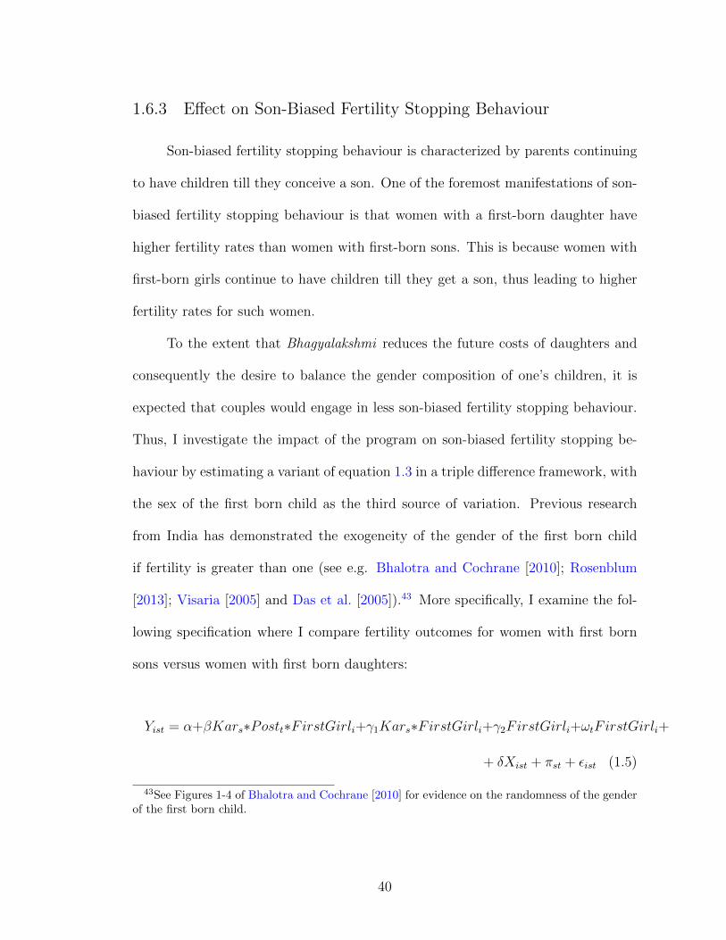
1.6.3 Effect on Son-Biased Fertility Stopping Behaviour
Son-biased fertility stopping behaviour is characterized by parents continuing
to have children till they conceive a son. One of the foremost manifestations of son-
biased fertility stopping behaviour is that women with a first-born daughter have
higher fertility rates than women with first-born sons. This is because women with
first-born girls continue to have children till they get a son, thus leading to higher
fertility rates for such women.
To the extent that Bhagyalakshmi reduces the future costs of daughters and
consequently the desire to balance the gender composition of one’s children, it is
expected that couples would engage in less son-biased fertility stopping behaviour.
Thus, I investigate the impact of the program on son-biased fertility stopping be-
haviour by estimating a variant of equation 1.3 in a triple difference framework, with
the sex of the first born child as the third source of variation. Previous research
from India has demonstrated the exogeneity of the gender of the first born child
if fertility is greater than one (see e.g. Bhalotra and Cochrane [2010]; Rosenblum
[2013]; Visaria [2005] and Das et al. [2005]).43 More specifically, I examine the fol-
lowing specification where I compare fertility outcomes for women with first born
sons versus women with first born daughters:
Yist = α+βKars∗Postt∗FirstGirli+γ1Kars∗FirstGirli+γ2FirstGirli+ωtFirstGirli+
+ δXist + πst + εist (1.5)
43See Figures 1-4 of Bhalotra and Cochrane [2010] for evidence on the randomness of the genderof the first born child.
40

The dependent variable Yist is the same as before: an indicator if woman i, in
state s gave birth in year t. FirstGirli is 1 if the gender of the first born child
is female. I control for state-by-year fixed effects, πst and allow year fixed effects
to vary by gender of the first born child, ωtFirstGirli. All the other variables are
defined as before. Finally, I only include women who have ever given birth since this
specification can be estimated for only those women who had at least one birth.
Table 1.4 presents the estimates from equation 1.5. Column (1) only includes
state and year effects, while column (2) includes state by year fixed effects and
year fixed effects that vary by gender of first child. Finally in column (3) I include
covariates. At baseline, before the introduction of the program, women in Karnataka
with a first born girl were 0.40 percentage points more likely to have another birth
compared to women in control states and to women with first born boys. This
baseline gap is however, not statistically significant, suggesting that women with
first born girls were more likely to have another birth, both in Karnataka and control
states, compared to women with first born boys.
However, after the introduction of the program in Karnataka, women with
first born girls were about 1.4 percentage points less likely to have another birth
(coefficient on Karnataka*Post*First Girl). This is statistically significant at the
1% level. This implies that, while in the pre-program period son-biased fertility
stopping behaviour was characteristic of both Karnataka and control states; in the
post-program period, Karnataka witnessed a reduction in such behaviour. The
results from this section and the previous section on sex ratio at birth, demonstrate
how the Bhagyalakshmi program simultaneously impacted selective abortions and
son-biased fertility stopping. I find that not only are couples with a first born girl
41
less likely to want to have another child, but they’re also increasingly indifferent
about the gender of that child.
1.6.4 Did The Desired Fertility Change?
One of the mechanisms through which the Bhagyalakshmi program could have
changed the willingness to abort female fetuses is by changing a couples’ desired or
ideal number of girls. The questions used are: Would you like to have another
child or would you prefer not to have any more children? Would you prefer your
next child to be a girl or boy? I construct variables for ideal number of boys, ideal
number of girls and ideal number of children using responses on these questions in
addition to information on current composition of a woman’s children.
I construct a similar difference-in-differences specification to the one in equa-
tion 1.3, except each woman contributes one observation for the survey year in which
she appears as opposed to 5 observations. The dependent variables I examine in-
clude: ideal number of girls, ideal number of boys and the probability of a woman
expressing the desire for her next child to be a girl.
I first examine if the trends in the ideal number of girls and ideal number
of boys are similar between Karnataka and the control states in the pre-program
period. I present this in Table A.5. Since I have only one pre-program survey
round in my sample (i.e. DLHS-2), I use the National Family Health Survey (NFHS
2005-06) to show pre-program trends. I next present the regression estimates in
Table 1.5. The program led to a significant increase in the ideal number of girls
(panel B), while the number of ideal boys does not significantly change (panel C).
More specifically, the ideal number of girls increased by about 9.5 percent over the
42
baseline ideal number of girls.44 Finally, the probability of desiring one’s next child
to be a girl increases by 2.5 percent, which represents a 22 percent increase over the
baseline mean of 11 percent. (panel D).
The results on desired fertility are in line with those found in Section 1.6.2 on
actual fertility. That is, the program led to an increase in the desired number of girls
and no change in the desired number of boys. This, in conjunction with an increase
in the actual probability of female births (which was larger than the change in male
births) implies that the actual and the desired willingness to abort female fetuses
declined. Additionally, from Figure A.3 it appears that the percentage of daughters
desired at different family sizes follows a monotonic relationship in Karnataka after
the introduction of the program. That is, after the introduction of the program, even
at an actual family size of 1, the percentage of daughters desired is high. That is,
couples desire about 0.8 girls at a family size of 1 after the program compared to 0.5
before the program.45 This is in stark contrast to Jayachandran [2017] who finds that
at smaller family sizes, the desired number of sons is extremely high. For instance,
she finds that for a hypothetical family size of 1, 84.9 percent of respondents in her
sample, would want this one child to be a son. This is because when faced with
lower fertility, couples desire at least one son because of high son preference. My
finding that, even at a family size of 1, the desired number of girls actually increases
after the program suggests that the program worked through decreasing this innate
son preference. After the introduction of the program, parents were increasingly
indifferent about the gender of their child, even at smaller family sizes.
44Percent increase is calculated by dividing the coefficient in column (2), Panel B by the baselinemean.
45Figure A.3 shows the relationship only for mother’s in their prime childbearing years, 25-34years. The results are similar for all other age groups as well.
43
While this is suggestive evidence of a reduction in son preference it doesn’t
necessarily tell us if post-natal discrimination against girls ended. This is what I
examine in Section 1.7.
1.6.5 Robustness
I test the validity of my findings through two placebo tests. First, I run a
falsification test that examines the impact of hypothetical programs introduced for
each year from 1997 to 2002, on the probability of a birth, unconditional probability
of a female birth and the unconditional probability of a male birth. Results are
presented in Table A.6. I expand my original sample to span the period 1995-
2005. Thus, for instance, Post1997 (column (1) of Table A.6) examines a program
introduced in 1997 with 1995-1997 as the pre-period and 1998-2005 as the post-
period and Post2003 (column (6) of Table A.6) examines a program introduced in
2002 with 1995-2002 as the pre-period and 2003-05 as the post-period.
The second robustness check re-estimates my main specification (equation 1.3)
after dropping one control state at a time. I present the results of this robustness
check in Table A.7.
1.7 Decomposing the Impact on Child Sex Ratio: Excess Female
Mortality and Health Investments
In this section I examine the impact of the Bhagyalakshmi program on post-
birth neglect measured by infant mortality and duration of exclusive breastfeeding.
Exclusive breastfeeding is defined as the number of months a child is exclusively
44
breastfed which implies no food or water during this period. Early and exclusive
breastfeeding is an important investment in children, helping them survive longer
and also supporting cognitive performance (World Health Organization, 2000).46
1.7.1 Empirical Strategy
To test the impact of the program on infant mortality and health investments
I perform a cohort analysis. I compare cohorts born after the introduction of the
program in Karnataka to cohorts born before the program and to cohorts in control
states. I use the gender of the recipient as the third source of variation in a triple
difference framework. According to the eligibility conditions, the program was ap-
plicable only for female children. Thus, I use male children as an additional control
group. Concerns over treatment endogeneity are eased by including an additional
control group that is also affected by the same time-varying state level variables.
Since only girls of birth orders 1,2 and 3 were eligible for the program, I estimate
the following specification for girls and boys of birth orders 1, 2 and 3. The ‘control
group’ constitutes (i) cohorts born before 2006 (ii) cohorts born in any year in the
control states and, (iii) boy cohorts. For child i of mother j in state s in year t, I
estimate the following:
Yijst = α + βKars ∗ Postt ∗ F + γ1Kars ∗ Fi + γ2Fi + ωtFi + ψbFi
+ δXijst + ρbt + νbs + πst + εijst (1.6)
46Jayachandran and Kuziemko [2011] provide evidence that in India, since breastfeeding acts asa natural contraceptive, women tend to breastfeed girls for fewer months. This is because, after thebirth of a girl women try to get pregnant sooner, thus reducing the number of months of exclusivebreastfeeding that a girl receives.
45
The dependent variable, Yijst is either an infant mortality indicator or measures
the duration of exclusive breastfeeding. Fi is indicator for being a female and can
be 0 or 1. Postt is equal to 1 if the child is born after March 31st, 2006 and 0
otherwise. Specifications with individual level controls serve as robustness checks to
the parsimonious specifications without controls.
A key advantage of this approach is that it allows me to account for state
specific shocks over the observation period through state-by-year fixed effects, πst.
Additionally I control for birth order specific time effects, ρbt and state specific birth
order fixed effects, νbs. I also allow birth year, and birth order fixed effects to vary
by child gender (ωtFi, ψbFi). Fixed effects for state and birth year are also included.
The coefficient of interest is β which measures the effect of the program on the
outcome of interest for female children of birth orders 1, 2, and 3 before and after
2006 in Karnataka, relative to other states.
Identification in the triple difference framework relies on the assumption that
the differences in female and male infant mortality (which will henceforth be re-
ferred to as excess female infant mortality or EFM) and differences in female and
male breastfeeding duration should follow a similar trend in Karnataka and control
states before the introduction of the Bhagyalakshmi program. Figure 1.4 Panel A
depicts the differential trend in excess female infant mortality (EFM) between Kar-
nataka and control states, while Panel B depicts the differential trend for exclusive
breastfeeding duration. The gap in EFM between Karnataka and control states is
relatively constant before 2006 and the same story holds for exclusive breastfeeding
duration providing credibility to the identification strategy.
46

1.7.2 Compositional vs. Causal Effects
Since there were changes in overall fertility, it is possible that I’m identify-
ing compositional as opposed to causal effects. To disentangle compositional and
causal effects, I estimate a specification similar to equation 1.6 where the dependent
variables are the family characteristics.47
1.7.3 Impacts on Infant Mortality and Health Investments: Triple
Difference Estimator
Table 1.6 presents estimates from equation 1.6. Panel A reports estimates
for infant mortality while Panel B presents estimates for exclusive breastfeeding
duration. Finally in Panel C the dependent variable is a dummy if the child is
exclusively breastfed for at least 6 months and is restricted to children who were at
least 6 months of age.
In column (1) I include the triple- and double-interactions of Female and
Karnataka with Post. Column (2), adds state by birth year fixed effects, birth year
fixed effects that vary by child gender, and covariates. Finally, in column (3) I add
birth order by state fixed effects, birth order by birth year fixed effects, as well as
birth order fixed effects that vary by child gender.48
47I do not include mother fixed effects in the estimating equations to account for selection as hasbeen done by recent literature (see e.g. Anukriti et al., 2016). This is due to several reasons. First,in a mother fixed effects model, siblings of the opposite sex but in the same household are comparedto each other. Given that, siblings of the opposite gender are not randomly selected within ahousehold because of son-biased fertility stopping rules and sex-selective abortions, this wouldintroduce bias. Additionally, given that health investment information in the data is availableonly for children born three years prior to the survey date, a mother fixed effects model wouldgenerate estimates for a selected sample of households (i.e. those who had births within the lastthree years of a survey) (Hu and Schlosser, 2015).
48In columns (2) and (3) I exclude the double interaction terms: Karnataka*Post and Fe-male*Post.
47
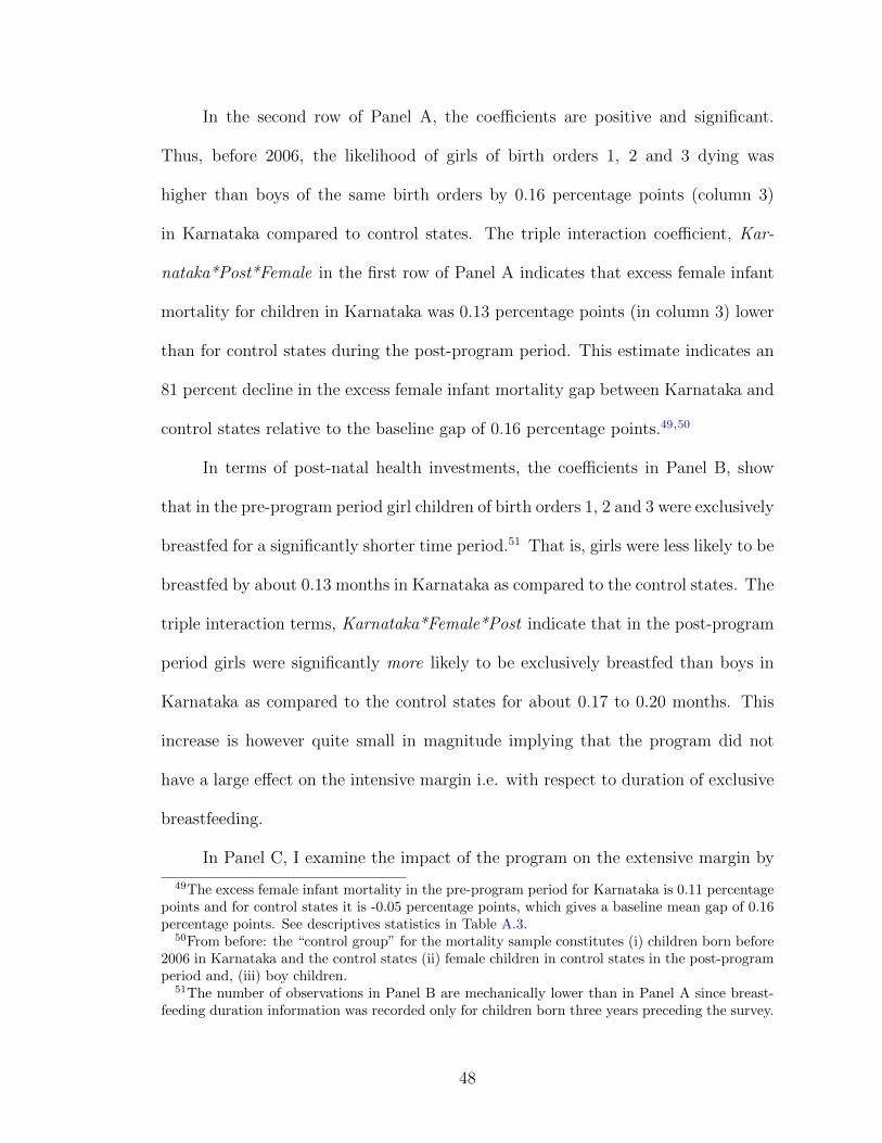
In the second row of Panel A, the coefficients are positive and significant.
Thus, before 2006, the likelihood of girls of birth orders 1, 2 and 3 dying was
higher than boys of the same birth orders by 0.16 percentage points (column 3)
in Karnataka compared to control states. The triple interaction coefficient, Kar-
nataka*Post*Female in the first row of Panel A indicates that excess female infant
mortality for children in Karnataka was 0.13 percentage points (in column 3) lower
than for control states during the post-program period. This estimate indicates an
81 percent decline in the excess female infant mortality gap between Karnataka and
control states relative to the baseline gap of 0.16 percentage points.49,50
In terms of post-natal health investments, the coefficients in Panel B, show
that in the pre-program period girl children of birth orders 1, 2 and 3 were exclusively
breastfed for a significantly shorter time period.51 That is, girls were less likely to be
breastfed by about 0.13 months in Karnataka as compared to the control states. The
triple interaction terms, Karnataka*Female*Post indicate that in the post-program
period girls were significantly more likely to be exclusively breastfed than boys in
Karnataka as compared to the control states for about 0.17 to 0.20 months. This
increase is however quite small in magnitude implying that the program did not
have a large effect on the intensive margin i.e. with respect to duration of exclusive
breastfeeding.
In Panel C, I examine the impact of the program on the extensive margin by
49The excess female infant mortality in the pre-program period for Karnataka is 0.11 percentagepoints and for control states it is -0.05 percentage points, which gives a baseline mean gap of 0.16percentage points. See descriptives statistics in Table A.3.
50From before: the “control group” for the mortality sample constitutes (i) children born before2006 in Karnataka and the control states (ii) female children in control states in the post-programperiod and, (iii) boy children.
51The number of observations in Panel B are mechanically lower than in Panel A since breast-feeding duration information was recorded only for children born three years preceding the survey.
48

measuring program impacts on the probability of being exclusively breastfed for at
least 6 months. I find that the improvement on the extensive margin is large, with
girls being more likely to be exclusively breastfed relative to boys, during the first six
months of life by 5.10 percentage points (column (3) of Panel C). This is in contrast
to Anukriti et al. [2016] who find that the introduction of the ultrasound technology
leads to improvements in breastfeeding duration in the second year of life and find
no changes in the first year of life. However, I examine exclusive breastfeeding which
is defined as ‘no other food, drink or water’. The recommended duration of exclusive
breastfeeding by the World Health Organization is at least 6 months.
1.7.4 Compositional vs. Causal Effects: Are Girls Born into Better
Endowed Families?
The improvement in girls’ infant mortality rates and post-natal health invest-
ments in Karnataka relative to boys, could be the result of girls being born into bet-
ter endowed families. I test whether family characteristics of girls (such as parental
education, mother’s age at first birth and household wealth status) improved relative
to boys in Karnataka and relative to control states. I estimate specification 1.6 with
mother’s age at first birth, mother’s years of education, father’s years of education,
residence in a rural area, standard of living (SLI) index, as dependent variables.
The results are in column (1), rows 1-5 of Table A.8. Triple interaction coefficients
for all these variables are small, with only one coefficient being marginally signifi-
cant. These results suggest that there is no differential improvement in household
characteristics among families with girls relative to families with boys and therefore
the improvement in girls’ outcomes is unlikely to be explained by the fact that girls
49

are born into ‘better’ households.
1.8 Heterogeneity
I examine impacts separately for the following groups: mother’s educational at-
tainment (less than secondary education or secondary education and higher), house-
hold wealth (low, medium and high wealth index), household caste (scheduled caste
(SC) and other), type of residence (rural versus urban) and religion (hindu versus
muslim).
In Table A.9 I first examine the heterogeneous impact of the program on the
probability of a birth, unconditional probability of a female birth and unconditional
probability of a male birth. With respect to mother’s education it appears that the
program led to an increase in the probability of a birth for all mothers - those with
either less than secondary education or those with secondary education or higher.
However, the increase in fertility stems from different sources. For mother’s with
secondary education or more, it appears that the Bhagyalakshmi program impacted
their willingness to abort in addition to increasing their willingness to conceive.
That is, the increase in the probability of female births is more than the increase in
the probability of male births suggesting a reduction in sex-selective abortions. For
mother’s with less than secondary education it appears the program impacted only
the willingness to conceive The probability of a female birth and the probability of a
male birth rise for this subsample and are roughly equal. Given that the baseline sex
ratio at birth was more skewed for women with secondary education or higher (47
percent as opposed to 48 percent), it is heartening that the impact of the program
50

on sex selective abortions is higher for precisely this subsample.52
With respect to household wealth I find that a very similar story holds. House-
holds with a medium or high SLI index see the most impact on the sex ratio at birth,
but again for different reasons. Relatively well off households, who have a more male
biased sex ratio at baseline see a decrease in the willingness to abort in addition
to a change in the willingness to conceive. The unconditional probabilities of male
and female births are very different for this group. Households in the middle of the
income distribution see only an increase in the willingness to conceive and a small
decrease in the willingness to abort female fetuses (the unconditional probabilities
are only marginally different). Thus on average, female children are born in both
middle and high income households. Households on the lowest end of the distribu-
tion see no impact. One of the reasons for this could be that these households are
unable to access the program because of lack of awareness and/or it is harder for
such households to meet all the bureaucratic procedures of the application process.
With respect to caste, religion and residence the same story holds. Probability of a
female birth increases in both rural and urban areas but only through an increase
in the willingness to conceive in the former and through both a decrease in the
willingness to abort and an increase in the willingness to conceive in the latter.
With respect to heterogeneity in post-natal mortality and investments, Table
A.10 (second row in both panels) shows that in the pre-program period, among
families in Karnataka, excess girl infant mortality was greater in low to middle-class
socio-economic groups (illiterate, poor to middle class, rural and lower caste). In the
52On average, this lines up with my finding in Table A.8 where I found that there was nodifferential selection of girls into families where mother’s education was higher. The program ledto more female births in households with all levels of education, with the reason for those birthseither stemming out of lower abortions (for women with more than secondary education), higherfertility or both (for women with less than secondary education).
51
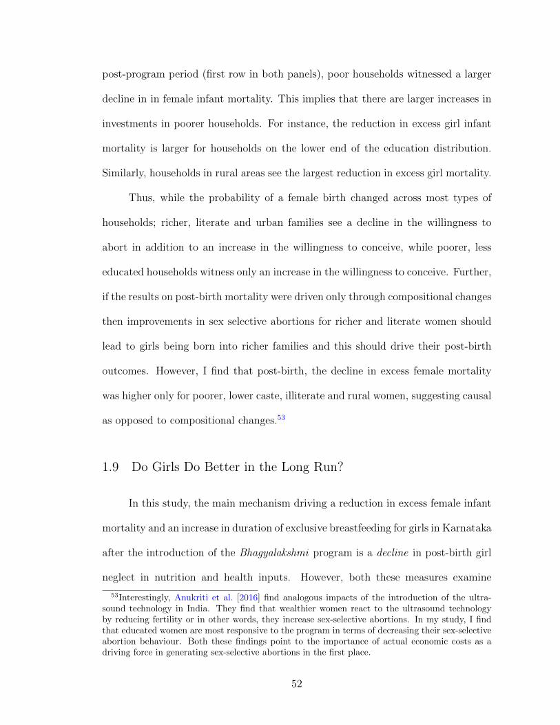
post-program period (first row in both panels), poor households witnessed a larger
decline in in female infant mortality. This implies that there are larger increases in
investments in poorer households. For instance, the reduction in excess girl infant
mortality is larger for households on the lower end of the education distribution.
Similarly, households in rural areas see the largest reduction in excess girl mortality.
Thus, while the probability of a female birth changed across most types of
households; richer, literate and urban families see a decline in the willingness to
abort in addition to an increase in the willingness to conceive, while poorer, less
educated households witness only an increase in the willingness to conceive. Further,
if the results on post-birth mortality were driven only through compositional changes
then improvements in sex selective abortions for richer and literate women should
lead to girls being born into richer families and this should drive their post-birth
outcomes. However, I find that post-birth, the decline in excess female mortality
was higher only for poorer, lower caste, illiterate and rural women, suggesting causal
as opposed to compositional changes.53
1.9 Do Girls Do Better in the Long Run?
In this study, the main mechanism driving a reduction in excess female infant
mortality and an increase in duration of exclusive breastfeeding for girls in Karnataka
after the introduction of the Bhagyalakshmi program is a decline in post-birth girl
neglect in nutrition and health inputs. However, both these measures examine
53Interestingly, Anukriti et al. [2016] find analogous impacts of the introduction of the ultra-sound technology in India. They find that wealthier women react to the ultrasound technologyby reducing fertility or in other words, they increase sex-selective abortions. In my study, I findthat educated women are most responsive to the program in terms of decreasing their sex-selectiveabortion behaviour. Both these findings point to the importance of actual economic costs as adriving force in generating sex-selective abortions in the first place.
52
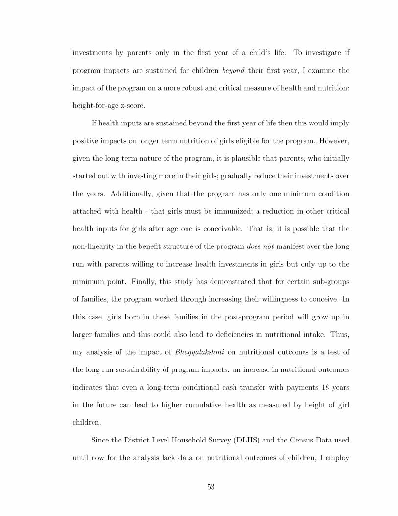
investments by parents only in the first year of a child’s life. To investigate if
program impacts are sustained for children beyond their first year, I examine the
impact of the program on a more robust and critical measure of health and nutrition:
height-for-age z-score.
If health inputs are sustained beyond the first year of life then this would imply
positive impacts on longer term nutrition of girls eligible for the program. However,
given the long-term nature of the program, it is plausible that parents, who initially
started out with investing more in their girls; gradually reduce their investments over
the years. Additionally, given that the program has only one minimum condition
attached with health - that girls must be immunized; a reduction in other critical
health inputs for girls after age one is conceivable. That is, it is possible that the
non-linearity in the benefit structure of the program does not manifest over the long
run with parents willing to increase health investments in girls but only up to the
minimum point. Finally, this study has demonstrated that for certain sub-groups
of families, the program worked through increasing their willingness to conceive. In
this case, girls born in these families in the post-program period will grow up in
larger families and this could also lead to deficiencies in nutritional intake. Thus,
my analysis of the impact of Bhagyalakshmi on nutritional outcomes is a test of
the long run sustainability of program impacts: an increase in nutritional outcomes
indicates that even a long-term conditional cash transfer with payments 18 years
in the future can lead to higher cumulative health as measured by height of girl
children.
Since the District Level Household Survey (DLHS) and the Census Data used
until now for the analysis lack data on nutritional outcomes of children, I employ
53
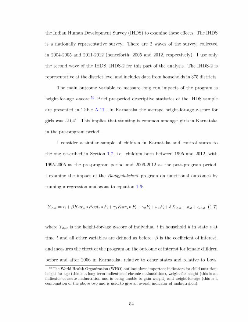
the Indian Human Development Survey (IHDS) to examine these effects. The IHDS
is a nationally representative survey. There are 2 waves of the survey, collected
in 2004-2005 and 2011-2012 (henceforth, 2005 and 2012, respectively). I use only
the second wave of the IHDS, IHDS-2 for this part of the analysis. The IHDS-2 is
representative at the district level and includes data from households in 375 districts.
The main outcome variable to measure long run impacts of the program is
height-for-age z-score.54 Brief pre-period descriptive statistics of the IHDS sample
are presented in Table A.11. In Karnataka the average height-for-age z-score for
girls was -2.041. This implies that stunting is common amongst girls in Karnataka
in the pre-program period.
I consider a similar sample of children in Karnataka and control states to
the one described in Section 1.7, i.e. children born between 1995 and 2012, with
1995-2005 as the pre-program period and 2006-2012 as the post-program period.
I examine the impact of the Bhagyalakshmi program on nutritional outcomes by
running a regression analogous to equation 1.6:
Yihst = α+βKars ∗Postt ∗Fi+γ1Kars ∗Fi+γ2Fi+ωtFi+ δXihst+πst+ εihst (1.7)
where Yihst is the height-for-age z-score of individual i in household h in state s at
time t and all other variables are defined as before. β is the coefficient of interest,
and measures the effect of the program on the outcome of interest for female children
before and after 2006 in Karnataka, relative to other states and relative to boys.
54The World Health Organization (WHO) outlines three important indicators for child nutrition:height-for-age (this is a long-term indicator of chronic malnutrition), weight-for-height (this is anindicator of acute malnutrition and is being unable to gain weight) and weight-for-age (this is acombination of the above two and is used to give an overall indicator of malnutrition).
54

Finally, Xihst includes the following set of covariates: highest years of education of
male in household, highest years of education of female in household, dummy for
residence in a rural area, dummies for belonging to scheduled caste, dummy for
religion and finally, household monthly consumption per capita.
I present the results from the above specification in Table 1.7 where the de-
pendent variable is the height-for-age z-score. At baseline, girls in Karnataka had
height-for-age z-scores that were 0.10 standard deviations less than boys in Kar-
nataka and relative to control states. However in the post-program period height-
for-age improves significantly for girls in Karnataka relative to boys by 0.36 to 0.41
standard deviations. These results are robust to controlling for state by birth year
fixed effects and female by birth year fixed effects in addition to covariates. This
illustrates that the Bhagyalakshmi program not only eliminated the baseline gap
between boys and girls with respect to nutritional inputs but that couples invested
in girls in a sustained fashion over the course of their childhood.
There is ample empirical evidence linking height to improved outcomes (see
e.g. Bozzoli et al., 2009; Thomas and Strauss, 1997; Schultz and Strauss, 2008;
Waaler, 1984 and Fogel, 2004). More importantly, Jayachandran and Pande [2015]
document that high son preference especially for elder sons, is linked to the high
stunting rate amongst Indian girls. The authors document that parental preferences:
specifically, a strong desire to have and invest in an eldest son, underlie much of
India’s child stunting especially amongst girls. They also find that the gender gap
in height is larger amongst wealthier households which implies that even as India
develops, the problem of stunting might be hard to address by policy. I find that, by
addressing one of the main causes of stunting amongst girls i.e high son preference,
55
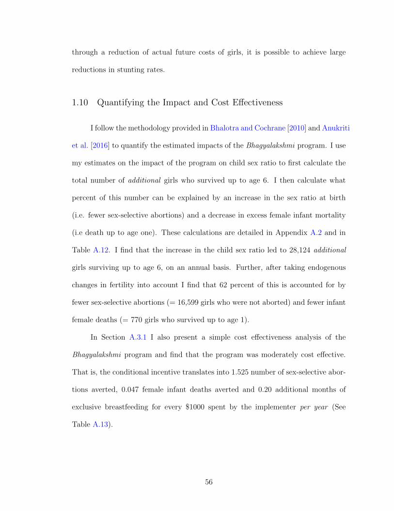
through a reduction of actual future costs of girls, it is possible to achieve large
reductions in stunting rates.
1.10 Quantifying the Impact and Cost Effectiveness
I follow the methodology provided in Bhalotra and Cochrane [2010] and Anukriti
et al. [2016] to quantify the estimated impacts of the Bhagyalakshmi program. I use
my estimates on the impact of the program on child sex ratio to first calculate the
total number of additional girls who survived up to age 6. I then calculate what
percent of this number can be explained by an increase in the sex ratio at birth
(i.e. fewer sex-selective abortions) and a decrease in excess female infant mortality
(i.e death up to age one). These calculations are detailed in Appendix A.2 and in
Table A.12. I find that the increase in the child sex ratio led to 28,124 additional
girls surviving up to age 6, on an annual basis. Further, after taking endogenous
changes in fertility into account I find that 62 percent of this is accounted for by
fewer sex-selective abortions (= 16,599 girls who were not aborted) and fewer infant
female deaths (= 770 girls who survived up to age 1).
In Section A.3.1 I also present a simple cost effectiveness analysis of the
Bhagyalakshmi program and find that the program was moderately cost effective.
That is, the conditional incentive translates into 1.525 number of sex-selective abor-
tions averted, 0.047 female infant deaths averted and 0.20 additional months of
exclusive breastfeeding for every $1000 spent by the implementer per year (See
Table A.13).
56
1.11 Conclusion and Policy Implications
“A great many women are simply not there because women are neglected com-
pared with men. If this situation is to be corrected, the reasons why there are so
many missing women must first be better understood.” (Sen, 1990)
In this paper I show that one important reason for high son preference and
the resultant missing women at young ages in India is, the high future costs of girls.
Using large scale Census data and retrospective birth history data, I show that a
financial incentive that exogenously reduced the actual future costs of girls, led to
a substantial increase in the female-to-male child sex ratio by 19 to 25 additional
girls for every 1000 boys. My estimates imply that 28,124 additional girls were born
in Karnataka or survived up to age 6 on an annual basis because of the program.
This paper uses temporal, geographic and compositional variation in a difference-
in-differences and triple difference framework to show that the improvement in child
sex ratio stems from both an improvement in the female-to-male sex ratio at birth
and more girls surviving up to age one.
I find that the probability of giving birth to a girl rises by 9% both due to
new pregnancies and due to fewer sex-selective abortions. The reduction in the
willingness to abort led to an improvement in the sex ratio at birth by 13 additional
girls for every 1000 boys. This reduction is accompanied by an increase in the
desired number of girls suggesting that the high future cost of girls was an important
determinant of son preference before the introduction of the program. Women are
also less likely to engage in son-biased fertility stopping behaviour after the program
57

indicating that they are increasingly indifferent about the gender of their next child.
Further, I find that girls tend to do better even post-birth. The introduction of
the program leads to an 81 percent decline in the excess female infant mortality gap
in Karnataka. With respect to exclusive breastfeeding, while there was only a small
improvement at the intensive margin, there was a large and significant increase at
the extensive margin. The probability of being exclusively breastfed increased for
girls by 5.1 percentage points. Height-for-age z-score, a long-run indicator for good
nutrition increases by 0.4 standard deviations for girls in Karnatak.
There are several policy implications from the above study. First, my results
indicate the importance of policy design. My analysis shows that a policy that
provides incentives to couples to give birth to girls and simultaneously does not put
a cap on the number of boys; is effective at reducing both girl deficit at birth and
girl deficit post-birth. Second, my results also point to the importance of identifying
heterogeneous impacts. Households at different spectrums of the income distribution
engage in different kinds of discriminatory behaviour. For instance, if the policy goal
is to reduce selective abortions, then relatively wealthier households with smaller
family sizes need to be targeted. Additionally, girls who have more sisters tend to be
the most disadvantaged which implies that these households should be targeted by
policymakers. Finally, my results imply that economic incentives may be effective in
dealing with the complex cultural roots of intra-household discrimination. Future
costs of girls are expected to increase with modernization and are unlikely to be
eradicated. My study provides evidence that changing actual costs of daughters,
as opposed to trying to change the culture that gives rise to these costs, may be a
crucial policy instrument.
58
The expected increase in female feticide as a result of declining desired and ac-
tual fertility has led to increased attention from policy makers and academics. From
a policy standpoint increasingly male-biased sex ratios are undesirable for multiple
reasons. First, sex-selective abortions lead to girls being consistently born in poorer
families and this severely hampers the upward mobility of women.55 Second, the
expected scarcity of women has implications for the marriage markets, labour mar-
kets and could lead to increased prostitution and higher trafficking of women (Qian,
2008, Nandi and Deolalikar, 2013 and Anukriti et al., 2016). Thus, identifying the
causes of high son preference is an important policy goal. This study, by identifying
high future costs of girls as one important determinant of such behaviours, helps in
moving us a step further towards tackling the critical problem of missing girls in
India.
55The societal cost of having a female population that is less healthy and less educated is im-mense. For instance, it can result in the inter-generational transmission of poverty since it iswidely known that more educated women tend to make higher investments in children. Thus,male-biased sex ratios lead to an externality wherein society would prefer women to be healthierand more educated but individual preferences are different.
59
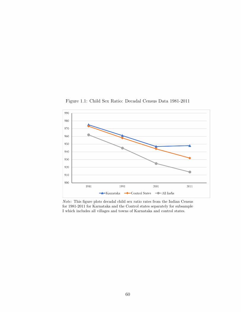
Figure 1.1: Child Sex Ratio: Decadal Census Data 1981-2011
Note: This figure plots decadal child sex ratio rates from the Indian Censusfor 1981-2011 for Karnataka and the Control states separately for subsampleI which includes all villages and towns of Karnataka and control states.
60
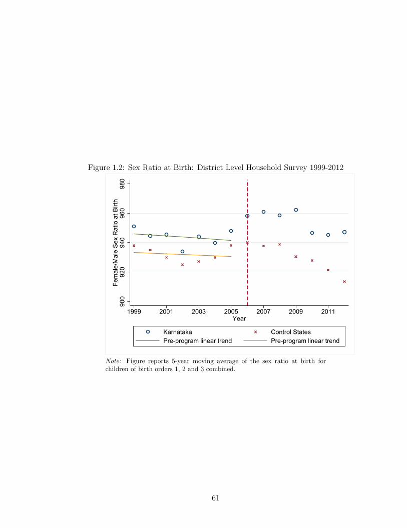
Figure 1.2: Sex Ratio at Birth: District Level Household Survey 1999-2012
900
920
940
960
980
Fem
ale/
Mal
e S
ex R
atio
at B
irth
1999 2001 2003 2005 2007 2009 2011Year
Karnataka Control StatesPre-program linear trend Pre-program linear trend
Note: Figure reports 5-year moving average of the sex ratio at birth forchildren of birth orders 1, 2 and 3 combined.
61
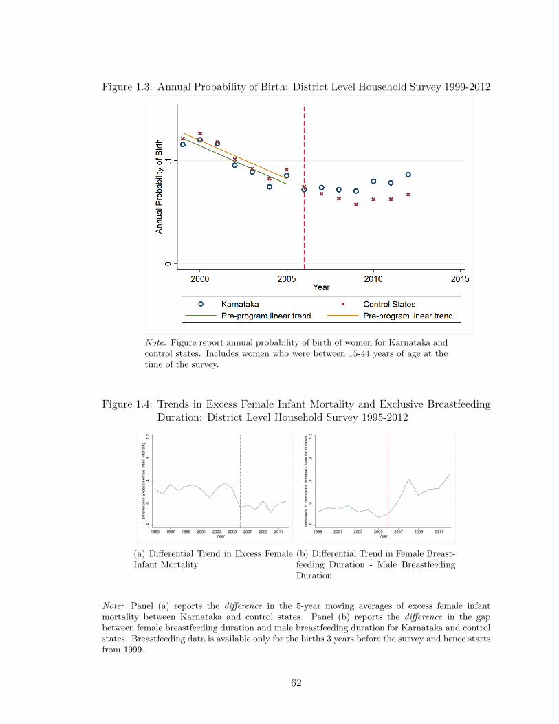
Figure 1.3: Annual Probability of Birth: District Level Household Survey 1999-2012
Note: Figure report annual probability of birth of women for Karnataka andcontrol states. Includes women who were between 15-44 years of age at thetime of the survey.
Figure 1.4: Trends in Excess Female Infant Mortality and Exclusive BreastfeedingDuration: District Level Household Survey 1995-2012
-.40
.4.8
1.2
Diff
eren
ce in
Exc
ess
Fem
ale
Infa
nt M
orta
lity
1995 1997 1999 2001 2003 2005 2007 2009 2011Year
(a) Differential Trend in Excess FemaleInfant Mortality
-.40
.4.8
1.2
Diff
eren
ce in
Fem
ale
BF
dura
tion
- Mal
e B
F du
ratio
n
1999 2001 2003 2005 2007 2009 2011Year
(b) Differential Trend in Female Breast-feeding Duration - Male BreastfeedingDuration
Note: Panel (a) reports the difference in the 5-year moving averages of excess female infantmortality between Karnataka and control states. Panel (b) reports the difference in the gapbetween female breastfeeding duration and male breastfeeding duration for Karnataka and controlstates. Breastfeeding data is available only for the births 3 years before the survey and hence startsfrom 1999.
62
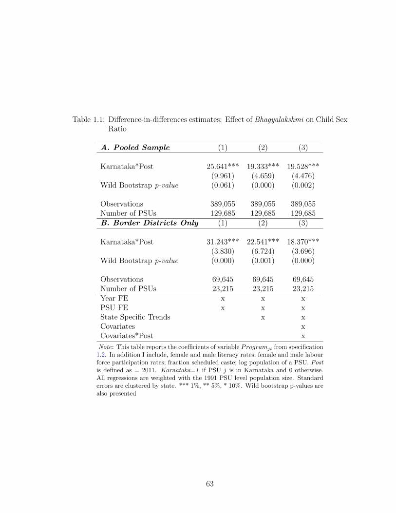
Table 1.1: Difference-in-differences estimates: Effect of Bhagyalakshmi on Child SexRatio
A. Pooled Sample (1) (2) (3)
Karnataka*Post 25.641*** 19.333*** 19.528***(9.961) (4.659) (4.476)
Wild Bootstrap p-value (0.061) (0.000) (0.002)
Observations 389,055 389,055 389,055Number of PSUs 129,685 129,685 129,685B. Border Districts Only (1) (2) (3)
Karnataka*Post 31.243*** 22.541*** 18.370***(3.830) (6.724) (3.696)
Wild Bootstrap p-value (0.000) (0.001) (0.000)
Observations 69,645 69,645 69,645Number of PSUs 23,215 23,215 23,215Year FE x x xPSU FE x x xState Specific Trends x xCovariates xCovariates*Post x
Note: This table reports the coefficients of variable Programjt from specification1.2. In addition I include, female and male literacy rates; female and male labourforce participation rates; fraction scheduled caste; log population of a PSU. Postis defined as = 2011. Karnataka=1 if PSU j is in Karnataka and 0 otherwise.All regressions are weighted with the 1991 PSU level population size. Standarderrors are clustered by state. *** 1%, ** 5%, * 10%. Wild bootstrap p-values arealso presented
63
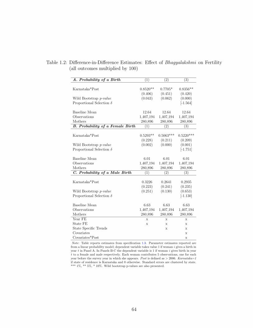
Table 1.2: Difference-in-Difference Estimates: Effect of Bhagyalakshmi on Fertility(all outcomes multiplied by 100)
A. Probability of a Birth (1) (2) (3)
Karnataka*Post 0.8520** 0.7705* 0.8356**(0.406) (0.451) (0.420)
Wild Bootstrap p-value (0.043) (0.062) (0.000)Proportional Selection δ [-1.564]
Baseline Mean 12.64 12.64 12.64Observations 1,407,194 1,407,194 1,407,194Mothers 280,896 280,896 280,896B. Probability of a Female Birth (1) (2) (3)
Karnataka*Post 0.5293** 0.5063*** 0.5220***(0.228) (0.211) (0.209)
Wild Bootstrap p-value (0.002) (0.000) (0.001)Proportional Selection δ [-1.751]
Baseline Mean 6.01 6.01 6.01Observations 1,407,194 1,407,194 1,407,194Mothers 280,896 280,896 280,896C. Probability of a Male Birth (1) (2) (3)
Karnataka*Post 0.3226 0.2641 0.2935(0.223) (0.241) (0.235)
Wild Bootstrap p-value (0.251) (0.130) (0.653)Proportional Selection δ [-1.130]
Baseline Mean 6.63 6.63 6.63Observations 1,407,194 1,407,194 1,407,194Mothers 280,896 280,896 280,896Year FE x x xState FE x x xState Specific Trends x xCovariates xCovariates*Post x
Note: Table reports estimates from specification 1.3. Parameter estimates reported arefrom a linear probability model; dependent variable takes value 1 if woman i gives a birth inyear t in Panel A. In Panels B-C the dependent variable is 1 if woman i gives birth in yeart to a female and male respectively. Each woman contributes 5 observations, one for eachyear before the survey year in which she appears. Post is defined as > 2006. Karnataka=1if state of residence is Karnataka and 0 otherwise. Standard errors are clustered by state.*** 1%, ** 5%, * 10%. Wild bootstrap p-values are also presented.
64
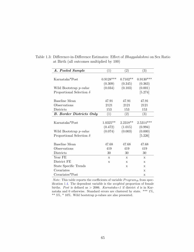
Table 1.3: Difference-in-Difference Estimates: Effect of Bhagyalakshmi on Sex Ratioat Birth (all outcomes multiplied by 100)
A. Pooled Sample (1) (2) (3)
Karnataka*Post 0.9128*** 0.7102** 0.9130***(0.309) (0.345) (0.363)
Wild Bootstrap p-value (0.034) (0.103) (0.001)Proportional Selection δ [5.274]
Baseline Mean 47.91 47.91 47.91Observations 2121 2121 2121Districts 153 153 153
B. Border Districts Only (1) (2) (3)
Karnataka*Post 1.0325** 2.2318** 2.5314***(0.472) (1.015) (0.994)
Wild Bootstrap p-value (0.074) (0.003) (0.000)Proportional Selection δ [5.226]
Baseline Mean 47.68 47.68 47.68Observations 419 419 419Districts 30 30 30
Year FE x x xDistrict FE x x xState Specific Trends x xCovariates xCovariates*Post x
Note: This table reports the coefficients of variable Programdt from spec-ification 1.4. The dependent variable is the weighted proportion of femalebirths. Post is defined as > 2006. Karnataka=1 if district d is in Kar-nataka and 0 otherwise. Standard errors are clustered by state. *** 1%,** 5%, * 10%. Wild bootstrap p-values are also presented.
65

Table 1.4: Difference-in-Difference Estimates: Effect of Bhagyalakshmi on Son-Biased Fertility Stopping Behaviour (all outcomes multiplied by 100)
A. Probability of a Birth (1) (2) (3)
Karnataka*Post*First Girl -1.4416*** -1.3255*** -1.4166***(0.547) (0.517) (0.551)
Wild Bootstrap p-value (0.001) (0.014) (0.009)
Karnataka*First Girl 0.3767 0.3881 0.3968(0.383) (0.381) (0.375)
Baseline Mean 0.40 0.40 0.40Observations 874,060 874,060 874,060Mothers 161,381 161,381 161,381Year FE x x xState FE x x xState-Year FE x xFemale-Year FE x xCovariates xCovariates*Post x
Note: This table reports estimates from specification 1.5. Parameter estimatesreported are from a linear probability model; dependent variable takes value 1 ifwoman i gives a birth in year t. Each woman contributes 5 observations, one foreach year before the survey year in which she appears. Post is defined as > 2006.Karnataka=1 if state of residence is Karnataka and 0 otherwise. Standard errorsare clustered by state. *** 1%, ** 5%, * 10%. Wild bootstrap p-values are alsopresented.
66
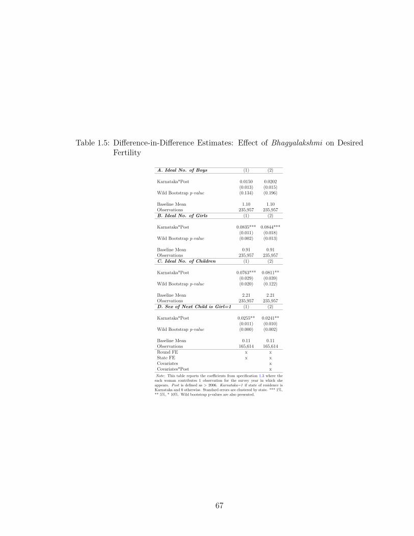
Table 1.5: Difference-in-Difference Estimates: Effect of Bhagyalakshmi on DesiredFertility
A. Ideal No. of Boys (1) (2)
Karnataka*Post 0.0150 0.0202(0.013) (0.015)
Wild Bootstrap p-value (0.134) (0.196)
Baseline Mean 1.10 1.10Observations 235,957 235,957B. Ideal No. of Girls (1) (2)
Karnataka*Post 0.0835*** 0.0844***(0.011) (0.018)
Wild Bootstrap p-value (0.002) (0.013)
Baseline Mean 0.91 0.91Observations 235,957 235,957C. Ideal No. of Children (1) (2)
Karnataka*Post 0.0763*** 0.0811**(0.029) (0.039)
Wild Bootstrap p-value (0.020) (0.122)
Baseline Mean 2.21 2.21Observations 235,957 235,957D. Sex of Next Child is Girl=1 (1) (2)
Karnataka*Post 0.0255** 0.0241**(0.011) (0.010)
Wild Bootstrap p-value (0.000) (0.002)
Baseline Mean 0.11 0.11Observations 165,614 165,614Round FE x xState FE x xCovariates xCovariates*Post x
Note: This table reports the coefficients from specification 1.3 where theeach woman contributes 1 observation for the survey year in which sheappears. Post is defined as > 2006. Karnataka=1 if state of residence isKarnataka and 0 otherwise. Standard errors are clustered by state. *** 1%,** 5%, * 10%. Wild bootstrap p-values are also presented.
67
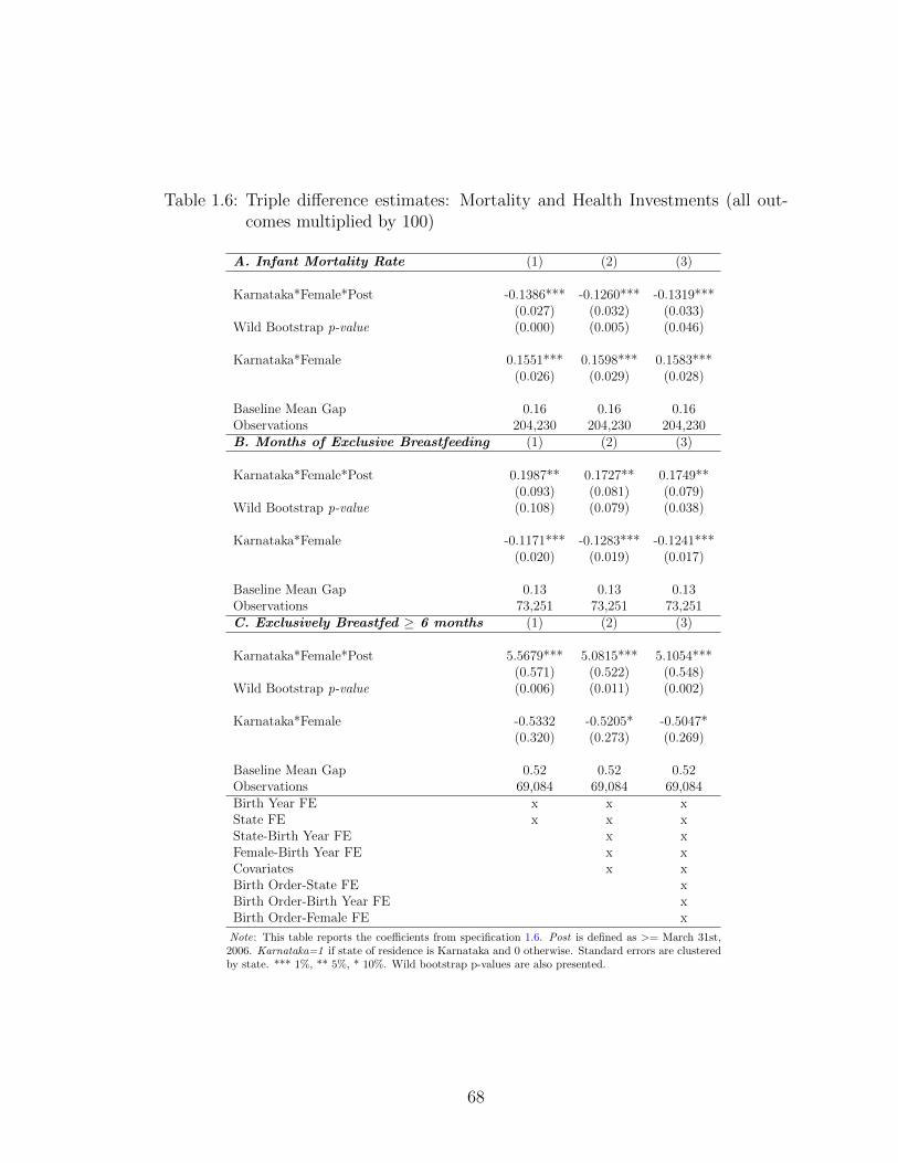
Table 1.6: Triple difference estimates: Mortality and Health Investments (all out-comes multiplied by 100)
A. Infant Mortality Rate (1) (2) (3)
Karnataka*Female*Post -0.1386*** -0.1260*** -0.1319***(0.027) (0.032) (0.033)
Wild Bootstrap p-value (0.000) (0.005) (0.046)
Karnataka*Female 0.1551*** 0.1598*** 0.1583***(0.026) (0.029) (0.028)
Baseline Mean Gap 0.16 0.16 0.16Observations 204,230 204,230 204,230B. Months of Exclusive Breastfeeding (1) (2) (3)
Karnataka*Female*Post 0.1987** 0.1727** 0.1749**(0.093) (0.081) (0.079)
Wild Bootstrap p-value (0.108) (0.079) (0.038)
Karnataka*Female -0.1171*** -0.1283*** -0.1241***(0.020) (0.019) (0.017)
Baseline Mean Gap 0.13 0.13 0.13Observations 73,251 73,251 73,251C. Exclusively Breastfed ≥ 6 months (1) (2) (3)
Karnataka*Female*Post 5.5679*** 5.0815*** 5.1054***(0.571) (0.522) (0.548)
Wild Bootstrap p-value (0.006) (0.011) (0.002)
Karnataka*Female -0.5332 -0.5205* -0.5047*(0.320) (0.273) (0.269)
Baseline Mean Gap 0.52 0.52 0.52Observations 69,084 69,084 69,084Birth Year FE x x xState FE x x xState-Birth Year FE x xFemale-Birth Year FE x xCovariates x xBirth Order-State FE xBirth Order-Birth Year FE xBirth Order-Female FE x
Note: This table reports the coefficients from specification 1.6. Post is defined as >= March 31st,2006. Karnataka=1 if state of residence is Karnataka and 0 otherwise. Standard errors are clusteredby state. *** 1%, ** 5%, * 10%. Wild bootstrap p-values are also presented.
68
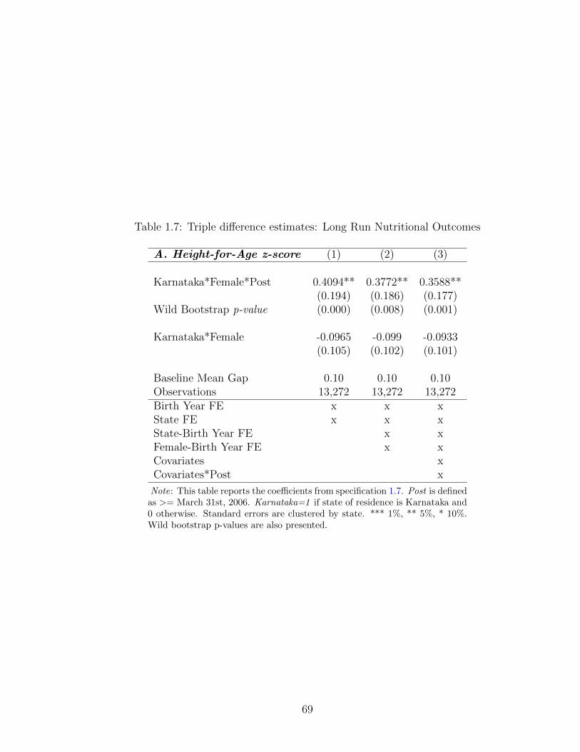
Table 1.7: Triple difference estimates: Long Run Nutritional Outcomes
A. Height-for-Age z-score (1) (2) (3)
Karnataka*Female*Post 0.4094** 0.3772** 0.3588**(0.194) (0.186) (0.177)
Wild Bootstrap p-value (0.000) (0.008) (0.001)
Karnataka*Female -0.0965 -0.099 -0.0933(0.105) (0.102) (0.101)
Baseline Mean Gap 0.10 0.10 0.10Observations 13,272 13,272 13,272Birth Year FE x x xState FE x x xState-Birth Year FE x xFemale-Birth Year FE x xCovariates xCovariates*Post x
Note: This table reports the coefficients from specification 1.7. Post is definedas >= March 31st, 2006. Karnataka=1 if state of residence is Karnataka and0 otherwise. Standard errors are clustered by state. *** 1%, ** 5%, * 10%.Wild bootstrap p-values are also presented.
69
Chapter 2: Is She Free to Work? Impact of Rural Health Insurance
on Labour Supply in India
2.1 Introduction
While there is much known about the labour market impacts of access to better
quality healthcare in developed countries, relatively little is known about these ef-
fects in developing countries. Given that illness impacts the poor disproportionately
more, it is important to understand whether access to better healthcare is welfare
improving overall. A large body of literature shows that better health increases
labour supply, wages and productivity in developing countries (see e.g. Strauss and
Thomas, 2007). Better quality healthcare through insurance, by mitigating the ad-
verse impacts of health shocks either through a reduction in the time spent caring
for sick individuals or through direct effects on health can impact labour market out-
comes.1 Health insurance can also impact the utility derived from leisure activities.
On the one hand, better health increases the utility derived from leisure. However,
risk averse consumers might enjoy leisure less if leisure results in more uncertainty
about health care expenditures (Currie and Madrian, 1999). Understanding how
the provision of health insurance impacts labour supply decisions of the household
1According to the efficiency wage theory the link between health and labour supply would bestronger in less healthy populations, and to the extent that health insurance impacts own health,this could lead to impacts on labour supply as well.
70
is important not only because labour market outcomes are indicators of overall wel-
fare but also because provision of non-contributory insurance to the underprivileged
may be an important redistributive policy tool.
This study examines whether access to free formal rural healthcare has a causal
effect on labour market outcomes by studying a plausibly exogenous policy change.
In 2008, India introduced the Rashtriya Swasthya Bima Yojana (RSBY) which pro-
vides each below poverty line (BPL) household access to health insurance at no
cost at selected private and public hospitals in the country. Designed to increase
access to healthcare and reduce the financial burden of health expenses, RSBY has
enrolled about 36 million households as of 2014 (about 12% of the total number
of households in the same year). While enrolling into the program is voluntary
and thus households self-select into the program, I take advantage of the phased
rollout of the program from 2008 through 2012 at the district level and employ a
differences-in-differences approach to examine the intent-to-treat impact of the pro-
gram on labour supply. I also examine RSBY beneficiary households and estimate
the average treatment effect on the treated.
India has one of the highest out-of-pocket (OOP) expenditures on healthcare
in the world. According to the National Health Accounts Data (2004-05) individual
OOP account for 78 percent of total expenditures while government expenditures
account for only 20 percent (Azam, 2016). Given the high proportion of total health
expenditures that are spent on out-of-pocket expenses, RSBY was devised to provide
cashless services to rural households. Households enrolled under RSBY can use a
‘smart card’ to avail services and pay an annual nominal enrollment fee.
While there is a growing literature on RSBY’s impact on out-of-pocket ex-
71

penditures (Johnson and Krishnaswamy, 2012; Nandi et al., 2013a; Sun, 2011; Ra-
jasekhar et al., 2011a), there is little evidence on the labour market impacts of the
program. Illness exposes households in developing countries to increased risk. Risk
pooling strategies such as social safety nets or formal health insurance are often
lacking and this forces households to engage in a variety of risk coping strategies
ranging from selling off durable assets, and reallocating labour away from produc-
tive activities (del Valle, 2014). Since health insurance is instrumental in reducing
household level out-of-pocket expenditures on health care it can protect households
from getting impoverished in addition to improving healthcare utilization and overall
health. Given the scope for government intervention, large scale healthcare reforms
have been introduced by many developing countries. One of the first of these was
in China in 2003 when rural health insurance was adopted (Wagstaff and Mana-
chotphong, 2012). In this context, using nationally representative data from two
large datasets - the Indian National Sample Survey (NSS) and the Indian Human
Development Survey (IHDS) - this paper seeks to understand the extent to which
a national rural health insurance program, the Rashtriya Swasthya Bima Yojana
(RSBY), impacts labour market outcomes of households in India, presenting both
Intent to Treat as well as Average Treatment on the Treated estimates.
Existing evidence on the impact of the RSBY program on financial risk pro-
tection is mixed. Karan et al. [2017] find that the reduction in out-of-pocket health
expenditures and catastrophic inpatient spending was small and statistically in-
significant. Using primary data from Maharashtra and Gujarat, Rathi et al. [2012]
and Devadasan et al. [2013] respectively, find that some families who have been
enrolled into the program continue to spend substantial amounts on out-of-pocket
72
health expenses. Johnson and Krishnaswamy [2012] find that the program led to
a small, statistically significant decrease in out-of-pocket expenditures while find-
ing no impact on inpatient expenditure. Similarly, Azam [2016] finds that while
out-of-pocket health expenses were not impacted by the program, expenditures on
medicines declined significantly in rural areas. One reason why Johnson and Kr-
ishnaswamy [2012] seem to find a significant reduction in outpatient expenditures
is because they examine program impacts only up to 2009-2010. As pointed out
by Nandi et al. [2013b] studies which examine impacts only up to 2009-2010 are
potentially biased since the program was still in its infancy in terms of implementa-
tion. Studies that have examined program effects up to 2011-12 seem to consistently
suggest low and statistically insignificant impacts of the RSBY on financial risk pro-
tection.
In contrast, with respect to hospital utilization, the literature consistently finds
that RSBY led to an increase in utilization rates. Azam [2016] finds a positive impact
on hospital utilization by households in rural areas. He also finds that RSBY led
to lower expenditures on medicines in rural areas. Ghosh and Gupta [2017] using a
matched sample of ‘potential’ RSBY treatment and control households, find that the
impact on inpatient care utilization was statistically significant - RSBY increases the
number of hospital admissions of insured families by 59% compared with the mean
inpatient care utilization of uninsured families. Finally, Johnson and Krishnaswamy
[2012] also find that the program impacted hospital utilization positively.
The evidence on the labour market impacts of non-contributory health insur-
ance, especially in developing countries is scarce. Moreover, most of the research
that exists focuses on the shift in employment from the formal to the informal
73

sector. This is because in most countries (e.g. Mexico, Thailand, Colombia) non-
contributory health insurance is only offered to those working in the informal sector.
In a study from Colombia, Camacho et al. [2013] find that public health insurance
led to an increase in informal employment of approximately 4 percentage points.
The present study is different from previous work in at least four ways. First,
this is the only study, in a developing country setting, that looks at the labour
market outcomes of a health insurance program that did not use the labour market
status as a determinant of eligibility, but instead had a pure income criterion for
eligibility. Thus, this study indirectly examines the ability of health insurance to
alleviate poverty because of health shocks and thereby impact labour market out-
comes. Second, this is the first study that examines the impact of household access
to health insurance, an important determinant of relative productivity for individual
members, on short term allocations across different types of work for children. Third,
it contributes to the nascent literature on the economic consequences of provision
of health insurance in developing countries. While much is known about the impact
of health shocks, little is known about how households reallocate labour supply as
a result of access to higher quality healthcare. The exception in this regard is Ad-
hvaryu and Nyshadham [2012] who estimate the effects of higher quality healthcare
through access to formal healthcare on labour supply of acutely sick individuals in
Tanzania and find that the ability to choose formal care led to individuals spending
more labour hours on the farm. Given that impoverishment due to health-related
expenses is a leading cause of poverty in India, it is important to understand the
extent to which social insurance programs trigger direct and indirect behavioural
responses that can mitigate this impoverishment. Finally, my paper contributes to
74
the literature on gender differentiated impacts of health insurance. It links the im-
pact of health insurance to a wider literature on the role of economic development
in helping either mitigate or reinforce gender inequalities.
Overall, I find significant positive effects of the RSBY program on the labour
supply of women in the private casual labour market using both the Intent-to-treat
(ITT) and Average treatment effect on the treated (ATT) estimates. On average,
household level access to free health insurance increases the number of days spent
in the past week by women on private casual labour by 0.29 days in early treatment
districts (i.e. districts that received RSBY treatment on or before March 2010).
Mean days spent in private casual work by women at baseline in 2004-05 is 0.45
days in a week. Thus, an ITT impact of 0.29 days is large; time spent in private
casual work increases by approximately 50 percent for women. This translates into
approximately 15 more days of work annually for women in the private labour
market. The ATT estimates are larger – time spent in private casual work increases
by about 81 percent for women. There was also a significant increase in time spent,
for women, in the private agricultural wage market by 0.25 days in the past week.
Importantly, this increase in labour supply in private sector work is accompanied
by a significant decrease in the number of days spent in the past week on domestic
work by 0.69 days. I examine various mechanisms that may explain the relationship
between the program and women’s labour supply. I consistently find that, for all
labour supply measures, the effect of accessing health insurance is largest for women
in households with fewer working age members and higher number of dependents.
Thus, I provide suggestive evidence that the impact of the program for women may
be due to the reduction in time spent at home in caregiving tasks.
75
For men, there is a smaller change in labour supply in private sector work. On
average, household level access to free health insurance increases the number of days
spent in the past week by men on private casual labour by 0.19 days (ITT estimate)
to 0.37 days (ATT estimate). This corresponds to a 20 percent increase over the
baseline mean. This increase in time spent in the private casual labour market is
accompanied by a decline in the time spent by men in self-employment activities.
This points to the fact that there is increased healthcare utilization by men which
improves their health and enables them to reduce time in self-employment activities
at home and work in the private casual labour market.2
Finally, I find that children substitute for adults in the two domains that men
and women are moving away from: domestic work and self-employment activities.
Consequently, I find that for children, time spent at educational institutions declines.
Overall, given positive changes in female and male private casual employment (and
significant negative changes in male self-employment and female domestic work), I
attribute the effect of the program to a reduction in caregiving tasks for women,
a reduction in self-employment activities for men and finally increased healthcare
utilization by both men and women.
Vulnerability to health shocks is a serious concern in India. Nearly 10% of
India’s population record out-of-pocket expenditures in excess of 25% of non-food
consumption (World Bank, 2008). There is a significant literature that shows that
households in India use productive assets to smooth consumption when faced with
2Self-employment activities at home here refers to working in household enterprises as own-account worker or as a helper. For e.g. opening a small shop inside one’s house if one is tooweek for manual labour in the private labour market. Such self-employment is not the sameas entrepreneurship. The goal of self-employment in this case, is to earn money for a time—preferably, a short time—before transitioning to a more remunerative activity when one’s physicalhealth improves.
76

negative productivity shocks. Rosenzweig and Wolpin [2017] find that in rural India,
bullocks, while also used as sources of mechanical power in agricultural production,
are sold to smooth consumption in the face of income shocks. This provides evidence
that efficiency in crop production is sacrificed to ensure low volatility in consump-
tion. Jodha [1978] again using data from India, argues that sales of productive assets
when faced with shocks (a drought in this case) is very common. While the specific
shock examined in this paper is different, the same argument is applicable in this
context too - the poor engage in costly consumption smoothing techniques in the
short run in response to catastrophic health shocks which can have severe long-term
impacts, both in terms of productive activity and labour market outcomes.
Accounting for close to USD 160 million in the union budget of 2012-13, RSBY
is one of the largest programs of its kind in a developing country. In this setting,
this study contributes to the ongoing policy debate regarding the benefits of in-
creased access to quality healthcare. While existing literature has failed to find a
significant change in out-of-pocket health expenditures, it has consistently found an
increase in health care utilization rates. This implies that the poor are availing of
the RSBY program which impacts their labour supply; but the maximum coverage
of Rs. 30,000 (about 440 USD in 2010-11) under the program is insufficient. Thus,
impacts on labour supply due to RSBY are not the result of an income effect of the
program, but instead are a consequence of the improved health of men and reduced
time in caregiving tasks for women.
The paper is organized as follows. Section 2.2 provides a brief review of the
previous developments in the literature on health insurance in India. It also provides
a description of the RSBY. Section 2.4 discusses the intent-to-treat estimation strat-
77

egy and results, while Section 2.5 describes the average treatment on the treated
estimation strategy and results. Section 2.6 examines the impact on health and
healthcare utilization and Section ?? performs robustness checks. Section 2.7 con-
cludes.
2.2 Context
2.2.1 Background of Health Insurance in India
Illness and poverty are closely linked to each other. The poor are often unable
to smooth consumption during periods of ill health and catastrophic health expenses
often push families into poverty (Xu et al., 2007; Rajasekhar et al., 2011b). Vulner-
ability to shocks is an important cause for deprivation (Dercon, 2001a). This is com-
pounded by the presence of weak financial instruments and the adoption of sub opti-
mal coping mechanisms such as asset sales, migration and child labour (Rosenzweig
and Wolpin, 2017; Haughton and Khandker, 2009). According to Krishna [2004],
the most common reason given by poor people for their descent into poverty is high
out-of-pocket expenditures on health care (Rajasekhar et al., 2011b). Shahrawat
and Rao [2012] note that the extent to which health related out-of-pocket (OOP)
expenditures exacerbate poverty is at a maximum for households below the poverty
line (BPL) in comparison to those above. The only government owned health in-
surance company that exists in India is the ‘New India Assurance’. New India
Assurance provides health insurance at slightly lower rates than private providers.
One has to purchase health insurance directly through this company as one would
purchase from a private provider. Thus, before RSBY was introduced in India, ac-
78
cess to health insurance of any kind depended on one’s ability to pay for insurance
through the marketplace.3 In the absence of adequate social safety nets households
can become impoverished not only because of out-of-pocket expenses and ill health,
but also because of missed work, disability or premature death (Fan et al., 2012). In
this context, to reduce the inequalities in health access and decrease health related
expenses for uninsured households, rural health insurance was introduced.
The empirical evidence on the effectiveness of health insurance in India is
sparse. Acharya et al. [2012] detail the myriad health insurance schemes in India
and analyze their effectiveness. The impact of these small community based schemes
has been mixed, at best. Aggarwal [2010] assesses the impact such a scheme in
Karnataka. The study finds that the Yeshasvini insurance reduced out-of-pocket
expenditures on health care out of savings, in addition to reducing borrowing money
to finance healthcare payments. However, Raza et al. [2016] using randomized
controlled trials from Bihar and Uttar Pradesh evaluate the impact of three CBHI
schemes and find no impact on both hospital utilization as well as on financial risk
protection. Using qualitative surveys the authors find that the main reason for the
lack of impact of these schemes is that most households tend to drop out after a
year, because of poor service quality and high premiums.
While the impact of health insurance on health utilization and expenditures is
relatively well studied, evidence on the impact of rural health insurance on labour
market outcomes in developing countries is limited. Given the importance of such
programs in mitigating the effects of a contraction in incomes due to health shocks
3India has a public health care system, wherein the government spends 1-2% of the GDP onpublic heath care. Thus, in the event that one cannot afford insurance from the marketplace, onecan, in theory, access government hospitals. However, free, public health system is so underfundedand understaffed that poor people are forced to pay exorbitant amounts to private-sector doctorsfor treatment.
79
and hence impacting labour supply, this lack of evidence seems stark. In one of
the first papers in this domain, Wagstaff et al. [2009] examine the universal health
coverage scheme in Thailand which was rolled out in 2001. They find that, at the
extensive margin the probability of employment increased for married women and
at the intensive margin increased time spent in informal employment for women.
Levy and Meltzer [2008] have argued that social insurance schemes, like rural
health insurance, can have unintended consequences such as encouraging an increase
in time spent in the informal sector. However, given that employer provided health
insurance in India is rare coupled with the fact that, unlike health insurance schemes
in other countries, RSBY is not restricted to informal workers, a decrease in the share
of formal sector workers post-RSBY is unlikely. The most critical part of RSBY is
that it allows households to transfer risk to the government while simultaneously
increasing access to health services. Impacts on labour supply are thus driven either
through impacts on own health or through decreased time spent caring for sick
dependents.
2.2.2 Overview of the Rashtriya Swasthya Bima Yojana
The Rashtriya Swasthya Bima Yojana was introduced in India in 2008. The
scheme aims at improving access of quality medical care to below poverty line (BPL)
families by providing cashless treatment at private and public hospitals for a variety
of ailments. RSBY provides cashless coverage up to Rs. 30,000 (about 440 USD in
2010-11) each year to each enrolled household for hospitalization procedures in em-
paneled private or public hospitals. This coverage is large in purchasing power terms:
the median level of income of the average person in my sample is about 616 USD
80
and the average household spends about 7-10% of their income towards healthcare
costs. The policy covers maternity care, hospitalization, day care treatment and
related tests, consultations, medicines and pre- and post-hospitalization expenses
excluding expenses for out-patient treatment. While the scheme covers most surgi-
cal and non-surgical procedures, not all diagnostic tests are covered. Importantly,
RSBY covers pre-existing conditions.
Under RSBY each below poverty line (BPL) household is issued an insurance
card or ‘smart card’ and up to five household members can be registered under one
card. To obtain treatment an individual just needs to present this smart card at
any participating hospital. The hospital receives reimbursement for treatment costs
by the insurance company. Both private and public hospitals are empaneled under
the scheme and thus households are free to choose between them.
2.2.3 Enrolment and Utilization of RSBY
RSBY is implemented at the state level. State governments choose an insur-
ance company through an open tender process. The central and state government
split the premium cost.
During the enrollment process, to ensure widespread coverage, states are re-
quired to prepare in advance a roadmap for the enrollment campaign in each village
in a district or taluk, and give the village prior notice of the enrollment team’s visit.
In addition, to ensure that eligible households are aware of the scheme in each village
and can plan to be present on the day of enrollment, a roster of eligible households
is displayed at the enrollment station. Households have to pay Rs. 30 (45 cents) as
annual registration fees.
81
Prior schemes of the government have been plagued by insufficient publicity
and lack of prior notice. The enrollment process of the RSBY aims to correct both
these flaws. Policies are issued for one year and are renewed on an annual basis.
Beneficiaries can utilize the scheme from the start date of the policy which is usually
three to four months after the enrollment process has been completed.
The state-wise number of beneficiaries enrolled from 2012-2015 in major states
is given in Appendix Table B.1. Up to October 2016, the program has covered
460 districts in India. About 41 million RSBY insurance cards have been issued
which cover about 150 million people (i.e. RSBY insurance cards are given one
per household). The district-wise enrollment ratio (share of eligible households
enrolled) has exhibited a fair amount of variation. For instance, enrolment ratios
in certain districts of Uttar Pradesh were as low as 3-6%, while enrollment was
nearly universal in districts of Chhattisgarh and Kerala (Karan et al., 2017). The
national enrollment rate was about 57% suggesting low enrollment. There are at
least two reasons for this: first, it is possible that even in the districts which have
begun implementing RSBY, all eligible households have not yet been enrolled due
administrative inefficiencies (Sun, 2010; Rathi et al., 2012). The second reason for
the low enrollment rate is that information and outreach campaigns by enrollment
agencies might have been insufficient (Rajasekhar et al., 2011b; Sun, 2010; Rathi
et al., 2012; Devadasan et al., 2004).
2.2.4 Rollout of RSBY
RSBY was introduced at the national level in 2008 and each state govern-
ment was expected to adopt the scheme in a phased manner over the next five
82
years. States are responsible for selecting districts for inclusion into the scheme.
In proposing districts for inclusion there were three criteria that were considered.
Districts selected under RSBY should have: (a) a sufficient network of private and
public hospitals, (b) intermediaries who can assist in spreading awareness about the
program and, (c) basic infrastructure necessary for implementation such as roads
and electricity. States began rolling out the program from 2008 in different districts
and in different years.
2.3 Theoretical Framework
This section formalizes the intuition that in the presence of health shocks, the
standard labour-leisure choice model of a poor household, without adequate coping
mechanisms, will be affected by their demand for health insurance. In this model, it
is assumed that health insurance can potentially impact the labour supply choice in
two ways. First, it may impact the labour force participation margin of the working
age population. This could also include the formal-informal work margin since it is
largely people with informal jobs who stand to benefit most from the RSBY.4 This
could arise both from improved health as a result of the program or the ability to
now enter the labour market since caregiving tasks are reduced.
Second, the program can change the number of hours spent in the labour mar-
ket. This can happen in two ways. First, better health impacts productivity. If
we assume that people don’t alter their consumption of leisure because of better
health, then health insurance should increase labour supply. Further, RSBY covers
4Section 2.2 outlines the details of the scheme. Eligibility was based on one’s poverty status.A household was deemed eligible for RSBY if the per capita consumption expenditure of thathousehold was below the government specified poverty line. While one’s employment status wasnot included in the definition of eligibility, most informal workers are part of BPL population.
83

hospitalizations only. Since major morbidities are more likely to result in hospital-
izations than short term illnesses, the potential for RSBY to impact labour supply
is greater.
Table 2.1 presents health related summary statistics in the last 4 weeks from
the Indian Human Development Survey (2004 - 05). From the table, it is clear that
a significant amount of time is lost because of major and minor illnesses especially
for those in the age group 0-5 years or in the age group 55 and above. Access to
free healthcare has the potential to treat these illnesses quickly, which can impact
labour supply for both men and women. Secondly, in the absence of health insurance,
individuals in households with a higher number of dependents would spend a large
amount of time in caregiving activities for the sick. Access to healthcare at zero
cost can, potentially, allow individual household members to spend more time on the
labour market. Given that household members from uninsured households spend a
significant amount of time in helping cope with illness, RSBY can potentially help
in freeing up household resources towards more productive activities.
A typical household spends on average about 5 days in a month with at least
one household member being unable to work due to short-term illness and about 4
days because of some major illness (see Table 2.1).5 It is also plausible that the pro-
vision of RSBY could lead to health gains; particularly among dependents.6 Prompt
medical attention coupled with the greater vulnerability of these sub-groups means
that RSBY is well-equipped to generate health impacts. This could be happening
through both the availability of and accessibility of prompt medical attention that
5Here major illnesses refer to: cataract, tuberculosis, heart disease, leprosy, cancer, polio,paralysis, epilepsy, mental illness, asthma and diabetes.
6Levy and Meltzer, 2008 review the literature on the impact of health insurance on health.
84

the RSBY generates.
2.4 Intent-to-Treat Effect
2.4.1 Program Rollout Data
Information about the rollout of the RSBY comes from administrative records
maintained by the Ministry of Health, Government of India. This is available online
on the RSBY website from where this information was accessed.
2.4.2 Household Survey Data
I use repeated cross sections of a nationally representative district level house-
hold survey, the Employment and Unemployment Survey (NSS Survey). My analysis
uses cross-sectional data for the years 2004-2005, 2007-2008 and 2011-2012 of the
NSS.
The NSSO has conducted national household level surveys since the early
1950s in India. The surveys conducted in 2004-2005 (61st Round), 2007-2008 (64th
Round) and 2011-2012 (68th Round) are large-sample surveys. The NSS collects
data on various individual and household level characteristics such as religion, caste,
employment status and household consumption. My identification uses the district-
wise phased rollout of the program. While constructing the sample the following
exclusion rules have been used: one, the states of Tamilnadu, Karnataka and Andhra
Pradesh have been excluded since these states had similar state run rural health
insurance programs during the period under consideration in this study. Two, I
also exclude the 3 Union Territories: Andaman & Nicobar Islands, Dadra & Nagar
85

Haveli and Daman & Diu. Three, individuals between 18 and 60 years have been
included for the adult labour market outcomes, while those between 6 and 17 years
have been included for the child outcomes. Four, I drop observations that have
missing information for age and gender. Finally, I only include districts that have
rural populations. The final sample includes households from 531 districts.
Implementation of the RSBY began in 2008-09. Thus, the 2011-12 wave (68th
round of the NSS) represents the post-intervention period. The 2004-05 and 2007-08
waves (61st and 64th rounds of the NSS respectively) represent the pre-intervention
period. Districts that began implementing the RSBY in 2008 did so in the latter half
of the year from August to December, and thus the 2007-08 NSS survey (64thround)
can be treated as pre-program data since it is canvassed from July 2007 – June 30,
2008, before any district began implementing RSBY.7
2.4.3 Outcomes of Interest
My main outcomes of interest are measures of employment for individual
household members. Each NSS survey records the daily activities of all individ-
uals above the age of four in a household. I construct the employment outcome as
follows. For each day and each activity, the NSS survey records whether the activity
was performed at an intensity of 0, 0.5 or 1 day. For each adult individual I calculate
the number of days in a week spent in five activities: (a) private casual work (b)
private salaried work (c) private agricultural wage work (d) domestic work and (e)
self-employment. Private casual work and private salaried work together constitute
private wage work. I also examine private agricultural wage work separately which
7Concerns of bias due to inter-district migration is likely to be low. Migrating from a ruraldistrict to another rural district for employment is uncommon.
86
can come under either private casual work or private salaried work. While domestic
work could be part of not in labour force, households in India also work in small
-scale agriculture which can be classified as domestic work. Additionally, domestic
work also includes time spent in caregiving tasks and thus I study this employment
measure separately.
2.4.4 District Level Information
To construct district controls I use data from two sources: first, I use individual-
level data from the 2002-2004 District Level Household Facility Survey, Wave 2
(DLHS-2) aggregated to the district level. The District Level Household Facility
Survey is a nationwide repeated cross-section survey which is representative at the
district level. The main district controls from the DLHS-2 are: the proportion of
villages in a district connected by a road, proportion of villages in a district with
a primary health center, proportion of villages in a district with a government hos-
pital, proportion of villages in a district with a health sub-center and the average
distance of a village in a district to the nearest town. I also use the 61st Round
of the National Sample Survey (NSS 2004-05) to control for baseline district-level
characteristics - fraction of scheduled castes and scheduled tribes, illiteracy rate,
male and female labor force participation and fraction living under the poverty line.
2.4.5 Empirical Framework
Previous studies have used several different approaches to identify treatment
effects of the RSBY program. In Karan et al. [2017], the authors define the treatment
group as all eligible households in RSBY treated districts. On the other hand in
87
Johnson and Krishnaswamy [2012], the authors use a difference-in-difference strat-
egy on districts that have first been matched on observable characteristics. Finally,
Ravi [2012] also use a similar district level difference-in-difference strategy and iden-
tify intent-to-treat (ITT) effects.
In this context, I employ two definitions of treatment and controls groups.
In the first definition, Sample I, I follow Karan et al. [2017] and classify all ‘poor’
i.e. below poverty line (BPL) households in districts that implemented RSBY as
treated households. While the 61st(2004-05) and 68th (2011-12) rounds of the NSS
data enquire about the below poverty line (BPL) status of households, this is not
true for the 64th round (2007-08). As pointed out by Karan et al. [2017], the two
lowest per capita expenditure quintiles account for about 70% of BPL households.8
Thus, I use households in the bottom two quintiles of consumer expenditure as a
proxy for ‘poor’ households. When constructing quintiles of asset-based poverty I
use the whole NSS sample by year i.e. this distribution is not constructed within
district. This is because the distribution may vary considerably at the district level,
leading to very different compositions of the bottom quintiles across districts.
Given that by 2011-12 the eligible population also includes National Rural
Employment Guarantee Scheme (NREGS) workers and other unorganized sector
workers, in the second definition, Sample II, I use an expanded sample and include
all households in the bottom two quartiles of consumer expenditure.
I consider two discrete cut-off points, March 2010 and June 2012 and iden-
tify two distinct treatment districts similar to Karan et al. [2017]. These are: (a)
poor households in districts which participated in RSBY before March 2010 (‘early’
8See Appendix Table A-III in Karan et al. [2017] for the percentage distribution of BPL house-holds by quintile groups in 2004-05.
88

treatment districts) and, (b) those living in districts which began participating be-
tween April 2010 and June 2012 (‘late’ treatment districts). Out of a total of 531
districts there are 191 districts which introduced the policy on or before March 2010
(these will be called the ‘early’ districts), 200 districts that introduced the policy
between April 2010 and June 2012 (these will be called the ‘late’ districts) and 140
districts that either introduced the program after June 2012 or have yet not intro-
duced the program (these are the ‘control’ districts). As mentioned before, states
such as Tamilnadu, Karnataka and Andhra Pradesh which had similar state run ru-
ral health insurance programs during the period under consideration in this study,
have been excluded. Appendix Table B.2 details the state-wise number of districts
in early and late treatment groups.
State governments decided the order in which RSBY was rolled out at the
district level. While it is unlikely that labour supply was one of the factors that
impacted the decision to implement the program; it is still possible that program
placement might be endogenous. Thus, I compare changes over time between dis-
tricts that implemented RSBY early (‘early’ districts) and districts which imple-
mented RSBY later (‘late’ districts) to ‘control’ districts. I estimate the following
difference-in-difference specification, similar to Karan et al. [2017]:
Yidt = β0 + β1Earlyd + β2 Lated +3∑t=2
timet∗Earlyd ∗ θt
+3∑t=2
timet∗Lated ∗ ψ+
timet + X idtγ + Zd ∗ 1t>2008δ + ηd+ εidt (2.1)
where Yidt is the outcome variable for individual i in district d in year t =
2004-05, 2007-08 and 2011-12. Earlyd and Lated are dummies for early and late
89

districts respectively. Timetare time dummies (time2 corresponds to 2007-08 and
time3 corresponds to 2011-12). Zd are time invariant district controls (detailed in
Section 4.4 and summarized in Table 3) and 1 t > 2008is a dummy variable equal
to 1 after 2008.
Xidt includes individual and household controls: dummy variables for age cat-
egories 30 to 40, 40 to 50 and older than 50, dummy variables for years of education
less or equal to 4, between 5 and 8, between 8 and 12, and equal to 129, dummies
for scheduled caste and scheduled tribe (omitted category “other”), dummies for
Muslim religion or other religion, dummies for single and widowed marital status
and household size and month of survey fixed effects. Finally, I include district fixed
effects, ηd, and cluster standard errors at the district level.
For early districts which implemented RSBY before March 2010, θ2 is the pre-
intervention differences-in-difference estimate (comparing 2007-08 to the baseline
year of 2004-05) and θ3 is the post-intervention differences-in-difference estimate
(comparing 2011-12 to the base line year of 2004-05). Similarly, for the treatment
group that joined RSBY between April 2010 and June 2012 (‘late districts’), ψ2
is the pre-intervention differences-in-difference estimate; ψ3 is the post-intervention
differences-in-difference estimate. Thus, the intent-to-treat treatment effect for early
districts is θ3– θ2 and the treatment effect for late districts is, ψ3 – ψ2.
This is a standard difference-in-difference specification. If unobservable dif-
ferences between treatment and control districts are correlated to the probability
of being treated, then this assumption might not hold. For instance, districts with
9I only keep observations of working-age adults (between 18 to 60 years old) for the mainanalysis. I study the labour supply responses of children between 6-17 years of age separately inSection 2.4.9.
90

better government implementation infrastructure might be more equipped to diffuse
information about the program and consequently enroll more households. Not ac-
counting for differential trends between treatment and control districts with result
in over estimation of the effects in the difference-in-difference framework (Heckman
and Vytlacil, 2007).
In Figures 2.1 & 2.2 I examine the trends of ‘early’ districts relative to ‘control’
districts and of ‘late’ districts relative to ‘control’ districts respectively. In Figure
2.1 which compares early and control districts the pre-period comprises 2004-5 to
2007-08; while in Figure 2.2 which compares late and control districts the pre-period
comprises 2004-5 to 2009-10. The outcome variables in both figures range from 0
to 7. I find that in both figures, pre-program trends in the main outcome variables
seem to be parallel.
In Table 2.2, I also use only the 2004-05 and 2007-08 (pre-program rounds) to
run a similar specification to the one presented in equation (2.1) except the program
dummy is equal to 1 for 2007-08 (i.e. 2007-08 is taken to be the hypothetical post
period). In the absence of the program, there should be no significant differences
between treated and control districts by future district treatment status. I present
results separately for males and females. The results in Table 2 show no significant
differences between early and control districts and late and control districts for
the main outcome variables (interaction terms Post*Early Treatment & Post*Late
Treatment in the first and third rows of Panels A and B), providing support for
using control districts as a comparison group for early and late districts.
Finally, Appendix Table B.3 presents the baseline means in 2004-05 for early,
late and control districts for the main outcome variables used in this study. All
91
outcome variables range from 0-7 and are defined as the number of days in the past
week spent in a particular activity.10
2.4.6 Results: Intent-to-Treat Estimates
My primary interest in this section is to examine the effect of RSBY on the
decision to change the number of hours worked in the labour market, among those
already employed. Table 2.3 presents the main estimates for sample I (i.e. house-
holds in the bottom two expenditure quintiles) while Appendix Table B.4 presents
the same for sample II (i.e. households in the bottom two expenditure quartiles).
In Table 2.3 Panel A, for women, among those who are already employed,
RSBY significantly (at the 5% level) increases labour supply by increasing the num-
ber of days worked in the past week in private casual work in early districts as com-
pared to control districts (column 2 in Panel A). That is, the number of days worked
in a week in private casual work increases by 0.286 days (effects of RSBY for early
districts is derived by subtracting the coefficient on EarlyTreatment*Time2 from
the coefficient on EarlyTreatment*Time3 and similarly for later districts). Mean
days spent in private casual work by women at baseline in 2004-05 is 0.45 days in a
week. Thus, an impact of 0.286 days is large; time spent in private casual work ap-
proximately increases by 50 percent for women. This translates into approximately
15 more days of work annually for women in the private labour market.
While the increase in labour supply is large for private casual work; private
10It is also important to note that confounding impacts of the National Rural EmploymentGuarantee Scheme (NREGS) which is a central government program may not be relevant in thiscontext. This is because in the period of interest in this paper this program was already fullyrolled out. The NREGS was rolled out in three phases in the country from February 2006 to May2008.
92
salaried work (column 4 of Panel A) does not change for women after the intro-
duction of RSBY. This makes intuitive sense since RSBY helps in reducing health
related disruptions which would increase labour supply in spot markets and other
types of short-term private contractual work which come under private casual work
as opposed to private salaried work which includes salaried longer-term regular em-
ployment. Late treatment districts also see an increase in private casual work and
private salaried work for women; however, these are not significant. This is poten-
tially because information about RSBY, like other government programs is slow to
trickle in and thus households in late treatment districts are still unaware of the
program.
Women also see an increase in private agricultural wage work and a significant
decline in domestic activities (columns 6 & 8 in Table 2.3 Panel A). For instance,
number of days in a week spent on private agricultural wage work increases by 0.254
days while it decreases by 0.694 days for domestic work. This implies that one of the
main mechanisms through which the program is operating is through a reduction in
time spent at home in caregiving duties after the introduction of the RSBY. Once
again, the effect of RSBY on private agricultural wage work and domestic work is
present only in early districts.
The significant increase in labour supply that I find for women in private casual
work and private agricultural wage work combined with the significant decline in
domestic work provides initial evidence that the RSBY program frees up some time
from domestic work in the week for women which allows them to engage in temporary
short-term employment. Finally, since only early districts see a program impact this
is consistent with low enrollment ratios of RSBY documented in Section 2.2.3. That
93

is, information about RSBY is slow to diffuse and impacts are only seen 2-3 years
after the program is already in place. Thus, late districts do not witness any impact
of the program in 2011-12.
Estimates from Sample II (i.e. households in the bottom three expenditure
quintiles) in Appendix Table B.4 reveal the same broad picture. Women witness an
increase in labour supply in private casual work and private salaried work and a de-
cline in labour supply in domestic work. All these effects are once again concentrated
in the early districts.
For men, in Table 2.3 Panel B, there is an increase in the number of days
in the past week spent in the private casual labour market by about 0.198 days.
However, this is not statistically significant. This increase in private casual labour
is accompanied by a significant decrease in the number of days spent in the last week
in early districts on self-employment activities for men. A significant fraction of men
in poor countries are self-employed (Datt and Ravallion, 1994). Indeed, according
to NSS 2004-05 about 58 percent of the male workforce across the country was self-
employed. For those men who were self-employed either to be close to home if they
were caregivers or they were too sick themselves to find outside employment; the
introduction of the RSBY should reduce self-employment for both these types.
2.4.7 Female Labour Supply Heterogeneity
In this section, I decompose the labour supply of women by household size.
First, in Panel A of Table 2.4, the program effect is allowed to vary by the num-
ber of working age members in a household where working age is defined as be-
tween 18 and 60 years of age. As a simplification, I use data only from NSS
94

Rounds 64 & 68 (2007-08 and 2011-12 respectively) in Equation (2.1). Thus,
I add the following terms to the regression model described in Equation (2.1):
Working Age*EarlyTreatment*Post; Working Age*LateTreatment*Post; Working
Age*EarlyTreatment; Working Age*LateTreatment; andWorking Age*Post. Here
Post refers to the year 2011-12 and Working Age refers to the number of working
age members (i.e. those in the 18-60 age group) in a household.11
The results in Panel A, Table 2.4 examine heterogeneity in labour supply for
women by the number of working age members in a household. The interaction
term between working age, early program districts and the post period is negative
and significant for most private labour supply outcomes for women (private casual
work and private agricultural wage work) suggesting that women living in house-
holds with more working age members experience a larger increase in labour supply.
Specifically, if rural women in early districts experience an average increase in pri-
vate casual work of 0.650 days in a week (coefficient on Early Treatment*Post in
column (2.2) in Panel A of Table 2.4) associated with the program; then women
who have working age members one standard deviation below the mean experience
0.83 days increase in labour supply, while women who have working age members
one standard deviation above the mean experience only an increase of 0.47 days.12
These estimates imply that the effect of the program is concentrated amongst
households with fewer working age members. There are potentially two explanations
11That is, I estimate the following equation: That is, I estimate the following equation: Yidt =β0 + β1Earlyd + β2Lated + θEarlyd ∗ Post + ψLated ∗ Post + δ1WorkingAge ∗ Earlyd ∗ Post +δ2WorkingAge∗Lated∗Post+δ3WorkingAge∗Earlyd+δ4WorkingAge∗Lated+δ5WorkingAge∗Post+ Post+Xidtγ + ηs + εidt
12Given a standard deviation of 1.71 for the number of working age members, the effect of aone-standard deviation decrease in working age members is -0.179. The total effect is thus: 0.650– (-0.179) = 0.83. Similarly, the total effect associated with an increase in working age membersis: 0.650 + (-0.179) = 0.47.
95
for this. One, the higher the number of working age members, the less likely it is that
the household as a whole is affected by one person’s illness. In smaller households
on the other hand, where the number of working age members is low, even one
person being ill can impact the labour supply of women adversely. If RSBY impacts
labour supply by improving health and health utilization then smaller households
stand to benefit more from it. Second, the larger the household, the less are the
number of hours spent on caregiving by any one person and hence the smaller is the
impact of RSBY on household labour supply. Thus, RSBY has a bigger potential to
impact labour supply for women in smaller households. In addition, heterogeneity
in program response according to household size acts as a robustness check that
unobserved factors are not driving the results. This is because, one would assume
that poverty increases with household size, and we see that program effect decreases
with the number of members in the household.
Panel B of Table 2.4 examines heterogeneity in labour supply for women by the
number of dependents in a household. Dependents are defined as those younger than
18 years or older than 65 years in a household. I add similar interaction terms to
those described above for working age members: Dependents*EarlyTreatment*Post;
Dependent*LateTreatment*Post; Dependent*Early Treatment; Dependent*LateTreatment
and Dependent*Post. The interaction term between dependent, early program dis-
tricts and post period is not significant for any of the private labour supply outcomes.
However, the interaction term is positive suggesting once again that households with
more dependents experience a larger increase in private labour supply. Specifically,
if rural women in early districts experience an average increase in private casual
work of 0.223 days in a week (coefficient on Early Treatment*Post in column (2) in
96
Panel B of Table 2.4) associated with the program, then women who have depen-
dents one standard deviation below the mean experience 0.19 days increase in labour
supply, while women who have dependents one standard deviation above the mean
experience an increase of 0.26 days.13 These estimates while not significant, provide
further evidence that the decrease in domestic labour supply of women and a con-
comitant increase in private labour supply is consistent with the hypothesis that in
the post-RSBY period, caregiving tasks for women decreased. That is, women with
fewer working age members in the household and/or a higher number of dependents
witness larger program impacts.
2.4.8 Intensity of Treatment
As a further test of the robustness of my empirical specification I also estimate
how the length of time a household has been exposed to RSBY affects labour market
outcomes. The number of days elapsed between the start of the policy and the date
of the NSS survey in a district varies substantially across households since each
survey round took a year to complete. The longer the length of time between
the start of the RSBY policy and the survey date, the higher the likelihood that
someone may have had the need for hospitalization and utilized RSBY for the same.
There are several other reasons why the impact of RSBY may vary with the time
since implementation. First, in many districts, awareness of RSBY has only spread
gradually and knowledge about the program was been extremely low in the first few
13Given a standard deviation of 2.7 for the number of dependents, the effect of a one-standarddeviation decrease in dependents is 0.035. The total effect is thus: 0.223 – (0.035) = 0.19. Similarly,the total effect associated with an increase in dependents is: 0.223 + (0.035) = 0.26.
97

months after initial rollout despite households being given smart cards.14 Second,
hospitals may take time to understand and become familiar with the scheme.
I estimate the impact of the duration of RSBY exposure using a modified
difference-in-difference model. The degree of RSBY exposure in a district is likely
to be exogenous and should not be correlated to other district characteristics since
I define intensity as the years since the program was implemented in the district.
Specifically, I estimate the following:
Yidt = β0 + β1RSBY Intensityd +3∑t=2
timet ∗RSBY Intensityd ∗ θt+
Xidtγ + Zd ∗ 1t>2008δ + ηs + εidt (2.2)
where RSBYIntensityd is defined as the number of years of RSBY exposure in
district d. All other variables are defined as before. The estimated average program
effect in this case, is the coefficient on (RSBYIntensity*Time3 ) – coefficient on
(RSBYIntensity*Time2 ).
Table 2.5 examines if the treatment effect of RSBY is larger when the number
of years of exposure to RSBY is higher. As expected, the results show that men
and women who face more years of exposure to the RSBY program have larger
program effects. A one standard deviation increase in RSBY exposure raises the
labour supply of women in the private casual and private agricultural wage market
by 0.034 to 0.043 days in the past week (columns (2) and (6) in Panel A). Increased
RSBY exposure also decreases time spent in the last week by women in domestic
14For instance, Johnson and Kumar (2011) find that a large proportion of enrolled householdsare only vaguely aware of the purpose of the RSBY smart card.
98

work by 0.17 days. Men also witness an increase in private casual work and private
agricultural wage work (significant at the 10% level) as RSBY exposure increases.
Additionally, a one standard deviation increase in RSBY exposure decreases self-
employment for men by 0.102 days in the past week (significant at the 5% level).
Thus, the results in this section provide support for the main identification strategy
outlined in Section 2.4.
2.4.9 Labour Force Participation of Children Aged 6-17 years
Labour force participation of dependents can be impacted in two ways as a
result of RSBY. One, following from the luxury and substitution axioms of the
Basu and Van (1998) model of child labour supply, in which children can substitute
for adults in the labour market, a family will send children to the labour market
only if the family’s income from non-child labour sources falls below some threshold
amount. Thus, if the program leads to income security for households then one
would expect that time spent by children in the labour market should decrease.
Second, in general adults have a comparative advantage in home production (i.e. in
caregiving tasks). That is, in the absence of health insurance, children will substitute
for adults in the labour market. In such a case, if total household labour hours rise
with the provision of health insurance, then labour hours of children should fall and
time spent at school should rise.
However, existing evidence on the impact of RSBY on reducing financial bur-
den due to health expenditures is mixed and a higher proportion of studies find that
RSBY did not significantly contribute to raising the income security of households.
In this scenario then, the mechanism that is driving the labour supply impacts of
99
RSBY is an increase in healthcare utilization. In this case, one would expect children
to substitute towards activities which adult men and women are moving away from
such as domestic work and self-employment. Thus, the overall impact of RSBY on
the labour supply of children and time spent on education activities is ambiguous.
Table 2.6 presents estimates of the fraction of days spent by children in dif-
ferent activities in a week. That is, I estimate Equation (2.1) but for children from
6-17 years of age. I find that the average number of days spent in the last week in
early districts in the post-RSBY period in self-employment and domestic activities
significantly increases for children. On the other hand, the time spent in educa-
tional institutions sees a significant decrease. For instance, children spend 0.601
less days in the past week in school and while they spend about 0.243 days more
on self-employment and domestic activities combined. This implies that after the
availability of free health insurance, in early districts, children are substituting into
the activities like domestic work and self-employment that their parents are moving
out of. Thus, availability of health insurance does not appear to have an income
effect for child labour but does seem to have a substitution effect with respect to
time. This is in line with existing evidence of RSBY which show that the pro-
gram did not significantly impact out-of-pocket expenditures on health care while
significantly increasing healthcare utilization.
2.5 Average Treatment Effect on the Treated
The Intent-to-treat (ITT) estimates, presented up to now, can approximate
the Average Treatment Effect on the Treated (ATT) in the scenario where enrolment
ratios are high. Since the national enrollment ratio is about 57%, the ITT parameter
100

might not be very informative. While most studies on RSBY provide ITT estimates
of the program, Raza et al. [2016] and Azam [2016] provide Average Treatment on
the Treated estimates. In this section I follow the methodology outlined in Azam
[2016] and evaluate the labour market impacts of RSBY on beneficiary households
using the nationally representative Indian Human Development Survey (IHDS).
2.5.1 Data
The IHDS is a national survey, representative at the national, state and district
level, with a sampling frame similar to the NSS. There are 2 waves of the survey,
collected in 2004-2005 and 2011-2012 (henceforth, 2005 and 2012, respectively).
There were 42,152 households interviewed in 1503 villages in IHDS-2. Like before,
I drop Andhra Pradesh, Karnataka, and Tamil Nadu from the sample since these
states had state-run health insurance programs operating at the same time as RSBY
was implemented. Similarly, like before, I restrict my analysis to rural areas.
Identification in this piece of the analysis comes from utilizing household’s
response to a direct question in the 2012 IHDS survey about having the RSBY
card. Approximately 13 percent of households had an RSBY card in the IHDS-2.
The official percentage pf population covered under RSBY was about 13.6 percent
in 2012. Thus, the IHDS-2 captures RSBY exposure well (Ministry of Labour &
Employment, 2012).
Similar to the NSS, the IHDS defines labour force participation through the
following 4 work categories: (1) private casual work (2) private salaried work (3)
business work (4) family farm work. There are two ways in which the labour supply
variables defined in this section differ from the analysis using NSS data – (a) the
101

IHDS does not record time spent in “domestic activities” and “self-employed” sep-
arately and, (b) I include time spent on the family farm and on business activities
as separate work categories, which were not available in the NSS.
2.5.2 Empirical Framework
I use the longitudinal nature of the IHDS data to estimate a matching difference-
in-difference strategy. The main advantage of such estimators relative to alterna-
tive methods used in the presence of non-experimental data relies on their semi-
parametric nature, allowing the estimation of treatment effects without imposing
restrictive distributional assumptions to the data generating process.
Following the methodology outlined in Azam [2016], I first start with the
following simple model:
Yiht = f(xit) + β1RSBY ht + ψt + ηh+ εiht (2.3)
where Yiht is the labour market outcome for individual i in household h at time t ;
ηh are time invariant household level characteristics and ψt are year fixed effects.
The treatment variable is RSBYht which takes the value 1 for households that were
enrolled in the program (i.e. beneficiary households who had an RSBY card) in
the post-time period i.e. 2011-12. That is, the variable takes the value 0 for all
households in 2004 and takes the value 1 in 2012 for those households who were
covered under the program. The effect of the program is given by β1.
The expectation of the difference between pre- and post-period changes in
RSBY beneficiary households (given by ‘T’ ) and pre- and post-period changes in
102
non-RSBY households (given by ‘C’ ) is:
E(∆Y Tih)− E(∆Y C
ih ) = E[f(∆xTih)]− E[f(∆xCih)] + β1+
[∆ψT − ∆ψC ] + E(∆εTih)− E(∆εCih) (2.4)
There are three assumptions required to recover the impact of RSBY on labour
supply in this framework as outlined in Azam [2016]: First, differences in observables
between the treated and control households should be zero. By carefully matching
each treated household (those who have the RSBY card i.e beneficiary) with one or
more control households (those who didn’t have the RSBY card) to ensure that the
matched sample is similar with respect to observable characteristics, the first term
of Equation 2.4 i.e. E[f(∆xTih)]− E[f(∆xCih)] can be eliminated.
The second assumption is that ∆ψT = ∆ψC . Since longitudinal data is used
in this piece of the analysis i.e. the same household is observed for both time periods,
this assumption seems reasonable. That is, the composition of treated households
and control households does not change in the pre- and post-program periods. This
combined with the fact that under assumption (1) detailed above, treatment and
control households have been matched so that they are very similar with respect to
observables, implies that the trend in the aggregate shock between treatment and
control groups could plausibly be the same.
Finally, the third assumption is that E(∆εTih) = E(∆εCih). For instance, it
is possible that there is some adverse selection wherein households who are more
vulnerable to health shocks could potentially be more likely to enroll in the program,
while relatively healthier households might be less likely to enroll. As pointed out
103

by Azam [2016] some features of the RSBY program helps mitigate concerns of time
varying idiosyncratic shocks to some extent. The average enrollment costs under
RSBY are very low, about Rs. 30 per year and there are no insurance premiums.
Given that the average daily wage rate in rural areas is about Rs. 140, this implies
that all households, irrespective of health-related vulnerabilities should be equally
likely to enroll into the program.
Now, there are two potential control groups in this setting – (a) non-RSBY
households in all districts in the country and, (b) non-RSBY households in only
those districts that implemented the program by 2012. I follow Azam [2016] and re-
strict the analysis to only those districts that had implemented the program by 2012.
That is, the control group includes only those households without an RSBY card
who resided in districts that implemented the program by 2012 (henceforth, RSBY
exposed districts). The intuition behind choosing this control group is straightfor-
ward – the time specific aggregate shock is more likely to exhibit a similar trend for
treatment and control households residing in the same geographic area rather than
for households residing in different geographic areas.
Following Blundell and Dias [2009], for longitudinal data the matching difference-
in-differences (MDID) estimator is given by:
αMDIM,L =∑j ε T
[Yi1 − Yi0] −∑j ε C
wij[Yj1 − Yj0] wi (2.5)
where T and C are defined as treated and control households respectively. wij is
defined as the weight on a control household j for the treated household i (Blundell
and Dias, 2009). Thus, I compare pre- and post-program labour market outcomes
104

between treated and control households in RSBY districts, after controlling for
baseline differences with matching.
Using the baseline data, Appendix Table B.5 reports summary statistics for
the main outcome variables. Panel A reports the intensive margin of labour supply
variables (number of hours worked in a day) and Panel B reports the extensive
margin (indicator variables for labour force participation). At both the extensive and
intensive margins, RSBY households are more likely to be engaged in private casual
work and private agricultural wage work and are also more likely to spend more
hours in a day engaged in these types of work (these differences are not statistically
significant).
2.5.3 Matching
Appendix Table B.6 reports the descriptive statistics of household level char-
acteristics (from the baseline 2005 data) which might potentially be correlated with
RSBY status. Column (1) reports the means for non-RSBY households and column
(2) reports means for RSBY households. In general, RSBY card holder households
have lower income and consumption and a larger proportion of RSBY households
are below the poverty line. Similarly, a larger proportion of RSBY household mem-
bers report short term illness in the past 30 days and a higher number of per capita
days being unable to work in the past month due to an illness.
To estimate the propensity score, P(T = 1|X) = P(X), i.e. the probability
of a household participating in RSBY given their observed covariates X, I use the
household characteristics described in Appendix Table B.6 and run a probit model.
The dependent variable is whether a household had an RSBY card in 2011. The
105
probit model is run using independent variables from only the baseline 2005 data.
Since RSBY was not available in 2005, the independent variables could not have been
affected by RSBY enrollment. The model also includes district fixed effects. The
results from the probit model are presented in Appendix Table B.7. As expected,
log per capita consumption and log income are negatively correlated with having an
RSBY card i.e. relatively richer households are less likely to enroll into the program.
Similarly, households where the household head has a formal government job are less
likely to enroll into RSBY. Socially disadvantaged groups like Scheduled Caste and
Scheduled Tribe households are more likely to enroll into the program. Households
without access to basic services like electricity and flush toilet are more likely to
enroll into the program. Additionally, households with good social networks such as
being part of a self-help group and attending local body meetings are more likely to
enroll into RSBY. None of the coefficients on prior household health status such as
proportion of household members with a short term or long-term illness, per capital
inpatient and outpatient expenditure and per capita hospital days predict RSBY
enrollment. Thus, this provides evidence in favor of potentially low adverse selection
and the validity of third assumption in the identification strategy.
Sub-setting the full sample of households to those with a common support of
the propensity score reduces the number of households to 19,906 (out of 21,943).
I use kernel matching as my main matching method. Figure 2.4 compares
the standardized bias before and after matching. The standardized median (mean)
bias before matching is 6.6 (7.9) percent and after matching is 0.9 (1.0) percent
indicating that the matching was effective at creating a good control group with
balanced covariates.
106
2.5.4 Results: ATT Estimates
Appendix Table B.8 presents the results. Column (3) presents the ATT estimates
while column (4) depicts the baseline average for RSBY households. The results
are larger than the ITT estimates presented in Section 2.4. In Panel A column
1, for women belonging to RSBY households in RSBY exposed districts, among
those already employed, the number of days spent in the past week in private casual
work increases by 0.335 days. Mean days spent in private casual work by women in
RSBY households at baseline in 2004-05 is 0.41 days in a week. Thus, an impact of
0.335 days is large; time spent in private casual work approximately increases by 81
percent for women (column 3, Panel A), compared to a 50 percent increase in the
ITT analysis. Number of days in the past week spent in business work also increases
for women by almost 50 percent compared to baseline 2004 levels (column 3, Panel
A).
In contrast to the ITT estimates, there is also a significant increase for men
in private casual labour. The number of days in the past week spent in the private
casual labour market increases by 0.373 days, which corresponds to a 20 percent
increase over the baseline mean. While the absolute increase in the number of
days in private casual labour is the same for both men and women, given the large
differences in their baseline levels, the increase for women is much larger.
2.6 Impact on Health and Health Care Utilization
One of the primary mechanisms through which labour supply could increase
after the introduction of the RSBY is through effects on own health and health care
107
utilization. Theoretically, better health leads to an increase in worker productivity.
Dow et al. [1997] find that in Indonesia, a reduction in access to health services
reduces objective heath indicators, such as activities of daily living, as well as female
labour force participation. Further, Baicker et al. [2014] find positive impacts of
Medicaid on health care use as well as on self-reported general health, even though
they don’t find impacts of Medicaid on employment of low income adults. Increased
access to insurance could also lead to increased financial security. While Karan et al.
[2017] do not find an effect of the program on out of pocket expenditures, Azam
[2016] finds that health utilization rates go up. This implies that the program helps
in preventing families from becoming impoverished because of a health shock. That
is, in the absence of the insurance, treatment for an illness would not have been
possible or would have been prohibitively expensive. However, after the program,
households need to only spend the amount that exceeds the insurance cap amount
(Rs. 30,000). This implies that one would not see any impact on out-of-pocket
expenditures, even though families are better off now, if their total healthcare bill
exceeds the insurance cap. However, an increase in health care utilization rates
would indicate that people are actually using the program. This is what I examine
next.
While Azam [2016] provides some of the first estimates of the program on
health care utilization, he excludes districts that have not been treated by 2010
from his analysis. In the following analysis, I define treatment and control groups as
detailed in Section 2.4 i.e. ‘control’ districts received the program after June 2012
or have not yet received it, ‘early’ districts are those received program before March
2010 and ‘late’ districts are those that received program between April 2010 and
108
June 2012. While the NSS data lacks information on health outcomes, I use the
Indian Human Development Survey (IHDS), described in the previous section, to
examine these effects.
I use IHDS Waves I (2004-2005) and II (2011-2012) for my analysis with IHDS-
I forming the pre-program period and IHDS-II forming the post-program period.
More specifically, I estimate the following specification:
Yidt = β0 + β1Earlyd + β2Lated + θEarlyd ∗ Post+ ψLated ∗ Post+ timet+
Xidtγ + Zd ∗ 1t>2008δ + ηs+ εidt (2.6)
Here Post refers to 2011-12 (IHDS-2). All other variables are defined as in Equation
1. Since there is only one pre-program round of data, θ is the differences-in-difference
estimate (comparing 2011-12 to the base line year of 2004-05) for early districts and
similarly ψ is the differences-in-difference estimate for late districts. The sample, like
before is restricted to individuals in the 18-60 years age group. The main dependent
variables I examine are: body mass index (BMI), short term morbidity (number of
days in a month an individual is unable to work because of a short-term illness such
as a fever or cough), long term morbidity (number of days in a month an individual
is unable to work because of a long-term illness), number of days ill because of a
short-term morbidity and an indicator for seeking formal care for a major morbidity.
Table 2.7 examines the physical health outcomes and healthcare utilization
patterns from the above specification. I find that access to RSBY significantly
improves women’s body mass index (BMI) by 0.737 points in early districts and by
0.87 points in late districts (column 2, Panel A). Men see an insignificant increase
109
in BMI. Both men and women see a decrease in the number of days in a month
affected by a short-term morbidity such as a fever or cough (column (3) in Panels
A and B). Surprisingly, I find that short term morbidity is also impacted positively
by the program. This could be explained by the fact that greater income security
makes households better equipped to handle short term morbidities.
Importantly, the number of days in a month that both men and women are
unable to work because of a major morbidity decreases significantly in both early
and late districts (column (8) in Panels A and B). For women, the decline in early
districts is almost 3.5 days in a month, while the decline for men is about 2.3 days in
a month. That is, men and women gain an additional 2.3 and 3.5 days in a month
respectively, because they can now get treatment for their major morbidities under
RSBY. This is an important contribution of the program. By enabling the poor to
access cashless hospitalization in hospitals of their choice means that acutely sick
individuals can get care in time as opposed to when it’s too late. Seeking formal
care for major morbidities is thus an important mechanism through which labour
supply is affected.
Days unable to work because of a short-term morbidity does not significantly
change possibly because short term morbidities are not debilitating enough to take
time off work. Finally, for both men and women healthcare utilization goes up signif-
icantly. I also find that the program impacts the number of days of hospitalization,
for men (significant at the 10% level).
Thus, overall, an increase in health and health care utilization, in addition to
a decrease in caregiving tasks and self-employment activities documented earlier,
seem to be the main mechanisms driving the labour supply impacts of the rural
110
health insurance program. That is, the RSBY program enables all members of
the household (men and women) to get treated for major morbidities. This in
turn, decreases the time they’re unable to work because of major morbidities and
decreases the time a caregiver needs to spend at home.
2.7 Conclusion
Many developing countries are beginning to experiment with free or subsidized
health insurance for the poor. Understanding the general equilibrium effects of
such policies particularly on labour supply is an important step towards designing
effective policies. In this paper, I use the phased implementation of a rural health
insurance scheme in India and apply a difference-in-difference design to examine
the link between health insurance and labour supply. My main finding is that the
program, Rashtriya Swasthya Bima Yojana (RSBY) increases the number of hours
spent in the private labour market per week for both men and women, but the
increase for women is disproportionately larger. I provide some suggestive evidence
that this increase is due to an increase in health care utilization as well as a decrease
in domestic caregiving tasks.
More specifically, I find that individuals are significantly more likely to seek
formal care for major morbidities after the program. Time spent out of the labour
force because of a major morbidity declines. Further, I find that there is a significant
reduction in time spent on domestic tasks in a week for women which implies that
the labour supply results for women are driven by a decrease in domestic caregiving
tasks as well as a decline in time spent being unable to work because of a major
morbidity.
111
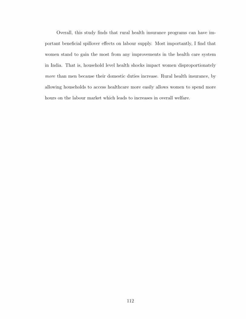
Overall, this study finds that rural health insurance programs can have im-
portant beneficial spillover effects on labour supply. Most importantly, I find that
women stand to gain the most from any improvements in the health care system
in India. That is, household level health shocks impact women disproportionately
more than men because their domestic duties increase. Rural health insurance, by
allowing households to access healthcare more easily allows women to spend more
hours on the labour market which leads to increases in overall welfare.
112
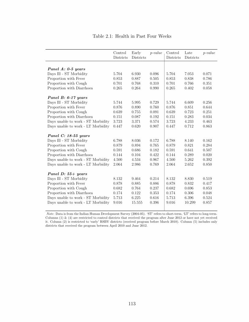
Table 2.1: Health in Past Four Weeks
Control Early p-value Control Late p-valueDistricts Districts Districts Districts
Panel A: 0-5 yearsDays Ill - ST Morbidity 5.704 6.930 0.096 5.704 7.053 0.071Proportion with Fever 0.853 0.887 0.505 0.853 0.838 0.786Proportion with Cough 0.701 0.768 0.310 0.701 0.766 0.351Proportion with Diarrhoea 0.265 0.264 0.990 0.265 0.402 0.058
Panel B: 6-17 yearsDays Ill - ST Morbidity 5.744 5.995 0.729 5.744 6.609 0.256Proportion with Fever 0.876 0.890 0.760 0.876 0.851 0.644Proportion with Cough 0.639 0.755 0.091 0.639 0.723 0.251Proportion with Diarrhoea 0.151 0.087 0.192 0.151 0.283 0.034Days unable to work - ST Morbidity 3.723 3.371 0.574 3.723 4.233 0.463Days unable to work - LT Morbidity 0.447 0.620 0.907 0.447 0.712 0.863
Panel C: 18-55 yearsDays Ill - ST Morbidity 6.788 8.036 0.172 6.788 8.140 0.162Proportion with Fever 0.879 0.894 0.765 0.879 0.821 0.284Proportion with Cough 0.591 0.686 0.182 0.591 0.641 0.507Proportion with Diarrhoea 0.144 0.104 0.422 0.144 0.289 0.020Days unable to work - ST Morbidity 4.500 4.534 0.967 4.500 5.262 0.392Days unable to work - LT Morbidity 2.064 2.986 0.769 2.064 2.652 0.850
Panel D: 55+ yearsDays Ill - ST Morbidity 8.132 9.464 0.214 8.132 8.830 0.519Proportion with Fever 0.878 0.885 0.886 0.878 0.832 0.417Proportion with Cough 0.682 0.764 0.237 0.682 0.696 0.853Proportion with Diarrhoea 0.174 0.122 0.353 0.174 0.306 0.048Days unable to work - ST Morbidity 5.713 6.225 0.616 5.713 6.396 0.524Days unable to work - LT Morbidity 9.016 15.555 0.396 9.016 10.299 0.857
Note: Data is from the Indian Human Development Survey (2004-05). ‘ST’ refers to short-term, ‘LT’ refers to long-term.Columns (1) & (4) are restricted to control districts that received the program after June 2012 or have not yet receivedit. Column (2) is restricted to ‘early’ RSBY districts (received program before March 2010). Column (5) includes onlydistricts that received the program between April 2010 and June 2012.
113

Table 2.2: Pre-program tests using NSS 61st and 64th Rounds
Private Casual Private Salaried Private Agricultural Domestic Self-EmployedWork Work Wage Work Work
Panel A: Females
Post*Early Treatment -0.014 -0.134 0.035 0.028 0.059 0.043 0.049 0.182 0.034 0.061(0.0878) (0.0904) (0.0370) (0.0376) (0.0465) (0.0493) (0.1734) (0.1824) (0.1309) (0.1419)
Post*Late Treatment -0.167 -0.166* 0.035 0.041 0.038 0.037 -0.022 -0.007 0.201 0.186(0.0856) (0.0890) (0.0370) (0.0360) (0.0431) (0.0505) (0.1749) (0.1875) (0.1300) (0.1348)
Individual Controls No Yes No Yes No Yes No Yes No YesDistrict controls No Yes No Yes No Yes No Yes No YesNumber of observations 71506 69869 71506 69869 71506 69869 71506 69869 71506 69869
Panel B: Males
Post*Early Treatment -0.056 -0.182 -0.063 -0.063 -0.094 -0.2 -0.014 -0.032 0.102 0.282(0.1542) (0.1479) (0.0649) (0.0657) (0.1478) (0.1413) (0.0227) (0.0241) (0.1389) (0.1457)
Post*Late Treatment -0.014 -0.14 0.097 0.147 -0.092 -0.269* -0.028 -0.026 0.137 0.212(0.1552) (0.1564) (0.0604) (0.0647) (0.1578) (0.1551) (0.0334) (0.0332) (0.1429) (0.1403)
Individual Controls No Yes No Yes No Yes No Yes No YesDistrict controls No Yes No Yes No Yes No Yes No YesNumber of observations 69809 67687 69809 67687 69809 67687 69809 67687 69809 67687
Note: Post indicates the hypothetical post round 2007-08. Regressions include state and month of interview fixed effects. District controls include fraction ST and SC,fraction illiterate, female and male employment rates, and fraction under poverty line separately for the whole district and for the rural areas of the district - calculatedfrom NSS 2004-05. Also includes: the proportion of villages in a district connected by a road, proportion of villages in a district with a primary health center, proportion ofvillages in a district with a government hospital, proportion of villages in a district with a health sub-center and the average distance of a village in a district to the nearesttown calculated from DLHS 2002-04. Individual controls include dummies for age 30 to 40, 40 to 50, and greater than 50, dummies for years of education under 4, between5 and 8, between 8 and 12, and 12, as well as marital status, and household size. Standard errors in parentheses, clustered at the district level. Number of districts=531. *denotes significance at the 10% level, ** denotes significance at the 5% level, and *** denotes significance at the 1% level.
Figure 2.1: Pre-Program Trends for ITT analysis - Early vs. Control Districts
Note: NSS 61, 62 and 64 rounds. ‘Control’ districts - received theprogram after June 2012 or have not yet received it; ‘Early’ districts- received program before March 2010.
114
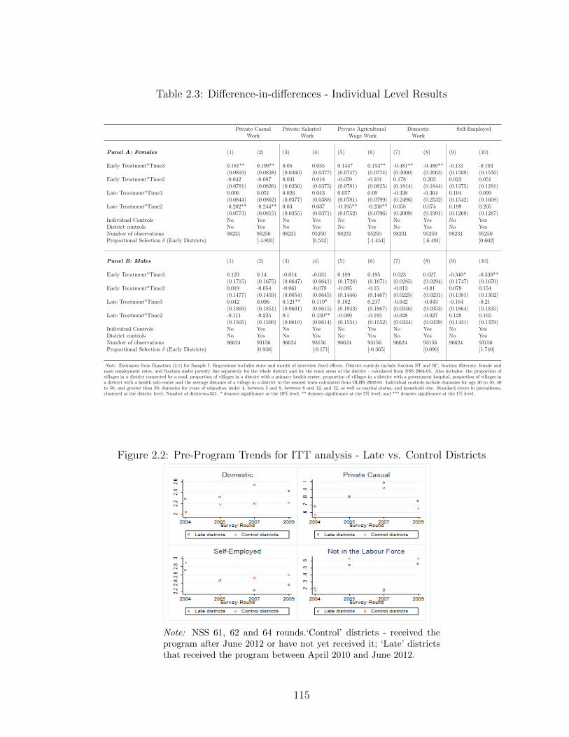
Table 2.3: Difference-in-differences - Individual Level Results
Private Casual Private Salaried Private Agricultural Domestic Self-EmployedWork Work Wage Work Work
Panel A: Females (1) (2) (3) (4) (5) (6) (7) (8) (9) (10)
Early Treatment*Time3 0.181** 0.199** 0.05 0.055 0.144* 0.153** -0.481** -0.489** -0.131 -0.103(0.0819) (0.0838) (0.0360) (0.0377) (0.0747) (0.0774) (0.2000) (0.2063) (0.1508) (0.1556)
Early Treatment*Time2 -0.042 -0.087 0.031 0.018 -0.059 -0.101 0.178 0.205 0.022 0.051(0.0781) (0.0826) (0.0356) (0.0375) (0.0781) (0.0825) (0.1814) (0.1844) (0.1275) (0.1281)
Late Treatment*Time3 0.006 0.051 0.026 0.043 0.057 0.09 -0.338 -0.364 0.104 0.099(0.0844) (0.0862) (0.0377) (0.0388) (0.0781) (0.0799) (0.2496) (0.2532) (0.1542) (0.1608)
Late Treatment*Time2 -0.202** -0.244** 0.03 0.037 -0.195** -0.238** 0.058 0.074 0.199 0.205(0.0773) (0.0815) (0.0355) (0.0371) (0.0752) (0.0796) (0.2009) (0.1991) (0.1269) (0.1287)
Individual Controls No Yes No Yes No Yes No Yes No YesDistrict controls No Yes No Yes No Yes No Yes No YesNumber of observations 98231 95250 98231 95250 98231 95250 98231 95250 98231 95250Proportional Selection δ (Early Districts) [-4.895] [0.552] [-1.454] [-6.491] [0.602]
Panel B: Males (1) (2) (3) (4) (5) (6) (7) (8) (9) (10)
Early Treatment*Time3 0.123 0.14 -0.014 -0.031 0.189 0.195 0.023 0.027 -0.340* -0.339**(0.1715) (0.1675) (0.0647) (0.0641) (0.1728) (0.1671) (0.0285) (0.0294) (0.1747) (0.1670)
Early Treatment*Time2 0.019 -0.054 -0.061 -0.078 -0.085 -0.15 -0.013 -0.01 0.079 0.154(0.1477) (0.1459) (0.0654) (0.0645) (0.1446) (0.1467) (0.0225) (0.0231) (0.1381) (0.1302)
Late Treatment*Time3 0.042 0.096 0.121** 0.119* 0.182 0.217 -0.042 -0.043 -0.184 -0.21(0.1869) (0.1851) (0.0601) (0.0615) (0.1943) (0.1867) (0.0346) (0.0353) (0.1864) (0.1835)
Late Treatment*Time2 -0.111 -0.235 0.1 0.130** -0.089 -0.185 -0.028 -0.027 0.128 0.165(0.1505) (0.1500) (0.0610) (0.0614) (0.1551) (0.1552) (0.0334) (0.0339) (0.1431) (0.1379)
Individual Controls No Yes No Yes No Yes No Yes No YesDistrict controls No Yes No Yes No Yes No Yes No YesNumber of observations 96624 93156 96624 93156 96624 93156 96624 93156 96624 93156Proportional Selection δ (Early Districts) [0.938] [-0.171] [-0.365] [0.090] [1.740]
Note: Estimates from Equation (2.1) for Sample I. Regressions includes state and month of interview fixed effects. District controls include fraction ST and SC, fraction illiterate, female andmale employment rates, and fraction under poverty line separately for the whole district and for the rural areas of the district - calculated from NSS 2004-05. Also includes: the proportion ofvillages in a district connected by a road, proportion of villages in a district with a primary health center, proportion of villages in a district with a government hospital, proportion of villages ina district with a health sub-center and the average distance of a village in a district to the nearest town calculated from DLHS 2002-04. Individual controls include dummies for age 30 to 40, 40to 50, and greater than 50, dummies for years of education under 4, between 5 and 8, between 8 and 12, and 12, as well as marital status, and household size. Standard errors in parentheses,clustered at the district level. Number of districts=531. * denotes significance at the 10% level, ** denotes significance at the 5% level, and *** denotes significance at the 1% level.
Figure 2.2: Pre-Program Trends for ITT analysis - Late vs. Control Districts
Note: NSS 61, 62 and 64 rounds.‘Control’ districts - received theprogram after June 2012 or have not yet received it; ‘Late’ districtsthat received the program between April 2010 and June 2012.
115
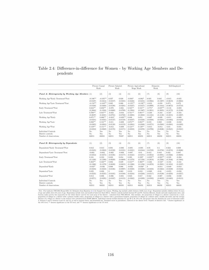
Table 2.4: Difference-in-difference for Women - by Working Age Members and De-pendents
Private Casual Private Salaried Private Agricultural Domestic Self-EmployedWork Work Wage Work Work
Panel A: Heterogeneity by Working Age Members (1) (2) (3) (4) (5) (6) (7) (8) (9) (10)
Working Age*Early Treatment*Post -0.106** -0.105** 0.027 0.028 -0.082* -0.082* 0.025 0.045 -0.015 -0.025(0.0437) (0.0454) (0.0217) (0.0221) (0.0436) (0.0455) (0.0964) (0.1007) (0.0619) (0.0664)
Working Age*Late Treatment*Post -0.152** -0.163** 0.005 0.006 -0.125** -0.139** -0.052 -0.059 0.074 0.073(0.0440) (0.0460) (0.0198) (0.0201) (0.0437) (0.0457) (0.0988) (0.1044) (0.0672) (0.0718)
Early Treatment*Post 0.634** 0.650** -0.078 -0.061 0.525** 0.531** -0.771* -0.837** -0.116 -0.083(0.2004) (0.1956) (0.0808) (0.0789) (0.1984) (0.1967) (0.3951) (0.3925) (0.2172) (0.2198)
Late Treatment*Post 0.798** 0.847** -0.023 -0.016 0.741** 0.801** -0.256 -0.244 -0.347 -0.345(0.2037) (0.2021) (0.0755) (0.0730) (0.2005) (0.2002) (0.4104) (0.4149) (0.2215) (0.2267)
Working Age*Early 0.071** 0.086** -0.024* -0.028** 0.046 0.051 -0.007 -0.029 -0.011 -0.009(0.0324) (0.0325) (0.0127) (0.0138) (0.0327) (0.0330) (0.0508) (0.0501) (0.0403) (0.0423)
Working Age*Late 0.088** 0.101** -0.011 -0.009 0.074** 0.084** 0.019 0.002 -0.039 -0.032(0.0305) (0.0304) (0.0138) (0.0152) (0.0304) (0.0308) (0.0574) (0.0568) (0.0384) (0.0402)
Working Age*Post 0.159** 0.151** -0.012 -0.009 0.124** 0.120** -0.013 -0.013 -0.04 -0.031(0.0353) (0.0368) (0.0170) (0.0171) (0.0358) (0.0376) (0.0796) (0.0826) (0.0521) (0.0561)
Individual Controls No Yes No Yes No Yes No Yes No YesDistrict controls No Yes No Yes No Yes No Yes No YesNumber of observations 62213 60233 62213 70327 62213 60233 62213 60233 62213 60233
Panel B: Heterogeneity by Dependents (1) (2) (3) (4) (5) (6) (7) (8) (9) (10)
Dependents*Early Treatment*Post 0.012 0.013 0.001 -0.006 -0.005 -0.005 0.05 0.1 0.024 0.008(0.0345) (0.0363) (0.0192) (0.0181) (0.0321) (0.0344) (0.0728) (0.0750) (0.0574) (0.0606)
Dependents*Late Treatment*Post -0.003 -0.003 -0.002 -0.009 -0.007 -0.01 0.012 0.043 0.021 0.007(0.0353) (0.0375) (0.0186) (0.0177) (0.0345) (0.0371) (0.0852) (0.0891) (0.0566) (0.0605)
Early Treatment*Post 0.181 0.223 0.023 0.054 0.205 0.229* -0.822** -0.922** -0.235 -0.204(0.1430) (0.1390) (0.0639) (0.0609) (0.1378) (0.1356) (0.2619) (0.2566) (0.1846) (0.1804)
Late Treatment*Post 0.263** 0.322** 0.002 0.029 0.313** 0.366** -0.464 -0.535* -0.184 -0.161(0.1306) (0.1270) (0.0638) (0.0615) (0.1266) (0.1256) (0.2970) (0.2921) (0.1852) (0.1837)
Dependent*Early -0.037* -0.036 0.008 0.006 -0.032 -0.036* 0 -0.014 -0.049 -0.053(0.0223) (0.0222) (0.0106) (0.0097) (0.0220) (0.0220) (0.0450) (0.0463) (0.0339) (0.0344)
Dependent*Late 0.025 0.026 0 0.003 0.018 0.018 -0.009 -0.03 -0.055 -0.058(0.0235) (0.0235) (0.0105) (0.0100) (0.0234) (0.0240) (0.0517) (0.0539) (0.0358) (0.0357)
Dependent*Post 0.013 0.006 -0.006 -0.001 0.023 0.017 0.042 -0.007 -0.056 -0.038(0.0271) (0.0295) (0.0167) (0.0155) (0.0262) (0.0289) (0.0593) (0.0623) (0.0483) (0.0515)
Individual Controls No Yes No Yes No Yes No Yes No YesDistrict controls No Yes No Yes No Yes No Yes No YesNumber of observations 62213 60233 62213 60233 62213 60233 62213 60233 62213 60233
Note: Post indicates NSS 68th Round 2011-12. Estimates from Equation (2.1) for Sample I for women. Working Age includes adults between 18-60 years of age. Dependents includes children below 18 yearsof age and adults above 65 years of age. Regressions include state and month of interview fixed effects. District controls include fraction ST and SC, fraction illiterate, female and male employment rates, andfraction under poverty line separately for the whole district and for the rural areas of the district - calculated from NSS 2004-05. Also includes: the proportion of villages in a district connected by a road,proportion of villages in a district with a primary health center, proportion of villages in a district with a government hospital, proportion of villages in a district with a health sub-center and the averagedistance of a village in a district to the nearest town calculated from DLHS 2002-04. Individual controls include dummies for age 30 to 40, 40 to 50, and greater than 50, dummies for years of education under4, between 5 and 8, between 8 and 12, and 12, as well as marital status, and household size. Standard errors in parentheses, clustered at the district level. Number of districts=531. * denotes significance atthe 10% level, ** denotes significance at the 5% level, and *** denotes significance at the 1% level.
116

Table 2.5: Difference-in-differences - Treatment Intensity
Private Casual Private Salaried Private Agricultural Domestic Self-EmployedWork Work Wage Work Work
Panel A: Females (1) (2) (3) (4) (5) (6) (7) (8) (9) (10)
RSBY Intensity*Time3 0.069** 0.065** 0.012 0.011 0.048** 0.044** -0.141** -0.135** -0.063 -0.055(0.0228) (0.0231) (0.0098) (0.0098) (0.0212) (0.0217) (0.0603) (0.0607) (0.0394) (0.0396)
RSBY Intensity*Time2 0.035 0.022 0.006 0.000 0.021 0.01 0.027 0.032 -0.039 -0.03(0.0217) (0.0219) (0.0088) (0.0089) (0.0215) (0.0217) (0.0558) (0.0554) (0.0342) (0.0343)
Individual Controls No Yes No Yes No Yes No Yes No YesDistrict controls No Yes No Yes No Yes No Yes No YesNumber of observations 98231 95250 98231 95250 98231 95250 98231 95250 98231 95250
Panel B: Males (1) (2) (3) (4) (5) (6) (7) (8) (9) (10)
RSBY Intensity*Time3 0.075* 0.079* -0.014 -0.031 0.189 0.071* 0.023 0.011* -0.340* -0.118**(0.0403) (0.0431) (0.0647) (0.0198) (0.1728) (0.0400) (0.0285) (0.0065) (0.1747) (0.0450)
RSBY Intensity*Time2 0.019 0.062 -0.061 -0.059** -0.085 0.013 -0.013 0.002 0.079 -0.016(0.1477) (0.0389) (0.0654) (0.0178) (0.1446) (0.0360) (0.0225) (0.0064) (0.1381) (0.0373)
Individual Controls No Yes No Yes No Yes No Yes No YesDistrict controls No Yes No Yes No Yes No Yes No YesNumber of observations 96624 93157 96624 93157 96624 93157 96624 93157 96624 93157
Note: Estimates from Equation (2.2). RSBY Intensity is defined as years of RSBY exposure by 2011-12. Regressions include state and month of interview fixed effects.District controls include fraction ST and SC, fraction illiterate, female and male employment rates, and fraction under poverty line separately for the whole district and forthe rural areas of the district - calculated from NSS 2004-05. Also includes: the proportion of villages in a district connected by a road, proportion of villages in a districtwith a primary health center, proportion of villages in a district with a government hospital, proportion of villages in a district with a health sub-center and the averagedistance of a village in a district to the nearest town calculated from DLHS 2002-04. Individual controls include dummies for age 30 to 40, 40 to 50, and greater than 50,dummies for years of education under 4, between 5 and 8, between 8 and 12, and 12, as well as marital status, and household size. Standard errors in parentheses, clusteredat the district level. Number of districts=531. * denotes significance at the 10% level, ** denotes significance at the 5% level, and *** denotes significance at the 1% level.
Table 2.6: Difference-in-differences - Child Level Results
Private Casual Private Salaried Private Agricultural Domestic Education Self-EmployedWork Work Wage Work Work
(1) (2) (3) (4) (5) (6) (7) (8) (9) (10) (11) (12)
Early Treatment*Time3 0.023 0.027 0.009 0.011 0.019 0.017 0.126** 0.072 -0.654** -0.571** 0.144** 0.161**(-0.0331) (0.0267) (0.0137) (0.0136) (0.0260) (0.0230) (0.0534) (0.0527) (0.1319) (0.1214) (0.0497) (0.0475)
Early Treatment*Time2 0.033 -0.031 0.005 0.007 -0.042 -0.041 0.045 0.034 -0.270* -0.206 0.044 0.01(0.0299) (0.0302) (0.0123) (0.0118) (0.0302) (0.0270) (0.0613) (0.0580) (0.1564) (0.1466) (0.0486) (0.0500)
Late Treatment*Time3 0.001 0.006 -0.006 -0.004 0.03 0.023 0.108** 0.049 -0.196 -0.112 0.120** 0.142**(0.0347) (0.0291) (0.0102) (0.0100) (0.0274) (0.0254) (0.0516) (0.0538) (0.1324) (0.1281) (0.0458) (0.0439)
Late Treatment*Time2 -0.055 -0.044 -0.004 0.000 -0.048 -0.046 0.189** 0.182** -0.208 -0.145 0.093* 0.052(0.0235) (0.0325) (0.0105) (0.0102) (0.0313) (0.0287) (0.0675) (0.0655) (0.1641) (0.1559) (0.0499) (0.0507)
Individual Controls No Yes No Yes No Yes No Yes No Yes No YesDistrict controls No Yes No Yes No Yes No Yes No Yes No YesNumber of observations 88984 87772 88984 87772 88984 87772 88984 87772 88984 87772 88984 87772
Note: Estimates from Equation (2.1) for Sample I for children from 6-17 years of age. Regressions include state and month of interview fixed effects. District controls include fraction ST and SC,fraction illiterate, female and male employment rates, and fraction under poverty line separately for the whole district and for the rural areas of the district - calculated from NSS 2004-05. Also includes:the proportion of villages in a district connected by a road, proportion of villages in a district with a primary health center, proportion of villages in a district with a government hospital, proportionof villages in a district with a health sub-center and the average distance of a village in a district to the nearest town calculated from DLHS 2002-04. Individual controls include dummies for age 30 to40, 40 to 50, and greater than 50, dummies for years of education under 4, between 5 and 8, between 8 and 12, and 12, as well as marital status, and household size. Standard errors in parentheses,clustered at the district level. Number of districts=531. * denotes significance at the 10% level, ** denotes significance at the 5% level, and *** denotes significance at the 1% level.
117

Table 2.7: Difference-in-difference - Health and Healthcare Utilization
Body Mass Index Days Affected Days Unable to Work Days Unable to Work Days Hospitalized Seeks Formal Care(BMI) by Short term Morbidity due to Short term Morbidity due to Major Morbidity for Major Morbidity
Panel A: Females (1) (2) (3) (4) (5) (6) (7) (8) (9) (10) (11) (12)
Early Treatment*Post 0.742** 0.737** -0.893** -0.727 0.076 0.22 -1.880* -3.417** 0.071 0.065 0.047** 0.031**(0.2949) (0.2592) (0.4037) (0.4449) (0.4001) (0.4465) (1.0177) (0.8989) (0.0604) (0.0656) (0.0132) (0.0136)
Late Treatment*Post 0.857** 0.870** -0.792* -0.625 -0.196 -0.124 -0.29 -1.776** 0.045 0.053 0.026** 0.01(0.3210) (0.2894) (0.4180) (0.4602) (0.4529) (0.4951) (1.0050) (0.8897) (0.0616) (0.0655) (0.0121) (0.0125)
Individual Controls No Yes No Yes No Yes No Yes No Yes No YesDistrict controls No Yes No Yes No Yes No Yes No Yes No YesNumber of observations 67433 63172 67433 63172 67433 63172 67433 63172 67433 63172 67433 63172
Note: Estimates from Equation 2.6 using the Indian Human Development Survet (IHDS). Regressions include state fixed effects. District controls include fraction ST and SC, fraction illiterate, female and maleemployment rates, and fraction under poverty line separately for the whole district and for the rural areas of the district - calculated from NSS 2004-05. Also includes: the proportion of villages in a district connected bya road, proportion of villages in a district with a primary health center, proportion of villages in a district with a government hospital, proportion of villages in a district with a health sub-center and the average distanceof a village in a district to the nearest town calculated from DLHS 2002-04. Individual controls include dummies for age 30 to 40, 40 to 50, and greater than 50, dummies for years of education under 4, between 5 and8, between 8 and 12, and 12, as well as marital status, and household size. Standard errors in parentheses, clustered at the district level. Number of districts=531. * denotes significance at the 10% level, ** denotessignificance at the 5% level, and *** denotes significance at the 1% level.
Figure 2.3: Density of Households in each Propensity Score Bin higher than 0.4 forATT analysis
118

Figure 2.4: Standardized Bias in Unmatched and Matched Samples
119
Chapter 3: Income Shocks, Public Works and Child Nutrition
3.1 Introduction
It is well known that poor households in developing countries are limited in
their ability to smooth consumption in the face of income shocks. This generates
large variations in consumption which can have adverse consequences for the well-
being of these households. The impact of such shocks on children has been well
researched (see e.g Jensen, 2000, Alderman et al., 2009 and Alderman et al., 2006).
Early life exposure to economic shocks has important implications not only for sub-
sequent adult health and other socio-economic outcomes but also for perpetuating
intergenerational poverty (Maccini and Yang, 2009). In such an event, social protec-
tion schemes such as the National Rural Employment Guarantee Scheme (NREGS)
in India may have the potential to mitigate the adverse impacts of an income shock
on child health by serving as a nutritional safety net.
Envisaged as being both a safety net and as providing alternative employment,
the NREGS is the largest employment guarantee program of its kind in the world
with annual expenditures equaling about 1 percent of India’s GDP.1,2 While the
use of public work programs in developed countries has declined, there has been
1The NREGS offers a legal guarantee to every rural household: about 68 percent of the popu-lation.
2About Rs. 33000 crores ($5500 million) in 2013-14.
120
a resurgence of such programs in developing countries.3 They have evolved into
long term anti-poverty measures rather than merely serving to reduce temporary
unemployment (Zimmermann, 2014). Using data from Andhra Pradesh in India,
this paper seeks to understand the extent to which a safety net like the NREGS
buffers the impact of income shocks on investments in children.4
While there is a growing literature on the impact of the NREGS on the labour
market (e.g. Berg et al., 2012, Azam, 2012, Imbert et al., 2012) there has been a
lack of focus on its role as a buffer for poor households in the event of a shock and
the consequent impact on children.5 To address this gap in the literature and using
pre and post-intervention data from the Young Lives Panel study in India, I use a
quasi-experimental approach to examine the extent to which the NREGS buffers the
impact of income fluctuations on child health. That is, I examine the intent-to-treat
effects of the program. I also assess the differential impact of the NREGS across
wealth quartiles, land ownership and gender. Since the NREGS was implemented
in a phased manner with the poorest districts getting it first, selection bias is a
serious issue. By assuming that program placement is additive and time invariant,
this study corrects for selection bias by using a difference-in-difference framework.
There are multiple channels through which the NREGS could impact child
health in the event of a shock. First, the NREGS will result in changes in the labour
supply of the household and as long as the income effect outweighs the substitution
effect, child health will not be negatively affected in the event of a shock. Second,
given that the NREGS leads to the strengthening of community level infrastructure
3Subbarao et al. [2012] provide an extensive review of public works programs - their design,implementation issues, poverty impacts and cost effectiveness - in developing countries.
4On June 2, 2014 Andhra Pradesh was split into two states: Telangana and Andhra Pradesh.This however doesn’t impact my analysis since the data used in this paper is from 2002 to 2009.
5Zimmermann [2014] and Dasgupta et al. [2013] are notable exceptions.
121

such as water supplies and roads, child health is positively impacted as a result of
this improved community infrastructure. Third, as a result of the NREGS, village
economies become functional again and this leads to an increase in the income/per
capita consumption of households which can again impact child welfare (Mani et al.,
2014).
There are a number of important findings that emerge. First, the NREGS has
large and positive mitigating effects on child health in the aftermath of a negative
productivity shock. There is a cumulative improvement of about 0.08 standard
deviations in height-for-age z-scores for those who had access to the NREGS in
the event of a shock. Second, the program has strong differential impacts. Those
belonging to higher wealth quartiles seem to benefit more from the NREGS after a
shock suggesting significant rent seeking. Moreover, there is an asymmetric burden
of shocks on girls with boys benefiting more from the safety net feature of the
NREGS. These results are robust to alternative specifications.
These findings are potentially very relevant from a policy perspective because
transitory shocks such as variable rainfall can induce path dependence and generate
long term losses in health and education. While households in developing coun-
tries face both idiosyncratic and covariate shocks, covariate risks such as droughts
and floods are harder to cope with since everyone in a community is impacted by
the shock to some degree.6 Ferreira and Schady [2009] show that the long term
impact on children of such covariate shocks can be significant. A social safety net
like the NREGS is expected to support poor households by acting as a basic insur-
6Idiosyncratic risks include events such as death or illness of a family member. These areusually uncorrelated among members of a community. There is some evidence in the literaturethat households have managed to offset the damages caused by idiosyncratic risks through variousmechanisms such as informal risk sharing (e.g. Townsend, 1995, Mobarak and Rosenzweig, 2013).
122
ance mechanism after a shock. By ensuring income in times of economic downturn
it prevents distress reactions such as asset sales which harm long run productive
possibilities. Further it also enables poor risk averse households to lengthen their
planning horizons and invest in high return-high risk activities such as newer tech-
nologies (Dasgupta et al., 2013, Ravi and Engler, 2009).
The remainder of the paper proceeds as follows. Section 3.2 provides a brief
review of the previous developments in the literature. It also provides a description
of the NREGS. Section 3.3 provides a basic theoretical framework linking intra-
household time allocation to child health. Section 3.4 discusses the data. Section
3.5 describes the econometric model and related methods. Section 3.6 presents the
results while Section 3.7 concludes.
3.2 Background
3.2.1 Previous Work
Rural households in developing countries often operate in risky environments.7
Vulnerability to shocks is an important cause of deprivation (Dercon, 2001b). This
is compounded by the presence of weak financial instruments and the adoption of
other sub-optimal coping mechanisms such as asset sales, migration and child labour
(Rosenzweig and Wolpin, 1993, Morduch, 1994 and Dercon, 2005). There is now
growing evidence on the permanence of income shocks on human capital formation,
nutrition and incomes. For instance, Foster [1995] finds that child growth (measured
by weight) is highly responsive to fluctuations in income and prices and the effect
7For instance the average coefficient of variation of household income of farmers is almost 40percent in the villages of the ICRISAT survey (Walker and Ryan, 1990).
123

is greater for credit constrained households. Alderman et al. [2006] have looked at
the impact of a drought in Zimbabwe on child nutrition outcomes. They find that
children aged 1-2 years lost 1.5 to 2 cm of height attainment after the drought and
catch up was very slow even four years after the drought. Using DHS data from
Peru, Paxson and Schady [2005] find that there was an increase of 2.5 percentage
points in infant mortality rates for children born during the Peruvian economic crisis
of the 1980s.
One of the more notable interventions used to alleviate the impacts of droughts
on child growth has been food aid. This has been motivated, among other things, for
its beneficial impact on child nutrition (Yamano et al., 2005). Quisumbing [2003] has
shown that food aid and food-for-work interventions have a positive direct impact on
weight-for-height z-scores of Ethiopian children in the aftermath of a shock. Yamano
et al. [2005] also estimate the impact of food aid on offsetting impacts of shocks in
communities that received the aid.
While direct interventions such as food aid and their impacts have been rela-
tively well studied, the role of larger safety nets like large scale public works programs
has been comparatively less researched. While their design has received much at-
tention the evidence on the impact of such programs on protecting households from
income shocks is sparse. Given the importance of such public works in mitigating the
effects of a contraction in incomes due to a shock as pointed out by Ravallion [1991],
this lack of evidence seems even starker. Moreover, as Alderman [2010] points out
while short term climate shocks have long term impacts on children that persist into
adulthood, safety nets whether in the form of income transfers or targeted nutrition
interventions, can go a long way in mitigating the impacts of these shocks.
124

3.2.2 The National Rural Employment Guarantee Scheme
Enacted into law by the Government of India in 2005, the National Rural
Employment Guarantee Scheme (NREGS) guarantees a minimum of 100 days of
unskilled wage-employment in a financial year to rural households on productive
public works at state prescribed minimum wages. Currently available to 56 million
households, it is the largest safety net scheme in the world (Subbarao et al., 2012). It
differs from other previous schemes in that it promises employment as an entitlement
and there are no eligibility requirements (Azam, 2012). The Act also stipulates that
one-third of all beneficiaries be women (Mani et al., 2014).
The NREGS was rolled out in three phases beginning in 2005. Districts in
India were ranked based on a Backwardness Index designed by the Planning Com-
mission. Based on this index the 200 poorest districts were covered in the first phase
of the program between September 2005 and February 2006. The second phase com-
menced in May 2007 and covered 130 districts while in April 2008 all the remaining
districts were covered.
The NREGS applies only to rural areas. The Act provides adult members of a
household casual manual labour at the statutory minimum wage which is about Rs.
120 (2 USD) per day (Azam, 2012).8,9 Given the susceptibility of rural households
in India to periodic weather shocks and seasonal variations, the NREGS has been
tailored to meet the objective of livelihood security by reducing the dependence on
agricultural wages (Subbarao et al., 2012).
The NREGS was designed to be a program based on self-selection. Work
8Farm wages in comparison are usually about 100-150 rupees, varying somewhat depending onthe agricultural season (Dasgupta et al., 2013).
9The statutory minimum wages varies across states.
125
carried out on identifying participation in the NREGS has found that holders of
Antodaya cards (below poverty line cards issued to the poorest) are 20 percent
more likely to register for the program (Shariff, 2009 and Uppal, 2009). Likewise,
Jha et al. [2009] find that targeting of the program has been satisfactory with there
being wide participation from groups such as scheduled castes and scheduled tribes.
Thus the NREGS seems to be encouraging participation from those who need it the
most.
3.3 Theoretical Framework
This section presents a simple model on the impact of intra-household time
allocation on child growth. I use this framework to show the mechanisms through
which the NREGS mitigates the impact of an income shock on child health.
3.3.1 Basics
An income shock affects household income adversely and thus impacts con-
sumption and consequently child health. Implicit in this is the assumption that
households are unable to insure their consumption fully from such income shocks.
This is plausible because my data includes only rural households who for the most
part have few, if any formal coping mechanisms for such shocks (see e.g. Dercon,
2001b for a review).
An employment guarantee program such as the NREGS can have two effects
in the event of an income shock. First, it is expected to have a positive impact
on child growth because it supplements household income during a shock and thus
enhances the households ability to purchase nutrition enhancing items (Yamano
126
et al., 2005).10 This can be directly through actual wages paid on the NREGS works
or indirectly through strengthening of village infrastructure, increased resilience to
shocks etc. Second, unlike food aid, under the NREGS households supply labour
on public works. This means that it could take away from the time that would have
been spent on child care. Moreover for about 57 percent of my sample the child’s
mother has participated in the NREGS. Assuming that the mother is the primary
caregiver especially for younger children this ‘substitution’ effect could negatively
impact child growth in the event of a shock.11
3.3.2 Wage Implications of a Transitory Shock
The NREGS functions both as an alternative source of employment ex-ante
and as an ex-post coping mechanism after an income shock. Assuming there are no
constraints on off-farm labour supply, a household will work either in the private
off-farm sector or in ex-ante NREGS employment and will work wherever the wage
is higher. This is because both these forms of employment are perfect substitutes
and contribute in the same manner to household utility. Exogenous income shocks
however, change the ex-post wage in the private off-farm sector. This is because in
the event of an income shock, when labour productivity is low, demand for labour
(whether own or hired) on one’s own farm decreases. This leads to an increase in
off-farm labour supply and a reduction in wages. Since the off-farm wage is now
10However as Debela et al. [2014] point out the degree to which an increase in income boostsnutrition depends on the marginal propensity to consume health and nutrition goods out of moneyincome. Moreover the effect of the NREGS on child growth further depends not only on intra-household allocation but also on the gender and age preferences of the parents.
11Most rural households in India have large families and thus it is true that even if the parentsare out on the NREGS works any other adult member of the family can take care of the child.Moreover, the NREGS also has provisions for child care outfits to be set up on the work site sothat the mother need not leave the child unattended at home. Both of these imply that the impactof the negative substitution effect may not be very large.
127
contingent on the weather it is less useful as a risk mitigation tool. In the event of
a shock not only are households adversely impacted because of direct losses in farm
income/profits because of the shock itself, but also from the reduction (and increased
variability) in off-farm wages. This can be easily seen in a simple one-period model.
Assume that each household in the economy has k units of land. Before the intro-
duction of the NREGS, households allocate time, T, between working in the off-farm
sector, l and working on their own family-farm, f.12 The period ends and total in-
come which is a combination of the wages earned working off-farm, wo and profits
from the family farm, y is realized. Household utility, u is a function of total income
earned from the two activities and u′ > 0, u′′ < 0.13
Production on the farm is Cobb-Douglas in land and labour:
y (k, d) = Adβk1−β (3.1)
where β ∈ (0, 1), A is total factor productivity, and d is labour demand. Let this
be stochastic and of the following form:
A =
AH with probability 1
2
AL with probability 12
with AH > AL. Thus during a good year total factor productivity is high (AH) and
during a drought it is low (AL).
Labour demand and supply decisions are made ex-post, once the shock, whether
high or low, has been realized. Assuming that the labour demand decision on the
12This could include working as an agricultural labourer for a landowner.13Thus I assume that households are risk averse.
128
family farm is separable from other choices, the labour demand decision is given by
equating the marginal product of labour to the agricultural wage (wf ):
∂y
∂d= Aβ
(k
d
)1−β
= wf
d∗ = k
(Aβ
w
) 11−β
(3.2)
From equation 3.2 it is clear that labour demand is lower in periods of low produc-
tivity (AL) such as when a drought occurs, than in periods of high productivity/in
good years (AH).
Given this reduction in demand for labour because of low agricultural produc-
tivity, households supply less labour on the farm and instead increase their off-farm
labour supply.14 The interior solution to the labour supply decision of the household
is given by:
maxl
u((T − l)y + lwo) (3.3)
The first order condition for off-farm labour supply is:
φ(l∗) = u′((T − l)y + lwo)(wo − y) = 0 (3.4)
Equation 3.4 pins down the optimal off-farm labour supply, l∗ and by extension f ∗.
Thus when the weather is more variable and total factor productivity is low,
labour demand on the farm is also low and there is a tendency to shift away from
employment on one’s own farm and towards the private casual sector. Off-farm
14This implicitly assumes that households are unable to borrow and/or draw on their savings tosmooth consumption and have to resort to looking for a job in the off-farm sector.
129

labour supply increases in the event of an exogenous shock. This excess supply of
labour drives down the off-farm wage further exacerbating the adverse impacts of
the shock.15
The introduction of the NREGS however changes the situation in a fundamen-
tal way. In the event of an income shock households can now work on the NREGS
works and are thus guaranteed employment after a shock. The wages paid on the
NREGS are fixed and thus there are no fluctuations in wages. Thus while house-
holds are still worse off compared to the situation without any shock, in the event
of a shock, they are better off with the NREGS than without it.16 This is because
the NREGS absorbs all the excess workforce without impacting the wage, which is
fixed. Thus not only is total household income higher in places where the NREGS is
available, it is also less variable. This is the particularly powerful role of the NREGS
- as a safety net.
3.3.3 Implications of NREGS Access for Child Health
A child’s height at time t, ht is a function of height last period, ht−1, over-
all income Yt (where Y = fy + lwo), labour allocated to child rearing activities,
LH , observable household and community characteristics, Xt, unobservable individ-
ual characteristics, εt and unobservable household and community characteristics,
15Jayachandran [2006] has found that productivity shocks causes large swings in wages andimpacts rural households adversely. Contrary to what is assumed here, she also finds that poorerhouseholds have fairly inelastic labour supply and thus are not easily able to switch labour fromthe farm to the off-farm sector.
16This is because shocks such as droughts lower agricultural labour productivity and thus reducereal agricultural wages.
130

ut17,18:
ht = f(ht−1, Yt, LH , Xt, εt, ut) (3.5)
Overall income, Yt in turn is a function of exogenous shocks such as drought or pest
damage, St, transfers in the form of income earned on the NREGS works, Ft, ob-
servable household and community characteristics, Xt and unobservable household
and community characteristics, ut:
Yt = f(St, Ft, Xt, ut) (3.6)
Substituting equation 3.6 in 3.5 we get:
ht = f(ht−1, St, Ft, LH , Xt, εt, ut) (3.7)
An income shock results in the familiar substitution effect where time spent at home
decreases and time spent on the NREGS works increases. However, the income
effect is positive because not only does the NREGS lead to wage payments in the
event of actual participation, it also indirectly enhances income through improved
community infrastructure, increased resilience to shocks etc. Thus if the increase in
income compensates for the ‘cost’ of reallocation of labour from activities at home,
then the overall impact on health outcomes could be positive. The critical point
is that these wage payments are both higher and less variable (in a relative sense)
than they would be in the absence of the NREGS. That is, were the NREGS not
17I model child growth by the widely used measure of height. In the empirical section this ismeasured using height-for-age z-scores.
18As Ferreira and Schady [2009] point out these time intensive activities at home can be veryimportant for children. These include antenatal checkups for pregnant women or preventive healthcheckups for children, cooking healthy meals or ensuring clean water.
131
available to buffer the impact of the shock, the income effect would be negative and
this combined with the substitution effect would unambiguously lead to a negative
impact on child health.
The net impact of the NREGS on health outcomes in the event of a shock
depends on the reallocation of labour, the size of the wage payment received and
the marginal impact of this payment on child health. Based on the theoretical
framework this study poses the following hypothesis: children from households that
have access to the NREGS in the event of an income shock are likely to have better
health outcomes. This is because the opportunity cost of reallocating labour to the
NREGS is most likely low and total household income in the presence of the NREGS
is most likely higher than in the absence of it.
3.4 Data
3.4.1 Data
In this study I use data from the Young Lives Longitudinal Study. The Young
Lives dataset is a rich panel that tracks two cohorts of children (younger cohort
born in 2001-02 and older cohort born in 1994-95) from 2002 to 2016. The study is
tracking approximately 12,000 children in four countries: Peru, Vietnam, Ethiopia
and India. In India the study has been conducted in the state of Andhra Pradesh.19
The sites chosen in India cover all three agro-climatic zones in Andhra Pradesh.
The survey covered the six districts: Cuddapah, Anantapur, Mahbubnagar, Karim-
nagar, West Godavari, and Srikakulam and also the capital city of Hyderabad. Since
19The data is thus not nationally representative. However, by comparing certain basic attributesand characteristics Outes-Leon and Dercon [2008] have found the data to be representative of thebroader region.
132
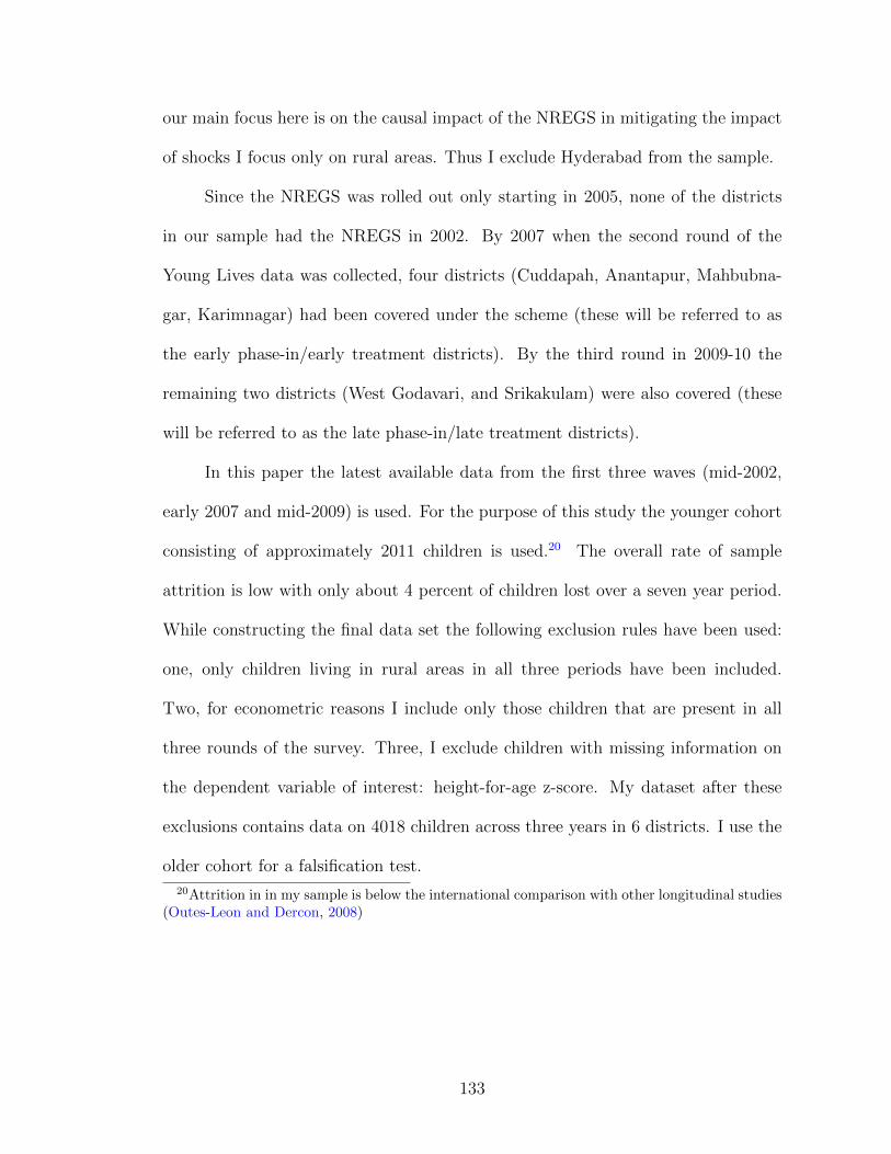
our main focus here is on the causal impact of the NREGS in mitigating the impact
of shocks I focus only on rural areas. Thus I exclude Hyderabad from the sample.
Since the NREGS was rolled out only starting in 2005, none of the districts
in our sample had the NREGS in 2002. By 2007 when the second round of the
Young Lives data was collected, four districts (Cuddapah, Anantapur, Mahbubna-
gar, Karimnagar) had been covered under the scheme (these will be referred to as
the early phase-in/early treatment districts). By the third round in 2009-10 the
remaining two districts (West Godavari, and Srikakulam) were also covered (these
will be referred to as the late phase-in/late treatment districts).
In this paper the latest available data from the first three waves (mid-2002,
early 2007 and mid-2009) is used. For the purpose of this study the younger cohort
consisting of approximately 2011 children is used.20 The overall rate of sample
attrition is low with only about 4 percent of children lost over a seven year period.
While constructing the final data set the following exclusion rules have been used:
one, only children living in rural areas in all three periods have been included.
Two, for econometric reasons I include only those children that are present in all
three rounds of the survey. Three, I exclude children with missing information on
the dependent variable of interest: height-for-age z-score. My dataset after these
exclusions contains data on 4018 children across three years in 6 districts. I use the
older cohort for a falsification test.
20Attrition in in my sample is below the international comparison with other longitudinal studies(Outes-Leon and Dercon, 2008)
133

3.4.2 Variables of interest
The World Health Organization (WHO) outlines three important indicators for
child nutrition: height-for-age (this is a long term indicator of chronic malnutrition),
weight-for-height (this is an indicator of acute malnutrition and is being unable to
gain weight) and weight-for-age (this is a combination of the above two and is used
to give an overall indicator of malnutrition).
In most survey data these indicators are standardized with respect to a refer-
ence population and are presented as z-scores. In this paper I focus my attention
on the first indicator: height-for-age. This is because when analyzing the impact of
shocks, height-for-age is the only accurate indicator of long term impact. Weight-
for-height and weight-for-age are short term indicators and children can make up
lost weight easily. They would thus give an inaccurate representation of the actual
impact of the shocks.
Since my sample consists of rural households it is reasonable to assume that
one of the main income shocks they face is variations in rainfall.21 To construct
the income shock variable, the long term average (1951-2009) for each district is
used. Standard deviation for the same period is also calculated at the district level.
Then rainfall shock is defined as the deviation of actual rainfall last year from the
long term average divided by the standard deviation. The shock variable is thus
normalized. I use prior rainfall deviations in order to give rainfall shocks some time
to feed through and for them to influence household decision making.22
I also include child and household level controls: age, household size, wealth
21Over 70 percent of the population in the state of Andhra Pradesh is engaged in agriculture.22Rainfall data has been obtained from the Indian Meteorological Department.
134

quartiles.23, land owned in acres, dummies for if head of the household has com-
pleted primary education, gender, Hindu, SC/ST24, OBC25 and debts.26 There is a
significant amount of literature that points to the current health status being deter-
mined by attainment till the previous period (Strauss and Thomas, 2007). This can
be captured by including a lagged dependent variable as a regressor. While I don’t
include this in my main specification I do re-estimate the above regressions using
the Arellano-Bond GMM estimator and use lagged height-for-age z-score in period
t-2 as an instrument (Arellano and Bond, 1991).
3.4.3 Descriptive Statistics
Tables 3.2 & 3.3 describe the relevant summary statistics for all three years.
The height-for-age z-scores deteriorates from the time of birth (round 1) to when the
children are five years (round 2) improving slightly by round 3. As Dasgupta et al.
[2013] points out this is more or less consistent with the case of developing countries
where height-for-age z-scores decline in the first few years and then stabilize. In
round 1 of the survey the mean height-for-age z-scores for those in the early phase-
in districts was -1.30 which goes down substantially to -1.82 in round 2 before
recovering slightly to -1.63 in round 3. The districts in the late phase-in group follow
a similar pattern of declining z-scores from rounds 1 to 2 with some improvement
being seen between rounds 2 and 3. What is also interesting is that the late phase-in
23Including the wealth index implies that I don’t include income explicitly as an explanatoryvariable not only because it would be endogenous but also because the wealth index captures all theimpact that income would have captured because the index is a far more comprehensive measure.
24Scheduled Caste/Scheduled Tribe25Other Backward Caste26In this data, gender is the only variable that is time invariant. Caste and religion do change
slightly over the three waves for some households. It is difficult but not uncommon in India forpeople to change castes and/or change their religion. Thus dummies for SC/ST, OBC and Hinduare not time invariant.
135

districts (which includes those districts that got the NREGS later which means that
they were higher up on the development index) had worse height-for-age z-scores
than the early phase-in districts in 2002 before the NREGS was in force.
There are no significant differences between the two groups in terms of age,
gender and religion. However, there are significant differences across the groups
in terms of caste, schooling of household head, household size, debt, land owned
and access to supplementary feeding programs. This is to be expected because
the NREGS was not a randomly assigned program. The poorest districts received
the program first. This implies that the early phase-in districts and late phase-in
districts are markedly different on a number of indicators. This however, as detailed
in the next section, is resolved by using a difference-in-difference methodology and
assuming that the placement bias is additive and time invariant.
Examining the other control variables I find that on average 53 percent of the
sample is male while the average age in 2002 and 2009-10 is approximately one year
and 7.5 years respectively. The average child has approximately four other members
co-residing with her. The children are primarily Hindu (92 percent) and a majority
belong to backward castes, SC/ST or OBC. Not surprisingly, the proportion of
the sample with caregivers having completed primary education is low (about 30
percent). The wealth index takes a value between 0 and 1. The average value of 0.19
suggests that households have only about 20 percent of all of these assets suggesting
that the children in the sample come from very poor households.
136

3.5 Empirical Strategy
The impact of the NREGS on child growth in the event of an income shock can
be multi-dimensional. First, the NREGS leads to wage payments and this income
effect may alone lead to higher expenditures on child health.27 Even if it doesn’t lead
to increased expenditures it is reasonable to assume that given this ‘insurance’ in
the event of a shock, expenditures on child health would potentially not be reduced.
Second, the NREGS will lead to increased labour supply by the parents in the
aftermath of the shock and this may lead to a substitution effect away from time
spent at home on activities beneficial for child health. Third, the NREGS leads to
the creation of village infrastructure such as roads and this may increase the risk
bearing capabilities of households after an income shock without necessitating an
increase in labour force participation.28 Fourth as Mani et al. [2014] point out, for
about a quarter of the sample of children from the Young Lives data, the NREGS
workers from the household are not biological parents. This means that considering
only parent’s labour force participation could bias the true impact of the NREGS.
This is because if none of the parents participate then only the income effect remains
and thus we would underestimate the true impact of the program if we focused only
on parental participation. Finally, the NREGS also reduces the ex-ante risk that
communities face as a result of covariate shocks regardless of actual participation
in the program. This leads to a rise in overall village income and consequently
better child outcomes. The study therefore estimates the intent-to-treat effects of
27This does depend on the marginal propensity to consume health goods out of cash income.28Skoufias [2003] points out that publicly provided mechanisms such as sound infrastructure play
an important role in reducing the risk for poor households vulnerable to shocks.
137

the program which includes both the income and substitution effects.29
3.5.1 Measuring overall impact
One of the main challenges in this study is that there is no untreated counter-
factual group since all six districts received the program at some point in time. This
identification issue can be potentially serious because before and after evaluations
can be biased if there is no comparison to untreated groups (Clemens and Demom-
bynes, 2010). Thus, it is necessary to evaluate benefits by comparing beneficiaries
to other beneficiaries (Hanson et al., 2013).
First, in order to eliminate the program placement bias, the main specification
I run is a fixed effects model given by the following equation:
Hidt = β0+β1NREGSd,t+β2Shockd,t−1+β3[NREGS∗Shock]d,t+εi+εd+εh+εit
The dependent variable Hidt refers to the height-for-age z-score for child i in district
d at time t. The variable NREGS measures access to the NREGS and varies by
district and time. Shockd,t−1 is the income shock at the district level in the previous
period. The coefficient on the interaction term, β3 is the parameter of interest
and captures the mitigating effects of the NREGS in the event of a shock.30 This
specification includes year dummies.
3.5.2 Measuring multi-year impacts
The above specification however does not allow me to disentangle the multi-
year impacts of the program. In order to do so, I examine two groups: the early
29Using this approach however means that I am unable to disentangle the income and substitu-tion effects since the intent-to-treat effects estimate the total impact of the program.
30The impact of the shock in the absence of the NREGS is given by β2 while in the presence ofthe NREGS the corresponding value is given by β3 − β2
138

phase-in districts and the late phase-in districts. The NREGS was rolled out in two
waves with four districts (Cuddapah, Anantapur, Mahbubnagar, Karimnagar) get-
ting the program in 2007 and the last two districts (West Godavri and Srikakulam)
getting it in 2009. Thus in the final year the differences between the two groups are
caused only by differential access to the program. Thus I examine two phases of
treatment (2007 and 2009) in addition to one pre-intervention year (2002).
Thus, in order to disentangle the multi-year impacts of the program I run the
following difference-in-difference model:
Hidt = β0 + β1Shockd,t−1 + β2Time1d,t + β3[Time1 ∗ Shock]d,t + β4Time2d,t +
β5[Time2 ∗ Shock]d,t + εi + εd + εh + εit
As before Hidt refers to the height-for-age z-score for child i in district d at
time t. Time1d,t and Time2d,t are indicator variables for NREGS assignment to
the first and second years of exposure respectively. They vary by district and time
(e.g. Time1d,t takes a value of 1 for the first four districts in 2007 and for the
last two districts in 2009. Similarly, Time2d,t takes a value of 1 for the first four
districts in 2009 since it was the second year of the program for these districts.
Table 3.1 outlines the implementation framework.). In this framework, β3 captures
the average mitigating effect of the first year of exposure to the NREGS on child
health in the event of a shock and β5 is the analogous buffering effect of the second
year of exposure to the NREGS.31 This specification also includes year dummies.
Both specifications also include a set of observable individual and household level
controls. Including these variables helps control for pre-treatment differences that
31Like above, the impact of the shock in the absence of the NREGS is given by β1 while theimpact of the shock with NREGS access for one year is given by β3 + β2− β1. The impact for twoyears of NREGS exposure is β5 + β4 − β1
139
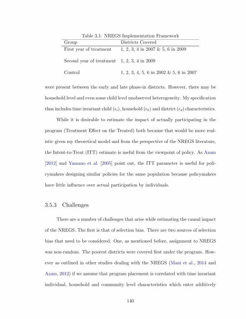
Table 3.1: NREGS Implementation Framework
Group Districts Covered
First year of treatment 1, 2, 3, 4 in 2007 & 5, 6 in 2009
Second year of treatment 1, 2, 3, 4 in 2009
Control 1, 2, 3, 4, 5, 6 in 2002 & 5, 6 in 2007
were present between the early and late phase-in districts. However, there may be
household level and even some child level unobserved heterogeneity. My specification
thus includes time invariant child (εi), household (εh) and district (εd) characteristics.
While it is desirable to estimate the impact of actually participating in the
program (Treatment Effect on the Treated) both because that would be more real-
istic given my theoretical model and from the perspective of the NREGS literature,
the Intent-to-Treat (ITT) estimate is useful from the viewpoint of policy. As Azam
[2012] and Yamano et al. [2005] point out, the ITT parameter is useful for poli-
cymakers designing similar policies for the same population because policymakers
have little influence over actual participation by individuals.
3.5.3 Challenges
There are a number of challenges that arise while estimating the causal impact
of the NREGS. The first is that of selection bias. There are two sources of selection
bias that need to be considered. One, as mentioned before, assignment to NREGS
was non-random. The poorest districts were covered first under the program. How-
ever as outlined in other studies dealing with the NREGS (Mani et al., 2014 and
Azam, 2012) if we assume that program placement is correlated with time invariant
individual, household and community level characteristics which enter additively
140
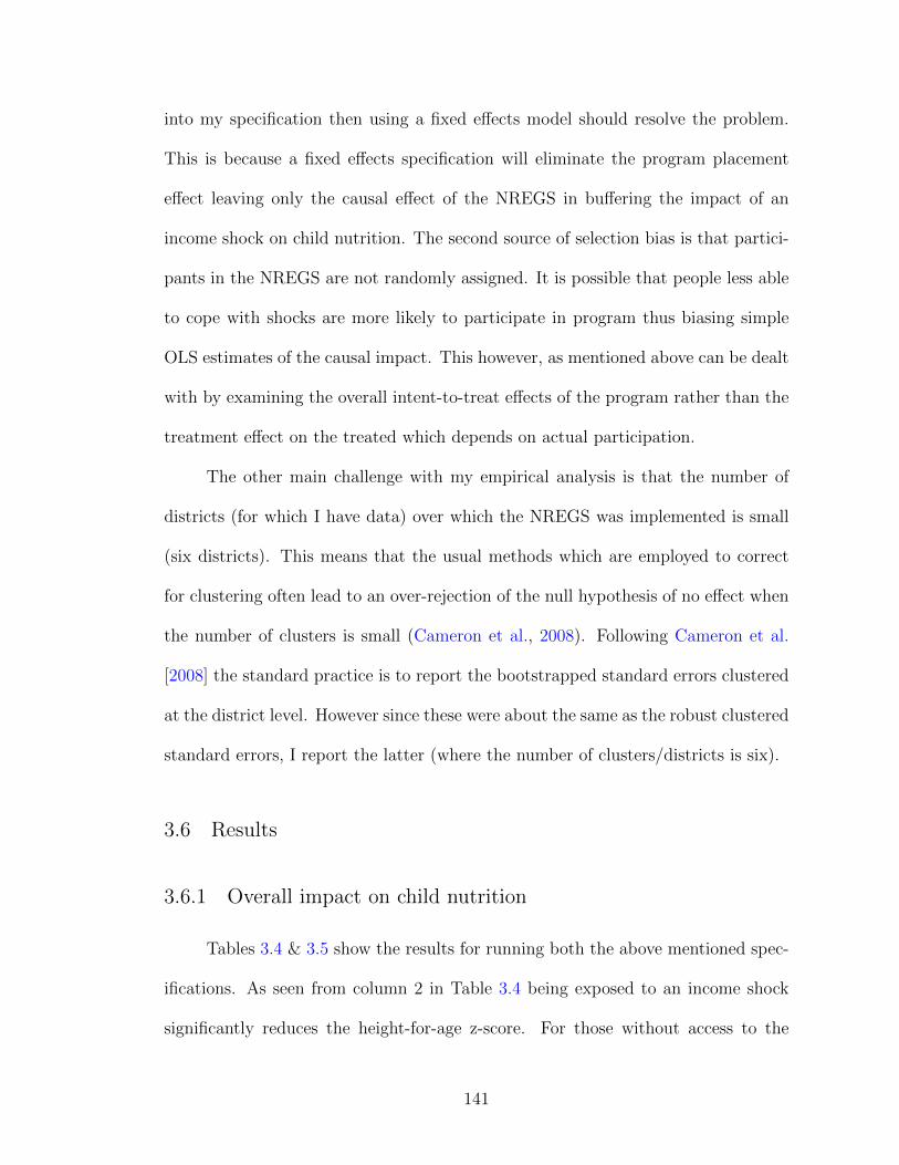
into my specification then using a fixed effects model should resolve the problem.
This is because a fixed effects specification will eliminate the program placement
effect leaving only the causal effect of the NREGS in buffering the impact of an
income shock on child nutrition. The second source of selection bias is that partici-
pants in the NREGS are not randomly assigned. It is possible that people less able
to cope with shocks are more likely to participate in program thus biasing simple
OLS estimates of the causal impact. This however, as mentioned above can be dealt
with by examining the overall intent-to-treat effects of the program rather than the
treatment effect on the treated which depends on actual participation.
The other main challenge with my empirical analysis is that the number of
districts (for which I have data) over which the NREGS was implemented is small
(six districts). This means that the usual methods which are employed to correct
for clustering often lead to an over-rejection of the null hypothesis of no effect when
the number of clusters is small (Cameron et al., 2008). Following Cameron et al.
[2008] the standard practice is to report the bootstrapped standard errors clustered
at the district level. However since these were about the same as the robust clustered
standard errors, I report the latter (where the number of clusters/districts is six).
3.6 Results
3.6.1 Overall impact on child nutrition
Tables 3.4 & 3.5 show the results for running both the above mentioned spec-
ifications. As seen from column 2 in Table 3.4 being exposed to an income shock
significantly reduces the height-for-age z-score. For those without access to the
141

NREGS, a one standard deviation change in rainfall from its mean results in loss
of height-for-age z-score by about 0.50 standard deviations. On the other hand,
for those who did have access to the NREGS, the impact of the shock is about
0.08 standard deviations.32 That is, the impact of the shock is differential based on
NREGS access.
3.6.2 Multi-year program impacts
Table 3.5 reports the multi-year impacts of the program. The coefficients for
each year of NREGS exposure and the mitigating role of the NREGS are cumulative
and not marginal. The impact of exposure to the NREGS in all years is significantly
different from zero. The mitigating role of the NREGS in the event of a shock is
clear. In the absence of the program, an income shock would have led to a decline
of height-for-age z-scores by 0.61 standard deviations. Exposure to one year of
the NREGS in the event of a shock, led to a positive and statistically significant
differential impact of 0.32 standard deviations in height-for-age z-scores.33 Thus the
shock fails to adversely impact children if they have access to the NREGS.
Being exposed to two years of the program led to a similar positive and statis-
tically significant improvement of 0.50 standard deviations for those who had access
to the NREGS during a shock. The joint test that both coefficients are zero is
rejected. However height-for-age increases by less in the second year.34 Moreover,
the coefficients for the first and second years of exposure are significantly different
32The magnitude of the impact is found by subtracting the impact of the shock from the impactdue to the NREGS (0.58-0.50)=0.08 standard deviation increase in height for age.
33The magnitude of the impact is found by subtracting the impact of the shock from the cu-mulative impact due to the NREGS (0.871 + 0.058 - 0.610)=0.32 standard deviation increase inheight for age.
34Impact of second year = Cumulative impact - impact of first year = 0.50 - 0.32 = 0.18 standarddeviations increase in height-for-age.
142

than each other.
Since the impact of the second year is lower than that of the first year, this
suggests that there is a decay in the short run effects. That is, the late phase-in
districts tend to catch up to the early phase-in districts and there are no long term
persistent effects of the program in buffering children against income shocks. This
however ties in with what one would expect given the dual nature of the NREGS in
enhancing capabilities and serving as a safety net. Since I am analyzing the same
cohort of children and their families it is possible that over time the NREGS has
enabled these households to become better equipped in dealing with shocks. This
can be either through the enhanced income that the NREGS provides or its implicit
role as an insurance mechanism which makes households less risk averse and more
able to cope with shocks. It is possible thus that for the same household, utility of
the NREGS as a safety net may diminish over time as they enhance their capabilities.
Thus there is no differential impact of the shock because of NREGS access in the
long run. Alternatively, it is also possible that there are diminishing returns to
improvements in height-for-age z-score i.e. improvements in height-for-age z-score
are bounded above.
Moreover, improvements in height-for-age are most significant when children
are younger and therefore between 2007 and 2009-10 (the time frame of the medium
run effects) when the children in my sample are between 5 and 7 years, there might
not be significant improvements in height. This is even more conceivable because in
both my specifications, the coefficient on age is negative which means the older the
child the lower is the increase in height-for-age.
Columns (3) and (2) in Tables 3.4 & 3.5 detail the regression results for both
143

specifications after including the food supplement variable. As is evident my re-
sults don’t change much and the mitigating effect of the NREGS is still positive
and statistically significant. However, the supplement variable is also positive and
statistically significant implying that access to supplementary feeding programs like
the ICDS and the Mid-Day Meal Scheme contribute significantly to children’s height
attainment.
Within the described controls, I perform a series of F-tests of the null hy-
pothesis that the coefficients of these variables are jointly equal to each other. I
reject the null hypothesis that the coefficients of the time dummies are jointly zero
(p-value=0.000). This implies that there are significant time effects. I am unable to
reject the null hypothesis that all the individual level controls are jointly equal to
zero (p-value=0.3775). I also fail to reject the null hypothesis that all the household
level controls are jointly zero (p-value=0.2474). Finally, I reject the null hypothesis
that the two variables of interest, access to NREGS and the income shock are jointly
zero (p-value=0.000).
These results validate those that have been found in similar studies. For
instance Dasgupta et al. [2013] finds an improvement of 0.27 standard deviations in
height-for-age as a result of the NREGS in India. Quisumbing [2003] finds that food-
for-work and food aid have positive impacts on weight-for-age for children between
0-5 years from low-asset households in Ethiopia. Similarly Yamano et al. [2005] also
find that food aid significantly helps in mitigating the impacts of income shocks on
height-for-age z-scores in rural Ethiopia.
144

3.6.3 Heterogeneous impacts —By wealth quartiles, land ownership
and gender
The role of the NREGS in helping mitigate the impacts of a shock may
hide large heterogeneity of impacts across households belonging to different socio-
economic groups. In order to address this I run both my specifications by an in-
dicator of household wealth, gender and land ownership. I examine children from
households with less than the median and more than the median wealth level index
(the median is the sum of the first two wealth quartiles and is based on the pooled
sample which includes all three years).
The results are given in Tables 3.6, 3.7 and 3.8. The mitigating impact of
the NREGS on children’s height after an income shock is positive and statistically
significant. Ideally one would expect that the NREGS should be most beneficial
for the poorest. However, contrary to expectations, the mitigating impact of the
NREGS is higher for households with wealth levels higher than the median level.
That is, for richer households, the differential impact of the shock for those who
have NREGS access is 0.08 standard deviations while for the poorer households the
improvement is only 0.07 standard deviations. This can be explained by a number
of factors. One, public works in developing countries are plagued by implementation
problems like corruption and underpayment of wages. If true, then this attenuates
the mitigating impact that the NREGS has in the event of a shock, especially for
the poor who are more dependent on the NREGS after a shock relative to richer
households. Two, an audit by the Indian government in 2012 reveals that awareness
(on a relative basis) about the NREGS and its entitlements is still very low. Richer
145

households with better connections (political and social) might be more aware of
the program and thus more able to access it in the event of a shock as opposed to
poorer households. Three, using nationally representative data Dutta et al. [2012]
have found that the demand for NREGS far outstrips the supply which leads to
rationing of projects. This leads to rent seeking and consequently richer households
are better placed to find work than poorer households after a shock. Thus, the overall
results I find above are significantly driven by the sub-sample of those children who
belonged to richer households for whom the impact of the NREGS contributes more
to improvements in child health than the total sample.35
I find a similar differential impact when I disaggregate my sample by gender.
Columns (3) & (4) of Table 3.6 detail the results of my specifications. The mitigating
impact of the NREGS is higher and statistically significant for boys relative to girls.
This implies that girls are impacted more by income shocks. That is, for those who
had access to the NREGS after a shock, there is an improvement of 0.12 standard
deviations in height-for-age z-scores for boys compared to 0.04 for girls. This ties in
with our expectations about the male preference bias in Indian households. While
because of data constraints I don’t examine it here, but it would be interesting to see
if the increase in female labour force participation that the NREGS has seen leads
to an increase in the bargaining power of women and an improvement in female
child health.
Table 3.7 highlights multi-year heterogeneous impacts. I find similar results
to those found above. The impact of the shock for those who were exposed to the
NREGS in the first year is 0.39 for those with wealth less than the median wealth
35It is important to remember that here ‘richer’ is used in a relative sense because my entiresample consists of the rural poor.
146
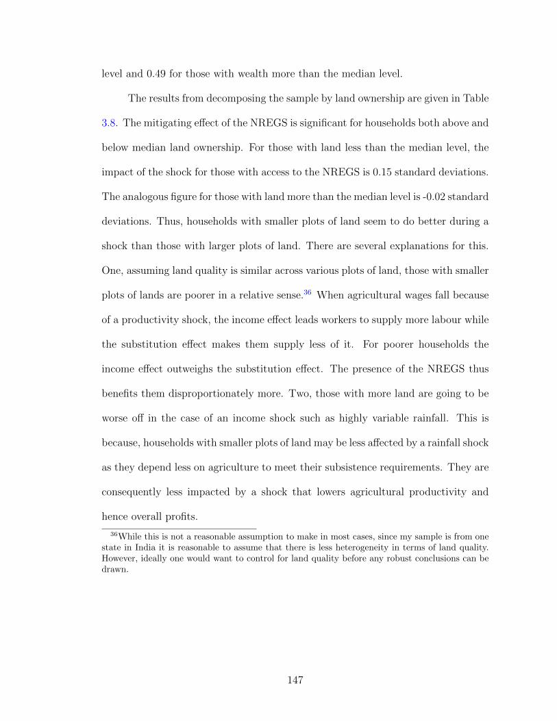
level and 0.49 for those with wealth more than the median level.
The results from decomposing the sample by land ownership are given in Table
3.8. The mitigating effect of the NREGS is significant for households both above and
below median land ownership. For those with land less than the median level, the
impact of the shock for those with access to the NREGS is 0.15 standard deviations.
The analogous figure for those with land more than the median level is -0.02 standard
deviations. Thus, households with smaller plots of land seem to do better during a
shock than those with larger plots of land. There are several explanations for this.
One, assuming land quality is similar across various plots of land, those with smaller
plots of lands are poorer in a relative sense.36 When agricultural wages fall because
of a productivity shock, the income effect leads workers to supply more labour while
the substitution effect makes them supply less of it. For poorer households the
income effect outweighs the substitution effect. The presence of the NREGS thus
benefits them disproportionately more. Two, those with more land are going to be
worse off in the case of an income shock such as highly variable rainfall. This is
because, households with smaller plots of land may be less affected by a rainfall shock
as they depend less on agriculture to meet their subsistence requirements. They are
consequently less impacted by a shock that lowers agricultural productivity and
hence overall profits.
36While this is not a reasonable assumption to make in most cases, since my sample is from onestate in India it is reasonable to assume that there is less heterogeneity in terms of land quality.However, ideally one would want to control for land quality before any robust conclusions can bedrawn.
147
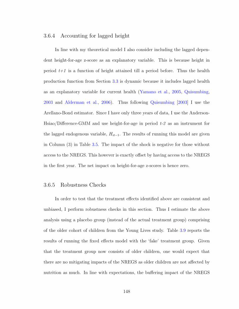
3.6.4 Accounting for lagged height
In line with my theoretical model I also consider including the lagged depen-
dent height-for-age z-score as an explanatory variable. This is because height in
period t+1 is a function of height attained till a period before. Thus the health
production function from Section 3.3 is dynamic because it includes lagged health
as an explanatory variable for current health (Yamano et al., 2005, Quisumbing,
2003 and Alderman et al., 2006). Thus following Quisumbing [2003] I use the
Arellano-Bond estimator. Since I have only three years of data, I use the Anderson-
Hsiao/Difference-GMM and use height-for-age in period t-2 as an instrument for
the lagged endogenous variable, Hit−1. The results of running this model are given
in Column (3) in Table 3.5. The impact of the shock is negative for those without
access to the NREGS. This however is exactly offset by having access to the NREGS
in the first year. The net impact on height-for-age z-scores is hence zero.
3.6.5 Robustness Checks
In order to test that the treatment effects identified above are consistent and
unbiased, I perform robustness checks in this section. Thus I estimate the above
analysis using a placebo group (instead of the actual treatment group) comprising
of the older cohort of children from the Young Lives study. Table 3.9 reports the
results of running the fixed effects model with the ‘fake’ treatment group. Given
that the treatment group now consists of older children, one would expect that
there are no mitigating impacts of the NREGS as older children are not affected by
nutrition as much. In line with expectations, the buffering impact of the NREGS
148

is not statistically significant. Since the treatment group in this case consisted of
older children an income shock does not have a statistically significant impact on
their health. Therefore the mitigating effect of the NREGS is insignificant as well.
3.6.6 Testing Parallel Trends
The key assumption with the fixed effects specification is that of parallel
trends. That is, in the absence of the NREGS the treatment and control districts
would have had parallel time trends and it is the introduction of the NREGS that
introduced a deviation in that trend. I test the parallel trend assumption both us-
ing the pre intervention data from the Young Lives data (first wave of the survey
2002) and using the Indian Human Development Survey (IHDS), 2005. The IHDS
was administered between November 2004 and October 2005, and the first phase
of the NREGS was rolled out in September 2005. So the IHDS is suitable to test
for pre-intervention time trends. Out of the six districts in my sample the IHDS
was administered in five of those excluding Srikakulam. I plot the mean height for
children from the early phase-in and late phase-in districts in Figure 3.1.37 Figure
3.2 plots the height-for-age z-scores for the early and late phase-in districts using
Round 1 (pre-NREGS) of the Young Lives data. Both figures, for the most part,
highlight parallel trends between the two groups. Given these, it is reasonable to
assume in this context that pre-intervention outcomes follow parallel trends.
37The IHDS recorded anthropometric outcomes differently than the Young Lives data. The datadoes not contain z-scores but only has absolute numbers measured in centimeters.
149

3.7 Policy Implications
Public works programs have a long history. More recently they have evolved
into policy instruments for generating employment and alleviating long term poverty.
Well designed programs provide income transfers to poor households in periods of
critical need. Evidence on their use as safety nets, however is low. In this regard,
this paper tests the effectiveness of one such program. Using longitudinal data from
the 2002, 2007 and 2009-10 waves of the Young Lives Survey in Andhra Pradesh,
India I assess the effectiveness of the National Rural Employment Guarantee Scheme
(NREGS) in mitigating the adverse impacts of income shocks on child health.
The main finding in this paper is that the NREGS has large and positive
mitigating effects on child health in the aftermath of a shock. This has important
policy implications. First, while the NREGS wasn’t designed to be a program that
helps in tackling child malnutrition, its ability to function effectively as a safety
net means that it can prevent large fluctuations in child health. If this were to be
combined with the proper functioning of on-site child care facilities then this would
further enhance the ability of the NREGS to buffer rural households. Second, from
my empirical analysis richer households benefit more from the mitigating impact of
the NREGS than poorer households. This suggests rent seeking and indicates that
there are implementation and institutional problems with the program. Given that
the poorest are the least able to cope with shocks it is important that the program
should benefit them positively as well. This differential impact suggests that the way
in which public programs are designed is of vital importance and has consequences
beyond the immediate aims of these programs. Third, while the results derived in
150

this paper rest on the unitary household assumption, the NREGS in practice leads
to increased female labour supply. This implies that the impact of the NREGS could
be stronger given that an increase in labour supply could enhance the bargaining
power of females and thus lead to improved child outcomes. Finally, given that the
early phase-in districts see large impacts of the NREGS it therefore implies that the
timing of these programs is critical. The gains from receiving the program early on
are significant and policymakers need to be cognizant of this.
151
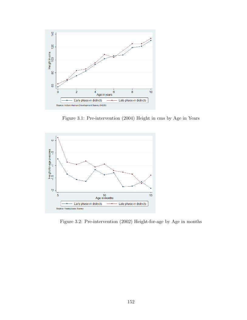
Figure 3.1: Pre-intervention (2004) Height in cms by Age in Years
Figure 3.2: Pre-intervention (2002) Height-for-age by Age in months
152
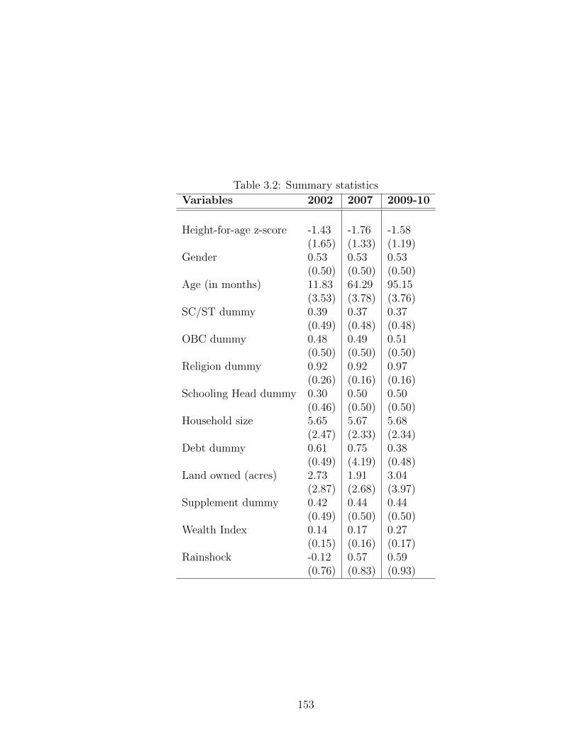
Table 3.2: Summary statistics
Variables 2002 2007 2009-10
Height-for-age z-score -1.43 -1.76 -1.58(1.65) (1.33) (1.19)
Gender 0.53 0.53 0.53(0.50) (0.50) (0.50)
Age (in months) 11.83 64.29 95.15(3.53) (3.78) (3.76)
SC/ST dummy 0.39 0.37 0.37(0.49) (0.48) (0.48)
OBC dummy 0.48 0.49 0.51(0.50) (0.50) (0.50)
Religion dummy 0.92 0.92 0.97(0.26) (0.16) (0.16)
Schooling Head dummy 0.30 0.50 0.50(0.46) (0.50) (0.50)
Household size 5.65 5.67 5.68(2.47) (2.33) (2.34)
Debt dummy 0.61 0.75 0.38(0.49) (4.19) (0.48)
Land owned (acres) 2.73 1.91 3.04(2.87) (2.68) (3.97)
Supplement dummy 0.42 0.44 0.44(0.49) (0.50) (0.50)
Wealth Index 0.14 0.17 0.27(0.15) (0.16) (0.17)
Rainshock -0.12 0.57 0.59(0.76) (0.83) (0.93)
153

Table 3.3: Summary statistics contd.Variable Early Late ta
Phase-in Districts Phase-in Districts
Height-for-age (in 2002) -1.30 -1.61 -3.97∗
Height-for-age (in 2007) -1.82 -1.63 2.84∗
Height-for-age (in 2009-10) -1.63 -1.48 2.21∗
Height-for-age if caregiver completed primary -1.50 -1.37 2.22*Height-for-age if caregiver not completed primary -1.66 -1.73 -1.34Height-for-age (Females) -1.51 -1.48 0.44Height-for-age (Males) -1.65 -1.69 -0.64Gender 0.53 0.52 -1.12Age (in months) 56.07 56.33 0.21SC/ST dummy 0.34 0.42 4.77∗∗
OBC dummy 0.49 0.49 -0.17Religion dummy 0.96 0.95 -1.70Schooling Head dummy 0.45 0.39 -3.96∗
Household Size 5.84 5.30 -6.79∗∗
Debt dummy 0.66 0.41 -3.12∗
Land owned (acres) 2.89 1.55 -11.31∗∗∗
Supplement dummy 0.37 0.56 11.31∗∗∗
Wealth Index 0.39 0.38 -2.72∗a Test of equality of means, ∗Significant at the 5 percent level
154

Table 3.4: Regression Results: Specification I - Dependent Variable: Height-for-agez-score
(1) (2) (3)Variables OLS FE FE
NREGS -0.003 0.093 0.081(0.144) (0.187) (0.183)
Shock -0.477** -0.496** -0.507***(0.170) (0.133) (0.122)
NREGS*Shock 0.428** 0.576*** 0.583***(0.141) (0.079) (0.069)
Debt -0.007** 0.008** 0.008**(0.002) (0.002) (0.002)
Age -0.024* -0.009 -0.008(0.011) (0.022) (0.023)
Wealth Quartile 1 -0.404*** -0.174 -0.172(0.077) (0.091) (0.092)
Wealth Quartile 2 -0.191 -0.108 -0.111(0.110) (0.091) (0.091)
Wealth Quartile 3 -0.147** -0.056 -0.053(0.050) (0.033) (0.036)
SC/ST -0.221** 0.047 0.026(0.075) (0.088) (0.079)
OBC -0.339** 0.024 0.019(0.090) (0.064) (0.060)
Gender -0.161**(0.061)
Geligion -0.009 -0.036 -0.040(0.233) (0.110) (0.107)
Schooling Head 0.221** 0.049 0.052(0.062) (0.068) (0.060)
Household Size -0.019* -0.001 -0.003(0.007) (0.010) (0.011)
Land Owned (acres) 0.010 -0.006 -0.006(0.009) (0.005) (0.005)
Food Supplement 0.139(0.083)
Constant -0.533 -1.206*** -1.257***(0.325) (0.240) (0.255)
Year Dummies Yes Yes YesObservations 3,232 3,232 3,232R-squared 0.115 0.145 0.149
Cluster robust standard errors in parentheses*** p<0.01, ** p<0.05, * p<0.1
155
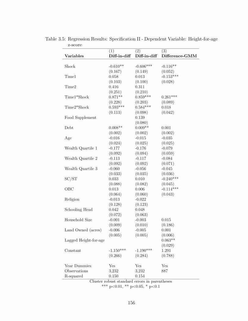
Table 3.5: Regression Results: Specification II - Dependent Variable: Height-for-agez-score
(1) (2) (3)Variables Diff-in-diff Diff-in-diff Difference-GMM
Shock -0.610** -0.606*** -0.116**(0.167) (0.149) (0.052)
Time1 0.058 0.013 -0.153***(0.103) (0.100) (0.028)
Time2 0.416 0.311(0.251) (0.210)
Time1*Shock 0.871** 0.859*** 0.261***(0.228) (0.203) (0.089)
Time2*Shock 0.593*** 0.584*** 0.018(0.113) (0.098) (0.042)
Food Supplement 0.139(0.080)
Debt 0.008** 0.009** 0.001(0.002) (0.002) (0.002)
Age -0.016 -0.015 -0.035(0.024) (0.025) (0.025)
Wealth Quartile 1 -0.177 -0.176 -0.079(0.092) (0.094) (0.059)
Wealth Quartile 2 -0.113 -0.117 -0.084(0.092) (0.092) (0.071)
Wealth Quartile 3 -0.060 -0.056 -0.045(0.033) (0.035) (0.036)
SC/ST 0.033 0.010 -0.240***(0.088) (0.082) (0.045)
OBC 0.013 0.006 -0.114***(0.064) (0.060) (0.043)
Religion -0.013 -0.022(0.128) (0.123)
Schooling Head 0.042 0.048(0.072) (0.063)
Household Size -0.001 -0.003 0.015(0.009) (0.010) (0.186)
Land Owned (acres) -0.006 -0.005 0.001(0.005) (0.005) (0.006)
Lagged Height-for-age 0.063**(0.029)
Constant -1.150*** -1.190*** 1.291(0.266) (0.284) (0.788)
Year Dummies Yes Yes YesObservations 3,232 3,232 887R-squared 0.150 0.154
Cluster robust standard errors in parentheses*** p<0.01, ** p<0.05, * p<0.1
156
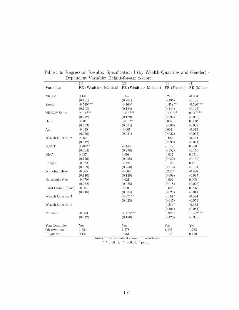
Table 3.6: Regression Results: Specification I (by Wealth Quartiles and Gender) -Dependent Variable: Height-for-age z-score
(1) (2) (3) (4)Variables FE (Wealth ≤ Median) FE (Wealth > Median) FE (Female) FE (Male)
NREGS 0.141 0.142 0.243 -0.054(0.161) (0.261) (0.195) (0.186)
Shock -0.549*** -0.469* -0.458** -0.530***(0.108) (0.184) (0.144) (0.123)
NREGS*Shock 0.616*** 0.545*** 0.499*** 0.647***(0.072) (0.129) (0.097) (0.066)
Debt 0.001 0.010** 0.007 0.008*(0.003) (0.004) (0.006) (0.003)
Age -0.030 -0.005 0.001 -0.013(0.020) (0.031) (0.022) (0.033)
Wealth Quartile 2 0.062 -0.083 -0.134(0.042) (0.093) (0.091)
SC/ST 0.200** -0.446 -0.112 0.230(0.064) (0.298) (0.352) (0.150)
OBC 0.087 0.098 -0.037 0.051(0.176) (0.095) (0.089) (0.130)
Religion -0.022 -0.127 -0.123 0.101(0.059) (0.260) (0.219) (0.184)
Schooling Head -0.065 -0.003 0.205* -0.098(0.110) (0.120) (0.098) (0.097)
Household Size -0.070* 0.021 -0.002 0.005(0.032) (0.025) (0.018) (0.022)
Land Owned (acres) -0.004 -0.001 -0.026 0.006(0.018) (0.004) (0.022) (0.014)
Wealth Quartile 3 -0.071** -0.101* -0.024(0.025) (0.047) (0.053)
Wealth Quartile 1 -0.214* -0.132(0.101) (0.081)
Constant -0.880 -1.178*** -0.995* -1.522***(0.442) (0.180) (0.423) (0.335)
Year Dummies Yes Yes Yes YesObservations 1,654 1,578 1,497 1,735R-squared 0.141 0.161 0.165 0.150
Cluster robust standard errors in parentheses*** p<0.01, ** p<0.05, * p<0.1
157
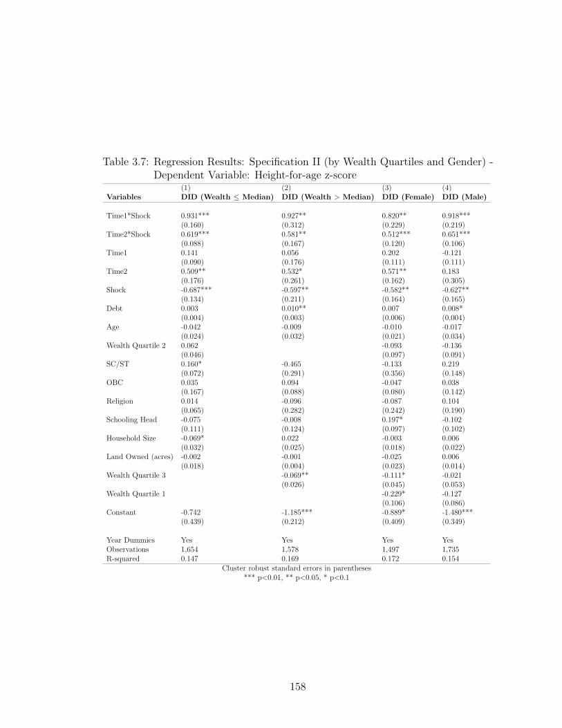
Table 3.7: Regression Results: Specification II (by Wealth Quartiles and Gender) -Dependent Variable: Height-for-age z-score
(1) (2) (3) (4)Variables DID (Wealth ≤ Median) DID (Wealth > Median) DID (Female) DID (Male)
Time1*Shock 0.931*** 0.927** 0.820** 0.918***(0.160) (0.312) (0.229) (0.219)
Time2*Shock 0.619*** 0.581** 0.512*** 0.651***(0.088) (0.167) (0.120) (0.106)
Time1 0.141 0.056 0.202 -0.121(0.090) (0.176) (0.111) (0.111)
Time2 0.509** 0.532* 0.571** 0.183(0.176) (0.261) (0.162) (0.305)
Shock -0.687*** -0.597** -0.582** -0.627**(0.134) (0.211) (0.164) (0.165)
Debt 0.003 0.010** 0.007 0.008*(0.004) (0.003) (0.006) (0.004)
Age -0.042 -0.009 -0.010 -0.017(0.024) (0.032) (0.021) (0.034)
Wealth Quartile 2 0.062 -0.093 -0.136(0.046) (0.097) (0.091)
SC/ST 0.160* -0.465 -0.133 0.219(0.072) (0.291) (0.356) (0.148)
OBC 0.035 0.094 -0.047 0.038(0.167) (0.088) (0.080) (0.142)
Religion 0.014 -0.096 -0.087 0.104(0.065) (0.282) (0.242) (0.190)
Schooling Head -0.075 -0.008 0.197* -0.102(0.111) (0.124) (0.097) (0.102)
Household Size -0.069* 0.022 -0.003 0.006(0.032) (0.025) (0.018) (0.022)
Land Owned (acres) -0.002 -0.001 -0.025 0.006(0.018) (0.004) (0.023) (0.014)
Wealth Quartile 3 -0.069** -0.111* -0.021(0.026) (0.045) (0.053)
Wealth Quartile 1 -0.229* -0.127(0.106) (0.086)
Constant -0.742 -1.185*** -0.889* -1.480***(0.439) (0.212) (0.409) (0.349)
Year Dummies Yes Yes Yes YesObservations 1,654 1,578 1,497 1,735R-squared 0.147 0.169 0.172 0.154
Cluster robust standard errors in parentheses*** p<0.01, ** p<0.05, * p<0.1
158
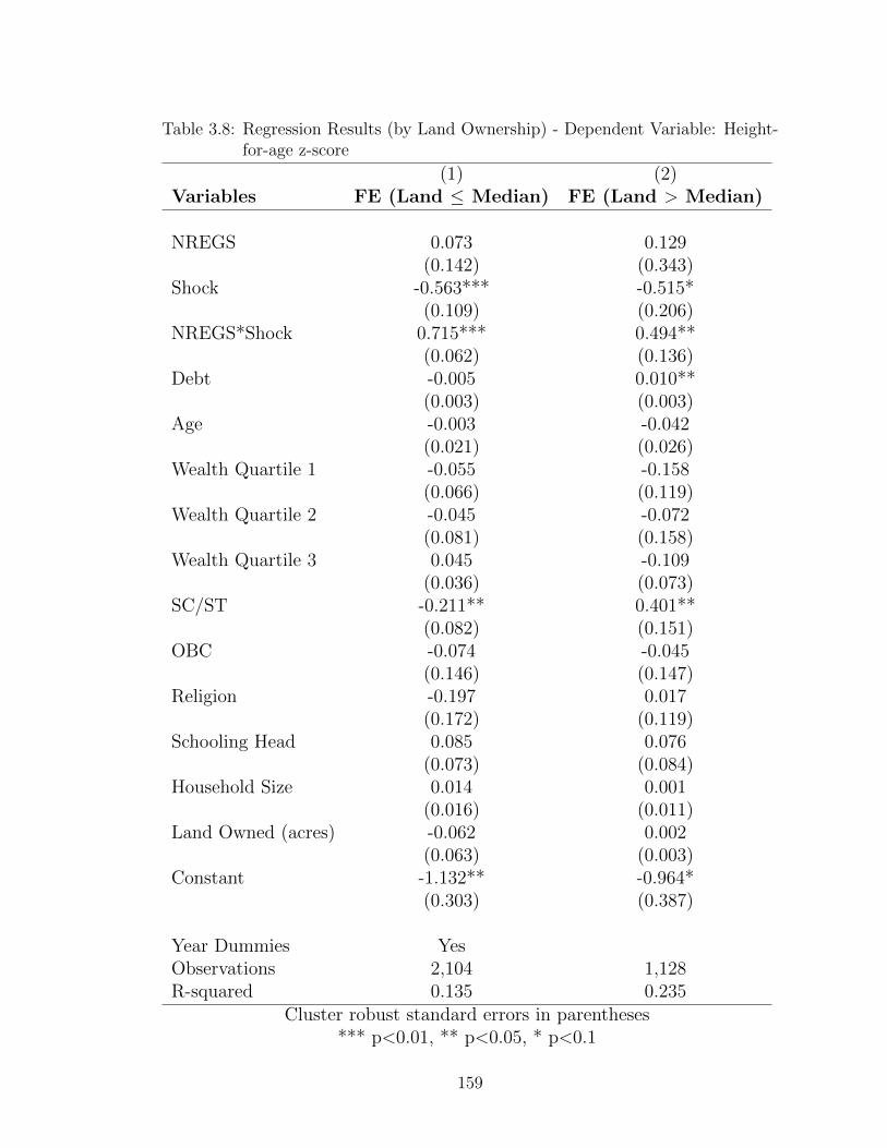
Table 3.8: Regression Results (by Land Ownership) - Dependent Variable: Height-for-age z-score
(1) (2)Variables FE (Land ≤ Median) FE (Land > Median)
NREGS 0.073 0.129(0.142) (0.343)
Shock -0.563*** -0.515*(0.109) (0.206)
NREGS*Shock 0.715*** 0.494**(0.062) (0.136)
Debt -0.005 0.010**(0.003) (0.003)
Age -0.003 -0.042(0.021) (0.026)
Wealth Quartile 1 -0.055 -0.158(0.066) (0.119)
Wealth Quartile 2 -0.045 -0.072(0.081) (0.158)
Wealth Quartile 3 0.045 -0.109(0.036) (0.073)
SC/ST -0.211** 0.401**(0.082) (0.151)
OBC -0.074 -0.045(0.146) (0.147)
Religion -0.197 0.017(0.172) (0.119)
Schooling Head 0.085 0.076(0.073) (0.084)
Household Size 0.014 0.001(0.016) (0.011)
Land Owned (acres) -0.062 0.002(0.063) (0.003)
Constant -1.132** -0.964*(0.303) (0.387)
Year Dummies YesObservations 2,104 1,128R-squared 0.135 0.235
Cluster robust standard errors in parentheses*** p<0.01, ** p<0.05, * p<0.1
159
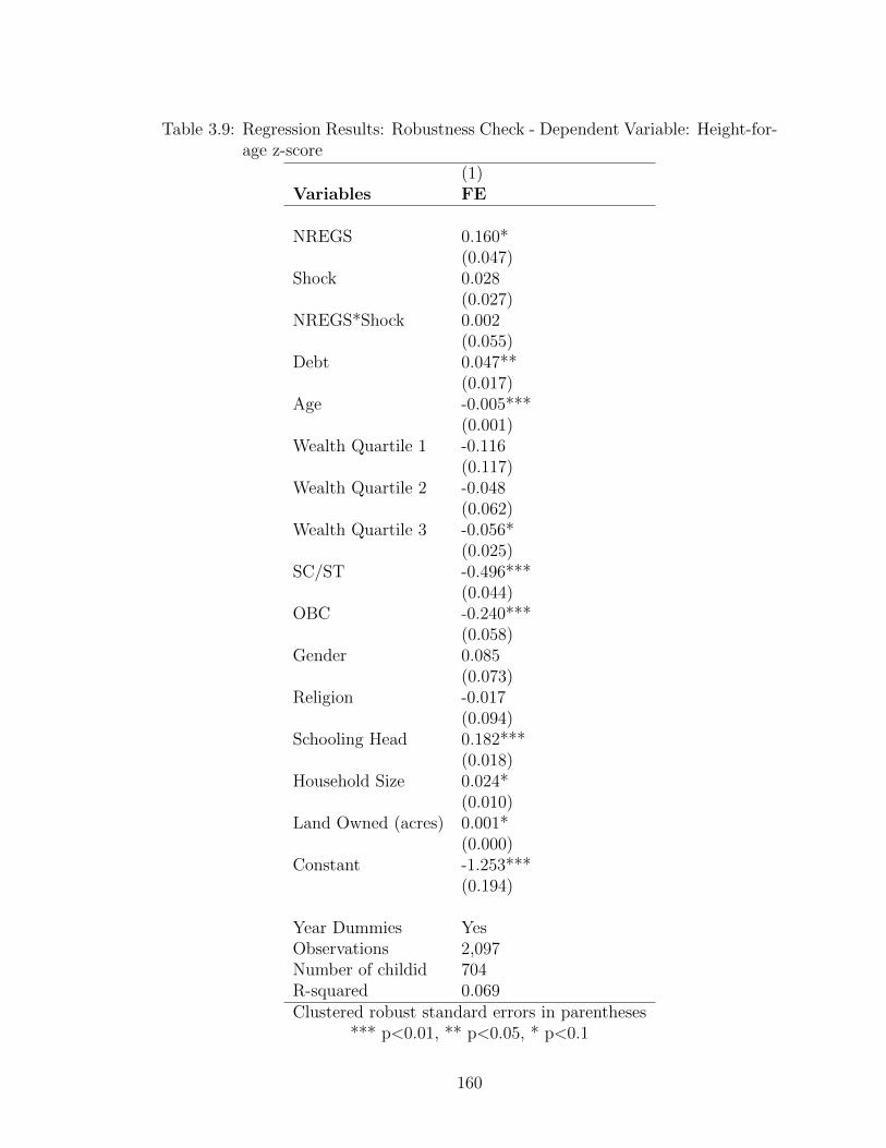
Table 3.9: Regression Results: Robustness Check - Dependent Variable: Height-for-age z-score
(1)Variables FE
NREGS 0.160*(0.047)
Shock 0.028(0.027)
NREGS*Shock 0.002(0.055)
Debt 0.047**(0.017)
Age -0.005***(0.001)
Wealth Quartile 1 -0.116(0.117)
Wealth Quartile 2 -0.048(0.062)
Wealth Quartile 3 -0.056*(0.025)
SC/ST -0.496***(0.044)
OBC -0.240***(0.058)
Gender 0.085(0.073)
Religion -0.017(0.094)
Schooling Head 0.182***(0.018)
Household Size 0.024*(0.010)
Land Owned (acres) 0.001*(0.000)
Constant -1.253***(0.194)
Year Dummies YesObservations 2,097Number of childid 704R-squared 0.069Clustered robust standard errors in parentheses
*** p<0.01, ** p<0.05, * p<0.1
160

Appendix A: Appendix for Chapter 1
161
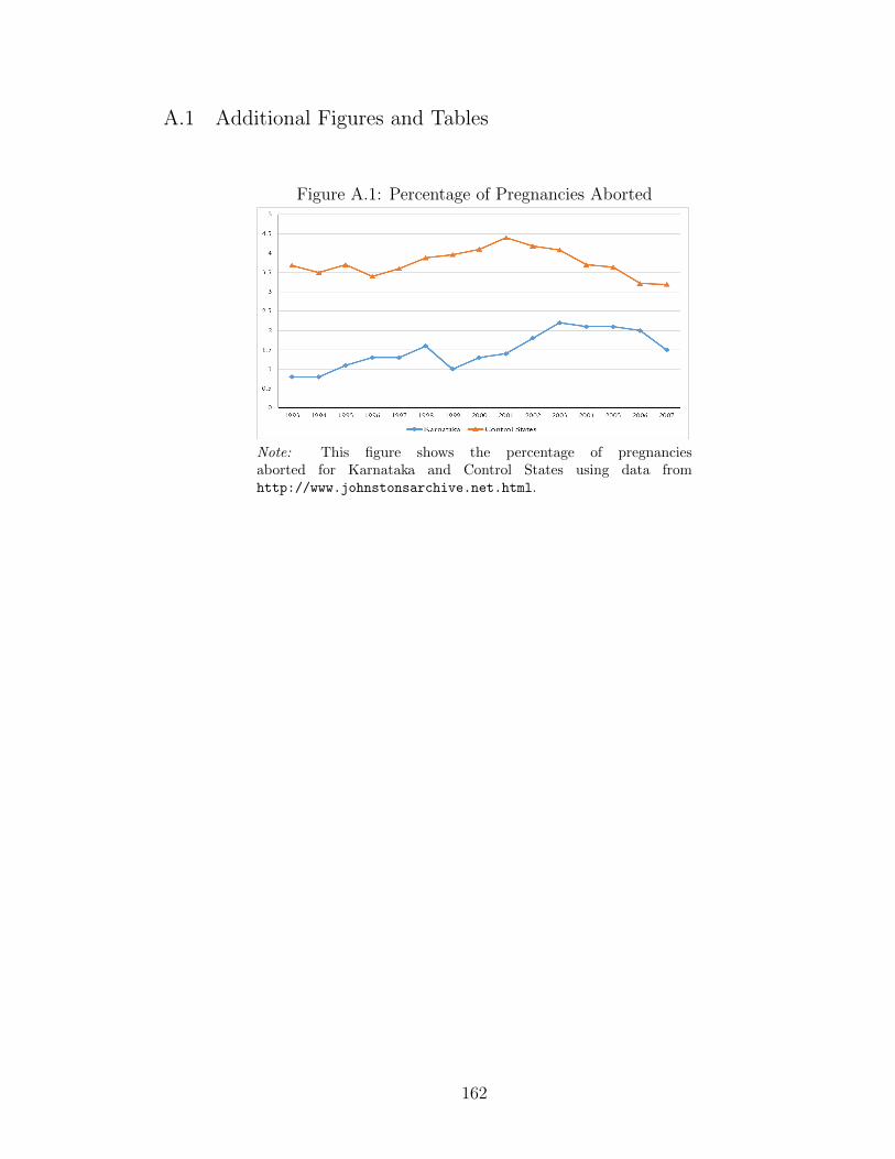
A.1 Additional Figures and Tables
Figure A.1: Percentage of Pregnancies Aborted
Note: This figure shows the percentage of pregnanciesaborted for Karnataka and Control States using data fromhttp://www.johnstonsarchive.net.html.
162

Figure A.2: Annual Probability of Birth for Control States: Survey Round Wise
Note: Data is from each survey round included inthe sample. Estimates are only for control states.Includes women who were between 15-44 years of ageat the time of the survey.
Table A.1: Census Data: Pre-Period Descriptive Statistics
1991 2001
Karnataka Control p-value Karnataka Control p-value
Average Child Sex Ratio 964 961 0.810 944 940 0.936Log of village population 6.643 6.861 0.287 6.761 6.988 0.264Fraction Literate - Male 0.585 0.598 0.731 0.703 0.735 0.277Fraction Literate - Female 0.323 0.336 0.719 0.474 0.503 0.370Labour Supply Rate - Male 0.705 0.686 0.539 0.602 0.614 0.625Labour Supply Rate - Female 0.295 0.314 0.539 0.602 0.614 0.624Fraction Scheduled Caste 0.195 0.191 0.912 0.196 0.189 0.849Primary School 0.910 0.899 0.859 0.877 0.906 0.665Middle School 0.416 0.507 0.376 0.593 0.374 0.032Secondary School 0.106 0.483 0.000 0.174 0.187 0.861Atleast 1 public health facility 0.064 0.103 0.458 0.242 0.232 0.909Tap water 0.187 0.195 0.922 0.575 0.467 0.293Paved approach road 0.671 0.441 0.020 0.726 0.724 0.978Power supply 0.979 0.801 0.000 0.989 0.616 0.000
Number of PSUs 25,044 104,641 25,044 104,641
Note: Data is from the Census datasets 1991 and 2001 for subsample I which includes all PSUs of Karnataka andcontrol states. Observations with child sex ratio values outside the Mean +/- 3 S.D. range have been dropped. OnlyPSUs which were matched in 1991, 2001 and 2011 have been retained. At least 1 public health facility includes theexistence of at least one primary health centre or sub-centre.
163
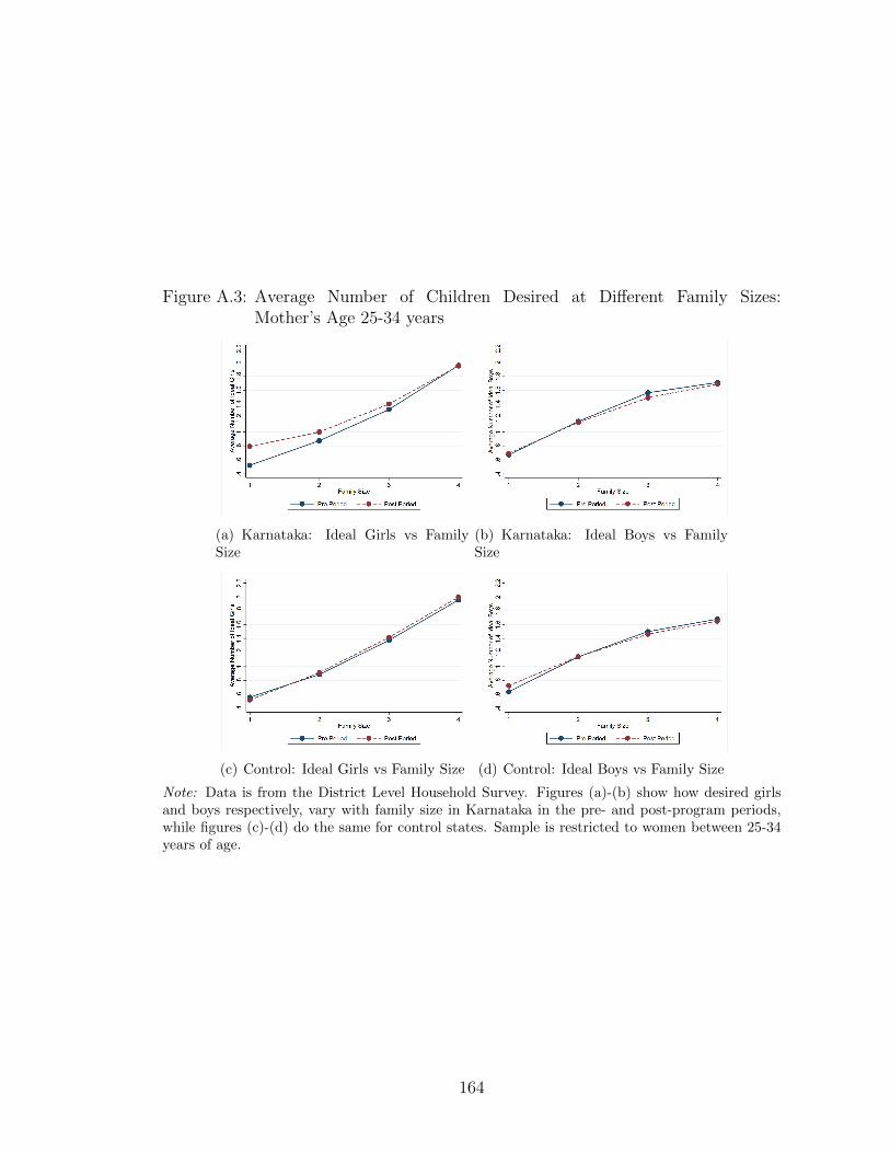
Figure A.3: Average Number of Children Desired at Different Family Sizes:Mother’s Age 25-34 years
(a) Karnataka: Ideal Girls vs FamilySize
(b) Karnataka: Ideal Boys vs FamilySize
(c) Control: Ideal Girls vs Family Size (d) Control: Ideal Boys vs Family Size
Note: Data is from the District Level Household Survey. Figures (a)-(b) show how desired girlsand boys respectively, vary with family size in Karnataka in the pre- and post-program periods,while figures (c)-(d) do the same for control states. Sample is restricted to women between 25-34years of age.
164

Table A.2: District Level Household Survey: Pre-Period Descriptive Statistics ofWoman Level Analysis
Pre-Period 1999-2006
Karnataka Control p-value
Total Fertility Rate 1.698 1.592 0.772Annual Probability of Birth 13.051 12.547 0.953Annual Probability of Female Birth 6.175 6.033 0.981Annual Probability of Male Birth 6.880 6.513 0.955Proportion of Females at Birth 0.479 0.483 0.812Ideal No. of Boys 1.147 1.100 0.092Ideal No. of Girls 0.996 0.977 0.056Fraction Scheduled Caste (SC) 0.182 0.209 0.798Fraction Rural 0.705 0.679 0.832Fraction Hindu 0.851 0.797 0.581Fraction Muslim 0.130 0.136 0.948Woman’s age cohort: 15-18 0.045 0.031 0.774Woman’s age cohort: 19-24 0.319 0.312 0.954Woman’s age cohort: 25-30 0.359 0.372 0.915Woman’s age cohort: 31-44 0.234 0.251 0.877Woman’s Years of Education 4.821 5.573 0.539Lowest Wealth Quintile 0.417 0.350 0.592Middle Wealth Quintile 0.368 0.382 0.912Highest Wealth Quintile 0.215 0.269 0.625
Note: Data is from the woman-year panel for the pre-program period from 1999-2006. This table presents means of the main outcomes and woman level covariatesused in the paper for the woman level analysis.
165
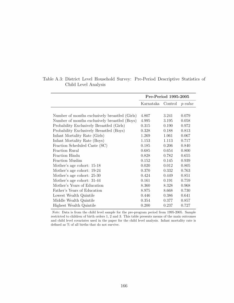
Table A.3: District Level Household Survey: Pre-Period Descriptive Statistics ofChild Level Analysis
Pre-Period 1995-2005
Karnataka Control p-value
Number of months exclusively breastfed (Girls) 4.807 3.241 0.079Number of months exclusively breastfed (Boys) 4.995 3.195 0.058Probability Exclusively Breastfed (Girls) 0.315 0.190 0.972Probability Exclusively Breastfed (Boys) 0.328 0.188 0.813Infant Mortality Rate (Girls) 1.269 1.061 0.067Infant Mortality Rate (Boys) 1.153 1.113 0.717Fraction Scheduled Caste (SC) 0.185 0.206 0.840Fraction Rural 0.685 0.654 0.800Fraction Hindu 0.828 0.782 0.655Fraction Muslim 0.152 0.145 0.939Mother’s age cohort: 15-18 0.020 0.012 0.805Mother’s age cohort: 19-24 0.370 0.332 0.763Mother’s age cohort: 25-30 0.424 0.449 0.851Mother’s age cohort: 31-44 0.161 0.191 0.759Mother’s Years of Education 8.360 8.328 0.968Father’s Years of Education 8.975 8.668 0.730Lowest Wealth Quintile 0.446 0.386 0.641Middle Wealth Quintile 0.354 0.377 0.857Highest Wealth Quintile 0.200 0.237 0.727
Note: Data is from the child level sample for the pre-program period from 1995-2005. Samplerestricted to children of birth orders 1, 2 and 3. This table presents means of the main outcomesand child level covariates used in the paper for the child level analysis. Infant mortality rate isdefined as % of all births that do not survive.
166

Table A.4: Effect of Hypothetical Bhagyalakshmi on Child Sex Ratio
A. Pooled Sample (1) (2)
Karnataka*Post 4.196 1.778(11.561) (5.193)
Observations 259,370 259,370Number of PSUs 129,685 129,685
B. Border Districts Only (1) (2)
Karnataka*Post 4.775 1.298(6.047) (3.598)
Observations 46,430 46,430Number of PSUs 23,215 23,215
Year FE x xPSU FE x xCovariates x
Note: This table reports the coefficients of variableProgramjt from specification 1.2 for a hypotheticalprogram introduced in 1996. In addition I include, fe-male and male literacy rates; female and male labourforce participation rates; fraction scheduled caste; logpopulation of a PSU. Post is defined as = 2001. Kar-nataka=1 if PSU j is in Karnataka and 0 otherwise.Standard errors are clustered by state. *** 1%, **5%, * 10%.
Table A.5: Ideal Number of Children: Pre-Program Trends
A. Ideal Girls Survey Round DLHS-2 Survey Round NFHS Change
Karnataka 0.859 0.690 -0.169Control States 0.885 0.773 -0.162B. Ideal Boys (1) (2) (3)
Karnataka 1.023 0.795 -0.228Control States 0.970 0.746 -0.224
Note: Data is from the DLHS-2 and the National Family Health Survey (NFHS 2005-06). Reportslevels of self-reported ideal number of girls and ideal number of boys for Karnataka and the controlstates in the pre-program period. The question used is: Would you like to have another child or wouldyou prefer not to have any more children? Would you prefer your next child to be a girl or boy?
167
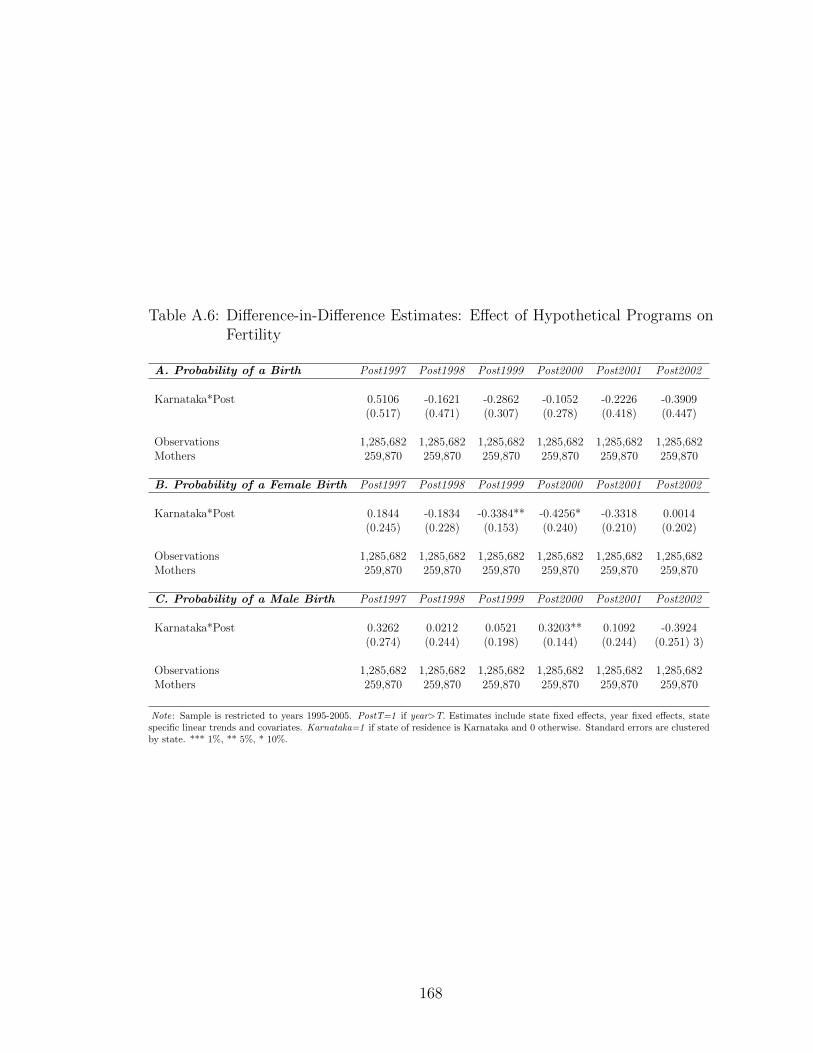
Table A.6: Difference-in-Difference Estimates: Effect of Hypothetical Programs onFertility
A. Probability of a Birth Post1997 Post1998 Post1999 Post2000 Post2001 Post2002
Karnataka*Post 0.5106 -0.1621 -0.2862 -0.1052 -0.2226 -0.3909(0.517) (0.471) (0.307) (0.278) (0.418) (0.447)
Observations 1,285,682 1,285,682 1,285,682 1,285,682 1,285,682 1,285,682Mothers 259,870 259,870 259,870 259,870 259,870 259,870
B. Probability of a Female Birth Post1997 Post1998 Post1999 Post2000 Post2001 Post2002
Karnataka*Post 0.1844 -0.1834 -0.3384** -0.4256* -0.3318 0.0014(0.245) (0.228) (0.153) (0.240) (0.210) (0.202)
Observations 1,285,682 1,285,682 1,285,682 1,285,682 1,285,682 1,285,682Mothers 259,870 259,870 259,870 259,870 259,870 259,870
C. Probability of a Male Birth Post1997 Post1998 Post1999 Post2000 Post2001 Post2002
Karnataka*Post 0.3262 0.0212 0.0521 0.3203** 0.1092 -0.3924(0.274) (0.244) (0.198) (0.144) (0.244) (0.251) 3)
Observations 1,285,682 1,285,682 1,285,682 1,285,682 1,285,682 1,285,682Mothers 259,870 259,870 259,870 259,870 259,870 259,870
Note: Sample is restricted to years 1995-2005. PostT=1 if year>T. Estimates include state fixed effects, year fixed effects, statespecific linear trends and covariates. Karnataka=1 if state of residence is Karnataka and 0 otherwise. Standard errors are clusteredby state. *** 1%, ** 5%, * 10%.
168

Table A.7: Difference-in-Difference Estimates: Effect of Bhagyalakshmi on FertilityExcluding One State at a Time
A. Probability of a Birth/State Excluded → Tamilnadu Kerala Maharashtra West Bengal Andhra Pradesh
Karnataka*Post 0.9382* 0.4097** 0.8844** 0.9298* 1.0223*(0.498) (0.198) (0.402) (0.554) (0.527)
Observations 1,159,348 1,300,851 1,045,331 1,205,321 1,220,519Mothers 231,641 259,468 208,406 240,464 243,957
B. Probability of a Female Birth/State Excluded → Tamilnadu Kerala Maharashtra West Bengal Andhra Pradesh
Karnataka*Post 0.5735** 0.3221*** 0.5432** 0.5803** 0.6031***(0.280) (0.094) (0.250) (0.266) (0.251)
Observations 1,159,348 1,300,851 1,045,331 1,205,321 1,220,519Mothers 231,641 259,468 208,406 240,464 243,957
C. Probability of a Male Birth/State Excluded → Tamilnadu Kerala Maharashtra West Bengal Andhra Pradesh
Karnataka*Post 0.3647 0.0876 0.3411 0.3495 0.4192(0.318) (0.107) (0.384) (0.308) (0.276)
Observations 1,159,348 1,300,851 1,045,331 1,205,321 1,220,519Mothers 231,641 259,468 208,406 240,464 243,957
Note: Each cell is a separate regression. Each cell excludes one of the control states and re-estimates specification 1.3. Estimates include state fixed effects, year fixedeffects, state specific linear trends and covariates. Karnataka=1 if state of residence is Karnataka and 0 otherwise. Standard errors are clustered by state. *** 1%, ** 5%,* 10%.
Table A.8: Effect of Bhagyalakshmi on Mortality and Breastfeeding: Family Char-acteristics
Dependent Variable ↓ Karnataka*Post*Female Karnataka*Female
Mother’s Age at 1st Birth -0.0091 -0.0326***(0.005) (0.007)
Mother’s Years of Education 0.0394 -0.0075(0.030) (0.013)
Father’s Years of Education -0.0412 -0.0087(0.044) (0.011)
Rural 0.0019 0.0017(0.004) (0.004)
Standard of Living Index 0.0054* 0.0079**(0.003) (0.004)
Observations 204,230 204,230
Note: Each row is a separate regression with the dependent variable in column (1) and the relevantindependent variables in columns (2) and (3). This table reports the coefficients from specification1.6 where dependent variables are: mother’s age at 1st birth (row 1), mother’s years of education(row 2), father’s years of education (row 3), residence in a rural area (row 4) and standard of livingindex (row 5). Each regression includes birth fixed FE, state FE, state-by-birth year FE and female-by-birth year FE. Post is defined as >= March 31st, 2006. Karnataka=1 if state of residence isKarnataka and 0 otherwise. Standard errors are clustered by state. *** 1%, ** 5%, * 10%.
169
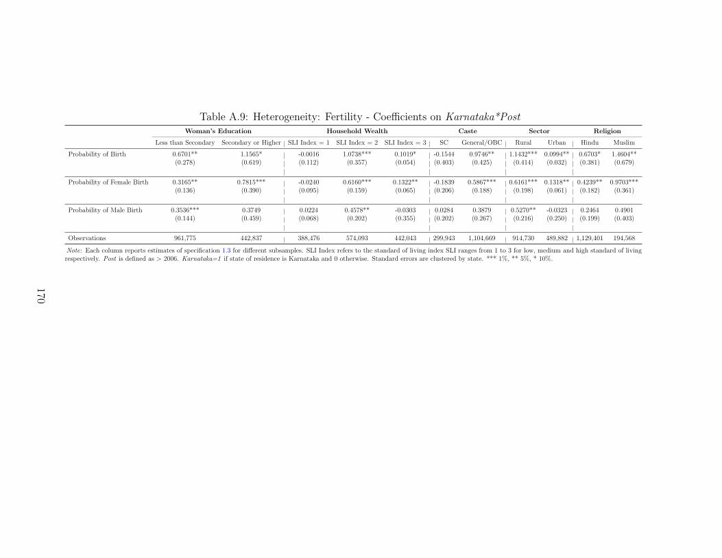
Table A.9: Heterogeneity: Fertility - Coefficients on Karnataka*PostWoman’s Education Household Wealth Caste Sector Religion
Less than Secondary Secondary or Higher SLI Index = 1 SLI Index = 2 SLI Index = 3 SC General/OBC Rural Urban Hindu Muslim
Probability of Birth 0.6701** 1.1565* -0.0016 1.0738*** 0.1019* -0.1544 0.9746** 1.1432*** 0.0994** 0.6703* 1.4604**(0.278) (0.619) (0.112) (0.357) (0.054) (0.403) (0.425) (0.414) (0.032) (0.381) (0.679)
Probability of Female Birth 0.3165** 0.7815*** -0.0240 0.6160*** 0.1322** -0.1839 0.5867*** 0.6161*** 0.1318** 0.4239** 0.9703***(0.136) (0.390) (0.095) (0.159) (0.065) (0.206) (0.188) (0.198) (0.061) (0.182) (0.361)
Probability of Male Birth 0.3536*** 0.3749 0.0224 0.4578** -0.0303 0.0284 0.3879 0.5270** -0.0323 0.2464 0.4901(0.144) (0.459) (0.068) (0.202) (0.355) (0.202) (0.267) (0.216) (0.250) (0.199) (0.403)
Observations 961,775 442,837 388,476 574,093 442,043 299,943 1,104,669 914,730 489,882 1,129,401 194,568
Note: Each column reports estimates of specification 1.3 for different subsamples. SLI Index refers to the standard of living index SLI ranges from 1 to 3 for low, medium and high standard of livingrespectively. Post is defined as > 2006. Karnataka=1 if state of residence is Karnataka and 0 otherwise. Standard errors are clustered by state. *** 1%, ** 5%, * 10%.
170
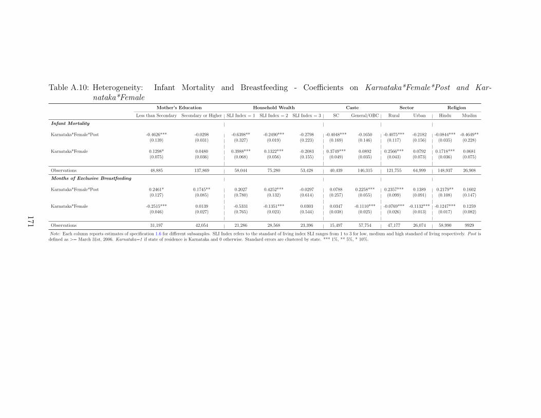
Table A.10: Heterogeneity: Infant Mortality and Breastfeeding - Coefficients on Karnataka*Female*Post and Kar-nataka*Female
Mother’s Education Household Wealth Caste Sector Religion
Less than Secondary Secondary or Higher SLI Index = 1 SLI Index = 2 SLI Index = 3 SC General/OBC Rural Urban Hindu Muslim
Infant Mortality
Karnataka*Female*Post -0.4626*** -0.0298 -0.6398** -0.2490*** -0.2798 -0.4048*** -0.1650 -0.4075*** -0.2182 -0.0844*** -0.4649**(0.139) (0.031) (0.327) (0.019) (0.223) (0.169) (0.146) (0.117) (0.156) (0.035) (0.228)
Karnataka*Female 0.1298* 0.0480 0.3988*** 0.1322*** -0.2083 0.3749*** 0.0892 0.2566*** 0.0792 0.1718*** 0.0681(0.075) (0.036) (0.068) (0.056) (0.155) (0.049) (0.035) (0.043) (0.073) (0.036) (0.075)
Observations 48,885 137,869 58,044 75,280 53,428 40,439 146,315 121,755 64,999 148,937 26,908
Months of Exclusive Breastfeeding
Karnataka*Female*Post 0.2461* 0.1745** 0.2027 0.4252*** -0.0297 0.0788 0.2258*** 0.2357*** 0.1389 0.2179** 0.1602(0.127) (0.085) (0.780) (0.132) (0.614) (0.257) (0.055) (0.099) (0.091) (0.108) (0.147)
Karnataka*Female -0.2515*** 0.0139 -0.5331 -0.1351*** 0.0303 0.0347 -0.1110*** -0.0769*** -0.1132*** -0.1247*** 0.1259(0.046) (0.027) (0.765) (0.023) (0.544) (0.038) (0.025) (0.026) (0.013) (0.017) (0.082)
Observations 31,197 42,054 21,286 28,568 23,396 15,497 57,754 47,177 26,074 58,990 9929
Note: Each column reports estimates of specification 1.6 for different subsamples. SLI Index refers to the standard of living index SLI ranges from 1 to 3 for low, medium and high standard of living respectively. Post isdefined as >= March 31st, 2006. Karnataka=1 if state of residence is Karnataka and 0 otherwise. Standard errors are clustered by state. *** 1%, ** 5%, * 10%.
171

Table A.11: Indian Human Development Survey: Pre-Period Descriptive Statisticsfor Analysis of Nutritional Outcomes
Pre-Period 1995-2005
Karnataka Control p-value
Height-for-Age z-score (Girls) -2.041 -1.758 0.594Height-for-Age z-score (Boys) -1.872 -1.694 0.738Weight-for-Age z-score (Girls) -1.835 -1.512 0.399Weight-for-Age z-score (Boys) -1.851 -1.503 0.428Fraction Scheduled Caste (SC) 0.201 0.238 0.741Fraction Rural 0.750 0.614 0.249Fraction Hindu 0.813 0.772 0.700Fraction Muslim 0.165 0.163 0.987Highest Years of Education of Adult Male 6.628 7.198 0.668Highest Years of Education of Adult Female 5.266 6.077 0.521Monthly Consumption per Capita 1916 1833 0.960
Note: Data is from the Indian Human Development Survey (IHDS) for the pre-programperiod from 1995-2005. This table presents means of the main outcomes and child levelcovariates used in the paper for the analysis of long run nutritional outcomes. Monthlyconsumption per capita is in rupees.
172

Table A.12: Quantification of Program Impacts
A. Regression Estimates Pre-Program Period Post-Program Period ∆ (Post-Pre)
FK 0.4791 0.4862 0.0071EFMK 0.0016 0.0002 -0.0013
B. Decomposition
mK (number of mothers in Karnataka) 14,300,000NK 1,144,000 1,158,243 (=1,144,000 + 0.00092*m) 13,213
C. Change in the number of missing girls
(1) NK,post ∗∆FK ∗ −10.51
= 16,124
(2) ∆NK ∗ (0.490.51− FK,pre
0.51) = 475
(3) = (1) + (2) 16,599
D. Change in the female infant mortality
(1) NK,post ∗ FK,post ∗∆EFMK = -738
(2) NK,post ∗∆FK ∗ EFMK,pre = -19
(3) ∆NK ∗ FK,pre ∗ EFMK,pre = -11
(4) = (1) + (2) + (3) -770
Table A.13: Cost-Effectiveness of the Incentive
A. Outcome Measure Discount Rate (%) Outcome per $1000 Spent (implementer & beneficiary) Outcome per $1000 Invested (implementer)
Number of sex-selective abortions averted 3 0.732 0.9096 1.227 1.5259 2.021 2.521
Number of excess female infant deaths averted 3 0.022 0.0286 0.038 0.0479 0.063 0.079
Additional Months of Exclusive Breastfeeding 3 0.095 0.1186 0.160 0.1989 0.264 0.328
173

A.2 Quantitative Estimates of the Impact of the Bhagyalakshmi Pro-gram
I first use the regression estimates on the impact of the Bhagyalakshmi pro-gram on child sex ratio to calculate the number of girls who survived up to age 6.Then, I decompose this number into the number of girls who were not selectivelyaborted as well as the number of girls who survived up to age one.
Following the methodology outlined in Anukriti et al. [2016], I first define thefollowing:
• N : Number of births in Karnataka and control states
• NK : Number of births in Karnataka
• MK : Fraction of male births among NK
• FK : Fraction of female births among NK
• ∆: Pre-post difference
• mK : Number of mothers in Karnataka
From Anukriti et al. [2016], the expression for the number of “missing girls”is:
0.49
0.51(NK ∗MK)−NK ∗ FK = NK(
0.49
0.51− FK
0.51)
The first term on the left hand side of the above equation represents the expectednumber of female births while the second term is the observed number of femalebirths in Karnataka.
To calculate the impact of the program on the total number of missing girlsI estimate the number of missing girls in the pre- and post program periods (seeAnukriti et al., 2016 for derivation of the following expression):
∆NK ∗ (0.49
0.51− FK,pre
0.51) +NK,post ∗∆FK ∗
−1
0.51(A1)
As outlined in Anukriti et al. [2016], the impact of Bhagyalakshmi on the number ofmissing girls is comprised of two major changes: changes in overall fertility or thechange in the probability of conceiving and changes in the probability of selectivelyaborting a girl.
A.2.1 Quantification of Impact on Child Sex Ratio
I convert the difference-in-differences estimates of 20 (estimate in column (3),Panel A of Table 1.1) into the number of additional female children who survivedup to age 6. That is, the total (0-6) population was approximately 7,182,100 and
174
7,161,033 in 2001 and 2011 respectively. An additional 20 females per 1000 malesimplies an average annual additional 28,124 girls who survived up to age 6.1
A.2.2 Quantification of Impact on Sex-Selective Abortions
In Panel A of Table A.12 I present the regression estimates for sex-ratio atbirth from the study. Column (1) reports the baseline mean of the sex ratio at birth(from Panel A of Table 1.3) and column (3) reports the regression estimate (column(2), Panel A of Table 1.3). Column (2) adds up columns (1) and (3). In Panel B,mK is calculated using the total number of births in Karnataka divided by the grossfertility rate for Karnataka from the Sample Registration System (SRS, 2001) as 80births per 1000 women. That is mK = NK
0.080.
Next, in Panel B, NK is the total number of births in Karnataka in 2001. I usethe Census 2001 to calculate the number in the pre-program period in column (1).2
In column (2) to calculate the number of births in Karnataka in the post-programperiod I use the number of mothers in Karnataka and the endogenous change infertility. To calculate the endogenous change in fertility I use the regression estimatein column (2), Panel A of Table 1.2 i.e 0.0077. I multiply this by a factor, 0.12 toarrive at 0.00092. Then, to calculate the total number of births in the post-programperiod I add total births in the pre-program period in column (1) to the total newbirths because of changing fertility (0.00092*m). The total change in the numberof births is in column (3).
Finally in Panel C I row (1) represents the calculation of the “sex-selectiveabortion effect” and row (2) represents the calculation of the “conception” effect.From row (3) I get that the Bhagyalakshmi program led to 16,599 additional girlsbeing born.
A.2.3 Quantification of Impact on Excess Female Mortality
Next, I estimate the number of girls that survived up to age 1 as a result ofthe program. Following the methodology outlined in Anukriti et al. [2016], excessfemale infant deaths annually is defined as:
NK ∗ FK ∗ EFMK
where NK and FK are defined as before and EFMK is the difference in the proba-bility of death by age one between girls and boys in Karnataka. Then the reductionin female infant deaths as a result of Bhagyalakshmi is the difference between the
1This is calculated as follows from equation A1: ∆NK ∗ ( 0.490.51 −
FK,pre
0.51 ) + NK,post ∗∆FK ∗ −10.51
=((0.49/0.51)-(0.48/0.51))*(-21067) + (7161033*0.020*(-1/0.51)) = 281,239. Averaging over theperiod of 2001-2011, I get an additional 28,124 girls in Karnataka.
2The male birth rate in Karnataka in the 2001 Census was 22 and the male population was27 million, translating into 594,000 male births. Total male births=Birth Rate x Total malepopulation. Similarly total female births is about 550,000. So total births in Karnataka wereabout 1,144,000 in 2001.
175

number of excess postnatal female deaths during the pre- and post-program periods(see Anukriti et al. [2016] for derivation of the following expression):
NK,post ∗ FK,post ∗∆EFMK +NK,post ∗∆FK ∗EFMK,pre + ∆NK ∗ FK,pre ∗EFMK,pre
The first term in the above expression is the decline in EFM due to better in-vestments such as breastfeeding; the second term is the increase in the fraction ofpost-program births that are female due to a reduction in sex-selective abortionsand finally the third term is the same endogenous fertility effect of the program.
In row 2, Panel A of Table A.12 I present the regression estimates from equa-tion 1.6. Column (1) reports the baseline mean of excess female infant mortalitywhile column (3) reports the triple difference estimate from Panel A, column 2,Table 1.6. In Panel D I calculate that Bhagyalakshmi program led to about 770additional girls who survived up to the age of one.
Thus, in total 17,368 girls (= 16,599 + 770) were ‘saved’ per year as a resultof the introduction of the Bhagyalakshmi program. Thus, out of the total annualaverage additional girls that survived up to age 6 i.e. 28,124; about 62 percent isattributable to fewer sex selective abortions and a larger fraction of girls survivingup to age 1.
A.3 Discussion
A.3.1 Cost Effectiveness Analysis
The most natural benchmark for the cost effectiveness of the Bhagyalakshmiprogram would be similar long-term conditional cash transfers that are offered tohouseholds with any or all of the following conditions: remaining unmarried till age18, being enrolled in school and being immunized. Unfortunately, there are no credi-ble evaluations of CCT programs in India and no experimental evaluations in SouthAsia more broadly (unlike in Africa and Latin America) which examine the fourmain outcomes from this study: child sex ratio; sex ratio at birth; infant mortal-ity and exclusive breastfeeding duration. Nevertheless, I present a cost-effectivenessanalysis of the Bhagyalakshmi program in Table A.13. These estimates are meant togive a sense of the relative efficiency of the program at meeting particular outcomeswithout requiring the full set of assumptions of a cost-benefit analysis.
To calculate the cost-effectiveness, I estimate the amount of a given outcomeachieved by a given investment. For example, I use the estimates from the previoussection on the total number of sex-selective abortions and number of excess femaleinfant deaths averted by the program in a year (16,599 and 770 respectively). I thendivide the present value of the costs of the program by the number of sex-selectiveabortions averted to determine the cost per sex-selective abortion averted and costper female infant death averted. I then divide 1,000 by the cost per outcome measureto express the figure in terms of returns to a $1,000 investment.
The present value of the costs of the program include implementation costs aswell as costs to the beneficiary. For the cost to the implementer, I consider actual
176
program costs detailed in Section 1.3.3 For the cost to the beneficiary I considertwo types of couples - (a) couples for whom the Bhagyalakshmi did not change theirtotal number of children born but only resulted in fewer sex-selective abortions. Theopportunity cost of this group is the foregone old-age income support and dowryreceipts from having fewer than the desired number of sons and, (b) couples for whomthe Bhagyalakshmi program changed both the number and gender composition ofchildren since such couples now had more than their expected number of childrenand more than their expected number of girls. For such couples, in addition tothe opportunity costs of foregone old-age income support and dowry receipts I alsoinclude the opportunity cost of raising an additional child.4,5
My estimates imply that the Bhagyalakshmi program is relatively cost-effective.The conditional incentive translates into 1.525 number of sex-selective abortionsaverted, 0.047 female infant deaths averted and 0.20 additional months of exclusivebreastfeeding for every $1000 spent by the implementer per year (See Table A.13).While comparable cost-effectiveness estimates for similar outcomes are not avail-able, Nandi and Deolalikar [2013] estimate the number of girls saved as a result ofthe Pre Conception Pre Natal Diagnostics Act (PNDT) of 1994 to be 81,500 over a10-year period from 1991 to 2001 across 6 Indian states. Using these estimates andthe district-wise budgetary allocation under the PNDT Act and performing similarcalculations I estimate that the PNDT Act translated into 0.853 number of sex se-lective abortions averted for every $1000 spent by the implementer. In contrast, theBhagyalakshmi was more cost-effective in spite of being only a state-level programas opposed to the PNDT Act which was a nation-wide legislation.6
3This is by all accounts an underestimate of the actual costs since I do not include monitoringcosts of the program.
4I estimate average net dowry receipts to a boy’s family to be Rs. 30,000 ($465) based onthe estimates in the Indian Human Development Survey (IHDS 2004-05). This includes dowryreceipts for a boy’s family minus their wedding expenses. I multiply this amount by the numberof additional girls born due to fewer sex-selective abortions in the previous section i.e. due to the“sex-selective abortion effect” under the assumption that each girl represents one household.
5I estimate the average expenditure on health and education of a child for 18 years based onthe National Sample Survey (2007-08) to be Rs. 96,000 ($1490) and multiply this by the numberof additional girls born due to the “conception effect” from the previous section, again assumingthat each girl represents one household.
6Buchmann et al. [2017] provide cost-effectiveness estimates for a conditional cash transferrandomized trial in Bangladesh which provided financial incentives to adolescent girls (as opposedto the incentive given at birth in Bhagyalakshmi in the form of an 18-year bond) to delay marriageand child bearing. The authors find that the financial incentive delayed marriage by 6.6 years,averted 1.5 child marriages, and led to 3.6 years of additional schooling for every $1,000 investedby the implementer.
177
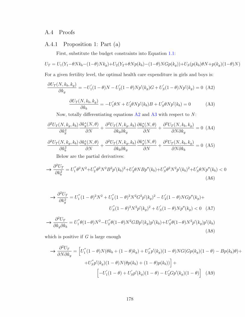
A.4 Proofs
A.4.1 Proposition 1: Part (a)
First, substitute the budget constraints into Equation 1.1:
UT = U1(Y1−θNkb−(1−θ)Nkg)+U2(Y2+θNp(kb)−(1−θ)NGp(kg))+US(p(kb)θN+p(kg)(1−θ)N)
For a given fertility level, the optimal health care expenditure in girls and boys is:
∂UT (N, kb, kg)
∂kg= −U ′1(1− θ)N −U ′2(1− θ)Np′(kg)G+U
′
S(1− θ)Np′(kg) = 0 (A2)
∂UT (N, kb, kg)
∂kb= −U ′1θN + U
′
2θNp′(kb)B + U
′
SθNp′(kb) = 0 (A3)
Now, totally differentiating equations A2 and A3 with respect to N :
∂2UT (N, kg, kb)
∂k2g
∂k∗g(N, θ)
∂N+∂2UT (N, kg, kb)
∂kb∂kg
∂k∗b (N, θ)
∂N+∂2UT (N, kb, kg)
∂N∂kg= 0 (A4)
∂2UT (N, kg, kb)
∂k2b
∂k∗b (N, θ)
∂N+∂2UT (N, kg, kb)
∂kb∂kg
∂k∗g(N, θ)
∂N+∂2UT (N, kb, kg)
∂N∂kb= 0 (A5)
Below are the partial derivatives:
→ ∂2UT∂k2
b
= U′′
1 θ2N2+U
′′
2 θ2N2B2p′(kb)
2+U′
2θNBp′′(kb)+U
′′
Sθ2N2p′(kb)
2+U′
SθNp′′(kb) < 0
(A6)
→ ∂2UT∂k2
g
= U′′
1 (1− θ)2N2 + U′′
2 (1− θ)2N2G2p′(kg)2 − U ′2(1− θ)NGp′′(kg)+
U′′
S (1− θ)2N2p′(kg)2 + U
′
S(1− θ)Np′′(kg) < 0 (A7)
→ ∂2UT∂kg∂kb
= U′′
1 θ(1−θ)N2−U ′′2 θ(1−θ)N2GBp′(kg)p′(kb)+U
′′
Sθ(1−θ)N2p′(kg)p′(kb)
(A8)which is positive if G is large enough
→ ∂2UT∂N∂kg
=[U′′
1 (1− θ)N(θkb + (1− θ)kg) + U′′
2 p′(kg)(1− θ)NG(Gp(kg)(1− θ)−Bp(kb)θ)+
+U′′
Sp′(kg)(1− θ)N(θp(kb) + (1− θ)p(kb))
]+[
−U ′1(1− θ) + U′
Sp′(kg)(1− θ)− U
′
2Gp′(kg)(1− θ)
](A9)
178
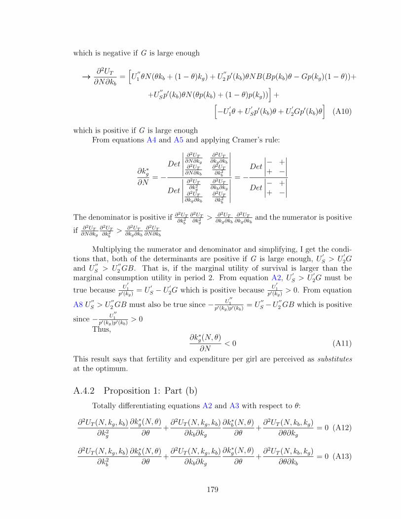
which is negative if G is large enough
→ ∂2UT∂N∂kb
=[U′′
1 θN(θkb + (1− θ)kg) + U′′
2 p′(kb)θNB(Bp(kb)θ −Gp(kg)(1− θ))+
+U′′
Sp′(kb)θN(θp(kb) + (1− θ)p(kg))
]+[
−U ′1θ + U′
Sp′(kb)θ + U
′
2Gp′(kb)θ
](A10)
which is positive if G is large enoughFrom equations A4 and A5 and applying Cramer’s rule:
∂k∗g∂N
= −Det
∣∣∣∣∣∂2UT∂N∂kg
∂2UT∂kg∂kb
∂2UT∂N∂kb
∂2UT∂k2b
∣∣∣∣∣Det
∣∣∣∣∣∂2UT∂k2g
∂2UT∂kb∂kg
∂2UT∂kg∂kb
∂2UT∂k2b
∣∣∣∣∣= −
Det
∣∣∣∣− ++ −
∣∣∣∣Det
∣∣∣∣− ++ −
∣∣∣∣The denominator is positive if ∂2UT
∂k2b
∂2UT∂k2g
> ∂2UT∂kg∂kb
∂2UT∂kg∂kb
and the numerator is positive
if ∂2UT∂N∂kg
∂2UT∂k2b
> ∂2UT∂kg∂kb
∂2UT∂N∂kb
Multiplying the numerator and denominator and simplifying, I get the condi-tions that, both of the determinants are positive if G is large enough, U
′S > U
′2G
and U′′S > U
′′2GB. That is, if the marginal utility of survival is larger than the
marginal consumption utility in period 2. From equation A2, U′S > U
′2G must be
true becauseU′1
p′(kg)= U
′S − U
′2G which is positive because
U′1
p′(kg)> 0. From equation
A8 U′′S > U
′′2GB must also be true since − U
′′1
p′(kg)p′(kb)= U
′′S −U
′′2GB which is positive
since − U′′1
p′(kg)p′(kb)> 0
Thus,∂k∗g(N, θ)
∂N< 0 (A11)
This result says that fertility and expenditure per girl are perceived as substitutesat the optimum.
A.4.2 Proposition 1: Part (b)
Totally differentiating equations A2 and A3 with respect to θ:
∂2UT (N, kg, kb)
∂k2g
∂k∗g(N, θ)
∂θ+∂2UT (N, kg, kb)
∂kb∂kg
∂k∗b (N, θ)
∂θ+∂2UT (N, kb, kg)
∂θ∂kg= 0 (A12)
∂2UT (N, kg, kb)
∂k2b
∂k∗b (N, θ)
∂θ+∂2UT (N, kg, kb)
∂kb∂kg
∂k∗g(N, θ)
∂θ+∂2UT (N, kb, kg)
∂θ∂kb= 0 (A13)
179

Calculating the remaining partials
→ ∂2UT∂θ∂kg
=[U′′
1 (1− θ)N2(kb − kg)− U′′
2 (1− θ)N2p′(kg)G(p(kb)B + p(kg)G)+
+U′′
S (1− θ)N2p′(kg)(p(kb)− p(kg))]
+[U′
1N − U′
Sp′(kg)N + U
′
2Gp′(kg)N
](A14)
which is positive if G is large enough
→ ∂2UT∂θ∂kb
=[U′′
1 θN2(kb − kg) + U
′′
2 θN2p′(kb)G(p(kb)B + p(kg)G)+
+U′′
SθN2p′(kb)(p(kb)− p(kg))
]+[
U′
1N − U′
Sp′(kb)N − U
′
2Bp′(kb)N
]< 0
(A15)
From equations A12 and A13 and applying Cramer’s rule:
∂k∗g∂θ
= −Det
∣∣∣∣∣∂2UT∂θ∂kg
∂2UT∂kg∂kb
∂2UT∂θ∂kb
∂2UT∂k2b
∣∣∣∣∣Det
∣∣∣∣∣∂2UT∂k2g
∂2UT∂kb∂kg
∂2UT∂kg∂kb
∂2UT∂k2b
∣∣∣∣∣= −
Det
∣∣∣∣+ +− −
∣∣∣∣Det
∣∣∣∣− ++ −
∣∣∣∣The determinant in the denominator will be positive as before. The numerator willbe negative if ∂2UT
∂θ∂kg
∂2UT∂k2b
> ∂2UT∂kg∂kb
∂2UT∂θ∂kb
Multiplying the numerator and simplifying I get the condition that the deter-minant is negative if G is large enough. Thus,
∂k∗g(N, θ)
∂θ> 0 (A16)
This result says that as the proportion of boys increases, the expenditure per girlalso increases.
A.4.3 Proposition 2: Part (a)
I will do the optimization over N and kg, kb in two stages: first, I will maximizethe objective function with respect to kg, kb for given N, and then I will choose theoptimal N. For a given level of fertility, the first order conditions with respect to kgand kb are given in equations A2 and A3.
180

The first order condition for N in the maximization of the second stage objec-tive function (that obtains after kg and kb have been “maximized out”) is:
∂UT (N, kb, kg)
∂N= −U ′1(1−θ)k∗g−U
′
1θk∗b−U
′
2(1−θ)p(k∗g)G+U′
2θp(k∗b )B+U
′
S(1−θ)p(k∗g)+U′
Sθp(k∗b ) = 0
(A17)Let N∗(G) be the solution to equation A17. Totally differentiating equation A17with respect to G, I obtain:
dN∗
dG
[U′′
1 (1− θ)2k2g + U
′′
1 θ2k2b + U
′′
2 (1− θ)2p(kg)2G2+
U′′
2 θ2p(kb)
2B2 + U′′
S (1− θ)2p(kg)2 + U
′′
Sθ2p(kb)
2]
+[−U ′2(1− θ)p(kg)
]= 0 (A18)
The term in the square brackets on the left is clearly negative, while the term onthe square brackets on the right is also negative. Then in order for equation A18 tosum to zero it must be true that,
dN∗(G)
dG< 0 (A19)
The introduction of the Bhagyalakshmi program will reduce the future net cost ofeach surviving daughter G and thus increase the willingness to conceive in thissimple framework.
A.4.4 Proposition 2: Part (b)
Using the chain rule it follows that:
dk∗g(N∗(G), θ, G)
dG=∂k∗g(N
∗(G), θ, G)
∂N
dN∗(G)
dG︸ ︷︷ ︸Indirect Effect
+∂k∗g(N
∗(G), θ, G)
∂G︸ ︷︷ ︸Direct Effect
(A20)
Direct Effect: Calculating the remaining partials
→ ∂2UT∂G∂kg
=[U′′
2 (1− θ)2N2p′(kg)2G2 − U ′2(1− θ)Np′(kg)
]< 0 (A21)
→ ∂2UT∂G∂kb
= 0 (A22)
181

By the implicit function theorem:
∂k∗g∂G
= −Det
∣∣∣∣∣∂2UT∂G∂kg
∂2UT∂kg∂kb
∂2UT∂G∂kb
∂2UT∂k2b
∣∣∣∣∣Det
∣∣∣∣∣∂2UT∂k2g
∂2UT∂kb∂kg
∂2UT∂kg∂kb
∂2UT∂k2b
∣∣∣∣∣= −
Det
∣∣∣∣− +0 −
∣∣∣∣Det
∣∣∣∣− ++ −
∣∣∣∣The denominator is positive as before. The numerator is also positive. Thus,
∂k∗g∂G
< 0 (A23)
Indirect Effect: From equations A19 and A11 we have,
∂k∗g(N∗(G), θ, G)
∂N< 0
dN∗(G)
dG< 0
Thus,∂k∗g(N∗(G),θ,G)
∂NdN∗(G)dG
> 0Thus, from equation A23 the direct effect is negative i.e. a decrease in future
costs leads to an increase in investments in girls, while from equations A19 and A11the indirect effect is positive i.e. a decrease in future costs of girls leads to a decreasein investments in girls.
Thus, the overall effect ofdk∗g(N∗(G),θ,G)
dGis ambiguous.
A.4.5 Proposition 3
In order to examine the impact of Bhagyalakshmi on son-biased fertility stop-ping behaviour I will calculate the following:(i) Change in investments in girls as the proportion of boys goes up after Bhagyalak-shmi, ∂kg
∂θ
(ii) Change in investments in boys as proportion of boys goes up after Bhagyalak-shmi, ∂kb
∂θand finally,
(iii) Impact on parents’ expected utility from having marginally more children as
the proportion of boys goes up,(1/2)
∂UT∂g
+(1/2)∂UT∂b
∂θwhere g = (1− θ)N and b = θN
Part (i): After the introduction of the Bhagyalakshmi program, for thosehouseholds for whom the program results in a large decrease in G ; equations A8 &A14 which depend on G being large, will flip signs. That is, a large decrease in Gdue to Bhagyalakshmi will result in: ∂2UT
∂kg∂kb< 0 and ∂2UT
∂kg∂θ< 0.
182

Thus,
∂k∗g∂θ
= −Det
∣∣∣∣∣∂2UT∂θ∂kg
∂2UT∂kg∂kb
∂2UT∂θ∂kb
∂2UT∂k2b
∣∣∣∣∣Det
∣∣∣∣∣∂2UT∂k2g
∂2UT∂kb∂kg
∂2UT∂kg∂kb
∂2UT∂k2b
∣∣∣∣∣= −
Det
∣∣∣∣− −− −
∣∣∣∣Det
∣∣∣∣− −− −
∣∣∣∣The denominator is positive if ∂2UT
∂k2b
∂2UT∂k2g
> ∂2UT∂kg∂kb
∂2UT∂kg∂kb
which is true from Propo-
sition 1(a). The numerator is positive if ∂2UT∂θ∂kg
∂2UT∂k2b
> ∂2UT∂kg∂kb
∂2UT∂θ∂kb
which is also true
from Proposition 1(a). Thus,∂k∗g(N, θ)
∂θ< 0 (A24)
Part (ii):
∂k∗b∂θ
= −Det
∣∣∣∣∣∂2UT∂k2g
∂2UT∂θ∂kg
∂2UT∂kg∂kb
∂2UT∂θ∂kb
∣∣∣∣∣Det
∣∣∣∣∣∂2UT∂k2g
∂2UT∂kb∂kg
∂2UT∂kg∂kb
∂2UT∂k2b
∣∣∣∣∣= −
Det
∣∣∣∣− −− −
∣∣∣∣Det
∣∣∣∣− −− −
∣∣∣∣The denominator and numerator are both positive from part (i) above and thus,
∂k∗b (N, θ)
∂θ< 0 (A25)
Thus, if Bhagyalakshmi leads to a large decrease in the future costs of girlsi.e. the reduction in G is large enough then, ∂kb
∂θ< 0 and ∂kg
∂θ< 0. That is, after the
introduction of the program, investments in girls and boys are no longer determinedby the proportion of children of a particular gender.
Part (iii):
Finally, I examine how (1/2)∂UT∂g
+ (1/2)∂UT∂b
changes as the proportion of boys
(or the proportion of girls) goes up, where g = (1− θ)N and b = θN :
(1/2)∂UT∂g
+ (1/2)∂UT∂b
= −U ′1kg −U′
2Gp(kg)−U′
1kb +U′
2Bp(kb) +U′
S(p(kg) + p(kb))
After Bhagyalakshmi if the proportion of boys goes up, investments in boys declineand investments in girls also decline (from parts i and ii above). Similarly, if theproportion of girls goes up investments in children of both genders falls. In bothscenarios, period 1 and survival marginal utility fall and period 2 marginal utilityof consumption must also fall. Thus, if the proportion of either boys goes up orthe proportion of girls goes up, parents will gain less utility from an extra childindependent of the existing proportion of children of a particular gender, if the
183

decrease in the future costs of girls is large enough.
A.4.6 Proposition 4
I extend the above framework to incorporate selective abortion behaviour.At the beginning of period 1, parents have 3 possible choices: no pregnancy, apregnancy without a prenatal scan determination, or a pregnancy with a prenatalscan determination followed by an abortion if the fetus is a female. When a childis born parents incur a fixed cost, and gender specific investment costs in the firstperiod. If parents select prenatal sex determination they also pay the cost of thescan, and the cost of a son if the fetus is a boy and therefore carried to term.7 Letthe probability of conceiving a child of either gender be 1
2. Additionally, let b and g
be less than the total number of children parents have in their lifetime. Then I canexamine the impact of a marginal birth on expected utility. For simplicity, I willassume that the ‘no pregnancy’ option is not available and the cost of sex-selectiveabortions to be negligible.
Expected change in utility from a pregnancy without a prenatal scan determi-nation, ∆UNS
T :
∆UNST =
1
2
∂UT∂g
+1
2
∂UT∂b
(A26)
If instead they decide to have a pregnancy without a prenatal scan determi-nation their change in expected utility will be, ∆US
T :
∆UST =
1
20 +
1
2
∂UT∂b
(A27)
where the second term on the right is the utility from having a scan, finding out it’sa boy and thus carrying it to term and the second term is the utility from having ascan, finding out it’s a girl and aborting it.
Before BhagyalakshmiBefore the introduction of Bhagyalakshmi, parents will choose a pregnancy
with sex determination if ∆UNST < ∆US
T . Intuitively, parents choose a pregnancywith a prenatal scan over a pregnancy without a prenatal scan if the marginalperiod 2 consumption utility from having a girl is smaller than the expected impacton consumption utility in period 1.
After BhagyalakshmiFrom equations A26 and A27:
∆UNST −∆US
T =1
2
∂UT∂g
(A28)
7The prenatal sex determination scan is best thought of as a bundled service that includesboth the prenatal sex determination scan and the abortion if the fetus is female. This is because,it is more tractable than including additional steps in the decision process, especially since theonly motivation for a prenatal scan in the model is sex selection, and a scan would therefore be“wasted” unless a female fetus was aborted.
184
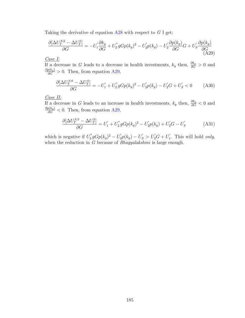
Taking the derivative of equation A28 with respect to G I get:
∂[∆UNST −∆US
T ]
∂G= −U ′1
∂kg∂G
+ U′′
2 gGp(kg)2 − U ′2p(kg)− U
′
2
∂p(kg)
∂GG+ U
′
S
∂p(kg)
∂G(A29)
Case I:If a decrease in G leads to a decrease in health investments, kg then, ∂kg
∂G> 0 and
∂p(kg)
∂G> 0. Then, from equation A29,
∂[∆UNST −∆US
T ]
∂G= −U ′1 + U
′′
2 gGp(kg)2 − U ′2p(kg)− U
′
2G+ U′
S < 0 (A30)
Case II:If a decrease in G leads to an increase in health investments, kg then, ∂kg
∂G< 0 and
∂p(kg)
∂G< 0. Then, from equation A29,
∂[∆UNST −∆US
T ]
∂G= U
′
1 + U′′
2 gGp(kg)2 − U ′2p(kg) + U
′
2G− U′
S (A31)
which is negative if U′′2 gGp(kg)
2 − U ′2p(kg) − U′S > U
′2G + U
′1. This will hold only,
when the reduction in G because of Bhagyalakshmi is large enough.
185

Appendix B: Appendix for Chapter 2
186

Table B.1: State-wise number of beneficiaries enrolled to avail the benefit underRSBY (2012 - 2015)
Major States Enrolled Families Enrolled Families Enrolled Families2012-13 2013-14 2014-15
Assam 176906 1416919 1416919Bihar 7634503 6102774 Enrolment in progressChhattisgarh 2285345 2265370 2142035Gujarat 1883179 1900903 1923732Haryana 560241 465797 419919Himachal Pradesh 286492 341818 448000Jammu & Kashmir 35521 4988 Not participated in RSBYJharkhand 1462235 1923138 1619697Kerala 2743665 3662511 3194638Madhya Pradesh 116510 608748 203208Maharashtra 1747157 234252 Not participated in RSBYManipur 66753 68140 30674Meghalaya 78395 108321 156086Mizoram 103545 145842 109744Nagaland 143585 151806 80229Odisha 3388096 4238040 4306702Puducherry 9486 9486 Enrolment not donePunjab 226878 236764 234169Rajasthan 732889 2511663 2692626Tripura 505327 505327 505327Uttar Pradesh 5396503 5541225 3307372Uttarakhand 334694 285435 285435West Bengal 5766731 5748689 5749646
Note: Data is from Government of India, Ministry of Health and Family Welfare
187
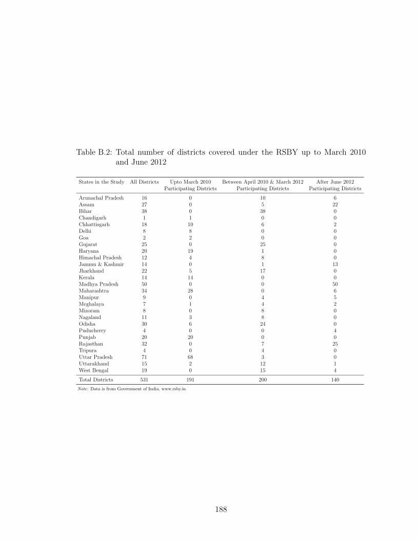
Table B.2: Total number of districts covered under the RSBY up to March 2010and June 2012
States in the Study All Districts Upto March 2010 Between April 2010 & March 2012 After June 2012Participating Districts Participating Districts Participating Districts
Arunachal Pradesh 16 0 10 6Assam 27 0 5 22Bihar 38 0 38 0Chandigarh 1 1 0 0Chhattisgarh 18 10 6 2Delhi 8 8 0 0Goa 2 2 0 0Gujarat 25 0 25 0Haryana 20 19 1 0Himachal Pradesh 12 4 8 0Jammu & Kashmir 14 0 1 13Jharkhand 22 5 17 0Kerala 14 14 0 0Madhya Pradesh 50 0 0 50Maharashtra 34 28 0 6Manipur 9 0 4 5Meghalaya 7 1 4 2Mizoram 8 0 8 0Nagaland 11 3 8 0Odisha 30 6 24 0Puducherry 4 0 0 4Punjab 20 20 0 0Rajasthan 32 0 7 25Tripura 4 0 4 0Uttar Pradesh 71 68 3 0Uttarakhand 15 2 12 1West Bengal 19 0 15 4
Total Districts 531 191 200 140
Note: Data is from Government of India, www.rsby.in
188
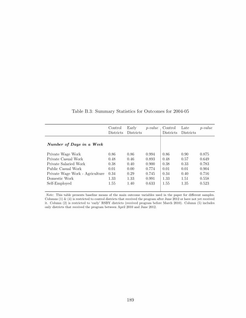
Table B.3: Summary Statistics for Outcomes for 2004-05
Control Early p-value Control Late p-valueDistricts Districts Districts Districts
Number of Days in a Week
Private Wage Work 0.86 0.86 0.994 0.86 0.90 0.875Private Casual Work 0.48 0.46 0.893 0.48 0.57 0.649Private Salaried Work 0.38 0.40 0.900 0.38 0.33 0.783Public Casual Work 0.01 0.00 0.774 0.01 0.01 0.904Private Wage Work - Agriculture 0.34 0.29 0.745 0.34 0.40 0.716Domestic Work 1.33 1.33 0.991 1.33 1.51 0.558Self-Employed 1.55 1.40 0.633 1.55 1.35 0.523
Note: This table presents baseline means of the main outcome variables used in the paper for different samples.Columns (1) & (4) is restricted to control districts that received the program after June 2012 or have not yet receivedit. Column (2) is restricted to ‘early’ RSBY districts (received program before March 2010). Column (5) includesonly districts that received the program between April 2010 and June 2012.
189
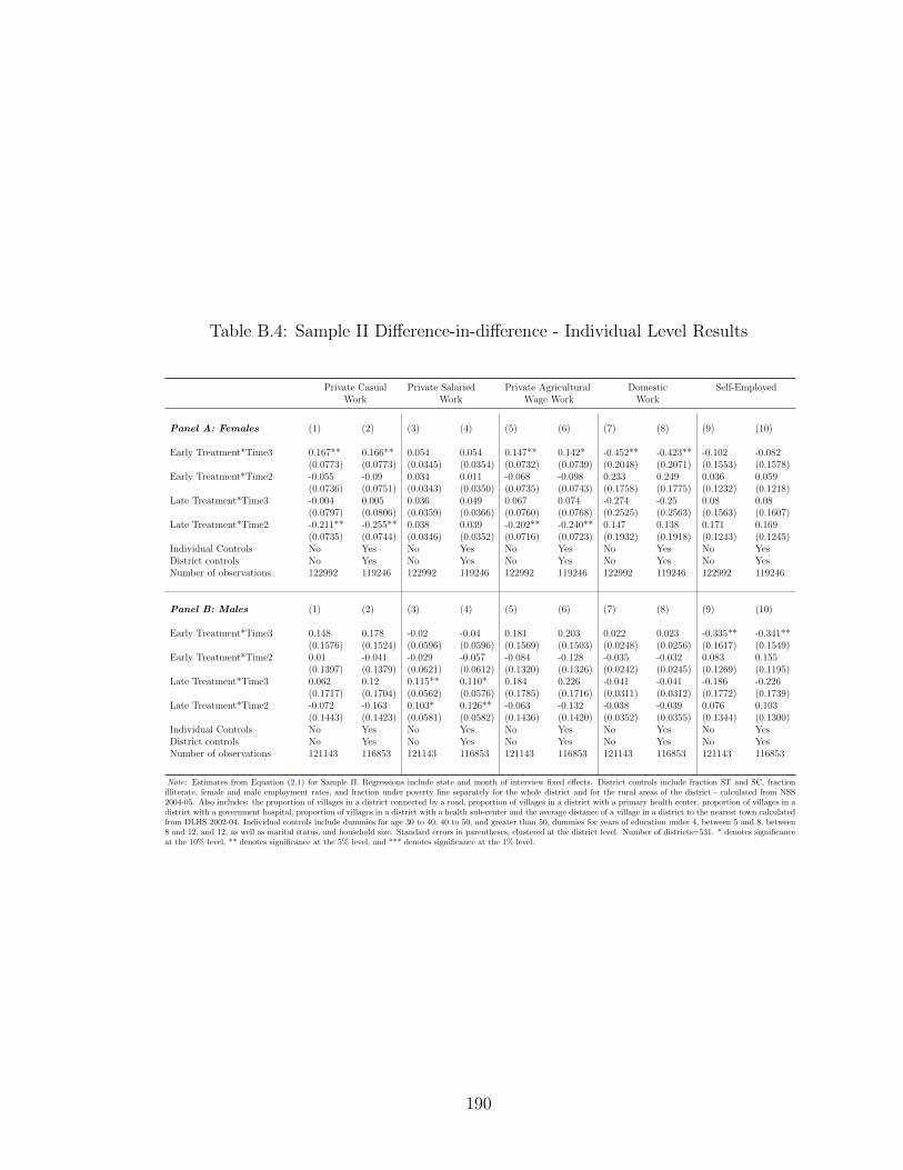
Table B.4: Sample II Difference-in-difference - Individual Level Results
Private Casual Private Salaried Private Agricultural Domestic Self-EmployedWork Work Wage Work Work
Panel A: Females (1) (2) (3) (4) (5) (6) (7) (8) (9) (10)
Early Treatment*Time3 0.167** 0.166** 0.054 0.054 0.147** 0.142* -0.452** -0.423** -0.102 -0.082(0.0773) (0.0773) (0.0345) (0.0354) (0.0732) (0.0739) (0.2048) (0.2071) (0.1553) (0.1578)
Early Treatment*Time2 -0.055 -0.09 0.034 0.011 -0.068 -0.098 0.233 0.249 0.036 0.059(0.0736) (0.0751) (0.0343) (0.0350) (0.0735) (0.0743) (0.1758) (0.1775) (0.1232) (0.1218)
Late Treatment*Time3 -0.004 0.005 0.036 0.049 0.067 0.074 -0.274 -0.25 0.08 0.08(0.0797) (0.0806) (0.0359) (0.0366) (0.0760) (0.0768) (0.2525) (0.2563) (0.1563) (0.1607)
Late Treatment*Time2 -0.211** -0.255** 0.038 0.039 -0.202** -0.240** 0.147 0.138 0.171 0.169(0.0735) (0.0744) (0.0346) (0.0352) (0.0716) (0.0723) (0.1932) (0.1918) (0.1243) (0.1245)
Individual Controls No Yes No Yes No Yes No Yes No YesDistrict controls No Yes No Yes No Yes No Yes No YesNumber of observations 122992 119246 122992 119246 122992 119246 122992 119246 122992 119246
Panel B: Males (1) (2) (3) (4) (5) (6) (7) (8) (9) (10)
Early Treatment*Time3 0.148 0.178 -0.02 -0.04 0.181 0.203 0.022 0.023 -0.335** -0.341**(0.1576) (0.1524) (0.0596) (0.0596) (0.1569) (0.1503) (0.0248) (0.0256) (0.1617) (0.1549)
Early Treatment*Time2 0.01 -0.041 -0.029 -0.057 -0.084 -0.128 -0.035 -0.032 0.083 0.155(0.1397) (0.1379) (0.0621) (0.0612) (0.1320) (0.1326) (0.0242) (0.0245) (0.1269) (0.1195)
Late Treatment*Time3 0.062 0.12 0.115** 0.110* 0.184 0.226 -0.041 -0.041 -0.186 -0.226(0.1717) (0.1704) (0.0562) (0.0576) (0.1785) (0.1716) (0.0311) (0.0312) (0.1772) (0.1739)
Late Treatment*Time2 -0.072 -0.163 0.103* 0.126** -0.063 -0.132 -0.038 -0.039 0.076 0.103(0.1443) (0.1423) (0.0581) (0.0582) (0.1436) (0.1420) (0.0352) (0.0355) (0.1344) (0.1300)
Individual Controls No Yes No Yes No Yes No Yes No YesDistrict controls No Yes No Yes No Yes No Yes No YesNumber of observations 121143 116853 121143 116853 121143 116853 121143 116853 121143 116853
Note: Estimates from Equation (2.1) for Sample II. Regressions include state and month of interview fixed effects. District controls include fraction ST and SC, fractionilliterate, female and male employment rates, and fraction under poverty line separately for the whole district and for the rural areas of the district - calculated from NSS2004-05. Also includes: the proportion of villages in a district connected by a road, proportion of villages in a district with a primary health center, proportion of villages in adistrict with a government hospital, proportion of villages in a district with a health sub-center and the average distance of a village in a district to the nearest town calculatedfrom DLHS 2002-04. Individual controls include dummies for age 30 to 40, 40 to 50, and greater than 50, dummies for years of education under 4, between 5 and 8, between8 and 12, and 12, as well as marital status, and household size. Standard errors in parentheses, clustered at the district level. Number of districts=531. * denotes significanceat the 10% level, ** denotes significance at the 5% level, and *** denotes significance at the 1% level.
190

Table B.5: Summary Statistics for Outcomes (ATT Analysis)
Non-RSBY RSBY p-valueHouseholds Households
Panel A: Intensive Margin - Number of Days in a Week
Private Casual Work 1.18 0.98 0.38Private Salaried Work 0.40 0.48 0.57Family Farm Work 1.96 2.32 0.10Self-Employed 0.44 0.47 0.86
Panel B: Extensive Margin - Labour Force Participation
Private Casual Work 0.21 0.18 0.37Private Salaried Work 0.07 0.09 0.55Family Farm Work 0.43 0.48 0.34Self-Employed 0.09 0.09 0.89
Note: This table presents baseline means of the main outcome variables used in the paper for the IHDS sample. Column (1)is restricted to households who did not have RSBY card in RSBY exposed districts. Column (2) is restricted to householdswho had an RSBY card in RSBY exposed districts.
191

Table B.6: Baseline Household Variables Before Matching (ATT analysis)
Non-RSBY RSBY p-valueHouseholds Households
Hindu (0/1) 0.88 0.88 0.890Scheduled caste/Scheduled Tribe (0/1) 0.33 0.40 0.000OBC caste (0/1) 0.34 0.33 0.589HH size 6.24 6.01 0.000Highest Years of Schooling by Adult 6.57 6.15 0.000No. of loans in the last 5 years 1.40 1.13 0.000Log per capita consumption 6.34 6.20 0.000Log household income 10.24 10.09 0.000HH has ration card (0/1) 0.87 0.87 0.919HH is Below Poverty Line (0/1) 0.25 0.32 0.000Age of HH Head (in Years) 48.57 47.87 0.011HH Head is Female (0/1) 0.08 0.09 0.192HH Head work type - casual (0/1) 0.44 0.56 0.000HH Head work type - govt (0/1) 0.56 0.44 0.000HH has piped water (0/1) 0.24 0.21 0.000HH has hand pump (0/1) 0.42 0.41 0.363HH does not have flush toilet (0/1) 0.89 0.88 0.273HH has no electricity (0/1) 0.35 0.41 0.000HH has health insurance (0/1) 0.02 0.01 0.315HH social network: doctor (0/1) 0.29 0.31 0.022HH social network: teacher (0/1) 0.37 0.37 0.951HH social network: govt official (0/1) 0.28 0.26 0.009Any member part of Self Help Group (0/1) 0.06 0.10 0.000Any member part of any religious/social group (0/1) 0.16 0.16 0.775Any member attended local body meeting (0/1) 0.36 0.43 0.000Any death in the last year (0/1) 0.05 0.05 0.325HH has confidence in medical staff (0/1) 0.99 1.00 0.203HH has confidence in state government (0/1) 0.98 0.99 0.531Per capita inpatient expenditure (in Rupees) 362.29 376.96 0.733Per capita outpatient expenditure (in Rupees) 45.67 49.57 0.170% HH member with fever in last 30 days 0.12 0.14 0.000% HH member with cough in last 30 days 0.10 0.11 0.000% HH member with diarrhea in last 30 days 0.03 0.04 0.000% HH member with ST Illness 0.14 0.16 0.000% HH member treated for ST Illness 0.13 0.15 0.000% HH member treated by Govt doctor for ST Illness 0.03 0.03 0.001% HH member treated by Private Doctor for ST Illness 0.11 0.12 0.004% HH member with LT Illness 0.05 0.06 0.000Per capita Hospital Days 0.23 0.31 0.008Per capita days unable to work due to Illness in past month 3.79 4.17 0.161
Note: Raw baseline sample means for ATT analysis sample. Sample restrictions include (1) Excluded states -Tamilnadu, Andhra Pradesh and Karnataka (2) only rural areas included (3) districts with no RSBY by 2012 havebeen dropped. OBC refers to other backward caste. ST refers to short-term. LT refers to long-term.
192

Table B.7: Probit Estimates: Dependent Variable - HH has RSBY in 2011 (ATTanalysis)
Coefficient Standard Error
Independent Variables
Hindu (0/1) -0.09 (0.1006)Scheduled caste/Scheduled Tribe (0/1) 0.285** (0.0777)OBC caste (0/1) 0.11 (0.0794)HH size -0.01 (0.0209)Highest Years of Schooling by Adult 0.00 (0.0064)No. of loans in the last 5 years -0.02 (0.0132)Log per capita consumption -0.308** (0.0692)Log household income -0.108** (0.03070)HH has ration card (0/1) 0.386** (0.0769)HH is Below Poverty Line (0/1) -0.05 (0.0734)Age of HH Head (in Years) 0.00 (0.0021)HH Head is Female (0/1) -0.03 (0.0857)HH Head work type - casual (0/1) 0.01 (0.1362)HH Head work type - govt (0/1) -0.304** (0.1362)HH has piped water (0/1) 0.08 (0.0840)HH has hand pump (0/1) 0.122* (0.0708)HH does not have flush toilet (0/1) 0.14 (0.0940)HH has no electricity (0/1) 0.183** (0.0626)HH has health insurance (0/1) -0.08 (0.1879)HH social network: doctor (0/1) 0.08 (0.0642)HH social network: teacher (0/1) -0.120* (0.0632)HH social network: govt official (0/1) -0.02 (0.0661)Any member part of Self Help Group (0/1) 0.324** (0.0913)Any member part of any religious/social group (0/1) -0.02 (0.0841)Any member attended local body meeting (0/1) 0.107** (0.0538)Any death in the last year (0/1) 0.02 (0.1071)HH has confidence in medical staff (0/1) 0.752* (0.3879)HH has confidence in state government (0/1) -0.01 (0.2048)Per capita inpatient expenditure (in Rupees) 0.00 (0.0000)Per capita outpatient expenditure (in Rupees) 0.00 (0.0002)% HH member with fever in last 30 days 0.48 (0.3735)% HH member with cough in last 30 days -0.15 (0.2377)% HH member with diarrhea in last 30 days 0.10 (0.2794)% HH member with ST Illness -0.27 (0.5273)% HH member with LT Illness 0.02 (0.2235)Per capita Hospital Days 0.00 (0.0141)Per capita days unable to work due to Illness in past month 0.00 (0.0020)
Note: Model also includes district fixed effects. Sample restrictions: (1) Excluded states - Tamilnadu, AndhraPradesh and Karnataka (2) only rural areas included (3) districts with no RSBY by 2012 have been dropped.Robust standard errors in parantheses. ***p ¡ 0.01, **p ¡ 0.05, *p ¡ 0.1.
193
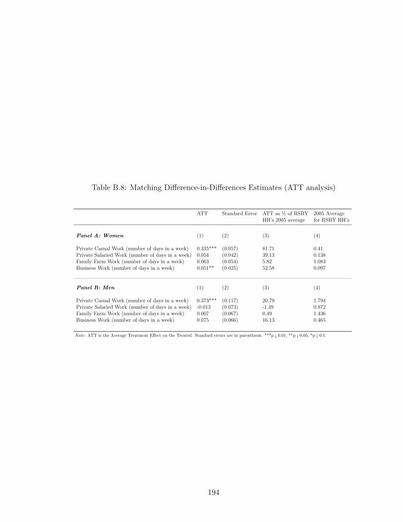
Table B.8: Matching Difference-in-Differences Estimates (ATT analysis)
ATT Standard Error ATT as % of RSBY 2005 AverageHH’s 2005 average for RSBY HH’s
Panel A: Women (1) (2) (3) (4)
Private Casual Work (number of days in a week) 0.335*** (0.057) 81.71 0.41Private Salaried Work (number of days in a week) 0.054 (0.042) 39.13 0.138Family Farm Work (number of days in a week) 0.063 (0.054) 5.82 1.083Business Work (number of days in a week) 0.051** (0.025) 52.58 0.097
Panel B: Men (1) (2) (3) (4)
Private Casual Work (number of days in a week) 0.373*** (0.117) 20.79 1.794Private Salaried Work (number of days in a week) -0.013 (0.073) -1.49 0.872Family Farm Work (number of days in a week) 0.007 (0.067) 0.49 1.436Business Work (number of days in a week) 0.075 (0.066) 16.13 0.465
Note: ATT is the Average Treatment Effect on the Treated. Standard errors are in parenthesis. ***p ¡ 0.01, **p ¡ 0.05, *p ¡ 0.1.
194
Bibliography
John Bongaarts and Christophe Z Guilmoto. How many more missing women?excess female mortality and prenatal sex selection, 1970–2050. Population andDevelopment Review, 41(2):241–269, 2015.
Amartya Sen. Missing women. BMJ: British Medical Journal, 304(6827):587, 1992.
Sonia R Bhalotra and Tom Cochrane. Where have all the young girls gone? identi-fication of sex-selection in india. 2010.
S Anukriti, Sonia R Bhalotra, and Hiu Fung Tam. On the quantity and quality ofgirls: New evidence on abortion, fertility, and parental investments. 2016.
Prabhat Jha, Rajesh Kumar, Priya Vasa, Neeraj Dhingra, Deva Thiruchelvam, andRahim Moineddin. Low male-to-female sex ratio of children born in india: Na-tional survey of 1 million households. The Lancet, 367(9506):211–218, 2006.
Amartya Sen. More than 100 million women are missing. The New York Review ofBooks, 1990.
Monica Das Gupta. Selective discrimination against female children in rural punjab,india. Population and Development Review, pages 77–100, 1987.
Mark R Rosenzweig and T Paul Schultz. Market opportunities, genetic endowments,and intrafamily resource distribution: Child survival in rural india. The AmericanEconomic Review, 72(4):803–815, 1982.
Amartya Sen. Missing women - revisited: Reduction in female mortality has beencounterbalanced by sex-selective abortions. BMJ: British Medical Journal, 327(7427):1297, 2003.
TV Sekher. Rural demography of india. In International Handbook of Rural De-mography, pages 169–189. Springer, 2012.
PN Mari Bhat. On the trail of ‘missing’ indian females: Illusion and reality. Eco-nomic and Political Weekly, pages 5244–5263, 2002.
195

Nancy Qian. Missing women and the price of tea in china: The effect of sex-specificearnings on sex imbalance. The Quarterly Journal of Economics, 123(3):1251–1285, 2008.
Monica Das Gupta, Jiang Zhenghua, Li Bohua, Xie Zhenming, Woojin Chung, andBae Hwa-Ok. Why is son preference so persistent in east and south asia? across-country study of china, india and the republic of korea. The Journal ofDevelopment Studies, 40(2):153–187, 2003.
Seema Jayachandran and Rohini Pande. Why are indian children so short? NationalBureau of Economic Research, 2015.
Geeta Gandhi Kingdon. Does the labour market explain lower female schooling inindia? The Journal of Development Studies, 35(1):39–65, 1998.
Siwan Anderson. Why dowry payments declined with modernization in europe butare rising in india. journal of Political Economy, 111(2):269–310, 2003.
Robert Jensen. Do labor market opportunities affect young women’s work andfamily decisions? experimental evidence from india. The Quarterly Journal ofEconomics, 127(2):753–792, 2012.
Shelley Clark. Son preference and sex composition of children: Evidence from india.Demography, 37(1):95–108, 2000.
Sonia Bhalotra and Arthur Van Soest. Birth-spacing, fertility and neonatal mortalityin india: Dynamics, frailty, and fecundity. Journal of Econometrics, 143(2):274–290, 2008.
Daniel Rosenblum. The effect of fertility decisions on excess female mortality inindia. Journal of Population Economics, 26(1):147–180, 2013.
Marco Alfano. Daughters, dowries, deliveries: The effect of marital payments onfertility choices in india. Journal of Development Economics, 125:89–104, 2017.
Rohini Pande, Anju Malhotra, Sanyukta Mathur, Manisha Mehta, Anju Malhotra,Margaret A Lycette, Sarah Degnan Kambou, Veronica Magar, Jill Gay, HeidiLary, et al. Son preference and daughter neglect in india. 2006.
Luojia Hu and Analia Schlosser. Prenatal sex selection and girls’ well-being: Evi-dence from india. The Economic Journal, 125(587):1227–1261, 2015.
Seema Jayachandran. Fertility decline and missing women. American EconomicJournal: Applied Economics, 9(1):118–139, 2017.
Seema Jayachandran and Ilyana Kuziemko. Why do mother’s breastfeed girls lessthan boys? evidence and implications for child health in india. National Bureauof Economic Research, 2009.
196

Prashant Bharadwaj and Leah K Lakdawala. Discrimination begins in the womb:Evidence of sex-selective prenatal investments. Journal of Human Resources, 48(1):71–113, 2013.
Emily Oster. Hepatitis b and the case of the missing women. Journal of PoliticalEconomy, 113(6):1163–1216, 2005.
Sonia R Bhalotra, Abhishek Chakravarty, and Selim Gulesci. The price of gold:Dowry and death in india. 2016.
Paul Gertler. Final report: The impact of progresa on health. International FoodPolicy Research Institute, Washington, DC, page 2000, 2000.
John Maluccio and Rafael Flores. Impact Evaluation of a Conditional Cash TransferProgram: The Nicaraguan Red de Proteccion Social. International Food PolicyResearch Institute, Washington, DC, 2005.
Daniel Gilligan and Anna Fruttero. The impact of bolsa familia on education andhealth outcomes in brazil. In Second Generation of CCTs Evaluations Conference.Washington, DC: World Bank, 2011.
Alan De Brauw, Amber Peterman, et al. Can conditional cash transfers improvematernal health and birth outcomes?: Evidence from el salvador’s comunidadessolidarias rurales. International Food Policy Research Institute (IFPRI), 2011.
Seema Jayachandran and Adriana Lleras-Muney. Life expectancy and human capitalinvestments: Evidence from maternal mortality declines. The Quarterly Journalof Economics, 124(1):349–397, 2009.
Lori Beaman, Esther Duflo, Rohini Pande, and Petia Topalova. Female leadershipraises aspirations and educational attainment for girls: A policy experiment inindia. Science, 335(6068):582–586, 2012.
Gaurav Khanna. Incentivizing standards or standardizing incentives? affirmativeaction in india. 2016.
Mukesh Eswaran. The empowerment of women, fertility, and child mortality: To-wards a theoretical analysis. Journal of Population Economics, 15(3):433–454,2002.
Ashish Garg and Jonathan Morduch. Sibling rivalry and the gender gap: Evidencefrom child health outcomes in ghana. Journal of Population Economics, 11(4):471–493, 1998.
Alessandro Cigno. Fertility decisions when infant survival is endogenous. Journalof Population Economics, 11(1):21–28, 1998.
David E Sopher. An Exploration of India: Geographical Perspectives on Society andCulture. Longman London, 1980.
197
Barbara D Miller. The endangered sex: Neglect of female children in rural northindia. 1981.
Tim Dyson and Mick Moore. On kinship structure, female autonomy, and demo-graphic behavior in india. Population and Development Review, pages 35–60,1983.
Satish B Agnihotri. Survival of the girl child: Tunnelling out of the chakravyuha.Economic and Political Weekly, pages 4351–4360, 2003.
Sharada Srinivasan and Arjun Singh Bedi. Daughter elimination in tamil nadu,india: A tale of two ratios. The Journal of Development Studies, 44(7):961–990,2008.
Esther Duflo. Grandmothers and granddaughters: Old-age pensions and intrahouse-hold allocation in south africa. The World Bank Economic Review, 17(1):1–25,2003.
Anne Case. Does money protect health status? evidence from south african pen-sions. In Perspectives on the Economics of Aging, pages 287–312. University ofChicago Press, 2004.
Christina Paxson and Norbert Schady. Cognitive development among young chil-dren in ecuador: The roles of wealth, health, and parenting. Journal of HumanResources, 42(1):49–84, 2007.
Paul Gertler. Do conditional cash transfers improve child health? evidence fromprogresa’s control randomized experiment. The American Economic Review, 94(2):336–341, 2004.
Juan A Rivera, Daniela Sotres-Alvarez, Jean-Pierre Habicht, Teresa Shamah, andSalvador Villalpando. Impact of the mexican program for education, health, andnutrition (progresa) on rates of growth and anemia in infants and young children:A randomized effectiveness study. Jama, 291(21):2563–2570, 2004.
Eliana Carranza. Soil endowments, female labor force participation, and the de-mographic deficit of women in india. American Economic Journal: Applied Eco-nomics, 6(4):197–225, 2014.
Lupin Rahman and Vijayendra Rao. The determinants of gender equity in india:Examining dyson and moore’s thesis with new data. Population and DevelopmentReview, 30(2):239–268, 2004.
Sanjukta Chaudhuri. The desire for sons and excess fertility: A household-levelanalysis of parity progression in india. International Perspectives on Sexual andReproductive Health, pages 178–186, 2012.
V Bhaskar and Bishnupriya Gupta. India’s missing girls: Biology, customs, andeconomic development. Oxford Review of Economic Policy, 23(2):221–238, 2007.
198
SSIR Sudha and S Irudaya Rajan. Female demographic disadvantage in india 1981–1991: Sex-selective abortions and female infanticide. Development and Change,30(3):585–618, 1999.
Arindam Nandi and Anil B Deolalikar. Does a legal ban on sex-selective abortionsimprove child sex ratios? evidence from a policy change in india. Journal ofDevelopment Economics, 103:216–228, 2013.
S Anukriti. The fertility-sex ratio trade-off: Unintended consequences of financialincentives. 2014.
Yaniv Stopnitzky. The bargaining power of missing women: Evidence from a sani-tation campaign in india. Available at SSRN 2031273, 2012.
Kaivan Munshi and Mark Rosenzweig. Why is mobility in india so low? socialinsurance, inequality, and growth. National Bureau of Economic Research, 2009.
A Colin Cameron, Jonah B Gelbach, and Douglas L Miller. Bootstrap-based im-provements for inference with clustered errors. The Review of Economics andStatistics, 90(3):414–427, 2008.
Nistha Sinha and Joanne Yoong. Long-term financial incentives and investment indaughters: Evidence from conditional cash transfers in north india. World BankPolicy Research Working Paper Series, Vol, 2009.
Leela Visaria. Female deficit in india: Role of prevention of sex-selective abortionact. In CEPED-CICREDINED Seminar on Female Deficit in Asia: Trends andPerspectives, Singapore, pages 5–7. Citeseer, 2005.
Jishnu Das, Quy-Toan Do, and Berk Ozler. Reassessing conditional cash transferprograms. The World Bank Research Observer, 20(1):57–80, 2005.
World Health Organization. Effect of breastfeeding on infant and child mortalitydue to infectious diseases in less developed countries: A pooled analysis whocollaborative study team on the role of breastfeeding on the prevention of infantmortality. Lancet, 355(9202):451–455, 2000.
Seema Jayachandran and Ilyana Kuziemko. Why do mothers breastfeed girls lessthan boys? evidence and implications for child health in india. The QuarterlyJournal of Economics, 126(3):1485–1538, 2011.
Carlos Bozzoli, Angus Deaton, and Climent Quintana-Domeque. Adult height andchildhood disease. Demography, 46(4):647–669, 2009.
Duncan Thomas and John Strauss. Health and wages: Evidence on men and womenin urban brazil. Journal of Econometrics, 77(1):159–185, 1997.
T Paul Schultz and John Strauss. Handbook of Development Economics, volume 4.Elsevier, 2008.
199

Hans Th Waaler. Height, weight and mortality: The norwegian experience. Journalof Internal Medicine, 215(S679):1–56, 1984.
Robert William Fogel. The Escape from Hunger and Premature Death, 1700-2100:Europe, America, and the Third World, volume 38. Cambridge University Press,2004.
John Strauss and Duncan Thomas. Health over the life course. Handbook of Devel-opment Economics, 4:3375–3474, 2007.
Janet Currie and Brigitte C. Madrian. Chapter 50 Health, health insurance and thelabor market. Handbook of Labor Economics, 3 PART(3):3309–3416, 1999. ISSN15734463. doi: 10.1016/S1573-4463(99)30041-9.
Mehtabul Azam. Does Social Health Insurance Reduce FinancialBurden? Panel Data Evidence from India. Panel Data Evidence fromIndia (May 3, 2016), 2016. URL http://papers.ssrn.com/sol3/papers.cfm?
abstract_id=2774452.
Douglas Johnson and Karuna Krishnaswamy. The Impact of RSBY on HospitalUtilization and Out-of-Pocket Health Expenditure. pages 1–33, 2012.
Arindam Nandi, Ashvin Ashok, and Ramanan Laxminarayan. The socioeconomicand institutional determinants of participation in india’s health insurance schemefor the poor. PloS One, 8(6):e66296, 2013a.
Changqing Sun. An analysis of rsby enrolment patterns: Preliminary evidence andlessons from the early experience. India’s Health Insurance Scheme for the Poor:Evidence From the Early Experience of the Rashtriya Swasthya Bima Yojana. NewDelhi: Centre for Policy Research, 2011.
D Rajasekhar, Erlend Berg, Maitreesh Ghatak, R Manjula, and Sanchari Roy. Im-plementing health insurance: The rollout of rashtriya swasthya bima yojana inkarnataka. Economic and Political Weekly, 46(20):56–63, 2011a.
Alejandro del Valle. From caring to work: The labor market effects of noncontrib-utory health insurance. University of California, Berkeley Mimeo, 2014.
Adam Wagstaff and Wanwiphang Manachotphong. Universal health care and infor-mal labor markets: The case of thailand. World Bank Policy Research WorkingPaper, (6116), 2012.
Anup Karan, Winnie Yip, and Ajay Mahal. Extending health insurance to the poorin India: An impact evaluation of Rashtriya Swasthya Bima Yojana on out ofpocket spending for healthcare. Social Science and Medicine, 181:83–92, 2017.ISSN 18735347. doi: 10.1016/j.socscimed.2017.03.053. URL http://dx.doi.
org/10.1016/j.socscimed.2017.03.053.
200
P Rathi, A Mukherji, and G Sen. Rashtriya Swasthya Bima Yojana: Eval-uating utilisation, roll-out and perceptions in Amaravati district, Maha-rashtra. Economic and Political Weekly, xlvii(39):57–64, 2012. ISSN00129976. URL http://www.indiaenvironmentportal.org.in/files/file/
RashtriyaSwasthyaBimaYojana.pdf.
N Devadasan, Tanya Seshadri, Mayur Trivedi, and Bart Criel. Promoting universalfinancial protection: evidence from the Rashtriya Swasthya Bima Yojana (RSBY)in Gujarat, India. Health Research Policy and Systems, 11(1):29, 2013. ISSN 1478-4505. doi: 10.1186/1478-4505-11-29. URL http://europepmc.org/articles/
PMC3751687.
Arindam Nandi, Ashvin Ashok, and Ramanan Laxminarayan. The Socioeco-nomic and Institutional Determinants of Participation in India’s Health Insur-ance Scheme for the Poor. PLoS ONE, 8(6), 2013b. ISSN 19326203. doi:10.1371/journal.pone.0066296.
Soumitra Ghosh and Nabanita Datta Gupta. Targeting and effects of rashtriyaswasthya bima yojana on access to care and financial protection. Econ PolitWkly, 52:61–70, 2017.
Adriana Camacho, Emily Conover, and Alejandro Hoyos. Effects of Colombia ’s Social Protection System on Workers ’ Choice between Formal and InformalEmployment. (August):446–466, 2013. doi: 10.1093/wber/lht028.
Achyuta R Adhvaryu and Anant Nyshadham. Schooling, Child Labor, and theReturns to Healthcare in Tanzania. Journal of Human Resources, 47(2):364–396,2012. ISSN 0022-166X. doi: 10.1353/jhr.2012.0009.
Mark R Rosenzweig and Kenneth Wolpin. Credit Market Constraints , ConsumptionSmoothing , and the Accumulation of Durable Production Assets in Low-IncomeCountries : Investments in Bullocks in India Author ( s ): Mark R . Rosenzweigand Kenneth I . Wolpin Source : Journal of Political Economy. 101(2):223–244,2017.
N S Jodha. Effectiveness of farmers’ adjustments to risk. Economic and PoliticalWeekly, XIII(25):38–48, 1978.
Ke Xu, David B. Evans, Guido Carrin, Ana Mylena Aguilar-Rivera, Philip Mus-grove, and Timothy Evans. Protecting households from catastrophic health spend-ing. Health Affairs, 26(4):972–983, 2007. ISSN 02782715. doi: 10.1377/hlthaff.26.4.972.
D Rajasekhar, Erlend Berg, Maitreesh Ghatak, R Manjula, and Sanchari Roy. Im-plementing Health Insurance : The Rollout of Rashtriya Swasthya Bima Yojana inKarnataka. Economic & Political Weekly, xlvi(20):56–63, 2011b. ISSN 00129976.
201
Stefan Dercon. Assessing vulnerability Assessing vulnerability. (August):80, 2001a.doi: http://info.worldbank.org/etools/docs/library/70436/4th%20Workshop/Srmafrica/helsinki/pdf/readingmaterial/Assessing%20Vulnerability.pdf. URLhttp://citeseerx.ist.psu.edu/viewdoc/download?doi=10.1.1.196.
3266&rep=rep1&type=pdf.
Jonathan Haughton and Shahidur R. Khandker. Vulnerability to Poverty. Hand-book on Poverty and Inequality, pages 231–248, 2009. doi: http://dx.doi.org/10.1596/978-0-8213-7613-3. URL http://ideas.repec.org/p/oxf/wpaper/
wps-2007-03.html.
Anirudh Krishna. Escaping poverty and becoming poor: Who gains, who loses, andwhy? World Development, 32(1):121–136, 2004. ISSN 0305750X. doi: 10.1016/j.worlddev.2003.08.002.
Renu Shahrawat and Krishna D. Rao. Insured yet vulnerable: Out-of-pocket pay-ments and India’s poor. Health Policy and Planning, 27(3):213–221, 2012. ISSN02681080. doi: 10.1093/heapol/czr029.
Victoria Fan, Anup Karan, and Ajay Mahal. State Health Insurance and Out-of-Pocket Health Expenditures in Andhra Pradesh, India. (June 2012), 2012.
Arnab Acharya, Sukumar Vellakkal, Fiona Taylor, Edoardo Masset, Ambika Satija,Margaret Burke, and Shah Ebrahim. Impact of national health insurance for thepoor and the informal sector in low- and middle-income countries: a systematicreview. Number July. 2012. ISBN 978-1-907345-34-0.
Aradhna Aggarwal. Impact evaluation of India’s Yeshasvini community-basedhealth insurance programme. Health Economics, 19(SUPPL. 1):5–35, 2010. ISSN10579230. doi: 10.1002/hec.1605.
Wameq A Raza, Ellen Poel, Arjun Bedi, and Frans Rutten. Impact of community-based health insurance on access and financial protection: Evidence from threerandomized control trials in rural india. Health economics, 25(6):675–687, 2016.
Adam Wagstaff, Magnus Lindelow, Gao Jun, Xu Ling, and Qian Juncheng. Extend-ing health insurance to the rural population: An impact evaluation of China’s newcooperative medical scheme. Journal of Health Economics, 28(1):1–19, 2009. ISSN01676296. doi: 10.1016/j.jhealeco.2008.10.007.
Helen Levy and David Meltzer. The impact of health insurance on health. Annu.Rev. Public Health, 29:399–409, 2008. ISSN 0163-7525. doi: 10.1146/annurev.publhealth.28.021406.144042.
Changqing Sun. An analysis of RSBY enrolment patterns: Preliminary evidenceand lessons from the early experience. RSBY Working paper, (October):1–20,2010. URL http://www.rsby.gov.in/Documents.aspx?ID=14.
202
N Devadasan, Kent Ranson, Wim Van Damme, and Bart Criel. Com-munity Health Insurance in India. Economic and Political Weekly,39(28):3179–3183, 2004. URL http://www.epw.in/special-articles/
community-health-insurance-india.html.
Shamika Ravi. Are Publicly Financed Health Insurance Schemes Working in India? pages 157–191, 2012.
Gaurav Datt and Martin Ravallion. Transfer benefits from public-works employ-ment: Evidence for rural India. The Economic Journal, 104(427):1346–1369,1994. ISSN 00130133. doi: 10.2307/2235452. URL http://www.jstor.org/
stable/10.2307/2235452.
Richard Blundell and Monica Costa Dias. Alternative approaches to evaluation inempirical microeconomics. Journal of Human Resources, 44(3):565–640, 2009.
Wil Dow, Paul Gerler, Robert F. Schoeni, John Strauss, and Duncan Thomas.Health care prices, health and labor outcomes- Experimental evidence, 1997.
Katherine Baicker, Amy Finkelstein, Jae Song, and Sarah Taubman. The Impact ofMedicaid on Labor Force Activity and Program Participation: Evidence from theOregon Health Insurance Experiment. American Economic Review P&P, 104(5):322–328, 2014. ISSN 00028282. doi: 10.3386/w19547. URL http://www.nber.
org/papers/w19547.pdf.
Robert Jensen. Agricultural volatility and investments in children. American Eco-nomic Review, pages 399–404, 2000.
Harold Alderman, Hans Hoogeveen, and Mariacristina Rossi. Preschool nutritionand subsequent schooling attainment: Longitudinal evidence from Tanzania. Eco-nomic Development and Cultural Change, 57(2):239–260, 2009.
Harold Alderman, John Hoddinott, and Bill Kinsey. Long term consequences ofearly childhood malnutrition. Oxford economic papers, 58(3):450–474, 2006.
Sharon Maccini and Dean Yang. Under the weather: Health, schooling, and eco-nomic consequences of early-life rainfall. The American Economic Review, pages1006–1026, 2009.
Kalanidhi Subbarao, Carlo del Ninno, Colin Andrews, and Claudia Rodrıguez-Alas.Public works as a safety net: Design, evidence, and implementation. World BankPublications, 2012.
Laura Zimmermann. Public works programs in developing countries have the po-tential to reduce poverty. IZA World of Labor, 2014.
Erlend Berg, Sambit Bhattacharyya, Rajasekhar Durgam, and Manjula Ramachan-dra. Can rural public works affect agricultural wages? Evidence from India.Centre for the Study of African Economies, Oxford University. Working Paper
203

WPS/2012-05. http://www. csae. ox. ac. uk/workingpapers/pdfs/csae-wps-2012-05. pdf, 2012.
Mehtabul Azam. The impact of Indian Job Guarantee Scheme on labor marketoutcomes: Evidence from a natural experiment. 2012.
Clement Imbert, John Papp, et al. Equilibrium Distributional Impacts of Gov-ernment Employment Programs: Evidence from India’s Employment Guarantee.2012.
Aparajita Dasgupta et al. Can the major public works policy buffer negative shocks?Young Lives Working Paper, 112, 2013.
Subha Mani, Jere R Behrman, Shaikh Galab, and Prudhvikar Reddy. Impact of theNREGS on Schooling and Intellectual Human Capital. 2014.
Robert M Townsend. Consumption Insurance: An evaluation of risk-bearing systemsin low-income economies. The Journal of Economic Perspectives, pages 83–102,1995.
Ahmed Mushfiq Mobarak and Mark R Rosenzweig. Informal risk sharing, index in-surance, and risk taking in developing countries. The American Economic Review,103(3):375–380, 2013.
Francisco HG Ferreira and Norbert Schady. Aggregate economic shocks, child school-ing, and child health. The World Bank Research Observer, 24(2):147–181, 2009.
Shamika Ravi and Monika Engler. Workfare in Low Income Countries: An EffectiveWay to Fight poverty? The Case of NREGS in India. Indian School of Businessworking paper. Hyderabad: Indian School of Business, 2009.
Thomas S Walker and James G Ryan. Village and household economics in India’ssemi-arid tropics. Johns Hopkins University Press, 1990.
Stefan Dercon. Assessing vulnerability. Publication of the Jesus College and CSAE,Department of Economics, Oxford University, 2001b.
Mark R Rosenzweig and Kenneth I Wolpin. Credit market constraints, consump-tion smoothing, and the accumulation of durable production assets in low-incomecountries: Investments in bullocks in india. Journal of Political Economy, pages223–244, 1993.
Jonathan Morduch. Poverty and vulnerability. The American Economic Review, 84(2):221–225, 1994.
Stefan Dercon. Risk, poverty and vulnerability in africa. Journal of AfricanEconomies, 14(4):483–488, 2005.
Andrew D Foster. Prices, credit markets and child growth in low-income rural areas.The Economic Journal, pages 551–570, 1995.
204

Christina Paxson and Norbert Schady. Child health and economic crisis in Peru.The World Bank Economic Review, 19(2):203–223, 2005.
Takashi Yamano, Harold Alderman, and Luc Christiaensen. Child growth, shocks,and food aid in rural Ethiopia. American Journal of Agricultural Economics, 87(2):273–288, 2005.
Agnes R Quisumbing. Food aid and child nutrition in rural Ethiopia. World Devel-opment, 31(7):1309–1324, 2003.
Martin Ravallion. Reaching the rural poor through public employment: arguments,evidence, and lessons from South Asia. The World Bank Research Observer, 6(2):153–175, 1991.
Harold Alderman. Safety nets can help address the risks to nutrition from increasingclimate variability. the Journal of Nutrition, 140(1):148S–152S, 2010.
Abusaleh Shariff. Assessment of National Rural Employment Guarantee Scheme ofIndia. Indian Journal of Labour Economics, 52(2):243–68, 2009.
Vinayak Uppal. Is the NREGS a Safety Net for Children? University of Oxford.http://knowledge. nrega. net/859/1/Is the NREGS a Safety Net for Children.pdf, 2009.
Raghbendra Jha, Sambit Bhattacharyya, Raghav Gaiha, and Shylashri Shankar.Capture of anti-poverty programs: An analysis of the National Rural EmploymentGuarantee Program in India. Journal of Asian Economics, 20(4):456–464, 2009.
Bethelhem L Debela, Gerald Shively, and Stein T Holden. Does Ethiopias Produc-tive Safety Net Program Improve Child Nutrition? 2014.
Seema Jayachandran. Selling labor low: Wage responses to productivity shocks indeveloping countries. Journal of political Economy, 114(3):538–575, 2006.
Ingo Outes-Leon and Stefan Dercon. Survey attrition and attrition bias in YoungLives. Young Lives Technical Note, 5, 2008.
Manuel Arellano and Stephen Bond. Some tests of specification for panel data:Monte Carlo evidence and an application to employment equations. The reviewof economic studies, 58(2):277–297, 1991.
Emmanuel Skoufias. Economic crises and natural disasters: Coping strategies andpolicy implications. World Development, 31(7):1087–1102, 2003.
Michael A Clemens and Gabriel Demombynes. When does rigorous impact evalua-tion make a difference? The case of the Millennium Villages. 2010.
205

James C Hanson, Kenneth L Leonard, and Timothy Essam. Listening while eval-uating: Examining the benefit of an NGO programme using season extenders(greenhouses) in Bosnia–Herzegovina. Journal of Development Effectiveness, 5(1):116–136, 2013.
Puja Dutta, Rinku Murgai, Martin Ravallion, and Dominique Van de Walle. DoesIndia’s employment guarantee scheme guarantee employment? World Bank PolicyResearch Working Paper, (6003), 2012.
Nina Buchmann, Erica Field, Rachel Glennerster, Shahana Nazneen, Svetlana Pimk-ina, and Iman Sen. Power vs money: Alternative approaches to reducing childmarriage in bangladesh: A randomized control trial. 2017.
206