SLAC-PUB-415 my 1968

PION PHOTOPRODUCTION AND FIXED-t-DISPERSION

RELATIONS

J. Engels

Institut fiir Theoretische Kernphysik der Univer sit at, Karlsruhe

A. Miillensiefen

Institut fiir Struktur der Materie der Universitat, Karlsruhe

W. Schmidt?

Stanford Linear Accelerator Center Stanford University, Stanford, California

ABSTRACT

We review the dispersion theoretic models of the isobar approximation

which predict single pion photoproduction in the region of the A(lZ36)-resonance.

The differences between the various models are explained and their conse-

quences discussed. Considerable efforts are made to look for further improve-

ments of the theory from the confrontation of theory and experiment. Antici-

pating the development of experimental techniques we discuss finally an example

for a more complete photoproduction experiment. Specifically, we study the

useful’ness of a To-photoproduction experiment with polarized y’s and/or polar-

ized target for the region of the A(1236) resonance.

Supported in part by the U.S. Atomic Energy Commission.

t On leave from Institut fur Experimentelle Kernphysik, Kernforschungszentrum, Karlsruhe, Germany.

(Submitted to Phys. Rev.)

-l-

INTRODUCTION

In this paper we continue our analysis of single pion photoproduction in the

region of the A(1236)-resonance by means of fixed-t-dispersion relations. The

main idea of a previous paper’ was to establish in the whole region of the first

pion nucleon resonance A(1236) the ansatz of Ball2 as a zero order approxima-

tion for the total amplitudes. 3/2 Ball retained only the large MI+ -contribution of

A(1236) in the dispersion integral. To get then an absolute prediction for the

angular distributions, 3/2 it was necessary to know the resonant multipole Ml+

taken in Refs. 1 and 2 from the work of Chew, et al. 3 Also the pion nucleon --

scattering phase shifts were needed in order to apply the Watson theorem for

the calculation of the imaginary parts of the amplitudes. Because of the domi-

nance of the A(1236) resonance, this isobar-approximation works surprisingly

well even at higher energies if it is applied there to the slowly varying real back-

ground amplitude. 495

Since the publication of Ref. 1 - four years ago - the same subject has

been treated by several authors again using fixed-t-dispersion relations and

again exploiting some type of isobar approximation. These new efforts have

had three general objectives:

1. to improve the theory of the A(1236) resonance in photoproduction, 312 6,7,8,9, lOa, 11,12,13 especially the prediction of the small El+

2. to retain also some of the smaller s,p imaginary parts under the

dispersion integral lOa, 13 ; and

3. to compare systematically the theoretical predictions with the

experimental data available, in order to look for deficiencies of

the theory. 14,15,16,17

-2-

The achievement of this work was a refinement of the calculations, partially

through the more involved use of computers. New ideas, which would supple-

ment the isobar approximation essentially, were not presented. For example,

in the present formulation of the isobar approximation the question of high energy

contributions arising from the dispersion integrals is completely unsettled. This

question deserves particular attention, if more refined calculations of partial

amplitudes are started (see, e.g., Ref. 12).

In this paper we consider in Section I some typical isobar approximations

for the evaluation of the lowest partial amplitudes. We then turn in Section II

to a comparison with the experiments, where we concentrate on situations,

which are particularly sensitive to the present approximations. Lastly we dis-

cuss in SectionIIIpossible new experiments in the region of the A(1236) resonance,

which should prove useful for the further development of the theory.

A word to motivate our method of confronting theory and experiment may be

useful. There are at least two ways to discuss the error in the experimental

prediction - implied by the uncertainty of the theory. One can include all known --

systematic errors in order to obtain the total error of the experimental

prediction. The result is represented by an error band. The uncer-

tainty of the theory is thus demonstrated in a very obvious way (see, e.g.,

lOa). Also one can calculate the effect of each known systematic error in order

to identify its particular contribution in the error band of the first method. In

this way - which we prefer - one can try to resolve a discrepancy in terms of

the main errors of the theory. One can then check if a possible explanation is

consistent with all available information. This check is not possible with the

first method. One may then overestimate the agreement between theory and

experiment. The danger of the second method lies in underestimating the

-3-

agreement. Hut it seems to be the only systematic way to analyze the experi-

mental data. 15 One can learn from a recent note lob that both methods may

lead to quite different conclusions.

Finally we mention that we use in the formulae units such that R = c = mn

= 1. Amplitudes are usually given in units 10 -2 % = 10-2B/ml,c’ so that, e.g.,

Im Mi{2 is of the order 1 around the resonance. Cross sections, etc., are

given in units pb/ster.

I. EVALUATION OF PARTIAL AMPLITUDE DISPERSION RELATIONS

IN PION-PHOTOPRODUCTION

A. Dispersion Relations

At present partial amplitude dispersion relations are the best tool in ana-

lysing pion photoproduction in the region of the first pion nucleon resonance,

since they allow us to incorporate most efficiently our phenomenological lmow-

ledge about

tion for the

the pion nucleon final state. Consider therefore a dispersion rela-

parity conserving helicity amplitudes HX J* WI

Re HF’I(W) = HE&(W) + i P Im HJfyl(W’)

dW’ wf’- w

A = l/2,3/2

(I. la)

I 3 The relation of these amplitudes to the conventional multipoles E:* , Mfi

is given in the appendix. From fixed-t-dispersion relations2 one obtains an

-4-

explicit result for the inhomogeneous term H J&I A,inhm l

20

00

J&,1 Hh,inh(W) = p.t.c. +; /

dW’ Ii-n HrS1(W1)

W’ + w “M-t1

(I. lb)

In this equation p,t.c. denotes the well-known pole term contribution. 20

(32, J’IP(W, W’) are known kinematical functions which represent the coupling of

the different partial amplitudes following from fixed-t-dispersion relations. The

sum in (I. lb) - infinite in principle - has been truncated at J’ = 3/2, so that the

system I. 1 is finite. It is expected to be valid in the region of the first resonance,

where the convergence of the series in (I. lb) is guaranteed, if the Mandelstam

representation is valid. 2

The largest contributions to the integrals in (I. 1) arise from the imaginary

3/2 - parts of the first resonance, i.e., Im Hh , A = l/2, 3/2. Therefore the eval-

uation of (I. 1) has always been based on some type of isobar approximation, of

which we consider three examples in the following. In this discussion we do not

treat the partial amplitudes of the first resonance, since they deserve more

sophisticated techniques. We shall rely on the work in Ref. 12 for the theory of

the first resonance.

B. Pure Isobar Approximation

3/2- We shall understand as “pure isobar approximations” if only Im Hh is

retained in the integrands of the set (I. 1). One then obtains from (I. 1) for

J,I # 3/2, P # +l

Re H?(W) x HEinh(W) * (1.2)

-5 -

In this approximation the remaining integrals in (I. lb) can be very well

evaluated by the narrow width approximation yielding the convenient expressions

312 33 JLZ Yj

HE&(W) =p.t.c. + c gh, Ghh’ tTW, WR) A’=112

(I. 3a)

where WR is the resonance energy and g A’

are the coupling constants of the first

resonance defined by

dW’ Im Hf{2-(W’) (gl,2 x 1.6 g3/2 w -6.4 m =mrO) 7r (1.3b)

The approximation (I. 3) for (I. lb) has been treated in Ref. 18 and has been shown

to be of reasonable accuracy for practical applications. Under the further sim-

3/2- plifying assumption that in Im Hh the Im Et{” -contribution can be neglected

(see (A. 1))) the partial amplitudes have been discussed in Part I. The dif-

3/2 ferences arising from the inclusion of Im El+ are only markable for the J= l/2 n+ ti multipoles Re Eo+ , Re Ml . Results for the real parts of the J = l/2, 3/2

multipoles are shown in Fig. 1.

From the Watson theorem

Im H?(W) = tg sJ*(W) Re H:(W) (I*3

with Re H?(W) taken from (1.3) and the pion nucleon scattering phase shift 6 J*

taken from e,xperiment 19 - one finds values for the imaginary parts Im H:(W)

in the region of the first resonance, which are negligibly small except for the

l/2,3/2 s-waves Im EO+ 3/2 , which are always of the order of l/10 0 Im Ml+ (WR)~

Therefore the inclusion of this imaginary part in the integrals of (I. 1) is a

presently possible and perceivable improvement of the pure isobar approximation. 13

-6-

C . Isobar Approximation 3/2- In the “isobar approximation” apart from Im Hh (W) , the s-wave multi-

1/2- pole Im Hli2 1/2- . is also retained in the integrands of the set (I. 1). Im Hl,2 is

l/2- taken from (1.4) with Re Hl,2 taken in the narrow width approximation (I. 3) Q

The multipoles in this approximation (Fig. 1) differ markably only for

l/2, 3/2 Re E6+ , because of contributions arising mainly from the principal value

integrals in (I. 1). But the relative changes are noticeable only in x0-photo-

production, because of a very sensitive cancellation of certain I = l/2 and 3/2

contributions. In no production, the new contributions reduce the modul of 7i-o

Re E6+ further if compared to the results of the pure isobar approximation. n-Q

This reduction is very critical, since the result for Re E6+ is of the order or

possibly smaller than unknown high energy contributions so that the present

results for Re ET: are very ambiguous.

The neglection of the imaginary parts at high energies is one of the most

serious sources for systematical errors. To estimate the uncertainty arising

from this ignorance, we considered the following contribution to the rescattering

terms

me HF’I(W) = i p /

ca dW’ ImHF’I(W’)

wC

where WC is an energy between the first and second resonance, above which

IIIl HP” is either unknown or at least uncertain. An upper limit for the modul

of (I. 5) follows from

with co

S;TfJ(w, =;

/ I

1 dw’ wt -W’GAA JIa n(rw,Tw’) .

wC

(I. Sa)

(I. 6b)

-7-

w is a suitable mean value parameter from the interval WC I w 5 00. The cor-

responding result for the multipoles MI&, can be written

(1.7)

The functions T;(W) are shown in Table I, with WC = 10.15 corresponding to a

photon energy EC = 600 MeV. The integrands in (I. 6b) decrease very rapidly

with increasing energy W’. From the unitarity of the Compton scattering one

concludes that

const W-+co: M&V)- w (1.8)

Therefore one expects that the main contribution to the integrals (I. 5) comes

from values W’ around WC, i. e., from the low energy part of the integration

interval., At these energies one can assume that the order 1 is a safe upper

limit for all Im M&(W) , which in fact should be reached only by the J = l/2 I

multipoles Re EO+, Re Ml o The results in Table I for T:*(W) indicate there-

fore that by neglecting the high energy contributions (I. 5), appreciable errors

can only appear in the J = l/2 multipoles. On the other hand, it has been

shown in Ref. 18 that the coupling of the other partial amplitudes to the J = l/2

multipoles is negligibly small apart from the first resonance, the effect of

which can be calculated rather reliably. So one possibility to overcome the

present difficulties in the calculation of the J = l/2 multipoles would be sub-

tractions, if the subtraction constants would be known from other sources,

which in principle could be low energy theorems but in practice presumably

no 21 7ro only multipole analyses of experimental data( E& , Ml- , see Section II).

Otherwise one can try to solve the present discrepancies between theory and

experiment by a suitable choice of the subtraction constants,

-8-

D. Isobar Approximation in Subtracted Dispersion Relations

Consider the subtracted dispersion relations following from (I. la)

Re H?“(W) = Re HF”(WO) + H$ih(W) - Hc;ih(Wo) w - W()) wC Im HJ*’ ‘(WI) + P T J dw’ (W’-i&w’-W,) ’

M+l

where W. is the subtraction energy and WC a cutoff energy (WC = 10.15,

AEC = 600 MeV).

We shall call isobar approximation of (I. 9) if

1. in the calculation of the difference

NJ% 1 A,iti(W) = H?&(W) - Hc&(WO) ’

(I*91

(I. 10)

according to (I. lb) only the pole term contribution and the

contribution of the first resonance is retained; and

2. in the principal value integrals of (I. 9) Im Hi* is taken

from the isobar approximation Section I. B.

The omission of all imaginary parts except those of the first resonance in

(I. 10) causes a negligible error. Their contribution - already quite small in

(I. lb) - partly cancels in the difference because of its slow energy dependence.

To check this we write (I. 10) for the multipoles Ml* in the form

A&, hh(W) = c $I { dW’ Im Mi:*(W’) r(Mi*, Mi:*, Wo; W, W’) . P*, I’ M+l (I. 11)

As a bound for (I. 11)’ one obtains

-9-

with

R (d&s i$:*, wo; w) = ii dw’ lr(ML, Mi”*, Wo; w,wl>i . (I, 12b)

i

To avoid the threshold singularity (q’)-f in r at W’ = (M+l) we started the inte-

gration somewhat above threshold at Wi = 8.0 (Ei = 200 MeV). Since the con-

tribution from the interval M + 15 W’ _< 3.0 is small, (I. 12) is still a realistic

bound for (I. 11). In (I. 11) this threshold singularity is compensated by the

threshold factor (q’) 2!2+1 of Im M 1*:’ In the sum (I. 12a) the contribution of Im 4* is excluded. It is discussed

together with the neglected rescattering term in (1.9), but will be taken into

account only for W’ 2 WC. This contribution is written in the form 03

/, dW’ Im d&(W’) ?(ML, Wo; W,W’)

C

with the bound

where

+$&Y wo’ w) = ;& dW’ Iy(ML, Wo; W,w’)~ 0 C

(I. 13)

(I. 14a)

(I. 14b)

The results in Table 2 for R indicate that the largest contributions to (I. 12)

come from the imaginary parts of the first resonance, which are supposedly

taken into account in (I. 10) or (I. 11). All other imaginary parts yield contri-

butions, which, to the accuracy presently required, are negligibly small.

Either the kinematical coupling factors R are too small or the imaginary parts

l/2’ 0 themselves Im El+ t ) D From the results in Table 3 for % follows the impor-

tant fact that even for J = l/2 the rescattering terms (I. 13) now can be neglected.

From this analysis we conclude that the present limits on handling the

system (I. 1) are very clearly manifested in the form of the subtracted dispersion

- 10 -

relations (I. 9). Our ignorance can thus be related to the uncertainty in calcu-

lating the subtraction constants Re HF(WO) in the low energy region. For

J = l/2 especially, these constants are largely determined by unknown high-

energy contributions.

Finally, we should like to mention that the successful use of subtracted

dispersion relations depends on the right choice of the kinematical factor,

which is separated from the physical amplitudes H J&,1 A (W) in (A.3). In that

equation, the threshold factor (qk)’ is separated. This choice is motivated

from the results in Ref. 20, where it is shown that the kernels GUI of (I. lb)

are slowly varying functions only after separation of the threshold factor (qk)‘.

The difference (I. 10) will therefore be small as long as W, W. belong to the

region of the threshold and the A(1236) resonance.

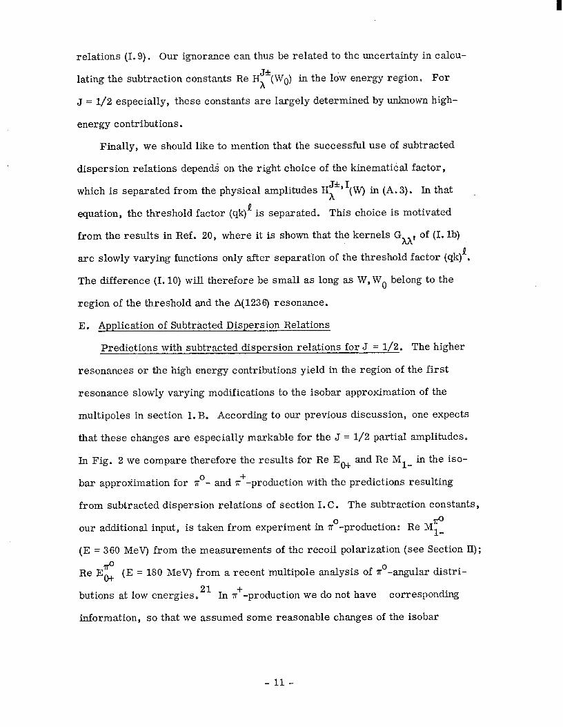
E. Application of Subtracted Dispersion Relations

Predictions with subtracted dispersion relations for J = l/2. The higher

resonances or the high energy contributions yield in the region of the first

resonance slowly varying modifications to the isobar approximation of the

multipoles in section I. B, According to our previous discussion, one expects

that these changes are especially markable for the J = l/2 partial amplitudes.

In Fig. 2 we compare therefore the results for Re Eo+ and Re Ml- in the iso-

bar approximation for r”- and ?r+-production with the predictions resulting

from subtracted dispersion relations of section I. C. The subtraction constants,

our additional input, is taken from experiment in a’-production: 7i-o

Re Ml

(E = 360 MeV) from the measurements of the recoil polarization (see Section II);

Re Ez (E = 180 MeV) from a recent multipole analysis of no-angular distri-

butions at low energies. 21 In *‘-production we do not have corresponding

information, so that we assumed some reasonable changes of the isobar

- 11 -

approximation at E = 400 MeV in order to see what the effect could be. The re-

sults in Fig. 2 for J = l/2 show that the main effect of the subtraction in (I. 1) is

only a parallel shift of the original isobar approximation. The change of the

functional behavior is only slight in all cases considered. This is at present

the most important consequence with respect to the use of subtracted dispersion

relations D

In this connection we should like to point out that the results in Fig. 2 exclude

the possibility of a phenomenological solution for Re Ez following from the multi-

pole analysis 21 of recent data by Govorkov, et al. 22 no -- This solution of Re Eo+

goes from negative values at threshold with positive slope to positive values

crossing zero at E w 210 MeV.

Comparison with the results from conformal mapping techniques. 10a In this

section we consider the numerical differences between the isobar approximation

(Section I. B) and the results derived for the J = l/2, 3/2 multipoles by Behrends,

Donnachie and Weaver. 10 These authors use conformal mapping techniques in

order to solve the coupled system (I. 1) 0 They retain the Pll and D13 resonances

in the dispersion integrals in addition to the effects, which are already taken into

account in the isobar approximation (Section I. B) e Therefore one should expect

markable changes at least in the partial amplit.udes leading into the Pll and D13

final states o

At E = 200 MeV the results for J = 3/2 of both approximations are either

identical or practically negligible. For J = l/2 the differences amount to 0,2 D D 0

0.01, which are all of the order 10%. At E = 400 MeV the differences are in

3/2 some cases clearer: for EO+ , j&2 1- , My M1/2 l/2 -’ 1-t ’ E2- and E; they are -37%’

57%, -51%’ 27%, 22% and 34% compared to the isobar approximation. In all other

cases they are smaller than 15%. Effects of this order in small multipoles should

- 12 -

not be taken very seriously in the existing models, since they are in the limits

of other unknown contributions D They can come as well by a different choice of

the cutoff parameters in the integrals or from different extrapolations of Im Ml*(W)

to high energies.

Finally we tried to parametrize the results of Ref. 10a by the isobar approx-

imation in the subtracted version (I. 9). We took as subtraction energy the point

E = 400 MeV and used as subtraction constants the results of Ref. lOa, The _

predictions at E = 200 MeV are shown in Table 4 together with the original result

of Ref. 10a. The agreement is not completely satisfying. The differences are

in some cases of the order 5%. They should be taken seriously in the case of

Re Eg” and Re Eg2, 7r” which largely cancel each other in Re Eo+. We checked

3/2 that the results are negligibly affected by the present uncertainty of Im Ml+

and Im Et{” used in (I. 9) D The reasons for the discrepancy are not known. They

might be connected with some of the approximations, which are made in the appli-

cation of the conformal mapping method and which might not be justified from a

physical point of view.

II. COMPARISON WITH EXPERIMENTS

As has been shown in Ref. 12 there exists no sufficiently precise prediction

for the partial amplitudes of the first resonance. The present ignorance can be

3/2 characterized by one parameter for each multipole Ml+ and E”1!” , e.g. by

3/2 Im Ml+ (WR) and Im El+ 3’2(w,) . 3/2 The theory can predict Im Ml+ (WR) only with

large systematical errors of the order of about st 10%. For the considerably

3/2 smaller multipole El+ even a statement on the sign of Im E 3/2 1+ 0%) is impos-

sible. Presently therefore these parameters have to be fixed by experimental

data, which determine them within the limits shown in Fig. 3. At the moment

- 13 -

it is not reasonable to introduce further parameters. These would yield smaller

effects in our energy region and cannot be identified uniquely because of the un-

certainty of other partial amplitudes. If not otherwise stated these amplitudes

are calculated in the isobar approximation of Section (I. C).

A. no-Production

The information on the a.ngul& distributions in no-production is conveniently

expressed by the coefficients A, B,C,D, o o 0 ,Io, . . . of the expansion

% g (E, 8, $) = $ g (E, @unpo10 + sin’ 8 cos 24 0 I(E, 8) =

= A(E) + B(E) cos 19 -t C(E) cos’ 8 + D(E) cos3 6 i- . . . tfl- 1)

+sin2 8 cos 2$ IO(E) + I1(E) cos 8 + . . .

In (II. 1) the term I(E, 13) represents the informationcomin, 0 from the use of plane polarized

7'~. $ is the azimuthal angle between the polarization-plane and the reaction

plane. We shall also use the information from measurements of the recoil polar-

ization Pz with unpolarized Y’S

sinle 4 dQ k - PZ(E, 0) = P,(E, 8)unpol. = a(E) + b(E) cos 19 + .e. P* 2)

The coefficient A(E). The present uncertainty of theoretical predictions for

the partial amplitudes of the first resonance is demonstrated by A(E). Its prediction -

with an unitary ansatz for the total amplitudes - was based mainly on a result for

M3/2 312 1+ ’ which deviates by +2 to 5% from the old result for Ml+ of Chew, Goldberger,

Low and Nambu, 3 The values for A(E) seemed to be in excellent agreement (e.g.,

Part I and Ref. 16a) with the experiments. But new experimental results 23,24 give an

A(E) which is higher by 10 -.15% around the maximum at 320 MeV. These discrepancies

- 14 -

3/2 question thus seriously the old predictions for Ml+ , since A(E) depends strongly

on Ml+. 3/2 Therefore we shall use A(E) to fix the constant Im Ml+ (WR). The re-

3/2 sults for A in Fig. 4 are calculated with four solutions for Ml+ , E312 - 1+ char-

acterized by the four points 1’2’3 and 5 in the Im M1+(WR) -

(see Fig. 3). 3/2 The different choices for Im El+ (WR) follow

below.

Im E1+(WR) - plane

from the discussion

The ratio 1,/C. The ratio IO/C depends very strongly on the prediction of ”

the ratio E1+/M1+. At the moment it is therefore the best source to fix Im El+ 3’2twR)

as has been discussed in Ref. 32. Figure 5a shows that solutions which fit the

experiments for 230 < E C 350 MeV yield values for IO/C around E = 400 MeV,

which are too large and show a systematical energy dependence different from

the experimental data.

In Fig. 5a are also shown the various ratios El+ 3i2/M31!2 for the solutions

1,2,3,5, with which IO/C has been calculated. Typical for these solutions are

the small values for E3,!2/Mt<2 above E = 350 MeV and the small slope, with which

these solutions change sign. One should note that because of the small values

for Eti2/Mti2 the results are very sensitive to the approximations of the theory,

particularly those which have to be applied to high energy contributions. In

Fig. 5b are also shown the experimental values for C/A with which the experi-

mental data for IO/A were multiplied to obtain IO/C.

The conclusion to be drawn from the ratio IO/C is that below the resonance

the experimental results together with the results from the multipole analysis

near threshold are in fair agreement with the chosen solutions for E1+/M1+.

Since there is a very critical cancellation of several multipole contributions in

IO and C near threshold, with a zero in IO and possibly also C, present predic-

tions for IO/C below E = 210 hleV are not reliable. Above E = 400 hleV the

- 15 -

experimental results seem to indicate a different energy dependence for El+/M1+

than predicted by our solutions. In this connection we should like to mention that

the Bonn group cites El+ 3’2(WR)/Mi{2 (w,) = - 0.004. ‘7b But no results for IO/C

have been published up to now*

The measurement of the recoil polarization, The most valuable information

obtained from present measurements of the proton recoil polarization (II. 2) is

represented in the parameter b. In terms of multipoles b is given by

b=3Im M;JJQ++ 3E1+) + *.. . (a* 3)

It is dominated by the contribution 14

b = 3 Re Ml- Im(M1+ + 3E1+) + . . . w 4)

The 3/2 inclusion of Im El+ % 2/3 Im El+ in b according to the solutions 1,2,3,5

becomes not effective because of the simultaneous change in Ml+ 0 At 360 MeV

the new measurements34 of the polarization are in fair agreement with the

theoretical calculations whereas at 300 MeV the experimental value of b is > 0,

what is in complete disagreement with the present theoretical predictions.

Unfortunately it is not possible at the moment to analyze in detail the dis-

crepancy in a(E). The errors can arise in various large multipole contributions

to a(E)14 and the present experimental errors do not allow to detect a typical

energy dependence for the discrepancy.

Results for the coefficients a(E) and b(E) are presented in Fig. 6.

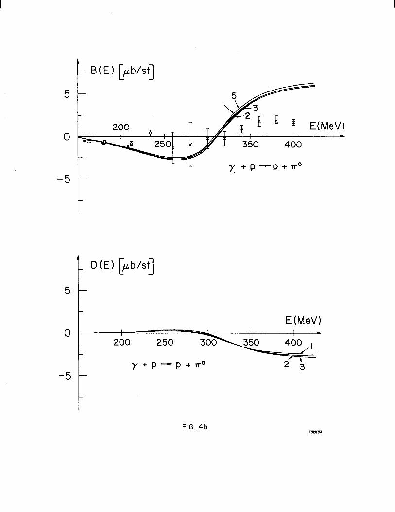
The coefficients B, D and C. Not many conclusions can be drawn at present

from the comparison of the asymmetry coefficients B and D. The recent values

for B at threshold up to E = 210 MeV serve more or less only as a check for the 0

cut off energy WC in the dispersion relation (I. la) for Re Ei+ . Above E = 210

MeV the experimental situation is presently completely unclear. Fits to angular

distributions, which neglect the coefficient D are dubious at least above E = 300

-16-

MeV as the results in Fig. 4 for D indicate. There is the possibility that B is

rather small in the region 220 to 340 MeV. In this case D should also be taken

into account in fits at lower energies.

Presently the most obvious discrepancies are connected with the

coefficient C. This is particularly true at low energies where C is not dominated

by Ml+- These deviations could be removed by noteworthy small contributions to

E 1-t'

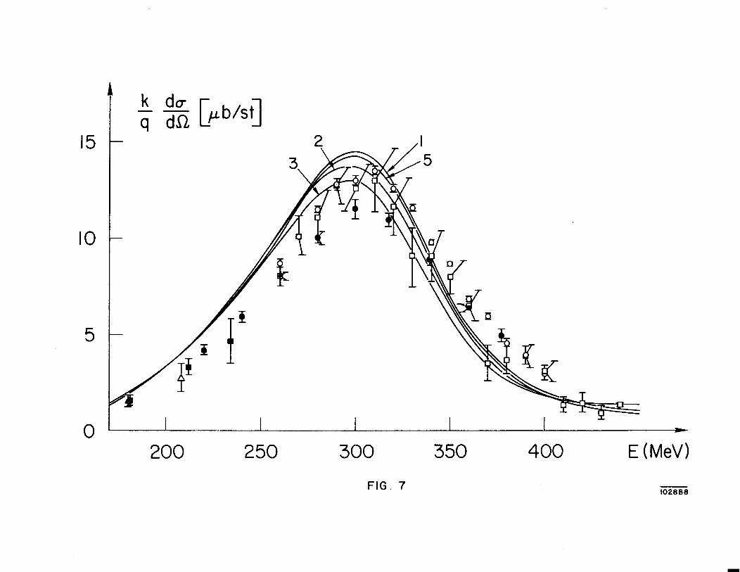
Summary to Section 1I.A. Very recent results in backward direction 15b, 24

confirm the present discrepancies in C and presumably also in B (Fig. 7). It is

not possible to explain them by reasonable changes in Re Eo+ and Re Ml as they

are suggested by subtracted dispersion relations (Section I. D and Fig. 2) for

Re EE andReM 7P l-’ One has to alter the amplitudes in such a way that the changes

in the excitation curves have on both sides of the resonance a different sign par-

ticularly at 6’= 180’. Because of the discrepancies in C and IO/C we believe at

the moment that the multipole El+ observes further detailed considerations 0 But

since the alterations of El+ 3/2 should be rather energy dependent the El+ part is

the most doubtful one. In the framework of the dispersion relations (I. 1) it seems

physically impossible to find a corresponding change of the other isospin parts.

B. n+-Production

In n+-production we shall discuss the discrepancies in the angular distri-

butions (Fig. 9) and excitation curves (Fig. 8) for unpolarized or plane-polarized

y’s.

8 = 9o” ?r+- excitation curves e The results for unpolarized Y’S with solutions

2,3,5 and 6 yield at 8 = 90’ (Fig. 8) better agreement with experiments than in

former calculations (see Part I, Fig. 5). Especially the typical discrepancy is

312 smaller on the low ener,gy side of the resonance, where Re Ml+ has its maximum

- 17 -

I

(E z 280). With the new results the prediction at threshold is about 10% higher

than the values in part I. i/2,3/2 The difference arises from the inclusion of Im EO+

3/2 and particularly of Im El+ in the dispersion integrals. The experimental data

suggest values which are 5% smaller up to E = 190 MeV. Presently it cannot be

decided whether this discrepancy arises by unknown high-energy contributions

or e,g., a too large f2 = 0.080:

For (A-IO) (Fig. 8) following from measurements with polarized Y’S the dis-

crepancy around E = 280 MeV is very markable. Because of its energy dependence

it must mainly arise in the p-wave multipoles Ml-, Ml+ - as already mentioned

in part I. With the new experimental results for (A-IO) in 7r+- and To-production 35

it now becomes possible to compare also the sum of both

S(E) = A(E) - IO(E) A(E-7MeV) -IO(E-7MeV) > nQ

= 2 3/2 + E3/2 2 + 2 3 Eo+ 2- I I I

3/2 3 2M1+ + M;j212 + ; IE;” + E;‘“/’ tn. 5)

-t +12M;i2 + M;!“i” + m..

as suggested in (Part I Section V). In (II. 5) the interference terms between the multi-

poles leading into the isospin I = l/2 and 3/2 states cancel (see (5. la) in Part I). The

results in Fig. 9 for the difference (Sexp - qheor) point clearly to a discrepancy,

which because of its energy dependence should mainly arise in the I = 3/2 part

of the real parts of the p-wave multipoles hfl 0

-

Assuming only changes A in

Re M”,/” one obtains for S from (II, 5)

3/2 B(E) = $ Re Ml+ l A Re nI”,/” (JJ. 6)

The result for AS in Fig. 9 was obtained with the rather large value

A Re M”1/” = 0.45 (in our units 10 -2 q. This would amount to a 60% change in

Re MiL2,t E = 300 MeV. In or+- and To-photoproduction it would yield the changes

- 18-

AM1 ‘1 = - &/3 Re M”,/_” = - 0.21 and AM; = + 2/3 Re M31/_2 = + 0.30. Changes

of this order one might expect according to Fig. 2. But in so-photoproduction

7r” changes AM1 = 0;30 would spoil the good agreement for b (II.4) at 360 MeV

(see Section II, A). To get a consistent result one obviously has therefore to

3/2 consider corrections in Re Ml- - and Re Mi/” as well as Re My 0 + T - angular distributions. In the angular distributions for unpolarized Y’S

one finds reasonably good agreement in forward direction up to. 8 = 50’ as can

be seen, e.g., in Fig. 10. Neither the new 37a nor the old37b data indicate a

peak at 8 = 10’ which is predicted in Ref. 10a. The discrepancy at lower angles

can very well be explained by reasonable alterations in the s- and p-wave multi-

poles as already discussed in Ref. 15a. But one can show that a single multipole

alone is not the reason for the total discrepancy. Unfortunately a more definite

conclusion cannot be drawn from the present data. The same agreement holds

also for angular distributions with plane polarized y9s, e.g., if the polarization

vector points perpendicular to the reaction plane (Cp = 90°) (Fig. 1 10)

doi && (0, + =90°, E) = do (8,E) =(A-lO) g

Summary to Section IL B. At 8 = 0’ the theory is very sensitive to small

alterations in all multipoles. Therefore the partly remarkable agreement in

Fig, 8 is noteworthy. On the other hand measurements of the asymmetry ratio

AR(e , E) = dcL - da;,

duL+ dq,

for plane-polarized 7’s indicate near E = 250 MeV and 8 = 30’ a completely

different energy-dependence (Fig. ll), which is very hard to underst‘and. But

better statistics is needed for a definite conclusion.

- 19 -

It was mainly our aim to exhibit the typical discrepancies in 7r+-production.

In our opinion these cannot be overcome purely by a refinement of the present

methods e Presumably one needs more physical information which effects several

multipoles in a correlated way. At very low energies this has been tried recently,

38 e.g. 3 in To-photoproduction by the inclusion of the w and B-meson resonances.

But these results are not very conclusive. In any case above E = 200 MeV the

authors expect that the effects of the meson resonances are of minor importance. _

There is at the moment also agreement that the effects of the p-resonance cannot

account for the main discrepancies. 39,13

III. PREDICTIONS FOR NEW KINDS OF EXPERIMENTS

IN no-PHOTOPRODUCTION

A. General Discussion

In this section we discuss predictions of the isobar approximation for some

more general experiments, in which, e.g., linear polarized y’s together with

a polarized target are used. The immediate question is then, which new infor-

mation on the low partial amplitudes follows from these more difficult-experi-

ments. Also as soon as more general experiments become possible one might

think of the possibility to perform a complete partial amplitude analysis or to

determine the full helicity amplitudes from experimental data. 40 But this pro-

gram can be successful only if the new experiments are sensitive to contributions

of the helicity amplitudes which are poorly known since they are otherwise hardly

detectable. To decide on the usefulness of a new type of experiment purely kine-

matic considerations are insufficient. Some dynamical input is needed. For this

we shall use the isobar approximation. As an example for this kind of discussion

we choose Ire-photoproduction on the proton.

- 20-

Assuming plane-polarized photons and a polarized nucleon target, we gener-

alize (II0 1) and (II. 2) 0 The result for the cross section is

k du - -=sl+ q d-2 [

-xcos2$sinBReL8+p21mL6-

w* 1)

-plKsin2~ImLg+p2KcoS2~*ImL10+p3Ksin2~sin81mL8 sin6 I This form shows explicitly the dependence on the polarization angle $ (Fig. 12) _

and on the components p,, py,,pz of the polarization vector of the nucleon target.

K denotes the polarization degree of the plane-polarized photons. Furthermore,

for the recoil-polarization Pi of the outgoing nucleon one obtains

k du - -Pz= q dQ [

K sin2$sin01mL7+pIReL5 1 sine+~~S~+.~~

k do ;dnPx= [

-Ksin2$ImL5+pIsin0ReL7+p3ReLg+... sin8 1 k*p = qdQ Y [ -ImL10 -KCOS 2@*ImL6+p2sin8ReL8+ e.O 1 sin8

The neglected terms in (III. 2) - (III.4) contribute only at measurements,

(III. 2)

(III. 3)

(III. 4)

where

polarized y’s and a polarized target are used simultaneously. For a derivation

of (III. 1) - (IlI.4) see, e.g., Ref. 20.

In (III. 1) - (III. 4)) the real functions Si(E, cos 0) [i = 1,2] and the complex

functions Li(E, cos 0) [i = 5 to lo] appear. (The notation has been taken from

Ref. 41.) The quantities

and

s = k du 1 ; do (E, cm 6)unpol~ , ReL8 = -I(E, cos 0)

ImL1o = P,(E, cos 0) unpol .

- 21 -

are already measured (see (II. 1) and (II. 2)) and therefore shall not be discussed

here. To determine S2 , Re L5, Re L7 and Re Lg by a measurement of the recoil

polarization, one necessarily needs a polarized target. To obtain ImL5, ImL6

and ImL 7, plane-polarized 7’s can be used. We restrict our discussion in the

following mainly to these two groups (1 and 2) of observables.

To go into more detail we shall assume an expansion in powers of cos 8

analogously as done in (II D 1) and (II. 2)

Si(E, COS 6) = Ai + Bi(E) cos 8 + Ci(E) COST 8 + Di COST 0 + . . o

i=l,2

Li(E, COS 6) = Ai + I%(E) cam 6 + Ci(E) cOS2 8

i=5 , 0.0 10

Note that one conventionally writes for i = 1: Al= A, Bl = B, etc.

B. Group 1: S2, Re L5, ReL7 and Re Lg - -

In Tables 5 and 6, we present numerical results for the coefficients of this

group at three energies using the isobar approximation (solution 5). For a better

understanding of these results we further expand the coefficients Ai, Bi, Ci and

Di into multipoles. Neglecting all multipoles with J? >, 2 one obtains 41

A2 = Re EZi+ (2M1- + Ml+ + 3E1+) (~10 7)

B2 = - Eo+ 2 I I + Re Mi-t-Ml- + 6E1+ + 21f1+) + 3 Re ET+ f Ed+ + MI+) (III. 8)

C2 = Re Bg = -3 Re E;+ (Ml+ + 3~~+) (I= 9)

Re A5 = -Re A8 =-I- IO = -3 Re M; (Ml+ - El+) _

l+ + MI;) -3 lEl+l”]

(III. 10)

(III. 11)

- 22 -

Re B5 = Re A7 = 3 Re E&(M~+ - El+) (III. 12)

Re C5 = Re B7 = -3Re A5 -9 Re Mi-tMl+ - El+) (III. 13)

ReC7=0 (IL 14)

Re A9 = A -2 IE0+12 (see Eq. (II. 1)). (Ill. 15)

It follows from these equations that the coefficients in Table 5 are dominated by_

s-p interference terms and those in Table 6 by p-p interference terms with the

exception of B2 and Re A9 which contain also Eo+ I I 2 . In the following discussion

we shall assume that the resonant multipoles Ml+ and El+ are already determined

e. g. , by the measurement of S1 and Re L3.

We should like to note:

1. From (III. 9), (III. lo), (III. 12) and (III. 13) one should expect that

certain pairs of coefficients are almost equal. The results in

Tables 5 and 6, which take.into account all multipoles, show that

this is generally true - apart at E = 280 in Table 5 - indicating

the minor importance of the higher multipoles in these and

similar cases.

2. At the first look Px(E, cos 6 = 0) might appear very suitable for

a determination of E6+ . One might expect from (III. 12) that the

s-p interference term Re E&(M1+ - El+), is best investigated

by measuring A7 0 This term can be direc’tly measured in con-

trast to B and Re B5. But from (III. l), (I&3), (III.S), (III. 6)

and the values in Table 5, one obtains

px(E = 340 MeV, cos 6 = 0) = px Re A+E = 340 MeV)

A(E = 340 MeV) = 0.24 p,

p =K=O Z

(III. 16)

- 23 -

a result, which should represent the order of magnitude correctly.

One sees from (III, 16) that only with a fairly high degree of polar-

ization p,, will one be able to beat the present limitations on the

accuracy of B, which around the resonance is typically 25% (see

Fig, 4) and which presumably will be improving.

With the same experimental arrangement but a different direction

of the initial polarization vector, one obtains also

Px(E, COS 6 = 0) = p, Re AgtE)

A(E) = P,

K=p x=o

For the last equality we used the approximate relation (III. 15) 0

The quantity (1 - 2/Ew/2/‘A) h as a very peculiar energy behavior.

It increases from its value -1 at threshold, where A = Eo+ I I

2 ,

(III. 17)

to z +1 within 20 MeV, since A increases very rapidly in contrast

to EO+ 0 I 1

2 Throughout the region of the first resonance, where

2 Eo+ I 1 2/A M l/30, ameasurement of (III, 1’7) would therefore need

an accuracy < 1% to yield any reliable information on EO+ I I 2 .

3. From the angular distribution of Re L5, which appears in Pz (III. 2),

one obtains the coefficients A5 and C5’ According to (III, 13)

> =-3ReMi-(M1+-EI+)+0en

Since in our energy region Im Ml x 0 (III. 18) is sensitive to

Re Ml apart from the immediate neighborhood of the resonance

where also Re (Ml+ - El+) x 0. This is in contrast to (11.4) from

which at present our best knowledge of Re Ml follows.

(HI. 18)

- 24 -

C. Group 2: Im Li, i = 5,6,7

The quantity Im L6 should be the easiest obtainable in this group since only

a measurement of the cross section with a polarized target is necessary (see

(III. l))- As in part III. B we present in Table 7 numerical results for some of the

relevant coefficients. Neglecting again all multipoles with L 2 2, one obtains from 41

ImA5= -Irn Ag = 3 Im Ml- (Ml+ - EIJ* + 6 Im El+ Mi+ (III. 19)

1x-n B5 = Im A6 = Im A7 = 3 Im E~(E~+ - Ml+)* (In. 20)

Im C5 = h B7 = -18 Im El+ MT+ (rn. 21)

Im B6 = 3 Irn Ml-tMl+ - El+)* -12 Im El+ Mi+ (III. 22)

Im C6 =Imc7=o (III. 23)

We should like to note:

1. The results in Table 7 show that the neglection of higher multipoles

is in Group 2 more severe. This is particularly true for Im A6,

Im A7 and Im Bg’

2. From (III. 21) it follows that Im B7 or Im C5 allow a very direct

determination of E l+a From (III. 2) it follows that

Im L7 Pz= Ksin2$sin26------

s1 P, = P, = 0 (III. 24)

With the values of Tables 6 and 7, one obtains then at E = 340 MeV

+ 0.03 6 = 60’

Pz = K Sin 2$ i - 0.06 6 = 90’

- 0.21

i

6 = 120’

(III. 25)

- 25 -

Since KW0.5 and with Isin 2$1 z 1, this experiment to determine

Im B7 should be feasible yielding an accuracy of less than 25%

around e= 12oO. According to (III. 19), (III. 22) and (III, 21)

1l-n (A5 - B6) = 18 Im El+ M;+

and Im C5 are independent quantities to determine E 1+, but

Im (A5 - B6) is less accessible.

3. Again from (III. 19) and (III. 22) one obtains

Im (H5 3- B6) = 9 Im Ml (Ml+ - El+)*

(III. 26)

(III. 27)

which is a quantity similar to (II. 3). Together with (III. 18) it

fixes completely the complex number Ml-(Ml+ - El+)*, which

would serve to determine M l- l

Finally we should like to mention that measurements of the quantities (III. 12)

and (III. 20) yield the real and imaginary part of EO+ (El+ - Ml+) * , which would

determine EO+ completely.

D. Final Remarks

The measurement of the cross section for simultaneously plane-polarized

Y’S and a polarized target yields the additional information on Im Li for i = 8,9,10.

In the approximation that all multipoles with P 1 2 can be neglected, one obtains 41

- Im ~~ = + Im Llo = P,(E, cos 0) unpol D (Et. 28)

ImB8=Im C8=0 (III. 29)

Because of these equations and (III. 19) for Im A*, no new information can be

obtained from these kind of experiments as long as the analysis is restricted to

multipoles with B 5 2.

-26-

From the preceding discussion we have learned for some cases how one has

to choose the experimental arrangements to improve the present accuracy for

our experimental determination of the multipoles with 1 = 0 and 1. It turned out

that measurements of the recoil polarization for photoproduction with plane-

polarized y’s and a polarized target are suitable for this purpose. But utmost

care should be taken in choosing the right kind of experimental arrangements.

It is now the challenge to the experimentalist to decide which of the useful exper-

iments are feasible. The results of these experiments can serve as an improved

check for the approximation scheme in solving the partial amplitude dispersion

relations. This scheme is presently based mainly on the isobar approximation

as discussed in Section I. Furthermore these kinds of experiments performed

with sufficient accuracy in n*- and To-photoproduction would yield, ultimately a

check of the Watson theorem, which is an implication of unitarity and time

reversal invariance.

-27-

APPENDIX

We give here the relation of the parity conserving helicity amplitudes H?(W)-

used in Section I - to the more familiar multipole amplitudes I&, M&. I 3 Let

for J=B+ l/2

$2 F;;2(W) = [I( 1+2@ kQ+ta - MI+(W)] (A. la)

$2 F$2(W = - p (Q +2)] 1’2 [MtQ +1)-(w) + Ete+l)_(W)] (A. lb)

$2 F;j2Wl = (I+,3 EQ+tV + Q Mn +tw) (A. lc)

$2 F:;2(Y = - tQ+2) Mtl+l)JW) + 1 Ete+l)-tW)

with the inversion (again J = I + l/2)

EQ+ = 3 Ei l l ($2 + (IsY2 $2)

MQ+ = -$!i 14-l ’ 1 (F;j2 - (#2 F;;,)

E(p+l)- = -jz ki (Fz2 - ($$‘2 Fz2)

Then WB define

HJ*, * h (W) =FF+V)

with

Q >o

Q >o

(A. 2a)

(A. 2b)

(A. 2c)

(A. 2d)

(A. 3)

J-1/2 up) =+ qu!qgL (A. 4)

- 28 -

and

C(w) = & ((w+Mp - 1r’2 (A. 5)

Note that

(3-w) = - * C(w) (A* 6) 2

J&,1 The McDowell symmetry relation has for the Hh the very convenient

form

HJ*, 1 A (-w) = H;T’l(w) (A. 7)

which follows from (A. 3) and the corresponding relation (2 . 10) in Ref. 20 for

the F’s

Ff-(+) = (-$+1’2 Ff+(-w) (A* 8)

-29-

REFERENCES

1.

2.

3.

4.

5.

6.

7.

8.

9.

10.

11.

12.

13.

14.

15.

16. (a) A. Donnachie and G, Shaw, Nucl. Phys. s, 556 {1966).

(b) T. Wennstr’dm, preprint, University of Lund (1968).

W. Schmidt, Z. Physik 182, 76 (1964)(referred to as Part I) +

J. S. Ball, Phys. Rev. 124, 20 14 (1961).

G. F. Chew, M. L. Goldberger, F. E. Low and Y D Nambu, Phys. Rev. 106,

1345 (1967).

G. Schwiderski, thesis 1967, Karlsruhe.

J. Engels, W. Schmidt and G. Schwiderski, Phys. Rev. 166, 1343 (1968).

P. Finkler, Phys. Rev. 159, 1377 (1967).

(a) D. Schwela, H. Rollnik, R. Weizel and W. Korth, Z. Physik 202, 452 (1967);

(b) H. Rollnik, Proc. of the 1967 Heidelberg International Conference on Elementary

Particles, p. 400, edited by H. Filthut (North-Holland Publishing Company, 1968).

Go Mennessier, Nuovo Cimento 46, 459 (1966).

N. Zagury, Phys. Rev. 145, 1112 (1966).

(a) F. A. Berends, A. Donnachie and D. L. Weaver, CERN preprint 67/146/5-

TH 744 (1967) and Nucl. Phys. g, l(l967); ibid. E, 55 (1967);

(b) F. A. Berends and A. Donnachie, Phys. Letters 25B, 275 (1967).

F. Selleri, V, Grecchi and G, Turchetti, Nuovo Cimento 52A, 314 (1967).

J. Engels and W. Schmidt, Phys. Rev. (to be published).

A. Donnachie and G. Shaw, Annals of Physics 37, 333 (1966).

A. Miillensiefen, Z. Physik l& 199 (1965); ibid E, 238 (1965).

(a) W. Schmidt, Proceedings of the International Symposium on Electron

and Photon Interactions at High Energies, Hamburg (1965), Vol. II, p. 323.

(b) M. Croissiaux, E. 8. Dally, R. Morand, J. P. Pahin and W. Schmidt,

Phys. Rev. 164, 1623 (1967).

-3o-

17.

18.

19.

20.

21.

22.

23.

24.

25.

26.

27.

28.

29.

A. I. Lebedev, S. P. Kharlamov, Contributions to the International Confer-

ence on Low and Intermediate Energy Electromagnetic Interactions, Dubna

(1967).

J. Engels, W. Schmidt and G. Schwiderski, external report 3/67-l,

Gesellschaft fiir Kernforschung, Karlsruhe, March (1967).

L.D. Roper, R. M. Wright and B. T. Feld, Phys. Rev. 138, B190 (1965);

P. Auvil, A. Donnachie, A. T. Lea and C. Lovelace, Phys. Letters 12,

76 (1964); P. Bareyre, C. Bricman, A. V. Stirling and G. Villet, Phys.

Letters l-8-, 342 (1965).

W. Schmidt and G. Schwiderski, Fortschr. d. Physik 15, 393 (1967).

A. Miillensiefen, Zeitschr. f. Physik 211, 360 (1968).

B. B. Govorkov, et al., Contributions to the International Conference on

Low and Intermediate Energy Electromagnetic Interactions, Dubna (1967).

F. Fischer, H. Fischer, H. J. Kampgen, G. Knop, P. Schulz and H. Wessels,

University of Bonn, preprint 1966 for the International Conference on High

Energy Physics at Berkeley.

R. Morand, E. Erikson , M. Croissiaux (private communication)(the cor-

rections to the previous values 15b will be published).

W. Hitzeroth, Contribution to the Dubna Conference on Low and Intermediate

Energy Electromagnetic Interactions and private communication (1967).

D. B. Miller and E. H. Bellamy, Proc. Phys D Sot. London 81, 343 (1963).

K. Berkelman and 3. A. Waggoner, Phys. Rev. 117, 1364 (1960).

G. Barbiellini, G. Bologna, J. DeWire, G. Diambrini, G. P. Murtas and

G. Sette; Proceedings of the Dubna Conference (1964).

G. Barbiellini, G. Capon, G. de Zorzi, F. Fabbri and G. P. Murtas,

preprint, Frascati (September 1967).

- 31 -

30. D. J. Drickey and R. F. Mozley, Phys. Rev. 136B, 543 (1964).

31. F. D. Dally, R. M. Mozley and R. W. Zdarko, preliminary results

(April 19 68).

32. W. Schmidt and H. Wunder, Phys. Letters 20, 541 (1966).

33. K. H. Althoff, K. Kamp, H. Matthsy and H. Piel, Z e Physik 194, 144 (1966).

34. K. H. Althoff, D. Finken, N. Minatti, H. Piel, D. Trines and M. Unger

Phys. Letters 26B, 677 (1968).

35. Bonn data; private communication by Professor Knop, April (1967).

36. M. Grilli, M. Nigro, E. Schiavuta, F. Soso, P. Spillantini and V. Valente,

Laboratori Nazionali di Frascati de1 CNEN; Nota interna, n. 356; March (1967) e

37. (a) C. B&ourne/, J. C. Bizot, J. Perez-y-Yorba, D. Treille and W. Schmidt,

Phys. Rev. (to be published), preprint L.A. L. 1186, Orsay.

(b) J. T. Beale, S. D. Ecklund and R. L. Walker, data compilation CAL-

TECH Report CTSL-42, CALT-68-108.

38. F. A Behrends, A. Donnachie and D. L. Weaver, Nucl. Phys. g, 103 (1967).

39. G. Hijhler and W. Schmidt, Annals of Phys. 25, 34 (1964).

40. B. Anderson, Nucl. Phys. 60, 144 (1964);

M. Kawaguchi, H. Shimoida, Y. Sumi and T. Ueda, Progr 0 Theor. Phys.

31, 1026 (1964).

41. A. Miillensiefen and W. Schmidt, external report 3/67-3, KernforschLmgszentrum,

Karlsruhe (19 67) e

- 32 -

I

TABLE 1. T:*(E) for the J =1/2, 3/2 multipoles 9: at different energies E

E(MeV) I

I=0 I = l/2 I = 3/2 I

I=0 I = l/2 I = 3/2

EIoc 152 0.351 0.148 0.249 0.007 0.006 0.007

200 0.447 0.200 0.323 0.051 0.042 0.047

300 0.644 0.324 0.484 0.148 0.125 0.137

400 0.868 0.492 0.680 0.298 0.259 0.278

E:+ 4+

152 0.001 0.000 0.001 0.004 0.002 0.003

200 0.010 0.005 0.007 0.031 0.013 0.022

300 0.049 0.031 0.040 0.097 0.054 0.075

400 0.142 0.103 0.122 0.213 0.142 0.177

E;'- 4

152 0.000 0.000 0.000 0.000 0.000 0.000

200 0.007 0.003 0.005 0.002 0.001 0.001

300 0.040 0.023 0.031 0.018 0.015 0.017

400 0.121 0.084 0.103 0.075 0.068 0.071

TABLE 2. R(ML, I$, Wo, W) for the J = l/2, J’ = l/2, 3/2 multipoles for

W. = 9.15 (E. =400 MeV) and W = 8.61 (E = 300 MeV).

Eo+ l/2 - 0. 02 0.01 0.01 0.74 0.42 0.01 0. 01

Eo+ 3’2 0 * 04 0.03 0.02 0.84 0.32 0.01 0.01

FL- l/2 0.00 0.00 - 0.00 0.01 0. 04 0.01 0.01 3/2 M1- 0. 01 0.00 0.01 - 0.07 0.03 0.02 0.01

0.03 0.10 0.01

0.00 I - 0. 06 0. 02

TABLE 3. !?(i&, Wo, W) for the J = l/2 multipoles.

W, , W as in Table 2.

E!‘) E1/2 o+

Ey3/2 0 M1/2 M3/2 o+ o+ M1- l- l-

0.06 0.07 0.06 0.03 0.03 0.03

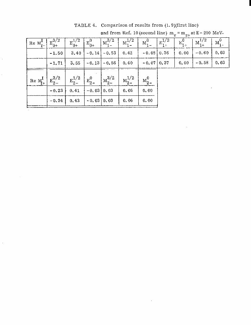
TABLE 4. Comparison of results from (1. S)(first line)

j 1 -0.24 ( 0.43 -

and from Ref. 10 (second line) rn= = m,+ at E = 200 MeVl

/ Mf/_” #+

0 I

3/2 E2- M2-

-0.03 0.03 =I= -0.03 0.03

-

- -

0.42 / -0.08

l/2 I 0 M2- M2-

0.37 0. 00 -0.58 I I

0, 03

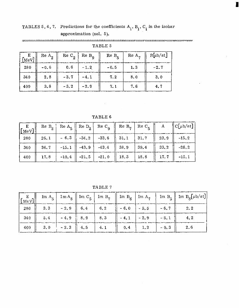
TABLE 5

(M:V] Re A2 Re C2 Re Bg Re B5 Re A7 BbClb/st]

280 -0.6 0.6 -1.2* -0.5 1.3 -2.7

340 2.8 -3.7 -4.1 7.2 8.0 3. 0

400 3.8 -3.2 -2.9 7.1 7.6 4.7 J

TABLES 5, 6, 7. Predictions for the coefficients Ai, Bi, Ci in the isobar

app.roximation (sol. 5).

TABLE 6

I II rM:Vl R le B 2 Re A5 Re D2 Re Cg Re B7 ReC5 A C[pWst]

26.1 - 6.3 -34.2 -33.6 31.1 31.7 23.9 -15.2

36.7 -15.1 -43.9 -43.4 38.9 39.4 33.2 -26.2

17.8 -10.4 -21.5 -21.0 18.3 18.8 17. 7 -15.1

TABLE 7

‘[Mzvl Im A5 ImA Im C5 Im B7 Im B6 Im A7 Im B5 h-~ B8[Pb/st]

280 3.3 -2.9 6.4 6.2 - 6.0 - 5.5 - 6.7 2.2

340 5.4 -4.9 8.9 8.3 - 4.1 - 2.9 - 5.1 4.2

400 3. 0 -2.3 4.5 4.1 0.4 1.2 - 0.3 2.6

FIGURE CAPTIONS

1. Real parts of J = l/2, 3/2 multipoles for the three isospin combinations

I = 0, l/2, 3/2. Pole term approximation: dashed line, isobar approximation:

full line with Im E = 0, dash-point-line with Im EO+ # 0. For J = I = 3/2,

P = +l, solution 5 (Section rr) has been taken. In some indicated cases results

have been multiplied by a factor of 10 or 100.

2. Real parts of J = l/2 multipoles following from subtracted dispersion relations

in the isobar approximation (solution 2). Dash-point-line unsubtracted and

full line subtracted dispersion relations; dashed line error limits arising from

the subtraction constant.

(3 To-production

04 *+-production

3. Present range of uncertainty for Im Ml+ .3’2(wf) and Im E3,/2(Wf) with Wf

= 9.016, i.e., Ef = 320 MeV. The numbers of 1 to 6 correspond to the solu-

tions used in this paper rnfl. = rn+, .

4. The coefficients A, B, C,D and A-IO in no-production for solutions 1,2,3 and

5 over the photon energy E. Experimental results for A: f 22,25,26 23

, f ,

27; for B and C: $22, 9 25, I”“; for A-IO: $28y2g, f3’, $“. @

interpolated values for A used to calculate (A-IO).

5. (a) The ratio IO/C and El+ 3/2,M;!2 for the solutions 1,2,3 and 5. IO/A from

$ 28, i2’, I”“, 1 31; --- Multipole analysis21; A/C, see Fig. 5b.

w The experimental ratio C/A with an eye-fit f25, $22, 12”.

6. The coefficients a and b for the polarization of the recoil proton in 7r”-

production, old data 33 H , new data P 34 a

To-production in backward direction for solutions 1,2,3 and 5;

7* 4 15b, $35 P 25, I 22,

with magnet spectrometer; P 35 with telescope spectrometer.

8. n+ excitation curves at 8 = 0’ and 90’ for $$ (0, E)unpol and for .

g (0 , Wunpol - $ (8,E,$ = 909 at 8 = 90’. Experimental results . from 36, 37a data and the compilation37b.

9. The difference S expStheor . (see (II. 5)) and AS (see text) for solutions 2

and5 . (4)

Experimental results, Refs. 28, 29 and 30.

10. Angular distribution for $!F (Ey ‘)unpol at E = 350 MeV and for .

g (E, 8, $I = 90°) at E = 280 MeV. Dashed line prediction according to

Part I. At 280 MeV the experimental results Ref. 36 at 350 MeV from Ref.

37a,b.

11. n+ excitation curve for the asymmetry A,(E,e) = dy -dq,

dcrl+dq, at Ref. 36.

12. Coordinate system for photoproduction.

{I E,I+ 0.5t [ 10-2 x] -

/----------- ____------

-3r

1 [lo-* X] I El+

3.- 0.5,-

-0.5 - -2s-

I -31

o,5 w* Xl

i f

--- I= l/2

t

[lo-* X]

EJ- 0.5

490 _______- --- I= l/2 - t

300 \ 400 E (MeV)

I

E

-----_____ ----

. ----v__ ---_ ---_

-0.5..

I --5 --

FIG. 2a

1 t

_________ m-v------ w--

7r+

MI+

1 I

200 300

FIG. 2b 1028AI

in -

NE)

250 300 350

E (MeV)

C (El kb/st] E(MeV) 1 I I I I I

300 400

y+P -p++

FIG. 4a 102ac3

A

- B(E) [pb/Sij

200 l-

I ‘Q I T I P 2501

y +p-p+7r”

1 D(E) [,b/st]

y+p-p+7P

I t

400 1

/ \ 2 3

FIG. 4b

60

50

40

30

20

IO

0

r -

y+ p-p+79

150 200 250 300 350 400 FIG. 4c

-0.25

0.5

0

-0.5

t IO Y +p -p+7+

FIG. 5a

A C/A Y+p -p+srO

E ( MeV) I I I I I

300 400 500

4 --,--

FIG. 5b 102666

75 l

50 l

i

y+p - p+7r”

2.5

0

FIG. 6 1028A7

I

-* c

1

K 1

N to’

bC: I

uw

4 I

ln 0

0

20

IO

(a)

0’ I I I I I L 200 300 400

30

20

IO

E(MeV) I I I I

300 400

40

30

20

IO -

E(MeV)

0 I I I I I 200 300 400

(b)

FIG. 8 ias

m

a I a G

v,

-

W I-

I G

I

t--e

I I

t < \

32

0

-$ I

)---1M

TL 0

-F2

0 -0 N

0 0

0 T

u3 t

1 “0 a, -

0 8 -

“0 cu

i k 0

0

\ \ \

\ \ \ \ \ +

\ \ \ \ \ + \ \ ‘\ -

\

+ k + c t “0

=m

+ II

xcb

7 s - W

L

\

8 Tf

0 L(! 0

In cu 6

0

0 8

A

A k z 9

FIG. 12 IO28Al3