ABSTRACT

Title of dissertation: MORTGAGE CONTRACTS ANDTHE DEFINITION OF AND DEMAND FORHOUSING WEALTH

Joseph B. Nichols, Doctor of Philosophy, 2005

Dissertation directed by: Professors John Rust and John SheaDepartment of Economics

Owner-occupied housing plays a central role in the portfolios of many households. Recent work has

explored the connection between a household’s position in home equity and the demand for risky assets in

the £nancial portfolio. This dissertation examines the roleof the mortgage contract on the de£nition of and

demand for housing wealth.

This £rst chapter develops a detailed partial equilibrium model of housing wealth’s role over the

life-cycle to explore (1) housing’s dual role as a consumption and investment good; (2) the signi£cance of

the mortgage contract being in nominal and not real terms; and (3) the tax bene£ts associated with owner-

occupied housing. The household’s dynamic stochastic programming problem is solved using parallel

processing. The results show that the “over-investment” inhousing is not just a function of consumption

demand but also can be driven by the bene£ts inherent in the mortgage contract. It also shows that the

nominal mortgage contract results in the non-neutrality ofperfectly expected in¤ation. Finally, the paper

documents the effect of preferential tax treatment on housing demand.

This paper develops an alternative measure of the return on housing that incorporates the consump-

tion stream and the required mortgage payments associated with owner-occupied housing. This measure is

then used to demonstrate how the total return on housing varies with anticipated holding length, terms of

the mortgage contract, and borrower income level. Data fromthe Panel Study of Income Dynamics and

the Survey of Consumer Fiance are used to explore the empirical relationship between property, mortgage,

and borrower characteristics and the total return on housing, the probability of negative total return, and the

demand for risky assets.

MORTGAGE CONTRACTS AND THE DEFINITION OFAND DEMAND FOR HOUSING WEALTH

by

Joseph B. Nichols

Dissertation submitted to the Faculty of the Graduate School of theUniversity of Maryland, College Park in partial ful£llment

of the requirements for the degree ofDoctor of Philosophy

2005

Advisory Committee:

Professor John Shea, Co-Chair,Professor John Rust, Co-ChairDr. Micheal PriesDr. Anthony YezerDr. Gurdip Bakshi

c© Copyright by

Joseph Nichols

2005

This dissertation is dedicated to Wesley Webster Nichols, my father.

ACKNOWLEDGMENTS

I had the fortune to be £rst introduced to economics by Dr. Bob Goldfard and Dr. Tony Yezer. Over

the years since, Dr. Yezer has been the foremost in¤uence on mygrowth as an economist, both in focusing

my attention on the role of housing and on the potential, unfortunately often unful£lled, of economics to

actual improve the life of everyday people.

My time at the University of Maryland has been enriched by many friendships among my fellow

students, in particular Haiyan Shui, Ignez Tristao, and Emine Boz. I have greatly bene£ted from having Dr.

Mike Pries on my dissertation committee. I am also deeply indebted to him for my time as his TA. I know

that I am and will be a much better teacher due to his support and example.

Dr. John Shea was my £rst key advisor in graduate school. He graciously took the time to talk with

a lst year student about possible research ideas, a rarity inany graduate program. He is also by far the best

and most demanding editor (with the sole exception of my wife) I have ever had.

Dr. John Rust provided the underlying model that is at the heart of my dissertation. He also provided

endless support, always encouraging me to submit my paper tojournals and conferences well before I

thought I was ready. By setting the bar high and expecting success he helped me accomplish far more that

I thought possible.

There is one person above all others that I owe thanks to, and that is my wife Julie. Far more that

any editing, the unlimited and unconditional support from her over the last £ve years have been essential to

not only my success but my sanity.

Finally, I would like to thank my parents, Wesley and Martha Nichols, for setting me on this path so

long ago. You gave be and foundation to build on and tools to build with. All of my accomplishments start

with you. Thank you.

iii

TABLE OF CONTENTS

List of Tables v

List of Figures v

1 Housing Wealth and Mortgage Contracts 11.1 Introduction. . . . . . . . . . . . . . . . . . . . . . . . . . . . . . . . . . . .. . . . . . . 1

1.1.1 The Importance of Housing Wealth . . . . . . . . . . . . . . . . . .. . . . . . . 11.1.2 Challenges of Modeling Housing Wealth . . . . . . . . . . . . .. . . . . . . . . 31.1.3 A Detailed Partial Equilibrium Model of Housing Wealth . . . . . . . . . . . . . . 4

1.2 Literature Review. . . . . . . . . . . . . . . . . . . . . . . . . . . . . . . .. . . . . . . . 51.3 A Partial Equilibrium Model of Housing Wealth with Mortgage Contracts. . . . . . . . . . 8

1.3.1 Consumption of Housing . . . . . . . . . . . . . . . . . . . . . . . . . .. . . . . 91.3.2 Accumulation of Financial Wealth and the Income Process . . . . . . . . . . . . . 101.3.3 Price of Housing . . . . . . . . . . . . . . . . . . . . . . . . . . . . . . . .. . . 121.3.4 The Mortgage . . . . . . . . . . . . . . . . . . . . . . . . . . . . . . . . . . .. . 141.3.5 Gains from Sale or Re£nancing . . . . . . . . . . . . . . . . . . . . . .. . . . . 161.3.6 Default Penalties . . . . . . . . . . . . . . . . . . . . . . . . . . . . . .. . . . . 171.3.7 Optimization Problem and Value Functions . . . . . . . . . .. . . . . . . . . . . 18

1.4 Baseline Model Results. . . . . . . . . . . . . . . . . . . . . . . . . . . .. . . . . . . . 201.4.1 Policy Functions . . . . . . . . . . . . . . . . . . . . . . . . . . . . . . .. . . . 201.4.2 Simulation Results . . . . . . . . . . . . . . . . . . . . . . . . . . . . .. . . . . 261.4.3 Tenure Transitions . . . . . . . . . . . . . . . . . . . . . . . . . . . . .. . . . . 33

1.5 Alternative Scenarios. . . . . . . . . . . . . . . . . . . . . . . . . . . .. . . . . . . . . . 351.5.1 Housing as an Investment and Consumption Good . . . . . . .. . . . . . . . . . 361.5.2 Effects of In¤ation on Housing Wealth . . . . . . . . . . . . . . .. . . . . . . . . 411.5.3 Tax Implications . . . . . . . . . . . . . . . . . . . . . . . . . . . . . . .. . . . 44

1.6 Conclusion. . . . . . . . . . . . . . . . . . . . . . . . . . . . . . . . . . . . . .. . . . . 48

2 Mortgage Contracts and the Heterogeneity in the Total Return on Housing 492.1 Introduction. . . . . . . . . . . . . . . . . . . . . . . . . . . . . . . . . . . .. . . . . . . 492.2 Literature Review. . . . . . . . . . . . . . . . . . . . . . . . . . . . . . . .. . . . . . . . 512.3 Theory. . . . . . . . . . . . . . . . . . . . . . . . . . . . . . . . . . . . . . . . . .. . . 532.4 Simulation Results. . . . . . . . . . . . . . . . . . . . . . . . . . . . . . .. . . . . . . . 592.5 Empirical Results. . . . . . . . . . . . . . . . . . . . . . . . . . . . . . . .. . . . . . . . 682.6 Conclusions. . . . . . . . . . . . . . . . . . . . . . . . . . . . . . . . . . . . .. . . . . . 79

A Baseline Model Parameter Values 81

B Model Parameter De£nitions 83

C Estimating Rent-to-Price Ratios 84

D Income Tax Rates 88

Bibliography 89

iv

LIST OF TABLES

1.1 Simulation Results - Baseline Model . . . . . . . . . . . . . . . . .. . . . . . . . . . . . 33

1.2 Tenure Transitions - Baseline Model . . . . . . . . . . . . . . . . .. . . . . . . . . . . . 34

1.3 Assumptions for Alternative Scenarios . . . . . . . . . . . . . .. . . . . . . . . . . . . . 36

1.4 Results of Alternative Scenarios . . . . . . . . . . . . . . . . . . .. . . . . . . . . . . . 36

2.1 Parameter Assumptions . . . . . . . . . . . . . . . . . . . . . . . . . . . .. . . . . . . . 60

2.2 Dependent Variables . . . . . . . . . . . . . . . . . . . . . . . . . . . . . .. . . . . . . 69

2.3 Independent Variables . . . . . . . . . . . . . . . . . . . . . . . . . . . .. . . . . . . . . 69

2.4 Probability of Negative Total Return . . . . . . . . . . . . . . . .. . . . . . . . . . . . . 75

2.5 Model of Return on Housing . . . . . . . . . . . . . . . . . . . . . . . . . .. . . . . . . 77

A.1 Log Income Regression Results . . . . . . . . . . . . . . . . . . . . . .. . . . . . . . . 81

A.2 Values of Market Parameters . . . . . . . . . . . . . . . . . . . . . . . .. . . . . . . . . 82

A.3 Values of Structural Parameters in Calibrated Model . . .. . . . . . . . . . . . . . . . . . 82

B.1 Model Parameter De£nitions . . . . . . . . . . . . . . . . . . . . . . . . .. . . . . . . . 83

C.1 Estimated Rent-to-Price Ratios . . . . . . . . . . . . . . . . . . . .. . . . . . . . . . . . 86

D.1 Progressive Income Tax Structure . . . . . . . . . . . . . . . . . . .. . . . . . . . . . . 88

LIST OF FIGURES

1.1 Timing of Decisions . . . . . . . . . . . . . . . . . . . . . . . . . . . . . . .. . . . . . . 17

1.2 Housing Tenure Policy Functions . . . . . . . . . . . . . . . . . . . .. . . . . . . . . . . 21

1.3 Consumption Policy Functions and Realized Wages . . . . . .. . . . . . . . . . . . . . . 23

1.4 Home Equity and Financial Wealth Policy Functions . . . . .. . . . . . . . . . . . . . . 24

1.5 Portfolio Allocation Policy Function . . . . . . . . . . . . . . .. . . . . . . . . . . . . . 25

1.6 Consumption and Income . . . . . . . . . . . . . . . . . . . . . . . . . . . .. . . . . . . 27

1.7 Wealth and Portfolio Choice . . . . . . . . . . . . . . . . . . . . . . . .. . . . . . . . . 28

1.8 Housing Tenure Choice . . . . . . . . . . . . . . . . . . . . . . . . . . . . .. . . . . . . 30

1.9 Why Trade Down at 50? . . . . . . . . . . . . . . . . . . . . . . . . . . . . . . . .. . . 32

v

1.10 Wealth and Portfolio Choice . . . . . . . . . . . . . . . . . . . . . . .. . . . . . . . . . 39

1.11 Housing Tenure Choice . . . . . . . . . . . . . . . . . . . . . . . . . . . .. . . . . . . . 40

1.12 Rent and Mortgage Payments . . . . . . . . . . . . . . . . . . . . . . . .. . . . . . . . . 41

1.13 Wealth and Portfolio Choice . . . . . . . . . . . . . . . . . . . . . . .. . . . . . . . . . 42

1.14 Housing Tenure Choice . . . . . . . . . . . . . . . . . . . . . . . . . . . .. . . . . . . . 43

1.15 Wealth and Portfolio Choice . . . . . . . . . . . . . . . . . . . . . . .. . . . . . . . . . 45

1.16 Housing Tenure Choice . . . . . . . . . . . . . . . . . . . . . . . . . . . .. . . . . . . . 46

2.1 Alternate Measures of Risk and Return . . . . . . . . . . . . . . . .. . . . . . . . . . . . 61

2.2 Components of Return on Housing . . . . . . . . . . . . . . . . . . . . .. . . . . . . . . 62

2.3 Risk, Return and Portfolio Allocation as a Function of Holding Period . . . . . . . . . . . 63

2.4 Risk, Return and Portfolio Allocation as a Function of LTV Ratio . . . . . . . . . . . . . 64

2.5 Risk, Return and Portfolio Allocation as a Function of Income . . . . . . . . . . . . . . . 66

2.6 Distribution of Total Return and Conditional Rate of Total Return . . . . . . . . . . . . . 67

2.7 Distribution of Return on Housing from AHS . . . . . . . . . . . .. . . . . . . . . . . . 71

2.8 Distribution of Total Return and Rate of Total Return . . .. . . . . . . . . . . . . . . . . 72

2.9 Distribution of Total Return and Rate of Total Return . . .. . . . . . . . . . . . . . . . . 73

vi

Chapter 1

Housing Wealth and Mortgage Contracts

1.1 Introduction.

This paper develops a detailed model of housing wealth’s role over the life-cycle. Three key issues

are explored: (1) housing’s dual role as a consumption and investment good; (2) the signi£cance of the

mortgage contract being in nominal and not real terms; and (3) the tax bene£ts associated with owner-

occupied housing. The paper then demonstrates how each of these unique aspects of housing wealth affect

consumption, savings, housing demand, and portfolio allocation over the life-cycle. This paper takes an

initial step toward integrating a realistic model of housing wealth into the larger literature of life-cycle

wealth accumulation and asset pricing.

1.1.1 The Importance of Housing Wealth

Housing wealth is a vitally important but understudied component of household wealth. The single

most signi£cant asset for many households in the United States is the equity held in their home. Flavin and

Yamashita (2002) used the Panel Study of Income Dynamics to show that among homeowner households

with a head between 18 and 30 years old, 67.8% of their portfolio is in their home. In the same article the

authors documented how a household’s exposure to risk through their housing wealth could impact the port-

folio allocation of their £nancial wealth. Fernandez-Villaverde and Krueger (2001) document how housing

could be used as collateral to relax lending constraints. These papers, among others, demonstrate that to un-

derstand the accumulation and composition of household wealth, one must £rst understand housing wealth.

The inclusion in a model of a simple consumption good, even one that is durable, or a simple in-

vestment good, even one with signi£cant transaction costs, is relatively straight forward. Housing’s unique

dual role as a consumption and an investment good makes it a far more interesting challenge to model. This

1

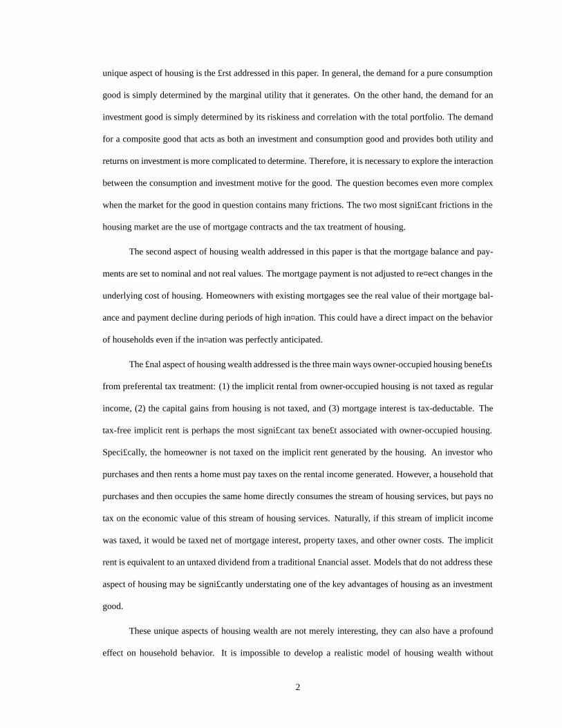
unique aspect of housing is the £rst addressed in this paper. In general, the demand for a pure consumption

good is simply determined by the marginal utility that it generates. On the other hand, the demand for an

investment good is simply determined by its riskiness and correlation with the total portfolio. The demand

for a composite good that acts as both an investment and consumption good and provides both utility and

returns on investment is more complicated to determine. Therefore, it is necessary to explore the interaction

between the consumption and investment motive for the good.The question becomes even more complex

when the market for the good in question contains many frictions. The two most signi£cant frictions in the

housing market are the use of mortgage contracts and the tax treatment of housing.

The second aspect of housing wealth addressed in this paper is that the mortgage balance and pay-

ments are set to nominal and not real values. The mortgage payment is not adjusted to re¤ect changes in the

underlying cost of housing. Homeowners with existing mortgages see the real value of their mortgage bal-

ance and payment decline during periods of high in¤ation. This could have a direct impact on the behavior

of households even if the in¤ation was perfectly anticipated.

The £nal aspect of housing wealth addressed is the three main ways owner-occupied housing bene£ts

from preferental tax treatment: (1) the implicit rental from owner-occupied housing is not taxed as regular

income, (2) the capital gains from housing is not taxed, and (3) mortgage interest is tax-deductable. The

tax-free implicit rent is perhaps the most signi£cant tax bene£t associated with owner-occupied housing.

Speci£cally, the homeowner is not taxed on the implicit rent generated by the housing. An investor who

purchases and then rents a home must pay taxes on the rental income generated. However, a household that

purchases and then occupies the same home directly consumesthe stream of housing services, but pays no

tax on the economic value of this stream of housing services.Naturally, if this stream of implicit income

was taxed, it would be taxed net of mortgage interest, property taxes, and other owner costs. The implicit

rent is equivalent to an untaxed dividend from a traditional£nancial asset. Models that do not address these

aspect of housing may be signi£cantly understating one of thekey advantages of housing as an investment

good.

These unique aspects of housing wealth are not merely interesting, they can also have a profound

effect on household behavior. It is impossible to develop a realistic model of housing wealth without

2

explicitly addressing these issues. A traditional model of£nancial assets cannot explain the portion of

housing demand driven by the desire to consume housing services. Likewise, a traditional model of durable

consumption goods cannot explain the portion of housing demand driven by investment motives. A model

that has real instead of nominal mortgage contracts is overstating the costs of the mortgage. The tax-free

status of the implicit rent is perhaps the single biggest taxadvantage housing has over other £nancial assets.

Given the importance of these issues, it is vital to explicitly include them in a model of housing wealth.

1.1.2 Challenges of Modeling Housing Wealth

The two approaches to modeling housing wealth’s role in the life-cycle each have advantages and

disadvantages. The £rst approach is to develop an abstract model that captures only a few of the most im-

portant aspects of housing as an investment good. Papers such as Martin (2001) and Fernandez-Villaverde

and Krueger (2001) follow this approach. This type of model’s advantages are that many can be solved

analytically, or embedded in a general equilibrium framework and solved numerically. The primary dis-

advantage is the relatively narrow scope of such a model. Thesecond approach is to sacri£ce simplicity

for a more complicated partial equilibrium model that can besolved numerically using stochastic dynamic

programming. Examples of this approach include Li and Yao (2004) and Hu (2002). Its advantage is that as

a more complex model it presents a more realistic picture of the role of housing wealth over the life-cycle.

The downside is an upper limit on the model’s complexity level, beyond which the solution times are no

longer tractable. Parallel processing can extend this upper limit in a grid-cluster or super-computer envi-

ronment. The greater complexity of the model requires greatcare in presenting the results and currently

precludes the option of embedding the model in a general equilibrium framework.

Both of the approaches described above are important and legitimate. Many of the questions the

more detailed partial equilibrium models can address are outside the scope of the general equilibrium

models. By explicitly including so many different aspects of housing wealth simultaneously, the partial

equilibrium model is extraordinarily ¤exible. For example,by incorporating a few simple changes to the

mortgage balance transition rule, the model can be used to simulate the effects of alternate mortgage con-

tracts on housing demand and portfolio allocation. The sameis true for changes in the tax treatment of

3

housing or the success of alternative preferences in explaining the role of housing wealth of the life-cycle.

The detailed partial equilibrium model in this paper provides important insight into how to develop an more

abstract general equilibrium model that can still capture the complexities associated with modeling housing

wealth.

1.1.3 A Detailed Partial Equilibrium Model of Housing Wealth

Housing wealth plays an important role, both as a signi£cant component of a household’s portfolio

and through its indirect effects on the demand for other types of investment assets. Housing wealth is also

very different from other types of £nancial assets, calling for a different modeling approach. The model

developed in this paper is used to demonstrate the importance of three unique aspects of housing wealth:

(1) the dual role as a consumption and investment good; (2) the signi£cance of the mortgage contract being

in nominal and not real terms; and (3) the tax bene£ts associated with owner-occupied housing. The paper

shows how each of these unique aspects of housing wealth has profound effects on the demand for housing

and the composition of household portfolios.

The model’s design allows households to choose their current consumption, their savings, their

savings allocated to risky assets, which type of housing to occupy, and whether to re£nance their mortgages.

The housing tenure choice includes a rental unit, a small home, and a large home. Households may increase

the sizes of their mortgage balances through the use of a cash-out re£nance. Renters choose the size of the

rental unit so that the intra-period marginal utility of housing is equal to the marginal utility of non-durable

consumption. The size of the large and small homes are £xed in terms of the number of housing units

they represent. Households face uncertainty in the returnson risky assets and housing, the probability of

survival, and a transitory shock to income; which is otherwise a deterministic function of age. The model

includes moving, maintenance, and transaction costs. Boththe option to and the costs of defaulting on a

mortgage are also included in the model. The model is solved given the terms of a traditional 30-year £xed

rate mortgage contract. The values of non-structural parameters, such as returns on different types of assets,

the survival probability, mortgage terms, and income process, are taken from historical data.

The model’s solution is then used to demonstrate the importance of each of the three unique aspects

4

of housing wealth being examined. Two different versions ofthe model are solved differentiating the

demands for housing as either an investment good or a consumption good. In the £rst version housing is

treated as only an investment good and there exists a perfectrental market. Households may always rent the

appropriate number of housing units such that the intra-period marginal utility of renting a house is equal to

the marginal utility of all other consumption. Housing merely represents an unusual investment good that

must be purchased using a traditional mortgage contract butgenerates no direct utility. The second version

of the model treats housing as only a consumption good. The downpayment and the mortgage payments by

the household are sunk costs and are not recouped when the home is sold. Instead households walk away

from home sales with no gain or loss from the transaction. Thepaper demonstrates the signi£cance of the

other two unique aspects of housing wealth in a similar way. To explore the effects of the nominal mortgage

contract to additional versions of the model are solve, one version where the mortgage contract is in real

and not nominal terms and another version with a historically high rate of in¤ation and a nominal mortgage

contract. Finally, versions of the model are solved where each of the three major tax bene£ts of owner-

occupied housing are removed: (1) the implicit rental from owner-occupied housing is taxed as regular

income, (2) the capital gains from housing is taxed, and (3) mortgage interest is no longer tax-deductable.

1.2 Literature Review.

Many of the existing papers on the role of housing wealth tended to focus on different factors behind

housing demand in isolation. Often housing was treated as either an investment good or as a consumption

good. Often the models that explicitly captured housing’s dual role did not include mortgage £nancing, or

at most included only an abstract version of the mortgage contract. One of the innovations of this paper

is to model housing as both an investment good and consumption good. The other key innovation is to

explicitly model the mortgage contract. An important aspect of this paper, shared by several of the papers

discussed below, is to model the portfolio allocation problem not just between one risky asset (stocks) and

one risk-free asset (government bonds) but the portfolio allocation across three different assets, two risky

(stocks and owner-occupied housing) and one risk-free asset (government bonds).

In several papers that explored in detail the role of housingwealth the actual decision of when and

5

how much housing to consume was not endogenous. Fratantoni (1997) solved a £nite-horizon model with

exogenous housing consumption and showed that introducinghousing in the model reduced the share of

risky assets held by households. The author extended the model in Fratantoni (2001) to show that the

commitment to make future mortgage payments resulted in a lower level of equity holdings. In Fernandez-

Villaverde and Krueger (2001) the authors observed that young consumers have portfolios with little liquid

assets but a signi£cant amount invested in durables. Fernandez-Villaverde and Krueger hypothesized that

young consumers can only borrow against future income by using their durable assets as collateral for loans.

They then developed a structural life-cycle model with endogenous borrowing constraints and interest rates.

Each of these papers explored an important aspect of housingwealth. However, by making the actual

demand for housing exogenous they are unable to explore whatexactly drives the demand for housing

wealth. In this paper housing demand is endogenous and it is possible to determine how some of the unique

aspects of housing wealth can drive the demand for housing.

Cocco (2000) developed a model with endogenous tenure choice to explore the effect of labor in-

come, interest rate, and house price risk on both housing choices and investor welfare. Cocco utilized an

abstract version of the mortgage contract where the level ofmortgage debt adjusts in each period so that

the loan-to-house value ratio remains £xed. Cocco’s automatically-re£nancing mortgage precludes the op-

portunity to pay down or pay off a mortgage, two very common strategies among households. The more

realistic mortgage model in this paper makes both of these strategies available to households.

Martin (2001) argued that consumers have an inaction regionin the purchase of durable goods

caused by transaction costs. Martin then argued that the inaction region in durable goods induces variation

in the consumption of non-durable goods. Martin’s model is ageneral equilibrium model and includes

only a risk-free £nancial asset. It does not address the interaction between housing investment and the

household’s portfolio allocation problem. Martin also models the mortgage used to purchase a house as

simply a negative position in the risk free bonds. In Martin,the inability of a single household to hold both

a mortgage and a £nancial asset prevents any discussion of household level portfolio allocation, one of the

key topics of this paper.

Hu (2002) developed a model very similar to the one in this paper where housing is endogenous. Hu

6

solved a £nite-horizon model that allowed for households to hold a risk-free asset, a risky asset, or risky

owner-occupied housing. Of the papers discussed here, Hu has the most detailed and realistic treatment

of the mortgage contract. Hu’s model re¤ects the composite nature of home equity and includes both the

current value of the house and the current balance of the mortgage. Hu also allows for the mortgage payment

to be £xed at the time of purchase. This model differs from Hu’sby £xing the nominal mortgage payment

while in¤ation reduces the real value of the mortgage payment. Additionally, Hu does not allow cash-out

re£nancing, a signi£cant aspect of this model.

Li and Yao (2004) explored the housing and mortgage decisions of a household over the life-cycle.

As this paper does, they utilized stochastic dynamic programming and parallel processing to solve an ex-

tremely detailed model. Many of their results were broadly consistent with this paper. However, this paper

differs signi£cantly from Li and Yao in the treatment of the mortgage contract. Li and Yao made two key

assumptions when modeling the mortgage contract in order tomake their model tractable. First, they as-

sumed that mortgages are amortized over the remainder of thehousehold’s life. Secondly, they assumed

that the mortgage payment is indexed to the current value of the house. These simpli£cations allowed them

to introduce permanent income shocks; which are absent fromthis paper. The cost of this simpli£cation was

to ignore the ability of a household to lock in its mortgage payments at a constant nominal value. The result

from Li and Yao’s approach was that mortgage payments were signi£cantly lower, understating the cost of

housing, and mortgage payments ¤uctuated with the value of the home, providing a form of insurance.

The dynamic stochastic optimizing framework adopted for the houshold for this paper is based on

Rust and Phelan (1996). Rust and Phelan set up and solve a dynamic programming problem of labor

supply with incomplete markets, Social Security, and Medicare. The dynamic programming problem in

their paper is solved by discretizing the continuous state spaces and then using backward recursion to solve

for the optimal value of the continuous choice variable at each point on the state space grid. The detailed

rules governing the Social Security and Medicare application processes and bene£ts are imbedded in the

income transition matrix. The model in this paper has a similar structure, but instead imbeds the detailed

characteristics of the mortgage market contract in the income transition matrix.

All of these papers represent important work on interestingaspects of housing wealth. However,

7

none of these papers attempts to develop a model that addresses all the unique characteristics of housing

wealth. The key issue in modeling housing wealth is the treatment of the mortgage contract. More than

any other single issue, it is mortgage £nancing that complicates realistically modeling housing wealth. The

main contribution of this paper is to include an unprecedentedly detailed model of the mortgage contract.

1.3 A Partial Equilibrium Model of Housing Wealth with Mortgage Contracts.

This section describes the structure of the £nite-horizon life-cycle model of a household’s savings,

investment, and housing decisions. The structure of the model described here was chosen to highlight the

effects of mortgage contracts on the evolution of housing wealth. In order to keep the model focused and

tractable aspects such as endogenous labor supply an marginaccount for risky asset are excluded. The

section concludes with a discussion of the method used to solve the household’s optimization problem.

The structure of the model is actually quite straight forward, with most of the complexities embedded in

the wealth transition rules. Households receive utility from the consumption of both a non-durable good

and the stock of housing that they own. Each period in the model represents a single year. Table B.1 in

Appendix B provides a listing of the model parameters and their de£nitions.

Their optimization problem is to maximize their lifetime utility, de£ned as:

E80

∑t=20

βtρtU(ct ,h(it))+βt(1−ρt)(θAUB(At)+θHUB(Ht)−θDUB(Dt)) ct > 0,∀t (1.1)

U(ct , it) =(c1−φ

t h(it)φ)1−λ

1−λ(1.2)

UB(b) =b1−λ

1−λ(1.3)

where,

• ct represents the consumption of non-durables;

• h(it) represents the number of units of housing services consumed, given the housing tenure choice in

period t (note that while the number of units of housing services consumed varies with tenure choice

8

the utility gained from a unit of services does not vary);

• At ,Ht , and Dt are respectively the value of the £nancial assets, home, and mortgage debt left as

bequests;

• β represents the discount rate;

• ρt is the survival probability;

• φ represents the measure of preference between of housing andconsumption;

• λ represents a measure of risk aversion; and,

• θA,θH , andθM represent bequest parameters.

A household lives at most 80 years. It faces uncertainty about its survival, temporary income shocks, and

the rate of return on both housing and risky assets. In addition to the stochastic elements for income and the

rate of return on risky assets, the households may experience an additional shock. A small probability exists

that the household will experience unemployment in one period, reducing income to zero. Also, a small

independent probability exists of a stock market crash where the household will lose 100% of its investment

in the risky £nancial asset. The probability of a stock marketcrash is in addition to the regular standard

deviation associated with the stochastic rate of return on risky assets. Households also are not allowed to

consume negative amounts of non-durable goods. The price ofthe consumption good is set equal to unity

and the rental price of housing is set equal to a constant ratio of the underlying price of the housing unit.

The in¤ation rate is constant and known.

1.3.1 Consumption of Housing

While consumption of the non-durable good in the model is continuous, the choices for housing

consumption are partially discrete. The model has three different alternatives for housing: a rental unit,

a small home, and a large home, represented by the corresponding symbolsir , is, andi l . The number of

housing units available to rent is continuous while the number of housing units provided by a small or large

9

home is £xed. Renter households are able to choose the number of housing units that equalizes their intra-

period marginal utility from housing to their intra-periodmarginal utility from non-durable consumption.

δU(ct ,h(it))δct

=δU(ct ,h(it))

δh(it)(1.4)

Optimal rental units may now be de£ned as a function of consumption,

h(ir) = (φ/(1−φ))ct (1.5)

Many other factors in the model are conditional on current housing tenure, including rent or mortgage

payments, maintenance costs, level of utility derived fromhousing, and the rate of appreciation in home

value. The size of a small home is set equal to that of a median priced home, while the size of a large home

is set to be twice that of a median priced home.

1.3.2 Accumulation of Financial Wealth and the Income Process

A household is “born” at age 20 with zero £nancial and housing wealth. It starts off as a renter with

no savings. In each period it receives a draw from an age-dependent income process. The model contains

no permanent income shock, only transitory shocks. In retirement, pension income is set to 60% of the

deterministic portion of age 65 income. Pension income is still subject to transitory shocks, representing

uncertainty regarding medical costs. Households can storetheir wealth in two different classes of assets,

£nancial and real. The household’s £nancial assets are held ina portfolio of risk free and risky assets. The

household can, at no cost, rebalance its £nancial portfolio between risk free and risky assets every period.

Households with zero wealth face a binding liquidity constraint for £nancial assets in that they cannot

borrow against their future income. Households also cannotpurchase leveraged portfolios, where they

borrow at the risk free rate to invest more in the risky asset.In addition to moving to one of the three types

of housing,{ir , is, i l}, the household can also decide to stay in its current home,{it+1 = it}. Households

may also either add to their mortgage balance through a cash-out re£nance or reduce their mortgage balance

through a pre-payment re£nance.

10

The transition rule for the level of £nancial wealth is de£ned as:

At+1 = (1+(1− γ)(αt rst +(1−αt)r))(At −ct −Xt(it ,κt)+ (1.6)

Gt(it , it+1,κt)+Zt(κt ,κt+1))+(1− γ)et+1 + γIt(it ,κt)

s.t. At+1 ≥ 0 & 0 ≤ αt ≤ 1

where,

• At is the level of £nancial assets in periodt;

• At+1 is a random variable that depends on the stochastic rate of return on risky assets (rst ) in period t

and the realizations of earning (et+1) in periodt +1;

• αt is the share invested in risky assets in time t;

• r is the deterministic rate of return on risk-free assets;

• Xt(it ,κt) (equation (C.7)) is the housing costs incurred in periodt for a household currently choosing

tenure typeit with a mortgageκt years old;

• It(it ,κt) (equation (1.15)) is the mortgage interest paid;

• Gt(it , it+1,κt) (equation (1.16)) is the net gain for a household choosingit this period andit+1 next

period;

• Zt(κt ,κt+1) (equation (1.17)) is the net gain from cash-out re£nancing; and

• γ is the tax rate on income and capital gains (note that both income and capital gains have the same

tax rate and taxes on capital gains are paid immediately).

The net gain from a home sale is tax-free and the mortgage interest paid is deducted from taxable income.

Both the housing expenses and the amount of the mortgage interest deduction are functions of the current

housing choice and age of mortgage. Re£nancing is modeled as achoice to lengthen the remaining number

of years on the mortgage, or inversely, to shorten the current age of the mortgage. The model only allows

11

cash-out re£nancing and does not allow prepayments. The age of a mortgage for a rental unit or a mortgage

that has been paid off is zero. Households receive their wages at the same time they realize the returns on

their investment from the previous period. As a result, the state variableAt represents all available cash on

hand, consisting of previous £nancial wealth and current income.

The income process is de£ned as a deterministic function of age plus a transitory shock, as shown

below in log form:

log(et) = ψ0 +ψ1t +ψ2t2 + εe (1.7)

εe ∼ N(0,σe)

The real rate of return on risky assets is a random variable with the distribution:

rst ∼ N(ηs,σ2s) (1.8)

whereηs is the expected real rate of return on the risky asset andσ2s is the variance.

1.3.3 Price of Housing

In addition to the portfolio of £nancial assets, households can also store their wealth in real assets

by purchasing a house. It is only through the purchase of a house, and the acquisition of a mortgage

loan, that households can borrow against their future income. The use of durable goods as collateral is

in the same spirit as Fernandez-Villaverde and Krueger (2001). The only mortgage contract available to

the household in this model requires a 20% down payment; has aterm of 30 years; and requires mortgage

payments based on a £xed interest rate and the size of the original mortgage. The mortgage balance and

the mortgage payment are both in nominal terms while the restof the model is in real terms. Households

selling their home are also required to pay a transaction cost equal to 10% of the value of the home that

they are purchasing. This represents realtors’ fees, credit checks, and other expenses associated with the

purchase.

The real price of housing has a positive trend over time. The purchase price of either a small or

12

large home increases non-stochastically by the average market price increase in each period. The value

of homes that have already been purchased changes accordingto a stochastic process, with the expected

increase equal to the non-stochastic market price increase. A household that has had a series of excellent

draws in home price appreciation will own a home worth relatively more than a comparable home on the

market. A household that has had a series of poor draws in homeprice appreciation will own a home worth

relatively less than a comparable home on the market.

The price per housing unit is the same across all types of housing. Large homes cost more than small

homes because they provide more units of housing for the homeowner to consume. Renters may choose

as small or as large a home to rent as they wish. Their rent is proportional to the current market value of

their chosen home. As the value of housing units change, so dotheir rental rates. The value of owner-

occupied units evolves stochastically while the value of newly purchased and rental units are set equal to

the current deterministic market price. The market price ofa housing unit is the number of housing units,

h(it), multiplied by the current market price of a housing unit,(1+ηh)tP0. The value of an owner-occupied

unit is the value of the unit from the previous period,Ht , multiplied by the realized rate of appreciation for

that unit in that period,(1+ rh). The price of owner-occupied housing is allowed to evolve differently from

the market price of housing in order to capture the idiosyncratic aspect of housing returns. The formulas

for the market price of home typeit (Pt(it)) and the housing wealth (Ht+1) transition rule are:

Pt(it) = (1+ηh)tP0h(it) (1.9)

Ht+1 =

Ht(1+ rh), it+1 = it

Pt(it), it+1 ∈ is, i l

0, it+1 = ir

(1.10)

rh ∼ N(ηh,σ2h) (1.11)

whereP0 is the price of a single unit of housing in period 0;rh is the realized rate of appreciation on housing

in period t;ηh is the expected rate of appreciation on housing; andσ2h is the variance of the house price

13

growth. Note that home prices are in real terms, the increasein the market price of housing is note due to

general in¤ation, but a real increase in the value of the housewith time.

1.3.4 The Mortgage

A signi£cant source of the complexity in the model is the need to include the age of the mortgage in

the state space. In the model this adds a discrete state variable with thirty-one discrete values, resulting in

over 1.7 million points in the £nal state space. The computational techniques used to solve a problem of this

scope are discussed brie¤y at the end of this section. The reason for including the age of the mortgage in the

state space is the nature of the 30-year self amortizing mortgage. First, the actual equity households hold in

their home is the difference between the value of the home minus the remaining balance on the outstanding

mortgage. To accurately track the value of the household’s home equity, it is necessary to track both the

value of the home and the mortgage balance independently. The nature of the mortgage contract further

complicates what would be a logical solution, the addition of a third continuous state variable for mortgage

debt. The principal paid on a self amortizing mortgage is notconstant over the life of the mortgage. Initial

payments are almost completely composed of interest, with very little principal being paid. The £nal

payments on a 30-year mortgage on the other hand are almost completely principal, with very little interest

being paid. Therefore, the transition rule for mortgage debt is a function of the age of the mortgage. The fact

that the mortgage balance and mortgage payment are in nominal terms provides an additional motivation for

including the age of the mortgage in the state space. The realvalues of the mortgage balance and payment

decline steadily over the life of the mortgage due to in¤ation.

The mortgage payment is based on the home price when purchased, and only changes when the

household re£nances the mortgage or sells the house. A cash-out re£nance increases the number of years

left on the mortgage. The formula for the real value of a mortgage payment at timet after κt years on a

house of typeit is:

Mt(it ,κt) = π(1−µ)Pt−κt [(1− (1+π)−κt )(1+ν)κt ]−1 (1.12)

whereπ is the nominal mortgage interest rate;ν is the in¤ation rate; andµ is the required down payment.

The cost of housing services also re¤ects the maintenance costs paid by homeowners. As a result,

14

the formula for the real cost of housing services is:

Xt(it ,κt) =

Mt(it ,κt)+δHt , it ∈ is, i l

0.06Pt(ir), it = ir

(1.13)

whereδ is the percent of current home value required in maintenancecosts. Rent is equal to 6% of the

current market value of the unit being rented and renters paynone of the maintenance costs for the property.

The present value of the household’s home equity is the current value of the house minus the amount

of the outstanding mortgage balance. While the value of the house increases or decreases according to the

stochastic return on housing, the outstanding mortgage balance is a monotonically declining function of the

age of the mortgage. The formula for the real value of the mortgage balance at timet after κt years on a

house of typeit is:

Dt(it ,κt) =

Mt(it ,κt)1−(1−π)κt−30

π , it ∈ is, i l & κt ≤ 30

0, (it ∈ is, i l & κt > 30) or (it = ir)

(1.14)

The formulas for the mortgage payment is used to calculate the amount of mortgage interest paid

for tax purposes. The values must be adjusted back from the real terms since this deduction is in nominal

terms. The formula for the mortgage interest deduction is:

It(it ,κt) = πMt(it ,κt)(1− (1+π)κt−30)(1+ν)κt (1.15)

15

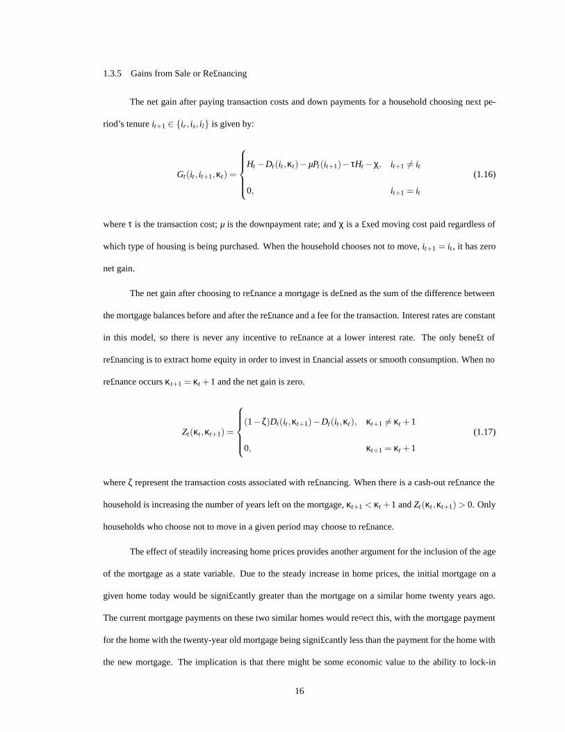
1.3.5 Gains from Sale or Re£nancing

The net gain after paying transaction costs and down payments for a household choosing next pe-

riod’s tenureit+1 ∈ {ir , is, i l} is given by:

Gt(it , it+1,κt) =

Ht −Dt(it ,κt)−µPt(it+1)− τHt −χ, it+1 6= it

0, it+1 = it

(1.16)

whereτ is the transaction cost;µ is the downpayment rate; andχ is a £xed moving cost paid regardless of

which type of housing is being purchased. When the household chooses not to move,it+1 = it , it has zero

net gain.

The net gain after choosing to re£nance a mortgage is de£ned as the sum of the difference between

the mortgage balances before and after the re£nance and a fee for the transaction. Interest rates are constant

in this model, so there is never any incentive to re£nance at a lower interest rate. The only bene£t of

re£nancing is to extract home equity in order to invest in £nancial assets or smooth consumption. When no

re£nance occursκt+1 = κt +1 and the net gain is zero.

Zt(κt ,κt+1) =

(1−ζ)Dt(it ,κt+1)−Dt(it ,κt), κt+1 6= κt +1

0, κt+1 = κt +1

(1.17)

whereζ represent the transaction costs associated with re£nancing. When there is a cash-out re£nance the

household is increasing the number of years left on the mortgage,κt+1 < κt +1 andZt(κt ,κt+1) > 0. Only

households who choose not to move in a given period may chooseto re£nance.

The effect of steadily increasing home prices provides another argument for the inclusion of the age

of the mortgage as a state variable. Due to the steady increase in home prices, the initial mortgage on a

given home today would be signi£cantly greater than the mortgage on a similar home twenty years ago.

The current mortgage payments on these two similar homes would re¤ect this, with the mortgage payment

for the home with the twenty-year old mortgage being signi£cantly less than the payment for the home with

the new mortgage. The implication is that there might be someeconomic value to the ability to lock-in

16

the recurring housing expense at a £xed level while the marketprice of housing ¤uctuates. This allows the

model to capture the role of housing as a hedge against variability in rents, as argued by Sinai and Souleles

(2003).

1.3.6 Default Penalties

Figure 1.1: Timing of Decisions

Realize income and investment returns from period t-1

Can household make housing payment with liquid assets?

Can household make housing payment after liquidating home equity?

No

Choose optimal new tenure, consumption and investment conditional on budget constraints

Yes

Yes, Must Move No, Must Rent

The model also contains a default penalty. In any period the household must be able to cover

its housing expenses, including the rent or mortgage and maintenance costs. If it fails to do so, it must

move the next period into rental housing, forfeiting all itshome equity and all its £nancial equity above

some small nominal amount. Households that can cover their expenses by selling their current house and

extracting their home equity are allowed to do so. Households that can afford the associated transaction

costs may also avoid defaulting through a cash out re£nance. The advantage of this for the household is the

ability to keep its housing equity. Current consumption is also constrained to equal that same small nominal

amount. The £rst constraint, shown in equation (2.8), affects those households that are forced to move but

can avoid defaulting and the second constraint affects those households that default. The restriction that

At+1 may not be negative, combined with the de£nitions ofXt(it ,κt), Zt(κt ,κt+1), andGt(it , it+1,κt), along

with the budget constraint, create an upper bound on possible levels of non-durable consumption, and also

17

rule out some possible choices of housing tenure. If the household cannot afford the down payment for a

large home without incurring negative wealth, it is not allowed to move to such a home. The ¤ow chart

above shows how the default penalties affect the household’s decisions.

1.3.7 Optimization Problem and Value Functions

The household’s optimization problem is to choose variables ct ,αt , it+1,κt+1 given a series of state

variablest,κt , it ,At ,Ht to optimize equation (2.2) given equations (2.4) (1.16). The household only has one

choice of mortgage contract, with a £xed downpayment rate. The choice variableκt+1 capture the ability of

a household to cash-out home equity by re£nancing, and therefore reduce the effective age of the mortgage

as described above.

The value function of the household is the maximum utility, subject to the default constraints of the

value functions for the households that choose next period tenure typeit+1 ∈ {ir , is, i l , it}:

(At −Xt(it ,κt) < 0) & (At −Xt(it ,κt)+ maxit+1,κt+1

(Gt(it , it+1)+Zt(κt ,κt+1))) > 0) ⇒ (1.18)

Vt(it ,At ,Ht ,κt) = maxit+1 6=itorκt+1 6=κt+1,ct ,αt

V it+1t (it+1,At ,Ht ,κt)

(At −Xt(it ,κt) < 0) & (At −Xt(it ,κt)+ maxit+1,κt+1

(Gt(it , it+1)+Zt(κt ,κt+1))) > 0) ⇒ (1.19)

Vt(it ,At ,Ht ,κt) = U(ω,h(it))+βρtVt(ir ,ω,0,0)+β(1−ρt)θAUB(ω)

(At −Xt(it ,κt) > 0) ⇒ (1.20)

Vt(it ,At ,Ht ,κt) = maxit+1∈{ir ,is,i l },ct ,αt ,κt+1

V it+1t (im,At ,Ht ,κt)

whereω is the amount of consumption and wealth protected in defaultfrom creditors. Equation (2.8)

is the value function when the households recurring housingexpenses,Xt(it ,κt), are greater than their

available liquid assets,At , but if their net equity after selling or re£nancing their home is positive,(At −

18

Xt(it ,κt)+ maxit+1,κt+1(Gt(it , it+1)+ Zt(κt ,κt+1))). Faced with this constraint, the household must either

more, it+1 6= it , or re£nance,κt+1 6= κt + 1. Equation (1.19) is the value function when the household

cannot cover their recurring housing expenses out of their liquid assets and their net equity after selling

or re£nancing their home is negative. These households must move to a rental unit ,i t+1 = ir , and have

both their consumption and remaining wealth limited toω. Equation (1.20) is the value function when the

households can cover their recurring housing expenses out of their liquid assets. The only limits to their

choices are those imbedded in the constraints in equation (2.9).

The value function conditional on next period’s tenure choice it+1 is:

V it+1t (it ,At ,Ht ,κt) =

maxct ,αt

U(ct ,h(it))+βρtVt(it+1,At+1,Ht+1,1)+

β(1−ρt)(θAUB(At)+θHUB(Ht)−θDUB(Dt)),

it+1 ∈ {ir , is, i l}

maxct ,αt ,κt+1

U(ct ,h(it))+βρtVt(it+1,At+1,Ht+1,1)+

β(1−ρt)(θAUB(At)+θHUB(Ht)−θDUB(Dt)),

it+1 = it

(1.21)

such that equations (2.4) to (1.20) hold.

The structure of this problem contains several signi£cant sources of non-continuity. The £rst is the

discrete nature of housing tenure, which functions as both achoice and a state variable. The second main

source of the non-continuity is the structure of the value function, which is de£ned as the maximum of

over sixty-six different value functions, one for each possible combination of four tenure choices or two

re£nance options and eleven portfolio allocations. This non-continuity of the model prevents the use of

analytical methods to derive a solution. It also prevents the derivation of Euler equations. The model is

instead solved using computational methods based on the methods used in Rust and Phelan (1997).

The code used to solve this problem is in C. One solution of theproblem initially took roughly two

weeks on a dual processor Pentium Xeon 1.8GHz with 512K L2 cache and 1GB of RAM running Linux.

In order to improve the run-time, the code was re-written to take advantage of parallel processing, using

the Message Passing Interface (MPI) standard. In this version of the code one processor is designated

the master while a pool of other processors are designated slaves. As the model is solved recursively by

19

year, the master distributes the current value function forall previous years to the slaves. Each slave then

solves for the optimal value function for a sub-set of state spaces for the given year. The slaves then return

the new value function values to the master. The master then combines the new values with the value

function for the previous year, completing the recursion for one year. The problem was solved using 61

high-performance Digital Alpha 64-bit microprocessors running at 450MHz each on a scalable parallel

Cray T3E at the Pittsburgh Supercomputing Center. One solution involved roughly 1.3 billion evaluations

of the value function and took roughly eight and a half hours.

1.4 Baseline Model Results.

The parameter values for the model calibration are chosen tobe consistent with other models in the

relevant literature. The parameter values for the size of small and large homes are set so that they represent,

respectively, a home 80% and 120% the size of a median priced home. Theφ value of 0.2 re¤ects the

share of total household expenditures allocated to housingexpenditures in the 2001 Consumer Expenditure

Survey from the U.S. Department of Labor. This paper does notrepresent a serious attempt to calibrate

a model of housing wealth or to estimate the maximum likelihood parameters of such a model. The goal

is to see how closely the model can match certain stylized facts while using fairly standard and common

parameter values. Appendix A contains more information on the values of the market and preference

parameters chosen. A series of graphs of the policy functions, from one of the calibrated models, for

households receiving different series of shocks are then presented, to illuminate the factors driving the

economic decisions of the household. Finally, some resultsfrom simulations based on the baseline model

are given. The baseline model matches several patterns seenin the empirical data.

1.4.1 Policy Functions

Figures 1.2 through 1.5 report sample policy functions for arange of households. Each £gures

contains the policy functions for three different types of households over the life-cycle, based on the type

of shocks to income and the returns to both housing and risky assets. In each £gure, the top panel reports

the policy function for a household that receives in each period above average shocks, the middle panel

20

Figure 1.2: Housing Tenure Policy Functions

20 30 40 50 60 70 800.5

1

1.5

2

2.5

3

3.5(a) Above Average Shocks

Age

1 = Rent

2 = Buy Small Home

3 = Buy Large Home

20 30 40 50 60 70 800.5

1

1.5

2

2.5

3

3.5(b) Average Shocks

Age

20 30 40 50 60 70 800.5

1

1.5

2

2.5

3

3.5(c) Below Average Shocks

Age

21

reports the policy functions for a household receiving average shocks, and the £nal panel reports the policy

function for a household that receives in each period below average shocks. It is important to note that these

households do not realize that their future shocks have beenarti£cially pre-ordained. They each believe that

the shocks each period are independent from those in other periods, just as was the case when the model

was solved.

The three panels in Figure 1.2 shows the tenure choices for each of our three sample households as

a function of age. Naturally the household with the above average shocks is the £rst to purchase a home

in their mid-twenties. The average household is only able toafford this transition in their earlier thirties

while the below average household is forced to wait until their mid-£fties. The above average household

is also able to trade-up to a larger home in their earlier thirties. In about ten-years they trade back down

to a small home, shifting a signi£cant portion of their wealthfrom housing to £nancial assets and reducing

their mortgage payment. After a few more years of above average returns, they trade-up again, only to

trade-down again after age 50. Once they reach this age, theycan lock in their nominal mortgage payments

for the rest of their life by purchasing a smaller home. The average household stays in their home until the

mid-seventies when they spend a brief time renting, before buying another small home. The below average

household sells their home in their late-seventies and rents for the rest of their life.

Figure 1.3 shows the consumption policy functions and realized wages for each of the three house-

holds. The higher realized investment returns allows the above average household to consume more than

their annual wage by the time they are £fty. As they continue toreceive above average shocks, they continue

to increase their consumption. One interesting results is that each of these three households reduce their

consumption immediately prior to purchasing a home. They also increase their consumption when they

trade-down. Households who choose not to move also have higher levels of consumption. Since they are

not adjusting their housing consumption, they compensate by increasing their consumption of non-durables.

This pattern of behavior is similar to that described in Martin (2001)

Figure 2.2 shows how the housing and £nancial wealth policy function for the three households. It

shows how £nancial wealth falls when households purchase homes, representing the effect of the down-

payment and transaction costs. The £gure also shows how households shift wealth back from housing

22

Figure 1.3: Consumption Policy Functions and Realized Wages

20 30 40 50 60 70 800

1

2

3

4

5

6(a) Above Average Shocks

Age

Mean

Valu

e ($

0,00

0) fo

r Sur

vivor

s in

Coho

rt

WagesConsumption

20 30 40 50 60 70 800

0.5

1

1.5

2

2.5(b) Average Shocks

Mea

n Va

lue ($

0,00

0) fo

r Sur

vivor

s in

Coho

rt

Age

20 30 40 50 60 70 800

0.2

0.4

0.6

0.8

1

1.2

1.4

1.6

1.8(c) Below Average Shocks

Mea

n Va

lue ($

0,00

0) fo

r Sur

vivor

s in

Coho

rt

Age

23

Figure 1.4: Home Equity and Financial Wealth Policy Functions

20 30 40 50 60 70 800

5

10

15

20

25

30

35

40

45

50(a) Above Average Shocks

Age

Mea

n Va

lue ($

0,00

0) fo

r Sur

vivor

s in

Coho

rt

Financial Wealth

Housing Wealth

20 30 40 50 60 70 800

1

2

3

4

5

6

7

8

9

10(b) Average Shocks

Mea

n Va

lue ($

0,00

0) fo

r Sur

vivor

s in

Coho

rt

Age

20 30 40 50 60 70 800

0.5

1

1.5

2

2.5

3

3.5(c) Below Average Shocks

Mea

n Va

lue ($

0,00

0) fo

r Sur

vivor

s in

Coho

rt

Age

24

Figure 1.5: Portfolio Allocation Policy Function

20 30 40 50 60 70 800

0.1

0.2

0.3

0.4

0.5

0.6

0.7

0.8

0.9

1(a) Above Average Shocks

Age

Mea

n Sh

are

of A

sset

s Held

for S

urviv

ors i

n Co

hort

Home Equity as Share of Total Wealth

Risk Assets as Share of Financial Wealth

20 30 40 50 60 70 800

0.1

0.2

0.3

0.4

0.5

0.6

0.7

0.8

0.9

1(b) Average Shocks

Mea

n Sh

are

of A

sset

s Held

for S

urviv

ors i

n Co

hort

Age

20 30 40 50 60 70 800

0.1

0.2

0.3

0.4

0.5

0.6

0.7

0.8

0.9

1(c) Below Average Shocks

Mea

n Sh

are

of A

sset

s Held

for S

urviv

ors i

n Co

hort

Age

25

to £nancial assets. Figure 1.5 reports the portfolio allocation policy functions for the three households.

Households who are remaining renters invest a smaller amount of their portfolio in risky assets. They

are focused on saving for a downpayment as quickly as possible, giving them a fairly short time horizon.

The renters therefore choose a conservative portfolio thatis more tilted towards asset protection than asset

growth. Those households purchasing homes now own a second risky asset, their house, that is uncorrelated

with the risky £nancial asset. In response to their increaseddiversi£cation, they increase their investment

in the risky asset. In the period in which households purchase their home they also sharply reduce their

holdings in the risky asset.

1.4.2 Simulation Results

To better explore the implications of the model, 1,000 simulations are generated using the calibrated

model. The table and £gures below contain the results from these simulations. Households begin at age 20

as renters with no assets. Households retire at age 65 and live to at most 80 years of age. The simulations

track their accumulation of housing and £nancial wealth overtheir lifetime. Figures 2.1 and 2.4 present the

simulation results across the life cycle. These £gures show the role of housing over the life cycle, and how

consumption and investment decisions are linked to housingdecisions.

Figure 2.1 shows the consumption and income paths over the life-cycle. The sharp drop in income in

retirement can be seen in panel (a), while consumption is much smoother. Panel (b) shows the path of con-

sumption as a share of total wealth. Younger households who are aggressively saving for a downpayment

consume the smallest share of their wealth. Once householdsbecome homeowners, their consumption as a

share of total wealth climbs, peaking near 16% around the ageof 30. As households approach retirement,

they start to accumulate more wealth, and consumption as a share of total wealth starts to fall reaching a

low point of 9% at age 65. In retirement households draw down their savings and consumption as a share

of total wealth climbs again. At retirement the average household has roughly forty-£ve times their annual

income saved in both housing and £nancial wealth.

The importance of housing wealth in retirement is emphasized by the next set of £gures. Fig-

ure 2.3 (a) shows that housing wealth has a hump over the life cycle, reaching a peak at 60 and starting to

26

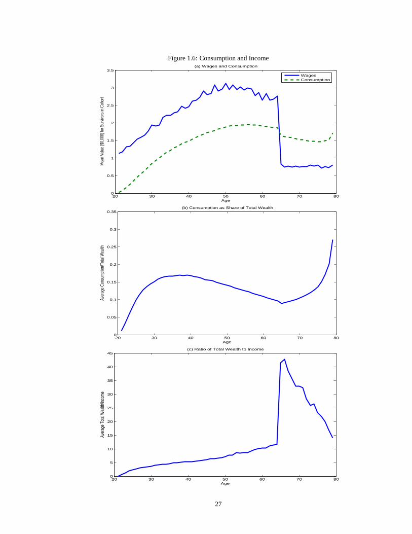
Figure 1.6: Consumption and Income

20 30 40 50 60 70 800

0.5

1

1.5

2

2.5

3

3.5(a) Wages and Consumption

Age

Mea

n Va

lue ($

0,00

0) fo

r Sur

vivor

s in

Coho

rt

WagesConsumption

20 30 40 50 60 70 800

0.05

0.1

0.15

0.2

0.25

0.3

0.35(b) Consumption as Share of Total Wealth

Age

Aver

age

Cons

umpt

ion/T

otal

Wea

lth

20 30 40 50 60 70 800

5

10

15

20

25

30

35

40

45(c) Ratio of Total Wealth to Income

Age

Aver

age

Tota

l Wea

lth/In

com

e

27

Figure 1.7: Wealth and Portfolio Choice

20 30 40 50 60 70 800

1

2

3

4

5

6(a) Simulated Housing Wealth

Age

Me

an

Va

lue

($

0,0

00

) fo

r S

urv

ivo

rs in

Co

ho

rt

20 30 40 50 60 70 800

2

4

6

8

10

12(b) Simulated Financial Wealth

Age

Me

an

Va

lue

($

0,0

00

) fo

r S

urv

ivo

rs in

Co

ho

rt

20 30 40 50 60 70 800

0.1

0.2

0.3

0.4

0.5

0.6

0.7

0.8(c) Simulated Share of Housing Assets for Owners

Age

Me

an

Sh

are

of A

sse

ts H

eld

fo

r S

urv

ivo

rs in

Co

ho

rt

20 30 40 50 60 70 800.2

0.3

0.4

0.5

0.6

0.7

0.8

0.9

1(d) Simulated Risky Share of Financial Assets

Age

Me

an

Sh

are

of A

sse

ts H

eld

fo

r S

urv

ivo

rs in

Co

ho

rt

28

decline as households approach retirement. The brief plateau in the growth of housing wealth at age 50 is

caused by many households either trading down to smaller homes or re£nancing their existing mortgage in

order to lock in nominal mortgage payments for the rest of their expected life. Financial wealth, shown in

Figure 2.3 (b), is more sharply humped and peaks at age 65.

One implication of the model is that accumulated home equityis used to £nance the consumption of

non-durables in only late in retirement. The actual role of housing wealth among the elderly is a bit more

complicated. Venti and Wise (2000) found that housing wealth was not in fact used to support non-housing

consumption. They £nd that households resort to their home equity only when faced by a signi£cant shock

such as the death of a spouse or a serious illness. This is similar to the £nding in Sheiner and Weiss (1992)

that anticipation of death and illness signi£cantly increases the probability that households reduce their

home equity. These conclusions £nd additional support in theresults of this model, in that households

do not tap into housing wealth in retirement until their reserves of £nancial wealth have been depleted.

However the model does result in more rapid decline in housing wealth than seen in the data. The lack of

health status as a state variable and the connection betweenhealth status and retiree tenure choice might

explain this failure of the model.

Figures 2.3 (c) and 2.3 (d) provide the most signi£cant results of the model. As Figure 2.3 (c) shows,

the simulated share of assets held in housing is consistently near 40%, a bit below the empirical average of

67%. The housing share is high among young households who must invest a large portion of their savings

in a downpayment. As £nancial wealth grows faster than housing wealth this share falls initially. The

jagged nature of the curve re¤ects a combination of re£nancingand trading up as younger households try

to keep their portfolios balanced while taking advantage oftheir greater £nancial resources to purchase

larger homes. The rate of increase in the share climbs in retirement, as households draw down £nancial

wealth prior to extracting home equity. Household’s face signi£cant transaction costs, due in part to the

nature of the mortgage contract, to access their home equity. As a result, households turn to £nancial equity

initially to fund consumption in retirement. This partially matches the ”over-investment” in housing seen

in the empirical data, as reported by Flavin and Yamashita, using a model of rational, forward looking

agents. The implication is that while some degree ”over-investment” in housing is the result of something

29

Figure 1.8: Housing Tenure Choice

20 30 40 50 60 70 800

0.1

0.2

0.3

0.4

0.5

0.6

0.7

0.8

0.9

1(a) Simulated Homeownership Rate

Age

Fra

ctio

n o

f S

urv

ivo

rs in

Co

ho

rt

20 30 40 50 60 70 800

0.05

0.1

0.15

0.2

0.25(a) Simulated Share of Homeowners in Large Homes

Age

Fra

ctio

n o

f S

urv

ivo

rs in

Co

ho

rt

20 30 40 50 60 70 800

0.1

0.2

0.3

0.4

0.5

0.6

0.7

0.8(c) Simulated Loan−to−Value Ratio

Age

Ave

rag

e R

atio

of L

oa

n−

to−

Va

lue

of

Ho

me

20 30 40 50 60 70 800

0.005

0.01

0.015

0.02

0.025

0.03

0.035

0.04

0.045

0.05(d) Simulated Refinancing Rate

Age

Fra

ctio

n o

f S

urv

ivo

rs in

Co

ho

rt

30

innate in the nature of the housing good or the mortgage contract used to purchase it and not the result

of sub-optimal behavior by non-rational consumers, the actual level of ”over-investment” in housing seen

empirically cannot be fully explained with this model.

Figure 2.3 (d) shows the pattern of allocation in the £nancialportfolio over the life cycle. Young

households who are aggressively saving for or already have large shares of their wealth tied up in down-

payments invest less in the risky asset, as do older households who have drawn down their £nancial wealth

relative to their housing wealth. The risky portfolio sharepeaks around age 50, just when the households

start to actively shift their total portfolio away from homeequity.

The £nal set of £gures from the simulations document the role ofhousing over the life-cycle. Fig-

ure 2.4 (a) shows home-ownership increasing rapidly for younger households and declining very slightly in

retirement. The share of homeowners living in larger homes has a similar hump, as seen in Figure 2.4 (b),

with a sharp drop at age 50. Both of these charts document the strategy of households trading down in re-

tirement to access housing wealth to £nance consumption. Figure 2.4 (c) documents an interesting pattern.

Households who have recently purchased their homes are required to have an initial loan-to-value ratio of

80%. They are then able to pay down their mortgage through theregular amortization schedule and the

average loan-to-value ratio falls. The average loan-to-value ratio seems to stabilize at 10% before climbing

late in retirement in response to a surge in cash-out re£nancing. Figure 2.4 (d) reports the level of re£nanc-

ing activity over the life-cycle. Younger households and those who have just purchased their homes take

advantage of re£nancing to re-balance their portfolios and smooth their income. Older households start to

use cash-out re£nances to access their equity.

In Figure 2.4 (b) there was a sharp drop in the share of households living in large homes at age 50,

with the share falling from a high of 20% to 16%. The timing of this sudden shift into smaller homes is a

result of the 30-year mortgage combined with a maximum age of80 imposed by the model speci£cations.

Households take advantage of the 30-year mortgage term to lock in their nominal mortgage payments for

the rest of their natural lives. Figuree 1.9 provides additional support for this hypothesis. In addition to

the baseline simulations this £gure also reports the simulations with the a 20-year mortgage and when

retirement is delayed until 75. The goal is to demonstrate that the shift into smaller homes is driven by the

31

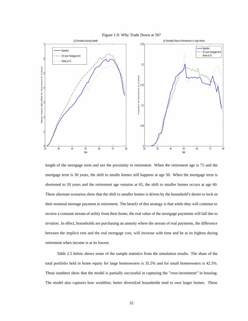
Figure 1.9: Why Trade Down at 50?

20 30 40 50 60 70 800

1

2

3

4

5

6

7(a) Simulated Housing Wealth

Age

Me

an

Va

lue

($

0,0

00

) fo

r S

urv

ivo

rs in

Co

ho

rt

Baseline

20−year mortgage term

Retire at 75

20 30 40 50 60 70 800

0.05

0.1

0.15

0.2

0.25(b) Simulated Share of Homeowners in Large Homes

Age

Fra

ctio

n o

f S

urv

ivo

rs in

Co

ho

rt

Baseline20−year mortgage termRetire at 75

length of the mortgage term and not the proximity to retirement. When the retirement age is 75 and the

mortgage term is 30 years, the shift to smalle homes still happens at age 50. When the mortgage term is

shortened to 20 years and the retirement age remains at 65, the shift to smaller homes occurs at age 60.

These alternate scenarios show that the shift to smaller homes is driven by the household’s desire to lock-in

their nominal mortage payment in retirement. The bene£t of this strategy is that while they will continue to

receive a constant stream of utility from their home, the real value of the mortgage payments will fall due to

in¤ation. In effect, households are purchasing an annuity where the stream of real payments, the difference

between the implicit rent and the real mortgage cost, will increase with time and be at its highest during

retirement when income is at its lowest.

Table 2.5 below shows some of the sample statistics from the simulation results. The share of the

total portfolio held in home equity for large homeowners is 35.5% and for small homeowners is 42.5%.

These numbers show that the model is partially successful incapturing the ”over-investment” in housing.

The model also captures how wealthier, better diversi£ed households tend to own larger homes. These

32

results also show how renters, who are aggressively saving for a down payment, have the smallest risky

asset portfolio share.

Table 1.1: Simulation Results - Baseline ModelTotal Rental Units Small Homes Large Homes

Percent 100% 12.6% 76.2% 11.2%Consumption 13,820 2,140 15,190 17,570

(7,380) (2,440) (6,230) (5,890)Financial Assets 58,090 9,670 60,810 94,010

(58,840) (11,120) (57,670) (64,490)Risky Asset Share 83.3% 28.9% 91.3% 90.0%

(26.3%) (21.8%) (15.4%) (15.6%)Tenure Length 8.5 1.0 9.4 10.3

(9.0) (0.0) (9.2) (8.8)Net Equity in Home 37,710 50,240

(28,530) (38,010)Home Equity Share 42.5% 35.5%

(195.3%) (28.1%)

Note: The standard deviations are presented in parentheses.

1.4.3 Tenure Transitions

Table 1.2 more fully explores the role of housing tenure decisions in the model. It demonstrates that

households are eager to move out of rental housing with almost 20% of all renters purchasing homes in the

next period. Households that have saved enough money by their mid-twenties are able to move into small

homes. In a only one case out of the 1,000 simulations, does a household move directly from a rental to a

large home. This household, in particular, had just recieved a very large positive income shock that allowed

them to £nance the purchase of the home. Huseholds that are still saving for a downpayment tend to have

the least held in risky assets, only 27.1% of the £nancial portfolio. Households that have already saved

enough to purchase a home hold more in risky assets.

The transition out of small homes seldom occurs. Almost 98.2% of small home-owners remain in

small homes. Half of those who do remain are trading up to larger homes, while one-quarter are returning

the rental market and one-quarter are extracting home equity through cash-out re£nancing. Households

who run into £nancial trouble and are forced to return to the rental market do so fairly quickly, averaging

less than four years in their current home. Given that their average age is close to 60, while the average

age of a £rst-time home buyer is close to 30, these are households who became homeowners late in life due

33

to poor income and return on equity shocks early in the life-cycle. As relatively recent homeowners, they

have not yet accumulated a signi£cant amount of home equity. Households with low loan-to-value ratios

but high share of housing in their portfolio are the most likely to take cash-out re£nances. Households

who are staying put and not re£nancing have the largest risky asset share in their £nancial portfolio, while

those being forced to move to rental housing have the lowest.Households trading up also hold lower shares

of risky assets in their £nancial portfolios. This is anotherexample of the inverse relationship between

demand for home equity and for risky assets. Recent poor income and investment shocks contribute to the

decision to return to rental housing while very strong positive shocks to housing encourage the households

to trade-up.

Table 1.2: Tenure Transitions - Baseline ModelCurrent Status Not Rent Buy Small Buy Large Cash-Out

Moving Home Home Re£Renter Transition Probability 82.2% 17.79% 0.01%

Financial Wealth 7,690 18,820 12,960Risky Portfolio Share 27.1% 37.2% 80.0%

Age 24.2 29.0 29.0Risky Asset Shock Last Period 5.5% 5.4% -7.8%

Wage Shock Last Period 3,090 2,640 4,440Small Home Transition Probability 98.2% 0.5% 0.9% 0.4%

Financial Wealth 61,390 7,880 45,120 1,400Housing Wealth 36,950 66,970 89,180 73,390

Risky Portfolio Share 91.8% 45.3% 76.9% 59.1%Portfolio Share of Housing 41.8% 87.1% 69.3% 86.8%

Loan-To-Value Ratio 38.4% 22.4% 26.0% 20.8%Age 49.5 59.0 45.6 57.8

Tenure Length 9.5 3.6 8.7 7.9Housing Shock Last Period 1.0% 0.3% 1.7% 0.5%

Risky Asset Shock Last Period 5.4% 6.8% 4.3% 5.7%Wage Shock Last Period 6,170 2,720 4,440 4,650

Large Home Transition Probability 96.0% 0.1% 3.9%Financial Wealth 95,320 1,980 64,150Housing Wealth 48,830 45,580 84,550

Risky Portfolio Share 90.7% 52.0% 72.3%Portfolio Share of Housing 34.5% 95.6% 58.7%

Loan-To-Value Ratio 47.6% 8.1% 40.0%Age 54.4 78.2 57.9

Tenure Length 10.5 4.8 5.5Housing Shock Last Period 1.0% -2.5% 0.8%

Risky Asset Shock Last Period 5.1% 10.4% 6.0%Wage Shock Last Period 6,610 2,410 10,420

Once households have managed to move into large homes, they naturally prefer to stay there. Of

these homeowners, 96%, do not move. Interestly, none of these households utilize cash-out re£nancing to

extract home equity. They do trade down to smaller homes or torental units. Most of the movers are trading

34

down into smaller homes. The households have a higher portfolio share of housing, a lower LTV ratio, and

lower share of their £nancial portfolio in risky assets than those households not trading down. Households

trading down to smaller homes also have large recent positive income shocks, allowing them the pay for

the transaction costs associated with the move. Householdswith very little £nancial wealth who have also

had recent poor income shocks are more likely to move directly into rental units. These households are also

signi£cantly older than those trading down to smaller homes or staying put. Again, these homeowners take

the most conservative positions in the £nancial portfolio.

This section has established the most signi£cant accomplishment of the model the ability to partially

match the ”over-investment” in housing seen in the data within a framework of rational, forward-looking

agents. This section has also argued that the optimal share of risky assets in the £nancial portfolio is effected

by both the level of investment in housing and the endogenoustenure choices of the household. The next

section will build on these results with a detailed examination of how the unique nature of housing wealth

affects the demand for housing and the allocation of household portfolios.

1.5 Alternative Scenarios.

The previous section provided evidence that the baseline model can match certain stylized facts

about housing wealth over the life-cycle. This section determines exactly in what way does these three

speci£c aspects of housing wealth affect the demand for housing and £nancial portfolio allocation over

the life-cycle. This is accomplished through a series of comparative static exercises. The three aspects of

housing wealth being investigated are in each turn excludedfrom the model. Each alternative model is then

re-solved and the simulations regenerated. The levels of wealth accumulation, housing demand, re£nance

activity, and portfolio allocation under each alternativeassumption are then compared to the base case.

Table 1.3 summarizes how the model is altered for each of the alternative scenarios. Table 1.4 summarizes

the effects of each scenario on the demand for housing wealth, £nancial assets, total portfolio share of

housing, and the £nancial portfolio share of risky assets.

35

Table 1.3: Assumptions for Alternative ScenariosAlternative Assumption Model Effects

Dual Investment/Consumption RoleConsumption Only Replace (1.16) with (1.22)

Replace (1.17) with (1.23)Replace (1.5) with (1.24)

Investment Only Replace (2.2) with (1.25)Replace (C.7) with (1.26)

Nominal Mortgage ContractHigh In¤ation ν = 6%

Real Mortgage Contract ν = 0%Taxes

Tax Implicit Rent Replace (C.7) with (1.27)Tax Capital Gains Replace (1.16) with (1.28)

No Mortgage Int. Deduction It(it ,κt) = 0, it ∈ ir , is, i l , it

Table 1.4: Results of Alternative ScenariosAlternative Assumption Ht At

HtHt+At

αt

Consumption Only NA ↔ NA ↓Investment Only ↑ ↓ ↑ ↑High In¤ation ↑,↓ in 50’s ↑ ↓ in 50’s ↑ young,↓ old

Real Mortgage Contract ↑,↓ old ↔ ↔ ↓ youngTax Implicit Rent ↓ ↔ ↔ ↓Tax Capital Gains ↓ ↑ ↓ ↓

No Mortgage Int. Deduction ↑ old ↑ ↔ ↔

1.5.1 Housing as an Investment and Consumption Good

The £rst set of alternate scenarios are used to examine the consumption and investment motives for

housing demand in isolation. To rede£ne housing as only a consumption good, the equation for the net

gain from a home sale is rede£ned. Households face the same downpayment constraints and transaction

costs for selling a home. They also make the same mortgage payments and still must repay the outstanding

mortgage balance when they sell the home. The difference is that these expenses merely purchase the stream

of housing services associated with the home, not the home itself. Under this alternative, no such thing as

housing wealth exists. Households have no home equity to access either by trading down or through cash out

re£nances. This de£nition of housing several handicaps owner-occupied housing as a consumption good

when compared to rental housing. The size of rental housing is allowed to shift so that the intra-period

marginal utility from housing equals the intra-period marginal utility from non-durable consumption. In

order to correct this handicap, rental housing in this scenario is restricted to be equal in size to that of a

small home. The new equation for the net gain from selling a home is:

36

Gt(it , it+1,κt) =

−max(Dt(it ,κt)−Ht)−µPt(it+1)− τHt −χ, it+1 ∈ ir , is, i l

0, it+1 = it

(1.22)

and the new equation for the net gain from re£nancing is:

Zt(κt ,κt+1) = 0, (1.23)

and the size of the rental unit is constrained to equal the size of a small home:

h(ir) = h(is). (1.24)

The ¤ip side of this scenario is one in which housing acts only as an investment good and does not

directly enter the utility function. Under this scenario all households rent in every period of their life. The

households always choose the number of housing units to rentsuch that intra-period marginal utility of

housing is equal to the marginal utility of non-durable consumption. Households may also purchase small

or large homes. However, now they do not consume the housing services associated with these homes.

Rather, they rent these homes and receive a stream of income based on the market rental rates. Homes are

still purchased with a mortgage and still have all their previous tax advantages. Now the utility function

assumes that households always rent:

E80

∑t=20

βtρtU(ct ,h(ir))+βt(1−ρt)(θAUB(At)+θHUB(Ht)−θDUB(Dt)) ct > 0,∀t (1.25)

The housing costs for home owners include their new rent payment for the housing that they con-

sume, 0.06Pt(ir), and the rent payment they receive as landlord for the housing that they own, 0.06Pt(it);

Xt(it ,κt) =

0.06Pt(ir)−0.06Pt(it)+Mt(it ,κt)+δHt , it ∈ is, i l

0.06Pt(ir), it = ir

(1.26)

37

Figures 1.10 and 1.11 show the simulation results for the alternate scenarios where housing is a con-

sumption good only and for when it is an investment good only.Note that when housing is a consumption

good only, no housing wealth results and naturally no share of the total portfolio is held in housing. When

housing is a consumption good only, households hold slightly more £nancial wealth. They also change the

allocation of their £nancial portfolio, with the younger andolder households holding fewer risky assets.

Young households no longer are able to diversify across bothrisky £nancial assets and risky housing equity

and invest less of their portfolio in risky assets. Older households no longer have a store of home equity that

they may replenish their £nancial portfolio with through cash-out re£nances. As a results, they too invest a

small share of their portfolio in risky assets. The demand for housing also drops with almost no households

purchasing large homes. This result implies that the demandfor large homes, absent any demographic

factors, is driven primarily by the investment motive.

The results from the investment good only scenario are especially enlightening. A common expla-

nation for the “over-investment” in housing is that household’s simply desire to consume more house than

they wish to invest in. Therefore, the consumption motive isoften £ngered as the culprit for the large share

of the household’s total portfolio held in home equity. Interestingly enough, when the consumption motive

is removed the demand for housing increases. As can be seen inFigure 1.10(a) the level of housing wealth

increases, at the expense of £nancial wealth. The share of thetotal housing portfolio held in home equity

also increases as does the share of the £nancial portfolio held in risky assets. This increase in exposure to

risk from both housing and risky assets is in response to the homeowners now having a risk-free stream

of rent payments from their housing investment. The presence of this risk-free income stream increases

their tolerance of risk elsewhere in their portfolio. The demand for housing increases as well with both the

home-ownership rate and the share of homeowners buying larger houses increasing.

It is important when comparing the results of these two scenarios to keep in mind that the consump-

tion and investment motives of housing are not being examined in isolation. The advantage of using the

detailed partial equilibrium model is the richness of the detail. The bene£ts from the tax treatment of hous-

ing and most importantly the mortgage contract are held constant across the scenarios. Investors are drawn

to the ability to create a leveraged portfolio through the mortgage and receive a steady tax-free stream of

38

Figure 1.10: Wealth and Portfolio Choice

20 30 40 50 60 70 800

1

2

3

4

5

6

7(a) Simulated Housing Wealth

Age

Me

an

Va

lue

($

0,0

00

) fo

r S

urv

ivo

rs in

Co

ho

rt

Baseline

Investment Only

20 30 40 50 60 70 800

2

4

6

8

10

12

14(b) Simulated Financial Wealth

Age

Me

an

Va

lue

($

0,0

00

) fo

r S

urv

ivo

rs in

Co

ho

rt

Baseline

Consumption Only

Investment Only

20 30 40 50 60 70 80−0.1

0

0.1

0.2

0.3

0.4

0.5

0.6

0.7

0.8(c) Simulated Share of Housing Assets

Age

Me

an

Sh

are

of

Asse

ts H

eld

fo

r S

urv

ivo

rs in

Co

ho

rt

BaselineInvestment Only

20 30 40 50 60 70 800.2

0.3

0.4

0.5

0.6

0.7

0.8

0.9

1(d) Simulated Risky Share of Financial Assets

Age

Me

an

Sh

are

of A

sse

ts H

eld

fo

r S

urv

ivo

rs in

Co

ho

rt

Baseline

Consumption Only

Investment Only

39

Figure 1.11: Housing Tenure Choice

20 30 40 50 60 70 800

0.1

0.2

0.3

0.4

0.5

0.6

0.7

0.8

0.9

1(a) Simulated Homeownership Rate

Age

Frac

tion

of S

urviv

ors i

n Co

hort

Baseline

Consumption Only

Investment Only

20 30 40 50 60 70 800

0.1

0.2

0.3

0.4

0.5

0.6

0.7(a) Simulated Share of Homeowners in Large Homes

Age

Frac

tion

of S

urviv

ors i

n Co

hort

Baseline

Consumption Only

Investment Only

20 30 40 50 60 70 800

0.1

0.2

0.3

0.4

0.5

0.6

0.7

0.8(a) Simulated Loan−To−Value Ratio

Age

Aver

age

Ratio

of L

oan−

to−V

alue

of H

ome

BaselineConsumption OnlyInvestment Only

40

dividends. Consumers appreciate the ability to lock in their housing costs at a £xed amount, even though

they will never see the money they put into the house again. This is true even though, in both alternate

scenarios, the deck is stacked against housing. The resultsemphasize the fact that the mortgage contract

itself has signi£cant economic value to the household, aboveand beyond the attraction of housing as a

consumption or investment good.

Figure 1.12: Rent and Mortgage Payments

0 5 10 15 20 25 30200

250

300

350

400

450

500

Years

$s

Rent

Nominal Mortgage

Real Mortgage

1.5.2 Effects of In¤ation on Housing Wealth

The next set of scenarios are relatively more simple to model. All that is needed in order to simulate

the effects of high in¤ation, or of mortgage contracts that are real and not nominal is to set the in¤ation

parameter respectively to a higher level or to zero. The presence of nominal mortgage contracts effectively

reduces the costs of home-ownership. The higher the in¤ationrate, the lower the costs of home-ownership,

as can be seen in Figure 1.12 which documents how the real value of the mortgage payment declines over

the life of the mortgage. This is of course factored into the rate of the orginal mortgage and partially

explains the gap between the mortgage and risk-free rate. Figures 2.5 and 1.14 show how housing demand

and portfolio allocation differs under different in¤ation rates. High in¤ation increases the rate at which the

nominal mortgage payments are discounted over time. As a result, there is a much more pronounced move

from large to small homes at age 50 under the high in¤ation scenario. Households are eager to purchase

41

Figure 1.13: Wealth and Portfolio Choice

20 30 40 50 60 70 800

1

2

3

4

5

6

7(a) Simulated Housing Wealth

Age

Me

an

Va

lue

($

0,0

00

) fo

r S

urv

ivo

rs in

Co

ho

rt

Baseline

High Inflation

Low Inflation

20 30 40 50 60 70 800

2

4

6

8

10

12

14(b) Simulated Financial Wealth

Age

Me

an

Va

lue

($

0,0

00

) fo

r S

urv

ivo

rs in

Co

ho

rt

Baseline

High Inflation

Low Inflation

20 30 40 50 60 70 800

0.1

0.2

0.3

0.4

0.5

0.6

0.7

0.8(c) Simulated Share of Housing Assets

Age

Me

an

Sh

are

of A

sse

ts H

eld

fo

r S

urv

ivo

rs in

Co

ho

rt

Baseline

High Inflation

Low Inflation

20 30 40 50 60 70 800.2

0.3

0.4

0.5

0.6

0.7

0.8

0.9

1(d) Simulated Risky Share of Financial Assets

Age

Me

an

Sh

are

of A

sse

ts H

eld

fo

r S

urv

ivo

rs in

Co

ho

rt

Baseline

High Inflation

Low Inflation

42

Figure 1.14: Housing Tenure Choice

20 30 40 50 60 70 800

0.1

0.2

0.3

0.4

0.5

0.6

0.7

0.8

0.9

1(a) Simulated Homeownership Rate

Age

Frac

tion

of S

urviv

ors i

n Co

hort

Baseline

High Inflation

Low Inflation

20 30 40 50 60 70 800

0.05

0.1

0.15

0.2

0.25

0.3

0.35(a) Simulated Share of Homeowners in Large Homes

Age

Frac

tion

of S

urviv

ors i

n Co

hort

BaselineHigh InflationLow Inflation

20 30 40 50 60 70 800

0.1

0.2

0.3

0.4

0.5

0.6

0.7

0.8(a) Simulated Loan−To−Value Ratio

Age

Aver

age

Ratio

of L

oan−

to−V

alue

of H

ome

BaselineHigh InflationLow Inflation

43

small homes at age 50 and lock in their nominal mortgage payments for the rest of their life. In fact they

almost never move or re£nance after age 50, due to the increasevalue of the in¤ation discounting of the

nominal mortgage payment. The main effect of zero in¤ation isto reduce the demand for large homes and

remove the tendency to lock in nominal mortgage payments at age 50 as the real mortgage payments no

longer decline with the age of the loan.

None of these results should come as a surprise. A reduction in the cost of housing will increase

demand. Reduced housing costs will also have a wealth effect, increasing the amount of housing and

£nancial wealth households can accumulate. What is of interest is the non-neutrality of in¤ation even when

the in¤ation is perfectly anticipated. As was the case previously, this result is dependent on the nature of the

mortgage contract, again highlighting the importance of including mortgage contracts in models of housing

wealth.

Homeowners face two different expenses in purchasing theirhomes. The £rst expense is the upfront

costs, or the downpayment. The second expense is the mortgage payments made on a monthly basis over

the life of the loan. These recurring expenses are signi£cant, in that if the household cannot make these

payments they will default on the mortgage and loose their existing home equity. Households in this model

trade down precisely because they fear they will not be able to make the mortgage payments once their

income falls in retirement. Nominal mortgage payments under high in¤ation are especially attractive to

households in their £fties. The real mortgage payment is intially high, during the prime of their earnings

potential. The real mortgage payment then falls rapidly during retirment, just when their income also falls.

Nominal mortgage payments allow households to shift the expense of housing forward while insuring the

consumption of housing later. In this way housing is a form ofannuity which provides housing services

instead of cash payments. The ability to shift the cost of housing forward is due to the nominal mortgage

contract. The higher the rate of in¤ation, the greater the shift in costs.

1.5.3 Tax Implications

The £nal aspect of housing wealth explored in this paper is three aspects of the tax treatment of

housing: (1) the implicit rental from owner-occupied housing is taxed as regular income, (2) the capital

44

Figure 1.15: Wealth and Portfolio Choice

20 30 40 50 60 70 800

1

2

3

4

5

6

7(a) Simulated Housing Wealth

Age

Me

an

Va

lue

($

0,0

00

) fo

r S

urv

ivo

rs in

Co

ho

rt

Baseline

Implicit Rent Taxed

Capital Gains Taxed

No Mortgage Int. Deduction

20 30 40 50 60 70 800

2

4

6

8

10

12

14(b) Simulated Financial Wealth

Age

Me

an

Va

lue

($

0,0

00

) fo

r S

urv

ivo

rs in

Co

ho

rt

Baseline

Implicit Rent Taxed

Capital Gains Taxed

No Mortgage Int. Deduction

20 30 40 50 60 70 800

0.1

0.2

0.3

0.4

0.5

0.6

0.7

0.8(c) Simulated Share of Housing Assets

Age

Me

an

Sh

are

of A

sse

ts H

eld

fo

r S

urv

ivo

rs in

Co

ho

rt

Baseline

Implicit Rent Taxed

Capital Gains Taxed

No Mortgage Int. Deduction

20 30 40 50 60 70 800.2

0.3

0.4

0.5

0.6

0.7

0.8

0.9

1(d) Simulated Risky Share of Financial Assets

Age

Me

an

Sh

are

of A

sse

ts H

eld

fo

r S

urv

ivo

rs in

Co

ho

rt

Baseline

Implicit Rent Taxed

Capital Gains Taxed

No Mortgage Int. Deduction

45

Figure 1.16: Housing Tenure Choice

20 30 40 50 60 70 800

0.1

0.2

0.3

0.4

0.5

0.6

0.7

0.8

0.9

1(a) Simulated Homeownership Rate

Age

Frac

tion

of S

urviv

ors i

n Co

hort

Baseline

Implicit Rent Taxed

Capital Gains Taxed

No Mortgage Int. Deduction

20 30 40 50 60 70 800

0.05

0.1

0.15

0.2

0.25(a) Simulated Share of Homeowners in Large Homes

Age

Frac

tion

of S

urviv

ors i

n Co

hort

Baseline

Implicit Rent Taxed

Capital Gains Taxed

No Mortgage Int. Deduction

20 30 40 50 60 70 800

0.1

0.2

0.3

0.4

0.5

0.6

0.7

0.8

0.9(a) Simulated Loan−To−Value Ratio

Age

Aver

age

Ratio

of L

oan−

to−V

alue

of H

ome

BaselineImplicit Rent TaxedCapital Gains TaxedNo Mortgage Int. Deduction

46

gains from housing is taxed, and (3) mortgage interest is no longer tax-deductable. These £nal scenarios

explore to what extent this bene£cial tax treatment contributes to the demand for housing and distorts

household portfolio allocation. Under the £rst scenario, the household must pay tax on the level of implicit

rent they receive from their home. Renters naturally receive no implicit rent, they are paying explicit rent

out of after-tax income. The implicit rent is de£ned based on the market rent for the type of home and not

the actual value of the individual home. The equation for thehousing costs now is:

Xt(it ,κt) =

Mt(it ,κt)+δHt + γ0.06Pt(it), it ∈ is, i l

0.06Pt(ir), it = ir

(1.27)

The second version of this scenario imposes a tax on the capital gains from home sale. Recent tax

legislation as progressively increase the amount of capital gains from home sales that can be shielded from

tax.

Gt(it , it+1,κt) =

(1− γ)(Ht −Dt(it ,κt))−µPt(it+1)− τHt −χ, it+1 ∈ ir , is, i l

0, it+1 = it

(1.28)

The £nal version of this scenario simple suppresses the mortgage interest tax deduction. Figures

1.15 and 1.16 show the simulation results from this scenario. In the case of the repeal of the mortgage

interest tax deduction, there is almost no change in the economic behavior of the households except a

slight decline in the demand for large homes, suggesting that this policy’s contribution to increasing home

ownership is questionable at best. Taxing implicit rent slightly reduces the level of £nancial wealth held,

the level of investment in risky assets and signi£cantly reduces the demand for larger homes. The taxation

of capital gains reduces the level of housing wealth signi£cantly and slightly increases the level of £nancial

wealth. Households also hold less of their portfolio in housing and less of their £nancial portfolio in risky

assets. They also purchase homes later in life and purchase fewer large homes. Interestingly the capital

gains provision seems to have the greatest effect on behavior, expect in the case of the demand for large

homes, where the tax on implicit rent seems to have the greatest effect. These results make it clear that the

tax treatment of housing has signi£cant and important impacts on economic behavior over the life-cycle.

47

1.6 Conclusion.

One of the goals of this paper is to explain the life-cycle patterns in both home ownership and

portfolio allocation using a model of rational agents. Two key innovations are incorporated in the model.

First, housing is explicitly modeled as both a consumption and investment good, as opposed to examining

just one aspect in isolation from the other. Second, mortgage contracts are explicitly introduced into the

model. The result is a more realistic treatment of the role ofhousing in an agent’s economic decision-

making over its lifetime. The model is then used to explore the relationship between the housing share and

risky asset share of household portfolios.

The baseline model succeeds in partially replicating home equity’s large position in household level

portfolios. The implication is that while some degree ”over-investment” in housing is the result of some-

thing innate in the nature of the housing good or the mortgagecontract used to purchase it and not the result

of sub-optimal behavior by non-rational consumers, the actual level of ”over-investment” in housing seen

empirically cannot be fully explained. The transitory nature of housing, as households react to wealth and

income shocks by trading up and down, is also captured by the model. Other key results are the importance

of housing wealth in retirement and the role of cash-out re£nances. Finally, the model shows how the al-

location of the £nancial portfolio varies in response to the position in housing wealth and tenure decisions.

The intial introduction of risky housing can increase the demand for risky £nancial assets, as household

gain the ability to diversify across uncorrelated risky assets. As the exposure to risky housing assets grows

however, household respond to the increased background risk by reducing their demand for risky assets.

The baseline model is then compared with a set of alternate scenarios to explore three key aspects

of housing wealth: (1) housing’s dual role as a consumption and investment good; (2) the signi£cance of

the mortgage contract being in nominal and not real terms; and (3) the bene£ts of the tax treatment of

owner-occupied housing. The results show that the “over-investment” in housing is not just a function of

consumption demand but can also be driven by the bene£ts inherent in the mortgage contract. It also shows

that the nominal mortgage contract results in the non-neutrality of perfectly expected in¤ation. Finally, the

contribution of the favorable tax treatment on housing demand is documented.

48

Chapter 2

Mortgage Contracts and the Heterogeneity in the Total Return on Housing

2.1 Introduction.

Of all the assets held by households, home equity is second inimportance only to human capital.

Households hold on average more than half of their portfolios in home equity. Recent work has explored

how a household’s holdings of home equity might distort the allocation of their £nancial portfolio. The

unique nature of home equity as an investment asset complicates efforts to measure its total rate of return

and the risk associated with it. This paper explores how three aspects of home equity can affect the risk and

return facing the household: (1) the role of the mortgage contract, (2) the consumption role of housing, and

(3) the uncertain holding period of housing.

Home equity differs from £nancial assets in many ways. There are large transaction costs associated

with the purchase of a home. There is no secondary market for home equity. A house is a large, non-

divisible asset that is inescapably tied with a given geographic location and the associated labor market.

However the most signi£cant aspect of home equity is the use ofa mortgage contract by the homeowner to

purchase the house. This paper focuses on three speci£c effects of the mortgage contract on the risk and

return on housing: (1) the cost of the associated stream of mortgage payments, (2) the mortgage interest tax

deduction, and (3) the leveraging effect of the mortgage.

Calculating the rate of return on a £nancial asset is fairly straightforward. The total return is sim-

ply divided by the original purchase amount. The situation is complicated when a household takes out a

mortgage to purchases a home. The asset in question, the home, is inextricably linked with a liability, the

mortgage. The original cost of establishing a portfolio consisting of the home and the associated mortgage

is the amount of the initial downpayment. A naive de£nition ofthe payoff would be the difference between

the value of the asset and the related liability at time of sale, i.e. the value of the house minus the remaining

balance of the mortgage. However, in addition to the initialdownpayment, the household commits to mak-

49

ing a stream of mortgage payments for the life of the mortgage. A de£nition of the total return on housing

must take into account the oppurtunity costs associated with this stream of payments.

Owner-occupant households with mortgages bene£t from generous tax treatment. They are allowed

to deduct from taxable income the portion of mortgage payments that go toward interest payments. This

bene£t introduces two important sources of variation in the total return on housing. First, households with

higher marginal tax rates reap a greater bene£t from the mortgage interest tax deduction, thereby reducing

the progressivity of the tax system and increasing the totalreturn on housing for those with higher incomes.

Secondly, the deduction applies only to the interest portion of the mortgage payment, not the entire payment.

With a standard self-amortizing loan, the interest portionof the payment is initially quite large and slowly

shrinks over time. As a result, two identical households holding two identical homes will have different

total returns on housing if they hold mortgages of differentages.

The £nal, and perhaps most signi£cant, aspect of home equity explored in this paper is the lever-

aging effect of the mortgage. A household is only required toput up a fraction of a home’s value as a

downpayment, while retaining the entire gain or loss associated with the home. In effect, the household

holds a leveraged portfolio in the local real estate market.As with any leveraged portfolio, this signi£cantly

increases both the risk and return association with the investment. Home equity also differs in a quite sig-

ni£cant way from a traditional leveraged portfolio in £nancial assets. With a traditional leveraged portfolio

the investor must maintain a minimum equity position. If thevalue of the underlying asset falls too far,

the investor faces a margin call and must either provide additional equity or sell the portfolio at the current

market value. A homeowner faces no such margin call if the value of her home falls below the remaining

balance of the mortgage.

The possibility of negative equity signi£cantly complicates the analysis of housing as an investment

good. A further complication is that households have the option to default and walk away from both the

house and the related mortgage at a cost to their future access to credit. Research has shown that the

probability of negative equity is one of the key predictors of mortgage defaults, see Deng, Quigley and Van

Order (2002) for a recent example. It is important to note that the mere existence of negative equity does

not force a default. The borrower only faces the requirementto repay the negative equity if they sell their

50

home. If the choice to move is entirely endogenous, the homeowner may choose to remain in the home

until the local housing market recovers and she no longer faces a negative equity position. The homeowner

must address this negative equity position only if she is unable to make her required mortgage payments

or faces an exogenous need to move. Such an exogenous move might be driven by a change in household

composition through marriage or divorce or an income shock through a job loss or signi£cant illness. In

calculating the risk and return on housing, special attention must be paid to the possibility of negative

equity.

Several recent papers have explored how a household with a large position in housing might respond

to the undiversi£ed risk associated with housing by loweringdemand for risky £nancial assets. Most of

these papers do not address the heterogenity in the return onhousing caused by institutional features of the

tax code and of mortgage contracts. If the mean and variance of the rate of return on housing vary with

property, mortgage, and borrower characteristics, so willthe demand for risky assets. If macroeconomic

shifts affect the housing and mortgage choices of households, such as a shift to higher loan-to-value ratios

in response to rapidly increasing prices, they might also affect the demand for risky assets by changing the

mean and variance of housing returns.

This paper develops an alternative measure of the return on housing that incorporates the consump-

tion stream and the required mortgage payments associated with owner-occupied housing. This measure is

then used to demonstrate how the total return on housing varies with anticipated holding length, terms of

the mortgage contract, and borrower income level using bothsimulated returns and data from the American

Housing Survey.

2.2 Literature Review.

Many papers have explored the return on housing; however, few have explicitly accounted for the

effect of mortgage contracts on that return. One common measure of the return on housing is the user

cost. As de£ned in Poterba (1984),the user cost equals the “after-tax depreciation, repair cost, property

taxes, mortgage interest payments, and the oppurtunity cost of housing equity, minus the capital gain on

the housing structure.” While this measure has proved very useful and is widely accepted, it does have

51

several signi£cant drawbacks. The measure does not capture the value associated with either the stream

of mortgage payments or the stream of implicit rents received from the house. This measure also does not

vary with holding period or re¤ect the risks associated with negative total return.

The connection between a household’s holdings in housing and the allocation of its £nancial port-

folio has been examined in several papers. Flavin and Yamashita (2002) document that households holding

larger positions in home equity hold smaller positions in £nancial equities. They abstract completely from

the mortgage contract and de£ne the return on housing solely as capital gains and implicit rents minus main-

tenance costs and property taxes. Fratantoni (1997) solvesa £nite-horizon model with exogenous housing

consumption and shows that introducing housing in the modelreduces the share of risky assets held by

households. Fratantoni (2001) then shows that the commitment to make future mortgage payments results

in a lower level of £nancial equity holdings.

Englund, Hwang, and Quigley (2000) estimate a VAR model of investment returns that includes both

risky assets and housing. They measure the return on housingusing repeat sales in Sweden. The authors do

not include the effects of the mortgage contract on the return on housing, but do observe how the risk and

return varies with the holding period. Case and Shiller (1990) £nd that persistent excess returns do exist

in the housing market and are positively related to the ratioof construction costs to prices, real per capita

income growth, and increases in the adult population. Theirmeasure represents an annual return on housing

for an existing home owner, but not the annualized return realized after a home sale. Therefore the measure

does not take into account how the annualized return varies over the length of a mortgage. Additionally,

their analysis is focused on MSA level housing returns, not individual returns.

The measure of housing return developed in this paper is closest to that of Hendershott and Hu

(1981). Their measure incorporates the effects of the stream of mortgage payments and implicit rents as-

sociated with the home. The measure in this paper differs most signi£cantly by including the oppurtunity

cost of these streams, instead of just the nominal level of the streams. In both Case and Shiller and Hender-

shott and Hu, the authors develop measures of the implicit rents either from MSA level rental rents or by

assuming that certain market clearing conditions are met. The implicit rent measure used in this paper is

based on an econometric estimates of the capitalization rate (discussed in Appendix C) and should provide

52

a better measure of the implicit rent. The other signi£cant difference in this work is its focus on explaining

variation in the return on housing at the individual level versus the MSA or economy-wide level.

2.3 Theory.

This section de£nes a measure that captures the total return on housing, including the stream of

consumption services and mortgage payments associated with owner-occupied housing. This measure is

similar to that developed in Hendershott and Hu (1981). The total rate of return is de£ned as interest rate

that sets the net present value (NPV) of the household’s out¤ows equal to the net present value of its in¤ows.

The out¤ows include the intial downpayment and the net present value of the stream of mortgage payments

and maintenance costs. The in¤ows include the net present value of the stream of implicit rent generated

by the home. The £nal component of the total return measure is the net present value of the net proceeds of

the sale of the home, or the current home value net of transaction costs and the remaining mortgage balance

at time of sale. The net proceeds from the home sale may be either positive or negative. When the value

of the home is greater than the sum of the transaction costs and the remaining mortgage balance, the net

proceeds represents an in¤ow for the household. When the sum ofthe transaction costs and the remaining

mortgage balance is greater than the value of the home, the net proceeds represents another out¤ow for the

household.

This treatment of the net proceeds is important. Previous de£nitions of the return on housing have

not explicitly addressed the risk of negative equity and howthat effects the rate of return. However, this

treatment, while more detailed, still includes a signi£cantommission. A household holding a mortgage on

a home has the option to default on the mortgage, and surrender the property to the lender. The default

will result in certain costs for the household, such as signi£cantly increasing their future borrowing costs.

However, if the household has a large negative equity position in their home, defaulting on the mortgage is

the optimal strategy . A true measure the rate of total returnwould include a lower bound for the out¤ows

associated with negative net proceeds. The lower bound would be the point at which it would be optimal for

a household to exercise their default option and walk away from the negative equity position in their home.

The out¤ows beyound this point would be £xed at the value associated with the households increased

53

borrowing costs resulting from the default. The increase inborrower costs will vary a great deal across

households, depending on their stage in the life-cycle and whether they plan to be net lenders or borrowers

in the future. A measure of the total rate of return on housingthat incorporated this household speci£c

lower bound on the net proceeds would result in even greater observed heterogenity in housing returns.

The rate of total return on housing is de£ned as the compound annual growth rate required to provide

set the net present value of out¤ows equal to the net present value of in¤ows after a holding period of t years.

The formula for the total ex post rate of total return on housing is;

[(H0−B0)− I(NPt < 0)(−NPt)+t

∑i(Mi +Pi − γ(y)Ii)](1+TRH

t )t = [I(NPt > 0)NPt +t

∑i

Di ] (2.1)

TRHt =

(I(NPt > 0)NPt +∑t

i Di

(H0−B0)− I(NPt < 0)(−NPt)+∑ti (Mi +Pi − γ(y)Ii)

) 1t

−1 (2.2)

where,

• TRHt represents the annualized total rate of return on housing attime t;

• NPt represents the NPV of the net proceeds from the home sale at time t;

• Ii represents the NPV of the interest payments at timei;

• Mi represents the NPV of the property taxes and maintenance costs at timei;

• Di represents the NPV of the implicit rent, or dividend, at timei;

• Pi represents the NPV of the mortgage payments at timei;

• (H0 −B0) is the difference between the home value and intial mortgagebalance at time 0, or the

downpayment; and,

• γ(y) is the marginal tax rate for income level y.

In reality, there are many sources of uncertainty associated with the total return on housing. The

expected holding timet is not perfectly forecastable. Households might be forced to sell their house due

54

to unforeseen shocks to household composition, i.e. divorce or job loss. Property taxes and maintenance

costs may vary stochastically. Households may choose to re£nance their mortgages, take out additional

home equity, or make improvements on their homes. Some households might choose mortgage contracts,

such as adjustable-rate mortgages, that introduce additional sources of uncertainty into the total return on

housing. However, the main thrust of this paper’s argument is that the total return on housing will vary with

anticipated holding length, terms of the mortgage contract, and borrower income level. Including additional

sources of risk would only strengthen the key argument by introducing additional sources of heterogeneity

in the return on housing, and is left to future work.

The net proceeds from the sale of a house is the difference between the value of the home and the

sum of the transaction costs and the remaining mortgage balance. The formula for the net proceeds if the

home is sold at timet is,

NPt = (Ht − τHt −Bt)(1+ν)−t , (2.3)

whereHt represents the value of the home at timet, Bt represents the mortgage balance at timet andτ is

the transaction costs associated with the home sale.

The only source of stochastic risk in the present de£nition ofthe total rate of return on housing is

the appreciation rate of the home. The value of the home at time t is de£ned as

Ht = (1+ rh)tH0, (2.4)

where,

rh ∼ N(ηh,σ2h) (2.5)

andH0 is the initial purchase price of the home,rh is the realized rate of appreciation on housing;ηh is the

expected rate of appreciation on housing, andσ2h is the variance of the house price growth. In general, the

distribution of rh is not independent of t. Case and Shiller (1990) found positive serial correlation in the

return on housing over the short run and negative serial correlation over the long run. The inclusion of a

more realistic stochastic process for home appreciation would result in increased heterogenity in the return

55

on housing. Households purchasing their home during an upswing in local home prices will anticipate a

very different path of appreciation that those purchasing during a fall in local home prices. The effect of

cycles in local housing markets on the composition and growth of household portfolios will be examined in

a companion paper.

The value of the consumption stream associated with owning ahome is de£ned as the market rent

the property would command. Naturally this value will change as the value of the underlying property

changes. The formula for the NPV of the implicit rent received by the household in periodi is,

Di = (µ(1+ rh)iH0)(1+ν)−t , (2.6)

whereµ is the rent-to-price ratio. It is assumed that the rent-to-price ratio is constant over the holding

period. Again, ¤uctuations in the rent-to-price ratio wouldbe yet another source of stochastic risk that

would only increase the degree of heterogeneity in the return on housing.

The household is assumed to £nance the purchase of its home with a standard £xed-rate, self-

amortizing mortgage. The remaining balance in periodt is de£ned as,

Bt = B0

1− (1+π( B0H0

))t−κ

1− (1+π( B0H0

))−κ, (2.7)

whereB0 is the initial mortgage balance,π( B0H0

) is the nominal mortgage interest rate, andκ is the term of the

mortgage. The mortgage interest rate is an increasing function of the loan-to-value ratio,( B0H0

). Households

willing to invest more equity bene£t from a lower mortgage interest rate. The NPV of the £xed nominal

mortgage payment associated with this mortgage is de£ned as;

Pi =

(π(

B0

H0)B0[1− (1+π(

B0

H0))−κ]−1

)(1+ν)−i . (2.8)

Note that this value is constant across all periods. The portion of the mortgage payment that goes toward

interest on the mortgage is deductible under current tax policy; the proportion that goes towards paying

down the principal is not deductible. The NPV of the amount ofthe interest repaid in periodi is given by

56

the formula,

Ii =

(π(

B0

H0)B0

1− (1+π( B0H0

))i−κ

1− (1+π( B0H0

))−κ

)(1+ν)−i (2.9)

Note that this value is decreasing ini. Property taxes could also be included in this term. Their inclusion

would increase the heteorgenity in the return on housing, both due to variation in property tax rates and

increasing the variation in the mortgage interest tax deduction due the progressive income tax.

The £nal component of the total return on housing is the NPV of the property tax and maintenance

costs associated with owning a home. It is assumed that thesecosts are a constant fraction of the current

value of the home and do not increase with the age of the home. The formula is

Mi = (δ(1+ rh)iH0)(1+ν)−i , (2.10)

whereδ is the annual percent of home value spent on maintenance and property taxes.

A longstanding puzzle in the £nance literature is the high share of households’ portfolios held in

home equity. It is instructive to observe how optimal portfolio allocation is different when this alternate

measure of the return on housing de£ned is used. Assume the households only have two risky assets,

their home and a diversi£ed portfolio of equities. The portfolio pays no dividends. The return on housing

de£ned in equation (2.2) is contingent on the length of the holding period. For consistency, it is necessary

to calculate a similar holding period speci£c return on equities. The value of the equity portfolio has an

annual rate of appreciation that is an i.i.d. normal random variable with the following distribution:

rs ∼ N(ηs,σ2s) (2.11)

whereηs is the expected rate of appreciation on equities andσ2h is the variance of the appreciation of

equities. The formula for the rate of return on equities after t periods is

Et = (1+ rs)tE0 (2.12)

57

rst =

((Et − γC(Et −E0))(1+ν)−i

E0

) 1t

−1, (2.13)

whereE0 is the intital investment in the equity portfolio andγC is the tax rate on capital gains.

The formulas for both the return on housing and return on equities presented here are fairly complex.

Instead of deriving the formula for the expected return and standard deviation analytically, the next section

simulates the values of both the home and the portfolio of equities over the life of the mortgage, using

equations (2.4) and (2.12). Equations (2.2) and (2.13) are then used to calculate the rate of return by year

over the life of the loan. The result is an estimate of the rateof return and standard deviation of both housing

and equities conditional on holding period. These estimates can be used to determine the composition of

an optimal risky portfolio of these two assets conditional on holding period. The optimal risky portfolio, as

de£ned by the Markowitz portfolio selection model, is the portfolio that maximizes the slope of the capital

allocation line,Sp. This is done by maximizing the following objective function,

maxαh

Sp =αhE(TRH

h )+(1−αh)E(rst )

α2hσ2

TRHh

+(1−αh)2σ2rst

, (2.14)

whereαh is the share of the risky portfolio held in housing. Solving equation (2.14) provides the formula

for the optimal portfolio share,

αh =E(TRH

h )σ2rst

E(TRHh )σ2

rst+E(rst )σ2

TRHh

(2.15)

It is important to keep in mind that equation (2.15) providesthe optimal portfolio allocation condi-

tional on the holding period. The de£nitions of the risk and return used abstracts from several important

sources of risk, most signi£cantly the risk associated with exogenous moving shocks. The optimal port-

folio allocation also ignores the role of downpayment constraints on home purchase. The idea behind this

particular thought experiment is not to nail down the true optimal portfolio allocation between equities and

housing, but to document how the optimal portfolio share varies with the holding period, the mortgage

terms, and the income of the borrower. The true optimal portfolio share of housing, accounting for all

sources of risk and binding downpayment constraints would no doubt be different, but the variation in the

optimal portfolio share doumented below should remain.

58

2.4 Simulation Results.

The expected total return on housing, as de£ned in equation (2.2) if a function of the holding period,

the mortgage terms, and the income of the borrower. Equations (2.4) and (2.12) were used to generate

10,000 simulated paths of the value of the home and of the equity portfolio over the life of the mortgage.

To demonstrate how the risk and return vary with the holding period the two equations are evaluated at each

period for the life of a mortgage. The assumed values of the parameters are reported in Table 2.1. Figure 2.3

reports how the risk, return, and optimal portfolio shares vary with the expected holding period. The £gure

contains four different de£nitions of return. The primary de£nition of housing return includes the mortgage

interest tax deduction. The other de£nitions are alternate versions of the primary de£ntion. The second

de£nition excludes the contribution of the mortgage interest tax deduction. The third de£nition excludes

the contribution of the implicit rent payments. The fourth and £nal de£nition excludes both the bene£ts of

the implicit rent and the costs of the mortgage payments and maintance, including only the return due to

capital gains.

The £rst panel shows how the different measures of the total rate of return on housing varies with

holding period. Given the large transaction costs associated with selling a home, a household must wait

several years until their expected appreciation can cover the transaction costs. For the £rst two de£nitions

of return, the rate of return levels off by year £ve and declines slightly over the rest of the holding period.

The rate of return is concave over the holding period for all de£nitions of return. Naturally, excluding the

bene£ts from the mortgage interest tax deduction or implicitrent signi£cantly lowers the rate of return.

The second panel reports the probability of negative total return as a function of holding period. Negative

total returns are de£ned as when the NPV of out¤ows exceeds the NPV of in¤ows. Immediately after a

home purchase, the probability of negative total return is quite high due to the large transaction costs. In

the absence of the bene£ts from implicit rent, the probability remains very high for all holding periods.

For the other de£nitions the probability drops rapidly with holding period, as the mortgage balance is paid

down and housing continues to apperciate. The £nal panel reports the standard deviation of the return on

housing. For all de£nitions of the return on housing, the standard deviation is quite high for short holding

periods. As the length of the holding period increases, the standard deviation falls. The standard deviation

59

is signi£cantly lower when the role of implicit rent is accounted for. The falling standard deviation is due

to two factors. First, The i.i.d. distribution of the appreciation rate of housing encourages mean reversion

over time. Second, longer holding periods reduce the size ofthe mortgage balance, reducing the amount of

leverage in housing, in turn lowering standard deviation associated with the investment.

Table 2.1: Parameter AssumptionsParameter Name and De£nition Symbol Value

In¤ation Rate ν 2%Initial price of house, in period 0 H0 100

Initial mortgage balance, in period 0 B0 80Initial equity portfolio balance, in period 0 E0 100

Annual appreciation rate for housing ηh 3%Standard deviation of housing spperciation σh 11.5%

Mean of return on risky asset ηs 8%Standard deviation of risky asset return σs 15.7%

Rent-to-price ratio µ 8%Nominal Mortgage interest rate π 8%

Mortgage term κ 30 yearsPercent of home price lost to transaction costs τ 10%

Maintenance and Property Taxes δ 3%Capital Gains Tax Rate γC 15%

Note: Units are in $10,000s or percent.

The concave nature of the return on housing over the holding period warrants further investigation.

This concavity is robust across different de£nitions of return and different parameter values. Figure 2.2

reports the average values of the components of housing return. This chart graphs the average value from

the simulations of the net present value of the home, the mortgage balance, and both the sum of net implicit

rent recieved to date and the sum of mortgage payments paid todate. The implicit rent is reported net of

maintance costs and property taxes. Both the value of the home and the value of the net implicit rent are

increasing linearly with holding period. The value of the mortgage balance is decreasing linearly, while

the value of the mortgage payments in increasing, but is concave over the holding period. The mortgage

payments are concave over the holding period because they are £xed in nominal terms. While the ¤ow

value of the implicit rent increases steadily with the valueof the home, the ¤ow value of the real mortgage

payments fall over time due to the effects of in¤ation. The value of the stream of mortgage payments

continues to rise over the holding period, but at a slower rate as the holding period lengthens.

The primary de£nition of return, including the effects of themortgage intrest tax deduction, is used

60

Figure 2.1: Alternate Measures of Risk and Return

0 5 10 15 20 25 30−0.5

−0.4

−0.3

−0.2

−0.1

0

0.1

0.2Rate of Internal Return on Housing

Age of Mortgage in Years

Rate

of R

etur

n W/ MITD

W/O MITD

W/O IR

CapGains

0 5 10 15 20 25 300

0.1

0.2

0.3

0.4

0.5

0.6

0.7

0.8

0.9

1Probability of Negative Return − W/O MITD

Age of Mortgage in Years

%

W/ MITD

W/O MITD

W/O IR

CapGains

0 5 10 15 20 25 300

0.05

0.1

0.15

0.2

0.25

0.3

0.35Std.Dev. of Internal Return on Housing

Stan

dard

Dev

iation

Age of Mortgage in Years

W/ MITDW/O MITDW/O IRCapGains

61

Figure 2.2: Components of Return on Housing

0 5 10 15 20 25 300

20

40

60

80

100

120

140Components of Return on Housing

$100

00s

Age of Mortgage in Years

Home Value

NPV Net Implicit Rent

Mortgage Balance

NPV Mortgage Payments

remainder of this section. Figure 2.3 reports the both how the return and standard deviation on housing

and equities varies with holding period and how the optimal portfolio allocation also changes. The return

on both housing and equities is concave over the holding period. The standard deviation for both is falling

over the holding period. For shorter holding period, equities are actually less risky investments. The risk

associated with housing falls more quickly over the holdingperiod, as the level of leverage in housing

falls. The £nal panel takes these measures of risk and return on housing and converts them into optimal

portfolio shares. The base case is the optimal portfolio using soley the rates of apperication for housing and

equities and the associated standard deviations irrespective of holding period, mortgage contracts, or taxes.

Households who plan to move after only a few years would prefer to hold a negative position in housing.

As the expected holding period increases the standard deviation of housing decreases, the expected total

rate of return increases, and the optimal share held in housing increases dramatically. The implication is

that the longer the expected holding period for the home buyer, the fewer stocks they purchase.

A great deal of variation exists in the mortgage interest rates paid by households. Lenders generally

require higher interest rates for loans that are riskier. One way that households might reduce their interest

rate is by increasing their downpayment. Figure 2.4 shows the risk and return of housing as a function of the

loan-to-value ratio for holding periods of 5, 10, and 20 years. It is assumed that the mortgage interest rate is a

declining function of the loan-to-value ratio, with a 100% LTV mortgage being charged 8% and a 80% LTV

62

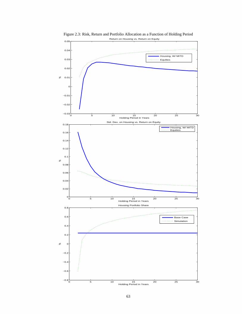
Figure 2.3: Risk, Return and Portfolio Allocation as a Function of Holding Period

0 5 10 15 20 25 30−0.03

−0.02

−0.01

0

0.01

0.02

0.03

0.04

0.05Return on Housing vs. Return on Equity

%

Holding Period in Years

Housing, W/ MITD

Equities

0 5 10 15 20 25 300

0.02

0.04

0.06

0.08

0.1

0.12

0.14

0.16

0.18Std. Dev. on Housing vs. Return on Equity

%

Holding Period in Years

Housing, W/ MITDEquities

0 5 10 15 20 25 30−0.8

−0.6

−0.4

−0.2

0

0.2

0.4

0.6

0.8Housing Portfolio Share

%

Holding Period in Years

Base Case

Simulation

63

Figure 2.4: Risk, Return and Portfolio Allocation as a Function of LTV Ratio

0 0.1 0.2 0.3 0.4 0.5 0.6 0.7 0.8 0.9 1−0.03

−0.02

−0.01

0

0.01

0.02

0.03

0.04Rate of Return on Housing

Loan−to−Value Ratio

Rate

of R

etur

n

5 Years

10 Years

20 Years

0 0.1 0.2 0.3 0.4 0.5 0.6 0.7 0.8 0.9 10.01

0.02

0.03

0.04

0.05

0.06

0.07

0.08

0.09

Stan

dard

Dev

iation

Std.Dev. on Housing

Loan−to−Value Ratio

5 Years

10 Years

20 Years

0 0.1 0.2 0.3 0.4 0.5 0.6 0.7 0.8 0.9 1−1

−0.8

−0.6

−0.4

−0.2

0

0.2

0.4

0.6

0.8

1

Portf

olio

Shar

e

Housing Portfolio Share

Loan−to−Value Ratio

5 Years

10 Years

20 Years

Base Case

64

mortgage being charged 6.4%. Higher downpayments reduce the interest rate paid by the household, but

also reduce the impact of leveraging on the return on housing. As a result, the return on housing is concave

over the loan-to-value ratio. For loans with high downpayments the bene£ts of increasing leveraging offset

the costs of higher interest rates, and the return increasesas the LTV ratio increases. For loans with low

downpayments, the costs of higher interest rates swamps theincreased bene£ts of leveraging, and the rate of

return falls as the LTV ratio increases. The standard deviation steadily increases as the LTV ratio increases

in response to the increased leverage. Longer holding periods result in lower mortgage balances, reduced

leverage, and both lower rates of return and lower standard deviation. Lower LTVs result in lower housing

risk and therefore the household holds more of their portfolio in housing, as shown in the third panel.

Figure 2.5 shows how the mortgage interest tax deduction results in an increasing expected total rate

of return on housing. The values for the fucntionγ(y) are reported in Appendix D and are based on estimates

from the CPS data. The progressive tax structure results in households with higher incomes receiving a

greater bene£t from the mortgage interest tax deduction due to their higher marginal tax rate. The £gure

shows that as income increases, so does the return on housingand the optimal share of the portfolio held

in housing. This effect is mitigated the longer the expectedholding period, since the importance of the

mortgage interest tax deduction to the total return falls asthe holding period increases.

The preceding £gures support the argument that the return andrisk on housing vary signi£cantly

with the holding period. Figure 2.6 shows how the distribution of both the total dollar return and the total

rate of return for holding periods of 5, 10, and 20 years. As holding period increases, the distribution

of the total dollar return, as shown in the bottom panel, becomes more skewed toward the right as the

probability of a negative total return falls. As a result, the distribution of the toal rate of return becomes

more symmetric and concentrated. The reason for the increasing skewness in total dollar return is two-fold.

First the remaining mortgage balance is steadily falling over time, and while the stock value of the stream

of mortgage payments is increasing, it is increasing at a slower rate. This is because, as seen in Figure 2.2,

the ¤ow value of the real mortgage payments is falling over time. Second, while the mortgage payments

remain £xed as the holding period increases, the implicit rent recieved increases as the value of the home

increases. These two factors act in concert to increase the skewness of the total return.

65

Figure 2.5: Risk, Return and Portfolio Allocation as a Function of Income

0 5 10 15 20 25 300

0.005

0.01

0.015

0.02

0.025

0.03

0.035Rate of Return on Housing

Income ($10,000s)

Rate

of R

etur

n5 Years

10 Years

20 Years

0 5 10 15 20 25 300.01

0.02

0.03

0.04

0.05

0.06

0.07

0.08

Stan

dard

Dev

iation

Income ($10,000s)

Std.Dev. on Housing

5 Years

10 Years

20 Years

0 5 10 15 20 25 300

0.1

0.2

0.3

0.4

0.5

0.6

0.7

0.8

Portf

olio

Shar

e

Housing Portfolio Share

Income ($10,000s)

5 Years

10 Years

20 Years

Base Case

66

Figure 2.6: Distribution of Total Return and Conditional Rate of Total Return

−0.2 −0.15 −0.1 −0.05 0 0.05 0.1 0.15 0.20

0.01

0.02

0.03

0.04

0.05

0.06

0.07

0.08

0.09

0.1Kernel Density of Total Rate of Return W/ MITD

Rate of Return, %

5 yrs10 yrs20 yrs

−100 −50 0 50 100 150 200 2500

0.01

0.02

0.03

0.04

0.05

0.06

0.07Kernel Density of Total Return W/ MITD

Total Return, $10,000s

5 yrs10 yrs20 yrs

67

2.5 Empirical Results.

The previous sections provided argued that the total rate ofreturn on housing varies with the ex-

pected holding period, mortgage terms, and borrower income. This section takes the above de£nition of

the total return on housing and estimates the effects of property, mortgage, and borrower characteristics

on the risk and return on housing using data from the 1985-2002 American Housing Survey. The sample

is restricted to households with £xed-rate mortgages who have not re£nanced or moved since purchasing

the home. Households with second mortgages or adjustable rate mortgages are excluded. The sample was

limited to a set of 20 MSAs where there was suf£cient data to estimate rent-to-price ratios by MSA and

by property type. Seperate rent-to-price ratios were estimated for single-family detached, single-family

attached, and multifamly properties. The methodology for estimating these rent-to-price ratios is discussed

in Appendix A.

A small number of obserations had inconsistent values for several key variables and were dropped

from the analysis. This included observations where the either total family annual income or the initial

purchase price of the home was less than $1,000, the initial mortgage balance was less than $100, or the

initial loan-to-value ratio was less than 1% or greater than120%. Observations where it was not possible to

determine the age of the mortgage or where the interest rate was missing were excluded. Observations with

unrealistic year-to-year changes in the home value were excluded. The resulting sample contains 9,711

observations.

The compound annual total rate of return on housing is calculated for each survey year in which the

household meets the above conditions, whether or not the household sold their home. The holding period

is de£ned as the length of time since the home was purchased. Aswas the case in the previous section, it

is assumed that the household pays transaction costs equal to 6% of the home when it is sold. The return

is calculated both with and without the effects of the mortgage interest tax deduction (MITD). Versions of

the return are also calculated without the effects of implicit rent and considering only the effect of capital

gains. Appreciation rates were taken from survey year to survey year and annualized. Appreciation rates

are only available for households in the same unit in consectutive panel years.

Tables 2.2 and 2.3 report the explanatory and dependent variables used in the analysis in this section.

68

Table 2.2: Dependent VariablesNumber Mean Standard Deviation

CAG Rate of Return with MITD 9,711 8.6% 22.6%CAG Rate of Return without MITD 9,711 8.5% 22.5%

CAG Rate of Return without Implicit Rent 9,711 -9.0% 27.1%CAG Rate of Return with Only Capital Gains 9,711 19.1% 79.7%

Probability of Negative Payoff with MITD 9,711 8.4%Probability of Negative Payoff without MITD 9,711 18.7%

Probability of Negative Payoff without Implicit Rent 9,711 66.4%Probability of Negative Payoff Only Capital Gains 9,711 18.8%

Appreciation Rate 6,511 1.9% 10.6%Appreciation Rate plus Rent-to-Price Ratio 6,511 9.8% 10.7%

The rent-to-price ratios were estimated by year and MSA fromthe AHS data. The MSA housing price

index data was taken from published Of£ce of Federal Housing Enterprice Oversight (OFHEO) data. In

calculating the marginal tax rate, the reported household income was used.

Table 2.3: Independent VariablesMean Standard Deviation

MSA HPI Change 5.7% 5.4%MSA Rent-to-Price Ratio 7.8% 2.4%

Central City 35.2% 47.8%Excellent Neighborhood 28.0% 44.9%

Poor Neighborhood 1.1% 10.4%Poor Public Schools 4.1% 19.9%

SF Detached 79.0% 40.7%SF Attached 12.1% 32.6%

Inadequate Housing 1.4% 11.5%1985 Value/Median MSA 1985 Value 90.9% 54.6%

30 Year Term 90.1% 29.9%Interest Rate 8.8% 1.9%

Loan-to-Value Ratio 79.7% 18.6%Payment-to-Income Ratio 20.3% 34.5%

Age of Mortgage 8.9 7.21st-Time Homebuyer 25.6% 43.6%

High School 47.6% 49.9%College 43.9% 49.6%Black 10.6% 30.7%

Married 75.5% 43.0%Children in Household 48.4% 50.0%

Log Income 10.8 0.7

Figure 2.7 shows an estimate of the distribution of both the total dollar return and the total rate of

return for three different measures of return from Table 2.2. The de£nition of the appreciation rate is based

on year to year changes while the capital gains measure is a function of the appreciation in the home since

purchase, the remaining mortgage balance, the intial downpayment, and the length of holding period. The

69

£rst panel shows that the distributions for the total rate of return are dispersed and have a slight skew towards

the right. A large number of the observations have very smallbut positive total returns. This distribution

then trails off to the right and drops sharply to the left. This measure results in more observations with

negative total returns than the capital gains measure due cases where the net present value of the mortgage

payments exceeds the net present value of the implicit rent.This group would consist of households with

high mortgage payments and low rent-to-price ratios.

Figures 2.8 and 2.9 report a series of distributions of the total return and rate of total return condi-

tional on several home or borrower characteristics. In the upper panels of Figure 2.8 the data is divided

based on whether the property type is single-family detached or not. The distibution of the total rate of

return for homes single-family detached homes was higher than the distribution of the rate of return for

other homes. The distibution for the total return for single-family detached homes had a more pronouced

righward skew than the distribution for other homes. The lower panels of Figure 2.8 show the distributions

for households with family income above and below the median. The distributions for the total rate of

return was slightly higher for families with higher income.Households with higher income have greater

rightward skew in their distribution of total dollar returns and sign£cantly lower probability of negative or

very small total dollar returns.

The upper panels of Figure 2.9 show the distributions of the total rate of return and total dollar re-

turns by race. The distribution for the total rate of return for non-blacks is skewed to the right and have a

signi£cantly lower probabiliy of negative or very small total dollar returns. The lower panels of Figure 2.9

provide the £nal set of distributions, broken out by education. College educated households have signi£-

cantly greater variation in the total rate of return and as well as a higher probability of large dollar returns.

Figures 2.8 and 2.9 suggest than both risk and return might vary with borrower characteristics. However

such a univariate analysis masks the many interactions between the characteristics of the household and

their mortgage and housing choices.

Table 2.4 contains the results from a set of logistic regressions on the probability of a negative dollar

return for different housing return measures. For the capital gains only de£nition, a negative total return is

equivalent to negative equity. The £rst section of the table contains variables associated with the location

70

Figure 2.7: Distribution of Return on Housing from AHS

−0.6 −0.4 −0.2 0 0.2 0.4 0.6 0.80

0.005

0.01

0.015

0.02

0.025

0.03

0.035

0.04

0.045

0.05Kernel Density of Conditional Rate of Return

Rate of Return

AppreciationCapital Gains OnlyTotal Rate of Return

−30 −20 −10 0 10 20 30 40 500

0.01

0.02

0.03

0.04

0.05

0.06

0.07

0.08

0.09

0.1Kernel Density of Total Return

Total Return, $10,000s

Capital Gains OnlyTotal Rate of Return

71

Figure 2.8: Distribution of Total Return and Rate of Total Return

−0.6 −0.4 −0.2 0 0.2 0.4 0.6 0.80

0.005

0.01

0.015

0.02

0.025

0.03

0.035Kernel Density of Total Rate of Return, by Home Type

Rate of Return

SF−DetachedOther

−30 −20 −10 0 10 20 30 40 500

0.01

0.02

0.03

0.04

0.05

0.06

0.07

0.08

0.09

0.1Kernel Density of Total Return, by Home Type

Total Return, $10,000s

SF−DetachedNot SF−Detached

−0.6 −0.4 −0.2 0 0.2 0.4 0.6 0.80

0.005

0.01

0.015

0.02

0.025

0.03Kernel Density of Total Rate of Return, by Income

Rate of Return

Income HighIncome Low

−30 −20 −10 0 10 20 30 40 500

0.02

0.04

0.06

0.08

0.1

0.12Kernel Density of Total Return, by Income

Total Return, $10,000s

Income HighIncome Low

72

Figure 2.9: Distribution of Total Return and Rate of Total Return

−0.6 −0.4 −0.2 0 0.2 0.4 0.6 0.80

0.005

0.01

0.015

0.02

0.025

0.03Kernel Density of Total Rate of Return, by Race

Rate of Return

Non−BlackBlack

−30 −20 −10 0 10 20 30 40 500

0.02

0.04

0.06

0.08

0.1

0.12Kernel Density of Total Return, by Race

Total Return. $10,000s

Non−BlackBlack

−0.6 −0.4 −0.2 0 0.2 0.4 0.6 0.80

0.005

0.01

0.015

0.02

0.025

0.03

0.035Kernel Density of Total Rate of Return, by Education

Rate of Return

CollegeNo College

−30 −20 −10 0 10 20 30 40 500

0.01

0.02

0.03

0.04

0.05

0.06

0.07

0.08

0.09

0.1Kernel Density of Total Return, by Education

Total Return, $10,000s

CollegeNo College

73

of the property. When local home prices have been increasing,the probability of a negative total return

decreases. Higher rent-to-price ratios reduce the probability of negative return only when the implicit rent

is taken into account. A higher rent-to-price ratio increases the value of the consumption stream the home

provides, increasing the overall return. Higher rent-to-price ratios increases the probability of negative

return when implicit rent is not taken into account. This re¤ects the negative correlation between rent-to-

price ratios and appreication rates discussed in more detail below. Neighborhood quality, a central city

location, and school quality do not explain much of the variability in negative total returns.

The next set of variables contains information on property characteristics. The reference category

for structure type is mobile homes and apartments. Households in single-family detached homes are less

likely to have negative total returns than those in single-family attached units. Single-family attached homes

are in turn are less likely than mobile homes or multi-familyunits to have negative total returns. The ratio

of the value of the unit in 1985 to the median value for the MSA in 1985 was used as a consistent measure

of how expensive a unit is. This ratio is not particularly signi£cant in the probability of negative total return

regressions.

Mortgage characteristics are included in the next group of variables. Households with 30-year mort-

gages have a higher probability of negative total dollar return than those with shorter term mortgages due

to the slower rate at which they pay down their mortgage balances. When implicit rent is accounted for the

interest rate is signi£cant and negative, but not the LTV ratio. When the implicit rent is not included in the

measure of return, the LTV ratio is signi£cant and negative, but not the interest rate. The negative effect of

the LTV ratio is inutitive. Naturally, the larger the intialequity position, the more the household can lose

before suffering a negative total return when the investment produces no dividends and only capital gains.

Higher interest rates also reduces the return on housing by increasing the costs. For returns without implicit

rent this relationship is still negative, just not signi£cant. The probability of a negative total return declines

with the age of the mortgage, as the remaining mortgage balance is paid down.

The next group of variables focuses on borrower characteristics. High school and college educated

households are less likely to have negative total dollar returns. Purchasing a home is a daunting and time

consuming task with a large degree of asymmetric information. Households with more education might be

74

Table 2.4: Probability of Negative Total ReturnW/O MITD W/ MITD W/O Implicit Rent Cap. Gains Only

Constant 3.565∗∗ 4.0353∗∗ 1.379∗ -1.172(0.666) (0.669) (0.539) (0.737)

MSA HPI Chg -1.403∗ -1.484∗ -4.345∗∗ -7.127∗∗

(0.580) (0.583) (0.433) (0.639)MSA RTP Ratio -9.269∗∗ -9.429∗∗ 26.262∗∗ 7.781∗∗

(1.408) (1.420) (1.228) (1.395)Central City 0.0770 0.103 -0.0114 0.190∗∗

(0.0644) (0.0648) (0.0518) (0.0665)Ex. Nbhd -0.0384 -0.0290 -0.124∗ -0.0923

(0.0685) (0.0690) (0.0535) (0.0712)Poor Nbhd 0.426 0.394 0.641∗ 0.396

(0.265) (0.267) (0.265) (0.295)Poor Sch -0.0576 -0.0827 0.0240 0.0522

(0.160) (0.161) (0.117) (0.155)SF-Detch -0.740∗∗ -0.757∗∗ -0.631∗∗ -1.0230∗∗

(0.105) (0.105) (0.0969) (0.104)SF-Attcd -0.494∗∗ -0.544∗∗ -0.330∗∗ -1.0261∗∗

(0.125) (0.278) (0.115) (0.126)Inadeq. -0.474 -0.552∗ -0.399∗ 0.203

(0.269) (0.278) (0.200) (0.241)Val85/ 0.0405 0.0264 -0.216∗∗ 0.0149

MedMSAVal85 (0.0637) (0.0644) (0.0478) (0.0626)30yr 0.345∗∗ 0.314∗∗ 0.721∗∗ 1.0208∗∗

(0.101) (0.102) (0.0779) (0.103)Int. -4.967∗∗ -5.812∗∗ -1.887 0.516

(1.647) (1.663) (1.370) (1.692)LTV 0.174 0.107 -0.894∗∗ -1.713∗∗

(0.175) (0.176) (0.138) (0.174)PTI -0.0647 -0.0739 0.0960 0.653∗∗

(0.0951) (0.0956) (0.0911) (0.107)Age -0.604∗∗ -0.583∗∗ -0.298∗∗ -0.489∗∗

(0.0162) (0.0162) (0.0143) (0.0185)Age2 0.0216∗∗ 0.0209∗∗ 0.0161∗∗ 0.0117∗∗

(0.000627) (0.000624) (0.000717) (0.000899)1stTime -0.0145 -0.0323 -0.0600 0.0526

(0.0678) (0.0685) (0.0549) (0.0696)HighSch -0.339∗∗ -0.286∗ -0.204∗ -0.146

(0.110) (0.111) (0.0924) (0.123)College -0.326∗∗ -0.258∗ -0.177 -0.159

(0.116) (0.116) (0.0968) (0.127)Black 0.476∗∗ 0.482∗∗ 0.322∗∗ 0.183

(0.0981) (0.0982) (0.0845) (0.108)Married -0.0292 -0.0251 0.0930 0.0615

(0.0739) (0.0744) (0.0602) (0.0771)Children 0.0150 0.0592 0.0871 0.00921

(0.0660) (0.0665) (0.0514) (0.0670)Log(Inc) -0.123∗ -0.167∗∗ -0.0631 0.252∗∗

(0.0549) (0.0551) (0.0440) (0.0615)Log L -3,621 -3,587 -5,327 -3,355

Num Obs. 9,722 9,722 9,722 9,722

Note: The standard deviations are presented in parentheses. ∗∗ represents signi£cance at the 1% level and∗ represents signi£cance at

the 5% level.

75

more adept at the home search and purchase process and therefore purchase homes and acquire mortgages

less likely to produce negative total dollar returns. Blacks are more likely to have negative total returns.

Both race and educational effects are only signi£cant when the cost of the mortgage payments are accounted

for. The effect of the mortgage interest tax deduction is to reduce the probability of a negative total return

for households with high levels of income and higher corresponding marginal tax rates. Income still have a

negative and signi£cant impact even when the mortgage interest tax deduction is not accounted for, but has

a positive effect on the probability of negative equity. This might re¤ect a selection effect. These measures

of return are unrealized measures. Negative equity is a problem that must be addressed only when the home

is sold, or if the household is unable to make the mortgage payments. High income households have lower

probability of missing mortgage payments, and therefore assign less concern to the problems of unrealized

negative equity. They feel they can continue to make their payments, until the local housing market recovers

and they pay down the balance on their mortgage.

Table 2.5 reports the results for OLS regressions of the measures of housing return. The £rst columns

uses the appreciation rate while the next four columns use the same measures of return used in Table 2.4,

conditional on a positive total return. The explanatory variables are the same as those used in the logistic

regression of the probability of negative total dollar return. Increases in the local MSA home price index

have positive and signi£cant effects on all the measures of housing return. The local rent-to-price ratio

has a positive and signi£cant effect only when the implicit rent is included in the measure of housing

return. Otherwise its impact is negative and signi£cant. These results support the hypothesis that, to some

extent, housing markets are clearing. That is, in markets where housing provides a large dividend to owners

through a high rent-to-price ratio, the rate of appreciation is lower. Conversely, in other markets the rate

of appreciation is higher to compensate for lower dividends. Homes in the central city had lower rates

of appreciation. The rate of appreciation also is sensitiveto the reported quality of the neighborhood,

with homes in excellent neighborhoods having on average a greater rate of appreciation than homes in

poor neighborhoods. However, for the most part, none of the measures of total return are sensistive to the

location or neighborhood quality of the home.

The effects of property type are as expected. Single-familyhomes have higher rates of appreciation

76

Table 2.5: Model of Return on HousingAppreciation W/O MITD W/ MITD W/O Implicit Rent Cap. Gains Only

Constant -0.130∗∗ -0.298∗∗ -0.323∗∗ -0.292∗∗ 0.445∗∗

(0.0291) (0.0403) (0.0406) (0.0452) (0.168)MSA HPI Chg 0.600∗∗ 0.309∗∗ 0.315∗∗ 0.511∗∗ 0.638∗∗

(0.0245) (0.0379) (0.0378) (0.0435) (0.104)MSA RTP Ratio -0.172∗∗ 0.644∗∗ 0.626∗∗ -0.987∗∗ -0.892∗

(0.0564) (0.0993) (0.100) (0.108) (0.294)Central City -0.01291∗∗ -0.00431 -0.00501 -0.00377 0.0219

(0.00293) (0.00496) (0.00496) (0.00550) (0.0184)Ex. Nbhd 0.0109∗∗ 0.00542 0.00646 0.00458 -0.00686

(0.00285) (0.00503) (0.00501) (0.00549) (0.0153)Poor Nbh -0.0338∗∗ 0.00560 0.00606 -0.0108 -0.0280

(0.00144) (0.0246) (0.0252) (0.0274) (0.0647)Poor Sch 0.000910 0.00832 0.00542 0.00876 -0.0417

(0.00644) (0.00981) (0.00973) (0.0121) (0.0215)SF-Detch 0.0333∗∗ 0.0673∗∗ 0.0685∗∗ 0.0903∗∗ 0.126∗∗

(0.00626) (0.00958) (0.00967) (0.0109) (0.0301)SF-Attcd 0.0298∗∗ 0.0445∗∗ 0.0465∗∗ 0.0576 ∗∗ 0.0818∗

(0.00701) (0.0109) (0.0110) (0.0124) (0.0331)Inadeq. 0.0145 0.00643 0.0197 0.0346 -0.0718

(0.00866) (0.0208) (0.0206) (0.0229) (0.0406)Val85/ -0.00912∗∗ -0.00922∗ -0.00698 -0.0136∗∗ -0.0164

MedMSAVal85 (0.00303) (0.00431) (0.00426) (0.00517) (0.0121)30yr 0.00851 -0.0319∗∗ -0.0298∗ -0.0886∗∗ -0.148∗∗

(0.00448) (0.00794) (0.00808) (0.00839) (0.0332)Int. -0.0687 0.216 0.195 0.588∗∗ -0.319

(0.0820) (0.143) (0.143) (0.158) (0.578)LTV -0.00388 0.114∗∗ 0.140∗∗ -0.156∗∗ 0.690∗∗

(0.00747) (0.0114) (0.0115) (0.0129) (0.0444)PTI 0.00604 0.00463 0.00390 -0.00968 -0.0917∗∗

(0.00381) (0.00537) (0.00548) (0.00719) (0.0209)Age -0.000362 0.0122∗∗ 0.00753∗∗ 0.0398∗∗ -0.0109∗∗

(0.000550) (0.00114) (0.00114) (0.00117)) (0.00423)Age2 0.00000606 -0.00201∗∗ -0.000466∗∗ -0.00121∗∗ 0.000135∗∗

(0.0000214) (0.0000316) (0.0000316) (0.000316) (0.000118)1stTime 0.00184 -0.00201 -0.00209 -0.00236 -0.0162

(0.00272) (0.00515) (0.00514) (0.00565) (0.0182)HighSch 0.0169∗∗ 0.0177∗ 0.0172∗∗ 0.0214∗ 0.0428

(0.00584) (0.00837) (0.00837) (0.00962) (0.0263)College 0.0245∗∗ 0.0283∗∗ 0.0281∗∗ 0.0360∗∗ 0.0103

(0.00595) (0.00897) (0.00896) (0.0102) (0.0255)Black -0.0151∗∗ -0.0258∗∗ -0.0263∗∗ -0.0254∗∗ -0.00679

(0.00487) (0.00843) (0.0153) (0.00921) (0.0354)Married 0.000371 -0.00367 -0.00202 -0.00291 -0.0135

(0.00336) (0.00591) (0.01099) (0.00660) (0.0216)Children 0.0000808 -0.00379 -0.00586 -0.00238 -0.0121

(0.000853) (0.00498) (0.00955) (0.00545) (0.0156)Log(Inc) 0.00890∗∗ 0.0120∗∗ 0.0154∗∗ 0.0113∗∗ -0.0572∗

(0.00234) (0.00330) (0.00790) (0.00372) (0.0154)R2 0.119 0.052 0.058 0.202 0.039

Num Obs. 6,510 9,722 9,722 9,722 9,722

Note: The standard deviations are presented in parentheses. ∗∗ represents signi£cance at the 1% level and∗ represents signi£cance at

the 5% level.

77

than do mobile and multi-family homes. This results, combined with the estimated rent-to-price ratios in

Appendix B, provide additional support that housing markets are clearing. Single family homes have higher

rates of appreciation but lower provide lower dividends dueto lower rent-to-price ratios. Multifamily units

have lower rates of appreciation, but provide higher dividends through higher rent-to-price ratios. Further

work will explore the differences in appreciation rates andrent-to-price ratios across property types. More

expensive units, as measured by the ratio of the value of the unit to the median MSA level value in 1985

have slightly lower rates of both return and appreciation. The effects of the mortgage terms on the total rate

of return on housing are also as expected. Households with 30year £xed rate terms are paying down their

mortgage balance more slowly, resulting in a lower rate of total return. Higher LTV ratios result in higher

rates of return by increasing the effects of leveraging, although this effect turn negative when the cost of

the mortgage payments but not the bene£ts of the implicit rentare included. The return is concave over the

holding period increases, as suggested by the simulation results.

The last set of independent variables represents the effects of borrower characterisitics. Households

with higher level of education or income have higher rates ofreturn and appreciation while blacks have

lower rates of return and appreciation. The one exception, as was the case the the models of the probability

of negative total return, is the measure including only capital gains. The results from the appreciation

regression indicates that households with higher level of education or income do in fact purchase homes

that appreciate at higher rates and blacks purchase homes that appreciate at lower rates. However, when

the size of the downpayment and remaining mortgage balance are used to calculate the rate of return from

capital gains, neither income, education, or race are signi£cant. When the costs of the mortgage payments

are then accounted for, all these characteristics are once more signi£cant.

One possible explanation that £ts this pattern is that households that have low income, low education,

or who are black might purchase homes with lower downpayments. If the cost of the downpayment is the

primary measure of the out¤ow associated with the investment, this might result in what appears to be

higher rates of return even when the appreciation on the underlying property is low. Once the true cost of

the mortgage is accounted for, the true rate of return is lower for this group. In fact the impacts of income,

education, property type, and race all increase once the effects of the mortgage contract and implicit rent are

78

accounted for. Households with low income, low education, or who are black are losing out not once but

twice. The homes they purchase appreciate at lower rates, and the mortgages they take out further reduces

their rate of return on their investment.

2.6 Conclusions.

The goal of this paper was two-fold. The £rst goal was to develop an alternative measure of the total

rate of return on housing that accurately accounts for the role of the mortgage contracts and the stream of

housing services associated with owner-occupied housing.The second goal was to provide both theoret-

ical and empirical evidence that the total return on housingvaries with property, mortgage, and borrower

characteristics.

The alternative measure developed here shows that the totalrate of return on housing is concave over

the holding period. The probability of negative equity peaks early in the holding period and then declines,

as does the standard deviation of the total rate of return. The total rate of return on housing is also concave

over the LTV ratio, as the bene£ts of higher leverage are balanced with higher interest rates. The mortgage

interest tax deduction increases the returns for higher-income borrowers through their higher marginal tax

rates. As the risk and return of housing varies with the holding period, mortgage terms, and income level,

so does the optimal portfolio share of investments held in equities.

Property, mortgage, and borrower characterisics all have signi£cant effect on the total rate of return

on housing. Single-family homes, espcially single-familydetached homes, provide higher rates of return.

Higher levels of human capital, measured either as the levelof education or household income, signi£cantly

decreases the probability of a negative total return and increases the appreciation rate of the home itself.

The high degree of assymentric information and uncertaintyassociated with the home search and purchase

process allows households with higher levels of human capital to make signi£cantly better investment de-

cisions. Households that have low income, low education, orwho are black have a higher probability of

negative total return and lower total rates of both return and appreciation. The role of the mortgage contract

seems to augment the effect of income, education, race and property type on the rate of return on housing.

To use only the appreciation rate of housing to measure return ignores the effects of the mortgage

79

contract on the total rate of return on housing. The total rate of return measure developed here captures

capture how the risk and return on housing varies with mortgage, property, and borrower characteristics.

Existing papers have documented how the demand for risky assets vary with the holdings of home equity,

but have not explored the heterogenity of the risk and returnon housing as a funciton of mortgage, property,

and borrower characteristics. The next step in this research is to see if there is empirical evidence of

household’s demand for risk assests varying with the probability of a negative total return and total rate of

return on housing.

80

Appendix A

Baseline Model Parameter Values

The parameter values for the baseline model are chosen to be consistent with other models in the

relevant literature. As was discussed in the Section 3, the income process consists of a deterministic and

a transitory factor. The income process is based on the results of regressions of Social Security earnings

on age and age-squared. The dependent variable is the log of the wage income in constant 1990 dollars.

The transitory factor of wage is re¤ected in the estimated standard error of the regression. The wage is

converted from log to level terms in the model. At age 65 the level of the deterministic wage falls to a ¤at

level equal to 60% of the last period’s income before any transitory shocks, representing a system of forced

retirement and a de£ned bene£t pension plan. The coef£cients and standard deviation used in this version

of the model are shown in Table A.1 below.

Table A.1: Log Income Regression ResultsConstant ψ0 7.28626

Coef£cient Age ψ1 0.10278Coef£cient of Age2 ψ2 -0.00098

Std. Dev. σw 0.80778R2 15.5%

Probability of Unemployment υ 1%

The market price of a housing unit is the result of setting thedeterministic home price at age 60 with

the National Association of Realtors’ 1990 median home price. It is assumed that a median home consists

of 10 housing units. The home prices are converted to constant 1990 dollars and the deterministic home

price series are calculated using the historical average return. The average and standard deviation of the

return on housing are at taken from Li and Yao (2004) and are consistent with Campbell Cocco (2003). The

mortgage interest rate used is the average rate on loans with80% loan-to-value ratios as reported by Freddie

Mac from 1969 to 2001, adjusting for the in¤ation rate. The percent required for downpayment represents

the minimum needed to avoid paying mortgage insurance. The transaction, maintenance, and moving costs

are based on survey data provided by the National Association of Realtors. The values chosen for the

81

current version of the model are presented in Table A.2 below. The risk and return on risky assets follows

Yao and Zhang (2004).

Table A.2: Values of Market ParametersParameter Name and De£nition Symbol Value

Real risk free rate of return r 2%Price of 1 housing unit, at age 60 P60(1) 1.003

Size of small homes h(is) 8Size of large homes h(i l ) 12

Mean of real return on housing ηh 1%Standard deviation of housing return σh 11.5%

Mean of real return on risky asset ηs 6%Standard deviation of risky asset return σs 15.7%Probability of 100% loss on risky asset ς 1%

Mortgage interest rate π 5%Percent required as downpayment µ 20%

Percent of home price lost to transaction costs τ 10%Maintenance costs δ 0.7%

Moving costs χ 0.3Tax Rate γ 30%

Re£nancing Costs ζ 3%In¤ation ν 2%

Note: Units are in $10,000s or percent.

The values for the preference parameters shown in Table A.3 below were chosen to replicate certain

stylized facts about the role of owner-occupied housing in portfolios, speci£cally the large share of total

wealth held in home equity. Anλ value of 2 represents a relatively low, but realistic, levelof risk aversion.

An β value of 0.96 is a commonly used discount rate. Theφ value of 0.2 re¤ects the share of total household

expenditures allocated to housing expenditures in the 2001Consumer Expenditure Survey from the U.S.

Department of Labor. The discount rate for bequests are 0.8 for θA, 0.8 for θH , and 0.8 forθM. They

are chosen to imply that households would rather consume oneadditional dollar than leave an additional

dollar as a bequest and that households place a premium on leaving their homes as bequests relative to other

assets.

Table A.3: Values of Structural Parameters in Calibrated Modelλ β φ θA θH θM

2 0.96 0.2 0.8 0.8 0.8

82

Appendix B

Model Parameter De£nitions

Table B.1: Model Parameter De£nitionsParameter Name and De£nition Symbol

Consumption ct

Tenure Choice, next period it+1

Share of Financial Assets held in risky assets αAge of Mortgage (Re£nancing=Change Age of Mortgage) κt+1

Tenure Choice, this period itCurrent Age of Mortgage κt

Value of Financial Assets At

Value of Home Ht

Tenure Choice, rent irTenure Choice, own small house isTenure Choice, own large house i l

Number of housing service units for tenure choiceit h(it)Realized Earnings et

Remaining Mortgage Balance Dt

Recurring Housing Costs Xt(it ,κt)Mortgage Interest paid It(it ,κt)

Net Gain/Loss from Home Sale/Purchase Gt(it , it+1,κt)Net Gain from Cash-Out Re£nancing Zt(κt ,κt+1)

Mortgage Payment Mt(it ,κt)Risk Aversion λDiscount rate β

Housing Utility Coef£cient φBequest Parameter - Financial Assets θA

Bequest Parameter - Housing θH

Bequest Parameter - Mortgage Debt θM

Survival Probability ρt

83

Appendix C

Estimating Rent-to-Price Ratios

A key component of the return on housing is the stream of implicit rent consumed by the owner.

In order to quantify the value of this stream, it is necessaryto estmate a rent-to-price ratio. This appendix

describes the methodology used to estimate rent-to-price ratios by year and MSA using the AHS data

following Phillips (1988). Assuming that markets clear, the asset value of the home should equal the net

present value of the rental income the home provides, or

V =n

∑i=1

Rt −Ct

(1+ r)t , (C.1)

whereV is the asset value of the home,Rt is the market clearing rent in period t,Ct is the £nancing and

operating cost in yeart, r is the discount rate, andn is the property’s useful life. This relationship can be

rewritten as

V =R1−C1

1+ r+

k

∑i=2

Rt −Ct

(1+ r)t +n

∑i=k

Rt −Ct

(1+ r)t (C.2)

where the £rst term represents current year net rent, the second term is the net present value of the rental

stream up until periodk, and the £nal term represents the home’s resale value in period k.

The current rent-to-price ratio is de£ned as

µ=R1

V. (C.3)

The formula can be rearranged as follows:

V =R1

µ(C.4)

implying that the rent-to-price ratio can be interpreted asthe rate at which current rents are capitalized into

asset values.

Estimating these rent-to-price ratios would be quite straight-forward if we possesed data on both

84

current rents and asset values of individual homes. In most datasets, including the AHS used here, there

is data on assets prices or current rent, but not both. These rent-to-price rates are imputed using a tenure

hedonic model based on Phillips (1988) in form of

ln(Pit ) = βit X + γit TENURE+θit TENURE∗Y + εit , (C.5)

wherePit is the natural logarithm of home values and rents in cityi at timet, X is a vector of unit character-

isics in city i at timet, Y is a matrix of property type, andTENUREequals 1 if the unit is owner-occupied

and 0 if it is a rental unit.

The difference between the rental and owner-occupied equations is

ln(Rit )− ln(Vit ) = −γit −θit ∗Y, (C.6)

or, equivalently,

ln(Rit

Vit) = −γit −θit ∗Y. (C.7)

Therefore the vector of rent-to-price ratios by property type for city i at timet can be imputed as

µit =Rit

Vit= e−γit−θit ∗Y. (C.8)

The model is estimated over a set of MSAs using the AHS from 1985 to 2003. The vector of

property types includes single-family detached, single-family attached, and multi-family. The resulting

imputations ofµit are then merged back in with the AHS data where they are used tocalculate the implicit

rent generated by owner-occupied housing. The estimated values ofµit are provided in Table??. In addition

to theTENUREdummy, the explanatory variables include the number of rooms, number of bathrooms,

and dummies for central city location, single-family detached, single-family attached, multi-family, air-

conditioning, excellent quality neighborhood, poor quality neighborhood, and garage.

85

Table C.1: Estimated Rent-to-Price Ratios

MSA Property Type 1985 1987 1989 1991 1993 1995 1997 1999 2001

Anaheim, CA SF-Detached 6.34% 6.25% 4.86% 5.37% 5.11% 5.37% 8.36% 6.17% 4.98%

SF-Attached 6.58% 4.85% 5.08% 4.53% 7.24% 6.70% 9.70% 8.28% 6.11%

MF 6.95% 7.93% 8.05% 6.45% 7.06% 8.57% 11.61% 8.57% 11.61%

Atlanta, GA SF-Detached 8.54% 8.50% 9.45% 10.40% 8.86% 9.03% 6.72% 8.30% 6.87%

SF-Attached 6.32% 9.85% 5.72% 6.91% 7.82% 10.64% 12.74% 9.23% 7.58%

MF 9.31% 6.96% 9.61% 9.44% 8.88% 10.46% 12.62% 9.27% 9.88%

Baltimore, MD SF-Detached 7.50% 7.25% 6.14% 10.14% 6.24% 9.74% 9.00% 5.74% 6.22%

SF-Attached 9.71% 8.43% 8.31% 10.14% 10.16% 9.74% 9.00% 10.95% 11.83%

MF 9.49% 8.15% 8.03% 10.14% 7.99% 9.74% 9.00% 5.74% 11.83%

Boston, MA SF-Detached 6.18% 5.40% 5.68% 5.73% 7.02% 6.86% 7.28% 6.79% 5.45%

SF-Attached 3.15% 16.12% 4.35% 5.61% 2.85% 17.84% 15.12% 1.26% 3.00%

MF 6.22% 4.98% 5.41% 5.77% 8.49% 7.69% 9.05% 8.90% 7.00%

Chicago, IL SF-Detached 6.42% 6.40% 6.56% 5.65% 6.48% 6.42% 9.38% 7.74% 8.20%

SF-Attached 7.15% 7.99% 6.32% 8.36% 4.95% 6.68% 8.59% 10.22% 9.53%

MF 11.08% 9.40% 10.11% 8.81% 9.54% 9.30% 12.66% 11.43% 8.98%

Dallas, TX SF-Detached 6.88% 8.63% 8.57% 9.52% 10.98% 10.91% 10.44% 9.33% 10.75%

SF-Attached 7.36% 4.59% 9.91% 8.88% 10.88% 12.45% 12.46% 14.37% 9.78%

MF 9.21% 12.07% 14.99% 7.96% 19.27% 14.58% 9.72% 16.67% 13.08%

Detroit, MI SF-Detached 10.69% 10.29% 10.65% 10.64% 12.38% 11.11% 9.15% 7.86% 6.93%

SF-Attached 13.08% 9.42% 12.92% 13.82% 11.41% 12.88% 14.36% 9.66% 9.39%

MF 16.53% 23.42% 13.92% 15.54% 13.11% 13.05% 16.22% 10.70% 11.09%

Houston, TX SF-Detached 9.77% 8.23% 10.44% 10.52% 10.32% 10.80% 12.27% 12.83% 11.37%

SF-Attached 8.62% 8.37% 18.13% 10.24% 11.15% 10.09% 13.38% 14.91% 12.46%

MF 6.02% 10.41% 12.10% 14.24% 15.71% 16.46% 18.67% 21.17% 18.10%

Los Angelos, CA SF-Detached 5.41% 5.75% 4.28% 4.54% 4.83% 5.22% 5.54% 5.91% 4.55%

SF-Attached 5.72% 6.83% 5.24% 5.12% 4.57% 6.62% 6.66% 5.90% 5.41%

MF 5.72% 6.96% 4.92% 5.38% 5.05% 6.00% 6.96% 8.07% 9.29%

Miami, FL SF-Detached 9.18% 7.19% 9.01% 7.71% 7.49% 7.82% 7.38% 6.79% 8.27%

SF-Attached 8.12% 9.75% 9.65% 10.33% 10.86% 9.58% 8.31% 7.98% 8.24%

MF 11.35% 11.25% 11.86% 11.53% 9.86% 12.18% 11.69% 8.23% 10.49%

Continued on next page

86

Table C.1 – continuted from previous page

MSA Property Type 1985 1987 1989 1991 1993 1995 1997 1999 2001

Minneapolis, MN SF-Detached 8.59% 8.02% 9.12% 8.31% 7.98% 6.80% 11.76% 9.26% 7.97%

SF-Attached 9.47% 11.27% 9.18% 9.29% 9.32% 9.78% 10.00% 8.64% 10.70%

MF 8.59% 9.87% 10.70% 12.08% 12.30% 11.17% 11.13% 10.67% 12.02%

New York, NY SF-Detached 9.50% 5.38% 3.94% 6.67% 6.24% 7.48% 5.06% 4.41% 11.52%

SF-Attached 4.97% 5.38% 3.74% 6.67% 6.24% 7.48% 4.41% 5.56% 11.52%

MF 9.50% 5.38% 5.19% 6.67% 6.24% 7.48% 10.65% 9.66% 11.52%

Newark, NJ SF-Detached 4.96% 6.85% 5.94% 6.47% 5.26% 8.46% 12.64% 10.47% 7.62%

SF-Attached 9.39% 6.85% 5.94% 6.47% 9.13% 8.46% 12.64% 10.47% 7.62%

MF 9.39% 6.85% 5.94% 6.47% 9.13% 8.46% 12.64% 10.47% 7.62%

Oakland, CA SF-Detached 5.99% 6.18% 4.67% 4.99% 5.17% 5.88% 6.01% 5.31% 3.74%

SF-Attached 7.85% 6.09% 5.55% 4.66% 5.56% 8.63% 5.52% 5.56% 4.65%

MF 5.62% 7.72% 4.85% 5.82% 4.66% 5.12% 10.75% 6.48% 4.36%

Philadelphia, PA SF-Detached 6.62% 5.91% 5.82% 7.73% 7.36% 6.83% 8.39% 6.36% 6.90%

SF-Attached 8.65% 10.23% 9.65% 8.87% 10.44% 9.70% 13.56% 10.96% 11.10%

MF 11.44% 8.59% 8.63% 10.44% 8.78% 10.70% 8.86% 16.68% 9.87%

Phoenix, AZ SF-Detached 8.27% 8.72% 10.84% 8.57% 7.65% 8.33% 7.56% 8.10% 8.16%

SF-Attached 9.40% 4.70% 15.67% 9.88% 10.75% 9.37% 8.39% 9.95% 10.97%

MF 10.92% 11.26% 8.48% 9.30% 12.97% 12.07% 9.80% 6.94% 10.95%

San Diego, CA SF-Detached 6.44% 5.92% 7.09% 5.21% 6.12% 6.19% 7.55% 7.95% 4.73%

SF-Attached 6.37% 6.43% 9.23% 5.66% 5.25% 5.68% 22.09% 10.47% 4.53%

MF 7.74% 7.47% 6.82% 4.77% 6.23% 5.64% 25.37% 7.92% 4.83%

San Francisco, CA SF-Detached 4.93% 4.38% 3.28% 3.98% 3.95% 4.57% 12.60% 4.28% 2.90%

SF-Attached 4.21% 4.51% 2.89% 3.98% 4.40% 3.63% 4.76% 5.16% 1.50%

MF 5.98% 5.72% 4.77% 3.98% 5.66% 4.98% 9.57% 5.69% 3.66%

Seattle, WA SF-Detached 7.08% 8.63% 6.74% 5.68% 5.85% 6.03% 4.91% 6.01% 4.03%

SF-Attached 5.79% 5.90% 10.73% 10.67% 5.85% 3.58% 0.01% 5.77% 6.47%

MF 6.24% 6.32% 10.03% 9.99% 7.49% 6.64% 7.49% 7.58% 7.47%

Washington, DC SF-Detached 7.00% 6.20% 6.49% 5.69% 5.86% 5.99% 6.91% 7.45% 5.01%

SF-Attached 7.42% 6.37% 6.32% 6.75% 6.85% 6.50% 6.58% 8.88% 9.09%

MF 8.71% 8.40% 7.43% 7.81% 8.49% 9.37% 14.97% 15.19% 8.60%

Continued on next page

87

Table C.1 – continuted from previous page

MSA Property Type 1985 1987 1989 1991 1993 1995 1997 1999 2001

United States SF-Detached 7.03% 6.60% 6.22% 6.58% 6.57% 6.92% 7.53% 6.93% 6.04%

SF-Attached 8.35% 8.04% 7.54% 7.77% 7.92% 8.94% 9.30% 9.45% 8.44%

MF 9.28% 7.26% 6.82% 7.39% 7.45% 8.35% 11.17% 10.07% 8.99%

Appendix D

Income Tax Rates

Table D.1: Progressive Income Tax StructureIncome Range Marginal Tax Rate$0 to $5000 0.15%

$5000 to $10000 2.38%$10000 to $15000 5.27%$15000 to $20000 7.93%$20000 to $25000 10.86%$25000 to $30000 12.15%$30000 to $35000 14.48%$35000 to $40000 15.92%$40000 to $45000 17.19%$45000 to $50000 17.17%$50000 to $55000 18.16%$55000 to $60000 20.09%$60000 to $65000 23.75%$65000 to $70000 26.64%$70000 to $75000 27.57%$75000 to $85000 28.07%$85000 to $90000 28.15%$90000 to $95000 28.10%$95000 to $100000 28.12%$100000 to $125000 28.65%$125000 to $150000 30.71%$150000 to $175000 31.42%$175000 to $200000 33.71%$200000 to $250000 37.34%

$250000 or more 38.24%

88

BIBLIOGRAPHY

[1] Attanasio, Orazio, P.K. Goldberg and E. Kyriazidou. “Credit Constraints in the Market for Consumer

Durables; Evidence from Mircodata on Car Loans.” NBER Working Paper No. 7694. 2000.

[2] Balvers, Ronald J. and Lszl Szerb. “Precaution and Liquidity in the Demand for Housing.”Economic

Inquiry. Vol. 38. No. 2. 2000.

[3] Bar-Ilan, Avner and Allan S. Blinder. “Life-Cycle Permanent-Income Model and Consumer

Durables.” NBER Working Paper No. 2149. 1987.

[4] Berkovec, James and Don Fullerton. “A General Equilibrium Model of Housing, Taxes, and Portfolio

Choice.”The Journal of Political Economy. Vol. 100. Issue 2. 1992. pp. 390-429.

[5] Bertola, Giuseppe, Luigi Guise, and Luigi Pistaferri. “Uncertainty and Consumer Durables Adjust-

ment.” Working Paper. European University Institute. 2002.

[6] Bodie, Zvi, Alex Kane, and Alan J. Marcus.Investments. Edition 5. McGraw-Hill. 2002.

[7] Buist, Henry and Tyler T. Yang. “Housing Finance in a Stochastic Economy: Contract Pricing and

Choice.”Real Estate Economics. Vol. 28. No. 1. 2000. pp. 117-139.

[8] Caplin, Andrew and Sewin Chan, Charles Freeman and Joseph Tracy. “Household Asset Portfolios and

the Reform of the Housing Finance Market.”TIAA-CREF Research Dialogues59. February 1999. pp.

1-12.

[9] Case, Karl E., and Robert J. Shiller, and Allan N. Weiss. “Index-Based Futures and Options Trading

in Real Estate.”Journal of Portfolio Management(Winter 1993).

[10] Case, Karl E., and Robert J. Shiller. “Forecasting Prices and Excess Returns in the Housing Market.”

AREUEA Journal. Vol. 18. No. 3. 1990. pp. 253-273.

[11] Chah, Eun Young, Valerie A. Ramey, and Ross M. Starr. “Liquidity Constraints and Intertemporal

Consumer Optimization: Theory and Evidence from Durable Goods.”Journal of Money, Credit, and

Banking. Vol. 27. issue 1. 1995. 272-287.

89

[12] Cocco, Joo F. “Hedging House Price Risk With IncompleteMarkets.” Working Paper. 2000.

[13] Engelhardt, Gary. “House Prices and Home Owner Saving Behavior.” NBER Working Paper No.

5183. 1995.

[14] Englund, Peter, Min Hwang, and John M. Quigley, “Hedging Housing Risk.” Berkely Program on

Housing and Urban Policy Working Paper W00’007. 2000.

[15] Ermisch, John. “The Demand for Housing in Britain and Population Aging: Microeconomic Evi-

dence.”Econometrica. Vol. 63. Issue 251. 1996. pp. 383-404.

[16] Deng, Yongheng, John M. Quigley, and Robert Van Order. “Mortgage Termination, Heterogenity and

the Exercise of Mortgage Option.”Econometrica’. Vol. 68. No. 2. 2000. pp. 275-307.

[17] Fernndez-Villaverde, Jess and Dirk Krueger. “Consumption and Saving over the Life-cycle: How

Important are Consumer Durables?” Working Paper. 2001.

[18] Flavin, Marjorie and Takashi Yamashita. “Owner-Occupied Housing and the Composition of the

Household Portfolio Over the Life-cycle.” University of California, San Diego Discussion Paper 98-

02. 1998.

[19] Flavin, Marjorie and Takashi Yamashita. “Owner-Occupied Housing and the Composition of the

Household Portfolio Over the Life-cycle.”The American Economic Review. Vol. 92. 2002. pp. 345-

362.

[20] Fratantoni, Michael C. “Housing Wealth, Precautionary Savings and the Equity Premium.” Disserta-

tion. Johns Hopkins University. 1997.

[21] Fratantoni, Michael C. “Homeownership, Committed Risk, and the Stockholding Puzzle.”Oxford

Economic Papers. Vol. 53. Issue 2. 2001. pp. 241-259.

[22] Fratantoni, Michael C. “Homeownership, Committed Risk, and the Stockholding Puzzle.”Oxford

Economic Papers. Vol. 53. Issue 2. 2001. pp. 241-259.

90

[23] Genesove, David and Christopher Mayer. “Equity and Time to Sale in the Real Estate Market,”The

American Economic Review. Vol. 87. No. 3. 1997. pp. 255-269.

[24] Gourinchas, P.O. and J.A. Parker. “Consumption over the Life-cycle.” NBER Working Paper No.7271.

1999.

[25] Green, Richard and Patric Hendershott. “Age, Housing Demand, and Real House Prices.”Regional

Science and Urban Economics. Vol. 26. 1996. pp. 465-480.

[26] Guisio, Luigi, Tullio Jappelli, and Daniele Terlizzese. “Income Risk, Borrowing Constraints, and

Portfolio Choice.”The American Economic Review. Vol. 86. Issue 1. pp. 158-172. 1996.

[27] Guisio, Luigi and Tullio Jappelli. “Private Transfers, Borrowing Constraints, and the Timing of Home-

ownership.” CSEF Working Paper No. 17. 1999.

[28] Grossman, Sanford and Guy Laroque. “Asset Pricing and Optimal Portfolio Choice in the Presence of

Illiquid Durable Consumption Goods.”Econometrica. Vol. 58. No. 1. 1993. pp.25-51.

[29] Haurin, Donald R. “Income Variability, Homeownership, and Housing Demand.”Journal of Housing

Economics. Vol. 1. 1991. pp. 60-74.

[30] Hendershott, Patric H. and Sheng Cheng Hu. “In¤ation andExtraordinary Returns on Owner-

Occupied Housing: Some Implications for Capital Allocation and Productivity Growth.”Journal of

Macroeconomics. Vol. 3. No. 2. 1981. pp. 177-203.

[31] Henderson, J. Vernon and Yannis M. Ioannides. “A Model of Housing Tenure Choice.”The American

Economic Review. Vol. 73. Issue 1. 1983. pp. 98-113.

[32] Henderson, J. Vernon and Yannis M. Ioannides. “DynamicAspects of Consumer Decision in Housing

Markets.”Journal of Urban Economics. Vol. 26. 1989. pp. 212-230.

[33] Hoyt, William H. and Stuart Rosenthal. “Capital Gains Taxation and the Demand for Owner-Occupied

Housing.”The Review of Economics and Statistics. Vol. 72. Issue 1. 1990. pp. 45-54.

91

[34] Hu, Xiaoqing. “Essays on Portfolio Choice for Homeowners.” Dissertation. Northwestern University.

2002.

[35] Hurst, Erik and Frank Stafford. “Home is Where the EquityIs: Liquidity Constraints, Re£nancing

and Consumption.” Working Paper. 2002.

[36] LaFayette, William C., Donald R. Haurin, and Patric H. Hendershott. “Endogenous Mortgage Choice,

Borrowing Constraints and The Tenure Decision.” NBER Working Paper No. 5074. 1995.

[37] Li, Wenli and Rui Yao. “A Life-Cycle Model of Housing andMortgage Choices with Labor Income

and House Price Risks.” Working Paper. 2004.

[38] Linneman, Peter and Susan Watcher. “The Impacts of Borrowing Constraints on Homeownership.”

AREUEA Journal. Vol. 17. No. 4. 1989. pp.389-402

[39] Maki, Atsushi. “Liquidity Constraints: A Cross-Section Analysis of the Housing Purchase Behavior

of Japanese Households.”The Review of Economics and Statistics. Vol. 75. Issue 3. 1993. pp. 429-437.

[40] Martin, Robert F. “Consumption, Durable Goods, and Transaction Costs.” Working Paper. 2001.

[41] Nordvik, Viggo. “Moving Costs and the Dynamics of Housing Demand.”Urban Studies. Vol. 38. No.

3. 2001. pp. 519-523.

[42] Ortalo-Mange, Francois and Sven Rady. “Housing MarketFluctuation in a Life-Cycle Economy with

Credit Constraints.” Stanford University, Graduate School of Business Research Paper No. 1501.

1998.

[43] Phelan, Christopher and John Rust. “How Social Security and Medicare Affect Retirement Behavior

in a World of Incomplete Markets.”Econometrica. Vol. 65. Issue 4. pp. 781-832. 1997.

[44] Phillips, Robyn S. “Residential Capitalization Rates: Explaining Intermetropolitian Variation, 1974-

1979.”Journal of Urban Economics. Vol. 23. 1988. pp. 278-290.

[45] Poterba, James M. “Tax Subsidies to Owner-Occupied Housing: An Asset-Market Approach.” Quar-

terly Journal of Economics. Vol. 99. issue 4. 1984. pp.729-752.

92

[46] Sheiner, Louise and David Weil. “The Housing Wealth of the Aged.” NBER Working Paper No. 4115.

1992.

[47] Sinai, Todd and Nicholas S. Souleles. “Owner-OccupiedHousing as a Hedge Against Rent Risk.”

Working Paper. 2003.

[48] Stein, Jeremy. “Prices and Trading Volume in the Housing Market: A Model with Downpayment

Effects.”Quarterly Journal of Economics. Vol. 110. No. 2. 1995. pp. 379-406.

[49] Smith, Lawrence B., Kenneth T. Rosen, and George Fallis. “Recent Developments in Economic Mod-

els of Housing Markets.”Journal of Economic Literature. Vol. 26. Issue 1. 1988. pp. 29-64.

[50] Venti, Steven F. and David A. Wise. “Aging and Housing Equity.” NBER Working Paper No. 7882.

2000.

[51] Yao, Rui and Harold H. Zhang. “Optimal Consumption and Portfolio Choices with Risky Housing

and Borrowing Constraints.” Forthcoming inThe Review of Financial Studies. 2004.

93