Strategic Investment in Networks*

Nalin Kulatilaka nalink@bu.edu

and

Lihui Lin

lhlin@bu.edu

January 2004

Abstract

We examine how the presence of network effects influences investment decisions. Building a network requires significant upfront investment but benefits carry tremendous uncertainty. This creates an incentive to defer the commitment of irreversible investments. However, such investments may also create the opportunity to convince the consumers about the network’s size, establish a network standard, and preempt future competitors. Our models account for the tradeoff between these countervailing forces to obtain the investment rules for building networks. First, we study the investment decision faced by a monopolist in both the investment opportunity and product market. By investing prior to the resolution of uncertainty, the monopolist convinces the consumers of the network size. We solve for the threshold level of expected demand which must be exceeded in order to commit the investment. This threshold is lowered by an increase in the intensity of the network effect but the effect of uncertainty on the investment threshold is ambiguous. Our second model allows for future competitor entry where the entrant may either adopt the monopolist’s standard or build its own network. We find that the optimal licensing fee may be lower than the highest level that the entrant would accept. When future competition is anticipated, the investment threshold is monotonically decreasing in both the intensity of network effects and the level of uncertainty.

* We would like to thank John Henderson, George Wyner, Chi-Hyon Lee, Kathleen Curley and other participants at the IS seminar series at Boston University for their insightful comments. Funding was provided by the Boston University Institute for Leading in a Dynamic Economy. All errors and omissions are ours.

0

1 Introduction

Networks are increasingly dominating our life by changing the very nature of how we work

and how we spend our leisure time. Advances in communications and information technologies

connect large populations of people, machines, and sensors to form a host of valuable networks. The

digitized content coupled with this pervasive connectivity has spawned a menagerie of new services

that touch our day-to-day life. Unlike in the case of normal goods, the value of network goods

extends beyond the standalone use to the consumer (autarky value). Consumers of network goods

reap additional utility from the ability to connect and collaborate with other users (network value).

As a result, the value of a network to each user increases with the number of other users in the

network.1

This tremendous value potential can present very attractive investment opportunities to firms

that build networks. Rushes to build new networks, however, have repeatedly been followed by

dramatic failures.2 It is, in fact, the very source of network effects that introduce the greatest

uncertainties to network investments. Builders of networks must commit large and irreversible

investments well ahead of widespread customer adoption of unproven goods and services. In the

early stages of a network’s evolution, it will have few users and each user will realize only low levels

of network benefits. As a result, consumers will remain unconvinced about the full value of the

network good until the network reaches maturity. The adoption decision of consumers introduces

tremendous uncertainty regarding the potential demand for the network good.3

1 Aggregating this phenomenon to the whole network has been articulated by Robert Metcalfe in the well known Metcalfe’s Law, which states that the value of a network increases with the square of the number of users (nodes) on a network (Gilder 2000, pp73, 151). 2 There are strong parallels between the investment booms and the subsequent busts in the railroad and telegraph industries with the recent Internet bubble. See “The Victorian Internet” (Standage 1998) for an enlightening historical case study of the telegraph industry. 3 The uncertainty is exacerbated when multiple firms compete to establish a network standard and when multiple components in a complementary network system must be developed in order to deliver the network good.

1

Firms making investments in networks face not only uncertainties around the creation of

value but also added uncertainties around the appropriation of value. When users decide whether to

adopt a network good, they not only take into account the current size of the network but also form

expectations about the future growth of the network. Without a mechanism to influence consumers’

expectation, even a monopolistic producer is unable to capture values that reflect the full extent of

the network effect.4 We examine the early commitment of an irreversible investment as a credible

way to convince consumers about the future size of the network and thus internalize the network

externality.

The value appropriation becomes further complicated in the presence of competition. In such

cases, the commitment of investment preempts potential competitors and yields various competitive

advantages. While the early commitment of investment often allows firms to gain cost advantages

(e.g., due to learning) that can be used to dissuade potential entrants, networks introduce an

additional benefit by allowing early investors to establish standards.5 Subsequent entrants to the

market must either license the standard by paying a fee or develop a new standard. Since the

network effect increases with the size of the network, having multiple standards will result in smaller

network effects and act as a further incentive to first movement in network investments.

In this paper, we examine the implications of network effects on a firm’s investment

decision. This inherently calls for a treatment of the inter-temporal effects (invest now and receive

benefits later) in the presence of uncertainty. On the one hand, committing to an irreversible network

investment kills the option to defer that investment.6 This option can be very valuable in the face of

uncertainty about the future market demand and lead to the postponement of network investments. 4 There is a substantial economics literature on network effects addressing issues of optimal network size, pricing of network goods, welfare implications of networks, and network externalities. See Katz and Shapiro (1994), Leibowitz and Margolis (1994) and Economides (1996) excellent surveys of the literature. These models tend to be set in a static setting and focus on equilibrium conditions. They also do not explicitly treat the effects of uncertainty. 5 For example, see Dixit (1980) and Spence (1984) for models of entry dissuasion through cost advantages. Kulatilaka and Perotti (1998 and 2000) and Grenadier (1996) have found that the presence of such strategic benefits offset the postponement incentives introduced by the option to defer investment. 6 McDonald and Siegel (1985) first modeled this investment-timing problem in the context of real options. A review of the ensuing literature is in Dixit and Pindyck (1994).

2

On the other hand, the immediate commitment to a network investment can have strategic benefits

that act as an incentive to accelerate investment decisions. We consider two specific mechanisms for

such strategic effects.

Our model has two time points. At the current time, a single firm has a monopoly over an

investment opportunity but is uncertain about the demand for the network good at some future time.

We first consider the case where there are no potential competitors even at the future date when

uncertainty about the potential number of consumers is fully resolved. The price they pay, however,

depends on whether or not the firm commits an immediate investment prior to the resolution of

demand uncertainty. If the firm makes such an investment, then potential consumers adjust their

expectations of the network size and the network value of the good accordingly. The monopolist can

thus charge a price that fully internalizes the network effect. We use a functional form that

generalizes the Metcalfe’s Law to introduce network effects with varying intensity. If the firm does

not commit the investment, it may avoid regret of having committed an investment into a market

with low demand.

We show that the resulting prices, quantities, and profits are largest when early investment is

made. We solve for the investment threshold as the expected demand that must be exceeded for the

firm to invest immediately. We find that the investment threshold monotonically decreases with the

intensity of the network effect. The impact of increased uncertainty on the threshold is ambiguous,

similar to the case when the strategic benefits were introduced via cost or timing advantages.

We next study the strategic network investment problem in an imperfect competition setting.

We maintain that a single firm (M) has a monopoly over the investment opportunity but allow for a

potential competitor (N) at a future time. Early investment allows M to establish a network standard

that can be licensed to N. Then N has the choice of adopting M’s standard by paying a licensing fee

or investing in a new standard. By adopting M’s standard, N eliminates the investment needed to

develop a new standard, and contributes to a large single network and consequently earns greater

3

profits. If N does not accept the licensing proposal, it can invest in a different standard leading to

two smaller incompatible networks.7 If M does not invest immediately, M and N will be identical

when the uncertainty is resolved. In this case, they may choose to invest but are unable to coordinate

on a single standard and two incompatible network standards will emerge.

The optimal licensing fee is obtained as M’s choice that maximizes its profits while

recognizing N’s ability to invest in a new network standard. We find that the intensity of the network

effect has opposite impacts on M’s profit maximization condition and N’s acceptance condition.

Therefore, depending on the level of network intensity, the optimal licensing fee may be determined

by one or the other of the above conditions. In other words, M may choose to charge a licensing fee

that is lower than the highest level that the entrant would accept. We also find that the optimal

licensing fee is monotonically increasing in the level of uncertainty because it has a similar impact on

both M and N’s incentives.

We find that early investment always leads to a single standard. Unlike in the continued

monopoly case, the investment threshold now is monotonically decreasing in both the intensity of the

network effect and the level of uncertainty.

The rest of the paper is organized as follows: In Section 2 we model the network effects

through its impact on the demand function. Section 3 solves the monopolist’s investment problem

and Section 4 focuses on the investment decisions under imperfect competition. In Section 5, we

discuss implications of our results and provide some concluding remarks.

2 The Economic Impact of Network Goods

Networks conjure an image of a myriad of connections that provide physical links that

facilitate the movement of goods, people, or information between dispersed locations. Highway and

rail systems facilitate the smooth and rapid movement of goods and people. Telephone networks

7 A similar situation results when M commits an early investment but does not offer a licensing opportunity to N.

4

enable people throughout the world to talk to each other. Most readers would recollect the days

when only a handful of scientists had access to e-mail. Anyone outside this community would not

find many friends or colleagues belonging to the network of e-mail users and would not find e-mail

to be of much value. However, as the community of email users widened to reach a larger

population, individual users found e-mail to be increasingly valuable. It is the widespread adoption

that brought about value of the network. As each new user joined the network, all existing users

benefited from the ability to connect to the new user. This surge in value is referred to as a network

effect.

Network effects can also arise without physical connections between the users. Common

standards establishing logical connections between users bring about a similar effect. For example, a

particular word processor or spreadsheet program “connects” a network of users who can collaborate

and share documents. As in the case of physically connected networks, as the community of users

adhering to the common standard grows, so does the value to each user.

In yet other instances, networks are formed around systems of complementary goods or

services. The proliferation of video game titles around a particular game console creates such a

complementary system, where a network of users become “connected” and benefit from the

proliferation of variety over time. The value of an operating system depends on the variety of

software developed for it. Such complementary systems of a hardware/software paradigm prevail

not only in technology industries, but also apply to markets such as cars/gas stations, credit

cards/merchants, and durable equipment/repair services. The common theme between all of the

above networks is that the value to each user grows with the number of users. Users of

complementary networks also reap network benefits but they arise through a very different

mechanism. As more consumers adopt a complimentary network system, it leads to increased

incentive to innovate, thus resulting in a proliferation of complementary components. Consumers

benefit from this proliferation of variety. For instance, as more users adopted VHS players, more

5

movies became available in the VHS format. Just as they derived utility from increased connectivity,

consumers also derive utility from the increased variety.

Understanding the impact of network effects is vital to producers of a network good. An

obvious economic effect of networks arises from the high fixed costs and very low (near zero)

variable costs of production. As a result, producers experience increasing returns to scale for

network goods and has led to the emergence of regulated natural monopolies like

telecommunications, electric power, railroads, and water. The tremendous consumer benefits of

networks, however, can play an even more vital role when committing investments in networks.

Increased consumer utility, however, does not necessarily translate into higher prices for

network goods or higher profits to the network investors. Network builders must cope with the

troubling feature of adoption externalities that can prevent the capture of the value added from

network effects. When a consumer joins the network, each existing consumer also stands to gain

increased utility. The producer is not always able to reflect this effect in the price to pre-existing

consumers. Therefore, it is vitally important to find mechanisms to convey the equilibrium size of

the network to its potential users.

The focus of this paper is on such strategic aspects of investments in networks. We postulate

situations where the investment acts to internalize the network effect. Specifically, we modify the

inverse demand function such that the price of the good is affected by the network effect. This

allows us to study the impact of investment timing and network effects isolated from all the other

network ramifications. Let the inverse demand function for a network good be given by

( ) ( ) qqvqP −+= θθ,

where q is the total demand for the good. We assume that consumers are homogeneous in their

valuation of the network effect while the maximum autarky value a consumer may derive from the

product is θ. Alternatively, θ can be interpreted as the maximum quantity demand in the absence of

network effects. In either case, θ captures the uncertainty surrounding the size of the future market.

6

The presence of network effects increases the value to consumers and their willingness to pay. We

represent this network effect by v(q), which will be an increasing function of q. i.e.,v . ' q( )> 0

There is a growing literature from which we can draw inferences about the form of the v(q)

function. Perhaps the most widely known form of the network value proposition is reflected in

Metcalfe’s Law, which states that the total value of a network increases in proportion to the square of

the number of users in the network. With homogenous consumers, the Metcalfe’s Law translates into

a linear v(q) function,8

v q( )= βq

The parameter β can be interpreted as the “intensity” of the network effect. At the one extreme for

normal goods where consumers realize their entire value from the standalone use, β =0. As β

increases more and more value comes from network effects. For instance, telecommunications

networks will be associated with high β. However, in order to maintain bounded solutions β <1.

3 Strategic Investment in Network by a Monopoly

In our first model, we assume that a single firm, M, has a monopoly over both the network

investment opportunity and the product market. At t=0, M has the opportunity to make an

irreversible investment I which enables the production of a network good at some future date (t=1).

We can think of this investment as R&D or some other fixed “entry fee” that allows the firm to

produce at time 1, when the market opens.9

While such an investment can impact future production costs (e.g., learning), in this model

we isolate its sole impact to be the credible communication of the size of the future network to

a licensing opportunity to N. 8 More generally, we know that network benefits tend to level off after it reaches sufficiently large size. In fact, in some cases very large networks may even become cumbersome to navigate and create congestion, so that user benefits may decline beyond a certain scale. These effects can be modeled by a more general function of the form, v q( )= βqα . 9 Since we deal only with a fixed amount of investment, and not one that varies with the amount of production, I is unlikely to be incurred in building production capacity.

7

potential consumers.10 Specifically, by committing an investment at time 0 monopolist can credibly

announce the output level to potential consumers. The consumers will take into account the resulting

equilibrium network size and the ensuing network benefits when making their purchase decision.

The firm will, thus, choose equilibrium output level such that its time-1 profits are maximized with

the recognition that consumers will accept this quantity. In the presence of network effects, the

resulting higher quantity (larger network size) will lead consumers to pay a higher price, and thereby,

internalize the network effect. The investment becomes the mechanism through which the

monopolist can internalize the network externality.

If the investment is not committed at time 0, the Monopolist can still invest I at time 1 and

produce the network good. However, consumers then must form their expectations on the size of the

network exogenously.11 The output choice is now determined as a fulfilled expectations equilibrium

(FEE) and results in a smaller network than before. In turn, the equilibrium price of the network

good will be lower than when investment is committed at time 0.

The monopolist must incur some cost in producing the network good at time 1. We assume

that the unit cost remains constant regardless of the time of the investment. The unit cost is a

combination of all production costs and may be a function of the output, which we denote by k(q).12

For a network good, k(q) is likely to be decreasing in q, leading to increasing return to scale on the

supply side. However, in order to isolate the network effects arising from the demand side, we

assume the variable cost of production to be constant. i.e., k(q)=k.

The profit function for the monopoly at time 1 is given by ( )[ ]kqqvq −−+= θπ , where θ is

fully revealed at time 1. At time 0, θ is uncertain and distributed on (0,∞), with expected value

E0 θ( )= θ0 > 0. By convincing users through committing an immediate, irreversible investment I,

10 Katz and Shapiro (1985) consider a similar situation where investment can be used to credibly communicate output levels in a multi-firm setting. 11 For example, based on predictions made by government agencies or market research firms. 12 In the Kulatilaka and Perotti (1998) model they allow for the early commitment of investment to lower k(q).

8

the Monopolist can optimize the output level by treating q as endogenous. The output level is chosen

by M, such that q MI = Argmax

qq(θ + v(q) − q − k)[

PMI )

]. The resulting equilibrium production

level ( , price ( , and profits (q MI ) π M

I )

MNI

are given in column1 of Table 1.

= q eMNI =q

=1

2 1− β( )θ − k( )

12

θ + k

θ ≤ k

If the monopoly does not invest at time 0, then it no longer has an ability to credibly convince

consumers about its future output level. Instead, consumers form expectations of the network size,

qe, and commit to pay a price based on this level of production. Therefore, M must take qe as given

in making the investment decision. This fulfilled expectations equilibrium is achieved when profit

maximizing output q . In other words, q e= Arg maxq

q(θ + v(q e) − q − k)[ ]. The

resulting equilibrium values are given in column 2 of Table 1. Finally for comparison purposes, we

report the equilibrium quantities, prices, and profits earned by a monopolist in the absence of

network effects in column 3 of Table 1.

Table 1 The Impact of Network Effects on Production Decisions

Network Effects

If M invests at time 0 (1)

If M doesn’t Invest at time 0 (2)

No Network Effect

(3)

Quantity q MI ( )kq NI

M −−

= θβ2

1 q M =

12

θ − k( )

Price PMI = ( ) kP NI

M

−

−+−

=β

θβ 2

112

1 PM =12

θ − k( )

Profit π MI =

14 1− β( )

θ − k( )2 ( )

( )222

1 kNIM −

−= θ

βπ π M =

14

θ − k( )2

Note: There is no production when .

We make several important observations. First, independent of when I is committed, the

presence of a network effect produces a larger network with higher prices and yield higher profits to

M (compare columns 1 and 2 with 3.). Second, investing at time 0 prior to the resolution of

9

uncertainty, results in higher quantities, prices, and profits when compared to when investment is

postponed. (Compare column 1 with 2.) In other words, q , , and MI > q M

N > q M PMI > PM

N > PM

π MI > π M

N > π M .13 In all cases, the firm will not produce if the realization of θ is lower than the

production cost, k. As we expect, the intensity of the network effect monotonically enhances the

effects due to early investment.

Although the immediate commitment of investment leads to higher profits, the investment

requires an irreversible expenditure of I. If θ turns out to be less than k, the firm would regret

having made the investment. Therefore, the investment decision would be based on a comparison of

the ex-ante expected profits under the two investment scenarios. The expected value when M makes

the investment at t=0, , is obtained by taking the expectations over the region of positive profits

and netting out the investment.

VMI

( ) ( ) IkEV IM −

−−

=+

20 14

1 θβ

Similarly, if no investment is made at time 0, the investment and production decisions at t=1 are

made if and only if π MNI > 0. Hence, the firm value is given by

( )( )

+

−−−

= IkEV NIM

220 2

1 θβ

The investment decision of the Monopolist is based on a comparison of the value functions

and V . Since these require taking expectations, they depend on the distribution of θ. VMI

MNI

Proposition 1: For general but well-behaved distributions of θ, there is a unique threshold level of

expected demand (θ0*), which must be exceeded in order for the Monopolist to commit I at time 0.

13 These results hold true for more general network value functions including the case where networks effects are tempered by congestion.

10

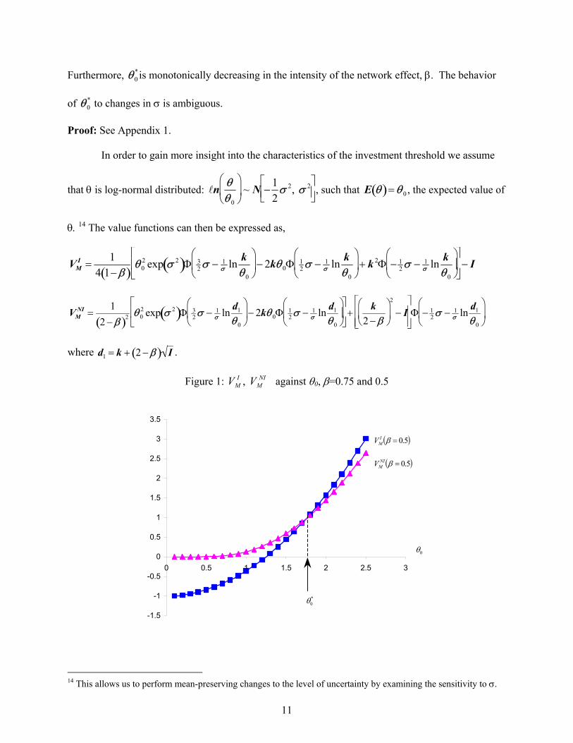
Furthermore, θ0*is monotonically decreasing in the intensity of the network effect, β. The behavior

of θ0* to changes in σ is ambiguous.

MI =

( )θ

MNI = 2 θ

+ 2

Proof: See Appendix 1.

In order to gain more insight into the characteristics of the investment threshold we assume

that θ is log-normal distributed: ln θ

θ0

~ N −

12

σ 2, σ 2

, such that E θ( )= θ0 , the expected value of

θ. 14 The value functions can then be expressed as,

V 14 1− β 0

2 exp σ 2( )Φ 32 σ − 1

σ ln kθ0

− 2kθ0Φ 1

2 σ − 1σ ln k

θ0

+ k 2Φ − 1

2 σ − 1σ ln k

θ0

− I

V 12 − β( ) 0

2 exp σ 2( )Φ 32 σ − 1

σ ln d1

θ0

− 2kθ0Φ 1

2 σ − 1σ ln d1

θ0

+

k2 − β

2

− I

Φ − 1

2 σ − 1σ ln d1

θ0

where d1 = k − β( ) I .

Figure 1: V against θ0, β=0.75 and 0.5 , NIM

IM V

-1.5

-1

-0.5

0

0.5

1

1.5

2

2.5

3

3.5

0 0.5 1 1.5 2 2.5 3

0θ

( 5.0=βIMV

( )5.0=βNIMV

)

*0θ

11

14 This allows us to perform mean-preserving changes to the level of uncertainty by examin

ing the sensitivity to σ.

Figure 1 plots and V functions against VMI

MNI θ0 . Several features about these plots are worth

noting. First, both functions are monotonically increasing in θ0. Second, since investing

immediately incurs the initial investment, VMI (0) < VM

NI (0)

VMI θ0

*

. It is also easy to show that

. Hence, from the intermediate value theorem we know that there is a

unique investment threshold, θ*0 at which

limθ 0 →∞

VMI (θ0) − VM

NI (0( ) > 0)

( )= θ0*VM

N ( ) and the firm is indifferent between

investing at t=0 or postponing the decision to t=1.

We now focus on the impact of β on θ0* . In cases where there is a greater network effect

(i.e., higher β), both V and functions have greater value. However, the impact of the network

effect is stronger on than on V . Consequently, the investment threshold falls with rising

network effect, β.

MI

VMI

VMNI

MNI

An important feature of our model is its ability to study the impact of uncertainty on the

investment threshold. Figure 2 plots the investment threshold against σ for three different values of

β. We note that for very high levels of β (β = .75), the threshold decreases monotonically with σ.

However, as the network effect intensity diminishes (β =.25), the threshold first rises with increasing

σ, but as s increases without bounds the threshold falls.

An interesting interpretation of the results comes from drawing an options analogy. Investing

immediately can be thought of as the acquisition of a growth option the value of which is given by

. In contrast, postponing the investment decision until time 1 retains the value of the wait-to-

invest option, represented by . When the network effect is strong (high β), increasing

uncertainty raises the value of the growth option from network effect more than the value of the wait-

to-invest option, lowering the investment threshold. When the network effect is weak, increasing

uncertainty makes the option of waiting more valuable at first, but eventually the growth option

VMI

VMNI

12

dominates. Consequently, the investment threshold rises with increasing σ but eventually falls when

σ increases without bound.15

Figure 2: Investment Threshold against σ for β=0.75, 0.5 and 0.25 *0θ

0

0.5

1

1.5

2

2.5

3

3.5

4

0

*0

4 Strategic Investm

We now turn to t

Unlike in the previous m

establishing a network st

around a single network

We retain the ass

invests at t=0, it establish

N then has the choice of

new standard at time 1. F

opportunity at time 1. If

15 The logic is similar to thatPerotti 1998). 16 This model can be interprebands may choose to give frefans. The band can capture t

θ

0.2 0.4 0.6 0.8 1

25.0=β

ent under Potential Imperfect Competition

he investment problem in the face of potential com

odel, now the source of advantage from early inv

andard. Licensing this standard, in effect, allows

standard.16

umption that the early investment opportunity lie

es a standard that may offer to license the standa

accepting M’s standard at a per-unit fee l or retain

irm N makes the choice knowing that it would h

N chooses not to adopt M’s standard, then it can i

when the early investment advantage comes from the co

ted in settings other than technology standards. For inste access to their music (initial investment) in an attempthe value of the resulting network by selling complement

13

5.0=β

75.0=β

1.2

σ

petition in the future.

estment arises from

the firms to coordinate

s with a single firm. If M

rd to another firm, N. Firm

s the option to develop a

ave an investment

nvest in a new standard

st side (see Kulatilaka and

ance, in the music industry to establish a community of ary goods (T-shirts) to the fans.

after all uncertainty regarding θ is fully resolved. Investment by N at time 1 will also require

spending I to produce a network good that is a perfect substitute (in its autarky value) to M’s product.

The presence of network effects plays a vital role in M’s choice of the licensing fee, N’s

adoption decision, and hence, M’s investment timing decision. When N licenses M’s standard, M

and N together will create a larger market, and will be in position to charge a higher price for the

product because of higher network value. Thus, by investing early and setting the appropriate

licensing fee, M can establish its standard as the industry standard and collect a licensing fee from

the other firm in addition to producing a good that has a greater network value. Thus, early

investment is a mechanism that enables the monopolist to establish an industry-wide standard,

internalizing the network effects through pricing and licensing contract. If M does not invest, the

two firms will make investment decisions simultaneously after the uncertainty is resolved, and it is

impossible for them to coordinate, so if they both invest, they will develop two different standards

and produce incompatible network goods. Each firm’s customers form their own smaller network

and realize a lower network value than those in a larger common network.17

The sequence of events and decisions are depicted in Figure 3. At time 0, M decides whether

or not to invest immediately. If M invests and develops a standard, then M decides whether to offer

N to adopt this standard and sets a licensing fee l. New entrant N chooses between adopting M’s

standard and developing a new standard. Although there is a time sequence to the decisions up to

now, new information becomes available only at time 1 when θ is fully revealed.

Consumers have exogenous expectations of the quantities and network size(s). Unlike in the

earlier model, the time-0 investment decision does not affect consumer expectations. When the

market opens, M and N choose the optimal quantity of the network good. If M does not invest, then

M and N have identical opportunities at time 1 and simultaneously decide whether to invest in new

17 Customers of both firms would be willing to pay a higher price if the products are compatible as could interact with users of the other firm’s product.

14

standards. When θ is large enough to trigger investment at time 1, both firms will invest and produce

incompatible products whose users belong to different networks.

Figure 3: Sequence of Events

M’s decision node N’s decision node

0 standard 0 production

M’s standard: M, N produce (q1+q2)

t=1t=0

q1q2

Not Invest

Invest

Not Invest

Invest

Invest

Not Invest

Invest

Not Invest

Invest

Offer l

No Offer

Accept

Not Accept

q1

q1 q2

q1

q2Invest

Not Invest

Not Invest

q1q2

q1q2

q1

M, N’s standards M, N produce q1, q2 respectively M’s Standard M produce q1

M’s standard M produce q1

M, N’s standards M, N produce q1, q2 respectively

N’s standard N produce q2

M, N’s standards M, N produce q1, q2 respectively

M’s standard M produce q1

We solve M’s investment and licensing fee choice through backward induction. We first

solve for the optimal licensing contract between M and N assuming that M has invested at t=0, then

solve for M’s investment threshold at t=0. First, suppose M has built a standard at t=0 and then

15

offers a contract to N with a unit licensing fee of l. If N accepts the contract and adopts M’s

standard, we can solve M’s and N’s profit maximization problems to get the equilibrium quantities

and profits: , . These are expressed as functions of θ and l, where subscripts 1 and 2

represent firms M and N respectively. Table 2a summarizes the equilibrium quantities and profits.

We allow for a general specification that also includes licensing fees that are negative (subsidies) or

zero (open standard). We later prove that the optimal licensing fee is positive and therefore, our

subsequent discussion is restricted to the case of positive licensing fees.

*2

*1 ,qq *

2*1 ,ππ

Table 2a: Equilibrium Quantities and Profits

When M invests at time 0 and N adopts M’s standard

M N L θ

Quantity *1q Profit *

1π Quantity *2q Profit *

2π

( )lk βθ −+> 2 ( )β

βθ231

−−+− lk ( ) ( )( ) ( )

( )2

222

235545

βββθβθ

−

+−−−−+− llkk ( )β

βθ232

−−−− lk ( ) 2

232

−

−−−β

βθ lk

( )lkk βθ −+≤< 2 β

θ−−

2k 2

2

−−

βθ k

0 0 l>0

k≤θ 0 0 0 0

k>θ βθ

23 −− k 2

23

−

−β

θ k β

θ23 −

− k 2 23

−−

βθ k

l=0 k≤θ 0 0 0 0

( )lk βθ −−> 1 ( )β

βθ231

−−+− lk ( ) ( )( ) ( )

( )2

222

235545

βββθβθ

−

+−−−−+− llkk ( )β

βθ232

−−−− lk ( ) 2

232

−

−−−β

βθ lk

( ) ( lklk )βθ −−≤<+ 1,0max 0 llk

−

−−β

θ2

β

θ−

−−2

lk 2

2

−

−−β

θ lk l<0

( )lk +≤ ,0maxθ 0 0 0 0

Note that when the realized demand θ is below the operating cost k, neither firm would

produce. In this case, M would regret its investment, which in effect, kills the option to postpone.

However, this potential loss is offset by several benefits. For higher levels of θ, M gains a strategic

advantage from its early investment. When demand falls in the range k < θ < k + (2 − β )l , N is

dissuaded from entering the market and M retains its monopoly. When θ is even higher

16

(θ > k + (2 − β )l ), the licensing fees act so that M produces a higher quantity than N. In other words,

the choice of the licensing fee can influence the resulting market structures.

θ

If N does not accept the fee, we solve for , as functions of θ. The resulting

equilibrium quantities, prices, and profits are given in Table 2b.

**2

**1 ,qq **

2**

1 ,ππ

Table 2b: Equilibrium Quantities and Profits when M invests at time 0 but N develops new standard at time 1

M N θ

Quantity **1q Profit **

1π Quantity **2q Profit **

2π

k> βθ

−−

3k 2

3

−−

βθ k

βθ

−−

3k 2

3

−−

βθ k

k≤θ 0 0 0 0

As before neither invests or produces for θ ≤ k . For θ > k the two firms engage in symmetric

Cournot competition.

Optimal Licensing Fee

If N accepts the contract and adopts M’s standard, the expected profits for M and N are

and respectively (M’s investment is sunk cost). If N rejects M’s standard, M

and N expect values and

E π1* l( )( +) )

)

E π 2* l( )( +

E π1**( )+

E π 2** − I( +

. Thus, N chooses to accept the contract and license

M’s standard if and only if E π 2* − Il( )( )+

≥ E π 2**( )+

. We assume that N accepts the standard when

indifferent.18

After committing the investment, M must decide whether to offer N a licensing contract, and

if so, the optimal licensing fee, . If M does not allow N to license the standard, M expects to earn

, which is the same payoff it gets if the offer l is made but declined by N. Thus, the best M

can do with a licensing contract is one that maximizes expected profit, and satisfies N’s acceptance

l*

E π1**( )+

18 Since we take expectations over the positive range, the strategy for N to stay out of the market with a reservation utility of zero is dominated and will not be chosen.

17

condition. Therefore, when offered the optimal licensing fee l* determined by the following

maximization problem, N accepts the licensing contract and adopts M’s standard.

Maxl ∈ −∞,+∞( )

E π1* l( )( +) (M’s profit maximization condition)

s.t. E π 2* l( )( )+

≥ E π 2** − I( )+

(N’s acceptance constraint)

Before solving for the optimal licensing fee l* we will closely examine each firm’s decision

criterion separately. We define as the solution to the unconstrained optimization problem l1*

Maxl

E π1*( )+

and l as the solution to *2 E π 2

* l2*( )( )+

= E π 2** − I( )+

1* l2

*

. The optimal licensing fee is

determined as l .19 The specific values of l and depend on the parameter β and the

distribution of θ. As before we assume that θ is log normal distributed in solving for l and .

l*

2*

* = Min(l1*,l2

*)

1* l

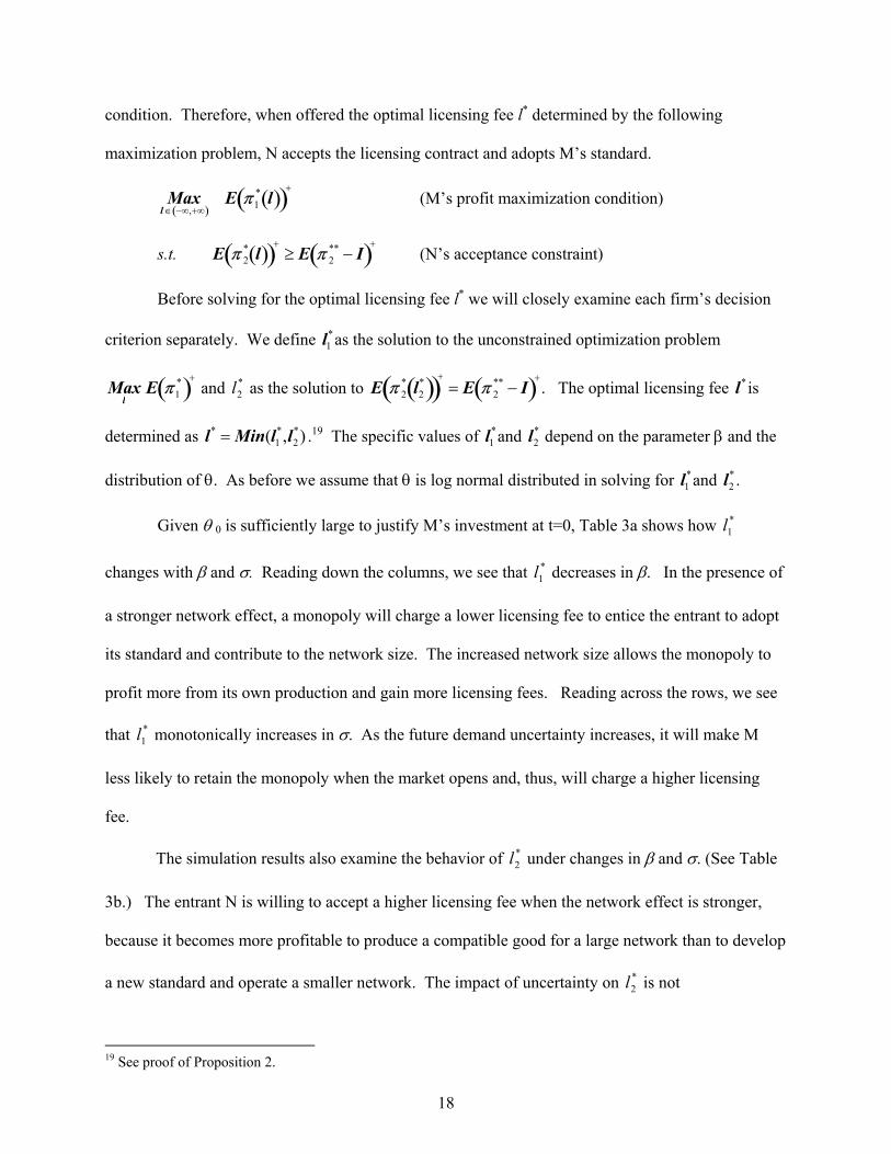
Given θ 0 is sufficiently large to justify M’s investment at t=0, Table 3a shows how l

changes with β and σ. Reading down the columns, we see that decreases in β. In the presence of

a stronger network effect, a monopoly will charge a lower licensing fee to entice the entrant to adopt

its standard and contribute to the network size. The increased network size allows the monopoly to

profit more from its own production and gain more licensing fees. Reading across the rows, we see

that l monotonically increases in σ. As the future demand uncertainty increases, it will make M

less likely to retain the monopoly when the market opens and, thus, will charge a higher licensing

fee.

*1

*1l

*1

The simulation results also examine the behavior of under changes in β and σ. (See Table

3b.) The entrant N is willing to accept a higher licensing fee when the network effect is stronger,

because it becomes more profitable to produce a compatible good for a large network than to develop

a new standard and operate a smaller network. The impact of uncertainty on l is not

*2l

*2

19 See proof of Proposition 2.

18

Table 3: Optimal Licensing Fee (a) l1

*

σ β 0.1 0.2 0.3 0.4 0.5 0.6 0.7 0.8 0.9 1 0.1 1.363 Inf 0.2 1.158 1.793 4.786 inf 0.3 1.109 1.433 2.273 4.370 11.369 Inf 0.4 1.096 1.285 1.757 2.770 5.013 10.398 27.034 64.850 inf 0.5 1.098 1.210 1.504 2.092 3.237 5.559 10.567 22.232 52.421 136.295 0.6 1.103 1.166 1.355 1.726 2.396 3.613 5.910 10.469 20.056 41.517 0.7 1.106 1.136 1.255 1.495 1.911 2.616 3.825 5.967 9.921 17.561 0.8 1.098 1.109 1.177 1.328 1.590 2.014 2.694 3.801 5.650 8.840 0.9 1.069 1.071 1.103 1.189 1.346 1.596 1.981 2.569 3.477 4.909

(b) l2

*

σ β 0.1 0.2 0.3 0.4 0.5 0.6 0.7 0.8 0.9 1 0.1 1.645 1.797 1.929 2.030 2.096 2.123 2.111 2.064 1.994 1.918 0.2 1.684 1.853 2.001 2.123 2.215 2.278 2.314 2.333 2.348 2.383 0.3 1.733 1.918 2.085 2.232 2.358 2.465 2.562 2.661 2.785 2.962 0.4 1.788 1.993 2.185 2.363 2.530 2.694 2.867 3.068 3.329 3.692 0.5 1.853 2.083 2.305 2.522 2.742 2.976 3.245 3.577 4.016 4.627 0.6 1.931 2.192 2.451 2.717 3.004 3.329 3.722 4.225 4.901 5.847 0.7 2.025 2.324 2.630 2.960 3.333 3.778 4.335 5.066 6.064 7.475 0.8 2.142 2.488 2.856 3.269 3.757 4.359 5.137 6.181 7.631 9.707 0.9 2.291 2.697 3.145 3.669 4.312 5.131 6.217 7.706 9.810 12.871

(c) l*

σ β 0.1 0.2 0.3 0.4 0.5 0.6 0.7 0.8 0.9 1 0.1 1.363 1.797 1.929 2.030 2.096 2.123 2.111 2.064 1.994 1.918 0.2 1.158 1.793 2.001 2.123 2.215 2.278 2.314 2.333 2.348 2.383 0.3 1.109 1.433 2.085 2.232 2.358 2.465 2.562 2.661 2.785 2.962 0.4 1.096 1.285 1.757 2.363 2.530 2.694 2.867 3.068 3.329 3.692 0.5 1.098 1.210 1.504 2.092 2.742 2.976 3.245 3.577 4.016 4.627 0.6 1.103 1.166 1.355 1.726 2.396 3.329 3.722 4.225 4.901 5.847 0.7 1.106 1.136 1.255 1.495 1.911 2.616 3.825 5.066 6.064 7.475 0.8 1.098 1.109 1.177 1.328 1.590 2.014 2.694 3.801 5.650 8.840 0.9 1.069 1.071 1.103 1.189 1.346 1.596 1.981 2.569 3.477 4.909

19

straightforward; it depends on the intensity of network effect. When β is low, l first increases in σ

but then decreases; when β is high however, increases in σ. The entrant is trading-off two

alternatives: to invest in its own standard or to adopt M’s standard. When the network effect is weak,

as uncertainty increases, the benefits of developing its own standard first decrease and then increase

(because of the same reasons that determine the investment threshold in the monopoly case);

therefore, the licensing fee that makes it indifferent is just the opposite. With a strong network effect

however, even though the expected profits from developing its own standard increase with

uncertainty, increasing uncertainty has an even stronger impact on the expected profits from adopting

M’s standard, thus N is willing to accept even higher licensing fees.

*2

*2l

The optimal licensing fee l is determined by the minimum of l and . When the network

effect is small, l is determined by N’s indifference condition. i.e.,

* *1

*2l

* l* = l2* . But as the intensity of

the network effect increases, M’s profit maximization is achieved with a lower licensing fee and

. Table 3c presents the comparative statics of with respect to β and σ. l* = l1* *l

When the network effect is significant (high β) and uncertainty low (low σ), is determined

by l and N’s acceptance constraint is not binding, in other words, M charges a low fee even though

N would accept a higher one. As the network effect becomes less significant or as uncertainty

increases (moves toward lower β or higher σ), M wants to charge a higher licensing fee, and N’s

acceptance constraint starts binding. For example, when β=0.1, the optimal licensing fee is

determined by N for all σ’s except for σ=0.1. When β=0.5, the optimal licensing fee is determined

by M for σ≤0.4, and by N for higher σ; keeps increasing, but at a smaller slope when determined

by N. When β=0.9, the optimal licensing fee is determined solely by M for the range of σ of interest,

and is strictly increasing. When the uncertainty level is fixed and the intensity of network effect

changes, the optimal licensing fee increases in β when determined by N and decreases when by M.

*l

*1

*l

20

For example, when σ=0.1, the optimal licensing fee is determined solely by M, thus decreases in β.

When σ=0.5, is decided by N for β≤0.5, where it keeps increasing and by M for higher β where it

declines accordingly. The pattern is the same for β=0.9.

*l

This is particularly significant for low uncertainty in demand (low σ) and a strong network

effect (high β). When σ is low, it is highly unlikely for a large θ to occur, and a high licensing fee

means that the market condition for N to produce is highly unlikely to happen, and thus the total

expected licensing income with higher per-unit fee can be too small to compensate for the loss of

licensing income when N is not producing.

When β is high, due to the strong network effect, the advantage of being a monopoly

becomes less significant, because a firm can charge a higher price for a product with a larger

network, even if the larger network is a result of other firms producing compatible products. On the

other hand, the disadvantage of being a monopoly, i.e. the loss of licensing income from competitors

is more significant, because under higher β, N would produce more if it were. Therefore, M will

choose a lower licensing fee to take advantage of the network effect and avoid being a monopoly

when it does not payoff.

We now formalize these properties of the optimal licensing fee in Proposition 2.

Proposition 2:

When the demand uncertainty is log-normal distributed, i.e., l n θ

θ0

~ N −

12

σ 2, σ 2

, the

optimal licensing fee l is positive and *

a) If M’s expected profits for any arbitrary licensing fee is less than the expected profits

to a monopolist in the product market, i.e., E π1* l( )( )+

<1

2 − β( )2 θ − k( )2 f θ( )dθk

∞∫ ,

21

then the optimal licensing fee is l , where l is determined implicitly by

.

*2

* l=

E

*2

E π 2* l2

*( )( )+= E π 2

** − I( )+

ˆ >lˆ l >

)*2

*1 , l* =

( )

*

)((( ) ln

ln1

0

1

−− kθ σ

σ

55245

22

120*

1 −Φ+−+Φ−

−lββ

θβσ

σσ

+ 2 −

*1

−lβ

β( )l)

b) If there exists a finite such that 0 π1*( )+

l =

12 − β( )2 θ − k( )2 f θ( )dθ

k

∞∫ , the

optimal licensing fee (min ll , where l is determined implicitly by M’s

profit maximization condition,

1

( ))( )( )( ) 0

2*1

=+

+lk β2

−ln10θ

σ

ln+

.

Proof: See Appendix 2.

Proposition 2 shows that the optimal licensing fee is only sometimes decided entirely by N’s

acceptance of the licensing contract. In particular, it may not be in the best interest of M to charge an

infinitely high licensing fee regardless of N’s reaction. Under certain conditions, M will charge a

finite licensing fee, not to deter N from developing a new standard that creates two smaller networks

and lowers M’s profits, but because M can earn higher profits in a single network.

The reason for this counter-intuitive result lies in the tradeoff between the two effects of the

licensing fee on M’s profit. A higher licensing fee increases the range of θ over which M retains a

monopoly k, k( and N’s entry is deterred. However, being a monopolist has a cost in

that M cannot collect licensing fee from N over a larger range of θ. The choice of the licensing fee

affects not only the range of monopoly but also the level of revenues to M. The licensing revenues to

M when N enters the market depends on the per-unit licensing fee paid by N and the level of N’s

production. With a higher l* M gets higher per-unit royalty from N but it also lowers the quantity

that N produces. Therefore, the net impact of increasing l* on the licensing revenue is not

necessarily positive. The combined effects of an increase in the licensing fee on M’s expected

profits can be ambiguous.

22

We have shown that M’s expected profit from the optimal licensing contract is E π1* l*( )( )+

.

M will choose to license his standard to N rather than not if and only if E π1* l*( )( )+

≥ E π1**( )+

. The

proof of Proposition 3 shows that E π1* l*( )( )+

≥ E π1**( )+

is always satisfied, and thus as long as M

has invested at time 0, it will always license the standard to N, resulting in one, compatible network

in the market.

Proposition 3: If M invests at t=0, then M chooses to license its standard to N with a licensing fee of

l*, as specified in Proposition 2, and N accepts and adopts M’s standard.

Proof: See Appendix 3.

Proposition 3 illustrates the decision path along the game tree in Figure 3. We have shown

that when M commits the investment at time 0, it will always choose to offer to license its standard to

N. Previously we have shown that the licensing fee can be chosen to ensure that N adopts M’s

standard. Therefore, an optimally managed investment will result in a single network. In other

words, failure to set the correct licensing fee or the decision to not license the standard will result in

sub optimal value. We now turn to M’s investment decision at time 0, given that the subsequent

management of the investment will be optimal.

Investment Threshold

As with the earlier case of the pure monopolist, we can now examine M’s investment

decision at t=0 and the investment threshold . We know from Proposition 3 that if M invests, M

will offer the optimal licensing fee l* to N and subsequently N will accept and adopt M’s standard.

When M makes its investment decision at t=0, its expected net payoff from investing is

, which is a function of

*0θ

( )( ) IlE −+**

1π ( )θθ 0E0 = .

If M does not invest at time 0, then at time 1, M, together with N, will decide whether to

invest, and if so, what the optimal quantity he should produce. If M invests at t=1, the optimal

23

quantities and associated profits are q , as functions of θ (see Table 2c). M’s

expected profit is at t=1 and

***2

***1 , q

E π

***2

***1 , ππ

1*** − IE π1

***( )+− I ( )+

at t=0.

Table 2(c) Equilibrium Quantities and Profits

When M does not invest at time 0, M and N develop their own standards at time 1

M N θ

Quantity ***1q Profit ***

1π Quantity ***2q Profit ***

2π

k>θ βθ

−−

3k 2

3

−−

βθ k

βθ

−−

3k 2

3

−−

βθ k

k≤θ 0 0 0 0

Proposition 4: M’s investment threshold is the solution to: *0θ E π1

* l*( )( )+− I = E π1

*** − I( +) , where

under the lognormal distribution for θ

E π1* l*( )( )+

= 12 − β( )2 θ0

2eσ 2

Φ 32 σ − 1

σ ln kθ0

− 2kθ0Φ 3

2 σ − 1σ ln k

θ0

+ k 2Φ 3

2 σ − 1σ ln k

θ0

( ) ( )

( )21

232

022 ln231

21 2

de σσ σθ

ββ−Φ

−−

−

( )( )

−

( )

( )21

21

022

*

ln2

223

245 dkklσσθ

βββ

−Φ

−+

−−−

+

+k 2 − 5 − 4β( )kl* − 5 − 5β + β 2( ) l*( )2

3 − 2β( )2 −k 2

2 − β( )2

Φ − 1

2 σ − 1σ lnd2( )

where d = [ ]2 k + 2 − β( )l* θ0 , and

E π1*** − I( )+

=θ0

2eσ 2

Φ 32 σ − 1

σ lnd3( )− 2kθ0Φ 12 σ − 1

σ lnd3( )[ ]3− β( )2 +

k3− β

2

− I

Φ − 1

2 σ − 1σ lnd3( )

where d3 = k + 3− β( ) I[ ] θ0 .

24

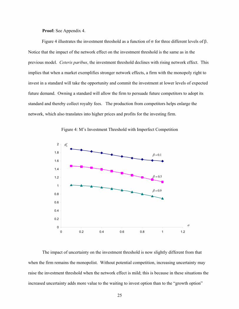
Proof: See Appendix 4.

Figure 4 illustrates the investment threshold as a function of σ for three different levels of β.

Notice that the impact of the network effect on the investment threshold is the same as in the

previous model. Ceteris paribus, the investment threshold declines with rising network effect. This

implies that when a market exemplifies stronger network effects, a firm with the monopoly right to

invest in a standard will take the opportunity and commit the investment at lower levels of expected

future demand. Owning a standard will allow the firm to persuade future competitors to adopt its

standard and thereby collect royalty fees. The production from competitors helps enlarge the

network, which also translates into higher prices and profits for the investing firm.

Figure 4: M’s Investment Threshold with Imperfect Competition

0

0.2

0.4

0.6

0.8

1

1.2

1.4

1.6

1.8

2

0 0.2 0.4 0.6 0.8

5.0=β

1.0=β

*0

The impact of uncertainty on the investment threshold is no

when the firm remains the monopolist. Without potential competiti

raise the investment threshold when the network effect is mild; this

increased uncertainty adds more value to the waiting to invest optio

25

9.0=β

θ

1 1.2

σ

w slightly different from that

on, increasing uncertainty may

is because in these situations the

n than to the “growth option”

resulting from the network effect. When the monopolist anticipates imperfect competition,

increasing uncertainty always lowers the investment threshold. This result arises from the ability to

use the licensing fee to induce future competitors to adopt the standard, thus, sharing the market and

the associated risks. Thus increasing uncertainty leads to lower investment threshold.

5 Concluding Remarks

In this paper, we study the strategic impact of investing in a network under different market

structures. We find that even a firm that is assured of being a continued monopoly has an incentive

to commit to network investments before uncertainty about the future demand is resolved. The key

feature of a network that drives our model is that each consumer experiences value from the presence

of other consumers of the network good (network effect), in addition to the autarky value of

consuming the standalone good. The benefit to early commitment comes from the credible

communication to the users about the future size of the network and thereby, internalizing the

adoption externality. We obtain the threshold level of expected demand above which the monopolist

will commit the investment by trading off this strategic benefit of investment against the value of

waiting to invest. Not surprisingly, the threshold level falls monotonically with increasing intensity

of network effect. This result stresses the importance of having an accurate estimate of the network

effect. Overestimating the network effect may make firms commit investment prematurely. This

effect is most pronounced in environments with high uncertainty.20

When we allow for potential competitors in the network, the strategic value of early

investment arises from the establishment of a network standard that can be licensed out. The choice

of the licensing fee plays a vital role in the adoption decision by the competitors. We show that there

is a unique level for the optimal fee at which the profits of the firm committing the investment to

establish a network standard are maximized and the competitors choose to adopt this single standard. 20 The rush to invest in dotcoms during the late 1990s and the investments in 3G spectrum by European mobile operators may be explained by a very high perceived network effects. The underestimation of the investment threshold is further exacerbated in highly uncertain environments.

26

Setting too high a licensing fee can result in incompatible networks and will be sub-optimal for the

network builders. The optimal licensing fees are also affected by the intensity of the network effect

and the level of uncertainty regarding future demand.

When the uncertainty is very low, the optimal licensing fee becomes very small. In the limit,

if there is no uncertainty, then open standards can lead to the largest networks and highest profits to

the network-building firms. The impact of the intensity of the network effect on the optimal

licensing fee leads to more interesting implications. For very low uncertainty, the licensing fee is

determined by the investing firm’s profit maximization and monotonically decreases with increasing

intensity of network effects. For higher levels of uncertainty, the licensing fee is determined by the

competitor’s adoption decision for low levels of network intensity. In such cases, as the network

increases the competitor is willing to accept a higher licensing fee. However, for further increases in

the network effect it becomes in the investing monopolist’s interest to limit the licensing fee. When

this condition is binding the optimal licensing fee falls with network intensity.

These results highlight the critical importance of setting the license fee in environments with

high uncertainty and high network effects. An investor may be tempted to charge a higher licensing

fee simply because competitors are showing willingness to adopt the standard. However, would be

in their best interest to charge a lower licensing fee and grow the network to realize larger network

profits. This is consistent with the view that opening the standards to competitors can have a

bandwagon effect.21

Once the optimal licensing fees are determined, we also solve for the expected demand

threshold at which the early investment should be committed. As with the earlier case of the

monopolist, the investment threshold is decreasing in network intensity, β. Now the investment

threshold also decreases monotonically with increasing uncertainty (σ). Unlike in the case of a

guaranteed monopolist, the investment threshold is not as sensitive to the intensity of the network 21 For instance Shapiro and Varian (1999) argue that “Openness is a more cautious strategy than control. The underlying idea is to forsake control over the technology to get the bandwagon rolling.” (p199)

27

effect. This is because the optimal licensing fee takes into account the impact of the network

intensity.

References Dixit, Avinash. 1980. The role of investment in entry deterrence. Economic Journal. Vol. 90, 95-106 Dixit, Avinash and Robert S. Pindyck. 1994. Investment Under Uncertainty, Princeton University Press, Princeton, New Jersey. Economides, Nicholas. 1996. The economics of networks. International Journal of Industrial Organization, Vol. 14, No. 6, 673-699. Gilder, George F. 2000. Telecosm: how infinite bandwidth will revolutionize our world, Free Press, First edition, New York, New York. Grenadier, Steven R. 1996. The Strategic Exercise of Options: Development Cascades and Overbuilding in Real Estate Markets, The Journal of Finance, Vol. 51, No. 5 (Dec.) 1653-1679 Katz, Michael L., Carl Shapiro. 1994. Systems competition and network effects, The Journal of Economic Perspectives, Vol. 8, No. 2, 93-115. Katz, Michael L., Carl Shapiro. 1985. “Network externalities, competition, and compatibility”, American Economic Review Vol. 75, No. 3 (Jun) 424-440 Kulatilaka, Nalin, Enrico Perotti. 1998. Strategic Growth Options,.Management Science, Vol. 44, No. 8 (August), 1021-1031. Kulatilaka, Nalin, Enrico Perotti. 2000. Time-to-Market Advantage as a Stackelberg Growth Option, in E. Schwartz and L. Trigeorgis (eds) Innovation and Strategy: New Developments and Applications in Real Options, Oxford University Press Leibowitz, Stan J., Stephen E. Margolis. 1994. Network externality: an uncommon tragedy, Journal of Economic Perspectives, Vol. 8, No. 2, 133-150. McDonald, Robert L. and Daniel R. Siegel. 1986. The Value of Waiting to Invest, Quarterly Journal of Economics, Vol. 101, No. 4, 707-728 Shapiro, Carl and Hal Varian. 1999. Information Rules: A Strategic Guide to the Network Economy, Harvard Business School Press, Boston, Massachusetts Spence, A. Michael. 1984. Cost Reduction, Competition, and Industry Performance, Econometrica, Vol. 52, No. 1 (Jan.), 101-122 Standage, Tom. 1998. The Victorian Internet: The remarkable story of the telegraph and the nineteenth century's on-line pioneers, Walker & Co, New York, New York.

28

Appendices Appendix 1: The proof of Proposition 1 (omitted) Appendix 2: The proof of Proposition 2.

We find the optimal licensing fee l* by solving:

( )

( )( )+

+∞∞−∈lEMax

l

*1,

π(A1)

s.t. (N’s acceptance constraint) ( )( ) ( ++−≥ IElE **

2*2 ππ )

)

We know that and are defined differently for positive and negative l. So we first

prove that the solution to (A1) is positive.

*1π *

2π

Lemma 1:

(a) The licensing fee at which N’s acceptance constraint is binding, denoted by l , is

positive;

*2

(b) is determined implicitly by: *2l

( )( ) ( ++−= IElE **

2*2

*2 ππ , or

13− 2β( )2 θ0

2eσ 2

Φ 32 σ − 1

σ lnd2( )− 2 k + 2 − β( )l2*[ ]Φ 1

2 σ − 1σ lnd2( )+ k + 2 − β( )l2

*[ ]2Φ − 1

2 σ − 1σ lnd2( ){ }

= 13− β( )2 θ0

2eσ 2

Φ 32 σ − 1

σ lnd3( )− 2kθ0Φ 12 σ − 1

σ lnd3( ){ }+k

3− β

2

− I

Φ − 1

2 σ − 1σ lnd3( )

where

( )θθ 00 E= , d2 = k + 2 − β( )l2*[ ] θ0 , d3 = k + 3− β( ) I[ ] θ0 .

(c) For any , N’s acceptance constraint is satisfied with “>” holding. *2ll <

Proof: From Table 2, we have:

29

( )( )( ) ( ) ( )

( )

( ) ( )( )

≥

−

−−−

<

−

−−−+

−

−−

=

∫

∫∫∞

−+

∞

−+

−+

++

lk

lk

lk

lk

ldflk

ldflkdflk

E

β

β

β

θθβ

βθ

θθβ

βθθθβ

θ

π

2

2

1

21

),0max(

2

*2

0232

0,232

2

It can be easily proved that is a continuous (but not differentiable at 0), globally

decreasing function of l.

( )+*2πE

We have:

( ) ( )∫∞

=

+

−−

=kl

dfkE θθβ

θπ2

0

*2 23

( ) ( )( )∫

∞

−+

+

−

−−

=−Ik

dfIkIEβ

θθβ

θπ3

2**

2 3

Thus, ( ) ( )+

=

+−> IEE

l

**2

0

*2 ππ .

We also have ( ) 0*2 =

∞→

+

lE π .

Therefore, there is one and only one positive l such that ( ) ( )++−= IEE **

2*2 ππ . We denote

this licensing fee by l . Solving the integrals will lead to the equation in (b). *2

Because is a decreasing function, in particular, ( )+*2πE ( ) 0

0

*2 <

∂∂

>

+

ll

E π and

( ) 00

*2 <

∂∂

<

+

ll

E π, for any l<l , ( ) ( )++

−> IEE **2

*2 ππ holds.

Q.E.D.

Lemma 2: ( ) ( ) ( )0

*1

0

*1

0

*1

<

+

=

+

>

+>>

lllEEE πππ

Proof: From Table 2, we have:

30

( )( )

( ) ( )( )

( )( )( ) ( ) ( )( )

( )∫

∫∞

−+

−+

>

+

−−−

−+−+−

−+

−−

=

lk

lk

kl

dfllklk

dfkE

β

β

θθβθβ

βθβ

θθθβ

π

2

22

2 22

0

*1

223

11231

21

( )

( ) =−

+

0

*1

lE π

( )( ) ( )∫

∞−

− kdfk θθθ

β2

2231

And

( ) ( ) ( ) ( )( )

( )( )( ) ( ) ( )( )

( )∫

∫∞

−+

−+

+<

−−−

−+−+−

−+

−−−

=

lk

lk

lkl

dfllklk

dlflkE

1

22

1

),0max(0

*1

223

11231

21

β

β

θθβθβ

βθβ

θθθβ

π

( )

It can be easily proved that ( ) ( ) ( )0

*1

0

*1

0

*1

<

+

=

+

>

+>>

lllEEE πππ .

Q.E.D.

Based on Lemma 1 and 2, we can focus on finding the optimal licensing fee l* in the positive

range. Solving (A1) is equivalent to solving

( )+

>

*10

πEMaxl

(A2)

s.t. (N’s acceptance constraint) ( ) ( )++−≥ IEE **

2*2 ππ

Lemma 3:

a) The unconstrained maximization problem ( )+

>

*10

πEMaxl

has an interior solution if and only

if there exists a finite such that 0ˆ >l

( )( )

( ) ( )∫∞

=

+−

−>

klldfkE θθθ

βπ 2

2ˆ

*1 2

1

(b) When the above condition is satisfied, the interior solution denoted by l , is determined

by the following implicit equation:

*1

31

( ) ( )( )( )( ) ( )( )( ) 0

2lnln5522lnln45

*1

11

12

2

*1

11

120*

1 =−+−+−Φ+−

−+−+Φ−−

lklk

lβθββ

βθθβ

σσσ

σσσ

(A3)

where Φ is the c.d.f. of standard normal distribution.

Proof:

(a) Since ( )( )

( ) ( )∫∞

∞→

+−

−=

kldfk θθθ

βπ 2

2*1 2

1E , an interior solution must satisfy the

above boundary condition.

(b) When the condition in (a) is satisfied, an interior solution exists. It must satisfy

( ) 0*1

*1 =

∂∂

=

+

lll

E π, and

( ) 0*1

2

*1

2

<∂

∂

=

+

lll

E π. Taking the derivative of ( )

0

*1

>

+

lE π with respect to l, and

making it equal to zero, we get (A3).

Q.E.D.

Proof of Proposition 2:

Lemmas 1 and 2 show that l* is positive.

Lemma 3 shows that when the unconstrained maximization problem has a

finite solution (denoted by ), it is determined implicitly by

( )+

>

*10

πEMaxl

*1l

( ) ( )( )( )( ) ( )( )( ) 0

2lnln5522ln45

*1

102

2

*1

10

120*

1 =−+−+−Φ+−

−+−+Φ−−

lklk

lβθββ

βθβ

σσ

σσσ ln

1

θ

σ

.

The optimal licensing fee l* must satisfy N’s acceptance constraint. When l exists, if

, by Lemma 1, satisfies the constraint, and therefore l . If l , l does not satisfy

the constraint; for all the l’s that satisfy the acceptance constraint i.e.

*1

*1

*2

*1 ll ≤ *

1l*1

* l= *2

*1 l>

( )*2, l∞−l ∈ , is

maximized at the l , because it can be proved that

( )+*1π1E

*2 ( )+*

1πE is increasing in l for ( )*1l,0l ∈ . To sum

up, ( )*2

*1 ,min ll=*l , where l is determined by (A3) and l is as specified in Lemma 1. *

1*2

32

When the condition specified in Lemma 3(a) is violated, it means that for any ( )+∞∞−∈ ,l ,

( )( )( )

( ) ( )∫∞+

−−

<k

dfklE θθθβ

π 22

*1 2

1

*2

* l=

, i.e. M would set the licensing fee infinitely high if he could

force N to accept it. In this case, the solution to (A1) will be decided solely by N’s acceptance

constraint binding. Therefore, l .

Q.E.D.

Appendix 3: The proof of Proposition 3.

The acceptance constraint in the maximization problem (1) guarantees that N accepts the

optimal licensing fee l*. Thus to prove Proposition 3, we only need E1 π1* l*( )( )+

≥ E1 π1**( )+

.

By Lemma 2, ( ) ( )0

*1

0

*1

=

+

>

+>

llEE ππ . Since l*>0, ( ) ( )

0

*1

*1 * =

+

=

+>

lllEE ππ .

We have

( )( )

( ) ( )∫∞

=

+−

−=

kldfkE θθθ

βπ 2

20

*1 23

1 ,

( )( )

( ) ( )∫∞+

−−

=k

dfkE θθθβ

π 22

**1 3

1

Obviously, ( ) ( )+

=

+≥ **

10

*1 ππ EE

l. Thus, ( )( ) ( )++

≥ **1

**1 ππ ElE .

Q.E.D.

Appendix 4: The proof of Proposition 4.

By Proposition 3, we know that if M invests at time 0, then M will license his standard to N

with a licensing fee of l*, and N accepts and adopts M’s standard. Thus the expected payoff for

investment is , which is a function of θ0. Since M has to make the investment upfront, the

net payoff is .

( )( +**1 lE π

( )( lE −+**

1π

)

) I

33

If M does not invest at time 0, then at time 1 M decides simultaneously with N whether to

invest and produce the network goods. Thus the expected payoff for not investing is

(no information on θ is revealed between time 0 and 1).

( )+− IE ***

1π

Therefore, the investment threshold is the solution to: *0θ ( )( ) ( ++

−=− IEIlE ***1

**1 ππ ) , and

solving the integrals will result in the analytical expressions of ( )( )+**1 lπ ( )+

− IE ***1πE and

presented in Proposition 4.

Q.E.D.

34