abstract minimizing total number of tardy jobs on a …

ABSTRACT

MINIMIZING TOTAL NUMBER OF TARDY JOBS ON A SINGLE BATCH PROCESSING

MACHINE BY GREEDY RANDOMIZED ADAPTIVE SEARCH PROCEDURE WITH PATH

RELINKING

Panteha Alipour, MS

Department of Industrial and Systems Engineering

Northern Illinois University, 2016

Purushothaman Damodaran, Director

Batch processing machines are commonly used in metal working, chemical processing,

and electronics manufacturing – to name a few. Scheduling these machines optimally is a hard

task; the number of decision variables used in the mathematical formulations grow exponentially.

Consequently, commercial solvers used to solve the formulations require prohibitively long run

times. Schedulers struggle to make good decisions due to the complexity of the problem.

This research considers the problem of scheduling a single batch processing machine such

that the total number of tardy jobs is minimized. The machine can simultaneously process several

jobs as a batch as long as the machine capacity is not violated. The batch processing time is equal

to the largest processing time among those jobs in the batch. Two decisions are made to schedule

jobs on the batch processing machines, namely grouping jobs to form batches and sequencing the

batches formed on the machines. Both the decisions are interdependent as the composition of the

batch affects the processing time of the batch. The problem under study is NP-hard. Consequently,

solving a mathematical formulation to find optimal solutions is computationally intensive.

A greedy randomized adaptive search procedure (GRASP) is proposed to solve the

problem under study with the assumption of arbitrary job sizes, arbitrary processing times and

arbitrary due dates. A novel construction phase for the GRASP approach is also proposed to

improve the solution quality. In addition, a path relinking procedure is also proposed for solving

large-sized problems effectively. The performance of the proposed GRASP approach is evaluated

by comparing its results to a commercial solver. Experimental studies suggest that the solution

obtained from the GRASP approach is superior compared to the commercial solver. The proposed

approach will benefit schedulers to schedule jobs on batch processing machines more efficiently.

The new solution approach proposed for the problem under study fills some gaps found in the

literature and will encourage other researchers to try new solution approaches or consider solving

other variants of the problem.

NORTHERN ILLINOIS UNIVERSITY

DE KALB, ILLINOIS

MINIMIZING TOTAL NUMBER OF TARDY JOBS ON A SINGLE BATCH PROCESSING

MACHINE BY GREEDY RANDOMIZED ADAPTIVE SEARCH PROCEDURE

WITH PATH RELINKING

BY

PANTEHA ALIPOUR

A THESIS SUBMITTED TO THE GRADUATE SCHOOL

IN PARTIAL FULLFILLMENT OF THE REQUIREMENTS

FOR THE DEGREE

MASTER OF SCIENCE

DEPARTMENT OF INDUSTRIAL AND SYSTEMS ENGINEERING

Thesis Director:

Dr. Purushothaman Damodaran

ACKNOWLEDGEMENTS

I would like to seize this opportunity and thank several people without whom this work would

never have been possible. First and foremost, I would like to express my sincere gratitude to my

supervising professor, Dr. Purushothaman Damodaran, for his continuous guidance, support, and

encouragement. I also thank him for constantly pushing me towards being creative and working

indefatigably towards utilizing my potentials. His work ethic, authenticity, and intelligence have

always been a source of inspiration to me. I have learned a lot from his profound insight, keen

observations, and vast knowledge. I am privileged to have had an opportunity to work with him. I

would like to express my gratitude to my committee members, Professors Ghrayeb and Krishnamurthi,

for careful review of my work and who gave challenging, insightful comments on my thesis and helped

me think more deeply in this research.

Dedicated

To My Beloved Parents

TABLE OF CONTENTS

Page

LIST OF FIGURES .......................................................................................................... vii

LIST OF TABLES ........................................................................................................... viii

CHAPTER 1 INTRODUCTION .........................................................................................1

1.1 Problem Description ..................................................................................................... 2

1.2 Research Objectives and Scope .................................................................................... 3

1.3 Research Benefits and Deliverables .............................................................................. 4

1.4 Organization .................................................................................................................. 5

CHAPTER 2 LITERATURE REVIEW ..............................................................................6

2.1 Characteristics of Batch Processing Machines ...................................................................... 8

2.1.1 Single Batch Processing Machine (BPM) Environment ............................................... 10

2.1.2 Parallel Batch Processing Machine (BPM) Environment ............................................. 10

2.2 Minimize Total Number of Tardy Jobs................................................................................ 12

2.3 Meta-heuristics ..................................................................................................................... 13

2.4 Summary .............................................................................................................................. 15

CHAPTER 3 MATHEMATICAL FORMULATION .......................................................16

CHAPTER 4 GRASP SOLUTION APPROACH .............................................................26

CHAPTER 5 COMPUTATIONAL RESULTS ................................................................39

CHAPTER 6 CONCLUSION AND FUTURE RESEARCH ...........................................45

6.1 Overview of the Poblem Under Study ................................................................................. 46

6.2 Findings ............................................................................................................................... 46

6.3 Future Research ................................................................................................................... 47

REFERENCES ..................................................................................................................48

APPENDIX: GRASP, CPLEX AND CONSTRUCTION PHASE ...................................45

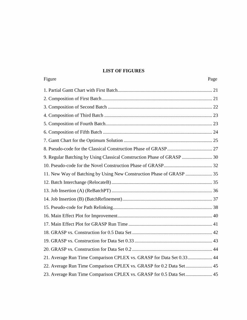
LIST OF FIGURES

Figure Page

1. Partial Gantt Chart with First Batch.............................................................................. 21

2. Composition of First Batch ........................................................................................... 21

3. Composition of Second Batch ...................................................................................... 22

4. Composition of Third Batch ......................................................................................... 23

5. Composition of Fourth Batch........................................................................................ 23

6. Composition of Fifth Batch .......................................................................................... 24

7. Gantt Chart for the Optimum Solution ......................................................................... 25

8. Pseudo-code for the Classical Construction Phase of GRASP ..................................... 27

9. Regular Batching by Using Classical Construction Phase of GRASP ......................... 30

10. Pseudo-code for the Novel Construction Phase of GRASP........................................ 32

11. New Way of Batching by Using New Construction Phase of GRASP ...................... 35

12. Batch Interchange (RelocateB) ................................................................................... 35

13. Job Insertion (A) (ReBatchPT) ................................................................................... 36

14. Job Insertion (B) (BatchRefinement) .......................................................................... 37

15. Pseudo-code for Path Relinking .................................................................................. 38

16. Main Effect Plot for Improvement .............................................................................. 40

17. Main Effect Plot for GRASP Run Time ..................................................................... 41

18. GRASP vs. Construction for 0.5 Data Set .................................................................. 42

19. GRASP vs. Construction for Data Set 0.33 ................................................................ 43

20. GRASP vs. Construction for Data Set 0.2 .................................................................. 44

21. Average Run Time Comparison CPLEX vs. GRASP for Data Set 0.33 .................... 44

22. Average Run Time Comparison CPLEX vs. GRASP for 0.2 Data Set ...................... 45

23. Average Run Time Comparison CPLEX vs. GRASP for 0.5 Data Set ...................... 45

LIST OF TABLES

Table Page

1. Literature Review Categories ...................................................................................................... 7

2. Parameters for Generating Problem Instances ........................................................................... 19

3. Data for a 9-Job Problem Instance ............................................................................................. 20

4. Evolution of the EDD Order in Classical Construction Phase of GRASP................................. 29

5. Evolution of the EDD Order in a Novel Construction Phase of GRASP .................................. 32

6. Data for a 9-Job Instance ........................................................................................................... 35

7. Factors and Levels ..................................................................................................................... 39

8. Solution and Run Time of Construction Phase and GRASP for Small Jobs, γ=0.2 .................. 54

9. Solution and Run Time of Construction Phase and GRASP for Large Jobs, γ=0.2 .................. 56

10. Solution and Run Time of Construction Phase and GRASP for Small Jobs, γ=0.5 ................ 57

11. Solution and Run Time of Construction Phase and GRASP for Large Jobs, γ=0.5 ................ 60

12. Solution and Run Time of Construction Phase and GRASP for Small Jobs, γ=0.33 .............. 61

13. Solution and Run Time of Construction Phase and GRASP for Large Jobs, γ=0.33 .............. 64

CHAPTER 1

INTRODUCTION

Batch processing is employed in many manufacturing environments, such as chemical

processing, wafer fabrications (Phojanamongkolkij, Fowler, & Cochran, 2002), metal working,

food and mineral processing industries and environmental stress screening (ESS) chambers

(Damodaran, Hirani, & Velez-Gallego, 2009). Unlike discrete processing machines, batch

processing machines (BPMs) can process several jobs simultaneously in a batch. Discrete

processing machines can process only one job at a time. By processing several jobs in a batch on

a BPM, the number of setups required can be minimized and the total time required to process all

the jobs can also be minimized in some cases. The BPM is typically expensive, so its utilization

should be improved. One of the performance measures commonly used in scheduling literature is

the minimization of the total number of tardy jobs. Minimizing total number of tardy jobs is of

great importance in the real world and it is identical to improving the on-time shipments percentage

(Pinedo, 2012).

This research is motivated by a practical application where printed circuit boards (PCBs)

are assembled and tested. In electronics manufacturing, after assembly, groups of PCBs are tested

in an ESS chamber to detect component and other board-level failures before they are used in the

field. ESS is the process of applying environmental stresses in conjunction with functional testing

in order to stimulate the failure mechanisms of defects to the point of detection that could not be

detected by visual inspection or in-circuit testing (Damodaran & Srihari, 2004). The PCBs are

typically subjected to vibration, humidity, and thermal cycling or power cycling in an ESS

chamber. The ESS chamber is referred to as BPM and the PCBs as jobs in this research to remain

consistent with the scheduling literature.

The jobs from different assembly lines line up in front of a BPM for testing. For

automation’s sake and repeatability, usually manufacturers have a tendency to set up processes for

2

handling uniformly sized panels of materials. However, if the board is large or needs special kinds

of processing, it will flow through the manufacturing process on panels with other designs (with

varying size). The jobs assumed are to vary in terms of size. The processing time, which is the

testing time, also varies depending upon the customer’s testing requirements. Once several jobs

are grouped as a batch, the processing time of the batch considered is the same as the longest

processing time of all jobs in the batch. Two tasks are carried out to schedule a set of jobs on a

BPM. The first task is to form batches such that the machine capacity is not violated, and the

second task is to determine a schedule that minimizes the total number of tardy jobs. The problem

of minimizing total number of tardy jobs on a single batch processing machine is NP-hard in strong

sense (Brucker, Kovalyov, Shafransky, & Werner, 1998), and hence a greedy randomized adaptive

search procedure (GRASP) with path relinking is proposed in this research. Path relinking

implements a novel local search strategy based on different neighborhood structures defined by

path exchanges, and it uses memory based on a local search strategy to find much better solutions

in much less computation time (Aiex, Binato, & Resendel, 2003; Resendel & Ribeiro, 2005).

1.1 Problem Description

The problem considered in this research is described as follows. Given a set of jobs, the

jobs are grouped to form batches and the batches are scheduled on a BPM for processing. The

processing time (pj), size (sj) and due date (dj) of each job j is given. The objective is to form

batches of jobs and schedule these batches on a BPM to minimize the total number of tardy or late

jobs. A job is tardy (Uj) if the completion time of job j is larger than its due date (i.e., 𝑐𝑗 > 𝑑𝑗).

The problem under study can be characterized as 1|𝑝 − 𝑏𝑎𝑡𝑐ℎ, 𝑠𝑗| ∑ 𝑈𝑗 using the three-

field notation 𝛼|𝛽|𝛾 introduced by Graham, Lawler, Lenstra and Kan (1979). The α field denotes

the machine environment. The β field denotes the constraints considered. The γ field denotes the

objective function. For the problem under study, there is one BPM, the processing time of the

batch is equal to the longest processing time of all the jobs in the batch (p-batch problem), the

sizes of the jobs are not identical, and the objective is to minimize the number of tardy jobs (∑ 𝑈𝑗).

3

The maximum number of batches required to process all the jobs is easy to determine.

Assuming one job per batch will result in 𝑛 batches, hence the maximum number of batches needed

is also 𝑛. The batch processing time is equal to the longest processing time of all the jobs in the

batch. When forming batches, the total size of all the jobs in the batch should not exceed the

machine capacity (S). In order to schedule the batch processing machine, two decisions need to

be made. First, jobs need to be grouped into batches, and second, the batches formed need to be

scheduled. Both decisions are considered dependent on each other as the formation of the batch

determines the batch processing time, which then affects the total number of tardy jobs. The batch

formation depends on the machine capacity, and the batch processing time depends on the

composition of the jobs in the batch which is assumed to be equal to the largest processing time of

jobs in the batch.

1.2 Research Objectives and Scope

Scheduling batch processing machines to minimize the total number of tardy jobs is

challenging – especially when a scheduler is asked to schedule a large number of jobs. The overall

goal of this research is to develop sound algorithms to help schedulers to efficiently schedule a

batch processing machine so that the total number of tardy jobs is minimized.

The objective of this research is to determine optimal or near optimal schedules for a batch

processing machine such that the total number of tardy jobs is minimized. As the problem under

study is NP-hard, a greedy randomized adoptive search procedure (GRASP) was developed to find

optimal or near optimal schedules. A path relinking approach was also developed and used in

conjunction with the GRASP approach to improve the objective. The effectiveness of the proposed

solution approach is evaluated by comparing its solution with a commercial solver used to solve a

mathematical formulation developed for the problem under study.

The assumptions made in this research are:

1. All parameters (such as processing times, sizes, machine capacity) are deterministic.

2. All jobs are available for processing at time 0.

4

3. The BPM cannot be stopped while processing to add or remove jobs from it.

4. BPM breakdowns are negligible.

5. Setup time is negligible.

1.3 Research Benefits and Deliverables

The findings of this research will help schedulers to schedule a batch processing machine

efficiently with the goal to minimize the number of tardy jobs. In real life, tardy deliveries can lead

to lost customer goodwill, penalties, and lost business – to name a few. To avoid late deliveries,

many companies adopt different strategies – outsourcing, overtime, discounts, etc. All the above

options will lead to erosion in profit margins for the company. However, if better scheduling

algorithms are developed the company is not only able to deliver on time but also grow its business

through good customer service. This research will help the schedulers by developing scheduling

algorithms which help them to minimize the total number of late deliveries. This research work

proposes a mathematical formulation and develops an efficient algorithm to solve large-size

problems of practical interest.

Solving the mathematical formulation can help find the optimum solution. However, as the

problem under study is NP-hard, the solver takes prohibitively long computational time to solve

larger problems. Consequently, GRASP approach is proposed to find optimal or near optimal

solution in shorter computational time. A path relinking approach is also proposed and used in

conjunction with GRASP to improve the objective function studied. As the GRASP approach does

not guarantee an optimal solution, its effectiveness is evaluated by comparing it with the solution

obtained by solving the mathematical formulation. An experimental study was conducted to

evaluate GRASP. The experimental study will help the schedulers to gain confidence in the

proposed approach.

The main deliverables of this research are:

1. A mathematical formulation for the problem under study.

5

2. An efficient GRASP approach for the problem under study.

3. An experimental study validating the usefulness of the proposed approach.

4. A report summarizing all the research findings.

The main contribution of this research is the mathematical formulation and the solution

approach proposed to solve the problem under study.

1.4 Organization

This thesis report is organized as follows: Chapter 2 summarizes the literature reviewed on

BPM and meta-heuristic approaches. Chapter 3 describes the mathematical model for the problem

under study and Chapter 4 presents the GRASP with path relinking approach. Chapter 5 presents

the experimental study. Finally, Chapter 6 concludes the research as well as proposes

recommendations for future research.

CHAPTER 2

LITERATURE REVIEW

Research on scheduling problems started as early as 1960 by Hanssmann and Hess (1960)

when they implemented the linear programming approach to production planning and employment

scheduling. To date, the research in machine scheduling has grown into various machine

environments, objectives, and methodologies. Machine environments in scheduling problems are

broadly divided into two major groups: discrete processing machines and batch processing

machines. Under machine environments, the scheduling problems can also be classified as a single

machine, parallel machine, flow shop, hybrid flow shop, job shop, and open shop problems.

The objectives considered varied from minimizing cost, completion time, makespan,

tardiness, and total number of tardy jobs. The solution approaches proposed also varied from exact

methods (e.g., branch-and-bound, dynamic programming, column generation, etc.) to heuristic

methods (e.g., simulated annealing, particle swarm optimization, genetic algorithm, etc.). This

research focuses on minimizing the total number of tardy jobs on a batch processing machine

(BPM) that can process several jobs in a batch simultaneously by GRASP approach with Path

relinking heuristic. Table 1 lists the literature reviewed for this research.

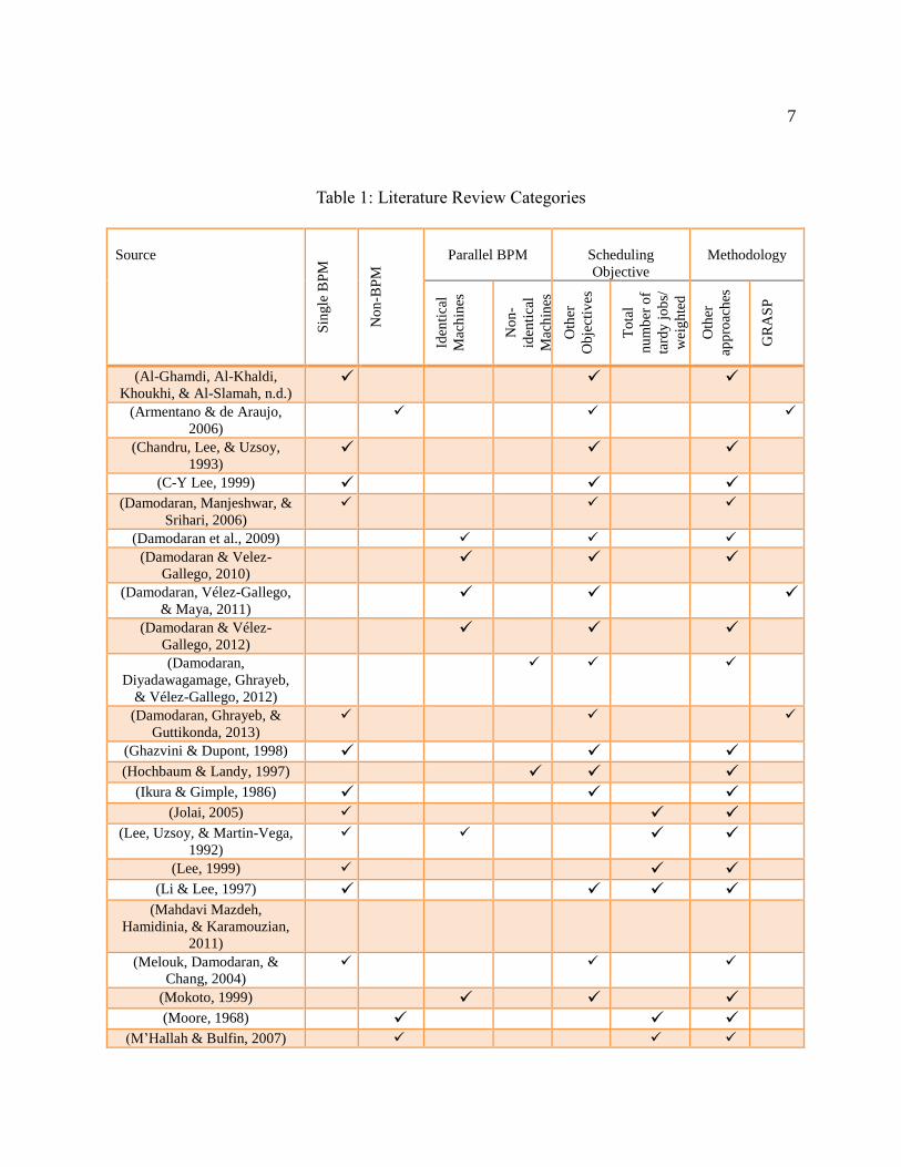
7

Table 1: Literature Review Categories

Source

Sin

gle

BP

M

No

n-B

PM

Parallel BPM

Scheduling

Objective

Methodology

Iden

tica

l

Mac

hin

es

No

n-

iden

tica

l

Mac

hin

es

Oth

er

Ob

ject

ives

To

tal

nu

mb

er o

f

tard

y j

ob

s/

wei

gh

ted

job

s O

ther

app

roac

hes

GR

AS

P

(Al-Ghamdi, Al-Khaldi,

Khoukhi, & Al-Slamah, n.d.)

(Armentano & de Araujo,

2006)

(Chandru, Lee, & Uzsoy,

1993)

(C-Y Lee, 1999)

(Damodaran, Manjeshwar, &

Srihari, 2006)

(Damodaran et al., 2009)

(Damodaran & Velez-

Gallego, 2010)

(Damodaran, Vélez-Gallego,

& Maya, 2011)

(Damodaran & Vélez-

Gallego, 2012)

(Damodaran,

Diyadawagamage, Ghrayeb,

& Vélez-Gallego, 2012)

(Damodaran, Ghrayeb, &

Guttikonda, 2013)

(Ghazvini & Dupont, 1998)

(Hochbaum & Landy, 1997)

(Ikura & Gimple, 1986)

(Jolai, 2005)

(Lee, Uzsoy, & Martin-Vega,

1992)

(Lee, 1999)

(Li & Lee, 1997)

(Mahdavi Mazdeh,

Hamidinia, & Karamouzian,

2011)

(Melouk, Damodaran, &

Chang, 2004)

(Mokoto, 1999)

(Moore, 1968)

(M’Hallah & Bulfin, 2007)

8

Source

Sin

gle

BP

M

No

n-B

PM

Parallel BPM Scheduling

Objective

Methodology

Iden

tica

l

Mac

hin

es

No

n-

iden

tica

l

Mac

hin

es

Oth

er

Ob

ject

ives

To

tal

nu

mb

er o

f

tard

y j

ob

s/

wei

gh

ted

job

sO

ther

app

roac

hes

GR

AS

P

(Ozturk, Espinouse, Di

Mascolo, & Gouin, 2010)

(Ozturk, Espinouse, Mascolo,

& Gouin, 2012)

(Ourari, Briand, & Bouzouiac,

n.d.)

(Perez, Fowler, & Carlyle,

2005)

(Péridy, Pinson, & Rivreau,

2003)

(Sevaux & Dauzère-Pérès,

2003)

(Sung & Choung, 2000)

(Shim & Kim, 2008)

(Uzsoy, 1994)

(Vélez-Gallego, Damodaran,

& Rodríguez, 2011)

(Xu & Bean, 2007)

(Alipour, 2016)

2.1 Characteristics of Batch Processing Machines

This study looks at a machine that is capable of processing a batch of jobs simultaneously.

The first researchers to address the batch processing scheduling problem, arising in a burn-in oven

of the final test in the semi-conductor industry, are Lee et al. (1992). Potts and Kovalyov (2000)

presented a comprehensive review on the scheduling problems when the jobs are processed or

Table 1. continued.

9

delivered in batches. They explained that a batch can contain anywhere from one job up to 𝑛 jobs

and the jobs are typically batched when they share the same setup on a machine or when the

machine can process several jobs at the same time.

Research efforts in this field can be classified using the following three independent

principles: (1) constant or varying batch processing time, (2) presence or absence of job sizes as a

variable, and (3) presence or absence of incompatible job families.

Under the first criterion, in varying batch processing problems, the processing time of the

batch depends on multiple jobs that constitute a batch. On the other hand, the processing times are

independent of the jobs in constant batch processing time. Some scholars considered problems

where processing time of the batches was dependent on the batches created (Ghazvini & Dupont,

1998; Hochbaum & Landy, 1997; Li & Lee, 1997; Sung & Choung, 2000; Uzsoy, 1994). Other

scholars dealt with constant batch processing times (Ikura & Gimple, 1986; Sung & Yoon, 1997).

There are two models of batching problems: p-batching problems and s-batching problems.

For s-batching problems, the processing time of the batch is the summation of processing times of

all jobs in the batch. However, for p-batching problems, the maximum processing time of all jobs

in the batch is considered as the processing time of the batch. The problem under study is a p-batch

problem as the batch processing time is equal to the longest processing time of all the jobs that

belong to the batch. All jobs in a batch are processed for a duration which is dictated by the longest

processing job in the batch. All the jobs in a batch begin and end their processing at the same time.

Consequently, the completion time of all the jobs in a batch is the same.

Under the second criterion, if job sizes are not considered, it is assumed that all jobs have

the same size and therefore the machine capacity is given by the maximum number of jobs it can

process at the same time. On the other hand, if job sizes are non-identical, the machine capacity is

given by the maximum number of size units the machine can process simultaneously (Damodaran

et al., 2012; Damodaran et al., 2006).

Under the third criterion, if incompatible job families are present, the jobs assigned to the

same batch must belong to the same family, and usually jobs belonging to the same family share

a common processing time, which determinse the batch processing time. Jolai (2005) considered

10

a set of n jobs which can be partitioned into m incompatible families such that the processing times

of all jobs belonging to the same family are equal and jobs of different families cannot be processed

together. The problem under study in this research assumes that the job sizes are non-identical,

and there is no incompatible job present.

2.1.1 Single Batch Processing Machine (BPM) Environment

Uzsoy (1994) showed that the single batch processing machine scheduling problem with

non-identical job sizes to minimize the total completion time and makespan is NP-hard. He has

also provided bin-packing-based heuristics for minimizing makespan and has used the branch-and-

bound approach to minimize the total completion times. He also developed effective heuristics for

minimizing makespan and completion time. Lee (1999) proposed polynomial and pseudo-

polynomial time algorithm to minimize makespan of a single BPM with dynamic job arrivals (i.e.,

job release times are not equal). The algorithm presented excellent results but took long

computational time. Chandru et al. (1993) investigated minimizing total completion time or

makespan objective in a single BPM by branch-and-bound (B&B). The set of jobs to be scheduled

are grouped into a number of families, where all jobs in the same family have the same processing

time. Perez et al. (2005) proposed a heuristic to minimize total weighted tardiness in the diffusion

step of semiconductor wafer fabrication process in single BPM with non-identical job sizes. Vélez-

Gallego et al. (2011) studied constructive heuristics named as modified successive knapsack

problem (MSKP) to minimize makespan in single BPM under the assumptions of non-identical

job sizes and non-zero job ready times. The heuristic was found to outperform other comparative

approaches for test instances with 50 or more jobs.

2.1.2 Parallel Batch Processing Machine (BPM) Environment

Various problems of scheduling on batch processing machines have been addressed

extensively in the literature. Lee et al. (1992) presented a heuristic for parallel batch processing

machine scheduling problem and found that the optimal solution will arise when all jobs are pre-

assigned to batches in non-increasing order of their processing times and batching the jobs with

11

largest processing times in the same batch. The formation resulted in a batch where the size of the

batch is the summation of all jobs’ size in the batch. In any circumstances, the batch size should

not exceed the capacity of the machine (Ozturk et al., 2012). In this research, literature on parallel

BPM is divided into two categories: identical and non-identical parallel BPM. Identical parallel

BPM simply means that all the machines have the same capacity. As for non-identical, the

capacities of BPM vary.

Identical parallel BPM scheduling problems have been widely researched. Damodaran et

al. (2011) applied greedy randomized adaptive search procedure (GRASP) to minimize makespan

for parallel BPM in an electronics manufacturing company. The proposed GRASP approach

outperformed other approaches mentioned in their paper and guaranteed an optimal solution for

all 10 job problem instances. Damodaran and Vélez-Gallego (2012) considered simulated

annealing (SA) algorithm to minimize the makespan on a group of identical parallel BPM and

compared the results with GRASP approach proposed by Damodaran et al. (2011). The SA

approach is comparable to GRASP in terms of solution quality and computation time. Mokoto

(1999) presents a new approximation algorithm based on linear programming (LP) for minimizing

makespan for identical parallel BPM. The MSKP heuristic in Vélez-Gallego et al. (2011) was

extended by Damodaran and Velez-Gallego (2010) to identical parallel BPM and called it

progressive successive knapsack problem (PKSP). The heuristic aimed to minimize makespan

with lesser computational time.

Tardiness is another objective that was studied in the literature on scheduling identical

parallel BPMs. Tardiness is equal to lateness, where the completion time of a job is greater than

its due date (Al-Ghamdi et al., n.d.). Sivrikaya-Şerifoǧlu & Ulusoy (1999) developed the genetic

algorithm (GA) which was able to minimize tardiness thus providing better results in larger size

problems than the comparing neighborhood exchange search. The B&B algorithm was

implemented in identical parallel BPM to minimize tardiness and was compared with a traditional

SA solution (Shim & Kim, 2008).

Scheduling non-identical parallel BPM is harder than identical BPM as the machine

capacity considerations are required for every batch formed. A common scheduling objective

12

studied for non-identical parallel BPM scenario is minimizing the total completion time or

makespan (Ozturk et al., 2012). Xu and Bean (2007) proposed a random key genetic algorithm

(RKGA) in minimizing makespan for non-identical parallel BPM. Following that, Damodaran et

al. (2012) proposed the particle swarm optimization (PSO) approach to minimize the makespan

for non-identical parallel BPM. They adapted the mathematical formulation from Xu and Bean

(2007) and simplified it with fewer binary variables.

2.2 Minimize Total Number of Tardy Jobs

On-time jobs are the ones which are completed before their due dates and tardy jobs are

the jobs which are finished after their due dates. Moore (1968) minimized the total number of tardy

jobs on a discrete processing machine (1| | ∑ 𝑈𝑗) using Hodgson’s algorithm. His approach was

able to guarantee an optimal solution. Lenstra, Kan, & Brucker (1977) showed that the discrete

machine problem of minimizing the total number of tardy jobs with ready time constraint

(1|𝑟𝑗| ∑ 𝑤𝑗𝑈𝑗) is NP-hard.

Batch machine scheduling problems where the batch processing time is given by the

processing time of the longest job in the batch have also been addressed. Brucker et al. (1998) give

several exact algorithms for the problem of 1|𝑝 − 𝑏𝑎𝑡𝑐ℎ| ∑ 𝑈𝑗. They present a dynamic

programming approach for minimizing total number of tardy jobs and show that minimizing total

weighted number of tardy jobs is binary NP-hard. They assumed that only a fixed number of jobs

are allowed in a batch. They did not consider the job sizes.

Ourari et al. (n.d.) considered the problem of 1|𝑟𝑗| ∑ 𝑈𝑗 and they used an original

mathematical integer programming formulation where they showed how both good-quality lower

and upper bounds can be computed. Sevaux and Dauzère-Pérès (2003) presented the first meta-

heuristic (i.e., genetic algorithm) for a discrete processing machine to minimize total number of

tardy jobs with ready time limitation (1|𝑟𝑗| ∑ 𝑤𝑗𝑈𝑗). M’Hallah and Bulfin (2007) also tried to

minimize the weighted number of tardy jobs with release date for single discrete machine

(1|𝑟𝑗| ∑ 𝑤𝑗𝑈𝑗). They gave a formulation to maximize the weighted number of on-time jobs instead

of minimizing weighted number of tardy jobs.

13

Jolai (2005) proved that minimizing the number of tardy jobs with incompatible job

families on a single batch processing machine is NP-hard. Also Liu and Zhang (2008) proved

that minimizing number of tardy jobs on a batch processing machine with incompatible job

families is unary NP-hard in strong sense. Mahdavi Mazdeh et al. (2011) exhibited a meta-heuristic

technique taking into account SA and the execution was analyzed versus exact algorithm.

A number of review papers provide expanded records of particular aspects of scheduling.

The survey of minimizing total number of late jobs problems is given by Leung (2004). To the

best of our knowledge, the problem of minimizing total number of tardy jobs on a batch processing

machine has not been studied so far.

2.3 Meta-heuristics

Many engineering optimization problems are usually quite difficult to solve, and many

applications have to deal with these complex problems. In these problems, search space grows

exponentially with the problem size. Therefore, the traditional optimization methods do not

provide a suitable solution for them. Hence, over the past few decades, many meta-heuristic

algorithms have been designed to solve such problems.

Researchers have shown good performance of meta-heuristic algorithms in a wide range

of complex problems such as image and video processing (Draa and Bouaziz, 2014; Fornarelli and

Giaquinto, 2013), scheduling problems (Behnamian, Fatemi Ghomi, and Zandieh, 2012,

Damodaran et al., 2011; Damodaran and Vélez-Gallego, 2012; Soltani, Jolai, and Zandieh, 2010)

and pattern recognition (Garai and Chaudhurii, 2013; Liu and Huang, 1998) – to name a few. In

all of the above applications, computing all combinations of solutions and evaluating any of them

concerning the declared objective function is feasible theoretically, and optimality will take place

if some of the solutions provide the most desirable result. Meta-heuristics are majestic methods

that adjust simple guidelines and heuristics to find good-quality solutions for many engineering

optimization problems that are usually too difficult to solve, and many applications have to deal

with these complex problems because they cease the use of exact algorithms.

14

Meta-heuristics have the ability to find very good solutions but not necessarily optimal

solutions. The strength of these approaches depends upon their ability to eschew entrapment at

local optima, a specific perception, and exploit the basic structure of the problem, for example, in

scheduling a natural ordering among its components. Greedy randomized adaptive search

procedure (GRASP) was proposed by (Feo and Resende, 1989). GRASP is an iterative procedure

which tries to improve the solution through a local search starting from a greedy heuristic. Particle

swarm optimization (PSO) mimics the social behaviors of a flock of migrating birds trying to reach

an unknown destination (Kennedy and Eberhart, 1995). Genetic algorithms (GA) simulate

Darwinian evolution concepts (Holland, 1975). Simulated annealing (SA) was introduced by

Kirkpatrick and Vecchi (1983) and it is motivated by the analogy between the physical annealing

of metals and the process of searching for the optimal solution (Kirkpatrick and Vecchi, 1983).

Meta-heuristics depend on definite patterns and propose particular mechanisms to get away

from locally optimal solutions. Meta-heuristics are one of the most powerful solution blueprints

for figuring out extremely hard combinatorial optimization problems in practice and they have

been applied to an ample range of real-world and academic situations. There has been considerable

research done in the areas of batch processing and different meta-heuristics mentioned above.

There are some constructive heuristics that are beneficial for gaining the first solution in

the neighborhood search. In neighborhood search the current solution is converted into a novel

solution based on some specific neighborhood frame. The decision for acceptance or not

acceptance of the move from current to remodeled solution will be made after complete

neighborhood exploration. If the move is approved, then the new solution will replace the previous

one. The confirmation rule is according to the current solution’s objective function value and its

neighbor and this process is repeated until some termination criterion is satisfied.

GRASP is a meta-heuristic which is an iterative process popularized by Feo and Resende

(1989). This multi-start method includes two different phases. A classical GRASP starts from

producing a feasible solution which is constructed by a greedy randomized algorithm and tries to

15

improve it in the local search phase. The procedure is repeated several times; and the local

optimum in the neighborhood of the constructed solution is desired and the best overall solution

is returned as a result. References (Feo & Resende, 1989; Feo & Resende, 1995; Resende &

Ribeiro (2014) present expanded surveys on GRASP and some recent references are found that

implemented GRASP to scheduling problems (Aiex et al., 2003; Armentano & de Araujo, 2006;

Damodaran et al., 2013; Damodaran et al., 2011).

2.4 Summary

This research presents GRASP approach to minimize the total number of tardy jobs on a

single BPM. Past literature demonstrates that the problem under study is not tackled yet utilizing

GRASP. GRASP approach has worked for different types of scheduling problems such as

makespan minimization on parallel BPM by Damodaran et al. (2011) and minimizing makespan

for a capacitated BPM machine by Damodaran et al. (2013). But GRASP approach has not been

tried to minimize total number of tardy jobs in non-identical parallel batch processing machine

environment.

CHAPTER 3

MATHEMATICAL FORMULATION

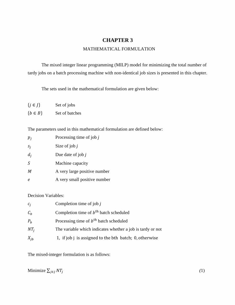
The mixed integer linear programming (MILP) model for minimizing the total number of

tardy jobs on a batch processing machine with non-identical job sizes is presented in this chapter.

The sets used in the mathematical formulation are given below:

{𝑗 ∈ 𝐽} Set of jobs

{𝑏 ∈ 𝐵} Set of batches

The parameters used in this mathematical formulation are defined below:

𝑝𝑗 Processing time of job j

𝑠𝑗 Size of job j

𝑑𝑗 Due date of job j

𝑆 Machine capacity

𝑀 A very large positive number

𝑒 A very small positive number

Decision Variables:

𝑐𝑗 Completion time of job j

𝐶𝑏 Completion time of 𝑏th batch scheduled

𝑃𝑏 Processing time of 𝑏th batch scheduled

𝑁𝑇𝑗 The variable which indicates whether a job is tardy or not

𝑋𝑗𝑏 1, if job j is assigned to the bth batch; 0, otherwise

The mixed-integer formulation is as follows:

Minimize ∑ 𝑁𝑇𝑗𝑗∈𝐽 (1)

17

Subject to:

∑ 𝑋𝑗𝑏 = 1

𝑏∈𝐵

∀𝑗 ∈ 𝐽 (2)

∑ 𝑠𝑗

𝑗∈𝐽

𝑋𝑗𝑏 ≤ 𝑆 ∀𝑏 ∈ 𝐵 (3)

𝑃𝑏 ≥ 𝑃𝑗𝑋𝑗𝑏 ∀𝑗 ∈ 𝐽, 𝑏 ∈ 𝐵 (4)

𝐶1 = 𝑃1 (5)

𝐶𝑏 ≥ 𝐶𝑏−1 + 𝑃𝑏 ∀𝑏 ∈ 𝐵/{1} (6)

𝑐𝑗 ≥ 𝐶𝑏 − 𝑀(1 − 𝑋𝑗𝑏) ∀𝑏 ∈ 𝐵 (7)

𝑐𝑗 − 𝑑𝑗 ≤ 𝑀(𝑁𝑇𝑗) ∀𝑗 ∈ 𝐽, 𝑏 ∈ 𝐵 (8)

𝑐𝑗 − 𝑑𝑗 ≥ 𝑒 − 𝑀(1 − 𝑁𝑇𝑗 ) ∀𝑗 ∈ 𝐽, 𝑏 ∈ 𝐵 (9)

𝐶𝑏 , 𝑃𝑏 ≥ 0 ∀𝑏 ∈ 𝐵 (10)

𝑐𝑗 , 𝑁𝑇𝑗 ≥ 0 ∀𝑗 ∈ 𝐽 (11)

𝑋𝑗𝑏 = {0,1} ∀𝑗 ∈ 𝐽, 𝑏 ∈ 𝐵 (12)

The objective (1) is to minimize the total number of tardy jobs. Constraint set (2) ensures

that each job is assigned to exactly one batch. Constraint set (3) ensures that the total size of all

jobs in each batch processed on the machine does not violate the machine capacity. Constraint set

(4) determines the processing time of the 𝑏𝑡ℎ batch processed on the machine. Batch processing

18

time is equal to the longest processing time of all the jobs in the batch. Constraint set (5) ensures

the completion time of the first batch is equal to the processing time of the first batch processed in

the sequence. Constraint set (6) determines that completion time of the batch is at least equal to

the summation of its processing time and completion time of the previous batch. Constraint set (7)

ensures that the completion time of a job is at least equal to the completion time of the batch in

which it is processed. Constraint sets (8) and (9) determine whether a job is tardy or not. Constraint

sets (10), (11), and (12) impose the non-negativity and binary restrictions on the decision variables.

Various instances of the problem are considered with 5 to 100 jobs. The data for each

instance was downloaded from the following website:

http://scheduling.iem.cyu.edu.tw/scheduling/modules/tinyd0/Burn_In_TWT_JCIIE2008.zip.

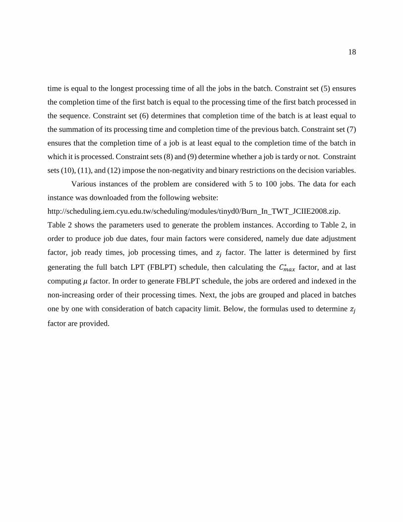
Table 2 shows the parameters used to generate the problem instances. According to Table 2, in

order to produce job due dates, four main factors were considered, namely due date adjustment

factor, job ready times, job processing times, and 𝑧𝑗 factor. The latter is determined by first

generating the full batch LPT (FBLPT) schedule, then calculating the 𝐶𝑚𝑎𝑥∗ factor, and at last

computing 𝜇 factor. In order to generate FBLPT schedule, the jobs are ordered and indexed in the

non-increasing order of their processing times. Next, the jobs are grouped and placed in batches

one by one with consideration of batch capacity limit. Below, the formulas used to determine 𝑧𝑗

factor are provided.

19

Table 2: Parameters for Generating Problem Instances

Parameters Description Values

𝑛 Number of jobs (problem size) 5-100

𝑚 Number of machines 1

Sm Machine capacity 40

𝑄 Interval for job sizes [1,30]

𝑅 Due date tightness R=0.5

𝑇 Due date spread out T=0.3

𝑟𝑗 Job ready times Discrete uniform [0,48]

𝑝𝑗 Job processing times Discrete uniform [8,48]

𝑤𝑗 Job priorities Discrete uniform [1,11]

𝑑𝑗 Job due dates γ. (rj + pj + zj)

Γ

Due date adjustment factor

Where

zj=Discrete uniform [𝜇.(1-R/2),

𝜇.(1+R/2)]

𝜇 = (1-T). 𝐶𝑚𝑎𝑥∗

Cmax∗ =MIN (rj) +FBLPT

FBLPT is Full Batch LPT (zero ready

times and unit sized jobs)

0.2, 0.33, 0.5

Throughout this study, small number of jobs data set refers to the data set consisting of 5,

7, 9, 11, 13 and 15 jobs instances, while large number of jobs data set refers to the data set

consisting of 50 and 100 jobs instances.

20

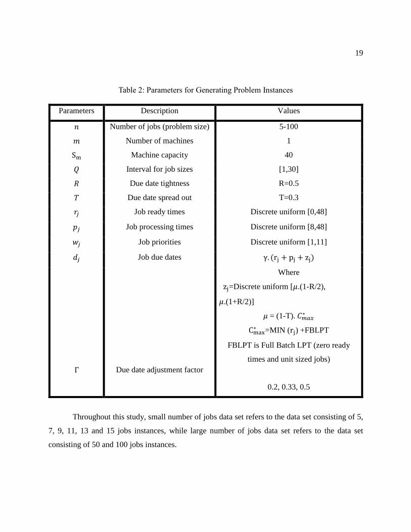
Table 3 presents an instance of 1|𝑝 − 𝑏𝑎𝑡𝑐ℎ, 𝑠𝑗| ∑ 𝑈𝑗 with 9 jobs. In this example the

machine capacity is assumed to be 40. The machine can process simultaneously several jobs as a

batch as long as the machine capacity is not violated.

In order to develop a feasible schedule, batches are first formed using a heuristic. In order

to form the batches, the jobs are first sequenced based on a dispatching rule (e.g., earliest due date).

One job at a time from the sequence is considered for batching. If a job does not fit in the open

batch, a new batch is opened to accommodate the job. The batches are scheduled on the BPM in

the order in which they were formed.

Table 3: Data for a 9-Job Problem Instance

Jobs # 1 2 3 4 5 6 7 8 9

Job size 17 13 27 7 15 14 27 2 28

Job Processing Time 19 28 44 14 16 23 37 10 43

Job Due Date 36 35 32 32 34 36 36 37 36

If the earliest due date (EDD) rule is applied to form the initial job sequence, then the

sequence is {3, 4, 5, 2, 1, 6, 7, 9, 8}. The heuristic followed to form the batches is shown below

and each figure is provided to show a partial Gantt chart after forming each batch.

First Iteration:

Job 3 has the size of 27 and 27< 40. Job 3 will fit in the batch.

Job 4 has the size of 7 and 27+7= 34 < 40. Job 4 will fit in the batch.

Job 5 has the size 15 and 34+15> 40. Job 5 will not fit in the 1st batch.




21



Job 8 has the size of 2 and 34+2= 36 < 40. Job 8 will fit in the 1st batch.

Batch 1, as shown in Figure 1, contains only jobs 3, 4 and 8 and the processing time and

completion time of the first batch is:

P1 = C1 = max {𝑝3 , 𝑝4 , 𝑝8 }

(i.e. P1 = max {44,14,10}=44)

Figure 1: Partial Gantt chart with first batch.

Second Iteration:

Jobs 3, 4 and 8 are deleted from the EDD list and the next job for examination is job 5

according to EDD initial sequence.

Job 5 has the size of 15 and 15< 40. Job 5 will fit in the 2nd batch.

Job 2 has the size of 13 and 15+13=28< 40. Job 2 will fit in the 2nd batch.

Job 6 has the size 14 and 28+14 > 40. Job 6 will not fit in the 2nd batch.

Job 7 has the size 27 and 28+27> 40. Job 7 will not fit in the 2nd batch.

Job 9 has the size 28 and 28+28> 40. Job 9 will not fit in the 2nd batch.

22

Batch 2 comprises jobs 5 and 2. Figure 2 presents the Gantt chart for the two batches

formed. The processing time of the second batch is 28 (i.e. max {p5, p2} = max {16, 28} =28). The

completion time of the 2nd batch is 72 (i.e., completion time of 1st batch + the processing time of

the 2nd batch).

Figure 2: Partial Gantt chart with first two batches.

Third Iteration:

Job 1 has the size of 17 and 17< 40. Job 1 will fit in the 3rd batch.

Job 6 has the size of 14 and 17+14=31< 40. Job 6 will fit in the 3rd batch.

Job 7 has the size of 27 and 31+27> 40. Job 7 will not fit in the 3rd batch.

Job 9 has the size of 28 and 31+28> 40. Job 9 will not fit in the 3rd batch.

Batch 3 contains only jobs 1 and 6 as shown in Figure 3 and the processing time of the 3rd

batch is:

P3 = max {𝑝1 , 𝑝6}

The completion time of the 3rd batch is the completion time of the previous batch plus the

processing time of the 3rd batch (e.g., C3 = C2 + P3 = 72 + max {19,23}=95).

23

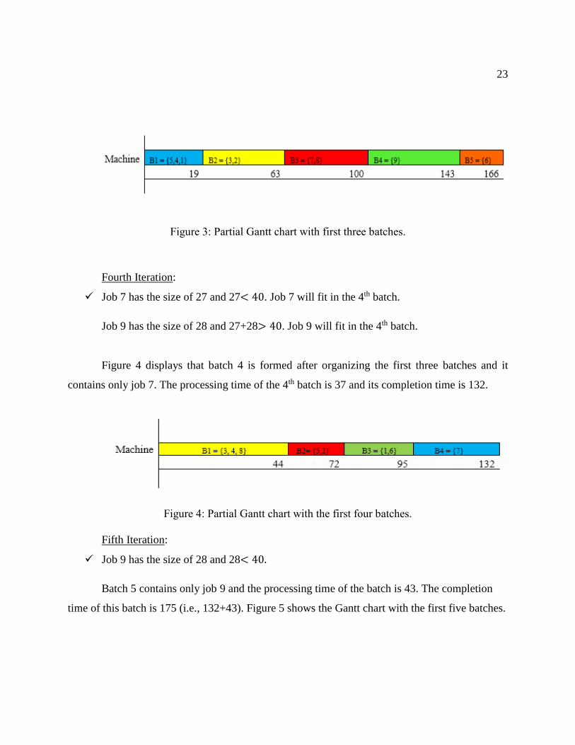
Figure 3: Partial Gantt chart with first three batches.

Fourth Iteration:

Job 7 has the size of 27 and 27< 40. Job 7 will fit in the 4th batch.

Job 9 has the size of 28 and 27+28> 40. Job 9 will fit in the 4th batch.

Figure 4 displays that batch 4 is formed after organizing the first three batches and it

contains only job 7. The processing time of the 4th batch is 37 and its completion time is 132.

Figure 4: Partial Gantt chart with the first four batches.

Fifth Iteration:

Job 9 has the size of 28 and 28< 40.

Batch 5 contains only job 9 and the processing time of the batch is 43. The completion

time of this batch is 175 (i.e., 132+43). Figure 5 shows the Gantt chart with the first five batches.

24

Figure 5: Gantt chart with all the batches formed.

After deleting all jobs from EDD list and grouping into batches, the completion time of

each job is compared to its due date and if the completion time of the job is larger than its due

date then the job would be marked as a tardy job.

Job 3: (44>32) job 3 is tardy.









Based on the batches formed using the EDD sequence, all 9 jobs are tardy. However, the

optimum solution for this example problem instance is 5. Figure 6 shows the Gantt chart for the

optimum solution.

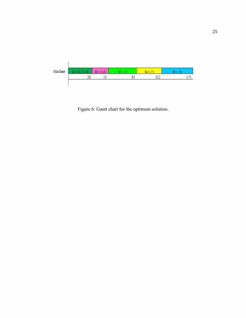
25

Figure 6: Gantt chart for the optimum solution.

CHAPTER 4

GRASP SOLUTION APPROACH

GRASP is a heuristic iterative sampling technique composed of two phases, a construction

and a local search phase. In the construction phase, an iterative algorithm builds a feasible solution

by adding one variable (or job) at a time. Each iteration of the algorithm starts with a solution

found by means of a randomized greedy heuristic. The solution is later taken as the initial solution

of the local search procedure and the procedure is repeated until some criteria of the search are

met. While a greedy heuristic is a construction heuristic that fixes one variable at a time using

some deterministic rule, in a randomized greedy heuristic, randomness is introduced to heuristic

rules in order to prevent generation of the same solution every time the greedy heuristic is called.

The randomized greedy heuristic proposed to find a starting solution in this research is based on

the earliest due date (EDD), shortest processing time (SPT), shortest size (SS), largest size (LS),

the subtraction of due date and processing time which is multiplied by size (Delta), shortest result

of multiplication of size and processing time (Pan SSPT), shortest result of multiplication of due

date and processing time (Pan DP), shortest result of multiplication of due date and size (Pan DS)

and random sequence (Random Permutation).

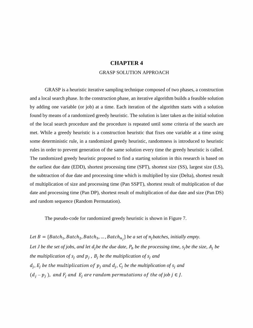
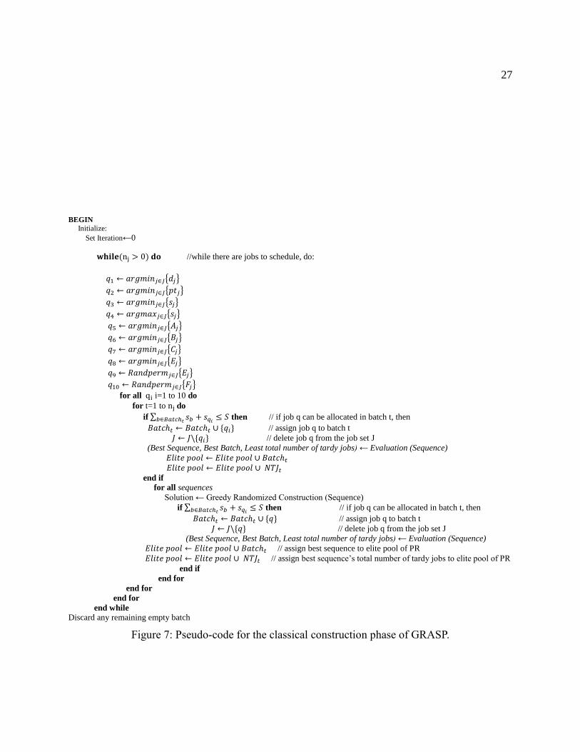
The pseudo-code for randomized greedy heuristic is shown in Figure 7.

Let 𝐵 = {𝐵𝑎𝑡𝑐ℎ1, 𝐵𝑎𝑡𝑐ℎ2, 𝐵𝑎𝑡𝑐ℎ3, … , 𝐵𝑎𝑡𝑐ℎ𝑛𝑗} be a set of 𝑛𝑗batches, initially empty.

Let J be the set of jobs, and let 𝑑𝑗be the due date, 𝑃𝑏 be the processing time, 𝑠𝑗be the size, 𝐴𝑗 be

the multiplication of 𝑠𝑗 and 𝑝𝑗 , 𝐵𝑗 be the multiplication of 𝑠𝑗 and

𝑑𝑗, 𝐸𝑗 𝑏𝑒 𝑡ℎ𝑒 𝑚𝑢𝑙𝑡𝑖𝑝𝑙𝑖𝑐𝑎𝑡𝑖𝑜𝑛 𝑜𝑓 𝑝𝑗 𝑎𝑛𝑑 𝑑𝑗, 𝐶𝑗 be the multiplication of 𝑠𝑗 and

(𝑑𝑗 – 𝑝𝑗 ), 𝑎𝑛𝑑 𝐹𝑗 𝑎𝑛𝑑 𝐸𝑗 𝑎𝑟𝑒 𝑟𝑎𝑛𝑑𝑜𝑚 𝑝𝑒𝑟𝑚𝑢𝑡𝑎𝑡𝑖𝑜𝑛𝑠 𝑜𝑓 𝑡ℎ𝑒 of job 𝑗 ∈ 𝐽.

27

BEGIN

Initialize:

Set Iteration←0

𝐰𝐡𝐢𝐥𝐞(nj > 0) 𝐝𝐨 //while there are jobs to schedule, do:

𝑞1 ← 𝑎𝑟𝑔𝑚𝑖𝑛𝑗∈𝐽{𝑑𝑗}

𝑞2 ← 𝑎𝑟𝑔𝑚𝑖𝑛𝑗∈𝐽{𝑝𝑡𝑗}

𝑞3 ← 𝑎𝑟𝑔𝑚𝑖𝑛𝑗∈𝐽{𝑠𝑗}

𝑞4 ← 𝑎𝑟𝑔𝑚𝑎𝑥𝑗∈𝐽{𝑠𝑗}

𝑞5 ← 𝑎𝑟𝑔𝑚𝑖𝑛𝑗∈𝐽{𝐴𝑗}

𝑞6 ← 𝑎𝑟𝑔𝑚𝑖𝑛𝑗∈𝐽{𝐵𝑗}

𝑞7 ← 𝑎𝑟𝑔𝑚𝑖𝑛𝑗∈𝐽{𝐶𝑗}

𝑞8 ← 𝑎𝑟𝑔𝑚𝑖𝑛𝑗∈𝐽{𝐸𝑗}

𝑞9 ← 𝑅𝑎𝑛𝑑𝑝𝑒𝑟𝑚𝑗∈𝐽{𝐸𝑗}

𝑞10 ← 𝑅𝑎𝑛𝑑𝑝𝑒𝑟𝑚𝑗∈𝐽{𝐹𝑗}

for all qi i=1 to 10 do

for t=1 to nj do

if ∑ 𝑠𝑏 + 𝑠𝑞𝑖≤ 𝑆𝑏∈𝐵𝑎𝑡𝑐ℎ𝑡

then // if job q can be allocated in batch t, then

𝐵𝑎𝑡𝑐ℎ𝑡 ← 𝐵𝑎𝑡𝑐ℎ𝑡 ∪ {𝑞𝑖} // assign job q to batch t

𝐽 ← 𝐽\{𝑞𝑖} // delete job q from the job set J

(Best Sequence, Best Batch, Least total number of tardy jobs) ← Evaluation (Sequence)

𝐸𝑙𝑖𝑡𝑒 𝑝𝑜𝑜𝑙 ← 𝐸𝑙𝑖𝑡𝑒 𝑝𝑜𝑜𝑙 ∪ 𝐵𝑎𝑡𝑐ℎ𝑡

𝐸𝑙𝑖𝑡𝑒 𝑝𝑜𝑜𝑙 ← 𝐸𝑙𝑖𝑡𝑒 𝑝𝑜𝑜𝑙 ∪ 𝑁𝑇𝐽𝑡

end if

for all sequences

Solution ← Greedy Randomized Construction (Sequence)

if ∑ 𝑠𝑏 + 𝑠𝑞𝑖≤ 𝑆𝑏∈𝐵𝑎𝑡𝑐ℎ𝑡

then // if job q can be allocated in batch t, then

𝐵𝑎𝑡𝑐ℎ𝑡 ← 𝐵𝑎𝑡𝑐ℎ𝑡 ∪ {𝑞} // assign job q to batch t

𝐽 ← 𝐽\{𝑞} // delete job q from the job set J

(Best Sequence, Best Batch, Least total number of tardy jobs) ← Evaluation (Sequence)

𝐸𝑙𝑖𝑡𝑒 𝑝𝑜𝑜𝑙 ← 𝐸𝑙𝑖𝑡𝑒 𝑝𝑜𝑜𝑙 ∪ 𝐵𝑎𝑡𝑐ℎ𝑡 // assign best sequence to elite pool of PR

𝐸𝑙𝑖𝑡𝑒 𝑝𝑜𝑜𝑙 ← 𝐸𝑙𝑖𝑡𝑒 𝑝𝑜𝑜𝑙 ∪ 𝑁𝑇𝐽𝑡 // assign best sequence’s total number of tardy jobs to elite pool of PR

end if

end for

end for

end for

end while

Discard any remaining empty batch

Figure 7: Pseudo-code for the classical construction phase of GRASP.

28

If each job is assigned to a unique batch, then the maximum number of batches formed is

equal to the number of jobs considered in an instance. Initially nj batches are opened and any

remaining unused batches are closed at the completion of the algorithm. The earliest job (based on

each heuristic) is assigned to the first available batch (i.e., adding a job should not violate the

machine capacity). This procedure is repeated until all jobs are assigned to a batch. After the

batches are formed, the batch processing time can be determined. The batch processing time is

equal to the largest processing time of all jobs in the batch. The completion time of each job in a

batch is equal to the completion time of the batch. The completion time of a batch can be easily

computed by summing the processing times of all the batches sequenced (including the processing

time of the current batch). The batches are sequenced in the order in which they were created. If

the completion time of the job is larger than its due date, the job would be tardy.

After generating all initial sequences, the sequences are used to find the total number of

tardy jobs. In the next step the pool of path relinking is created which contains all these initial

sequences and their total number of tardy jobs.

Randomization is introduced to the EDD, SPT, SST and other initial sequences by means

of the so-called Restricted Candidate List (RCL) which works as follows: while assigning jobs to

the batches, instead of selecting the unscheduled job with the earliest due date first (for EDD

sequence), the job is randomly chosen among the first k earliest due date jobs. Here k is the size of

the RCL.

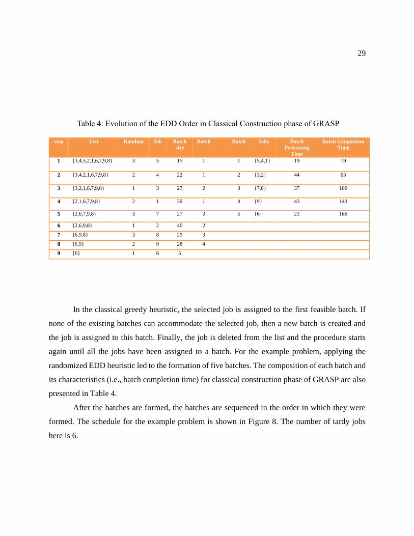
Table 4 shows how the randomized greedy algorithm is applied to a 9-job problem instance.

The data for the problem instance was presented in Table 3. The machine capacity is assumed as

40 and the RCL as 3. The jobs are first arranged in EDD order (i.e., list={3,4,5,2,1,6,7,9,8}).

29

Table 4: Evolution of the EDD Order in Classical Construction phase of GRASP

step List Random Job Batch

size

Batch Batch Jobs Batch

Processing

Time

Batch Completion

Time

1 {3,4,5,2,1,6,7,9,8} 3 5 15 1 1 {5,4,1} 19 19

2 {3,4,2,1,6,7,9,8} 2 4 22 1 2 {3,2} 44 63

3 {3,2,1,6,7,9,8} 1 3 27 2 3 {7,8} 37 100

4 {2,1,6,7,9,8} 2 1 39 1 4 {9} 43 143

5 {2,6,7,9,8} 3 7 27 3 5 {6} 23 166

6 {2,6,9,8} 1 2 40 2

7 {6,9,8} 3 8 29 3

8 {6,9} 2 9 28 4

9 {6} 1 6 5

In the classical greedy heuristic, the selected job is assigned to the first feasible batch. If

none of the existing batches can accommodate the selected job, then a new batch is created and

the job is assigned to this batch. Finally, the job is deleted from the list and the procedure starts

again until all the jobs have been assigned to a batch. For the example problem, applying the

randomized EDD heuristic led to the formation of five batches. The composition of each batch and

its characteristics (i.e., batch completion time) for classical construction phase of GRASP are also

presented in Table 4.

After the batches are formed, the batches are sequenced in the order in which they were

formed. The schedule for the example problem is shown in Figure 8. The number of tardy jobs

here is 6.

30

Figure 8: Regular batching by using classical construction phase of GRASP.

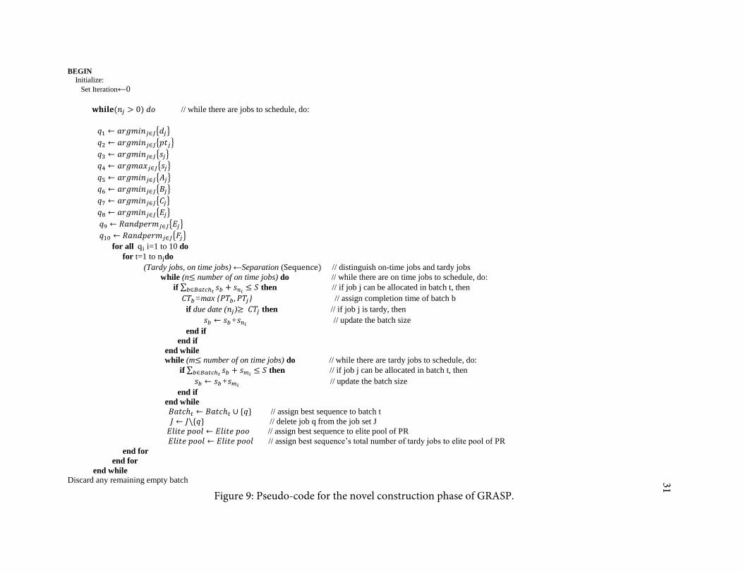
In this research a new construction phase is developed to determine good initial solutions.

This construction phase starts with one of the initial sequences (i.e., EDD, SPT, etc.) and a job is

randomly chosen using the RCL. The chosen job is assigned to one batch at a time (when the

machine capacity is not violated) and its completion is determined. If the job is completed before

its due date in any one of the existing batches, then the job is assigned to the batch. Otherwise, the

job will be tardy immaterial of the batch to which it is assigned. These jobs are scheduled after all

the on-time jobs are scheduled. The on-time jobs are scheduled first so it helps the algorithm to

find a good solution. This proposition is inspired by Jolai (2005) and Sevaux and Dauzère-Pérès

(2003).

The pseudo-code for the new construction phase is shown in Figure 9.

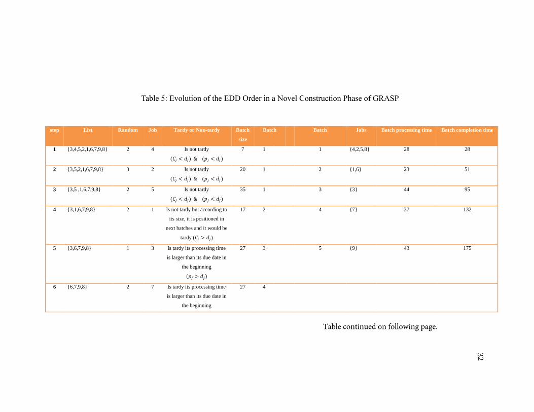
Table 5 summarizes the steps followed in the new construction phase using the 9-job

problem instance (as shown in Table 3).

Once the jobs are grouped into batches using the new construction heuristic, the batches

are assigned to the machine. The schedule for this construction approach is shown in Figure 9. The

total number of tardy jobs for the schedule is 5. The new construction phase is better, in terms of

total number of tardy jobs, for the 9-job problem instance. It also identified the optimal solution

for the example problem instance.

BEGIN

Initialize:

Set Iteration←0

𝐰𝐡𝐢𝐥𝐞(𝑛𝑗 > 0) 𝑑𝑜 // while there are jobs to schedule, do:

𝑞1 ← 𝑎𝑟𝑔𝑚𝑖𝑛𝑗∈𝐽{𝑑𝑗}

𝑞2 ← 𝑎𝑟𝑔𝑚𝑖𝑛𝑗∈𝐽{𝑝𝑡𝑗}

𝑞3 ← 𝑎𝑟𝑔𝑚𝑖𝑛𝑗∈𝐽{𝑠𝑗}

𝑞4 ← 𝑎𝑟𝑔𝑚𝑎𝑥𝑗∈𝐽{𝑠𝑗}

𝑞5 ← 𝑎𝑟𝑔𝑚𝑖𝑛𝑗∈𝐽{𝐴𝑗}

𝑞6 ← 𝑎𝑟𝑔𝑚𝑖𝑛𝑗∈𝐽{𝐵𝑗}

𝑞7 ← 𝑎𝑟𝑔𝑚𝑖𝑛𝑗∈𝐽{𝐶𝑗}

𝑞8 ← 𝑎𝑟𝑔𝑚𝑖𝑛𝑗∈𝐽{𝐸𝑗}

𝑞9 ← 𝑅𝑎𝑛𝑑𝑝𝑒𝑟𝑚𝑗∈𝐽{𝐸𝑗}

𝑞10 ← 𝑅𝑎𝑛𝑑𝑝𝑒𝑟𝑚𝑗∈𝐽{𝐹𝑗}

for all qi i=1 to 10 do

for t=1 to njdo

(Tardy jobs, on time jobs) ←Separation (Sequence) // distinguish on-time jobs and tardy jobs

while (n≤ number of on time jobs) do // while there are on time jobs to schedule, do:

if ∑ 𝑠𝑏 + 𝑠𝑛𝑖≤ 𝑆𝑏∈𝐵𝑎𝑡𝑐ℎ𝑡

then // if job j can be allocated in batch t, then

𝐶𝑇𝑏=max {𝑃𝑇𝑏, 𝑃𝑇𝑗} // assign completion time of batch b

if due date (𝑛𝑗)≥ 𝐶𝑇𝑗 then // if job j is tardy, then

𝑠𝑏 ← 𝑠𝑏+𝑠𝑛𝑖 // update the batch size

end if

end if

end while

while (m≤ number of on time jobs) do // while there are tardy jobs to schedule, do:

if ∑ 𝑠𝑏 + 𝑠𝑚𝑖≤ 𝑆𝑏∈𝐵𝑎𝑡𝑐ℎ𝑡

then // if job j can be allocated in batch t, then

𝑠𝑏 ← 𝑠𝑏+𝑠𝑚𝑖 // update the batch size

end if

end while

𝐵𝑎𝑡𝑐ℎ𝑡 ← 𝐵𝑎𝑡𝑐ℎ𝑡 ∪ {𝑞} // assign best sequence to batch t

𝐽 ← 𝐽\{𝑞} // delete job q from the job set J

𝐸𝑙𝑖𝑡𝑒 𝑝𝑜𝑜𝑙 ← 𝐸𝑙𝑖𝑡𝑒 𝑝𝑜𝑜 // assign best sequence to elite pool of PR

𝐸𝑙𝑖𝑡𝑒 𝑝𝑜𝑜𝑙 ← 𝐸𝑙𝑖𝑡𝑒 𝑝𝑜𝑜𝑙 // assign best sequence’s total number of tardy jobs to elite pool of PR

end for

end for

end while

Discard any remaining empty batch

Figure 9: Pseudo-code for the novel construction phase of GRASP.

31

32

Table 5: Evolution of the EDD Order in a Novel Construction Phase of GRASP

step List Random Job Tardy or Non-tardy Batch

size

Batch Batch Jobs Batch processing time Batch completion time

1 {3,4,5,2,1,6,7,9,8} 2 4 Is not tardy

(𝐶𝑗 < 𝑑𝑗) & (𝑝𝑗 < 𝑑𝑗)

7 1 1 {4,2,5,8} 28 28

2 {3,5,2,1,6,7,9,8} 3 2 Is not tardy

(𝐶𝑗 < 𝑑𝑗) & (𝑝𝑗 < 𝑑𝑗)

20 1 2 {1,6} 23 51

3 {3,5 ,1,6,7,9,8} 2 5 Is not tardy

(𝐶𝑗 < 𝑑𝑗) & (𝑝𝑗 < 𝑑𝑗)

35 1 3 {3} 44 95

4 {3,1,6,7,9,8} 2 1 Is not tardy but according to

its size, it is positioned in

next batches and it would be

tardy (𝐶𝑗 > 𝑑𝑗)

17 2 4 {7} 37 132

5 {3,6,7,9,8} 1 3 Is tardy its processing time

is larger than its due date in

the beginning

(𝑝𝑗 > 𝑑𝑗)

27 3 5 {9} 43 175

6 {6,7,9,8} 2 7 Is tardy its processing time


the beginning

27 4

Table continued on following page.

33


7 {6,9,8} 3 8 Is not tardy but according to



tardy

(𝐶𝑗 > 𝑑𝑗)

37 1

8 {6,9} 2 9 Is tardy its processing time


the beginning


28 5

9 {6} 1 6 Is not tardy but according to



tardy

(𝐶𝑗 > 𝑑𝑗)

31 2

Table 5. continued.

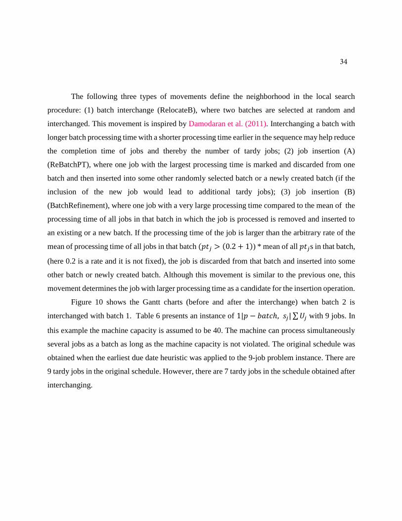
The following three types of movements define the neighborhood in the local search

procedure: (1) batch interchange (RelocateB), where two batches are selected at random and

interchanged. This movement is inspired by Damodaran et al. (2011). Interchanging a batch with

longer batch processing time with a shorter processing time earlier in the sequence may help reduce

the completion time of jobs and thereby the number of tardy jobs; (2) job insertion (A)

(ReBatchPT), where one job with the largest processing time is marked and discarded from one

batch and then inserted into some other randomly selected batch or a newly created batch (if the

inclusion of the new job would lead to additional tardy jobs); (3) job insertion (B)

(BatchRefinement), where one job with a very large processing time compared to the mean of the

processing time of all jobs in that batch in which the job is processed is removed and inserted to

an existing or a new batch. If the processing time of the job is larger than the arbitrary rate of the

mean of processing time of all jobs in that batch (𝑝𝑡𝑗 > (0.2 + 1)) * mean of all 𝑝𝑡𝑗s in that batch,

(here 0.2 is a rate and it is not fixed), the job is discarded from that batch and inserted into some

other batch or newly created batch. Although this movement is similar to the previous one, this

movement determines the job with larger processing time as a candidate for the insertion operation.

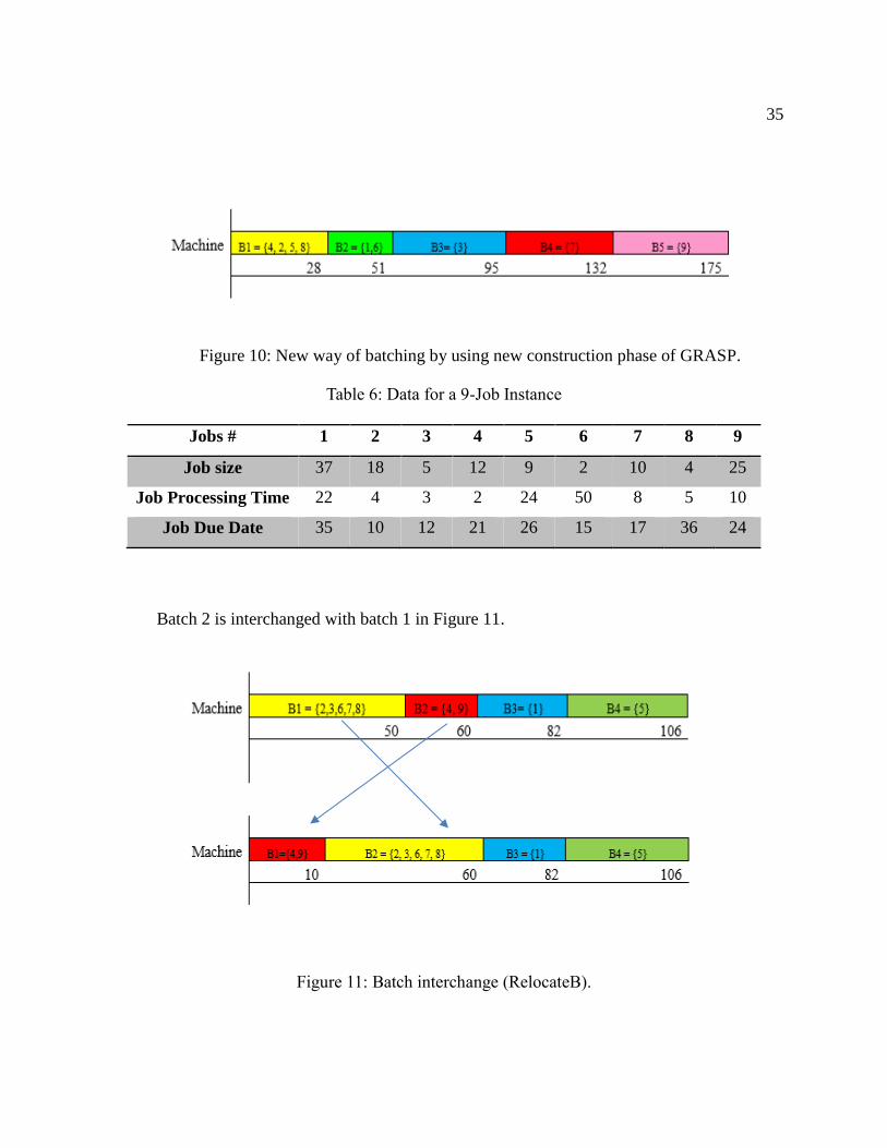
Figure 10 shows the Gantt charts (before and after the interchange) when batch 2 is

interchanged with batch 1. Table 6 presents an instance of 1|𝑝 − 𝑏𝑎𝑡𝑐ℎ, 𝑠𝑗| ∑ 𝑈𝑗 with 9 jobs. In

this example the machine capacity is assumed to be 40. The machine can process simultaneously

several jobs as a batch as long as the machine capacity is not violated. The original schedule was

obtained when the earliest due date heuristic was applied to the 9-job problem instance. There are

9 tardy jobs in the original schedule. However, there are 7 tardy jobs in the schedule obtained after

interchanging.

34

35

Figure 10: New way of batching by using new construction phase of GRASP.

Table 6: Data for a 9-Job Instance

Jobs # 1 2 3 4 5 6 7 8 9

Job size 37 18 5 12 9 2 10 4 25

Job Processing Time 22 4 3 2 24 50 8 5 10

Job Due Date 35 10 12 21 26 15 17 36 24

Batch 2 is interchanged with batch 1 in Figure 11.

Figure 11: Batch interchange (RelocateB).

36

A job insertion type (A) is shown in Figure 12 where job 6 with larger processing time is

discarded from batches 1 and inserted into a newly created batch (batch 5). Here the total number

of tardy jobs is 3. Job 6 is discarded from the first batch and inserted into a newly created batch to

avoid making other jobs tardy.

Figure 12: Job insertion (A) (ReBatchPT).

A job insertion type (B) is shown in Figure 13. This movement is slightly similar to the

previous movement; however, here jobs with larger processing time will be chosen for the

interchange. For batch number one the mean of processing time of all jobs is 50+4+3+8+5

5= 14

and the processing time of job 6, which is 50, is larger than the mean of processing time of all jobs.

Thus job 6 is removed from the batch and the batch completion time is reduced (or job completion

times are reduced). Again for the second batch the mean of processing time of jobs 4 and 9 is 6.

Job number 9 with processing time equal to 10 is the job with largest processing time in the second

batch (comparing to the mean of processing time of jobs 4 and 9), so it is also removed from the

second batch. All in all, jobs 9 and 6 with larger processing times are discarded from batches 1

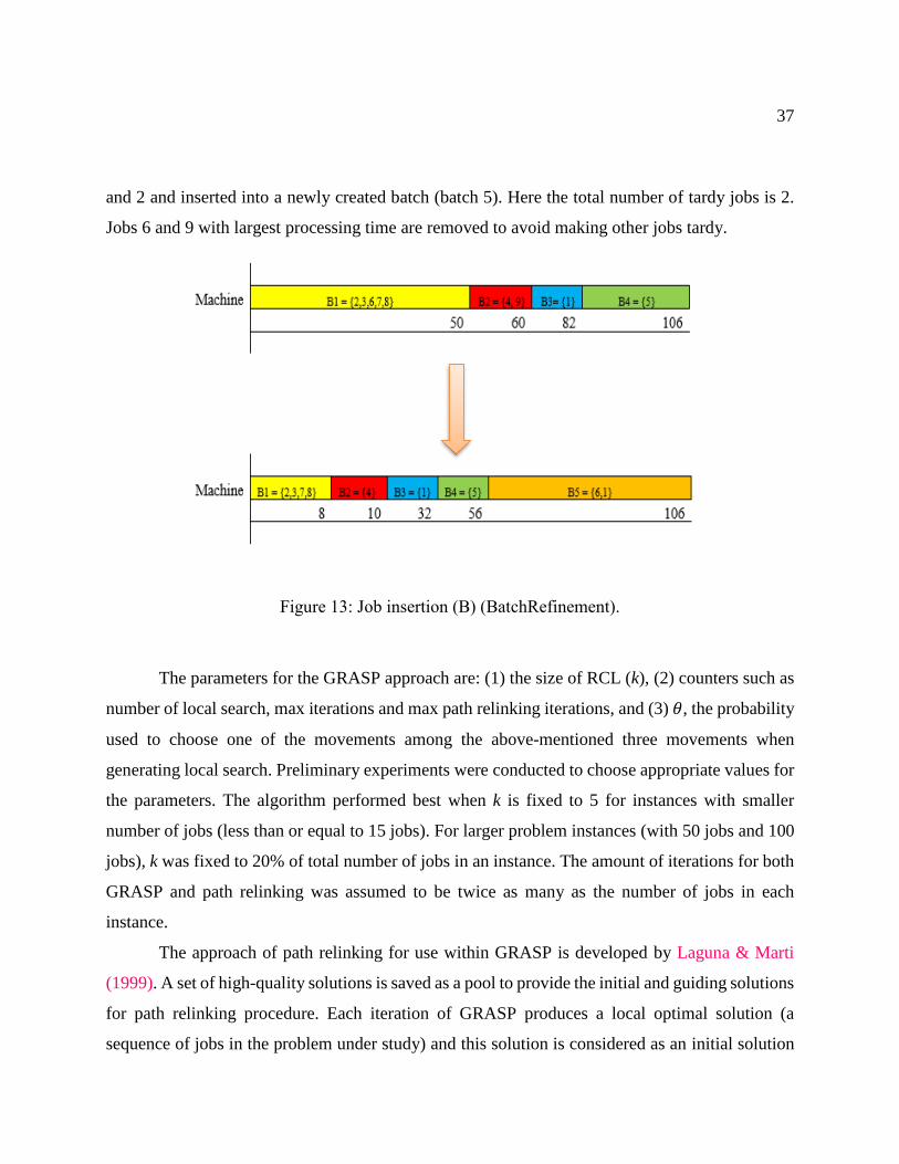
37

and 2 and inserted into a newly created batch (batch 5). Here the total number of tardy jobs is 2.

Jobs 6 and 9 with largest processing time are removed to avoid making other jobs tardy.

Figure 13: Job insertion (B) (BatchRefinement).

The parameters for the GRASP approach are: (1) the size of RCL (k), (2) counters such as

number of local search, max iterations and max path relinking iterations, and (3) 𝜃, the probability

used to choose one of the movements among the above-mentioned three movements when

generating local search. Preliminary experiments were conducted to choose appropriate values for

the parameters. The algorithm performed best when k is fixed to 5 for instances with smaller

number of jobs (less than or equal to 15 jobs). For larger problem instances (with 50 jobs and 100

jobs), k was fixed to 20% of total number of jobs in an instance. The amount of iterations for both

GRASP and path relinking was assumed to be twice as many as the number of jobs in each

instance.

The approach of path relinking for use within GRASP is developed by Laguna & Marti

(1999). A set of high-quality solutions is saved as a pool to provide the initial and guiding solutions

for path relinking procedure. Each iteration of GRASP produces a local optimal solution (a

sequence of jobs in the problem under study) and this solution is considered as an initial solution

38

(I). Another good solution, which is the best among other solutions, in the pool is chosen and it is

named guiding (G) solution, and a path of solutions linking the initial solution to the guiding

solution is constructed by applying a series of changes to the original solution (Resende & Ribeiro,

2005). For instance, let I= (1,3,4,2,5) and G= (5,3,2,4,1). A path relinking I to G is I = (1,3,4,5,2)

(2,3,4,5,1) (5,3,4,2,1) (5,3,2,4,1) = G and each of these solutions is evaluated for solution

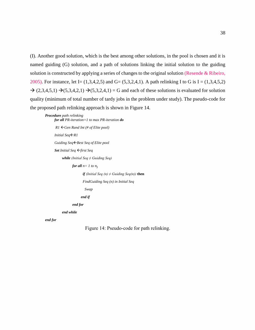
quality (minimum of total number of tardy jobs in the problem under study). The pseudo-code for

the proposed path relinking approach is shown in Figure 14.

Procedure path relinking

for all PR-iteration=1 to max PR-iteration do

R1 Gen Rand Int (# of Elite pool)

Initial SeqR1

Guiding SeqBest Seq of Elite pool

Set Initial Seq first Seq

while (Initial Seq ≠ Guiding Seq)

for all n= 1 to 𝑛𝑗

if (Initial Seq (n) ≠ Guiding Seq(n)) then

FindGuiding Seq (n) in Initial Seq

Swap

end if

end for

end while

end for

Figure 14: Pseudo-code for path relinking.

CHAPTER 5

COMPUTATIONAL RESULTS

An experiment was conducted to fine tune GRASP with path relinking parameters (i.e., the

size of RCL, number of iterations, and number of path relinking iterations). Table 7 presents the

different factors and levels considered during preliminary study to tune GRASP parameters. The

levels tested were k= {5 for small jobs instances, 10% of number of jobs, 25% of number of jobs

and 50% of number of jobs for large jobs instances}, total number of iterations for GRASP= {300,

1000}, and path relinking iterations = {300, 1000}.

Table 7: Factors and Levels

Factors Levels

The size of RCL, K 10%nj, 25%nj and 50%nj

Number of iterations 300, 1000

Number of path relinking iterations 300, 1000

During this process, all 50-job instances were solved using the GRASP algorithm and the

commercial solver. There were altogether ten 50-job instances assuming a machine capacity S=40;

each instance was run for all combinations of the GRASP with path relinking parameters shown

in Table 7 (i.e., 10×2×2×3 = 120 experiments). The combination of each parameter which

yielded the most improvement in minimizing the total number of tardy jobs will be chosen for

further experimentation. The average percent improvement in minimizing total number of tardy

jobs was computed using Equation 16.

40

% Improvement = (∑ 𝑈𝑗 𝑓𝑟𝑜𝑚 𝐶𝑃𝐿𝐸𝑋 −∑ 𝑈𝑗 𝑓𝑟𝑜𝑚 𝐺𝑅𝐴𝑆𝑃)

∑ 𝑈𝑗 𝑓𝑟𝑜𝑚 𝐶𝑃𝐿𝐸𝑋 (16)

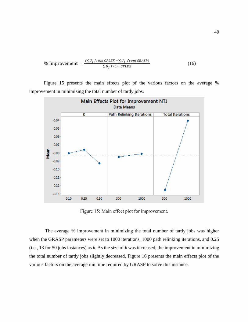
Figure 15 presents the main effects plot of the various factors on the average %

improvement in minimizing the total number of tardy jobs.

Figure 15: Main effect plot for improvement.

The average % improvement in minimizing the total number of tardy jobs was higher

when the GRASP parameters were set to 1000 iterations, 1000 path relinking iterations, and 0.25

(i.e., 13 for 50 jobs instances) as k. As the size of k was increased, the improvement in minimizing

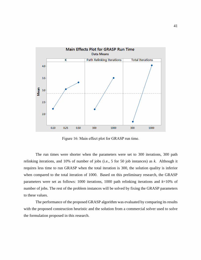
the total number of tardy jobs slightly decreased. Figure 16 presents the main effects plot of the

various factors on the average run time required by GRASP to solve this instance.

41

Figure 16: Main effect plot for GRASP run time.

The run times were shorter when the parameters were set to 300 iterations, 300 path

relinking iterations, and 10% of number of jobs (i.e., 5 for 50 job instances) as k. Although it

requires less time to run GRASP when the total iteration is 300, the solution quality is inferior

when compared to the total iteration of 1000. Based on this preliminary research, the GRASP

parameters were set as follows: 1000 iterations, 1000 path relinking iterations and k=10% of

number of jobs. The rest of the problem instances will be solved by fixing the GRASP parameters

to these values.

The performance of the proposed GRASP algorithm was evaluated by comparing its results

with the proposed construction heuristic and the solution from a commercial solver used to solve

the formulation proposed in this research.

42

The total number of tardy jobs obtained from the GRASP was compared to the best results

gained from construction heuristic. The proposed GRASP algorithm and construction heuristic

was implemented in Matlab R2012a.

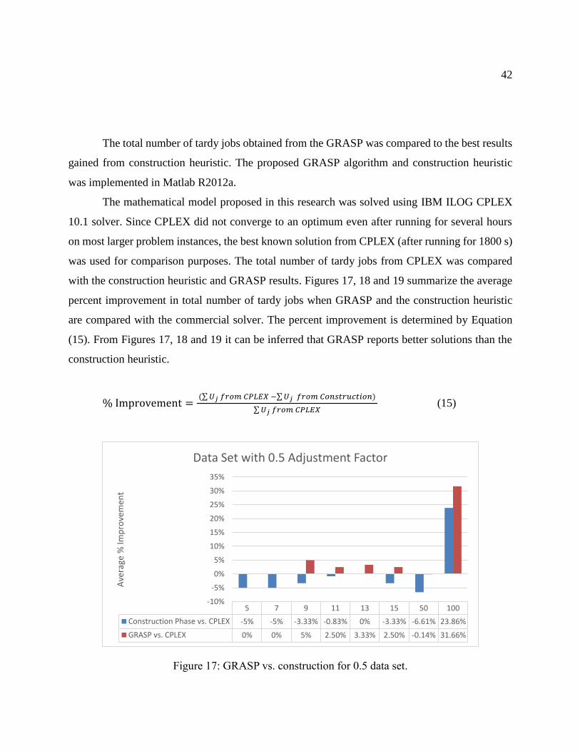
The mathematical model proposed in this research was solved using IBM ILOG CPLEX

10.1 solver. Since CPLEX did not converge to an optimum even after running for several hours

on most larger problem instances, the best known solution from CPLEX (after running for 1800 s)

was used for comparison purposes. The total number of tardy jobs from CPLEX was compared

with the construction heuristic and GRASP results. Figures 17, 18 and 19 summarize the average

percent improvement in total number of tardy jobs when GRASP and the construction heuristic

are compared with the commercial solver. The percent improvement is determined by Equation

(15). From Figures 17, 18 and 19 it can be inferred that GRASP reports better solutions than the

construction heuristic.

% Improvement = (∑ 𝑈𝑗 𝑓𝑟𝑜𝑚 𝐶𝑃𝐿𝐸𝑋 −∑ 𝑈𝑗 𝑓𝑟𝑜𝑚 𝐶𝑜𝑛𝑠𝑡𝑟𝑢𝑐𝑡𝑖𝑜𝑛)

∑ 𝑈𝑗 𝑓𝑟𝑜𝑚 𝐶𝑃𝐿𝐸𝑋 (15)

Figure 17: GRASP vs. construction for 0.5 data set.

5 7 9 11 13 15 50 100

Construction Phase vs. CPLEX -5% -5% -3.33% -0.83% 0% -3.33% -6.61% 23.86%

GRASP vs. CPLEX 0% 0% 5% 2.50% 3.33% 2.50% -0.14% 31.66%

-10%

-5%

0%

5%

10%

15%

20%

25%

30%

35%

Ave

rage

% Im

pro

vem

ent

Data Set with 0.5 Adjustment Factor

43

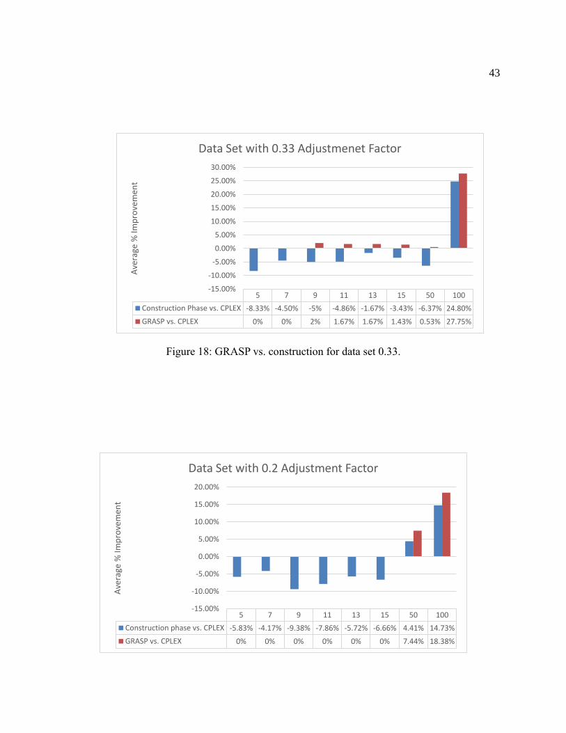
Figure 18: GRASP vs. construction for data set 0.33.

5 7 9 11 13 15 50 100

Construction Phase vs. CPLEX -8.33% -4.50% -5% -4.86% -1.67% -3.43% -6.37% 24.80%

GRASP vs. CPLEX 0% 0% 2% 1.67% 1.67% 1.43% 0.53% 27.75%

-15.00%

-10.00%

-5.00%

0.00%

5.00%

10.00%

15.00%

20.00%

25.00%

30.00%

Ave

rage

% Im

pro

vem

ent

Data Set with 0.33 Adjustmenet Factor

5 7 9 11 13 15 50 100

Construction phase vs. CPLEX -5.83% -4.17% -9.38% -7.86% -5.72% -6.66% 4.41% 14.73%

GRASP vs. CPLEX 0% 0% 0% 0% 0% 0% 7.44% 18.38%

-15.00%

-10.00%

-5.00%

0.00%

5.00%

10.00%

15.00%

20.00%

Ave

rage

% Im

pro

vem

ent


44

Figure 19: GRASP vs. construction for data set 0.2.

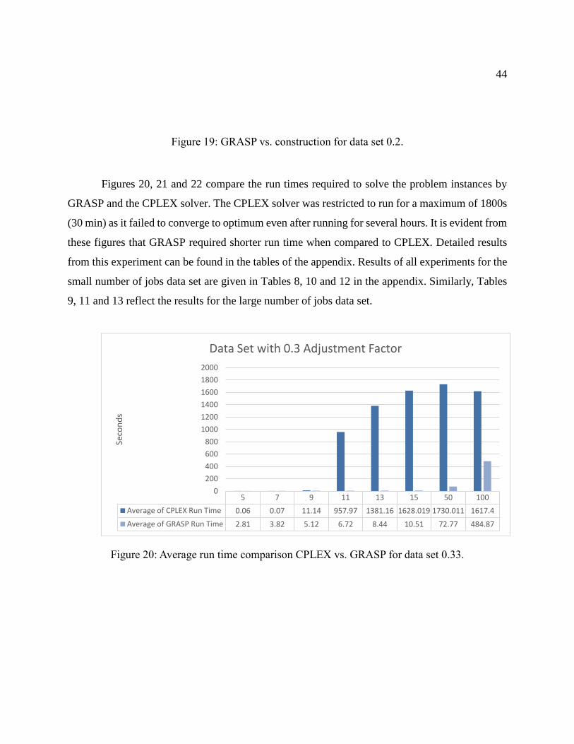
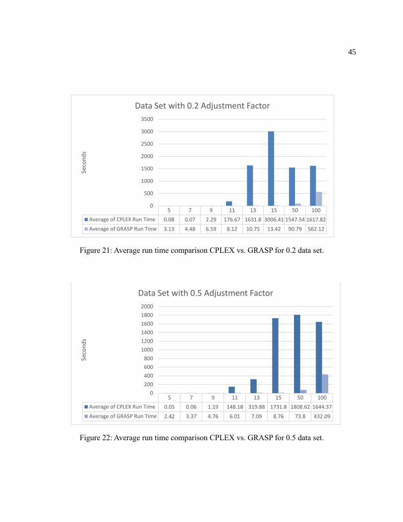
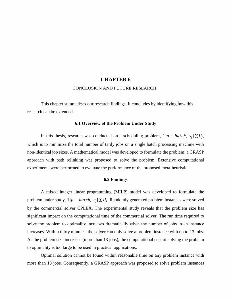
Figures 20, 21 and 22 compare the run times required to solve the problem instances by

GRASP and the CPLEX solver. The CPLEX solver was restricted to run for a maximum of 1800s

(30 min) as it failed to converge to optimum even after running for several hours. It is evident from

these figures that GRASP required shorter run time when compared to CPLEX. Detailed results

from this experiment can be found in the tables of the appendix. Results of all experiments for the

small number of jobs data set are given in Tables 8, 10 and 12 in the appendix. Similarly, Tables

9, 11 and 13 reflect the results for the large number of jobs data set.

Figure 20: Average run time comparison CPLEX vs. GRASP for data set 0.33.

5 7 9 11 13 15 50 100

Average of CPLEX Run Time 0.06 0.07 11.14 957.97 1381.16 1628.019 1730.011 1617.4

Average of GRASP Run Time 2.81 3.82 5.12 6.72 8.44 10.51 72.77 484.87

0

200

400

600

800

1000

1200

1400

1600

1800

2000

Seco

nd

s


45

Figure 21: Average run time comparison CPLEX vs. GRASP for 0.2 data set.

Figure 22: Average run time comparison CPLEX vs. GRASP for 0.5 data set.

5 7 9 11 13 15 50 100



0

500

1000

1500

2000

2500

3000

3500

Seco

nd

s


5 7 9 11 13 15 50 100



0

200

400

600

800

1000

1200

1400

1600

1800

2000

Seco

nd

s


CHAPTER 6

CONCLUSION AND FUTURE RESEARCH

This chapter summarizes our research findings. It concludes by identifying how this

research can be extended.

6.1 Overview of the Problem Under Study

In this thesis, research was conducted on a scheduling problem, 1|𝑝 − 𝑏𝑎𝑡𝑐ℎ, 𝑠𝑗| ∑ 𝑈𝑗,

which is to minimize the total number of tardy jobs on a single batch processing machine with

non-identical job sizes. A mathematical model was developed to formulate the problem; a GRASP

approach with path relinking was proposed to solve the problem. Extensive computational

experiments were performed to evaluate the performance of the proposed meta-heuristic.

6.2 Findings

A mixed integer linear programming (MILP) model was developed to formulate the

problem under study, 1|𝑝 − 𝑏𝑎𝑡𝑐ℎ, 𝑠𝑗| ∑ 𝑈𝑗 . Randomly generated problem instances were solved

by the commercial solver CPLEX. The experimental study reveals that the problem size has

significant impact on the computational time of the commercial solver. The run time required to

solve the problem to optimality increases dramatically when the number of jobs in an instance

increases. Within thirty minutes, the solver can only solve a problem instance with up to 13 jobs.

As the problem size increases (more than 13 jobs), the computational cost of solving the problem

to optimality is too large to be used in practical applications.

Optimal solution cannot be found within reasonable time on any problem instance with

more than 13 jobs. Consequently, a GRASP approach was proposed to solve problem instances

47

with a larger number of jobs. This meta-heuristic has a novel construction phase and an advanced

local search. Two hundred and forty instances with 5, 7, 9, 11, 13, 15, 50, and 100 jobs were tested

to evaluate the quality of the new construction phase and advanced local search movements of the

proposed GRASP approach. The solutions obtained from GRASP and novel construction phase

were compared with the solution obtained from the CPLEX solver. The experimental results show

that the proposed GRASP approach with path relinking performs much better when compared to

CPLEX as the number of jobs increases. On smaller problem instances, the proposed GRASP

approach reports optimal solution (same as the solution from CPLEX).

6.3 Future Research

This research can be extended to consider parallel machines (𝑃𝑚) easily. The only change

to be made is that the jobs should be grouped into batches and scheduled on a set M of q non-

identical parallel BPMs such that the total number of tardy jobs is minimized. The job ready times

can also be considered by adding a couple of constraints. The unrelated machines in parallel (𝑅𝑚)

can also examined. Objectives other than minimizing total number of tardy jobs are also interesting

for investigation. Another important issue which needs to be addressed is that of how to handle

uncertainties occurring on the BPM. The design of effective heuristic for the case of stochastic

arrivals, in which the arrival of the job is not known in advance, is also an opportunity for future

research.

As mentioned in the literature, most scheduling problems related to BPM are solved for

minimizing makespan, completion time, tardiness or weighted tardiness, and maximum lateness

objective functions. However, minimizing number of tardy jobs or weighted number of tardy jobs

is also of importance in many practical applications. This research explores the GRASP approach

to minimize number of tardy jobs. The research findings indicate that this approach is successful

in solving large problem instances. The contributions of this research would motivate other

researchers to consider GRASP for other variants of this and other BPM scheduling problems with

a number of tardy jobs objective.

REFERENCES

Aiex, R. M., Binato, S., & Resende, M. G. C. (2003). Parallel GRASP with path relinking for job shop

scheduling. Parallel Computing, 29(4), 393–430.

Al-Ghamdi, F., Al-Khaldi, M., Khoukhi, A., & Al-Slamah, M. (n.d.). Minimizing the Tardiness in a

Single Machine Batch Processing.

Armentano, V. A., & de Araujo, O. C. B. (2006). Grasp with memory-based mechanisms for minimizing

total tardiness in single machine scheduling with setup times. Journal of Heuristics, 12(6), 427–446.

Behnamian, J., Fatemi Ghomi, S. M. T., & Zandieh, M. (2012). Hybrid flowshop scheduling with

sequence‐dependent setup times by hybridizing max–min ant system, simulated annealing and

variable neighbourhood search. Expert Systems, 29(2), 156–169.

Brucker, P., Kovalyov, M. Y., Shafransky, Y. M., & Werner, F. (1998). Batch scheduling with deadlines

on parallel machines. Annals of Operations Research, 83, 23–40.

Chandru, V., Lee, C.-Y., & Uzsoy, R. (1993). Minimizing total completion time on batch processing

machines. THE INTERNATIONAL JOURNAL OF PRODUCTION RESEARCH, 31(9), 2097–2121.

Damodaran, P., Diyadawagamage, D. A., Ghrayeb, O., & Vélez-Gallego, M. C. (2012). A particle swarm

optimization algorithm for minimizing makespan of nonidentical parallel batch processing

machines. The International Journal of Advanced Manufacturing Technology, 58(9-12), 1131–1140.

Damodaran, P., Ghrayeb, O., & Guttikonda, M. (2013). GRASP to minimize makespan for a capacitated

batch-processing machine. International Journal of Advanced Manufacturing Technology, 68.

Damodaran, P., Hirani, N. S., & Velez-Gallego, M. C. (2009). Scheduling identical parallel batch

processing machines to minimise makespan using genetic algorithms. European Journal of

Industrial Engineering, 3(2), 187–206.

Damodaran, P., Manjeshwar, P. K., & Srihari, K. (2006). Minimizing makespan on a batch-processing

machine with non-identical job sizes using genetic algorithms. International Journal of Production

Economics, 103(2), 882–891.

Damodaran, P., Rao, A. G., & Mestry, S. (2013). Particle swarm optimization for scheduling batch

processing machines in a permutation flowshop. The International Journal of Advanced

Manufacturing Technology, 64(5-8), 989–1000.

49

Damodaran, P., & Srihari, K. (2004). Mixed integer formulation to minimize makespan in a flow shop

with batch processing machines. Mathematical and Computer Modelling, 40(13), 1465–1472.

Damodaran, P., & Velez-Gallego, M. C. (2010). Heuristics for makespan minimization on parallel batch

processing machines with unequal job ready times. The International Journal of Advanced

Manufacturing Technology, 49(9-12), 1119–1128.

Damodaran, P., & Vélez-Gallego, M. C. (2012). A simulated annealing algorithm to minimize makespan

of parallel batch processing machines with unequal job ready times. Expert Systems with

Applications, 39(1), 1451–1458.

Damodaran, P., Vélez-Gallego, M. C., & Maya, J. (2011). A GRASP approach for makespan

minimization on parallel batch processing machines. Journal of Intelligent Manufacturing, 22(5),

767–777.

Draa, A., & Bouaziz, A. (2014). An artificial bee colony algorithm for image contrast enhancement.

Swarm and Evolutionary Computation, 16, 69–84.

Feo, T. A., & Resende, M. G. C. (1989). A probabilistic heuristic for a computationally difficult set

covering problem. Operations Research Letters, 8(2), 67–71.

Feo, T. A., & Resende, M. G. C. (1995). Greedy randomized adaptive search procedures. Journal of

Global Optimization, 6(2), 109–133.

Fornarelli, G., & Giaquinto, A. (2013). An unsupervised multi-swarm clustering technique for image

segmentation. Swarm and Evolutionary Computation, 11, 31–45.

Garai, G., & Chaudhurii, B. B. (2013). A novel hybrid genetic algorithm with Tabu search for optimizing

multi-dimensional functions and point pattern recognition. Information Sciences, 221, 28–48.

Ghazvini, F. J., & Dupont, L. (1998). Minimizing mean flow times criteria on a single batch processing

machine with non-identical jobs sizes. International Journal of Production Economics, 55(3), 273–

280.

Graham, R. L., Lawler, E. L., Lenstra, J. K., & Kan, A. H. G. R. (1979). Optimization and approximation

in deterministic sequencing and scheduling: a survey. Annals of Discrete Mathematics, 5, 287–326.

Hanssmann, F., & Hess, S. W. (1960). A linear programming approach to production and employment

scheduling. Management Science, (1), 46–51.

Hochbaum, D. S., & Landy, D. (1997). Scheduling semiconductor burn-in operations to minimize total

flowtime. Operations Research, 45(6), 874–885.

50

Holland, J. H. (1975). Adaptation in natural and artificial systems: an introductory analysis with

applications to biology, control, and artificial intelligence. U Michigan Press.

Ikura, Y., & Gimple, M. (1986). Efficient scheduling algorithms for a single batch processing machine.

Operations Research Letters, 5(2), 61–65.

Jolai, F. (2005). Minimizing number of tardy jobs on a batch processing machine with incompatible job

families. European Journal of Operational Research, 162(1), 184–190.

Kennedy, J., & Eberhart, R. C. (1995). Particle swarm optimization. In Proceedings of IEEE

International Conference on Neural Networks (Vol. 4, pp. 1942–1948).

Kirkpatrick, S., & Vecchi, M. P. (1983). Optimization by simmulated annealing. Science, 220(4598),

671–680.

Laguna, M., & Marti, R. (1999). GRASP and path relinking for 2-layer straight line crossing

minimization. INFORMS Journal on Computing, 11(1), 44–52.

Lee, C.-Y. (1999). Minimizing makespan on a single batch processing machine with dynamic job arrivals.

International Journal of Production Research, 37(1), 219–236.

Lee, C.-Y., Uzsoy, R., & Martin-Vega, L. A. (1992). Efficient algorithms for scheduling semiconductor

burn-in operations. Operations Research, 40(4), 764–775.

Lenstra, J. K., Kan, A. H. G. R., & Brucker, P. (1977). Complexity of machine scheduling problems.

Annals of Discrete Mathematics, 1, 343–362.

Leung, J. Y. T. (2004). Handbook of scheduling: algorithms, models, and performance analysis. CRC

Press.

Li, C.-L., & Lee, C.-Y. (1997). Scheduling with agreeable release times and due dates on a batch

processing machine. European Journal of Operational Research, 96(3), 564–569.

Liu, H.-C., & Huang, J.-S. (1998). Pattern recognition using evolution algorithms with fast simulated

annealing. Pattern Recognition Letters, 19(5), 403–413.

Liu, L., & Zhang, F. (2008). Minimizing Number of Tardy Jobs on a Batch Processing Machine with

Incompatible Job Families. 2008 ISECS International Colloquium on Computing, Communication,

Control, and Management. http://doi.org/10.1109/CCCM.2008.107

M’Hallah, R., & Bulfin, R. L. (2007). Minimizing the weighted number of tardy jobs on a single machine

with release dates. European Journal of Operational Research, 176(2), 727–744.

Mahdavi Mazdeh, M., Hamidinia, A., & Karamouzian, A. (2011). A mathematical model for weighted

51

tardy jobs scheduling problem with a batched delivery system. International Journal of Industrial

Engineering Computations, 2(3), 491–498.

Manjeshwar, P. K., Damodaran, P., & Srihari, K. (2009). Minimizing makespan in a flow shop with two

batch-processing machines using simulated annealing. Robotics and Computer-Integrated

Manufacturing, 25(3), 667–679.

Melouk, S., Damodaran, P., & Chang, P.-Y. (2004). Minimizing makespan for single machine batch

processing with non-identical job sizes using simulated annealing. International Journal of

Production Economics, 87(2), 141–147.

Mokoto, E. (1999). Scheduling to minimize the makespan on identical parallel machines: An LP-based

algorithm. Investigacion Operative, 97–107.

Moore, J. M. (1968). An n job, one machine sequencing algorithm for minimizing the number of late

jobs. Management Science, 15(1), 102–109.

Mucherino, A., & Seref, O. (2007). Monkey search: a novel metaheuristic search for global optimization.

In Data Mining, Systems Analysis and Optimization in Biomedicine (Vol. 953, pp. 162–173). AIP

Publishing.

Ourari, S., Briand, C., & Bouzouiac, B. (n.d.). A MIP approach for the minimization of the number of late

jobs in single machine scheduling.

Ozturk, O., Espinouse, M.-L., Di Mascolo, M., & Gouin, A. (2010). Optimizing the makespan of washing

operations of medical devices in hospital sterilization services. In Health Care Management

(WHCM), 2010 IEEE Workshop on (pp. 1–6). IEEE.

Ozturk, O., Espinouse, M.-L., Mascolo, M., & Gouin, A. (2012). Makespan minimisation on parallel

batch processing machines with non-identical job sizes and release dates. International Journal of

Production Research, 50(20), 6022–6035.

Perez, I. C., Fowler, J. W., & Carlyle, W. M. (2005). Minimizing total weighted tardiness on a single

batch process machine with incompatible job families. Computers & Operations Research, 32(2),

327–341.

Péridy, L., Pinson, E., & Rivreau, D. (2003). Using short-term memory to minimize the weighted number

of late jobs on a single machine. European Journal of Operational Research, 148(3), 591–603.

Phojanamongkolkij, N., Fowler, J. W., & Cochran, J. K. (2002). Determining operating criterion of batch

processing operations for wafer fabrication. Journal of Manufacturing Systems, 21(5), 363–379.

52

Pinedo, M. L. (2012). Scheduling: theory, algorithms, and systems. Springer Science & Business Media.

Potts, C. N., & Kovalyov, M. Y. (2000). Scheduling with batching: a review. European Journal of

Operational Research, 120(2), 228–249.

Resendel, M. G. C., & Ribeiro, C. C. (2005). GRASP with path relinking: Recent advances and

applications. In Metaheuristics: progress as real problem solvers (pp. 29–63). Springer.

Resende, M. G. C., & Ribeiro, C. C. (2014). GRASP: greedy randomized adaptive search procedures. In

Search methodologies (pp. 287–312). Springer.

Sevaux, M., & Dauzère-Pérès, S. (2003). Genetic algorithms to minimize the weighted number of late

jobs on a single machine. European Journal of Operational Research, 151(2), 296–306.

Shim, S.-O., & Kim, Y.-D. (2008). A branch and bound algorithm for an identical parallel machine

scheduling problem with a job splitting property. Computers & Operations Research, 35(3), 863–

875.

Sivrikaya-Şerifoǧlu, F., & Ulusoy, G. (1999). Parallel machine scheduling with earliness and tardiness

penalties. Computers & Operations Research, 26(8), 773–787.

Soltani, R., Jolai, F., & Zandieh, M. (2010). Two robust meta-heuristics for scheduling multiple job

classes on a single machine with multiple criteria. Expert Systems with Applications, 37(8), 5951–

5959.

Sung, C. S., & Choung, Y. I. (2000). Minimizing makespan on a single burn-in oven in semiconductor

manufacturing. European Journal of Operational Research, 120(3), 559–574.

SUNG, C. S., & YOON, S. H. (1997). Minimizing maximum completion time in a two-batch-processing-

machine flowshop with dynamic arrivals allowed. Engineering Optimization+ A35, 28(3), 231–243.

Uzsoy, R. (1994). Scheduling a single batch processing machine with non-identical job sizes. THE

INTERNATIONAL JOURNAL OF PRODUCTION RESEARCH, 32(7), 1615–1635.

Vélez-Gallego, M. C., Damodaran, P., & Rodríguez, M. (2011). MAKESPAN MINIMIZATION ON A

SINGLE BATCH PROCESSING MACHINE WITH UNEQUAL JOB READY TIMES.

International Journal of Industrial Engineering, 18(10).

Xu, S., & Bean, J. C. (2007). A genetic algorithm for scheduling parallel non-identical batch processing

machines. In Computational Intelligence in Scheduling, 2007. SCIS’07. IEEE Symposium on (pp.

143–150). IEEE.

APPENDIX A: GRASP, CPLEX and Construction Phase

54

Table 8: Solution and Run Time of Construction Phase and GRASP for Small Jobs, γ=0.2

CPLEX Construction Phase GRASP

Instance

Number

of Jobs

Number

of

Tardy

Jobs

GAP%

Run

Time Number of Tardy Jobs

Number of

Jobs Run Time

1 5 4 0.00% 0.13 4 4 3.1476

2 5 4 25.00% 0.12 4 4 3.4401

3 5 4 0.00% 0.03 5 4 2.6832

4 5 4 25.00% 0.05 4 4 3.1111

5 5 4 25.00% 0.11 4 4 3.2508

6 5 4 25.00% 0.05 4 4 3.4652

7 5 3 0.00% 0.05 3 3 3.1104

8 5 3 0.00% 0.14 3 3 3.0956

9 5 3 0.00% 0.03 4 3 3.0938

10 5 4 0.00% 0.13 4 4 2.8699

11 7 6 0.00% 0.14 6 6 4.4075

12 7 4 0.00% 0.12 5 4 4.6622

13 7 4 25.00% 0.05 4 4 4.724

14 7 5 60.00% 0.05 5 5 4.4536

15 7 6 0.00% 0.05 7 6 4.0111

16 7 4 25.00% 0.06 4 4 4.0829

17 7 5 40.00% 0.05 5 5 4.5108

18 7 5 60.00% 0.09 5 5 5.0636

19 7 6 0.00% 0.02 6 6 3.8767

20 7 5 40.00% 0.06 5 5 4.9873

21 9 7 28.57% 0.08 7 7 6.6747

22 9 7 0.00% 0.14 8 7 6.5825

23 9 6 33.33% 0.06 6 6 6.6997

24 9 6 33.33% 0.08 7 6 7.2739

25 9 5 40.00% 0.14 5 5 6.2386

26 9 4 50.00% 0.13 4 4 4.9547

27 9 7 28.57% 0.09 8 7 6.995

28 9 6 33.33% 0.11 6 6 7.1937

29 9 7 28.57% 0.13 9 7 7.9524

30 9 5 40.00% 21.9 6 5 5.3363

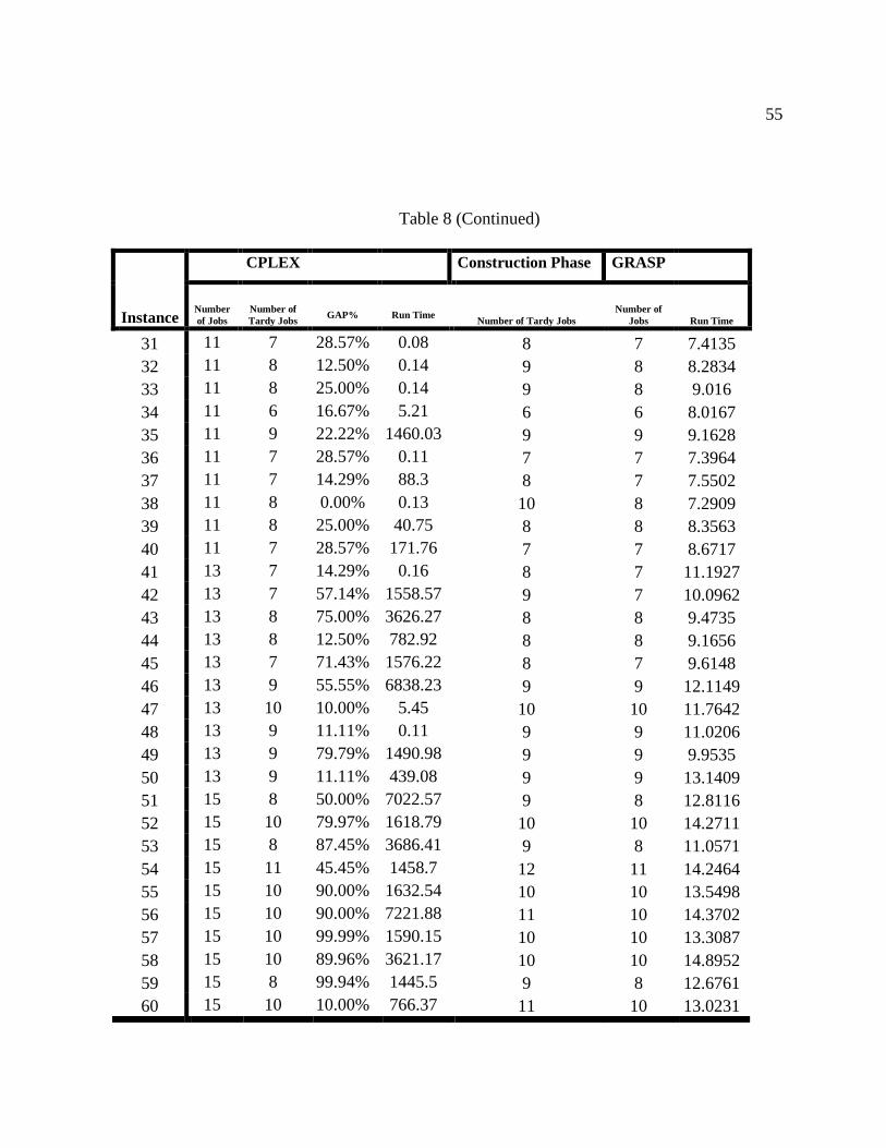
55

Table 8 (Continued)


Instance

Number

of Jobs

Number of

Tardy Jobs

GAP%

Run Time

Number of Tardy Jobs Number of

Jobs Run Time

31 11 7 28.57% 0.08 8 7 7.4135

32 11 8 12.50% 0.14 9 8 8.2834

33 11 8 25.00% 0.14 9 8 9.016

34 11 6 16.67% 5.21 6 6 8.0167

35 11 9 22.22% 1460.03 9 9 9.1628

36 11 7 28.57% 0.11 7 7 7.3964

37 11 7 14.29% 88.3 8 7 7.5502

38 11 8 0.00% 0.13 10 8 7.2909

39 11 8 25.00% 40.75 8 8 8.3563

40 11 7 28.57% 171.76 7 7 8.6717

41 13 7 14.29% 0.16 8 7 11.1927

42 13 7 57.14% 1558.57 9 7 10.0962

43 13 8 75.00% 3626.27 8 8 9.4735

44 13 8 12.50% 782.92 8 8 9.1656

45 13 7 71.43% 1576.22 8 7 9.6148

46 13 9 55.55% 6838.23 9 9 12.1149

47 13 10 10.00% 5.45 10 10 11.7642

48 13 9 11.11% 0.11 9 9 11.0206

49 13 9 79.79% 1490.98 9 9 9.9535

50 13 9 11.11% 439.08 9 9 13.1409

51 15 8 50.00% 7022.57 9 8 12.8116

52 15 10 79.97% 1618.79 10 10 14.2711

53 15 8 87.45% 3686.41 9 8 11.0571

54 15 11 45.45% 1458.7 12 11 14.2464

55 15 10 90.00% 1632.54 10 10 13.5498

56 15 10 90.00% 7221.88 11 10 14.3702

57 15 10 99.99% 1590.15 10 10 13.3087

58 15 10 89.96% 3621.17 10 10 14.8952

59 15 8 99.94% 1445.5 9 8 12.6761

60 15 10 10.00% 766.37 11 10 13.0231

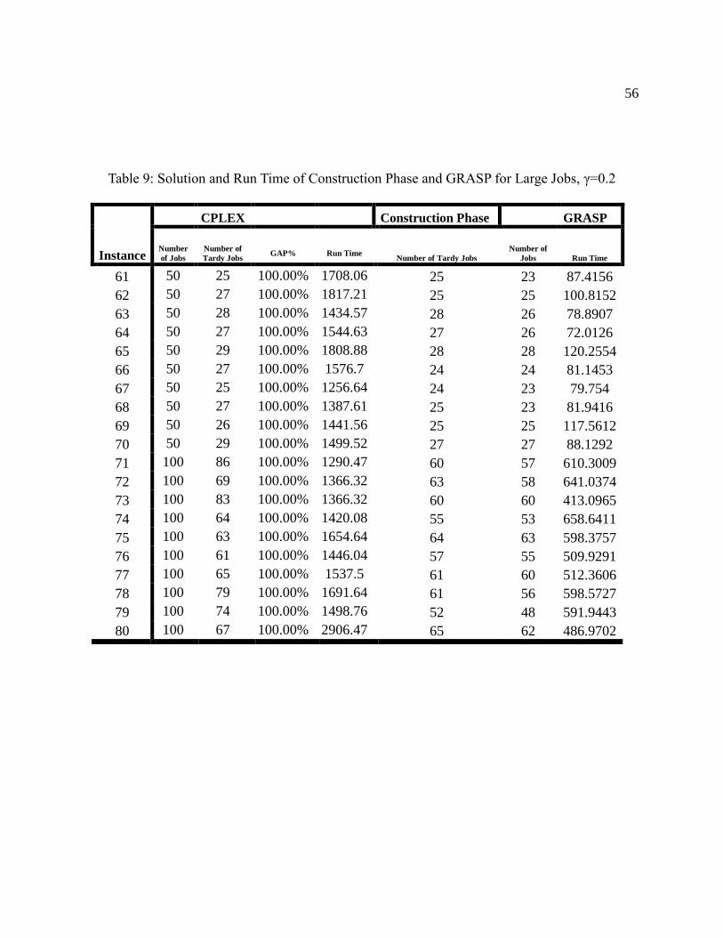
56

Table 9: Solution and Run Time of Construction Phase and GRASP for Large Jobs, γ=0.2


Instance

Number

of Jobs

Number of

Tardy Jobs

GAP%

Run Time


Jobs Run Time

61 50 25 100.00% 1708.06 25 23 87.4156

62 50 27 100.00% 1817.21 25 25 100.8152

63 50 28 100.00% 1434.57 28 26 78.8907

64 50 27 100.00% 1544.63 27 26 72.0126

65 50 29 100.00% 1808.88 28 28 120.2554

66 50 27 100.00% 1576.7 24 24 81.1453

67 50 25 100.00% 1256.64 24 23 79.754

68 50 27 100.00% 1387.61 25 23 81.9416

69 50 26 100.00% 1441.56 25 25 117.5612

70 50 29 100.00% 1499.52 27 27 88.1292

71 100 86 100.00% 1290.47 60 57 610.3009

72 100 69 100.00% 1366.32 63 58 641.0374

73 100 83 100.00% 1366.32 60 60 413.0965

74 100 64 100.00% 1420.08 55 53 658.6411

75 100 63 100.00% 1654.64 64 63 598.3757

76 100 61 100.00% 1446.04 57 55 509.9291

77 100 65 100.00% 1537.5 61 60 512.3606

78 100 79 100.00% 1691.64 61 56 598.5727

79 100 74 100.00% 1498.76 52 48 591.9443

80 100 67 100.00% 2906.47 65 62 486.9702

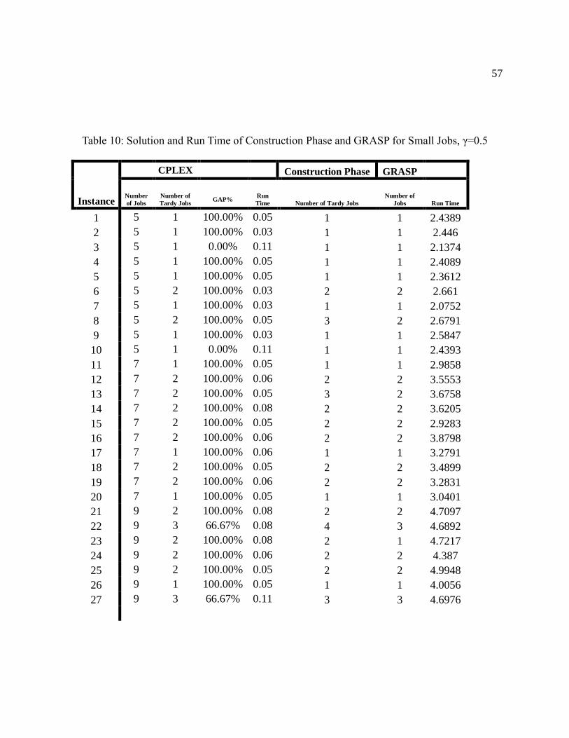
57


CPLEX

Construction Phase GRASP

Instance

Number

of Jobs

Number of

Tardy Jobs

GAP%

Run

Time Number of Tardy Jobs Number of

Jobs Run Time

1 5 1 100.00% 0.05 1 1 2.4389

2 5 1 100.00% 0.03 1 1 2.446

3 5 1 0.00% 0.11 1 1 2.1374

4 5 1 100.00% 0.05 1 1 2.4089

5 5 1 100.00% 0.05 1 1 2.3612

6 5 2 100.00% 0.03 2 2 2.661

7 5 1 100.00% 0.03 1 1 2.0752

8 5 2 100.00% 0.05 3 2 2.6791

9 5 1 100.00% 0.03 1 1 2.5847

10 5 1 0.00% 0.11 1 1 2.4393

11 7 1 100.00% 0.05 1 1 2.9858

12 7 2 100.00% 0.06 2 2 3.5553

13 7 2 100.00% 0.05 3 2 3.6758

14 7 2 100.00% 0.08 2 2 3.6205

15 7 2 100.00% 0.05 2 2 2.9283

16 7 2 100.00% 0.06 2 2 3.8798

17 7 1 100.00% 0.06 1 1 3.2791

18 7 2 100.00% 0.05 2 2 3.4899

19 7 2 100.00% 0.06 2 2 3.2831

20 7 1 100.00% 0.05 1 1 3.0401

21 9 2 100.00% 0.08 2 2 4.7097

22 9 3 66.67% 0.08 4 3 4.6892

23 9 2 100.00% 0.08 2 1 4.7217

24 9 2 100.00% 0.06 2 2 4.387

25 9 2 100.00% 0.05 2 2 4.9948

26 9 1 100.00% 0.05 1 1 4.0056

27 9 3 66.67% 0.11 3 3 4.6976

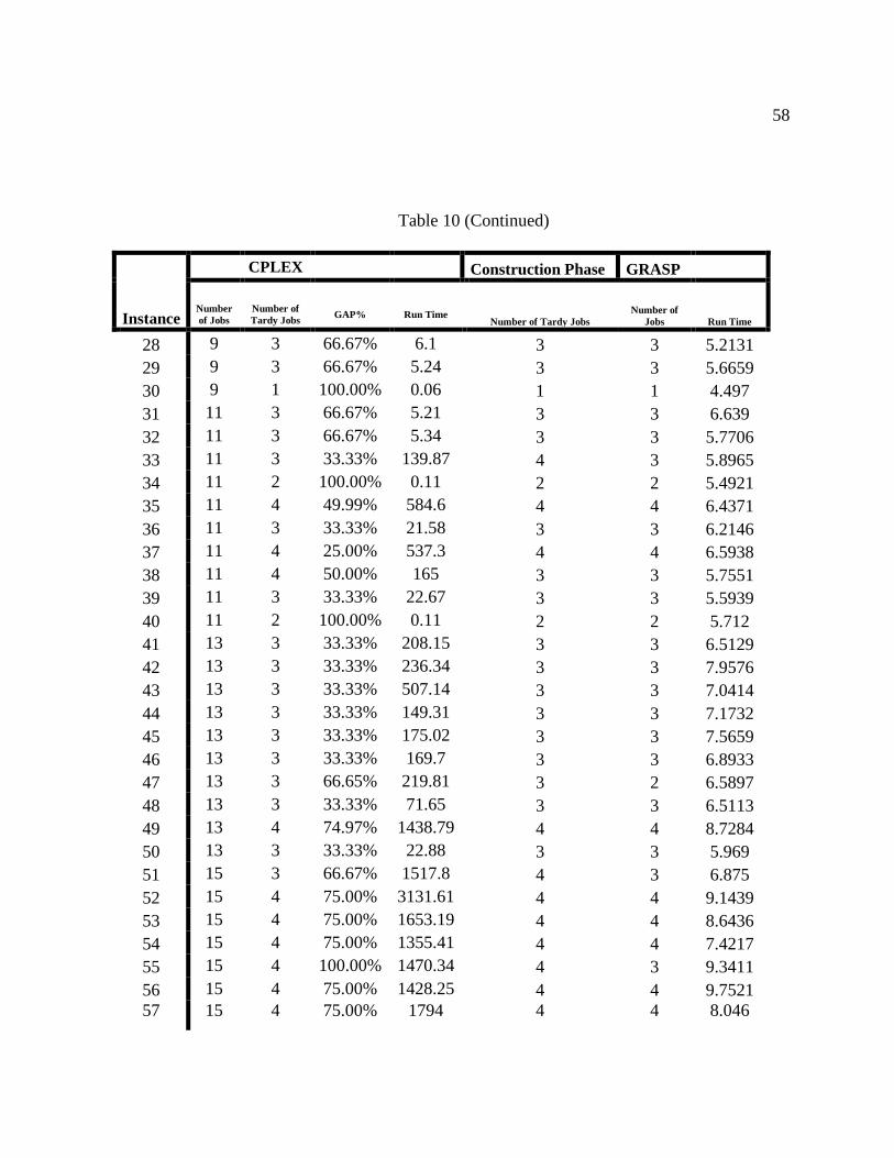
58

Table 10 (Continued)


Instance

Number

of Jobs

Number of

Tardy Jobs

GAP%

Run Time


Jobs Run Time

28 9 3 66.67% 6.1 3 3 5.2131

29 9 3 66.67% 5.24 3 3 5.6659

30 9 1 100.00% 0.06 1 1 4.497

31 11 3 66.67% 5.21 3 3 6.639

32 11 3 66.67% 5.34 3 3 5.7706

33 11 3 33.33% 139.87 4 3 5.8965

34 11 2 100.00% 0.11 2 2 5.4921

35 11 4 49.99% 584.6 4 4 6.4371

36 11 3 33.33% 21.58 3 3 6.2146

37 11 4 25.00% 537.3 4 4 6.5938

38 11 4 50.00% 165 3 3 5.7551

39 11 3 33.33% 22.67 3 3 5.5939

40 11 2 100.00% 0.11 2 2 5.712

41 13 3 33.33% 208.15 3 3 6.5129

42 13 3 33.33% 236.34 3 3 7.9576

43 13 3 33.33% 507.14 3 3 7.0414

44 13 3 33.33% 149.31 3 3 7.1732

45 13 3 33.33% 175.02 3 3 7.5659

46 13 3 33.33% 169.7 3 3 6.8933

47 13 3 66.65% 219.81 3 2 6.5897

48 13 3 33.33% 71.65 3 3 6.5113

49 13 4 74.97% 1438.79 4 4 8.7284

50 13 3 33.33% 22.88 3 3 5.969

51 15 3 66.67% 1517.8 4 3 6.875

52 15 4 75.00% 3131.61 4 4 9.1439

53 15 4 75.00% 1653.19 4 4 8.6436

54 15 4 75.00% 1355.41 4 4 7.4217

55 15 4 100.00% 1470.34 4 3 9.3411

56 15 4 75.00% 1428.25 4 4 9.7521

57 15 4 75.00% 1794 4 4 8.046

59



Instance

Number

of Jobs

Number of

Tardy Jobs

GAP%

Run Time


Jobs Run Time

58 15 4 75.00% 1795.93 4 4 10.5381

59 15 4 50.00% 1718.29 4 4 10.4169

60 15 3 66.67% 1453.17 3 3 7.4068

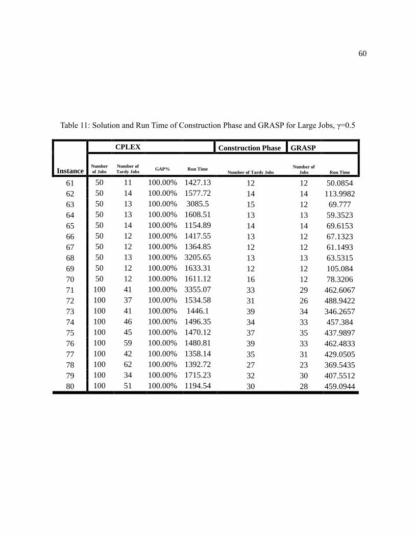
60



Instance

Number

of Jobs

Number of

Tardy Jobs

GAP%

Run Time


Jobs Run Time

61 50 11 100.00% 1427.13 12 12 50.0854

62 50 14 100.00% 1577.72 14 14 113.9982

63 50 13 100.00% 3085.5 15 12 69.777

64 50 13 100.00% 1608.51 13 13 59.3523

65 50 14 100.00% 1154.89 14 14 69.6153

66 50 12 100.00% 1417.55 13 12 67.1323

67 50 12 100.00% 1364.85 12 12 61.1493

68 50 13 100.00% 3205.65 13 13 63.5315

69 50 12 100.00% 1633.31 12 12 105.084

70 50 12 100.00% 1611.12 16 12 78.3206

71 100 41 100.00% 3355.07 33 29 462.6067

72 100 37 100.00% 1534.58 31 26 488.9422

73 100 41 100.00% 1446.1 39 34 346.2657

74 100 46 100.00% 1496.35 34 33 457.384

75 100 45 100.00% 1470.12 37 35 437.9897

76 100 59 100.00% 1480.81 39 33 462.4833

77 100 42 100.00% 1358.14 35 31 429.0505

78 100 62 100.00% 1392.72 27 23 369.5435

79 100 34 100.00% 1715.23 32 30 407.5512

80 100 51 100.00% 1194.54 30 28 459.0944

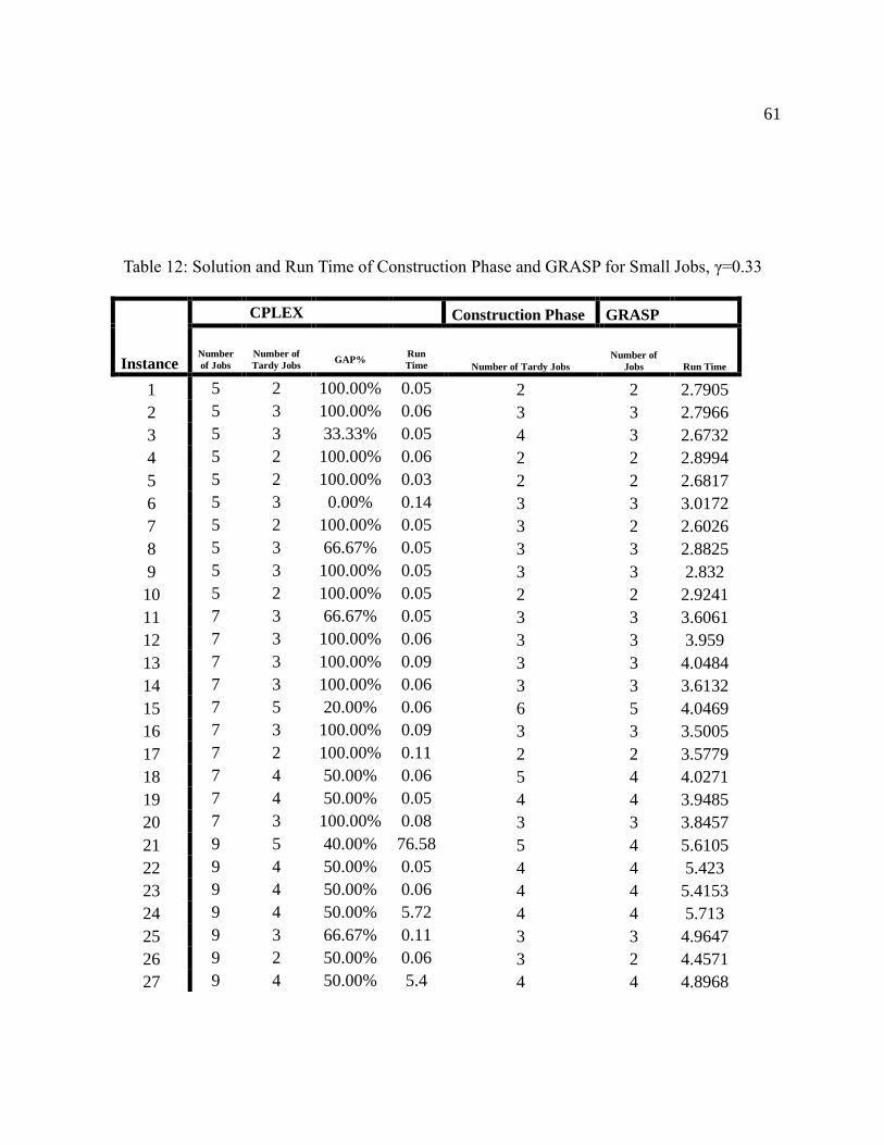
61



Instance

Number

of Jobs

Number of

Tardy Jobs

GAP%

Run

Time Number of Tardy Jobs Number of

Jobs Run Time

1 5 2 100.00% 0.05 2 2 2.7905

2 5 3 100.00% 0.06 3 3 2.7966

3 5 3 33.33% 0.05 4 3 2.6732

4 5 2 100.00% 0.06 2 2 2.8994

5 5 2 100.00% 0.03 2 2 2.6817

6 5 3 0.00% 0.14 3 3 3.0172

7 5 2 100.00% 0.05 3 2 2.6026

8 5 3 66.67% 0.05 3 3 2.8825

9 5 3 100.00% 0.05 3 3 2.832

10 5 2 100.00% 0.05 2 2 2.9241

11 7 3 66.67% 0.05 3 3 3.6061

12 7 3 100.00% 0.06 3 3 3.959

13 7 3 100.00% 0.09 3 3 4.0484

14 7 3 100.00% 0.06 3 3 3.6132

15 7 5 20.00% 0.06 6 5 4.0469

16 7 3 100.00% 0.09 3 3 3.5005

17 7 2 100.00% 0.11 2 2 3.5779

18 7 4 50.00% 0.06 5 4 4.0271

19 7 4 50.00% 0.05 4 4 3.9485

20 7 3 100.00% 0.08 3 3 3.8457

21 9 5 40.00% 76.58 5 4 5.6105

22 9 4 50.00% 0.05 4 4 5.423

23 9 4 50.00% 0.06 4 4 5.4153

24 9 4 50.00% 5.72 4 4 5.713

25 9 3 66.67% 0.11 3 3 4.9647

26 9 2 50.00% 0.06 3 2 4.4571

27 9 4 50.00% 5.4 4 4 4.8968

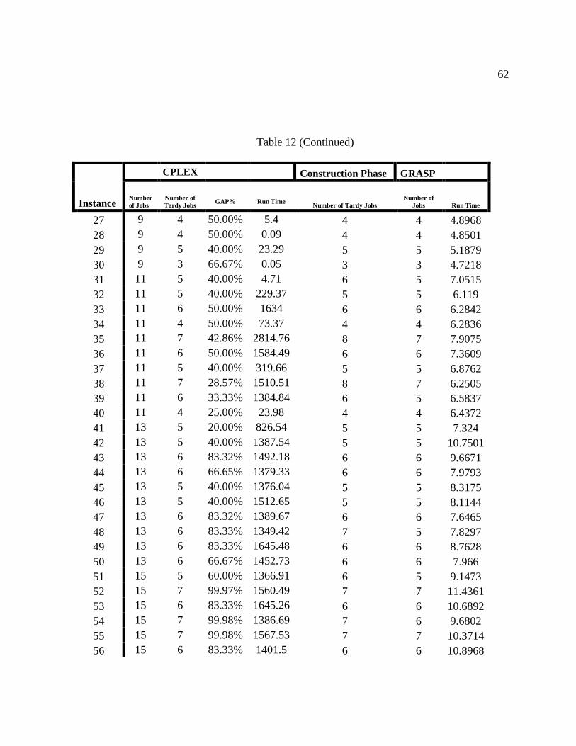
62



Instance

Number

of Jobs

Number of

Tardy Jobs

GAP%

Run Time


Jobs Run Time

27 9 4 50.00% 5.4 4 4 4.8968

28 9 4 50.00% 0.09 4 4 4.8501

29 9 5 40.00% 23.29 5 5 5.1879

30 9 3 66.67% 0.05 3 3 4.7218

31 11 5 40.00% 4.71 6 5 7.0515

32 11 5 40.00% 229.37 5 5 6.119

33 11 6 50.00% 1634 6 6 6.2842

34 11 4 50.00% 73.37 4 4 6.2836

35 11 7 42.86% 2814.76 8 7 7.9075

36 11 6 50.00% 1584.49 6 6 7.3609

37 11 5 40.00% 319.66 5 5 6.8762

38 11 7 28.57% 1510.51 8 7 6.2505

39 11 6 33.33% 1384.84 6 5 6.5837

40 11 4 25.00% 23.98 4 4 6.4372

41 13 5 20.00% 826.54 5 5 7.324

42 13 5 40.00% 1387.54 5 5 10.7501

43 13 6 83.32% 1492.18 6 6 9.6671

44 13 6 66.65% 1379.33 6 6 7.9793

45 13 5 40.00% 1376.04 5 5 8.3175

46 13 5 40.00% 1512.65 5 5 8.1144

47 13 6 83.32% 1389.67 6 6 7.6465

48 13 6 83.33% 1349.42 7 5 7.8297

49 13 6 83.33% 1645.48 6 6 8.7628

50 13 6 66.67% 1452.73 6 6 7.966

51 15 5 60.00% 1366.91 6 5 9.1473

52 15 7 99.97% 1560.49 7 7 11.4361

53 15 6 83.33% 1645.26 6 6 10.6892

54 15 7 99.98% 1386.69 7 6 9.6802

55 15 7 99.98% 1567.53 7 7 10.3714

56 15 6 83.33% 1401.5 6 6 10.8968

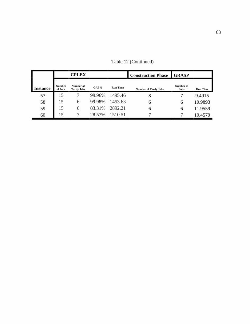
63



Instance

Number

of Jobs

Number of

Tardy Jobs

GAP%

Run Time


Jobs Run Time

57 15 7 99.96% 1495.46 8 7 9.4915

58 15 6 99.98% 1453.63 6 6 10.9893

59 15 6 83.31% 2892.21 6 6 11.9559

60 15 7 28.57% 1510.51 7 7 10.4579

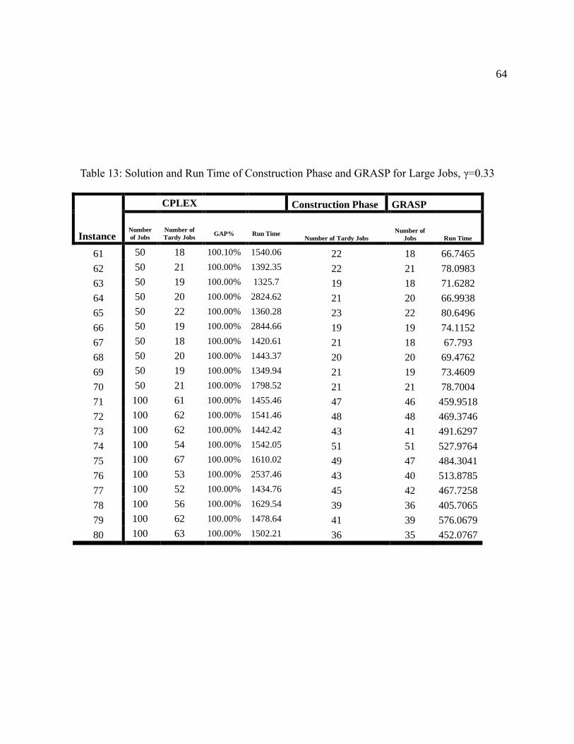
64



Instance

Number

of Jobs

Number of

Tardy Jobs

GAP%

Run Time


Jobs Run Time

61 50 18 100.10% 1540.06 22 18 66.7465

62 50 21 100.00% 1392.35 22 21 78.0983

63 50 19 100.00% 1325.7 19 18 71.6282

64 50 20 100.00% 2824.62 21 20 66.9938

65 50 22 100.00% 1360.28 23 22 80.6496

66 50 19 100.00% 2844.66 19 19 74.1152

67 50 18 100.00% 1420.61 21 18 67.793

68 50 20 100.00% 1443.37 20 20 69.4762

69 50 19 100.00% 1349.94 21 19 73.4609

70 50 21 100.00% 1798.52 21 21 78.7004

71 100 61 100.00% 1455.46 47 46 459.9518

72 100 62 100.00% 1541.46 48 48 469.3746

73 100 62 100.00% 1442.42 43 41 491.6297

74 100 54 100.00% 1542.05 51 51 527.9764

75 100 67 100.00% 1610.02 49 47 484.3041

76 100 53 100.00% 2537.46 43 40 513.8785

77 100 52 100.00% 1434.76 45 42 467.7258

78 100 56 100.00% 1629.54 39 36 405.7065

79 100 62 100.00% 1478.64 41 39 576.0679

80 100 63 100.00% 1502.21 36 35 452.0767

abstract minimizing total number of tardy jobs on a …

Documents