Particle tracking in the vicinity of Helgoland, North Sea:

a model comparison

Ulrich Callies, Helmholtz-Zentrum Geesthacht, Geesthacht, Germany1

Andreas Plüß, Federal Waterways Engineering and Research Institute (BAW), Hamburg, Germany

Jens Kappenberg, Helmholtz-Zentrum Geesthacht, Geesthacht, Germany

Hartmut Kapitza, Helmholtz-Zentrum Geesthacht, Geesthacht, Germany

Keywords: Lagrangian particle tracking, backward trajectories, model comparison, North Sea, Helgoland Roads

Abstract

Station Helgoland Roads in the southeastern North Sea (German Bight) hosts one of the richest long-term time series of marine observations. Hydrodynamic transport simulations can help understand variability in the local data brought about by intermittent changes of water masses. The objective of our study is an estimate of to which extent the outcome of such transport simulations depends on the choice of a specific hydrodynamic model. Our basic experiment consists of 3377 Lagrangian simulations in time-reversed mode initialized every seven hours within the period Feb 2002 – Oct 2004. 50 day backward simulations were performed based on hourly current fields from four different hydrodynamic models that are all well established but differ with regard to spatial resolution, dimensionality (2D or 3D), the origin of atmospheric forcing data, treatment of boundary conditions, presence or absence of baroclinic terms, and the numerical scheme. The particle tracking algorithm is 2D, fields from 3D models were averaged vertically. Drift simulations were evaluated quantitatively in terms of the fraction of released particles that crossed each cell of a network of receptor regions centred at the island of Helgoland. We found substantial systematic differences between drift simulations based on each of the four hydrodynamic models. Sensitivity studies with regard to spatial resolution and the effects of baroclinic processes suggest that differences in model output cannot unambiguously be assigned to certain model properties or restrictions. Therefore multi-model simulations are needed for a proper identification of uncertainties in long-term Lagrangian drift simulations.

1 Introduction Lagrangian transport models are useful for transport analyses in many different contexts. An early estimate of long-term pollution transport routes in the North Sea was provided by Hainbucher et al. (1987). Schönfeld (1995) simulated dispersion of artificial radionuclides released into the English Channel at Cap de La Hague. Lagrangian dispersion modelling was applied also for estimates of egg and larval dispersal from their spawning areas (e.g. van den Veer et al. 1998; Brandt et al. 2008) or in the context of particulate matter transport studies (e.g. Puls et al. 1997; Rolinski 1999).

1 Corresponding author: U. Callies Helmholtz-Zentrum Geesthacht Institute of Coastal Research Max-Planck-Str. 1 21502 Geesthacht Germany e-mail: ulrich.callies@hzg.de Tel.: +49 (0)4152 87 2837 Fax: +49 (0)4152 87 2818

2

Running a Lagrangian particle dispersion model in backward (i.e. time-reversed) mode is advantageous and most efficient in a receptor oriented perspective (e.g. Seibert and Frank 2004), a prototypical example for which is the interpretation of observations at some monitoring station. The present study is motivated by the existence of a rich time series of long-term marine observations (starting in 1962) at station Helgoland Roads (Wiltshire et al. 2010) located in the German Bight, North Sea (cf. Fig. 1). The idea is that Lagrangian particle tracking based on detailed simulations of the hydrodynamic regime might help understand both temporal variability and spatial representativity of the marine data observed. Existing model-based reconstructions of environmental conditions (e.g. Weisse et al. 2009) provide a valuable basis for detailed simulations of weather driven transports in support of the interpretation of long-term observational data. Chrastansky et al. (2009), for instance, applied forward drift simulations to explain time variability in the occurrence of oil-contaminated dead birds on the German North Sea coast. Another monitoring-related recent paper by Kako et al. (2010) on beach-litter simulation involves also backward integrations. In the present paper we will refer to backward simulations initialized at Helgoland. Hickel (1972) stressed the highly variable conditions in this region with large tidal excursions but relatively small residual currents that depend predominantly on prevailing weather conditions. The focus of our paper is an investigation of how reliable long-term drift simulations under these conditions can be. Generally the synopsis and cross-check of different models is hoped to improve the robustness of conclusions from model simulations (Jones 2002; Delhez et al. 2004). In a recent study Liu et al. (2011) demonstrated the use of ensemble simulations in the context of the Deepwater Horizon accident. The concept of multi-model simulations was also recommended by Plüß and Schüttrumpf (2004) and Plüß and Heyer (2007). In this study we will try an assessment of model errors to be expected for passive tracer particle tracking. For short time drift predictions (1-2 days) recently a hyper-ensemble approach was proposed that statistically combines information from different models (Rixen and Ferreira-Coelho 2007; Rixen et al. 2008; Vandenbulcke 2009). The main problem with long-term particle tracking, however, is the lack of comprehensive data models could be fitted to. Even when two models seem consistent with regard to the simulation of momentary current fields, long-term transports arising from small residuals of oscillating tidal currents may still differ substantially. We will describe systematic differences between passive tracer simulations based on current fields from four different hydrodynamic models. For this purpose a large number (3377) of time-reversed Lagrangian transport simulations for some thousands of particles initialized once every seven hours within the period Feb 2002 to Oct 2004 will be analysed with regard to mean transport patterns and distributions of transit times. The use of detailed atmospheric forcing for the nearly three year period allows for covering realistically the whole spectrum of possible flow conditions. At first sight the passive tracer assumption may seem too simplistic for practical applications. Most substances of interest in the North Sea ecosystem are not conservative and their distribution depends on processes like sedimentation and re-suspension (suspended matter) or biological growth rates (nutrients, chlorophyll a), for instance. Different parameterizations of such processes in different models are likely to be main reasons for model discrepancies as model outputs are sensitive to parameters not well known. The main justification for our study is that basic passive tracer transport routes in possibly complex terrain establish a general framework that constrains also any more detailed simulation. Section 2 provides a short description of our study area (Section 2.1), the Lagrangian transport module PELETS-2D and its setup we use (Section 2.2), and the four hydrodynamic models our Lagrangian simulations are based on (Section 2.3). Section 2.4 gives an example of how detailed particle tracking simulations are aggregated in the present study. In Section 3 we present results with regard to Eulerian volume fluxes near Helgoland (Section 3.1), patterns of Lagrangian transports and corresponding transit time distributions (Section 3.2) and some sensitivity studies (Section 3.3). After a discussion of these results in Section 4 we summarize main conclusions in Section 5.

2 Material and methods

2.1 Study area The German Bight is the southeastern part of the North Sea on the shelf between the European continent, the British Isles and Norway. Our study area is confined to that part of the German Bight that adjoins the Dutch and the German coast (cf. Fig. 1). Mean water depth in this area is little more than 20 m, maximum water depth is

about 56 m in a small region to the southwest of the island of Helgoland (54°11.3’ N, 7°54.0’ E) located about 70 km off the German coast. Helgoland accommodates a long-term time series (at Helgoland Roads) initiated by the Biological Station Helgoland in 1962. Observations of marine water parameters are taken on a work-daily basis. On average, residual currents in the German Bight are part of an anti-clockwise circulation in the North Sea. This circulation and corresponding transports, however, are much influenced by atmospheric wind forcing (e.g. van der Veer et al. 1998). For most of the time, strong vertical mixing prevents the formation of persistent thermal stratification. Density dependent currents due to strong salinity gradients occur mainly in a narrow range close to the European coast (‘coastal current’). In the present paper we focus on a description of conditions near the island of Helgoland.

2.2 Lagrangian transport module PELETS-2D The program package PELETS-2D allows for off-line Lagrangian transport calculations based on 2D current fields stored on at least an hourly basis. The toolbox was developed at the Helmholtz-Zentrum Geesthacht2 for the use in connection with the data base coastDat (www.coastdat.de) that contains state-of-the-art model based re-analyses of past atmospheric and sea state conditions (Weisse et al. 2009). For the simulation of substances drifting at the water surface current velocities used in the particle tracking algorithm may be modified by the inclusion of an extra wind drift component. Recent applications of this type include the analysis of trends in chronic oil pollution of the German coast and the interpretation of related beached bird survey data (Chrastansky and Callies (2009); Chrastansky et al. (2009)). For the present study an extra wind drift factor is not meaningful. Instead we used an option to weight initial particle densities with water depths so as to better represent water masses in a 2D set-up. PELETS-2D consists of two components dealing with a) the tracking particles based on pre-calculated hydrodynamic fields (cf. Section 2.2.1) and b) the set-up of ensemble simulations and their statistical evaluation (cf. Section 2.2.2). In Section 2.2.3 the framework for our specific study will be detailed.

2.2.1 Dispersion modelling The particle tracking module PELETS-2D assumes tracer particles of negligible mass and size that passively move with the local currents. Subscale turbulent processes are included via a random diffusion term. Assuming that movements in the two directions are decoupled (diagonal tensor of horizontal eddy diffusivity), updates of a particle’s position vector rr after time dt are described by the following stochastic differential equation in the sense of Itô,

[ ] )(2)()(')()( tBdDdttvdttvtvtrdrrrrr

+=+= , (1) where vr denotes the (pre-calculated) deterministic velocity vector and )(tBd

r is a white noise driven diffusion

term with variance dt. At each time step the random velocity component is specified as

)(2)(2)(' tRdtDtBd

dtDtv

rrr== (2)

where vector is made up by two mutually independent random numbers from a distribution with zero mean

and variance one. If the distribution of)(tR

r

Rr

is standard normal, Bdr

becomes the increment of a Wiener process. In this case the implicit assumption is that each random particle displacement already consists of a number of smaller steps so that the central limit theorem is applicable. Being interested just in distributions of the stochastic process rather than in individual trajectories (weak instead of strong approximation), the assumption of a Wiener process in Eq. (1) can be relaxed and random numbers may be drawn from a distribution with similar moment properties (Kloeden and Platen 1992). Some authors used a model with random numbers from a uniform distribution (e.g. Maier-Reimer and Sündermann 1982; Dippner 1993; Schönfeld 1995). Test runs showed that in our simulations effects of different choices of the distribution of R

r could hardly be noticed, due to the fact

32 Until 1st Nov 2010 officially called GKSS-Forschungszentrum Geesthacht.

that we tracked particles over longer times and that the evaluation of ensemble simulations involves further averaging. In the 2D particle tracking algorithm the horizontal eddy diffusivity D is assumed to be constant in time but to depend on grid resolution l. Following Schönfeld (1995), dependence of D on length scale l is assumed to follow a 4/3 law (Stommel 1949),

34

00 )()( ⎟⎟

⎠

⎞⎜⎜⎝

⎛=

lllDlD , (3)

with a reference length scale l0=1 km and D(l0) = 1 m2/s. This value roughly agrees with the value of 2.5 m2/s for a reference length scale of one nautical mile chosen by Schönfeld (1995). Note that two of the hydrodynamic models we compare (UnTRIM and TELEMAC-2D, cf. Section 2.3) provide current fields on grids with variable resolution (see Fig. 2) so that the relevant spatial scale in Eq. (3) changes with a particle’s location. We did not expand, however, the deterministic velocity in Eq. (1) to correct for an artificial drift induced by random particle displacements when diffusivity and/or water depth depend on location (cf. Heemink 1990). This simplification seems justified given that gradients of diffusivity are smooth (on regular grids even constant) and differences between water depths in neighbouring grid cells are small compared to absolute values of water depth. The PELETS-2D algorithm was designed for two-dimensional current fields on unstructured triangular grids. When velocity fields are provided on a rectangular grid, the grid topology must be pre-processed by adding a diagonal in each grid cell (cf. Fig. 2). This emulation of an unstructured grid does not affect the information content of the hydrodynamic fields. For 3D velocity fields, we eliminated vertical dependency by vertical averaging. A simple Euler method was used for particle tracking, arising from a replacement of dt in Eq. (1) by a finite time increment Δt. This time increment, however, is not treated as a constant. Although an upper limit Δtmax = 900 s is imposed on time step Δt, a particle’s velocities is updated earlier (by linear interpolation between two nodes) in case the particle crosses an edge of the underlying triangular grid. As a result time steps (and times between velocity updates) tend to shrink when particles enter regions with refined resolution of the numerical grid. A side benefit of the method is that particle trajectories can never cross the model boundary due to large time steps. If the maximum time step Δtmax is reached without the particle crossing an edge, new particle velocities are linearly interpolated (in space and time) between values prescribed at the three nodes the current triangle is made up by. According to Rümelin (1982) it is difficult to surpass the order of convergence of Euler’s method when dealing with a multi-dimensional stochastic differential equation. More recently, Penland (2003) mentions problems with using higher-order Runge-Kutta schemes for solving stochastic differential equations. Gräwe and Wolff (2010) compare three different schemes and mention that differences are supposed to become visible only in advection-dominated problems. Although this is the case in our application, it must be kept in mind that the maximum time step we use (900 s) seems small considering the fact that pre-calculated current fields are updated only once per hour. It is also computationally costly to integrate Runge-Kutta schemes based on pre-specified time steps into the framework described above. When a particle approaches a grid element’s edge, an iterative algorithm is needed to adapt the time step such that the Runge-Kutta update of location places the particle exactly (within the limits of pre-specified accuracy) on the edge being crossed. We therefore preferred the simple and much faster Euler method for our extensive calculations. Test simulations revealed a negligible impact of different integration schemes on our description of mean model behaviour. To avoid the need for any iterative adjustments, an additional simplification was introduced by evaluating Eq. (2) based on the previous time step rather than the present one. Again, however, this assumption turned out to have no major effect on the outcome of our study.

2.2.2 Ensemble simulations PELETS-2D was designed for dealing with large ensembles of particle cloud simulations. Given a data base of meteo-marine long-term re-analyses (e.g. Weisse et al. 2009), initializing drift simulations with fixed time increments weights properly the occurrence of different forcing conditions in the ensemble of drift simulations. Alternatively, a time schedule may be prescribed to meet special requirements (e.g. the selection of seasons) of

4

5

biological studies, for instance. PELETS-2D provides a couple of general tools for the evaluation of such large ensemble simulations. Each individual simulation involves the integration of some thousand trajectories, initialized at random within one or a couple of source regions. These user defined source regions are delimited by arbitrarily shaped polygons. Weighting of particle density with water depth is optional but should always be applied when particles are meant to represent a certain water volume. If, instead, a study deals with material drifting on the surface (e.g. oil slicks) a depth weighted initialization will not be meaningful. The initial partitioning of particles between different source regions can either be uniform or weighted with the subregions’ areas. Depending on a study’s objective, drift simulations may be performed either forward or backward in time. In addition to the set of source regions the user may define an arbitrary number of target or receptor regions. In this case for any simulation initialized at time t0 the number of particles from each source region that reside within a given receptor region will be stored on an hourly basis. In practice, detailed particle locations will be stored mainly for the purposes of graphical visualization. For large applications (many particles, long integration times and/or a large number of different initial times), however, storing all trajectory details will require too many resources. Particle density distributions after a given travel time, however, do not convey information on how particles got where they are. Therefore we chose an alternative output option that replaces particle distributions after integration time t-t0 by the fraction of particles from each source region that visited a given receptor region at any time within the period [t0, t], regardless of how long and how often. We will refer to the latter variable as the Cumulative Travel History (CTH). Section 2.4 (Figure 3) provides an illustration of how detailed information about a particle cloud’s movement gets transformed into a spatial pattern of CTH. As CTH values at time t accumulate the whole history of particle locations from release time t0 to time t, they can never decrease when integration time proceeds. An interpretation of CTH patterns in terms of travel routes seems appropriate. The price to be paid for the more compact representation is a loss of information about the drift simulation’s exact timing. If needed, however, PELETS-2D allows for supplementation of CTHs with percentiles (e.g. the median) of the distribution of transit times between source and receptor regions. These transit times are defined as times of particles’ first arrivals. Corresponding distributions refer to the relevant subsets of released particles that reach a receptor region of interest within the integration period. CTH-patterns will be the basis of the analyses in this study. For each simulation we obtain a vector of percentages that refer to the set of pre-specified receptor regions. Ensemble simulations provide a large number of such vectors that can then be averaged to obtain presentations of mean transport conditions.

2.2.3 Set-up for this study Source and receptor regions our CTH patterns will be defined on are shown in Fig. 1. Regions are organized in 24 sectors of circles centred at Helgoland, widths of which gradually increase from 3.5 km to a maximum of 20 km. Particles will be released in the centre circle (diameter 7 km) that encompasses the island of Helgoland and in the four colour coded sectors in the island’s vicinity. The definition of source regions in different sectors allows for the analysis of effects brought about by the presence of the island. In each simulation integration time will extend 50 days back in time. CTH values and transit time distributions will be monitored for each pair of source and receptor regions. A transect between Helgoland and the German coast (yellow line in Fig. 1) was defined for a comparison of residual volume fluxes around Helgoland as simulated by different hydrodynamic models in an Eulerian framework.

Fig. 1 Source and receptor regions used for the evaluation of drift simulations. Particles are released in the centre circle (encompassing the island of Helgoland) and/or in the colour coded sectors that surround the island. The yellow line indicates a transect across which residual volume fluxes were calculated (cf. Figs. 4, 8 and 10). The above map does not show the much larger domain of the hydrodynamic models. All hydrodynamic models cover the whole North Sea with northern boundaries at least at about 59°N and western boundaries at least at about 4°W.

2.3 Hydrodynamic simulations Drift simulations presented in this study are based on pre-calculated flow fields from four different hydrodynamic models. These flow fields were all produced independently for different purposes. The four models basically use three quite different numerical grids. Fig. 2 shows the different grid resolutions in the German Bight. Both TELEMAC-2D and UnTRIM are operating on an unstructured triangular grid. Due to some algorithmic constraints, the grid topologies of the two models are not quite the same, but the numbers of nodes and spatial resolutions are identical. The unstructured grid is the type of grid PELETS-2D was originally adapted to. To deal with the regular grids of BSHcmod (spherical coordinates) and TRIM (Cartesian coordinates), each rectangular grid cell was subdivided by an additional diagonal edge. Orientations of the new edges vary so as not to provoke a bias in the Lagrangian transport calculations. Domains of all models cover the whole North Sea (BSHcmod is run in a nested mode with lower resolution outside the German Bight). Some more details with regard to each of the models will be given in the subsections below. Most important differences between the models are summarized in Tab. 1.

2.3.1 UnTRIM

To be able to cover complicated topographies, the numerical model UnTRIM (Casulli and Walters 2000) solves the 3-dimensional shallow water equations on an unstructured orthogonal triangular grid using a semi-implicit finite difference / finite volume scheme. Spatial resolution varies between about 100 m near the coast and a couple of kilometres in offshore regions. Vertical resolution (z-coordinate) is variable, thicknesses of layers are 2.5 m near the water surface, 5-10 m at depths up to 100 m and 20-50 m below that depth. Effects of flooding and drying are included. Water levels at open boundaries are given by astronomy (12 partial tides). To take into account effects of external surges, values at the North Sea’s northern boundary are modified using filtered observations of surge levels at Aberdeen. In our application the model was run in hydrostatic mode and without temperature effects but taking into account the salt budget and its baroclinic effects. Vertically averaged velocity fields are used as inputs for PELETS-2D.

6

To study the relevance of salinity driven baroclinic effects in the context of drift simulations, the same version of UnTRIM was re-run for a one year period 2002 a) in 3D without salt and b) in a 2D mode.

To avoid spin-up problems, UnTRIM simulations were started one year before the 3 year period we study. This was primarily for letting salinity distributions develop from an assumed homogeneous initial distribution. For the 2D and 3D-simulations without salt such a long spin-up period was considered unnecessary.

2.3.2 TELEMAC-2D The finite element model TELEMAC-2D (Hervouet and van Haren 1996) was included to contrast UnTRIM simulations with the results of a genuine 2D barotropic model based on a different numerical technique. Lateral boundary conditions including the effects of external surges, however, are treated in the same way as for UnTRIM. Flooding and drying of coastal grid points is taken into account. The data we use are part of the long-term simulations described in Weisse and Plüß (2006). About 5 decades of simulated data for the whole North Sea are available on an hourly basis from the data base coastDat (www.coastdat.de; cf. Weisse et al. 2009). In a recent study, Jones and Davies (2005) contrasted the model with the finite difference approach, Jones and Davies (2006) used the model to study the sensitivity of wind forced flow simulations to variations in horizontal grid resolution.

Fig. 2 Resolutions of grids on which pre-calculated hydrodynamic fields from different models are specified. For the purpose of Lagrangian transport simulations, the regular grids from both BSHcmod and TRIM were triangulated by adding diagonal edges. Note that panels show just small segments (see Fig. 1) of the much larger full model domains covering the whole North Sea.

2.3.3 BSHcmod We refer to a version of the 3D finite difference hydrodynamic model BSHcmod that has been used operationally at the Bundesamt für Seeschifffahrt und Hydrographie (BSH) in Germany between the early 1990s and 2007 (Dick et al. 2001) before it was replaced by a revised update. The model is baroclinic, hydrostatic and uses the Boussinesq assumption. The primitive equations are discretized on an Arakawa C grid in spherical coordinates with a z-coordinate in the vertical. The model is run in a nested mode with resolution of 1 nautical mile in the German Bight and 6 nautical miles in the open North Sea. Budgets of salt and heat are taken into account. The Smagorinsky scheme is employed for horizontal turbulent diffusion, dependent on the horizontal deformation field. Sub-scale vertical exchange is parameterized via a non-local mixing-length turbulence model. At its open boundaries between Scotland and Norway and in the English Channel, respectively, the model is forced by surges from a barotropic North East Atlantic model and by astronomic tides.

7

8

The hydrodynamic fields we use have been produced and stored as part of the operational forecast procedure so that spin-up problems are not an issue. No data assimilation was included in the production of these fields. At the open boundaries climatologic monthly mean values were prescribed for both temperature and salinity.

2.3.4 TRIM Casulli and Cattani (1994) and Casulli and Stelling (1998) provide a detailed description of the finite difference Model TRIM. Like UnTRIM, TRIM simulates 3-dimensional fields of currents and water levels based on the Reynolds-averaged Navier-Stokes equations on an Arakawa-C grid. In contrast to UnTRIM, however, the underlying grid is regular. The present simulations used Cartesian coordinates with a spatial resolution of 12.8 km allowing for flooding and drying of coastal grid points. In the vertical direction a z-coordinate was used. In order to be able to resolve the thermocline a total of 50 layers was used with a resolution of 1 m in the uppermost 20 meters and gradually increasing thickness below that depth. To avoid excessively small time steps, vertical diffusion and water levels were computed semi-implicitly. For advection, the semi-Lagrangian method was used. Baroclinic effects originating from temperature and salinity distributions are included. For studying effects of variable grid resolution (Section 3.3.1), we refer to a set-up with one-way nesting implemented for a hierarchy of four models with grid resolutions of 12.8 km, 6.4 km, 3.2 km, and 1.6 km. In the following we will sometimes add grid resolution as a subscript so that TRIM12.8km refers to the model version used in the main body of the study. The nested runs of TRIM were initialized at January 1st, 1957, from a state of rest. Temperature and salinity for the initial state and for boundary conditions were taken from monthly mean Levitus data. Water levels at the outer boundaries are obtained from astronomy only, neglecting any external surges. These boundaries, however, are sufficiently far away from the area of interest to allow the atmospheric forcing to generate realistic surges in the interior. Also, the initial state is sufficiently far in the past to be forgotten by the model in the time period of interest.

2.3.5 Atmospheric forcing Simulations with UnTRIM, TELEMAC-2D and TRIM were all forced with the same NCEP/NCAR re-analysed wind fields (Kistler et al. 2001), regionalized via dynamical downscaling with the nested regional climate model SN-REMO (Meinke et al. 2004) to achieve a spatial resolution of about 50 km. Simulations with BSHcmod were produced in an operational mode and hence forced by predicted wind fields provided by the German weather service (DWD). Table 1: Main properties of the hydrodynamic models used. UnTRIM BSHcmod TELEMAC-2D TRIM Forcing coastDat DWD coastDat coastDat Dimensions 3 3 2 3 Baroclinic Yes Yes No Yes Grid type Unstructured Regular spherical Unstructured Regular Cartesian Num. method Finite differences Finite differences Finite elements Finite differences Resolution Cariable ~1.8 km Variable 12.8 km

2.4 Example Simulation Fig. 3 shows an arbitrary simulation based on fields from the hydrodynamic model UnTRIM. It gives an example of how detailed tracking of one particle cloud translates into a CTH-pattern. A total of 34,000 tracer particles released near Helgoland on Feb 26, 2002 (14:00) was tracked 50 days back in time. Colours indicate each particle’s origin from one of the colour coded source regions in Fig. 1. Black particles were released from the centre circle encompassing the island of Helgoland. Note that dots are partly plotted on the top of each other so that a visual assessment of the densities of particles from different sources is unreliable. CTH patterns, however, provide an aggregated description of essential transport characteristics without retaining too many details. The last two panels in Fig. 3 illustrate how detailed drift calculations transform into CTH patterns, optionally complemented by corresponding patterns of transit times. As CTH patterns do not take into

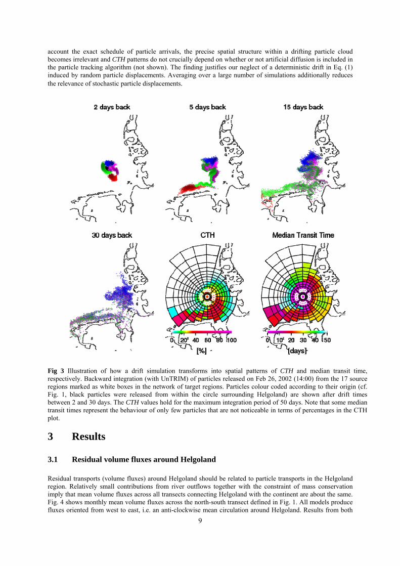
account the exact schedule of particle arrivals, the precise spatial structure within a drifting particle cloud becomes irrelevant and CTH patterns do not crucially depend on whether or not artificial diffusion is included in the particle tracking algorithm (not shown). The finding justifies our neglect of a deterministic drift in Eq. (1) induced by random particle displacements. Averaging over a large number of simulations additionally reduces the relevance of stochastic particle displacements.

Fig 3 Illustration of how a drift simulation transforms into spatial patterns of CTH and median transit time, respectively. Backward integration (with UnTRIM) of particles released on Feb 26, 2002 (14:00) from the 17 source regions marked as white boxes in the network of target regions. Particles colour coded according to their origin (cf. Fig. 1, black particles were released from within the circle surrounding Helgoland) are shown after drift times between 2 and 30 days. The CTH values hold for the maximum integration period of 50 days. Note that some median transit times represent the behaviour of only few particles that are not noticeable in terms of percentages in the CTH plot.

3 Results

3.1 Residual volume fluxes around Helgoland Residual transports (volume fluxes) around Helgoland should be related to particle transports in the Helgoland region. Relatively small contributions from river outflows together with the constraint of mass conservation imply that mean volume fluxes across all transects connecting Helgoland with the continent are about the same. Fig. 4 shows monthly mean volume fluxes across the north-south transect defined in Fig. 1. All models produce fluxes oriented from west to east, i.e. an anti-clockwise mean circulation around Helgoland. Results from both

9

UnTRIM and BSHcmod tend to have higher means than the other two models. Patterns of temporal variability, however, are similar for all models. With regard to differences between UnTRIM and BSHcmod in winter 2003/2004 it should be kept in mind that atmospheric forcing data used for running BSHcmod were different from those used for the other three models (cf. Tab. 1).

Fig 4 Monthly running averages of volume fluxes across a north/south oriented transect between the island of Helgoland and the German coast (cf. Fig. 1). Positive values correspond with flows to the east.

3.2 Drift climatology around Helgoland

3.2.1 Mean CTH patterns Fig. 5 displays averages of 3377 CTH patterns from simulations initialized every seven hours between 20th Feb 2002 and 31st Oct 2004. Panels for each of the four models on the left hand side refer to particle releases to the south or west of Helgoland, while panels on the right hand side refer to particle releases to the north or east of the island. Respective source regions are indicated by white-rimmed grid cells. Two thousand particles were released within each of these regions. According to Fig. 5, simulations based on UnTRIM very much emphasize particle advection towards the Helgoland region from southwesterly directions. BSHcmod confirms this pattern to some extent, but with lower intensity and with advection more from the west superimposed in the near field. Generally TRIM12.8km simulations resemble BSHcmod simulations but show less intense advection from westerly directions. The enhanced relevance of the southern adjacency for the northern and eastern regions may be attributed to the absence of Helgoland in the coarse bathymetry of TRIM12.8km. Results from TELEMAC-2D deviate most within the ensemble of the four models. In particular, advection from the southwest is clearly less pronounced for TELEMAC-2D than for the other three models.

10

Fig 5 Mean CTH patterns for drift simulations integrated 50 days backward in time. A total of 3377 simulations was started every seven hours between 20th Feb 2002 and 31st Oct 2004. Results are shown for simulations based on the outputs of four different hydrodynamic models. Panels on the right and left hand side, respectively, refer to particle releases within different source regions in the vicinity of Helgoland (white-rimmed grid cells). Each simulation considers 16,000 particles (2000 from each of the eight white boxes).

3.2.2 Travel routes and transit time distributions To shed some more light on the four models’ behaviours with regard to advection from the southwest, let us now have a closer look at travel routes and corresponding transit times. Considering particles released in the island’s immediate neighbourhood (rather than from within different sectors around it), CTH patterns in Fig. 6 are restricted to the subset of only those (backward) trajectories that at some point within the maximum integration period enter the white-edged grid cell on the southwest part of the network. The resulting conditional CTH patterns now illustrate advection routes between Helgoland and the selected target grid cell (in which by construction the CTH value is 100%). Histograms on the left of Fig. 6 give for each model the distribution of a) corresponding transit times and b) the seasonal distribution of the number of particles that cover the distance between the two regions (within the maximum integration time of 50 days). However, with regard to the seasonal distribution it should be noted that for simulations initialized between 20th Feb 2002 and 31st Oct 2004, simulations starting in Jan, Feb, Nov or Dec are a priori underrepresented.

11

Fig. 6 Conditional CTH patterns (right hand side) referring to only those particle trajectories from the Helgoland area (white circle in the network’s centre) that reach the white-rimmed region on the south-western edge of the network. The analysis is based on 3377 simulations (every seven hours between 20th Feb 2002 and 31st Oct 2002) each of which deals with tracking 2000 particles. Histograms on the left hand side give a) distributions of corresponding transit times (annotated percentages refer to the number of trajectories that cross the selected receptor region) and b) the seasonal distribution of release times of trajectories in this subset.

The main result from Fig. 6 is that transit times of the fastest particles are similar for all models but TELEMAC-2D. For UnTRIM the most probable transit time is about 25-30 days. For TRIM12.8km the distribution’s maximum is similar but its slope for longer transit times is less pronounced. For BSHcmod the distribution even increases towards longer transit times. The corresponding CTH pattern for BSHcmod suggests that this might result from particles first taking a pathway more to the west before moving down to the coast (in time-reversed mode). The overall percentage of particles reaching the white-rimmed grid cell is clearly smaller for BSHcmod (19%) than it is for UnTRIM (47%). Although the transit time distribution for TRIM12.8km resembles the distribution for UnTRIM, the number of trajectories it refers to (12%) is much smaller. TELEMAC-2D is the only model for which the onset of particle arrivals is clearly delayed. It seems consistent that the corresponding number of particles (3%) is very low. With regard to the seasonal distribution there seems to be a coincidence between TRIM12.8km and TELEMAC-2D with most occurrences between autumn and spring.

12

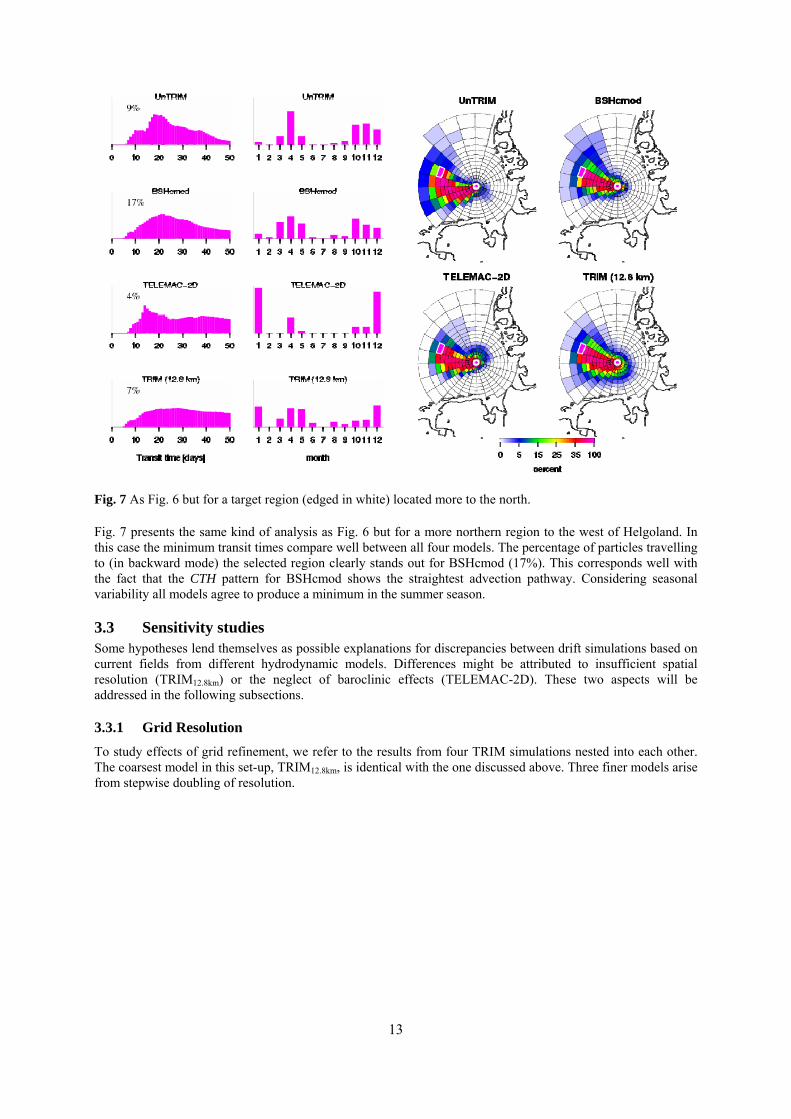
Fig. 7 As Fig. 6 but for a target region (edged in white) located more to the north. Fig. 7 presents the same kind of analysis as Fig. 6 but for a more northern region to the west of Helgoland. In this case the minimum transit times compare well between all four models. The percentage of particles travelling to (in backward mode) the selected region clearly stands out for BSHcmod (17%). This corresponds well with the fact that the CTH pattern for BSHcmod shows the straightest advection pathway. Considering seasonal variability all models agree to produce a minimum in the summer season.

3.3 Sensitivity studies Some hypotheses lend themselves as possible explanations for discrepancies between drift simulations based on current fields from different hydrodynamic models. Differences might be attributed to insufficient spatial resolution (TRIM12.8km) or the neglect of baroclinic effects (TELEMAC-2D). These two aspects will be addressed in the following subsections.

3.3.1 Grid Resolution To study effects of grid refinement, we refer to the results from four TRIM simulations nested into each other. The coarsest model in this set-up, TRIM12.8km, is identical with the one discussed above. Three finer models arise from stepwise doubling of resolution.

13

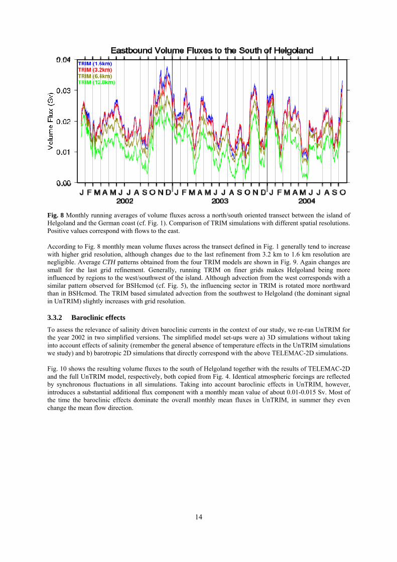
Fig. 8 Monthly running averages of volume fluxes across a north/south oriented transect between the island of Helgoland and the German coast (cf. Fig. 1). Comparison of TRIM simulations with different spatial resolutions. Positive values correspond with flows to the east. According to Fig. 8 monthly mean volume fluxes across the transect defined in Fig. 1 generally tend to increase with higher grid resolution, although changes due to the last refinement from 3.2 km to 1.6 km resolution are negligible. Average CTH patterns obtained from the four TRIM models are shown in Fig. 9. Again changes are small for the last grid refinement. Generally, running TRIM on finer grids makes Helgoland being more influenced by regions to the west/southwest of the island. Although advection from the west corresponds with a similar pattern observed for BSHcmod (cf. Fig. 5), the influencing sector in TRIM is rotated more northward than in BSHcmod. The TRIM based simulated advection from the southwest to Helgoland (the dominant signal in UnTRIM) slightly increases with grid resolution.

3.3.2 Baroclinic effects To assess the relevance of salinity driven baroclinic currents in the context of our study, we re-ran UnTRIM for the year 2002 in two simplified versions. The simplified model set-ups were a) 3D simulations without taking into account effects of salinity (remember the general absence of temperature effects in the UnTRIM simulations we study) and b) barotropic 2D simulations that directly correspond with the above TELEMAC-2D simulations. Fig. 10 shows the resulting volume fluxes to the south of Helgoland together with the results of TELEMAC-2D and the full UnTRIM model, respectively, both copied from Fig. 4. Identical atmospheric forcings are reflected by synchronous fluctuations in all simulations. Taking into account baroclinic effects in UnTRIM, however, introduces a substantial additional flux component with a monthly mean value of about 0.01-0.015 Sv. Most of the time the baroclinic effects dominate the overall monthly mean fluxes in UnTRIM, in summer they even change the mean flow direction.

14

Fig. 9 Mean CTH patterns obtained from 3377 50d-backward simulations (started every seven hours between 20th Feb 2002 and 31st Oct 2004) based on hydrodynamic fields from TRIM with different spatial resolutions. The coarsest TRIM model (12.8 km) is identical with the model version discussed in Section 3.2. For simulations on the right and left hand side, respectively, particles were released within different source regions indicated by white-rimmed grid cells. Each simulation considers 16,000 particles (2000 from each of the white boxes). Given the differences between UnTRIM and UnTRIM-2D, monthly mean flows simulated by TELEMAC-2D tend to be in between. In some periods (e.g. February, July) TELEMAC-2D and UnTRIM simulations are more alike than TELEMAC-2D and UnTRIM-2D. In this context it is interesting, however, to have a look at daily mean values shown in the upper panel of Fig. 10. On the shorter time scale the three barotropic models still more or less synchronize, while major discrepancies between UnTRIM and the barotropic simulations occur intermittently on a timescale of about one week.

15

Fig. 10 Daily (top panel) and monthly (bottom panel) running means of volume fluxes across the transect to the south of Helgoland. Values for simulations with full UnTRIM are compared with two simplified model versions (neglect of salt and a 2D setup, respectively). In addition the results of TELEMAC-2D are copied from Fig. 4 (black lines).

Based on both of the two barotropic simulations with UnTRIM-2D and UnTRIM 3D without salt, respectively, we set up ensembles of 1080 backward drift simulations, initialized between 20th Feb and 31st Dec 2002. Fig. 11 compares CTH patterns based on the two simplified model versions with those based on the full UnTRIM model. Although we chose the Helgoland area (rather than sectors around it) as particle source region for the sensitivity study, the left panel of Fig. 11 and the results from Fig. 5 (particle releases to the south and west of Helgoland) turn out to be much alike. CTH patterns from the two simplified UnTRIM simulations are more or less indistinguishable, i.e. vertically averaged 3D currents are well represented by 2D simulations (although volume fluxes differed according to Fig. 10). The most important result, however, is that the neglect of baroclinic effects does not eliminate the intense advection from the southwest towards Helgoland. Results of the simplified runs are (at least on average) much closer to the full baroclinic simulation than to the barotropic simulation obtained based on TELEMAC-2D. This is not obvious from the flux-related results shown in Fig. 10.

16

Fig. 11 CTH patterns obtained from 1080 50d-backward simulations in 2002 based on hydrodynamic fields from UnTRIM. Particles were released within the Helgoland region (circled in white). The left panel shows results from the full model, the other two panels results from simplified model versions: 3D but neglect of salt effects (centre) and 2D barotropic (right), respectively. Fig. 12 repeats for UnTRIM and its two simplified versions the analysis of drift routes previously shown in Fig. 6. As already suggested by Fig. 11, the two barotropic simulations tend to produce drift routes that are somewhat displaced towards the coast. The modified drift routes seem to manifest themselves by a reduced mean percentage of particles arriving and a longer tail of the transit time distribution. Clear evidence for a slowdown of all drift velocities, however, is lacking. There seems also not to be a distinct change in the seasonal distribution of transport along this advection route.

17

Fig. 12 Conditional CTH patterns that refer to only those particle trajectories from the Helgoland area that cross the white-rimmed region (same as in Fig. 6). Histograms display distributions of corresponding transit times and the seasonal distributions of particle density. Annotated percentages refer to the numbers of trajectories that cross the selected receptor region.

The finding of a more inshore transport route in the simplified model versions is confirmed by a similar analysis for a more inshore receptor region (Fig. 13). Rates of particle arrival in Fig. 13 are now even higher in the barotropic than in the baroclinic simulation. In all three simulations, however, transit time distributions have maxima at about 25 days. The explanation of a secondary peak at very small transit times (about 15 days) already visible in Fig. 12 is unclear. Most probably the non-smooth distribution arises from the use of data from only one year. This limitation also hampers identification of possibly existing shifts in seasonal distributions.

4 Discussion The use of CTH-patterns ignores the explicit schedules of drift simulations but concentrates on a summary of characteristic drift routes. Major systematic discrepancies between drift simulations based on different hydrodynamic models were found. Simulations based on TELEMAC-2D stand out most among the models we chose. In TELEMAC-2D average advection from the southeast is the weakest, Fig. 6 provides also evidence for a prolongation of corresponding transit times. This result seems consistent with the fact that mean volume fluxes to the south of Helgoland simulated with TELEMAC-2D are systematically smaller than corresponding fluxes obtained from UnTRIM or BSHcmod (Fig. 4). Monthly mean fluxes obtained from TRIM12.8km tend to be small as well, but here an observed systematic deficit of about 0.01 Sv relative to UnTRIM, for instance, could be explained by poor spatial resolution (cf. Fig. 8). TELEMAC-2D and UnTRIM, however, are run on nearly identical grids.

18

Fig. 13 As Fig. 12 but for another target region (edged in white). A conceivable explanation for the deviant behaviour of TELEMAC-2D would be the lack of baroclinic residual currents. Smith et al. (1996) summarize long-term simulations of volume transports across a number of different transects in the North Sea, obtained by running three different models, two three-dimensional baroclinic models and one two-dimensional barotropic storm surge model. The three models were found to produce similar patterns of time variability, although mean levels and inter-seasonal variations of transports in the baroclinic and barotropic model, respectively, differed substantially at locations where seasonal stratification and related baroclinic effects are supposed to be relevant. This finding is generally confirmed by our results. According to Fig. 10, however, differences between mean fluxes obtained from different barotropic simulations may be as large as differences between barotropic and baroclinic simulations. It is also interesting to note that according to the upper panel in Fig. 10 major differences between baroclinic and barotropic UnTRIM simulations occur on short time scales of about a week related to weather variability. According to Figs. 11 and 12, however, the elimination of baroclinic effects from UnTRIM by either the disregard of salt (remember that from the beginning temperature effects were not taken into account) or the assumption of a 2D set-up affects advection patterns and corresponding transit times to a much lesser extent than it might be expected. Both UnTRIM-2D and TELEMAC-2D use nearly the same numerical grid and both models were driven by identical atmospheric forcing. Hence, an explanation of differences between the model outputs from UnTRIM-2D and TELEMAC-2D would need an in depth analysis of algorithms and parameterizations involved which, however, is beyond the scope of our present study. There seems to be no direct correspondence between the average strengths of eastbound volume fluxes to the south of Helgoland and Lagrangian transports from the southwest towards the island. Despite mean volume fluxes being clearly stronger in TELEMAC-2D than in UnTRIM-2D (cf. Fig. 10), mean particle advection from the southwest was found to be much smaller in TELEMAC-2D (compare Figs. 5 and 11, or Figs. 6 and 12). Fig. 6 reveals very different seasonal patterns of advection from the southwest in UnTRIM and TELEMAC-2D

19

20

simulations, respectively. While in TELEMAC-2D advection dominates in spring and autumn (i.e. is possibly related to stormy conditions), in UnTRIM the maximum occurs more in summer, when baroclinic residual currents are unlikely to be masked by wind effects. For UnTRIM-2D (cf. Fig. 12) the seasonal pattern does not resemble the TELEMAC-2D pattern. For advection more from the northwest (cf. Fig. 7), seasonal distributions for all models are much more consistent. The agreement between full UnTRIM and UnTRIM-2D simulations with regard to nearshore transports and the corresponding failure of TELEMAC-2D suggest the existence of other (possibly tunable) factors that determine advection patterns in a similar way as baroclinic effects. Given that residual currents and water transports are sensitive to baroclinic effects, their proper simulation will depend on the correctness of the underlying salinity distributions. Simulated salinity distributions, however, involve a large amount of uncertainty. Delhez et al. (2004) compared simulations of nine three-dimensional shelf-sea models. For salinity influencing baroclinic flows, Delhez and co-authors found that the mean errors for all models and seasons between model simulations and existing observations reached 90% of natural variability. With regard to volume fluxes across a transect at 54.5°N, the range of simulated monthly mean values using different baroclinic models was found to be of about the same order of magnitude as the overall mean. To explore effects of grid resolution, we referred to a nested simulation with the model TRIM (Fig. 9). It does not come as a surprise that a resolution of 12.8 km proves to be poor and that simulation results change with stepwise grid refinements. Effects of the last refinement (from 3.2 km to 1.6 km), however, remain negligible and for particle releases (in backward mode!) to the west or south of Helgoland, even the resolution of 6.4 km (which still is unable to represent the small island itself) seems sufficient. For all drift simulations the hydrodynamic fields were updated consistently once per hour. However, BSHcmod and UnTRIM fields are available more frequently which gave us the opportunity to check the extent to which this schedule of external forcing affected the outcome of our analysis. It turned out that results of refined tracer experiments with current fields from BSHcmod provided on a 15 min basis, for instance, could hardly be distinguished from the results discussed in the paper (not shown). For a 2D model of the Dutch Wadden Sea, Ridderinkhof et al. (1990) and Ridderinkhof and Zimmerman (1992) showed that trajectories of water parcels may represent a substantial amount of chaotic stirring so that proper modelling of deterministic tidal velocity fields can be more important than modelling turbulence. To avoid uncertain specifications of diffusivity coefficients, Hainbucher et al. (1987) confined their study of tracer transports to pure advection. In our simulations we included artificial dispersion although a representation of subscale processes for models with different grid resolution might introduce discrepancies that are external to the models themselves. Fortunately it turned out, however, that an analysis in terms of average CTH-patterns is not much affected by the inclusion of isotropic subscale diffusion (not shown).

5 Conclusions Based on simulated circulation patterns from different hydrodynamic models, we compared the means of a large number of backward drift simulations initialized in the vicinity of Helgoland within a period of nearly three years. According to all hydrodynamic models the history of a water body observed near Helgoland varies with its precise location relative to the island. This allows for the existence of systematic gradients of water quality and has implications for the relevance of observations at Helgoland in the presence of large tidal excursions. Rixen et al. (2008) state that deterministic models still have great difficulties to accurately predict surface drift velocities as they are limited by empirical assumptions on underlying physics. In this and other recent papers on operational surface drift prediction (Rixen and Ferreira-Coelho 2007; Vandenbulcke et al. 2009) it was shown that even on a time scale of 1-2 days results are associated with a large amount of uncertainty. Considering a large ensemble of such simulations that cover a whole spectrum of realistically reconstructed environmental conditions, allows for the elimination of any random variability via averaging. Our study showed, however, that even the means of large numbers of simulated long-term advection patterns differ substantially for different models in their specific set-ups. The skill of particle tracking models may vary in time (Vandenbulcke et al. 2009). Such time-dependent model deficiencies can be counteracted by data assimilation in an operational framework but they complicate calibration of long-term model behaviour. The present study was meant to give a general impression of the amount of uncertainty to be expected in simulated mean transport patterns. An important next step would be to look into the responses of different models to changes in driving weather conditions. It has to be checked

21

whether (a) models are similarly sensitive to such changes and (b) whether reaction patterns of different models look similar. Assume that a certain model can be shown to reliably respond to a certain type of atmospheric forcing but that this response in terms of a spatial pattern of transports is systematically wrong. This model would still be informative in the sense that statistical postprocessing allows for a correction of the error. An extension of the idea of statistical postprocessing would be to use least-squares linear combinations of the outputs from all of the different models as predictors. This approach used by Vandenbulcke (2009) for short term predictions, however, is not applicable as long as data for the calibration of regression coefficients are missing. It must be noted that long-term residual transports in the German Bight are obtained by adding up much stronger oscillating tidal currents that tend to nearly compensate each other. Even for two models that both satisfactorily reproduce observations of water level and velocity, for instance, long-term drifts may differ considerably. For none of the models we discussed calibration was focussed on long-term residual transports. However, a field experiment our simulations could be compared with is hardly feasible. The aforementioned papers on operational surface drift prediction suggest differences between individual simulations and corresponding observations to be of the same order of magnitude as differences between simulations based on different models. Averaging over a large number of simulations, however, stabilizes characteristic differences between individual models. Possibly typical spatial distributions of water constituents obtained by remote sensing could aid at least qualitative assessment of simulated transport patterns. One of our conclusions is that one must be careful not to rashly associate differences between transport patterns from different models with specific model properties or restrictions. The models we investigated differ in many respects including grid resolution, dimensionality, presence of baroclinic effects, treatment of boundary conditions, and the origin of wind fields used as atmospheric forcing. It is tempting to associate the striking differences between simulations based on vertically averaged fields from UnTRIM and fields from TELEMAC-2D (two models operated on nearly the same grid) with the lack of baroclinic effects in TELEMAC-2D. We showed, however, that the strong advection from the southwest towards Helgoland simulated in UnTRIM does not crucially depend on the inclusion of salinity driven baroclinic effects (temperature was not taken into account). Hence differences between simulations based on vertically averaged fields from UnTRIM and fields from TELEMAC-2D must reflect algorithmic differences, treatment of boundary conditions or differences in parameterizations of friction and turbulence, for instance. The role of parameterizations must also be kept in mind when studying effects of spatial resolution. As shown by Burchard et al. (2004), too coarse spatial resolution near the coast leads to reduced tidal range and associated flow. The same applies to model runs with too large time steps. This discrepancy is sometimes compensated by reduced bottom friction with the argument that the true values of friction are not well known anyway. The fact that different model behaviours could not be explained by differences in single model parameters or the model set-up has also been reported by Delhez et al. (2004). This clearly complicates the selection of a most useful (realistic) hydrodynamic model. Completeness of processes included does not obviate the need for multi-model simulations to properly assess uncertainties. This is even more important in the context of long-term transport simulations, for which corresponding direct observations are mostly lacking. If we had taken into account processes like deposition, re-suspension or any other aspect of a substance’s fate, the analysis of uncertainties and their association with specific parameterizations would have become much more complex. Our simplified study, however, shows that already the choice of a specific hydrodynamic model and/or its specific setup may narrow or bias the range of possible results (concerning directions and ranges of transport) from more comprehensive simulations.

Acknowledgements We gratefully acknowledge the provision of output from the model BSHcmod by our colleagues from the Bundesamt für Seeschifffahrt und Hydrographie (BSH) in Hamburg. Levitus (NODC_WOA98) salinity data were provided by the NOAA/OAR/ESRL PSD, Boulder, Colorado, USA, from their web site at http://www.esrl.noaa.gov/psd/. For graphical display we used the Generic Mapping Tools software (GMT) available from www.soest.hawaii.edu/gmt/. The study was conducted within the framework of the WIMO project (Scientific monitoring concepts for the German Bight), jointly funded by Niedersächsisches Ministerium für Wissenschaft und Kultur (MWK) and Niedersächsisches Ministerium für Umwelt und Klimaschutz (MUK).

22

References Brandt G, Wehrmann A, Wirtz KW (2008) Rapid invasion of Crassostrea gigas into the German Wadden Sea

dominated by larval supply. J Sea Res 59: 279-296 Burchard H, Bolding K, Villareal MR (2004) Three-dimensional modelling of estuarine turbidity maxima in a

tidal estuary. Ocean Dynamics 54: 250-265 Casulli V, Cattani E (1994) Stability, accuracy and efficiency of a semi-implicit method for three-dimensional

shallow water flow. Computers Math Appl 27 (4): 99-112 Casulli V, Stelling GS (1998) Numerical simulation of 3D quasi-hydrostatic, free-surface flows. J Hydraul Eng

124: 678-686 Casulli V, Walters RA (2000) An unstructured three-dimensional model based on the shallow water equations.

Int J Numer Methods Fluids 32: 331-348 Chrastansky A, Callies U (2009) Model-based long-term reconstruction of weather-driven variations in chronic

oil pollution along the German North Sea coast. Mar Pollut Bull 58: 967-975 Chrastansky A, Callies U, Fleet DM (2009) Estimation of the impact of prevailing weather conditions on the

occurrence of oil-contaminated dead birds on the German North Sea coast. Environ Pollut 157: 194-198 Delhez EJM, Damm P, de Goede E, de Kok JM, Dumas F, Gerritsen H, Jones JE, Ozer J, Pohlmann T, Rasch

PS, Skogen M, Proctor R (2004) Variability of shelf-seas hydrodynamic models: lessons from the NOMADS2 project. J Mar Syst 45: 39-53

Dick S, Kleine E, Müller-Navarra SH, Klein H, Komo H (2001) The Operational Circulation Model of BSH (BSHcmod)-Model description and validation. Berichte des Bundesamtes für Seeschifffahrt und Hydrographie 29 (ISSN 0946-6010)

Dippner JW (1993) A frontal-resolving model for the German Bight. Cont Shelf Res 13, 49-66 Gräwe U, Wolff J-O (2010) Suspended particulate matter dynamics in a particle framework. Environ Fluid

Mech 10: 21-39Hainbucher D, Pohlmann T, Backhaus J (1987) Transport of conservative passive tracers in the North Sea: first

results of a circulation and transport model. Cont Shelf Res 7: 1161-1179 Heemink AW (1990) Stochastic modelling of dispersion in shallow water. Stochastic Hydrol Hydraul 4, 161-

174 Hervouet JM, van Haren L (1996) TELEMAC2D version 3.0 Principle Note. Chatou CEDEX. Rapport EDF

HE-4394052B Hickel W (1972) Kurzzeitige Veränderungen hydrographischer Faktoren und der Sestonkomponenten in

driftenden Wassermassen in der Helgoländer Bucht. Helgoländer wiss. Meeresunters. 23: 383-392 Jones JE (2002) Coastal and shelf-sea modelling in the European context. Oceanogr Marine Biol: an Annual

Review 40: 37-141 Jones JE, Davies AM (2005) An intercomparison between finite difference and finite element (TELEMAC)

approaches to modelling west coast of Britain tides. Ocean Dynamics 55: 178-198 Jones JE, Davies AM (2006) Application of a finite element model (TELEMAC) to computing the wind induced

response of the Irish Sea. Cont Shelf Res 26: 1519-1541 Kako S, Isobe A, Magome S, Hinata H, Seino S, Kojima A (2010) Establishment of numerical beach-litter

hindcast/forecast models: An application to Goto Islands, Japan. Mar Pollut Bull. doi:10.1016/j.marpolbul.2010.10.011

Kistler R, Kalnay E, Collins W, Saha S, White G, Wollen J, Chelliah M, Ebisuzaki W, Kanamitsu M, Kousky V, van den Dool H, Jenne R, Fioriono M (2001) The NCEP-NCAR 50-year reanalysis: monthly means CD-ROM and documentation. Bull Am Meteorol Soc 82: 247-268

Kloeden PE, Platen E (1992) Numerical solution of stochastic differential equations. Springer, Heidelberg Liu Y, Weisberg RH, Hu C (2011) Tracking the Deepwater Horizon oil spill: A modeling perspective. Eos 92:

45-52. Maier-Reimer E, Sündermann J (1982) On tracer methods in computational hydrodynamics. In: Abbot MB,

Cunge JA (eds) Engineering Applications of Computational Hydraulics 1. Pitman, London, pp 198-217 Meinke I, von Storch H, Feser F (2004) A validation of the cloud parameterization in the regional model SN-

REMO. J Geophys Res 109, D13205. doi:10.1029/2004JD004520 Penland C (2003) A stochastic approach to nonlinear dynamics. BAMS 84: ES43-ES52 Plüß A, Heyer H (2007) Morphodynamic multi-model approach for the Elbe estuary. Proceedings of the 5th

IAHR Symposium on River, Coastal and Estuarine Morphodynamics (RCEM), Enschede/NL, pp 113-117 Plüß A, Schüttrumpf H (2004) Comparison of numerical tidal models for practical applications. Proceedings of

the 29th Int. Conference of Coastal Engineering, pp 1199-1211

23

Puls W, Pohlmann T, Sündermann J (1997) Suspended particulate matter in the Southern North Sea: Application of a numerical model to extend NERC North Sea project data interpretation. Deutsche Hydrographische Zeitschrift 49: 307-327

Ridderinkhof H, Zimmerman JTF, Philippart ME (1990) Tidal exchange between the North Sea and Dutch Wadden Sea and mixing time scales of the tidal basins. Neth J Sea Res 25(3): 331-350

Ridderinkhof H, Zimmerman JTF (1992) Chaotic Stirring in a Tidal System. Science 258: 1107-1111 Rixen M, Ferreira-Coelho E (2007) Operational surface drift prediction using linear and non-linear hyper-

ensemble statistics on atmospheric and ocean models. J Mar Syst 65, 105-121 Rixen M, Ferreira-Coelho E, Signell R (2008) Surface drift prediction in the Adriatic Sea using hyper-ensemble

statistics on Atmospheric, ocean and wave models: Uncertainties and probability distributions. J Mar Syst 69, 86-98

Rolinski S (1999) On the dynamics of suspended matter transport in the tidal river Elbe: Description and results of a Lagrangian model. J Geophys Res 104 (C11): 26043-26057

Rümelin W (1982) Numerical treatment of stochastic differential equations. SIAM Journ Num Anal 19 604-613 Schönfeld W (1995) Numerical simulation of the dispersion of artificial radionuclides in the English Channel

and the North Sea. J Mar Sys 6: 529-544 Seibert P, Frank A (2004) Source-receptor matrix calculation with a Lagrangian particle dispersion model in

backward mode. Atmos Chem Phys 4: 51-63 Smith JA, Damm PE, Skogen MD, Flather RA, Pätsch J (1996) An investigation into the variability of

circulation and transport on the north-west European shelf using three hydrodynamic models. Deutsche Hydrographische Zeitschrift 48: 325-348

Stommel H (1949) Horizontal diffusion due to oceanic turbulence. J Mar Res 8: 199-225 Vandenbulcke L, Beckers J-M, Lenartz F, Barth A, Poulain P-M, Aidonidis M, Meyrat J, Ardhuin F, Tonani M,

Fratianni C, Torrisi L, Pallela D, Chiggiato J, Tudor M, Book JW, Martin P, Peggion G, Rixen M (2009) Super-ensemble techniques: Application to surface drift prediction. Prog Oceanogr 82, 149-167

van der Veer HW, Ruardij P, Van den Berg AJ, Ridderinkhof H (1998) Impact of interannual variability in hydrodynamic circulation on egg and larval transport of plaice Pleuronectes platessa L. in the southern North Sea. J Sea Res 39: 29-40

Weisse R, Plüß A (2006) Storm-related sea level variations along the North Sea coast as simulated by a high-resolution model 1958-2002. Ocean Dynamics 56: 16-25

Weisse R, von Storch H, Callies U, Chrastansky A, Feser F, Grabemann I, Guenther H, Pluess A, Stoye T, Tellkamp J, Winterfeldt J, Woth K (2009) Regional meteo-marine reanalyses and climate change projections: Results for Northern Europe and potentials for coastal and offshore applications. Bull Am Meteorol Soc 90(6): 849-860

Wiltshire KH, Kraberg A, Bartsch I, Boersma M, Franke H-D, Freund J, Gebühr C, Gerdts G, Stockmann K, Wichels A (2010) Helgoland Roads, North Sea: 45 years of change. Estuaries Coasts 33: 295-310