abstract effect in the lower troposphere and the planetary ... · effect in the lower troposphere...
TRANSCRIPT
ABSTRACT Title of dissertation: INTERACTION BETWEEN THE AEROSOL DIRECT
EFFECT IN THE LOWER TROPOSPHERE AND THE PLANETARY BOUNDARY LAYER DEPTH
Virginia Ruth Sawyer, Doctor of Philosophy, 2015
Dissertation directed by: Professor Zhanqing Li Department of Atmospheric and Oceanic Science/Earth
System Science Interdisciplinary Center The planetary boundary layer (PBL) limits the vertical mixing of aerosol emitted
to the lower troposphere. The PBL depth and its change over time affect weather, surface
air quality and radiative forcing. While model simulations have suggested that the
column optical properties of aerosol are associated with changes in the PBL depth in turn,
there are few long-term measurements of PBL depth with which to validate the theory.
Of the existing methods to detect the PBL depth from atmospheric profiles, many require
supporting information from multiple instruments or cannot adapt to changing
atmospheric conditions. This study combines two common methods for PBL depth
detection (wavelet covariance and iterative curve-fitting) in order to produce more
reliable PBL depths for micropulse lidar backscatter (MPL). The combined algorithm is
also flexible enough to use with radiosonde and atmospheric emitted radiance
interferometer (AERI) data.
PBL depth retrievals from these three instruments collected at the Atmospheric
Radiation Measurement (ARM) Southern Great Plains (SGP) site are compared to one
another to show the robustness of the algorithm. The comparisons were made for
different times of day, four seasons, and variable sky conditions. While considerable
uncertainties exist in PBL detection using all three types of measurements, the agreement
among the PBL products is promising, and the different measurements have
complementary advantages. The best agreement in the seasonal cycle occurs in winter,
and the best agreement in the diurnal cycle when the boundary-layer regime is mature
and changes slowly. PBL depths from instruments with higher temporal resolution (MPL
and AERI) are of comparable accuracy to radiosonde-derived PBL depths.
The new PBL depth measurements for SGP are compared to MPL-derived PBL
depths from a multiyear lidar deployment at the Hefei Radiation Observatory (HeRO),
and the column aerosol optical depth (AOD) for each site is considered. A one-month
period at SGP is also modeled to relate AOD to PBL depth. These comparisons show a
weak inverse relationship between AOD and daytime PBL depth. This is consistent with
predictions that aerosol suppresses surface convection and causes shallower PBLs.
INTERACTION BETWEEN THE AEROSOL DIRECT EFFECT IN THE LOWER TROPOSPHERE AND THE PLANETARY BOUNDARY LAYER DEPTH
by
Virginia Ruth Sawyer
Dissertation submitted to the Faculty of the Graduate School of the University of Maryland, College Park in partial fulfillment
of the requirements for the degree of Doctor of Philosophy
2015 Advisory Committee: Professor Zhanqing Li, Chair Professor Russell R. Dickerson Professor Derrick J. Lampkin Professor Rachel Pinker Dr. Ellsworth J. Welton Professor George Hurtt, Dean’s Representative

©Copyright by
Virginia Ruth Sawyer
2015
ii
ACKNOWLEDGMENTS
First of all, I’d like to thank my advisor, Dr. Zhanqing Li, for all his help, support
and constructive criticism throughout my time at the University of Maryland. This work
could not have proceeded without the additional help of Dr. Zhenzhu Wang and Dong
Liu at the Key Laboratory of Atmospheric Composition and Optical Radiation, Anhui
Institute of Optics and Fine Mechanics, Chinese Academy of Sciences, who graciously
guided me through the use of their data; Jianping Guo, who analyzed additional data
using my algorithm; and Dr. Shuyan Liu at the University of Maryland, College Park,
who provided important insights along with the results she graciously allowed me to
borrow.
This project also uses data from the Atmospheric Radiation Measurement (ARM)
Program sponsored by the U.S. Department of Energy, Office of Science, Office of
Biological and Environmental Research, Climate and Environmental Sciences Division.
I’d like to thank Dr. Chitra Sivaraman and other members of the PBL interest group for
their encouragement.
Finally, thanks to my husband, Rustom, and to my family and friends. None of
this would be possible without their love and moral support.
iii
TABLE OF CONTENTS
ACKNOWLEDGMENTS .................................................................................................. ii
LIST OF FIGURES ............................................................................................................ v
LIST OF ABBREVIATIONS AND SYMBOLS .............................................................. ix
Chapter 1. Background .................................................................................................... 1
1.1 The Planetary Boundary Layer ............................................................................ 1
1.2 Aerosol and Clouds as Proxy ............................................................................... 2
1.3 Modeled Aerosol-PBL Interaction ....................................................................... 5
1.4 Objectives and Outline ......................................................................................... 8
Chapter 2. Data Sources ................................................................................................. 11
2.1 Micropulse Lidar ................................................................................................ 11
2.2 Thermodynamic Profiles .................................................................................... 13
2.3 Column Aerosol Optical Properties ................................................................... 16
2.4 Model Output and Previous PBL Results .......................................................... 18
Chapter 3. PBL Detection .............................................................................................. 22
3.1 Backscatter Gradient Methods ........................................................................... 22
3.2 The Combined Algorithm .................................................................................. 26
Chapter 4. Instrument Intercomparison at SGP ......................................................... 30
4.1 Intercomparison of PBL Depth Detection .......................................................... 30
4.2 Diurnal Cycles .................................................................................................... 33
4.3 Seasonal Cycles .................................................................................................. 38
Chapter 5. Comparison Between MPL Sites ................................................................ 46
5.1 Diurnal Cycles .................................................................................................... 46
5.2 Seasonal Cycles and Interannual Variability ..................................................... 53
Chapter 6. PBL Depth and AOD ................................................................................... 60
6.1 WRF-Chem Results for April 2004 at SGP ....................................................... 60
6.2 PBL Depth vs. AOD at SGP and HeRO ............................................................ 64
6.3 Operational Radiosonde and Satellite-Based AOD ........................................... 75
Chapter 7. Future Work................................................................................................. 79
iv
7.1 Varying SSA, Humidity and Clouds .................................................................. 79
7.2 An Alternative Modeling Approach ................................................................... 80
Chapter 8. Conclusions ................................................................................................... 83
8.1 PBL Detection .................................................................................................... 83
8.2 Comparison to AOD........................................................................................... 86
LIST OF REFERENCES .............................................................................................. 90

v
LIST OF FIGURES
Figure 1.1. Schematic of PBL regimes and transitions, adapted from Stull [1988]. .......... 3
Figure 1.2. From Medeiros et al. [2005], PBL regimes by cloud type. ............................. 5
Figure 2.1. Locations of MPL deployments used in this project. .................................... 13
Figure 2.2. All θv values, irrespective of height, from radiosonde and AERI during the study period at SGP. ......................................................................................................... 15
Figure 2.3. Mean θv profiles from radiosonde and AERI (left) and their mean difference with altitude (right). .......................................................................................................... 16
Figure 2.4. Range of AOD and SSA values at the SGP and HeRO sites. ....................... 18
Figure 2.5. Daily mean AOD and SSA at the SGP site for April 2004, observed during the period of the WRF-Chem simulation. ......................................................................... 20
Figure 2.6. From Liu and Liang [2010], θv profiles representing idealized PBL regimes and PBL depth determination procedure. ......................................................................... 21
Figure 3.1. Wavelet covariance-detected PBL depths with varying dilation. The assumed 1-km dilation (crossed) is within the plateau range. ......................................................... 24
Figure 3.2. The combined PBL detection algorithm using an example MPL backscatter profile from SGP. The solid horizontal line is the PBL depth detected by each algorithm step. The dotted lines show the limits of the EZD. ........................................................... 27
Figure 3.3. Aug. 15, 2003 at SGP. The dotted line indicates the PBL detected by the combined algorithm before smoothing; the solid line applies the running-median filter. 28
Figure 4.1. Comparison between AERI- and radiosonde-derived PBL depths at SGP. After the removal of artifacts indicating weak signal (gray points), the orthogonal regression is PBLAERI = 0.62PBLsonde + 0.12. .................................................................... 30
Figure 4.2. Radiosonde- vs. MPL-derived PBL depths at SGP, cloudy cases (left) and cloud-free cases (right). R2 values for the orthogonal regression are 0.551 and 0.515, respectively. Gray points, excluded from regression, are outside the lidar overlap range............................................................................................................................................ 32
vi
Figure 4.3. Intercomparison between all radiosonde- and MPL-derived PBL depths at SGP. The orthogonal regression is PBLMPL = 0.71PBLsonde + 0.22. Gray points, excluded from regression, are outside the lidar overlap range. ........................................................ 33
Figure 4.4. PBL heights detected by MPL, AERI and radiosonde, overlaid on MPL backscatter during a nine-day period of typical conditions. ............................................. 34
Figure 4.5. Boxplots show the distribution of PBL depths from different radiosonde launch times by radiosonde (left) and MPL (right), excluding PBL depths outside the lidar overlap range. ........................................................................................................... 34
Figure 4.6. Diurnal variations of PBL depth from radiosonde (left) and AERI (right). .. 35
Figure 4.7. Variation of R2 values with the time of radiosonde launches, assessing the quality of fit between PBLMPL and PBLsonde (left) and between PBLAERI and PBLsonde (right). ............................................................................................................................... 38
Figure 4.8. Boxplots show the distribution of radiosonde-derived and MPL-derived PBL depths by month, with shallow PBLs excluded from the radiosonde record. ................... 39
Figure 4.9. R2 values assessing the quality of fit to the 1:1 line for the radiosonde-vs.-MPL intercomparison by month. ...................................................................................... 40
Figure 4.10. Boxplots show the monthly distribution of MPL-retrieved cloud base depths located below 4 km at the SGP site for the period 1996-2004. ........................................ 41
Figure 4.11. Boxplots for the monthly distribution of PBL depths from radiosonde and AERI, with shallow PBLs included. ................................................................................. 42
Figure 4.12. R2 values assessing the quality of fit to the 1:1 line for radiosonde vs. AERI, shallow PBL depths included............................................................................................ 43
Figure 5.1. PBL depths analyzed for the operational radiosonde network in China, August 1, 2011. ................................................................................................................. 46
Figure 5.2. For SGP, the mean diurnal cycle of PBL depths at 5-minute resolution. Time of day is given in hours local time (UTC-6). Left, the overall mean and standard deviation; right, the overall mean and the mean for each season. .................................... 48
Figure 5.3. The same as Figure 5.1 but for Hefei, where the temporal resolution is 15 minutes. Time of day is given in hours local time (UTC+8). ........................................... 49

vii
Figure 5.4. The mean diurnal cycle of PBL depths at 5-minute resolution for two shorter-term MPL deployments, Shouxian (left, 2008) and Xianghe (right, 2013). Time of day is given in hours local time (UTC+8). .................................................................................. 51
Figure 5.5. A single day of PBL depth retrievals (red) overlaid on the MPL backscatter at the Xianghe site, showing a “washboard” effect as evidence of poor telescope temperature control. .......................................................................................................... 52
Figure 5.6. Daily mean, maximum and minimum PBL depth at SGP, with a 31-day running-median filter applied. Gaps represent periods of unreliable or nonexistent MPL data. ................................................................................................................................... 53
Figure 5.7. Daily mean AOD values at SGP for the period overlapping with MPL observations, 2001-2006. .................................................................................................. 54
Figure 5.8. Boxplots show the distribution of MPL-derived PBL depths by month at the HeRO site, analogous to Figure 4.8. ................................................................................. 55
Figure 5.9. The same as Figure 5.4 but at Hefei. ............................................................. 57
Figure 5.10. From Wang et al. [2014], monthly and seasonal mean 500-nm AOD (a,d), mean Angstrom exponent (b, e), and number of measurements (c, f), at Hefei, 2007-2013............................................................................................................................................ 58
Figure 6.1. AOD vs. PBL depth for model-derived PBL depths at the radiosonde launch interval. Left, YSU scheme; right, simulated radiosonde. ................................................ 61
Figure 6.2. Radiosonde-derived PBL depths from two different algorithms, using observations taken from the simulated period at SGP. ..................................................... 62
Figure 6.3. AOD vs. PBL depth for radiosonde-derived PBL depths from Liu and Liang [2010] (left) and Sawyer and Li [2013] (right). ................................................................ 63
Figure 6.4. Boxplots showing the distribution of PBL depths with increasing AOD, at SGP (left) and Hefei (right). ............................................................................................. 64
Figure 6.5. Boxplots showing the distribution of maximum daily CBL depth (left) and minimum daily SBL depth (right) at the HeRO site. ........................................................ 65
Figure 6.6. Kernel density estimates of daily mean AOD vs. daily maximum PBL depth at SGP (left) and Hefei (right). ......................................................................................... 67
Figure 6.7. Kernel density estimates of daily mean AOD vs. daily maximum PBL depth at SGP (left) and Hefei (right), for the winter months only. ............................................. 68
viii
Figure 6.8. Kernel density estimates of daily mean AOD vs. daily maximum PBL depth at SGP (left) and Hefei (right), for the summer months only. .......................................... 69
Figure 6.9. Mean daily AOD vs. maximum daily PBL depth at SGP. The Nadaraya-Watson estimator is overlaid on the kernel density estimate. ........................................... 71
Figure 6.10. The Nadaraya-Watson estimator overlaid on the daily mean AOD vs. the daily maximum PBL at SGP, during winter (left) and summer (right). ........................... 72
Figure 6.11. Mean daily AOD vs. maximum daily PBL depth at Hefei. The Nadaraya-Watson estimator is overlaid on the kernel density estimate. ........................................... 73
Figure 6.12. As in Figure 6.10, but with all PBL depths above 2.0 km removed. ........... 74
Figure 6.13. AOD measurements from MODIS/Aqua for the geographic area coinciding with the operational radiosonde network in China. Radiosonde sites within four pollution “hot spots” are shown: squares “□” for NCP, circles “○” for YRD, diamonds “◇” for SCB, and five-pointed stars “☆” for PRD. ...................................................................... 76
Figure 6.14. Probability distribution function of PBL depth under clean (blue) and polluted (red) conditions, for the regions a) NCP, b) SCB, c) YRD and d) PRD. ........... 77
Figure 7.1. From Cheinet [2003], a sketched overview of the model including the generation of convective updrafts, the parameterization of their ascent, and the diagnosis of compensating downdrafts. ............................................................................................ 82
Figure 8.1. Schematic of PBL diurnal cycle with consequences for the detection of boundary-layer regimes. ................................................................................................... 84
ix
LIST OF ABBREVIATIONS AND SYMBOLS
θv Virtual potential temperature
ACM2 Asymmetric convective model, version 2; a PBL scheme for WRF-Chem
AERI Atmospheric emitted radiance interferometer
ARM Atmospheric Radiation Measurement (US Department of Energy)
AOD Aerosol optical depth
CBL Convective boundary layer
CMAQ Community Multi-scale Air Quality Model
EZD Entrainment zone depth
HeRO Hefei Radiation Observatory (31°52′ N, 117°17′E)
LLJ Low-level jet
MODIS Moderate Resolution Imaging Spectroradiometer
MFRSR Multifilter rotating shadowband radiometer
MPL Micropulse lidar
MPLNET Micropulse Lidar Network (NASA)
NCP North China Plain
NIMFR Normal incidence multifilter radiometer
PBL Planetary boundary layer
PRD Pearl River Delta
RL Residual layer
SASHE Shortwave array spectroradiometer – hemispheric
SBL Stable boundary layer
SCB Sichuan Basin

x
SGP Southern Great Plains site (36°36'18.0" N, 97°29'6.0" W)
SSA Single-scattering albedo
TKE Turbulent kinetic energy
WRF-Chem Weather Research and Forecasting model coupled with Chemistry
YRD Yangtze River Delta
YSU Yonsei University scheme; a PBL scheme for WRF-Chem

1
Chapter 1. Background
1.1 The Planetary Boundary Layer
The planetary boundary layer (PBL) is the part of the lower troposphere in direct
contact with the surface, ranging from several hundred meters to a few kilometers in
depth. It may be defined in terms of thermodynamics or in terms of turbulent mixing; the
mixed layer below the PBL top is distinguishable from the free troposphere by
differences in temperature and stability as well as turbulent flow. The difference in
chemical content may be the most important, however, because of its impact on surface
air quality [Seinfeld and Pandis, 2006]. The PBL depth defines a finite but varying
volume into which pollutants can disperse.
Changes in the depth of the PBL over time follow several different processes, the
most important of which over land is the diurnal cycle in radiative surface heating. Under
typical conditions, the PBL grows deeper in response to rising temperatures through the
morning, peaks in the afternoon or early evening, and collapses after sunset [Stull, 1988].
The PBL top may rise as high as 5 km in extreme cases of clear-sky convection [Ma et
al., 2011]. If insolation stops during the day, as during the solar eclipse observed by
Amiridis et al. [2007], the PBL top height decreases just as it typically does in the
evening. Over the ocean, where strong surface heating is rare, changes in the PBL depth
are more often driven by synoptic weather, but may nevertheless occur on time scales of
only a few hours.
The most common measurements of thermodynamic profiles are taken by
radiosonde. These are launched twice a day operationally, or 4-8 times daily during field
experiments [Seibert et al., 2000]. The temporal resolution in radiosonde-derived PBL

2
data is therefore too sparse to detect the evolution of the diurnal structure. Smaller-scale
boundary layer processes and waves are obscured. For many sites in the western
hemisphere, operational radiosonde launches also occur during transition times when the
PBL is changing rapidly (00UTC and 12UTC) so extremes of the diurnal cycle go
unobserved. PBL detection by remote sensing can improve the temporal resolution of the
data, usually by using a proxy for the thermodynamic profile. Wind profiling provides
some clues about the turbulence structure, so radar wind profilers [Bianco and Wilczak,
2002] and sodars are used to detect the PBL under a definition based on turbulence rather
than the thermodynamic structure [Beyrich and Görsdorf, 1995].
The seasonal cycle echoes the diurnal cycle, with the strongest deep convection in
the summer months [e.g., Liu and Liang, 2010]. In the winter, changes in the synoptic
weather govern the PBL depth and generally lead to shallower PBLs with a weaker
diurnal cycle. It is important for any PBL detection method to replicate both the diurnal
and seasonal cycles of PBL behavior in order to fully understand its effects on air quality
and climate.
1.2 Aerosol and Clouds as Proxy
Buoyant stability restricts the mixing of aerosols through the PBL top to just three
mechanisms: deep convection, orographic lifting and transport by warm conveyor belt
processes [Donnell et al., 2001; Twohy et al., 2002; Henne et al., 2004; Ding et al.,
2009]. Highly polluted airmasses that enter long range transport in these three ways form
aerosol plumes that may persist for thousands of kilometers in the middle and upper
3
troposphere. In the Arctic, where there are few local sources, long range transport of
aerosol is responsible for intense springtime pollution events [Law and Stohl, 2007;
Quinn et al., 2007]. By contrast, the mineral dust aerosol that enters long range transport
during Asian dust events continues to interact with urban aerosols emitted downstream,
and may not be easily distinguishable from mixed-layer aerosol [e.g., Li et al., 2010; Sun
et al., 2010].
However, most aerosols that are emitted within the mixed layer remain there until
removal from the atmosphere, usually within a few kilometers of their origin [Seinfeld
and Pandis, 2006]. The vertical distribution of aerosols through the lower troposphere
therefore depends heavily on the depth of the PBL, and the PBL depth can be inferred in
turn from the aerosol profile. Several “gradient” methods rely on the drop in aerosol
concentration across the boundary in order to detect the PBL top height, defined as the
center of a transition zone or inversion at the top of the surface layer.
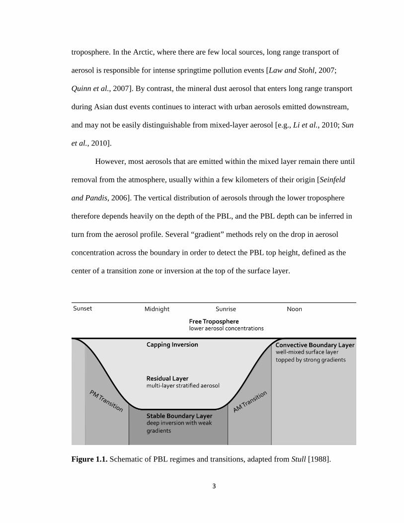
Figure 1.1. Schematic of PBL regimes and transitions, adapted from Stull [1988].
4
Figure 1.1 illustrates the regimes of a typical PBL diurnal cycle, with labels
describing their characteristic relative aerosol concentration and structure. During the
day, the convective boundary layer (CBL) is well-mixed both thermodynamically and
with respect to aerosol content, and is also typically more polluted than the free
troposphere above its top [Melfi et al., 1985]. This uniform higher concentration of
aerosols is easily detected by aerosol lidar, distinct from the lower and more stratified
concentration of aerosol in the free troposphere. At night, much of the aerosol from the
CBL of the previous day remains in a residual layer (RL) between the capping inversion
and the surface, while a shallow nocturnal inversion—the stable boundary layer (SBL)—
forms near the surface in response to radiative cooling. Transition times are defined by
the development of the CBL as surface insolation strengthens in the morning, and then by
the collapse of the CBL as nightfall cuts off the source of heating.
In addition, the PBL top is often associated with cumulus cloud layers. Figure 1.2
illustrates the various conceptual regimes for cloud layers interacting with the PBL
[Medeiros et al., 2005]: whether forming the cloud base of deep convection or the
capping inversion inhibiting the growth of stratocumulus, the PBL top is so bound up
with cloud processes that the cloud signal in remote sensing can also help determine the
PBL depth [Davis et al., 2000]. Therefore gradient methods for PBL detection can
potentially work for both clear-sky and cloudy conditions.

5
Figure 1.2. From Medeiros et al. [2005], PBL regimes by cloud type.
1.3 Modeled Aerosol-PBL Interaction
The aerosol direct effect is the change in heating of the atmosphere caused by
direct absorption or scattering of radiation by particulate matter. The integrated column
heating by the aerosol direct effect is a major factor in anthropogenic climate change and
among the least understood after cloud-aerosol interaction [IPCC, 2007]. However, not
only the column total heating but also the distribution of radiative effects along the
column makes a difference to the climate. Venkatram and Viskanta [1977] warned in a
simple modeling study that aerosols alter the energy distribution between the surface and
the PBL top, increasing the absorption of solar energy in the mixed layer at the expense
of heating at the surface. The effect would be a reduction in the CBL depth and greater

6
atmospheric stability, countered by warming in the lower troposphere that could lead to
later convection. Other studies simulated nuclear winter scenarios, and modeled a thick
smoke layer at tropopause height. The reduction in surface heating still occurs, but the
aerosol-induced heating of the atmosphere occurs at too high an altitude to involve the
PBL. Garratt et al. [1990] found that under such conditions the maximum CBL depth
could be suppressed from 2300 m in the control case to 1650 m at an aerosol optical
depth (AOD) of 0.2 and 600 m at an AOD of 1.0. Yu et al. [2002] found that such a
pronounced effect is highly dependent on the single-scattering albedo (SSA) of the
aerosol layer. For the same AOD, the maximum depth of the CBL increased by several
hundred meters with each 0.1 decrease in SSA. The simulated CBL began to develop
later in the day and collapsed earlier in the evening as the aerosol became less scattering
and more absorbing. This suggests that both AOD and SSA affect the maximum depth of
the CBL, but that the shape and phase of the PBL diurnal cycle is more sensitive to SSA.
Using a single-column chemical transport model, Park et al. [2001] found that the
suppression of surface convection by the mostly scattering aerosols typical of their
eastern US study region impacted the surface air quality not only through the reduced
dilution volume available under a shallow PBL, but also by enhancing the production of
surface ozone, resulting in further radiative forcing within the PBL. The importance of
aerosol to the PBL depth and surface air quality is magnified by its interaction with other
atmospheric processes.
More recently, it has been shown that aerosol within the PBL itself may also have
a net effect of significantly suppressed convection. Ding et al. [2013] found that regional
plumes bearing absorbing aerosol, especially from a combination of biomass burning and
7
fossil fuel combustion, could enhance the stability of the PBL by heating its upper levels
at the expense of the surface. The absence of this effect in some forecast models may
explain their underestimation of surface air pollution episodes in urban China. The study
recommends that forecast models be fully coupled with atmospheric chemistry. Aside
from the surface air quality forecast, the changed PBL dynamics have consequences for
convective precipitation. As in Andreae et al. [2004] and Feingold et al. [2005] in their
studies of Amazon smoke, suppressed convection delays the onset of precipitation but
may lead to later invigoration and intense storms. Zhang et al. [2010] used the Weather
Research and Forecasting model coupled with Chemistry (WRF-Chem) to investigate the
effects of aerosols over the continental U.S. in January and July 2001; the study found
that with a reduction of incoming solar radiation of 11.3 W m-2 and 39.5 W m-2,
respectively, there was a resulting temperature decrease of 0.16-0.37 K and a reduction in
PBL depth of 23-24%, compared to the aerosol-free case.
Finally, in a recent presentation at the AMS Annual Meeting, Xing et al. [2015]
presented results of a simulation using WRF coupled with the Community Multi-scale
Air Quality (CMAQ) Model, for the period 1990-2010 in eastern China, the eastern U.S.
and Europe. The study predicted that for each 1.0 unit of increased AOD, there is a
corresponding decrease of 0.3 to 0.4 K in average surface temperature and a resulting 69
to 79 m decrease in PBL depth: a difference so small that it may be difficult to detect in
observations, but with significant climate effects when taken on a continental scale.
Because the PBL depth and aerosol loading are subject to many interconnected processes,
the effort to quantify the suppression of convection by boundary-layer aerosol is ongoing.
8
However, models consistently find such a mechanism; accurate observations of the PBL
over long time periods in the instrument record should be able to find the same effect.
The stabilization of the PBL by convection suppression exacerbates decreases in
overall surface air quality, as periods of stagnation lengthen and the washout by
precipitation is limited to less frequent but more intense events. In combination with the
projected weakening of global circulation and a decreasing frequency of mid-latitude
cyclones due to greenhouse effect-induced climate change [Jacob and Winner, 2009]
boundary-layer aerosol loading is therefore projected to increase even when emission
rates are held constant, a climate penalty for particulate pollution analogous to the penalty
by which warmer temperatures increase the formation of tropospheric ozone [e.g.,
Bloomer et al., 2009; He et al., 2013]. This aerosol climate penalty is driven not by
greater formation of aerosols, but by changes in the end of their lifetime in the
atmosphere: reduced dilution volume and washout rates, to which the aerosol itself
contributes through direct, indirect and semi-direct radiative effects. Models have shown
that the health and radiative effects of boundary-layer aerosols are likely to increase in
future climates. At polluted sites in China, shallower PBL depths, exacerbated air quality
problems and suppressed convective precipitation have already been observed [Yang et
al., 2013a,b]. The link to increased aerosol loading must be made explicit.
1.4 Objectives and Outline
The purpose of this dissertation is to investigate whether the predicted
suppression of surface convection and PBL depth can be detected in long-term instrument

9
records. The first step toward this goal is to accurately detect the PBL depth, which
requires the development of an algorithm that can operate with minimal human
intervention or prior knowledge of atmospheric or instrument conditions, over time series
that cover multiple years at high temporal resolution. The second step is to demonstrate
that remote sensing of the aerosol distribution with height is an effective measurement to
show PBL depth, which can be shown if the resulting PBL depths are comparable to PBL
depths reached by other instruments in the same location and time period; in order to
eliminate variables and demonstrate the flexibility of the algorithm, the same algorithm
can be applied to profiles from each instrument. Because remote sensing is capable of
providing much more detailed information about atmospheric structure than the lower-
resolution thermodynamic profiles from radiosonde and other sources, the resulting PBL
depth retrievals are more representative of actual PBL behavior. Locations with
contrasting AOD values can then show the relationship between the PBL depth and
AOD, for comparison with model predictions.
Chapter 1 provides an overview of the PBL, its regimes and its relationship to
aerosol, and model predictions for the behavior of the PBL in polluted conditions.
Chapter 2 lists the sources of data and model output used in this project. Chapter 3
describes methods used to detect the PBL depth and the development of a new algorithm
for PBL detection that combines the advantages of its predecessors. Chapter 4 evaluates
the reliability of this algorithm by applying it to observations from three types of
atmospheric profile. Chapter 5 compares PBL depth results from sites in the U.S. and
China. Chapter 6 uses PBL depth results from the two sites with the longest available
time series, including results from a modeled PBL scheme, and compares them to column

10
AOD measurements. Chapter 7 presents a summary of the project, and Chapter 8
suggests approaches for future work.

11
Chapter 2. Data Sources
2.1 Micropulse Lidar
Micropulse lidar (MPL) [Spinhirne et al., 1995] is the primary instrument used in
this project, which relies on the similar configurations of MPL instruments at sites across
the globe, including networks such as the Atmospheric Radiation Measurement (ARM)
facilities [Spinhirne, 1993; Flynn et al., 2007] and NASA’s Micropulse Lidar Network
(MPLNET) [Welton et al., 2001], in order to make comparisons among their locations.
Ground-based, upward-directed lidar are in the best position to observe boundary-layer
processes with a maximum signal-to-noise ratio; the use of a single wavelength at 527-
532 nm ensures sensitivity to aerosol and cloud layers [Campbell et al., 2002]. MPL
offers high temporal resolution compared to radiosonde, while requiring minimal human
oversight. As a result, it is able to observe clouds and aerosols on a time scale that
matches PBL processes, potentially for many years at a stretch. For these reasons, while
the PBL detection algorithm described in a later section is adaptable to multiple
atmospheric profile measurements from many different instrument types, it was
originally developed for MPL.
The Southern Great Plains site near Ponca City, OK (36°36'18.0" N, 97°29'6.0"
W) has included MPL as part of the ARM program measurements since May 1996. A
number of changes to the instrument have been made over time, and some significant
gaps in the time series exist. The original data set, used for the instrument
intercomparison, extends to 2004. Data collected after the lidar was upgraded with a
polarization switch in June 2006 [Coulter, 2012] are not included in this project. The ten-
year time series analyzed here is nevertheless longer than any of the time series available
12
from MPL deployments in China. The time series includes one attenuated backscatter
profile per minute, which is averaged to five-minute intervals for PBL detection. While
the vertical resolution of the backscatter data is 75 m, the incomplete overlap between the
beam spread and the telescope field of view means that accurate measurements begin at
an altitude of approximately 600 m even after correction. After 2006, an error in the
overlap correction makes backscatter profiles of the lower troposphere too unreliable to
draw conclusions about aerosol content, though the more recent data is available through
ARM for the purposes of cloud studies. Cloud attenuation and interference from sunlight
limit the upper range of the profile. This study also makes use of cloud base heights
determined by the algorithm described in Wang and Sassen [2001] and included in the
ARM data product for MPL [Sivaraman and Comstock, 2011]. While the MPL cloud
mask includes information about cloud base and top heights at levels throughout the
troposphere, the height of the lowest cloud base is the variable most directly relevant to
PBL detection.
In China, the longest MPL deployment used in this study is at the Hefei Radiation
Observatory (HeRO; 31°52′ N, 117°17′E), which has data running from 2002 to 2008
[Wang et al., 2014]. Profiles from the HeRO MPL are available on 15-minute intervals,
and are analyzed for PBL depth at the same time interval. The overlap correction for the
instrument is shallower than at SGP, providing accurate backscatter measurements
starting at approximately 400 m altitude. Shorter MPL time series of several months’
duration, each with their own resolution and overlap functions, are available from
Shouxian (32°35′ N, 116°47′ E) in 2008 and Xianghe (39°45′ N, 116°59′ E) in 2013
(Figure 2.1).

13
Figure 2.1. Locations of MPL deployments used in this project.
2.2 Thermodynamic Profiles
In order to assess the reliability of the PBL detection algorithm, the project uses
profiles from radiosonde and infrared spectrometer taken at the SGP site during the
period for which the MPL data is analyzed. ARM radiosonde launches at the site
[Holdridge et al., 2011] took place at least four times per day, usually at 00:00, 06:00,
12:00 and 18:00 UTC but also in significant numbers at 03:00, 09:00, 15:00 and 21:00.
The multiyear length of the analysis period makes it possible to construct a mean diurnal
cycle at three-hour intervals even though no single day had all eight measurements taken.
The vertical profile of virtual potential temperature θv is calculated from the temperature
and relative humidity measurements. While the vertical resolution of the data varies
14
according to the ascent rate of the balloon, data points within the boundary layer occur
approximately 10 m apart.
The atmospheric emitted radiance interferometer (AERI) instrument at SGP can
retrieve one θv profile every eight minutes [Feltz et al., 1998; Feltz et al., 2003; Feltz et
al., 2007]. The high temporal resolution has advantages over radiosonde for the purposes
of PBL detection, but the vertical resolution is much lower and varies with altitude. θv is
retrieved every 50 m at the surface but by 500 m, retrievals are made at 500-m intervals.
At the top of the profile, the resolution is 2 km. Another disadvantage compared to
radiosonde is that AERI cannot make reliable measurements of the temperature and
moisture within a cloud layer; profiles with clouds in or near the boundary layer must be
excluded from analysis. AERI retrievals are available from June 1996 to the present, with
a change to the data format in 2002. There are therefore AERI profiles corresponding to
nearly the entire period of MPL observations at SGP.
While the radiosonde and AERI data used in this study measure the same
variable, the thermodynamic profiles from the two sources are not identical. When the
AERI θv profiles are matched to radiosonde launch times and the radiosonde θv profiles
are interpolated to match the AERI vertical resolution, there is strong but not perfect
agreement between the two instruments. The linear regression returns an R2 value of
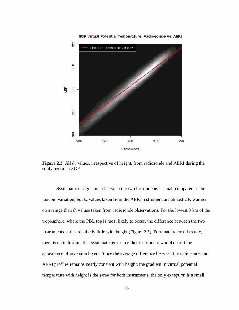
0.86. Because the size of the data set renders a traditional scatterplot uninformative,
Figure 2.2 uses a two-dimensional kernel density estimate instead to represent the
probability density function; this method is further described in Chapter 6.
15
Figure 2.2. All θv values, irrespective of height, from radiosonde and AERI during the study period at SGP.
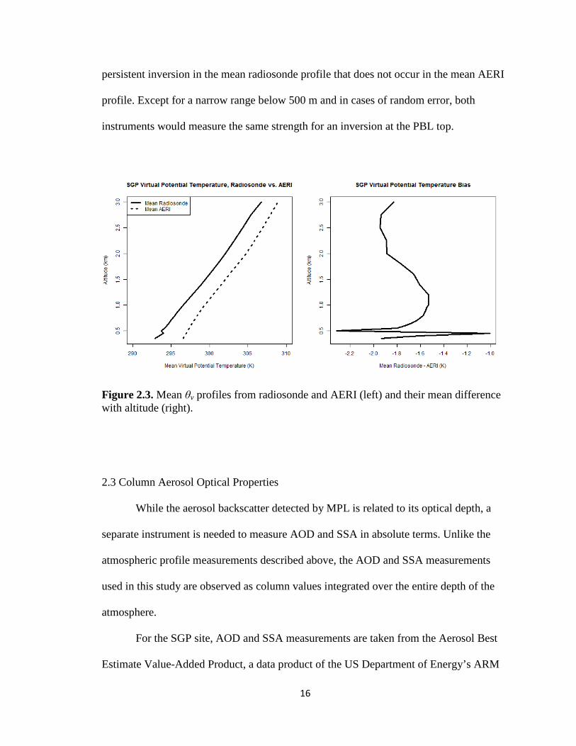
Systematic disagreement between the two instruments is small compared to the
random variation, but θv values taken from the AERI instrument are almost 2 K warmer
on average than θv values taken from radiosonde observations. For the lowest 3 km of the
troposphere, where the PBL top is most likely to occur, the difference between the two
instruments varies relatively little with height (Figure 2.3). Fortunately for this study,
there is no indication that systematic error in either instrument would distort the
appearance of inversion layers. Since the average difference between the radiosonde and
AERI profiles remains nearly constant with height, the gradient in virtual potential
temperature with height is the same for both instruments; the only exception is a small
16
persistent inversion in the mean radiosonde profile that does not occur in the mean AERI
profile. Except for a narrow range below 500 m and in cases of random error, both
instruments would measure the same strength for an inversion at the PBL top.
Figure 2.3. Mean θv profiles from radiosonde and AERI (left) and their mean difference with altitude (right).
2.3 Column Aerosol Optical Properties
While the aerosol backscatter detected by MPL is related to its optical depth, a
separate instrument is needed to measure AOD and SSA in absolute terms. Unlike the
atmospheric profile measurements described above, the AOD and SSA measurements
used in this study are observed as column values integrated over the entire depth of the
atmosphere.
For the SGP site, AOD and SSA measurements are taken from the Aerosol Best
Estimate Value-Added Product, a data product of the US Department of Energy’s ARM

17
program that takes advantage of the multi-instrument site at SGP. [Flynn et al., 2012].
This data product combines AOD observations from three instruments—multifilter
rotating shadowband radiometer (MFRSR), normal incidence multifilter radiometer
(NIMFR), and shortwave array spectroradiometer – hemispheric (SASHE)—and other
optical properties, including SSA, from the Aerosol Observing Station. It interpolates
over gaps in order to produce a near-continuous record despite cloudy weather and
instrument failures. Because the PBL has a strong diurnal cycle independently of aerosol
conditions, and because the 500 nm wavelength is most directly comparable to the
wavelengths used for MPL, the measurements used in this project are the daily mean
values of 500-nm AOD and SSA (with observations taken during daylight only). Daily
mean 500-nm AOD and SSA values are likewise used for the HeRO site, which has been
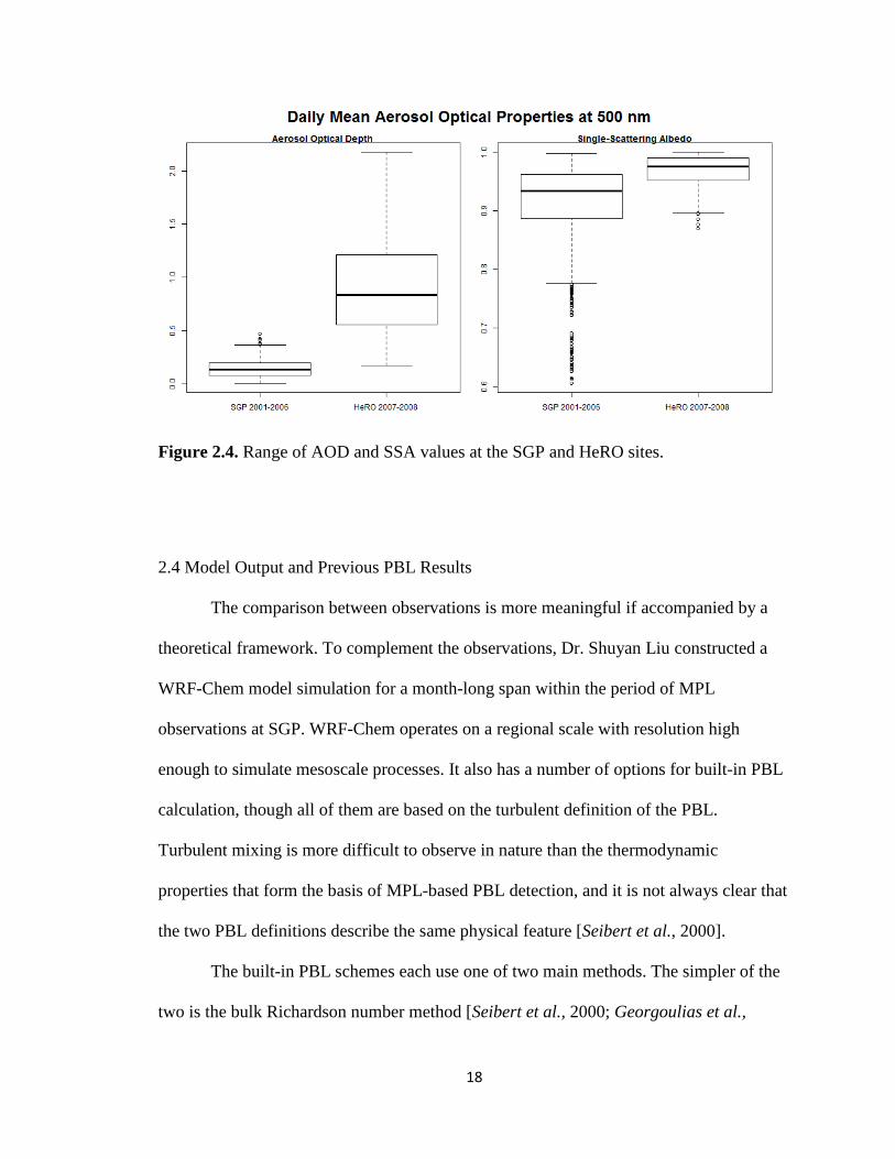
equipped with a PREDE sky radiometer since March 2007 [Wang et al. 2014]. Crucially
for the project, the HeRO site has very different aerosol conditions from the SGP site,
with an AOD range more than four times greater and SSA measurements with a
correspondingly more reliable precision (Figure 2.4).
18
Figure 2.4. Range of AOD and SSA values at the SGP and HeRO sites.
2.4 Model Output and Previous PBL Results
The comparison between observations is more meaningful if accompanied by a
theoretical framework. To complement the observations, Dr. Shuyan Liu constructed a
WRF-Chem model simulation for a month-long span within the period of MPL
observations at SGP. WRF-Chem operates on a regional scale with resolution high
enough to simulate mesoscale processes. It also has a number of options for built-in PBL
calculation, though all of them are based on the turbulent definition of the PBL.
Turbulent mixing is more difficult to observe in nature than the thermodynamic
properties that form the basis of MPL-based PBL detection, and it is not always clear that
the two PBL definitions describe the same physical feature [Seibert et al., 2000].
The built-in PBL schemes each use one of two main methods. The simpler of the
two is the bulk Richardson number method [Seibert et al., 2000; Georgoulias et al.,
19
2009], which is suitable whether the boundary-layer turbulence is primarily due to
convection or wind shear. The bulk Richardson number is defined
𝑅𝐵 = 𝑔∆𝜃�𝑣∆𝑧𝜃�𝑣[(∆𝑈�)2+(∆𝑉�)2], (2.1)
where θv is again the virtual potential temperature, U and V are horizontal winds, and g is
gravitational acceleration; bars indicate mean values. It serves as a measure of the
turbulence of the air for a height interval Δz. The PBL is then defined as the lowest height
at which RB exceeds the critical value 0.25 [Hennemuth and Lammert, 2006]. Other
schemes rely on turbulent kinetic energy (TKE), which is defined
𝑇𝑇𝑇𝑚
= 12�𝑢′2���� + 𝑣′2���� + 𝑤′2������. (2.2)
Here u’, v’ and w’ represent the turbulent component of the mean wind in each vector
direction. The conceptual model of the PBL considers TKE to be uniform with height
within a well-mixed boundary layer, then rapidly decreasing at the transition to the free
troposphere [Stull, 1988]; this is the same basic structure that appears in the aerosol
backscatter signal. However, neither the bulk Richardson number method nor the various
TKE approaches respond directly to changes in mixed-layer radiative forcing. Hu et al.
[2010] found that the Yonsei University (YSU) scheme, which had recently been
updated, and the new asymmetric convective model, version 2 (ACM2) scheme,
outperformed other commonly-used PBL schemes. Considerable uncertainty nevertheless
remains in model PBL schemes, and it is necessary to keep several versions available to

20
modelers. Dr. Liu’s simulation used YSU, a PBL scheme based on the bulk Richardson
number method, to calculate PBL depths for the purposes of comparison to observations.
The period at SGP chosen for simulation was April 2004. This month was chosen
for its high contrasts in daily mean AOD values, which varied between 0.1 and 0.4,
sometimes dramatically from one day to the next (Figure 2.5). SSA values remained
close to 0.9 throughout the month, as is most often the case for the site as a whole. In
addition to reducing the computational requirements of the model run, the choice of a
single month with varied AOD eliminates seasonal differences from the simulation.
Figure 2.5. Daily mean AOD and SSA at the SGP site for April 2004, observed during the period of the WRF-Chem simulation.
Finally, this study uses PBL depth results provided by Dr. Shuyan Liu and
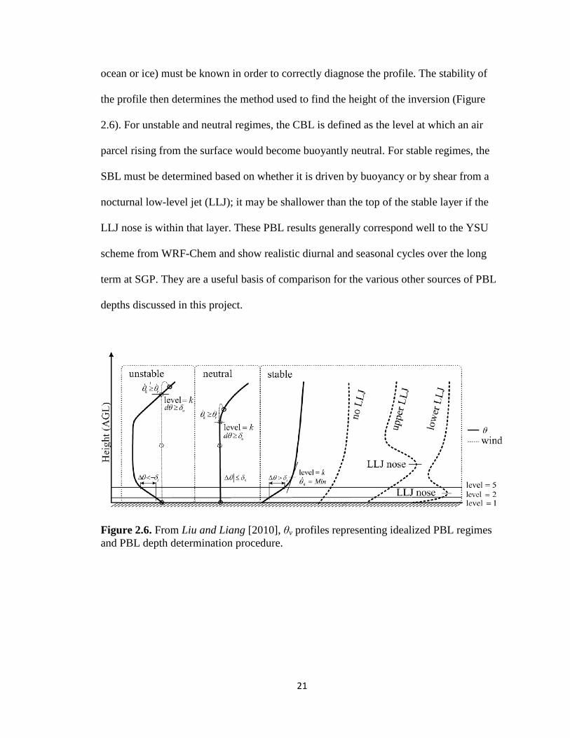
described in Liu and Liang [2010], resulting from radiosonde observations at SGP. The
PBL detection algorithm used in that study first evaluates to which of three regimes the
potential temperature profile belongs: unstable, neutral or stable. The surface type (land,
21
ocean or ice) must be known in order to correctly diagnose the profile. The stability of
the profile then determines the method used to find the height of the inversion (Figure
2.6). For unstable and neutral regimes, the CBL is defined as the level at which an air
parcel rising from the surface would become buoyantly neutral. For stable regimes, the
SBL must be determined based on whether it is driven by buoyancy or by shear from a
nocturnal low-level jet (LLJ); it may be shallower than the top of the stable layer if the
LLJ nose is within that layer. These PBL results generally correspond well to the YSU
scheme from WRF-Chem and show realistic diurnal and seasonal cycles over the long
term at SGP. They are a useful basis of comparison for the various other sources of PBL
depths discussed in this project.
Figure 2.6. From Liu and Liang [2010], θv profiles representing idealized PBL regimes and PBL depth determination procedure.

22
Chapter 3. PBL Detection
3.1 Backscatter Gradient Methods
While it is possible to detect the PBL using the variance in lidar backscatter
[Jordan et al., 2010; Kong and Yi, 2015], backscatter gradient methods are more common
and have used a number of approaches. The simplest ways to detect the PBL using
aerosol backscatter gradient are to define a threshold value for the transition from mixed
layer to free troposphere [Melfi et al., 1985; Palm et al., 1998] or to find the maximum of
the first derivative of the backscatter signal [Amiridis et al., 2007; Tskaknakis et al.,
2011]. With the backscatter signal formatted as an image file, it is also possible to detect
layers by using edge detection software in programs such as Photoshop [Parikh and
Parikh, 2002]. All these methods are effective for short-term, relatively uniform data sets,
but they require either too much prior knowledge about the instrument and atmospheric
conditions, or too much human judgment, to automate over multiyear data sets or
multiple sites.
By contrast, the wavelet covariance transform method [Davis et al., 2000; Brooks,
2003] is commonly used for longer time series because it can adapt to very different
backscatter signals without additional human input. It compares the backscatter sounding
to the Haar wavelet, defined as
�𝑧−𝑏𝑎� = �
−1: 𝑏 − 𝑎2≤ 𝑧 ≤ 𝑏
1: 𝑏 ≤ 𝑧 ≤ 𝑏 + 𝑎2
0: 𝑒𝑒𝑒𝑒𝑤ℎ𝑒𝑒𝑒
, (3.1)
23
where a is the dilation of the Haar wavelet, b is the translation of the Haar wavelet, and z
is the altitude. The wavelet covariance transform, 𝑊𝑓(𝑎, 𝑏), is expressed as
𝑊𝑓(𝑎, 𝑏) = 𝑎−1 ∫ 𝑓(𝑧)ℎ �𝑧−𝑏𝑎�𝑧𝑧
𝑧𝑏 𝑑𝑧 , (3.2)
where f(z) is the backscatter sounding. The maximum value of 𝑊𝑓(𝑎, 𝑏) occurs where b
equals the altitude of the strongest negative gradient in the backscatter; this is the top of
the PBL. In equations 3.1 and 3.2, the dilation a corresponds physically to the depth of
the transition zone between the mixed layer and the free troposphere. The given PBL
depth is the center point in this zone, midway through the capping inversion or layer of
entrainment.
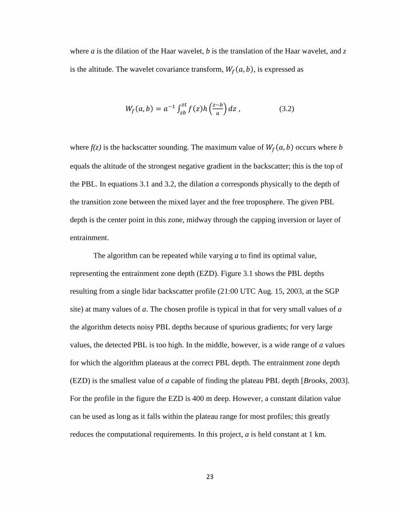
The algorithm can be repeated while varying a to find its optimal value,
representing the entrainment zone depth (EZD). Figure 3.1 shows the PBL depths
resulting from a single lidar backscatter profile (21:00 UTC Aug. 15, 2003, at the SGP
site) at many values of a. The chosen profile is typical in that for very small values of a
the algorithm detects noisy PBL depths because of spurious gradients; for very large
values, the detected PBL is too high. In the middle, however, is a wide range of a values
for which the algorithm plateaus at the correct PBL depth. The entrainment zone depth
(EZD) is the smallest value of a capable of finding the plateau PBL depth [Brooks, 2003].
For the profile in the figure the EZD is 400 m deep. However, a constant dilation value
can be used as long as it falls within the plateau range for most profiles; this greatly
reduces the computational requirements. In this project, a is held constant at 1 km.
24
Figure 3.1. Wavelet covariance-detected PBL depths with varying dilation. The assumed 1-km dilation (crossed) is within the plateau range.
The wavelet covariance transform requires less prior information about the
atmosphere or the lidar than many other PBL detection algorithms, and works equally
well with data from several instrument types. This makes the algorithm useful for
automated PBL detection in multiple data sets. It is independent of absolute backscatter
values as long as the signal-to-noise ratio is high enough to distinguish the PBL.
However, strong backscatter signals from high clouds and elevated aerosol plumes often
overshadow the signal from the PBL, causing an elevated bias in PBL detection. Lewis et
al. [2013] uses image processing methods to correct the wavelet covariance transform
25
algorithm in such cases. However, the solution used in this study is to limit the vertical
extent of the backscatter profile to which the algorithm is applied. While the full vertical
profile for lidar backscatter extends tens of kilometers into the atmosphere, the PBL does
not occur beyond the low troposphere; a limit on the algorithm of 3 km is suitable for
temperate sites such as in the US and China. This also reduces the computing time.
Steyn et al. [1999] developed a different algorithm for PBL detection in the lidar
backscatter gradient. To avoid the problems posed by multiple non-PBL features in the
backscatter, the algorithm uses the shape of a curve representing an idealized backscatter
profile, namely,
𝐵(𝑧) = (𝐵𝑚+𝐵𝑢)2
− (𝐵𝑚−𝐵𝑢)2
e rf �𝑧−𝑧𝑚𝑠�. (3.3)
Here, Bm and Bu are the backscatter values for the mixed layer and the lower free
troposphere, respectively, zm is the depth of the PBL, and s is a parameter defining the
depth of the sigmoid curve between Bm and Bu. As before, zm is defined as the center of a
transition zone, which in this case has a depth equal to 2.77 times the value of s,
assuming as in Steyn et al. [1999] that the entrainment zone encompasses 95% of the
depth of the curve. The algorithm solves for these four parameters simultaneously to
minimize the root-mean-square difference between the idealized curve and the
backscatter sounding. As such, it arrives at an estimate of the transition, or EZD, as well
as the PBL depth. Simulated annealing, as detailed by Press et al. [1992], is a robust
method for fitting the curve; the fit improves with the quality of the initial guess. Steyn et
al. [1999] used the algorithm with airborne lidar data, which necessarily operates for
26
short periods of time alongside other instruments. For longer-term, ground-based
deployments, no single initial guess is appropriate for the entire time series.
The simulated annealing routine escapes from local minima and troughs that
would trap a downhill simplex routine because it introduces a small random element to
the solution [Press et al., 1992]. It can therefore find multiple solutions given the same
input. Over a time series in which the PBL changes slowly compared to the measurement
interval, PBL returns from a simulated annealing algorithm appear “noisy”, with
unrealistically abrupt changes in height. Hägeli et al. [2000] details the appropriate
interval for a running-mean filter, based on the dimensions of the data and the estimated
vertical motion at the boundary layer top. For a stationary lidar deployment, a 25-minute
interval matches the scale of the boundary-layer turbulence. With smoothing, the Steyn et
al. [1999] algorithm is more sensitive to small-scale boundary layer waves than the
wavelet covariance transform. Because curve-fitting uses the whole backscatter signal as
a single shape, it also tolerates more extraneous features and noise.
Ground-based MPL cannot retrieve backscatter near the surface. Regardless of algorithm,
shallow PBLs are sometimes missed, and RLs are detected instead.
3.2 The Combined Algorithm
The advantages and disadvantages of the two gradient methods suggest that PBL
depth detection might be improved by using both in combination. The wavelet covariance
transform is suitable alone for automated PBL detection, but it can also generate a first
guess for the simulated annealing routine. The backscatter values for the free troposphere
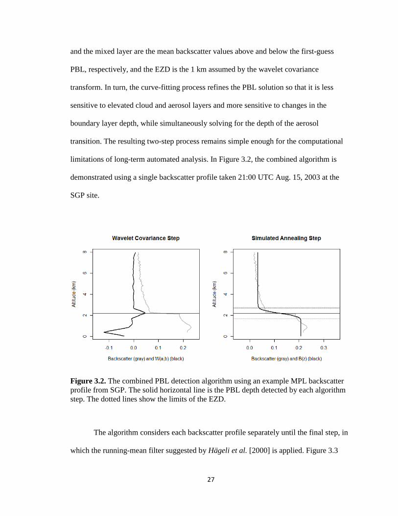
27
and the mixed layer are the mean backscatter values above and below the first-guess
PBL, respectively, and the EZD is the 1 km assumed by the wavelet covariance
transform. In turn, the curve-fitting process refines the PBL solution so that it is less
sensitive to elevated cloud and aerosol layers and more sensitive to changes in the
boundary layer depth, while simultaneously solving for the depth of the aerosol
transition. The resulting two-step process remains simple enough for the computational
limitations of long-term automated analysis. In Figure 3.2, the combined algorithm is
demonstrated using a single backscatter profile taken 21:00 UTC Aug. 15, 2003 at the
SGP site.
Figure 3.2. The combined PBL detection algorithm using an example MPL backscatter profile from SGP. The solid horizontal line is the PBL depth detected by each algorithm step. The dotted lines show the limits of the EZD.
The algorithm considers each backscatter profile separately until the final step, in
which the running-mean filter suggested by Hägeli et al. [2000] is applied. Figure 3.3

28
illustrates how this smooths the PBL time series to eliminate random jumps introduced
by the simulated annealing process. PBL depths for the MPL at SGP are detected at a 5-
minute resolution, so the 25-minute smoothing interval is a five-cell filter. The details of
small-scale waves within the boundary layer top are preserved in the final time series.
Figure 3.3. Aug. 15, 2003 at SGP. The dotted line indicates the PBL detected by the combined algorithm before smoothing; the solid line applies the running-median filter.
With modification, the same algorithm can be applied to thermodynamic profiles
from radiosondes and ground-based remote sensing. For the AERI instrument at SGP,
this is the first attempt to detect the PBL depth; for radiosonde, using the same algorithm
as the other two instrument sources instead of the Liu and Liang [2010] results (for
example) eliminates differences in algorithm bias as a variable in the comparison.
Defining the PBL as before—the center of an inversion in the virtual potential
temperature (θv) profile [Stull, 1988]—the algorithm must detect a sharp increase in θv
29
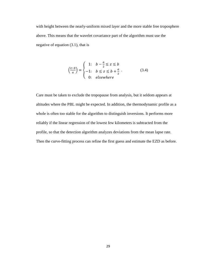
with height between the nearly-uniform mixed layer and the more stable free troposphere
above. This means that the wavelet covariance part of the algorithm must use the
negative of equation (3.1), that is
�𝑧−𝑏𝑎� = �
1: 𝑏 − 𝑎2≤ 𝑧 ≤ 𝑏
−1: 𝑏 ≤ 𝑧 ≤ 𝑏 + 𝑎2
0: 𝑒𝑒𝑒𝑒𝑤ℎ𝑒𝑒𝑒
. (3.4)
Care must be taken to exclude the tropopause from analysis, but it seldom appears at
altitudes where the PBL might be expected. In addition, the thermodynamic profile as a
whole is often too stable for the algorithm to distinguish inversions. It performs more
reliably if the linear regression of the lowest few kilometers is subtracted from the
profile, so that the detection algorithm analyzes deviations from the mean lapse rate.
Then the curve-fitting process can refine the first guess and estimate the EZD as before.
30
Chapter 4. Instrument Intercomparison at SGP
4.1 Intercomparison of PBL Depth Detection
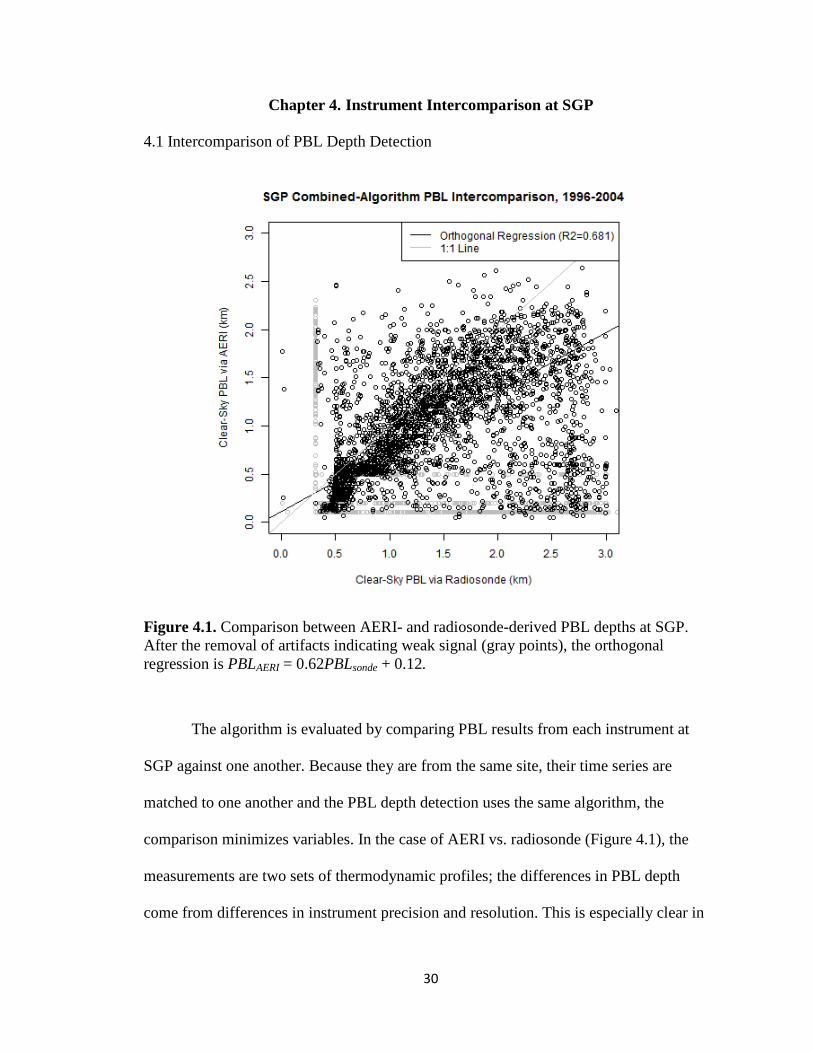
Figure 4.1. Comparison between AERI- and radiosonde-derived PBL depths at SGP. After the removal of artifacts indicating weak signal (gray points), the orthogonal regression is PBLAERI = 0.62PBLsonde + 0.12.
The algorithm is evaluated by comparing PBL results from each instrument at
SGP against one another. Because they are from the same site, their time series are
matched to one another and the PBL depth detection uses the same algorithm, the
comparison minimizes variables. In the case of AERI vs. radiosonde (Figure 4.1), the
measurements are two sets of thermodynamic profiles; the differences in PBL depth
come from differences in instrument precision and resolution. This is especially clear in

31
the very shallow PBL depths, as there are no radiosonde observations between the surface
and approximately 300 m, while AERI has no such restriction. Because neither method is
considered true, an orthogonal regression is used instead of a simple linear fit. Two-thirds
of the variation is accounted for (R2=0.681). Most points lie close to the 1:1 line. While
the regression is influenced by a cluster of results in which the radiosonde-derived PBL
depth is much higher than the AERI-derived PBL depth, the overall systematic error is
low. Much of the correspondence with AERI data is only achieved using the combined
algorithm, because the low vertical resolution of the AERI-derived thermodynamic
profiles strongly affects the wavelet covariance transform.
For comparison between radiosonde and MPL-derived PBL depths, it is important
to assure that clouds do not interfere with PBL detection (Figure 4.2). Clouds return
strong backscatter at the lidar wavelength, and the attenuation of the laser pulse through
an optically thick cloud deck appears as a sharp backscatter gradient that may be targeted
by the PBL detection algorithm; the same features can be used to produce cloud base and
top heights as a standard MPL data product [Sivaraman and Comstock, 2011]. The
wavelet covariance transform component of the PBL detection algorithm is restricted to 3
km from the surface, partly because the PBL typically occurs there [Stull, 1988; see Ma
et al., 2011 for a rare exception], but partly to eliminate interference by higher-altitude
clouds. However, most low-level cloud bases occur at or near the PBL, either because the
capping inversion prevents stratocumulus clouds from developing farther or because the
cloud base in a deep convective cell marks the PBL top [Stull, 1988]. The algorithm
therefore returns an answer about as accurate as it would have from aerosol backscatter
alone.

32
Figure 4.2. Radiosonde- vs. MPL-derived PBL depths at SGP, cloudy cases (left) and cloud-free cases (right). R2 values for the orthogonal regression are 0.551 and 0.515, respectively. Gray points, excluded from regression, are outside the lidar overlap range.
In all MPL-derived PBL depths, the incomplete overlap between the laser beam
spread and the telescope field of view imposes a lower limit on the instrument range.
Radiosonde-derived PBL results below 600 m (27% of cases) are excluded from
regression because the lidar cannot observe them, although radiosonde can. There is little
difference between cloudy and cloud-free lidar PBL detection, however. The following
intercomparison therefore uses the full set of results (Figure 4.3).

33
Figure 4.3. Intercomparison between all radiosonde- and MPL-derived PBL depths at SGP. The orthogonal regression is PBLMPL = 0.71PBLsonde + 0.22. Gray points, excluded from regression, are outside the lidar overlap range.
4.2 Diurnal Cycles
Although the lidar-derived PBL depths are matched to radiosonde launch times, the
comparison does not discriminate between day and nighttime observations. Continental
boundary layers undergo strong diurnal cycling through regimes (Figure 4.4), classified
according to whether the surface undergoes radiative heating (daytime) or cooling
(night).

34
Figure 4.4. PBL heights detected by MPL, AERI and radiosonde, overlaid on MPL backscatter during a nine-day period of typical conditions.
Figure 4.5. Boxplots show the distribution of PBL depths from different radiosonde launch times by radiosonde (left) and MPL (right), excluding PBL depths outside the lidar overlap range.
35
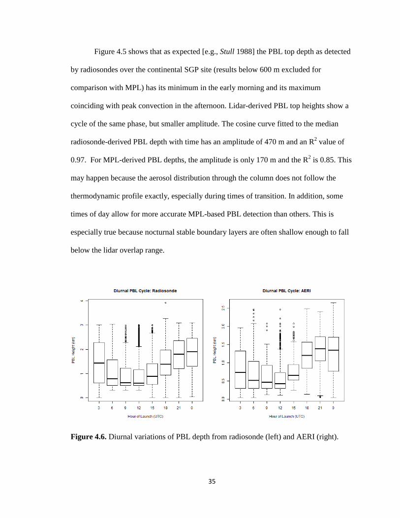
Figure 4.5 shows that as expected [e.g., Stull 1988] the PBL top depth as detected
by radiosondes over the continental SGP site (results below 600 m excluded for
comparison with MPL) has its minimum in the early morning and its maximum
coinciding with peak convection in the afternoon. Lidar-derived PBL top heights show a
cycle of the same phase, but smaller amplitude. The cosine curve fitted to the median
radiosonde-derived PBL depth with time has an amplitude of 470 m and an R2 value of
0.97. For MPL-derived PBL depths, the amplitude is only 170 m and the R2 is 0.85. This
may happen because the aerosol distribution through the column does not follow the
thermodynamic profile exactly, especially during times of transition. In addition, some
times of day allow for more accurate MPL-based PBL detection than others. This is
especially true because nocturnal stable boundary layers are often shallow enough to fall
below the lidar overlap range.
Figure 4.6. Diurnal variations of PBL depth from radiosonde (left) and AERI (right).

36
The AERI-derived PBL depths show a similar cycle (Figure 4.6) to the
radiosonde-derived PBL, with shallow PBLs included in the analysis. While the MPL
overlap range limits its ability to observe lower altitudes, the AERI profile improves near
the surface. Because the vertical resolution of the instrument decreases with height, it can
detect shallow PBL depths with greater precision than deeper PBLs. The results that can
be compared to MPL-derived PBL depths, i.e. those that occur above the overlap range
limit, are less reliable than the shallower AERI-derived PBL depths that can be compared
only to radiosonde. Consequently, the relationship between AERI-derived and MPL-
derived PBL depths is not strong enough for a meaningful comparison of the diurnal
cycle. It makes more sense to compare the AERI-derived PBL diurnal cycle to that of
radiosonde, this time with shallow PBL depths from both instruments included. The
amplitude of the cosine regression expands to 660 m for radiosonde results (R2 = 0.90).
For AERI-derived PBL depths, the amplitude is 440 m and the R2 value is 0.64. Because
the strengths and limitations of the PBL products complement each other, all the products
are valuable despite their inconsistency, with more or less reliability in different
circumstances as detailed below.
The agreement of PBL detection by the three methods varies with the time of day
as seen in Figure 4.7. Note that R2 values do not fall between zero and one. To prevent
any systematic error specific to one time interval from appearing as misleading high
agreement, R2 is always evaluated for the 1:1 line, i.e. perfect agreement between the two
instruments, instead of the linear regression for each time interval. Daytime PBL top
heights show closer agreement between instruments than nighttime PBL top heights, and
mature boundary layers, whether stable or convective, show more agreement than
37
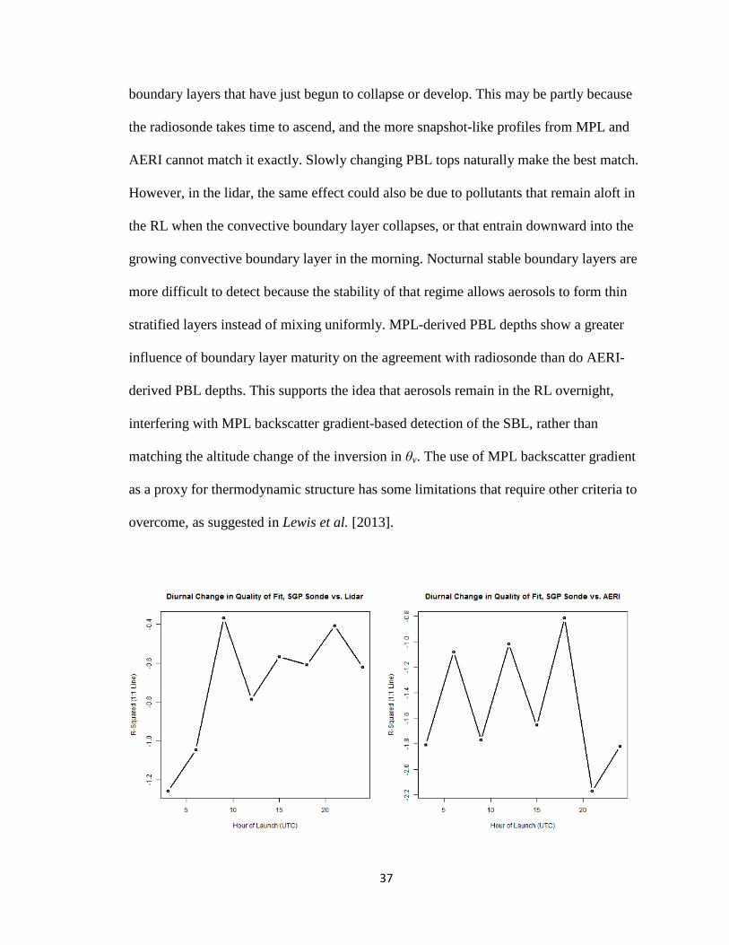
boundary layers that have just begun to collapse or develop. This may be partly because
the radiosonde takes time to ascend, and the more snapshot-like profiles from MPL and
AERI cannot match it exactly. Slowly changing PBL tops naturally make the best match.
However, in the lidar, the same effect could also be due to pollutants that remain aloft in
the RL when the convective boundary layer collapses, or that entrain downward into the
growing convective boundary layer in the morning. Nocturnal stable boundary layers are
more difficult to detect because the stability of that regime allows aerosols to form thin
stratified layers instead of mixing uniformly. MPL-derived PBL depths show a greater
influence of boundary layer maturity on the agreement with radiosonde than do AERI-
derived PBL depths. This supports the idea that aerosols remain in the RL overnight,
interfering with MPL backscatter gradient-based detection of the SBL, rather than
matching the altitude change of the inversion in θv. The use of MPL backscatter gradient
as a proxy for thermodynamic structure has some limitations that require other criteria to
overcome, as suggested in Lewis et al. [2013].
38
Figure 4.7. Variation of R2 values with the time of radiosonde launches, assessing the quality of fit between PBLMPL and PBLsonde (left) and between PBLAERI and PBLsonde (right).
4.3 Seasonal Cycles
The seasonal cycle of the PBL depth is as important as the diurnal cycle to mixed
layer processes. Surface convection is stronger in the summer months than in the winter
at continental sites, and the PBL top depth responds accordingly. Again the radiosonde
results follow a cosine curve, its peak coinciding with the most intense surface heating.
The difference in wave amplitude between the radiosonde- and MPL-based PBL top
heights is still present but less pronounced (Figure 4.8). The cosine curve fitted to the
radiosonde-derived median values has an amplitude of 380 m and an R2 value of 0.93,
while the cosine curve fitted to the MPL-derived median values has an amplitude of 330
m and an R2 value of 0.90. The radiosonde-derived PBL top heights average slightly
higher and are more variable within any given month. This is consistent with the greater
amplitude of the diurnal cycle shown in Figure 4.3.

39
Figure 4.8. Boxplots show the distribution of radiosonde-derived and MPL-derived PBL depths by month, with shallow PBLs excluded from the radiosonde record.
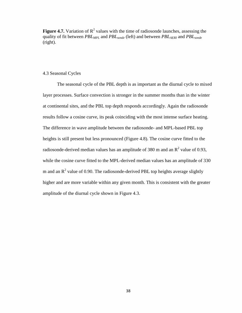
It seems counterintuitive, given that convective PBLs are analyzed more
accurately than stable nocturnal boundary layers, that the instruments diverge most in the
summer months (Figure 4.9). For the diurnal cycle analysis, the highest PBL tops have
the best agreement between the two instruments. For the seasonal cycle, they have the
least, despite the fact that the MPL-derived seasonal cycle of PBL depths more closely
resembles a cosine curve than the MPL-derived diurnal cycle. R-squared values vary to
almost exactly the same degree as they do for the diurnal cycle shown in Figure 4.6, but
this time there is a steep drop in the quality of fit in the summer and a peak in the winter
months.
40
Figure 4.9. R2 values assessing the quality of fit to the 1:1 line for the radiosonde-vs.-MPL intercomparison by month.
The difference between the seasonal cycles in Figure 4.8 appears mostly in the
higher summertime PBL depths detected by radiosonde than by MPL, and this is a clue as
to its cause. The reason for the discrepancy appears to be the effect of deep convection on
the thermodynamic structure of the middle troposphere. Figure 4.10 shows the seasonal
variation of MPL-retrieved cloud base heights occuring at altitudes below 4 km, which
can be considered typical of boundary-layer clouds.

41
Figure 4.10. Boxplots show the monthly distribution of MPL-retrieved cloud base depths located below 4 km at the SGP site for the period 1996-2004.
The seasonal cycle peaks with a median cloud base height of approximately 1500
m in August, similar to the seasonal peak for the MPL-derived PBL depths. The
radiosonde-derived PBL depths for the summer months are typically higher, and vary
more. Although a schematic of PBL regimes in Medeiros et al. [2005] puts the PBL near
the cloud base in cases of deep convection, the convective turbulence fueled by surface
heating extends all the way to the cloud top, which may well reach the tropopause during
the kind of deep convection that is typical of summer in the Southern Great Plains.
Temperature and moisture properties are similarly carried upward into the cloud. This
renders the thermodynamic definition of the PBL ambiguous (the algorithm is designed
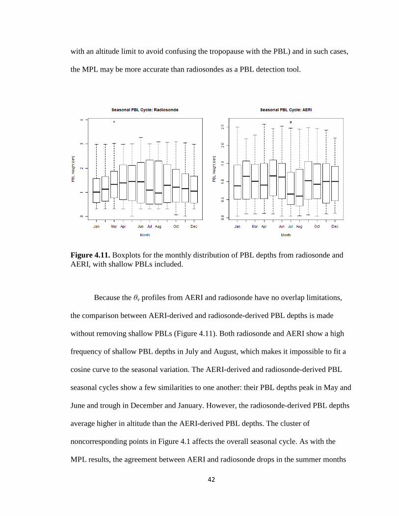
42
with an altitude limit to avoid confusing the tropopause with the PBL) and in such cases,
the MPL may be more accurate than radiosondes as a PBL detection tool.
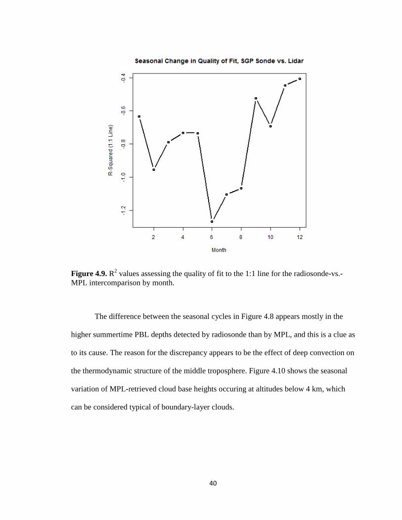
Figure 4.11. Boxplots for the monthly distribution of PBL depths from radiosonde and AERI, with shallow PBLs included.
Because the θv profiles from AERI and radiosonde have no overlap limitations,
the comparison between AERI-derived and radiosonde-derived PBL depths is made
without removing shallow PBLs (Figure 4.11). Both radiosonde and AERI show a high
frequency of shallow PBL depths in July and August, which makes it impossible to fit a
cosine curve to the seasonal variation. The AERI-derived and radiosonde-derived PBL
seasonal cycles show a few similarities to one another: their PBL depths peak in May and
June and trough in December and January. However, the radiosonde-derived PBL depths
average higher in altitude than the AERI-derived PBL depths. The cluster of
noncorresponding points in Figure 4.1 affects the overall seasonal cycle. As with the
MPL results, the agreement between AERI and radiosonde drops in the summer months
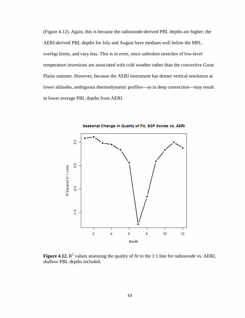
43
(Figure 4.12). Again, this is because the radiosonde-derived PBL depths are higher; the
AERI-derived PBL depths for July and August have medians well below the MPL
overlap limits, and vary less. This is in error, since unbroken stretches of low-level
temperature inversions are associated with cold weather rather than the convective Great
Plains summer. However, because the AERI instrument has denser vertical resolution at
lower altitudes, ambiguous thermodynamic profiles—as in deep convection—may result
in lower average PBL depths from AERI.
Figure 4.12. R2 values assessing the quality of fit to the 1:1 line for radiosonde vs. AERI, shallow PBL depths included.

44
The agreement between MPL and radiosonde in the presence of boundary-layer
clouds (Figure 4.2) conforms to expectations about boundary-layer stratocumulus, for
which the cloud thickness remains shallow due to the PBL top acting as a capping
inversion. This is one of several boundary-layer regimes discussed in Medeiros et al.
[2005], which also notes two complications. The first is decoupling of the flow within the
stratocumulus deck from the rest of the mixed layer. Decoupling does not imply an
additional temperature inversion, but is mostly apparent in measurements capable of
profiling vertical motion, including wind lidar. Decoupling within a cloud layer does not
appear in thermodynamic profiles, and to lidar it is hidden by the opacity of the cloud.
The second complication is the possibility of a low stable boundary layer forming well
below the level of the lowest cloud base. The wavelet covariance transform may then
miss the signal of the PBL top because of the much stronger gradient caused by cloud
attenuation. The combined algorithm avoids this problem by restricting the depth of the
profile used in analysis, but may still err if the PBL is shallow and the elevated cloud
base occurs at an altitude reasonable for PBL depths. Lastly, lidar cannot distinguish
between shallow stratocumulus and deep cumulus convection, although both are distinct
from other cloud types. The PBL is detected where the backscatter signal fully attenuates,
which is slightly too high for deep convection and slightly too low for a capping
inversion over stratocumulus.
Steyn et al. [1999] recommends the simulated annealing routine partly because it
finds the EZD, used to estimate fluxes through the boundary layer top. However, in the
SGP results the detected EZD values hardly deviate from the constant initial guess,
making EZD intercomparison among the different instruments impossible. A varying
45
initial guess for the EZD, as there is for the PBL, would produce better results. However,
wavelet covariance-based determination of the EZD is only possible by trial-and-error
repetition with different values of the wavelet dilation, a computationally intensive
process. The transition between mixed-layer aerosol loading and the cleaner free
troposphere may also have a different depth than the potential temperature inversion;
aerosol content need not be as good a proxy for the transition as it is for the PBL. If this
were the only obstacle, however, some relationship between radiosonde- and AERI-
derived EZD results would be expected. None is found. EZD obtained by the combined
algorithm is therefore unreliable, not suited to flux estimates.
For PBL detection, however, the benefit of the simulated annealing step is clear.
Much of the correspondence in the AERI-derived PBL depth set is due to the use of the
combined algorithm. Because the wavelet covariance transform works its way along the
profile, comparing each data point to the others separately, the PBL depths it detects must
fall on the same intervals as the original data; a low-resolution profile returns blocky,
low-resolution PBLs. By contrast, the curve-fitting routine detects PBL depths based on
the overall shape of the profile and is therefore free to return heights between the
profile’s data points. For intercomparison between instruments, this property eliminates
aliasing caused by the differing height intervals of the profiling data. For PBL depths
from a single instrument with high temporal resolution, it returns PBL depths with
realistic rates of change and development that better match the shape of the contour in
lidar backscatter or virtual potential temperature.
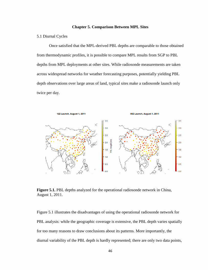
46
Chapter 5. Comparison Between MPL Sites
5.1 Diurnal Cycles
Once satisfied that the MPL-derived PBL depths are comparable to those obtained
from thermodynamic profiles, it is possible to compare MPL results from SGP to PBL
depths from MPL deployments at other sites. While radiosonde measurements are taken
across widespread networks for weather forecasting purposes, potentially yielding PBL
depth observations over large areas of land, typical sites make a radiosonde launch only
twice per day.
Figure 5.1. PBL depths analyzed for the operational radiosonde network in China, August 1, 2011.
Figure 5.1 illustrates the disadvantages of using the operational radiosonde network for
PBL analysis: while the geographic coverage is extensive, the PBL depth varies spatially
for too many reasons to draw conclusions about its patterns. More importantly, the
diurnal variability of the PBL depth is hardly represented; there are only two data points,

47
and the timing of the launches is coordinated globally rather than targeted to the likely
maximum and minimum PBL depth. In China, where the local time is eight hours ahead
of universal coordinated time, the 00:00 UTC and 12:00 UTC launch times (i.e., 8:00 AM
and 8:00 PM local time, respectively) are most likely to catch the PBL during a period of
regime transition; in North America, where the time zone at the SGP site corresponds to
UTC-6 (00:00 and 12:00 UTC correspond to 6:00 PM and 6:00 AM CST), operational
radiosonde launches are made at nearly the worst possible time to observe mature SBL
and CBL regimes. As a result, while the PBL depth record derived from the operational
radiosonde network does show systematic differences between the two launch times—the
12:00 UTC launch, which takes place during or just after the CBL collapse in the
evening, is consistently associated with deeper PBLs than the midmorning 00:00 UTC
launch—it greatly underestimates the diurnal variability of the PBL depth and conveys
almost no information about the structure of the diurnal cycle.
None of the MPL sites in China used in this study include intensive radiosonde
observations like the frequent launches at SGP. However, with the MPL observations no
longer bound to radiosonde launch times for the purposes of evaluation, this part of the
analysis can use the full MPL temporal resolution. The mean diurnal cycle is therefore
observable in much greater detail, though the accuracy varies by time of day as described
in Chapter 4, and the overnight segment of the cycle in particular is skewed toward
deeper residual layers. At three-hour intervals, the diurnal cycle fits a smooth cosine
curve, but this obscures the rapid development of the typical CBL and the much slower
change in the overnight SBL or RL. Furthermore, the diurnal cycle varies by season
(Figure 5.2).

48
Figure 5.2. For SGP, the mean diurnal cycle of PBL depths at 5-minute resolution. Time of day is given in hours local time (UTC-6). Left, the overall mean and standard deviation; right, the overall mean and the mean for each season.
Because SGP is a continental site, the amplitude of the diurnal cycle is driven by
surface convection: the deepest CBLs occur in summer, when surface convection is
strongest, while the winter PBL stays shallower throughout the 24 hours and has no
visible CBL development. There is little difference between the spring and autumn
months, which show roughly equivalent transitions between winter and summer
conditions. None of this is surprising given the Stull [1988] conceptual model. The only
difference from expectations is the depth of the SBL, which is much shallower in most
conceptual models. This is due to the tendency of MPL-based observations to miss
shallow SBLs, especially but not exclusively those within the overlap zone, and mark the
capping inversion, or top of the RL, as the PBL instead. The relatively deep overnight
PBL explains why the diurnal cycle has a smaller amplitude than might be expected; it
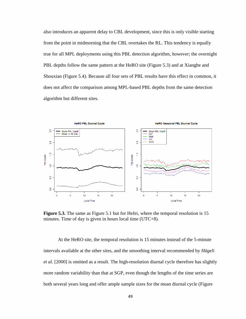
49
also introduces an apparent delay to CBL development, since this is only visible starting
from the point in midmorning that the CBL overtakes the RL. This tendency is equally
true for all MPL deployments using this PBL detection algorithm, however; the overnight
PBL depths follow the same pattern at the HeRO site (Figure 5.3) and at Xianghe and
Shouxian (Figure 5.4). Because all four sets of PBL results have this effect in common, it
does not affect the comparison among MPL-based PBL depths from the same detection
algorithm but different sites.
Figure 5.3. The same as Figure 5.1 but for Hefei, where the temporal resolution is 15 minutes. Time of day is given in hours local time (UTC+8).
At the HeRO site, the temporal resolution is 15 minutes instead of the 5-minute
intervals available at the other sites, and the smoothing interval recommended by Hägeli
et al. [2000] is omitted as a result. The high-resolution diurnal cycle therefore has slightly
more random variability than that at SGP, even though the lengths of the time series are
both several years long and offer ample sample sizes for the mean diurnal cycle (Figure

50
5.4). The timing of the trough and peak PBL depths during the diurnal cycle is
approximately the same as at SGP: 10:00 AM and 3:00 PM local time, respectively.
However, they are significantly shallower, averaging around 1 km instead of the 1.5 km
average at SGP. This difference is magnified in summer. The summertime PBL diurnal
cycle still has the strongest signal of CBL development, but it has the shallowest overall
PBL depths. The deepest PBLs occur in winter instead, and the springtime diurnal cycle
resembles the winter much more strongly than does the autumn diurnal cycle.
Meanwhile, Shouxian and Xianghe have PBL diurnal cycles that correspond to
the shape and phase of the cycles at SGP and Hefei, although the shorter time series leave
much more random variation in the data (Figure 5.4). Neither is long enough to make an
analysis of the seasonal cycle or to determine how the diurnal cycle might change from
one season to the next. However, they can be compared to the corresponding seasons at
the HeRO site. The Shouxian diurnal cycle, drawn from data taken in May through
December of 2008, closely resembles the summertime diurnal cycle at Hefei in phase,
amplitude and mean depth. The Xianghe data comes from January through July of 2013,
and may represent a more winter- and spring-like pattern for the area. Because the sites in
China are subject to much higher AOD values than what is observed at SGP, these
differences in the behavior of the PBL during the day point to aerosol involvement in the
suppression of convection during the day, especially in summer. The fact that the
wintertime PBL diurnal cycles at the HeRO and SGP sites are more similar to each other
than any other season pair supports this idea; the effect of aerosol on boundary-layer
stability should be weakest during the colder months, when there is little to no surface
convection to suppress.

51
Figure 5.4. The mean diurnal cycle of PBL depths at 5-minute resolution for two shorter-term MPL deployments, Shouxian (left, 2008) and Xianghe (right, 2013). Time of day is given in hours local time (UTC+8).
The higher-than-usual random variability in the diurnal cycle at Xianghe requires
some explanation. Where data are available, the PBL depth at Xianghe is analyzed at 5-
minute intervals just as it is at SGP. However, many of the observation days at Xianghe
leave hours-long gaps in the observation record, exacerbating the small sample size
caused by the relatively short deployment; there are extended periods in which the MPL
collected data for only a few hours each day, making it difficult to establish a diurnal
cycle. In addition, the Xianghe MPL backscatter record shows evidence of a common
problem with MPL data collection, especially in underprepared short-term deployments
that have not made extensive calibration and adjustments: the temperature of the
instrument was allowed to fluctuate, causing its laser signal strength to fluctuate or its
optics to be distorted by the thermal expansion of the telescope. Figure 5.5 shows an
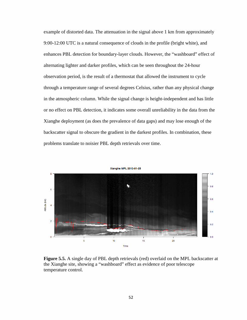
52
example of distorted data. The attenuation in the signal above 1 km from approximately
9:00-12:00 UTC is a natural consequence of clouds in the profile (bright white), and
enhances PBL detection for boundary-layer clouds. However, the “washboard” effect of
alternating lighter and darker profiles, which can be seen throughout the 24-hour
observation period, is the result of a thermostat that allowed the instrument to cycle
through a temperature range of several degrees Celsius, rather than any physical change
in the atmospheric column. While the signal change is height-independent and has little
or no effect on PBL detection, it indicates some overall unreliability in the data from the
Xianghe deployment (as does the prevalence of data gaps) and may lose enough of the
backscatter signal to obscure the gradient in the darkest profiles. In combination, these
problems translate to noisier PBL depth retrievals over time.
Figure 5.5. A single day of PBL depth retrievals (red) overlaid on the MPL backscatter at the Xianghe site, showing a “washboard” effect as evidence of poor telescope temperature control.
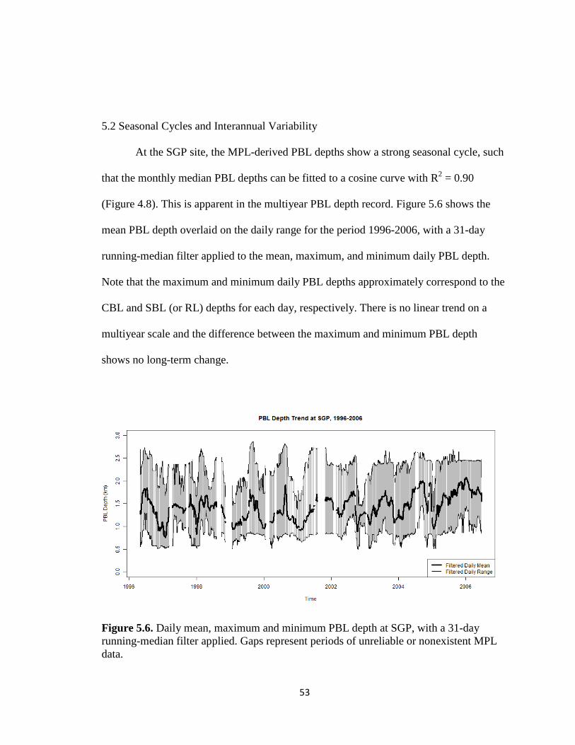
53
5.2 Seasonal Cycles and Interannual Variability
At the SGP site, the MPL-derived PBL depths show a strong seasonal cycle, such
that the monthly median PBL depths can be fitted to a cosine curve with R2 = 0.90
(Figure 4.8). This is apparent in the multiyear PBL depth record. Figure 5.6 shows the
mean PBL depth overlaid on the daily range for the period 1996-2006, with a 31-day
running-median filter applied to the mean, maximum, and minimum daily PBL depth.
Note that the maximum and minimum daily PBL depths approximately correspond to the
CBL and SBL (or RL) depths for each day, respectively. There is no linear trend on a
multiyear scale and the difference between the maximum and minimum PBL depth
shows no long-term change.
Figure 5.6. Daily mean, maximum and minimum PBL depth at SGP, with a 31-day running-median filter applied. Gaps represent periods of unreliable or nonexistent MPL data.

54
The daily mean AOD at the SGP site also follows a predictable seasonal cycle
(Figure 5.7). Values remain below 0.1 in the winter months but become more variable in
the summer, with summertime AOD values generally falling between 0.2 and 0.4. There
is no long-term trend in the part of the AOD record that overlaps with the MPL
observations under analysis in this project.
Figure 5.7. Daily mean AOD values at SGP for the period overlapping with MPL observations, 2001-2006.
While most of 2002 is missing from the data record, there is still a multiyear time series
that can be compared to the MPL-derived PBL depths. The level of interannual
variability is low enough that conclusions can be drawn about the seasonal cycle.
However, the similarities between Figure 5.6 and Figure 5.7 also illustrate the difficulty
in demonstrating that aerosol in the boundary layer suppresses convection: while there
are often high springtime AOD values that correspond to seasonal peaks in aerosol long-
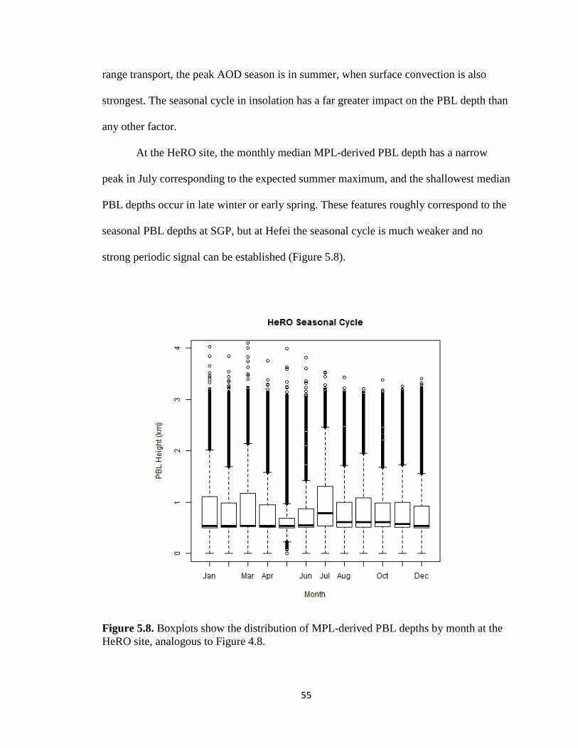
55
range transport, the peak AOD season is in summer, when surface convection is also
strongest. The seasonal cycle in insolation has a far greater impact on the PBL depth than
any other factor.
At the HeRO site, the monthly median MPL-derived PBL depth has a narrow
peak in July corresponding to the expected summer maximum, and the shallowest median
PBL depths occur in late winter or early spring. These features roughly correspond to the
seasonal PBL depths at SGP, but at Hefei the seasonal cycle is much weaker and no
strong periodic signal can be established (Figure 5.8).
Figure 5.8. Boxplots show the distribution of MPL-derived PBL depths by month at the HeRO site, analogous to Figure 4.8.
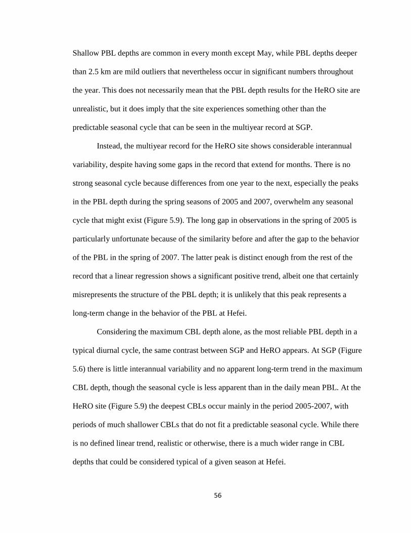
56
Shallow PBL depths are common in every month except May, while PBL depths deeper
than 2.5 km are mild outliers that nevertheless occur in significant numbers throughout
the year. This does not necessarily mean that the PBL depth results for the HeRO site are
unrealistic, but it does imply that the site experiences something other than the
predictable seasonal cycle that can be seen in the multiyear record at SGP.
Instead, the multiyear record for the HeRO site shows considerable interannual
variability, despite having some gaps in the record that extend for months. There is no
strong seasonal cycle because differences from one year to the next, especially the peaks
in the PBL depth during the spring seasons of 2005 and 2007, overwhelm any seasonal
cycle that might exist (Figure 5.9). The long gap in observations in the spring of 2005 is
particularly unfortunate because of the similarity before and after the gap to the behavior
of the PBL in the spring of 2007. The latter peak is distinct enough from the rest of the
record that a linear regression shows a significant positive trend, albeit one that certainly
misrepresents the structure of the PBL depth; it is unlikely that this peak represents a
long-term change in the behavior of the PBL at Hefei.
Considering the maximum CBL depth alone, as the most reliable PBL depth in a
typical diurnal cycle, the same contrast between SGP and HeRO appears. At SGP (Figure
5.6) there is little interannual variability and no apparent long-term trend in the maximum
CBL depth, though the seasonal cycle is less apparent than in the daily mean PBL. At the
HeRO site (Figure 5.9) the deepest CBLs occur mainly in the period 2005-2007, with
periods of much shallower CBLs that do not fit a predictable seasonal cycle. While there
is no defined linear trend, realistic or otherwise, there is a much wider range in CBL
depths that could be considered typical of a given season at Hefei.

57
Figure 5.9. The same as Figure 5.4 but at Hefei.
The causes for this interannual variability cannot be determined from the CBL
depth, or the underlying MPL data, alone. Because the available AOD data only begins in
2007, it is not even possible to determine whether changes in aerosol loading correspond
to the seasonal cycle or to features found in the MPL data from the site. Hefei is subject
to a monsoon pattern that produces extended periods of precipitation in early summer;
this is one of many processes that may make the synoptic conditions less consistent from
year to year. Nevertheless Wang et al. [2014], a later study at the same site, was able to
establish a rough seasonal cycle for AOD for the period 2007-2013 (Figure 5.10). It’s
equally possible that the PBL peaks in 2005 and 2007 correspond to aerosol rainout, or to
synoptically driven differences in the cloud base height.

58
Figure 5.10. From Wang et al. [2014], monthly and seasonal mean 500-nm AOD (a,d), mean Angstrom exponent (b, e), and number of measurements (c, f), at Hefei, 2007-2013.
Summer at Hefei is characterized by the highest AOD values of the year (and
fewest available measurements). The seasonal diurnal cycle in Figure 5.3 suggests that
summer is also characterized by the shallowest PBL depths despite the presence of
surface convection, but the monsoon cycle and the high interannual variability at the site
cast doubt on the effectiveness of dividing the data into four seasons for analysis. The
behavior of the AOD and PBL depth in early summer is very different from their
behavior in late summer, and the early summer especially shows signs that it depends on
other factors for that particular year. However, there is circumstantial evidence in these
results, and especially when compared to the generally deeper and more predictable PBLs

59
at SGP, that aerosol loading affects the PBL depth and may suppress convection at Hefei
when AOD values are high.
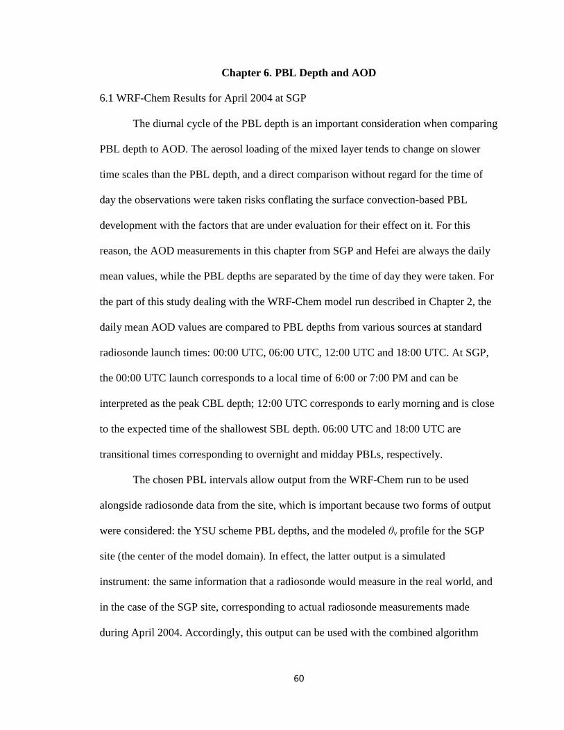
60
Chapter 6. PBL Depth and AOD
6.1 WRF-Chem Results for April 2004 at SGP
The diurnal cycle of the PBL depth is an important consideration when comparing
PBL depth to AOD. The aerosol loading of the mixed layer tends to change on slower
time scales than the PBL depth, and a direct comparison without regard for the time of
day the observations were taken risks conflating the surface convection-based PBL
development with the factors that are under evaluation for their effect on it. For this
reason, the AOD measurements in this chapter from SGP and Hefei are always the daily
mean values, while the PBL depths are separated by the time of day they were taken. For
the part of this study dealing with the WRF-Chem model run described in Chapter 2, the
daily mean AOD values are compared to PBL depths from various sources at standard
radiosonde launch times: 00:00 UTC, 06:00 UTC, 12:00 UTC and 18:00 UTC. At SGP,
the 00:00 UTC launch corresponds to a local time of 6:00 or 7:00 PM and can be
interpreted as the peak CBL depth; 12:00 UTC corresponds to early morning and is close
to the expected time of the shallowest SBL depth. 06:00 UTC and 18:00 UTC are
transitional times corresponding to overnight and midday PBLs, respectively.
The chosen PBL intervals allow output from the WRF-Chem run to be used
alongside radiosonde data from the site, which is important because two forms of output
were considered: the YSU scheme PBL depths, and the modeled θv profile for the SGP
site (the center of the model domain). In effect, the latter output is a simulated
instrument: the same information that a radiosonde would measure in the real world, and
in the case of the SGP site, corresponding to actual radiosonde measurements made
during April 2004. Accordingly, this output can be used with the combined algorithm

61
from Chapter 3 to produce PBL depths based on the thermodynamic definition of the
PBL, in contrast to the Richardson number method-based derivation of the YSU scheme
PBLs. Figure 6.1 shows the resulting comparisons between model-output PBL depths and
the observed daily mean AOD side by side.
Figure 6.1. AOD vs. PBL depth for model-derived PBL depths at the radiosonde launch interval. Left, YSU scheme; right, simulated radiosonde.
While the linear correlation between PBL depth and AOD is weak for any given
time of day—the highest R2 values found by linear regression were borderline significant
at approximately 0.3—the 00:00 UTC PBL depths show a consistent decline with higher
values of AOD, while the 12:00 UTC PBL depths show a weaker positive correlation. No
correlation between PBL depth and AOD should be expected overnight, when there is no
insolation to be affected by the radiative forcing of aerosols.
The observations for April 2004 at SGP include PBL depths detected by two
methods, first the method from Liu and Liang [2010] and then the method described in
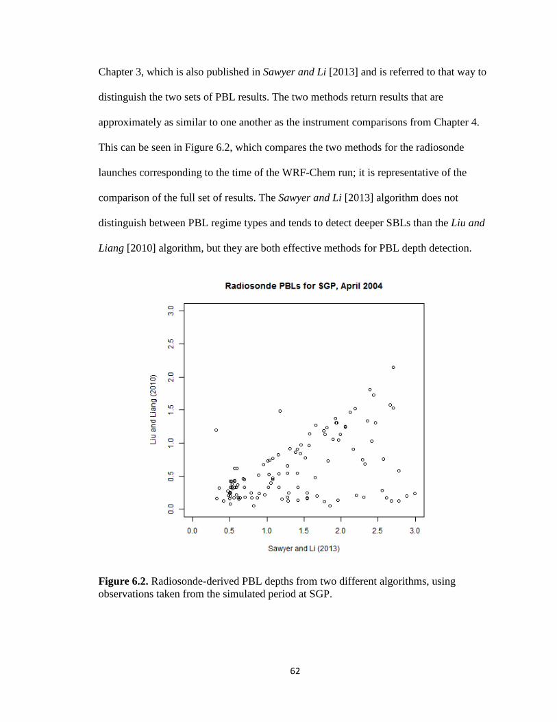
62
Chapter 3, which is also published in Sawyer and Li [2013] and is referred to that way to
distinguish the two sets of PBL results. The two methods return results that are
approximately as similar to one another as the instrument comparisons from Chapter 4.
This can be seen in Figure 6.2, which compares the two methods for the radiosonde
launches corresponding to the time of the WRF-Chem run; it is representative of the
comparison of the full set of results. The Sawyer and Li [2013] algorithm does not
distinguish between PBL regime types and tends to detect deeper SBLs than the Liu and
Liang [2010] algorithm, but they are both effective methods for PBL depth detection.
Figure 6.2. Radiosonde-derived PBL depths from two different algorithms, using observations taken from the simulated period at SGP.

63
Figure 6.3 shows the comparison between the daily mean AOD at the SGP site for
April 2004 and the two sets of radiosonde-derived PBL depths. As in Figure 6.1, the
00:00 UTC launch time is associated with PBL depths that get shallower as AOD
increases, while there are weaker positive correlations between AOD and PBL depth for
the overnight and early-morning launch times. The similarity in the findings among all
four comparisons shows that the PBL depths are valid and that the relationship between
daytime CBLs and the AOD is probably different from the relationship between
overnight SBLs and the AOD. However, the radiative effect is weak compared to other
variations in PBL depth, and a data set covering much more than the 30 days of the
WRF-Chem run would be needed to fully quantify the relationship.
Figure 6.3. AOD vs. PBL depth for radiosonde-derived PBL depths from Liu and Liang [2010] (left) and Sawyer and Li [2013] (right).

64
6.2 PBL Depth vs. AOD at SGP and HeRO
In data sets much larger than the 30-day WRF-Chem run, scatterplots obscure the
relative frequency of different values. One solution to this problem was to examine the
distribution of PBL depths for different daily mean values of AOD, as shown in Figure
6.4: each boxplot shows the PBL depths for a limited range of AOD values. Both sites
show at least a slight decrease in PBL depth with AOD, especially in a loss of deep PBLs
while the very shallow PBL depths remain unaffected. At the HeRO site, the effect is
much more dramatic than it is at SGP; the range of AOD values is more than four times
the range at SGP, and there is a wider sampling of polluted conditions. In fact the HeRO
time series contains only one day with a mean AOD value less than 0.25, while AOD
values above 0.25 are somewhat rare at SGP.
Figure 6.4. Boxplots showing the distribution of PBL depths with increasing AOD, at SGP (left) and Hefei (right).
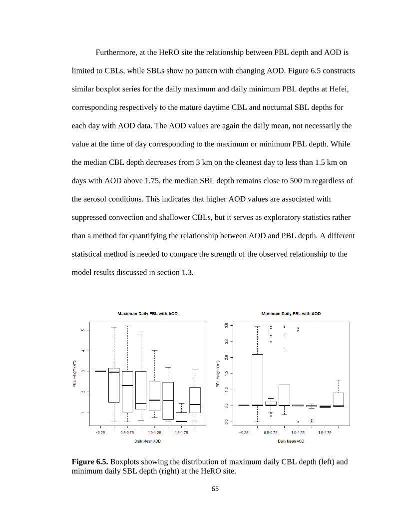
65
Furthermore, at the HeRO site the relationship between PBL depth and AOD is
limited to CBLs, while SBLs show no pattern with changing AOD. Figure 6.5 constructs
similar boxplot series for the daily maximum and daily minimum PBL depths at Hefei,
corresponding respectively to the mature daytime CBL and nocturnal SBL depths for
each day with AOD data. The AOD values are again the daily mean, not necessarily the
value at the time of day corresponding to the maximum or minimum PBL depth. While
the median CBL depth decreases from 3 km on the cleanest day to less than 1.5 km on
days with AOD above 1.75, the median SBL depth remains close to 500 m regardless of
the aerosol conditions. This indicates that higher AOD values are associated with
suppressed convection and shallower CBLs, but it serves as exploratory statistics rather
than a method for quantifying the relationship between AOD and PBL depth. A different
statistical method is needed to compare the strength of the observed relationship to the
model results discussed in section 1.3.
Figure 6.5. Boxplots showing the distribution of maximum daily CBL depth (left) and minimum daily SBL depth (right) at the HeRO site.
66
Since a scatterplot obscures features of the data and exploratory methods lack
quantitative rigor, it is helpful to use probability density functions instead. All probability
density function methods find a continuous curve to represent the distribution of data,
whether by assessing the fit of a prescribed curve or by estimating one directly from the
data. As a form of the latter method, a kernel density estimate allows the fewest possible
prior assumptions about the structure of the probability density. For two variables, this
takes the form
𝑓(𝒙𝟎) = 1𝑛ℎ1ℎ2
∑ 𝐾 �𝑥0−𝑥𝑖ℎ1
�𝐾 �𝑦0−𝑦𝑖ℎ2
�𝑛𝑖=1 , (6.1)
where h is a smoothing parameter for each variable and K is the kernel function [Wilks,
2006], in this case the Gaussian function shown below:
(2𝜋)−12 exp �− 𝑧2
2� . (6.2)
The result is analogous to a two-dimensional probability histogram except that it is
continuous, not subject to arbitrary binning decisions, and more readily represented as a
contour plot. The volume under the surface is an estimate of the probability of the two
variables falling within a given range, with the total volume equal to one.
Figure 6.6 shows the resulting distributions for daily mean AOD and daily
maximum PBL depth (representing the peak of the CBL) at SGP and the HeRO site. One
immediate advantage over the boxplots in Figure 6.4 is that the kernel density estimate
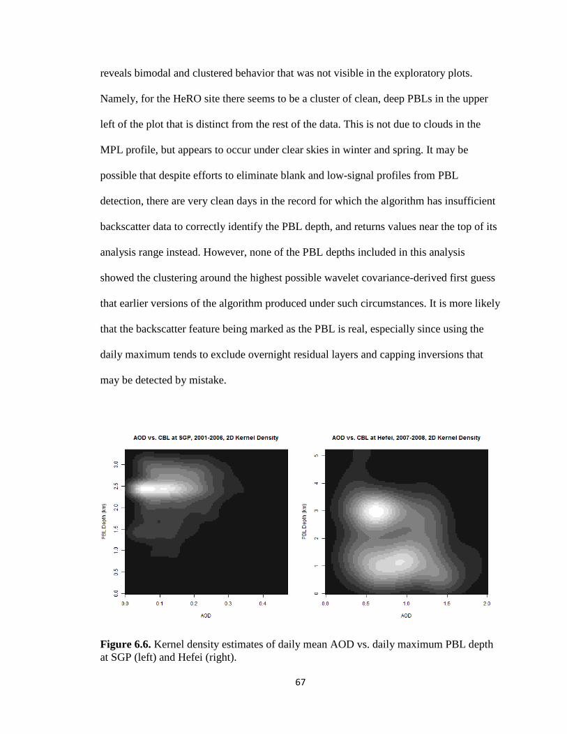
67
reveals bimodal and clustered behavior that was not visible in the exploratory plots.
Namely, for the HeRO site there seems to be a cluster of clean, deep PBLs in the upper
left of the plot that is distinct from the rest of the data. This is not due to clouds in the
MPL profile, but appears to occur under clear skies in winter and spring. It may be
possible that despite efforts to eliminate blank and low-signal profiles from PBL
detection, there are very clean days in the record for which the algorithm has insufficient
backscatter data to correctly identify the PBL depth, and returns values near the top of its
analysis range instead. However, none of the PBL depths included in this analysis
showed the clustering around the highest possible wavelet covariance-derived first guess
that earlier versions of the algorithm produced under such circumstances. It is more likely
that the backscatter feature being marked as the PBL is real, especially since using the
daily maximum tends to exclude overnight residual layers and capping inversions that
may be detected by mistake.
Figure 6.6. Kernel density estimates of daily mean AOD vs. daily maximum PBL depth at SGP (left) and Hefei (right).
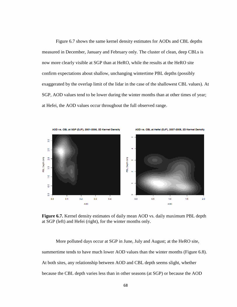
68
Figure 6.7 shows the same kernel density estimates for AODs and CBL depths
measured in December, January and February only. The cluster of clean, deep CBLs is
now more clearly visible at SGP than at HeRO, while the results at the HeRO site
confirm expectations about shallow, unchanging wintertime PBL depths (possibly
exaggerated by the overlap limit of the lidar in the case of the shallowest CBL values). At
SGP, AOD values tend to be lower during the winter months than at other times of year;
at Hefei, the AOD values occur throughout the full observed range.
Figure 6.7. Kernel density estimates of daily mean AOD vs. daily maximum PBL depth at SGP (left) and Hefei (right), for the winter months only.
More polluted days occur at SGP in June, July and August; at the HeRO site,
summertime tends to have much lower AOD values than the winter months (Figure 6.8).
At both sites, any relationship between AOD and CBL depth seems slight, whether
because the CBL depth varies less than in other seasons (at SGP) or because the AOD
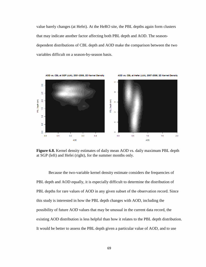
69
value barely changes (at Hefei). At the HeRO site, the PBL depths again form clusters
that may indicate another factor affecting both PBL depth and AOD. The season-
dependent distributions of CBL depth and AOD make the comparison between the two
variables difficult on a season-by-season basis.
Figure 6.8. Kernel density estimates of daily mean AOD vs. daily maximum PBL depth at SGP (left) and Hefei (right), for the summer months only.
Because the two-variable kernel density estimate considers the frequencies of
PBL depth and AOD equally, it is especially difficult to determine the distribution of
PBL depths for rare values of AOD in any given subset of the observation record. Since
this study is interested in how the PBL depth changes with AOD, including the
possibility of future AOD values that may be unusual in the current data record, the
existing AOD distribution is less helpful than how it relates to the PBL depth distribution.
It would be better to assess the PBL depth given a particular value of AOD, and to use

70
conditional probability instead of treating both variables equally in the kernel density
estimate.
In the most general possible terms the conditional probability is given by the
equation
𝑃𝑒{𝐸1|𝐸2} = 𝑃𝑃{𝑇1∩𝑇2}𝑃𝑃{𝑇2} , (6.3)
where E1 and E2 are the two variables under consideration. It follows that the conditional
probability of PBL depth given AOD can be determined by dividing the two-dimensional
kernel density estimate by the one-dimensional estimate for AOD.
The Nadaraya-Watson Estimator, first described by Nadaraya [1963] and Watson
[1964], adapts the principles of conditional probability to kernel density estimates. It is
given by the equation
𝑓(𝑦|𝑥) =∑ 𝑇ℎ1(𝑦−𝑦𝑖)𝑇ℎ2(𝑥−𝑥𝑖)𝑛𝑖=1
∑ 𝑇ℎ2(𝑥−𝑥𝑖)𝑛𝑖=1
, (6.4)
where h and K are again the smoothing parameter for each variable and kernel function,
respectively, as in equation 6.1. For the version of the Nadaraya-Watson estimator that is
available through the ksmooth function in R, h1 is set equal to h2 to form a single
bandwidth h that can be set by the user. The smaller the bandwidth, the more complex the
shape of the ensuing estimate and the more responsive to small-scale changes; the
optimal bandwidth value minimizes the average error of the estimate.
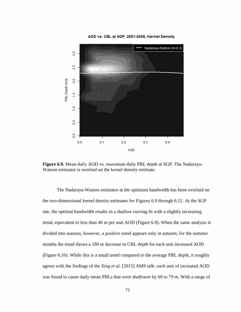
71
Figure 6.9. Mean daily AOD vs. maximum daily PBL depth at SGP. The Nadaraya-Watson estimator is overlaid on the kernel density estimate.
The Nadaraya-Watson estimator at the optimum bandwidth has been overlaid on
the two-dimensional kernel density estimates for Figures 6.9 through 6.12. At the SGP
site, the optimal bandwidth results in a shallow curving fit with a slightly increasing
trend, equivalent to less than 40 m per unit AOD (Figure 6.9). When the same analysis is
divided into seasons, however, a positive trend appears only in autumn; for the summer
months the trend shows a 180 m decrease in CBL depth for each unit increased AOD
(Figure 6.10). While this is a small trend compared to the average PBL depth, it roughly
agrees with the findings of the Xing et al. [2015] AMS talk: each unit of increased AOD
was found to cause daily mean PBLs that were shallower by 69 to 79 m. With a range of

72
0.4 in AOD values, this predicts that the lowest-AOD days should have PBL depths
approximately 30 m deeper than those of the days with the highest AOD values: a small
difference that is difficult to confirm through observation. When using the daily mean
PBL as Xing et al. [2015] did rather than the maximum, the Nadaraya-Watson estimator
found that the PBL depths at SGP changed by approximately 50 m instead, a slightly
stronger relationship than the model predicted.
Figure 6.10. The Nadaraya-Watson estimator overlaid on the daily mean AOD vs. the daily maximum PBL at SGP, during winter (left) and summer (right).
In the same way, the Xing et al. [2015] linear relationship between AOD and PBL
depth predicts a difference between the aerosol-free and most polluted days at the HeRO
site of almost 150 m. The Nadaraya-Watson estimator finds a difference of closer to 880
m, or approximately 440 m per unit AOD. When the same relationship is found for AOD
vs. the daily maximum PBL (Figure 6.11) the rate is 580 m per unit AOD.

73
Figure 6.11. Mean daily AOD vs. maximum daily PBL depth at Hefei. The Nadaraya-Watson estimator is overlaid on the kernel density estimate.
The steepness of this slope is certainly due to the bimodal behavior of the PBL
depths at Hefei. However, the negative trend remains even if the entire upper-left cluster
of PBL depths is considered unreliable and removed from the analysis. As seen in Figure
6.12, the Nadaraya-Watson estimator cutting through the center of the lower cluster
retains a negative slope of about 160 m per unit AOD. The cleanest days are estimated to
have a peak CBL depth of about 1.2 km, while the most polluted days have peak CBLs
shallower than 900 m.
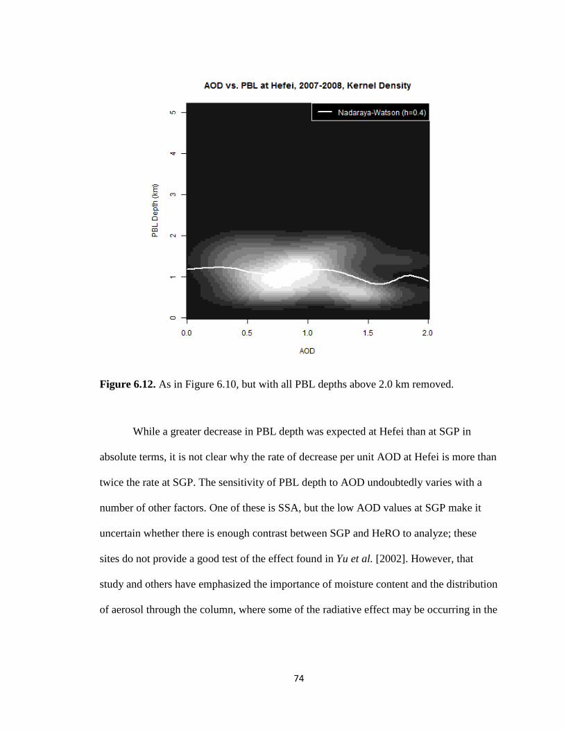
74
Figure 6.12. As in Figure 6.10, but with all PBL depths above 2.0 km removed.
While a greater decrease in PBL depth was expected at Hefei than at SGP in
absolute terms, it is not clear why the rate of decrease per unit AOD at Hefei is more than
twice the rate at SGP. The sensitivity of PBL depth to AOD undoubtedly varies with a
number of other factors. One of these is SSA, but the low AOD values at SGP make it
uncertain whether there is enough contrast between SGP and HeRO to analyze; these
sites do not provide a good test of the effect found in Yu et al. [2002]. However, that
study and others have emphasized the importance of moisture content and the distribution
of aerosol through the column, where some of the radiative effect may be occurring in the
75
free troposphere instead of within the PBL. These factors are discussed in Chapter 7 as
directions for future work.
6.3 Operational Radiosonde and Satellite-Based AOD
While the shortcomings of operational radiosonde for PBL detection are discussed
in Chapter 5, the network has denser spatial coverage in China than any other ground-
based measurement network of atmospheric profiles. This feature becomes crucial when
working with satellite data, such as AOD measurements taken from the Moderate
Resolution Imaging Spectroradiometer (MODIS) instrument aboard the NASA Aqua
satellite. Figure 6.12, created by Jianping Guo, demonstrates the geographic coverage of
satellite-based AOD measurements over China and identifies four typical pollution “hot
spots” for further study. These are the North China Plain (NCP), the Yangtze River Delta
(YRD), the Sichuan Basin (SCB) and the Pearl River Delta (PRD). Three radiosonde
sites from each region provide a comprehensive perspective of each “hot spot.”

76
Figure 6.13. AOD measurements from MODIS/Aqua for the geographic area coinciding with the operational radiosonde network in China. Radiosonde sites within four pollution “hot spots” are shown: squares “□” for NCP, circles “○” for YRD, diamonds “◇” for SCB, and five-pointed stars “☆” for PRD.
Over the period 2011-2013, each radiosonde site conducted over 2,000 launches,
mostly at 00:00 and 12:00 UTC (8:00 AM and 8:00 PM local) but with a few launches at
06:00 and 18:00 UTC (2:00 PM and 2:00 AM local). Guo used the PBL detection code
from this study to analyze the radiosonde profiles for PBL depth. Operational
observations of visibility are used to divide the profiles into thirds, with the highest third
(visibilities above 15 km at YRD, NCP and SCB or 18 km at PRD) considered “clean”
atmospheric conditions and the lowest third (visibilities below 7 km at YRD, 10 km at
NCP and SCB and 12 km at PRD) considered “polluted.” While this binary comparison
cannot reveal a linear relationship between PBL depth and AOD, the contrast in the
distribution of PBL depths is more clearly visible. Figure 6.13 shows the difference in the
likelihood of a range of PBL depths under clean and polluted conditions. The strength of

77
the apparent effect varies from one region to the next, but all four regions show an
increased probability of shallow PBL depths and a decreased probability of deep PBL
depths under polluted conditions as compared to clean conditions. This is consistent with
expectations that higher AOD values cause suppressed surface convection and shallower
overall PBL depths.
Figure 6.14. Probability distribution function of PBL depth under clean (blue) and polluted (red) conditions, for the regions a) NCP, b) SCB, c) YRD and d) PRD.
The extent of the difference in PBL depth between clean and polluted conditions
varies spatially; the smallest difference is observed at PRD, where it should be noted that
the threshold for polluted cases was significantly higher than for the other three regions.
Because the determination of “clean” and “polluted” days in Figure 6.13 is relative to
each site, regional differences in the absolute pollution levels during clean and polluted

78
cases are undoubtedly a factor. However, these results qualitatively confirm the findings
at the MPL sites for a wider variety of locations, showing that the relationship between
PBL depth and AOD is not an artifact due to limited observations.
79
Chapter 7. Future Work
7.1 Varying SSA, Humidity and Clouds
While the SGP and HeRO sites used in this study were necessary because of their
long MPL instrument records and contrasting AOD, neither site shows much internal
variation or contrast from one another in SSA that can be demonstrated conclusively.
Since the reflectivity and absorptivity of aerosols are at least as important as AOD to the
radiative impact and the resulting behavior of the PBL, this rather unrepresentative view
of aerosols is problematic. High SSA values are also often linked to moisture content, and
boundary-layer moisture has its own impact on PBL development [Garratt et al., 1990;
Yu et al., 2002]. Garratt et al. [1990] mentioned that the formation of fog can alter the
stability of the PBL. Humidity soundings are available at the SGP site from radiosonde
and AERI, but not at the other MPL deployments, and it is by no means certain that this
data would be available from a site that experienced high contrast in SSA values or
simply more absorbing aerosols. Raman lidar, which is capable of measuring both aerosol
backscatter and vertical moisture profiles, may offer the best of both worlds, but there are
few long-term deployments of this instrument in the US and China.
As the mention of fog makes clear, there is considerable overlap in the radiative
effects of aerosol, moisture, and clouds. The aerosol direct effect is not the only process
affecting the behavior of the PBL, and changes in the PBL depth will also change
boundary-layer clouds. Cloud bases are easily detected by MPL (and already included in
this project); at the SGP site, aerosol loading has been shown to affect cloud development
in a previous study by Li et al. [2011]. For convective clouds, the PBL top and the lifting
condensation level are linked, and aerosol affects them together. For stratocumulus
80
clouds, the possibility of decoupling is a further complication that cannot be addressed by
MPL—and has an ambiguous place in the thermodynamic definition of the PBL. Future
work must find a way to reconcile the effects of aerosol on boundary-layer clouds with
competing PBL definitions and the limitations of different measurement types.
7.2 An Alternative Modeling Approach
Previous modeling studies have simulated the PBL depth using the turbulent
definition, parameterizing the PBL depth in a way that does not explicitly simulate the
convective processes that are affected by aerosol radiative effects within the PBL. As
computational resources become available, there have been efforts to model convective
plumes and associated processes more directly. Some of this effort is directed at
improving the simulation of convective cloud development and precipitation [Rio et al.,
2013], but because boundary-layer cloud processes are intimately linked to the behavior
of the PBL, an advance to one process will also improve the other as long as the model
aims for greater overall realism. Rio et al. [2013] suggests basing boundary-layer cloud
schemes upon the available lifting power from the surface, rather than convective
available potential energy; this requires a more direct approach to convective thermals.
Gentine et al. [2013] uses probabilistic bulk convection to parameterize surface
convection, resulting in a more flexible simulation of the entrainment at the boundary
layer top and a unified approach to clear-sky and cloud-topped PBLs. Both these studies
evaluate their PBL results by comparing precipitation rates to observations; were direct
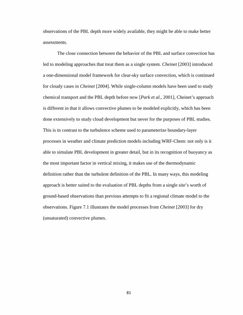
81
observations of the PBL depth more widely available, they might be able to make better
assessments.
The close connection between the behavior of the PBL and surface convection has
led to modeling approaches that treat them as a single system. Cheinet [2003] introduced
a one-dimensional model framework for clear-sky surface convection, which is continued
for cloudy cases in Cheinet [2004]. While single-column models have been used to study
chemical transport and the PBL depth before now [Park et al., 2001], Cheinet’s approach
is different in that it allows convective plumes to be modeled explicitly, which has been
done extensively to study cloud development but never for the purposes of PBL studies.
This is in contrast to the turbulence scheme used to parameterize boundary-layer
processes in weather and climate prediction models including WRF-Chem: not only is it
able to simulate PBL development in greater detail, but in its recognition of buoyancy as
the most important factor in vertical mixing, it makes use of the thermodynamic
definition rather than the turbulent definition of the PBL. In many ways, this modeling
approach is better suited to the evaluation of PBL depths from a single site’s worth of
ground-based observations than previous attempts to fit a regional climate model to the
observations. Figure 7.1 illustrates the model processes from Cheinet [2003] for dry
(unsaturated) convective plumes.
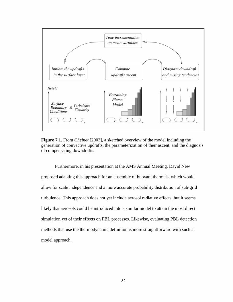
82
Figure 7.1. From Cheinet [2003], a sketched overview of the model including the generation of convective updrafts, the parameterization of their ascent, and the diagnosis of compensating downdrafts.
Furthermore, in his presentation at the AMS Annual Meeting, David New
proposed adapting this approach for an ensemble of buoyant thermals, which would
allow for scale independence and a more accurate probability distribution of sub-grid
turbulence. This approach does not yet include aerosol radiative effects, but it seems
likely that aerosols could be introduced into a similar model to attain the most direct
simulation yet of their effects on PBL processes. Likewise, evaluating PBL detection
methods that use the thermodynamic definition is more straightforward with such a
model approach.

83
Chapter 8. Conclusions
8.1 PBL Detection
The two main techniques for gradient-based PBL detection, wavelet covariance
[Davis et al., 2000; Brooks, 2003] and simulated annealing [Steyn et al., 1999; Hägeli et
al., 2000] have complementary strengths and weaknesses, as do different measurement
types. The former technique is flexible and simple enough to automate for analyses of
long time series and multiple sites, while the latter compensates for noisy signals and low
vertical resolution. Both are applicable to the aerosol gradient approximated by lidar
backscatter and also the gradient of potential temperature (θv) found in thermodynamic
profiles. Used together, they make it possible to detect the PBL depth in radiosonde, lidar
and infrared spectrometer profiles from the same location and to compare the resulting
PBL products. An algorithm combining the two approaches was developed and applied to
MPL backscatter, AERI θv and radiosonde profile data measured at the Southern Great
Plains site over the period of 1996-2004. Intercomparison between AERI- and
radiosonde-derived PBL depths shows that the combined algorithm can partly overcome
the limitations of the low AERI vertical resolution, with two-thirds of the variation
explained by the regression. Unlike MPL and radiosonde, AERI retrievals are unreliable
in cloudy conditions. The PBL depth is only detectable in cloud-free profiles.
The intercomparison between MPL- and radiosonde-derived PBL depths is
divided into subsets based on cloud conditions and temporal cycling. The algorithm is
able to detect the PBL to approximately equal agreement with radiosonde results whether
clouds are present or not: in both cases, while there is considerable scatter in the
intercomparison, regression R2 values are above 0.5 and the systematic error is low.
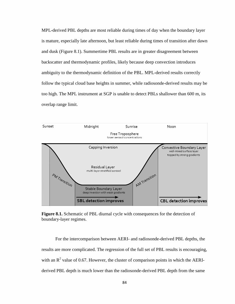
84
MPL-derived PBL depths are most reliable during times of day when the boundary layer
is mature, especially late afternoon, but least reliable during times of transition after dawn
and dusk (Figure 8.1). Summertime PBL results are in greater disagreement between
backscatter and thermodynamic profiles, likely because deep convection introduces
ambiguity to the thermodynamic definition of the PBL. MPL-derived results correctly
follow the typical cloud base heights in summer, while radiosonde-derived results may be
too high. The MPL instrument at SGP is unable to detect PBLs shallower than 600 m, its
overlap range limit.
Figure 8.1. Schematic of PBL diurnal cycle with consequences for the detection of boundary-layer regimes.
For the intercomparison between AERI- and radiosonde-derived PBL depths, the
results are more complicated. The regression of the full set of PBL results is encouraging,
with an R2 value of 0.67. However, the cluster of comparison points in which the AERI-
derived PBL depth is much lower than the radiosonde-derived PBL depth from the same

85
launch time becomes more significant when the results are broken down by time of day
and season. The diurnal cycle of the AERI-derived PBL depth is weak but present when
shallow PBLs are included in the analysis, but the seasonal cycle is not resolvable. AERI-
derived PBL depths are much too shallow during the summer months, at the same time
that radiosonde-derived PBL depths are wildly variable and MPL-derived PBL depths
stay close to the typical cloud base depth. The greater sensitivity of the AERI instrument
at lower levels may be responsible.
The combined PBL detection algorithm is able to retrieve PBL depths from both
remote sensing instruments that correspond well to radiosonde. The differences in the
two instruments are even complementary, with AERI best able to find shallow PBL
depths that MPL cannot detect, and MPL performing well in cloudy conditions that AERI
cannot reliably observe. MPL and AERI-derived PBL depths can therefore be considered
accurate at temporal resolutions much higher than the four times daily radiosonde launch,
and high-resolution PBL depths may be used for data assimilation and modeling. The
detected PBL-to-free-tropospheric transition depths are not reliable, but the more detailed
view of diurnal cycling in the PBL is useful in studies of aerosol transport and cloud-
aerosol interactions.
The PBL depth results from Chapter 4 of this project are now available as a data
product from the ARM archive, and can be found at the following link:
http://www.arm.gov/data/pi/84. There is an accompanying research highlight at
http://www.arm.gov/science/highlights/RNTA1/view with a brief overview of the method
and instruments used in that part of the project. This section of the project is described in
full in Sawyer and Li [2013]. In addition, work is underway to include the PBL detection
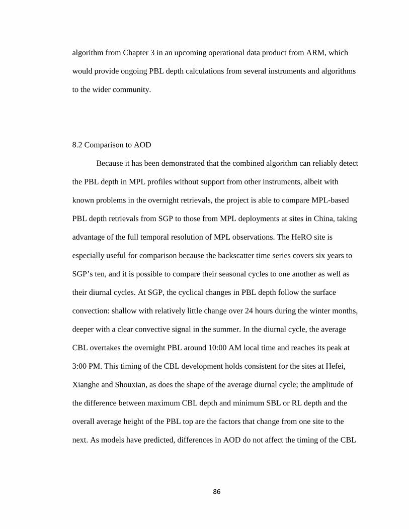
86
algorithm from Chapter 3 in an upcoming operational data product from ARM, which
would provide ongoing PBL depth calculations from several instruments and algorithms
to the wider community.
8.2 Comparison to AOD
Because it has been demonstrated that the combined algorithm can reliably detect
the PBL depth in MPL profiles without support from other instruments, albeit with
known problems in the overnight retrievals, the project is able to compare MPL-based
PBL depth retrievals from SGP to those from MPL deployments at sites in China, taking
advantage of the full temporal resolution of MPL observations. The HeRO site is
especially useful for comparison because the backscatter time series covers six years to
SGP’s ten, and it is possible to compare their seasonal cycles to one another as well as
their diurnal cycles. At SGP, the cyclical changes in PBL depth follow the surface
convection: shallow with relatively little change over 24 hours during the winter months,
deeper with a clear convective signal in the summer. In the diurnal cycle, the average
CBL overtakes the overnight PBL around 10:00 AM local time and reaches its peak at
3:00 PM. This timing of the CBL development holds consistent for the sites at Hefei,
Xianghe and Shouxian, as does the shape of the average diurnal cycle; the amplitude of
the difference between maximum CBL depth and minimum SBL or RL depth and the
overall average height of the PBL top are the factors that change from one site to the
next. As models have predicted, differences in AOD do not affect the timing of the CBL

87
peak; changes in SSA may, but the relatively low AOD values at SGP render the SSA
values too uncertain to compare conclusively to the sites in China.
While the seasonal cycle at SGP is relatively predictable, at the HeRO site the
interannual variability is strong enough to obscure it entirely. The summer diurnal cycle
still shows the strongest signs of surface convection over a 24-hour period, but counter to
expectations it is the shallowest on average; deeper PBL depths occur in winter, and there
are extended periods in the spring of 2005 and 2007 with very deep PBLs. More detailed
synoptic weather data from the site might help to determine whether the changes from
one year to the next are due to differences in the monsoon, the Asian dust season, or other
causes. In their study at the HeRO site, Wang et al. [2014] characterized the changes in
AOD with the seasonal cycle; from the patterns they found and the record of PBL depths
at Hefei, it can be inferred that higher AOD values disrupt the periodic behavior of the
PBL depth and may suppress convection.
The WRF-Chem simulation of April 2004 at SGP is a first step to comparing
AOD to PBL depth directly. PBL depths taken at the standard radiosonde launch interval
show a weak negative trend with increasing AOD for daytime and early-evening
retrievals, with a weaker positive or null trend for the overnight and early-morning
retrievals. The trends are qualitatively similar for both the YSU scheme PBL depths
calculated by the model and for the PBL depths found by extracting the simulated θv
profile and using the combined algorithm as if for radiosonde or infrared spectrometer.
The same trends are found when actual radiosonde-derived PBL depths are compared to
the daily mean AOD values from the modeled period instead, whether using the Sawyer
and Li [2013] retrievals or the set from Liu and Liang [2010]. While the relationship is
88
only borderline significant and the sample size is too small to quantify the effect with any
confidence, it is not dependent on the method used to find the PBL.
Much larger sample sizes are available by comparing the daily mean AOD values
to the PBL depth retrievals from the full observation period that coincides with the AOD
product. Though AOD observations are never available for the full length of the MPL
deployment, the comparison can be made for 2001-2006 at SGP and for 2007-2008 at
Hefei. Even exploratory statistics show that the distribution of daily mean PBL depths
trends shallower with increasing AOD, with a much more pronounced effect at Hefei
because of its greater available range in AOD values. It can also be shown that this trend
is limited to the CBL while the overnight SBL and RL retrievals are unaffected;
increasing AOD values suppress surface convection, but have no impact on the PBL
depth when convection cannot occur.
Probability density functions offer a more detailed analysis of the large data sets.
Kernel density estimates show that the CBL depth and AOD distributions form clusters
that are specific to certain times of year. While the highest PBL tops at Hefei seem
suspicious because of their separation from the rest of the data and the possibility that the
cleanest AOD days offer the least MPL backscatter in which to detect the PBL depth,
they can be excluded from the data entirely without affecting the conclusion that the daily
mean PBL depth decreases with increasing AOD. The rate of decrease as well as the
absolute change in PBL depth is much greater at the HeRO site than at SGP. For every
unit of increased mean daily AOD, the mean daily PBL depth is roughly 120 m shallower
at SGP and 220 m shallower at Hefei (suspicious cluster excluded); this is somewhat
greater than previous estimates of the relationship made through model simulations. For

89
maximum daily PBL depths, which the algorithm detects most reliably, the relationship
ranges from a slight increase with AOD at SGP to a decrease of 580 m per unit AOD at
Hefei.
It would be helpful in future to expand the study of aerosol-PBL interactions to
include the effects of varying SSA, moisture content, and distribution of aerosols through
the atmospheric column. There are also modeling approaches that have yet to be applied
to this problem. However, this study has already shown that the PBL depth can be
detected more accurately and with greater flexibility than was possible using previous
methods, and that it interacts with AOD in a way that is consistent with or stronger than
the modeled radiative effects. As aerosol emissions increase and the optical depth of
aerosol in the atmosphere is enhanced, even aerosols that primarily scatter rather than
absorb solar radiation are able to disrupt the energy balance of the lower troposphere,
heating the mixed layer at the expense of the surface and enhancing atmospheric stability.
This in turn prevents the CBL from reaching its maximum depth over the course of the
day, resulting in shallower daily mean PBLs and a reduced volume for the dilution of
aerosols and other pollution within the mixed layer. Absorbing aerosol is likely to have a
stronger effect than scattering aerosol, and the behavior of boundary-layer convection and
cloud layers may change as consequences of the stability within the PBL. Aerosol-PBL
interactions must be studied in order to understand the impact of climate change and
future emissions on surface air quality, the water cycle and the energy balance within the
lower troposphere.
90
LIST OF REFERENCES
Amiridis, V., et al. (2007), Aerosol lidar observations and model calculations of the
planetary boundary layer evolution over Greece, during the March 2006 total
solar eclipse, Atmos. Chem. Phys., 7, 6181–6189.
Andreae, M.O., et al. (2004), Smoking rain clouds over the Amazon, Science, 303, 1338-
1342.
Beyrich, F. and U. Görsdorf (1995), Composing the diurnal cycle of mixing height from
simultaneous sodar and wind profiler measurements, Bound.-Layer Meteor., 76,
387-394.
Bianco, L. and J.M. Wilczak (2002), Convective boundary layer depth: Improved
measurement by Doppler radar wind profiler using fuzzy logic methods. J. Atmos.
Oceanic Technol., 19, 1745-1758.
Bloomer, B. J., et al. (2009), Observed relationships of ozone air pollution with
temperature and emissions, Geophys. Res. Lett., 36, L09803,
doi:10.1029/2009GL037308.
Brooks, Ian M. (2003), Finding boundary layer top: Application of a wavelet covariance
transform to lidar backscatter profiles, J. Atmos. Oceanic Technol., 20, 1092-
1105.
Campbell, J.R., et al. (2002), Full-Time, Eye-Safe Cloud and Aerosol Lidar Observation
at Atmospheric Radiation Measurement Program Sites: Instruments and Data
Processing. J. Atmos. Oceanic Technol., 19, 431-442.
Cheinet, Silvain (2003), A Multiple Mass-Flux Parameterization for the Surface-
Generated Convection. Part I: Dry Plumes, J. Atmos. Sci., 60, 2313-2327.
91
Cheinet, Silvain (2004), A Multiple Mass Flux Parameterization for the Surface-
Generated Convection. Part II: Cloudy Cores, J. Atmos. Sci., 61, 1093-1113.
Coulter, R. (2012), Micropulse Lidar (MPL) Handbook. U.S. Department of Energy.
http://www.arm.gov/publications/tech_reports/handbooks/mpl_handbook.pdf
Davis, K. J., et al. (2000), An objective method for deriving atmospheric structure from
airborne lidar observations, J. Atmos. Oceanic Technol., 17, 1455-1468.
Ding, A., et al. (2009), Transport of north China air pollution by midlatitude cyclones:
Case study of aircraft measurements in summer 2007, J. Geophys. Res., 114, doi:
10.1029/2009JD012339.
Ding, A., et al. (2013), Intense atmospheric pollution modifies weather: a case of mixed
biomass burning with fossil fuel combustion pollution in eastern China. Atmos.
Chem. Phys., 13, 10545-10554.
Donnell, E.A., D.J. Fish and E.M. Dicks (2001), Mechanisms for pollutant transport
between the boundary layer and the free troposphere, J. Geophys. Res., 106, 7847-
7856.
Feingold, G., et al. (2005), On smoke suppression of clouds in Amazonia, Geophys. Res.
Lett., 32, L02804, doi:10.1029/2004GL021369.
Feltz, W.F., et al. (1998), Meteorological applications of temperature and water vapor
retrievals from the ground-based atmospheric emitted radiance interferometer
(AERI). J. Appl. Meteor. 37, 857-875.
Feltz, W.F., et al. (2003), Near-continuous profiling of temperature, moisture, and
atmospheric stability using the atmospheric emitted radiance interferometer
(AERI). J. Appl. Meteor. 42, 584-597.
92
Feltz, W.F., et al. (2007), Retrieving Temperature and Moisture Profiles from AERI
Radiance Observations: AERIPROF Value-Added Product Technical
Description. U.S. Department of Energy.
http://www.arm.gov/publications/tech_reports/doe-sc-arm-tr-066.1.pdf?id=168
Fernald, F.G. (1984), Analysis of atmospheric lidar observations: some comments,
Applied Optics 23, 652-653.
Flynn, Connor J., et al. (2007), "Novel polarization-sensitive micropulse lidar
measurement technique." Optics Express, 15.6, 2785-2790.
Flynn, C. et al. (2012), Aerosol Best Estimate (AEROSOLBE) Value-Added Product. U.S.
Department of Energy. http://www.arm.gov/publications/tech_reports/doe-sc-
arm-tr-115.pdf?id=472
Garratt, J.R., A.B. Pittock and K. Walsh, 1990. Response of atmospheric boundary layer
and soil layer to a high altitude, dense aerosol cover. J. Appl. Meteor. 29, 35-52.
Georgoulias, A.K., et al. (2009), Statistical analysis of boundary layer heights in a
suburban environment, Meteorol. Atmos. Phys. 104, 103-111.
Gentine, Pierre, et al. (2013), A Probabilistic Bulk Model of Coupled Mixed Layer and
Convection. Part I: Clear-Sky Case, J. Atmos. Sci. 70, 1543-1556.
Hägeli, P., D.G. Steyn and K.B. Strawbridge (2000), Spatial and temporal variability of
mixed-layer depth and entrainment zone thickness, Boundary-Layer Meteorol.,
97, 47-71.
He, H., et al. (2013), High ozone concentrations on hot days: The role of electric power
demand and NOx emissions, Geophys. Res. Lett., 40, 5291–5294.

93
Henne, S., et al. (2004), Quantification of topographic venting of boundary layer air to
the free troposphere, Atmos. Chem. Phys., 4, 497–509.
Hennemuth, B. and A. Lammert (2006), Determination of the atmospheric boundary
layer height from radiosonde and lidar backscatter, Boundary-Layer Meteorol.
120, 181-200.
Holdridge, D., et al. (2011), Balloon-Borne Sounding System (SONDE) Handbook. U.S.
Department of Energy.
http://www.arm.gov/publications/tech_reports/handbooks/sonde_handbook.pdf
Hu, X.-M., et al. (2010), Evaluation of three boundary layer schemes in the WRF model,
J. Appl. Meteor. Climatol., 49, 1831-1844.
IPCC, 2007. Climate Change 2007: The Physical Science Basis. Contribution of Working
Group I to the Fourth Assessment Report of the Intergovernmental Panel on
Climate Change [Solomon, S., D. Qin, M. Manning, Z. Chen, M. Marquis, K.B.
Averyt, M. Tignor and H.L. Miller (eds.)]. Cambridge University Press,
Cambridge, United Kingdom and New York, NY, USA.
Jacob, D. J. and D.A. Winner (2009), Effect of climate change on air quality, Atmos. Env.
43, 51-63.
Jordan, N.S., et al. (2010), Validation of Goddard Earth Observing System‐version
5 MERRA planetary boundary layer heights using CALIPSO, J. Geophys. Res., 115,
D24218, doi:10.1029/2009JD013777.
Klett, J.D. (1985), Lidar inversion with variable backscatter/extinction ratios, Applied
Optics 24, 1638-1643.
94
Kong, W., and F. Yi (2015), Convective boundary layer evolution from lidar backscatter
and its relationship with surface aerosol concentration at a location of a central
China megacity, J. Geophys. Res. Atmos., 120, doi:10.1002/2015JD023248.
Law, K.S. and A. Stohl (2007), Arctic air pollution: origins and impacts, Science, 315,
1537.
Lewis, J. R., et al. (2013), Improved boundary layer depth retrievals from MPLNET, J.
Geophys. Res., 118, 9870-9879.
Li, C., et al. (2010), Transport and evolution of a pollution plume from northern China: A
satellite-based case study, J. Geophys. Res., 115, D00K03,
doi:10.1029/2009JD012245.
Li, Z., et al. (2011), Long-term impacts of aerosols on the vertical development of clouds
and precipitation, Nature Geoscience 4, 888-894.
Liu, S. and X.-Z. Liang (2010), Observed diurnal cycle climatology of planetary
boundary layer height, J. Climate, 23, 5790-5809.
Ma, M., et al. (2011), Characteristics and numerical simulations of extremely large
atmospheric boundary-layer heights over an arid region in north-west China,
Boundary-Layer Meteorol.,140, doi:10.1007/s10546-011-9608-2.
Marenco, F., et al. (1997), Optical properties of tropospheric aerosols determined by lidar
and spectrophotometric measurements (Photochemical Activity and Solar
Ultraviolet Radiation campaign), Applied Optics 36, 6875-6886.
Medeiros, B., A. Hall and B. Stevens (2005), What controls the mean depth of the PBL?,
J. Climate, 18, 3157-3172.

95
Melfi, S.H., et al. (1985), Lidar observations of vertically organized convection in the
planetary boundary layer over the ocean, J. Climate Appl. Meteor., 24, 806-821.
Nadaraya, E.A. (1963), On estimating regression, Theory Probab. Appl., 9, 141-142.
New, David A. (2015, January), A unified model of the planetary boundary layer and
shallow cumulus convection. Paper presented at the AMS Annual Meeting,
Phoenix, AZ.
Palm, S., et al. (1998), Inference of marine atmospheric boundary layer moisture and
temperature structure using airborne lidar and infrared radiometer data, J. Appl.
Meteor., 37, 308-324.
Parikh, N.C. and J.A. Parikh (2002), Systematic tracking of boundary layer aerosols with
laser radar, Optics & Laser Technology, 34, 177-185.
Park, R.J., et al. (2001), Regional air pollution and its radiative forcing: Studies with a
single-column chemical and radiation transport model, J. Geophys. Res. 106,
28,751-28,770.
Press, W. H., S. A. Teukolsky, W. T. Vettering, and B. R. Flannery (1992), Numerical
Recipes in FORTRAN: The Art of Scientific Computing, 2nd ed., Cambridge
University Press, pp. 436-447.
Quinn, P. K., et al. (2007), Arctic haze: current trends and knowledge gaps. Tellus 59B, 99-114.
Rio, Catherine, et al. (2013), Control of deep convection by sub-cloud lifting processes:
the ALP closure in the LMDZ5B general circulation model, Clim. Dyn. 40, 2271–
2292.

96
Sawyer, V.R. and Z. Li (2013), Detection, variations and intercomparison of the
planetary boundary layer depth from radiosonde, lidar and infrared spectrometer,
Atmos. Env. 79, 518-528.
Seibert, P., et al. (2000), Review and intercomparison of operational methods for the
determination of the mixing height, Atmos. Environ., 34, 1001-1027.
Seinfeld, John H. and Spyros N. Pandis (2006), Atmospheric Chemistry and Physics:
from Air Pollution to Climate Change, 2nd ed., WileyBlackwell, Hoboken, N.J.
Sivaraman, C. and J. Comstock (2011), Micropulse Lidar Cloud Mask Value-Added
Product Technical Report. U.S. Department of Energy.
http://www.arm.gov/publications/tech_reports/doe-sc-arm-tr-098.pdf
Spinhirne, J.D., et al. (1995), "Compact Eye Safe Lidar Systems," Rev. Laser Eng., 23,
112-118.
Spinhirne, James D (1993), "Micro pulse lidar." Geoscience and Remote Sensing, IEEE
Transactions 31.1 (1993): 48-55.
Steyn, D.G., M. Baldi and R.M. Hoff (1999), The detection of mixed layer depth and
entrainment zone thickness from lidar backscatter profiles, J. Atmos. Ocean.
Technol., 16, 953-959.
Stull, Ronald B. (1988), An Introduction to Boundary Layer Meteorology, Springer-
Verlag New York, LLC.
Sun, Y., et al. (2010), Asian dust over northern China and its impact on the downstream
aerosol chemistry in 2004, J. Geophys. Res., 115, D00K09,
doi:10.1029/2009JD012757.

97
Tskaknakis, G. et al. (2011), Inter-comparison of lidar and ceilometer retrievals for
aerosol and Planetary Boundary Layer profiling over Athens, Greece, Atmos.
Meas. Tech. 4, 1261–1273.
Twohy, C.H., et al. (2002), Deep convection as a source of new particles in the
midlatitude upper troposphere, J. Geophys. Res., 107, D21, doi:
10.1029/2001JD000323.
Venkatram, A. and R. Viskanta (1977), Effects of aerosol-induced heating on the
convective boundary layer. J. Atmos. Sci., 34, 1918-1933.
Wang, Z., and K. Sassen (2001), Cloud Type and Macrophysical Property Retrieval
Using Multiple Remote Sensors, J. Appl. Meteor., 40, 1665-1682.
Wang, Z. et al. (2014), Seasonal characteristics of aerosol optical properties at the
SKYNET Hefei site (31.90°N, 117.17°E) from 2007 to 2013, J. Geophys. Res.
Atmos., 119, 6128–6139, doi:10.1002/2014JD021500.
Watson, G.S. (1964), Smooth regression analysis, Sankhyā: The Indian Journal of
Statistics, Series A, 26, 359-372.
Welton, E. J., et al. (2001), Global monitoring of clouds and aerosols using a network of
micro-pulse lidar systems, in Lidar Remote Sensing for Industry and
Environmental Monitoring, U. N. Singh, T. Itabe, N. Sugimoto, (eds.), Proc.
SPIE, 4153, 151-158.
Xing, J., et al. (2015, January), Air pollution and climate response to aerosol direct
radiative effects: a modeling study of decadal trends across the northern
hemisphere. Paper presented at the AMS Annual Meeting, Phoenix, AZ.
98
Yang, X., M. Ferrat, and Z. Li (2013a), New evidence of orographic precipitation
suppression by aerosols in central China, Meteorol. Atmos. Phys.,
doi:10.1007/s00703-012-0221-9.
Yang, X., Z. Yao, Z. Li, and T. Fan (2013b), Heavy air pollution suppresses summer
thunderstorms in central China, J. Atmos. Sol-Terr. Phy., 95-96, 28-40.
Yu, H., S. C. Liu and R. E. Dickinson, 2002. Radiative effects of aerosols on the
evolution of the atmospheric boundary layer. J. Geophys. Res. 107,
doi:10.1029/2001JD000754.
Zhang, Y., X.-Y. Wen and C.J. Jang (2010), Simulating chemistry-aerosol-cloud-
radiation-climate feedbacks over the continental U.S. using the online-coupled
Weather Research Forecasting Model with chemistry (WRF/Chem), Atmos. Env.,
44, 3568-3582.