ABSTRACT

Title of dissertation: DICTIONARIES AND MANIFOLDS FOR

FACE RECOGNITION ACROSS

ILLUMINATION, AGING AND QUANTIZATION

Tao Wu, Doctor of Philosophy, 2013

Dissertation directed by: Professor Rama Chellappa

Department of Electrical and Computer Engineering

During the past many decades, many face recognition algorithms have beenproposed. The face recognition problem under controlled environment has beenwell studied and almost solved. However, in unconstrained environments, the per-formance of face recognition methods could still be significantly affected by factorssuch as illumination, pose, resolution, occlusion, aging, etc. In this thesis, we lookinto the problem of face recognition across these variations and quantization.

We present a face recognition algorithm based on simultaneous sparse approx-imations under varying illumination and pose with dictionaries learned for eachclass. A novel test image is projected onto the span of the atoms in each learneddictionary. The resulting residual vectors are then used for classification. An im-age relighting technique based on pose-robust albedo estimation is used to generatemultiple frontal images of the same person with variable lighting. As a result, theproposed algorithm has the ability to recognize human faces with high accuracyeven when only a single or a very few images per person are provided for train-ing. The efficiency of the proposed method is demonstrated using publicly availabledatabases and it is shown that this method is efficient and can perform significantlybetter than many competitive face recognition algorithms.

The problem of recognizing facial images across aging remains an open prob-lem. We look into this problem by studying the growth in the facial shapes. Buildingon recent advances in landmark extraction, and statistical techniques for landmark-based shape analysis, we show that using well-defined shape spaces and its associatedgeometry, one can obtain significant performance improvements in face verification.Toward this end, we propose to model the facial shapes as points on a Grassmann

manifold. The face verification problem is then formulated as a classification prob-lem on this manifold. We then propose a relative craniofacial growth model which isbased on the science of craniofacial anthropometry and integrate it with the Grass-mann manifold and the SVM classifier. Experiments show that the proposed methodis able to mitigate the variations caused by the aging progress and thus effectivelyimprove the performance of open-set face verification across aging.

In applications such as document understanding, only binary face images maybe available as inputs to a face recognition algorithm. We investigate the effects ofquantization on several classical face recognition algorithms. We study the perfor-mances of PCA and multiple exemplar discriminant analysis (MEDA) algorithmswith quantized images and with binary images modified by distance and Box-Coxtransforms. We propose a dictionary-based method for reconstructing the grey scalefacial images from the quantized facial images. Two dictionaries with low mutualcoherence are learned for the grey scale and quantized training images respectivelyusing a modified KSVD method. A linear transform function between the sparsevectors of quantized images and the sparse vectors of grey scale images is estimatedusing the training data. In the testing stage, a grey scale image is reconstructedfrom the quantized image using the transform matrix and normalized dictionaries.The identities of the reconstructed grey scale images are then determined using thedictionary-based face recognition (DFR) algorithm. Experimental results show thatthe reconstructed images are similar to the original grey-scale images and the perfor-mance of face recognition on the quantized images is comparable to the performanceon grey scale images.

The online social network and social media is growing rapidly. It is interestingto study the impact of social network on computer vision algorithms. We addressthe problem of automated face recognition on a social network using a loopy beliefpropagation framework. The proposed approach propagates the identities of facesin photos across social graphs. We characterize its performance in terms of struc-tural properties of the given social network. We propose a distance metric definedusing face recognition results for detecting hidden connections. The performance ofthe proposed method is analyzed on graph structure networks, scalability, differentdegrees of nodes, labeling errors correction and hidden connections discovery. Theresult demonstrates that the constraints imposed by the social network have thepotential to improve the performance of face recognition methods. The result alsoshows it is possible to discover hidden connections in a social network based on facerecognition.

DICTIONARIES AND MANIFOLDS FOR FACE RECOGNITIONACROSS ILLUMINATION, AGING AND QUANTIZATION

by

Tao Wu

Dissertation submitted to the Faculty of the Graduate School of theUniversity of Maryland, College Park in partial fulfillment

of the requirements for the degree ofDoctor of Philosophy

2013

Advisory Committee:Professor Rama Chellappa, Chair/AdvisorProfessor Larry DavisProfessor Min WuDr. Jonathon PhillipsDr. David Doermann

c© Copyright byTao Wu

2013

Dedication

In memory of my grandmother

To my grandfather and parents

and my wife

ii

Acknowledgements

I am grateful to all the people who have made this dissertation possible.

First and foremost, I owe my deepest gratitude to my advisor, Professor Rama

Chellappa, for giving me invaluable opportunities to work on challenging and ex-

tremely interesting projects. He has always made himself available for help and

advice. Without his immeasurable support, guidance and encouragement through

the past five years, this thesis would have been a distant dream. He is the one who

saw my potential and has given me so much insightful inspirations and generous

help both in research and in life that I will cherish for my life. I, truly, am honored

to work with and learn from such an extraordinary scholar.

I am deeply grateful to Dr. Jonathon Phillips for his generous sponsorship

from the NIST-ARRA fellowship. Without his kind and continuous support, this

dissertation would not be possible. I am also very grateful to have the opportunity

to work with and learn from him. He played a crucial role in the social network

project. His brilliant theoretical ideas, insightful guidance and his polite manners

have always made our discussions fruitful and enjoyable.

I would like to express my sincere appreciation to Professor Larry Davis, Pro-

fessor Min Wu and Dr. David Doermann for serving as my defense committee

members and devoting their precious time reviewing the manuscript. I would also

like to thank Dr. David Doermann for his helpful advice in the project of quantized

facial image recognition.

I am also grateful to Professor Eric Slud, Professor Adrian Papamarcou, Pro-

fessor Jaydev Desai, Professor Prakash Narayan and Professor Mark Shayman for

their enlightening instructions during my graduate studies.

Many thanks to Professor Paven Turaga for his kind support in the collabora-

tion of the face recognition across aging project and Dr. Vishal Patel and Dr. Soma

Biswas for their helpful discussions and support while working on the dictionary-

based face recognition project. I would also like to thank Dr. Kaushik Mitra, Dr.

Ruonan Li, Dr. Raghuram Gopalan, Dr. Narayanan Ramanathan, Dr. Jaishanker

iii

Pillai, Ming Du, Dr. Yi-Chen Chen, Dr. Sima Taheri, and Huy Tho Ho for stimu-

lating helpful discussions on various topics.

I would like to acknowledge help and support from all the administrative and

technical staff members. In particular, thanks are due to Melanie Prange, Janice

Perrone, Arlene Schenk, Maria Hoo, Barbara Brawn-Cinani and Roxanne Defendini.

Graduate life would not have been better without my fellow graduate stu-

dents and friends. I would like to thank Dr. Yongle Wu, Hua Chen, Dr. Wei-Hong

Chuang, Dr. Nitesh Shroff, Jie Ni, Garrett Warnell, Kota Hara, Xavier Gibert Serra,

Dr. Dikpal Reddy, Dr. Qiang Qiu, Jingjing Zheng, Ching-Hui Chen, Raviteja Vem-

ulapalli, Nazre Batool, Ashish Srivastava, Sumit Shekhar, Priyanka Vageeswaran,

Ming-Yu Liu and Hien Nguyen.

Last but not least, I would like to give my special thanks to my kind grand-

mother in heaven, my beloved grandfather and parents. For so many years, they

always give me unconditional love, support and encouragement. I wound also like

to thank my parents-in-law for loving me as their own son. Finally, this thesis is

dedicated to the love of my life, my wife, for her love, support and understanding.

It is impossible to remember all and I apologize to those I have inadvertently

left out.

iv

Table of Contents

List of Figures viii

1 Introduction 11.1 Motivation . . . . . . . . . . . . . . . . . . . . . . . . . . . . . . . . . 11.2 Organization . . . . . . . . . . . . . . . . . . . . . . . . . . . . . . . 21.3 Contributions . . . . . . . . . . . . . . . . . . . . . . . . . . . . . . . 3

2 Background 72.1 Dictionaries . . . . . . . . . . . . . . . . . . . . . . . . . . . . . . . . 72.2 Manifolds . . . . . . . . . . . . . . . . . . . . . . . . . . . . . . . . . 82.3 The Role of Facial Shapes . . . . . . . . . . . . . . . . . . . . . . . . 122.4 Face Recognition Challenges . . . . . . . . . . . . . . . . . . . . . . . 15

2.4.1 Illumination and Pose . . . . . . . . . . . . . . . . . . . . . . 152.4.2 Aging . . . . . . . . . . . . . . . . . . . . . . . . . . . . . . . 162.4.3 Quantization . . . . . . . . . . . . . . . . . . . . . . . . . . . 17

3 Dictionary Based Face Recognition 223.1 Dictionary-based Recognition . . . . . . . . . . . . . . . . . . . . . . 22

3.1.1 Learning Class Specific Reconstructive Dictionaries . . . . . . 223.1.2 Classification based on Learned Dictionaries . . . . . . . . . . 243.1.3 Dealing with Small Arbitrary Noise . . . . . . . . . . . . . . . 253.1.4 Rejection Rule for Non-face Images . . . . . . . . . . . . . . . 27

3.2 Face Recognition across Varying Illumination and Pose . . . . . . . . 303.2.1 Albedo Estimation . . . . . . . . . . . . . . . . . . . . . . . . 303.2.2 Image Relighting . . . . . . . . . . . . . . . . . . . . . . . . . 313.2.3 Pose-robust Albedo Estimation . . . . . . . . . . . . . . . . . 33

3.3 Experimental Results . . . . . . . . . . . . . . . . . . . . . . . . . . . 363.3.1 Results on Extended Yale B Database . . . . . . . . . . . . . 373.3.2 Results on PIE Database . . . . . . . . . . . . . . . . . . . . . 393.3.3 Results on AR Database . . . . . . . . . . . . . . . . . . . . . 433.3.4 Experiment on a Remote Face Dataset . . . . . . . . . . . . . 443.3.5 Recognition with Partial Face Features . . . . . . . . . . . . . 47

v

3.3.6 Rejecting Non-face Images . . . . . . . . . . . . . . . . . . . . 483.3.7 Recognition Rate vs. Number of Dictionary Atoms . . . . . . 503.3.8 Recognition Rate vs. Number of Training Images . . . . . . . 503.3.9 Efficiency . . . . . . . . . . . . . . . . . . . . . . . . . . . . . 533.3.10 Limitations . . . . . . . . . . . . . . . . . . . . . . . . . . . . 53

4 Face Recognition Across Aging 554.1 Geometry of the Grassmann Manifold . . . . . . . . . . . . . . . . . . 554.2 Experimental Results of Grassmann Manifold . . . . . . . . . . . . . 58

4.2.1 Experiment on the MUCT Dataset . . . . . . . . . . . . . . . 584.2.2 Experiment on the FG-NET Database . . . . . . . . . . . . . 594.2.3 Effect of the Age Gap . . . . . . . . . . . . . . . . . . . . . . 62

4.3 Facial Growth Model . . . . . . . . . . . . . . . . . . . . . . . . . . . 634.3.1 Classical Craniofacial Growth Model . . . . . . . . . . . . . . 634.3.2 Relative Craniofacial Growth Model . . . . . . . . . . . . . . . 654.3.3 Learning the Relative Growth Parameters . . . . . . . . . . . 684.3.4 Experiment Results with Facial Growth Model . . . . . . . . . 69

4.3.4.1 Verification Experiments . . . . . . . . . . . . . . . . 694.3.4.2 Effect of the Age Gap . . . . . . . . . . . . . . . . . 724.3.4.3 Robustness Against Inaccurate Age Information . . . 73

4.4 Texture-based Face Recognition . . . . . . . . . . . . . . . . . . . . . 754.4.1 Method . . . . . . . . . . . . . . . . . . . . . . . . . . . . . . 754.4.2 Experiment Results of Texture Features . . . . . . . . . . . . 76

4.4.2.1 Verification on FG-NET . . . . . . . . . . . . . . . . 764.4.2.2 Verification and Identification on MORPH . . . . . . 76

5 Face Recognition with Quantized Images 805.1 Introduction . . . . . . . . . . . . . . . . . . . . . . . . . . . . . . . . 805.2 Algorithms . . . . . . . . . . . . . . . . . . . . . . . . . . . . . . . . . 80

5.2.1 Review of Principal Component Analysis . . . . . . . . . . . . 805.2.2 Multiple-Exemplar Discriminant Analysis . . . . . . . . . . . . 81

5.3 Recognition of Quantized Face Images . . . . . . . . . . . . . . . . . 825.3.1 Quantization and Binarization Method . . . . . . . . . . . . . 825.3.2 Dataset . . . . . . . . . . . . . . . . . . . . . . . . . . . . . . 845.3.3 Effect of the Number of Grey Levels . . . . . . . . . . . . . . 855.3.4 Performance Comparison on Binary Images . . . . . . . . . . 875.3.5 Face Verification under Noise, Down Sampling and Different

Binarization Threshold . . . . . . . . . . . . . . . . . . . . . . 915.4 Reconstruction Method . . . . . . . . . . . . . . . . . . . . . . . . . . 925.5 Experiment Results . . . . . . . . . . . . . . . . . . . . . . . . . . . . 96

5.5.1 Reconstruction . . . . . . . . . . . . . . . . . . . . . . . . . . 965.5.2 Recognition . . . . . . . . . . . . . . . . . . . . . . . . . . . . 99

vi

6 Face Recognition Across Social Networks 1036.1 Introduction . . . . . . . . . . . . . . . . . . . . . . . . . . . . . . . . 103

6.1.1 The Effects of Social Network on Computer Vision . . . . . . 1036.1.2 The Effects of Computer Vision on Social Network . . . . . . 1056.1.3 Models and Algorithms for Social Networks . . . . . . . . . . 105

6.2 Propagation of Facial Identities . . . . . . . . . . . . . . . . . . . . . 1076.2.1 Representation of a Social Network . . . . . . . . . . . . . . . 1076.2.2 Belief Propagation . . . . . . . . . . . . . . . . . . . . . . . . 1086.2.3 Classifiers . . . . . . . . . . . . . . . . . . . . . . . . . . . . . 1106.2.4 Discovery of Hidden Connections . . . . . . . . . . . . . . . . 111

6.3 Experimental Results . . . . . . . . . . . . . . . . . . . . . . . . . . . 1136.3.1 Dataset . . . . . . . . . . . . . . . . . . . . . . . . . . . . . . 1136.3.2 Results . . . . . . . . . . . . . . . . . . . . . . . . . . . . . . . 116

6.3.2.1 Comparison with Methods without Social Network . 1166.3.2.2 Scalability Over the Size of the Graph . . . . . . . . 1186.3.2.3 Effects of the Degrees of the Nodes . . . . . . . . . . 1196.3.2.4 Correction of Incorrectly Labeled Images . . . . . . . 1206.3.2.5 Discovery of Hidden Connections . . . . . . . . . . . 121

7 Conclusions and Future Work 1237.1 Conclusions . . . . . . . . . . . . . . . . . . . . . . . . . . . . . . . . 1237.2 Future Work . . . . . . . . . . . . . . . . . . . . . . . . . . . . . . . . 126

Bibliography 128

vii

List of Figures

3.1 Overview of our approach. (a) Given C sets of training images corre-sponding to C different faces, the K-SVD algorithm is used to learnface specific dictionaries. Then, a novel test image is projected ontothe span of the atoms in each of the learned dictionaries and the ap-proximation errors are computed. (b) The class that is associated toa test image is then declared as the one that produces the smallestapproximation error. In this example, class 1 is declared as the trueclass. (c) and (d) illustrate an example of a non-face test image andthe resulting residuals, respectively. . . . . . . . . . . . . . . . . . . . 26

3.2 Score values normalized using equation (3.10) and sorted. Plot (a)corresponds to the test image shown in Fig. 3.1(a) and plot (b) cor-responds to the non-face test image shown in Fig. 3.1(c). . . . . . . . 29

3.3 Examples of the original images (first column) and the correspondingrelighted images with different light source directions from the PIEdata set. . . . . . . . . . . . . . . . . . . . . . . . . . . . . . . . . . . 32

3.4 Pose-robust albedo estimation. Left column: Original input images.Middle column: Recovered albedo maps corresponding to frontal faceimages. Right column: Pose normalized relighted images. . . . . . . . 34

3.5 The DFR algorithm. . . . . . . . . . . . . . . . . . . . . . . . . . . . 353.6 Performance comparison on the Extended Yale B database with var-

ious features, feature dimensions and methods. (a) Our method(DFR) (b) CDPCA (c) SRC [1]. . . . . . . . . . . . . . . . . . . . . . 38

3.7 A few learned dictionaries from the Extended YaleB dataset. Eachrow corresponds to a learned dictionary. By looking at each row, wesee that the learned atoms are able to extract the common internalstructure of images belonging the same class and are able to removemuch of the illumination. . . . . . . . . . . . . . . . . . . . . . . . . . 39

3.8 A few cropped face images from the remote face dataset. (a) Sampleimages from the illumination folder. (b) Sample images from the posefolder. . . . . . . . . . . . . . . . . . . . . . . . . . . . . . . . . . . . 45

3.9 Recognition results on the remote face dataset corresponding to (a)illumination folder and (b) pose folder. . . . . . . . . . . . . . . . . . 46

viii

3.10 Examples of partial facial features. (a) Eye (b) Nose (c) Mouth. . . . 473.11 (a) ROC curves corresponding to rejecting outliers. The solid curve is

generated by the DFR method based on our rejection rule. The dot-ted curves correspond to the cases when different levels of occlusionhas been added to the test images. (b) ROC curve corresponding torejecting invalid test samples. . . . . . . . . . . . . . . . . . . . . . . 49

3.12 Recognition rate vs. number of dictionary atoms on the ExtendedYale B dataset. . . . . . . . . . . . . . . . . . . . . . . . . . . . . . . 51

4.1 Two shapes S1 and S2 are mapped to Y1 and Y2 on the Grassmannmanifold. The distance is computed by embedding the shapes to theambient space Pn,d. . . . . . . . . . . . . . . . . . . . . . . . . . . . . 57

4.2 An example of the image and the facial landmarks in the MUCTdataset. [2] . . . . . . . . . . . . . . . . . . . . . . . . . . . . . . . . 58

4.3 The ROC curve for the three-fold validation experiment on the MUCTdataset. . . . . . . . . . . . . . . . . . . . . . . . . . . . . . . . . . . 59

4.4 Examples of the images and landmarks (labeled as red) at differentages of the same subject in the FG-NET database. (a) An image andthe facial shape at age 8; (b) An image and the facial shape at age 18. 61

4.5 The ROC curve of our method on FG-NET database. . . . . . . . . . 614.6 Verification performance under different age gaps. . . . . . . . . . . . 624.7 (a) Illustration of the craniofacial growth model. (b) Illustration of

the relative craniofacial growth model. . . . . . . . . . . . . . . . . . 664.8 The CRR-CAR curves and equal error rates (EER) of the three-fold

validation experiments on the FG-NET database, best viewed in color. 714.9 Equal error rates under different age gaps. . . . . . . . . . . . . . . . 734.10 Equal error rates of the proposed method with inaccurate age infor-

mation on children and adult subsets. . . . . . . . . . . . . . . . . . . 744.11 An example of the self quotient image. . . . . . . . . . . . . . . . . . 75

5.1 Face images quantized by the MMSE quantizer. (a) The original greyimage with 256 grey levels. (b) The original image is quantized into8 grey levels. (c) The original image is quantized into 4 grey levels.(d) The original image is quantized into 2 grey levels. . . . . . . . . . 83

5.2 The original image in Fig. 5.1 is binarized under the contrast crite-rion. The percentage of the bright pixels is 80%. . . . . . . . . . . . . 84

5.3 The mean PSNR when the images were quantized into different num-ber of grey levels . . . . . . . . . . . . . . . . . . . . . . . . . . . . . 85

5.4 Eigenvalues of the covariance matrix of 2, 4, 8, 16, 256 grey levelsimages. Their spectrums almost overlap in low order eigenvalues,and have high order tails. The tails from up to down are from 2, 4,8, 16, 256 grey levels images. . . . . . . . . . . . . . . . . . . . . . . . 86

ix

5.5 Recognition accuracies of PCA and PCA+MEDA methods on rank1 when using different distance metrics and the images have differentnumber of grey levels on FRGC version 1 experiment 1. The x-axisis logarithmically scaled. The performance of PCA using the cosinedistance and Euclidean distance are almost the same, so only the oneusing Euclidean distance is plotted. . . . . . . . . . . . . . . . . . . . 87

5.6 Eigenvalues of the covariance matrices estimated from binary imagesand transformed binary images. . . . . . . . . . . . . . . . . . . . . . 88

5.7 Performance on binary FRGC version 1 experiment 1 images. Theaccuracies on rank 1 for binary images, images processed by Gaussianconvolution and images processed by distance and Box-Cox transfor-mation are 82.73%, 82.24% and 87.66%, respectively. . . . . . . . . . 89

5.8 Performance of PCA+MEDA on binarized images from experiment1, 2, and 4 of FRGC. The accuracies on rank 1 are 87.66%, 91.74%and 53.95%, respectively. . . . . . . . . . . . . . . . . . . . . . . . . . 90

5.9 Performance of EBGM on binarized images from experiment 1. . . . . 915.10 Degraded binary face images. (a) A binary face image obtained from

the original grey image with a contrast of 70%. (b) A binary faceimage obtained from the original grey image with a contrast of 90%.(c) A binary face image with a contrast of 80% was downsampled to20% of the original size. (d) A binary face image degraded by additiverandom noise, PSNR=8db. . . . . . . . . . . . . . . . . . . . . . . . . 92

5.11 Same source verification rate under noise. . . . . . . . . . . . . . . . . 935.12 Same source verification rate on down sampled images. . . . . . . . . 935.13 Same source verification rate on binary images obtained by different

threshold. . . . . . . . . . . . . . . . . . . . . . . . . . . . . . . . . . 935.14 The mean square error between the original images and the recon-

structed images. . . . . . . . . . . . . . . . . . . . . . . . . . . . . . . 975.15 Examples of the quantized images and reconstructed images. The

first column are the original images with 256 grey levels; the secondcolumn are the quantized images with 2, 3, 4 and 8 grey levels; thethird column are the reconstruction results of the proposed method. . 98

5.16 The rank-1 identification accuracies with the reconstructed imageswhen the quantized images have different number of grey levels. . . . 99

5.17 The mean square error between the reconstructed images from 2, 3,4 and 8 grey levels and the ground truth images when there is erroron the quantization threshold. . . . . . . . . . . . . . . . . . . . . . . 100

5.18 The rank-1 identification accuracies with the reconstructed imagesfrom 2, 3, 4 and 8 grey levels when there is error on the quantizationthreshold. . . . . . . . . . . . . . . . . . . . . . . . . . . . . . . . . . 101

5.19 The mean square error between the reconstructed images from 2, 3,4 and 8 grey levels and the ground truth images when there is noisein the quantized images. . . . . . . . . . . . . . . . . . . . . . . . . . 102

x

5.20 The rank-1 identification accuracies with the reconstructed imagesfrom 2, 3, 4 and 8 grey levels when there is noise in the quantizedimages. . . . . . . . . . . . . . . . . . . . . . . . . . . . . . . . . . . . 102

6.1 Illustration of message propagation on the network with albums offacial images. . . . . . . . . . . . . . . . . . . . . . . . . . . . . . . . 109

6.2 An example of a local structure of the social network extracted fromthe Stanford Large Network Dataset Collection [3] . . . . . . . . . . . 114

6.3 The distribution of the degrees of the nodes. . . . . . . . . . . . . . . 1156.4 The means and standard deviations of the number of images in the

albums of the nodes of different degrees. . . . . . . . . . . . . . . . . 1156.5 The overall rank-1 identification accuracies of the proposed meth-

ods and baselines 1 and 2. Performance is also characterized by thepercentage of the initially labeled images. . . . . . . . . . . . . . . . 117

6.6 The overall rank-1 identification accuracy on graphs with differentnumber of nodes. . . . . . . . . . . . . . . . . . . . . . . . . . . . . . 118

6.7 The means and standard deviations of the local (within albums) rank-1 identification accuracies at nodes of different degrees. . . . . . . . . 119

6.8 The overall rank-1 identification accuracy when different percentageof images have incorrect initial labels. . . . . . . . . . . . . . . . . . . 121

6.9 The ROC curves of detecting hidden connections between nodes. . . . 122

xi

Chapter 1: Introduction

1.1 Motivation

Face recognition is a challenging problem that has been actively researched

for over two decades [4]. Current systems work very well when the test images

are captured under controlled conditions. However, their performance degrades

significantly when the test image contains variations that are not present in the

training set.

In an uncontrolled environment, both the light sources and the positions of

the cameras can vary easily. Illumination and poses are two of the most common

factors that can alter the appearance of the facial images. For a practical system,

robustness to variations in illumination and poses is highly desired.

Face verification across aging has a wide range of applications. Age-separated

facial images usually differ significantly in both shape and texture. Although many

algorithms have been proposed in the past decade [4] for face recognition, recognizing

facial images across aging is still a hard problem [5].

Besides, the grey levels of pixels may be distorted or lost when the facial

images are photocopied or faxed as documents, by photocopiers or fax machines,

which work in black and white mode only. Since information collected from different

1

sources may be inconsistent, it is desirable to validate and verify the face images

collected from these low-quality sources. In these cases, both the gallery and probe

set may consist of binary face images only. Thus, face recognition techniques that

work on quantized images are needed.

A social network reflects the relationship structure among entities. It typically

consists of different kinds of information, such as text, images and videos. The

structure of a social network has been shown to play an important role in many fields

such as marketing and epidemiology. It is an open question in face recognition, and

computer vision in general, how algorithms can be adapted to solve vision problems

on a social network. In this dissertation we address this question for face recognition

algorithms.

Millions of facial images are uploaded to social network websites. The faces

in these images are usually taken with point and shoot cameras or cell phones in

unconstrained environments. This class of images is among the most challenging

for face recognition. We study how the structure of a social network can be used to

improve the performance of automated face recognition algorithms.

In this dissertation, we investigate the aforementioned problems.

1.2 Organization

The rest of this dissertation is organized as follows.

A summary of the background and related work is presented in Chapter 2. We

study the problem of face recognition under illumination/pose variations and dis-

2

cuss the details of dictionary-based face recognition in Chapter 3. Face recognition

among age separated facial images using Grassmann manifold, relative craniofacial

growth model and texture features are discussed in Chapter 4. The problem of

face recognition under quantized images and a dictionary-based quantized image

reconstruction method are investigated in Chapter 5. We address the problem of

automated face recognition on a social network using the loopy belief propagation

framework in Chapter 6. Conclusions and future research directions are summarized

in Chapter 7.

1.3 Contributions

The contributions of this dissertation are as follows:

1. We present an algorithm to perform face recognition across varying illumina-

tion and pose based on learning a small sized class specific dictionaries. Our

method consists of two main stages. In the first stage, given training sam-

ples from each class, class specific dictionaries are trained with some fixed

number of atoms 1. In the second stage, a novel test face image is projected

onto the span of the atoms in each learned dictionary. The residual vectors

are then used for classification. Furthermore, assuming the Lambertian re-

flectance model for the surface of a face, we integrate a relighting approach

within our framework so that we can add many elements to gallery to realize

robustness to illumination and pose changes. In this setting, as will become

1Elements of a dictionary are commonly referred to as atoms.

3

apparent, our method has the ability to recognize faces even when only a single

or just a few images are provided for training.

2. We present a framework for modeling facial landmarks using an affine-invariant

shape space. Simple and robust algorithms for devising age regressors and

intra- inter- person classifiers which exploit the geometry of the underlying

manifold are presented.

Based on recent advances in facial shape detection and age estimation, we

propose a relative craniofacial growth model which is derived from the sci-

ence of craniofacial anthropometry. Compared to the traditional craniofacial

growth model, the proposed method introduces a set of linear equations on the

relative growth parameters which can be easily employed for face verification.

Given a pair of shapes and their corresponding ages, the first one is warped

to have the age of the second one using the relative growth model, and thus

the effects due to aging could be reduced.

We then adopt the Grassmann manifold and the SVM classifier and present

experimental evidence that the proposed model is effective for improving open-

set face verification across aging with only shapes, especially on children. The

proposed model demonstrates a way in which the age information could help

improve shape-based face recognition algorithms.

3. We investigate the performance of a PCA-based face recognition algorithm un-

der different numbers of grey levels. Then we process the binary face images

with distance and Box-Cox transforms, which make the probability distribu-

4

tion of pixels much more Gaussian-like, and analyze the performance of the

combination of PCA and MEDA [6] algorithms on the transformed face im-

ages.

We proposed a dictionary based method for reconstructing the grey scale fa-

cial images from the quantized facial images. Two dictionaries with low mu-

tual coherence are learned for the grey scale and quantized training images

respectively using a modified KSVD method [7]. The sparse vectors of the

images in the training set are obtained by projecting the images onto the

corresponding dictionaries. A linear transform function between the sparse

vectors of quantized images and the sparse vectors of grey scale images is es-

timated using the training data. In the testing stage, a grey scale image can

be reconstructed from a quantized image using the transform matrix and the

normalized dictionaries. The identities of the reconstructed grey scale images

are then determined using the dictionary-based face recognition (DFR) algo-

rithm [8]. Experimental results show that the reconstructed images are similar

to the original grey-scale images and the face recognition performance on the

quantized images is comparable to the performance on grey scale images.

4. For the problem of face recognition across social networks, our primary con-

tributions focus on characterizing the properties of the structure of a social

network in improving face recognition performance. The proposed loopy belief

propagation framework formulates the problem of face recognition on social

networks as propagating identities of face images on social graphs. We also

5

propose a distance metric which is defined using face recognition results for

detecting hidden connections. The performance of the proposed method is

analyzed in terms of graph structure, scalability, degrees of nodes, ability to

correct labeling errors and discovering hidden connections.

6

Chapter 2: Background

2.1 Dictionaries

It has been observed that since human faces have similar overall configuration,

face images can be described by a relatively low dimensional subspace. Dimension-

ality reduction methods such as Principle Component Analysis (PCA) [9], Linear

Discriminant Analysis (LDA) [10], [11] and Independent Component Analysis (ICA)

[12] have been proposed for the task of face recognition. These approaches can be

classified as either generative or discriminative methods. One of the major advan-

tages of using generative approaches is that they are known to be less sensitive to

noise than discriminative approaches [4].

In recent years, theories of Sparse Representation (SR) and Compressed Sens-

ing (CS) have emerged as powerful tools for efficiently processing data in non-

traditional ways. This has led to a resurgence in interest in the principles of SR

and CS for face recognition [13, 1, 14, 15, 16, 17]. Wright et al. [1] introduced

an algorithm, called Sparse Representation-based Classification (SRC), where the

training face images are the dictionary and a novel test image is classified by find-

ing its sparse representation with respect to this dictionary. The SRC approach

recognizes faces by solving an optimization problem over the set of images enrolled

7

into the database. This solution trades robustness and size of the database against

computational efficiency. This work was later extended to handle misalignment and

illumination variations [14], [15]. Also, Nagesh and Li presented an expression-

invariant face recognition method using distributed compressed sensing and joint

sparsity models in [16]. A face recognition method based on sparse representation

for recognizing 3D face meshes under expressions using low-level geometric features

was presented by Li et al. in [17]. Phillips [13] proposed matching pursuit filters

for face feature detection and identification. The filters were designed through a

simultaneous decomposition of a training set into a 2D wavelet expansion designed

to discriminate among faces. It was shown that the resulting algorithm was robust

to facial expression and the surrounding environment.

2.2 Manifolds

The shape observed in an image of a face is a perspective projection of the

3D locations of the landmarks. Standard approaches to describe shapes involve

extracting features such as shape context [18] etc. These approaches extract coarse

features which correspond to the average properties of the shape. These approaches

are particularly useful when landmarks on shapes cannot be reliably located across

different images or do not necessarily correspond to physically meaningful parts of

the object. However, in the case of faces, there exist physically meaningful locations

such as eyes, mouth, nose etc which can be reliably located on most faces [19]. This

suggests the use of a representation that exploits the information offered by the

8

location of landmarks instead of relying on coarse features. As described in the

previous section, there exist several automatic methods to locate facial landmarks

which work well on constrained images such as passport photos. It is in constrained

scenarios the methods proposed here are applicable.

Facial shapes are usually represented by the coordinates of facial landmarks.

For a configuration of n landmarks, it is usually represented by an n×2 matrix. Many

approaches have shown the effectiveness of exploiting shape information only. Shi, et

al. [19], show the effectiveness of using only the configuration of the landmarks in the

face recognition problem based on improved Procrustes distance measure. Biswas

et al. [20], proposed a method that measures the drift in landmarks between age-

separated facial images. In [21], an affine invariant shape representation was used

in quasi view-invariant expression analysis based on facial landmarks and promising

results were obtained.

The drawback of using the locations of landmarks is that they are sensitive

to affine transforms, view changes, etc. To account for this, shape theory stud-

ies the equivalent class of all configurations that can be obtained by a specific

transformation (e.g. linear, affine, projective) from a given base shape. A clas-

sic approach, termed Procrustes analysis proposed in [22], measures the distance

between two shapes while providing invariance to translation, scale and rotation in

2D. Here, we consider full-affine invariance as a way of compensating for small view-

changes. A shape is represented by a set of landmark points, given by a m×2 matrix

L = [(x1, y1); (x2, y2); . . . ; (xm, ym)], of the set of m landmarks of the centered shape.

The shape space of this base shape is the set of equivalent configurations that are

9

obtained by transforming the base shape by an appropriate spatial transformation.

For example, the set of all affine transformations forms the affine shape space of

that base shape.

The affine shape space [23] is useful to account for small changes in camera

location or change in the pose of the subject. The affine transforms of the shape can

be derived from the base shape simply by multiplying the shape matrix L by a 2×2

full rank matrix on the right. For example, let A be a 2×2 affine transformation

matrix i.e. A =

a11 a12

a21 a22

. Then, all affine transforms of the base shape Lbase

can be expressed as Laffine(A) = Lbase∗AT . Note that, multiplication by a full-rank

matrix on the right preserves the column-space of the matrix Lbase. Thus, the 2D

subspace of Rm spanned by the columns of the matrix Lbase is an affine-invariant

representation of the shape. i.e. span(Lbase) is invariant to affine transforms of the

shape.

Given a face and its landmarks, we extract the tall-thin orthonormal matrix to

represent the associated subspace as follows. Given the matrix of centered (mean-

removed) landmarks L = [(x1, y1); (x2, y2); . . . ; (xm, ym)], we compute its SVD L =

UΣV T . The affine-invariant Grassmann representation of L is then given by YL = U .

Subspaces such as these can be identified as points on a Grassmann manifold.

We now define the Grassmann manifold. The Grassmann manifold Gk,m is the space

whose points are k-planes or k -dimensional hyperplanes (containing the origin) in

Rm [24]. To each k-plane ν in Rm, we can associate an m × k orthonormal matrix

Y such that the columns of Y form an orthonormal basis for the plane. However,

10

since the choice of basis is not unique, we need to define an equivalence class of

orthonormal basis vectors which span the same subspace. Hence, each k-plane ν in

Gk,m is associated an equivalence class ofm×k matrices Y R in Rm×k, for R ∈ SO(k),

where Y is an orthonormal basis for the k-plane.

The Grassmann manifold is not a vector space, thus precluding the use of

classical techniques. To solve this problem we use the intrinsic geometry of the

manifold. All points on the manifold are projected onto the tangent plane at a

mean-point and standard vector-space methods are applied on the tangent plane.

The Grassmann manifold has found application in various other applications

in recent years. Fundamental geometric properties of the Grassmann and associated

Stiefel manifold were described in [24] in the context of eigen-value problems. Liu,

et al. [25], adopted a stochastic gradient algorithm on the Grassmann manifold to

find the optimal linear representations of images for appearance-based object recog-

nition. Chang, et al. [26], proposed to project the linear span of the facial images

with illumination and pose variations onto the Grassmann manifold and then per-

form the classification on the manifold. Hamm, et al. [27], proposed a discriminative

learning method on the Grassmann manifold for the problem of classifying linear

subspaces. Harandi, et al. [28], exploited the discriminative analysis approach on

the Grassmann manifold for biometrics applications. Lui, et al. [29, 30], demon-

strated the effectiveness of the Grassmann manifold-based methods on image-set

based face recognition and human action recognition from video. Park, et al. [31],

extended the Grassmann manifold to multiple factor frameworks and obtained im-

proved performance on facial images with illumination and viewpoint variations.

11

Turaga, et al. [32], used statistical analysis on Grassmann manifolds for face and

activity recognition from image-sets and videos. While most of these approaches

use statistical or kernel-based classifiers which build on geodesic distances, we are

interested in devising inter-person and intra-person classifiers which require tools

beyond just distance comparisons.

2.3 The Role of Facial Shapes

Both shapes and textures of facial images contain identity information. Signif-

icant work has been done towards extracting texture features from faces, and now

facial shapes play an important role in face recognition. Facial shape variations due

to aging are often manifested as subtle drifts in facial features and progressive vari-

ations in the shape of facial contours. Although facial shape could be affected by

many factors, such as expression and pose, it still conveys much information about

the identity of the subject. It has been shown that facial geometry has a strong

influence on age perception in studies in neuroscience [33] and signal processing

[34].

Many researches have shown the effectiveness of performing recognition using

shape information only. Procrustes analysis [22] is a classical method of measuring

the distance between two shapes under translation, scale and rotation variation in

2D. This method has been widely used in shape analysis. Shi, et al., [19] proposed

an improved Procrustes distance measure and showed the effectiveness of using only

the configuration of the landmarks. Biswas, et al., [20] proposed a metric that

12

measures the drifts of landmarks on age-separated facial images. Turaga, et al.,

[35] used statistical analysis on Stiefel and Grassmann manifolds to measure the

distance between shapes. They showed the effectiveness of this affine-transform

invariant distance in shape recognition problems. Lui [36] and Hamm [27] also

showed that the Grassmann manifold is helpful in face recognition problems. These

methods show that it is possible to design face recognition algorithms using the

configuration of landmarks. Although they do not consider the possible intrinsic

correlation between age-separated facial shapes, they show the power of facial shapes

in face recognition/verification tasks.

Facial shapes are represented by the locations of a set of landmarks. Auto-

matically detect facial landmarks is an important step for facial shape analysis. A

semi-supervised landmark extraction method is proposed by Tong, et al. [37], in

2009. Their method can extract landmarks on nearly frontal face images effectively

and reliably by minimizing an objective function defined on both labeled and unla-

beled images under a constrain of a learnt shape model. Milborrow and Nicolls [38]

proposed the STASM method and improved the original ASM method by introduc-

ing several extensions. Zhou, et al. [39], also tried to improve the ASM method by

combining it with the SIFT descriptor. Efraty, et al. [40], proposed an automatic

facial landmark detection method which was robust to pose and illumination varia-

tion using multiresolution analysis, adaptive bag-of-words descriptors and a cascade

of boosted classifiers. Yang’s work [41] showed that the facial landmarks can be

located when there is a small proportion of the facial region is occluded. They ex-

tracted the facial landmarks by introducing an error term and iteratively solved a

13

sparse optimization algorithm. Zhao, et al. [42], proposed to extract the landmarks

using Real Adaboost with a combination of a novel discontinuous Haar-like feature

with the traditional Haar feature. Nam, et al. [43], showed the effectiveness of their

method for extracting the landmarks from frontal facial images using an interesting-

region model and the Bayesian discrimination method. Rapp, et al. [44], proposed

to use multiple resolution patches with multiple kernel learning SVM to extract fa-

cial landmarks under expression variations. Seshadri and Savvides [45] improved the

original expand ASM on frontal facial images by introducing several modifications,

such as a different landmark configuration, a new metric. Facial landmarks can also

be extracted from range images. Segundo, et al. [46], proposed to extract facial

landmarks by combining the relief curves from the depth information and surface

curvature analysis.

All these advance have pushed the envelope in extracting facial landmarks.

In this dissertation, we consider flexible and powerful shape representations that

can exploit these advances with the potential of advancing the performance of face

recognition tasks. Coupled with the fact that facial landmarks are known to provide

robust recognition results and that facial landmark extraction methods have made

reasonable advances in recent years, we believe that shape-based techniques can now

be exploited to advance the state-of-the-art in problems related to facial aging.

14

2.4 Face Recognition Challenges

2.4.1 Illumination and Pose

There are a number of hurdles that face recognition systems must overcome.

One is designing algorithms that are robust to changes in illumination and pose; a

second is that algorithms need to efficiently scale as the number of people enrolled

in the system increases.

Many works have been devoted to the face recognition problem across illu-

mination and pose variations. Jacobs, et al., [47] showed that the direction of the

image gradient is insensitive to changes in illumination direction. Basri, et al., [48]

proved that the set of all Lambertian reflectance functions lies close to a 9D linear

subspace using spherical harmonics representations of lighting. Biswas, et al., [49]

proposed to estimate the albedo in facial images using the error statistics of surface

normals and illumination direction. Blanz, et al., [33] studied the contributions of

three-dimensional shape and two-dimensional surface reflectance to human recog-

nition of faces across pose variations. Vetter, et al., [50] proposed to estimate the

3D shape and texture of faces by fitting a statistical and morphable model of 3D

faces to images for the face recognition problem across variations in a wide range of

illuminations and poses. Yue, et al., [51] proposed to synthesize and recognize facial

images obtained under different illumination and pose using spherical harmonics

representations.

In some of the above approaches, the challenges mentioned above are met by

15

collecting a set of images of each person that spans the space of expected variations

in illumination.

2.4.2 Aging

Several approaches have been proposed in the past few years for studying fa-

cial aging. Ramanathan, et al., [52] proposed a Bayesian age-difference classifier,

built using a probabilistic eigen-spaces framework and appearance features. In their

work, they assumed that the intra-person image difference samples are Gaussian

distributed and the distribution of extra-person image difference samples are repre-

sented by a Gaussian mixture model. They did not consider the possible intrinsic

correlation between two age-separated face images. Ling et. al. [53] proposed an

algorithm for face verification across age progression using a gradient orientation

pyramid feature and an SVM classifier to verify the identity of the person. A model

for age progression in young face images was proposed in [54], using a growth model

based on a cardioidal strain transformation. The face growth model predicts the

general shape of the face at different ages and then extracts appearance features.

[54] did not predict the change in texture across aging, which might affect the accu-

racy of the appearance feature. Singh et. al. [55] proposed an age transformation

algorithm that minimizes the variations between facial features caused by aging.

They adopted a Gabor feature-based face recognition algorithm on the transformed

images. Park et. al. [56] proposed a 3D shape and texture prediction model to

account for variations in face images due to age separation. After the appearance is

16

predicted, they used commercial face recognition software to evaluate the recognition

performance and observed that aging prediction model improves the performance of

face recognition algorithms.

Age prediction models usually need the age information of the images which are

used as references and the target age at which it predicts. Such age information could

either be obtained from the collected metadata or from age estimation algorithms.

There have been many advances in age estimation in recent years which

achieved reasonable accuracy for estimating the age from facial images [5]. An

aging function based on a parametric model was proposed by Lanitis et al. [57] for

human faces, and used for automatic age progression, age estimation and close-set

face identification experiments. Fu et al. [58] combined multiple dimensionality re-

duction methods with age regression. Guo et. al. [59] proposed a robust regression

and showed that local adjustments could improve the performance of age estimation.

Turaga et. al. [34] proposed a Grassmann manifold-based age estimation method

using the facial shapes.

2.4.3 Quantization

Generally, face recognition task includes two steps. First, some features are

extracted from a face image. Then identification or classification is accomplished us-

ing the extracted features. When face images are binarized using a global threshold,

significant information is lost. Traditional intensity-based recognition algorithms

would not work well on binary face images. The loss of information will lead to a

17

reduction in recognition accuracy of almost all popular face recognition algorithms.

Turk and Pentland [9] proposed an eigen face method which used principal

component analysis (PCA) to identify face images. This method has become a com-

mon method for face recognition on greyscale face images [60]. When the number

of grey levels decreases, the performance of PCA could be impacted. Independent

component analysis (ICA) was introduced by Jutten et al [61] and Comon et al [62].

This method tries to find statistically independent components lying in the observed

data. ICA may have a better performance than PCA under some conditions [63].

In practice, the probability distribution of the observed data is usually unavailable.

ICA derives independent components through numerical methods, which are not

always guaranteed to yield strictly statistically independent components. Schein

etc. proposed a logistic version of PCA for analyzing binary data [64]. Although

logistic PCA can achieve less reconstruction error than PCA applied to binary data,

it has neither a closed form of computation, nor a unique solution. This restricts

the application of logistic PCA to pattern recognition problems. Tang and Tao pro-

posed a binary PCA method [65] by combining the PCA algorithm with Haar-like

binary box functions. This method actually was designed to decompose intensity

images into a linear combination of binary box functions. Maver and Leonardis pro-

posed a PCA-based method to recognize binary images using grey-level parametric

eigenspaces [66]. Their methods attempted to match binary face images against

a greyscale image by estimating the information lost during the binarization using

eigenvectors obtained from greyscale images. They introduced an assumption that

the true values of edge pixels in the binary image equal to the threshold value.

18

Generally, this assumption does not hold. Thus, their method cannot estimate the

lost information effectively. Belhumeur etc. [67] and Eternad and Chellappa [11]

proposed linear discriminant analysis (LDA), to analysis the feature extracted from

face images. This method can be related to the Bayesian rule when the features

obey Gaussian distribution, which is not true for binary images.

Other popular face recognition methods, based on elastic bunch graph match-

ing (EBGM) [68], active appearance model (AAM) [69], active shape model (ASM)

[70] and albedo estimation [49], will also face some difficulties, since the intensive fea-

ture cannot be extracted from binary images. Although local binary pattern (LBP)

based methods [71] extract features through local binarization, it also encounters

problems on a binary image obtained by a global threshold

The detail information of images is usually lost during the quantization step.

Theoretically it is impossible to reconstruct the content of any images from its

quantized version. However, since the facial images are actually sparse signals, it is

possible to estimate the original images from the quantized images using compressive

sensing theory.

Curtis, et al., [72] looked into the reconstruction of signals from their zero

crossings, which is another representation of quantized signals. They showed that

band-limited signals can be reconstructed given enough zero crossings. Boufounous,

et al., [73] proposed a convex optimization based algorithm for reconstructing the 1-

bit quantized signals. They treat the 1-bit measurement as sign constraints instead

of ±1 values. In 2009, Boufounous [74] proposed a Matched Sign Pursuit (MSP)

algorithm which is a modified version of the Matching Pursuit algorithm and can

19

reconstruct sparse signal from the signs of signal measurements. Their results show

that the performance of their method is much better than the classical compressive

sensing method for 1-bit quantized signals. Gupta, et al., [75] proposed an adaptive

algorithm for the problem of identifying the support set of a high-dimensional sparse

vector from noise-corrupted 1-bit measurements. Jacques, et al., [76] showed a lower

bound on the best achievable reconstruction error for 1-bit quantized signals. They

also proposed a Binary Iterative Hard Thresholding (BIHT) algorithm for practi-

cally reconstructing signals from 1-bit measurements. Jacques, et al., [77] proposed

the Basis Pursuit Dequantizer method which is based on convex optimization for

reconstructing quantized signals. Their simulation results showed the effectiveness

of their method. Sun, et al., [78] proposed an optimized quantizer for random

measurements of sparse signals with respect to the mean square error of the lasso

reconstruction. Their method achieved a noticeable improvement in the operational

distortion rate performance. Laska, et al., [79] studied the problem of compressive

sensing under saturation and proposed to integrate saturated measurements as con-

straints into standard linear programming and greedy recovery techniques. Dai, et

al., [80, 81] studied the distortion caused by the quantization in compressive sens-

ing. They proposed modified Basis Pursuit and Subspace Pursuit algorithms for

reconstructing the original signal and achieved much less reconstruction distortion

than the standard methods. Yan, et al., [82] proposed the Binary Matching Pursuit

method for recovering signals from the 1-bit measurements. Zymnis, et al., [83]

proposed a method based on minimizing a differentiable convex function plus an `1

regularization term. Their numerical simulation shows that their method can solve

20

the compressive sensing problem with 1-bit measurements.

21

Chapter 3: Dictionary Based Face Recognition

In this chapter, we present an algorithm for face recognition across varying

illumination and pose based on learning small sized class specific dictionaries. Our

method consists of two main stages. In the first stage, given training samples from

each class, class specific dictionaries are trained with some fixed number of atoms 1.

In the second stage, a novel test face image is projected onto the span of the atoms

in each learned dictionary. The residual vectors are then used for classification.

Furthermore, assuming the Lambertian reflectance model for the surface of a face,

we integrate a relighting approach within our framework so that we can add many

elements to gallery and robustness to illumination and pose changes can be realized.

In this setting, as will become apparent, our method has the ability to recognize

faces even when only a single or a few images are provided for training.

3.1 Dictionary-based Recognition

3.1.1 Learning Class Specific Reconstructive Dictionaries

In face recognition, given labeled training images, the objective is to identify

the class of a novel probe face image. Suppose that we are given C distinct classes

1Elements of a dictionary are commonly referred to as atoms.

22

and a set of m training images per class. We identify an l × q greyscale image as

an N -dimensional vector, x, which can be obtained by stacking its columns, where

N = l × q. Let

Bi = [x1i , · · · ,xmi ] ∈ RN×m (3.1)

be an N ×m matrix of training images corresponding to the ith class.

In face recognition, there are numerous techniques that exploit the structure

of the matrix Bi [4]. Images of the same person can vary significantly due to the

variations present during the data capture process. Hence, it is essential to develop

a method that extracts the common internal structure of given images and neglects

minor variations. To this end, we seek a dictionary Di ∈ RN×K that leads to the

best representation for each member in Bi, under strict sparsity constraints. One

can obtain this by solving the following optimization problem

(Di, Γi) = arg minDi,Γi

‖Bi −DiΓi‖2F s. t. ∀i ‖γki ‖0 ≤ T0, (3.2)

where γki ∈ RK , k ∈ {1, · · · ,m} represents a column of Γi ∈ RK×m, T0 is a sparsity

parameter and the `0 sparsity measure ‖.‖0 counts the number of nonzero elements

in the representation. Here, ‖A‖F denotes the Frobenius norm. One of the simplest

algorithms for finding such dictionary is the K-SVD algorithm [7].

The K-SVD algorithm is an iterative method and it alternates between sparse-

coding and dictionary update steps. First, a dictionary Di with `2 normalized

columns is initialized. For example, this can be done by randomly selecting face

images from the gallery set. Then, the main iteration is composed of the following

two stages:

23

• Sparse coding : In this step, Di is fixed and the following optimization problem

is solved to compute the representation vector γki for each example xki , k ∈

{1, · · · ,m}, i.e.

k = 1, · · · ,m, minγki

‖xki −Diγki ‖2

2 s. t. ‖γki ‖0 ≤ T0. (3.3)

Since the above problem is NP-hard, approximate solutions are usually sought.

Any standard technique [84] can be used but a greedy pursuit algorithm such

as orthogonal matching pursuit [85],[86] is often employed due to its efficiency

[87].

• Dictionary update: In this stage, the dictionary update is performed atom-

by-atom in an efficient way. It has been observed that the K-SVD algorithm

converges in a few iterations.

3.1.2 Classification based on Learned Dictionaries

Given C distinct classes and m training images per class, let Bi be as defined

in equation (3.1) for i = 1, · · · , C. For training, we first learn C class specific

dictionaries, Di, to represent the training samples in each Bi, with some sparsity

level, using the K-SVD algorithm. Once the dictionaries have been learned for each

class, given a test sample y, we project it onto the span of the atoms in each Di

using the orthogonal projector

Pi = Di(DTi Di)

−1DTi . (3.4)

24

The approximation and residual vectors can then be calculated as

yi = Piy = Diαi (3.5)

and

ri(y) = y − yi = (I−Pi)y, (3.6)

respectively, where I is the identity matrix and

αi = (DTi Di)

−1DTi y (3.7)

are the coefficients. Since the K-SVD algorithm finds the dictionary, Di, that leads

to the best representation for each example in Bi, we expect ‖ri(y)‖2 to be small

if y were to belong to the ith class and large for the other classes. Based on this,

we can classify y by assigning it to the class, d ∈ {1, · · · , C}, that gives the lowest

reconstruction error, ‖ri(y)‖2:

d = identity(y)

= arg mini‖ri(y)‖2. (3.8)

An example of how our algorithm works is illustrated in Fig. 3.1.

3.1.3 Dealing with Small Arbitrary Noise

An assumption underlying the treatment given above is that the test vector

y is free of error. In practice, y will often be contaminated by some small noise

perturbations. Hence, we consider the following more general model for y:

y = y + z, (3.9)

25

(a)

01

02

03

04

002468

10

x 1

01

3

Residual power

Cla

ss i

nd

ex

(b)

(c)

01

02

03

04

001234567

x 1

014

Residual power

Cla

ss i

nd

ex

(d)

Fig

ure

3.1:

Ove

rvie

wof

our

appro

ach.

(a)

Giv

enC

sets

oftr

ainin

gim

ages

corr

esp

ondin

gto

Cdiff

eren

tfa

ces,

the

K-S

VD

algo

rith

mis

use

dto

lear

nfa

cesp

ecifi

cdic

tion

arie

s.T

hen

,a

nov

elte

stim

age

ispro

ject

edon

toth

esp

anof

the

atom

sin

each

ofth

ele

arned

dic

tion

arie

san

dth

eap

pro

xim

atio

ner

rors

are

com

pute

d.

(b)

The

clas

sth

atis

asso

ciat

edto

ate

stim

age

isth

en

dec

lare

das

the

one

that

pro

duce

sth

esm

alle

stap

pro

xim

atio

ner

ror.

Inth

isex

ample

,cl

ass

1is

dec

lare

das

the

true

clas

s.(c

)

and

(d)

illu

stra

tean

exam

ple

ofa

non

-fac

ete

stim

age

and

the

resu

ltin

gre

sidual

s,re

spec

tive

ly.

26

where y and z are the underlying noise free image and random noise term, respec-

tively. Recall that constructing an approximation ˆy to y as

ˆyi = Diαi

requires an estimation of αi. In the case of least-squares approximation, αi are

those that minimize the following error:

αi = minαi

‖y −Dαi‖22.

In this case, αi are given by (3.7). However, it is commonly known that least-squares

method is sensitive to gross errors or outliers. To robustly estimate the coefficients

αi one can replace the quadratic error norm with a more robust error norm. This

can be done by minimizing the following problem

αi = minαi

‖y −Dαi‖1,

where ‖ x ‖1=∑

i |(xi)|. The resulting estimate is known as least absolute deviation

(LAD) [88] and can be solved by linear programming methods.

3.1.4 Rejection Rule for Non-face Images

For classification, it is important to be able to detect and then reject invalid

test samples. To decide whether a given test sample is valid or not, we define the

following rejection rule.

Given a test image y, for all classes in the training set, the score syi of the test

image y to the ith class is computed as

syi =1

‖ri(y)‖22

,

27

where ri(y) is the residual vector as defined in (3.6). Then, for each test image y,

the score values are sorted in the decreasing order such that s′y1 ≥ s′y2 ≥ · · · ≥ s′yC .

The corresponding sorted classes are the candidate classes for each test image. The

first candidate class is the most likely class that the test image belongs to. We define

the ratio between the score of the first candidate class to the score of the second

candidate class:

λy =s′y1

s′y2

(3.10)

as a measure of the reliability of the recognition rate. Based on this, a threshold τ

can be chosen such that, y is accepted as a valid/good image if λy ≥ τ , otherwise

rejected as an invalid/bad image. Since the score values to all the candidate classes

are sorted, the score values of the third and the higher order candidates are less than

or equal to the score of the second candidate class. Hence, a high ratio λy for the

test image y would show that the score of the first candidate class is significantly

greater than all the other scores. Therefore, the identification result can be claimed

to be reliable.

To illustrate how this rejection rule works, consider the test images shown in

Fig. 3.1(a) and Fig. 3.1(c). Since, the image shown in Fig. 3.1(a) belongs to class 1,

the corresponding ratio comes out to be λy = 26.29, whereas the ratio corresponding

to an invalid test image shown in Fig. 3.1(c) comes out to be λy = 1.17. Hence,

setting a threshold, τ , high enough this non-face image can be rejected.

28

0 10 20 30 400

0.2

0.4

0.6

0.8

1

1.2x 10

−6

Sco

re v

alu

es

Sorted class labels

(a)

0 10 20 30 400

0.5

1

1.5x 10

−7

Sco

re v

alu

es

Sorted class labels

(b)

Figure 3.2: Score values normalized using equation (3.10) and sorted. Plot (a)

corresponds to the test image shown in Fig. 3.1(a) and plot (b) corresponds to the

non-face test image shown in Fig. 3.1(c).

29

3.2 Face Recognition across Varying Illumination and Pose

Images of the same person can vary significantly due to variations in illumina-

tion conditions. Hence, the performance of most existing face recognition algorithms

is highly sensitive to illumination variations. In this section, we introduce a relight-

ing method to deal with this illumination problem. The idea is to capture the

illumination conditions that might occur in the test sample in the training samples.

3.2.1 Albedo Estimation

Assuming the Lambertian reflectance model for the facial surface, one can

relate the surface normals, albedo and the intensity image by an image formation

model. The diffused component of the surface reflection is given by

xi,j = ρi,j max(nTi,js, 0), (3.11)

where xi,j is the pixel intensity at position (i, j), s is the light source direction, ρi,j is

the surface albedo at position (i, j), ni,j is the surface normal of the corresponding

surface point and 1 ≤ i ≤ l, 1 ≤ j ≤ q. The max function in (3.11) accounts for

the formation of attached shadows. Neglecting the attached shadows, (3.11) can be

linearized as

xi,j = ρi,j max(nTi,js, 0)

≈ ρi,jnTi,js. (3.12)

Let n(0)i,j and s(0) be the initial values of the surface normal and illumination direction.

These initial values can be domain dependent average values. The Lambertian

30

assumption imposes the following constraints on the initial albedo

ρ(0)i,j =

xi,j

n(0)i,j .s

(0), (3.13)

where . denotes the standard dot product operation. Using (3.12), (3.13) can be

re-written as

ρ(0)i,j = ρi,j

ni,j.s

n(0)i,j .s

(0)= ρi,j +

ni,j.s− n(0)i,j .s

(0)

n(0)i,j .s

(0)ρi,j

= ρi,j + ωi,j, (3.14)

where

ωi,j =ni,j.s− n

(0)i,j .s

(0)

n(0)i,j .s

(0)ρi,j.

This can be viewed as a signal estimation problem where ρ is the original signal,

ρ(0) is the degraded signal and ω is the signal dependent noise. Using this model,

the albedo can be estimated using the method of minimum mean squared error

criterion [49]. Then, using the estimated albedo map, one can generate new images

for a given light source direction using the image formation model in (3.11). This

can be done by combining the estimated albedo map and light source direction with

a generic 3D face model [50].

3.2.2 Image Relighting

It has been found that the set of images under all possible illumination condi-

tions can be well approximated by a 9-dimensional linear subspace [89]. Based on

this result, Lee et al. [89] showed that there exists a configuration of 9 light source

directions such that the subspace formed by the images taken under these nine

31

sources is effective for recognizing faces under a wide range of lighting conditions.

The nine pre-specified light source directions are given by [89]

φ = {0, 49,−68, 73, 77,−84,−84, 82,−50}◦

θ = {0, 17, 0,−18, 37, 47,−47,−56,−84}◦.

Hence, the image formation equation can be re-written as

x =9∑i=1

aixi, (3.15)

where xi = ρmax(nT si, 0), and {s1, · · · , s9} are the pre-specified illumination di-

rections. To characterize the set of images under various illumination conditions,

one can generate images under the nine pre-specified illumination directions and use

them in the gallery. By generating multiple face images with different lighting from

a single face image, one can achieve good recognition accuracy even when only a

single or a very few images are provided for training. Fig. 3.3 shows some relighted

images and the corresponding input images.

Figure 3.3: Examples of the original images (first column) and the corresponding

relighted images with different light source directions from the PIE data set.

32

3.2.3 Pose-robust Albedo Estimation

The method presented above can be generalized such that it can handle pose

variations [90]. Let ni,j, s and Θ be some initial estimates of the surface normals,

illumination direction and initial estimate of surface normals in pose Θ, respectively.

Then, the initial albedo at pixel (i, j) can be obtained by

ρi,j =xi,j

nΘi,j.s

,

where nΘi,j denotes the initial estimate of surface normals in pose Θ. Using this

model, we can re-formulate the problem of recovering albedo as a signal estima-

tion problem. Using arguments similar to equation (3.13), we get the following

formulation for the albedo estimation problem in the presence of pose

ρi,j = ρi,jhi,j + ωi,j,

where

wi,j =nΘi,j.s− nΘ

i,j.s

nΘi,j.s

ρi,j,

hi,j =nΘi,j.s

nΘi,j.s

,

ρi,j is the true albedo and ρi,j is the degraded albedo. In the case when the pose is

known accurately, Θ = Θ and hi,j = 1. Hence, this can be viewed as a generalization

of (3.14) in the case of unknown pose. Using this model, a stochastic filtering

framework was recently presented in [90] to estimate the albedo from a single non-

frontal face image. Once pose and illumination have been normalized, one can use

the relighting method described in the previous section to generate multiple frontal

33

images with different lighting to achieve illumination and pose-robust recognition.

Fig. 3.4 shows some examples of pose normalized images using this method.

Figure 3.4: Pose-robust albedo estimation. Left column: Original input images.

Middle column: Recovered albedo maps corresponding to frontal face images. Right

column: Pose normalized relighted images.

We summarize our dictionary-based face recognition (DFR) algorithm in Fig. 3.5.

Note that a K-SVD based face recognition algorithm was recently proposed in [91],

but we differ from this work in a few key areas. Unlike [91], we do not take discrim-

inative approach to face recognition. Our method is a reconstructive approach to

discrimination and does not require multiple images to be available. Another dif-

ference is that our algorithm has the ability to identify and reject non-face images.

34

Given a test sample y and C training matrices B1, · · · ,BC where each

Bi ∈ RN×m contains m training samples.

Procedure:

1. For each training image, use the relighting approach described in sec-

tion 3.2 to generate multiple images with different illumination conditions

and use them in the gallery.

2. Learn the best dictionaries Di, to represent the face images in Bi,

using the K-SVD algorithm.

3. Compute the approximation vectors, yi, and the residual vectors, ri(y),

using (3.5) and (3.6), respectively for i = 1, · · · , C.

4. Identify y using (3.8).

Figure 3.5: The DFR algorithm.

35

3.3 Experimental Results

To illustrate the effectiveness of our method, we present experimental results

on three available databases for face recognition such as the Extended Yale B dataset

[92], the AR dataset [93] and PIE dataset [94]. We also present the experimental

results on a remote face database which has been acquired in an unconstrained out-

door maritime environment [95]. In the experiments with the Extended Yale B,

PIE, and AR face datasets, the input face and eye locations are detected automati-

cally using the Viola-Jones object detection framework [96]. The cropped faces are

then aligned using the center of the eyes located by the Viola-Jones algorithm. An

implementation of this object detection framework can be found in the OpenCV

library [97].

The comparison with other existing face recognition methods in [1] suggests

that the SRC algorithm is among the best. Hence, we treat it as state-of-the-art and

use it as a bench mark for comparisons in this chapter. The methods compared in

[1] include nearest neighbor (NN), nearest subspace (NS), support vector machines

(SVM) [98].

In all of our experiments, the K-SVD [7] algorithm is used to train the dictio-

naries with 15 atoms unless otherwise stated. The performance of our algorithm is

compared with that of SRC and class dependent principal component analysis (CD-

PCA) [99]. Our algorithm is also tested using several features, namely, Eigenfaces,

Fisherfaces, Randomfaces, and downsampled images. All the experiments were done

on a Linux system with Intel Xeon E5506/2.13 GHz processor using Matlab.

36

3.3.1 Results on Extended Yale B Database

The extended Yale B database is a publicly available database of facial images

obtained under controlled environments. There are a total of 2, 414 frontal face

images of 38 individuals in the Extended Yale B database. These images were

captured under various controlled indoor lighting conditions. They were cropped

and normalized to the size of 192× 168 [89].

Our first set of experiments on the Extended Yale B data set consists of test-

ing the performance of our algorithm with different features and dimensions. The

objective is to verify the ability of our algorithm in recognizing faces with different

illumination conditions. We follow the experimental setup as used in [1]. The fea-

ture space dimensions of 30, 56, 120, and 504 corresponding to the downsampling

ratios of, 1/32, 1/24, 1/16, and 1/8, respectively are computed. We randomly se-

lect 32 images per subject (i.e. half of the images) for training and the other half

for testing. Recognition rates of different methods with different dimensions and

features are compared in Fig. 3.6.

The maximum recognition rates achieved by DFR are 95.99%, 97.16%, 98.58%

and 99.17% for all 30, 56, 120 and 504 dimensional feature spaces, respectively. The

maximum recognition rate achieved by SRC is 98.1% with 504D randomfaces [1].

Also, NN, NS, and SVM achieve the maximum recognition rates of 90.7%, 94.1%,

and 97.7%, respectively [1]. CDPCA also performed quite well on this experiment.

It achieved the maximum recognition rate of 96.24%. As can be seen from Fig.

3.6, the DFR performs favorably over some of the competitive methods for face

37

0 100 200 300 400 500 6000.4

0.5

0.6

0.7

0.8

0.9

1

Feature dimension

Rec

ognit

ion r

ate

DFR

Eigen+DFR

Random+DFR

Downsample+DFR

Fisher+DFR

(a)

0 100 200 300 400 500 6000.4

0.5

0.6

0.7

0.8

0.9

1

Feature dimension

Rec

ognit

ion r

ate

CDPCA

Eigen+CDPCA

Random+CDPCA

Downsample+CDPCA

Fisher+CDPCA

(b)

0 100 200 300 400 500 6000.4

0.5

0.6

0.7

0.8

0.9

1

Feature dimension

Rec

ognit

ion r

ate

SRC

Eigen+SRC

Random+SRC

Downsample+SRC

Fisher+SRC

(c)

Figure 3.6: Performance comparison on the Extended Yale B database with various

features, feature dimensions and methods. (a) Our method (DFR) (b) CDPCA (c)

SRC [1].

38

recognition on the Extended Yale B database.

In Fig. 3.7, we show some of the learned dictionaries from the Extended YaleB

dataset. In Fig. 3.7, each row corresponds to a learned dictionary. By looking at

each row, we see that the learned atoms are able to extract the common internal

structure of images belonging the same class and are able to remove much of the

illumination.

Figure 3.7: A few learned dictionaries from the Extended YaleB dataset. Each row

corresponds to a learned dictionary. By looking at each row, we see that the learned

atoms are able to extract the common internal structure of images belonging the

same class and are able to remove much of the illumination.

3.3.2 Results on PIE Database

The PIE database contains face images of 68 subjects. The images were cap-

tured under 13 different poses and 21 flashes under pose, illumination and expression

variations. The face images were cropped with the size 48× 40.

39

In the first set of experiments on the PIE data set, our objective is to perform

recognition across illumination with images from one illumination condition forming

the gallery while images from another illumination condition forming the test set.

In this setting, there is just one image per subject in each gallery and probe set.

See [100] for more details on how the training and test data sets are created for this

experiment. The rank-1 results obtained using our method are reported in Table

3.1. As can be seen from Table 3.1, that our method achieves recognition rate over

99% in most of the experiments and on average it achieves the recognition rate of

99%.

For comparison purpose, we have also included the average recognition rates

from [100] and [49] which follow a similar experimental setting. In Table 3.1, MA

and MB correspond to method A and method B as presented in [100]. Based on

their albedo estimation method, Biswas et al. [49] report an average recognition

rate of 94%. Our results on this data set are also comparable to that of [101] and

[102]. Using only f12 as the gallery set, [101] reported an average recognition rate

of 98% for color images. Similarly, an average recognition rate of 99% (with f12 as

gallery) is reported by Zhang and Samaras using their spherical harmonics based

approach [102]. Based on grey scale images, we obtain an average recognition rate

of 100% when f12 is used as the gallery. Furthermore, DFR is much faster than

the algorithms presented in [101] and [102] with an advantage that it can deal with

images of much smaller size.

In the second set of experiments using this database, we test the ability of our

algorithm in recognizing faces in the presence of different poses and illumination. In

40

Tab

le3.

1:R

ecog

nit

ion

resu

lton

the

fron

tal

imag

esin

the

PIE

dat

ase

t.f i

den

otes

the

imag

esw

ith

theith

flas

hon

asla

bel

ed

inth

eP

IEdat

ase

t.E

ach

(i,j

)th

entr

yis

the

rank-1

reco

gnit

ion

rate

obta

ined

wit

hth

eim

ages

inf i

asga

ller

yan

df j

aspro

be

sets

. Pro

be

f 8f 9

f 11

f 12

f 13

f 14

f 15

f 16

f 17

f 20

f 21

f 22

Avg

Avg:

MA

[100

]A

vg:

MB

[100

]A

vg

[49]

Gal

lery

f 8-

100

100

100

9999

9794

7999

9797

9689

9287

f 910

0-

100

100

100

9999

9997

9997

9799

9397

95

f 11

100

100

-10

010

010

099

9996

100

9999

9992

9592

f 12

100

100

100

-10

010

010

099

9910

010

010

010

096

9898

f 13

100

100

100

100

-10

010

010

010

010

010

099

100

9810

099

f 14

100

9910

010

010

0-

100

100

100

100

100

100

100

9999

98

f 15

9697

9910

010

010

0-

100

100

100

100

9999

9697

96

f 16

9697

100

100

9699

99-

100

9710

010

098

9194

93

f 17

7885

9499

9796

9999

-90

9696

9380

8783

f 20

100

100

100

100

9999

9999

97-

100

100

9991

9593

f 21

9710

010

010

010

010

010

010

099

100

-10

010

096

9997

f 22

9797

100

9910

010

010

010

010

010

010

0-

9998

9897

Avg

9798

9910

099

9999

9997

9999

9999

--

-

Avg

[100

]88

9493

9799

9996

8975

9398

98-

93-

-

Avg

[100

]90

9794

9999

9998

9387

9599

99-

-96

-

Avg

[49]

9197

9399

9998

9491

8093

9996

--

-94

41

particular, we use images corresponding to f12 as the gallery set which contains the

images in frontal pose (camera 27) and frontal illumination. The probe images are in

side pose (camera 5) with various illumination conditions. See [94] for more details

on camera, c, and flash, f , positions corresponding to this dataset. Each gallery

and probe set contains just one image per subject. Table 3.2 reports the rank-1

recognition rates achieved by different methods. It can be seen that the proposed

dictionary-based method performs favorably with some of the competitive methods

[90], [102], [101].

Table 3.2: Rank-1 recognition results (in %) on the PIE dataset.

c05 f21 f20 f12 f11 f9 f8

DFR 97 97 100 97 100 97

[102] 96 94 99 98 96 93

[90] 96 97 99 97 97 97

[101] 98 97 98 97 97 94

To better analyze the robustness of our method to pose variations, we repeat

the above experiment on the PIE dataset with different poses. In particular, we

select four poses corresponding to cameras 07, 09, 29, and 37 with different illumi-

nation conditions as the probe set. Table 3.3 reports the rank-1 recognition rates

achieved by our method. As can be seen from this table, even in the presence

of extreme pose variation (camera 37) our method is able to provide reasonable

recognition performance.

42

Table 3.3: Rank-1 recognition results (in %) on the PIE dataset with different poses

and illumination variations.

f21 f20 f12 f11 f9 f8

c07 94 93 93 88 86 87

c09 94 92 97 94 97 99

c29 92 96 92 96 93 96

c37 61 70 68 75 64 76

3.3.3 Results on AR Database

The AR database consists of over 4,000 frontal face images of 126 subjects

(70 men and 56 women). All the images were converted to grey scale and cropped

with the size of 165 × 120. The images feature frontal view faces with different

facial expression, illumination variation and occlusion. Hence, this database is more

challenging than the Yale B and PIE datasets.

In this experiment, we choose a subset of the images consisting of 50 male

subjects and 50 female subjects. 14 images per subject with illumination variations

and expressions are used. From these 14 images, 7 images from Session 1 are used

for training and the other 7 from Session 2 are used for testing [1].

The best recognition rate achieved by our algorithm is 93.7% which is a little

lower than that of SRC and SVM whose reported best recognition rates are 94.7%

and 95.7%, respectively [1]. NN and NS achieve the recognition rates of 89.7% and

43

90.3%, respectively [1] whereas CDPCA achieves the recognition rate of 59.00%.

3.3.4 Experiment on a Remote Face Dataset

In this section, we evaluate the effectiveness of our method on a remote face

dataset [95]. In this dataset, a significant number of images are taken from long

distances and under unconstrained outdoor environments. The distance from which

the face images are taken varies from 5m to 250m under different scenarios. Since

all the faces in the data set could not be extracted reliably using existing state-of-

the-art face detection algorithms and the faces only occupied small regions in large

background scenes, the faces were manually cropped and rescaled to a fixed size

[95]. The database contains 17 different individuals and 2102 face images in total.

The number of faces per subject varies from 29 to 306. All the images are 120×120

pixel PNG images. The images are partitioned into various folders corresponding

to different variations present during the data acquisition. We only use the folders

containing images with illumination and pose variations. Five clear images from

each class are used for training and the rest of the images from the corresponding

folders are used as the test set. Sample images from the illumination and pose

folders are shown in Fig. 3.8.

The number of images in gallery is varied from one to five images per sub-

ject. The rank-1 recognition results obtained using SRC and DFR are compared

in Fig. 3.9. The best recognition rate achieved by DFR on the images containing

illumination is 85.8% compared to 85.0% for the SRC method. On the pose folder,

44

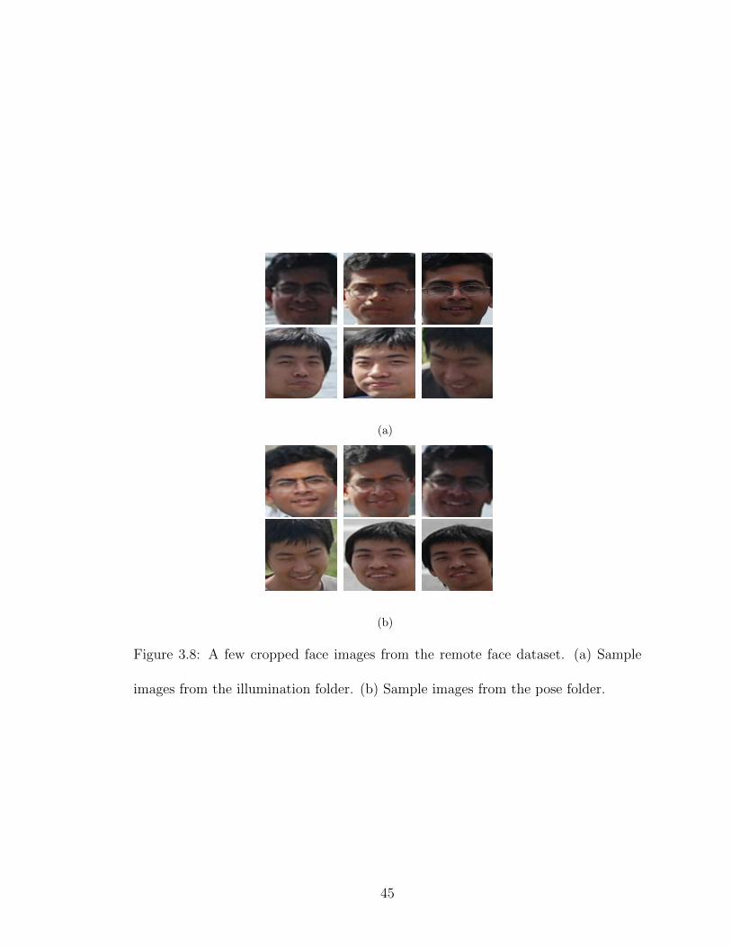
(a)

(b)

Figure 3.8: A few cropped face images from the remote face dataset. (a) Sample

images from the illumination folder. (b) Sample images from the pose folder.

45

DFR significantly outperforms the SRC method. The best recognition rate achieved

by the SRC method on the pose folder is 52% whereas the DFR method achieves

60%.

1 2 3 4 50.2

0.4

0.6

0.8

1

Number of gallery images

Rec

ognit

ion R

ate

DFR

SRC

(a)

1 2 3 4 5

0.2

0.4

0.6

0.8

1

Number of gallery images

Rec

ognit

ion R

ate

DFR

SRC

(b)

Figure 3.9: Recognition results on the remote face dataset corresponding to (a)

illumination folder and (b) pose folder.

46

3.3.5 Recognition with Partial Face Features

In this section, we report the ability of our algorithm in recognizing faces from

the partial face features. Partial face features have been used in recovering the

identity of human faces before [13], [1], [103]. We use the images in the Extended

Yale B database for this experiment. For each subject, 32 images are randomly

selected for training, and the remaining images are used for testing. The region of

eye, nose and mouth are selected as partial face features [1]. These partial facial

parts are manually cropped. Examples of these features are shown in Fig. 3.10.

Note that in this experiment, we omit the relighting step of our algorithm. We learn

dictionaries directly on the partial facial features. Table 3.4 compares the results

obtained by using our method with the other methods presented in [1]. As can

be seen from the table, our method achieves recognition rates of 99.3%, 98.8% and

99.8% on eye, nose and mouth region, respectively and it significantly outperforms

SRC, NN, NS and SVM [1].

(a) (b) (c)

Figure 3.10: Examples of partial facial features. (a) Eye (b) Nose (c) Mouth.

47

Table 3.4: Recognition results with partial facial features.

Right Eye Nose Mouth

Dimension 5,040 4,270 12,936

DFR 99.3% 98.8% 99.8%

SRC 93.7% 87.3% 98.3%

NN 68.8% 49.2% 72.7%

NS 78.6% 83.7% 94.4%

SVM 85.8% 70.8% 95.3%

3.3.6 Rejecting Non-face Images

In this section, we demonstrate the effectiveness of our method in dealing with

invalid test images with and without block occlusion. We test our rejection rule,

described in Section 3.1.4, on the Extended Yale B data set. We use Subsets 1 and

2 for training and Subset 3 for testing. We simulate varying levels of occlusion by

replacing a randomly chosen block of each test image with random noise. We include

only half of the subjects in the training set. This way, half of the subjects in the test

set are new to the algorithm. We plot the Receiver Operating Characteristic (ROC)

curves according to different τ values in Fig. 3.11(a). As can be seen from this

figure, that simple rejection rule performs quite well. It performs nearly perfectly

at 10% occlusion and without any occlusion. Even at 50% occlusion, it performs

better than making a random decision. This performance, can be further improved

48

by applying our DFR method on different features such as PCA and LDA.

0 0.2 0.4 0.6 0.8 10.3

0.4

0.5

0.6

0.7

0.8

0.9

1

False Positive Rate

Tru

e P

ositiv

e R

ate

No occlusion

10% occlusion

30% occlusion

50% occlusion

(a)

0 0.2 0.4 0.6 0.8 10.95

0.96

0.97

0.98

0.99

1

False Positive Rate

Tru

e P

osit

ive R

ate

(b)

Figure 3.11: (a) ROC curves corresponding to rejecting outliers. The solid curve

is generated by the DFR method based on our rejection rule. The dotted curves

correspond to the cases when different levels of occlusion has been added to the test

images. (b) ROC curve corresponding to rejecting invalid test samples.

In the second set of experiments on rejecting invalid test samples, we use the

same experimental set up as in Section 3.3.1. In order to test the ability of our

rejection rule in rejecting invalid samples, we add 1198 randomly selected object

49

images from the Eth80 dataset [104] to the probe set. The ROC curve corresponding

to this experiment is shown in Fig. 3.11(b). As can be seen from this figure, that

our simple rejection rule is able to remove most of the non-face images and performs

nearly perfectly.

3.3.7 Recognition Rate vs. Number of Dictionary Atoms

In this section, we evaluate the performance of DFR as the number of trained

dictionary atoms are changed. To this end, we repeat the experiment described in

Section 3.3.1 on DFR using 504 dimensional eigenfaces with different numbers of

dictionary atoms. Fig. 3.12 shows the recognition rate vs. number of atoms bar plot

for this experiment. It can be observed that even selecting only 5 atoms per class

dictionary, DFR provides a reasonable recognition performance on the Extended

Yale B database. Experiments have shown that increasing the number of atoms to

more than 23 usually degrades the performance of our algorithm. This is the case

because with more dictionary atoms the representation gets more exact and it has to

deal with all the noise/distortion present in the data. Whereas with fewer number

of dictionary atoms, much more accurate description of the internal structure of the

class is captured and the robustness to distortions is realized [13] [105], [106].

3.3.8 Recognition Rate vs. Number of Training Images

In this section, we study the performance of DFR as we vary the number

of training images in each class. We use the Extended Yale B database for the

50

5 10 15 20 25 3095

96

97

98

99

100

Number of atomsR

eco

gn

itio

n r

ate

(%

)

Figure 3.12: Recognition rate vs. number of dictionary atoms on the Extended Yale

B dataset.

experiments in this section. All the images are scaled to the size of 64 × 64. We

randomly select 1, 2, and 3 images per subject for training and the others for testing.

We compare the performance of our method with that of SRC and dictionary-based

SRC (DSRC) 2. For DSRC, we define a new training matrix A as the concatenation

of learned dictionaries from all classes as

A = [D1, · · · ,DC ], (3.16)

where Di is the learned dictionary corresponding to the class matrix Bi. Given a

novel face image, y, we solve the following `1−minimization problem to obtain the

2Note that one can use the introduced relighting method to first enlarge the training set to

capture the illumination variations and then use the SRC method for classification. However,

as discussed earlier, with enlarged dictionary, the computational complexity of SRC increases

tremendously. To reduce the complexity of the `1−minimization method, we first reduce the size

of the enlarged dictionaries using small-sized learned dictionaries. We then apply the SRC method

on a dictionary that is obtained by concatenating the learned dictionaries.

51

sparse coefficients

β = minβ‖β‖1 subject to Aβ = y. (3.17)

Once the sparse solution is obtained, we follow the procedure of SRC to classify

the test image. The experiment is carried out 10 times and the average recognition

rates of DFR along with SRC, DSRC and CDPCA are compared in Table 3.5. This

experiment shows that even in the presence of a few training images, our method

can provide reasonable recognition of human faces. This performance can be further

enhanced by learning dictionaries on features such as PCA and LDA.

Table 3.5: Performance comparison (in %) of different methods with respect to the

number of training samples per subject.

No. images DFR SRC DSRC CDPCA GF LTV

1 75.89 32.37 30.98 5.52 66.65 67.92

2 84.71 37.20 44.23 26.22 76.35 79.61

3 85.18 37.45 53.57 30.25 77.18 84.93

Note that this experiment violates SRC’s working premise that any test im-

age that belongs to the same class will approximately lie in the linear span of the

training samples from the corresponding class. As a result, SRC fails to provide

reasonable recognition performance on this experiment. Similarly, 15 atoms per

learned dictionary are not enough for DSRC to classify a novel test image with

illumination variations via `1−minimization. Experiments have shown that the per-

formance of DSRC generally increases as more number of atoms are kept in each

52

learned dictionary.

We also compare the performance of our method with several state-of-the-art

illumination normalization-based methods such as Gradient faces (GF) [107] and

LTV [108]. Once the GF or LTV features are found, the recognition is performed

by the nearest neighbor rule (in the case of 1 training image) or by the nearest

subspace rule. The results are shown in the last two columns of Table 3.5. As

can be seen from Table 3.5 that DFR significantly outperforms GF and LTV based

methods. Gradient faces and LTV features tend to be very noisy, especially in the

dark regions of the face. This in turn effects the recognition performance. Since

we are extending the gallery by adding multiple images of the subject with various

illumination, DFR does not suffer from the above mentioned artifacts and gives

better recognition performance.

3.3.9 Efficiency

To illustrate the efficiency of our algorithm, in Table 3.6, we report the aver-

age runtime of DSRC and DFR in classifying a test sample with a gallery matrix

containing 32 images from which 15 dictionary atoms are learned. As can be seen

from the table that DFR is efficient even when the data dimension increases.

3.3.10 Limitations

One limitation of the albedo estimation methods [49] and [90] is that they

require the images to be aligned, as is the case with most state-of-the-art face

53

Table 3.6: Average runtime in seconds

Dimension DFR DSRC

30 5.5× 10−4 0.28

56 6.8× 10−4 0.63

120 7.1× 10−4 0.80

504 1.5× 10−3 0.97

recognition algorithms. The albedo estimation methods are also sensitive to facial

expressions. Hence, when our method is used to estimate the albedo maps from

a given face image with expressions, it produces artifacts in the final estimated

albedo. As a result, DFR produces inferior recognition results on the databases

with expressions such as AR face dataset.

54

Chapter 4: Face Recognition Across Aging

Face recognition has a wide range of applications. But face verification on age-

separated facial images is challenging since usually there are significant changes in

the shapes and textures. In the past decades many face recognition algorithms have

been proposed[4], however the problem of recognizing facial images across aging

remains an open problem. The aging process changes both the shapes and the

textures of facial images. In this chapter, we look in to this problem from the points

of view of shape and the texture respectively.

4.1 Geometry of the Grassmann Manifold

The Grassmann manifold Gk,m can be viewed as a quotient group of the or-

thogonal group SO(m). An in depth treatment of this subject can be found in

[24]. Briefly, geodesic paths on SO(m) are given by one-parameter exponential

flows t → exp(tB), where B ∈ Rm×m is a skew-symmetric matrix. The quotient

geometry of the Grassmann manifold implies that geodesics in Gk,m are given by

one-parameter exponential flows t→ exp(tB) where B has a more specific structure

given by B =

0 AT

−A 0

, where A ∈ R(m−k)×k. The matrix A parameterizes the

55

direction and speed of geodesic flow. Given a point on the Grassmann manifold S0

represented by orthonormal basis Y0, and a direction matrix A, the one-parameter

geodesic path emanating from Y0 in direction B is given by Y (t) = Q exp(tB) J ,

where, Q ∈ SO(m) and QTY0 = J and J = [Ik; 0m−k,k].

In this chapter we use an extrinsic approach for computing the mean shape,

where one embeds the shape space into a large ambient space and computes the

mean in the ambient space. Finally, the result is projected back to the manifold.

For each point on the Grassmann manifold, we can associate to each d-dimensional

subspace an n× n idempotent projection matrix P of rank d, such that P = Y Y T ,

where Y is an orthonormal basis for the subspace. The space of n× n projectors of

rank d, denoted by Pn,d can be embedded into the set of all n× n matrices – Rn×n

– which is a vector space. The projection Π from Rn×n to Pn,d is given by

Π(M) = UUT ,where M = USV T is the d-rank SVD of M. (4.1)

Using this embedding, we can define an extrinsic distance metric on the Grass-

mann manifold using the distance metric inherited from Rn×n. The embedding is

illustrated in Fig. 4.1.

The representation of the facial shapes on the Grassmann manifold can also

be used for face verification to devise inter-person and intra-person classifiers. From

a given facial shape, as before we compute an orthonormal basis Y for the centered

landmark matrix. From this, we compute the projection matrix P = Y Y T as the

representation of the shape S on the Grassmann manifold.

From [109], the geodesic between two subspaces represented by projectors P1

56

Shape space+

+

1S

2S

Grassmann

manifold++

1Y

2Y

Geodesic

distance

dnP

,

++

1P

2P

Extrinsic

distance

Figure 4.1: Two shapes S1 and S2 are mapped to Y1 and Y2 on the Grassmann

manifold. The distance is computed by embedding the shapes to the ambient space

Pn,d.

and P2 on the Grassmann manifold has the form:

P2 = exp(tX)P1exp(−tX) (4.2)

This equation defines a geodesic that passes through P1 when t = 0 and passes

through P2 when t = 1. The matrix X can be solved by the eigen- decomposition

of matrix B = P1 − P2. [109] Thus the n× n matrix B contains all the information

about the geodesic between the two shapes.

The face verification problem is actually a two-class classification problem.

Given a pair of shapes (P1, P2), they are either from the same person or from different

people. In our experiment, we use the matrix B as the feature vector, with the SVM

classifier [110], to classify if a pair of shapes belong to the same person.

Although the presentation of the facial shapes are used for both age estimation

and face verification, we rely on the classifier to adjust its weights appropriately

based on training.

57

Figure 4.2: An example of the image and the facial landmarks in the MUCT dataset.

[2]

4.2 Experimental Results of Grassmann Manifold

In this section, we present experiments that illustrate the strength and flexi-

bility of the proposed representations for both age-estimation and face verification

across aging.

4.2.1 Experiment on the MUCT Dataset

We used the MUCT dataset [2] to test the effectiveness of the proposed method

on face verification using only the facial shapes first. The MUCT dataset contains

3755 facial images from 276 subjects. The facial images were obtained under 10

different lighting conditions and from 5 different viewpoints. Each facial image was

manually landmarked with 76 landmarks. An example of the image and the facial

landmarks is shown in Fig. 4.2. Among all these images, 2253 images are frontal.

Since some landmarks may be obscured by other facial features in the non-frontal

images, we tested our method on the frontal images only.

We adopted a three-fold cross validation in the verification experiment. The

58

0 0.1 0.2 0.3 0.4 0.5 0.6 0.7 0.8 0.9 10

0.1

0.2

0.3

0.4

0.5

0.6

0.7

0.8

0.9

1

Correct Acceptance Rate

Co

rre

ct

Re

jectio

n R

ate

ROC

Proposed

Baseline

Figure 4.3: The ROC curve for the three-fold validation experiment on the MUCT

dataset.

result of a nearest neighbor classifier based on the Euclidean distance between two

shapes after they are aligned using the classical Procrustes analysis [22] is taken as

the baseline performance. In each fold, the images of a subject only appear in either

the training set or the testing set. 2900 intra-personal pairs and 2900 extra-personal

pairs from 92 subjects were generated for training in each fold. Our method achieved

an EER of 14.9%, while the EER of the baseline method is 28.5%. The results of

the proposed method and the baseline are shown in Fig. 4.3.

The experiment result shows that the proposed method can effectively verify

the identities in a pair of images using only the configuration of facial landmarks.

The information conveyed in the facial shapes is a good source for face verification.

4.2.2 Experiment on the FG-NET Database

Next we used the FG-NET database [111] to test the proposed method under

age variations. The FG-NET database [111] is a publicly available database and

59

Table 4.1: The distribution of the number of images and subjects in different ages

range.

Age Range 0-5 6-10 11-15 16-20 21-30 31-40 41-50 51-60 61-70

# of Images 233 178 164 155 143 69 39 14 7

# of Subjects 75 70 71 68 84 35 22 8 4

has been widely used for evaluating face verification algorithms across aging. It

has facial images collected at ages in the range from 0 to 69. We use the FG-

NET database in our experiments since it is by far the largest database that covers

such a wide age range and provides annotated facial landmarks as well as the age

information of each image. In this database, there are 1002 images of 82 subjects.

The distribution of the number of images and subjects is summarized in Table 4.1.

About 64% of the images are from the children (with age < 18), and around 36%

of the images is from the adults (with age ≥ 18). For each facial image there are 68

hand labeled landmarks representing the facial shape. Examples of the images and

the corresponding facial shapes in the database are shown in Fig. 4.4.

We compared our method with Ling’s method [53], the LRPCA algorithm

[112] and the same baseline method using the classical Procustes analysis as in the

experiment on MUCT. The equal error rates (EER) of are shown in Table 4.2. And

the ROC curves are shown in Fig. 4.5.

The result shows that our method is effective in verifying the identities of

the facial images, and has comparable result with the state-of-art method [53].

60

(a) (b)

Figure 4.4: Examples of the images and landmarks (labeled as red) at different ages

of the same subject in the FG-NET database. (a) An image and the facial shape at

age 8; (b) An image and the facial shape at age 18.

0 0.1 0.2 0.3 0.4 0.5 0.6 0.7 0.8 0.9 10

0.1

0.2

0.3

0.4

0.5

0.6

0.7

0.8

0.9

1

Correct Acceptance Rate

Co

rre

ct

Re

jectio

n R

ate

ROC

Proposed

Baseline

LRPCA

Figure 4.5: The ROC curve of our method on FG-NET database.

Table 4.2: The comparison of different methods on the FG-NET database.

Our Method Ling’s Method LRPCA Baseline

EER 23.6% 24.1% 32.1% 38.2%

61

0 2 4 6 8 10 120

0.05

0.1

0.15

0.2

0.25

0.3

0.35

0.4

0.45

0.5

Age gap

Eq

ua

l e

rro

r ra

te (

EE

R)

Proposed

Baseline

LRPCA

Figure 4.6: Verification performance under different age gaps.

Since our method uses only the shapes as the feature, while Ling’s method uses

appearance-based features, our method has the potential to improve the overall

face recognition performance after it is integrated with other appearance-based face

recognition methods.

4.2.3 Effect of the Age Gap

We studied the performance of the proposed method under the influence of

facial aging empirically. We conducted this investigation using the FGNET database

since it has a large age range. Based on the age gaps between the image pairs, the

three-fold verification result on the FGNET was grouped into 6 classes: age gaps

from 0 to 1 year, 2 to 3 years, 4 to 5 years, 6 to 7 years, 8 to 9 years and 10 to 11

years. There are about 500 image pairs, which contain around 65 intra-person pairs

for testing on average in each group. An equal error rate was calculated for each

group respectively. Fig. 4.6 shows the performances of our method, the baseline

method and the LRPCA under different age gaps.

62

The results show that as the age gap increases, it is more difficult to verify

if an image pair comes from the same person. It also shows that the performance

of our method is more stable under aging variation compared to the baseline and

the appearance-based LRPCA method. Specifically, the proposed method has a

comparable performance with LRPCA when the age gap is less than 1 year, and has

a better performance when the age gap is greater than 1 year. This may be because

the facial shape is stable across aging for an adult person, while the appearance of

the face may have more variation due to the its effect on facial skin and texture.

4.3 Facial Growth Model

4.3.1 Classical Craniofacial Growth Model

We first give a brief introduction to the craniofacial growth model, which was

proposed by Todd, et al, [113], and has been used in modelling the age progression

by Ramanathan, et al, [54]. The relative craniofacial growth model, which is derived

from this traditional growth model, is discussed in the following sections.

The craniofacial growth model is illustrated in Fig. 4.7(a). For a given facial

shape, the craniofacial growth model assumes that there is a growth origin and each

landmark will grow along the radial direction from the growth origin with a growth

rate. Let the angular coordinates of a landmark at age t0 be (R(t0)i , θ

(t0)i ) and the

coordinates of the landmark age t1 be (R(t1)i , θ

(t1)i ), (t1 > t0), then the traditional

growth model can be expressed as follows: [54]

63

R(t1)i = R

(t0)i + k

(t0,t1)i (R

(t0)i +R

(t0)i cos(θ

(t0)i )) (4.3)

θ(t1)i = θ

(t0)i (4.4)

where k(t0,t1)i is the growth parameter from age t0 to age t1 for the ith landmark.

The growth parameters are learned by solving a set of non-linear equations. [54]

Since the angle θ(t)i for the ith landmark does not change across time, we denote it

as θi.

Let the growth origin Og be the origin of the coordinate system. Denote the

cartesian coordinates of the ith landmark in the facial shape at age t by (x(t)i , y

(t)i ).

Then we have:

x(t)i = R

(t)i cos(θi) (4.5)

y(t)i = R

(t)i sin(θi) (4.6)

Substituting Eqn. 4.6 to Eqn. 4.4, the craniofacial growth model from age t0 to age

t1 can be expressed in cartesian coordinate system as:

x(t1)i = [1 + k

(t0,t1)i (1 + cos θi)]x

(t0)i (4.7)

y(t1)i = [1 + k

(t0,t1)i (1 + cos θi)]y

(t0)i (4.8)

Assuming bilateral symmetry of faces [54], the growth origin should be located on

the axis of bilateral symmetry, then we have ytle + ytre = 0 and Rle = Rre, where the

subscripts le and re refer to the landmarks at the centers of the left eye and the

right eye respectively and will be used in the following discussion.

64

4.3.2 Relative Craniofacial Growth Model

The craniofacial growth model [113], which was based on the science of face

anthropometry, has an implicit assumption that all the facial shapes are in the same

scale. This prerequisite is also true when the growth model is applied to simulating

the aging progress [54] using a single facial image. The scale of that single image is

actually used as an absolute reference for synthesizing the appearances at different

ages.

For the face verification problem, this condition usually does not hold because

face images can be easily enlarged. The shapes extracted from face images lose their

absolute scales. This raises two problems in applying the growth model in a real

scenario:

1) the growth parameters from age t1 to age t2 are not easy to be learned from

the facial shapes extracted from the training data at these ages directly;

2) given two facial shapes S1 and S2 at different ages t1 and t2, S1 must be

normalized to the same scale at which the growth parameters are learned before

synthesizing the new shape of S1 at age t2.

Since the absolute scale information is lost in facial images, a relative scale has

to be adopted to normalize the facial shapes. The distance between the centers of

two eyes is usually not affected by expressions and thus is relatively stable. Hence

we used this distance as the reference scale. Specifically, we align the center of

the left eye to (0,−1) and the center of right eye to (0, 1), and set the coordinate

system of the relative craniofacial growth model as shown in Figure 4.7(b). Let

65

(a) (b)

Figure 4.7: (a) Illustration of the craniofacial growth model. (b) Illustration of the

relative craniofacial growth model.

S ′ =

u′(t)1 · · · u′

(t)N

v′(t)1 · · · v′

(t)N

T

t, and S =

u(t)1 · · · u

(t)N

v(t)1 · · · v

(t)N

T

denote the coordinates of

the N landmarks detected from a facial image at age t and in the coordinate system

of the proposed model (Fig. 4.7(b)), respectively. Then the alignment can be

achieved as: S = S ′A, where the transform matrix A can be easily solved from:ule′(t) vle′(t)

ure′(t) vre

′(t)

A =

0 −1

0 1

(4.9)

In the traditional growth model, the half distance d(t)e between the eye centers

at age t is given by:

d(t)e = R(t)

re sin θre (4.10)

So the transformation between the traditional growth model and the proposed model

66

is given by:

u(t)i = (x

(t)i −R(t)

re cos θre)/d(t)e (4.11)

v(t)i = y

(t)i /d

(t)e (4.12)

Substituting Eqn. 4.6 and let γi = cos θisin θi

, then we have a set of linear equations

about γi:

u(t)i = γiv

(t)i − γre, 1 ≤ i ≤ N (4.13)

And the coordinates of the growth origin Og in the proposed model are given by

(−γre, 0). Note that γi is the cotangent value of θi and thus does not change across

time.

Substituting the traditional growth model into the above equation, we have:

u(t1)i =

R(t0)i (1 + k

(t0,t1)i (1 + cos θi)) cos θi −R(t0)

re (1 + k(t0,t1)re (1 + cos θre))

R(t0)re (1 + k

(t0,t1)re (1 + cos θre)) sin θre

(4.14)

v(t1)i =

R(t0)i (1 + k

(t0,t1)i (1 + cos θi)) sin θi

R(t0)re (1 + k

(t0,t1)re (1 + cos θre)) sin θre

(4.15)

where k(t0,t1)i and k

(t0,t1)re are the growth parameters of the ith landmark and the left

eye respectively. We call this model as relative craniofacial growth model since for

each facial shape, the scale at each age is relative to the distance between the eyes

at that age.

Let

β(t0,t1)i =

1 + k(t0,t1)i (1 + cos θi)

1 + k(t0,t1)re (1 + cos θre)

(4.16)

Then it can be simplified to a set of linear equations of βt0,t1i as:

u(t1)i = β

(t0,t1)i (u

(t0)i + γre)− γre (4.17)

v(t1)i = β

(t0,t1)i v

(t0)i (4.18)

67

The set of linear equations Eqn. 4.13 and Eqn. 4.18 are the relative craniofa-

cial growth model and we call β(t0,t1)i as the relative growth parameters of the ith

landmark starting at age t0 and ending at age t1.

4.3.3 Learning the Relative Growth Parameters

The relative craniofacial growth model is described using a set of linear equa-

tions, and thus the parameters can be easily learned from a set of training facial

shapes and their corresponding ages.

The parameters γi, 1 ≤ i ≤ N do not change across time for the same person.

A set of γi can be solved for each subject from the linear equations (4.13) and

then personalized relative growth parameters can be learned by solving (4.18) given

the shapes at different ages of the same person. However, for face verification

experiments, the training set does not contain any subject that appears in the

testing set. So the personalized growth parameters cannot be used for testing.

Thus a general relative growth model is learned using all the training data in our

experiments.

A training set containing Q shapes yields a set of QN linear equations for γi,

1 ≤ i ≤ N using (4.13) so that γre can be easily solved. For the relative growth

parameters β(t0,t1)i , 1 ≤ i ≤ N , we select all the training shapes at age t0 or t1.

Each pair of shapes of the same subject at these two ages yield a set of two linear

equations for β(t0,t1)i based on (4.18). Then M pairs of shapes from ages t0 and t1

yield a set of 2MN linear equations for all the N relative growth parameters β(t0,t1)i .

68

Hence the relative growth parameters can be simply solved using the minimum least

square method.

4.3.4 Experiment Results with Facial Growth Model

After a pair of facial shapes is warped to the same age, the difference between

them can be measured by various shape analysis methods and then appropriate pat-

tern recognition methods can be invoked for verifying their identities. The Grass-

mann manifold has been shown to be effective for shape recognition [35] in general

and face recognition [27, 36]. Hence we adopted the Grassmann manifold to describe

the difference between a pair of shapes that is warped to the same age and then

verify their identities using a two-class SVM classifier.

4.3.4.1 Verification Experiments

In order to compare with the state-of-art face verification methods across ag-

ing, we follow the protocol suggested in [53] which divides the FGNET dataset into

three subsets:

1. FGnet-8 consists of all the data collected at ages between 0 and 8. It includes

290 facial images from 74 subjects, among which 580 intra-person pairs and

6000 extra-person pairs are randomly generated for verification.

2. FGnet-18 consists of all the data collected at ages between 8 and 18. It includes

311 facial images from 79 subjects, among which 577 intra-person pairs and

6000 extra-person pairs are randomly generated for verification.

69

3. FGnet-adult consists of all the data collected at ages 18 or above and roughly

frontal. It includes 272 images from 62 subjects, among which 665 intra-

personal pairs and about 6000 extra-personal pairs are randomly generated

for verification.

Three-fold cross validations are conducted on all the subsets such that there is no

overlap between the subjects in the training and testing sets.

For the FGnet-8 subset, 72 relative growth models that start at ages between 0

and 8 and end at all other possible ages are learned from the training data. Similarly,

110 models are learned using the FGnet-18 subset for all possible starting and ending

ages. The facial aging progress is much slower for adults and thus the facial shapes

are relatively stable. We group the adult data into 7 groups based on the ages: age

from 18 to 20, from 21 to 30, from 31 to 40, from 41 to 50, from 51 to 60, and from

61 to 69. The facial shapes in the same group are treated as having the same age.

Forty-two relative growth models that start at one of the groups and end at other

groups are learned.

We compare the performance of our method with the method based on the

Grassmann shape analysis without using the relative growth model, the classical

Procrustes shape analysis method [22] which is a baseline performance on shape

analysis, and the GOP method [53] which is a state-of-art method using the texture

features. The CRR-CAR curves on each subset are shown in Fig. 4.8(a), Fig. 4.8(b),

and Fig. 4.8(c), respectively. The equal error rates (ERR) are shown in Fig. 4.8(d).

70

0

0.2

0.4

0.6

0.8

1

0 0.1 0.2 0.3 0.4 0.5 0.6 0.7 0.8 0.9 1

Corr

ect re

jection r

ate

(C

RR

)

Correct acceptance rate (CAR)

ProposedManifold

ProcrustesGOP

(a) CRR-CAR curve on FGnet-8

0

0.2

0.4

0.6

0.8

1

0 0.1 0.2 0.3 0.4 0.5 0.6 0.7 0.8 0.9 1

Corr

ect re

jection r

ate

(C

RR

)

Correct acceptance rate (CAR)

ProposedManifold

ProcrustesGOP

(b) CRR-CAR curve on FGnet-18

0

0.2

0.4

0.6

0.8

1

0 0.1 0.2 0.3 0.4 0.5 0.6 0.7 0.8 0.9 1

Corr

ect re

jection r

ate

(C

RR

)

Correct acceptance rate (CAR)

ProposedManifold

ProcrustesGOP

(c) CRR-CAR curve on FGnet-adult

0.1

0.2

0.3

0.4

0.5

FGnet-8 FGnet-18 FGnet-adult

Equal err

or

rate

(E

ER

)

ProposedManifold

ProcrustesGOP

28.1%

22.4% 22.3%

32.5%

27.0%

23.6%

43.6%

41.1%

38.1%38.6%

30.5%

24.1%

(d) Equal error rates (EER) on FG-NET

Figure 4.8: The CRR-CAR curves and equal error rates (EER) of the three-fold

validation experiments on the FG-NET database, best viewed in color.

The results show that for children, the proposed method outperforms all the

other methods on both subsets on children. The results are also consistent with

the observation reported in [53] that face recognition is extremely hard for small

children younger than 8 years old. For adults, the proposed method has comparable

performance with the state-of-art texture based method. The proposed algorithm

has slightly better results with the Grassmann manifold method which does not

predict the facial shapes at different ages. This is mainly because the aging progress

is relatively slow and subtle for adults. This also means that the proposed method

71

does not have any negative effect on the performance of face verification when the

aging progress is subtle.

Note that the proposed method has similar performance on both the FGnet-

adult and the FGnet-18 subsets. However the performance of the manifold method

without using the growth model has a significant difference on these two sets. This

suggests that the relative growth model captures the aging progress and predicts

new facial shapes successfully for the teenagers and thus significantly improves the

face recognition performance.

4.3.4.2 Effect of the Age Gap

Age gap is one of the major reasons that affect the performance of mordern

face recognition algorithms. The main goal of the proposed method is to capture

the aging progress in age-separated image pairs and eliminate the effects of aging.

Hence we study the influence of age gaps on the proposed method empirically using

a FGnet-children subset which consists of 676 facial images with ages less than

or equal to 18 years old from 80 subjects. We generated 3034 intra-person pairs

and 6000 intra-person pairs. This subset is challenging since the aging progress

in children is much more rapid than in adult. However, a method would be more

applicable in practice if its performance is stable with large age gaps.

We group the three-fold cross verification results by the age gaps into the

testing image pairs into 5 classes : 2 to 3 years, 4 to 5 years, 6 to 7 years, 8 to

9 years and 10 to 11 years. The EER of each method is calculated in each of the

72

0

0.1

0.2

0.3

0.4

0.5

2 3 4 5 6 7 8 9 10 11

Eq

ua

l e

rro

r ra

te (

EE

R)

Age gap (years)

ProposedManifold

Procrustes

Figure 4.9: Equal error rates under different age gaps.

group. The EERs of the proposed method, the manifold method, and the Procrustes

analysis is shown in Fig. 4.9.

The results show that the performance of the proposed relative growth model

method is relatively stable across different aging gaps; while the EERs of the other

methods increase as the aging gap increases. It shows that the proposed method is

able to capture and remove the intrinsic aging progress over facial shapes and thus

improve the performance on age-separated facial image pairs.

4.3.4.3 Robustness Against Inaccurate Age Information

The proposed method relies on the ages of input facial images in order to

predict the new facial shapes. The ages can be either provided from the collected

metadata or from age estimation algorithms, such as in [34]. Thus the age infor-

mation is sometimes not accurate and the robustness of the proposed method over

inaccurate age information system is important. Since the growth progress is much

faster for children and relatively slow for adults, we test our method on the FGnet-

73

0

0.1

0.2

0.3

0.4

0.5

0 1 2 3 4 5

Eq

ua

l e

rro

r ra

te (

EE

R)

Mean absolute error (MAE) of the age error (years)

FGnet-childrenFGnet-adult

Figure 4.10: Equal error rates of the proposed method with inaccurate age informa-

tion on children and adult subsets.

children and the FGnet-adult sets. The same three-fold cross validation protocol as

in previous sections is adopted in the experiments and a random noise is added to

the age information of the testing images. The EERs of the proposed method on

these two datasets against the mean absolute error (MAE) of the noise added on

the age information are shown in Fig. 4.10.

The results show that in general the proposed method is affected slightly by

the error in age estimation. When the MAE of age is 5 years, the EERs of the

proposed method is consistently low at about 23% for adults and increases about

4% for children. The proposed method is more stable on the FG-adult than the

FGnet-children set, which is consistent with the facts that children’s faces changes

rapidly while the facial shapes are relatively stable on adults. Thus the relative

growth model is not sensitive to the accuracy of age information, especially for

adults.

74

(a) The original image. (b) The blurred image. (c) The self quotient image

Figure 4.11: An example of the self quotient image.

4.4 Texture-based Face Recognition

4.4.1 Method

We first calculate the self quotient images of all facial images. Self quotient

images is proposed by Wang, et al, [114] to improve face recognition under varying

lighting conditions. The self quotient image is calculated by dividing the original

image by a blurred version of the original image. This method is adopted as a

preprocessing step since it does not need training and can work on a single image

and in shadow regions without alignment. It can effectively suppress illumination

effects and preserve discriminative information. An example of the self quotient

image is shown in Fig. 4.11.

Then PHOW features are extracted on the self quotient images. PHOW was

proposed by Bosch, et al, in 2007 [115]. It has been successfully applied in the

problem of object classification. In this method, an image was cropped into patches

at different scales. SIFT features [116] are extracted from each of the patches. The

75

PHOW feature vector is obtained by concatenating all the extracted SIFT feature

vectors. We adopted the Chi-square distance to measure the difference between the

feature vectors extracted from a pair of images. Let the feature vectors extracted

from two images be denoted as u = [u1, · · · , um] and v = [v1, · · · , vm]. Then a

difference vector d = [d1, · · · , dm] between the images is defined as:

di =‖ui − vi‖2

2

|ui|+ |vi|1 ≤ i ≤ m (4.19)

where m is the dimension of the PHOW feature vector. Hence each entry of d is the

CHi-square distance between the corresponding entries in u and v. It is a two class

pattern recognition problem to verify if a pair of facial images belong to the same

subject. So a two-class SVM classifier is trained using the vector d as the feature

vector of a pair of images.

4.4.2 Experiment Results of Texture Features

4.4.2.1 Verification on FG-NET

We tested this method on the images of all the adult people in FGNET

database and compared it with the gradient of pyramid based method [53] and the

metric learning based method [117, 118]. The equal error rates in the verification

experiment are summarized in Table 4.3.

4.4.2.2 Verification and Identification on MORPH

The proposed method is also tested on the MORPH-1 dataset [119]. MORPH

[119] is a publicly available database of age-separated facial images. In MORPH-

76

Table 4.3: Comparison of different texture-based method on FGNET.

GOP GOP+SVM ITML LMNN Proposed

Equal error rate 32.3% 24.1% 42.8% 36.3% 23.4%

Table 4.4: The distribution of the images and subjects in MORPH-1 database.

Age Range 18-29 30-39 40-49 >49

# of images 936 428 124 33

# of subjects 514 296 93 20

1, all the images were obtained under controlled condition with aging and minor

pose variations. But some images have low quality due to blur and stains. The

distribution of the number of images and subjects in different age groups is shown

in Table 4.4.

The equal error rates in the verification experiments are summarized in Table

4.5. We also tested the identification performance of our method on the MORPH-1.

The recognition accuracies of our method and the baseline reported in [119] are

summarized in Table 4.6.

The results show that the proposed method has better performance than the

baseline in most of the subsets in datasets. In future, sophisticated machine learning

method, such as SVM and metric learning, could be combined. The fusion of both

the shape-based method and the texture-based method can be explored in order to

improve the performance.

77

Table 4.5: The equal error rate on MORPH-1 database.

Age difference

Subset Age in the gallery 0-5 6-10 11-15 16-20

All people

18-29 17.6 22.0 26.1 34.7

30-39 13.4 19.3 17.9 n/a

40-49 6.3 n/a n/a n/a

Male

18-29 17.4 22.9 26.8 35.4

30-39 12.7 19.4 19.3 n/a

40-49 7.7 n/a n/a n/a

Female18-29 21.1 21.9 23.1 34.4

30-39 16.7 21.3 n/a n/a

African 18-29 19.9 23.9 27.3 40.0

American 30-39 16.5 20.9 21.3 n/a

White18-29 16.4 22.0 30.4 n/a

30-39 7.7 15.6 n/a n/a

78

Table 4.6: The recognition accuracies on MORPH-1 database. For the two number

in each entry, the left is our result, the right is the baseline result.

Age difference

Subset Age in the gallery 0-5 6-10 11-15 16-20

All people

18-29 45.9 — 42.0 29.2 — 25.7 20.7 — 13.4 6.9 — 8.0

30-39 57.5 — 45.2 42.1 — 30.0 17.4 — 23.1 n/a

40-49 71.9 — 80.0 n/a n/a n/a

Male

18-29 48.8 — 43.1 30.4 — 29.4 20.6 — 19.9 6.3 — 7.3

30-39 58.2 — 51.3 42.9 — 29.2 25.0 — 16.7 n/a

40-49 73.1 — 80.0 n/a n/a n/a

Female18-29 44.2 26.2 38.5 20.0

30-39 62.5 50.0 n/a n/a

African 18-29 43.9 — 42.3 27.2 — 25.2 22.7 — 10.7 4.0 — 9.3

American 30-39 51.9 — 44.4 34.9 — 30.4 15.0 — 33.3 n/a

White18-29 54.8 — 41.3 41.5 — 25.0 13.0 — 22.7 n/a

30-39 80.8 — 57.1 64.3 — 28.6 n/a n/a

79

Chapter 5: Face Recognition with Quantized Images

5.1 Introduction

As an important biometric feature, face images have been used widely to iden-

tify humans. In most applications, face images to be identified are grey or colored,

which have sufficient information to extract good features, especially when the face

images are obtained under controlled conditions. A review of face recognition re-

search conducted before 2003 may be found in [4].

5.2 Algorithms

5.2.1 Review of Principal Component Analysis

Let C denotes the covariance matrix of images, then the PCA basis vectors

are obtained by solving the eigenvalues and eigenvectors of C:

C =1

N

N∑i=1

(xi −m)(xi −m)TC = V ΣV T (5.1)

where N is the number of images, xi is the ith image, m is the mean of all images,

Σ is a diagonal matrix of all eigenvalues, V = [v1...vi...vN ]. vi is the eigenvectors

corresponding to the ith eigenvalue λi. Assume λ1 ≥ ...λi ≥ ...λN . The PCA

80

coefficients are obtained by:

yi = W Txi (5.2)

where W T = [v1...vi...vn], n is the number of desired principal components.

Though PCA does not make any assumption on the probability distribution

of the pixel values, when the values of pixels obey a Gaussian distribution, PCA

coefficients are independent and obey a Gaussian distribution. The eigenvalue λi is

proportional to the energy, of the image along the direction of vi. So the number of

desired principal components n could be determined by specifying the percentage

of energy to be preserved:

n = arg min

∑ni=1 λi∑Mi=1 λi

> p (5.3)

where M is the number of pixels of an image, p is the specified percentage of energy

to be preserved. When the input to PCA does not obey a Gaussian distribution, λi

still represent the energy, since xi −m is a zero-mean random vector.

5.2.2 Multiple-Exemplar Discriminant Analysis

Linear discriminant analysis (LDA) is widely used in the field of pattern recog-

nition. MEDA [6] uses several exemplar or even the whole sample set to represent

each class. Its effectiveness was demonstrated in [120]. MEDA is an extension of

LDA, but has different definitions of within-class and between-class scatter matri-

ces. The MEDA method is summarized as follows. Let xij denotes the jth sample

in the ith class. The within-class scatter matrix ΣW and between-class matrix ΣB

81

are defined by

ΣW =C∑i=1

1

Ni

Ni∑j=1

Ni∑k=1

(xij − xik)(xij − xik)T (5.4)

ΣB =C∑i=1

C∑j=1;j 6=i

1

NiNj

Ni∑k=1

Nj∑l=1

(xik − xjl )(x

ik − x

jl )T (5.5)

where C and Ni are the number of all samples and the number of samples in the

ithe class respectively. Then the projection matrix W is obtained by maximizing

the function

JW =det(W TΣBW

)det (W TΣWW )

(5.6)

Generally, MEDA requires multiple samples for each subject in the gallery

set. For the face recognition problem, because of the symmetry of human faces,

images in the gallery set could be mirrored vertically so as to increase the number

of samples.

5.3 Recognition of Quantized Face Images

5.3.1 Quantization and Binarization Method

In our experiments, images with different numbers of grey levels were obtained

by quantizing the original images using the minimum mean square error (MMSE)

criterion [121]. Some examples of normalized face images quantized by the MMSE

quantizer are given in Fig. 5.1.

Although the quantizer is able to quantize an image into a specified number of

grey levels using the MMSE criterion, it is sensitive to illumination variations if it is

used to binarize images. When recognizing faces from binary images, regions around

82

(a) (b) (c) (d)

Figure 5.1: Face images quantized by the MMSE quantizer. (a) The original grey

image with 256 grey levels. (b) The original image is quantized into 8 grey levels.

(c) The original image is quantized into 4 grey levels. (d) The original image is

quantized into 2 grey levels.

eyes, nose and mouth are very important. Since the illumination on the whole

face is generally not evenly-distributed, the global binarization threshold could be

affected even by slight shadows in the above-mentioned regions. In Fig. 5.1(a), the

surrounding region of the original face image is slightly darker than the center region.

So the MMSE quantizer assigned darker values to the pixels in the surrounding

regions, as shown in Fig. 5.1(d). The shapes of facial organs were submerged in

this result, though the quantization error is minimized. We adopted the MMSE

quantizer in the experiments to investigate the effect of the number of grey levels

on the performance of face recognition algorithms.

For the binary face recognition problem, we adopted a contrast based quan-

tizer. Regions, such as eyes, nose and mouth, on a face image are generally much

darker than other regions. The shapes of these regions could be better preserved

when the original image is binarized under a contrast criterion, which requires that

83

the bright pixels in the binary result account for a specified percentage. An example

is given in Fig. 5.2. Compared to the MMSE quantizer, this method could not only

preserve the shapes of the organs better in binary result, but also can be easily

implemented in an ordinary fax machine.

Figure 5.2: The original image in Fig. 5.1 is binarized under the contrast criterion.

The percentage of the bright pixels is 80%.

5.3.2 Dataset

The performance of PCA, MEDA and the elastic bunch graph matching (EBGM)

algorithms was investigated using the Face Recognition Grand Challenge (FRGC)

database version 1 [122]. In this database, experiment 1 is focused on the recogni-

tion of still frontal face images obtained under controlled illumination. In the gallery

set there is only one controlled still image for each subject. Totally, there are 152

images in the gallery set for 152 subjects, 608 images in the probe set. Images were

mirrored vertically in order to meet the requirements of MEDA. Similar to exper-

iment 1, experiment 2 is focused on the face recognition problem under controlled

illumination, but has 4 different images for each subject in the gallery set. There

are a total of 608 images in the gallery set for 152 subjects and 2432 images in the

probe set. Experiment 4 concerns with face recognition under different illumination

84

conditions, where the images in the gallery set were obtained under controlled con-

ditions and those in the probe set were obtained under uncontrolled conditions. We

investigated the performance of the algorithms on experiments 1, 2 and 4 of FRGC.

5.3.3 Effect of the Number of Grey Levels

In order to investigate the effect of the number of grey levels, we quantized the

images in version 1 experiment 1 database using the MMSE quantizer. The mean

peak signal noise ratio (PSNR) of the output of the quantizer when the original

images are quantized into different number of grey levels is plotted in Fig. 5.3.

The quantization PSNR drops as the number of grey levels decreases. When there

are less than 8 grey levels, the PSNR is less than 35db. A significant amount of

information is lost.

0 10 20 30 40 50 60 7020

25

30

35

40

45

50

Number of gray levels

PS

NR

(d

b)

Figure 5.3: The mean PSNR when the images were quantized into different number

of grey levels .

The eigenvalues of the PCA covariance matrix estimated from the images

with different number of grey levels are plotted in Fig. 5.4. The eigenvalues of

85

the covariance matrix were sorted in the descending order. It shows that for the

100

101

102

103

104

101

102

103

104

105

106

107

108

Eigen index

Eig

en

va

lue

Figure 5.4: Eigenvalues of the covariance matrix of 2, 4, 8, 16, 256 grey levels images.

Their spectrums almost overlap in low order eigenvalues, and have high order tails.

The tails from up to down are from 2, 4, 8, 16, 256 grey levels images.

top n eigenvalues, the percentage of the energy they account for decreases as the

number of grey levels decreases. As the number of grey levels decreases, the values

of the middle and high orders eigenvalues of the covariance matrix increases, and

the energy tends to spread to high order eigenvalues. According to Fig. 5.3, when

images are quantized into fewer greylevels, the power of quantization noise increases.

This might be a major reason for the energy spread phenomenon.

We quantized all the images in the training, gallery and probe sets of exper-

iment 1 and tested the performance of PCA, MEDA and EBGM algorithms. The

recognition accuracies of the algorithms using the Euclidean distance or the cosine

of the angles between two representations [122] as the metric on rank 1 when the

images have different number of grey levels are plotted in Fig. 5.5. It appears that

the combination of PCA and MEDA always has better performance than the PCA

86

100

101

102

103

0.5

0.55

0.6

0.65

0.7

0.75

0.8

0.85

0.9

0.95

1

Number of grey levelsA

ccu

racy o

n r

an

k 1

PCA, Euclidean distance

PCA+MEDA, cosine distance

PCA+MEDA, Euclidean distance

Figure 5.5: Recognition accuracies of PCA and PCA+MEDA methods on rank 1

when using different distance metrics and the images have different number of grey

levels on FRGC version 1 experiment 1. The x-axis is logarithmically scaled. The

performance of PCA using the cosine distance and Euclidean distance are almost

the same, so only the one using Euclidean distance is plotted.

only method. The cosine distance metric yields a better result than the Euclidean

distance metric. The performance of each algorithm is almost the same, when the

number of grey levels is greater than 8. But the recognition accuracies drop severely

when the images have fewer grey levels. Since the quantization noise increases as

the number of grey levels decreases, according to Fig. 5.3, much information could

be lost or corrupted when the images are nearly binary. This might be an leading

to the reduction in performance.

5.3.4 Performance Comparison on Binary Images

The distribution of the values of pixels in a binary image is much more like a

Bernoulli distribution, rather than a Gaussian distribution. It has been suggested

87

in [64] that the performance may drop for non-Gaussian data. We tested the perfor-

mance of PCA-based methods after the distribution of the pixels were transformed

to be more Gaussian.

We tried two different ways to transform the binary images. One is to convolute

the images with a Gaussian kernel. The other way is to perform a distance transform

(DT)[123] on the binary images first, in order to extend the support of the pixels

values. Each pixel is assigned a value of the Euclidean distance from it to its nearest

edge point. In our experiment, the pixels were assigned positive values if they were

white in the binary images. Otherwise, they were assigned negative values. Then

the Box-Cox transform[124] is adopted to convert the images processed by DT to

be more like Gaussian. The eigenvalues, in descending order, of the covariance

100

101

102

103

104

10−2

100

102

104

106

108

Eigen index

Eig

en

va

lue

From binary images

From binary images convoluted by Gaussian kernel

From binary images processed by DT and Box−Cox

Figure 5.6: Eigenvalues of the covariance matrices estimated from binary images

and transformed binary images.

matrices estimated from images binarized by the contrast criterion, and from the

transformed binary images are plotted in Fig. 5.6. After Gaussian or distance

and Box-Cox transformations, the energy of the covariance matrix concentrates

88

more in the low to middle order eigenvalues. Although a Gaussian kernel could

make most of the energy concentrate in low order eigenvalues, it blurs the image

and suppresses the high frequency components, which generally carry significant

discriminant information. The distance and Box-Cox transformations do not damp

these components. A cumulative match curve (CMC) comparison of the PCA +

MEDA method on binary images, images processed by Gaussian convolution and

images processed by distance and Box-Cox transformation is shown in Fig. 5.7.

0 20 40 60 80 100 120 140 1600.82

0.84

0.86

0.88

0.9

0.92

0.94

0.96

0.98

1

Index

Accu

racy

On binary images

On images processed by Gaussian convolution

On images processed by distance and Box−Cox transform

Figure 5.7: Performance on binary FRGC version 1 experiment 1 images. The

accuracies on rank 1 for binary images, images processed by Gaussian convolution

and images processed by distance and Box-Cox transformation are 82.73%, 82.24%

and 87.66%, respectively.

We binarized the images in FRGC experiments 1, 2 and 4 by the contrast

criterion, and then processed them with distance and Box-Cox transformations.

The CMC curve of PCA + MEDA method is shown in Fig. 5.8, which shows that

with the help of distance and Box-Cox transforms, the accuracy of PCA + MEDA

method on rank 1 is 87.66%, which is about 10% lower than the performance on

89

256 grey levels image (which is 95.96%, as shown in Fig. 5.5). In experiment

4, the original images were obtained under uncontrolled illumination conditions.

The illumination on the face region varies significantly. The shadows on the face

images severely corrupt the output of the global binarization, thus the recognition

performance in this situation is very low.

0 20 40 60 80 100 120 140 1600.5

0.55

0.6

0.65

0.7

0.75

0.8

0.85

0.9

0.95

1

Index

Accu

racy

Experiment 1

Experiment 2

Experiment 4

Figure 5.8: Performance of PCA+MEDA on binarized images from experiment 1,

2, and 4 of FRGC. The accuracies on rank 1 are 87.66%, 91.74% and 53.95%,

respectively.

In addition, we tested the EBGM method implemented by CSU [125] on the

same binary dataset obtained from experiment 1 so as to investigate whether binary

image data could have any impact on feature-based algorithm. Fig. 5.9 shows the

best result we obtained. The reason for the poor performance may be that the

bunch graph cannot be fit precisely and the features cannot describe the images

effectively. This implies that the lose of intensity information could severely reduce

the performance of intensity-based methods.

90

0 20 40 60 80 100 120 140 160

0.4

0.5

0.6

0.7

0.8

0.9

1

Index

Accu

racy

Figure 5.9: Performance of EBGM on binarized images from experiment 1.

5.3.5 Face Verification under Noise, Down Sampling and Different

Binarization Threshold

In the application of binary face image recognition, the problem of verifying a

degraded low-quality image against a high-quality image is also of interest. When

processing documents containing binary text and face images information about

one’s identity, it is required to verify if the text and face images are consistent.

In this case, a high-quality binary image may be obtained by searching a database

using the text information, and cropping the low-quality binary face images from the

document. Actually, the binary high-quality and low-quality images are from the

same source, but the low-quality images are degraded. We used the images in FRGC

version 1 experiment 1 to simulate this situation. The gallery set is constructed

from binary face images with 80% contrast. An example is shown in Fig. 5.2. The

probe set is binarized with different global threshold from the same source images,

or degraded by adding random noise or downsampling. Fig. 5.10 shows some

91

examples of the images in the gallery set and the degraded images in the probe

set. The performance of the PCA+MEDA method on noisy images, downsampled

(a) (b) (c) (d)

Figure 5.10: Degraded binary face images. (a) A binary face image obtained from

the original grey image with a contrast of 70%. (b) A binary face image obtained

from the original grey image with a contrast of 90%. (c) A binary face image with

a contrast of 80% was downsampled to 20% of the original size. (d) A binary face

image degraded by additive random noise, PSNR=8db.

images and images binarized with different parameter under the contrast criterion

is shown in Fig. 5.11, 5.12 and 5.13, respectively. According to these results, for

the same source images verification problem, the algorithm is able to maintain a

high accuracy rate on rank 1 when the PSNR is greater than 7 db, or the images

are downsampled to not less than 20% of the original size, or the parameters in the

contrast based binarization varies no more than 10%.

5.4 Reconstruction Method

Let y, yQ and Q denote a vectorized image, its corresponding quantized image

and the quantizer respectively, such that yQ = Q(y). Our goal is to reconstruct

the original image y given the observation yQ. Given a dictionary DQ, traditional

92

5 5.5 6 6.5 7 7.5 8 8.5 9 9.5 100.2

0.3

0.4

0.5

0.6

0.7

0.8

0.9

1

Peak SNRA

ccu

racy o

n r

an

k 1

Figure 5.11: Same source verification rate under noise.

0.1 0.2 0.3 0.4 0.5 0.6 0.7 0.8 0.9 10.4

0.5

0.6

0.7

0.8

0.9

1

Down sample scale

Accu

racy o

n r

an

k 1

Figure 5.12: Same source verification rate on down sampled images.

0.65 0.7 0.75 0.8 0.85 0.9 0.95 10.5

0.55

0.6

0.65

0.7

0.75

0.8

0.85

0.9

0.95

1

Contrast

Accu

racy o

n r

an

k 1

Figure 5.13: Same source verification rate on binary images obtained by different

threshold.

93

compressive sensing method [126] tries to find a sparse vector xq such that

xQ = arg minxq

‖yQ −DQxQ‖22 + λ‖xQ‖1 (5.7)

Similarly, a sparse vector x which represent the original image y can be obtained by

x = arg minx‖y −Dx‖2

2 + λ‖x‖1 (5.8)

where D is a dictionary for the original image.

The dictionaries D and DQ can be learned using the K-SVD algorithm [7] such

that

{D,X} = arg minD,X

‖Y −DX‖22, ‖Xi‖0 ≤ K (5.9)

{DQ, XQ} = arg minDQ,XQ

‖YQ −DQXQ‖22, ‖XQi‖0 ≤ K (5.10)

where each column of Y is a training image and YQ = Q(Y ), K is the sparsity, Xi

and XQi are the ithe column of X and XQ, respectively.

Mutual coherence of M(D) of a matrix D, which columns are normalized to

uniform l2 norm, is defined as

M(D) = max1≤i,j≤n,i 6=j

‖DTi Dj‖ (5.11)

Donoho, et al, [126] shows that the mutual coherence plays an important role

in stably estimating the sparse vectors. Assuming the sparse vector x1 and x2 of

the images y1 and y2 exists, the dictionary D has a small mutual coherence M(D)

such that ‖xi‖0 = N ≤ (1/M + 1)/4, i = {1, 2}, then

‖x1 − x2‖22 ≤

1

1−M(D)(4N − 1)‖y1 − y2‖2

2 (5.12)

94

However, the K-SVD algorithm does not guarantee that the solutions of (5.9)

and (5.10) have a low mutual coherence. We add the penalty term of the mutual

coherence of the dictionary into (5.9) and (5.10) such that

{D,X} = arg minD,X

‖Y −DX‖22 + λ‖DTD − I‖2

2, ‖Xi‖0 ≤ K (5.13)

{DQ, XQ} = arg minDQ,XQ

‖YQ −DQXQ‖22 + λ‖DT

QDQ − I‖22, ‖Xi‖0 ≤ K (5.14)

Given a quantized image yQ, our goal is to find a transform matrix such that

X = f(XQ) and recover the original image y by y = Df(XQ). We assume that there

is a linear transformation matrix A such that X = AXQ. We add this constraint

into (5.13) such that

{D,X,A} = arg minD,X,A

‖Y −DX‖22+λ‖DTD−I‖2

2+β‖X−AXQ‖22, ‖Xi‖0 ≤ K (5.15)

Equation (5.14) can be solved by alternatively updating DQ, XQ. We use

the OMP algorithm [87] to update XQ. The dictionary DQ is updated using the

algorithm in [127]. The algorithm for solving (5.14) is summarized in Algorithm 1.

Algorithm 1: Solving the dictionary for quantized images.

Input: Quantized image YQ, sparsity K, number of iterations max iter

Output: Dictionary DQ, sparse vectors XQ

for t← 1 to max iter do

Update the sparse matrix XQ in (5.14) using the OMP algorithm [87].

Update the dictionary DQ as follows:

D{t+1}Q = (YQX

TQ + 2λD

{t}Q ) ∗ (XQX

TQ + 2λDT

QDQ)

end

95

Similarly, (5.15) can be solved by alternatively updating D,X and A. The

problem can be written as the follows in order to update X using the OMP algo-

rithm:

X = arg minX

∥∥∥∥∥∥∥∥ Y

AXQ

−DI

X∥∥∥∥∥∥∥∥

2

2

, ‖Xi‖0 ≤ K (5.16)

The steps are summarized in Algorithm 2.

Algorithm 2: Solving the dictionary for the original images.

Input: Original image Y , sparsity K, number of iterations max iter

Output: Dictionary D, sparse vectors X

for t← 1 to max iter do

Update the sparse matrix X in (5.16) using the OMP algorithm [87].

Update the dictionary D as follows:

D{t+1} = (Y XT + 2λD{t}) ∗ (XXT + 2λDTD)

Update the transform matrix A: A = XX†

end

In the reconstruction stage, for a quantized image yQ, the sparse vector XQ is

computed with dictionary DQ using the OMP algorithm. Then the reconstructed

image y is obtained by y = DAXQ.

5.5 Experiment Results

5.5.1 Reconstruction

We tested the proposed method on the Extended YaleB dataset [92]. The

images are downsampled to 48x40. We randomly select 32 images per subject (i.e.

96

half of the images) for training and the other half for testing. The testing images

are quantized into 2, 3, 4, 8, 16 and 64 grey levels. The reconstruction error is

calculated as the mean square error after the values of the pixels of both original

image and the reconstructed image are rescaled to [0, 1]. The mean reconstruction

error of the proposed method when the testing images have different number of grey

levels are shown in Fig. 5.14. The mean square error between the quantized images

and the original images is shown as the baseline. Examples of the quantized images

and reconstructed images are shown in Fig. 5.15.

0

0.02

0.04

0.06

0.08

0.1

1 10 100

Mean s

quare

err

or

Number of grey levels

ProposedBaseline

Figure 5.14: The mean square error between the original images and the recon-

structed images.

The result shows that the proposed method is able to recovery the 256 grey

level images from the quantized images. When there are less than 8 grey levels in

the quantized images, the mean square error between the reconstructed images and

the original images is significantly lower. The reconstructed images have similar

appearances with the original images.

97

(a) Two grey levels in quantized

images.

(b) Three grey levels in quan-

tized images.

(c) Four grey levels in quantized

images.

(d) Eight grey levels in quantized

images.

Figure 5.15: Examples of the quantized images and reconstructed images. The first

column are the original images with 256 grey levels; the second column are the quan-

tized images with 2, 3, 4 and 8 grey levels; the third column are the reconstruction

results of the proposed method.

98

5.5.2 Recognition

We use the dictionary-based method in [8] to test the performance of face

recognition with the reconstructed images. The rank-1 identification accuracies with

the reconstructed images when the quantized images have different number of grey

levels are shown in Fig. 5.16. The identification performance with the quantized

images is used as the baseline.

0.5

0.6

0.7

0.8

0.9

1

1 10 100

Rank-1

accura

cy

Number of grey levels

ProposedBaseline

Figure 5.16: The rank-1 identification accuracies with the reconstructed images

when the quantized images have different number of grey levels.

The result shows that when there are more than 8 grey levels in the quantized

images, the performance of face recognition is slightly affected. However, when there

are less than 8 grey levels, the performance of face recognition on the quantized

images is significantly impacted. The performance of face recognition using the

reconstructed images is about 3% lower than using the original images when there are

only 2 grey levels, and at each number of grey levels, the performance is comparable

to the one using images with 256 grey level.

99

In real applications, the MMSE quantizer may be not a perfect model for

the image acquisition process. Different quantization thresholds may be used to in

scanners to obtain quantized images. Thus we empirically analysis the performance

of the proposed method when there is error in the quantization thresholds. The

mean square error and the rank-1 identification rate of the images reconstructed

from 2, 3, 4, and 8 grey levels when there is different mean error in the thresholds

are shown in Fig. 5.17 and 5.18.

0

0.02

0.04

0.06

0.08

0.1

0 10 20 30 40 50

Mean s

quare

err

or

Mean error of thresold values

8 grey levels4 grey levels3 grey levels2 grey levels

Figure 5.17: The mean square error between the reconstructed images from 2, 3, 4

and 8 grey levels and the ground truth images when there is error on the quantization

threshold.

The result shows that as the error in quantization thresholds increases, the

reconstruction error increases and the rank-1 identification rate drops. When the

mean error in thresholds is less than 15, the performance of face identification in

reconstructed images is almost unaffected.

We also empirically analyzed the performance of the proposed method when

100

0.5

0.6

0.7

0.8

0.9

1

0 10 20 30 40 50

Rank-1

accura

cy

Mean error of threshold values

8 grey levels4 grey levels3 grey levels2 grey levels

Figure 5.18: The rank-1 identification accuracies with the reconstructed images from

2, 3, 4 and 8 grey levels when there is error on the quantization threshold.

there is noise in the quantized images. The mean square error and the rank-1

identification rate of the images reconstructed from quantized images with different

numbers of grey levels and different levels of noise are shown in Fig. 5.19 and 5.20.

The result shows that when the peak SNR in quantized images is greater than

10db, the performance of reconstruction and face identification is almost unaffected.

It also shows that in all cases, the more grey levels in the quantized images, the better

performance could be obtained.

101

0

0.02

0.04

0.06

0.08

0.1

5 10 15 20 25 30

Mean s

quare

err

or

Peak SNR

8 grey levels4 grey levels3 grey levels2 grey levels

Figure 5.19: The mean square error between the reconstructed images from 2, 3, 4

and 8 grey levels and the ground truth images when there is noise in the quantized

images.

0.5

0.6

0.7

0.8

0.9

1

5 10 15 20 25 30

Rank-1

accura

cy

Peak SNR

8 grey levels4 grey levels3 grey levels2 grey levels

Figure 5.20: The rank-1 identification accuracies with the reconstructed images from

2, 3, 4 and 8 grey levels when there is noise in the quantized images.

102

Chapter 6: Face Recognition Across Social Networks

6.1 Introduction

Measuring the performance in terms of a network’s structure is vital to under-

standing the impact of face recognition, and computer vision in general, on social

networks. This dissertation presents the effort to characterize face recognition in

terms of the structure of a social network.

Stone, et. al., [128, 129] showed that massive social media data can improve

the performance of traditional computer vision and pattern recognition methods.

Yu, et. al., [130] showed that hidden social connections could be found by analyzing

the results of computer vision algorithms on social media data. A brief summary of

related works is presented below.

6.1.1 The Effects of Social Network on Computer Vision

The social network structure and social media have wide applications in many

fields. The social media contains not only face images, but also text and manual

annotations. The information provided in various forms could be combined with

computer vision methods. Recent efforts have shown the performance of face recog-

103

nition and computer vision algorithms can be improved by incorporating available

meta data into algorithms.

Stone, et al., [128, 129] automatically tagged facial images on a social network

by combining face recognition results using a conditional random field model with

social context, such as timestamp, geotags and other manual annotations. Dantone,

et al., [131] extended this method to a practical automatic face recognition system

for mobile devices. Choi, et al., [132] proposed a collaborative face recognition

framework based on recursive polynomial models and sharing supervised identity

information from users’ feedback on face recognition for social network platforms.

Another collaborative face recognition method for social network is presented in

[133]. They proposed to fuse the results of a set of face recognition engines. Each

classifier in the set of engines works on different features extracted from facial images.

This work is further extended in [134], where the final face identities are obtained

by fusing the results of the face recognition engine selected with the help of social

context. Mavridis, et. al., [135] described several algorithms that enhance face

recognition by selecting multiple classifiers based on co-occurrence of faces in photos.

Tseng, et. al., [136] designed a photo identity suggestion method which relies only on

the co-occurrence contexts, such as which user is manually tagged or left comments

in albums. Poppe [137, 138] introduced several face labeling strategies based on the

co-occurrence of faces in the same photos to infer their identities and validated the

scalability of the strategies on large social networks. The social context information

retrieved from communication, calender and collaborative applications and etc. is

also able to improve the accuracy of face recognition on user-uploaded facial images

104

[139]. These works show that traditional computer vision and pattern recognition

algorithms could be improved using social networks.

6.1.2 The Effects of Computer Vision on Social Network

It is worth noting that the information obtained from computer vision algo-

rithms enables improved social network analysis. Yu, et. al., [130] presented a

graph-cut based algorithm to discover hidden social connections using the results of

face recognition and person tracking in images and videos captured by a pan-tilt-

zoom (PTZ) camera system; Mavridis, et. al., [135] proposed to predict friendship

between people by counting the co-occurrence of faces in photos; Ding, et. al.,

[140] illustrated an algorithm based on support vector regression using visual and

auditory features and an affinity learning procedure to build the social network of

characters in movies; another visual concept-based algorithm for discovering the so-

cial network of the characters in movies is reported in [141]; Minder, et. al., [142]

described a method for user re-identification in different social network sites based

on the results of face recognition and text-attribute comparison. These works show

that it is possible to discover new knowledge in a social network based on the results

of computer vision algorithms.

6.1.3 Models and Algorithms for Social Networks

In this dissertation, we focus on the role of social connectivity in propagating

facial identities. We assume each person has a photo album consisting of facial

105

images of him/herself and his/her friends. A face classifier can be trained for each

person and tested on his/her friends. There are interactions between the classifiers

on different subjects since the image labels in one’s album could be updated using

the outputs of classifiers trained on others’ albums. We formulate the problem of

identifying the unlabeled facial images based on the already labeled facial images

and the connections in the social network as a belief propagation problem on an

undirected graph. This is a popular method for graph-based inference.

There is a large body of research work on belief propagation and graphs. Belief

propagation is an algorithm for inference on graphical models, such as Bayesian net-

work and Markov random fields. Several exact and approximate Bayesian network

inference algorithms are summarized in [143]. Loopy belief propagation is an impor-

tant method for Bayesian networks with loops. Murphy, et. al., [144] empirically

studied the application of belief propagation algorithms in networks with loops and

suggested that good approximation could be obtained when the algorithm converges

and the momentum could be helpful in reducing the oscillations. Acemoglu, et. al.,

[145] employed Bayesian learning in social networks and studied the condition of

asymptotic learning. They showed that expanding observations and unbounded pri-

vate beliefs are sufficient conditions for asymptotic learning. Mossel, et. al., [146]

proposed a Bayesian model for iterative learning on social networks. They assumed

that in a connected network, each agent estimates the status of variables by itera-

tively taking the optimal action given its belief and its neighbors’ actions. Zheleva,

et. al., [147] explored the application of Markov random fields for inferring hidden

attributes in social and affiliation networks. Everitt [148] applied a particle Markov

106

chain Monte Carlo method to the problem of estimating the parameter of exponen-

tial random graphs from social network data. Tang, et. al., [149] utilized loopy

belief propagation to infer the type of social relationships for publication, email

and mobile networks. These works show the effectiveness of Bayesian network and

Markov random field methods in graphs.

6.2 Propagation of Facial Identities

6.2.1 Representation of a Social Network

A social network has a graph structure. In the graph, we model each person as

a node, and connections between two people as an edge. In a social network, each

person has connections to a set of friends. We consider the relationship between

two people to be symmetric, and model the social network as an undirected graph

(V,E), where V is the set of nodes that represent people, and E is the set of edges

that represent the friendship between a pair of people. The degree of a node is the

number of edges adjacent to it. Of interest to our investigation, are social networks

where a person can upload photos. Since we are performing face recognition, we will

assume that the uploaded photos contain only faces. In our model, we assume that

each person uploads a set of images that contain faces. We attach an album Ai to

each node vi that contain the set of face images. The album Ai consists of a set of

face images: Ai = {Ii,l}, where 1 ≤ l ≤ ni and ni is the number of images in Ai.

107

6.2.2 Belief Propagation

In our model, a face image could be initially labeled by the uploader or his/her

friends. The probability of an image of person vi appearing in album Aj depends

on the distance between vi and vj on the graph. We are interested in estimating the

identities of the unlabeled faces. There is usually a correlation between the images

uploaded by friends, so we model the social network as a pair-wise Markov ran-

dom field (MRF). The identities of the unlabeled images are represented as random

variables in the MRF. The problem of inferring the identities of unlabeled images

given the labeled images and the social network structure can then be formulated

as a loopy belief propagation (BP) framework. Numerous papers have empirically

demonstrated the performance of loopy BP algorithms [143, 150], although theoret-

ically it is not proven to converge on networks with loops.

We denote Ali as an ni-dimension random vector in order to represent the

identities of all the images in album Ai, such that:

Ali = [Li,1, · · · , Li,l, · · · , Li,ni] (6.1)

where Li,l is the identity of the image Ii,l.

A face recognition classifier Ci is trained for each node vi with images in Ai

and their corresponding labels Ali, and is expected to give a probability distribution

Ci(Lj,k) of the candidate identities for each image Ij,k.

Assuming that the labels Li,l are independent random variables, the joint

probability distribution of the identities of all the images in the social network is

108

Figure 6.1: Illustration of message propagation on the network with albums of facial

images.

given by:

P (Al1, · · · , AlN) =1

Z

∏<i,j>

Ci(Alj) (6.2)

where Z is a normalizing factor and

Ci(Alj) =

nj∏l=1

Ci(Lj,l) (6.3)

Applying the max-product BP algorithm framework, the updated message

mnewi,j from vi to vj is given by:

mnewi,j (Alj) = max

AliCi(Alj)Ci(Ali)

∏k∈Nbd(i)/j

moldk,i (Ali) (6.4)

where Nbd(i) is the set of nodes that have direct connections to vi, and mi,j(Alj) =∏nj

l=1 Ci(Lj,l). The message propagation is illustrated in Fig. 6.1.

The belief of the image Li,l in the album of vi can be read out from the graph

by:

bi(Li,l) ∝ Ci(Li,l)∏

k∈Nbd(i)/j

mk,i(Li,l) (6.5)

If there are p possible identities for a facial image, the number of possible

states of Ai is npi . It becomes infeasible to compute over such a large number of

109

possible states. We adopt a method which is similar to the particle filter method

developed for BP [151] that resamples particles with high importance. The new

message in (6.4) is updated using the identities with high probabilities. The images

with high belief identities in the album of vi will be added to the training set of Ci

in the next iteration.

6.2.3 Classifiers

The proposed framework assumes that face recognition algorithms can be

trained with a set of training images with their labels, and then output a probabil-

ity distribution of candidate labels for each test image. Any classification method

that satisfies this requirement can be adopted. Note that the proposed method can

also be applied to other pattern recognition problems other than face recognition

by using appropriate training and testing features. In our experiments, we use the

Bayesian classifier [152] as the face recognition method.

For each node, a classifier is trained first using the initially labeled facial

images in the node’s album. Then the classifier is tested on all the images in albums

associated with the node and its neighbor, and is re-trained in the next iteration

using images with beliefs higher than a threshold in its album. These steps are

repeated according to the loopy belief propagation algorithm so that the identities

of facial images can be propagated through the social network.

110

6.2.4 Discovery of Hidden Connections

One of the interesting application is discovering hidden connections among

people in a social network. A hidden connection means that people vi and vj are

actually friends, but this connection is not explicitly shown in the graph structure.

Discovery of hidden connections has many applications, such as modeling recom-

mendations from friends in a social network website.

In order to determine if a relationship exists, we need a measurement of the

relationship between two people, given some labels of facial images in their albums.

A straightforward method is to examine the overlap between the given labels be-

tween two albums, for example, the percentage of the labels that appear in both

albums. This method could be easily affected by wrong or ambiguous labels. In

addition, as this method does not analyze the content of the images, it cannot make

use of the unlabeled facial images.

We introduce an algorithm which measures the relationship based on face

recognition results. The idea is to measure how well one person knows the facial

images present in the album of the other. Consider a node vi with an album Ai, and

the beliefs bi(Li,l) of the facial images which is computed from (6.5). The probability

of the candidate labels of images Pi(Li,l) can be obtained by normalizing bi(Li,l) such

that

Pi(Li,l = id(i)k ) =

bi(Li,l = id(i)k )∑

k bi(Li,l = id(i)k )

(6.6)

where id(i)k ∈ ID(i) = {id(i)

1 , · · · , id(i)ni } is the set of possible candidate labels of image

Ii,l.

111

A classifier Cj trained with Aj is tested on images in Ai. It yields a probability

distribution Pj(Li,l) of the candidate labels of all the images in Ai. Similarly, Pj(Li,l)

can be computed by normalizing Cj(Li,l) as

Pj(Li,l = id(j)k ) =

Cj(Li,l = id(j)k )∑

k Cj(Li,l = id(j)k )

(6.7)

where id(j)k ∈ ID(j) = {id(j)

1 , · · · , id(j)nj } is the set of possible candidate labels given

by Cj.

The distance between vi and vj is measured by comparing these two proba-

bility distributions. We use the Kullback-Leibler divergence as a measurement of

this distance. It is possible that there is no common support between Pi(Li,l) and

Pj(Lj,l), in which case the Kullback-Leibler divergence is not defined. Hence we

apply Laplacian smoothing [153] such that

Pi(Li,l = idk) =bi(Li,l = idk) + α∑k bi(Li,l = idk) + αd

(6.8)

Pj(Li,l = idk) =Cj(Li,l = idk) + α∑k Cj(Li,l = idk) + αd

(6.9)

where idk ∈ ID(i) ∪ ID(j), d = |ID(i) ∪ ID(j)|, and α is the smoothing parameter.

The KL divergence can then be computed as:

kldj,i =1

ni

ni∑l=1

∑k

ln(Pj(Li,l = idk)

Pi(Li,l = idk))Pi(Li,l = idk) (6.10)

and the score si,j of the connection between vi and vj can be defined as:

si,j =kldi,j + kldj,i

2(6.11)

We use this score to determine if a connection between two nodes exists.

112

6.3 Experimental Results

In this section, we first discuss the dataset we used in our experiments. Then

we present experimental results that characterize the performance of our method

on graph structure networks, and discuss dependence on factors such as scalability,

degrees of nodes, ability to correct labeling errors and discovery of hidden connec-

tions.

6.3.1 Dataset

To the best of our knowledge, there is no publicly available database that

provides facial images as well as the social connections among them. Hence, we use

a publicly available social network dataset and a facial image database to generate

a social network of facial image dataset.

The Stanford Large Network Dataset Collection in Stanford Network Analy-

sis Platform (SNAP) [154] is a publicly available dataset which provides network

structures of large networks datasets, including the network data collected from real

online social networks. It contains thousands of nodes and millions of edges. An

example of the social network structure is shown in Fig. 6.2. We extracted a random

subset of nodes and their edges to construct the structure of a social network.

We are interested in the impact of the connections in a social network on

face recognition algorithms. Thus we use cropped facial images to avoid other

interferences such as the uncertainty in the performance of face detection algorithms.

The FRGC2.0 [122] is one of the largest facial image database, which consists of

113

Figure 6.2: An example of a local structure of the social network extracted from the

Stanford Large Network Dataset Collection [3]

39328 facial images collected from 568 subjects. The facial regions are extracted

from original facial images using the eye coordinates provided in the database. We

use this facial image dataset to generate the album for each node in the social

network since it enables the result to reveal the effects of the structure of the network

without interference from other factors such as poses, aging and etc.

Each node is randomly assigned a unique identity of the subjects in FRGC.

We observe that in online social networks, the images of one user often appear in

the user or the user’s friends’ albums, and seldom appears in strangers’ albums. So

we generate the album for each node such that the probability of an image Ii of

vi that appears in the album Aj of vj is a non-negative decreasing function of the

distance between two nodes in the graph:

P (Ii ∈ Aj) = f(d(vi, vj)) (6.12)

The exponential distribution function is a good candidate for the non-negative de-

114

0

20

40

60

80

100

120

0 5 10 15 20 25 30

Fre

qu

en

cy

Degree of nodes

Figure 6.3: The distribution of the degrees of the nodes.

0

200

400

600

800

1000

1200

0 5 10 15 20 25 30

Nu

mb

er

of

ima

ge

s in

alb

um

s

Degree of nodes

Figure 6.4: The means and standard deviations of the number of images in the

albums of the nodes of different degrees.

screasing function. The distribution of the degrees of the nodes in the social graph

is shown in Fig. 6.3. The means and standard deviations of the number of images

in the albums of the nodes of different degrees are shown in Fig. 6.4. It shows that

the size of the album of each node is proportional to the degree of the nodes since

the images of all the friends of a node could appear in its album.

115

6.3.2 Results

6.3.2.1 Comparison with Methods without Social Network

We randomly select a subset of the images and assume they are labeled initially.

The proposed method is then tested on the dataset. In order to investigate the

effect of social networks, we compare the overall rank-1 identification accuracy (i.e.

the accuracy of the first candidate identity given by the classifier) of the proposed

method with the result obtained using a Bayesian classifier [152] which is applied

on this dataset under the following situations:

S1) apply the face recognition algorithm individually on each album, i.e., the

structure of the network is not exploited and no message is propagated across dif-

ferent albums. The results obtained in this situation are used as baseline 1.

S2) apply the union of the albums of all the nodes, i.e., all the albums are

merged to a dataset such that the initially labeled images serve as the training set

and other images serve as the testing set. The classifier does not use any information

from the social network. The results obtained in this situation are used as baseline

2.

We empirically study the effect of the percentage of the initially labeled images

on the performance of face recognition methods. At each percentage of initially

labeled images, all the methods are tested on three randomly generated dataset. The

average overall rank-1 identification accuracies on unlabeled images using different

methods with different percentage of initially labeled images are shown in Fig. 6.5.

116

0.3

0.4

0.5

0.6

0.7

0.8

0.9

1

0.1 0.2 0.3 0.4

Ove

rall

accu

racy

Percentage of initially labeled images

ProposedBaseline 1Baseline 2

Figure 6.5: The overall rank-1 identification accuracies of the proposed methods

and baselines 1 and 2. Performance is also characterized by the percentage of the

initially labeled images.

The result demonstrates that compared to the traditional method that does

not model the connectivity in a social network, the performance of face recognition

is improved by exploring the structure of the social network. In situation S1, the

Bayesian classifiers are applied locally to each album individually. The number of

possible identities is fewer in a local album than the whole image set, which may

be helpful to the local classifiers. In situation S2, the union of all the albums could

attain more labeled training samples, which is helpful for training a single classifier.

These may be the reasons that the performance of Bayesian classifiers are close under

S1 and S2. However, when applied to large scale social networks with millions of

subjects and training samples, both complexity and computational load will increase

significantly. Thus face recognition under scenario S2 may be not feasible in real

social networks.

117

0.5

0.6

0.7

0.8

0.9

1

100 200 300 400 500

Ove

rall

accu

racy

Number of nodes in the graph

ProposedBaseline

Figure 6.6: The overall rank-1 identification accuracy on graphs with different num-

ber of nodes.

6.3.2.2 Scalability Over the Size of the Graph

Scalability is an important attribute for social network applications. We tested

the performance of the proposed method on social graphs with different sizes.

We randomly extract a sub-network with 50 to 550 nodes from the SNAP

dataset. Similarly, we generate the albums for the nodes. In this experiment, we

assume that 40% of the images are initially labeled and test the proposed method

and the baseline algorithm (scenario S2). The experiments are repeated 5 times for

each set of nodes and the average overall rank-1 identification accuracies are shown

in Fig. 6.6.

The result shows that the performance of the proposed method is stable as the

size of the graph grows, while the performance of the traditional method slightly

decreases. Since each node has its own album, adding new nodes to the graph in-

troduces new identities and new facial images. This increases both the classification

difficulty and the required computing resources for a global classifier. Under the

118

0.5

0.6

0.7

0.8

0.9

1

0 2 4 6 8 10 12 14

Lo

ca

l a

ccu

racy

Degree of nodes

Figure 6.7: The means and standard deviations of the local (within albums) rank-1

identification accuracies at nodes of different degrees.

proposed framework, the classification task is always restricted to a local region

which might be the reason that the performance is stable. This suggests that the

proposed method is scalable to large scale social networks.

6.3.2.3 Effects of the Degrees of the Nodes

The degree is an important property for nodes. A node with a large degree

implies that the node has many neighbors and that its album contains facial images

from a large number of different subjects. We empirically study the relationship

between the degrees of the nodes and the performance of face recognition.

The means and standard deviations of the local rank-1 accuracies on nodes

with different degrees are shown in Fig. 6.7, assuming 30% of the images has been

initially labeled. The result shows that as the degree of the node increases, the local

performance increases and the standard deviation of the performance decreases. It

also shows the performance tends to be stable with high accuracy on nodes with

119

high degrees. This may be because such nodes have more facial images in their

albums such that the classifiers on these nodes could be better trained. The result

on nodes with degrees higher than 15 are not shown since there are few nodes with

such high degrees in the graph, as shown in Fig. 6.3, which makes the estimation of

the means and standard deviations on these nodes not reliable.

6.3.2.4 Correction of Incorrectly Labeled Images

For images on a social network website, the initial identities are usually manu-

ally labeled by users. It is possible that some labels could be incorrect. Determina-

tion of facial identity when there are incorrectly labeled faces in the training images

is an open question. We are interested in how the proposed method performs when

the training data contains errors. This problem is different from the partial label

problem [155], since there is only one candidate label, either correct or incorrect for

an image; while the partial label problem assumes that there are initially a set of

candidate labels for an image and one of them is the correct label.

We first set the labels of all the images as the grondtruth. Then we randomly

select a percentage of the images and change their labels to other identities. The

proposed method and the traditional classification method are then tested on the

datasets which contain errors. The overall rank-1 identification accuracies of differ-

ent methods under different percentage of initially incorrect labels are shown in Fig.

6.8.

The result shows that when there are errors in the training set, the classifiers

120

0

0.2

0.4

0.6

0.8

1

0.1 0.2 0.3 0.4 0.5 0.6 0.7 0.8 0.9

Ove

rall

accu

racy

Percentage of incorrect labels

ProposedBaseline

Figure 6.8: The overall rank-1 identification accuracy when different percentage of

images have incorrect initial labels.

could learn all the errors and reflect them on the testing set, which makes the per-

formance of the baseline method to be represented along a diagonal line. In the

proposed framework, the classification results of the same image from multiple clas-

sifiers that are trained on different training set are fused. This gives the algorithm

the capability to correct some of the incorrect labels. It also shows that the rank-1

identification accuracy of the proposed method is greater than 90% when no more

than 40% of the images are incorrectly labeled.

6.3.2.5 Discovery of Hidden Connections

In order to evaluate the ability for discovering the hidden connections, we first

extract the sub-network and generate a set of albums. Then we randomly remove a

number of connections from the graph so that we have a groundtruth to the hidden

connections. These connections are expected to be detected with high confidence,

thus we may use ROC curves to characterize the performance. The proposed method

121

0.1

0.2

0.3

0.4

0.5

0.6

0.7

0.8

0.9

1

0 0.2 0.4 0.6 0.8 1

Tru

e P

ositiv

e R

ate

False Positive Rate

ProposedBaseline

Figure 6.9: The ROC curves of detecting hidden connections between nodes.

is tested on the graph with removed edges. The score is computed between each

pair of nodes when the connection is not known. The hidden connection can then

be detected by selecting a threshold on the scores of the connections.

We take a straightforward method which examines the percentage of the labels

that appear in both albums as a baseline. The ROC curves of detecting the hidden

connections using the proposed method and the baseline are shown in Fig. 6.9.

It shows that the proposed method is capable of detecting the hidden connections

effectively. The detected result can be used in applications such as recommending

friends on a social network website.

122

Chapter 7: Conclusions and Future Work

7.1 Conclusions

In this dissertation, we have studied the problem of face recognition under illu-

mination and pose variation, age variation and quantization. We have also studied

the performance of face recognition on social networks.

We discussed the problem of face recognition under illumination and pose vari-

ations in Chapter 3. We proposed a face recognition algorithm based on dictionary

learning methods that is robust to changes in lighting and pose. This entails using

a relighting approach based on robust albedo estimation. Various experiments on

popular face recognition data sets demonstrate that our method is efficient and can

perform significantly better than many competitive face recognition algorithms.

In Chapter 4, we presented shape and texture-based methods for face verifi-

cation across aging. We proposed to model the configuration of 2D landmarks on

a face using an affine-invariant shape representation. This representation leads to a

Grassmann manifold interpretation of the shape space. We show that the geometry

of the manifold can be applied to face verification across aging. The performance on

face verification across aging is comparable to the methods based on the textures.

It shows that the projection of the facial geometry on the Grassmann manifold pre-

123

served the age and the identity information of the facial images. A classifier is able

to extract the right source of information through the training stage.

We also proposed a relative craniofacal growth model which yields a set of

linear equations and thus can be easily applied for open-set facial image verification

tasks. Combined with Grassmann manifold shape analysis, the proposed method

can improve the performance of face recognition, especially on the children group.

The proposed method also achieves comparable performance with the state-of-art

texture-based method on the adult data set. Although the proposed method needs

age information to predict the new shapes, it is not sensitive to errors in the ages of

the images.

This work suggests a way in which age could be used to help improve the face

recognition algorithms. Since the proposed method is effective with shape features,

it can be used as a stand-alone classifier, and fused with other face recognition

methods. We also demonstrate that the PHOW and Chi-square distance are useful

features for texture-based face recognition across aging.

In Chapter 5, we investigated the effect of the number of grey levels on the per-

formance of PCA, MEDA and EBGM methods. When there are more than 8 grey

levels, the performance is only slightly affected. Otherwise, the performance drops

severely. The output of MMSE quantizer could be affected by uneven illumination

if it is used for binarization. A contrast-based quantizer can convey shape infor-

mation about facial organs more precisely. With the help of distance and Box-Cox

transforms, which make the distribution to be more Gaussian-like and concentrate

the energy in the lower orders of eigenvalues, the performance of PCA + MEDA

124

method achieved an accuracy of 87.66% on rank 1 in FRGC version 1 experiment 1.

Compared to accuracies of 95.96% on 256 grey levels images, the performance de-

creases about 10% for binary images. The EBGM method did not perform well. For

the same source verification problem, that arises in many document understanding

applications, the performance of the algorithm is stable. Variations in illumina-

tion, however, will lead to a severe performance drop when the images are globally

binarized.

We proposed a reconstruction method for quantized images using dictionaries

with low mutual coherence and a linear transform function. Experimental results

show that the proposed method can significantly reduce the mean square error

between the quantized images and the original images when there are less than 8

grey levels in the quantized images. With the help of the reconstructed images, the

performance of face recognition is significantly improved. It is about 3% lower than

the one using the original images when there are only 2 grey levels. And the overall

face recognition performance at each number of grey levels is comparable to the one

using images with 256 grey levels.

In Chapter 6, we studied the problem of face recognition across social network

by formulating it as a belief propagation problem. We built a social network facial

image dataset by combining a publicly available social network and facial image

datasets. The results demonstrate that the structure of the social network contains

information which could help improve the performance of traditional face recogni-

tion. As the degree of the node increases, the local performance on the album of a

node increases and the uncertainty of the performance decreases. The result implies

125

that on nodes with high degrees, the local performance tends to stay at high levels.

It also implies that it is possible to discover hidden connections in the social network

based on face recognition results. Although we adopted a Bayesian classifier as the

face recognition technique in our experiments, other face recognition techniques can

be integrated in the proposed framework.

7.2 Future Work

While we took a reconstructive approach to dictionary learning, it is possible

to learn discriminative dictionaries [105, 106, 156, 157, 158, 159, 160, 161, 162, 163]

for the task of face recognition, as was done in [91]. One of the main drawbacks

of learning discriminative dictionaries is that it can tremendously increase the over

all computational complexity which can make real-time processing very difficult.

Discriminative methods are also sensitive to noise. It remains an interesting topic

for future work to develop and analyze the accuracy of a discriminative dictionary

learning algorithm that is robust to pose, expression and illumination variations

[164].

For face recognition on age-separated images, texture-based facial growth

model can be exploited in the future. Age can be used as a parameter for parametric

facial aging dictionary learning either for synthesizing the appearance of the facial

images at different ages. PHOW features can be applied on the synthesized facial

images then. The results of both shape-based and texture-based face recognition

methods can also be fused in the future.

126

For face recognition with quantized images, non-linear transform functions

could be explored to further improve the performance for both reconstruction and

identification.

On social networks, there is a limitation of the proposed method that since the

classifiers are trained and tested locally. It is difficult to identify if a user uploaded

facial images that belong to someone not close to him or her on the social network.

This is another open question for future work.

127

Bibliography

[1] J. Wright, A. Yang, A. Ganesh, S. Sastry, and Y. Ma, “Robust face recognitionvia sparse representation,” Pattern Analysis and Machine Intelligence, IEEETransactions on, vol. 31, no. 2, pp. 210 –227, Feb. 2009.

[2] S. Milborrow, J. Morkel, and F. Nicolls, “The MUCT landmarkedface database,” Pattern Recognition Association of South Africa, 2010,http://www.milbo.org/muct.

[3] J. Leskovec, J. Kleinberg, and C. Faloutsos, “Graph evolution: Densificationand shrinking diameters,” ACM Trans. Knowl. Discov. Data, vol. 1, no. 1, pp.2–, 2007.

[4] W. Zhao, R. Chellappa, P. J. Phillips, and A. Rosenfeld, “Face recognition:A literature survey,” ACM Computing Surveys, vol. 35, no. 4, pp. 399–458,2003.

[5] Y. Fu, G. Guo, and T. S. Huang, “Age synthesis and estimation via faces: Asurvey,” IEEE Trans. on Pattern Analysis and Machine Intelligence, vol. 32,no. 11, pp. 1955–1976, 2010.

[6] S. Zhou and R. Chellappa, “Multiple-exemplar discriminan analysis forface recognition,” Pattern Recognition, 17th International Conference on(ICPR’04), vol. 4, pp. 191–194, 2004.

[7] M. Aharon, M. Elad, and A. M. Bruckstein, “The k-svd: an algorithm fordesigning of overcomplete dictionaries for sparse representation,” IEEE Trans.Signal Process., vol. 54, no. 11, pp. 4311–4322, 2006.

[8] V. M. Patel, T. Wu, S. Biswas, P. J. Phillips, and R. Chellappa, “Dictionary-based face recognition under variable lighting and pose,” IEEE Transactionson Information Forensics and Security, pp. 954–965, 2012.

[9] M. Turk and A. Pentland, “Eigenfaces for recognition,” Journal of CognitiveNeuroscience, vol. 3, no. 1, pp. 71–86, 1991.

128

[10] P. Belhumeur, J. Hespanda, and D. Kriegman, “Eigenfaces versus fisherfaces:Recognition using class specific linear projection,” IEEE Trans. Pattern Anal-ysis and Machine Intelligence, vol. 19, no. 7, pp. 711–720, July 1997.

[11] K. Etemad and R. Chellappa, “Discriminant analysis for recognition of humanface images,” J. Opt. Soc. Am. A, vol. 14, no. 8, pp. 1724–1733, Aug 1997.

[12] M. Bartlett, J. Movellan, and T. Sejnowski, “Face recognition by independentcomponent analysis,” IEEE Transactions on Neural Networks, vol. 13, no. 6,pp. 1450 – 1464, Nov. 2002.

[13] P. J. Phillips, “Matching pursuit filters applied to face identification,” IEEETransactions on Image Processing, vol. 7, no. 8, pp. 1150–1164, 1998.

[14] J. Huang, X. Huang, and D. Metaxas, “Simultaneous image transformationand sparse representation recovery,” Proc. IEEE Conf. Computer Vision andPattern Recognition, pp. 1–8, Ancorage, Alaska, June, 2008.

[15] A. Wagner, J. Wright, A. Ganesh, Z. Zhou, and Y. Ma, “Towards a practicalface recognition system: Robust registration and illumination by sparse repre-sentation,” Proc. IEEE Conf. Computer Vision and Pattern Recognition, pp.597–604, Miami, FL, June, 2009.

[16] P. Nagesh and B. Li, “A compressive sensing approach for expression-invariantface recognition,” Proc. IEEE Conf. Computer Vision and Pattern Recogni-tion, pp. 1518–1525, Miami, FL, June 2009.

[17] X. Li, T. Jia, and H. Zhang, “Expression-insensitive 3D face recognition us-ing sparse representation,” Proc. IEEE Conf. Computer Vision and PatternRecognition, pp. 2575–2582, Miami, FL, June 2009.

[18] S. Belongie, J. Malik, and J. Puzicha, “Shape matching and object recogni-tion using shape contexts,” IEEE Trans. on Pattern Analysis and MachineIntelligence, vol. 24, no. 4, pp. 509–522, 2002.

[19] J. Shi, A. Samal, and D. Marx, “How effective are landmarks and their geom-etry for face recognition?” Comput. Vis. Image Underst., vol. 102, no. 2, pp.117–133, 2006.

[20] S. Biswas, G. Aggarwal, N. Ramanathan, and R. Chellappa, “A non-generativeapproach for face recognition across aging,” Sep. 2008, pp. 1 –6.

[21] S. Taheri, P. Turaga, and R. Chellappa, “Towards view-invariant expressionanalysis using analytic shape manifolds,” in Automatic Face Gesture Recog-nition and Workshops (FG 2011), 2011 IEEE International Conference on,march 2011, pp. 306 –313.

[22] D. Kendall, “Shape manifolds, procrustean metrics and complex projectivespaces,” Bulletin of London Mathematical society, vol. 16, pp. 81–121, 1984.

129

[23] C. R. Goodall and K. V. Mardia, “Projective shape analysis,” Journal ofComputational and Graphical Statistics, vol. 8, no. 2, pp. 143–168, 1999.

[24] A. Edelman, T. A. Arias, and S. T. Smith, “The geometry of algorithms withorthogonality constraints,” SIAM Journal Matrix Analysis and Application,vol. 20, no. 2, pp. 303–353, 1999.

[25] X. Liu, A. Srivastava, and K. Gallivan, “Optimal linear representations ofimages for object recognition,” in Computer Vision and Pattern Recognition,2003. Proceedings. 2003 IEEE Computer Society Conference on, vol. 1, Jun.2003, pp. I–229 – I–234 vol.1.

[26] J.-M. Chang, M. Kirby, and C. Peterson, “Set-to-set face recognition undervariations in pose and illumination,” in Biometrics Symposium, 2007, Sep.2007, pp. 1 –6.

[27] J. Hamm and D. D. Lee, “Grassmann discriminant analysis: a unifying viewon subspace-based learning,” International Conference on Machine Learning,pp. 376–383, 2008.

[28] M. Harandi, C. Sanderson, S. Shirazi, and B. Lovell, “Graph embedding dis-criminant analysis on grassmannian manifolds for improved image set match-ing,” in IEEE Conference on Computer Vision and Pattern Recognition. Col-orado, USA: IEEE, June 2011, pp. 2705 – 2712.

[29] Y. M. Lui, J. Beveridge, B. Draper, and M. Kirby, “Image-set matching usinga geodesic distance and cohort normalization,” in Automatic Face GestureRecognition, 2008. FG ’08. 8th IEEE International Conference on, sept. 2008,pp. 1 –6.

[30] Y. M. Lui and J. Beveridge, “Tangent bundle for human action recognition,”in Automatic Face Gesture Recognition and Workshops (FG 2011), 2011 IEEEInternational Conference on, Mar. 2011, pp. 97 –102.

[31] S. W. Park and M. Savvides, “The multifactor extension of grassmann mani-folds for face recognition,” in Automatic Face Gesture Recognition and Work-shops (FG 2011), 2011 IEEE International Conference on, Mar. 2011, pp. 464–469.

[32] P. K. Turaga, A. Veeraraghavan, A. Srivastava, and R. Chellappa, “Statis-tical computations on grassmann and stiefel manifolds for image and video-based recognition,” IEEE Trans. on Pattern Analysis and Machine Intelli-gence, vol. 33, no. 11, pp. 2273–2286, 2011.

[33] A. J. O’Toole, T. Price, T. Vetter, J. C. Bartlett, and V. Blanz, “Three-dimensional shape and two-dimensional surface textures of human faces: Therole of ”averages” in attractiveness and age,” Image and Vision ComputingJournal, vol. 18, no. 1, pp. 9–19, 1999.

130

[34] P. Turaga, S. Biswas, and R. Chellappa, “The role of geometry in age esti-mation,” in Acoustics Speech and Signal Processing (ICASSP), 2010 IEEEInternational Conference on, Mar. 2010, pp. 946 –949.

[35] P. Turaga, A. Veeraraghavan, and R. Chellappa, “Statistical analysis on stiefeland grassmann manifolds with applications in computer vision,” IEEE Con-ference on Computer Vision and Pattern Recognition, pp. 1–8, 2008.

[36] Y. M. Lui and J. R. Beveridge, “Grassmann registration manifolds for facerecognition,” in ECCV ’08: Proceedings of the 10th European Conference onComputer Vision. Berlin, Heidelberg: Springer-Verlag, 2008, pp. 44–57.

[37] Y. Tong, X. Liu, F. Wheeler, and P. Tu, “Automatic facial landmark label-ing with minimal supervision,” in Computer Vision and Pattern Recognition,2009. CVPR 2009. IEEE Conference on, Jun. 2009, pp. 2097 –2104.

[38] S. Milborrow and F. Nicolls, “Locating facial features with an extended activeshape model,” in Proceedings of the 10th European Conference on ComputerVision: Part IV. Berlin, Heidelberg: Springer-Verlag, 2008, pp. 504–513.

[39] D. Zhou, D. Petrovska-Delacretaz, and B. Dorizzi, “Automatic landmark lo-cation with a combined active shape model,” in Biometrics: Theory, Applica-tions, and Systems, 2009. BTAS ’09. IEEE 3rd International Conference on,sept. 2009, pp. 1 –7.

[40] B. Efraty, M. Papadakis, A. Profitt, S. Shah, and I. Kakadiaris, “Facialcomponent-landmark detection,” in Automatic Face Gesture Recognition andWorkshops (FG 2011), 2011 IEEE International Conference on, march 2011,pp. 278 –285.

[41] F. Yang, J. Huang, and D. Metaxas, “Sparse shape registration for occludedfacial feature localization,” in Automatic Face Gesture Recognition and Work-shops (FG 2011), 2011 IEEE International Conference on, march 2011, pp.272 –277.

[42] X. Zhao, X. Chai, Z. Niu, C. Heng, and S. Shan, “Context constrained faciallandmark localization based on discontinuous haar-like feature,” in AutomaticFace Gesture Recognition and Workshops (FG 2011), 2011 IEEE InternationalConference on, march 2011, pp. 673 –678.

[43] M. Y. Nam, Z. Yu, G. H. Kim, and P. K. Rhee, “Facial landmark detectionsystem using interest-region model and edge energy function,” in Systems,Man and Cybernetics, 2009. SMC 2009. IEEE International Conference on,oct. 2009, pp. 2580 –2584.

[44] V. Rapp, T. Senechal, K. Bailly, and L. Prevost, “Multiple kernel learningsvm and statistical validation for facial landmark detection,” in AutomaticFace Gesture Recognition and Workshops (FG 2011), 2011 IEEE InternationalConference on, march 2011, pp. 265 –271.

131

[45] K. Seshadri and M. Savvides, “Robust modified active shape model for au-tomatic facial landmark annotation of frontal faces,” in Biometrics: Theory,Applications, and Systems, 2009. BTAS ’09. IEEE 3rd International Confer-ence on, sept. 2009, pp. 1 –8.

[46] M. Segundo, L. Silva, O. Bellon, and C. Queirolo, “Automatic face segmenta-tion and facial landmark detection in range images,” vol. 40, no. 5, Oct. 2010,pp. 1319 –1330.

[47] H. Chen, P. Belhumeur, and D. Jacobs, “In search of illumination invariants,”Proc. IEEE Conf. Computer Vision and Pattern Recognition, pp. 1–8, 2000.

[48] R. Basri and D. W. Jacobs, “Lambertian reflectance and linear subspaces,”IEEE Trans. Pattern Analysis and Machine Intelligence, vol. 25, no. 2, pp.218–233, Feb. 2003.

[49] S. Biswas, G. Aggarwal, and R. Chellappa, “Robust estimation of albedo forillumination-invariant matching and shape recovery,” IEEE Trans. PatternAnalysis and Machine Intelligence, vol. 29, no. 2, pp. 884–899, Mar. 2009.

[50] V. Blanz and T. Vetter, “Face recognition based on fitting a 3D morphablemodel,” IEEE Trans. Pattern Analysis and Machine Intelligence, vol. 25,no. 9, pp. 1063–1074, Sep. 2003.

[51] Z. Yue, W. Zhao, and R. Chellappa, “Pose-encoded spherical harmonics forface recognition and synthesis using a single image,” EURASIP Journal onAdvances in Signal Processing, vol. 2008, no. 65, pp. 65:1–65:18, Jan. 2008.

[52] N. Ramanathan and R. Chellappa, “Face verification across age progression,”Computer Vision and Pattern Recognition, 2005. CVPR 2005. IEEE Com-puter Society Conference on, vol. 2, pp. 462 – 469 vol. 2, Jun. 2005.

[53] H. Ling, S. Soatto, N. Ramanathan, and D. Jacobs, “Face verification acrossage progression using discriminative methods,” Information Forensics and Se-curity, IEEE Transactions on, vol. 5, no. 1, pp. 82 –91, Mar. 2010.

[54] N. Ramanathan and R. Chellappa, “Modeling age progression in young faces,”Computer Vision and Pattern Recognition, 2006 IEEE Computer Society Con-ference on, vol. 1, pp. 387 – 394, jun. 2006.

[55] R. Singh, M. Vatsa, A. Noore, and S. Singh, “Age transformation for improv-ing face recognition performance,” vol. 4815, pp. 576–583, 2007.

[56] U. Park, Y. Tong, and A. K. Jain, “Age-invariant face recognition,” IEEETransactions on Pattern Analysis and Machine Intelligence, vol. 32, pp. 947–954, 2010.

132

[57] A. Lanitis, C. Taylor, and T. Cootes, “Toward automatic simulation of ag-ing effects on face images,” IEEE Trans. on Pattern Analysis and MachineIntelligence, vol. 24, no. 4, pp. 442–455, 2002.

[58] Y. Fu, Y. Xu, and T. S. Huang, “Estimating human age by manifold analysisof face pictures and regression on aging features,” International Conferenceon Multimedia and Expo, pp. 1383–1386, 2007.

[59] G. D. Guo, Y. Fu, C. R. Dyer, and T. S. Huang, “Image-based human ageestimation by manifold learning and locally adjusted robust regression,” IEEETrans. on Image Processing, vol. 17, no. 7, pp. 1178–1188, July 2008.

[60] G. Shakhnarovich and B. Moghaddam, “Face recognition in subspaces,” pp.141–168, 2004.

[61] C. Jutten and J. Herault, “Blind separation of sources, part 1: an adaptivealgorithm based on neuromimetic architecture,” Signal Process., vol. 24, no. 1,pp. 1–10, Aug. 1991.

[62] P. Comon, “Independent component analysis, a new concept?” Signal Pro-cessing, vol. 36, no. 3, pp. 287 – 314, 1994.

[63] M. S. Bartlett, H. M. Lades, and T. J. Sejnowski, “Independent componentrepresentations for face recognition,” SPIE: Conference on Human Vision andElectronic Imaging III, vol. 3299, pp. 528–539, 1998.

[64] A. Schein, L. Saul, and L. Ungar, “A generalized linear model for principalcomponent analysis of binary data,” the 9th International Workshop on Arti-ficail Intelligence ans Statistics, pp. 1–8, 2003.

[65] F. Tang and H. Tao, “Binary principal component analysis,” British MachineVision Conference (BMVC), vol. 1, pp. 377–386, 2006.

[66] J. Maver and A. Leonardis, “Recognizing 2-tone images in grey-level paramet-ric eigenspaces,” Pattern Recognition Letters, vol. 23, pp. 1631–1640, 2002.

[67] P. Belhumeur, J. Hespanha, and D. Kriegman, “Eigenfaces vs. fisherfaces:recognition using class specific linear projection,” IEEE Transactions on Pat-tern Analysis and Machine Intelligence, vol. 19, no. 7, pp. 711 –720, 1997.

[68] L. Wiskott, J.-M. Fellous, N. Kruger, and C. von der Malsburg, “Face recog-nition by elastic bunch graph matching,” IEEE Trans. on Pattern Analysisand Machine Intelligence, vol. 19, no. 7, pp. 775–779, 1997.

[69] T. F. Cootes, G. J. Edwards, and C. J. Taylor, “Active appearance models,”IEEE Transactions on Pattern Analysis and Machine Intelligence, vol. 23, pp.681–685, 2001.

133

[70] T. F. Cootes, C. J. Taylor, D. H. Cooper, and J. Graham, “Active shapemodels–their training and application,” Computer Vision Image Understand-ing, vol. 61, pp. 38–59, 1995.

[71] A. Hadid, M. Pietikainen, and T. Ahonen, “Face description with local binarypatterns: Application to face recognition,” IEEE Transactions on PatternAnalysis and Machine Intelligence, vol. 28, pp. 2037–2041, 2006.

[72] S. R. Curtis and A. V. Oppenheim, “Reconstruction of multidimensional sig-nals from zero crossings,” J. Opt. Soc. Am. A, vol. 4, no. 1, pp. 221–231, Jan1987.

[73] P. Boufounos and R. Baraniuk, “1-bit compressive sensing,” in InformationSciences and Systems, 2008. CISS 2008. 42nd Annual Conference on, march2008, pp. 16 –21.

[74] P. Boufounos, “Greedy sparse signal reconstruction from sign measurements,”in Signals, Systems and Computers, 2009 Conference Record of the Forty-Third Asilomar Conference on, nov. 2009, pp. 1305 –1309.

[75] A. Gupta, R. Nowak, and B. Recht, “Sample complexity for 1-bit compressedsensing and sparse classification,” in Information Theory Proceedings (ISIT),2010 IEEE International Symposium on, june 2010, pp. 1553 –1557.

[76] L. Jacques, J. Laska, P. Boufounos, and R. Baraniuk, “Robust 1-bit com-pressive sensing via binary stable embeddings of sparse vectors,” InformationTheory, IEEE Transactions on, vol. 59, no. 4, pp. 2082–2102, 2013.

[77] L. Jacques, D. K. Hammond, and J. M. Fadili, “Dequantizing CompressedSensing: When Oversampling and Non-Gaussian Constraints Combine,” IEEETransactions on Information Theory, vol. 57, no. 1, pp. 559–571, Jan. 2011.

[78] J. Sun and V. Goyal, “Optimal quantization of random measurements in com-pressed sensing,” in Information Theory, 2009. ISIT 2009. IEEE InternationalSymposium on, 28 2009-july 3 2009, pp. 6 –10.

[79] J. N. Laska, P. T. Boufounos, M. A. Davenport, and R. G. Baraniuk, “Democ-racy in action: Quantization, saturation, and compressive sensing,” Appliedand Computational Harmonic Analysis, vol. 31, no. 3, pp. 429 – 443, 2011.

[80] W. Dai, H. V. Pham, and O. Milenkovic, “A comparative study of quantizedcompressive sensing schemes,” in Information Theory, 2009. ISIT 2009. IEEEInternational Symposium on, 28 2009-july 3 2009, pp. 11 –15.

[81] ——, “Distortion-rate functions for quantized compressive sensing,” in Net-working and Information Theory, 2009. ITW 2009. IEEE Information TheoryWorkshop on, june 2009, pp. 171 –175.

134

[82] M. Yan, Y. Yang, and S. Osher, “Robust 1-bit compressive sensing usingbinary matching pursuit,” Tech. Rep., 2011.

[83] A. Zymnis, S. Boyd, and E. Candes, “Compressed sensing with quantizedmeasurements,” Signal Processing Letters, IEEE, vol. 17, no. 2, pp. 149 –152,feb. 2010.

[84] S. Chen, D. Donoho, and M. Saunders, “Atomic decomposition by basis pur-suit,” SIAM J. Sci. Comp., vol. 20, no. 1, pp. 33–61, 1998.

[85] S. Mallat and Z. Zhang, “Matching pursuit with time-frequency dictionaries,”IEEE Transactions on Signal Processing, vol. 41, pp. 3397–3415, 1993.

[86] Y. C. Pati, R. Rezaiifar, and P. S. Krishnaprasad, “Orthogonal matching pur-suit: recursive function approximation with applications to wavelet decompo-sition,” 1993 Conference Record of the 27th Asilomar Conference on Signals,Systems and Computers, pp. 40–44, Pacific Grove, CA, 1993.

[87] J. A. Tropp, “Greed is good: Algorithmic results for sparse approximation,”IEEE Trans. Info. Theory, vol. 50, no. 10, pp. 2231–2242, Oct. 2004.

[88] P. J. Huber and E. M. Ronchetti, Robust Statistics, second ed. Wiley, NewJersey, 2009.

[89] K. Lee, J. Ho, and D. J. Kriegman, “Acquiring linear subspaces for face recog-nition under variable lighting,” IEEE Trans. Pattern Analysis and MachineIntelligence, vol. 27, no. 5, pp. 684–698, May 2005.

[90] S. Biswas and R. Chellappa, “Pose-robust albedo estimation from a singleimage,” Proc. IEEE Conf. Computer Vision and Pattern Recognition, pp.2683–2690, June, San Francisco, CA 2010.

[91] Q. Zhang and B. Li, “Discriminative K-SVD for dictionary learning in facerecognition,” Proc. IEEE Conf. Computer Vision and Pattern Recognition,pp. 2691–2698, June, San Francisco, CA 2010.

[92] A. S. Georghiades, P. N. Belhumeur, and D. J. Kriegman, “From few to many:Ilumination cone models for face recognition under variable lighting and pose,”IEEE Trans. Pattern Analysis and Machine Intelligence, vol. 23, no. 6, pp.643–660, June 2001.

[93] A. Martinez and R. Benavente, “The AR face database,” CVC Technical Re-port 24, 1998.

[94] T. Sim, S. Baker, and M. Bsat, “The cmu pose, illumination, and expressiondatabase,” IEEE Trans. Pattern Analysis and Machine Intelligence, vol. 25,no. 12, pp. 1615–1618, Dec. 2003.

135

[95] J. Ni and R. Chellappa, “Evaluation of state-of-the-art algorithms for remoteface recognition,” in IEEE Intl. Conf. on Image Processing, Sept., Hong Kong2011, pp. 1581–1584.

[96] P. Viola and M. Jones, “Rapid object detection using a boosted cascade ofsimple features,” in Proc. IEEE Conference on Computer Vision and PatternRecognition, Hilton Head, SC June, 2001, pp. 511–518.

[97] G. R. Bradski and V. Pisarevsky, “Intel’s computer vision library: Appli-cations in calibration, stereo segmentation, tracking, gesture, face and ob-ject recognition,” in Proc. IEEE Conference on Computer Vision and PatternRecognition, 2000, pp. 796–797.

[98] P. J. Phillips, “Support vector machines applied to face recognition,” in Ad-vances in Neural Information Processing Systems 11. MIT Press, 1999, pp.803–809.

[99] M. Deriche, “A simple face recognition algorithm using eigeneyes and a class-dependent pca implementation,” International Journal of Soft Computing,vol. 3, pp. 438–442, 2008.

[100] S. K. Zhou, G. Aggarwal, R. Chellappa, and D. W. Jacobs, “Appearancecharacterization of linear lambertian objects, generalized photometric stereo,and illumination-invariant face recognition,” IEEE Trans. Pattern Analysisand Machine Intelligence, vol. 29, no. 2, pp. 230–245, Feb. 2007.

[101] S. Romdhani, V. Blanz, and T. Vetter, “Face identification by fitting a 3dmorphable model using linear shape and texture error functions,” in Proc. ofEuropean Conference on Computer Vision, pp. 3–19, Copenhagen, Denmark,May, 2002.

[102] L. Zhang and D. Samaras, “Face recognition from a single training image underarbitrary unknown lighting using spherical harmonics,” IEEE Transactions onPattern Analysis and Machine Intelligence, vol. 28, no. 3, pp. 351 –363, Mar.2006.

[103] P. Sinha, B. Balas, Y. Ostrovsky, and R. Russell, “Face recognition by humans:nineteen results all computer vision researchers should know about,” Proc.IEEE, vol. 94, no. 11, pp. 1948–1962, 2006.

[104] B. Leibe and B. Schiele, “Analyzing appearance and contour based methodsfor object categorization,” in Proc. IEEE Conference on Computer Vision andPattern Recognition, 2003, pp. 409–415.

[105] F. Rodriguez and G. Sapiro, “Sparse representations for image classifica-tion: Learning discriminative and reconstructive non-parametric dictionaries,”Tech. Report, University of Minnesota, pp. 1–15, Dec. 2007.

136

[106] E. Kokiopoulou and P. Frossard, “Semantic coding by supervised dimension-ality reduction,” IEEE Trans. Multimedia, vol. 10, no. 5, pp. 806–818, Aug.2008.

[107] T. Zhang, Y. Y. Tang, B. Fang, Z. Shang, and X. Liu, “Face recognitionunder varying illumination using gradientfaces,” IEEE Transactions on ImageProcessing, vol. 18, no. 11, pp. 2599–2606, Nov. 2009.

[108] T. Chen, W. Yin, X. S. Zhou, D. Comaniciu, and T. S. Huang, “Total variationmodels for variable lighting face recognition,” IEEE Trans. Pattern Analysisand Machine Intelligence, vol. 28, no. 9, pp. 1519–1524, Sep. 2006.

[109] A. Srivasatava and E. Klassen, “Bayesian geometric subspace tracking,” Ad-vances in Applied Probability, vol. 36(1), pp. 43–56, March 2004.

[110] C.-C. Chang and C.-J. Lin, “LIBSVM: A library for support vector machines,”ACM Transactions on Intelligent Systems and Technology, vol. 2, pp. 27:1–27:27, 2011.

[111] “Face and gesture recognition working group,” http://www--prima.inrialpes.fr/FGnet/, 2000.

[112] P. Phillips, J. Beveridge, B. Draper, G. Givens, A. O’Toole, D. Bolme, J. Dun-lop, Y. M. Lui, H. Sahibzada, and S. Weimer, “An introduction to the good,the bad, amp; the ugly face recognition challenge problem,” in AutomaticFace Gesture Recognition and Workshops (FG 2011), 2011 IEEE Interna-tional Conference on, march 2011, pp. 346 –353.

[113] J. T. Todd, L. S. Mark, R. E. Shaw, and J. B. Pittenger, “The perception ofhuman growth,” Scientific American, vol. 242, no. 2, pp. 132–144, 1980.

[114] H. Wang, S. Li, Y. Wang, and J. Zhang, “Self quotient image for face recog-nition,” in Image Processing, 2004. ICIP ’04. 2004 International Conferenceon, vol. 2, oct. 2004, pp. 1397 – 1400 Vol.2.

[115] A. Bosch, A. Zisserman, and X. Muoz, “Image classification using randomforests and ferns.” in ICCV. IEEE, 2007, pp. 1–8.

[116] D. G. Lowe, “Distinctive image features from scale-invariant keypoints,” Int.J. Comput. Vision, vol. 60, no. 2, pp. 91–110, Nov. 2004.

[117] J. V. Davis, B. Kulis, P. Jain, S. Sra, and I. S. Dhillon, “Information-theoreticmetric learning,” in Proceedings of the 24th international conference on Ma-chine learning, ser. ICML ’07. New York, NY, USA: ACM, 2007, pp. 209–216.

[118] K. Q. Weinberger and L. K. Saul, “Fast solvers and efficient implementationsfor distance metric learning,” in Proceedings of the 25th international confer-ence on Machine learning, ser. ICML ’08. New York, NY, USA: ACM, 2008,pp. 1160–1167.

137

[119] K. Ricanek Jr. and T. Tesafaye, “Morph: A longitudinal image database ofnormal adult age-progression,” in Proceedings of the 7th International Confer-ence on Automatic Face and Gesture Recognition, ser. FGR ’06. Washington,DC, USA: IEEE Computer Society, 2006, pp. 341–345.

[120] G. Aggarwal, S. Biswas, and R. Chellappa, “UMD experiments with FRGCdata,” IEEE Computer Society Conference on Computer Vision and PatternRecognition (CVPR’05), vol. 3, pp. 172–, 2005.

[121] J. Max, “Quantizing for minimum distortion,” IRE Transaction on Informa-tion Theory, vol. 6, pp. 7–12, 1960.

[122] P. Phillips, P. Flynn, T. Scruggs, K. Bowyer, J. Chang, K. Hoffman, J. Mar-ques, J. Min, and W. Worek, “Overview of the face recognition grand chal-lenge,” IEEE Conference on Computer Vision and Pattern Recognition, pp.947–954, 2005.

[123] G. Borgefors, “Hierarchial chamfer matching: A parametric edge matchingalgorithm,” IEEE Transactions on Pattern Analysis and Machine Intelligence,vol. 10, pp. 849–865, 1988.

[124] R. Sakia, “The box-cox transformation technique: A review,” The Statistician,vol. 41, pp. 169–178, 1992.

[125] J. Beveridge, D. Bolme1, B. Draper, and M. Teixeira, “The csu face iden-tification evaluation system,” Machine Vision and Applications, vol. 16, pp.128–138, 2005.

[126] D. L. Donoho, M. Elad, and V. N. Temlyakov, “Stable recovery of sparseovercomplete representations in the presence of noise,” IEEE Transactions onInformation Theory, vol. 52, no. 1, pp. 6–18, 2006.

[127] I. Ramirez, F. Lecumberry, and G. Sapiro, “Universal priors for sparse model-ing,” in Computational Advances in Multi-Sensor Adaptive Processing (CAM-SAP), 2009 3rd IEEE International Workshop on, 2009, pp. 197–200.

[128] Z. Stone, T. Zickler, and T. Darrell, “Autotagging facebook: Social networkcontext improves photo annotation,” in Computer Vision and Pattern Recog-nition Workshops, 2008. CVPRW ’08. IEEE Computer Society Conferenceon, Jun. 2008, pp. 1 –8.

[129] ——, “Toward large-scale face recognition using social network context,” Pro-ceedings of the IEEE, vol. 98, no. 8, pp. 1408 –1415, Aug. 2010.

[130] T. Yu, S. N. Lim, K. Patwardhan, and N. Krahnstoever, “Monitoring, rec-ognizing and discovering social networks,” in Computer Vision and PatternRecognition, 2009. CVPR 2009. IEEE Conference on, June 2009, pp. 1462–1469.

138

[131] M. Dantone, L. Bossard, T. Quack, and L. V. Gool, “Augmented faces,” inIEEE International Workshop on Mobile Vision (ICCV 2011), 2011, pp. 24–31.

[132] K. Choi, H. Byun, and K.-A. Toh, “A collaborative face recognition frameworkon a social network platform,” in Automatic Face Gesture Recognition, 2008.FG ’08. 8th IEEE International Conference on, Sep. 2008, pp. 1 –6.

[133] J. Y. Choi, W. De Neve, Y. M. Ro, and K. N. Plataniotis, “Face annota-tion for personal photos using collaborative face recognition in online socialnetworks,” in Proceedings of the 16th international conference on Digital Sig-nal Processing, ser. DSP’09. Piscataway, NJ, USA: IEEE Press, 2009, pp.240–247.

[134] J. Y. Choi, W. De Neve, K. Plataniotis, and Y. Ro, “Collaborative face recog-nition for improved face annotation in personal photo collections shared ononline social networks,” Multimedia, IEEE Transactions on, vol. 13, no. 1, pp.14 –28, feb. 2011.

[135] N. Mavridis, W. Kazmi, and P. Toulis, “Friends with faces: How social net-works can enhance face recognition and vice versa,” in Computational SocialNetwork Analysis, ser. Computer Communications and Networks, A. Abra-ham, A.-E. Hassanien, and V. Snel, Eds. Springer London, 2010, pp. 453–482.

[136] C.-Y. Tseng and M.-S. Chen, “Photo identity tag suggestion using only socialnetwork context on large-scale web services,” in Proceedings of the 2011 IEEEInternational Conference on Multimedia and Expo, ser. ICME ’11. Washing-ton, DC, USA: IEEE Computer Society, 2011, pp. 1–4.

[137] R. Poppe, “Scalable face labeling in online social networks.” in FG. IEEE,2011, pp. 566–571.

[138] ——, “Facing scalability: Naming faces in an online social network,” PatternRecogn., vol. 45, no. 6, pp. 2335–2347, June 2012.

[139] D. Petrou, A. Rabinovich, and H. Adam, “Facial recognition with social net-work aiding,” Patent US8 121 618, 2011.

[140] L. Ding and A. Yilmaz, “Learning relations among movie characters: a socialnetwork perspective,” in Proceedings of the 11th European conference on Com-puter vision: Part IV, ser. ECCV’10. Berlin, Heidelberg: Springer-Verlag,2010, pp. 410–423.

[141] ——, “Inferring social relations from visual concepts,” in Proceedings of the2011 International Conference on Computer Vision, ser. ICCV ’11. Wash-ington, DC, USA: IEEE Computer Society, 2011, pp. 699–706.

139

[142] P. Minder and A. Bernstein, “Social network aggregation using face-recognition,” in ISWC 2011 Workshop: Social Data on the Web, ser. CEURWorkshop Proceedings, no. 830. Bonn, Germany: CEUR-WS.org, 2011, pp.1–12.

[143] H. Guo and W. Hsu, “A survey of algorithms for real-time bayesian networkinference,” in In the joint AAAI-02/KDD-02/UAI-02 workshop on Real-TimeDecision Support and Diagnosis Systems, 2002, pp. 1–12.

[144] K. P. Murphy, Y. Weiss, and M. I. Jordan, “Loopy belief propagation forapproximate inference: An empirical study,” in In Proceedings of Uncertaintyin AI, 1999, pp. 467–475.

[145] D. Acemoglu, M. A. Dahleh, I. Lobel, and A. Ozdaglar, “Bayesian learning insocial networks,” no. 14040, pp. 1201–1236, May 2008.

[146] E. Mossel and O. Tamuz, “Efficient Bayesian learning in social networks withGaussian estimators,” Computing Research Repository, pp. 1–10, Feb. 2010.

[147] E. Zheleva, L. Getoor, and S. Sarawagi, “Higher-order graphical models forclassification in social and affiliation networks,” in NIPS Workshop on Net-works Across Disciplines: Theory and Applications, 2010, pp. 1–7.

[148] R. G. Everitt, “Bayesian parameter estimation for latent markov random fieldsand social networks,” CoRR, vol. abs/1203.3725, 2012.

[149] W. Tang, H. Zhuang, and J. Tang, “Learning to infer social ties in large net-works,” in Proceedings of the 2011 European conference on Machine learningand knowledge discovery in databases - Volume Part III, ser. ECML PKDD’11.Berlin, Heidelberg: Springer-Verlag, 2011, pp. 381–397.

[150] T. X. Han, H. Ning, and T. S. Huang, “Efficient nonparametric belief propaga-tion with application to articulated body tracking,” in Proceedings of the 2006IEEE Computer Society Conference on Computer Vision and Pattern Recog-nition - Volume 1, ser. CVPR ’06. Washington, DC, USA: IEEE ComputerSociety, 2006, pp. 214–221.

[151] E. B. Sudderth, A. T. Ihler, M. Isard, W. T. Freeman, and A. S. Willsky,“Nonparametric belief propagation,” Commun. ACM, vol. 53, no. 10, pp. 95–103, Oct. 2010.

[152] R. O. Duda, P. E. Hart, and D. G. Stork, Pattern Classification (2nd Edition).Wiley-Interscience, 2000.

[153] C. D. Manning, P. Raghavan, and H. Schutze, Introduction to InformationRetrieval. New York, NY, USA: Cambridge University Press, 2008.

[154] “Stanford large network dataset collection,” http://snap.stanford.edu/data,2012.

140

[155] T. Cour, B. Sapp, and B. Taskar, “Learning from partial labels,” J. Mach.Learn. Res., vol. 12, pp. 1501–1536, July 2011.

[156] K. Etemand and R. Chellappa, “Separability-based multiscale basis selectionand feature extraction for signal and image classification,” IEEE Transactionson Image Processing, vol. 7, no. 10, pp. 1453–1465, Oct. 1998.

[157] K. Huang and S. Aviyente, “Sparse representation for signal classification,”Proc. Neural and Information Processing Systems, vol. 19, pp. 609–616, 2007.

[158] M. Ranzato, F. Haung, Y. Boureau, and Y. LeCun, “Unsupervised learningof invariant feature hierarchies with applications to object recognition,” Proc.IEEE Conf. Computer Vision and Pattern Recognition, pp. 1–8, Minneapolis,MN, 2007.

[159] M. Ranzato, C. Poultney, S. Chopra, and Y. LeCun, “Efficient learning ofsparse representations with an energy-based model,” Advances in Neural In-formation Processing Systems, pp. 1137–1144, Vancouver, B.C., Canada 2006.

[160] J. Mairal, F. Bach, J. Pnce, G. Sapiro, and A. Zisserman, “Discriminativelearned dictionaries for local image analysis,” Proc. of the Conference on Com-puter Vision and Pattern Recognition, pp. 1–9, Anchorage, AL, June 2008.

[161] J. Mairal, M. Leordeanu, F. Bach, M. Herbert, and J. Ponce, “Discrimina-tive sparse image models for class-specific edge detection and image interpre-tation,” Proc. of the European Conference on Computer Vision, pp. 43–56,Marseille, France, Oct., 2008.

[162] J. Mairal, F. Bach, J. Ponce, and G. Sapiro, “Online dictionary learning forsparse coding,” International Conference on Machine Learning, pp. 689–696,Montreal, Canada, June 2009.

[163] J. Mairal, F. Bach, J. Ponce, G. Sapiro, and A. Zisserman, “Supervised dic-tionary learning,” Advances in Neural Information Processing Systems, pp.1033–1040, Vancouver, B.C., Canada, Dec. 2008.

[164] M. Gamassi, M. Lazzaroni, M. Misino, V. Piuri, D. Sana, and F. Scotti,“Quality assessment of biometric systems: a comprehensive perspective basedon accuracy and performance measurement,” IEEE Transactions on Instru-mentation and Measurement, vol. 54, no. 4, pp. 1489–1496, 2005.

141