abstract - brandeis universitypeople.brandeis.edu/~tslocz/sloczynski_paper_emcs.pdfabstract in this...

MOSTLY HARMLESS SIMULATIONS? ON THE INTERNAL

VALIDITY OF EMPIRICAL MONTE CARLO STUDIES∗

ARUN ADVANI† AND TYMON SŁOCZYNSKI‡

Abstract

In this paper we evaluate the premise from the recent literature on MonteCarlo studies that an empirically motivated simulation exercise is informa-tive about the actual performance of various estimators in a particular ap-plication. We develop a theoretical framework within which this claim canbe assessed. We also provide an empirical test for two leading designs of anempirical Monte Carlo study. We conclude that the internal validity of suchsimulation exercises is dependent on the value of the parameter of interest.This severely limits the usefulness of such procedures, since were this objectknown, the procedure would be unnecessary.

JEL Classification: C15, C21, C25, C52

Keywords: empirical Monte Carlo studies, program evaluation, selection onobservables, treatment effects

∗This version: May 5, 2017. For helpful comments, we thank Thierry Magnac (Co-Editor), four anony-mous referees, Alberto Abadie, Cathy Balfe, Richard Blundell, A. Colin Cameron, Monica Costa Dias, GilEpstein, Alfonso Flores-Lagunes, Ira Gang, Martin Huber, Justin McCrary, Blaise Melly, Mateusz Mysliwski,Pedro Sant’Anna, Anthony Strittmatter, Timothy Vogelsang, Jeffrey Wooldridge, and seminar and confer-ence participants at Brandeis University, Ce2 workshop, CERGE-EI, IAAE (Thessaloniki), Institute for FiscalStudies, Michigan State University, SOLE (Arlington), Warsaw International Economic Meeting, WarsawSchool of Economics, and ZEW Summer Workshop for Young Economists. We also thank Michael Lechnerand Blaise Melly for providing us with copies of their codes as well as Francesco Pontiggia for helping uswith the HPC cluster at Brandeis. This research was supported by a grant from the CERGE-EI Foundationunder a program of the Global Development Network (Grant No.: RRC12+09). All opinions expressed arethose of the authors and have not been endorsed by CERGE-EI or the GDN. Arun Advani also acknowl-edges support from Programme Evaluation for Policy Analysis, a node of the National Centre for ResearchMethods, supported by the UK Economic and Social Research Council (Grant No: RES-576-25-0042). TymonSłoczynski also acknowledges a START scholarship from the Foundation for Polish Science (FNP).†University College London and Institute for Fiscal Studies.‡Brandeis University and IZA. Correspondence: Department of Economics & International Business

School, Brandeis University, MS 021, 415 South Street, Waltham, MA 02453. E-mail: [email protected].

1 Introduction

A large literature focuses on estimating average treatment effects under the assumptionvariously referred to as exogeneity, ignorability, selection on observables, or unconfound-edness (see, e.g., Blundell and Costa Dias 2009, Imbens and Wooldridge 2009). Becausethe number of estimators that are available to researchers in this context is very largeand many of these estimators have similar asymptotic properties, Monte Carlo studiesare often seen as a useful tool for examining the small-sample properties of these estima-tion methods.1 Early contributions, such as Frolich (2004), focus on very stylized data-generating processes (DGPs) which do not necessarily resemble any empirical settings.This reliance on unrealistic DGPs is criticized by Huber et al. (2013) and Busso et al. (2014)who also recommend that Monte Carlo studies should intend to replicate actual datasetsof interest. Such an approach to examining the small-sample properties of estimators istermed an “empirical Monte Carlo study” (EMCS) by Huber et al. (2013). In this sensemoving away from unrealistic DGPs can be viewed as a useful improvement.

A further reading of Huber et al. (2013) and Busso et al. (2014) reveals a second recom-mendation for practitioners. Because the performance of estimators of average treatmenteffects under unconfoundedness is highly dependent on the features of the DGP, there islittle clear guidance as to which estimator is most appropriate in a particular application.Consequently, Busso et al. (2014) recommend that “researchers estimate average treat-ment effects using a variety of approaches,” but also that they might want to “conduct asmall-scale simulation study designed to mimic their empirical context.” In fact, one ofthe concluding statements of Busso et al. (2014) is that their results “suggest the wisdomof conducting a small-scale simulation study tailored to the features of the data at hand.”

This recommendation mirrors one of the statements in the concluding paragraph ofHuber et al. (2013). In particular, when discussing several possible avenues for future re-search, Huber et al. (2013) suggest that “future work may help to better understand thegeneral external validity of the results presented in [their] paper, as even an [e]mpiricalMonte Carlo study has the important limitation that it may not necessarily be valid in adifferent environment.” At the same time, however, Huber et al. (2013) maintain that “theadvantage [of an empirical Monte Carlo study] is that it is valid in at least one relevantenvironment,” or, in other words, that it necessarily has a high degree of internal validity.Clearly, this usage of the terms “internal validity” and “external validity” is somewhat

1See, for example, Frolich (2004), Lunceford and Davidian (2004), Zhao (2004, 2008), Busso et al. (2009),Millimet and Tchernis (2009), Austin (2010), Abadie and Imbens (2011), Khwaja et al. (2011), Diamond andSekhon (2013), Huber et al. (2013), Busso et al. (2014), and Frolich et al. (2015), all studying the finite-sampleperformance of estimators of average treatment effects under unconfoundedness.

2

nonstandard, as these terms now refer to the ability of EMCS procedures to provide evi-dence on the finite-sample performance of various estimators in the initial dataset of in-terest (internal validity) and in other empirical contexts (external validity).2 Throughoutthis paper we follow Huber et al. (2013) in using this adapted terminology.

It must be noted, however, that Huber et al. (2013) do not offer any formal justificationas to why it might be reasonable to expect that EMCS procedures are internally valid, es-sentially taking it for granted that a high degree of internal validity follows automaticallyfrom the design of their empirical Monte Carlo study. In this paper we aim at filling thisgap in the recent literature. Our starting point is to develop a simple framework withinwhich the claim of internal validity of EMCS procedures can be assessed. We show that,in general, there is little reason to expect that the performance of estimators in a simula-tion study is informative about the performance of estimators in the sample of interest.In principle, taking the simulation results as given, the internal validity of an EMCS isfunctionally related to the value of the population parameter of interest. This severelylimits the usefulness of these simulation procedures, since were this parameter known,the procedure would not be necessary.

Do we therefore conclude that EMCS procedures can never be useful? Apparently,the answer to this question is quite complex. First, we develop a rule of thumb for maxi-mizing our preferred measure of the internal validity of a simulation exercise, namely thecorrelation between the absolute bias in the sample of interest and the absolute mean biasin simulations. This rule of thumb represents the optimal value of the mean benchmarkeffect in simulations as a function of the parameter of interest and two other parameters.Although these additional objects can be estimated, assuming a particular value for theparameter of interest would render the simulation exercise useless. Hence, our rule ofthumb is more interesting from a theoretical than from a practical perspective, and it alsoreiterates the dependence of the internal validity of an EMCS on the population objectof interest. Second, we note that our preferred measure of internal validity can easilybe calculated—taking the simulation results as given—for every possible value of theparameter of interest. Consequently, if we were willing to place some bounds on the re-

2Following the work of Campbell and Stanley (1963) in psychology, these terms are now widely usedin social sciences, including economics. Angrist and Krueger (1999) define internal validity as the ques-tion of “whether an empirical relationship has a causal interpretation in the setting where it is observed,”while external validity is the question of “whether a set of internally valid estimates has predictive valuefor groups or values of the response variable other than those observed in a given study.” At the sametime, other social sciences formulate broader definitions of these terms. For example, Punch (2014) definesinternal validity as referring to “the internal logic and consistency of the research.” Namely, “[i]f research isseen as an argument . . . then internal validity is about the logic and internal consistency of this argument.”Then, external validity is simply the question of generalizability of the findings of a given study. Our usageof these terms, and that of Huber et al. (2013), can be seen as an adaptation of these broader definitions.

3

gion in which this parameter must lie—say, assume that the effect of a given treatment isnonnegative—we would sometimes be able to conclude that a given simulation exerciseis at least internally valid under this condition. Yet another possibility is that boundingthe effect of interest will not allow us to sign the correlation coefficient, in which case wewill treat a given study as uninformative.

Another contribution of this paper is to test our theoretical predictions about the in-ternal validity of EMCS procedures, using the data from LaLonde (1986), Heckman andHotz (1989), Dehejia and Wahba (1999, 2002), and Smith and Todd (2001, 2005). Thesedata come from the National Supported Work (NSW) Demonstration—a U.S. job trainingprogram that operated in the 1970s and randomized treatment assignment among eligibleparticipants—as well as from two representative samples of the U.S. population, the Cur-rent Population Survey (CPS) and the Panel Study of Income Dynamics (PSID).3 The keyinsight of our test is that we can compare the performance of estimators in simulationswith their performance in the original data. Whilst performance in the data of interest isusually unknown, in half of our analyses we follow LaLonde (1986) in using both the ex-perimental treatment and experimental control group to recover an unbiased estimate ofthe average treatment effect on employment and earnings—which, as in LaLonde (1986),becomes our “true effect” as well as our benchmark for nonexperimental estimators. Inthe second half of our analyses, we follow Smith and Todd (2005) in focusing on estimatesusing the experimental control group and one of the comparison groups; this approachhas the advantage that the “true effect” is zero by construction and is not subject to sam-pling error. We then use these “true effects” to calculate biases (in the original data) fora number of estimators, and test how well the performance of estimators in simulationspredicts their performance in the original data.

We apply this test to two alternative approaches to conducting an EMCS that are pro-posed in the recent literature. The first, which we term the “structured” design, is consid-ered by Busso et al. (2014).4 Loosely speaking, in this setting treatment status and covari-ate values are drawn from a distribution similar to that in the data, and then outcomesare generated using parameters estimated from the data. The effect of treatment can becalculated directly from the specified DGP. The second approach, which we term the“placebo” design, is proposed by Huber et al. (2013).5 Here both covariates and outcome

3We make use of two alternative versions of the data from the NSW experiment, namely the sampleused by Dehejia and Wahba (1999) and the “early random assignment” (“early RA”) sample used by Smithand Todd (2005). Thus, we implicitly restrict our attention to two subsamples of men from LaLonde (1986).We also use two nonexperimental comparison groups constructed by LaLonde (1986), CPS-1 and PSID-1.

4A similar approach is also used by Abadie and Imbens (2011), Lee (2013), and Dıaz et al. (2015).5It is also applied by Lechner and Wunsch (2013), Frolich et al. (2015), Huber et al. (2016), and Lechner

and Strittmatter (2016).

4

are drawn jointly from the comparison data with replacement, and treatment status is as-signed using parameters estimated from the full data. Since all observations come fromthe comparison data and the original outcomes are retained, the effect of this “placebotreatment” is always zero by construction.

We run a total of sixty-four simulation studies, half of which are placebo and half ofwhich are structured, based on the combined NSW-CPS and NSW-PSID datasets. Theresults of these simulations corroborate our theoretical predictions about the internal va-lidity of EMCS procedures. First, the average correlation between the absolute bias in theoriginal data and the absolute mean bias in simulations is close to zero. Second, our ruleof thumb has predictive power for the magnitude of this correlation; indeed, the larger isthe difference between the “optimal” value and the actual value of the mean benchmarkeffect in simulations, the smaller is this correlation. Third, we document the existence ofsimulation studies in which placing sensible bounds on the parameter of interest allowsus to conclude that a given EMCS might potentially be helpful in estimator choice; notsurprisingly, we document that the opposite cases also exist. Our general advice to practi-tioners follows from these considerations. We suggest that empirical Monte Carlo studiesare approached with caution; however, for a simulation study that has already been run,it might be possible to assess how likely we are to learn something useful from it. Finally,it is important that researchers continue using several different estimators as a form of arobustness check, as Busso et al. (2014) also suggest.

2 Theory

This section introduces our theoretical framework and demonstrates that the ability ofempirical Monte Carlo studies to provide evidence on the finite-sample performance ofvarious estimators hinges on the relationship between the benchmark effect in simula-tions and the (unknown) true effect. The notation in this section is adapted from thediscussion of bootstrap methods in Horowitz (2001).

General Framework

We begin by introducing {Xi : i = 1, . . . , N} as generic notation for observed data, where iindexes observations. Xi = (Yi, Di, Zi) is a vector, where Yi denotes the outcome variable,Di denotes the treatment variable, and Zi denotes the vector of control variables. Weassume {Xi} to be a set of iid random draws from an underlying distribution with cdfF0(x) = P(X ≤ x).

5

Let θ denote the population parameter of interest, which we take to be a scalar forsimplicity; in this paper, we take θ to be the average treatment effect on the treated (ATT).We also consider a number of estimators (indexed by j) of θ, namely

{θj : j = 1, . . . , K

}.

Each θj is a function of observed data, θj = θj(X1, . . . , XN), and has an exact finite-sampledistribution with cdf Gj(t, N, F0) = P(θj ≤ t). We can also use Gj(·, ·, F) to denote theexact cdf of θj when the data are sampled from a distribution whose cdf is F.

This distinction between Gj(t, N, F0)—which is unknown, because F0 is unknown—and Gj(·, ·, F)—which can be estimated for a known distribution F—allows us to formal-ize the sense in which a Monte Carlo study can be “empirical.” Such a study is necessarilybased on a mapping from {Xi} to F, say, ψ : {Xi} → Fψ(x). However, note that there existsensible functions Fψ which do not translate into an empirical Monte Carlo study. First,the current framework contains the bootstrap as a special case; in particular, in the caseof the nonparametric bootstrap, we take Fψ to be the empirical distribution function ofobserved data (see, e.g., Horowitz 2001). However, as will be noted below, in an EMCSwe also require the existence of a benchmark effect, against which all the estimates canbe compared (and this is absent in the bootstrap). Second, a Monte Carlo study is termed“empirical” if Fψ is a nondegenerate function of {Xi}. In other words, a Monte Carlostudy will not be considered “empirical” if Fψ does not indeed depend on observed data.

Once Fψ has been determined, we can draw random samples (indexed by s) fromthis distribution and analyze the empirical distribution of various statistics of interest. Inparticular, each sample

{Xi,s : i = 1, . . . , Nψ

}yields an estimate θj,s = θj(X1,s, . . . , XNψ,s).

Drawing R such samples, and applying the estimators to each, yields{

θj,s : s = 1, . . . , R}

.Using

{θj,s}

, we can also estimate Gj(t, Nψ, Fψ) by Gj(t, Nψ, Fψ) = R−1 ∑Rs=1 1[θj,s ≤ t].

Finally, we need to select some value, θs, to be the benchmark effect in simulations,against which all the estimates will be compared. Importantly, θs is determined differ-ently in the two approaches to conducting an EMCS that we consider in this paper. In theplacebo design, θs = 0 for all s. In the structured design, θs is determined by the para-metric model for E(Y|D, X) which is also used to generate the observations on Y. In thislatter case, θs may vary across replications, together with the observations on D and X.

Finite-Sample Performance of Estimators

It is now possible to define several measures that can be used to evaluate the finite-sampleperformance of

{θj : j = 1, . . . , K

}. In particular, let

bj,s = θj,s − θs (1)

6

denote the bias of estimator θj in sample s. We are more likely, however, to be interestedin the mean bias of estimator θj, namely

bj = R−1R

∑s=1

bj,s =¯θj − ¯θ. (2)

The mean estimate, ¯θj, will also turn out to be useful in what follows. Moreover, it isimportant to note that minimization of bj is not helpful in evaluating the finite-sampleperformance of

{θj}

, since such an approach could simply lead to choosing estimatorswith “very negative” biases. Instead, in order to finally be able to discriminate betweenthe elements of

{θj : j = 1, . . . , K

}, we might focus on minimization of the absolute mean

bias of estimator θj, namely ∣∣bj∣∣ = ∣∣∣ ¯θj − ¯θ

∣∣∣ . (3)

When we focus on∣∣bj∣∣, it is clear that we should prefer estimators with small values

of this measure. Of course, other measures of finite-sample performance of estimatorsalso exist, such as (absolute) median bias and mean squared error. Although we focuson absolute mean bias for conciseness, our theoretical discussion could be extended toabsolute median bias. On the other hand, the case of mean squared error is more difficult.It is well known, however, that the mean squared error is the sum of the variance and thesquared mean bias (or, equivalently, squared absolute mean bias). Since our theoreticalpredictions on the internal validity of EMCS procedures with respect to absolute meanbias will be negative, the predictions with respect to mean squared error could only bepositive if EMCS procedures were able to predict estimator variance very well, and thiseffect was able to completely offset the negative result on absolute mean bias.6 Thus,we believe that our results on absolute mean bias have very general implications in thecontext of internal validity of empirical Monte Carlo studies.

Internal Validity of Empirical Monte Carlo Studies

Applied researchers may be tempted to choose estimators that have small values of ab-solute mean bias in a particular simulation study. In what follows, we will discuss apossible approach to evaluating the internal validity of empirical Monte Carlo studies,

6Regardless of whether this is plausible, it is unclear why one would use an empirical Monte Carlostudy—instead of the bootstrap—as a data-driven method to study estimator variance in a particular set-ting. In principle, we might prefer an EMCS over the bootstrap in order to control several features of theDGP, thereby increasing the number of relevant settings. But in this paper we focus solely on internalvalidity of EMCS procedures, not on their external validity.

7

thereby assessing also the appropriateness of such practice.Suppose we have an initial set of observed data,

{X∗i : i = 1, . . . , N∗

}. Using this

dataset, we can obtain K estimates of θ, namely{

θ∗j : j = 1, . . . , K}

. Which of these valuesshould we trust? Let

b∗j = θ∗j − θ (4)

denote the (true) bias of estimator θj in the initial dataset. As before, we are more likelyto be interested in the absolute bias of θj, defined as∣∣∣b∗j ∣∣∣ = ∣∣∣θ∗j − θ

∣∣∣ . (5)

Clearly, we would like to choose θj such that∣∣∣b∗j ∣∣∣ is as small as possible. In practice, of

course, we cannot calculate the absolute bias of θj because we do not know θ. If we knewθ, we would not need any estimators to estimate it. In this situation, we might think thatit is at least possible to predict the relative magnitudes of

{∣∣∣b∗j ∣∣∣ : j = 1, . . . , K}

using anempirical Monte Carlo study. This would amount to applying ψ to

{X∗i}

, obtaining F∗ψ,and drawing a large number of samples from this distribution.

Recall that our general definition of an internally valid EMCS is that the performanceof estimators in this study is informative about the performance of estimators in the initialdataset of interest. To operationalize this definition, given our focus on absolute meanbias, we will say that an empirical Monte Carlo study is internally valid if a given ψ ensuresthat Cor(

∣∣bj∣∣ ,∣∣∣b∗j ∣∣∣) > 0. Also, the higher this correlation the better is an EMCS, as larger

values of the correlation coefficient translate into better predictive power of∣∣bj∣∣ for

∣∣∣b∗j ∣∣∣.Intuitively, Cor(

∣∣bj∣∣ ,∣∣∣b∗j ∣∣∣) > 0 corresponds to being more likely to get what we need—an

estimator with a small value of∣∣∣b∗j ∣∣∣, that is, absolute (true) bias—whenever we choose

an estimator with small absolute mean bias (in simulations),∣∣bj∣∣. In what follows, we

will demonstrate that this is not a realistic expectation, regardless of ψ, that is, regardlessof whether we use the placebo design, the structured design, or any other approach toconducting an EMCS. (In fact, our results apply also to stylized DGPs, as in Frolich 2004.)

Relationship between∣∣bj∣∣ and

∣∣∣b∗j ∣∣∣We begin by defining several additional objects of interest. First, write the linear projec-tion of ¯θj onto θ∗j as

¯θj = αθ + βθ θ∗j + υjθ, (6)

8

where βθ = Cov( ¯θj, θ∗j )/V(θ∗j ). Next, the linear projection of bj onto b∗j can be written as

bj = αb + βbb∗j + υjb, (7)

where βb = Cov(bj, b∗j )/V(b∗j ) = Cov( ¯θj − ¯θ, θ∗j − θ)/V(θ∗j − θ) = Cov( ¯θj, θ∗j )/V(θ∗j ) =

βθ; of course, even though βb = βθ, it is not necessarily the case that αb is equal to αθ.Finally, write the linear projection of

∣∣bj∣∣ onto

∣∣∣b∗j ∣∣∣ as

∣∣bj∣∣ = αa + βa

∣∣∣b∗j ∣∣∣+ υja, (8)

where βa = Cov(∣∣bj∣∣ ,∣∣∣b∗j ∣∣∣)/V(

∣∣∣b∗j ∣∣∣) = Cov(∣∣∣ ¯θj − ¯θ

∣∣∣ ,∣∣∣θ∗j − θ

∣∣∣)/V(∣∣∣θ∗j − θ

∣∣∣). The relation-

ship between βa and βb, or Cov(∣∣bj∣∣ ,∣∣∣b∗j ∣∣∣) and Cov(bj, b∗j ), is therefore unclear; in par-

ticular, βa depends (unlike βb = βθ) on the exact values of ¯θ and θ. This dependence isproblematic, as it implies that the ability of an empirical Monte Carlo study to help usfind a “good” estimator of θ depends on the (unknown) value of θ.

Figure 1, which contains three rows and three columns of scatter plots, provides anillustration of this problem using a stylized dataset. This is a purely hypothetical exam-ple whose role is to effectively illustrate our argument. Point estimates (x axis), whichrepresent the initial dataset of interest, were drawn from a mixture of two normal distri-butions, N [.2, .1] and N [.6, .1]. Mean estimates in simulations (y axis) were generated asthe sum of each point estimate and iid random noise with distribution N [0, .1]. Clearly,the assumption that the estimates are iid is unrealistic, but this is just an illustration.

In Figure 1 the first column always depicts raw estimates, that is, the relationshipbetween ¯θj and θ∗j . Next, the second column always depicts the relationship betweenmean biases and (true) biases, or bj and b∗j . Finally, the third column always depicts

the relationship between the absolute values of these measures, or∣∣bj∣∣ and

∣∣∣b∗j ∣∣∣. What isparticularly important, each row presents the same dataset, with the same value of θ (equalto 0.6). The only difference between each pair of rows is that ¯θ, the mean benchmark effectin simulations, changes from 0.6 in the first row to 0.4 in the second row to 0.2 in thethird row. Thus, the first row represents a situation in which the mean benchmark effect,¯θ, is equal to the true effect, θ. This leads to a strong (positive) correlation between theabsolute bias and the absolute mean bias,

∣∣∣b∗j ∣∣∣ and∣∣bj∣∣. If we were to choose an estimator

on the basis of this Monte Carlo study, we would be likely to make a good decision.However, when instead we observe a mild difference between ¯θ and θ in the second row( ¯θ = 0.4 6= 0.6 = θ), this positive correlation disappears. When the difference between θ

9

Figure 1: Internal Validity of an EMCS in a Stylized Dataset (αθ ' 0 and βθ ' 1)

True effect

Mean benchmark effect

-.20

.2.4

.6.8

11.

21.

4M

ean

estim

ate

-.2 0 .2 .4 .6 .8 1 1.2 1.4Estimate

Correlation coefficient = .904

-.8-.6

-.4-.2

0.2

.4.6

.8M

ean

bias

-.8 -.6 -.4 -.2 0 .2 .4 .6 .8Bias


-.8-.6

-.4-.2

0.2

.4.6

.8A

bsol

ute

mea

n bi

as

-.8 -.6 -.4 -.2 0 .2 .4 .6 .8Absolute bias


True effect


-.20

.2.4

.6.8

11.

21.

4M

ean

estim

ate

-.2 0 .2 .4 .6 .8 1 1.2 1.4Estimate


-.6-.4

-.20

.2.4

.6.8

1M

ean

bias

-.8 -.6 -.4 -.2 0 .2 .4 .6 .8Bias


-.6-.4

-.20

.2.4

.6.8

1A

bsol

ute

mea

n bi

as

-.8 -.6 -.4 -.2 0 .2 .4 .6 .8Absolute bias


True effect


-.20

.2.4

.6.8

11.

21.

4M

ean

estim

ate

-.2 0 .2 .4 .6 .8 1 1.2 1.4Estimate


-.4-.2

0.2

.4.6

.81

1.2

Mea

n bi

as

-.8 -.6 -.4 -.2 0 .2 .4 .6 .8Bias


-.4-.2

0.2

.4.6

.81

1.2

Abs

olut

e m

ean

bias

-.8 -.6 -.4 -.2 0 .2 .4 .6 .8Absolute bias

Correlation coefficient = -.661

Note: The first column depicts the relationship between ¯θj and θ∗j . The second column depicts the relation-ship between bj and b∗j . The third column depicts the relationship between the absolute values of bj and b∗j .Each row presents the same dataset, with the same value of θ (equal to 0.6). The only difference betweeneach pair of rows is that ¯θ changes from 0.6 in the first row to 0.4 in the second row to 0.2 in the third row.Orange triangles (blue squares/black circles/red diamonds) are used for data points that are located in thefirst (second/third/fourth) quadrant of the second-column plots. Each data point is depicted using thesame symbol in all plots.

and ¯θ increases from 0.2 to 0.4 in the third row, the correlation again becomes strong, butnegative. Unlike in the first row, we would now be likely to make a good decision if wewere to choose an estimator that performs badly in this Monte Carlo study. In practice,however, we would never know which situation applies, unless we actually knew thevalue of θ. If this parameter were to be known, however, no Monte Carlo study would benecessary—and, in fact, no estimator of θ would be necessary either.

10

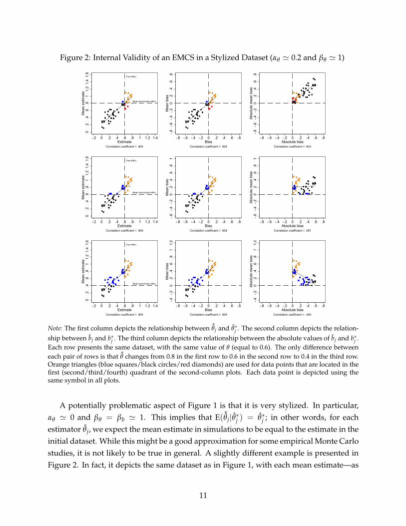
Figure 2: Internal Validity of an EMCS in a Stylized Dataset (αθ ' 0.2 and βθ ' 1)

True effect


0.2

.4.6

.81

1.2

1.4

1.6

Mea

n es

timat

e

-.2 0 .2 .4 .6 .8 1 1.2 1.4Estimate


-.8-.6

-.4-.2

0.2

.4.6

.8M

ean

bias

-.8 -.6 -.4 -.2 0 .2 .4 .6 .8Bias


-.8-.6

-.4-.2

0.2

.4.6

.8A

bsol

ute

mea

n bi

as

-.8 -.6 -.4 -.2 0 .2 .4 .6 .8Absolute bias


True effect


0.2

.4.6

.81

1.2

1.4

1.6

Mea

n es

timat

e

-.2 0 .2 .4 .6 .8 1 1.2 1.4Estimate


-.6-.4

-.20

.2.4

.6.8

1M

ean

bias

-.8 -.6 -.4 -.2 0 .2 .4 .6 .8Bias


-.6-.4

-.20

.2.4

.6.8

1A

bsol

ute

mea

n bi

as

-.8 -.6 -.4 -.2 0 .2 .4 .6 .8Absolute bias


True effect


0.2

.4.6

.81

1.2

1.4

1.6

Mea

n es

timat

e

-.2 0 .2 .4 .6 .8 1 1.2 1.4Estimate


-.4-.2

0.2

.4.6

.81

1.2

Mea

n bi

as

-.8 -.6 -.4 -.2 0 .2 .4 .6 .8Bias


-.4-.2

0.2

.4.6

.81

1.2

Abs

olut

e m

ean

bias

-.8 -.6 -.4 -.2 0 .2 .4 .6 .8Absolute bias



A potentially problematic aspect of Figure 1 is that it is very stylized. In particular,αθ ' 0 and βθ = βb ' 1. This implies that E( ¯θj|θ∗j ) = θ∗j ; in other words, for eachestimator θj, we expect the mean estimate in simulations to be equal to the estimate in theinitial dataset. While this might be a good approximation for some empirical Monte Carlostudies, it is not likely to be true in general. A slightly different example is presented inFigure 2. In fact, it depicts the same dataset as in Figure 1, with each mean estimate—as

11

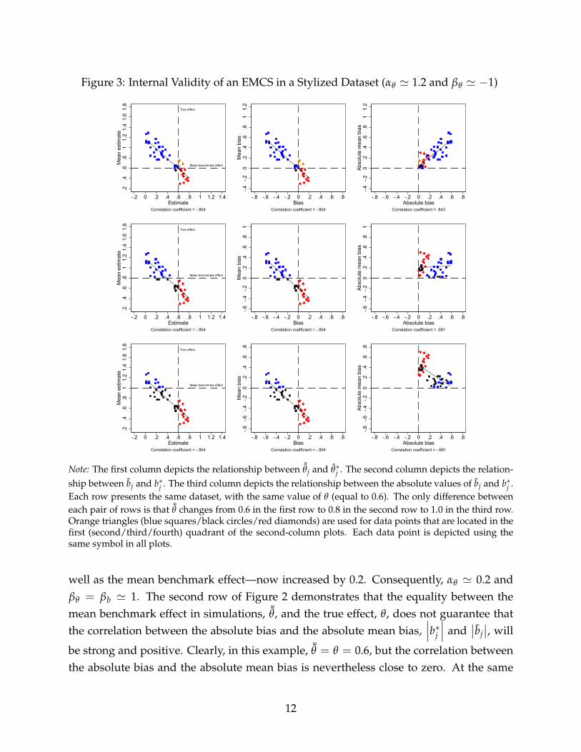
Figure 3: Internal Validity of an EMCS in a Stylized Dataset (αθ ' 1.2 and βθ ' −1)

True effect


.2.4

.6.8

11.

21.

41.

61.

8M

ean

estim

ate

-.2 0 .2 .4 .6 .8 1 1.2 1.4Estimate


-.4-.2

0.2

.4.6

.81

1.2

Mea

n bi

as

-.8 -.6 -.4 -.2 0 .2 .4 .6 .8Bias


-.4-.2

0.2

.4.6

.81

1.2

Abs

olut

e m

ean

bias

-.8 -.6 -.4 -.2 0 .2 .4 .6 .8Absolute bias


True effect


.2.4

.6.8

11.

21.

41.

61.

8M

ean

estim

ate

-.2 0 .2 .4 .6 .8 1 1.2 1.4Estimate


-.6-.4

-.20

.2.4

.6.8

1M

ean

bias

-.8 -.6 -.4 -.2 0 .2 .4 .6 .8Bias


-.6-.4

-.20

.2.4

.6.8

1A

bsol

ute

mea

n bi

as

-.8 -.6 -.4 -.2 0 .2 .4 .6 .8Absolute bias


True effect


.2.4

.6.8

11.

21.

41.

61.

8M

ean

estim

ate

-.2 0 .2 .4 .6 .8 1 1.2 1.4Estimate


-.8-.6

-.4-.2

0.2

.4.6

.8M

ean

bias

-.8 -.6 -.4 -.2 0 .2 .4 .6 .8Bias


-.8-.6

-.4-.2

0.2

.4.6

.8A

bsol

ute

mea

n bi

as

-.8 -.6 -.4 -.2 0 .2 .4 .6 .8Absolute bias



well as the mean benchmark effect—now increased by 0.2. Consequently, αθ ' 0.2 andβθ = βb ' 1. The second row of Figure 2 demonstrates that the equality between themean benchmark effect in simulations, ¯θ, and the true effect, θ, does not guarantee thatthe correlation between the absolute bias and the absolute mean bias,

∣∣∣b∗j ∣∣∣ and∣∣bj∣∣, will

be strong and positive. Clearly, in this example, ¯θ = θ = 0.6, but the correlation betweenthe absolute bias and the absolute mean bias is nevertheless close to zero. At the same

12

time, we observe a strong and positive correlation between∣∣∣b∗j ∣∣∣ and

∣∣bj∣∣ in the first row of

Figure 2. In this example, there is a mild difference between the mean benchmark effect,¯θ = 0.8, and the true effect, θ = 0.6, but this difference is offset by αθ ' 0.2.

We might also wonder what the consequences of a negative relationship between themean estimate in simulations and the estimate in the initial dataset, Cov( ¯θj, θ∗j ) < 0,might be. Another stylized example, based on a transformation of the previous data, istherefore presented in Figure 3. Once again we observe that, dependent on the relation-ship between the mean benchmark effect in simulations and the true effect, it is entirelypossible that the correlation between the absolute bias and the absolute mean bias can bestrong and positive, close to zero, or strong and negative—even though the underlyingestimates once again do not change between rows. An example with a strong and positivecorrelation between

∣∣∣b∗j ∣∣∣ and∣∣bj∣∣ is presented, again, in the first row of Figure 3.

What do the first rows of Figures 1–3 have in common? In other words, what conditionis required to enable the correlation between the absolute bias and the absolute mean biasto be as strong and positive as possible? We might notice that the condition that is sharedby the first rows of Figures 1–3 is actually very simple. The linear projection of ¯θj ontoθ∗j always passes through the point (θ, ¯θ); equivalently, the linear projection of bj onto b∗jalways passes through the origin.

We can now examine the consequences of this observation. In fact, we can rewriteequation (7) as

bj = αb + βbb∗j + υjb (9)¯θj − ¯θ = αb + βθ

(θ∗j − θ

)+ υjb (10)

¯θj =(

αb +¯θ − βθθ

)+ βθ θ∗j + υjb. (11)

But equation (11) represents the linear projection of ¯θj onto θ∗j , which was previously

defined in equation (6). What follows, αθ = αb +¯θ− βθθ. Moreover, if the linear projection

of bj onto b∗j were to pass through the origin, we would also require that αb = 0, which in

turn implies that αθ = ¯θ − βθθ. This restriction leads to a rule of thumb for maximizingthe correlation between the absolute bias in the sample of interest and the absolute meanbias in simulations,

∣∣∣b∗j ∣∣∣ and∣∣bj∣∣. If we use ¯θopt to denote the correlation-maximizing

(“optimal”) value of the mean benchmark effect, this rule of thumb can be written as

¯θopt = αθ + βθθ. (12)

13

Equation (12) demonstrates that any claim of internal validity of empirical Monte Carlostudies is necessarily based on circular reasoning. First, one might suggest that we canlearn about the value of θ because an empirical Monte Carlo study has helped us choose“good” estimators of this parameter. Then, however, our ability to discriminate between“good” and “bad” estimators depends on θ, and is maximized if ¯θ = ¯θopt.

Implications

The discussion thus far has important implications for the internal validity of empiricalMonte Carlo studies, some of which have already been mentioned. Here we providea more detailed discussion as well as an illustration which, again, uses the previouslyintroduced stylized dataset (more precisely, its version from Figure 1).

First, it is clear that the internal validity of an empirical Monte Carlo study is function-ally related to the value of the parameter of interest, θ. This severely limits the usefulnessof EMCS procedures, since the whole point of conducting such a simulation study is tofind “good” estimators of θ. This conclusion is not related to the fact that Figures 1–3present an oversimplified example of a possible simulation study. It is clear that our tar-get measure, Cor(

∣∣bj∣∣ ,∣∣∣b∗j ∣∣∣) = Cor(

∣∣∣ ¯θj − ¯θ∣∣∣ ,∣∣∣θ∗j − θ

∣∣∣), does in general depend on θ.7 In

the case of our stylized dataset, the dependence of Cor(∣∣bj∣∣ ,∣∣∣b∗j ∣∣∣) on θ, holding ¯θ fixed

at 0.6, is presented in the left-hand segment of Figure 4. The correlation between the ab-solute bias in the sample of interest and the absolute mean bias in simulations fluctuatesbetween –0.771 and 0.846, and the only source of variation is the value of θ. In practice,if we decided to conduct an empirical Monte Carlo study, we would never know whichsituation applies because we would not know the value of θ. Thus, we should not, ingeneral, expect that EMCS procedures can provide reliable information about the perfor-mance of estimators in the sample of interest.

Second, equation (12) suggests that Cor(∣∣bj∣∣ ,∣∣∣b∗j ∣∣∣) will be maximized if ¯θ = αθ + βθθ.

It is important to see that the accuracy of this rule of thumb does, in general, depend onwhether the linear projection of ¯θj onto θ∗j provides a good fit to the data. If the data are

highly dispersed or the relationship between ¯θj and θ∗j is nonlinear, this rule of thumbwill be imperfect. In the case of our stylized dataset, the accuracy of equation (12) inpredicting the maximum of Cor(

∣∣bj∣∣ ,∣∣∣b∗j ∣∣∣) can be seen visually in the central segment of

Figure 4, which displays the dependence of Cor(∣∣bj∣∣ ,∣∣∣b∗j ∣∣∣) on ¯θ, holding θ fixed at 0.6.

7It should be straightforward to realize that, for any other set of simulation results and for fixed ¯θ,manipulating θ (the vertical dashed line in the first column of Figures 1–3) would induce variation in thecorrelation between the absolute bias in the sample of interest and the absolute mean bias in simulations.

14

Figure 4: The Impact of θ and ¯θ on the Internal Validity of an EMCS-1

-.50

.51

Cor

rela

tion

coef

ficie

nt

0 .2 .4 .6 .8 1True effect

-1-.5

0.5

1C

orre

latio

n co

effic

ient

0 .2 .4 .6 .8 1Mean benchmark effect

0.2

.4.6

.81

Opt

imal

mea

n be

nchm

ark

effe

ct

0 .2 .4 .6 .8 1True effect

Note: Data come from the stylized dataset introduced in Figure 1. The left-hand segment presents thedependence of Cor(

∣∣bj∣∣ ,∣∣∣b∗j ∣∣∣) on θ, holding ¯θ fixed at 0.6. The central segment presents the dependence

of Cor(∣∣bj∣∣ ,∣∣∣b∗j ∣∣∣) on ¯θ, holding θ fixed at 0.6. The vertical (red) line presents the value of ¯θopt implied by

equation (12). The right-hand segment presents the dependence of ¯θopt on θ, using two formulas for ¯θopt;the straight (red) line uses equation (12) and the curved (black) line uses equation (13).

Clearly, the value of ¯θ that is suggested by the rule of thumb (represented by the verticalred line) does a reasonably good job of predicting the maximum of Cor(

∣∣bj∣∣ ,∣∣∣b∗j ∣∣∣).

It is important to note that equation (12) can be thought of as a linear approximationto the true value of ¯θopt, where

¯θopt = arg max¯θ

Cor(∣∣bj∣∣ ,∣∣∣b∗j ∣∣∣) = arg max

¯θCor(

∣∣∣ ¯θj − ¯θ∣∣∣ ,∣∣∣θ∗j − θ

∣∣∣). (13)

In the case of our stylized dataset, the fact that equation (12) is indeed a linear approxima-tion to equation (13) can be seen in the right-hand segment of Figure 4. For each value ofθ, we compare two “optimal” values of ¯θ, namely the value that is suggested by the ruleof thumb (straight red line) and the actual correlation-maximizing value (curved blackline), which we can find numerically. Clearly, the interpretation of our rule of thumb as alinear approximation to equation (13) is quite accurate in this case.

Third, even though our results on the internal validity of EMCS procedures are gen-erally quite negative, it is not impossible to formulate a potentially more optimistic im-plication of our findings. Namely, it can sometimes be helpful to place some bounds onthe region in which our population parameter of interest is assumed to lie. Since ourtarget measure, Cor(

∣∣bj∣∣ ,∣∣∣b∗j ∣∣∣), can easily be calculated for every possible value of θ, we

can also determine the bounds on θ which guarantee that this correlation coefficient willbe positive (or negative). If these bounds are sensible, an empirical Monte Carlo study

15

might be genuinely helpful. In the case of our stylized dataset, this information can begathered from the left-hand segment of Figure 4. For example, if we were convinced thatθ ≥ 0.370, we would know that our correlation of interest must be nonnegative (whichmight not be informative enough); if we were willing to increase this lower bound, say, to0.438, we would know that Cor(

∣∣bj∣∣ ,∣∣∣b∗j ∣∣∣) ≥ 0.5, and then this simulation exercise could

certainly be useful. On the other hand, these particular bounds might have questionablepractical value, given that many point estimates in our hypothetical example are smallerthan the proposed lower bounds on θ.

3 Data

This section discusses the data that we use as the basis for our empirical Monte Carlostudies; the role of these simulations is to provide a test for our theoretical predictions.As noted in Section 1, we focus on the data on men from LaLonde (1986), Heckman andHotz (1989), Dehejia and Wahba (1999, 2002), and Smith and Todd (2001, 2005). A subsetof these data comes from the National Supported Work (NSW) Demonstration, which wasa work experience program that operated in the mid-1970s at 15 locations in the UnitedStates (for a detailed description of the program see Smith and Todd, 2005). This programserved several groups of disadvantaged workers, such as women with dependent chil-dren receiving welfare, former drug addicts, ex-convicts, and school drop-outs. Unlikemany similar programs, the NSW implemented random assignment among eligible par-ticipants. This random selection allowed for straightforward evaluation of the programvia a comparison of mean outcomes in the treatment and control groups.

In an influential paper, LaLonde (1986) uses the design of this program to assess theperformance of a large number of nonexperimental estimators of average treatment ef-fects, many of which are based on the assumption of unconfoundedness. He discardsthe original control group from the NSW data and creates several alternative comparisongroups using data from the Current Population Survey (CPS) and the Panel Study of In-come Dynamics (PSID), two standard datasets on the U.S. population. His key insight isthat a “good” estimator should be able to closely replicate the experimental estimate ofthe effect of NSW using nonexperimental data. He finds that very few of the estimatesare close to this benchmark. This result motivated a large number of replications andfollow-ups, and established a testbed for estimators of average treatment effects underunconfoundedness (see, e.g., Heckman and Hotz 1989; Dehejia and Wahba 1999, 2002;Smith and Todd 2001, 2005; Abadie and Imbens 2011; Diamond and Sekhon 2013). Likemany other papers, we use the largest of the six nonexperimental comparison groups

16

constructed by LaLonde (1986), which he refers to as CPS-1 and PSID-1.In this paper we take the key insight of LaLonde (1986) one step further. We note that

if we treat the experimental estimate of the impact of NSW as the “true effect,” we cancalculate “true biases” of various estimators in the original nonexperimental datasets. Wecan also conduct an empirical Monte Carlo study in an attempt to replicate these data,and compare the performance of estimators in simulations with their performance in theoriginal data. It must be noted, however, that in this scenario the “true effect” is estimatedand, therefore, is subject to sampling error. Thus, we also use an insight of Smith andTodd (2005) that if we discard the original treatment group from the NSW data and studythe control group and the nonexperimental comparison groups, the “true effect” in thesedata will be zero by construction and will not be subject to sampling error. This approachhas a clear advantage if we are concerned about the uncertainty in the “true effect.”

Moreover, we use two alternative versions of the data from the NSW experiment,namely the sample used by Dehejia and Wahba (1999), henceforth DW, and the “earlyrandom assigment” (“early RA”) sample used by Smith and Todd (2005), henceforth ST.What follows, we construct a total of eight datasets, namely “DW control/CPS,” “DWtreated/CPS,” “ST control/CPS,” “ST treated/CPS” (jointly referred to as “NSW-CPS”),“DW control/PSID,” “DW treated/PSID,” “ST control/PSID,” and “ST treated/PSID”(jointly referred to as “NSW-PSID”). For each of these datasets, we conduct eight empir-ical Monte Carlo studies, where we vary three aspects of a study: the outcome variable(earnings or nonemployment), the set of control variables (“simple” or “balanced”), andthe design of the study itself (“placebo” or “structured”).8 Descriptive statistics as well as“true effects” for our “original datasets” are presented in the Appendix.

4 Designs

This section provides a more detailed discussion of our application of both approaches toconducting an EMCS, namely the structured design of Busso et al. (2014) and the placebodesign of Huber et al. (2013).

8Both outcome variables are measured in 1978. The “simple” set of control variables is taken fromAbadie and Imbens (2011) and includes age (age), education (educ), earnings in months 13–24 prior to ran-domization (re74), earnings in 1975 (re75), as well as indicators for whether black (black), whether married(married), whether had zero earnings in months 13–24 prior to randomization (u74), and whether had zeroearnings in 1975 (u75). The “balanced” set of control variables is borrowed from Dehejia and Wahba (2002).For CPS, it includes all the variables in the “simple” specification as well as age squared (age2), age cubed(age3), education squared (educ2), an indicator for whether a high school dropout (nodegree), an indicatorfor whether Hispanic (hispanic), and an interaction between re74 and educ (re74ed). For PSID, it includesall the variables in the “simple” specification as well as age2, educ2, nodegree, hispanic, re74 squared(re742), re75 squared (re752), and an interaction between u74 and hispanic (u74h).

17

The Structured Design

In the structured design we begin by generating a fixed number of treated and nontreatedobservations in each replication, so that the original sample sizes and proportions of bothgroups are retained. We then draw an employment status pair of u74 and u75, conditionalon treatment status, to match the observed conditional joint probability. For individualswho are employed in only one period, an income is drawn from a log normal distributionconditional on treatment and employment statuses, with mean and variance calibrated tothe respective conditional moments in the data. Where individuals are employed in bothperiods a joint log normal distribution is used, again conditioning on treatment status. Inall cases, whenever the income draw in a particular year lies outside the relevant supportobserved in the data, conditional on treatment status, the observation is replaced with thelimit point of the empirical support, as also suggested by Busso et al. (2014).

We model the joint distribution of the remaining control variables as a particular tree-structured conditional probability distribution, so that we can better fit the correlationstructure in the data. The process for generating these covariates is as follows:

1. The covariates are ordered: treatment status, employment statuses, income in eachperiod, whether a high school dropout (nodegree), education, age, whether mar-ried, whether black, and whether Hispanic. This ordering is arbitrary, and a similarcorrelation structure would be generated if the ordering were changed.

2. Using the original data, each covariate from nodegree onward is regressed on allthe covariates listed before it (we use the logit model for binary variables).9 Theseregressions are not to be interpreted causally; they simply give the conditional meanof each variable given all preceding covariates.

3. In the simulated dataset, covariates are drawn sequentially in the same order. Forbinary covariates a temporary value is drawn from a U [0, 1] distribution. Then thecovariate is equal to one if the temporary value is less than the conditional probabil-ity for that observation. The conditional probability is found using the values of theexisting generated covariates and the estimated coefficients from step 2. Age andeducation are drawn from a normal distribution whose mean depends on the othercovariates and whose variance is equal to that of the residuals from the relevantmodel. Again, we replace extreme values with the limit of the support, conditionalon treatment status (for education, also conditional on dropout status).

9One exception is educ which is regressed on the prior listed covariates conditional on nodegree.Clearly, it is not possible for a high school dropout to have twelve years of schooling or more; it is alsonot possible for a non-dropout to have less than twelve years of schooling.

18

The simulated outcome, Yi,s, is then generated in two steps. In the first step, we generatea conditional mean using the parameters of a flexible logit model (for u78) or a flexiblelinear model (for re78) fitted from the original data. Precisely, we estimate either (γ0, γ1)

from the following logit model:

P(Y∗i = 1|D∗i , Z∗i ) = Λ((1− D∗i )Z∗i γ0 + D∗i Z∗i γ1), (14)

or (δ0, δ1) from the following linear model:

E(Y∗i |D∗i , Z∗i ) = (1− D∗i )Z∗i δ0 + D∗i Z∗i δ1. (15)

Importantly, Z∗i contains all the control variables that are included in a given specification,“simple” or “balanced.” The predicted conditional mean in the simulated data is then cal-culated using the estimated coefficients (γ0, γ1) or (δ0, δ1), and the simulated treatmentstatus and covariates, Di,s and Zi,s. In the second step, the simulated outcome, Yi,s, is de-termined either—in the case of nonemployment—as a draw from a Bernoulli distributionwith the estimated conditional probability Λ((1−Di,s)Zi,sγ0 + Di,sZi,sγ1) or—in the caseof earnings—as a draw from a normal distribution with the estimated conditional mean(1− Di,s)Zi,sδ0 + Di,sZi,sδ1 and the variance that is fitted to that of the residuals from themodel in equation (15), conditional on treatment status. Once again, we replace extremevalues of re78 with the limit point of the support, also conditional on treatment status.“True effects” in each replication, θs, are calculated using the conditional means for bothtreatment statuses, and the difference in conditional means, i.e. the individual-level treat-ment effect, is averaged over the subsample of treated units.10

We approximate the sample-size selection rule in Huber et al. (2013), which suggestshow the number of generated samples should vary with the number of observations, bygenerating 2,000 samples in each EMCS based on the NSW-PSID data and 500 samples ineach EMCS based on the larger NSW-CPS.

The Placebo Design

In the placebo design covariates are drawn jointly with outcomes from the empirical dis-tribution, rather than a parameterized approximation. In particular, pairs (Yi,s, Zi,s) aredrawn with replacement from the sample of comparison observations from CPS or PSID.

10Thus, we implicitly focus on the sample average treatment effect on the treated (SATT), not on thepopulation average treatment effect on the treated (PATT). Both of these measures can be used as thebenchmark effect in simulations and we have no particular preference for either. Our theoretical predictionsfrom Section 2 also support using either of these parameters.

19

The data from the NSW experiment—both the treatment and control groups, as in Smithand Todd (2005)—are used with the comparison data to estimate the propensity scoresusing the logit model. The vector of coefficients from this model is referred to as φ, andin each case we estimate the propensity scores using all the control variables that are in-cluded in a given specification, “simple” or “balanced.” The inclusion of the “balanced”specification might be particularly important, given that Huber et al. (2013) stress the im-portance of the correct specification of the model for the propensity scores.

We then assign treatment status to observations in the simulated data using the esti-mated vector, φ; iid logistic errors, εi,s; and two scalar parameters, λ and π, where λ de-termines the degree of covariate overlap between the “placebo treated” and “nontreated”observations and π determines the proportion of the “placebo treated.” More precisely,

Di,s = 1[Si,s > 0], (16)

Si,s = π + λZi,sφ + εi,s. (17)

Since the outcome variable, Yi,s, is drawn directly from the data together with Zi,s, wedo not need to specify any DGP for the outcome. Instead we know that the effect of the“placebo treatment” is zero, and that it is also constant across samples, θs = 0 for all s.11

This design requires some choice of π and λ. We choose π to ensure that the propor-tion of the “placebo treated” observations in each simulated sample is as close as possibleto the proportion of treated units in the corresponding original dataset.12 We also followHuber et al. (2013) in choosing λ = 1. As before, we generate 2,000 samples in each EMCSbased on NSW-PSID and 500 samples in each EMCS based on NSW-CPS.

5 Estimators

This section provides an overview of estimators which we use in our EMCS procedures.All of these estimators are based on the assumption of unconfoundedness which, looselyspeaking, requires that there is no omitted variables bias. Unfortunately, this assumptionis not uncontroversial in the context of the NSW-CPS and NSW-PSID datasets. Follow-

11A similar approach is developed by Bertrand et al. (2004) who study inference in difference-in-differences methods using simulations with randomly generated “placebo laws” in state-level data, i.e. pol-icy changes which never actually happened. For follow-up studies, see Hansen (2007), Cameron et al. (2008),and Brewer et al. (2013).

12It should be noted, however, that the way these datasets were constructed by LaLonde (1986) resultsin samples that are best described as choice-based. More precisely, the treatment and control groups areheavily overrepresented relative to their population proportions. See Smith and Todd (2005) for a furtherdiscussion of this issue.

20

ing LaLonde (1986), Heckman and Hotz (1989), Dehejia and Wahba (1999, 2002), Smithand Todd (2001, 2005), Abadie and Imbens (2011), and Diamond and Sekhon (2013), weproceed, however, as if this assumption were satisfied.

We begin by discussing estimators which we use to study the impact of NSW onnonemployment. We consider estimators which belong to one of five main classes: stan-dard parametric (regression-based), flexible parametric (Oaxaca–Blinder), kernel-based(kernel matching, local linear regression, and local logit), nearest-neighbor (NN) match-ing, and inverse probability weighting (IPW) estimators. In each case we focus on theaverage treatment effect on the treated (ATT), unless a given method does not allow forheterogeneity in effects (in which case we estimate the overall effect of treatment).

In particular, we use as regression-based methods the linear probability model (LPM)as well as the logit, probit, and complementary log-log models. The complementary log-log model uses an asymmetric link function, which makes it more appropriate when theprobability of success takes values close to zero or one, as is the case in our application.

We also follow Kline (2011) in using the Oaxaca–Blinder (OB) decomposition to esti-mate the ATT.13 Since we consider a binary outcome, we use both linear and nonlinearOB methods. The linear OB decomposition is equivalent to the LPM but with the treat-ment indicator interacted with appropriately demeaned covariates. Similarly, nonlinearOB decompositions impose either a logit or a probit link function around the linear index,separately for both groups of interest (see, e.g., Yun 2004, Fairlie 2005).

Turning to more standard treatment effect estimators, we consider several kernel-based methods, in particular kernel matching, local linear regression, and local logit.Kernel matching estimators play a prominent role in the program evaluation literature(see, e.g., Heckman et al. 1997, Frolich 2004), and their asymptotic properties are estab-lished by Heckman et al. (1998). Similarly, local linear regression is studied by Fan (1992)and Heckman et al. (1998). Because our outcome is binary, we also consider local logit, asapplied in Frolich and Melly (2010). Note that each of these estimators requires estimat-ing the propensity score in the first step (based on the logit model) as well as choosinga bandwidth. For each of the methods, we select the bandwidth on the basis of leave-one-out cross-validation (as in Busso et al. 2009 and Huber et al. 2013) from a search grid.005× 1.25g−1 for g = 1, 2, . . . , 15, and repeat this process in each replication.14

13Kline (2011) shows that Oaxaca–Blinder is equivalent to a particular reweighting estimator and that ittherefore satisfies the property of double robustness. See also Oaxaca (1973) and Blinder (1973) for seminalformulations of this method as well as Fortin et al. (2011) for a recent review of decomposition methods.

14Note that the computation time is already quite large in the case of the NSW-PSID datasets, but it iscompletely prohibitive for NSW-CPS. Consequently, in the case of the NSW-CPS datasets, we calculateoptimal bandwidths only once, for the original dataset, and use these values in our simulations.

21

We also apply several NN matching estimators, including both matching on covari-ates and on the estimated propensity score. Asymptotic properties for some of theseestimators are derived by Abadie and Imbens (2006). Since these matching estimators areshown not to be

√N-consistent in general, we also consider the bias-adjusted variant of

both versions of matching (Abadie and Imbens, 2011). Like kernel-based methods, NNmatching estimators require choosing a tuning parameter, M, the number of neighbors.We consider the workhorse case of M = 1 as well as M = 2 and M = 4, so we applytwelve NN matching estimators in total. We always match with replacement; if there areties, all of the tied observations are used.

The last class of estimators includes two versions of inverse probability weighting(see, e.g., Horvitz and Thompson 1952, Hirano et al. 2003, Wooldridge 2007) as well astwo doubly robust estimators (see, e.g., Robins et al. 1994, Wooldridge 2007, Uysal 2015,Słoczynski and Wooldridge 2016). We consider normalized reweighting, in which theweights are rescaled to sum to unity, and efficient reweighting, as proposed by Lunce-ford and Davidian (2004).15 Our doubly robust estimators combine inverse probabilityweighting with a model for the conditional mean, and we consider both linear and lo-gistic mean functions. The resulting estimators are consistent if at least one of the twomodels is correctly specified.

Moreover, for regression-based, Oaxaca–Blinder, and inverse probability weightingestimators we also consider a separate case in which we restrict our estimation proce-dures to those treated (or placebo treated) whose estimated propensity scores are largerthan the minimum and smaller than the maximum estimated propensity score among thenontreated, i.e. to those who are located in the overlap region.16 On the other hand, whenwe study the impact of NSW on earnings, the number of available estimators is smaller,since we cannot use those methods that require the outcome variable to be binary: logit,probit, and complementary log-log models (6 estimators in total); nonlinear OB methods(4 estimators in total); local logit (1 estimator); and the doubly robust estimator with alogistic mean function (2 estimators in total).

What follows, our final number of estimators for nonemployment (earnings) is equal

15Initially, we also considered unnormalized reweighting where the sum of weights is stochastic. How-ever, in line with the results in Frolich (2004), the performance of this estimator was often extremely poor,to the extent that we treat this method as an outlier and leave it out of the analysis.

16We do not consider such a variant of kernel-based and nearest-neighbor matching estimators for tworeasons. First, these estimators explicitly compute a counterfactual for each individual using data fromthe closest neighborhood of this individual. Second, these two classes of estimators account for nearly100% of our computation time, and therefore such an inclusion would be prohibitive timewise. This is notproblematic, since our interest is not in how well any particular estimator performs, but rather in comparingthe performance of estimators in the original data and in the Monte Carlo samples.

22

to 39 (26), including 8 (2) regression-based estimators, 6 (2) OB estimators, 5 (4) kernel-based estimators, 12 (12) NN matching estimators, and 8 (6) IPW estimators. We conductour simulations in Stata and use several user-written commands in our estimation proce-dures: locreg (Frolich and Melly 2010), nnmatch (Abadie et al. 2004), oaxaca (Jann 2008),and psmatch2 (Leuven and Sianesi 2003).

6 Results

This section provides a discussion of our empirical results. We begin by adding a fewmore remarks about some aspects of our simulation procedures.

The total number of simulation studies that we consider is sixty-four. Recall that weconstruct eight nonexperimental datasets, which we enumerate in Section 3, and we con-duct eight empirical Monte Carlo studies for each of them. We vary three aspects of anEMCS procedure, namely the outcome variable, the set of control variables, and whetherthe study is designed as placebo or structured. There are two possible choices in each ofthese three cases, which gives a total of eight combinations.

Further details on our nonexperimental datasets are presented in the Appendix. Foreach dataset, we provide information on the “true effects” (or θ) and associated standarderrors. Moreover, for each dataset, we present summary statistics for the outcome andmain control variables, separately for each treatment status. We also present two mea-sures of overlap as well as a matrix of correlations between the main control variables,again conditional on treatment status. A “good” empirical Monte Carlo study, apart fromhaving high internal validity, should be able to replicate these statistics reasonably well.Thus, the same statistics are also presented in the Web Appendix for each of the simula-tion studies. In general, the simulations replicate the “original datasets” well.

Further analysis proceeds as follows. In each of the nonexperimental datasets, weestimate the impact of NSW on both nonemployment and earnings using estimators dis-cussed in Section 5. For each estimator, we consider two sets of control variables, “simple”and “balanced.” Using our notation from Section 2, this gives us thirty-two sets of valuesof θ∗j .17 Because we already know the values of θ, we also create thirty-two sets of “true

biases,” namely b∗j = θ∗j − θ, and “absolute true biases,” namely∣∣∣b∗j ∣∣∣ = ∣∣∣θ∗j − θ

∣∣∣. Thesedata are presented in the Web Appendix.

17The reason for having thirty-two sets of nonexperimental estimates—and not sixty-four—is very sim-ple. Namely, we use eight nonexperimental datasets and—in each of them—we estimate the effect of NSWon two outcomes (nonemployment and earnings) using two specifications (“simple” and “balanced”). Thefact that we also conduct two simulation studies (placebo and structured) for each such combination hasno impact on the number of sets of nonexperimental estimates.

23

We also calculate mean estimates, or ¯θj, mean biases, or bj =¯θj− ¯θ, and absolute mean

biases, or∣∣bj∣∣ = ∣∣∣ ¯θj − ¯θ

∣∣∣, for each estimator in each of the sixty-four simulation studies.18

The fact that a given study is referred to as “simple” or “balanced” determines the setof control variables in all estimation procedures. These data on biases in simulations arepresented in the Web Appendix. Finally, this allows us to construct sixty-four datasets inwhich an estimator is the unit of observation. For each estimator, we observe θ∗j and ¯θj;

b∗j and bj; and, finally,∣∣∣b∗j ∣∣∣ and

∣∣bj∣∣. In each of these datasets we calculate the correlations

between these measures (across estimators), analogous to the theoretical considerationsin Section 2, and analyze the results. The disaggregated data on correlation coefficientsin each of the sixty-four datasets are presented in the Web Appendix. In the body of thepaper we focus on summary statistics for these correlations and we also analyze thesedata in a regression framework.

Average Correlations

The first set of results concerns the average values of correlations across simulation stud-ies. Our theoretical results suggest that there is no reason to expect a systematic relation-ship between the absolute biases in the sample of interest and the absolute mean biases insimulations. In column 3 of Table 1 we can see that on average across our EMCS designsthis correlation is indeed close to zero. More precisely, it is equal to –0.054 and, in fact,different from zero at the 10% significance level. It turns out to be the case that this resultis driven by placebo simulations. For the placebo design, the average correlation is alsonegative but larger in absolute value; namely, it is equal to –0.111 and different from zeroat the 1% significance level. The average correlation for the structured design is equal to0.003 and indistinguishable from zero. Although we do not offer any predictions on theaverage correlations between estimates and between biases, we report these results forcompleteness in columns 1 and 2 of Table 1.

As a robustness check for our results on absolute mean biases, we also calculate theaverage correlation between the “true biases” and the median biases in simulations aswell as between the “absolute true biases” and the absolute median biases in simulations.This might be important if the results for mean biases are in some way affected by out-liers. These results are presented in the Appendix; they are similar to those for meanbiases, although we can no longer conclude that, for the placebo design, the average cor-relation between the absolute biases is significantly different from zero. In other words,we have less reasons to believe that placebo simulations have lower internal validity than

18As already discussed, the mean benchmark effect in simulations, ¯θ, is easily calculated for each study.

24

Table 1: Average Correlations in the Empirical Monte Carlo Studies

Estimates—Meanestimates

Biases—Meanbiases

Absolutebiases—Absolute

mean biases(1) (2) (3)

All simulationsCorrelation 0.063* 0.063* –0.054*

(0.036) (0.036) (0.028)Observations 64 64 64

PlaceboCorrelation –0.015 –0.015 –0.111***

(0.051) (0.051) (0.035)Observations 32 32 32

StructuredCorrelation 0.141*** 0.141*** 0.003

(0.046) (0.046) (0.041)Observations 32 32 32

Note: The values in each cell represent mean correlation coefficients averaged acrosssimulation studies. Standard errors are in parentheses. Tests of significance are two-tailed and the null hypothesis is that of a zero average correlation.*Statistically significant at the 10% level; **at the 5% level; ***at the 1% level.

structured in our application. Hence, our simulation results are in line with our earlierprediction that the internal validity of empirical Monte Carlo studies might be quite low.Neither of the EMCS designs appears to be helpful for selecting estimators in this context.

We also consider an additional robustness check, loosely inspired by Heckman andHotz (1989), where we study whether empirical Monte Carlo studies, like specificationtests in Heckman and Hotz (1989), are at least able to “eliminate the most unreliable andmisleading estimators.” We operationalize this idea in the following way. For each com-bination of a nonexperimental dataset, an outcome variable, and a set of control variables,we evaluate which estimators belong to the group of 20% of the estimators with highest“absolute true biases.” These are the “worst estimators” we would like to avoid. Then,for each simulation study, we calculate what percentage of these estimators can be foundin the top x% with lowest absolute mean biases, and we consider x = 10, x = 25, andx = 50. In this test, if x% of the worst estimators can be found in the top x% of estimatorsaccording to an EMCS, then this EMCS is as good as random in helping with estimatorchoice. If we can find less than x% of the worst estimators at the top, then an EMCS ishelpful; if more than x%, then it is actively misleading. These results are presented inthe Appendix. There is no test in which we would conclude that empirical Monte Carlo

25

studies are actually helpful. In one case, that of placebo simulations with x = 50, theymight be evaluated as harmful.

Determinants of Internal Validity

The second set of results concerns the determinants of the magnitudes of the correlationcoefficients. For conciseness we omit the results on correlations between estimates, sincethese results are again numerically identical to the results on biases. We study this prob-lem in a regression framework, using the magnitude of a given correlation coefficientas a dependent variable and characteristics of a given simulation study as independentvariables. These results are presented in Table 2.

Turning to the reported estimates, we first examine the determinants of correlationsbetween biases (column 1). We regress the correlation coefficient on all the characteristicsof the original dataset and of the simulation study that we are able to control: whether weuse the placebo or the structured design; whether we use the CPS or the PSID nonexper-imental comparison group; whether we use earnings or nonemployment as the outcomevariable; whether we use the Dehejia and Wahba (1999) or the Smith and Todd (2005)version of the NSW dataset; whether we use the “simple” or the “balanced” set of controlvariables; and whether we use the treatment or the control group from the NSW experi-ment. It turns out that two out of six coefficients are statistically significant. The placebodesign does a worse job than the structured design in replicating biases. On the otherhand, it seems easier to replicate the biases for the NSW-CPS datasets than for the NSW-PSID datasets. Moreover, column 2 reports coefficient estimates from a regression withthe same independent variables, but with a different dependent variable: the correlationbetween absolute biases. As before, the estimated coefficient on placebo is negative andstatistically significant; thus, at least in our study, the internal validity of placebo is lowerthan that of structured. It also turns out to be the case that it is more difficult to predictabsolute biases using the Smith and Todd (2005) version of the NSW dataset. This is anal-ogous to one of the results in Smith and Todd (2005), namely that it is more difficult torecover the experimental estimate of the impact of NSW using their version of the dataset,as compared with the version of Dehejia and Wahba (1999).

We also develop a further test of our theoretical predictions from Section 2. More pre-cisely, we can now examine whether our rule of thumb for maximizing the correlationbetween the absolute biases, namely equation (12), is indeed capable of predicting themagnitude of this correlation. We construct a new variable,

∣∣∣ ¯θopt − ¯θ∣∣∣ = ∣∣∣αθ + βθθ − ¯θ

∣∣∣,which measures the distance between the “optimal” value and the actual value of the

26

Table 2: Regression Analysis of the Simulation Results

Biases—Meanbiases

Absolute biases—Absolute mean biases

(1) (2) (3) (4)Placebo –0.156** –0.114** –0.155*** –0.211

(0.069) (0.051) (0.051) (0.160)CPS 0.117* –0.031 –0.045 –0.095

(0.069) (0.051) (0.049) (0.072)Earnings 0.095 –0.025 –0.024 –0.073

(0.069) (0.051) (0.050) (0.078)DW 0.036 0.156*** 0.132** 0.170**

(0.069) (0.051) (0.051) (0.074)Balanced 0.027 0.006 0.033 0.029

(0.069) (0.051) (0.049) (0.085)Control 0.025 0.036 0.047 0.098

(0.069) (0.051) (0.050) (0.078)Std. distance –0.078** –0.079*

(0.035) (0.046)CPS × Placebo 0.099

(0.102)Earnings × Placebo 0.122

(0.131)DW × Placebo –0.067

(0.109)Balanced × Placebo 0.010

(0.112)Control × Placebo –0.094

(0.109)Std. distance × Placebo 0.040

(0.112)Constant –0.009 –0.068 0.013 0.020

(0.078) (0.056) (0.064) (0.072)

Observations 64 64 64 64R2 0.156 0.211 0.262 0.311

Note: The dependent variables are the correlation between the bias in the sample of interest and the meanbias in simulations (column 1) and the correlation between the absolute bias in the sample of interest andthe absolute mean bias in simulations (columns 2–4). “Placebo” is an indicator variable that equals one ifa given study is designed as placebo and zero otherwise. “CPS” is an indicator variable that equals oneif a given study is based on the CPS comparison group and zero otherwise. “Earnings” is an indicatorvariable that equals one if re78 is the outcome variable in a given study and zero otherwise. “DW” is anindicator variable that equals one if a given study is based on the Dehejia and Wahba (1999) version ofthe NSW data and zero otherwise. “Balanced” is an indicator variable that equals one if a given studyuses the “balanced” set of control variables and zero otherwise. “Control” is an indicator variable thatequals one if a given study is based on the control group from the NSW experiment and zero otherwise.“Std. distance” is the standardized distance between the “optimal” value and the actual value of the meanbenchmark effect in simulations. Huber–White standard errors are in parentheses.*Statistically significant at the 10% level; **at the 5% level; ***at the 1% level.

27

mean benchmark effect in simulations. Intuitively, we would expect that, other thingsequal, the more distant we are from the correlation-maximizing value of the mean bench-mark effect, the smaller is the correlation between the absolute biases. Because distanceis measured in different units (dollars or percentage points) dependent on the outcomevariable in a given simulation study (earnings or nonemployment), we begin by stan-dardizing this new variable; more precisely, we divide raw values of ¯θopt − ¯θ by its stan-dard deviation, separately for studies of earnings and nonemployment, and then calcu-late absolute values. Finally, we add this “standardized distance” to our earlier set ofindependent variables and report the estimated coefficients in column 3. In line withour predictions, the coefficient on standardized distance is negative; it is also statisticallysignificant. Thus, our rule of thumb does indeed have predictive power for the internalvalidity of empirical Monte Carlo studies.

Column 4 reports the final set of estimated coefficients, where we interact the indicatorfor placebo simulations with the remaining independent variables, including standard-ized distance. Thus, we examine whether the effects of these variables on our correlationof interest differ between placebo and structured simulations. The answer to this ques-tion is negative. Neither of the estimated coefficients is statistically significant, and quiteclearly so, with all t-statistics for the interaction terms smaller than one.

Bounding the Effect of Interest

The third set of results concerns our earlier claim that it might sometimes be helpful toplace some bounds on the population parameter of interest—in the hope that this mightallow one to conclude that a given simulation study is at least informative under thecondition that these bounds are correct. In other words, our results thus far suggest thatone should not expect a priori that an empirical Monte Carlo study will be internally valid.However, for a simulation study that has already been conducted, we might perhaps beable to claim its internal validity by making additional assumptions a posteriori.

For each of our sixty-four simulation studies we calculate how the correlation betweenthe absolute biases would change with θ, holding ¯θ fixed at its actual value. These figuresare presented in the Web Appendix. Due to space restrictions, in the body of the paper werestrict our attention to only four cases which we present in Figure 5. The upper segmentsfocus on two placebo simulations, while the lower segments focus on structured. The left-hand segments of Figure 5 present the dependence of our correlation of interest on θ fortwo studies of nonemployment; the right-hand segments—for two studies of earnings.

The upper left segment of Figure 5 is an example of a pessimistic scenario. Since this

28

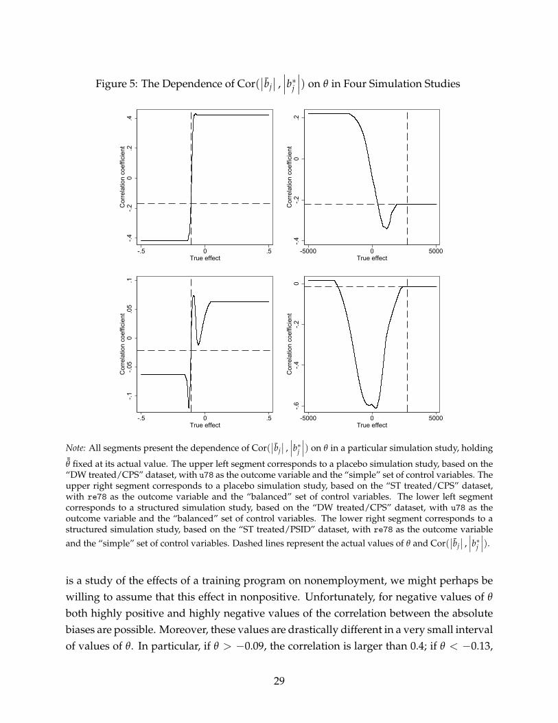
Figure 5: The Dependence of Cor(∣∣bj∣∣ ,∣∣∣b∗j ∣∣∣) on θ in Four Simulation Studies

-.4-.2

0.2

.4C

orre

latio

n co

effic

ient

-.5 0 .5True effect

-.4-.2

0.2

Cor

rela

tion

coef

ficie

nt

-5000 0 5000True effect

-.1-.0

50

.05

.1C

orre

latio

n co

effic

ient

-.5 0 .5True effect

-.6-.4

-.20

Cor

rela

tion

coef

ficie

nt

-5000 0 5000True effect

Note: All segments present the dependence of Cor(∣∣bj∣∣ ,∣∣∣b∗j ∣∣∣) on θ in a particular simulation study, holding

¯θ fixed at its actual value. The upper left segment corresponds to a placebo simulation study, based on the“DW treated/CPS” dataset, with u78 as the outcome variable and the “simple” set of control variables. Theupper right segment corresponds to a placebo simulation study, based on the “ST treated/CPS” dataset,with re78 as the outcome variable and the “balanced” set of control variables. The lower left segmentcorresponds to a structured simulation study, based on the “DW treated/CPS” dataset, with u78 as theoutcome variable and the “balanced” set of control variables. The lower right segment corresponds to astructured simulation study, based on the “ST treated/PSID” dataset, with re78 as the outcome variableand the “simple” set of control variables. Dashed lines represent the actual values of θ and Cor(

∣∣bj∣∣ ,∣∣∣b∗j ∣∣∣).

is a study of the effects of a training program on nonemployment, we might perhaps bewilling to assume that this effect in nonpositive. Unfortunately, for negative values of θ

both highly positive and highly negative values of the correlation between the absolutebiases are possible. Moreover, these values are drastically different in a very small intervalof values of θ. In particular, if θ > −0.09, the correlation is larger than 0.4; if θ < −0.13,

29

the correlation is smaller than –0.4. In this case it would not be reasonable to bound θ,since we observe very different values of our correlation of interest for plausible—andvery similar—values of this parameter.

The lower left segment of Figure 5 presents a further example of a simulation studywhich is unlikely to be useful. As before, the assumption that the effects of training onnonemployment are negative would provide no information about the sign of our corre-lation coefficient of interest. Moreover, this correlation is uniformly very close to zero—never smaller than –0.117 and never larger than 0.073—and hence the predictive powerof this simulation study is extremely low even in the best-case scenario.

A somewhat different situation is presented in the upper right segment of Figure 5.Since we now focus on the effects of training on earnings, it might be reasonable to assumethat θ is nonnegative. If this is the case, however, our correlation of interest is guaranteedto be negative; more precisely, it will be smaller than –0.084 but not smaller than –0.341.At first, this might seem to be bad news—according to our definition, internal validityof this study is certainly low as long as θ is indeed nonnegative. However, this studycan still be helpful in estimator choice—if only we decide to choose estimators whichperform badly in this simulation study. If we did this, we would increase our chances ofusing an estimator with a small value of absolute true bias—although this help would besomewhat restricted by the fact that the magnitudes of these correlations are quite low.

Moreover, the lower right segment of Figure 5 is another example of a more optimisticoutcome. Again, we focus on the effects of a training program on earnings and we mightperhaps be willing to assume that this effect is positive. In this case our correlation ofinterest would again be guaranteed to be negative; it could be as strong as –0.611 but alsomuch closer to zero. As before, this is a case where, if anything, one would want to chooseestimators which perform badly in the simulations.

In other cases, we would expect that bounding the population parameter could some-times allow us to conclude that our correlation of interest must be positive. Then, ofcourse, we would choose estimators which perform well in a given EMCS. However, nosuch cases are available among the simulation studies that we have conducted.

7 Conclusions

In this paper we contribute to the recent literature on the finite-sample performance ofestimators of average treatment effects under unconfoundedness. Influential papers byHuber et al. (2013) and Busso et al. (2014) suggest that an empirically motivated simu-lation exercise might be informative about the performance of estimators in a particular

30

context. In this paper we claim that such a high degree of internal validity of empiricalMonte Carlo studies is, in fact, far from self-evident. We begin by developing a simpleframework within which we demonstrate that there is little reason to expect our preferredmeasure of internal validity—the correlation between the absolute bias in the sample ofinterest and the absolute mean bias in simulations—to be systematically positive. We alsoshow that this measure is dependent on the true value of the population parameter of in-terest. This is an important limitation of EMCS procedures, since were this object known,no simulation studies and no estimation procedures would be necessary.

We consider two different designs of an empirical Monte Carlo study. The first, whichwe term the structured design, is based on Busso et al. (2014). Here we generate newdata which match particular features of the original dataset, and then generate outcomesusing parameters estimated from the original data. We also consider the placebo design,as suggested by Huber et al. (2013). Here a sample of observations is drawn from thecomparison data, and a placebo treatment is assigned using the propensity score fromthe full data. The treatment effect in the sample is therefore zero by construction.

Using the data on men from the influential papers by LaLonde (1986), Heckman andHotz (1989), Dehejia and Wahba (1999, 2002), and Smith and Todd (2001, 2005), we con-struct an empirical test for both designs. Our results are quite negative—but they alsocorroborate our theoretical predictions. The average degree of internal validity of EMCSprocedures is very low. In fact, we have no evidence that practitioners would be betteroff, on average, using an empirical Monte Carlo study than choosing estimators at random.However, we also demonstrate that if a simulation study has already been run then it isgenerally possible to assess how likely we are to learn something useful from its results.We discuss two actual cases of a simulation study which might, in fact, be helpful.

Consequently, we would generally discourage applied researchers who consider con-ducting an empirical Monte Carlo study. In our view, the expected gains are very limited.But, for clarity, we also note that we are far from dismissing empirical Monte Carlo studiesin their entirety. The contributions of Huber et al. (2013) and Busso et al. (2014) are a veryreasonable response to the limitations of the earlier literature, which had been assessingthe performance of estimators using only data-generating processes that were entirelyunlike what applied researchers encounter in practice. In this paper we merely state thatthe EMCS approach has more limitations than Huber et al. (2013) and Busso et al. (2014)might have hoped. Instead empirical researchers would be best advised to continue usingdifferent methods, as Busso et al. (2014) also suggest, as an important robustness check.

31

References

ABADIE, A., D. DRUKKER, J. L. HERR, AND G. W. IMBENS (2004): “Implementing Match-ing Estimators for Average Treatment Effects in Stata,” Stata Journal, 4, 290–311.

ABADIE, A. AND G. W. IMBENS (2006): “Large Sample Properties of Matching Estimatorsfor Average Treatment Effects,” Econometrica, 74, 235–267.

——— (2011): “Bias-Corrected Matching Estimators for Average Treatment Effects,” Jour-nal of Business & Economic Statistics, 29, 1–11.

ANGRIST, J. D. AND A. B. KRUEGER (1999): “Empirical Strategies in Labor Economics,”in Handbook of Labor Economics, ed. by O. C. Ashenfelter and D. Card, Elsevier, vol. 3,1277–1366.

AUSTIN, P. C. (2010): “The Performance of Different Propensity-Score Methods for Es-timating Differences in Proportions (Risk Differences or Absolute Risk Reductions) inObservational Studies,” Statistics in Medicine, 29, 2137–2148.

BERTRAND, M., E. DUFLO, AND S. MULLAINATHAN (2004): “How Much Should WeTrust Differences-in-Differences Estimates?” Quarterly Journal of Economics, 119, 249–275.

BLINDER, A. S. (1973): “Wage Discrimination: Reduced Form and Structural Estimates,”Journal of Human Resources, 8, 436–455.

BLUNDELL, R. AND M. COSTA DIAS (2009): “Alternative Approaches to Evaluation inEmpirical Microeconomics,” Journal of Human Resources, 44, 565–640.

BREWER, M., T. F. CROSSLEY, AND R. JOYCE (2013): “Inference with Difference-in-Differences Revisited,” IZA Discussion Paper no. 7742.

BUSSO, M., J. DINARDO, AND J. MCCRARY (2009): “Finite Sample Properties of Semi-parametric Estimators of Average Treatment Effects,” Unpublished.

——— (2014): “New Evidence on the Finite Sample Properties of Propensity ScoreReweighting and Matching Estimators,” Review of Economics and Statistics, 96, 885–897.

CAMERON, A. C., J. B. GELBACH, AND D. L. MILLER (2008): “Bootstrap-Based Improve-ments for Inference with Clustered Errors,” Review of Economics and Statistics, 90, 414–427.

32

CAMPBELL, D. T. AND J. C. STANLEY (1963): “Experimental and Quasi-ExperimentalDesigns for Research on Teaching,” in Handbook of Research on Teaching, ed. by N. L.Gage, Rand McNally & Company, 171–246.

DEHEJIA, R. H. AND S. WAHBA (1999): “Causal Effects in Nonexperimental Studies:Reevaluating the Evaluation of Training Programs,” Journal of the American StatisticalAssociation, 94, 1053–1062.

——— (2002): “Propensity Score-Matching Methods for Nonexperimental Causal Stud-ies,” Review of Economics and Statistics, 84, 151–161.

DIAMOND, A. AND J. S. SEKHON (2013): “Genetic Matching for Estimating Causal Ef-fects: A General Multivariate Matching Method for Achieving Balance in ObservationalStudies,” Review of Economics and Statistics, 95, 932–945.

D IAZ, J., T. RAU, AND J. RIVERA (2015): “A Matching Estimator Based on a Bilevel Opti-mization Problem,” Review of Economics and Statistics, 97, 803–812.

FAIRLIE, R. W. (2005): “An Extension of the Blinder-Oaxaca Decomposition Technique toLogit and Probit Models,” Journal of Economic and Social Measurement, 30, 305–316.

FAN, J. (1992): “Design-Adaptive Nonparametric Regression,” Journal of the American Sta-tistical Association, 87, 998–1004.

FORTIN, N., T. LEMIEUX, AND S. FIRPO (2011): “Decomposition Methods in Economics,”in Handbook of Labor Economics, ed. by O. C. Ashenfelter and D. Card, Elsevier, vol. 4,1–102.

FROLICH, M. (2004): “Finite-Sample Properties of Propensity-Score Matching andWeighting Estimators,” Review of Economics and Statistics, 86, 77–90.

FROLICH, M., M. HUBER, AND M. WIESENFARTH (2015): “The Finite Sample Perfor-mance of Semi- and Nonparametric Estimators for Treatment Effects and Policy Evalu-ation,” IZA Discussion Paper no. 8756.

FROLICH, M. AND B. MELLY (2010): “Estimation of Quantile Treatment Effects withStata,” Stata Journal, 10, 423–457.

HANSEN, C. B. (2007): “Generalized Least Squares Inference in Panel and MultilevelModels with Serial Correlation and Fixed Effects,” Journal of Econometrics, 140, 670–694.

33

HECKMAN, J. J. AND V. J. HOTZ (1989): “Choosing Among Alternative NonexperimentalMethods for Estimating the Impact of Social Programs: The Case of Manpower Train-ing,” Journal of the American Statistical Association, 84, 862–874.

HECKMAN, J. J., H. ICHIMURA, AND P. E. TODD (1997): “Matching as an EconometricEvaluation Estimator: Evidence from Evaluating a Job Training Programme,” Review ofEconomic Studies, 64, 605–654.

——— (1998): “Matching as an Econometric Evaluation Estimator,” Review of EconomicStudies, 65, 261–294.

HIRANO, K., G. W. IMBENS, AND G. RIDDER (2003): “Efficient Estimation of AverageTreatment Effects Using the Estimated Propensity Score,” Econometrica, 71, 1161–1189.

HOROWITZ, J. L. (2001): “The Bootstrap,” in Handbook of Econometrics, ed. by J. J. Heck-man and E. Leamer, Elsevier, vol. 5, 3159–3228.

HORVITZ, D. G. AND D. J. THOMPSON (1952): “A Generalization of Sampling WithoutReplacement from a Finite Universe,” Journal of the American Statistical Association, 47,663–685.

HUBER, M., M. LECHNER, AND G. MELLACE (2016): “The Finite Sample Performanceof Estimators for Mediation Analysis Under Sequential Conditional Independence,”Journal of Business & Economic Statistics, 34, 139–160.

HUBER, M., M. LECHNER, AND C. WUNSCH (2013): “The Performance of EstimatorsBased on the Propensity Score,” Journal of Econometrics, 175, 1–21.

IMBENS, G. W. AND J. M. WOOLDRIDGE (2009): “Recent Developments in the Economet-rics of Program Evaluation,” Journal of Economic Literature, 47, 5–86.

JANN, B. (2008): “The Blinder–Oaxaca Decomposition for Linear Regression Models,”Stata Journal, 8, 453–479.

KHWAJA, A., G. PICONE, M. SALM, AND J. G. TROGDON (2011): “A Comparison ofTreatment Effects Estimators Using a Structural Model of AMI Treatment Choices andSeverity of Illness Information from Hospital Charts,” Journal of Applied Econometrics,26, 825–853.

KLINE, P. (2011): “Oaxaca-Blinder as a Reweighting Estimator,” American Economic Re-view: Papers & Proceedings, 101, 532–537.

34

LALONDE, R. J. (1986): “Evaluating the Econometric Evaluations of Training Programswith Experimental Data,” American Economic Review, 76, 604–620.

LECHNER, M. AND A. STRITTMATTER (2016): “Practical Procedures to Deal with Com-mon Support Problems in Matching Estimation,” Econometric Reviews, forthcoming.

LECHNER, M. AND C. WUNSCH (2013): “Sensitivity of Matching-Based Program Evalua-tions to the Availability of Control Variables,” Labour Economics, 21, 111–121.

LEE, W.-S. (2013): “Propensity Score Matching and Variations on the Balancing Test,”Empirical Economics, 44, 47–80.

LEUVEN, E. AND B. SIANESI (2003): “PSMATCH2: Stata Module to Perform Full Ma-halanobis and Propensity Score Matching, Common Support Graphing, and CovariateImbalance Testing,” This version 4.0.6.

LUNCEFORD, J. K. AND M. DAVIDIAN (2004): “Stratification and Weighting via thePropensity Score in Estimation of Causal Treatment Effects: A Comparative Study,”Statistics in Medicine, 23, 2937–2960.

MILLIMET, D. L. AND R. TCHERNIS (2009): “On the Specification of Propensity Scores,with Applications to the Analysis of Trade Policies,” Journal of Business & EconomicStatistics, 27, 397–415.

OAXACA, R. (1973): “Male-Female Wage Differentials in Urban Labor Markets,” Interna-tional Economic Review, 14, 693–709.

PUNCH, K. F. (2014): Introduction to Social Research: Quantitative & Qualitative Approaches,SAGE.

ROBINS, J. M., A. ROTNITZKY, AND L. P. ZHAO (1994): “Estimation of Regression Co-efficients when Some Regressors Are Not Always Observed,” Journal of the AmericanStatistical Association, 89, 846–866.

SŁOCZYNSKI, T. AND J. M. WOOLDRIDGE (2016): “A General Double Robustness Resultfor Estimating Average Treatment Effects,” Econometric Theory, forthcoming.

SMITH, J. A. AND P. E. TODD (2001): “Reconciling Conflicting Evidence on the Perfor-mance of Propensity-Score Matching Methods,” American Economic Review: Papers &Proceedings, 91, 112–118.

35

——— (2005): “Does Matching Overcome LaLonde’s Critique of Nonexperimental Esti-mators?” Journal of Econometrics, 125, 305–353.

UYSAL, S. D. (2015): “Doubly Robust Estimation of Causal Effects with MultivaluedTreatments: An Application to the Returns to Schooling,” Journal of Applied Economet-rics, 30, 763–786.

WOOLDRIDGE, J. M. (2007): “Inverse Probability Weighted Estimation for General Miss-ing Data Problems,” Journal of Econometrics, 141, 1281–1301.

YUN, M.-S. (2004): “Decomposing Differences in the First Moment,” Economics Letters,82, 275–280.

ZHAO, Z. (2004): “Using Matching to Estimate Treatment Effects: Data Requirements,Matching Metrics, and Monte Carlo Evidence,” Review of Economics and Statistics, 86,91–107.

——— (2008): “Sensitivity of Propensity Score Methods to the Specifications,” EconomicsLetters, 98, 309–319.

36

Appendix

Table A1: “True Effects” in Nonexperimental Datasets

Outcomevariable

Version of NSWdata

Subset of NSWdata

Effect Std. error

re78 DW treated 1,794 671re78 DW control 0 0re78 ST treated 2,748 1,005re78 ST control 0 0u78 DW treated –0.1106 0.0434u78 DW control 0 0u78 ST treated –0.1744 0.0570u78 ST control 0 0

Note: Values in this table are used as “true effects,” or θ, for our calculations of “true biases” and“absolute true biases” in nonexperimental datasets. “DW” refers to the Dehejia and Wahba (1999)version of the NSW data. “ST” refers to the Smith and Todd (2005) version of the NSW data. “Subset ofNSW data” refers to whether we compare the treatment or the control group from the NSW experimentwith the nonexperimental comparison groups, CPS-1 and PSID-1. If we use the treatment group, thenθ is estimated, following LaLonde (1986), using the experimental data—as the coefficient on treatmentin a univariate regression of the outcome variable on the treatment indicator. Huber–White standarderrors are also presented. If we use the control group, then θ is zero by construction and is not subjectto sampling error, as suggested by Smith and Todd (2005).

37

Table A2: Summary Statistics for the “DW control/CPS” Dataset

Comparison ControlMean SD Mean SD

u78 0.136 0.343 0.354 0.479re78 14,847 9,647 4,555 5,484age 33.23 11.05 25.05 7.058educ 12.03 2.871 10.09 1.614married 0.712 0.453 0.154 0.361black 0.0735 0.261 0.827 0.379u74 0.120 0.325 0.750 0.434u75 0.109 0.312 0.685 0.466re74 14,017 9,570 2,107 5,688re75 13,651 9,270 1,267 3,103

Observations 15,992 260Note: The comparison group in this dataset is “CPS-1,” as constructed by LaLonde

(1986). It is accompanied by the Dehejia and Wahba (1999) version of the controlgroup from the NSW experiment.

Table A3: Summary Statistics for the “DW treated/CPS” Dataset

Comparison TreatedMean SD Mean SD



(1986). It is accompanied by the Dehejia and Wahba (1999) version of the treatmentgroup from the NSW experiment.

38

Table A4: Summary Statistics for the “ST control/CPS” Dataset




(1986). It is accompanied by the Smith and Todd (2005) version of the control groupfrom the NSW experiment.

Table A5: Summary Statistics for the “ST treated/CPS” Dataset




(1986). It is accompanied by the Smith and Todd (2005) version of the treatmentgroup from the NSW experiment.

39

Table A6: Summary Statistics for the “DW control/PSID” Dataset



Observations 2,490 260Note: The comparison group in this dataset is “PSID-1,” as constructed by

LaLonde (1986). It is accompanied by the Dehejia and Wahba (1999) version ofthe control group from the NSW experiment.

Table A7: Summary Statistics for the “DW treated/PSID” Dataset




LaLonde (1986). It is accompanied by the Dehejia and Wahba (1999) version ofthe treatment group from the NSW experiment.

40

Table A8: Summary Statistics for the “ST control/PSID” Dataset




LaLonde (1986). It is accompanied by the Smith and Todd (2005) version of thecontrol group from the NSW experiment.

Table A9: Summary Statistics for the “ST treated/PSID” Dataset




LaLonde (1986). It is accompanied by the Smith and Todd (2005) version of thetreatment group from the NSW experiment.

41

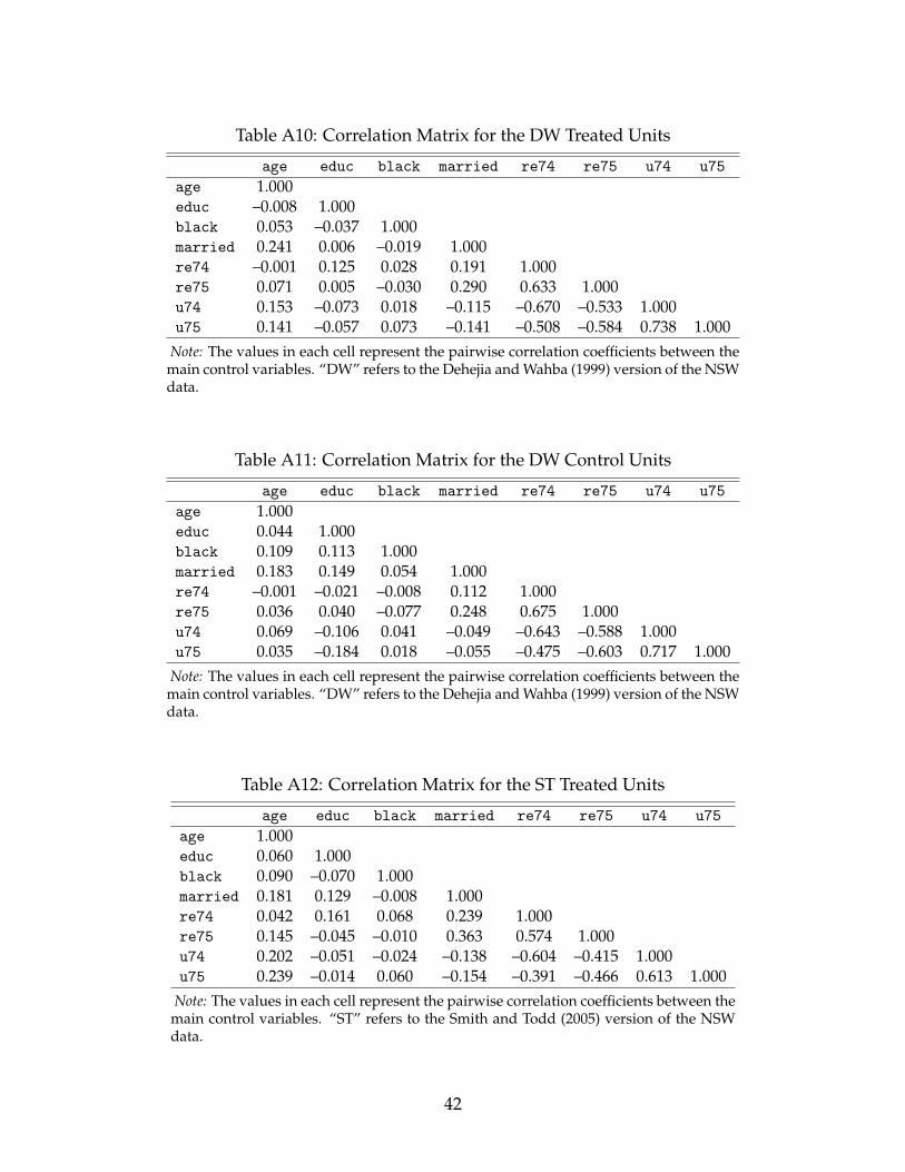
Table A10: Correlation Matrix for the DW Treated Units

age educ black married re74 re75 u74 u75

age 1.000educ –0.008 1.000black 0.053 –0.037 1.000married 0.241 0.006 –0.019 1.000re74 –0.001 0.125 0.028 0.191 1.000re75 0.071 0.005 –0.030 0.290 0.633 1.000u74 0.153 –0.073 0.018 –0.115 –0.670 –0.533 1.000u75 0.141 –0.057 0.073 –0.141 –0.508 –0.584 0.738 1.000

Note: The values in each cell represent the pairwise correlation coefficients between themain control variables. “DW” refers to the Dehejia and Wahba (1999) version of the NSWdata.

Table A11: Correlation Matrix for the DW Control Units


age 1.000educ 0.044 1.000black 0.109 0.113 1.000married 0.183 0.149 0.054 1.000re74 –0.001 –0.021 –0.008 0.112 1.000re75 0.036 0.040 –0.077 0.248 0.675 1.000u74 0.069 –0.106 0.041 –0.049 –0.643 –0.588 1.000u75 0.035 –0.184 0.018 –0.055 –0.475 –0.603 0.717 1.000

Note: The values in each cell represent the pairwise correlation coefficients between themain control variables. “DW” refers to the Dehejia and Wahba (1999) version of the NSWdata.

Table A12: Correlation Matrix for the ST Treated Units


age 1.000educ 0.060 1.000black 0.090 –0.070 1.000married 0.181 0.129 –0.008 1.000re74 0.042 0.161 0.068 0.239 1.000re75 0.145 –0.045 –0.010 0.363 0.574 1.000u74 0.202 –0.051 –0.024 –0.138 –0.604 –0.415 1.000u75 0.239 –0.014 0.060 –0.154 –0.391 –0.466 0.613 1.000

Note: The values in each cell represent the pairwise correlation coefficients between themain control variables. “ST” refers to the Smith and Todd (2005) version of the NSWdata.

42

Table A13: Correlation Matrix for the ST Control Units


age 1.000educ 0.069 1.000black 0.060 0.106 1.000married 0.143 0.167 0.044 1.000re74 –0.074 –0.094 0.003 0.099 1.000re75 –0.023 –0.007 –0.094 0.281 0.631 1.000u74 0.233 –0.065 0.040 0.013 –0.581 –0.504 1.000u75 0.157 –0.193 –0.027 –0.027 –0.409 –0.551 0.670 1.000

Note: The values in each cell represent the pairwise correlation coefficients between themain control variables. “ST” refers to the Smith and Todd (2005) version of the NSWdata.

Table A14: Correlation Matrix for the CPS Comparison Units


age 1.000educ –0.128 1.000black –0.014 –0.102 1.000married 0.440 –0.002 –0.057 1.000re74 0.407 0.093 –0.076 0.421 1.000re75 0.350 0.121 –0.082 0.395 0.870 1.000u74 –0.105 –0.023 0.018 –0.179 –0.540 –0.485 1.000u75 –0.017 0.014 0.042 –0.092 –0.445 –0.516 0.600 1.000

Note: The values in each cell represent the pairwise correlation coefficients between themain control variables.

Table A15: Correlation Matrix for the PSID Comparison Units


age 1.000educ –0.236 1.000black –0.038 –0.324 1.000married 0.199 –0.022 –0.132 1.000re74 0.199 0.306 –0.211 0.164 1.000re75 0.169 0.325 –0.216 0.148 0.841 1.000u74 0.168 –0.036 –0.059 –0.001 –0.446 –0.334 1.000u75 0.162 –0.062 –0.023 –0.007 –0.363 –0.467 0.670 1.000

Note: The values in each cell represent the pairwise correlation coefficients between themain control variables.

43

Table A16: Overlap in Nonexperimental Datasets

Comparisongroup

Version of NSWdata

Controlvariables

Subset of NSWdata

Measure 1 Measure 2

CPS DW balanced control 0.394 1.000CPS DW balanced treated 0.249 1.000CPS DW simple control 0.539 1.000CPS DW simple treated 0.457 1.000CPS ST balanced control 0.420 1.000CPS ST balanced treated 0.210 1.000CPS ST simple control 0.609 1.000CPS ST simple treated 0.441 1.000PSID DW balanced control 0.444 0.998PSID DW balanced treated 0.465 1.000PSID DW simple control 0.515 0.998PSID DW simple treated 0.574 0.999PSID ST balanced control 0.410 0.998PSID ST balanced treated 0.445 0.999PSID ST simple control 0.524 1.000PSID ST simple treated 0.575 0.999

Note: “DW” refers to the Dehejia and Wahba (1999) version of the NSW data. “ST” refers to the Smith and Todd (2005)version of the NSW data. “Simple” and “balanced” sets of control variables are explained in detail in footnote 8. “Subsetof NSW data” refers to whether we compare the treatment or the control group from the NSW experiment with the nonex-perimental comparison groups, CPS-1 and PSID-1. “Measure 1” is calculated as the proportion of all units whose estimatedpropensity scores are not larger than the smaller of the two subgroup-specific maximums and not smaller than the largerof the two subgroup-specific minimums of the estimated propensity score. “Measure 2” is calculated as the proportion ofall units whose estimated propensity scores are not larger than the maximum and not smaller than the minimum estimatedpropensity score among the comparison units.

44

Table A17: Average Correlations in the Empirical Monte Carlo Studies: Median Biases

Biases—Median biasesAbsolute biases—Absolute median

biasesAll simulations

Correlation 0.109*** –0.037(0.034) (0.025)

Observations 64 64

PlaceboCorrelation 0.090* –0.052

(0.047) (0.035)Observations 32 32

StructuredCorrelation 0.128** –0.022

(0.051) (0.037)Observations 32 32

Note: The values in each cell represent mean correlation coefficients averaged across simulation studies.Standard errors are in parentheses. Tests of significance are two-tailed and the null hypothesis is that ofa zero average correlation.*Statistically significant at the 10% level; **at the 5% level; ***at the 1% level.

45

Table A18: Eliminating the “Worst Estimators” in EMCS

Top 10% Top 25% Top 50%All simulations

Proportion 0.103 0.263 0.588***(0.016) (0.023) (0.032)

Observations 64 64 64

PlaceboProportion 0.091 0.272 0.620***

(0.019) (0.029) (0.042)Observations 32 32 32

StructuredProportion 0.115 0.254 0.555

(0.026) (0.037) (0.048)Observations 32 32 32

Note: The values in each cell represent mean proportions of the worst estimators—defined as those that belong to the group of 20% of the estimators with highest ab-solute true biases—that belong to the top x% with lowest absolute mean biases insimulations, where x = 10, x = 25, or x = 50. In this test, if x% of the worst esti-mators belong to the top x% of estimators according to an EMCS, then this EMCSis as good as random in helping with estimator choice. If less than x% of the worstestimators belong at the top, then an EMCS is helpful; if more than x%, then it isactively misleading. Standard errors are in parentheses. Tests of significance aretwo-tailed and the null hypothesis is that of the average proportion equal to x/100.*Statistically significant at the 10% level; **at the 5% level; ***at the 1% level.

46

abstract - brandeis universitypeople.brandeis.edu/~tslocz/sloczynski_paper_emcs.pdfabstract in this...

Documents