abstract - arts.units.it
TRANSCRIPT


i
ABSTRACT
Since its conception in the mid 90’s, cross-laminated timber, known also as CLT or X-
Lam, has achieved a great popularity as construction material thanks to its numerous intrinsic
qualities, worldwide effort to erect reliable structures in seismic-prone areas and necessity to
build a more eco-friendly environment.
Many tests have been carried out in the last 15 years, aimed to better understand the
behavior of connections in CLT buildings, CLT assemblies and CLT structures in order to
provide reliable rules for designers to calculate structures made of CLT in any loading
condition.
Based on these tests, many numerical models have been suggested through the years.
They represent a fundamental tool for the design of CLT structures when specific design
problems arise.
Despite many years of efforts, reliable design rules are still missing in almost every code
worldwide and many are still the unknown related to CLT structures behavior at many levels
(connections, assemblies, structures).
This thesis summarizes three years of numerical investigations, which have faced
different problems related to the comprehension of CLT assemblies and structures behavior
under dynamic loading conditions. The first part of this path focused on the continuation of a
previous study made within the Master Degree thesis, which was the formulation of a simplified
method to obtain an axial-load/bending moment limit domain for a CLT panel connected to the
supporting surface through hold-down and angle bracket connections.
Without test results of interest, the focus of the study returned to be the formulation of
simple methods for CLT assemblies design. The problem of panel-to-panel connections was
investigated. In particular, the stiffness of such connections related to the rocking behavior of 2-
panel wall assemblies was studied through full-scale tests and FE numerical analyses. A
formula for the design of these connections was firstly suggested and then, after further
analyses, revised and corrected.
In order to extend the analyses and consider more complex assemblies, the influence of
diaphragm and wall-to-diaphragm connections stiffness on the rocking behavior of wall
assemblies was numerically investigated, taking into account configuration with and without
diaphragm, varying several parameters to obtain statistically significant results.
In the summer of 2017 the candidate actively participated to the NHERI TallWood

Abstract
ii
Project, an American research project intended to test CLT structures in order to provide design
rules for these structures in the future US codes. Sponsored by the Colorado State University, in
the person of Professor John W. van de Lindt, the candidate collaborated to the setup of a 2-
story CLT building that was tested on the UCSD shaking table located in San Diego
(California).
In order to assess the most proper value of damping for CLT structures under low-
intensity seismic events and to better investigate the potential of the component approach for the
modelling of CLT structures, the 0,15 g shaking table tests of the 3-story building within the
SOFIE Project were reproduced and analyzed. Further considerations on the role of friction for
this type of structure have been made together with the problem of linear analyses for CLT
structures (non-symmetric response for tension-compression loaded connections).
Keywords: Cross-laminated timber, Seismic behavior, Seismic design, Finite Element, Non-
linear analysis

iii
SOMMARIO
Dalla sua concezione a metà degli anni novanta, il legno lamellare a strati incrociati,
anche noto come CLT o X-Lam, ha raggiunto grande popolarità tra i materiali da costruzione
grazie alle numerose innate qualità, gli sforzi a livello mondiale per costruire strutture affidabili
in zone a rischio sismico e la necessità di costruire un ambiente più eco-sostenibile.
Molti test sono stati fatti negli ultimi 15 anni, volti a comprendere meglio il
comportamento delle connessioni in edifici in CLT, di parti strutturali o di intere strutture in
CLT, in modo da fornire regole affidabili per i progettisti per progettare strutture in CLT sotto
ogni condizione di carico.
Sulla base di questi test, molti sono stati i modelli numerici che sono stati suggeriti negli
anni. Questi rappresentano uno strumento fondamentale per la progettazione di strutture in CLT
quando insorgono specifiche problematiche ed un approccio analitico da solo non è sufficiente.
Nonostante i molti anni di sforzi, non esistono ancora affidabili metodologie di progetto
nella quasi totalità dei codici a livello mondiale e ancora molte sono le incognite relative al
comportamento delle strutture in CLT a molti livelli (connessioni, parti strutturali, strutture).
Questa tesi riassume tre anni di ricerche numeriche, le quali hanno affrontato diversi
problemi relativi al comportamento di elementi strutturali e strutture in CLT sotto azioni
dinamiche. Durante la prima parte di questo percorso l’attenzione è stata posta sulla
continuazione di un precedente studio, portato avanti durante la tesi di laurea magistrale, il quale
era incentrato sulla formulazione di un metodo semplificato per la costruzione di un dominio
resistente sforzo normale-momento flettente per pannelli in CLT connessi alla base da
connessioni tipo hold-down e angle bracket.
In mancanza di risultati di test di interesse, la concentrazione è stata rivolta ancora alla
formulazione di metodi semplificati per la progettazione di elementi strutturali in CLT. È stato
analizzato il problema delle connessioni pannello-pannello all’interno di una stessa parete. In
particolare, è stata studiata la rigidezza di queste connessioni in relazione al comportamento
ribaltante di pareti a due pannelli attraverso l’analisi di test a scala reale indipendenti e analisi
numeriche agli elementi finiti. Una formula per il calcolo di queste connessioni è stata dapprima
proposta e poi, dopo ulteriori analisi, rivista e corretta.
Per estendere l’analisi e considerare elementi strutturali più complessi, è stata investigata,
a livello di analisi numerica, l’influenza del solaio e delle connessioni parete-solaio superiore
sul comportamento ribaltante delle pareti, prendendo in considerazione configurazioni con e
senza solaio, variando diversi parametri di modo da ottenere risultati statisticamente

iv
significativi.
Nell’estate del 2017 il candidato ha partecipato attivamente al NHERI TallWood Project,
una ricerca statunitense intesa a testare strutture in CLT per fornire regole di progettazione per
tali strutture nei futuri codici nazionali. Sponsorizzato dalla Colorado State University, nella
persona del Prof. John W. van de Lindt, il candidato ha collaborato alla preparazione di un
edificio con due orizzontamenti fuori terra testato sulla tavola vibrante della UCSD a San Diego
(California)
Per valutare il più corretto valore di smorzamento per strutture in CLT sotto l’azione di
eventi sismici di bassa intensità, sono stati riprodotti numericamente ed analizzati i test su tavola
vibrante del progetto SOFIE a 0,15 g. Ulteriori considerazioni sono state fatte sul ruolo
dell’attrito su questo tipo di strutture e sul problema delle analisi lineari per strutture in CLT
(risposta non simmetrica di connessioni caricate in tensione-compressione)
Parole chiave: Legno lamellare a strati incrociati, Comportamento sismico, Progettazione
sismica, Analisi non lineare, elementi finiti

v
TABLE OF CONTENTS
ABSTRACT I
SOMMARIO III
TABLE OF CONTENTS V
LIST OF FIGURES IX
LIST OF TABLES XVI
LIST OF PUBLICATIONS XVIII
NOTATIONS XX
INTRODUCTION 1
1.1. Research background and motivation 1
1.2. Thesis structure 2
CLT: PRODUCT, APPLICATIONS AND MODELLING APPROACHES 4
2.1. Product description 4
2.1.1. Panels for structural applications 5
2.2. Connections in CLT structures 5
2.2.1. Typical connection systems 6
2.2.2. New connections for CLT buildings 10
2.3. Modelling approaches 13
2.3.1. Background in CLT modelling 13
2.3.2. Creating the mesh: X-lam Wall Mesher 14
2.3.3. Component approach 16
2.3.4. SAP2000 modelling 19
2.3.5. Damping in FE analyses 20

Table of contents
vi
A NOVEL METHOD FOR NON-LINEAR DESIGN OF CLT WALL
SYSTEMS 22
3.1. Introduction 22
3.2. Method derivation 25
3.2.1. Hypotheses 25
3.2.2. Limit States definition 28
3.3. Method validation 33
3.3.1. SAP2000 analyses 34
3.3.2. Abaqus analyses 38
3.4. Concluding remarks 43
ROCKING OF A TWO-PANEL CLT WALL: BEHAVIOR PREDICTION
AND INFLUENCE OF FLOOR DIAPHRAGM 45
4.1. Introduction 46
4.2. Formula derivation 48
4.2.1. Two panels of equal length 48
4.2.2. Two panels of different length 50
4.3. Validation of the proposed formulation 51
4.3.1. Validation through full-scale experimental tests results 51
4.3.2. Validation through FE analyses results 56
4.4. Lateral force estimation 62
4.4.1. 6-screw assemblies 62
4.4.2. 23-screw assemblies 63
4.4.3. 12-screw assemblies 64
4.5. Influence of the floor diaphragm 64
4.5.1. Analyzed cases 64
4.5.2. Analyses results 66
4.6. Concluding remarks 70
EXPERIMENTAL SEISMIC BEHAVIOR OF A TWO-STORY CLT
PLATFORM BUILDING 73
5.1. Introduction 73
5.2. Test building layout and configuration 75

Table of contents
vii
5.3. Test description 78
5.3.1. Phase 3.1 78
5.3.2. Phase 3.2 test description 80
5.3.3. Phase 3.3 80
5.3.4. Instrumentation 81
5.4. Ground motion and testing program 83
5.4.1. Displacement profile 85
5.4.2. Inter-story drift 86
5.4.3. Global hysteresis 87
5.4.4. Torsion 88
5.4.5. CLT panel uplift 88
5.4.6. Sliding 90
5.4.7. Relative panel displacement 91
5.4.8. Forces in tie-down rods 92
5.4.9. Overall performance 94
5.5. Concluding remarks 95
METHODS FOR PRACTICE-ORIENTED LINEAR ANALYSIS IN
SEISMIC DESIGN OF CLT BUILDINGS 96
6.1. Introduction 96
6.2. Test structure and experimental data 97
6.3. Numerical models 99
6.3.1. Distributed-connection model 99
6.3.2. Component model 104
6.4. Results 106
6.4.1. Modal analysis results 106
6.4.2. Time-history analysis results for 5% damping 107
6.4.3. Parametric study for additional damping values 109
6.5. Concluding remarks 114
CONCLUSIONS 115
ANNEX A – DESIGN EXAMPLE 117

Table of contents
viii
8.1. Introduction 117
8.2. Example 117
REFERENCES 120

ix
LIST OF FIGURES
Figure 2.1.1 – CLT panel structure. 4
Figure 2.2.1 – Type of connections in CLT structures: wall-to-lower diaphragm / wall-to-
foundation (red line), panel-to-panel in a wall (purple line), wall-to-wall
(pink line), wall-to-upper diaphragm (blue line), panel-to-panel in a
diaphragm (green line). 6
Figure 2.2.2 – Examples of wall-to-foundation connections: metal bracket (a), concealed
metal plate (b) [32]. 6
Figure 2.2.3 – Examples of panel-to-panel connections: internal spline (a), single surface
spline (b), double surface spline (c), half-lapped joint (d) [32]. 7
Figure 2.2.4 – Examples of wall-to-wall connections: self-tapping screw connection (a),
toe-screwing (b), metal bracket (c), concealed metal plate (d) [32]. 8
Figure 2.2.5 – Examples of wall-to-diaphragm connections on platform type buildings:
self-tapping screws (a), metal brackets (b), self-tapping screws and metal
brackets (c), concealed metal plates (d) [32]. 9
Figure 2.2.6 - Examples of wall-to-diaphragm connections on balloon type buildings:
wood ledgers (a), metal brackets (b,c) [32]. 9
Figure 2.2.7 – Examples of a hold-down (a) and an angle bracket (b) (Rothoblaas). 10
Figure 2.2.8 – Detail of the ATS steel rod connection. 11
Figure 2.2.9 – The X-Rad connection with all its parts exposed (a) and an assembly of
three connections (b) [53][54]. 11
Figure 2.2.10 – Example of RSFJ connection (a) and its placement in a shear wall (b)
[79]. 12
Figure 2.3.1 - Piecewise-linear law of shear spring component [60]. 16
Figure 2.3.2 - Piecewise-linear law of axial spring component [60]. 17
Figure 3.1.1 - Typical hold-down (a), angle bracket (b), nail (c), screw (d) and bolt (e)
used in CLT structures (from Rothoblaas catalogs). 23
Figure 3.1.2 - Example of a box type CLT structure (a) and a shear type CLT structure
(b). 23
List of figures
x
Figure 3.1.3 - Typical CLT wall panel connected to the foundation with hold-downs and
angle brackets (a), failure mechanisms considered for hold-down design
(b) and angle bracket design (c). 24
Figure 3.2.1 - Stress-strain relationship of wood in compression at the wall-foundation
interface. 26
Figure 3.2.2 - Experimental force-displacement relationship (line with dashes and dots),
tri-linear approximation of the test result (dashed line) and elasto-plastic
approximation of the test results (solid line) for connections. 26
Figure 3.2.3 - Rotational mechanism and forces involved. 27
Figure 3.2.4 - Schematic representation of the considered sub-domains. 29
Figure 3.2.5 - Starting condition for the definition of subdomains 1 and 2 (a), attainment
of the ultimate condition in two different connections (b) and change in the
point of rotation of the system (c). 30
Figure 3.2.6 - Examples of axial force-bending moment resisting domain for a
symmetrical (black line (a) and black connections (b)) and non-
symmetrical (orange line (a) and orange connections (b)) arrangement of
connections. In the second configuration, only the two connections on the
left are present with respect to the symmetrical one (b). X and + marks
denote the passage from a sub-domain to another for symmetrical and non-
symmetrical arrangement of connections, respectively. Circles denote the
starting (left, sub-domain 1) and end (right, sub-domain 5) points of the
domains. 33
Figure 3.3.1 - Comparison between SAP2000 connections force-displacement
relationship (bold solid line), trilinear force-displacement relationship
(dashed line) and elasto-plastic force-displacement relationship (solid
line). 35
Figure 3.3.2 - Plan of the ground floor of the case study building with the investigated
wall highlighted. 37
Figure 3.3.3 - Force distribution on top of the wall for the case with bending moment. 40
Figure 3.3.4 - Values of the distribution coefficient k for (a) axial-horizontal load
condition (case 4) and (b) bending moment-horizontal load condition (case
5) for rigid support and for (c) axial-horizontal load condition (case 4) and
(d) bending moment-horizontal load condition (case 5) for CLT support. 41

List of figures
xi
Figure 3.3.5 - Dependency of (a) the first part of the M-N domain on the k value and (b)
M-N domain for different k values (0,2 and 0,3). 42
Figure 4.2.1 – Analyzed scheme. 48
Figure 4.3.1 - Test setups #1 and #2 (measures in mm) [36]. 52
Figure 4.3.2 - Elevation (right) and cross-section (left) of test setup used for wall-
foundation hold-down connection loaded in tension (Test configuration #1)
[35]. 52
Figure 4.3.3 - Wall panel test configurations: (a) configuration I - single walls; (b)
configuration II - coupled walls with half-lap joint; (c) configuration III -
coupled walls with spline (LVL) joint (measures in cm) [37]. 53
Figure 4.3.4 – Variation of the panel-to-panel stiffness varying the F/qv2b ratio (a) and
the h/b ratio (b). 56
Figure 4.3.5 - Validation of the model (dashed red line) against test results (solid black
line) (force-displacement graph taken from [37]) (a) and an example of
undeformed shape of a FE model described in this chapter (b). 58
Figure 4.3.6 - Imposed cyclic displacement for the FE analyses. 58
Figure 4.3.7 - Different configurations of base connection used in the FE analyses. 59
Figure 4.4.1 - Normal distribution for the 6-screw case. 62
Figure 4.4.2 - Normal distribution for the 23-screw case. 63
Figure 4.5.1 - Arrangements of bottom connections implemented in the FE model. 65
Figure 4.5.2 - Configurations of wall-to-diaphragm connections implemented in the FE
model. 65
Figure 4.5.3 - Layout of the four diaphragms analyzed (measures in mm). 66
Figure 4.5.4 – Graphical explanation of the terms dtop and dbottom. The dashed line depicts
the initial position of the wall while the solid line shows the deformed
shape of the same wall due to a lateral load applied at the top of the wall
itself. 67
Figure 4.5.5 - Deformed shapes for different combinations of thin/thick diaphragm and
loose/stiff wall-to-floor diaphragm connections: thin diaphragm-loose
connections (a), thick diaphragm-loose connections (b), thin diaphragm-
stiff connections (c), thick diaphragm-stiff connections (d). Measures in
mm. Deformation scale factor equal to 5 for all figures. 68

List of figures
xii
Figure 4.5.6 - Percentage of difference in slip displacement in the panel-to-panel
connection from the reference analyses for connections arrangements A
and B (a) and C (b) between wall and floors diaphragm. Squared markers
are for assemblies with aspect ratio equal to 2, circles for aspect ratios
equal to 3 or 4. 69
Figure 4.5.7 - Percentage of difference in rocking capacity from the reference analyses for
assemblies with 6 (a) and 12 screws (b). 70
Figure 5.2.1 - Test Building: (a) Front elevation and plan view (solid lines for CLT
panels, dashed lines for the beam system underneath); (b) Side elevation
view; (c) Isometric view. 76
Figure 5.2.2 - Position of the two-story CLT Platform Building on the shake table. 78
Figure 5.3.1 - Phase 3.1: 3.5:1 aspect ratio panels shear wall stack layout. 79
Figure 5.3.2 - Phase 3.2: 2.1:1 aspect ratio panels shear wall stack layout. 80
Figure 5.3.3 - Phase 3: (a) Transverse CLT walls; (b) 3.5:1 aspect ratio panels shear wall
stack layout. 81
Figure 5.3.4 - Phase 3.1 instrumentation on south face of south shear wall (typ. across
phases). 83
Figure 5.4.1 - Spectral accelerations for Loma Prieta scaled to SLE, DBE, and MCE
levels. 84
Figure 5.4.2 - Fundamental building period and the effect of repairs and different wall
configurations. 85
Figure 5.4.3 - Average displacement of first and second stories for each test. 86
Figure 5.4.4 - Interstory drift: (a) Phase 3.1 MCE second story; (b) Phase 3.1 MCE first
story; (c) Phase 3.3 MCE second story; (d) Phase 3.3 MCE first story. 86
Figure 5.4.5 - Global hysteresis curves: (a) Phase 3.1 MCE second story; (b) Phase 3.1
MCE first story; (c) Phase 3.3 MCE second story; (d) Phase 3.3 MCE first
story. 87
Figure 5.4.6 - 3.1 MCE Displacement: (a) first floor level northeast corner; (b) first floor
level center east side; (c) first floor level southeast corner; (d) second floor
level northeast corner; (e) second floor level center east side; (f) second
floor level southeast corner. 88
Figure 5.4.7 - Phase 3.1 MCE Wall Uplift: (a) First story shear wall top west corner; (b)

List of figures
xiii
First story shear wall bottom west corner; (c) Second story shear wall top
west corner; (d) Second story shear wall bottom west corner. 89
Figure 5.4.8 - Phase 3.3 MCE Uplift: (a) Second story shear wall bottom west corner; (b)
First story shear wall bottom west corner; (c) Second story transverse wall
top south corner; (d) First story shear wall bottom south corner. 90
Figure 5.4.9 - Phase 3.2 MCE Uplift: (a) First story shear wall top west corner; (b) First
story shear wall bottom west corner; (c) Second story shear wall top west
corner; (d) Second story shear wall bottom west corner. 90
Figure 5.4.10 - Phase 3.1 MCE Sliding: (a) First story shear wall top west corner; (b)
First story shear wall bottom west corner; (c) Second story shear wall top
west corner; (d) Second story shear wall bottom west corner. 91
Figure 5.4.11 - Phase 3.2 MCE Sliding: (a) First story shear wall top west corner; (b)
First story shear wall bottom west corner (nail shear failure occurred in
brackets); (c) Second story shear wall bottom west corner. 91
Figure 5.4.12 - Phase 3.1 MCE Vertical Relative Panel Displacement: (a) First story shear
wall top west corner; (b) First story shear wall bottom west corner; (c)
Second story shear wall top west corner; (d) Second story shear wall
bottom west corner. 92
Figure 5.4.13 - Phase 3.2 MCE Vertical Relative Panel Displacement: (a) First story shear
wall top west corner; (b) First story shear wall bottom west corner; (c)
Second story shear wall top west corner; (d) Second story shear wall
bottom west corner. 92
Figure 5.4.14 - Phase 3.1 ATS Rod Load Cells: (a) First story north wall east side; (b)
First story north wall west side; (c) First story south wall west side; (d)
First story south wall east side; (e) Second story north wall west side; (f)
Second story north wall east side; (g) Second story south wall east side; (h)
Second story south wall west side. 94
Figure 6.2.1 - North/South elevations (a), East/West elevations (b), and typical floor plan
of Configuration B of the 3-storey structure with location of the metal
connectors for the first storey (c) (from [40][62], measures in m). 97
Figure 6.2.2 - Pseudo spectral acceleration spectra of the three ground motions considered
(a), and base shear versus roof displacement response of the test structure
(b). 98
Figure 6.3.1 - Geometry and component identification (a) and location of common edges

List of figures
xiv
with coincident nodes, for a typical inter-storey CLT assembly (b). 100
Figure 6.3.2 - Distribution of angle brackets at the base of the walls for the first (a),
second (b) and third (c) storey. 102
Figure 6.3.3 - West view (a) and north view (b), of the geometry of the distributed-
connection model. 104
Figure 6.3.4 - West (a) and North (b) views for the component model in NextFEM
Designer [44]. 105
Figure 6.4.1 - Deformed shape for the (a) first [T1 = 0,239 s], (b) second [T2 = 0,199 s],
and (c) third [T3 = 0,137 s] mode of vibration for the distributed-
connection model. 106
Figure 6.4.2 - Deformed shape for the (a) first [T1 = 0,254 s], (b) second [T2 = 0,223 s],
and (c) third [T3 = 0,152 s] mode for the component model. 107
Figure 6.4.3 - Hysteretic loops for 5% damping for the distributed-connection model:
Kobe (a), El Centro (c), Nocera Umbra (e). Hysteretic loops for 5%
damping for the component model: Kobe (b), El Centro (d), Nocera Umbra
(f). 108
Figure 6.4.4 - Roof displacement vs. base shear diagram from the experimental response
under Nocera Umbra and a loop with an equivalent damping of 5% for the
same maximum displacement and base shear. 109
Figure 6.4.5 - Hysteretic loops for the distributed-connection model: Kobe – 20% (a), El
Centro – 10% (c), Nocera Umbra – 10% (e). Hysteretic loops for the
component model: Kobe – 20% (b), El Centro – 10% (d), Nocera Umbra –
10% (f). 111
Figure 6.4.6 - Roof displacement time-histories for: Kobe – 20% (a), El Centro – 10%
(b), and Nocera Umbra – 10% (c). 112
Figure 6.4.7 - Base shear force time-histories for: Kobe – 20% (a), El Centro – 10% (b),
and Nocera Umbra – 10% (c). 113
Figure 8.2.1 – Arrangement of the connection of the designed wall (measures in cm). 118
Figure 8.2.2 – Bending moment-axial load resistant domain for the given wall and
verification of the calculated external loads (blue X) (figure taken from the
purposely developed software). 118
Figure 8.2.3 – First attempt arrangement of the connection of the designed segmented
wall (measures in cm). 119

List of figures
xv
Figure 8.2.4 - Second attempt arrangement of the connection of the designed segmented
wall (measures in cm). 119

xvi
LIST OF TABLES
Table 3.2.1 - Position of the neutral axis at the lower and upper limit for each sub-
domain. 30
Table 3.3.1 - Comparison between numerical and analytical results - single panel wall. 36
Table 3.3.2 - Comparison between numerical and analytical results - 3-panel wall. 37
Table 3.3.3 - 3-story building verification in the different cases. 38
Table 3.3.4 - Tensile behavior of hold-downs and angle brackets. 39
Table 3.3.5 - Values of k for rigid and CLT support for different loads and h/l ratios. 40
Table 3.3.6 - Comparison between neutral axis position prediction using the proposed
algorithm and the FE model case with bottom rigid support. 43
Table 3.3.7 - Comparison between neutral axis position prediction using the proposed
algorithm and the FE model case with bottom CLT support. 43
Table 4.3.1 - Test configuration. 54
Table 4.3.2 - Stiffnesses considered. 54
Table 4.3.3 - Forces considered for each test. 54
Table 4.3.4 - Comparison between analytically predicted and experimentally observed
rocking behavior. 55
Table 4.3.5 - Mechanical properties of the connections used in the model – shear. 57
Table 4.3.6 - Mechanical properties of the connections used in the model – tension. 57
Table 4.3.7 - Rocking behavior of the walls in the analyses (S-C: single-coupled: C:
coupled). 60
Table 4.3.8 - Rocking behavior prediction of the walls using the proposed analytical
method and comparison with the results of the FE analyses. 60
Table 4.3.9 - Rocking behavior prediction of the walls using with the adjusted analytical
method and comparison with the results of the FE analyses. 61
Table 4.4.1 - Analytical-numerical comparison – 6-screws case. 62
Table 4.4.2 - Analytical-numerical comparison – 23-screw case. 63

List of tables
xvii
Table 4.4.3 - Analytical-numerical comparison – 12-screw case. 64
Table 5.3.1 – Instrumentation on gravity frame and diaphragm. 82
Table 5.3.2 - Instrumentation on shear walls. 83
Table 5.4.1 – Test sequencing and global story response for each phase. 84
Table 5.4.2 – Test sequencing and local story response for each phase. 89
Table 6.3.1 - Elastic orthotropic properties considered for the boards of the CLT panels. 101
Table 6.3.2 - Effective mechanical cross-section properties of the CLT panels. 101
Table 6.3.3 - Equivalent elastic material properties for orthotropic shell elements. 101
Table 6.3.4 - Properties of angle brackets. 102
Table 6.3.5 - Properties of vertical joints between in-plane wall panels in the same
assembly. 102
Table 6.3.6 - Properties of floor-to-wall connections at the top of the wall panels. 103
Table 6.3.7 - Properties of vertical joints between perpendicular wall panels. 103
Table 6.3.8 - Stiffnesses implemented for metal plate connections. 106
Table 6.4.1 - Periods of vibration of the test structure, in the direction of shaking, and the
numerical models. 107
Table 6.4.2 - Comparison for the Kobe event in terms of maximum and minimum values
of roof displacement d and base shear V [bold numbers indicate the best
fit]. 109
Table 6.4.3 - Comparison for the El Centro event in terms of maximum and minimum
values of roof displacement d and base shear V [bold numbers indicate the
best fit]. 110
Table 6.4.4 - Comparison for the El Centro event in terms of maximum and minimum
values of roof displacement d and base shear V [bold numbers indicate the
best fit]. 110

xviii
LIST OF PUBLICATIONS
G. Tamagnone, G. Rinaldin, M. Fragiacomo. A simplified non-linear procedure for seismic
design of CLT wall systems. 14th World Conference on Timber Engineering (WCTE
2016), Technische Universität Wien, Wien, Austria, 2016.
G. Tamagnone, G. Rinaldin, M. Fragiacomo. A novel method for non-linear design of CLT
wall systems. Engineering Structures. 167(2018):760–771.
DOI:10.1016/j.engstruct.2017.09.010. 2017.
G. Tamagnone, M. Fragiacomo. Sul Progetto in Zona Sismica di Strutture a Pareti Lignee in
Xlam. Convegno ANIDIS 2017. Pistoia, Italia.
G. Tamagnone, M. Fragiacomo. On the rocking behavior of CLT wall assemblies. 15th World
Conference on Timber Engineering (WCTE 2018). COEX exhibition and convention
center. Seoul, South Korea, 2018.
J. W. Van de Lindt, J. Furley, M. O. Amini, S. Pei, G. Tamagnone, A. R. Barbosa, D. Rammer,
P. Line, M. Fragiacomo, M. Popovski. Experimental Seismic Behaviour of a Two-Storey
CLT Platform Building: Design and Shake Table Testing. 16th European Conference on
Earthquake Engineering (ECEE 2018). The Thessaloniki Concert Hall, Thessaloniki,
Greece, 2018.
J. W. Van de Lindt, J. Furley, M. O. Amini, S. Pei, G. Tamagnone, A. R. Barbosa, D. Rammer,
P. Line, M. Fragiacomo, M. Popovski. Experimental seismic behavior of a two-story clt
platform building: shake table testing results. 15th World Conference on Timber
Engineering (WCTE 2018). COEX exhibition and convention center. Seoul, South Korea,
2018.
C. Bedon, M. Fragiacomo, G. Tamagnone. Numerical Investigation on Timber-to-Timber
Joints and Composite Beams with Inclined Self-Tapping Screws. 15th World Conference
on Timber Engineering (WCTE 2018). COEX exhibition and convention center. Seoul,
South Korea, 2018.
J. W. Van de Lindt, J. Furley, M. O. Amini, S. Pei, G. Tamagnone, A. R. Barbosa, D. Rammer,
P. Line, M. Fragiacomo, M. Popovski. Experimental seismic behavior of a two-story clt

List of publications
xix
platform building. Engineering Structures. 183(2019): 408–422
https://doi.org/10.1016/j.engstruct.2018.12.079
G. Tamagnone, G. Rinaldin, M. Fragiacomo. Influence of the floor diaphragm on the rocking
behavior of CLT. Undergoing revision. ASCE Journal of Structural Engineering.
I. Christovasilis. L. Riparbelli, G. Rinaldin, G. Tamagnone. Methods for Practice-oriented
Linear Analysis in Seismic Design of Cross Laminated Timber Buildings. Undergoing
revision, Soil Dynamics and Earthquake Engineering.

xx
NOTATIONS
A Cross-section area
C Damping matrix
E Elastic modulus/Young modulus
E0 Modulus of elasticity parallel to grain
E90 Modulus of elasticity perpendicular to grain
EL Modulus of elasticity in the longitudinal direction
EN Modulus of elasticity in the normal direction
ET Modulus of elasticity in the transverse direction
F Lateral force applied at the top of the wall
FAB Reaction force in each angle bracket due to the load condition
Fc Value of the reaction force in compression in the contact zone between panel and
supporting surface
FHD Reaction force in the hold-down due to the load condition
Fmax Maximum force of the connection
FRd,AB Design resistance of the angle brackets
FRd,HD Design resistance of the hold-down
Fi Value of the reaction force in the ith connection
Fu Force corresponding to the ultimate displacement of the connection
Fy Yielding force of connections
G0 Shear modulus in planes parallel to grain
G90 Shear modulus in planes perpendicular to grain
K Stiffness matrix
LTN Longitudinal Transverse Normal
M Bending moment
M Mass matrix
N Axial force
R Compressive reaction force at the interface between the first panel and the supporting
surface during the rocking mechanism
Rp Reaction force at the interface between panels during the rocking mechanism
S Modal matrix
T Period
Uult Ultimate displacement of connections

Notations
xxi
Uult,max Maximum ultimate displacement among the two available
Uult,min Minimum ultimate displacement among the two available
V Shear force
Vi Reaction force in the ith connection during the rocking mechanism
W Self-weight of the panel
b Length of the panel
d Uplift of the uncompressed edge of the panel
dbottom Lateral displacement of the bottom corner of the assembly
drock Lateral displacement of the top corner of the assembly due to rocking
dslip Lateral displacement of the top corner of the assembly due to slip
dtop Lateral displacement of the top corner of the assembly
fc Ultimate compressive strength in CLT
h Height of the wall
k Compressive stress distribution coefficient
k Modal stiffness matix
kel Elastic stiffness of the backbone
kpl Hardening stiffness of the backbone
ks Elastic stiffness of connections in the resistant domain calculation
ki Vertical stiffness of the ith connection
l Length of the wall
m Modal mass matrix
n Number of connections
nAB Number of angle brackets
np Number of connections between wall panels
qv Axial load per linear meter applied to the assembly
s Thickness of the panel
uc Fictitious displacement underneath the foundation surface
uc,max Maximum fictitious displacement underneath the foundation surface
ui Vertical displacement of the ith connection
vmax Displacement corresponding to the maximum force in the connection
vu Ultimate displacement of the connection
vy Yielding displacement
x̅ Distance of the neutral axis from the bottom right corner
xi Distance of the ith connection from the compressed panel corner
xi,dx Distances of the ith connection from the bottom right corner of the wall
xi,sx Distances of the ith connection from the bottom left corner of the wall

Notations
xxii
xmax Position of the farthest connection from the bottom right corner having Uult,max as
ultimate displacement
xmin Position of the farthest connection from the bottom right corner having Uult,min as
ultimate displacement
α Mass-proportional damping coefficient
β Stiffness-proportional damping coefficient
ζ Damping
ξn Critical damping ratio
θ Angle between the panel and the supporting surface during the rocking mechanism
ν Poisson’s ratio
σc Compressive stress at the bottom right corner of the wall
σd Compressive stress at the bottom left corner of the wall
φ Diameter
ωn Natural frequency of the system

1
INTRODUCTION
1.1. Research background and motivation
The use of Cross-Laminated Timber as structural material has increased rapidly in the last
fifteen years for low- and mid-rise buildings, as it proved to be a good and more environmental-
friendly alternative to more common materials, such as concrete or masonry.
However, few codes provide design formulas for the design of this type of structures, not
accounting for all the possible scenarios the structure could undergo during its lifetime. Many
aspects still need to be investigated in order to predict efficaciously the behavior and structural
capacity of CLT assemblies and structures. Moreover, designers who deals with the project of
buildings in seismic-prone areas needs to be provided with rules for a reliable numerical
modelling of such structures to predict their dynamic response and possible critical issues,
which could not be directly deducible from a not detailed investigation considering every load
scheme.
For these reasons, it is evident how crucial is to keep on studying these type of structure
and all the different parts, their behavior and how elements interact with each other, to find a
proper design procedure specifically devised for CLT buildings, Among the different aspects
that needs to be clarified, the thesis proposes a procedure to calculate the rocking capacity of a
single-panel CLT wall, giving information on the most probable failure mechanism for a given
set of external loads. After that, the vertical connection between panels in a same wall is
considered, suggesting a formula for its design in order to give a determined type of behavior to
the wall assembly. Furthermore, the influence of an overlaying diaphragm is investigated in
terms of rocking behavior and capacity.
Full-scale tests are a very useful mean to collect data in structural engineering, and CLT
structures are no exception. This thesis presents results of the tests carried out on a 2-story CLT
platform building made for the validation of a specific design procedure. Results of this type of
tests can also give information on the behavior and how to predict it when a numerical model
needs to be created. Numerical analyses are a powerful tool that helps designers to test the
capacity of a structure that needs to be built and check the goodness of the design. In this thesis,
results of several full-scale tests are used to study, with two different modelling approaches, the
influence of different parameters on the most proper value of damping to be implemented in FE
analyses in CLT structures for low intensity motion, for which the effect of friction have proven
to be more important.

Introduction
2
1.2. Thesis structure
The focus of this PhD thesis is not unique and the studies made encompass different
fields. The general topic is the research of formulations and tools to properly design and predict
the behavior of CLT structures and their singular parts (e.g. walls, connections, etc)
The thesis itself is a collection of journal articles written during the last three years of
research. After an introductive chapter (chapter 2), four studies (chapters 3 to 6) are presented.
Each of the latter four chapters opens with few lines summarizing the content of that chapter,
then an introductive chapter gives information on the topic under discussion and previous
research in the same field. In the subsequent sections, experimental, analytical, and numerical
results are compared and discussed.
Chapter 2 introduces the CLT as wood product. Its structural use is described and the
most common connection systems, together with few of novel conception, are presented. The
second part of this chapter addresses the problem of the numerical modeling of CLT structures
and components, discussing the possible approaches and presenting the ones considered within
this work.
Chapter 3 presents a simplified non-linear method to calculate the rocking capacity of a
single-panel CLT wall connected to the supporting surface through angle brackets and hold-
downs. The method, basing on the mechanical properties of the connections and the geometry
of the system, calculates, for a given value of axial force applied, the most probable failure
mechanism (i.e. crushing of CLT or failure of connections) and the position of the neutral axis
in the corresponding ultimate state condition.
In chapter 4, a formula for the prediction of the rocking behavior (i.e. coupled or
uncoupled) of a two-panels CLT wall is derived and validated against unrelated full scale tests
and numerical analyses. The method accounts for external loads, mechanical properties of the
connections and geometry of the system. In the second part of this chapter, the influence of the
upper diaphragm and the wall-to-floor slab connections on the rocking behavior of a two-panel
CLT wall assembly is investigated through several numerical analyses varying different
parameters (e.g. stiffness of the connections, stiffness of the diaphragm, axial load applied).
Chapter 5 analyzes the findings of different shaking-table tests on a two-story CLT
platform building with three different type of shear wall to compare the various responses
depending on the system utilized. Several parameters are investigated, such as the slip between
panels composing a wall, the uplift and lateral displacement of the wall or the presence of an
orthogonal wall.
Finally, chapter 6 discusses two different modelling approaches for the linear modelling
of CLT buildings and the influence of the value of damping set, when low-intensity seismic
action is considered, upon the global response of the model compared to the results of a full-

Introduction
3
scale building tested on a shaking-table.

4
CLT: PRODUCT, APPLICATIONS AND
MODELLING APPROACHES
2.1. Product description
Cross Laminated Timber (CLT) is a wood-based product, which structure is depicted in
Figure 2.1.1. As shown, CLT is composed of overlapping layers of wood lamellas, glued
together to form a massive panel. The peculiarity of CLT is that lamellas of adjoining layers
have grains running orthogonally to each other.
Figure 2.1.1 – CLT panel structure.
Lamellas used are generally 20 to 40mm thick and 80 to 250mm wide, they are dried to a
moisture content of 12%, to ensure a perfect bond between layers and to avoid biological
damages (pests, fungi or insects), graded and, if necessary, finger-jointed to create longer pieces
or to avoid knots and reach higher performances; they are usually arranged in odd layers from
three to seven. Species typically used are softwood qualities like spruce, pine and fir.
The glues utilized are the polyurethane-based glues (PUR), in some cases formaldehyde-
based resins (RF and MUF) can be used too.
Once the layers are ready, panels are pressed. The equipment used can vary depending on
the thickness of the panel and the type of adhesive used. Typical pesses utilized are: hydraulic
press, compressed air press and vacuum press. Panels’ thickness ranges from 60 to 300mm, but
panels thick up to 500mm can be produced for specific purposes. The size, length and hight, is
limited by factory equipment or transportation restrictions, but usually they are produced
oversize, up to over 30m, and then cut to the disred geometry, especially in length, rather than
be tailored manufactured.
The cross-laminating process provides the final product with high dimensional stability,
in- and out-of-plane stiffness and strength, with the possibility of having comparable
characteristics in two directions (in-plane directions), depending on number and thickness of

CLT: Product, applications and modelling approaches
5
layers in each direction.
In Europe, the standard regulating CLT manufacturing is the UNI EN 16351:2015
(Timber structures – a Cross laminated timber – Requirements). In the US, there is the
ANSI/APA PRG 320-2018 (Standard for Performance-Rated Cross-Laminated Timber).
2.1.1. Panels for structural applications
Panels are produced for general purposes. Different uses requires different panels’
dimensions, but no significant difference is encountered during the production process.
CLT panels can be utilized for different purposes within a structure: walls, floor slabs,
roofs, stairways and shafts. Panels can undergo different post-production processing, such as the
cutting for openings, as door, windows, stairs and service channels, or to allow the proper
installation of specific connections (see Chapter 2.2). Cuts and other manufacturing are usually
performed by CNC machining tools, such as saws, drills, boring tools or lathes, at the
production site, but some specific non-precision works can be made manually on-site.
Panels are usually placed matching the orientation of the grains of the outer layers with
the direction of maximum stress in the specific element: walls have grains of outer layers
running vertically; diaphragms have grains of outer layers running in the direction of maximum
span. This is made because panels are manufactured in odd layers, so the majority of lamellas
have grains parallel to those of the outer layer, thus this is the direction having the best
characteristics within the panel.
For diaphragm applications, depending on the span between walls or thickness of panels,
panels can be used alone or coupled to beams, in order to satisfy deformation, structural and
vibration requirements.
2.2. Connections in CLT structures
Structures made of CLT panels can be of two different type: platform type and balloon
type structures. The main difference between the two is that platform type structures have walls
height coinciding with the inter-story height, that is that all the wall at a certain level have a
diaphragm on the top of them, diaphragm that serve as supporting level for walls of the upper
floor, etc.
In balloon type structures, walls height coincides with the height of the building. In this
case, diaphragm can be placed following two structural approaches:
Diaphragms are directly supported by walls, which bear axial and shear loads;
Diaphragms can be supported by columns, which bear vertical loads, and be connected to
the walls through special connections that allow exchanging only shear loads between the

CLT: Product, applications and modelling approaches
6
two. In this case, the wall act exclusively as shear wall.
Connections play a crucial role in every timber structure. CLT is no exception. In this
chapter, several connections are presented. Figure 2.2.1 shows the position of the connections
within a platform type construction, as it is the type analyzed in this thesis. Balloon type
structures presents differences in some connections, especially in wall-to-diaphragm
connections, as diaphragms lean on the side of continuous wall rather than lay on the top of
them, as occurring in the platform type buildings.
Figure 2.2.1 – Type of connections in CLT structures: wall-to-lower diaphragm / wall-to-foundation (red line), panel-
to-panel in a wall (purple line), wall-to-wall (pink line), wall-to-upper diaphragm (blue line), panel-to-panel in a
diaphragm (green line).
2.2.1. Typical connection systems
2.2.1.1. Wall-to-foundation connections
(a) (b)
Figure 2.2.2 – Examples of wall-to-foundation connections: metal bracket (a), concealed metal plate (b) [32].
Usually, foundations in wood structures are made of Reinforced Concrete (RC). In order
to link together the two materials, threaded bars are embedded in concrete in correspondence
with the position of the connections. In some specific cases, especially in balloon type structures
with shear walls, this solution can be unfeasible for uplift preventing connections, depending on
the connection used or the load to be born. In such cases, steel plates underneath the concrete

CLT: Product, applications and modelling approaches
7
slab are used.
In platform structures, typical connections consist in metal plates fixed to the foundation
through a bolt and linked to the wall through nails or screws (Figure 2.2.2.a). Another option is
to hide the connection within the panel. This is made to improve the fire resistance of the
connection and for aesthetic (Figure 2.2.2.b). The process here requires more attention in the
preparation of the panel and selection of fasteners than in ordinary connections.
2.2.1.2. Panel-to-panel connections
Panel-to-panel connections can be performed in many ways. The two more used are the
spline joint and the half-lapped joint. This joint can be a single or double, internal or surface
joint, depending if the spline is placed within or outside the panels and the number of strips
used.
(a) (b)
(c) (d)
Figure 2.2.3 – Examples of panel-to-panel connections: internal spline (a), single surface spline (b), double surface
spline (c), half-lapped joint (d) [32].
Materials used for splines are Laminated Veneer Lumber (LVL), Parallel Strand Lumber
(PSL), Laminated Strand Lumber (LSL) or other Structural Composite Lumber (SCL) materials.
The surface spline is a connection that can be performed completely on-site, as the profiling of
the panel is superficial (Figure 2.2.3.b and c). Internal splines need the profiling to be made at
the plant due to the position of the cut (Figure 2.2.3.a). Half spline is connected to a panel and
the other half is connected to the other panel. Both sides are connected through metal fasteners,
such as self-tapping screws, wood screws or nails. The main advantage of the internal spline is
that it provides a double shear connection. On the other hand, profiling and fitting the different
part together on-site could be challenging. Surface splines are easier to be made, even on-site
manually, as the cut is exposed. The main disadvantages are the single shear connection type for
single splines and the doubling in the number of fasteners and cut to be performed, increasing
the time needed for this joint. On the other hand, double surface splines perform a double shear
joint, increasing the resistance of the connection.
As suggested by the name, half-lapped joints are performed removing part of the edge of
both panels involved (Figure 2.2.3.d). Self-tapping screws are usually utilized to perform this
joint. The main disadvantage of this connection is the concentration of tension perpendicular to

CLT: Product, applications and modelling approaches
8
the grain in the notched area.
2.2.1.3. Wall-to-wall connections
Wall-to-wall connections are designed to be over resisting compared to panel-to-panel in
wall connections, as they have to maintain the box behavior of the structure though out the
hypothetical loading event (e.g. strong wind, earthquake). The most common and fast way to
link two walls together is to use self-tapping screws (Figure 2.2.4.a). They can be placed from
outside or inside the structure. The main concern about this practice is that screws are driven in
the narrow side of panels, thing that could result critical in case of strong seismic motions or
high wind load. To optimize the performance of the connection, screws can be driven at an
angle to avoid the direct installation of screws in the narrow side of the panel (toe-screwing)
(Figure 2.2.4.b).
Other connections used can be metal brackets (Figure 2.2.4.c) or concealed metal plates
(Figure 2.2.4.d). These last two connections are set as seen in wall-to-foundation connections.
(a) (b) (c) (d)
Figure 2.2.4 – Examples of wall-to-wall connections: self-tapping screw connection (a), toe-screwing (b), metal
bracket (c), concealed metal plate (d) [32].
2.2.1.4. Wall-to-diaphragm connections in platform type construction
Various can be the combinations of connections involving walls of two levels and the
diaphragm in between. The same approaches seen for the wall-to-wall connections can be
applied to this joint, merging them to find the best designing solution depending on expected
external loads, availability of fasteners and degree of prefabrication.
The use of self-tapping screws is more common for linking together floors above and
walls below than to joint upper walls to lower diaphragms (Figure 2.2.5.a and c). This solution,
especially for 45° driven screws, maximize the strength of the connection to the detriment of its
ductility.
Metal brackets represent a good solution in terms of strength and ductility and they are a
more appropriate connection, compared to self-tapping screws, in high seismicity areas where a
greater ductility needs to be achieved (Figure 2.2.5.b and c).
Concealed plates can be used to both for wall below to diaphragm above connection and

CLT: Product, applications and modelling approaches
9
diaphragm below to walls above connection, screwing the plate to the floor slab first and then
using fasteners, usually dowels, to connect the inner plate and the wall panel (Figure 2.2.5.d).
As previously discussed, this solution requires a high degree of prefabrication, thing that make
designers prefer other connections in ordinary CLT buildings.
(a) (b) (c) (d)
Figure 2.2.5 – Examples of wall-to-diaphragm connections on platform type buildings: self-tapping screws (a), metal
brackets (b), self-tapping screws and metal brackets (c), concealed metal plates (d) [32].
2.2.1.5. Wall-to-diaphragm connections in balloon type construction
While platform type structures are still the most common CLT constructions in Europe,
due to ease and speed of erection and a quite simple design, balloon type structures are getting
more and more attention in seismic-prone areas due to several studies made on CLT shear walls
and the optimization, ductility and strength bearing capacity of related connections, examples of
which are given in chapter 2.2.2.
In balloon type structures, when walls bear vertical and lateral loads, diaphragms lay on
supports attached to the wall. Typical floor-to-wall connection solutions includes wood ledgers
(Figure 2.2.6.a), made of LVL, LSL, PSL or even CLT, or metal brackets (Figure 2.2.6.b and c).
(a) (b) (c)
Figure 2.2.6 - Examples of wall-to-diaphragm connections on balloon type buildings: wood ledgers (a), metal
brackets (b,c) [32].

CLT: Product, applications and modelling approaches
10
In these kind of connections, it is important to account for detachment between wall and
diaphragm, due to potential wind suction in external walls.
2.2.2. New connections for CLT buildings
The usual practice in CLT constructions is to use typical fasteners, such as screws, bolts
and nails, and metal bracket connections like hold-down and angle brackets. Hold-downs
(Figure 2.2.7.a) are placed in the corner of walls and are designed to prevent uplift and resist
tension loads. On the other hand, angle brackets (Figure 2.2.7.b) are designed to prevent slip
and resist shear loads, even if it is well known their tension strength has a non-negligible
contribution [35].
(a) (b)
Figure 2.2.7 – Examples of a hold-down (a) and an angle bracket (b) (Rothoblaas).
This type of connections have been widely used and their behavior has been extensively
studied by many academics.
In the last years, many have been the new connections and structural systems that have
been devised in order to ease and speed up even more CLT construction, to simplify designing
or to increase energy dissipation. In the following, some interesting findings are presented.
2.2.2.1. ATS Steel rods
In CLT constructions, a reliable designing process is still missing, despite CLT has been
used as structural material for nearly 20 years. The main problem is that many are the different
connections involved, and some of them, like hold-downs and angle brackets, have different
parts composing the connection itself (i.e. metal plate with nails, screws or bolts). It is not
entirely clear how nails, metal plate and screws, or bolts, act together to give a certain behavior
and how it would vary once a parameter within the connection is changed. To ease the
designing process, several connections have been devised to be a simpler solution than metal
brackets.
One example is the use of steel rods instead of hold-downs. The working principles are
the following: near the edge of a wall, on the upper and lower diaphragm a hole is cut, both on

CLT: Product, applications and modelling approaches
11
the same vertical line; a steel rod, passing through both the holes, is then anchored to the
intrados of the lower floor and to the extrados of the upper one (see Figure 2.2.8). In this way,
the design for uplift is limited to the design of a steel rod, of which material and section are
known. Furthermore, this approach makes it easy to replace the rod once it yields, if the strength
hierarchy principles are adopted and the damage of other parts is prevented [67]. This
connection has been recently used in the third part of the shaking table tests carried out in San
Diego in 2017 within the NHERI TallWood Project (see chapter 5).
Figure 2.2.8 – Detail of the ATS steel rod connection.
2.2.2.2. X-Rad
The X-Rad connection combines a higher prefabrication, a higher speed of assembly at
the construction site and an easier design. The connection is pre-installed to the panels at the
plant and consist in metal plates screwed in each corner of the panel (generally four per panel).
The high precision prefabrication allows matching each part on-site and to connect them
together through bolts and purposely created metal plates. Connections can also be used to lift
the panels, without any need of cutting holes in it for the purpose.
Figure 2.2.9 – The X-Rad connection with all its parts exposed (a) and an assembly of three connections (b) [53][54].

CLT: Product, applications and modelling approaches
12
Structural performances of this connection have been tested in all the direction of loading,
making, possible to derive a resistant domain and designing rules. Performances of panels and
composed walls have been tested too and compared to those of a typically connected wall,
giving almost the same results in terms of strength, stiffness and ductility.
2.2.2.3. Post-tensioning
In CLT structure, the recentring of the structure after a major earthquake could be a
problematic issue due to residual slip. Studies have highlighted that, depending on the
displacement referred to the size of the structure, it is sometimes more economically efficient to
demolish the old building to erect a new one.
Efforts have been made in order to achieve a self-recentring system, and one of the most
known method is the use of post-tensioned shear walls [38][47].
This solution applies mainly to balloon type structures. Shear walls in the structure are
coupled to steel rods, which are anchored at the top of the wall through metal plates and at the
foundation level. These rods have threaded parts, at least at both ends, in which nuts are
screwed. Screwing in these nuts pushing on the metal plates, the rods are tensioned to a fixed
value of stress, depending on the load they are designed to born. When the shear wall rocks
because of an external lateral load, the rods operate in the opposite direction of motion, forcing
the wall to go back to its starting position. This mechanism prevents slip favoring rocking and,
most importantly, recentring.
2.2.2.4. Resilient Slip Friction Joint – RSFJ
(a) (b)
Figure 2.2.10 – Example of RSFJ connection (a) and its placement in a shear wall (b) [79].
This connection can be used in many structural systems (wood, steel, concrete). For what
concerns CLT structures, it can be used as bottom connection of shear walls [79].
It is composed by two inner slotted plates, one linked to each member jointed by the
connection, and two outer cap plates clamping the two inner plates through high strength bolts.

CLT: Product, applications and modelling approaches
13
All the plates are grooved. When the load overcomes the frictional resistance between the
surfaces, the inner plate starts to slide inside the outer plates, dissipating energy. The design of
such connections is quite easy and the system is completely self-recentring. Furthermore, the
modelling of this connection have already been done in previous studies and guidelines are
provided by the producer.
2.3. Modelling approaches
Numerical modelling is an essential tool for the design of any construction, when specific
problems arise, and an analytical procedure is not sufficient, or in case of lack of regulation for
the specific structural type. In Europe, the Eurocodes 5 and 8, regulating timber structures
design and general structures seismic design, respectively, do not provide the designer with
specific rule for CLT structures, who is forced to follow generic rules and opt for standard
geometries, in order to be able to us analytical approaches. Unlike steel or concrete structures,
however, structures made in CLT have not a well-established set of rules for modelling, being a
relatively new construction material and due to higher uncertainties related to almost all timber
structures (e.g. cyclic behavior of connections, impairment of strength and stiffness).
From an academic point of view, CLT modelling has been used to try to reproduce lab
tests, investigating connections, assemblies and entire structures, to better evaluate the behavior
of each component, to enlarge the number of analyzed cases and to give designers hints on how
to perform a numerical analysis of this type of structures.
As previously mentioned, a unique and comprehensive method to model CLT structures
is still missing. In this thesis, the component approach developed by Rinaldin et al. [60] is used
for different purposes (see chapter 1 and chapter 4). In this chapter, after a brief introduction on
numerical modelling in CLT structures, the approach is presented, together with all the phases
of the modelling procedure followed.
2.3.1. Background in CLT modelling
As previously stated, connections are the elements dissipating energy, so their behavior
needs to be calibrated with more accuracy than the one of panels.
The main challenge, dealing with connection modelling, is to describe all the different
characteristics a joint presents when subjected to cyclic loads (e.g. pinching, degradation of
stiffness and strength, etc). Through the years, several have been the attempts to model CLT
connections, but many of those were not able to depict accurately the hysteretic behavior.
The behavior of connections is typically defined according one of the following method:
Connections resist only in their primary direction: hold-downs in tension and angle
brackets in shear [10][57][78];
CLT: Product, applications and modelling approaches
14
Connections are modelled through a biaxial behavior, resisting both shear and tension
forces independently [30][39][66][69];
Connections are modelled through a biaxial behavior and an interaction domain is
considered [58][60].
As for other structural materials, the use of assemblies of non-linear springs have been
considered for CLT connections [56]. A major disadvantage of using this technique is that
impairment of strength and softening cannot be accounted. Another method is to use hysteretic
laws already implemented in FE modelling software, like SAP2000 [15], calibrating the
parameters of the springs to match the behavior of connections [30][31][70]. This approach is
limited by the hysteretic behaviors implemented in the FE software and how they are able to
accurately represent the behavior of the connection. Finally, the use of purposely-developed
springs has been considered. The method uses external subroutines and specific FE solvers that
permit their implementation. This last procedure represents the best option when hysteretic laws
implemented in a FE solver are not able to depict accurately the desired behavior and all its
characteristics, as it permits to fully tune all the parameters and to purposely-create a hysteretic
behavior. On the other hand, coding could be demanding and many parameters needs to be
defined.
The last method presented is the one used in most of the numerical analyses presented in
this thesis. Its principles are described in chapter 2.3.3.
2.3.2. Creating the mesh: X-lam Wall Mesher
The first step in the conception of every model is the definition of the geometry. To do so,
the purposely-developed software X-lam Wall Mesher, created by G. Rinaldin, gives the user
the possibility to define the geometry of the assembly or of the structure and the position of the
various connections. The software is organized in four sheets: Walls, Springs, Loading and
Solver. The software allowed the user to export models for several FE solvers: SAP2000,
Abaqus, OpenSees, Midas GEN and OOFEM.
2.3.2.1. Walls
In this sheet, the panels are created. The user defines the position of the bottom left corner
of the panel (x, y and z), the height, the length and thickness, the number of divisions to be
performed in the mesh, the working plane (x-y, x-z or y-z) and the identification number of the
wall. Openings can be created too, specifying the origin, within the mesh of the selected panel,
and the size, measured in mesh division or giving the desired size, which is then compared to
the actual size of the mesh.
The main advantage of this tool is that panels can be replicated, using the drawing

CLT: Product, applications and modelling approaches
15
controls, moving up, down, left or right from the original panel position and creating there an
equal sized panel. In structures, where panel arrangements are the same at each level, this tool
speed up the modelling process.
2.3.2.2. Springs
After having defined a set of connections (Tools → Spring declarations...), the user can
place them within the various panels defined in the previous sheet. Once a panel is selected, the
user can choose a point specifying the edge (i.e. top, left, bottom or right) and the position of the
point to be connected within the mesh. A graphical representation of the wall ease the process.
Basing on the mutual position of the panels (i.e. in-plane or orthogonal), the software
suggests the point belonging to another panel to be connected to the chosen one. Where needed,
the user can specify the points to be connected. Single connections or set of connections can
then be duplicated automatically in other points of the same panel or different panels.
2.3.2.3. Loading
In this sheet, loads are assigned to the panels created. Loads can be applied as distributed,
specifying the value per unit area, or as point load, specifying the value and the points where the
load will be placed. The mass is applied here too, together with the mass damping. User have
also to select the direction in which the load acts
2.3.2.4. Solver
Here the user can select which type of analysis will be performed, set the properties of the
springs, set the properties of the material composing the panels, etc.
2.3.2.5. Additional features
2.3.2.5.1 Additional nodes
This comes useful when nodes not belonging to the mesh have to be placed. For example,
when it is necessary to add restrained points to which the model is linked (e.g. foundation level).
Here nodes are specified matching the position of existing points of the mesh, selecting
the active panel, the side (i.e. top, left, bottom or right) and the place within the divisions of that
specific edge.
2.3.2.5.2 Gmsh
This powerful tool permits graphically to see in a 3-dimensional space the model created,
in order to check its accuracy. This external software, developed by Geuzaine and Remacle, is
present in the X-lam Wall Mesher package by default.

CLT: Product, applications and modelling approaches
16
2.3.3. Component approach
This method has been developed by Rinaldin et al. [60][63] and has been used in many
numerical studies, showing good accuracy [41][62][75].
The approach consider nonlinear springs characterized by linear branches in the force-
displacement domain. The springs work with several input parameters, which can be set to
describe not only wood connections, but also force-displacement behavior of other materials.
Springs can be calibrated through results of cyclic tests or through simplified models based on
analytical approaches. The model considers stiffness and strength degradation.
In following, working principles of this method, together with the parameters to be
defined, are presented.
2.3.3.1. Shear hysteresis law
Figure 2.3.1 - Piecewise-linear law of shear spring component [60].
Figure 2.3.1 shows the general force-displacement piecewise-linear law implemented in
the model. The parameters defining the entire behavior are:
kel Elastic stiffness;
Fy Yielding force;
kp1 First inelastic stiffness (Hardening);
Fmax Maximum strength;
kp2 Second inelastic stiffness (Softening);
KSC Unloading stiffness of branches #4 and #50 are obtained multiplying this factor by kel;
RC Lower limit of branches #5 and #40 are obtained multiplying this factor by the value of
the force F attained before entering the unloading path;
SC Lower limit of branches #4 and #50 are obtained by multiplying this factor by the value
of the force F attained before entering the unloading path;
du Ultimate displacement;
c5 Stiffness of branch #5 is obtained multiplying this factor by kel;

CLT: Product, applications and modelling approaches
17
dkf Stiffness degradation parameter.
When the ultimate displacement is reached, a brittle failure occurs. The stiffness
degradation parameter dkf controls the linear degradation of the unloading stiffness once entered
in the plastic range (see chapter 2.3.3.3)
2.3.3.2. Axial Hysteresis law
Figure 2.3.2 - Piecewise-linear law of axial spring component [60].
Figure 2.3.2 shows the general force-displacement piecewise-linear law implemented in
the model. The parameters defining the entire behavior are the same listed for the shear law,
with the addiction of the following three parameters:
c10 The stiffness of the compression branches #10 and #20 are obtained multiplying this
factor by kel;
F6 The force value at the end of branch #6 is obtained multiplying this factor (percentage)
by Fy;
F60 The force value at the beginning of branch #60 is obtained multiplying this factor
(percentage) by Fy.
2.3.3.3. Stiffness and strength degradation
The stiffness degradation is proportional to the maximum displacement attained during
the load history for the last unloading branches #4 and #50:
maxdeg el kf
ult
dk k 1 1 d
d
[2.3.1]
where
kdeg Degraded stiffness;
kel Elastic stiffness;
dmax Maximum displacement attained during the load history;
dult Ultimate displacement;

CLT: Product, applications and modelling approaches
18
dkf Stiffness degradation parameter.
The strength degradation is function of both the maximum displacement attained during
the load history and the energy dissipated:
dis dis(A) max
y
dis ult
E E dd d
E d
[2.3.2]
where
Δd Additional displacement at reloading because of the strength degradation;
γ Linear parameter;
dy Displacement at yielding force;
α Exponential energy degradation parameter;
Edis Dissipated energy;
Edis(A) Dissipated energy at the beginning of unloading path;
dmax Maximum displacement attained during the load history;
dult Ultimate displacement;
β Exponential displacement degradation parameter.
2.3.3.4. Strength domain and static friction contribution
An axial-shear load domain formulation taken from a European Technical Approval
document for CLT connections is considered (ETA 06/0106).
2 2
N V
N V
F F1
R R
[2.3.3]
where
FN Axial force at the previous analysis step;
RN Yielding axial strength of the connector;
FV Shear force at the previous analysis step;
RV Yielding shear strength of the connector.
Friction at the interface between panels has a significant contribution to the global
response of a CLT structure [19][68]. The contribution of static friction is taken into account
within the method:
f f NF k F [2.3.4]
where
Ff Static friction force;
kf Static friction coefficient;
FN Axial force at the current analysis step.
A value equal to 0,4 has been chosen for the coefficient kf as suggested by Dujič et al.

CLT: Product, applications and modelling approaches
19
[18].
2.3.3.5. Springs calibration with software So.Ph.I
The parameters of the springs used throughout this thesis have been taken from the results
of the tests on metal plate and screwed connections carried out by Gavrić et al. [35][36] (for
more information, see chapter 4).
To calibrate the springs using these results, the purposely-developed software So.Ph.I
(SOftware for PHenomenological Implementations) [59] has been used. The software allows the
user to import a set of parameters, obtained from cyclic tests or analytically calculated, giving as
output the parameters describing the spring, usable, with the purposely-developed subroutine, to
perform FE analyses using the component approach described earlier in this chapter.
The software permits to calibrate springs not only from a set of given parameters, but to
attain the same result also analyzing an image of a force-displacement plot.
2.3.4. SAP2000 modelling
SAP2000 [15] is one of the most utilized software for FE analysis and calculations in
structural design worldwide. One of the aims of this thesis is to give suggestions for CLT
structures modelling. For this reason, this software has been considered due to its popularity.
While FE solvers like Abaqus [17] or OpenSees [42] allow users to implement external
subroutines to integrate the already present features of the software, SAP2000 does not. As
mentioned earlier (chapter 2.3.1), approaches that use internal features of a software to perform
non-linear cyclic analyses are limited by the limited number of the already present hysteretic
laws within the software and how they are able to correctly simulate the behavior needed.
In SAP2000, three are the hysteretic laws implemented for Multilinear plastic links:
Kinematic, Takeda and Pivot. For wood connections, the Pivot model appears to be the more
suitable.
Using this model, it is possible to set the values of the points of the backbone once they
are available, from lab tests or analytical calculations. In this thesis, as previously mentioned,
results of cyclic tests on typical connections have been used. They were taken and processed
with the So.Ph.I software (chapter 2.3.3.5) to draw the backbone of each connection.
During Master Degree thesis studies [70], this approach was followed to model and
perform numerical analyses of a 3-story building tested within the SOFIE Project [10][11][40].
The analyses highlighted several problems when connections passed from the hardening branch
to the softening one of their force-displacement behavior. After various attempts trying to
modify the backbone in order to avoid convergence problems, the final solution was to change
the softening branch slope to a stiffness equal to 1/10 of the elastic one. This was made because
the software does not work fine with changes in stiffness sign (in this case, from positive

CLT: Product, applications and modelling approaches
20
stiffness to negative stiffness) when the second branch is too steep. This approach overestimates
maximum displacements and misrepresent the global behavior of the structure when near-
collapse loads are considered.
For this reason, SAP2000 has not been used for non-linear analyses within this thesis, but
it has only been used for monotonic load analyses (see chapter 6).
2.3.5. Damping in FE analyses
2.3.5.1. Rayleigh damping
This approach defines the damping matrix as proportional to the mass and stiffness
matrices:
C M K [2.3.5]
where
C Damping matrix
K Stiffness matrix
M Mass matrix
α Mass-proportional damping coefficient
β Stiffness-proportional damping coefficient
Using the orthogonality properties of the mass and stiffness matrices, the critical damping
ratio can be written as follows:
nn
n
1
2 2
[2.3.6]
where
ξn Critical damping ratio
ωn Natural frequency of the system
The constants α and β can be chosen basing on a specific value of critical damping and
two given modes of the system:
i jn
n
i j i j
TT14
T T T T
[2.3.7]
where Ti and Tj are two periods with Ti > Tj.
The damping matrix C can be defined, if more favorable, as proportional only to either
the mass matrix M or the stiffness matrix K, depending on the type of model analyzed (e.g.
geometry, force-displacement/stress-strain relationships, etc)
2.3.5.2. Caughey damping
This approach is based on the Rayleigh method. In this case, a number (greater than two)

CLT: Product, applications and modelling approaches
21
of damping ratios are available.
1
p p
n
l l
p 1
C a K
[2.3.8]
where lp is an arbitrary selected integer, alp is an arbitrary coefficient and Klp is a matrix that
fulfills the following orthogonality property:
l
T 1
lS K S km m l 0, 1, 2,.... [2.3.9]
where
S Modal matrix
k Modal stiffness matrix
m Modal mass matrix
The Rayleigh model is obtained for n1 equal to 2 and for the indices l1 and l2 equal to 0
and 1, respectively.
1 0
1
2 1
l 0 K M
l 1 K KM M K
[2.3.10]
From the modal matrix c diagonal components, the selected number j of damping ratios
can be determined:
1 1
p p
p p
n n2l 2l 1
j j j j l j j j l j
p 1 p 1
1c 2 m a m a j 1, 2, ..., n
2
[2.3.11]
If the damping ratio ξj and the frequency ωj are known for all the coefficient j from 1 to
n1, then the coefficient alp of Equation [2.3.8] can be directly calculated from Equation [2.3.11]
for an arbitrary selection of indices l1,….,ln1.
With this method, the representation of the damping ratios for the first n1 modes is
correct. For higher modes, the damping ratios are calculated using Equation [2.3.11].

22
A NOVEL METHOD FOR NON-LINEAR
DESIGN OF CLT WALL SYSTEMS
SHORT SUMMARY
In this chapter, a non-linear procedure for the seismic design of metal connections in
cross-laminated timber (CLT) walls subjected to bending and axial force is presented. Timber is
conservatively modelled as an elasto-brittle material, whereas metal connections (hold-downs
and angle brackets) are modelled with an elasto-plastic behavior. The reaction force in each
connection is iteratively calculated by varying the position of the neutral axis at the base of the
wall using a simple algorithm that was implemented first in a purposely developed spreadsheet,
and then into a purposely developed software. This method is based on the evaluation of five
different failure mechanisms at ultimate limit state, starting from the fully tensioned wall to the
fully compressed one, similarly to reinforced concrete (RC) section design. By setting the
mechanical properties of timber and metal connections and the geometry of the CLT panel, the
algorithm calculates, for every axial load value, the ultimate resisting moment of the entire wall
and the position of the neutral axis. The procedure mainly applies to platform-type structures
with hold-downs and angle brackets connections at the base of the wall and rocking mechanism
as the prevalent way of dissipation. This method allows the designer to have information on the
rocking capacity of the system and on the failure mechanism for a given distribution of external
loads. The proposed method was validated on the results of FE analyses using SAP2000 and
ABAQUS showing acceptable accuracy.
3.1. Introduction
Cross-laminated timber (CLT) panels have become a common prefabricated structural
element used for multi-story timber and hybrid buildings.
In normal practice, CLT structures are made using panels connected with various type of
metal connections [32]. Walls are usually connected to the foundation or floor slabs using two
types of metal plates: hold-downs (Figure 3.1.1.a) and angle brackets (Figure 3.1.1.b). These
plates are connected to the walls using nails (Figure 3.1.1.c) and to the foundation or floor slab
using screws (Figure 3.1.1.d) or bolts (Figure 3.1.1.e). To construct wider floor slabs or walls,
different panels are commonly linked together through nails, or screws when a stiffer joint is
needed, whereas perpendicular walls are usually connected with screws.

A novel method for non-linear design of CLT wall systems
23
(a) (b) (c) (d) (e)
Figure 3.1.1 - Typical hold-down (a), angle bracket (b), nail (c), screw (d) and bolt (e) used in CLT structures (from
Rothoblaas catalogs).
Two types of CLT structures can be built: platform-type, where floor diaphragms bear
directly on wall panels that interrupt at each level, and balloon-type, where walls continue for
several stories and floors are attached to them. Among platform type construction, two types of
structure can be constructed: box type structures (Figure 3.1.2.a) and shear wall type structures
(Figure 3.1.2.b). The two types differ for the presence or the lack, respectively, of connections
between walls at the corners of the building.
(a) (b)
Figure 3.1.2 - Example of a box type CLT structure (a) and a shear type CLT structure (b).
Although the CLT construction system is relatively new, it is being used extensively in
Europe and overseas. Nevertheless, comprehensive regulations are still missing. A clear and
widely accepted design procedure under seismic actions has not been defined yet, even though
research is in progress [26][33][34][49].
Currently, specific rules for the design of CLT structures are given in few standards
around the world [14], though various design method have been proposed during the last years
[34]. A simple straightforward way to calculate the reaction force in each metal connection at
the base of a CLT wall is still needed [23][24]. Nowadays, designers deal with this problem
through a simplified approach and treat hold-downs and angle brackets in two different ways.
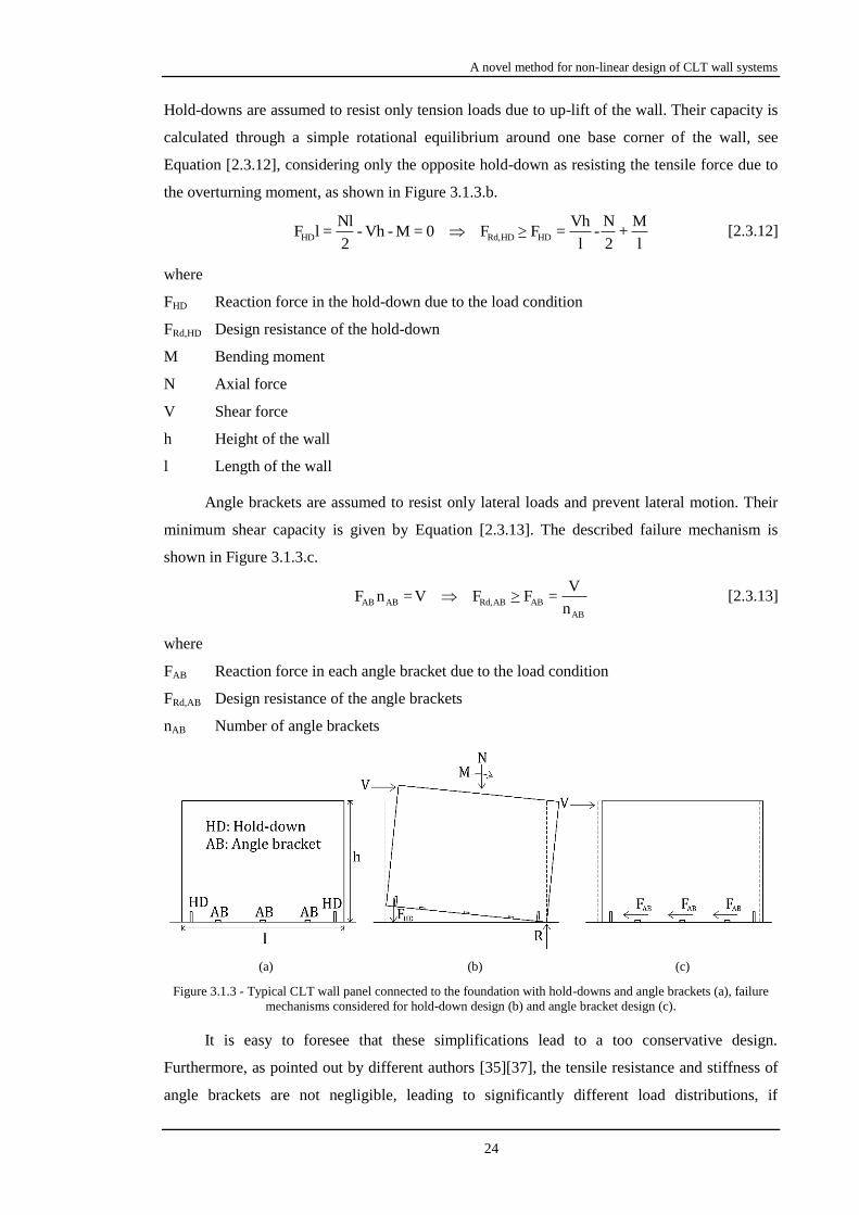
A novel method for non-linear design of CLT wall systems
24
Hold-downs are assumed to resist only tension loads due to up-lift of the wall. Their capacity is
calculated through a simple rotational equilibrium around one base corner of the wall, see
Equation [2.3.12], considering only the opposite hold-down as resisting the tensile force due to
the overturning moment, as shown in Figure 3.1.3.b.
HD Rd,HD HD
Nl Vh N MF l = - Vh - M = 0 F > F = - +
2 l 2 l [2.3.12]
where
FHD Reaction force in the hold-down due to the load condition
FRd,HD Design resistance of the hold-down
M Bending moment
N Axial force
V Shear force
h Height of the wall
l Length of the wall
Angle brackets are assumed to resist only lateral loads and prevent lateral motion. Their
minimum shear capacity is given by Equation [2.3.13]. The described failure mechanism is
shown in Figure 3.1.3.c.
AB AB Rd,AB AB
AB
VF n =V F > F =
n [2.3.13]
where
FAB Reaction force in each angle bracket due to the load condition
FRd,AB Design resistance of the angle brackets
nAB Number of angle brackets
(a) (b) (c)
Figure 3.1.3 - Typical CLT wall panel connected to the foundation with hold-downs and angle brackets (a), failure
mechanisms considered for hold-down design (b) and angle bracket design (c).
It is easy to foresee that these simplifications lead to a too conservative design.
Furthermore, as pointed out by different authors [35][37], the tensile resistance and stiffness of
angle brackets are not negligible, leading to significantly different load distributions, if

A novel method for non-linear design of CLT wall systems
25
compared to those obtained using the aforementioned method.
In this chapter, a more realistic and less conservative method for the calculation of tensile
force in the metal connectors at the base of a CLT wall is proposed considering the tensile
resistance and stiffness of both hold-downs and angle brackets. The shear reaction forces of
hold-downs have not been considered because their shear resistance and stiffness are
significantly lower than the ones offered by angle brackets [35][37]. Usually, only two hold-
downs are used per wall and, during the first part of a lateral motion, they rotate rigidly, acting
mostly like a truss element. Furthermore, in order to allow recentring of the structure after a
seismic event, lateral displacements should be kept in the elastic range. Plasticization should
occur in vertical joints, such as connections between wall panels, and tension resisting
connections, such as hold-downs and angle brackets in tension, rather than horizontal shear
resisting elements, such as angle brackets in shear. For these reasons, since only angle brackets
resist lateral loads and they should remain elastic, the simplified approach mentioned before
could be used (see Figure 3.1.3.c and Equation [2.3.13]).
The proposed method is based on the analogy between the design of rectangular
reinforced concrete sections and the design of the base of a CLT wall with metal connections
(hold-downs and angle brackets). A similar subdivision into sub-domains was made by setting
different well-defined failure mechanisms [22]. With this method, the load distribution in the
connections can be calculated for a certain load condition, and the most probable collapse
mechanism is identified. The procedure mainly applies to platform frame structures with hold-
downs and angle brackets connections at the base of the wall and rocking mechanism as
prevalent way of dissipation.
3.2. Method derivation
The proposed method, compared to the usual practice, considers the tensile strength of
angle brackets. It is based on the assumption that a design, in order to allow the recentring of the
structure after a later load, due to wind loads or earthquake, should favor rocking over slip, and
so favor the plasticization of tension resisting connections, such as hold-downs and angle
brackets in vertical direction, rather than the plasticization of shear resisting connections, such
as angle brackets in horizontal direction, which should remain in their elastic domain.
For these reasons, only tension is considered
3.2.1. Hypotheses
In order to derive a simplified method, some assumptions were made:
Wood is modelled with a conservative elasto-brittle behavior (see Figure 3.2.1),
characterized by the Young modulus E and the ultimate compressive stress fc. Such a

A novel method for non-linear design of CLT wall systems
26
behavior has been chosen as in a typical design wood members are regarded as rigid and
ductility is concentrated in the connections. A triangular stress-block in compression is
assumed;
Figure 3.2.1 - Stress-strain relationship of wood in compression at the wall-foundation interface.
Only compression stresses are assumed to be transferred by the wood of the wall to the
floor/foundation interface. Tensile forces are only transferred by metal connections.
As wall panels are in direct contact with the surface underneath, whether it is the
foundation or a floor slab, the contribution of hold-downs and angle brackets to the
compression resistance of the system is negligible. As a consequence, both connections
are modelled as only resisting in tension through elasto-plastic behaviors with limited
ductility (see Figure 3.2.2), characterized by the yielding force Fy, the elastic stiffness ks
and the ultimate displacement Uult;
Figure 3.2.2 - Experimental force-displacement relationship (line with dashes and dots), tri-linear approximation of
the test result (dashed line) and elasto-plastic approximation of the test results (solid line) for connections.
CLT wall panels are regarded as rigid bodies. For this reason, the compressive stress at
the bottom corner of the wall σc is related to a fictitious displacement uc underneath the
foundation surface and a coefficient k (see chapter 3.3.1.1 and Equation [2.5.1]) of
compressive stress distribution along the height of the panel h through Equation [2.4.1]:

A novel method for non-linear design of CLT wall systems
27
c cc c,max
u E f khu
k h E [2.4.1]
Figure 3.2.3 depict the rocking mechanism and the forces considered.
Figure 3.2.3 - Rotational mechanism and forces involved.
With reference to Figure 3.2.3
Fc Value of the reaction force in compression in the contact zone between panel and
supporting surface
Fi Value of the reaction force in the ith connection
W Self-weight of the panel
k Compressive stress distribution coefficient
n Number of connections
uc Fictitious displacement underneath the foundation surface
x̅ Distance of the neutral axis from the bottom right corner
xi Distance of the ith connection from the compressed panel corner

A novel method for non-linear design of CLT wall systems
28
σc Compressive stress at the bottom corner of the wall
The reference point for the position of the neutral axis is the bottom right corner of the
panel if the lateral force at the top of the wall is directed rightward, the bottom left corner of the
panel if the lateral force at the top of the wall is directed leftward. All forces are regarded as
positive if they are oriented like those indicated in Figure 3.2.3. The axial force N is therefore
considered positive if the wall is compressed.
3.2.2. Limit States definition
As previously mentioned, the proposed method is developed by analogy with the design
of RC cross-sections.
According to the assumptions made, five failure sub-domains were defined to consider
the occurrence of all the possible ultimate limit states at the wall-support interface. The case
discussed herein is for lateral load at the top of the panel directed rightward:
1. Pure tension: At least one connection attains its ultimate displacement Uult. Timber is not
compressed;
2. At least one connection attains its ultimate displacement Uult. The bottom right corner of
the panel is compressed with a stress lower than fc;
3. At least one connection is subjected to tension. The bottom right corner of the panel
attains the compression resistance fc;
4. No connection is in tension. The bottom left corner of the panel is not compressed;
5. The whole base of the panel is compressed. None of the connections is in tension.
The subdivision detailed herein is displayed in Figure 3.2.4.
Referring to Figure 3.2.4
s.s. Supporting surface
Limit in tension, starting configuration of the domain
Interface between sub-domains 1 and 2
Interface between sub-domains 2 and 3
Interface between sub-domains 3 and 4
Interface between sub-domains 4 and 5
Limit in compression, ending configuration of the domain.
It can be noticed that in sub-domains 1, 2 and 3 the connections are loaded in tension, and
therefore an iterative solutions will have to be computed as the force-displacement relationship
is elasto-plastic with limited ductility.

A novel method for non-linear design of CLT wall systems
29
Figure 3.2.4 - Schematic representation of the considered sub-domains.
On the other hand, sub-domains 4 and 5 do not depend on anything but the timber
compressive stress. The choice of an elasto-brittle relationship leads to closed form solutions for
these last two cases.
From Figure 3.2.4 it can be noted that the position of the neutral axis at the boundaries of
each sub-domain is a mere geometrical problem since it can be deduced from the values Uult and
uc.max. Consequently, the possible range of axial forces leading to the attainment of a particular
ultimate limit state condition can be immediately assessed: by knowing the geometry of the
wall, the location of the connections, the stress-strain and force-displacement relationships of
wall and metal connections, respectively, the minimum and maximum value of axial force
allowed in the system and all the four values of axial force at the boundary between sub-
domains can be immediately derived. Once the value of the axial load is known, the failure
mechanism occurring first and the corresponding sub-domain can be determined.
In Figure 3.2.4, the notation Uult,min is used since two different types of connection are
generally used, each one with its own force-displacement behavior, and therefore a different
ultimate displacement, so that Uult,min is the minimum ultimate elongation, among the two
available connections, and Uult,max is the largest one. Usually, in a structure, at least in the same
wall, all the hold-downs have the same mechanical properties and all the angle brackets have the
same mechanical properties. Having two different ultimate displacements leads to two possible
rotation points of the wall in order to fulfill the ultimate state conditions of sub-domains 1 and

A novel method for non-linear design of CLT wall systems
30
2. In the example shown in Figure 3.2.4, the lower ultimate displacement is the angle brackets
one. For a connection arrangement similar to that depicted in Figure 3.2.4, the rotation point
used to trace sub-domains 1 and 2 is (xmin;Uult,min), where xmin signifies the distance of the
farthest connection, characterized by an ultimate displacement Uult,min, from the right wall
corner. However, the possibility for the base of the wall to reach the point (xmax;Uult,max) should
be considered (Figure 3.2.5.b), where xmax is the distance of the last connection, having Uult,max
as ultimate displacement, from the right wall corner. If this condition occurs, two connections
attain the ultimate displacement, leading to the shift of the rotation point from (xmin;Uult,min) to
(xmax;Uult,max), in order not to overcome the ultimate elongation of the more flexible connection,
as shown in Figure 3.2.5.c.
(a) (b) (c)
Figure 3.2.5 - Starting condition for the definition of subdomains 1 and 2 (a), attainment of the ultimate condition in
two different connections (b) and change in the point of rotation of the system (c).
This shift cannot take place in sub-domains 3, 4 or 5, since the rotation point is always
(0;uc,max) (see Equation [2.4.1] and Figure 3.2.4). The position of the neutral axis where this shift
occurs is defined as x̅p and its value can be calculated by a proportion of similar triangles, as
shown in Equation [2.4.2]:
ult,max min ult,min max
P
ult,max ult,min
U x -U xx
U -U [2.4.2]
The value of x̅p has to be limited to the position of the neutral axis between sub-domains 2
and 3. This restriction results in the condition given by Equation [2.4.3]:
min c,max
P
ult,min c,max
x ux
U u
[2.4.3]
Once the value of x̅p is known, sub-domains 1 and 2 can be easily defined.
Table 3.2.1 - Position of the neutral axis at the lower and upper limit for each sub-domain.
Sub-domain 1 2 3 4 5
x̅ -∞ 0
min c,max
P
ult ,min c,max
max c,max
P
ult ,max c,max
x ux if x
U u
x ux if x
U u
[2.4.4] xn l +∞
Referring to Table 3.2.1, xn signifies the distance of the leftmost connection from the right

A novel method for non-linear design of CLT wall systems
31
base corner, as this corner is taken as reference point to measure distances and positions, and l is
the length of the wall.
The definition of sub-domains 1, 2 and 3 needs an iterative process to be made. The first
quantity to assess is the elongation of each connection. A simple proportion between similar
triangles is used. The value of x̅p is crucial, for sub-domains 1 and 2, because it sets whether this
proportion has to be made using Uult,min or Uult,max, as shown in Equation [2.4.5]:
ult ,min i
P
min
i
ult ,max i
P
max
when
when
U (x -x)x x
x -xu
U (x -x)x x
x -x
[2.4.5]
In sub-domain 3, where the elongation of the connections still plays a role, the proportion
is made using uc,max, as the rotation point for this sub-domain becomes the bottom right corner:
c,max i
i
u (x -x)u
x [2.4.6]
Knowing the value of vertical displacement in each connection allows calculation of the
corresponding reaction force:
y,i i y,i
i
i i i y,i
when
when
F u UF
k u 0 u U
[2.4.7]
The last unknown to be calculated is the contact reaction force in wood Fc. This value
depends on the position of the neutral axis x̅ and the stress value at the right base corner. The
compressive stress can be calculated using Equation [2.4.1] as seen in chapter 3.2.1 for sub-
domain 2. For sub-domain 3 this value is constant and equal to fc. The contact force FC is given
by Equation [2.4.8] for sub-domain 2 and by Equation [2.4.9] for sub-domains 3 and 4:
cc
sxF
2
[2.4.8]
cc
f s xF
2 [2.4.9]
s signifies the thickness of the panel.
All the previously derived quantities depend upon the value of x̅. The value of x̅ can be
determined with some iterations by solving the equilibrium of the vertical forces (Equation
[2.4.10]):
n
c i1
N F (x) - F (x)- W [2.4.10]
If the value of the axial force N is greater than the value at the limit between sub-domain
3 and 4, a closed form solution can be employed. In this case, the summation term in Equation
[2.4.10] disappears, leading to a solution that only depends on the compressive force Fc, which

A novel method for non-linear design of CLT wall systems
32
is a linear function of the neutral axis position x̅.
In sub-domain 4, which is a particular case of sub-domain 3 where the summation term is
equal to zero, the value of the neutral axis position is given by Equation [2.4.11]:
c cc
c
f s x f s x 2(N W)F N -W x
2 2 f s
[2.4.11]
For sub-domain 5, an additional consideration has to be made in order to find the correct
value of the contact force Fc. Here the neutral axis lays outside the base of the wall, meaning
that the stress block has a trapezoidal shape, and therefore the stress at the left base corner σd is
needed. This value is calculated again via a simple proportion between similar triangles, as
shown in Equation [2.4.12]:
d c cd c
f f (x -l) lf 1-
x -l x x x
[2.4.12]
Having found the value of σd, the value of Fc can then be calculated according to
Equation [2.4.13]:
c c
c dc c c
l lf f 1- sl 2-x(f )sl lxF f sl f sl 1-
2 2 2 2x
[2.4.13]
The position of the neutral axis can then be calculated using the equilibrium equation:
2
c cc
c c c
f sl f sll l N W 2xN f sl 1- -W 1- x
2x 2x f sl l f sl- N-W 2(f sl- N-W)
[2.4.14]
Once the position of the neutral axis x̅ and all the reacting forces at the ultimate limit state
are known, the resisting bending moment of the system MRd can be calculated. This is made
through a simple rotational equilibrium around the midpoint of the wall base:
n
Rd C i i1
l x lM F - - F -x
2 3 2
[2.4.15]
Equation [2.4.15] is valid for sub-domains 1 to 4, recalling that the reaction contact force
Fc is equal to zero for sub-domain 1 and so is the summation term for sub-domain 4.
In sub-domain 5, having a trapezoidal stress block, a different equation to calculate MRd is
needed:
d cRd C
d c
2 fl lM F -
2 3 f
[2.4.16]
The procedure displayed above is valid for a lateral force applied at the top of the wall
directed rightward. When the lateral force is directed leftward, the reference point has to be
moved from the bottom right corner to the bottom left corner. The distances of the connections
xi should be changed in accordance to Equation [2.4.17]:

A novel method for non-linear design of CLT wall systems
33
i,sx i,dxx l - x [2.4.17]
where xi,sx and xi,dx signify the distances of the ith connection from the bottom left and the
bottom right corner, respectively.
By using these new values, the problem is equivalent to the one for lateral load directed
rightward.
By varying the position of the neutral axis from -∞ to +∞ for both cases of lateral force
directed rightward and leftward, all the possible couples (N;MRd) can be calculated, and an axial
force-bending moment resisting domain can be drawn. An example is displayed in Figure 3.2.6.
(a) (b)
Figure 3.2.6 - Examples of axial force-bending moment resisting domain for a symmetrical (black line (a) and black
connections (b)) and non-symmetrical (orange line (a) and orange connections (b)) arrangement of connections. In
the second configuration, only the two connections on the left are present with respect to the symmetrical one (b). X
and + marks denote the passage from a sub-domain to another for symmetrical and non-symmetrical arrangement of
connections, respectively. Circles denote the starting (left, sub-domain 1) and end (right, sub-domain 5) points of the
domains.
Initially, the procedure was implemented into a spreadsheet, and then in a Windows
application. This software, written in VB.NET and available both in Italian and English, allows
the user, once the needed parameters have been set, to calculate the resisting domain. It draws
the positions of the neutral axis at the intersection of the various sub-domains for the analyzed
wall. Furthermore, the sub-domain where the ultimate limit state takes place for the given value
of axial force N can be determined.
3.3. Method validation
This section investigates the values of the stress distribution coefficient k and validates
the proposed method using two different numerical approaches. The first approach is based on
the use of SAP2000 [15] and derives values of k for walls on a rigid support. The second
approach uses ABAQUS [17] and derives values of k for both rigid foundation and CLT
support. All numerical models used within this chapter were validated in previous papers and

A novel method for non-linear design of CLT wall systems
34
studies [62][70].
3.3.1. SAP2000 analyses
3.3.1.1. Investigation of the stress distribution coefficient k
The proposed method converts the strain of the wall panel at the interface with the
supporting foundation/floor panel into an equivalent fictitious displacement of the panel
underneath the support surface, so that the loss of height of the panel due to the compression of
CLT is equal to the fictitious displacement underneath the supporting surface. This permits to
regard the panel as rigid, easing the computation. The change is made through a coefficient of
stress distribution k. This coefficient depends upon the stress distribution along the CLT panel
above the rocking corner, and can be calculated according to Equation [2.5.1]:
h
c0
c
z dz
kf h
[2.5.1]
In order to find a proper value for this coefficient, several numerical analyses using the
software SAP2000 [15] were carried out. Two CLT panels 3 m long and 85 mm thick with
different heights, 3 m and 1,75 m, were analyzed. The unit weight of wood and the Young
modulus were assumed 4,2 kN/m3 and 5,7 GPa, respectively [7][62][70]. The geometric
characteristics of the panels have been taken from the panels tested within the SOFIE Project
[10][11][40], while the choice of a single MOE was made because the method takes into
account only compression stiffness of CLT and the analyses have been carried out by modelling
the panels via isotropic shell elements. The value is an average between perpendicular and
parallel to the grain MOEs accounting for number and orientation of layers within the panel
[62].
The two panels were linked with three different types of connections to the foundation
surface. The tension force-displacement relationships of the connections are described in the
following (Figure 3.3.1):
1. Hold-down
Elastic phase with a stiffness of 4,82 kN/mm and a yielding force of 40,31 kN;
Hardening phase with a slope of 0,37 kN/mm and a peak strength of 48,33 kN;
Quasi-vertical failure;
Residual horizontal strength at 5% of the peak strength.
2. Angle bracket
Elastic phase with a stiffness of 2,7 kN/mm and a yielding force of 19,27 kN;
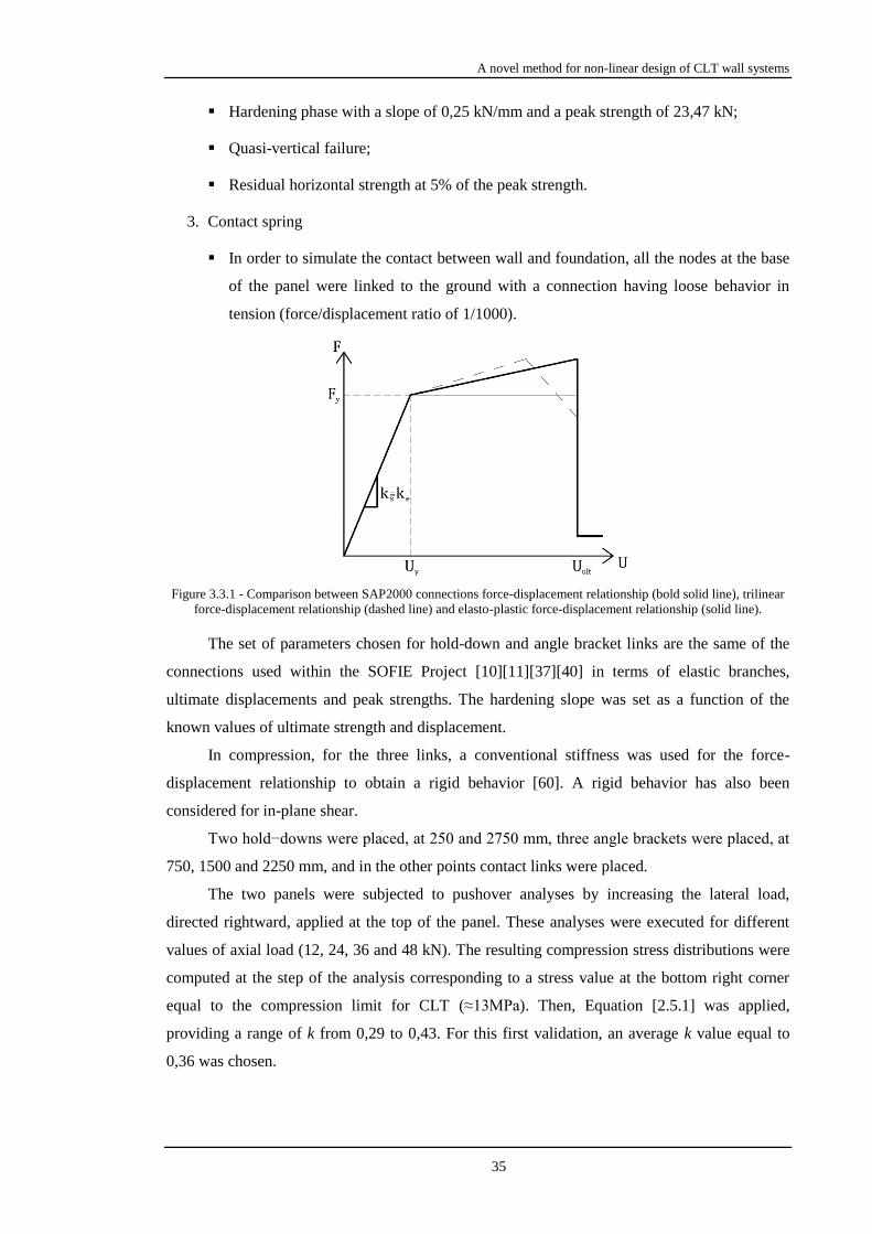
A novel method for non-linear design of CLT wall systems
35
Hardening phase with a slope of 0,25 kN/mm and a peak strength of 23,47 kN;
Quasi-vertical failure;
Residual horizontal strength at 5% of the peak strength.
3. Contact spring
In order to simulate the contact between wall and foundation, all the nodes at the base
of the panel were linked to the ground with a connection having loose behavior in
tension (force/displacement ratio of 1/1000).
Figure 3.3.1 - Comparison between SAP2000 connections force-displacement relationship (bold solid line), trilinear
force-displacement relationship (dashed line) and elasto-plastic force-displacement relationship (solid line).
The set of parameters chosen for hold-down and angle bracket links are the same of the
connections used within the SOFIE Project [10][11][37][40] in terms of elastic branches,
ultimate displacements and peak strengths. The hardening slope was set as a function of the
known values of ultimate strength and displacement.
In compression, for the three links, a conventional stiffness was used for the force-
displacement relationship to obtain a rigid behavior [60]. A rigid behavior has also been
considered for in-plane shear.
Two hold−downs were placed, at 250 and 2750 mm, three angle brackets were placed, at
750, 1500 and 2250 mm, and in the other points contact links were placed.
The two panels were subjected to pushover analyses by increasing the lateral load,
directed rightward, applied at the top of the panel. These analyses were executed for different
values of axial load (12, 24, 36 and 48 kN). The resulting compression stress distributions were
computed at the step of the analysis corresponding to a stress value at the bottom right corner
equal to the compression limit for CLT (≈13MPa). Then, Equation [2.5.1] was applied,
providing a range of k from 0,29 to 0,43. For this first validation, an average k value equal to
0,36 was chosen.

A novel method for non-linear design of CLT wall systems
36
3.3.1.2. Analyses description
In order to validate the proposed simplified method, some pushover analyses were
performed on different systems using SAP2000, comparing the results obtained through the
numerical analyses with those obtained with the proposed method. The investigated systems
are:
1. Two 2-dimensional models:
A single-panel CLT wall;
A 3-panel CLT wall.
2. A 3-dimensional model of a 3-story building.
The single panel was modelled in the same way as described in chapter 3.3.1.1 for an
aspect ratio of 1. The 3-panel wall was modelled by linking together the panels using springs
simulating screws in a half-lap joint. Multilinear plastic joints with a conventional stiffness of
100 kN/mm in the two in-plane directions were used. A semi-rigid connection was chosen here
because the method does not account yet for loose connections between panels.
The 3-story building model schematizes a building tested within the SOFIE Project
[10][11][62][70] and numerically investigated through SAP2000 [15]. To ease the convergence
in non-linear analyses, the quasi-vertical failure branch was replaced by a softening branch with
a slope of one-tenth of the elastic slope. In these analyses, in fact, this software proved to be
unstable using steep descending gradients in the softening branch of the force-displacement
relationship [70].
3.3.1.3. Validation through a 2-D model
Both 2D validations were carried out through several displacement-controlled pushover
analyses. Using the spreadsheet, four different values of axial forces at the interface of the five
sub-domains were calculated. Such values were used to run the analyses in SAP2000.
For each case, the ultimate limit state which occurred first was investigated and, at that
step, the position of the neutral axis was assessed. These results were compared to those
obtained using the spreadsheet. A summary of the comparison for the single panel and the 3-
panel wall is presented in Table 3.3.1 and Table 3.3.2, respectively.
Table 3.3.1 - Comparison between numerical and analytical results - single panel wall.
N [kN] Neutral axis position [mm]
Difference [mm] Error related to the
wall length [%] Algorithm SAP2000
462 3000 3050 50 1,7
423 2750 2800 50 1,7
-101 63 138 75 2,5
-114 0 -83 83 2,8

A novel method for non-linear design of CLT wall systems
37
Table 3.3.2 - Comparison between numerical and analytical results - 3-panel wall.
N [kN] Neutral axis position [mm]
Difference [mm] Error related to the
wall length [%] Algorithm SAP2000
1386 9000 8750 250 2,8
1347 8750 8733 17 0,2
-112 525 370 155 1,7
-154 0 36 36 0,4
In the first case, the error is always lower than 10 cm (3% of the wall length). Even in the
second case, the evaluation of the neutral axis using the method is good, leading to an error of
less than 3% of the wall length in this case too.
3.3.1.4. Validation through a 3-D model
In the 3D validation, the comparison was made for a wall of the ground floor.
Figure 3.3.2 - Plan of the ground floor of the case study building with the investigated wall highlighted.
Contact springs were placed in each node of the wall base where neither hold-downs nor
angle brackets are applied. Such springs are placed at the base of the various walls in the same
way as for the single panel wall and for the 3-panel wall (see chapter 3.3.1.1). The axial force
applied on the wall used for the analytical calculation was obtained by summing the axial
reaction forces in the connections and in the contact links of the SAP2000 FE model after the
application of the permanent loads. The numerical investigation was carried out by searching for
the step of the analysis where an ultimate condition occurred and evaluating the position of the
neutral axis there. The resulting position of the neutral axis was 2500 mm from the compressed
edge, with an ultimate limit state characterized by crushing of CLT. The method predicted the
same ultimate limit state, but a neutral axis at 1304 mm. This difference (1196 mm), if
compared to the wall length, gives an error of 17,7%.
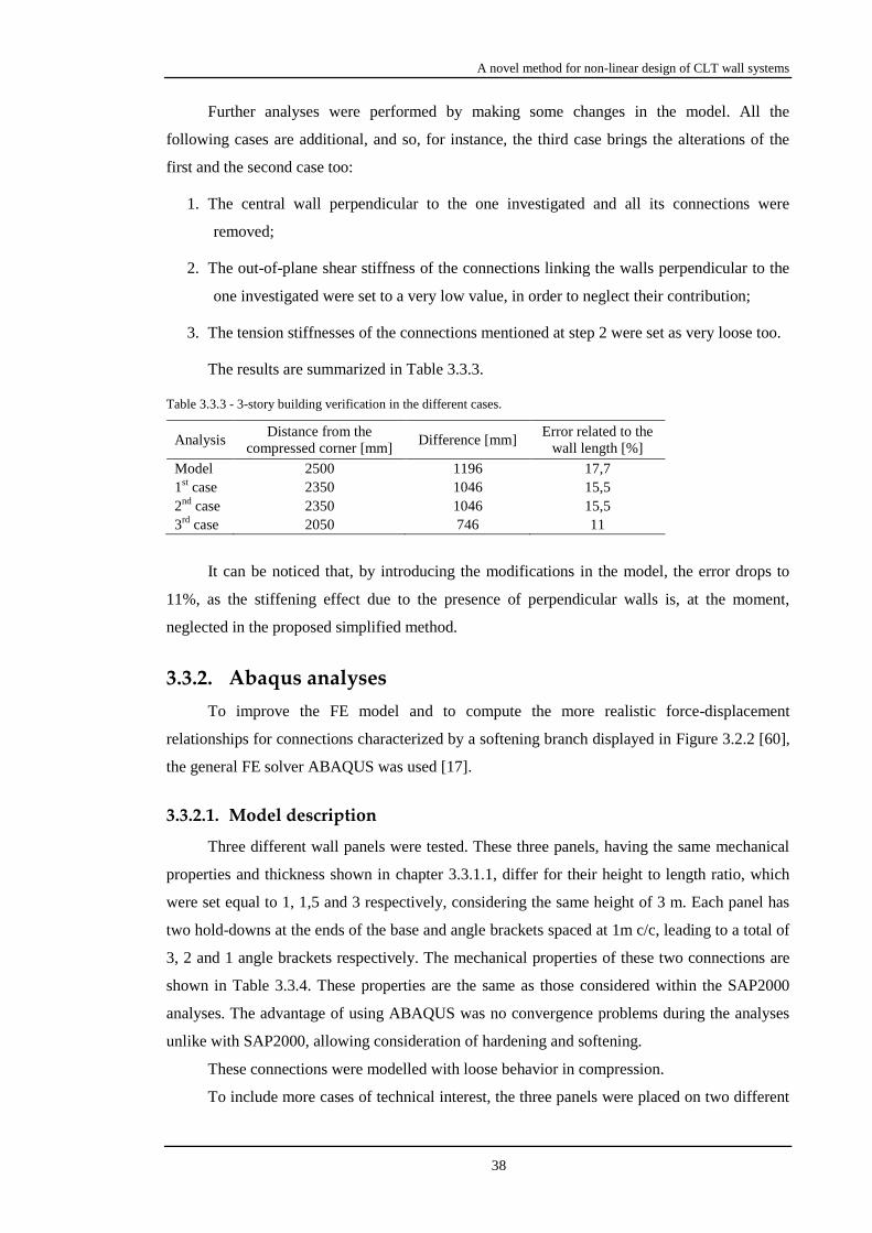
A novel method for non-linear design of CLT wall systems
38
Further analyses were performed by making some changes in the model. All the
following cases are additional, and so, for instance, the third case brings the alterations of the
first and the second case too:
1. The central wall perpendicular to the one investigated and all its connections were
removed;
2. The out-of-plane shear stiffness of the connections linking the walls perpendicular to the
one investigated were set to a very low value, in order to neglect their contribution;
3. The tension stiffnesses of the connections mentioned at step 2 were set as very loose too.
The results are summarized in Table 3.3.3.
Table 3.3.3 - 3-story building verification in the different cases.
Analysis Distance from the
compressed corner [mm] Difference [mm]
Error related to the
wall length [%]
Model 2500 1196 17,7
1st case 2350 1046 15,5
2nd
case 2350 1046 15,5
3rd
case 2050 746 11
It can be noticed that, by introducing the modifications in the model, the error drops to
11%, as the stiffening effect due to the presence of perpendicular walls is, at the moment,
neglected in the proposed simplified method.
3.3.2. Abaqus analyses
To improve the FE model and to compute the more realistic force-displacement
relationships for connections characterized by a softening branch displayed in Figure 3.2.2 [60],
the general FE solver ABAQUS was used [17].
3.3.2.1. Model description
Three different wall panels were tested. These three panels, having the same mechanical
properties and thickness shown in chapter 3.3.1.1, differ for their height to length ratio, which
were set equal to 1, 1,5 and 3 respectively, considering the same height of 3 m. Each panel has
two hold-downs at the ends of the base and angle brackets spaced at 1m c/c, leading to a total of
3, 2 and 1 angle brackets respectively. The mechanical properties of these two connections are
shown in Table 3.3.4. These properties are the same as those considered within the SAP2000
analyses. The advantage of using ABAQUS was no convergence problems during the analyses
unlike with SAP2000, allowing consideration of hardening and softening.
These connections were modelled with loose behavior in compression.
To include more cases of technical interest, the three panels were placed on two different

A novel method for non-linear design of CLT wall systems
39
types of support: rigid foundation and CLT floor panel support. In order to simulate such
conditions, various contact connections were placed at the base of the CLT walls. These contact
springs were modelled depending on whether a rigid or a CLT support was investigated. For
both of them, a loose behavior in tension was set. For the rigid support case, the same value of
stiffness was considered for the three panels. A linear elastic behavior was introduced in this
case. In the case of the CLT wall panel supported by a CLT floor panel, a possible plasticization
of timber of the CLT floor panel in the direction perpendicular to the grain may occur. Since the
contact links cannot plasticize in compression, new elasto-plastic springs were introduced. The
compressive stiffness and strength were derived by multiplying the mean values of the modulus
of elasticity and compression strength perpendicular to the grain of the CLT floor panel by a
tributary area. The mechanical properties were taken from the compression tests carried out on
CLT specimens at Växjö University [1]. The tributary area was calculated by considering a 45°
diffusion angle within the CLT floor panel from the bearing area of the CLT wall panel. As
consequence, each type of panel resulted to have a different value of compressive strength of its
contact links due to different ratios of tributary surface over base area.
Table 3.3.4 - Tensile behavior of hold-downs and angle brackets.
Hold-downs Angle brackets
Branch Stiffness [kN/mm] Stiffness [kN/mm]
Elastic 4,8 2,7
Hardening 0,69 0,4
Softening -0,38 -0,81
Characteristic Value Value
Fy 40,31 kN 19,27 kN
Fmax 48,33 kN 23,47 kN
Uult 35 mm 24 mm
3.3.2.2. Investigation of the stress distribution coefficient k
Numerical analyses were performed for the three panels in five different conditions of
load applied on the top of them:
1. Only compressive axial load;
2. Only horizontal shear load;
3. Only bending moment;
4. Axial compressive and horizontal shear loads;
5. Bending moment and horizontal shear load.
The values of the k coefficient were assessed using the results of these analyses. Cases 4
and 5 were investigated for different values of the shear-axial load ratio V/N and Vh/M ratio,
where Vh signifies the overturning moment due to the horizontal shear force and M denotes the
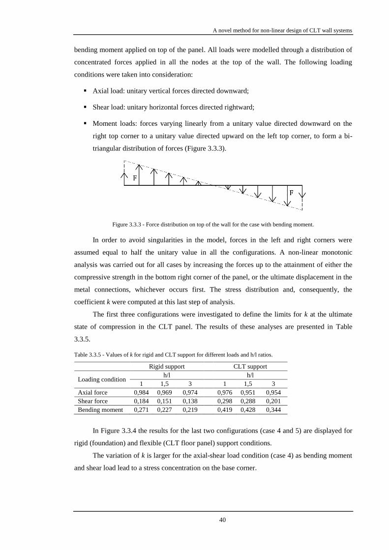
A novel method for non-linear design of CLT wall systems
40
bending moment applied on top of the panel. All loads were modelled through a distribution of
concentrated forces applied in all the nodes at the top of the wall. The following loading
conditions were taken into consideration:
Axial load: unitary vertical forces directed downward;
Shear load: unitary horizontal forces directed rightward;
Moment loads: forces varying linearly from a unitary value directed downward on the
right top corner to a unitary value directed upward on the left top corner, to form a bi-
triangular distribution of forces (Figure 3.3.3).
Figure 3.3.3 - Force distribution on top of the wall for the case with bending moment.
In order to avoid singularities in the model, forces in the left and right corners were
assumed equal to half the unitary value in all the configurations. A non-linear monotonic
analysis was carried out for all cases by increasing the forces up to the attainment of either the
compressive strength in the bottom right corner of the panel, or the ultimate displacement in the
metal connections, whichever occurs first. The stress distribution and, consequently, the
coefficient k were computed at this last step of analysis.
The first three configurations were investigated to define the limits for k at the ultimate
state of compression in the CLT panel. The results of these analyses are presented in Table
3.3.5.
Table 3.3.5 - Values of k for rigid and CLT support for different loads and h/l ratios.
Rigid support CLT support
Loading condition h/l h/l
1 1,5 3 1 1,5 3
Axial force 0,984 0,969 0,974 0,976 0,951 0,954
Shear force 0,184 0,151 0,138 0,298 0,288 0,201
Bending moment 0,271 0,227 0,219 0,419 0,428 0,344
In Figure 3.3.4 the results for the last two configurations (case 4 and 5) are displayed for
rigid (foundation) and flexible (CLT floor panel) support conditions.
The variation of k is larger for the axial-shear load condition (case 4) as bending moment
and shear load lead to a stress concentration on the base corner.

A novel method for non-linear design of CLT wall systems
41
(a) (b)
(c) (d)
Figure 3.3.4 - Values of the distribution coefficient k for (a) axial-horizontal load condition (case 4) and (b) bending
moment-horizontal load condition (case 5) for rigid support and for (c) axial-horizontal load condition (case 4) and
(d) bending moment-horizontal load condition (case 5) for CLT support.
However, the values of k of technical interest are those for V/N ratios greater than 2 as
shear in CLT structures is, for the conventional design approach, resisted only by walls parallel
to the seismic forces whereas axial loads are resisted by all the walls, and therefore the V/N ratio
usually exceeds the value of 2 in Damage and Near Collapse limit states.
For this reason, the coefficient k was chosen as an average value for V/N greater than 2,
resulting in a value of 0,23 and 0,33 for rigid and CLT support, respectively. It is important to
highlight that these values strongly depend on the compressive resistance of the wall. Lower
values of fc lead to higher values of k [70].
For example, for a timber stress value equal to the compressive strength perpendicular to
the grain (≈ 3 MPa) and a V/N ratio of 2, a value of k around 0,29 is obtained for panels with an
h/l ratio equal to 1 on a rigid support. In this investigation, a timber stress of 11 MPa, which can
be regarded as an average value between parallel and perpendicular to the grain compressive
resistance, was considered, leading, for the same kind of panel, to a k value of 0,22. However,

A novel method for non-linear design of CLT wall systems
42
the variation of k within a suitable range does not significantly affect the results of the proposed
method (see Figure 3.3.5).
(a) (b)
Figure 3.3.5 - Dependency of (a) the first part of the M-N domain on the k value and (b) M-N domain for different k
values (0,2 and 0,3).
3.3.2.3. Analyses description
To validate the proposed simplified method, sixteen analyses, differing for load and
supporting conditions, were performed on the 3×3 m panel used for the k coefficient
investigation (see chapter 3.3.2.2). The load conditions correspond to the axial load and bending
moment values at the limit between the various sub-domains as calculated using the proposed
algorithm. The bending moment was applied in two different ways:
As an equivalent distribution of concentrated forces applied at the top of the wall;
Through a corresponding value of horizontal shear load applied at the top of the wall.
In this way, four cases with bending moment and four cases with shear load were
considered. In this second approach, the analyses were carried out for both rigid concrete
foundation and flexible (CLT) support, using k values of 0,23 and 0,33, respectively.
3.3.2.4. Validation through a 2-D model
The position of the neutral axis obtained from the FE analysis was compared with the one
predicted by the proposed simplified algorithm.
The first investigation was performed to check whether the given external loads lead to
the attainment of the ultimate conditions, that are (i) the compression strength of the CLT panel
fc for the boundaries between sub-domains characterized by crushing of timber panel and/or (ii)
the ultimate displacement in at least one connection for the boundaries between sub-domains
characterized by failure of at least one connection. For all failure mechanisms between sub-
domains 3 and 4 and between sub-domains 4 and 5, this verification was satisfied with a
negligible error of 3% on average. However, the verification was not satisfied for the failure
mechanism between sub-domains 1 and 2 and between sub-domains 2 and 3. In these cases, a

A novel method for non-linear design of CLT wall systems
43
second investigation was carried-out, where the values of the imposed loads were increased and
their proportions was not changed until either the ultimate displacement of a connection or the
compressive strength of timber was attained.
In Table 3.3.6 and Table 3.3.7, the results of both investigations are presented for rigid
and flexible support, respectively. In these tables, the “Shear” column lists the results for the
configurations with axial and shear loads as external loads, while the “Bending moment”
column reports the results for the load conditions with axial and flexural loads.
Table 3.3.6 - Comparison between neutral axis position prediction using the proposed algorithm and the FE model
case with bottom rigid support.
N [kN] M [kNm]
Neutral Axis Prediction [mm] Error related to the wall length [%]
Proposed
Algorithm FE-Shear
FE-Bending
moment FE-Shear FE-Bend. mom.
-108,69 38,09 0 -156 -153 5,2 5,1
-38,75 137,19 131,4 110 140 0,7 0,3
1259,19 757,35 2700 2590 2632 3,7 2,3
1399,44 701,25 3000 3200 3080 6,7 2,7
Table 3.3.7 - Comparison between neutral axis position prediction using the proposed algorithm and the FE model
case with bottom CLT support.
N [kN] M [kNm]
Neutral Axis Prediction [mm] Error related to the wall length [%]
Proposed
Algorithm FE-Shear
FE-Bending
moment FE-Shear FE-Bend. mom.
-108,69 38,09 0 -156 -153 5,2 5,1
-38,75 175,87 184,3 288 290 3,5 3,5
1259,19 757,35 2700 2100 2594 20 3,5
1399,44 701,25 3000 2226 2886 25,8 3,8
If the rigid support case is considered, load cases with shear load and bending moment
give similar results in terms of neutral axis position.
Furthermore, even when the numerical values of load to achieve the ultimate condition
are higher than the ones predicted using the proposed algorithm, the neutral axis position
calculated with the proposed method is close to the numerically predicted one in most of the
cases.
It should also be pointed out that the collected differences in loads leading to collapse
between FE analyses and proposed method are mainly due to the fact that hardening and
softening in connections were conservatively neglected in the proposed method.
3.4. Concluding remarks
In this chapter, a simplified non-linear procedure for seismic design of CLT wall systems
has been proposed. This method assumes the wall as rigid with an elasto-brittle behavior in
compression, and metal connections with an elasto-plastic force-elongation relationship. A

A novel method for non-linear design of CLT wall systems
44
triangular compressive stress distribution at the wall-support interface is considered. The forces
in the connections are calculated by considering the base section of a CLT wall as a reinforced
concrete section. The position of the neutral axis is found with an iterative procedure. The
method mainly applies to platform-type structures with hold-downs and angle brackets
connections at the base of the wall and rocking mechanism as prevalent way of dissipation.
The proposed method was validated against different numerical results carried out using
SAP2000 and ABAQUS software packages.
In the analyses carried out using SAP2000, acceptable accuracy was obtained in 2-
dimensional numerical simulations, whereas larger errors were detected in 3-dimensional
simulations due to the box effect of the CLT structure investigated. The box effect has a
stiffening influence on the actual in-plane response of the wall, decreasing the actual sliding and
rocking deformations and leading to larger differences if compared to the simplified method.
Further analyses were performed using ABAQUS in order to improve the evaluation of
the stress distribution coefficient k for both cases of rigid and flexible support. In addition, the
effect of using a more realistic trilinear force-displacement relationship for the angle bracket
connections in shear was investigated. The proposed method was found to provide acceptable
results, as the neutral axis position was predicted with good accuracy in most of the cases
analyzed. The safety factor, calculated as ratio between the loads leading to the ultimate
condition and the predicted ones, was found to be in the range from 1 to 1,85.
The proposed approach is intended to be a starting point for further studies aimed to find
simplified rules for CLT seismic design. While the proposed method is now limited to single
monolithic CLT walls subjected to in-plane load, it will be developed further in order to
consider more cases of technical interest such as, for example, the stiffness contribution of
perpendicular walls, with the final aim to have a complete design tool for CLT designers. In
addition to that, the method could also be used to evaluate the axial force-bending moment
resistant domain or the lateral displacement of the top corner of the wall due to rocking for
inter-story drift calculations.

45
ROCKING OF A TWO-PANEL CLT WALL:
BEHAVIOR PREDICTION AND
INFLUENCE OF FLOOR DIAPHRAGM
SHORT SUMMARY
In the design of CLT buildings in earthquake-prone areas, a crucial role in energy
dissipation is played by the panel-to-panel joint. Such linkage, theoretically, could be designed
for three different types of behavior: coupled and uncoupled behaviors, providing a certain
amount of energy dissipation, and monolithic behavior, without any dissipation. Currently, no
specific design rules to attain such conditions are provided in any code.
In this chapter, a formula for the design of wall-to-floor and wall-to-wall connections is
proposed. Giving the external loads (axial load and shear load on the wall), the geometry of the
wall assembly and the characteristics of the connections involved, the proposed method allows
the designer to evaluate the stiffness of the connections between adjacent panels in order to
obtain a monolithic or a coupled behavior. This formula has been validated based on the results
of experimental tests and numerical analyses.
Furthermore, no information on the dependency of the panel-to-panel behavior upon
other variables such as the out-of-plane stiffness of the floor slabs and the stiffness of other
metal connections, such as hold-downs and angle brackets, can be found in literature.
In an attempt to fill in this gap, this chapter presents the results of numerical analyses
carried out using the Abaqus FE software package. In these analyses, the influence of the upper
floor diaphragms on the rocking behavior of a two-panel wall assembly is investigated. Fully
reversed displacement-controlled cyclic tests are simulated by varying the geometrical
properties (aspect ratio of the wall panels), mechanical properties (types and number of
connectors used for the panel-to-panel, wall-to-foundation and wall-to-upper floor connections,
out-of-plane stiffness of the floor panels) and gravity load applied on top of the walls. The
rocking capacity of the walls is investigated, together with displacements and global behavior of
the assembly. Obtained results highlight the important role played by the stiffness of wall-to-
floor diaphragm joint, whereas the out-of-plane stiffness of the slab has a negligible effect on
the overall response of the assembly.

Rocking of a two-panel CLT wall: behavior prediction and influence OF floor diaphragm
46
4.1. Introduction
Different research projects carried out around the world, such as the SOFIE [10][11][40],
the SERIES [52] and the NHERI TallWood Research [6][8][51][76], have highlighted that CLT
structures can perform satisfactorily in earthquake-prone areas.
Many tests have been performed and studies undertaken over the years to investigate the
structural behavior of components and assemblies made of CLT. In particular, great effort has
been devoted to experimentally assess the capacity and behavior of typical connections under
monotonic and cyclic loads (Gavric et al. [35][36] and Tomasi [74]), as well as to investigate
innovative connections. Zarnani et al. [79] tested a new Resilient Slip Friction Joint (RSFJ) for
seismic damage avoidance design of structures, Polastri et al. [53][54] tested a new connection
system for CLT structures aimed to speed up the erection without losing performance compared
to traditional connection systems, D’Arenzo et al. [16] tested a new type of angle bracket with
similar behavior in both tension and compression to be able to build typical CLT structures
using only one type of connection for wall-to-diaphragm joints.
The capacity and the behavior of CLT wall assemblies was investigated via experimental
cyclic tests carried out in order to assess the rocking behavior and performances (Gavric et al.
[37], Popovski and Gavrić [55]). The most proper value of the seismic behavior factor was
investigated by Amini et al. [4] for the seismic design of CLT structures, and by Follesa and
Fragiacomo [28] for hybrid CLT and light-frame buildings. A proposal of revision of the current
version of the timber chapter of the Eurocode 8 [24] is given by Follesa et al. [29], which
includes specific provisions for capacity-based design and the behavior factor of CLT buildings.
A worked example of application of such rules for the design of a six-story building is presented
in the paper by Vassallo et al. [77].
Furthermore, several numerical investigations have been carried out to extend the
experimental results to other cases of technical interest. As CLT panels are designed to behave
elastically, careful consideration was given to an accurate modelling of connectors, which are
the only component able to deform plastically and to dissipate energy. Rinaldin et al. [60]
proposed a phenomenological model that, through the definition of a set of parameters, allows
the user to properly reproduce the cyclic behavior of single connections, including the energy
dissipation, the pinching behavior, and the strength degradation.
Numerical models have been also used to reproduce two-dimensional and three-
dimensional full scale tests, like the one published by Rinaldin and Fragiacomo [62] where the
3- and 7-story buildings tested within the SOFIE Project [10][11][40] are reproduced.
Reliable designing rules, however, are still needed. Only basic rules are available for
designers. Specific rules for CLT structures are still missing, including the design of panels and
connections or the consideration of all the different scenarios (e.g. failure mechanisms, load

Rocking of a two-panel CLT wall: behavior prediction and influence OF floor diaphragm
47
patterns) this structural system could undergo during its lifetime.
In CLT structures, like in almost all timber structures, connections play a crucial role in
terms of energy dissipation if a dynamic action such as earthquake is considered. The panel-to-
panel vertical joint is an important way to increase ductility and dissipated energy, and can give
a very different response depending on the way they are design. In the case of a wall assembly
made of two adjacent panels linked with a vertical joint, three different rocking behaviors can be
observed depending on the stiffness of the panel-to-panel connection:
Coupled: the panels rock separately, rotating around one of their base corners;
Uncoupled: the link is stiff enough to prevent the contact along the base of one panel, but
not enough to entail a monolithic behavior;
Monolithic: the entire wall rotates monolithically around one of the two edge base corners
acting like a single panel.
While the first two situations are realistic, the third one would be realistic only in the
event of infinite stiffness, namely only if glue was used, which is usually not the case.
Several tests have been carried out to assess the behavior of CLT wall assemblies
subjected to lateral loads, highlighting the importance of the vertical panel-to-panel joints. The
different behavior (i.e. stiffness) of such connections influences the amount of sliding and
rocking displacements contribution to the total lateral movement of top of the assembly.
Furthermore, this joint influences the energy dissipation and structural capacity of the assembly,
as it provides the wall with higher energy dissipation and ductility when a coupled behavior is
obtained, compared to an uncoupled behavior or a monolithic wall [37]. Some attempts have
been made to give analytical predictions of their behavior and design with respect to the other
connections involved in the rocking mechanism [9].
The main issue is to move from the assembly behavior to the complete structure response.
In a building, the walls at a certain level are restrained, in- and out-of-plane, by the floor slabs.
In laboratory tests, wall assemblies are usually linked to the foundation via usual connectors,
such as angle brackets or hold-downs, but may have different types of constraints at the top,
depending on the testing equipment and on the nature of the test itself.
In this chapter, results from nonlinear displacement-controlled fully reversed cyclic
analyses performed on two-panel wall assemblies are presented. Such analyses have been
carried out to assess the influence of a CLT floor diaphragm on the top of the two-panel CLT
wall in terms of rocking behavior. Among all the parameters analyzed, different sets of
connections linking wall and slab together with different types of floor diaphragms have been
considered.
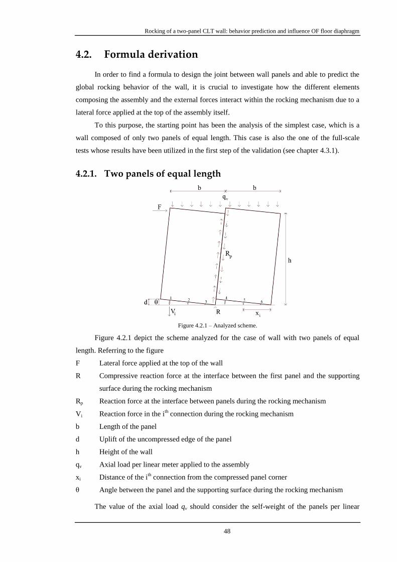
Rocking of a two-panel CLT wall: behavior prediction and influence OF floor diaphragm
48
4.2. Formula derivation
In order to find a formula to design the joint between wall panels and able to predict the
global rocking behavior of the wall, it is crucial to investigate how the different elements
composing the assembly and the external forces interact within the rocking mechanism due to a
lateral force applied at the top of the assembly itself.
To this purpose, the starting point has been the analysis of the simplest case, which is a
wall composed of only two panels of equal length. This case is also the one of the full-scale
tests whose results have been utilized in the first step of the validation (see chapter 4.3.1).
4.2.1. Two panels of equal length
Figure 4.2.1 – Analyzed scheme.
Figure 4.2.1 depict the scheme analyzed for the case of wall with two panels of equal
length. Referring to the figure
F Lateral force applied at the top of the wall
R Compressive reaction force at the interface between the first panel and the supporting
surface during the rocking mechanism
Rp Reaction force at the interface between panels during the rocking mechanism
Vi Reaction force in the ith connection during the rocking mechanism
b Length of the panel
d Uplift of the uncompressed edge of the panel
h Height of the wall
qv Axial load per linear meter applied to the assembly
xi Distance of the ith connection from the compressed panel corner
θ Angle between the panel and the supporting surface during the rocking mechanism
The value of the axial load qv should consider the self-weight of the panels per linear

Rocking of a two-panel CLT wall: behavior prediction and influence OF floor diaphragm
49
meter, as it contributes to the stabilizing forces in the analyzed scheme. However, its value is
generally low if compared to the axial forces considered during the design (e.g. weight of upper
floors).
The aim of this method is to be able to predict the behavior of a panel-to-panel joint in
order to achieve a coupled behavior, which is characterized by a higher energy dissipation and
provides the system with higher ductility, if compared to the other possible behaviors [37].
The first step is the imposition of the equilibrium for the vertical forces in the first panel.
3
p v i
1
R R q b V 0 [3.2.1]
The necessary condition to obtain a coupled behavior is that the compressive reaction
force at the interface between the first panel and the supporting surface R is equal to or greater
than zero. Imposing this condition corresponds to:
3
v i p
1
R 0 q b V R 0 [3.2.2]
From Equation [3.2.2], the condition on the joint between panels is obtained.
3
v i p
1
q b V R [3.2.3]
The unknowns Vi and Rp needs to be evaluated. The reaction force at the interface
between panels Rp depends upon the shear stiffness of the single connection kp, the number of
connections between wall panels np and the mutual shear displacement of the two panels, which
could be, for little values of the angle θ, be set equal to uplift d.
p p pR n k d [3.2.4]
The uplift of the uncompressed edge of the panel d con be expressed as a function of the
length of the panel b and the angle between the panel and the supporting surface θ.
d b [3.2.5]
By substituting Equation [3.2.5] in Equation [3.2.4], an equation depending on θ is
obtained.
p p pR n k b [3.2.6]
The reaction force in the ith connection Vi is function of the vertical stiffness ki and the
vertical displacement ui of the connection itself.
i i iV k u [3.2.7]
The vertical elongation ui can be expressed as a function of distance of the connection
from the compressed panel corner xi and the angle between the panel and the supporting surface
θ.
i iu x [3.2.8]

Rocking of a two-panel CLT wall: behavior prediction and influence OF floor diaphragm
50
By substituting Equation [3.2.8] in Equation [3.2.7], an expression with the only
unknown θ is obtained.
i i iV k x [3.2.9]
By substituting Equation [3.2.6] and Equation [3.2.9] in Equation [3.2.3], a new equation
with the only unknown θ can be written.
3
v i i p p
1
q b k x n k b [3.2.10]
The value of the angle θ is obtained by imposing the equilibrium to the rotation of the
entire assembly around the compressed corner of the second panel.
3 6
2
v i i i i
1 4
Fh q 2b Rb V (x b) V x 0 [3.2.11]
By substituting the values of R (Equation [3.2.1]), Vi (Equaiton [3.2.9]) and Rp (Equation
[3.2.6]) in Equation [3.2.11], a new equation with the angle θ as only unknown is obtained.
3 3 6
2
v v i i p p i i i i i i
1 1 4
Fh q 2b q b k x n k b b k x (x b) k x x 0
[3.2.12]
From Equation [3.2.12], the value of θ is derived.
2
v
62 2
i i p p
1
Fh q b
k x n k b
[3.2.13]
By substituting [3.2.13] in Equation [3.2.10]:
3
2
p p i i v
1
v 62 2
i i p p
1
n k b k x Fh q b
q b
k x n k b
[3.2.14]
By isolating the npkp term, the condition sought is obtained:
3 62
v i i v i i
1 1p p 2
v
Fhq b k x q k x
bn k
Fh 2q b
[3.2.15]
4.2.2. Two panels of different length
The length of the first and second panel are named b1 and b2, respectively. In this case,
the vertical slip between the two panels is equal to the uplift of the second panel, namely d2.
Equation [3.2.5] is consequently modified as follows.
2 2d b [3.2.16]
The new equilibrium equation of the vertical forces in the first panel, and consequently
the value of the compressive reaction force R, is given by Equation [3.2.17].

Rocking of a two-panel CLT wall: behavior prediction and influence OF floor diaphragm
51
3
v 1 i i p p 2
1
R q b k x n k b [3.2.17]
Accordingly, a new rotational equilibrium, defined by Equation [3.2.18], and a
consequent new value of the angle θ, defined by Equation [3.2.19], are obtained.
3
1 2
v 1 2 v 1 i i p p 2 2
1
3 6
i i i 2 i i i
1 4
b bFh q b b q b k x n k b b
2
k x (x b ) k x x 0
[3.2.18]
2 2v
1 2
62 2
i i p p 2
1
qFh b b
2
k x n k b
[3.2.19]
By imposing the second member of Equation [3.2.17] to be greater than zero and by
substituting the value of θ obtained through Equation [3.2.19], the condition for the coupled
behavior of a wall composed of two panels of different length is obtained.
2 3 62 2vi i i v 1 i i
1 1 1
p p 22
vi 2
1
qFh b k x q b k x
2n k
qFh b b
2
[3.2.20]
It is worth nothing to say that if b1 and b2 were equal, Equation [3.2.20] and Equation
[3.2.15] would be the same.
4.3. Validation of the proposed formulation
4.3.1. Validation through full-scale experimental tests results
In order to validate the proposed formulation, the method has been applied to predict the
behavior of several wall assemblies tested at IVALSA Trees and Timber Institute, whose
connection characteristics, geometry and rocking behavior observed, namely coupled,
uncoupled or monolithic, are reported in literature.
4.3.1.1. Experimental program
The data used are the results of tests on screwed connections [36], nailed metal plate
connections, namely hold-downs and angle brackets [35], and CLT wall assemblies [37].
4.3.1.1.1 Tests on screwed connections
In this test campaign, several screwed joints between CLT panels were tested, mainly
under cyclic shear loads.

Rocking of a two-panel CLT wall: behavior prediction and influence OF floor diaphragm
52
The tests of interest for this validation are the tests assessing the vertical shear
performance of spline joints and half-lapped joints, named test #1 and test #2 [36]. Both type of
connections were used in the test on wall assemblies [37] described in chapter 4.3.1.1.3.
For the panel-to-panel connection, the elastic stiffness against a shear load along the joint
line of a single screw, for the half-lapped joint, and of two screws, for the spline joint, is
considered. The values obtained 1,24 and 0,84 kN/mm, respectively.
Figure 4.3.1 - Test setups #1 and #2 (measures in mm) [36].
4.3.1.1.2 Tests on metal plates connections
Figure 4.3.2 - Elevation (right) and cross-section (left) of test setup used for wall-foundation hold-down connection
loaded in tension (Test configuration #1) [35].
As for the screwed connections described previously, these connections were used within
the tests described in chapter 4.3.1.1.3. In this test campaign, angle bracket and hold-down
connections were tested against cyclic loads of both tension and shear. For the purpose of the
validation, the tests of interest are the ones evaluating the tension performance of hold-down
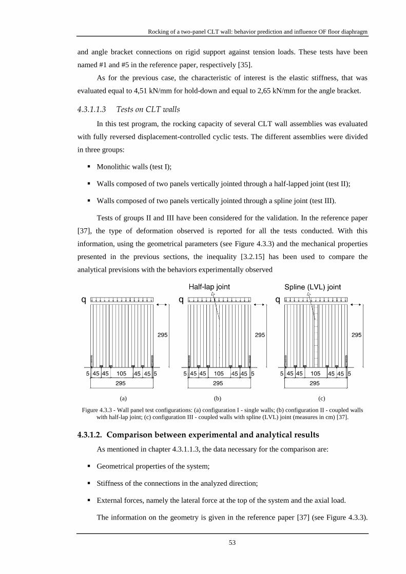
Rocking of a two-panel CLT wall: behavior prediction and influence OF floor diaphragm
53
and angle bracket connections on rigid support against tension loads. These tests have been
named #1 and #5 in the reference paper, respectively [35].
As for the previous case, the characteristic of interest is the elastic stiffness, that was
evaluated equal to 4,51 kN/mm for hold-down and equal to 2,65 kN/mm for the angle bracket.
4.3.1.1.3 Tests on CLT walls
In this test program, the rocking capacity of several CLT wall assemblies was evaluated
with fully reversed displacement-controlled cyclic tests. The different assemblies were divided
in three groups:
Monolithic walls (test I);
Walls composed of two panels vertically jointed through a half-lapped joint (test II);
Walls composed of two panels vertically jointed through a spline joint (test III).
Tests of groups II and III have been considered for the validation. In the reference paper
[37], the type of deformation observed is reported for all the tests conducted. With this
information, using the geometrical parameters (see Figure 4.3.3) and the mechanical properties
presented in the previous sections, the inequality [3.2.15] has been used to compare the
analytical previsions with the behaviors experimentally observed
(a) (b) (c)
Figure 4.3.3 - Wall panel test configurations: (a) configuration I - single walls; (b) configuration II - coupled walls
with half-lap joint; (c) configuration III - coupled walls with spline (LVL) joint (measures in cm) [37].
4.3.1.2. Comparison between experimental and analytical results
As mentioned in chapter 4.3.1.1.3, the data necessary for the comparison are:
Geometrical properties of the system;
Stiffness of the connections in the analyzed direction;
External forces, namely the lateral force at the top of the system and the axial load.
The information on the geometry is given in the reference paper [37] (see Figure 4.3.3).

Rocking of a two-panel CLT wall: behavior prediction and influence OF floor diaphragm
54
Panels have the same length of 1475 mm. Table 4.3.1 show the number of connections used in
each test. The properties of interest, which have already been discussed in chapters 4.3.1.1.1 and
4.3.1.1.2, are summarized in Table 4.3.2.
Table 4.3.1 - Test configuration.
Test ID num. HD num. AB num. Screws
II.1 2 4 20
II.2 2 4 20
II.3 2 4 10
II.4 4 4 5
III.1 2 4 2x20
III.2 2 4 2x10
III.3 4 4 2x5
III.4 2 4 2x10
III.5 2 4 2x10
III.6 2 4 2x10
III.7 2 4 2x10
III.8 2 4 2x10
Table 4.3.2 - Stiffnesses considered.
Connection Stiffness [kN/mm]
Half-lap joint 1,24
Spline joint 0,84
Hold-down 4,51
Angle bracket 2,65
The forces considered in the proposed method are the lateral force applied at the top of
the wall F and the axial load per linear meter applied to the assembly qv. The axial load is an
input data of the test, whereas the lateral force, being an unknown, has been set equal to the
yielding force (Fy) and maximum force (Fmax), both at the first cycle, obtained during the same
test. The values of these forces are given in Table 4.3.3.
Table 4.3.3 - Forces considered for each test.
Test ID qv [kN/m] Fy [kN] Fmax [kN]
II.1 18,5 69,2 97,2
II.2 18,5 65,5 92,3
II.3 18,5 65,4 84,4
II.4 18,5 69,2 93,1
III.1 18,5 72,1 102,5
III.2 18,5 67,6 91,8
III.3 18,5 80,4 102,9
III.4 18,5 61,7 82,4
III.5 18,5 68,1 86,4
III.6 0 46,5 63,4
III.7 18,5 60,0 84,6
III.8 18,5 64,9 79,3
Through a purposely-developed spreadsheet, the goodness of the proposed method has

Rocking of a two-panel CLT wall: behavior prediction and influence OF floor diaphragm
55
been assessed. The results obtained for the comparison between analytically predicted, through
Equation [3.2.15], and experimentally observed rocking behavior are summarized in Table
4.3.4.
As it can be observed, the analytical method correctly predicted the behavior for almost
all the cases (83,3%).
Table 4.3.4 - Comparison between analytically predicted and experimentally observed rocking behavior.
Test ID
Right member of the
inequality [kN/mm] nsks Behavior Verification
with Fy with Fmax with Fy with Fmax
II.1 11,46 9,64 24,8 Single-Coupled YES YES
II.2 11,90 9,85 24,8 Single-Coupled YES YES
II.3 11,91 10,25 12,4 Coupled NO NO
II.4 13,09 10,94 6,2 Coupled YES YES
III.1 11,17 9,45 16,8 Single-Coupled YES YES
III.2 11,64 9,87 8,4 Coupled YES YES
III.3 11,84 10,45 4,2 Coupled YES YES
III.4 12,45 10,37 8,4 Coupled YES YES
III.5 11,58 10,14 8,4 Coupled YES YES
III.6 6,93 6,93 8,4 Coupled NO NO
III.7 12,73 10,24 8,4 Coupled YES YES
III.8 11,98 10,58 8,4 Coupled YES YES
4.3.1.3. Parametric studies
The proposed inequality could be rewritten highlighting ratios between forces and
dimensions involved. In particular, the inequality could be rewritten as function of the ratio
between lateral force and axial load (F/qv2b) and the ratio between the height and the length of
the panel (h/b). In this way, Equation [3.2.15] turns into Equation [3.3.1].
3 62
i i i i
1 1p p
F h 1 1k x k x
V b 2 2bn k
Fh b
V
[3.3.1]
It is possible to evaluate the incidence of these ratios on the formula itself. Figure 4.3.4.a
and b depict the variation of the term npkp to fulfil Equation [3.3.1] varying the value of the ratio
F/qv2b and the ratio h/b, respectively. It is important to highlight that, in both cases, the left
limit of the curve is given by the condition of denominator different from zero. For the first
curve, the limit is set by the b/h ratio. For lower values of this ratio, Equation [3.3.1] gives
negatives values of the panel-to-panel joint stiffness. For the second curve, the limit is set by the
ratio qv2b/F.

Rocking of a two-panel CLT wall: behavior prediction and influence OF floor diaphragm
56
(a) (b)
Figure 4.3.4 – Variation of the panel-to-panel stiffness varying the F/qv2b ratio (a) and the h/b ratio (b).
Within a parametric study, the variation range of the ratio F/qv2b must be considered. For
the validation of the proposed method, the yielding force and the maximum force as obtained
through the test have been taken into account. Designing a wall, unless of a too much over
resisting design, these are the forces considered. It is then reasonable to assume the range of
validity of the aforementioned forces has to be determined based on the design condition. In
fact, when the axial force varies, so does the capacity of the system. In the examples analyzed,
disregarding the case of no axial force applied, the ratio is always included between 1,08 and
1,86. These values belong to the part of the curve (Figure 4.3.4.a) where, even with great
variation of the ratio, there is not a high difference in the resulting panel-to-panel stiffness.
Same considerations must be made on the aspect ratio h/b. The aspect ratio of the panel
plays a crucial role in the determination of the rocking capacity of the assembly.
It is necessary to carry out tests investigating different schemes in order to obtain reliable
results describing the relationships among the different terms of the proposed formula and
giving more information on the goodness of the output.
4.3.2. Validation through FE analyses results
In order to extend the validation to further cases, several FE analyses using the Abaqus
software have been performed [17].
In these analyses, a cyclic displacement time-history was applied in the model at the top
points of the assembly.
The non-linear springs used in the model to describe the connections behavior are those
discussed in [60], which have been successfully used in [62] and other publications.
4.3.2.1. Model description
The FE models have been created through the purposely-developed software X-lam Wall
Mesher [62], which allows the user to build the geometry of 4-node shell models for different

Rocking of a two-panel CLT wall: behavior prediction and influence OF floor diaphragm
57
FE solver, including Abaqus [17], which has been used for these analyses.
The characteristics of the connections have been taken from the tests analyzed in [35],
[36] and [37]. The values of the mechanical properties of the connections in shear and tension
are listed in Table 4.3.5 and Table 4.3.6, respectively.
Table 4.3.5 - Mechanical properties of the connections used in the model – shear.
Mechanical property Connection
Spline joint Angle Bracket Hold-down
kel [kN/mm] 0,84 1,96 3,2
kpl [kN/mm] 0,1 0,23 0,28
Fy [kN] 4,85 22,98 3,61
vy [mm] 5,7 11,74 1,13
Fmax [kN] 7,33 26,85 10,0
vmax [mm] 34,37 28,51 23,95
Fu [kN] 5,86 21,48 12,2
vu [mm] 37,66 31,86 48,42
Table 4.3.6 - Mechanical properties of the connections used in the model – tension.
Mechanical property Connection
Spline joint Angle Bracket Hold-down
kel [kN/mm] 0,94 2,65 4,51
kpl [kN/mm] 0,16 0,41 0,75
Fy [kN] 3,23 19,22 40,46
vy [mm] 3,13 7,26 8,81
Fmax [kN] 6,4 23,47 48,33
vmax [mm] 39,4 17,69 20,3
Fu [kN] 5,12 18,74 38,79
vu [mm] 50,52 23,19 23,75
Referring to Table 4.3.5 and Table 4.3.6: kel and kpl signify the elastic and hardening
stiffness of the backbone, respectively, Fy and vy signify the yielding force and yielding
displacement, respectively, Fmax and vmax signify the maximum force and the corresponding
displacement, respectively, and vu and Fu signify the ultimate displacement and the
corresponding force, respectively.
The tension properties for the spline joint refer to the shear strength of the screws for in-
plane panel separation.
Compression has been set as rigid for every connection. Connections Additional
connections simulating wall-to-supporting foundation and wall-to-diaphragm contact have been
considered in the nodes of the base and top of the assembly where no metal connection was
placed. Out-of-plane stiffness of the connections has been disregarded since the wall panels
were loaded in-plane.
The connections have been modeled through an Abaqus sub-routine created by Rinaldin
et al. [60]. The model, which was already used in [62], has been validated against results of full-
scale cyclic load tests on CLT wall assemblies, whose description is found in [37].
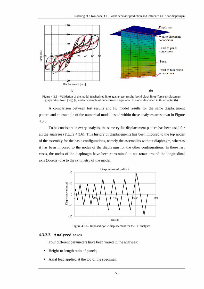
Rocking of a two-panel CLT wall: behavior prediction and influence OF floor diaphragm
58
(a) (b)
Figure 4.3.5 - Validation of the model (dashed red line) against test results (solid black line) (force-displacement
graph taken from [37]) (a) and an example of undeformed shape of a FE model described in this chapter (b).
A comparison between test results and FE model results for the same displacement
pattern and an example of the numerical model tested within these analyses are shown in Figure
4.3.5.
To be consistent in every analysis, the same cyclic displacement pattern has been used for
all the analyses (Figure 4.3.6). This history of displacements has been imposed to the top nodes
of the assembly for the basic configurations, namely the assemblies without diaphragm, whereas
it has been imposed to the nodes of the diaphragm for the other configurations. In these last
cases, the nodes of the diaphragm have been constrained to not rotate around the longitudinal
axis (X-axis) due to the symmetry of the model.
Figure 4.3.6 - Imposed cyclic displacement for the FE analyses.
4.3.2.2. Analyzed cases
Four different parameters have been varied in the analyses:
Height-to-length ratio of panels;
Axial load applied at the top of the specimen;
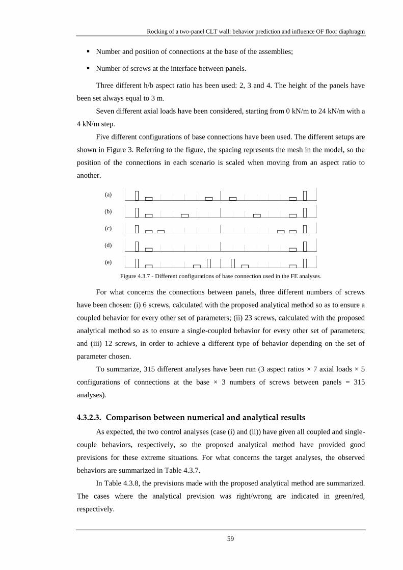
Rocking of a two-panel CLT wall: behavior prediction and influence OF floor diaphragm
59
Number and position of connections at the base of the assemblies;
Number of screws at the interface between panels.
Three different h/b aspect ratio has been used: 2, 3 and 4. The height of the panels have
been set always equal to 3 m.
Seven different axial loads have been considered, starting from 0 kN/m to 24 kN/m with a
4 kN/m step.
Five different configurations of base connections have been used. The different setups are
shown in Figure 3. Referring to the figure, the spacing represents the mesh in the model, so the
position of the connections in each scenario is scaled when moving from an aspect ratio to
another.
(a)
(b)
(c)
(d)
(e)
Figure 4.3.7 - Different configurations of base connection used in the FE analyses.
For what concerns the connections between panels, three different numbers of screws
have been chosen: (i) 6 screws, calculated with the proposed analytical method so as to ensure a
coupled behavior for every other set of parameters; (ii) 23 screws, calculated with the proposed
analytical method so as to ensure a single-coupled behavior for every other set of parameters;
and (iii) 12 screws, in order to achieve a different type of behavior depending on the set of
parameter chosen.
To summarize, 315 different analyses have been run (3 aspect ratios × 7 axial loads × 5
configurations of connections at the base × 3 numbers of screws between panels = 315
analyses).
4.3.2.3. Comparison between numerical and analytical results
As expected, the two control analyses (case (i) and (ii)) have given all coupled and single-
couple behaviors, respectively, so the proposed analytical method have provided good
previsions for these extreme situations. For what concerns the target analyses, the observed
behaviors are summarized in Table 4.3.7.
In Table 4.3.8, the previsions made with the proposed analytical method are summarized.
The cases where the analytical prevision was right/wrong are indicated in green/red,
respectively.

Rocking of a two-panel CLT wall: behavior prediction and influence OF floor diaphragm
60
Table 4.3.7 - Rocking behavior of the walls in the analyses (S-C: single-coupled: C: coupled).
qv
[kN/m] h/b A B C D E
0
2 S-C S-C S-C S-C S-C
3 S-C S-C S-C S-C S-C
4 S-C S-C S-C S-C C
4
2 S-C S-C S-C S-C S-C
3 S-C S-C S-C S-C S-C
4 S-C S-C S-C S-C C
8
2 S-C S-C S-C S-C S-C
3 S-C S-C C S-C C
4 S-C S-C C S-C C
12
2 S-C C C S-C C
3 S-C C C S-C C
4 S-C C C S-C C
16
2 C C C S-C C
3 C C C C C
4 C C C S-C C
20
2 C C C C C
3 C C C C C
4 C C C C C
24
2 C C C C C
3 C C C C C
4 C C C C C
Table 4.3.8 - Rocking behavior prediction of the walls using the proposed analytical method and comparison with the
results of the FE analyses.
qv
[kN/m] h/b A B C D E
0
2 S-C S-C S-C S-C S-C
3 S-C S-C S-C S-C S-C
4 S-C S-C S-C S-C S-C
4
2 S-C S-C S-C S-C S-C
3 S-C S-C S-C S-C S-C
4 S-C S-C S-C S-C S-C
8
2 S-C S-C S-C S-C S-C
3 S-C S-C S-C S-C S-C
4 S-C S-C S-C S-C S-C
12
2 S-C S-C S-C S-C S-C
3 S-C S-C S-C S-C S-C
4 S-C S-C S-C S-C S-C
16
2 S-C S-C C S-C S-C
3 S-C S-C S-C S-C S-C
4 S-C S-C S-C S-C S-C
20
2 S-C C C S-C C
3 S-C S-C C S-C S-C
4 S-C S-C S-C S-C S-C
24
2 C C C C C
3 S-C S-C C S-C S-C
4 S-C S-C S-C S-C S-C

Rocking of a two-panel CLT wall: behavior prediction and influence OF floor diaphragm
61
As can be seen, the analytical method leads to right predictions for the majority of the
cases (55%).
Looking at the results, it can be noticed that configurations with a lower aspect ratio of
panels are more prone to rock with a coupled behavior than the ones with a higher aspect ratio.
Nevertheless, the analytical method foresee a coupled behavior for higher aspect ratios. For this
reason, a corrective coefficient equal to (h/b)α multiplying the right member of Equation
[3.2.15] has been introduced.
If the term Σkixi is calculated alone, it can be noticed that configuration C presents higher
values of this quantity than configuration E, which is the one resulting in the highest number of
coupled behaviors. For this reason, this member have been adjusted as shown in Equation
[3.3.2]:
3 3 6
i i i i i i
1 1 4
k x k x k x [3.3.2]
The coefficients α and β have been calibrated in order to find the best match with the FE
analyses.
The values found are 0.1 and 0.35 for α and β respectively. The adjusted analytical
relationship correctly predicts 91.4% of the cases. The new results and comparison are
summarized in Table 4.3.9.
Table 4.3.9 - Rocking behavior prediction of the walls using with the adjusted analytical method and comparison with
the results of the FE analyses.
qv
[kN/m] h/b A B C D E
0
2 S-C S-C S-C S-C S-C
3 S-C S-C S-C S-C S-C
4 S-C S-C S-C S-C C
4
2 S-C S-C S-C S-C C
3 S-C S-C S-C S-C C
4 S-C S-C S-C S-C C
8
2 S-C S-C C S-C C
3 S-C S-C C S-C C
4 S-C S-C C S-C C
12
2 C C C S-C C
3 S-C C C S-C C
4 S-C C C S-C C
16
2 C C C S-C C
3 C C C S-C C
4 C C C S-C C
20
2 C C C C C
3 C C C S-C C
4 C C C S-C C
24
2 C C C C C
3 C C C C C
4 C C C S-C C

Rocking of a two-panel CLT wall: behavior prediction and influence OF floor diaphragm
62
For the two control configurations, the predictions remain unchanged.
The new analytical formulation has the following expression:
3 6 62
0.1v i i i i v i i
1 4 1
p 2
v
Fhq b k x 0.35 k x q k x
b hR
Fh 2q b b
[3.3.3]
Comparing the different behavior basing on the base connection arrangements, it can be
noted the stronger the base connection is, the higher the number of coupled behavior cases is
(conf. D vs conf. E).
4.4. Lateral force estimation
In the presented methodology, the top lateral force to be applied to the wall, present in
Equation [3.3.3], is unknown. This force can be assumed as the lateral load capacity of the
assembly. In this section, the method proposed in chapter 3 is used to find this force. As the
method applies to single-panel walls, it has been used accordingly to hypotheses discussed in
each sub-section, depending on the predicted rocking behavior.
4.4.1. 6-screw assemblies
The control configuration characterized by the presence of 6 screws connecting the two
panels exhibits a coupled behavior. For this reason, the method to calculate the rocking capacity
of the assembly has been used by calculating separately the capacity of the two panels and
summing them up. Then, a comparison with the maximum forces obtained through the FE
analyses has been made.
Table 4.4.1 - Analytical-numerical comparison – 6-screws case.
Fmet/FFE
Mean value 0,666
Maximum value 0,802
Minimum value 0,528
Standard deviation 0,061
Figure 4.4.1 - Normal distribution for the 6-screw case.

Rocking of a two-panel CLT wall: behavior prediction and influence OF floor diaphragm
63
Table 4.4.1 summarizes this comparison. Fmet and FFE signifies the force obtained from
the application of the proposed method and the FE analysis, respectively. Using the mean value
and the standard deviation, a normal distribution of 10000 random numbers has been created. In
Figure 4.4.1 the aforementioned distribution is shown.
This distribution has been used to assess the proper coefficient used to divide the Fmet
value and find an estimated capacity of the assembly. According to the rules governing the
European codes, the coefficient was chosen so that the 5% of the resulting values are greater
than 1, that is only 5% of the capacities are overestimated. The resulting number is 0,76.
metFE FE met
FF F 1,32F
0,76 [3.4.1]
4.4.2. 23-screw assemblies
The control configuration characterized by the presence of 23 screws connecting the two
panels has always shown a single-coupled behavior. For this reason, the method to calculate the
rocking capacity of the assembly has been used as the assembly was a single-panel wall. Table
4.4.2 provides the results of this comparison.
Table 4.4.2 - Analytical-numerical comparison – 23-screw case.
Fmet/FFE
Mean value 1,023
Maximum value 1,268
Minimum value 0,789
Standard deviation 0,100
Figure 4.4.2 - Normal distribution for the 23-screw case.
Using the mean value and the standard deviation, a normal distribution of 10000 random
numbers has been created. In Figure 4.4.2, the aforementioned distribution is shown.
Using the same considerations made for the 6-screw case, a coefficient equal to 1,19 has
been found.
metFE FE met
FF F 0,84F
1,19 [3.4.2]

Rocking of a two-panel CLT wall: behavior prediction and influence OF floor diaphragm
64
4.4.3. 12-screw assemblies
The target configuration characterized by the presence of 12 screws connecting the two
panels is the one showing both a single-coupled and a coupled behavior.
To compare the capacities calculated using the proposed method and the ones resulting
from the FE analyses, the following steps have been followed:
Equation [3.3.3] has been used to evaluate if the given assembly would show a coupled or
a single-coupled behavior;
When predicting a coupled behavior, the capacity is calculated using the approach
described in chapter 4.4.1 and divided by the coefficient given in the same chapter (0,76).
When predicting a single-coupled behavior, the capacity is calculated using the approach
described in chapter 4.4.2 and divided by the coefficient given in the same chapter (1,19);
The calculated capacity is then divided by the capacity estimated via FE analysis in order
to calculate a safety factor.
In Table 4.4.3 the characteristic values of this comparison are listed.
Table 4.4.3 - Analytical-numerical comparison – 12-screw case.
Fmet/FFE
Mean value 0,799
Maximum value 1,114
Minimum value 0,557
Standard deviation 0,130
Only 4 ratios exceed 1, that is more than 95% of the cases are in the safe zone.
Furthermore, all these 4 cases are single-coupled behaviors, meaning that the coefficient
dividing the capacity for the coupled cases could be lowered (in the analyzed cases till 0,71)
without increasing the unsafe cases.
4.5. Influence of the floor diaphragm
In this section, the analyses and results assessing the dependency of the rocking behavior
of a two-panel wall assembly upon the presence of a diaphragm above are described and
discussed. The FE model utilized is the same depicted at chapter 4.3.2.1.
4.5.1. Analyzed cases
In order to assess the dependency of the rocking behavior of a two-panel wall with an
upper floor diaphragm on various parameters, many non-linear displacement-controlled cyclic
analyses have been carried out using the FE software Abaqus [17]. The variables investigated
are the following:

Rocking of a two-panel CLT wall: behavior prediction and influence OF floor diaphragm
65
Different aspect ratio of panels (3 ratios);
Different arrangements of wall-to-foundation connections (2 sets);
Different position and type of connectors linking the wall to the slab (3 sets);
Different number of screws linking the two panels vertically (2 sets);
Different thickness of the floor diaphragm (4 values, as specified in the following);
Different value of the gravity load applied on the wall per linear meter (3 values).
The total amount of analyses, adding the basic analyses without the diaphragm, is 468.
For what concerns the aspect ratio h/b, to be consistent with the previous analyses, the
chosen values are 2, 3 and 4.
The two sets of connections linking the wall to the foundation are shown in Figure 4.5.1.
It has been decided to choose sets representing something similar to a typical distribution of
connectors rather than less realistic cases.
(a) (b)
Figure 4.5.1 - Arrangements of bottom connections implemented in the FE model.
The patterns of connections linking the panels to the overlapping diaphragm are the same
as the ones on the bottom side, plus a set of stiffer links simulating 45° inclined screws (Figure
4.5.2).
(a) (b) (c)
Figure 4.5.2 - Configurations of wall-to-diaphragm connections implemented in the FE model.
For the vertical joint, 6 and 12 screws have been considered.
In order to account for different scenarios, four floor diaphragms have been investigated.
Their cross-sections are depicted in Figure 4.5.3. Floor slabs have been modelled through an
isotropic material and their stiffness has been calculated considering a C24 wood through the
Blaβ-Fellmoser composition factors [7] for the out-of-plane load/bending stiffness. Floor slabs
are only loaded in one direction (one-way systems), so their Young modulus has been calculated
using the Blaβ-Fellmoser’s constant k1. The values obtained for the elastic modulus are 10,61
GPa, 9,05 GPa, 10,51 GPa, 10,25 GPa for diaphragm (1), (2), (3) and (4) (Figure 4.5.3),
respectively. All the configurations present a diaphragm 3 m long in the out-of-plane direction
and as long as the wall in the in-plane direction.

Rocking of a two-panel CLT wall: behavior prediction and influence OF floor diaphragm
66
(1) (2)
(3) (4)
Figure 4.5.3 - Layout of the four diaphragms analyzed (measures in mm).
The values chosen for the gravity load on the walls are 12 kN/m, 20 kN/m and 28 kN/m.
Loads have been applied as point loads at the top of the panels in the base configurations and on
every point of the diaphragm in the others.
4.5.2. Analyses results
The main issues investigated have been the effect of the out-of-plane stiffness of the floor
slab and the effect of the wall-to-diaphragm joint on the rocking behavior of the system
compared to the configuration without floor diaphragm, and the comparison between schemes
differing for either slab stiffness or wall-to-diaphragm connections stiffness, or both.
Collected results include: (i) the reaction forces in the displacement direction for the base
joints; (ii) the percentage, for the displacement of the top of the assembly, of horizontal slip
displacement or displacement due to rocking, calculated as shown in Equation [3.5.1]; (iii) the
uplift at the center of the wall assembly, calculated as the minimum uplift between the bottom
right corner of the left panel and the bottom left corner of the right panel.
top bottom
rock slip rock
top
d dd d 1 d
d
[3.5.1]
where dtop is the lateral displacement of the top corner of the assembly, which is applied
during the simulation of the cyclic test, while dbottom is the lateral displacement of the bottom
corner of the assembly.
The rocking deformation, as calculated with Equation [3.5.1], has a contribution given by
the shear and bending deformation of the wall. This amount, according to [37], is usually lower
than 3% of the total top displacement.

Rocking of a two-panel CLT wall: behavior prediction and influence OF floor diaphragm
67
Figure 4.5.4 – Graphical explanation of the terms dtop and dbottom. The dashed line depicts the initial position of the
wall while the solid line shows the deformed shape of the same wall due to a lateral load applied at the top of the wall
itself.
The results of the analyses of all the models with the same base configuration without
floor diaphragms have been collected, and the minimum, maximum and average value of
reaction force, slip displacement, rocking displacement and central uplift have been calculated
for each analysis. Four diagrams have been created: reaction force vs. top displacement, slip vs.
time, rocking vs. time and central uplift vs. time.
It is worth nothing that the maximum and minimum values are not very significant when
the slip displacement and the rocking displacement are considered, as the value of dtop, which is
at the denominator in the drock formula, goes to zero every half cycle, making the value of drock,
and dslip consequently, to infinite. For this reason, the average value is more interesting. On the
other hand, for what concerns the reaction force, no information can be extrapolated from the
average value; the maximum and minimum values together with the force-displacement graph
provide more useful information.
The first important remark is that the out-of-plane stiffness of the slab has almost no
influence on any value of the output variables analyzed. No specific trend has been recognized
when this parameter is varied alone within the same configuration (see Figure 4.5.5). What
really influences the behavior of the models is the stiffness of the connections between the floor
diaphragm and the wall. This result seems quite reasonable if the rocking mechanism in this
specific scheme (single wall alone with an upper diaphragm) is considered: a loose wall-to-floor
slab linkage makes the wall detach from the diaphragm, so that its stiffness does not play a role
on the global behavior of the assembly. On the other hand, if a stiff bond is used, the assembly
behaves as a single rigid body, removing the potential contribution of the slab stiffness on the
global behavior of the assembly. In this case, the assembly behavior is governed by the bottom
connections, which are less resistant. An example of what discussed above is depicted in Figure
4.5.5a and b, which display the results for the specimens with the set of top connectors named
(a) in Figure 4.5.2, whereas Figure 4.5.5c and d display the set of top joints named (c) in Figure

Rocking of a two-panel CLT wall: behavior prediction and influence OF floor diaphragm
68
4.5.2. Figure 4.5.5a and c refer to the specimens with the diaphragm named (a) in Figure 4.5.3,
whereas Figure 4.5.5b and d refer to the specimens with the diaphragm named (d) in Figure
4.5.3. The other parameters are the same for all the configurations shown.
(a) (b)
(c) (d)
Figure 4.5.5 - Deformed shapes for different combinations of thin/thick diaphragm and loose/stiff wall-to-floor
diaphragm connections: thin diaphragm-loose connections (a), thick diaphragm-loose connections (b), thin
diaphragm-stiff connections (c), thick diaphragm-stiff connections (d). Measures in mm. Deformation scale factor
equal to 5 for all figures.
As it can be seen, different floor slabs with the same joint exhibit similar behavior ((a) vs.
(b) and (c) vs. (d)). Conversely, the stiffness of the connections changes significantly the
assembly behavior ((a) vs. (c) and (b) vs. (d)).
The out-of-plane stiffness of the floor diaphragm might play a role in the global capacity
and behavior of more complex assemblies. However, no significant difference has been found
within these analyses.
As only the connections between floor diaphragm and wall panels contribute to the
differences encountered during the analysis of the results, the schemes differing only for the
stiffness of the floor slab have been averaged and are presented together.
Considering wall-to-floor diaphragm joint, arrangements A and B (Figure 4.5.2) did not
present any significant difference for any of the parameters analyzed. For this reason, the
corresponding results are averaged and presented as a unique case.

Rocking of a two-panel CLT wall: behavior prediction and influence OF floor diaphragm
69
As mentioned in the introduction, the motivation for this study was to investigate the
rocking behavior of simple wall assemblies and the validation of an empirical formulation to
predict the interaction between panels. Bearing this in mind, it was first assessed whether the
wall assembly behavior, such as coupled or uncoupled, is affected by the presence of the slab.
In configurations A and B of the wall-to-floor diaphragm connections, the six-screw
panel-to-panel joint do not show any significant variation in behavior, which is always coupled.
For the twelve-screw models, in general, the amount of uplift was found to increase due to the
presence of the floor diaphragm, and the tendency to have an uncoupled behavior is greater too.
However, no clear trend in relation to the various parameters have been detected.
With an arrangement C of the wall-to-floor slab connections, the behavior has been
uncoupled for both the six- and twelve-screw cases, proving that the stiffness of this joint play
an important role in the rocking behavior of the assembly.
As discussed previously, a coupled behavior ensures, in most cases, a higher level of
energy dissipation and a more ductile behavior of the assembly [37]. A coupled behavior is
characterized by the prevalence of rocking displacement among the different contribution to the
total lateral top displacement, with a consequent lower amount of base slip displacement. Since
the floor diaphragm stiffens the assembly, it may cause a different amount of slip deformation.
For this reason, this aspect has been investigated in details.
As expected, since the C configuration assemblies always showed an uncoupled behavior,
their difference in slip displacement from the reference scheme is generally larger than the A
and B arrangements assemblies. The schemes with an aspect ratio h/b of the panels equal to 2
have significantly larger differences compared to the 3 and 4 aspect ratios for all A, B and C
patterns, as shown in Figure 4.5.6. No substantial difference can be noticed when six-screw and
twelve-screw models are analyzed individually.
(a) (b)
Figure 4.5.6 - Percentage of difference in slip displacement in the panel-to-panel connection from the reference
analyses for connections arrangements A and B (a) and C (b) between wall and floors diaphragm. Squared markers
are for assemblies with aspect ratio equal to 2, circles for aspect ratios equal to 3 or 4.

Rocking of a two-panel CLT wall: behavior prediction and influence OF floor diaphragm
70
The differences in rocking capacity between the reference scheme and the configurations
with the floor diaphragm have been also investigated.
The higher the axial load, the greater the difference between the rocking capacity of the
analyzed assembly and the rocking capacity of the reference assembly without diaphragm
subjected to the same axial load. The differences are larger for the six-screw model than for the
twelve-screw case. Last, arrangements A and B present a lower difference than pattern C.
As no trend has been found when varying either the aspect ratio or the layout of the
connectors at the base of the wall, the results of this comparison, presented in Figure 4.5.7, have
been averaged among all the ratios and base connections.
(a) (b)
Figure 4.5.7 - Percentage of difference in rocking capacity from the reference analyses for assemblies with 6 (a) and
12 screws (b).
4.6. Concluding remarks
In the first part of this chapter, a method to predict the rocking behavior of a two CLT
panel wall assembly is proposed. The method is validated using real scale cyclic test results and,
furthermore, several FE analyses carried out in Abaqus to extend the number of considered
cases. The method have been derived from equilibrium equations using connections’ stiffnesses
and external loads.
In the first part of the validation, the method have provided good results for the analyzed
cases (83.3% of correct predictions).
Being the variability of tested cases relatively poor, three different set of 105 FE analyses
each have been carried out based on the data used in the previous validation. Here the method
proved not to be so reliable for the target group (12 connections between panels), giving a good
prediction for only the 55.2% of the cases.
Some changes have therefore been made to the original formulation by introducing two
new coefficients (α and β). With this modification, the number of right previsions have

Rocking of a two-panel CLT wall: behavior prediction and influence OF floor diaphragm
71
increased to 91.4%.
In addition to that, a previously developed method to calculate the structural capacity of a
CLT wall has been used for the three group of analyzed walls separately. Being such a method
derived for a single panel wall, some considerations have been made and two coefficients have
been calculated to extend the formulation to a two-panels CLT wall assemblies and the
corresponding rocking behaviors.
In the second part of this chapter, the influence of floor slab out-of-plane stiffness and
wall-to-floor diaphragm joints on the rocking behavior of two-panel CLT wall assemblies are
investigated. The investigation have been conducted via FE analyses using the Abaqus software
package. The influence of different parameters, including height-to-length ratio of the panels,
gravity load, base and wall-to-floor diaphragm connections pattern, number of panel-to-panel
connections and out-of-plane stiffness of the diaphragm, have been assessed. The assembly
behavior has been analyzed for a displacement-controlled cyclic analysis. The reference model
has been validated through the results of full-scale experimental tests.
The main result is that the bending stiffness of the floor slab has no influence on any of
the collected results for these specific analyses, different configurations, such as different
geometries, number of panels or connections (newer connections are stiffer and stronger), could
lead to a different influence of the overlapping floor diaphragm. On the other hand, the stiffness
of the wall-to-floor diaphragm connections has a strong influence. Rocking capacity, lateral
displacement contributions (rocking and slip) and rocking behavior (coupled or uncoupled) have
been investigated by comparing configurations with different out-of-plane floor diaphragm
stiffness and top wall-to-floor slab linkage with the same assembly without floor diaphragm,
and differences have been highlighted, reporting the general trends.
Stiff connections between wall and floor diaphragm always lead to an uncoupled
behavior, regardless the other variables. A general increase in wall-foundation slip
displacements, as contribution to the total lateral displacement of the assembly, has been noted
for all the cases analyzed and it has been found to be greater for an aspect ratio h/b equal to 2.
The difference in rocking capacity between assemblies with and without floor slab has been
found to be larger when:
A higher axial load is applied;
A looser joint between wall panels is used;
A stiffer wall-to-floor diaphragm connection is used.
As no result from full-scale test involving walls with diaphragm have been available, and
thus no comparison with real specimens have been made, these numerical tests are meant as a
preliminary study to the topic and could be taken as a base for future full-scale tests.

Rocking of a two-panel CLT wall: behavior prediction and influence OF floor diaphragm
72
Further analyses could be performed to explore the influence of the position of the joints
between panels composing the floor diaphragm, the influence of the upper floors, the effect of
the orthogonal walls and number of wall panels on floor slab and wall behavior.

73
EXPERIMENTAL SEISMIC BEHAVIOR OF A
TWO-STORY CLT PLATFORM BUILDING
SHORT SUMMARY
In the US, the growth of the CLT adoption is inhibited by the lack of codified design
provisions for CLT in high seismic regions. This led to a multi-year study conducted by
Colorado State University to investigate suitable seismic design parameters of CLT shear wall
systems. This chapter presents the results from a series of shake-table tests featuring a full-scale
two-story mass-timber building utilizing CLT Seismic Force Resisting Systems (SFRS). The
building was designed using an R- factor equal to 4.0 under the equivalent lateral force
procedure specifications of the ASCE 7-16 Standard. The test program included three phases
with different wall configurations, reflecting different wall panel aspect ratios and the existence
of transverse CLT walls. Test results indicate that the code-level life safety objective was
achieved in all test configurations. The addition of transverse walls did not affect the ability of
the panels to rock, and improved the performance of the building structural system.
5.1. Introduction
In the United States of America (US), Cross-laminated Timber (CLT) has only been
introduced into the construction market recently, but it has been used in Europe since the 1990s.
The use of CLT in the US has largely been limited to regions of low seismicity primarily due to
the lack of code and standards allowing the use of CLT as a seismic force resisting system
(SFRS). Existing design using CLT in these regions has to either adopted a different lateral
system (steel or concrete) or used the alternate design means and methods available within
American Society of Civil of Engineers Standard 7 (ASCE 7). The additional cost associated
with the alternate design pathway makes the CLT lateral solutions less competitive
economically. As the interest in directly using CLT as a SFRS has been growing in North
America, there is an immediate need for further research into CLT as a code- recognized SFRS
in the US.
Research into CLT as a SFRS has been a globally notable trend for over a decade [50].
One of the first studies investigating CLT as a SFRS was performed at the University of
Ljubljana, Slovenia [18]. That study involved subjecting fifteen CLT panels with various
anchorages and vertical loads to reversed cyclic lateral loading. From these experiments, it was
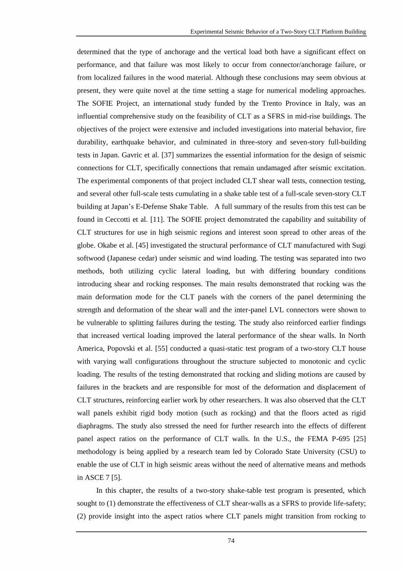
Experimental Seismic Behavior of a Two-Story CLT Platform Building
74
determined that the type of anchorage and the vertical load both have a significant effect on
performance, and that failure was most likely to occur from connector/anchorage failure, or
from localized failures in the wood material. Although these conclusions may seem obvious at
present, they were quite novel at the time setting a stage for numerical modeling approaches.
The SOFIE Project, an international study funded by the Trento Province in Italy, was an
influential comprehensive study on the feasibility of CLT as a SFRS in mid-rise buildings. The
objectives of the project were extensive and included investigations into material behavior, fire
durability, earthquake behavior, and culminated in three-story and seven-story full-building
tests in Japan. Gavric et al. [37] summarizes the essential information for the design of seismic
connections for CLT, specifically connections that remain undamaged after seismic excitation.
The experimental components of that project included CLT shear wall tests, connection testing,
and several other full-scale tests cumulating in a shake table test of a full-scale seven-story CLT
building at Japan’s E-Defense Shake Table. A full summary of the results from this test can be
found in Ceccotti et al. [11]. The SOFIE project demonstrated the capability and suitability of
CLT structures for use in high seismic regions and interest soon spread to other areas of the
globe. Okabe et al. [45] investigated the structural performance of CLT manufactured with Sugi
softwood (Japanese cedar) under seismic and wind loading. The testing was separated into two
methods, both utilizing cyclic lateral loading, but with differing boundary conditions
introducing shear and rocking responses. The main results demonstrated that rocking was the
main deformation mode for the CLT panels with the corners of the panel determining the
strength and deformation of the shear wall and the inter-panel LVL connectors were shown to
be vulnerable to splitting failures during the testing. The study also reinforced earlier findings
that increased vertical loading improved the lateral performance of the shear walls. In North
America, Popovski et al. [55] conducted a quasi-static test program of a two-story CLT house
with varying wall configurations throughout the structure subjected to monotonic and cyclic
loading. The results of the testing demonstrated that rocking and sliding motions are caused by
failures in the brackets and are responsible for most of the deformation and displacement of
CLT structures, reinforcing earlier work by other researchers. It was also observed that the CLT
wall panels exhibit rigid body motion (such as rocking) and that the floors acted as rigid
diaphragms. The study also stressed the need for further research into the effects of different
panel aspect ratios on the performance of CLT walls. In the U.S., the FEMA P-695 [25]
methodology is being applied by a research team led by Colorado State University (CSU) to
enable the use of CLT in high seismic areas without the need of alternative means and methods
in ASCE 7 [5].
In this chapter, the results of a two-story shake-table test program is presented, which
sought to (1) demonstrate the effectiveness of CLT shear-walls as a SFRS to provide life-safety;
(2) provide insight into the aspect ratios where CLT panels might transition from rocking to
Experimental Seismic Behavior of a Two-Story CLT Platform Building
75
sliding behavior for platform style construction; and (3) suggest design provisions of shear walls
using the equivalent lateral force procedure.
5.2. Test building layout and configuration
The two-story test building constructed in this study utilized CLT panel shear walls in a
platform construction configuration. The CLT shear walls were connected by generic shear
connectors at the base and ceiling to a CLT floor/roof diaphragm. The overturning was resisted
by continuous hold down rods typically used in stacked shear walls in light-frame wood
construction (see chapter 2.2.2.1). The gravity frame of the test building was designed to
facilitate the needs of two previous stages of testing [8][51] that investigated CLT rocking wall
systems. This chapter focuses exclusively on the third stage of testing and its three sub-phases:
Phase 3.1, Phase 3.2, and Phase 3.3. Phase 3.1 and Phase 3.2 investigate the effects of different
CLT panel aspect ratios on the performance of the stacked shear walls, while Phase 3.3
investigates the effects of adding transverse walls to either end of each shear wall stack. The test
structure was a two-story mass-timber building with glulam (vertical loads bearing system and
beams) and CLT panel (lateral load bearing system and floor diaphragms) components, as can
be seen in Figure 5.2.1, which was constructed over several days by professional contractors
experienced in CLT construction.. The dimension of the building is shown in the figure with a
height, width, and length of 6.7 m (22 ft.), 6.1 m (20 ft.), and 17.7 m (58 ft.), respectively.
Structurally, the building can be divided into three sub-systems, namely the gravity frame, the
floor/roof diaphragms, and the CLT shear wall seismic force resisting system (SRFS).
Figure 5.2.1.a shows the gravity frame, which consists of the glulam beams and columns
that support the dead load (gravity) loads of the structure, which can be split into the first and
second story. The column system on the first story consists of 12 columns, all grade L2, with
four (4) columns being continuous to the second story and roof level. The first floor level
consists of four grade 24F-V8 longitudinal beams spanning the N-S direction, nine (9) grade
24F-V4 transverse beams spanning the E-W direction, and with beams and columns connected
using commercial connectors [50]. The second story of the structure has a similar column layout
to the first story with 12 total columns, also grade L2, with the four (4) continuous columns
terminating at the roof level, and eight (8) discontinuous columns located above their respective
first story counterparts. The roof level beam system was significantly different than the first
floor level since it had only beams in the longitudinal directions. There were a total of six (6)
beams, four (4) grade 24F-V8, and two (2) grade 24F-V4 which are also connected using
similar hardware to the first floor level.
Similar to the gravity frame, the diaphragms for the first floor level and the roof floor
level were different with the objective of investigating two design configurations in one test [6].

Experimental Seismic Behavior of a Two-Story CLT Platform Building
76
The floor diaphragm (first floor) level panels were all 3-ply grade V1 CLT panels, although the
size of the panels varied. The roof diaphragm was a composite system consisting of CLT panels
with a concrete topping slab. The CLT panels were 1.5 m x 6 m (5 ft x 20 ft), with the exception
of two 1.2 m x 6 m (4 ft x 20 ft) panels, 5-ply grade V1 panels spanning the E-W direction, as
seen in Figure 5.2.1.a. The concrete layer was a 57.2 mm (2.25 inch) concrete topping on the
CLT panels with composite action being achieved with 45-degree anchors installed into the
CLT panels.
Figure 5.2.1 - Test Building: (a) Front elevation and plan view (solid lines for CLT panels, dashed lines for the beam
system underneath); (b) Side elevation view; (c) Isometric view.
The SFRS system used for the testing varied for each phase, but were all consisted of
CLT panels connected with metal hardware to form a wall at each story. There are two parallel
shear wall lines as it is shown in Figure 5.2.2. The two-story stacked wall system was designed
against overturning by two continuous steel tie-down rods while the shear demand was designed
to be resisted by inter-panel connectors and generic angle brackets (both fastened using 16D
sinker nails) [3]. The assumption of decoupled shear and overturning force transfer using
different components is a common design assumption that leads to conservative designs, and is
the main assumption consistent with the design approach for platform CLT construction

Experimental Seismic Behavior of a Two-Story CLT Platform Building
77
standards developed in the US. The design method being proposed for CLT platform
construction in the U.S. assumes the brackets only take shear forces and the continuous steel rod
hold downs take only uplift, both of which are not exactly correct since the wall does try to
rock. However, the phi factor for capacity reduction was adjusted within the design method to
account for this during calibration of the proposed design procedure. The loading used in the
design was derived using the Equivalent Lateral Force (ELF) method as described in ASCE 7
[5], with design spectral values of 1.5g for SDS and 1.0g for SD1 for a site near San Francisco,
California. An R-factor of 4.0 was used for the design of the lateral resisting system and the
diaphragm was assumed to be rigid. The number and spacing of the shear connectors for each
phase were such to maintain a constant design shear story capacity of 174 kN (39 kips) and 120
kN (27 kips) per wall line for the first and second stories respectively. The linear per foot design
capacity varied between the phases however, and for Phase 3.1 and Phase 3.3, the shear
connectors had a capacity of 4.7 kN/m (3.4 kips/ft) and 3.4 kN/m (2.5 kips/ft) for the first and
second stories respectively, while in Phase 3.2 the connectors had a capacity of 5.4 kN/m (4
kips/ft) and 4.2 kN/m (3 kips/ft) for the first and second stories. The steel tie-down rods
resisting the overturning moment in Phase 3.1 and Phase 3.3 had a design capacity of 124.5 kN
(28 kips) and 320 kN (72 kips) per wall for the first and second stories respectively, while the
tie-down rods in Phase 3.2 had a design capacity of 138 kN (31 kips) and 351 kN (79 kips) for
the first and second stories.
The NHERI@UCSD Shake-Table is a 7.6m x 12.2 m (25 ft x 40 ft) uniaxial table
equipped with two actuators with a total maximum payload of 20,000 kN (4,496 kips). This
location has been used for many previous tests, and the full details of the shake-table can be
found in Ozcelik et al. [46]. The footprint of the test structure was larger than the table in the N-
S, which is the direction perpendicular to the actuator movements that apply shaking in the E-W
direction, so large steel outrigging beams were used as a way to extend the table to the
appropriate dimensions. To ensure safety, two steel towers were installed in front of the control
building to the south of the building specimen. A third tower was installed on the east side of
the structure with safety straps wrapping around the center of the structure, with the straps
remaining slack unless the structure became unstable and began to collapse. Figure 5.2.2 shows
the orientation of the structure on the shake-table and the location of the safety towers.

Experimental Seismic Behavior of a Two-Story CLT Platform Building
78
Figure 5.2.2 - Position of the two-story CLT Platform Building on the shake table.
5.3. Test description
5.3.1. Phase 3.1
Two shear walls were designated as the north and south wall system throughout the test
program. The first story wall height was 3,200 mm (126 in) and second story wall height was
2.8 m (110 in). There were shear connectors installed at both the top and the bottom of the wall.
The overturning restraint was provided by the ATS rods at the end of each wall similar to that
used in stacked light-frame wood shear walls. The Phase 3.1 walls consisted of four (4) 900 mm
x 3,200 mm (36 in x 126 in) CLT panels with a thickness of 105 mm (4-1/8 in), resulting in a
total wall length of 3,700 mm (144 in), which is shown in the schematic of Figure 5.3.1. The
shear capacity of the walls is provided by the inter-panel flat shear connectors, that are
perforated metal plates placed half over a panel and half over the adjacent panel with screws
fastening, along the vertical splices between panels and angle shear connectors at the top and
bottom of the each panel. The base/top shear connectors were generic 76 mm x 57 mm x 3 mm

Experimental Seismic Behavior of a Two-Story CLT Platform Building
79
(3 in x 2-1/4 in x 3/25 in) L angle brackets with a length of 121 mm (4-3/4 in) with the number
of connectors varying between the first and second story based on the calculated shear demands.
Brackets were installed on the first and second story based on the required shear capacity. On
the first story, the brackets were placed on both sides of the wall, resulting in a total of eight (8)
brackets per panel and 32 per wall on the first story. The brackets on the second story walls
were only located on the outside face of each wall and were spaced to ensure three brackets per
panel on both the base and top, resulting in a total of six (6) brackets per panel and 24 per wall.
The brackets were secured to each panel using 16 16D box nails (4.2 mm diameter x 89 mm).
The brackets were connected to the diaphragm and the foundation by two 19 mm (3/4 in)
diameter fully threaded, A36 bolts. The inter-panel shear resistance consists of inter-panel
connectors vertically spaced at 406 mm (16 in). These inter-panel connectors are placed on both
sides of each of the three inter-panel joints in the walls, resulting in a total of 14 connectors per
vertical joint on the first story (total of 42) and 10 per vertical joint on the second story (total of
30). The overturning moment resisting system was comprised of vertical steel rods spanning the
full height of the building. The tie down rods were located at the end of each wall on both sides,
for a total of four (4) per wall and eight total and were allowed to reach at each floor (second
flood diaphragm and roof level in this case) using a bearing plate to distribute the load. The
diameter of the rods was not constant throughout the height of the building, with a coupler
located above the first floor level bearing plate reducing the diameter from 31.8 mm (1-1/4 in)
at the base to 19 mm (3/4 in) at the roof.
Figure 5.3.1 - Phase 3.1: 3.5:1 aspect ratio panels shear wall stack layout.
The rods were not designed for compression loading, only tension, so, to prevent
buckling, the tie-down rods were allowed to slip through the oversized holes at the diaphragm
when the corresponding side of the shear wall was in compression. The SFRS configuration for
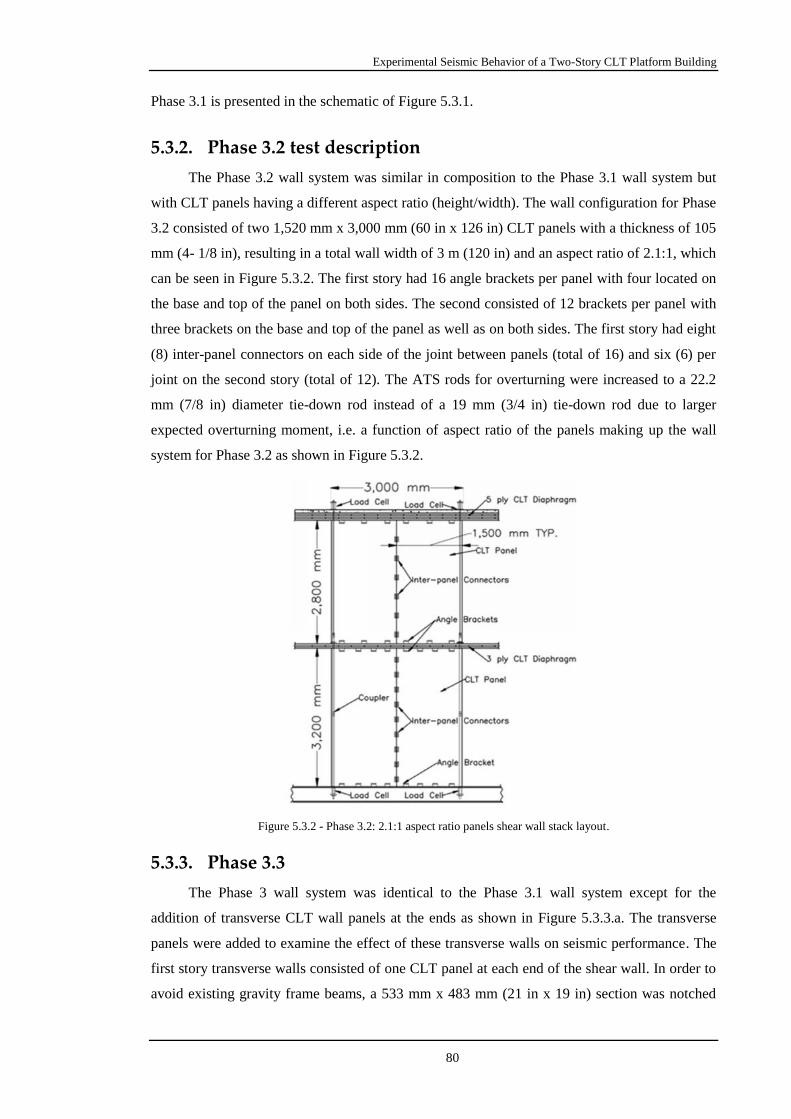
Experimental Seismic Behavior of a Two-Story CLT Platform Building
80
Phase 3.1 is presented in the schematic of Figure 5.3.1.
5.3.2. Phase 3.2 test description
The Phase 3.2 wall system was similar in composition to the Phase 3.1 wall system but
with CLT panels having a different aspect ratio (height/width). The wall configuration for Phase
3.2 consisted of two 1,520 mm x 3,000 mm (60 in x 126 in) CLT panels with a thickness of 105
mm (4- 1/8 in), resulting in a total wall width of 3 m (120 in) and an aspect ratio of 2.1:1, which
can be seen in Figure 5.3.2. The first story had 16 angle brackets per panel with four located on
the base and top of the panel on both sides. The second consisted of 12 brackets per panel with
three brackets on the base and top of the panel as well as on both sides. The first story had eight
(8) inter-panel connectors on each side of the joint between panels (total of 16) and six (6) per
joint on the second story (total of 12). The ATS rods for overturning were increased to a 22.2
mm (7/8 in) diameter tie-down rod instead of a 19 mm (3/4 in) tie-down rod due to larger
expected overturning moment, i.e. a function of aspect ratio of the panels making up the wall
system for Phase 3.2 as shown in Figure 5.3.2.
Figure 5.3.2 - Phase 3.2: 2.1:1 aspect ratio panels shear wall stack layout.
5.3.3. Phase 3.3
The Phase 3 wall system was identical to the Phase 3.1 wall system except for the
addition of transverse CLT wall panels at the ends as shown in Figure 5.3.3.a. The transverse
panels were added to examine the effect of these transverse walls on seismic performance. The
first story transverse walls consisted of one CLT panel at each end of the shear wall. In order to
avoid existing gravity frame beams, a 533 mm x 483 mm (21 in x 19 in) section was notched

Experimental Seismic Behavior of a Two-Story CLT Platform Building
81
out from the top corner of each panel to fit it around the beams. The walls were secured to the
diaphragm on the top and the steel beam at the base by six angle brackets with three for the top
and base respectively. The second story transverse walls were similar to the first floor with CLT
panels on both ends of the shear walls. These panels were secured to the top and base
diaphragms by three angle brackets on both the top and bottom. The Phase 3 wall system can be
seen in Figure 5.3.3.
(a) (b)
Figure 5.3.3 - Phase 3: (a) Transverse CLT walls; (b) 3.5:1 aspect ratio panels shear wall stack layout.
5.3.4. Instrumentation
The response of the building during shaking was recorded by over 300 sensors placed in
strategic locations throughout the building. As mentioned previously, the structure was part of a
collaborative test program with various lateral systems and throughout the testing, the sensors
installed to measure the response of the gravity frame and diaphragms remained unchanged.
However, the sensors installed on the SFRS varied from each stage and in some cases within the
stage. The diaphragms and gravity frame had 274 sensors installed throughout both floors of the
building, and the quantity of each type of sensor can be seen in Table 5.3.1. Strain gauges were
used to measure the deformation in the chord splices on the diaphragms as well as the rebar
installed in the concrete of the composite roof. Linear potentiometers were used to measure the
relative displacement between various components of the structure such as: CLT panels and the
diaphragm, the diaphragm and gravity frame, and between the concrete and CLT panels in the
composite roof diaphragm. String potentiometers were installed in the center of the diaphragm
as well as on each corner of both floors to measure the global displacement of the building.
They were also used to measure the relative vertical displacement between floors and the

Experimental Seismic Behavior of a Two-Story CLT Platform Building
82
relative vertical and horizontal displacement of the two farthest corners of the structure. Three
directional accelerometers units were installed to measure the acceleration in the X, Y, and Z
directions, and were installed in a similar fashion on each floor with one located at each corner
of the diaphragm, as well as at quarter points along the centerline of the diaphragm.
Table 5.3.1 – Instrumentation on gravity frame and diaphragm.
Instrument Quantity
Strain Gauge 133
Linear Potentiometers 63
String Potentiometers 42
Accelerometer 36
Figure 5.3.4 shows the location and details of the typical Phase 3.1 wall instrumentation.
A total of 72 sensors were installed for Phase 3.1 (see Table 5.3.2) on both the north and south
walls systems to capture the wall responses. Linear potentiometers were installed horizontally
on the base and top of the first and second stories on both the north and south wall systems in
order to capture any sliding motion. They were also installed vertically at each corner on the
first and second stories on the south wall system to capture the uplift behavior of the walls.
However, due to constraints on the quantity of sensors, the north wall system only had vertical
linear potentiometers on two corners of the walls on both the first and second story. String
potentiometers were installed in the horizontal and vertical directions on two of the three joints
between the CLT panels on each of the four walls that comprised the north and south wall
systems, to measure any relative panel displacement in either the vertical or horizontal
directions. Two string potentiometers were also installed diagonally in opposing directions on
both a first and second story wall on the north wall system to measure any panel deformation. A
total of 16 load cells were installed in line with the anchor bolts on the base and top of each
ATS anchor rod on both the north and south wall system to measure the tension in the rods
caused by the overturning moment. Strain gauges were also installed strategically along the
lengths of the rods as a redundant measurement to determine the tension in the tie down rods in
case of load cell failure.
The Phase 3.2 SFRS sensors were installed in a similar fashion to Phase 3.1; however,
there were some minor differences due to the smaller wall dimensions and fewer CLT panels
making up each wall. With only one inter-panel joint in each wall, there were several unused
string potentiometers previously utilized in Phase 3.1 for relative panel deformation.
These sensors were instead used to measure panel deformation on additional panels on
both the north and south wall systems. All four panels comprising the two-story north wall
system were measured for panel deformation as well as one panel from each floor on the south
wall system. The total quantity of sensors for Phase 3.2 can be seen in Table 5.3.2.

Experimental Seismic Behavior of a Two-Story CLT Platform Building
83
Table 5.3.2 - Instrumentation on shear walls.
Instrument Quantity for each phase
3.1 3.2 3.3
Strain Gauge 16 4 3
Load Cell 16 16 16
Linear Potentiometers 20 20 20
String Potentiometers 20 20 20
Accelerometer 0 0 0
Figure 5.3.4 - Phase 3.1 instrumentation on south face of south shear wall (typ. across phases).
The Phase 3.3 string potentiometers, load cells, and strain gauges were installed in the
same locations as Phase 3.1; however, the locations of some of the linear potentiometers
changed due to the addition of transverse walls on either end of all four walls comprising the
north and south wall systems. Some of the sensors measuring sliding were moved from the end
of the walls towards the center due to the previous locations being blocked by the installed
transverse walls. One potentiometer from each floor on the south wall system was moved to the
end of the transverse wall on their respective floors to capture any potential uplift. The total
quantity of sensors for Phase 3.3 can also be seen in Table 5.3.2.
5.4. Ground motion and testing program
Component 2 of 1989 Loma Prieta earthquake record from the Capitola recording station
was used and scaled to various intensities for all testing according to ASCE 7-16. The scaling of
the motion was done according to FEMA P695 for a location in San Francisco, California.
Intensities were selected based on levels corresponding to a service level earthquake (SLE),
design basis earthquake (DBE), and maximum considered earthquake (MCE), with mean return

Experimental Seismic Behavior of a Two-Story CLT Platform Building
84
periods of 72 years, 475 years, and 2475 years respectively. For the MCE motion, this led to a
SDS and SD1 of 1.5 g and 1.0 g, respectively. The MCE scaled response spectra is presented in
Figure 5.4.1, while the spectral accelerations for each phase is shown in Table 5.4.1. Due to
time constraints for repairs, Phase 3.2 and 3.3 testing used only the SLE and MCE scaled
ground motions, which optimized the amount of data collected with a minimal amount of repair.
Figure 5.4.1 - Spectral accelerations for Loma Prieta scaled to SLE, DBE, and MCE levels.
Table 5.4.1 – Test sequencing and global story response for each phase.
Average peak
displacement(c)
[mm]
Peak average inter-
story drift(e)
[%]
Peak story
shear(f)
[kN]
Phase(a)
Test(b)
Sa [g] PGA [g] Story I Story II Story I Story II Story I Story II
3.1
SLE 0,525 0,25 18 29 0,49 0,42 306 206
DBE 0,92 0,42 51 94 1,4 1,4 582 456
MCE 1,36 0,62 99 158 2,7 1,95 765 579
3.2 SLE 0,54 0,24 17 32 0,47 0,54 308 219
MCE 1,29 0,66 93 159 2,54 2,15 873 643
3.3 SLE 0,68 0,265 40 48 1,08 0,59 301 190
MCE 1,49 0,68 89 151 2,42 2,06 873 645 a) Phase 1 (3.5:1 aspect ratio). Phase 2 (2.1:1 aspect ratio). Phase 3 (4:1 aspect ratio with additional transverse walls). b) Loma Prieta earthquake ground motion was used for all tests, and scaled appropriately to SLE, DBE and MCE levels
respectively.
c) Average of the displacements recorded at the center, and both ends of each story e) 3663 mm and 3043 mm were used for the height of the first and second story respectively.
f) 342,5 kN and 422,5 kN were used for the weight of the first and second story respectively.
The natural period of the test structure varied between tests due to structural damage and
changes in wall configuration. White noise tests were conducted before and after every test in
order to determine the natural period. Figure 5.4.2 presents a plot of the change in the natural
period of the structure over the platform CLT testing program. Initially with Phase 3.1 (3.5:1
aspect ratio shear walls), the test structure had a natural period of approximately 0.38 seconds,
which increased following testing with the peak natural period following Phase 3.1 being
approximately 0.89 seconds. The installation of the Phase 3.2 shear walls, which had an aspect
ratio of 2.1:1, returned the natural period of the structure to approximately 0.41 seconds. The
peak natural period following Phase 3.2 testing was 0.73 seconds after the MCE level test.
Phase 3, with the return to the 3.5:1 aspect ratio shear walls, and the addition of transverse CLT
walls, reduced the natural period of the structure to 0.17 seconds. This decrease is most likely

Experimental Seismic Behavior of a Two-Story CLT Platform Building
85
due to the additional stiffness provided by the transverse CLT walls, including some potential
“flanging” action during smaller deformations in and near the elastic range. The peak natural
period for the structure following Phase 3 testing after the MCE level test was the shortest of the
phases at 0.35 seconds. This indicates that the least amount of softening occurred in Phase 3
with the transverse walls in place.
Figure 5.4.2 - Fundamental building period and the effect of repairs and different wall configurations.
5.4.1. Displacement profile
Figure 5.4.3 presents the displacement profile of the test structure for each test, with the
profile constructed using the average maximum displacement of the story relative to the shake
table. The horizontal displacement was measured at the north, south, and middle of the
diaphragm on each story. Across all of the phases, primarily a first mode response was
observed, with the peak interstory drift for each story occurring simultaneously to the peak
displacement. Phase 3.1 and Phase 3.2 had similar peak MCE level average displacements of
158 mm (6.22 in.) and 159 mm (6.26 in), respectively, and Phase 3.3 had the smallest peak
average displacement of 151 mm (5.94 in.). As mentioned previously, the objective of the
testing was to demonstrate the performance of CLT shear walls using typical design techniques,
in the case when ELF was used for the design. In the design, 2/3 of the MCE level spectral
acceleration is reduced by a seismic reduction factor (R), developed over the course of the
project, to account for the nonlinear response of the structure, specifically through its
deformation capacity and ability to dissipate energy. The nonlinear response is confirmed by the
results in Figure 5.4.3, as the MCE level motion is 1.5 times greater than the DBE level motion,
but the maximum displacement for the Phase 3.1 MCE test (158 mm) is greater than 1.5 times
the maximum displacement for the Phase 3.1 DBE test (94 mm). It was theorized in Popovski et
al. [55] that the addition of walls transverse to the shear walls would improve the performance
of the structure, and as can be seen in Table 5.4.1 and Figure 5.4.3, even though Phase 3.3 MCE
had the largest peak ground acceleration (PGA) recorded by the table, its peak floor
displacements were less than Phase 3.1 and Phase 3.2 on both floors.
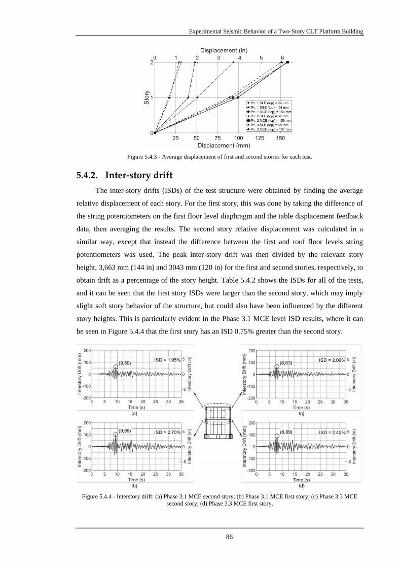
Experimental Seismic Behavior of a Two-Story CLT Platform Building
86
Figure 5.4.3 - Average displacement of first and second stories for each test.
5.4.2. Inter-story drift
The inter-story drifts (ISDs) of the test structure were obtained by finding the average
relative displacement of each story. For the first story, this was done by taking the difference of
the string potentiometers on the first floor level diaphragm and the table displacement feedback
data, then averaging the results. The second story relative displacement was calculated in a
similar way, except that instead the difference between the first and roof floor levels string
potentiometers was used. The peak inter-story drift was then divided by the relevant story
height, 3,663 mm (144 in) and 3043 mm (120 in) for the first and second stories, respectively, to
obtain drift as a percentage of the story height. Table 5.4.2 shows the ISDs for all of the tests,
and it can be seen that the first story ISDs were larger than the second story, which may imply
slight soft story behavior of the structure, but could also have been influenced by the different
story heights. This is particularly evident in the Phase 3.1 MCE level ISD results, where it can
be seen in Figure 5.4.4 that the first story has an ISD 0.75% greater than the second story.
Figure 5.4.4 - Interstory drift: (a) Phase 3.1 MCE second story; (b) Phase 3.1 MCE first story; (c) Phase 3.3 MCE
second story; (d) Phase 3.3 MCE first story.
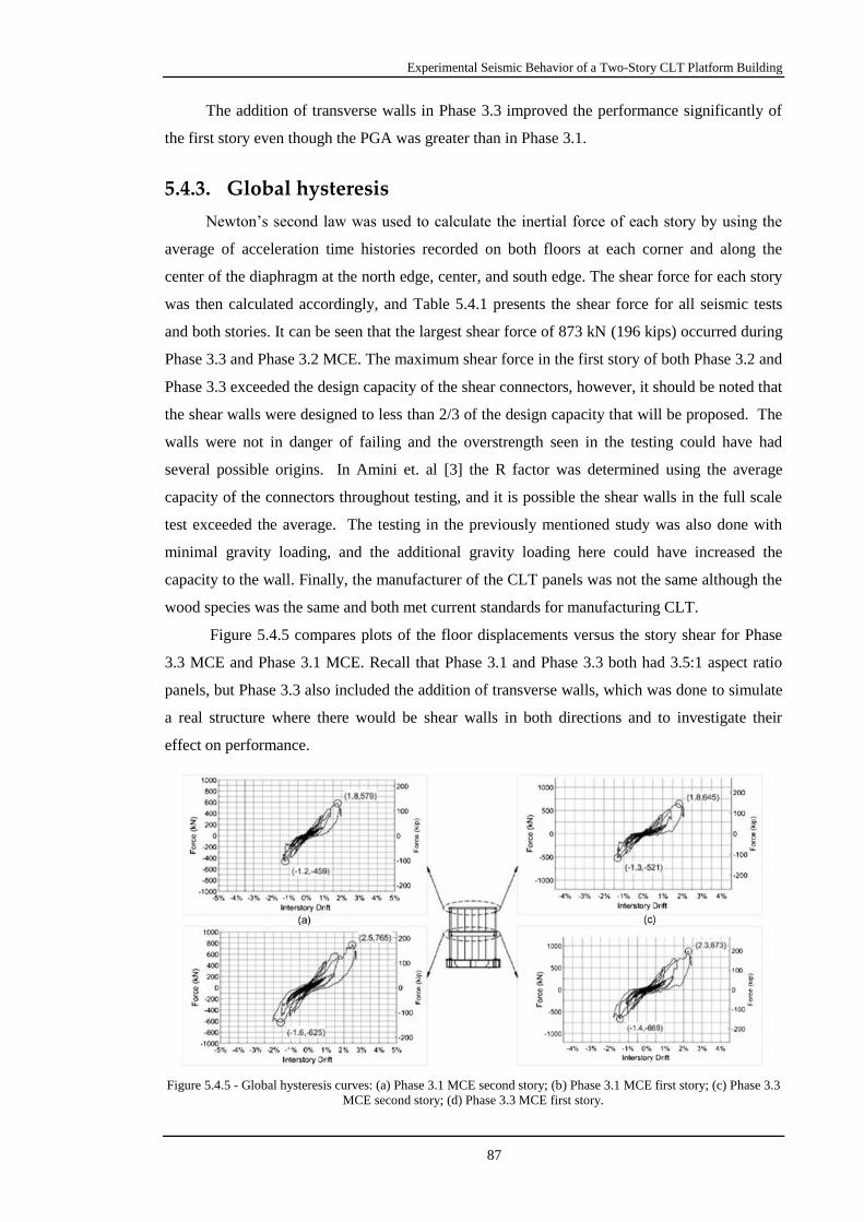
Experimental Seismic Behavior of a Two-Story CLT Platform Building
87
The addition of transverse walls in Phase 3.3 improved the performance significantly of
the first story even though the PGA was greater than in Phase 3.1.
5.4.3. Global hysteresis
Newton’s second law was used to calculate the inertial force of each story by using the
average of acceleration time histories recorded on both floors at each corner and along the
center of the diaphragm at the north edge, center, and south edge. The shear force for each story
was then calculated accordingly, and Table 5.4.1 presents the shear force for all seismic tests
and both stories. It can be seen that the largest shear force of 873 kN (196 kips) occurred during
Phase 3.3 and Phase 3.2 MCE. The maximum shear force in the first story of both Phase 3.2 and
Phase 3.3 exceeded the design capacity of the shear connectors, however, it should be noted that
the shear walls were designed to less than 2/3 of the design capacity that will be proposed. The
walls were not in danger of failing and the overstrength seen in the testing could have had
several possible origins. In Amini et. al [3] the R factor was determined using the average
capacity of the connectors throughout testing, and it is possible the shear walls in the full scale
test exceeded the average. The testing in the previously mentioned study was also done with
minimal gravity loading, and the additional gravity loading here could have increased the
capacity to the wall. Finally, the manufacturer of the CLT panels was not the same although the
wood species was the same and both met current standards for manufacturing CLT.
Figure 5.4.5 compares plots of the floor displacements versus the story shear for Phase
3.3 MCE and Phase 3.1 MCE. Recall that Phase 3.1 and Phase 3.3 both had 3.5:1 aspect ratio
panels, but Phase 3.3 also included the addition of transverse walls, which was done to simulate
a real structure where there would be shear walls in both directions and to investigate their
effect on performance.
Figure 5.4.5 - Global hysteresis curves: (a) Phase 3.1 MCE second story; (b) Phase 3.1 MCE first story; (c) Phase 3.3
MCE second story; (d) Phase 3.3 MCE first story.
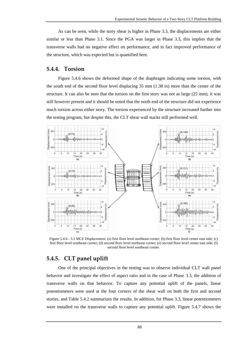
Experimental Seismic Behavior of a Two-Story CLT Platform Building
88
As can be seen, while the story shear is higher in Phase 3.3, the displacements are either
similar or less than Phase 3.1. Since the PGA was larger in Phase 3.3, this implies that the
transverse walls had no negative effect on performance, and in fact improved performance of
the structure, which was expected but is quantified here.
5.4.4. Torsion
Figure 5.4.6 shows the deformed shape of the diaphragm indicating some torsion, with
the south end of the second floor level displacing 35 mm (1.38 in) more than the center of the
structure. It can also be seen that the torsion on the first story was not as large (25 mm), it was
still however present and it should be noted that the north end of the structure did not experience
much torsion across either story. The torsion experienced by the structure increased further into
the testing program, but despite this, the CLT shear wall stacks still performed well.
Figure 5.4.6 - 3.1 MCE Displacement: (a) first floor level northeast corner; (b) first floor level center east side; (c)
first floor level southeast corner; (d) second floor level northeast corner; (e) second floor level center east side; (f)
second floor level southeast corner.
5.4.5. CLT panel uplift
One of the principal objectives in the testing was to observe individual CLT wall panel
behavior and investigate the effect of aspect ratio and in the case of Phase 3.3, the addition of
transverse walls on that behavior. To capture any potential uplift of the panels, linear
potentiometers were used at the four corners of the shear wall on both the first and second
stories, and Table 5.4.2 summarizes the results. In addition, for Phase 3.3, linear potentiometers
were installed on the transverse walls to capture any potential uplift. Figure 5.4.7 shows the

Experimental Seismic Behavior of a Two-Story CLT Platform Building
89
uplift recorded on the west side of the south shear wall stack during Phase 3.1 MCE, and it can
be seen that the bottom of the panels experienced the most rocking, with the first story having
the largest uplift values. The top of the panels experienced smaller uplift and hence less rocking,
which was expected. Figure 5.4.8 shows the uplift recorded during Phase 3.3 MCE on both
floors of the south shear wall stack as well as the uplift recorded at the base of the transverse
walls. There was a concern that the addition of transverse walls on either end of the shear wall
stack could inhibit the ability of the CLT panels to rock. Figure 5.4.8.a and b demonstrate that
the CLT panels were still able to exhibit rocking behavior even with transverse walls present,
and the behavior was similar to Phase 3.1.
Table 5.4.2 – Test sequencing and local story response for each phase.
Peak uplift
(a)
[mm]
Peak vertical
relative panel
displacement(b)
[mm]
Peak sliding(c)
[mm]
Peak ATS rod
force(d)
[kN]
Phase
Test
Story I Story II Story I Story II Story I Story II Story I Story II
3.1
SLE 4,7 3,3 2,6 1,2 1,7 2,4 44,5 9,8
DBE 13,2 12,5 7,8 4,7 8,1 9,0 105,1 31,3
MCE 21,7 16,7 19,6 10,0 12,0 9,4 170,0 66,3
3.2 SLE 4,2 2,7 1,9 1,0 1,1 1,7 45,8 12,7
MCE 26,1 12,2 13,6 9,9 56,1 32,7 237,6 74,4
3.3 SLE 3,7 2,7 2,1 1,4 2,6 1,1 31,6 10,2
MCE 14,5 9,4 15,7 13,6 7,2 6,5 - - a) Uplift was measured at the upper and lower corners of each wall on both the first and second story b) Vertical relative panel displacement is the vertical displacement measured at the inter-panel joint between CLT panels
c) Sliding was measured at the top and base of each wall on both the first and second story
d) Load cells were placed on the top and base of each ATS rod
Figure 5.4.7 - Phase 3.1 MCE Wall Uplift: (a) First story shear wall top west corner; (b) First story shear wall bottom
west corner; (c) Second story shear wall top west corner; (d) Second story shear wall bottom west corner.

Experimental Seismic Behavior of a Two-Story CLT Platform Building
90
Figure 5.4.8 - Phase 3.3 MCE Uplift: (a) Second story shear wall bottom west corner; (b) First story shear wall
bottom west corner; (c) Second story transverse wall top south corner; (d) First story shear wall bottom south corner.
Figure 5.4.9 - Phase 3.2 MCE Uplift: (a) First story shear wall top west corner; (b) First story shear wall bottom west
corner; (c) Second story shear wall top west corner; (d) Second story shear wall bottom west corner.
It was expected that the transverse walls would experience minimal uplift during testing,
and Figure 5.4.9.c and d show that is indeed the case. The largest uplifts recorded during testing
occurred during the Phase 3.2 MCE test, with a peak uplift of 24.4 mm (0.96 in) recorded at the
bottom of the first story, but it should be noted that this measurement could have been affected
by the nail shearing observed on the first story. Even though the uplift was the largest in Phase
3.2, the test structure still exhibited no risk of collapse. The uplift in Phase 3.2 followed a
similar pattern to the other phases with the bottom of the CLT panel experiencing the most
rocking behavior on both the first and second stories.
5.4.6. Sliding
The sliding of the shear wall panels was recorded using linear potentiometers positioned

Experimental Seismic Behavior of a Two-Story CLT Platform Building
91
horizontally at the base and top of each shear wall, and Table 5.4.2 summarizes the results. The
panel sliding followed a similar pattern to the uplift, with the largest sliding occurring at the
base of the panel at each story, and this can be seen in Figure 5.4.10 for Phase 3.1 MCE. The
sliding behavior can be partially explained by nail withdrawal as the deformation of the angle
brackets work the nails from the CLT. This was especially present for the Phase 3.2 MCE test,
where nail shear was observed on the first story, resulting in a sliding of 56.1 mm (2.2 in) as
seen in Figure 5.4.11, but although the sliding was large, the test structure was in no danger of
collapsing with the tie down rods providing uplift restraint and likely some level of shear
through bearing on the hole they passed through in the CLT diaphragm and, in the case of the
lower shear walls, the steel support beam acting as a foundation into the shake table.
Figure 5.4.10 - Phase 3.1 MCE Sliding: (a) First story shear wall top west corner; (b) First story shear wall bottom
west corner; (c) Second story shear wall top west corner; (d) Second story shear wall bottom west corner.
Figure 5.4.11 - Phase 3.2 MCE Sliding: (a) First story shear wall top west corner; (b) First story shear wall bottom
west corner (nail shear failure occurred in brackets); (c) Second story shear wall bottom west corner.
5.4.7. Relative panel displacement
Relative panel displacement was measured in the horizontal and vertical direction using

Experimental Seismic Behavior of a Two-Story CLT Platform Building
92
string potentiometers at the inter-panel joints of each CLT panel for all tests and phases. No
significant relative displacement was recorded or observed in the horizontal direction, so the
vertical direction will be the primary focus, and Table 5.4.2 summarizes the results across the
phases. Figure 5.4.12 presents the Phase 3.1 MCE results, and as can be seen, the first story
experienced more relative panel displacement than the second story, which was expected given
it deformed more overall. The displacement was also relatively consistent across the story with
only a 3 mm (0.11 in) difference between the two recorded joints for Phase 3.1 MCE. The
relative panel displacements for the 2.1:1 shear wall aspect ratio followed a similar trend to the
3.5:1 aspect ratio walls in Phase 3.1, the largest displacement occurred on the first story, this
can be seen in Figure 5.4.13.
Figure 5.4.12 - Phase 3.1 MCE Vertical Relative Panel Displacement: (a) First story shear wall top west corner; (b)
First story shear wall bottom west corner; (c) Second story shear wall top west corner; (d) Second story shear wall
bottom west corner.
Figure 5.4.13 - Phase 3.2 MCE Vertical Relative Panel Displacement: (a) First story shear wall top west corner; (b)
First story shear wall bottom west corner; (c) Second story shear wall top west corner; (d) Second story shear wall
bottom west corner.
5.4.8. Forces in tie-down rods
ATS tie-down rods were installed in the SFRS, with a rod on each end of the wall and
both faces, with a bearing plate providing a reaction point on each story, similar to standard
construction for light-frame wood buildings. This was consistent throughout all the phases, and

Experimental Seismic Behavior of a Two-Story CLT Platform Building
93
in the design of the SFRS, it was assumed that the CLT wall panels worked as a continuous
segment with the inter-panel connectors transferring shear, and because of this, tie-down rods
were only required at the ends of the walls. The tie-down rods are designed to absorb tension
from the overturning moment present in the structure, while the CLT panels and brackets
transfer shear. The rods therefore are not designed to take any compression force, and are thus
allowed to slide through at the bottom of the structure, allowing the CLT panels to absorb the
compression load. The summary of the recorded forces in the rods can be seen in Table 5.4.2.
No load cell data was available for the Phase 3.3 MCE level test, so data from strain gauges
placed on the tie-down rods was used instead. The largest tension force in the rods was 237.6
kN (53 kips) recorded at the base on the first story during the Phase 3.2 MCE test, which was
approximately 94% of the ultimate capacity of the rod. This test included the 2.1:1 aspect ratio
walls, and it most likely due to the nail failure in the shear brackets, essentially forcing the hold
downs to do 100% of the resistance in uplift. Although the shear brackets are assumed to only
resist shear in the design approach for the platform CLT stacked walls herein, they do resist
some overturning as the CLT panels rack. A large tension force of 170 kN (38 kips), or 68% of
the rod’s ultimate capacity, was also recorded during the Phase 3.1 MCE level test, and the
tension both in this test and the Phase 3.2 MCE test were enough to cause some yielding in the
A36 tie-down rods. Figure 5.4.14 presents the average tension force across both wall faces on
the CLT panels from Phase 3.1 MCE level test at both the base and roof of the structure. It can
be seen that the loading was not homogenous across the structure, and the east side received
more load than the west side. This is a result of the torsion discussed earlier, and both Phase 3.2
and Phase 3.3 showed a similar trend. An objective of the test program was to determine if the
addition of transverse walls in Phase 3.3 would decrease the loading in the tie-down rods.
Unfortunately, load cell data for Phase 3.3 was unavailable due to technical difficulties.
However, strain gauges were placed in strategic locations along the tie-down rods to act as a
backup in such an event. Table 3 presents the strain gauge data for one of the tie-down rods for
both the Phase 3.1MCE level test and Phase 3.3 MCE level test. It should be noted that in
Phase 3.1 MCE level test the maximum recorded force (approx. 167 kN) was approaching the
yield point of the tie-down rod, and due to this, it was not possible to convert the strain to force
with a satisfactory degree of accuracy. However the difference in strains between the tests are
rather significant, with the Phase 3.3 MCE level test experiencing strains an order of magnitude
smaller, thus making the conversions to force unnecessary to analyze the performance of the
structure. As anticipated, the addition of transverse walls reduced the strain in the tie-down rods,
implying reduced force, and ultimately, reduced overturning moment and improved
performance.

Experimental Seismic Behavior of a Two-Story CLT Platform Building
94
Figure 5.4.14 - Phase 3.1 ATS Rod Load Cells: (a) First story north wall east side; (b) First story north wall west
side; (c) First story south wall west side; (d) First story south wall east side; (e) Second story north wall west side; (f)
Second story north wall east side; (g) Second story south wall east side; (h) Second story south wall west side.
5.4.9. Overall performance
In all three phases presented herein, each of which consisted of several different ground
motion intensities, the structure provided life safety as no significant damage have been spotted
throughout the test. Phase 3.1 and Phase 3.3 CLT panels both clearly were governed by rocking
behavior as had been demonstrated to occur in high aspect ratio panels. Partial nail pull-out and
some steel angle bracket deformation was observed during Phase 3.1 and Phase 3.3 MCE level
tests, but this was expected and results indicated that the connectors behaved as intended. It
was also observed that the transverse walls installed in Phase 3.3 did not significantly affect the
ability of the CLT panels to rock or the connections to perform as designed. Phase 3.2 and the
lower aspect ratio panels were governed by sliding, and during the MCE level test, significant
sliding and nail shearing was observed, resulting failure of the shear brackets at the base.
Although this is far from an ideal behavior, it should be noted that the design used in this test
was less than 2/3 the capacity eventually to be proposed for design of platform CLT systems in
the U.S.; and also it is important to note that the stability of the structure was never in jeopardy.
The tie-down rods experienced some yielding effects in both the Phase 3.1 and Phase 3.2 MCE
level tests, but still performed as designed and resisted the overturning moment. In Phase 3.3,

Experimental Seismic Behavior of a Two-Story CLT Platform Building
95
there was no yielding observed due to the improvement in performance provided by the addition
of the transverse walls. At SLE and DBE level tests, there was no observable damage in the
connections in the shear wall stacks, and no yielding recorded in the tie-down rods. Towards the
end of the testing, torsion in structure began to become more pronounced, and introduced some
asymmetric loading into the structure, but the SFRS still performed such that there was never
risk of collapse at MCE level shaking.
5.5. Concluding remarks
A full-scale two-story CLT platform building with two CLT panel shear wall stacks with
tie-downs rods with three different shear wall configurations each tested, namely, 3.5:1 aspect
ratio panels, 2.1:1 aspect ratio panels, and 3.5:1 aspect ratio panels with transverse walls
installed on each end, being tested. All of the configurations were subjected to the 1989 Loma
Prieta ground motion scaled to intensities corresponding to SLE, DBE, and MCE levels
respectively, with spectral accelerations ranging from 0.52 g to 1.5 g. The design of the shear
wall stacks used the equivalent lateral force procedure with the intent of providing life safety to
would-be occupants. Each of the designs met the life safety criteria, and the structure was never
in danger of collapse over the course of the testing program. This met the primary objective of
the test to demonstrate the effectiveness of CLT shear-walls to provide life safety. The
configurations performed as expected with the 3.5:1 aspect ratio being governed by rocking of
the panels, and the 2.1:1 aspect ratio governed by sliding of the panels. However, the sliding in
the 2.1:1 panels in Phase 3.2 was the result of nail shear failure in the base shear brackets, and
thus no true conclusion that 2.1:1 aspect ratio panels has a sliding mechanism as its failure
model can be drawn. This was more of a capacity issue given the shear wall capacities were
designed at less than 2/3 of what is to eventually be proposed. This was mainly the result of the
timing of the shake table test, which was an opportunity to perform the test with a gravity frame
in place already, prior to completion of the design method for CLT platform construction being
fully validated. However, as described in this study, a number of valuable conclusions were able
to be drawn related to the behavior of this type of construction and connections for CLT, and
accomplished the goal of providing insight into CLT panel aspect ratios. For example, it was
also confirmed that the addition of transverse walls does not affect the ability of the panels to
rock, and improves the performance of the tie-down rods. The results of this testing will be used
to further refine the methodology for designing CLT SFRS using the equivalent lateral force
procedure in the U.S., which will be used to suggest design provisions in the future.

96
METHODS FOR PRACTICE-ORIENTED
LINEAR ANALYSIS IN SEISMIC DESIGN
OF CLT BUILDINGS
SHORT SUMMARY
In the context of innovative seismic-resistant structures, Cross Laminated Timber (CLT)
construction holds an important position at a global level, supported by important full-scale tests
and studies of the non-linear behaviour of these structures for severe events, demonstrating
excellent performance. The present study aims to transfer current knowledge in the form of
modelling approaches applicable to design engineers presenting tools and methodologies
pertinent to the daily procedures of professional practice, thus relating to linear static and
dynamic analyses. Two different approaches of structural modelling are presented, validated
and compared; the perspective is to cover two different points of view and conception of
connections and calculation of the mechanical characteristics of members and connections. Both
models are validated by comparing the time-history responses with the full-scale shake-table
test results of a 3-storey CLT structure under three earthquakes, showing in both cases a reliable
estimate of the structural response. Finally, a parametric study for the damping coefficient of the
structural response is presented and the typical value of 5% is discussed.
6.1. Introduction
The primary deformation mechanisms of CLT structures under seismic loads are the
rocking and sliding response of the wall panels. Such mechanisms are highly non-linear:
rocking is associated to asymmetric resisting mechanisms like mono-lateral wood-to-wood
contact between panels and tension-only hold-downs, while sliding depends on the friction
characteristics between panels and can affect the initial stiffness of the structure and its energy
dissipation capacity. Given that the current state-of-practice of seismic design still lies on the
use of linear static or response-spectrum modal analysis, practicing engineers can face
significant challenges in the definition and representation of a linear numerical building model.
To consider the effective stiffness of the actual connections between the CLT panels, and to
yield more accurate estimates of the load paths and the partition of the global shear within the
walls of each storey, the modelling approach is a fundamental matter.
Within this context, this chapter presents two different approaches for the construction of

Methods for practice-oriented linear analysis in seismic design of CLT buildings
97
linear numerical models of CLT buildings and the definition of the mechanical properties of the
structural components, including the connections. The two methodologies are evaluated based
on the experimental data from a series of low-amplitude shake-table tests of a 3-storey full-scale
CLT structure [10][40], by performing transient dynamic analyses of the corresponding linear
models and comparing the numerical and experimental results in terms of global base shear and
lateral roof displacement. The use of linear models is justified since the structure during these
tests remained within the elastic range with no plasticity in the connections. Furthermore, the
applicability of the typical value of 5% damping in the form of a classical matrix is investigated,
calculating the numerical predictions for four different values of viscous damping ratios.
6.2. Test structure and experimental data
This chapter presents the test structure and the experimental data that were used for the
validation of the two modelling approaches. A three-storey full-scale rectangular CLT structure
with a double-pitched roof, as shown in Figure 6.2.1, was tested under shake-table tests in
Tsukuba, Japan, as part of the SOFIE Project [40], which was a co-operative research project
supported by the Trento Province, Italy, and coordinated and conducted by the CNR-IVALSA
(Italian National Research Council – Trees and Timber Institute). Three different configurations
of the test structure were implemented in the testing programme by varying the length of the
door opening at the first storey. This study considers the second configuration (conf. B [10])
with a door opening of 2.23 m.
The structure consisted of 5-layer, 85 mm thick (17-17-17-17-17, bold numbers refer to
fibres along the primary orientation) CLT wall panels with the primary orientation along the
vertical direction and of 6-layer 142 mm thick (27-17-27-27-17-27) CLT floor panels. The roof
was made of 5-layer 85 mm thick CLT panels, similarly to the walls. A detailed description of
the various connections between the CLT panels is provided in chapter 6.3.1.
(a) (b) ( c)
Figure 6.2.1 - North/South elevations (a), East/West elevations (b), and typical floor plan of Configuration B of the 3-
storey structure with location of the metal connectors for the first storey (c) (from [40][62], measures in m).

Methods for practice-oriented linear analysis in seismic design of CLT buildings
98
With the scope of validating numerical models for linear dynamic analysis, three
unidirectional shake-table tests with ground motions scaled to a Peak Ground Acceleration
(PGA) of 0.15g were considered in this chapter, since the structure under these seismic motions
did not exhibit any sign of plasticization in the connections, as verified by the researchers after
the tests. The ground motions applied in sequence were Kobe (JMA station, 1995), El Centro
(Imperial Valley, 1940) and Nocera Umbra (Marche, Italy, 1997). The pseudo spectral
acceleration spectra of the effective table accelerations of these records are illustrated in Figure
6.2.2.a, while Figure 6.2.2.b shows the base shear versus roof displacement response of the test
structure. The base shear was calculated from the acceleration measurements in each level, thus
including the contribution of internal resisting and damping forces. First an average acceleration
time-history was computed for each level, which was then multiplied by the total mass of each
storey, taken equal to 21,93, 21,93 and 4,74 tons for the first, second and third storey,
respectively. Finally, the three time-histories were summed and multiplied by (-1) to yield the
base shear time-history.
The spectral ordinates at the fundamental period of the test structure in the shaking
direction (T2 = 0,183 s), as estimated from white-noise tests, are also identified in Figure 6.2.2.a.
As observed in Figure 6.2.2.b, the structural response is coherent with the intensity of each
motion in the fundamental period, but it can be clearly noticed that the effective lateral stiffness
is slightly decreasing with the increase of the structural response. Since no inelastic response
was identified in the connections, this non-linearity is attributed to the friction developed
between wall and floor panels. This is the first time that such non-linearity is directly identified
in the response of a test structure, mostly because research efforts are typically focused on large-
intensity motions that result in a non-linear elastic structural response due to connection
plasticization.
Figure 6.2.2 - Pseudo spectral acceleration spectra of the three ground motions considered (a), and base shear versus
roof displacement response of the test structure (b).
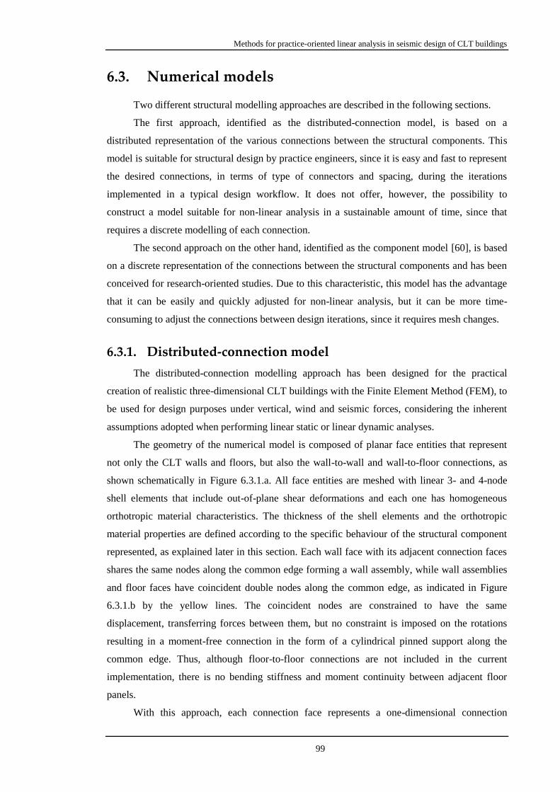
Methods for practice-oriented linear analysis in seismic design of CLT buildings
99
6.3. Numerical models
Two different structural modelling approaches are described in the following sections.
The first approach, identified as the distributed-connection model, is based on a
distributed representation of the various connections between the structural components. This
model is suitable for structural design by practice engineers, since it is easy and fast to represent
the desired connections, in terms of type of connectors and spacing, during the iterations
implemented in a typical design workflow. It does not offer, however, the possibility to
construct a model suitable for non-linear analysis in a sustainable amount of time, since that
requires a discrete modelling of each connection.
The second approach on the other hand, identified as the component model [60], is based
on a discrete representation of the connections between the structural components and has been
conceived for research-oriented studies. Due to this characteristic, this model has the advantage
that it can be easily and quickly adjusted for non-linear analysis, but it can be more time-
consuming to adjust the connections between design iterations, since it requires mesh changes.
6.3.1. Distributed-connection model
The distributed-connection modelling approach has been designed for the practical
creation of realistic three-dimensional CLT buildings with the Finite Element Method (FEM), to
be used for design purposes under vertical, wind and seismic forces, considering the inherent
assumptions adopted when performing linear static or linear dynamic analyses.
The geometry of the numerical model is composed of planar face entities that represent
not only the CLT walls and floors, but also the wall-to-wall and wall-to-floor connections, as
shown schematically in Figure 6.3.1.a. All face entities are meshed with linear 3- and 4-node
shell elements that include out-of-plane shear deformations and each one has homogeneous
orthotropic material characteristics. The thickness of the shell elements and the orthotropic
material properties are defined according to the specific behaviour of the structural component
represented, as explained later in this section. Each wall face with its adjacent connection faces
shares the same nodes along the common edge forming a wall assembly, while wall assemblies
and floor faces have coincident double nodes along the common edge, as indicated in Figure
6.3.1.b by the yellow lines. The coincident nodes are constrained to have the same
displacement, transferring forces between them, but no constraint is imposed on the rotations
resulting in a moment-free connection in the form of a cylindrical pinned support along the
common edge. Thus, although floor-to-floor connections are not included in the current
implementation, there is no bending stiffness and moment continuity between adjacent floor
panels.
With this approach, each connection face represents a one-dimensional connection
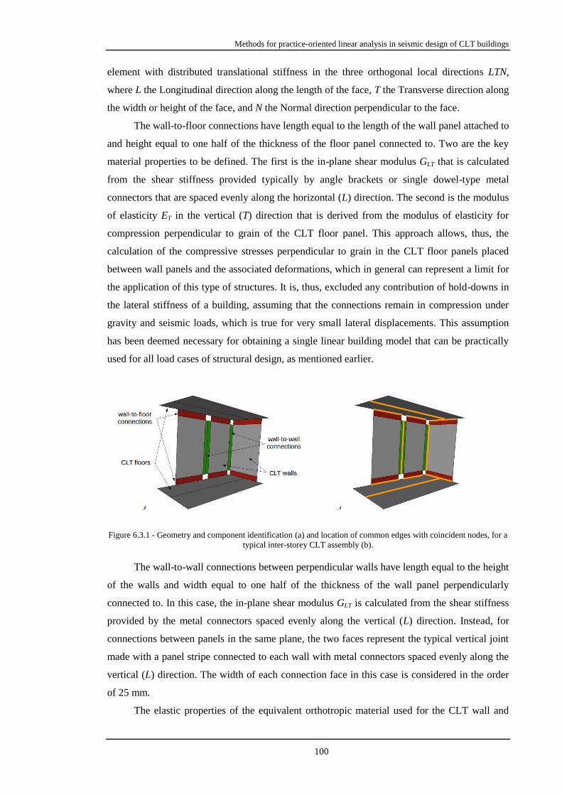
Methods for practice-oriented linear analysis in seismic design of CLT buildings
100
element with distributed translational stiffness in the three orthogonal local directions LTN,
where L the Longitudinal direction along the length of the face, T the Transverse direction along
the width or height of the face, and N the Normal direction perpendicular to the face.
The wall-to-floor connections have length equal to the length of the wall panel attached to
and height equal to one half of the thickness of the floor panel connected to. Two are the key
material properties to be defined. The first is the in-plane shear modulus GLT that is calculated
from the shear stiffness provided typically by angle brackets or single dowel-type metal
connectors that are spaced evenly along the horizontal (L) direction. The second is the modulus
of elasticity ET in the vertical (T) direction that is derived from the modulus of elasticity for
compression perpendicular to grain of the CLT floor panel. This approach allows, thus, the
calculation of the compressive stresses perpendicular to grain in the CLT floor panels placed
between wall panels and the associated deformations, which in general can represent a limit for
the application of this type of structures. It is, thus, excluded any contribution of hold-downs in
the lateral stiffness of a building, assuming that the connections remain in compression under
gravity and seismic loads, which is true for very small lateral displacements. This assumption
has been deemed necessary for obtaining a single linear building model that can be practically
used for all load cases of structural design, as mentioned earlier.
Figure 6.3.1 - Geometry and component identification (a) and location of common edges with coincident nodes, for a
typical inter-storey CLT assembly (b).
The wall-to-wall connections between perpendicular walls have length equal to the height
of the walls and width equal to one half of the thickness of the wall panel perpendicularly
connected to. In this case, the in-plane shear modulus GLT is calculated from the shear stiffness
provided by the metal connectors spaced evenly along the vertical (L) direction. Instead, for
connections between panels in the same plane, the two faces represent the typical vertical joint
made with a panel stripe connected to each wall with metal connectors spaced evenly along the
vertical (L) direction. The width of each connection face in this case is considered in the order
of 25 mm.
The elastic properties of the equivalent orthotropic material used for the CLT wall and

Methods for practice-oriented linear analysis in seismic design of CLT buildings
101
floor panels have been calculated based on the effective mechanical cross-section properties that
are derived from the basic material properties of the boards and the specific layer configuration
of each type of panel. Table 6.3.1 lists the elastic material properties of the boards, which are
based on the European C24 strength class [23], and Table 6.3.2 lists the effective flexural (EI),
shear (GA) and axial (EA) cross-section properties per linear meter in each direction. The
flexural and shear properties are based on the Timoshenko beam theory [72] that has been
shown to yield accurate estimates of the elastic response of CLT panels [12], while the last is
computed based on the basic composite theory [73]. Indices L, T and N are used to represent the
longitudinal or primary direction, the transverse or secondary direction and the normal or
direction perpendicular to panel.
Table 6.3.1 - Elastic orthotropic properties considered for the boards of the CLT panels.
Modulus of elasticity
parallel to grain,
E0 [MPa]
Modulus of elasticity
perpendicular to grain,
E90 [MPa]
Shear modulus in
planes parallel to grain,
G0 [MPa]
Shear modulus in plane
perpendicular to grain,
G90 [MPa]
11000,0 370,0 690,0 69,0
Table 6.3.2 - Effective mechanical cross-section properties of the CLT panels.
Panel ID EIL
[kNm2/m]
EAL
[kN/m]
GAL
[kN/m]
EIT
[kNm2/m]
EAT
[kN/m]
GAT
[kN/m]
CLT-85 449,8 573580,0 9121,9 132,1 392870,0 5605,8
CLT-142 1210,5 903580,0 14971,1 230,5 403970,0 6109,4
The equivalent properties of the homogeneous orthotropic material for each panel,
considering the same equivalent thickness, are listed in Table 6.3.3. The equivalent modulus of
elasticity in L and T directions is selected to match the effective axial stiffness EA. The only
Poisson’s ratio that needs to be defined is νLT, since shell elements do not account for
deformations perpendicular to plane. In this study, νLT is taken equal to zero assuming that
deformations in each of the two principal directions are a direct result of stresses in the same
direction. This is consistent with the fact that a single homogeneous material is considered
based on the actual layers in each principal direction.
Table 6.3.3 - Equivalent elastic material properties for orthotropic shell elements.
Panel ID EL [MPa] ET [MPa] EN [MPa] GLN [MPa] GTN [MPa] GLT [MPa]
CLT-85 6748,0 4622,0 370,0 128,8 79,1 690,0
CLT-142 8454,8 2915,2 370,0 212,5 60,2 690,0
The type and distribution of the angle brackets located at the base of the wall panels for
each storey is shown in Figure 6.3.2. Table 6.3.4 lists the characteristics of each type and the
elastic stiffness under shear load. The latter is based on the stiffness of each connector, using the
EC5 [23] formula for screws rather than for nails, similarly to [27], because of the saw-tooth
shape of the Anker nails as opposed to the case of smooth nails.

Methods for practice-oriented linear analysis in seismic design of CLT buildings
102
(a) (b) (c)
Figure 6.3.2 - Distribution of angle brackets at the base of the walls for the first (a), second (b) and third (c) storey.
The total stiffness of the angle bracket is computed by multiplying the single connector
stiffness by an effective number of connectors, assuming no flexibility from the deformation
and rotation of the angle brackets. A multiplier of 2 is also considered for steel-to-timber
connections as per the EC5.
Table 6.3.4 - Properties of angle brackets.
Type and characteristics Stiffness under shear load
AB1: BMF 90x48x3,0x116 angle bracket connected to the
wall with 11 φ4x60 anker nails and to the foundation with
one φ16 anchor bolt
11*2*420^1.5*4/23 = 32,9 kN/mm
AB2: BMF 105 angle bracket connected to the wall with 8
φ4x60 anker nails and to the floor with 8 φ4x60 anker nails (8/2)*2*420^1,5*4/23 = 12,0 kN/mm
AB3: BMF 105 angle bracket connected to the wall with 5
φ4x60 anker nails and to the floor with 5 φ4x60 anker nails (5/2)*2*420^1,5*4/23 = 7,5 kN/mm
Vertical joints between in-plane wall panels in the same assembly are realized with an
internal LVL stripe connected to each panel with a row of screws. Table 6.3.5 lists the
connection schedule for each storey and the elastic stiffness per linear meter under shear load.
The latter is calculated from the stiffness of each row divided by 2 to apply the effect of the two
springs in series.
Table 6.3.5 - Properties of vertical joints between in-plane wall panels in the same assembly.
Storey Type and characteristics Stiffness under shear load
1 2 φ8x80 @ 450 mm 420^1,5*8/23/0,45/2 = 3,3 kN/mm/m
2 2 φ8x80 @ 600 mm 420^1,5*8/23/0,60/2 = 2,5 kN/mm/m
3 2 φ8x80 @ 900 mm 420^1,5*8/23/0,90/2 = 1,7 kN/mm/m
Table 6.3.6 lists the connection schedule for each storey and the elastic stiffness per linear
meter under shear load for the floor-to-wall connections at the top of the wall panels. Table
6.3.7 lists the connection schedule for each storey and the elastic stiffness per linear meter under
shear load for the vertical joints between perpendicular wall panels.

Methods for practice-oriented linear analysis in seismic design of CLT buildings
103
Table 6.3.6 - Properties of floor-to-wall connections at the top of the wall panels.
Storey Type and characteristics Stiffness under shear load
1 φ10x260 @ 150 mm 420^1,5*10/23/0,15 = 24,9 kN/mm/m
2 φ10x260 @ 150 mm 420^1,5*10/23/0,15 = 24,9 kN/mm/m
3 φ10x260 @ 900 mm 420^1,5*10/23/0,90 = 4,2 kN/mm/m
Table 6.3.7 - Properties of vertical joints between perpendicular wall panels.
Storey Type and characteristics Stiffness under shear load
1 φ10x180 @ 150 mm 420^1,5*10/23/0,15 = 24,9 kN/mm/m
2 φ10x180 @ 150 mm 420^1,5*10/23/0,15 = 24,9 kN/mm/m
3 φ10x180 @ 150 mm 420^1,5*10/23/0,15 = 24,9 kN/mm/m
For the floor-to-wall connections the following method has been followed to obtain the
equivalent material properties and the equivalent thickness of the shell elements. Considering an
equivalent thickness equal to that of the wall attached to, the modulus of elasticity ET in the
vertical (T) direction is taken equal to 450 MPa as a more representative average value of the
modulus of elasticity for compression perpendicular to grain of CLT floor panels [65]. The
other two moduli in the horizontal in-plane (L) and out-of-plane (N) directions, EL and EN, are
taken equal to 1% of ET to minimize the contribution of these elements in the out-of-plane floor-
and in-plane wall-bending mechanisms. The in-plane shear modulus GLT is computed based on
the corresponding shear stiffness of the connectors provided in Table 6.3.4 and Table 6.3.6,
assuming that only shear deformations contribute to the lateral in-plane deformations of the
connection face. Regarding the lateral out-of-plane deformations, the other two shear moduli,
GLN and GTN, have the same values as GLT for practical reasons and based on the fact that they
have minimal effect on the global stiffness of the building. The three Poisson’s ratios are all
taken equal to zero.
The same method is applied for the wall-to-wall vertical connections, considering the
same value of 450 MPa for the elastic modulus in the horizontal (T) direction and using the
connection stiffness values provided in Table 6.3.5 and Table 6.3.7, for joints between in-plane
and perpendicular wall panels, respectively.
The seismic mass of 21,93, 21,93 and 4,74 tons for the first, second and third storey,
respectively, is evenly distributed to the CLT floor and roof panels of each level by adjusting
the density of the homogeneous material to reflect the contribution of the mass of additional
weights and of the self-weight of the portions of the CLT walls attributed to each floor.
The numerical model is implemented in the general, open-source, FEM solver
Code_Aster [20], an industry-validated solver with a vast library of displacement-based
isoparametric elements and a complete range of features for performing all major types of
analyses, including the consideration of material and geometric non-linearities. The geometry
and mesh of the numerical model are created using Salome-Meca, an open-source simulation

Methods for practice-oriented linear analysis in seismic design of CLT buildings
104
platform that includes specific modules for the generation of the geometry and mesh of the
building model and for the visualization of the graphical results obtained by Code_Aster.
With the objective of proposing and implementing a detailed numerical model suitable
for linear analysis by practicing engineers, a dedicated tool, Aetherium, has been developed to
specifically facilitate the entire workflow, from the creation of the model, such as the
assignment of object properties and the definition of boundary conditions, to the execution of
the desired type of analysis and the extraction of specific results. Aetherium is based on a native
geometry algorithm for managing all information related to each structural component at each
point of the workflow and on specific script-driven operations to achieve the automatic creation
of the specific input data needed for performing the analysis with Code_Aster. Figure 6.3.3
shows the geometry of the distributed-connection model of the test structure.
(a) (b)
Figure 6.3.3 - West view (a) and north view (b), of the geometry of the distributed-connection model.
6.3.2. Component model
The component model described is based on the meshing approach presented in [60], but
using only connections with linear behaviour.
On the base of the geometry depicted, a FEM model has been created using the general-
purpose software NextFEM Designer [44]. For wooden panels, 4-nodes linear shell elements
have been used, whereas linear spring elements have been used to model metal fasteners and
screw connections. The mesh is structured and has been easily created from inside the
mentioned software.
The wooden material is assumed as isotropic. The Blaβ-Fellmoser formulas have been
used to find an average Young modulus, which has been found equal to 5,7 GPa [7] for vertical
walls. No mass is associated to these elements, since it has been lumped at floor levels only. For
slab panels, they have been set as rigid, in order to avoid unrealistic local modes for these panels

Methods for practice-oriented linear analysis in seismic design of CLT buildings
105
as all masses are concentrated there. A conventional Young modulus of 10 times the one for
vertical walls has been used for floor diaphragms and roofing panels.
The solver used in NextFEM Designer is OOFEM [48]. Figure 6.3.4 shows the geometry
of the component model of the test structure.
(a) (b)
Figure 6.3.4 - West (a) and North (b) views for the component model in NextFEM Designer [44].
As a linear elastic model, the following schematizations has been adopted:
Friction has been neglected;
No analysis is carried out before the modal analysis. In other words, modal forms are
calculated considering the undeformed shape without applying vertical loads, as happens
for any linear analysis used for design;
The axial tension and compression stiffnesses of hold-downs and angle brackets have
been averaged with the aim to have a single (elastic) value, and by using a conventional
value of compression stiffness, equal to 100 times the tension stiffness. Hence, the
resulting elastic conventional stiffness is 50 times the elastic one in tension;
Shear and tension stiffnesses of hold-downs and angle brackets have been taken from the
tests made on single connections [35];
In order to ease the computation, screws linking floor diaphragms and underlying walls
have been modelled through less springs, but accounting for the effective number of them
in terms of equivalent stiffness;
All screwed connections have been accounted as rigid, with a conventional stiffness of

Methods for practice-oriented linear analysis in seismic design of CLT buildings
106
100 kN/m, as the friction and the dowel action here (and the 45° inclination of the screws
in the floor to underlying walls connection) perform a stiffer joint than the ones of the
angle brackets and hold-downs.
Table 6.3.8 shows the values of the stiffnesses (tension/compression and shear) set for
metal plates and screw connections.
Table 6.3.8 - Stiffnesses implemented for metal plate connections.
Connection Tension/Compression stiffness
[kN/mm]
Shear stiffness
[kN/mm]
Angle brackets ground floor 136 = 50 * 2,72 1,8
Hold-downs ground floor 244 = 50 * 4,88 1,0
Screws for floor to wall connection 383 = (1screw/15cm) * 100 kN/m 383
Hold-downs upper side panels and upper floors 142 = 50 * 2,84 0,8
Angle brackets upper floors 156 = 50 * 3,12 1,5
6.4. Results
This section presents the results obtained from the two numerical models regarding the
fundamental periods calculated from a modal analysis and the base shear and roof displacement
time-history responses from the linear dynamic analyses with the three experimental motions.
6.4.1. Modal analysis results
The first three vibration periods of the numerical models along with the period of the
structure in the shaking direction, associated with the second mode, are listed in Table 6.4.1,
while the deformed shapes are illustrated in Figure 6.4.1 and Figure 6.4.2 for the distributed-
connection and component model, respectively.
(a) (b) (c)
Figure 6.4.1 - Deformed shape for the (a) first [T1 = 0,239 s], (b) second [T2 = 0,199 s], and (c) third [T3 = 0,137 s]
mode of vibration for the distributed-connection model.

Methods for practice-oriented linear analysis in seismic design of CLT buildings
107
(a) (b) (c)
Figure 6.4.2 - Deformed shape for the (a) first [T1 = 0,254 s], (b) second [T2 = 0,223 s], and (c) third [T3 = 0,152 s]
mode for the component model.
Table 6.4.1 - Periods of vibration of the test structure, in the direction of shaking, and the numerical models.
Mode Experimental [s] Connection-distributed model Component model
Value [s] Diff. Value [s] Diff.
1 N/A 0,239 N/A 0,254 N/A
2 0,183 0,199 +8,7% 0,223 +21,9%
3 N/A 0,137 N/A 0,152 N/A
Both numerical models predict a fundamental period in the direction of shaking that is
higher than the experimental one, by about 10% and 20% for the distributed-connection and
component model, respectively. This discrepancy results in a little offset in the response when
numerical model and real building are compared.
6.4.2. Time-history analysis results for 5% damping
This section presents the results of the two models in terms of base shear versus roof
displacement response, under the three ground motions presented in chapter 6.2 that were scaled
to a PGA of 0,15 g, are shown in Figure 6.4.3. The base shear has been calculated similarly to
the experimental values; that is from the acceleration results in each level, thus including the
contribution of internal resisting and damping forces. The damping in the numerical models is
considered with a classical damping matrix in the form of Caughey damping [13] for both
models, assigning a single reference value of the viscous damping coefficient desired to the first
9 fundamental modes of vibration. A value of 5% damping, typical in the structural design of
buildings, has been considered for these analyses given that the connections of the structure
remained elastic; there was, thus, no additional dissipation in the structural response, other than
the internal inherent damping.
The predictions obtained from the distributed-connection model are closer to the
experimental response, compared to the component model, which is attributed to the closer
agreement of the former model, for this case, with the fundamental period of vibration of the

Methods for practice-oriented linear analysis in seismic design of CLT buildings
108
test structure. Nevertheless, in general both models demonstrate a relatively good agreement for
El Centro and Nocera Umbra events, while over-estimate substantially the response for the
Kobe event where the structure seems to respond in a higher stiffness regime, as discussed in
chapter 6.2.
(a) (b)
(c) (d)
(e) (f)
Figure 6.4.3 - Hysteretic loops for 5% damping for the distributed-connection model: Kobe (a), El Centro (c), Nocera
Umbra (e). Hysteretic loops for 5% damping for the component model: Kobe (b), El Centro (d), Nocera Umbra (f).

Methods for practice-oriented linear analysis in seismic design of CLT buildings
109
It is observed, however, that the experimental loops have a higher dissipation capacity
with thicker response cycles, a characteristic that is governed by structural damping. This can be
seen qualitatively in Figure 6.4.4 that superposes the experimental loop obtained for the ground
motion of Nocera Umbra, with the response, shown in dashed line, of a system having the area
corresponding to a damping of 5% with the same displacement and force limits. As it can be
clearly seen, the experimental response is much wider. A bigger size of these cycles together
with the awareness that, in this kind of buildings subjected to seismic loads, wood pieces rub
against each other, led to the consideration of friction as an important contribution for energy
dissipation, especially for low intensity motion as the ones considered. For this reason, analyses
with higher damping have been carried-out and presented in the following section.
Figure 6.4.4 - Roof displacement vs. base shear diagram from the experimental response under Nocera Umbra and a
loop with an equivalent damping of 5% for the same maximum displacement and base shear.
6.4.3. Parametric study for additional damping values
To better represent the real behaviour of the structure accounting for a higher dissipation,
different values of damping have been tested numerically. More specifically additional values of
10%, 15% and 20% of viscous damping have been considered for both numerical models for the
three seismic motions to identify the most suitable value for each case.
Table 6.4.2 - Comparison for the Kobe event in terms of maximum and minimum values of roof displacement d and
base shear V [bold numbers indicate the best fit].
Test
Distributed-connection model Component model
ζ = 5% ζ = 10% ζ = 15% ζ = 20% ζ = 5% ζ = 10% ζ = 15% ζ = 20%
dmin [mm] -1,91 -2,34 -2,36 -2,17 -2,00 -4,61 -3,81 -3,36 -3,09
Error [%] 22,6 23,9 14,1 5,1 141,7 100,1 76,0 61,9
dmax [mm] 1,76 2,72 2,62 2,45 2,31 4,14 3,66 3,44 3,22
Error [%] 54,7 48,9 39,2 31,4 135,4 108,1 96,0 83,1
Vmin [kN] -76,47 -73,05 -74,79 -71,60 -68,38 -121,03 -102,47 -91,85 -86,53
Error [%] -4,5 -2,2 -6,4 -10,6 58,3 34,0 20,1 13,2
Vmax [kN] 85,33 87,21 85,34 82,55 79,95 106,92 98,17 94,38 89,91
Error [%] 2,2 0,0 -3,3 -6,3 25,3 15,0 10,6 5,4

Methods for practice-oriented linear analysis in seismic design of CLT buildings
110
Table 6.4.3 - Comparison for the El Centro event in terms of maximum and minimum values of roof displacement d
and base shear V [bold numbers indicate the best fit].
Test
Distributed-connection model Component model
ζ = 5% ζ = 10% ζ = 15% ζ = 20% ζ = 5% ζ = 10% ζ = 15% ζ = 20%
dmin [mm] -5,18 -4,32 -3,72 -3,41 -3,13 -7,16 -5,79 -4,55 -3,93
Error [%] -16,5 -28,1 -34,2 -39,4 38,4 11,8 -12,2 -24,1
dmax [mm] 3,09 3,84 3,13 2,43 2,11 5,49 4,56 3,66 3,11
Error [%] 24,2 1,2 -21,4 -31,6 77,6 47,7 18,6 0,6
Vmin [kN] -131,69 -127,27 -110,74 -106,50 -101,90 -174,73 -143,95 -117,47 -107,05
Error [%] -3,4 -15,9 -19,1 -22,6 32,7 9,3 -10,8 -18,7
Vmax [kN] 113,15 112,55 94,11 77,08 76,50 140,84 119,97 99,81 86,92
Error [%] -0,5 -16,8 -31,9 -32,4 24,5 6,0 -11,8 -23,2
Table 6.4.4 - Comparison for the El Centro event in terms of maximum and minimum values of roof displacement d
and base shear V [bold numbers indicate the best fit].
Test
Distributed-connection model Component model
ζ = 5% ζ = 10% ζ = 15% ζ = 20% ζ = 5% ζ = 10% ζ = 15% ζ = 20%
dmin [mm] -5,75 -6,14 -4,24 -3,42 -2,98 -7,50 -5,11 -4,25 -3,77
Error [%] 6,8 -26,2 -40,5 -48,1 30,6 -11,1 -26,0 -34,4
dmax [mm] 5,61 6,20 4,44 3,43 2,88 7,76 5,75 4,50 3,83
Error [%] 10,5 -21,0 -38,8 -48,7 38,2 2,5 -19,9 -31,8
Vmin [kN] -134,66 -171,15 -127,77 -106,33 -96,46 -183,95 -132,55 -115,10 -105,12
Error [%] 27,1 -5,1 -21,0 -28,4 36,6 -1,6 -14,5 -21,9
Vmax [kN] 144,42 188,28 135,37 111,55 98,09 188,23 143,26 119,74 106,21
Error [%] 30,4 -6,3 -22,8 -32,1 30,3 -0,8 -17,1 -26,5
Figure 6.4.5 shows the analyses for which the best agreement with the experimental
results was obtained, while a summarizing view of the maximum and minimum values of the
roof displacements and base shear forces for both models for Kobe, El Centro and Nocera
Umbra ground motions are shown in Table 6.4.2, Table 6.4.3 and Table 6.4.4 respectively.
Although the analyses with 5% damping demonstrate a relatively good agreement, a
value of 10% seems to be on average more representative of the inherent damping of the
system. More specifically, for the Kobe event the numerical loops for 20% damping illustrate a
width comparable to the thickness of the test loops. For El Centro and Nocera Umbra the
numerical loops are not as wide as the test loops but the response in terms of maximum values
is closer, while the effective global stiffness is in good agreement.
A final comparison between experimental and numerical results in terms of roof
displacement and base shear time-histories is shown in Figure 6.4.6 and Figure 6.4.6,
respectively. This different aspect of visualization of the same results reveals that the agreement
of the transient responses is, on the contrary of what the plots evidences, better for the Kobe
event and less accurate for the El Centro and Nocera Umbra events. These observations lead to
a strong indication that the test structure does remain linear elastic during the first event, while
some type of nonlinearity is instilled in the response of the system during the latter two events.
This is believed to be relevant to the friction that is primarily developed in the interface between

Methods for practice-oriented linear analysis in seismic design of CLT buildings
111
walls and floor panels.
(a) (b)
(c) (d)
(e) (f)
Figure 6.4.5 - Hysteretic loops for the distributed-connection model: Kobe – 20% (a), El Centro – 10% (c), Nocera
Umbra – 10% (e). Hysteretic loops for the component model: Kobe – 20% (b), El Centro – 10% (d), Nocera Umbra –
10% (f).
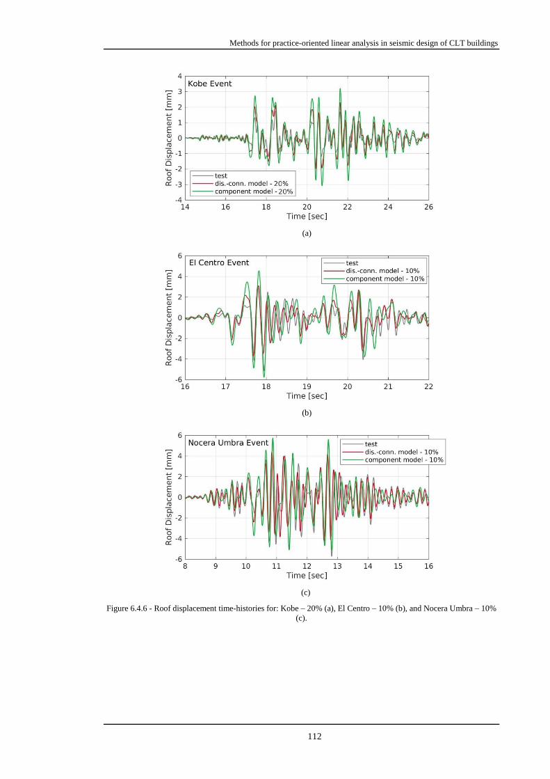
Methods for practice-oriented linear analysis in seismic design of CLT buildings
112
(a)
(b)
(c)
Figure 6.4.6 - Roof displacement time-histories for: Kobe – 20% (a), El Centro – 10% (b), and Nocera Umbra – 10%
(c).
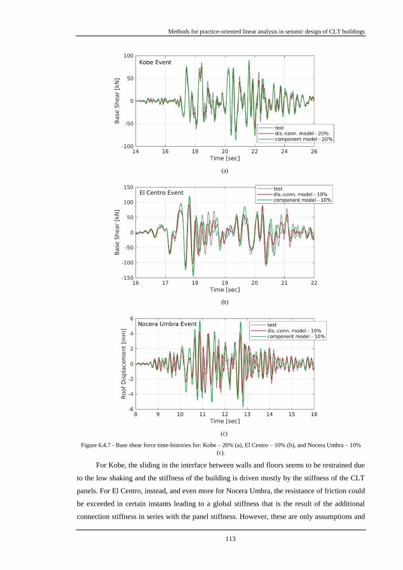
Methods for practice-oriented linear analysis in seismic design of CLT buildings
113
(a)
(b)
(c)
Figure 6.4.7 - Base shear force time-histories for: Kobe – 20% (a), El Centro – 10% (b), and Nocera Umbra – 10%
(c).
For Kobe, the sliding in the interface between walls and floors seems to be restrained due
to the low shaking and the stiffness of the building is driven mostly by the stiffness of the CLT
panels. For El Centro, instead, and even more for Nocera Umbra, the resistance of friction could
be exceeded in certain instants leading to a global stiffness that is the result of the additional
connection stiffness in series with the panel stiffness. However, these are only assumptions and

Methods for practice-oriented linear analysis in seismic design of CLT buildings
114
further research of these aspects is needed for a better investigation of these very important
phenomena, which cannot be easily accounted for in an equivalent way on linear analyses.
6.5. Concluding remarks
In this chapter, the dynamic response of the 3-storey CLT building tested within the
SOFIE project [40] has been investigated through linear models built using two different
approaches. In the first approach, the metal connectors between CLT panels have been modelled
with shell elements, by distributing their stiffness along the wall edge. In the second approach,
the walls have been connected by elastic spring elements, representing each one a single
connector.
The results obtained from the transient dynamic analyses with the two approaches have
been compared with the experimental results available from SOFIE project. Such comparison
has been conducted on the base of the maximum and minimum base shear and roof
displacement obtained.
The linear building models based on the described modelling approaches can provide
reliable estimates of the structural response under low-amplitude seismic excitations. Moreover,
it has been found that the analysed structure exhibited a higher energy dissipation than the
simulation conducted with the 5% of damping ratio. For this reason, more linear analyses with
higher damping ratios have been conducted. As a result, they evidenced a better estimation of
the structural response.
Hence, one interesting aspect evidenced in the present work is that the equivalent
damping ratio to be considered in a linear analysis of a CLT building could be used to take into
account the energy dissipation provided by friction. Such effect is conservative, as it leads to
higher equivalent damping ratios. By taking into account the principle of structural resilience
[64], a seismic swarm that could hit the building will probably lower the damping in the
structure. Such fact allows the designer to use the most common value of the damping ratio
(5%) and to implicitly accept higher design displacements, as a result of the progressive
deterioration of the friction effect between panel edges and as a conservative parameter.
Obviously, the kind of structural behaviour showed in this work is related to the analysed
building, and this work has to be extended to other static schemes and seismic events to draw
general provisions.
The simplifications introduced in this work are oriented to the representation of the
fundamental structural components with a practice-oriented approach, and not to a research-
oriented modelling procedure. The use of conventional stiffnesses and any other simplifications
are addressed to practicing engineers, with the final aim to allow that reliable results be obtained
with common tools.

115
CONCLUSIONS
In this thesis, different aspects concerning CLT structures and their behavior have been
investigated.
In chapter 3, a simplified method for the design of CLT connections is presented. This
approach have proven to be reliable when compared to FE analyses, showing always a safety
factor higher than one. It also gives information on the inter-story drift, the resistant axial force-
bending moment domain and the neutral axis position for a given set of external loads.
In chapter 4, the design and behavior of the panel-to-panel connection and how an
overlaying diaphragm influences its behavior is investigated. In the chapter a formula for the
design of such connection is suggested basing on the characteristics of the other elements
composing the assembly (i.e. panels and base connections). The formula has given acceptable
results when used to predict the behavior of full-scale tests and, after a modification, it has
shown good accuracy when predicting FE models behavior for a very large set of different
parameters (e.g. connections arrangement, axial load, etc). In the second part of this chapter, the
influence of the diaphragm and relative connection have been investigated. Connections have
proven to play a very important role, whereas different type of diaphragm have not. The study
highlighted. Results of assemblies with diaphragm and same assembly without diaphragm have
been compared in terms of rocking capacity, lateral displacement contribution and rocking
behavior
Chapter 5 presents the results of different full-scale shaking table tests of a 2-story CLT
platform structure. These tests have been performed to evaluate the goodness of a novel design
approach for these structures to be implemented in the US codes. The structure, subjected to
seismic motion, ranging from 0.52 to 1.5 g, was never in danger to collapse. Phase 3.2,
characterized by an aspect ratio of panels 2,1:1 gave different results from what expected due to
the particular type of construction (i.e. walls placed in an already built structure), but, besides
that, the tests gave valuable information and confirmed many predictions.
The last chapter, chapter 6, assess the influence of different modelling approaches and
different value of damping in the prediction of the real behavior of CLT structures subjected to
low intensity seismic motions. Damping, in this configuration, can be used to account for the
energy dissipated through friction, as in full-scale tests it has been proven that this contribution
is consistent and the structure itself show a higher energy dissipation than the one related to a
common value of 5%. However, as the contribution of friction tends to lower for subsequent
seismic motion, designers can use the value of 5%, accepting implicitly that the structure would
Conclusions
116
dissipate more than for what has been designed.
Further research should address the influence of the segmentation of the CLT diaphragm,
walls formed with a higher number of panels, perpendicular walls and other story on the rocking
behavior and capacity of wall assemblies.
Moreover, with lab tests, in order to devise reliable design procedures, researchers should
study how different number and type of fasteners in a same metal plate connection influence its
behavior and its capacity and how different arrangements of metal plates connection (i.e.
number and disposition) influence the capacity and behavior of wall assemblies. These type of
tests could give very useful hints on the design and numerical model of CLT structures when
specific lab tests on the same connections or arrangements are not available.

annex A – DESIGN example
117
ANNEX A – DESIGN EXAMPLE
8.1. Introduction
In this section, a brief example of a design made through the formulations proposed in
chapter 3 and 4 is presented.
8.2. Example
Using the Italian design regulation (NTC2018) for the calculation of the seismic action on
the structures, the following data is set:
The building is regular in plan and elevation, hence the lateral force method is
considered;
The building is composed of two above the ground floors weighting, after the application
of the seismic combination, 200kN each;
The axial load is bore by columns and the lateral force by two 100mm thick, 3x3m2 shear
walls, respectively, so that the two design problems can be considered separately.
The ordinate of the design spectrum at the period T1 Sd(T1) is equal to 0.25g.
Developing the calculation:
h d 1F WS (T ) 200 200 0.25 1 100kN [8.1.1]
where
Fh Base shear force
Sd(T1) Ordinate of the design spectrum at the period
T1 Fundamental period of the structure
W Weight of the structure
Each wall on the ground floor is loaded with 50kN in shear and 0kN in compression.
Connections already presented in chapters 3 and 4 are used, placing two hold-downs at the
edges of the wall and one angle bracket per meter along the base, as shown in Figure 8.2.1.

annex A – DESIGN example
118
Figure 8.2.1 – Arrangement of the connection of the designed wall (measures in cm).
For this examples, the following parameters are considered:
CLT strength in compression: 11N/mm2;
CLT Young modulus: 4600N/mm2;
Density of wood: 420kg/m3;
Stress distribution coefficient k equal to 0.23 (CLT on rigid support, see chapter 3.3.2.2).
In order to make the iterative process this method is characterized by automatic, a
purposely developed software has been created. This software, once all the geometric and
material parameters are set, draws the resistant domain for the given wall; calculates the values
of bending moment, axial load and neutral axis position at the interface of the different sub-
domains; calculates the neutral axis position, the compressive reaction force in the CLT panel
and the sub-domain interested for the given external loads.
Figure 8.2.2 – Bending moment-axial load resistant domain for the given wall and verification of the calculated
external loads (blue X) (figure taken from the purposely developed software).

annex A – DESIGN example
119
For the given scenario and the loads set, the domain calculated is the one shown in Figure
8.2.2. As it can be seen from Figure 8.2.2, the point having the external loads as coordinates
lays inside the resistant domain, so the supposed arrangement of connections satisfies the design
conditions.
Now, let’s suppose the shear walls are composed by two panels linked by six screws, as
the one presented in chapter 4, each. In this example, the arrangement of connections just
considered is not valid as the central angle brackets is placed between the panels. The
configuration of base connections for the first attempt is the one shown in Figure 8.2.3.
Figure 8.2.3 – First attempt arrangement of the connection of the designed segmented wall (measures in cm).
For the number of screws chosen, the behavior expected is coupled. For the hypotheses
made in chapter 4.4, the capacity of the segmented shear wall is calculated by summing the
capacity of each panel, obtained using the method presented in chapter 3. If the parameters for
the two panels are used in the purposely developed software, the capacities obtained for the
bending moment are 69.6kNm and 36.4kNm. In chapter 4.4.1. a corrective coefficient equal to
1.32 is suggested. The resulting capacity is the following:
Rd Rd,left Rd,rightM M M 1.32 69.6 36.4 1.32 139.92kNm [8.1.2]
The applied bending moment is greater than the resisting one, being equal to 150kNm.
The proposed solution is to considered two wider CLT panels, passing from 1.5m to
1.6m. The second attempt shear wall is depict in Figure 8.2.4.
Figure 8.2.4 - Second attempt arrangement of the connection of the designed segmented wall (measures in cm).
Using this characteristics, the two separated capacities are 75.9kNm and 38.2kNm, that
summed together and multiplied by the coefficient 1.32, give a total capacity of 150.61kNm,
which satisfies the design requirements.

120
REFERENCES
[1] Al-douri K, Hamodi M, Hasuni H. Compression strength perpendicular to grain in cross-
laminated timber (CLT). Master thesis, Växjö University, 2009.
[2] Amini M O, van de Lindt J W, Pei S, Rammer D, Line P, Popovski M. Overview of a
Project to Quantify Seismic Performance Factors for Cross Laminated Timber Structures
in the United States. RILEM Bookseries. 9. 2014. 531-541.
[3] Amini M O, van de Lindt J W, Rammer D, Pei S, Line P, Popovski M. Determination of
Seismic Performance Factors for CLT Building Systems. 14th
World Conference on
Timber Engineering WCTE 2016. Vienna, Austria.
[4] Amini M O, van de Lindt J W, Rammer D, Pei S, Line P, Popovski M. Systematic
experimental investigation to support the development of seismic performance factors for
cross laminated timber shear wall systems. Engineering Structures, 172(2018):392–404.
DOI:10.1016/j.engstruct.2018.06.021. 2018.
[5] ASCE. Minimum design loads for buildings and other structures. Reston, Virginia. 2010
[6] Barbosa A R, DeMeza B, Sinha A, Higgins C, Rodrigues L, Zimmerman R B,
McDonnell E, Breneman S, Pei S, van de Lindt J W, Berman J, Branco J. Design and
Shake-Table Experimental Results of CLT and CLT-Concrete Composite Diaphragms.
15th World Conference on Timber Engineering WCTE 2018. Seoul, Korea.
[7] Blaβ H J, Fellmoser P. Design of solid wood panels with cross layers. 8th World
Conference on Timber Engineering WCTE 2004. Lahti, Finland, 2004.
[8] Blomgren H-E, Pei S, Powers J, Dolan J, Wilson A, Morrel I, Jin Z. Cross-Laminated
Timber Rocking Wall with Replaceable Fuses: Validation Through Full-Scale Shake
Table Testing. 15th
World Conference on Timber Engineering WCTE 2018, Seoul, Korea.
[9] Casagrande D, Doudak G, Mauro L, Polastri A. Analytical approach to establishing the
elastic behavior of multipanel CLT shear walls subjected to lateral loads. Journal of
Structural Engineering 2018; 144(2): 04017193.
[10] Ceccotti A. New technologies for construction of medium-rise buildings in seismic
regions: the XLAM case. Struct Eng Int 2008; 18(2):156–65.
http://dx.doi.org/10.2749/101686608784218680
[11] Ceccotti A, Sandhaas C, Okabe M, Yasumura M, Minowa C, Kawai N. SOFIE project–
3D shaking table test on a seven-storey full-scale cross-laminated timber building.
Earthquake Engineering & Structural Dynamics 2013; 42(13): 2003-2021.
[12] Christovasilis I P, Brunetti M, Follesa M, Nocetti M, Vassallo D. Evaluation of the
Mechanical Properties of Cross Laminated Timber with Elementary Beam Theories.
Construction and Building Materials 2016; 122:202-213.

References
121
[13] Clough, R W, Penzien J. Dynamics of Structures, 2nd ed. (revised). Computers and
Structures, 2003.
[14] CSA, O86-14. Canadian Standard for Engineering design in wood. CSA Publisher, 2014.
[15] CSI, “SAP2000 Integrated Software for Structural Analysis and Design,” Computers and
Structures Inc., Berkeley, California, 2018.
[16] D’Arenzo G, Rinaldin G, Fossetti M, Fragiacomo M, Nebiolo F, Chiodega M. Tensile
and shear behaviour of an innovative angle bracket for CLT structures. 15th World
Conference on Timber Engineering. COEX exhibition and convention center. Seoul,
South Korea. 2018.
[17] Dassault Systèmes Simulia Corp.. "Abaqus 2018 documentation." Johnston, Rhode
Island, US, 2018.
[18] Dujic B, Pucelj J, Zarnic R. Testing of racking behavior of massive wooden wall panels.
Proc., 37th CIB-W18 Meeting, International Council for Building Research and
Innovation, Rotterdam, Netherlands. 2004.
[19] Dujič B, Strus K, Zarnic R, Ceccotti A.Prediction of dynamic response of a 7-storey
massive Xlam wooden building tested on a shaking table. 11th World Conference on
Timber Engineering WCTE 2010. Riva del Garda, Italy, CD
[20] Électricité De France - EDF. Finite element code_aster, Analyse des Structures et
Thermo-mécanique pour des Etudes et des Recherches, open source on www.code-
aster.org, 1989-2018.
[21] ETA Danmark A\S. European technical approval ETA-06/0106. Technical Approval for
Simpson Strong-Tie Angle Bracket 90, http://www.strongtie.dk/, in Danish.
[22] European Committee for Standardization (CEN). Eurocode 2: Design of concrete
structures - Part 1-1: General rules and rules for buildings. 2004.
[23] European Committee for Standardization (CEN). Eurocode 5: Design of timber structures
- Part 1-1: General - Common rules and rules for buildings. 2014.
[24] European Committee for Standardization (CEN). Eurocode 8: Design of structures for
earthquake resistance - Part 1: General rules, seismic actions and rules for building. 2004.
[25] FEMA, Federal Emergency Management Agency. Quantification of Building Seismic
Performance Factors – FEMA P695. 2009.
[26] Follesa M, Fragiacomo M, Lauriola M P. A Proposal for Revision of the Current Timber
Part (Section 8) of Eurocode 8 Part 1. CIB-W18, 44-15-1. Alghero, Italy. 2011.
[27] Follesa M, Christovasilis I P, Vassallo D, Fragiacomo M, Ceccotti A. Seismic design of
multi-storey cross laminated timber buildings according to Eurocode 8. Ingegneria
Sismica, 30 (4), pp. 27-53. 2013.

References
122
[28] Follesa M, Fragiacomo M. Force-based seismic design of mixed CLT/Light-Frame
buildings. Engineering Structures 2018, 168(2018)628–642.
https://doi.org/10.1016/j.engstruct.2018.04.091.
[29] Follesa M, Fragiacomo M, Casagrande D, Tomasi R, Piazza M, Vassallo D, Canetti D,
Rossi S. The new provisions for the seismic design of timber buildings in Europe.
Engineering Structures 2018, 168(2018)736–747.
https://doi.org/10.1016/j.engstruct.2018.04.090.
[30] Fragiacomo M, Dujič B, Šušteršič I. Elastic and ductile design of multi-storey crosslam
massive wooden buildings under seismic actions. Eng Struct 2011; 33(11):3043–53.
http://dx.doi.org/10.1016/j.engstruct.2011.05.020
[31] Fragiacomo M, Rinaldin G. Advanced models for seismic analyses of timber buildings.
Außergewöhnliche Einwirkung - Erdbeben - im Holzbau. Workshop on timber
construction. Grazer Holzbau-Fachtagung–9. Gra FHT’11. Technical University of Graz,
Austria
[32] Gagnon S, Pirvu C. CLT handbook: cross-laminated timber. Québec: FPInnovations,
2011.
[33] Gavrić I, Fragiacomo M, Ceccotti A. Capacity Seismic Design of X-Lam Wall Systems
Based on Connection Mechanical Properties. CIB-W18, 46-15-2. Vancouver, Canada.
2013.
[34] Gavrić I, Popovski M. 2014. Design models for CLT shearwalls and assemblies based on
connection properties. CIB-W18, 47-15-4, Bath, United Kingdom. 2014.
[35] Gavrić I, Fragiacomo M, Ceccotti A. Cyclic behaviour of typical metal connectors for
cross-laminated (CLT) structures. Materials and Structures 2014; 48(15):1841–1857. DOI
10.1617/s11527-014-0278-7
[36] Gavrić I, Fragiacomo M, Ceccotti A. Cyclic behavior of typical screwed connections for
cross-laminated (CLT) structures. Eur J Wood Prod 2015. 73(2):179–191. DOI
10.1007/s00107-014-0877-6
[37] Gavrić I, Fragiacomo M, Ceccotti A. Cyclic behavior of cross-laminated timber (CLT)
wall systems: Experimental tests and analytical prediction models. ASCE Journal of
Structural Engineering 2015; 141(11), 04015034, DOI: 10.1061/(ASCE)ST.1943-
541X.0001246
[38] Granello G, Leyder C, Palermo A, Frangi A, Pampanin S. Design Approach to Predict
Post-Tensioning Losses in Post-Tensioned Timber Frames. ASCE Journal of Structural
Engineering 2018. 144. 10.1061/(asce)st.1943-541x.0002101.
[39] Hristovski V, Dujič B, Stojmanovska M, Mircevska V. Full-scale shaking-table tests of
XLam panel systems and numerical verification: Specimen 1. ASCE Journal of Structural
Engineering 2013; 139(11):2010–8. http://dx.doi.org/10.1061/(ASCE)ST.1943-
541X.0000754

References
123
[40] IVALSA-CNR Trees and Timber Institute. SOFIE Project – new architecture with wood,
http://www.ivalsa.cnr.it/sofie.html. 2008 (in Italian).
[41] Izzi M, Rinaldin G, Polastri A, Fragiacomo M. A hysteresis model for timber joints with
dowel-type fasteners. Engineering Structures 2017; 157(18)170–178.
https://doi.org/10.1016/j.engstruct.2017.12.011
[42] McKenna F, Scott M H, Fenves G L. Nonlinear finite element analysis software
architecture using object composition. Journal of Computing in Civil Engineering 2010,
24(1):95-107, http://dx.doi.org/10.1061/(ASCE)CP.1943-5487.0000002
[43] Miura S, Isoda H, Tsuchimoto T, Nakagawa T, Kitamori A, Suzuki K, Tsuda C. Lateral
Structural Performance of Narrow Size Cross Laminated Timber Connected with Tensile
Bolts. Journal of Structural and Construction Engineering (Transactions of AIJ) 2016;
vol. 81, no. 721, 2016, pp. 585-593.
[44] NextFEM Designer Users’ manual, v. 1.20b, 2018, Internet site: nextfem.it.
[45] Okabe M, Yasumura M, Kobayashi K, Haramiishi T, Nakashima Y, Fujita, K. Effect of
vertical load under cyclic lateral load test for evaluating Sugi CLT wall panel. 12th World
Conference on Timber Engineering WCTE 2012. Auckland, New Zealand, 2012, DVD.
[46] Ozcelik O, Luco J E, Conte J P, Trombetti T L, Restrepo J I. Experimental
characterization, modeling and identification of the NEES-UCSD shake table mechanical
system. Earthquake Eng. Struct. Dyn. 2008; 37(2), 243-264.
[47] Pampanin S, Palermo A, Buchanan A, Fragiacomo M, Deam B. Code Provisions for
Seismic Design of Multi-Storey Post-tensioned Timber Buildings. CIB-WG18, 39-15-
6. Florence, Italy. 2006.
[48] Patzák B. OOFEM - an object-oriented simulation tool for advanced modeling of
materials and structures. Acta Polytechnica, 52(6):59–66. 2012.
[49] Pei S, Popovski M, Van de Lindt J W. Performance Based Design and Force
Modification Factors for CLT Structures. CIB-W18, 45-15-1. Växjö, Sweden. 2012.
[50] Pei S, van de Lindt J W, Popovski M, Berman J W, Dolan J D, Ricles J, Sause R,
Blomgren H, Rammer D R. Cross-Laminated Timber for Seismic Regions: Progress and
Challenges for Research and Implementation. Journal of Structural Engineering 2014;
E2514001
[51] Pei S, van de Lindt J W, Barbosa A R, Berman J, McDonnel E, Dolan J, Zimmerman R,
Sause R, Ricles J, Ryan K. Full-Scale Shake Table Test of Mass-Timber Building with
Resilient Post-Tensioned Rocking Walls. 15th
World Conference on Timber Engineering
WCTE 2018, Seoul, Korea.
[52] Piazza M, Schickhofer G, Flatscher G, Campos Costa A, Candeias P X. Seismic
performance of multi-storey timber buildings - TUGraz building. Final Report. SERIES -
Seismic Engineering Research Infrastructures for European Synergies. TUGraz, Graz,
Austria. 2013.

References
124
[53] Polastri A, Giongo I, Piazza M. An innovative connection system for cross-laminated
timber structures. Structural Engineering International 2017; 27:4, 502-511. DOI:
10.2749/222137917X14881937844649.
[54] Polastri A, Giongo I, Angeli A, Brandner R. Mechanical characterization of a pre-
fabricated connection system for cross laminated timber structures in seismic regions.
Engineering Structures 2017; 167(2017):705-715.
https://doi.org/10.1016/j.engstruct.2017.12.022
[55] Popovski M, Gavrić I. Performance of a 2-Story CLT House Subjected to Lateral Loads.
Journal of Structural Engineering 2016; 142 (4). https://doi.org/10.1061/(ASCE)ST.1943-
541X.0001315
[56] Pozza L, Scotta R, Vitaliani R. A non linear numerical model for the assessment of the
seismic behavior and ductility factor of X-Lam timber structures. International
Symposium “Timber Structures from Antiquity to the Present” edited by J. Chilton and I.
Mungan, Istanbul (Turkey), June 25‐27, pp. 151‐162, 2009.
[57] Pozza L, Scotta R, Trutalli D, Polastri A, Smith I. Experimentally based q-factor
estimation of cross-laminated timber walls. Proc ICE Struct Build 2016; 169(7):492–507.
http://dx.doi.org/10.1680/jstbu.15.00009.
[58] Pozza L, Saetta A, Savoia M, Talledo D. Coupled axial-shear numerical model for CLT
connections. Constr Build Mater 2017; 150:568–82.
http://dx.doi.org/10.1016/j.conbuildmat.2017.05.141
[59] Rinaldin G, So.ph.i. program, internet site: giovanni.rinaldin.org
[60] Rinaldin G, Amadio C, Fragiacomo M. A component approach for the hysteretic
behaviour of connections in cross-laminated wooden structures. Earthquake Eng Struct
Dyn 2013; 42(13):2023–42. http://dx.doi.org/10.1002/eqe.2310
[61] Rinaldin G, Poh’sie G H, Fragiacomo M, Amadio C, Pontarin F. Non-linear modelling of
the three and seven storey X−Lam buildings tested within the SOFIE project. 13th World
Conference on Timber Engineering WCTE 2014. Quebec City, Quebec, CA. 2014.
[62] Rinaldin G, Fragiacomo M. Non-linear simulation of shaking-table tests on 3- and 7-
storey X-Lam timber buildings, Engineering Structures 2016; 113(16)133-148
http://dx.doi.org/10.1016/j.engstruct.2016.01.055
[63] Rinaldin G, Amadio C, Macorini L. A macro-model with nonlinear springs for seismic
analysis of URM buildings. Earthquake Engng Struct. Dyn. 2016; 45 no.14: 2261-2281.
DOI: 10.1002/eqe.2759
[64] Rinaldin G, Fragiacomo M, Amadio C. On the accuracy of the N2 inelastic spectrum for
timber structures. Soil Dynamics and Earthquake Engineering 2017; 100(17)49-58
http://dx.doi.org/10.1016/j.soildyn.2017.05.026
[65] Schickhofer G, Brandner R, Bauer, H. Introduction to CLT, Product Properties, Strength
Classes. Cross Laminated Timber - a competitive wood product for visionary and fire
References
125
safe buildings: Joint Conference of COST Actions FP1402 and FP1404, Stockholm,
Sweden. 2016.
[66] Shen Y-L, Schneider J, Tesfamariam S, Stiemer SF, Mu Z-G. Hysteresis behavior of
bracket connection in cross-laminated-timber shear walls. Constr Build Mater 2013;
48:980–91. http://dx.doi.org/10.1016/j.conbuildmat.2013.07.050
[67] Simpson Strong-Tie. Strong-Rod™ Systems for Multi-Storey Overturing Restraint,
Canadian Edtion, Simpson Strong-Tie. 2016.
[68] Šušteršič I, Fragiacomo M, Dujič B. Influence of the connection behaviour on the seismic
resistance of multi-storey crosslam buildings. 12th World Conference on Timber
Engineering WCTE 2012. Auckland, New Zealand, 2012, DVD.
[69] Šušteršič I, Fragiacomo M, Dujič B. Seismic analysis of Cross-Laminated multistory
timber buildings using code-described methods: influence of panel size, connection
ductility, and schematization. J Struct Eng 2016; 142(4):E4015012.
http://dx.doi.org/10.1061/(ASCE)ST.1943-541X.0001344
[70] Tamagnone G. Numerical analysis of X-Lam buildings under seismic loads and
validation of design procedures. Master thesis, Politecnico di Torino, Italy. 2015.
[71] Tamagnone G, Rinaldin G, Fragiacomo M. A novel method for non-linear design of CLT
wall systems. Engineering Structures 2018; 167(18)760-771
https://doi.org/10.1016/j.engstruct.2017.09.010
[72] Thiel A, Schickhofer G. CLTdesigner – A Software Tool for Designing Cross Laminated
Timber Elements: 1D-Plate-Design. 11th World Conference on Timber Engineering
WCTE 2010. Riva del Garda, Italy. 2010.
[73] Thiel, A. ULS and SLS Design of CLT and its Implementation in the CLT designer. In:
Harris R, Ringhofer A, Schickhofer G (ed.), Focus Solid Timber Solutions – European
Conference on Cross Laminated Timber (CLT), Graz, Austria. 2013.
[74] Tomasi R. Seismic behaviour of connections for buildings in CLT. COST Action FP1004
Conf. on the State-of-the Art in CLT Research. Univ. of Bath. Bath, North East Somerset,
UK. 2013.
[75] van Bakel R, Rinaldin G, Leijten A J, Fragiacomo M. Experimental-numerical
investigation on the seismic behaviour of moment-resisting timber frames with densified
veneer wood-reinforced timber joints and expanded tube fasteners. Earthquake Engng
Struct. Dyn. 2017; 46:1307–1324 DOI: 10.1002/eqe.2857
[76] van de Lindt J W, Furley J, Amini M O, Pei S, Tamagnone G, Barbosa A R, Rammer D.,
Line P, Fragiacomo M, Popovski M. Experimental seismic behavior of a two-story CLT
platform building: shake table testing results. 15th World Conference on Timber
Engineering. COEX exhibition and convention center. Seoul, South Korea. 2018.
[77] Vassallo D, Follesa M, Fragiacomo M. Seismic design of a six-storey CLT building in
Italy. Engineering Structures 2018, 175(2018)322–338.
https://doi.org/10.1016/j.engstruct.2018.08.025.

References
126
[78] Yasumura M, Kobayashi K, Okabe M, Miyake T, Matsumoto K. Full-scale tests and
numerical analysis of low-rise CLT structures under lateral loading. J Struct Eng 2016;
142(4):E4015007. http://dx.doi.org/10.1061/(ASCE)ST.1943-541X.0001348
[79] Zarnani P, Valadbeigi A, Hashemi A, Darani F M, Yousef-beik S M M, Bagheri H,
Quenneville P. Rotational performance of Resilient Slip Friction Joint (RSFJ) as a new
damage free seismic connection. 15th World Conference on Timber Engineering WCTE
2018. COEX exhibition and convention center. Seoul, South Korea. 2018.