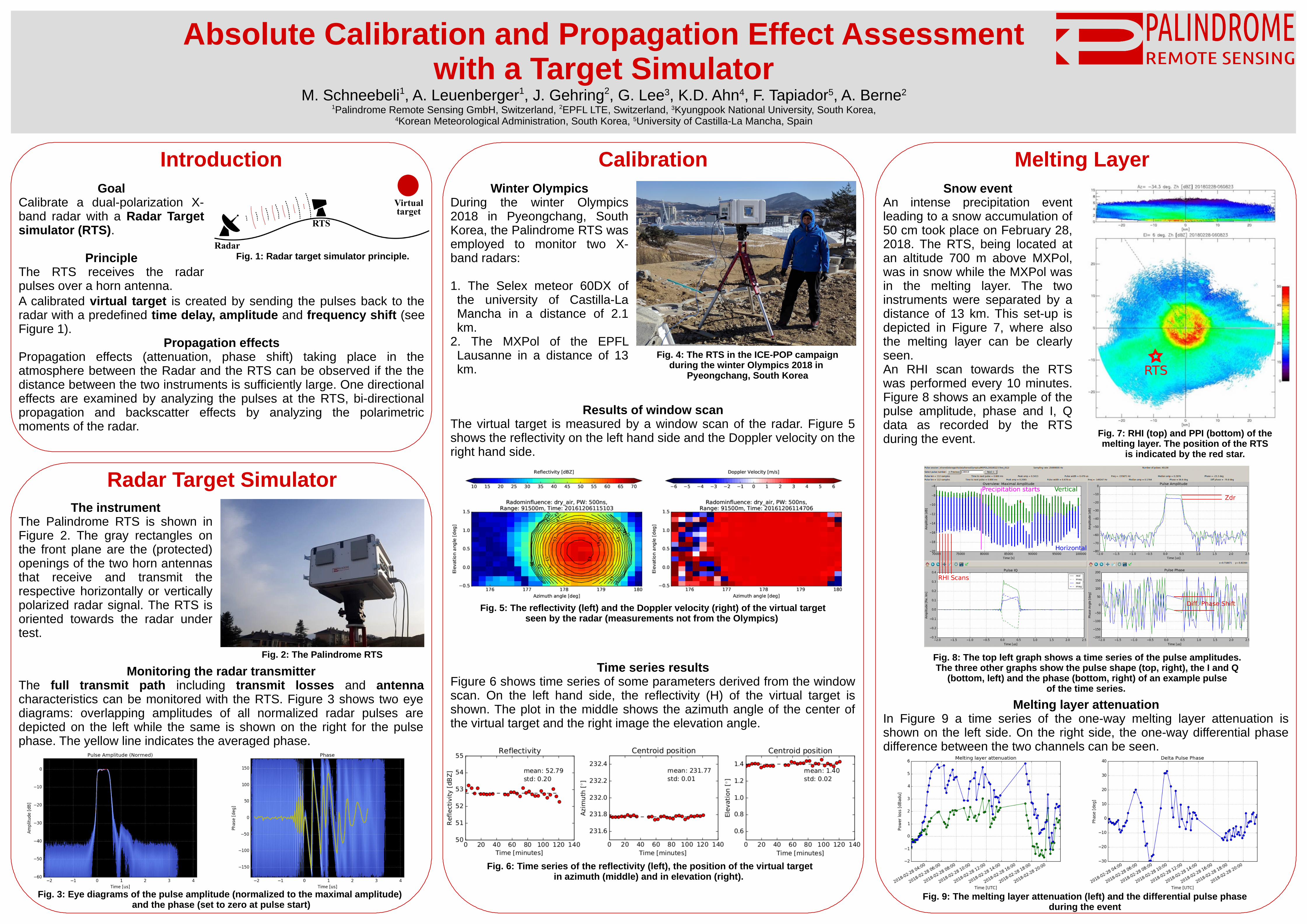
A calibrated virtual target is created by sending the pulses back to the radar with a predefined time delay, amplitude and frequency shift (see Figure 1).

Propagation effectsPropagation effects (attenuation, phase shift) taking place in the atmosphere between the Radar and the RTS can be observed if the the distance between the two instruments is sufficiently large. One directional effects are examined by analyzing the pulses at the RTS, bi-directional propagation and backscatter effects by analyzing the polarimetric moments of the radar.

Absolute Calibration and Propagation Effect Assessmentwith a Target Simulator

M. Schneebeli1, A. Leuenberger1, J. Gehring2, G. Lee3, K.D. Ahn4, F. Tapiador5, A. Berne2

1Palindrome Remote Sensing GmbH, Switzerland, 2EPFL LTE, Switzerland, 3Kyungpook National University, South Korea,4Korean Meteorological Administration, South Korea, 5University of Castilla-La Mancha, Spain

Introduction

Radar Target Simulator

Calibration Melting Layer Goal

Calibrate a dual-polarization X-band radar with a Radar Target simulator (RTS).

PrincipleThe RTS receives the radar pulses over a horn antenna.

Fig. 1: Radar target simulator principle.

Monitoring the radar transmitterThe full transmit path including transmit losses and antenna characteristics can be monitored with the RTS. Figure 3 shows two eye diagrams: overlapping amplitudes of all normalized radar pulses are depicted on the left while the same is shown on the right for the pulse phase. The yellow line indicates the averaged phase.

Fig. 3: Eye diagrams of the pulse amplitude (normalized to the maximal amplitude) and the phase (set to zero at pulse start)

Fig. 5: The reflectivity (left) and the Doppler velocity (right) of the virtual targetseen by the radar (measurements not from the Olympics)

Fig. 4: The RTS in the ICE-POP campaignduring the winter Olympics 2018 in

Pyeongchang, South Korea

Winter OlympicsDuring the winter Olympics 2018 in Pyeongchang, South Korea, the Palindrome RTS was employed to monitor two X-band radars:

1. The Selex meteor 60DX of the university of Castilla-La Mancha in a distance of 2.1 km.

2. The MXPol of the EPFL Lausanne in a distance of 13 km.

Results of window scanThe virtual target is measured by a window scan of the radar. Figure 5 shows the reflectivity on the left hand side and the Doppler velocity on the right hand side.

Fig. 2: The Palindrome RTS

Time series resultsFigure 6 shows time series of some parameters derived from the window scan. On the left hand side, the reflectivity (H) of the virtual target is shown. The plot in the middle shows the azimuth angle of the center of the virtual target and the right image the elevation angle.

Fig. 6: Time series of the reflectivity (left), the position of the virtual targetin azimuth (middle) and in elevation (right).

The instrumentThe Palindrome RTS is shown in Figure 2. The gray rectangles on the front plane are the (protected) openings of the two horn antennas that receive and transmit the respective horizontally or vertically polarized radar signal. The RTS is oriented towards the radar under test.

Fig. 7: RHI (top) and PPI (bottom) of themelting layer. The position of the RTS

is indicated by the red star.

Fig. 8: The top left graph shows a time series of the pulse amplitudes.The three other graphs show the pulse shape (top, right), the I and Q

(bottom, left) and the phase (bottom, right) of an example pulseof the time series.

Fig. 9: The melting layer attenuation (left) and the differential pulse phaseduring the event

Snow eventAn intense precipitation event leading to a snow accumulation of 50 cm took place on February 28, 2018. The RTS, being located at an altitude 700 m above MXPol, was in snow while the MXPol was in the melting layer. The two instruments were separated by a distance of 13 km. This set-up is depicted in Figure 7, where also the melting layer can be clearly seen.An RHI scan towards the RTS was performed every 10 minutes. Figure 8 shows an example of the pulse amplitude, phase and I, Q data as recorded by the RTS during the event.

Melting layer attenuationIn Figure 9 a time series of the one-way melting layer attenuation is shown on the left side. On the right side, the one-way differential phase difference between the two channels can be seen.