Abbreviations and Notation Summary

CHAPTER 4

APR annual percentage rate (nominal interest)

EOY end of year

f a geometric change from one time period to the next in cash flowsor equivalent values

i effective interest rate per interest period

r nominal interest rate per period (usually a year)

CHAPTER 5

AW(i%) equivalent uniform annual worth, computed at i% interest, of oneor more cash flows

CR(i%) equivalent annual cost of capital recovery, computed at i% interest

CW(i%) capitalized worth (a present equivalent), computed at i% interest

FW(i%) future equivalent worth, calculated at i% interest, of one or morecash flows

EUAC(i%) equivalent uniform annual cost, calculated at i% interest

IRR internal rate of return, also designated i%

MARR minimum attractive rate of return

N length of the study period (usually years)

PW(i%) present equivalent worth, computed at i% interest, of one or morecash flows

CHAPTER 6

�(B − A) incremental net cash flow (difference) calculated from the cash flowof Alternative B minus the cash flow of Alternative A (read: delta Bminus A)

CHAPTER 7

ATCF after-tax cash flow

BTCF before-tax cash flow

EVA economic value added

MACRS modified accelerated cost recovery system

NOPAT net operating profit after taxes

WACC tax-adjusted weighted average cost of capital

CHAPTER 8

A$ actual (current) dollars

f general inflation rate

R$ real (constant) dollars

CHAPTER 9

EUAC equivalent uniform annual cost

TCk total (marginal) cost for year k

CHAPTER 12

E(X) mean of a random variable

f (x) probability density function of a continuous random variable

p(x) probability mass function of a discrete random variable

SD(X) standard deviation of a random variable

V(X) variance of a random variable

CHAPTER 13

CAPM capital asset pricing model

RF risk-free rate of return

SML security market line

Xj binary decision variable in capital allocation problems

Right now, in your course, there are young men and women whose engineering achievements could revolutionize, improve, and sustain future generations.

Don’t Let Them Get Away. Engineering Economy, 16th Edition, together with MyEngineeringLab, is a complete solution for providing an engaging in-class experience that will inspire your students to stay in engineering, while also giving them the practice and scaffolding they need to keep up and be successful in the course.

Learn more at myengineeringlab.com

This page intentionally left blank

ENGINEERINGECONOMY

Sixteenth Edition

This page intentionally left blank

ENGINEERING ECONOMYSIXTEENTH EDITION

WILLIAM G. SULLIVAN ELIN M. WICKS C. PATRICK KOELLINGVirginia Polytechnic Institute Wicks and Associates, L.L.P. Virginia Polytechnic Institute

and State University and State University

Upper Saddle River Boston Columbus San Francisco New YorkIndianapolis London Toronto Sydney Singapore Tokyo Montreal

Dubai Madrid Hong Kong Mexico City Munich Paris Amsterdam Cape Town

Vice President and Editorial Director, ECS: Marcia J. Horton Cover Designer: Black Horse DesignsExecutive Editor: Holly Stark Photo Researcher: Marta SamselEditorial Assistant: Carlin Heinle Image Permission Coordinator: Karen SanatarDirector of Operations: Nick Sklitsis Text Permission Coordinator: Michael FarmerExecutive Marketing Manager: Tim Galligan Composition: Jouve India Private LimitedMarketing Assistant: Jon Bryant Full-Service Project Management: Pavithra JayapaulSenior Managing Editor: Scott Disanno Printer/Binder: CourierProduction Project Manager: Greg Dulles Typeface: 10/12 PalatinoOperations Specialist: Linda Sager

Credits and acknowledgments borrowed from other sources and reproduced, with permission, in this textbook appear onappropriate page within text.

Copyright © 2015, 2012, 2009, 2006, 2003, 1997 by Pearson Higher Education, Inc., Upper Saddle River, NJ 07458. All rightsreserved. Manufactured in the United States of America. This publication is protected by Copyright and permissionsshould be obtained from the publisher prior to any prohibited reproduction, storage in a retrieval system, or transmission inany form or by any means, electronic, mechanical, photocopying, recording, or likewise. To obtain permission(s) to usematerials from this work, please submit a written request to Pearson Higher Education, Permissions Department, One LakeStreet, Upper Saddle River, NJ 07458.

Many of the designations by manufacturers and seller to distinguish their products are claimed as trademarks. Where thosedesignations appear in this book, and the publisher was aware of a trademark claim, the designations have been printed ininitial caps or all caps.

The author and publisher of this book have used their best efforts in preparing this book. These efforts include thedevelopment, research, and testing of theories and programs to determine their effectiveness. The author and publisher makeno warranty of any kind, expressed or implied, with regard to these programs or the documentation contained in this book.The author and publisher shall not be liable in any event for incidental or consequential damages with, or arising out of, thefurnishing, performance, or use of these programs.

Pearson Education Ltd., London Pearson Education North Asia, Ltd., Hong KongPearson Education Singapore, Pte. Ltd. Pearson Educación de Mexico, S.A. de C.V.Pearson Education Canada, Inc. Pearson Education Malaysia, Pte. Ltd.Pearson Education–Japan Pearson Education, Upper Saddle River, New JerseyPearson Education Australia PTY, Limited

Library of Congress Cataloging-in-Publication Data

Sullivan, William G., 1942–Engineering economy / William G. Sullivan, Elin M. Wicks, C. Patrick Koelling. — Sixteenth edition.

pages cm1. Engineering economy—Textbooks. I. Wicks, Elin M. II. Koelling, C. Patrick, 1953- III. Title.TA177.4.S85 2014658.15—dc23 2013028782

ISBN-13:978-1-29-201949-9ISBN-10:1-29-201949-2

CONTENTS

Preface xiGreen Content xviii

CHAPTER 1Introduction to Engineering Economy 1

1.1 Introduction 21.2 The Principles of Engineering Economy 31.3 Engineering Economy and the Design Process 71.4 Using Spreadsheets in Engineering Economic Analysis 151.5 Try Your Skills 151.6 Summary 16

CHAPTER 2Cost Concepts and Design Economics 20

2.1 Cost Terminology 212.2 The General Economic Environment 272.3 Cost-Driven Design Optimization 382.4 Present Economy Studies 432.5 Case Study—The Economics of Daytime Running Lights 492.6 Try Your Skills 512.7 Summary 52Appendix 2-A Accounting Fundamentals 60

CHAPTER 3Cost-Estimation Techniques 67

3.1 Introduction 683.2 An Integrated Approach 703.3 Selected Estimating Techniques (Models) 783.4 Parametric Cost Estimating 833.5 Case Study—Demanufacturing of Computers 943.6 Electronic Spreadsheet Modeling: Learning Curve 963.7 Try Your Skills 983.8 Summary 100

v

vi CONTENTS

CHAPTER 4The Time Value of Money 107

4.1 Introduction 1084.2 Simple Interest 1094.3 Compound Interest 1104.4 The Concept of Equivalence 1104.5 Notation and Cash-Flow Diagrams and Tables 1134.6 Relating Present and Future Equivalent Values

of Single Cash Flows 1174.7 Relating a Uniform Series (Annuity) to Its Present

and Future Equivalent Values 1234.8 Summary of Interest Formulas and Relationships

for Discrete Compounding 1334.9 Deferred Annuities (Uniform Series) 1354.10 Equivalence Calculations Involving Multiple

Interest Formulas 1374.11 Uniform (Arithmetic) Gradient of Cash Flows 1434.12 Geometric Sequences of Cash Flows 1484.13 Interest Rates that Vary with Time 1534.14 Nominal and Effective Interest Rates 1554.15 Compounding More Often than Once per Year 1574.16 Interest Formulas for Continuous Compounding

and Discrete Cash Flows 1604.17 Case Study—Understanding Economic “Equivalence” 1634.18 Try Your Skills 1664.19 Summary 169

CHAPTER 5Evaluating a Single Project 186

5.1 Introduction 1875.2 Determining the Minimum Attractive Rate

of Return (MARR) 1885.3 The Present Worth Method 1895.4 The Future Worth Method 1965.5 The Annual Worth Method 1975.6 The Internal Rate of Return Method 2025.7 The External Rate of Return Method 2135.8 The Payback (Payout) Period Method 2155.9 Case Study—A Proposed Capital Investment

to Improve Process Yield 2185.10 Electronic Spreadsheet Modeling: Payback Period Method 2205.11 Try Your Skills 2225.12 Summary 224Appendix 5-A The Multiple Rate of Return Problem

with the IRR Method 236

CONTENTS vii

CHAPTER 6Comparison and Selection among Alternatives 240

6.1 Introduction 2416.2 Basic Concepts for Comparing Alternatives 2416.3 The Study (Analysis) Period 2456.4 Useful Lives Are Equal to the Study Period 2476.5 Useful Lives Are Unequal among the Alternatives 2646.6 Personal Finances 2776.7 Case Study—Ned and Larry’s Ice Cream Company 2816.8 Postevaluation of Results 2846.9 Project Postevaluation Spreadsheet Approach 2846.10 Try Your Skills 2876.11 Summary 291

CHAPTER 7Depreciation and Income Taxes 308

7.1 Introduction 3097.2 Depreciation Concepts and Terminology 3097.3 The Classical (Historical) Depreciation Methods 3127.4 The Modified Accelerated Cost Recovery System 3177.5 A Comprehensive Depreciation Example 3267.6 Introduction to Income Taxes 3307.7 The Effective (Marginal) Corporate Income Tax Rate 3337.8 Gain (Loss) on the Disposal of an Asset 3367.9 General Procedure for Making

After-Tax Economic Analyses 3377.10 Illustration of Computations of ATCFs 3417.11 Economic Value Added 3537.12 Try Your Skills 3557.13 Summary 356

CHAPTER 8Price Changes and Exchange Rates 368

8.1 Introduction 3698.2 Terminology and Basic Concepts 3708.3 Fixed and Responsive Annuities 3768.4 Differential Price Changes 3818.5 Spreadsheet Application 3838.6 Foreign Exchange Rates and Purchasing

Power Concepts 3858.7 Case Study—Selecting Electric Motors to Power

an Assembly Line 3908.8 Try Your Skills 3938.9 Summary 394

viii CONTENTS

CHAPTER 9Replacement Analysis 403

9.1 Introduction 4049.2 Reasons for Replacement Analysis 4049.3 Factors that Must Be Considered

in Replacement Studies 4059.4 Typical Replacement Problems 4089.5 Determining the Economic Life of a New

Asset (Challenger) 4119.6 Determining the Economic Life of a Defender 4159.7 Comparisons in Which the Defender’s Useful Life

Differs from that of the Challenger 4189.8 Retirement without Replacement (Abandonment) 4219.9 After-Tax Replacement Studies 4229.10 Case Study—Replacement of a Hospital’s Emergency

Electrical Supply System 4309.11 Summary 433

CHAPTER 10Evaluating Projects with the Benefit−Cost Ratio Method 443

10.1 Introduction 44410.2 Perspective and Terminology for Analyzing

Public Projects 44510.3 Self-Liquidating Projects 44610.4 Multiple-Purpose Projects 44610.5 Difficulties in Evaluating Public-Sector Projects 44910.6 What Interest Rate Should Be Used for Public Projects? 45010.7 The Benefit−Cost Ratio Method 45210.8 Evaluating Independent Projects by B−C Ratios 45810.9 Comparison of Mutually Exclusive Projects

by B−C Ratios 46010.10 Case Study—Improving a Railroad Crossing 46510.11 Summary 467

CHAPTER 11Breakeven and Sensitivity Analysis 475

11.1 Introduction 47611.2 Breakeven Analysis 47611.3 Sensitivity Analysis 48311.4 Multiple Factor Sensitivity Analysis 48911.5 Summary 493

CONTENTS ix

CHAPTER 12Probabilistic Risk Analysis 502

12.1 Introduction 50312.2 Sources of Uncertainty 50412.3 The Distribution of Random Variables 50412.4 Evaluation of Projects with Discrete Random Variables 50812.5 Evaluation of Projects with Continuous

Random Variables 51712.6 Evaluation of Risk and Uncertainty

by Monte Carlo Simulation 52212.7 Performing Monte Carlo Simulation

with a Computer 52612.8 Decision Trees 53012.9 Real Options Analysis 53512.10 Summary 538

CHAPTER 13The Capital Budgeting Process 546

13.1 Introduction 54713.2 Debt Capital 54913.3 Equity Capital 55013.4 The Weighted Average Cost of Capital (WACC) 55313.5 Project Selection 55713.6 Postmortem Review 56113.7 Budgeting of Capital Investments

and Management Perspective 56213.8 Leasing Decisions 56313.9 Capital Allocation 56513.10 Summary 571

CHAPTER 14Decision Making Considering Multiattributes 575

14.1 Introduction 57614.2 Examples of Multiattribute Decisions 57614.3 Choice of Attributes 57814.4 Selection of a Measurement Scale 57814.5 Dimensionality of the Problem 57914.6 Noncompensatory Models 57914.7 Compensatory Models 58414.8 Summary 592

x CONTENTS

Appendix A Using Excel to Solve Engineering EconomyProblems 598

Appendix B Abbreviations and Notation 615Appendix C Interest and Annuity Tables for Discrete

Compounding 619Appendix D Interest and Annuity Tables for Continuous

Compounding 638Appendix E Standard Normal Distribution 642Appendix F Selected References 645Appendix G Solutions to Try Your Skills 648

Index 660

PREFACE

We live in a sea of economic decisions.

—Anonymous

About Engineering EconomyA succinct job description for an engineer consists of two words: problem solver.Broadly speaking, engineers use knowledge to find new ways of doing thingseconomically. Engineering design solutions do not exist in a vacuum but within thecontext of a business opportunity. Given that every problem has multiple solutions,the issue is, How does one rationally select the design with the most favorableeconomic result? The answer to this question can also be put forth in two words:engineering economy. Engineering economy provides a systematic framework forevaluating the economic aspects of competing design solutions. Just as engineersmodel the stress on a support column, or the thermodynamic response of a steamturbine, they must also model the economic impact of their recommendations.

Engineering economy—what is it, and why is it important? The initial reactionof many engineering students to these questions is, “Money matters will be handledby someone else. They are not something I need to worry about.” In reality, anyengineering project must be not only physically realizable but also economicallyaffordable.

Understanding and applying economic principles to engineering have neverbeen more important. Engineering is more than a problem-solving activity focusingon the development of products, systems, and processes to satisfy a needor demand. Beyond function and performance, solutions must also be viableeconomically. Design decisions affect limited resources such as time, material,labor, capital, and natural resources, not only initially (during conceptual design)but also through the remaining phases of the life cycle (e.g., detailed design,manufacture and distribution, service, retirement and disposal). A great solutioncan die a certain death if it is not profitable.

• MyEngineeringLab is now available with Engineering Economy, 16/e and pro-vides a powerful homework and test manager which lets instructors create,import, and manage online homework assignments, quizzes, and tests that areautomatically graded. You can choose from a wide range of assignment options,

xi

xii PREFACE

including time limits, proctoring, and maximum number of attempts allowed.The bottom line: MyEngineeringLab means less time grading and more timeteaching.• Algorithmic-generated homework assignments, quizzes, and tests that

directly correlate to the textbook.• Automatic grading that tracks students’ results.• Assignable Spreadsheet Exercises that students can complete in an Excel-

simulated environment.• Interactive “Help Me Solve This” tutorials provide opportunity for point-of-

use help and more practice.• Learning Objectives mapped to ABET outcomes provide comprehensive

reporting tools. If adopted, access to MyEngineeringLab can be bundled withthe book or purchased separately.

What’s New to This Edition?The basic intent behind this revision of the text is to integrate computer technologyand realistic examples to facilitate learning engineering economy. Here are thehighlights of changes to the sixteenth edition:

• There are more integrated videos keyed to material in the text and designed toreinforce learning through analogy with marked problems and examples.

• Many new spreadsheet models have been added to the sixteenth edition(several contributed by James A. Alloway).

• This edition contains over 900 examples, solved problems and end-of-chapterproblems. These include 70 “Try Your Skills” problems in selected chapters,with full solutions given in Appendix G.

• Over 160 “green” examples and problems populate this edition as a subsetof 750 problems at the conclusion of the 14 chapters in this book. Many ofthese problems incorporate energy conservation in commonly experiencedsituations with which students can identify.

• PowerPoint visual aids for instructors have been expanded and enhanced.• Chapter 2, dealing with choice among alternatives when the time value of

money can be ignored, has been revised for improved readability.• Optional student resources include MyEngineeringLab with Pearson e-text, a

complete on-line version of the book. It allows highlighting, note taking, andsearch capabilities. This resource permits access to the Video Solutions fileswhich accompany this text as well as additional study materials. All end-of-chapter problems with this icon [ ] indicate the availability of some form ofVideo Solutions.

Strategies of This BookThis book has two primary objectives: (1) to provide students with a soundunderstanding of the principles, basic concepts, and methodology of engineeringeconomy; and (2) to help students develop proficiency with these methods and with

PREFACE xiii

the process for making rational decisions they are likely to encounter in professionalpractice. Interestingly, an engineering economy course may be a student’s only collegeexposure to the systematic evaluation of alternative investment opportunities. In thisregard, Engineering Economy is intended to serve as a text for classroom instructionand as a basic reference for use by practicing engineers in all specialty areas(e.g., chemical, civil, computer, electrical, industrial, and mechanical engineering).The book is also useful to persons engaged in the management of technicalactivities.

As a textbook, the sixteenth edition is written principally for the first formalcourse in engineering economy. A three-credit-hour semester course should beable to cover the majority of topics in this edition, and there is sufficient depthand breadth to enable an instructor to arrange course content to suit individualneeds. Representative syllabi for a three-credit and a two-credit semester coursein engineering economy are provided in Table P-1. Moreover, because severaladvanced topics are included, this book can also be used for a second course inengineering economy.

All chapters and appendices have been revised and updated to reflect currenttrends and issues. Also, numerous exercises that involve open-ended problemstatements and iterative problem-solving skills are included throughout the book.A large number of the 750-plus end-of-chapter exercises are new, and manysolved examples representing realistic problems that arise in various engineeringdisciplines are presented.

In the 21st century, America is turning over a new leaf for environmentalsustainability. We have worked hard to capture this spirit in many of our examplesand end-of-chapter problems. In fact, more than 160 “green” problems andexamples have been integrated throughout this edition. They are listed in the GreenContent section following the Preface.

Fundamentals of Engineering (FE) exam–style questions are included tohelp prepare engineering students for this milestone examination, leading toprofessional registration. Passing the FE exam is a first step in getting licensedas a professional engineer (PE). Engineering students should seriously considerbecoming a PE because it opens many employment opportunities and increaseslifetime earning potential.

It is generally advisable to teach engineering economy at the upper divisionlevel. Here, an engineering economy course incorporates the accumulated knowl-edge students have acquired in other areas of the curriculum and also deals withiterative problem solving, open-ended exercises, creativity in formulating andevaluating feasible solutions to problems, and consideration of realistic constraints(economic, aesthetic, safety, etc.) in problem solving.

Also available to adopters of this edition is an instructor’s Solutions Manualand other classroom resources. In addition, PowerPoint visual aids are readilyavailable to instructors. Visit www.pearsonhighered.com/sullivan for moreinformation.

Engineering Economy PortfolioIn many engineering economy courses, students are required to design, develop,and maintain an engineering economy portfolio. The purpose of the portfoliois to demonstrate and integrate knowledge of engineering economy beyond

TABLE P-1 Typical Syllabi for Courses in Engineering Economy

Semester Course (Three Credit Hours) Semester Course (Two Credit Hours)

Week of the No. of ClassChapter Semester Topic(s) Chapter(s) Periods Topic(s)

1 1 Introduction to Engineering Economy 1 1 Introduction to Engineering Economy2 2 Cost Concepts and Design 2 4 Cost Concepts, Single Variable

Economics Trade-Off Analysis, and3 3 Cost-Estimation Techniques Present Economy4 4–5 The Time Value of Money 4 5 The Time Value of Money5 6 Evaluating a Single Project 1, 2, 4 1 Test #16 7 Comparison and Selection 3 3 Developing Cash Flows and

among Alternatives Cost-Estimation Techniques8 Midterm Examination 5 2 Evaluating a Single Project

7 9 Depreciation and Income Taxes 6 4 Comparison and Selection10 10 Evaluating Projects with the among Alternatives

Benefit–Cost Ratio Method 3, 5, 6 1 Test #28 11 Price Changes and Exchange Rates 11 2 Breakeven and Sensitivity Analysis11 12 Breakeven and Sensitivity Analysis 7 5 Depreciation and Income Taxes9 13 Replacement Analysis 14 1 Decision Making Considering

12 14 Probabilistic Risk Analysis Multiattributes13–14 15 The Capital Budgeting Process, All the above 1 Final Examination

Decision MakingConsidering Multiattributes

15 Final ExaminationNumber of class periods: 45 Number of class periods: 30

xiv

PREFACE xv

the required assignments and tests. This is usually an individual assignment.Professional presentation, clarity, brevity, and creativity are important criteria tobe used to evaluate portfolios. Students are asked to keep the audience (i.e., thegrader) in mind when constructing their portfolios.

The portfolio should contain a variety of content. To get credit for content,students must display their knowledge. Simply collecting articles in a folderdemonstrates very little. To get credit for collected articles, students should readthem and write a brief summary of each one. The summary could explain howthe article is relevant to engineering economy, it could critique the article, or itcould check or extend any economic calculations in the article. The portfolio shouldinclude both the summary and the article itself. Annotating the article by writingcomments in the margin is also a good idea. Other suggestions for portfolio contentfollow (note that students are encouraged to be creative):

• Describe and set up or solve an engineering economy problem from your owndiscipline (e.g., electrical engineering or building construction).

• Choose a project or problem in society or at your university and applyengineering economic analysis to one or more proposed solutions.

• Develop proposed homework or test problems for engineering economy.Include the complete solution. Additionally, state which course objective(s)this problem demonstrates (include text section).

• Reflect upon and write about your progress in the class. You might include aself-evaluation against the course objectives.

• Include a photo or graphic that illustrates some aspects of engineering economy.Include a caption that explains the relevance of the photo or graphic.

• Include completely worked out practice problems. Use a different color pen toshow these were checked against the provided answers.

• Rework missed test problems, including an explanation of each mistake.

(The preceding list could reflect the relative value of the suggested items; that is,items at the top of the list are more important than items at the bottom of thelist.)

Students should develop an introductory section that explains the purposeand organization of the portfolio. A table of contents and clearly marked sectionsor headings are highly recommended. Cite the source (i.e., a complete bibliographicentry) of all outside material. Remember, portfolios provide evidence that studentsknow more about engineering economy than what is reflected in the assignmentsand exams. The focus should be on quality of evidence, not quantity.

Icons Used in This BookThroughout this book, these two icons will appear in connection with numerouschapter opening materials, examples, and problems:

This icon identifies environmental (green) elements of the book. These elementspertain to engineering economy problems involving energy conservation, materialssubstitution, recycling, and other green situations.

xvi PREFACE

This icon informs students of the availability of video tutorials for the examplesand problems so marked. Students are encouraged to access the tutorials atwww.pearsonhighered.com/sullivan. These icon-designated instances areintended to reinforce the learning of engineering economy through analogy withthe marked problems and examples.

Overview of the BookThis book is about making choices among competing engineering alternatives.Most of the cash-flow consequences of the alternatives lie in the future, so ourattention is directed toward the future and not the past. In Chapter 2, we examinealternatives when the time value of money is not a complicating factor in theanalysis. We then turn our attention in Chapter 3 to how future cash flows areestimated. In Chapter 4 and subsequent chapters, we deal with alternatives wherethe time value of money is a deciding factor in choosing among competing capitalinvestment opportunities.

Students can appreciate Chapters 2 and 3 and later chapters when theyconsider alternatives in their personal lives, such as which job to accept upongraduation, which automobile or truck to purchase, whether to buy a home or renta residence, and many other choices they will face. To be student friendly, we haveincluded many problems throughout this book that deal with personal finance.These problems are timely and relevant to a student’s personal and professionalsuccess, and these situations incorporate the structured problem-solving processthat students will learn from this book.

Chapter 4 concentrates on the concepts of money–time relationships andeconomic equivalence. Specifically, we consider the time value of money inevaluating the future revenues and costs associated with alternative uses ofmoney. Then, in Chapter 5, the methods commonly used to analyze the economicconsequences and profitability of an alternative are demonstrated. These methods,and their proper use in the comparison of alternatives, are primary subjects ofChapter 6, which also includes a discussion of the appropriate time period foran analysis. Thus, Chapters 4, 5, and 6 together develop an essential part ofthe methodology needed for understanding the remainder of the book and forperforming engineering economy studies on a before-tax basis.

In Chapter 7, the additional details required to accomplish engineeringeconomy studies on an after-tax basis are explained. In the private sector, mostengineering economy studies are done on an after-tax basis. Therefore, Chapter 7adds to the basic methodology developed in Chapters 4, 5, and 6.

The effects of inflation (or deflation), price changes, and internationalexchange rates are the topics of Chapter 8. The concepts for handling pricechanges and exchange rates in an engineering economy study are discussed bothcomprehensively and pragmatically from an application viewpoint.

Often, an organization must analyze whether existing assets should becontinued in service or replaced with new assets to meet current and futureoperating needs. In Chapter 9, techniques for addressing this question are

PREFACE xvii

developed and presented. Because the replacement of assets requires significantcapital, decisions made in this area are important and demand special attention.

Chapter 10 is dedicated to the analysis of public projects with the benefit–costratio method of comparison. The development of this widely used method ofevaluating alternatives was motivated by the Flood Control Act passed by theU.S. Congress in 1936.

Concern over uncertainty and risk is a reality in engineering practice. InChapter 11, the impact of potential variation between the estimated economicoutcomes of an alternative and the results that may occur is considered. Breakevenand sensitivity techniques for analyzing the consequences of risk and uncertaintyin future estimates of revenues and costs are discussed and illustrated.

In Chapter 12, probabilistic techniques for analyzing the consequences of riskand uncertainty in future cash-flow estimates and other factors are explained.Discrete and continuous probability concepts, as well as Monte Carlo simulationtechniques, are included in Chapter 12.

Chapter 13 is concerned with the proper identification and analysis of allprojects and other needs for capital within an organization. Accordingly, the capitalfinancing and capital allocation process to meet these needs is addressed. Thisprocess is crucial to the welfare of an organization, because it affects most operatingoutcomes, whether in terms of current product quality and service effectiveness orlong-term capability to compete in the world market. Finally, Chapter 14 discussesmany time-tested methods for including nonmonetary attributes (intangibles) inengineering economy studies.

We would like to extend a heartfelt “thank you” to our colleagues and studentsfor their many helpful suggestions (and critiques!) for this sixteenth edition of“Engineering Economy.” We owe an enormous debt of gratitude to numerousindividuals who have contributed to this edition: Jim Alloway, Karen Bursic,Thomas Cassel, Linda Chattin, Robert Dryden, Jim Luxhoj, Thomas Keyser,Samantha Marcum and Shayam Moondra. Also special thanks to our PearsonPrentice Hall team who have made invaluable improvements to this effort: ScottDisanno, Greg Dulles, Pavithra Jayapaul, Miguel Leonarte, Clare Romeo, and HollyStark.

GREEN CONTENT

Chapter 1p. 1 (chapter opener)p. 14 (Example 1-3)p. 16 (Problems 1-1 and 1-3)p. 17 (Problems 1-5, 1-7, 1-9 to 1-12)p. 18 (Problem 1-15)p. 19 (Problems 1-20 and 1-21)

Chapter 2p. 42 (Example 2-7)p. 44 (Example 2-8)p. 49 (Example 2-11)p. 52 (Problems 2-3 and 2-4)p. 53 (Problem 2-12)p. 54 (Problems 2-16, 2-21, and 2-22)p. 55 (Problems 2-23, 2-24, 2-28, and 2-30)p. 56 (Problems 2-31 to 2-33 and 2-37)p. 57 (Problems 2-38, 2-39, 2-41, and 2-42)p. 58 (Problems 2-45 and 2-47, Spreadsheet Exercise 2-49)

Chapter 3p. 67 (chapter opener)p. 94 (Case Study 3.5)p. 100 (Problems 3-1 and 3-4)p. 101 (Problems 3-6, 3-11, and 3-12)p. 102 (Problems 3-14 and 3-15)p. 106 (FE Practice Problems 3-37 and 3-40)

Chapter 4p. 107 (chapter opener)p. 115 (Example 4-2)p. 127 (Example 4-10)p. 141 (Example 4-18)p. 172 (Problems 4-33, 4-36, 4-37, and 4-40)p. 173 (Problem 4-43)

xviii

GREEN CONTENT xix

p. 174 (Problem 4-53)p. 175 (Problems 4-65, 4-70, and 4-71)p. 177 (Problems 4-82, 4-84, and 4-85)p. 178 (Problem 4-88)

Chapter 5p. 186 (chapter opener)p. 192 (Example 5-2)p. 197 (Example 5-7)p. 200 (Example 5-10)p. 217 (Example 5-19)p. 225 (Problems 5-2, 5-6, and 5-9)p. 227 (Problem 5-25)p. 228 (Problems 5-28, 5-29, 5-31, 5-33, and 5-34)p. 229 (Problems 5-35, 5-39, and 5-41)p. 231 (Problems 5-49 to 5-51)p. 232 (Problems 5-56 to 5-59)p. 235 (FE Practice Problems 5-75, 5-81, and 5-83)

Chapter 6p. 240 (chapter opener)p. 269 (Example 6-9)p. 281 (Case Study 6-7)p. 292 (Problem 6-2)p. 293 (Problem 6-6)p. 294 (Problems 6-8 and 6-13)p. 295 (Problems 6-16 and 6-17)p. 296 (Problems 6-20, 6-23, and 6-24)p. 297 (Problem 6-29)p. 298 (Problem 6-34)p. 299 (Problems 6-35, 6-38, and 6-41)p. 300 (Problem 6-43)p. 301 (Problems 6-46 and 6-49)p. 302 (Problems 6-51 and 6-53)p. 303 (Problems 6-57 to 6-59)p. 304 (Problems 6-64 and 6-66)p. 306 (FE Practice Problem 6-79)

Chapter 7p. 308 (chapter opener)p. 341 (Example 7-14)p. 361 (Problems 7-37 and 7-40)p. 365 (Problem 7-60)

xx GREEN CONTENT

Chapter 8p. 382 (Example 8-8)p. 390 (Case Study 8-7)p. 395 (Problem 8-11)p. 396 (Problem 8-18)p. 397 (Problems 8-21, 8-23, and 8-25)p. 399 (Problems 8-41 and 8-42)p. 400 (Problem 8-46)p. 402 (Case Study Exercises 8-52 to 8-54, FE Practice Problem 8-61)

Chapter 9p. 403 (chapter opener)p. 436 (Problem 9-6)p. 437 (Problem 9-12)p. 440 (Problem 9-25)

Chapter 10p. 468 (Problems 10-2, 10-4, and 10-5)p. 470 (Problem 10-13)p. 472 (Problems 10-21 and 10-24)

Chapter 11p. 478 (Example 11-1)p. 479 (Example 11-2)p. 480 (Example 11-3)p. 493 (Problems 11-2 and 11-3)p. 494 (Problem 11-6)p. 496 (Problems 11-16 to 11-18)p. 497 (Problems 11-21 and 11-22)p. 498 (Spreadsheet Exercises 11-24 and 11-25)p. 499 (Spreadsheet Exercises 11-27 to 11-29)p. 501 (FE Practice Problem 11-40)

Chapter 12p. 502 (chapter opener)p. 539 (Problems 12-4 and 12-6)p. 540 (Problem 12-7)

Chapter 13p. 546 (chapter opener)

Chapter 14p. 575 (chapter opener)p. 590 (Example 14-2)p. 597 (Problem 14-17)

ENGINEERINGECONOMY

Sixteenth Edition

This page intentionally left blank

CHAPTER 1

Introduction to EngineeringEconomy

The purpose of Chapter 1 is to present the concepts and principles ofengineering economy.

Green Engineering in Action

E nergy conservation comprises an important element inenvironmentally-conscious (green) engineering. In a Southeas-tern city, there are 310 traffic intersections that have been

converted from incandescent lights to light-emitting diode (LED) lights. Thestudy that led to this decision was conducted by the sustainability manager ofthe city. The wattage used at the intersections has been reduced from 150 wattsto 15 watts at each traffic light. The resultant lighting bill has been lowered from$440,000 annually to $44,000 annually. When engineers went to check the trafficlight meters for the first time, they were shocked by the low wattage numbersand the associated cost. One of them said, “We thought the meters were brokenbecause the readings were so low.” The annual savings of $396,000 per year fromthe traffic light conversion more than paid for the $150,000 cost of installing theLED lights. Chapter 1 introduces students to the decision-making process thataccompanies “go/no go” evaluations of investments in engineering projects suchas the one described above.

1

The best alternative may be the one you haven’t yet discovered.

—Anonymous

Icons Used in This BookThroughout this book, these two icons will appear in connection with numerouschapter opening materials, examples, and problems:

This icon identifies environmental (green) elements of the book. These elementspertain to engineering economy problems involving energy conservation, materialssubstitution, recycling, and other green situations.

This icon informs students of the availability of video tutorials for the examplesand problems so marked. Students are encouraged to access the tutorials atwww.pearsonhighered.com/sullivan. These icon-designated instances areintended to reinforce the learning of engineering economy through analogy withthe marked problems and examples.

1.1 IntroductionThe technological and social environments in which we live continue to changeat a rapid rate. In recent decades, advances in science and engineering havetransformed our transportation systems, revolutionized the practice of medicine,and miniaturized electronic circuits so that a computer can be placed on asemiconductor chip. The list of such achievements seems almost endless. In yourscience and engineering courses, you will learn about some of the physical lawsthat underlie these accomplishments.

The utilization of scientific and engineering knowledge for our benefit isachieved through the design of things we use, such as furnaces for vaporizing trashand structures for supporting magnetic railways. However, these achievementsdon’t occur without a price, monetary or otherwise. Therefore, the purpose ofthis book is to develop and illustrate the principles and methodology requiredto answer the basic economic question of any design: Do its benefits exceed itscosts?

The Accreditation Board for Engineering and Technology states that engineer-ing “is the profession in which a knowledge of the mathematical and naturalsciences gained by study, experience, and practice is applied with judgment todevelop ways to utilize, economically, the materials and forces of nature for thebenefit of mankind.”∗ In this definition, the economic aspects of engineering areemphasized, as well as the physical aspects. Clearly, it is essential that the economicpart of engineering practice be accomplished well. Thus, engineers use knowledgeto find new ways of doing things economically.

∗ Accreditation Board of Engineering and Technology, Criteria for Accrediting Programs in Engineering in the United States(New York; Baltimore, MD: ABET, 1998).

2

SECTION 1.2 / THE PRINCIPLES OF ENGINEERING ECONOMY 3

Engineering economy involves the systematic evaluation of the economic meritsof proposed solutions to engineering problems. To be economically acceptable(i.e., affordable), solutions to engineering problems must demonstrate a positivebalance of long-term benefits over long-term costs, and they must also

• promote the well-being and survival of an organization,• embody creative and innovative technology and ideas,• permit identification and scrutiny of their estimated outcomes, and• translate profitability to the “bottom line” through a valid and acceptable

measure of merit.

Engineering economy is the dollars-and-cents side of the decisions thatengineers make or recommend as they work to position a firm to be profitablein a highly competitive marketplace. Inherent to these decisions are trade-offsamong different types of costs and the performance (response time, safety, weight,reliability, etc.) provided by the proposed design or problem solution. The missionof engineering economy is to balance these trade-offs in the most economical manner.For instance, if an engineer at Ford Motor Company invents a new transmissionlubricant that increases fuel mileage by 10% and extends the life of the transmissionby 30,000 miles, how much can the company afford to spend to implement thisinvention? Engineering economy can provide an answer.

A few more of the myriad situations in which engineering economy plays acrucial role in the analysis of project alternative come to mind:

1. Choosing the best design for a high-efficiency gas furnace2. Selecting the most suitable robot for a welding operation on an automotive

assembly line3. Making a recommendation about whether jet airplanes for an overnight delivery

service should be purchased or leased4. Determining the optimal staffing plan for a computer help desk

From these illustrations, it should be obvious that engineering economy includessignificant technical considerations. Thus, engineering economy involves technicalanalysis, with emphasis on the economic aspects, and has the objective of assistingdecisions. This is true whether the decision maker is an engineer interactivelyanalyzing alternatives at a computer-aided design workstation or the ChiefExecutive Officer (CEO) considering a new project. An engineer who is unprepared toexcel at engineering economy is not properly equipped for his or her job.

1.2 The Principles of Engineering EconomyThe development, study, and application of any discipline must begin with abasic foundation. We define the foundation for engineering economy to be a set ofprinciples that provide a comprehensive doctrine for developing the methodology.These principles will be mastered by students as they progress through this book.

4 CHAPTER 1 / INTRODUCTION TO ENGINEERING ECONOMY

Once a problem or need has been clearly defined, the foundation of the disciplinecan be discussed in terms of seven principles.

PRINCIPLE 1 Develop the Alternatives

Carefully define the problem! Then the choice (decision) is among alternatives.The alternatives need to be identified and then defined for subsequent analysis.

A decision situation involves making a choice among two or more alternatives.Developing and defining the alternatives for detailed evaluation is importantbecause of the resulting impact on the quality of the decision. Engineers andmanagers should place a high priority on this responsibility. Creativity andinnovation are essential to the process.

One alternative that may be feasible in a decision situation is making no changeto the current operation or set of conditions (i.e., doing nothing). If you judge thisoption feasible, make sure it is considered in the analysis. However, do not focuson the status quo to the detriment of innovative or necessary change.

PRINCIPLE 2 Focus on the Differences

Only the differences in expected future outcomes among the alternatives arerelevant to their comparison and should be considered in the decision.

If all prospective outcomes of the feasible alternatives were exactly the same, therewould be no basis or need for comparison. We would be indifferent among thealternatives and could make a decision using a random selection.

Obviously, only the differences in the future outcomes of the alternatives areimportant. Outcomes that are common to all alternatives can be disregarded inthe comparison and decision. For example, if your feasible housing alternativeswere two residences with the same purchase (or rental) price, price would beinconsequential to your final choice. Instead, the decision would depend on otherfactors, such as location and annual operating and maintenance expenses. Thissimple example illustrates Principle 2, which emphasizes the basic purpose of anengineering economic analysis: to recommend a future course of action based onthe differences among feasible alternatives.

PRINCIPLE 3 Use a Consistent Viewpoint

The prospective outcomes of the alternatives, economic and other, should beconsistently developed from a defined viewpoint (perspective).

The perspective of the decision maker, which is often that of the owners of thefirm, would normally be used. However, it is important that the viewpoint for the

SECTION 1.2 / THE PRINCIPLES OF ENGINEERING ECONOMY 5

particular decision be first defined and then used consistently in the description,analysis, and comparison of the alternatives.

As an example, consider a public organization operating for the purpose ofdeveloping a river basin, including the generation and wholesale distribution ofelectricity from dams on the river system. A program is being planned to upgradeand increase the capacity of the power generators at two sites. What perspectiveshould be used in defining the technical alternatives for the program? The “ownersof the firm” in this example means the segment of the public that will pay the costof the program, and their viewpoint should be adopted in this situation.

Now let us look at an example where the viewpoint may not be that of theowners of the firm. Suppose that the company in this example is a private firm andthat the problem deals with providing a flexible benefits package for the employees.Also, assume that the feasible alternatives for operating the plan all have the samefuture costs to the company. The alternatives, however, have differences fromthe perspective of the employees, and their satisfaction is an important decisioncriterion. The viewpoint for this analysis should be that of the employees of thecompany as a group, and the feasible alternatives should be defined from theirperspective.

PRINCIPLE 4 Use a Common Unit of Measure

Using a common unit of measurement to enumerate as many of the prospectiveoutcomes as possible will simplify the analysis of the alternatives.

It is desirable to make as many prospective outcomes as possible commensurable(directly comparable). For economic consequences, a monetary unit such as dollarsis the common measure. You should also try to translate other outcomes (whichdo not initially appear to be economic) into the monetary unit. This translation, ofcourse, will not be feasible with some of the outcomes, but the additional efforttoward this goal will enhance commensurability and make the subsequent analysisof alternatives easier.

What should you do with the outcomes that are not economic (i.e., the expectedconsequences that cannot be translated (and estimated) using the monetary unit)?First, if possible, quantify the expected future results using an appropriate unit ofmeasurement for each outcome. If this is not feasible for one or more outcomes,describe these consequences explicitly so that the information is useful to thedecision maker in the comparison of the alternatives.

PRINCIPLE 5 Consider All Relevant Criteria

Selection of a preferred alternative (decision making) requires the use of acriterion (or several criteria). The decision process should consider both theoutcomes enumerated in the monetary unit and those expressed in some otherunit of measurement or made explicit in a descriptive manner.

6 CHAPTER 1 / INTRODUCTION TO ENGINEERING ECONOMY

The decision maker will normally select the alternative that will best serve thelong-term interests of the owners of the organization. In engineering economicanalysis, the primary criterion relates to the long-term financial interests of theowners. This is based on the assumption that available capital will be allocated toprovide maximum monetary return to the owners. Often, though, there are otherorganizational objectives you would like to achieve with your decision, and theseshould be considered and given weight in the selection of an alternative. Thesenonmonetary attributes and multiple objectives become the basis for additionalcriteria in the decision-making process. This is the subject of Chapter 14.

PRINCIPLE 6 Make Risk and Uncertainty Explicit

Risk and uncertainty are inherent in estimating the future outcomes of the alter-natives and should be recognized in their analysis and comparison.

The analysis of the alternatives involves projecting or estimating the futureconsequences associated with each of them. The magnitude and the impact of futureoutcomes of any course of action are uncertain. Even if the alternative involves nochange from current operations, the probability is high that today’s estimates of,for example, future cash receipts and expenses will not be what eventually occurs.Thus, dealing with uncertainty is an important aspect of engineering economicanalysis and is the subject of Chapters 11 and 12.

PRINCIPLE 7 Revisit Your Decisions

Improved decision making results from an adaptive process; to the extentpracticable, the initial projected outcomes of the selected alternative should besubsequently compared with actual results achieved.

A good decision-making process can result in a decision that has an undesirableoutcome. Other decisions, even though relatively successful, will have resultssignificantly different from the initial estimates of the consequences. Learning fromand adapting based on our experience are essential and are indicators of a goodorganization.

The evaluation of results versus the initial estimate of outcomes for the selectedalternative is often considered impracticable or not worth the effort. Too often,no feedback to the decision-making process occurs. Organizational discipline isneeded to ensure that implemented decisions are routinely postevaluated and thatthe results are used to improve future analyses and the quality of decision making.For example, a common mistake made in the comparison of alternatives is thefailure to examine adequately the impact of uncertainty in the estimates for selectedfactors on the decision. Only postevaluations will highlight this type of weaknessin the engineering economy studies being done in an organization.

SECTION 1.3 / ENGINEERING ECONOMY AND THE DESIGN PROCESS 7

1.3 Engineering Economy and the Design Process

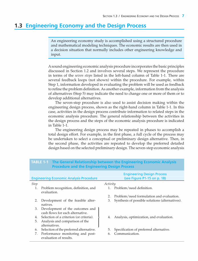
An engineering economy study is accomplished using a structured procedureand mathematical modeling techniques. The economic results are then used ina decision situation that normally includes other engineering knowledge andinput.

Asound engineering economic analysis procedure incorporates the basic principlesdiscussed in Section 1.2 and involves several steps. We represent the procedurein terms of the seven steps listed in the left-hand column of Table 1-1. There areseveral feedback loops (not shown) within the procedure. For example, withinStep 1, information developed in evaluating the problem will be used as feedbackto refine the problem definition. As another example, information from the analysisof alternatives (Step 5) may indicate the need to change one or more of them or todevelop additional alternatives.

The seven-step procedure is also used to assist decision making within theengineering design process, shown as the right-hand column in Table 1-1. In thiscase, activities in the design process contribute information to related steps in theeconomic analysis procedure. The general relationship between the activities inthe design process and the steps of the economic analysis procedure is indicatedin Table 1-1.

The engineering design process may be repeated in phases to accomplish atotal design effort. For example, in the first phase, a full cycle of the process maybe undertaken to select a conceptual or preliminary design alternative. Then, inthe second phase, the activities are repeated to develop the preferred detaileddesign based on the selected preliminary design. The seven-step economic analysis

TABLE 1-1 The General Relationship between the Engineering Economic AnalysisProcedure and the Engineering Design Process

Engineering Design ProcessEngineering Economic Analysis Procedure (see Figure P1-15 on p. 18)

Step Activity1. Problem recognition, definition, and

evaluation.1. Problem/need definition.

2. Problem/need formulation and evaluation.2. Development of the feasible alter-

natives.3. Synthesis of possible solutions (alternatives).

3. Development of the outcomes andcash flows for each alternative.

4. Selection of a criterion (or criteria).

⎫⎪⎪⎪⎪⎬⎪⎪⎪⎪⎭

4. Analysis, optimization, and evaluation.5. Analysis and comparison of the

alternatives.6. Selection of the preferred alternative. 5. Specification of preferred alternative.7. Performance monitoring and post-

evaluation of results.6. Communication.

8 CHAPTER 1 / INTRODUCTION TO ENGINEERING ECONOMY

procedure would be repeated as required to assist decision making in each phaseof the total design effort. This procedure is discussed next.

1.3.1 Problem Definition

The first step of the engineering economic analysis procedure (problem definition)is particularly important, since it provides the basis for the rest of the analysis. Aproblem must be well understood and stated in an explicit form before the projectteam proceeds with the rest of the analysis.

The term problem is used here generically. It includes all decision situations forwhich an engineering economy analysis is required. Recognition of the problem isnormally stimulated by internal or external organizational needs or requirements.An operating problem within a company (internal need) or a customer expectationabout a product or service (external requirement) are examples.

Once the problem is recognized, its formulation should be viewed from asystems perspective. That is, the boundary or extent of the situation needs tobe carefully defined, thus establishing the elements of the problem and whatconstitutes its environment.

Evaluation of the problem includes refinement of needs and requirements, andinformation from the evaluation phase may change the original formulation of theproblem. In fact, redefining the problem until a consensus is reached may be themost important part of the problem-solving process!

1.3.2 Development of Alternatives∗

The two primary actions in Step 2 of the procedure are (1) searching for potentialalternatives and (2) screening them to select a smaller group of feasible alternativesfor detailed analysis. The term feasible here means that each alternative selected forfurther analysis is judged, based on preliminary evaluation, to meet or exceed therequirements established for the situation.

1.3.2.1 Searching for Superior Alternatives In the discussion of Prin-ciple 1 (Section 1.2), creativity and resourcefulness were emphasized as beingabsolutely essential to the development of potential alternatives. The differencebetween good alternatives and great alternatives depends largely on an indi-vidual’s or group’s problem-solving efficiency. Such efficiency can be increased inthe following ways:

1. Concentrate on redefining one problem at a time in Step 1.2. Develop many redefinitions for the problem.3. Avoid making judgments as new problem definitions are created.4. Attempt to redefine a problem in terms that are dramatically different from the

original Step 1 problem definition.

∗ This is sometimes called option development. This important step is described in detail in A. B. Van Gundy, Techniquesof Structured Problem Solving, 2nd ed. (New York: Van Nostrand Reinhold Co., 1988). For additional reading, seeE. Lumsdaine and M. Lumsdaine, Creative Problem Solving—An Introductory Course for Engineering Students (New York:McGraw-Hill Book Co., 1990) and J. L. Adams, Conceptual Blockbusting—A Guide to Better Ideas (Reading, MA: Addison-Wesley Publishing Co., 1986).

SECTION 1.3 / ENGINEERING ECONOMY AND THE DESIGN PROCESS 9

5. Make sure that the true problem is well researched and understood.

In searching for superior alternatives or identifying the true problem, severallimitations invariably exist, including (1) lack of time and money, (2) preconcep-tions of what will and what will not work, and (3) lack of knowledge. Consequently,the engineer or project team will be working with less-than-perfect problemsolutions in the practice of engineering.

EXAMPLE 1-1 Defining the Problem and Developing Alternatives

The management team of a small furniture-manufacturing company is underpressure to increase profitability to get a much-needed loan from the bank topurchase a more modern pattern-cutting machine. One proposed solution is tosell waste wood chips and shavings to a local charcoal manufacturer instead ofusing them to fuel space heaters for the company’s office and factory areas.

(a) Define the company’s problem. Next, reformulate the problem in a varietyof creative ways.

(b) Develop at least one potential alternative for your reformulated problemsin Part (a). (Don’t concern yourself with feasibility at this point.)

Solution(a) The company’s problem appears to be that revenues are not sufficiently

covering costs. Several reformulations can be posed:1. The problem is to increase revenues while reducing costs.2. The problem is to maintain revenues while reducing costs.3. The problem is an accounting system that provides distorted cost

information.4. The problem is that the new machine is really not needed (and hence

there is no need for a bank loan).

(b) Based only on reformulation 1, an alternative is to sell wood chips andshavings as long as increased revenue exceeds extra expenses that maybe required to heat the buildings. Another alternative is to discontinuethe manufacture of specialty items and concentrate on standardized, high-volume products. Yet another alternative is to pool purchasing, accounting,engineering, and other white-collar support services with other small firmsin the area by contracting with a local company involved in providing theseservices.

1.3.2.2 Developing Investment Alternatives “It takes money to makemoney,” as the old saying goes. Did you know that in the United States the averagefirm spends over $250,000 in capital on each of its employees? So, to make money,each firm must invest capital to support its important human resources—butin what else should an individual firm invest? There are usually hundreds ofopportunities for a company to make money. Engineers are at the very heart ofcreating value for a firm by turning innovative and creative ideas into new or

10 CHAPTER 1 / INTRODUCTION TO ENGINEERING ECONOMY

reengineered commercial products and services. Most of these ideas require invest-ment of money, and only a few of all feasible ideas can be developed, due to lackof time, knowledge, or resources.

Consequently, most investment alternatives created by good engineering ideasare drawn from a larger population of equally good problem solutions. But howcan this larger set of equally good solutions be tapped into? Interestingly, studieshave concluded that designers and problem solvers tend to pursue a few ideas thatinvolve “patching and repairing” an old idea.∗ Truly new ideas are often excludedfrom consideration! This section outlines two approaches that have found wideacceptance in industry for developing sound investment alternatives by removingsome of the barriers to creative thinking: (1) classical brainstorming and (2) theNominal Group Technique (NGT).

(1) Classical Brainstorming. Classical brainstorming is the most well-knownand often-used technique for idea generation. It is based on the fundamentalprinciples of deferment of judgment and that quantity breeds quality. There are fourrules for successful brainstorming:

1. Criticism is ruled out.2. Freewheeling is welcomed.3. Quantity is wanted.4. Combination and improvement are sought.

A. F. Osborn lays out a detailed procedure for successful brainstorming.† Aclassicalbrainstorming session has the following basic steps:

1. Preparation. The participants are selected, and a preliminary statement of theproblem is circulated.

2. Brainstorming. A warm-up session with simple unrelated problems isconducted, the relevant problem and the four rules of brainstorming arepresented, and ideas are generated and recorded using checklists and othertechniques if necessary.

3. Evaluation. The ideas are evaluated relative to the problem.

Generally, a brainstorming group should consist of four to seven people, althoughsome suggest larger groups.

(2) Nominal Group Technique. The NGT, developed by Andre P. Delbecqand Andrew H. Van de Ven,‡ involves a structured group meeting designed toincorporate individual ideas and judgments into a group consensus. By correctlyapplying the NGT, it is possible for groups of people (preferably, 5 to 10) to generateinvestment alternatives or other ideas for improving the competitiveness of the

∗ S. Finger and J. R. Dixon, “A Review of Research in Mechanical Engineering Design. Part I: Descriptive, Prescriptive,and Computer-Based Models of Design Processes,” in Research in Engineering Design (New York: Springer-Verlag, 1990).† A. F. Osborn, Applied Imagination, 3rd ed. (New York: Charles Scribner’s Sons, 1963). Also refer to P. R. Scholtes,B. L. Joiner, and B. J. Streibel, The Team Handbook, 2nd ed. (Madison, WI: Oriel Inc., 1996).‡ A. Van de Ven and A. Delbecq, “The Effectiveness of Nominal, Delphi, and Interactive Group Decision MakingProcesses,” Academy of Management Journal 17, no. 4 (December 1974): 605–21.

SECTION 1.3 / ENGINEERING ECONOMY AND THE DESIGN PROCESS 11

firm. Indeed, the technique can be used to obtain group thinking (consensus) on awide range of topics. For example, a question that might be given to the group is,“What are the most important problems or opportunities for improvement of . . .?”

The technique, when properly applied, draws on the creativity of the individualparticipants, while reducing two undesirable effects of most group meetings: (1) thedominance of one or more participants and (2) the suppression of conflicting ideas.The basic format of an NGT session is as follows:

1. Individual silent generation of ideas2. Individual round-robin feedback and recording of ideas3. Group clarification of each idea4. Individual voting and ranking to prioritize ideas5. Discussion of group consensus results

The NGT session begins with an explanation of the procedure and a statementof question(s), preferably written by the facilitator.∗ The group members arethen asked to prepare individual listings of alternatives, such as investmentideas or issues that they feel are crucial for the survival and health of theorganization. This is known as the silent-generation phase. After this phase hasbeen completed, the facilitator calls on each participant, in round-robin fashion,to present one idea from his or her list (or further thoughts as the round-robinsession is proceeding). Each idea (or opportunity) is then identified in turn andrecorded on a flip chart or board by the NGT facilitator, leaving ample spacebetween ideas for comments or clarification. This process continues until all theopportunities have been recorded, clarified, and displayed for all to see. At thispoint, a voting procedure is used to prioritize the ideas or opportunities. Finally,voting results lead to the development of group consensus on the topic beingaddressed.

1.3.3 Development of Prospective Outcomes

Step 3 of the engineering economic analysis procedure incorporates Principles 2, 3,and 4 from Section 1.2 and uses the basic cash-flow approach employed in engineeringeconomy. A cash flow occurs when money is transferred from one organizationor individual to another. Thus, a cash flow represents the economic effects of analternative in terms of money spent and received.

Consider the concept of an organization having only one “window” to itsexternal environment through which all monetary transactions occur—receiptsof revenues and payments to suppliers, creditors, and employees. The key todeveloping the related cash flows for an alternative is estimating what wouldhappen to the revenues and costs, as seen at this window, if the particularalternative were implemented. The net cash flow for an alternative is the differencebetween all cash inflows (receipts or savings) and cash outflows (costs or expenses)during each time period.

∗ A good example of the NGT is given in D. S. Sink, “Using the Nominal Group Technique Effectively,” NationalProductivity Review, 2 (Spring 1983): 173–84.

12 CHAPTER 1 / INTRODUCTION TO ENGINEERING ECONOMY

In addition to the economic aspects of decision making, nonmonetary factors(attributes) often play a significant role in the final recommendation. Examplesof objectives other than profit maximization or cost minimization that can beimportant to an organization include the following:

1. Meeting or exceeding customer expectations2. Safety to employees and to the public3. Improving employee satisfaction4. Maintaining production flexibility to meet changing demands5. Meeting or exceeding all environmental requirements6. Achieving good public relations or being an exemplary member of the

community

1.3.4 Selection of a Decision Criterion

The selection of a decision criterion (Step 4 of the analysis procedure) incorporatesPrinciple 5 (consider all relevant criteria). The decision maker will normally selectthe alternative that will best serve the long-term interests of the owners of theorganization. It is also true that the economic decision criterion should reflecta consistent and proper viewpoint (Principle 3) to be maintained throughout anengineering economy study.

1.3.5 Analysis and Comparison of Alternatives

Analysis of the economic aspects of an engineering problem (Step 5) is largelybased on cash-flow estimates for the feasible alternatives selected for detailed study.A substantial effort is normally required to obtain reasonably accurate forecasts ofcash flows and other factors in view of, for example, inflationary (or deflationary)pressures, exchange rate movements, and regulatory (legal) mandates that oftenoccur. Clearly, the consideration of future uncertainties (Principle 6) is an essentialpart of an engineering economy study. When cash flow and other required estimatesare eventually determined, alternatives can be compared based on their differencesas called for by Principle 2. Usually, these differences will be quantified in terms ofa monetary unit such as dollars.

1.3.6 Selection of the Preferred Alternative

When the first five steps of the engineering economic analysis procedure have beendone properly, the preferred alternative (Step 6) is simply a result of the total effort.Thus, the soundness of the technical-economic modeling and analysis techniquesdictates the quality of the results obtained and the recommended course of action.Step 6 is included in Activity 5 of the engineering design process (specification ofthe preferred alternative) when done as part of a design effort.

1.3.7 Performance Monitoring and Postevaluation of Results

This final step implements Principle 7 and is accomplished during and after thetime that the results achieved from the selected alternative are collected. Monitoring

SECTION 1.3 / ENGINEERING ECONOMY AND THE DESIGN PROCESS 13

project performance during its operational phase improves the achievement ofrelated goals and objectives and reduces the variability in desired results. Step 7 isalso the follow-up step to a previous analysis, comparing actual results achievedwith the previously estimated outcomes. The aim is to learn how to do betteranalyses, and the feedback from postimplementation evaluation is important tothe continuing improvement of operations in any organization. Unfortunately, likeStep 1, this final step is often not done consistently or well in engineering practice;therefore, it needs particular attention to ensure feedback for use in ongoing andsubsequent studies.

EXAMPLE 1-2 Application of the Engineering Economic Analysis Procedure

A friend of yours bought a small apartment building for $100,000 in a collegetown. She spent $10,000 of her own money for the building and obtained amortgage from a local bank for the remaining $90,000. The annual mortgagepayment to the bank is $10,500. Your friend also expects that annual maintenanceon the building and grounds will be $15,000. There are four apartments (twobedrooms each) in the building that can each be rented for $360 per month.

Refer to the seven-step procedure in Table 1-1 (left-hand side) to answerthese questions:

(a) Does your friend have a problem? If so, what is it?(b) What are her alternatives? (Identify at least three.)(c) Estimate the economic consequences and other required data for the

alternatives in Part (b).(d) Select a criterion for discriminating among alternatives, and use it to advise

your friend on which course of action to pursue.(e) Attempt to analyze and compare the alternatives in view of at least one

criterion in addition to cost.(f) What should your friend do based on the information you and she have

generated?

Solution(a) A quick set of calculations shows that your friend does indeed have a

problem. Alot more money is being spent by your friend each year ($10,500 +$15,000 = $25,500) than is being received (4 × $360 × 12 = $17,280). Theproblem could be that the monthly rent is too low. She’s losing $8,220 peryear. (Now, that’s a problem!)

(b) Option (1). Raise the rent. (Will the market bear an increase?)Option (2). Lower maintenance expenses (but not so far as to cause safetyproblems).Option (3). Sell the apartment building. (What about a loss?)Option (4). Abandon the building (bad for your friend’s reputation).

(c) Option (1). Raise total monthly rent to $1,440+$R for the four apartments tocover monthly expenses of $2,125. Note that the minimum increase in rent

14 CHAPTER 1 / INTRODUCTION TO ENGINEERING ECONOMY

would be ($2,125 − $1,440)/4 = $171.25 per apartment per month (almost a50% increase!).Option (2). Lower monthly expenses to $2,125 − $C so that these expensesare covered by the monthly revenue of $1,440 per month. This would haveto be accomplished primarily by lowering the maintenance cost. (There’snot much to be done about the annual mortgage cost unless a favorablerefinancing opportunity presents itself.) Monthly maintenance expenseswould have to be reduced to ($1,440 − $10,500/12) = $565. This representsmore than a 50% decrease in maintenance expenses.Option (3). Try to sell the apartment building for $X, which recovers theoriginal $10,000 investment and (ideally) recovers the $685 per month loss($8,220 ÷ 12) on the venture during the time it was owned.Option (4). Walk away from the venture and kiss your investment good-bye.The bank would likely assume possession through foreclosure and may tryto collect fees from your friend. This option would also be very bad for yourfriend’s credit rating.

(d) One criterion could be to minimize the expected loss of money. In this case,you might advise your friend to pursue Option (1) or (3).

(e) For example, let’s use “credit worthiness” as an additional criterion. Option(4) is immediately ruled out. Exercising Option (3) could also harm yourfriend’s credit rating. Thus, Options (1) and (2) may be her only realistic andacceptable alternatives.

(f) Your friend should probably do a market analysis of comparable housingin the area to see if the rent could be raised (Option 1). Maybe a fresh coatof paint and new carpeting would make the apartments more appealingto prospective renters. If so, the rent can probably be raised while keeping100% occupancy of the four apartments.

A tip to the wise—as an aside to Example 1-2, your friend would need a good creditreport to get her mortgage approved. In this regard, there are three major creditbureaus in the United States: Equifax, Experian, and TransUnion. It’s a good idea toregularly review your own credit report for unauthorized activity. You are entitledto a free copy of your report once per year from each bureau. Consider getting areport every four months from www.annualcreditreport.com.

EXAMPLE 1-3 Get Rid of the Old Clunker?

Engineering economy is all about deciding among competing alternatives. Whenthe time value of money is NOT a key ingredient in a problem, Chapter 2 shouldbe referenced. If the time value of money (e.g., an interest rate) is integral to anengineering problem, Chapter 4 (and beyond) provides an explanation of howto analyze these problems.

Consider this situation: Linda and Jerry are faced with a car replacementopportunity where an interest rate can be ignored. Jerry’s old clunker that

SECTION 1.5 / TRY YOUR SKILLS 15

averages 10 miles per gallon (mpg) of gasoline can be traded in toward a vehiclethat gets 15 mpg. Or, as an alternative, Linda’s 25 mpg car can be traded intoward a new hybrid vehicle that averages 50 mpg. If they drive both cars 12,000miles per year and their goal is to minimize annual gas consumption, which carshould be replaced—Jerry’s or Linda’s? They can only afford to upgrade onecar at this time.

SolutionJerry’s trade-in will save (12,000 miles/year)/10 mpg − (12,000 miles/year)/15 mpg = 1,200 gallons/year − 800 gallons/year = 400 gallons/year.

Linda’s trade-in will save (12,000 miles/year)/25 mpg − (12,000 miles/year)/50 mpg = 480 gallons/year − 240 gallons/year = 240 gallons/year.Therefore, Jerry should trade in his vehicle to save more gasoline.

1.4 Using Spreadsheets in Engineering Economic AnalysisSpreadsheets are a useful tool for solving engineering economy problems. Mostengineering economy problems are amenable to spreadsheet solution for thefollowing reasons:

1. They consist of structured, repetitive calculations that can be expressed asformulas that rely on a few functional relationships.

2. The parameters of the problem are subject to change.3. The results and the underlying calculations must be documented.4. Graphical output is often required, as well as control over the format of the

graphs.

Spreadsheets allow the analyst to develop an application rapidly, without beinginundated by the housekeeping details of programming languages. They relievethe analyst of the drudgery of number crunching but still focus on problemformulation. Computer spreadsheets created in Excel are integrated throughout allchapters in this book. More on spreadsheet modeling can be found in Appendix A.

1.5 Try Your SkillsThe number in parentheses that follows each problem refers to the sectionfrom which the problem is taken. Solutions to these problems can be found inAppendix G.

1-A. For every penny that the price of gasoline goes up, the U.S. Postal Service(USPS) experiences a monthly fuel cost increase of $8 million. State whatassumptions you need to make to answer this question: “How many maildelivery vehicles does the USPS have in the United States?”

16 CHAPTER 1 / INTRODUCTION TO ENGINEERING ECONOMY

1-B. Assume that your employer is a manufacturing firm that produces severaldifferent electronic consumer products. What are five nonmonetary factors(attributes) that may be important when a significant change is considered inthe design of the current bestselling product? (1.2, 1.3)

1.6 SummaryIn this chapter, we defined engineering economy and presented the fundamentalconcepts in terms of seven basic principles (see pp. 3–6). Experience has shownthat most errors in engineering economic analyses can be traced to some violationof these principles. We will continue to stress these principles in the chapters thatfollow.

The seven-step engineering economic analysis procedure described in thischapter (see p. 7) has direct ties to the engineering design process. Following thissystematic approach will assist engineers in designing products and systems andin providing technical services that promote the economic welfare of the companythey work for. This same approach will also help you as an individual make soundfinancial decisions in your personal life.

In summary, engineering economy is a collection of problem-solving tools andtechniques that are applied to engineering, business, and environmental issues.Common, yet often complex, problems involving money are easier to understandand solve when you have a good grasp on the engineering economy approach toproblem solving and decision making. The problem-solving focus of this text willenable you to master the theoretical and applied principles of engineering economy.

ProblemsThe number in parentheses that follows each problemrefers to the section from which the problem is taken.

1-1. Stan Moneymaker needs 15 gallons ofgasoline to top off his automobile’s gas tank. If

he drives an extra eight miles (round trip) to a gasstation on the outskirts of town, Stan can save $0.10per gallon on the price of gasoline. Suppose gasolinecosts $3.90 per gallon and Stan’s car gets 25 mpg forin-town driving. Should Stan make the trip to get lessexpensive gasoline? Each mile that Stan drives createsone pound of carbon dioxide. Each pound of CO2 hasa cost impact of $0.02 on the environment. What otherfactors (cost and otherwise) should Stan consider in hisdecision making? (1.2)

1-2. The decision was made by NASA to abandonrocket-launched payloads into orbit around the earth.We must now rely on the Russians for this capability.Use the principles of engineering economy to examinethis decision. (1.2)

1-3. A typical discounted price of a AAA batteryis $0.75. It is designed to provide 1.5 volts and

1.0 amps for about an hour. Now we multiply volts andamps to obtain power of 1.5 watts from the battery. Thus,it costs $0.75 for 1.5 Watt-hours of energy. How muchwould it cost to deliver one kilo Watt-hour? How doesthis compare with the cost of energy from your localelectric utility at $0.10 per kilo Watt-hour? (1.2, 1.3)

1-4. Tyler just wrecked his new Nissan, and the acci-dent was his fault. The owner of the other vehicle gottwo estimates for the repairs: one was for $803 andthe other was for $852. Tyler is thinking of keepingthe insurance companies out of the incident to keephis driving record “clean.” Tyler’s deductible on hiscomprehensive coverage insurance is $500, and hedoes not want his premium to increase because of theaccident. In this regard, Tyler estimates that his semi-annual premium will rise by $60 if he files a claimagainst his insurance company. In view of the aboveinformation, Tyler’s initial decision is to write a personalcheck for $803 payable to the owner of the other vehicle.

PROBLEMS 17

Did Tyler make the most economical decision? Whatother options should Tyler have explored? In youranswer, be sure to state your assumptions and quantifyyour thinking. (1.3)

1-5. Henry Ford’s Model T was originallydesigned and built to run on ethanol. Today,

ethanol (190-proof alcohol) can be produced withdomestic stills for about $0.85 per gallon. Whenblended with gasoline costing $4.00 per gallon, a20% ethanol and 80% gasoline mixture costs $3.37 pergallon. Assume fuel consumption at 25 mpg and engineperformance in general are not adversely affected withthis 20–80 blend (called E20). (1.3)

a. How much money can be saved for 15,000 miles ofdriving per year?

b. How much gasoline per year is being converted ifone million people use the E20 fuel?

1-6. The Russian air force is being called on this yearto intercept storms advancing on Moscow and to seedthem with dry ice and silver iodine particles. Theidea is to make the snow drop on villages in thecountryside instead of piling up in Moscow. The cost ofthis initiative will be 180 million rubles, and the savingsin snow removal will be in the neighborhood of 300million rubles. The exchange rate is 30 rubles per dollar.Comment on the hidden costs and benefits of such aplan from the viewpoint of the villagers in terms ofdollars. (1.2)

1-7. A large electric utility company hasproposed building an $820 million combined

cycle, gas-powered plant to replace the electricgeneration capacity at one of its coal-fired facilities.Develop three other alternatives for replacing thiselectric generation capacity.

1-8. Studies have concluded that a college degree is avery good investment. Suppose that a college graduateearns about 75% more money per hour than a high-school graduate. If the lifetime earnings of a high-schoolgraduate average $1,200,000, what is the expected valueof earning a college degree? (1.3)

1-9. Automobile repair shops typically recomm-end that their customers change their oil and oil

filter every 3,000 miles. Your automobile user’s manualsuggests changing your oil every 5,000–7,000 miles. Ifyou drive your car 15,000 miles each year and an oiland filter change costs $30, how much money would

you save each year if you had this service performedevery 5,000 miles? (1.3)

1-10. Often it makes a lot of sense to spend somemoney now so you can save more money in the

future. Consider filtered water. A high-tech water filtercost about $60 and can filter 7,200 ounces of water. Thiswill save you purchasing two 20-ounce bottle of filteredwater every day, each costing $1.15. The filter will needreplacing every 6 months. How much will this filter saveyou in a year’s time?

1-11. The manufacturer of Brand A automobiletires claims that its tire can save 110 gallons of

fuel over 55,000 miles of driving, as compared to apopular competitor (Brand B). If gasoline costs $4.00 pergallon, how much per mile driven does this tire save thecustomer (Brand A versus Brand B)?

1-12. During your first month as an employee atGreenfield Industries (a large drill-bit manufac-

turer), you are asked to evaluate alternatives forproducing a newly designed drill bit on a turningmachine. Your boss’ memorandum to you haspractically no information about what the alternativesare and what criteria should be used. The same taskwas posed to a previous employee who could notfinish the analysis, but she has given you the followinginformation: An old turning machine valued at $350,000exists (in the warehouse) that can be modified for thenew drill bit. The in-house technicians have givenan estimate of $40,000 to modify this machine, andthey assure you that they will have the machine readybefore the projected start date (although they havenever done any modifications of this type). It is hopedthat the old turning machine will be able to meetproduction requirements at full capacity. An outsidecompany, McDonald Inc., made the machine sevenyears ago and can easily do the same modificationsfor $60,000. The cooling system used for this machineis not environmentally safe and would require somedisposal costs. McDonald Inc. has offered to build a newturning machine with more environmental safeguardsand higher capacity for a price of $450,000. McDonaldInc. has promised this machine before the startup dateand is willing to pay any late costs. Your company has$100,000 set aside for the start-up of the new productline of drill bits. For this situation,

a. Define the problem.

b. List key assumptions.

c. List alternatives facing Greenfield Industries.

d. Select a criterion for evaluation of alternatives.

18 CHAPTER 1 / INTRODUCTION TO ENGINEERING ECONOMY

e. Introduce risk into this situation.

f. Discuss how nonmonetary considerations mayimpact the selection.

g. Describe how a postaudit could be performed.

1-13. The Almost-Graduating Senior Problem. Considerthis situation faced by a first-semester senior in civilengineering who is exhausted from extensive jobinterviewing and penniless from excessive partying.Mary’s impulse is to accept immediately a highlyattractive job offer to work in her brother’s successfulmanufacturing company. She would then be able torelax for a year or two, save some money, and thenreturn to college to complete her senior year andgraduate. Mary is cautious about this impulsive desire,because it may lead to no college degree at all!

a. Develop at least two formulations for Mary’sproblem.

b. Identify feasible solutions for each problemformulation in Part (a). Be creative!

1-14. While studying for the engineering economy finalexam, you and two friends find yourselves craving afresh pizza. You can’t spare the time to pick up the pizzaand must have it delivered. “Pick-Up-Sticks” offers a1-1/4-inch-thick (including toppings), 20-inch squarepizza with your choice of two toppings for $15 plus 5%sales tax and a $1.50 delivery charge (no sales tax on

Recognition ofa problem to

be solved

Completelyspecifiedsolution

Thedesignprocess

Needs definition

Problem formulation

Possible solutions

Analysis

Communication

Specification(preferred alternative)

Figure P1-15 Figure for Problem 1-15

delivery charge). “Fred’s” offers the round, deep-dishSasquatch, which is 20 inches in diameter. It is 1-3/4inches thick, includes two toppings, and costs $17.25plus 5% sales tax and free delivery.

a. What is the problem in this situation? Please state itin an explicit and precise manner.

b. Systematically apply the seven principles ofengineering economy (pp. 3–6) to the problem youhave defined in Part (a).

c. Assuming that your common unit of measure isdollars (i.e., cost), what is the better value for gettinga pizza based on the criterion of minimizing cost perunit of volume?

d. What other criteria might be used to select whichpizza to purchase?

1-15. Storm doors have been installed on 50%of all homes in Anytown, USA. The remaining

50% of homeowners without storm doors think theymay have a problem that a storm door could solve,but they’re not sure. Use Activities 1, 2, and 3in the engineering design process (Table 1-1) to helpthese homeowners systematically think through thedefinition of their need (Activity 1), a formal statementof their problem (Activity 2), and the generation ofalternatives (Activity 3).

PROBLEMS 19

The design process begins in Figure P1-15 with astatement of need and terminates with the specificationsfor a means of fulfilling that need.

1-16. Extended Learning Exercise.Bad news: You have just wrecked your car! You needanother car immediately because you have decidedthat walking, riding a bike, and taking a bus arenot acceptable. An automobile wholesaler offers you$2,000 for your wrecked car “as is.” Also, yourinsurance company’s claims adjuster estimates thatthere is $2,000 in damages to your car. Because youhave collision insurance with a $1,000 deductibilityprovision, the insurance company mails you a checkfor $1,000. The odometer reading on your wrecked caris 58,000 miles.

What should you do? Use the seven-step procedurefrom Table 1-1 to analyze your situation. Also, identifywhich principles accompany each step.

1-17. “What you do at work is your boss’ business” isa timely warning for all employees to heed. Last year,your company installed a new computer surveillanceprogram in an effort to improve office productivity.As a courtesy, all employees were informed of thischange. The license for the software costs $30,000per year. After a year of use, productivity has risen 10%,which translates into a savings of $30,000. Discuss otherfactors, in addition to productivity, that could have beenused to justify the surveillance software.

1-18. Owing to the rising cost of copper, in 1982 theU.S. Mint changed the composition of pennies from 95%copper (and 5% zinc) to 2.5% copper (and 97.5% zinc) tosave money. Your favorite aunt has a collection of 5,000

pennies minted before 1982, and she intends on giftingthe collection to you.

a. What is the collection’s value based on metal contentalone? Copper sells for $3.50 per pound and zinc for$1 per pound. It takes approximately 130 pre-1982pennies to add up to one pound of total weight.

b. If it cost the U.S. Mint $0.017 to produce a penny in2012, is it time to eliminate pennies and round off allfinancial transactions to the nearest 5 cents (nickel)?As a matter of interest, it cost the government almost10 cents to produce a nickel in 2012.

1-19. A home mortgage is “under water” when theamount of money owed on it is much greater than(say, twice) the market value of the home. Discuss theeconomic and ethical issues of walking away from (i.e.,defaulting on) an underwater loan. Assume you have$10,000 equity in the home and your monthly paymentsare $938. (1.3)

1-20. A deep-water oil rig has just collapsedinto the Gulf of Mexico. Its blowout-preventer

system has failed, so thousands of barrels of crudeoil each day are gushing into the ocean. List somealternatives for stopping the unchecked flow of oil intothe Gulf. (1.3)

1-21. Energy can be conserved when your homeheating/cooling system works less during the

heating and cooling seasons. In fact a one degreeFahrenheit difference in your thermostat setting canreduce energy consumption by up to 5%. Identify theassumptions necessary to make this statement valid forheating and cooling a 2,000 square foot home. (1.3)

CHAPTER 2

Cost Concepts and DesignEconomics

The objective of Chapter 2 is to analyze short-term alternatives when thetime value of money is not a factor. We accomplish this with three types ofproblems: 1) economic breakeven analysis; 2) cost-driven designoptimization; and 3) present economy studies.

The A380 Superjumbo’s Breakeven Point

W hen Europe’s Airbus Company approved the A380 program in 2000,it was estimated that only 250 of the giant, 555-seat aircraft needed tobe sold to break even. The program was initially based on expected

deliveries of 751 aircraft over its life cycle. Long delays and mounting costs,however, have dramatically changed the original breakeven figure. In 2005, thisfigure was updated to 270 aircraft. According to an article in the Financial Times(October 20, 2006, p. 18), Airbus would have to sell 420 aircraft to break even—a 68% increase over the original estimate. To date, only 262 firm orders for theaircraft have been received. The topic of breakeven analysis is an integral part ofthis chapter.

20

The correct solution to any problem depends primarily on a trueunderstanding of what the problem really is.

—Arthur M. Wellington (1887)

2.1 Cost TerminologyThere are a variety of costs to be considered in an engineering economic analysis.∗These costs differ in their frequency of occurrence, relative magnitude, and degreeof impact on the study. In this section, we define a number of cost categories andillustrate how they should be treated in an engineering economic analysis.

2.1.1 Fixed, Variable, and Incremental Costs

Fixed costs are those unaffected by changes in activity level over a feasible rangeof operations for the capacity or capability available. Typical fixed costs includeinsurance and taxes on facilities, general management and administrative salaries,license fees, and interest costs on borrowed capital.

Of course, any cost is subject to change, but fixed costs tend to remain constantover a specific range of operating conditions. When larger changes in usage ofresources occur, or when plant expansion or shutdown is involved, fixed costs canbe affected.

Variable costs are those associated with an operation that varies in total withthe quantity of output or other measures of activity level. For example, the costsof material and labor used in a product or service are variable costs, because theyvary in total with the number of output units, even though the costs per unit staythe same.

An incremental cost (or incremental revenue) is the additional cost (or revenue)that results from increasing the output of a system by one (or more) units.Incremental cost is often associated with “go–no go” decisions that involve a limitedchange in output or activity level. For instance, the incremental cost per mile fordriving an automobile may be $0.49, but this cost depends on considerations suchas total mileage driven during the year (normal operating range), mileage expectedfor the next major trip, and the age of the automobile. Also, it is common to readabout the “incremental cost of producing a barrel of oil” and “incremental cost tothe state for educating a student.” As these examples indicate, the incremental cost(or revenue) is often quite difficult to determine in practice.

EXAMPLE 2-1 Fixed and Variable Costs

In connection with surfacing a new highway, a contractor has a choice of two siteson which to set up the asphalt-mixing plant equipment. The contractor estimatesthat it will cost $2.75 per cubic yard mile (yd3-mile) to haul the asphalt-pavingmaterial from the mixing plant to the job location. Factors relating to the twomixing sites are as follows (production costs at each site are the same):

∗ For the purposes of this book, the words cost and expense are used interchangeably.

21

22 CHAPTER 2 / COST CONCEPTS AND DESIGN ECONOMICS

Cost Factor Site A Site B

Average hauling distance 4 miles 3 milesMonthly rental of site $2,000 $7,000Cost to set up and remove equipment $15,000 $50,000Hauling expense $2.75/yd3-mile $2.75/yd3-mileFlagperson Not required $150/day

The job requires 50,000 cubic yards of mixed-asphalt-paving material. It isestimated that four months (17 weeks of five working days per week) will berequired for the job. Compare the two sites in terms of their fixed, variable, andtotal costs. Assume that the cost of the return trip is negligible. Which is thebetter site? For the selected site, how many cubic yards of paving material doesthe contractor have to deliver before starting to make a profit if paid $12 percubic yard delivered to the job location?

SolutionThe fixed and variable costs for this job are indicated in the table shown next. Siterental, setup, and removal costs (and the cost of the flagperson at Site B) wouldbe constant for the total job, but the hauling cost would vary in total amountwith the distance and thus with the total output quantity of yd3-miles (x).

Cost Fixed Variable Site A Site B

Rent√ = $8,000 = $28,000

Setup/removal√ = 15,000 = 50,000

Flagperson√ = 0 5(17)($150) = 12,750

Hauling√

4(50,000)($2.75) = 550,000 3(50,000)($2.75) = 412,500

Total: $573,000 $503,250

Site B, which has the larger fixed costs, has the smaller total cost for thejob. Note that the extra fixed costs of Site B are being “traded off” for reducedvariable costs at this site.

The contractor will begin to make a profit at the point where total revenueequals total cost as a function of the cubic yards of asphalt pavement mixdelivered. Based on Site B, we have

3($2.75) = $8.25 in variable cost per yd3 delivered

Total cost = total revenue

$90,750 + $8.25x = $12x

x = 24,200 yd3 delivered.

Therefore, by using Site B, the contractor will begin to make a profit on thejob after delivering 24,200 cubic yards of material.

SECTION 2.1 / COST TERMINOLOGY 23

2.1.2 Direct, Indirect, and Standard Costs

These frequently encountered cost terms involve most of the cost elements thatalso fit into the previous overlapping categories of fixed and variable costs. Directcosts are costs that can be reasonably measured and allocated to a specific outputor work activity. The labor and material costs directly associated with a product,service, or construction activity are direct costs. For example, the materials neededto make a pair of scissors would be a direct cost.

Indirect costs are costs that are difficult to allocate to a specific output or workactivity. Normally, they are costs allocated through a selected formula (such asproportional to direct labor hours, direct labor dollars, or direct material dollars)to the outputs or work activities. For example, the costs of common tools, generalsupplies, and equipment maintenance in a plant are treated as indirect costs.

Overhead consists of plant operating costs that are not direct labor or directmaterial costs. In this book, the terms indirect costs, overhead, and burden areused interchangeably. Examples of overhead include electricity, general repairs,property taxes, and supervision. Administrative and selling expenses are usuallyadded to direct costs and overhead costs to arrive at a unit selling price for a productor service. (Appendix 2-A provides a more detailed discussion of cost accountingprinciples.)

Standard costs are planned costs per unit of output that are established inadvance of actual production or service delivery. They are developed fromanticipated direct labor hours, materials, and overhead categories (with theirestablished costs per unit). Because total overhead costs are associated with a certainlevel of production, this is an important condition that should be remembered whendealing with standard cost data (for example, see Section 2.4.2). Standard costs playan important role in cost control and other management functions. Some typicaluses are the following:

1. Estimating future manufacturing costs2. Measuring operating performance by comparing actual cost per unit with the

standard unit cost3. Preparing bids on products or services requested by customers4. Establishing the value of work in process and finished inventories

2.1.3 Cash Cost versus Book Cost

A cost that involves payment of cash is called a cash cost (and results in a cash flow)to distinguish it from one that does not involve a cash transaction and is reflectedin the accounting system as a noncash cost. This noncash cost is often referred to as abook cost. Cash costs are estimated from the perspective established for the analysis(Principle 3, Section 1.2) and are the future expenses incurred for the alternativesbeing analyzed. Book costs are costs that do not involve cash payments but ratherrepresent the recovery of past expenditures over a fixed period of time. The mostcommon example of book cost is the depreciation charged for the use of assets suchas plant and equipment. In engineering economic analysis, only those costs thatare cash flows or potential cash flows from the defined perspective for the analysisneed to be considered. Depreciation, for example, is not a cash flow and is important in

24 CHAPTER 2 / COST CONCEPTS AND DESIGN ECONOMICS

an analysis only because it affects income taxes, which are cash flows. We discussthe topics of depreciation and income taxes in Chapter 7.

2.1.4 Sunk Cost

A sunk cost is one that has occurred in the past and has no relevance to estimates offuture costs and revenues related to an alternative course of action. Thus, a sunkcost is common to all alternatives, is not part of the future (prospective) cash flows,and can be disregarded in an engineering economic analysis. For instance, sunkcosts are nonrefundable cash outlays, such as earnest money on a house or moneyspent on a passport.

The concept of sunk cost is illustrated in the next simple example. Supposethat Joe College finds a motorcycle he likes and pays $40 as a down payment,which will be applied to the $1,300 purchase price, but which must be forfeited ifhe decides not to take the cycle. Over the weekend, Joe finds another motorcyclehe considers equally desirable for a purchase price of $1,230. For the purpose ofdeciding which cycle to purchase, the $40 is a sunk cost and thus would not enterinto the decision, except that it lowers the remaining cost of the first cycle. Thedecision then is between paying an additional $1,260 ($1,300 − $40) for the firstmotorcycle versus $1,230 for the second motorcycle.

In summary, sunk costs are irretrievable consequences of past decisions andtherefore are irrelevant in the analysis and comparison of alternatives that affect thefuture. Even though it is sometimes emotionally difficult to do, sunk costs shouldbe ignored, except possibly to the extent that their existence assists you to anticipatebetter what will happen in the future.

EXAMPLE 2-2 Sunk Costs in Replacement Analysis

A classic example of sunk cost involves the replacement of assets. Suppose thatyour firm is considering the replacement of a piece of equipment. It originallycost $50,000, is presently shown on the company records with a value of $20,000,and can be sold for an estimated $5,000. For purposes of replacement analysis,the $50,000 is a sunk cost. However, one view is that the sunk cost should beconsidered as the difference between the value shown in the company recordsand the present realizable selling price. According to this viewpoint, the sunkcost is $20,000 minus $5,000, or $15,000. Neither the $50,000 nor the $15,000,however, should be considered in an engineering economic analysis, except forthe manner in which the $15,000 may affect income taxes, which will be discussedin Chapter 9.

2.1.5 Opportunity Cost

An opportunity cost is incurred because of the use of limited resources, such that theopportunity to use those resources to monetary advantage in an alternative use isforegone. Thus, it is the cost of the best rejected (i.e., foregone) opportunity and isoften hidden or implied.

SECTION 2.1 / COST TERMINOLOGY 25

Consider a student who could earn $20,000 for working during a year, butchooses instead to go to school for a year and spend $5,000 to do so. The opportunitycost of going to school for that year is $25,000: $5,000 cash outlay and $20,000 forincome foregone. (This figure neglects the influence of income taxes and assumesthat the student has no earning capability while in school.)

EXAMPLE 2-3 Opportunity Cost in Replacement Analysis

The concept of an opportunity cost is often encountered in analyzing thereplacement of a piece of equipment or other capital asset. Let us reconsiderExample 2-2, in which your firm considered the replacement of an existing pieceof equipment that originally cost $50,000, is presently shown on the companyrecords with a value of $20,000, but has a present market value of only $5,000.For purposes of an engineering economic analysis of whether to replace theequipment, the present investment in that equipment should be considered as$5,000, because, by keeping the equipment, the firm is giving up the opportunityto obtain $5,000 from its disposal. Thus, the $5,000 immediate selling price isreally the investment cost of not replacing the equipment and is based on theopportunity cost concept.

2.1.6 Life-Cycle Cost

In engineering practice, the term life-cycle cost is often encountered. This term refersto a summation of all the costs related to a product, structure, system, or serviceduring its life span. The life cycle is illustrated in Figure 2-1. The life cycle beginswith identification of the economic need or want (the requirement) and ends withretirement and disposal activities. It is a time horizon that must be defined inthe context of the specific situation—whether it is a highway bridge, a jet enginefor commercial aircraft, or an automated flexible manufacturing cell for a factory.The end of the life cycle may be projected on a functional or an economic basis.For example, the amount of time that a structure or piece of equipment is able toperform economically may be shorter than that permitted by its physical capability.Changes in the design efficiency of a boiler illustrate this situation. The old boilermay be able to produce the steam required, but not economically enough for theintended use.

The life cycle may be divided into two general time periods: the acquisitionphase and the operation phase. As shown in Figure 2-1, each of these phases isfurther subdivided into interrelated but different activity periods.

The acquisition phase begins with an analysis of the economic need or want—the analysis necessary to make explicit the requirement for the product, structure,system, or service. Then, with the requirement explicitly defined, the otheractivities in the acquisition phase can proceed in a logical sequence. The conceptualdesign activities translate the defined technical and operational requirementsinto a preferred preliminary design. Included in these activities are developmentof the feasible alternatives and engineering economic analyses to assist in theselection of the preferred preliminary design. Also, advanced development and

26 CHAPTER 2 / COST CONCEPTS AND DESIGN ECONOMICS

Needsassessment;definition ofrequirements.

Conceptual (preliminary)design;advanceddevelopment;prototypetesting.

Detailed design;production orconstructionplanning;facilityand resourceacquisition.

Production orconstruction.

Operation orcustomer use;maintenanceand support.

Retirementand disposal.

Potential for life-cycle cost savings

Cumulativelife-cycle cost

Cumulativecommittedlife-cyclecost

Cost($)

High

0TIME

ACQUISITION PHASE OPERATION PHASE

Figure 2-1 Phases of the Life Cycle and Their Relative Cost

prototype-testing activities to support the preliminary design work occur duringthis period.

The next group of activities in the acquisition phase involves detailed designand planning for production or construction. This step is followed by the activitiesnecessary to prepare, acquire, and make ready for operation the facilities andother resources needed. Again, engineering economy studies are an essential part ofthe design process to analyze and compare alternatives and to assist in determining thefinal detailed design.

In the operation phase, the production, delivery, or construction of the enditem(s) or service and their operation or customer use occur. This phase ends withretirement from active operation or use and, often, disposal of the physical assetsinvolved. The priorities for engineering economy studies during the operationphase are (1) achieving efficient and effective support to operations, (2) determiningwhether (and when) replacement of assets should occur, and (3) projecting thetiming of retirement and disposal activities.

SECTION 2.2 / THE GENERAL ECONOMIC ENVIRONMENT 27

Figure 2-1 shows relative cost profiles for the life cycle. The greatest potentialfor achieving life-cycle cost savings is early in the acquisition phase. How much ofthe life-cycle costs for a product (for example) can be saved is dependent on manyfactors. However, effective engineering design and economic analysis during thisphase are critical in maximizing potential savings.

The cumulative committed life-cycle cost curve increases rapidly during theacquisition phase. In general, approximately 80% of life-cycle costs are “lockedin” at the end of this phase by the decisions made during requirements analysisand preliminary and detailed design. In contrast, as reflected by the cumulativelife-cycle cost curve, only about 20% of actual costs occur during the acquisitionphase, with about 80% being incurred during the operation phase.

Thus, one purpose of the life-cycle concept is to make explicit the interrelatedeffects of costs over the total life span for a product. An objective of the designprocess is to minimize the life-cycle cost—while meeting other performancerequirements—by making the right trade-offs between prospective costs duringthe acquisition phase and those during the operation phase.

The cost elements of the life cycle that need to be considered will vary withthe situation. Because of their common use, however, several basic life-cycle costcategories will now be defined.

The investment cost is the capital required for most of the activities in theacquisition phase. In simple cases, such as acquiring specific equipment, aninvestment cost may be incurred as a single expenditure. On a large, complexconstruction project, however, a series of expenditures over an extended periodcould be incurred. This cost is also called a capital investment.

Operation and maintenance cost (O&M) includes many of the recurring annualexpense items associated with the operation phase of the life cycle. The direct andindirect costs of operation associated with the five primary resource areas—people,machines, materials, energy, and information—are a major part of the costs in thiscategory.

Disposal cost includes those nonrecurring costs of shutting down the operationand the retirement and disposal of assets at the end of the life cycle. Normally,costs associated with personnel, materials, transportation, and one-time specialactivities can be expected. These costs will be offset in some instances by receiptsfrom the sale of assets with remaining market value. A classic example of a disposalcost is that associated with cleaning up a site where a chemical processing planthad been located.

2.2 The General Economic EnvironmentThere are numerous general economic concepts that must be taken into account inengineering studies. In broad terms, economics deals with the interactions betweenpeople and wealth, and engineering is concerned with the cost-effective use of

28 CHAPTER 2 / COST CONCEPTS AND DESIGN ECONOMICS

scientific knowledge to benefit humankind. This section introduces some of thesebasic economic concepts and indicates how they may be factors for considerationin engineering studies and managerial decisions.

2.2.1 Consumer and Producer Goods and Services

The goods and services that are produced and utilized may be divided convenientlyinto two classes. Consumer goods and services are those products or services thatare directly used by people to satisfy their wants. Food, clothing, homes, cars,television sets, haircuts, opera, and medical services are examples. The providersof consumer goods and services must be aware of, and are subject to, the changingwants of the people to whom their products are sold.

Producer goods and services are used to produce consumer goods and services orother producer goods. Machine tools, factory buildings, buses, and farm machineryare examples. The amount of producer goods needed is determined indirectly bythe amount of consumer goods or services that are demanded by people. However,because the relationship is much less direct than for consumer goods and services,the demand for and production of producer goods may greatly precede or lagbehind the demand for the consumer goods that they will produce.

2.2.2 Measures of Economic Worth

Goods and services are produced and desired because they have utility—thepower to satisfy human wants and needs. Thus, they may be used or consumeddirectly, or they may be used to produce other goods or services. Utility is mostcommonly measured in terms of value, expressed in some medium of exchangeas the price that must be paid to obtain the particular item.

Much of our business activity, including engineering, focuses on increasingthe utility (value) of materials and products by changing their form or location.Thus, iron ore, worth only a few dollars per ton, significantly increases in valueby being processed, combined with suitable alloying elements, and converted intorazor blades. Similarly, snow, worth almost nothing when found high in distantmountains, becomes quite valuable when it is delivered in melted form severalhundred miles away to dry southern California.

2.2.3 Necessities, Luxuries, and Price Demand

Goods and services may be divided into two types: necessities and luxuries.Obviously, these terms are relative, because, for most goods and services, what oneperson considers a necessity may be considered a luxury by another. For example,a person living in one community may find that an automobile is a necessity to getto and from work. If the same person lived and worked in a different city, adequatepublic transportation might be available, and an automobile would be a luxury. Forall goods and services, there is a relationship between the price that must be paid

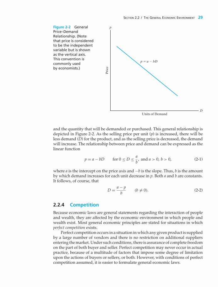
SECTION 2.2 / THE GENERAL ECONOMIC ENVIRONMENT 29

Figure 2-2 GeneralPrice–DemandRelationship. (Notethat price is consideredto be the independentvariable but is shownas the vertical axis.This convention iscommonly usedby economists.)

Units of Demand

p � a � bD

Pri

ce

p

D

and the quantity that will be demanded or purchased. This general relationship isdepicted in Figure 2-2. As the selling price per unit (p) is increased, there will beless demand (D) for the product, and as the selling price is decreased, the demandwill increase. The relationship between price and demand can be expressed as thelinear function

p = a − bD for 0 ≤ D ≤ ab

, and a > 0, b > 0, (2-1)

where a is the intercept on the price axis and −b is the slope. Thus, b is the amountby which demand increases for each unit decrease in p. Both a and b are constants.It follows, of course, that

D = a − pb

(b �= 0). (2-2)

2.2.4 Competition

Because economic laws are general statements regarding the interaction of peopleand wealth, they are affected by the economic environment in which people andwealth exist. Most general economic principles are stated for situations in whichperfect competition exists.

Perfect competition occurs in a situation in which any given product is suppliedby a large number of vendors and there is no restriction on additional suppliersentering the market. Under such conditions, there is assurance of complete freedomon the part of both buyer and seller. Perfect competition may never occur in actualpractice, because of a multitude of factors that impose some degree of limitationupon the actions of buyers or sellers, or both. However, with conditions of perfectcompetition assumed, it is easier to formulate general economic laws.

30 CHAPTER 2 / COST CONCEPTS AND DESIGN ECONOMICS

Monopoly is at the opposite pole from perfect competition. A perfect monopolyexists when a unique product or service is only available from a single supplierand that vendor can prevent the entry of all others into the market. Undersuch conditions, the buyer is at the complete mercy of the supplier in termsof the availability and price of the product. Perfect monopolies rarely occur inpractice, because (1) few products are so unique that substitutes cannot be usedsatisfactorily, and (2) governmental regulations prohibit monopolies if they areunduly restrictive.

2.2.5 The Total Revenue Function

The total revenue, TR, that will result from a business venture during a given periodis the product of the selling price per unit, p, and the number of units sold, D.Thus,

TR = price × demand = p · D. (2-3)

If the relationship between price and demand as given in Equation (2-1) is used,

TR = (a − bD)D = aD − bD2 for 0 ≤ D ≤ ab

and a > 0, b > 0. (2-4)

The relationship between total revenue and demand for the condition expressedin Equation (2-4) may be represented by the curve shown in Figure 2-3. Fromcalculus, the demand, D, that will produce maximum total revenue can be obtainedby solving

dTRdD

= a − 2bD = 0. (2-5)

Figure 2-3 TotalRevenue Functionas a Function ofDemand

Price � a � bD

Demand

Tota

l Rev

enue

D �a

2b^

Maximum TR � aD – bD2 �^ ^ a2

2b�

a2

4b�

a2

4b

SECTION 2.2 / THE GENERAL ECONOMIC ENVIRONMENT 31

Thus,∗

D = a2b

. (2-6)

It must be emphasized that, because of cost–volume relationships (discussedin the next section), most businesses would not obtain maximum profits by maximizingrevenue. Accordingly, the cost–volume relationship must be considered and relatedto revenue, because cost reductions provide a key motivation for many engineeringprocess improvements.

2.2.6 Cost, Volume, and Breakeven Point Relationships

Fixed costs remain constant over a wide range of activities, but variable costs varyin total with the volume of output (Section 2.1.1). Thus, at any demand D, totalcost is

CT = CF + CV , (2-7)

where CF and CV denote fixed and variable costs, respectively. For the linearrelationship assumed here,

CV = cv · D, (2-8)

where cv is the variable cost per unit. In this section, we consider two scenarios forfinding breakeven points. In the first scenario, demand is a function of price. Thesecond scenario assumes that price and demand are independent of each other.

Scenario 1 When total revenue, as depicted in Figure 2-3, and total cost, asgiven by Equations (2-7) and (2-8), are combined, the typical results as a functionof demand are depicted in Figure 2-4. At breakeven point D′

1, total revenue is equal

Figure 2-4 CombinedCost and Revenue Functions,and Breakeven Points, asFunctions of Volume, andTheir Effect on Typical Profit(Scenario 1)

D*

Volume (Demand)

Cos

t and

Rev

enue Profit

Maximum Profit

Loss

CV

CT

CF

D

Total Revenue

∗ To guarantee that D maximizes total revenue, check the second derivative to be sure it is negative:

d2TRdD2 = −2b.

Also, recall that in cost-minimization problems, a positively signed second derivative is necessary to guarantee aminimum-value optimal cost solution.

32 CHAPTER 2 / COST CONCEPTS AND DESIGN ECONOMICS

to total cost, and an increase in demand will result in a profit for the operation.Then at optimal demand, D∗, profit is maximized [Equation (2-10)]. At breakevenpoint D′

2, total revenue and total cost are again equal, but additional volume willresult in an operating loss instead of a profit. Obviously, the conditions for whichbreakeven and maximum profit occur are our primary interest. First, at any volume(demand), D,

Profit (loss) = total revenue − total costs

= (aD − bD2) − (CF + cvD)

= −bD2 + (a − cv)D − CF for 0 ≤ D ≤ ab

and a > 0, b > 0. (2-9)

In order for a profit to occur, based on Equation (2-9), and to achieve the typicalresults depicted in Figure 2-4, two conditions must be met:

1. (a − cv) > 0; that is, the price per unit that will result in no demand has to begreater than the variable cost per unit. (This avoids negative demand.)

2. Total revenue (TR) must exceed total cost (CT) for the period involved.

If these conditions are met, we can find the optimal demand at which maximumprofit will occur by taking the first derivative of Equation (2-9) with respect to Dand setting it equal to zero:

d(profit)dD

= a − cv − 2bD = 0.

The optimal value of D that maximizes profit is

D∗ = a − cv

2b. (2-10)

To ensure that we have maximized profit (rather than minimized it), the sign of thesecond derivative must be negative. Checking this, we find that

d2(profit)dD2 = −2b,

which will be negative for b > 0 (as specified earlier).An economic breakeven point for an operation occurs when total revenue

equals total cost. Then for total revenue and total cost, as used in the developmentof Equations (2-9) and (2-10) and at any demand D,

Total revenue = total cost (breakeven point)

aD − bD2 = CF + cvD

−bD2 + (a − cv)D − CF = 0. (2-11)

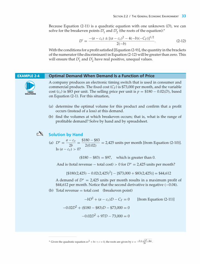
SECTION 2.2 / THE GENERAL ECONOMIC ENVIRONMENT 33

Because Equation (2-11) is a quadratic equation with one unknown (D), we cansolve for the breakeven points D′

1 and D′2 (the roots of the equation):∗

D′ = −(a − cv) ± [(a − cv)2 − 4(−b)(−CF)]1/2

2(−b). (2-12)

With the conditions for a profit satisfied [Equation (2-9)], the quantity in the bracketsof the numerator (the discriminant) in Equation (2-12) will be greater than zero. Thiswill ensure that D′

1 and D′2 have real positive, unequal values.

EXAMPLE 2-4 Optimal Demand When Demand Is a Function of Price

A company produces an electronic timing switch that is used in consumer andcommercial products. The fixed cost (CF) is $73,000 per month, and the variablecost (cv) is $83 per unit. The selling price per unit is p = $180 − 0.02(D), basedon Equation (2-1). For this situation,

(a) determine the optimal volume for this product and confirm that a profitoccurs (instead of a loss) at this demand.

(b) find the volumes at which breakeven occurs; that is, what is the range ofprofitable demand? Solve by hand and by spreadsheet.

Solution by Hand

(a) D∗ = a − cv

2b= $180 − $83

2(0.02)= 2,425 units per month [from Equation (2-10)].

Is (a − cv) > 0?

($180 − $83) = $97, which is greater than 0.

And is (total revenue − total cost) > 0 for D∗ = 2,425 units per month?

[$180(2,425) − 0.02(2,425)2] − [$73,000 + $83(2,425)] = $44,612

A demand of D∗ = 2,425 units per month results in a maximum profit of$44,612 per month. Notice that the second derivative is negative (−0.04).

(b) Total revenue = total cost (breakeven point)

−bD2 + (a − cv)D − CF = 0 [from Equation (2-11)]

−0.02D2 + ($180 − $83)D − $73,000 = 0

−0.02D2 + 97D − 73,000 = 0

∗ Given the quadratic equation ax2 + bx + c = 0, the roots are given by x = −b ±√

b2−4ac2a .

34 CHAPTER 2 / COST CONCEPTS AND DESIGN ECONOMICS

And, from Equation (2-12),

D′ = −97 ± [(97)2 − 4(−0.02)(−73,000)]0.5

2(−0.02)

D′1 = −97 + 59.74

−0.04= 932 units per month

D′2 = −97 − 59.74

−0.04= 3,918 units per month.

Thus, the range of profitable demand is 932–3,918 units per month.

Spreadsheet SolutionFigure 2-5(a) displays the spreadsheet solution for this problem. This spread-sheet calculates profit for a range of demand values (shown in column A). Fora specific value of demand, price per unit is calculated in column B by usingEquation (2-1) and Total Revenue is simply demand × price. Total Expense iscomputed by using Equations (2-7) and (2-8). Finally, Profit (column E) is thenTotal Revenue − Total Expense.

A quick inspection of the Profit column gives us an idea of the optimaldemand value as well as the breakeven points. Note that profit steadily increasesas demand increases to 2,500 units per month and then begins to drop off. Thistells us that the optimal demand value lies in the range of 2,250 to 2,750 unitsper month. A more specific value can be obtained by changing the Demand Startpoint value in cell E1 and the Demand Increment value in cell E2. For example,if the value of cell E1 is set to 2,250 and the increment in cell E2 is set to 10,the optimal demand value is shown to be between 2,420 and 2,430 units permonth.

The breakeven points lie within the ranges 750–1,000 units per month and3,750–4,000 units per month, as indicated by the change in sign of profit. Again,by changing the values in cells E1 and E2, we can obtain more exact values ofthe breakeven points.

Figure 2-5(b) is a graphical display of the Total Revenue, Total Expense,and Profit functions for the range of demand values given in column A ofFigure 2-5(a). This graph enables us to see how profit changes as demandincreases. The optimal demand value (maximum point of the profit curve)appears to be around 2,500 units per month.

Figure 2-5(b) is also a graphical representation of the breakeven points.By graphing the total revenue and total cost curves separately, we can easilyidentify the breakeven points (the intersection of these two functions). From thegraph, the range of profitable demand is approximately 1,000 to 4,000 units permonth. Notice also that, at these demand values, the profit curve crosses thex-axis ($0).

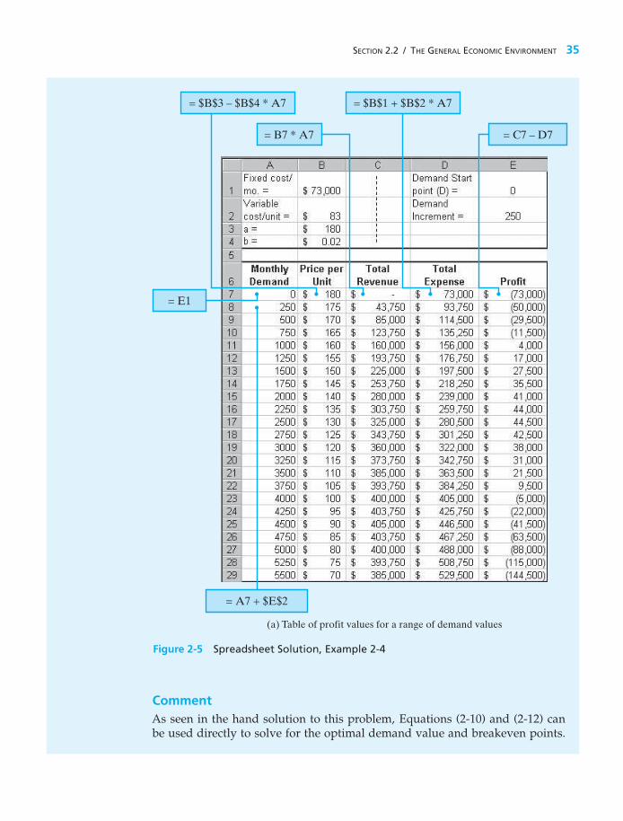
SECTION 2.2 / THE GENERAL ECONOMIC ENVIRONMENT 35

= C7 – D7= B7 * A7

= $B$1 + $B$2 * A7= $B$3 – $B$4 * A7

= A7 + $E$2

(a) Table of profit values for a range of demand values

= E1

Figure 2-5 Spreadsheet Solution, Example 2-4

CommentAs seen in the hand solution to this problem, Equations (2-10) and (2-12) canbe used directly to solve for the optimal demand value and breakeven points.

36 CHAPTER 2 / COST CONCEPTS AND DESIGN ECONOMICS

(b) Graphical display of optimal demand and breakeven values

Figure 2-5 (continued)

The power of the spreadsheet in this example is the ease with which graphicaldisplays can be generated to support your analysis. Remember, a picture reallycan be worth a thousand words. Spreadsheets also facilitate sensitivity analysis(to be discussed more fully in Chapter 11). For example, what is the impact onthe optimal demand value and breakeven points if variable costs are reducedby 10% per unit? (The new optimal demand value is increased to 2,632 units permonth, and the range of profitable demand is widened to 822 to 4,443 units permonth.)

Scenario 2 When the price per unit (p) for a product or service can berepresented more simply as being independent of demand [versus being a linearfunction of demand, as assumed in Equation (2-1)] and is greater than the variablecost per unit (cv), a single breakeven point results. Then, under the assumption thatdemand is immediately met, total revenue (TR) = p · D. If the linear relationshipfor costs in Equations (2-7) and (2-8) is also used in the model, the typical situationis depicted in Figure 2-6. This scenario is typified by the Airbus example presentedat the beginning of the chapter.

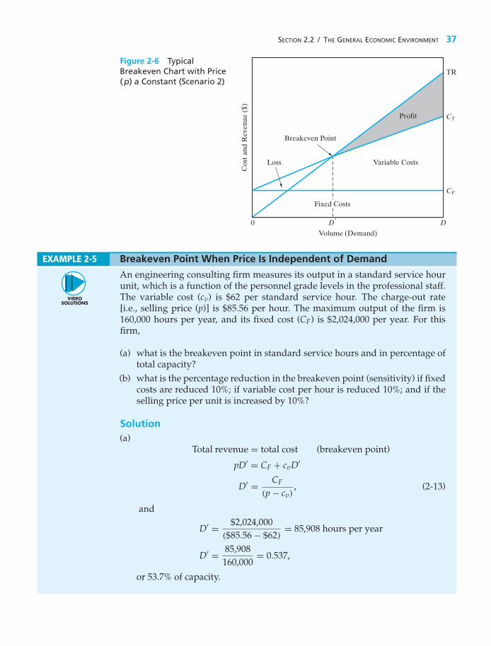
SECTION 2.2 / THE GENERAL ECONOMIC ENVIRONMENT 37

Figure 2-6 TypicalBreakeven Chart with Price( p) a Constant (Scenario 2)

Fixed Costs

Profit

Breakeven Point

CF

CT

TR

0 D

Volume (Demand)C

ost a

nd R

even

ue (

$)

Variable Costs

D�

Loss

EXAMPLE 2-5 Breakeven Point When Price Is Independent of Demand

An engineering consulting firm measures its output in a standard service hourunit, which is a function of the personnel grade levels in the professional staff.The variable cost (cv) is $62 per standard service hour. The charge-out rate[i.e., selling price (p)] is $85.56 per hour. The maximum output of the firm is160,000 hours per year, and its fixed cost (CF) is $2,024,000 per year. For thisfirm,

(a) what is the breakeven point in standard service hours and in percentage oftotal capacity?

(b) what is the percentage reduction in the breakeven point (sensitivity) if fixedcosts are reduced 10%; if variable cost per hour is reduced 10%; and if theselling price per unit is increased by 10%?

Solution(a)

Total revenue = total cost (breakeven point)

pD′ = CF + cvD′

D′ = CF

(p − cv), (2-13)

and

D′ = $2,024,000($85.56 − $62)

= 85,908 hours per year

D′ = 85,908160,000

= 0.537,

or 53.7% of capacity.

38 CHAPTER 2 / COST CONCEPTS AND DESIGN ECONOMICS

(b) A 10% reduction in CF gives

D′ = 0.9($2,024,000)

($85.56 − $62)= 77,318 hours per year

and85,908 − 77,318

85,908= 0.10,

or a 10% reduction in D′.A 10% reduction in cv gives

D′ = $2,024,000[$85.56 − 0.9($62)] = 68,011 hours per year

and85,908 − 68,011

85,908= 0.208,

or a 20.8% reduction in D′.A 10% increase in p gives

D′ = $2,024,000[1.1($85.56) − $62] = 63,021 hours per year

and85,908 − 63,021

85,908= 0.266,

or a 26.6% reduction in D′.

Thus, the breakeven point is more sensitive to a reduction in variable cost perhour than to the same percentage reduction in the fixed cost. Furthermore,notice that the breakeven point in this example is highly sensitive to the sellingprice per unit, p.

Market competition often creates pressure to lower the breakeven point ofan operation; the lower the breakeven point, the less likely that a loss willoccur during market fluctuations. Also, if the selling price remains constant(or increases), a larger profit will be achieved at any level of operation above thereduced breakeven point.

2.3 Cost-Driven Design OptimizationAs discussed in Section 2.1.6, engineers must maintain a life-cycle (i.e., “cradleto grave”) viewpoint as they design products, processes, and services. Such acomplete perspective ensures that engineers consider initial investment costs,

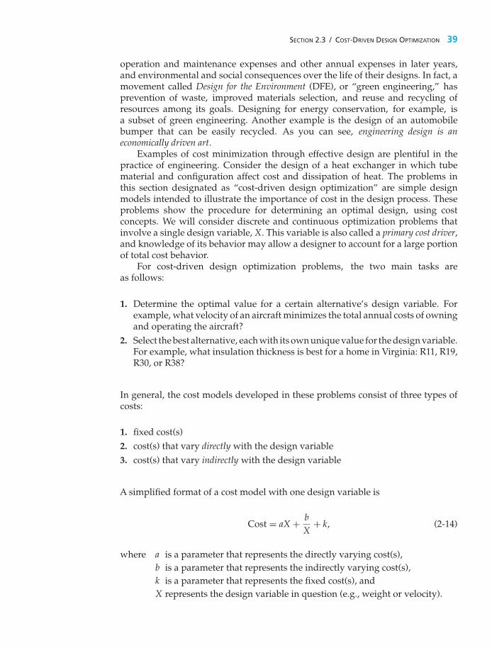
SECTION 2.3 / COST-DRIVEN DESIGN OPTIMIZATION 39

operation and maintenance expenses and other annual expenses in later years,and environmental and social consequences over the life of their designs. In fact, amovement called Design for the Environment (DFE), or “green engineering,” hasprevention of waste, improved materials selection, and reuse and recycling ofresources among its goals. Designing for energy conservation, for example, isa subset of green engineering. Another example is the design of an automobilebumper that can be easily recycled. As you can see, engineering design is aneconomically driven art.

Examples of cost minimization through effective design are plentiful in thepractice of engineering. Consider the design of a heat exchanger in which tubematerial and configuration affect cost and dissipation of heat. The problems inthis section designated as “cost-driven design optimization” are simple designmodels intended to illustrate the importance of cost in the design process. Theseproblems show the procedure for determining an optimal design, using costconcepts. We will consider discrete and continuous optimization problems thatinvolve a single design variable, X. This variable is also called a primary cost driver,and knowledge of its behavior may allow a designer to account for a large portionof total cost behavior.

For cost-driven design optimization problems, the two main tasks areas follows:

1. Determine the optimal value for a certain alternative’s design variable. Forexample, what velocity of an aircraft minimizes the total annual costs of owningand operating the aircraft?

2. Select the best alternative, each with its own unique value for the design variable.For example, what insulation thickness is best for a home in Virginia: R11, R19,R30, or R38?

In general, the cost models developed in these problems consist of three types ofcosts:

1. fixed cost(s)2. cost(s) that vary directly with the design variable3. cost(s) that vary indirectly with the design variable

A simplified format of a cost model with one design variable is

Cost = aX + bX

+ k, (2-14)

where a is a parameter that represents the directly varying cost(s),b is a parameter that represents the indirectly varying cost(s),k is a parameter that represents the fixed cost(s), andX represents the design variable in question (e.g., weight or velocity).

40 CHAPTER 2 / COST CONCEPTS AND DESIGN ECONOMICS

In a particular problem, the parameters a, b, and k may actually represent the sumof a group of costs in that category, and the design variable may be raised to somepower for either directly or indirectly varying costs.∗

The following steps outline a general approach for optimizing a design withrespect to cost:

1. Identify the design variable that is the primary cost driver (e.g., pipe diameteror insulation thickness).

2. Write an expression for the cost model in terms of the design variable.3. Set the first derivative of the cost model with respect to the continuous

design variable equal to zero. For discrete design variables, compute the valueof the cost model for each discrete value over a selected range of potentialvalues.

4. Solve the equation found in Step 3 for the optimum value of the continuousdesign variable.† For discrete design variables, the optimum value has theminimum cost value found in Step 3. This method is analogous to taking thefirst derivative for a continuous design variable and setting it equal to zero todetermine an optimal value.

5. For continuous design variables, use the second derivative of the costmodel with respect to the design variable to determine whether theoptimum value found in Step 4 corresponds to a global maximum orminimum.

EXAMPLE 2-6 How Fast Should the Airplane Fly?

The cost of operating a jet-powered commercial (passenger-carrying) airplanevaries as the three-halves (3/2) power of its velocity; specifically, CO = knv3/2,where n is the trip length in miles, k is a constant of proportionality, and v isvelocity in miles per hour. It is known that at 400 miles per hour, the averagecost of operation is $300 per mile. The company that owns the aircraft wantsto minimize the cost of operation, but that cost must be balanced againstthe cost of the passengers’ time (CC), which has been set at $300,000 perhour.

(a) At what velocity should the trip be planned to minimize the total cost, whichis the sum of the cost of operating the airplane and the cost of passengers’time?

(b) How do you know that your answer for the problem in Part (a) minimizesthe total cost?

∗ A more general model is the following: Cost = k + ax + b1xe1 + b2xe2 + · · · , where e1 = −1 reflects costs that varyinversely with X, e2 = 2 indicates costs that vary as the square of X, and so forth.† If multiple optima (stationary points) are found in Step 4, finding the global optimum value of the design variablewill require a little more effort. One approach is to systematically use each root in the second derivative equation andassign each point as a maximum or a minimum based on the sign of the second derivative. A second approach wouldbe to use each root in the objective function and see which point best satisfies the cost function.

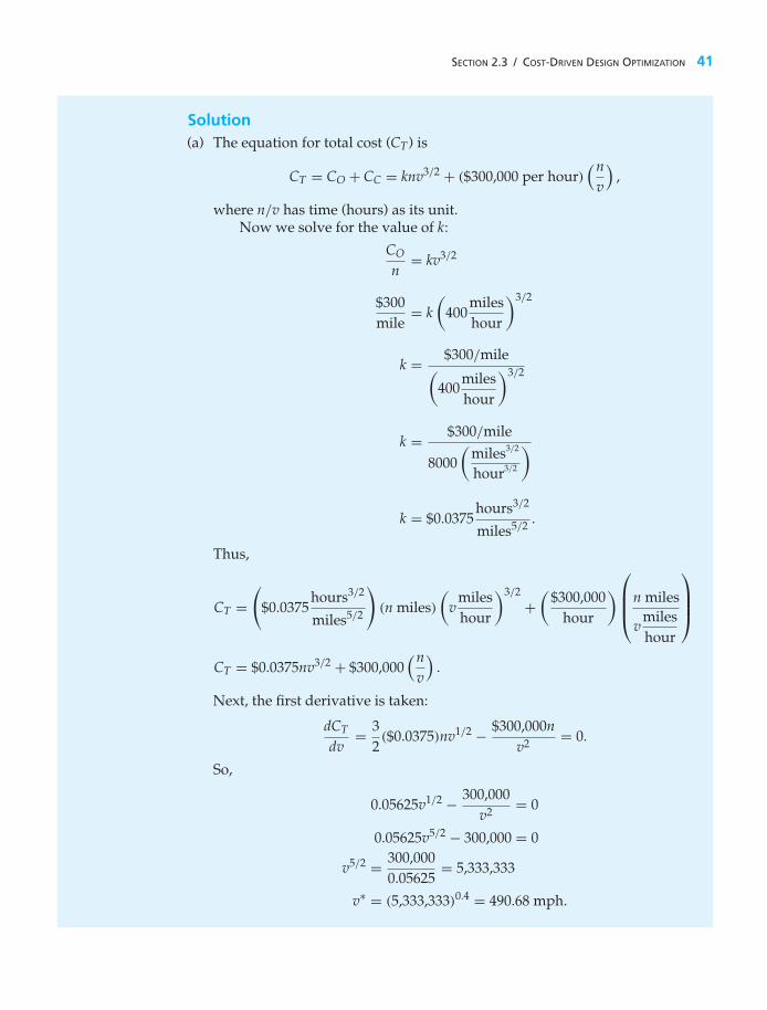
SECTION 2.3 / COST-DRIVEN DESIGN OPTIMIZATION 41

Solution(a) The equation for total cost (CT) is

CT = CO + CC = knv3/2 + ($300,000 per hour)(n

v

),

where n/v has time (hours) as its unit.Now we solve for the value of k:

CO

n= kv3/2

$300mile

= k(

400mileshour

)3/2

k = $300/mile(400

mileshour

)3/2

k = $300/mile

8000(

miles3/2

hour3/2

)

k = $0.0375hours3/2

miles5/2 .

Thus,

CT =(

$0.0375hours3/2

miles5/2

)(n miles)

(v

mileshour

)3/2

+(

$300,000hour

)⎛⎜⎜⎝n miles

vmileshour

⎞⎟⎟⎠

CT = $0.0375nv3/2 + $300,000(n

v

).

Next, the first derivative is taken:

dCT

dv= 3

2($0.0375)nv1/2 − $300,000n

v2 = 0.

So,

0.05625v1/2 − 300,000v2 = 0

0.05625v5/2 − 300,000 = 0

v5/2 = 300,0000.05625

= 5,333,333

v∗ = (5,333,333)0.4 = 490.68 mph.

42 CHAPTER 2 / COST CONCEPTS AND DESIGN ECONOMICS

(b) Finally, we check the second derivative to confirm a minimum cost solution:

d2CT

dv2 = 0.028125v1/2 + 600,000

v3 for v > 0, and therefore,d2CT

dv2 > 0.

The company concludes that v = 490.68 mph minimizes the total cost of thisparticular airplane’s flight.

EXAMPLE 2-7 Energy Savings through Increased Insulation

This example deals with a discrete optimization problem of determining the mosteconomical amount of attic insulation for a large single-story home in Virginia.In general, the heat lost through the roof of a single-story home is

Heat lossin Btu

per hour=(

� Temperaturein ◦F

)⎛⎝Areainft2

⎞⎠⎛⎝Conductance in

Btu/hour

ft2 − ◦F

⎞⎠ ,

or

Q = (Tin − Tout) · A · U.

In southwest Virginia, the number of heating days per year is approximately230, and the annual heating degree-days equals 230 (65◦F−46◦F) = 4,370 degree-days per year. Here, 65◦F is assumed to be the average inside temperature and46◦F is the average outside temperature each day.

Consider a 2,400-ft2 single-story house in Blacksburg. The typical annualspace-heating load for this size of a house is 100 × 106 Btu. That is, with noinsulation in the attic, we lose about 100 × 106 Btu per year.∗ Common sensedictates that the “no insulation” alternative is not attractive and is to be avoided.

With insulation in the attic, the amount of heat lost each year will be reduced.The value of energy savings that results from adding insulation and reducingheat loss is dependent on what type of residential heating furnace is installed.For this example, we assume that an electrical resistance furnace is installed bythe builder, and its efficiency is near 100%.

Now we’re in a position to answer the following question: What amount ofinsulation is most economical? An additional piece of data we need involves thecost of electricity, which is $0.074 per kWh. This can be converted to dollars per106 Btu as follows (1 kWh = 3,413 Btu):

kWh3,413 Btu

= 293 kWh per million Btu

∗ 100 × 106 Btu/yr ∼=(

4,370 ◦F-days per year1.00 efficiency

)(2,400 ft2)(24 hours/day)

(0.397 Btu/hr

ft2−◦F

), where 0.397 is the

U-factor with no insulation.

SECTION 2.4 / PRESENT ECONOMY STUDIES 43

293 kWh106 Btu

($0.074kWh

)∼= $21.75/106 Btu.

The cost of several insulation alternatives and associated space-heating loadsfor this house are given in the following table (an R-value indicates the resistanceto heat transfer—the higher the number the less the heat transfer):

Amount of Insulation

R11 R19 R30 R38

Investment cost ($) 600 900 1,300 1,600Annual heating load (Btu/year) 74 × 106 69.8 × 106 67.2 × 106 66.2 × 106

In view of these data, which amount of attic insulation is most economical?The life of the insulation is estimated to be 25 years.

SolutionSet up a table to examine total life-cycle costs:

R11 R19 R30 R38

A. Investment cost $600 $900 $1,300 $1,600B. Cost of heat loss per year $1,609.50 $1,518.15 $1,461.60 $1,439.85C. Cost of heat loss over 25 years $40,237.50 $37,953.75 $36,540 $35,996.25D. Total life cycle costs (A + C) $40,837.50 $38,853.75 $37,840 $37,596.25

Answer: To minimize total life-cycle costs, select R38 insulation.

CautionThis conclusion may change when we consider the time value of money (i.e., aninterest rate greater than zero) in Chapter 4. In such a case, it will not necessarilybe true that adding more and more insulation is the optimal course of action.

2.4 Present Economy StudiesWhen alternatives for accomplishing a specific task are being compared over oneyear or less and the influence of time on money can be ignored, engineering economicanalyses are referred to as present economy studies. Several situations involvingpresent economy studies are illustrated in this section. The rules, or criteria, shownnext will be used to select the preferred alternative when defect-free output (yield)is variable or constant among the alternatives being considered.

44 CHAPTER 2 / COST CONCEPTS AND DESIGN ECONOMICS

RULE 1: When revenues and other economic benefits are present and vary amongalternatives, choose the alternative that maximizes overall profitability based onthe number of defect-free units of a product or service produced.

RULE 2: When revenues and other economic benefits are not present or are constant amongall alternatives, consider only the costs and select the alternative that minimizestotal cost per defect-free unit of product or service output.

2.4.1 Total Cost in Material Selection

In many cases, economic selection among materials cannot be based solely on thecosts of materials. Frequently, a change in materials will affect the design andprocessing costs, and shipping costs may also be altered.

EXAMPLE 2-8 Choosing the Most Economic Material for a Part

A good example of this situation is illustrated by a part for which annualdemand is 100,000 units. The part is produced on a high-speed turret lathe,using 1112 screw-machine steel costing $0.30 per pound. A study was conductedto determine whether it might be cheaper to use brass screw stock, costing $1.40per pound. Because the weight of steel required per piece was 0.0353 poundsand that of brass was 0.0384 pounds, the material cost per piece was $0.0106for steel and $0.0538 for brass. However, when the manufacturing engineeringdepartment was consulted, it was found that, although 57.1 defect-free partsper hour were being produced by using steel, the output would be 102.9 defect-free parts per hour if brass were used. Which material should be used for thispart?

SolutionThe machine attendant is paid $15.00 per hour, and the variable (i.e., traceable)overhead costs for the turret lathe are estimated to be $10.00 per hour. Thus, thetotal cost comparison for the two materials is as follows:

1112 Steel Brass

Material $0.30 × 0.0353 = $0.0106 $1.40 × 0.0384 = $0.0538Labor $15.00/57.1 = 0.2627 $15.00/102.9 = 0.1458Variable overhead $10.00/57.1 = 0.1751 $10.00/102.9 = 0.0972

Total cost per piece $0.4484 $0.2968Saving per piece by use of brass = $0.4484 − $0.2968 = $0.1516

SECTION 2.4 / PRESENT ECONOMY STUDIES 45

Because 100,000 parts are made each year, revenues are constant across thealternatives. Rule 2 would select brass, and its use will produce a savings of$151.60 per thousand (a total of $15,160 for the year). It is also clear that costsother than the cost of material (such as labor and overhead) were important inthe study.

Care should be taken in making economic selections between materials toensure that any differences in shipping costs, yields, or resulting scrap are takeninto account. Commonly, alternative materials do not come in the same stock sizes,such as sheet sizes and bar lengths. This may considerably affect the yield obtainedfrom a given weight of material. Similarly, the resulting scrap may differ for variousmaterials.

In addition to deciding what material a product should be made of, there areoften alternative methods or machines that can be used to produce the product,which, in turn, can impact processing costs. Processing times may vary with themachine selected, as may the product yield. As illustrated in Example 2-9, theseconsiderations can have important economic implications.

EXAMPLE 2-9 Choosing the Most Economical Machine for Production

Two currently owned machines are being considered for the production of a part.The capital investment associated with the machines is about the same and canbe ignored for purposes of this example. The important differences between themachines are their production capacities (production rate×available productionhours) and their reject rates (percentage of parts produced that cannot be sold).Consider the following table:

Machine A Machine B

Production rate 100 parts/hour 130 parts/hourHours available for production 7 hours/day 6 hours/dayPercent parts rejected 3% 10%

The material cost is $6.00 per part, and all defect-free parts produced canbe sold for $12 each. (Rejected parts have negligible scrap value.) For eithermachine, the operator cost is $15.00 per hour and the variable overhead rate fortraceable costs is $5.00 per hour.

(a) Assume that the daily demand for this part is large enough that all defect-freeparts can be sold. Which machine should be selected?

(b) What would the percent of parts rejected have to be for Machine B to be asprofitable as Machine A?

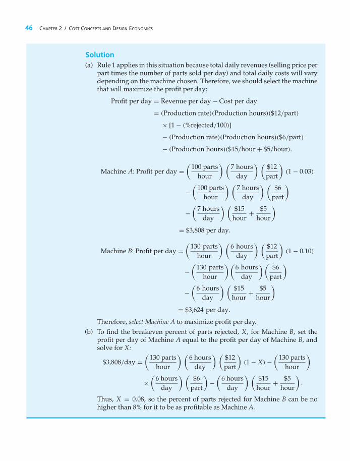
46 CHAPTER 2 / COST CONCEPTS AND DESIGN ECONOMICS

Solution(a) Rule 1 applies in this situation because total daily revenues (selling price per

part times the number of parts sold per day) and total daily costs will varydepending on the machine chosen. Therefore, we should select the machinethat will maximize the profit per day:

Profit per day = Revenue per day − Cost per day

= (Production rate)(Production hours)($12/part)

× [1 − (%rejected/100)]− (Production rate)(Production hours)($6/part)

− (Production hours)($15/hour + $5/hour).

Machine A: Profit per day =(

100 partshour

) (7 hours

day

) ($12part

)(1 − 0.03)

−(

100 partshour

) (7 hours

day

) ($6

part

)

−(

7 hoursday

) ($15

hour+ $5

hour

)= $3,808 per day.

Machine B: Profit per day =(

130 partshour

) (6 hours

day

) ($12part

)(1 − 0.10)

−(

130 partshour

)(6 hours

day

)($6

part

)

−(

6 hoursday

) ($15

hour+ $5

hour

)= $3,624 per day.

Therefore, select Machine A to maximize profit per day.(b) To find the breakeven percent of parts rejected, X, for Machine B, set the

profit per day of Machine A equal to the profit per day of Machine B, andsolve for X:

$3,808/day =(

130 partshour

) (6 hours

day

) ($12part

)(1 − X) −

(130 parts

hour

)

×(

6 hoursday

) ($6

part

)−(

6 hoursday

) ($15

hour+ $5

hour

).

Thus, X = 0.08, so the percent of parts rejected for Machine B can be nohigher than 8% for it to be as profitable as Machine A.

SECTION 2.4 / PRESENT ECONOMY STUDIES 47

2.4.2 Making versus Purchasing (Outsourcing) Studies∗

In the short run, say, one year or less, a company may consider producing an itemin-house even though the item can be purchased (outsourced) from a supplier at aprice lower than the company’s standard production costs. (See Section 2.1.2.) Thiscould occur if (1) direct, indirect, and overhead costs are incurred regardless ofwhether the item is purchased from an outside supplier and (2) the incremental costof producing an item in the short run is less than the supplier’s price. Therefore,the relevant short-run costs of make versus purchase decisions are the incrementalcosts incurred and the opportunity costs of the resources involved.

Opportunity costs may become significant when in-house manufacture ofan item causes other production opportunities to be forgone (often because ofinsufficient capacity). But in the long run, capital investments in additionalmanufacturing plant and capacity are often feasible alternatives to outsourcing.(Much of this book is concerned with evaluating the economic worthiness ofproposed capital investments.) Because engineering economy often deals withchanges to existing operations, standard costs may not be too useful in make-versus-purchase studies. In fact, if they are used, standard costs can lead to uneconomicaldecisions. Example 2-10 illustrates the correct procedure to follow in performingmake-versus-purchase studies based on incremental costs.

EXAMPLE 2-10 To Produce or Not to Produce?−−That Is the Question

A manufacturing plant consists of three departments: A, B, and C. Department Aoccupies 100 square meters in one corner of the plant. Product X is one of severalproducts being produced in Department A. The daily production of Product Xis 576 pieces. The cost accounting records show the following average dailyproduction costs for Product X:

Direct labor (1 operator working 4 hours per dayat $22.50/hr, including fringe benefits,plus a part-time foreman at $30 per day) $120.00

Direct material 86.40Overhead (at $0.82 per square meter of floor area) 82.00

Total cost per day = $288.40

The department foreman has recently learned about an outside company thatsells Product X at $0.35 per piece. Accordingly, the foreman figured a cost per dayof $0.35(576) = $201.60, resulting in a daily savings of $288.40−$201.60 = $86.80.Therefore, a proposal was submitted to the plant manager for shutting downthe production line of Product X and buying it from the outside company.

∗ Much interest has been shown in outsourcing decisions. For example, see P. Chalos, “Costing, Control, and StrategicAnalysis in Outsourcing Decisions,” Journal of Cost Management, 8, no. 4 (Winter 1995): pp. 31–37.

48 CHAPTER 2 / COST CONCEPTS AND DESIGN ECONOMICS

However, after examining each component separately, the plant managerdecided not to accept the foreman’s proposal based on the unit cost ofProduct X:

1. Direct labor: Because the foreman was supervising the manufacture of otherproducts in Department A in addition to Product X, the only possible savingsin labor would occur if the operator working 4 hours per day on Product Xwere not reassigned after this line is shut down. That is, a maximum savingsof $90.00 per day would result.

2. Materials: The maximum savings on direct material will be $86.40. However,this figure could be lower if some of the material for Product X is obtainedfrom scrap of another product.

3. Overhead: Because other products are made in Department A, no reduction intotal floor space requirements will probably occur. Therefore, no reduction inoverhead costs will result from discontinuing Product X. It has been estimatedthat there will be daily savings in the variable overhead costs traceable toProduct X of about $3.00 due to a reduction in power costs and in insurancepremiums.

SolutionIf the manufacture of Product X is discontinued, the firm will save at most$90.00 in direct labor, $86.40 in direct materials, and $3.00 in variable overheadcosts, which totals $179.40 per day. This estimate of actual cost savings perday is less than the potential savings indicated by the cost accounting records($288.40 per day), and it would not exceed the $201.60 to be paid to the outsidecompany if Product X is purchased. For this reason, the plant manager usedRule 2 and rejected the proposal of the foreman and continued the manufactureof Product X.

In conclusion, Example 2-10 shows how an erroneous decision might bemade by using the unit cost of Product X from the cost accounting recordswithout detailed analysis. The fixed cost portion of Product X’s unit cost, whichis present even if the manufacture of Product X is discontinued, was not properlyaccounted for in the original analysis by the foreman.

2.4.3 Trade-Offs in Energy Efficiency Studies

Energy efficiency affects the annual expense of operating an electrical device suchas a pump or motor. Typically, a more energy-efficient device requires a highercapital investment than does a less energy-efficient device, but the extra capitalinvestment usually produces annual savings in electrical power expenses relativeto a second pump or motor that is less energy efficient. This important trade-off between capital investment and annual electric power consumption will beconsidered in several chapters of this book. Hence, the purpose of Section 2.4.3 is

SECTION 2.5 / CASE STUDY−−THE ECONOMICS OF DAYTIME RUNNING LIGHTS 49

to explain how the annual expense of operating an electrical device is calculatedand traded off against capital investment cost.

If an electric pump, for example, can deliver a given horsepower (hp) orkilowatt (kW) rating to an industrial application, the input energy requirementis determined by dividing the given output by the energy efficiency of the device.The input requirement in hp or kW is then multiplied by the annual hours that thedevice operates and the unit cost of electric power. You can see that the higher theefficiency of the pump, the lower the annual cost of operating the device is relativeto another less-efficient pump.

EXAMPLE 2-11 Investing in Electrical Efficiency

Two pumps capable of delivering 100 hp to an agricultural application are beingevaluated in a present economy study. The selected pump will only be utilizedfor one year, and it will have no market value at the end of the year. Pertinentdata are summarized as follows:

ABC Pump XYZ Pump

Purchase price $2,900 $6,200Maintenance cost $170 $510Efficiency 80% 90%

If electric power costs $0.10 per kWh and the pump will be operated 4,000hours per year, which pump should be chosen? Recall that 1 hp = 0.746 kW.

SolutionThe expense of electric power for the ABC pump is

(100 hp/0.80)(0.746 kW/hp)($0.10/kWh)(4,000 hours/yr) = $37,300.

For the XYZ Pump, the expense of electric power is

(100 hp/0.90)(0.746 kW/hp)($0.10/kWh)(4,000 hours/yr) = $33,156.

Thus, the total cost of owning and operating the ABC pump is $40,370,while the total cost of owning and operating the XYZ pump for one year is$39,866. Consequently, the more energy-efficient XYZ pump should be selectedto minimize total cost. Notice the difference in energy expense ($4,144) thatresults from a 90% efficient pump relative to an 80% efficient pump. This costreduction more than balances the extra $3,300 in capital investment and $340 inmaintenance required for the XYZ pump.

2.5 CASE STUDY—The Economics of Daytime Running Lights

The use of Daytime Running Lights (DRLs) has increased in popularity with cardesigners throughout the world. In some countries, motorists are required to drivewith their headlights on at all times. U.S. car manufacturers now offer models

50 CHAPTER 2 / COST CONCEPTS AND DESIGN ECONOMICS

equipped with daytime running lights. Most people would agree that driving withthe headlights on at night is cost effective with respect to extra fuel consumption andsafety considerations (not to mention required by law!). Cost effective means thatbenefits outweigh (exceed) the costs. However, some consumers have questionedwhether it is cost effective to drive with your headlights on during the day.

In an attempt to provide an answer to this question, let us consider the followingsuggested data:

75% of driving takes place during the daytime.2% of fuel consumption is due to accessories (radio, headlights, etc.).Cost of fuel = $4.00 per gallon.Average distance traveled per year = 15,000 miles.Average cost of an accident = $2,800.Purchase price of headlights = $25.00 per set (2 headlights).Average time car is in operation per year = 350 hours.Average life of a headlight = 200 operating hours.Average fuel consumption = 1 gallon per 30 miles.

Let’s analyze the cost effectiveness of driving with headlights on during theday by considering the following set of questions:

• What are the extra costs associated with driving with headlights on duringthe day?

• What are the benefits associated with driving with headlights on during the day?• What additional assumptions (if any) are needed to complete the analysis?• Is it cost effective to drive with headlights on during the day?

SolutionAfter some reflection on the above questions, you could reasonably contend thatthe extra costs of driving with headlights on during the day include increasedfuel consumption and more frequent headlight replacement. Headlights increasevisibility to other drivers on the road. Another possible benefit is the reduced chanceof an accident.

Additional assumptions needed to consider during our analysis of the situationinclude:

1. the percentage of fuel consumption due to headlights alone and2. how many accidents can be avoided per unit time.

Selecting the dollar as our common unit of measure, we can compute the extracost associated with daytime use of headlights and compare it to the expectedbenefit (also measured in dollars). As previously determined, the extra costsinclude increased fuel consumption and more frequent headlight replacement.

SECTION 2.6 / TRY YOUR SKILLS 51

Let’s develop an estimate of the annual fuel cost:

Annual fuel cost = (15,000 mi/yr)(1 gal/30 mi)($4.00/gal) = $2,000/yr.

Assume (worst case) that 2% of fuel consumption is due to normal (night-time) useof headlights.

Fuel cost due to normal use of headlights = ($2,000/yr)(0.02) = $40/yr.

Fuel cost due to continuous use of headlights = (4)($40/yr) = $160/yr.

Headlight cost for normal use = (0.25)

(350 hours/yr200 hours/set

) ($25set

)= $10.94/yr.

Headlight cost for continuous use =(

350 hours/yr200 hours/set

) ($25set

)= $43.75/yr.

Total cost associated with daytime use = ($160 − $40) + ($43.75 − $10.94)

= $152.81/yr.

If driving with your headlights on during the day results in at least oneaccident being avoided during the next ($2,800)/($152.81) = 18.3 years, then thecontinuous use of your headlights is cost effective. Although in the short term,you may be able to contend that the use of DRLs lead to increased fuel andreplacement bulb costs, the benefits of increased personal safety and mitigation ofpossible accident costs in the long run more than offset the apparent short-term costsavings.

2.6 Try Your SkillsThe number in parentheses that follows each problem refers to the sectionfrom which the problem is taken. Solutions to these problems can be found inAppendix G.

2-A. A company in the process industry produces a chemical compound that issold to manufacturers for use in the production of certain plastic products.The plant that produces the compound employs approximately 300 people.Develop a list of six different cost elements that would be fixed and a similarlist of six cost elements that would be variable. (2.1)

2-B. A farmer estimates that if he harvests his soybean crop now, he will obtain1,000 bushels, which he can sell at $3.00 per bushel. However, he estimatesthat this crop will increase by an additional 1,200 bushels of soybeans foreach week he delays harvesting, but the price will drop at a rate of 50 centsper bushel per week; in addition, it is likely that he will experience spoilageof approximately 200 bushels per week for each week he delays harvesting.When should he harvest his crop to obtain the largest net cash return, andhow much will be received for his crop at that time? (2.3)

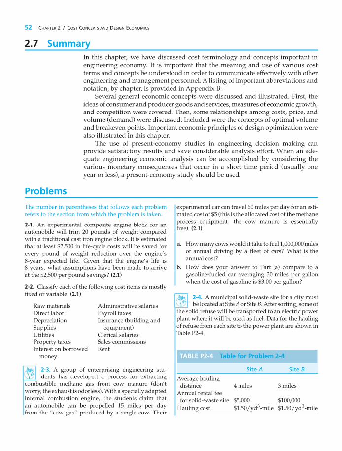
52 CHAPTER 2 / COST CONCEPTS AND DESIGN ECONOMICS

2.7 SummaryIn this chapter, we have discussed cost terminology and concepts important inengineering economy. It is important that the meaning and use of various costterms and concepts be understood in order to communicate effectively with otherengineering and management personnel. A listing of important abbreviations andnotation, by chapter, is provided in Appendix B.

Several general economic concepts were discussed and illustrated. First, theideas of consumer and producer goods and services, measures of economic growth,and competition were covered. Then, some relationships among costs, price, andvolume (demand) were discussed. Included were the concepts of optimal volumeand breakeven points. Important economic principles of design optimization werealso illustrated in this chapter.

The use of present-economy studies in engineering decision making canprovide satisfactory results and save considerable analysis effort. When an ade-quate engineering economic analysis can be accomplished by considering thevarious monetary consequences that occur in a short time period (usually oneyear or less), a present-economy study should be used.

ProblemsThe number in parentheses that follows each problemrefers to the section from which the problem is taken.

2-1. An experimental composite engine block for anautomobile will trim 20 pounds of weight comparedwith a traditional cast iron engine block. It is estimatedthat at least $2,500 in life-cycle costs will be saved forevery pound of weight reduction over the engine’s8-year expected life. Given that the engine’s life is8 years, what assumptions have been made to arriveat the $2,500 per pound savings? (2.1)

2-2. Classify each of the following cost items as mostlyfixed or variable: (2.1)

Raw materials Administrative salariesDirect labor Payroll taxesDepreciation Insurance (building andSupplies equipment)Utilities Clerical salariesProperty taxes Sales commissionsInterest on borrowed Rent

money

2-3. A group of enterprising engineering stu-dents has developed a process for extracting

combustible methane gas from cow manure (don’tworry, the exhaust is odorless). With a specially adaptedinternal combustion engine, the students claim thatan automobile can be propelled 15 miles per dayfrom the “cow gas” produced by a single cow. Their

experimental car can travel 60 miles per day for an esti-mated cost of $5 (this is the allocated cost of the methaneprocess equipment—the cow manure is essentiallyfree). (2.1)

a. How many cows would it take to fuel 1,000,000 milesof annual driving by a fleet of cars? What is theannual cost?

b. How does your answer to Part (a) compare to agasoline-fueled car averaging 30 miles per gallonwhen the cost of gasoline is $3.00 per gallon?

2-4. A municipal solid-waste site for a city mustbe located at Site A or Site B. After sorting, some of

the solid refuse will be transported to an electric powerplant where it will be used as fuel. Data for the haulingof refuse from each site to the power plant are shown inTable P2-4.

TABLE P2-4 Table for Problem 2-4

Site A Site B

Average haulingdistance 4 miles 3 miles

Annual rental feefor solid-waste site $5,000 $100,000

Hauling cost $1.50/yd3-mile $1.50/yd3-mile

PROBLEMS 53

If the power plant will pay $8.00 per cubic yard ofsorted solid waste delivered to the plant, where shouldthe solid-waste site be located? Use the city’s viewpointand assume that 200,000 cubic yards of refuse will behauled to the plant for one year only. One site must beselected. (2.1)

2-5. Stan Moneymaker presently owns a 10-year-oldautomobile with low mileage (78,000 miles). The NADA“blue book” value of the car is $2,500. Unfortunately,the car’s transmission just failed, and Stan decided tospend $1,500 to have it repaired. Now, six months later,Stan has decided to sell the car, and he reasons thathis asking price should be $2,500 + $1,500 = $4,000.Comment on the wisdom of Stan’s logic. If he receivesan offer for $3,000, should he accept it? Explain yourreasoning. (2.1)

2-6. You have been invited by friends to fly to Germanyfor Octoberfest next year. For international travel,you apply for a passport that costs $97 and is validfor 10 years. After you receive your passport, yourtravel companions decide to cancel the trip becauseof “insufficient funds.” You decide to also cancel yourtravel plans because traveling alone is no fun. Is yourpassport expense a sunk cost or an opportunity cost?Explain your answer. (2.1)

2-7. Suppose your company has just discovered$100,000 worth (this is the original manufacturing cost)of obsolete inventory in an old warehouse. Your bossasks you to evaluate two options: (1) remachine theobsolete parts at a cost of $30,000 and then hopefullyresell them for $60,000 or (2) scrap them for $15,000cash (which is certain) through a secondhand market.What recommendation would you make to your boss?Explain your reasoning. (2.1)

2-8. A friend of yours has been thinking about quittingher regular day job and going into business for herself.She currently makes $60,000 per year as an employee ofthe Ajax Company, and she anticipates no raise for atleast another year. She believes she can make $200,000as an independent consultant in six-sigma “black belt”training for large corporations. Her start-up expensesare expected to be $120,000 over the next year. If shedecides to keep her current job, what is the expectedopportunity cost of this decision? Attempt to balance thepros and cons of the option that your friend is turningaway from. (2.1)

2-9. Suppose your wealthy aunt has given you a giftof $25,000. You have come up with three optionsfor spending (or investing) the money. First, you’d

like (but do not need) a new car to brighten upyour home and social life. Second, you can investthe money in a high-tech firm’s common stock. It isexpected to increase in value by 20% per year, but thisoption is fairly risky. Third, you can put the moneyinto a three-year certificate of deposit with a local bankand earn 6% per year. There is little risk in the thirdoption. (2.1)

a. If you decide to purchase the new car, what isthe opportunity cost of this choice? Explain yourreasoning.

b. If you invest in the high-tech common stock, whatis the opportunity cost of this choice? Explain yourreasoning.

2-10. In your own words, describe the life-cycle costconcept. Why is the potential for achieving life-cyclecost savings greatest in the acquisition phase of the lifecycle? (2.1)

2-11. A large, profitable commercial airline companyflies 737-type aircraft, each with a maximum seatingcapacity of 132 passengers. Company literature statesthat the economic breakeven point with these aircraft is62 passengers. (2.2)

a. Draw a conceptual graph to show total revenue andtotal costs that this company is experiencing.

b. Identify three types of fixed costs that the airlineshould carefully examine to lower its breakevenpoint. Explain your reasoning.

c. Identify three types of variable costs that canpossibly be reduced to lower the breakeven point.Why did you select these cost items?

2-12. A lash adjuster keeps pressure constant onengine valves, thereby increasing fuel efficiency

in automobile engines. The relationship between price(p) and monthly demand (D) for lash adjusters madeby the Wicks Company is given by this equation: D =(2,000 − p)/0.10. What is the demand (D) when totalrevenue is maximized? What important data are neededif maximum profit is desired? (2.2)

2-13. A large company in the communication andpublishing industry has quantified the relationshipbetween the price of one of its products and the demandfor this product as Price = 150 − 0.01 × Demand foran annual printing of this particular product. The fixedcosts per year (i.e., per printing) = $50,000 and thevariable cost per unit = $40. What is the maximum profitthat can be achieved if the maximum expected demand

54 CHAPTER 2 / COST CONCEPTS AND DESIGN ECONOMICS

is 6,000 units per year? What is the unit price at thispoint of optimal demand? (2.2)

2-14. A large wood products company is negotiating acontract to sell plywood overseas. The fixed cost that canbe allocated to the production of plywood is $800,000per month. The variable cost per thousand board feetis $155.50. The price charged will be determined byp = $600 − (0.5)D per 1,000 board feet. (2.2)

a. For this situation, determine the optimal monthlysales volume for this product and calculate the profit(or loss) at the optimal volume.

b. What is the domain of profitable demand during amonth?

2-15. A company produces and sells a consumerproduct and is able to control the demand for theproduct by varying the selling price. The approximaterelationship between price and demand is

p = $38 + 2,700D

− 5,000D2 , for D > 1,

where p is the price per unit in dollars and D isthe demand per month. The company is seeking tomaximize its profit. The fixed cost is $1,000 per monthand the variable cost (cv) is $40 per unit. (2.2)

a. What is the number of units that should be producedand sold each month to maximize profit?

b. Show that your answer to Part (a) maximizes profit.

2-16. An electric power plant uses solid wastefor fuel in the production of electricity. The

cost Y in dollars per hour to produce electricity isY = 12 + 0.3X + 0.27X2, where X is in megawatts.Revenue in dollars per hour from the sale of electricityis 15X −0.2X2. Find the value of X that gives maximumprofit. (2.2)

2-17. The annual fixed costs for a plant are $100,000,and the variable costs are $140,000 at 70% utilization ofavailable capacity, with net sales of $280,000. What isthe breakeven point in units of production if the sellingprice per unit is $40? (2.2)

2-18. The world price of zinc has increased to the pointwhere “moth balled” zinc mines in east Tennessee havebeen reopened because of their potential profitability.(a) What is the estimated annual profit for a mineproducing 20,000 tons per year (which is at 100%capacity) when zinc sells for $1.00 per pound? Thereare variable costs of $20 million at 100% capacity andfixed costs of $17 million per year. (b) If production

is only 17,000 tons per year, will the mine beprofitable? (2.2)

2-19. A cell phone company has a fixed cost of$1,500,000 per month and a variable cost of $20 permonth per subscriber. The company charges $39.95 permonth to its cell phone customers. (2.2)

a. What is the breakeven point for this company?

b. The company currently has 73,000 subscribers andproposes to raise its monthly fees to $49.95 tocover add-on features such as text messaging, songdownloads, game playing, and video watching.What is the new breakeven point if the variable costincreases to $25 per customer per month?

c. If 10,000 subscribers will drop their service becauseof the monthly fee increase in Part (b), will thecompany still be profitable?

2-20. A plant operation has fixed costs of $2,000,000per year, and its output capacity is 100,000 electricalappliances per year. The variable cost is $40 per unit,and the product sells for $90 per unit.

a. Construct the economic breakeven chart.

b. Compare annual profit when the plant is operatingat 90% of capacity with the plant operation at 100%capacity. Assume that the first 90% of capacityoutput is sold at $90 per unit and that the remaining10% of production is sold at $70 per unit. (2.2)

2-21. A regional airline company estimated fouryears ago that each pound of aircraft weight adds

$30 per year to its fuel expense. Now the cost of jet fuelhas doubled from what it was four years ago. A recentengineering graduate employed by the company hasmade a recommendation to reduce fuel consumption ofan aircraft by installing leather seats as part of a “cabinrefurbishment program.” The total reduction in weightwould be approximately 600 pounds per aircraft. Ifseats are replaced annually (a worst-case situation),how much can this airline afford to spend on the cabinrefurbishments? What nonmonetary advantages mightbe associated with the refurbishments? Would yousupport the engineer’s recommendation? (2.1)

2-22. Jerry Smith’s residential air conditioning(AC) system has not been able to keep his house

cool enough in 90◦F weather. He called his local ACmaintenance person, who discovered a leak in theevaporator. The cost to recharge the AC unit is $40 forgas and $45 for labor, but the leak will continue andperhaps grow worse. The AC person cautioned that this

PROBLEMS 55

service would have to be repeated each year unless theevaporator is replaced. A new evaporator would runabout $800–$850.

Jerry reasons that fixing the leak in the evaporatoron an annual basis is the way to go. “After all, it willtake 10 years of leak repairs to equal the evaporator’sreplacement cost.” Comment on Jerry’s logic. Whatwould you do? (2.1)

2-23. Ethanol blended with gasoline can be usedto power a “flex-fueled” car. One particular blend

that is gaining in popularity is E85, which is 85%ethanol and 15% gasoline. E85 is 80% cleaner burningthan gasoline alone, and it reduces our dependency onforeign oil. But a flex-fueled car costs $1,000 more thana conventional gasoline-fueled car. Additionally, E85fuel gets 10% less miles per gallon than a conventionalautomobile.

Consider a 100% gasoline-fueled car that averages30 miles per gallon. The E85-fueled car will averageabout 27 miles per gallon. If either car will be driven81,000 miles before being traded in, how much willthe E85 fuel have to cost (per gallon) to make the flex-fueled car as economically attractive as a conventionalgasoline-fueled car? Gasoline costs $3.89 per gallon.Work this problem without considering the time valueof money. (2.1)

2-24. The fixed cost for a steam line per meter ofpipe is $450X + $50 per year. The cost for loss of

heat from the pipe per meter is $4.8/X1/2 per year. Here,X represents the thickness of insulation in meters, andX is a continuous design variable. (2.3)

a. What is the optimum thickness of the insulation?

b. How do you know that your answer in Part (a)minimizes total cost per year?

c. What is the basic trade-off being made in thisproblem?

2-25. The fixed costs incurred by a small geneticsresearch lab are $200,000 per year. Variable costs are 60%of the annual revenue. If annual revenue is $300,000, theannual profit (loss) is most nearly (2.2):

(a) $66,000 profit (b) ($66,000) loss(c) $80,000 profit (d) ($80,000) loss

2-26. The cost of operating a large ship (CO) varies asthe square of its velocity (v); specifically, CO = knv2,where n is the trip length in miles and k is a constant ofproportionality. It is known that at 12 miles/hour, theaverage cost of operation is $100 per mile. The owner of

the ship wants to minimize the cost of operation, butit must be balanced against the cost of the perishablecargo (Cc), which the customer has set at $1,500 perhour. At what velocity should the trip be planned tominimize the total cost (CT ), which is the sum of thecost of operating the ship and the cost of perishablecargo? (2.3)

2-27. Refer to Example 2-7 on pages 42–43. Whichalternative (insulation thickness) would be mosteconomical if the cost of insulation triples? Show allyour work. (2.3)

2-28. According to the U.S. Department of theInterior, the amount of energy lost because of

poorly insulated homes is equivalent to 2 million barrelsof oil per day. In 2009, this is more oil than the UnitedStates imports from Saudi Arabia each day. If we were toinsulate our homes as determined by Example 2-7, wecould eliminate our oil dependence on Saudi Arabia.If the cost of electricity increases to $0.15 per kWh andthe cost of insulation quadruples, how much insulationshould be chosen in Example 2-7? (2.3)

2-29. One component of a system’s life-cycle cost isthe cost of system failure. Failure costs can be reducedby designing a more reliable system. A simplifiedexpression for system life-cycle cost, C, can be writtenas a function of the system’s failure rate:

C = CIλ

+ CR · λ · t.

Here, CI = investment cost ($ per hour per failure),CR = system repair cost,λ = system failure rate(failures/operating hour),t = operating hours.

a. Assume that CI , CR, and t are constants. Derive anexpression for λ, say λ∗, that optimizes C. (2.3)

b. Does the equation in Part (a) correspond to amaximum or minimum value of C? Show all workto support your answer.

c. What trade-off is being made in this problem?

2-30. Stan Moneymaker has been shopping fora new car. He is interested in a certain 4-cylinder

sedan that averages 28 miles per gallon. But the sales-person tried to persuade Stan that the 6-cylinder modelof the same automobile only costs $2,500 more and isreally a “more sporty and responsive” vehicle. Stan isimpressed with the zip of the 6-cylinder car and reasonsthat $2,500 is not too much to pay for the extra power.

56 CHAPTER 2 / COST CONCEPTS AND DESIGN ECONOMICS

How much extra is Stan really paying if the6-cylinder car averages 22 miles per gallon? Assumethat Stan will drive either automobile 100,000 miles,gasoline will average $4.00 per gallon, and maintenanceis roughly the same for both cars. State other assum-ptions you think are appropriate. (2.4)

2-31. A producer of synthetic motor oil forautomobiles and light trucks has made the

following statement: “One quart of Dynolube added toyour next oil change will increase fuel mileage by onepercent. This one-time additive will improve your fuelmileage over 50,000 miles of driving.” (2.4)

a. Assume the company’s claim is correct. How muchmoney will be saved by adding one quart ofDynolube if gasoline costs $4.00 per gallon andyour car averages 20 miles per gallon without theDynolube?

b. If a quart of Dynolube sells for $19.95, would youuse this product in your automobile?

2-32. An automobile dealership offers to fill thefour tires of your new car with 100% nitrogen for

a cost of $20. The dealership claims that nitrogen-filledtires run cooler than those filled with compressed air,and they advertise that nitrogen extends tire mileage(life) by 25%. If new tires cost $50 each and are guaran-teed to get 50,000 miles (filled with air) before theyrequire replacement, is the dealership’s offer a gooddeal? (2.4)

2-33. In the design of an automobile radiator, anengineer has a choice of using either a brass–

copper alloy casting or a plastic molding. Eithermaterial provides the same service. However, the brass–copper alloy casting weighs 25 pounds, compared with20 pounds for the plastic molding. Every pound of extraweight in the automobile has been assigned a penalty of$6 to account for increased fuel consumption during thelife cycle of the car. The brass–copper alloy casting costs$3.35 per pound, whereas the plastic molding costs $7.40per pound. Machining costs per casting are $6.00 for thebrass–copper alloy. Which material should the engineerselect, and what is the difference in unit costs? (2.4)

2-34. Rework Example 2-9 for the case where thecapacity of each machine is further reduced by 25%because of machine failures, materials shortages, andoperator errors. In this situation, 30,000 units of good(nondefective) product must be manufactured duringthe next three months. Assume one shift per day andfive work days per week. (2.4)

a. Can the order be delivered on time?

b. If only one machine (A or B) can be used in Part (a),which one should it be?

2-35. Two alternative designs are under considerationfor a tapered fastening pin. The fastening pins are soldfor $0.70 each. Either design will serve equally welland will involve the same material and manufacturingcost except for the lathe and drill operations. Design Awill require 12 hours of lathe time and 5 hours of drilltime per 1,000 units. Design B will require 7 hours oflathe time and 8 hours of drill time per 1,000 units. Thevariable operating cost of the lathe, including labor, is$18.60 per hour. The variable operating cost of the drill,including labor, is $16.90 per hour. Finally, there is asunk cost of $5,000 for Design A and $9,000 for Design Bdue to obsolete tooling. (2.4)

a. Which design should be adopted if 125,000 units aresold each year?

b. What is the annual saving over the other design?

2-36. A bicycle component manufacturer produceshubs for bike wheels. Two processes are possible formanufacturing, and the parameters of each process areas follows:

Process 1 Process 2

Production rate 35 parts/hour 15 parts/hourDaily production time 4 hours/day 7 hours/dayPercent of parts 20% 9%

rejected based onvisual inspection

Assume that the daily demand for hubs allows alldefect-free hubs to be sold. Additionally, tested orrejected hubs cannot be sold.

Find the process that maximizes profit per day ifeach part is made from $4 worth of material and can besold for $30. Both processes are fully automated, andvariable overhead cost is charged at the rate of $40 perhour. (2.4)

2-37. The speed of your automobile has a hugeeffect on fuel consumption. Traveling at 65 miles

per hour (mph) instead of 55 mph can consume almost20% more fuel. As a general rule, for every mile per hourover 55, you lose 2% in fuel economy. For example, ifyour automobile gets 30 miles per gallon at 55 mph, thefuel consumption is 21 miles per gallon at 70 mph.

PROBLEMS 57

If you take a 400-mile trip and your average speedis 80 mph rather than the posted speed limit of 70 mph,what is the extra cost of fuel if gasoline costs $4.00per gallon? Your car gets 30 miles per gallon (mpg) at60 mph. (2.4)

2-38. Suppose that four 85-octane gasolinepumps and three 89-octane gasoline pumps

provide as much profit at a local convenience store infive days as three 85-octane pumps and five 89-octanepumps provide in four days. Which gasoline pumpproduces greater profit for the store? (2.4)

2-39. Refer to Example 2-11. Would the pumprecommendation change if the cost of electricity

was $0.15 per kWh? What if the pumps were onlyrequired for 3,000 operating hours? (2.4)

2-40. A company is analyzing a make-versus-purchasesituation for a component used in several products,and the engineering department has developed thesedata:

Option A: Purchase 10,000 items per year at a fixedprice of $8.50 per item. The cost of placingthe order is negligible according to thepresent cost accounting procedure.

Option B: Manufacture 10,000 items per year, usingavailable capacity in the factory. Costestimates are direct materials = $5.00per item and direct labor = $1.50 peritem. Manufacturing overhead is allocatedat 200% of direct labor (= $3.00 per item).

Based on these data, should the item be purchased ormanufactured? (2.4)

2-41. A national car rental agency asks, “Do youwant to bring back the economy-class car full of

gas or with an empty tank? If we fill up the tank for you,we’ll charge you $3.50 per gallon, which is 50 cents lessthan the local price for gasoline.” Which choice shouldyou make? State your assumptions. (2.4)

2-42. One method for developing a minecontaining an estimated 100,000 tons of ore will

result in the recovery of 62% of the available oredeposit and will cost $23 per ton of material removed.A second method of development will recover only50% of the ore deposit, but it will cost only $15 perton of material removed. Subsequent processing of theremoved ore recovers 300 pounds of metal from each tonof processed ore and costs $40 per ton of ore processed.The recovered metal can be sold for $0.80 per pound.

Which method for developing the mine should be usedif your objective is to maximize total profit from themine? (2.4)

2-43. Ocean water contains 0.9 ounces of gold per ton.Method Acosts $550 per ton of water processed and willrecover 90% of the metal. Method B costs $400 per tonof water processed and will recover 60% of the metal.The two methods require the same capital investmentand are capable of producing the same amount of goldeach day. If the extracted gold can be sold for $1,750 perounce, which method should be recommended? Thesupply of ocean water is essentially unlimited. Hint:Work this problem on the basis of profit per ounce ofgold extracted. (2.4)

2-44. Which of the following statements are true andwhich are false? (all sections)

a. Working capital is a variable cost.

b. The greatest potential for cost savings occurs in theoperation phase of the life cycle.

c. If the capacity of an operation is significantlychanged (e.g., a manufacturing plant), the fixedcosts will also change.

d. A noncash cost is a cash flow.

e. Goods and services have utility because they havethe power to satisfy human wants and needs.

f. The demand for necessities is more inelastic than thedemand for luxuries.

g. Indirect costs can normally be allocated to a specificoutput or work activity.

h. Present economy studies are often done when thetime value of money is not a significant factor in thesituation.

i. Overhead costs normally include all costs that arenot direct costs.

j. Optimal volume (demand) occurs when total costsequal total revenues.

k. Standard costs per unit of output are established inadvance of actual production or service delivery.

l. A related sunk cost will normally affect theprospective cash flows associated with a situation.

m. The life cycle needs to be defined within the contextof the specific situation.

n. The greatest commitment of costs occurs in theacquisition phase of the life cycle.

o. High breakeven points in capital intensive indus-tries are desirable.

58 CHAPTER 2 / COST CONCEPTS AND DESIGN ECONOMICS

p. The fixed return on borrowed capital (i.e., interest)is more risky than profits paid to equity investors(i.e., stockholders) in a firm.

q. There is no D∗ for this Scenario 1 situation: p =40 − 0.2D and CT = $100 + $50D.

r. Most decisions are based on differences that areperceived to exist among alternatives.

s. A nonrefundable cash outlay (e.g., money spent ona passport) is an example of an opportunity cost.

2-45. A hot water leak in one of the faucets ofyour apartment can be very wasteful. A

continuous leak of one quart per hour (a “slow” leak) at155◦F causes a loss of 1.75 million Btu per year. Supposeyour water is heated with electricity. (2.3)

a. How many pounds of coal delivered to your electricutility does this leak equate to if one pound ofcoal contains 12,000 Btu and the boiler combustionprocess and water distribution system have anoverall efficiency of 30%?

b. If a pound of coal produces 1.83 pounds of CO2during the combustion process, how much extracarbon dioxide does the leaky faucet produce ina year?

2-46. Extended Learning Exercise The student chapterof the American Society of Mechanical Engineers isplanning a six-day trip to the national conference inAlbany, NY. For transportation, the group will rent acar from either the State Tech Motor Pool or a localcar dealer. The Motor Pool charges $0.36 per mile, hasno daily fee, and pays for the gas. The local car dealercharges $30 per day and $0.20 per mile, but the groupmust pay for the gas. The car’s fuel rating is 20 milesper gallon, and the price of gas is estimated to be $2.00per gallon. (2.2)

a. At what point, in miles, is the cost of both optionsequal?

b. The car dealer has offered a special student discountand will give the students 100 free miles per day.What is the new breakeven point?

c. Suppose now that the Motor Pool reduces its all-inclusive rate to $0.34 per mile and that the car dealerincreases the rate to $30 per day and $0.28 per mile. Inthis case, the car dealer wants to encourage studentbusiness, so he offers 900 free miles for the entire six-day trip. He claims that if more than 750 miles aredriven, students will come out ahead with one of hisrental cars. If the students anticipate driving 2,000miles (total), from whom should they rent a car? Isthe car dealer’s claim entirely correct?

2-47. Web Exercise Home heating accounts forapproximately one-third of energy consumption

in a typical U.S. household. Despite soaring pricesof oil, coal, and natural gas, one can make his/herwinter heating bill noninflationary by installing anultraconvenient corn burning stove that costs in theneighborhood of $2,400. That’s right—a small radiant-heating stove that burns corn and adds practicallynothing to global warming or air pollution can beobtained through www.magnumfireplace.com. Itsestimated annual savings per household in fuel is $300in a regular U.S. farming community.

Conduct research on this means of home heating byaccessing the above Web site. Do the annual savings youdetermine in your locale for a 2,000-square foot ranch-style house more than offset the cost of installing andmaintaining a corn-burning stove? What other factorsbesides dollars might influence your decision to usecorn for your home heating requirements? Be specificwith your suggestions. (2.4)

Spreadsheet Exercises

2-48. Refer to Example 2-4. If your focus was onreducing expenses, would it be better to reduce the fixedcost (B1) or variable cost (B2) component? What is theeffect of a ± 10% change in both of these factors? (2.2)

2-49. Refer to Example 2-7. If the average insidetemperature of this house in Virginia is increased

from 65◦F to 72◦F, what is the most economicalinsulation amount? Assume that 100,000,000 Btu arelost with no insulation when the thermostat is set at65◦F. The cost of electricity is now $0.086 per kWh. Inaddition, the cost of insulation has increased by 50%.Develop a spreadsheet to solve this problem. (2.3)

FE PRACTICE PROBLEMS 59

Case Study Exercises

2-50. What are the key factors in this analysis, andhow would your decision change if the assumed valueof these factors changes? For example, what impactdoes rising fuel costs have on this analysis? Or, whatif studies have shown that drivers can expect to avoidat least one accident every 10 years due to daytime useof headlights? (2.5)

2-51. Visit your local car dealer (either in person oronline) to determine the cost of the daytime runninglights option. How many accidents (per unit time)would have to be avoided for this option to be costeffective? (2.5)

FE Practice Problems

A company has determined that the price and themonthly demand of one of its products are related bythe equation

D = √(400 − p),

where p is the price per unit in dollars and D isthe monthly demand. The associated fixed costs are$1,125/month, and the variable costs are $100/unit.Use this information to answer Problems 2-52 and 2-53.Select the closest answer. (2.2)

2-52. What is the optimal number of units that shouldbe produced and sold each month?

(a) 10 units (b) 15 units (c) 20 units(d) 25 units

2-53. Which of the following values of D represents thebreakeven point?

(a) 10 units (b) 15 units (c) 20 units(d) 25 units

A manufacturing company leases a building for$100,000 per year for its manufacturing facilities. Inaddition, the machinery in this building is being paidfor in installments of $20,000 per year. Each unit ofthe product produced costs $15 in labor and $10 inmaterials. The product can be sold for $40. Use thisinformation to answer Problems 2-54 through 2-56.Select the closest answer. (2.2)

2-54. How many units per year must be sold for thecompany to breakeven?

(a) 4,800 (b) 3,000 (c) 8,000(d) 6,667 (e) 4,000

2-55. If 10,000 units per year are sold, what is the annualprofit?

(a) $280,000 (b) $50,000 (c) $150,000(d) −$50,000 (e) $30,000

2-56. If the selling price is lowered to $35 per unit, howmany units must be sold each year for the company toearn a profit of $60,000 per year?

(a) 12,000 (b) 10,000 (c) 16,000(d) 18,000 (e) 5,143

2-57. The fixed costs incurred by a small geneticsresearch lab are $200,000 per year. Variable costs are60% of the annual revenue. If annual revenue is$300,000, the annual profit/loss is most nearly whichanswer below? (2.2)

(a) $66,000 profit (b) $66,000 loss(c) $80,000 profit (d) $80,000 loss

2-58. A manufacturer makes 7,900,000 memory chipsper year. Each chip takes 0.4 minutes of direct laborat the rate of $8 per hour. The overhead costs areestimated at $11 per direct labor hour. A new processwill reduce the unit production time by 0.01 minutes.If the overhead cost will be reduced by $5.50 for eachhour by which total direct hours are reduced, what isthe maximum amount you will pay for the new process?Assume that the new process must pay for itself by theend of the first year. (2.4)

(a) $25,017 (b) $1,066,500 (c) $10,533(d) $17,775 (e) $711,000

60 CHAPTER 2 / COST CONCEPTS AND DESIGN ECONOMICS

Appendix 2-A Accounting FundamentalsAccounting is often referred to as the language of business. Engineers should make seriousefforts to learn about a firm’s accounting practice so that they can better communicate withtop management. This section contains an extremely brief and simplified exposition of theelements of financial accounting in recording and summarizing transactions affecting thefinances of the enterprise. These fundamentals apply to any entity (such as an individual ora corporation) called here a firm.

2-A.1 The Accounting EquationAll accounting is based on the fundamental accounting equation, which is

Assets = liabilities + owners’ equity, (2-A-1)

where assets are those things of monetary value that the firm possesses, liabilities are thosethings of monetary value that the firm owes, and owners’ equity is the worth of what the firmowes to its stockholders (also referred to as equities, net worth, etc.). For example, typicalaccounts in each term of Equation (2-A-1) are as follows:

Asset Accounts = Liability Accounts + Owner’s Equity Accounts

Cash Short-term debt Capital stockReceivables Payables Retained earnings (incomeInventories Long-term debt retained in the firm)EquipmentBuildingsLand

The fundamental accounting equation defines the format of the balance sheet, which isone of the two most common accounting statements and which shows the financial positionof the firm at any given point in time.

Another important, and rather obvious, accounting relationship is

Revenues − expenses = profit (or loss). (2-A-2)

This relationship defines the format of the income statement (also commonly known as aprofit-and-loss statement), which summarizes the revenue and expense results of operationsover a period of time. Equation (2-A-1) can be expanded to take into account profit as definedin Equation (2-A-2):

Assets = liabilities + (beginning owners’ equity + revenue − expenses). (2-A-3)

Profit is the increase in money value (not to be confused with cash) that results from afirm’s operations and is available for distribution to stockholders. It therefore represents thereturn on owners’ invested capital.

A useful analogy is that a balance sheet is like a snapshot of the firm at an instant in time,whereas an income statement is a summarized moving picture of the firm over an intervalof time. It is also useful to note that revenue serves to increase owners’ interests in a firm,but an expense serves to decrease the owners’ equity amount for a firm.

To illustrate the workings of accounts in reflecting the decisions and actions of afirm, suppose that an individual decides to undertake an investment opportunity and thefollowing sequence of events occurs over a period of one year:1. Organize XYZ firm and invest $3,000 cash as capital.

2. Purchase equipment for a total cost of $2,000 by paying cash.

APPENDIX 2-A / ACCOUNTING FUNDAMENTALS 61

3. Borrow $1,500 through a note to the bank.

4. Manufacture year’s supply of inventory through the following:

(a) Pay $1,200 cash for labor.

(b) Incur $400 accounts payable for material.

(c) Recognize the partial loss in value (depreciation) of the equipment amounting to$500.

5. Sell on credit all goods produced for year, 1,000 units at $3 each. Recognize that theaccounting cost of these goods is $2,100, resulting in an increase in equity (throughprofits) of $900.

6. Collect $2,200 of accounts receivable.

7. Pay $300 of accounts payable and $1,000 of bank note.

Asimplified version of the accounting entries recording the same information in a formatthat reflects the effects on the fundamental accounting equation (with a “+” denoting anincrease and a “−” denoting a decrease) is shown in Figure 2-A-1. A summary of the resultsis shown in Figure 2-A-2.

It should be noted that the profit for a period serves to increase the value of the owners’equity in the firm by that amount. Also, it is significant that the net cash flow from operationof $700 (= $2,200 − $1,200 − $300) is not the same as profit. This amount was recognizedin transaction 4(c), in which capital consumption (depreciation) for equipment of $500 wasdeclared. Depreciation serves to convert part of an asset into an expense, which is thenreflected in a firm’s profits, as seen in Equation (2-A-2). Thus, the profit was $900, or $200more than the net cash flow. For our purposes, revenue is recognized when it is earned, andexpenses are recognized when they are incurred.

One important and potentially misleading indicator of after-the-fact financial perfor-mance that can be obtained from Figure 2-A-2 is “annual rate of return.” If the investedcapital is taken to be the owners’ (equity) investment, the annual rate of return at the end ofthis particular year is $900/$3,900 = 23%.

Financial statements are usually most meaningful if figures are shown for two or moreyears (or other reporting periods such as quarters or months) or for two or more individualsor firms. Such comparative figures can be used to reflect trends or financial indicationsthat are useful in enabling investors and management to determine the effectiveness ofinvestments after they have been made.

2-A.2 Cost AccountingCost accounting, or management accounting, is a phase of accounting that is of particularimportance in engineering economic analysis because it is concerned principally withdecision making and control in a firm. Consequently, cost accounting is the source of muchof the cost data needed in making engineering economy studies. Modern cost accountingmay satisfy any or all of the following objectives:

1. Determination of the actual cost of products or services

2. Provision of a rational basis for pricing goods or services

3. Provision of a means for allocating and controlling expenditures

4. Provision of information on which operating decisions may be based and by means ofwhich operating decisions may be evaluated

Although the basic objectives of cost accounting are simple, the exact determinationof costs usually is not. As a result, some of the procedures used are arbitrary devices that

Transaction

Balances atAccount 1 2 3 4 5 6 7 End of Year

Cash +$3,000 −$2,000 +$1,500 −$1,200 +$2,200 −$1,300 +$2,200Accounts +$3,000 −2,200 +800

Assets

⎧⎪⎪⎪⎪⎨⎪⎪⎪⎪⎩

receivable

⎫⎪⎪⎪⎪⎬⎪⎪⎪⎪⎭

$4,500

Inventory +2,100 −2,100 0Equipment +2,000 −500 +1,500

equalsAccounts +400 −300 +100

Liabilities

⎧⎪⎪⎪⎨⎪⎪⎪⎩ payable

Bank note +1,500 −1,000 +500

⎫⎪⎪⎪⎬⎪⎪⎪⎭

$4,500

plusOwners’ equity { Equity +3,000 +900 +3,900

Figure 2-A-1 Accounting Effects of Transactions: XYZ Firm

62

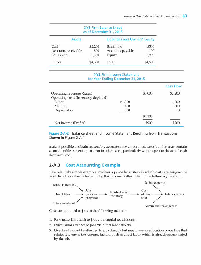
APPENDIX 2-A / ACCOUNTING FUNDAMENTALS 63

XYZ Firm Balance Sheetas of December 31, 2015

Assets Liabilities and Owners’ Equity

Cash $2,200 Bank note $500Accounts receivable 800 Accounts payable 100Equipment 1,500 Equity 3,900

Total $4,500 Total $4,500

XYZ Firm Income Statementfor Year Ending December 31, 2015

Cash Flow

Operating revenues (Sales) $3,000 $2,200Operating costs (Inventory depleted)

Labor $1,200 −1,200Material 400 −300Depreciation 500 0

$2,100

Net income (Profits) $900 $700

Figure 2-A-2 Balance Sheet and Income Statement Resulting from TransactionsShown in Figure 2-A-1

make it possible to obtain reasonably accurate answers for most cases but that may containa considerable percentage of error in other cases, particularly with respect to the actual cashflow involved.

2-A.3 Cost Accounting ExampleThis relatively simple example involves a job-order system in which costs are assigned towork by job number. Schematically, this process is illustrated in the following diagram:

Direct materials

Direct labor

Factory overhead

Jobs(work inprogress)

Finished goodsinventory

Costof goodssold

Selling expenses

Administrative expenses

Total expenses

Costs are assigned to jobs in the following manner:

1. Raw materials attach to jobs via material requisitions.

2. Direct labor attaches to jobs via direct labor tickets.

3. Overhead cannot be attached to jobs directly but must have an allocation procedure thatrelates it to one of the resource factors, such as direct labor, which is already accumulatedby the job.

64 CHAPTER 2 / COST CONCEPTS AND DESIGN ECONOMICS

Consider how an order for 100 tennis rackets accumulates costs at the Bowling SportingGoods Company:

Job #161 100 tennis racketsLabor rate $7 per hourLeather 50 yards at $2 per yardGut 300 yards at $0.50 per yardGraphite 180 pounds at $3 per poundLabor hours for the job 200 hoursTotal annual factory overhead costs $600,000Total annual direct labor hours 200,000 hours

The three major costs are now attached to the job. Direct labor and material expensesare straightforward:

Job #161Direct labor 200 × $7 = $1,400Direct material leather: 50 × $2 = 100

gut: 300 × $0.5 = 150graphite: 180 × $3 = 540

Prime costs (direct labor + direct materials) $2,190

Notice that this cost is not the total cost. We must somehow find a way to attach (allocate)factory costs that cannot be directly identified to the job but are nevertheless involved inproducing the 100 rackets. Costs such as the power to run the graphite molding machine, thedepreciation on this machine, the depreciation of the factory building, and the supervisor’ssalary constitute overhead for this company. These overhead costs are part of the coststructure of the 100 rackets but cannot be directly traced to the job. For instance, do wereally know how much machine obsolescence is attributable to the 100 rackets? Probablynot. Therefore, we must allocate these overhead costs to the 100 rackets by using the overheadrate determined as follows:

Overhead rate = $600,000200,000

= $3 per direct labor hour.

This means that $600 ($3 × 200) of the total annual overhead cost of $600,000 would beallocated to Job #161. Thus, the total cost of Job #161 would be as follows:

Direct labor $1,400Direct materials 790Factory overhead 600

$2,790

The cost of manufacturing each racket is thus $27.90. If selling expenses andadministrative expenses are allocated as 40% of the cost of goods sold, the total expenseof a tennis racket becomes 1.4($27.90) = $39.06.

APPENDIX 2-A PROBLEMS 65

Appendix 2-A Problems

2-A-1.∗ Jill Smith opens an apartment-locator businessnear a college campus. She is the sole owner of theproprietorship, which she names Campus ApartmentLocators. During the first month of operations, July2015, she engages in the following transactions:

a. Smith invests $35,000 of personal funds to start thebusiness.

b. She purchases on account office supplies costing$350.

c. Smith pays cash of $30,000 to acquire a lot next tothe campus. She intends to use the land as a futurebuilding site for her business office.

d. Smith locates apartments for clients and receivescash of $1,900.

e. She pays $100 on the account payable she created intransaction (b).

f. She pays $2,000 of personal funds for a vacation.

g. She pays cash expenses for office rent, $400, andutilities, $100.

h. The business sells office supplies to another businessfor its cost of $150.

i. Smith withdraws cash of $1,200 for personal use.

Required

(a) Analyze the preceding transactions in terms oftheir effects on the accounting equation of CampusApartment Locators. Use Figure 2-A-1 as a guide.

(b) Prepare the income statement and balance sheet ofthe business after recording the transactions. UseFigure 2-A-2 as a guide.

TABLE P2-A-2 Data for Problem 2-A-2

Assets = Liabilities + Owner’s Equity

Accounts Accounts Daniel Peavy,Cash + Receivable + Supplies + Land = Payable + Capital

Bal. 1,720 3,240 24,100 5,400 23,660

∗ Adapted from C. T. Horngren, W. T. Harrison Jr., and L. S. Bamber, Accounting, 6th ed. (Upper Saddle River, NJ: Prentice Hall, 2005), p. 23 andp. 32. Reprinted by permission of the publisher.

† Adapted from C. T. Horngren, G. L. Sundem, and W. O. Stratton, Introduction to Management Accounting, 11th ed. (Upper Saddle River, NJ: PrenticeHall, 1999), pp. 528–529. Reprinted by permission of the publisher.

2-A-2.† Daniel Peavy owns and operates anarchitectural firm called Peavy Design. Table P2-A-2summarizes the financial position of his business onApril 30, 2015.

During May 2015, the following events occurred:

a. Peavy received $12,000 as a gift and deposited thecash in the business bank account.

b. He paid off the beginning balance of accountspayable.

c. He performed services for a client and received cashof $1,100.

d. He collected cash from a customer on account, $750.

e. Peavy purchased supplies on account, $720.

f. He consulted on the interior design of a major officebuilding and billed the client for services rendered,$5,000.

g. He invested personal cash of $1,700 in the business.

h. He recorded the following business expenses for themonth:

1. Paid office rent, $1,200.

2. Paid advertising, $660.

i. Peavy sold supplies to another interior designer for$80 cash, which was the cost of the supplies.

j. He withdrew cash of $4,000 for personal use.

Required

(a) Analyze the effects of the preceding transactions onthe accounting equation of Peavy Design. Adaptthe format of Figure 2-A-1.

66 CHAPTER 2 / COST CONCEPTS AND DESIGN ECONOMICS

(b) Prepare the income statement of Peavy Design forthe month ended May 31, 2015. List expenses indecreasing order by amount.

(c) Prepare the balance sheet of Peavy Design atMay 31, 2015.

2-A-3.∗ Lubbock Engineering Consultants is a firm ofprofessional civil engineers. It mostly does surveyingjobs for the heavy construction industry throughoutTexas. The firm obtains its jobs by giving fixed-pricequotations, so profitability depends on the ability topredict the time required for the various subtaskson the job. (This situation is similar to that in theauditing profession, where times are budgeted for suchaudit steps as reconciling cash and confirming accountsreceivable.)

A client may be served by various professional staff,who hold positions in the hierarchy from partners tomanagers to senior engineers to assistants. In addition,there are secretaries and other employees.

Lubbock Engineering has the following budget for2016:

Compensation of professional staff $3,600,000Other costs 1,449,000

Total budgeted costs $5,049,000

Each professional staff member must submit aweekly time report, which is used for charging hoursto a client job-order record. The time report has seven

∗ Adapted from C. T. Horngren, G. L. Sundem, and W. O. Stratton, Introduction to Management Accounting, 11th ed. (Upper Saddle River, NJ: PrenticeHall, 1999), pp. 528–529. Reprinted by permission of the publisher.

columns, one for each day of the week. Its rows are asfollows:

• Chargeable hoursClient 156Client 183Etc.

• Nonchargeable hoursAttending seminar on new equipmentUnassigned timeEtc.

In turn, these time reports are used for charging hoursand costs to the client job-order records. The managingpartner regards these job records as absolutely essentialfor measuring the profitability of various jobs andfor providing an “experience base for improvingpredictions on future jobs.”

a. The firm applies overhead to jobs at a budgetedpercentage of the professional compensationcharged directly to the job (“direct labor”). Forall categories of professional personnel, charge-able hours average 85% of available hours.Nonchargeable hours are regarded as additionaloverhead. What is the overhead rate as a percentageof “direct labor,” the chargeable professionalcompensation cost?

b. A senior engineer works 48 weeks per year, 40 hoursper week. His compensation is $60,000. He hasworked on two jobs during the past week, devoting10 hours to Job #156 and 30 hours to Job #183. Howmuch cost should be charged to Job #156 because ofhis work there?

CHAPTER 3

Cost-Estimation Techniques

The objective of Chapter 3 is to present an assortment of methodsfor estimating important factors in an engineering economy study.

The High Cost of EnvironmentalCleanup

I n December of 1980, Congress enacted the Comprehensive Envi-ronmental Response, Compensation and Liability Act (CERCLA),also known as the “Superfund.” This law created broad federal

authority to respond to releases or threatened releases of hazardous substances.CERCLAprovides liability for corporations responsible for closed and abandonedhazardous waste sites. Regrettably, affected parties soon found that the cost ofneglecting hazardous waste sites was extremely high. But how high?

Prior to 1980, many corporations had not set aside money for cleaning upbehind themselves as their business models evolved and changed. For example,hazardous chemicals were left behind in tanks and piping, and most of thefacilities had used asbestos for insulation. Transformers contained oil that wasoften contaminated with PCBs. As plant and equipment deteriorated, these typesof hazardous substances migrated into the environment and contaminated theland and the ground water. The cost of cleanup became astronomical.

In addition to the possible impact on human health and the environment,it is abundantly clear that the cost of doing business must include surveillance,maintenance, and safe closure of contaminated facilities. In the long run, it savesmoney to act early to responsibly comply with CERCLA. In Chapter 3, you willlearn about many techniques that are useful for estimating the costs associatedwith environmental cleanup.

Decisions, both great and small, depend in part on estimates. “Looking down the barrel” neednot be an embarrassment for the engineer if newer techniques, professional staffing, and a

greater awareness are assigned to the engineering cost estimating function.

—Phillip F. Ostwald (1992)

3.1 IntroductionIn Chapter 1, we described the engineering economic analysis procedure in termsof seven steps. In this chapter, we address Step 3, development of the outcomesand cash flows for each alternative. Because engineering economy studies dealwith outcomes that extend into the future, estimating the future cash flows forfeasible alternatives is a critical step in the analysis procedure. Often, the mostdifficult, expensive, and time-consuming part of an engineering economy studyis the estimation of costs, revenues, useful lives, residual values, and other datapertaining to the alternatives being analyzed. A decision based on the analysis iseconomically sound only to the extent that these cost and revenue estimates arerepresentative of what subsequently will occur. In this chapter, we introduce therole of cost estimating in engineering practice. Definitions and examples of importantcost concepts were provided in Chapter 2.

Whenever an engineering economic analysis is performed for a major capitalinvestment, the cost-estimating effort for that analysis should be an integral part ofa comprehensive planning and design process requiring the active participation ofnot only engineering designers but also personnel from marketing, manufacturing,finance, and top management. Results of cost estimating are used for a variety ofpurposes, including the following:

1. Providing information used in setting a selling price for quoting, bidding, orevaluating contracts

2. Determining whether a proposed product can be made and distributed at aprofit (for simplicity, price = cost + profit)

3. Evaluating how much capital can be justified for process changes or otherimprovements

4. Establishing benchmarks for productivity improvement programs

There are two fundamental approaches to cost estimating: the “top-down”approach and the “bottom-up” approach. The top-down approach basically useshistorical data from similar engineering projects to estimate the costs, revenues, andother data for the current project by modifying these data for changes in inflationor deflation, activity level, weight, energy consumption, size, and other factors.This approach is best used early in the estimating process when alternatives arestill being developed and refined.

The bottom-up approach is a more detailed method of cost estimating. Thismethod breaks down a project into small, manageable units and estimates theireconomic consequences. These smaller unit costs are added together with othertypes of costs to obtain an overall cost estimate. This approach usually works bestwhen the detail concerning the desired output (a product or a service) has beendefined and clarified.

68

SECTION 3.1 / INTRODUCTION 69

EXAMPLE 3-1 Estimating the Cost of a College Degree

A simple example of cost estimating is to forecast the expense of getting aBachelor of Science (B.S.) from the university you are attending. In our solution,we outline the two basic approaches just discussed for estimating these costs.

SolutionA top-down approach would take the published cost of a four-year degree atthe same (or a similar) university and adjust it for inflation and extraordinaryitems that an incoming student might encounter, such as fraternity/sororitymembership, scholarships, and tutoring. For example, suppose that the pub-lished cost of attending your university is $15,750 for the current year. Thisfigure is anticipated to increase at the rate of 6% per year and includes full-time tuition and fees, university housing, and a weekly meal plan. Notincluded are the costs of books, supplies, and other personal expenses. Forour initial estimate, these “other” expenses are assumed to remain constant at$5,000 per year.

The total estimated cost for four years can now be computed. We simplyneed to adjust the published cost for inflation each year and add in the cost of“other” expenses.

Tuition, Fees, “Other” Total EstimatedYear Room and Board Expenses Cost for Year

1 $15,750 × 1.06 = $16,695 $5,000 $21,6952 16,695 × 1.06 = 17,697 5,000 22,6973 17,697 × 1.06 = 18,759 5,000 23,7594 18,759 × 1.06 = 19,885 5,000 24,885

Grand Total $93,036

In contrast with the top-down approach, a bottom-up approach to the samecost estimate would be to first break down anticipated expenses into the typicalcategories shown in Figure 3-1 for each of the four years at the university.Tuition and fees can be estimated fairly accurately in each year, as can books andsupplies. For example, suppose that the average cost of a college textbook is $100.You can estimate your annual textbook cost by simply multiplying the averagecost per book by the number of courses you plan to take. Assume that youplan on taking five courses each semester during the first year. Your estimatedtextbook costs would be(

5 coursessemester

)(2 semesters)

(1 bookcourse

)($100book

)= $1,000.

The other two categories, living expenses and transportation, are probablymore dependent on your lifestyle. For example, whether you own and operatean automobile and live in a “high-end” apartment off-campus can dramaticallyaffect the estimated expenses during your college years.

70 CHAPTER 3 / COST-ESTIMATION TECHNIQUES

Tuition andFees

TuitionActivities feesMembershipsMedical insuranceLab fees

Books andSupplies

BooksDuplicationSuppliesComputer rentalSoftware

LivingExpenses

RentFoodClothingRecreationUtilities

Transportation

FuelMaintenance on carInsuranceTraffic tickets

2014

2015

2016

2017

Sum Over Four Years to Obtain Total Costof a B.S. at Your University

Figure 3-1 Bottom-Up Approach to Determining the Costof a College Education

3.2 An Integrated ApproachAn integrated approach to developing the net cash flows for feasible projectalternatives is shown in Figure 3-2. This integrated approach includes three basiccomponents:

1. Work breakdown structure (WBS) This is a technique for explicitly defining,at successive levels of detail, the work elements of a project and theirinterrelationships (sometimes called a work element structure).

2. Cost and revenue structure (classification) Delineation of the cost and revenuecategories and elements is made for estimates of cash flows at each level of theWBS.

3. Estimating techniques (models) Selected mathematical models are used toestimate the future costs and revenues during the analysis period.

These three basic components, together with integrating procedural steps, providean organized approach for developing the cash flows for the alternatives.

Describe project inwork breakdown

structure (WBS) form

(Basic Component 1)

Delineate cost and revenuecategories

and elements

Describe afeasible alternativeusing project WBS

Determine WBS level(s) for

estimating

Estimatingtechniques(models)

Cost andrevenue database

Develop cash flow foralternative

Lastalternative

?

Yes

No

Stop

(Basic Component 3)(Basic Component 2)

DefineCash flow perspectiveEstimating baselineStudy (analysis) period

Figure 3-2 Integrated Approach for Developing the Cash Flows for Alternatives

71

72 CHAPTER 3 / COST-ESTIMATION TECHNIQUES

As shown in Figure 3-2, the integrated approach begins with a descriptionof the project in terms of a WBS. WBS is used to describe the project and eachalternative’s unique characteristics in terms of design, labor, material requirements,and so on. Then these variations in design, resource requirements, and othercharacteristics are reflected in the estimated future costs and revenues (net cashflow) for that alternative.

To estimate future costs and revenues for an alternative, the perspective(viewpoint) of the cash flow must be established and an estimating baseline andanalysis period defined. Normally, cash flows are developed from the owner’sviewpoint. The net cash flow for an alternative represents what is estimated tohappen to future revenues and costs from the perspective being used. Therefore, theestimated changes in revenues and costs associated with an alternative have to berelative to a baseline that is consistently used for all the alternatives being compared.

3.2.1 The Work Breakdown Structure (WBS)

The first basic component in an integrated approach to developing cash flowsis the work breakdown structure (WBS). The WBS is a basic tool in projectmanagement and is a vital aid in an engineering economy study. The WBS servesas a framework for defining all project work elements and their interrelationships,collecting and organizing information, developing relevant cost and revenue data,and integrating project management activities.

Figure 3-3 shows a diagram of a typical four-level WBS. It is developed fromthe top (project level) down in successive levels of detail. The project is dividedinto its major work elements (Level 2). These major elements are then divided todevelop Level 3, and so on. For example, an automobile (first level of the WBS) canbe divided into second-level components (or work elements) such as the chassis,drive train, and electrical system. Then each second-level component of the WBScan be subdivided further into third-level elements. The drive train, for example,can be subdivided into third-level components such as the engine, differential, andtransmission. This process is continued until the desired detail in the definitionand description of the project or system is achieved.

Different numbering schemes may be used. The objectives of numbering are toindicate the interrelationships of the work elements in the hierarchy. The schemeillustrated in Figure 3-3 is an alphanumeric format. Another scheme often used is allnumeric—Level 1: 1-0; Level 2: 1-1, 1-2, 1-3; Level 3: 1-1-1, 1-1-2, 1-2-1, 1-2-2, 1-3-1,1-3-2; and so on (i.e., similar to the organization of this book). Usually, the level isequal (except for Level 1) to the number of characters indicating the work element.

Other characteristics of a project WBS are as follows:

1. Both functional (e.g., planning) and physical (e.g., foundation) work elementsare included in it:

(a) Typical functional work elements are logistical support, projectmanagement, marketing, engineering, and systems integration.

(b) Physical work elements are the parts that make up a structure, product,piece of equipment, or similar item; they require labor, materials, and otherresources to produce or construct.

SECTION 3.2 / AN INTEGRATED APPROACH 73

Level 1

Level 2

A � 0

A � 1

A � 1 � A

A � 1 � A � 1 A � 1 � B � 2

A � 1 � B

A � 2 A � 3

Level 3

Level 4

Figure 3-3 The WBS Diagram

2. The content and resource requirements for a work element are the sum of theactivities and resources of related subelements below it.

3. A project WBS usually includes recurring (e.g., maintenance) and nonrecurring(e.g., initial construction) work elements.

EXAMPLE 3-2 A WBS for a Construction Project

You have been appointed by your company to manage a project involvingconstruction of a small commercial building with two floors of 15,000 grosssquare feet each. The ground floor is planned for small retail shops, andthe second floor is planned for offices. Develop the first three levels of arepresentative WBS adequate for all project efforts from the time the decisionwas made to proceed with the design and construction of the building untilinitial occupancy is completed.

SolutionThere would be variations in the WBSs developed by different individuals for acommercial building. A representative three-level WBS is shown in Figure 3-4.Level 1 is the total project. At Level 2, the project is divided into seven majorphysical work elements and three major functional work elements. Then eachof these major elements is divided into subelements as required (Level 3). Thenumbering scheme used in this example is all numeric.

74C

HA

PTER3

/C

OST-E

STIMA

TION

TEC

HN

IQU

ES

74

Commercial Building Project

1-0

Site Work and Foundation

1-1

Exterior

1-2

Interior

1-3

Roof

1-4

1-4-1Framing

1-4-2Sheathing

1-4-3Roofing

1-3-1Framing

1-3-2Flooring/Stairways

1-3-3Walls/Ceilings

1-3-4Doors

1-3-5Special Additions

1-2-1Framing

1-2-2Siding

1-2-3Windows

1-2-4Entrances

1-2-5Insulation

1-1-1Site Grading

1-1-2Excavation

1-1-3Sidewalks/Parking

1-1-4Footing/Foundation

1-1-5Floor Slab

ElectricalSystems

1-5

MechanicalSystems

1-6

RealEstate

1-7

ProjectManagement

1-8

Arch/Engr.Services

1-9

Sales

1-10

1-10-1Leasing/Asset Sales

1-10-2Admin. Support

1-10-3Legal

1-9-1Design

1-9-2Cost Estimating

1-9-3Consulting

1-8-1Admin. Support

1-8-2Technical Mgt.

1-8-3Legal

1-6-1Heating/Cooling

1-6-2Hot Water

1-6-3Lavatories

1-5-1Service Delivery

1-5-2Devices

1-5-3Lighting

LEVEL1

2

3

2

3

Figure 3-4 WBS (Three Levels) for Commercial Building Project in Example 3-2

SECTION 3.2 / AN INTEGRATED APPROACH 75

3.2.2 The Cost and Revenue Structure

The second basic component of the integrated approach for developing cashflows (Figure 3-2) is the cost and revenue structure. This structure is used toidentify and categorize the costs and revenues that need to be included inthe analysis. Detailed data are developed and organized within this structurefor use with the estimating techniques of Section 3.3 to prepare the cash-flowestimates.

The life-cycle concept and the WBS are important aids in developing the costand revenue structure for a project. The life cycle defines a maximum time periodand establishes a range of cost and revenue elements that need to be consideredin developing cash flows. The WBS focuses the analyst’s effort on the specificfunctional and physical work elements of a project and on its related costsand revenues.

Perhaps the most serious source of errors in developing cash flows is overlookingimportant categories of costs and revenues. The cost and revenue structure,prepared in tabular or checklist form, is a good means of preventing suchoversights. Technical familiarity with the project is essential in ensuring thecompleteness of the structure, as are using the life-cycle concept and the WBSin its preparation.

The following is a brief listing of some categories of costs and revenues thatare typically needed in an engineering economy study:

1. Capital investment (fixed and working)2. Labor costs3. Material costs4. Maintenance costs5. Property taxes and insurance6. Overhead costs7. Disposal costs8. Revenues based on sales, etc.9. Quality (and scrap) costs

10. Market (or salvage) values

3.2.3 Estimating Techniques (Models)

The third basic component of the integrated approach (Figure 3-2) involvesestimating techniques (models). These techniques, together with the detailed costand revenue data, are used to develop individual cash-flow estimates and theoverall net cash flow for each alternative.

76 CHAPTER 3 / COST-ESTIMATION TECHNIQUES

The purpose of estimating is to develop cash-flow projections—not to produceexact data about the future, which is virtually impossible. Neither a preliminaryestimate nor a final estimate is expected to be exact; rather, it should adequatelysuit the need at a reasonable cost and is often presented as a range of numbers.

Cost and revenue estimates can be classified according to detail, accuracy, andtheir intended use as follows:

1. Order-of-magnitude estimates: used in the planning and initial evaluation stageof a project.

2. Semidetailed, or budget, estimates: used in the preliminary or conceptualdesign stage of a project.

3. Definitive (detailed) estimates: used in the detailed engineering/constructionstage of a project.

Order-of-magnitude estimates are used in selecting the feasible alternatives for thestudy. They typically provide accuracy in the range of±30 to 50% and are developedthrough semiformal means such as conferences, questionnaires, and generalizedequations applied at Level 1 or 2 of the WBS.

Budget (semidetailed) estimates are compiled to support the preliminarydesign effort and decision making during this project period. Their accuracy usuallylies in the range of ±15%. These estimates differ in the fineness of cost and revenuebreakdowns and the amount of effort spent on the estimate. Estimating equationsapplied at Levels 2 and 3 of the WBS are normally used.

Detailed estimates are used as the basis for bids and to make detailed designdecisions. Their accuracy is ±5%. They are made from specifications, drawings,site surveys, vendor quotations, and in-house historical records and are usuallydone at Level 3 and successive levels in the WBS.

Thus, it is apparent that a cost or revenue estimate can vary from a “back of theenvelope” calculation by an expert to a very detailed and accurate prediction ofthe future prepared by a project team. The level of detail and accuracy of estimatesshould depend on the following:

1. Time and effort available as justified by the importance of the study2. Difficulty of estimating the items in question3. Methods or techniques employed4. Qualifications of the estimator(s)5. Sensitivity of study results to particular factor estimates

As estimates become more detailed, accuracy typically improves, but the cost ofmaking the estimate increases dramatically. This general relationship is shownin Figure 3-5 and illustrates the idea that cost and revenue estimates should beprepared with full recognition of how accurate a particular study requires themto be.

SECTION 3.2 / AN INTEGRATED APPROACH 77

Figure 3-5Accuracy of Costand RevenueEstimates versusthe Cost ofMaking Them

Cos

t of E

stim

ate

as a

Per

cent

age

of P

roje

ct C

ost

Ord

er-o

f-M

agni

tude

Est

imat

es

Accuracy (�%)

5

10

25Levels3–4

in WBS

Levels1–2

in WBS

50

Det

aile

d E

stim

ates

3.2.3.1 Sources of Estimating Data The information sources useful in costand revenue estimating are too numerous to list completely. The following fourmajor sources of information are listed roughly in order of importance:

1. Accounting records. Accounting records are a prime source of informationfor economic analyses; however, they are often not suitable for direct,unadjusted use.

A brief discussion of the accounting process and information was givenin Appendix 2-A. In its most basic sense, accounting consists of a series ofprocedures for keeping a detailed record of monetary transactions betweenestablished categories of assets. Accounting records are a good source ofhistorical data but have some limitations when used in making prospectiveestimates for engineering economic analyses. Moreover, accounting recordsrarely contain direct statements of incremental costs or opportunity costs, bothof which are essential in most engineering economic analyses. Incrementalcosts are decision specific for one-of-a-kind investments and are unlikely tobe available from the accounting system.

2. Other sources within the firm. The typical firm has a number of people andrecords that may be excellent sources of estimating information. Examplesof functions within firms that keep records useful to economic analyses areengineering, sales, production, quality, purchasing, and personnel.

3. Sources outside the firm. There are numerous sources outside the firm thatcan provide helpful information. The main problem is in determining thosethat are most beneficial for particular needs. The following is a listing of somecommonly used outside sources:

(a) Published information. Technical directories, buyer indexes, U.S. governmentpublications, reference books, and trade journals offer a wealth of infor-mation. For instance, Standard and Poor’s Industry Surveys gives monthlyinformation regarding key industries. The Statistical Abstract of the UnitedStates is a remarkably comprehensive source of cost indexes and data. TheBureau of Labor Statistics publishes many periodicals that are good sourcesof labor costs, such as the Monthly Labor Review, Employment and Earnings,

78 CHAPTER 3 / COST-ESTIMATION TECHNIQUES

Current Wage Developments, Handbook of Labor Statistics, and the Chartbookon Wages, Prices and Productivity.

(b) Personal contacts are excellent potential sources. Vendors, salespeople,professional acquaintances, customers, banks, government agencies,chambers of commerce, and even competitors are often willing to furnishneeded information on the basis of a serious and tactful request.

4. Research and development (R&D). If the information is not published andcannot be obtained by consulting someone, the only alternative may be toundertake R&D to generate it. Classic examples are developing a pilot plantand undertaking a test market program.

The Internet can also be a source of cost-estimating data, though you should assureyourself that the information is from a reputable source. The following Web sitesmay be useful to you both professionally and personally.

www.enr.com Engineering News-Record Construction and labor costswww.kbb.com Kelley Blue Book Automobile pricingwww.factsonfuel.com American Petroleum Institute Fuel costs

3.2.3.2 How Estimates Are Accomplished Estimates can be prepared in anumber of ways, such as the following examples:

1. A conference of various people who are thought to have good information orbases for estimating the quantity in question. A special version of this is theDelphi method, which involves cycles of questioning and feedback in which theopinions of individual participants are kept anonymous.

2. Comparison with similar situations or designs about which there is moreinformation and from which estimates for the alternatives under considerationcan be extrapolated. This is sometimes called estimating by analogy. Thecomparison method may be used to approximate the cost of a design or productthat is new. This is done by taking the cost of a more complex design for a similaritem as an upper bound and the cost of a less complex item of similar designas a lower bound. The resulting approximation may not be very accurate, butthe comparison method does have the virtue of setting bounds that might beuseful for decision making.

3. Using quantitative techniques, which do not always have standardized names.Some selected techniques, with the names used being generally suggestive ofthe approaches, are discussed in the next section.

3.3 Selected Estimating Techniques (Models)The estimating models discussed in this section are applicable for order-of-magnitude estimates and for many semidetailed or budget estimates. They areuseful in the initial selection of feasible alternatives for further analysis and in theconceptual or preliminary design phase of a project. Sometimes, these models canbe used in the detailed design phase of a project.

SECTION 3.3 / SELECTED ESTIMATING TECHNIQUES (MODELS) 79

3.3.1 Indexes

Costs and prices∗ vary with time for a number of reasons, including (1) tech-nological advances, (2) availability of labor and materials, and (3) inflation. An indexis a dimensionless number that indicates how a cost or a price has changed withtime (typically escalated) with respect to a base year. Indexes provide a convenientmeans for developing present and future cost and price estimates from historicaldata. An estimate of the cost or selling price of an item in year n can be obtainedby multiplying the cost or price of the item at an earlier point in time (year k) bythe ratio of the index value in year n (In) to the index value in year k (Ik);† that is,

Cn = Ck

(In

Ik

), (3-1)

where k = reference year (e.g., 2000) for which cost or price of item is known;n = year for which cost or price is to be estimated (n > k);

Cn = estimated cost or price of item in year n;Ck = cost or price of item in reference year k.

Equation (3-1) is sometimes referred to as the ratio technique of updating costs andprices. Use of this technique allows the cost or potential selling price of an itemto be taken from historical data with a specified base year and updated with anindex. This concept can be applied at the lower levels of a WBS to estimate the costof equipment, materials, and labor, as well as at the top level of a WBS to estimatethe total project cost of a new facility, bridge, and so on.

EXAMPLE 3-3 Indexing the Cost of a New Boiler

A certain index for the cost of purchasing and installing utility boilers is keyed to1988, where its baseline value was arbitrarily set at 100. Company XYZ installeda 50,000-lb/hour boiler for $525,000 in 2000 when the index had a value of 468.This same company must install another boiler of the same size in 2014. Theindex in 2014 is 542. What is the approximate cost of the new boiler?

SolutionIn this example, n is 2014 and k is 2000. From Equation (3-1), an approximatecost of the boiler in 2014 is

C2014 = $525,000(542/468) = $608,013.

Indexes can be created for a single item or for multiple items. For a single item,the index value is simply the ratio of the cost of the item in the current year to thecost of the same item in the reference year, multiplied by the reference year factor

∗ The terms cost and price are often used together. The cost of a product or service is the total of the resources, directand indirect, required to produce it. The price is the value of the good or service in the marketplace. In general, priceis equal to cost plus a profit.† In this section only, k is used to denote the reference year.

80 CHAPTER 3 / COST-ESTIMATION TECHNIQUES

(typically, 100). A composite index is created by averaging the ratios of selecteditem costs in a particular year to the cost of the same items in a reference year.The developer of an index can assign different weights to the items in the indexaccording to their contribution to total cost. For example, a general weighted indexis given by

In = W1(Cn1/Ck1) + W2(Cn2/Ck2) + · · · + WM(CnM/CkM)

W1 + W2 + · · · + WM× Ik , (3-2)

where M = total number of items in the index (1 ≤ m ≤ M);Cnm = unit cost (or price) of the mth item in year n;Ckm = unit cost (or price) of the mth item in year k;Wm = weight assigned to the mth item;

Ik = composite index value in year k.

The weights W1, W2, . . . , WM can sum to any positive number, but typically sumto 1.00 or 100. Almost any combination of labor, material, products, services, andso on can be used for a composite cost or price index.

EXAMPLE 3-4 Weighted Index for Gasoline Cost

Based on the following data, develop a weighted index for the price of a gallonof gasoline in 2014, when 1996 is the reference year having an index valueof 99.2. The weight placed on regular unleaded gasoline is three times that ofeither premium or unleaded plus, because roughly three times as much regularunleaded is sold compared with premium or unleaded plus.

Price (Cents/Gal) in Year

1996 2010 2014

Premium 114 240 315Unleaded plus 103 230 305Regular unleaded 93 221 285

SolutionIn this example, k is 1996 and n is 2014. From Equation (3-2), the value of I2014 is

(1)(315/114) + (1)(305/103) + (3)(285/93)

1 + 1 + 3× 99.2 = 296.

Now, if the index in 2016, for example, is estimated to be 327, it is a simple matterto determine the corresponding 2016 prices of gasoline from I2014 = 296:

Premium: 315 cents/gal(

327296

)= 348 cents/gal,

SECTION 3.3 / SELECTED ESTIMATING TECHNIQUES (MODELS) 81

Unleaded plus: 305 cents/gal(

327296

)= 337 cents/gal,

Regular unleaded: 285 cents/gal(

327296

)= 315 cents/gal.

Many indexes are periodically published, including the Engineering NewsRecord Construction Index (www.enr.com), which incorporates labor and materialcosts and the Marshall and Swift cost index.

3.3.2 Unit Technique

The unit technique involves using a per unit factor that can be estimated effectively.Examples are as follows:

1. Capital cost of plant per kilowatt of capacity2. Revenue per mile3. Capital cost per installed telephone4. Revenue per customer served5. Temperature loss per 1,000 feet of steam pipe6. Operating cost per mile7. Construction cost per square foot

Such factors, when multiplied by the appropriate unit, give a total estimate of cost,savings, or revenue.

As a simple example of the unit technique, suppose the Air Force’s B-2 aircraftcosts $68,000 per hour to own, operate, and maintain. A certain mission requirestwo B-2 aircrafts to fly a total round-trip time of 45 hours. Thus, the total cost ofthis mission is (2 planes) (45 hours per mission per plane) ($68,000 per hour) =$6,120,000 per mission.

While the unit technique is very useful for preliminary estimating purposes,such average values can be misleading. In general, more detailed methods willresult in greater estimation accuracy.

3.3.3 Factor Technique

The factor technique is an extension of the unit method in which we sum the productof several quantities or components and add these to any components estimateddirectly. That is,

C =∑

d

Cd +∑

m

fmUm, (3-3)

82 CHAPTER 3 / COST-ESTIMATION TECHNIQUES

where C = cost being estimated;

Cd = cost of the selected component d that is estimated directly;

fm = cost per unit of component m;

Um = number of units of component m.

As a simple example, suppose that we need a slightly refined estimate of thecost of a house consisting of 2,000 square feet, two porches, and a garage.Using a unit factor of $85 per square foot, $10,000 per porch, and $8,000 pergarage for the two directly estimated components, we can calculate the totalestimate as

($10,000 × 2) + $8,000 + ($85 × 2,000) = $198,000.

The factor technique is particularly useful when the complexity of theestimating situation does not require a WBS, but several different parts are involved.Example 3-5 and the cost-estimating example to be presented in Section 3.5 furtherillustrate this technique.

EXAMPLE 3-5 Analysis of Building Space Cost Estimates

The detailed design of the commercial building described in Example 3-2 affectsthe utilization of the gross square feet (and, thus, the net rentable space)available on each floor. Also, the size and location of the parking lot and theprime road frontage available along the property may offer some additionalrevenue sources. As project manager, analyze the potential revenue impacts ofthe following considerations.

The first floor of the building has 15,000 gross square feet of retailspace, and the second floor has the same amount planned for office use.Based on discussions with the sales staff, develop the following additionalinformation:

(a) The retail space should be designed for two different uses—60% for arestaurant operation (utilization = 79%, yearly rent = $23/sq.ft.) and 40%for a retail clothing store (utilization = 83%, yearly rent = $18/sq.ft.).

(b) There is a high probability that all the office space on the second floor willbe leased to one client (utilization = 89%, yearly rent = $14/sq.ft.).

(c) An estimated 20 parking spaces can be rented on a long-term basis to twoexisting businesses that adjoin the property. Also, one spot along the roadfrontage can be leased to a sign company, for erection of a billboard, withoutimpairing the primary use of the property.

SolutionBased on this information, you estimate annual project revenue (R) as

R = W(r1)(12) + ϒ(r2)(12) +3∑

j=1

Sj(uj)(dj),

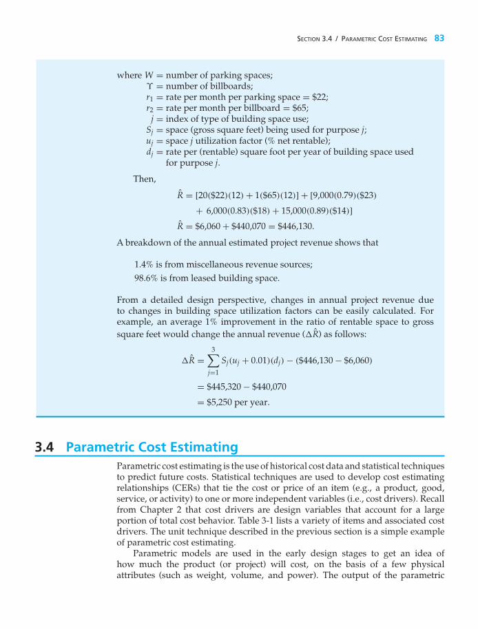
SECTION 3.4 / PARAMETRIC COST ESTIMATING 83

where W = number of parking spaces;ϒ = number of billboards;r1 = rate per month per parking space = $22;r2 = rate per month per billboard = $65;

j = index of type of building space use;Sj = space (gross square feet) being used for purpose j;uj = space j utilization factor (% net rentable);dj = rate per (rentable) square foot per year of building space used

for purpose j.

Then,

R = [20($22)(12) + 1($65)(12)] + [9,000(0.79)($23)

+ 6,000(0.83)($18) + 15,000(0.89)($14)]R = $6,060 + $440,070 = $446,130.

A breakdown of the annual estimated project revenue shows that

1.4% is from miscellaneous revenue sources;98.6% is from leased building space.

From a detailed design perspective, changes in annual project revenue dueto changes in building space utilization factors can be easily calculated. Forexample, an average 1% improvement in the ratio of rentable space to grosssquare feet would change the annual revenue (�R) as follows:

�R =3∑

j=1

Sj(uj + 0.01)(dj) − ($446,130 − $6,060)

= $445,320 − $440,070

= $5,250 per year.

3.4 Parametric Cost EstimatingParametric cost estimating is the use of historical cost data and statistical techniquesto predict future costs. Statistical techniques are used to develop cost estimatingrelationships (CERs) that tie the cost or price of an item (e.g., a product, good,service, or activity) to one or more independent variables (i.e., cost drivers). Recallfrom Chapter 2 that cost drivers are design variables that account for a largeportion of total cost behavior. Table 3-1 lists a variety of items and associated costdrivers. The unit technique described in the previous section is a simple exampleof parametric cost estimating.

Parametric models are used in the early design stages to get an idea ofhow much the product (or project) will cost, on the basis of a few physicalattributes (such as weight, volume, and power). The output of the parametric

84 CHAPTER 3 / COST-ESTIMATION TECHNIQUES

TABLE 3-1 Examples of Cost Drivers Used in Parametric CostEstimates

Product Cost Driver (Independent Variable)

Construction Floor space, roof surface area, wall surface areaTrucks Empty weight, gross weight, horsepowerPassenger car Curb weight, wheel base, passenger space, horsepowerTurbine engine Maximum thrust, cruise thrust, specific fuel consumptionReciprocating engine Piston displacement, compression ratio, horsepowerAircraft Empty weight, speed, wing areaElectrical power plants KilowattsMotors HorsepowerSoftware Number of lines of code

models (an estimated cost) is used to gauge the impact of design decisions on thetotal cost.

Various statistical and other mathematical techniques are used to developthe CERs. For example, simple linear regression and multiple linear regressionmodels, which are standard statistical methods for estimating the value ofa dependent variable (the unknown quantity) as a function of one or moreindependent variables, are often used to develop estimating relationships. Thissection describes two commonly used estimating relationships, the power-sizingtechnique and the learning curve, followed by an overview of the procedure usedto develop CERs.

3.4.1 Power-Sizing Technique

The power-sizing technique, which is sometimes referred to as an exponential model,is frequently used for developing capital investment estimates for industrial plantsand equipment. This CER recognizes that cost varies as some power of the changein capacity or size. That is,

CA

CB=(

SA

SB

)X

,

CA = CB

(SA

SB

)X

, (3-4)

where CA = cost for plant ACB = cost for plant B

}(both in $ as of the point intime for which the estimate isdesired);

SA = size of plant ASB = size of plant B

}(both in same physical units);

X = cost-capacity factor to reflect economies of scale.∗

∗ This may be calculated or estimated from experience by using statistical techniques. For typical factors, seeW. R. Park, Cost Engineering Analysis (New York: John Wiley & Sons, 1973), p. 137.

SECTION 3.4 / PARAMETRIC COST ESTIMATING 85

The value of the cost-capacity factor will depend on the type of plant or equipmentbeing estimated. For example, X = 0.68 for nuclear generating plants and 0.79for fossil-fuel generating plants. Note that X < 1 indicates decreasing economiesof scale (each additional unit of capacity costs less than the previous unit), X > 1∗indicates increasing economies of scale (each additional unit of capacity costs morethan the previous unit), and X = 1 indicates a linear cost relationship with size.

EXAMPLE 3-6 Power-Sizing Model for Cost Estimating

Suppose that an aircraft manufacturer desires to make a preliminary estimate ofthe cost of building a 600-MW fossil-fuel plant for the assembly of its new long-distance aircraft. It is known that a 200-MW plant cost $100 million 20 years agowhen the approximate cost index was 400, and that cost index is now 1,200. Thecost-capacity factor for a fossil-fuel power plant is 0.79.

SolutionBefore using the power-sizing model to estimate the cost of the 600-MW plant(CA), we must first use the cost index information to update the known cost ofthe 200-MW plant 20 years ago to a current cost. Using Equation (3-1), we findthat the current cost of a 200-MW plant is

CB = $100 million(

1,200400

)= $300 million.

So, using Equation (3-4), we obtain the following estimate for the 600-MW plant:

CA = $300 million(

600-MW200-MW

)0.79

CA = $300 million × 2.38 = $714 million.

Note that Equation (3-4) can be used to estimate the cost of a larger plant (asin Example 3-6) or the cost of a smaller plant. For example, suppose we need toestimate the cost of building a 100-MW plant. Using Equation (3-4) and the datafor the 200-MW plant in Example 3-6, we find that the current cost of a 100-MWplant is

CA = $300 million(

100 MW200 MW

)0.79

CA = $300 million × 0.58 = $174 million.

Cost-capacity factors can also have a role in figuring the costs associated withenvironmental cleanup. The cost of cleaning up an oil spill in the Gulf of Mexicois $10 billion when the spilled oil amounts to 18 million gallons. The cleanup costis $14 billion when the amount of spilled oil is 32 million gallons. We can use

∗ Precious gems are an example of increasing economies of scale. For example, a one-carat diamond typically costsmore than four quarter-carat diamonds.

86 CHAPTER 3 / COST-ESTIMATION TECHNIQUES

Equation (3-4) to estimate the value of the cost-capacity factor in this situation.

$10 billion$14 billion

=(

18 million gallons32 million gallons

)X

log(0.7143) = X log(0.5625)

X = 0.58

3.4.2 Learning and Improvement

A learning curve is a mathematical model that explains the phenomenon ofincreased worker efficiency and improved organizational performance withrepetitive production of a good or service. The learning curve is sometimescalled an experience curve or a manufacturing progress function; fundamentally, itis an estimating relationship. The learning (improvement) curve effect was firstobserved in the aircraft and aerospace industries with respect to labor hoursper unit. However, it applies in many different situations. For example, thelearning curve effect can be used in estimating the professional hours expendedby an engineering staff to accomplish successive detailed designs within a familyof products, as well as in estimating the labor hours required to assembleautomobiles.

The basic concept of learning curves is that some input resources (e.g.,energy costs, labor hours, material costs, engineering hours) decrease, on a per-output-unit basis, as the number of units produced increases. Most learning curvesare based on the assumption that a constant percentage reduction occurs in, say,labor hours, as the number of units produced is doubled. For example, if 100 laborhours are required to produce the first output unit and a 90% learning curve isassumed, then 100(0.9) = 90 labor hours would be required to produce the secondunit. Similarly, 100(0.9)2 = 81 labor hours would be needed to produce the fourthunit, 100(0.9)3 = 72.9 hours to produce the eighth unit, and so on. Therefore, a 90%learning curve results in a 10% reduction in labor hours each time the productionquantity is doubled.

Equation (3-5) can be used to compute resource requirements assuming aconstant percentage reduction in input resources each time the output quantityis doubled.

Zu = K(un), (3-5)

where u = the output unit number;Zu = the number of input resource units needed to produce output unit u;K = the number of input resource units needed to produce the first

output unit;s = the learning curve slope parameter expressed as a decimal

(s = 0.9 for a 90% learning curve);

n = log slog 2

= the learning curve exponent.

SECTION 3.4 / PARAMETRIC COST ESTIMATING 87

EXAMPLE 3-7 Learning Curve for a Formula Car Design Team

The Mechanical Engineering department has a student team that is designing aformula car for national competition. The time required for the team to assemblethe first car is 100 hours. Their improvement (or learning rate) is 0.8, which meansthat as output is doubled, their time to assemble a car is reduced by 20%. Use thisinformation to determine

(a) the time it will take the team to assemble the 10th car.(b) the total time required to assemble the first 10 cars.(c) the estimated cumulative average assembly time for the first 10 cars.

Solve by hand and by spreadsheet.

Solution by Hand(a) From Equation (3-5), and assuming a proportional decrease in assembly time

for output units between doubled quantities, we have

Z10 = 100(10)log 0.8/ log 2

= 100(10)−0.322

= 1002.099

= 47.6 hours.

(b) The total time to produce x units, Tx, is given by

Tx =x∑

u=1

Zu =x∑

u=1

K(un) = Kx∑

u=1

un. (3-6)

Using Equation (3-6), we see that

T10 = 10010∑

u=1

u−0.322 = 100[1−0.322 + 2−0.322 + · · · + 10−0.322] = 631 hours.

(c) The cumulative average time for x units, Cx, is given by

Cx = Tx/x. (3-7)

Using Equation (3-7), we get

C10 = T10/10 = 631/10 = 63.1 hours.

Spreadsheet SolutionFigure 3-6 shows the spreadsheet solution for this example problem. For eachunit number, the unit time to complete the assembly, the cumulative total time,and the cumulative average time are computed with the use of Equations (3-5),

88 CHAPTER 3 / COST-ESTIMATION TECHNIQUES

= LOG(B2) / LOG(2)

= $B$1 * A6 ^ $B$4 = AVERAGE($B$6:B6)

= SUM($B$6:B6)

Figure 3-6 Spreadsheet Solution, Example 3-7

SECTION 3.4 / PARAMETRIC COST ESTIMATING 89

(3-6), and (3-7), respectively. Note that these formulas are entered once in row 6of the spreadsheet and are then simply copied into rows 7 through 15.

A plot of unit time and cumulative average time is easily created with thespreadsheet software. This spreadsheet model can be used to examine the impactof a different learning slope parameter (e.g., s = 90%) on predicted car assemblytimes by changing the value of cell B2.

3.4.3 Developing a Cost Estimating Relationship (CER)

A CER is a mathematical model that describes the cost of an engineering projectas a function of one or more design variables. CERs are useful tools because theyallow the estimator to develop a cost estimate quickly and easily. Furthermore,estimates can be made early in the design process before detailed information isavailable. As a result, engineers can use CERs to make early design decisions thatare cost effective in addition to meeting technical requirements.

There are four basic steps in developing a CER:

1. Problem definition2. Data collection and normalization3. CER equation development4. Model validation and documentation

3.4.3.1 Problem Definition The first step in any engineering analysis is todefine the problem to be addressed. A well-defined problem is much easier tosolve. For the purposes of cost estimating, developing a WBS is an excellent way ofdescribing the elements of the problem. A review of the completed WBS can alsohelp identify potential cost drivers for the development of CERs.

3.4.3.2 Data Collection and Normalization The collection and normaliza-tion of data is the most critical step in the development of a CER. We’re all familiarwith the adage “garbage in—garbage out.” Without reliable data, the cost estimatesobtained by using the CER would be meaningless. The WBS is also helpful in thedata collection phase. The WBS helps to organize the data and ensure that noelements are overlooked.

Data can be obtained from both internal and external sources. Costs of similarprojects in the past are one source of data. Published cost information is anothersource of data. Once collected, data must be normalized to account for differencesdue to inflation, geographical location, labor rates, and so on. For example, costindexes or the price inflation techniques to be described in Chapter 8 can be usedto normalize costs that occurred at different times. Consistent definition of the datais another important part of the normalization process.

3.4.3.3 CER Equation Development The next step in the development of aCER is to formulate an equation that accurately captures the relationship between

90 CHAPTER 3 / COST-ESTIMATION TECHNIQUES

TABLE 3-2 Typical Equation Forms

Type of Relationship Generalized Equation

Linear Cost = b0 + b1x1 + b2x2 + b3x3 + · · ·Power Cost = b0 + b1xb11

1 xb122 + · · ·

Logarithmic Cost = b0 + b1 log(x1) + b2 log(x2) + b3 log(x3) + · · ·Exponential Cost = b0 + b1 expb11x1 + b2 expb22x2 + · · ·

the selected cost driver(s) and project cost. Table 3-2 lists four general equationtypes commonly used in CER development. In these equations, b0, b1, b2, and b3are constants, while x1, x2, and x3 represent design variables.

A simple, yet very effective, way to determine an appropriate equation formfor the CER is to plot the data. If a plot of the data on regular graph paper appears tofollow a straight line, then a linear relationship is suggested. If a curve is suggested,then try plotting the data on semilog or log-log paper. If a straight line results onsemilog paper, then the relationship is logarithmic or exponential. If a straight lineresults on log-log paper, then the relationship is a power curve.

Once we have determined the basic equation form for the CER, the next step isto determine the values of the coefficients in the CER equation. The most commontechnique used to solve for the coefficient values is the method of least squares.Basically, this method seeks to determine a straight line through the data thatminimizes the total deviation of the actual data from the predicted values. (The lineitself represents the CER.) This method is relatively easy to apply manually and isalso available in many commercial software packages. (Most spreadsheet packagesare capable of performing a least-squares fit of data.) The primary requirement forthe use of the least-squares method is a linear relationship between the independentvariable (the cost driver) and the dependent variable (project cost).∗

All of the equation forms presented in Table 3-2 can easily be transformed intoa linear form. The following equations can be used to calculate the values of thecoefficients b0 and b1 in the simple linear equation y = b0 + b1x:

b1 =n

n∑i=1

xiyi −( n∑

i=1

xi

)( n∑i=1

yi

)

nn∑

i=1

x2i −

( n∑i=1

xi

)2 , (3-8)

b0 =

n∑i=1

yi − b1

n∑i=1

xi

n. (3-9)

Note that the variable n in the foregoing equations is equal to the number of datasets used to estimate the values of b0 and b1.

∗ In addition, the observations should be independent. The difference between predicted and actual values is assumedto be normally distributed with an expected value of zero. Furthermore, the variance of the dependent variable isassumed to be equal for each value of the independent variable.

SECTION 3.4 / PARAMETRIC COST ESTIMATING 91

EXAMPLE 3-8 Cost Estimating Relationship (CER) for a Spacecraft

In the early stages of design, it is believed that the cost of a Martian roverspacecraft is related to its weight. Cost and weight data for six spacecraft havebeen collected and normalized and are shown in the next table. A plot of thedata suggests a linear relationship. Use a spreadsheet model to determine thevalues of the coefficients for the CER.

Spacecraft Weight (lb) Cost ($ million)i xi yi

1 400 2782 530 4143 750 5574 900 6895 1,130 7406 1,200 851

Spreadsheet SolutionFigure 3-7 displays the spreadsheet model for determining the coefficients of theCER. This example illustrates the basic regression features of Excel. No formulas

(a) Regression Dialog Box

Figure 3-7 Spreadsheet Solution, Example 3-8

92 CHAPTER 3 / COST-ESTIMATION TECHNIQUES

(b) Regression Results

Figure 3-7 (continued)

are entered, only the cost and weight data for the spacecraft. The challengein spreadsheet regression lies in making sure that the underlying regressionassumptions are satisfied and in interpreting the output properly.

The Tools | Data Analysis | Regression menu command brings up the Reg-ression dialog box shown in Figure 3-7(a) and shows the values used forthis model. The results of the analysis are generated by Excel and aredisplayed beginning in cell A9 of Figure 3-7(b). For the purposes of thisexample, the coefficients b0 and b1 of the CER are found in cells B25 and B26,respectively.

SECTION 3.4 / PARAMETRIC COST ESTIMATING 93

The resulting CER relating spacecraft cost (in millions of dollars) to space-craft weight is

Cost = 48.28 + 0.6597x,

where x represents the weight of the spacecraft in pounds, and 400 ≤ x ≤ 1,200.

3.4.3.4 Model Validation and Documentation Once the CER equation hasbeen developed, we need to determine how well the CER can predict cost (i.e.,model validation) and document the development and appropriate use of theCER. Validation can be accomplished with statistical “goodness of fit” measuressuch as standard error and the correlation coefficient. Analysts must use goodnessof fit measures to infer how well the CER predicts cost as a function of theselected cost driver(s). Documenting the development of the CER is importantfor future use of the CER. It is important to include in the documentationthe data used to develop the CER and the procedures used for normalizingthe data.

The standard error (SE) measures the average amount by which the actual costvalues and the predicted cost values vary. The SE is calculated by

SE =

√√√√√√n∑

i=1

(yi − Costi)2

n − 2, (3-10)

where Costi is the cost predicted by using the CER with the independentvariable values for data set i and yi is the actual cost. A small value of SE ispreferred.

The correlation coefficient (R) measures the closeness of the actual data pointsto the regression line (y = b0 + b1x). It is simply the ratio of explained deviation tototal deviation.

R =

n∑i=1

(xi − x)(yi − y)

√√√√[ n∑i=1

(xi − x)2

][ n∑i=1

(yi − y)2

] , (3-11)

where x = 1n∑n

i=1 xi and y = 1n∑n

i=1 yi. The sign (+/−) of R will be the sameas the sign of the slope (b1) of the regression line. Values of R close to one (or minusone) are desirable in that they indicate a strong linear relationship between thedependent and independent variables.

In cases where it is not clear which is the “best” cost driver to select or whichequation form is best, you can use the goodness of fit measures to make a selection.In general, all other things being equal, the CER with better goodness of fit measuresshould be selected.

94 CHAPTER 3 / COST-ESTIMATION TECHNIQUES

EXAMPLE 3-9 Regression Statistics for the Spacecraft CER

Determine the SE and the correlation coefficient for the CER developed inExample 3-8.

SolutionFrom the spreadsheet for Example 3-8 (Figure 3-7), we find that the SE is 41.35(cell B15) and that the correlation coefficient is 0.985 (cell B12). The value ofthe correlation coefficient is close to one, indicating a strong positive linearrelationship between the cost of the spacecraft and the spacecraft’s weight.

In summary, CERs are useful for a number of reasons. First, given the requiredinput data, they are quick and easy to use. Second, a CER usually requires verylittle detailed information, making it possible to use the CER early in the designprocess. Finally, a CER is an excellent predictor of cost if correctly developed fromgood historical data.

3.5 CASE STUDY—Demanufacturing of Computers

Let’s consider a case that deals with a timely and important issue concerningenvironmental economics. What are companies to do with all of the old computersthat typically accumulate at their facilities?

As one possible solution to this problem, a number of states and companieshave jointly established “resource recovery” facilities to process the handling ofold electronic equipment, such as used computers. Demanufacturing of com-puters involves disassembly, refurbishing, and either donating or reselling theunits. However, there are some residuals, or remaining components, that cannotbe reused, are harmful to the environment, and contribute to the cost of demanu-facturing.

Let’s consider the case of one resource recovery center in the Northeast thatcurrently handles approximately 2,000 computers per year. Of these computers,approximately 50% are refurbished and donated, 40% are remanufactured andresold, and 10% are “residuals.” What to do with the residuals is a challengingproblem.

The facility currently has a contract with an outside source to take the monitorsand CPUs. This leads to storage requirements in their facility, and there are issuesconcerning the determination of the optimal truckload capacity. The labor costs forthe outside contractor are $10.00 per unit, and transportation costs are $1.70 perunit, for a total of $11.70 per unit, based on a full capacity truck load.

The recovery facility is seeking an alternative solution to the handling ofresiduals. One alternative under consideration is to establish a method for demanu-facturing of the computers that will consider the CPUs only, since there areenvironmental issues associated with computer monitors.

The recovery facility recently completed a work measurement study to developa method for demanufacture of the CPUs. The method is as follows:

SECTION 3.5 / CASE STUDY—DEMANUFACTURING OF COMPUTERS 95

1. Remove fasteners or screws.2. Remove metal casing.3. Remove power and data cables from CD drive.4. Unfasten CD drive.5. Unfasten supporting bar.6. Remove support and floppy drive.7. Remove power and data cables from power supply.8. Remove motherboard.9. Unfasten and remove power supply.

10. Unfasten drive housing.11. Remove rubber feet.

From the predetermined time study, it is determined that the demanufacturing rateis 7.35 minutes/unit. The facility uses an internal labor rate of $12.00/hour, and it isestimated that training costs for the demanufacturing method will be 10% of totallabor costs. Setup costs and transportation costs are estimated at 150% and 20%of total labor costs, respectively. The facility’s goal is to demanufacture 200 unitsduring regular operations. Determine the estimated cost per unit for the proposeddemanufacturing method. What percentage reduction is this over the per unit costof using the outside contractor?

SolutionAs one possible solution, the industrial engineer performs the following calcu-lations. For 200 units, the labor quantity is estimated as

7.35 minutes/unit × 200 units = 1,470 minutes = 24.5 hours.

The engineer develops the cost template provided below:

Unit Elements Factor EstimatesRow

Demanufacturing Cost Elements Units Cost/Unit Factor of Row Total

A: Factory labor 24.5 hrs $12.00/hr $294.00B: Quality costs—Training 10% A $29.40

C: Total labor $323.40

D: Factory overhead—Setup costs 150% C $485.10E: Transportation cost 20% C $64.68

F: Total direct charge $550.08

G: Facility rental —

H: Total demanufacturing cost $873.48

I: Quantity—Lot size 200J: Demanufacturing cost per unit $4.37

Outside cost per unit $11.70

96 CHAPTER 3 / COST-ESTIMATION TECHNIQUES

The per unit cost of the proposed internal demanufacturing method is $4.37,while the per unit cost of using the outside contractor is $11.70. Should the pro-posed demanufacturing method be adopted, the estimated per unit cost savings is$7.33 for a 62.6% reduction over the per unit cost for the outside contractor.

This case illustrates that developing creative solutions for internal demanu-facturing methods not only results in cost savings of approximately 63% fromcurrent practices for the case company, but proper demanufacturing methods willminimize the number of computer residuals entering the waste stream. What makeseconomic sense is also good for the environment!

3.6 Electronic Spreadsheet Modeling: Learning CurveRegardless of its form, modeling is an integral part of every engineering discipline.It is important to establish good skills early in your career and then to continuallyrefine them as you gain experience. Using the guidelines in Appendix A andthe learning curve formulation in Equation (3-5), we will illustrate the electronicspreadsheet modeling process. This simple spreadsheet can stand on its own or beincorporated into a work breakdown structure as part of a more detailed estimate.

Spreadsheet modeling begins by identifying the decision criteria, the funda-mental relationships defining the decision criteria, the parameter values required inthe equations, and then creating an infrastructure within the worksheet to supportthese calculations and present the results. Agood model should make it easy for theuser to know what input is required, where it goes, and where to find the results.

Equation (3-5) contains four parameters and one intermediate calculation. Formaximum flexibility, we will allow the user to provide any three parameters, andthe model will return the value for the unspecified parameter. Basic algebraicmanipulation is used to create three additional equations, resulting in one equationfor each of the parameters.

The preliminary model is shown in Figure 3-8. Column A identifies the fourparameters that can be estimated and the intermediate calculation for n, column Bholds the user-specified values for the parameters, and column C contains theequations for the final result. We will solve for Zu to validate the model by providingparameter values for K, s, and u in column B.

Figure 3-8 Preliminary LearningCurve Model

SECTION 3.6 / ELECTRONIC SPREADSHEET MODELING: LEARNING CURVE 97

Once the infrastructure is created, we enter the equations. The intermediateequation for the learning curve exponent, n, is in cell B8:

= LOG(B5)/LOG(2)

We could have incorporated this calculation directly into each of the equationsin column C, but it is better to separate intermediate calculations to aid introubleshooting and validating the model.

The newly derived learning curve equations are inserted in column C. Forexample, cell C4 is:

= B7/(B6^B8)

The other equations go into cells C5, C6, and C7. Note the results of these equations:cell C4 displays the value 0, which conflicts with the value of 100 specified in cell B4.Cells C5 and C6 return the error code #NUM!, indicating an invalid parameter valuein each formula. In both cases, the formula is trying to evaluate log(0) because cellB7 is blank. In this format, the answer in cell C7 is difficult to spot.

Model usability is improved by adding an IF function to each equation incolumn C to check if the corresponding cell in column B is blank. Recall that the usercan enter three of the four parameters, and the model will solve for the unspecifiedparameter. The modified equation for cell C4 is shown below. The IF functionreturns the equation result if cell B4 is empty, or a blank (indicated by the twoconsecutive double quotes) if B4 contains a value. This approach eliminates theconflicting values and error codes.

= IF(ISBLANK(B4),B7/(B6^B9),””)

Model usability is further enhanced with some simple formatting. We add a titlefor the parameter names and then set the column titles Parameters, Value, andRESULT in bold and center them for emphasis. The last header is in uppercasefor additional emphasis. The parameter names are added in column A, in additionto their symbols, and the names are right justified with a trailing equal sign tofurther link them to the adjacent column values.

The value cells are outlined to clearly delineate them from their names incolumn A. The result area in column C is shaded, and the corresponding color usedin the column title. Finally, a key is provided at the bottom of the spreadsheet foradditional clarification. The revised spreadsheet is in Figure 3-9. The final answeris now obvious.

Significant digits play a critical role in estimation. Implied precision throughextraneous digits is very common in spreadsheet modeling. Indeed, our answerimplies that we are capable of measuring time to the nearest millionth of an hour.Our next enhancement is to incorporate a mechanism for specifying the numberof significant digits in the result. For additional emphasis, the input cell for thenumber of digits is placed at the top of the model, still using column B as the inputregion. The column C results are retained, since these values may be intermediatecalculations in a larger model.

Spreadsheet software contains a wealth of guidance for using functions andimproving usability. Microsoft Excel help provides an approach for incorporating

98 CHAPTER 3 / COST-ESTIMATION TECHNIQUES

Figure 3-9 Revised LearningCurve Spreadsheet Model

significant digits in our answer. The newly revised formula in cell D6 is shownbelow.

= IF(ISBLANK(B6),ROUND(C6,$B$3-LEN(INT(C6))),””)

The equation in C6 still provides the actual calculation; cell D6 simply reportsthis result to the number of significant digits specified in cell B3. This approachreduces the length of the equation in D6, making troubleshooting easier. TheISBLANK function is retained so that only one cell in column D displays results.The ROUND function uses the number of significant digits specified in B3 andthe number of digits in the initial answer to provide the final answer with theappropriate number of significant digits. The dollar signs in the B3 cell addressrepresent absolute addressing, as described in Appendix A. The final model isshown in Figure 3-10.

We see that modeling is an iterative process—we begin with the basics, validatethe results by hand, then enhance the results for usability. The level of sophisticationis a function of how often the model will be used and who will be using it.

3.7 Try Your SkillsThe number in parentheses that follows each problem refers to the sectionfrom which the problem is taken. Solutions to these problems can be found inAppendix G.

3-A. Develop an estimate for the cost of washing and drying a 12-pound loadof laundry. Remember to consider all the costs. Your time is worth nothingunless you have an opportunity to use it for making (or saving) money onother activities. (3.2)

3-B. The manufacturer of commercial jets has a cost index equal to 94.9 per aircraftin 2013. The anticipated cost index for the airplane in 2018 is 106.8. Theaverage compound rate of growth should hold steady for the next 15 years.If an aircraft costs $10.2 million to build in 2014, what is its expected cost in2016? State your assumptions. (3.3)

Figure 3-10 Final Learning Curve Model with Formulas

99

100 CHAPTER 3 / COST-ESTIMATION TECHNIQUES

3-C. Four hundred pounds of copper go into a 2,000-square-foot, newlyconstructed house. Today’s price of copper is $3.50 per pound. If the cost ofcopper is expected to increase 4.5% per year into the foreseeable future, whatis the cost of copper going to be in a new 2,400-square-foot house 10 yearsfrom now? Assume the cost capacity factor for increases of copper in housesequals 1.0. (3.4)

3.8 SummaryDeveloping the cash flow for each alternative in a study is a pivotal, and usually themost difficult, step in the engineering economic analysis procedure. An integratedapproach for developing cash flows includes three major components: (1) a WBSdefinition of the project, (2) a cost and revenue structure that identifies all thecost and revenue elements involved in the study, and (3) estimating techniques(models).

Estimating techniques (models) are used to develop the cash flows for thealternatives as they are defined by the WBS. Thus, the estimating techniques forma bridge between the WBS and detailed cost and revenue data and the estimatedcash flows for the alternatives.

The results of the cost-estimating process are a set of cash flows for a proposedengineering project. Since these cash flows will occur at different points in timeover the life cycle of the project, Chapter 4 will demonstrate how to account for thetime value of money in our analysis. Then, in Chapter 5, we will learn proceduresfor determining the profitability, or economic feasibility, of the proposed project.

ProblemsThe number in parentheses that follows each problemrefers to the section from which the problem is taken.

3-1. A “green” (environmentally friendly) officebuilding costs as average of $3.50 per square foot

each year to heat and cool. What is the total annualheating and cooling cost of an office building that has10,000 square meters of space? (3.3)

3-2. You are planning to build a new home withapproximately 2,000–2,500 gross square feet of livingspace on one floor. In addition, you are planningan attached two-car garage (with storage space) ofapproximately 450 gross square feet. Develop a costand revenue structure for designing and constructing,operating (occupying) for 10 years, and then selling thehome at the end of the 10th year. (3.2)

3-3. Estimate the cost of an oil change (5 quarts of oil)and a new oil filter for your automobile at a local service

station. It takes a technician 20 minutes to do this job.Compare your estimate with the actual cost of an oilchange at the service station. What percent markup isbeing made by the service station? (3.3)

3-4. A large electric utility company releases62 million tons of greenhouse gases (mostly

carbon dioxide) into the environment each year. Thiscompany has committed to spending $1.2 billion incapital over the next five years to reduce its annualemissions by 5%. More will be spent after five yearsto reduce greenhouse gases further. (3.3)

a. What is the implicit cost of a ton of greenhouse gas?

b. If the United States produces 3 billion tons ofgreenhouse gases per year, how much capitalmust be spent to reduce total emissions by 3%over the next five years based on your answer inPart (a)?

PROBLEMS 101

3-5. The proposed small office building in Exam-ple 3-2 had 24,000 net square feet of area heated by anatural gas furnace. The owner of the building wants toknow the approximate cost of heating the structure fromOctober through March (6 months) because she willlease heated space to the building’s occupants. Duringthe heating season, the building will require roughly60,000 Btu per cubic foot of heated area. Natural gas has1,000 Btu per cubic foot, and natural gas costs $10.50 perthousand cubic foot. What will the owner pay to heather building? (3.3)

3-6. An electric power distributor chargesresidential customers $0.10 per kilowatt-hour

(kWh). The company advertises that “green power” isavailable in 150 kWh blocks for an additional $4 permonth. (Green power is generated from solar, windpower, and methane sources.) (3.3)

a. If a certain customer uses an average of 400 kWhper month and commits to one monthly 150 kWhblock of green power, what is her annual powerbill?

b. What is the average cost per kWh with green powerduring the year?

c. Why does green power cost more than conventionalpower?

3-7. Suppose that your brother-in-law has decided tostart a company that produces synthetic lawns forsenior homeowners. He anticipates starting productionin 18 months. In estimating future cash flows of thecompany, which of the following items would be rela-tively easy versus relatively difficult to obtain? Also,suggest how each might be estimated with reasonableaccuracy. (3.2)

a. Cost of land for a 10,000-square-foot building.

b. Cost of the building (cinder block construction).

c. Initial working capital.

d. Total capital investment cost.

e. First year’s labor and material costs.

f. First year’s sales revenues.

3-8. A water filtration system in an industrial processwas purchased in 2014 for $250,000. It will be replacedat the end of year 2019. What is the estimated cost ofthe replacement, based on the following equipment costindex? (3.3)

Year Index Year Index

2014 220 2017 2572015 238 2018 2792016 247 2019 298

3-9. Prepare a composite (weighted) index for housingconstruction costs in 2014, using the following data: (3.3)

ReferenceType of YearHousing Percent (l = 100) 2014

Single units 70 41 62Duplex units 5 38

⎫⎪⎬⎪⎭$/ft2 57

⎫⎪⎬⎪⎭$/ft2

Multiple 25 33 53

3-10. A microbrewery was built in 2012 at a total costof $650,000. Additional information is given in theaccompanying table (all 2000 indices = 100). (3.3)

AveragePercentage of Index Index

Cost Element Total Brewery Cost (2012) (2016)

Labor 30 160 200Materials 20 145 175Equipment 50 135 162

a. Calculate a weighted index for microbreweryconstruction in 2016.

b. Prepare a budget estimate for a microbrewery in2016.

3-11. The purchase price of a natural gas-firedcommercial boiler (capacity X) was $181,000

eight years ago. Another boiler of the same basicdesign, except with capacity 1.42X, is currently beingconsidered for purchase. If it is purchased, someoptional features presently costing $28,000 would beadded for your application. If the cost index was 162for this type of equipment when the capacity X boilerwas purchased and is 221 now, and the applicablecost capacity factor is 0.8, what is your estimate of thepurchase price for the new boiler? (3.3, 3.4)

3-12. Today (year 0) a new 7-megaWatt (MW)solar panel farm is constructed at a cost of $14

million. Four years from today, a smaller 6-MW solar

102 CHAPTER 3 / COST-ESTIMATION TECHNIQUES

farm will be added to the existing farm. The inflationrate on solar panel construction projects averages 8%per year. If the cost-capacity factor is 0.85 for solar panelconstruction, what is the estimated capital investmentfor the smaller 6-MW solar farm? (3.4)

3-13. Six years ago, an 80-kW diesel electric set cost$160,000. The cost index for this class of equipment sixyears ago was 187 and is now 194. The cost-capacityfactor is 0.6. (3.4)

a. The plant engineering staff is considering a 120-kWunit of the same general design to power asmall isolated plant. Assume we want to add aprecompressor, which (when isolated and estimatedseparately) currently costs $18,000. Determine thetotal cost of the 120-kW unit.

b. Estimate the cost of a 40-kW unit of the samegeneral design. Include the cost of the $18,000precompressor.

3-14. The capital investment cost for aswitchgrass-fueled ethanol plant with a capacity

of 250,000 gallons per year is $3 million. The cost-capacity factor for this particular plant technology is0.59 for capacities ranging from 200,000 gallons peryear to 500,000 gallons per year. What is the estimatedcapital investment for a similar ethanol plant with acapacity of 500,000 gallons per year? (3.4)

3-15. In a building construction project, 7,500feet of insulated ductwork is required. The

ductwork is made from 14-gauge steel costing $8.50 perpound. The 24-inch-diameter duct weighs 15 poundsper foot. Insulation for the ductwork costs $10 per foot.Engineering design will cost $16,000, and labor to installthe ductwork will amount to $180,000. What is the totalcost of the installed ductwork for this project? (3.3)

3-16. A biotech firm is considering abandoning its oldplant, built 23 years ago, and constructing a new facilitythat has 50% more square footage. The original cost ofthe old facility was $300,000, and its capacity in terms ofstandardized production units is 250,000 units per year.The capacity of the new laboratory is to be 400,000 unitsper year. During the past 23 years, costs of laboratoryconstruction have risen by an average of 5% per year. Ifthe cost-capacity factor, based on square footage, is 0.80,what is the estimated cost of the new laboratory? (3.4)

3-17. The structural engineering design section withinthe engineering department of a regional electricalutility corporation has developed several standarddesigns for a group of similar transmission line towers.

The detailed design for each tower is based on one of thestandard designs. A transmission line project involving50 towers has been approved. The estimated numberof engineering hours needed to accomplish the firstdetailed tower design is 126. Assuming a 95% learningcurve,

a. What is your estimate of the number of engineeringhours needed to design the eighth tower and todesign the last tower in the project?

b. What is your estimate of the cumulative averagehours required for the first five designs? (3.4)

3-18. The overhead costs for a company are presently$X per month. The management team of the company,in cooperation with the employees, is ready to imple-ment a comprehensive improvement program to reducethese costs. If you (a) consider an observation ofactual overhead costs for one month analogous to anoutput unit, (b) estimate the overhead costs for thefirst month of program implementation to be 1.15Xdue to extra front-end effort, and (c) consider a 90%improvement curve applicable to the situation, whatis your estimate of the percentage reduction in presentoverhead costs per month after 30 months of programimplementation? (3.4)

3-19. In a learning curve application, 658.5 work hoursare required for the third production unit and 615.7work hours are required for the fourth productionunit. Determine the value of n (and therefore s) inEquation (3-5). (3.4)

3-20. You have been asked to estimate the cost of100 prefabricated structures to be sold to a localschool district. Each structure provides 1,000 squarefeet of floor space, with 8-feet ceilings. In 2003, youproduced 70 similar structures consisting of the samematerials and having the same ceiling height, buteach provided only 800 square feet of floor space.The material cost for each structure was $25,000 in2003, and the cost capacity factor is 0.65. The costindex values for 2003 and 2014 are 200 and 289,respectively. The estimated manufacturing cost for thefirst 1,000-square-foot structure is $12,000. Assumea learning curve of 88% and use the cost of the50th structure as your standard time for estimatingmanufacturing cost. Estimate the total material cost andthe total manufacturing cost for the 100 prefabricatedstructures. (3.3, 3.4)

3-21. The cost of building a supermarket is relatedto the total area of the building. Data for the last 10

PROBLEMS 103

supermarkets built for Regork, Inc., are shown in theaccompanying table.

Building Area (ft2) Cost ($)

1 14,500 800,0002 15,000 825,0003 17,000 875,0004 18,500 972,0005 20,400 1,074,0006 21,000 1,250,0007 25,000 1,307,0008 26,750 1,534,0009 28,000 1,475,500

10 30,000 1,525,000

a. Develop a CER for the construction of supermarkets.Use the CER to estimate the cost of Regork’s nextstore, which has a planned area of 23,000 squarefeet. (3.4)

b. Compute the standard error and correlationcoefficient for the CER developed in Part (a). (3.4)

3-22. In the packaging department of a large aircraftparts distributor, a fairly reliable estimate of packagingand processing costs can be determined by knowing theweight of an order. Thus, the weight is a cost driverthat accounts for a sizable fraction of the packagingand processing costs at this company. Data for the past10 orders are given as follows: (3.4)

Packaging and WeightProcessing Costs ($), y (Pounds), x

97 230109 280

88 21086 190

123 320114 300112 280102 260107 270

86 190

a. Estimate the b0 and b1 coefficients, and determinethe linear regression equation to fit these data.

b. What is the correlation coefficient (R)?

c. If an order weighs 250 lb, how much should it costto package and process it?

3-23. A 250 square foot shell and tube heat exchangerwas purchased for $15,250 in 2004 when the index valuewas 830. Estimate the cost of 150 square foot shell andtube heat exchanger in 2014 when the index value is1,059 and the appropriate cost-capacity factor is 0.6. (3.4)

3-24. Today a proposed community college is estimatedto cost $34.6 million, which is $127 per square foot ofspace multiplied by 272,310 square feet. If constructioncosts are expected to increase by 19% per year because ofhigh demand for construction labor and materials, howmuch would a 320,000-square-foot community collegecost five years from now? The cost capacity factoris 1.0. (3.3)

3-25. Your FICO score is a commonly used measure ofcredit risk (see www.myfico.com). A score of 850 is thebest (highest) score possible. Thirty-five percent of theFICO score is based on payment history for credit cards,car loans, home mortgages, and so on. Suppose yourcurrent FICO score is 720 and you have just missed acredit card payment due date and have incurred a late-payment fee! If your FICO score will drop 10% in the“payment history” category because of the late paymenton your credit card, what is your new FICO score? (3.3)

3-26. A small plant has been constructed and the costsare known. A new plant is to be estimated with theuse of the exponential (power sizing) costing model.Major equipment, costs, and factors are as shown inTable P3-26. (Note MW = 106 Watts.)

If ancillary equipment will cost an additional$200,000, find the cost for the proposed plant. (3.4)

3-27. Extended Learning Exercise. You have been askedto prepare a quick estimate of the construction cost fora coal-fired electricity generating plant and facilities. Awork breakdown structure (levels one through three)is shown is Table P3-27. You have the following infor-mation available:

• A coal-fired generating plant twice the size of theone you are estimating was built in 1993. The 1993boiler (1.2) and boiler support system (1.3) cost $110million. The cost index for boilers was 110 in 1993,it is 492 in 2016. The cost capacity factor for similarboilers and support systems is 0.9. The 600-acre siteis on property you already own, but improvements(1.1.1) and roads (1.1.2) will cost $2,000 per acre,

104 CHAPTER 3 / COST-ESTIMATION TECHNIQUES

TABLE P3-26 Table for Problem 3-26

Equipment Reference Size Unit Reference Cost Cost-Capacity Factor New Design Size

Two boilers 6 MW $300,000 0.80 10 MWTwo generators 6 MW $400,000 0.60 9 MWTank 80,000 gal $106,000 0.66 91,500 gal

TABLE P3-27 Work Breakdown Structure for Problem 3-27

PROJECT: Coal-Fired Electricity Generating Plant and FacilitiesLine No. Title WBS Element Code

001 Coal-fired power plant 1.002 Site 1.1003 Land improvements 1.1.1004 Roads, parking, and paved areas 1.1.2005 Railroads 1.1.3006 Boiler 1.2007 Furnace 1.2.1008 Pressure vessel 1.2.2009 Heat exchange system 1.2.3010 Generators 1.2.4011 Boiler support system 1.3012 Coal transport system 1.3.1013 Coal pulverizing system 1.3.2014 Instrumentation and control 1.3.3015 Ash disposal system 1.3.4016 Transformers and distribution 1.3.5017 Coal storage facility 1.4018 Stockpile reclaim system 1.4.1019 Rail car dump 1.4.2020 Coal handling equipment 1.4.3021 Support facilities and equipment 1.5022 Hazardous waste systems 1.5.1023 Support equipment 1.5.2024 Utilities and communications system 1.5.3025 Security systems 1.5.4026 Project integration 1.9027 Project management 1.9.1028 Environmental management 1.9.2029 Project safety 1.9.3030 Quality assurance 1.9.4031 Test, start-up, and transition management 1.9.5

and railroads (1.1.3) will cost $3,000,000. Projectintegration (1.9) is projected to cost 3% of all otherconstruction costs.

• The security systems (1.5.4) are expected tocost $1,500 per acre, according to recent (2016)construction of similar plants. All other support

facilities and equipment (1.5) elements are to be builtby Viscount Engineering. Viscount Engineering hasbuilt the support facilities and equipment elementsfor two similar generating plants. Their experience isexpected to reduce labor requirements substantially;a 90% learning curve can be assumed. Viscount built

CASE STUDY EXERCISES 105

the support facilities and equipment on their first jobin 95,000 hours. For this project, Viscount’s labor willbe billed to you at $60 per hour. Viscount estimatesthat materials for the construction of the supportfacilities and equipment elements (except 1.5.4) willcost you $15,000,000.

• The coal storage facility (1.4) for the coal-firedgenerating plant built in 1993 cost $5 million.

Although your plant is smaller, you require thesame size coal storage facility as the 1993 plant. Youassume you can apply the cost index for similarboilers to the coal storage facility.

What is your estimated 2016 cost for buildingthe coal-fired generating facility? Summarize yourcalculations in a cost estimating worksheet, and statethe assumptions you make.

Spreadsheet Exercises

3-28. Refer to Example 3-7. Construct a graph to showhow the time to complete the 10th car changes as thelearning curve slope parameter is varied from 75%to 95%. (3.4)

3-29. The Betterbilt Construction Company designsand builds residential mobile homes. The company isready to construct, in sequence, 16 new homes of 2,400square feet each. The successful bid for the constructionmaterials in the first home is $64,800, or $27 per squarefoot. The purchasing manager believes that severalactions can be taken to reduce material costs by 8% eachtime the number of homes constructed doubles. Basedon this information,

a. What is the estimated cumulative average materialcost per square foot for the first five homes?

b. What is the estimated material cost per square footfor the last (16th) home? (3.4)

3-30. Refer to Example 3-8. While cleaning outan old file, someone uncovers the first spacecraftmanufactured by your company—30 years ago! Itweighed 100 pounds and cost $600 million. Extendthe spreadsheet to include this data point. How doesadding this observation affect R and the standard error?How about the regression coefficients? Should this newdata point be included in the model used for predictingfuture costs? (3.4)

Case Study Exercises

3-31. What other cost factors might you include in suchan economic analysis? (3.5)

3-32. What cost factor is the per unit demanufacturingcost most sensitive to and why? (3.5)

3-33. What is the projected impact on the per unitdemanufacturing cost of a 50% increase in training costscoupled with a 90% increase in transportation costs?What is the revised cost reduction percentage? (3.5)

Use the cost template presented in Section 3.5 tosolve Problems (3-34) and (3-35).

3-34. You have been asked to estimate the per unit sellingprice of a new line of clothing. Pertinent data are asfollows:

Direct labor rate: $15.00 per hourProduction material: $375 per 100 itemsFactory overhead: 125% of direct laborPacking costs: 75% of direct laborDesired profit: 20% of total manufacturing

cost

Past experience has shown that an 80% learningcurve applies to the labor required for producing theseitems. The time to complete the first item has beenestimated to be 1.76 hours. Use the estimated time tocomplete the 50th item as your standard time for thepurpose of estimating the unit selling price. (3.4, 3.5)

106 CHAPTER 3 / COST-ESTIMATION TECHNIQUES

3-35. Given the following information, how many unitsmust be sold to achieve a profit of $25,000? [Note thatthe units sold must account for total production costs(direct and overhead) plus desired profit.] (3.4, 3.5)

Direct labor hours: 0.2 hour/unitDirect labor costs: $21.00/hourDirect materials cost: $4.00/unitOverhead costs: 120% of direct laborPackaging and shipping: $1.20/unitSelling price: $20.00/unit

FE Practice Problems

3-36. Find the average time per unit required toproduce the first 30 units, if the slope parameter of thelearning rate is 92% and the first unit takes 460 hours.

(a) −3.30693E-11 (b) 305.5404 (c) 245(d) 347.3211

3-37. A student is considering the purchase oftwo alternative cars. Car A initially costs $1,500

more than Car B, but uses 0.05 gallons per mile, versus0.07 gallons per mile for Car B. Both cars will last for10 years, and B’s market value is $800 less than A’s. Fuelcosts $4.00 per gallon. If all else is equal, at how manymiles driven per year does Car A become preferable toCar B?

(a) 875 (b) 1,167 (c) 1,723 (d) 1,892

3-38. An automatic process controller will eliminate thecurrent manual control operation. Annual cost of thecurrent method is $4,000. If the controller has a servicelife of 13 years and an expected market value of 11% ofthe first cost, what is the maximum economical price forthe controller? Ignore interest.

(a) $28,869 (b) $58,426 (c) $26,358(d) $25,694 (e) $53,344

3-39. A foreman supervises A, B, and eight otheremployees. The foreman states that he spends twiceas much time supervising A and half as much timesupervising B, compared with the average time spent

supervising his other subordinates. All employees havethe same production rate. On the basis of equal cost perunit production, what monthly salary is justified for Bif the foreman gets $3,800 per month and A gets $3,000per month?

(a) $3,543 (b) $3,800 (c) $3,000(d) $2,457 (e) $3,400

3-40. A car rental agency is considering a modi-fication in its oil change procedure. Currently, it

uses a Type X filter, which costs $5 and must be changedevery 7,000 miles along with the oil (5 quarts). Betweeneach oil change, one quart of oil must be added aftereach 1,000 miles. The proposed filter (Type Y) has to bereplaced every 5,000 miles (along with 5 quarts of oil)but does not require any additional oil between filterchanges. If the oil costs $1.08 per quart, what is themaximum acceptable price for the Type Y filter?

(a) $12.56 (b) $7.43 (c) $11.48 (d) $6.66

3-41. A small textile plant was constructed in 2004. Themajor equipment, costs, and factors are shown below.

Estimate the cost to build a new plant in 2014 if theindex for this type of equipment has increased at anaverage rate of 12% per year for the past 10 years. Selectthe closest answer. (3.4)

(a) $4,618,000 (b) $10,623,000(c) $14,342,000 (d) $14,891,000

Equipment Reference Size Reference Cost Cost-Capacity Factor New Design Size

Finishing machine 150 yd/min $900,000 0.92 200 yd/minJet dyer 200 yd/min $1,125,000 0.87 450 yd/minSteam dyer 100 yd/min $750,000 0.79 175 yd/min

CHAPTER 4

The Time Value of Money

The primary focus of Chapter 4 is to explain time value of moneycalculations and to illustrate economic equivalence.

Crisis in the Gulf

H ow vividly do you remember the biggest man-made envi-ronmental catastrophe in American history—millions ofgallons of oil flowing unchecked into the Gulf of Mexico from

an undersea well? In response to this tragedy, British Petroleum (BP) will makepayments into a fund to pay for some of the damages to the Gulf Coast resultingfrom their massive oil spill in April and following months of 2010. BP will pay$3 billion at the end of the third quarter of 2010 and another $2 billion in thefourth quarter of 2010. BP will then make payments of $1.25 billion each quarterthereafter until a total of $20 billion has been paid into the fund. If the opportunitycost of capital (interest rate) is 3% per quarter, what is the equivalent value of thispayment stream at the beginning of the third quarter of 2010? This is one type ofproblem you can answer after studying Chapter 4. We will return to this problemin Example 4-18.

107

If you would know the value of money, go and try to borrow some.

—Benjamin Franklin

4.1 IntroductionThe term capital refers to wealth in the form of money or property that can be usedto produce more wealth. The majority of engineering economy studies involvecommitment of capital for extended periods of time, so the effect of time must beconsidered. In this regard, it is recognized that a dollar today is worth more thana dollar one or more years from now because of the interest (or profit) it can earn.Therefore, money has a time value. It has been said that often the riskiest thing aperson can do with money is nothing! Money has value, and if money remainsuninvested (like in a large bottle), value is lost. Money changes in value not onlybecause of interest rates (Chapter 4)—inflation (or deflation) and currency exchangerates also cause money to change in value. The latter two topics will be discussedin Chapter 8.

4.1.1 Why Consider Return to Capital?

There are fundamental reasons why return to capital in the form of interest andprofit is an essential ingredient of engineering economy studies. First, interestand profit pay the providers of capital for forgoing its use during the time thecapital is being used. The fact that the supplier can realize a return on capitalacts as an incentive to accumulate capital by savings, thus postponing immediateconsumption in favor of creating wealth in the future. Second, interest and profitare payments for the risk the investor takes in permitting another person, or anorganization, to use his or her capital.

In typical situations, investors must decide whether the expected return ontheir capital is sufficient to justify buying into a proposed project or venture. Ifcapital is invested in a project, investors would expect, as a minimum, to receive areturn at least equal to the amount they have sacrificed by not using it in some otheravailable opportunity of comparable risk. This interest or profit available froman alternative investment is the opportunity cost of using capital in the proposedundertaking. Thus, whether borrowed capital or equity capital is involved, thereis a cost for the capital employed in the sense that the project and venture mustprovide a sufficient return to be financially attractive to suppliers of money orproperty.

In summary, whenever capital is required in engineering and other businessprojects and ventures, it is essential that proper consideration be given to its cost(i.e., time value). The remainder of this chapter deals with time value of moneyprinciples, which are vitally important to the proper evaluation of engineeringprojects that form the foundation of a firm’s competitiveness, and hence to its verysurvival.

108

SECTION 4.2 / SIMPLE INTEREST 109

4.1.2 The Origins of Interest

Like taxes, interest has existed from earliest recorded human history. Records revealits existence in Babylon in 2000 b.c. In the earliest instances, interest was paid inmoney for the use of grain or other commodities that were borrowed; it was alsopaid in the form of grain or other goods. Many existing interest practices stem fromearly customs in the borrowing and repayment of grain and other crops.

History also reveals that the idea of interest became so well established that afirm of international bankers existed in 575 b.c., with home offices in Babylon. Thefirm’s income was derived from the high interest rates it charged for the use of itsmoney for financing international trade.

Throughout early recorded history, typical annual rates of interest on loans ofmoney were in the neighborhood of 6% to 25%, although legally sanctioned rates ashigh as 40% were permitted in some instances. The charging of exorbitant interestrates on loans was termed usury, and prohibition of usury is found in the Bible.(See Exodus 22: 21–27.)

During the Middle Ages, interest taking on loans of money was generallyoutlawed on scriptural grounds. In 1536, the Protestant theory of usury wasestablished by John Calvin, and it refuted the notion that interest was unlawful.Consequently, interest taking again became viewed as an essential and legal partof doing business. Eventually, published interest tables became available to thepublic.

4.2 Simple InterestWhen the total interest earned or charged is linearly proportional to the initialamount of the loan (principal), the interest rate, and the number of interest periodsfor which the principal is committed, the interest and interest rate are said to besimple. Simple interest is not used frequently in modern commercial practice.

When simple interest is applicable, the total interest, I , earned or paid may becomputed using the formula

I = (P)(N)(i), (4-1)

where P = principal amount lent or borrowed;N = number of interest periods (e.g., years);

i = interest rate per interest period.

The total amount repaid at the end of N interest periods is P + I. Thus, if $1,000were loaned for three years at a simple interest rate of 10% per year, the interestearned would be

I = $1,000 × 3 × 0.10 = $300.

The total amount owed at the end of three years would be $1,000 + $300 = $1,300.Notice that the cumulative amount of interest owed is a linear function of timeuntil the principal (and interest) is repaid (usually not until the end of period N).

110 CHAPTER 4 / THE TIME VALUE OF MONEY

The Importance of Interest in Your Daily LifeIn 2005, total debt (credit cards, auto loans, home mortgages, etc.) amountedto more than 100% of total disposable income for the average U.S. household. Ifyour total disposable income is $50,000, how much interest can you expect topay when the average interest rate on your debt is 12% per year?

Answer: You can expect to pay $50,000 (0.12) = $6,000 per year!

4.3 Compound InterestWhenever the interest charge for any interest period (a year, for example) is basedon the remaining principal amount plus any accumulated interest charges upto the beginning of that period, the interest is said to be compound. The effect ofcompounding of interest can be seen in the following table for $1,000 loaned forthree periods at an interest rate of 10% compounded each period:

(1) (2) = (1) × 10% (3) = (1) + (2)Amount Owed Interest Amount Amount Owed

Period at Beginning of Period for Period at End of Period

1 $1,000 $100 $1,1002 $1,100 $110 $1,2103 $1,210 $121 $1,331

As you can see, a total of $1,331 would be due for repayment at the end of the thirdperiod. If the length of a period is one year, the $1,331 at the end of three periods(years) can be compared with the $1,300 given earlier for the same problem withsimple interest. A graphical comparison of simple interest and compound interestis given in Figure 4-1. The difference is due to the effect of compounding, which isessentially the calculation of interest on previously earned interest. This differencewould be much greater for larger amounts of money, higher interest rates, or greaternumbers of interest periods. Thus, simple interest does consider the time valueof money but does not involve compounding of interest. Compound interest ismuch more common in practice than simple interest and is used throughout theremainder of this book.

4.4 The Concept of EquivalenceAlternatives should be compared when they produce similar results, serve the samepurpose, or accomplish the same function. This is not always possible in sometypes of economy studies (as we shall see later), but now our attention is directedat answering the question: How can alternatives for providing the same serviceor accomplishing the same function be compared when interest is involved overextended periods of time? Thus, we should consider the comparison of alternative

SECTION 4.4 / THE CONCEPT OF EQUIVALENCE 111

Figure 4-1Illustration of Simpleversus CompoundInterest

1,300

1,200

1,100

1,000

Am

ount

Ow

ed (

$)

0 1 2 3

SimpleInterest

Compound Interest1,331

1,300

End of Interest Period

1,200

1,210

1,100

1,100

options, or proposals, by reducing them to an equivalent basis that is dependent on(1) the interest rate, (2) the amounts of money involved, and (3) the timing of themonetary receipts or expenses.

To better understand the mechanics of interest and to explain the concept ofequivalence, suppose you have a $17,000 balance on your credit card. “This hasgot to stop!” you say to yourself. So you decide to repay the $17,000 debt in fourmonths. An unpaid credit card balance at the beginning of a month will be chargedinterest at the rate of 1% by your credit card company. For this situation, we haveselected three plans to repay the $17,000 principal plus interest owed.∗ These threeplans are illustrated in Table 4-1, and we will demonstrate that they are equivalent(i.e., the same) when the interest rate is 1% per month on the unpaid balance ofprincipal.

Plan 1 indicates that none of the principal is repaid until the end of the fourthmonth. The monthly payment of interest is $170, and all of the principal is alsorepaid at the end of month four. Because interest does not accumulate in Plan 1,compounding of interest is not present in this situation. In Table 4-1, there are 68,000dollar-months of borrowing ($17,000×4 months) and $680 total interest. Therefore,the monthly interest rate is ($680 ÷ 68,000 dollar-months) × 100% = 1%.

Plan 2 stipulates that we repay $4,357.10 per month. Later we will show howthis number is determined (Section 4.9). For our purposes here, you should observethat interest is being compounded and that the $17,000 principal is completelyrepaid over the four months. From Table 4-1, you can see that the monthly interestrate is ($427.10 ÷ 42,709.5 dollar-months of borrowing) × 100% = 1%. There arefewer dollar-months of borrowing in Plan 2 (as compared with Plan 1) becauseprincipal is being repaid every month and the total amount of interest paid ($427.10)is less.

∗ These repayment plans are for demonstration purposes only. It is very unlikely that a credit card company wouldagree to either Plan 1 or Plan 3 without additional charges and/or damaging your credit history.

112 CHAPTER 4 / THE TIME VALUE OF MONEY

TABLE 4-1 Three Plans for Repayment of $17,000 in Four Months with Interestat 1% per Month

(1) (2) (3) = 1% × (2) (4) = (2) + (3) (5) (6) = (3) + (5)Amount Owed Interest Total Money Totalat Beginning Accrued Owed at Principal End-of-Month

Month of Month for Month End of Month Payment Payment (Cash Flow)

Plan 1: Pay interest due at end of each month and principal at end of fourth month.1 $17,000 $170 $17,170 $0 $1702 17,000 170 17,170 0 1703 17,000 170 17,170 0 1704 17,000 170 17,170 17,000 17,170

68,000 $-mo. $680(total interest)

Plan 2: Pay off the debt in four equal end-of-month installments (principal and interest).1 $17,000 $170 $17,170 $4,187.10 $4,357.102 12,812.90 128.13 12,941.03 4,228.97 4,357.103 8,583.93 85.84 8,669.77 4,271.26 4,357.104 4,312.67 43.13 4,355.80 4,313.97 4,357.10

42,709.5 $-mo. $427.10⌊ ⌋

(total interest) Difference = $1.30 due to roundoff

Plan 3∗: Pay principal and interest in one payment at end of fourth month.1 $17,000 $170 $17,170 $0 $02 17,170 171.70 17,341.70 0 03 17,341.70 173.42 17,515.12 0 04 17,515.12 175.15 17,690.27 17,000 17,690.27

69,026.8 $-mo. $690.27(total interest)

∗ Here, column 6 �= column 3 + column 5.

Finally, Plan 3 shows that no interest and no principal are repaid in the first threemonths. Then at the end of month four, a single lump-sum amount of $17,690.27 isrepaid. This includes the original principal and the accumulated (compounded)interest of $690.27. The dollar-months of borrowing are very large for Plan 3(69,026.8) because none of the principal and accumulated interest is repaid untilthe end of the fourth month. Again, the ratio of total interest paid to dollar-monthsis 0.01.

This brings us back to the concept of economic equivalence. If the interest rateremains at 1% per month, you should be indifferent as to which plan you use torepay the $17,000 to your credit card company. This assumes that you are charged1% of the outstanding principal balance (which includes any unpaid interest) eachmonth for the next four months. If interest rates in the economy go up and increaseyour credit card rate to say, 1 1

4 % per month, the plans are no longer equivalent.What varies among the three plans is the rate at which principal is repaid and howinterest is repaid.

SECTION 4.5 / NOTATION AND CASH-FLOW DIAGRAMS AND TABLES 113

4.5 Notation and Cash-Flow Diagrams and TablesThe following notation is utilized in formulas for compound interest calculations:

i = effective interest rate per interest period;N = number of compounding (interest) periods;P = present sum of money; the equivalent value of one or more cash flows

at a reference point in time called the present;F = future sum of money; the equivalent value of one or more cash flows at

a reference point in time called the future;A = end-of-period cash flows (or equivalent end-of-period values) in a

uniform series continuing for a specified number of periods, startingat the end of the first period and continuing through the last period.

The use of cash-flow (time) diagrams or tables is strongly recommended forsituations in which the analyst needs to clarify or visualize what is involvedwhen flows of money occur at various times. In addition, viewpoint (rememberPrinciple 3?) is an essential feature of cash-flow diagrams.

The difference between total cash inflows (receipts) and cash outflows (expen-ditures) for a specified period of time (e.g., one year) is the net cash flow for theperiod. As discussed in Chapters 2 and 3, cash flows are important in engineeringeconomy because they form the basis for evaluating alternatives. Indeed, theusefulness of a cash-flow diagram for economic analysis problems is analogousto that of the free-body diagram for mechanics problems.

Figure 4-2 shows a cash-flow diagram for Plan 3 of Table 4-1, and Figure 4-3depicts the net cash flows of Plan 2. These two figures also illustrate the definitionof the preceding symbols and their placement on a cash-flow diagram. Notice thatall cash flows have been placed at the end of the month to correspond with theconvention used in Table 4-1. In addition, a viewpoint has been specified.

The cash-flow diagram employs several conventions:

1. The horizontal line is a time scale, with progression of time moving from left toright. The period (e.g., year, quarter, month) labels can be applied to intervals oftime rather than to points on the time scale. Note, for example, that the end ofPeriod 2 is coincident with the beginning of Period 3. When the end-of-periodcash-flow convention is used, period numbers are placed at the end of each timeinterval, as illustrated in Figures 4-2 and 4-3.

Figure 4-2 Cash-FlowDiagram for Plan 3 ofTable 4-1 (Credit CardCompany’s Viewpoint)

P � $17,000

F � $17,690.27

0i � 1% per Month

Beginning ofMonth 1

End ofMonth 1

1 2End of Month

3 4 � N

114 CHAPTER 4 / THE TIME VALUE OF MONEY

Figure 4-3 Cash-FlowDiagram for Plan 2 of Table4-1 (Lender’s Viewpoint)

P � $17,000

A � $4,357.10

0

i � 1% per Month1 2

End of Month3 4 � N

2. The arrows signify cash flows and are placed at the end of the period. If adistinction needs to be made, downward arrows represent expenses (negativecash flows or cash outflows) and upward arrows represent receipts (positivecash flows or cash inflows).

3. The cash-flow diagram is dependent on the point of view. For example, thesituations shown in Figures 4-2 and 4-3 were based on cash flow as seen bythe lender (the credit card company). If the directions of all arrows had beenreversed, the problem would have been diagrammed from the borrower’sviewpoint.

EXAMPLE 4-1 Cash-Flow Diagramming

Before evaluating the economic merits of a proposed investment, the XYZCorporation insists that its engineers develop a cash-flow diagram of theproposal. An investment of $10,000 can be made that will produce uniformannual revenue of $5,310 for five years and then have a market (recovery) valueof $2,000 at the end of year (EOY) five. Annual expenses will be $3,000 at theend of each year for operating and maintaining the project. Draw a cash-flowdiagram for the five-year life of the project. Use the corporation’s viewpoint.

SolutionAs shown in the figure below, the initial investment of $10,000 and annualexpenses of $3,000 are cash outflows, while annual revenues and the marketvalue are cash inflows.

$2,000

$5,310$5,310$5,310$5,310$5,310

$3,000 $3,000 $3,000 $3,000 $3,000

10 2 3 4 5

$10,000

End of Year (EOY)

� N

SECTION 4.5 / NOTATION AND CASH-FLOW DIAGRAMS AND TABLES 115

Notice that the beginning of a given year is the end of the preceding year.For example, the beginning of year two is the end of year one.

Example 4-2 presents a situation in which cash flows are represented in tabularform to facilitate the analysis of plans and designs.

EXAMPLE 4-2 Developing a Net Cash-Flow Table

In a company’s renovation of a small office building, two feasible alternatives forupgrading the heating, ventilation, and air conditioning (HVAC) system havebeen identified. Either Alternative A or Alternative B must be implemented. Thecosts are as follows:

Alternative A Rebuild (overhaul) the existing HVAC system• Equipment, labor, and materials to rebuild . . . . . . . . . . . $18,000• Annual cost of electricity . . . . . . . . . . . . . . . . . . . . . . . . . . . . . 32,000• Annual maintenance expenses . . . . . . . . . . . . . . . . . . . . . . . 2,400

Alternative B Install a new HVAC system that utilizes existing ductwork• Equipment, labor, and materials to install . . . . . . . . . . . . $60,000• Annual cost of electricity . . . . . . . . . . . . . . . . . . . . . . . . . . . . . 9,000• Annual maintenance expenses . . . . . . . . . . . . . . . . . . . . . . . 16,000• Replacement of a major component four years hence . . 9,400

At the end of eight years, the estimated market value for Alternative A is $2,000and for Alternative B it is $8,000. Assume that both alternatives will providecomparable service (comfort) over an eight-year period, and assume that themajor component replaced in Alternative B will have no market value at EOYeight. (1) Use a cash-flow table and end-of-year convention to tabulate thenet cash flows for both alternatives. (2) Determine the annual net cash-flowdifference between the alternatives (B − A).

SolutionThe cash-flow table (company’s viewpoint) for this example was developed byusing a spreadsheet and is shown in Figure 4-4. On the basis of these results,several points can be made: (1) Doing nothing is not an option—either A or Bmust be selected; (2) even though positive and negative cash flows are includedin the table, on balance we are investigating two “cost-only” alternatives; (3) adecision between the two alternatives can be made just as easily on the differencein cash flows (i.e., on the avoidable difference) as it can on the stand-alone netcash flows for Alternatives A and B; (4) Alternative B has cash flows identicalto those of Alternative A, except for the differences shown in the table, so if theavoidable difference can “pay its own way,” Alternative B is the recommendedchoice; (5) cash-flow changes caused by inflation or other suspected influencescould have easily been inserted into the table and included in the analysis; and

116 CHAPTER 4 / THE TIME VALUE OF MONEY

= – 25000 – 9400

= – 25000 + 8000

= C3 – B3 = SUM(D$3:D3)

= SUM(B3:B11)

= – 34400 + 2000

Figure 4-4 Cash-Flow Table, Example 4-2

(6) it takes six years for the extra $42,000 investment in Alternative B to generatesufficient cumulative savings in annual expenses to justify the higher investment.(This ignores the time value of money.) So, which alternative is better? We’ll beable to answer this question later when we consider the time value of money inorder to recommend choices between alternatives.

CommentCash-flow tables are invaluable when using a spreadsheet to model engineeringeconomy problems.

It should be apparent that a cash-flow table clarifies the timing of cash flows,the assumptions that are being made, and the data that are available. A cash-flowtable is often useful when the complexity of a situation makes it difficult to showall cash-flow amounts on a diagram.

The remainder of Chapter 4 deals with the development and illustrationof equivalence (time value of money) principles for assessing the economicattractiveness of investments, such as those proposed in Examples 4-1 and 4-2.

Viewpoint: In most examples presented in this chapter, the company’s(investor’s) viewpoint will be taken.

SECTION 4.6 / RELATING PRESENT AND FUTURE EQUIVALENT VALUES OF SINGLE CASH FLOWS 117

4.6 Relating Present and Future Equivalent Valuesof Single Cash Flows

Figure 4-5 shows a cash-flow diagram involving a present single sum, P, anda future single sum, F, separated by N periods with interest at i% per period.Throughout this chapter, a dashed arrow, such as that shown in Figure 4-5, indicatesthe quantity to be determined.

4.6.1 Finding F when Given P

If an amount of P dollars is invested at a point in time and i% is the interest (profitor growth) rate per period, the amount will grow to a future amount of P + Pi =P(1 + i) by the end of one period; by the end of two periods, the amount will growto P(1 + i)(1 + i) = P(1 + i)2; by the end of three periods, the amount will grow toP(1 + i)2(1 + i) = P(1 + i)3; and by the end of N periods the amount will grow to

F = P(1 + i)N . (4-2)

EXAMPLE 4-3 Future Equivalent of a Present Sum

Suppose that you borrow $8,000 now, promising to repay the loan principal plusaccumulated interest in four years at i = 10% per year. How much would yourepay at the end of four years?

Solution

TotalAmount Owed Interest Owed Amount Owed End-of-Year

Year at Start of Year for Each Year at End of Year Payment

1 P = $ 8,000 iP = $ 800 P(1 + i) = $ 8,800 02 P(1 + i) = $ 8,800 iP(1 + i) = $ 880 P(1 + i)2 = $ 9,680 03 P(1 + i)2 = $ 9,680 iP(1 + i)2 = $ 968 P(1 + i)3 = $10,648 04 P(1 + i)3 = $10,648 iP(1 + i)3 = $1,065 P(1 + i)4 = $11,713 F = $11,713

In general, we see that F = P(1+i)N , and the total amount to be repaid is $11,713.

The quantity (1 + i)N in Equation (4-2) is commonly called the single paymentcompound amount factor. Numerical values for this factor are given in the secondcolumn from the left in the tables of Appendix C for a wide range of values ofi and N. In this book, we shall use the functional symbol (F/P, i%, N) for (1 + i)N .Hence, Equation (4-2) can be expressed as

F = P(F/P, i%, N). (4-3)

where the factor in parentheses is read “find F given P at i% interest per periodfor N interest periods.” Note that the sequence of F and P in F/P is the same as in

118 CHAPTER 4 / THE TIME VALUE OF MONEY

P � Present Equivalent (Given)

F � Future Equivalent (Find)

0

1 32End of Period

i � Interest Rate per Period

N–1N–2 N

Figure 4-5 General Cash-Flow Diagram Relating Present Equivalent and FutureEquivalent of Single Payments

the initial part of Equation (4-3), where the unknown quantity, F, is placed on theleft-hand side of the equation. This sequencing of letters is true of all functionalsymbols used in this book and makes them easy to remember.

Let’s look at Example 4-3 again. Using Equation (4-3) and Appendix C, wehave

F = $8,000(F/P, 10%, 4)

= $8,000(1.4641)

= $11,713.

This, of course, is the same result obtained in Example 4-3 since (F/P, 10%, 4) =(1 + 0.10)4 = 1.4641.

Another example of finding F when given P, together with a cash-flow diagramand solution, appears in Table 4-2. Note in Table 4-2 that, for each of the six commondiscrete compound interest circumstances covered, two problem statements aregiven—(1) in borrowing–lending terminology and (2) in equivalence terminology—butthey both represent the same cash-flow situation. Indeed, there are generally manyways in which a given cash-flow situation can be expressed.

In general, a good way to interpret a relationship such as Equation (4-3) is thatthe calculated amount, F, at the point in time at which it occurs, is equivalent to (i.e.,can be traded for) the known value, P, at the point in time at which it occurs, forthe given interest or profit rate, i.

4.6.2 Finding P when Given F

From Equation (4-2), F = P(1 + i)N . Solving this for P gives the relationship

P = F(

11 + i

)N

= F(1 + i)−N . (4-4)

The quantity (1 + i)−N is called the single payment present worth factor. Numericalvalues for this factor are given in the third column of the tables in Appendix C for

SECTION 4.6 / RELATING PRESENT AND FUTURE EQUIVALENT VALUES OF SINGLE CASH FLOWS 119

a wide range of values of i and N. We shall use the functional symbol (P/F, i%, N)for this factor. Hence,

P = F(P/F, i%, N). (4-5)

EXAMPLE 4-4 Present Equivalent of a Future Amount of Money

An investor (owner) has an option to purchase a tract of land that will be worth$10,000 in six years. If the value of the land increases at 8% each year, how muchshould the investor be willing to pay now for this property?

SolutionThe purchase price can be determined from Equation (4-5) and Table C-11 inAppendix C as follows:

P = $10,000(P/F, 8%, 6)

P = $10,000(0.6302)

= $6,302.

Another example of this type of problem, together with a cash-flow diagramand solution, is given in Table 4-2.

Based on Equations (4-2) and (4-4), the following three simple rules apply whenperforming arithmetic calculations with cash flows:

Rule A. Cash flows cannot be added or subtracted unless they occur at the samepoint in time.

Rule B. To move a cash flow forward in time by one time unit, multiply themagnitude of the cash flow by (1 + i), where i is the interest rate thatreflects the time value of money.

Rule C. To move a cash flow backward in time by one time unit, divide themagnitude of the cash flow by (1 + i).

4.6.3 Finding the Interest Rate Given P, F , and N

There are situations in which we know two sums of money (P and F) and howmuch time separates them (N), but we don’t know the interest rate (i) that makesthem equivalent. For example, if we want to turn $500 into $1,000 over a periodof 10 years, at what interest rate would we have to invest it? We can easily solveEquation (4-2) to obtain an expression for i.

i = N√

F/P − 1 (4-6)

So, for our simple example, i = 10√

$1,000/$500 − 1 = 0.0718 or 7.18% per year.Inflation is another example of when it may be necessary to solve for an interest

rate. Suppose you are interested in determining the annual rate of increase in the

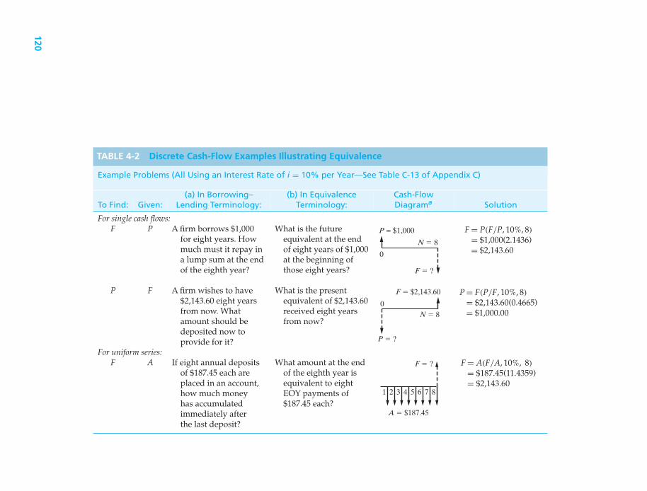
TABLE 4-2 Discrete Cash-Flow Examples Illustrating Equivalence

Example Problems (All Using an Interest Rate of i = 10% per Year—See Table C-13 of Appendix C)

(a) In Borrowing– (b) In Equivalence Cash-FlowTo Find: Given: Lending Terminology: Terminology: Diagrama Solution

For single cash flows:F P A firm borrows $1,000

for eight years. Howmuch must it repay ina lump sum at the endof the eighth year?

What is the futureequivalent at the endof eight years of $1,000at the beginning ofthose eight years?

P = $1,000

N � 8

F � ?

0

F = P(F/P, 10%, 8)

= $1,000(2.1436)= $2,143.60

P F A firm wishes to have$2,143.60 eight yearsfrom now. Whatamount should bedeposited now toprovide for it?

What is the presentequivalent of $2,143.60received eight yearsfrom now?

F � $2,143.60

N � 8

P � ?

0

P = F(P/F, 10%, 8)

= $2,143.60(0.4665)= $1,000.00

For uniform series:F A If eight annual deposits

of $187.45 each areplaced in an account,how much moneyhas accumulatedimmediately afterthe last deposit?

What amount at the endof the eighth year isequivalent to eightEOY payments of$187.45 each?

A � $187.45

F � ?

1 2 3 4 5 6 7 8

F = A(F/A, 10%, 8)

= $187.45(11.4359)= $2,143.60

120

TABLE 4-2 (Continued)

P A How much should bedeposited in a fundnow to providefor eight EOYwithdrawals of$187.45 each?

What is the presentequivalent of eightEOY payments of$187.45 each?

A � $187.45

P � ?

1 2 3 4 5 6 7 8

P = A(P/A, 10%, 8)

= $187.45(5.3349)= $1,000.00

A F What uniform annualamount should bedeposited each year inorder to accumulate$2,143.60 at the time ofthe eighth annualdeposit?

What uniform paymentat the end of eightsuccessive years isequivalent to $2,143.60at the end of theeighth year? A � ?

F � $2,143.60

1 2 3 4 5 6 7 8

A = F(A/F, 10%, 8)

= $2,143.60(0.0874)= $187.45

A P What is the size of eightequal annualpayments to repay aloan of $1,000? Thefirst payment is dueone year afterreceiving the loan.

What uniform paymentat the end of eightsuccessive years isequivalent to $1,000at the beginning ofthe first year? A � ?

P � $1,000

1 2 3 4 5 6 7 8

A = P(A/P, 10%, 8)

= $1,000(0.18745)= $187.45

a The cash-flow diagram represents the example as stated in borrowing-lending terminology.

121

122 CHAPTER 4 / THE TIME VALUE OF MONEY

price of gasoline. Given the average prices in different years, you can use therelationship between P and F to solve for the inflation rate.

EXAMPLE 4-5 The Inflating Price of Gasoline

The average price of gasoline in 2005 was $2.31 per gallon. In 1993, the averageprice was $1.07.∗ What was the average annual rate of increase in the price ofgasoline over this 12-year period?

SolutionWith respect to the year 1993, the year 2005 is in the future. Thus, P = $1.07, F =$2.31, and N = 12. Using Equation (4-6), we find i = 12

√2.31/1.07 − 1 = 0.0662

or 6.62% per year.

∗ This data was obtained from the Energy Information Administration of the Department of Energy. Historicalprices of gasoline and other energy sources can be found at www.eia.doe.gov.

4.6.4 Finding N when Given P, F , and i

Sometimes we are interested in finding the amount of time needed for a presentsum to grow into a future sum at a specified interest rate. For example, how longwould it take for $500 invested today at 15% interest per year to be worth $1,000? Wecan use the equivalence relationship given in Equation (4-2) to obtain an expressionfor N.

F = P(1 + i)N

(1 + i)N = (F/P)

Using logarithms,

N log(1 + i) = log(F/P)

and

N = log(F/P)

log(1 + i). (4-7)

For our simple example, N = log($1,000/$500)/ log(1.15) = 4.96 ∼= 5 years.

EXAMPLE 4-6 When Will Gasoline Cost $5.00 per Gallon?

In Example 4-5, the average price of gasoline was given as $2.31 in 2005. Wecomputed the average annual rate of increase in the price of gasoline to be 6.62%.If we assume that the price of gasoline will continue to inflate at this rate, howlong will it be before we are paying $5.00 per gallon?

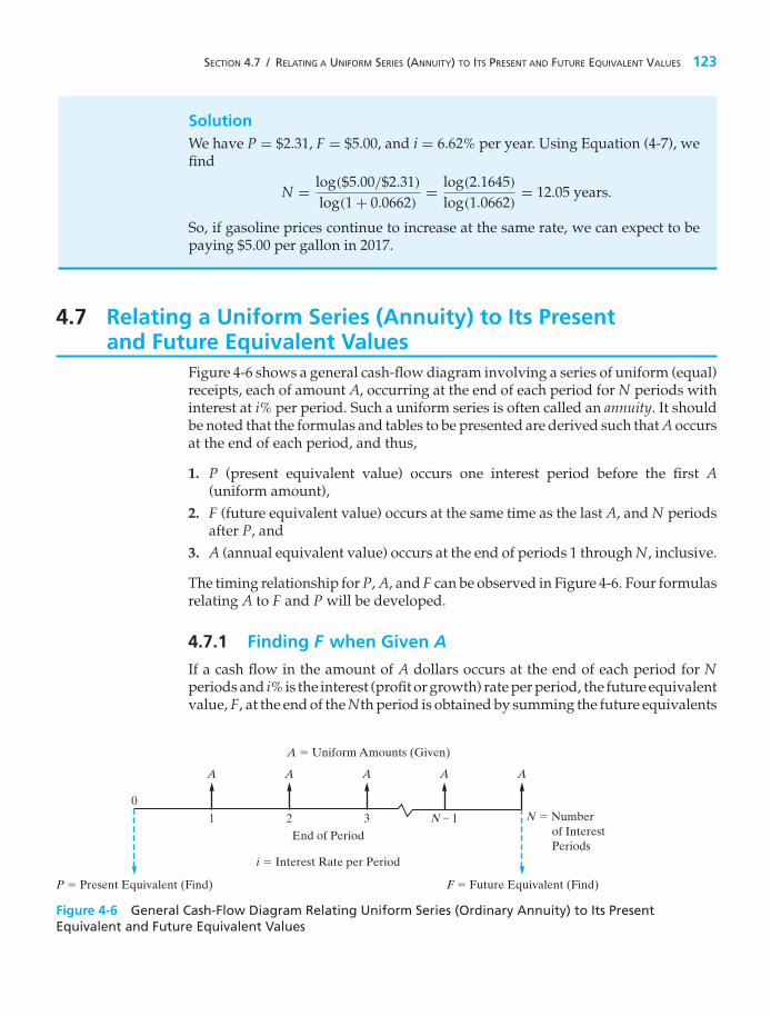
SECTION 4.7 / RELATING A UNIFORM SERIES (ANNUITY) TO ITS PRESENT AND FUTURE EQUIVALENT VALUES 123

SolutionWe have P = $2.31, F = $5.00, and i = 6.62% per year. Using Equation (4-7), wefind

N = log($5.00/$2.31)

log(1 + 0.0662)= log(2.1645)

log(1.0662)= 12.05 years.

So, if gasoline prices continue to increase at the same rate, we can expect to bepaying $5.00 per gallon in 2017.

4.7 Relating a Uniform Series (Annuity) to Its Presentand Future Equivalent Values

Figure 4-6 shows a general cash-flow diagram involving a series of uniform (equal)receipts, each of amount A, occurring at the end of each period for N periods withinterest at i% per period. Such a uniform series is often called an annuity. It shouldbe noted that the formulas and tables to be presented are derived such that A occursat the end of each period, and thus,

1. P (present equivalent value) occurs one interest period before the first A(uniform amount),

2. F (future equivalent value) occurs at the same time as the last A, and N periodsafter P, and

3. A (annual equivalent value) occurs at the end of periods 1 through N, inclusive.

The timing relationship for P, A, and F can be observed in Figure 4-6. Four formulasrelating A to F and P will be developed.

4.7.1 Finding F when Given A

If a cash flow in the amount of A dollars occurs at the end of each period for Nperiods and i% is the interest (profit or growth) rate per period, the future equivalentvalue, F, at the end of the Nth period is obtained by summing the future equivalents

i � Interest Rate per Period

End of Period

P � Present Equivalent (Find) F � Future Equivalent (Find)

A A A A

A � Uniform Amounts (Given)

1

0

2 3 N – 1 N � Number of Interest Periods

A

Figure 4-6 General Cash-Flow Diagram Relating Uniform Series (Ordinary Annuity) to Its PresentEquivalent and Future Equivalent Values

124 CHAPTER 4 / THE TIME VALUE OF MONEY

of each of the cash flows. Thus,

F = A(F/P, i%, N − 1) + A(F/P, i%, N − 2) + A(F/P, i%, N − 3) + · · ·+ A(F/P, i%, 1) + A(F/P, i%, 0)

= A[(1 + i)N−1 + (1 + i)N−2 + (1 + i)N−3 + · · · + (1 + i)1 + (1 + i)0].The bracketed terms comprise a geometric sequence having a common ratio

of (1 + i)−1. Recall that the sum of the first N terms of a geometric sequence is

SN = a1 − baN

1 − b(b �= 1),

where a1 is the first term in the sequence, aN is the last term, and b is the commonratio. If we let b = (1 + i)−1, a1 = (1 + i)N−1, and aN = (1 + i)0, then

F = A

⎡⎢⎢⎣

(1 + i)N−1 − 1(1 + i)

1 − 1(1 + i)

⎤⎥⎥⎦ ,

which reduces to

F = A

[(1 + i)N − 1

i

]. (4-8)

The quantity {[(1 + i)N − 1]/i} is called the uniform series compound amount factor.It is the starting point for developing the remaining three uniform series interestfactors.

Numerical values for the uniform series compound amount factor are givenin the fourth column of the tables in Appendix C for a wide range of values ofi and N. We shall use the functional symbol (F/A, i%, N) for this factor. Hence,Equation (4-8) can be expressed as

F = A(F/A, i%, N). (4-9)

Examples of this type of “wealth accumulation” problem based on the (F/A, i%, N)factor are provided here and in Table 4-2.

EXAMPLE 4-7 Future Value of a College Degree

A recent government study reported that a college degree is worth an extra$23,000 per year in income (A) compared to what a high-school graduate makes.If the interest rate (i) is 6% per year and you work for 40 years (N), what is thefuture compound amount (F) of this extra income?

SolutionThe viewpoint we will use to solve this problem is that of “lending” the $23,000of extra annual income to a savings account (or some other investment vehicle).The future equivalent is the amount that can be withdrawn after the 40th depositis made.

SECTION 4.7 / RELATING A UNIFORM SERIES (ANNUITY) TO ITS PRESENT AND FUTURE EQUIVALENT VALUES 125

Graduatefrom

College 0 1 2 3 39 40

A � $23,000

F � ?

End of Year

Notice that the future equivalent occurs at the same time as the last deposit of$23,000.

F = $23,000(F/A, 6%, 40)

= $23,000(154.762)

= $3,559,526

The bottom line is “Get your college degree!”

EXAMPLE 4-8 Become a Millionaire by Saving $1.00 a Day!

To illustrate further the amazing effects of compound interest, we consider thecredibility of this statement: “If you are 20 years of age and save $1.00 each dayfor the rest of your life, you can become a millionaire.” Let’s assume that youlive to age 80 and that the annual interest rate is 10% (i = 10%). Under thesespecific conditions, we compute the future compound amount (F) to be

F = $365/year (F/A, 10%, 60 years)

= $365 (3,034.81)

= $1,107,706.

Thus, the statement is true for the assumptions given! The moral is to start savingearly and let the “magic” of compounding work on your behalf!

A few words to the wise: Saving money early and preserving resources throughfrugality (avoiding waste) are extremely important ingredients of wealth creationin general. Often, being frugal means postponing the satisfaction of immediatematerial wants for the creation of a better tomorrow. In this regard, be very cautiousabout spending tomorrow’s cash today by undisciplined borrowing (e.g., withcredit cards). The (F/A, i%, N) factor also demonstrates how fast your debt canaccumulate!

126 CHAPTER 4 / THE TIME VALUE OF MONEY

4.7.2 Finding P when Given A

From Equation (4-2), F = P(1 + i)N . Substituting for F in Equation (4-8) wedetermine that

P(1 + i)N = A

[(1 + i)N − 1

i

].

Dividing both sides by (1 + i)N , we get

P = A

[(1 + i)N − 1

i(1 + i)N

]. (4-10)

Thus, Equation (4-10) is the relation for finding the present equivalent value(as of the beginning of the first period) of a uniform series of end-of-period cashflows of amount A for N periods. The quantity in brackets is called the uniform seriespresent worth factor. Numerical values for this factor are given in the fifth columnof the tables in Appendix C for a wide range of values of i and N. We shall use thefunctional symbol (P/A, i%, N) for this factor. Hence,

P = A(P/A, i%, N). (4-11)

EXAMPLE 4-9 Present Equivalent of an Annuity (Uniform Series)

A micro-brewery is considering the installation of a newly designed boilersystem that burns the dried, spent malt and barley grains from the brewingprocess. The boiler will produce process steam that powers the majority of thebrewery’s energy operations, saving $450,000 per year over the boiler’s expectedlife of 10 years. If the interest rate is 12% per year, how much money can thebrewery afford to invest in the new boiler system?

SolutionIn the cash flow diagram below, notice that the affordable amount (i.e., thepresent equivalent, P) occurs one time period (year) before the first end-of-yearcash flow of $450,000.

1 2 3 4 5 6 7 8 9 10

P = ?

End of Year

A = $450,000

0

SECTION 4.7 / RELATING A UNIFORM SERIES (ANNUITY) TO ITS PRESENT AND FUTURE EQUIVALENT VALUES 127

The increase in annual cash flow is $450,000, and it continues for 10 years at 12%annual interest. The upper limit on what the brewery can afford to spend on thenew boiler is:

P = $450,000 (P/A, 12%, 10)

= $450,000 (5.6502)

= $2,542,590.

EXAMPLE 4-10 How Much Is a Lifetime Oil Change Offer Worth?

“Make your best deal with us on a new automobile and we’ll change your oil forfree for as long as you own the car!” If you purchase a car from this dealership,you expect to have four free oil changes per year during the five years you keepthe car. Each oil change would normally cost you $30. If you save your moneyin a mutual fund earning 2% per quarter, how much are the oil changes worthto you at the time you buy the car?

SolutionIn this example, we need to find the present equivalent of the cost of futureoil changes. The cash-flow diagram is shown below. Notice that P occurs onetime period (a quarter of a year, in this example) before the first oil change cashflow (A).

A � $30

10 19 202 3

P � ?

End of Quarter

Time ofPurchase

The interest rate is 2% per quarter, and a total of (4 oil changes/year × 5 years) =20 oil changes (cash flows) are anticipated.

P = $30(P/A, 2%, 20)

= $30(16.3514)

= $490.54

128 CHAPTER 4 / THE TIME VALUE OF MONEY

Now you are in a position to determine how great of a deal you are being offered.If the best price of another dealership is more than $490.54 cheaper than whatyou are being offered at this dealership, maybe this deal isn’t so great.

4.7.3 Finding A when Given F

Taking Equation (4-8) and solving for A, we find that

A = F[

i(1 + i)N − 1

]. (4-12)

Thus, Equation (4-12) is the relation for finding the amount, A, of a uniformseries of cash flows occurring at the end of N interest periods that would beequivalent to (have the same value as) its future value occurring at the end ofthe last period. The quantity in brackets is called the sinking fund factor. Numericalvalues for this factor are given in the sixth column of the tables in Appendix C fora wide range of values of i and N. We shall use the functional symbol (A/F, i%, N)for this factor. Hence,

A = F(A/F, i%, N). (4-13)

Another example of this type of problem, together with a cash-flow diagramand solution, is given in Table 4-2.

4.7.4 Finding A when Given P

Taking Equation (4-10) and solving for A, we find that

A = P

[i(1 + i)N

(1 + i)N − 1

]. (4-14)

Thus, Equation (4-14) is the relation for finding the amount, A, of a uniformseries of cash flows occurring at the end of each of N interest periods that wouldbe equivalent to, or could be traded for, the present equivalent P, occurring at thebeginning of the first period. The quantity in brackets is called the capital recoveryfactor.∗ Numerical values for this factor are given in the seventh column of the tablesin Appendix C for a wide range of values of i and N. We shall use the functionalsymbol (A/P, i%, N) for this factor. Hence,

A = P(A/P, i%, N). (4-15)

An example that uses the equivalence between a present lump-sum loanamount and a series of equal uniform monthly payments starting at the end ofmonth one and continuing through month four was provided in Table 4-1 as Plan 2.

∗ The capital recovery factor is more conveniently expressed as i/[1 − (1 + i)−N ] for computation with a hand-heldcalculator.

SECTION 4.7 / RELATING A UNIFORM SERIES (ANNUITY) TO ITS PRESENT AND FUTURE EQUIVALENT VALUES 129

$17,1701% interest

$17,000

Amount Owed

($)

Repay$4,357.10 $12,941.03

Repay$4,357.10

Repay$4,357.10

Repay$4,357.10

$8,669.77

$4,355.80

$12,812.90

$8,583.93

$4,312.67

0 1 2 3 4End of Month

~0

Figure 4-7 Relationship of Cash Flows for Plan 2 of Table 4-1 to Repaymentof the $17,000 Loan Principal

Equation (4-15) yields the equivalent value of A that repays the $17,000 loan plus1% interest per month over four months:

A = $17,000(A/P, 1%, 4) = $17,000(0.2563) = $4,357.10

The entries in columns three and five of Plan 2 in Table 4-1 can now be betterunderstood. Interest owed at the end of month one equals $17,000(0.01), andtherefore the principal repaid out of the total end-of-month payment of $4,357.10is the difference, $4,187.10. At the beginning of month two, the amount of prin-cipal owed is $17,000 − $4,187.10 = $12,812.90. Interest owed at the end ofmonth two is $12,812.90(0.01) = $128.13, and the principal repaid at that timeis $4,357.10 − $128.13 = $4,228.97. The remaining entries in Plan 2 are obtained byperforming these calculations for months three and four.

A graphical summary of Plan 2 is given in Figure 4-7. Here it can be seen that1% interest is being paid on the beginning-of-month amount owed and that month-end payments of $4,357.10, consisting of interest and principal, bring the amountowed to $0 at the end of the fourth month. (The exact value of A is $4,356.78 andproduces an exact value of $0 at the end of four months.) It is important to notethat all the uniform series interest factors in Table 4-2 involve the same concept asthe one illustrated in Figure 4-7.

EXAMPLE 4-11 Computing Your Monthly Car Payment

You borrow $15,000 from your credit union to purchase a used car. The interestrate on your loan is 0.25% per month∗ and you will make a total of 36 monthlypayments. What is your monthly payment?

∗ A good credit score (rating) can help you secure lower interest rates on loans. The Web site www.annualcreditreport.com allows you to check your credit score once per year at no cost.

130 CHAPTER 4 / THE TIME VALUE OF MONEY

SolutionThe cash-flow diagram shown below is drawn from the viewpoint of the bank.Notice that the present amount of $15,000 occurs one month (interest period)before the first cash flow of the uniform repayment series.

10 2 3 35 36

A � ?

End of Month

P � $15,000

The amount of the car payment is easily calculated using Equation (4-15).

A = $15,000(A/P, 1/4%, 36)

= $15,000(0.0291)

= $436.50 per month

Another example of a problem where we desire to compute an equivalentvalue for A, from a given value of P and a known interest rate and number ofcompounding periods, is given in Table 4-2.

For an annual interest rate of 10%, the reader should now be convinced fromTable 4-2 that $1,000 at the beginning of year one is equivalent to $187.45 at theEOYs one through eight, which is then equivalent to $2,143.60 at EOY eight.

4.7.5 Finding the Number of Cash Flows in an AnnuityGiven A, P, and i

Sometimes we may have information about a present amount of money (P), themagnitude of an annuity (A), and the interest rate (i). The unknown factor in thiscase is the number of cash flows in the annuity (N).

EXAMPLE 4-12 Prepaying a Loan−−Finding N

Your company has a $100,000 loan for a new security system it just bought. Theannual payment is $8,880 and the interest rate is 8% per year for 30 years. Yourcompany decides that it can afford to pay $10,000 per year. After how manypayments (years) will the loan be paid off?

SECTION 4.7 / RELATING A UNIFORM SERIES (ANNUITY) TO ITS PRESENT AND FUTURE EQUIVALENT VALUES 131

SolutionThe original loan payment was found using Equation (4-15).

A = $100,000 (A/P, 8%, 30) = $100,000 (0.0888) = $8,800 per year

Now, instead of paying $8,880 per year, your company is going to pay $10,000per year. Common sense tells us that less than 30 payments will be necessary topay off the $100,000 loan. Using Equation (4-11), we find

$100,000 = $10,000 (P/A, 8%, N)

(P/A, 8%, N) = 10.

We can now use the interest tables provided in Appendix C to find N. Lookingdown the Present Worth Factor column (P/A) of Table C-11, we see that

(P/A, 8%, 20) = 9.8181

and

(P/A, 8%, 21) = 10.0168.

So, if $10,000 is paid per year, the loan will be paid off after 21 years instead of30. The exact amount of the 21st payment will be slightly less than $10,000 (butwe’ll save that solution for another example).

Spreadsheet SolutionThere is a financial function in Excel that would allow us to solve for the unknownnumber of periods. NPER(rate, pmt, pv) will compute the number of paymentsof magnitude pmt required to pay off a present amount (pv) at a fixed interestrate (rate).

N = NPER(0.08, −10000, 100000) = 20.91

Note that from your company’s viewpoint, it received $100,000 (a cashinflow) at time 0 and is making $10,000 payments (cash outflows). Hencethe annuity is expressed as a negative number in NPER( ) and the presentamount as a positive number. If we were to reverse the signs—which wouldrepresent the lender’s viewpoint—the same result would be obtained, namelyNPER(0.08, 10000, −100000) = 20.91.

CommentPrepaying loans can save thousands of dollars in interest. For example, look atthe total interest paid under these two repayment plans.

Original payment plan ($8,880 per year for 30 years):

Total interest paid = $8,880 × 30 − $100,000 = $166,400

132 CHAPTER 4 / THE TIME VALUE OF MONEY

New payment plan ($10,000 per year for 21 years):

Total interest paid = $10,000 × 21 − $100,000 = $110,000

Prepaying the loan in this way would save $56,400 in interest!

4.7.6 Finding the Interest Rate, i, Given A, F , and N

Now let’s look at the situation in which you know the amount (A) and duration (N)of a uniform payment series. You also know the desired future value of the series (F).What you don’t know is the interest rate that makes them equivalent. As was thecase for an unknown N, there is no single equation to determine i. However, wecan use the known relationships between i, A, F, and N and the method of linearinterpolation to approximate the interest rate.

EXAMPLE 4-13 Finding the Interest Rate to Meet an Investment Goal

After years of being a poor, debt-encumbered college student, you decide thatyou want to pay for your dream car in cash. Not having enough money now,you decide to specifically put money away each year in a “dream car” fund. Thecar you want to buy will cost $60,000 in eight years. You are going to put aside$6,000 each year (for eight years) to save for this. At what interest rate must youinvest your money to achieve your goal of having enough to purchase the carafter eight years?

SolutionWe can use Equation (4-9) to show our desired equivalence relationship.

$60,000 = $6,000 (F/A, i%, 8)

(F/A, i%, 8) = 10

Now we can use the interest tables in Appendix C to help track down theunknown value of i. What we are looking for are two interest rates, one withan (F/A, i%, 8) value greater than 10 and one with an (F/A, i%, 8) less than 10.Thumbing through Appendix C, we find

(F/A, 6%, 8) = 9.8975 and (F/A, 7%, 8) = 10.2598,

which tells us that the interest rate we are looking for is between 6% and 7%per year. Even though the function (F/A, i%, N) is nonlinear, we can use linearinterpolation to approximate the value of i.

The dashed curve in Figure 4-8 is what we are linearly approximating. Theanswer, i′, can be determined by using the similar triangles dashed in Figure 4-8.

line dAline ed

= line BAline CB

SECTION 4.8 / SUMMARY OF INTEREST FORMULAS AND RELATIONSHIPS FOR DISCRETE COMPOUNDING 133

9.8975

10

0.06 0.07i�Interest Rate per Year

10.2598

A

e

C

Bd

(F/A

, i%

, 8)

Figure 4-8 Using Linear Interpolation to Approximate i in Example 4-13

i′ − 0.0610 − 9.8975

= 0.07 − 0.0610.2598 − 9.8975

i′ = 0.0628 or 6.28% per year

So if you can find an investment account that will earn at least 6.28% interestper year, you’ll have the $60,000 you need to buy your dream car in eight years.

Spreadsheet SolutionExcel has another financial function that allows you to solve for an unknowninterest rate. RATE(nper, pmt, pv, fv) will return the fixed interest rate that equatesan annuity of magnitude pmt that lasts for nper periods to either its present value(pv) or its future value (fv).

i′ = RATE(8, −6000, 0, 60000) = 0.0629 or 6.29% per year

Note that a 0 was entered for pv since we were working with a known futurevalue in this example.

4.8 Summary of Interest Formulas and Relationshipsfor Discrete Compounding

Table 4-3 provides a summary of the six most common discrete compound interestfactors, utilizing notation of the preceding sections. The formulas are for discretecompounding, which means that the interest is compounded at the end of each finite-length period, such as a month or a year. Furthermore, the formulas also assume

134 CHAPTER 4 / THE TIME VALUE OF MONEY

discrete (i.e., lump sum) cash flows spaced at the end of equal time intervals on acash-flow diagram. Discrete compound interest factors are given in Appendix C,where the assumption is made that i remains constant during the N compoundingperiods.

There are also several useful relationships between the compound interestfactors. These relationships are summarized in the following equations.

(P/F, i%, N) = 1(F/P, i%, N)

; (4-16)

(A/P, i%, N) = 1(P/A, i%, N)

; (4-17)

(A/F, i%, N) = 1(F/A, i%, N)

; (4-18)

(F/A, i%, N) = (P/A, i%, N)(F/P, i%, N); (4-19)

(P/A, i%, N) =N∑

k=1

(P/F, i%, k); (4-20)

TABLE 4-3 Discrete Compounding-Interest Factors and Symbolsa

Factor by which Factorto Multiply Functional

To Find: Given: “Given”a Factor Name Symbolb

For single cash flows:F P (1 + i)N Single payment compound

amount(F/P, i%, N)

P F 1(1+i)N Single payment present

worth(P/F, i%, N)

For uniform series (annuities):

F A (1+i)N−1i Uniform series compound

amount(F/A, i%, N)

P A (1+i)N−1i(1+i)N Uniform series present

worth(P/A, i%, N)

A F i(1+i)N−1

Sinking fund (A/F, i%, N)

A P i(1+i)N

(1+i)N−1Capital recovery (A/P, i%, N)

a i equals effective interest rate per interest period; N, number of interest periods; A, uniform series amount(occurs at the end of each interest period); F, future equivalent; P, present equivalent.b The functional symbol system is used throughout this book.

SECTION 4.9 / DEFERRED ANNUITIES (UNIFORM SERIES) 135

(F/A, i%, N) =N∑

k=1

(F/P, i%, N − k); (4-21)

(A/F, i%, N) = (A/P, i%, N) − i. (4-22)

4.9 Deferred Annuities (Uniform Series)All annuities (uniform series) discussed to this point involve the first cash flowbeing made at the end of the first period, and they are called ordinary annuities.If the cash flow does not begin until some later date, the annuity is known as adeferred annuity. If the annuity is deferred for J periods (J < N), the situation isas portrayed in Figure 4-9, in which the entire framed ordinary annuity has beenmoved away from “time present,” or “time zero,” by J periods. Remember that, inan annuity deferred for J periods, the first payment is made at the end of period(J + 1), assuming that all periods involved are equal in length.

The present equivalent at the end of period J of an annuity with cash flows ofamount A is, from Equation (4-9), A(P/A, i%, N − J). The present equivalent of thesingle amount A(P/A, i%, N − J) as of time zero will then be

P0 = A(P/A, i%, N − J)(P/F, i%, J).

Time Present0 1 J � 1 J J � 1 J � 2 J � 3 N � 1 N

End of Period

i %

Figure 4-9 General Cash-Flow Representation of a Deferred Annuity(Uniform Series)

EXAMPLE 4-14 Present Equivalent of a Deferred Annuity

To illustrate the preceding discussion, suppose that a father, on the day his sonis born, wishes to determine what lump amount would have to be paid into anaccount bearing interest of 12% per year to provide withdrawals of $2,000 oneach of the son’s 18th, 19th, 20th, and 21st birthdays.

SolutionThe problem is represented in the following cash-flow diagram. One should firstrecognize that an ordinary annuity of four withdrawals of $2,000 each is involvedand that the present equivalent of this annuity occurs at the 17th birthday whena (P/A, i%, N − J) factor is utilized. In this problem, N = 21 and J = 17. It isoften helpful to use a subscript with P or F to denote the respective point in time.

136 CHAPTER 4 / THE TIME VALUE OF MONEY

Hence,

P17 = A(P/A, 12%, 4) = $2,000(3.0373) = $6,074.60.

P0 � ?

212019181721

0

A � $2,000

i � 12% per YearP17 � F17

End of Year

Note the dashed arrow in the cash-flow diagram denoting P17. Now that P17is known, the next step is to calculate P0. With respect to P0, P17 is a futureequivalent, and hence it could also be denoted F17. Money at a given point intime, such as the end of period 17, is the same regardless of whether it is calleda present equivalent or a future equivalent. Hence,

P0 = F17(P/F, 12%, 17) = $6,074.60(0.1456) = $884.46,

which is the amount that the father would have to deposit on the day his son isborn.

EXAMPLE 4-15 Deferred Future Value of an Annuity

When you take your first job, you decide to start saving right away for yourretirement. You put $5,000 per year into the company’s 401(k) plan, whichaverages 8% interest per year. Five years later, you move to another job and starta new 401(k) plan. You never get around to merging the funds in the two plans.If the first plan continued to earn interest at the rate of 8% per year for 35 yearsafter you stopped making contributions, how much is the account worth?

SolutionThe following cash-flow diagram clarifies the timing of the cash flows for theoriginal 401(k) investment plan.

1 2 3 4

A � $5,000

39 405 6

End of Year (EOY)

F � ?

SECTION 4.10 / EQUIVALENCE CALCULATIONS INVOLVING MULTIPLE INTEREST FORMULAS 137

The easiest way to approach this is to first find the future equivalent of theannuity as of time 5.

F5 = $5,000 (F/A, 8%, 5) = $5,000 (5.8666) = $29,333.

To determine F40, F5 can now be denoted P5, and

F40 = P5 (F/P, 8%, 35) = $29,333 (14.7853) = $433,697.

4.10 Equivalence Calculations Involving MultipleInterest Formulas

You should now be comfortable with equivalence problems that involve discretecompounding of interest and discrete cash flows. All compounding of interesttakes place once per time period (e.g., a year), and to this point cash flows alsooccur once per time period. This section provides examples involving two ormore equivalence calculations to solve for an unknown quantity. The end-of-yearcash-flow convention is used. Again, the interest rate is constant over the N timeperiods.

EXAMPLE 4-16 Calculating Equivalent P, F , and A Values

Figure 4-10 depicts an example problem with a series of year-end cash flowsextending over eight years. The amounts are $100 for the first year, $200 forthe second year, $500 for the third year, and $400 for each year from thefourth through the eighth. These could represent something like the expectedmaintenance expenditures for a certain piece of equipment or payments intoa fund. Note that the payments are shown at the end of each year, which is astandard assumption (convention) for this book and for economic analyses ingeneral, unless we have information to the contrary. It is desired to find

(a) the present equivalent expenditure, P0;(b) the future equivalent expenditure, F8;(c) the annual equivalent expenditure, A

of these cash flows if the annual interest rate is 20%. Solve by hand and by usinga spreadsheet.

Solution by Hand(a) To find the equivalent P0, we need to sum the equivalent values of all

payments as of the beginning of the first year (time zero). The requiredmovements of money through time are shown graphically in Figure 4-10(a).

138 CHAPTER 4 / THE TIME VALUE OF MONEY

P0 = F1(P/F, 20%, 1) = $100(0.8333) = $83.33

+F2(P/F, 20%, 2) + $200(0.6944) + 138.88

+F3(P/F, 20%, 3) + $500(0.5787) + 289.35

+A(P/A, 20%, 5) × (P/F, 20%, 3) + $400(2.9900) × (0.5787) + 692.26$1,203.82.

(b) To find the equivalent F8, we can sum the equivalent values of all paymentsas of the end of the eighth year (time eight). Figure 4-10(b) indicates these

P0 � $1,203.82

$400

10 2 3 4 5 6 7 8End of Year

$400$400$400$400$500

$200

$100

� (P/F, 20%, 2)

� (P/F, 20%, 3)

� (P/F, 20%, 1)

� (P/A, 20%, 5)(P/F, 20%, 3)

(a)

F8 � $5,176.19

0 1 2 3 4 5 6 7 8

End of Year

$400$400$400$400$500

$200

$100

� (F/P, 20%, 7) � (F/A, 20%, 5)

(b)

� (F/P, 20%, 5)

� (F/P, 20%, 6)

F8 (from b)

10 2 3 4 5 6 7 8

� (A/F, 20%, 8)

(c)

A � $313.73 A A A A A A A

P0(from a)

� (A/P, 20%, 8)

End of Year

$400

Figure 4-10 Example 4-16 for Calculating the Equivalent P, F ,and A Values

SECTION 4.10 / EQUIVALENCE CALCULATIONS INVOLVING MULTIPLE INTEREST FORMULAS 139

movements of money through time. However, since the equivalent P0 isalready known to be $1,203.82, we can directly calculate

F8 = P0(F/P, 20%, 8) = $1,203.82(4.2998) = $5,176.19.

(c) The equivalent A of the irregular cash flows can be calculated directly fromeither P0 or F8 as

A = P0(A/P, 20%, 8) = $1,203.82(0.2606) = $313.73

or

A = F8(A/F, 20%, 8) = $5,176.19(0.0606) = $313.73.

The computation of A from P0 and F8 is shown in Figure 4-10(c). Thus, wefind that the irregular series of payments shown in Figure 4-10 is equivalentto $1,203.82 at time zero, $5,176.19 at time eight, or a uniform series of $313.73at the end of each of the eight years.

Spreadsheet SolutionFigure 4-11 displays a spreadsheet solution for this example. The presentequivalent (P0) of the tabulated cash flows is easily computed by using the NPVfunction with the stated interest rate (20% in cell B1). The future equivalent (F8) isdetermined from the present equivalent by using the (F/P, i%, N) relationship.The annual equivalent is also determined from the present equivalent by

Figure 4-11SpreadsheetSolution,Example 4-16

= PMT(B1, B2, –B12)

= B12 * (1 + B1) ^ B2

= NPV(B1, E3:E10)

140 CHAPTER 4 / THE TIME VALUE OF MONEY

applying the PMT function. The slight differences in results when comparedto the hand solution are due to rounding of the interest factor values in the handsolution.

EXAMPLE 4-17 How Much is that Last Payment? (Example 4-12 Revisited)

In Example 4-12, we looked at paying off a loan early by increasing the annualpayment. The $100,000 loan was to be repaid in 30 annual installments of $8,880at an interest rate of 8% per year. As part of the example, we determined that theloan could be paid in full after 21 years if the annual payment was increased to$10,000.

As with most real-life loans, the final payment will be something different(usually less) than the annuity amount. This is due to the effect of rounding inthe interest calculations—you can’t pay in fractions of a cent! For this example,determine the amount of the 21st (and final) payment on the $100,000 loan when20 payments of $10,000 have already been made. The interest rate remains at 8%per year.

SolutionThe cash-flow diagram for this example is shown below. It is drawn from thelender’s viewpoint.

0 1 2 3

$100,000

19 20 21

$10,000

End of Year

F � ?

We need to determine the value of F that will make the present equivalent of allloan payments equal to the amount borrowed. We can do this by discountingall of the payments to time 0 (including the final payment, F) and setting theirvalue equal to $100,000.

$10,000 (P/A, 8%, 20) + F (P/F, 8%, 21) = $100,000

$10,000 (9.8181) + F (0.1987) = $100,000

F = $9,154.50

Thus, a payment of $9,154.50 is needed at the end of year 21 to pay off the loan.

SECTION 4.10 / EQUIVALENCE CALCULATIONS INVOLVING MULTIPLE INTEREST FORMULAS 141

EXAMPLE 4-18 The Present Equivalent of BP’s Payment Schedule

In this example, we answer the question posed at the beginning of the chapter—what is the present equivalent value of BP’s proposed payment schedule? Recallthat BP will pay $3 billion at the end of the third quarter of 2010 and another $2billion in the fourth quarter of 2010. Twelve additional payments of $1.25 billioneach quarter thereafter will result in a total of $20 billion having been paid intothe fund. The interest rate is 3% per quarter.

SolutionFigure 4-12 shows the cash-flow diagram for this situation. The presentequivalent of the cash flows is

P = $3 billion (P/F, 3%, 1) + $2 billion (P/F, 3%, 2)

+ $1.25 billion (P/A, 3%, 12) (P/F, 3%, 2)

= $3 billion (0.9709) + $2 billion (0.9426) + $1.25 (9.9540)(0.9426)

= $16.53 billion.

1 2 3 4 5 6 7 8 9 10 11 12 13 14

0

P = ?

$1.25 billion

$2 billion

$3 billion

End of Quarter

Figure 4-12 Cash-Flow Diagram for Example 4-18

EXAMPLE 4-19 Determining an Unknown Annuity Amount

Two receipts of $1,000 each are desired at the EOYs 10 and 11. To make thesereceipts possible, four EOY annuity amounts will be deposited in a bank at EOYs2, 3, 4, and 5. The bank’s interest rate (i) is 12% per year.

(a) Draw a cash-flow diagram for this situation.(b) Determine the value of A that establishes equivalence in your cash-flow

diagram.(c) Determine the lump-sum value at the end of year 11 of the completed cash-

flow diagram based on your answers to Parts (a) and (b).

142 CHAPTER 4 / THE TIME VALUE OF MONEY

Solution(a) Cash-flow diagrams can make a seemingly complex problem much clearer.

The cash-flow diagram for this example is shown below.

1 2 3 4 5

$1,000

6 7 8 9 10 11

$1,000

End of Year

A � ?

(b) Because the unknown annuity, A, begins at EOY two, it makes sense toestablish our reference year for the equivalence calculations at EOY one(remember that the first annuity amount follows its P-equivalent amount byone year). So the P-equivalent at EOY 1 of the four A amounts is

P1 = A(P/A, 12%, 4).

Next we calculate the EOY one P-equivalent of $1,000 at EOY 10 and $1,000at EOY 11 as follows:

P′1 = $1,000 (P/A, 12%, 2) (P/F, 12%, 8).

The (P/F, 12%, 8) factor is needed to discount the equivalent value of the Aamounts at EOY nine to EOY one. By equating both P-equivalents at EOYone, we can solve for the unknown amount, A.

P1 = P′1

A (P/A, 12%, 4) = $1,000 (P/A, 12%, 2) (P/F, 12%, 8),

or

3.0373 A = $682.63

and

A = $224.75.

Therefore, we conclude that deposits of $224.75 at EOYs two, three, four,and five are equivalent to $1,000 at EOYs 10 and 11 if the interest rate is 12%per year.

(c) Now we need to calculate the F-equivalent at time 11 of the −$224.75 annuityin years 2 through 5 and the $1,000 annuity in years 10 and 11.

− $224.75 (F/A, 12%, 4) (F/P, 12%, 6) + $1,000 (F/A, 12%, 2)

= − $0.15This value should be zero, but round-off error in the interest factors causesa small difference of $0.15.

SECTION 4.11 / UNIFORM (ARITHMETIC) GRADIENT OF CASH FLOWS 143

4.11 Uniform (Arithmetic) Gradient of Cash FlowsSome problems involve receipts or expenses that are projected to increase ordecrease by a uniform amount each period, thus constituting an arithmetic sequenceof cash flows. For example, because of leasing a certain type of equipment,maintenance and repair savings relative to purchasing the equipment may increaseby a roughly constant amount each period. This situation can be modeled as auniform gradient of cash flows.

Figure 4-13 is a cash-flow diagram of a sequence of end-of-period cash flowsincreasing by a constant amount, G, in each period. The G is known as the uniformgradient amount. Note that the timing of cash flows on which the derived formulasand tabled values are based is as follows:

End of Period Cash Flows

1 (0)G2 (1)G3 (2)G· ·· ·· ·

N − 1 (N − 2)GN (N − 1)G

Notice that the first uniform gradient cash flow, G, occurs at the end of period two.

(N � 1)G

(N � 2)G

(N � 3)G

3G

2G

G

10 2 3 4 N � 2 N � 1 N

End of Period

i � Effective Interest Rate per Period

Figure 4-13 Cash-Flow Diagram for a Uniform Gradient Increasingby G Dollars per Period

144 CHAPTER 4 / THE TIME VALUE OF MONEY

4.11.1 Finding P when Given G

The present equivalent, P, of the arithmetic sequence of cash flows shown inFigure 4-13 is

P = G(1)

(1 + i)2 + G(2)

(1 + i)3 + G(3)

(1 + i)4 + · · · + G(N − 2)

(1 + i)N−1 + G(N − 1)

(1 + i)N .

If we add in the dummy term G(0)/(1 + i)1 to represent the “missing” cash flow attime one, we can rewrite the above equation as:

P = GN∑

n=1

(n − 1)

(1 + i)n .

Recognizing the above equation as the summation of a geometric sequence, we canmake the appropriate substitutions as we did in the development of Equation (4-6).After some algebraic manipulation, we have

P = G

{1i

[(1 + i)N − 1

i(1 + i)N − N(1 + i)N

]}. (4-23)

The term in braces in Equation (4-23) is called the gradient to present equivalentconversion factor. It can also be expressed as (1/i)[(P/A, i%, N) − N(P/F, i%, N)].Numerical values for this factor are given in column 8 of Appendix C for a wideassortment of i and N values. We shall use the functional symbol (P/G, i%, N) forthis factor. Hence,

P = G (P/G, i%, N). (4-24)

4.11.2 Finding A when Given G

From Equation (4-23), it is easy to develop an expression for A as follows:

A = P(A/P, i%, N)

= G

{1i

[(1 + i)N − 1

i(1 + i)N − N(1 + i)N

]}(A/P, i%, N)

= Gi

[(P/A, i%, N) − N

(1 + i)N

](A/P, i%, N)

= Gi

[1− Ni(1 + i)N

(1 + i)N[(1 + i)N − 1

]]

= Gi−G

[N

(1 + i)N − 1

]

= G[

1i

− N(1 + i)N − 1

]. (4-25)

The term in brackets in Equation (4-25) is called the gradient to uniform seriesconversion factor. Numerical values for this factor are given on the right-hand side

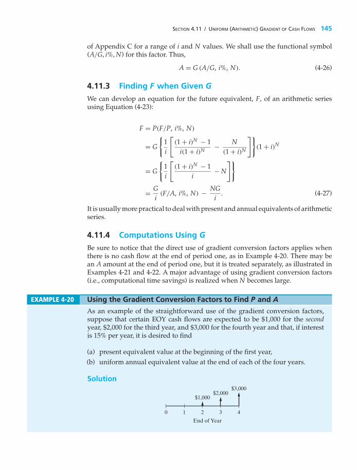
SECTION 4.11 / UNIFORM (ARITHMETIC) GRADIENT OF CASH FLOWS 145

of Appendix C for a range of i and N values. We shall use the functional symbol(A/G, i%, N) for this factor. Thus,

A = G (A/G, i%, N). (4-26)

4.11.3 Finding F when Given G

We can develop an equation for the future equivalent, F, of an arithmetic seriesusing Equation (4-23):

F = P(F/P, i%, N)

= G

{1i

[(1 + i)N − 1

i(1 + i)N − N(1 + i)N

]}(1 + i)N

= G

{1i

[(1 + i)N − 1

i− N

]}

= Gi

(F/A, i%, N) − NGi

. (4-27)

It is usually more practical to deal with present and annual equivalents of arithmeticseries.

4.11.4 Computations Using G

Be sure to notice that the direct use of gradient conversion factors applies whenthere is no cash flow at the end of period one, as in Example 4-20. There may bean A amount at the end of period one, but it is treated separately, as illustrated inExamples 4-21 and 4-22. A major advantage of using gradient conversion factors(i.e., computational time savings) is realized when N becomes large.

EXAMPLE 4-20 Using the Gradient Conversion Factors to Find P and A

As an example of the straightforward use of the gradient conversion factors,suppose that certain EOY cash flows are expected to be $1,000 for the secondyear, $2,000 for the third year, and $3,000 for the fourth year and that, if interestis 15% per year, it is desired to find

(a) present equivalent value at the beginning of the first year,(b) uniform annual equivalent value at the end of each of the four years.

Solution

0 1 2 3 4

$1,000$2,000

$3,000

End of Year

146 CHAPTER 4 / THE TIME VALUE OF MONEY

Observe that this schedule of cash flows fits the model of the arithmetic gradientformulas with G = $1,000 and N = 4. Note that there is no cash flow at the endof the first period.

(a) The present equivalent can be calculated as

P0 = G(P/G, 15%, 4) = $1,000(3.79) = $3,790.

(b) The annual equivalent can be calculated from Equation (4-26) as

A = G(A/G, 15%, 4) = $1,000(1.3263) = $1,326.30.

Of course, once P0 is known, the value of A can be calculated as

A = P0(A/P, 15%, 4) = $3,790(0.3503) = $1,326.30.

EXAMPLE 4-21 Present Equivalent of an Increasing Arithmetic Gradient Series

As a further example of the use of arithmetic gradient formulas, suppose thatwe have cash flows as follows:

End of Year Cash Flows ($)

1 5,0002 6,0003 7,0004 8,000

Also, assume that we wish to calculate their present equivalent at i = 15% peryear, using gradient conversion factors.

SolutionThe schedule of cash flows is depicted in the left-hand diagram of Figure 4-14.The right two diagrams of Figure 4-14 show how the original schedule can bebroken into two separate sets of cash flows, an annuity series of $5,000 plusan arithmetic gradient of $1,000 that fits the general gradient model for whichfactors are tabled. The summed present equivalents of these two separate setsof cash flows equal the present equivalent of the original problem. Thus, usingthe symbols shown in Figure 4-14, we have

P0T = P0A + P0G

= A(P/A, 15%, 4) + G(P/G, 15%, 4)

= $5,000(2.8550) + $1,000(3.79) = $14,275 + 3,790 = $18,065.

SECTION 4.11 / UNIFORM (ARITHMETIC) GRADIENT OF CASH FLOWS 147

The annual equivalent of the original cash flows could be calculated withthe aid of Equation (4-26) as follows:

AT = A + AG

= $5,000 + $1,000(A/G, 15%, 4) = $6,326.30.

AT is equivalent to P0T because $6,326.30(P/A, 15%, 4) = $18,061, which is thesame value obtained previously (subject to round-off error).

P0T

$7,000$8,000

0 1 2 3 4

$6,000$5,000

End of Year

P0A

0 1 2 3 4

$5,000

End of Year

� �

P0G

0 1 2 3 4

$1,000$2,000

$3,000

End of Year

Figure 4-14 Breakdown of Cash Flows for Example 4-21

EXAMPLE 4-22 Present Equivalent of a Decreasing Arithmetic Gradient Series

For another example of the use of arithmetic gradient formulas, suppose thatwe have cash flows that are timed in exact reverse of the situation depictedin Example 4-21. The left-hand diagram of Figure 4-15 shows the followingsequence of cash flows:

End of Year Cash Flows ($)

1 8,000

2 7,000

3 6,000

4 5,000

Calculate the present equivalent at i = 15% per year, using arithmetic gradientinterest factors.

SolutionThe right two diagrams of Figure 4-15 show how the uniform gradient can bebroken into two separate cash-flow diagrams. In this example, we are subtractingan arithmetic gradient of $1,000 from an annuity series of $8,000.

148 CHAPTER 4 / THE TIME VALUE OF MONEY

P0T

$7,000$8,000

0 1 2 3 4

$6,000$5,000

End of Year

P0A

0 1 2 3 4

$8,000

End of Year

� �

P0G

0 1 2 3 4

$1,000$2,000

$3,000

End of Year

Figure 4-15 Breakdown of Cash Flows for Example 4-22

So,

P0T = P0A − P0G

= A(P/A, 15%, 4) − G(P/G, 15%, 4)

= $8,000(2.8550) − $1,000(3.79)

= $22,840 − $3,790 = $19,050.

Again, the annual equivalent of the original decreasing series of cash flowscan be calculated by the same rationale:

AT = A − AG

= $8,000 − $1,000(A/G, 15%, 4)

= $6,673.70.

Note from Examples 4-21 and 4-22 that the present equivalent of $18,065 foran increasing arithmetic gradient series of payments is different from the presentequivalent of $19,050 for an arithmetic gradient of payments of identical amounts,but with reversed timing (decreasing series of payments). This difference wouldbe even greater for higher interest rates and gradient amounts and exemplifies themarked effect of the timing of cash flows on equivalent values.

4.12 Geometric Sequences of Cash FlowsSome economic equivalence problems involve projected cash-flow patterns thatare changing at an average rate, f , each period. A fixed amount of a commoditythat inflates in price at a constant rate each year is a typical situation that can bemodeled with a geometric sequence of cash flows. The resultant EOY cash-flowpattern is referred to as a geometric gradient series and has the general appearanceshown in Figure 4-16. Notice that the initial cash flow in this series, A1, occurs atthe end of period one and that Ak = (Ak−1)(1 + f ), 2 ≤ k ≤ N. The Nth term in

SECTION 4.12 / GEOMETRIC SEQUENCES OF CASH FLOWS 149

P F

A1

A2A3

1

0

2 3. . .

N � 2 N � 1 N

f % of A1

f % of AN � 2

f % of AN � 1

AN � 2

AN � 1

AN

� A

1 (1 � f)

� A

1 (1 � f) 2 �

A1 (1 �

f) N �

3

� A

1 (1 � f) N

� 2

� A

1 (1 � f) N

� 1

End of Period

Figure 4-16 Cash-Flow Diagram for a Geometric Sequence of Payments Increasingat a Constant Rate of f per Period

this geometric sequence is AN = A1(1 + f )N−1, and the common ratio throughoutthe sequence is (Ak − Ak−1)/Ak−1 = f . Be sure to notice that f can be positive ornegative.

Each term in Figure 4-16 could be discounted, or compounded, at interest rate iper period to obtain a value of P or F, respectively. However, this becomes quitetedious for large N, so it is convenient to have a single equation instead.

The present equivalent of the geometric gradient series shown in Figure 4-16 is

P = A1(P/F, i%, 1) + A2(P/F, i%, 2) + A3(P/F, i%, 3)

+ · · · + AN(P/F, i%, N)

= A1(1 + i)−1 + A2(1 + i)−2 + A3(1 + i)−3 + · · · + AN(1 + i)−N

= A1(1 + i)−1 + A1(1 + f )(1 + i)−2 + A1(1 + f )2(1 + i)−3

+ · · · + A1(1 + f )N−1(1 + i)−N

= A1(1 + i)−1[1 + x + x2 + · · · + xN−1], (4-28)

where x = (1 + f )/(1 + i). The expression in brackets in Equation (4-28) reduces to(1 + xN)/(1 − x) when x �= 1 or f �= i. If f = i, then x = 1 and the expression in

150 CHAPTER 4 / THE TIME VALUE OF MONEY

brackets reduces to N, the number of terms in the summation. Hence,

P ={

A1(1 + i)−1(1 − xN)/(1 − x) f �= i

A1N(1 + i)−1 f = i,

which reduces to

P =

⎧⎪⎨⎪⎩

A1[1 − (1 + i)−N(1 + f )N ]i − f

f �= i

A1N(1 + i)−1 f = i,

(4-29)

or

P =

⎧⎪⎨⎪⎩

A1[1 − (P/F, i%, N)(F/P, f%, N)]∗i − f

f �= i

A1N(P/F, i%, 1) f = i.

(4-30)

Once we know the present equivalent of a geometric gradient series, we caneasily compute the equivalent uniform series or future amount using the basicinterest factors (A/P, i%, N) and (F/P, i%, N).

Additional discussion of geometric sequences of cash flows is provided inChapter 8, which deals with price changes and exchange rates.

EXAMPLE 4-23Equivalence Calculations for an Increasing GeometricGradient Series

Consider the following EOY geometric sequence of cash flows and determinethe P, A, and F equivalent values. The rate of increase is 20% per year after thefirst year, and the interest rate is 25% per year.

Solution

0 1 2End of Year

3 4

$1,000$1,000(1.2)1

$1,000(1.2)3

$1,000(1.2)2

P = $1,000[1 − (P/F, 25%, 4)(F/P, 20%, 4)

]0.25 − 0.20

∗ Equation (4-30) for f �= i is mathematically equivalent to the following:

P = A1(1 + f )

(P/A,

1 + i

1 + f− 1, N

).

SECTION 4.12 / GEOMETRIC SEQUENCES OF CASH FLOWS 151

P = $1,0000.05

[1 − (0.4096)(2.0736)

]= $20,000(0.15065)

= $3,013;

A = $3,013(A/P, 25%, 4) = $1,275.70;

F = $3,013(F/P, 25%, 4) = $7,355.94.

EXAMPLE 4-24Equivalence Calculations for a Decreasing GeometricGradient Series

Suppose that the geometric gradient in Example 4-23 begins with $1,000 at EOYone and decreases by 20% per year after the first year. Determine P, A, and Funder this condition.

SolutionThe value of f is −20% in this case. The desired quantities are as follows:

P = $1,000[1 − (P/F, 25%, 4)(F/P, −20%, 4)]0.25 − (−0.20)

= $1,0000.45

[1 − (0.4096)(1 − 0.20)4

]= $2,222.22(0.83222)

= $1,849.38;

A = $1,849.38(A/P, 25%, 4) = $783.03;

F = $1,849.38(F/P, 25%, 4) = $4,515.08.

EXAMPLE 4-25 Using a Spreadsheet to Model Geometric Gradient Series

Create a spreadsheet to solve

(a) Example 4-23(b) Example 4-24.

SolutionFigure 4-17 displays the spreadsheet solution for this problem. A formula is usedto compute the actual cash flow for each year on the basis of EOY one cash flow(A1) and the yearly rate of change ( f ). Once we have the set of EOY cash flows,P can be computed by using the NPV function. The values of A and F are easily

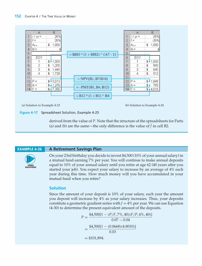
152 CHAPTER 4 / THE TIME VALUE OF MONEY

(a) Solution to Example 4-23 (b) Solution to Example 4-24

Figure 4-17 Spreadsheet Solution, Example 4-25

derived from the value of P. Note that the structure of the spreadsheets for Parts(a) and (b) are the same—the only difference is the value of f in cell B2.

EXAMPLE 4-26 A Retirement Savings Plan

On your 23rd birthday you decide to invest $4,500 (10% of your annual salary) ina mutual fund earning 7% per year. You will continue to make annual depositsequal to 10% of your annual salary until you retire at age 62 (40 years after youstarted your job). You expect your salary to increase by an average of 4% eachyear during this time. How much money will you have accumulated in yourmutual fund when you retire?

SolutionSince the amount of your deposit is 10% of your salary, each year the amountyou deposit will increase by 4% as your salary increases. Thus, your depositsconstitute a geometric gradient series with f = 4% per year. We can use Equation(4-30) to determine the present equivalent amount of the deposits.

P = $4,500[1 − (P/F, 7%, 40)(F/P, 4%, 40)]0.07 − 0.04

= $4,500[1 − (0.0668)(4.8010)]0.03

= $101,894.

SECTION 4.13 / INTEREST RATES THAT VARY WITH TIME 153

Now the future worth at age 62 can be determined.

F = $101,894(F/P, 7%, 40)

= $101,894(14.9745)

= $1,525,812.

This savings plan will make you a millionaire when you retire. Moral: Startsaving early!

4.13 Interest Rates that Vary with TimeStudent loans under the U.S. government’s popular Stafford program let studentsborrow money up to a certain amount each year (based on their year in school andfinancial need). Stafford loans are the most common type of educational loan, andthey have a floating interest rate that readjusts every year (but cannot exceed 8.25%per year). When the interest rate on a loan can vary with time, it is necessary totake this into account when determining the future equivalent value of the loan.Example 4-27 demonstrates how this situation is treated.

EXAMPLE 4-27 Compounding with Changing Interest Rates

Ashea Smith is a 22-year-old senior who used the Stafford loan program toborrow $4,000 four years ago when the interest rate was 4.06% per year. $5,000was borrowed three years ago at 3.42%. Two years ago she borrowed $6,000 at5.23%, and last year $7,000 was borrowed at 6.03% per year. Now she would liketo consolidate her debt into a single 20-year loan with a 5% fixed annual interestrate. If Ashea makes annual payments (starting in one year) to repay her totaldebt, what is the amount of each payment?

SolutionThe following cash-flow diagram clarifies the timing of Ashea’s loans and theapplicable interest rates. The diagram is drawn using Ashea’s viewpoint.

$7,000

i � 5%

�4 �3 �2 �1 0 1 2 19 20

$6,000$5,000

$4,000

A � ?

F0 � P0

4.06% 3.42% 5.23% 6.03%

End of Year

154 CHAPTER 4 / THE TIME VALUE OF MONEY

Before we can find the annual repayment amount, we need to find the current(time 0) equivalent value of the four loans. This problem can be solved bycompounding the amount owed at the beginning of each year by the interestrate that applies to each individual year and repeating this process over the fouryears to obtain the total current equivalent value.

F−3 = $4,000(F/P, 4.06%, 1) + $5,000 = $4,000(1.0406)

+ $5,000 = $9,162.40

F−2 = $9,162.40(F/P, 3.42%, 1) + $6,000 = $15,475.75

F−1 = $15,475.75(F/P, 5.23%, 1) + $7,000 = $23,285.13

F0 = $23,285.13(F/P, 6.03%, 1) = $24,689.22

Notice that it was a simple matter to substitute (F/P, i%, N) = (1 + i)N for thenoninteger values of i.

Now that we have the current equivalent value of the amount Asheaborrowed (F0 = P0), we can easily compute her annual repayment amountover 20 years when the interest rate is fixed at 5% per year.

A = $24,689.22(A/P, 5%, 20) = $24,689.22(0.0802) = $1,980.08 per year

CommentThe total principal borrowed was $4,000 + $5,000 + $6,000 + $7,000 = $22,000.Notice that a total of $17,601.60 (20 × $1,980.08 − $22,000) in interest is repaidover the entire 20-year loan period. This interest amount is close to the amountof principal originally borrowed. Moral: Borrow as little as possible and repayas quickly as possible to reduce interest expense! See www.finaid.com.

To obtain the present equivalent of a series of future cash flows subject tovarying interest rates, a procedure similar to the preceding one would be uti-lized with a sequence of (P/F, ik%, k) factors. In general, the present equivalentvalue of a cash flow occurring at the end of period N can be computed usingEquation (4-31), where ik is the interest rate for the kth period (the symbol

∏means

“the product of”):

P = FN∏Nk=1(1 + ik)

. (4-31)

For instance, if F4 = $1,000 and i1 = 10%, i2 = 12%, i3 = 13%, and i4 = 10%,then

P = $1,000[(P/F, 10%, 1)(P/F, 12%, 1)(P/F, 13%, 1)(P/F, 10%, 1)]= $1,000[(0.9091)(0.8929)(0.8850)(0.9091)] = $653.

SECTION 4.14 / NOMINAL AND EFFECTIVE INTEREST RATES 155

4.14 Nominal and Effective Interest RatesVery often the interest period, or time between successive compounding, is lessthan one year (e.g., daily, weekly, monthly, or quarterly). It has become customaryto quote interest rates on an annual basis, followed by the compounding period ifdifferent from one year in length. For example, if the interest rate is 6% per interestperiod and the interest period is six months, it is customary to speak of this rate as“12% compounded semiannually.” Here the annual rate of interest is known as thenominal rate, 12% in this case. A nominal interest rate is represented by r. But theactual (or effective) annual rate on the principal is not 12%, but something greater,because compounding occurs twice during the year.

Consequently, the frequency at which a nominal interest rate is compoundedeach year can have a pronounced effect on the dollar amount of total interest earned.For instance, consider a principal amount of $1,000 to be invested for three years ata nominal rate of 12% compounded semiannually. The interest earned during thefirst six months would be $1,000 × (0.12/2) = $60.

Total principal and interest at the beginning of the second six-month period is

P + Pi = $1,000 + $60 = $1,060.

The interest earned during the second six months would be

$1,060 × (0.12/2) = $63.60.

Then total interest earned during the year is

$60.00 + $63.60 = $123.60.

Finally, the effective annual interest rate for the entire year is

$123.60$1,000

× 100 = 12.36%.

If this process is repeated for years two and three, the accumulated (com-pounded) amount of interest can be plotted as in Figure 4-18. Suppose that the same$1,000 had been invested at 12% compounded monthly, which is 1% per month.

Figure 4-18 $1,000Compounded at a SemiannualFrequency (r = 12%, M = 2)

Cum

ulat

ive

Am

ount

of I

nter

est E

arne

d ($

)

Effective Annual Interest Rate

= (100%) = 12.36%$123.60

$1,000.00

$60

$123.60

$191.02

$262.48

$338.23

$418.52

0 1End of Year

2 31½ 2½½

156 CHAPTER 4 / THE TIME VALUE OF MONEY

The accumulated interest over three years that results from monthly compoundingis shown in Figure 4-19.

The actual or exact rate of interest earned on the principal during one yearis known as the effective rate. It should be noted that effective interest rates arealways expressed on an annual basis, unless specifically stated otherwise. In thistext, the effective interest rate per year is customarily designated by i and thenominal interest rate per year by r. In engineering economy studies in whichcompounding is annual, i = r. The relationship between effective interest, i, andnominal interest, r, is

i = (1 + r/M)M − 1, (4-32)

where M is the number of compounding periods per year. It is now clear fromEquation (4-32) why i > r when M > 1.

The effective rate of interest is useful for describing the compounding effectof interest earned on interest during one year. Table 4-4 shows effective rates forvarious nominal rates and compounding periods.

Interestingly, the federal truth-in-lending law now requires a statement reg-arding the annual percentage rate (APR) being charged in contracts involving

Figure 4-19$1,000 Compoundedat a Monthly Frequency(r = 12%, M = 12)

0 1 2 3

End of Year

Cum

ulat

ive

Am

ount

of I

nter

est E

arne

d ($

)

$126.83

$269.73

$430.77

$10.00$20.10

$30.30$40.60

$51.01$61.52

Effective Annual Interest Rate

� $126.83$1,000.00

(100%) � 12.68%

TABLE 4-4 Effective Interest Rates for Various Nominal Rates and CompoundingFrequencies

Number of Effective Rate (%) for Nominal Rate ofCompounding Compounding PeriodsFrequency per Year, M 6% 8% 10% 12% 15% 24%

Annually 1 6.00 8.00 10.00 12.00 15.00 24.00Semiannually 2 6.09 8.16 10.25 12.36 15.56 25.44Quarterly 4 6.14 8.24 10.38 12.55 15.87 26.25Bimonthly 6 6.15 8.27 10.43 12.62 15.97 26.53Monthly 12 6.17 8.30 10.47 12.68 16.08 26.82Daily 365 6.18 8.33 10.52 12.75 16.18 27.11

SECTION 4.15 / COMPOUNDING MORE OFTEN THAN ONCE PER YEAR 157

borrowed money. The APR is a nominal interest rate and does not account forcompounding that may occur, or be appropriate, during a year. Before thislegislation was passed by Congress in 1969, creditors had no obligation to explainhow interest charges were determined or what the true cost of money on a loan was.As a result, borrowers were generally unable to compute their APR and comparedifferent financing plans.

EXAMPLE 4-28 Effective Annual Interest Rate

A credit card company charges an interest rate of 1.375% per month onthe unpaid balance of all accounts. The annual interest rate, they claim, is12(1.375%) = 16.5%. What is the effective rate of interest per year being chargedby the company?

SolutionEquation (4-32) is used to compute the effective rate of interest in this example:

i =(

1 + 0.16512

)12

− 1

= 0.1781, or 17.81%/year.

Note that r = 12(1.375%) = 16.5%, which is the APR. In general, it is truethat r = M(r/M), where r/M is the interest rate per period.

Numerous Web sites are available to assist you with personal finance decisions.Take a look at www.dinkytown.net and www.bankrate.com.

4.15 Compounding More Often than Once per Year4.15.1 Single Amounts

If a nominal interest rate is quoted and the number of compounding periodsper year and number of years are known, any problem involving future,annual, or present equivalent values can be calculated by straightforward use ofEquations (4-3) and (4-32), respectively.

EXAMPLE 4-29 Future Equivalent when Interest Is Compounded Quarterly

Suppose that a $100 lump-sum amount is invested for 10 years at a nominalinterest rate of 6% compounded quarterly. How much is it worth at the end ofthe 10th year?

SolutionThere are four compounding periods per year, or a total of 4 × 10 = 40 interestperiods. The interest rate per interest period is 6%/4 = 1.5%. When the values

158 CHAPTER 4 / THE TIME VALUE OF MONEY

are used in Equation (4-3), one finds that

F = P(F/P, 1.5%, 40) = $100.00(1.015)40 = $100.00(1.814) = $181.40.

Alternatively, the effective interest rate from Equation (4-32) is 6.14%. Therefore,

F = P(F/P, 6.14%, 10) = $100.00(1.0614)10 = $181.40.

4.15.2 Uniform Series and Gradient Series

When there is more than one compounded interest period per year, the formulasand tables for uniform series and gradient series can be used as long as there is acash flow at the end of each interest period, as shown in Figures 4-6 and 4-13 for auniform annual series and a uniform gradient series, respectively.

EXAMPLE 4-30 Computing a Monthly Auto Payment

Stan Moneymaker has a bank loan for $10,000 to pay for his new truck. Thisloan is to be repaid in equal end-of-month installments for five years with anominal interest rate of 12% compounded monthly. What is the amount of eachpayment?

SolutionThe number of installment payments is 5 × 12 = 60, and the interest rate permonth is 12%/12 = 1%. When these values are used in Equation (4-15), onefinds that

A = P(A/P, 1%, 60) = $10,000(0.0222) = $222.

Notice that there is a cash flow at the end of each month (interest period),including month 60, in this example.

EXAMPLE 4-31 Uniform Gradient Series and Semiannual Compounding

Certain operating savings are expected to be 0 at the end of the first six months,to be $1,000 at the end of the second six months, and to increase by $1,000 at theend of each six-month period thereafter, for a total of four years. It is desired tofind the equivalent uniform amount, A, at the end of each of the eight six-monthperiods if the nominal interest rate is 20% compounded semiannually.

SolutionA cash-flow diagram is given below, and the solution is

A = G(A/G, 10%, 8) = $1,000(3.0045) = $3,004.50.

SECTION 4.15 / COMPOUNDING MORE OFTEN THAN ONCE PER YEAR 159

$7,000

i � 10% per 6 month1 2 3 4 5 6 7 8

End of Six-Month Period

$6,000$5,000

$4,000$3,000

$2,000$1,000

A � ?

0 1 2 3 4 5 6 7 8End of Six-Month Period

0

The symbol “⇐⇒” in between the cash-flow diagrams indicates that the left-hand cash-flow diagram is equivalent to the right-hand cash-flow diagram whenthe correct value of A has been determined. In Example 4-31, the interest rateper six-month period is 10%, and cash flows occur every six months.

EXAMPLE 4-32 Finding the Interest Rate on a Loan

A loan of $15,000 requires monthly payments of $477 over a 36-month period oftime. These payments include both principal and interest.

(a) What is the nominal interest rate (APR) for this loan?(b) What is the effective interest rate per year?(c) Determine the amount of unpaid loan principal after 20 months.

Solution(a) We can set up an equivalence relationship to solve for the unknown interest

rate since we know that P = $15,000, A = $477, and N = 36 months.

$477 = $15,000(A/P, imo, 36)

(A/P, imo, 36) = 0.0318

We can now look through Appendix C to find values of i that have an(A/P, i, 36) value close to 0.0318. From Table C-3 (i = 3/4%), we find(A/P, 3/4%, 36) = 0.0318. Therefore,

imo = 0.75% per month

and

r = 12 × 0.75% = 9% per year, compounded monthly.

(b) Using Equation (4-32),

ieff =(

1 + 0.0912

)12

− 1 = 0.0938 or 9.38% per year.

160 CHAPTER 4 / THE TIME VALUE OF MONEY

(c) We can find the amount of the unpaid loan principal after 20 months byfinding the equivalent value of the remaining 16 monthly payments as ofmonth 20.

P20 = $477(P/A, 3/4%, 16) = $477(15.0243) = $7,166.59

After 20 payments have been made, almost half of the original principalamount remains. Notice that we used the monthly interest rate of 3/4% inour calculation since the cash flows are occurring monthly.

4.16 Interest Formulas for Continuous Compoundingand Discrete Cash Flows

In most business transactions and economy studies, interest is compounded atthe end of discrete periods, and, as has been discussed previously, cash flows areassumed to occur in discrete amounts at the end of such periods. This practice will beused throughout the remaining chapters of this book. However, it is evident that in mostenterprises, cash is flowing in and out in an almost continuous stream. Becausecash, whenever it’s available, can usually be used profitably, this situation createsopportunities for very frequent compounding of the interest earned. So that thiscondition can be dealt with (modeled) when continuously compounded interestrates are available, the concept of continuous compounding is sometimes usedin economy studies. Actually, the effect of this procedure, compared with that ofdiscrete compounding, is rather small in most cases.

Continuous compounding assumes that cash flows occur at discrete intervals(e.g., once per year), but that compounding is continuous throughout the interval.For example, with a nominal rate of interest per year of r, if the interest iscompounded M times per year, one unit of principal will amount to [1 + (r/M)]M

at the end of one year. Letting M/r = p, we find that the foregoing expressionbecomes [

1 + 1p

]rp

=[(

1 + 1p

)p]r

. (4-33)

Because

limp→∞

(1 + 1

p

)p

= e1 = 2.71828 . . . ,

Equation (4-33) can be written as er. Consequently, the continuously compoundedcompound amount factor (single cash flow) at r% nominal interest for N years is erN .Using our functional notation, we express this as

(F/P, r%, N) = erN . (4-34)

Note that the symbol r is directly comparable to that used for discrete compoundingand discrete cash flows (i%), except that r% is used to denote the nominal rate andthe use of continuous compounding.

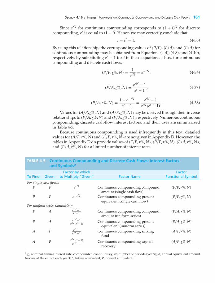
SECTION 4.16 / INTEREST FORMULAS FOR CONTINUOUS COMPOUNDING AND DISCRETE CASH FLOWS 161

Since erN for continuous compounding corresponds to (1 + i)N for discretecompounding, er is equal to (1 + i). Hence, we may correctly conclude that

i = er − 1. (4-35)

By using this relationship, the corresponding values of (P/F), (F/A), and (P/A) forcontinuous compounding may be obtained from Equations (4-4), (4-8), and (4-10),respectively, by substituting er − 1 for i in these equations. Thus, for continuouscompounding and discrete cash flows,

(P/F, r%, N) = 1erN = e−rN ; (4-36)

(F/A, r%, N) = erN − 1er − 1

; (4-37)

(P/A, r%, N) = 1 − e−rN

er − 1= erN − 1

erN(er − 1). (4-38)

Values for (A/P, r%, N) and (A/F, r%, N) may be derived through their inverserelationships to (P/A, r%, N) and (F/A, r%, N), respectively. Numerous continuouscompounding, discrete cash-flow interest factors, and their uses are summarizedin Table 4-5.

Because continuous compounding is used infrequently in this text, detailedvalues for (A/F, r%, N) and (A/P, r%, N) are not given inAppendix D. However, thetables in Appendix D do provide values of (F/P, r%, N), (P/F, r%, N), (F/A, r%, N),and (P/A, r%, N) for a limited number of interest rates.

TABLE 4-5 Continuous Compounding and Discrete Cash Flows: Interest Factorsand Symbolsa

Factor by which FactorTo Find: Given: to Multiply “Given” Factor Name Functional Symbol

For single cash flows:F P erN Continuous compounding compound

amount (single cash flow)(F/P, r%, N)

P F e−rN Continuous compounding presentequivalent (single cash flow)

(P/F, r%, N)

For uniform series (annuities):

F A erN−1er−1 Continuous compounding compound

amount (uniform series)(F/A, r%, N)

P A erN−1erN (er−1)

Continuous compounding presentequivalent (uniform series)

(P/A, r%, N)

A F er−1erN−1

Continuous compounding sinkingfund

(A/F, r%, N)

A P erN (er−1)

erN−1Continuous compounding capital

recovery(A/P, r%, N)

a r , nominal annual interest rate, compounded continuously; N, number of periods (years); A, annual equivalent amount(occurs at the end of each year); F, future equivalent; P, present equivalent.

162 CHAPTER 4 / THE TIME VALUE OF MONEY

Note that tables of interest and annuity factors for continuous compoundingare tabulated in terms of nominal rates of interest per time period.

EXAMPLE 4-33 Continuous Compounding and Single Amounts

You have $10,000 to invest for two years. Your bank offers 5% interest,compounded continuously for funds in a money market account. Assuming noadditional deposits or withdrawals, how much money will be in that account atthe end of two years?

SolutionF = $10,000 (F/P, r = 5%, 2) = $10,000 e(0.05)(2) = $10,000 (1.1052) = $11,052

CommentIf the interest rate was 5% compounded annually, the account would have beenworth

F = $10,000 (F/P, 5%, 2) = $10,000 (1.1025) = $11,025.

EXAMPLE 4-34 Continuous Compounding and Annual Payments

Suppose that one has a present loan of $1,000 and desires to determine whatequivalent uniform EOY payments, A, could be obtained from it for 10 years ifthe nominal interest rate is 20% compounded continuously (M = ∞).

SolutionHere we utilize the formulation

A = P(A/P, r%, N).

Since the (A/P) factor is not tabled for continuous compounding, we substituteits inverse (P/A), which is tabled in Appendix D. Thus,

A = P × 1(P/A, 20%, 10)

= $1,000 × 13.9054

= $256.

Note that the answer to the same problem, with discrete annual compound-ing (M = 1), is

A = P(A/P, 20%, 10)

= $1,000(0.2385) = $239.

SECTION 4.17 / CASE STUDY—UNDERSTANDING ECONOMIC “EQUIVALENCE” 163

EXAMPLE 4-35 Continuous Compounding and Semiannual Payments

An individual needs $12,000 immediately as a down payment on a new home.Suppose that he can borrow this money from his insurance company. He mustrepay the loan in equal payments every six months over the next eight years.The nominal interest rate being charged is 7% compounded continuously. Whatis the amount of each payment?

SolutionThe nominal interest rate per six months is 3.5%. Thus, A each six months is$12,000(A/P, r = 3.5%, 16). By substituting terms in Equation (4-38) and thenusing its inverse, we determine the value of A per six months to be $997:

A = $12,000[

1(P/A, r = 3.5%, 16)

]= $12,000

12.038= $997.

4.17 CASE STUDY—Understanding Economic “Equivalence”

Enrico Suarez just graduated with a B.S. in engineering and landed a new job witha starting annual salary of $48,000. There are a number of things that he wouldlike to do with his newfound “wealth.” For starters, he needs to begin repaying hisstudent loans (totaling $20,000) and he’d like to reduce some outstanding balanceson credit cards (totaling $5,000). Enrico also needs to purchase a car to get to workand would like to put money aside to purchase a condo in the future. Last, but notleast, he wants to put some money aside for his eventual retirement.

Our recent graduate needs to do some financial planning for which he hasselected a 10-year time frame. At the end of 10 years, he’d like to have paid off hiscurrent student loan and credit card debt, as well as have accumulated $40,000 fora down payment on a condo. If possible, Enrico would like to put aside 10% ofhis take home salary for retirement. He has gathered the following information toassist him in his planning.∗

• Student loans are typically repaid in equal monthly installments over a periodof 10 years. The interest rate on Enrico’s loan is 8% compounded monthly.

• Credit cards vary greatly in the interest rate charged. Typical APR rates are closeto 17%, and monthly minimum payments are usually computed using a 10-yearrepayment period. The interest rate on Enrico’s credit card is 18% compoundedmonthly.

• Car loans are usually repaid over three, four, or five years. The APR on a car loancan be as low as 2.9% (if the timing is right) or as high as 12%. As a first-timecar buyer, Enrico can secure a $15,000 car loan at 9% compounded monthly tobe repaid over 60 months.

∗ The stated problem data are current as of 2014.

164 CHAPTER 4 / THE TIME VALUE OF MONEY

• A 30-year, fixed rate mortgage is currently going for 5.75%–6.0% per year. IfEnrico can save enough to make a 20% down payment on the purchase ofhis condo, he can avoid private mortgage insurance that can cost as much as$60 per month.

• Investment opportunities can provide variable returns. “Safe” investments canguarantee 7% per year, while “risky” investments could return 30% or more peryear.

• Enrico’s parents and older siblings have reminded him that his monthly takehome pay will be reduced by income taxes and benefit deductions. He shouldnot count on being able to spend more than 80% of his gross salary.

As Enrico’s friend (and the one who took Engineering Economy instead ofAppreciating the Art of Television Commercials), you have been asked to reviewhis financial plans. How reasonable are his goals?

SolutionSince all repayments are done on a monthly basis, it makes sense to adopt themonth as Enrico’s unit of time. There are five categories for his cash flows: debtrepayment, transportation costs, housing costs, other living expenses, and savings.The following paragraphs summarize his estimates of monthly expenses in eachof these categories.

Debt RepaymentEnrico’s student loan debt is $20,000 and is to be repaid over the next 120 months(10 years) at a nominal interest rate of 8% compounded monthly (imonth = 8/12% =2/3%). His monthly loan payment is then

AStudent Loan = $20,000(A/P, 2/3%, 120) = $20,000(0.01213) = $242.60 per month.

Enrico’s credit card debt is $5,000 and is to be completely repaid over the next 120months at a nominal interest rate of 18% compounded monthly (imonth = 1.5%).His monthly credit card payment, assuming no additional usage, is then

ACredit Card = $5,000(A/P, 1.5%, 120) = $5,000(0.01802) = $90.10 per month.

Enrico’s monthly debt repayment totals $242.60 + $90.10 = $332.70.

Transportation CostsThe certified pre-owned vehicle Enrico would like to buy costs $15,000. The bestrate he can find as a first-time car buyer with no assets or credit history is 9%compounded monthly with a 60-month repayment period. Based on these figures,his monthly car payment will be

ACar = $15,000(A/P, 0.75%, 60) = $15,000(0.02076) = $311.40 per month.

Even though the car will be completely repaid after five years, Enrico knows thathe will eventually need to replace the car. To accumulate funds for the replacement

SECTION 4.17 / CASE STUDY—UNDERSTANDING ECONOMIC “EQUIVALENCE” 165

of the car, he wants to continue to set aside this amount each month for the secondfive years.

Insurance for this vehicle will cost $1,200 per year, and Enrico has budgeted$100 per month to cover fuel and maintenance. Thus, his monthly transportationcosts total $311.40 + $1,200/12 + $100 = $511.40.

Housing CostsA nice two-bedroom apartment near Enrico’s place of work has a monthly rent of$800. The rental office provided him with a monthly utility cost estimate of $150to cover water and electricity. Based on this information, $800 + $150 = $950 permonth has been budgeted for his housing costs.

Other Living ExpensesThis expense category has troubled Enrico the most. While all the previouscategories are pretty straightforward, he knows that his day-to-day spending willhave the most variability and that it will be tempting to overspend. Nonetheless,he has developed the following estimates of monthly living expenses not alreadycovered in the other categories:

Food $200Phone $70Entertainment $100Miscellaneous

(clothing, household items) $150

Subtotal $520

SavingsEnrico wants to accumulate $40,000 over the next 10 years to be used as a downpayment on a condo. He feels that if he chooses relatively “safe” investments (CDsand bonds), he should be able to earn 6% compounded monthly on his savings. Hemust then set aside

ACondo = $40,000(A/F, 0.5%, 120) = $40,000(0.00610) = $244.00 per month

to reach his goal.Enrico’s gross monthly starting salary is $48,000/12 = $4,000. Based on the

information gathered from his family, he estimates his monthly net (take home)pay to be $4,000(0.80) = $3,200. His monthly retirement savings will then be$3,200(0.10) = $320. Thus, the total amount to be set aside each month for thefuture is $244 + $320 = $564.

Monthly Financial PlanBased on the preceding calculations, the following table summarizes Enrico’smonthly financial plan.

166 CHAPTER 4 / THE TIME VALUE OF MONEY

Net Income Expense

Salary $3,200Debt repayment $332.70Transportation costs 511.40Housing costs 950.00Living expenses 520.00Savings 564.00

Total $3,200 $2,878.10

Enrico is aware that he has not explicitly accounted for price increases over the next10 years; however, neither has he increased his annual salary. He is hopeful that,if he works hard, his annual salary increases will at least cover the increase in thecost of living.

You congratulate your friend on his efforts. You feel that he has covered themajor areas of expenses, as well as savings for the future. You note that he has$3,200 − $2,878.10 = $321.90 of “extra” money each month to cover unanticipatedcosts. With this much leeway, you feel that he should have no problem meeting hisfinancial goals.

4.18 Try Your SkillsThe number in parentheses that follows each problem refers to the sectionfrom which the problem is taken. Solutions to these problems can be found inAppendix G.

4-A. What lump-sum amount of interest will be paid on a $10,000 loan that wasmade on August 1, 2012, and repaid on November 1, 2016, with ordinarysimple interest at 10% per year? (4.2)

4-B. The municipality of Smallville has arranged to borrow $30 million in orderto implement several public projects (flood control, school security, etc.). Theinterest rate will be 3% per year, payable at the end of each year. This $30million debt will be retired by making principal payments of $5 million atthe end of each year. The Board of Supervisors is concerned that it will taketoo long to pay off this debt. How many years will it take to retire this $30million debt and its associated interest payments? (4.3).

4-C. Your spendthrift cousin wants to buy a fancy watch for $425. Instead, yousuggest that she buy an inexpensive watch for $25 and save the difference of$400. Your cousin agrees with your idea and invests $400 for 40 years in anaccount earning 9% interest per year. How much will she accumulate in thisaccount after 40 years have passed? (4.6)

4-D. What is the present equivalent of $18,000 to be received in 15 years when theinterest rate is 7% per year? (4.6)

SECTION 4.18 / TRY YOUR SKILLS 167

4-E. The price of oil in 2005 was $67 per barrel. “This price is still lower than theprice of oil in 1981” says a government publication. If inflation has averaged3.2% per year from 1981 to 2005, what was the price per barrel of oil in1981? (4.6)

4-F. How long does it take (to the nearest whole year) for $1,000 to quadruple invalue when the interest rate is 15% per year? (4.6)

4-G. The first U.S. congress in 1789 set the president’s salary at $25,000 per year. In2014, the president’s salary is $400,000 each year. What is the compoundedaverage annual increase in the president’s salary for the past 225 years? (4.6)

4-H. An enterprising student invests $1,000 at an annual interest rate that will growthe original investment to $2,000 in 4 years. In 4 more years, the amount willgrow to $4,000, and this pattern of doubling every 4 years repeats over a totaltime span of 36 years. How much money will the student gain in 36 years?What is the magical annual interest rate the student is earning? (4.6)

4-I. At a certain state-supported university, annual tuition and fees have risendramatically in recent years as shown in the table below. (4.6)

Consumer PriceYear Tuition and Fees Index

1982–1983 $827 96.51987–1988 $1,404 113.61993–1994 $2,018 144.52003–2004 $4,450 184.02005–2006 $5,290 198.1 (est.)

Source: www.bls.gov.

a. If all tuition and fees are paid at the beginning of each academic year, whatis the compound annual rate of increase from 1982 to 2005?

b. What is the annual rate of increase from 1993 to 2005?c. How do the increases in Parts (a) and (b) compare with the CPI for the

same period of time?4-J. The cost of 1,000 cubic feet of natural gas has increased from $6 in 2000 to

$15 in 2006. What compounded annual increase in cost is this? How does theincrease in the cost of natural gas compare to a 3% annual rate of inflationduring the same period of time? (4.6)

4-K. If a certain machine undergoes a major overhaul now, its output can beincreased by 20%, which translates into additional cash flow of $20,000 atthe end of each year for 5 years. If i = 15% per year, how much can we affordto invest to overhaul this machine? (4.7)

4-L. Albert Einstein once noted that “compounding of interest is one of humanity’sgreatest inventions.” To illustrate the mind-boggling effects of compounding,suppose $100 is invested at the end of each year for 25 years at i = 50% peryear. In this case, the accumulated sum is $5,050,000! Now it is your turn.What amount is accumulated after 25 years if the interest rate is 30% peryear? (4.7)

168 CHAPTER 4 / THE TIME VALUE OF MONEY

4-M. One of life’s great lessons is to start early and save all the money you can! Ifyou save $2 today and $2 each and every day thereafter until you are 60 yearsold (say $730 per year for 35 years), how much money will you accumulateif the annual interest rate is 7%? (4.7)

4-N. A large retailer is going to run an experiment at one of its stores to see howcost effective it will be to imbed merchandise with small radio frequencyidentification (RFID) chips. Shoppers will select items from the store andwalk out without stopping to pay at a checkout lane. The RFID chips willrecord what items are taken and will automatically deduct their price fromshoppers’ bank accounts. The retailer expects to save the cost of staffing12 checkout lanes, which amounts to $100,000 per year. How much canthe retailer afford to spend on its RFID investment if the system has a lifeof 10 years and no residual value? The retailer’s interest rate is 15% peryear. (4.7)

4-O. Jason makes six EOY deposits of $2,000 each in a savings account paying5% compounded annually. If the accumulated account balance is withdrawn4 years after the last deposit, how much money will be withdrawn? (4.7)

4-P. You can buy a machine for $100,000 that will produce a net income, afteroperating expenses, of $10,000 per year. If you plan to keep the machine for4 years, what must the market (resale) value be at the end of 4 years to justifythe investment? You must make a 15% annual return on your investment. (4.7)

4-Q. An expenditure of $20,000 is made to modify a material-handling system ina small job shop. This modification will result in first-year savings of $2,000,a second-year savings of $4,000, and a savings of $5,000 per year thereafter.How many years must the system last if an 18% return on investment isrequired? The system is tailor made for this job shop and has no market(salvage) value at any time. (4.10)

4-R. Find the uniform annual amount that is equivalent to a uniform gradientseries in which the first year’s payment is $500, the second year’s paymentis $600, the third year’s payment is $700, and so on, and there are a total of20 payments. The annual interest rate is 8%. (4.11)

4-S. A geometric gradient has a positive cash flow of $1,000 at EOY zero (now),and it increases 5% per year for the following 5 years. Another geometricgradient has a positive value of $2,000 at the EOY 1, and it decreases 6%per year for years two through five. If the annual interest rate is 10%, whichgeometric gradient would you prefer? (4.12)

4-T. In a geometric sequence of annual cash flows starting at the EOY zero, thevalue of A0 is $1,304.35 (which is a cash flow). The value of the last term in theseries, A10, is $5,276.82. What is the equivalent value of A for years 1 through10? Let i = 20% per year. (4.12)

4-U. Compute the effective annual interest rate in each of these situations: (4.14)

a. 10% nominal interest, compounded semiannually.b. 10% nominal interest compounded quarterly.c. 10% nominal interest compounded weekly.

PROBLEMS 169

4-V. A mortgage banking company has been evaluating the merits of a 50-yearmortgage (in addition to their popular 30-year mortgage). The basic idea isto reduce the monthly payment and make home ownership more affordable.The APR of either mortgage is 6%, and the compounding is monthly. (4.15)

a. For a mortgage loan of $300,000, what is the difference in the monthlypayment for the 30-year mortgage and the 50-year mortgage?

b. What is the difference in total interest paid between the two mortgages?

4-W. A health club offers you a special low membership rate of $29 per month fora “guaranteed no price increase” period of 100 months. The manager of theclub tells you proudly that “this $29 a month for a lifetime membership isless expensive than a major medical treatment for heart disease costing $4,000one hundred months from now.” If your personal interest rate is 9% (APR)compounded monthly, is the manager correct in his statement? (4.15)

4-X. On January 1, 2005, a person’s savings account was worth $200,000. Everymonth thereafter, this person makes a cash contribution of $676 to the ac-count. If the fund was expected to be worth $400,000 on January 1, 2010,what annual rate of interest was being earned on this fund? (4.15)

4-Y. An effective annual interest rate of 35% has been determined with continuouscompounding. What is the nominal interest rate that was compoundedcontinuously to get this number? (4.16)

4-Z. A bank offers a nominal interest rate (APR) of 6%, continuously com-pounded. What is the effective interest rate? (4.16)

4.19 SummaryChapter 4 presented the fundamental time value of money relationships thatare used throughout the remainder of this book. Considerable emphasis hasbeen placed on the concept of equivalence—if two cash flows (or series of cashflows) are equivalent for a stated interest rate, you are willing to trade onefor the other. Formulas relating present and future amounts to their equivalentuniform, arithmetic, and geometric series have been presented. You should feelcomfortable with the material in this chapter before embarking on your journeythrough subsequent chapters. Important abbreviations and notation are listed inAppendix B.

In the next chapter, we will see how to apply time value of money relationshipsto the estimated cash flows of a project (the topic of Chapter 3) to arrive at a measureof its economic worth.

ProblemsThe number in parentheses that follows each problemrefers to the section from which the problem is taken.

4-1. You borrow $500 from a family member and agreeto pay it back in 6 months. Because you are part of the

family, you are only being charged simple interest at therate of 0.5% per month. How much will you owe after6 months? How much is the interest? (4.2)

4-2. What is the future equivalent of $1,000 invested at6% simple interest per year for 3½ years? (4.2)

170 CHAPTER 4 / THE TIME VALUE OF MONEY

4-3. The interest rate on short-term German bondsis −0.1%. Explain how this is possible and what itmeans. (4.3, 4.4)

4-4. Compare the interest earned by P dollars at i%per year simple interest with that earned by thesame amount P for five years at i% compoundedannually. (4.2)

4-5. How much interest is payable each year on a loan of$2,000 if the interest rate is 10% per year when half ofthe loan principal will be repaid as a lump sum at theend of four years and the other half will be repaid in onelump-sum amount at the end of eight years? How muchinterest will be paid over the eight-year period? (4.4)

4-6. Suppose that, in Plan 1 of Table 4-1, $8,500 of theoriginal unpaid balance is to be repaid at the end ofmonths two and four only. How much total interestwould have been paid by the end of month four? (4.4)

4-7. Refer to Plan 2 in Table 4-1. This is the customaryway to pay off loans on automobiles, house mortgages,etc. A friend of yours has financed $24,000 on thepurchase of a new automobile, and the annual interestrate is 12% (1% per month). (4.4)

a. Monthly payments over a 60-month loan period willbe how much?

b. How much interest and principal will be paid in thethird month of this loan?

4-8. Jonathan borrowed $10,000 at 6% annualcompound interest. He agreed to repay the loan withfive equal annual payments at end-of-years 1–5. Howmuch of the annual payment is interest, and how muchprincipal is there in each annual payment? (4.4)

4-9. Suppose you contribute $10 per week ($520 peryear) into an interest-bearing account that earns 6% ayear (compounded once per year). That’s probably oneless pizza per week! But if you contribute faithfully eachweek into this account, how much money would youhave saved through the compounding of interest by theend of 15 years? (4.6)

4-10. A lump-sum loan of $5,000 is needed by Chandrato pay for college expenses. She has obtained smallconsumer loans with 12% interest per year in the pastto help pay for college. But her father has advisedChandra to apply for a PLUS student loan chargingonly 8.5% interest per year. If the loan will be repaid infull in five years, what is the difference in total interestaccumulated by these two types of student loans? (4.6)

4-11. You have just invested a one-time amount of$5,000 in a stock-based mutual fund. This fund shouldearn (on average) 9% per year over a long period oftime. How much will your investment be worth in35 years? (4.6)

4-12. A 12-cylinder heavy-duty diesel engine will havea guaranteed residual value of $1,000 in 5 years. Today(year 0) the equivalent worth of this engine is how muchif the interest rate is 9% per year? (4.6)

4-13. You just inherited $10,000. While you planto squander some of it away, how much shouldyou deposit in an account earning 5% interest peryear if you’d like to have $10,000 in the account in10 years? (4.6)

4-14. A certain college graduate, Sallie Evans, has$24,000 in student-loan debt at the end of her collegecareer. The interest rate on this debt is 0.75% per month.If monthly payments on this loan are $432.61, howmany months will it take for Sallie to repay the entireloan? (4.6)

4-15. Mr. Smith has saved $1,800 each year for 20years. A year after the saving period ended, Mr. Smithwithdrew $7,500 each year for a period of 5 years. Inthe sixth and seventh years, he only withdrew $5,000per year. In the eighth year, he decided to withdrawthe remaining money in his account. If the interest ratewas 6% per year throughout the whole period, whatwas the amount he withdrew at the end of the eighthyear? (4.10)

4-16. Use the rule of 72 to determine how long it takesto accumulate $10,000 in a savings account when P =$5,000 and i = 10% per year. (4.6)

Rule of 72: The time (years) required to double thevalue of a lump-sum investment that is allowed tocompound is approximately

72 ÷ annual interest rate (as a %).

4-17. In 1803, Napoleon sold the Louisiana Territory tothe United States for $0.04 per acre. In 2014, the averagevalue of an acre at this location is $10,000. What annualcompounded percentage increase in value of an acre ofland has been experienced? (4.7)

4-18. Calculate the compounded future value of 20annual payments of $5,000 each into a savings accountthat earns 6% per year. All 20 payments are made at thebeginning of each year. (4.6)

PROBLEMS 171

4-19. In 2014, the average debt for college student loansis $28,700. This amounts to a $330 monthly payment fora “standard” loan repayment plan over 10 years. Whatmonthly interest rate is being charged on this typicalstudent loan? (4.6)

4-20. In 1885, first-class postage for a one-ounce lettercost $0.02. The same postage in 2015 costs $0.49.What compounded annual increase in the cost of first-class postage has been experienced over this period oftime? (4.6)

4-21. A good stock-based mutual fund should earn atleast 10% per year over a long period of time. Considerthe case of Barney and Lynn, who were overheardgloating (for all to hear) about how well they haddone with their mutual fund investment. “We turneda $25,000 investment of money in 1982 into $100,000 in2007.” (4.6)

a. What return (interest rate) did they really earn ontheir investment? Should they have been braggingabout how investment-savvy they were?

b. Instead, if $1,000 had been invested each year for25 years to accumulate $100,000, what return didBarney and Lynn earn?

4-22. In 1972, the maximum earnings of a workersubject to Social Security tax (SST) was $9,000. Themaximum earnings subject to SST in 2012 is $110,100.What compound annual increase has been experiencedover this 40-year period of time? How does it comparewith a 3% annual increase in the consumer price indexover this same period of time? (4.6)

4-23. The value of an investment comes from its cashflows. Let’s say you are intent on receiving $45,000 peryear, starting at the end of year one and continuing over10 years. A lump-sum of $380,000 invested now (year 0)will allow you to receive your desired annual amount.What interest rate is required to make this happen?(4.7)

4-24. The Dominion Freight Company has invested$50,000 in a new sorting machine that is expected toproduce a return of $7,500 per year for the next 10years. At a 7% annual interest rate, is this investmentworthwhile? (4.7)

4-25. Your parents make 20 equal annual deposits of$2,000 each into a bank account earning 3% interest peryear. The first deposit will be made one year from today.How much money can be withdrawn from this accountimmediately after the 20th deposit? (4.7)

4-26. Football coach Ira Blooper has just been fired ashead coach at a large university. His buyout amountis $7.5 million, and Blooper will be repaid (as per hiscontract) in monthly installments over the next 4 years.If the interest rate is 1% per month, how much willBlooper receive each month? (4.7)

4-27. A credit card company wants your business.If you accept their offer and use their card, they willdeposit 1% of your monetary transactions into a savingsaccount that will earn a guaranteed 5% per year. Ifyour annual transactions total an average of $20,000,how much will you have in this savings plan after15 years? (4.7)

4-28. Enrico Suarez (see Section 4.17) has decided topurchase a house instead of renting an apartment. Hecan afford a monthly payment of $800, and he hassaved $6,000 to use as a down-payment on a house.If the mortgage is 4% nominal interest (compoundedmonthly) on a 30-year loan, how much can Enrico affordto spend on a house? (4.7, 4.14)

4-29. Liam O’Kelly is 20 years old and is thinking aboutbuying a term life insurance policy with his wife asthe beneficiary. The quoted annual premium for Liamis $8.48 per thousand dollars of insurance coverage.Because Liam wants a $100,000 policy (which is 2.5 timeshis annual salary), the annual premium would be $848,with the first payment due immediately (i.e., at age 21).

A friend of Liam’s suggests that the $848 annualpremium should be deposited in a good mutual fundrather than in the insurance policy. “If the mutual fundearns 10% per year, you can become a millionaire by thetime you retire at age 65,” the friend advises. (4.7)

a. Is the friend’s statement really true?

b. Discuss the trade-off that Liam is making if hedecides to invest his money in a mutual fund.

4-30. Luis wants to have $2,000,000 in net worth whenhe retires. To achieve this goal, he plans to invest$10,000 each year (starting one year from now) into anaccount that earns 10% interest compounded annually.The amount of time before Luis can retire as a multi-millionaire is how many years? (4.7)

4-31. Twelve payments of $10,000 each are to be repaidmonthly at the end of each month. The monthly interestrate is 2%. (4.7)

a. What is the present equivalent (i.e., P0) of thesepayments?

172 CHAPTER 4 / THE TIME VALUE OF MONEY

b. Repeat Part (a) when the payments are made atthe beginning of the month. Note that the presentequivalent will be at the same time as the firstmonthly payment.

c. Explain why the present equivalent amounts in Parts(a) and (b) are different.

4-32. An outright purchase of $20,000 now (a lump-sum payment) can be traded for 24 equal payments of$941.47 per month, starting one month from now. Whatis the monthly interest rate that establishes equivalencebetween these two payment plans? (4.7)

4-33. Automobiles of the future will most likelybe manufactured largely with carbon fibers made

from recycled plastics, wood pulp, and cellulose.Replacing half the ferrous metals in current automobilescould reduce a vehicle’s weight by 60% and fuelconsumption by 30%. One impediment to using carbonfibers in cars is cost. If the justification for the extrasticker price of carbon-fiber cars is solely based on fuelsavings, how much extra sticker price can be justifiedover a six-year life span if the carbon-fiber car wouldaverage 39 miles per gallon of gasoline compared to aconventional car averaging 30 miles per gallon? Assumethat gasoline costs $4.00 per gallon, the interest rate is20% per year, and 117,000 miles are driven uniformlyover six years. (4.7)

4-34. It is estimated that a certain piece of equipmentcan save $22,000 per year in labor and materials costs.The equipment has an expected life of five yearsand no market value. If the company must earn a15% annual return on such investments, how muchcould be justified now for the purchase of this pieceof equipment? Draw a cash-flow diagram from thecompany’s viewpoint. (4.7)

4-35. Spivey just won the Powerball lottery! The$20,000,000 jackpot will be paid in 20 annualinstallments of $1,000,000 each, with the first paymentto be paid immediately. Spivey’s opportunity cost ofcapital (interest rate) is 6% per year. What is the presentequivalent of Spivey’s lottery winnings at the time ofthe first payment? (4.7)

4-36. A geothermal heat pump can save up to80% of the annual heating and cooling bills of

a certain home in the northeastern U.S. In this region,the yearly cost of conventionally heating and cooling a2,000 square foot house is about $2,500. With a federaltax credit of 30% on the total installation of the system,how much can a homeowner afford to spend for a

geothermal heat pump if the interest rate is 9% per year?The expected life of the heat pump is 15 years. (4.7)

4-37. The Anderson County board of super-visors has agreed to fund an ambitious project

that will “spend money now to save much more moneyin the future.” A total of $16.2 million will be awardedto the York Corporation for energy improvements in40 buildings, 27 parks, and 37 traffic intersections.These improvements include lighting upgrades, solarhot water collectors, more efficient heating/coolingsystems, and light-emitting diodes for traffic signals.Bonds paying 7% per year over the next 15 years willbe used to pay for these improvements. If the annualsavings fail to average $2 million, York Corporation willreimburse the county the difference. Will York need topay any money to the county? If so, how much? (4.7)

4-38. The U.S. stock market has returned an average ofabout 9% per year since 1900. This return works out to areal return (i.e., adjusted for inflation) of approximately6% per year. (4.7)

a. If you invest $100,000 and you earn 6% a year on it,how much real purchasing power will you have in30 years?

b. If you invest $5,000 per year for 20 years, how muchreal purchasing power will you have at the end of30 years? The interest rate is 6% per year.

4-39. A 45-year-old person wants to accumulate$750,000 by age 70. How much will she need to saveeach month, starting one month from now, if the interestrate is 0.5% per month? (4.7)

4-40. Qwest Airlines has implemented a pro-gram to recycle all plastic drink cups used on their

aircraft. Their goal is to generate $5 million by the end ofthe recycle program’s five-year life. Each recycled cupcan be sold for $0.005 (1/2 cent). (4.7)

a. How many cups must be recycled annually to meetthis goal? Assume uniform annual plastic cup usageand a 0% interest rate.

b. Repeat Part (a) when the annual interest rate is 15%.

c. Why is the answer to Part (b) less than the answerto Part (a)?

4-41. Show that the following relationship is true:(A/P, i%, N) = i/[1 − (P/F, i%, N)]. (4.7)

PROBLEMS 173

4-42. A large electronic retailer is considering the pur-chase of software that will minimize shipping expensesin its supply chain network. This software, includinginstallation and training, would be a $10-millioninvestment for the retailer. If the firm’s effective interestrate is 15% per year and the life of the software is fouryears, what annual savings in shipping expenses mustthere be to justify the purchase of the software? (4.7)

4-43. A large automobile manufacturer hasdeveloped a continuous variable transmission

(CVT) that provides smooth shifting and enhances fuelefficiency by 2 mpg of gasoline. The extra cost of a CVTis $800 on the sticker price of a new car. For a particularmodel averaging 28 miles per gallon with the CVT, whatis the cost of gasoline (dollars per gallon) that makes thisoption affordable when the buyer’s interest rate is 10%per year? The car will be driven 100,000 miles uniformlyover an eight-year period. (4.7)

4-44. The Dell Corporation borrowed $10,000,000 at7% interest per year, which must be repaid in equalEOY amounts (including both interest and principal)over the next six years. How much must Dell repay atthe end of each year? How much of the total amountrepaid is interest? (4.7)

4-45. The cost to equip a large cruise ship with securitycameras is $500,000. If the interest rate is 15% per yearand the cameras have a life of six years, what is theequivalent annual cost (A) of the security cameras? (4.7)

4-46. A piece of airport baggage handling equipmentcan be purchased for $80,000 cash or for $84,000 to befinanced over 60 months at 0% interest. This specialoffer is good for only the next two days. The salespersonstates that at least $20,000 can be saved by the 0% offercompared to their “traditional” financing plan at 0.75%per month over 60 months. Is this claim really true?Show all your work. (4.7)

N – 1 N

A/year

End of Year1 2 3 4 50

P

Interest � i%/year

Figure P4-49 Figure for Problem 4-49

4-47. The Golden Gate Bridge in San Francisco wasfinanced with construction bonds sold for $35 millionin 1931. These were 40-year bonds, and the $35 millionprincipal plus almost $39 million in interest were repaidin total in 1971. If interest was repaid as a lumpsum, what interest rate was paid on the constructionbonds? (4.6)

4-48. Rework Problem 4-47 assuming the constructionbonds had been retired as an annuity (i.e., equal uni-form annual payments had been made to repay the$35 million). (4.7)

4-49. Consider the accompanying cash-flow diagram.(See Figure P4-49.) (4.7)

a. If P = $1,000, A = $200, and i% = 12% per year,then N = ?

b. If P = $1,000, A = $200, and N = 10 years, theni = ?

c. If A = $200, i% = 12% per year, and N = 5 years,then P = ?

d. If P = $1,000, i% = 12% per year, and N = 5 years,then A = ?

4-50. Suppose that your rich uncle has $1,000,000 thathe wishes to distribute to his heirs at the rate of $100,000per year. If the $1,000,000 is deposited in a bank accountthat earns 6% interest per year, how many years will ittake to completely deplete the account? How long willit take if the account earns 8% interest per year insteadof 6%? (4.7)

4-51. Today the average undergraduate student isresponsible for paying off a $3,500 balance on his/hercredit card. Suppose the monthly interest rate is 1.75%(21% APR). How many months will it take to repay the$3,500 balance, assuming monthly payments of $100are made and no additional expenses are charged to the

174 CHAPTER 4 / THE TIME VALUE OF MONEY

credit card? [What is the APR on your personal creditcard(s)?] (4.7)

4-52. You have just inherited $100,000 as a lump-sumamount from your distant aunt. After depositing themoney in a practically risk-free certificate of deposit(CD) earning 5% per year, you plan to withdraw $10,000per year for your living expenses. How many years willyour $100,000 last in view of these withdrawals? (Hint:It is longer than 10 years!) (4.7)

4-53. Suppose you drive a 2013 model auto-mobile that averages 25 miles per gallon (mpg) for

15,000 miles annually. If you purchase a new automobilethat averages 30 mpg, how much extra money can youafford, based on fuel savings, to invest in the new car?Your personal interest rate is 6% per year, and you keepthe new automobile for 5 years. Gasoline costs $4.00 pergallon. (4.7)

4-54. Kris borrows some money in her senior year tobuy a new car. The car dealership allows her to deferpayments for 12 months, and Kris makes 48 end-of-month payments thereafter. If the original note (loan) isfor $28,000 and interest in 0.5% per month on the unpaidbalance, how much will Kris’ payment be? (4.9)

4-55. Leon and Heidi decided to invest $3,000 annuallyfor only the first eight years of their marriage. The firstpayment was made at age 25. If the annual interest rateis 10%, how much accumulated interest and principalwill they have at age 65? (4.9)

4-56. How much money should be deposited each yearfor 12 years if you wish to withdraw $309 each year forfive years, beginning at the end of the 14th year? Leti = 8% per year. (4.9)

4-57. What lump sum of money must be depositedinto a bank account at the present time so that $500per month can be withdrawn for five years, withthe first withdrawal scheduled for six years fromtoday? The interest rate is 3/4% per month. (Hint:Monthly withdrawals begin at the end of the month72.) (4.9)

4-58. Lisa plans to retire on her 61st birthday. On her22nd birthday, Lisa will start saving $A per year for40 years. Starting on her 62nd birthday, Lisa plans onwithdrawing $10,000 and will continue these annualwithdrawals until the account is exhausted on her 85thbirthday. If Lisa’s bank account pays 3% per year, whatannual amount of $Awill Lisa need to invest in her bankaccount to achieve her retirement goal? (4.10)

4-59. Major overhaul expenses of $5,000 each areanticipated for a large piece of earthmoving equipment.The expenses will occur at EOY four and will continueevery three years thereafter up to and including year 13.The interest rate is 12% per year. (4.10)

a. Draw a cash-flow diagram.

b. What is the present equivalent of the overhaulexpenses at time 0?

c. What is the annual equivalent expense during onlyyears 5–13?

4-60. Maintenance expenses for a bridge on the OhioRiver are estimated to be $20,000 per year for thefirst 8 years, followed by two separate $100,000expenditures in years 12 and 18. The expected life ofthe bridge is 30 years. If i = 6% per year, what isthe equivalent uniform annual expense over the entire30-year period? (4.10)

4-61. It is estimated that you will pay about $80,000into the Social Security system (FICA) over your 40-yearwork span. For simplicity, assume this is an annuity of$2,000 per year, starting with your 26th birthday andcontinuing through your 65th birthday. (4.10)

a. What is the future equivalent worth of your SocialSecurity savings when you retire at age 65 if thegovernment’s interest rate is 6% per year?

b. What annual withdrawal can you make if you expectto live 20 years in retirement? Let i = 6% per year.

4-62. A father wants to set up a bank account that willpay his daughter $18,000 at the end-of-quarter (EOQ)4 and $32,000 at EOQ 8. He will fund this account bymaking quarterly payments of $X from the present (timezero) through EOQ 7.

a. Draw a cash-flow diagram from the father’sviewpoint.

b. If the quarterly percentage rate is 2%, what is thevalue $X that must be deposited into the account?

4-63. The Turners have 10 years to save a lump-sumamount for their child’s college education. Today afour-year college education costs $75,000, and this isexpected to increase by 10% per year into the foreseeablefuture. (4.10)

a. If the Turners can earn 6% per year on a conservativeinvestment in a highly rated tax-free municipalbond, how much money must they save each year

PROBLEMS 175

for the next 10 years to afford to send their child tocollege?

b. If a certain college will “freeze” the cost of educationin 10 years for a lump-sum of current value $150,000,is this a good deal?

4-64. Baby boomers can save up to $22,000 per year ina 401(k) account. If Eileen’s starting balance at age 50 is$200,000 and she saves the full amount available to her,how much money will she have saved when she is 65years old (after 15 years of saving)? The interest rate is7% per year. (4.10)

4-65. An auto dealership is running a promo-tional deal whereby they will replace your tires

free of charge for the life of the vehicle when youpurchase your car from them. You expect the originaltires to last for 30,000 miles, and then they will needreplacement every 30,000 miles thereafter. Your drivingmileage averages 15,000 miles per year. A set of newtires costs $400. If you trade in the car at 150,000 mileswith new tires then, what is the lump-sum present valueof this deal if your personal interest rate is 12% peryear? (4.10)

4-66. Transform the cash flows on the left-hand side ofthe accompanying diagram (see Figure P4-66) to theirequivalent amount, F, shown on the right-hand side.The interest rate is 8% per year. (4.10)

0 1 5 7 0 1 2 3 4 5

100 100 100

End of YearEnd of Year

100 100100

F

2 3 4 6

Figure P4-66 Figure for Problem 4-66

4-67. In recent years, the United States has gonefrom being a “positive savings” nation to a “negativesavings” nation (i.e., we spend more money than weearn). Suppose a typical American household spends$10,000 more than it makes and it does this for eightconsecutive years. If this debt will be financed at aninterest rate of 15% per year, what annual repaymentwill be required to repay the debt over a 10-year period(repayments will start at EOY 9)? (4.10)

4-68. Determine the value of W on the right-hand sideof the accompanying diagram (see Figure P4-68) that

makes the two cash-flow diagrams equivalent wheni = 12% per year. (4.10)

$1,000 $1,000

5

7

End of Year

$1,000

End of Year

W W

0 1 2 3

4

0

Figure P4-68 Figure for Problem 4-68

4-69. A friend of yours just bought a new sports carwith a $5,000 down payment, and her $30,000 car loanis financed at an interest rate of 0.75% per month for48 months. After 2 years, the “Blue Book” value of hervehicle in the used-car marketplace is $15,000. (4.10)

a. How much does your friend still owe on the car loanimmediately after she makes her 24th payment?

b. Compare your answer to Part (a) to $15,000. Thissituation is called being “upside down.” What canshe do about it? Discuss your idea(s) with yourinstructor.

4-70. A certain fluidized-bed combustion vesselhas an investment cost of $100,000, a life of

10 years, and negligible market (resale) value. Annualcosts of materials, maintenance, and electric power forthe vessel are expected to total $10,000. A major reliningof the combustion vessel will occur during the fifth yearat a cost of $30,000. If the interest rate is 15% per year,what is the lump-sum equivalent cost of this project atthe present time? (4.10)

4-71. It costs $30,000 to retrofit the gasolinepumps at a certain filling station so the pumps can

dispense E85 fuel (85% ethanol and 15% gasoline). If thestation makes a profit of $0.08 per gallon from sellingE85 and sells an average of 20,000 gallons of E85 permonth, how many months will it take for the owner torecoup her $30,000 investment in the retrofitted pumps?The interest rate is 1% per month. (4.10)

4-72. John has just graduated from State University. Heowes $35,000 in college loans, but he does not have a jobyet. The college loan company has agreed to give John abreak on a deferred-payment plan that works as follows.John will not have to repay his loan for 5 years. Duringthis “grace period” the loan obligation will compoundat 4% per year. For the next 5 years, a monthly paymentwill be required, and the interest rate will be 0.5% permonth. What will be John’s monthly payment over the60-month repayment period? (4.10)

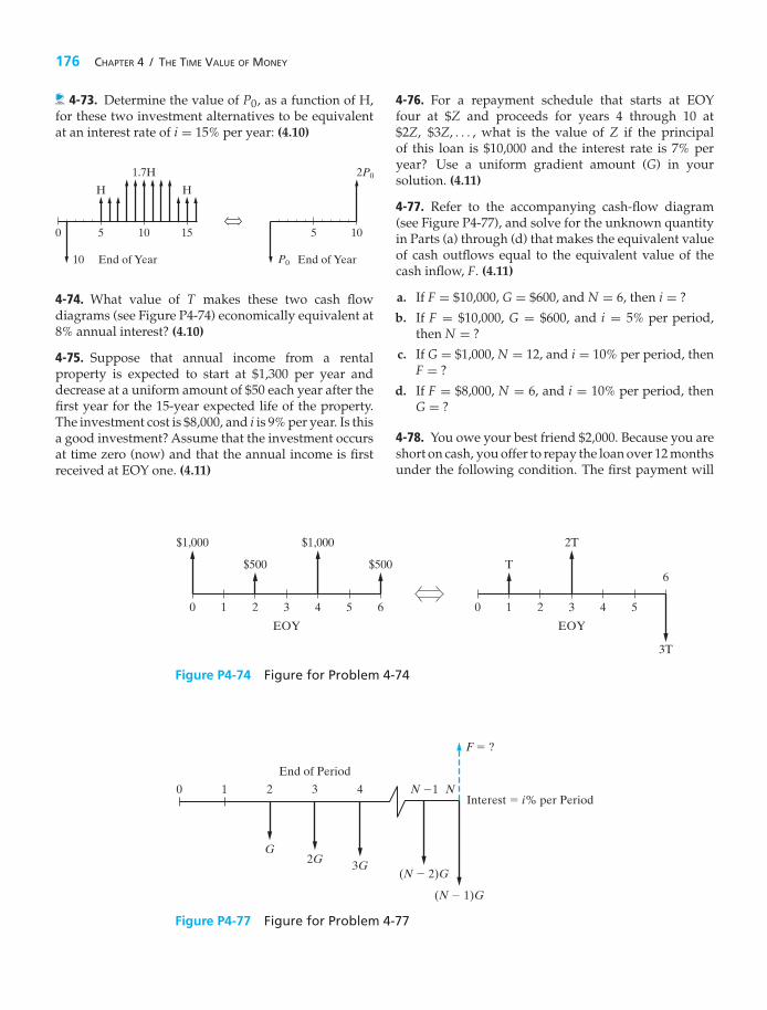
176 CHAPTER 4 / THE TIME VALUE OF MONEY

4-73. Determine the value of P0, as a function of H,for these two investment alternatives to be equivalentat an interest rate of i = 15% per year: (4.10)

50 10

End of Year End of Year

1.7H

HH

10

15 5

2P0

P0

10

4-74. What value of T makes these two cash flowdiagrams (see Figure P4-74) economically equivalent at8% annual interest? (4.10)

4-75. Suppose that annual income from a rentalproperty is expected to start at $1,300 per year anddecrease at a uniform amount of $50 each year after thefirst year for the 15-year expected life of the property.The investment cost is $8,000, and i is 9% per year. Is thisa good investment? Assume that the investment occursat time zero (now) and that the annual income is firstreceived at EOY one. (4.11)

1 2 3 4 5 6

EOY

$1,000

0

$1,000

$500 $500

1 2 3 4 5

6

EOY

2T

0

3T

T

Figure P4-74 Figure for Problem 4-74

43210 N �1 N

G2G 3G

(N � 2)G

(N � 1)G

F � ?

Interest � i% per Period

End of Period

Figure P4-77 Figure for Problem 4-77

4-76. For a repayment schedule that starts at EOYfour at $Z and proceeds for years 4 through 10 at$2Z, $3Z, . . . , what is the value of Z if the principalof this loan is $10,000 and the interest rate is 7% peryear? Use a uniform gradient amount (G) in yoursolution. (4.11)

4-77. Refer to the accompanying cash-flow diagram(see Figure P4-77), and solve for the unknown quantityin Parts (a) through (d) that makes the equivalent valueof cash outflows equal to the equivalent value of thecash inflow, F. (4.11)

a. If F = $10,000, G = $600, and N = 6, then i = ?

b. If F = $10,000, G = $600, and i = 5% per period,then N = ?

c. If G = $1,000, N = 12, and i = 10% per period, thenF = ?

d. If F = $8,000, N = 6, and i = 10% per period, thenG = ?

4-78. You owe your best friend $2,000. Because you areshort on cash, you offer to repay the loan over 12 monthsunder the following condition. The first payment will

PROBLEMS 177

650540

430320

210

100

0 1 2 3 4 5 6 7

End of Year

K K

4 53

End of Year

210

Figure P4-79 Figure for Problem 4-79

be $100 at the end of month one. The second paymentwill be $100 + G at the end of month two. At the endof month three, you’ll repay $100 + 2G. This pattern ofincreasing G amounts will continue for all remainingmonths. (4.11)

a. What is the value of G if the interest rate is 0.5% permonth?

b. What is the equivalent uniform monthly payment?

c. Repeat Part (a) when the first payment is $150 (i.e.,determine G).

4-79. In the accompanying diagram, Figure P4-79,what is the value of K on the left-hand cash-flowdiagram that is equivalent to the right-hand cash-flowdiagram? Let i = 12% per year. (4.11)

4-80. Calculate the future equivalent at the end of 2012,at 8% per year, of the following series of cash flows inFigure P4-80: [Use a uniform gradient amount (G) inyour solution.] (4.11)

$1,000

F � ?

$800$600

$400

Years2009 2010 2011 2012

Figure P4-80 Figure for Problem 4-80

4-81. Suppose that the parents of a young child decideto make annual deposits into a savings account, with thefirst deposit being made on the child’s fifth birthday and

the last deposit being made on the 15th birthday. Then,starting on the child’s 18th birthday, the withdrawalsas shown will be made. If the effective annual interestrate is 8% during this period of time, what are theannual deposits in years 5 through 15? Use a uniformgradient amount (G) in your solution. (See Figure P4-81,p. 178.) (4.11)

4-82. The heat loss through the exterior walls ofa certain poultry processing plant is estimated to

cost the owner $3,000 next year. A salesperson fromSuperfiber Insulation, Inc., has told you, the plantengineer, that he can reduce the heat loss by 80% withthe installation of $18,000 worth of Superfiber now. Ifthe cost of heat loss rises by $200 per year (uniformgradient) after the next year and the owner plans to keepthe present building for 15 more years, what would yourecommend if the interest rate is 10% per year? (4.11)

4-83. What value of N comes closest to making the left-hand cash-flow diagram of the accompanying figure,Figure P4-83 (p. 178), equivalent to the one on the right?Let i = 15% per year. Use a uniform gradient amount(G) in your solution. (4.11)

4-84. A retail outlet is being designed in a stripmall in Nebraska. For this outlet, the installed

fiberglass insulation to protect against heat loss inthe winter and heat gain in the summer will cost anestimated $100,000. The annual savings in energy due tothe insulation will be $18,000 at EOY one in the 10-yearlife of the outlet, and these savings will increase by12% each year thereafter. If the annual interest rate is15%, is the cost of the proposed amount of insulationjustified? (4.12)

4-85. You are the manager of a large crude-oilrefinery. As part of the refining process, a certain

heat exchanger (operated at high temperatures and withabrasive material flowing through it) must be replaced

178 CHAPTER 4 / THE TIME VALUE OF MONEY

5thBirthday

$3,200

A � ?

6 7 8 9 10 11 12 13 14 15 16 17

18 19 20 21

$2,800

$2,400

$2,000

i � 8%/yrYears

Figure P4-81 Figure for Problem 4-81

10 0 42 3 4 5 N � ?

2R

3R

Years

(N � 2)R

27R

10Years

27R

R

Figure P4-83 Figure for Problem 4-83

every year. The replacement and downtime cost in thefirst year is $175,000. This cost is expected to increasedue to inflation at a rate of 8% per year for five years, atwhich time this particular heat exchanger will no longerbe needed. If the company’s cost of capital is 18% peryear, how much could you afford to spend for a higherquality heat exchanger so that these annual replacementand downtime costs could be eliminated? (4.12)

4-86. Start saving for retirement immediately! Even amodest amount will add up in a hurry. Jay decides tofollow this advice and puts away 1% of his annual salaryof $50,000 per year. This equates to $500 on his 21stbirthday, and his salary will increase by 2% (on average)every year thereafter until Jay turns 60 years old. Whatis the worth of Jay’s account at age 60 when the annualinterest rate on Jay’s account is 4% per year? (4.12)

4-87. A geometric gradient that increases at f = 6%per year for 15 years is shown in the accompanyingdiagram. The annual interest rate is 12%. What is thepresent equivalent value of this gradient? (4.12)

0 1 2 14 15Years

$500$500(1.06)1

$500(1.06)14

4-88. A small company heats its building andspends $8,000 per year on natural gas for this

purpose. Cost increases of natural gas are expected tobe 10% per year starting one year from now (i.e., thefirst cash flow is $8,800 at EOY one). Their maintenanceon the gas furnace is $345 per year, and this expense isexpected to increase by 15% per year starting one yearfrom now. If the planning horizon is 15 years, what isthe total annual equivalent expense for operating andmaintaining the furnace? The interest rate is 18% peryear. (4.12)

PROBLEMS 179

4-89. It is likely that your college tuition will in-crease an average of 8% per year for the next 4 years.The annual cost of tuition at the beginning of yourfreshman year in college will be $12,000 (A1). Howmuch money will you and your parents have to depositin a mutual fund account one year prior to yourfreshman year to pay for your tuition for the 4 yearsyou will spend earning your degree in engineering?The mutual fund will earn an average of 5% annualinterest. (4.12)

4-90. Amy Parker, a 22-year-old and newly hiredmarine biologist, is quick to admit that she does notplan to keep close tabs on how her 401(k) retirementplan will grow with time. This sort of thing does notreally interest her. Amy’s contribution, plus that of heremployer, amounts to $2,200 per year starting at age 23.Amy expects this amount to increase by 3% each yearuntil she retires at the age of 62 (there will be 40 EOYpayments). What is the compounded future value ofAmy’s 401(k) plan if it earns 7% per year? (4.12)

4-91. An electronic device is available that will reducethis year’s labor costs by $8,000. The equipment isexpected to last for 10 years. Labor costs increase ata rate of 5% per year and the interest rate is 10% peryear. (4.12)

a. What is the maximum amount that we could justifyspending for the device?

b. What is the uniform annual equivalent value (A) ofthe labor costs over the eight-year period?

4-92. An amount, P, must be invested now to allowwithdrawals of $1,000 per year for the next 15 years andto permit $300 to be withdrawn starting at the end ofyear 6 and continuing over the remainder of the 15-yearperiod as the $300 increases by 6% per year thereafter.That is, the withdrawal at EOY seven will be $318,$337.08 at EOY eight, and so forth for the remainingyears. The interest rate is 12% per year. Hint: Draw acash-flow diagram. (4.12)

4-93. Consider an EOY geometric gradient, which lastsfor eight years, whose initial value at EOY one is$5,000 and f = 6% per year thereafter. Find theequivalent uniform gradient amount over the sameperiod if the initial value of the cash flows at the endof year one is $4,000. Complete the following questionsto determine the value of the gradient amount, G. Theinterest rate is 8% per year. (4.12)

a. What is P0 for the geometric gradient series?

b. What is P′0 of the uniform (arithmetic) gradient of

cash flows?

c. What is the value of G?

4-94. An individual makes five annual deposits of$2,000 in a savings account that pays interest at a rateof 4% per year. One year after making the last deposit,the interest rate changes to 6% per year. Five years afterthe last deposit, the accumulated money is withdrawnfrom the account. How much is withdrawn? (4.13)

4-95. A person has made an arrangement to borrow$1,000 now and another $1,000 two years hence. Theentire obligation is to be repaid at the end of four years.If the projected interest rates in years one, two, three,and four are 10%, 12%, 12%, and 14%, respectively, howmuch will be repaid as a lump-sum amount at the endof four years? (4.13)

4-96. Suppose that you have a money market certificateearning an annual rate of interest, which varies overtime as follows:

Year k 1 2 3 4 5

ik 6% 4% 2% 2% 5%

If you invest $10,000 in this certificate at the beginningof year one and do not add or withdraw any money forfive years, what is the value of the certificate at the endof the fifth year? (4.13)

4-97. Determine the present equivalent value of thecash-flow diagram of Figure P4-97 (p. 180) when theannual interest rate, ik , varies as indicated. (4.13)

4-98. Mary’s credit card situation is out of controlbecause she cannot afford to make her monthlypayments. She has three credit cards with the followingloan balances and APRs: Card 1, $4,500, 21%; Card 2,$5,700, 24%; and Card 3, $3,200, 18%. Interestcompounds monthly on all loan balances. A creditcard loan consolidation company has captured Mary’sattention by stating they can save Mary 25% per monthon her credit card payments. This company charges16.5% APR. Is the company’s claim correct? (4.14)

4-99.

a. What is the effective annual interest rate whena nominal rate of 12% per year is compoundedmonthly?

180 CHAPTER 4 / THE TIME VALUE OF MONEY

P � ?$2,000$2,000

$1,000 $1,000

10 2 3 4 5 6

Years

i1 � 8% i2 � 10% i3 � 8% i4 � 6% i5 � 6% i6 � 10%

Figure P4-97 Figure for Problem 4-97

b. How many months does it take for a present sum ofmoney to double if the nominal interest rate is 12%per year and compounding is monthly?

c. How many months does it take for a present sumof money to triple if the nominal interest rate is 12%per year and compounding is monthly?

4-100. An APR of 3.75% produces an effective annualinterest rate of 3.82% What is the compoundingfrequency (M) in this situation? (4.14)

4-101. A large bank has increased its annual percentagerate (APR) on credit cards to 30%. This move wasnecessary because of the “additional risks” faced by thebank in a weak economy. If monthly compounding isin effect, what is the effective annual interest rate beingcharged by the bank? (4.15)

4-102. Compute the effective annual interest rate ineach of the following situations. (4.14)

a. 5.75% nominal interest, compounded quarterly.

b. 5.75% nominal interest, compounded daily.

4-103. Determine the current amount of money thatmust be invested at 12% nominal interest, compoundedmonthly, to provide an annuity of $10,000 (per year) for6 years, starting 12 years from now. The interest rateremains constant over this entire period of time. (4.15)

4-104. To pay off $50,000,000 worth of new constructionbonds when they come due in 20 years, a watermunicipality must deposit money into a sinking fund.Payments to the fund will be made quarterly, startingthree months from now. If the interest rate for thesinking fund is 8% compounded quarterly, how muchwill each deposit be? (4.15)

4-105. An automobile salesperson states that hiscompany will pay the interest for the first 12 monthsof your automobile loan if you buy the vehicle today.

Suppose you go ahead and purchase a car for $25,000and finance it with a 48-month loan having an APRof 9%. What is your monthly payment going to be inmonths 13–60 of this loan? How much lower will yourmonthly payment be if you finance your loan over 60months (months 13–72)? (4.14)

4-106. A light-duty pickup truck has a manufacturer’ssuggested retail price (MSRP) of $14,000 on its window.After haggling with the salesperson for several days,the prospective buyer is offered the following deal:“You pay a $1,238 down payment now and $249 eachmonth thereafter for 39 months and the truck will beyours.” The APR at this dealership is 2.4% compoundedmonthly. How good a deal is this relative to theMSRP? (4.15)

4-107. You borrow $10,000 from a bank for three years atan annual interest rate, or annual percentage rate (APR),of 12%. Monthly payments will be made until all theprincipal and interest have been repaid. (4.14, 4.15)

a. What is your monthly payment?

b. If you must pay two points up front, meaning thatyou get only $9,800 from the bank, what is your trueAPR on the loan?

4-108. Many people get ready for retirement bydepositing money into a monthly or annual savingsplan. (4.15)

a. If $300 per month is deposited in a bank accountpaying a 6% APR compounded monthly, how muchwill be accumulated in the account after 30 years?

b. If inflation is expected to average 2% per year intothe foreseeable future, what is today’s equivalentspending power for your answer to Part (a)?

4-109. The longer a loan schedule lasts, the moreinterest you will pay. To illustrate, a $20,000-car-loan

PROBLEMS 181

at 9% APR (compounded monthly) for three years(36 monthly payments) will incur total interest of$2,896. But a $20,000 car loan at 9% APR over sixyears (72 payments) will have a total interest costof $5,920. (4.15)

a. Verify that the difference in total interest of $3,024 iscorrect.

b. Why would you be willing to pay this extra interest?

4-110. The average college graduate owes $22,500 inloans incurred over his/her college career. Now that itis so difficult to land a job after graduation, an optionfor the graduate seeking relief is to stretch the loan over20 years (with the bank’s approval, of course) instead ofrepaying the loan over the normal 10 years. Doublingthe repayment period of the loan slices 29% off themonthly payments. However, this action also increasesthe total amount of interest repaid over the life of theloan by 121%! What is the monthly interest rate beingcharged in this scenario? (4.15)

4-111. Suppose you owe $1,100 on your credit card.The annual percentage rate (APR) is 18%, compoundedmonthly. The credit card company says your minimummonthly payment is $19.80. (4.15)

a. If you make only this minimum payment, howlong will it take for you to repay the $1,100 balance(assuming no more charges are made)?

b. If you make the minimum payment plus $10 extraeach month (for a total of $29.80), how long will ittake to repay the $1,100 balance?

c. Compare the total interest paid in Part (a) with thetotal interest paid in Part (b).

4-112. Determine the annual equivalent amount over4 years for the following cash flow (CF) pattern. Thenominal interest rate is 10%, and it is compoundedmonthly. (4.15)

EOY 0 1 2 3 4CF −$7,500 −$2,000 $14,000 $18,000 $4,000

4-113. A nominal interest rate of 11.333%, continuouslycompounded, yields an effective annual interest rate ofhow much? (4.16)

4-114. College students are now graduating with loandebts averaging $24,000. (4.15, 4.16)

a. If students repay their loan of $24,000 over 10 yearswith an annual effective interest rate of 8.3%, whatwill their annual payment be?

b. What is the annual payment going to be when theinterest rate is 9.6%, continuously compounded eachyear?

c. What is the effective interest rate in Part (b)?

4-115. If a nominal interest rate of 8% is compoundedcontinuously, determine the unknown quantity in eachof the following situations: (4.16)

a. What uniform EOY amount for 10 years isequivalent to $8,000 at EOY 10?

b. What is the present equivalent value of $1,000 peryear for 12 years?

c. What is the future equivalent at the end of thesixth year of $243 payments made every six monthsduring the six years? The first payment occurs sixmonths from the present and the last occurs at theend of the sixth year.

d. Find the equivalent lump-sum amount at EOY ninewhen P0 = $1,000.

4-116. Find the value of the unknown quantity Z inthe following diagram, such that the equivalent cashoutflow equals the equivalent cash inflows when r =20% compounded continuously: (4.16)

Z

Z

0

1

A � $500/year

Years2 3 4 5 6 7 8 9

4-117. Juan deposits $5,000 into a savings account thatpays 7.2% per year, continuously compounded. What isthe effective annual interest rate? Determine the valueof his account at the end of two years. (4.16)

4-118. A man deposited $10,000 in a savings accountwhen his son was born. The nominal interest rate was8% per year, compounded continuously. On the son’s18th birthday, the accumulated sum is withdrawn fromthe account. How much will this accumulated amountbe? (4.16)

4-119. A person needs $18,000 immediately as a downpayment on a new home. Suppose that she can borrowthis money from her company credit union. She will berequired to repay the loan in equal payments made everysix months over the next 12 years. The annual interest

182 CHAPTER 4 / THE TIME VALUE OF MONEY

rate being charged is 10% compounded continuously.What is the amount of each payment? (4.16)

4-120. What is the present equivalent of a uniformseries of annual payments of $3,500 each for fiveyears if the interest rate, compounded continuously,is 10%? (4.16)

4-121. The amount of $7,000 is invested in a Certificateof Deposit (CD) and will be worth $16,000 in nineyears. What is the continuously compounded nominal(annual) interest rate for this CD? (4.16)

4-122. Many persons prepare for retirement by makingmonthly contributions to a savings program. Supposethat $2,000 is set aside each year and invested ina savings account that pays 10% interest per year,compounded continuously. (4.16)

a. Determine the accumulated savings in this accountat the end of 30 years.

b. In Part (a), suppose that an annuity will bewithdrawn from savings that have been accum-ulated at the EOY 30. The annuity will extend fromthe EOY 31 to the EOY 40. What is the value ofthis annuity if the interest rate and compoundingfrequency in Part (a) do not change?

4-123. Indicate whether each of the following sta-tements is true (T) or false (F). (all sections)

a. T F Interest is money paid for the use of equitycapital.

b. T F (A/F, i%, N) = (A/P, i%, N) + i.

c. T F Simple interest ignores the time value ofmoney principle.

d. T F Cash-flow diagrams are analogous to free-body diagrams for mechanics problems.

e. T F $1,791 10 years from now is equivalent to$900 now if the interest rate equals 8% peryear.

f. T F It is always true that i > r when M ≥ 2.

g. T F Suppose that a lump sum of $1,000 is in-vested at r = 10% for eight years. The futureequivalent is greater for daily compoundingthan it is for continuous compounding.

h. T F For a fixed amount, F dollars, that is receivedat EOY N, the “A equivalent” increases as theinterest rate increases.

i. T F For a specified value of F at EOY N, P at timezero will be larger for r = 10% per year than

it will be for r = 10% per year, compoundedmonthly.

4-124. Mark each statement true (T) or false (F), and fillin the blanks in Part (e). (all sections)

a. T F The nominal interest rate will always be lessthan the effective interest rate when r = 10%and M = ∞.

b. T F A certain loan involves monthly repaymentsof $185 over a 24-month period. If r = 10%per year, more than half of the principal isstill owed on this loan after the 10th monthlypayment is made.

c. T F $1,791 in 10 years is equivalent to $900 now ifthe nominal interest rate is 8% compoundedsemiannually.

d. T F On a $200,000 mortgage, a half-point interestrate increase adds about $700 per year to 12mortgage payments.

e. Fill in the missing interest factor:

i. (P/A, i%, N)(———) = (F/A, i%, N).

ii. (A/G, i%, N)(P/A, i%, N) = (———).

4-125. A mutual fund investment is expected to earn11% per year for the next 25 years. If inflation willaverage 3% per year during this 25-year period of time,what is the compounded value (in today’s dollars) ofthis savings vehicle when $10,000 is invested now? (4.6)

4-126. Javier just bought a condominium in College-town, USA. His $100,000 mortgage is 6% compoundedmonthly, and Javier will make monthly payments on hisloan for 30 years. In addition, property taxes and titleinsurance amount to $400 per month. (4.15)

a. What is the total mortgage-related amount ofJavier’s monthly condo payment?

b. Develop an estimate of Javier’s total monthlyexpenses (maintenance, utilities, and so on) for hiscondominium.

c. If Javier qualifies for a 15-year mortgage having anAPR of 5.8% compounded monthly, what will hismonthly mortgage payment be (there will be 180payments)?

4-127. Analyze the truth of this statement, assumingyou are 20 years old: “For every five years that youwait to start accumulating money for your retirement,it takes twice as much savings per year to catch up.”Base your analysis on the target of having $1,000,000

CASE STUDY EXERCISES 183

when you retire at age 60. Be sure to state yourassumptions. (4.7)

4-128. A mortgage company advertises that their 6%APR is an effective annual rate of 6.58% with monthly

payments and compounding. Let’s assume this is madepossible by paying points on a mortgage (one point is 1%of the loan amount). How many points are being paidup front on a $100,000 mortgage loan over 15 years toarrive at an effective interest rate of 6.58%? (4.15)

Spreadsheet Exercises

4-129. Create a spreadsheet that duplicates Table 4-1.Make it flexible enough that you can investigatethe impact of different interest rates and principalloan amounts without changing the structure of thespreadsheet. (4.7)

4-130. A $15,000 investment is to be made withanticipated annual returns as shown in the spreadsheetin Figure P4-130. If the investor’s time value of money is10% per year, what should be entered in cells B11, B12,and B13 to obtain present, annual, and future equivalentvalues for the investment? (4.10)

A B1 EOY Cash flow2 0 −$15,0003 1 $2,0004 2 $2,5005 3 $3,0006 4 $3,5007 5 $4,0008 6 $4,0009 7 $4,000

10 8 $4,00011 P12 A13 F

Figure P4-130 Spreadsheetfor Problem 4-130

4-131. Refer to Example 4-23. Suppose the cash-flowsequence continues for 10 years (instead of four).Determine the new values of P, A, and F. (4.12)

4-132. Higher interest rates won’t cost you as muchto drive a car as do higher gasoline prices. This isbecause automobile loans have payment schedules thatare only modestly impacted by Federal Reserve Boardinterest-rate increases. Create a spreadsheet to comparethe difference in monthly payments for a $25,000 loanhaving 60 monthly payments for a select number ofinterest rates. Use 3% as the base APR and go as highas an APR of 12%. Challenge: Make your spreadsheetflexible enough to be able to look at the impact of thedifferent interest rates for different loan amounts anddifferent repayment periods. (4.15)

Case Study Exercises

4-133. After Enrico’s car is paid off, he plans tocontinue setting aside the amount of his car payment toaccumulate funds for the car’s replacement. If he investsthis amount at a rate of 3% compounded monthly, howmuch will he have saved by the end of the initial 10-yearperiod? (4.17)

4-134. Enrico has planned to have $40,000 at the endof 10 years to place a down payment on a condo.Property taxes and insurance can be as much as 30%

of the monthly principal and interest payment (i.e., fora principal and interest payment of $1,000, taxes andinsurance would be an additional $300). What is themaximum purchase price he can afford if he’d like tokeep his housing costs at $950 per month? (4.17)

4-135. If Enrico is more daring with his retirementinvestment savings and feels he can average 10% peryear, how much will he have accumulated for retirementat the end of the 10-year period? (4.17)

184 CHAPTER 4 / THE TIME VALUE OF MONEY

FE Practice Problems

4-136. If you borrow $3,000 at 6% simple interest peryear for seven years, how much will you have to repayat the end of seven years? (4.2)

(a) $3,000 (b) $4,511 (c) $1,260(d) $1,511 (e) $4,260

4-137. When you were born, your grandfatherestablished a trust fund for you in the CaymanIslands. The account has been earning interest atthe rate of 10% per year. If this account will beworth $100,000 on your 25th birthday, how muchdid your grandfather deposit on the day you wereborn? (4.6)(a) $4,000 (b) $9,230 (c) $10,000(d) $10,150 (e) $10,740

4-138. Every year you deposit $2,000 into an accountthat earns 2% interest per year. What will be the balanceof your account immediately after the 30th deposit? (4.7)

(a) $44,793 (b) $60,000 (c) $77,385(d) $81,136 (e) $82,759

4-139. Your monthly mortgage payment (principal plusinterest) is $1,500. If you have a 30-year loan with afixed interest rate of 0.5% per month, how much did youborrow from the bank to purchase your house? Selectthe closest answer. (4.7)

(a) $154,000 (b) $180,000 (c) $250,000(d) $300,000 (e) $540,000

4-140. Consider the following sequence of year-endcash flows:

EOY 1 2 3 4 5Cash $8,000 $15,000 $22,000 $29,000 $36,000Flow

What is the uniform annual equivalent if the interestrate is 12% per year? (4.11)

(a) $20,422 (b) $17,511 (c) $23,204(d) $22,000 (e) $12,422

4-141. A cash flow at time zero (now) of $9,982 isequivalent to another cash flow that is an EOY annuityof $2,500 over five years. Each of these two cash-flowseries is equivalent to a third series, which is a uniformgradient series. What is the value of G for this thirdseries over the same five-year time interval? (4.11)

(a) $994 (b) $1,150 (c) $1,250(d) $1,354 (e) Not enough information

given

4-142. Bill Mitselfik borrowed $10,000 to be repaidin quarterly installments over the next five years.The interest rate he is being charged is 12% peryear compounded quarterly. What is his quarterlypayment? (4.15)

(a) $400 (b) $550 (c) $650(d) $800

4-143. Sixty monthly deposits are made into an accountpaying 6% nominal interest compounded monthly. Ifthe objective of these deposits is to accumulate $100,000by the end of the fifth year, what is the amount of eachdeposit? (4.15)

(a) $1,930 (b) $1,478 (c) $1,667(d) $1,430 (e) $1,695

4-144. What is the principal remaining after 20 monthlypayments have been made on a $20,000 five-year loan?The annual interest rate is 12% nominal compoundedmonthly. (4.15)

(a) $10,224 (b) $13,333 (c) $14,579(d) $16,073 (e) $17,094

4-145. If you borrow $5,000 to buy a car at 12%compounded monthly, to be repaid over the next fouryears, what is your monthly payment? (4.15)

(a) $131 (b) $137 (c) $1,646(d) $81 (e) $104

4-146. The effective annual interest rate is given to be19.2%. What is the nominal interest rate per year (r)if continuous compounding is being used? Choose theclosest answer below. (4.16)

(a) 19.83% (b) 18.55% (c) 17.56%(d) 16.90%

4-147. A bank advertises mortgages at 12% com-pounded continuously. What is the effective annualinterest? (4.16)

(a) 12.36% (b) 12.55% (c) 12.75%(d) 12.68% (e) 12.00%

4-148. If you invest $7,000 at 12% compoundedcontinuously, how much would it be worth in threeyears? (4.16)

FE PRACTICE PROBLEMS 185

(a) $9,449 (b) $4,883 (c) $10,033(d) $9,834 (e) $2,520

4-149. On a $200,000, 30-year fixed mortgage, themonthly payment will be approximately how muchwhen the nominal interest rate on the mortgage is4.2%? (4.7)(a) $568 (b) $980 (c) $918(d) $1,000 (e) $895

4-150. Adding a small amount to your monthly homemortgage payment will shorten the life of your loan.Adding $10 per month to your $540 monthly mortgagepayment will trim how many months from a 30 year, 5%mortgage of $100,000? Select the closest answer. (4.7)

(a) 25 months (b) 19 months (c) 13 months(d) 6 months

4-151. Suppose a friend of yours invests $100 eachmonth in an individual retirement account (IRA) for adecade and earns an unbelievable APR of 12% a year(1% per month) on her investment. She will end up with$100 (F/A, 1%, 120) = $100 (230.0387) = $23,003.87 after10 years. If you decide to invest $200 each month over10 years, but can earn only a meager APR of 3% per yearon it, roughly how much will you have accumulatedafter 10 years? Choose the closest answer. (4.15).

(a) $19,000 (b) $24,000 (c) $28,000(d) $46,000

CHAPTER 5

Evaluating a Single Project

The objective of Chapter 5 is to discuss and critique contemporary methodsfor determining project profitability.

Carbon Fibers versus Metal

T here is a rule-of-thumb that “if the weight of an automobilecan be reduced by 10%, then 6% of the annual cost of gasolinecan be saved.” Light weight and high strength carbon fibers

costing about $15–$20 per pound are currently being considered to replace themetal in automobile and aerospace applications. (The objective of recent researchis to reduce this cost to $5 per pound.) Engineers believe they can economicallyreduce the weight of an automobile by substituting carbon fibers for metal to save20% to 30% on fuel consumption each year. Other structures such as stronger windturbines can also be built with light weight carbon fibers. After working throughthis chapter, you will be able to evaluate the economic trade-off between annualfuel savings and up-front cost of carbon fibers and to determine whether it is asmart trade-off.

186

The final test of any system is, does it pay?

—Frederick W. Taylor (1912)

5.1 IntroductionAll engineering economy studies of capital projects should consider the returnthat a given project will or should produce. A basic question this book addressesis whether a proposed capital investment and its associated expenditures can berecovered by revenue (or savings) over time in addition to a return on the capital thatis sufficiently attractive in view of the risks involved and the potential alternativeuses. The interest and money–time relationships discussed in Chapter 4 emergeas essential ingredients in answering this question, and they are applied to manydifferent types of problems in this chapter.

Because patterns of capital investment, revenue (or savings) cash flows, andexpense cash flows can be quite different in various projects, there is no singlemethod for performing engineering economic analyses that is ideal for all cases.Consequently, several methods are commonly used. A project focus will be takenas we introduce ways of gauging profitability.

In this chapter, we concentrate on the correct use of five methods for evaluatingthe economic profitability of a single proposed problem solution (i.e., alternative).∗Later, in Chapter 6, multiple alternatives are evaluated. The five methods describedin Chapter 5 are Present Worth (PW), Future Worth (FW), Annual Worth (AW),Internal Rate of Return (IRR), and External Rate of Return (ERR). The first threemethods convert cash flows resulting from a proposed problem solution into theirequivalent worth at some point (or points) in time by using an interest rate knownas the Minimum Attractive Rate of Return (MARR). The concept of a MARR, as wellas the determination of its value, is discussed in the next section. The IRR and ERRmethods compute annual rates of profit, or returns, resulting from an investmentand are then compared to the MARR.

The payback period is also discussed briefly in this chapter. The paybackperiod is a measure of the speed with which an investment is recovered by thecash inflows it produces. This measure, in its most common form, ignores timevalue of money principles. For this reason, the payback method is often used tosupplement information produced by the five primary methods featured in thischapter.

Unless otherwise specified, the end-of-period cash-flow convention and discretecompounding of interest are used throughout this and subsequent chapters.A planning horizon, or study (analysis) period, of N compounding periods(usually years) is used to evaluate prospective investments throughout theremainder of the book.

∗ The analysis of engineering projects using the benefit–cost ratio method is discussed in Chapter 10.

187

188 CHAPTER 5 / EVALUATING A SINGLE PROJECT

5.2 Determining the Minimum Attractive Rateof Return (MARR)

The Minimum Attractive Rate of Return (MARR) is usually a policy issue resolvedby the top management of an organization in view of numerous considerations.Among these considerations are the following:

1. The amount of money available for investment, and the source and cost of thesefunds (i.e., equity funds or borrowed funds)

2. The number of good projects available for investment and their purpose (i.e.,whether they sustain present operations and are essential, or whether theyexpand on present operations and are elective)

3. The amount of perceived risk associated with investment opportunitiesavailable to the firm and the estimated cost of administering projects over shortplanning horizons versus long planning horizons

4. The type of organization involved (i.e., government, public utility, or privateindustry)

In theory, the MARR, which is sometimes called the hurdle rate, should be chosento maximize the economic well-being of an organization, subject to the types ofconsiderations just listed. How an individual firm accomplishes this in practiceis far from clear-cut and is frequently the subject of discussion. One popularapproach to establishing a MARR involves the opportunity cost viewpoint describedin Chapter 2, and it results from the phenomenon of capital rationing. This situationmay arise when the amount of available capital is insufficient to sponsor all worthyinvestment opportunities. The subject of capital rationing is covered in Chapter 13.

A simple example of capital rationing is given in Figure 5-1, where thecumulative investment requirements of seven acceptable projects are plottedagainst the prospective annual rate of profit of each. Figure 5-1 shows a limit of$600 million on available capital. In view of this limitation, the last funded projectwould be E, with a prospective rate of profit of 19% per year, and the best rejectedproject is F. In this case, the MARR by the opportunity cost principle would be 16%per year. By not being able to invest in project F, the firm would presumably beforfeiting the chance to realize a 16% annual return. As the amount of investmentcapital and opportunities available change over time, the firm’s MARR will alsochange.∗

Superimposed on Figure 5-1 is the approximate cost of obtaining the$600 million, illustrating that project E is acceptable only as long as its annualrate of profit exceeds the cost of raising the last $100 million. As shown in Figure5-1, the cost of capital will tend to increase gradually as larger sums of money areacquired through increased borrowing (debt) or new issuances of common stock(equity). Determining the MARR is discussed further in Chapter 13.

∗ As we shall see in Chapter 11, the selection of a project may be relatively insensitive to the choice of a value for theMARR. Revenue estimates, for example, are much more important to the selection of the most profitable investment.

SECTION 5.3 / THE PRESENT WORTH METHOD 189

5

10

15

20

25

30

35

100 200 300 400 500 600 700 800

Cumulative Investment Amount (Millions of Dollars)

Ann

ual R

ate

of P

rofi

t (%

)

35

30

26

23

19

1614

GF

E

D

C

B

A

Independent Projects (Demand)—Any Subset (or All) Can Be Selected

Approximate Costof Capital Obtained(Supply)

Reject G

Reject F

MARR � 16%/year

Figure 5-1 Determination of the MARR Based on the Opportunity Cost Viewpoint(A popular measure of annual rate of profit is “Internal Rate of Return,” discussedlater in this chapter.)

5.3 The Present Worth MethodThe PW method is based on the concept of equivalent worth of all cash flowsrelative to some base or beginning point in time called the present. That is, all cashinflows and outflows are discounted to the present point in time at an interest ratethat is generally the MARR. A positive PW for an investment project is a dollaramount of profit over the minimum amount required by investors. It is assumedthat cash generated by the alternative is available for other uses that earn interestat a rate equal to the MARR.

To find the PW as a function of i% (per interest period) of a series of cash inflowsand outflows, it is necessary to discount future amounts to the present by using theinterest rate over the appropriate study period (years, for example) in the followingmanner:

PW(i%) = F0(1 + i)0 + F1(1 + i)−1 + F2(1 + i)−2

+ · · · + Fk(1 + i)−k + · · · + FN(1 + i)−N

=N∑

k=0

Fk(1 + i)−k . (5-1)

Here, i = effective interest rate, or MARR, per compounding period;k = index for each compounding period (0 ≤ k ≤ N);

Fk = future cash flow at the end of period k;N = number of compounding periods in the planning horizon (i.e., study

period).

190 CHAPTER 5 / EVALUATING A SINGLE PROJECT

The relationship given in Equation (5-1) is based on the assumption of a constantinterest rate throughout the life of a particular project. If the interest rate is assumedto change, the PW must be computed in two or more steps, as was illustrated inChapter 4.

To apply the PW method of determining a project’s economic worthiness, wesimply compute the present equivalent of all cash flows using the MARR as theinterest rate. If the present worth is greater than or equal to zero, the project isacceptable.

PW Decision Rule: If PW (i = MARR) ≥ 0, the project is economically justified.

It is important to observe that the higher the interest rate and the farther intothe future a cash flow occurs, the lower its PW is. This is shown graphically inFigure 5-2. The PW of $1,000 10 years from now is $613.90 when i = 5% per year.However, if i = 10%, that same $1,000 is only worth $385.50 now.

Figure 5-2 PW of $1,000Received at the End of Yeark at an Interest Rate of i%per Year

0 1 2 3 4 5 6 7 8 9 10

End of Year k

100

200

300

400

500

600

700

800

900

1,000

Pre

sent

Wor

th (

PW

) in

$

0

PW of $1,000 Receivedat End of Year 10

$613.90

$1,000

$385.50

$161.50

$72.50

i � 30%

i � 20%

i � 10%

i � 5%

i = 0%

as i , PW

SECTION 5.3 / THE PRESENT WORTH METHOD 191

EXAMPLE 5-1 Evaluation of New Equipment Purchase Using PW

A piece of new equipment has been proposed by engineers to increase theproductivity of a certain manual welding operation. The investment cost is$25,000, and the equipment will have a market value of $5,000 at the endof a study period of five years. Increased productivity attributable to theequipment will amount to $8,000 per year after extra operating costs havebeen subtracted from the revenue generated by the additional production.A cash-flow diagram for this investment opportunity is given below. If thefirm’s MARR is 20% per year, is this proposal a sound one? Use the PWmethod.

$25,000

$8,000

1 2 3 4 5

$8,000 $8,000 $8,000 $8,000

$5,000

End of Year

i � 20%/yr

Solution

PW = PW of cash inflows − PW of cash outflows,

or

PW(20%) = $8,000(P/A, 20%, 5) + $5,000(P/F, 20%, 5) − $25,000

= $934.29.

Because PW(20%) ≥ 0, this equipment is economically justified.

The MARR in Example 5-1 (and in other examples throughout this chapter)is to be interpreted as an effective interest rate (i). Here, i = 20% per year. Cashflows are discrete, end-of-year (EOY) amounts. If continuous compounding had been

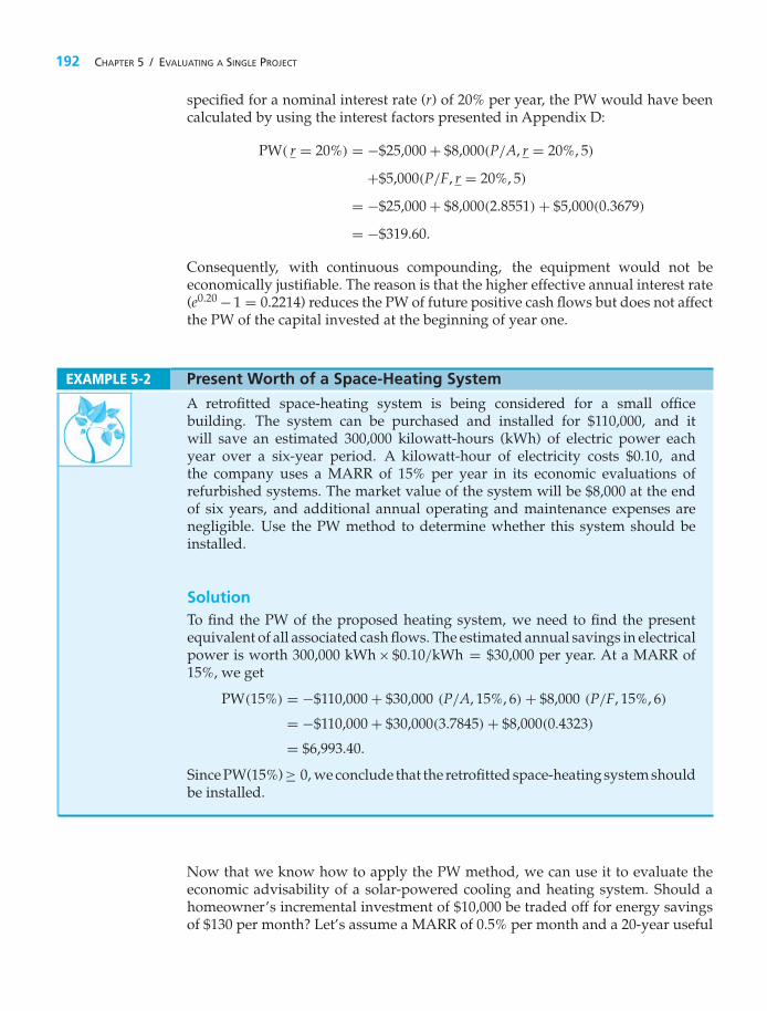
192 CHAPTER 5 / EVALUATING A SINGLE PROJECT

specified for a nominal interest rate (r) of 20% per year, the PW would have beencalculated by using the interest factors presented in Appendix D:

PW( r = 20%) = −$25,000 + $8,000(P/A, r = 20%, 5)

+$5,000(P/F, r = 20%, 5)

= −$25,000 + $8,000(2.8551) + $5,000(0.3679)

= −$319.60.

Consequently, with continuous compounding, the equipment would not beeconomically justifiable. The reason is that the higher effective annual interest rate(e0.20 − 1 = 0.2214) reduces the PW of future positive cash flows but does not affectthe PW of the capital invested at the beginning of year one.

EXAMPLE 5-2 Present Worth of a Space-Heating System

A retrofitted space-heating system is being considered for a small officebuilding. The system can be purchased and installed for $110,000, and itwill save an estimated 300,000 kilowatt-hours (kWh) of electric power eachyear over a six-year period. A kilowatt-hour of electricity costs $0.10, andthe company uses a MARR of 15% per year in its economic evaluations ofrefurbished systems. The market value of the system will be $8,000 at the endof six years, and additional annual operating and maintenance expenses arenegligible. Use the PW method to determine whether this system should beinstalled.

SolutionTo find the PW of the proposed heating system, we need to find the presentequivalent of all associated cash flows. The estimated annual savings in electricalpower is worth 300,000 kWh × $0.10/kWh = $30,000 per year. At a MARR of15%, we get

PW(15%) = −$110,000 + $30,000 (P/A, 15%, 6) + $8,000 (P/F, 15%, 6)

= −$110,000 + $30,000(3.7845) + $8,000(0.4323)

= $6,993.40.

Since PW(15%)≥ 0, we conclude that the retrofitted space-heating system shouldbe installed.

Now that we know how to apply the PW method, we can use it to evaluate theeconomic advisability of a solar-powered cooling and heating system. Should ahomeowner’s incremental investment of $10,000 be traded off for energy savingsof $130 per month? Let’s assume a MARR of 0.5% per month and a 20-year useful

SECTION 5.3 / THE PRESENT WORTH METHOD 193

life of the solar-powered system. In this case, the PW of the system is

PW = −$10,000 + $130(P/A, 0.5%, per month, 240 months)

= −$10,000 + $130(139.5808)

= $8,145.50.

The positive-valued PW signals a favorable investment. Additionally, 13 tons/year× 20 years = 260 tons of carbon dioxide will be avoided. Can you rework thisproblem when the MARR is 1% per month? Is the system still a judicious choice?

5.3.1 Assumptions of the PW Method

There are several noteworthy assumptions that we make when using PW to modelthe wealth-creating promise of a capital investment opportunity. First, it is assumedthat we know the future with certainty (we don’t live in a certain world!). Forexample, we presume to know with certainty future interest rates and other factors.Second, it is assumed we can borrow and lend money at the same interest rate (i.e.,capital markets are perfect). Regrettably, the real world has neither certainty norperfect (frictionless, e.g., no taxes and/or commissions) capital markets.

The PW (and FW and AW, to follow) model is built on these seeminglyrestrictive assumptions, but it is cost-beneficial in the sense that the cost of usingthe PW model is less than the benefits of improved decisions resulting fromPW analysis. More sophisticated models exist, but they usually do not reversedecisions made with the PW model. Therefore, our goal is to cost-beneficiallyrecommend capital investments that maximize the wealth of a firm to its owners(i.e., stockholders). A positive-valued PW (and FW and AW) means that acceptinga project will increase the worth, or value, of the firm.

5.3.2 Bond Value

A bond is an IOU where you agree to lend the bond issuer money for a specifiedlength of time (say, 10 years). In return, you receive periodic interest payments(e.g., quarterly) from the issuer plus a promise to return the face value of the bondwhen it matures. A bond provides an excellent example of commercial value asbeing the PW of the future net cash flows that are expected to be received throughownership of an interest-bearing certificate. Thus, the value of a bond, at any time,is the PW of future cash receipts. For a bond, let

Z = face, or par, value;C = redemption or disposal price (usually equal to Z);r = bond rate (nominal interest) per interest period;

N = number of periods before redemption;i = bond yield rate per period;

VN = value (price) of the bond N interest periods prior toredemption—this is a PW measure of merit.

The owner of a bond is paid two types of payments by the borrower. The firstconsists of the series of periodic interest payments he or she will receive until the

194 CHAPTER 5 / EVALUATING A SINGLE PROJECT

bond is retired. There will be N such payments, each amounting to rZ. Theseconstitute an annuity of N payments. In addition, when the bond is retired or sold,the bondholder will receive a single payment equal in amount to C. The PW of thebond is the sum of PWs of these two types of payments at the bond’s yield rate (i%):

VN = C(P/F, i%, N) + rZ(P/A, i%, N). (5-2)

The most common situations faced by you as a potential investor in bonds are(1) for a desired yield rate, how much should you be willing to pay for the bondand (2) for a stated purchase price, what will your yield be? Examples 5-3 and 5-4demonstrate how to solve these types of problems.

EXAMPLE 5-3 Stan Moneymaker Wants to Buy a Bond

Stan Moneymaker has the opportunity to purchase a certain U.S. Treasury bondthat matures in eight years and has a face value of $10,000. This means that Stanwill receive $10,000 cash when the bond’s maturity date is reached. The bondstipulates a fixed nominal interest rate of 8% per year, but interest payments aremade to the bondholder every three months; therefore, each payment amountsto 2% of the face value.

Stan would like to earn 10% nominal interest (compounded quarterly) peryear on his investment, because interest rates in the economy have risen sincethe bond was issued. How much should Stan be willing to pay for the bond?

SolutionTo establish the value of this bond, in view of the stated conditions, the PWof future cash flows during the next eight years (the study period) must beevaluated. Interest payments are quarterly. Because Stan Moneymaker desiresto obtain 10% nominal interest per year on the investment, the PW is computedat i = 10%/4 = 2.5% per quarter for the remaining 8(4) = 32 quarters of thebond’s life:

VN = $10,000(P/F, 2.5%, 32) + $10,000(0.02)(P/A, 2.5%, 32)

= $4,537.71 + $4,369.84 = $8,907.55.

Thus, Stan should pay no more than $8,907.55 when 10% nominal interest peryear is desired.

EXAMPLE 5-4 Current Price and Annual Yield of Bond Calculations

A bond with a face value of $5,000 pays interest of 8% per year. This bond will beredeemed at par value at the end of its 20-year life, and the first interest paymentis due one year from now.

(a) How much should be paid now for this bond in order to receive a yield of10% per year on the investment?

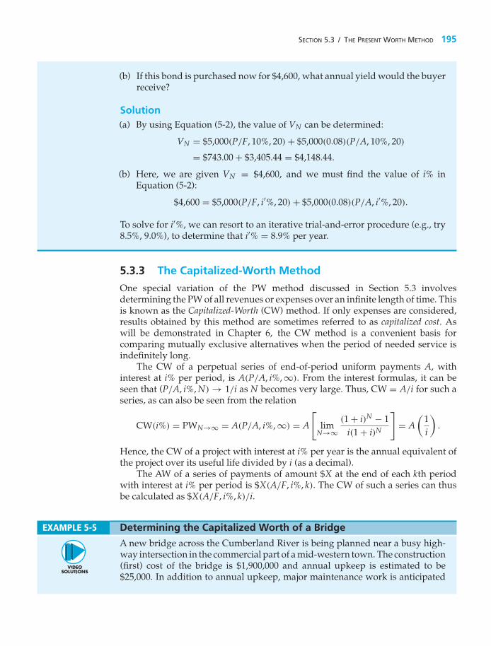
SECTION 5.3 / THE PRESENT WORTH METHOD 195

(b) If this bond is purchased now for $4,600, what annual yield would the buyerreceive?

Solution(a) By using Equation (5-2), the value of VN can be determined:

VN = $5,000(P/F, 10%, 20) + $5,000(0.08)(P/A, 10%, 20)

= $743.00 + $3,405.44 = $4,148.44.

(b) Here, we are given VN = $4,600, and we must find the value of i% inEquation (5-2):

$4,600 = $5,000(P/F, i′%, 20) + $5,000(0.08)(P/A, i′%, 20).

To solve for i′%, we can resort to an iterative trial-and-error procedure (e.g., try8.5%, 9.0%), to determine that i′% = 8.9% per year.

5.3.3 The Capitalized-Worth Method

One special variation of the PW method discussed in Section 5.3 involvesdetermining the PW of all revenues or expenses over an infinite length of time. Thisis known as the Capitalized-Worth (CW) method. If only expenses are considered,results obtained by this method are sometimes referred to as capitalized cost. Aswill be demonstrated in Chapter 6, the CW method is a convenient basis forcomparing mutually exclusive alternatives when the period of needed service isindefinitely long.

The CW of a perpetual series of end-of-period uniform payments A, withinterest at i% per period, is A(P/A, i%, ∞). From the interest formulas, it can beseen that (P/A, i%, N) → 1/i as N becomes very large. Thus, CW = A/i for such aseries, as can also be seen from the relation

CW(i%) = PWN→∞ = A(P/A, i%, ∞) = A

[lim

N→∞(1 + i)N − 1

i(1 + i)N

]= A

(1i

).

Hence, the CW of a project with interest at i% per year is the annual equivalent ofthe project over its useful life divided by i (as a decimal).

The AW of a series of payments of amount $X at the end of each kth periodwith interest at i% per period is $X(A/F, i%, k). The CW of such a series can thusbe calculated as $X(A/F, i%, k)/i.

EXAMPLE 5-5 Determining the Capitalized Worth of a Bridge

A new bridge across the Cumberland River is being planned near a busy high-way intersection in the commercial part of a mid-western town. The construction(first) cost of the bridge is $1,900,000 and annual upkeep is estimated to be$25,000. In addition to annual upkeep, major maintenance work is anticipated

196 CHAPTER 5 / EVALUATING A SINGLE PROJECT

every eight years at a cost of $350,000 per occurrence. The town government’sMARR is 8% per year.

(a) For this problem, what analysis period (N) is, practically speaking, definedas forever?

(b) If the bridge has an expected life of 50 years, what is the capitalized worth(CW) of the bridge over a 100-year study period?

Solution(a) Apractical approximation of “forever” (infinity) is dependent on the interest

rate. By examining the (A/P, i%, N) factor as N increases in the Appendix Ctables, we observe that this factor approaches a value of i as N becomes large.For i = 8% (Table C-11), the (A/P, 8%, 100) factor is 0.08. So N = 100 years is,for practical purposes, “forever” in this example.

(b) The CW is determined as follows:

CW(8%) = −$1,900,000 − $1,900,000 (P/F, 8%, 50)

− [$350,000 (A/F, 8%, 8)]/0.08 − $25,000/0.08.

The CW turns out to be −$2,664,220 over a 100-year study period, assumingthe bridge is replaced at the end of year 50 for $1,900,000.

5.4 The Future Worth MethodBecause a primary objective of all time value of money methods is to maximizethe future wealth of the owners of a firm, the economic information provided bythe FW method is very useful in capital investment decision situations. The FWis based on the equivalent worth of all cash inflows and outflows at the end ofthe planning horizon (study period) at an interest rate that is generally the MARR.Also, the FW of a project is equivalent to its PW; that is, FW = PW(F/P, i%, N). IfFW ≥ 0 for a project, it would be economically justified.

FW Decision Rule: If FW (i = MARR) ≥ 0, the project is economically justified.

Equation (5-3) summarizes the general calculations necessary to determine aproject’s FW:

FW(i%) = F0(1 + i)N + F1(1 + i)N−1 + · · · + FN(1 + i)0

=N∑

k=0

Fk(1 + i)N−k . (5-3)

SECTION 5.5 / THE ANNUAL WORTH METHOD 197

EXAMPLE 5-6 The Relationship between FW and PW

Evaluate the FW of the potential improvement project described in Example 5-1.Show the relationship between FW and PW for this example.

Solution

FW(20%) = −$25,000(F/P, 20%, 5)

+ $8,000(F/A, 20%, 5) + $5,000

= $2,324.80.

Again, the project is shown to be a good investment (FW ≥ 0). The PW isa multiple of the equivalent FW value:

PW(20%) = $2,324.80(P/F, 20%, 5) = $934.29.

To this point, the PW and FW methods have used a known and constantMARR over the study period. Each method produces a measure of merit expressedin dollars and is equivalent to the other. The difference in economic informationprovided is relative to the point in time used (i.e., the present for the PW versusthe future, or end of the study period, for the FW).

EXAMPLE 5-7 Sensitivity Analysis Using FW (Example 5-2 Revisited)

In Example 5-2, the $110,000 retrofitted space-heating system was projected tosave $30,000 per year in electrical power and be worth $8,000 at the end of thesix-year study period. Use the FW method to determine whether the project isstill economically justified if the system has zero market value after six years.The MARR is 15% per year.

SolutionIn this example, we need to find the future equivalent of the $110,000 investmentand the $30,000 annual savings at an interest rate of 15% per year.

FW(15%) = −$110,000 (F/P, 15%, 6) + $30,000 (F/A, 15%, 6)

= −$110,000 (2.3131) + $30,000 (8.7537)

= $8,170.

The heating system is still a profitable project (FW ≥ 0) even if it has no marketvalue at the end of the study period.

5.5 The Annual Worth MethodThe AW of a project is an equal annual series of dollar amounts, for a stated studyperiod, that is equivalent to the cash inflows and outflows at an interest rate that isgenerally the MARR. Hence, the AW of a project is annual equivalent revenues or

198 CHAPTER 5 / EVALUATING A SINGLE PROJECT

savings (R) minus annual equivalent expenses (E), less its annual equivalent capitalrecovery (CR) amount, which is defined in Equation (5-5). An annual equivalentvalue of R , E , and CR is computed for the study period, N, which is usually inyears. In equation form, the AW, which is a function of i%, is

AW(i%) = R − E − CR(i%). (5-4)

Also, we need to notice that the AW of a project is equivalent to its PW and FW.That is, AW = PW(A/P, i%, N), and AW = FW(A/F, i%, N). Hence, it can be easilycomputed for a project from these other equivalent values.

As long as the AW evaluated at the MARR is greater than or equal to zero,the project is economically attractive; otherwise, it is not. An AW of zero meansthat an annual return exactly equal to the MARR has been earned. Many decisionmakers prefer the AW method because it is relatively easy to interpret whenthey are accustomed to working with annual income statements and cash-flowsummaries.

AW Decision Rule: If AW (i = MARR) ≥ 0, the project is economically justified.

The CR amount for a project is the equivalent uniform annual cost of the capitalinvested. It is an annual amount that covers the following two items:

1. Loss in value of the asset2. Interest on invested capital (i.e., at the MARR)

As an example, consider a device that will cost $10,000, last five years, and havea salvage (market) value of $2,000. Thus, the loss in value of this asset over fiveyears is $8,000. Additionally, the MARR is 10% per year.

It can be shown that, no matter which method of calculating an asset’s lossin value over time is used, the equivalent annual CR amount is the same. Forexample, if a uniform loss in value is assumed ($8,000/5 years = $1,600 peryear), the equivalent annual CR amount is calculated to be $2,310, as shown inTable 5-1.

There are several convenient formulas by which the CR amount (cost) maybe calculated to obtain the result in Table 5-1. Probably the easiest formula tounderstand involves finding the annual equivalent of the initial capital investmentand then subtracting the annual equivalent of the salvage value.∗ Thus,

CR(i%) = I(A/P, i%, N) − S(A/F, i%, N), (5-5)

∗ The following two equations are alternative ways of calculating the CR amount:

CR(i%) = (I − S)(A/F, i%, N) + I(i%);

CR(i%) = (I − S)(A/P, i%, N) + S(i%).

It is left as a student exercise to show that the above equations are equivalent to Equation (5-5).

SECTION 5.5 / THE ANNUAL WORTH METHOD 199

TABLE 5-1 Calculation of Equivalent Annual CR Amount

Interest onValue of Beginning- CR

Investment Uniform of-Year Amountat Beginning Loss in Investment for PW of CR Amount

Year of Yeara Value at i = 10% Year at i = 10%

1 $10,000 $1,600 $1,000 $2,600 $2,600(P/F, 10%, 1) = $2,3642 8,400 1,600 840 2,440 $2,440(P/F, 10%, 2) = $2,0163 6,800 1,600 680 2,280 $2,280(P/F, 10%, 3) = $1,7134 5,200 1,600 520 2,120 $2,120(P/F, 10%, 4) = $1,4485 3,600 1,600 360 1,960 $1,960(P/F, 10%, 5) = $1,217

$8,758CR(10%) = $8,758(A/P, 10%, 5) = $2,310.

a This is also referred to later as the beginning-of-year unrecovered investment.

where I = initial investment for the project;∗S = salvage (market) value at the end of the study period;

N = project study period.

Thus, by substituting the CR(i%) expression of Equation (5-5) into the AWexpression, Equation (5-4) becomes

AW(i%) = R − E − I(A/P, i%, N) + S(A/F, i%, N).

When Equation (5-5) is applied to the example in Table 5-1, the CR cost is

CR(10%) = $10,000(A/P, 10%, 5) − $2,000(A/F, 10%, 5)

= $10,000(0.2638) − $2,000(0.1638) = $2,310.

EXAMPLE 5-8Using AW to Evaluate the Purchase of New Equipment(Example 5-1 Revisited)

By using the AW method and Equation (5-4), determine whether the equipmentdescribed in Example 5-1 should be recommended.

SolutionThe AW Method applied to Example 5-1 yields the following:

AW(20%) =R−E︷ ︸︸ ︷

$8,000 −CR amount [Equation (5-5)]︷ ︸︸ ︷

[$25,000(A/P, 20%, 5) − $5,000(A/F, 20%, 5)]= $8,000 − $8,359.50 + $671.90

= $312.40.

∗ In some cases, the investment will be spread over several periods. In such situations, I is the PW of all investmentamounts.

200 CHAPTER 5 / EVALUATING A SINGLE PROJECT

Because its AW(20%) is positive, the equipment more than pays for itself overa period of five years, while earning a 20% return per year on the unrecoveredinvestment. In fact, the annual equivalent “surplus” is $312.40, which meansthat the equipment provided more than a 20% return on beginning-of-yearunrecovered investment. This piece of equipment should be recommended asan attractive investment opportunity. Also, we can confirm that the AW(20%)is equivalent to PW(20%) = $934.29 in Example 5-1 and FW(20%) = $2,324.80 inExample 5-6. That is,

AW(20%) = $934.29(A/P, 20%, 5) = $312.40, and also

AW(20%) = $2,324.80(A/F, 20%, 5) = $312.40.

When revenues are absent in Equation (5-4), we designate this metric asEUAC(i%) and call it “equivalent uniform annual cost.” A low-valued EUAC(i%)is preferred to a high-valued EUAC(i%).

EXAMPLE 5-9 Equivalent Uniform Annual Cost of a Corporate Jet

A corporate jet costs $1,350,000 and will incur $200,000 per year in fixed costs(maintenance, licenses, insurance, and hangar rental) and $277 per hour invariable costs (fuel, pilot expense, etc.). The jet will be operated for 1,200 hoursper year for five years and then sold for $650,000. The MARR is 15% per year.

(a) Determine the capital recovery cost of the jet.(b) What is the EUAC of the jet?

Solution(a) CR = $1,350,000 (A/P, 15%, 5) − $650,000 (A/F, 15%, 5) = $306,310.(b) The total annual expense for the jet is the sum of the fixed costs and the

variable costs.

E = $200,000 + (1,200 hours)($277/hour) = $532,400

EUAC(15%) = $532,400 + $306,310 = $838,710

EXAMPLE 5-10Determination of Annual Savings by Using the AW Method(Example 5-2 Revisited)

Consider the retrofitted space-heating system described in Example 5-2. Giventhe investment of $110,000 and market value of $8,000 at the end of the six-yearstudy period, what is the minimum annual electrical power savings (in kWh)

SECTION 5.5 / THE ANNUAL WORTH METHOD 201

required to make this project economically acceptable? The MARR = 15% peryear and electricity costs $0.10 per kWh.

SolutionTo make this project acceptable, the annual power savings must be at least asgreat as the annual CR amount. Using Equation (5-5),

CR = $110,000(A/P, 15%, 6) − $8,000 (A/F, 15%, 6) = $28,148.40.

This value ($28,148.40) is the minimum annual dollar savings needed to justifythe space-heating system. This equates to

$28,148.40$0.10/kWh

= 281,480 kWh per year.

If the space-heating system can save 281,480 kWh per year, it is economicallyjustified (exactly 15% is earned on the beginning-of-year unrecovered invest-ment). Any savings greater than 281,480 kWh per year (such as the originalestimate of 300,000 kWh per year) will serve to make this project even moreattractive.

EXAMPLE 5-11 Avoid Getting Fleeced on an Auto Lease

Automobile leases are built around three factors: negotiated sales price, residualvalue, and interest rate. The residual value is what the dealership expects thecar’s value will be when the vehicle is returned at the end of the lease period. Themonthly cost of the lease is the capital recovery amount determined by usingthese three factors.

(a) Determine the monthly lease payment for a car that has an agreed-upon salesprice of $34,995, an APR of 9% compounded monthly, and an estimatedresidual value of $20,000 at the end of a 36-month lease.∗ An up-frontpayment of $3,000 is due when the lease agreement (contract) is signed.

(b) If the estimated residual value is raised to $25,000 by the dealership to getyour business, how much will the monthly payment be?

Solution(a) The effective sales price is $31,995 ($34,995 less the $3,000 due at signing). The

monthly interest rate is 9%/12 = 0.75% per month. So the capital recoveryamount is:

CR = $31,995(A/P, 0.75%, 36) − $20,000(A/F, 0.75%, 36)

= $1,017.44 − $486

= $531.44 per month.

∗ There are many excellent Web sites offering free calculators for car loans, home mortgages, life insurance,and credit cards. In this regard, check out www.choosetosave.org.

202 CHAPTER 5 / EVALUATING A SINGLE PROJECT

(b) The capital recovery amount is now $1,017.44 − $25,000 (A/F, 0.75%, 36) =$409.94 per month. But the customer might experience an actual residualvalue of less than $25,000 and have to pay the difference in cash when thecar is returned after 36 months. This is the “trap” that many experiencewhen they lease a car, so be careful not to drive the car excessively or todamage it in any way.

5.6 The Internal Rate of Return MethodThe IRR method is the most widely used rate-of-return method for performingengineering economic analyses. It is sometimes called by several other names, suchas the investor’s method, the discounted cash-flow method, and the profitability index.

This method solves for the interest rate that equates the equivalent worth ofan alternative’s cash inflows (receipts or savings) to the equivalent worth of cashoutflows (expenditures, including investment costs). Equivalent worth may becomputed using any of the three methods discussed earlier. The resultant interestrate is termed the Internal Rate of Return (IRR). The IRR is sometimes referred to asthe breakeven interest rate.

For a single alternative, from the lender’s viewpoint, the IRR is not positive unless(1) both receipts and expenses are present in the cash-flow pattern, and (2) the sum of receiptsexceeds the sum of all cash outflows. Be sure to check both of these conditions in orderto avoid the unnecessary work involved in finding that the IRR is negative. (Visualinspection of the total net cash flow will determine whether the IRR is zero or less.)

Using a PW formulation, we see that the IRR is the i′%∗ at which

N∑k=0

Rk(P/F, i′%, k) =N∑

k=0

Ek(P/F, i′%, k), (5-6)

where Rk = net revenues or savings for the kth year;Ek = net expenditures, including any investment costs for the kth year;N = project life (or study period).

Once i′ has been calculated, it is compared with the MARR to assess whether thealternative in question is acceptable. If i′ ≥ MARR, the alternative is acceptable;otherwise, it is not.

IRR Decision Rule: If IRR ≥ MARR, the project is economically justified.

A popular variation of Equation (5-6) for computing the IRR for an alternativeis to determine the i′ at which its net PW is zero. In equation form, the IRR is the

∗ i′ is often used in place of i to mean the interest rate that is to be determined.

SECTION 5.6 / THE INTERNAL RATE OF RETURN METHOD 203

value of i′ at which

PW =N∑

k=0

Rk(P/F, i′%, k) −N∑

k=0

Ek(P/F, i′%, k) = 0. (5-7)

For an alternative with a single investment cost at the present time followed bya series of positive cash inflows over N, a graph of PW versus the interest ratetypically has the general convex form shown in Figure 5-3. The point at whichPW = 0 in Figure 5-3 defines i′%, which is the project’s IRR. The value of i′% canalso be determined as the interest rate at which FW = 0 or AW = 0.

Another way to interpret the IRR is through an investment-balance diagram.Figure 5-4 shows how much of the original investment in an alternative is still tobe recovered as a function of time. The downward arrows in Figure 5-4 representannual returns, (Rk−Ek) for 1 ≤ k ≤ N, against the unrecovered investment, and thedashed lines indicate the opportunity cost of interest, or profit, on the beginning-of-year investment balance. The IRR is the value of i′ in Figure 5-4 that causes theunrecovered investment balance to exactly equal zero at the end of the study period (yearN) and thus represents the internal earning rate of a project. It is important to noticethat i′% is calculated on the beginning-of-year unrecovered investment through thelife of a project rather than on the total initial investment.

The method of solving Equations (5-6) and (5-7) normally involves trial-and-error calculations until the i′% is converged upon or can be interpolated. Example5-12 presents a typical solution. We also demonstrate how a spreadsheet applicationsignificantly assists in the computation of the IRR.

Figure 5-3 Plot of PW versusInterest Rate

0

�

�

PW(i%)i�%

i%

1 � i�1 � i�

1 � i�

1 � i�

P(1 � i�)[ P(1 � i�) � (R1 � E1)](1 � i�)

Note: RN would include market(salvage) value, if any, at time N.

(R1 � E1)(R2 � E2)

(R3 � E3)

(RN�1 � EN�1)(RN � EN)

Initial Investment � P

UnrecoveredInvestmentBalance, $

0 1 2 3 N

Years

etc.

$0

Figure 5-4 Investment-Balance Diagram Showing IRR

204 CHAPTER 5 / EVALUATING A SINGLE PROJECT

EXAMPLE 5-12 Economic Desirability of a Project Using the IRR Method

AMT, Inc., is considering the purchase of a digital camera for the maintenanceof design specifications by feeding digital pictures directly into an engineeringworkstation where computer-aided design files can be superimposed overthe digital pictures. Differences between the two images can be noted, andcorrections, as appropriate, can then be made by design engineers. The capitalinvestment requirement is $345,000 and the estimated market value of thesystem after a six-year study period is $115,000. Annual revenues attributableto the new camera system will be $120,000, whereas additional annual expenseswill be $22,000. You have been asked by management to determine the IRR ofthis project and to make a recommendation. The corporation’s MARR is 20% peryear. Solve first by using linear interpolation and then by using a spreadsheet.

Solution by Linear InterpolationIn this example, we can easily see that the sum of positive cash flows ($835,000)exceeds the sum of negative cash flows ($455,000). Thus, it is likely that a positive-valued IRR can be determined. By writing an equation for the PW of the project’stotal net cash flow and setting it equal to zero, we can compute the IRR:

PW = 0 = −$345,000 + ($120,000 − $22,000)(P/A, i′%, 6)

+ $115,000(P/F, i′%, 6)

i′% = ?

To use linear interpolation, we first need to try a few values for i′. Agood startingpoint is to use the MARR.

At i′ = 20%: PW = −$345,000 + $98,000(3.3255) + $115,000(0.3349)

= +$19,413

Since the PW is positive at 20%, we know that i′ > 20%.

At i′ = 25%: PW = −$345,000 + $98,000(2.9514) + $115,000(0.2621)

= −$25,621

Now that we have both a positive and a negative PW, the answer is bracketed(20% ≤ i′% ≤ 25%). The dashed curve in Figure 5-5 is what we are linearlyapproximating. The answer, i′%, can be determined by using the similar trianglesrepresented by dashed lines in Figure 5-5.

line BAline BC

= line dAline de

.

Here, BA is the line segment B − A = 25% − 20%. Thus,

25% − 20%$19,413 − (−$25,621)

= i′% − 20%$19,413 − $0

i′ ≈ 22.16%.

Because the IRR of the project (22.16%) is greater than the MARR, the project isacceptable.

SECTION 5.6 / THE INTERNAL RATE OF RETURN METHOD 205

Figure 5-5 Use ofLinear Interpolation toFind the Approximationof IRR for Example 5-12

$19,413

0

�$25,621

20% 25%

A dB

C

e

i�%

Pre

sent

Wor

th

Figure 5-6 Spreadsheet Solution, Example 5-12

Spreadsheet SolutionFigure 5-6 displays the spreadsheet solution for this example. The Excel functionIRR(range, guess) requires the net cash flows for the study period and an initial

206 CHAPTER 5 / EVALUATING A SINGLE PROJECT

guess for the IRR value (using the MARR is a good idea). Unlike the trial-and-error approach required when solving for the IRR by hand, the Excel IRR functionis direct and simple. In cell E18, the IRR is calculated to be 22.03%.

EXAMPLE 5-13Evaluation of New Equipment Purchase, Using the InternalRate of Return Method (Example 5-1 Revisited)

A piece of new equipment has been proposed by engineers to increase theproductivity of a certain manual welding operation. The investment cost is$25,000, and the equipment will have a market (salvage) value of $5,000 at theend of its expected life of five years. Increased productivity attributable to theequipment will amount to $8,000 per year after extra operating costs have beensubtracted from the value of the additional production. Use a spreadsheet toevaluate the IRR of the proposed equipment. Is the investment a good one?Recall that the MARR is 20% per year.

Spreadsheet SolutionThe spreadsheet solution for this problem is shown in Figure 5-7. In column Eof Figure 5-7(a), the individual EOY cash flows for year five (net annual savings

(a) Direct Computation of IRR

Figure 5-7 Spreadsheet Solution, Example 5-13

SECTION 5.6 / THE INTERNAL RATE OF RETURN METHOD 207

(b) Graphical Determination of IRR

Figure 5-7 Continued

and market value) are combined into a single entry for the direct computationof the IRR via the IRR function. The IRR for the proposed piece of equipment is21.58%, which is greater than the MARR of 20%. Thus, we conclude that the newequipment is economically feasible. We reached the same conclusion by usingthe equivalent worth method in previous examples, summarized as follows:

Example 5-1 PW(20%) = $934.29;

Example 5-6 FW(20%) = $2,324.80; and

Example 5-8 AW(20%) = $312.40.

Figure 5-7(b) is a graph of the PW of the proposed equipment as a functionof the interest rate, i. For the given problem data, the graph shows the IRR tobe approximately 22%. This graph can be used to get a feel for how the IRRfluctuates with changes in the original cash-flow estimates. For example, if thenet annual savings estimate [cell B5 of Figure 5-7(a)] is revised to be $7,500, thegraph would update and show the IRR to be 19%, and the project would nolonger be economically viable.

208 CHAPTER 5 / EVALUATING A SINGLE PROJECT

A final point needs to be made for Example 5-13. The investment-balancediagram is provided in Figure 5-8, and the reader should notice that i′ = 21.577% isa rate of return calculated on the beginning-of-year unrecovered investment. TheIRR is not an average return each year based on the total investment of $25,000.

5.6.1 Installment Financing

A rather common application of the IRR method is in so-called installment financingtypes of problems. These problems are associated with financing arrangements forpurchasing merchandise “on time.” The total interest, or finance, charge is oftenpaid by the borrower on the basis of what amount is owed at the beginning of theloan instead of on the unpaid loan balance, as illustrated in Figure 5-8. Usually,the average unpaid loan balance is about one-half of the initial amount borrowed.Clearly, a finance charge based solely on the entire amount of money borrowedinvolves payment of interest on money not actually borrowed for the full term.This practice leads to an actual interest rate that often greatly exceeds the statedinterest rate. To determine the true interest rate being charged in such cases, the IRRmethod is frequently employed. Examples 5-14, 5-15, and 5-16 are representativeinstallment-financing problems.

Years

Unr

ecov

ered

Inv

estm

ent

1.21577

$25,000 $22,394

$30,394

$8,000

$27,226

$19,226

$23,375

$15,375

$18,692

$10,692

$12,999

$13,000

~$0

1.21577

1.21577

1.21577

1.21577

$8,000

$8,000

$8,000

01 2 3 4 5

IRR � i� � 21.577%equals the rate ofreturn calculated on thebeginning-of-year unrecovered investment.

Figure 5-8 Investment-Balance Diagram for Example 5-13

EXAMPLE 5-14 Do You Know What Your Effective Interest Rate Is?

In 1915, Albert Epstein allegedly borrowed $7,000 from a large New York bankon the condition that he would repay 7% of the loan every three months, until

SECTION 5.6 / THE INTERNAL RATE OF RETURN METHOD 209

a total of 50 payments had been made. At the time of the 50th payment, the$7,000 loan would be completely repaid. Albert computed his annual interestrate to be [0.07($7,000) × 4]/$7,000 = 0.28 (28%).

(a) What true effective annual interest rate did Albert pay?(b) What, if anything, was wrong with his calculation?

Solution(a) The true interest rate per quarter is found by equating the equivalent value

of the amount borrowed to the equivalent value of the amounts repaid.Equating the AW amounts per quarter, we find

$7,000(A/P, i′%/quarter, 50 quarters) = 0.07($7,000) per quarter,

(A/P, i′%, 50) = 0.07.

Linearly interpolating to find i′%/quarter by using similar triangles is thenext step:

(A/P, 6%, 50) = 0.0634,

(A/P, 7%, 50) = 0.0725.

0.0725

0.07

0.0634

(A/P

, i%

, 50)

6% 7%

�

i�

AB

de

C

line deline BA

line Cdline CB

7% − i′%7% − 6%

= 0.0725 − 0.070.0725 − 0.0634

,

i′% = 7% − 1%(

0.00250.0091

),

or i′% � 6.73% per quarter.

210 CHAPTER 5 / EVALUATING A SINGLE PROJECT

Now we can compute the effective i′% per year that Albert was paying:

i′% = [(1.0673)4 − 1]100%

� 30% per year.

(b) Even though Albert’s answer of 28% is close to the true value of 30%, hiscalculation is insensitive to how long his payments were made. For instance,he would get 28% for an answer when 20, 50, or 70 quarterly paymentsof $490 were made! For 20 quarterly payments, the true effective interestrate is 14.5% per year, and for 70 quarterly payments, it is 31% per year.As more payments are made, the true annual effective interest rate beingcharged by the bank will increase, but Albert’s method would not reveal byhow much.

Another SolutionWhen the initial loan amount, the payment amount, and the number ofpayments are known, Excel has a useful financial function, RATE (nper, pmt,pv), that will return the interest rate per period. For this example,

RATE(50, −490, 7000) = 6.73%.

This is the same quarterly interest rate we obtained via linear interpolation inPart (a).

EXAMPLE 5-15 Be Careful with “Fly-by-Night” Financing!

The Fly-by-Night finance company advertises a “bargain 6% plan” for financingthe purchase of automobiles. To the amount of the loan being financed, 6% isadded for each year money is owed. This total is then divided by the number ofmonths over which the payments are to be made, and the result is the amount ofthe monthly payments. For example, a woman purchases a $10,000 automobileunder this plan and makes an initial cash payment of $2,500. She wishes to paythe $7,500 balance in 24 monthly payments:

Purchase price = $10,000−Initial payment = 2,500= Balance due, (P0) = 7,500+6% finance charge = 0.06 × 2 years × $7,500 = 900= Total to be paid = 8,400∴ Monthly payments (A) = $8,400/24 = $350

What effective annual rate of interest does she actually pay?

SECTION 5.6 / THE INTERNAL RATE OF RETURN METHOD 211

SolutionBecause there are to be 24 payments of $350 each, made at the end of eachmonth, these constitute an annuity (A) at some unknown rate of interest, i′%,that should be computed only upon the unpaid balance instead of on the entire$7,500 borrowed. A cash-flow diagram of this situation is shown below.

0

P0 � $7,500

1 24235432

End of Month

A � $350 per Month

In this example, the amount owed on the automobile (i.e., the initial unpaidbalance) is $7,500, so the following equivalence expression is employed tocompute the unknown monthly interest rate:

P0 = A(P/A, i′%, N),

$7,500 = $350/month(P/A, i′%, 24 months),

(P/A, i′%, 24) = $7,500$350

= 21.43.

Examining the interest tables for P/A factors at N = 24 that come closest to 21.43,we find that (P/A, 3/4%, 24) = 21.8891 and (P/A, 1%, 24) = 21.2434.

Using the linear interpolation procedure, the IRR is computed as 0.93% permonth∗, since payments are monthly. The nominal rate paid on the borrowedmoney is 0.93%(12) = 11.16% compounded monthly. This corresponds to aneffective annual interest rate of [(1 + 0.0093)12 − 1] × 100% ∼= 12%. Whatappeared at first to be a real bargain turns out to involve effective annual interestat twice the stated rate. The reason is that, on the average, only $3,750 is borrowedover the two-year period, but interest on $7,500 over 24 months was charged bythe finance company.

∗ Using Excel, RATE(24, −350, 7500) = 0.93%.

EXAMPLE 5-16 Effective Interest Rate for Purchase of New Aircraft Equipment

A small airline executive charter company needs to borrow $160,000 to pur-chase a prototype synthetic vision system for one of its business jets. The SVS isintended to improve the pilots’ situational awareness when visibility is impaired.The local (and only) banker makes this statement: “We can loan you $160,000 ata very favorable rate of 12% per year for a five-year loan. However, to secure this

212 CHAPTER 5 / EVALUATING A SINGLE PROJECT

loan, you must agree to establish a checking account (with no interest) in whichthe minimum average balance is $32,000. In addition, your interest paymentsare due at the end of each year, and the principal will be repaid in a lump-sumamount at the end of year five.” What is the true effective annual interest ratebeing charged?

SolutionThe cash-flow diagram from the banker’s viewpoint appears below. Whensolving for an unknown interest rate, it is good practice to draw a cash-flow diagram prior to writing an equivalence relationship. Notice that P0 =$160,000 − $32,000 = $128,000. Because the bank is requiring the companyto open an account worth $32,000, the bank is only $128,000 out of pocket.This same principal applies to F5 in that the company only needs to repay$128,000 since the $32,000 on deposit can be used to repay the original principal.

P0 � $128,000 (� $160,000 � $32,000)

F5 � $128,000

A � 0.12($160,000) � $19,200

1 2 3 4 5

End of Year

The interest rate (IRR) that establishes equivalence between positive andnegative cash flows can now easily be computed:∗

P0 = F5(P/F, i′%, 5) + A(P/A, i′%, 5),

$128,000 = $128,000(P/F, i′%, 5) + $19,200(P/A, i′%, 5).

If we try i′ = 15%, we discover that $128,000 = $128,000. Therefore, the trueeffective interest rate is 15% per year.

∗ Several Web sites provide excellent tutorials for equivalent worth (e.g., PW) and rate-of-return calculations.For example, see www.investopedia.com and www.datadynamica.com/IRR.asp.

5.6.2 Difficulties Associated with the IRR Method

The PW, AW, and FW methods assume that net receipts less expenses (positiverecovered funds) each period are reinvested at the MARR during the studyperiod, N. However, the IRR method is not limited by this common assumption

SECTION 5.7 / THE EXTERNAL RATE OF RETURN METHOD 213

and measures the internal earning rate of an investment.∗ The reinvestment ratefor the IRR method is the computed value of the IRR.

Two difficulties with the IRR method are its computational difficulty and theoccurrence of multiple IRRs in some types of problems. A procedure for dealingwith seldom-experienced multiple rates of return is discussed and demonstrated inAppendix 5-A. Generally speaking, multiple rates are not meaningful for decision-making purposes, and another method of evaluation (e.g., PW) should be utilized.

Another possible drawback to the IRR method is that it must be carefullyapplied and interpreted in the analysis of two or more alternatives when only oneof them is to be selected (i.e., mutually exclusive alternatives). This is discussedfurther in Chapter 6. The key advantage of the method is its widespread acceptanceby industry, where various types of rates of return and ratios are routinely used inmaking project selections. The difference between a project’s IRR and the requiredreturn (i.e., MARR) is viewed by management as a measure of investment safety.A large difference signals a wider margin of safety (or less relative risk). Anotherdifficulty of the IRR method is that the actual reinvestment rate may be much lowerthan the computed IRR.

5.7 The External Rate of Return Method†

The reinvestment assumption of the IRR method may not be valid in an engineeringeconomy study. For instance, if a firm’s MARR is 20% per year and the IRR for aproject is 42.4%, it may not be possible for the firm to reinvest net cash proceeds fromthe project at much more than 20%. This situation, coupled with the computationaldemands and possible multiple interest rates associated with the IRR method, hasgiven rise to other rate of return methods that can remedy some of these weaknesses.

One such method is the ERR method. It directly takes into account the interestrate (∈) external to a project at which net cash flows generated (or required) by theproject over its life can be reinvested (or borrowed). If this external reinvestmentrate, which is usually the firm’s MARR, happens to equal the project’s IRR, thenthe ERR method produces results identical to those of the IRR method.

In general, three steps are used in the calculating procedure. First, all net cashoutflows are discounted to time zero (the present) at ∈% per compounding period.Second, all net cash inflows are compounded to period N at ∈%. Third, the ERR,which is the interest rate that establishes equivalence between the two quantities,is determined. The absolute value of the present equivalent worth of the net cashoutflows at ∈% (first step) is used in this last step. In equation form, the ERR is thei′% at which

N∑k=0

Ek(P/F, ∈%, k)(F/P, i′%, N) =N∑

k=0

Rk(F/P, ∈%, N − k), (5-8)

∗ See H. Bierman and S. Smidt, The Capital Budgeting Decision: Economic Analysis of Investment Projects, 8th ed. (UpperSaddle River, NJ: Prentice Hall, 1993). The term internal rate of return means that the value of this measure dependsonly on the cash flows from an investment and not on any assumptions about reinvestment rates: “One does notneed to know the reinvestment rates to compute the IRR. However, one may need to know the reinvestment rates tocompare alternatives” (p. 60).† This method is also known as the “modified internal rate of return” (MIRR) method. For example, see C. S. Park andG. P. Sharp-Bette, Advanced Engineering Economy. (New York: John Wiley & Sons, 1990), 223–226.

214 CHAPTER 5 / EVALUATING A SINGLE PROJECT

where Rk = excess of receipts over expenses in period k;Ek = excess of expenditures over receipts in period k;N = project life or number of periods for the study;∈ = external reinvestment rate per period.

Graphically, we have the following (the numbers relate to the three steps):

1

2

3

0i�%�?

Time N

� Rk (F/P, �%, N–k)N

k�0

k�0� Ek (P/F, �%, k)N

A project is acceptable when i′% of the ERR method is greater than or equal to thefirm’s MARR.

ERR Decision Rule: If ERR ≥ MARR, the project is economically justified.

The ERR method has two basic advantages over the IRR method:

1. It can usually be solved for directly, without needing to resort to trial and error.2. It is not subject to the possibility of multiple rates of return. (Note: The multiple-

rate-of-return problem with the IRR method is discussed in Appendix 5-A.)

EXAMPLE 5-17 Calculation of the ERR

Referring to Example 5-13, suppose that ∈ = MARR = 20% per year. What is theproject’s ERR, and is the project acceptable?

SolutionBy utilizing Equation (5-8), we have the following relationship to solve for i′:

$25,000(F/P, i′%, 5) = $8,000(F/A, 20%, 5) + $5,000,

(F/P, i′%, 5) = $64,532.80$25,000

= 2.5813 = (1 + i′)5,

i′ = 20.88%.

Because i′ > MARR, the project is justified, but just barely.

SECTION 5.8 / THE PAYBACK (PAYOUT) PERIOD METHOD 215

EXAMPLE 5-18 Determining the Acceptability of a Project, Using ERR

When ∈ = 15% and MARR = 20% per year, determine whether the project(whose net cash-flow diagram appears next) is acceptable. Notice in this examplethat the use of an ∈% different from the MARR is illustrated. This might occurif, for some reason, part or all of the funds related to a project are “handled”outside the firm’s normal capital structure.

0

$10,000

$5,000

1

65432

$5,000

End of Year

Solution

E0 = $10,000 (k = 0),

E1 = $5,000 (k = 1),

Rk = $5,000 for k = 2, 3, . . . , 6,

[$10,000 + $5,000(P/F, 15%, 1)](F/P, i′%, 6) = $5,000(F/A, 15%, 5);

i′% = 15.3%.

The i′% is less than the MARR = 20%; therefore, this project would beunacceptable according to the ERR method.

5.8 The Payback (Payout) Period MethodAll methods presented thus far reflect the profitability of a proposed alternativefor a study period of N. The payback method, which is often called the simplepayout method, mainly indicates a project’s liquidity rather than its profitability.Historically, the payback method has been used as a measure of a project’sriskiness, since liquidity deals with how fast an investment can be recovered. Alow-valued payback period is considered desirable. Quite simply, the payback methodcalculates the number of years required for cash inflows to just equal cash outflows.Hence, the simple payback period is the smallest value of θ(θ ≤ N) for which thisrelationship is satisfied under our normal EOY cash-flow convention. For a projectwhere all capital investment occurs at time 0, we have

θ∑k=1

(Rk − Ek) − I ≥ 0. (5-9)

216 CHAPTER 5 / EVALUATING A SINGLE PROJECT

The simple payback period, θ , ignores the time value of money and all cashflows that occur after θ . If this method is applied to the investment project inExample 5-13, the number of years required for the undiscounted sum of cashinflows to exceed the initial investment is four years. This calculation is shown inColumn 3 of Table 5-2. Only when θ = N (the last time period in the planninghorizon) is the market (salvage) value included in the determination of a paybackperiod. As can be seen from Equation (5-9), the payback period does not indicateanything about project desirability except the speed with which the investmentwill be recovered. The payback period can produce misleading results, and it isrecommended as supplemental information only in conjunction with one or moreof the five methods previously discussed.

Sometimes, the discounted payback period, θ ′(θ ′ ≤ N), is calculated so that thetime value of money is considered. In this case,

θ ′∑k=1

(Rk − Ek)(P/F, i%, k) − I ≥ 0, (5-10)

where i% is the MARR, I is the capital investment usually made at the presenttime (k = 0), and θ ′ is the smallest value that satisfies Equation (5-10). Table 5-2(Columns 4 and 5) also illustrates the determination of θ ′ for Example 5-13. Noticethat θ ′ is the first year in which the cumulative discounted cash inflows exceed the$25,000 capital investment. Payback periods of three years or less are often desiredin U.S. industry, so the project in Example 5-13 could be rejected, even thoughit is profitable. [IRR = 21.58%, PW(20%) = $934.29.] The simple and discountedpayback periods are shown graphically in Figure 5-9.

TABLE 5-2 Calculation of the Simple Payback Period (θ ) and theDiscounted Payback Period (θ ′) at MARR = 20% forExample 5-13a

Column 3 Column 4 Column 5Column 1 Column 2 Cumulative PW PW of Cumulative PW

End of Net Cash at i = 0%/yr Cash Flow at i = 20%/yrYear k Flow through Year k at i = 20%/yr through Year k

0 −$25,000 −$25,000 −$25,000 −$25,0001 8,000 −17,000 6,667 −18,3332 8,000 −9,000 5,556 −12,7773 8,000 −1,000 4,630 −8,1474 8,000 +7,000 3,858 −4,2895 13,000 5,223 +934

↑ ↑θ = 4 years because the θ ′ = 5 years because thecumulative balance cumulative discountedturns positive at balance turns positiveEOY 4. at EOY 5.

a Notice that θ ′ ≥ θ for MARR ≥ 0%.

SECTION 5.8 / THE PAYBACK (PAYOUT) PERIOD METHOD 217

10,000

5,000

�5,000

0

�10,000

�15,000

�20,000

�25,000

Cum

ulat

ive

Pre

sent

Wor

th (

$)1 2 3 4

End of Year

i � 20% per Year

i � 0% per Year

5

�

�

�

�

�

Figure 5-9 Graph of Cumulative PW for Example 5-13

EXAMPLE 5-19 Determining the Simple Payback Period

Apublic school is being renovated for $13.5 million. The building has geothermalheating and cooling, high-efficiency windows, and a solar array that permitsthe school to sell electricity back to the local electric utility. The annual value ofthese benefits is estimated to be $2.7 million. In addition, the residual value ofthe school at the end of its 40-year life is negligible. What is the simple paybackperiod and internal rate of return for the renovated school?

SolutionThe simple payback period is

$13.5 million$2.7 million/year

= 5 years.

This is fairly good for a publically sponsored project. The IRR can be computedusing the equation

0 = −$13.5 million + $2.7 million (P/A, i′%, 40),

yielding i’% (the IRR) = 20% per year. The IRR indicates the project is profitablefor a MARR of 20% per year or less.

This variation (θ ′) of the simple payback period produces the breakeven life ofa project, in view of the time value of money. However, neither payback periodcalculation includes cash flows occurring after θ (or θ ′). This means that θ (or θ ′)may not take into consideration the entire useful life of physical assets. Thus,

218 CHAPTER 5 / EVALUATING A SINGLE PROJECT

these methods will be misleading if one alternative has a longer (less desirable)payback period than another but produces a higher rate of return (or PW) on theinvested capital.

Using the payback period to make investment decisions should generally beavoided except as a secondary measure of how quickly invested capital will berecovered, which is an indicator of project risk. The simple payback and discountedpayback period methods tell us how long it takes cash inflows from a project toaccumulate to equal (or exceed) the project’s cash outflows. The longer it takes torecover invested monies, the greater is the perceived riskiness of a project.

5.9 CASE STUDY—A Proposed Capital Investment to Improve Process Yield

Many engineering projects aim at improving facility utilization and process yields.This case study illustrates an engineering economy analysis related to the redesignof a major component in the manufacture of semiconductors.

Semiconductor manufacturing involves taking a flat disc of silicon, calleda wafer, and depositing many layers of material on top of it. Each layer has apattern on it that, upon completion, defines the electrical circuits of the finishedmicroprocessor. Each 8-inch wafer has up to 100 microprocessors on it. However,the typical average yield of the production line is 75% good microprocessorsper wafer.

At one local company, the process engineers responsible for the chemical-vapor-deposition (CVD) tool (i.e., process equipment) that deposits one of the manylayers have an idea for improving overall yield. They propose to improve this tool’svacuum with a redesign of one of its major components. The engineers believe theproject will result in a 2% increase in the average production yield of nondefectivemicroprocessors per wafer.

This company has only one CVD tool, and it can process 10 wafers per hour. Theprocess engineers have determined that the CVD tool has an average utilizationrate (i.e., “time running”) of 80%. A wafer costs $5,000 to manufacture, and agood microprocessor can be sold for $100. These semiconductor fabrication plants(“fabs”) operate 168 hours per week, and all good microprocessors produced canbe sold.

The capital investment required for the project is $250,000, and maintenanceand support expenses are expected to be $25,000 per month. The lifetime of themodified tool will be five years, and the company uses a 12% MARR per year(compounded monthly) as its “hurdle rate.”

Before implementing the proposed engineering solution, top management hasposed the following questions to you (hired as an independent consultant) toevaluate the merits of the proposal:

(a) Based on the PW method, should the project be approved?(b) If the achievable improvement in production yield has been overestimated by

the process engineers, at what percent yield improvement would the projectbreakeven?

SECTION 5.9 / CASE STUDY—A PROPOSED CAPITAL INVESTMENT TO IMPROVE PROCESS YIELD 219

SolutionYou start your economic evaluation of the engineering proposal by first calculatingthe production rate of wafers. The average number of wafers per week is

(10 wafers/hour) × (168 hours/week) × (0.80) = 1,344.

Since the cost per wafer is $5,000 and good microprocessors can be sold for$100 each, you determine that profit is earned on each microprocessor producedand sold after the 50th microprocessor on each wafer. Thus, the 2% increase inproduction yield is all profit (i.e., from 75 good microprocessors per wafer on theaverage to 76.5). The corresponding additional profit per wafer is $150. The addedprofit per month, assuming a month is (52 weeks/year ÷ 12 months per year) =4.333 weeks, is

(1,344 wafers/week)(4.333 weeks/month)($150/wafer) = $873,533.

Therefore, the PW of the project is

PW(1%) = −$250,000 − $25,000(P/A, 1% per month, 60 months)

+ $873,533(P/A, 1%, 60)

= $37,898,813.

You advise company management that, based on PW, the project should beundertaken.

It is known that at the breakeven point, profit equals zero. That is, the PW ofthe project is equal to zero, or PW of costs = PW of revenues. In other words,

$1,373,875 = (1,344 wafers/week) × (4.333 weeks/month) × ($X/wafer)

× (P/A, 1%, 60),

where X = $100 times the number of extra microprocessors per wafer. Then,

$1,373,875(1,344)(4.333)(44.955)

= X, or X ∼= $5.25 per wafer.

Thus, ($5.25/$100) = 0.0525 extra microprocessors per wafer (total of 75.0525)equates PW of costs to PW of revenues. This corresponds to a breakeven increasein yield of

1.5 die per wafer0.0525 die per wafer

= 2.0% increasebreakeven increase

,

or breakeven increase in yield = 0.07%.You advise management that an increase of only 0.07% in process yield would

enable the project to breakeven. Thus, although management may believe that theprocess engineers have overestimated projected process yield improvements in thepast, there is quite a bit of “economic safety margin” provided by the engineersin their current projection of process yield improvement as long as the otherassumptions concerning the average utilization rate of the CVD tool, the waferproduction rate, and the plant operating hours are valid.

220 CHAPTER 5 / EVALUATING A SINGLE PROJECT

5.10 Electronic Spreadsheet Modeling:Payback Period Method

We continue modeling skill development with a spreadsheet that determines boththe simple and discounted payback periods. Like the learning curve model inSection 3.6, this model was created incrementally: (1) the simple payback model wascreated and validated, then (2) the discounted payback enhancement was addedby inserting the Discount Factor and Adjusted Cash Flows columns. This piecewiseapproach is common as models become more complex.

Equation (5-9) contains four variables used to determine the simple paybackperiod: annual revenue (Rk), annual expense (Ek), the capital investment (I), andthe number of years (k). For greater flexibility, we use separate columns for theannual revenues and expenses as seen in Figure 5-10. Input values not directly tiedto each row are placed in the upper left corner of the worksheet for ease of locationand modification.

The remaining infrastructure consists of columns for Period, Revenue, Expense,Net Cash Flow, Discount Factor, Adjusted Cash Flow, Cumulative Cash Flow, and PaybackPeriod. Rows represent each period. Following the conventions in the Chapter 3model, cells for user input are outlined. These are B3:B4, B7, and B8:C12. Wearbitrarily selected a 5-year study period, knowing that we can extend the studyperiod by copying the base formulas down the worksheet.

The next step is to create the base formulas needed to determine the paybackperiod. The formula in cell C7 transfers the initial investment in B4 to the workarea. Cell D7 contains the first intermediate calculation, which determines the netcash flow for each period.

Cell E7 calculates the present worth factor based on the time period and theMARR. Cell F7 adjusts the net cash flow value for the time value of money. Ifthe MARR is zero, the present worth factor is unity and the net cash flows areunaffected, resulting in the simple payback period. A positive MARR results in thediscounted payback period.

The basic infrastructure to support the results area is complete. The next stepis to incorporate the summation operation from Equation (5-9) to determine thepayback period, which involves a cumulative sum from k = 0, up to the end ofeach period. To do this with a single formula, we use mixed addressing, as describedin Appendix A. This model introduces a new level of complexity. The measure ofmerit is no longer the result of a single calculation, but of an accumulation of othercalculations.

The payback period is the smallest positive value of θ . To make this transitionfrom negative to positive stand out, we format column G so that negative valuesare blue and positive values are black. To further enhance the visibility of theresult, column H uses an IF function to display a blank if the cumulative cash flowsare less than or equal to zero, or the period number if the cumulative cash flowsare positive. As this is the final answer, the range is shaded in a different color tomake it more prominent. Cell H5 contains a formula to label the type of analysis,simple or discounted, to emphasize the measure of merit used.

Figure 5-10 Final Spreadsheet Model for Simple and Discounted Payback Period Methods

221

222 CHAPTER 5 / EVALUATING A SINGLE PROJECT

The final step in creating the model is to copy all of the base cell formulas downthe worksheet. Highlight D7:H7 and copy down to row 12. If the payback periodis greater than 5 years, simply copy the formulas further down the worksheet.

The model shows values of 4 and 5 in column H. As the payback period is thesmallest value of θ , we conclude that the payback period is 4 years, assuming thetime period is years. We know that this is the simple payback period because ofthe label in H5, as well as an MARR of zero.

Errors are an unfortunate fact of spreadsheet models. The errors in formulas,logic, or use can be there from the start, or enter over time. This model providesa Notes area to help users understand the input requirements and the results,a Key area to highlight the functions of the various infrastructure cells, and aDocumentation area that displays the original unique formulas as well as theirpurpose. This last area is used to verify that the formulas have remained unchangedwith use.

While the payback criterion model is complete and we have a solution, themodeling process is not yet over. Remember that models, no matter how elegantand detailed, are simplifications of reality. As such, they need to be explored beforeyou can have confidence in the results.

In this particular model, we can explore the impact of changes in investment,annual revenues, and annual expenses on the payback period. What perturbationsin initial values will cause a change in the measure of merit? Which parameter hasthe greatest impact? How does using the simple or discounted method change thepayback period? How high does the MARR have to be for the two methods to givedifferent results? These types of questions will be explored in later chapters.

5.11 Try Your SkillsThe number in parentheses that follows each problem refers to the sectionfrom which the problem is taken. Solutions to these problems can be found inAppendix G.

5-A. “The higher the MARR, the higher the price that a company should be willingto pay for equipment that reduces annual operating expenses.” Do you agreewith this statement? Explain your answer. (5.2)

5-B. A project your firm is considering for implementation has these estimatedcosts and revenues: an investment cost of $50,000; maintenance costs thatstart at $5,000 at the end of year (EOY) 1 and increase by $1,000 for each ofthe next 4 years, and then remain constant for the following 5 years; savingsof $20,000 per year (EOY 1–10); and finally a resale value of $35,000 at theEOY 10. If the project has a 10-year life and the firm’s MARR is 10% peryear, what is the present worth of the project? Is it a sound investmentopportunity? (5.3)

5-C. The higher the FICO score, the lower the interest rate on a car loan. (Formore on FICO scores, refer to www.fico.com.) For example, the total interestpaid on a $20,000 car loan over 3 years will be $2,181 for a FICO score of660. The total interest on a $20,000 car loan with a FICO score of 760 will beonly $1,056. Thus, the higher FICO score results in a total savings of $1,125

SECTION 5.11 / TRY YOUR SKILLS 223

(over the life of the loan) or $31.25 per month. If the MARR of the buyer is1% per month, what is the present worth of the savings? Be sure to state yourassumptions. (5.3)

5-D. A company has issued 10-year bonds, with a face value of $1,000,000, in$1,000 units. Interest at 8% is paid quarterly. If an investor desires to earn 12%nominal interest (compounded quarterly) on $10,000 worth of these bonds,what would the purchase price have to be? (5.3)

5-E. The cash flow diagram below has an internal rate of return of 35%. What isthe value of Y if perpetual service is assumed? (5.3)

$Y $Y $Y $Y $Y

0

$1,000,000

$500,000

1

65432

$500,000

�

5-F. A drug store is looking into the possibility of installing a 24/7-automatedprescription refill system to increase its projected revenues by $20,000 per yearover the next 5 years. Annual expenses to maintain the system are expectedto be $5,000. The system will cost $50,000 and will have no market value atthe end of the 5-year study period. The store’s MARR is 20% per year. Usethe AW method to evaluate this investment. (5.5)

5-G. An office supply company has purchased a light duty delivery truck for$15,000. It is anticipated that the purchase of the truck will increase thecompany’s revenue by $10,000 annually, whereas the associated operatingexpenses are expected to be $3,000 per year. The truck’s market value isexpected to decrease by $2,500 each year it is in service. If the company plansto keep the truck for only 2 years, what is the annual worth of this investment?The MARR = 18% per year. (5.5)

5-H. Anderson County has 35 older-model school buses that will be salvaged for$5,000 each. These buses cost $144,000 per year for fuel and maintenance.Now the county will purchase 35 new school buses for $40,000 each. Theywill travel an average of 2,000 miles per day for a total of 360,000 miles peryear. These new buses will save $10,000 per year in fuel (compared with theolder buses) for the entire group of 35 buses. If the new buses will be drivenfor 15 years and the county’s MARR is 6% per year, what is the equivalentuniform annual cost of the new buses if they have negligible market valueafter 15 years? (5.5)

5-I. An assembly operation at a software company now requires $100,000 peryear in labor costs. A robot can be purchased and installed to automate thisoperation. The robot will cost $200,000 and will have no market value at the

224 CHAPTER 5 / EVALUATING A SINGLE PROJECT

end of the 10-year study period. Maintenance and operation expenses of therobot are estimated to be $64,000 per year. Invested capital must earn at least12% per year. Use the IRR method to determine if the robot is a justifiableinvestment. (5.6)

5-J. The “Arctic Express” mutual fund company invests its monies in Russia. Theyclaim that money invested with them will quadruple in value over the next10 years. Suppose you decide to invest $200 per month for the next 10 yearsin this fund. If their claim is true, what effective annual rate of return (IRR)will you have earned in this fund? (5.6)

5-K. A small start-up biotech firm anticipates that it will have cash outflows of$200,000 per year at the end of the next 3 years. Then the firm expects apositive cash flow of $50,000 at the EOY 4 and positive cash flows of $250,000at the EOY 5–9. Based on these estimates, would you invest money in thiscompany if your MARR is 15% per year? (all sections).

5-L. In your own words, explain to your grandmother why the values of variousgovernment bonds go up when the interest rates in the U.S. economydrops. (5.3)

5.12 SummaryThroughout this chapter, we have examined five basic methods for evaluating thefinancial profitability of a single project: PW, AW, FW, IRR, and ERR. These methodslead to the use of simple decision rules for economic evaluation of projects aspresented in Table 5-3. Two supplemental methods for assessing a project’s liquiditywere also presented: the simple payback period and the discounted payback period.Computational procedures, assumptions, and acceptance criteria for all methodswere discussed and illustrated with examples. Appendix B provides a listing ofnew abbreviations and notations that have been introduced in this chapter.

TABLE 5-3 Summary of Decision Rules

Economic Measureof Merit Notes Decision Rule

AW, PW, FW All are functions of the If PW (or AW, FW) ≥ 0, acceptMARR the project; otherwise, reject it

IRR, ERR Solve for unknown interest If i′ ≥ MARR, accept the project;rate, i′ otherwise, reject it

ProblemsUnless stated otherwise, discrete compounding ofinterest and end-of-period cash flows should beassumed in all problem exercises for the remainder

of the book. All MARRs are “per year.” The numberin parentheses that follows each problem refers to thesection from which the problem is taken.

PROBLEMS 225

5-1. Tennessee Tool Works (TTW) is consideringinvestment in five independent projects, Any profitablecombination of them is feasible.

A B C D E

Capital investment(millions) $10 $25 $30 $30 $5

Annual rate ofprofit (%) 30 10 12 15 25

TTW has $50 million available to invest, and thesefunds are currently earning 7% interest annually frommunicipal bonds. If the funds available are limited to$50 million, what is TTW’s MARR that is implied bythis particular situation? (5.2)

5-2. Buildings that are constructed to be envi-ronmentally responsible are referred to as “green

buildings.” They cut down on energy consumption,increase water efficiency, improve indoor air quality,and use recycled materials in their construction.According to recent studies, money spent on a greenbuilding will pay for itself ten times over the 50-year lifeof the building. Assuming end-of-year annual savingsof P/5, where P is the investment cost of the building,draw a cash flow diagram for this situation. (5.3)

5-3. Josh Ritchey has just been hired as a cost engineerby a large airlines company. Josh’s first idea is to stopgiving complimentary cocktails, wine, and beer to theinternational flying public. He calculates this will save5,000,000 drinks per year, and each drink costs $0.50, fora total of $2.5 million per year. Instead of complimentarydrinks, Josh estimates that the airlines company cansell 2,000,000 drinks at $5.00 per drink. The net savingswould amount to $12.5 million per year! Josh’s bossreally likes the idea and agrees to give Josh a lump-sum bonus now equaling 0.1% of the present equivalentworth of three years of net savings. If the company’sMARR is 20% per year, what is Josh’s bonus? (5.3)

5-4. Evaluate a combined cycle power plant on the basisof the PW method when the MARR is 12% per year.Pertinent cost data are as follows: (5.3)

Power Plant(thousands of $)

Investment cost $13,000Useful life 15 years

Market value (EOY 15) $3,000Annual operating expenses $1,000Overhaul cost—end of 5th year $200Overhaul cost—end of 10th year $550

5-5. To join an upscale country club, an individualmust first purchase a membership bond for $20,000. Inaddition, monthly membership dues are $250. Supposean individual wants to put aside a lump sum of moneynow to pay for her basic country club membershipexpenses (including the $20,000 bond) over the next30 years. She can earn an APR of 6%, compoundedmonthly, on her investments. What amount must thisperson now commit to the membership? (5.3)

5-6. A large induced-draft fan is needed for anupgraded industrial process. The motor to drive

this fan is rated at 100 horsepower, and the motor willoperate at full load for 8,760 hours per year. The motor’sefficiency is 92%. Because the motor is fairly large, ademand charge of $92 per kilowatt per year will beincurred in addition to an energy charge of $0.08 perkilowatt-hour. If the installed cost of the motor is $4,000,what is the present worth of the motor over a 10-yearperiod when the MARR is 15% per year? (5.3)

5-7. A new municipal refuse-collection truck can bepurchased for $84,000. Its expected useful life is sixyears, at which time its market value will be zero.Annual receipts less expenses will be approximately$18,000 per year over the six-year study period. Use thePW method and a MARR of 18% to determine whetherthis is a good investment. (5.3)

5-8. The winner of a state lottery will receive $5,000 perweek for the rest of her life. If the winner’s interest rate is6.5% per year compounded weekly, what is the presentworth of this jackpot? (5.3)

5-9. A new six-speed automatic transmissionfor automobiles offers an estimated 4% improve-

ment in fuel economy compared to traditional four-speed transmissions in front-wheel drive cars. If afour-speed transmission car averages 30 miles pergallon and gasoline costs $4.00 per gallon, how muchextra can a motorist pay for a fuel-efficient six-speedtransmission? Assume that the car will be driven for120,000 miles over its lifetime of 10 years. The motoristcan earn 6% per year on investments. (5.3)

5-10. What is the maximum price you will pay for abond with a face value of $1,000 and a coupon rate of

226 CHAPTER 5 / EVALUATING A SINGLE PROJECT

14%, paid annually, if you want a yield to maturity of10%? Assume that the bond will mature in 10 years andthe first payment will be received in one year. (5.3)

5-11. Last month Jim purchased $10,000 of U.S.Treasury bonds (their face value was $10,000). Thesebonds have a 30-year maturity period, and they pay1.5% interest every three months (i.e., theAPR is 6%, andJim receives a check for $150 every three months). Butinterest rates for similar securities have since risen to a7% APR because of interest rate increases by the FederalReserve Board. In view of the interest-rate increase to7%, what is the current value of Jim’s bonds? (5.3)

5-12. The price of a 10-year bond can decline byapproximately 9% if interest rates rise by 1% point. Toillustrate this, suppose you own a 10-year U.S. Treasurybond that has a bond rate of 2% per year. How muchmoney will you lose if the value of the bond today is$10,000 (face value of the bond) and the yield increasesto 3% within the next few months? (5.3)

5-13. A company sold a $1,000,000 issue of bonds witha 15-year life, paying 4% interest per year. The bondswere sold at par value. If the company paid a sellingfee of $50,000 and has an annual expense of $70,256 formailing and record keeping, what is the true rate ofinterest that the company is paying for the borrowedmoney? (5.3)

5-14. A U.S. government bond matures in 10 years. Itsquoted price is now 96.4, which means the buyer willpay $96.40 per $100 of the bond’s face value. The bondpays 5% interest on its face value each year. If $10,000(the face value) worth of these bonds are purchasednow, what is the yield to the investor who holds thebonds for 10 years? (5.3)

5-15. The Western Railway Company (WRC) has beenoffered a 100-year contract to haul a fixed amount of coaleach year from Wyoming to Illinois. Under the termsof the agreement, WRC will receive $4,200,000 now inexchange for its hauling services valued at $360,000at the end of year (EOY) one, $375,000 at EOY 2 andcontinuing to grow by $15,000 per year through EOY100. If WRC’s cost of capital is 12% per year, is this aprofitable agreement for WRC? (5.3)

5-16.

a. What is the CW, when i = 10% per year, of $1,500per year, starting in year one and continuing forever;and $10,000 in year five, repeating every four yearsthereafter, and continuing forever? (5.3)

b. When i = 10% per year in this type of problem,what value of N, practically speaking, defines“forever”? (5.3)

5-17. A city is spending $20 million on a new sewagesystem. The expected life of the system is 40 years,and it will have no market value at the end of its life.Operating and maintenance expenses for the system areprojected to average $0.6 million per year. If the city’sMARR is 8% per year, what is the capitalized worth ofthe system? (5.3)

5-18. A foundation was endowed with $15,000,000 inJuly 2010. In July 2014, $5,000,000 was expended forfacilities, and it was decided to provide $250,000 at theend of each year forever to cover operating expenses.The first operating expense is in July 2015, and thefirst replacement expense in July 2014. If all moneyearns interest at 5% after the time of endowment, whatamount would be available for the capital replacementsat the end of every fifth year forever? (Hint: Draw acash-flow diagram first.) (5.3)

5-19. Vidhi is investing in some rental property inCollegeville and is investigating her income from theinvestment. She knows the rental revenue will increaseeach year, but so will the maintenance expenses. She hasbeen able to generate the data that follows regardingthis investment opportunity. Assume that all cash flowsoccur at the end of each year and that the purchase andsale of this property are not relevant to the study. IfVidhi’s MARR = 6% per year, what is the FW of Vidhi’sprojected net income? (5.4)

Year Revenue Year Expenses

1 $6,000 1 $3,1002 6,200 2 3,3003 6,300 3 3,5004 6,400 4 3,7005 6,500 5 3,9006 6,600 6 6,1007 6,700 7 4,3008 6,800 8 4,5009 6,900 9 4,700

10 7,000 10 4,900

5-20. After graduation, you have been offered anengineering job with a large company that has officesin Tennessee and Pennsylvania. The salary is $55,000per year at either location. Tennessee’s tax burden (stateand local taxes) is 6% and Pennsylvania’s is 3.07%. Ifyou accept the position in Pennsylvania and stay with

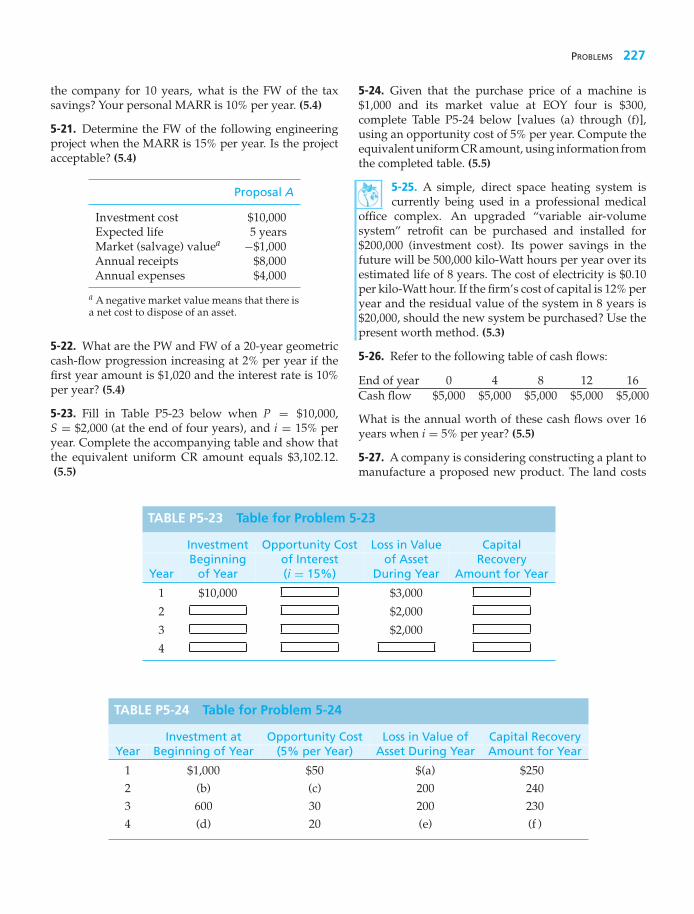
PROBLEMS 227

the company for 10 years, what is the FW of the taxsavings? Your personal MARR is 10% per year. (5.4)

5-21. Determine the FW of the following engineeringproject when the MARR is 15% per year. Is the projectacceptable? (5.4)

Proposal A

Investment cost $10,000Expected life 5 yearsMarket (salvage) valuea −$1,000Annual receipts $8,000Annual expenses $4,000

a A negative market value means that there isa net cost to dispose of an asset.

5-22. What are the PW and FW of a 20-year geometriccash-flow progression increasing at 2% per year if thefirst year amount is $1,020 and the interest rate is 10%per year? (5.4)

5-23. Fill in Table P5-23 below when P = $10,000,S = $2,000 (at the end of four years), and i = 15% peryear. Complete the accompanying table and show thatthe equivalent uniform CR amount equals $3,102.12.(5.5)

TABLE P5-23 Table for Problem 5-23

Investment Opportunity Cost Loss in Value CapitalBeginning of Interest of Asset Recovery

Year of Year (i = 15%) During Year Amount for Year

1 $10,000 $3,000

2 $2,000

3 $2,000

4

TABLE P5-24 Table for Problem 5-24

Investment at Opportunity Cost Loss in Value of Capital RecoveryYear Beginning of Year (5% per Year) Asset During Year Amount for Year

1 $1,000 $50 $(a) $2502 (b) (c) 200 2403 600 30 200 2304 (d) 20 (e) (f )

5-24. Given that the purchase price of a machine is$1,000 and its market value at EOY four is $300,complete Table P5-24 below [values (a) through (f)],using an opportunity cost of 5% per year. Compute theequivalent uniform CR amount, using information fromthe completed table. (5.5)

5-25. A simple, direct space heating system iscurrently being used in a professional medical

office complex. An upgraded “variable air-volumesystem” retrofit can be purchased and installed for$200,000 (investment cost). Its power savings in thefuture will be 500,000 kilo-Watt hours per year over itsestimated life of 8 years. The cost of electricity is $0.10per kilo-Watt hour. If the firm’s cost of capital is 12% peryear and the residual value of the system in 8 years is$20,000, should the new system be purchased? Use thepresent worth method. (5.3)

5-26. Refer to the following table of cash flows:

End of year 0 4 8 12 16Cash flow $5,000 $5,000 $5,000 $5,000 $5,000

What is the annual worth of these cash flows over 16years when i = 5% per year? (5.5)

5-27. A company is considering constructing a plant tomanufacture a proposed new product. The land costs

228 CHAPTER 5 / EVALUATING A SINGLE PROJECT

$300,000, the building costs $600,000, the equipmentcosts $250,000, and $100,000 additional working capitalis required. It is expected that the product will resultin sales of $750,000 per year for 10 years, at whichtime the land can be sold for $400,000, the buildingfor $350,000, and the equipment for $50,000. All of theworking capital would be recovered at the EOY 10. Theannual expenses for labor, materials, and all other itemsare estimated to total $475,000. If the company requiresa MARR of 15% per year on projects of comparable risk,determine if it should invest in the new product line.Use the AW method. (5.5)

5-28. A 50-kilowatt gas turbine has an invest-ment cost of $40,000. It costs another $14,000

for shipping, insurance, site preparation, fuel lines,and fuel storage tanks. The operation and maintenanceexpense for this turbine is $450 per year. Additionally,the hourly fuel expense for running the turbine is $7.50per hour, and the turbine is expected to operate 3,000hours each year. The cost of dismantling and disposingof the turbine at the end of its 8-year life is $8,000. (5.5)

a. If the MARR is 15% per year, what is the annualequivalent life-cycle cost of the gas turbine?

b. What percent of annual life-cycle cost is related tofuel?

5-29. Combined-cycle power plants use twocombustion turbines to produce electricity. Heat

from the first turbine’s exhaust is captured to heat waterand produce steam sent to a second steam turbinethat generates additional electricity. A 968-megawattcombined-cycle gas fired plant can be purchased for$450 million, has no salvage value, and produces a netcash flow (revenues less expenses) of $50 million peryear over its expected 30-year life. (5.5, 5.8)

a. If the hurdle rate (MARR) is 12% per year, howprofitable an investment is this power plant?

b. What is the simple payback period for the plant? Isthis investment acceptable?

5-30. Your sister just bought a new car having a stickerprice (manufacturer’s suggested retail price) of $36,000.She was crafty and was able to negotiate a sales priceof $33,500 from the auto dealership. In addition, shereceived $4,500 for her old trade-in car under the U.S.government’s “Cash for Clunkers” program. If hernew car will have a resale value of $3,500 after sevenyears when your sister will shop for a replacement car,what is the annual capital recovery cost of your sister’spurchase? The relevant interest rate is 8% per year, and

your sister can afford to spend a maximum of $5,000per year to finance the car (operating and other costsare extra). (5.5)

5-31. An environmentally friendly green home(99% air tight) costs about 8% more to construct

than a conventional home. Most green homes can save15% per year on energy expenses to heat and cool thedwelling. For a $250,000 conventional home, how muchwould have to be saved in energy expenses per yearwhen the life of the home is 30 years and the interestrate is 10% per year? Assume the additional cost of agreen home has no value at the end of 30 years. (5.5)

5-32. Your company is considering the introduction ofa new product line. The initial investment required forthis project is $500,000, and annual maintenance costsare anticipated to be $45,000. Annual operating costswill be directly proportional to the level of productionat $8.50 per unit, and each unit of product can be soldfor $65. If the MARR is 15% and the project has a life of5 years, what is the minimum annual production levelfor which the project is economically viable? (5.5)

5-33. Stan Moneymaker has been informed ofa major automobile manufacturer’s plan to

conserve on gasoline consumption through improvedengine design. The idea is called “engine displace-ment,” and it works by switching from 8-cylinder opera-tion to 4-cylinder operation at approximately 40 milesper hour. Engine displacement allows enough power toaccelerate from a standstill and to climb hills while alsopermitting the automobile to cruise at speeds over 40miles per hour with little loss in driving performance.

The trade literature studied by Stan makes theclaim that the engine displacement option will cost thecustomer an extra $1,200 on the automobile’s stickerprice. This option is expected to save 4 miles pergallon (an average of in-town and highway driving).A regular 8-cylinder engine in the car that Stan isinterested in buying gets an average of 20 miles pergallon of gasoline. If Stan drives approximately 1,200miles per month, how many months of ownership willbe required to make this $1,200 investment pay for itself?Stan’s opportunity cost of capital (i) is 0.5% per month,and gasoline costs $4.00 per gallon. (5.3)

5-34. The world’s largest carpet maker has justcompleted a feasibility study of what to do with

the 16,000 tons of overruns, rejects, and remnants itproduces every year. The company’s CEO launchedthe feasibility study by asking, why pay someone todig coal out of the ground and then pay someone else

PROBLEMS 229

to put our waste into a landfill? Why not just burnour own waste? The company is proposing to builda $10-million power plant to burn its waste as fuel,thereby saving $2.8 million a year in coal purchases.Company engineers have determined that the waste-burning plant will be environmentally sound, and afterits four-year study period the plant can be sold to a localelectric utility for $5 million. (5.6)

a. What is the IRR of this proposed power plant?

b. If the firm’s MARR is 15% per year, should thisproject be undertaken?

5-35. Each year in the United States nearly5 billion pounds of discarded carpet end up

in land fills. In response to this situation, the carpetmanufacturer in Problem 5-34 has decided to starta take-back program whereby obsolete carpet isreclaimed at the end of its useful life (about 7 years).The remanufactured carpet will then be recycled into thecompany’s supply chain. The out-of-pocket (variable)cost of recycling is $1.00 per square yard of carpet, andthe remanufactured carpet can be sold for $3.00 persquare yard. If the recycling equipment costs $1 millionand has no market value at the end of its eight-year life,how much carpet must be remanufactured annuallyto make this a profitable undertaking? The company’sMARR is 15% per year. (5.5)

5-36. A large automobile manufacturer is consideringthe installation of a high-tech material handling systemfor $30,000,000. This system will save $7,500,000 peryear in manual labor, and it will incur $2,750,000 inannual operating and maintenance expenditures. Thesalvage value at the end of the system’s 10-year lifeis negligible. If the company’s hurdle rate (MARR) is10% per year, should the system be recommended forimplementation? (5.6)

5-37. The EZ Credit Company offers to loan a collegestudent $6,000 for school expenses. Repayment of theloan will be in monthly installments of $304.07 for24 months. The total repayment of money is $7,297.68,which includes the original $6,000, $1,207.04 in interestcharges, and $90.64 for a required life insurance policycovering the amount of the loan. Assume monthlycompounding of interest. What nominal interest rateis being charged on this loan? (5.6)

5-38. A loan of $3,000 for a new, high-end laptopcomputer is to be repaid in 15 end-of-month payments(starting one month from now). The monthly paymentsare determined as follows.

Loan principal $3,000Interest for 15 months at1.5% per month 675

Loan application fee 150

Total $3,825

Monthly payment = $3,825/15 = $255

What nominal and effective interest rates per year areactually being paid? Hint: Draw a cash-flow diagramfrom the perspective of the lender. (5.6)

5-39. A large lithium-ion phosphate battery packfor an industrial application is expected to save

$20,000 in annual energy expenses over its 6-year life.For a 3-year simple payback period, the permissiblecapital investment is $60,000. What is the internal rateof return on this $60,000 battery pack if it has a residualvalue of $10,000 at the end of 6 years? The MARR is 18%per year. (5.6)

5-40. In July of 2012, Taylor purchased 2,000 sharesof XYZ common stock for $75,000. He then sold 1,000shares of XYZ in July of 2013 for $39 per share. Theremaining 1,000 shares were finally sold for $50 pershare in July 2014. (5.6, 5.7)

a. Draw a cash-flow diagram of this situation.

b. What was Taylor’s internal rate of return (IRR) onthis investment?

c. What was the ERR on this investment if the externalreinvestment rate is 8% per year?

5-41. Nowadays it is very important to reduceone’s carbon “footprint” (how much carbon we

produce in our daily lifestyles). Minimizing the useof fossil fuels and instead resorting to renewablesources of energy (e.g., solar energy) are vital to a“sustainable” lifestyle and a lower carbon footprint.Let’s consider solar panels that prewarm the waterfed to a conventional home water heater. The solarpanels have an installed cost of $3,000, and they reducethe homeowner’s energy bill by $30 per month. Theresidual value of the solar panels is negligible at theend of their 10-year life. What is the annual effectiveIRR of this investment? (5.6)

5-42. Sergeant Jess Frugal has the problem of runningout of money near the end of each month (he gets paidonce a month). Near his army base there is a paydaylender company, called Predatory Lenders, Inc., thatwill give Jess a cash advance of $350 if he will repay

230 CHAPTER 5 / EVALUATING A SINGLE PROJECT

the loan a month later with a post-dated check for$375. Almost as soon as Frugal’s check for $375 clearsthe bank, he unfortunately must again borrow $350 tomake ends meet. Jess’s wife has gotten a bit concernedthat her husband might be paying an exorbitant interestrate to this payday lender. Assuming Jess has repeatedthis borrowing and repayment scheme for 12 months ina row, what effective annual interest rate is he reallypaying? Is Jess’s wife correct in her worry? Hint:Draw a cash-flow diagram from the viewpoint of thelender. (5.6)

5-43. At a military base in Texas, Corporal StanMoneymaker has been offered a wonderful savingsplan. These are the salesperson’s words: “During your48-month tour of duty, you will invest $200 per monthfor the first 45 months. We will make the 46th, 47th, and48th payments of $200 each for you. When you leavethe service, we will pay you $10,000 cash.”

Is this a good deal for Corporal Moneymaker? Usethe IRR method in developing your answer. Whatassumptions are being made by Corporal Moneymakerif he enters into this contract? (5.6)

5-44. To purchase a used automobile, you borrow$10,000 from Loan Shark Enterprises. They tell you theinterest rate is 1% per month for 35 months. They alsocharge you $200 for a credit investigation, so you leavewith $9,800 in your pocket. The monthly payment theycalculated for you is

$10,000 (0.1) (35) + $10,00035

= $385.71/month.

If you agree to these terms and sign their contract, whatis the actual APR (annual percentage rate) that you arepaying? (5.6)

5-45. Your boss has just presented you with thesummary in the accompanying table of projected costsand annual receipts for a new product line. He asksyou to calculate the IRR for this investment opportunity.What would you present to your boss, and how wouldyou explain the results of your analysis? (It is widelyknown that the boss likes to see graphs of PW versusinterest rate for this type of problem.) The company’sMARR is 10% per year. (5.6)

End of Net CashYear Flow

0 −$450,0001 −42,5002 +92,8003 +386,0004 +614,6005 −$202,200

5-46. Experts agree that the IRR of a college education isabout 12%/yr. This results from the increased earningsover your lifetime. Draw a CFD that supports the 12%annual return over the 40 years of your career. State yourassumptions. (5.6)

5-47. A company has the opportunity to take over aredevelopment project in an industrial area of a city.No immediate investment is required, but it must razethe existing buildings over a four-year period and, atthe end of the fourth year, invest $2,400,000 for newconstruction. It will collect all revenues and pay all costsfor a period of 10 years, at which time the entire project,and properties thereon, will revert to the city. The netcash flows are estimated to be as follows:

Year End Net Cash Flow

1 $500,0002 300,0003 100,0004 −2,400,0005 150,0006 200,0007 250,0008 300,0009 350,000

10 400,000

Tabulate the PW versus the interest rate and determinewhether multiple IRRs exist. If so, use the ERR methodwhen ∈ = 8% per year to determine a rate of return. (5.7)

5-48. The prospective exploration for oil in the outercontinental shelf by a small, independent drillingcompany has produced a rather curious pattern of cashflows, as follows:

PROBLEMS 231

End of Year Net Cash Flow

0 −$520,0001–10 +200,000

10 −1,500,000

The $1,500,000 expense at EOY 10 will be incurredby the company in dismantling the drilling rig.

a. Over the 10-year period, plot PW versus the interestrate (i) in an attempt to discover whether multiplerates of return exist. (5.6)

b. Based on the projected net cash flows and results inPart (a), what would you recommend regarding thepursuit of this project? Customarily, the companyexpects to earn at least 20% per year on investedcapital before taxes. Use the ERR method (∈ = 20%).(5.7)

5-49. In this problem, we consider replacingan existing electrical water heater with an array

of solar panels. The net installed investment cost of thepanels is $1,400 ($2,000 less a 30% tax credit from thegovernment). Based on an energy audit, the existingwater heater uses 200 kilowatt hours (kWh) of electricityper month, so at $0.12 per kWh, the cost of operatingthe water heater is $24 per month. Assuming the solarpanels can save the entire cost of heating water withelectricity, answer the following questions. (5.6, 5.8)

a. What is the simple payback period for the solarpanels?

b. What is the IRR of this investment if the solar panelshave a life of 10 years?

5-50. An integrated, combined cycle power plantproduces 285 MW of electricity by gasifying coal.

The capital investment for the plant is $570 million,spread evenly over two years. The operating life of theplant is expected to be 20 years. Additionally, the plantwill operate at full capacity 75% of the time (downtimeis 25% of any given year). (5.8)

a. If this plant will make a profit of three cents perkilowatt-hour of electricity sold to the power grid,what is the simple payback period of the plant? Is ita low-risk venture?

b. What is the IRR for the plant? Is it profitable?

5-51. A computer call center is going to replaceall of its incandescent lamps with more energy-

efficient fluorescent lighting fixtures. The total energy

savings are estimated to be $1,875 per year, and thecost of purchasing and installing the fluorescent fixturesis $4,900. The study period is five years, and terminalmarket values for the fixtures are negligible. (5.8)

a. What is the IRR of this investment?

b. What is the simple payback period of theinvestment?

c. Is there a conflict in the answers to Parts (a) and (b)?List your assumptions.

d. The simple payback “rate of return” is 1/θ . Howclose does this metric come to matching your answerin Part (a)?

5-52. A plasma arc furnace has an internal combustiontemperature of 7,000◦C and is being considered forthe incineration of medical wastes at a local hospital.The initial investment is $300,000 and annual revenuesare expected to be $175,000 over the six-year life ofthe furnace. Annual expenses will be $100,000 at theend of year one and will increase by $5,000 each yearthereafter. The resale value of the furnace after six yearsis $20,000. (5.6, 5.8)

a. What is the simple payback period of the furnace?

b. What is the internal rate of return on the furnace?

5-53. Advanced Modular Technology (AMT) typicallyexhibits net annual revenues that increase over a fairlylong period. In the long run, an AMT project may beprofitable as measured by IRR, but its simple paybackperiod may be unacceptable. Evaluate this AMT projectusing the IRR method when the company MARR is15% per year and its maximum allowable paybackperiod is three years. What is your recommenda-tion? (5.6, 5.8)

Capital investment at time 0 $100,000Net revenues in year k $20,000+

$10,000 · (k − 1)Market (salvage) value $10,000Life 5 years

5-54. The American Pharmaceutical Company (APC)has a policy that all capital investments must have afour-year or less discounted payback period in order tobe considered for funding. The MARR at APC is 8% per

232 CHAPTER 5 / EVALUATING A SINGLE PROJECT

End of Year Cash Flow

0 −$275,0001 −$35,0002 $55,0003 $175,0004 $250,0005 $350,000

6–10 $100,000

year. Is the above project able to meet this benchmarkfor funding? (5.8)

5-55. The International Parcel Service has installeda new radio frequency identification system to helpreduce the number of packages that are incorrectlydelivered. The capital investment in the system is$65,000, and the projected annual savings are tabledbelow. The system’s market value at the EOY five isnegligible, and the MARR is 18% per year.

End of Year Savings

1 $25,0002 30,0003 30,0004 40,0005 46,000

a. What is the FW of this investment?

b. What is the IRR of the system?

c. What is the discounted payback period for thisinvestment?

5-56. The Fischer-Tropsch (F-T) process wasdeveloped in Germany in 1923 to convert syn-

thesis gas (i.e., a mixture of hydrogen and carbonmonoxide) into liquid with some gaseous hydrocar-bons. Interestingly, the F-T process was used in WorldWar II to make gasoline and other fuels. (5.8)

a. If the U.S. military can save one billion gallons peryear of foreign oil by blending its jet fuel with F-Tproducts, how much can the government afford toinvest (through tax breaks and subsidies) in the F-Tindustry in the United States? The government’sMARR is 7% per year, the study period is 40 years,and one gallon of jet fuel costs $2.50.

b. If Congress appropriates $25 billion to support theF-T process industry, what is the simple paybackperiod?

5-57. Asolar sea power plant (SSPP) is being con-sidered in a North American location known for

its high temperature ocean surface and its much lowerocean temperature 100 meters below the surface. Powercan be produced based on this temperature differential.With high costs of fossil fuels, this particular SSPP maybe economically attractive to investors. For an initialinvestment of $100 million, annual net revenues areestimated to be $15 million in years 1–5 and $20 millionin years 6–20. Assume no residual market value for theSSPP. (5.8)

a. What is the simple payback period for the SSPP?

b. What is the discounted payback period when theMARR is 6% per year?

c. Would you recommend investing in this project?

5-58. Aremotely situated fuel cell has an installedcost of $2,000 and will reduce existing survei-

llance expenses by $350 per year for eight years. Theborder security agency’s MARR is 10% per year. (5.6)

a. What is the minimum salvage (market) valueafter eight years that makes the fuel cell worthpurchasing?

b. What is the fuel cell’s IRR if the salvage value isnegligible?

5-59. A new automotive “dry paint” separationprocess is environmentally friendly and is

expected to save $8.00 per car painted at a Detroit plant.The installed cost of the process is $8 million, and250,000 cars are painted each year. What is the simplepayback for the new technology? (5.8)

5-60.

a. Calculate the IRR for each of the three cash-flowdiagrams that follow. Use EOY zero for (i) and EOYfour for (ii) and (iii) as the reference points in time.What can you conclude about “reference year shift”and “proportionality” issues of the IRR method?

b. Calculate the PW at MARR = 10% per year at EOYzero for (i) and (ii) and EOY four for (ii) and (iii).How do the IRR and PW methods compare?

SPREADSHEET EXERCISES 233

0

$1,000

1 5432

$300 $300$300$300$300

End of Year

40

$1,000

5 9876

$300 $300$300$300$300

End of Year

0 4iii.

ii.

i.

$5,000

5 9876

$1,500 $1,500 $1,500 $1,500 $1,500

End of Year

5-61. A group of private investors borrowed$30 million to build 300 new luxury apartments neara large university. The money was borrowed at 6%annual interest, and the loan is to be repaid in equalannual amounts (principal and interest) over a 40-yearperiod. Annual operating, maintenance, and insuranceexpenses are estimated to be $4,000 per apartment,and these expenses are incurred independently of theoccupancy rate for the apartments. The rental feefor each apartment will be $12,000 per year, and theworst-case occupancy rate is projected to be 80%. (5.5)

a. How much profit (or loss) will the investors makeeach year with 80% occupancy?

b. Repeat Part (a) when the occupancy rate is 95%.

5-62. Javier borrows $50,000 from a local bank atan APR of 9%, compounded monthly. His monthlypayments amount to $50,000 (A/P, 0.75%, 60) = $1,040for a 60-month loan. If Javier makes an extra paymenton the first month of each year, his repayment durationfor the loan will be reduced by how many months? (5.5)

5-63. Extended Learning Exercise A company isproducing a high-volume item that sells for $0.75 per

unit. The variable production cost is $0.30 per unit. Thecompany is able to produce and sell 10,000,000 itemsper year when operating at full capacity.

The critical attribute for this product is weight.The target value for weight is 1,000 grams, and thespecification limits are set at ±50 grams. The fillingmachine used to dispense the product is capableof weights following a normal distribution with anaverage (μ) of 1,000 grams and a standard deviation(σ ) of 40 grams. Because of the large standard deviation(with respect to the specification limits), 21.12% of allunits produced are not within the specification limits.(They either weigh less than 950 grams or more than1,050 grams.) This means that 2,112,000 out of 10,000,000units produced are nonconforming and cannot be soldwithout being reworked.

Assume that nonconforming units can be reworkedto specification at an additional fixed cost of $0.10 perunit. Reworked units can be sold for $0.75 per unit. Ithas been estimated that the demand for this productwill remain at 10,000,000 units per year for the next fiveyears.

To improve the quality of this product, the companyis considering the purchase of a new filling machine.The new machine will be capable of dispensing theproduct with weights following a normal distributionwith μ = 1,000 grams and σ = 20 grams. As a result, thepercent of nonconforming units will be reduced to 1.24%of production. The new machine will cost $710,000 andwill last for at least five years. At the end of five years,this machine can be sold for $100,000.

a. If the company’s MARR is 15% per year, is thepurchase of the new machine to improve quality(reduce variability) economically attractive? Use theAW method to make your recommendation.

b. Compute the IRR, simple payback period, anddiscounted payback period of the proposedinvestment.

c. What other factors, in addition to reduced totalrework costs, may influence the company’s decisionabout quality improvement?

Spreadsheet Exercises

5-64. Jane Roe’s plan is to accumulate $250,000 in herpersonal savings account by the time she retires at 60.The longer she stalls on getting started, the tougher it

will be to meet her objective. Jane is now 25 years old.Create a spreadsheet to complete the following tableto show how much Jane will have to save each year

234 CHAPTER 5 / EVALUATING A SINGLE PROJECT

(assuming she waits N years to start saving) to have$250,000 in her account when she is 60. Comment onthe pattern you observe in the table. (5.4)

Interest Rate per Year4% 8% 12%

N � 5N � 10N � 15N � 20

5-65. An investor has a principal amount of $P. If hedesires a payout (return) of 0.1P each year, how manyyears will it take to deplete an account that earns 8% peryear?

0.1P = P(A/P, 8%, N), so N ∼= 21 years.

A payout duration table can be constructed forselect payout percentages and compound interest rates.Complete the following table. (Note: table entries areyears.) Summarize your conclusions about the patternobserved in the table. (5.5)

Interest Rate per Year4% 6% 8% 10%

Payout per Year 10% 20.9(% of principal) 20%

30%

5-66. Refer to Example 5-13. Create a single spreadsheetthat calculates PW, FW, AW, IRR, and ERR for theproposed investment. Assume that ∈ = MARR = 20%per year. Does your recommendation change if theMARR decreases to 18%? Increases to 22%? (5.6, 5.7)

5-67. A certain medical device will result in anestimated $15,000 reduction in hospital labor expensesduring its first year of operation. Labor expenses (andthus savings) are projected to increase at a rate of 7% peryear after the first year. Additional operating expensesfor the device (maintenance, electric power, etc.) are$3,500 annually, and they increase by $250 per yearthereafter (i.e., $3,750 in year two and so on). It isanticipated that the device will last for 10 years andwill have no market value at that time. If the MARRis 10% per year, how much can the hospital afford topay for this device? Use an Excel spreadsheet in yoursolution. (5.3)

5-68. Refer to Problem 5-61. Develop a spreadsheetto investigate the sensitivity of annual profit (loss)to changes in the occupancy rate and the annualrental fee. (5.5)

Case Study Exercises

5-69. Suppose that the industrial engineers are able toincrease the average utilization rate of the CVD toolfrom 80% to 90%. What is the projected impact of this10% increase on the PW of the project? (5.9)

5-70. Suppose that the mechanical engineer in theplant has retrofitted the CVD tool so that it nowproduces 15 wafers per hour. What is the new breakevenpoint? (5.9)

5-71. Suppose that the average utilization of theCVD tool increased to 90%; however, the operatinghours of the fabrication plant were decreased from168 hours to 150 hours. What are the corres-ponding impacts on the PW and breakeven point,respectively? (5.9)

FE Practice Problems

5-72. Doris Wade purchased a condominium for$50,000 in 1987. Her down payment was $20,000. Shefinanced the remaining amount as a $30,000, 30-yearmortgage at 7%, compounded monthly. Her monthlypayments are $200. It is now 2007 (20 years later)and Doris has sold the condominium for $100,000,immediately after making her 240th payment on the

unit. Her effective annual internal rate of return on thisinvestment is closest to which answer below? (5.6)

(a) 3.6% (b) 8.5% (c) 5.3% (d) 1.5%

5-73. Elin purchased a used car for $10,000. She wrotea check for $2,000 as a down payment for the car andfinanced the $8,000 balance. The annual percentage rate

FE PRACTICE PROBLEMS 235

(APR) is 9% compounded monthly, and the loan is tobe repaid in equal monthly installments over the nextfour years. Which of the following is most near to Elin’smonthly car payment? (5.5)

(a) $167 (b) $172 (c) $188(d) $200 (e) $218

5-74. A specialized automatic machine costs $300,000and is expected to save $111,837.50 per year whilein operation. Using a 12% interest rate, what is thediscounted payback period? (5.8)

(a) 4 (b) 5 (c) 6(d) 7 (e) 8

5-75. Street lighting fixtures and their sodiumvapor bulbs for a two-block area of a large city

need to be installed at a first cost (investment cost) of$120,000. Annual maintenance expenses are expected tobe $6,500 for the first 20 years and $8,500 for each yearthereafter. The lighting will be needed for an indefinitelylong period of time. With an interest rate of 10% peryear, what is the capitalized cost of this project (choosethe closest answer below)? (5.3)

(a) $178,313 (b) $188,000 (c) $202,045(d) $268,000

5-76. What is the IRR in the following cash flow? (5.6)

Year End 0 1 2 3 4Cash Flow ($) −3,345 1,100 1,100 1,100 1,100

(a) 12.95% (b) 11.95% (c) 9.05%(d) 10.05% (e) 11.05%

5-77. A bond has a face value of $1,000, is redeemablein eight years, and pays interest of $100 at the end ofeach of the eight years. If the bond can be purchased for$981, what is the rate of return if the bond is held untilmaturity? (5.3)

(a) 10.65% (b) 12.65% (c) 10.35%(d) 11.65%

5-78. If you invest $5,123 in a long-term venture, youwill receive $1,110 per year forever. Assuming yourinterest rate is 10% per year, what is the capitalizedworth of your investment? Choose the most closestanswer below. (5.3)

(a) $4,327 (b) $5,977 (c) $5,819(d) $6,103

5-79. What is the equivalent AW of a two-year contractthat pays $5,000 at the beginning of the first month andincreases by $500 for each month thereafter? MARR =12% compounded monthly. (5.5)

(a) $10,616 (b) $131,982 (c) $5,511(d) $5,235 (e) $134,649

5-80. A new machine was bought for $9,000 with a lifeof six years and no salvage value. Its annual operatingcosts were as follows:

$7,000, $7,350, $7,717.50, . . . , $8,933.97.

If the MARR = 12%, what was the annual equivalentcost of the machine? (5.5)

(a) $7,809 (b) $41,106 (c) $9,998(d) $2,190 (e) $9,895

5-81. A town in Wyoming wants to drill a geo-thermal well to provide district heating steam

and hot water for its businesses and residences. Aftergovernment subsidies, the capital investment for thewell is $500,000, and the geothermal well will reducenatural gas consumption for steam and hot waterproduction by $50,000 per year. The salvage value ofthe well is negligible. The simple payback period forthis well is 10 years. If the MARR of the town is 8% peryear and the life of the geothermal well is 25 years, whatis the IRR for this project? Choose the closest answerbelow. (5.6)

(a) 6.2% (b) 9.1% (c) 8.8%(d) 10.3%

5-82. An automobile dealership offers a car with $0down payment, $0 first month’s payment, and $0 dueat signing. The monthly payment, starting at the end ofmonth two, is $386 and there are a total of 38 payments.If the APR is 12% compounded monthly, the negotiatedsales price is closest to which answer below? (5.3)

(a) $14,668 (b) $12,035 (c) $12,415(d) $13,175

5-83. A 2,000 square foot house in New Jerseycosts $1,725 each winter to heat with its existing

oil-burning furnace. For an investment of $5,000, anatural gas furnace can be installed, and the winterheating bill is estimated to be $1,000. If the homeowner’sMARR is 6% per year, what is the discounted paybackperiod of this proposed investment? (5.8)

(a) 7 years (b) 8 years (c) 9 years(d) 10 years

236 CHAPTER 5 / EVALUATING A SINGLE PROJECT

5-84. Refer to Problem 5-2. Assuming the residualvalue of the building alone (no land) is negligible, theinternal rate of return for this situation is closest to:

(a) 0% (b) 4% (c) 10%(d) 20%

Appendix 5-A The Multiple Rate of Return Problemwith the IRR Method

Whenever the IRR method is used and the cash flows reverse sign (from net cash outflowto net cash inflow or the opposite) more than once over the study period, we should beaware of the rather remote possibility that either no interest rate or multiple interest ratesmay exist. According to Descartes’ rule of signs, the maximum number of possible IRRs inthe (−1, ∞) interval for any given project is equal to the number of cash flow sign reversalsduring the study period. Nordstrom’s criterion says if there is only one sign change in thecumulative cash flows over time, a unique interest rate exists. Two or more sign changesin the cumulative cash flow indicates the possibility of multiple interest rates. Descartes’rule of signs and Nordstrom’s criterion guarantee a unique internal rate of return if thereis only one sign change in the cash-flow sequence and in the cumulative cash flows overtime, respectively. The simplest way to check for multiple IRRs is to plot equivalent worth (e.g.,PW) against the interest rate. If the resulting plot crosses the interest rate axis more than once,multiple IRRs are present and another equivalence method is recommended for determiningproject acceptability.

As an example, consider the following project for which the IRR is desired.

EXAMPLE 5-A-1

Plot the PW versus interest rate for the following cash flows. Are there multiple IRRs?If so, what do they mean? Notice there are two sign changes in net cash flows (positive,negative, positive), so at most two IRRs exist for this situation. Nordstrom’s criterionalso suggests a maximum of two interest rates because there are two sign changes incumulative cash flow.

Year, k Net Cash Flow i% PW(i%) Year, k Cumulative Cash Flow

0 $500 0 $250 0 $5001 −1,000 10 105 1 −5002 0 20 32 2 −5003 250 30 ∼ 0 3 −2504 250 40 −11 4 05 250 62 ∼ 0 5 250

80 24

Thus, the PW of the net cash flows equals zero at interest rates of about 30% and 62%, somultiple IRRs do exist. Whenever there are multiple IRRs, which is seldom, it is likelythat none are correct.

APPENDIX 5-A / THE MULTIPLE RATE OF RETURN PROBLEM WITH THE IRR METHOD 237

In this situation, the ERR method (see Section 5.7) could be used to decide whetherthe project is worthwhile. Or, we usually have the option of using an equivalent worthmethod. In Example 5-A-1, if the external reinvestment rate (∈) is 10% per year, we seethat the ERR is 12.4%.

$1,000(P/F, 10%, 1)(F/P, i′%, 5) = $500(F/P, 10%, 5) + $250(F/A, 10%, 3)

(P/F, 10%, 1)(F/P, i′, 5) = 1.632

i′ = 0.124 (12.4%).

In addition, PW(10%) = $105, so both the ERR and PW methods indicate that this projectis acceptable when the MARR is 10% per year.

�11 �1020%10% 30%

32

40% 50%24

62% 80%

250

0

PW

(i)

in $

PW � 0 PW � 0

i%

Interest Rate

Plot for Example 5-A-1

EXAMPLE 5-A-2

Use the ERR method to analyze the cash-flow pattern shown in the accompanying table.The IRR is indeterminant (none exists), so the IRR is not a workable procedure. Theexternal reinvestment rate (∈) is 12% per year, and the MARR equals 15%.

Year Cash Flows

0 $5,0001 −7,0002 2,0003 2,000

238 CHAPTER 5 / EVALUATING A SINGLE PROJECT

SolutionThe ERR method provides this result:

$7,000(P/F, 12%, 1)(F/P, i′%, 3) = $5,000(F/P, 12%, 3)

+$2,000(F/P, 12%, 1) + $2,000

(F/P, i′, 3) = 1.802

i′ = 21.7%.

Thus, the ERR is greater than the MARR. Hence, the project having this cash-flow patternwould be acceptable. The PW at 15% is equal to $1,740.36, which confirms the acceptabilityof the project.

4,000

3,000

2,000

1,000

00 50% 100%

i1,000%

PW

(i)

in $

Appendix 5-A Problems

5-A-1. Use the ERR method with ∈ = 8% per year tosolve for a unique rate of return for the following cash-flow diagram. How many IRRs (the maximum) aresuggested by Descartes’ rule of signs?

0

1

2

$235

$360

$50

3

$180

MARR � 8%/yr

End of Year

5-A-2. Apply the ERR method with ∈ = 12% per yearto the following series of cash flows. Is there a single,unique IRR for these cash flows? What is the maximumnumber of IRRs suggested by Nordstrom’s criterion?

0

1

2

$6,000

$1,000

$5,000

3

$4,000

MARR � 12%/yr

End of Year

APPENDIX 5-A PROBLEMS 239

5-A-3. Are there multiple IRRs for the following cash-flow sequence? How many are possible according toDescartes’ rule of signs? If ∈ = 10% per year, what is the ERR for the cash flows of this project? Let MARR =10% per year.

EOY 0 1 2 3 4 5 6 7 8 9 10Cash Flow ($) 120 90 60 30 −1,810 600 500 400 300 200 100

5-A-4. Are there multiple IRRs for the following cash flows? If so, how many are there? If not, what is the uniqueIRR? (Appendix 5-A)

EOY 0 1 2 3Cash flow −$1,000 $1,500 −$600 $500

CHAPTER 6

Comparison and Selectionamong Alternatives

Our aim in Chapter 6 is to compare capital investment alternatives when thetime value of money is a key influence.

Alternatives for Waste Storage

A large electric utility company is considering two methodsfor containing and storing its coal combustion by-products(fly ash). One method is wet slurry storage, and the second

method is dry storage of the fly ash. The company will adopt one of these methodsfor all 28 fly ash impoundments at its seven coal-fired power plants. Wet storagehas an initial capital investment of $2 billion, followed by annual maintenanceexpenses of $300 million over the 10-year life of the method. Dry storage has a $2.5billion capital investment and $150 million per year annual upkeep expendituresover its 7-year life. If the utility’s MARR is 10% per year, which method of flyash storage should be selected assuming an indefinitely long study period? InChapter 6, investment problems of this type will be considered. We will return tothis problem in Example 6-9.

240

A penny saved is a penny earned.

—Benjamin Franklin (1789)

6.1 IntroductionMost engineering projects can be accomplished by more than one feasible designalternative. When the selection of one of these alternatives excludes the choiceof any of the others, the alternatives are called mutually exclusive. Typically, thealternatives being considered require the investment of different amounts of capital,and their annual revenues and costs may vary. Sometimes the alternatives may havedifferent useful lives. The fundamental question is “do the added benefits from amore-expensive alternative bring a positive return relative to the added costs?”

A seven-step procedure for accomplishing engineering economy studies wasdiscussed in Chapter 1. In this chapter, we address Step 5 (analysis and comparisonof the feasible alternatives) and Step 6 (selection of the preferred alternative) ofthis procedure, and we compare mutually exclusive alternatives on the basis ofeconomic considerations alone.

Five of the basic methods discussed in Chapter 5 for analyzing cash flows areused in the analyses in this chapter [present worth (PW), annual worth (AW), futureworth (FW), internal rate of return (IRR), and external rate of return (ERR)]. Thesemethods provide a basis for economic comparison of alternatives for an engineeringproject. When correctly applied, these methods result in the correct selection of apreferred alternative from a set of mutually exclusive alternatives. The comparisonof mutually exclusive alternatives by means of the benefit–cost ratio method isdiscussed in Chapter 10.

6.2 Basic Concepts for Comparing AlternativesPrinciple 1 (Chapter 1) emphasized that a choice (decision) is among alternatives.Such choices must incorporate the fundamental purpose of capital investment;namely, to obtain at least the minimum attractive rate of return (MARR) foreach dollar invested. In practice, there are usually a limited number of feasiblealternatives to consider for an engineering project. The problem of deciding whichmutually exclusive alternative should be selected is made easier if we adopt thisrule based on Principle 2 (focus on the differences) in Chapter 1: The alternative thatrequires the minimum investment of capital and produces satisfactory functional resultswill be chosen unless the incremental capital associated with an alternative having a largerinvestment can be justified with respect to its incremental benefits.

Under this rule, we consider the acceptable alternative that requires the leastinvestment of capital to be the base alternative. The investment of additional capitalover that required by the base alternative usually results in increased capacity,increased quality, increased revenues, decreased operating expenses, or increasedlife. Therefore, before additional money is invested, it must be shown that each

241

242 CHAPTER 6 / COMPARISON AND SELECTION AMONG ALTERNATIVES

avoidable increment of capital can pay its own way relative to other availableinvestment opportunities.

In summary, if the extra benefits obtained by investing additional capital arebetter than those that could be obtained from investment of the same capitalelsewhere in the company at the MARR, the investment should be made.

If this is not the case, we obviously would not invest more than the minimumamount of capital required, and we may even do nothing at all. Stated simply, ourrule will keep as much capital as possible invested at a rate of return equal to orgreater than the MARR.

6.2.1 Investment and Cost Alternatives

This basic policy for the comparison of mutually exclusive alternatives can bedemonstrated with two examples. The first example involves an investment projectsituation. Alternatives A and B are two mutually exclusive investment alternativeswith estimated net cash flows,∗ as shown. Investment alternatives are those withinitial (or front-end) capital investment(s) that produce positive cash flows from increasedrevenue, savings through reduced costs, or both. The useful life of each alternative inthis example is four years.

Alternative

A B �(B − A)

Capital investment −$60,000 −$73,000 −$13,000

Annual revenues less expenses 22,000 26,225 4,225

The cash-flow diagrams for Alternatives A and B, and for the year-by-yeardifferences between them (i.e., B minus A), are shown in Figure 6-1. These diagramstypify those for investment project alternatives. In this first example, at MARR =10% per year, the PW values are

PW(10%)A = −$60,000 + $22,000(P/A, 10%, 4) = $9,738,

PW(10%)B = −$73,000 + $26,225(P/A, 10%, 4) = $10,131.

Since the PWA is greater than zero at i = MARR, Alternative A is the basealternative and would be selected unless the additional (incremental) capitalassociated with Alternative B ($13,000) is justified. In this case, Alternative B ispreferred to A because it has a greater PW value. Hence, the extra benefits obtained

∗ In this book, the terms net cash flow and cash flow will be used interchangeably when referring to periodic cash inflowsand cash outflows for an alternative.

SECTION 6.2 / BASIC CONCEPTS FOR COMPARING ALTERNATIVES 243

Figure 6-1 Cash-FlowDiagrams forAlternatives Aand B and TheirDifference

$60,000

A � $22,000

1. Alternative A 2. Alternative B

1

0

$73,000

2 3 4 � N 1

0

2 3 4 � N

1

0

2 3 4 � N

A � $26,225

$13,000

A � $4,225

3. Alternative B minus Alternative A (year-by-year)

Difference

End of Year End of Year

End of Year

by investing the additional $13,000 of capital in B (diagram 3, Figure 6-1) have a PWof $10,131 − $9,738 = $393. That is,

PW(10%)Diff = −$13,000 + $4,225(P/A, 10%, 4) = $393,

and the additional capital invested in B is justified.The second example involves a cost project situation. Alternatives C and D are

two mutually exclusive cost alternatives with estimated net cash flows, as shown,over a three-year life. Cost alternatives are those with all negative cash flows, exceptfor a possible positive cash-flow element from disposal of assets at the end of the project’suseful life. This situation occurs when the organization must take some action, andthe decision involves the most economical way of doing it (e.g., the addition ofenvironmental control capability to meet new regulatory requirements). It alsooccurs when the expected revenues are the same for each alternative.

Alternative

End of Year C D �(D − C)

0 −$380,000 −$415,000 −$35,0001 −38,100 −27,400 10,7002 −39,100 −27,400 11,7003 −40,100 −27,400 12,7003a 0 26,000 26,000

a Market value.

The cash-flow diagrams for Alternatives C and D, and for the year-by-yeardifferences between them (i.e., D minus C), are shown in Figure 6-2. Thesediagrams typify those for cost project alternatives. In this “must take action”

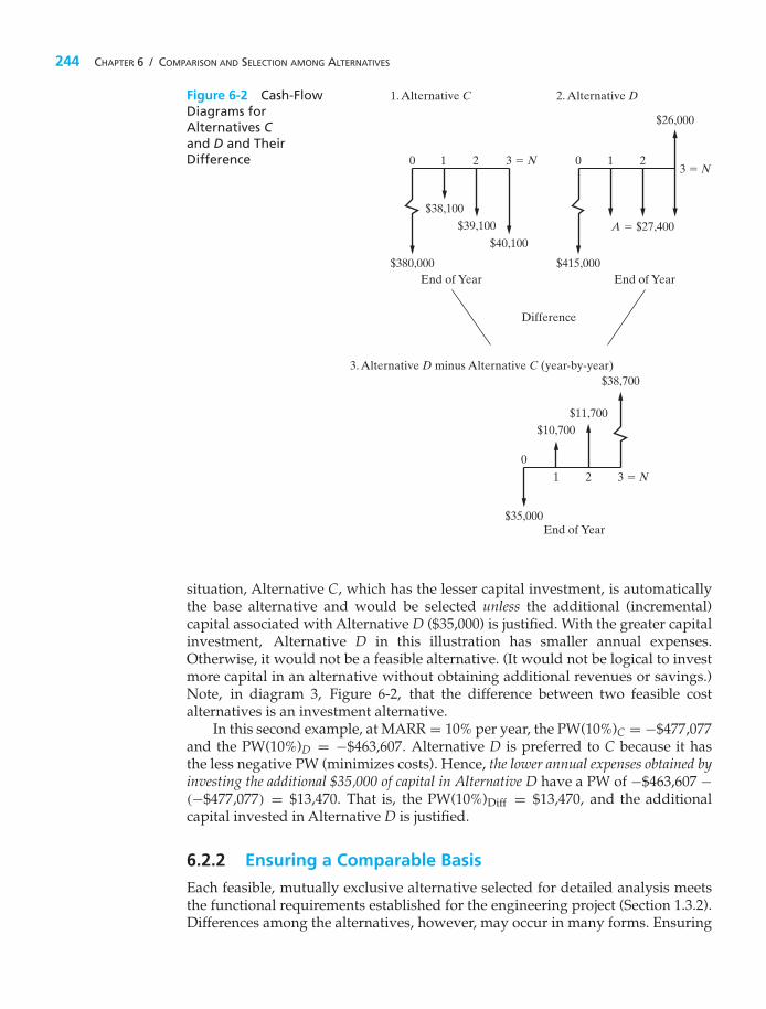
244 CHAPTER 6 / COMPARISON AND SELECTION AMONG ALTERNATIVES

Figure 6-2 Cash-FlowDiagrams forAlternatives Cand D and TheirDifference 10 02 3 � N

3 � N

1

0

2

1. Alternative C 2. Alternative D

$380,000

$38,100

$39,100

$40,100

Difference

$35,000

$10,700$11,700

$38,7003. Alternative D minus Alternative C (year-by-year)

1 2

$415,000

$26,000

A � $27,400

3 � N

End of Year

End of Year End of Year

situation, Alternative C, which has the lesser capital investment, is automaticallythe base alternative and would be selected unless the additional (incremental)capital associated with Alternative D ($35,000) is justified. With the greater capitalinvestment, Alternative D in this illustration has smaller annual expenses.Otherwise, it would not be a feasible alternative. (It would not be logical to investmore capital in an alternative without obtaining additional revenues or savings.)Note, in diagram 3, Figure 6-2, that the difference between two feasible costalternatives is an investment alternative.

In this second example, at MARR = 10% per year, the PW(10%)C = −$477,077and the PW(10%)D = −$463,607. Alternative D is preferred to C because it hasthe less negative PW (minimizes costs). Hence, the lower annual expenses obtained byinvesting the additional $35,000 of capital in Alternative D have a PW of −$463,607 −(−$477,077) = $13,470. That is, the PW(10%)Diff = $13,470, and the additionalcapital invested in Alternative D is justified.

6.2.2 Ensuring a Comparable Basis

Each feasible, mutually exclusive alternative selected for detailed analysis meetsthe functional requirements established for the engineering project (Section 1.3.2).Differences among the alternatives, however, may occur in many forms. Ensuring

SECTION 6.3 / THE STUDY (ANALYSIS) PERIOD 245

a comparable basis for their analysis requires that any economic impacts of thesedifferences be included in the estimated cash flows for the alternatives (as wellas comparing them over the same analysis period—see Section 6.3). Otherwise,the wrong design alternative may be selected for implementing the project. Thefollowing are examples of the types of differences that may occur:

1. Operational performance factors such as output capacity, speed, thrust, heatdissipation rate, reliability, fuel efficiency, setup time, and so on

2. Quality factors such as the number of defect-free (nondefective) units producedper period or the percentage of defective units (reject rate)

3. Useful life, capital investment required, revenue changes, various annualexpenses or cost savings, and so on

This list of examples could be expanded. The specific differences, however, foreach engineering project and its design alternatives must be identified. Then, thecash-flow estimates for the alternatives must include the economic impact of thesedifferences. This is a fundamental premise for comparing alternatives in Chapter 6 and inthe chapters that follow.

Two rules were given in Section 2.4 for facilitating the correct analysis andcomparison of mutually exclusive alternatives when the time value of money isnot a factor (present economy studies). For convenience, these rules are repeatedhere and extended to account for the time value of money:

Rule 1: When revenues and other economic benefits are present and vary amongthe alternatives, choose the alternative that maximizes overall profitability.That is, select the alternative that has the greatest positive equivalent worthat i = MARR and satisfies all project requirements.

Rule 2: When revenues and other economic benefits are not present or are constantamong the alternatives, consider only the costs and select the alternativethat minimizes total cost. That is, select the alternative that has theleast negative equivalent worth at i = MARR and satisfies all projectrequirements.

6.3 The Study (Analysis) PeriodThe study (analysis) period, sometimes called the planning horizon, is the selectedtime period over which mutually exclusive alternatives are compared. Thedetermination of the study period for a decision situation may be influencedby several factors—for example, the service period required, the useful life∗ ofthe shorter-lived alternative, the useful life of the longer-lived alternative, andcompany policy. The key point is that the selected study period must be appropriate forthe decision situation under investigation.

∗ The useful life of an asset is the period during which it is kept in productive use in a trade or business.

246 CHAPTER 6 / COMPARISON AND SELECTION AMONG ALTERNATIVES

The useful lives of alternatives being compared, relative to the selected studyperiod, can involve two situations:

1. Useful lives are the same for all alternatives and equal to the study period.2. Useful lives are unequal among the alternatives, and at least one does not match

the study period.

Unequal lives among alternatives somewhat complicate their analysis andcomparison. To conduct engineering economy analyses in such cases, we adoptthe rule of comparing mutually exclusive alternatives over the same period oftime.

The repeatability assumption and the coterminated assumption are the two typesof assumptions used for these comparisons.

The repeatability assumption involves two main conditions:

1. The study period over which the alternatives are being compared is eitherindefinitely long or equal to a common multiple of the lives of the alternatives.

2. The economic consequences that are estimated to happen in an alternative’sinitial useful life span will also happen in all succeeding life spans(replacements).

Actual situations in engineering practice seldom meet both conditions. This hastended to limit the use of the repeatability assumption, except in those situationswhere the difference between the AW of the first life cycle and the AW over morethan one life cycle of the assets involved is quite small.∗

The coterminated assumption uses a finite and identical study period for all alter-natives. This planning horizon, combined with appropriate adjustments to theestimated cash flows, puts the alternatives on a common and comparable basis.For example, if the situation involves providing a service, the same time periodrequirement applies to each alternative in the comparison. To force a match ofcash-flow durations to the cotermination time, adjustments (based on additionalassumptions) are made to cash-flow estimates of project alternatives having usefullives different from the study period. For example, if an alternative has a usefullife shorter than the study period, the estimated annual cost of contracting forthe activities involved might be assumed and used during the remaining years.Similarly, if the useful life of an alternative is longer than the study period, areestimated market value is normally used as a terminal cash flow at the end of aproject’s coterminated life.

∗ T. G. Eschenbach and A. E. Smith, “Violating the Identical Repetition Assumption of EAC,” Proceedings, InternationalIndustrial Engineering Conference (May 1990), The Institute of Industrial Engineers, Norcross, GA, pp. 99–104.

SECTION 6.4 / USEFUL LIVES ARE EQUAL TO THE STUDY PERIOD 247

6.4 Useful Lives Are Equal to the Study PeriodWhen the useful life of an alternative is equal to the selected study period,adjustments to the cash flows are not required. In this section, we discuss thecomparison of mutually exclusive alternatives, using equivalent-worth methodsand rate-of-return methods when the useful lives of all alternatives are equal to thestudy period.

6.4.1 Equivalent-Worth Methods

In Chapter 5, we learned that the equivalent-worth methods convert all relevantcash flows into equivalent present, annual, or future amounts. When thesemethods are used, consistency of alternative selection results from this equivalencyrelationship. Also, the economic ranking of mutually exclusive alternatives willbe the same when using the three methods. Consider the general case of twoalternatives A and B. If PW(i%)A < PW(i%)B, then the FW and AW analyses willresult in the same preference for Alternative B.

The most straightforward technique for comparing mutually exclusivealternatives when all useful lives are equal to the study period is to determinethe equivalent worth of each alternative based on total investment at i = MARR.Then, for investment alternatives, the one with the greatest positive equivalentworth is selected. And, in the case of cost alternatives, the one with the leastnegative equivalent worth is selected.

EXAMPLE 6-1 Analyzing Investment Alternatives by Using Equivalent Worth

Best Flight, Inc., is considering three mutually exclusive alternatives for imple-menting an automated passenger check-in counter at its hub airport. Eachalternative meets the same service requirements, but differences in capitalinvestment amounts and benefits (cost savings) exist among them. The studyperiod is 10 years, and the useful lives of all three alternatives are also 10 years.Market values of all alternatives are assumed to be zero at the end of their usefullives. If the airline’s MARR is 10% per year, which alternative should be selectedin view of the cash-flow diagrams shown on page 248?

Solution by the PW MethodPW(10%)A = −$390,000 + $69,000(P/A, 10%, 10) = $33,977,

PW(10%)B = −$920,000 + $167,000(P/A, 10%, 10) = $106,148,

PW(10%)C = −$660,000 + $133,500(P/A, 10%, 10) = $160,304.

Based on the PW method, Alternative C would be selected because it has thelargest PW value ($160,304). The order of preference is C � B � A, where C � Bmeans C is preferred to B.

248 CHAPTER 6 / COMPARISON AND SELECTION AMONG ALTERNATIVES

10 2 3 9 10

$390,000

$69,000

End of Year

Alternative A:

10 2 3 9 10

$920,000

$167,000

End of Year

Alternative B:

10 2 3 9 10

$660,000

$133,500

End of Year

Alternative C:

Solution by the AW MethodAW(10%)A = −$390,000(A/P, 10%, 10) + $69,000 = $5,547,

AW(10%)B = −$920,000(A/P, 10%, 10) + $167,000 = $17,316,

AW(10%)C = −$660,000(A/P, 10%, 10) + $133,500 = $26,118.

Alternative C is again chosen because it has the largest AW value ($26,118).

SECTION 6.4 / USEFUL LIVES ARE EQUAL TO THE STUDY PERIOD 249

Solution by the FW MethodFW(10%)A = −$390,000(F/P, 10%, 10) + $69,000(F/A, 10%, 10) = $88,138,

FW(10%)B = −$920,000(F/P, 10%, 10) + $167,000(F/A, 10%, 10) = $275,342,

FW(10%)C = −$660,000(F/P, 10%, 10) + $133,500(F/A, 10%, 10) = $415,801.

Based on the FW method, the choice is again Alternative C because it has thelargest FW value ($415,801). For all three methods (PW, AW, and FW) in thisexample, notice that C � B � A because of the equivalency relationship amongthe methods. Also, notice that Rule 1 (Section 6.2.2) applies in this example, sincethe economic benefits (cost savings) vary among the alternatives.

Example 6-2 and Example 6-3 illustrate the impact that estimated differences inthe capability of alternatives to produce defect-free products have on the economicanalysis. In Example 6-2, each of the plastic-molding presses produces the sametotal amount of output units, all of which are defect free. Then, in Example 6-3,each press still produces the same total amount of output units, but the percentageof defective units (reject rate) varies among the presses.

EXAMPLE 6-2 Analyzing Cost-Only Alternatives, Using Equivalent Worth

A company is planning to install a new automated plastic-molding press.Four different presses are available. The initial capital investments and annualexpenses for these four mutually exclusive alternatives are as follows:

Press

P1 P2 P3 P4

Capital investment $24,000 $30,400 $49,600 $52,000Useful life (years) 5 5 5 5Annual expenses

Power 2,720 2,720 4,800 5,040Labor 26,400 24,000 16,800 14,800Maintenance 1,600 1,800 2,600 2,000Property taxes and insurance 480 608 992 1,040

Total annual expenses $31,200 $29,128 $25,192 $22,880

Assume that each press has the same output capacity (120,000 units per year)and has no market value at the end of its useful life; the selected analysis periodis five years; and any additional capital invested is expected to earn at least 10%per year. Which press should be chosen if 120,000 nondefective units per yearare produced by each press and all units can be sold? The selling price is $0.375per unit. Solve by hand and by spreadsheet.

250 CHAPTER 6 / COMPARISON AND SELECTION AMONG ALTERNATIVES

Solution by HandSince the same number of nondefective units per year will be produced andsold using each press, revenue can be disregarded (Principle 2, Chapter 1). Theend-of-year cash-flow diagrams of the four presses are:

10 2 3 4 5

$24,000$31,200

Press P1

10 2 3 4 5

$30,400$29,128

Press P2

10 2 3 4 5

$49,600

$25,192

Press P310 2 3 4 5

$52,000

$22,880

Press P4

The preferred alternative will minimize the equivalent worth of total costs overthe five-year analysis period (Rule 2, page 245). That is, the four alternativescan be compared as cost alternatives. The PW, AW, and FW calculations forAlternative P1 are

PW(10%)P1 = −$24,000 − $31,200(P/A, 10%, 5) = −$142,273,

AW(10%)P1 = −$24,000(A/P, 10%, 5) − $31,200 = −$37,531,

FW(10%)P1 = −$24,000(F/P, 10%, 5) − $31,200(F/A, 10%, 5)

= −$229,131.

The PW, AW, and FW values for Alternatives P2, P3, and P4 are determined withsimilar calculations and shown for all four presses in Table 6-1. Alternative P4minimizes all three equivalent-worth values of total costs and is the preferredalternative. The preference ranking (P4 � P2 � P1 � P3) resulting from theanalysis is the same for all three methods.

TABLE 6-1 Comparison of Four Molding Presses, Using the PW,AW, and FW Methods to Minimize Total Costs

Press (Equivalent-Worth Values)

Method P1 P2 P3 P4

Present worth −$142,273 −$140,818 −$145,098 −$138,734Annual worth −37,531 −37,148 −38,276 −36,598Future worth −229,131 −226,788 −233,689 −223,431

SECTION 6.4 / USEFUL LIVES ARE EQUAL TO THE STUDY PERIOD 251

Spreadsheet SolutionFigure 6-3 presents a spreadsheet solution for identifying the press thatminimizes total equivalent costs. The top section of the spreadsheet displaysthe problem data. These data are then tabulated as total end-of-year (EOY)cash flows in the middle section of the spreadsheet. Finally, the PW, AW, andFW amounts are computed and the results displayed at the bottom of thespreadsheet. Note that the AW and FW cell formulas make use of the PW resultin row 22. The results are the same (except for rounding) as those computed byhand and displayed in Table 6-1.

NOTE: This spreadsheet model allows us to easily do what the solution byhand does not—evaluate how our recommendation will change if data valueschange. For example, if MARR changes from 10% to 15%, then Press 2 becomesthe lowest cost alternative.

= –B5

= –SUM(B6:B9)

= NPV($B$1, B16:B20) + B15 = B22*(1 + $B$1)^$B$2

= PMT($B$1, $B$2, –B22)

= B$16

Figure 6-3 Spreadsheet Solution, Example 6-2

252 CHAPTER 6 / COMPARISON AND SELECTION AMONG ALTERNATIVES

EXAMPLE 6-3 Analyzing Alternatives with Different Reject Rates

Consider the four plastic molding presses of Example 6-2. Suppose that eachpress is still capable of producing 120,000 total units per year, but the estimatedreject rate is different for each alternative. This means that the expected revenuewill differ among the alternatives since only nondefective units can be sold. Thedata for the four presses are summarized below. The life of each press (and thestudy period) is five years.

Press

P1 P2 P3 P4

Capital investment $24,000 $30,400 $49,600 $52,000Total annual expenses $31,200 $29,128 $25,192 $22,880Reject rate 8.4% 0.3% 2.6% 5.6%

If all nondefective units can be sold for $0.375 per unit, which press should bechosen? Solve by hand and by spreadsheet.

Solution by HandIn this example, each of the four alternative presses produces 120,000 units peryear, but they have different estimated reject rates. Therefore, the number ofnondefective output units produced and sold per year, as well as the annualrevenues received by the company, varies among the alternatives. But the annualexpenses are assumed to be unaffected by the reject rates. In this situation, thepreferred alternative will maximize overall profitability (Rule 1, Section 6.2.2).That is, the four presses need to be compared as investment alternatives. ThePW, AW, and FW calculations for Alternative P4 are given below:

PW(10%)P4 = −$52,000 + [(1−0.056)(120,000)($0.375)−$22,880](P/A, 10%, 5)

= $22,300,

AW(10%)P4 = −$52,000(A/P, 10%, 5) + [(1 − 0.056)(120,000)($0.375) − $22,880]= $5,882,

FW(10%)P4 = −$52,000(F/P, 10%, 5)

+ [(1 − 0.056)(120,000)($0.375) − $22,800](F/A, 10%, 5)

= $35,914.

The PW, AW, and FW values for Alternatives P1, P2, and P3 are determinedwith similar calculations and shown for all four alternatives in Table 6-2.Alternative P2 maximizes all three equivalent-worth measures of overallprofitability and is preferred [versus P4 in Example 6-2]. The preference ranking(P2 � P4 � P3 � P1) is the same for the three methods but is different fromthe ranking in Example 6-2. The different preferred alternative and preferenceranking are the result of the varying capability among the presses to producenondefective output units.

SECTION 6.4 / USEFUL LIVES ARE EQUAL TO THE STUDY PERIOD 253

TABLE 6-2 Comparison of Four Molding Presses, Using the PW, AW,and FW Methods to Maximize Overall Profitability

Press (Equivalent-Worth Values)

Method P1 P2 P3 P4

Present worth $13,984 $29,256 $21,053 $22,300Annual worth 3,689 7,718 5,554 5,882Future worth 22,521 47,117 33,906 35,914

Spreadsheet SolutionFigure 6-4 displays the spreadsheet solution for identifying the preferred presswhen the impact of different annual revenues among the alternatives is included.The data section of the spreadsheet includes the reject rate for each press, whichis used to compute expected annual revenues in row 12. The revenue valuesare then combined with annual expenses to arrive at the EOY net cash flows foreach alternative. The resulting equivalent-worth amounts are the same (exceptfor rounding) as those computed by hand and shown in Table 6-2.

= (1 – B11) *$E$1 *$E$2

= –SUM(B6:B9) + B$12

Figure 6-4 Spreadsheet Solution, Example 6-3

254 CHAPTER 6 / COMPARISON AND SELECTION AMONG ALTERNATIVES

6.4.2 Rate-of-Return Methods

Annual return on investment is a popular metric of profitability in the United States.When using rate-of-return methods to evaluate mutually exclusive alternatives, thebest alternative produces satisfactory functional results and requires the minimuminvestment of capital. This is true unless a larger investment can be justified interms of its incremental benefits and costs. Accordingly, these three guidelines areapplicable to rate-of-return methods:

1. Each increment of capital must justify itself by producing a sufficient rate ofreturn (greater than or equal to MARR) on that increment.

2. Compare a higher investment alternative against a lower investment alternativeonly when the latter is acceptable. The difference between the two alternativesis usually an investment alternative and permits the better one to be determined.

3. Select the alternative that requires the largest investment of capital, as long asthe incremental investment is justified by benefits that earn at least the MARR.This maximizes equivalent worth on total investment at i = MARR.

Do not compare the IRRs of mutually exclusive alternatives (or IRRs ofthe differences between mutually exclusive alternatives) against those ofother alternatives. Compare an IRR only against MARR (IRR ≥ MARR) indetermining the acceptability of an alternative.

These guidelines can be implemented using the incremental investment analysistechnique with rate-of-return methods.∗ First, however, we will discuss theinconsistent ranking problem that can occur with incorrect use of rate-of-returnmethods in the comparison of alternatives.

6.4.2.1 The Inconsistent Ranking Problem In Section 6.2, we discussed asmall investment project involving two alternatives, A and B. The cash flow foreach alternative is restated here, as well as the cash flow (incremental) difference.

Alternative Difference

A B �(B − A)

Capital investment $60,000 $73,000 $13,000Annual revenues less expenses 22,000 26,225 4,225

The useful life of each alternative (and the study period) is four years. Also, assumethat MARR = 10% per year. First, check to see if the sum of positive cash flows

∗ The IRR method is the most celebrated time value-of-money–based profitability metric in the United States. Theincremental analysis technique must be learned so that the IRR method can be correctly applied in the comparison ofmutually exclusive alternatives.

SECTION 6.4 / USEFUL LIVES ARE EQUAL TO THE STUDY PERIOD 255

exceeds the sum of negative cash flows. This is the case here, so the IRR andPW(10%) of each alternative are calculated and shown as follows:

Alternative IRR PW(10%)

A 17.3% $9,738B 16.3 10,131

If, at this point, a choice were made based on maximizing the IRR of the totalcash flow, Alternative A would be selected. But, based on maximizing the PWof the total investment at i = MARR, Alternative B is preferred. Obviously,here we have an inconsistent ranking of the two mutually exclusive investmentalternatives.

Now that we know Alternative A is acceptable (IRR > MARR; PW atMARR > 0), we will analyze the incremental cash flow between the twoalternatives, which we shall refer to as �(B − A). The IRR of this increment, IRR�,is 11.4%. This is greater than the MARR of 10%, and the incremental investment of$13,000 is justified. This outcome is confirmed by the PW of the increment, PW�

(10%), which is equal to $393. Thus, when the IRR of the incremental cash flow isused, the rankings of A and B are consistent with that based on the PW on totalinvestment.

The fundamental role that the incremental net cash flow, �(B − A), plays in thecomparison of two alternatives (where B has the greater capital investment) isbased on the following relationship:

Cash flow of B = Cash flow of A + Cash flow of the difference.

Clearly, the cash flow of B is made up of two parts. The first part is equal to thecash flow ofAlternative A, and the second part is the incremental cash flow betweenA and B, �(B − A). Obviously, if the equivalent worth of the difference is greaterthan or equal to zero at i = MARR, then Alternative B is preferred. Otherwise,given that Alternative A is justified (an acceptable base alternative), Alternative A ispreferred. It is always true that if PW� ≥ 0, then IRR� ≥ MARR.

Figure 6-5 illustrates how ranking errors can occur when a selection amongmutually exclusive alternatives is based wrongly on maximization of IRR on thetotal cash flow. When MARR lies to the left of IRR� (11.4% in this case), an incorrectchoice will be made by selecting an alternative that maximizes IRR. This is becausethe IRR method assumes reinvestment of cash flows at the calculated rate of return(17.3% and 16.3%, respectively, for Alternatives A and B in this case), whereas thePW method assumes reinvestment at MARR (10%).

Figure 6-5 shows our previous results with PWB > PWA at MARR = 10%,even though IRRA > IRRB. Also, the figure shows how to avoid this rankinginconsistency by examining the IRR of the increment, IRR�, which correctly leadsto the selection of Alternative B, the same as with the PW method.

256 CHAPTER 6 / COMPARISON AND SELECTION AMONG ALTERNATIVES

0 10.0

Present Worth

$

MARR = 10%

IRR� � 11.4%

IRRB IRRA

B

A

11.4 16.3 17.3 i (%)

PWA � $9,738

PWB � $10,131

Figure 6-5 Illustration of the Ranking Error in Studies Using the IRR Method

6.4.2.2 The Incremental Investment Analysis Procedure

We recommend the incremental investment analysis procedure to avoidincorrect ranking of mutually exclusive alternatives when using rate-of-returnmethods. We will use this procedure in the remainder of the book.

The incremental analysis procedure for the comparison of mutually exclusivealternatives is summarized in three basic steps (illustrated in Figure 6-6):

1. Arrange (rank-order) the feasible alternatives based on increasing capitalinvestment.∗

2. Establish a base alternative.(a) Cost alternatives—the first alternative (least capital investment) is the base.(b) Investment alternatives—if the first alternative is acceptable (IRR ≥ MARR;

PW, FW, or AW at MARR ≥ 0), select it as the base. If the first alternativeis not acceptable, choose the next alternative in order of increasing

∗ This ranking rule assumes a logical set of mutually exclusive alternatives. That is to say, for investment or costalternatives, increased initial investment results in additional economic benefits, whether from added revenues,reduced costs, or a combination of both. Also, this rule assumes that for any nonconventional investment cash flow,the PW, AW, FW, or ERR analysis method would be used instead of IRR. Simply stated, a nonconventional investmentcash flow involves multiple sign changes or positive cash flow at time zero, or both. For a more detailed discussionof ranking rules, see C. S. Park and G. P. Sharp-Bette, Advanced Engineering Economy (New York: John Wiley & Sons,1990).

SECTION 6.4 / USEFUL LIVES ARE EQUAL TO THE STUDY PERIOD 257

NoNo

Select theNext MEA

STOP. The CurrentBase Is the Preferred

Alternative

MEA: mutually exclusive alternativeLCI: least capital investment

YES

NO YES

YES

STOP. This MEA Is thePreferred Alternative

This MEA Isthe New

Current Base

Arrange (rank-order) MEAs byIncreasing Capital Investment

Is This the Last MEA?

Is This theLast MEA?

Figure 6-6 Incremental Investment Analysis Procedure

capital investment and check the profitability criterion (PW, etc.) values.Continue until an acceptable alternative is obtained. If none is obtained,the do-nothing alternative is selected.

3. Use iteration to evaluate differences (incremental cash flows) between alter-natives until all alternatives have been considered.

(a) If the incremental cash flow between the next (higher capital investment)alternative and the current selected alternative is acceptable, choose thenext alternative as the current best alternative. Otherwise, retain the lastacceptable alternative as the current best.

258 CHAPTER 6 / COMPARISON AND SELECTION AMONG ALTERNATIVES

(b) Repeat and select as the preferred alternative the last one for which theincremental cash flow was acceptable.

EXAMPLE 6-4 Incremental Analysis: Investment Alternatives

Suppose that we are analyzing the following six mutually exclusive alternativesfor a small investment project, using the IRR method. The useful life of eachalternative is 10 years, and the MARR is 10% per year. Also, net annual revenuesless expenses vary among all alternatives, and Rule 1, Section 6.2.2, applies. Ifthe study period is 10 years, and the market (salvage) values are zero, whichalternative should be chosen? Notice that the alternatives have been rank-orderedfrom low capital investment to high capital investment.

Alternative

A B C D E F

Capital investment $900 $1,500 $2,500 $4,000 $5,000 $7,000Annual revenues less 150 276 400 925 1,125 1,425

expenses

SolutionFor each of the feasible alternatives, the IRR on the total cash flow can becomputed by determining the interest rate at which the PW, FW, or AW equalszero (use of AW is illustrated for Alternative A):∗

0 = −$900(A/P, i′A%, 10) + $150; i′% = ?

By trial and error, we determine that i′A% = 10.6%. In the same manner, the IRRsof all the alternatives are computed and summarized:

A B C D E F

IRR on total cash flow 10.6% 13.0% 9.6% 19.1% 18.3% 15.6%

At this point, only Alternative C is unacceptable and can be eliminated from thecomparison because its IRR is less than MARR of 10% per year. Also, A isthe base alternative from which to begin the incremental investment analysisprocedure, because it is the mutually exclusive alternative with the lowestcapital investment whose IRR (10.6%) is equal to or greater than MARR (10%).

∗ The three steps of the incremental analysis procedure previously discussed (and illustrated in Figure 6-6) donot require the calculation of the IRR value for each alternative. In this example, the IRR of each alternative isused for illustrating common errors made with the IRR method.

SECTION 6.4 / USEFUL LIVES ARE EQUAL TO THE STUDY PERIOD 259

TABLE 6-3 Comparison of Five Acceptable Investment Alternatives Usingthe IRR Method (Example 6-4)

Increment Considered A �(B − A) �(D − B) �(E − D) �(F − E)

� Capital investment $900 $600 $2,500 $1,000 $2,000� Annual revenues less expenses $150 $126 $649 $200 $300IRR� 10.6% 16.4% 22.6% 15.1% 8.1%Is increment justified? Yes Yes Yes Yes No

This pre-analysis of the feasibility of each alternative is not required by theincremental analysis procedure. It is useful, however, when analyzing a larger setof mutually exclusive alternatives. You can immediately eliminate nonfeasible(nonprofitable) alternatives, as well as easily identify the base alternative.

As discussed in Section 6.4.2.1, it is not necessarily correct to select the alter-native that maximizes the IRR on total cash flow. That is to say, Alternative D maynot be the best choice, since maximization of IRR does not guarantee maximizationof equivalent worth on total investment at the MARR. Therefore, to make the correctchoice, we must examine each increment of capital investment to see if it will payits own way. Table 6-3 provides the analysis of the five remaining alternatives,and the IRRs on incremental cash flows are again computed by settingAW� (i′) = 0 for cash-flow differences between alternatives.

From Table 6-3, it is apparent that Alternative E will be chosen (not D)because it requires the largest investment for which the last increment of capitalinvestment is justified. That is, we desire to invest additional increments of the$7,000 presumably available for this project as long as each avoidable incrementof investment can earn 10% per year or better.

It was assumed in Example 6-4 (and in all other examples involving mutuallyexclusive alternatives, unless noted to the contrary) that available capital for aproject not committed to one of the feasible alternatives is invested in some otherproject where it will earn an annual return equal to the MARR. Therefore, in thiscase, the $2,000 left over by selecting Alternative E instead of F is assumed to earn10% per year elsewhere, which is more than we could obtain by investing it in F.

In sum, three errors commonly made in this type of analysis are to choosethe mutually exclusive alternative (1) with the highest overall IRR on total cashflow, (2) with the highest IRR on an incremental capital investment, or (3) withthe largest capital investment that has an IRR greater than or equal to the MARR.None of these criteria are generally correct. For instance, in Example 6-4, we mighterroneously choose Alternative D rather than E because the IRR for the incrementfrom B to D is 22.6% and that from D to E is only 15.1% (error 2). A more obviouserror, as previously discussed, is the temptation to maximize the IRR on total cashflow and select Alternative D (error 1). The third error would be committed byselecting Alternative F for the reason that it has the largest total investment withan IRR greater than the MARR (15.6% > 10%).

260 CHAPTER 6 / COMPARISON AND SELECTION AMONG ALTERNATIVES

EXAMPLE 6-5 Incremental Analysis: Cost-Only Alternatives

The estimated capital investment and the annual expenses (based on 1,500hours of operation per year) for four alternative designs of a diesel-poweredair compressor are shown, as well as the estimated market value for each designat the end of the common five-year useful life. The perspective (Principle 3,Chapter 1) of these cost estimates is that of the typical user (constructioncompany, plant facilities department, government highway department, andso on). The study period is five years, and the MARR is 20% per year. One ofthe designs must be selected for the compressor, and each design provides thesame level of service. On the basis of this information,

(a) determine the preferred design alternative, using the IRR method(b) show that the PW method (i = MARR), using the incremental analysis

procedure, results in the same decision.

Solve by hand and by spreadsheet.

Design Alternative

D1 D2 D3 D4

Capital investment $100,000 $140,600 $148,200 $122,000Annual expenses 29,000 16,900 14,800 22,100Useful life (years) 5 5 5 5Market value 10,000 14,000 25,600 14,000

Observe that this example is a cost-type situation with four mutually exclusive costalternatives. The following solution demonstrates the use of the incrementalanalysis procedure to compare cost alternatives and applies Rule 2 inSection 6.2.2.

Solution by HandThe first step is to arrange (rank-order) the four mutually exclusive costalternatives on the basis of their increasing capital investment costs. Therefore,the order of the alternatives for incremental analysis is D1, D4, D2, and D3.

Since these are cost alternatives, the one with the least capital investment,D1, is the base alternative. Therefore, the base alternative will be preferred unlessadditional increments of capital investment can produce cost savings (benefits)that lead to a return equal to or greater than the MARR.

The first incremental cash flow to be analyzed is that between designs D1and D4, �(D4 − D1). The results of this analysis, and of subsequent differencesbetween the cost alternatives, are summarized in Table 6-4, and the incrementalinvestment analysis for the IRR method is illustrated in Figure 6-7. These resultsshow the following:

SECTION 6.4 / USEFUL LIVES ARE EQUAL TO THE STUDY PERIOD 261

TABLE 6-4 Comparison of Four Cost (Design) Alternatives Usingthe IRR and PW Methods with Incremental Analysis(Example 6-5)

Increment Considered �(D4 − D1) �(D2 − D4) �(D3 − D4)

� Capital investment $22,000 $18,600 $26,200� Annual expense (savings) 6,900 5,200 7,300� Market value 4,000 0 11,600Useful life (years) 5 5 5IRR� 20.5% 12.3% 20.4%Is increment justified? Yes No YesPW�(20%) $243 −$3,049 $293Is increment justified? Yes No Yes

Incremental Investment Analysis

Increment ofInvestment

CapitalInvestment IRR�

Selection

DesignCapital

Investment

Since these are cost alternatives, the IRR of D3 cannot be determined.*

$26,200

$18,600

$22,000

$100,000

$148,200D3*

20.4% (Accept)

12.3% (Reject)

20.5% (Accept)

Base Alternative*

� (D3 � D4)

� (D2 � D4)

� (D4 � D1)

D1

Figure 6-7 Representation of Capital Investment Increments and IRRon Increments Considered in Selecting Design 3 (D3) in Example 6-5

1. The incremental cash flows between the cost alternatives are, in fact,investment alternatives.

2. The first increment, �(D4 − D1), is justified (IRR� = 20.5% is greater thanMARR = 20%, and PW�(20%) = $243 > 0); the increment �(D2 − D4) isnot justified; and the last increment, �(D3 − D4)—not �(D3 − D2), becauseDesign D2 has already been shown to be unacceptable—is justified, resultingin the selection of Design D3 for the air compressor. It is the highest investmentfor which each increment of investment capital is justified from the user’sperspective.

3. The same capital investment decision results from the IRR method and the PWmethod, using the incremental analysis procedure, because when the equivalentworth of an investment at i = MARR is greater than zero, its IRR is greater thanMARR (from the definition of the IRR; Chapter 5).

262 CHAPTER 6 / COMPARISON AND SELECTION AMONG ALTERNATIVES

Spreadsheet SolutionFigure 6-8 shows the complete spreadsheet solution for this example. The firstset of incremental EOY cash flows has two EOY five entries: one for the differencein annual expense savings and one for the difference in market value. These twovalues are combined in the second set of incremental EOY cash flows for directcomputation of the incremental IRR and PW amounts. Note that the IRR functioncan handle EOY zero through EOY five cash flows as given, while the PWcomputation needs to add the EOY zero cash flow outside of the NPV function.

As was previously discovered via manual computation, the first increment�(D4 − D1) is justified; the increment �(D2 − D4) is not justified; and thelast increment �(D3 − D4) is justified. Thus, D3 is selected as the preferredcompressor.

As previously mentioned, spreadsheets make it easy to answer what if typesof questions. For example, how much would the annual expense have to be forcompressor D4 for it to become preferable to D3? (Hint: The incremental PWhas to be positive.) It is easy to change the value in cell E6 by hand to bracket asmall positive PW value. This corresponds to an annual expense of $22,002 forD4. It can also be solved quickly by using the Solver tool.

= B5 – E5

= E5 – C5

= $B$6 – $E$6= $E$6 – $D$6

= $E$6 – $C$6

= E7 – B7= C7 – E7

= D7 – E7

= E5 – D5

= B10

= B$11

= B15 + B16

= IRR(B19:B24, $B$1) = NPV($B$1, B20:B24) + B19

Figure 6-8 Spreadsheet Solution, Example 6-5

SECTION 6.4 / USEFUL LIVES ARE EQUAL TO THE STUDY PERIOD 263

Now we turn our attention to the ERR method which was explained inChapter 5. Also, inAppendix 5-A, the ERR method was illustrated as a substitute forthe IRR method when analyzing a nonconventional investment type of cash flow. InExample 6-6, the ERR method is applied using the incremental investment analysisprocedure to compare the mutually exclusive alternatives for an engineeringimprovement project.

EXAMPLE 6-6 Incremental Analysis Using ERR

In an automotive parts plant, an engineering team is analyzing an improvementproject to increase the productivity of a flexible manufacturing center. Theestimated net cash flows for the three feasible alternatives being compared areshown in Table 6-5. The analysis period is six years, and MARR for capitalinvestments at the plant is 20% per year. Using the ERR method, whichalternative should be selected? (∈ = MARR.)

SolutionThe procedure for using the ERR method to compare mutually exclusivealternatives is the same as for the IRR method. The only difference is in thecalculation methodology.

Table 6-5 provides a tabulation of the calculation and acceptability ofeach increment of capital investment considered. Since these three feasiblealternatives are a mutually exclusive set of investment alternatives, the basealternative is the one with the least capital investment cost that is economicallyjustified. For Alternative A, the PW of the negative cash-flow amounts (at i =∈%)

TABLE 6-5 Comparison of Three Mutually Exclusive Alternatives Using the ERR Method(Example 6-6)

Alternative Cash Flows Incremental Analysis of Alternatives

End of Period A B C Aa �(B − A) �(C − A)

0 −$640,000 −$680,000 −$755,000 −$640,000 −$40,000 −$115,0001 262,000 −40,000 205,000 262,000 −302,000 −57,0002 290,000 392,000 406,000 290,000 102,000 116,0003 302,000 380,000 400,000 302,000 78,000 98,0004 310,000 380,000 390,000 310,000 70,000 80,0005 310,000 380,000 390,000 310,000 70,000 80,0006 260,000 380,000 324,000 260,000 120,000 64,000

Incremental analysis:� PW of negative cash-flow amounts 640,000 291,657 162,498� FW of positive cash-flow amounts 2,853,535 651,091 685,082

ERR 28.3% 14.3% 27.1%Is increment justified? Yes No Yes

a The net cash flow for Alternative A, which is the incremental cash flow between making no change ($0) and implementingAlternative A.

264 CHAPTER 6 / COMPARISON AND SELECTION AMONG ALTERNATIVES

is just the $640,000 investment cost. Therefore, the ERR for Alternative A is thefollowing:

$640,000(F/P, i′%, 6) = $262,000(F/P, 20%, 5) + · · · + $260,000

= $2,853,535

(F/P, i′%, 6) = (1 + i′)6 = $2,853,535/$640,000 = 4.4586

(1 + i′) = (4.4586)1/6 = 1.2829

i′ = 0.2829, or ERR = 28.3%.

Using a MARR = 20% per year, this capital investment is justified, andAlternative A is an acceptable base alternative. By using similar calculations, theincrement �(B − A), earning 14.3%, is not justified and the increment �(C − A),earning 27.1%, is justified. Therefore, Alternative C is the preferred alternativefor the improvement project. Note in this example that revenues varied amongthe alternatives and that Rule 1, Section 6.2.2, was applied.

By this point in the chapter, three key observations are clear concerning thecomparison of mutually exclusive alternatives: (1) equivalent-worth methodsare computationally less cumbersome to use, (2) both the equivalent-worth andrate-of-return methods, if used properly, will consistently recommend the bestalternative, but (3) rate-of-return methods may not produce correct choices if theanalyst or the manager insists on maximizing the rate of return on the total cashflow. That is, incremental investment analysis must be used with rate-of-returnmethods to ensure that the best alternative is selected.

6.5 Useful Lives Are Unequal among the AlternativesWhen the useful lives of mutually exclusive alternatives are unequal, therepeatability assumption may be used in their comparison if the study period canbe infinite in length or a common multiple of the useful lives. This assumes that theeconomic estimates for an alternative’s initial useful life cycle will be repeated inall subsequent replacement cycles. As we discussed in Section 6.3, this condition ismore robust for practical application than it may appear. Another viewpoint is toconsider the repeatability assumption as a modeling convenience for the purposeof making a current decision. When this assumption is applicable to a decision situation,it simplifies comparison of the mutually exclusive alternatives.

If the repeatability assumption is not applicable to a decision situation, then anappropriate study period needs to be selected (coterminated assumption). This is theapproach most frequently used in engineering practice because product life cyclesare becoming shorter. Often, one or more of the useful lives will be shorter or longerthan the selected study period. When this is the case, cash-flow adjustments based

SECTION 6.5 / USEFUL LIVES ARE UNEQUAL AMONG THE ALTERNATIVES 265

on additional assumptions need to be used so that all the alternatives are comparedover the same study period. The following guidelines apply to this situation:

1. Useful life < Study period

(a) Cost alternatives: Because each cost alternative has to provide the samelevel of service over the study period, contracting for the service or leasingthe needed equipment for the remaining years may be appropriate. Anotherpotential course of action is to repeat part of the useful life of the originalalternative and then use an estimated market value to truncate it at the endof the study period.

(b) Investment alternatives: The first assumption is that all cash flows will bereinvested in other opportunities available to the firm at the MARR to theend of the study period. A second assumption involves replacing the initialinvestment with another asset having possibly different cash flows overthe remaining life. A convenient solution method is to calculate the FW ofeach mutually exclusive alternative at the end of the study period. The PWcan also be used for investment alternatives, since the FW at the end of thestudy period, say N, of each alternative is its PW times a common constant(F/P, i%, N), where i% = MARR.

2. Useful life > Study period: The most common technique is to truncate thealternative at the end of the study period, using an estimated market value.This assumes that the disposable assets will be sold at the end of the studyperiod at that value.

The underlying principle, as discussed in Section 6.3, is to compare the mutuallyexclusive alternatives being considered in a decision situation over the samestudy (analysis) period.

In this section, we explain how to evaluate mutually exclusive alternativeshaving unequal useful lives. First we consider equivalent-worth methods formaking comparisons of alternatives. Then we turn our attention to the use of therate-of-return method for performing the analysis.

6.5.1 Equivalent-Worth Methods

When the useful lives of alternatives are not the same, the repeatability assumption isappropriate if the study period is infinite (very long in length) or a common multipleof the useful lives. Under this assumption, the cash flows for an alternative’s initiallife cycle will be repeated (i.e., they are identical) in all subsequent replacementcycles. Because this assumption is applicable in many decision situations, it isextremely useful and greatly simplifies the comparison of mutually exclusivealternatives. With repeatability, we will simply compute the AW of each alternativeover its own useful life and recommend the one having the most economical value(i.e., the alternative with the highest positive AW for investment alternatives andthe alternative with the least negative AW for cost alternatives).

266 CHAPTER 6 / COMPARISON AND SELECTION AMONG ALTERNATIVES

Example 6-7 demonstrates the computational advantage of using the AWmethod (instead of PW or FW) when the repeatability assumption is applicable.Example 6-8 illustrates the use of the coterminated assumption for the same setof alternatives when the selected study period is not a common multiple of theuseful lives.

EXAMPLE 6-7 Useful Lives �= Study Period: The Repeatability Assumption

The following data have been estimated for two mutually exclusive investmentalternatives, A and B, associated with a small engineering project for whichrevenues as well as expenses are involved. They have useful lives of four andsix years, respectively. If MARR = 10% per year, show which alternative ismore desirable by using equivalent-worth methods (computed by hand and byspreadsheet). Use the repeatability assumption.

A B

Capital investment $3,500 $5,000Annual cash flow 1,255 1,480Useful life (years) 4 6Market value at end of useful life 0 0

SolutionThe least common multiple of the useful lives of Alternatives A and B is 12years. Using the repeatability assumption and a 12-year study period, the firstlike (identical) replacement of Alternative A would occur at EOY four, and thesecond would be at EOY eight. For Alternative B, one like replacement wouldoccur at EOY six. This is illustrated in Part 1 of Figure 6-9.

Solution by the PW MethodThe PW (or FW) solution must be based on the total study period (12 years). ThePW of the initial useful life cycle will be different than the PW of subsequentreplacement cycles:

PW(10%)A = −$3,500 − $3,500[(P/F, 10%, 4) + (P/F, 10%, 8)]+ ($1,255)(P/A, 10%, 12)

= $1,028,

PW(10%)B = −$5,000 − $5,000(P/F, 10%, 6)

+ ($1,480)(P/A, 10%, 12)

= $2,262.

Based on the PW method, we would select Alternative B.

SECTION 6.5 / USEFUL LIVES ARE UNEQUAL AMONG THE ALTERNATIVES 267

Repeatability Assumption, Example 6-7,Least Common Multiple of Useful LivesIs 12 years.

Part 1: Coterminated Assumption, Example 6-8,Six-Year Analysis Period.

Part 2:

Three cycles of Alternative A:

Two cycles of Alternative B:

A1 A2

B1 B2

A3

0 12 years84

0 12 years6

Assumed reinvestment ofcash flows at the MARRfor 2 years

B

A

0 6 years

0 6 years

Figure 6-9 Illustration of Repeatability Assumption (Example 6-7) and Coterminated Assumption(Example 6-8)

Solution by the AW MethodThe like replacement of assets assumes that the economic estimates for theinitial useful life cycle will be repeated in each subsequent replacement cycle.Consequently, the AW will have the same value for each cycle and for the studyperiod (12 years). This is demonstrated in the next AW solution by calculating (1)theAW of each alternative over the 12-year analysis period based on the previousPW values and (2) determining the AW of each alternative over one useful lifecycle. Based on the previously calculated PW values, the AW values are

AW(10%)A = $1,028(A/P, 10%, 12) = $151,

AW(10%)B = $2,262(A/P, 10%, 12) = $332.

Next, the AW of each alternative is calculated over one useful life cycle:

AW(10%)A = −$3,500(A/P, 10%, 4) + ($1,255) = $151,

AW(10%)B = −$5,000(A/P, 10%, 6) + ($1,480) = $332.

This confirms that both calculations for each alternative result in the sameAW value, and we would again select Alternative B because it has the largervalue ($332).

Spreadsheet SolutionFigure 6-10 shows the spreadsheet solution for this example. EOY cash flowsare computed for each alternative over the entire 12-year study period. ForAlternative A, the annual cash flow of $1,255 is combined with the necessary

268 CHAPTER 6 / COMPARISON AND SELECTION AMONG ALTERNATIVES

reinvestment cost ($3,500) at the end of each useful life cycle (at EOY 4 andEOY 8). A similar statement can be made for Alternative B at the end of its firstlife cycle (EOY 6 = $1,480 − $5,000). As was the case in the previous solution byhand, Alternative B is selected because it has the largest PW (and therefore AW)value. (How much would the annual cash flow for Alternative A have to be forit to be as desirable as Alternative B? Answer: $1,436.)

= C$6 + C$5= B$6 + B$5

= NPV ($B$1, B11:B22) + B10 = PMT ($B$1, $B$2, – B24)

= B5

= B$6

Figure 6-10 Spreadsheet Solution, Example 6-7

EXAMPLE 6-8 Useful Lives �= Study Period: The Coterminated Assumption

Suppose that Example 6-7 is modified such that an analysis period of sixyears is used (coterminated assumption) instead of 12 years, which was basedon repeatability and the least common multiple of the useful lives. Perhapsthe responsible manager did not agree with the repeatability assumption andwanted a six-year analysis period because it is the planning horizon used in thecompany for small investment projects.

SECTION 6.5 / USEFUL LIVES ARE UNEQUAL AMONG THE ALTERNATIVES 269

SolutionAn assumption used for an investment alternative (when useful life is less thanthe study period) is that all cash flows will be reinvested by the firm at theMARR until the end of the study period. This assumption applies to AlternativeA, which has a four-year useful life (two years less than the study period), andit is illustrated in Part 2 of Figure 6-9. We use the FW method to analyze thissituation:

FW(10%)A = [−$3,500(F/P, 10%, 4) + ($1,255)(F/A, 10%, 4)](F/P, 10%, 2)

= $847,

FW(10%)B = −$5,000(F/P, 10%, 6) + ($1,480)(F/A, 10%, 6)

= $2,561.

Based on the FW of each alternative at the end of the six-year study period, wewould select Alternative B because it has the larger value ($2,561).

In the solution to Example 6-7, it was shown that, when repeatability isassumed, the AW of an alternative over a single life cycle is equal to the AW of thealternative over the entire study period. As a result, we can adopt the following ruleto simplify the analysis of alternatives with unequal lives when the repeatabilityassumption is applicable:

When the repeatability assumption is applied, simply compare the AW amountsof each alternative over its own useful life and select the alternative thatmaximizes AW.

The capitalized-worth (CW) method was introduced in Chapter 5 as a specialvariation of the PW method when revenues and expenses occur over an infinitelength of time. CW is a convenient basis for comparing mutually exclusivealternatives when the period of needed service is indefinitely long and therepeatability assumption is applicable.

EXAMPLE 6-9 Comparing Alternatives Using CW

We now revisit the problem posed at the beginning of the chapter involvingtwo containment alternatives for coal combustion by-products. Because anindefinitely long study period is specified, we use the CW method to comparethe two storage methods. First we compute the AW of each system over its useful

270 CHAPTER 6 / COMPARISON AND SELECTION AMONG ALTERNATIVES

life, and then we determine the capitalized worth (refer to Section 5.3.3) over avery long study period.

Wet: AW(10%) = −$2,000,000,000 (A/P, 10%, 10) − $300,000,000

= −$625,400,000

CW(10%) = AW(10%)/0.10 = −$6,254,000,000

Dry: AW(10%) = −$2,500,000,000 (A/P, 10%, 7) − $150,000,000

= −$663,500,000

CW(10%) = AW(10%)/0.10 = −$6,635,000,000

We recommend the wet slurry storage method because it has the lesser negative(greater) CW.

Example 6-10 demonstrates how to deal with situations in which multiplemachines are required to satisfy a fixed annual demand for a product or service.Such problems can be solved by using Rule 2 and the repeatability assumption.

EXAMPLE 6-10 AW and Repeatability: Perfect Together!

Three products will be manufactured in a new facility at theApex ManufacturingCompany. They each require an identical manufacturing operation, but differentproduction times, on a broaching machine. Two alternative types of broachingmachines (M1 and M2) are being considered for purchase. One machine typemust be selected.

For the same level of annual demand for the three products, annualproduction requirements (machine hours) and annual operating expenses (permachine) are listed next. Which machine should be selected if the MARRis 20% per year? Solve by hand and by spreadsheet. Show all work tosupport your recommendation. (Use Rule 2 on page 245 to make yourrecommendation.)

Product Machine M1 Machine M2

ABC 1,500 hr 900 hr

MNQ 1,750 hr 1,000 hr

STV 2,600 hr 2,300 hr

5,850 hr 4,200 hr

Capital investment $15,000 per machine $22,000 per machine

Expected life five years eight years

Annual expenses $4,000 per machine $6,000 per machine

SECTION 6.5 / USEFUL LIVES ARE UNEQUAL AMONG THE ALTERNATIVES 271

Assumptions: The facility will operate 2,000 hours per year. Machine availabilityis 90% for Machine M1 and 80% for Machine M2. The yield of Machine M1 is95%, and the yield of Machine M2 is 90%. Annual operating expenses are basedon an assumed operation of 2,000 hours per year, and workers are paid duringany idle time of Machine M1 or Machine M2. Market values of both machinesare negligible.

Solution by HandThe company will need 5,850 hours/[2,000 hours (0.90)(0.95)] = 3.42 (fourmachines of type M1) or 4,200 hours/[2,000 hours (0.80)(0.90)] = 2.92 (threemachines of type M2). The maximum operation time of 2,000 hours per year

Figure 6-11 Spreadsheet Solution, Example 6-10

272 CHAPTER 6 / COMPARISON AND SELECTION AMONG ALTERNATIVES

in the denominator must be multiplied by the availability of each machine andthe yield of each machine, as indicated.

The annual cost of ownership, assuming a MARR = 20% per year, is$15,000(4)(A/P, 20%, 5) = $20,064 for Machine M1 and $22,000(3)(A/P, 20%,8) = $17,200 for Machine M2.

There is an excess capacity when four Machine M1s and three Machine M2sare used to provide the machine-hours (5,850 and 4,200, respectively) just given.If we assume that the operator is paid for idle time he or she may experienceon M1 or M2, the annual expense for the operation of four M1s is 4 machines ×$4,000 per machine = $16,000. For three M2s, the annual expense is 3 machines ×$6,000 per machine = $18,000.

The total equivalent annual cost for four Machine M1s is $20,064 + $16,000 =$36,064. Similarly, the total equivalent annual expense for three MachineM2s is $17,200 + $18,000 = $35,200. By a slim margin, Machine M2 is thepreferred choice to minimize equivalent annual costs with the repeatabilityassumption.

Spreadsheet SolutionFigure 6-11 on page 271 shows the complete spreadsheet solution for thisexample. Note the use of the CEILING function in cell B15 to convert thenoninteger theoretical number of machines required into an actual requirement.This actual requirement is used to compute the total EOY cash flows for eachalternative by multiplying the per-machine costs by the number of machinesrequired.

Since we are assuming repeatability, the EOY cash flows are shown onlyfor the initial useful life span for each alternative. These cash flows are thenused to compute the AW of each alternative. As seen previously, purchasingthree broaching machines of type M2 is preferred to purchasing four machinesof type M1.

EXAMPLE 6-11 Modeling Estimated Expenses as Arithmetic Gradients

You are a member of an engineering project team that is designing a newprocessing facility. Your present design task involves the portion of the catalyticsystem that requires pumping a hydrocarbon slurry that is corrosive andcontains abrasive particles. For final analysis and comparison, you haveselected two fully lined slurry pump units, of equal output capacity, fromdifferent manufacturers. Each unit has a large-diameter impeller required andan integrated electric motor with solid-state controls. Both units will provide thesame level of service (support) to the catalytic system but have different usefullives and costs.

SECTION 6.5 / USEFUL LIVES ARE UNEQUAL AMONG THE ALTERNATIVES 273

Pump Model

SP240 HEPS9

Capital investment $33,200 $47,600Annual expenses:

Electrical energy $2,165 $1,720Maintenance $1,100 in year 1,

and increasing$500/yr thereafter

$500 in year 4, andincreasing $100/yrthereafter

Useful life (years) 5 9Market value (end of useful life) 0 5,000

The new processing facility is needed by your firm at least as far into thefuture as the strategic plan forecasts operating requirements. The MARR is 20%per year. Based on this information, which slurry pump should you select?

SolutionNotice that the estimates for maintenance expenses involve an arithmeticgradient series (Chapter 4). A cash-flow diagram is very useful in this situationto help keep track of the various cash-flow series. The cash-flow diagrams forpump models SP240 and HEPS9 are shown in Figure 6-12.

The repeatability assumption is a logical choice for this analysis, and a studyperiod of either infinite or 45 years (least common multiple of the useful lives) inlength can be used. With repeatability, the AW over the initial useful life of eachalternative is the same as its AW over the length of either study period:

AW(20%)SP240 = −$33,200(A/P, 20%, 5) − $2,165

−[$1,100 + $500(A/G, 20%, 5)]= −$15,187,

AW(20%)HEPS9 = −$47,600(A/P, 20%, 9) + $5,000(A/F, 20%, 9)

−$1,720 − [$500(P/A, 20%, 6)

+ $100(P/G, 20%, 6)] × (P/F, 20%, 3) × (A/P, 20%, 9)

= −$13,622.

Based on Rule 2 (Section 6.2.2), you should select pump model HEPS9, since theAW over its useful life (nine years) has the smaller negative value (−$13,622).

As additional information, the following two points support in choosing therepeatability assumption in Example 6-11:

1. The repeatability assumption is commensurate with the long planninghorizon for the new processing facility and with the design and operatingrequirements of the catalytic system.

274 CHAPTER 6 / COMPARISON AND SELECTION AMONG ALTERNATIVES

$1,100

$33,200

$1,600$2,100

$2,600 $3,100

A � $2,165

10 2 3 4 5

Model SP240

$600$500

$47,600

$700$800

$900$1,000

$5,000

A � $1,720

10 2 3 4 95 6 7 8

Model HEPS9

End of Year

End of Year

Figure 6-12 Cash-Flow Diagrams for the Pump Models Being Comparedin Example 6-11

2. If the initial estimated costs change for future pump-replacement cycles,a logical assumption is that the ratio of the AW values for the twoalternatives will remain approximately the same. Competition between thetwo manufacturers should cause this to happen. Hence, the pump selected(model HEPS9) should continue to be the preferred alternative.

If the existing model is redesigned or new models of slurry pumps becomeavailable, however, another study to analyze and compare all feasible alter-natives is required before a replacement of the selected pump occurs.

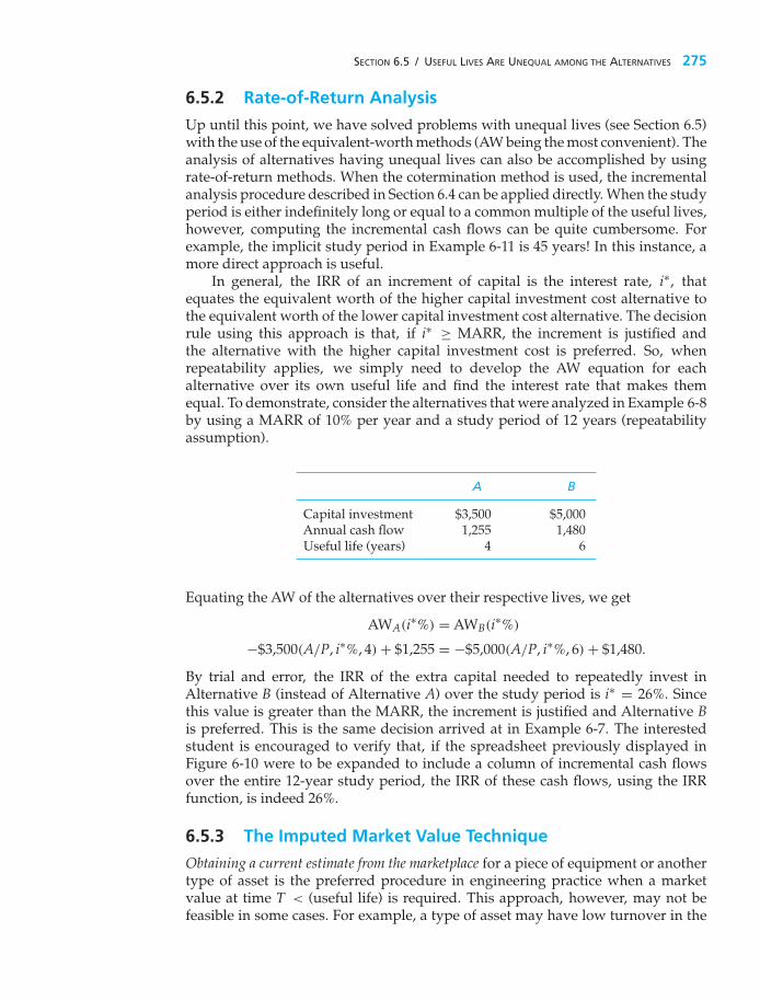
SECTION 6.5 / USEFUL LIVES ARE UNEQUAL AMONG THE ALTERNATIVES 275

6.5.2 Rate-of-Return Analysis

Up until this point, we have solved problems with unequal lives (see Section 6.5)with the use of the equivalent-worth methods (AW being the most convenient). Theanalysis of alternatives having unequal lives can also be accomplished by usingrate-of-return methods. When the cotermination method is used, the incrementalanalysis procedure described in Section 6.4 can be applied directly. When the studyperiod is either indefinitely long or equal to a common multiple of the useful lives,however, computing the incremental cash flows can be quite cumbersome. Forexample, the implicit study period in Example 6-11 is 45 years! In this instance, amore direct approach is useful.

In general, the IRR of an increment of capital is the interest rate, i∗, thatequates the equivalent worth of the higher capital investment cost alternative tothe equivalent worth of the lower capital investment cost alternative. The decisionrule using this approach is that, if i∗ ≥ MARR, the increment is justified andthe alternative with the higher capital investment cost is preferred. So, whenrepeatability applies, we simply need to develop the AW equation for eachalternative over its own useful life and find the interest rate that makes themequal. To demonstrate, consider the alternatives that were analyzed in Example 6-8by using a MARR of 10% per year and a study period of 12 years (repeatabilityassumption).

A B

Capital investment $3,500 $5,000Annual cash flow 1,255 1,480Useful life (years) 4 6

Equating the AW of the alternatives over their respective lives, we get

AWA(i∗%) = AWB(i∗%)

−$3,500(A/P, i∗%, 4) + $1,255 = −$5,000(A/P, i∗%, 6) + $1,480.

By trial and error, the IRR of the extra capital needed to repeatedly invest inAlternative B (instead of Alternative A) over the study period is i∗ = 26%. Sincethis value is greater than the MARR, the increment is justified and Alternative Bis preferred. This is the same decision arrived at in Example 6-7. The interestedstudent is encouraged to verify that, if the spreadsheet previously displayed inFigure 6-10 were to be expanded to include a column of incremental cash flowsover the entire 12-year study period, the IRR of these cash flows, using the IRRfunction, is indeed 26%.

6.5.3 The Imputed Market Value Technique

Obtaining a current estimate from the marketplace for a piece of equipment or anothertype of asset is the preferred procedure in engineering practice when a marketvalue at time T < (useful life) is required. This approach, however, may not befeasible in some cases. For example, a type of asset may have low turnover in the

276 CHAPTER 6 / COMPARISON AND SELECTION AMONG ALTERNATIVES

marketplace, and information for recent transactions is not available. Hence, it issometimes necessary to estimate the market value for an asset without current andrepresentative historical data.

The imputed market value technique, which is sometimes called the impliedmarket value, can be used for this purpose as well as for comparison withmarketplace values when current data are available. The estimating procedureused in the technique is based on logical assumptions about the value of theremaining useful life for an asset. If an imputed market value is needed for a pieceof equipment, say, at the end of year T < (useful life), the estimate is calculated onthe basis of the sum of two parts, as follows:

MVT = [PW at EOY T of remaining capital recovery (CR) amounts]+[PW at EOY T of original market value at end of useful life],

where PW is computed at i = MARR.The next example uses information from Example 6-11 to illustrate the

technique.

EXAMPLE 6-12 Estimating a New Market Value when Useful Life > Study Period

Use the imputed market value technique to develop an estimated market valuefor pump model HEPS9 (Example 6-11) at EOY five. The MARR remains 20%per year.

SolutionThe original information from Example 6-11 will be used in the solution: capitalinvestment = $47,600, useful life = nine years, and market value = $5,000 at theend of useful life.

First, compute the PW at EOY five of the remaining CR amounts[Equation (5-5)]:

PW(20%)CR = [$47,600(A/P, 20%, 9) − $5,000(A/F, 20%, 9)] × (P/A, 20%, 4)

= $29,949.

Next, compute the PW at EOY five of the original MV at the end of useful life(nine years):

PW(20%)MV = $5,000(P/F, 20%, 4) = $2,412.

Then, the estimated market value at EOY five (T = 5) is as follows:

MV5 = PWCR + PWMV

= $29,949 + $2,412 = $32,361.

In summary, utilizing the repeatability assumption for unequal lives amongalternatives reduces to the simple rule of “comparing alternatives over theiruseful lives using the AW method, at i = MARR.” This simplification, however,

SECTION 6.6 / PERSONAL FINANCES 277

may not apply when a study period, selected to be shorter or longer than thecommon multiple of lives (coterminated assumption), is more appropriate forthe decision situation. When utilizing the coterminated assumption, cash flowsof alternatives need to be adjusted to terminate at the end of the study period.Adjusting these cash flows usually requires estimating the market value of assetsat the end of the study period or extending service to the end of the study periodthrough leasing or some other assumption.

6.6 Personal FinancesSound financial planning is all about making wise choices for your particularcircumstances (e.g., your amount of personal savings, your job security, yourattitude toward risk). Thus far in Chapter 6, we have focused on facilitating gooddecision making from the perspective of a corporation. Now we apply these sameprinciples (remember them from Chapter 1?) to several problems you are likely toface soon in your personal decision making.

Two of the largest investments you’ll ever make involve houses andautomobiles. This section presents examples of acquiring these assets, usually withborrowed money. Another concern is the extensive use of credit cards (maybe wethink that nothing is expensive on a credit card). It turns out that people who usecredit cards (almost all of us!) tend to spend more money than others who pay cashor write checks. An enlightening exercise to see how addicted you are to creditcards is to go cold turkey for two months.

A fundamental lesson underlying this section is to save now rather thanspending on luxury purchases. By choosing to save now, we are making an attemptto minimize the risk of making poor decisions later on. Check out the savingscalculators at www.Choosetosave.org.

EXAMPLE 6-13 Automobile Financing Options

You have decided to purchase a new automobile with a hybrid-fueled engineand a six-speed transmission. After the trade-in of your present car, the purchaseprice of the new automobile is $30,000. This balance can be financed by an autodealer at 2.9% APR with payments over 48 months. Alternatively, you can get a$2,000 discount on the purchase price if you finance the loan balance at an APRof 8.9% over 48 months. Should you accept the 2.9% financing plan or accept thedealer’s offer of a $2,000 rebate with 8.9% financing? BothAPRs are compoundedmonthly.

SolutionIn this example, we assume that your objective is to minimize your monthly carpayment.

2.9% financing monthly payment:

$30,000 (A/P, 2.9%/12, 48 months) = $30,000(0.0221) = $663.00 per month

278 CHAPTER 6 / COMPARISON AND SELECTION AMONG ALTERNATIVES

8.9% financing monthly payment:

$28,000 (A/P, 8.9%/12, 48 months) = $28,000(0.0248) = $694.90 per month

Therefore, to minimize your monthly payment, you should select the 2.9%financing option.

What If QuestionsWhen shopping for an automobile you’ll find that there are many financingoptions like the ones in this example available to you. You may find it useful toask yourself questions such as “how high would the rebate have to be for meto prefer the rebate option,” or “how low would the APR have to be for me toselect the rebate option?” The answers to these questions can be found throughsimple equivalence calculations.

(a) How much would the rebate have to be?Let X = rebate amount. Using the monthly payment of $663 from the 2.9%financing option, we can solve for the rebate amount that would yield thesame monthly payment.

($30,000 − X)(A/P, 8.9%/12 months, 48 months) = $663

($30,000 − X)(0.0248) = $663

X = $3,266

(b) How low would the interest rate have to be?Now we want to find the interest rate that equates borrowing $28,000 to 48monthly payments of $663. This question is easily solved using a spreadsheetpackage.

RATE (48, −663, 28000) = 0.535% per month

APR = 0.535% × 12 = 6.42%

EXAMPLE 6-14 Mortgage Financing Options

A general rule of thumb is that your monthly mortgage payment should notexceed 28% of your household’s gross monthly income. Consider the situation ofJerry and Tracy, who just committed to a $300,000 mortgage on their dream home.They have reduced their financing choices to a 30-year conventional mortgageat 6% APR, or a 30-year interest-only mortgage at 6% APR.

(a) Which mortgage, if either, do they qualify for if their combined gross annualincome is $70,000?

(b) What is the disadvantage in an interest-only mortgage compared to theconventional mortgage?

SECTION 6.6 / PERSONAL FINANCES 279

Solution(a) Using the general rule of thumb, Jerry and Tracy can afford a monthly

mortgage payment of (0.28)($70,000/12) = $1,633. The monthly paymentfor the conventional mortgage is

$300,000 (A/P, 0.5%, 360) = $1,800.

For the interest-only mortgage, the monthly payment is

(0.005)($300,000) = $1,500.

Thus, the conventional mortgage payment is larger than what the guidelinesuggests is affordable. This type of loan is marginal because it stretches theirbudget too much. They easily qualify for the interest-only mortgage becausethe $1,500 payment is less than $1,633.

(b) If home prices fall in the next several years, Jerry and Tracy may have“negative equity” in their home because no principal has been repaid intheir monthly interest-only payments. They will not have any buffer to fallback on should they have to sell their house for less than they purchasedit for.

It is important to note that interest-only loans don’t remain interest-onlyfor the entire loan period. The length of time that interest-only payments maybe made is defined in the mortgage contract and can be as short as 5 yearsor as long as 15 years. After the interest-only period is over, the monthlypayment adjusts to include principal and interest. It is calculated to repaythe entire loan by the end of the loan period. Suppose Jerry and Tracy’sinterest-only period was five years. After this time, the monthly paymentwould become

$300,000(A/P, 0.5%, 300) = $1,932.90.

Before Jerry and Tracy accept this type of loan, they should be confident thatthey will be able to afford the $1,932.90 monthly payment in five years.

EXAMPLE 6-15 Comparison of Two Savings Plans

Suppose you start a savings plan in which you save $500 each year for 15 years.You make your first payment at age 22 and then leave the accumulated sum inthe savings plan (and make no more annual payments) until you reach age 65,at which time you withdraw the total accumulated amount. The average annualinterest rate you’ll earn on this savings plan is 10%.

A friend of yours (exactly your age) from Minnesota State University waits10 years to start her savings plan. (That is, she is 32 years old.) She decides tosave $2,000 each year in an account earning interest at the rate of 10% per year.She will make these annual payments until she is 65 years old, at which timeshe will withdraw the total accumulated amount.

280 CHAPTER 6 / COMPARISON AND SELECTION AMONG ALTERNATIVES

How old will you be when your friend’s accumulated savings amount(including interest) exceeds yours? State any assumptions you think arenecessary.

SolutionCreating cash-flow diagrams for Example 6-15 is an important first step insolving for the unknown number of years, N, until the future equivalent valuesof both savings plans are equal. The two diagrams are shown below. The futureequivalent (F) of your plan is $500(F/A, 10%, 15)(F/P, 10%, N − 36) and that ofyour friend is F′ = $2,000(F/A, 10%, N − 31). It is clear that N, the age at whichF = F′, is greater than 32. Assuming that the interest rate remains constant at10% per year, the value of N can be determined by trial and error:

F�65 � ?

21 22 23 24 35 36 37 38 64

65

F65 � ?

A � $500/year

End of year

Your savings plan:

Your friend’s savings plan:

End of year

A�� $2,000/year

21 22 23 32 33 34 35 36 64

65

N Your Plan’s F Friend’s F ′

36 $15,886 $12,21038 $19,222 $18,97439 $21,145 $22,87240 $23,259 $27,159

By the time you reach age 39, your friend’s accumulated savings will exceedyours. (If you had deposited $1,000 instead of $500, you would be over 76 yearswhen your friend’s plan surpassed yours. Moral: Start saving early!)

SECTION 6.7 / CASE STUDY—NED AND LARRY’S ICE CREAM COMPANY 281

EXAMPLE 6-16 Credit Card Offers

Randy just cancelled his credit card with a large bank. A week later, arepresentative of the bank called Randy with an offer of a “better” credit cardthat will advance Randy $2,000 when he accepts it. Randy could not refuse theoffer and several days later receives a check for $2,000 from the bank. With thismoney, Randy decides to buy a new computer.

At the next billing cycle (a month later), the $2,000 advance appears as acharge against Randy’s account, and the APR is stated to be 21% (compoundedmonthly). At this point in time, Randy elects to pay the minimum monthlypayment of $40 and cuts up the credit card so that he cannot make any additionalpurchases.

(a) Over what period of time does this payment extend in order to repay the$2,000 principal?

(b) If Randy decides to repay all remaining principal after having made15 monthly payments, how much will he repay?

Solution(a) You may be surprised to know that the majority of credit card companies

determine the minimum monthly payment based on a repayment periodof 10 years. The monthly interest rate being charged for Randy’s card is21%/12 = 1.75%. We can solve the following equivalence relationship todetermine the number of $40 monthly payments required to pay off a loanprincipal of $2,000.

$2,000 = $40(P/A, 1.75%, N)

This is easily solved using the NPER (rate, payment, principal) function inExcel.

NPER(1.75%, −40, 2000) = 119.86

Sure enough, it will take Randy 120 months to pay off this debt.(b) After having made 15 payments, Randy has 105 payments remaining. To

find the single sum payoff for this loan, we simply have to determine thepresent worth of the remaining payments.

Payoff = $40(P/A, 1.75%, 105) = $1,915.96

This payoff amount assumes no penalty for early repayment of the loan(which is typically the case when it comes to credit cards). Notice how verylittle principal ($84.06) was repaid in the early part of the loan.

6.7 CASE STUDY−−Ned and Larry’s Ice Cream Company

Ned and Larry’s Ice Cream Company produces specialty ice cream and frozenyogurt in pint-sized containers. The latest annual performance report praised thefirm for its progressive policies but noted that environmental issues like packaging

282 CHAPTER 6 / COMPARISON AND SELECTION AMONG ALTERNATIVES

disposal were a concern. In an effort to reduce the effects of consumer disposalof product packaging, the report stated that Ned and Larry’s should consider thefollowing proposals:

Proposal A—Package all ice cream and frozen yogurt in quart containers.Proposal B—Package all ice cream and frozen yogurt in half-gallon containers.

By packaging the product in containers larger than the current pints, the plastic-coated bleached sulfate board containers will hold more ounces of product persquare inch of surface area. The net result is less discarded packaging per ounceof product consumed. Additional advantages to using larger containers includelower packaging costs per ounce and less handling labor per ounce.

Changing to a larger container requires redesign of the packaging andmodifications to the filling production line. The existing material-handlingequipment can handle the pints and quarts, but additional equipment will berequired to handle half-gallons. Any new equipment purchased for proposals Aand B has an expected useful life of six years. The total capital investment for eachproposal is shown in the accompanying table. The table summarizes the details ofthese proposals, as well as the current production of pints.

Current (Pints) (A) Quarts (B) Half-Gallons

Capital investment $0 $1,200,000 $1,900,000Packaging cost per gallon $0.256 $0.225 $0.210Handling labor cost per gallon $0.128 $0.120 $0.119Postconsumer landfill contribution 6,500 5,200 4,050

from discarded packaging (yd3/yr)

Because Ned and Larry’s promotes partnering with suppliers, customers, andthe community, they wish to include a portion of the cost to society when evaluatingthese alternatives. They will consider 50% of the postconsumer landfill cost as partof the costs for each alternative. They have estimated landfill costs to average $20per cubic yard nationwide.

Ned and Larry’s uses a MARR of 15% per year and IRR analyses to evaluatecapital investments. A study period of six years will be used, at which time theequipment purchased for proposals A and B will have negligible market value.Production will remain constant at 10,625,000 gallons per year. Determine whetherNed and Larry’s should package ice cream and frozen yogurt in pints, quarts, orhalf-gallons.

SolutionAssuming that Ned and Larry’s is able to sell all ice cream and frozen yogurtproduced, we can focus on the differences in costs associated with the threepackaging alternatives. Since our recommendation is to be supported by IRRanalysis, we must use the incremental analysis procedure.

SECTION 6.7 / CASE STUDY—NED AND LARRY’S ICE CREAM COMPANY 283

The first step in the incremental analysis procedure is to rank-order thealternatives by increasing capital investment:

Current(pints) → A(quarts) → B(half-gallons).

Now we can compute the incremental difference between producing in quarts (A)instead of pints (current) and determine whether the incremental capital investmentis justified.

� (A − current)

� Capital investment −$1,200,000� Packaging cost savings [$0.031/gal](10,625,000 gal/yr) = $329,375/yr� Handling cost savings [$0.008/gal](10,625,000 gal/yr) = $85,000/yr� Landfill cost savings [1,300 yd3/yr](0.5)($20/yd3) = $13,000/yr

To determine the IRR of the incremental investment, we can find the interest rateat which the PW of the incremental cash flows is zero.

PW(i′�%) = 0 = −$1,200,000 + ($329,375 + $85,000 + $13,000)(P/A, i′�%, 6).

By trial and error, i′�% = 27.2% > MARR. Thus, the investment required to producethe quart-size containers for ice cream is economically justified. Our decision iscurrently to produce quart-size containers unless the extra investment requiredto produce in half-gallon-size containers (B) earns at least the MARR based onprojected savings.

� (B − A)

� Capital investment −$700,000� Packaging cost savings [$0.015/gal](10,625,000 gal/yr) = $159,375/yr� Handling cost savings [$0.001/gal](10,625,000 gal/yr) = $10,625/yr� Landfill cost savings [1,150 yd3/yr](0.5)($20/yd3) = $11,500/yr

PW(i′�%) = 0 = −$700,000 + ($159,375 + $10,625 + $11,500)(P/A, i′�%, 6)

By trial and error, i′�% = 14.3% < MARR. Therefore, the extra investment requiredto produce in half-gallon-size containers (B) is not justified by the quantified extrasavings.

Based on the preceding incremental IRR analysis, the final recommendation forNed and Larry’s Ice Cream Company is to produce ice cream and frozen yogurt inquart containers (i.e., Proposal A). The foregoing incremental analysis procedureindicates that this recommendation will yield an i′�% = 27.2%, which is greaterthan the MARR of 15%. So, by making the recommended change to packaging allice cream and frozen yogurt in quart containers, not only will Ned and Larry’s bedelivering great tasting products that are economically attractive to the company,but also the company will be environmentally conscious as well! A win all around!What flavor would you like?

284 CHAPTER 6 / COMPARISON AND SELECTION AMONG ALTERNATIVES

6.8 Postevaluation of ResultsAfter comparing alternatives and identifying the preferred course of action (Step 6),we return to the important Step 7 of the economic analysis procedure in Table 1-1.Postaudit reviews, which are appraisals of how a project is progressing againstcritical milestones, should be conducted during and after a project, recommendedby the procedures in Chapter 6, has been approved and funded. This periodicfeedback will inform management about the following:

1. Are the planned objectives and milestones being (or have been) attained by theproject?

2. Is corrective action required to bring the project in line with the expectations?3. What can be learned from the selected (and implemented) project that will

improve estimating for future projects?

Learning from past decisions (both good and bad!) is critical to improvingfuture decisions.

Periodic postaudit reviews serve to reduce, and often correct for, possible biasin favor of what individual corporate units, divisions, and subsidiaries wouldlike to accomplish to serve their own self-interests. The tendency to estimateoptimistically future cash flows and other conditions for pet projects seems tobe human nature, but a fair and above-board audit during and after each majorproject should keep this in check. As a result, estimating project outcomes willbe taken more seriously when projects are tracked and monitored over their lifecycles. However, a balance must be struck between overly aggressive postauditsand the counter behavior of causing estimators to become overly conservative intheir project appraisals.

6.9 Project Postevaluation Spreadsheet ApproachThus far, we have addressed parameter estimation, economic modeling, anddecision making. We now present a means to assess the performance of thisentire modeling process. In a reversal of our normal approach to spreadsheets,the analysis is presented first, followed by the spreadsheet model.

Quality engineers rely on Individuals control charts, which are based onindividual values rather than averages, to identify areas for process improvement.These charts identify cases that are drastically different from the rest, providinga primary focus for improvement efforts. As economic modeling is an ongoingprocess, control charts serve as a first step in improving accuracy. While controlcharts can guide improvement efforts, they do not indicate specifically how toimprove a process.

Consider a project tracking database with the following information: Product(Legacy or Joint Venture), Estimated Savings, Actual Savings, and Facility (North,East, West, South, or Central). The accuracy of the estimation process is typicallymeasured by looking at the Savings Gap, which is the difference between the actualand estimated savings. When the estimation process is performing well, the averageSavings Gap will be zero with minimal variation.

SECTION 6.9 / PROJECT POSTEVALUATION SPREADSHEET APPROACH 285

A control chart uses process data to establish a region of typical performance,which is bounded by the Upper and Lower Control Limits. If the data fall withinthis region and exhibit no unusual patterns, the process is deemed to be in a stateof statistical control. Future performance measures will be centered around theaverage and fall within the region defined by the control limits. If the process isnot in control, investigating the outlying cases will point to promising areas forimprovement.

Figure 6-13 shows an Individuals control chart for 40 projects. There are four out-of-control points: Projects 7, 17, 34, and 35. We can identify these in the spreadsheetby hovering the cursor over each plotted point. All four projects are Joint Ventures,implying that there is something significantly different about how those projectbenefits were estimated. Three of these four project significantly overestimated thesavings.

To explore this preliminary finding, code the Product Type numerically andcreate a scatter plot of Savings Gap versus Product Type. Select the “no fill” optionon the plot symbols to provide a cleaner view of the overlapping data values.Refer to Figure 6-14. The spread and center of the Savings Gap data for the Legacyproducts indicate that these products are estimated more precisely and with lessbias then the Joint Venture products.

The large range of Savings Gap values for the Joint Venture products indicatesthat there are additional sources of variation in the estimation process. Figure 6-15is a scatter plot by Facility. As in Figure 6-14, numeric coding of Facility is requiredto create this graph. To facilitate comparisons, the ranges of the X-axes are the sameon both plots.

The range of the Savings Gap is greatest at the West facility. We know from thecontrol chart that these extreme values are for Joint Venture products. There is an

1�$600,000

�$400,000

�$200,000

$0

$200,000

$400,000

$600,000

3 5 7 9 11 13 15 17 19 21

Project ID

Individuals Control Chart

Savi

ngs

Gap

LCL

UCL

CL

23 25 27 29 31 33 35 37 39

Figure 6-13 Individuals control chart for Savings Gap by Project ID. Four projects(7, 17, 34, and 35) had gaps that are beyond the control limits and are classified asout of control. Determining what is different about how these estimates weredetermined will likely lead to a way to improve the process.

286 CHAPTER 6 / COMPARISON AND SELECTION AMONG ALTERNATIVES

�$600,000

�$400,000

�$200,000 $0

$200,000

$400,000

$600,000

1

2

Pro

duct

Product: 1 Legacy 2 Joint Venture

Savings Gap by Product Type

Figure 6-14 Scatter plot of Savings Gap versus Product Type. The smaller variation ofthe Legacy product estimation process is clearly evident in this view of the data.

�$600,000

�$400,000

�$200,000 $0

$200,000

$400,000

$600,000

1

4

3

2

5

Faci

lity

Facility: 1 North 2 East 3 West 4 South 5 Central

Savings Gap by Facility

Figure 6-15 Scatter plot of Savings Gap versus Facility. The symbol outlines allow oneto visualize points with similar values. The West and East facilities have much greatervariation in their savings estimates than the other locations.

overall bias to overestimate savings on Joint Venture products, but the pattern isbroken here, since West has the largest underestimation as well. Investigation isrequired to understand this exception to the pattern to better understand how theestimates are obtained.

The East facility has the next greatest variation, and the low value is anotherJoint Venture product. Additional review shows that the Joint Venture productscome only from these two facilities.

SECTION 6.10 / TRY YOUR SKILLS 287

Figure 6-16 Spreadsheet formulas for Individuals control chart. Only the first five projects from thedatabase are shown to conserve space.

The analysis has narrowed the scope of our investigation to Joint Ventureproducts at the West and East facilities. Understanding the issues affecting thisblend of product and facility will provide the quickest reduction in bias in variationin the estimation process.

The spreadsheet model is shown in Figure 6-16. Only the first five rows ofthe data base are included. There are two intermediate calculations involved:(1) the Savings Gap in cell E2 and (2) the moving range (mR) in cell I3, which isthe absolute value of the difference between consecutive Savings Gap values. Thislocal measure of variation is used to determine the control limits. Both cells arecopied down the worksheet.

There is also a set of summary calculations used to create the control chartlimits: the average Savings Gap in cell O2 (which is the center line on the chart),the average moving range in cell O3, and a constant in cell O4 that is used todetermine the control limits. The UCL and LCL equations are in cells O5 and O6.Readers interested in control charts are encouraged to consult suitable referencesfor the constants and equations used.

The next step is to have cells J2, K2, and L2 use absolute addressing to copythe respective values from O2, O5, and O6. These cells are then copied down theworksheet. To create the chart, select line plot and specify data ranges of E2:E41 forthe data, J2:J41 for the center line, K2:K41 for the UCL, and L2:L41 for the LCL.

Like any other process, estimation can be improved by comparing actual andpredicted results and then incorporating a variety of techniques to identify andeliminate sources of bias and variation. Graphic methods work best in these initialefforts.

6.10 Try Your SkillsThe number in parentheses that follows each problem refers to the sectionfrom which the problem is taken. Solutions to these problems can be found inAppendix G.

288 CHAPTER 6 / COMPARISON AND SELECTION AMONG ALTERNATIVES

6-A. Four mutually exclusive alternatives are being evaluated, and their costs andrevenues are itemized below. (6.4)a. If the MARR is 15% per year and the analysis period is 12 years, use the

PW method to determine which alternatives are economically acceptableand which one should be selected.

b. If the total capital investment budget available is $200,000, which alter-native should be selected?

c. Which rule (Section 6.2.2) applies? Why?

Mutually Exclusive Alternative

I II III IV

Capital investment $100,000 $152,000 $184,000 $220,000Annual revenues less expenses 15,200 31,900 35,900 41,500Market value (end of useful life) 10,000 0 15,000 20,000Useful life (years) 12 12 12 12

6-B. At the Motorola plant in Mesa, Arizona, it is desired to determine whetherone-inch-thick insulation or two-inch-thick insulation should be used toreduce heat loss from a long section of steam pipe. The heat loss from thispipe without any insulation would cost $2.00 per linear foot per year. The one-inch insulation will eliminate 88% of the heat loss and will cost $0.60 per foot.Two-inch insulation will eliminate 92% of the heat loss and will cost $1.10 perfoot. The steam pipe is 1,000 feet in length and will last for10 years. MARR =6% per year. Which insulation thickness should be recommended? (6.4)

6-C. Your company is environmentally conscious and is looking at two heatingoptions for a new research building. What you know about each option isbelow, and your company will use an annual interest rate of 8% for thisdecision:

Gas Heating Option: The initial equipment and installment of the naturalgas system would cost $225,000 right now. The maintenance costs of theequipment are expected to be $2,000 per year, starting next year, for each ofthe next 20 years. The energy cost is expected to be $5,000, starting next year,and is expected to rise by 5% per year for each of the next 20 years due to theprice of natural gas increasing.

Geothermal Heating Option: Because of green energy incentives providedby the government, the geothermal equipment and installation is expectedto cost only $200,000 right now, which is cheaper than the gas lines. Therewould be no energy cost with geothermal, but because this is a relativelynewer technology, the maintenance costs are expected to be $10,000 per year,starting next year, for each of the next 20 years.

Which is the lower cost option for the company? (4.12 and 6.4)

6-D. A steam generator is needed in the design of a new power plant. Thisgenerator can be fired by three different fuels, A, B, or C, with the followingcost implications.

SECTION 6.10 / TRY YOUR SKILLS 289

A B C

Installed investment cost $30,000 $55,000 $180,000Annual fuel expense X + $7,500 X X − $1,500Residual value None None None

If the study period is 20 years and the MARR is 8% per year, which type offuel is most economical? (6.4)

6-E. Four mutually exclusive projects are being considered for a new two-milejogging track. The life of the track is expected to be 80 years, and thesponsoring agency’s MARR is 12% per year. Annual benefits to the publichave been estimated by an advisory committee and are shown below. Usethe IRR method (incrementally) to select the best jogging track. (6.4)

Alternative A B C D

Initial cost $62,000 $52,000 $150,000 $55,000Annual benefits $10,000 $8,000 $20,000 $9,000Rate of return on investment 16.1% 15.4% 13.3% 16.4%

6-F. An industrial coal-fired boiler for process steam is equipped with a 10-year-old electrostatic precipitator (ESP). Changes in coal quality have caused stackemissions to be in noncompliance with federal standards for particulates. Twomutually exclusive alternatives have been proposed to rectify this problem(doing nothing is not an option).

New Baghouse New ESP

Capital investment $1,140,000 $992,500Annual operating expenses 115,500 73,200

The life of both alternatives is 10 years, and the MARR is 15% per year. Usethe IRR method (incrementally) to make a recommendation regarding whichalternative to select. Can you list some nonmonetary factors that would favorthe new baghouse? (6.4)

6-G. The local police department is considering two types of sidearms for itsofficers. The Glock 40 costs $400 apiece and has a life of 5 years. The otheroption is a Sauer 45 that costs $800 and has a 10-year life. The Sauer pistolhas a residual value of $200 at the end of its 10-year service life. Assumerepeatability and compute the internal rate of return on the incremental cashflow of the two pistols. If the department uses a MARR of 5% per year, is theSauer 45 the better choice? (6.5)

290 CHAPTER 6 / COMPARISON AND SELECTION AMONG ALTERNATIVES

6-H. Two insulation thickness alternatives have been proposed for a process steamline subject to severe weather conditions. One alternative must be selected.Estimated savings in heat loss and installation cost are given below.

Thickness Installed Cost Annual Savings Life

2 cm $20,000 $5,000 4 years5 cm $40,000 $7,500 6 years

Which thickness would you recommend for a MARR = 15% per year andnegligible market (salvage) values? The study period is 12 years. (6.5)

6-I. Refer to Problem 6-H. Which thickness would you recommend if the studyperiod was 4 years? Use the imputed market value technique to estimate themarket value of the 5 cm alternative after 4 years. (6.5)

6-J. Your rich uncle has offered you two living trust payouts for the rest of yourlife. The positive cash flows of each trust are shown below. If your personalMARR is 10% per year, which trust should you select? (6.5)

End of Year Trust A Trust B

0 $0 $01–10 $1,000 $1,20011–∞ $1,500 $1,300

Note: At 10% per year interest, infinity occurs when N = 80 years.6-K. Two proposals have been offered for streamlining the business operations

of a customer call center. Proposal A has an investment cost of $30,000, anexpected life of 5 years, property taxes of $450 per year, and no market value.Annual expenses are estimated to be $6,000. Proposal B has an investmentcost of $38,000, an expected life of 4 years, property taxes of $600 per year,and no market value. Its annual operating expenses are expected to be $4,000.Using a MARR = 10% per year, which proposal should be recommended?Use the AW method and state your assumption(s). (6.5)

6-L. You have been requested to offer a recommendation of one of the mutuallyexclusive industrial sanitation control systems that follow. If the MARR is15% per year, which system would you select? Use the IRR method. (6.5)

Gravity-fed Vacuum-led

Capital investment $24,500 $37,900Annual receipts less expenses 8,000 8,000Life (in years) 5 10IRR 18.9% 16.5%

SECTION 6.11 / SUMMARY 291

6-M. Automobile repair shops typically remind customers to change their oil andoil filter every 3,000 miles. Let’s call this Strategy 1. Usually you can savemoney by following another legitimate guideline—your automobile user’smanual. It suggests changing your oil every 5,000–7,000 miles. We’ll call thisStrategy 2. To conserve a nonrenewable and valuable resource, you decide tofollow Strategy 2 and change your oil every 5,000 miles (you are conservative).You drive an average of 15,000 miles per year, and you expect each oil changeto cost $30. Usually you drive your car 90,000 miles before trading it in on anew one. (6.6)

a. Develop an EOY cash-flow diagram for each strategy.b. If your personal MARR is 10% per year, how much will you save with

Strategy 2 over Strategy 1, expressed as a lump sum at the present time?

6-N. A certain U.S. government savings bond can be purchased for $7,500. Thisbond will be worth $10,000 when it matures in 5 years. As an alternative, a60-month certificate of deposit (CD) can be purchased for $7,500 from a localbank, and the CD yields 6.25% per year. Which is the better investment ifyour personal MARR is 5% per year? (6.6)

6.11 SummaryThe following chart is a bird’s eye view of the methods used in Chapter 6 to identifythe preferred alternative.∗

When Lives of Alternatives = Study Period

Simplest Approach: Compute the equivalent worth of each alternative (PW, AW,FW, or CW)

Decision Rule: Select alternative with the highest equivalent worth.If comparing cost alternatives, this will be the alternative with the leastnegative equivalent worth.

Rate-of-Return Methods: The base alternative is the one with the smallest investmentcost (if an investment alternative, the IRRbase ≥ MARR). Use incrementalanalysis to compare base alternative to next smallest investment cost alternative.

DecisionRule: If IRR� ≥ MARR, eliminate base and move on to next comparison.If IRR� < MARR, keep base and move on to next comparison.

When Lives of Alternatives Are Different:

Repeatability Assumption:

Simplest Approach: Use AW over each alternative’s own life. Select thealternative with the greatest AW.

∗ Special thanks to Karen Bursic for suggesting this format for the summary.

292 CHAPTER 6 / COMPARISON AND SELECTION AMONG ALTERNATIVES

Rate-of-Return Approach: Set AW of base = AW of next smallest investmentcost and solve for the unknown interest rate i�’.

Decision Rule: If IRR� ≥ MARR, eliminate base and move to next comparison.If IRR� < MARR, keep base and move to next comparison.

Coterminated Assumption:

Simplest Approach: For investment alternatives, the most logical approachis to bring all cash flows to time N, the end of the life of the longestlived alternative without repeating any cash flows (use FW). You couldalso use the shortest life and the imputed market value for longer livedalternatives.

Rate-of-Return Approach: Perform an incremental analysis with anappropriate study period and assumptions regarding extended orshortened alternative lives.

ProblemsThe number in parentheses that follows each problemrefers to the section from which the problem is taken.

6-1. Refer to Example 6-7 and develop the incrementalcash flows of Alternative B minus Alternative A, �

(B-A), over a 12-year study period. Do multiple interestrates exist for � (B-A) cash flows? (6.2, Appendix 5A)

6-2. The Consolidated Oil Company mustinstall antipollution equipment in a new refinery

to meet federal clean-air standards. Four designalternatives are being considered, which will havecapital investment and annual operating expenses asshown below. Assuming a useful life of 8 years for eachdesign, no market value, a desired MARR of 10% peryear, determine which design should be selected on thebasis of the PW method. Confirm your selection byusing the FW and AW methods. Which rule (Section6.2.2) applies? Why? (6.4)

Design Capital Investment Annual Expenses

D1 $600,000 $780,000D2 760,000 728,000D3 1,240,000 630,000D4 1,600,000 574,000

6-3. Which mutually exclusive project below wouldyou recommend? Explain your answer. (6.4)

Project PW (12%) IRR

R15 $45,252 15%S19 $42,591 18%

6-4. Three mutually exclusive design alternatives arebeing considered. The estimated sales and cost data for

A B C

Investment cost $30,000 $60,000 $50,000Estimated units 15,000 20,000 18,000to be sold/year

Unit selling price, $3.50 $4.40 $4.10$/unit

Variable costs, $1.00 $1.40 $1.15$/unit

Annual expenses $15,000 $30,000 $26,000(fixed)

Market value 0 $20,000 $15,000Useful life 10 years 10 years 10 years

PROBLEMS 293

each alternative are given on p. 292. The MARR is 20%per year. Annual revenues are based on the numberof units sold and the selling price. Annual expensesare based on fixed and variable costs. Determinewhich selection is preferable based on AW. State yourassumptions. (6.4)

6-5. An airport needs a modern material handlingsystem for facilitating access to and from a busymaintenance hangar. A second-hand system will cost$75,000. A new system with improved technologycan decrease labor hours by 20% compared to theused system. The new system will cost $150,000 topurchase and install. Both systems have a useful lifeof five years. The market value of the used system isexpected to be $20,000 in five years, and the marketvalue of the new system is anticipated to be $50,000in five years. Current maintenance activity will requirethe used system to be operated 8 hours per day for20 days per month. If labor costs $40 per hour andthe MARR is 1% per month, which system should berecommended? (6.4)

6-6. You have been asked to evaluate theeconomic implications of various methods for

cooling condenser effluents from a 200-MW steam-electric plant. In this regard, cooling ponds and once-through cooling systems have been eliminated fromconsideration because of their adverse ecological effects.It has been decided to use cooling towers to dissipatewaste heat to the atmosphere. There are two basic

TABLE P6-6 Alternative Types of Cooling Towers for a 200-Megawatt Fossil-FiredPower Plant Operating at Full Capacitya in Problem 6-6

Alternative

Wet Tower Wet Tower Dry Tower Dry TowerMech. Draft Natural Draft Mech. Draft Natural Draft

Initial cost $3 million $8.7 million $5.1 million $9.0 millionPower for I.D. 40 200-hp None 20 200-hp I.D. Nonefans induced-draft fans fans

Power for pumps 20 150-hp pumps 20 150-hp pumps 40 100-hp pumps 40 100-hp pumpsMechanical $0.15 million $0.10 million $0.17 million $0.12 millionmaintenance/year

Service life 30 years 30 years 30 years 30 yearsMarket value 0 0 0 0

a 100 hp = 74.6 kW; cost of power to plant is 2.2 cents per kWh or kilowatt-hour; induced-draft fans and pumps operatearound the clock for 365 days/year (continuously). Assume that electric motors for pumps and fans are 90% efficient.

types of cooling towers: wet and dry. Furthermore, heatmay be removed from condenser water by (1) forcing(mechanically) air through the tower or (2) allowingheat transfer to occur by making use of naturaldraft. Consequently, there are four basic cooling towerdesigns that could be considered. Assuming that thecost of capital to the utility company is 12% peryear, your job is to recommend the best alternative(i.e., the least expensive during the service life) inview of the data in Table P6-6. Further, assume thateach alternative is capable of satisfactorily removingwaste heat from the condensers of a 200-MW powerplant. What noneconomic factors can you identifythat might also play a role in the decision-makingprocess? (6.4)

6-7. Three mutually exclusive design alternatives arebeing considered. The estimated cash flows for eachalternative are given next. The MARR is 20% per year.At the conclusion of the useful life, the investment willbe sold.

A B C

Investment cost $28,000 $55,000 $40,000Annual expenses $15,000 $13,000 $22,000Annual revenues $23,000 $28,000 $32,000Market value $6,000 $8,000 $10,000Useful life 10 years 10 years 10 yearsIRR 26.4% 24.7% 22.4%

294 CHAPTER 6 / COMPARISON AND SELECTION AMONG ALTERNATIVES

A decision-maker can select one of these alternatives ordecide to select none of them. Make a recommendationusing the PW method. (6.4)

6-8. Your boss has asked you to evaluate theeconomics of replacing 1,000 60-Watt incan-

descent light bulbs (ILBs) with 1,000 compactfluorescent lamps (CFLs) for a particular lightingapplication. During your investigation you discoverthat 13-Watt CFLs costing $2.00 each will provide thesame illumination as standard 60-Watt ILBs costing$0.50 each. Interestingly, CFLs last, on average, eighttimes as long as incandescent bulbs. The average life ofan ILB is one year over the anticipated usage of 1,000hours each year. Each incandescent bulb costs $2.00 toinstall/replace. Installation of a single CFL costs $3.00,and it will also be used 1,000 hours per year.

Electricity costs $0.12 per kiloWatt hour (kWh), andyou decide to compare the two lighting options overan 8-year study period. If the MARR is 12% per year,compare the economics of the two alternatives and writea brief report of your findings for the boss. (6.4)

6-9. On her thirty-first birthday, Jean invests $1,000into her employer’s retirement plan, and she continuesto make annual $1,000 payments for 10 years. Soher total contribution (principal) is $10,000. Jean thenstops making payments into her plan and keeps hermoney in the savings plan untouched for 25 moreyears. Doug starts putting money aside on his forty-first birthday when he deposits $1,000, and he continuesthese payments until he gets to be 65 years old. Doug’scontributed principal amounts to $25,000 over thisperiod of time.

If Jean’s and Doug’s retirement plans earn interestof 6% per year, how much will they have accumulated(principal plus interest) when they reach 65 years old?What is the moral of this situation? (6.4)

6-10. Consider the following cash flows for twomutually exclusive alternatives. Which one should berecommended? The MARR is 25% per year. (6.4)

EOY Oval Re-Bar (O) Rectangular Re-Bar (R)

0 −$9,000 −$15,0001 4,050 4,0502 5,400 5,4003 4,500 16,218IRR 25% 25%

6-11. Acme Semiconductor is expanding its facility andneeds to add equipment. There are three process toolsunder consideration. You have been asked to per-form an economic analysis to select the most appro-priate tool to acquire. You have gathered the followinginformation for evaluation. Each of these tools hasa useful life of seven years. Acme’s accounting staffhas established a company-wide MARR of 8% peryear. Which one of the process tools should beselected? (6.4)

Tool A Tool B Tool C

Investment costs $55,000 $45,000 $80,000Annual expenses $6,250 $8,550 $3,200Annual revenue $18,250 $16,750 $20,200Market value $18,000 $3,750 $22,000IRR 15.9% 7.9% 14.6%

6-12. A new highway is to be constructed. Design Acalls for a concrete pavement costing $90 per foot with a20-year life; two paved ditches costing $3 per foot each;and three box culverts every mile, each costing $9,000and having a 20-year life. Annual maintenance will cost$1,800 per mile; the culverts must be cleaned every fiveyears at a cost of $450 each per mile.

Design B calls for a bituminous pavement costing$45 per foot with a 10-year life; two sodded ditchescosting $1.50 per foot each; and three pipe culvertsevery mile, each costing $2,250 and having a 10-year life.The replacement culverts will cost $2,400 each. Annualmaintenance will cost $2,700 per mile; the culverts mustbe cleaned yearly at a cost of $225 each per mile; and theannual ditch maintenance will cost $1.50 per foot perditch.

Compare the two designs on the basis of equivalentworth per mile for a 20-year period. Find the mosteconomical design on the basis of AW and PW if theMARR is 6% per year. (6.3, 6.4)

6-13. The alternatives for an engineering pro-ject to recover most of the energy presently

being lost in the primary cooling stage of a chemicalprocessing system have been reduced to three designs.The estimated capital investment amounts and annualexpense savings are as follows:

Assume that the MARR is 12% per year, the studyperiod is six years, and the market value is zero for all

PROBLEMS 295

Design

EOY ER1 ER2 ER3

0 −$98,600 −$115,000 −$81,2001 25,800 29,000 19,75023

⏐⏐⏐⏐⏐⏐⏐4f = 6%a

⏐⏐⏐⏐⏐⏐⏐4G = $150b

⏐⏐⏐⏐⏐⏐⏐4c

456 34,526 29,750 19,750

a After year one, the annual savings are estimated to increaseat the rate of 6% per year.b After year one, the annual savings are estimated to increase$150 per year.c Uniform sequence of annual savings.

three designs. Apply an incremental analysis method todetermine the preferred alternative. (6.4)

6-14. Two parcels of land are being considered for anew office building. Both sites cost the same amount butdiffer mainly in their annual property tax assessments.The parcel in City A has a current property tax of$15,500 per year. This tax is expected to increase by $500per year starting at EOY 2. The other site, in City B,has a property tax of $12,000 per year with an antici-pated increase of $2,000 per year starting at EOY 2.How much money would have to be set aside todayfor each site to provide for property taxes spanning thenext 10 years? The interest rate is 12% per year. (6.4)

6-15. Consider the three mutually exclusive projectsthat follow. The firm’s MARR is 10% per year. (6.4)

EOY Project 1 Project 2 Project 3

0 −$10,000 −$8,500 −$11,0001–3 $5,125 $4,450 $5,400

a. Calculate each project’s PW.

b. Determine the IRR of each project.

c. Which project would you recommend?

d. Why might one project have the highest PW whilea different project has the largest IRR?

6-16. A special-purpose 30-horsepower electricmotor has an efficiency of 90%. Its purchase and

installation price is $2,200. A second 30-horsepowerhigh-efficiency motor can be purchased for $3,200, and

its efficiency is 93%. Either motor will be operated 4,000hours per year at full load, and electricity costs $0.10per kilowatt-hour (kWh). MARR = 15% per year, andneither motor will have a market value at the end of theeight-year study period. (6.4)

a. Which motor should be chosen?

b. For an incremental investment of $1,000 in the moreefficient motor, what is the PW of the energy savingsover the eight-year period?

6-17. Refer to the situation in Problem 6-16.Most motors are operated at a fraction of their

rated capacity (i.e., full load) in industrial applications.Suppose the average usage (load factor) of the motorin Problem 6-16 is expected to be 60%. Which motorshould be recommended under this condition? (6.4)

6-18. A stem cell research project requires expensivespecialized laboratory equipment. For this purpose,three pieces of equipment and their associated cashflows (listed below) are under consideration. One pieceof equipment must be selected, and the laboratory’sMARR is 15% per year. (6.4)

EOY A B C

0 −$136,500 −$84,000 −$126,0001−4 −$12,500 −$28,500 −$15,500

5 −$10,000 −$28,500 −$15,500

a. Use the PW method to rank-order the economicattractiveness of the three projects.

b. Determine the interest rate at which the laboratorywould be indifferent between Equipment B andEquipment C.

6-19. Consider the following two mutually exclusivealternatives for reclaiming a deteriorating inner-cityneighborhood (one of them must be chosen). Notice thatthe IRR for both alternatives is 27.19%. (6.4)

Alternative

EOY X Y

0 −$100,000 −$100,0001 $50,000 02 $51,000 03 $60,000 $205,760

IRR 27.19% 27.19%

296 CHAPTER 6 / COMPARISON AND SELECTION AMONG ALTERNATIVES

a. If MARR is 15% per year, which alternative is better?

b. What is the IRR on the incremental cash flow [i.e.,�(Y − X)]?

c. If the MARR is 27.5% per year, which alternative isbetter?

d. What is the simple payback period for eachalternative?

e. Which alternative would you recommend?

6-20. Insulated concrete forms (ICF) can beused as a substitute for traditional wood framing

in building construction. Heating and cooling billswill be about 50% less than in a similar wood-framehome in Vermont. An ICF home will be approximately10% more expensive to construct than a wood-framehome.

A typical 2,000 square foot home costs $120 persquare foot to build with wood framing in Vermontand costs $200 per month (on average) to heat or cool.What is the IRR on the incremental investment in anequivalent-sized ICF home? The home’s residual valuewith both framing methods in 20 years is expected to be$280,000. (6.4)

6-21. A movie theatre is considering the purchase of anew three-dimensional (3D) digital projection system.The new ticket price for a 3D movie will be $15 perperson, which is $2.00 higher than for the conventionaltwo-dimensional cellulose film projection system. Thenew 3D system will cost $50,000. (6.4)

a. If the theatre expects to sell 20,000 tickets per year,how many years (as an integer) will it take for thetheatre to recover the $50,000 investment in the newsystem (i.e., what is the simple payback period?)

b. What is the discounted payback period (as aninteger) if the MARR is 20% per year?

c. If the 3D projection system has a life of 5 years andhas a salvage value of $5,000 at that time, what is theIRR of the new system?

6-22. Two flight guidance systems are being evaluatedfor a backup control tower at a local airport. One systemutilizes conventional radar, and the second uses a globalpositioning system (GPS). The life of both systems is6 years, and the MARR is 12% per year. Based on theinternal rate of return criterion, which guidance systemwould you recommend? (6.4)

Radar GPS

Capital investment $300,000 $450,000Annual expenses 60,000 30,000Salvage value 40,000 80,000

6-23. Environmentally conscious companies arelooking for ways to be less damaging to the

environment while saving money with innovative in-vestments in capital equipment. DuPont is sponsoringa project to recover much of the energy presently beinglost in the primary stage of one of their chemical reactorvessels. Three mutually exclusive designs are beingconsidered for implementation. The estimated capitalrequirements and annual savings in operating expensesare given below. Assume a MARR = 15% per year,and the study period is 6 years. Salvage values of thethree designs are negligible. Which design should beselected? (6.4)

EOY ER1 ER2 ER3

0 −$110,000 −$115,000 −$81,2001–6 $25,800 $29,000 $19,750

in year 1, in year 1, per yeargrowing at growing by6% per year $250 per year

6-24. Are you thinking of bypassing a gasoline-fueled car in favor of a hybrid (gasoline and

electric) automobile? Let’s take a look at the relativeeconomics of your possible choice. The gasoline-fueledcar sells for $20,000 and gets 25 miles per gallon (mpg) offuel. The alternative hybrid vehicle sells for $25,000 andaverages 46 mpg. The resale value of the hybrid car is$2,000 more than that of the gasoline-only car after fiveyears of anticipated ownership. If you drive 15,000 milesper year and gasoline costs $4.00 per gallon, what is theinternal rate of return on the incremental investment inthe hybrid automobile? (6.4)

6-25. A municipal police department has decided toacquire an unmanned drone for aerial surveillance of ahigh-crime region of their city. Three mutually exclusivedrones are being studied and their data are provided onp. 297. All alternatives are expected to have negligiblemarket (salvage) values at the end of 5 years. Thepolice department’s MARR is 8% per year. Which droneshould be selected? (6.4)

PROBLEMS 297

Alternative Capital Investment Annual Expenses

A $740,000 $361,940B 1,840,000 183,810C 540,000 420,000

6-26. In the Rawhide Company (a leather productsdistributor), decisions regarding approval of proposalsfor capital investment are based upon a stipulatedMARR of 18% per year. The five packaging deviceslisted in Table P6-26 were compared, assuming a 10-yearlife and zero market value for each at that time. Whichone (if any) should be selected? Make any additionalcalculations that you think are needed to make acomparison, using the ERR method. Let ∈ = 18%. (6.4)

6-27. Refer to Problem 6-2. Solve this problem using theERR method. Let ∈ = 10% per year. (6.4)

6-28. Consider the following EOY cash flows for twomutually exclusive alternatives (one must be chosen):

Lead Acid Lithium Ion

Capital investment $6,000 $14,000Annual expenses $2,500 $2,400Useful life 12 years 18 yearsMarket value at $0 $2,800end of useful life

The MARR is 5% per year. (6.5)

a. Determine which alternative should be selected ifthe repeatability assumption applies.

b. Determine which alternative should be selected ifthe analysis period is 18 years, the repeatabilityassumption does not apply, and a battery system canbe leased for $8,000 per year after the useful life ofeither battery is over.

TABLE P6-26 Table for Problem 6-26

Packaging Equipment

A B C D E

Capital investment $38,000 $50,000 $55,000 $60,000 $70,000Annual revenues less expenses 11,000 14,100 16,300 16,800 19,200External rate of return (ERR) 21.1% 20.8% 21.4% 20.7% 20.5%

6-29. Two electric motors are being consideredto drive a centrifugal pump. One of the motors

must be selected. Each motor is capable of delivering60 horsepower (output) to the pumping operation. It isexpected that the motors will be in use 800 hours peryear. The following data are available: (6.5)

Motor A Motor B

Capital investment $1,200 $1,000Electrical efficiency 0.92 0.80Annual maintenance $160 $100Useful life 3 years 6 years

a. If electricity costs $0.07 per kilowatt-hour, whichmotor should be selected if the MARR is 8%per year? Recall that 1 hp = 0.746 kW. Assumerepeatability.

b. What is the basic trade-off being made in thisproblem?

6-30. The National Park Service is considering twoplans for rejuvenating the forest and landscape of a largetract of public land. The study period is indefinitelylong, and the Park Service’s MARR is 10% per year.You have been asked to compare the two plans usingthe CW method.

The first plan (Skyline) calls for an initial investmentof $500,000, with expenses of $20,000 per year for thefirst 20 years and $30,000 per year thereafter. Skylinealso requires an expenditure of $200,000 twenty yearsafter the initial investment, and this will repeat every20 years thereafter. The second plan (Prairie View) has aninitial investment of $700,000 followed by a single (one-time) investment of $300,000 thirty years later. PrairieView will incur annual expenses of $10,000 forever.

Based on the CW measure, which plan would yourecommend? (6.5)

6-31. A new manufacturing facility will produce twoproducts, each of which requires a drilling operation

298 CHAPTER 6 / COMPARISON AND SELECTION AMONG ALTERNATIVES

TABLE P6-31 Table for Problem 6-31

Product Machine D1 Machine D2

R-43 1,200 hours 800 hoursT-22 2,250 hours 1,550 hours

3,450 hours 2,350 hours

Capital investment $16,000/machine $24,000/machineUseful life six years eight yearsAnnual expenses $5,000/machine $7,500/machineMarket value $3,000/machine $4,000/machine

during processing. Two alternative types of drillingmachines (D1 and D2) are being considered for pur-chase. One of these machines must be selected. Forthe same annual demand, the annual production re-quirements (machine hours) and the annual operatingexpenses (per machine) are listed in Table P6-31.Which machine should be selected if the MARR is 15%per year? Show all your work to support your rec-ommendation. (6.5)

Assumptions: The facility will operate 2,000 hours peryear. Machine availability is 80% for Machine D1 and75% for Machine D2. The yield of D1 is 90%, and theyield of D2 is 80%. Annual operating expenses are basedon an assumed operation of 2,000 hours per year, andworkers are paid during any idle time of Machine D1or Machine D2. State any other assumptions needed tosolve the problem.

6-32. As the supervisor of a facilities engineeringdepartment, you consider mobile cranes to be criticalequipment. The purchase of a new medium-sized,truck-mounted crane is being evaluated. The economicestimates for the two best alternatives are shown in thefollowing table. You have selected the longest usefullife (nine years) for the study period and would leasea crane for the final three years under Alternative A.On the basis of previous experience, the estimatedannual leasing cost at that time will be $66,000 per year(plus the annual expenses of $28,800 per year). TheMARR is 15% per year. Show that the same selection ismade with

a. the PW method.

b. the IRR method.

c. the ERR method.

d. Would leasing crane A for nine years, assuming thesame costs per year as for three years, be preferredover your present selection? (∈ = MARR =15%). (6.4, 6.5)

Alternatives

A B

Capital investment $272,000 $346,000Annual expensesa 28,800 19,300Useful life (years) 6 9Market value (at end of life) $25,000 $40,000

a Excludes the cost of an operator, which is the same forboth alternatives.

6-33. Estimates for a proposed small public facilityare as follows: Plan A has a first cost of $50,000, alife of 25 years, a $5,000 market value, and annualmaintenance expenses of $1,200. Plan B has a first cost of$90,000, a life of 50 years, no market value, and annualmaintenance expenses of $6,000 for the first 15 yearsand $1,000 per year for years 16 through 50. Assuminginterest at 10% per year, compare the two plans, usingthe CW method. (6.4)

6-34. Potable water is in short supply in manycountries. To address this need, two mutually

exclusive water purification systems are being con-sidered for implementation in China. Doing nothing isnot an option. Refer to the data below and state yourkey assumptions in working this problem. (6.5)

System 1 System 2

Capital investment $100,000 $150,000Annual revenues 50,000 70,000Annual expenses 22,000 40,000MV at end of useful life 20,000 0Useful life 5 years 10 yearsIRR 16.5% 15.1%

a. Use the PW method to determine which systemshould be selected when MARR = 8% per year.

PROBLEMS 299

b. Which system should be selected when MARR =15% per year?

6-35. Your plant must add another boiler to itssteam generating system. Bids have been ob-

tained from two boiler manufacturers as follows:

Boiler A Boiler B

Capital investment $50,000 $100,000Useful life, N 20 years 40 yearsMarket value at $10,000 $20,000EOY N

Annual operating $9,000 $3,000, increasingcosts $100 per year

after the firstyear

If the MARR is 10% per year, which boiler would yourecommend? Use the repeatability assumption. (6.5)

6-36. Three mutually exclusive alternatives are beingconsidered for the production equipment at a tissuepaper factory. The estimated cash flows for eachalternative are given here. (All cash flows are inthousands.)

A B C

Capital investment $2,000 $4,200 $7,000Annual revenues 3,200 6,000 8,000Annual costs 2,100 4,000 5,100Market value at 100 420 600end of useful life

Useful life (years) 5 10 10

Which equipment alternative, if any, should beselected? The firm’s MARR is 20% per year. Please stateyour assumptions. (6.5)

6-37. In the design of a special-use structure, twomutually exclusive alternatives are under consi-deration. These design alternatives are as follows:

D1 D2

Capital investment $50,000 $120,000Annual expenses $9,000 $5,000Useful life (years) 20 50Market value (at end $10,000 $20,000of useful life)

If perpetual service from the structure is assumed, whichdesign alternative do you recommend? The MARR is10% per year. (6.4)

6-38. Two mutually exclusive alternatives foroffice building refrigeration and air conditioning

are being investigated. Their relevant costs and lives aresummarized as follows:

Absorption CompressionChilling (AC) Chilling (CC)

Capitalinvestment $60,000 $80,000

Annual operatingexpenses 40,000 32,000

Salvage (market)value 10,000 0

Useful life 6 years 9 years

If the hurdle rate (MARR) is 15% per year and the studyperiod is 18 years, which chilling system should berecommended? (6.5)

6-39.

a. Compare the probable part cost from Machine A andMachine B, assuming that each will make the partto the same specification. Which machine yields thelowest part cost? Assume that the MARR = 10% peryear. (6.5)

b. If the cost of labor can be cut in half by usingpart-time employees, which machine should berecommended? (6.5)

Machine A Machine B

Initial capital investment $35,000 $150,000Life 10 years 8 yearsMarket value $3,500 $15,000Parts required per year 10,000 10,000Labor cost per hour $16 $20Time to make one part 20 minutes 10 minutesMaintenance cost per year $1,000 $3,000

6-40. Work Problem 6-38 by using the internal rateof return (IRR) method. The MARR is 15% per year.Remember to think incrementally! (6.5)

6-41. Two mutually exclusive alternatives arebeing considered for the environmental protec-

tion equipment at a petroleum refinery. One of these

300 CHAPTER 6 / COMPARISON AND SELECTION AMONG ALTERNATIVES

alternatives must be selected. The estimated cash flowsfor each alternative are as follows: (6.5)

Alternative A Alternative B

Capital investment $20,000 $38,000Annual expenses 5,500 4,000Market value at 1,000 4,200end of useful life

Useful life 5 years 10 years

a. Which environmental protection equipmentalternative should be selected? The firm’s MARRis 20% per year. Assume the equipment will beneeded indefinitely.

b. Assume the study period is shortened to five years.The market value of Alternative B after five yearsis estimated to be $15,000. Which alternative wouldyou recommend?

6-42. A “greenway” walking trail has been proposedby the city of Richmond. Two mutually exclusivealternative locations for the 2-meter-wide trail havebeen proposed: one is on flat terrain and is 14 kilometersin length, and the other is in hilly terrain and is12 kilometers in length.

Planning and site preparation cost is 20% of theasphalt-paving cost, which is $3.00 per square meter.Annual maintenance for the flat terrain trail is 5% of thepaving cost, and annual maintenance for the hilly trailis 8% of the paving cost.

If the city’s MARR is 6% per year and perpetuallife of the trail is assumed, which trail should berecommended to minimize the capitalized cost of thisproject? (6.5)

6-43. IBM is considering an environmentallyconscious green building at one of its new pro-

duction facilities. The company will decide among threedifferent green designs for the facility, and each ofthe final mutually exclusive concepts for the facility

Concept A Concept B Concept C

Initialinvestment $85,000,000 $100,000,000 $50,000,000

Net annualsavings 11,300,000 12,000,000 7,500,000

Salvage(market) value 85,000,000 100,000,000 50,000,000

Useful life 60 years 60 years 40 years

results in different costs and savings. These threeconcepts are summarized below. IBM uses 10% peryear as its profitability benchmark (hurdle rate) forsuch comparisons. Which facility concept should beselected? (6.5)

6-44. Three mutually exclusive earth-moving piecesof equipment are being considered for several largebuilding projects in India over the next five years. Theestimated cash flows for each alternative are givenbelow. The construction company’s MARR is 15% peryear. Which of the three alternatives, if any, should beadopted? State your main assumptions. (6.5)

Caterpillar Deere Case

Capital investment $22,000 $26,200 $17,000Net annual revenue $7,000 $9,500 $5,200Salvage value $4,000 $5,000 $3,500Useful life 4 years 3 years 5 years

6-45. A piece of production equipment is to bereplaced immediately because it no longer meetsquality requirements for the end product. The two bestalternatives are a used piece of equipment (E1) and anew automated model (E2). The economic estimates foreach are shown in the accompanying table.

Alternative

E1 E2

Capital investment $14,000 $65,000Annual expenses $14,000 $9,000Useful life (years) 5 20Market value (at end $8,000 $13,000

of useful life)

The MARR is 15% per year.

a. Which alternative is preferred, based on therepeatability assumption? (6.5)

b. Show, for the coterminated assumption with a five-year study period and an imputed market value forAlternative B, that the AW of B remains the sameas it was in Part (a). [And obviously, the selection isthe same as in Part (a).] Explain why that occurs inthis problem. (6.5)

PROBLEMS 301

6-46. A high-pressure pump at a methane gas(biofuel) plant in Memphis costs $30,000 for

installation and has an estimated life of 12 years. By theaddition of a specialized piece of auxiliary equipment,an annual savings of $400 in operating expense for thepump can be realized, and the estimated life of thepump can be doubled to 24 years. The salvage (market)value of either alternative is negligible at any time. Ifthe MARR is 6% per year, what present expenditurefor the auxiliary equipment can plant managers justifyspending? (6.5)

6-47. Use the CW method to determine which mutuallyexclusive bridge design (L or H) to recommend, basedon the data provided in the accompanying table. TheMARR is 15% per year. (6.4)

Bridge BridgeDesign L Design H

Capital investment $274,000 $326,000Annual expenses $10,000 $8,000Periodic upgrade cost $50,000 $42,000

(every sixth (every seventhyear) year)

Market value 0 0Useful life (years) 83 92

6-48. It has been decided that whole body scanningtechnology will be used for airport security purposes.Two types of devices are being considered at a certainairport (only one will be selected): back scatter (B) andmillimeter wave (W). The selected scanning equipmentis to be used for six years. The economic decisioncriterion at this airport is to meet or exceed a 15% annualreturn on its investment. Based on the data found inTable P6-48, which scanner should be selected? Use thePW method of analysis. Which rule, Section 6.2.2, didyou use in your analysis? (6.5)

TABLE P6-48 Table for Problem 6-48

Factor B W

Capital investment $210,000 $264,000Useful life (years) 6 10Annual expenses $31,000 in the first year and increasing $19,000 in the first year and increasing

$2,000 per year thereafter 5.7% per year thereafterMarket value (end $21,000 $38,000of useful life)

6-49. Three mutually exclusive electric-vehiclebattery systems are being investigated by a large

automobile manufacturer. Pertinent data are givenbelow:

Battery System A B C

Initial investment(millions) $2,000 $8,000 $20,000

Annual receiptsless expenses(millions) 600 2,200 3,600

System life (years) 5 5 10

a. Use the PW method to select the best batterysystem. The MARR is 15% per year, and the systemchosen must provide service for 10 years. Assumerepeatability. (6.5)

b. Confirm your recommendation in Part A using theIRR method. (6.5)

6-50. Consider these mutually exclusive alternatives.MARR = 8% per year, so all the alternatives areacceptable. (6.5)

Alternative

A B C

Capital investment $250 $375 $500(thousands)

Uniform annual savings $40.69 $44.05 $131.90(thousands)

Useful life 10 20 5(years)

Computed IRR 10% 10% 10%(over useful life)

302 CHAPTER 6 / COMPARISON AND SELECTION AMONG ALTERNATIVES

a. At the end of their useful lives, alternatives Aand C will be replaced with identical replacements(the repeatability assumption) so that a 20-yearservice requirement (study period) is met. Whichalternative should be chosen and why?

b. Now suppose that at the end of their usefullives, alternatives A and C will be replaced withreplacement alternatives having an 8% internal rateof return. Which alternative should be chosen andwhy? (Note: This assumption allows MEAs tobe directly compared with the PW method overtheir individual useful lives—which violates therepeatability assumption implicit to Chapter 6.)

6-51. The U.S. Border Patrol is consideringtwo remotely operated, solar-powered survei-

llance systems for a popular border crossing point.One system must be chosen and the study period isindefinitely long. The MARR is 15% per year. Basedon the following cash flows, which system should beselected? (6.5)

System RX-1 System ABY

Capital investment $24,000 $45,000Market value at end $1,000 $4,000

of useful lifeAnnual expenses $2,500 $1,500Useful life (years) 5 10

6-52. A firm is considering three mutually exclusivealternatives as part of an upgrade to an existingtransportation network.

I II III

Installed cost $40,000 $30,000 $20,000Net annual revenue $6,400 $5,650 $5,250Salvage value 0 0 0Useful life 20 years 20 years 10 yearsCalculated IRR 15.0% 18.2% 22.9%

At EOY 10, alternative III would be replaced withanother alternative III having the same installed costand net annual revenues.

If MARR is 10% per year, which alternative (ifany) should be chosen? Use the incremental IRRprocedure. (6.5)

6-53. The migration of Asian carp into the GreatLakes must be stopped. Two mutually exclusive

alternatives with useful lives of three years have beenproposed to keep the carp from travelling further north:

Fish Nets Electric Barriers

Initial investment $1,000,000 $2,000,000Annual benefits

less expensesEOY 1 $600,000 $1,200,000EOY 2 $500,000 $1,500,000EOY 3 $500,000 $0

If the MARR is 12%, which alternative should be chosenif it is specified that the internal rate-of-return methodmust be utilized? (6.4)

6-54. Use the ERR method incrementally to decidewhether project A or B should be recommended.These are two mutually exclusive cost alternatives, andone of them must be selected. MARR = ∈ = 10%per year. Assume repeatability is appropriate for thiscomparison. (6.5)

Alternative

A B

Capital investment $100,000 $5,000Annual operating expense $5,000 $17,500Useful life 20 years 10 yearsMarket (salvage) value None None

6-55. Refer to Problem 6-52. Suppose the study per-iod has been coterminated at 10 years. Use theimputed market value technique and determine whichalternative is the most economical. (6.5)

6-56. You do not start saving money until age 46. Onyour 46th birthday you dutifully invest $10,000 eachyear until you finish your deposits when you reach theage of 65. The annual interest rate is 8% that you earnon your deposits. Your brother starts saving $10,000 ayear on his 36th birthday but stops making depositsafter 10 years. He then withdraws the compounded sumwhen he reaches age 65. How much more money willyour brother have than you at age 65? Choose one ofthe following. (6.6)

a. Your brother will not have more money than youhave

b. $50,000

c. $176,000

d. $217,600

PROBLEMS 303

6-57. A single-stage centrifugal blower is to beselected for an engineering design application.

Suppliers have been consulted, and the choice has beennarrowed down to two new models, both made by thesame company and both having the same rated capacityand pressure. Both are driven at 3,600 rpm by identical90-hp electric motors (output).

One blower has a guaranteed efficiency of 72% atfull load and is offered for $42,000. The other is moreexpensive because of aerodynamic refinement, whichgives it a guaranteed efficiency of 81% at full load.

Except for these differences in efficiency and in-stalled price, the units are equally desirable in otheroperating characteristics such as durability, mainte-nance, ease of operation, and quietness. In both cases,plots of efficiency versus amount of air handled are flatin the vicinity of full rated load. The application is suchthat, whenever the blower is running, it will be at fullload.

Assume that both blowers have negligible marketvalues at the end of the useful life, and the firm’s MARRis 20% per year. Develop a formula for calculating howmuch the user could afford to pay for the more efficientunit. (Hint: You need to specify important parametersand use them in your formula, and remember 1 hp =0.746 kW.) (6.4)

6-58. A pump for a reservoir must be operatedcontinuously (8,760 hours per year). In the

event of a large storm, the electricity from the localutility’s power grid may be interrupted for an indefiniteperiod of time. To deal with this emergency situation,two mutually exclusive backup diesel generators arebeing investigated. One of them will be chosen forimplementation. Relevant data are provided as follows:

Generator A Generator B

Initial investment $100,000 $130,000Annual operating

and maint. 9,500 8,000Useful life, years 15 20

If salvage values of both generators are negligible andthe study period is 60 years, which generator should bechosen? The MARR is 10% per year. (6.5)

6-59. A high-quality filter for tap water and areusable drinking container cost $75 and typically

will last for three years. If a family drinks an average

of eight cups of water per day (one cup is 8 fluidounces), the consumption of water is 547.5 gallonsover a three-year period. Tap water costs $0.01 pergallon. Alternatively, bottled water may be purchasedin 16-ounce bottles for $1.29 each. Compare the presentworth of tap filtered water versus bottled water if thefamily can earn 10% per year on their investments.Assume uniform water consumption over the three-year study period. (6.6)

6-60. Your FICO score makes a big difference in howlenders determine what interest rate to charge you.Consider the situation faced by Edward and Jorge.Edward has a fairly poor FICO score of 660 and, as aresult, pays 18.0% APR on the unpaid balance of hiscredit card. Jorge has a FICO score of 740 and pays only7.3% APR on the unpaid balance of his credit card. Ifboth persons carry an average balance of $3,000 on theircredit cards for three years, how much more moneywill Edward repay compared with what Jorge owes(moral: you want a high FICO score)? Assume monthlycompounding of interest. (6.6)

6-61. A telecommunications firm is considering aproduct expansion of a popular cell phone. Twoalternatives for the cell phone expansion are summa-rized below. The company uses a MARR of 8% peryear for decisions of this type, and repeatability maybe assumed. Which alternative should be recommen-ded and why? (6.6)

Expansion A Expansion B

Capital investment $1,000,000 $1,250,000Annual revenue $760,000 $580,000Annual expenses $500,000 $360,000Salvage value $100,000 $150,000Useful life 6 years 8 years

6-62. On your student loans, if possible, try to makeinterest-only payments while you are still in school.If interest is not repaid, it folds into principal aftergraduation and can cost you hundreds (or thousands)of extra dollars in finance charges.

For example, Sara borrowed $5,000 at the beginningof her freshman year and another $5,000 at thebeginning of her junior year. The interest rate (APR)is 9% per year, compounded monthly, so Sara’s interestaccumulates at 0.75% per month. Sara will repay whatshe owes as an ordinary annuity over 60 months,

304 CHAPTER 6 / COMPARISON AND SELECTION AMONG ALTERNATIVES

starting one month after she graduates in the summerterm of her fourth full year of college. (6.6)

a. How much money does Sara owe upon graduationif she pays off monthly interest during school?

b. How much money does Sara owe if she pays nointerest at all during her school years?

c. After graduation, what is the amount of the monthlyloan repayment in Parts (a) and (b)?

d. How much interest does Sara repay without interestpayments during school and with interest paymentswhile in college?

6-63. A 30-year fixed rate–mortgage is available now at7% APR. Monthly payments (360 of them) will be madeon a $200,000 loan. The realtor says that if you waitseveral months to obtain a mortgage, the APR could beas high as 8%, “and the monthly payments will jumpby 14%.” Is the realtor’s claim true? If not, what percentincrease in monthly payment will result from this 1%increase in APR? (6.6)

6-64. Your brother has decided to purchase anew automobile with a hybrid-fueled engine

and a six-speed transmission. After the trade-in of hispresent car, the purchase price of the new automobileis $30,000. This balance can be financed by the autodealership at 2.9% APR and payments over 48 months.Compounding of interest is monthly. Alternatively, hecan get a $2,000 discount on the purchase price if hefinances the loan balance at an APR of 8.9% over 48months. Should your brother accept the 2.9% financingplan or accept the dealer’s offer of a $2,000 rebate with8.9% financing? (6.6)

6-65. Your university advertises that next year’s“discounted” tuition is $18,000 and can be paid in fullby July 1. The other option is to pay the first semester’stuition of $9,500 by July 1, with the remaining $9,500due of January 1. Assuming you (or your parents) have$18,000 available for the full year’s tuition, which tuitionplan is more economical if you (or your parents) can earn6% annually on a six-month CD? (6.6)

6-66. Bob and Sally have just bought a newhouse and they are considering the installation

of 10 compact fluorescent bulb (CFB) fixtures insteadof the 10 conventional incandescent lighting fixtures(which cost a total of $500) typically installed by thebuilder. According to the home builder, CFBs use 70%less electricity than incandescent bulbs, and they last10 times longer before the bulb needs replacement. Bobcalculates that 1,000 watts of incandescent lighting will

be required in the house for 3,000 hours of usage peryear. The cost of electricity is $0.10 per kWh. Also,each CFB will save 150 pounds of CO2 per year. Eachpound of CO2 has a penalty of $0.02. If incandescentbulbs cost $0.75 each and last for one year, use a 10-yearstudy period to determine the maximum cost of CFBfixtures and bulbs that can be justified in this house.MARR = 8% per year. (6.4)

6-67. Three models of baseball bats will bemanufactured in a new plant in Pulaski. Each batrequires some manufacturing time at either Lathe 1 orLathe 2, according to the following table. Your task isto help decide which type of lathe to install. Show andexplain all work to support your recommendation. (6.5)

Machining Hours for the Productionof Baseball Bats

Product Lathe 1 (L1) Lathe 2 (L2)

Wood bat 1,600 hr 950 hrAluminum bat 1,800 hr 1,100 hrKevlar bat 2,750 hr 2,350 hr

Total machining 6,150 hr 4,400 hrhours

The plant will operate 3,000 hours per year. Machineavailability is 85% for Lathe 1 and 90% for Lathe 2. Scraprates for the two lathes are 5% versus 10% for L1 and L2,respectively. Cash flows and expected lives for the twolathes are given in the table below.

Annual operating expenses are based on an assumedoperation of 3,000 hours per year, and workers are paidduring any idle time of L1 and L2. Upper managementhas decided that MARR = 18% per year.

Cash Flows and Expected Lives for L1 and L2

Lathe 1 (L1) Lathe 2 (L2)

Capital $18,000 per lathe $25,000 per latheinvestment

Expected life 7 years 11 yearsAnnual $5,000 per lathe $9,500 per lathe

expenses

a. How many type L1 lathes will be required to meetthe machine-hour requirement?

FE PRACTICE PROBLEMS 305

b. What is the CR cost of the required type L2 lathes?

c. What is the annual operating expense of the type L2lathes?

d. Which type of lathe should be selected on the basisof lowest total equivalent annual cost?

Spreadsheet Exercises

6-68. Refer to Example 6-3. Re-evaluate the rec-ommended alternative if (a) the MARR = 15% peryear; (b) the selling price is $0.50 per good unit; and(c) rejected units can be sold as scrap for $0.10 perunit. Evaluate each change individually. (d) What is therecommended alternative if all three of these changesoccur simultaneously? (6.4)

6-69. Wilbur is a college student who desires toestablish a long-term Roth IRA account with $4,000that his grandmother gifted to him. He intends toinvest the money in a mutual fund that earns anexpected 5% per year on his account (this is a veryconservative estimate). The sales agent says, “Thereis a 5% up-front commission (payable now) on aClass A account, which every year thereafter then

charges a 0.61% management fee. A Class B accounthas no up-front commission, but its management feeis 2.35% in year one, 0.34% in year two, and 1.37%per year thereafter.” Set up a spreadsheet to determinehow many years are required before the worth of theClass A account overtakes (is preferred to) the Class Baccount. (6.6)

6-70. Create a spreadsheet to solve Example 6-11. Whatwould the capital investment amount for pump SP240have to be such that the firm would be indifferent as towhich pump model is selected? (6.5)

6-71. Using the data from Problem 6-7, create aspreadsheet to identify the best design using an IRRanalysis. (6.4)

Case Study Exercises

6-72. What other factors might you include in such ananalysis? Should projected revenues be included in theanalysis? (6.7)

6-73. Would the recommendation change if landfillcosts double to $40 per cubic yard? (6.7)

6-74. Go to your local grocery store to obtain the price ofice cream packaged in different-sized containers. Usethis information (along with additional assumptionsyou feel necessary) to make a recommendation. (6.7)

FE Practice Problems

6-75. You can earn thousands of dollars more from yourmutual funds. The secret is to purchase no-load (nofront-end commission) funds directly from companiesspecializing in this area. You can save 5.75% commissioncompared to “loaded” mutual funds when you buyno-load funds. That means you earn $4,000 more ona $23,000 investment over 10 years. In this situation, theaverage annual interest rate of the fund is most closelywhich answer below? (6.6)

(a) 6% (b) 12% (c) 15%(d) 9%

6-76. The Tree Top Airline (TTA) is a small feeder-freight line started with very limited capital to servethe independent petroleum operators in the aridSouthwest. All of its planes are identical, although theyare painted different colors. TTA has been contractingits overhaul work to Alamo Airmotive for $40,000 perplane per year. TTA estimates that, by building a$500,000 maintenance facility with a life of 15 yearsand a residual (market) value of $100,000 at the endof its life, they could handle their own overhaul at acost of only $30,000 per plane per year. What is theminimum number of planes they must operate to make

306 CHAPTER 6 / COMPARISON AND SELECTION AMONG ALTERNATIVES

it economically feasible to build this facility? The MARRis 10% per year. (6.4)

(a) 7 (b) 4 (c) 5(d) 3 (e) 8

6-77. Complete the following analysis of investmentalternatives and select the preferred alternative. Thestudy period is three years and the MARR = 15% peryear. (6.4)

Alternative Alternative AlternativeA B C

Capital $11,000 $16,000 $13,000investment

Annual 4,000 6,000 5,540revenues

Annual costs 250 500 400Market value 5,000 6,150 2,800at EOY 3

PW(15%) 850 ??? 577

(a) Do Nothing (b) Alternative A(c) Alternative B (d) Alternative C

6-78. Complete the following analysis of costalternatives and select the preferred alternative. Thestudy period is 10 years and the MARR = 12% per year.“Do Nothing” is not an option. (6.4)

A B C D

Capital $15,000 $16,000 $13,000 $18,000investment

Annual costs 250 300 500 100Market value 1,000 1,300 1,750 2,000at EOY 10

FW(12%) −$49,975 −$53,658 ??? −$55,660

(a) Alternative A (b) Alternative B(c) Alternative C (d) Alternative D

6-79. The Ford Motor Company is consideringthree mutually exclusive electronic stability

control systems for protection against rollover of itsautomobiles. The investment period is four years (equal

lives), and the MARR is 12% per year. Data for fixturingcosts of the systems are given below.

AnnualReceipts

Capital Less SalvageAlternative IRR Investment Expenses Value

A 19.2% $12,000 $4,000 $3,000B 18% $15,800 $5,200 $3,500C 23% $8,000 $3,000 $1,500

Which alternative should the company select? (6.4)

(a) Alternative A (b) Alternative B(c) Alternative C (d) Do nothing

6-80. For the following table, assume a MARR of 10%per year and a useful life for each alternative of sixyears that equals the study period. The rank-order ofalternatives from least capital investment to greatestcapital investment is Do Nothing → A → C → B.Complete the IRR analysis by selecting the preferredalternative. (6.4)

DoNothing → A A → C C → B

� Capital −$15,000 −$2,000 −$3,000investment

� Annual 4,000 900 460revenues

� Annual costs −1,000 −150 100� Market value 6,000 −2,220 3,350� IRR 12.7% 10.5% ???

(a) Do nothing (b) Alternative A(c) Alternative B (d) Alternative C

6-81. For the following table, assume a MARR of 15%per year and a useful life for each alternative of eightyears which equals the study period. The rank-orderof alternatives from least capital investment to greatestcapital investment is Z → Y → W → X. Completethe incremental analysis by selecting the preferredalternative. “Do nothing” is not an option. (6.4)

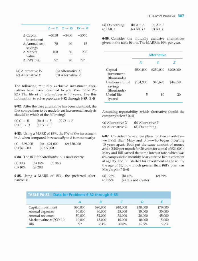
FE PRACTICE PROBLEMS 307

Z → Y Y → W W → X

� Capital −$250 −$400 −$550investment

� Annual cost 70 90 15savings

� Market 100 50 200value

� PW(15%) 97 20 ???

(a) Alternative W (b) Alternative X(c) Alternative Y (d) Alternative Z

The following mutually exclusive investment alter-natives have been presented to you. (See Table P6-82.) The life of all alternatives is 10 years. Use thisinformation to solve problems 6-82 through 6-85. (6.4)

6-82. After the base alternative has been identified, thefirst comparison to be made in an incremental analysisshould be which of the following?

(a) C → B (b) A → B (c) D → E(d) C → D (e) D → C

6-83. Using a MARR of 15%, the PW of the investmentin A when compared incrementally to B is most nearly:

(a) −$69,000 (b) −$21,000 (c) $20,000(d) $61,000 (e) $53,000

6-84. The IRR for Alternative A is most nearly:

(a) 30% (b) 15% (c) 36%(d) 10% (e) 20%

6-85. Using a MARR of 15%, the preferred Alter-native is:

TABLE P6-82 Data for Problems 6-82 through 6-85

A B C D E

Capital investment $60,000 $90,000 $40,000 $30,000 $70,000Annual expenses 30,000 40,000 25,000 15,000 35,000Annual revenues 50,000 52,000 38,000 28,000 45,000Market value at EOY 10 10,000 15,000 10,000 10,000 15,000IRR ??? 7.4% 30.8% 42.5% 9.2%

(a) Do nothing (b) Alt. A (c) Alt. B(d) Alt. C (e) Alt. D (f) Alt. E

6-86. Consider the mutually exclusive alternativesgiven in the table below. The MARR is 10% per year.

Alternative

X Y Z

Capital $500,000 $250,000 $400,000investment(thousands)

Uniform annual $131,900 $40,690 $44,050savings(thousands)

Useful life 5 10 20(years)

Assuming repeatability, which alternative should thecompany select? (6.5)

(a) Alternative X (b) Alternative Y(c) Alternative Z (d) Do nothing

6-87. Consider the savings plans for two investors—we’ll call them Mary and Bill—who began investing10 years apart. Both put the same amount of moneyaside ($100 per month for 20 years for a total of $24,000).Mary and Bill earned the same interest rate, which was8% compounded monthly. Mary started her investmentat age 35, and Bill started his investment at age 45. Bythe age of 65, how much greater than Bill’s plan wasMary’s plan? (6.6)

(a) 122% (b) 48% (c) 89%(d) 55% (e) It is not greater

CHAPTER 7

Depreciation and Income Taxes

The objective of Chapter 7 is to explain how depreciation affects incometaxes and how income taxes affect economic decision making.

The After-Tax Cost of ProducingElectricity

T he PennCo Electric Utility Company is going to construct an800 megawatt (MW) coal-fired plant that will have a 30-yearoperating life. The $1.12-billion construction cost will be depre-

ciated with the straight-line method over 30 years to a terminal book value ofzero. Its market value will also be negligible after 30 years. This plant’s efficiencywill be 35%, its capacity factor is estimated to be 80%, and annual operatingand maintenance expenses are expected to be $0.02 per kilowatt hour (kWh). Inaddition, the cost of coal is estimated to average $3.50 per million Btu, and thetax on carbon dioxide emissions will be $15 per metric ton. Burning coal emits90 metric tons of CO2 per billion Btu produced. If the effective income tax rate forPennCo is 40%, what is the after-tax cost of electricity per year for this plant? Thefirm’s after-tax minimum attractive rate of return (MARR) is 10% per year. Afterstudying this chapter, you will be able to include the impact of income taxes onengineering projects and answer this question (see Example 7-14).

308

Nothing in this world is certain but death and taxes.

—Benjamin Franklin (1789)

7.1 IntroductionTaxes have been collected since the dawn of civilization. Interestingly, in the UnitedStates, a federal income tax did not exist until March 13, 1913, when Congressenacted the Sixteenth Amendment to the Constitution.∗ Most organizationsconsider the effect of income taxes on the financial results of a proposed engineeringproject because income taxes usually represent a significant cash outflow thatcannot be ignored in decision making. Based on the previous chapters, we cannow describe how income tax liabilities (or credits) and after-tax cash flows aredetermined in engineering practice. In this chapter, an After-Tax Cash Flow (ATCF)procedure will be used in capital investment analysis because it avoids innumer-able problems associated with measuring corporate net income. This theoreticallysound procedure provides a quick and relatively easy way to define a project’sprofitability.†

Because the amount of material included in the Internal Revenue Code (and instate and municipal laws, where they exist) is very extensive, only selected partsof the subject can be discussed within the scope of this textbook. Our focus inthis chapter is federal corporate income taxes and their general effect on the financialresults of proposed engineering projects. The material presented is for educationalpurposes. In practice, you should seek expert counsel when analyzing a specificproject.

Due to the effect of depreciation on the ATCFs of a project, this topic is discussedfirst. The selected material on depreciation will then be used in the remainder ofthe chapter for accomplishing after-tax analyses of engineering projects.

7.2 Depreciation Concepts and Terminology

Depreciation is the decrease in value of physical properties with the passageof time and use. More specifically, depreciation is an accounting concept thatestablishes an annual deduction against before-tax income such that the effect oftime and use on an asset’s value can be reflected in a firm’s financial statements.

∗ During the Civil War, a federal income tax rate of 3% was initially imposed in 1862 by the Commissioner of InternalRevenue to help pay for war expenditures. The federal rate was later raised to 10%, but eventually eliminated in 1872.† ATCF is used throughout this book as a measure of the after-tax profitability of an investment project. Other measures,however, are employed for this purpose by management accountants (net income after taxes) and finance professionals(free cash flow). For additional information, refer to Horngren, Sundem, and Stratton (Management Accounting) andBodie and Merton (Finance) in Appendix F.

309

310 CHAPTER 7 / DEPRECIATION AND INCOME TAXES

Depreciation is a noncash cost that is intended to “match” the yearly fractionof value used by an asset in the production of income over the asset’s life. Theactual amount of depreciation can never be established until the asset is retiredfrom service. Because depreciation is a noncash cost that affects income taxes, wemust consider it properly when making after-tax engineering economy studies.

Depreciable property is property for which depreciation is allowed underfederal, state, or municipal income tax laws and regulations. To determine whetherdepreciation deductions can be taken, the classification of various types of propertymust be understood. In general, property is depreciable if it meets the followingbasic requirements:

1. It must be used in business or held to produce income.2. It must have a determinable useful life (defined in Section 7.2.2), and the life

must be longer than one year.3. It must be something that wears out, decays, gets used up, becomes obsolete,

or loses value from natural causes.4. It is not inventory, stock in trade, or investment property.

Depreciable property is classified as either tangible or intangible. Tangible propertycan be seen or touched, and it includes two main types called personal propertyand real property. Personal property includes assets such as machinery, vehicles,equipment, furniture, and similar items. In contrast, real property is land andgenerally anything that is erected on, growing on, or attached to land. Land itself,however, is not depreciable, because it does not have a determinable life.

Intangible property is personal property such as a copyright, patent, orfranchise. We will not discuss the depreciation of intangible assets in this chapterbecause engineering projects rarely include this class of property.

A company can begin to depreciate property it owns when the property isplaced in service for use in the business and for the production of income. Propertyis considered to be placed in service when it is ready and available for a specificuse, even if it is not actually used yet. Depreciation stops when the cost of placingan asset in service has been recovered or when the asset is sold, whichever occursfirst.

7.2.1 Depreciation Methods and Related Time Periods

The depreciation methods permitted under the Internal Revenue Code havechanged with time. In general, the following summary indicates the primary methodsused for property placed in service during three distinct time periods:

Before 1981 Several methods could be elected for depreciating propertyplaced in service before 1981. The primary methods used were Straight-Line (SL),Declining-Balance (DB), and Sum of the Years Digits (SYD). We will refer to thesemethods, collectively, as the classical, or historical, methods of depreciation.

After 1980 and before 1987 For federal income taxes, tangible propertyplaced in service during this period must be depreciated by using the AcceleratedCost Recovery System (ACRS). This system was implemented by the EconomicRecovery Tax Act of 1981 (ERTA).

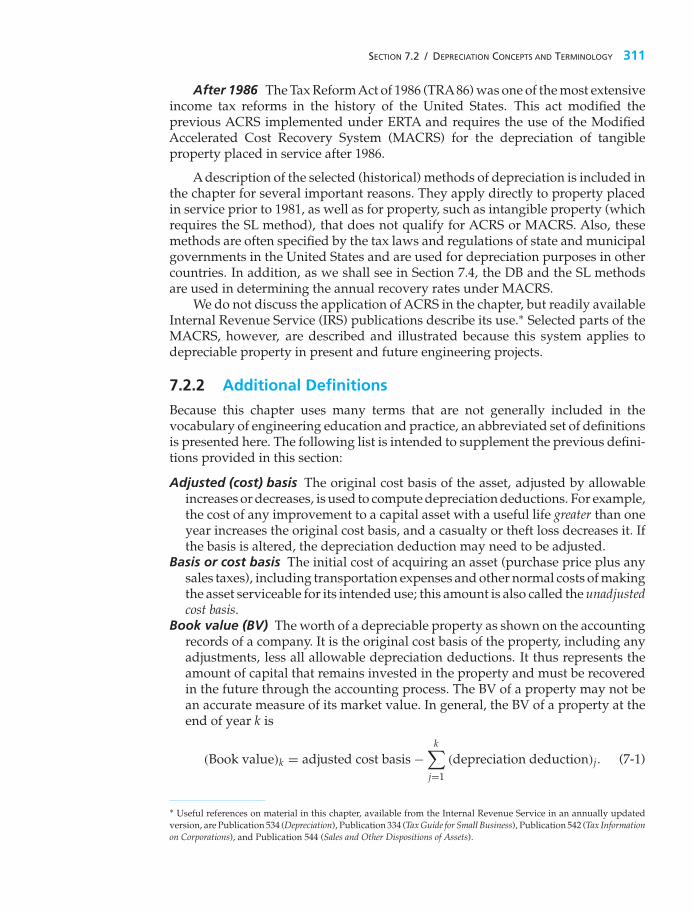
SECTION 7.2 / DEPRECIATION CONCEPTS AND TERMINOLOGY 311

After 1986 The Tax Reform Act of 1986 (TRA86) was one of the most extensiveincome tax reforms in the history of the United States. This act modified theprevious ACRS implemented under ERTA and requires the use of the ModifiedAccelerated Cost Recovery System (MACRS) for the depreciation of tangibleproperty placed in service after 1986.

A description of the selected (historical) methods of depreciation is included inthe chapter for several important reasons. They apply directly to property placedin service prior to 1981, as well as for property, such as intangible property (whichrequires the SL method), that does not qualify for ACRS or MACRS. Also, thesemethods are often specified by the tax laws and regulations of state and municipalgovernments in the United States and are used for depreciation purposes in othercountries. In addition, as we shall see in Section 7.4, the DB and the SL methodsare used in determining the annual recovery rates under MACRS.

We do not discuss the application of ACRS in the chapter, but readily availableInternal Revenue Service (IRS) publications describe its use.∗ Selected parts of theMACRS, however, are described and illustrated because this system applies todepreciable property in present and future engineering projects.

7.2.2 Additional Definitions

Because this chapter uses many terms that are not generally included in thevocabulary of engineering education and practice, an abbreviated set of definitionsis presented here. The following list is intended to supplement the previous defini-tions provided in this section:

Adjusted (cost) basis The original cost basis of the asset, adjusted by allowableincreases or decreases, is used to compute depreciation deductions. For example,the cost of any improvement to a capital asset with a useful life greater than oneyear increases the original cost basis, and a casualty or theft loss decreases it. Ifthe basis is altered, the depreciation deduction may need to be adjusted.

Basis or cost basis The initial cost of acquiring an asset (purchase price plus anysales taxes), including transportation expenses and other normal costs of makingthe asset serviceable for its intended use; this amount is also called the unadjustedcost basis.

Book value (BV) The worth of a depreciable property as shown on the accountingrecords of a company. It is the original cost basis of the property, including anyadjustments, less all allowable depreciation deductions. It thus represents theamount of capital that remains invested in the property and must be recoveredin the future through the accounting process. The BV of a property may not bean accurate measure of its market value. In general, the BV of a property at theend of year k is

(Book value)k = adjusted cost basis −k∑

j=1

(depreciation deduction)j. (7-1)

∗ Useful references on material in this chapter, available from the Internal Revenue Service in an annually updatedversion, are Publication 534 (Depreciation), Publication 334 (Tax Guide for Small Business), Publication 542 (Tax Informationon Corporations), and Publication 544 (Sales and Other Dispositions of Assets).

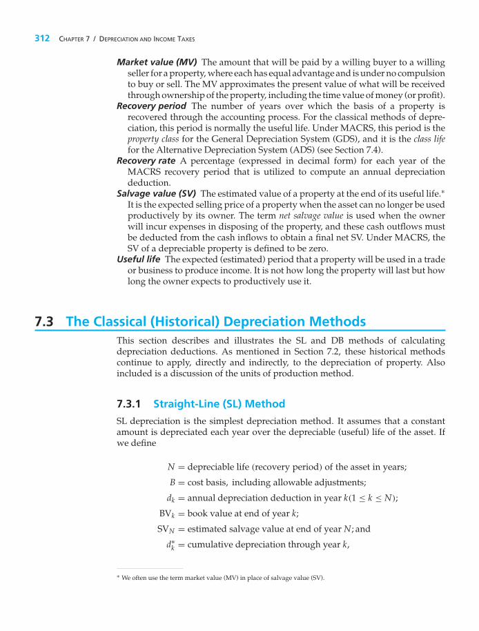
312 CHAPTER 7 / DEPRECIATION AND INCOME TAXES

Market value (MV) The amount that will be paid by a willing buyer to a willingseller for a property, where each has equal advantage and is under no compulsionto buy or sell. The MV approximates the present value of what will be receivedthrough ownership of the property, including the time value of money (or profit).

Recovery period The number of years over which the basis of a property isrecovered through the accounting process. For the classical methods of depre-ciation, this period is normally the useful life. Under MACRS, this period is theproperty class for the General Depreciation System (GDS), and it is the class lifefor the Alternative Depreciation System (ADS) (see Section 7.4).

Recovery rate A percentage (expressed in decimal form) for each year of theMACRS recovery period that is utilized to compute an annual depreciationdeduction.

Salvage value (SV) The estimated value of a property at the end of its useful life.∗It is the expected selling price of a property when the asset can no longer be usedproductively by its owner. The term net salvage value is used when the ownerwill incur expenses in disposing of the property, and these cash outflows mustbe deducted from the cash inflows to obtain a final net SV. Under MACRS, theSV of a depreciable property is defined to be zero.

Useful life The expected (estimated) period that a property will be used in a tradeor business to produce income. It is not how long the property will last but howlong the owner expects to productively use it.

7.3 The Classical (Historical) Depreciation MethodsThis section describes and illustrates the SL and DB methods of calculatingdepreciation deductions. As mentioned in Section 7.2, these historical methodscontinue to apply, directly and indirectly, to the depreciation of property. Alsoincluded is a discussion of the units of production method.

7.3.1 Straight-Line (SL) Method

SL depreciation is the simplest depreciation method. It assumes that a constantamount is depreciated each year over the depreciable (useful) life of the asset. Ifwe define

N = depreciable life (recovery period) of the asset in years;

B = cost basis, including allowable adjustments;

dk = annual depreciation deduction in year k(1 ≤ k ≤ N);

BVk = book value at end of year k;

SVN = estimated salvage value at end of year N; and

d∗k = cumulative depreciation through year k,

∗ We often use the term market value (MV) in place of salvage value (SV).

SECTION 7.3 / THE CLASSICAL (HISTORICAL) DEPRECIATION METHODS 313

then dk = (B − SVN)/N, (7-2)

d∗k

= k · dk for 1 ≤ k ≤ N, (7-3)

BVk = B − d∗k . (7-4)

Note that, for this method, you must have an estimate of the final SV, whichwill also be the final BV at the end of year N. In some cases, the estimated SVN maynot equal an asset’s actual terminal MV.

EXAMPLE 7-1 SL Depreciation

A laser surgical tool has a cost basis of $200,000 and a five-year depreciablelife. The estimated SV of the laser is $20,000 at the end of five years. Determinethe annual depreciation amounts using the SL method. Tabulate the annualdepreciation amounts and the book value of the laser at the end of each year.

SolutionThe depreciation amount, cumulative depreciation, and BV for each year areobtained by applying Equations (7-2), (7-3), and (7-4). Sample calculations foryear three are as follows:

d3 = $200,000 − $20,0005

= $36,000

d∗3 = 3

($200,000 − $20,000

5

)= $108,000

BV3 = $200,000 − $108,000 = $92,000

The depreciation and BV amounts for each year are shown in the following table.

EOY, k dk BVk

0 — $200,0001 $36,000 $164,0002 $36,000 $128,0003 $36,000 $92,0004 $36,000 $56,0005 $36,000 $20,000

Note that the BV at the end of the depreciable life is equal to the SV used tocalculate the yearly depreciation amount.

314 CHAPTER 7 / DEPRECIATION AND INCOME TAXES

7.3.2 Declining-Balance (DB) Method

In the DB method, sometimes called the constant-percentage method or the Mathesonformula, it is assumed that the annual cost of depreciation is a fixed percentage ofthe BV at the beginning of the year. The ratio of the depreciation in any one yearto the BV at the beginning of the year is constant throughout the life of the assetand is designated by R (0 ≤ R ≤ 1). In this method, R = 2/N when a 200% DB isbeing used (i.e., twice the SL rate of 1/N), and N equals the depreciable (useful)life of an asset. If the 150% DB method is specified, then R = 1.5/N. The followingrelationships hold true for the DB method:

d1 = B(R), (7-5)

dk = B(1 − R)k−1(R), (7-6)

d∗k = B[1 − (1 − R)k], (7-7)

BVk = B(1 − R)k . (7-8)

Notice that Equations (7-5) through (7-8) do not contain a term for SVN .

EXAMPLE 7-2 DB Depreciation

A new electric saw for cutting small pieces of lumber in a furniture manufac-turing plant has a cost basis of $4,000 and a 10-year depreciable life. The esti-mated SV of the saw is zero at the end of 10 years. Use the DB method to calculatethe annual depreciation amounts when

(a) R = 2/N (200% DB method)(b) R = 1.5/N (150% DB method).

Tabulate the annual depreciation amount and BV for each year.

SolutionAnnual depreciation, cumulative depreciation, and BV are determined by usingEquations (7-6), (7-7), and (7-8), respectively. Sample calculations for year sixare as follows:

(a)

R = 2/10 = 0.2,

d6 = $4,000(1 − 0.2)5(0.2) = $262.14,

d∗6 = $4,000[1 − (1 − 0.2)6] = $2,951.42,

BV6 = $4,000(1 − 0.2)6 = $1,048.58.

(b)

R = 1.5/10 = 0.15,

d6 = $4,000(1 − 0.15)5(0.15) = $266.22,

SECTION 7.3 / THE CLASSICAL (HISTORICAL) DEPRECIATION METHODS 315

d∗6 = $4,000[1 − (1 − 0.15)6] = $2,491.40,

BV6 = $4,000(1 − 0.15)6 = $1,508.60.

The depreciation and BV amounts for each year, when R = 2/N = 0.2, are shownin the following table:

200% DB Method Only

EOY, k dk BVk

0 — $4,0001 $800 3,2002 640 2,5603 512 2,0484 409.60 1,638.405 327.68 1,310.726 262.14 1,048.587 209.72 838.868 167.77 671.099 134.22 536.87

10 107.37 429.50

7.3.3 DB with Switchover to SL

Because the DB method never reaches a BV of zero, it is permissible to switch fromthis method to the SL method so that an asset’s BVN will be zero (or some otherdetermined amount, such as SVN ). Also, this method is used in calculating theMACRS recovery rates (shown later in Table 7-3).

Table 7-1 illustrates a switchover from double DB depreciation to SL depre-ciation for Example 7-2. The switchover occurs in the year in which an equal ora larger depreciation amount is obtained from the SL method. From Table 7-1, itis apparent that d6 = $262.14. The BV at the end of year six (BV6) is $1,048.58.Additionally, observe that BV10 is $4,000−$3,570.50 = $429.50 without switchoverto the SL method in Table 7-1. With switchover, BV10 equals zero. It is clear that thisasset’s dk , d∗

k , and BVk in years 7 through 10 are established from the SL method,which permits the full cost basis to be depreciated over the 10-year recovery period.

7.3.4 Units-of-Production Method

All the depreciation methods discussed to this point are based on elapsed time(years) on the theory that the decrease in value of property is mainly a functionof time. When the decrease in value is mostly a function of use, depreciation maybe based on a method not expressed in terms of years. The units-of-productionmethod is normally used in this case.

316 CHAPTER 7 / DEPRECIATION AND INCOME TAXES

TABLE 7-1 The 200% DB Method with Switchover to theSL Method (Example 7-2)

Depreciation Method

(1) (2) (3) (4)Beginning- 200% DB SL Depreciation

Year, k of-Year BVa Methodb Methodc Amount Selectedd

1 $4,000.00 $800.00 >$400.00 $800.002 3,200.00 640.00 >355.56 640.003 2,560.00 512.00 >320.00 512.004 2,048.00 409.60 >292.57 409.605 1,638.40 327.68 >273.07 327.686 1,310.72 262.14 =262.14 262.14 (switch)7 1,048.58 209.72 <262.14 262.148 786.44 167.77 <262.14 262.149 524.30 134.22 <262.14 262.14

10 262.16 107.37 <262.14 262.14

$3,570.50 $4,000.00

a Column 1 for year k less column 4 for year k equals the entry in column 1 for yeark + 1.b 200%(= 2/10) of column 1.c Column 1 minus estimated SVN divided by the remaining years from the beginningof the year through the 10th year.d Select the larger amount in column 2 or column 3.

This method results in the cost basis (minus final SV) being allocated equallyover the estimated number of units produced during the useful life of the asset.The depreciation rate is calculated as

Depreciationper unit of production = B − SVN

(Estimated lifetime production units). (7-9)

EXAMPLE 7-3 Depreciation Based on Activity

A piece of equipment used in a business has a basis of $50,000 and is expected tohave a $10,000 SV when replaced after 30,000 hours of use. Find its depreciationrate per hour of use, and find its BV after 10,000 hours of operation.

Solution

Depreciation per unit of production = $50,000 − $10,00030,000 hours

= $1.33 per hour.

After 10,000 hours, BV = $50,000 − $1.33hour

(10,000 hours), or BV = $36,700.

SECTION 7.4 / THE MODIFIED ACCELERATED COST RECOVERY SYSTEM 317

7.4 The Modified Accelerated Cost Recovery SystemAs we discussed in Section 7.2.1, the MACRS was created by TRA 86 and isnow the principal method for computing depreciation deductions for property inengineering projects. MACRS applies to most tangible depreciable property placedin service after December 31, 1986. Examples of assets that cannot be depreciatedunder MACRS are property you elect to exclude because it is to be depreciatedunder a method that is not based on a term of years (units-of-production method)and intangible property. Previous depreciation methods have required estimates ofuseful life (N) and SV at the end of useful life (SVN ). Under MACRS, however, SVNis defined to be zero, and useful life estimates are not used directly in calculatingdepreciation amounts.

MACRS consists of two systems for computing depreciation deductions. Themain system is called the General Depreciation System (GDS), and the secondsystem is called the Alternative Depreciation System (ADS).

In general, ADS provides a longer recovery period and uses only the SLmethod of depreciation. Property that is placed in any tax-exempt use and propertyused predominantly outside the United States are examples of assets that must bedepreciated under ADS. Any property that qualifies under GDS, however, can bedepreciated under ADS, if elected.

When an asset is depreciated under MACRS, the following information isneeded before depreciation deductions can be calculated:

1. The cost basis (B)2. The date the property was placed in service3. The property class and recovery period4. The MACRS depreciation method to be used (GDS or ADS)5. The time convention that applies (half year)

The first two items were discussed in Section 7.2. Items 3 through 5 are discussedin the sections that follow.

7.4.1 Property Class and Recovery Period

Under MACRS, tangible depreciable property is categorized (organized) into assetclasses. The property in each asset class is then assigned a class life, GDS recoveryperiod (and property class), and ADS recovery period. For our use, a partial listing ofdepreciable assets used in business is provided in Table 7-2. The types of depreciableproperty grouped together are identified in the second column. Then the class life,GDS recovery period (and property class), and ADS recovery period (all in years)for these assets are listed in the remaining three columns.

Under the GDS, the basic information about property classes and recoveryperiods is as follows:

1. Most tangible personal property is assigned to one of six personal property classes(3-, 5-, 7-, 10-, 15-, and 20-year property). The personal property class (in years)is the same as the GDS recovery period. Any depreciable personal property that

318 CHAPTER 7 / DEPRECIATION AND INCOME TAXES

TABLE 7-2 MACRS Class Lives and Recovery Periodsa

Recovery Period

Asset Class Description of Assets Class Life GDSb ADS

00.11 Office furniture and equipment 10 7 1000.12 Information systems, including

computers6 5 5

00.22 Automobiles, taxis 3 5 500.23 Buses 9 5 900.241 Light general purpose trucks 4 5 500.242 Heavy general purpose trucks 6 5 600.26 Tractor units for use over the road 4 3 401.1 Agriculture 10 7 1010.0 Mining 10 7 1013.2 Production of petroleum and natural gas 14 7 1413.3 Petroleum refining 16 10 1615.0 Construction 6 5 622.3 Manufacture of carpets 9 5 924.4 Manufacture of wood products and

furniture10 7 10

28.0 Manufacture of chemicals and alliedproducts

9.5 5 9.5

30.1 Manufacture of rubber products 14 7 1432.2 Manufacture of cement 20 15 2034.0 Manufacture of fabricated metal products 12 7 1236.0 Manufacture of electronic components,

products, and systems6 5 6

37.11 Manufacture of motor vehicles 12 7 1237.2 Manufacture of aerospace products 10 7 1048.12 Telephone central office equipment 18 10 1849.13 Electric utility steam production plant 28 20 2849.21 Gas utility distribution facilities 35 20 3579.0 Recreation 10 7 10

a Partial listing abstracted from How to Depreciate Property, IRS Publication 946, Tables B-1 and B-2, 2006.b Also the GDS property class.

does not “fit” into one of the defined asset classes is depreciated as being in theseven-year property class.

2. Real property is assigned to two real property classes: nonresidential real propertyand residential rental property.

3. The GDS recovery period is 39 years for nonresidential real property (31.5 years ifplaced in service before May 13, 1993) and 27.5 years for residential real property.

The following is a summary of basic information for the ADS:

1. For tangible personal property, the ADS recovery period is shown in the lastcolumn on the right of Table 7-2 (and is normally the same as the class life of theproperty; there are exceptions such as those shown in asset classes 00.12 and00.22).

SECTION 7.4 / THE MODIFIED ACCELERATED COST RECOVERY SYSTEM 319

2. Any tangible personal property that does not fit into one of the asset classes isdepreciated under a 12-year ADS recovery period.

3. The ADS recovery period for nonresidential real property is 40 years.

The use of these rules under the MACRS is discussed further in the next section.

7.4.2 Depreciation Methods, Time Convention,and Recovery Rates

The primary methods used under MACRS for calculating the depreciationdeductions over the recovery period of an asset are summarized as follows:

1. GDS 3-, 5-, 7-, and 10-year personal property classes: The 200% DB method,which switches to the SL method when that method provides a greater dedu-ction. The DB method with switchover to SL was illustrated in Section 7.3.3.

2. GDS 15- and 20-year personal property classes: The 150% DB method, whichswitches to the SL method when that method provides a greater deduction.

3. GDS nonresidential real and residential rental property classes: The SL methodover the fixed GDS recovery periods.

4. ADS: The SL method for both personal and real property over the fixed ADSrecovery periods.

A half-year time convention is used in MACRS depreciation calculations fortangible personal property. This means that all assets placed in service duringthe year are treated as if use began in the middle of the year, and one-half year ofdepreciation is allowed. When an asset is disposed of, the half-year convention isalso allowed. If the asset is disposed of before the full recovery period is used, then onlyhalf of the normal depreciation deduction can be taken for that year.

The GDS recovery rates (rk) for the six personal property classes that we will usein our depreciation calculations are listed in Table 7-3. The GDS personal propertyrates in Table 7-3 include the half-year convention, as well as switchover from theDB method to the SL method when that method provides a greater deduction. Notethat, if an asset is disposed of in year N, the final BV of the asset will be zero.

The depreciation deduction (dk) for an asset under MACRS (GDS) is com-puted with

dk = rk·B; 1 ≤ k ≤ N, (7-10)

where rk = recovery rate for year k from Table 7-3.The information in Table 7-4 provides a summary of the principal features of

GDS under MACRS. Included are some selected special rules about depreciableassets. A flow diagram for computing depreciation deductions under MACRS isshown in Figure 7-1. As indicated in the figure, an important choice is whether themain GDS is to be used for an asset or whether ADS is elected instead (or required).Normally, the choice would be to use the GDS for calculating the depreciationdeductions.

320 CHAPTER 7 / DEPRECIATION AND INCOME TAXES

TABLE 7-3 GDS Recovery Rates (rk) for the Six Personal Property Classes

Depreciation Rate for Recovery Period

Year 3-yeara 5-yeara 7-yeara 10-yeara 15-yearb 20-yearb

1 0.3333 0.2000 0.1429 0.1000 0.0500 0.03752 0.4445 0.3200 0.2449 0.1800 0.0950 0.07223 0.1481 0.1920 0.1749 0.1440 0.0855 0.06684 0.0741 0.1152 0.1249 0.1152 0.0770 0.06185 0.1152 0.0893 0.0922 0.0693 0.0571

6 0.0576 0.0892 0.0737 0.0623 0.05287 0.0893 0.0655 0.0590 0.04898 0.0446 0.0655 0.0590 0.04529 0.0656 0.0591 0.0447

10 0.0655 0.0590 0.0447

11 0.0328 0.0591 0.044612 0.0590 0.044613 0.0591 0.044614 0.0590 0.044615 0.0591 0.0446

16 0.0295 0.044617 0.044618 0.044619 0.044620 0.044621 0.0223

Source: IRS Publication 946. Depreciation. Washington, D.C.: U.S. Government Printing Office, for 2006tax returns.aThese rates are determined by applying the 200% DB method (with switchover to the SL method) tothe recovery period with the half-year convention applied to the first and last years. Rates for eachperiod must sum to 1.0000.bThese rates are determined with the 150% DB method instead of the 200% DB method (with switchoverto the SL method) and are rounded off to four decimal places.

EXAMPLE 7-4 MACRS Depreciation with GDS

A firm purchased and placed in service a new piece of semiconductor manu-facturing equipment. The cost basis for the equipment is $100,000. Determine

(a) the depreciation charge permissible in the fourth year,(b) the BV at the end of the fourth year,(c) the cumulative depreciation through the third year,(d) the BV at the end of the fifth year if the equipment is disposed of at that

time.

SECTION 7.4 / THE MODIFIED ACCELERATED COST RECOVERY SYSTEM 321

TABLE 7-4 MACRS (GDS) Property Classes and Primary Methodsfor Calculating Depreciation Deductions

GDS Property Class and Class LifeDepreciation Method (Useful Life) Special Rules

3-year, 200% DB withswitchover to SL

Four years orless

Includes some race horses and tractorunits for over-the-road use.

5-year, 200% DB withswitchover to SL

More than 4years to lessthan 10

Includes cars and light trucks,semiconductor manufacturingequipment, qualified technologicalequipment, computer-basedcentral office switching equipment,some renewable and biomasspower facilities, and research anddevelopment property.

7-year, 200% DB withswitchover to SL

10 years to lessthan 16

Includes single-purpose agriculturaland horticultural structures andrailroad track. Includes officefurniture and fixtures, and propertynot assigned to a property class.

10-year, 200% DB withswitchover to SL

16 years to lessthan 20

Includes vessels, barges, tugs,and similar water transportationequipment.

15-year, 150% DB withswitchover to SL

20 years to lessthan 25

Includes sewage treatment plants,telephone distribution plants, andequipment for two-way voice anddata communication.

20-year, 150% DB withswitchover to SL

25 years ormore

Excludes real property of 27.5 years ormore. Includes municipal sewers.

27.5 year, SL N/A Residential rental property.

39-year, SL N/A Nonresidential real property.

Source: IRS Publication 946. Depreciation. Washington, D.C.: U.S. Government Printing Office, for2006 tax returns.

SolutionFrom Table 7-2, it may be seen that the semiconductor (electronic) manufacturingequipment has a class life of six years and a GDS recovery period of five years.The recovery rates that apply are given in Table 7-3.

(a) The depreciation deduction, or cost-recovery allowance, that is allowable inyear four (d4) is 0.1152 ($100,000) = $11,520.

322 CHAPTER 7 / DEPRECIATION AND INCOME TAXES

Figure 7-1Flow Diagram forComputingDepreciationDeductions underMACRS

Ascertain property class;same as recoveryperiod for personalproperty:

• Table 7-2, based on asset description• Table 7-4, based on class life

Obtain recovery rates:Table 7-3, personal property

Compute depreciationdeduction in year k (dk)by multiplying the asset’s cost basis byappropriate recoveryrate

Ascertain recovery period:

MACRS DepreciationGDS or ADS?

GDS ADS

Table 7-2, personalproperty

Compute depreciationamount:

SL �Asset’s cost basisRecovery period (years)

Compute depreciationdeduction in year k (dk):

• d1 � 0.5 (SL amount)

• d2 thru dN � SL amount

• dN�1 � 0.5 (SL amount)

(b) The BV at the end of year four (BV4) is the cost basis less depreciation chargesin years one through four:

BV4 = $100,000 − $100,000(0.20 + 0.32 + 0.192 + 0.1152)

= $17,280.

(c) Accumulated depreciation through year three, d∗3, is the sum of depreciation

amounts in years one through three:

d∗3 = d1 + d2 + d3

= $100,000(0.20 + 0.32 + 0.192)

= $71,200.

(d) The depreciation deduction in year five can only be (0.5)(0.1152)($100,000) =$5,760 when the equipment is disposed of prior to year six. Thus, the BV atthe end of year five is BV4 − $5,760 = $11,520.

SECTION 7.4 / THE MODIFIED ACCELERATED COST RECOVERY SYSTEM 323

EXAMPLE 7-5 MACRS with a Trade-in

In May 2011, your company traded in a computer and peripheral equipment,used in its business, that had a BV at that time of $25,000. A new, faster computersystem having a fair MV of $400,000 was acquired. Because the vendor acceptedthe older computer as a trade-in, a deal was agreed to whereby your companywould pay $325,000 cash for the new computer system.

(a) What is the GDS property class of the new computer system?(b) How much depreciation can be deducted each year based on this class life?

(Refer to Figure 7-1.)

Solution(a) The new computer is in Asset Class 00.12 and has a class life of six years.

(See Table 7-2.) Hence, its GDS property class and recovery period are fiveyears.

(b) The cost basis for this property is $350,000, which is the sum of the $325,000cash price of the computer and the $25,000 BV remaining on the trade-in.(In this case, the trade-in was treated as a nontaxable transaction.)

MACRS (GDS) rates that apply to the $350,000 cost basis are found inTable 7-3. An allowance (half-year) is built into the year-one rate, so it does notmatter that the computer was purchased in May 2011 instead of, say, November2011. The depreciation deductions (dk) for 2011 through 2016 are computed usingEquation (7-10) and Table 7-3.

Date Placed Cost Class MACRS (GDS)Property in Service Basis Life Recovery Period

Computer System May 2005 $350,000 6 years 5 years

Year Depreciation Deductions

2011 0.20 × $350,000 = $70,0002012 0.32 × 350,000 = 112,0002013 0.192 × 350,000 = 67,2002014 0.1152 × 350,000 = 40,3202015 0.1152 × 350,000 = 40,3202016 0.0576 × 350,000 = 20,160

Total $350,000

From Example 7-5, we can conclude that Equation 7-11 is true from the buyer’sviewpoint when property of the same type and class is exchanged:

Basis = Actual cash cost + BV of the trade-in. (7-11)

324 CHAPTER 7 / DEPRECIATION AND INCOME TAXES

To illustrate Equation (7-11), suppose your company has operated an opticalcharacter recognition (OCR) scanner for two years. Its BV now is $35,000, andits fair MV is $45,000. The company is considering a new OCR scanner that costs$105,000. Ordinarily, you would trade the old scanner for the new one and pay thedealer $60,000. The basis (B) for depreciation is then $60,000 + $35,000 = $95,000.∗

EXAMPLE 7-6 MACRS Depreciation with ADS

A large manufacturer of sheet metal products in the Midwest purchased andplaced in service a new, modern, computer-controlled flexible manufacturingsystem for $3.0 million. Because this company would not be profitable untilthe new technology had been in place for several years, it elected to utilizethe ADS under MACRS in computing its depreciation deductions. Thus, thecompany could slow down its depreciation allowances in hopes of postponingits income tax advantages until it became a profitable concern. What depreciationdeductions can be claimed for the new system?

SolutionFrom Table 7-2, the ADS recovery period for a manufacturer of fabricated metalproducts is 12 years. Under ADS, the SL method with no SV is applied tothe 12-year recovery period, using the half-year convention. Consequently, thedepreciation in year one would be

12

($3,000,000

12

)= $125,000.

Depreciation deductions in years 2 through 12 would be $250,000 eachyear, and depreciation in year 13 would be $125,000. Notice how the half-yearconvention extends depreciation deductions over 13 years (N + 1).

7.4.3 MACRS Spreadsheet

We have used electronic spreadsheets to perform complex calculations, repetitivecalculations, and to evaluate the accuracy of the estimation process. Spreadsheetscan also assist in understanding complex relationships. In this section, we seek abetter understanding of the GDS recovery rates in Table 7-3.

There is an inherent danger in taking tabulated values at face value in anyanalysis. Recall that the GDS values incorporate the half-year convention, decliningbalance and straight-line depreciation, as well as a switch from one method to theother. Electronic spreadsheets provide a framework to explore and understandthese relationships without getting bogged down with calculations.

A spreadsheet for determining the GDS recovery rate for a 5-year class life isshown in Figure 7-2. There are three user input cells: B3 for the declining balancepercentage, B4 for the class life, and E9, which is one. This last entry allows us

∗ The exchange price of the OCR scanner is $105,000−$45,000(= actual cash cost). Equation (7-11) prevents exaggeratedcost bases to be claimed for new assets having large “sticker prices” compared with their exchange price.

Figure 7-2 GDS Recovery Rate for 5-year Recovery Period Spreadsheet

325

326 CHAPTER 7 / DEPRECIATION AND INCOME TAXES

to calculate rates, rather than a depreciation amount. Cell B5 is an intermediatecalculation for R, which used in subsequent declining balance calculations.

The consequence of the half-year convention is seen in columns A and B.Column A has 6 years, rather than 5, and cell B10 adds a half-year to the remaininglife. Cell B10 is copied down to row 15.

Column C contains the straight-line depreciation calculations. The standarddepreciation equation is in cell C11 and is the ratio of the remaining book valuepercent in column E divided by the remaining life from column B. Because thedeclining balance depreciation amount is larger in the earlier years, we cannot usethe simplified straight-line depreciation approach in Equation (7-2). Cells C10 andC15 compensate for the half-year convention by taking only half of the calculatedamount.

The declining balance calculations are in column D. The standard depreciationequation is in cell D11, which is copied down to cell D14. As in column C,adjustments are necessary in D10 and D15 to adjust for the half-year convention.

The year end book value percent calculation is in cell E10:

= E9 − MAXA(C10:D10)

This equation takes the percent of remaining book value at the start of the year andsubtracts the maximum depreciation from column C and D for the current year.This result is used by columns C and D to determine the depreciation percentagein the following year.

The final GDS recovery rate equation in F10 is:

= MAXA(D10,C10)

This is the switchover component of the method. Cell F17 is a check to ensure thatthe proportions sum to unity.

To emphasize when the switch takes place, cell G10 has an equation that labelsthe switch year.

= IF(C10 >= D10, “Switch to S-L”,””)

This model has allowed us to fully examine how the GDS rates are determined.Having all intermediate results displayed, as well as the check sum in F17, permitsone to quickly identify errors in logic to speed the learning process. The equationsare general enough to be applied to the remaining property classes by extendingor contracting the number of rows. Just be sure that the final row in columns C andD have the half-year corrections in the equations.

7.5 A Comprehensive Depreciation ExampleWe now consider an asset for which depreciation is computed by the historicaland MACRS (GDS) methods previously discussed. Be careful to observe thedifferences in the mechanics of each method, as well as the differences in the annualdepreciation amounts themselves. Also, we compare the present worths (PWs) atk = 0 of selected depreciation methods when MARR = 10% per year. As we shallsee later in this chapter, depreciation methods that result in larger PWs (of thedepreciation amounts) are preferred by a firm that wants to reduce the presentworth of its income taxes paid to the government.

SECTION 7.5 / A COMPREHENSIVE DEPRECIATION EXAMPLE 327

EXAMPLE 7-7 Comparison of Depreciation Methods

The La Salle Bus Company has decided to purchase a new bus for $85,000 witha trade-in of their old bus. The old bus has a BV of $10,000 at the time of thetrade-in. The new bus will be kept for 10 years before being sold. Its estimatedSV at that time is expected to be $5,000.

First, we must calculate the cost basis. The basis is the original purchase priceof the bus plus the BV of the old bus that was traded in [Equation (7-11)]. Thus,the basis is $85,000 + $10,000, or $95,000. We need to look at Table 7-2 and findbuses, which are asset class 00.23. Hence, we find that buses have a nine-yearclass recovery period, over which we depreciate the bus with historical methodsdiscussed in Section 7.3, and a five-year GDS class life.

Solution: SL MethodFor the SL method, we use the class life of 9 years, even though the bus will bekept for 10 years. By using Equations (7-2) and (7-4), we obtain the followinginformation:

dk = $95,000 − $5,0009 years

= $10,000, for k = 1 to 9.

SL Method

EOY k dk BVk

0 — $95,0001 $10,000 85,0002 10,000 75,0003 10,000 65,0004 10,000 55,0005 10,000 45,0006 10,000 35,0007 10,000 25,0008 10,000 15,0009 10,000 5,000

Notice that no depreciation was taken after year nine because the class lifewas only nine years. Also, the final BV was the estimated SV, and the BV willremain at $5,000 until the bus is sold.

Solution: DB MethodTo demonstrate this method, we will use the 200% DB equations. With Equations(7-6) and (7-8), we calculate the following:

R = 2/9 = 0.2222;

d1 = $95,000(0.2222) = $21,111;

328 CHAPTER 7 / DEPRECIATION AND INCOME TAXES

d5 = $95,000(1 − 0.2222)4(0.2222) = $7,726;

BV5 = $95,000(1 − 0.2222)5 = $27,040.

200% DB Method

EOY k dk BVk

0 — $95,0001 $21,111 73,8892 16,420 57,4693 12,771 44,6984 9,932 34,7655 7,726 27,0406 6,009 21,0317 4,674 16,3578 3,635 12,7229 2,827 9,895

Solution: DB with Switchover to SL DepreciationTo illustrate the mechanics of Table 7-1 for this example, we first specify that thebus will be depreciated by the 200% DB method (R = 2/N). Because DB methodsnever reach a zero BV, suppose that we further specify that a switchover to SLdepreciation will be made to ensure a BV of $5,000 at the end of the vehicle’snine-year class life.

Beginning- 200% DB SL Method DepreciationEOY k of-Year BV Method (BV9 = $5,000) Amount Selected

1 $95,000 $21,111 $10,000 $21,1112 73,889 16,420 8,611 16,4203 57,469 12,771 7,496 12,7714 44,698 9,933 6,616 9,9335 34,765 7,726 5,953 7,7266 27,040 6,009 5,510 6,0097 21,031 4,674 5,344 5,344a

8 15,687 3,635 5,344 5,3449 10,344 2,827 5,344 5,344

a Switchover occurs in year seven.

SECTION 7.5 / A COMPREHENSIVE DEPRECIATION EXAMPLE 329

Solution: MACRS (GDS) with Half-Year ConventionTo demonstrate the GDS with the half-year convention, we will change the LaSalle bus problem so that the bus is now sold in year five for Part (a) and in yearsix for Part (b).

(a) Selling bus in year five:

EOY k Factor dk BVk

0 — — $95,0001 0.2000 $19,000 76,0002 0.3200 30,400 45,6003 0.1920 18,240 27,3604 0.1152 10,944 16,4165 0.0576 5,472 10,944

(b) Selling bus in year six:

EOY k Factor dk BVk

0 — — $95,0001 0.2000 $19,000 76,0002 0.3200 30,400 45,6003 0.1920 18,240 27,3604 0.1152 10,944 16,4165 0.1152 10,944 5,4726 0.0576 5,472 0

Notice that, when we sold the bus in year five before the recovery period hadended, we took only half of the normal depreciation. The other years (yearsone through four) were not changed. When the bus was sold in year six, atthe end of the recovery period, we did not divide the last year amount bytwo.

Selected methods of depreciation, illustrated in Example 7-7, are comparedin Figure 7-3. In addition, the PW (10%) of each method is shown inFigure 7-3. Because large PWs of depreciation deductions are generally viewedas desirable, it is clear that the MACRS method is very attractive to profitablecompanies.

330 CHAPTER 7 / DEPRECIATION AND INCOME TAXES

$100

90

80

70

60

50

40

30

20

10

00 1 2 3 4 5

End of Year k

Boo

k V

alue

(th

ousa

nds)

MACRS(GDS)

Zero

Straight Line

200% Declining Balance (no switchover)

PWSL (10%) � $57,590PWDB (10%) � $62,623PWMACRS (10%) � $66,973

6 7 8 9

Figure 7-3 BV Comparisons for Selected Methods of Depreciation in Example 7-7(Note: The bus is assumed to be sold in year six for the MACRS-GDS method.)

7.6 Introduction to Income TaxesUp to this point, there has been no consideration of income taxes in our discussionof engineering economy, except for the influence of depreciation and othertypes of deductions. By not complicating our studies with income tax effects,we have placed primary emphasis on basic engineering economy principles andmethodology. There, however, is a wide variety of capital investment problems inwhich income taxes do affect the choice among alternatives, and after-tax studiesare essential.∗

In the remainder of this chapter, we shall be concerned with how income taxesaffect a project’s estimated cash flows. Income taxes resulting from the profitableoperation of a firm are usually taken into account in evaluating engineering projects.The reason is quite simple: Income taxes associated with a proposed project mayrepresent a major cash outflow that should be considered together with other cashinflows and outflows in assessing the overall economic profitability of that project.

There are other taxes discussed in Section 7.6.1 that are not directly associatedwith the income-producing capability of a new project, but they are usually

∗ Some U.S. firms do not pay income taxes, but this is not a valid reason for ignoring income taxes. We assume thatmost firms have a positive taxable income in their overall operations.

SECTION 7.6 / INTRODUCTION TO INCOME TAXES 331

negligible when compared with federal and state income taxes. When other typesof taxes are included in engineering economy studies, they are normally deducted fromrevenue, as any other operating expense would be, in determining the before-tax cash flow(BTCF) that we considered in Chapters 5 and 6.

The mystery behind the sometimes complex computation of income taxes isreduced when we recognize that income taxes paid are just another type of expense,and income taxes saved (through depreciation, expenses, and direct tax credits)are identical to other kinds of reduced expenses (e.g., savings in maintenanceexpenses).

The basic concepts underlying federal and state income tax laws and regu-lations that apply to most economic analyses of capital investments generally canbe understood and applied without difficulty. This discussion of income taxes isnot intended to be a comprehensive treatment of the subject. Rather, we utilizesome of the more important provisions of the federal Tax Reform Act of 1986(TRA 86), followed by illustrations of a general procedure for computing thenet ATCF for an engineering project and conducting after-tax economic analyses.Where appropriate, important changes to TRA 86 enacted by the Omnibus BudgetReconciliation Act of 1993 (OBRA 93) and the Taxpayer Relief Act of 1997 are alsoincluded in this chapter.

7.6.1 Distinctions between Different Types of Taxes

Before discussing the consequences of income taxes in engineering economystudies, we need to distinguish between income taxes and several other typesof taxes:

1. Income taxes are assessed as a function of gross revenues minus allowabledeductions. They are levied by the federal, most state, and occasionallymunicipal governments.

2. Property taxes are assessed as a function of the value of property owned, such asland, buildings, equipment, and so on, and the applicable tax rates. Hence, theyare independent of the income or profit of a firm. They are levied by municipal,county, or state governments.

3. Sales taxes are assessed on the basis of purchases of goods or services andare thus independent of gross income or profits. They are normally levied bystate, municipal, or county governments. Sales taxes are relevant in engineeringeconomy studies only to the extent that they add to the cost of items purchased.

4. Excise taxes are federal taxes assessed as a function of the sale of certaingoods or services often considered nonnecessities and are hence independentof the income or profit of a business. Although they are usually charged tothe manufacturer or original provider of the goods or services, a portion of thecost is passed on to the purchaser.

7.6.2 The Before-Tax and After-Tax Minimum AttractiveRates of Return

In the preceding chapters, we have treated income taxes as if they are not applicable,or we have taken them into account, in general, by using a before-tax MARR,

332 CHAPTER 7 / DEPRECIATION AND INCOME TAXES

which is larger than the after-tax MARR.An approximation of the before-tax MARRrequirement, which includes the effect of income taxes, for studies involving onlyBTCF can be obtained from the following relationship:

(Before-tax MARR)[(1 − Effective income tax rate)] ∼= After-tax MARR.

Thus,

Before-tax MARR ≈ After-tax MARR(1 − Effective income tax rate)

. (7-12)

Determining the effective income tax rate for a firm is discussed in Section 7.7.This approximation is exact if the asset is nondepreciable and there are no

gains or losses on disposal, tax credits, or other types of deductions involved.Otherwise, these factors affect the amount and timing of income tax payments,and some degree of error is introduced into the relationship in Equation (7-12).

7.6.3 The Interest Rate to Use in After-Tax Studies

Any practical definition of a MARR should serve as a guide for investment policyto attain the goals toward which a firm is, or will be, striving. One obvious goal is tomeet shareholder expectations. Clearly, long-term goals and capital structure willbe changing as a firm matures. In this regard, it is widely accepted that in after-tax engineering economy studies, the MARR should be at least the tax-adjustedweighted average cost of capital (WACC):

WACC = λ(1 − t)ib + (1 − λ)ea. (7-13)

Here, λ = fraction of a firm’s pool of capital that is borrowed from lenders,t = effective income tax rate as a decimal,

ib = before-tax interest paid on borrowed capital,ea = after-tax cost of equity capital.

The adjustment on the borrowed capital component of WACC, (1 − t)ib, accountsfor the fact that interest on borrowed capital is tax deductible.

Often a value higher than the WACC is assigned to the after-tax MARR toreflect the opportunity cost of capital, perceived risk and uncertainty of projectsbeing evaluated, and policy issues such as organizational growth and shareholdersatisfaction. We are now in a position to understand how a firm’s after-tax MARR isdetermined and why its value may change substantially over time. To summarize,suppose a firms’ WACC is 10% per year. The after-tax MARR may be set at 15%per year to better reflect the business opportunities that are available for capitalinvestment. If the firm’s effective income tax rate is 40%, the approximate value ofthe before-tax MARR is 15%/(1 − 0.4) = 25% per year.

7.6.4 Taxable Income of Corporations (Business Firms)

At the end of each tax year, a corporation must calculate its net (i.e., taxable)before-tax income or loss. Several steps are involved in this process, beginningwith the calculation of gross income. The corporation may deduct from grossincome all ordinary and necessary operating expenses to conduct the businessexcept capital investments. Deductions for depreciation are permitted each tax

SECTION 7.7 / THE EFFECTIVE (MARGINAL) CORPORATE INCOME TAX RATE 333

period as a means of consistently and systematically recovering capital investment.Consequently, allowable expenses and deductions may be used to determinetaxable income:

Taxable income = Gross income − All expenses except capital investments

− Depreciation deductions. (7-14)

EXAMPLE 7-8 Determination of Taxable Income

A company generates $1,500,000 of gross income during its tax year and incursoperating expenses of $800,000. Property taxes on business assets amount to$48,000. The total depreciation deductions for the tax year equal $114,000. Whatis the taxable income of this firm?

SolutionBased on Equation (7-14), this company’s taxable income for the tax yearwould be

$1,500,000 − $800,000 − $48,000 − $114,000 = $538,000.

7.7 The Effective (Marginal) CorporateIncome Tax Rate

The federal corporate income tax rate structure in 2006 is shown in Table 7-5.Depending on the taxable income bracket that a firm is in for a tax year, themarginal federal rate can vary from 15% to a maximum of 39%. Note, however,that the weighted average tax rate at taxable income = $335,000 is 34%, and theweighted average tax rate at taxable income = $18,333,333 is 35%. Therefore, ifa corporation has a taxable income for a tax year greater than $18,333,333, federaltaxes are computed by using a flat rate of 35%.

TABLE 7-5 Corporate Federal Income Tax Rates (2006)

If Taxable Income Is: The Tax Is:

Over But Not Over of the Amount Over

0 $50,000 15% 0$50,000 75,000 $7,500 + 25% $50,000

75,000 100,000 13,750 + 34% 75,000100,000 335,000 22,250 + 39% 100,000335,000 10,000,000 113,900 + 34% 335,000

10,000,000 15,000,000 3,400,000 + 35% 10,000,00015,000,000 18,333,333 5,150,000 + 38% 15,000,00018,333,333 . . . . . . . . 35% 0

Source: Tax Information on Corporations, IRS Publication 542, 2006.

334 CHAPTER 7 / DEPRECIATION AND INCOME TAXES

EXAMPLE 7-9 Calculating Income Taxes

Suppose that a firm for a tax year has a gross income of $5,270,000, expenses(excluding capital) of $2,927,500, and depreciation deductions of $1,874,300.What would be its taxable income and federal income tax for the tax year, basedon Equation (7-14) and Table 7-5?

Solution

Taxable income = Gross income − Expenses − Depreciation deductions

= $5,270,000 − $2,927,500 − $1,874,300

= $468,200

Income tax = 15% of first $50,000 $7,500

+ 25% of the next $25,000 6,250

+ 34% of the next $25,000 8,500

+ 39% of the next $235,000 91,650

+ 34% of the next $133,200 45,288Total $159,188

The total tax liability in this case is $159,188. As an added note, we could haveused a flat rate of 34% in this example because the federal weighted average taxrate at taxable income = $335,000 is 34%. The remaining $133,200 of taxableincome above this amount is in a 34% tax bracket (Table 7-5). So we have0.34($468,200) = $159,188.

Although the tax laws and regulations of most of the states (and somemunicipalities) with income taxes have the same basic features as the federal lawsand regulations, there is significant variation in income tax rates. State income taxesare in most cases much less than federal taxes and often can be closely approximatedas ranging from 6% to 12% of taxable income. No attempt will be made here todiscuss the details of state income taxes. To illustrate the calculation of an effectiveincome tax rate (t) for a large corporation based on the consideration of both federaland state income taxes, however, assume that the applicable federal income taxrate is 35% and the state income tax rate is 8%. Further assume the common case inwhich taxable income is computed the same way for both types of taxes, except thatstate income taxes are deductible from taxable income for federal tax purposes, butfederal income taxes are not deductible from taxable income for state tax purposes.Based on these assumptions, the general expression for the effective income taxrate is

t = State rate + Federal rate(1 − State rate), or (7-15)

t = Federal rate + (1 − Federal rate)(State rate). (7-16)

SECTION 7.7 / THE EFFECTIVE (MARGINAL) CORPORATE INCOME TAX RATE 335

6,000

5,000

3,400

100

20

10

25 50 75 100 375

$6,416,667

0.38

0.35

0.35

0.34

0.39

0.34

0.25

0.15

$5,150,000

$3,400,000

$113,900

$22,250

$13,750

$7,500

10,000

Taxable Income from Equation (7-14) (thousands of dollars)

Fede

ral I

ncom

e Ta

x (t

hous

ands

of d

olla

rs)

Incrementaltaxable income

Incremental income tax

18,33315,000

Taxable incomewithout proposedproject

Taxableincomewith theproposedproject

Figure 7-4 The Federal Income Tax Rates for Corporations (Table 7-5) with IncrementalIncome Tax for a Proposed Project (assumes, in this case, corporate taxable income withoutproject > $18,333,333)

In this example, the effective income tax rate for the corporation would be

t = 0.08 + 0.35(1 − 0.08) = 0.402, or approximately 40%.

In this chapter, we will often use an effective corporate income tax rate ofapproximately 40% as a representative value that includes state income taxes.

The effective income tax rate on increments of taxable income is of importance inengineering economy studies. This concept is illustrated in Figure 7-4, which plotsthe federal income tax rates and brackets listed in Table 7-5 and shows the added(incremental) taxable income and federal income taxes that would result from aproposed engineering project (shaded in Figure 7-4). In this case, the corporationis assumed to have a taxable income greater than $18,333,333 for their tax year. Thesame concept, however, applies to a smaller firm with less taxable income for itstax year, which is illustrated in Example 7-10.

EXAMPLE 7-10 Project-Based Income Taxes

A small corporation is expecting an annual taxable income of $45,000 for itstax year. It is considering an additional capital investment of $100,000 in anengineering project, which is expected to create an added annual net cash

336 CHAPTER 7 / DEPRECIATION AND INCOME TAXES

flow (revenues minus expenses) of $35,000 and an added annual depreciationdeduction of $20,000. What is the corporation’s federal income tax liability

(a) without the added capital investment,(b) with the added capital investment?

Solution(a) Income Taxes Rate Amount

On first $45,000 15% $6,750Total $6,750

(b) Taxable IncomeBefore added investment $45,000+ added net cash flow +35,000− depreciation deduction −20,000

Taxable Income $60,000

Income Taxes on $60,000 Rate AmountOn first $50,000 15% $7,500On next $10,000 25% 2,500

Total $10,000

The increased income tax liability from the investment is $10,000 − $6,750 =$3,250.

As an added note, the change in tax liability can usually be determinedmore readily by an incremental approach. For instance, this example involvedchanging the taxable income from $45,000 to $60,000 as a result of the newinvestment. Thus, the change in income taxes for the tax year could be calculatedas follows:

First $50,000 − $45,000 = $5,000 at 15% = $750

Next $60,000 − $50,000 = $10,000 at 25% = 2,500Total $3,250

The average federal income tax rate on the additional $35,000 − $20,000 =$15,000 of taxable income is calculated as ($3,250/$15,000) = 0.2167, or 21.67%.

7.8 Gain (Loss) on the Disposal of an AssetWhen a depreciable asset (tangible personal or real property, Section 7.2) is sold, theMV is seldom equal to its BV [Equation (7-1)]. In general, the gain (loss) on saleof depreciable property is the fair market value minus its book value at that time.That is,

[Gain (loss) on disposal]N = MVN − BVN . (7-17)

SECTION 7.9 / GENERAL PROCEDURE FOR MAKING AFTER-TAX ECONOMIC ANALYSES 337

When the sale results in a gain, it is often referred to as depreciation recapture. Thetax rate for the gain (loss) on disposal of depreciable personal property is usuallythe same as for ordinary income or loss, which is the effective income tax rate, t.

When a capital asset is sold or exchanged, the gain (loss) is referred to as a capitalgain (loss). Examples of capital assets are stocks, bonds, gold, silver, and othermetals, as well as real property such as a home. Because engineering economicanalysis seldom involves an actual capital gain (loss), the more complex details ofthis situation are not discussed further.

EXAMPLE 7-11 Tax Consequences of Selling an Asset

A corporation sold a piece of equipment during the current tax year for$78,600. The accounting records show that its cost basis, B, is $190,000 and theaccumulated depreciation is $139,200. Assume that the effective income tax rateas a decimal is 0.40 (40%). Based on this information, what is

(a) the gain (loss) on disposal,(b) the tax liability (or credit) resulting from this sale,(c) the tax liability (or credit) if the accumulated depreciation was $92,400

instead of $139,200?

Solution(a) The BV at the time of sale is $190,000 − $139,200 = $50,800. Therefore, the

gain on disposal is $78,600 − $50,800 = $27,800.(b) The tax owed on this gain is −0.40($27,800) = −$11,120.(c) With d∗

k = $92,400, the BV at the time of sale is $190,000−$92,400 = $97,600.The loss is $78,600 − $97,600 = −$19,000. The tax credit resulting from thisloss on disposal is −0.40(−$19,000) = $7,600.

7.9 General Procedure for MakingAfter-Tax Economic Analyses

After-tax economic analyses utilize the same profitability measures as do before-tax analyses. The only difference is that ATCFs are used in place of before-taxcash flows (BTCFs) by including expenses (or savings) to income taxes and thenmaking equivalent worth calculations using an after-tax MARR. The tax rates andgoverning regulations may be complex and subject to changes, but, once those ratesand regulations have been translated into their effect on ATCFs, the remainder ofthe after-tax analysis is relatively straightforward. To formalize the procedure, let

Rk = revenues (and savings) from the project (this is the cash inflow fromthe project during period k);

Ek = cash outflows during year k for deductible expenses;

338 CHAPTER 7 / DEPRECIATION AND INCOME TAXES

dk = sum of all noncash, or book, costs during year k, such as depreciation;t = effective income tax rate on ordinary income (federal, state, and other),

with t assumed to remain constant during the study period;Tk = income tax consequences during year k;

ATCFk = ATCF from the project during year k.

Because the taxable income is (Rk − Ek − dk), the ordinary income tax consequencesduring year k are computed with Equation (7-18):

Tk = −t(Rk − Ek − dk). (7-18)

Therefore, when Rk > (Ek + dk), a tax liability (i.e., negative cash flow) occurs.When Rk < (Ek + dk), a decrease in the tax amount (a credit) occurs.

In the economic analyses of engineering projects, ATCFs in year k can becomputed in terms of BTCFk (i.e., BTCF in year k):

BTCFk = Rk − Ek . (7-19)

Thus,∗

ATCFk = BTCFk + Tk (7-20)

= (Rk − Ek) − t(Rk − Ek − dk)

= (1 − t)(Rk − Ek) + tdk . (7-21)

Equation (7-21) shows that after income taxes, a revenue becomes (1 − t)Rk and anexpense becomes (1 − t)Ek . Note that the ATCF attributable to depreciation (a taxsavings) is tdk in year k.

Tabular headings to facilitate the computation of ATCFs using Equations (7-18)and (7-21) are as follows:

(C) = (A) − (B) (D) = −t(C)(A) (B) Taxable Cash Flow for (E) = (A) + (D)

Year BTCF Depreciation Income Income Taxes ATCF

k Rk − Ek dk Rk − Ek − dk −t(Rk − Ek − dk) (1 − t)(Rk − Ek) + tdk

Column A consists of the same information used in before-tax analyses, namelythe cash revenues (or savings) less the deductible expenses. Column B containsdepreciation that can be claimed for tax purposes. Column C is the taxable incomeor the amount subject to income taxes. Column D contains the income taxes paid (orsaved). Finally, column E shows the ATCFs to be used directly in after-tax economicanalyses.

Anote of caution concerning the definition of BTCFs (and ATCFs) for projects isin order at this point. BTCF is defined to be annual revenue (or savings) attributableto a project minus its annual cash expenses. These expenses should not includeinterest and other financial cash flows. The reason is that project cash flows shouldbe analyzed separately from financial cash flows. Including interest expense withproject cash flows is incorrect when the firm’s pool of capital is being used to

∗ In Figure 7-5, we use −t in column D, so algebraic subtraction of income taxes in Equation (7-20) is accomplished.

SECTION 7.9 / GENERAL PROCEDURE FOR MAKING AFTER-TAX ECONOMIC ANALYSES 339

(A)Before-Tax Cash

Flow (BTCF)End of Year, k

Capital investment

Ordinary incomeis positive (or

negative) in sign

Market value(MV)

Depreciation(positive in sign)

TI can be negativeor positive in sign

MV � BV†

(B)Depreciation

Deduction

(C) � (A) � (B)

Taxable Income (TI)

�t (TI)(opposite in sign

from TI)

�t(MV � BV)

(D) � �t(C)Cash Flow forIncome Taxes

(E) � (A) � (D)After-Tax CashFlow (ATCF)

Capitalinvestment

After-tax cashflows fromoperations

MV�t(MV�BV)

After-Tax IRR,PW, and so on

(Computed from Col. E,using the after-tax MARR)

Before-Tax IRR,PW, and so on

(Computed from Col. A,using the before-tax MARR)

12...

N

†BV � book value at end of year N

0

N

Figure 7-5 General Format (Worksheet) for After-Tax Analysis; Determining the ATCF

undertake an engineering project. Why? A firm’s pool of capital consists of debtcapital and equity capital. Because the MARR typically uses the weighted averagecost of capital as its lower limit, discounting at the MARR for investments from thepool of capital takes account of the cost of debt capital (interest). Thus, there is noneed to subtract interest expense in determining BTCFs—to do so would amountto double counting the interest expense associated with debt capital.

A summary of the process of determining ATCF during each year of an N-yearstudy period is provided in Figure 7-5. The format of Figure 7-5 is used extensivelythroughout the remainder of this chapter, and it provides a convenient way toorganize data in after-tax studies.

The column headings of Figure 7-5 indicate the arithmetic operations forcomputing columns C, D, and E when k = 1, 2, . . . , N. When k = 0, capitalinvestments are usually involved, and their tax treatment (if any) is illustratedin the examples that follow. The table should be used with the conventions of +for cash inflow or savings and − for cash outflow or opportunity forgone.

EXAMPLE 7-12 PW of MACRS Depreciation Amounts

Suppose that an asset with a cost basis of $100,000 and an ADS recovery periodof five years is being depreciated under the Alternate Depreciation System (ADS)of MACRS, as follows:

Year 1 2 3 4 5 6

Depreciation Deduction $10,000 $20,000 $20,000 $20,000 $20,000 $10,000

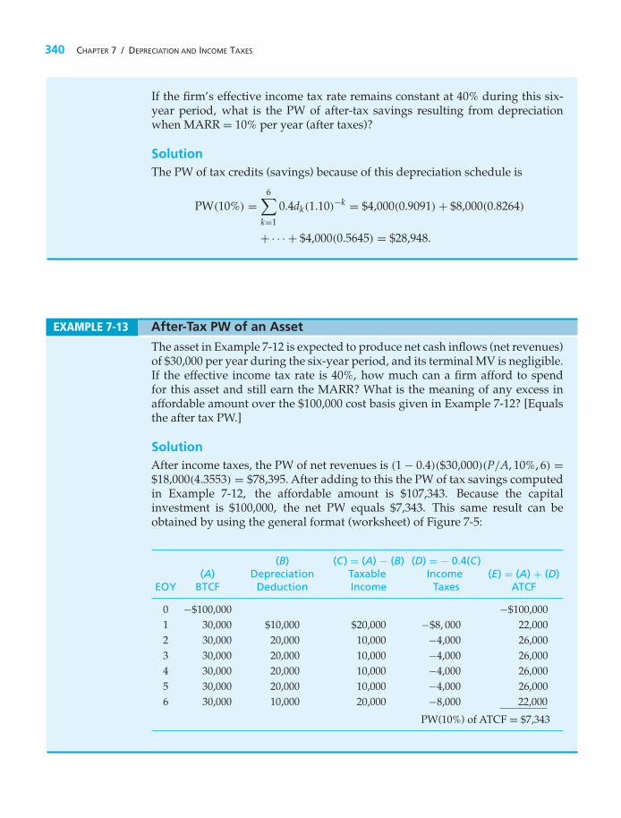
340 CHAPTER 7 / DEPRECIATION AND INCOME TAXES

If the firm’s effective income tax rate remains constant at 40% during this six-year period, what is the PW of after-tax savings resulting from depreciationwhen MARR = 10% per year (after taxes)?

SolutionThe PW of tax credits (savings) because of this depreciation schedule is

PW(10%) =6∑

k=1

0.4dk(1.10)−k = $4,000(0.9091) + $8,000(0.8264)

+ · · · + $4,000(0.5645) = $28,948.

EXAMPLE 7-13 After-Tax PW of an Asset

The asset in Example 7-12 is expected to produce net cash inflows (net revenues)of $30,000 per year during the six-year period, and its terminal MV is negligible.If the effective income tax rate is 40%, how much can a firm afford to spendfor this asset and still earn the MARR? What is the meaning of any excess inaffordable amount over the $100,000 cost basis given in Example 7-12? [Equalsthe after tax PW.]

SolutionAfter income taxes, the PW of net revenues is (1 − 0.4)($30,000)(P/A, 10%, 6) =$18,000(4.3553) = $78,395. After adding to this the PW of tax savings computedin Example 7-12, the affordable amount is $107,343. Because the capitalinvestment is $100,000, the net PW equals $7,343. This same result can beobtained by using the general format (worksheet) of Figure 7-5:

(B) (C) = (A) − (B) (D) = − 0.4(C)(A) Depreciation Taxable Income (E) = (A) + (D)

EOY BTCF Deduction Income Taxes ATCF

0 −$100,000 −$100,0001 30,000 $10,000 $20,000 −$8, 000 22,0002 30,000 20,000 10,000 −4,000 26,0003 30,000 20,000 10,000 −4,000 26,0004 30,000 20,000 10,000 −4,000 26,0005 30,000 20,000 10,000 −4,000 26,0006 30,000 10,000 20,000 −8,000 22,000

PW(10%) of ATCF = $7,343

SECTION 7.10 / ILLUSTRATION OF COMPUTATIONS OF ATCFS 341

EXAMPLE 7-14 PennCo Electric Utility Company

Here we refer back to the chapter opener where the question of the after-taxcost of electricity production was raised. For the PennCo plant, the annual fuelexpense† will be $191,346,432 per year. The operating and maintenance expensewill be $112,128,000 per year, and the carbon tax will be $73,805,052 per year.The total annual expense of operating the plant will therefore be $377,279,484.Armed with these cost estimates, we can calculate the after-tax cost of the plantby using the template of Figure 7-5 (all numbers are millions of dollars).

Taxable Cash Flow forEOY BTCF Depreciation Income Income Taxes ATCF

0 −$1,120.000 — — — −$1,120.0001 − 30 −377.279 37.333∗ −414.613 165.845 −211.434∗dk = $1,120/30 = $37.333

The annual worth of the PennCo plant, assuming inflation is negligible, is−$1,120 (A/P, 10%, 30) − $211.434, which equals −$330.266 million. We cancalculate the after-tax cost of a kilowatt-hour by dividing this number($330,266,000) by the electrical output of 5,606,400,000 kWh. It is close to $0.06per kWh.

† The details of the annual expense calculations are left as a student exercise in Problem 7-60.

7.10 Illustration of Computations of ATCFsThe following problems (Examples 7-15 through 7-19) illustrate the computation ofATCFs, as well as many common situations that affect income taxes. All problemsinclude the assumption that income tax expenses (or savings) occur at the sametime (year) as the revenue or expense that gives rise to the taxes. For purposes ofcomparing the effects of various situations, the after-tax IRR or PW is computedfor each example. We can observe from the results of Examples 7-15, 7-16, and 7-17that the faster (i.e., earlier) the depreciation deduction is, the more favorable theafter-tax IRR and PW will become.

EXAMPLE 7-15 Computing After-Tax PW and IRR

Certain new machinery, when placed in service, is estimated to cost $180,000.It is expected to reduce net annual operating expenses by $36,000 per year for10 years and to have a $30,000 MV at the end of the 10th year.

(a) Develop the ATCFs and BTCFs.(b) Calculate the before-tax and after-tax IRR. Assume that the firm is in the

federal taxable income bracket of $335,000 to $10,000,000 and that the state

342 CHAPTER 7 / DEPRECIATION AND INCOME TAXES

income tax rate is 6%. State income taxes are deductible from federal taxableincome. This machinery is in the MACRS (GDS) five-year property class.

(c) Calculate the after-tax PW when the after-tax MARR = 10% per year.

In this example, the study period is 10 years, but the property class of themachinery is 5 years. Solve by hand and by spreadsheet.

Solution by Hand(a) Table 7-6 applies the format illustrated in Figure 7-5 to calculate the BTCF

and ATCF for this example. In column D, the effective income tax rate is veryclose to 0.38 [from Equation (7-15)] based on the information just provided.

(b) The before-tax IRR is computed from column A:

0 = −$180,000 + $36,000(P/A, i′%, 10) + $30,000(P/F, i′%, 10).

By trial and error, we find that i′ = 16.1%.The entry in the last year is shown to be $30,000 because the machinery

will have this estimated MV. The asset, however, was depreciated to zerowith the GDS method. Therefore, when the machine is sold at the end ofyear 10, there will be $30,000 of recaptured depreciation, or gain on disposal[Equation (7-16)], which is taxed at the effective income tax rate of 38%. Thistax entry is shown in column D (EOY 10).

By trial and error, the after-tax IRR for Example 7-15 is found to be 12.4%.(c) When MARR = 10% per year is inserted into the PW equation at the bottom

of Table 7-6, it can be determined that the after-tax PW of this investment is$17,208.

Spreadsheet SolutionFigure 7-6 displays the spreadsheet solution for Example 7-15. This spreadsheetuses the form given in Figure 7-5 to compute the ATCFs. The spreadsheet alsoillustrates the use of the VDB (variable declining balance) function to computeMACRS (GDS) depreciation amounts.

Cell B9 contains the cost basis, cells B10:B19 contain the BTCFs, and theyear 10 MV is given in cell B20. The VDB function is used to determine theMACRS (GDS) depreciation amounts in column C. Cell B7 contains the DBpercentage used for a five-year property class (see Table 7-4).

Note that in Figure 7-6, there are two row entries for the last year of the studyperiod (year 10). The first entry accounts for expected revenues less expenses,while the second entry accounts for the disposal of the asset. To use the NPVand IRR financial functions, these values must be combined into a net cash flowfor the year. This is accomplished by the adjusted ATCF and adjusted BTCFcolumns in the spreadsheet.

SEC

TION

7.10/

ILLUSTR

ATIO

NO

FC

OM

PUTA

TION

SO

FA

TCF

S343

343

TABLE 7-6 ATCF Analysis of Example 7-15

(A) (B) Depreciation Deduction (C) = (A)−(B) (D) = −0.38(C) (E) = (A) + (D)

End of Cost GDS Recovery Taxable Cash Flow forYear, k BTCF Basis × Rate = Deduction Income Income Taxes ATCF

0 −$180,000 — — — −$180,0001 36,000 $180,000 × 0.2000 = $36,000 0 0 36,0002 36,000 180,000 × 0.3200 = 57,600 −21,600 +8,208 44,2083 36,000 180,000 × 0.1920 = 34,560 1,440 −547 35,4534 36,000 180,000 × 0.1152 = 20,736 15,264 −5,800 30,2005 36,000 180,000 × 0.1152 = 20,736 15,264 −5,800 30,2006 36,000 180,000 × 0.0576 = 10,368 25,632 −9,740 26,2607–10 36,000 0 0 36,000 −13,680 22,320

10 30,000 30,000a −11,400b 18,600Total $210,000 Total $130,201

PW (10%) = $17,208

a Depreciation recapture = MV10 − BV10 = $30,000 − 0 = $30,000 (gain on disposal).b Tax on depreciation recapture = $30,000(0.38) = $11,400.After-tax IRR: Set PW of column E = 0 and solve for i′ in the following equation:0 = −$180,000 + $36,000(P/F, i′, 1) + $44,208(P/F, i′, 2) + $35,453(P/F, i′, 3) + $30,200(P/F, i′, 4) + $30,200(P/F, i′, 5) + $26,260(P/F, i′, 6)

+$22,320(P/A, i′, 4)(P/F, i′, 6) + $18,600(P/F, i′, 10); IRR = 12.4%.

344C

HA

PTER7

/D

EPREC

IATIO

NA

ND

INC

OM

ET

AX

ES

344

= ROUND (B3 + B4*(1–B3), 2)

= NPV($B$1, G10:G19) + G9 = IRR(G9: G19, $B$1)

= PMT($B$1, $E$4, – G22)

= IF(B2 >= 15,1.5, 2)= B10 – C10

= F19 + F20

= B19 + B20

= IF(A10=$B$2+1, 0.5*C9, VDB($E$1, 0, $B$2, MAX(0, A10-1.5), A10-0.5, $B$7, FALSE) )

= –E1

= $E$3

= E2

= -$B$6 * D10 = B9 + E9 = F9

= B9

Figure 7-6 Spreadsheet Solution, Example 7-15

SECTION 7.10 / ILLUSTRATION OF COMPUTATIONS OF ATCFS 345

In Example 7-16, we demonstrate the impact of a longer depreciation scheduleon the after-tax profitability of an investment.

EXAMPLE 7-16 Impact of a Longer Depreciation Schedule on After-Tax PW and IRR

Suppose the machinery in Example 7-15 had been classified in the 10-yearMACRS (GDS) property class. Calculate the new after-tax PW and after-tax IRR.Why are these results different than the results of Example 7-15?

SolutionIf the machinery in Example 7-15 had been classified in the 10-year MACRS(GDS) property class instead of the five-year property class, depreciationdeductions would be slowed down in the early years of the study period andshifted into later years, as shown in Table 7-7. Compared with entries in Table 7-6,entries in columns C, D, and E of Table 7-7 are less favorable, in the sense thata fair amount of ATCF is deferred until later years, producing a lower after-taxPW and IRR. For instance, the PW is reduced from $17,208 in Table 7-6 to $9,136in Table 7-7. The basic difference between Table 7-6 and Table 7-7 is the timing ofthe ATCF, which is a function of the timing and magnitude of the depreciationdeductions. In fact, the curious reader can confirm that the sums of entries incolumns A through E of Tables 7-6 and 7-7 are nearly the same (except for thehalf-year of depreciation only in year 10 of Table 7-7). The timing of cash flowsdoes, of course, make a difference!

Depreciation does not affect BTCF. Fast (accelerated) depreciation produces alarger PW of tax savings than does the same amount of depreciation claimedlater in an asset’s life.

A minor complication is introduced in ATCF analyses when the study periodis shorter than an asset’s MACRS recovery period (e.g., for a five-year recoveryperiod, the study period is five years or less). In such cases, we shall assumethroughout this book that the asset is sold for its MV in the last year of the studyperiod. Due to the half-year convention, only one-half of the normal MACRSdepreciation can be claimed in the year of disposal or end of the study period,so there will usually be a difference between an asset’s BV and its MV. Resultingincome tax adjustments will be made at the time of the sale (see the last row inTable 7-7) unless the asset in question is not sold but instead kept for standbyservice. In such a case, depreciation deductions usually continue through the endof the asset’s MACRS recovery period. Our assumption of project terminationat the end of the study period makes good economic sense, as illustrated inExample 7-17.

TABLE 7-7 ATCF Analysis of Example 7-16 [Reworked Example 7-15 with Machinery in the 10-YearMACRS (GDS) Property Class]

(A) (B) Depreciation Deduction (C) = (A) − (B) (D) = −0.38(C) (E) = (A) + (D)

End of Cost GDS Recovery Taxable Cash Flow forYear, k BTCF Basis × Rate = Deduction Income Income Taxes ATCF

0 −$180,000 — — — −$180,0001 36,000 $180,000 × 0.1000 = $18,000 $18,000 −$6,840 29,1602 36,000 180,000 × 0.1800 = 32,400 3,600 −1,368 34,6323 36,000 180,000 × 0.1440 = 25,920 10,080 −3,830 32,1704 36,000 180,000 × 0.1152 = 20,736 15,264 −5,800 30,2005 36,000 180,000 × 0.0922 = 16,596 19,404 −7,374 28,6266 36,000 180,000 × 0.0737 = 13,266 22,734 −8,639 27,3617 36,000 180,000 × 0.0655 = 11,790 24,210 −9,200 26,8008 36,000 180,000 × 0.0655 = 11,790 24,210 −9,200 26,8009 36,000 180,000 × 0.0656 = 11,808 24,192 −9,193 26,807

10 36,000 180,000 × 0.0655/2 = 5,895 30,105 −11,440 24,56010 30,000 18,201a −6,916 23,084

Total $130,196PW (10%) � $9,136

IRR = 11.2%

a Gain on disposal = MV10 − BV10 = $30,000 −(

0.06552

+ 0.0328)

($180,000) = $18,201.

346

SECTION 7.10 / ILLUSTRATION OF COMPUTATIONS OF ATCFS 347

EXAMPLE 7-17 Study Period < MACRS Recovery Period

A highly specialized piece of equipment has a first cost of $50,000. If thisequipment is purchased, it will be used to produce income (through rental)of $20,000 per year for only four years. At the end of year four, the equipmentwill be sold for a negligible amount. Estimated annual expenses for upkeep are$3,000 during each of the four years. The MACRS (GDS) recovery period for theequipment is seven years, and the firm’s effective income tax rate is 40%.

(a) If the after-tax MARR is 7% per year, should the equipment be purchased?(b) Rework the problem, assuming that the equipment is placed on standby

status such that depreciation is taken over the full MACRS recovery period.

Solution(a)

(B) (C) = (A) − (B) (D) = −0.4(C)End of (A) Depreciation Taxable Cash Flow for (E) = (A) + (D)Year, k BTCF Deduction Income Income Taxes ATCF

0 −$50,000 −$50,0001 17,000 $7,145 $9,855 −$3,942 13,0582 17,000 12,245 4,755 −1,902 15,0983 17,000 8,745 8,255 −3,302 13,6984 17,000 3,123a 13,877 −5,551 11,4494 0 −18,742b 7,497 7,497

a Half-year convention applies with disposal in year four.b Remaining BV.

PW(7%) = $1,026. Because the PW > 0, the equipment should be purchased.

(b)

(B) (D)End of (A) Depreciation (C) Cash Flow for (E)Year, k BTCF Deduction Taxable Income Income Taxes ATCF

0 −$50,000 −$50,0001 17,000 $7,145 $9,855 −$3,942 13,0582 17,000 12,245 4,755 −1,902 15,0983 17,000 8,745 8,255 −3,302 13,6984 17,000 6,245 10,755 −4,302 12,6985 0 4,465 −4,465 1,786 1,7866 0 4,460 −4,460 1,784 1,7847 0 4,465 −4,465 1,786 1,7868 0 2,230 −2,230 892 8928 0 0

PW(7%) = $353, so the equipment should be purchased.

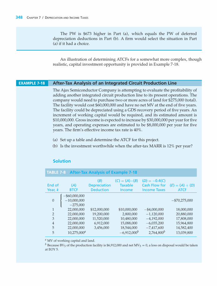
348 CHAPTER 7 / DEPRECIATION AND INCOME TAXES

The PW is $673 higher in Part (a), which equals the PW of deferreddepreciation deductions in Part (b). A firm would select the situation in Part(a) if it had a choice.

An illustration of determining ATCFs for a somewhat more complex, thoughrealistic, capital investment opportunity is provided in Example 7-18.

EXAMPLE 7-18 After-Tax Analysis of an Integrated Circuit Production Line

The Ajax Semiconductor Company is attempting to evaluate the profitability ofadding another integrated circuit production line to its present operations. Thecompany would need to purchase two or more acres of land for $275,000 (total).The facility would cost $60,000,000 and have no net MV at the end of five years.The facility could be depreciated using a GDS recovery period of five years. Anincrement of working capital would be required, and its estimated amount is$10,000,000. Gross income is expected to increase by $30,000,000 per year for fiveyears, and operating expenses are estimated to be $8,000,000 per year for fiveyears. The firm’s effective income tax rate is 40%.

(a) Set up a table and determine the ATCF for this project.(b) Is the investment worthwhile when the after-tax MARR is 12% per year?

Solution

TABLE 7-8 After-Tax Analysis of Example 7-18

(B) (C) = (A)−(B) (D) = −0.4(C)End of (A) Depreciation Taxable Cash Flow for (E) = (A) + (D)Year, k BTCF Deduction Income Income Taxes ATCF

−$60,000,0000

⎧⎨⎩ −10,000,000 −$70,275,000

−275,0001 22,000,000 $12,000,000 $10,000,000 −$4,000,000 18,000,0002 22,000,000 19,200,000 2,800,000 −1,120,000 20,880,0003 22,000,000 11,520,000 10,480,000 −4,192,000 17,808,0004 22,000,000 6,912,000 15,088,000 −6,035,200 15,964,8005 22,000,000 3,456,000 18,544,000 −7,417,600 14,582,4005 10,275,000a −6,912,000b 2,764,800b 13,039,800

a MV of working capital and land.b Because BV5 of the production facility is $6,912,000 and net MV5 = 0, a loss on disposal would be takenat EOY 5.

SECTION 7.10 / ILLUSTRATION OF COMPUTATIONS OF ATCFS 349

(a) The format recommended in Figure 7-5 is followed in Table 7-8 to obtainATCFs in years zero through five. Acquisitions of land, as well as additionalworking capital, are treated as nondepreciable capital investments whoseMVs at the end of year five are estimated to equal their first costs. (Ineconomic evaluations, it is customary to assume that land and workingcapital do not inflate in value during the study period because they are“nonwasting” assets.) By using a variation of Equation (7-21), we are ableto compute ATCF in year three (for example) to be

ATCF3 = ($30,000,000 − $8,000,000 − $11,520,000)(1 − 0.40) + $11,520,000

= $17,808,000.

(b) The depreciable property in Example 7-18 ($60,000,000) will be disposed offor $0 at the end of year five, and a loss on disposal of $6,912,000 will beclaimed at the end of year five. Only a half-year of depreciation ($3,456,000)can be claimed as a deduction in year five, and the BV is $6,912,900 atthe end of year five. Because the selling price (MV) is zero, the loss ondisposal equals our BV of $6,912,000. As seen from Figure 7-5, a tax credit of0.40($6,912,000) = $2,764,800 is created at the end of year five. The after-taxIRR is obtained from entries in column E of Table 7-8 and is found to be12.5%. The after-tax PW equals $936,715 at MARR = 12% per year. Based oneconomic considerations, this integrated circuit production line should berecommended because it appears to be quite attractive.

In the next example, the after-tax comparison of mutually exclusive alternativesinvolving only costs is illustrated.

EXAMPLE 7-19 After-Tax Comparison of Purchase versus Leasing Alternatives

An engineering consulting firm can purchase a fully configured computer-aided design (CAD) workstation for $20,000. It is estimated that the usefullife of the workstation is seven years, and its MV in seven years should be$2,000. Operating expenses are estimated to be $40 per eight-hour workday, andmaintenance will be performed under contract for $8,000 per year. The MACRS(GDS) property class is five years, and the effective income tax rate is 40%.

As an alternative, sufficient computer time can be leased from a servicecompany at an annual cost of $20,000. If the after-tax MARR is 10% per year,how many workdays per year must the workstation be needed in order to justifyleasing it?

SolutionThis example involves an after-tax evaluation of purchasing depreciableproperty versus leasing it. We are to determine how much the workstation mustbe utilized so that the lease option is a good economic choice. A key assumption

350 CHAPTER 7 / DEPRECIATION AND INCOME TAXES

is that the cost of engineering design time (i.e., operator time) is unaffected bywhether the workstation is purchased or leased. Variable operations expensesassociated with ownership result from the purchase of supplies, utilities, and soon. Hardware and software maintenance cost is contractually fixed at $8,000 peryear. It is further assumed that the maximum number of working days per yearis 250.

Lease fees are treated as an annual expense, and the consulting firm (thelessee) may not claim depreciation of the equipment to be an additional expense.(The leasing company presumably has included the cost of depreciation in itsfee.) Determination of ATCF for the lease option is relatively straightforwardand is not affected by how much the workstation is utilized:

(After-tax expense of the lease)k = − $20,000(1 − 0.40)= − $12,000; k = 1, . . . , 7.

ATCFs for the purchase option involve expenses that are fixed (not a functionof equipment utilization) in addition to expenses that vary with equipmentusage. If we let X equal the number of working days per year that the equipmentis utilized, the variable cost per year of operating the workstation is $40X. Theafter-tax analysis of the purchase alternative is shown in Table 7-9.

The after-tax annual worth (AW) of purchasing the workstation is

AW(10%) = −$20,000(A/P, 10%, 7) − $24X − [$3,200(P/F, 10%, 1) + · · ·+ $4,800(P/F, 10%, 7)](A/P, 10%, 7) + $1,200(A/F, 10%, 7)

= −$24X − $7,511.

TABLE 7-9 After-Tax Analysis of Purchase Alternative (Example 7-19)

(B) (C) = (A) − (B) (D) = −t(C)End of (A) Depreciation Taxable Cash Flow for (E) = (A) + (D)Year, k BTCF Deductiona Income Income Taxes ATCF

0 −$20,000 −$20,0001 −40X − 8,000 $4,000 −$40X − $12,000 $16X + $4,800 −24X − 3,2002 −40X − 8,000 6,400 −40X − 14,400 16X + 5,760 −24X − 2,2403 −40X − 8,000 3,840 −40X − 11,840 16X + 4,736 −24X − 3,2644 −40X − 8,000 2,304 −40X − 10,304 16X + 4,122 −24X − 3,8785 −40X − 8,000 2,304 −40X − 10,304 16X + 4,122 −24X − 3,8786 −40X − 8,000 1,152 −40X − 9,152 16X + 3,661 −24X − 4,3397 −40X − 8,000 0 −40X − 8,000 16X + 3,200 −24X − 4,8007 2,000 2,000 −800 1,200

a Depreciation deductionk = $20,000 × (GDS recovery rate).

SECTION 7.10 / ILLUSTRATION OF COMPUTATIONS OF ATCFS 351

Figure 7-7Summary ofExample 7-19

Aft

er-T

ax A

nnua

l Wor

th, (

$)

Purchase theworkstation

Point ofindifference

Lease the workstation

�12,000

�7,511

0 125 187 250Number of Working Days/Year (X)

To solve for X, we equate the after-tax annual worth of both alternatives:

−$12,000 = −$24X − $7,511.

Thus, X = 187 days per year. Therefore, if the firm expects to utilize theCAD workstation in its business more than 187 days per year, the equipmentshould be leased. The graphic summary of Example 7-19 shown inFigure 7-7 provides the rationale for this recommendation. The importance ofthe workstation’s estimated utilization, in workdays per year, is now quiteapparent.

EXAMPLE 7-20 After-Tax Analysis of Alternatives with Unequal Lives

A firm must decide between two system designs, S1 and S2, whose estimatedcash flows are shown in the following table. The effective income tax rate is 40%and MACRS (GDS) depreciation is used. Both designs have a GDS recoveryperiod of five years. If the after-tax desired return on investment is 10% per year,which design should be chosen?

Design

S1 S2

Capital investment $100,000 $200,000Useful life (years) 7 6MV at end of useful life $30,000 $60,000Annual revenues less expenses $20,000 $40,000

352 CHAPTER 7 / DEPRECIATION AND INCOME TAXES

SolutionNote that the design alternatives have different useful lives. The same basicprinciples of engineering economy apply to both before-tax and after-tax anal-yses. Therefore, we must analyze the two system designs over a common periodof time. As we discovered in Chapter 6, using the repeatability assumption alongwith the annual worth method simplifies the analysis of alternatives havingunequal lives.

Both alternatives would be depreciated using a five-year GDS recoveryperiod. No adjustments to the GDS rates are required because the useful life ofeach alternative is greater than or equal to six years of depreciation deductions.Tables 7-10 and 7-11 summarize the calculation of the ATCFs for the designalternatives.

TABLE 7-10 After-Tax Analysis of Design S1, Example 7-20

(A) (B) (C) = (A) − (B) (D) = − t(C) (E) = (A) + (D)End of Depreciation Cash Flow forYear, k BTCF Deduction Taxable Income Income Taxes ATCF PW(10%)

0 −$100,000 −$100,000 −$100,0001 20,000 $20,000 $0 $0 20,000 18,1822 20,000 32,000 −12,000 4,800 24,800 20,4953 20,000 19,200 800 −320 19,680 14,7864 20,000 11,520 8,480 −3,392 16,608 11,3435 20,000 11,520 8,480 −3,392 16,608 10,3126 20,000 5,760 14,240 −5,696 14,304 8,0757 20,000 0 20,000 −8,000 12,000 6,1587 30,000 30,000 −12,000 18,000 9,238

PWS1(10%) = −$1,411

TABLE 7-11 After-Tax Analysis of Design S2, Example 7-20

(A) (B) (C) = (A) − (B) (D) = −t(C) (E) = (A) + (D)End of Depreciation Cash Flow forYear, k BTCF Deduction Taxable Income Income Taxes ATCF PW(10%)

0 −$200,000 −$200,000 −$200,0001 40,000 $40,000 $0 $0 40,000 36,3642 40,000 64,000 −24,000 9,600 49,600 40,9893 40,000 38,400 1,600 −640 39,360 29,5714 40,000 23,040 16,960 −6,784 33,216 22,6875 40,000 23,040 16,960 −6,784 33,216 20,6246 40,000 11,520 28,480 −11,392 28,608 16,1496 50,000 50,000 −20,000 30,000 16,935

PWS2(10%) = −$16,681

SECTION 7.11 / ECONOMIC VALUE ADDED 353

We can’t directly compare the PW of the after-tax cash flows because of thedifference in the lives of the alternatives. We can, however, directly compare theAWs of the ATCFs by using the repeatability assumption from Chapter 6.

AWS1(10%) = PWS1(A/P, 10%, 7) = −$1,411(0.2054) = −$290

AWS2(10%) = PWS2(A/P, 10%, 6) = −$16,681(0.2296) = −$3,830

Based on an after-tax annual worth analysis, Design S1 is preferred since it hasthe greater (less negative) AW. Neither design however makes money, so if asystem is not required, don’t recommend either one.

7.11 Economic Value AddedThis section discusses an economic measure for estimating the wealth creationpotential of capital investments that is experiencing increased attention and use.The measure, called economic value added (EVA),∗ can be determined from someof the data available in an after-tax analysis of cash flows generated by a capitalinvestment. Through retroactive analysis of a firm’s common stock valuation, ithas been established that some companies experience a statistically significantrelationship between the EVA metric and the historical value of their commonstock.† For our purposes, EVA can also be used to estimate the profit-earningpotential of proposed capital investments in engineering projects.

Simply stated, EVA is the difference between the company’s adjusted netoperating profit after taxes (NOPAT) in a particular year and its after-tax cost ofcapital during that year. Another way to characterize EVA is “the spread betweenthe return on the capital and the cost of the capital.”‡ On a project-by-project basis(i.e., for discrete investments), the EVA metric can be used to gauge the wealthcreation opportunity of proposed capital expenditures. We now define annualEVA as

EVAk = (Net operating profit after taxes)k

− (Cost of capital used to produce profit)k

= NOPATk − i · BVk−1, (7-22)

where

k = an index for the year in question(1 ≤ k ≤ N);

i = after-tax MARR based on a firm’s cost of capital,

BVk−1 = beginning-of-year book value;

N = the study (analysis) period in years.

∗ EVA is a registered trademark of Stern Stewart & Company, New York City, NY.† See J. L. Dodd and S. Chen, “EVA:ANew Panacea?” B & E Review, 42 (July–September 1996): 26–28, and W. Freedman,“How Do You Add Up?” Chemical Week, October 9, 1996, pp. 31–34.‡ S. Tully, “The Real Key To Creating Wealth,” Fortune, September 30, 1993, p. 38ff.

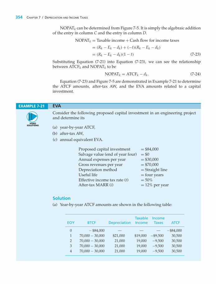
354 CHAPTER 7 / DEPRECIATION AND INCOME TAXES

NOPATk can be determined from Figure 7-5. It is simply the algebraic additionof the entry in column C and the entry in column D.

NOPATk = Taxable income + Cash flow for income taxes

= (Rk − Ek − dk) + (−t)(Rk − Ek − dk)

= (Rk − Ek − dk)(1 − t) (7-23)

Substituting Equation (7-21) into Equation (7-23), we can see the relationshipbetween ATCFk and NOPATk to be

NOPATk = ATCFk − dk . (7-24)

Equation (7-23) and Figure 7-5 are demonstrated in Example 7-21 to determinethe ATCF amounts, after-tax AW, and the EVA amounts related to a capitalinvestment.

EXAMPLE 7-21 EVA

Consider the following proposed capital investment in an engineering projectand determine its

(a) year-by-year ATCF,(b) after-tax AW,(c) annual equivalent EVA.

Proposed capital investment = $84,000Salvage value (end of year four) = $0Annual expenses per year = $30,000Gross revenues per year = $70,000Depreciation method = Straight lineUseful life = four yearsEffective income tax rate (t) = 50%After-tax MARR (i) = 12% per year

Solution(a) Year-by-year ATCF amounts are shown in the following table:

Taxable IncomeEOY BTCF Depreciation Income Taxes ATCF

0 − $84,000 — — — −$84,0001 70,000 − 30,000 $21,000 $19,000 −$9,500 30,5002 70,000 − 30,000 21,000 19,000 −9,500 30,5003 70,000 − 30,000 21,000 19,000 −9,500 30,5004 70,000 − 30,000 21,000 19,000 −9,500 30,500

SECTION 7.12 / TRY YOUR SKILLS 355

(b) The annual equivalent worth of the ATCFs equals −$84,000(A/P, 12%, 4) +$30,500 = $2,844.

(c) The EVA in year k equals NOPATk −0.12 BVk−1 [Equation (7-22)]. The year-by-year EVA amounts and the annual equivalent worth of EVA ($2,844) areshown in the next table. Hence, the after-tax AW and the annual equivalentworth of EVA of the project are identical.

EOYk NOPAT EVA = NOPAT − i · BVk−1

1 $19,000 − $9,500 = $9,500 $9,500 − 0.12($84,000) = −$5802 = $9,500 $9,500 − 0.12($63,000) = $1,9403 = $9,500 $9,500 − 0.12($42,000) = $4,4604 = $9,500 $9,500 − 0.12($21,000) = $6,980

Annual equivalent EVA = [−$580(P/F, 12%, 1) + $1,940(P/F, 12%, 2) +$4,460(P/F, 12%, 3) + $6,980(P/F, 12%, 4)](A/P, 12%, 4) = $2,844.

In Example 7-21, it was shown that the after-tax AW (12%) of the proposedengineering project is identical to the annual equivalent EVA at the same interestrate. Therefore, the annual equivalent EVA is simply the annual worth, at the after-tax MARR, of a project’s ATCFs. This straightforward relationship is also validwhen accelerated depreciation methods (such as MACRS) are used in the analysisof a proposed project. The reader is referred to Problems 7-47, 7-48, and 7-49 at theend of the chapter for EVA exercises.

7.12 Try Your SkillsThe number in parentheses that follows each problem refers to the sectionfrom which the problem is taken. Solutions to these problems can be found inAppendix G.

7-A. Why would a business elect, under MACRS, to use the ADS rather than theGDS? (7.4)

7-B. If the incremental federal income tax rate is 34% and the incremental stateincome tax rate is 6%, what is the effective combined income tax rate (t)? Ifstate income taxes are 12% of taxable income, what now is the value of t? (7.7)

7-C. The before-tax MARR for a particular firm is 18% per year. The state incometax rate is 5%, and the federal income tax rate is 39%. State income taxesare deductible from federal taxable income. What is this firm’s after-taxMARR? (7.7)

356 CHAPTER 7 / DEPRECIATION AND INCOME TAXES

7-D. If a company’s total effective income tax rate is 40% and its state income taxrate is 20%, what is the company’s federal income tax rate? (7.7)

(a) 20% (b) 25% (c) 35% (d) 40% (e) 52%

7-E. A drug store is looking into the possibility of installing a “24/7” automatedprescription refill system to increase its projected revenues by $20,000 per yearover the next 5 years. Annual expenses to maintain the system are expectedto be $5,000. The system will have no market value at the end of its 5-year life,and it will be depreciated by the SL method. The store’s effective income taxrate is 40%, and the after-tax MARR is 12% per year. What is the maximumamount that is justified for the purchase of this prescription refill system? (7.9)

7-F. In a chlorine-fluxing installation in a large aluminum company, engineersare considering the replacement of existing plastic pipe fittings with moreexpensive, but longer lived, copper fittings. The following table gives acomparison of the capital investments, lives, salvage values, and so on ofthe two mutually exclusive alternatives under consideration:

Plastic Copper

Capital investment $5,000 $10,000Useful (class) life 5 years 10 yearsSalvage value for depreciation purposes $1,000(= SV5) $5,000(= SV10)Annual expenses $300 $100Market value at end of useful life $0 $0

Depreciation amounts are calculated with the SL method. Assume anincome tax rate of 40% and a MARR after-taxes of 12% per year. Which pipefitting would you select and why? Carefully list all assumptions that youmake in performing the analysis. (7.9, 7.10)

7.13 SummaryIn this chapter, we have presented important aspects of federal legislation relatingto depreciation and income taxes. It is essential to understand these topics so thatcorrect after-tax engineering economy evaluations of proposed projects may beconducted. Depreciation and income taxes are also integral parts of subsequentchapters in this book.

In this chapter, many concepts regarding current federal income tax laws weredescribed. For example, topics such as taxable income, effective income tax rates,taxation of ordinary income, and gains and losses on disposal of assets wereexplained. A general format for pulling together and organizing all these appar-ently diverse subjects was presented in Figure 7-5. This format offers the studentor practicing engineer a means of collecting, on one worksheet, information thatis required for determining ATCFs and properly evaluating the after-tax economicworth of a proposed capital investment. Figure 7-5 was then employed in numerousexamples. The student’s challenge is now to use this worksheet in organizing datapresented in problem exercises at the end of this and subsequent chapters and toanswer questions regarding the after-tax profitability of proposed projects.

PROBLEMS 357

ProblemsThe number in parentheses that follows each problemrefers to the section from which the problem is taken.

7-1. How are depreciation deductions different fromother production or service expenses such as labor,material, and electricity? (7.2)

7-2. What conditions must a property satisfy to beconsidered depreciable? (7.2)

7-3. Explain the difference between real and personalproperty. (7.2)

7-4. Explain how the cost basis of depreciable propertyis determined. (7.2)

7-5. An asset purchased for $50,000 has a depreciablelife of 5 years, and it has a terminal book (salvage)value of $5,000 at the end of its depreciable life. With thestraight-line method of depreciation, what is the asset’sbook value at the end of year 3? (7.3)

7-6. The “Big-Deal” Company has purchased newfurniture for their offices at a retail price of $125,000.An additional $20,000 has been charged for insurance,shipping, and handling. The company expects to use thefurniture for 10 years (useful life = 10 years) and thensell it at a salvage (market) value of $15,000. Use the SLmethod of depreciation to answer these questions. (7.3)

a. What is the depreciation during the second year?

b. What is the BV of the asset at the end of the first year?

c. What is the BV of the asset after 10 years?

7-7. Cisco Systems is purchasing a new bar code–scanning device for its service center in San Francisco.The table that follows lists the relevant cost items for thispurchase. The operating expenses for the new systemare $10,000 per year, and the useful life of the systemis expected to be five years. The SV for depreciationpurposes is equal to 25% of the hardware cost. (7.3)

Cost Item Cost

Hardware $160,000Training $15,000Installation $15,000

a. What is the BV of the device at the end of year threeif the SL depreciation method is used?

b. Suppose that after depreciating the device for twoyears with the SL method, the firm decides to switchto the double declining balance depreciation methodfor the remainder of the device’s life (the remainingthree years). What is the device’s BV at the end offour years?

7-8. An asset for drilling was purchased and placedin service by a petroleum production company. Itscost basis is $60,000, and it has an estimated MV of$12,000 at the end of an estimated useful life of 14 years.Compute the depreciation amount in the third year andthe BV at the end of the fifth year of life by each of thesemethods: (7.3, 7.4)

a. The SL method.

b. The 200% DB method with switchover to SL.

c. The GDS.

d. The ADS.

7-9. What is the depreciation deduction, using eachof the following methods, for the second year for anasset that costs $35,000 and has an estimated MV of$7,000 at the end of its seven-year useful life? Assumeits MACRS class life is also seven years. (a) 200% DB,(b) GDS (MACRS), and (c) ADS (MACRS). (7.3, 7.4)

7-10. Your company just purchased office furniture(asset class 00.11) for $100,000 and placed it in serviceon August 13, 2007. The cost basis for the furniture is$100,000, and it will be depreciated with the GDS usinghalf-year convention. The expected salvage (market)value of the furniture is $5,000 in 2015. Determine therecovery period for the furniture and its depreciationdeductions over the recovery period. (7.4)

7-11. Your company has purchased a large new truck-tractor for over-the-road use (asset class 00.26). It has acost basis of $180,000. With additional options costing$15,000, the cost basis for depreciation purposes is$195,000. Its MV at the end of five years is estimatedas $40,000. Assume it will be depreciated under theGDS: (7.4)

358 CHAPTER 7 / DEPRECIATION AND INCOME TAXES

a. What is the cumulative depreciation through the endof year three?

b. What is the MACRS depreciation in the fourth year?

c. What is the BV at the end of year two?

7-12. A construction company is considering changingits depreciation from the MACRS method to the his-torical SL method for a general purpose hauling truck.The cost basis of the truck is $100,000, and the expectedsalvage value for depreciation purposes is $8,000. Thecompany will use the truck for eight years and willdepreciate it over this period of time with the SLmethod.What is the difference in the amount of depreciationthat would be claimed in year five (i.e., MACRS versusSL)? (7.3, 7.4)

7-13. A piece of construction equipment (asset class15.0) was purchased by the Jones Construction Com-pany. The cost basis was $300,000.

a. Determine the GDS and ADS depreciationdeductions for this property. (7.4)

b. Compute the difference in PW of the two sets ofdepreciation deductions in Part (a) if i = 12% peryear. (7.5)

7-14. During its current tax year (year one), apharmaceutical company purchased a mixing tank thathad a fair market price of $120,000. It replaced anolder, smaller mixing tank that had a BV of $15,000.Because a special promotion was underway, the oldtank was used as a trade-in for the new one, and thecash price (including delivery and installation) was setat $99,500. The MACRS class life for the new mixingtank is 9.5 years. (7.4, 7.3)

a. Under the GDS, what is the depreciation deductionin year three?

b. Under the GDS, what is the BV at the end of yearfour?

c. If 200% DB depreciation had been applied tothis problem, what would be the cumulativedepreciation through the end of year four?

7-15. A manufacturer of aerospace products purchasedthree flexible assembly cells for $500,000 each. Deliveryand insurance charges were $35,000, and installation ofthe cells cost another $50,000. (7.4, 7.8)

a. Determine the cost basis of the three cells.

b. What is the class life of the cells?

c. What is the MACRS depreciation in year five?

d. If the cells are sold to another company for $120,000each at the end of year six, how much is therecaptured depreciation?

7-16. A special-purpose machine is to be depreciated asa linear function of use (units-of-production method). Itcosts $35,000 and is expected to produce 150,000 unitsand then be sold for $5,000. Up to the end of the thirdyear, it had produced 60,000 units, and during the fourthyear it produced 18,000 units. What is the depreciationdeduction for the fourth year and the BV at the end ofthe fourth year? (7.3)

7-17. A concrete and rock crusher for demolition workhas been purchased for $60,000, and it has an estimatedSV of $10,000 at the end of its five-year life. Engineershave estimated that the following units of production(in m3 of crushed material) will be contracted over thenext five years.

EOY 1 2 3 4 5

m3 16,000 24,000 36,000 16,000 8,000

Using the units of production depreciation method,what is the depreciation allowance in year three, andwhat is the BV at the end of year two? (7.3)

7-18. During a particular year, a corporation has$18.6 million in revenue, $2.4 million of operatingexpenses, and depreciation expenses of $6.4 million.What is the approximate federal tax this corporationwill have to pay for this tax year? (7.7)

7-19. Suppose state income taxes and local incometaxes are treated as expenses for purposes of calculatingfederal taxable income and hence federal income taxes.Determine the effective income tax rate when the federalincome tax rate is 35%, the state income tax rate is 6%,and the local income tax rate is 1%. (7.7)

7-20. A start-up biotech company is consideringmaking an investment of $100,000 in a new filtrationsystem. The associated estimates are summarizedbelow:

Annual receipts $75,000Annual expenses $45,000Useful life 8 yearsTerminal book value (EOY 8) $20,000Terminal market value $0

PROBLEMS 359

Straight-line depreciation will be used, and the effectiveincome tax rate is 20%. The after-tax MARR is 15% peryear. Determine whether this investment is an attractiveoption for the company. (7.9)

7-21. A new municipal refuse collection vehicle can bepurchased for $84,000. Its expected useful life is 6 years,at which time the market value and book value will bezero. Before-tax cash flow (BTCF) will be +$18,000 peryear over the 6-year life of the vehicle. (7.9)

a. Use straight-line depreciation, an effective incometax rate of 40% and an after-tax MARR of 12% todetermine the present worth of the investment.

b. What is the after-tax internal rate of return?

c. Is this vehicle a sound investment? Explain youranswer.

7-22. A $125,000 tractor-trailer is being depreciated bythe SL method over five years to a final BV of zero. Half-year convention does not apply to this asset. After threeyears, the rig is sold for (a) $70,000 or (b) $20,000. Ifthe effective income tax rate is 40%, what is the netcash inflow from the sale for situation (a) and situation(b)? (7.8)

7-23. An injection molding machine can be purchasedand installed for $90,000. It is in the seven-year GDSproperty class and is expected to be kept in service foreight years. It is believed that $10,000 can be obtainedwhen the machine is disposed of at the end of year eight.The net annual value added (i.e., revenues less expenses)that can be attributed to this machine is constant overeight years and amounts to $15,000. An effective incometax rate of 40% is used by the company, and the after-taxMARR equals 15% per year. (7.4, 7.9)

a. What is the approximate value of the company’sbefore-tax MARR?

b. Determine the GDS depreciation amounts in yearsone through eight.

c. What is the taxable income at the end of year eightthat is related to capital investment?

d. Set up a table and calculate the ATCF for thismachine.

e. Should a recommendation be made to purchase themachine?

7-24. Refer to Example 6-10. Work this problem onan after-tax basis when the MARR is 12% per year.The effective income tax rate is 40%, and MACRSdepreciation is appropriate with a property class of five

years. Recall that the market values of M1 and M2 arezero at the end of years five and eight, respectively. (7.9)

7-25. An office supply company has purchased a light-duty delivery truck for $18,000. The truck will bedepreciated under the MACRS with a property classof 5 years. The truck’s MV is expected to decrease by$3,000 per year. It is anticipated that the purchase of thetruck will increase the company’s revenue by $10,000annually, whereas the associated operating expensesare expected to be $3,500 annually. The company hasan effective income tax rate of 40%, and its after-taxMARR is 15% per year. If the company plans to keepthe truck only 2 years, what would be the equivalentafter-tax annual worth of this investment? (7.9)

7-26. An assembly operation at a software companycurrently requires $100,000 per year in labor costs. Arobot can be purchased and installed to automate thisoperation, and the robot will cost $200,000 with no MVat the end of its 10-year life. The robot, if acquired,will be depreciated using SL depreciation to a terminalBV of zero after 10 years. Maintenance and operationexpenses of the robot are estimated to be $64,000 peryear. The company has an effective income tax rate of40%. Invested capital must earn at least 8% after incometaxes are taken into account. (7.9)

a. Use the IRR method to determine if the robot is ajustifiable investment.

b. If MACRS (seven-year recovery period) had beenused in Part (a), would the after-tax IRR be lower orhigher than your answer to Part (a)?

7-27. Liberty Airways is considering an investment of$800,000 in ticket purchasing kiosks at selected airports.The kiosks (hardware and software) have an expectedlife of four years. Extra ticket sales are expected to be60,000 per year at a discount price of $40 per ticket.Fixed costs, excluding depreciation of the equipment,are $400,000 per year, and variable costs are $24 perticket. The kiosks will be depreciated over four years,using the SL method with a zero salvage value. Theonetime commitment of working capital is expected tobe 1/12 of annual sales dollars. The after-tax MARR is15% per year, and the company pays income tax at therate of 34%. What’s the after-tax PW of this proposedinvestment? Should the investment be made? (7.9)

7-28. Nordique Fab is an Arizona company dedicatedto circuit board design and fabrication. It has justacquired new workstations and modeling softwarefor its three “Valley of the Sun” design facilities, at

360 CHAPTER 7 / DEPRECIATION AND INCOME TAXES

a cost of $425,000 per site. This cost includes thehardware, software, transportation, and installationcosts. Additional software training has been purchasedat a cost of $25,000 per site. The estimated MV foreach system during the fourth year is expected to be5% of the total capital investment, at which time thesystems will all be sold. The company believes that useof the new systems will enhance their circuit designbusiness, resulting in a total increase in annual incomeof $1,000,000. The engineering design manager wantsto determine the tax implications of this purchase. Heestimates that annual operating and maintenance costson the systems will be approximately $220,000 (all sitescombined). The company’s marginal effective tax rate is35% and the MACRS depreciation method (with a five-year GDS recovery period) will be used. Use Figure 7-5to determine the after-tax cash flows for this project.If the after-tax MARR is 20% per year, would yourecommend this investment? (7.9)

7-29. Your company has just signed a three-yearnonrenewable contract with the city of New Orleans forearthmoving work. You are investigating the purchaseof heavy construction equipment for this job. Theequipment costs $200,000 and qualifies for five-yearMACRS depreciation. At the end of the three-yearcontract, you expect to be able to sell the equipmentfor $70,000. If the projected operating expense for theequipment is $65,000 per year, what is the after-taxequivalent uniform annual cost (EUAC) of owning andoperating this equipment? The effective income tax rateis 40%, and the after-tax MARR is 12% per year. (7.9)

7-30. The Greentree Lumber Company is attemptingto evaluate the profitability of adding another cuttingline to its present sawmill operations. They wouldneed to purchase two more acres of land for $30,000(total). The equipment would cost $130,000 and couldbe depreciated over a five-year recovery period withthe MACRS method. Gross revenue is expected toincrease by $50,000 per year for five years, and operatingexpenses will be $15,000 annually for five years. It isexpected that this cutting line will be closed down afterfive years. The firm’s effective income tax rate is 50%. Ifthe company’s after-tax MARR is 5% per year, is this aprofitable investment? (7.9)

7-31. A high-pressure reactor vessel in a pharma-ceutical company was purchased for $200,000. It hasa useful life of 10 years, and the vessel can be sold for$30,000 at that time. The vessel will be depreciated withthe MACRS method (its class life is 5 years). Annual netcash flow (revenue less expenses) is $200,000 per year

over the useful life. The effective income tax rate is 40%.What is the after-tax cash flow of the vessel at the endof year 10? (7.9)

7-32. Your company is considering the introduction ofa new product line. The initial investment required forthis project is $500,000, and annual maintenance costsare anticipated to be $35,000. Annual operating costwill be in direct proportion to the level of productionat $8.50 per unit, and each unit of product can be soldfor $50.00. If the project has a life of 7 years, what is theminimum annual production level for which this projectis economically viable? Work this problem on an after-tax basis. Assume 5-year SL depreciation (SV5 = 0),MV7 = 0, an effective income tax rate of 40%, and anafter-tax MARR of 10% per year. (7.9)

7-33. Your company has purchased equipment (for$50,000) that will reduce materials and labor costs by$14,000 each year for N years. After N years, there willbe no further need for the machine, and because themachine is specially designed, it will have no MV atany time. The IRS, however, has ruled that you mustdepreciate the equipment on a SL basis with a tax life offive years. If the effective income tax rate is 40%, what isthe minimum number of years your firm must operatethe equipment to earn 10% per year after taxes on itsinvestment? (7.9)

7-34. Refer to Problem 6-79. The alternatives all havea MACRS (GDS) property class of three years. Ifthe effective income tax rate is 40% and the after-taxMARR = (1 − 0.4)(12%) = 7.2% per year, whichalternative should be recommended? Is this the samerecommendation you made when the alternatives wereanalyzed on a before-tax basis? (7.10)

7-35. The following information is for a proposedproject that will provide the capability to produce aspecialized product estimated to have a short market(sales) life:

• Capital investment is $1,000,000. (This includes landand working capital.)

• The cost of depreciable property, which is part of the$1,000,000 total estimated project cost, is $420,000.

• Assume, for simplicity, that the depreciable propertyis in the MACRS (GDS) three-year property class.

• The analysis period is three years.

• Annual operating and maintenance expenses are$636,000 in the first year, and they increase at therate of 6% per year (i.e., f = 6%) thereafter. (Seegeometric gradient, Chapter 4.)

PROBLEMS 361

• Estimated MV of depreciable property from theproject at the end of three years is $280,000.

• Federal income tax rate = 34%; state income taxrate = 4%.

• MARR (after taxes) is 10% per year.Based on an after-tax analysis using the PW method,what minimum amount of equivalent uniformannual revenue is required to justify the projecteconomically? (7.9, 7.10)

7-36. The expected annual maintenance expense for anew piece of equipment is $10,000. This is Alternative A.Alternatively, it is possible to perform the maintenanceevery fifth year at a cost of $50,000 (Alternative B). Ineither case, maintenance will be performed in the fifthyear so that the equipment can be sold for $100,000 atthat time. If the MARR is 15% per year (before incometaxes), which alternative should be recommended ineach of these situations? (7.10)

a. Before income taxes are considered.

b. After income taxes are considered when t = 40%.

c. Is there a different selection before and after incometaxes are considered?

7-37. An industrial coal-fired boiler for processsteam is equipped with a 10-year-old electrostatic

precipitator (ESP). Changes in coal quality have causedstack emissions to be in noncompliance with federalstandards for particulates. Two mutually exclusivealternatives have been proposed to rectify this problem(doing nothing is not an option).

New Baghouse New ESP

Capital investment $1,140,000 $992,500Annual operating expenses 115,500 73,200

The life of both alternatives is 10 years, the effectiveincome tax rate is 40%, and the after-tax MARR is

TABLE P7-39 Table for Problem 7-39

Fixture X Fixture Y

Capital investment $30,000 $40,000Annual operating expenses $3,000 $2,500Useful life 6 years 8 yearsMarket value $6,000 $4,000Depreciation method SL to zero book MACRS (GDS) with 5-year

value over 5 years recovery period

9% per year. Both alternatives qualify as seven-yearMACRS (GDS) properties. Make a recommendationregarding which alternative to select based on an after-tax analysis. (7.10)

7-38. Storage tanks to hold a highly corrosive chemicalare currently made of material Z26. The capitalinvestment in a tank is $30,000, and its useful lifeis eight years. Your company manufactures electroniccomponents and uses the ADS under MACRS tocalculate depreciation deductions for these tanks. Thenet MV of the tanks at the end of their useful life is zero.When a tank is four years old, it must be relined at acost of $10,000. This cost is not depreciated and can beclaimed as an expense during year four.

Instead of purchasing the tanks, they can be leased.A contract for up to 20 years of storage tank servicecan be written with the Rent-All Company. If yourfirm’s after-tax MARR is 12% per year, what is thegreatest annual amount that you can afford to pay fortank leasing without causing purchasing to be the moreeconomical alternative? Your firm’s effective income taxrate is 40%. State any assumptions you make. (7.4, 7.9)

7-39. Two fixtures are being considered for a parti-cular job in a manufacturing firm. The pertinent datafor their comparison are summarized in Table P7-39.

The effective federal and state income tax rate is50%. Depreciation recapture is also taxed at 50%. Ifthe after-tax MARR is 8% per year, which of the twofixtures should be recommended? State any importantassumptions you make in your analysis. (7.9)

7-40. Individual industries will use energy asefficiently as it is economical to do so, and

there are several incentives to improve the efficiencyof energy consumption. To illustrate, consider theselection of a new water pump. The pump is to operate800 hours per year. Pump A costs $2,000, has an overallefficiency of 82.06%, and it delivers 11 hp. The otheravailable alternative, pump B, costs $1,000, has anoverall efficiency of 45.13%, and delivers 12.1 hp. Both

362 CHAPTER 7 / DEPRECIATION AND INCOME TAXES

pumps have a useful life of five years and will be soldat that time. (Remember 1 hp = 0.746 kW.)

PumpAwill use SLdepreciation over five years withan estimated SV of zero. Pump B will use the MACRSdepreciation method with a class life of three years.After five years, pump A has an actual market value of$400, and pump B has an actual market value of $200.

Using the IRR method on the after-tax cash flowsand a before-tax MARR of 16.67%, is the incrementalinvestment in pump A economically justifiable? Theeffective income tax rate is 40%. The cost of electricity is$0.05/kWh, and the pumps are subject to a study periodof five years. (7.10)

7-41. Two alternative machines will produce the sameproduct, but one is capable of higher-quality work,which can be expected to return greater revenue. Thefollowing are relevant data:

Machine A Machine B

Capital investment $20,000 $30,000Life 12 years 8 yearsTerminal BV (and MV) $4,000 $0Annual receipts $150,000 $188,000Annual expenses $138,000 $170,000

Determine which is the better alternative, assumingrepeatability and using SL depreciation, an income-taxrate of 40%, and an after-tax MARR of 10%. (7.9)

7-42. A firm must decide between two silicon layerchip designs from Intel. Their effective income taxrate is 40%, and MACRS depreciation is used. Ifthe desired after-tax return on investment is 10% peryear, which design should be chosen? State yourassumptions. (7.10)

Design A Design B

Capital investment $1,000,000 $2,000,000MV at end of useful life $1,000,000 $1,100,000Annual revenues less $200,000 $400,000

expensesMACRS property class 5 years 5 yearsUseful life 7 years 6 years

7-43. Alternative Methods I and II are proposed fora security operation. The following is comparativeinformation:

Method I Method II

Initial investment $10,000 $40,000Useful (ADR) life 5 years 10 yearsTerminal market value $1,000 $5,000Annual expenses $14,500 $7,000

Determine which is the better alternative based on anafter-tax annual cost analysis with an effective incometax rate of 40% and an after-tax MARR of 15%, assumingthe following methods of depreciation: (7.9)

a. SL

b. MACRS

7-44. A biotech company has an effective income taxrate of 40%. Recaptured depreciation is also taxed atthe rate of 40%. The company must choose one of thefollowing mutually exclusive cryogenic freezers for itstissue samples. The after-tax MARR is 12% per year.Which freezer should be selected based on after-taxpresent worth? (7.10)

Freezer 1 Freezer 2

Capital investment $10,000 $30,000Annual benefit $3,000 $9,000Depreciation method SL MACRSDepreciable life 3 years 3 yearsIRS approved SV for $2,000 $0depreciation

Useful life 5 years 5 yearsActual MV at end of $2,000 $2,000

useful life

7-45. A manufacturing process can be designed forvarying degrees of automation. The following is rele-vant cost information:

Annual Annual PowerFirst Labor and Maintenance

Degree Cost Expense Expense

A $10,000 $9,000 $500B 14,000 7,500 800C 20,000 5,000 1,000D 30,000 3,000 1,500

PROBLEMS 363

Determine which is best by after-tax analysis using anincome tax rate of 40%, an after-tax MARR of 15%, andSL depreciation. Assume that each has a life of five yearsand no BV or MV. (7.9)

7-46. Allen International, Inc., manufactures chemicals.It needs to acquire a new piece of production equipmentto work on production for a large order that Allen hasreceived. The order is for a period of three years, and atthe end of that time the machine would be sold.

Allen has received two supplier quotations, both ofwhich will provide the required service. Quotation Ihas a first cost of $180,000 and an estimated salvagevalue of $50,000 at the end of three years. Its costfor operation and maintenance is estimated at $28,000per year. Quotation II has a first cost of $200,000 andan estimated salvage value of $60,000 at the end ofthree years. Its cost for operation and maintenanceis estimated at $17,000 per year. The company paysincome tax at a rate of 40% on ordinary income and28% on depreciation recovery. The machine will bedepreciated using MACRS-GDS (asset class 28.0). Allenuses an after-tax MARR of 12% for economic analysis,and it plans to accept whichever of these two quotationscosts less. (7.10)

To perform an after-tax analysis to determine whichof these machines should be acquired, you must

a. state the study period you are using.

b. show all numbers necessary to support yourconclusions.

c. state what the company should do.

7-47. AMT, Inc., is considering the purchase of a digitalcamera for maintenance of design specifications byfeeding digital pictures directly into an engineeringworkstation where computer-aided design files can besuperimposed over the digital pictures. Differencesbetween the two images can be noted, and corrections,as appropriate, can then be made by design engi-neers. (7.12)

a. You have been asked by management to determinethe PW of the EVA of this equipment, assuming thefollowing estimates: capital investment = $345,000;market value at end of year six = $120,000; annualrevenues = $120,000; annual expenses = $8,000;equipment life = 6 years; effective income tax rate =50%; and after-tax MARR = 10% per year. MACRSdepreciation will be used with a five-year recoveryperiod.

b. Compute the PW of the equipment’s ATCFs. Isyour answer in Part (a) the same as your answerin Part (b)?

7-48. Refer to Example 7-15. Show that the PW of theannual EVA amounts by the new machinery is the sameas the PW of the ATCF amounts ($17,208) given inTable 7-6. (7.10, 7.11)

7-49. Rework Example 7-21 using the MACRSdepreciation method (assume three-year property class)instead of the SL depreciation method. (7.11)

7-50. Extended Learning ExerciseYou have the option to purchase or lease a five-axishorizontal machining center. Any revenues generatedfrom the operation of the machine will be the samewhether it is leased or purchased. Considering theinformation given, should you lease or purchase themachine? Conduct after-tax analyses of both options.The effective income tax rate is 40%, the evaluationperiod is five years, and the MARR is 10% per year.NOTES: (1) Under the Lease Option, maintenance costsare included in the annual leasing cost. (2) Leasingcosts are paid at the beginning of each year and aretax deductible. (3) Depreciation deductions cannot betaken on leased equipment. (4) Deposits are not taxdeductible, and refunds of deposits are not taxable;however, owing to the difference in timing betweenpayment and refund, they must be considered in youranalysis. (7.10)Leasing OptionAnnual leasing cost: $55,000Deposit (paid at EOY zero, refunded at EOY five):$75,000Purchasing OptionPurchase price: $350,000 capital to be borrowed at i = 8%,equal annual payments (Principal + Interest) for three yearsDepreciation: three year, MACRSAnnual maintenance cost: $20,000Resale value at EOY five: $150,000

7-51. Suppose that you invest $200 per month (beforetaxes) for 30 years (360 payments) and the annualinterest rate (APR) is 8%, compounded monthly. Ifyour income tax bracket is 28%, what lump sum,after-tax distribution can be taken at the end of 30years? (7.7)

7-52. A $5,000 balance in a tax-deferred savings planwill grow to $50,313.50 in 30 years at an 8% per yearinterest rate. What would be the future worth if the$5,000 had been subject to a 28% income tax rate? (7.7)

364 CHAPTER 7 / DEPRECIATION AND INCOME TAXES

7-53. Determine the after-tax yield (i.e., IRR on theATCF) obtained by an individual who purchases a$10,000, 10-year, 10% nominal interest rate bond. Thefollowing information is given: (7.7)

• Interest is paid semi-annually, and the bond wasbought after the fifth payment had just been receivedby the previous owner.

• The purchase price for the bond was $9,000.

• All revenues (including capital gains) are taxed at anincome rate of 28%.

• The bond is held to maturity.

7-54. A 529-state-approved Individual RetirementAccount (IRA) permits parents to invest tax-free dollarsinto their children’s college education fund (this moneymay only be used for educational expenses). Anotherpopular plan, the Roth IRA, requires after-tax dollarsto be invested in a savings fund that may (or may not)be used for paying future college expenses. Both plansare tax free when the money is eventually withdrawn toassist with college expenses. Clearly, the 529 IRA planis a better way to save for college expenses than theRoth IRA. Quantify “better” when the marginal incometax rate is 28% and $10,000 each year is invested in amutual fund earning 8% per year for 10 years. Note:The estimated cost of a college education 10 years fromnow is $110,000. (7.7)

7-55. A Roth IRA enables an individual to investafter-tax dollars during the accumulation phase ofa retirement plan. The money is then income tax

free when it is withdrawn during retirement. A tax-deductible IRA, on the other hand, provides an up-front tax deduction for the annual contribution, butit then requires income taxes to be paid on all futuredistributions. A basic assumption as to which plan ismore beneficial concerns the current income tax ratesversus their projected rates in the future.

To illustrate, suppose that $2,000 is available toinvest at the end of each year for 30 years. The incometax rate now and into the foreseeable future is 28%, so$2,000(1 − 0.28) = $1,440 is invested annually into theRoth IRA. However, $2,000 per year can be investedinto a tax-deductible IRA. Money invested under eitherplan will be deposited into a mutual fund earning 8%per year, and all accumulated money will be withdrawnas a lump sum at the end of year 30. (7.7)

a. Which plan is better if future distributions of thetraditional (tax-free) IRA are taxed at an income taxrate of 28%?

b. Which plan is better if the future income tax rate atretirement (end of year 30) is 30%?

7-56. The income tax-free yield on a certain municipalbond is 7% per year. This translates into approximatelya 5% annual yield if the municipal bond’s interesthad been taxable in the 28% income tax bracket[7% (1 − 0.28) approx. = 5%]. Compare the futureworth of the two situations (i.e., non-taxable versustaxable interest) when $15,000 is deposited annuallyfor 30 years. What is the learning “take away” of thisproblem? (7.9)

Spreadsheet Exercises

7-57. A bowling alley costs $500,000 and has a usefullife of 10 years. Its estimated MV at the end of year10 is $20,000. Create a spreadsheet that calculates thedepreciation for years 1–10 using (i) the SL method,(ii) the 200% DB method, and (iii) the MACRS method(GDS class life = 10 years). For each method, computethe PW of the depreciation deductions (at EOY 0). TheMARR is 10% per year. If a large PW is desirable,what do you conclude regarding which method ispreferred? (7.5)

7-58. Create a spreadsheet to solve Problem 7-24. Whatwould the MV of M1 have to be (at the end of year five)for the firm to select M1? (7.9)

7-59. Interest on municipal bonds is usually exemptfrom federal income taxes. The interest rate on thesebonds is therefore an after-tax rate of return (ROR). Othertypes of bonds (e.g., corporate bonds) pay interest thatis taxable for federal income tax purposes. Thus, thebefore-tax ROR on such bonds is typically higher than

FE PRACTICE PROBLEMS 365

the ROR on municipal bonds. Develop a spreadsheetthat contains the before-tax ROR (on taxable bonds) thatare equivalent to after-tax RORs of 4%, 5%, and 6% forincome tax rates of 15%, 28%, and 35%. (7.6)

7-60. Refer to the chapter opener and Exam-ple 7-14. As an alternative to the coal-fired

plant, PennCo could construct an 800 MW natural gas–fired plant. This plant would require the same initialinvestment of $1.12 billion dollars to be depreciated overits 30-year life using the SL method with SV30 = 0. Thecapacity factor estimate of the plant would still be 80%,

but the efficiency of the natural gas–fired plant wouldbe 40%. The annual operating and maintenance expenseis expected to be $0.01 per kWh. The cost of natural gasis $8.00 per million Btu and the carbon dioxide tax is$15 per metric ton. Natural gas emits 55 metric tons ofcarbon dioxide per billion Btu produced. The effectiveincome tax rate is 40%, and the after-tax MARR is 10%per year. Based on the after-tax cost of electricity, createa spreadsheet to determine whether PennCo shouldconstruct a natural gas–fired or coal-fired plant. Note:1 kWh = 3,413 Btu. (7.9)

FE Practice Problems

The Parkview Hospital is considering the purchase ofa new autoclave. This equipment will cost $150,000.This asset will be depreciated using an MACRS (GDS)recovery period of three years. Use this information tosolve Problems 7-61 to 7-63.

7-61. The depreciation amount in the second year is

(a) $50,000 (b) $66,675 (c) $33,338(d) $55,563

7-62. The BV at the end of the second year is

(a) $27,771 (b) $41,667 (c) $116,675(d) $33,325

7-63. If the autoclave is sold during the third year ofownership, the allowable depreciation charge for thethird year is

(a) $25,000 (b) $33,338 (c) $22,215(d) $11,108

An oil refinery has decided to purchase some newdrilling equipment for $550,000. The equipment willbe kept for 10 years before being sold. The estimatedSV for depreciation purposes is to be $25,000. Use thisinformation to solve Problems 7-64 to 7-67.

7-64. Using the SL method, the annual depreciation onthe equipment is

(a) $50,000 (b) $51,500 (c) $52,500(d) $55,000

7-65. Using the SL method, the BV at the end of thedepreciable life is

(a) $0 (b) $25,000 (c) $35,000(d) $50,000

7-66. If SL depreciation is used and the equipment issold for $35,000 at the end of 10 years, the taxable gainon the disposal of the equipment is

(a) $35,000 (b) $25,000 (c) $15,000(d) $10,000

7-67. If MACRS depreciation is used, the recoveryperiod of the equipment using the GDS guidelines is

(a) 3 years (b) 5 years (c) 7 years(d) 10 years

A wood products company has decided to purchasenew logging equipment for $100,000 with a trade-inof its old equipment. The old equipment has a BV of$10,000 at the time of the trade-in. The new equipmentwill be kept for 10 years before being sold. Its estimatedSV at the time is expected to be $5,000. Use thisinformation to solve Problems 7-68 through 7-72.

7-68. The recovery period of the asset, using the GDSguidelines, is

(a) 10 years (b) 7 years (c) 5 years(d) 3 years

366 CHAPTER 7 / DEPRECIATION AND INCOME TAXES

7-69. Using the SL method, the depreciation on theequipment over its depreciable life period is

(a) $10,500 (b) $9,500 (c) $8,000(d) $7,000

7-70. Using the SL method, the BV at the end of thedepreciable life is

(a) $11,811 (b) $10,000 (c) $5,000 (d) $0

7-71. Using the MACRS (GDS recovery period), thedepreciation charge permissible at year 6 is equal to

(a) $9,812 (b) $6,336 (c) $4,912 (d) $0

7-72. Using the MACRS (GDS recovery period), if theequipment is sold in year five, the BV at the end of yearfive is equal to

(a) $29,453 (b) $24,541 (c) $12,672(d) $6,336

7-73. A small pump costs $16,000 and has a life of eightyears and a $2,000 SV at that time. If the 200% DBmethod is used to depreciate the pump, the BV at theend of year four is

(a) $9,000 (b) $8,000 (c) $6,000(d) $5,000

7-74. Air handling equipment that costs $12,000 hasa life of eight years with a $2,000 SV. What is the SLdepreciation amount for each year?

(a) $1,500 (b) $1,000 (c) $1,200(d) $1,250

7-75. The air handling equipment just described is tobe depreciated, using the MACRS with a GDS recoveryperiod of seven years. The BV of the equipment at theend of (including) year four is most nearly

(a) $3,749 (b) $3,124 (c) $5,000(d) $8,251

7-76. If the federal income tax rate is 35% and the statetax rate is 5% (and state taxes are deductible from federaltaxes), the effective income tax rate is

(a) 35% (b) 37.5% (c) 38.3%(d) 40%

7-77. Your company just purchased a bar-code systemfor $70,000. It has a five-year MACRS class life. Theexpected market value of the bar-code system in 3 years

is $32,000. What is the gain (or loss) when this asset issold at end year 3?

(a) $11,840 (b) $5,120 (c) −$1,600(d) $11,120

7-78. Acme Manufacturing makes their preliminaryeconomic studies using a before-tax MARR of 18%.More detailed studies are performed on an after-taxbasis. If their effective tax rate is 40%, the after-taxMARR is

(a) 6% (b) 7% (c) 11% (d) 13%

7-79. Suppose for some year the income of a smallcompany is $110,000; the expenses are $65,000; thedepreciation is $25,000; and the effective income taxrate = 40%. For this year, the ATCF is most nearly

(a) −$8,900 (b) $4,700 (c) $13,200(d) $29,700 (e) $37,000

Your company is contemplating the purchase of a largestamping machine. The machine will cost $180,000.With additional transportation and installation costsof $5,000 and $10,000, respectively, the cost basis fordepreciation purposes is $195,000. Its MV at the endof five years is estimated as $40,000. The IRS hasassured you that this machine will fall under a three-year MACRS class life category. The justifications forthis machine include $40,000 savings per year in laborand $30,000 savings per year in reduced materials. Thebefore-tax MARR is 20% per year, and the effectiveincome tax rate is 40%. Use this information to solveproblems 7-80 through 7-83.

7-80. The total before-tax cash flow in year five is mostnearly (assuming you sell the machine at the end of yearfive):

(a) $9,000 (b) $40,000 (c) $70,000(d) $80,000 (e) $110,000

7-81. The taxable income for year three is most nearly

(a) $5,010 (b) $16,450 (c) $28,880(d) $41,120 (e) $70,000

7-82. The PW of the after-tax savings from the machine,in labor and materials only, (neglecting the first cost,depreciation, and the salvage value) is most nearly(using the after tax MARR)

(a) $12,000 (b) $95,000 (c) $151,000(d) $184,000 (e) $193,000

FE PRACTICE PROBLEMS 367

7-83. Assume the stamping machine will now be usedfor only three years, owing to the company’s losingseveral government contracts. The MV at the end ofyear three is $50,000. What is the income tax owed atthe end of year three owing to depreciation recapture(capital gain)?

(a) $8,444 (b) $14,220 (c) $21,111(d) $35,550 (e) $20,000

7-84. Given a MARR of 10%, which alternative shouldthe company select? (7.10)

Alternative IRR PW(10%)

A 18.2% $12,105B 15.6% $12,432

(a) A (b) B (c) Do nothing

CHAPTER 8

Price Changes andExchange Rates

Chapter 8 discusses how inflation/deflation is dealt with in engineeringeconomy studies.

The Impact of Inflation on Household Income

A ccording to government statistics, the median household income in theUnited States in 1953 was $3,700 per year. Using the consumer price indexas a measure of inflation, this is equivalent to $30,000 in 2008. This means

that it requires $30,000 in 2008 to purchase the same amount of goods and servicesthat $3,700 would have bought you in 1953.∗ After studying this chapter, you willbe able to determine such figures as the compounded annual rate of growth inmedian household income from 1953 to 2008, as well as many more.

∗ The effects of inflation should be carefully considered in evaluating capital investments. Inflation risk is the dangerthat your money will not grow as fast as inflation or be worth as much tomorrow as it is today.

368

{Engineering} is the art of doing well with one dollar which any bungler can do with two.

—Arthur M. Wellington (1887)

8.1 IntroductionIn earlier chapters, we assumed that prices for goods and services in the market-place remain relatively unchanged over extended periods. Unfortunately, this isnot generally a realistic assumption.

General price inflation, which is defined here as an increase in the average pricepaid for goods and services bringing about a reduction in the purchasingpower of the monetary unit, is a business reality that can affect the economiccomparison of alternatives.

The history of price changes shows that price inflation is much more commonthan general price deflation, which involves a decrease in the average price forgoods and services with an increase in the purchasing power of the monetary unit.The concepts and methodology discussed in this chapter, however, apply to anyprice changes.

One measure of price changes in our economy (and an estimate of general priceinflation or deflation for the average consumer) is the consumer price index (CPI).The CPI is a composite price index that measures average change in the prices paidfor food, shelter, medical care, transportation, apparel, and other selected goodsand services used by individuals and families. The average annual rate of CPIinflation from 1982 to 1994 was 3.33%. For the period 1994–2004, the annual rate ofCPI inflation was only 2.59%.

Another measure of price changes in the economy (and also an estimate ofgeneral price inflation or deflation) is the producer price index (PPI). In actuality, anumber of different indexes are calculated covering most areas of the U.S. economy.These indexes are composite measures of average changes in the selling prices ofitems used in the production of goods and services. These different indexes arecalculated by stage of production [crude materials (e.g., iron ore), intermediatematerials (rolled sheet steel), and finished goods (automobiles)], by standardindustrial classification (SIC), and by the census product code extension of theSIC areas. Thus, PPI information is available to meet the needs of most engineeringeconomy studies.

The CPI and PPI indexes are calculated monthly from survey information bythe Bureau of Labor Statistics in the U.S. Department of Labor. These indexes arebased on current and historical information and may be used, as appropriate, torepresent future economic conditions or for short-term forecasting purposes only.

The published annual CPI and PPI end-of-year values can be used to obtain anestimate of general price inflation (or deflation). This is accomplished by computingan annual change rate (%). The annual change rates are calculated as follows:

(CPI or PPI annual change rate, %)k = (Index)k − (Index)k−1

(Index)k−1(100%).

369

370 CHAPTER 8 / PRICE CHANGES AND EXCHANGE RATES

For example, the end-of-year CPI for 2006 was 201.6, and the estimated end-of-yearCPI for 2007 is 208.0. The CPI annual change rate for 2007 is then estimated to be

(CPI)2007 − (CPI)2006

(CPI)2006(100%) = 208.0 − 201.6

201.6(100%) = 3.17%.

In this chapter, we develop and illustrate proper techniques to account forthe effects of price changes caused by inflation and deflation. The case study at theconclusion of the chapter illustrates the analysis of alternatives when price changesare expected to occur.

8.2 Terminology and Basic ConceptsTo facilitate the development and discussion of the methodology for includingprice changes of goods and services in engineering economy studies, we need todefine and discuss some terminology and basic concepts. The dollar is used as themonetary unit in this book except when discussing foreign exchange rates.

1. Actual dollars (A$) The number of dollars associated with a cash flow (or anoncash-flow amount such as depreciation) as of the time it occurs. For example,people typically anticipate their salaries two years in advance in terms of actualdollars. Sometimes, A$ are referred to as nominal dollars, current dollars, then-current dollars, and inflated dollars, and their relative purchasing power isaffected by general price inflation or deflation.

2. Real dollars (R$) Dollars expressed in terms of the same purchasing powerrelative to a particular time. For instance, the future unit prices of goods orservices that are changing rapidly are often estimated in real dollars (relative tosome base year) to provide a consistent means of comparison. Sometimes, R$are termed constant dollars.

3. General price inflation (or deflation) rate (f ) Ameasure of the average change inthe purchasing power of a dollar during a specified period of time. The generalprice inflation or deflation rate is defined by a selected, broadly based index ofmarket price changes. In engineering economic analysis, the rate is projected fora future time interval and usually is expressed as an effective annual rate. Manylarge organizations have their own selected index that reflects the particularbusiness environment in which they operate.

4. Market (nominal) interest rate (im) The money paid for the use of capital,normally expressed as an annual rate (%) that includes a market adjustment forthe anticipated general price inflation rate in the economy. Thus, it is a marketinterest rate and represents the time value change in future actual dollar cashflows that takes into account both the potential real earning power of moneyand the estimated general price inflation or deflation in the economy.

5. Real interest rate (ir) The money paid for the use of capital, normally expressedas an annual rate (%) that does not include a market adjustment for theanticipated general price inflation rate in the economy. It represents the timevalue change in future real-dollar cash flows based only on the potential realearning power of money. It is sometimes called the inflation-free interest rate.

SECTION 8.2 / TERMINOLOGY AND BASIC CONCEPTS 371

6. Base time period (b) The reference or base time period used to define the constantpurchasing power of real dollars. Often, in practice, the base time period isdesignated as the time of the engineering economic analysis or reference timezero (i.e., b = 0). However, b can be any designated point in time.

With an understanding of these definitions, we can delineate and illustrate someuseful relationships that are important in engineering economy studies.

8.2.1 The Relationship between Actual Dollarsand Real Dollars

The relationship between actual dollars (A$) and real dollars (R$) is defined interms of the general price inflation (or deflation) rate; that is, it is a functionof f .

Actual dollars as of any period (e.g., a year), k, can be converted into real dollarsof constant market purchasing power as of any base period, b, by the relationship

(R$)k = (A$)k

(1

1 + f

)k−b

= (A$)k(P/F, f%, k − b), (8-1)

for a given b value. This relationship between actual dollars and real dollars appliesto the unit prices, or costs of fixed amounts of individual goods or services, usedto develop (estimate) the individual cash flows related to an engineering project.The designation for a specific type of cash flow, j, would be included as

(R$)k, j = (A$)k, j

(1

1 + f

)k−b

= (A$)k, j(P/F, f%, k − b), (8-2)

for a given b value, where the terms R$k, j and A$k, j are the unit price, or cost for afixed amount, of goods or services j in period k in real dollars and actual dollars,respectively.

EXAMPLE 8-1 Real-Dollar Purchasing Power of Your Salary

Suppose that your salary is $45,000 in year one, will increase at 4% per yearthrough year four, and is expressed in actual dollars as follows:

End of Year, k Salary (A$)

1 45,0002 46,8003 48,6724 50,619

372 CHAPTER 8 / PRICE CHANGES AND EXCHANGE RATES

If the general price inflation rate (f ) is expected to average 6% per year, whatis the real-dollar equivalent of these actual-dollar salary amounts? Assume thatthe base time period is year one (b = 1).

SolutionBy using Equation (8-2), we see that the real-dollar salary equivalents are readilycalculated relative to the base time period, b = 1:

Year Salary (R$, b = 1)

1 45,000(P/F, 6%, 0) = 45,0002 46,800(P/F, 6%, 1) = 44,1513 48,672(P/F, 6%, 2) = 43,3184 50,619(P/F, 6%, 3) = 42,500

In year one (the designated base time period for the analysis), the annual salaryin actual dollars remained unchanged when converted to real dollars. Thisillustrates an important point: In the base time period (b), the purchasing power ofan actual dollar and a real dollar is the same; that is, R$b, j = A$b, j. This example alsoillustrates the results when the actual annual rate of increase in salary (4% inthis example) is less than the general price inflation rate (f ). As you can see, theactual-dollar salary cash flow shows some increase, but a decrease in the real-dollar salary cash flow occurs (and thus a decrease in total market purchasingpower). This is the situation when people say their salary increases have notkept pace with market inflation.

EXAMPLE 8-2 Real-Dollar Equivalent of Actual After-Tax Cash Flow

An engineering project team is analyzing the potential expansion of an existingproduction facility. Different design alternatives are being considered. Theestimated after-tax cash flow (ATCF) in actual dollars for one alternative is shownin column 2 of Table 8-1. If the general price inflation rate (f ) is estimated to be5.2% per year during the eight-year analysis period, what is the real-dollar ATCFthat is equivalent to the actual-dollar ATCF? The base time period is year zero(b = 0).

SolutionThe application of Equation (8-1) is shown in column 3 of Table 8-1. The ATCFin real dollars shown in column 4 has purchasing power in each year equivalentto the original ATCF in actual dollars (column 2).

SECTION 8.2 / TERMINOLOGY AND BASIC CONCEPTS 373

TABLE 8-1 ATCFs for Example 8-2

(1) (2) (3) (4)End-of-Year, ATCF (P/F , f%, k − b) ATCF

k (A$) = [1/(1.052)k−0] (R$), b = 0

0 −172,400 1.0 −172,4001 −21,000 0.9506 −19,9632 51,600 0.9036 46,6263 53,000 0.8589 45,5224 58,200 0.8165 47,5205 58,200 0.7761 45,1696 58,200 0.7377 42,9347 58,200 0.7013 40,8168 58,200 0.6666 38,796

EXAMPLE 8-3 Inflation and Household Income

In this example, we return to the question raised in the chapter opener. Accordingto government statistics, the median household income in the United States in1953 was $3,700 per year. Based on the CPI, this is equivalent to $30,000 in 2008.We can now answer the following questions.

(a) What was the annual compound rate of growth in median household incomefrom 1953 to 2008?

(b) By 1978, median household income was actually $15,000. Based on youranswer in Part (a), what is the equivalent household income in 2008?

(c) Was the actual median household income in 1978 higher than what youwould have predicted in Part (a)? If so, give some reasons for thisphenomenon.

Solution(a) The annual compound rate of growth is the interest rate that makes $3,700

in 1953 equivalent to $30,000 in 2008.

$30,000 = $3,700(F/P, i′%, 55) = $3,700 (1 + i′)55

i′% = 3.88% per year

(b) Income2008 = $15,000(F/P, 3.88%, 30) = $15,000(3.133) = $46,995.This is higher than $30,000 because inflation eased.

(c) Income1978 = $3,700(F/P, 3.88%, 25) = $9,583.

The actual 1978 income of $15,000 is greater than $9,583 because more personsfrom an individual household were in the workforce in 1978 than in 1953. Also,the inflation rate may have exceeded 3.88% on the average during this timeperiod.

374 CHAPTER 8 / PRICE CHANGES AND EXCHANGE RATES

8.2.2 The Correct Interest Rate to Use in EngineeringEconomy Studies

In general, the interest rate that is appropriate for equivalence calculations inengineering economy studies depends on whether actual-dollar or real-dollarcash-flow estimates are used:

If Cash Flows Are Then the InterestMethod in Terms of Rate to Use Is

A Actual dollars (A$) Market interest rate, imB Real dollars (R$) Real interest rate, ir

This table should make intuitive sense as follows: If one is estimating cash flowsin terms of actual (inflated) dollars, the market interest rate (interest rate with aninflation/deflation component) is used. Similarly, if one is estimating cash flows interms of real dollars, the real (inflation-free) interest rate is used. Thus, one can makeeconomic analyses in either the actual- or real-dollar domain with equal validity,provided that the appropriate interest rate is used for equivalence calculations.

It is important to be consistent in using the correct interest rate for the type ofanalysis (actual or real dollars) being done. The two mistakes commonly made areas follows:

Interest Rate Type of Analysis

(MARR) A$ R$

im√

(Correct) Mistake 1Bias is against capital investment

ir Mistake 2√

(Correct)Bias is toward capital investment

In Mistake 1, the market interest rate (im), which includes an adjustment for thegeneral price inflation rate (f ), is used in equivalent-worth calculations for cashflows estimated in real dollars. There is a tendency to develop future cash-flowestimates in terms of dollars with purchasing power at the time of the study (i.e., realdollars with b = 0), and then to use the market interest rate in the analysis [a firm’sMARRm is normally a combined (market) interest rate]. The result of Mistake 1 is abias against capital investment. The cash-flow estimates in real dollars for a projectare numerically lower than the actual-dollar estimates with equivalent purchasingpower (assuming that f > 0). Additionally, the im value (which is usually greaterthan the ir value that should be used) further reduces (understates) the equivalentworth of the results of a proposed capital investment.

In Mistake 2, the cash-flow estimates are in actual dollars, which include theeffect of general price inflation (f ), but the real interest rate (ir) is used for equivalent-worth calculations. Since the real interest rate does not include an adjustment forgeneral price inflation, we again have an inconsistency. The effects of this mistake,in contrast to those in Mistake 1, result in a bias toward capital investment byoverstating the equivalent worth of future cash flows.

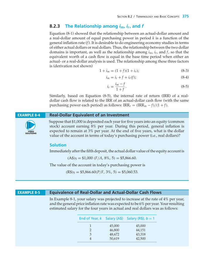
SECTION 8.2 / TERMINOLOGY AND BASIC CONCEPTS 375

8.2.3 The Relationship among im, ir , and f

Equation (8-1) showed that the relationship between an actual-dollar amount anda real-dollar amount of equal purchasing power in period k is a function of thegeneral inflation rate (f ). It is desirable to do engineering economy studies in termsof either actual dollars or real dollars. Thus, the relationship between the two dollardomains is important, as well as the relationship among im, ir, and f , so that theequivalent worth of a cash flow is equal in the base time period when either anactual- or a real-dollar analysis is used. The relationship among these three factorsis (derivation not shown)

1 + im = (1 + f )(1 + ir); (8-3)

im = ir + f + ir(f ); (8-4)

ir = im − f1 + f

. (8-5)

Similarly, based on Equation (8-5), the internal rate of return (IRR) of a real-dollar cash flow is related to the IRR of an actual-dollar cash flow (with the samepurchasing power each period) as follows: IRRr = (IRRm − f )/(1 + f ).

EXAMPLE 8-4 Real-Dollar Equivalent of an Investment

Suppose that $1,000 is deposited each year for five years into an equity (commonstock) account earning 8% per year. During this period, general inflation isexpected to remain at 3% per year. At the end of five years, what is the dollarvalue of the account in terms of today’s purchasing power (i.e., real dollars)?

SolutionImmediately after the fifth deposit, the actual dollar value of the equity account is

(A$)5 = $1,000 (F/A, 8%, 5) = $5,866.60.

The value of the account in today’s purchasing power is

(R$)5 = $5,866.60(P/F, 3%, 5) = $5,060.53.

EXAMPLE 8-5 Equivalence of Real-Dollar and Actual-Dollar Cash Flows

In Example 8-1, your salary was projected to increase at the rate of 4% per year,and the general price inflation rate was expected to be 6% per year. Your resultingestimated salary for the four years in actual and real dollars was as follows:

End of Year, k Salary (A$) Salary (R$), b = 1

1 45,000 45,0002 46,800 44,1513 48,672 43,3184 50,619 42,500

376 CHAPTER 8 / PRICE CHANGES AND EXCHANGE RATES

What is the present worth (PW) of the four-year actual- and real-dollar salarycash flows at the end of year one (base year) if your personal MARRm is 10% peryear (im)?

Solution(a) Actual-dollar salary cash flow:

PW(10%)1 = $45,000 + $46,800(P/F, 10%, 1)

+ $48,672(P/F, 10%, 2) + $50,619(P/F, 10%, 3)

= $165,798.

(b) Real-dollar salary cash flow:

ir = im − f1 + f

= 0.10 − 0.061.06

= 0.03774, or 3.774%;

PW(3.774%)1 = $45,000 + $44,151(

11.03774

)1

+ $43,318(

11.03774

)2

+ $42,500(

11.03774

)3

= $165,798.

Thus, we obtain the same PW at the end of year one (the base time period)for both the actual-dollar and real-dollar four-year salary cash flows when theappropriate interest rate is used for the equivalence calculations.

8.3 Fixed and Responsive AnnuitiesWhenever future cash flows are predetermined by contract, as in the case of abond or a fixed annuity, these amounts do not respond to general price inflation ordeflation. In cases where the future amounts are not predetermined, however, theymay respond to general price changes. To illustrate the nature of this situation, letus consider two annuities. The first annuity is fixed (unresponsive to general priceinflation) and yields $2,000 per year in actual dollars for 10 years. The secondannuity is of the same duration and yields enough future actual dollars to beequivalent to $2,000 per year in real dollars (purchasing power). Assuming ageneral price inflation rate of 6% per year, pertinent values for the two annuitiesover a 10-year period are as shown in Table 8-2.

Thus, when the amounts are constant in actual dollars (unresponsive to generalprice inflation), their equivalent amounts in real dollars decline over the 10-yearinterval to $1,117 in the final year. When the future cash-flow amounts are fixedin real dollars (responsive to general price inflation), their equivalent amounts inactual dollars rise to $3,582 by year 10.

SECTION 8.3 / FIXED AND RESPONSIVE ANNUITIES 377

TABLE 8-2 Illustration of Fixed and Responsive Annuities withGeneral Price Inflation Rate of 6% per Year

Fixed Annuity Responsive Annuity

End of In Actual In Equivalent In Actual In EquivalentYear k Dollars Real Dollarsa Dollars Real Dollarsa

1 $2,000 $1,887 $2,120 $2,0002 2,000 1,780 2,247 2,0003 2,000 1,679 2,382 2,0004 2,000 1,584 2,525 2,0005 2,000 1,495 2,676 2,0006 2,000 1,410 2,837 2,0007 2,000 1,330 3,007 2,0008 2,000 1,255 3,188 2,0009 2,000 1,184 3,379 2,000

10 2,000 1,117 3,582 2,000

a See Equation (8-1).

Use of Equation (4-30)

The actual dollars for a responsive annuity in Table 8-2 form a geometric gradientseries with f = 6% per year. Suppose we wish to determine its present worth at10% per year. From Equation (4-30), we see that

PW(10%) = $2,120[1 − (P/F, 10%, 10)(F/P, 6%, 10)]/(0.10 − 0.06)

= $2,120[1 − (0.3855)(1.7908)]/0.04

= $16,411.

We can obtain the same result (subject to round-off differences) using the equationin the footnote on page 150:

PW(10%) = $2,1201.06

(P/A, 3.774%, 10)

= $2,000(8.2030)

= $16,406.

Included in engineering economy studies are certain quantities unresponsive togeneral price inflation. For instance, depreciation amounts, once determined, donot increase (with present accounting practices) to keep pace with general priceinflation; lease fees and interest charges typically are contractually fixed for agiven period of time. Thus, it is important when doing an actual-dollar analysisto recognize the quantities that are unresponsive to general price inflation, andwhen doing a real-dollar analysis to convert these A$ quantities to R$ quantities,using Equation (8-2).

If this is not done, not all cash flows will be in the same dollar domain (A$ orR$), and the analysis results will be distorted. Specifically, the equivalent worths ofthe cash flows for an A$ and an R$ analysis will not be the same in the base year, b,

378 CHAPTER 8 / PRICE CHANGES AND EXCHANGE RATES

and the A$ IRR and the R$ IRR for the project will not have the proper relationshipbased on Equation (8-5); that is, IRRr = (IRRm − f )/(1 + f ).

In Example 8-6, we look at a bond (Chapter 5), which is a fixed-income asset,and see how its current value is affected by a period of projected deflation.

EXAMPLE 8-6 Impact of Deflation on the Current Price of a Bond

Suppose that deflation occurs in the U.S. economy and that the CPI (as a measureof f ) is expected to decrease an average of 2% per year for the next five years.A bond with a face (par) value of $10,000 and a life of five years (i.e., it will beredeemed in five years) pays an interest (bond) rate of 5% per year. The interestis paid to the owner of the bond once each year. If an investor expects a real rateof return of 4% per year, what is the maximum amount that should be paid nowfor this bond?

SolutionThe cash flows over the life of the bond are 0.05($10,000) = $500 per year ininterest (actual dollars) for years one through five, plus the redemption of $10,000(the face value of the bond), also in actual dollars, at the end of year five. Todetermine the current value of this bond (i.e., the maximum amount an investorshould pay for it), these cash flows must be discounted to the present, using themarket interest rate. From Equation (8-4), we can compute im (where f = −2%per year) as follows:

im = ir + f + ir(f ) = 0.04 − 0.02 − 0.04(0.02)

= 0.0192, or 1.92% per year.

Therefore, the current market value of the bond is

PW = $500(P/A, 1.92%, 5) + $10,000(P/F, 1.92%, 5)

= $500(4.7244) + $10,000(0.9093)

= $11,455.

In general, if the rate used to discount the future cash flows over the life of abond is less than the bond rate (the situation in this example), then the current(market) value will be greater than the bond’s face value. Therefore, duringperiods of deflation, owners of bonds (or other types of fixed-income assets)need to monitor their market values closely because a favorable sell situationmay occur.

Engineering economy studies that include the effects of price changes caused byinflation or deflation may also include such items as interest charges, depreciationamounts, lease payments, and other contract amounts that are actual-dollar cashflows based on past commitments. They are generally unresponsive to further pricechanges. At the same time, many other types of cash flows (e.g., labor, materials) areresponsive to market price changes. In Example 8-7, an after-tax analysis is presentedthat shows the correct handling of these different situations.

SECTION 8.3 / FIXED AND RESPONSIVE ANNUITIES 379

EXAMPLE 8-7 After-Tax Analysis: A Mixture of Fixed and Responsive Cash Flows

The cost of a new and more efficient electrical circuit switching equipment is$180,000. It is estimated (in base year dollars, b = 0) that the equipment willreduce current net operating expenses by $36,000 per year (for 10 years) andwill have a $30,000 market value at the end of the 10th year. For simplicity,these cash flows are estimated to increase at the general price inflation rate(f = 8% per year). Due to new computer control features on the equipment, itwill be necessary to contract for some maintenance support during the first threeyears. The maintenance contract will cost $2,800 per year. This equipment will bedepreciated under the MACRS (GDS) method, and it is in the five-year propertyclass. The effective income tax rate (t) is 38%; the selected analysis period is10 years; and the MARRm (after taxes) is im = 15% per year.

(a) Based on an actual-dollar after-tax analysis, is this capital investmentjustified?

(b) Develop the ATCF in real dollars.

Solution(a) The actual-dollar after-tax economic analysis of the new equipment is shown

in Table 8-3 (columns 1–7). The capital investment, savings in operatingexpenses, and market value (in the 10th year) are estimated in actual dollars(column 1), using the general price inflation rate and Equation (8-1). Themaintenance contract amounts for the first three years (column 2) are alreadyin actual dollars. (They are unresponsive to further price changes.) Thealgebraic sum of columns 1 and 2 equals the before-tax cash flow (BTCF)in actual dollars (column 3).

In columns 4, 5, and 6, the depreciation and income-tax calculations areshown. The depreciation deductions in column 4 are based on the MACRS(GDS) method and, of course, are in actual dollars. The entries in columns 5and 6 are calculated as discussed in Chapter 7. The effective income taxrate (t) is 38% as given. The entries in column 6 are equal to the entries incolumn 5 multiplied by −t. The algebraic sum of columns 3 and 6 equals theATCF in actual dollars (column 7). The PW of the actual-dollar ATCF, usingim = 15% per year, is

PW(15%) = −$180,000 + $36,050(P/F, 15%, 1)

+ · · · + $40,156(P/F, 15%, 10) = $33,790.

Therefore, the project is economically justified.(b) Next, Equation (8-1) is used to calculate the ATCF in real dollars from

the entries in column 7. The real-dollar ATCF (column 9) shows theestimated economic consequences of the new equipment in dollars that havethe constant purchasing power of the base year. The actual-dollar ATCF(column 7) is in dollars that have the purchasing power of the year in whichthe cost or saving occurs. The comparative information provided by theATCF in both actual dollars and real dollars is helpful in interpreting the

380C

HA

PTER8

/P

RIC

EC

HA

NG

ESA

ND

EX

CH

AN

GE

RA

TES

380

TABLE 8-3 Example 8-7 When the General Price Inflation Rate Is 8% per Year

(6) (8)End of (1) (2) (3) (4) (5) Income (7) R$ (9)Year A$ Cash Contract BTCF Depreciation Taxable Taxes ATCF Adjustment ATCF(k) Flows (A$) (A$) (A$) Income (t = 0.38) (A$) [1/(1 + f )]k−b (R$)

0 −$180,000 −$180,000 −$180,000 1.0000 −$180,0001 38,880a −$2,800 36,080 $36,000 $80 −$30 36,050 0.9259 33,3792 41,990 −2,800 39,190 57,600 −18,410 +6,996 46,186 0.8573 39,5953 45,349 −2,800 42,549 34,560 7,989 −3,036 39,513 0.7938 31,3664 48,978 48,978 20,736 28,242 −10,732 38,246 0.7350 28,1115 52,895 52,895 20,736 32,159 −12,220 40,675 0.6806 27,6836 57,128 57,128 10,368 46,760 −17,769 39,359 0.6302 24,8047 61,697 61,697 61,697 −23,445 38,252 0.5835 22,3208 66,632 66,632 66,632 −25,320 41,312 0.5403 22,3209 71,964 71,964 71,964 −27,346 44,618 0.5003 22,320

10 77,720 77,720 77,720 −29,534 48,186 0.4632 22,32010 64,767b 64,767 64,767 −24,611 40,156 0.4632 18,600

a (A$)k = $36,000(1.08)k−0, k = 1, . . . , 10.b MV10,A$ = $30,000(1.08)10 = $64,767.

SECTION 8.4 / DIFFERENTIAL PRICE CHANGES 381

results of an economic analysis. Also, as illustrated in this example, theconversion between actual dollars and real dollars can easily be done. ThePW of the real-dollar ATCF (column 9), using ir = (im − f )/(1 + f ) = (0.15 −0.08)/1.08 = 0.06481, or 6.48%, is

PW(6.48%) = −$180,000 + $33,379(P/F, 6.48%, 1)

+ · · · + $18,600(P/F, 6.48%, 10)

= $33,790.

Thus, the PW (equivalent worth in the base year with b = 0) of the real-dollarATCF is the same as the PW calculated previously for the actual-dollar ATCF.

8.4 Differential Price ChangesThe general price inflation (or deflation) rate ( f) may not be the best estimate offuture price changes for one or more cost and revenue cash flows in an engineeringeconomy study. The variation between the general price inflation rate and thebest estimate of future price changes for specific goods and services is calleddifferential price inflation (or deflation), and it is caused by factors such as technologicalimprovements, and changes in productivity, regulatory requirements, and soon. Also, a restriction in supply, an increase in demand, or a combination ofboth may change the market value of a particular good or service relative toothers. Price changes caused by some combination of general price inflation anddifferential price inflation (or deflation) can be represented by a total price escalation(or de-escalation) rate. These rates are further defined as follows:

1. Differential price inflation (or deflation) rate (e′j): The increment (%) of price

change (in the unit price or cost for a fixed amount), above or below the generalprice inflation rate, during a period (normally a year) for good or service j.

2. Total price escalation (or de-escalation) rate (ej): The total rate (%) of price change(in the unit price or cost for a fixed amount) during a period (normally a year),for good or service j. The total price escalation rate for a good or service includesthe effects of both the general price inflation rate ( f ) and the differential priceinflation rate (e′

j) on price changes.

8.4.1 The Relationship among ej , e′j , and f

The differential price inflation rate (e′j) is a price change in good or service j in

real dollars caused by various factors in the marketplace. Similarly, the total priceescalation rate (ej) is a price change in actual dollars. The relationship among thesetwo factors (ej, e′

j) and f is (derivation not shown)

1 + ej = (1 + e′j)(1 + f ); (8-6)

382 CHAPTER 8 / PRICE CHANGES AND EXCHANGE RATES

ej = e′j + f + e′

j(f ); (8-7)

e′j = ej − f

1 + f. (8-8)

Thus, as shown in Equation (8-7), the total price escalation rate (ej) for good orservice j in actual dollars is the sum of the general price inflation rate and thedifferential price inflation rate plus their product. Also, as shown in Equation(8-8), the differential price inflation rate (e′

j) in real dollars can be calculated fromthe total price escalation rate and the general price inflation rate.

In practice, the general price inflation rate ( f ) and the total price escalation rate(ej) for each good and service involved are usually estimated for the study period.For each of these rates, different values may be used for subsets of periods withinthe analysis period if justified by the available data. The differential price inflationrates (e′

j), when needed, normally are not estimated directly but are calculatedusing Equation (8-8).

EXAMPLE 8-8

The prospective maintenance expenses for a commercial heating, ventilating,and air-conditioning (HVAC) system are estimated to be $12,200 per year inbase-year dollars (assume that b = 0). The total price escalation rate is estimatedto be 7.6% for the next three years (e1,2,3 = 7.6%), and for years four and fiveit is estimated to be 9.3% (e4,5 = 9.3%). The general price inflation rate ( f ) forthis five-year period is estimated to be 4.7% per year. Develop the maintenanceexpense estimates for years one through five in actual dollars and in real dollars,using ej and e′

j values, respectively.

TABLE 8-4 Example 8-8 Calculations

(1) (2) (3) (4) (5)End of A$ Maintenance R$ MaintenanceYear, k Adjustment (ej) Expenses, A$ Adjustment (e′

j) Expenses, R$

1 $12,200(1.076)1 $13,127 $12,200(1.0277)1 $12,5382 12,200(1.076)2 14,125 12,200(1.0277)2 12,8853 12,200(1.076)3 15,198 12,200(1.0277)3 13,2424 12,200(1.076)3 (1.093)1 16,612 12,200(1.0277)3 (1.0439)1 13,8235 12,200(1.076)3 (1.093)2 18,157 12,200(1.0277)3 (1.0439)2 14,430

SolutionThe development of the annual maintenance expenses in actual dollars is shownin column 2 of Table 8-4. In this example, the general price inflation rate is not thebest estimate of changes in future maintenance expenses. The five-year period isdivided into two subperiods corresponding to the two different price escalation

SECTION 8.5 / SPREADSHEET APPLICATION 383

rates (e1,2,3 = 7.6%; e4,5 = 9.3%). These rates are then used with the estimatedexpenses in the base year; (A$)0 = (R$)0 = $12,200.

The development of the maintenance expenses in real dollars is shown incolumn 4. This development is the same as for actual dollars, except that thee′

j values [Equation (8-8)] are used instead of the ej values. The e′j values in this

example are as follows:

e′1,2,3 = 0.076 − 0.047

1.047= 0.0277, or 2.77%;

e′4,5 = 0.093 − 0.047

1.047= 0.0439, or 4.39%.

This illustrates that differential inflation, or deflation, also results in market pricechanges in real dollars, as well as in actual dollars.

An additional example of differential price changes is provided in Section8.7 (case study).

8.5 Spreadsheet ApplicationThe following example illustrates the use of spreadsheets to convert actual dollarsto real dollars, and vice versa.

EXAMPLE 8-9 Saving to Meet a Retirement Goal

Sara B. Goode wishes to retire in the year 2022 with personal savings of $500,000(1997 spending power). Assume that the expected inflation rate in the economywill average 3.75% per year during this period. Sara plans to invest in a 7.5%per year savings account, and her salary is expected to increase by 8.0% per yearbetween 1997 and 2022. Assume that Sara’s 1997 salary was $60,000 and that thefirst deposit took place at the end of 1997. What percent of her yearly salary mustSara put aside for retirement purposes to make her retirement plan a reality?

SolutionThis example demonstrates the flexibility of a spreadsheet, even in instanceswhere all of the calculations are based on a piece of information (percentage ofsalary to be saved) that we do not yet know. If we deal in actual dollars, thecash-flow relationships are straightforward. The formula in cell B7 in Figure 8-1converts the desired ending balance into actual dollars. The salary is paid at theend of the year, at which point some percentage is placed in a bank account.The interest calculation is based on the cumulative deposits and interest in theaccount at the beginning of the year, but not on the deposits made at the end ofthe year. The salary is increased and the cycle repeats.

The spreadsheet model is shown in Figure 8-1. We can enter the formulasfor the annual salary increase (column B), the percentage of the salary (cell E1)that goes into savings (column C), and the bank balance at the end of the year(column D) without knowing the percentage of salary being saved.

384 CHAPTER 8 / PRICE CHANGES AND EXCHANGE RATES

Figure 8-1 Spreadsheet Solution, Example 8-9

A slider control (cells F1 and G1) is used in this model to vary the percentageof salary saved value in cell E1. The value in cell E1 can be changed by using themouse to click on either the left or right arrows. We’ll know when we’ve found

SECTION 8.6 / FOREIGN EXCHANGE RATES AND PURCHASING POWER CONCEPTS 385

the correct percentage when the difference between the desired balance andactual balance (cell D37) is approximately zero. The steps involved in creatinga slider control in Excel can be found in Appendix A. (As an alternative to theslider control, we could have manually changed the value in cell E1 or made useof the solver feature that most spreadsheet packages include.)

Once the problem has been formulated in a spreadsheet, we can determinethe impact of different interest rates, inflation rates, and so on, on the retirementplan, with minimal changes and effort. [Answer: 12.44%]

8.6 Foreign Exchange Rates and PurchasingPower Concepts

Unless you are planning to travel abroad, you probably haven’t given muchthought to how currency fluctuations can affect purchasing power. With the worldeconomy becoming increasingly interconnected, a dollar rising in price (or aweakening euro) will have an impact on the estimated cash flows associated withforeign investments. Many factors influence the price of a currency due to supply-and-demand considerations, including a country’s interest rates, cross-borderinvesting, national debt, inflation, and trade balance. When a currency changesin value because of these factors, holders of that country’s currency experiencea change in overseas buying power. For example, if one dollar goes from beingworth 1.0 euros to 0.8 euros (in this situation the dollar is weakening), 1,000 eurosworth of goods from a European company that previously cost a U.S. purchaser$1,000 must now be bought for $1,250. This applies to consumer products as well ascapital investments, and the purpose of Section 8.6 is to explore the consequencesof exchange rate fluctuations on the profitability of foreign investments.

Changes in the exchange rate between two currencies over time are analogousto changes in the general inflation rate because the relative purchasing powerbetween the two currencies is changing similar to the relative purchasing powerbetween actual dollar amounts and real dollar amounts.

Assume the following:ius = rate of return in terms of a market interest rate relative to U.S. dollars.ifm = rate of return in terms of a market interest rate relative to the currency

of a foreign country.fe = annual devaluation rate (rate of annual change in the exchange rate) be-

tween the currency of a foreign country and the U.S. dollar. In the follow-ing relationships, a positive fe is used when the foreign currency is beingdevalued relative to the dollar, and a negative fe is used when the dollaris being devalued relative to the foreign currency.

386 CHAPTER 8 / PRICE CHANGES AND EXCHANGE RATES

Then (derivation not shown)

1 + ius = 1 + ifm1 + fe

,

or

ifm = ius + fe + fe(ius), (8-9)

and

ius = ifm − fe1 + fe

. (8-10)

EXAMPLE 8-10 Investing in a Foreign Assembly Plant

The CMOS Electronics Company is considering a capital investment of50,000,000 pesos in an assembly plant located in a foreign country. Currencyis expressed in pesos, and the exchange rate is now 100 pesos per U.S. dollar.

The country has followed a policy of devaluing its currency against thedollar by 10% per year to build up its export business to the United States. Thismeans that each year the number of pesos exchanged for a dollar increases by10% (fe = 10%), so in two years (1.10)2(100) = 121 pesos would be tradedfor one dollar. Labor is quite inexpensive in this country, so management ofCMOS Electronics feels that the proposed plant will produce the following ratherattractive ATCF, stated in pesos:

End of Year 0 1 2 3 4 5

ATCF −50 +20 +20 +20 +30 +30(millions of pesos)

If CMOS Electronics requires a 15% IRR per year, after taxes, in U.S. dollars (ius)on its foreign investments, should this assembly plant be approved? Assumethat there are no unusual risks of nationalization of foreign investments in thiscountry.

SolutionTo earn a 15% annual rate of return in U.S. dollars, the foreign plant must earn,based on Equation (8-9), 0.15 + 0.10 + 0.15(0.10) = 0.265, which is 26.5% on itsinvestment in pesos (ifm). As shown next, the PW (at 26.5%) of the ATCF, in pesos,is 9,165,236, and its IRR is 34.6%. Therefore, investment in the plant appears to be

SECTION 8.6 / FOREIGN EXCHANGE RATES AND PURCHASING POWER CONCEPTS 387

economically justified. We can also convert pesos into dollars when evaluatingthe prospective investment:

End of Year ATCF (Pesos) Exchange Rate ATCF (Dollars)

0 −50,000,000 100 pesos per $1 −500,0001 20,000,000 110 pesos per $1 181,8182 20,000,000 121 pesos per $1 165,2893 20,000,000 133.1 pesos per $1 150,2634 30,000,000 146.4 pesos per $1 204,9185 30,000,000 161.1 pesos per $1 186,220

IRR: 34.6% IRR: 22.4%PW(26.5%): 9,165,236 pesos PW(15%): $91,632

The PW (at 15%) of theATCF, in dollars, is $91,632, and its IRR is 22.4%. Therefore,the plant again appears to be a good investment, in economic terms. Noticethat the two IRRs can be reconciled by using Equation (8-10):

ius(IRR in $) = ifm(IRR in pesos) − 0.10

1.10

= 0.346 − 0.101.10

= 0.224, or 22.4%.

Remember that devaluation of a foreign currency relative to the U.S. dollarproduces less expensive exports to the United States. Thus, devaluation meansthat the U.S. dollar is stronger relative to the foreign currency. That is, fewer dollarsare needed to purchase a fixed amount (barrels, tons, items) of goods and servicesfrom the foreign source or, stated differently, more units of the foreign currency arerequired to purchase U.S. goods. This phenomenon was observed in Example 8-10.

Conversely, when exchange rates for foreign currencies gain strength againstthe U.S. dollar (fe has a negative value and the U.S. dollar is weaker relative to theforeign currency), the prices for imported goods and services into the United Statesrise. In such a situation, U.S. products are less expensive in foreign markets.

In summary, if the average devaluation of currency A is fe% per year relative tocurrency B, then each year it will require fe% more of currency A to exchangefor the same amount of currency B.

EXAMPLE 8-11 Estimating Future Exchange Rates

The monetary (currency) unit of another country, A, has a present exchange rateof 10.7 units per U.S. dollar.

388 CHAPTER 8 / PRICE CHANGES AND EXCHANGE RATES

(a) If the average devaluation of currency A in the international market isestimated to be 4.2% per year (for the next five years) relative to the U.S.dollar, what would be the exchange rate three years from now?

(b) If the average devaluation of the U.S. dollar (for the next five years) isestimated to be 3% per year relative to currency A, what would be theexchange rate three years from now?

Solution(a) 10.7(1.042)3 = 12.106 units of A per U.S. dollar.(b) 10.7 units of A = 1(1.03)3 U.S. dollars,

1 U.S. dollar = 10.71.09273

= 9.792 units of A.

EXAMPLE 8-12 Profitability Analysis of a Foreign Investment

A U.S. firm is analyzing a potential investment project in another country. Thepresent exchange rate is 425 of their currency units (A) per U.S. dollar. Thebest estimate is that currency A will be devalued in the international marketat an average of 2% per year relative to the U.S. dollar over the next severalyears. The estimated before-tax net cash flow (in currency A) of the project is asfollows:

End of Year Net Cash Flow (Currency A)

0 −850,000,0001 270,000,0002 270,000,0003 270,000,0004 270,000,0005 270,000,0006 270,000,0006 (MV)a 120,000,000

a Estimated market value at the end of year six.

(a) If the MARR value of the U.S. firm (before taxes and based on the U.S. dollar)is 20% per year, is the project economically justified?

(b) Instead, if the U.S. dollar is estimated to be devalued in the internationalmarket an average of 2% per year over the next several years, what wouldbe the rate of return based on the U.S. dollar? Is the project economicallyjustified?

SECTION 8.6 / FOREIGN EXCHANGE RATES AND PURCHASING POWER CONCEPTS 389

Solution(a) PW(i′%) = 0 = −850,000,000 + 270,000,00(P/A, i′%, 6)

+ 120,000,000(P/F, i′%, 6).

By trial and error (Chapter 5), we determine that i′% = ifm = IRRfm =24.01%. Now, using Equation (8-10), we have

ius = IRRus = 0.2401 − 0.021.02

= 0.2158, or 21.58%.

Since this rate of return in terms of the U.S. dollar is greater than the firm’sMARR (20% per year), the project is economically justified (but very closeto the minimum rate of return required on the investment).

A Second Solution to Part (a)Using Equation (8-9), we can determine the firm’s MARR value in terms ofcurrency A as follows:

ifm = MARRfm = 0.20 + 0.02 + 0.02(0.20) = 0.244, or 22.4%.

Using this MARRfm value, we can calculate the PW(22.4%) of the project’s netcash flow (which is estimated in units of currency A); that is, PW(22.4%) =32,597,000 units of currency A. Since this PW is greater than zero, we confirmthat the project is economically justified.

(b) Using Equation (8-10) and the IRRfm value [24.01% calculated in the solutionto Part (a)], we have

ius = IRRus = 0.2401 − (−0.02)

1 − 0.02= 0.2654, or 26.54%.

Since the rate of return in terms of the U.S. dollar is greater than the requiredMARRus = 20%, the project is economically justified.

As additional information, notice in the first solution to Part (a), whencurrency A is estimated to be devalued relative to the U.S. dollar, IRRus =21.58%; whereas in Part (b), when the U.S. dollar is estimated to be devaluedrelative to currency A, IRRus = 26.54%. What is the relationship between thedifferent currency devaluations in the two parts of the problem and theseresults?

Answer: Since the annual earnings to the U.S. firm from the investmentare in units of currency A originally, and currency A is being devaluedrelative to the U.S. dollar in Part (a), these earnings would be exchanged fordecreasing annual amounts of U.S. dollars, causing an unfavorable impacton the project’s IRRus. In Part (b), however, the U.S. dollar is being devaluedrelative to currency A, and these annual earnings would be exchanged forincreasing annual amounts of U.S. dollars, causing a favorable impact onthe project’s IRRus.

390 CHAPTER 8 / PRICE CHANGES AND EXCHANGE RATES

8.7 CASE STUDY−−Selecting Electric Motors to Power an Assembly Line

A large computer manufacturing company is expanding its operations in responseto an increase in demand. To meet the new production goals, the company needsto upgrade its assembly line. This upgrade requires additional electric motors thatwill be able to deliver a total of 1,550 horsepower output.

There are two types of motors available, induction and synchronous, whosespecifications are listed in the accompanying table. Both motor types are three-phase, and the quoted voltage is rms line-to-line. If the synchronous motors areoperated at a power factor (pf) of 1.0, their efficiency is reduced to 80%, but the localpower utility will provide electricity at a discounted rate of $0.025 per kilowatt-hourfor the first year.

Type of Motor

Synchronous SynchronousSpecifications Induction (pf = 0.9 lag) (pf = 1.0)

Rated horsepower 400 500 500Efficiency 85% 90% 80%Line voltage 440 440 440Capital investment $17,640 $24,500 $24,500Maintenance cost (First year) $1,000 $1,250 $1,250Electricity cost (First year) $0.030/kWh $0.030/kWh $0.025/kWh

Historical data indicate that maintenance costs increase at the rate of 4% peryear and that the cost of electricity increases at the rate of 5% per year. The assemblyline must operate two eight-hour shifts per day, six days per week, for 50 weeks peryear. An eight-year study period is being used for the project, and the company’smarket-based cost of capital (MARRm) is 8% per year. Your engineering projectteam has been tasked with determining what combination of motors should bepurchased to provide the additional power requirements of the upgraded assemblyline.

SolutionYour project team has decided that the overall problem of motor selection can bebroken down into the following subproblems to arrive at a recommendation:

(a) Determine whether it is less expensive to operate a synchronous motor at apower factor of 0.9 or 1.0.

(b) Determine the PW of the cost of operating one motor of each type at ratedhorsepower for the total period of operational time during the eight-yearproject lifetime.

(c) Determine the combination of motors that should be purchased. The objectiveis to minimize the PW of the total cost.

SECTION 8.7 / CASE STUDY—SELECTING ELECTRIC MOTORS TO POWER AN ASSEMBLY LINE 391

Solution to Subproblem (a)Because the capital investment and maintenance costs of the synchronous motorare independent of the power factor employed, only the cost of electricity needs tobe considered at this stage of the analysis.

The efficiency of the 500-horsepower synchronous motor operating at a powerfactor of 0.9 is 90%. Therefore, the cost of electricity per operating hour is (recallthat 1 hp = 746 watts)

(500 hp/0.9)(0.746 kW/hp)($0.030/kWh) = $12.43/hour.

When operated at a power factor (pf) of 1.0, the efficiency of the motor is reducedto 80%. The electric company, however will provide electricity at a discounted rate.The resulting cost of electricity is

(500 hp/0.8)(0.746 kW/hp)($0.025/kWh) = $11.66/hour.

Therefore, it is less expensive to operate the synchronous motor at pf = 1.0. Thediscounted electricity rate more than compensates for the loss in efficiency. Giventhis information, operating the synchronous motor at pf = 0.9 is no longer a feasiblealternative.

Solution to Subproblem (b)The total cost of each motor over the study period consists of the capital investment,maintenance costs, and electricity costs. Specifically, for each motor type,

PWTotal costs = Capital investment + PW(maintenance costs)

+ PW(electricity costs).

Maintenance costs increase 4% annually over the eight-year period and can bemodeled as a geometric gradient series. Recall from Chapter 4 that the presentequivalent of a geometric gradient series is given by:

P =⎧⎨⎩

A1[1 − (P/F, i%, N)(F/P, f%, N)]i − f

f �= i

A1N(P/F, i%, 1) f = i,(8-11)

where f is the rate of increase per period. Using this relationship,

PW(maintenance costs) = A1[1 − (P/F, 8%, 8)(F/P, 4%, 8)]0.08 − 0.04

= A1

0.04[1 − (0.5403)(1.3686)]

= A1(6.5136),

where A1 = $1,000 for the induction motor and A1 = $1,250 for the synchronousmotor.

392 CHAPTER 8 / PRICE CHANGES AND EXCHANGE RATES

Electricity costs are estimated to increase 5% annually over the eight-year studyperiod and can also be modeled as a geometric gradient series.

PW(electricity costs) = A1[1 − (P/F, 8%, 8)(F/P, 5%, 8)]0.08 − 0.05

= A1

0.03[1 − (0.5403)(1.4775)]

= A1(6.7236).

Now, the number of hours of motor operation per year is

(8 hours/shift)(2 shifts/day)(6 days/week)(50 weeks/year) = 4,800 hours/year.

Thus, for the induction motor,

A1 = (400 hp/0.85)(0.746 kW/hp)(4,800 hours/year)($0.030/kWh) = $50,552

and

A1 = (500 hp/0.8)(0.746 kW/hp)(4,800 hours/year)($0.025/kWh) = $55,950

for the synchronous motor running at pf = 1.0.We can now compute the PW of total costs for each motor type over the entire

eight-year study period.

PWTotal costs(induction motor) = $17,640 + $1,000(6.5136) + $50,552(6.7236)

= $17,640 + $6,514 + $339,891

= $364,045.

PWTotal costs(synchronous motor) = $24,500 + $1,250(6.5136) + $55,950(6.7236)

= $24,500 + $8,142 + $376,185

= $408,827.

Solution to Subproblem (c)The last step of the analysis is to determine what combination of motors to use toobtain the required 1,550 horsepower output. The following four options will beconsidered:

(A) Four induction motors (three at 400 horsepower, one at 350 horsepower)(B) Four synchronous motors (three at 500 horsepower, one at 50 horsepower)(C) Three induction motors at 400 horsepower plus one synchronous motor at

350 horsepower(D) Three synchronous motors at 500 horsepower plus one induction motor at

50 horsepower.

For a motor used at less than rated capacity, the electricity cost is proportional tothe fraction of capacity used—all other costs are unaffected.

SECTION 8.8 / TRY YOUR SKILLS 393

The PW of total costs for each of the preceding options is computed using theresults of subproblem (b):

PWTotal costs(A) = (3)($364,045) + [$17,640 + $6,514 + (350/400)($339,891)]= $1,413,694

PWTotal costs(B) = (3)($408,827) + [$24,500 + $8,142 + (50/500)($376,185)]= $1,296,742

PWTotal costs(C) = (3)($364,045) + [$24,500 + $8,142 + (350/500)($376,185)]= $1,388,107

PWTotal costs(D) = (3)($408,827) + [$17,640 + $6,514 + (50/400)($339,891)]= $1,293,121

Option (D) has the lowest PW of total costs. Thus, your project team’s recommen-dation is to power the assembly line using three 500-horsepower synchronousmotors operated at a power factor of 1.0 and one 400-horsepower induction motor.You also include a note to management that there is additional capacity availableshould future modifications to the assembly line require more power.

This case study illustrates the inclusion of price changes in the analysis ofengineering projects. The cost of goods and services changes over time and needsto be addressed. Sensitivity analyses on key performance and cost parameters canbe used to quantify project risk.

8.8 Try Your SkillsThe number in parentheses that follows each problem refers to the sectionfrom which the problem is taken. Solutions to these problems can be found inAppendix G.

8-A. To estimate when your money will be worth half of what it is worth today,divide 72 by the expected average annual rate of inflation. If the long-termannual rate of inflation is 3%, in how many years will your money be worthhalf of its current value? What if the average annual inflation rate increasesto 4%? (8.2)

8-B. Health care costs are reportedly rising at an annual rate that is triple thegeneral inflation rate. The current inflation rate is running at 4% per year.In 10 years, how much greater will health care costs be compared witha service/commodity that increases at exactly the 4% general inflationrate? (8.2)

8-C. Which of these situations would you prefer? (8.2)

a. You invest $2,500 in a certificate of deposit that earns an effective interestrate of 8% per year. You plan to leave the money alone for 5 years, andthe general price inflation rate is expected to average 5% per year. Incometaxes are ignored.

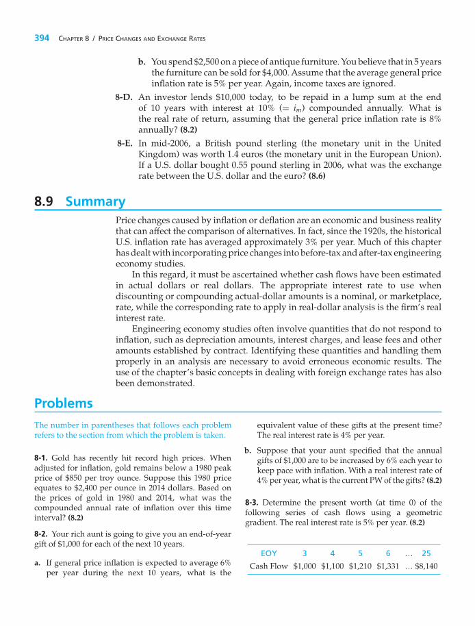
394 CHAPTER 8 / PRICE CHANGES AND EXCHANGE RATES

b. You spend $2,500 on a piece of antique furniture. You believe that in 5 yearsthe furniture can be sold for $4,000. Assume that the average general priceinflation rate is 5% per year. Again, income taxes are ignored.

8-D. An investor lends $10,000 today, to be repaid in a lump sum at the endof 10 years with interest at 10% (= im) compounded annually. What isthe real rate of return, assuming that the general price inflation rate is 8%annually? (8.2)

8-E. In mid-2006, a British pound sterling (the monetary unit in the UnitedKingdom) was worth 1.4 euros (the monetary unit in the European Union).If a U.S. dollar bought 0.55 pound sterling in 2006, what was the exchangerate between the U.S. dollar and the euro? (8.6)

8.9 SummaryPrice changes caused by inflation or deflation are an economic and business realitythat can affect the comparison of alternatives. In fact, since the 1920s, the historicalU.S. inflation rate has averaged approximately 3% per year. Much of this chapterhas dealt with incorporating price changes into before-tax and after-tax engineeringeconomy studies.

In this regard, it must be ascertained whether cash flows have been estimatedin actual dollars or real dollars. The appropriate interest rate to use whendiscounting or compounding actual-dollar amounts is a nominal, or marketplace,rate, while the corresponding rate to apply in real-dollar analysis is the firm’s realinterest rate.

Engineering economy studies often involve quantities that do not respond toinflation, such as depreciation amounts, interest charges, and lease fees and otheramounts established by contract. Identifying these quantities and handling themproperly in an analysis are necessary to avoid erroneous economic results. Theuse of the chapter’s basic concepts in dealing with foreign exchange rates has alsobeen demonstrated.

ProblemsThe number in parentheses that follows each problemrefers to the section from which the problem is taken.

8-1. Gold has recently hit record high prices. Whenadjusted for inflation, gold remains below a 1980 peakprice of $850 per troy ounce. Suppose this 1980 priceequates to $2,400 per ounce in 2014 dollars. Based onthe prices of gold in 1980 and 2014, what was thecompounded annual rate of inflation over this timeinterval? (8.2)

8-2. Your rich aunt is going to give you an end-of-yeargift of $1,000 for each of the next 10 years.

a. If general price inflation is expected to average 6%per year during the next 10 years, what is the

equivalent value of these gifts at the present time?The real interest rate is 4% per year.

b. Suppose that your aunt specified that the annualgifts of $1,000 are to be increased by 6% each year tokeep pace with inflation. With a real interest rate of4% per year, what is the current PW of the gifts? (8.2)

8-3. Determine the present worth (at time 0) of thefollowing series of cash flows using a geometricgradient. The real interest rate is 5% per year. (8.2)

EOY 3 4 5 6 … 25

Cash Flow $1,000 $1,100 $1,210 $1,331 … $8,140

PROBLEMS 395

8-4. Jeff just received a refund of $2,178 from his familyphysician. This was an overpayment on his account,and it has been 3 years since the overpayment wasdue. Jeff is really frosted by this delay! What is thepurchasing power now (year 0) of the overpayment ifinflation has been 4%, 3%, and 2%, respectively, in years−3 (three years ago), −2 (two years ago), and −1 (lastyear)? (4.13, 8.2)

8-5. Re-work Problem 4-89 when the tuition increasefor your sophomore year is 10%; for your junior year,12%; and for your senior year, 8%. Your parents’ savingsaccount earns 4% for the first two years, then it increasesto 6% for the last two years. (4.13 and 8.2)

8-6. Annual expenses for two alternatives have beenestimated on different bases as follows:

Alternative A Alternative BAnnual Expenses Annual Expenses

End of Estimated in Estimated in RealYear Actual Dollars Dollars with b = 0

1 $120,000 $100,0002 132,000 110,0003 148,000 120,0004 160,000 130,000

If the average general price inflation rate is expectedto be 4% per year and the real rate of interest is 8%per year, show which alternative has the least negativeequivalent worth in the base period? (8.2)

8-7. The incredible shrinking $50 bill in 1957 was worth$50, but in 2007 it is worth only $6.58. (8.2)

a. What was the compounded average annual inflationrate (loss of purchasing power) during this period oftime?

b. Fifty dollars invested in the stock market in 1957was worth $1,952 in 2007. In view of your answerto Part (a), what was the annual real interest rateearned on this investment?

8-8. The price of cotton sky-rocketed during the CivilWar because of Union naval blockades of Confederateports. This was a primary reason the South experienced4,000% inflation from 1861 to 1865 (four years).Specifically, what cost 1 cent in 1861 cost $40 in 1865.What was the equivalent annual inflation rate that theSouth was forced to endure? (8.2)

8-9. A recent college graduate has received the annualsalaries shown in the following table over the past

four years. During this time, the CPI has performedas indicated. Determine the annual salaries in year-zerodollars (b = 0), using the CPI as the indicator of generalprice inflation. (8.2)

End of Year Salary (A$) CPI

1 $34,000 2.4%2 36,200 1.9%3 38,800 3.3%4 41,500 3.4%

8-10. Paul works for a government agency in southernCalifornia making $70,000 per year. He is now beingtransferred to a branch office in Tennessee. The salaryreduction associated with this transfer is 11%. Paul is notinsulted by this reduction in pay and accepts his newlocation and salary gladly. He researched that the costof living index in California is 132 whereas the cost ofliving index in Tennessee is 95. Over the next five years,what is the FW of Paul’s extra income/improved lifestyle (through the reduced cost of living) from havingmade this move? Paul’s MARR is 10% per year (im). (8.2)

8-11. A large corporation’s electricity billamounts to $400 million. During the next 10

years, electricity usage is expected to increase by 65%,and the estimated electricity bill 10 years hence hasbeen projected to be $920 million. Assuming electricityusage and rates increase at uniform annual rates overthe next 10 years, what is the annual rate of inflation ofelectricity prices expected by the corporation? (8.2)

8-12. Your older brother is concerned more aboutinvestment safety than about investment performance.For example, he has invested $100,000 in safe 10-yearcorporate AAA bonds yielding an average of 6% peryear, payable each year. His effective income tax rateis 33%, and inflation will average 3% per year. Howmuch will his $100,000 be worth in 10 years in today’spurchasing power after income taxes and inflation aretaken into account? (8.2)

8-13. Your younger brother is very concerned aboutinvestment performance, but he is willing to toleratesome risk. He decides to invest $100,000 in a mutualfund that will earn 10% per year. The proceeds will beaccumulated as a lump sum and paid out at the end ofyear 10. Based on the data given in Problem 8-12, what istoday’s purchasing power equivalent of your youngerbrother’s investment? (8.2)

396 CHAPTER 8 / PRICE CHANGES AND EXCHANGE RATES

8-14. Acommercial building design cost $89/square-foot to construct eight years ago (for an 80,000-square-foot building). This construction cost has increased5.4% per year since then. Presently, your companyis considering construction of a 125,000-square-footbuilding of the same design. The cost capacity factoris X = 0.92. In addition, it is estimated that workingcapital will be 5% of construction costs, and that projectmanagement, engineering services, and overhead willbe 4.2%, 8%, and 31%, respectively, of constructioncosts. Also, it is estimated that annual expenses in thefirst year of operation will be $5/square-foot, and theseare estimated to increase 5.66% per year thereafter. Thefuture general inflation rate is estimated to be 7.69% peryear, and the market-based MARR = 12% per year (im).(Chapter 3 and 8.2)

a. What is the estimated capital investment for the125,000-square-foot building?

b. Based on a before-tax analysis, what is the PW forthe first 10 years of ownership of the building?

c. What is the AW for the first 10 years of ownership inreal dollars (R$)?

8-15. Twenty years ago your rich uncle invested $10,000in an aggressive (i.e., risky) mutual fund. Much to youruncle’s chagrin, the value of his investment declinedby 18% during the first year and then declined another31% during the second year. But your uncle decidedto stick with this mutual fund, reasoning that long-term sustainable growth of the U.S. economy wasbound to occur and enhance the value of his mutualfund. Eighteen more years have passed, and youruncle’s cumulative return over the 20-year period is awhopping 507%! (8.2)

a. What is the value of the original investment now?

b. If inflation has averaged 6% per year over the past20 years, what is the spending power equivalent ofthe answer to Part (a) in terms of real dollars 20 yearsago?

c. What is the real compound interest rate earned overthe 20-year period?

d. During the past 18 years, what compound annualrate of return (yield) was earned on your uncle’sinvestment?

8-16. A woman desires to have $400,000 in a savingsaccount when she retires in 20 years. Because of theeffects of inflation on spending power, she stipulatesthat her future “nest egg” will be equivalent to$400,000 in today’s purchasing power. If the expected

average inflation rate is 7% per year and the savingsaccount earns 5% per year, what lump-sum amount ofmoney should the woman deposit now in her savingsaccount? (8.2)

8-17. Alfred Smith wants to purchase life insurance thatwill guarantee his family $50,000 (in R-dollars) per yearin bond interest income forever. The interest rate (im)from corporate bonds is expected to pay 8% per year,and the inflation rate is expected to average 3% peryear. How much life insurance should Alfred purchaseto protect his family forever? (8.2)

8-18. In 2009, the average cost to construct a150,000-barrel-a-day oil refinery was $2.4 billion

(excluding any interest payments). This capital invest-ment is spread uniformly over a five-year constructioncycle (i.e., the refinery starts producing products in2014). Assume end-of-year cash-flow convention andanswer the following questions. (Chapter 3 and 8.2)

a. If the cost of capital spent to build the refinery is10% per year, how much interest will be charged (asa lump sum in 2014) during the construction of thisproject?

b. If the cost-capacity factor is 0.91, what is theapproximate cost to build a 200,000-barrel-a-dayrefinery in 2009?

c. If inflation of the construction cost of a refinery is9.2% per year, what is the estimated cost of buildinga 200,000-barrel-a-day refinery in 2019?

8-19. In January of 1980, a troy ounce of gold sold for$850 (an all-time high). Over the past 28 years, supposethe CPI has grown at a compounded annual rate of3.2%. Today a troy ounce of gold sells for $690. (8.2)

a. In real terms, with 1980 as the reference year, what istoday’s price of gold per ounce in 1980 purchasingpower?

b. If gold increases in value to keep pace with the CPI,how many years will it take to grow to $850 perounce in today’s purchasing power?

c. What was the real interest rate earned from 1980 to2010 on an ounce of gold?

8-20. Suppose it costs $18,000 per year (in early 2014dollars) for tuition, room, board, and living expenses toattend a public university in the Southeastern UnitedStates. (8.2)

PROBLEMS 397

a. If inflation averages 8% per year, what is the totalcost of a four-year college education starting in 2024(i.e., 10 years from now)?

b. Starting in January of 2014, what monthly savingsamount must be put aside to pay for this four-yearcollege education? Assume your savings accountearns 6% per year, compounded monthly (0.5% permonth).

8-21. Suppose natural gas experiences a 1.8%increase per year in real terms over the foresee-

able future. The cost of a 1,000 cubic feet of natural gasis now $7.50. (8.2)

a. What will be the cost in real terms of 1,000 cubic feetof natural gas in 22 years?

b. If the general price inflation rate (e.g., the CPI) forthe next 22 years is expected to average 3.2% peryear, what will a 1,000 cubic feet of natural gas costin actual dollars 22 years from now?

8-22. Refer to Example 4-8. If inflation is expected toaverage 3% per year over the next 60 years, yourpurchasing power will be less than $1,107,706. (8.2)

a. When f = 3% per year, what is the purchasing powerof this future sum of money in today’s dollars whenyou reach age 80?

b. Repeat Part (a) when inflation averages 2% per year.

8-23. Four hundred pounds of copper are usedin a typical 2,200-square-foot newly constructed

house. Today’s copper price is $3.75 per pound. (8.2)

a. If copper prices are expected to increase 8.5% peryear (on average), what is the cost of copper goingto be in a new 2,400-square-foot house built 10 yearsfrom now? Use a cost-capacity factor of 1.0.

b. To minimize building costs, do you think thatanother less-expensive material (e.g., aluminum)will be substituted for copper in the electrical wiringin new homes?

8-24. The cost of first-class postage has risen by about5% per year over the past 30 years. The U.S. PostalService introduced a one-time forever stamp in 2008that cost 41 cents for first-class postage (one ounce orless), and it will be valid as first-class postage regardlessof all future price increases. Let’s say you decided topurchase 1,000 of these stamps for this one-time specialrate. Assume 5% inflation and your personal MARR is10% per year (im). Did you make a sound economicaldecision? (8.2)

8-25. Refer to Problem 5-56. If the governmentexpects inflation to average 3% per year, what is

the equivalent uniform annual savings in fuel (jet fuelsavings will be $2.5 billion one year from now). MARRremains at 7% per year (im).

8-26. With interest rates on the rise, many Americansare wondering what their investment strategy shouldbe. A safe (i.e., a virtually risk-free) and increasinglypopular way to keep pace with the cost of living is topurchase inflation-indexed government bonds. Theseso called I-bonds pay competitive interest rates andincrease in value when the CPI rises. These bonds canbe held for up to 30 years.

Suppose you purchased an I-bond for $10,000 andheld it for 11 years, at which time you received $20,000for the bond. Inflation has averaged 3% per year duringthis 11-year period. What real annual rate of return didyou earn on your inflation-adjusted I-bond? Is it reallycompetitive? (8.3)

8-27. The capital investment for a new highway pavingmachine is $950,000. The estimated annual expense, inyear zero dollars, is $92,600. This expense is estimatedto increase at the rate of 5.7% per year. Assume thatf = 4.5%, N = 7 years, MV at the end of year 7 is 10% ofthe capital investment, and the MARR (in real terms) is10.05% per year. What uniform annual revenue (beforetaxes), in actual dollars, would the machine need togenerate to break even? (8.4)

8-28. A hospital has two different medical devices itcan purchase to perform a specific task. Both deviceswill perform an accurate analysis. Device A costs$100,000 initially, whereas device B (the deluxe model)costs $150,000. It has been estimated that the cost ofmaintenance will be $5,000 for device A and $3,000 fordevice B in the first year. Management expects thesecosts to increase 10% per year. The hospital uses a six-year study period, and its effective income tax rate is50%. Both devices qualify as five-year MACRS (GDS)property. Which device should the hospital choose if theafter-tax, market-based MARR is 8% per year (im)? (8.3)

8-29. The cost of conventional medications for diabeteshas risen by an average of 13.1% per year over the pastfour years. During this same period of time, the costof a specialty drug for rheumatoid arthritis (RA) hasincreased 22.5% per year. If these increases continue intothe foreseeable future, in how many years will an RAmedicine now costing $20 per dose be at least five timesas expensive as a diabetes inhaler that now costs $10 peruse? (8.3)

398 CHAPTER 8 / PRICE CHANGES AND EXCHANGE RATES

8-30. XYZ rapid prototyping (RP) software costs$20,000, lasts one year, and will be expensed (i.e.,written off in one year). The cost of the upgrades willincrease 10% per year, starting at the beginning of yeartwo. How much can be spent now for an RP softwareupgrade agreement that lasts three years and mustbe depreciated with the SL method to zero over threeyears? MARR is 20% per year (im), and the effectiveincome tax rate (t) is 34%. (Chapter 7, and 8.3)

8-31. A health services firm is thinking about pur-chasing a large autoclave for $180,000. The autoclave isexpected to generate $60,000 in its first year of operation.This amount will increase by 5% per year (so it wouldbe $63,000 in year 2). Furthermore, the autoclave hasa useful life of 8 years and an expected annual usageof 2,000 hours. Its salvage (market) value at the end ofyear 8 will be 10% of the initial investment. What is theequivalent annual worth of the autoclave, per hour ofutilization, if the firm’s MARR is 8% per year? (4.12 andEquation 8-11)

8-32. In a certain foreign country in 2009, the localcurrency (the ‘Real’) was pegged to the U.S. dollar atthe rate of $1 U.S. = 1 Real. The Real was then devaluedover the next five years so that $1 U.S. = 2 Real. A bankin the Northeastern United States bought assets in thiscountry valued at 100 million Real in 2009. Now that it isyear 2014, what is the worth of this bank’s investment inU.S. dollars? Should the bank sell out of its investmentin this foreign country or should it buy more assets? (8.6)

8-33. An international corporation located in CountryA is considering a project in the United States. Thecurrency in Country A, say X, has been strengtheningrelative to the U.S. dollar; specifically, the averagedevaluation of the U.S. dollar has been 2.6% per year(which is projected to continue). Assume the presentexchange rate is 6.4 units of X per U.S. dollar. (a) Whatis the estimated exchange rate two years from now, and(b) if, instead, currency X was devaluing at the same rate(2.6% per year) relative to the U.S. dollar, what wouldbe the exchange rate three years from now? (8.6)

8-34. A certain commodity cost 0.5 pound sterling inthe United Kingdom. In U.S. denominated dollars, thissame item can be purchased for 85 cents. The exchangerate is 1 pound sterling = $1.80 U.S. (8.6)

a. Should this commodity be purchased in the UnitedKingdom or in the United States?

b. If 100,000 items comprise the purchase quantity,how much can be saved in view of your answer toPart (a)?

8-35. A company requires a 26% internal rate of return(before taxes) in U.S. dollars on project investments inforeign countries. (8.6)

a. If the currency of Country A is projected to averagean 8% annual devaluation relative to the dollar, whatrate of return (in terms of the currency there) wouldbe required for a project?

b. If the dollar is projected to devaluate 6% annuallyrelative to the currency of Country B, what rateof return (in terms of the currency there) would berequired for a project?

8-36. Apex, Inc. is a U.S.-based firm that is in the processof buying a medium-sized company in Brazil. Becausethe Brazilian company sells its services to the globalmarketplace, revenues are dollar denominated. Itscosts, however, are expressed in the Brazilian currency.If Apex anticipates a stronger dollar, which tends todecrease the value of the Brazilian currency, explainwhy the Brazilian company’s purchase price may berelatively insensitive to exchange-rate fluctuations. (8.6)

8-37. A U.S. company is considering a high-technology project in a foreign country. The estimatedeconomic results for the project (after taxes), in theforeign currency (T-marks), is shown in the followingtable for the seven-year analysis period being used.The company requires an 18% rate of return inU.S. dollars (after taxes) on any investments in thisforeign country. (8.6)

End of Year Cash Flow (T-marks after Taxes)

0 −3,600,0001 450,0002 1,500,0003 1,500,0004 1,500,0005 1,500,0006 1,500,0007 1,500,000

a. Should the project be approved, based on a PWanalysis in U.S. dollars, if the devaluation of theT-mark, relative to the U.S. dollar, is estimated toaverage 12% per year and the present exchange rateis 20 T-marks per dollar?

b. What is the IRR of the project in T-marks?

c. Based on your answer to (b), what is the IRR in U.S.dollars?

PROBLEMS 399

8-38. Sanjay has 100 euros to spend before he flies backto the United States. He wishes to purchase jewelrypriced at $160 (U.S.) in a duty-free shop at the airport.Euros can be bought for $1.32 and sold for $1.24. Theowner of the duty-free shop tells Sanjay that the jewelrycan be purchased for 100 euros plus $40 (U.S.). Is this agood deal for Sanjay? Explain your reasoning. (8.6)

8-39. An automobile manufacturing company in Coun-try X is considering the construction and operation of alarge plant on the eastern seaboard of the United States.Their MARR = 20% per year on a before-tax basis. (Thisis a market rate relative to their currency in Country X.)The study period used by the company for this typeof investment is 10 years. Additional information isprovided as follows:

• The currency in Country X is the Z-Kron.

• It is estimated that the U.S. dollar will become weakerrelative to the Z-Kron during the next 10 years.Specifically, the dollar is estimated to be devaluedat an average rate of 2.2% per year.

• The present exchange rate is 92 Z-Krons perU.S. dollar.

• The estimated before-tax net cash flow (inU.S. dollars) is as follows:

EOY Net Cash Flow (U.S. Dollars)

0 −$168,000,0001 −32,000,0002 69,000,000...

...10 69,000,000

Based on a before-tax analysis, will this project meet thecompany’s economic decision criterion? (8.6)

8-40. Your company must obtain some laser meas-urement devices for the next six years and is consideringleasing. You have been directed to perform an actual-dollar after-tax study of the leasing approach. Thepertinent information for the study is as follows:

Lease costs: First year, $80,000; second year, $60,000;third through sixth years, $50,000 per year. Assumethat a six-year contract has been offered by the lessorthat fixes these costs over the six-year period.

Other costs (not covered under contract): $4,000 in year-zero dollars, and estimated to increase 10% each year.

Effective income tax rate: 40%. (8.7)

a. Develop the actual-dollar ATCF for the leasingalternative.

b. If the real MARR (ir) after taxes is 5% per year andthe annual inflation rate (f ) is 9.524% per year, whatis the actual-dollar after-tax equivalent annual costfor the leasing alternative?

8-41. A gas-fired heating unit is expected tomeet an annual demand for thermal energy of

500 million Btu, and the unit is 80% efficient. Assumethat each 1,000 cubic feet of natural gas, if burned at100% efficiency, can deliver one million Btu. Furthersuppose that natural gas is now selling for $7.50 per1,000 cubic feet. What is the PW of fuel cost for thisheating unit over a 12-year period if natural gas pricesare expected to increase at an average rate of 10% peryear? The firm’s MARR (= im) is 18% per year. (8.7)

8-42. A small heat pump, including the ductsystem, now costs $2,500 to purchase and in-

stall. It has a useful life of 15 years and incurs ann-ual maintenance expenses of $100 per year in real(year-zero) dollars over its useful life. A compressorreplacement is required at the end of the eighth year at acost of $500 in real dollars. The annual cost of electricityfor the heat pump is $680, based on present prices.Electricity prices are projected to increase at an annualrate of 10%. All other costs are expected to increaseat 6%, which is the projected general price inflationrate. The firm’s MARR, which includes an allowancefor general price inflation, is 15% per year (im). Nomarket value is expected from the heat pump at theend of 15 years. (8.7)

a. What is the AW, expressed in actual dollars, ofowning and operating the heat pump?

b. What is the AW in real dollars of owning andoperating the heat pump?

8-43. A certain engine lathe can be purchased for$150,000 and depreciated over three years to a zerosalvage value with the SL method. This machine willproduce metal parts that will generate revenues of$80,000 (time zero dollars) per year. It is a policy ofthe company that the annual revenues will be increasedeach year to keep pace with the general inflation rate,which is expected to average 5%/year ( f = 0.05). Labor,materials, and utilities totaling $20,000 (time 0 dollars)per year are all expected to increase at 9% per year. Thefirm’s effective income tax rate is 50%, and its after-taxMARR (im) is 26% per year.

Perform an actual-dollar (A$) analysis and deter-mine the annual ATCFs of the preceding investment

400 CHAPTER 8 / PRICE CHANGES AND EXCHANGE RATES

opportunity. Use a life of three years and work to thenearest dollar. What interest rate would be used fordiscounting purposes? (Chapter 7 and 8.3, 8.7)

8-44. Your company manufactures circuit boards andother electronic parts for various commercial products.Design changes in part of the product line, whichare expected to increase sales, will require changesin the manufacturing operation. The cost basis ofnew equipment required is $220,000 (MACRS five-yearproperty class). Increased annual revenues, in year zerodollars, are estimated to be $360,000. Increased annualexpenses, in year zero dollars, are estimated to be$239,000. The estimated market value of equipment inactual dollars at the end of the six-year analysis period is$40,000. General price inflation is estimated at 4.9% peryear; the total increase rate of annual revenues is 2.5%,and for annual expenses it is 5.6%; the after-tax MARR(in market terms) is 10% per year (im); and t = 39%.(Chapter 7 and 8.3, 8.7)

a. Based on an after-tax, actual-dollar analysis, whatis the maximum amount that your company canafford to spend on the total project (i.e., changing themanufacturing operations)? Use the PW method ofanalysis.

b. Develop (show) your ATCF in real dollars.

8-45. You have been assigned the task of analyzingwhether to purchase or lease some transportationequipment for your company. The analysis period issix years, and the base year is year zero (b = 0). Otherpertinent information is given in Table P8-45. Also,

a. The contract terms for the lease specify a cost of$300,000 in the first year and $200,000 annually inyears two through six (the contract, i.e., these rates,does not cover the annual expense items).

b. The after-tax MARR (not including inflation) is13.208% per year (ir).

c. The general inflation rate (f ) is 6%.

TABLE P8-45 Table for Problem 8-45

Estimate in Year-0 Dollars Best Estimateof Price Change

Cash Flow Item Purchase Lease (% per year)

Capital investment $600,000 — —MV at end of six years 90,000 — 2%Annual operating, insurance, and other expenses 26,000 $26,000 6Annual maintenance expenses 32,000 32,000 9

d. The effective income tax rate (t) is 34%.

e. Assume the equipment is in the MACRS (GDS)five-year property class.

Which alternative is preferred? (Use an after-tax, actualdollar analysis and the FW criterion.) (Chapter 7 and8.3, 8.7)

8-46. Extended Learning ExerciseChrysler is considering a cost reduction program

with its major suppliers wherein the suppliers mustreduce the cost of the components that they furnish toChrysler by 5% each year. (The total amount of savingswould increase each year.) The initial costs for settingup the program include the following:

• Program Setup: $12,500,000• Feasibility Study

(completed six months ago): 1,500,000• Supplier Training: 7,500,000

Chrysler is currently paying a total of $85,000,000 peryear for components purchased from the vendors whowill be involved in this program. (Assume that, if theprogram is not approved, the annual cost of purchasedcomponents will remain constant at $85,000,000 peryear.) The program has been designed as a five-yearinitiative, and Chrysler’s MARR for such projects is12% (im). There will be annual operating expensesassociated with the program for further training ofvendors, updating internal documentation, and so on.Given the projected savings in purchased components,what would be the maximum annual operating expensefor this program such that it is marginally justified? (8.3)

8-47. Extended Learning Exercise The yuan is the cur-rency of the People’s Republic of China (PRC). Theyuan has been pegged by the PRC government to theU.S. dollar for the past 10 years at a fixed rate of 8.28yuan to the dollar. If the May 2005 undervalued yuanwere allowed to rise to its true value, Chinese imports

SPREADSHEET EXERCISES 401

would become more expensive compared to U.S.-madeproducts. One scenario is to allow the yuan to float invalue against the U.S. dollar. Assume the yuan increasesin value 25% against the dollar so that the dollar is worth0.75(8.28 yuan) = 6.21 yuan.

If an American firm buys a lot of Chinese-madetextile products for 10 yuan apiece, it would cost10 yuan ($1 U.S./6.21 yuan) = $1.6103 per item withthe revalued yuan. The lot of 10,000 items would cost$16,103. Before the revaluing of the yuan, each itemwould have cost 10 yuan ($1 U.S./8.28 yuan) = $1.2077per item, or $12,077 for the lot. Discuss the followingwith your classmates. (8.6)

a. What happens to the cost of PRC goods in Europeancountries when the dollar is strong (still 8.28yuan per dollar)? What happens when the dollarweakens?

b. Will Americans buy the same amount of Chinesegoods when $1 U.S. = 6.21 yuan? Will this fuelinflation in the United States?

c. What happens to the PRC–U.S. trade balance ifmore expensive Chinese goods are bought at thesame level as with the $1 U.S. per 8.28 yuan policy?

8-48. Extended Learning ExerciseThis case study is a justification of a computer systemfor, the ABC Company. The following are known data:

• The combined initial hardware and software cost is$80,000.

• Contingency costs have been set at $15,000. These arenot necessarily incurred.

• A service contract on the hardware costs $500 permonth.

• The effective income tax rate (t) is 38%.

• Company management has established a 15% (= im)per year hurdle rate (MARR).

In addition, the following assumptions and projectionshave been made:

• In order to support the system on an ongoing basis,a programmer/analyst will be required. The startingsalary (first year) is $28,000, and fringe benefitsamount to 30% of the base salary. Salaries are expectedto increase by 6% each year thereafter.

• The system is expected to yield a staff savings of threepersons (to be reduced through normal attrition) atan average salary of $16,200 per year per person (basesalary plus fringes) in year-zero (base year) dollars.It is anticipated that one person will retire during thesecond year, another in the third year, and a third inthe fourth year.

• A 3% reduction in purchased material costs isexpected; first year purchases are $1,000,000 inyear-zero dollars and are expected to grow at acompounded rate of 10% per year.

• The project life is expected to be six years, and thecomputer capital investment will be fully depreciatedover that time period [MACRS (GDS) five-yearproperty class].

Based on this information, perform an actual-dollarATCF analysis. Is this investment acceptable based oneconomic factors alone? (8.3, 8.7)

Spreadsheet Exercises

8-49. Develop a spreadsheet to verify that the fol-lowing table entries are correct (to the nearest wholepercent). (8.2)

Erosion of Money’sPurchasing Power

Inflation Rate 10 years 25 years

2% −18% −39%4% −32% −62%

8-50. Refer to Example 8-9. Sara has decided that savingmore than 12% of her annual salary was unrealistic. Sheis considering postponing her retirement until 2027, but

still wishes to have $500,000 (in 1997 spending power)at that time. Determine what percentage of her annualsalary Sara will have to save to meet her objective. (8.4)

8-51. Because of tighter safety regulations, an improvedair filtration system must be installed at a plant thatproduces a highly corrosive chemical compound. Thecapital investment in the system is $260,000 in present-day dollars. The system has a useful life of 10 yearsand is in the MACRS (GDS) five-year property class.It is expected that the MV of the system at the end ofits 10-year life will be $50,000 in present-day dollars.Annual expenses, estimated in present-day dollars, areexpected to be $6,000 per year, not including an annual

402 CHAPTER 8 / PRICE CHANGES AND EXCHANGE RATES

property tax of 4% of the investment cost (does notinflate). Assume that the plant has a remaining life of20 years and that replacement costs, annual expenses,and MV increase at 6% per year.

If the effective income tax rate is 40%, set up aspreadsheet to determine the ATCF for the system over

a 20-year period. The after-tax market rate of returndesired on investment capital is 12% per year (im). Whatis the PW of costs of this system after income taxes havebeen taken into account? Develop the real-dollar ATCF.(Assume that the annual general price inflation rate is4.5% over the 20-year period.) (Chapter 7 and 8.3, 8.7)

Case Study Exercises

8-52. Repeat the analysis for a reduced studyperiod of five years. (8.7)

8-53. Suppose the cost of electricity is expec-ted to increase at the rate of 6% per year. How will

this new information change your recommendation?

Use the original eight-year study period in youranalysis. (8.7)

8-54. A redesign of the assembly line would onlyrequire 1,300 horsepower output. Determine

the best combination of motors given this reducedhorsepower requirement. (8.7)

FE Practice Problems

8-55. A machine cost $2,550 on January 1, 2000, and$3,930 on January 1, 2004. The average inflation rateover these four years was 7% per year. What is the truepercentage increase in the cost of the machine from 2000to 2004? (8.2)(a) 14.95% (b) 54.12% (c) 7.00%(d) 17.58% (e) 35.11%

8-56. If you want to receive a 7% inflation-free returnon your investment and you expect inflation to be 9%per year, what actual interest rate must you earn? (8.2)(a) 16% (b) −2% (c) 1% (d) 7% (e) 9%

8-57. A person just turned 21 years old. If inflation isexpected to average 2.4% per year for the next 44 years,how much will $1 today be worth when this personretires at age 65?(a) $0.055 (b) $0.35 (c) $0.56 (d) $0.65

8-58. Two alternatives, A and B, are under consi-deration. Both have a life of five years. Alternative Aneeds an initial investment of $17,000 and provides a netrevenue of $4,000 per year for five years. Alternative Brequires an investment of $19,000 and has an annual netrevenue of $5,000. All estimates are in actual dollars.Inflation is expected to be 2% per year for the next fiveyears, and the inflation-free (real) MARR is 9.8% peryear. Which alternative should be chosen? (8.2)

(a) Alternative A (b) Alternative B(c) Neither alternative

8-59. How much life insurance should Stan Money-maker buy if he wants to leave enough money to hisfamily so that they get $25,000 per year forever inconstant dollars as of the year of his death? The interestrate from the life insurance company is 7% per year,while the inflation rate is expected to be 4% per year. Thefirst payment occurs one year after Stan’s death. (8.2)

(a) $866,000 (b) $357,000 (c) $625,000(d) $841,000

8-60. If the European euro is worth Canadian $1.60 anda Canadian dollar trades for U.S. $0.75, what is theexchange rate from U.S. dollars to European euros? (8.6)

(a) $2.13 (b) $1.44 (c) $1.20 (d) $0.95

8-61. Light, sweet crude oil in the world marketis U.S. dollar denominated. The price of oil is

rising partially because the dollar is not worth what itused to be (i.e., the dollar is now worth less than lastyear or last month). If the dollar today is worth 0.75euros in Europe (i.e., 1 euro = $1.333 U.S.), the value ineuros of $67 U.S. per barrel oil is most nearly (8.6)

(a) 40 euros per barrel (b) 50 euros per barrel(c) 60 euros per barrel (d) 80 euros per barrel

CHAPTER 9

Replacement Analysis

The objective of Chapter 9 is to address the question of whether a currentlyowned asset should be kept in service or immediately replaced.

New Flood Control Pumps

A fter Hurricane Katrina there was a need to replace outdatedhydraulic flood control pumps in New Orleans. These oldpumps are powered by pressurized oil, and they can be

replaced by a newer and more expensive type of pump that utilizes an up-to-date drive design having solid drive shafts instead of pressurized oil. This chapterdeals with systematic and formal comparisons of replacement alternatives such asthe one in New Orleans. Such studies can lead to enormous savings in subsequentoperating and ownership costs to an organization.

403

If you need a new machine and don’t buy it, you pay for it without ever gettingthe machine.

—Henry Ford (1922)

9.1 IntroductionA decision situation often encountered in business firms and governmentorganizations, as well as by individuals, is whether an existing asset should beretired from use, continued in service, or replaced with a new asset. As the pressuresof worldwide competition continue to increase, requiring higher quality goodsand services, shorter response times, and other changes, this type of decision isoccurring more frequently. Thus, the replacement problem, as it is commonly called,requires careful engineering economy studies to provide the information neededto make sound decisions that improve the operating efficiency and the competitiveposition of an enterprise.

Engineering economy studies of replacement situations are performed usingthe same basic methods as other economic studies involving two or morealternatives. Often the decision is whether to replace an existing (old) asset,descriptively called the defender, with a new asset. The one or more alternativereplacement (new) assets are then called challengers.

The specific decision situation, however, occurs in different forms. Sometimesit may be whether to retire an asset without replacement (abandonment) or to retainthe asset for backup rather than primary use. Also, the decision may be influencedif changed production requirements can be met by augmenting the capacity orcapability of the existing asset(s).

9.2 Reasons for Replacement AnalysisThe need to evaluate the replacement, retirement, or augmentation of assetsresults from changes in the economics of their use in an operating environment.Various reasons can underlie these changes, and unfortunately they are sometimesaccompanied by unpleasant financial facts. The following are the three majorreasons that summarize most of the factors involved:

1. Physical Impairment (Deterioration) These are changes that occur in thephysical condition of an asset. Normally, continued use (aging) results in the lessefficient operation of an asset. Routine maintenance and breakdown repair costsincrease, energy use may increase, more operator time may be required, and soforth. Or, some unexpected incident such as an accident occurs that affects thephysical condition and the economics of ownership and use of the asset.

404

SECTION 9.3 / FACTORS THAT MUST BE CONSIDERED IN REPLACEMENT STUDIES 405

2. Altered Requirements Capital assets are used to produce goods and services thatsatisfy human wants. When the demand for a good or service either increasesor decreases or the design of a good or service changes, the related asset(s) mayhave the economics of its use affected.

3. Technology The impact of changes in technology varies among different typesof assets. For example, the relative efficiency of heavy highway constructionequipment is impacted less rapidly by technological changes than automatedmanufacturing equipment. In general, the costs per unit of production, as wellas quality and other factors, are favorably impacted by changes in technology,which result in more frequent replacement of existing assets with new and betterchallengers.

Reason 2 (altered requirements) and Reason 3 (technology) are sometimes referredto as different categories of obsolescence. In any replacement problem, factors frommore than one of these three major areas may be involved. Regardless of the specificconsiderations, the replacement of assets often represents an economic opportunityfor the firm.

For the purposes of our discussion of replacement studies, the following is adistinction between various types of lives for typical assets:

Economic life is the period of time (years) that results in the minimumequivalent uniform annual cost (EUAC) of owning and operating an asset.∗ If weassume good asset management, economic life should coincide with the period oftime extending from the date of acquisition to the date of abandonment, demotionin use, or replacement from the primary intended service.

Ownership life is the period between the date of acquisition and the date ofdisposal by a specific owner. A given asset may have different categories of use bythe owner during this period. For example, a car may serve as the primary familycar for several years and then serve only for local commuting for several more years.

Physical life is the period between original acquisition and final disposal of anasset over its succession of owners. For example, the car just described may haveseveral owners over its existence.

Useful life is the time period (years) that an asset is kept in productive service(either primary or backup). It is an estimate of how long an asset is expected to beused in a trade or business to produce income.

9.3 Factors that Must Be Consideredin Replacement Studies

There are several factors that must be considered in replacement studies. Once aproper perspective has been established regarding these factors, little difficultyshould be experienced in making replacement studies. Six factors and relatedconcepts are discussed in this section:

1. Recognition and acceptance of past errors2. Sunk costs

∗ The AW of a primarily cost cash-flow pattern is sometimes called the EUAC. Because this term is commonly used inthe definition of the economic life of an asset, we will often use EUAC in this chapter.

406 CHAPTER 9 / REPLACEMENT ANALYSIS

3. Existing asset value and the outsider viewpoint

4. Economic life of the proposed replacement asset (challenger)5. Remaining (economic) life of the old asset (defender)6. Income tax considerations

9.3.1 Past Estimation Errors

The economic focus in a replacement study is the future. Any estimation errors madein a previous study related to the defender are not relevant (unless there are incometax implications). For example, when an asset’s book value (BV) is greater than itscurrent market value (MV), the difference frequently has been designated as anestimation error. Such errors also arise when capacity is inadequate, maintenanceexpenses are higher than anticipated, and so forth.

This implication is unfortunate because in most cases these differences are notthe result of errors but of the inability to foresee future conditions better at thetime of the original estimates. Acceptance of unfavorable economic realities maybe made easier by posing a hypothetical question, What will be the costs of mycompetitor who has no past errors to consider? In other words, we must decidewhether we wish to live in the past, with its errors and discrepancies, or to be ina sound competitive position in the future. A common reaction is, I can’t afford totake the loss in value of the existing asset that will result if the replacement is made.The fact is that the loss already has occurred, whether or not it could be afforded,and it exists whether or not the replacement is made.

9.3.2 The Sunk-Cost Trap

Only present and future cash flows should be considered in replacement studies.Any unamortized values (i.e., unallocated value of an asset’s capital investment)of an existing asset under consideration for replacement are strictly the result ofpast decisions—that is, the initial decision to invest in that asset and decisionsas to the method and number of years to be used for depreciation purposes. Forpurposes of this chapter, we define a sunk cost to be the difference between anasset’s BV and its MV at a particular point in time. Sunk costs have no relevanceto the replacement decisions that must be made (except to the extent that they affectincome taxes). When income tax considerations are involved, we must include thesunk cost in the engineering economy study. Clearly, serious errors can be made inpractice when sunk costs are incorrectly handled in replacement studies.

9.3.3 Investment Value of Existing Assetsand the Outsider Viewpoint

Recognition of the nonrelevance of BVs and sunk costs leads to the properviewpoint to use in placing value on existing assets for replacement study purposes.In this chapter, we use the so-called outsider viewpoint for approximating theinvestment worth of an existing asset (defender). In particular, the outsiderviewpoint∗ is the perspective that would be taken by an impartial third party to

∗ The outsider viewpoint is also known as the opportunity cost approach to determining the value of the defender.

SECTION 9.3 / FACTORS THAT MUST BE CONSIDERED IN REPLACEMENT STUDIES 407

establish the fair MV of a used (secondhand) asset. This viewpoint forces the analystto focus on present and future cash flows in a replacement study, thus avoiding thetemptation to dwell on past (sunk) costs.

The present realizable MV is the correct capital investment amount to be assignedto an existing asset in replacement studies.∗ A good way to reason that this is trueis to use the opportunity cost or opportunity forgone principle. That is, if it is decided tokeep the existing asset, we are giving up the opportunity to obtain its net realizableMV at that time. Therefore, this situation represents the opportunity cost of keepingthe defender.

There is one addendum to this rationale: If any new investment expenditure(such as for overhaul) is needed to upgrade the existing asset so that it will becompetitive in level of service with the challenger, the extra amount should beadded to the present realizable MV to determine the total investment in the existingasset for replacement study purposes.

When using the outsider viewpoint, the total investment in the defender is theopportunity cost of not selling the existing asset for its current MV, plus the costof upgrading it to be competitive with the best available challenger. (All feasiblechallengers are to be considered.)

Clearly, the MV of the defender must not also be claimed as a reduction inthe challenger’s capital investment, because doing so would provide an unfairadvantage to the challenger by double counting the defender’s selling price.

EXAMPLE 9-1 Investment Cost of the Defender (Existing Asset)

The purchase price of a certain new automobile (challenger) being considered foruse in your business is $21,000. Your firm’s present automobile (defender) canbe sold on the open market for $10,000. The defender was purchased with cashthree years ago, and its current BV is $12,000. To make the defender comparablein continued service to the challenger, your firm would need to make somerepairs at an estimated cost of $1,500.

Based on this information,

(a) What is the total capital investment in the defender, using the outsiderviewpoint?

(b) What is the unamortized value of the defender?

Solution(a) The total capital investment in the defender (if kept) is its current MV (an

opportunity cost) plus the cost of upgrading the car to make it comparable inservice to the challenger. Hence, the total capital investment in the defenderis $10,000 + $1,500 = $11,500 (from an outsider’s viewpoint). This representsa good starting point for estimating the cost of keeping the defender.

∗ In after-tax replacement studies, the before-tax MV is modified by income tax effects related to potential gains (losses)forgone if the defender is kept in service.

408 CHAPTER 9 / REPLACEMENT ANALYSIS

(b) The unamortized value of the defender is the book loss (if any) associatedwith disposing of it. Given that the defender is sold for $10,000, theunamortized value (loss) is $12,000−$10,000 = $2,000. This is the differencebetween the current MV and the current BV of the defender. As discussed inSection 9.3.2, this amount represents a sunk cost and has no relevance to thereplacement decision, except to the extent that it may impact income taxes(to be discussed in Section 9.9).

9.3.4 Economic Life of the Challenger

The economic life of an asset minimizes the EUAC of owning and operating theasset, and it is often shorter than the useful or physical life. It is essential to knowa challenger’s economic life, in view of the principle that new and existing assetsshould be compared over their economic (optimum) lives. Economic data regardingchallengers are periodically updated (often annually), and replacement studies arethen repeated to ensure an ongoing evaluation of improvement opportunities.

9.3.5 Economic Life of the Defender

As we shall see later in this chapter, the economic life of the defender is often oneyear. Consequently, care must be taken when comparing the defender asset with achallenger asset, because different lives (Chapter 6) are involved in the analysis. Weshall see that the defender should be kept longer than its apparent economic life,as long as its marginal cost is less than the minimum EUAC of the challenger overits economic life. What assumptions are involved when two assets having differentapparent economic lives are compared, given that the defender is a nonrepeatingasset? These concepts will be discussed in Section 9.7.

9.3.6 The Importance of Income Tax Consequences

The replacement of assets often results in gains or losses from the sale of depreciableproperty, as discussed in Chapter 7. Consequently, to perform an accurate economicanalysis in such cases, the studies must be made on an after-tax basis. It is evidentthat the existence of a taxable gain or loss, in connection with replacement, can havea considerable effect on the results of an engineering study. Aprospective gain fromthe disposal of assets can be reduced by as much as 40% or 50%, depending on theeffective income tax rate used in a particular study. Hence, the decision to disposeof or retain an existing asset can be influenced by income tax considerations.

9.4 Typical Replacement ProblemsThe following typical replacement situations are used to illustrate several of thefactors that must be considered in replacement studies. These analyses use theoutsider viewpoint to determine the investment in the defenders.

SECTION 9.4 / TYPICAL REPLACEMENT PROBLEMS 409

EXAMPLE 9-2 Replacement Analysis Using Present Worth (Before Taxes)

Afirm owns a pressure vessel that it is contemplating replacing. The old pressurevessel has annual operating and maintenance expenses of $60,000 per year and itcan be kept for five more years, at which time it will have zero MV. It is believedthat $30,000 could be obtained for the old pressure vessel if it were sold now.

A new pressure vessel can be purchased for $120,000. The new pressurevessel will have an MV of $50,000 in five years and will have annual operatingand maintenance expenses of $30,000 per year. Using a before-tax MARR of 20%per year, determine whether or not the old pressure vessel should be replaced.A study period of five years is appropriate.

SolutionThe first step in the analysis is to determine the investment value of the defender(old pressure vessel). Using the outsider viewpoint, the investment value of thedefender is $30,000, its present MV. We can now compute the PW (or FW or AW)of each alternative and decide whether the old pressure vessel should be keptin service or replaced immediately.

Defender: PW(20%) = −$30,000 − $60,000(P/A, 20%, 5)

= −$209,436.

Challenger: PW(20%) = −$120,000 − $30,000(P/A, 20%, 5)

+ $50,000(P/F, 20%, 5) = −$189,623.

The PW of the challenger is greater (less negative) than the PW of the defender.Thus, the old pressure vessel should be replaced immediately. (The EUAC ofthe defender is $70,035 and that of the challenger is $63,410.)

EXAMPLE 9-3 Before-Tax Replacement Analysis Using EUAC

The manager of a carpet manufacturing plant became concerned about theoperation of a critical pump in one of the processes. After discussing this situationwith the supervisor of plant engineering, they decided that a replacement studyshould be done, and that a nine-year study period would be appropriate for thissituation. The company that owns the plant is using a before-tax MARR of 10%per year for its capital investment projects.

The existing pump, Pump A, including driving motor with integratedcontrols, cost $17,000 five years ago. An estimated MV of $750 could beobtained for the pump if it were sold now. Some reliability problems have beenexperienced with Pump A, including annual replacement of the impeller andbearings at a cost of $1,750. Annual operating and maintenance expenses havebeen averaging $3,250. Annual insurance and property tax expenses are 2% ofthe initial capital investment. It appears that the pump will provide adequate

410 CHAPTER 9 / REPLACEMENT ANALYSIS

TABLE 9-1 Summary of Information for Example 9-3

MARR (before taxes) = 10% per year

Existing Pump A (defender)Capital investment when purchased five years ago $17,000Annual expenses:

Replacement of impeller and bearings $1,750Operating and maintenance 3,250Taxes and insurance: $17,000 × 0.02 340

Total annual expenses $5,340Present MV $750Estimated market value at the end of nine additional years $200

Replacement Pump B (challenger)Capital investment $16,000Annual expenses:

Operating and maintenance $3,000Taxes and insurance: $16,000 × 0.02 320

Total annual expenses $3,320Estimated MV at the end of nine years: $16,000 × 0.20 $3,200

service for another nine years if the present maintenance and repair practice iscontinued. It is estimated that if this pump is continued in service, its final MVafter nine more years will be about $200.

An alternative to keeping the existing pump in service is to sell itimmediately and to purchase a replacement pump, Pump B, for $16,000. Anestimated MV at the end of the nine-year study period would be 20% of the initialcapital investment. Operating and maintenance expenses for the new pump areestimated to be $3,000 per year. Annual taxes and insurance would total 2%of the initial capital investment. The data for Example 9-3 are summarized inTable 9-1.

Based on these data, should the defender (Pump A) be kept [and thechallenger (Pump B) not purchased], or should the challenger be purchased now(and the defender sold)? Use a before-tax analysis and the outsider viewpointin the evaluation.

SolutionIn an analysis of the defender and challenger, care must be taken to correctlyidentify the investment amount in the existing pump. Based on the outsiderviewpoint, this would be the current MV of $750; that is, the opportunity costof keeping the defender. Note that the investment amount of Pump A ignoresthe original purchase price of $17,000. Using the principles discussed thus far, abefore-tax analysis of EUAC of Pump A and Pump B can now be made.

SECTION 9.5 / DETERMINING THE ECONOMIC LIFE OF A NEW ASSET (CHALLENGER) 411

The solution of Example 9-3 using EUAC (before taxes) as the decisioncriterion follows:

Keep Old ReplacementStudy Period = 9 Years Pump A Pump B

EUAC(10%):Annual expenses $5,340 $3,320Capital recovery cost (Equation 5-5):

[$750(A/P, 10%, 9) − $200(A/F, 10%, 9)] 115[$16,000(A/P, 10%, 9) − $3,200(A/F, 10%, 9)] 2,542

Total EUAC(10%) $5,455 $5,862

Because Pump A has the smaller EUAC ($5,455 < $5,862), the replacementpump is apparently not justified and the defender should be kept at least onemore year. We could also make the analysis using other methods (e.g., PW), andthe indicated choice would be the same.

9.5 Determining the Economic Life of a NewAsset (Challenger)

Sometimes in practice the useful lives of the defender and the challenger(s) are not knownand cannot be reasonably estimated. The time an asset is kept in productive servicemight be extended indefinitely with adequate maintenance and other actions, orit might be suddenly jeopardized by an external factor such as technological change.

It is important to know the economic life, minimum EUAC, and total year-by-year (marginal) costs for both the best challenger and the defender so that theycan be compared on the basis of an evaluation of their economic lives and the costs mostfavorable to each.

The economic life of an asset was defined in Section 9.2 as the time that resultsin the minimum EUAC of owning and operating the asset. Also, the economiclife is sometimes called the minimum-cost life or optimum replacement interval.For a new asset, its EUAC can be computed if the capital investment, annualexpenses, and year-by-year MVs are known or can be estimated. The apparentdifficulties of estimating these values in practice may discourage performing theeconomic life and equivalent cost calculations. Similar difficulties, however, areencountered in most engineering economy studies when estimating the futureeconomic consequences of alternative courses of action. Therefore, the estimatingproblems in replacement analysis are not unique and can be overcome in mostapplication studies (see Chapter 3).

The estimated initial capital investment, as well as the annual expense and MVestimates, may be used to determine the PW through year k of total costs, PWk .

412 CHAPTER 9 / REPLACEMENT ANALYSIS

That is, on a before-tax basis,

PWk(i%) = I − MVk(P/F, i%, k) +k∑

j=1

Ej(P/F, i%, j), (9-1)

which is the sum of the initial capital investment, I, (PW of the initial investmentamounts, if any, that occur after time zero) adjusted by the PW of the MV at the endof year k, and of the PW of annual expenses (Ej) through year k. The total marginalcost for each year k, TCk , is calculated using Equation (9-1) by finding the increasein the PW of total cost from year k−1 to year k and then determining the equivalentworth of this increase at the end of year k. That is, TCk = (PWk−PWk−1)(F/P, i%, k).The algebraic simplification of this relationship results in the formula

TCk(i%) = MVk−1 − MVk + iMVk−1 + Ek , (9-2)

which is the sum of the loss in MV during the year of service, the opportunitycost of capital invested in the asset at the beginning of year k, and the annualexpenses incurred in year k (Ek). These total marginal (or year-by-year) costs,according to Equation (9-2), are then used to find the EUAC of each year priorto and including year k. The minimum EUACk value during the useful life of theasset identifies its economic life, N∗

C. This procedure is illustrated in Examples 9-4and 9-5.

EXAMPLE 9-4 Economic Life of a Challenger (New Asset)

Anew forklift truck will require an investment of $30,000 and is expected to haveyear-end MVs and annual expenses as shown in columns 2 and 5, respectively,of Table 9-2. If the before-tax MARR is 10% per year, how long should the assetbe retained in service? Solve by hand and by spreadsheet.

TABLE 9-2 Determination of the Economic Life, N∗, of a New Asset (Example 9-4)

(1)End ofYear, k

(2)MV, Endof Year k

(3)Loss in Market

Value (MV)during Year k

(4)Cost of

Capital = 10%of Beginningof Year MV

(5)Annual

Expenses(Ek)

(6)[= (3) + (4) + (5)]Total (Marginal)

Cost for Year(TCk)

(7)EUACa

throughYear k

0 $30,0001 22,500 $7,500 $3,000 $3,000 $13,500 $13,5002 16,875 5,625 2,250 4,500 12,375 12,9643 12,750 4,125 1,688 7,000 12,813 12,918 N∗

C = 34 9,750 3,000 1,275 10,000 14,275 13,2115 7,125 2,625 975 13,000 16,600 13,766

a EUACk =[∑k

j=1 TCj(P/F, 10%, j)](A/P, 10%, k)

SECTION 9.5 / DETERMINING THE ECONOMIC LIFE OF A NEW ASSET (CHALLENGER) 413

Solution by HandThe solution to this problem is obtained by completing columns 3, 4, 6[Equation (9-2)], and 7 of Table 9-2. In the solution, the customary year-endoccurrence of all cash flows is assumed. The loss in MV during year k is simplythe difference between the beginning-of-year market value, MVk−1, and theend-of-year market value, MVk . The opportunity cost of capital in year k is10% of the capital unrecovered (invested in the asset) at the beginning of eachyear. The values in column 7 are the EUACs that would be incurred each year(1 to k) if the asset were retained in service through year k and then replaced (orretired) at the end of the year. The minimum EUAC occurs at the end of year N∗

C.It is apparent from the values shown in column 7 that the new forklift

truck will have a minimum EUAC if it is kept in service for only three years(i.e., N∗

C = 3).

Spreadsheet SolutionFigure 9-1 illustrates the use of a spreadsheet to solve for the economic life of theasset described in Example 9-4. The capital recovery formula in column C usesabsolute addressing for the original capital investment and relative addressingto obtain the current year market value. Column E calculates the PW of the

Figure 9-1 Spreadsheet Solution, Example 9-4

414 CHAPTER 9 / REPLACEMENT ANALYSIS

annual expense values in column D. Column F determines the EUAC of theannual expenses. The cumulative EUAC column (G) is the sum of columns Cand F. The IF function in column H places a label that identifies the minimumEUAC value, which corresponds to the economic life of the asset.

The computational approach in the preceding example, as shown in Table 9-2,was to determine the total marginal cost for each year and then to convert these intoan EUAC through year k. The before-tax EUAC for any life can also be calculatedusing the more familiar capital recovery formula presented in Chapter 5. Forexample, for a life of two years, the EUAC can be calculated with the help ofEquation (5-5), as follows:

EUAC2(10%) = $30,000(A/P, 10%, 2) − $16,875(A/F, 10%, 2)

+ [$3,000(P/F, 10%, 1) + $4,500(P/F, 10%, 2)]× (A/P, 10%, 2) = $12,964.

This agrees with the corresponding row in column 7 of Table 9-2.

EXAMPLE 9-5 Economic Life of a Laptop Computer

Determine the economic life of an $800 laptop computer. Your personal interestrate is 10% per year. Annual expenses and year-end resale values are expectedto be the following:

Year 1 Year 2 Year 3

Software upgrades and maintenance $150 $200 $300Resale value at end of year $600 $450 $200

SolutionThe marginal cost of keeping the computer for each of the three years is asfollows:

Year 1 Year 2 Year 3

Upgrades and maintenance $150 $200 $300Depreciation $200 $150 $250Interest on capital at 10% $80 $60 $45

Total marginal cost $430 $410 $595

SECTION 9.6 / DETERMINING THE ECONOMIC LIFE OF A DEFENDER 415

EUAC1(10%) = $430EUAC2(10%) = [$430(P/F, 10%, 1) + $410(P/F, 10%, 2)](A/P, 10%, 2) = $420EUAC3(10%) = [$420(P/A, 10%, 2) + $595(P/F, 10%, 3)](A/P, 10%, 3) = $473

Therefore, based upon economics alone, the computer should be kept for twoyears before being replaced.

Although the differences in the EUACk(10%) values may seem small enoughto make this analysis not worth the effort, consider the viewpoint of aninternational company that supplies its employees with laptop computers. Themoney saved by replacing the computer after two years (as opposed to keepingit for a third year) becomes significant when you are considering hundreds (oreven thousands) of computers company-wide. This also applies to the thousandsof college students who need to purchase laptop computers.

9.6 Determining the Economic Life of a DefenderIn replacement analyses, we must also determine the economic life (N∗

D) that ismost favorable to the defender. This gives us the choice of keeping the defender aslong as its EUAC at N∗

D is less than the minimum EUAC of the challenger. When amajor outlay for defender alteration or overhaul is needed, the life that will yieldthe minimum EUAC is likely to be the period that will elapse before the next majoralteration or overhaul is needed. Alternatively, when there is no defender MV now orlater (and no outlay for alteration or overhaul) and when the defender’s operating expensesare expected to increase annually, the remaining life that will yield the minimum EUACwill be one year.

When MVs are greater than zero and expected to decline from year to year, itis necessary to calculate the apparent remaining economic life, which is done inthe same manner as for a new asset. Using the outsider viewpoint, the investmentvalue of the defender is considered to be its present realizable MV.

Regardless of how the remaining economic life for the defender is determined, adecision to keep the defender does not mean that it should be kept only for thisperiod of time. Indeed, the defender should be kept longer than the apparenteconomic life as long as its marginal cost (total cost for an additional year ofservice) is less than the minimum EUAC for the best challenger.

This important principle of replacement analysis is illustrated in Example 9-6.

EXAMPLE 9-6 Economic Life of a Defender (Existing Asset)

It is desired to determine how much longer a forklift truck should remain inservice before it is replaced by the new truck (challenger) for which data weregiven in Example 9-4 and Table 9-2. The defender in this case is two years old,

416 CHAPTER 9 / REPLACEMENT ANALYSIS

originally cost $19,500, and has a present realizable MV of $7,500. If kept, itsMVs and annual expenses are expected to be as follows:

End of Year, k MV, End of Year k Annual Expenses, Ek

1 $6,000 $8,2502 4,500 9,9003 3,000 11,7004 1,500 13,200

Determine the most economical period to keep the defender before replacingit (if at all) with the present challenger of Example 9-4. The before-tax cost ofcapital (MARR) is 10% per year.

SolutionTable 9-3 shows the calculation of total cost for each year (marginal cost) andthe EUAC at the end of each year for the defender based on the format usedin Table 9-2. Note that the minimum EUAC of $10,500 corresponds to keepingthe defender for one more year. The marginal cost of keeping the truck for thesecond year is, however, $12,000, which is still less than the minimum EUACfor the challenger (i.e., $12,918, from Example 9-4). The marginal cost for keepingthe defender the third year and beyond is greater than the $12,918 minimumEUAC for the challenger. Based on the available data shown, it would be mosteconomical to keep the defender for two more years and then to replace it withthe challenger.

TABLE 9-3 Determination of the Economic Life N∗ of an Existing Asset (Example 9-6)

(1)End ofYear, k

(2)MV, End

of Year, k

(3)Loss in Market

Value (MV)during Year k

(4)Cost of

Capital = 10%of Beginningof Year MV

(5)Annual

Expenses(Ek)

(6)[= (3) + (4) + (5)]Total (Marginal)

Cost for Year,(TCk)

(7)EUACa

throughYear k

0 $7,5001 6,000 $1,500 $750 $8,250 $10,500 $10,500 N∗

D = 12 4,500 1,500 600 9,900 12,000 11,2143 3,000 1,500 450 11,700 13,650 11,9504 1,500 1,500 300 13,200 15,000 12,607

a EUACk = [∑kj=1 TCj(P/F, 10%, j)

](A/P, 10%, k)

Example 9-6 assumes that a comparison is being made with the best challengeralternative available. In this situation, if the defender is retained beyond thepoint where its marginal costs exceed the minimum EUAC for the challenger, the

SECTION 9.6 / DETERMINING THE ECONOMIC LIFE OF A DEFENDER 417

$9,000

$10,000

$11,000

$12,000

$13,000

$14,000

Cos

t ($

)

0 1 2 3 4 Year fromTime ofStudy

Extra cost if defender iskept for three years ratherthan two years Total (Marginal)

Cost for Year,Defender

Minimum EUACof Challenger($12,918)

Year after whichreplacementshould be made

Figure 9-2 Defender versus Challenger Forklift Trucks (Based on Examples 9-4and 9-6)

$14,000

$10,000

$11,000

$12,000

$13,000

$9,000

Cos

t ($)

0 1 2 5Year

3 4

Total (Marginal) Cost forYear, Defender

Minimum EUAC of New Asset (Challenger A)

Minimum EUAC of Challenger X

Minimum EUAC of Challenger Y

Challenger XBecomes Available

Challenger YBecomes Available

Figure 9-3 Old versus New Asset Costs with Improved Challengers BecomingAvailable in the Future

difference in costs continues to grow and replacement becomes more urgent. Thisis illustrated to the right of the intersection in Figure 9-2.

Figure 9-3 illustrates the effect of improved new challengers in the future. If animproved challenger X becomes available before replacement with the new assetof Figure 9-2, then a new replacement study should take place to consider theimproved challenger. If there is a possibility of a further-improved challenger Yas of, say, four years later, it may be better still to postpone replacement untilthat challenger becomes available. Although retention of the old asset beyondits breakeven point with the best available challenger has a cost that may wellgrow with time, this cost of waiting can, in some instances, be worthwhile if it

418 CHAPTER 9 / REPLACEMENT ANALYSIS

permits the purchase of an improved asset having economies that offset the costof waiting. Of course, a decision to postpone a replacement may also “buy timeand information.” Because technological change tends to be sudden and dramaticrather than uniform and gradual, new challengers with significantly improvedfeatures can arise sporadically and can change replacement plans substantially.

When replacement is not signaled by the engineering economy study, moreinformation may become available before the next analysis of the defender. Hence,the next study should include any additional information. Postponement generallyshould mean a postponement of the decision on when to replace, not the decisionto postpone replacement until a specified future date.

9.7 Comparisons in Which the Defender’s Useful LifeDiffers from that of the Challenger

In Section 9.4, we discussed a typical replacement situation in which the usefullives of the defender and the challenger were known and were the same, as wellas equal to the study period. When this situation occurs, any of the equivalencemethods, properly applied, may be used.

In the previous two sections (9.5 and 9.6), we discussed the economic lives ofa new asset and of a defender and how these results (along with the related costinformation) are used in replacement analysis when the useful lives of the assetsmay or may not be known.

A third situation occurs when the useful lives of the best challenger and the defenderare known, or can be estimated, but are not the same. The comparison of the challengerand the defender under these circumstances is the topic of this section.

In Chapter 6, two assumptions used for the economic comparisons ofalternatives, including those having different useful lives, were described: (1)repeatability and (2) cotermination. Under either assumption, the analysis periodused is the same for all alternatives in the study. The repeatability assumption,however, involves two main stipulations:

1. The period of needed service for which the alternatives are being compared iseither indefinitely long or a length of time equal to a common multiple of theuseful lives of the alternatives.

2. What is estimated to happen in the first useful life span will happen in allsucceeding life spans, if any, for each alternative.

For replacement analyses, the first of these conditions may be acceptable, butnormally the second is not reasonable for the defender. The defender is typicallyan older and used piece of equipment. An identical replacement, even if it couldbe found, probably would have an installed cost in excess of the current MV of thedefender.

Failure to meet the second stipulation can be circumvented if the period ofneeded service is assumed to be indefinitely long and if we recognize that the analysisis really to determine whether now is the time to replace the defender. When the defenderis replaced, either now or at some future date, it will be by the challenger—the bestavailable replacement.

SECTION 9.7 / COMPARISONS IN WHICH THE DEFENDER’S USEFUL LIFE DIFFERS FROM THAT OF THE CHALLENGER 419

Figure 9-4 Effectof the RepeatabilityAssumption Appliedto Alternatives inExample 9-6

..., and so on.

A: Keep Defender for Two More Years

$10,500$12,000

A � $12,918

Defender Challenger 1(Years 3–5)

Challenger 2(Years 6–8)

1 2 3 4 5 6 7 8

..., and so on.

B: Replace with Challenger Now

A � $12,918

Challenger 1(Years 1–3)

Challenger 2(Years 4–6)

Challenger 3(Years 7–9)

1 2 3 4 5 6 7 8 9

Example 9-6, involving a before-tax analysis of the defender versus a challengerforklift truck, made implicit use of the repeatability assumption. That is, it wasassumed that the particular challenger analyzed in Table 9-2 would have aminimum EUAC of $12,918 regardless of when it replaces the defender. Figure 9-4shows time diagrams of the cost consequences of keeping the defender for twomore years versus adopting the challenger now, with the challenger costs to berepeated in the indefinite future. Recall that the economic life of the challenger isthree years. It can be seen in Figure 9-4 that the only difference between the alternativesis in years one and two.

The repeatability assumption, applied to replacement problems involvingassets with different useful or economic lives, often simplifies the economiccomparison of the alternatives. For example, the comparison of the PW values ofthe alternatives in Figure 9-4 over an infinite analysis period (refer to the capitalizedworth calculation in Chapter 5) will confirm our previous answer to Example 9-6that Alternative A (keep defender for two more years) is preferred to Alternative B(replace with challenger now). Using a MARR = 10% per year, we have

PWA(10%) = −$10,500(P/F, 10%, 1) − $12,000(P/F, 10%, 2)

− $12,9180.10

(P/F, 10%, 2)

= −$126,217;

PWB(10%) = −$12,9180.10

= −$129,180.

The difference (PWB − PWA) is −$2,963, which confirms that the additional costof the challenger over the next two years is not justified and it is best to keep thedefender for two more years before replacing it with the challenger.

420 CHAPTER 9 / REPLACEMENT ANALYSIS

Whenever the repeatability assumption is not applicable, the coterminatedassumption may be used; it involves using a finite study period for allalternatives. When the effects of price changes and taxes are to be consideredin replacement studies, it is recommended that the coterminated assumption beused.

EXAMPLE 9-7 Replacement Analysis Using the Coterminated Assumption

Suppose that we are faced with the same replacement problem as in Example 9-6,except that the period of needed service is (a) three years or (b) four years. Thatis, a finite analysis period under the coterminated assumption is being used. Ineach case, which alternative should be selected?

Solution(a) For a planning horizon of three years, we might intuitively think that

either the defender should be kept for three years or it should be replacedimmediately by the challenger to serve for the next three years. FromTable 9-3, the EUAC for the defender for three years is $11,950; fromTable 9-2, the EUAC for the challenger for three years is $12,918. Thus,following this reasoning, the defender would be kept for three years. This,however, is not quite right. Focusing on the Total (Marginal) Cost for EachYear columns, we can see that the defender has the lowest cost in the firsttwo years, but in the third year its cost is $13,650; the EUAC of one yearof service for the challenger is only $13,500. Hence, it would be moreeconomical to replace the defender after the second year. This conclusioncan be confirmed by enumerating all replacement possibilities and theirrespective costs and then computing the EUAC for each, as will be done forthe four-year planning horizon in Part (b).

TABLE 9-4 Determination of When to Replace the Defender for a PlanningHorizon of Four Years [Example 9-7, Part (b)]

Keep Keep Total (Marginal) Costs for Each Year EUAC atDefender Challenger 10% for

for for 1 2 3 4 4 Years

0 years 4 years $13,500a $12,375a $12,813a $14,275a $13,2111 3 10,500 13,500 12,375 12,813 12,2252 2 10,500 12,000 13,500 12,375 12,006 ← Least cost3 1 10,500 12,000 13,650 13,500 12,284 alternative

4 0 10,500b 12,000b 13,650b 15,000b 12,607

a Column 6 of Table 9-2.b Column 6 of Table 9-3.

SECTION 9.8 / RETIREMENT WITHOUT REPLACEMENT (ABANDONMENT) 421

(b) For a planning horizon of four years, the alternatives and their respectivecosts for each year and the EUAC of each are given in Table 9-4. Thus, themost economical alternative is to keep the defender for two years and thenreplace it with the challenger, to be kept for the next two years. The decisionto keep the defender for two years happens to be the same as when therepeatability assumption was used, which, of course, would not be true ingeneral.

When a replacement analysis involves a defender that cannot be continued inservice because of changes in technology, service requirements, and so on, a choiceamong two or more new challengers must be made. Under this situation, therepeatability assumption may be a convenient economic modeling approach forcomparing the alternatives and making a present decision. Note that, when thedefender is not a feasible alternative, the replacement problem is no different thanany other analysis involving mutually exclusive alternatives.

9.8 Retirement without Replacement (Abandonment)Consider a project for which the period of required service is finite and that haspositive net cash flows following an initial capital investment. Market values, orabandonment values, are estimated for the end of each remaining year in theproject’s life. In view of an opportunity cost (MARR) of i% per year, should theproject be undertaken? Given that we have decided to implement the project, whatis the best year to abandon the project? In other words, what is the economic lifeof the project?

For this type of problem, the following assumptions are applicable:

1. Once a capital investment has been made, the firm desires to postpone thedecision to abandon a project as long as its present equivalent value (PW) is notdecreasing.

2. The existing project will be terminated at the best abandonment time and willnot be replaced by the firm.

Solving the abandonment problem is similar to determining the economic life ofan asset. In abandonment problems, however, annual benefits (cash inflows) arepresent, but in economic life analysis, costs (cash outflows) are dominant. In bothcases, the objective is to increase the overall wealth of the firm by finding the lifethat maximizes profits or, equivalently, minimizes costs.

EXAMPLE 9-8 When to Retire an Asset (No Replacement)

An $80,000 baling machine for recycled paper was purchased by the XYZcompany two years ago. The current MV of the machine is $50,000, and it can bekept in service for seven more years. MARR is 12% per year and the projectednet annual receipts (revenues less expenses) and end-of-year market values for

422 CHAPTER 9 / REPLACEMENT ANALYSIS

the machine are shown below. When is the best time for the company to abandonthis project?

End of Year

1 2 3 4 5 6 7

Net annual receipts $20,000 $20,000 $18,000 $15,000 $12,000 $6,000 $3,000Market value 40,000 32,000 25,000 20,000 15,000 10,000 5,000

SolutionThe PWs that result from deciding now to keep the machine exactly one, two,three, four, five, six, and seven years are as follows:

Keep for one year:

PW(12%) = −$50,000 + ($20,000 + $40,000)(P/F, 12%, 1) = $3,571.

Keep for two years:

PW(12%) = −$50,000 + $20,000(P/F, 12%, 1) + ($20,000 + $32,000)

× (P/F, 12%, 2) = $9,311.

In the same manner, the PW for years three through seven can be computed.The results are as follows.

Keep for three years: PW(12%) = $14,408

Keep for four years: PW(12%) = $18,856

Keep for five years: PW(12%) = $21,466 ← Best abandonment time

Keep for six years: PW(12%) = $21,061

Keep for seven years: PW(12%) = $19,614

As you can see, PW is maximized ($21,466) by retaining the machine for fiveyears. Thus, the best abandonment time for this project would be in five years.

9.9 After-Tax Replacement StudiesAs discussed in Chapter 7, income taxes associated with a proposed project mayrepresent a major cash outflow for a firm. Therefore, income taxes should beconsidered along with all other relevant cash flows when assessing the economicprofitability of a project. This fact also holds true for replacement decisions.The replacement of an asset often results in gains or losses from the sale of theexisting asset (defender). The income tax consequence resulting from the gain (loss)associated with the sale (or retention) of the defender has the potential to impactthe decision to keep the defender or to sell it and purchase the challenger. The

SECTION 9.9 / AFTER-TAX REPLACEMENT STUDIES 423

remainder of this section is devoted to demonstrating the procedure for performingreplacement analyses on an after-tax basis. Note that after-tax replacement analysesrequire knowledge of the depreciation schedule already in use for the defender, aswell as the appropriate depreciation schedule to be used for the challenger.

9.9.1 After-Tax Economic Life

In earlier sections, the economic life of a new asset (Examples 9-4 and 9-5) and theeconomic life of an existing asset (Example 9-6) were determined on a before-taxbasis. An after-tax analysis, however, can also be used to determine the economiclife of an asset by extending Equation (9-1) to account for income tax effects:

PWk(i%) = I +k∑

j=1

[(1 − t)Ej − tdj](P/F, i%, j) − [(1 − t)MVk + t(BVk)](P/F, i%, k).

(9-3)

This computation finds the PW of the after-tax cash flows (ATCFs, expressed ascosts) through year k, PWk , by (1) adding the initial capital investment, I, (PW ofinvestment amounts if any that occur after time zero) and the sum of the after-tax PW of annual expenses through year k, including adjustments for annualdepreciation amounts (dj), and then (2) adjusting this total after-tax PW of costsby the after-tax consequences of gain or loss on disposal of the asset at the end ofyear k. Similar to the previous before-tax analysis using Equation (9-1), Equation(9-3) is used to develop the after-tax total marginal cost for each year k, TCk . That is,TCk = (PWk − PWk−1)(F/P, i%, k). The algebraic simplification of this relationshipresults in Equation (9-4):

TCk(i%) = (1 − t)(MVk−1 − MVk + iMVk−1 + Ek) + i(t)(BVk−1). (9-4)

Equation (9-4) is (1 − t) times Equation (9-2) plus interest on the tax adjustmentfrom the BV of the asset at the beginning of year k. A tabular format incorporatingEquation (9-4) is used in the solution of the next example to find the economic lifeof a new asset on an after-tax basis (N∗

AT). This same procedure can also be used tofind the after-tax economic life of an existing asset.

EXAMPLE 9-9 After-Tax Economic Life of an Asset

Find the economic life on an after-tax basis for the new forklift truck (challenger)described in Example 9-4. Assume that the new forklift is depreciated as aMACRS (GDS)∗ three-year property class asset, the effective income tax rateis 40%, and the after-tax MARR is 6% per year.

SolutionThe calculations using Equation (9-4) are shown in Table 9-5. The expected year-by-year MVs and annual expenses are repeated from Example 9-4 in columns 2

∗ In Chapter 7, the GDS (general depreciation system) andADS (alternative depreciation system) are discussed.

424 CHAPTER 9 / REPLACEMENT ANALYSIS

TABLE 9-5 Determination of the After-Tax Economic Life for the Asset Described inExample 9-4

(6)

(1)End ofYear, k

(2)MV, Endof Year k

(3)Loss in MV

during Year k

(4)Cost of

Capital = 6%of BOY MV

in Col. 2

(5)Annual

Expenses

ApproximateAfter-Tax Total(Marginal) Cost

for Year k(1 − t) · (Col.3 + 4 + 5)

0 $30,000 0 0 0 01 22,500 $7,500 $1,800 $3,000 $7,3802 16,875 5,625 1,350 4,500 6,8853 12,750 4,125 1,013 7,000 7,2834 9,750 3,000 765 10,000 8,2595 7,125 2,625 585 13,000 9,726

(7) (8) (9)

End ofYear, k

MACRSBV atEnd ofYear k

Interest on TaxAdjustment =

6% · t · BOY BVin Col. 7

Adjusted After-TaxTotal (Marginal)

Cost (TCk)(Col. 6 + Col. 8)

(10)EUACa (After Tax)

through Year k

0 $30,000 0 0 01 20,001 $720 $8,100 $8,1002 6,666 480 7,365 7,7433 2,223 160 7,442 7,649 N∗

AT = 34 0 53 8,312 7,8005 0 0 9,726 8,142

a EUACk =[∑k

j=1(Col.9)j(P/F, 6%, j)](A/P, 6%, k)

and 5, respectively. In column 6, the sum of the loss in MV during year k, cost ofcapital based on the MV at the beginning-of-year (BOY) k, and annual expensesin year k are multiplied by (1 − t) to determine an approximate after-tax totalmarginal cost in year k.

The BV amounts at the end of each year, based on the new forklift truckbeing a MACRS (GDS) three-year property class asset, are shown in column 7.These amounts are then used in column 8 to determine an annual tax adjustment[last term in Equation (9-4)], based on the beginning of year (BOY) book values(BVk−1). This annual tax adjustment is algebraically added to the entry incolumn 6 to obtain an adjusted after-tax total marginal cost in year k, TCk . Thetotal marginal cost amounts are used in column 10 to calculate, successively, theEUACk of retirement of the asset at the end of year k. In this case, the after-taxeconomic life (N∗

AT) is three years, the same result obtained on a before-tax basisin Example 9-4.

SECTION 9.9 / AFTER-TAX REPLACEMENT STUDIES 425

It is not uncommon for the before-tax and after-tax economic lives of an assetto be the same (as occurred in Examples 9-4 and 9-9).

9.9.2 After-Tax Investment Value of the Defender

The outsider viewpoint has been used in this chapter to establish a before-taxinvestment value of an existing asset. Using this viewpoint, the present realizableMV of the defender is the appropriate before-tax investment value. This value(although not an actual cash flow) represents the opportunity cost of keepingthe defender. In determining the after-tax investment value, we must also includethe opportunity cost of gains (losses) not realized if the defender is kept [Chapter 7,Section 7.8].

Consider, for example, a printing machine that was purchased three yearsago for $30,000. It has a present MV of $5,000 and a current BV of $8,640. If theprinting machine were sold now, the company would experience a loss on disposalof $5,000 − $8,640 = −$3,640. Assuming a 40% effective income tax rate, thisloss would translate into a (−0.40)(−$3,640) = $1,456 tax savings. Thus, if it isdecided to keep the printing machine, not only would the company be giving upthe opportunity to obtain the $5,000 MV, it would also be giving up the opportunityto obtain the $1,456 tax credit that would result from selling the printing machineat a price less than its current BV. Thus, the total after-tax investment value of theexisting printing machine is $5,000 + $1,456 = $6,456.

The computation of the after-tax investment value of an existing asset isquite straightforward. Using the general format for computing ATCFs presentedpreviously in Figure 7-5, we would have the following entries if the defender weresold now (year zero). Note that MV0 and BV0 represent the MV and BV, respectively,of the defender at the time of the analysis.

End ofYear, k BTCF Depreciation

TaxableIncome

Cash Flow forIncome Taxes

ATCF(if defender is sold)

0 MV0 None MV0 − BV0 −t(MV0 − BV0) MV0 − t(MV0 − BV0)

Now, if it was decided to keep the asset, the preceding entries become theopportunity costs associated with keeping the defender. The appropriate year-zero entries for analyzing the after-tax consequences of keeping the defender areshown in Figure 9-5. Note that the entries in Figure 9-5 are simply the same valuesshown in the preceding table, only reversed in sign to account for the change inperspective (keep versus sell).

(C) (D) = −t(C) (E) = (A) + (D)End ofYear, k

(A)BTCF

(B)Depreciation

TaxableIncome

Cash Flow forIncome Taxes

ATCF(if defender is kept)

0 −MV0 None −(MV0 − BV0) −t[−(MV0 − BV0)] −MV0 + t(MV0 − BV0)= t(MV0 − BV0)

Figure 9-5 General Procedure for Computing the After-Tax Investment Value of a Defender

426 CHAPTER 9 / REPLACEMENT ANALYSIS

EXAMPLE 9-10 After-Tax Investment Cost of a Defender: BV > MV

An existing asset being considered for replacement has a current MV of $12,000and a current BV of $18,000. Determine the after-tax investment value of theexisting asset (if kept) using the outsider viewpoint and an effective income taxrate of 34%.

SolutionGiven that MV0 = $12,000, BV0 = $18,000, and t = 0.34, we can easily computethe ATCF associated with keeping the existing asset by using the format ofFigure 9-5:

End of Taxable Cash Flow forYear, k BTCF Depreciation Income Income Taxes ATCF

0 −$12,000 None −($12,000 − $18,000) (−0.34)($6,000) −$12,000 − $2,040= $6,000 = −$2,040 = −$14,040

The appropriate after-tax investment value for the existing asset is $14,040. Notethat this is higher than the before-tax investment value of $12,000, owing to thetax credit given up by not selling the existing machine at a loss.

EXAMPLE 9-11 After-Tax Investment Cost of a Defender: BV < MV

An engineering consulting firm is considering the replacement of its CADworkstation. The workstation was purchased four years ago for $20,000.Depreciation deductions have followed the MACRS (GDS) five-year propertyclass schedule. The workstation can be sold now for $4,000. Assuming theeffective income tax rate is 40%, compute the after-tax investment value of theCAD workstation if it is kept.

SolutionTo compute the ATCF associated with keeping the defender, we must firstcompute the current BV, BV0. The workstation has been depreciated for fouryears under the MACRS (GDS) system with a five-year property class. Thus,

BV0 = $20,000(1 − 0.2 − 0.32 − 0.192 − 0.1152) = $3,456.∗

Using the format presented in Figure 9-5, we find that the ATCF associated withkeeping the defender can be computed as follows:

∗ Current tax law dictates that gains and losses be taxed as ordinary income. As a result, it is not necessary toexplicitly account for the MACRS half-year convention when computing the if sold BV (the increase in taxableincome because of a higher BV is offset by the half-year of depreciation that could be claimed if the defender iskept). This allows us to simplify the procedure for computing the after-tax investment value of the defender.

SECTION 9.9 / AFTER-TAX REPLACEMENT STUDIES 427

End ofYear, k BTCF Depreciation

TaxableIncome

Cash Flow forIncome Taxes ATCF

0 −$4,000 None −($4,000 − $3,456) (−0.4)(−$544) −$4,000 + $218= −$544 =$218 = −$3,782

The after-tax investment value of keeping the existing CAD workstation is$3,782. Note that, in the case where MV0 is higher than BV0, the after-taxinvestment value is lower than the before-tax investment value. This is becausethe gain on disposal (and resulting tax liability) does not occur at this time if thedefender is retained.

9.9.3 Illustrative After-Tax Replacement Analyses

The following examples represent typical after-tax replacement analyses. Theyillustrate the appropriate method for including the effect of income taxes, as wellas several of the factors that must be considered in general replacement studies.

EXAMPLE 9-12After-Tax EUAC Analysis (Restatement of Example 9-3with Tax Information)

The manager of a carpet manufacturing plant became concerned about theoperation of a critical pump in one of the processes. After discussing this situationwith the supervisor of plant engineering, they decided that a replacement studyshould be done and that a nine-year study period would be appropriate for thissituation. The company that owns the plant is using an after-tax MARR of 6%per year for its capital investment projects. The effective income tax rate is 40%.

The existing pump, Pump A, including driving motor with integratedcontrols, cost $17,000 five years ago. The accounting records show thedepreciation schedule to be following that of an asset with a MACRS (ADS)recovery period of nine years. Some reliability problems have been experiencedwith Pump A, including annual replacement of the impeller and bearings at acost of $1,750. Annual expenses have been averaging $3,250. Annual insuranceand property tax expenses are 2% of the initial capital investment. It appearsthat the pump will provide adequate service for another nine years if the presentmaintenance and repair practice is continued. An estimated MV of $750 couldbe obtained for the pump if it is sold now. It is estimated that, if this pump iscontinued in service, its final MV after nine more years will be about $200.

An alternative to keeping the existing pump in service is to sell itimmediately and to purchase a replacement pump, Pump B, for $16,000. Anine-year class life (MACRS five-year property class) would be applicable tothe new pump under the GDS. An estimated MV at the end of the nine-yearstudy period would be 20% of the initial capital investment. Operating andmaintenance expenses for the new pump are estimated to be $3,000 per year.

428 CHAPTER 9 / REPLACEMENT ANALYSIS

TABLE 9-6 Summary of Information for Example 9-12

MARR (after taxes) = 6% per yearEffective income tax rate = 40%

Existing Pump A (defender)MACRS (ADS) recovery period 9 yearsCapital investment when purchased five years ago $17,000Total annual expenses $5,340Present MV $750Estimated market value at the end of nine additional years $200

Replacement Pump B (challenger)MACRS (GDS) property class 5 yearsCapital investment $16,000Total annual expenses $3,320Estimated MV at the end of nine years $3,200

Annual taxes and insurance would total 2% of the initial capital investment. Thedata for Example 9-12 are summarized in Table 9-6.

Based on these data, should the defender (Pump A) be kept [and thechallenger (Pump B) not purchased], or should the challenger be purchased now(and the defender sold)? Use an after-tax analysis and the outsider viewpoint inthe evaluation.

SolutionThe after-tax computations for keeping the defender (Pump A) and notpurchasing the challenger (Pump B) are shown in Table 9-7. Year zero of theanalysis period is at the end of the current (fifth) year of service of the defender. The

TABLE 9-7 ATCF Computations for the Defender (Existing Pump A) inExample 9-12

(B) (C) = (A) − (B) (D) = −0.4(C)End of (A) MACRS (ADS) Taxable Income Taxes (E) = (A) + (D)Year, k BTCFa Depreciation Income at 40% ATCF

0 −$750 None $7,750 −$3,100 −$3,8501–4 −5,340 $1,889 −7,229 2,892 −2,4485 −5,340 944 −6,284 2,514 −2,826

6–9 −5,340 0 −5,340 2,136 −3,2049 200 200b −80 120

a Before-tax cash flow (BTCF).b Gain on disposal (taxable at the 40% rate).

SECTION 9.9 / AFTER-TAX REPLACEMENT STUDIES 429

year-zero entries of Table 9-7 are computed using the general format presentedin Figure 9-5 and are further explained in the following:

1. BTCF (−$750): The same amount used in the before-tax analysis ofExample 9-3. This amount is based on the outsider viewpoint and is theopportunity cost of keeping the defender instead of replacing it (and sellingit for the estimated present MV of $750).

2. Taxable income ($7,750): This amount is the result of an increase in taxableincome of $7,750 due to the tax consequences of keeping the defender insteadof selling it. Specifically, if we sold the defender now, the loss on disposal wouldbe as follows:

Gain or loss on disposal (if sold now) = MV0 − BV0,

BV0 = $17,000[1 − 0.0556 − 4(0.1111)] = $8,500,

Loss on disposal (if sold now) = $750 − $8,500 = −$7,750.

But since we are keeping the defender (Pump A) in this alternative, we have thereverse effect on taxable income, an increase of $7,750 due to an opportunityforgone.

3. Cash flow for income taxes (−$3,100): The increase in taxable income becauseof the tax consequences of keeping the defender results in an increased taxliability (or tax credit forgone) of −0.4($7,750) = −$3,100.

4. ATCF (−$3,850): The total after-tax investment value of the defender isthe result of two factors: the present MV ($750) and the tax credit ($3,100)forgone by keeping the existing Pump A. Therefore, the ATCF representingthe investment in the defender (based on the outsider viewpoint) is −$750 −$3,100 = −$3,850.

The remainders of the ATCF computations over the nine-year analysis periodfor the alternative of keeping the defender are shown in Table 9-7. The after-tax computations for the alternative of purchasing the challenger (Pump B) areshown in Table 9-8.

The next step in an after-tax replacement study involves equivalencecalculations using an after-tax MARR. The following is the after-tax EUACanalysis for Example 9-12:

EUAC(6% ) of Pump A(defender) = $3,850(A/P, 6%, 9)

+ $2,448(P/A, 6%, 4)(A/P, 6%, 9)

+ [$2,826(F/P, 6%, 4)

+ $3,204(F/A, 6%, 4) − $120]× (A/F, 6%, 9)

= $3,332;

430 CHAPTER 9 / REPLACEMENT ANALYSIS

TABLE 9-8 ATCF Computations for the Challenger (Replacement Pump B)in Example 9-12

(B) (C) = (A) − (B) (D) = −0.4 (C)End ofYear, k

(A)BTCF

MACRS (GDS)Depreciation

TaxableIncome

Income Taxesat 40%

(E) = (A) + (D)ATCF

0 −$16,000 None −$16,0001 −3,320 $3,200 −$6,520 $2,608 −7122 −3,320 5,120 −8,440 3,376 563 −3,320 3,072 −6,392 2,557 −7634 −3,320 1,843 −5,163 2,065 −1,2555 −3,320 1,843 −5,163 2,065 −1,2556 −3,320 922 −4,242 1,697 −1,623

7–9 −3,320 0 −3,320 1,328 −1,9929 3,200 3,200a −1,280 1,920

a Gain on disposal (taxable at the 40% rate).

EUAC(6% ) of Pump B (challenger) = $16,000(A/P, 6%, 9)

+ [$712(P/F, 6%, 1) − $56(P/F, 6%, 2)

+ $763(P/F, 6%, 3)

+ · · · + $1,992(P/F, 6%, 9)](A/P, 6%, 9)

− $1,920(A/F, 6%, 9)

= $3,375.

Because the EUACs of both pumps are very close, other considerations,such as the improved reliability of the new pump, could detract from the slighteconomic preference for Pump A. The after-tax annual costs of both alternativesare considerably less than their before-tax annual costs.

The after-tax analysis does not reverse the results of the before-tax analysisfor this problem (see Example 9-3). Due to income tax considerations, however,identical before-tax and after-tax recommendations should not necessarily beexpected.

9.10 CASE STUDY−−Replacement of a Hospital’s EmergencyElectrical Supply System

Sometimes in engineering practice a replacement analysis involves an existingasset that cannot meet future service requirements without augmentation of itscapabilities. When this is the case, the defender with increased capability shouldbe competitive with the best available challenger. The analysis of this situation isincluded in the following case study.

SECTION 9.10 / CASE STUDY—REPLACEMENT OF A HOSPITAL’S EMERGENCY ELECTRICAL SUPPLY SYSTEM 431

The emergency electrical supply system of a hospital owned by a medicalservice corporation is presently supported by an 80-kW diesel-powered electricalgenerator that was put into service five years ago [capital investment = $210,000;MACRS (GDS) seven-year property class]. An engineering firm is designingmodifications to the electrical and mechanical systems of the hospital as part of anexpansion project. The redesigned emergency electrical supply system will require120 kW of generating capacity to serve the increased demand. Two preliminarydesigns for the system are being considered. The first involves the augmentation ofthe existing 80-kW generator with a new 40-kW diesel-powered unit (GDS seven-year property class). This alternative represents the augmented defender. Thesecond design includes replacement of the existing generator with the best availablealternative, a new turbine-powered unit with 120 kW of generating capacity (thechallenger). Both alternatives will provide the same level of service to the operationof the emergency electrical supply system.

The challenger, if selected, will be leased by the hospital for a 10-year period.At that time, the lease contract would be renegotiated either for the original pieceof equipment or for a replacement generator with the same capacity. The followingadditional estimates have been generated for use in the replacement analysis.

Alternative

Defender

80 kW 40 kW Challenger

Capital investment $90,000a $140,000 $10,000b

Annual lease amount 0 0 $39,200Operating hours per year 260 260 260Annual expenses (year zero $):

Operating and maintenance (O&M)expense per hour $80 $35 $85

Other expenses $3,200 $1,000 $2,400Useful life 10 years 15 years 15 years

a Opportunity cost based on present MV of the defender (outsider viewpoint).b Deposit required by the terms of the contract to lease the challenger. It is refundable at theend of the study period.

The annual lease amount for the challenger will not change over the 10-year contractperiod. The operating and maintenance expense per hour of operation and the otherannual expense amounts for both alternatives are estimated in year-zero dollars andare expected to increase at the rate of 4% per year (assume base year, b, is year zero;see Chapter 8 for dealing with price changes).

The present estimated MV of the 80-kW generator is $90,000, and its estimatedMV at the end of an additional 10 years, in year-zero dollars, is $30,000. Theestimated MV of the new 40-kW generator, 10 years from now in year-zero dollars,is $38,000. Both future market values are estimated to increase at the rate of 2%per year.

The corporation’s after-tax, market-based MARR (im) is 12% per year, andits effective income tax rate is 40%. A 10-year planning horizon (study period)

Figure 9-6 Spreadsheet Analysis of the Defender (Existing Generator with Augmentation)

432

SECTION 9.11 / SUMMARY 433

is considered appropriate for this decision situation. (Note that, with income taxconsiderations and price changes in the analysis, a study period based on thecoterminated assumption is being used.)

Based on an after-tax, actual-dollar analysis, which alternative (augmentationof the defender or lease of the challenger) should be selected as part of the designof the modified emergency electrical power system?

SolutionThe after-tax analysis of the first alternative (defender), keeping the existing 80-kWgenerator and augmenting its capacity with a new 40-kW generator, is shown inFigure 9-6. The initial $230,000 before-tax capital investment amount (cell B11) isthe sum of (1) the present $90,000 MV of the existing 80-kW generator, which isan opportunity cost based on an outsider viewpoint, and (2) the $140,000 capitalinvestment for the new 40-kW generator. The −$43,145 of taxable income at timezero (cell E11) is because of the gain on disposal, which is not incurred when the80-kW generator is kept instead of sold. The after-tax PW of keeping the defenderand augmenting its capacity is −$282,472.

A spreadsheet analysis of the leasing alternative (challenger) is shown inFigure 9-7. Under the contract terms for leasing the challenger, there is an initial$10,000 deposit, which is fully refundable at the end of the 10-year period. Thereare no tax consequences associated with the deposit transaction. The annual before-tax cash flow (BTCF) for the challenger is the sum of (1) the annual lease amount,which stays constant over the 10-year contract period, and (2) the annual operatingand maintenance and other expenses, which increase at the rate of 4% per year.For example, the BTCF for the challenger in year one is −$39,200 − [$85(260) +$2,400](1.04) = −$64,680. These annual BTCF amounts for years one throughten are fully deductible from taxable income by the corporation, and they arealso the taxable income amounts for the alternative (the corporation cannot claimany depreciation on the challenger because it does not own the equipment). Hence,the after-tax PW of selecting the challenger, assuming it is leased under thesecontract terms, is −$239,695.

Based on an after-tax analysis, the challenger or a new turbine-poweredunit with 120 kW of generating capacity is economically preferable for use inthe emergency electrical supply system because its PW has the least negativevalue. This case study also illustrates the importance of a life cycle costing (LCC)approach to the economic evaluation of engineering alternatives. In the foregoingcase, not only is the initial capital investment considered but annual operatingand maintenance costs for each alternative as well. Leasing the 120-kW generatorover a 10-year period is economically preferable to the other alternatives in thiscase.

9.11 SummaryIn sum, there are several important points to keep in mind when conducting areplacement or retirement study:

The MV of the defender must not also be deducted from the purchase price ofthe challenger when using the outsider viewpoint to analyze a replacement problem.

434 CHAPTER 9 / REPLACEMENT ANALYSIS

Figure 9-7 Spreadsheet Analysis of the Challenger (Leasing a New Turbine-Powered Unit)

This error double-counts the defender’s MV and biases the comparison toward thechallenger.

A sunk cost (i.e., MV − BV < 0) associated with keeping the defender must notbe added to the purchase price of the best available challenger. This error resultsin an incorrect penalty that biases the analysis in favor of retaining the defender.

In Section 9.6, we observed that the economic life of the defender is often oneyear, which is generally true if annual expenses are high relative to the defender’sinvestment cost when using the outsider viewpoint. Hence, the marginal cost of thedefender should be compared with the EUAC at the economic life of the challengerto answer the fundamental question, Should the defender be kept for one or moreyears or disposed of now? The typical pattern of the EUAC for a defender and achallenger is illustrated in Figure 9-8.

The income tax effects of replacement decisions should not be ignored. Theforgone income tax credits associated with keeping the defender may swingthe economic preference away from the defender, thus making the challenger thebetter choice.

The best available challenger(s) must be determined. Failure to do so representsunacceptable engineering practice.

PROBLEMS 435

0

EU

AC

(i%

)

0 NTime

Total

O&M Expenses

Capital RecoveryAmount

Defender: Typical ND* � 1 Year

0

EU

AC

(i%

)

0 N � Useful LifeTime

Total

O&M Expenses

Capital RecoveryAmount

Challenger: Typical 1 � NC* � (Useful Life)

Figure 9-8 Typical Pattern of the EUAC for a Defender and a Challenger

Any excess capacity, reliability, flexibility, safety, and so on of the challengermay have value to the owner and should be claimed as a dollar benefit if a dollarestimate can be placed on it. Otherwise, this value would be treated as a nonmonetarybenefit. (Chapter 14 describes methods for including nonmonetary benefits in theanalysis of alternatives.)

ProblemsThe number in parentheses that follows each problemrefers to the section from which the problem is taken.

9-1. You own an old “water skiing” motor boat that is areal gas guzzler. It is 10-years old and can be sold nowfor $3,000 cash. Assume its market value (MV) in 2 yearswill be $500. The annual maintenance expenses areexpected to be $400 into the foreseeable future, and theboat averages only 2 miles per gallon of fuel. Gasolinecosts $5.00 per gallon, and the boat will be used forabout 200 miles per year.

Defender Challenger

Current MV $38,000 Purchase price $51,000Required upgrade $2,000 Installation cost $5,500Annual expenses $1,400 Annual expenses $1,000Remaining useful life 6 years Useful life 10 yearsMV at end of useful life −$1,500 MV at end of useful life $7,000

If you sell the old boat, you can buy a newer model boatfor $10,000. It will be under a maintenance warranty for2 years, so this expense is negligible. The newer boatwill average 10 miles per gallon of fuel and will havean MV of $7,000 in 2 years. Use a 2-year study period todetermine which alternative is preferred. The MARR is15% per year. State your assumptions. (9.4)

9-2. An existing robot can be kept if $2,000 is spentnow to upgrade it for future service requirements.Alternatively, the company can purchase a new robot toreplace the old robot. The following estimates have beendeveloped for both the defender and the challenger.

436 CHAPTER 9 / REPLACEMENT ANALYSIS

The company’s before-tax MARR is 20% per year.Based on this information, should the existing robot bereplaced right now? Assume the robot will be neededfor an indefinite period of time. (9.7)

9-3. The Ajax Corporation has an overhead crane thathas an estimated remaining life of 10 years. The cranecan be sold now for $8,000. If the crane is kept in service,it must be overhauled immediately at a cost of $5,000.Operating and maintenance costs will be $3,000 peryear after the crane is overhauled. The overhauled cranewill have zero MV at the end of the 8-year study period.A new crane will cost $20,000, will last for 8 years,and will have a $4,000 MV at that time. Operating andmaintenance costs are $1,000 per year for the new crane.The company uses a before-tax interest rate of 10% peryear in evaluating investment alternatives. Should thecompany replace the old crane? (9.4)

9-4. A special purpose NASA fuel cell requires aninvestment of $80,000 and has no MV at any time.Operating expenses in year k are given by Ck =$10,000 + $6,000 (k − 1). Obsolescence is reflected inincreased operating expenses and is equivalent to $4,000per year—this expense has not been included in theequation for Ck . (9.5)

a. Determine the economic life of the fuel cell if i = 0%.

b. Repeat Part (a) when the $4,000 per year is ignored.What can you conclude about the influence of anexpense that is constant over time on the economiclife?

9-5. In a replacement analysis for a vacuum seal ona spacecraft, the following data are known about thechallenger: the initial investment is $12,000; there isno annual maintenance cost for the first three years,however, it will be $2,000 in each of years four andfive, and then $4,500 in the sixth year and increasingby $2,500 each year thereafter. The salvage value is $0at all times, and MARR is 10% per year. What is theeconomic life of this challenger? (9.5)

9-6. A steam generation system at a biomass-fueled power plant uses an electrostatic preci-

pitator (ESP) to clean its gaseous effluents. The powerplant has consistently made use of the same type of ESPover the past several years. The installed cost of a newESP has been relatively constant at $80,000. Recordsof operation and maintenance expenses indicate thefollowing average expenses per year as a function of theage of the ESP. The MVs of the ESP are also reasonablywell known as a function of age.

Year 1 2 3 4 5

O&Mexpense $30,000 $30,000 $35,000 $40,000 $45,000

Marketvalue 60,000 50,000 40,000 25,000 12,500

Determine the best time to replace the ESP if the MARRis 15% per year. (9.5)

9-7. A high-speed electronic assembly machine waspurchased two years ago for $50,000. At the presenttime, it can be sold for $25,000 and replaced by a newermodel having a purchase price of $42,500; or it can bekept in service for a maximum of one more year. Thenew assembly machine, if purchased, has a useful lifeof not more than two years. The projected resale valuesand operating and maintenance costs for the challengerand the defender are shown in the accompanying tableon a year-by-year basis. If the before-tax MARR is 15%,when should the old assembly machine be replaced?Use the following data table for your analysis. (9.6, 9.7)

Challenger Defender

Market O&M Market O&MYear Value Costs Value Costs

0 $42,500 — $25,000 —1 31,000 $10,000 17,000 $14,0002 25,000 12,500 — —

9-8. A city water and waste-water department has afour-year-old sludge pump that was initially purchasedfor $65,000. This pump can be kept in service for anadditional four years, or it can be sold for $35,000and replaced by a new pump. The purchase price ofthe replacement pump is $50,000. The projected MVsand operating and maintenance costs over the four-year planning horizon are shown in the table thatfollows. Assuming the MARR is 10%, (a) determine theeconomic life of the challenger and (b) determine whenthe defender should be replaced. (9.5, 9.6)

Defender Challenger

MV at O&M MV at O&MYear EOY Cost EOY Cost

1 $25,000 $18,500 $40,000 $13,0002 21,000 21,000 32,000 15,5003 17,000 23,500 24,000 18,0004 13,000 26,000 16,000 20,500

PROBLEMS 437

9-9. The replacement of a planing machine is beingconsidered by the Reardorn Furniture Company. (Thereis an indefinite future need for this type of machine.)The best challenger will cost $30,000 for installation andwill have an estimated economic life of 12 years anda $2,000 MV at that time. It is estimated that annualexpenses will average $16,000 per year. The defenderhas a present BV of $6,000 and a present MV of $4,000.Data for the defender for the next three years are asfollows:

MV at BV at ExpensesEnd of End of during the

Year Year Year Year

1 $3,000 $4,500 $20,0002 2,500 3,000 25,0003 2,000 1,500 30,000

Using a before-tax interest rate of 15% per year, makea comparison to determine whether it is economical tomake the replacement now. (9.6, 9.7)

9-10. An existing robot is used in a commercial materiallaboratory to handle ceramic samples in the high-temperature environment that is part of several testprocedures. Due to changing customer needs, the robotwill not meet future service requirements unless it isupgraded at a cost of $2,000. Because of this situation,a new advanced technology robot has been selectedfor potential replacement of the existing robot. Theaccompanying estimates have been developed frominformation provided by some current users of the newrobot and data obtained from the manufacturer. Thefirm’s before-tax MARR is 25% per year. Based on thisinformation, should the existing robot be replaced?Assume that a robot will be needed for an indefiniteperiod. (9.4, 9.7)

Defender

Current MV $38,200Upgrade cost (year 0) $2,000Annual expenses $1,400 in year one,

and increasing at therate of 8% peryear thereafter

Useful life (years) 6MV at end of useful life −$1,500

Challenger

Purchase price $51,000Installation cost $5,500Annual expenses $1,000 in year one, and

increasing by $150 peryear thereafter

Useful life (years) 10MV at end of useful life $7,000

9-11. A steel pedestrian overpass must either bereinforced or replaced. Reinforcement would cost$25,000 and would make the overpass adequate for anadditional 6 years of service. If the overpass is torndown now, the scrap value of the steel would exceedthe removal cost by $15,000. If it is reinforced, it isestimated that its net salvage (market) value would be$18,000 at the time it is retired from service. A newpre-stressed concrete overpass would cost $140,000 andwould meet the foreseeable requirements of the next40 years. Such a design would have no net scrap or MV.It is estimated that the annual expenses of the reinforcedoverpass would exceed those of the concrete overpassby $3,200. Assume that money costs the state 8% peryear and that the state pays no taxes. What would yourecommend? (9.4, 9.7)

9-12. The corporate average fuel economy(CAFE) standard for mileage is currently

27.5 miles per gallon of gasoline (the defender) for pas-senger cars. To conserve fuel and reduce air pollution,suppose the U.S. Congress sets the CAFE standard at36 miles per gallon (the challenger) in 2014. An auto willemit on average 0.9 pounds of carbon dioxide (CO2)per mile driven at 27.5 miles per gallon, and it willemit 0.8 pounds of CO2 per mile driven at 36 miles pergallon. (9.4)

a. How much fuel and carbon dioxide would be savedover the lifetime of a passenger car with the newstandard? Assume a car will be driven 99,000 milesover its lifetime.

b. If CO2 costs $0.02/lb to capture and sequester,what penalty does this place on the defender?Should this penalty affect the CAFE replacementanalysis?

9-13. Use the PW method to select the better of thefollowing alternatives:

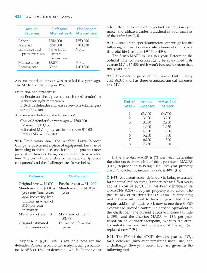
438 CHAPTER 9 / REPLACEMENT ANALYSIS

Annual Defender: Challenger:Expenses Alternative A Alternative B

Labor $300,000 $250,000Material 250,000 100,000Insurance and 4% of initial None

property taxes capitalinvestment

Maintenance $8,000 NoneLeasing cost None $100,000

Assume that the defender was installed five years ago.The MARR is 10% per year. (9.7)

Definition of alternatives:A: Retain an already owned machine (defender) inservice for eight more years.B: Sell the defender and lease a new one (challenger)for eight years.

Alternative A (additional information):

Cost of defender five years ago = $500,000BV now = $111,550Estimated MV eight years from now = $50,000Present MV = $150,000

9-14. Four years ago, the Attaboy Lawn MowerCompany purchased a piece of equipment. Because ofincreasing maintenance costs for this equipment, a newpiece of machinery is being considered for the assemblyline. The cost characteristics of the defender (presentequipment) and the challenger are shown below:

Defender Challenger

Original cost = $9,000 Purchase cost = $11,000Maintenance = $500 in Maintenance = $150 per

year one (four years yearago) increasing by auniform gradient of$100 per yearthereafter

MV at end of life = 0 MV at end of life =$3,000

Original estimated Estimated life = fivelife = nine years years

Suppose a $6,000 MV is available now for thedefender. Perform a before-tax analysis, using a before-tax MARR of 15%, to determine which alternative to

select. Be sure to state all important assumptions youmake, and utilize a uniform gradient in your analysisof the defender. (9.4)

9-15. Asmall high-speed commercial centrifuge has thefollowing net cash flows and abandonment values overits useful life (see Table P9-15, p. 439).

The firm’s MARR is 10% per year. Determine theoptimal time for the centrifuge to be abandoned if itscurrent MV is $7,500 and it won’t be used for more thanfive years. (9.8)

9-16. Consider a piece of equipment that initiallycost $8,000 and has these estimated annual expensesand MV:

End of Annual MV at EndYear, k Expenses of Year

1 $3,000 $4,7002 3,000 3,2003 3,500 2,2004 4,000 1,4505 4,500 9506 5,250 6007 6,250 3008 7,750 0

If the after-tax MARR is 7% per year, determinethe after-tax economic life of this equipment. MACRS(GDS) depreciation is being used (five-year propertyclass). The effective income tax rate is 40%. (9.9)

9-17. A current asset (defender) is being evaluatedfor potential replacement. It was purchased four yearsago at a cost of $62,000. It has been depreciated asa MACRS (GDS) five-year property-class asset. Thepresent MV of the defender is $12,000. Its remaininguseful life is estimated to be four years, but it willrequire additional repair work now (a one-time $4,000expense) to provide continuing service equivalent tothe challenger. The current effective income tax rateis 39%, and the after-tax MARR = 15% per year.Based on an outsider viewpoint, what is the after-tax initial investment in the defender if it is kept (notreplaced now)? (9.9)

9-18. The PW of the ATCFs through year k, PWk ,for a defender (three-year remaining useful life) anda challenger (five-year useful life) are given in thefollowing table:

PROBLEMS 439

TABLE P9-15 Cash Flows and Abandonment Values forProblem 9-15

End of Year

1 2 3 4 5

Annual revenues less expenses $2,000 $2,000 $2,000 $2,000 $2,000Abandonment value of machinea $6,200 $5,200 $4,000 $2,200 0

a Estimated MV.

PW of ATCF through Year k, PWk

Year Defender Challenger

1 −$14,020 −$18,6302 −28,100 −34,5753 −43,075 −48,1304 −65,3205 −77,910

Assume the after-tax MARR is 12% per year. Onthe basis of this information, answer the followingquestions:

a. What are the economic life and the related minimumEUAC when k = N∗

AT, for both the defender and thechallenger? (9.5, 9.6)

b. When should the challenger (based on the presentanalysis) replace the defender? Why? (9.6, 9.7)

c. What assumption(s) have you made in answeringPart (b)?

9-19. A pharmaceutical company has some existingsemiautomated production equipment that they areconsidering replacing. This equipment has a presentMV of $57,000 and a BV of $30,000. It has five moreyears of straight-line depreciation available (if kept) of$6,000 per year, at which time its BV would be $0. Theestimated MV of the equipment five years from now (inyear-zero dollars) is $18,500. The MV rate of increaseon this type of equipment has been averaging 3.2% peryear. The total operating and maintenance and otherrelated expenses are averaging $27,000 (A$) per year.

New automated replacement equipment would beleased. Estimated operating and maintenance andrelated company expenses for the new equipment

are $12,200 per year. The annual leasing cost wouldbe $24,300. The after-tax MARR (with an inflationcomponent) is 9% per year (im); t = 40%; and theanalysis period is five years. Based on an after-tax,A$ analysis, should the replacement be made? Baseyour answer on the actual IRR of the incremental cashflow. (9.9)

9-20. It is being decided whether or not to replacean existing piece of equipment with a newer, moreproductive one that costs $80,000 and has an estimatedMV of $20,000 at the end of its useful life of six years.Installation charges for the new equipment will amountto $3,000; this is not added to the capital investmentbut will be an expensed item during the first yearof operation. MACRS (GDS) depreciation (five-yearproperty class) will be used. The new equipment willreduce direct costs (labor, maintenance, rework, etc.) by$10,000 in the first year, and this amount is expected toincrease by $500 each year thereafter during its six-yearlife. It is also known that the BV of the fully depreciatedold machine is $10,000 but that its present fair MV is$14,000. The MV of the old machine will be zero in sixyears. The effective income tax rate is 40%. (9.9)

a. Determine the prospective after-tax incremental cashflow associated with the new equipment if it isbelieved that the existing machine could performsatisfactorily for six more years.

b. Assume that the after-tax MARR is 12% per year.Based on the ERR method, should you replace thedefender with the challenger? Assume ∈ = MARR.

9-21. Five years ago a chemical plant invested $90,000in a pumping station on a nearby river to provide thewater required for their production process. Straight-line depreciation is employed for tax purposes, using a30-year life and zero salvage value. During the past fiveyears, operating costs have been as follows:

440 CHAPTER 9 / REPLACEMENT ANALYSIS

Maintenance $2,000 per yearPower and labor 4,500 per yearTaxes and insurance 1,000 per year

Total $7,500 per year

A nearby city has offered to purchase the pumpingstation for $75,000 as it is in the process of developinga city water distribution system. The city is willing tosign a 10-year contract with the plant to provide theplant with its required volume of water for a price of$10,000 per year. Plant officials estimate that the salvagevalue of the pumping station 10 years hence will beabout $30,000. The before-tax MARR is 10% per year.An effective income tax rate of 50% is to be assumed.Compare the annual cost (after taxes) of the defender(keep the pumping station) to the challenger (sell stationto the city) and help plant management determine themore economical course of action. (9.9)

9-22. A hydraulic press was installed 10 years ago at acapital investment cost of $70,000. This press presentlyhas a market value of $14,000. If kept, the press hasan economic life of three years, operating expenses of$14,000 per year, and a market value of $10,000 at theend of year (EOY) three. The existing press is beingdepreciated by the straight line method using a 15-yearwrite-off period with an estimated salvage value fordepreciation purposes of $10,000.

As an alternative, the currently owned press canbe replaced with an improved challenger press whichwill cost $65,000 to install, have operating expensesof $9,000 per year, and have a final market valueof $10,000 at the end of its 20-year economic life. Ifthe replacement is made, the challenger press will bedepreciated with the straight line method over a 20-yearlife with an estimated salvage value of $10,000 at EOY20. It is thought that a hydraulic press will be neededindefinitely.

If the after-tax MARR is 10% per year and theeffective income tax rate is 40%, should the defenderor the challenger be recommended? (9.9)

9-23. A manufacturing company has some existingsemiautomatic production equipment that it is consi-dering replacing. This equipment has a present MV of$57,000 and a BV of $27,000. It has five more years ofdepreciation available under MACRS (ADS) of $6,000per year for four years and $3,000 in year five. (Theoriginal recovery period was nine years.) The estimated

MV of the equipment five years from now is $18,500.The total annual operating and maintenance expensesare averaging $27,000 per year.

New automated replacement equipment wouldthen be leased. Estimated annual operating expensesfor the new equipment are $12,200 per year. The annualleasing costs would be $24,300. The MARR (after taxes)is 9% per year, t = 40%, and the analysis period is fiveyears. (Remember: The owner claims depreciation, andthe leasing cost is an operating expense.)

Based on an after-tax analysis, should the newequipment be leased? Base your answer on the IRR ofthe incremental cash flow. (9.9, 9.10)

9-24. Five years ago, a company in New Jersey installeda diesel-electric unit costing $50,000 at a remote sitebecause no dependable electric power was availablefrom a public utility. The company has computed dep-reciation by the straight-line method with a useful life of10 years and a zero salvage value. Annual operation andmaintenance expenses are $16,000, and property taxesand insurance cost another $3,000 per year.

Dependable electric service is now available at anestimated annual cost of $30,000. The company inNew Jersey wishes to know whether it would be moreeconomical to dispose of the diesel-electric unit now,when it can be sold for $35,000, or to wait five yearswhen the unit would have to be replaced anyway (withno MV). The company has an effective income tax rateof 50% and tries to limit its capital expenditures toopportunities that will earn at least 15% per year afterincome taxes. What would you recommend? (9.9)

9-25. Extended Learning Exercise There are twocustomers requiring three-phase electrical ser-

vice, one existing at location A and a new customerat location B. The load at location A is known to be110 kVA, and at location B it is contracted to be 280 kVA.Both loads are expected to remain constant indefi-nitely into the future. Already in service at A are three100-kVA transformers that were installed some yearsago when the load was much greater. Thus, thealternatives are as follows:

Alternative A: Install three 100-kVA transformers(new) B now and replace those at A with three37.5-kVA transformers only when the existingones must be retired.

Alternative B: Remove the three 100-kVA trans-formers now at A and relocate them to B. Theninstall three 37.5-kVA transformers (new) at A.

SPREADSHEET EXERCISES 441

TABLE P9-25 Table for Problem 9-25

Existing and New Transformers

Three 37.5-kVA Three 100-kVA

Capital Investment:Equipment $900 $2,100Installation $340 $475

Property tax 2% of capital investment 2% of capital investmentRemoval cost $100 $110Market value $100 $110Useful life (years) 30 30

Data for both alternatives are provided inTable P9-25. The existing transformers have 10 years oflife remaining. Suppose that the before-tax MARR = 8%per year. Recommend which action to follow aftercalculating an appropriate criterion for comparing thesealternatives. List all assumptions necessary and ignoreincome taxes. (9.7)

9-26. Extended Learning Exercise A truck was purchasedfour years ago for $65,000 to move raw materials andfinished goods between a production facility and four

Defender Challenger

EOY Market O&M EOY Market O&MValue Costs Value Costs

1 $30,000 $8,500 1 $56,000 $5,5002 20,000 10,500 2 44,000 6,8003 12,000 14,000 3 34,000 7,4004 4,000 16,000 4 22,000 9,700

remote warehouses. This truck (the defender) can besold at the present time for $40,000 and replaced bya new truck (the challenger) with a purchase price of$70,000.

a. Given the MVs and operating and maintenancecosts that follow, what is the economic life of thechallenger if MARR = 10%? Note: This is a before-taxanalysis that does not require any calculations involvingthe defender. (9.5)

b. Suppose that the defender was set up on adepreciation schedule with a five-year MACRS classlife at the time of its purchase (four years ago). Thedefender can be sold now for $40,000, or a rebuiltengine and transmission can be purchased andinstalled at a cost of $12,000 (capital investment withthree-year depreciable life, straight line, salvagevalue = 0). If the defender is kept in service, assumethat it will have operating and maintenance costsas shown in Part (a) and a MV of $0 at the end offour years. Determine the ATCFs for the defender.(t = 40%). (9.9)

Spreadsheet Exercises

9-27. Refer to Example 9-4. By how much wouldthe MARR have to change before the economic lifedecreases by one year? How about to increase theeconomic life by one year? (9.5)

9-28. Create a spreadsheet to solve Problem 9-9. Whatpercent reduction in the annual expenses of thedefender would result in a delay of its replacement bythe challenger? (9.4, 9.7)

442 CHAPTER 9 / REPLACEMENT ANALYSIS

Case Study Exercises

9-29. Determine how much the annual lease amount ofthe challenger can increase before the defender becomesthe preferred alternative. (9.10)

9-30. Suppose the study period is reduced to five years.Will this change the replacement decision? (9.10)

9-31. Before committing to a 10-year lease, it wasdecided to consider one more alternative. Instead of

simply augmenting the existing generator with a new40-kW unit, this alternative calls for replacing the80-kW generator with two 40-kW units (for a total ofthree 40-kW units). The company selling the 40-kWunits will reduce the purchase price to $120,000 pergenerator if three generators are bought. How does thisnew challenger compare to the augmented defenderand the original challenger? (9.10)

FE Practice Problems

9-32. Machine A was purchased last year for $20,000and had an estimated MV of $2,000 at the end of itssix-year life. Annual operating costs are $2,000. Themachine will perform satisfactorily over the next fiveyears. A salesperson for another company is offeringa replacement, Machine B, for $14,000, with an MVof $1,400 after five years. Annual operating costs forMachine B will only be $1,400. A trade-in allowance of$10,400 has been offered for Machine A. If the before-tax MARR is 12% per year, should you buy the newmachine? (9.4)

(a) No, continue with Machine A.(b) Yes, purchase Machine B.

9-33. A company is considering replacing a machinethat was bought six years ago for $50,000. The machine,however, can be repaired and its life extended by fivemore years. If the current machine is replaced, the newmachine will cost $44,000 and will reduce the operatingexpenses by $6,000 per year. The seller of the newmachine has offered a trade-in allowance of $15,000 forthe old machine. If MARR is 12% per year before taxes,how much can the company spend to repair the existingmachine? Choose the closest answer. (9.4)

(a) $22,371 (b) $50,628 (c) $7,371 (d) −$1,000

Machine A was purchased three years ago for $10,000and had an estimated MV of $1,000 at the end of its10-year life. Annual operating costs are $1,000. The

machine will perform satisfactorily for the next sevenyears. A salesperson for another company is offeringMachine B for $50,000 with an MV of $5,000 after 10years. Annual operating costs will be $600. Machine Acould be sold now for $7,000, and MARR is 12% per year.Use this information to answer Problems 9-34 and 9-35.

9-34. Using the outsider viewpoint, what is the EUACof continuing to use Machine A? Choose the closestanswer. (9.6)

(a) $1,000 (b) $2,182 (c) $2,713(d) $901 (e) $2,435

9-35. Using the outsider viewpoint, what is theEUAC of buying Machine B? Choose the closestanswer. (9.5)

(a) $8,565 (b) $11,361 (c) $9,750(d) $9,165 (e) $900

9-36. A corporation purchased a machine for $60,000five years ago. It had an estimated life of 10 years andan estimated salvage value of $9,000. The current BV ofthis machine is $34,500. If the current MV of the machineis $40,500 and the effective income tax rate is 29%, whatis the after-tax investment value of the machine? Usethe outsider viewpoint. (9.9)

(a) $28,755 (b) $40,500 (c) $38,760(d) $37,455 (e) $36,759

CHAPTER 10

Evaluating Projects with theBenefit−Cost Ratio Method

The objective of Chapter 10 is to demonstrate the use of the benefit–cost(B–C) ratio for the evaluation of public projects.

Constructing a Bypass to RelieveTraffic Congestion

Two heavily traveled interstate highways currently intersect in the middle ofa major metropolitan area. A 25-mile, four-lane bypass is being considered toconnect the busy interstate highways at a point outside of the metropolitan

area. The projected construction cost of the bypass is $20 million. Annual main-tenance of the roadway is expected to be $500,000. Major monetary benefits ofreduced time delays due to traffic congestion, improved traveler safety (fewertraffic accidents), and expanded opportunities for commercial businesses areanticipated to be around $2 million per year.

This bypass would be state owned and maintained and is therefore considereda public project. In this chapter, you will learn how public projects such as this areevaluated using a benefit–cost ratio.

443

. . . the Federal Government should improve or participate in the improvement of navigablewaters or their tributaries, including watersheds thereof, for flood-control purposes if the

benefits to whomsoever they may accrue are in excess of the estimated costs . . .

—Flood Control Act (1936)

10.1 IntroductionPublic projects are those authorized, financed, and operated by federal, state, orlocal governmental agencies. Such public works are numerous, and although theymay be of any size, they are frequently much larger than private ventures. Sincethey require the expenditure of capital, such projects are subject to the principlesof engineering economy with respect to their design, acquisition, and operation.Because they are public projects, however, a number of important special factorsexist that are not ordinarily found in privately financed and operated businesses.The differences between public and private projects are listed in Table 10-1.

TABLE 10-1 Some Basic Differences between Privately Owned and Publicly Owned Projects

Private Public

Purpose Provide goods or services at aprofit; maximize profit orminimize cost

Protect health; protect lives and property;provide services (at no profit); provide jobs

Sources of capital Private investors and lenders Taxation; private lendersMethod of financing Individual ownership;

partnerships; corporationsDirect payment of taxes; loans without interest;

loans at low interest; self-liquidating bonds;indirect subsidies; guarantee of private loans

Multiple purposes Moderate Common (e.g., reservoir project for flood control,electrical power generation, irrigation,recreation, education)

Project life Usually relatively short (5 to10 years)

Usually relatively long (20 to 60 years)

Relationship ofsuppliers of capitalto project

Direct Indirect, or none

Nature of benefits Monetary or relatively easy toequate to monetary terms

Often nonmonetary, difficult to quantify,difficult to equate to monetary terms

Beneficiaries ofproject

Primarily, entity undertakingproject

General public

Conflict of purposes Moderate Quite common (dam for flood control versusenvironmental preservation)

Conflict of interests Moderate Very common (between agencies)Effect of politics Little to moderate Frequent factors; short-term tenure for decision

makers; pressure groups; financialand residential restrictions; etc.

Measurement ofefficiency

Rate of return on capital Very difficult; no direct comparison withprivate projects

444

SECTION 10.2 / PERSPECTIVE AND TERMINOLOGY FOR ANALYZING PUBLIC PROJECTS 445

As a consequence of these differences, it is often difficult to make engineeringeconomy studies and investment decisions for public-works projects in exactly thesame manner as for privately owned projects. Different decision criteria are oftenused, which creates problems for the public (who pays the bill), for those who mustmake the decisions, and for those who must manage public-works projects.

The benefit–cost ratio method, which is normally used for the evaluation ofpublic projects, has its roots in federal legislation. Specifically, the Flood ControlAct of 1936 requires that, for a federally financed project to be justified, its benefitsmust be in excess of its costs. In general terms, B–C analysis is a systematicmethod of assessing the desirability of government projects or policies when itis important to take a long-term view of future effects and a broad view of possibleside effects. In meeting the requirements of this mandate, the B–C ratio methodevolved into the calculation of a ratio of project benefits to project costs. Ratherthan allowing the analyst to apply criteria more commonly used for evaluatingprivate projects (IRR, PW, and so on), most governmental agencies require the useof the B–C method.

10.2 Perspective and Terminology for AnalyzingPublic Projects

Before applying the B–C ratio method to evaluate a public project, the appropriateperspective (Chapter 1, Principle 3) must be established. In conducting anengineering economic analysis of any project, whether it is a public or a privateundertaking, the proper perspective is to consider the net benefits to the owners ofthe enterprise considering the project. This process requires that the question ofwho owns the project be addressed. Consider, for example, a project involving theexpansion of a section of I-80 from four to six lanes. Because the project is paid forprimarily with federal funds channeled through the Department of Transportation,we might be inclined to say that the federal government is the owner. These funds,however, originated from tax dollars—thus, the true owners of the project arethe taxpayers.

As mentioned previously, the B–C method requires that a ratio of benefits tocosts be calculated. Project benefits are defined as the favorable consequences ofthe project to the public, but project costs represent the monetary disbursement(s)required of the government. It is entirely possible, however, for a project tohave unfavorable consequences to the public. Considering again the widening ofI-80, some of the owners of the project—farmers along the interstate—would lose aportion of their arable land, along with a portion of their annual revenues. Becausethis negative financial consequence is borne by (a segment of) the public, it cannotbe classified as either a benefit or a cost. The term disbenefits is generally used torepresent the negative consequences of a project to the public.

EXAMPLE 10-1 Benefits and Costs of a Convention Center and Sports Complex

A new convention center and sports complex has been proposed to the GothamCity Council. This public-sector project, if approved, will be financed throughthe issue of municipal bonds. The facility will be located in the City Park near

446 CHAPTER 10 / EVALUATING PROJECTS WITH THE BENEFIT–COST RATIO METHOD

downtown Gotham City, in a wooded area, which includes a bike path, a naturetrail, and a pond. Because the city already owns the park, no purchase of landis necessary. List separately the project’s benefits, costs, and any disbenefits.

SolutionBENEFITS Improvement of the image of the downtown area of Gotham City

Potential to attract conferences and conventions to Gotham CityPotential to attract professional sports franchises to Gotham CityRevenues from rental of the facilityIncreased revenues for downtown merchants of Gotham CityUse of facility for civic events

COSTS Architectural design of the facilityConstruction of the facilityDesign and construction of parking garage adjacent to the facilityOperating and maintenance costs of the facilityInsurance costs of the facility

DISBENEFITS Loss of use of a portion of the City Park to Gotham Cityresidents, including the bike path, the nature trail, and the pond

Loss of wildlife habitat in urban area

10.3 Self-Liquidating ProjectsThe term self-liquidating project is applied to a governmental project that is expectedto earn direct revenue sufficient to repay its cost in a specified period of time. Mostof these projects provide utility services—for example, the fresh water, electricpower, irrigation water, and sewage disposal provided by a hydroelectric dam.Other examples of self-liquidating projects include toll bridges and highways.

As a rule, self-liquidating projects are expected to earn direct revenues thatoffset their costs, but they are not expected to earn profits or pay income taxes.Although they also do not pay property taxes, in some cases in-lieu paymentsare made to state, county, or municipal governments in place of the property orfranchise taxes that would have been paid had the project been under privateownership. For example, the U.S. government agreed to pay the states of Arizonaand Nevada $300,000 each annually for 50 years in lieu of taxes that would haveaccrued if Hoover Dam had been privately constructed and operated.

10.4 Multiple-Purpose ProjectsAn important characteristic of public-sector projects is that many such projects havemultiple purposes or objectives. One example of this would be the constructionof a dam to create a reservoir on a river. (See Figure 10-1.) This project wouldhave multiple purposes: (1) assist in flood control, (2) provide water for irrigation,

SECTION 10.4 / MULTIPLE-PURPOSE PROJECTS 447

Irrigation

PowerFlood Control

Figure 10-1 Schematic Representation of a Multiple-Purpose Project Involving FloodControl, Irrigation, and Power

(3) generate electric power, (4) provide recreational facilities, and (5) providedrinking water. Developing such a project to meet more than one objective ensuresthat greater overall economy can be achieved. Because the construction of a daminvolves very large sums of capital and the use of a valuable natural resource—ariver—it is likely that the project could not be justified unless it served multiplepurposes. This type of situation is generally desirable, but, at the same time, itcreates economic and managerial problems due to the overlapping utilization offacilities and the possibility of a conflict of interest between the several purposesand the agencies involved.

The basic problems that often arise in evaluating public projects can beillustrated by returning to the dam shown in Figure 10-1. The project underconsideration is to be built in the semiarid central portion of California, primarilyto provide control against spring flooding resulting from the melting snow in theSierra Nevadas. If a portion of the water impounded behind the dam could bediverted onto the adjoining land below the dam, the irrigation water would greatlyincrease the productivity, and thus the value, of that land, which would result inan increase in the nation’s resources. So the objectives of the project should beexpanded to include both flood control and irrigation.

The existence of a dam with a high water level on one side and a much lowerlevel on the other side also suggests that some of the nation’s resources will bewasted unless a portion of the water is diverted to run through turbines, generatingelectric power. This electricity can be sold to customers in the areas surroundingthe reservoir, giving the project the third purpose of generating electric power.

In this semiarid region, the creation of a large reservoir behind the dam wouldprovide valuable facilities for hunting, fishing, boating, swimming, and camping.Thus, the project has the fourth purpose of providing recreation facilities. A fifthpurpose would be the provision of a steady, reliable supply of drinking water.

Each of the above-mentioned objectives of the project has desirable economicand social value, so what started out as a single-purpose project now has fivepurposes. The failure to meet all five objectives would mean that valuable nationalresources are being wasted. On the other hand, there are certain disbenefits to thepublic that must also be considered. Most apparent of these is the loss of farm land

448 CHAPTER 10 / EVALUATING PROJECTS WITH THE BENEFIT–COST RATIO METHOD

above the dam in the area covered by the reservoir. Other disbenefits might include(1) the loss of a white-water recreational area enjoyed by canoeing, kayaking, andrafting enthusiasts, (2) the loss of annual deposits of fertile soil in the river basinbelow the dam due to spring flooding, and (3) the negative ecological impact ofobstructing the flow of the river.

If the project is built to serve five purposes, the fact that one dam will serve allof them leads to at least three basic problems. The first of these is the allocation ofthe cost of the dam to each of its intended purposes. Suppose, for example, that theestimated costs of the project are $35,000,000. This figure includes costs incurredfor the purchase and preparation of land to be covered by water above the damsite; the actual construction of the dam, the irrigation system, the power generationplant, and the purification and pumping stations for drinking water; and the designand development of recreational facilities. The allocation of some of these costs tospecific purposes is obvious (e.g., the cost of constructing the irrigation system), butwhat portion of the cost of purchasing and preparing the land should be assigned toflood control? What amounts should be assigned to irrigation, power generation,drinking water, and recreation?

The second basic problem is the conflict of interest among the several purposesof the project. Consider the decision as to the water level to be maintained behindthe dam. In meeting the first purpose—flood control—the reservoir should bemaintained at a near-empty level to provide the greatest storage capacity duringthe months of the spring thaw. This lower level would be in direct conflict withthe purpose of power generation, which could be maximized by maintaining ashigh a level as possible behind the dam at all times. Further, maximizing therecreational benefits would suggest that a constant water level be maintainedthroughout the year. Thus, conflicts of interest arise among the multiple purposes,and compromising decisions must be made. These decisions ultimately affect themagnitude of benefits resulting from the project.

A third problem with multiple-purpose public projects is political sensitivity.Because each of the various purposes, or even the project itself, is likely to bedesired or opposed by some segment of the public and by various interest groupsthat may be affected, inevitably such projects frequently become political issues.∗This conflict often has an effect on cost allocations and thus on the overall economyof these projects.

The net result of these three factors is that the cost allocations made in multiple-purposepublic-sector projects tend to be arbitrary. As a consequence, production and sellingcosts of the services provided also are arbitrary. Because of this, these costscannot be used as valid yardsticks with which similar private-sector projectscan be compared to determine the relative efficiencies of public and privateownership.

∗ The construction of the Tellico Dam on the Little Tennessee River was considerably delayed due to two importantdisbenefits: (1) concerns over the impact of the project on the environment of a small fish, the snail darter, and (2) theflooding of burial grounds considered sacred by the Cherokee Nation.

SECTION 10.5 / DIFFICULTIES IN EVALUATING PUBLIC-SECTOR PROJECTS 449

10.5 Difficulties in Evaluating Public-Sector ProjectsWith all of the difficulties that have been cited in evaluating public-sector projects,we may wonder whether engineering economy studies of such projects shouldbe attempted. In most cases, economy studies cannot be made in as complete,comprehensive, and satisfactory a manner as in the case of studies of privatelyfinanced projects. In the private sector, the costs are borne by the firm undertakingthe project, and the benefits are the favorable outcomes of the project accrued by thefirm. Any costs and benefits that occur outside of the firm are generally ignoredin evaluations unless it is anticipated that those external factors will indirectlyimpact the firm. But the opposite is true in the case of public-sector projects. Inthe wording of the Flood Control Act of 1936, “if the benefits to whomsoever theymay accrue are in excess of the estimated costs,” all of the potential benefits ofa public project are relevant and should be considered. Simply enumerating allof the benefits for a large-scale public project is a formidable task! Further, themonetary value of these benefits to all of the affected segments of the public mustsomehow be estimated. Regardless, decisions about the investment of capital inpublic projects must be made by elected or appointed officials, by managers, or bythe general public in the form of referendums. Because of the magnitude of capitaland the long-term consequences associated with many of these projects, followinga systematic approach for evaluating their worthiness is vital.

There are a number of difficulties inherent in public projects that must beconsidered in conducting engineering economy studies and making economicdecisions regarding those projects. Some of these are as follows:

1. There is no profit standard to be used as a measure of financial effectiveness.Most public projects are intended to be nonprofit.

2. The monetary impact of many of the benefits of public projects is difficultto quantify.

3. There may be little or no connection between the project and the public, whichis the owner of the project.

4. There is often strong political influence whenever public funds are used. Whendecisions regarding public projects are made by elected officials who will soonbe seeking reelection, the immediate benefits and costs are stressed, often with littleor no consideration for the more important long-term consequences.

5. Public projects are usually much more subject to legal restrictions than areprivate projects. For example, the area of operations for a municipally ownedpower company may be restricted such that power can be sold only within thecity limits, regardless of whether a market for any excess capacity exists outsidethe city.

6. The ability of governmental bodies to obtain capital is much more restrictedthan that of private enterprises.

7. The appropriate interest rate for discounting the benefits and costs of publicprojects is often controversially and politically sensitive. Clearly, lower interestrates favor long-term projects having major social or monetary benefits in thefuture. Higher interest rates promote a short-term outlook whereby decisionsare based mostly on initial investments and immediate benefits.

450 CHAPTER 10 / EVALUATING PROJECTS WITH THE BENEFIT–COST RATIO METHOD

A discussion of several viewpoints and considerations that are often used toestablish an appropriate interest rate for public projects is included in the nextsection.

10.6 What Interest Rate Should Be Usedfor Public Projects?

When public-sector projects are evaluated, interest rates∗ play the same role ofaccounting for the time value of money as in the evaluation of projects in the privatesector. The rationale for the use of interest rates, however, is somewhat different.The choice of an interest rate in the private sector is intended to lead directly toa selection of projects to maximize profit or minimize cost. In the public sector,on the other hand, projects are not usually intended as profit-making ventures.Instead, the goal is the maximization of social benefits, assuming that these havebeen appropriately measured. The choice of an interest rate in the public sectoris intended to determine how available funds should best be allocated amongcompeting projects to achieve social goals. The relative differences in magnitude ofinterest rates between governmental agencies, regulated monopolies, and privateenterprises are illustrated in Figure 10-2.

Three main considerations bear on what interest rate to use in engineeringeconomy studies of public-sector projects:

1. The interest rate on borrowed capital2. The opportunity cost of capital to the governmental agency3. The opportunity cost of capital to the taxpayers

As a general rule, it is appropriate to use the interest rate on borrowed capital asthe interest rate for cases in which money is borrowed specifically for the project(s)under consideration. For example, if municipal bonds are issued specifically for

Figure 10-2 RelativeDifferences inInterest Rates forGovernmentalAgencies, RegulatedMonopolies, andPrivate Enterprises

GovernmentalAgencies

RegulatedMonopolies

PrivateEnterprises

Inte

rest

Rat

e

∗ The term discount rate is often used instead of interest rate (or MARR) in government literature on B–C analysis.

SECTION 10.6 / WHAT INTEREST RATE SHOULD BE USED FOR PUBLIC PROJECTS? 451

the financing of a new school, the effective interest rate on those bonds should bethe interest rate.

For public-sector projects, the opportunity cost of capital to a governmentalagency encompasses the annual rate of benefit to either the constituency served bythat agency or the composite of taxpayers who will eventually pay for the project.If projects are selected such that the estimated return (in terms of benefits) on allaccepted projects is higher than that on any of the rejected projects, then the interestrate used in economic analyses is that associated with the best opportunity forgone.If this process is done for all projects and investment capital available within agovernmental agency, the result is an opportunity cost of capital for that governmentalagency. A strong argument against this philosophy, however, is that the differentfunding levels of the various agencies and the different nature of projects underthe direction of each agency would result in different interest rates for each of theagencies, even though they all share a common primary source of funds—taxationof the public.

The third consideration—the opportunity cost of capital to the taxpayers—isbased on the philosophy that all government spending takes potential investmentcapital away from the taxpayers. The taxpayers’ opportunity cost is generallygreater than either the cost of borrowed capital or the opportunity cost togovernmental agencies, and there is a compelling argument for applying thelargest of these three rates as the interest rate for evaluating public projects; itis not economically sound to take money away from a taxpayer to invest in agovernment project yielding benefits at a rate less than what could have beenearned by that taxpayer.

This argument was supported by a federal government directive issued in1997—and still in force—by the Office of Management and Budget (OMB).∗According to this directive, a 7% interest rate should be used in economicevaluations for a wide range of federal projects, with certain exceptions (e.g., alower rate can be applied in evaluating water resource projects). This 7%, it can beargued, is at least a rough approximation of the real-dollar return that taxpayerscould earn from the use of that money for private investment. This corresponds toan approximate nominal interest rate of 10% per year.

One additional theory on establishing interest rates for federal projects advo-cates that the social discount rate used in such analyses should be the market-determined risk-free rate for private investments.† According to this theory, anominal interest rate in the order of 3–4% per year should be used.

The preceding discussion focuses on the considerations that should play a role inestablishing an interest rate for public projects. As in the case of the private sector,there is no simple formula for determining the appropriate interest rate for publicprojects. With the exception of projects falling under the 1997 OMB directive, settingthe interest rate is ultimately a policy decision at the discretion of the governmentalagency conducting the analysis.

∗ Office of Management and Budget, “Guidelines and Discount Rates for Benefit–Costs Analysis of Federal Programs,”OMB Circular No. A-94 (revised), February 21, 1997. The OMB home page is http://www.whitehouse.gov/omb.† K. J. Arrow and R. C. Lind, “Uncertainty and the Evaluation of Public Investment Decisions,” American EconomicReview, 60 ( June 1970): 364–378.

452 CHAPTER 10 / EVALUATING PROJECTS WITH THE BENEFIT–COST RATIO METHOD

10.7 The Benefit−Cost Ratio MethodAs the name implies, the B–C ratio method involves the calculation of a ratio ofbenefits to costs. Whether evaluating a project in the private sector or in the publicsector, the time value of money must be considered to account for the timing of cashflows (or benefits) occurring after the inception of the project. Thus, the B–C ratiois actually a ratio of discounted benefits to discounted costs.

Any method for formally evaluating projects in the public sector must considerthe worthiness of allocating resources to achieve social goals. For over 70 years, theB–C ratio method has been the accepted procedure for making go/no-go decisionson independent projects and for comparing mutually exclusive projects in thepublic sector, even though the other methods discussed in Chapter 5 (PW, AW,IRR, etc.) will lead to identical recommendations, assuming all these procedures areproperly applied.

Accordingly, the purpose of this section is to describe and illustrate themechanics of the B–C ratio method for evaluating projects. Two different B–C ratioswill be presented because they are used in practice by various government agenciesand municipalities. Both ratios lead to the identical choice of which project is bestwhen comparing mutually exclusive alternatives.

The B–C ratio is defined as the ratio of the equivalent worth of benefits to theequivalent worth of costs. The equivalent-worth measure applied can be presentworth, annual worth, or future worth, but customarily, either PW or AW is used. Aninterest rate for public projects, as discussed in the previous section, is used in theequivalent-worth calculations. The B–C ratio is also known as the savings-investmentratio (SIR) by some governmental agencies.

Several different formulations of the B–C ratio have been developed. Two ofthe more commonly used formulations are presented in this section, illustratingthe use of both present worth and annual worth.

Conventional B–C ratio with PW:

B–C = PW(benefits of the proposed project)PW(total costs of the proposed project)

= PW(B)

I − PW(MV) + PW(O&M)(10-1)

where PW(·) = present worth of (·);B = benefits of the proposed project;I = initial investment in the proposed project;

MV = market value at the end of useful life;O&M = operating and maintenance costs of the proposed project.

Modified B–C ratio with PW:

B–C = PW(B) − PW(O&M)

I − PW(MV). (10-2)

SECTION 10.7 / THE BENEFIT–COST RATIO METHOD 453

The numerator of the modified B–C ratio expresses the equivalent worth of thebenefits minus the equivalent worth of the operating and maintenance costs, andthe denominator includes only the initial investment costs (less any market value).A project is acceptable when the B–C ratio, as defined in either Equation (10-1) or(10-2), is greater than or equal to 1.0.

Equations (10-1) and (10-2) can be rewritten in terms of equivalent annualworth, as follows:

Conventional B–C ratio with AW:

B–C = AW(benefits of the proposed project)AW(total costs of the proposed project)

= AW(B)

CR + AW(O&M), (10-3)

where AW(·) = annual worth of (·);B = benefits of the proposed project;

CR = capital-recovery amount (i.e., the equivalent annualcost of the initial investment, I, including an allowancefor market, or salvage value, if any);

O&M = operating and maintenance costs of the proposed project.

Modified B–C ratio with AW:

B–C = AW(B) − AW(O&M)

CR. (10-4)

The resulting B–C ratios for all the previous formulations will give identicalresults in determining the acceptability of a project (i.e., either B–C ≥ 1.0 orB–C < 1.0). The conventional B–C ratio will give identical numerical results forboth PW and AW formulations; similarly, the modified B–C ratio gives identicalnumerical results whether PW or AW is used. Although the magnitude of the B–Cratio will differ between conventional and modified B–C ratios, go/no-go decisionsare not affected by the choice of approach, as shown in Example 10-2.

EXAMPLE 10-2 Equivalence of the B−C Ratio Formulations

The city of Columbia is considering extending the runways of its municipalairport so that commercial jets can use the facility. The land necessary for therunway extension is currently a farmland that can be purchased for $350,000.Construction costs for the runway extension are projected to be $600,000, andthe additional annual maintenance costs for the extension are estimated to be$22,500. If the runways are extended, a small terminal will be constructedat a cost of $250,000. The annual operating and maintenance costs for theterminal are estimated at $75,000. Finally, the projected increase in flights

454 CHAPTER 10 / EVALUATING PROJECTS WITH THE BENEFIT–COST RATIO METHOD

will require the addition of two air traffic controllers at an annual cost of$100,000. Annual benefits of the runway extension have been estimated asfollows:

$325,000 Rental receipts from airlines leasing space at the facility$65,000 Airport tax charged to passengers$50,000 Convenience benefit for residents of Columbia$50,000 Additional tourism dollars for Columbia

Apply the B–C ratio method with a study period of 20 years and a MARR of10% per year to determine whether the runways at Columbia Municipal Airportshould be extended.

Solution

Conventional B–C: B–C = PW(B)/[I − PW(MV) + PW(O&M)]Equation (10-1) B–C = $490,000 (P/A, 10%, 20)/[$1,200,000 + $197,500 (P/A, 10%, 20)]

B–C = 1.448 > 1; extend runways.

Modified B–C: B–C = [PW(B) − PW(O&M)]/[I − PW(MV)]Equation (10-2) B–C = [$490,000 (P/A, 10%, 20) − $197,500 (P/A, 10%, 20)]/$1,200,000

B–C = 2.075 > 1; extend runways.

Conventional B–C: B–C = AW(B)/[CR + AW(O&M)]Equation (10-3) B–C = $490,000/[$1,200,000 (A/P, 10%, 20) + $197,500]

B–C = 1.448 > 1; extend runways.

Modified B–C: B–C = [AW(B) − AW(O&M)]/CREquation (10-4) B–C = [$490,000 − $197,500]/[$1,200,000 (A/P, 10%, 20)]

B–C = 2.075 > 1; extend runways.

As can be seen in the preceding example, the difference between conventionaland modified B–C ratios is essentially due to subtracting the equivalent-worthmeasure of operating and maintenance costs from both the numerator and thedenominator of the B–C ratio. In order for the B–C ratio to be greater than 1.0,the numerator must be greater than the denominator. Similarly, the numeratormust be less than the denominator for the B–C ratio to be less than 1.0. Subtractinga constant (the equivalent worth of operating and maintenance costs) from bothnumerator and denominator does not alter the relative magnitudes of the numeratorand denominator. Thus, project acceptability is not affected by the choice ofconventional versus modified B–C ratio. This information is stated mathematicallyas follows for the case of B–C > 1.0:

SECTION 10.7 / THE BENEFIT–COST RATIO METHOD 455

Let N = the numerator of the conventional B–C ratio,D = the denominator of the conventional B–C ratio,

O&M = the equivalent worth of operating and maintenance costs.

If B–C = ND

> 1.0, then N > D.

If N > D, and [N − O&M] > [D − O&M], thenN − O&MD − O&M

> 1.0.

Note thatN − O&MD − O&M

is the modified B–C ratio; thus, if conventional B–C > 1.0,

then modified B–C > 1.0

EXAMPLE 10-3 B−C Ratio of the Proposed Bypass

In this example, we will evaluate the bypass described in the beginning of thechapter. The construction cost of the bypass is $20 million, and $500,000 wouldbe required each year for annual maintenance. The annual benefits to the publichave been estimated to be $2 million. If the study period is 50 years and thestate’s interest rate is 8% per year, should the bypass be constructed? Whatimpact does a social interest rate of 4% per year have on the B–C ratio of theproject?

SolutionAt an interest rate of 8% per year, the conventional B–C ratio of the proposedbypass is

B–C = $2,000,000$20,000,000 (A/P, 8%, 50) + $500,000

= 0.94.

Because this ratio is less than one, the bypass is not economically acceptable at8% interest.

If a social interest rate of 4% per year was used, the B–C ratio would be 1.40and the bypass would be acceptable.

Two additional issues of concern are the treatment of disbenefits in B–C analysesand the decision as to whether certain cash flow items should be treated as additionalbenefits or as reduced costs. The first concern arises whenever disbenefits are formallydefined in a B–C evaluation of a public-sector project. An example of the secondconcern would be a public-sector project proposing to replace an existing assethaving high annual operating and maintenance costs with a new asset havinglower operating and manual costs. As will be seen in Sections 10.7.1 and 10.7.2,the final recommendation on a project is not altered by either the approach toincorporating disbenefits or the classification of an item as a reduced cost or anadditional benefit.

456 CHAPTER 10 / EVALUATING PROJECTS WITH THE BENEFIT–COST RATIO METHOD

10.7.1 Disbenefits in the B−C Ratio

In a previous section, disbenefits were defined as negative consequences to thepublic resulting from the implementation of a public-sector project. The traditionalapproach for incorporating disbenefits into a B–C analysis is to reduce benefits bythe amount of disbenefits (i.e., to subtract disbenefits from benefits in the numeratorof the B–C ratio). Alternatively, the disbenefits could be treated as costs (i.e., adddisbenefits to costs in the denominator). Equations (10-5) and (10-6) illustrate thetwo approaches for incorporating disbenefits in the conventional B–C ratio, withbenefits, costs, and disbenefits in terms of equivalent AW. (Similar equations couldalso be developed for the modified B–C ratio or for PW as the measure of equivalentworth.) Again, the magnitude of the B–C ratio will be different depending uponwhich approach is used to incorporate disbenefits, but project acceptability—thatis, whether the B–C ratio is >, <, or = 1.0—will not be affected, as shown inExample 10-4.

Conventional B–C ratio with AW, benefits reduced by amount of disbenefits:

B–C = AW(benefits) − AW(disbenefits)AW(costs)

= AW(B) − AW(D)

CR + AW(O&M). (10-5)

Here, AW(·) = annual worth of (·);B = benefits of the proposed project;D = disbenefits of the proposed project;

CR = capital recovery amount (i.e., the equivalent annual cost ofthe initial investment, I, including an allowance for marketvalue, if any);

O&M = operating and maintenance costs of the proposed project.

Conventional B–C ratio with AW, costs increased by amount of disbenefits:

B–C = AW(benefits)AW(costs)+AW(disbenefits)

= AW(B)

CR+AW(O&M)+AW(D). (10-6)

EXAMPLE 10-4 Including Disbenefits in a B−C Analysis

Refer back to Example 10-2. In addition to the benefits and costs, suppose thatthere are disbenefits associated with the runway extension project. Specifically,the increased noise level from commercial jet traffic will be a serious nuisanceto homeowners living along the approach path to the Columbia MunicipalAirport. The annual disbenefit to citizens of Columbia caused by this noisepollution is estimated to be $100,000. Given this additional information, reapplythe conventional B–C ratio, with equivalent annual worth, to determinewhether this disbenefit affects your recommendation on the desirability ofthis project.

SECTION 10.7 / THE BENEFIT–COST RATIO METHOD 457

Solution

Disbenefits reduce B–C = [AW(B) − AW(D)]/[CR + AW(O&M)]benefits, Equation (10-5) B–C = [$490,000 − $100,000]/[$1,200,000 (A/P, 10%, 20) + $197,500]

B–C = 1.152 > 1; extend runways.

Disbenefits treated as additional B–C = AW(B)/[CR + AW(O&M) + AW(D)]costs, Equation (10-6) B–C = $490,000/[$1,200,000 (A/P, 10%, 20) + $197,500 + $100,000]

B–C = 1.118 > 1; extend runways.

As in the case of conventional and modified B–C ratios, the treatment ofdisbenefits may affect the magnitude of the B–C ratio, but it has no effect on projectdesirability in go/no-go decisions. It is left to the reader to develop a mathematicalrationale for this, similar to that included in the discussion of conventional versusmodified B–C ratios.

10.7.2 Added Benefits versus Reduced Costs in B−C Analyses

The analyst often needs to classify certain cash flows as either added benefits orreduced costs in calculating a B–C ratio. The questions arise, How critical is theproper assignment of a particular cash flow as an added benefit or a reduced cost?Is the outcome of the analysis affected by classifying a reduced cost as a benefit?An arbitrary decision as to the classification of a benefit or a cost has no impact on projectacceptability. The mathematical rationale for this information is presented next andin Example 10-5.

Let B = the equivalent annual worth of project benefits,C = the equivalent annual worth of project costs,X = the equivalent annual worth of a cash flow (either an added

benefit or a reduced cost) not included in either B or C.

If X is classified as an added benefit, then B–C = B + XC

. Alternatively,

if X is classified as a reduced cost, then B–C = BC − X

.

Assuming that the project is acceptable, that is, B–C ≥ 1.0,

B + XC

≥ 1.0, which indicates that B + X ≥ C, and

BC − X

≥ 1.0, which indicates that B ≥ C − X,

which can be restated as B + X ≥ C.

458 CHAPTER 10 / EVALUATING PROJECTS WITH THE BENEFIT–COST RATIO METHOD

EXAMPLE 10-5 Added Benefit versus Reduced Cost in a Bridge Widening Project

A project is being considered by the Tennessee Department of Transportation toreplace an aging bridge across the Cumberland River on a state highway. Theexisting two-lane bridge is expensive to maintain and creates a traffic bottleneckbecause the state highway is four lanes wide on either side of the bridge. Thenew bridge can be constructed at a cost of $300,000, and estimated annualmaintenance costs are $10,000. The existing bridge has annual maintenance costsof $18,500. The annual benefit of the new four-lane bridge to motorists, due tothe removal of the traffic bottleneck, has been estimated to be $25,000. Conduct aB–C analysis, using a MARR of 8% and a study period of 25 years, to determinewhether the new bridge should be constructed.

SolutionTreating the reduction in annual maintenance costs as a reduced cost:

B–C = $25,000/[$300,000(A/P, 8%, 25) − ($18,500 − $10,000)]B–C = 1.275 > 1; construct new bridge.

Treating the reduction in annual maintenance costs as an increased benefit:

B–C = [$25,000 + ($18,500 − $10,000)]/[$300,000(A/P, 8%, 25)]B–C = 1.192 > 1; construct new bridge.

Therefore, the decision to classify a cash-flow item as an additional benefitor as a reduced cost will affect the magnitude of the calculated B–C ratio, but itwill have no effect on project acceptability.

10.8 Evaluating Independent Projects by B−C RatiosIndependent projects are categorized as groupings of projects for which the choiceto select any particular project in the group is independent of choices regarding anyand all other projects within the group. Thus, it is permissible to select none of theprojects, any combination of projects, or all of the projects from an independentgroup. (Note that this does not hold true under conditions of capital rationing.Methods of evaluating otherwise independent projects under capital rationing arediscussed in Chapter 13.) Because any or all projects from an independent set canbe selected, formal comparisons of independent projects are unnecessary. The issueof whether one project is better than another is unimportant if those projects areindependent; the only criterion for selecting each of those projects is whether theirrespective B–C ratios are equal to or greater than 1.0.

Mutually exclusive alternatives can be formed from independent projects. Forinstance, from three independent projects there are 23 = 8 mutually exclusivecombinations possible (including “do nothing”). See if you can list them all. Forfive independent projects, there are 25 = 32 mutually exclusive alternatives.

A typical example of an economy study of a federal project—using theconventional B–C-ratio method—is the study of a flood control and power

SECTION 10.8 / EVALUATING INDEPENDENT PROJECTS BY B–C RATIOS 459

project on the White River in Missouri and Arkansas. Considerable flooding andconsequent damage had occurred along certain portions of this river, as shown inTable 10-2. In addition, the uncontrolled water flow increased flood conditionson the lower Mississippi River. In this case, there were independent optionsof building a reservoir and/or a channel improvement to alleviate the problem.The cost and benefit summaries for the Table Rock reservoir and the Bull Shoalschannel improvement are shown in Table 10-3. The fact that the Bull Shoals

TABLE 10-2 Annual Loss as a Result of Floods on Three Stretches of the White River

Annual Loss per Acre Annual Loss per AcreAnnual Value of Improved Land for Total Area

Item of Loss in Floodplain in Floodplain

Crops $1,951,714 $6.04 $1.55Farm (other than crops) 215,561 0.67 0.17Railroads and highways 119,800 0.37 0.09Leveesa 87,234 0.27 0.07Other losses 168,326 0.52 0.13

Total $2,542,635 $7.87 $2.01

a Expenditures by the United States for levee repairs and high-water maintenance.

TABLE 10-3 Estimated Costs, Annual Charges, and Annual Benefits for the Table RockReservoir and Bull Shoals Channel Improvement Projects

Table Rock Bull Shoals ChannelItem Reservoir Improvement

Cost of dam and appurtenances, and reservoir:Dam, including reservoir-clearing, camp, access railroads and $20,447,000 $25,240,000

highways, and foundation exploration and treatmentPowerhouse and equipment 6,700,000 6,650,000Power-transmission facilities to existing load-distribution centers 3,400,000 4,387,000Land 1,200,000 1,470,000Highway relocations 2,700,000 140,000Cemetery relocations 40,000 18,000Damage to villages 6,000 94,500Damage to miscellaneous structures 7,000 500

Total Construction Cost (estimated appropriation of $34,500,000 $38,000,000public funds necessary for the execution of the project)

Federal investment:Total construction cost $34,500,000 $38,000,000Interest during construction $1,811,300 1,995,000

Total $36,311,300 $39,995,000

Present value of federal properties 1,200 300Total Federal Investment $36,312,500 $39,995,300

Total Annual Costs $1,642,200 $1,815,100

(Continued)

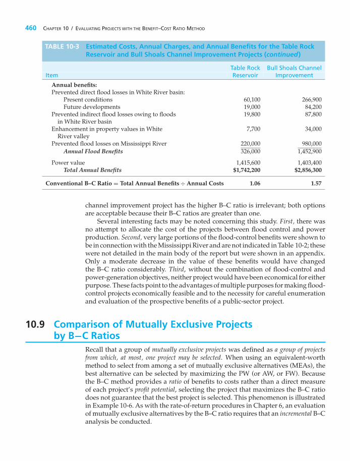
460 CHAPTER 10 / EVALUATING PROJECTS WITH THE BENEFIT–COST RATIO METHOD

TABLE 10-3 Estimated Costs, Annual Charges, and Annual Benefits for the Table RockReservoir and Bull Shoals Channel Improvement Projects (continued)

Table Rock Bull Shoals ChannelItem Reservoir Improvement

Annual benefits:Prevented direct flood losses in White River basin:

Present conditions 60,100 266,900Future developments 19,000 84,200

Prevented indirect flood losses owing to floods 19,800 87,800in White River basin

Enhancement in property values in White 7,700 34,000River valley

Prevented flood losses on Mississippi River 220,000 980,000Annual Flood Benefits 326,000 1,452,900

Power value 1,415,600 1,403,400Total Annual Benefits $1,742,200 $2,856,300

Conventional B–C Ratio = Total Annual Benefits ÷ Annual Costs 1.06 1.57

channel improvement project has the higher B–C ratio is irrelevant; both optionsare acceptable because their B–C ratios are greater than one.

Several interesting facts may be noted concerning this study. First, there wasno attempt to allocate the cost of the projects between flood control and powerproduction. Second, very large portions of the flood-control benefits were shown tobe in connection with the Mississippi River and are not indicated in Table 10-2; thesewere not detailed in the main body of the report but were shown in an appendix.Only a moderate decrease in the value of these benefits would have changedthe B–C ratio considerably. Third, without the combination of flood-control andpower-generation objectives, neither project would have been economical for eitherpurpose. These facts point to the advantages of multiple purposes for making flood-control projects economically feasible and to the necessity for careful enumerationand evaluation of the prospective benefits of a public-sector project.

10.9 Comparison of Mutually Exclusive Projectsby B−C Ratios

Recall that a group of mutually exclusive projects was defined as a group of projectsfrom which, at most, one project may be selected. When using an equivalent-worthmethod to select from among a set of mutually exclusive alternatives (MEAs), thebest alternative can be selected by maximizing the PW (or AW, or FW). Becausethe B–C method provides a ratio of benefits to costs rather than a direct measureof each project’s profit potential, selecting the project that maximizes the B–C ratiodoes not guarantee that the best project is selected. This phenomenon is illustratedin Example 10-6. As with the rate-of-return procedures in Chapter 6, an evaluationof mutually exclusive alternatives by the B–C ratio requires that an incremental B–Canalysis be conducted.

SECTION 10.9 / COMPARISON OF MUTUALLY EXCLUSIVE PROJECTS BY B–C RATIOS 461

EXAMPLE 10-6Inconsistent Ranking Problem When B−C RatiosAre Inappropriately Compared

The required investments, annual operating and maintenance costs, and annualbenefits for two mutually exclusive alternative projects are shown subsequently.Both conventional and modified B–C ratios are included for each project. Notethat Project A has the greater conventional B–C, but Project B has the greatermodified B–C. Given this information, which project should be selected?

Project A Project B

Capital investment $110,000 $135,000 MARR = 10% per yearAnnual O&M cost 12,500 45,000 Study period = 20 yearsAnnual benefit 37,500 80,000

Conventional B–C 1.475 1.314Modified B–C 1.934 2.206

SolutionThe B–C analysis has been conducted improperly. Although each of theB–C ratios shown is numerically correct, a comparison of mutually exclusivealternatives requires that an incremental analysis be conducted.

When comparing mutually exclusive alternatives with the B–C ratio method,they are first ranked in order of increasing total equivalent worth of costs. This rank-ordering will be identical whether the ranking is based on PW, AW, or FW ofcosts. The do-nothing alternative is selected as a baseline alternative. The B–Cratio is then calculated for the alternative having the lowest equivalent cost. If theB–C ratio for this alternative is equal to or greater than 1.0, then that alternativebecomes the new baseline; otherwise, do-nothing remains as the baseline.The next least equivalent cost alternative is then selected, and the difference (�)in the respective benefits and costs of this alternative and the baseline is used tocalculate an incremental B–C ratio (�B/�C). If that ratio is equal to or greaterthan 1.0, then the higher equivalent cost alternative becomes the new baseline;otherwise, the last baseline alternative is maintained. Incremental B–C ratios aredetermined for each successively higher equivalent cost alternative until the lastalternative has been compared. The flowchart of this procedure is included asFigure 10-3, and the procedure is illustrated in Example 10-7.

EXAMPLE 10-7 Incremental B−C Analysis of Mutually Exclusive Projects

Three mutually exclusive alternative public-works projects are currently underconsideration. Their respective costs and benefits are included in the table thatfollows. Each of the projects has a useful life of 50 years, and MARR is 10% per

462 CHAPTER 10 / EVALUATING PROJECTS WITH THE BENEFIT–COST RATIO METHOD

Calculate B–C Ratio ofMEA With LeastEquivalent Cost

Rank-Order MEAsby Increasing Equivalent

Worth of Costs

Select Do-Nothing or Least Equivalent Cost

MEA as Baseline

IsB/C � 1.0

?

Is Thisthe Last MEA

?

This MEA is the NewBaseline

Compare Next MEA withBaseline; Calculate �B/�C

STOP. Baseline is thePreferred Alternative

STOP. This is thePreferred Alternative

Is Thisthe Last MEA

?

Calculate Equivalent Worth(PW, AW, or FW) of Costs

for Each MEA

YES

YES

YES

NO

NO

NO

Figure 10-3 The Incremental B–C Ratio Procedure

year. Which, if any, of these projects should be selected? Solve by hand and byspreadsheet.

A B C

Capital investment $8,500,000 $10,000,000 $12,000,000Annual operating and 750,000 725,000 700,000

maintenance costsMarket value 1,250,000 1,750,000 2,000,000Annual benefit 2,150,000 2,265,000 2,500,000

SECTION 10.9 / COMPARISON OF MUTUALLY EXCLUSIVE PROJECTS BY B–C RATIOS 463

Solution by Hand

PW(Costs, A) = $8,500,000 + $750,000(P/A, 10%, 50)

−$1,250,000(P/F, 10%, 50) = $15,925,463,

PW(Costs, B) = $10,000,000 + $725,000(P/A, 10%, 50)

−$1,750,000(P/F, 10%, 50) = $17,173,333,

PW(Costs, C) = $12,000,000 + $700,000(P/A, 10%, 50)

−$2,000,000(P/F, 10%, 50) = $18,923,333,

PW(Benefit, A) = $2,150,000(P/A, 10%, 50) = $21,316,851,

PW(Benefit, B) = $2,265,000(P/A, 10%, 50) = $22,457,055,

PW(Benefit, C) = $2,500,000(P/A, 10%, 50) = $24,787,036.

B–C(A) = $21,316,851/$15,925,463

= 1.3385 > 1.0.

Therefore, Project A is acceptable.

�B/�C of (B − A) = ($22,457,055 − $21,316,851)/($17,173,333 − $15,925,463)

= 0.9137 < 1.0.

Therefore, increment required for Project B is not acceptable.

�B/�C of (C − A) = ($24,787,036 − $21,316,851)/($18,923,333 − $15,925,463)

= 1.1576 > 1.0.

Therefore, increment required for Project C is acceptable.

Decision: Recommend Project C.

Spreadsheet SolutionA spreadsheet analysis for this example is shown in Figure 10-4. For eachmutually exclusive project, the PW of total benefits (cells B11:B13) and the PWof total costs (cells C11:C13) are calculated. Note that annual operating andmaintenance costs are included in the total cost calculation in accordance withthe conventional B–C ratio formulation.

Since the projects are mutually exclusive, they must be ranked from smallestto largest according to the equivalent worth of costs (do nothing → A → B →C). The B–C ratio for Project A is calculated to be 1.34 (row 17), and Project Areplaces do-nothing as the baseline alternative.

Project B is now compared with Project A (row 18). The ratio of incrementalbenefits to incremental costs is less than 1.0, so Project A remains the baselinealternative. Finally, in row 19, the incremental benefits and incremental costs

464 CHAPTER 10 / EVALUATING PROJECTS WITH THE BENEFIT–COST RATIO METHOD

= B17 / C17

= B11

= B12 – B11

= B13 – B11

= PV($B$2, $B$1, –D5)

= B5 + PV($B$2, $B$1, -C5) - E5 / (1 + $B$2)^$B$1

Figure 10-4 Spreadsheet Solution, Example 10-7

associated with selecting Project C instead of Project A are used to calculate anincremental B–C ratio of 1.16. Since this ratio is greater than one, the incrementrequired for Project C is acceptable, and thus Project C becomes the recom-mended project.

It is not uncommon for some of the projects in a set of mutually exclusivepublic-works projects to have different lives. Recall from Chapter 6 that the AWcriterion can be used to select from among alternatives with different lives as longas the assumption of repeatability is valid. Similarly, if a mutually exclusive set ofpublic-works projects includes projects with varying useful lives, it may be possibleto conduct an incremental B–C analysis by using the AW of benefits and costs ofthe various projects. This analysis is illustrated in Example 10-8.

EXAMPLE 10-8 B−C Analysis with Unequal Project Lives

Two mutually exclusive alternative public-works projects are under cons-ideration. Their respective costs and benefits are included in the table thatfollows. Project I has an anticipated life of 35 years, and the useful life of Project II

SECTION 10.10 / CASE STUDY—IMPROVING A RAILROAD CROSSING 465

has been estimated to be 25 years. If the MARR is 9% per year, which, if either,of these projects should be selected? The effect of inflation is negligible.

Project I Project II

Capital investment $750,000 $625,000Annual operating and maintenance 120,000 110,000Annual benefit 245,000 230,000Useful life of project (years) 35 25

SolutionAW(Costs, I) = $750,000(A/P, 9%, 35) + $120,000 = $190,977,

AW(Costs, II) = $625,000(A/P, 9%, 25) + $110,000 = $173,629,

B–C(II) = $230,000/$173,629 = 1.3247 > 1.0.

Therefore, Project II is acceptable.

�B/�C of (I–II) = ($245,000 − $230,000)/($190,977 − $173,629)

= 0.8647 < 1.0.

Therefore, increment required for Project I is not acceptable.

Decision: Project II should be selected.

10.10 CASE STUDY−−Improving a Railroad Crossing

Traffic congestion and vehicle safety are significant concerns in most major cities inthe Northeast United States. Amajor metropolitan city in New Jersey is consideringthe elimination of a railroad grade crossing by building an overpass. Trafficengineers estimated that approximately 2,000 vehicles per day are delayed at anaverage of 2 minutes each due to trains at the grade crossing. Trucks comprise 40%of the vehicles, and the opportunity cost of their delay is assumed to average $20per truck-hour. The other vehicles are cars having an assumed average opportunitycost of $4 per car-hour. It is also estimated that the new overpass will save the cityapproximately $4,000 per year in expenses directly due to accidents.

The traffic engineers determined that the overpass would cost $1,000,000and is estimated to have a useful life of 40 years and a $100,000 salvage value.Annual maintenance costs of the overpass would cost the city $5,000 more than themaintenance costs of the existing grade crossing. The installation of the overpasswill save the railroad an annual expense of $30,000 for lawsuits and maintenanceof crossing guards.

Since this is a public project, there are special considerations and a complete andcomprehensive engineering economy study is more challenging than in the case of

466 CHAPTER 10 / EVALUATING PROJECTS WITH THE BENEFIT–COST RATIO METHOD

privately financed projects. For example, in the private sector, costs are accrued bythe firm undertaking the project, and benefits are the favorable outcomes achievedby the firm. Typically, any costs and benefits that are external to the firm are ignoredin economic evaluations unless those external costs and benefits indirectly affectthe firm. With economic evaluations of public projects, however, the opposite istrue. As in the case of improving the railroad crossing, there are multiple purposesor objectives to consider. The true owners of the project are the taxpayers! Themonetary impacts of the diverse benefits are oftentimes hard to quantify, and theremay be special political or legal issues to consider.

In this case study, the city council is now in the process of considering the meritsof the engineering proposal to improve the railroad crossing. The city council isconsidering the following questions in its deliberations:

• Should the overpass be built by the city if it is to be the owner and the opportunitycost of the city’s capital is 8% per year?

• How much should the railroad reasonably be asked to contribute towardconstruction of the bridge if its opportunity cost of capital is assumed to be15% per year?

SolutionThe city uses the conventional B–C ratio with AW for its analyses of public projects.The annual benefits of the overpass are comprised of the time savings for vehicles(whose drivers are “members” of the city) and the reduction in accident expenses.The city’s cost engineer makes the following estimates.

Annual Benefits:

Cars =(

2,000×0.6 vehiclesday

)(365 days

year

)(hour

60 minutes

)($4.00

car − hour

)= $58,400

Trucks =(

2,000 × 0.4 vehiclesday

)(365 days

year

)(hour

60 minutes

)($20.00

truck − hour

)= $194,667

Annual savings = $4,000

Total annual benefits = $58,400 + $194,667 + $4,000 = $257,067.

Notice that the estimated $30,000 annual expense savings for lawsuits andmaintenance of the crossing guard is not included in the annual benefits calculation.This savings will be experienced by the owners of the railroad, not by the city.

The costs of the overpass to the city are the construction of the overpass (lessits salvage value) and the increased maintenance costs. The cost engineer makesthe following estimates.

Annual Costs:

Capital recovery = $1,000,000(A/P, 8%, 40) − $100,000(A/F, 8%, 40) = $83,474

Increased maintenance = $5,000

Total annual costs = $83,474 + $5,000 = $88,474.

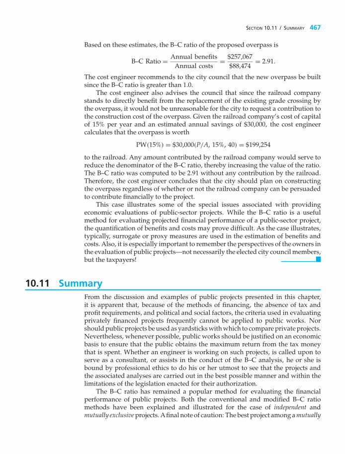
SECTION 10.11 / SUMMARY 467

Based on these estimates, the B–C ratio of the proposed overpass is

B–C Ratio = Annual benefitsAnnual costs

= $257,067$88,474

= 2.91.

The cost engineer recommends to the city council that the new overpass be builtsince the B–C ratio is greater than 1.0.

The cost engineer also advises the council that since the railroad companystands to directly benefit from the replacement of the existing grade crossing bythe overpass, it would not be unreasonable for the city to request a contribution tothe construction cost of the overpass. Given the railroad company’s cost of capitalof 15% per year and an estimated annual savings of $30,000, the cost engineercalculates that the overpass is worth

PW(15%) = $30,000(P/A, 15%, 40) = $199,254

to the railroad. Any amount contributed by the railroad company would serve toreduce the denominator of the B–C ratio, thereby increasing the value of the ratio.The B–C ratio was computed to be 2.91 without any contribution by the railroad.Therefore, the cost engineer concludes that the city should plan on constructingthe overpass regardless of whether or not the railroad company can be persuadedto contribute financially to the project.

This case illustrates some of the special issues associated with providingeconomic evaluations of public-sector projects. While the B–C ratio is a usefulmethod for evaluating projected financial performance of a public-sector project,the quantification of benefits and costs may prove difficult. As the case illustrates,typically, surrogate or proxy measures are used in the estimation of benefits andcosts. Also, it is especially important to remember the perspectives of the owners inthe evaluation of public projects—not necessarily the elected city council members,but the taxpayers!

10.11 SummaryFrom the discussion and examples of public projects presented in this chapter,it is apparent that, because of the methods of financing, the absence of tax andprofit requirements, and political and social factors, the criteria used in evaluatingprivately financed projects frequently cannot be applied to public works. Norshould public projects be used as yardsticks with which to compare private projects.Nevertheless, whenever possible, public works should be justified on an economicbasis to ensure that the public obtains the maximum return from the tax moneythat is spent. Whether an engineer is working on such projects, is called upon toserve as a consultant, or assists in the conduct of the B–C analysis, he or she isbound by professional ethics to do his or her utmost to see that the projects andthe associated analyses are carried out in the best possible manner and within thelimitations of the legislation enacted for their authorization.

The B–C ratio has remained a popular method for evaluating the financialperformance of public projects. Both the conventional and modified B–C ratiomethods have been explained and illustrated for the case of independent andmutually exclusive projects. Afinal note of caution: The best project among a mutually

468 CHAPTER 10 / EVALUATING PROJECTS WITH THE BENEFIT–COST RATIO METHOD

exclusive set of projects is not necessarily the one that maximizes the B–C ratio. Inthis chapter, we have seen that an incremental analysis approach to evaluatingbenefits and costs is necessary to ensure the correct choice.

ProblemsThe number in parentheses that follows each problemrefers to the section from which the problem is taken.

10-1. The Adams Construction Company is bidding ona project to install a large flood drainage culvert fromDandridge to a distant lake. If they bid $2,000,000 for thejob, what is the benefit-cost ratio in view of the followingdata? The MARR is 6% per year, and the project’s life is30 years. (10.7)

Initial construction bid $2,000,000Right of way maintenance $30,000 per yearMajor upkeep every six years,

starting at the present time $50,000Annual benefit to the taxpayers $135,000

10-2. An environmentally friendly 2,800-square-foot green home (99% air tight) costs

about 8% more to construct than a same-sized con-ventional home. Most green homes can save 15% peryear on energy expenses to heat and cool the livingspace. For a $250,000 conventional home with a heatingand cooling bill of $3,000 per year, how much wouldhave to be saved in energy expenses per year to justifythis home (i.e., B–C ratio greater than or equal to one)?The discount rate is 10% per year, and the expected lifeof the home is 30 years. (10.7)

10-3. A proposal has been made for improving thedowntown area of a small town. The plan callsfor banning vehicular traffic on the main street andturning this street into a pedestrian mall with treeplantings and other beautification features. This planwill involve actual costs of $6,000,000 and, accordingto its proponents, the plan will produce benefits anddisbenefits to the town as follows:

Design A Design B Design C

Cost of the building, including cost of the land $1,300,000 $1,700,000 $3,500,000Resale value of land and building at end of 20-year planning horizon $500,000 $900,000 $2,000,000Annual net rental income (after deducting all operating expenses) $120,000 $300,000 $450,000

Benefits:Increased sales tax revenue $450,000 per yearIncreased real estate property taxes $325,000 per yearBenefits due to decreased air pollution $80,000 per yearQuality of life improvements to users $70,000 per year

Disbenefits:Increased maintenance $175,000 per year

a. Compute the B–C ratio of this plan based on aMARR of 10% per year and an infinite life for theproject. (10.7)

b. How does the B–C ratio change for a 20-year projectlife? (10.7)

10-4. A retrofitted space-heating system isbeing considered for a small office building. The

system can be purchased and installed for $120,000,and it will save an estimated 300,000 kilowatt-hours(kWh) of electric power each year over a six-yearperiod. Akilowatt-hour of electricity costs $0.10, and thecompany uses a MARR of 15% per year in its economicevaluations of refurbished systems. The market valueof the system will be $8,000 at the end of six years, andadditional annual operating and maintenance expensesare negligible. Use the benefit–cost method to make arecommendation. (10.7)

10-5. In Problem 10-4, what is the benefit–costratio of the project if the general inflation rate

is 4% per year and the market value is negligible?The market interest rate (im) is 18% per year, and theannual savings are expressed in year-zero dollars. (10.7,Chapter 8)

10-6. A city is considering buying a piece of land for$500,000 and constructing an office complex on it. Theirplanning horizon is 20 years. Three mutually exclusivebuilding designs (shown below) have been drawn up

PROBLEMS 469

by an architectural firm. Use the modified benefit-costratio method and a MARR of 10% per year to determinewhich alternative, if any, should be recommended to thecity council. (10.9)

10-7. A toll bridge across the Mississippi River is beingconsidered as a replacement for the current I-40 bridgelinking Tennessee to Arkansas. Because this bridge, ifapproved, will become a part of the U.S. InterstateHighway system, the B–C ratio method must be appliedin the evaluation. Investment costs of the structure areestimated to be $17,500,000, and $325,000 per year inoperating and maintenance costs are anticipated. Inaddition, the bridge must be resurfaced every fifth yearof its 30-year projected life at a cost of $1,250,000 peroccurrence (no resurfacing cost in year 30). Revenuesgenerated from the toll are anticipated to be $2,500,000in its first year of operation, with a projected annualrate of increase of 2.25% per year due to the anticipatedannual increase in traffic across the bridge. Assumingzero market (salvage) value for the bridge at the end of30 years and a MARR of 10% per year, should the tollbridge be constructed? (10.7)

10-8. Refer back to Problem 10-7. Suppose that thetoll bridge can be redesigned such that it will havea (virtually) infinite life. MARR remains at 10% peryear. Revised costs and revenues (benefits) are givenas follows: (10.7, 10.9)

Capital investment: $22,500,000Annual operating and maintenance costs: $250,000Resurface cost every seventh year: $1,000,000Structural repair cost, every 20th year: $1,750,000Revenues (treated as constant—no rate of increase):

$3,000,000

a. What is the capitalized worth of the bridge?

b. Determine the B–C ratio of the bridge over an infinitetime horizon.

c. Should the initial design (Problem 10-7) or the newdesign be selected?

10-9. Five independent projects consisting of reinfor-cing dams, levees, and embankments are availablefor funding by a certain public agency. The followingtabulation shows the equivalent annual benefits andcosts for each: (10.8)

a. Assume that the projects are of the type for whichthe benefits can be determined with considerablecertainty and that the agency is willing to invest

Project Annual Benefits Annual Costs

A $1,800,000 $2,000,000B 5,600,000 4,200,000C 8,400,000 6,800,000D 2,600,000 2,800,000E 6,600,000 5,400,000

money as long as the B–C ratio is at least one. Whichalternatives should be selected for funding?

b. What is the rank-ordering of projects from best toworst?

c. If the projects involved intangible benefits thatrequired considerable judgment in assigning theirvalues, would your recommendation be affected?

10-10. In the development of a publicly owned,commercial waterfront area, three possible independentplans are being considered. Their costs and estimatedbenefits are as follows: (10.8)

PW ($000s)

Plan Costs Benefits

A $123,000 $139,000B 135,000 150,000C 99,000 114,000

a. Which plan(s) should be adopted, if any, if thecontrolling board wishes to invest any amountrequired, provided that the B–C ratio on the requiredinvestment is at least 1.0?

b. Suppose that 10% of the costs of each plan arereclassified as disbenefits. What percentage changein the B–C ratio of each plan results from thereclassification?

c. Comment on why the rank-orderings in (a) areunaffected by the change in (b).

10-11. Five mutually exclusive alternatives are beingconsidered for providing a sewage-treatment facility.The annual equivalent costs and estimated benefits ofthe alternatives are as follows:

470 CHAPTER 10 / EVALUATING PROJECTS WITH THE BENEFIT–COST RATIO METHOD

Annual Equivalent (in thousands)

Alternative Cost Benefits

A $1,050 $1,110B 900 810C 1,230 1,390D 1,350 1,500E 990 1,140

Which plan, if any, should be adopted if the SewageAuthority wishes to invest if, and only if, the B–C ratiois at least 1.0.? (10.9)

10-12. A town in northern Colorado is planning oninvesting in a water purification system. Three mutuallyexclusive systems have been proposed, and theircapital investment costs and net annual benefits are thefollowing (salvage values are negligible).

System

EOY A B C

0 −$160,000 −$245,000 −$200,0001 80,000 120,000 80,0002 70,000 100,000 80,0003 60,000 80,000 80,0004 50,000 60,000 80,000

If the town’s MARR is 10% per year, use the B–C ratiomethod to determine which system is best. (10.9)

10-13. A nonprofit government corporation isconsidering two alternatives for generating

power:

Alternative A. Build a coal-powered generatingfacility at a cost of $20,000,000. Annual power sales areexpected to be $1,000,000 per year. Annual operatingand maintenance costs are $200,000 per year. A benefitof this alternative is that it is expected to attract newindustry, worth $500,000 per year, to the region.

Alternative B. Build a hydroelectric generatingfacility. The capital investment, power sales, andoperating costs are $30,000,000, $800,000, and $100,000per year, respectively. Annual benefits of this alternativeare as follows:

Flood-control savings $600,000Irrigation $200,000Recreation $100,000Ability to attract new industry $400,000

The useful life of both alternatives is 50 years. Usingan interest rate of 5%, determine which alternative (ifeither) should be selected according to the conventionalB–C-ratio method. (10.9)

10-14. A new storm drainage system must beconstructed right away to reduce periodic flooding thatoccurs in a city that is in a valley. Five mutually exclusivedesigns have been proposed, and their present worth(in thousands of dollars) of costs and benefits are thefollowing. (10.9)

System

1 2 3 4 5

PW of $1,000 $4,000 $4,000 $10,000 $12,000costs

PW of 8,000 8,000 14,000 16,000 24,000benefits

a. Which system has the greatest B–C ratio?

b. Which system has the largest incremental B–C ratio(based on differences between alternatives)?

c. Which system should be chosen?

10-15. There are two mutually exclusive proposalsfor a for a flood control project in Illinois. The firstproposal involves an initial outlay of $1,350,000 andannual expenses of $110,000. This plan is assumedto be permanent. The second proposal requires aninitial outlay of $700,000, followed by $200,000 every12 years thereafter. Annual expenses for the secondproposal are estimated to be $95,000 for the first 12 yearsand $150,000 each year thereafter. Annual benefits areidentical for both projects, and terminal salvage valuesare negligible. The interest rate is 6% per year. Whichproposal should be recommended? (6.5 and 10.9)

10-16. Consider the mutually exclusive alternativesin Table P10-16. Which alternative would be chosenaccording to these decision criteria?

PROBLEMS 471

TABLE P10-16 Mutually Exclusive Alternatives for Problem 10-16

Equivalent Annual Expected AnnualAlternative Cost of Project Flood Damage Annual Benefits

I. No flood control 0 $100,000 0II. Construct levees $30,000 80,000 $112,000

III. Build small dam $100,000 5,000 110,000

TABLE P10-19 Mutually Exclusive Plans for Problem 10-19

Construction Annual Annual Savings Annual Recreational Annual TimberRoute Costs Maintenance Cost in Fire Damage Benefit Access Benefit

A $185,000 $2,000 $5,000 $3,000 $500B 220,000 3,000 7,000 6,500 1,500C 290,000 4,000 12,000 6,000 2,800

a. Maximum benefit

b. Minimum cost

c. Maximum benefits minus costs

d. Largest investment having an incremental B–C ratiolarger than one

e. Largest B–C ratio

Which project should be chosen? (10.9)

10-17. Four mutually exclusive projects are beingconsidered for a new 2-mile jogging track. The life ofthe track is expected to be 80 years, and the sponsoringagency’s MARR is 12% per year. Annual benefits to thepublic have been estimated by an advisory committeeand are shown on the next page. Use the B–C method(incrementally) to select the best jogging track. (10.9)

Alternative

A B C D

Initial cost $62,000 $52,000 $150,000 $55,000Annual $10,000 $8,000 $20,000 $9,000

benefitsB–C ratio 1.34 1.28 1.11 1.36

10-18. Two municipal cell tower designs are beingconsidered by the city of Newton. If the city expects amodified benefit–cost ratio of 1.0 or better, which designwould you recommend based on the data that follows?Assume repeatability. The city’s cost of capital is 10%per year. (10.8)

Verizon Cellgene

Initial investment (first cost) $75,000 $175,000Useful life in years 6 12Market value at end of useful life $20,000 $37,500Annual benefits from operation $28,800 $38,800Annual operating expenses $9,800 $11,300

10-19. A state-sponsored Forest Management Bureauis evaluating alternative routes for a new road into aformerly inaccessible region. Three mutually exclusiveplans for routing the road provide different benefits,as indicated in Table P10-19. The roads are assumed tohave an economic life of 50 years, and MARR is 8% peryear. Which route should be selected according to theB–C ratio method? (10.9)

10-20. The city of Oak Ridge is evaluating threemutually exclusive landscaping plans for refurbishing apublic greenway. Benefits to the community have beenestimated by a landscaping committee, and the costs ofplanting trees and shrubbery, as well as maintaining thegreenway, are summarized below. The city’s discountrate is 8% per year, and the planning horizon is10 years. (10.9)

a. Use the B–C ratio method to recommend the bestplan when annual maintenance expenses offsetannual benefits in the numerator.

b. Repeat Part (a) when annual maintenance expensesadd to total costs in the denominator. Which plan isbest?

472 CHAPTER 10 / EVALUATING PROJECTS WITH THE BENEFIT–COST RATIO METHOD

Landscaping Plan

A B C

Initial planting $75,000 $50,000 $65,000cost

Annual maintenance 4,000 5,000 4,700expense

Annual community 20,000 18,000 20,000benefits

c. Should the recommendations in Part (a) and (b) bethe same? Why or why not?

10-21. An area on the Colorado River is subjectto periodic flood damage that occurs, on the

average, every two years and results in a $2,000,000loss. It has been proposed that the river channel bestraightened and deepened, at a cost of $2,500,000, toreduce the probable damage to not over $1,600,000 foreach occurrence during a period of 20 years beforeit would have to be deepened again. This procedurewould also involve annual expenditures of $80,000 forminimal maintenance. One legislator in the area hasproposed that a better solution would be to constructa flood-control dam at a cost of $8,500,000, whichwould last indefinitely, with annual maintenance costsof not over $50,000. He estimates that this projectwould reduce the probable annual flood damage to notover $450,000. In addition, this solution would providea substantial amount of irrigation water that wouldproduce annual revenue of $175,000 and recreationalfacilities, which he estimates would be worth at least$45,000 per year to the adjacent populace. A secondlegislator believes that the dam should be built andthat the river channel also should be straightened anddeepened, noting that the total cost of $11,000,000would reduce the probable annual flood loss to notover $350,000 while providing the same irrigation andrecreational benefits. If the state’s capital is worth10%, determine the B–C ratios and the incrementalB–C ratio. Recommend which alternative should beadopted. (10.9)

TABLE P10-22 Pier Replacement Cost for Problem 10-22

Annual Cost of Present Pier Annual Cost of Proposed Pier

Depreciation ($300,000/50) $6,000 Depreciation ($600,000/50) $12,000Maintenance cost 27,000 Maintenance cost 2,000Total $33,000 Total $14,000

10-22. Ten years ago, the port of Secoma built a newpier containing a large amount of steel work, at a costof $300,000, estimating that it would have a life of50 years. The annual maintenance cost, much of it forpainting and repair caused by environmental damage,has turned out to be unexpectedly high, averaging$27,000. The port manager has proposed to the portcommission that this pier be replaced immediately witha reinforced concrete pier at a construction cost of$600,000. He assures them that this pier will have a lifeof at least 50 years, with annual maintenance costs of notover $2,000. He presents the information in Table P10-22as justification for the replacement, having determinedthat the net market value of the existing pier is $40,000.

He has stated that, because the port earns a netprofit of over $3,000,000 per year, the project could befinanced out of annual earnings. Thus, there would beno interest cost, and an annual savings of $19,000 wouldbe obtained by making the replacement. (10.9)

a. Comment on the port manager’s analysis.

b. Make your own analysis and recommendationregarding the proposal.

10-23. You have been requested to recommend oneof the mutually exclusive industrial sanitation controlsystems that are given below. If MARR is 15% peryear, which system would you select? Use the B–Cmethod. (10.9)

Alternative

Gravity-fed Vacuum-led

Capital investment $24,500 $37,900Annual receipts 8,000 8,000

less expensesLife in years 5 10

10-24. In the aftermath of Hurricane Thelma,the U.S. Army Corps of Engineers is considering

two alternative approaches to protect a freshwaterwetland from the encroaching seawater during high

FE PRACTICE PROBLEMS 473

TABLE P10-25 Bridge Design Information for Problem 10-25

Bridge Design

A B C

Capital investment $17,000,000 $14,000,000 $12,500,000Annual maintenance cost∗ 12,000 17,500 20,000Resurface (every fifth year)∗ – 40,000 40,000Resurface (every seventh year)∗ 40,000 – –Bridge replacement cost 3,000,000 3,500,000 3,750,000Annual benefit 2,150,000 1,900,000 1,750,000Useful life of bridge (years)∗∗ 35 25 25

∗ Cost not incurred in last year of bridge’s useful life.∗∗ Applies to roadbed only; structural portion of bridge has indefinite useful life.

tides. The first alternative, the construction of a 5-milelong, 20-foot-high levee, would have an investmentcost of $25,000,000 with annual upkeep costs estimatedat $725,000. A new roadway along the top of thelevee would provide two major benefits: (1) improvedrecreational access for fishermen and (2) reduction of thedriving distance between the towns at opposite ends ofthe proposed levee by 11 miles. The annual benefit forthe levee has been estimated at $1,500,000. The secondalternative, a channel-dredging operation, would havean investment cost of $15,000,000. The annual cost ofmaintaining the channel is estimated at $375,000. Thereare no documented benefits for the channel-dredgingproject. Using a MARR of 8% and assuming a 25-yearlife for either alternative, apply the incremental B–Cratio (�B/�C) method to determine which alternativeshould be chosen. (Note: The null alternative, Donothing, is not a viable alternative.) (10.9)

10-25. Extended Learning Exercise The Fox River isbordered on the east by Illinois Route 25 and on thewest by Illinois Route 31. Along one stretch of theriver, there is a distance of 16 miles between adjacentcrossings. An additional crossing in this area has beenproposed, and three alternative bridge designs areunder consideration. Two of the designs have 25-yearuseful lives, and the third has a useful life of 35 years.Each bridge must be resurfaced periodically, and theroadbed of each bridge will be replaced at the end ofits useful life, at a cost significantly less than initialconstruction costs. The annual benefits of each designdiffer on the basis of disruption to normal traffic flowalong Routes 25 and 31. Given the information inTable P10-25, use the B–C ratio method to determinewhich bridge design should be selected. Assume thatthe selected design will be used indefinitely, and use aMARR of 10% per year. (10.9)

FE Practice Problems

The city council of Morristown is considering thepurchase of one new fire truck. The options are TruckX and Truck Y. The appropriate financial data are asfollows:

Truck X Truck Y

Capital investment $50,000 $64,000Maintenance cost per year $6,000 $5,000Useful life 6 years 6 yearsReduction in fire damage $20,000 $22,000per year

The purchase is to be financed by money borrowed at12% per year. Use this information to answer problems10-26 and 10-27.

10-26. What is the conventional B–C ratio for TruckX? (10.7)

(a) 1.41 (b) 0.87 (c) 1.64 (d) 1.10 (e) 1.15

10-27. Which fire truck should be purchased? (10.9)

(a) Neither Truck X nor Truck Y

(b) Truck X

474 CHAPTER 10 / EVALUATING PROJECTS WITH THE BENEFIT–COST RATIO METHOD

(c) Truck Y

(d) Both Truck X and Truck Y

10-28. A state government is considering constructionof a flood control dike having a life span of 15 years.History indicates that a flood occurs every five yearsand causes $600,000 in damages, on average. If the stateuses a MARR of 12% per year and expects every public-works project to have a B–C ratio of at least 1.0, what isthe maximum investment that will be allowed for thedike? Assume that the flood occurs in the middle of eachfive-year period. (10.7)

(a) $1,441,000 (b) $643,000 (c) $843,000(d) $4,087,000 (e) $1,800,000

A flood control project with a life of 16 years will requirean investment of $60,000 and annual maintenance costsof $5,000. The project will provide no benefits for the firsttwo years but will save $24,000 per year in flood damagestarting in the third year. The appropriate MARR is 12%per year. Use this information to answer problems 10-29and 10-30. Select the closest answer. (10.7)

10-29. What is the conventional B–C ratio for the floodcontrol project?

(a) 1.53 (b) 1.33 (c) 1.76 (d) 2.20 (e) 4.80

10-30. What is the modified B–C ratio for the floodcontrol project?

(a) 1.53 (b) 1.33 (c) 1.76 (d) 2.20 (e) 4.80

10-31. You have been tasked with recommending oneof the mutually exclusive industrial sanitation controlsystems summarized below. The life of both alternativesis 30 years, and residual salvage values are negligible.Use the benefit–cost ratio method in your analysis. Ifthe MARR is 8% per year, which answer below wouldyou recommend? (10.9)

Alternative Gravity-fed Vacuum-led

Capital investment $800,000 $1,000,000Annual benefits less costs $106,500 $119,000

(a) Gravity-fed (b) Vacuum-led(c) Both systems (d) Neither system

CHAPTER 11

Breakeven and SensitivityAnalysis

Our aim in Chapter 11 is to illustrate breakeven and sensitivity methodsfor investigating variability in outcomes of engineering projects.

Renting versus Purchasing a Home

A common situation faced by young families is whether to rent or buy a home.Many of the decision factors are speculative, such as the future resale valueof the house and how long the family will be in a particular area. For

example, what will be the resale value of a home currently valued at $150,000five years from now? If you plan to stay in your current location for only threeyears, should you rent or purchase a home? In this chapter, you will learn how toevaluate decision problems such as this by examining the sensitivity of the decisionto changes in the estimates of selected factor estimates.

475

Money is the seed of money, and the first guinea is sometimes more difficultto aquire than the second million.

—Jean Jacques Rousseau (1762)

11.1 IntroductionThere is much common wisdom relating to uncertainty in Yogi Berra’s observationabout the future! In previous chapters, we presented specific assumptions concern-ing revenues, costs, and other quantities important to an engineering economystudy. It was assumed that a high degree of confidence could be placed in allestimated values. That degree of confidence is sometimes called assumed certainty.Decisions made solely on the basis of this kind of analysis are sometimes calleddecisions under certainty. The term is rather misleading in that there rarely is a casein which the best of estimates of quantities can be assumed as certain.

In virtually all situations, there is doubt as to the ultimate economic resultsthat will be obtained from an engineering project. The motivation for breakevenand sensitivity analysis is to establish the bounds of error in our estimates suchthat another alternative being considered may become a better choice than theone we recommended under assumed certainty. Thus, this chapter deals withnonprobabilistic techniques for dealing with risk and uncertainty.

Breakeven analysis determines the value of a critical factor at which economictrade-offs are balanced. It is also helpful in some situations to investigate howsensitive a project’s economics are to variations in its estimates of life, interestrate, initial capital investment, and so on. Sensitivity, in general, means the relativemagnitude of change in the measure of merit (such as present worth [PW] or internalrate of return [IRR]) caused by one or more changes in estimated factor values. Thespecific factors of concern will vary with each project, but one or more of them willnormally need to be further analyzed before the best decision can be made. Simplystated, engineering economy studies focus on the future, and lack of knowledgeabout the estimated economic results cannot be avoided.

In engineering economy studies, breakeven and sensitivity analysis are generalmethodologies, readily available, that provide information about the potentialimpact on equivalent worth due to variability in selected factor estimates. Theirroutine use is fundamental to developing economic information useful in thedecision process.

11.2 Breakeven AnalysisWhen the selection between two engineering project alternatives (or outcomes) isheavily dependent on a single factor, we can solve for the value of that factor atwhich the conclusion is a standoff. That value is known as the breakeven point, thatis, the value at which we are indifferent between the two alternatives. (The use ofbreakeven points with respect to production and sales volumes was discussed inChapter 2.) Then, if the best estimate of the actual outcome of the common factor ishigher or lower than the breakeven point, and assumed certain, the best alternativebecomes apparent.

476

SECTION 11.2 / BREAKEVEN ANALYSIS 477

In mathematical terms, we have

EWA = f1(y) and EWB = f2(y),

where EWA = an equivalent worth (PW, annual worth [AW], or future worth[FW]) calculation for the net cash flow of Alternative A;

EWB = the same equivalent-worth calculation for the net cash flowof Alternative B;

y = a common factor of interest affecting the equivalent-worthvalues of Alternative A and Alternative B.

Therefore, the breakeven point betweenAlternative A andAlternative B is the valueof factor y for which the two equivalent-worth values are equal. That is, EWA =EWB, or fl(y) = f2(y), which may be solved for y.

Similarly, when the economic acceptability of an engineering project dependsupon the value of a single factor, say z, mathematically we can set an equivalentworth of the project’s net cash flow for the analysis period equal to zero [EW =f (z) = 0] and solve for the breakeven value of z. That is, the breakeven value of z isthe value of z at which we would be indifferent (economically) between acceptingand rejecting the project. Then, if the best estimate of the value of z is higher or lowerthan the breakeven point value, and assumed certain, the economic acceptabilityof the project is known.

The following are examples of common factors for which breakeven analysesmight provide useful insights into the decision problem:

1. Annual revenue and expenses. Solve for the annual revenue required to equal(breakeven with) annual expenses. Breakeven annual expenses of an alternativecan also be determined in a pairwise comparison when revenues are identicalfor both alternatives being considered.

2. Rate of return. Solve for the rate of return on the increment of invested capital atwhich two given alternatives are equally desirable.

3. Minimum attractive rate of return. Solve for the interest rate value that wouldresult in indifference as to the preference for an alternative.

4. Equipment life. Solve for the useful life required for an engineering project to beeconomically justified.

5. Capacity utilization. Solve for the hours of utilization per year, for example,at which an alternative is justified or at which two alternatives are equallydesirable.

The usual breakeven problem involving two alternatives can be most easilyapproached mathematically by equating an equivalent worth of the twoalternatives expressed as a function of the factor of interest. Using the sameapproach for the economic acceptability of an engineering project, we canmathematically equate an equivalent worth of the project to zero as a functionof the factor of concern. In breakeven studies, project lives may or may notbe equal, so care should be taken to determine whether the coterminated orrepeatability assumption best fits the situation.

478 CHAPTER 11 / BREAKEVEN AND SENSITIVITY ANALYSIS

The following examples illustrate both mathematical and graphical solutionsto typical breakeven problems involving one or more engineering projects.

EXAMPLE 11-1 Single Project Breakeven Analysis: Solar Panels

A homeowner is considering whether to invest in solar panels. This homeownerhas gathered the following information for her town:

• The average cost for residential energy is $0.124/kWh.• The government subsidizes 70% of whatever is invested by the household.• Each square foot of panel produces 19.13 kWh every year.• The cost of installation per square foot of solar panel is $93.91.

The house has 350 square feet of roof space. What is the breakeven point in yearsfor the installation of solar panels? Assume the homeowner’s interest rate is 6%per year.

SolutionThe breakeven point is where the annual savings from the solar panels offsetsthe initial investment. The initial investment is calculated as follows.

350 square feet of roof space × $93.91/square foot = $32,869

With a 70% government subsidy, the purchase price is (0.3)($32,869) = $9,861.To find the breakeven point in years (X), we set the purchase price equal to thepotential energy savings.

$9,861 = (350 square feet)(19.13 kWh/sq ft-year)($0.124/kWh)(P/A, 6%, X)

$9,861 = ($830.24)(P/A, 6%, X)

11.87 = (P/A, 6%, X)

From Table C-9 (i = 6%), we see that 21 ≤ X ≤ 22 years. It would takeapproximately 22 years of energy savings to offset the installation cost of thesolar panels. A graph of this breakeven situation is shown in Figure 11-1.

Figure 11-1 Graphical Plotof the Breakeven Pointfor the Solar PanelInvestment

0 4$0

$2,000

$4,000

$6,000

$8,000

$10,000

$12,000

8 12 16 20 24 28

Energy SavingsInvestment

Years

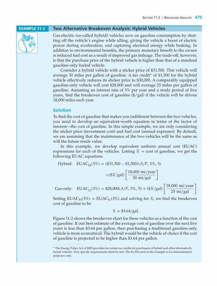
SECTION 11.2 / BREAKEVEN ANALYSIS 479

EXAMPLE 11-2 Two Alternative Breakeven Analysis: Hybrid Vehicles

Gas-electric (so-called hybrid) vehicles save on gasoline consumption by shut-ting off the vehicle’s engine while idling, giving the vehicle a boost of electricpower during acceleration, and capturing electrical energy while braking. Inaddition to environmental benefits, the primary monetary benefit to the owneris reduced fuel cost as a result of improved gas mileage. The trade-off, however,is that the purchase price of the hybrid vehicle is higher than that of a standardgasoline-only fueled vehicle.

Consider a hybrid vehicle with a sticker price of $31,500. This vehicle willaverage 30 miles per gallon of gasoline. A tax credit∗ of $1,500 for the hybridvehicle effectively reduces its sticker price to $30,000. A comparably equippedgasoline-only vehicle will cost $28,000 and will average 25 miles per gallon ofgasoline. Assuming an interest rate of 3% per year and a study period of fiveyears, find the breakeven cost of gasoline ($/gal) if the vehicle will be driven18,000 miles each year.

SolutionTo find the cost of gasoline that makes you indifferent between the two vehicles,you need to develop an equivalent-worth equation in terms of the factor ofinterest—the cost of gasoline. In this simple example, we are only consideringthe sticker price (investment cost) and fuel cost (annual expenses). By default,we are assuming that the maintenance of the two vehicles will be the same aswill the future resale value.

In this example, we develop equivalent uniform annual cost (EUAC)expressions for each of the vehicles. Letting X = cost of gasoline, we get thefollowing EUAC equations.

Hybrid: EUACH(3%) = ($31,500 − $1,500)(A/P, 3%, 5)

+($X/gal)[

18,000 mi/year30 mi/gal

]

Gas-only: EUACG(3%) = $28,000(A/P, 3%, 5) + ($X/gal)[

18,000 mi/year25 mi/gal

]Setting EUACH(3%) = EUACG(3%) and solving for X, we find the breakevencost of gasoline to be

X = $3.64/gal.

Figure 11-2 shows the breakeven chart for these vehicles as a function of the costof gasoline. If our best estimate of the average cost of gasoline over the next fiveyears is less than $3.64 per gallon, then purchasing a traditional gasoline-onlyvehicle is more economical. The hybrid would be the vehicle of choice if the costof gasoline is projected to be higher than $3.64 per gallon.

∗ The Energy Policy Act of 2005 provides for certain tax credits for purchasers of hybrid and other alternativelyfueled vehicles. Very specific requirements must be met. The $1,500 used in the example is for demonstrationpurposes only.

480 CHAPTER 11 / BREAKEVEN AND SENSITIVITY ANALYSIS

$3.64

Gas-Only

$7,500

$8,000

$8,500

$9,000

$9,500

$10,000

$2.00 $2.50 $3.00 $3.50 $4.00 $4.50 $5.00

Cost of Gasoline ($/gal)

Hybrid

EU

AC

(3%

)

Figure 11-2 Breakeven Chart for Hybrid versus Gas-Only Vehicle

CommentIn this example, we only considered the easily measured monetary benefit ofthe hybrid vehicle. Other important factors that may influence this decision arereduced emissions and more efficient use of a scarce resource.

EXAMPLE 11-3 Three Alternative Breakeven Analysis: Hours of Operation

Suppose that there are three alternative electric motors capable of providing100 horsepower (hp) output. These motors differ in their purchase price, main-tenance costs, and efficiency. The efficiency of the motor impacts the energy costof the motor. Specific data are listed below.

Alpha Beta Gamma

Purchase price $10,000 $15,000 $20,000Annual maintenance $800 $500 $250Efficiency 74% 86% 92%

If we look at the annual cost of owning and operating a motor, a factor ofinterest is the hours of operation, which drives the energy cost of the motor.Over what range of hours operated per year (at full load) is the Beta motor thebest choice? How many hours would the motor have to be operated each year

SECTION 11.2 / BREAKEVEN ANALYSIS 481

before the Gamma motor is the most economical? Use a spreadsheet to answerthese questions. Assume that the minimum attractive rate of return (MARR) =15% per year, the study period is 5 years, and none of the motors will have amarket value after 5 years.

Spreadsheet SolutionBecause we are dealing with costs only in this example (revenues are assumedto be equal), we use the EUAC metric to solve for the breakeven points betweenthe motors. The basic equation used to develop the spreadsheet model is

EUAC(15%) = Purchase price (A/P, 15%, 5) + Annual maintenance

+Annual energy cost

The energy cost portion of the equation can be expressed in terms of the hoursof operation.

Energy cost = (Operating hours/year)($0.05/kWh)

[(100 hp)(0.746 kW/hp)

Motor efficiency

]

For instance, the annual energy expense of the Alpha motor is

(X hours/year)($0.05/kWh)

[(100 hp)(0.746 kW/hp)

0.74

]= $5.04 X

where X is the annual hours of operation. We can now solve for the breakevenpoint between each pair of motors.

Figure 11-3 shows the spreadsheet model. The Goal Seek function was usedto solve for the individual breakeven points between motors (cells B18, B21, andB24). In Goal Seek (under the Tools menu), the spreadsheet software changesthe value of a single cell (hours of operation in this example) to find the valuethat sets a different cell (difference in EUAC) equal to a target amount ($0).

Goal Seek

Set cell: E18To value: 0By changing cell: B18

The breakeven graph is shown in Figure 11-4. The numbers at the bottom ofFigure 11-3 (cells A27:D38) are used to generate the breakeven chart. Althoughwe solved for the exact values of the breakeven points, the graph is useful inreminding us which motor is preferred over which range of operating hours. Insummary, the Alpha motor is preferred if annual operating hours are less than1,694; the Gamma motor would be selected if annual operating hours are greaterthan 4,389; otherwise the Beta motor is the most economical choice.

482 CHAPTER 11 / BREAKEVEN AND SENSITIVITY ANALYSIS

%51RRAM

A B C D E

Electricity ($/kWh) $ 0.05

Useful Life (years) 5

Alpha Beta Gamma

Purchase Price $10,000 $15,000 $20,000

Annual Maintenance $800 $500 $250

%29%68%47ycneiciffE

Alpha Beta Gamma

CR Amount $2,983 $4,475 $5,966

Annual Maintenance $800 $500 $250

612,6$579,4$387,3$latot-buS

Energy Expense ($/hr) 5.04 4.34 4.05

Alpha - Beta Hours Alpha Beta Difference

Breakeven Point 1694 $12,323 $12,323 $0

Alpha - Gamma Hours Alpha Gamma Difference

Breakeven Point 2467 $16,219 $16,219 $0

Beta - Gamma Hours Beta Gamma Difference

Breakeven Point 4389 $24,012 $24,012 $0

Hours Alpha Beta Gamma

1500 $11,344 $11,481 $12,298

2000 $13,864 $13,649 $14,325

2500 $16,385 $15,818 $16,352

3000 $18,905 $17,986 $18,379

3500 $21,425 $20,155 $20,407

4000 $23,945 $22,324 $22,434

4500 $26,466 $24,492 $24,461

5000 $28,986 $26,661 $26,488

5500 $31,506 $28,829 $28,515

6000 $34,026 $30,998 $30,542

6500 $36,547 $33,167 $32,570

1

2

3

4

5

6

7

8

9

10

11

12

13

14

15

16

17

18

19

20

21

22

23

24

25

26

27

28

29

30

31

32

33

34

35

36

37

38

Figure 11-3 Spreadsheet Solution to Example 11-3

SECTION 11.3 / SENSITIVITY ANALYSIS 483

Figure 11-4 Graphical Plotof Breakeven Analysisof Example 11-3

$8,0001,500 2,500 3,500 4,500 5,500 6,500

$13,000

$18,000

$23,000

$28,000

$33,000

$38,000

Hours of Operation

EU

AC

(15%

)

Alpha

Beta

Gamma

11.3 Sensitivity AnalysisSensitivity analysis is used to explore what happens to a project’s profitabilitywhen the estimated value of study factors are changed. For example, if annualexpenses turn out to be 10% higher than expected, will the project still be acceptable?Sometimes, sensitivity is specifically defined to mean the percent change in one ormore factors that will reverse a decision among project alternatives or reverse adecision about the economic acceptability of a single project. This percent changeis called sensitivity with respect to decision reversal. Example 11-4 shows thecalculation of decision reversal points.

Another useful sensitivity tool is the spiderplot. This approach makes explicitthe impact of variability in the estimates of each factor of concern on the economicmeasure of merit. Example 11-5 demonstrates this technique by plotting theresults of changes in the estimates of several factors, separately, on the PW ofan engineering project. Spreadsheet applications provide an excellent capability toanswer what if questions and are useful for generating the spiderplot.

EXAMPLE 11-4 Decision Reversal

Consider a proposal to enhance the vision system used by a postal service tosort mail. The new system is estimated to cost $1.1 million and will incur anadditional $200,000 per year in maintenance costs. The system will produceannual savings of $500,000 each year (primarily by decreasing the percentage ofmisdirected mail and reducing the amount of mail that must be sorted manually).The MARR is 10% per year, and the study period is five years at which time the

484 CHAPTER 11 / BREAKEVEN AND SENSITIVITY ANALYSIS

system will be technologically obsolete (worthless). The PW of this proposal is

PW(10%) = −$1,100,000 + ($500,000 − $200,000)(P/A, 10%, 5) = $37,236.

Determine how sensitive the decision to invest in the system is to the estimatesof investment cost and annual savings.

SolutionOur initial appraisal of the project shows it to be a profitable venture. Now let’slook at what happens if we are wrong in our estimates. Essentially, we needto find the breakeven investment cost and the breakeven annual savings. Letx be the percent change in investment cost that would cause us to reverse ourdecision. Then

PW(10%) = 0 = −$1,100,000(1 + x) + ($500,000 − $200,000) (P/A, 10%, 5)

x = +3.4%.

Similarly, let y be the percent change in annual savings.

PW(10%) = 0 = −$1,100,000 + [$500,000(1 + y) − $200,000] (P/A, 10%, 5)

y = −2.0%

If the investment cost increases by more than 3.4%, the new vision system wouldno longer be acceptable. Likewise, if the estimate of annual savings is lowerby more than 2% of its most likely value, the project would be a no-go. Theresponsible engineer now needs to take a hard look at how the original estimateswere made and decide whether or not more detailed estimates are required.

NoteWhen examining the impact of changing one estimate value, all other factorvalues are held at their original amounts.

EXAMPLE 11-5 Spiderplot for the Proposed Vision System

We will now further explore the sensitivity of the proposed vision system bycreating a spiderplot. The best (most likely) estimates for the vision systemdescribed in Example 11-4 are listed below.

Capital investment, I $1,100,000Annual savings, A 500,000Annual expenses, E 200,000MARR 10%

We are interested in investigating the sensitivity of the PW of the system over arange of ±20% changes in all of the above estimates. Recall that the useful lifeof the system is five years.

SECTION 11.3 / SENSITIVITY ANALYSIS 485

Spreadsheet SolutionFigure 11-5(a) shows the table of PW values as each factor of the PW calculationsis varied over a range of ±20% from the most likely estimate. Each column has aunique formula that refers to the factors located in the range C2:C6 to determinePW. The particular factor of interest—for example, the capital investment incolumn B—is multiplied by the factor (1 + percent change as a decimal) to createthe table. You can verify your formulas by noting that all columns are equal atthe most likely value (percent change = 0). The cell formulas in the range B9:E9(listed below) are simply copied down the columns to complete the spreadsheet.

Cell Contents

B9 = −$C$2 ∗(1 + A9) + PV($C$6, $C$5, −($C$3 − $C$4))

C9 = −$C$2 + PV($C$6, $C$5, −($C$3 ∗(1 + A9) − $C$4))

D9 = −$C$2 + PV($C$6, $C$5, −($C$3 − $C$4 ∗(1 + A9)))

E9 = −$C$2 + PV($C$6 ∗(1 + A9), $C$5, −($C$3 − $C$4))

The spiderplot in Figure 11-5(b) shows the sensitivity of the PW to percentdeviation changes in each factor’s best estimate. The other factors are assumedto remain at their most likely values. The PW of this project based on the bestestimates of the factors is

PW(10%) = −$1,100,000 + ($500,000 − $200,000)(P/A, 10%, 5) = $37,236.

(a) Table of PW Values for Varied Factor Values

Figure 11-5 Spreadsheet Solution for Example 11-5

486 CHAPTER 11 / BREAKEVEN AND SENSITIVITY ANALYSIS

–$400,000–20% –15% –10% –5% 0%

% Change from Most Likely Value

Sensitivity Analysis Spiderplot

Capital Investment

Annual Expenses

Annual Savings

MARR

5% 10% 15% 20%

–$300,000

–$200,000

–$100,000

$0

$100,000

$200,000

$300,000

$400,000

$500,000P

rese

nt W

orth

, $

(b) Sensitivity Graph

Figure 11-5 (continued)

This value of the highly favorable PW occurs at the common intersection pointof the percent deviation graphs for the four separate project factors. The relativedegree of sensitivity of the PW to each factor is indicated by the slope of the curves (thesteeper the slope of a curve the more sensitive the PW is to the factor). Also, theintersection of each curve with the abscissa (PW = 0) shows the decision reversalpoint—the percent change from each factor’s most likely value at which the PWis zero. Based on the spiderplot, we see that the PW is insensitive to the MARRbut quite sensitive to changes in the capital investment, annual savings, andannual expenses. Such an analytical tool as the spiderplot can assist with theinsightful exploration of the variable aspects of an engineering economy study.

For additional information, consider using the sensitivity graph techniqueto compare two or more mutually exclusive project alternatives. If only twoalternatives are being compared, a spiderplot based on the incremental cash flowbetween the alternatives can be used to aid in the selection of the preferredalternative. Extending this approach to three alternatives, two sequential pairedcomparisons can be used to help select the preferred alternative. Another approachis to plot (overlay) in the same figure a sensitivity graph for each alternative.Obviously, if this latter approach is used for the comparison of more than, say,three alternatives (with two or three factors each), interpreting the results maybecome a problem.

SECTION 11.3 / SENSITIVITY ANALYSIS 487

EXAMPLE 11-6 Rent or Purchase a Home?

In this example, we return to the decision problem discussed in the chapteropener: Is it more economical to purchase or rent a home? Evaluate theeconomics of renting versus buying a $150,000 home and living in it for fiveyears. Use the data below in your analysis.∗

Rental Option: Rent is $1,200 per month for the first year. The monthly rental fee willincrease by $25 for each subsequent year of renting. There is also a $1,200 depositpayable when the lease is signed and refundable when the house is left in goodcondition. Renter’s insurance is $35 per month.

Purchase Option: A $30,000 down payment is made, so $120,000 will be financed with a30-year mortgage having a 7% annual interest rate. Additional closing costs of $2,000are paid at the time of purchase. Property taxes and homeowners’ insurance total $200per month, and maintenance is expected to average $50 per month. The resale valueof the home after five years is anticipated to be $160,000. The commission paid to therealtor at the time of the sale is expected to be 7% of the selling price.

If your personal interest rate is 10% per year (compounded monthly), is it moreeconomical to rent or purchase this home? Examine the sensitivity of the decisionto changes in the resale value of the home, the mortgage rate, and the length ofownership.

SolutionFigure 11-6 shows a spreadsheet solution for this example. For the stated problemdata, it is more economical to purchase this home than to rent it (PW of ownershipcosts < PW of rental costs). The formulas used to compute the values in thehighlighted cells are shown below.

Cell Contents

F8 = C8 + PV(C5/12, C4 ∗ 12„ C8)F9 = −PV(C5/12, C4 ∗ 12, C9)F10 = (C10 ∗ 12/C5) ∗ (−PV(C5, C4, 1) + PV(C5, C4„ C4))F11 = −PV(C5/12, C4 ∗ 12, C11)F12 = SUM(F8:F11)F15 = C15F16 = −PV(C5/12, C4 ∗ 12, C26)F17 = C16 ∗ C17F20 = −PV(C5/12, C4 ∗ 12, C20)F21 = −PV(C5/12, C4 ∗ 12, C21)F22 = PV(C5/12, C4 ∗ 12„ (C22 − C27))F23 = −PV(C5/12, C4 ∗ 12„ C23 ∗ C22)F24 = SUM(F15:F23)C26 = −PMT(C18/12, C19 ∗ 12, (C16 ∗ (1− C17)))C27 = −FV(C18/12, C4 ∗ 12„ (C16 ∗ (1− C17))) + FV(C18/12, C4 ∗ 12, C26)E27 = IF(F12 < F24, “Rent Home”, “Purchase Home”)F27 = ABS(F12 − F24)

∗ The data used in this example are for demonstration purposes only. Actual data will be location specific.

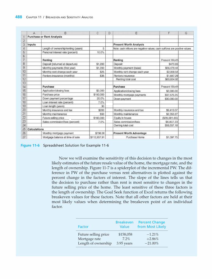
488 CHAPTER 11 / BREAKEVEN AND SENSITIVITY ANALYSIS

Figure 11-6 Spreadsheet Solution for Example 11-6

Now we will examine the sensitivity of this decision to changes in the mostlikely estimates of the future resale value of the home, the mortgage rate, and thelength of ownership. Figure 11-7 is a spiderplot of the incremental PW. The dif-ference in PW of the purchase versus rent alternatives is plotted against thepercent change in the factors of interest. The slope of the lines tells us thatthe decision to purchase rather than rent is most sensitive to changes in thefuture selling price of the home. The least sensitive of these three factors isthe length of ownership. The Goal Seek function of Excel returns the followingbreakeven values for these factors. Note that all other factors are held at theirmost likely values when determining the breakeven point of an individualfactor.

Breakeven Percent ChangeFactor Value from Most Likely

Future selling price $158,058 −1.21%Mortgage rate 7.2% +2.86%Length of ownership 3.95 years −21.00%

SECTION 11.4 / MULTIPLE FACTOR SENSITIVITY ANALYSIS 489

–$30,000

–$26,034 –$16,990 –$7,946 $1,098 $10,142 $19,186 $29,229

$10,474 $7,380 $4,253 $1,098 –$2,083 –$5,286 –$8,507

–$451 $50 $567 $1,098 $1,639 $2,190 $2,746

–$20,000

–$10,000

$0

$10,000

$20,000

$30,000

$40,000

–30% –20% –10% 0% 10% 20% 30%

Percent Change from Most Likely Value

PW

(pur

chas

e)–P

W(r

ent)

Future selling price

Mortgage rateLength of ownership

Figure 11-7 Sensitivity Graph for Example 11-6

In reality, there are more factors to consider in the decision to rent or purchasea home. Many other mortgage options exist, such as different repayment periods(15 or 20 years) and the option of paying points to reduce the interest rate. Also,interest paid on home loans is tax deductible. These factors are considered inProblem 11-23. The following Web sites offer more comprehensive calculatorsfor the rent versus purchase decision.

http://www.calculators.interest.com/index.asphttp://www.mortgage-net.com/calculatorshttp://www.ginniemae.gov

11.4 Multiple Factor Sensitivity AnalysisIn the previous section, we looked at the impact of changing a single factor estimateon the equivalent worth of a project (all other values were held constant). Weare often concerned about the combined effects of changes in two or more projectfactors. In this situation, the following approach can be used to develop additionalinformation.

1. Develop a sensitivity graph (spiderplot) for the project as discussed inSection 11.3. For the most sensitive factors, try to develop improved estimatesand reduce the range of variability before proceeding further with the analysis.

2. Select the most sensitive project factors based on the information in thesensitivity graph. Analyze the combined effects of these factors on the project’seconomic measure of merit by determining the impact of selected combinationsof three or more factors. (These combinations are sometimes called scenarios.)

490 CHAPTER 11 / BREAKEVEN AND SENSITIVITY ANALYSIS

The combined impact of changes in the best estimate values for three ormore factors on the economic measure of merit for an engineering project canbe analyzed by using selected combinations of the changes. This approach and theOptimistic-Most Likely-Pessimistic (O-ML-P) technique of estimating factor valuesare illustrated in Example 11-7.

An optimistic estimate for a factor is one that is in the favorable direction (say,the minimum capital investment cost). The most likely value for a factor is definedfor our purposes as the best estimate value. The pessimistic estimate for a factoris one that is in the unfavorable direction (say, the maximum capital investmentcost). In applications of this technique, the optimistic condition for a factor is oftenspecified as a value that has 19 out of 20 chances of being better than the actualoutcome. Similarly, the pessimistic condition has 19 out of 20 chances of beingworse than the actual outcome. In operational terms, the optimistic condition fora factor is the value when things occur as well as can be reasonably expected, andthe pessimistic estimate is the value when things occur as detrimentally as can bereasonably expected.

EXAMPLE 11-7 Optimistic-Most Likely-Pessimistic (O-ML-P) Scenarios

Consider a proposed ultrasound inspection device for which the optimistic,and most likely, pessimistic estimates are given in Table 11-1. The MARR is8% per year. Also shown at the end of Table 11-1 are the AWs for all threeestimation conditions. Based on this information, analyze the combined effectsof uncertainty in the factors on the AW value.

SolutionStep 1: Before proceeding further with the solution, we need to evaluate thetwo extreme values of the AW. As shown at the end of Table 11-1, the AW forthe optimistic estimates is very favorable ($73,995), whereas the AW for thepessimistic estimates is quite unfavorable (−$33,100). If both extreme AW valueswere positive, we would make a go decision with respect to the device withoutfurther analysis, because no combination of factor values based on the estimateswill result in AW less than zero. By similar reasoning, if all AW values werenegative, a no-go decision would be made regarding the device. In this example,

TABLE 11-1 Optimistic, Most Likely, and Pessimistic Estimates andAWs for Proposed Ultrasound Device (Example 11-7)

Estimation Condition

Optimistic (O) Most Likely (ML) Pessimistic (P)

Capital investment, I $150,000 $150,000 $150,000Useful life, N 18 years 10 years 8 yearsMarket value, MV 0 0 0Annual revenues, R $110,000 $70,000 $50,000Annual expenses, E 20,000 43,000 57,000

AW (8%): +$73,995 +$4,650 −$33,100

SECTION 11.4 / MULTIPLE FACTOR SENSITIVITY ANALYSIS 491

however, the decision is sensitive to other combinations of outcomes, and weproceed to Steps 2 and 3.

Step 2: A sensitivity graph (spiderplot) for this situation is needed to showexplicitly the sensitivity of the AW to the three factors of concern: useful life,N; annual revenues, R; and annual expenses, E. The spiderplot is shown inFigure 11-8. The curves for N, R, and E plot percent deviation changes from themost likely (best) estimate, over the range of values defined by the optimisticand pessimistic estimates for each factor, versus AW. As additional information,a curve is also shown for MARR versus AW. Based on the spiderplot, AW forthe proposed ultrasound device appears very sensitive to annual revenues andquite sensitive to annual expenses and reductions in useful life. Even if we wereto significantly change the MARR (8%), however, it would have little impacton the AW.

Step 3: The various combinations of the optimistic, most likely, andpessimistic factor values (outcomes) for annual revenues, useful life, and annualexpenses need to be analyzed for their combined impacts on the AW. The resultsfor these 27 (3 × 3 × 3) combinations are shown in Table 11-2.

Making the AW Results Easier to InterpretSince the AW values in Table 11-2 result from estimates subject to differingdegrees of variation, little information of value would be lost if the numbers wererounded to the nearest thousand dollars. Further, suppose that management ismost interested in the number of combinations of outcomes in which AW is,

Figure 11-8Sensitivity Graphfor ProposedUltrasoundDevice(Example 11-7)

�70

�60

�50

�40

�30

�20

�10

10

0

20

30

40

50

�100 �80 �60 �40 �20 0 20 40 60 80 100

Percent Deviation Changes from Most Likely Estimate

Ann

ual W

orth

(T

hous

ands

of D

olla

rs)

Annual Expenses, E

Minimum AttractiveRate of Return, MARR(nonlinear)

Useful Life, N(nonlinear)

Annual Revenues, R

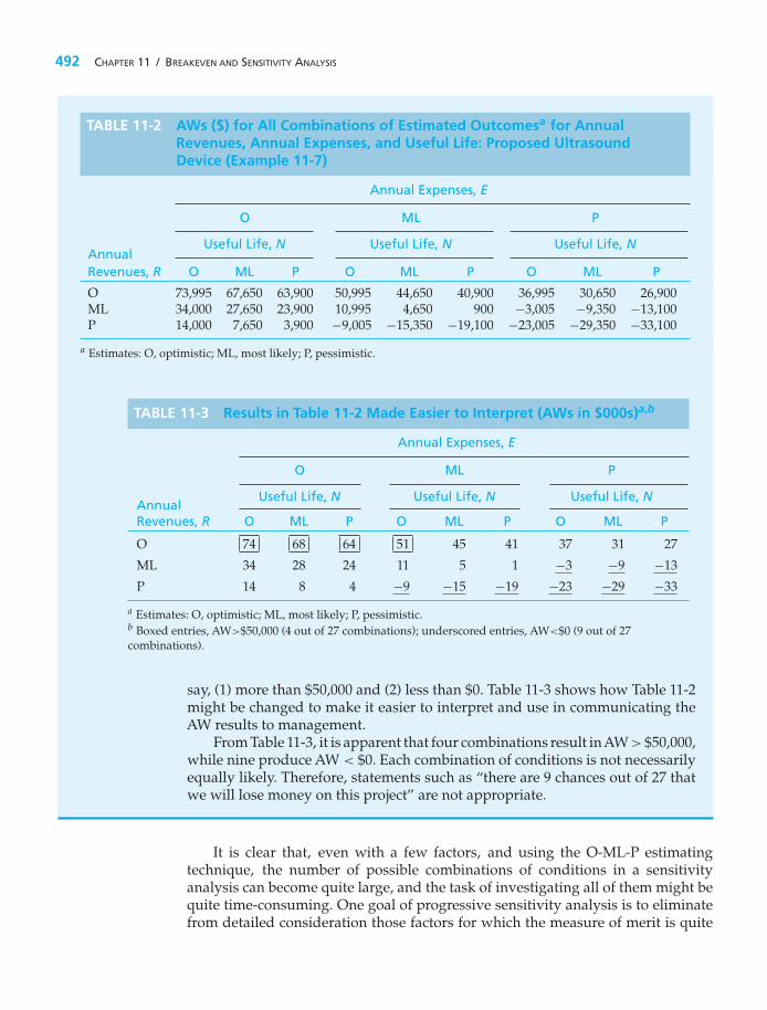
492 CHAPTER 11 / BREAKEVEN AND SENSITIVITY ANALYSIS

TABLE 11-2 AWs ($) for All Combinations of Estimated Outcomesa for AnnualRevenues, Annual Expenses, and Useful Life: Proposed UltrasoundDevice (Example 11-7)

Annual Expenses, E

O ML P

Useful Life, N Useful Life, N Useful Life, NAnnualRevenues, R O ML P O ML P O ML P

O 73,995 67,650 63,900 50,995 44,650 40,900 36,995 30,650 26,900ML 34,000 27,650 23,900 10,995 4,650 900 −3,005 −9,350 −13,100P 14,000 7,650 3,900 −9,005 −15,350 −19,100 −23,005 −29,350 −33,100

a Estimates: O, optimistic; ML, most likely; P, pessimistic.

TABLE 11-3 Results in Table 11-2 Made Easier to Interpret (AWs in $000s)a,b

Annual Expenses, E

O ML P

Useful Life, N Useful Life, N Useful Life, NAnnualRevenues, R O ML P O ML P O ML P

O 74 68 64 51 45 41 37 31 27

ML 34 28 24 11 5 1 −3 −9 −13

P 14 8 4 −9 −15 −19 −23 −29 −33

a Estimates: O, optimistic; ML, most likely; P, pessimistic.b Boxed entries, AW>$50,000 (4 out of 27 combinations); underscored entries, AW<$0 (9 out of 27combinations).

say, (1) more than $50,000 and (2) less than $0. Table 11-3 shows how Table 11-2might be changed to make it easier to interpret and use in communicating theAW results to management.

From Table 11-3, it is apparent that four combinations result inAW > $50,000,while nine produce AW < $0. Each combination of conditions is not necessarilyequally likely. Therefore, statements such as “there are 9 chances out of 27 thatwe will lose money on this project” are not appropriate.

It is clear that, even with a few factors, and using the O-ML-P estimatingtechnique, the number of possible combinations of conditions in a sensitivityanalysis can become quite large, and the task of investigating all of them might bequite time-consuming. One goal of progressive sensitivity analysis is to eliminatefrom detailed consideration those factors for which the measure of merit is quite

PROBLEMS 493

insensitive, highlighting the conditions for other factors to be studied further inaccordance with the degree of sensitivity of each. Thus, the number of combinationsof conditions included in the analysis can perhaps be kept to a manageable size.

11.5 SummaryEngineering economy involves decision making among competing uses of scarcecapital resources. The consequences of these decisions usually extend far into thefuture. In this chapter, we have used techniques to deal with the realization that theconsequences or outcomes (cash flows, useful lives, etc.) of engineering projectscan never be known with absolute certainty.

Several of the most commonly applied and useful procedures for dealing withthe variability of estimates in engineering economy studies have been presented inthis chapter. Breakeven analysis determines the value of a key common factor, suchas utilization of capacity, at which the economic desirability of two alternatives isequal or a project is economically justified. This breakeven point is then comparedto an independent estimate of the factor’s most likely (best estimate) value to assistwith the selection between alternatives or to make a decision about a project. Thesensitivity graph technique makes explicit the impact of variations in the estimatesof each project factor of concern on the economic measure of merit, and it is avaluable analysis tool. The technique discussed in Section 11.4 for evaluating thecombined impact of changes in two or more factors is important when additionalinformation is needed to assist decision making.

Regrettably, there is no quick and easy answer to the question, How shouldvariability best be considered in an engineering economic analysis? Generally,simple procedures (e.g., sensitivity analysis) allow reasonable discriminationamong alternatives to be made or the acceptability of a project to be determined onthe basis of the variations present, and they are relatively inexpensive to apply. SoYogi Berra is right—prediction is usually difficult, especially about the future!

ProblemsThe number in parentheses that follows each problemrefers to the section from which the problem is taken.

11-1. The Metropolitan Transit Authority (MTA) hasjust opened a new subway line (the Orange Line) inits underground transportation network. The OrangeLine had a capital investment of $20 million, expectedoperating and maintenance expenses are $3 millionper year, and the final salvage value at the end ofa 40-year life is negligible. If the revenue generatedby each customer is $3, how many customers perday will be required before the Orange Line canbreak even? The MTA’s hurdle (interest) rate is 5%

compounded annually. Assume there are 365 days ina year. (11.2)

11-2. Refer to Example 11-2. Assuming gasolinecosts $4.00 per gallon, find the breakeven mileage

per year between the hybrid vehicle and the gas-onlyvehicle. All other factors remain the same.

11-3. The Universal Postal Service is consider-ing the possibility of fixing wind deflectors on

the tops of 500 of their long-haul tractors. Three types ofdeflectors, with the following characteristics, are beingconsidered (MARR = 10% per year):

494 CHAPTER 11 / BREAKEVEN AND SENSITIVITY ANALYSIS

Windshear Blowby Air-vantage

Capital investment $1,000 $400 $1,200Drag reduction 20% 10% 25%Maintenance per $10 $5 $5year

Useful life 10 years 10 years 5 years

If 5% in drag reduction means 2% in fuel savings permile, how many miles do the tractors have to be drivenper year before the windshear deflector is favored overthe other deflectors? Over what range of miles drivenper year is air-vantage the best choice? (Note: Fuelcost is expected to be $4.00 per gallon, and averagefuel consumption is 5 miles per gallon without thedeflectors.) State any assumptions you make. (11.2)

11-4. In planning a small two-story office building, thearchitect has submitted two designs. The first providesfoundation and structural details so that two additionalstories can be added to the required initial two storiesat a later date and without modifications to the originalstructure. This building would cost $1,400,000. Thesecond design, without such provisions, would costonly $1,250,000. If the first plan is adopted, an additionaltwo stories could be added at a later date at a costof $850,000. If the second plan is adopted, however,considerable strengthening and reconstruction wouldbe required, which would add $300,000 to the cost ofa two-story addition. Assuming that the building isexpected to be needed for 75 years, by what time wouldthe additional two stories have to be built to make theadoption of the first design justified? MARR is 10% peryear. (11.2)

11-5. Consider these two alternatives. (11.2)

Alternative 1 Alternative 2

Capital investment $4,500 $6,000Annual revenues $1,600 $1,850Annual expenses $400 $500Estimated market $800 $1,200value

Useful life 8 years 10 years

a. Suppose that the capital investment of Alternative1 is known with certainty. By how much would theestimate of capital investment for Alternative 2 haveto vary so that the initial decision based on these datawould be reversed? The annual MARR is 15% peryear.

b. Determine the life of Alternative 1 for which theAWs are equal.

11-6. An area can be irrigated by pumping waterfrom a nearby river. Two competing installations

are being considered.

Pump A Pump B6 in. System 8 in. System

Operating load on motor 15 hp 10 hpEfficiency of pump motor 0.60 0.75Cost of installation $2,410 $4,820Market value $80 $0Useful life 8 years 8 years

The MARR is 12% per year and electric power for thepumps costs $0.06 per kWh. Recall that 1 horsepower(hp) equals 0.746 kilowatts. (11.2, 11.3)

a. At what level of operation (hours per year) wouldyou be indifferent between the two pumpingsystems? If the pumping system is expected tooperate 2,000 hours per year, which system shouldbe recommended?

b. Perform a sensitivity analysis on the efficiency ofPump A. Over what range of pumping efficiency isPump A preferred to Pump B? Assume 2,000 hoursof operation per year, and draw a graph to illustrateyour answer.

11-7. Consider the following two investment alter-natives. Determine the range of investment costs forAlternative B (i.e., min. value < X < max. value)that will convince an investor to select Alternative B.MARR = 10% per year, and other relevant dataare shown in the following table. State clearly anyassumptions that are necessary to support your answer.(11.2)

Alt. A Alt. B

Capital investment $5,000 $ XNet annual receipts $1,500 $1,400Market value $1,900 $4,000Useful life 5 years 7 years

11-8. The Ford Motor Company is considering threemutually exclusive electronic stability control systemsfor protection against rollover of its automobiles. The

PROBLEMS 495

investment (study) period is four years, and MARR is12% per year. Data for the fixture costs of the systemsare as follows.

Alternatives

A B C

Capital investment $12,000 $15,800 $8,000Annual savings $4,000 $5,200 $3,000MV (after 4 years) $3,000 $3,500 $1,500IRR 19.2% 18% 23%

Plot the AW of each alternative against MARR as theMARR varies across this range: 4%, 8%, 12%, 16%, and20%. What can you generalize about the range of theMARR for which each alternative is preferred? (11.2)

11-9. Your company operates a fleet of light trucks thatare used to provide contract delivery services. As theengineering and technical manager, you are analyzingthe purchase of 55 new trucks as an addition to the fleet.These trucks would be used for a new contract the salesstaff is trying to obtain. If purchased, the trucks wouldcost $21,200 each; estimated use is 20,000 miles per yearper truck; estimated operation and maintenance andother related expenses (year-zero dollars) are $0.45 permile, which is forecasted to increase at the rate of 5%per year; and the trucks are MACRS (GDS) three-yearproperty class assets. The analysis period is four years;t = 38%; MARR = 15% per year (after taxes; includesan inflation component); and the estimated MV at theend of four years (in year-zero dollars) is 35% of thepurchase price of the vehicles. This estimate is expectedto increase at the rate of 2% per year.

Based on an after-tax, actual-dollar analysis, what isthe annual revenue required by your company from thecontract to justify these expenditures before any profit isconsidered? This calculated amount for annual revenueis the breakeven point between purchasing the trucksand which other alternative? (11.2, Chapters 7 and 8)

11-10. Anationwide motel chain is considering locatinga new motel in Bigtown, USA. The cost of building a150-room motel (excluding furnishings) is $5 million.The firm uses a 15-year planning horizon to evaluateinvestments of this type. The furnishings for this motelmust be replaced every five years at an estimated cost of$1,875,000 (at k = 0, 5, and 10). The old furnishings haveno market value. Annual operating and maintenanceexpenses for the facility are estimated to be $125,000.

The market value of the motel after 15 years is estimatedto be 20% of the original building cost.

Rooms at the motel are projected to be rented at anaverage rate of $45 per night. On the average, the motelwill rent 60% of its rooms each night. Assume the motelwill be open 365 days per year. MARR is 10% per year.(11.3)

a. Using an annual-worth measure of merit, is theproject economically attractive?

b. Investigate sensitivity to decision reversal forthe following three factors: (1) capital investment,(2) MARR, and (3) occupancy rate (average percentof rooms rented per night). To which of these factorsis the decision most sensitive?

c. Graphically investigate the sensitivity of the AWto changes in the above three factors. Investigatechanges over the interval ±40%. On your graph, usepercent change as the x-axis and AW as the y-axis.

11-11. A large city in the mid-West needs to acquire astreet-cleaning machine to keep its roads looking niceyear round. A used cleaning vehicle will cost $85,000and have a $20,000 market (salvage) value at the end ofits five-year life. A new system with advanced featureswill cost $150,000 and have a $40,000 market valueat the end of its five-year life. The new system isexpected to reduce labor hours compared with the usedsystem. Current street-cleaning activity requires theused system to operate 8 hours per day for 20 daysper month. Labor costs $50 per hour (including fringebenefits), and MARR is 12% per year. (11.2)

a. Find the breakeven percent reduction in labor hoursfor the new system.

b. If the new system is expected to be able to reducelabor hours by 17% compared with the used system,which machine should the city purchase?

11-12. Refer to Problem 11-11. The best estimate forthe reduction of labor hours for the new system is17% (compared with the used system). Investigate howsensitive the decision is to (a) changes in the MARR,(b) changes in the market value of the new system, and(c) the productivity improvement of the new system.Graph your results. Hint: Think incrementally! (11.3)

11-13. A group of private investors borrowed $30million to build 300 new luxury apartments near a largeuniversity. The money was borrowed at 6% annualinterest, and the loan is to be repaid in equal annualamounts over a 40-year period. Annual operating,maintenance, and insurance expenses are estimated to

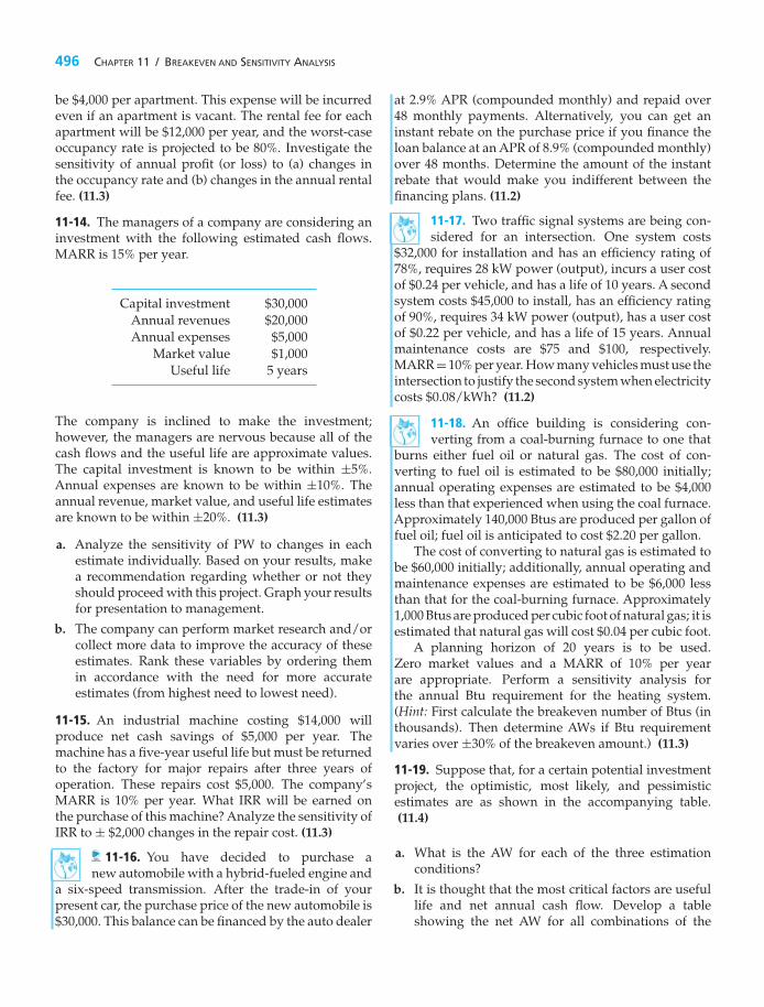
496 CHAPTER 11 / BREAKEVEN AND SENSITIVITY ANALYSIS

be $4,000 per apartment. This expense will be incurredeven if an apartment is vacant. The rental fee for eachapartment will be $12,000 per year, and the worst-caseoccupancy rate is projected to be 80%. Investigate thesensitivity of annual profit (or loss) to (a) changes inthe occupancy rate and (b) changes in the annual rentalfee. (11.3)

11-14. The managers of a company are considering aninvestment with the following estimated cash flows.MARR is 15% per year.

Capital investment $30,000Annual revenues $20,000Annual expenses $5,000

Market value $1,000Useful life 5 years

The company is inclined to make the investment;however, the managers are nervous because all of thecash flows and the useful life are approximate values.The capital investment is known to be within ±5%.Annual expenses are known to be within ±10%. Theannual revenue, market value, and useful life estimatesare known to be within ±20%. (11.3)

a. Analyze the sensitivity of PW to changes in eachestimate individually. Based on your results, makea recommendation regarding whether or not theyshould proceed with this project. Graph your resultsfor presentation to management.

b. The company can perform market research and/orcollect more data to improve the accuracy of theseestimates. Rank these variables by ordering themin accordance with the need for more accurateestimates (from highest need to lowest need).

11-15. An industrial machine costing $14,000 willproduce net cash savings of $5,000 per year. Themachine has a five-year useful life but must be returnedto the factory for major repairs after three years ofoperation. These repairs cost $5,000. The company’sMARR is 10% per year. What IRR will be earned onthe purchase of this machine? Analyze the sensitivity ofIRR to ± $2,000 changes in the repair cost. (11.3)

11-16. You have decided to purchase anew automobile with a hybrid-fueled engine and

a six-speed transmission. After the trade-in of yourpresent car, the purchase price of the new automobile is$30,000. This balance can be financed by the auto dealer

at 2.9% APR (compounded monthly) and repaid over48 monthly payments. Alternatively, you can get aninstant rebate on the purchase price if you finance theloan balance at an APR of 8.9% (compounded monthly)over 48 months. Determine the amount of the instantrebate that would make you indifferent between thefinancing plans. (11.2)

11-17. Two traffic signal systems are being con-sidered for an intersection. One system costs

$32,000 for installation and has an efficiency rating of78%, requires 28 kW power (output), incurs a user costof $0.24 per vehicle, and has a life of 10 years. A secondsystem costs $45,000 to install, has an efficiency ratingof 90%, requires 34 kW power (output), has a user costof $0.22 per vehicle, and has a life of 15 years. Annualmaintenance costs are $75 and $100, respectively.MARR = 10% per year. How many vehicles must use theintersection to justify the second system when electricitycosts $0.08/kWh? (11.2)

11-18. An office building is considering con-verting from a coal-burning furnace to one that

burns either fuel oil or natural gas. The cost of con-verting to fuel oil is estimated to be $80,000 initially;annual operating expenses are estimated to be $4,000less than that experienced when using the coal furnace.Approximately 140,000 Btus are produced per gallon offuel oil; fuel oil is anticipated to cost $2.20 per gallon.

The cost of converting to natural gas is estimated tobe $60,000 initially; additionally, annual operating andmaintenance expenses are estimated to be $6,000 lessthan that for the coal-burning furnace. Approximately1,000 Btus are produced per cubic foot of natural gas; it isestimated that natural gas will cost $0.04 per cubic foot.

A planning horizon of 20 years is to be used.Zero market values and a MARR of 10% per yearare appropriate. Perform a sensitivity analysis forthe annual Btu requirement for the heating system.(Hint: First calculate the breakeven number of Btus (inthousands). Then determine AWs if Btu requirementvaries over ±30% of the breakeven amount.) (11.3)

11-19. Suppose that, for a certain potential investmentproject, the optimistic, most likely, and pessimisticestimates are as shown in the accompanying table.(11.4)

a. What is the AW for each of the three estimationconditions?

b. It is thought that the most critical factors are usefullife and net annual cash flow. Develop a tableshowing the net AW for all combinations of the

PROBLEMS 497

MostOptimistic Likely Pessimistic

Capital $90,000 $100,000 $120,000investment

Useful life 12 years 10 years 6 yearsMarket value $30,000 $20,000 $0Net annual $35,000 $30,000 $20,000cash flow

MARR 10% 10% 10%(per year)

estimates for these two factors, assuming all otherfactors to be at their most likely values.

11-20. Abridge is to be constructed now as part of a newroad. Engineers have determined that traffic density onthe new road will justify a two-lane road and a bridgeat the present time. Because of uncertainty regardingfuture use of the road, the time at which an extra twolanes will be required is currently being studied.

The two-lane bridge will cost $200,000 and the four-lane bridge, if built initially, will cost $350,000. Thefuture cost of widening a two-lane bridge to four laneswill be an extra $200,000 plus $25,000 for every year thatwidening is delayed. The MARR used by the highwaydepartment is 12% per year. The following estimateshave been made of the times at which the four-lanebridge will be required:

Pessimistic estimate 4 yearsMost likely estimate 5 yearsOptimistic estimate 7 years

In view of these estimates, what would you recom-mend? What difficulty, if any, do you have ininterpreting your results? List some advantagesand disadvantages of this method of preparingestimates. (11.4)

11-21. An aerodynamic three-wheeled auto-mobile (the Dart) runs on compressed natural

gas stored in two cylinders in the rear of the vehicle.The $13,000 Dart can cruise at speeds up to 80 milesper hour, and it can travel 100 miles per gallon offuel. Another two-seater automobile costs $10,000 and

averages 50 miles per gallon of compressed natural gas.If fuel costs $8.00 per gallon and MARR is 10% per year,over what range of annual miles driven is the Dart moreeconomical? Assume a useful life of five years for bothcars. (11.2)

11-22. Extended Learning ExerciseConsider these two alternatives for solid-waste

removal (11.3, Chapter 7):

Alternative A: Build a solid-waste processing facility.Financial variables are as follows:

Capital investment $108 million in 2008(commercial operationstarts in 2008)

Expected life of facility 20 yearsAnnual operating $3.46 million

expensesEstimated market value 40% of initial capital cost

at all times

Alternative B: Contract with vendors for solid-wastedisposal after intermediate recovery. Financial variablesare as follows:

Capital investment $17 million in 2008 (This isfor intermediate recoveryfrom the solid-wastestream.)

Expected contract 20 yearsperiod

Annual operating $2.10 millionexpenses

Repair costs to $3.0 millionintermediaterecovery systemevery five years

Annual fee to vendors $10.3 millionEstimated market value $0at all times

Related Data:

MACRS (GDS) property class 15 yr (Chapter 7)Study period 20 yrEffective income tax rate 40%Company MARR (after-tax) 10% per yearInflation rate 0% (ignore inflation)

498 CHAPTER 11 / BREAKEVEN AND SENSITIVITY ANALYSIS

a. How much more expensive (in terms of capitalinvestment only) could Alternative B be in order tobreakeven with Alternative A?

b. How sensitive is the after-tax PW of Alternative Bto cotermination of both alternatives at the end ofyear 10?

c. Is the initial decision to adopt Alternative B inPart (a) reversed if our company’s annual operatingexpenses for Alternative B ($2.10 million per year)unexpectedly double? Explain why (or why not).

d. Use a computer spreadsheet available to you to solvethis problem.

11-23. Extended Learning Exercise Construct thespreadsheet used in Example 11-6. Use this spreadsheetas a starting point to answer the following questions.Be sure to clearly state your assumptions. (11.3)

a. How sensitive is the decision to the amount of thedown payment for the purchase option? If a downpayment of less than 20% is used, you will needto account for monthly mortgage insurance (about$56/month).

b. How sensitive is the decision to the type of mortgageacquired? You can look at different repaymentperiods (15 or 20 years) as well as the impact ofpoints paid on the loan. One point is equal to 1%of the loan value and is paid as part of the closingcosts.

c. Interest paid on a mortgage is tax deductible if youitemize deductions on your personal income taxreturn. Discuss how you would incorporate thisand what impact it would have on the decision topurchase versus rent a home.

Spreadsheet Exercises

11-24. We know the standard means of cuttingthe high cost of driving our automobiles—slow

down your speed, no jack rabbit starts, inflate tiresproperly, clean air filters regularly, and so on. Anotherway to reduce the cost of driving is to join everybig-rigger in the United States and half of Europe—go diesel. Diesels are inherently more efficient thangasoline engines because they deliver a third better fuelmileage. They also offer a reliable high-torque engine!

The initial extra sticker price of a diesel-fueled car isabout $1,200. Agallon of diesel fuel costs about the sameas a gallon of gasoline. Assume your gasoline-fueled caraverages 24–27 miles per gallon. You drive an averageof 20,000 miles per year, and your personal MARR is inthe 12–15% per year ballpark. Develop a spreadsheetto compare the economics of driving 100,000 milesin your car fueled by gasoline versus diesel. Explorevarious what if questions that you have regarding thiscomparison. (11.3)

11-25. It is desired to determine the most eco-nomical thickness of insulation for a large cold-

storage room. Insulation is expected to cost $150 per1,000 square feet of wall area per inch of thicknessinstalled, and to require annual property taxes andinsurance of 5% of the capital investment. It is expectedto have $0 market value after a 20-year life. The

following are estimates of the heat loss per 1,000 squarefeet of wall area for several thicknesses:

Insulation, in. Heat loss, Btu per hr

3 4,4004 3,4005 2,8006 2,4007 2,0008 1,800

The cost of heat removal (loss) is estimated at $0.04per 1,000 Btu. The MARR is 20% per year. Assumingcontinuous operation throughout the year, develop aspreadsheet to analyze the sensitivity of the optimalthickness to errors in estimating the cost of heat removal.Use the AW technique. (11.3)

11-26. Suppose that, for an engineering project, theoptimistic, most likely, and pessimistic estimates are asshown in the accompanying table.

Develop a spreadsheet to determine the AW for eachof the three estimate conditions. It is thought that the

FE PRACTICE PROBLEMS 499

Optimistic Most Likely Pessimistic

Capital $90,000 $100,000 $120,000investment

Useful life 12 years 10 years 6 yearsMarket value $30,000 $20,000 $0Net annual $35,000 $30,000 $20,000cash flow

MARR (per 11% 11% 11%year)

most critical elements are useful life and net annual cashflow. Include in your spreadsheet a table showing theAW for all combinations of the estimates for these twofactors, assuming that all other factors remain at theirmost likely values. (11.4)

11-27. The world’s largest carpet maker hasjust completed a feasibility study of what to do

with the 16,000 tons of overruns, rejects, and remnantsit produces every year. The company’s CEO launchedthe feasibility study by asking, Why pay someone todig coal out of the ground and then pay someone elseto put our waste into a landfill? Why not just burnour own waste? The company is proposing to builda $10-million power plant to burn its waste as fuel,thereby saving $2.8 million a year in coal purchases.Company engineers have determined that the waste-burning plant will be environmentally sound, and afterits four-year study period the plant can be sold to a localelectric utility for $5 million.

The firm’s MARR is 15%. Develop a spreadsheetto investigate the sensitivity of the proposal’s PWto changes in the estimates of (a) initial investment

amount, (b) annual savings of fuel cost, and (c)future resale value of the plant. To which factor isthe decision most sensitive? Include in your solutionthe specific values of these factors that would causedecision reversal. Use the charting feature to create aspiderplot. (11.3)

11-28. Refer to Problem 6-8. Disposing of incan-descent light bulbs is just like getting rid of and

recycling glassware in general. However, this is not thecase for CFLs. Disposing of CFLs is complicated by thefact that each lamp contains a small amount of mercury,which is a very environmentally dangerous substance.Write a brief report of your findings for your boss foreach of the following scenarios (11.3):

a. Develop an Excel spreadsheet to investigate thesensitivity of choice of lighting systems when theCFL disposal cost varies from $1.00 to $5.00 perlamp.

b. Use your spreadsheet to explore the sensitivity ofbulb or lamp choice as the cost of electricity variesfrom $0.04 per kWh to $0.16 per kWh.

c. Use your spreadsheet to quantify the sensitivity ofbulb or lamp choice when CFLs last 5, 6, 7, 8, 9, and10 times as long as incandescent bulbs.

11-29. Refer to Problem 6-24. Set up a spread-sheet to answer various “what if” questions such

as “How does the IRR vary as the cost of gasoline takeson these values: $3.00 per gallon, $4.00 per gallon, and$5.00 per gallon?” Also, how does IRR change when theownership period changes across this range: 3 years, 4years, 5 years, 6 years, and 7 years? How does the IRRvary when the differential resale value is $1,000, $2,000,$3,000, and $4,000? (11.3)

FE Practice Problems

11-30. A highway bridge is being considered forreplacement. The new bridge would cost $X and wouldlast for 20 years. Annual maintenance costs for thenew bridge are estimated to be $24,000. People will becharged a toll of $0.25 per car to use the new bridge.Annual car traffic is estimated at 400,000 cars. Thecost of collecting the toll consists of annual salariesfor five collectors at $10,000 per collector. The existingbridge can be refurbished for $1,600,000 and would

need to be replaced in 20 years. There would beadditional refurbishing costs of $70,000 every five yearsand regular annual maintenance costs of $20,000 forthe existing bridge. There would be no toll to use therefurbished bridge. If MARR is 12% per year, what is themaximum acceptable cost (X) of the new bridge? (11.2)

(a) $1,943,594 (b) $2,018,641 (c) $1,652,425(d) $1,570,122 (e) $2,156,209

500 CHAPTER 11 / BREAKEVEN AND SENSITIVITY ANALYSIS

11-31. An analysis of accidents in a rural state indicatesthat widening a highway from 30 ft to 40 ft will decreasethe annual accident rate from 1,250 to 710 per millionvehicle-miles. Calculate the average daily number ofvehicles that should use the highway to justify wideningon the basis of the following estimates: (i) the averageloss per accident is $1,200; (ii) the cost of widening is$117,000 per mile; (iii) the useful life of the widenedroad is 25 years; (iv) annual maintenance costs are 3%of the capital investment; and (v) MARR is 12% peryear. (11.2)

(a) 78 (b) 63 (c) 34 (d) 59 (e) 27

A supermarket chain buys loaves of bread from itssupplier at $0.50 per loaf. The chain is considering twooptions to bake its own bread.

Machine A Machine B

Capital investment $8,000 $16,000Useful life (years) 7 7Annual fixed cost $2,000 $4,000Variable cost per loaf $0.26 $0.16

Graph for Problems 11-35 to 11-39

0%–10%–20%–30%–40%

$0

10% 20% 30% 40%

($2,000)

($1,000)

$1,000

$2,000

$3,000

X-Axis (Percent Change in Parameter)

Y-A

xis,

PW

(12%

)

InitialInvestment

Useful Life(R – E)

Neither machine has a market value at the end of sevenyears, and MARR is 12% per year. Use this informationto answer Problems 11-32, 11-33, and 11-34. Select theclosest answer. (11.2)

11-32. What is the minimum number of loaves thatmust be sold per year to justify installing Machine Ainstead of buying the loaves from the supplier?

(a) 7,506 (b) 22,076 (c) 37,529 (d) 75,059(e) 15,637

11-33. What is the minimum number of loaves thatmust be sold per year to justify installing Machine Binstead of buying the loaves from the supplier?

(a) 37,529 (b) 15,637 (c) 22,076 (d) 75,059(e) 7,506

11-34. If the demand for bread at this supermarket is35,000 loaves per year, what strategy should be adoptedfor acquiring bread? Both Machine A and Machine B arecapable of meeting annual demand.

(a) Continue buying from the supplier.

(b) Install Machine A.

(c) Install Machine B.

(d) Install both Machine A and Machine B.

FE PRACTICE PROBLEMS 501

Answer Problems 11-35 through 11-39 on the basis ofthe graph on page 500 and the most likely estimatesgiven as follows:

MARR 12% per yearUseful life 5 yearsInitial investment $5,000Receipts–Expenses (R − E) $1,500/year

11-35. If the initial investment is increased by morethan 9%, the project is profitable.(a) True (b) False

11-36. If the profit (R − E) is decreased by 5%, thisproject is not profitable.(a) True (b) False

11-37. Variations in the profit and useful life of theproject are inversely related.(a) True (b) False

11-38. This project (based upon the most likelyestimates) is profitable.(a) True (b) False

11-39. An initial investment of $5,500 is profitable.

(a) True (b) False

11-40. Two electric motors are being economi-cally evaluated for use in a submersible robotic

device. Each is capable of delivering 90 horsepower toa necessary application that the device performs. Datafor the mutually exclusive motors are as follows.

Motor

General Electric Phillips

Initial investment $2,500 $3,200Electrical efficiency 0.74 0.89Annual maintenance $400 $600Useful life (years) 10 10

The MARR is 12% per year. If the expected usage ofthe motor is 500 hours per year, what would the costof electric power have to be before the Phillips motoris favored over the General Electric motor? Recall that1 horsepower = 0.746 kilowatts. Choose the closestanswer from those below. (11.3)

(a) $0.02 per kWh (b) $0.19 per kWh(c) $0.09 per kWh (d) $0.05 per kWh

11-41. A carpet manufacturer in Georgia plans toexpand its plant for a capital investment of $500,000.The extra capacity will permit the company to produce400,000 yards of carpet each year during the plant’s five-year life. Each yard of carpet will produce a revenue of$2.00, and the plant’s incremental operating expensesare expected to be $150,000 each year. Assume theexpansion has no salvage value at the end of year five.If the manufacturer’s MARR is 18% per year, whatis the minimum annual production rate to make theexpansion a worthwhile investment?

(a) 103,400 yards (b) 310,000 yards(c) 154,950 yards (d) 250,350 yards

11-42. A centrifuge is required in a chemical separationprocess. Two centrifuges (A and B) are availableand summarized below. The net annual revenues forcentrifuge B are not known. If the MARR is 10% peryear and salvage values can be ignored, what is theminimum value of X to make centrifuge B the betterchoice? Select the closest answer below.

Year Centrifuge A Centrifuge B

0 −$30,000 −$25,0001–5 $8,000 $X

(a) $500 (b) $6,700(c) $8,000 (d) $9,800

CHAPTER 12

Probabilistic Risk Analysis

The aim of Chapter 12 is to discuss and illustrate several probabilisticmethods that are useful in analyzing risk and uncertainty associatedwith engineering economy studies.

The Risks of Global Warming∗

R isk is a condition where there is a possibility of adversedeviation from a desired and expected outcome. The risksof global climate change caused by carbon dioxide and other

greenhouse gases include heightened regulation, revenue loss, and increasedphysical property impairment. Opportunities for mitigating the risks associatedwith climate change are numerous: increased efficiency of energy production anduse, improved agricultural practices, and carbon capture and sequestration arejust a few of the choices we have. In this chapter, you will learn how variousprobabilistic techniques can be used to assess the risks of engineering projectssuch as those that mitigate the effects of global warming.

502

Higher risk is what we pay for higher return.

—Anonymous

12.1 IntroductionIn previous chapters, we stated specific assumptions concerning applicable reven-ues, costs, and other quantities important to an engineering economy analysis. Itwas assumed that a high degree of confidence could be placed in all estimatedvalues. That degree of confidence is sometimes called assumed certainty. Decisionsmade solely on the basis of this kind of analysis are sometimes called decisions undercertainty. The term is rather misleading in that there rarely is a case in which thebest of estimates of quantities can be assumed as certain.

We now consider the more realistic situation in which estimated futurequantities are uncertain and project outcomes are risky. The motivation for dealingwith risk and uncertainty is to establish the bounds of error such that anotheralternative being considered may turn out to be a better choice than the one werecommended under assumed certainty.

Both risk and uncertainty in decision-making activities are caused by lack ofprecise knowledge regarding future business conditions, technological develop-ments, synergies among funded projects, and so on. Decisions under risk aredecisions in which the analyst models the decision problem in terms of assumedpossible future outcomes, or scenarios, whose probabilities of occurrence canbe estimated. A decision under uncertainty, by contrast, is a decision problemcharacterized by several unknown futures for which probabilities of occurrencecannot be estimated. In reality, the difference between risk and uncertainty issomewhat arbitrary.

The probability that a cost, revenue, useful life, or other factor value will occur,or that a particular equivalent-worth or rate-of-return value for a cash flow willoccur, is usually considered to be the long-run relative frequency with which theevent (value) occurs or the subjectively estimated likelihood that it will occur.Factors such as these, having probabilistic outcomes, are called random variables.For example, the cash-flow amounts for an alternative, such as CO2 capture andsequestration at a power plant, often result from the sum, difference, product, orquotient of random variables. In such cases, the measures of profitability (e.g.,equivalent-worth and rate-of-return values) of an alternative’s cash flows will alsobe random variables.

The information about these random variables, which is particularly helpfulin decision making, is their expected values and variances, especially forthe economic measures of merit of the alternatives. These derived quantitiesfor the random variables are used to make the uncertainty associated witheach alternative more explicit, including any probability of loss. Thus, when

503

504 CHAPTER 12 / PROBABILISTIC RISK ANALYSIS

uncertainty is considered, the variability in the economic measures of merit andthe probability of loss associated with the alternatives are normally used in thedecision-making process.

12.2 Sources of UncertaintyIt is useful to consider some of the factors that affect the uncertainty involvedin the analysis of the future economic consequences of an engineering project. Itwould be almost impossible to list and discuss all of the potential factors. Thereare four major sources of uncertainty, however, that are nearly always present inengineering economy studies.

The first source that is always present is the possible inaccuracy of the cash-flowestimates used in the study. The accuracy of the cash-inflow estimates is difficultto determine. If they are based on past experience or have been determined byadequate market surveys, a fair degree of reliance may be placed on them. On theother hand, if they are based on limited information with a considerable elementof hope thrown in, they probably contain a sizable element of uncertainty.

The second major source affecting uncertainty is the type of business involvedin relation to the future health of the economy. Some types of business operations areless stable than others. For example, most mining enterprises are more risky thanone engaged in manufactured homes. Whenever capital is to be invested in anengineering project, the nature of the business as well as expectations of futureeconomic conditions (e.g., interest rates) should be considered in deciding whatrisk is present.

A third source affecting uncertainty is the type of physical plant and equipmentinvolved. Some types of structures and equipment have rather definite lives andmarket values. A good engine lathe generally can be used for many purposes innearly any fabrication shop. Quite different would be a special type of lathe thatwas built to do only one unusual job. Its value would be dependent almost entirelyupon the demand for the special task that it can perform. Thus, the type of physicalproperty involved affects the accuracy of the estimated cash-flow patterns.

The fourth important source of uncertainty that must always be consideredis the length of the study period used in the analysis. A long study period naturallydecreases the probability of all the factors turning out as estimated. Therefore, along study period, all else being equal, generally increases the uncertainty of acapital investment.

12.3 The Distribution of Random VariablesCapital letters such as X, Y, and Z are usually used to represent random variablesand lowercase letters (x, y, z) to denote the particular values that these variablestake on in the sample space (i.e., in the set of all possible outcomes for each variable).When a random variable’s sample space is discrete, its probability mass function isusually indicated by p(x) and its cumulative distribution function by P(x). When arandom variable’s sample space is continuous, its probability density function and itscumulative distribution function are usually indicated by f (x) and F(x), respectively.

SECTION 12.3 / THE DISTRIBUTION OF RANDOM VARIABLES 505

12.3.1 Discrete Random Variables

A random variable X is said to be discrete if it can take on at most a countable (finite)number of values (x1, x2, . . . , xL). The probability that a discrete random variable Xtakes on the value xi is given by

Pr{X = xi} = p(xi) for i = 1, 2, . . . , L (i is a sequential index of thediscrete values, xi, that the variable takes on),

where p(xi) ≥ 0 and∑

ip(xi) = 1.

The probability of events about a discrete random variable can be computedfrom its probability mass function p(x). For example, the probability of the eventthat the value of X is contained in the closed interval [a, b] is given by (where thecolon is read such that)

Pr{a ≤ X ≤ b} =∑

i:a≤Xi≤b

p(xi). (12-1)

The probability that the value of X is less than or equal to x = h, the cumulativedistribution function P(x) for a discrete case, is given by

Pr{X ≤ h} = P(h) =∑

i:Xi≤h

p(xi). (12-2)

In most practical applications, discrete random variables represent countabledata such as the useful life of an asset in years, number of maintenance jobs perweek, or number of employees as positive integers.

12.3.2 Continuous Random Variables

A random variable X is said to be continuous if there exists a nonnegative functionf (x) such that, for any set of real numbers [c, d], where c < d, the probability of theevent that the value of X is contained in the set is given by

Pr{c ≤ X ≤ d} =d∫

c

f (x) dx (12-3)

and∞∫

−∞f (x) dx = 1.

Thus, the probability of events about the continuous random variable X can becomputed from its probability density function, and the probability that X assumesexactly any one of its values is zero. Also, the probability that the value of X is lessthan or equal to a value x = k, the cumulative distribution function F(x) for acontinuous case, is given by

Pr{X ≤ k} = F(k) =k∫

−∞f (x) dx. (12-4)

506 CHAPTER 12 / PROBABILISTIC RISK ANALYSIS

Also, for a continuous case,

Pr{c ≤ X ≤ d} =d∫

c

f (x) dx = F(d) − F(c). (12-5)

In most practical applications, continuous random variables represent measureddata such as time, cost, and revenue on a continuous scale. Depending upon thesituation, the analyst decides to model random variables in engineering economicanalysis as either discrete or continuous.

12.3.3 Mathematical Expectation and SelectedStatistical Moments

The expected value of a single random variable X, E(X), is a weighted average ofthe distributed values x that it takes on and is a measure of the central locationof the distribution (central tendency of the random variable). The E(X) is the firstmoment of the random variable about the origin and is called the mean (centralmoment) of the distribution. The expected value is

E(X) =

⎧⎪⎪⎪⎪⎨⎪⎪⎪⎪⎩

∑i

xi p(xi) for x discrete and i = 1, 2, . . . , L

∞∫−∞

x f (x) dx for x continuous.

⎫⎪⎪⎪⎪⎬⎪⎪⎪⎪⎭

(12-6)

Although E(X) provides a measure of central tendency, it does not measurehow the distributed values x cluster around the mean. The variance, V(X), whichis nonnegative, of a single random variable X is a measure of the dispersion of thevalues it takes on around the mean. It is the expected value of the square of thedifference between the values x and the mean, which is the second moment ofthe random variable about its mean:

E{[X − E(X)]2} = V(X) =

⎧⎪⎪⎪⎪⎨⎪⎪⎪⎪⎩

∑i

[xi − E(X)]2 p(xi) for x discrete

∞∫−∞

[x − E(X)]2 f (x) dx for x continuous.

⎫⎪⎪⎪⎪⎬⎪⎪⎪⎪⎭

(12-7)

From the binomial expansion of [X − E(X)]2, it can be easily shown that V(X) =E(X2) − [E(X)]2. That is, V(X) equals the second moment of the random variablearound the origin, which is the expected value of X2, minus the square of its mean.This is the form often used for calculating the variance of a random variable X:

V(X) =

⎧⎪⎪⎪⎪⎨⎪⎪⎪⎪⎩

∑i

x2i p(xi) − [E(X)]2 for x discrete

∞∫−∞

x2i f (x) dx − [E(X)]2 for x continuous.

⎫⎪⎪⎪⎪⎬⎪⎪⎪⎪⎭

(12-8)

SECTION 12.3 / THE DISTRIBUTION OF RANDOM VARIABLES 507

The standard deviation of a random variable, SD(X), is the positive square root ofthe variance; that is, SD(X) = [V(X)]1/2.

12.3.4 Multiplication of a Random Variable by a Constant

Acommon operation performed on a random variable is to multiply it by a constant,for example, the estimated maintenance labor expense for a time period, Y = cX,when the number of labor hours per period (X) is a random variable, and thecost per labor hour (c) is a constant. Another example is the present worth (PW)calculation for a project when the before-tax or after-tax net cash-flow amounts, Fk ,are random variables, and then each Fk is multiplied by a constant (P/F, i%, k) toobtain the PW value.

When a random variable, X, is multiplied by a constant, c, the expected value,E(cX), and the variance, V(cX), are given by

E(cX) = c E(X) =

⎧⎪⎪⎪⎪⎨⎪⎪⎪⎪⎩

∑i

cxi p(xi) for x discrete

∞∫−∞

cx f (x) dx for x continuous

⎫⎪⎪⎪⎪⎬⎪⎪⎪⎪⎭

(12-9)

and

V(cX) = E{[cX − E(cX)]2

}= E

{c2X2 − 2c2X · E(X) + c2[E(X)]2

}= c2E{[X − E(X)]2}= c2V(X). (12-10)

12.3.5 Multiplication of Two Independent Random Variables

A cash-flow random variable, say Z, may result from the product of two otherrandom variables, Z = XY. Sometimes, X and Y can be treated as statisticallyindependent random variables. For example, consider the estimated annualexpenses, Z = XY, for a repair part repetitively procured during the year on acompetitive basis, when the unit price (X) and the number of units used per year(Y) are modeled as independent random variables.

When a random variable, Z, is a product of two independent random variables,X and Y, the expected value, E(Z), and the variance, V(Z), are

Z = XY

E(Z) = E(X) E(Y);

V(Z) = E[XY − E(XY)]2 (12-11)

= E{

X2Y2 − 2X Y E(XY) + [E(XY)]2}

= E(X2) E(Y2) − [E(X) E(Y)]2.

508 CHAPTER 12 / PROBABILISTIC RISK ANALYSIS

But the variance of any random variable, V(RV), is

V(RV) = E[(RV)2] − [E(RV)]2,

E[(RV)2] = V(RV) + [E(RV)]2.

Then, V(Z) = {V(X) + [E(X)]2}{V(Y) + [E(Y)]2} − [E(X)]2[E(Y)]2

or

V(Z) = V(X)[E(Y)]2 + V(Y)[E(X)]2 + V(X) V(Y). (12-12)

12.4 Evaluation of Projects with DiscreteRandom Variables

Expected value and variance concepts apply theoretically to long-run conditionsin which it is assumed that the event is going to occur repeatedly. Application ofthese concepts, however, is often useful even when investments are not going tobe made repeatedly over the long run. In this section, several examples are usedto illustrate these concepts with selected economic factors modeled as discreterandom variables.

EXAMPLE 12-1 Premixed-Concrete Plant Project

We now apply the expected value and variance concepts to a small premixed-concrete plant project. Suppose that the estimated probabilities of attainingvarious capacity utilizations are as follows:

Capacity (%) Probability Annual Revenue AW(15%)

50 0.10 $405,000 −$25,09365 0.30 526,500 22,13675 0.50 607,500 53,62290 0.10 729,000 100,850

It is desired to determine the expected value and variance of annual revenue.Subsequently, the expected value and variance of annual worth (AW) for theproject can be computed. By evaluating both E(AW) and V(AW) for the concreteplant, indications of the venture’s average profitability and its riskiness areobtained. The calculations are shown in Tables 12-1 and 12-2.

SolutionExpected value of annual revenue:

∑(A × B) = $575,100.

Variance of annual revenue:∑

(A × C) − (575,100)2 = 6,360 × 106($)2.

Expected value of AW:∑

(A × B) = $41,028

SECTION 12.4 / EVALUATION OF PROJECTS WITH DISCRETE RANDOM VARIABLES 509

TABLE 12-1 Solution for Annual Revenue (Example 12-1)

(A) (B) (A) × (B)Capacity Probability Revenue Expected (C) = (B)2

i (%) p(xi) xi Revenue x2i (A) × (C)

1 50 0.10 $405,000 $40,500 1.64 × 1011 0.164 × 1011

2 65 0.30 526,500 157,950 2.77 × 1011 0.831 × 1011

3 75 0.50 607,500 303,750 3.69 × 1011 1.845 × 1011

4 90 0.10 729,000 72,900 5.31 × 1011 0.531 × 1011

$575,100 3.371 × 1011($)2

TABLE 12-2 Solution for AW (Example 12-1)

Capacity (A) (B) (A) × (B) (C) = (B)2

i (%) p(xi) AW,xi Expected AW (AW)2 (A) × (C)

1 50 0.10 −$25,093 −$2,509 0.63 × 109 0.063 × 109

2 65 0.30 22,136 6,641 0.49 × 109 0.147 × 109

3 75 0.50 53,622 26,811 2.88 × 109 1.440 × 109

4 90 0.10 100,850 10,085 10.17 × 109 1.017 × 109

$41,028 2.667 × 109($)2

Variance of AW:∑

(A × C) − (41,028)2 = 9,837 × 105($)2

Standard deviation of AW: $31,364

The standard deviation of AW, SD(AW), is less than the expected AW,E(AW), and only the 50% capacity utilization situation results in a negative AW.Consequently, with this additional information, the investors in this undertakingmay well judge the venture to be an acceptable one.

There are projects, such as the flood-control situation in the next example,in which future losses due to natural or human-made risks can be decreased byincreasing the amount of capital that is invested. Drainage channels or dams, builtto control floodwaters, may be constructed in different sizes, costing differentamounts. If they are correctly designed and used, the larger the size, the smallerwill be the resulting damage loss when a flood occurs. As we might expect, themost economical size would provide satisfactory protection against most floods,although it could be anticipated that some overloading and damage might occurat infrequent periods.

510 CHAPTER 12 / PROBABILISTIC RISK ANALYSIS

EXAMPLE 12-2 Channel Enlargement for Flash Flood Control

A drainage channel in a community where flash floods are experienced hasa capacity sufficient to carry 700 cubic feet per second. Engineering studiesproduced the following data regarding the probability that a given water flowin any one year will be exceeded and the cost of enlarging the channel:

Water Flow Probability of a Greater Flow Capital Investment to Enlarge(ft3/sec) Occurring in Any One Year Channel to Carry This Flow

700 0.20 —1,000 0.10 $20,0001,300 0.05 30,0001,600 0.02 44,0001,900 0.01 60,000

Records indicate that the average property damage amounts to $20,000when serious overflow occurs. It is believed that this would be the averagedamage whenever the storm flow is greater than the capacity of the channel.Reconstruction of the channel would be financed by 40-year bonds bearing 8%interest per year. It is thus computed that the capital recovery amount for debtrepayment (principal of the bond plus interest) would be 8.39% of the capitalinvestment, because (A/P, 8%, 40) = 0.0839. It is desired to determine the mosteconomical channel size (water-flow capacity).

SolutionThe total expected equivalent uniform annual cost for the structure and propertydamage for all alternative channel sizes would be as shown in Table 12-3. Thesecalculations show that the minimum expected annual cost would be achievedby enlarging the channel so that it would carry 1,300 cubic feet per second, withthe expectation that a greater flood might occur in 1 year out of 20 on the averageand cause property damage of $20,000.

TABLE 12-3 Expected Equivalent Annual Cost (Example 12-2)

Total ExpectedWater Flow Capital Expected Annual Equivalent Uniform(ft3/sec) Recovery Amount Property Damagea Annual Cost

700 None $20,000(0.20) = $4,000 $4,0001,000 $20,000(0.0839) = $1,678 20,000(0.10) = 2,000 3,6781,300 30,000(0.0839) = 2,517 20,000(0.05) = 1,000 3,5171,600 44,000(0.0839) = 3,692 20,000(0.02) = 400 4,0921,900 60,000(0.0839) = 5,034 20,000(0.01) = 200 5,234

a These amounts are obtained by multiplying $20,000 by the probability of greater water flow occurring.

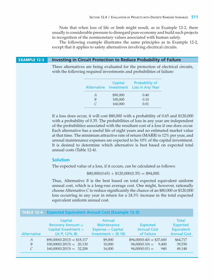
SECTION 12.4 / EVALUATION OF PROJECTS WITH DISCRETE RANDOM VARIABLES 511

Note that when loss of life or limb might result, as in Example 12-2, thereusually is considerable pressure to disregard pure economy and build such projectsin recognition of the nonmonetary values associated with human safety.

The following example illustrates the same principles as in Example 12-2,except that it applies to safety alternatives involving electrical circuits.

EXAMPLE 12-3 Investing in Circuit Protection to Reduce Probability of Failure

Three alternatives are being evaluated for the protection of electrical circuits,with the following required investments and probabilities of failure:

Capital Probability ofAlternative Investment Loss in Any Year

A $90,000 0.40B 100,000 0.10C 160,000 0.01

If a loss does occur, it will cost $80,000 with a probability of 0.65 and $120,000with a probability of 0.35. The probabilities of loss in any year are independentof the probabilities associated with the resultant cost of a loss if one does occur.Each alternative has a useful life of eight years and no estimated market valueat that time. The minimum attractive rate of return (MARR) is 12% per year, andannual maintenance expenses are expected to be 10% of the capital investment.It is desired to determine which alternative is best based on expected totalannual costs (Table 12-4).

SolutionThe expected value of a loss, if it occurs, can be calculated as follows:

$80,000(0.65) + $120,000(0.35) = $94,000.

Thus, Alternative B is the best based on total expected equivalent uniformannual cost, which is a long-run average cost. One might, however, rationallychoose Alternative C to reduce significantly the chance of an $80,000 or $120,000loss occurring in any year in return for a 24.3% increase in the total expectedequivalent uniform annual cost.

TABLE 12-4 Expected Equivalent Annual Cost (Example 12-3)

Capital Annual TotalRecovery Amount = Maintenance Expected ExpectedCapital Investment × Expense = Capital Annual Cost Equivalent

Alternative (A/P, 12%, 8) Investment × (0.10) of Failure Annual Cost

A $90,000(0.2013) = $18,117 $9,000 $94,000(0.40) = $37,600 $64,717B 100,000(0.2013) = 20,130 10,000 94,000(0.10) = 9,400 39,530C 160,000(0.2013) = 32,208 16,000 94,000(0.01) = 940 49,148

512 CHAPTER 12 / PROBABILISTIC RISK ANALYSIS

In Examples 12-1 through 12-3, a revenue or cost factor was modeled as adiscrete random variable, with project life assumed certain. A second type ofsituation involves the cash-flow estimates being certain, but the project life beingmodeled as a discrete random variable. This is illustrated in Example 12-4.

EXAMPLE 12-4 Project Life as a Random Variable

The heating, ventilating, and air-conditioning (HVAC) system in a commercialbuilding has become unreliable and inefficient. Rental income is being hurt,and the annual expenses of the system continue to increase. Your engineeringfirm has been hired by the owners to (1) perform a technical analysis ofthe system, (2) develop a preliminary design for rebuilding the system, and(3) accomplish an engineering economic analysis to assist the owners inmaking a decision. The estimated capital-investment cost and annual savingsin operating and maintenance expenses, based on the preliminary design,are shown in the following table. The estimated annual increase in rentalrevenue with a modern HVAC system has been developed by the owner’smarketing staff and is also provided in the following table. These estimatesare considered reliable because of the extensive information available. Theuseful life of the rebuilt system, however, is quite uncertain. The estimatedprobabilities of various useful lives are provided. Assume that MARR = 12%per year and the estimated market value of the rebuilt system at the end ofits useful life is zero. Based on this information, what are E(PW), V(PW), andSD(PW) of the project’s cash flows? Also, what is the probability of PW ≥ 0?What decision would you make regarding the project, and how would youjustify your decision using the available information? Solve by hand and byspreadsheet.

Economic Factor Estimate Useful Life, Year (N) p (N)

Capital investment $521,000 12 0.1Annual savings 48,600 13 0.2Increased annual revenue 31,000 14 0.3

15 0.2

⎫⎪⎪⎪⎪⎪⎪⎪⎪⎬⎪⎪⎪⎪⎪⎪⎪⎪⎭∑ = 1.00

16 0.117 0.0518 0.05

Solution by HandThe PW of the project’s cash flows, as a function of project life (N), is

PW(12%)N = −$521,000 + $79,600(P/A, 12%, N).

The calculation of the value of E(PW) = $9,984 and the value of E[(PW)2] =577.527 × 106($)2 are shown in Table 12-5. Then, by using Equation (12-8), the

SECTION 12.4 / EVALUATION OF PROJECTS WITH DISCRETE RANDOM VARIABLES 513

TABLE 12-5 Calculation of E(PW) and E[(PW)2] (Example 12-4)

(1) Useful (2) (3) (4) = (2) × (3) (5) = (2)2 (6) = (3) × (5)Life (N) PW(N) p(N) E[PW(N)] [PW(N)]2 p(N)[PW(N)]2

12 −$27,926 0.1 −$2,793 779.86 × 106 77.986 × 106

13 −9,689 0.2 −1,938 93.88 × 106 18.776 × 106

14 6,605 0.3 1,982 43.63 × 106 13.089 × 106

15 21,148 0.2 4,230 447.24 × 106 89.448 × 106

16 34,130 0.1 3,413 1,164.86 × 106 116.486 × 106

17 45,720 0.05 2,286 2,090.32 × 106 104.516 × 106

18 56,076 0.05 2,804 3,144.52 × 106 157.226 × 106

E(PW) = $9,984 E[(PW)2] = 577.527 × 106($)2

variance of the PW is

V(PW) = E[(PW)2] − [E(PW)]2

= 577.527 × 106 − ($9,984)2

= 477.847 × 106($)2.

The SD(PW) is equal to the positive square root of the variance, V(PW):

SD(PW) = [V(PW)]1/2 = (477.847 × 106)1/2

= $21,859.

Based on the PW of the project as a function of N (column 2), and the probabilityof each PW(N) value occurring (column 3), the probability of the PW being ≥ 0 is

Pr{PW ≥ 0} = 1 − (0.1 + 0.2) = 0.7.

The results of the engineering economic analysis indicate that the project isa questionable business action. The E(PW) of the project is positive ($9,984) butsmall relative to the large capital investment. Also, even though the probabilityof the PW being greater than zero is somewhat favorable (0.7), the SD(PW) valueis large [over two times the E(PW) value].

Spreadsheet SolutionSpreadsheets are well suited for the number crunching involved in computingexpected values and variances associated with discrete probability functions.Figure 12-1 illustrates the use of a spreadsheet to perform the necessarycalculations for this example. The basic format of Table 12-5 is used andthe results are same, subject to rounding differences. Once the spreadsheet,however, is formulated, we can easily perform sensitivity analyses to support

514 CHAPTER 12 / PROBABILISTIC RISK ANALYSIS

= E2

= D18

= B11 * C11

= B11 * E11

= C11 ^ 2

= SUM (D11:D17)

= F18 – D18 ^ 2

= SQRT (B21)

= PV($B$1, A11, –($B$3 + $B$4)) –$B$2

Figure 12-1 Spreadsheet Solution, Example 12-4

our recommendation. For example, a 5% decrease in annual savings results ina negative E(PW), supporting our conclusion that the profitability of the projectis questionable.

12.4.1 Probability Trees

The discrete distribution of cash flows sometimes occurs in each time period. Aprobability tree diagram is useful in describing the prospective cash flows, and theprobability of each value occurring, for this situation. Example 12-5 is a problemof this type.

EXAMPLE 12-5 Project Analysis Using a Probability Tree

The uncertain cash flows for a small improvement project are described by theprobability tree diagram in Figure 12-2. (Note that the probabilities emanatingfrom each node sum to unity.) The analysis period is two years, and MARR =12% per year. Based on this information,

SECTION 12.4 / EVALUATION OF PROJECTS WITH DISCRETE RANDOM VARIABLES 515

$500

$580

$460

0.3

0.5

�$1,000

0.2

0.4

0.3

0.3 $1,000

$960

$800

$770

$720

$680

$760

$650

$600

0.5

0.2

0.3

0.1

0.8

0.1

End of Year

0 1 2

Figure 12-2 Probability Tree Diagram for Example 12-5

(a) What are the E(PW), V(PW), and SD(PW) of the project?(b) What is the probability that PW ≤ 0?(c) Which analysis result(s) favor approval of the project, and which ones appear

unfavorable?

Solution(a) The calculation of the values for E(PW) and E[(PW)2] is shown in Table 12-6.

In column 2, PWj is the PW of branch j in the tree diagram. The probability ofeach branch occurring, p( j), is shown in column 3. For example, proceedingfrom the right node for each cash flow in Figure 12-2 to the left node, wehave p(1) = (0.3)(0.2) = 0.06 and p(9) = (0.5)(0.3) = 0.15. Hence,

E(PW) =∑

j

(PWj)p( j) = $39.56.

Then, V(PW) = E[(PW)2] − [E(PW)]2

= 15,227 − ($39.56)2

= 13,662($)2,

516 CHAPTER 12 / PROBABILISTIC RISK ANALYSIS

TABLE 12-6 Calculation of E(PW) and E[(PW)2] (Example 12-5)

(1)Net Cash Flow

EOY (2) (3) (4) = (2) × (3) (5) = (2)2 (6) = (3) × (5)j 0 1 2 PWj p( j) E(PWj) (PWj)

2 E[(PWj)2]

1 −$1,000 $580 $1,000 $315 0.06 $18.90 99,225$2 5,953$2

2 −1,000 580 960 283 0.06 16.99 80,089 4,8053 −1,000 580 800 156 0.08 12.45 24,336 1,9474 −1,000 500 770 60 0.05 3.04 3,600 1805 −1,000 500 720 20 0.40 8.17 400 1606 −1,000 500 680 −11 0.05 −0.57 121 67 −1,000 460 760 17 0.09 1.49 289 268 −1,000 460 650 −71 0.06 −4.27 5,044 3029 −1,000 460 600 −111 0.15 −16.64 12,321 1,848

E(PW) = $39.56 E[(PW)2] = 15,227$2

and SD(PW) = [V(PW)]1/2 = (13,662)1/2 = $116.88.

(b) Based on the entries in column 2, PWj, and column 3, p(j), we have

Pr{PW ≤ 0} = p(6) + p(8) + p(9)

= 0.05 + 0.06 + 0.15

= 0.26.

(c) The analysis results that favor approval of the project are E(PW) = $39.56,which is greater than zero only by a small amount, and Pr{PW > 0} =1 − 0.26 = 0.74. The SD(PW) = $116.92, however, is approximately threetimes the E(PW). This indicates a relatively high variability in the measureof economic merit, PW of the project, and is usually an unfavorable indicatorof project acceptability.

12.4.2 An Application Perspective

One of the major problems in computing expected values is the determination ofthe probabilities. In many situations, there is no precedent for the particular venturebeing considered. Therefore, probabilities seldom can be based on historical dataand rigorous statistical procedures. In most cases, the analyst, or the personmaking the decision, must make a judgment based on all available informationin estimating the probabilities. This fact makes some people hesitate to use theexpected-value concept, because they cannot see the value of applying such atechnique to improve the evaluation of risk and uncertainty when so much apparentsubjectivity is present.

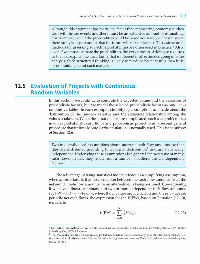
SECTION 12.5 / EVALUATION OF PROJECTS WITH CONTINUOUS RANDOM VARIABLES 517

Although this argument has merit, the fact is that engineering economy studiesdeal with future events and there must be an extensive amount of estimating.Furthermore, even if the probabilities could be based accurately on past history,there rarely is any assurance that the future will repeat the past. Thus, structuredmethods for assessing subjective probabilities are often used in practice.∗ Also,even if we must estimate the probabilities, the very process of doing so requiresus to make explicit the uncertainty that is inherent in all estimates going into theanalysis. Such structured thinking is likely to produce better results than littleor no thinking about such matters.

12.5 Evaluation of Projects with ContinuousRandom Variables

In this section, we continue to compute the expected values and the variances ofprobabilistic factors, but we model the selected probabilistic factors as continuousrandom variables. In each example, simplifying assumptions are made about thedistribution of the random variable and the statistical relationship among thevalues it takes on. When the situation is more complicated, such as a problem thatinvolves probabilistic cash flows and probabilistic project lives, a second generalprocedure that utilizes Monte Carlo simulation is normally used. This is the subjectof Section 12.6.

Two frequently used assumptions about uncertain cash-flow amounts are thatthey are distributed according to a normal distribution† and are statisticallyindependent. Underlying these assumptions is a general characteristic of manycash flows, in that they result from a number of different and independentfactors.

The advantage of using statistical independence as a simplifying assumption,when appropriate, is that no correlation between the cash-flow amounts (e.g., thenet annual cash-flow amounts for an alternative) is being assumed. Consequently,if we have a linear combination of two or more independent cash-flow amounts,say PW = c0F0+· · ·+cNFN , where the ck values are coefficients and the Fk values areperiodic net cash flows, the expression for the V(PW), based on Equation (12-10),reduces to

V(PW) =N∑

k=0

c2kV(Fk). (12-13)

∗ For further information, see W. G. Sullivan and W. W. Claycombe, Fundamentals of Forecasting (Reston, VA: RestonPublishing Co., 1977), Chapter 6.† This frequently encountered continuous probability function is discussed in any good statistics book, such as R. E.Walpole and R. H. Myers, Probability and Statistics for Engineers and Scientists (New York: Macmillan Publishing Co.,1989), 139–154.

518 CHAPTER 12 / PROBABILISTIC RISK ANALYSIS

And, based on Equation (12-9), we have

E(PW) =N∑

k=0

ckE(Fk). (12-14)

EXAMPLE 12-6 Annual Net Cash Flow as a Continuous Random Variable

For the following annual cash-flow estimates, find the E(PW), V(PW), andSD(PW) of the project. Assume that the annual net cash-flow amounts arenormally distributed with the expected values and standard deviations as givenand statistically independent and that the MARR = 15% per year.

End of Expected Value of SD of NetYear, k Net Cash Flow, Fk Cash Flow, Fk

0 −$7,000 01 3,500 $6002 3,000 5003 2,800 400

A graphical portrayal of these normally distributed cash flows is shown inFigure 12-3.

SolutionThe expected PW, based on Equation (12-14), is calculated as follows, where E(Fk)

is the expected net cash flow in year k (0 ≤ k ≤ N) and ck is the single-payment

�7,000 �5,000 0 �5,000

Cash Flow, $

k � 0k � 1

k � 2

k � 3

0

1

Probability

Time

3,500

3,000

2,800

Figure 12-3 Probabilistic Cash Flows over Time (Example 12-6)

SECTION 12.5 / EVALUATION OF PROJECTS WITH CONTINUOUS RANDOM VARIABLES 519

PW factor (P/F, 15%, k):

E(PW) =3∑

k=0

(P/F, 15%, k)E(Fk)

= −$7,000 + $3,500(P/F, 15%, 1) + $3,000(P/F, 15%, 2)

+$2,800(P/F, 15%, 3)

= $153.

To determine V(PW), we use the relationship in Equation (12-13). Thus,

V(PW) =3∑

k=0

(P/F, 15%, k)2V(Fk)

= 0212 + 6002(P/F, 15%, 1)2 + 5002(P/F, 15%, 2)2

+ 4002(P/F, 15%, 3)2

= 484,324$2

and

SD(PW) = [V(PW)]1/2 = $696.

When we can assume that a random variable, say the PW of a project’s cashflow, is normally distributed with a mean, E(PW), and a variance, V(PW), wecan compute the probability of events about the random variable occurring. Thisassumption can be made, for example, when we have some knowledge of theshape of the distribution of the random variable and when it is appropriate to doso. Also, this assumption may be supportable when a random variable, such as aproject’s PW value, is a linear combination of other independent random variables(say, the cash-flow amounts, Fk), regardless of whether the form of the probabilitydistribution(s) of these variables is known.∗

EXAMPLE 12-7 Probability of an Unfavorable Project Outcome

Refer to Example 12-6. For this problem, what is the probability that theinternal rate of return (IRR) of the cash-flow estimates is less than MARR,Pr{IRR < MARR}? Assume that the PW of the project is a normally distributedrandom variable, with its mean and variance equal to the values calculated inExample 12-6.

∗ The theoretical basis of this assumption is the central limit theorem of statistics. For a summary discussion of thesupportability of this assumption under different conditions, see C. S. Park and G. P. Sharpe-Bette, Advanced EngineeringEconomics (New York: John Wiley & Sons, 1990), 420–421.

520 CHAPTER 12 / PROBABILISTIC RISK ANALYSIS

SolutionFor a decreasing PW(i) function having a unique IRR, the probability that IRRis less than MARR is the same as the probability that PW is less than zero.Consequently, by using the standard normal distribution in Appendix E, we candetermine the probability that PW is less than zero:∗

Z = PW − E(PW)

SD(PW)= 0 − 153

696= −0.22;

Pr{PW ≤ 0} = Pr{Z ≤ −0.22}.From Appendix E, we find that Pr{Z ≤ −0.22} = 0.4129.

EXAMPLE 12-8 Linear Combination of Independent Random Variables

The estimated cash-flow data for a project are shown in the following table forthe five-year study period being used. Each annual net cash-flow amount, Fk , isa linear combination of two statistically independent random variables, Xk andYk , where Xk is a revenue factor and Yk is an expense factor. The Xk cash-flowamounts are statistically independent of each other, and the same is true of theYk amounts. Both Xk and Yk are continuous random variables, but the form oftheir probability distributions is not known. MARR = 20% per year. Based onthis information,

(a) What are the E(PW), V(PW), and SD(PW) values of the project’s cash flows?(b) What is the probability that PW is less than zero, that is, Pr{PW ≤ 0}, and

the project is economically attractive?

StandardExpected Value Deviation (SD)

End of Net Cash FlowYear, k Fk = akXk − bkYk Xk Yk Xk Yk

0 F0 = X0 + Y0 $0 −$100,000 $0 $10,0001 F1 = X1 + Y1 60,000 −20,000 4,500 2,0002 F2 = X2 + 2Y2 65,000 −15,000 8,000 1,2003 F3 = 2X3 + 3Y3 40,000 −9,000 3,000 1,0004 F4 = X4 + 2Y4 70,000 −20,000 4,000 2,0005 F5 = 2X5 + 2Y5 55,000 −18,000 4,000 2,300

∗ The standard normal distribution, f (Z), of the variable Z = (X −μ)/σ has a mean of zero and a variance of one, whenX is a normally distributed random variable with mean μ and standard deviation σ .

SECTION 12.5 / EVALUATION OF PROJECTS WITH CONTINUOUS RANDOM VARIABLES 521

TABLE 12-7 Calculation of E(Fk) and V (Fk) (Example 12-8)

End of E(Fk) = V (Fk) =Year, k Fk akE(Xk) + bkE(Yk) a2

kV (Xk) + b2kV (Yk)

0 F0 $0 − $100,000 = −$100,000 0 + (1)2(10,000)2 = 100.0 × 106$2

1 F1 60,000 − 20,000 = 40,000 (4,500)2 + (1)2 (2,000)2 = 24.25 × 106

2 F2 65,000 − 2(15,000) = 35,000 (8,000)2 + (2)2 (1,200)2 = 69.76 × 106

3 F3 2(40,000) − 3(9,000) = 53,000 (2)2(3,000)2 + (3)2 (1,000)2 = 45.0 × 106

4 F4 70,000 − 2(20,000) = 30,000 (4,000)2 + (2)2 (2,000)2 = 32.0 × 106

5 F5 2(55,000) − 2(18,000) = 74,000 (2)2(4,000)2 + (2)2 (2,300)2 = 85.16 × 106

Solution(a) The calculations of the E(Fk) and V(Fk) values of the project’s annual net cash

flows are shown in Table 12-7. The E(PW) is calculated by using Equation(12-14) as follows:

E(PW) =5∑

k=0

(P/F, 20%, k)E(Fk)

= −$100,000 + $40,000(P/F, 20%, 1)

+ · · · + $74,000(P/F, 20%, 5)

= $32,517.

Then, the V(PW) is calculated using Equation (12-13) as follows:

V(PW) =5∑

k=0

(P/F, 20%, k)2V(Fk)

= 100.0 × 106 + (24.25 × 106)(P/F, 20%, 1)2

+ · · · + (85.16 × 106)(P/F, 20%, 5)2

= 186.75 × 106($)2.

Finally, SD(PW) = [V(PW)]1/2

= [186.75 × 106]1/2

= $13,666.

(b) The PW of the project’s net cash flow is a linear combination of the annualnet cash-flow amounts, Fk , that are independent random variables. Each ofthese random variables, in turn, is a linear combination of the independentrandom variables Xk and Yk . We can also observe in Table 12-7 that theV(PW) calculation does not include any dominant V(Fk) values. Therefore,we have a reasonable basis on which to assume that the PW of the project’s

522 CHAPTER 12 / PROBABILISTIC RISK ANALYSIS

net cash flow is approximately normally distributed, with E(PW) = $32,517and SD(PW) = $13,666.

Based on this assumption, we have

Z = PW − E(PW)

SD(PW)= 0 − $32,517

$13,666= −2.3794;

Pr{PW ≤ 0} = Pr{Z ≤ −2.3794}.From Appendix E, we find that Pr{Z ≤ −2.3794} = 0.0087. Therefore,the probability of loss on this project is negligible. Based on this result,the E(PW) > 0, and the SD(PW) = 0.42[E(PW)]; therefore, the project iseconomically attractive and has low risk of failing to add value to the firm.

12.6 Evaluation of Risk and Uncertaintyby Monte Carlo Simulation

The modern development of computers and related software has resulted in theincreased use of Monte Carlo simulation as an important tool for analysis ofproject uncertainties. For complicated problems, Monte Carlo simulation generatesrandom outcomes for probabilistic factors so as to imitate the randomness inherentin the original problem. In this manner, a solution to a rather complex problem canbe inferred from the behavior of these random outcomes.

To perform a simulation analysis, the first step is to construct an analyticalmodel that represents the actual decision situation. This may be as simple asdeveloping an equation for the PW of a proposed industrial robot in an assemblyline or as complex as examining the economic effects of proposed environmentalregulations on typical petroleum refinery operations. The second step is todevelop a probability distribution from subjective or historical data for eachuncertain factor in the model. Sample outcomes are randomly generated byusing the probability distribution for each uncertain quantity and are then usedto determine a trial outcome for the model. Repeating this sampling processa large number of times leads to a frequency distribution of trial outcomesfor a desired measure of merit, such as PW or AW. The resulting frequencydistribution can then be used to make probabilistic statements about the originalproblem.

This section has been adapted from W. G. Sullivan and R. Gordon Orr, “Monte Carlo Simulation Analyzes Alternativesin Uncertain Economy,” Industrial Engineering, 14, no. 11 (November 1982): 42–49. Reprinted with permission fromthe Institute of Industrial Engineers, 3577 Parkway Lane, Suite 200, Norcross, GA, 30092, www.iienet.org. Copyright© 2010 by Institute of Industrial Engineers.

SECTION 12.6 / EVALUATION OF RISK AND UNCERTAINTY BY MONTE CARLO SIMULATION 523

To illustrate the Monte Carlo simulation procedure, suppose that theprobability distribution for the useful life of a piece of machinery has beenestimated as shown in Table 12-8. The useful life can be simulated by assigningrandom numbers to each value such that they are proportional to the respectiveprobabilities. (A random number is selected in a manner such that each numberhas an equal probability of occurrence.) Because two-digit probabilities are givenin Table 12-8, random numbers can be assigned to each outcome, as shown inTable 12-9. Next, a single outcome is simulated by choosing a number at randomfrom a table of random numbers.∗ For example, if any random number betweenand including 00 and 19 is selected, the useful life is three years. As a furtherexample, the random number 74 corresponds to a life of seven years.

If the probability distribution that describes a random variable is normal, aslightly different approach is followed. Here the simulated outcome is based onthe mean and standard deviation of the probability distribution and on a randomnormal deviate, which is a random number of standard deviations above or belowthe mean of a standard normal distribution. An abbreviated listing of typicalrandom normal deviates is shown in Table 12-10. For normally distributed randomvariables, the simulated outcome is based on Equation (12-15):

Outcome value = mean + [random normal deviate× standard deviation]. (12-15)

For example, suppose that an annual net cash flow is assumed to be normallydistributed, with a mean of $50,000 and a standard deviation of $10,000, as shownin Figure 12-4.

TABLE 12-8 Probability Distribution for UsefulLife

Number of Years, N p(N)

357

10

⎫⎪⎪⎬⎪⎪⎭possible values

0.200.400.250.15

⎫⎪⎪⎬⎪⎪⎭∑

p(N) = 1.00

TABLE 12-9 Assignment of RandomNumbers

Number of Years, N Random Numbers

3 00–195 20–597 60–84

10 85–99

∗ The last two digits of randomly chosen telephone numbers in a telephone directory are usually quite close to beingrandom numbers.

524 CHAPTER 12 / PROBABILISTIC RISK ANALYSIS

TABLE 12-10 Random Normal Deviates (RNDs)

−1.565 0.690 −1.724 0.705 0.0900.062 −0.072 0.778 −1.431 0.2400.183 −1.012 −0.844 −0.227 −0.448

−0.506 2.105 0.983 0.008 0.2951.613 −0.225 0.111 −0.642 −0.292

Figure 12-4 NormallyDistributed AnnualCash Flow

Annual Net Cash Flow

TABLE 12-11 Example of the Use of RNDs

Annual Net Cash FlowYear RND [$50,000 + RND ($10,000)]

1 0.090 $50,9002 0.240 52,4003 −0.448 45,5204 0.295 52,9505 −0.292 47,080

Simulated cash flows for a period of five years are listed in Table 12-11. Noticethat the average annual net cash flow is $248,850/5, which equals $49,770. Thisapproximates the known mean of $50,000 with an error of 0.46%.

If the probability distribution that describes a random event is uniform andcontinuous, with a minimum value of A and a maximum value of B, anotherprocedure should be followed to determine the simulated outcome. Here theoutcome can be computed with the formula

Simulation outcome = A + RNRNm

[B − A], (12-16)

where RNm is the maximum possible random number (9 if one digit is used, 99 iftwo are used, etc.) and RN is the random number actually selected. This equationshould be used when the minimum outcome, A, and the maximum outcome, B,are known.

For example, suppose that the market value in year N is assumed to be uni-formly and continuously distributed between $8,000 and $12,000. A value of this

SECTION 12.6 / EVALUATION OF RISK AND UNCERTAINTY BY MONTE CARLO SIMULATION 525

random variable would be generated as follows with a random number of 74:

Simulation outcome = $8,000 + 7499

($12,000 − $8,000) = $10,990.

Proper use of these procedures, coupled with an accurate model, will resultin an approximation of the actual outcome. But how many simulation trials arenecessary for an accurate approximation of, for example, the average outcome? Ingeneral, the greater the number of trials, the more accurate the approximation ofthe mean and standard deviation will be. One method of determining whethera sufficient number of trials has been conducted is to keep a running average ofresults. At first, this average will vary considerably from trial to trial. The amount ofchange between successive averages should decrease as the number of simulationtrials increases. Eventually, this running (cumulative) average should level off atan accurate approximation.

EXAMPLE 12-9 Project Analysis Using Monte Carlo Simulation

Monte Carlo simulation can also simplify the analysis of a more complex pro-blem. The following estimates relate to an engineering project being consideredby a large manufacturer of air-conditioning equipment. Subjective probabilityfunctions have been estimated for the four independent uncertain factors asfollows:

(a) Capital investment: Normally distributed with a mean of $50,000 and astandard deviation of $1,000.

(b) Useful life: Uniformly and continuously distributed with a minimum lifeof 10 years and a maximum life of 14 years.

(c) Annual revenue:

$35,000 with a probability of 0.4

$40,000 with a probability of 0.5

$45,000 with a probability of 0.1

(d) Annual expense: Normally distributed, with a mean of $30,000 and astandard deviation of $2,000.

The management of this company wishes to determine whether the capitalinvestment in the project will be a profitable one. The interest rate is 10% peryear. To answer this question, the PW of the venture will be simulated.

SolutionTo illustrate the Monte Carlo simulation procedure, five trial outcomes arecomputed manually in Table 12-12. The estimate of the average PW based on thisvery small sample is $19,010/5 = $3,802. For more accurate results, hundreds oreven thousands of repetitions would be required.

526 CHAPTER 12 / PROBABILISTIC RISK ANALYSIS

TABLE 12-12 Monte Carlo Simulation of PW Involving Four IndependentFactors (Example 12-9)

Random Capital ProjectNormal Investment, l Project Life, N

Trial Deviate [$50,000 + Life, N (NearestNumber (RND1) RND1($1,000)] Three-Digit RNs [10 + RN

999 (14 − 10)] Integer)

1 −1.003 $48,997 807 13.23 132 −0.358 49,642 657 12.63 133 +1.294 51,294 488 11.95 124 −0.019 49,981 282 11.13 115 +0.147 50,147 504 12.02 12

Annual Revenue, R$35,000 for 0–3 Annual Expense, E

One-Digit 40,000 for 4–8 [$30,000 + PW = −l +RN 45,000 for 9 RND2 RND2 ($2,000)] (R − E)(P/A, 10%, N)

1 2 $35,000 −0.036 $29,928 −$12,9692 0 35,000 +0.605 31,210 −22,7203 4 40,000 +1.470 32,940 −3,1894 9 45,000 +1.864 33,728 +23,2325 8 40,000 −1.223 27,554 +34,656

Total +$19, 010

The applications of Monte Carlo simulation for investigating risk and uncer-tainty are many and varied. Remember that the results, however, can be no moreaccurate than the model and the probability estimates used. In all cases, the pro-cedure and rules are the same: careful study of the problem and development ofthe model; accurate assessment of the probabilities involved; true randomizationof outcomes as required by the Monte Carlo simulation procedure; and calculationand analysis of the results. Furthermore, a sufficiently large number of Monte Carlotrials should always be used to reduce the estimation error to an acceptable level.

12.7 Performing Monte Carlo Simulationwith a Computer

It is apparent from the preceding section that a Monte Carlo simulation of a complexproject requiring several thousand trials can be accomplished only with the help ofa computer. Indeed, there are numerous simulation programs that can be obtainedfrom software companies and universities. MS Excel also has a simulation featurethat can generate random data for seven different probability distributions. In thissection, we will demonstrate that Monte Carlo simulation is not only feasible butalso relatively easy to perform with spreadsheets.

SECTION 12.7 / PERFORMING MONTE CARLO SIMULATION WITH A COMPUTER 527

At the heart of Monte Carlo simulation is the generation of random numbers.Most spreadsheet packages include a RAND( ) function that returns a randomnumber between zero and one. Other advanced statistical functions, such asNORMSINV( ), will return the inverse of a cumulative distribution function (thestandard normal distribution in this case). This function can be used to generaterandom normal deviates. The spreadsheet model shown in Figure 12-5 makes useof these functions in performing a Monte Carlo simulation for the project beingevaluated in Example 12-9.

The probabilistic functions for the four independent uncertain factors areidentified in the spreadsheet model. The input parameter names and distributions

Figure 12-5 Monte Carlo Simulation Using a Spreadsheet, Example 12-9

528 CHAPTER 12 / PROBABILISTIC RISK ANALYSIS

are identified in cells A2:B7. The mean and standard deviation of the normallydistributed factors (capital investment and annual expenses) are identified in therange C2:D4. The maximum and minimum values for the uniformly distributedproject life are shown in E5:F5. A discrete probability function was compiled forannual revenues. The associated cumulative probability distribution is shownin G6:I7.

The formulas in cells B12:E12 return values for the uncertain factors, based onthe underlying distribution and parameters. These values are used in cell F12 tocalculate the PW. As these formulas are copied down the spreadsheet, each rowbecomes a new trial in the simulation. Each time the F9 (recalculate) key is pressed,the RAND( ) functions are reevaluated and a new simulation begins. The formulasin the range B1013:F1017 calculate basic statistics for the input parameters and thePW. By comparing these results with the input values, one can rapidly check forerrors in the basic formulas.

A true simulation involves hundreds, or perhaps thousands, of trials. In thisexample, 1,000 trials were used. The first and last five trials are shown in Figure12-5 (rows 17 through 1006 have been hidden for display purposes). The averagePW is $8,345 (cell F1015), which is larger than the $3,802 obtained from Table 12-12.This underscores the importance of having a sufficient number of simulation trialsto ensure reasonable accuracy in Monte Carlo analyses. The cumulative averagePW calculated in column G is one simple way to determine whether enough trialshave been run. A plot of these values will stabilize and show little change when thesimulation has reached a steady state. Figure 12-6 shows the plot of the cumulativeaverage PW for the 1,000 trials generated for this example.

The average PW is of interest, but the distribution of PW is often even moresignificant. A histogram of the PW values in column F displays the shape of thedistribution, as shown in Figure 12-7. The dispersion of PW trial outcomes in this

Figure 12-6 Plot of Cumulative Average PW to Determine whether EnoughSimulation Trials Have Been Run

SECTION 12.7 / PERFORMING MONTE CARLO SIMULATION WITH A COMPUTER 529

Figure 12-7 Histogram Showing Distribution of PW for 1,000 Simulation Trials

example is considerable. The standard deviation of simulated trial outcomes is oneway to measure this dispersion. In addition, the proportion of values less than zeroindicates the probability of a negative PW. Based on Figure 12-7, approximately 40%of all simulation outcomes have a PW less than zero. Consequently, this project maybe too risky for the company to undertake, because the downside risk of failing torealize at least a 10% per year return on the capital investment is about 4 chancesout of 10. Perhaps another project investment should be considered.

A typical application of simulation involves the analysis of several mutuallyexclusive alternatives. In such studies, how can one compare alternatives thathave different expected values and standard deviations of, for instance, PW? Oneapproach is to select the alternative that minimizes the probability of attaining a PWthat is less than zero. Another popular response to this question utilizes a graph ofexpected value (a measure of the reward) plotted against standard deviation (anindicator of risk) for each alternative. An attempt is then made to assess subjectivelythe trade-offs that result from choosing one alternative over another in pairwisecomparisons.

To illustrate the latter concept, suppose that three alternatives having varyingdegrees of uncertainty have been analyzed with Monte Carlo computer simulationand the results shown in Table 12-13 have been obtained. These results are plottedin Figure 12-8, where it is apparent that Alternative C is inferior to Alternatives Aand B because of its lower E(PW) and larger standard deviation. Therefore, C offersa smaller PW that has a greater amount of risk associated with it! Unfortunately,the choice of B versus A is not as clear because the increased expected PW of B hasto be balanced against the increased risk of B. This trade-off may or may not favor B,depending on management’s attitude toward accepting the additional uncertainty

530 CHAPTER 12 / PROBABILISTIC RISK ANALYSIS

TABLE 12-13 Simulation Results for Three MutuallyExclusive Alternatives

Alternative E(PW) SD(PW) E(PW) ÷ SD(PW)

A $37,382 $1,999 18.70B 49,117 2,842 17.28C 21,816 4,784 4.56

SD (

PW),

$

20,000 30,000 40,000 50,000

2,000

3,000

4,000

5,000

Increased E (PW)

Increased risk of PWA

B

C

E (PW), $

Figure 12-8 Graphical Summary of Computer Simulation Results

associated with a larger expected reward. The comparison also presumes thatAlter-native A is acceptable to the decision maker. One simple procedure for choosingbetween A and B is to rank alternatives based on the ratio of E(PW) to SD(PW). Inthis case, Alternative A would be chosen because it has the more favorable (larger)ratio.

12.8 Decision Trees

Decision trees, also called decision flow networks and decision diagrams, arepowerful means of depicting and facilitating the analysis of important problems,especially those that involve sequential decisions and variable outcomes overtime. Decision trees are used in practice because they make it possible to breakdown a large, complicated problem into a series of smaller simple problems,and they enable objective analysis and decision making that includes explicitconsideration of the risk and effect of the future.

This section has been adapted (except Section 12.8.3) from John R. Canada and William G. Sullivan, Economic andMultiattribute Evaluation of Advanced Manufacturing Systems (Upper Saddle River, NJ: Prentice Hall, 1989), 341–343,347. Reprinted by permission of the publisher.

SECTION 12.8 / DECISION TREES 531

The name decision tree is appropriate, because it shows branches for eachpossible alternative for a given decision and for each possible outcome (event) thatcan result from each alternative. Such networks reduce abstract thinking to a logicalvisual pattern of cause and effect. When costs and benefits are associated with eachbranch and probabilities are estimated for each possible outcome, analysis of thedecision flow network can clarify choices and risks.

12.8.1 Deterministic Example

The most basic form of a decision tree occurs when each alternative can be assumedto result in a single outcome—that is, when certainty is assumed. The replacementproblem in Figure 12-9 illustrates this. The problem illustrates that the decision onwhether to replace the defender (old machine) with the new machine (challenger)is not just a one-time decision but rather one that recurs periodically. That is, ifthe decision is made to keep the old machine at decision point one, then later, atdecision point two, a choice again has to be made. Similarly, if the old machine ischosen at decision point two, then a choice again has to be made at decision pointthree. For each alternative, the cash inflow and duration of the project are shownabove the arrow, and the capital investment is shown below the arrow.

For this problem, the question initially seems to be which alternative to chooseat decision point 1. But an intelligent choice at decision point 1 should takeinto account the later alternatives and decisions that stem from it. Hence, thecorrect procedure is to start at the most distant decision point, determine the bestalternative and quantitative result of that alternative, and then roll back to eachpreceding decision point, repeating the procedure until finally the choice at theinitial or present decision point is determined. By this procedure, one can makea present decision that directly takes into account the alternatives and expecteddecisions of the future.

For simplicity in this example, timing of the monetary outcomes will first beneglected, which means that a dollar has the same value regardless of the year inwhich it occurs. Table 12-14 shows the necessary computations and decisions using

Old: $4 M/year,3 years

Old: $3.5 M/year,3 years

Old: $3 M/year,3 years

�$0.8 M �$1 M �$2 MNew: $6.5 M

/year, 6 years�

$15 M

$6.5 M/year,

3 years�

$17 M

�$18 MNew: $5 M

/year, 9 years

Dec.1

Dec.2

Dec.3

New

Figure 12-9 Deterministic Replacement Example

532 CHAPTER 12 / PROBABILISTIC RISK ANALYSIS

TABLE 12-14 Monetary Outcomes and Decisions at Each Point−−Deterministic Replacement Example of Figure 12-9a

Decision Point Alternative Monetary Outcome Choice

Old $3M(3) − $2M = $7.0M Old3{

New $6.5M(3) − $18M = $1.5M

Old $7M + $3.5M(3) − $1M = $16.5M2{

New $6.5M(6) − $17M = $22.0M New

Old $22.0M + $4M(3) − $0.8M = $33.2M Old1{

New $5M(9) − $15M = $30.0M

a Interest = 0% per year, that is, ignore timing of cash flows.

a nine-year study period. Note that the monetary outcome of the best alternativeat decision point 3 ($7.0M for the old) becomes part of the outcome for the oldalternative at decision point 2. Similarly, the best alternative at decision point 2($22.0M for the new) becomes part of the outcome for the defender alternative atdecision point 1.

The computations in Table 12-14 show that the answer is to keep the oldalternative now and plan to replace it with the new one at the end of three years (atdecision point 2). But this does not mean that the old machine should necessarilybe kept for a full three years and a new machine bought without question at the endof that period. Conditions may change at any time, necessitating a fresh analysis—probably a decision tree analysis—based on estimates that are reasonable in lightof conditions at that time.

12.8.1.1 Deterministic Example Considering Timing For decision treeanalyses, which involve working from the most distant to the nearest decisionpoint, the easiest way to take into account the timing of money is to use the PWapproach and thus discount all monetary outcomes to the decision points in question. Todemonstrate, Table 12-15 shows computations for the same replacement problemof Figure 12-9, using an interest rate of 25% per year.

Note from Table 12-15 that, when taking into account the effect of timing bycalculating PWs at each decision point, the indicated choice is not only to keep theold alternative at decision point 1 but also to keep the old alternative at decisionpoints 2 and 3 as well. This result is not surprising since the high interest rate tendsto favor the alternatives with lower capital investments, and it also tends to placeless weight on long-term returns (benefits).

12.8.2 General Principles of Diagramming

The proper diagramming of a decision problem is, in itself, generally very useful tothe understanding of the problem, and it is essential to correct subsequent analysis.

The placement of decision points (nodes) and chance outcome nodes from theinitial decision point to the base of any later decision point should give an accuraterepresentation of the information that will and will not be available when the choice

SECTION 12.8 / DECISION TREES 533

TABLE 12-15 Decision at Each Point with Interest = 25% per Year for DeterministicReplacement Example of Figure 12-9

Decision Point Alternative PW of Monetary Outcome Choice

Old $3M(P/A, 3) − $2M$3M(1.95) − $2M = $3.85M Old3

⎧⎪⎪⎨⎪⎪⎩New $6.5M(P/A, 3) − $18M

$6.5M(1.95) − $18M = −$5.33MOld $3.85M(P/F, 3) + $3.5M(P/A, 3) − $1M

$3.85M(0.512) + $3.5M(1.95) − $1M = $7.79M Old2

⎧⎪⎪⎨⎪⎪⎩New $6.5M(P/A, 6) − $17M

$6.5M(2.95) − $17M = $2.18MOld $7.79M(P/F, 3) + $4M(P/A, 3) − $0.8M

$7.79M(0.512) + $4M(1.95) − $0.8M = $10.99M Old1

⎧⎪⎪⎨⎪⎪⎩New $5.0M(P/A, 9) − $15M

$5.0M(3.46) − $15M = $2.30M

represented by the decision point in question actually has to be made. The decisiontree diagram should show the following (normally, a square symbol is used todepict a decision node, and a circle symbol is used to depict a chance outcomenode):

1. all initial or immediate alternatives among which the decision maker wishes tochoose

2. all uncertain outcomes and future alternatives that the decision maker wishes toconsider because they may directly affect the consequences of initial alternatives

3. all uncertain outcomes that the decision maker wishes to consider becausethey may provide information that can affect his or her future choices amongalternatives and hence indirectly affect the consequences of initial alternatives

Note that the alternatives at any decision point and the outcomes at any chanceoutcome node must be

1. mutually exclusive (i.e., no more than one can be chosen)2. collectively exhaustive (i.e., one event must be chosen or something must occur

if the decision point or outcome node is reached)

12.8.3 Decision Trees with Random Outcomes

The deterministic replacement problem discussed in Section 12.8.1 introduced theconcept of sequential decisions using assumed certainty for alternative outcomes.An engineering problem requiring sequential decisions, however, often includesrandom outcomes, and decision trees are very useful in structuring this type ofsituation. The decision tree diagram helps to make the problem explicit and assistsin its analysis. This is illustrated in Example 12-10.

534 CHAPTER 12 / PROBABILISTIC RISK ANALYSIS

EXAMPLE 12-10 Probabilistic Decision Tree Analysis

The Ajax Corporation manufactures compressors for commercial air-conditioning systems. Anew compressor design is being evaluated as a potentialreplacement for the most frequently used unit. The new design involves majorchanges that have the expected advantage of better operating efficiency. From theperspective of a typical user, the new compressor (as an assembled componentin an air-conditioning system) would have an increased investment of $8,600relative to the present unit and an annual expense saving dependent upon theextent to which the design goal is met in actual operations.

Estimates by the multidisciplinary design team of the new compressorachieving four levels (percentages) of the efficiency design goal and theprobability and annual expense saving at each level are as follows:

Level (Percentage) Probability Annual Expenseof Design Goal Met (%) p(L) Saving

90 0.25 $3,47070 0.40 2,92050 0.25 2,31030 0.10 1,560

Based on a before-tax analysis (MARR = 18% per year, analysis period = 6 years,and market value = 0) and E(PW) as the decision criterion, is the new compressordesign economically preferable to the current unit?

SolutionThe single-stage decision tree diagram for the design alternatives is shown inFigure 12-10. The PWs associated with each of the efficiency design goal levels

Probabilityp(L)

AnnualExpense Saving PW

90: 0.25

70: 0.40

50: 0.25

30: 0.10

$3,470

2,920

2,310

1,560

$0$0

$1,086

New Design

Current Unit

$3,538

1,614

�520

�3,143

Figure 12-10 Single-Stage Decision Tree (Example 12-10)

SECTION 12.9 / REAL OPTIONS ANALYSIS 535

being met are as follows:

PW(18%)90 = −$8,600 + $3,470(P/A, 18%, 6) = $3,538

PW(18%)70 = −$8,600 + $2,920(P/A, 18%, 6) = $1,614

PW(18%)50 = −$8,600 + $2,310(P/A, 18%, 6) = −$520

PW(18%)30 = −$8,600 + $1,560(P/A, 18%, 6) = −$3,143

Based on these values, the E(PW) of each installed unit of the new compressoris as follows:

E(PW) = 0.25($3,538) + 0.40($1,614)

+0.25(−$520) + 0.10(−$3,143)

= $1,086.

The E(PW) of the current unit is zero since the cash-flow estimates for the newdesign are incremental amounts relative to the present design. Therefore, theanalysis indicates that the new design is economically preferable to the presentdesign. (The parallel lines across the current unit path on the diagram indicatethat it was not selected.)

12.9 Real Options AnalysisCompanies make capital investments to exploit opportunities for shareholder(owner) wealth creation. Often these opportunities are real options, which areopportunities available to a firm when it invests in real assets such as plant,equipment, and land. Real options allow decision makers to invest capital now orto postpone all or part of the investment until later. Decision trees are a convenientmeans for portraying the resolution of risk/uncertainty in the analysis of realoptions.∗

The real options approach to capital investments is based on an interestinganalogy about financial options. A company with an opportunity to invest capitalactually owns something much like a financial call option—the company has theright but not the obligation to invest in (purchase) an asset at a future time ofits choosing. When a firm makes an irreversible capital investment that could bepostponed, it exercises its call option, which has value by virtue of the flexibility itgives the firm.

∗ The reader interested in details regarding real options analysis is referred to these two articles: Luehrman, T. A.,“Investment Opportunities as Real Options: Getting Started with the Numbers,” Harvard Business Review, 76, no. 4(July–August 1998a): 51–67; Luehrman, T. A., “Strategy as a Portfolio of Real Options,” Harvard Business Review, 76,no. 5 (September–October 1998b): 89–99.

536 CHAPTER 12 / PROBABILISTIC RISK ANALYSIS

An example of a postponable investment is coal-fired generating capacity of anelectric utility. Anticipated capacity needed for the next 10 years can be added inone large expansion project, or the capacity addition can be acquired in staggeredstages, which permits the utility to better respond to future demand patterns andpossibly different types of generating capacity, such as natural gas or nuclearpower. If the utility company decides to go ahead with a single, large, irreversibleexpansion project, it eliminates the option of waiting for new information thatmight represent a more valuable phased approach to meeting customers’ demandsfor electricity. The lost option’s value is an opportunity cost that must be includedin the overall evaluation of the investment. This is the essence of the real optionsapproach to capital investment—to fairly value the option of waiting to invest in allor a part of the project and to include this value in the overall project profitability.Clearly, viewing capital investments as real options forces a greater emphasis to beplaced on the value of information in risky situations facing a firm.

In the previous section, we have shown how decision trees are useful indetermining the value of information of anticipated future outcomes. In thisregard, decision trees enable the analyst to model real options that are hidden inclassical present worth analysis. These options, not treated formally in classic singleoutcome analyses, are often understood by management and factored informallyinto their assessment of the analysis (and the assessment of the analyst!). Thispresence of hidden options is most easily understood with an example.

EXAMPLE 12-11 Hytech Industries

Hytech is considering opening an entirely new electronic interface using radiofrequency identification with a new coding system that deviates from somestandards but offers advantages to bulk chemical manufacturers. The cost todevelop the manufacturing capacity and build the market is estimated at $700million, and the resulting net cash inflows after income taxes are estimated at$100 million per year (albeit with much potential variation depending uponacceptance of the product). The after-tax MARR is 15% per year, and the newproduct will have a life of 20 years.

Solution as Classical Single Outcome AnalysisThe PW of this project is

PW(15%) = −$700 million + $100 million(P/A, 15%, 20) = −$74.1 million,

and the recommendation would be to avoid the investment.Suppose, however, that the $100 million cash inflow per year is merely an

average. If the device catches on, potential sales will exceed the annual capacityfor the new facilities, and annual inflows will be limited to $200 million. In fact,if this happens, a second plant can be acquired one year later for an additionalinvestment of $500 million, and it would be able to generate an additional $150million cash inflow annually. On the other hand, if the new product fails tocatch on, sales could effectively be zero, but the plant could be salvaged for$150 million.

SECTION 12.9 / REAL OPTIONS ANALYSIS 537

Solution as a Decision Tree with Embedded OptionsThe decision tree appears as shown in Figure 12-11. If the end-of-path conventionis used, then the tip values are as shown in Table 12-16. Note that path 3,abandoned when first year inflows exceed $200 million, is not reasonable and isnot evaluated. Similarly, path 4 and 7 would involve expansion when the markethas not developed and are not evaluated.

As shown in the table, when first year net inflows are high ($200 million +),the better of paths 1 and 2 is to expand and realize a PW of $926 million. Ifresponse is tepid ($100 million inflow), then path 5 is better than path 6. The PWof path 5 is negative, but staying in business recoups some of the investment andis better than abandoning the project. Finally, if the market is negligible, path9 is better than path 8, because the ability to salvage some of the investmentmitigates the loss.

Invest

With OptionAfter First

Year

Do N

ot Invest

First Year

InflowNegligible

First Year

Inflow = $100 Mill.

First Year

Inflow = $200 Mill.

Expand

Continue

Abandon

Expand

Continue

Abandon

Expand

Continue

Abandon

PW Path No.

+$926 MILL.

+$552 MILL.

(NOT EVAL)

(NOT EVAL)

(NOT EVAL)

–$74.1 MILL.

–$569 MILL.

–$700 MILL.

–$569 MILL.

$0 MILL.

1

2

3

4

5

6

7

8

9

Figure 12-11 Hytech Industries Example

538 CHAPTER 12 / PROBABILISTIC RISK ANALYSIS

TABLE 12-16 Decision Tree Endpoint Evaluation

Path First Year Inflows Option Evaluation Net PW

1 $200 million + Expand −$700 + $200(P/A, 15%, 20) +$926 million−$500(P/F, 15%, 1)

+$150(P/A, 15%, 19)(P/F, 15%, 1)

2 $200 million + Continue −$700 + $200(P/A, 15%, 20) +$552 million3 $200 million + Abandon Not evaluated4 $100 million Expand Not evaluated5 $100 million Continue −$700 + $100(P/A, 15%, 20) −$74.1 million6 $100 million Abandon −$700 + $150(P/F, 15%, 1) −$569 million7 Negligible Expand Not evaluated8 Negligible Continue −$700 −$700 million9 Negligible Abandon −$700 + $150(P/F, 15%, 1) −$569 million

If each outcome of the first year cash flows were equally likely and managementis risk neutral, then the expected monetary value is $94.3 (= [+$926 − $74.1 −$569]/3) million, an improvement of $168.4 million over the $74.1 million lossprojected in the single outcome analysis. This improvement can be viewed as thevalue of the combined options to expand, if the market develops, or to salvagesome investment if the project is a flop.

12.10 SummaryEngineering economy involves decision making among competing uses of scarcecapital resources. The consequences of resultant decisions usually extend far intothe future. In this chapter, we have presented various statistical and probabilityconcepts that address the fact that the consequences (cash flows, project lives, etc.)of engineering alternatives can never be known with certainty, including MonteCarlo computer simulation techniques, and decision tree analysis. Cash inflow andcash outflow factors, as well as project life, were modeled as discrete and continuousrandom variables. The resulting impact of uncertainty on the economic measuresof merit for an alternative was analyzed. Included in the discussion were severalconsiderations and limitations relative to the use of these methods in application.

Regrettably, there is no quick and easy answer to the question, How shouldrisk best be considered in an engineering economic evaluation? Generally, simpleprocedures (e.g., breakeven analysis and sensitivity analysis, discussed in Chapter11) allow some discrimination among alternatives to be made on the basis of theuncertainties present, and they are relatively inexpensive to apply. Additionaldiscrimination among alternatives is possible with more complex procedures thatutilize probabilistic concepts. These procedures, however, are more difficult toapply and require additional time and expense.

ProblemsThe number in parentheses that follows each problemrefers to the section from which the problem is taken.

12-1. A large mudslide caused by heavy rains willcost Sabino County $1,000,000 per occurrence in lost

PROBLEMS 539

property tax revenues. In any given year, there is onechance in 100 that a major mudslide will occur.

A civil engineer has proposed constructing a culverton a mountain where mudslides are likely. This culvertwill reduce the likelihood of a mudslide to near zero.The investment cost would be $50,000, and annualmaintenance expenses would be $2,000 in the first year,increasing by 5% per year thereafter. If the life of theculvert is expected to be 20 years and the cost of capitalto Sabino County is 7% per year, should the culvert bebuilt? (12.4)

12-2. A bridge is to be constructed now as part of anew road. An analysis has shown that traffic densityon the new road will justify a two-lane bridge at thepresent time. Because of uncertainty regarding futureuse of the road, the time at which an extra two lanes willbe required is currently being studied. The estimatedprobabilities of having to widen the bridge to four lanesat various times in the future are as follows:

Widen Bridge In Probability

3 years 0.14 years 0.25 years 0.36 years 0.4

The present estimated cost of the two-lane bridgeis $2,000,000. If constructed now, the four-lane bridgewill cost $3,500,000. The future cost of widening a two-lane bridge will be an extra $2,000,000 plus $250,000 forevery year that widening is delayed. If money can earn12% per year, what would you recommend? (12.4)

12-3. A new snow making machine utilizes technologythat permits snow to be produced in ambient tem-perature of 70 degrees Fahrenheit or below. The esti-mated cash flows for the ski resort contemplating thisinvestment are uncertain as shown below (note: pr. =probability).

Capital investment $120,000 (certain, pr. = 1.0)Annual revenues $140,000 with pr. 0.6, or $135,000

with pr. 0.4Annual expenses $60,000 with pr. 0.6, or $50,000

with pr. 0.4Salvage value $40,000 with pr. 0.5, or $35,000

with pr. 0.5

The machine is expected to have a useful life of 12 years,and the MARR of the ski resort is 8% per year. What isthe expected present worth of this investment? (12.4)

12-4. It costs $250,000 to drill a natural gaswell. Operating expenses will be 10% of the

revenue from the sale of natural gas from this particularwell. If found, natural gas from a highly productivewell will amount to 260,000 cubic feet per day. Theprobability of locating such a productive well, however,is about 10%. (12.4)

a. If natural gas sells for $8 per thousand cubic feet,what is the E(PW) of profit to the owner/operator ofthis well? The life of the well is 10 years and MARRis 15% per year.

b. Repeat Part (a) when the life of the well is sevenyears.

c. Perform one-at-a-time sensitivity analyses for ±20%changes in daily well production and selling priceof natural gas. Use a 10-year life for the well.

12-5. Annual profit (P) is the product of total annualsales (S) and profit per unit sold (X); that is, P =X · S. It is desired to know the probability distributionof the random variable P when X and S have thefollowing assumed probability mass functions (X and Sare independent):

X (Unit Profit) S (Annual Sales)

Value Probability Value Probability

0 0.05 5 0.41 0.45 6 0.22 0.30 8 0.43 0.20

What are the mean, variance, and standard devia-tion of the probability distribution for annual profit,P? (12.4)

12-6. A very important levee spans a distanceof 10 miles on the outskirts of a large metropolitan

area. Hurricanes have hit this area twice in the past 20years, so there is concern over the structural integrityof this particular levee. City engineers have proposedreinforcing and increasing the height of the leveeby various designs to withstand the storm surge ofnumerous strength categories of hurricanes.

Study results regarding the probability that highflood water from a hurricane in any one year willexceed the increased height of the levee, and the costof construction of the levee for each storm category, aresummarized next.

540 CHAPTER 12 / PROBABILISTIC RISK ANALYSIS

Probability Capitalof a Storm Surge Investment

Hurricane Exceeding the to Increase theCategory Levee Height Levee Height

5 0.005 $70,000,0004 0.010 50,000,0003 0.030 35,000,0002 0.050 20,000,0001 0.100 10,000,000

Apanel of experts suggests that the average propertydamage will amount to $100,000,000 if a storm surgecauses the levee to overflow. The capital investment torebuild the levee for each hurricane category will befinanced with 30-year municipal bonds earning 6% peryear. These bonds will be retired as annuity paymentseach year. What is the most economical way to rebuildthe levee to protect the city from flooding during ahurricane? What other factors might affect the decisionin this situation? What if the average damage from aflood is $200,000,000? (12.4)

12-7. A diesel generator is needed to provideauxiliary power in the event that the primary

source of power is interrupted. Various generatordesigns are available, and more expensive generatorstend to have higher reliabilities should they be calledon to produce power. Estimates of reliabilities, capitalinvestment costs, operating and maintenance expenses,market value, and damages resulting from a completepower failure (i.e., the standby generator fails tooperate) are given in Table P12-7 for three alternatives.If the life of each generator is 10 years and MARR =10% per year, which generator should be chosen if youassume one main power failure per year? Does yourchoice change if you assume two main power failuresper year? (Operating and maintenance expenses remainthe same.) (12.4)

TABLE P12-7 Three Generator Designs for Problem 12-7

Capital O&M Cost of MarketAlternative Investment Expenses/Year Reliability Power Failure Value

R $200,000 $5,000 0.96 $400,000 $40,000S 170,000 7,000 0.95 400,000 25,000T 214,000 4,000 0.98 400,000 38,000

12-8. The owner of a ski resort is considering installinga new ski lift that will cost $900,000. Expenses for oper-ating and maintaining the lift are estimated to be $1,500per day when operating. The U.S. Weather Service esti-mates that there is a 60% probability of 80 days of skiingweather per year, a 30% probability of 100 days per year,and a 10% probability of 120 days per year. The oper-ators of the resort estimate that during the first 80 daysof adequate snow in a season, an average of 500 peoplewill use the lift each day, at a fee of $10 each. If 20 addi-tional days are available, the lift will be used by only400 people per day during the extra period; and if20 more days of skiing are available, only 300 peopleper day will use the lift during those days. The ownerswish to recover any invested capital within five yearsand want at least a 25% per year rate of return beforetaxes. Based on a before-tax analysis, should the lift beinstalled? (12.4)

12-9. Refer to Problem 12-8. Assume the followingchanges: the study period is eight years; the ski liftwill be depreciated by using the MACRS AlternativeDepreciation System (ADS); the ADS recovery periodis seven years; MARR = 15% per year (after-tax);and the effective income tax rate (t) is 40%. Based onthis information, what is the E(PW) and SD(PW) ofthe ATCF? Interpret the analysis results and make arecommendation on installing the ski lift. (12.4)

12-10. An energy conservation project is beingevaluated. Four levels of performance are consideredfeasible. The estimated probabilities of each perform-ance level and the estimated before-tax cost savings inthe first year are shown in the following table:

Performance Cost SavingsLevel (L) p(L) (1st yr; before taxes)

1 0.15 $22,5002 0.25 35,0003 0.35 44,2004 0.25 59,800

PROBLEMS 541

Assume the following:

• Initial capital investment: $100,000 [80% is dep-reciable property and the rest (20%) are costs thatcan be immediately expensed for tax purposes].

• The ADS under MACRS is being used. The ADSrecovery period is four years.

• The before-tax cost savings are estimated to increase6% per year after the first year.

• MARRAT = 12% per year; the analysis period is fiveyears; MV5 = 0.

• The effective income tax rate is 40%.

Based on E(PW) and after-tax analysis, should theproject be implemented? (12.4)

12-11. The purchase of a new piece of electronicmeasuring equipment for use in a continuous metal-forming process is being considered. If this equipmentwere purchased, the capital cost would be $418,000, andthe estimated savings are $148,000 per year. The usefullife of the equipment in this application is uncertain.The estimated probabilities of different useful livesoccurring are shown in the following table. Assume thatMARR=15% per year before taxes and the market valueat the end of its useful life is equal to zero. Based on abefore-tax analysis,

a. What are the E(PW), V(PW), and SD(PW) associatedwith the purchase of the equipment?

b. What is the probability that the PW is less than zero?Make a recommendation and give your supportinglogic based on the analysis results. (12.4)

Useful Life, Years (N) p(N)

3 0.14 0.15 0.26 0.37 0.28 0.1

12-12. The tree diagram in Figure P12-12 describes theuncertain cash flows for an engineering project. Theanalysis period is two years, and MARR = 15% per year.Based on this information,

a. What are the E(PW), V(PW), and SD(PW) of theproject?

b. What is the probability that PW ≥ 0? (12.3)

12-13. A potential project has an initial capitalinvestment of $100,000. Net annual revenues minusexpenses are estimated to be $40,000 (A$) in the first yearand to increase at the rate of 6.48% per year. The usefullife of the primary equipment, however, is uncertain, asshown in the following table:

Useful Life, Years (N) p(N)

1 0.032 0.103 0.304 0.305 0.176 0.10

Assume that im = MARR = 15% per year and f = 4%per year. Based on this information,

a. What are the E(PW) and SD(PW) for this project?

b. What is the Pr{PW ≥ 0}?

c. What is the E(AW) in R$?

Do you consider the project economically acceptable,questionable, or not acceptable, and why? (Chapter 8,12.4)

12-14. A hospital administrator is faced with theproblem of having a limited amount of funds availablefor capital projects. He has narrowed his choice downto two pieces of x-ray equipment, since the radiologydepartment is his greatest producer of revenue. Thefirst piece of equipment (Project A) is a fairly standardpiece of equipment that has gained wide acceptanceand should provide a steady flow of income. The otherpiece of equipment (Project B), although more risky,may provide a higher return. After deliberation withhis radiologist and director of finance, the administratorhas developed the following table:

Cash Flow per Year (thousands)

Probability Project A Probability Project B

0.6 $2,000 0.2 $4,0000.3 1,800 0.5 1,2000.1 1,000 0.3 900

542 CHAPTER 12 / PROBABILISTIC RISK ANALYSIS

Discovering that the budget director of the hospitalis taking courses in engineering, the hospital admini-strator has asked him to analyze the two projects andmake his recommendation. Prepare an analysis that willaid the budget director in making his recommendation.In this problem, do risk and reward travel in the samedirection? (12.4)

12-15. In an industrial setting, process steam has beenfound to be normally distributed with an average valueof 25,000 pounds per hour. There is an 80% probabilitythat steam flow lies between 20,000 and 30,000 poundsper hour. What is the variance of the steam flow? (12.5)

12-16. Suppose that a random variable (e.g., marketvalue for a piece of equipment) is normally distributed,with mean = $175 and variance = 25$2. What isthe probability that the actual market value is at least$171? (12.5)

12-17. The use of three estimates (defined here asH = high, L = low, and M = most likely) for

$17,500

$19,000

$23,000

$20,000

$24,600

$28,000

$22,400

$27,500

$31,000

Time Period

0 1 2

$6,000

$12,000

$19,000

�$29,000

0.3

0.4

0.3

0.2

0.5

0.3

0.7

0.2

0.1

0.2

0.6

0.2

Figure P12-12 Probability Tree Diagram for Problem 12-12

random variables is a practical technique for modelinguncertainty in some engineering economy studies.Assume that the mean and variance of the randomvariable, Xk , in this situation can be estimated byE(Xk) = (1/6)(H + 4M + L) and V(Xk) = [(H − L)/6]2.The estimated net cash-flow data for one alternativeassociated with a project are shown in Table P12-17.

The random variables, Xk , are assumed to be stati-stically independent, and the applicable MARR = 15%per year. Based on this information,

a. What are the mean and variance of the PW?

b. What is the probability that PW ≥ 0 (state anyassumptions that you make)?

c. Is this the same as the probability that the IRR isacceptable? Explain. (12.5)

12-18. Two mutually exclusive investment alternativesare being considered, and one of them must be selected.

Alternative A requires an initial investment of$13,000 in equipment. Annual operating and main-tenance costs are anticipated to be normally distributed,

PROBLEMS 543

TABLE P12-17 Estimates for Problem 12-17

Three-Point Estimates for XkEnd of NetYear, k Cash Flow L M H

0 F0 = X0 −$38,000 −$41,000 −$45,0001 F1 = 2X1 −1,900 −2,200 −2,5502 F2 = X2 9,800 10,600 11,4003 F3 = 4X3 5,600 6,100 6,4004 F4 = 5X4 4,600 4,800 5,1005 F5 = X5 16,500 17,300 18,300

with a mean of $5,000 and a standard deviation of $500.The terminal salvage value at the end of the eight-year planning horizon is anticipated to be normallydistributed, with a mean of $2,000 and a standarddeviation of $800.

Alternative B requires end-of-year annual expen-ditures over the eight-year planning horizon, with theannual expenditure being normally distributed with amean of $7,500 and a standard deviation of $750. Usinga MARR of 15% per year, what is the probability thatAlternative A is the most economic alternative (i.e., theleast costly)? (12.5)

12-19. Two investment alternatives are beingconsidered. The data below have been estimated bya panel of experts, and all cash flows are assumed to beindependent. Life is not a variable.

Alternative A Alternative B

Std. Std.Expected Deviation Expected Deviation

End of Cash of Cash Cash of CashYear Flow Flow Flow Flow

0 −$8,000 $0 −$12,000 $5001 4,000 600 4,500 3002 6,000 600 4,500 3003 4,000 800 4,500 3004 6,000 800 4,500 300

With MARR = 15% per year, determine the meanand standard deviation of the incremental PW [i.e.,�(B − A)]. (12.5)

12-20. The market value of a certain asset dependsupon its useful life as follows:

Useful Life Market Value

3 years $18,0004 years $12,0005 years $6,000

a. The asset requires a capital investment of $120,000,and MARR is 15% per year. Use Monte Carlosimulation and generate four trial outcomes to findits expected equivalent AW if each useful life isequally likely to occur. (12.6)

b. Set up an equation to determine the variance of theasset’s AW. (12.5)

12-21. A company that manufactures automobile partsis weighing the possibility of investing in an FMC(Flexible Manufacturing Cell). This is a separateinvestment and not a replacement of the existingfacility. Management desires a good estimate of thedistribution characteristics for the AW. There are threerandom variables; i.e., they have uncertainties in theirvalues.

An economic analyst is hired to estimate thedesired parameter, AW. He concludes that thescenario presented to him is suitable for Monte Carlosimulation (method of statistical trials) because there areuncertainties in three variables and the direct analyticalapproach is virtually impossible.

The company has done a preliminary economicstudy of the situation and provided the analyst withthe following estimates:

544 CHAPTER 12 / PROBABILISTIC RISK ANALYSIS

Investment Normally distributed with mean of$200,000 and standard deviationof $10,000

Life Uniformly distributed withminimum of 5 years andmaximum of 15 years

Market value $20,000 (single outcome)Annual net $20,000 probability 0.3

cash flow $16,000 probability 0.5$22,000 probability 0.2

Interest rate 10%

All the elements subject to variation vary inde-pendently. Use Monte Carlo simulation to generate10 AW outcomes for the proposed FMC. What is thestandard deviation of the outcomes? (12.6, 12.7)

12-22. Simulation results are available for two mutuallyexclusive alternatives. A large number of trials havebeen run with a computer, with the results shown inFigure P12-22.

Present Worth at 12% per Year

E(PW)1 E(PW)2

Rel

ativ

e Fr

eque

ncy

Alternative 1

Alternative 2

PW � 0

Figure P12-22 Simulation Results for Problem 12-22

$200,000 profit per yearfor six years, starting at EOY 3

$280,000 profit per yearfor six years, starting at EOY 3

$0 profit/yr. for 8 yearsYear 0

Introduce

New Product

�$1,000,000 at

EOY 2

Do N

othing

(0.4)

(0.6)

Figure P12-23 Decision Tree Diagram for Problem 12-23

Discuss the issues that may arise when attemptingto decide between these two alternatives. (12.6, 12.7)

12-23. If the interest rate is 8% per year, what decisionwould you make based on the decision tree diagram inFigure P12-23? (12.8)

12-24. Extended Learning Exercise The additionalinvestment in a new computer system is a certain$300,000. It is likely to save an average of $100,000 peryear compared to the old, outdated system. Becauseof uncertainty, this estimate is expected to be normallydistributed, with a standard deviation of $7,000. Themarket value of the system at any time is its scrap value,which is $20,000 with a standard deviation of $3,000.MARR on such investments is 15% per year.

What is the smallest value of N (the life of the system)that can exist such that the probability of getting a 15%internal rate of return or greater is 0.90? Ignore theeffects of income taxes. Also note that market value isindependent of N. (Hint: Start with N = 4 years.) (12.4)

SPREADSHEET EXERCISES 545

(10 years) 0.55

(10 years)

(5 yr)

(5 yr)

(5 yr)

Inflates at 7 %/year

Inflates at 10 %/year

0.25

(10 years)

(10 years)

0.60

0.20

0.75

(5 yr)

(5 yr)

0.60

R

B

BA

RA

B - Build New FacilityR - Rent New FacilityBA - Build AdditionRA - Rent Additionk - thousandsmil - millions

1

2

Figure P12-25 Decision Tree Diagram for Problem 12-25

12-25. Extended Learning Exercise A firm must decidebetween constructing a new facility or renting a com-parable office space. There are two random outcomesfor acquiring space, as shown in Figure P12-25. Eachwould accommodate the expected growth of thiscompany over the next 10 years. The cost of rental spaceis expected to escalate over the 10 years for each rentaloutcome.

The option of constructing a new facility is alsodefined in Figure P12-25. An initial facility could

be constructed with the costs shown. In five years,additional space will be required. At that time, therewill be an option to build an office addition or rent spacefor the additional space requirements.

The probabilities for each alternative are shown.MARR for the situation is 10% per year. A PW analysisis to be conducted on the alternatives. Which courseof action should be recommended? Note: At 2 , thePW(10%) of the upper branch is −$5,111.14 k and thePW(10%) for the lower branch is −$4,119.06 k.

Spreadsheet Exercises

12-26. Refer to Example 12-4. After additional research,the range of probable useful lives has been narroweddown to the following three possibilities:

Useful Life, Years (N) p(N)

14 0.315 0.416 0.3

How does this affect E(PW) and SD(PW)? What arethe benefits associated with the cost of obtaining moreaccurate estimates? (12.4)

12-27. Refer to Problem 12-21. Use a spreadsheet toextend the number of trials to 500. Compute E(AW) andplot the cumulative average AW. Are 500 trials enoughto reach steady state? (12.7)

CHAPTER 13

The Capital Budgeting Process*

Our aim in Chapter 13 is to give the student an understanding of the basiccomponents of the capital budgeting process so that the important role ofthe engineer in this strategic function will be made clear.

Turning Trash into Treasure

Imagine a future in which landfills are obsolete and trash is usedas fuel. Although this vision is not new, a southern-based U.S.company has plans to make this a reality. Instead of placing

consumer waste in a landfill, trash would be vaporized into steam and a syntheticgas that can be used as a substitute for natural gas. The steam could be soldto neighboring facilities as a power source, and enough synthetic gas could beproduced to power 43,000 homes annually.

The company plans to let no by-product go unused. Organic materials wouldbe melted and hardened into materials that could be used for roadway andconstruction projects. It is projected that the sale of the transformed trash wouldallow the company to recoup the initial $425 million investment within 20 years.This project deals with not only the environmental concern of waste disposalbut also the need for alternative energy sources. Chapter 13 discusses capitalbudgeting issues associated with the selection and implementation of this type ofenvironmentally–friendly project.

∗ This chapter is adapted from J. R. Canada, W. G. Sullivan, D. J. Kulonda and J. A. White, Capital Investment Analysisfor Engineering and Management (3rd ed.), (Upper Saddle River, NJ: Prentice Hall Inc., 2005). Reprinted by permissionof the publisher.

Don’t be penny wise and pound foolish.

—Benjamin Franklin (1789)

13.1 IntroductionThe decision by a company to implement an engineering project involves theexpenditure of current capital funds to obtain future economic benefits or to meetsafety, regulatory, or other operating requirements. This implementation decisionis normally made, in a well-managed company, as part of a capital budgetingprocess. The capital financing and allocation functions are primary components ofthis process.

13.1.1 The Capital Financing and Allocation Functions

The capital financing and allocation functions are closely linked, as illustratedin Figure 13-1, and they are simultaneously managed as part of the capitalbudgeting process. The amounts of new funds needed from investors and lenders,as well as funds available from internal sources to support new capital projects, aredetermined in the capital financing function. Also, the sources of any new externallyacquired funds—issuing additional stock, selling bonds, obtaining loans, and soon—are determined. These amounts, in total, as well as the ratio of debt to equity

CapitalFinancingFunction

CapitalAllocationFunction

ProjectPortfolio

1.2....

M.

International

Divisions

Dept. Z

Dept. A .

.

.

Dollars to Invest

CompanyManagement

EngineeringEconomicAnalysis

Project(s)

Dollars inReturn to Lendersand Investors

Figure 13-1 Overview of Capital Financing and Allocation Activitiesin a Typical Organization

547

548 CHAPTER 13 / THE CAPITAL BUDGETING PROCESS

capital, must be commensurate with the financial status of the firm and balancedwith the current and future capital investment requirements.

The selection of the engineering projects for implementation occurs in thecapital allocation function. The total capital investment in new projects is con-strained by the amount decided upon for this purpose during the capital financingconsiderations. The capital allocation activities begin in the various organizationsin the company—departments (say, engineering), operating divisions, research anddevelopment, and so on. During each capital budgeting cycle, these organizationsplan, evaluate, and recommend projects for funding and implementation. Eco-nomic and other justification information is required with each project recom-mendation. Engineering economy studies are accomplished as part of this processto develop much of the information required.

As shown in Figure 13-1, the available capital is allocated among the projectsselected on a company-wide basis in the capital allocation function. Management,through its integrated activities in both functions, is responsible for ensuring that areasonable return (in dollars) is earned on these investments, so providers of debtand equity capital will be motivated to furnish more capital when the need arises.Thus, it should be apparent why the informed practice of engineering economy isan essential element in the foundation of an organization’s competitive culture.

In sum, the capital financing and allocation functions are closely linked decisionprocesses regarding how much and where financial resources will be obtained andexpended on future engineering and other capital projects to achieve economicgrowth and to improve the competitiveness of a firm.

13.1.2 Sources of Capital Funds

Outside sources of capital include, for example, equity partners, stockholders,bondholders, banks, and venture capitalists, all of whom expect a return on theirinvestment. If a company seeks to obtain new outside capital for investment inthe business, it must attract new investors. It does so by paying a rate of returnthat is attractive in a competitive market in which many differing securities areoffered. The variety of securities available and their special provisions are limitedonly by human creativity. A complete exploration is beyond the scope of this text,but an understanding of the cost of capital is a key concept. Hence, the theory ofcapital cost is developed for the most important equities and debts or liabilitiesthat form the capitalization, or total capital base, for a company. Here, we focuson those financing concepts that guide the capital planning phase, as comparedto the specific details needed in the execution phase (i.e., the actual acquisitionof funds). Many refinements to the models we develop are appropriate whenconsidering an action such as selling equity shares (stocks) or issuing new bonds.These kinds of actions and more complex models lie in the realm of finance andare not explicitly detailed here. The fundamental models presented in this chapterconvey the understanding needed by engineers and nonfinancial managers. Thosereaders interested in the specifics of the capital acquisition process and morecomplex models should look to the references provided in Appendix F for detailsand procedures involved in the capital acquisition process.

Some perspective on the costs of various sources of capital can be gained byexamining the returns provided to investors for various kinds of securities. To

SECTION 13.2 / DEBT CAPITAL 549

TABLE 13-1 Rates of Return From 1926–2002 on FiveTypes of Securities

Average Annual Standard DeviationType of Security Return, Rm of Returns

Treasury bills 3.8% 4.4%Long-term U.S. bonds 5.8 9.4Corporate bonds 6.2 8.7S&P 500 stocks 12.2 20.5Small-firm stocks 16.9 33.2

Source: R. G. Ibbotson Associates, Chicago, IL, 2003.

provide some stable benchmarks, it is helpful to review historical values of ratesof returns on various securities. A widely circulated reference is the yearbook,published by Ibbotson Associates,∗ which tracks the long-term performance of fivedifferent portfolios of securities.

Information from 1926 to 2002 is compiled in Table 13-1. Returns fluctuatesignificantly over time, but the long-term perspective used by Ibbotson providessome valuable insights. For example, it is obvious that the rates earned by investorsincrease as we move down the columns in Table 13-1 toward increasingly riskysecurities. The standard deviation of annual returns is our proxy measure of risk.Since the averages are the annual returns that investors expect, they are indicativeof the rates that a company must offer in order to attract investors. During this sameperiod, the average annual rate of inflation has been 3.1%. Investors, of course, arevery aware of inflation, and the rates in the table are therefore nominal annualreturns, already adjusted for the inflation expected by the marketplace.

13.2 Debt CapitalOne source of capital is borrowed money. The money may be loaned by banks as aline of credit, or it may be obtained from the sale of bonds or debentures. The returnto the buyer or bondholder is the interest on the bond and the eventual return of theprincipal. In order to market the bonds successfully, the return must be attractiveto buyers. The attractiveness will depend upon the interest rate offered and theperceived riskiness of the offering. In the United States, two major investmentcompanies, (1) Moody’s and (2) Standard and Poor’s Investment Services, publishratings of various bond issues based upon their analyses of each company’sfinancial health. The higher the rating, the lower the interest rate required to attractinvestors. The four highest rating categories are associated with investment gradebonds; the lowest, with junk bonds. The junk bonds have a significant risk of defaultand therefore offer higher interest rates to attract investors. Many investors poolthat risk by developing investment portfolios that include such risky bonds. At theother end of the spectrum, treasury bills are backed by the U.S. government andare regarded as the safest investment, because they have never defaulted. As might

∗ R. G. Ibbotson Associates, Stocks, Bonds, Bills and Inflation Yearbook (Chicago, IL: R. G. Ibbotson Associates, 2003.)

550 CHAPTER 13 / THE CAPITAL BUDGETING PROCESS

be guessed, the interest rate paid by the government for T-bills is very low. Thecurrent treasury bill rate is often used as a proxy for the risk-free rate of return, RF.

Regardless of the rate that companies pay for the money they borrow, theinterest that they pay is tax deductible. This tax deductibility results in a tax savingsthat generally should be considered in engineering economic analysis of capitalinvestments. There are basically two ways to accomplish this.

One way would be first to compute the interest during each year and deductit from the project cash flows before computing income taxes and next to considerinterest and principal reductions to the cash outflows in lieu of the lump-suminvestment amount. This adds a computational chore, as the interest amountchanges from period to period with level debt service or uniform annual amounts.More importantly, it is generally not easy to assign debt repayment to a specificproject, as debt is determined at the corporate, not the project, level.

The second, and most commonly used, approach is to modify the cost of debtto account for its tax deductibility in the interest rate (MARR) used. To make itclear that the interest tax shield is being picked up in the MARR, rather than in thecash flows, we can modify the descriptors for the elements of after-tax cash flow.Specifically, in year k let

ATCFk = after-tax cash flow (excluding interest on debt);

NOPATk = the net operating profit after taxes;

EBITk = the earnings before interest and taxes (R − E); and

t = the effective income tax rate (as a decimal).

Then in year k, we have

ATCFk = NOPATk + dk = (1 − t)EBITk + t dk . (13-1)

When calculating the weighted average cost of capital (WACC), as inSection 13.4, the cost of debt capital (ib) is offset by the tax deduction it provides,and the after-tax cost of a company’s debt is (1 − t) ib, where ib is the before-tax costof debt as an annual rate.

13.3 Equity CapitalEquity sources of funding include not only stockholder’s capital but also earningsretained by the company for reinvestment in the business and the cash flowresulting from depreciation charges against income. Just as with bonds, thepercentage cost of equity funds, ea, can be determined by market forces whenevernew equity is issued. This, however, is often an infrequent event. Furthermore, thecost of internal equity funds should be based upon opportunity costs associatedwith the best use of those funds within the firm. Here we must resort to somemeans of inferring that cost, on the basis of historical performance as a proxy foranticipated future costs. For example, one way might be to consider the trend in pastvalues of return on equity (ROE). If these have been satisfactory, that might be anindication of the value of ea. Another approach is to look at the return demandedby the shareholders; however, this fluctuates widely and creates an estimatingchallenge. Table 13-1 shows representative long-term values for ea, but these are

SECTION 13.3 / EQUITY CAPITAL 551

not especially useful as indicators at a given point in time. We need a way to obtaina fairly current value (yet to remove the impact of daily and other fluctuations).When this equity is issued as common stock, a theoretical construct, the capitalasset pricing model (CAPM), offers a fruitful approach.

13.3.1 The Capital Asset Pricing Model (CAPM)

The CAPM appeared in the 1960s as a classic piece of economic research, developedindependently by three eminent economists. Their work is based upon the classicalportfolio theory developed by Harry Markowitz.∗ It forms the basis for much ofcontemporary thought about risk and return. The economic logic underpinningthis work is elegant. Dedicated readers can consult the seminal works cited in thefootnote or a good finance text. Our immediate needs are well served with anintuitive explanation of their results, as shown in Figure 13-2.

Markowitz showed that the best combinations of risk and return on investmentcan be achieved by investing in a portfolio that includes a mixture of stocks. Further,the most efficient portfolios lie on a curve that specifies the maximum return fora given level of risk. This concave-shaped curve is called the Markowitz efficientmarket portfolio and is shown in Figure 13-2. Return is measured as expectedreturn, and risk is measured as the standard deviation of returns. An investorcould then diversify his or her stock investments to achieve the maximum return,commensurate with the level of risk he or she is willing to tolerate. Or, conversely,the investor could minimize the risk associated with a required return by choosinga portfolio on the Markowitz curve in Figure 13-2.

Using some rather idealistic assumptions and sound economic reasoning, theCAPM asserts that the best combinations of return and risk must lie along a straight

Risk0

RF

RS

Markowitz Efficient Market Portfolio

Risk-Free RateExp

ecte

d R

etur

n, R

S

Figure 13-2 Markowitz Efficient Portfolio and the Security Market Line

∗ This work first appeared in the article, “Portfolio Selection,” Journal of Finance, 7, no. 1 (March 1952): 77–91. Thearticles that developed the CAPM include W.F. Sharpe, “Capital Asset Prices: A Theory of Market Equilibrium underConditions of Risk.” Journal of Finance, 19, (September 1964): 425–442 and J. Lintner, “The Valuation of Risk Assets andthe Selection of Risky Investments in Stock Portfolios and Capital Budgets,” Review of Economics and Statistics, 47, no. 1(February 1965): 13–37.

552 CHAPTER 13 / THE CAPITAL BUDGETING PROCESS

SML

Systematic Risk

RF

RS

Risk Premium � RS � RF � bS(RM � RF)

Exp

ecte

d R

etur

n, R

S

0 .5 1.0 1.5 2.0

RM

bM

bS

Figure 13-3 Risk and Return in the Capital Asset Pricing Model (CAPM)

line called the security market line, SML. This line is established by the risk-free rateRF and the point of tangency with the Markowitz efficient market portfolio. Thatis, rather than choosing an equity portfolio based upon risk and return preference,investors can always achieve the best combination of risk and return by investingin the efficient market portfolio and then borrowing or lending at the risk-free rateto achieve their personal preference for combined risk and return values. Becauseof this ability, any security must lie on the SML. As shown in Figure 13-3, the SMLcan be used to develop a standardized estimate of the risk, and hence the return,associated with any security.

Using this model, risk is calibrated to the risk associated with a market portfolio(i.e., a portfolio consisting of all the stocks in the market). The return on the marketportfolio, RM, is keyed to a level of risk that we will call βM and assign a value of1.0. This is one point on the SML, which identifies the market return, RM, and thelevel of market risk, βM. The risk-free rate, RF, and a beta value of zero indicatethat the risk-free rate does not fluctuate with the market.

The CAPM asserts that the return RS on any stock depends upon its risk relativeto the market. That risk, βS, is the stock’s contribution to the riskiness of the marketportfolio. CAPM suggests that the risk premium of any stock is proportional to itsbeta. That is,

RS − RF = βS(RM − RF). (13-2)

Equation (13-2) states that the quantity (RS − RF) is the current risk premiumassociated with a stock S relative to a risk-free investment. The quantity (RM−RF) isthe market premium for the average stock market risk. Over many years, the marketpremium has steadily hovered at 8.4% above the risk-free rate, as suggested inTable 13-1 and confirmed in studies showing an annual range between 8% and10%. In this chapter, the long-term average market premium of 8.4% is used.

βs is the beta value of stock S. It is a widely published and periodically updatedstatistic for any stock. It is measured by regressing changes in the price of the stock

SECTION 13.4 / THE WEIGHTED AVERAGE COST OF CAPITAL (WACC) 553

against changes in the market index. The slope of that regression line is labeled asbeta and is a widely used measure of a stock’s riskiness. Many investment advisoryservices compute and publish estimates of beta.

13.3.2 Estimating the Cost of Equity

The bottom line of all this is that we can estimate the cost of equity, ea, as the returnon equity, Rs, required in the market by solving Equation (13-2).

EXAMPLE 13-1 Microsoft’s Cost of Equity

Microsoft has a beta value of 1.68. They have no long-term debt. What is theircost of equity, based upon the CAPM?

SolutionUsing CAPM, a long-term market premium (RM −RF) of 8.4%, and an estimatedrisk-free rate (RF) of 2% in 2002, we see that

ea = RS = RF + βS(RM − RF) = 0.02 + 1.68(0.084) = 0.161 = 16.1%.

In 2002, Microsoft reported a ROE of 15.7%. This is consistent with the precedingestimate.

13.4 The Weighted Average Cost of Capital (WACC)The WACC is the product of the fraction of total capital from each source and the costof capital from that source, summed over all sources. To illustrate the concept, wewill simply look at debt and equity sources and their respective costs. This usuallyprovides an adequate figure for planning. For our purposes, Equation (13-3) is usedto compute a firm’s WACC.

Let

λ = the fraction of the total capital obtained from debt;

(1 − λ) = the fraction of the total capital obtained from equity;

t = effective income tax rate as a decimal;

ib = the cost of debt financing, as measured from appropriate bond rates;

ea = the cost of equity financing, as measured from historical performanceof the CAPM.

Then

WACC = λ(1 − t)ib + (1 − λ)ea. (13-3)

Equation (13-3) says that the average cost of funds is a weighted average of the costsof each of its capital sources. Further, if we assess or value investment projects bydiscounting their returns at the WACC, then any project with a PW > 0 providesvalue in excess of the cost of the capital required to accomplish it.

554 CHAPTER 13 / THE CAPITAL BUDGETING PROCESS

EXAMPLE 13-2 Weighted Average Cost of Capital

Refer to Problem 13-15 at the end of this chapter. Determine the weighted averagecost of capital (WACC) for the firm.

SolutionThe weighted after-tax cost of long-term debt is (0.49)(1 − 0.4924)(9.34%) =2.323%. The (1 − t) term is necessary because 9.34% is the before-tax cost oflong-term debt, and we desire an after-tax number. To determine the equityportion of the WACC for this firm, we must recognize that the cost of preferredstock and the cost of common equity are already after-tax values because theyare determined after income taxes are paid. Their weighted after-tax values are(0.13)(8.22%) = 1.069% and (0.38)(16.5%) = 6.270%, respectively. We calculatethe WACC by adding these weighted components.

WACC = 2.323% + 1.069% + 6.270% = 9.662%

EXAMPLE 13-3 More WACC Calculations

What is the WACC for Microsoft? What is the WACC for Duke Energy?

Solution for MicrosoftSince Microsoft has no debt, it is 100% equity financed. Therefore,

WACC = ea = RS = 16.1%, as calculated in Example 13-1.

Solution for Duke EnergySince the Enron debacle, energy companies have been viewed cautiously byinvestors. Research sources show that Duke Energy’s stock prices have beenmore stable than most, with a beta of 0.32, but their post-Enron bond rating ofBBB has become much lower than the pre-Enron value. Their effective incometax rate is 0.35. As of 2003, Duke’s balance sheet shows $20 billion in debt androughly $15 billion in equity. But there are 900 million shares outstanding, andthe price per share is approximately $20, resulting in a market value of the equityof $18 billion. Long-term bonds rated BBB currently earn 6% per year.

λ = $20 billion ÷ ($20 billion + $18 billion) = 0.526

ib = 0.06

ea = RS = RF + βS(RM − RF) = 0.02 + 0.32(0.084) = 0.047

t = 0.35

WACC = 0.526(1 − 0.35)(0.06) + 0.474(0.047) = 0.043

Notice that the market value of the equity ($18 billion) rather than the book value($15 billion) is used to compute λ. This reflects the relevance of current marketinformation vis-a-vis the historical book value of equity. Market values of debtdo not fluctuate as dramatically as equity values.

SECTION 13.4 / THE WEIGHTED AVERAGE COST OF CAPITAL (WACC) 555

13.4.1 The Separation Principle

A related point is that, for every firm, there is an optimal mix of debt and equityfinancing that minimizes the WACC to that firm. The task of the company treasureris to identify that mix and maintain it as a permanent part of the capital structure ofthe company. One difficulty is that it is not easy to determine or maintain the optimalmix. Because any new bond or stock issue incurs underwriting and marketing costs,there is a fixed charge of “going to the well.” New capital is procured in chunks,rather than in small amounts, that would permit close adherence to the optimalratio. It does not make business sense for the hurdle rate (MARR) for investmentsto be low when the cost of capital is low because this year’s projects are to be fundedwith debt. A more consistent long-term view is obtained by evaluating investmentprojects at the WACC or the MARR, regardless of how they are being financed.This concept is referred to as the separation principle. This, in effect, separates theinvestment decision from the financing decision and requires projects to have aPW ≥ 0 at the WACC or MARR, or an IRR ≥ WACC or MARR, thus creating valuefor the investors.

13.4.2 WACC and Risk

The economic theory behind the CAPM was hardly needed to persuade experi-enced managers that some capital projects are riskier than others and that prudenceis required for achieving a higher return (or very conservative estimates of the cashflows) for riskier projects. In reality, every project should be evaluated on the basis ofthe risk it adds to the company as well as its return. If the risks are roughly normal,and if there are no significant capital limitations, then WACC is an appropriatehurdle rate (i.e., the MARR). If the project is riskier than the current business, thenan upward adjustment in the MARR might be appropriate. As intuitively appealingas this may be, the problem becomes one of operationalizing the rate adjustment.

An alternative is to use more formal techniques of risk assessment such asthose discussed in Chapters 11 and 12. In those chapters, we recommended thatrisk be attributed to mutually exclusive projects by quantifying the variability ofthe estimated cash flows and discounting at a single MARR value. In this chapter,however, we are frequently dealing with independent projects in capital budgetingstudies, and risk is dealt with by discounting projects at multiple interest rates(MARRs) to account for different degrees of anticipated riskiness. This practiceis widespread in industry and is used where appropriate in this chapter in thecomparison of independent projects.

13.4.3 Relation of WACC to the MARR

Thus far, we have been comparing investment alternatives with the MARR usedas the hurdle rate. The WACC merely establishes a floor on the MARR. In manycircumstances, a higher MARR than the WACC may be chosen, because of ashortage of investment funds as well as differences in risk.

The theory developed thus far has implicitly assumed that the firm can obtainas much capital as it needs at the WACC and thus should go forward with anynormal risk project that has a PW ≥ 0 when evaluated at the WACC. In the realworld, however, opportunities often occur in lumps rather than in a continuous

556 CHAPTER 13 / THE CAPITAL BUDGETING PROCESS

stream. Management may wish to conserve capital in anticipation of a large futureopportunity, or it may wish to encourage investment in a new division whilediscouraging investments in mature product lines. For that reason, the MARRmay be deliberately raised above the WACC in some years or for some divisions.There may be instances in which unusually risk-free cash flows could be evaluatedat a MARR lower than the WACC.

13.4.4 Opportunity Costs and Risk Categoriesin Determining MARRs

A commonly overlooked viewpoint on the determination of the MARR is theopportunity cost viewpoint; it comes as a direct result of the capital rationingnecessary when there is a limitation of funds relative to prospective proposalsto use the funds. This limitation may be either internally or externally imposed. Itsparameter is often expressed as a fixed sum of capital; but when the prospectivereturns from investment proposals, together with the fixed sum of capital availableto invest, are known, then the parameter can be expressed as a minimum acceptablerate of return or cut-off rate.

Ideally, the cost of capital by the opportunity cost principle can be determinedby ranking prospective projects of similar risk according to a ladder of profitabilityand then establishing a cut-off point such that the capital is used on the betterprojects. The return earned by the last project after the cut-off point is the minimumattractive rate of return (MARR) by the opportunity cost principle.

To illustrate the preceding, Figure 13-4 ranks projects according to prospectiveinternal rate of return (IRR) and the cumulative investment required. For purposesof illustration, the amount of capital shown available is $4 million. By connectingdown (to the next whole project outside the $4 million) and across, one can readthe minimum rate of return under the given conditions, which turns out to be 22%.

00 1 2 3

Investment Amount (millions of dollars)

Pro

spec

tive

Int

erna

l Rat

e of

Ret

urn

(per

cent

)

4 5

5

10

15

20

25

30

35

40

45

50 Each Rectangle Represents ADifferent Independent Project

Figure 13-4 Schedule of Prospective Returns and Investment Amounts

SECTION 13.5 / PROJECT SELECTION 557

This is the return on the rejected project that causes the cumulative investmentamount to be more than $4 million.

It is not uncommon for firms to set two or more MARR levels, according torisk categories. For example, one major industrial firm defines risk categoriesfor income-producing projects and normal MARR standards for each of thesecategories as follows:

1. High Risk (MARR = 25%)

New productsNew businessAcquisitionsJoint ventures

2. Moderate Risk (MARR = 18%)

Capacity increase to meet forecasted sales3. Low Risk (MARR = 10%)

Cost improvementsMake versus buyCapacity increase to meet existing orders

To illustrate how the preceding set of MARR standards could be determined,the firm could rank prospective projects in each risk category according toprospective rates of return and investment amounts. After tentatively decidinghow much investment capital should be allocated to each risk category, the firmcould then determine the MARR for each risk category, as illustrated in Figure 13-4for a single category. Of course, the firm might reasonably shift its initial allocationof funds according to the opportunities available in each risk category, therebyaffecting the MARR for each category.

In principle, it would be desirable for a firm to invest additional capital aslong as the return from that capital were greater than the cost of obtaining thatcapital. In such a case, the opportunity cost would equal the marginal cost (ininterest and/or stockholder returns) of the best rejected investment. In practice,however, the amount of capital actually invested is more limited because of riskand conservative money policies; thus, the opportunity cost is higher than themarginal cost of the capital.

13.5 Project SelectionTo the extent that project proposals can be justified through profitability measures,the most common basis of selection is to choose those proposals that offerthe highest prospective profitability, subject to allowances for intangibles ornonmonetary considerations, risk considerations, and limitations on the avail-ability of capital. If the minimum acceptable rate of return has been determinedcorrectly, one can choose proposals according to the IRR, annual worth (AW)method, future worth (FW) method, or present worth (PW) method.

For certain types of project proposals, monetary justification is not feasible—or at least any monetary return is of minor importance compared with intangible

558 CHAPTER 13 / THE CAPITAL BUDGETING PROCESS

or nonmonetary considerations. These types of projects should require carefuljudgment and analysis, including how they fit in with long-range strategy andplans.

The capital budgeting concepts discussed in this chapter are based on thepresumption that the projects under consideration are not mutually exclusive. (Thatis, the adoption of one does not preclude the adoption of others, except withregard to the availability of funds.) Whenever projects are mutually exclusive,the alternative chosen should be based on justification through the incrementalreturn on any incremental investment(s), as well as on proper consideration ofnonmonetary factors.

13.5.1 Classifying Investment Proposals

For purposes of study of investment proposals, there should be some system orsystems of classification into logical, meaningful categories. Investment proposalshave so many facets of objective, form, and competitive design that no oneclassification plan is adequate for all purposes. Several possible classification plansare the following:

1. According to the kinds and amounts of scarce resources used, such as equitycapital, borrowed capital, available plant space, the time required of keypersonnel, and so on

2. According to whether the investment is tactical or strategic: a tactical investmentdoes not constitute a major departure from what the firm has been doing inthe past and generally involves a relatively small amount of funds; strategicinvestment decisions, on the other hand, may result in a major departure fromwhat a firm has done in the past and may involve large sums of money

3. According to the business activity involved, such as marketing, production,product line, warehousing, and so on

4. According to priority, such as absolutely essential, necessary, economicallydesirable, or general improvement

5. According to the type of benefits expected to be received, such as increasedprofitability, reduced risk, community relations, employee benefits, and so on

6. According to whether the investment involves facility replacement, facilityexpansion, or product improvement

7. According to the way benefits from the proposed project are affected byother proposed projects; this is generally a most important classificationconsideration, for there quite often exist interrelationships or dependenciesamong pairs or groups of investment projects

Of course, all of the preceding classification systems probably are not neededor desirable. As an example, one major corporation uses the following four majorcategories for higher management screening:

1. Expanded facilities2. Research and development

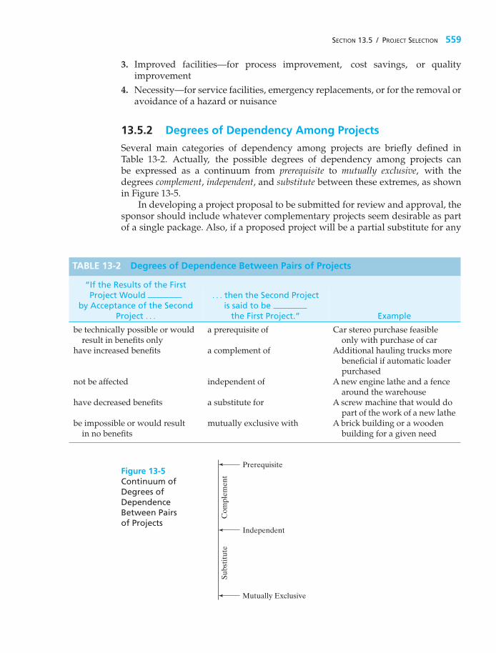
SECTION 13.5 / PROJECT SELECTION 559

3. Improved facilities—for process improvement, cost savings, or qualityimprovement

4. Necessity—for service facilities, emergency replacements, or for the removal oravoidance of a hazard or nuisance

13.5.2 Degrees of Dependency Among Projects

Several main categories of dependency among projects are briefly defined inTable 13-2. Actually, the possible degrees of dependency among projects canbe expressed as a continuum from prerequisite to mutually exclusive, with thedegrees complement, independent, and substitute between these extremes, as shownin Figure 13-5.

In developing a project proposal to be submitted for review and approval, thesponsor should include whatever complementary projects seem desirable as partof a single package. Also, if a proposed project will be a partial substitute for any

TABLE 13-2 Degrees of Dependence Between Pairs of Projects

“If the Results of the FirstProject Would

by Acceptance of the SecondProject . . .

. . . then the Second Projectis said to be

the First Project.” Example

be technically possible or wouldresult in benefits only

a prerequisite of Car stereo purchase feasibleonly with purchase of car

have increased benefits a complement of Additional hauling trucks morebeneficial if automatic loaderpurchased

not be affected independent of A new engine lathe and a fencearound the warehouse

have decreased benefits a substitute for A screw machine that would dopart of the work of a new lathe

be impossible or would resultin no benefits

mutually exclusive with A brick building or a woodenbuilding for a given need

Figure 13-5Continuum ofDegrees ofDependenceBetween Pairsof Projects

Prerequisite

Independent

Com

plem

ent

Subs

titu

te

Mutually Exclusive

560 CHAPTER 13 / THE CAPITAL BUDGETING PROCESS

projects to which the firm is already committed or that are under consideration,this fact should be noted in the proposal.

For cases in which choices involved in planning a proposed project are con-sidered sufficiently important that the final decision should be made by higherlevels of management, the project proposal should be submitted in the form of aset of mutually exclusive alternatives. For example, if it is to be decided whetherto move a plant to a new location and several alternative sites are possible, thenseparate proposals should be made for each site so as to facilitate the choice ofwhich site, if any, should be chosen.

Whenever capital budgeting decisions involve several groups of mutually ex-clusive projects and independent projects to be considered within capital avail-ability constraints, the mathematical programming models presented later in thischapter can be useful for selecting the optimal combination of projects.

13.5.3 Organization for Capital Planning and Budgeting

In most large organizations, project selections are accomplished by sequentialreview through various levels of the organization. The levels required for approvalshould depend on the nature and importance of the individual project, as well ason the particular organizational makeup of the firm. In general, a mix of centralcontrol and coordination, together with authority to make project commitmentsdelegated to operating divisions, is considered desirable. Three typical basic plansfor delegating investment decisions are as follows:

1. Whenever proposals are clearly good in terms of economic desirability accord-ing to operating division analysis, the division is given the power to commit, aslong as appropriate controls can be maintained over the total amount investedby each division and as long as the division analyses are considered reliable.

2. Whenever projects represent the execution of policies already established byheadquarters, such as routine replacements, the division is given the power tocommit within the limits of appropriate controls.

3. Whenever a project requires a total commitment of more than a certain amount,this request is sent to higher levels within the organization. This is often coupledwith a budget limitation regarding the maximum total investment that a divisionmay undertake in a budget period.

To illustrate the concept of larger investments requiring higher administrativeapproval, the limitations for a small-sized firm might be as follows:

If the Total Investment Is . . .Then Approval Is

More Than But Less Than Required Through

$50 $5,000 Plant manager5,000 50,000 Division vice president

50,000 125,000 President125,000 — Board of directors

SECTION 13.6 / POSTMORTEM REVIEW 561

13.5.4 Communication

The importance of effective communication of capital investment proposals is oftenoverlooked. No matter how great are the merits of a proposed project, if thosemerits are not communicated to the decision maker(s) in understandable terms,with emphasis on the proper matters, that proposal may well be rejected in favorof less desirable, though better communicated, proposals. Klausner∗ providesgood insight into this problem, with emphasis on the differing perspectivesof engineers responsible for technical design and proposal preparation andthe management decision makers responsible for monitoring the firm’s capitalresources. The proposal preparer should be as aware as possible of the decisionmaker’s perspective and related informational needs. For example, in addition tobasic information such as investment requirements, measures of merit, and otherexpected benefits, the decision maker may well want clearly presented answers tosuch questions as the following:

1. What bases and assumptions were used for estimates?2. What level of confidence does the proposer have regarding these estimates?3. How would the investment outcome be affected by variations in these estimated

values?

If project proposals are to be transmitted from one organizational unit toanother for review and approval, there must be effective means for communi-cation. The means can vary from standard forms to personal appearances. Incommunicating proposals to higher levels, it is desirable to use a format that is asstandardized as possible to help assure uniformity and completeness of evaluationefforts. In general, the technical and marketing aspects of each proposal should becompletely described in a format that is most appropriate to each individual case.The financial implications of all proposals, however, should be summarized in astandardized manner so that they may be uniformly evaluated.

13.6 Postmortem ReviewThe provision of a system for periodic postmortem reviews (postaudits) of the per-formance of consequential projects previously authorized is an important aspect ofa capital budgeting system. That is, the earnings or costs actually realized on eachsuch project undertaken should be compared with the corresponding quantitiesestimated at the time the project investment was committed.

This kind of feedback review serves at least three main purposes, as follows:

1. It determines if planned objectives have been obtained.2. It determines if corrective action is required.3. It improves estimating and future planning.

∗ R. F. Klausner, “Communicating Investment Proposals to Corporate Decision Makers,” The Engineering Economist,17, no. 1 (Fall 1971): 45–55.

562 CHAPTER 13 / THE CAPITAL BUDGETING PROCESS

Postmortem reviews should tend to reduce biases in favor of what individualdivisions or units preparing project proposals see as their own interests. Whendivisions of a firm have to compete with each other for available capital funds,there is a tendency for them to evaluate their proposals optimistically. Estimatingresponsibilities can be expected to be taken more seriously when the estimatorsknow that the results of their estimates will be checked. This checking function,however, should not be overexercised, for there is a human tendency to becomeoverly conservative in estimating when one fears severe accountability forunfavorable results.

It should be noted that a postmortem audit is inherently incomplete. That is,if only one of several alternative projects is selected, it can never be known exactlywhat would have happened if one of the other alternatives had been chosen. Whatmight have been if . . . is at best conjecture, and all postmortem audits should be madewith this reservation in proper perspective.

13.7 Budgeting of Capital Investmentsand Management Perspective

The approved capital budget is limited typically to a one- or two-year period orless, but this should be supplemented by a long-range capital plan, with provisionfor continual review and change as new developments occur. The long-range plan(or plans) can be for a duration of 2 to 20 years, depending on the nature of thebusiness and the desire of the management to force preplanning.

Even when the technological and market factors in the business are so change-able that plans are no more than guesses to be continually revised, it is valuableto plan and budget as far ahead as possible. Planning should encourage thesearch for investment opportunities, provide a basis for adjusting other aspectsof management of the firm as needed, and sharpen management’s forecastingabilities. Long-range budget plans also provide a better basis for establishingminimum rate of return figures that properly take into account future investmentopportunities.

An aspect of capital budgeting that is difficult and often important is decidinghow much to invest now as opposed to later. If returns are expected to increasefor future projects, it may be profitable to withhold funds from investment forsome time. The loss of immediate return, of course, must be balanced against theanticipation of higher future returns.

In a similar vein, it may be advantageous to supplement funds available forpresent projects whenever returns for future projects are expected to become lessthan those for present projects. Funds for present investment can be supplementedby the reduction of liquid assets, the sale of other assets, and the use of borrowedfunds.

The procedures and practices discussed in this book are intended to aidmanagement in making sound investment decisions. Management’s ability to sense

SECTION 13.8 / LEASING DECISIONS 563

the opportunities for growth and development and to time their investments toachieve optimum advantage is a primary ingredient of success for an organization.

13.8 Leasing DecisionsLeasing of assets is a business arrangement that makes assets available withoutincurring initial capital investment costs of purchase. By the term lease, we normallyare referring to the financial type of lease; that is, a lease in which the firm has alegal obligation to continue making payments for a well-defined period of time forwhich it has use, but not ownership, of the asset(s) leased. Financial leases usuallyhave fixed durations of at least one year. Many financial leases are very similar todebt and should be treated in essentially the same manner as debt. A significantproportion of assets in some firms is acquired by leasing, thus making the firm’scapital available for other uses. Buildings, railroad cars, airplanes, productionequipment, and business machines are examples of the wide array of facilitiesthat may be leased.∗

Lease specifications are generally detailed in a formal written contract. Thecontract may contain such specifications as the amount and timing of rentalpayments; cancellability and sublease provisions, if any; subsequent purchaseprovisions; and lease renewability provisions.

Although the financial lease provides an important alternative source of capital,it carries with it certain subtle, but important, disadvantages. Its impact is similarto that of added debt capital. The acquisition of financial leases or debt capitalwill reduce the firm’s ability to attract further debt capital and will increase thevariability (leverage) in prospective earnings on equity (owner) capital. Higherleverage results in more fixed charges for debt interest and repayment and thuswill make good conditions even better and poor conditions even worse for theequity owners.

Figure 13-6 depicts the types of analyses that should be made for lease-related decisions and also shows what conclusion (final choice) should be madefor various combinations of conditions (analysis outcomes). The buy versus statusquo (do nothing) decision is to determine long-run economy or feasibility and issometimes referred to as an equipment decision. In general practice, only if thisis investigated and buy is found to be preferable should one be concerned withthe buy versus lease question, which is considered a financing decision. We cannot,however, always separate the equipment and financing decisions. For example, ifthe equipment decision results in status quo being preferable and yet it is possiblethat the equipment might be favorable if leased, then we should compare statusquo with lease. This, by definition, is a mixed decision involving both equipment andfinancing considerations.

The main point one should retain from the preceding is that one should notmerely compare buy versus lease alternatives; one should also compare, if possible,

∗ So-called leases with an option to buy are treated as conditional sales contracts and are not considered to be truefinancial leases.

564 CHAPTER 13 / THE CAPITAL BUDGETING PROCESS

StatusQuo

(But Equipment Might Possibly BeFavorable If Leased)

StatusQuo

Buyversus

Status Quo

BuyversusLease

Buy

Buy

Lease

Lease

Leaseversus

Status Quo

Lease

Lease

StatusQuo

Buy

Mix

ed D

ecis

ion

Equ

ipm

ent

Dec

isio

nFi

nanc

ing

Dec

isio

nFi

nal C

hoic

e(d

ecis

ion)

Condition(combination

of choice)A B C D

Figure 13-6 Separability of Buy versus Lease versus Status Quo Decisions,and the Choices that Should Result

against the status quo alternative to determine whether the asset is justified underany financing plan.

A major factor in evaluating the economics of leasing versus buying is the taxdeductions (reductions in taxable income) allowable. In the case of leasing, oneis allowed to deduct the full cost of normal financial lease payments. In the caseof buying (ownership), only depreciation charges and interest payments, if any,are deductible. Of course, other disbursements for operating the property are taxdeductible under either financing plan.

EXAMPLE 13-4 After-Tax Analysis: Buy, Lease, or Status Quo

Suppose a firm is considering purchasing equipment for $200,000 that would lastfor five years and have zero market value. Alternatively, the same equipmentcould be leased for $52,000 at the beginning of each of those five years. Theeffective income tax rate for the firm is 55% and straight-line depreciationis used. The net before-tax cash benefits from the equipment are $56,000 atthe end of each year for five years. If the after-tax MARR for the firm is 10%,use the PW method to show whether the firm should buy, lease, or maintain thestatus quo.

SECTION 13.9 / CAPITAL ALLOCATION 565

Solution

(A) (B) (C) = (A) − (B) (D) = −0.55(C) (E) = (A) + (D)

Alternative YearBefore-taxCash Flow Depreciation

TaxableIncome

Cash Flow ForIncome Taxes

After-taxCash Flow

Buy{

01–5

−$200,000−$40,000 −$40,000 +$22,000

−$200,000+22,000

Lease{

01–4

−52,000−52,000

−52,000−52,000

+28,600+28,600

− 23,400− 23,400

Status quo {1–5 −56,000 −56,000 +30,800 − 25,200

Thus, the PWs (after taxes) for the three alternatives are as follows:

Buy: −$200,000 + $22,000(P/A, 10%, 5) = −$116,600.Lease: −$23,400 − $23,400(P/A, 10%, 4) = −$97,600.Status quo: −$25,200(P/A, 10%, 5) = −$95,500.

If the sequence of analysis follows that in Figure 13-6, we would first comparebuy (PW = −$116,600) against status quo (PW = −$95,500) and find the statusquo to be better. Then we would compare lease (PW = −$97,600) against statusquo (PW = −$95,500) and find the status quo to be better. Thus, status quo is thebetter final choice. It should be noted that, had we merely compared buy versuslease, lease would have been the choice. But the final decision should not havebeen made without comparison against status quo.

Another way the problem could have been solved would have been to includethe +$56,000 before-tax cash benefits with both the buy and the lease alternatives.Then the two alternatives being considered would have been buy rather than statusquo (PW = −$116,600 + $95,500 = −$21,100) and lease rather than status quo(PW = −$97,600 + $95,500 = −$2,100). Of these alternatives, lease rather thanstatus quo is the better, but lease is still not justified because of the negative PW,indicating that the costs of lease are greater than the benefits.

13.9 Capital AllocationThis section examines the capital expenditure decision-making process, alsoreferred to as capital allocation. This process involves the planning, evaluation, andmanagement of capital projects. In fact, much of this book has dealt with conceptsand techniques required to make correct capital-expenditure decisions involvingengineering projects. Now our task is to place them in the broader context of uppermanagement’s responsibility for proper planning, measurement, and control of thefirm’s overall portfolio of capital investments.

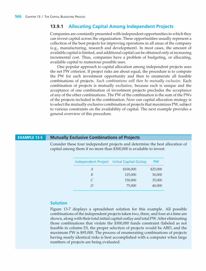
566 CHAPTER 13 / THE CAPITAL BUDGETING PROCESS

13.9.1 Allocating Capital Among Independent Projects

Companies are constantly presented with independent opportunities in which theycan invest capital across the organization. These opportunities usually represent acollection of the best projects for improving operations in all areas of the company(e.g., manufacturing, research and development). In most cases, the amount ofavailable capital is limited, and additional capital can be obtained only at increasingincremental cost. Thus, companies have a problem of budgeting, or allocating,available capital to numerous possible uses.

One popular approach to capital allocation among independent projects usesthe net PW criterion. If project risks are about equal, the procedure is to computethe PW for each investment opportunity and then to enumerate all feasiblecombinations of projects. Such combinations will then be mutually exclusive. Eachcombination of projects is mutually exclusive, because each is unique and theacceptance of one combination of investment projects precludes the acceptanceof any of the other combinations. The PW of the combination is the sum of the PWsof the projects included in the combination. Now our capital allocation strategy isto select the mutually exclusive combination of projects that maximizes PW, subjectto various constraints on the availability of capital. The next example provides ageneral overview of this procedure.

EXAMPLE 13-5 Mutually Exclusive Combinations of Projects

Consider these four independent projects and determine the best allocation ofcapital among them if no more than $300,000 is available to invest:

Independent Project Initial Capital Outlay PW

A $100,000 $25,000

B 125,000 30,000

C 150,000 35,000

D 75,000 40,000

SolutionFigure 13-7 displays a spreadsheet solution for this example. All possiblecombinations of the independent projects taken two, three, and four at a time areshown, along with their total initial capital outlay and total PW.After eliminatingthose combinations that violate the $300,000 funds constraint (labeled as notfeasible in column D), the proper selection of projects would be ABD, and themaximum PW is $95,000. The process of enumerating combinations of projectshaving nearly identical risks is best accomplished with a computer when largenumbers of projects are being evaluated.

SECTION 13.9 / CAPITAL ALLOCATION 567

= B4 + B5

= B3 + B5

= B3 + B4

= B2 + B5

= B2 + B4

= B2 + B3

= B2 + B3 + B4 + B5

= B2 + B3 + B5

= B3 + B4 + B5

= B2 + B4 + B5

= B2 + B3 + B4

= IF(B11<=$B$7, C11, "not feasible")

= IF(D11=MAX($D$11:$D$21), "<<Optimal","")

Figure 13-7 Spreadsheet Solution, Example 13-5

13.9.2 Linear Programming Formulations of CapitalAllocation Problems

For large numbers of independent or interrelated investments, the “brute force”enumeration and evaluation of all combinations of projects, as illustrated inExample 13-5, is impractical. This section describes a mathematical procedurefor efficiently determining the optimal portfolio of projects in industrial capitalallocation problems (Figure 13-1). Only the formulations of these problems willbe presented in this section; their solution is beyond the scope of this book.

Suppose that the goal of a firm is to maximize its net PW by adopting a capitalbudget that includes a large number of mutually exclusive combinations of projects.When the number of possible combinations becomes fairly large, manual methodsfor determining the optimal investment plan tend to become complicated and timeconsuming, and it is worthwhile to consider linear programming as a solutionprocedure. Linear programming is a mathematical procedure for maximizing (orminimizing) a linear objective function, subject to one or more linear constraintequations. Hopefully, the reader will obtain some feeling for how more involvedproblems might also be modeled.

568 CHAPTER 13 / THE CAPITAL BUDGETING PROCESS

Linear programming is a useful technique for solving certain types of multi-period capital allocation problems when a firm is not able to implement all projects thatmay increase its PW. For example, constraints often exist on how much investmentcapital can be committed during each fiscal year, and interdependencies amongprojects may affect the extent to which projects can be successfully carried outduring the planning period.

The objective function of the capital allocation problem can be written as

Maximize net PW =m∑

j=1

B∗j Xj,

where B∗j = net PW of investment opportunity (project) j during the planning

period being considered;Xj = fraction of project j that is implemented during the planning period

(Note: In most problems of interest, Xj will be either zero or one;the Xj values are the decision variables);

m = number of mutually exclusive combinations of projects underconsideration.

In computing the net PW of each mutually exclusive combination of projects, aMARR must be specified.

The following notation is used in writing the constraints for a linearprogramming model:

ckj = cash outlay (e.g., initial capital investment or annual operating budget)required for project j in time period k;

Ck = maximum cash outlay that is permissible in time period k.

Typically, two types of constraints are present in capital budgeting problems:

1. Limitations on cash outlays for period k of the planning horizon,m∑

j=1

ckjXj ≤ Ck .

2. Interrelationships among the projects. The following are examples:(a) If projects p, q, and r are mutually exclusive, then

Xp + Xq + Xr ≤ 1.

(b) If project r can be undertaken only if project s has already been selected,then

Xr ≤ Xs or Xr − Xs ≤ 0.

(c) If projects u and v are mutually exclusive and project r is dependent(contingent) on the acceptance of u or v, then

Xu + Xv ≤ 1

and

Xr ≤ Xu + Xv.

SECTION 13.9 / CAPITAL ALLOCATION 569

To illustrate the formulation of linear programming models for capitalallocation problems, Example 13-6 and Example 13-7 are presented.

EXAMPLE 13-6 Linear Programming Formulation of the Capital Allocation Problem

Five engineering projects are being considered for the upcoming capital budgetperiod. The interrelationships among the projects and the estimated net cashflows of the projects are summarized in the following table:

Cash Flow ($000s)for End of Year k

PW ($000s) atProject 0 1 2 3 4 MARR = 10% per year

B1 −50 20 20 20 20 13.4B2 −30 12 12 12 12 8.0C1 −14 4 4 4 4 −1.3C2 −15 5 5 5 5 0.9D −10 6 6 6 6 9.0

Projects B1 and B2 are mutually exclusive. Projects C1 and C2 are mutuallyexclusive and dependent on the acceptance of B2. Finally, project D is dependenton the acceptance of C1.

Using the PW method, and assuming that MARR = 10% per year, determinewhich combination (portfolio) of projects is best if the availability of capital islimited to $48,000.

SolutionThe objective function and constraints for this problem are written as follows:Maximize

Net PW = 13.4XB1 + 8.0XB2 − 1.3XC1 + 0.9XC2 + 9.0XD,

subject to

50XB1 + 30XB2 + 14XC1 + 15XC2 + 10XD ≤ 48;

(constraint on investment funds)

XB1 + XB2 ≤ 1;

(B1 and B2 are mutually exclusive)

XC1 + XC2 ≤ XB2;

(C1 or C2 is contingent on B2)

XD ≤ XC1;

(D is contingent on C1)

Xj = 0 or 1 for j = B1, B2, C1, C2, D.

(No fractional projects are allowed.)

570 CHAPTER 13 / THE CAPITAL BUDGETING PROCESS

A problem such as this could be solved readily by using the simplex methodof linear programming if the last constraint (Xj = 0 or 1) were not present. Withthat constraint included, the problem is classified as a linear integer programmingproblem. (Many computer programs are available for solving large linear integerprogramming problems.)

EXAMPLE 13-7 Another Linear Programming Formulation

Consider a three-period capital allocation problem having the net cash-flowestimates and PW values shown in Table 13-3. MARR is 12% per year, andthe ceiling on investment funds available is $1,200,000. In addition, there isa constraint on operating funds for support of the combination of projectsselected—$400,000 in year one. From these constraints on funds outlays and the

TABLE 13-3 Project Interrelationships and PW Values

Net Cash Flow ($000s), Net PW ($000s)Project End of Yeara at 12% per yearb

0 1 2 3

150 150 150−225 (60) (70) (70) +135.3A1

A2A3

⎫⎬⎭ mutually exclusive

200 180 160−290 (180) (80) (80) +146.0

210 200 200−370 (290) (170) (170) +119.3

B1B2

}independent

100 400 500−600 (100) (200) (300) +164.1

500 600 600−1,200 (250) (400) (400) +151.9

70 70 70

C1C2C3

⎫⎬⎭

mutually exclusive anddependent on acceptanceof A1 or A2

−160 (80) (50) (50) +8.1

90 80 60−200 (65) (65) (65) −13.1

90 95 100−225 (100) (60) (70) +2.3

a Estimates in parentheses are annual operating expenses (which have already been subtracted in thedetermination of net cash flows).b For example, net PW for A1 = −$225,000 + $150,000(P/A, 12%, 3) = +$135,300.

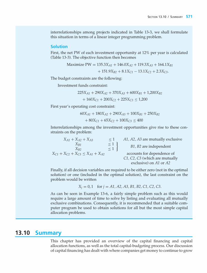
SECTION 13.10 / SUMMARY 571

interrelationships among projects indicated in Table 13-3, we shall formulatethis situation in terms of a linear integer programming problem.

SolutionFirst, the net PW of each investment opportunity at 12% per year is calculated(Table 13-3). The objective function then becomes

Maximize PW = 135.3XA1 + 146.0XA2 + 119.3XA3 + 164.1XB1

+ 151.9XB2 + 8.1XC1 − 13.1XC2 + 2.3XC3.

The budget constraints are the following:

Investment funds constraint:

225XA1 + 290XA2 + 370XA3 + 600XB1 + 1,200XB2

+ 160XC1 + 200XC2 + 225XC3 ≤ 1,200

First year’s operating cost constraint:

60XA1 + 180XA2 + 290XA3 + 100XB1 + 250XB2

+ 80XC1 + 65XC2 + 100XC3 ≤ 400

Interrelationships among the investment opportunities give rise to these con-straints on the problem:

XA1 + XA2 + XA3 ≤ 1 A1, A2, A3 are mutually exclusiveXB1XB2

≤ 1≤ 1

}B1, B2 are independent

XC1 + XC2 + XC3 ≤ XA1 + XA2 accounts for dependence ofC1, C2, C3 (which are mutually

exclusive) on A1 or A2

Finally, if all decision variables are required to be either zero (not in the optimalsolution) or one (included in the optimal solution), the last constraint on theproblem would be written

Xj = 0, 1 for j = A1, A2, A3, B1, B2, C1, C2, C3.

As can be seen in Example 13-6, a fairly simple problem such as this wouldrequire a large amount of time to solve by listing and evaluating all mutuallyexclusive combinations. Consequently, it is recommended that a suitable com-puter program be used to obtain solutions for all but the most simple capitalallocation problems.

13.10 SummaryThis chapter has provided an overview of the capital financing and capitalallocation functions, as well as the total capital-budgeting process. Our discussionof capital financing has dealt with where companies get money to continue to grow

572 CHAPTER 13 / THE CAPITAL BUDGETING PROCESS

and prosper and the costs to obtain this capital. Also included was a discussion ofthe weighted average cost of capital. In this regard, differences between debt capitaland owner’s (equity) capital were made clear. Leasing, as a source of capital, wasalso described, and a lease-versus-purchase example was analyzed.

Our treatment of capital allocation among independent investment oppor-tunities has been built on two important observations. First, the primary concernin capital expenditure activity is to ensure the survival of the company byimplementing ideas to maximize future shareholder wealth, which is equivalentto maximization of shareholder PW. Second, engineering economic analysis playsa vital role in deciding which projects are recommended for funding approval andincluded in a company’s overall capital investment portfolio.

ProblemsThe number in parentheses that follows each problemrefers to the section from which the problem is taken.

13-1. In 2015, a firm has receipts of $8 million andexpenses (excluding depreciation) of $4 million. Itsdepreciation for 2015 amounts to $2 million. If theeffective income tax rate is 40%, what is this firm’s netoperating income after taxes (NOPAT)? (13.2)

13-2. The Caterpillar Company has a beta (a measure ofcommon stock volatility) of 1.28. What is its estimatedcost of equity capital based on the CAPM when therisk-free interest rate is 2.5%? (13.3)

13-3. Refer to the associated graph. Identify when theWACC approach to project acceptability agrees withthe CAPM approach. When do recommendations ofthe two approaches differ? Explain why. (13.3)

0.30

0.25

0.20

0.15

0.10

0.05

0 1.0�

2.0 3.0

A

B

D

C WACC

CAPM RequiredRate of Return

Rat

e of

Ret

urn

RM � 10%

13-4. A firm is considering a capital investment.The risk premium is 0.04, and it is considered tobe constant through time. Riskless investments maynow be purchased to yield 0.06 (6%). If the project’sbeta (β) is 1.5, what is the expected return for thisinvestment? (13.3)

13-5. The price to earnings (P/E) ratio is an after-taxmetric reflecting growth potential of the common stockof a corporation. P is the selling price (per share) ofthe common stock, and E is the after-tax earnings peryear of a share of stock. A high P/E ratio, for example,indicates that a firm is in a high-growth industry (suchas biotechnology) and that annual earnings are not asimportant to investors as the growth rate of the price ofcommon stock is. Because a corporation can be assumedto have an indefinitely long life, the P/E ratio can belikened to the (P/A, i′%, N) factor when N approachesinfinity. For a certain transportation company, the P/Eratio is 12. What is the implied IRR for this relativelystable company? (13.3)

13-6. Explain the various degrees of dependencyamong two or more projects. If one or more projectsseem desirable and are complementary to a givenproject, should those complementary projects beincluded in a proposal package or kept separate forreview by management? (13.5)

13-7. A four-year-old truck has a present net realizablevalue of $6,000 and is now expected to have a marketvalue of $1,800 after its remaining three-year life. Itsoperating disbursements are expected to be $720 peryear.

An equivalent truck can be leased for $0.40 per mileplus $30 a day for each day the truck is kept. Theexpected annual utilization is 3,000 miles and 30 days.If the before-tax MARR is 15%, find which alternativeis better by comparing before-tax equivalent annualcosts

a. using only the preceding information (13.8);

b. using further information that the annual cost ofhaving to operate without a truck is $2,000. (13.8)

PROBLEMS 573

13-8. Work Problem 13-7 by comparing after-tax equi-valent PWs if the effective income tax rate is 40%,the present book value is $5,000, and the depreciationcharge is $1,000 per year if the firm continues to own thetruck. Any gains or losses on disposal of the old truckaffect taxes at the full 40% rate, and the after-tax MARRis 5%. (13.8)

13-9. A lathe costs $56,000 and is expected to result innet cash inflows of $20,000 at the end of each year forthree years and then have a market value of $10,000at the end of the third year. The equipment could beleased for $22,000 a year, with the first payment dueimmediately. (13.8)

a. If the organization does not pay income taxes andits MARR is 10%, show whether the organizationshould lease or purchase the equipment.

b. If the lathe is thought to be worth only, say, $18,000per year to the organization, what is the bettereconomic decision?

13-10. The Shakey Company can finance the purchaseof a new building costing $2 million with a bond issue,for which it would pay $100,000 interest per year, andthen repay the $2 million at the end of the life of thebuilding. Instead of buying in this manner, the companycan lease the building by paying $125,000 per year,the first payment being due one year from now. Thebuilding would be fully depreciated for tax purposesover an expected life of 20 years. The income tax rate is40% for all expenses and capital gains or losses, and thefirm’s after-tax MARR is 5%. Use AW analysis based onequity (nonborrowed) capital to determine whether thefirm should borrow and buy or lease if, at the end of20 years, the building has the following market valuesfor the owner: (a) nothing, (b) $500,000. Straight-linedepreciation will be used but is allowable only if thecompany purchases the building. (13.8)

13-11. The Capitalpoor Company is consideringpurchasing a business machine for $100,000. Analternative is to rent it for $35,000 at the beginning ofeach year. The rental would include all repairs andservice. If the machine is purchased, a comparablerepair and service contract can be obtained for $1,000per year.

The salesperson of the business machine firm hasindicated that the expected useful service life of thismachine is five years, with zero market value, but thecompany is not sure how long the machine will actuallybe needed. If the machine is rented, the company cancancel the lease at the end of any year. Assuming an

income tax rate of 25%, a straight-line depreciationcharge of $20,000 for each year the machine is kept,and an after-tax MARR of 10%, prepare an appropriateanalysis to help the firm decide whether it is moredesirable to purchase or rent. (13.8)

13-12. A firm is considering the development of severalnew products. The products under consideration arelisted in the next table. Products in each group aremutually exclusive. At most, one product from eachgroup will be selected. The firm has a MARR of 10%per year and a budget limitation on development costsof $2,100,000. The life of all products is assumed to be10 years, with no salvage value. Formulate this capitalallocation problem as a linear integer programmingmodel. (13.9)

Group ProductDevelopment

CostAnnual Net Cash

Income

A

{ A1A2A3

$500,000650,000700,000

$90,000110,000115,000

B{

B1B2

600,000675,000

105,000112,000

C{

C1C2

800,0001,000,000

150,000175,000

13-13. Four proposals are under consideration by yourcompany. Proposals A and C are mutually exclusive;proposals B and D are mutually exclusive and cannot beimplemented unless proposal A or C has been selected.No more than $140,000 can be spent at time zero. Thebefore-tax MARR is 15% per year. The estimated cashflows are shown in the accompanying table. Formall mutually exclusive combinations in view of thespecified contingencies, and formulate this problem asa linear integer programming model. (13.9)

End Proposalofyear A B C D

0 −$100,000 −$20,000 −$120,000 −$30,0001 40,000 6,000 25,000 6,0002 40,000 10,000 50,000 10,0003 60,000 10,000 85,000 19,000

13-14. Three alternatives are being considered for anengineering project. Their cash-flow estimates are

574 CHAPTER 13 / THE CAPITAL BUDGETING PROCESS

shown in the accompanying table. A and B aremutually exclusive, and C is an optional add-onfeature to alternative A. Investment funds are limitedto $5,000,000. Another constraint on this project is theengineering personnel needed to design and implementthe solution. No more than 10,000 person-hours ofengineering time can be committed to the project. Setup a linear integer programming formulation of thisresource allocation problem. (13.9)

Alternative

A B C

Initial investment ($106) 4.0 4.5 1.0Personnel requirement 7,000 9,000 3,000

(hours)

Alternative

A B C

After-tax annual 1.3 2.2 0.9savings, years onethrough four ($106)

PW at 10% per year 0.12 2.47 1.85($106)

13-15. Companies obtain the funds needed for capitalinvestments from multiple sources. To evaluate poten-tial projects, the cost of the different sources of capitalmust be accounted for in the interest rate used todiscount cash flows and measure project profitability.Consider a large multinational company with an effec-tive income tax rate of 49.24%. The percentage oflong-term debt in its capital structure is 49%, and itsbefore-tax annual cost is 9.34%. In its capital structure,the firm also has 13% preferred stock paying 8.22% peryear and 38% common equity valued at 16.5% per year.What is the weighted average cost of capital for this firm(after taxes)?

CHAPTER 14

Decision Making ConsideringMultiattributes

The aim of Chapter 14 is to present situations in which a decision makermust recognize and address multiple problem attributes.

The Aftermath of Hurricane Katrina

I n 2005, the city of New Orleans and many areas in Louisiana,Mississippi, and Alabama were devastated by Hurricane Katrina.The cost in lives and property damage was tremendous. Although

there was much finger pointing and time spent determining whom to blame,the biggest questions were how to restore the area and what to do to preventsuch devastation in the future. The answers are not simple. Consider the decisionregarding what to do to prevent this from reoccurring. Of course, cost is a majorelement of the decision, but dollars are not the only consideration. Time is alsoimportant—how quickly can residents get some level of protection? What aboutthe environmental impact of the solution? What about the confidence of theresidents who want to stay and rebuild? In this chapter, we consider how tomake decisions when we take into account the many attributes present in thistype of problem.

575

All models are wrong, some are useful.

—George E.P. Box

14.1 IntroductionAll chapters up to Chapter 14 dealt principally with the assessment of equivalentmonetary worth of competing alternatives and proposals, but few decisions arebased strictly on dollars and cents. In this chapter, our attention is directed at howdiverse nonmonetary considerations (attributes) that arise from multiple objectivescan be explicitly included in the evaluation of engineering and business ventures.By nonmonetary, we mean that a formal market mechanism does not exist in whichvalue can be established for various aspects of a venture’s performance such asaesthetic appeal, employee morale, and environmental enhancement.

Value is difficult to define because it is used in a variety of ways. In fact, in350 bc, Aristotle conceived seven classes of value that are still recognized today:(1) economic, (2) moral, (3) aesthetic, (4) social, (5) political, (6) religious, and(7) judicial. Of these classes, only economic value (hopefully) can be measured interms of objective monetary units such as dollars, yen, or euros. Economic value,however, is also established through an item’s use value (properties that providea unit of use, work, or service) and esteem value (properties that make somethingdesirable). In highly simplified terms, we can say that use values cause a product toperform (e.g., a car serves as a reliable means of transportation), and esteem valuescause it to sell (e.g., a convertible automobile has a look of sportiness). Use valueand esteem value defy precise quantification in monetary terms, so we often resortto multiattribute techniques for evaluating the total value of complex designs andcomplicated systems.

14.2 Examples of Multiattribute DecisionsA common situation encountered by a new engineering graduate is selecting hisor her first permanent professional job. Suppose that Mary Jones, a 22-year-oldgraduate engineer, is fortunate enough to have four acceptable job offers in writing.A choice among the four offers must be made within the next four weeks or theybecome void. She is not sure which offer to accept, but she decides to base herchoice on these four important factors or attributes (not necessarily listed in theirorder of importance to her): (1) social climate of the town in which she will beworking, (2) the opportunity for outdoor sports, (3) starting salary, and (4) potentialfor promotion and career advancement. Mary Jones next forms a table and fills itin with objective and subjective data relating to differences among the four offers.

576

SECTION 14.2 / EXAMPLES OF MULTIATTRIBUTE DECISIONS 577

The completed table (or matrix) is shown as Table 14-1. Notice that three attributesare rated subjectively on a scale ranging from poor to excellent.

It is not uncommon for monetary and nonmonetary data to be key ingredientsin decision situations such as this rather elementary one. Take a minute or two toponder which offer you would accept, given only the data in Table 14-1. Wouldstarting salary dominate all other attributes, so that your choice would be the ApexCorporation in New York? Would you try to trade off poor social climate againstexcellent career advancement in Flagstaff to make the McGraw-Wesley offer yourtop choice?

Many decision problems in industry can be reduced to matrix form similar tothat of the foregoing job selection example. To illustrate the wide applicability ofsuch a tabular summary of data, consider a second example involving the choiceof a computer-aided design (CAD) workstation by an architectural engineeringfirm. The data are summarized in Table 14-2. Three vendors and do nothingcompose the list of feasible alternatives (choices) in this decision problem, and atotal of seven attributes is judged sufficient for purposes of discriminating amongthe alternatives. Aside from the question of which workstation to select, othersignificant questions come to mind in multiattribute decision making: (1) How arethe attributes chosen in the first place? (2) Who makes the subjective judgmentsregarding nonmonetary attributes such as quality or operating flexibility?(3) What response is required—a partitioning of alternatives or a rank-ordering ofalternatives, for instance? Several simple, though workable and credible, modelsfor selecting among alternatives such as those in Tables 14-1 and 14-2 are describedin this chapter.

TABLE 14-1 Job Offer Selection Problem

Alternative (Offers and Locations)

Apex Corp., Sycon, Inc., Sigma Ltd., McGraw-Wesley,Attribute New York Los Angeles Macon, GA Flagstaff, AZ

Social climate Good Good Fair PoorWeather/outdoor sports Poor Excellent Good Very goodStarting salary (per annum) $50,000 $45,000 $49,500 $46,500Career advancement Fair Very good Good Excellent

TABLE 14-2 CAD Workstation Selection Problem

Alternative

ReferenceAttribute Vendor A Vendor B Vendor C (“Do Nothing”)

Cost of purchasing the system $115,000 $338,950 $32,000 $0Reduction in design time 60% 67% 50% 0Flexibility Excellent Excellent Good PoorInventory control Excellent Excellent Excellent PoorQuality Excellent Excellent Good FairMarket share Excellent Excellent Good FairMachine utilization Excellent Excellent Good Poor

578 CHAPTER 14 / DECISION MAKING CONSIDERING MULTIATTRIBUTES

14.3 Choice of AttributesThe choice of attributes used to judge alternative designs, systems, products,processes, and so on is one of the most important tasks in multiattribute decisionanalysis. (The most important task, of course, is to identify the feasible alternativesfrom which to select.) The articulation of attributes for a particular decision can, insome cases, shed enough light on the problem to make the final choice obvious.

Consider again the data in Tables 14-1 and 14-2. Some general observationsregarding the attributes used to discriminate among alternatives can immediatelybe made: (1) each attribute distinguishes at least two alternatives—in no caseshould identical values for an attribute apply to all alternatives; (2) each attributecaptures a unique dimension or facet of the decision problem (i.e., attributesare independent and nonredundant); (3) all attributes, in a collective sense, areassumed to be sufficient for the purpose of selecting the best alternative; and(4) differences in values assigned to each attribute are presumed to be meaningfulin distinguishing among feasible alternatives.

Selecting a set of attributes is usually the result of group consensus and is clearlya subjective process. The final list of attributes, both monetary and nonmonetary, isheavily influenced by the decision problem at hand, as well as by an intuitive feelfor which attributes will or will not pinpoint relevant differences among feasiblealternatives. If too many attributes are chosen, the analysis will become unwieldy,unreliable, and difficult to manage. Too few attributes, on the other hand, will limitdiscrimination among alternatives. Again, judgment is required to decide whatnumber is too few or too many. If some attributes in the final list lack specificityor cannot be quantified, it will be necessary to subdivide them into lower-levelattributes that can be measured.

To illustrate these points, we might consider adding an attribute calledcost of operating and maintaining the system in Table 14-2 to capture a vitaldimension of the CAD system’s life-cycle cost. The attribute flexibility shouldperhaps be subdivided into two other, more specific attributes such as abilityto communicate with computer-aided manufacturing equipment (such as numericallycontrolled machine tools) and ability to create and analyze solid geometry representationsof engineering design concepts. Finally, it would be constructive to aggregate twoattributes in Table 14-2, namely quality and market share. Because there is nodifference in the values assigned to these two attributes across the four alternatives,they could be combined into a single attribute, possibly named achievement of greatermarket share through quality improvements. But one should take great care in doingthis. If it is possible that a new alternative might have differences in the valuesassigned to these two attributes, then they should be left as they are.

14.4 Selection of a Measurement ScaleIdentifying feasible alternatives and appropriate attributes represents a largeportion of the work associated with multiattribute decision analysis. The nexttask is to develop metrics, or measurement scales, that permit various states ofeach attribute to be represented. For example, in Table 14-1, “dollars” was anobvious choice for the metric of starting salary. A subjective assessment of career

SECTION 14.6 / NONCOMPENSATORY MODELS 579

advancement was made on a metric having the gradations poor, fair, good, verygood, and excellent. In many problems, the metric is simply the scale upon which aphysical measurement is made. For instance, anticipated noise pollution for variousroutings of an urban highway project might be a relevant attribute whose metricis decibels.

14.5 Dimensionality of the ProblemIf you refer once again to Table 14-1, notice that there are two basic ways to processthe information presented there. First, you could attempt to collapse each job offerinto a single metric or dimension. For instance, all attributes could somehow beforced into their dollar equivalents, or they could be reduced to a utility equivalentranging from, say, 0 to 100. Assigning a dollar value to good career advancementmay not be too difficult, but how about placing a dollar value on a poor versus anexcellent social climate? Similarly, translating all job offer data to a scale of worth orutility that ranges from 0 to 100 may not be plausible to most individuals. This firstway of dealing with the data of Table 14-1 is called single-dimension analysis. (Thedimension corresponds to the number of metrics used to represent the attributesthat discriminate among alternatives.)

Collapsing all information into a single dimension is popular in practicebecause a complex problem can be made computationally tractable in this manner.Several useful models presented later are single-dimensioned. Such models aretermed compensatory because changes in the values of a particular attribute can beoffset by, or traded off against, opposing changes in another attribute.

The second basic way to process information in Table 14-1 is to retain theindividuality of the attributes as the best alternative is being determined. That is,there is no attempt to collapse attributes into a common scale. This is referredto as full-dimension analysis of the multiattribute problem. For example, if rattributes have been chosen to characterize the alternatives under consideration,the predicted values for all r attributes are considered in the choice. If a metric iscommon to more than one attribute, as in Table 14-1, we have an intermediate-dimension problem that is analyzed with the same models as a full-dimensionproblem would be. Several of these models are illustrated in the next section, andthey are often most helpful in eliminating inferior alternatives from the analysis.We refer to these models as noncompensatory because trade-offs among attributesare not permissible. Thus, comparisons of alternatives must be judged on anattribute-by-attribute basis.

14.6 Noncompensatory ModelsIn this section, we examine four noncompensatory models for making a choicewhen multiple attributes are present. They are (1) dominance, (2) satisficing,(3) disjunctive resolution, and (4) lexicography. In each model, an attempt is madeto select the best alternative in view of the full dimensionality of the problem.Example 14-1 is presented after the description of these models and will be utilizedto illustrate each.

580 CHAPTER 14 / DECISION MAKING CONSIDERING MULTIATTRIBUTES

14.6.1 Dominance

Dominance is a useful screening method for eliminating inferior alternativesfrom the analysis. When one alternative is better than another with respect toall attributes, there is no problem in deciding between them. In this case, thefirst alternative dominates the second one. By comparing each possible pair ofalternatives to determine whether the attribute values for one are at least as goodas those for the other, it may be possible to eliminate one or more candidates fromfurther consideration or even to select the single alternative that is clearly superiorto all the others. Usually it will not be possible to select the best alternative basedon dominance.

14.6.2 Satisficing

Satisficing, sometimes referred to as the method of feasible ranges, requires theestablishment of minimum or maximum acceptable values (the standard) for eachattribute. Alternatives having one or more attribute values that fall outside theacceptable limits are excluded from further consideration.

The upper and lower bounds of these ranges establish two fictitious alternativesagainst which maximum and minimum performance expectations of feasiblealternatives can be defined. By bounding the permissible values of attributes fromtwo sides (or from one), information processing requirements are substantiallyreduced, making the evaluation problem more manageable.

Satisficing is more difficult to use than dominance because minimum accep-table attribute values must be determined. Furthermore, satisficing is usuallyemployed to evaluate feasible alternatives in more detail and to reduce the numberbeing considered rather than to make a final choice. The satisficing principle isfrequently used in practice when satisfactory performance on each attribute, ratherthan optimal performance, is good enough for decision-making purposes.

14.6.3 Disjunctive Resolution

The disjunctive method is similar to satisficing in that it relies on comparing theattributes of each alternative to the standard. The difference is that the disjunctivemethod evaluates each alternative on the best value achieved for any attribute. If analternative has just one attribute that meets or exceeds the standard, that alternativeis kept. In satisficing, all attributes must meet or exceed the standard in order foran alternative to be kept in the feasible set.

14.6.4 Lexicography

This model is particularly suitable for decision situations in which a single attributeis judged to be more important than all other attributes. A final choice might bebased solely on the most acceptable value for this attribute. Comparing alternativeswith respect to one attribute reduces the decision problem to a single dimension(i.e., the measurement scale of the predominant attribute). The alternative havingthe highest value for the most important attribute is then chosen. When two or morealternatives have identical values for the most important attribute, however, thesecond most important attribute must be specified and used to break the deadlock.

SECTION 14.6 / NONCOMPENSATORY MODELS 581

If ties continue to occur, the analyst examines the next most important attributeuntil a single alternative is chosen or until all alternatives have been evaluated.

Lexicography requires that the importance of each attribute be specified todetermine the order in which attributes are to be considered. If a selection is madeby using one or a few of the attributes, lexicography does not take into account allthe collected data. Lexicography does not require comparability across attributes,but it does process information in its original metric.

EXAMPLE 14-1 Selecting a Dentist by Using Noncompensatory Models

Mary Jones, the engineering graduate whose job offers were given in Table 14-1,has decided, based on comprehensive reasoning, to accept the Sigma positionin Macon, Georgia. (Problem 14-9 will provide insight into why this choicewas made.) Having moved to Macon, Mary now faces several other importantmultiattribute problems. Among them are (1) renting an apartment versuspurchasing a small house, (2) what type of automobile or truck to purchase,and (3) whom to select for long-overdue dental work.

In this example, we consider the selection of a dentist as a means ofillustrating noncompensatory (full-dimensioned) and compensatory (single-dimensioned) models for analyzing multiattribute decision problems.

After calling many dentists she found through online Web sites, Mary findsthat there are only four who are accepting new patients. They are Dr. Molar,Dr. Feelgood, Dr. Whoops, and Dr. Pepper. The alternatives are clear to Mary,and she decides that her objectives in selecting a dentist are to obtain high-qualitydental care at a reasonable cost with minimum disruption to her schedule andlittle (or no) pain involved. In this regard, Mary adopts these attributes to assistin gathering data and making her final choice: (1) reputation of the dentist,(2) cost per hour of dental work, (3) available office hours each week, (4) traveldistance, and (5) method of anesthesia. Notice that these attributes are moreor less independent in that the value of one attribute cannot be predicted byknowing the value of any other attribute.

Mary collects data by interviewing the receptionist in each dental office,talking with local townspeople, calling the Georgia Dental Association, and soon. A summary of information gathered by Mary is presented in Table 14-3.

We are now asked to determine whether a dentist can be selected by using(a) dominance, (b) satisficing, (c) disjunctive resolution, and (d) lexicography.

Solution(a) To check for dominance in Table 14-3, pairwise comparisons of each

dentist’s set of attributes must be inspected. There will be 4(3)/2 = 6pairwise comparisons necessary for the four dentists, and they are shownin Table 14-4. It is clear from Table 14-4 that Dr. Molar dominatesDr. Feelgood, so Dr. Feelgood will be dropped from further consideration.With dominance, it is not possible for Mary to select the best dentist.

582 CHAPTER 14 / DECISION MAKING CONSIDERING MULTIATTRIBUTES

TABLE 14-3 Summary Information for Choice of a Dentist

Alternatives

Attribute Dr. Molar Dr. Feelgood Dr. Whoops Dr. Pepper

Cost ($/hour) $50 $80 $20 $40

Method of anesthesiaa Novocaine Acupuncture Hypnosis Laughing Gas

Driving distance (mi) 15 20 5 30

Weekly office hours 40 25 40 40

Quality of work Excellent Fair Poor Good

Best value Worst valuea Mary has decided that novocaine > laughing gas > acupuncture > hypnosis, where a > b meansthat a is preferred to b.

TABLE 14-4 Check for Dominance Among Alternatives

Paired Comparison

Molar vs. Molar vs. Molar vs. Feelgood Feelgood WhoopsAttribute Feelgood Whoops Pepper vs. Whoops vs. Pepper vs. Pepper

Cost Better Worse Worse Worse Worse BetterAnesthesia Better Better Better Better Worse WorseDistance Better Worse Better Worse Better BetterOffice hours Better Equal Equal Worse Worse EqualQuality Better Better Better Better Worse WorseDominance? Yes No No No No No

(b) To illustrate the satisficing model, acceptable limits (feasible ranges) must beestablished for each attribute. After considerable thought, Mary determinesthe feasible ranges given in Table 14-5.

Comparison of attribute values for each dentist against the feasible rangereveals that Dr. Whoops uses a less desirable type of anesthesia (hypnosis< acupuncture), and his quality rating is also not acceptable (poor < good).Thus, Dr. Whoops joins Dr. Feelgood on Mary’s list of rejects. Notice thatsatisficing, by itself, did not produce the best alternative.

(c) By applying the feasible ranges in Table 14-5 to the disjunctive resolutionmodel, all dentists would be acceptable because each has at least oneattribute value that meets or exceeds the minimum expectation. Forinstance, Dr. Whoops scores acceptably on three out of five attributes, andDr. Feelgood passes two out of five minimum expectations. Clearly, thismodel does not discriminate well among the four candidates.

(d) Many models, including lexicography, require that all attributes first beranked in order of importance. Perhaps the easiest way to obtain a consistent

SECTION 14.6 / NONCOMPENSATORY MODELS 583

TABLE 14-5 Feasible Ranges for Satisficing

Minimum MaximumAcceptable Acceptable

Attribute Value Value Unacceptable Alternative

Cost — $60 None (Dr. Feelgood already eliminated)Anesthesia Acupuncture — Dr. WhoopsDistance (miles) — 30 NoneOffice hours 30 40 None (Dr. Feelgood already eliminated)Quality Good Excellent Dr. Whoops

TABLE 14-6 Ordinal Ranking of Dentists’ Attributes

A. Results of Paired ComparisonsCost > anesthesia (Cost is more important than anesthesia)Quality > cost (Quality is more important than cost)Cost > distance (Cost is more important than distance)Cost > office hours (Cost is more important than office hours)Anesthesia > distance (Anesthesia is more important than distance)Anesthesia > office hours (Anesthesia is more important than office hours)Quality > anesthesia (Quality is more important than anesthesia)Office hours > distance (Office hours are more important than distance)Quality > distance (Quality is more important than distance)Quality > office hours (Quality is more important than office hours)

B. Attribute Number of times on left of > (= Ordinal ranking)Cost 3Anesthesia 2Distance 0Office hours 1Quality 4

ordinal ranking is to make paired comparisons between each possibleattribute combination.∗ This is illustrated in Table 14-6. Each attribute can beranked according to the number of times it appears on the left-hand side ofthe comparison when the preferred attribute is placed on the left as shown.In this case, the ranking is found to be quality > cost > anesthesia > officehours > distance.

Table 14-7 illustrates the application of lexicography to the ordinal rankingdeveloped in Table 14-6. The final choice would be Dr. Molar because quality

∗ An ordinal ranking is simply an ordering of attributes from the most preferred to the least preferred.

584 CHAPTER 14 / DECISION MAKING CONSIDERING MULTIATTRIBUTES

TABLE 14-7 Application of Lexicography

Attribute Ranka Alternative Rankb

Cost 3 Whoops > Pepper > Molar > FeelgoodAnesthesia 2 Molar > Pepper > Feelgood > WhoopsOffice hours 1 Molar = Whoops = Pepper > FeelgoodDistance 0 Whoops > Molar > Feelgood > PepperQuality 4 Molar > Pepper > Feelgood > Whoops

a Rank of 4 = most important, rank of 0 = least important.b Selection is based on the highest-ranked attribute (Whoops and Feelgoodincluded only to illustrate the full procedure).

is the top-ranked attribute, and Molar’s quality rating is the best of all. IfDr. Pepper’s work quality had also been rated as excellent, the choice wouldbe made on the basis of cost. This would have resulted in the selection ofDr. Pepper. Therefore, lexicography does allow the best dentist to be chosenby Mary.

14.7 Compensatory ModelsThe basic principle behind all compensatory models, which involve a singledimension, is that the values for all attributes must be converted to a commonmeasurement scale such as dollars or utiles,∗ from which it is possible to constructan overall dollar index or utility index for each alternative. The form of the functionused to calculate the index can vary widely. For example, the converted attributevalues may be added together, they may be weighted and then added, or they maybe sequentially multiplied. Regardless of the functional form, the end result is thatgood performance in one attribute can compensate for poor performance in another.This allows trade-offs among attributes to be made during the process of selectingthe best alternative. Because lexicography involves no trade-offs, it was classifiedas a full-dimensional model in Section 14.6.4.

In this section, we examine two compensatory models for evaluatingmultiattribute decision problems: nondimensional scaling and the additive weight-ing technique. Each model will be illustrated by using the data of Example 14-1.The interested reader can consult Canada et al. for a discussion of other methods.†

14.7.1 Nondimensional Scaling

Apopular way to standardize attribute values is to convert them to nondimensionalform. There are two important points to consider when doing this. First, the

∗ A utile is a dimensionless unit of worth.† Canada, et al., Capital Investment Decision Analysis for Engineering and Management, 3rd ed. (Upper Saddle River, NJ:Prentice Hall, 2005).

SECTION 14.7 / COMPENSATORY MODELS 585

nondimensional values should all have a common range, such as 0 to 1 or 0 to100. Without this constraint, the dimensionless attributes will contain implicitweighting factors. Second, all of the dimensionless attributes should follow thesame trend with respect to desirability; the most preferred values should be eitherall small or all large. This is necessary in order to have a believable overall scale forselecting the best alternative.

Nondimensional scaling can be illustrated with the data of Example 14-1.As shown in Table 14-8, the preceding constraints may require that differentprocedures be used to remove the dimension from each attribute. For example,a cost-related attribute is best when it is low, but office hours are best when theyare high. The goal should be to devise a procedure that rates each attribute interms of its fractional accomplishment of the best attainable value. Table 14-3, theoriginal table of information for Example 14-1, is restated in dimensionless termsin Table 14-9. The procedure for converting the original data in Table 14-3 for aparticular attribute to its dimensionless rating is

Rating = Worst outcome − Outcome being made dimensionlessWorst outcome − Best outcome

. (14-1)

Equation (14-1) applies when large numerical values, such as cost or drivingdistance, are considered to be undesirable. When large numerical values areconsidered to be desirable (anesthesia, office hours, quality), however, therelationship for converting original data to their dimensionless ratings is

Rating = Outcome being made dimensionless − Worst outcomeBest outcome − Worst outcome

. (14-2)

TABLE 14-8 Nondimensional Scaling for Example 14-1

Attribute Value Rating Procedure Dimensionless Value

Cost $20 (80 − cost)/60 1.040 0.6750 0.5080 0.0

Anesthesia Hypnosis (Relative ranka − 1)/3 0.0Acupuncture 0.33Laughing gas 0.67Novocaine 1.0

Distance 5 (30 − distance)/25 1.015 0.6020 0.4030 0.0

Office hours 25 (Office hours−25)/15 0.040 1.0

Quality Poor (Relative ranka − 1)/3 0.0Fair 0.33Good 0.67Excellent 1.0

a Scale of 1 to 4 is used, 4 being the best (from Table 14-3).

586 CHAPTER 14 / DECISION MAKING CONSIDERING MULTIATTRIBUTES

If all the attributes in Table 14-9 are of equal importance, a score for each dentistcould be found by merely summing the nondimensional values in each column.The results would be Dr. Molar = 4.10, Dr. Feelgood = 1.06, Dr. Whoops = 3.00,and Dr. Pepper = 3.01. Presumably, Dr. Molar would be the best choice in this case.

Figure 14-1 displays a spreadsheet application of the nondimensional scalingprocedure for Example 14-1. The attribute ratings for each alternative are enteredinto the table in the range B2:E6. Next, tables for the qualitative attributes (qualityand method of anesthesia) are entered into conversion tables (A9:B12 and D9:E12).These tables must have the qualitative rating in alphabetical order.

The dimensionless rating for each alternative/attribute combination is deter-mined by comparing the difference between the alternative under considerationwith the lowest scoring alternative. This difference is then divided by the rangebetween the best and worst scoring alternatives to arrive at the nondimensionalvalue. The total score for each alternative is found by summing these values. Theformulas in the highlighted cells in Figure 14-1 are given on the next page.

TABLE 14-9 Nondimensional Data for Example 14-1

Attribute Dr. Molar Dr. Feelgood Dr. Whoops Dr. Pepper

Cost 0.50 0.0 1.0 0.67Method of anesthesia 1.0 0.33 0.0 0.67Driving distance 0.60 0.40 1.0 0.0Weekly office hours 1.0 0.0 1.0 1.0Quality of work 1.0 0.33 0.0 0.67

Figure 14-1 Spreadsheet Solution, Nondimensional Scaling

SECTION 14.7 / COMPENSATORY MODELS 587

Cell Contents

B15 = ABS(B2-MAX($B$2:$E$2))/ABS(MAX($B$2:$E$2)-MIN($B$2:$E$2))B16 = (VLOOKUP(B3,$D$9:$E$12,2)-MIN($E$9:$E$12))/(MAX($E$9:$E$12)

−MIN($E$9:$E$12))B17 = ABS(B4-MAX($B$4:$E$4))/ABS(MAX($B$4:$E$4)-MIN($B$4:$E$4))B18 = ABS(B5-MIN($B$5:$E$5))/ABS(MAX($B$5:$E$5)-MIN($B$5:$E$5))B19 = (VLOOKUP(B6,$A$9:$B$12,2)-MIN($B$9:$B$12))/(MAX($B$9:$B$12)

−MIN($B$9:$B$12))B20 = SUM(B15:B19)B21 = IF(B20 = MAX($B$20:$E$20),”∧ Best Choice”,“”)

14.7.2 The Additive Weighting Technique

Additive weighting provides for the direct use of nondimensional attributes such asthose in Table 14-9 and the results of ordinal ranking as illustrated in Table 14-6. Theprocedure involves developing weights for attributes (based on ordinal rankings)that can be multiplied by the appropriate nondimensional attribute values toproduce a partial contribution to the overall score for a particular alternative. Whenthe partial contributions of all attributes are summed, the resulting set of alternativescores can be used to compare alternatives directly. In the previous section, thesepartial contributions were assumed to be equal, but in this section they can beunequal based on how important they are believed to be.

Attribute weights should be determined in two steps following the completionof ordinal ranking. First, relative weights are assigned to each attribute accordingto its ordinal ranking. The simplest procedure is to use rankings of 1, 2, 3,…, basedon position, with higher numbers signifying greater importance; but one mightalso include subjective considerations by using uneven spacing in some cases. Forinstance, in a case where there are four attributes, two of which are much moreimportant than the others, the top two may be rated as 7 and 5 instead of 4 and 3.The second step is to normalize the relative ranking numbers by dividing eachranking number by the sum of all the rankings. Table 14-10 summarizes thesesteps for Example 14-1 and demonstrates how the overall score for each alternativeis determined.

Additive weighting is probably the most popular single-dimensional methodbecause it includes both the performance ratings and the importance weightsof each attribute when evaluating alternatives. Furthermore, it produces recom-mendations that tend to agree with the intuitive feel of the decision makerconcerning the best alternative. Perhaps its biggest advantage is that removingthe dimension from data and weighting attributes are separated into two distinctsteps. This reduces confusion and allows for precise definition of each of thesecontributions. From Table 14-10, it is apparent that the additive weighting score forDr. Molar (0.84) makes him the top choice as Mary’s dentist.

Figure 14-2 shows a spreadsheet application of the additive weightingtechnique for the dentist selection problem of Example 14-1. The relative rankingof attributes (Table 14-6) is entered in the range B3:B7. These values are normalized(put on a 0–1 scale) in column C. For each alternative, the normalized weight of theattribute is multiplied by the nondimensional attribute value (obtained from the

TABLE 14-10 The Additive Weighting Technique Applied to Example 14-1

Calculation of Weighting Factors Calculation of Scores for Each Alternativeb

Step 2:Step 1: Normalized Dr. Molar Dr. Feelgood Dr. Whoops Dr. Pepper

Attribute Relative Ranka Weight (A) (B) (A) × (B) (B) (A) × (B) (B) (A) × (B) (B) (A) × (B)

Cost 4 4/15 = 0.27 0.50 0.14 0.00 0.00 1.00 0.27 0.67 0.18Anesthesia 3 3/15 = 0.20 1.00 0.20 0.33 0.07 0.00 0.00 0.67 0.13Distance 1 1/15 = 0.07 0.60 0.04 0.40 0.03 1.00 0.07 0.00 0.00Office hours 2 2/15 = 0.13 1.00 0.13 0.00 0.00 1.00 0.13 1.00 0.13Quality 5 5/15 = 0.33 1.00 0.33 0.33 0.11 0.00 0.00 0.67 0.22

Sum = 15 Sum = 1.00 Sum = 0.84 Sum = 0.21 Sum = 0.47 Sum = 0.66

a Based on Table 14-6, relative rank = ordinal ranking + 1. A rank of 5 is best.b Data in column B are from Table 14-9.

588

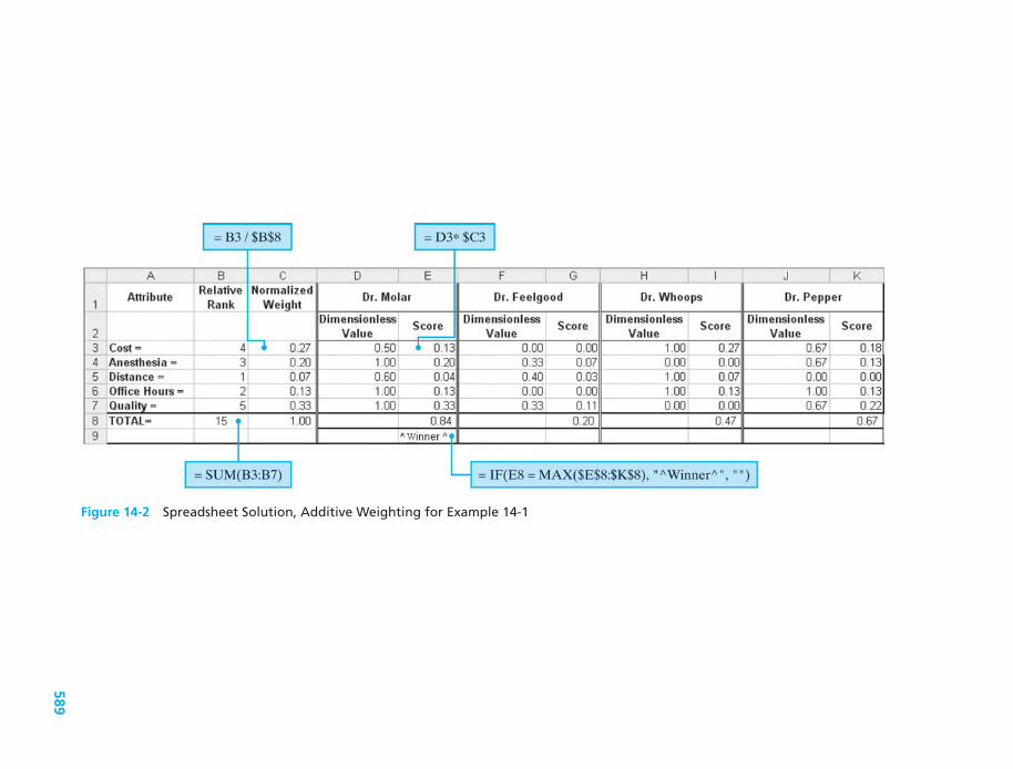
Figure 14-2 Spreadsheet Solution, Additive Weighting for Example 14-1

589

590 CHAPTER 14 / DECISION MAKING CONSIDERING MULTIATTRIBUTES

nondimensional scaling spreadsheet in Figure 14-1) to arrive at a weighted scorefor the attribute. These weighted scores are then summed to arrive at an overallscore for each alternative.

EXAMPLE 14-2 Decision Making in the Aftermath of Hurricane Katrina

Let us revisit Hurricane Katrina. Decisions must be made about how to replacethe flood protection and prevent the type of devastation that occurred. Thesedecisions are based on myriad factors and certainly have many social andpolitical consequences. There is no way to do justice to this type of problem inthis text, but we will examine a fictitious example based on data available inthe popular press (ABC News and Time magazine—www.time.com/time/specials/2007/article/0.28804, 1646611_1646683_1648904-2,00.html).

Plans must be put into place to protect life and property in and around thecity of New Orleans, in the event of another hurricane event such as Katrina.Interestingly, the hurricane was not one of the most powerful and had beendowngraded to a category 3 storm when she made landfall. This speaks of amore urgent need, knowing that the devastation could have been worse.

Assume that, after using the noncompensatory models, three primaryalternatives remain available, as given in Table 14-11. Also shown in the tableare a number of attributes to be considered in making the decision about whichalternative to select. In reality, of course, there would likely be many morealternatives (and variations on alternatives) available after initial analysis, andmany more attributes to consider.

We will use the additive weighting technique to recommend a course ofaction.

TABLE 14-11 Data for Example 14-2

Restoration andRestructure through

Standard Levee Massive Levee NonstructuralAttribute Repair Construction Methods

Cost (billion) $1.3 $35 $20Time until completion 2 13 15

(years)Environmental impact Moderate High Low

(low to high)Resident confidence 5 9 7

(1–10, 10 being highestconfidence)

Category of hurricane 3 5 5alternative willwithstand (1–5)

Economic development Moderate High Low(low to high)

SECTION 14.7 / COMPENSATORY MODELS 591

SolutionSection 14.7.2 presents the methods used in additive weighting. Table 14-12contains ordinal rankings and the resulting weights of the various attributes (ofcourse, these may vary from one decision maker to another).

The nondimensional scaling of the possible attribute values (usingmaximum and minimum values from the given alternatives) are presented inTable 14-13.

When the weights are combined with the performance for each alternative,we obtain the results shown in Table 14-14.

TABLE 14-12 Attribute Weight for Example 14-2

Attribute Ordinal Ranking Weight

Cost 6 0.29Time until completion 3 0.14Environmental impact 4 0.19Resident confidence 2 0.09Category of hurricane alternative will withstand 5 0.24Economic development 1 0.05

Total 21 1.00

TABLE 14-13 Dimensionless Values for Example 14-2

Attribute Value Rating Procedure DimensionlessValue

Cost 1.3 (35−cost)/33.7 1.0020 0.4535 0.00

Time until completion 2 (15−time)/13 1.0013 0.1515 0.00

Environmental impact Low (3−Relative Rank)/2 1.00Moderate 0.50

High 0.00

Resident confidence 5 (confidence−5)/4 0.007 0.509 1.00

Category of hurricane 3 (category−3)/2 0.00alternative will withstand 5 1.00

Economic development Low (Relative Rank−1)/2 0.00Moderate 0.50

High 1.00

592 CHAPTER 14 / DECISION MAKING CONSIDERING MULTIATTRIBUTES

TABLE 14-14 Weighted Scores for Example 14-2

Restoration andRestructure through

Standard Levee Massive Levee NonstructuralRepair Construction Methods

Perfor- Weight Perfor- Weight Perfor- WeightAttribute Weights mance Value mance Value mance Value

Cost 0.29 1.0 0.29 0.0 0.0 0.45 0.131Time until 0.14 1.0 0.14 0.15 0.021 0.0 0.0

completionEnvironmental 0.19 0.5 0.095 0.0 0.0 1.0 0.19

impactResident 0.09 0.0 0.0 1.0 0.09 0.5 0.045

confidenceCategory of

hurricanealternative 0.24 0.0 0.0 1.0 0.24 1.0 0.24willwithstand

Economic 0.05 0.5 0.025 1.0 0.05 0.0 0.0development

Total Score 0.55 0.401 0.606

Examining Table 14-14, and given the scaling and weights used, the decisionwould be restoration and restructure through nonstructural methods.

14.8 SummarySeveral methods have been described for dealing with multiattribute decisions.Some key points are as follows:

1. When it is desired to maximize a single criterion of choice, such as PW, theevaluation of multiple alternatives is relatively straightforward.

2. For any decision, the objectives, available alternatives, and important attributesmust be clearly defined at the beginning. Construction of a decision matrix suchas that in Table 14-1 helps this process.

3. Decision making can become quite convoluted when multiple objectives andattributes must be included in an engineering economy study.

4. Multiattribute models can be classified as either multidimensional or single-dimensional. Multidimensional techniques analyze the attributes in termsof their original metrics. Single-dimensional techniques reduce attributemeasurements to a common measurement scale.

5. Multidimensional, or noncompensatory, models are most useful for the initialscreening of alternatives. In some instances, they can be used to make a

PROBLEMS 593

final selection, but this usually involves a high degree of subjectivity. Of themultidimensional methods discussed, dominance is probably the least selective,while satisficing is probably the most selective.

6. Single-dimensional, or compensatory, models are useful for making a finalchoice among alternatives. The additive weighting technique allows superbperformance in some attributes to compensate for poor performance in others.

7. When dealing with multiattribute problems that have many attributes andalternatives to be considered, it is advisable to apply a combination of severalmodels in sequence for the purpose of reducing the selection process to amanageable activity.

ProblemsThe number in parentheses that follows each problemrefers to the section from which the problem is taken.

14-1. As a recent college graduate you are ready forthe same thing every recent graduate is ready for—anew car! You know this is a big decision, so you wantto immediately put to use the tools you learned inengineering economy. Define five attributes you woulduse in the selection of a new car and rank them inorder of importance. Assign approximate weights to theattributes by using a method discussed in this chapter.Be prepared to defend your attributes and their weights.(14.3, 14.7)

14-2. List two advantages and two disadvantagesof noncompensatory models for dealing with multi-attribute decision problems. Do the same forcompensatory models. (14.6, 14.7)

14-3. You have inherited a large sum of moneyfrom Aunt Bee. You think the purchase of a beachhouse would be a good investment. Besides a goodinvestment, you could enjoy the house with your familyfor many years to come. You live about 150 milesfrom the ocean, and there are several communities thatwould be excellent candidates for your purchase (or forbuilding a new house). Identify five attributes, with

TABLE P14-5 Matrix of Outcomes for Problem 14-5

Alternative

Attribute 1 2 3 Ideal (Minimum Acceptable)

A 60 75 90 100 70B 7 8 8 10 6C Fair Excellent Poor Excellent GoodD 7 6 8 10 6

at least three nonmonetary, that would be importantin your decision of where to purchase or build.Specify appropriate values that you might assign to thenonmonetary attributes. Assign approximate weightsto these attributes by using a method discussed in thischapter. (14.3, 14.7)

14-4. Use the additive weighting technique to rankorder the overall success of these five presidents:T. Jefferson, A. Lincoln, F.D. Roosevelt, R. Reagan, andW. Clinton. Five broad criteria to assist you in yourrank ordering task are leadership, accomplishments,political skill, appointments, and character. (14.7)

14-5. Given the matrix of outcomes in Table P14-5for alternatives and attributes (with higher numbersbeing better), show what you can conclude, using thefollowing methods: (14.6)

a. Satisficing

b. Dominance

c. Lexicography, with rank-order of attributes D > C >

B > A

14-6. With reference to the data provided inTable P14-6 on p. 594, recommend the preferredalternative by using (a) dominance, (b) satisficing, (c)disjunctive resolution, and (d) lexicography. (14.6)

594 CHAPTER 14 / DECISION MAKING CONSIDERING MULTIATTRIBUTES

TABLE P14-6 Data for Problem 14-6

Alternative

Retain WorstExisting Acceptable

Attribute Vendor I Vendor II Vendor III System Value

A. Reduction in 75% 70% 84% — 50%throughput time

B. Flexibility Good Excellent Excellent Poor GoodC. Reliability Excellent Good Good — GoodD. Quality Good Excellent Excellent Fair GoodE. Cost of system $270,000 $310,000 $280,000 $0 $350,000

(PW of life-cycle cost)

Pairwise comparisons: 1. A < B 6. B > D2. A = C 7. B < E3. A < D 8. C < D4. A < E 9. C < E5. B < C 10. D < E

14-7. You are ready to finally plan your family summervacation. After what seems like an eternity of long hoursat work, you deserve a week of total relaxation. Now,where do you go? The mountains? The beach? Maybesomewhere with a lot of excitement, like Las Vegas?Table P14-7 contains the three alternatives and attributevalues for each, some of which are not available in termsof money.

TABLE P14-7 Data for Problem 14-7

Alternative

Attribute Mountains Beach Vegas

Travel cost $1,300 $1,500 $1,000Avg. lodging/night $275 $250 $225Avg. daily entertainment cost Low Moderate ExpensiveRelaxation level Moderate High Low

TABLE P14-8 Data for Problem 14-8

Design

Attribute Weight A B C Feasible Range

Initial cost 0.25 $140,000 $180,000 $100,000 $80,000–$180,000Maintenance 0.10 Good Excellent Fair Fair–excellentSafety 0.15 Not known Good Excellent Good–excellentReliability 0.20 98% 99% 94% 94–99%Product quality 0.30 Good Excellent Good Fair–excellent

Use the noncompensatory methods to evaluate thesealternatives. Can any be eliminated? Can any beselected? You will have some extra work to do, beyondTable P 14-7, before you can complete the analysis. (14.6)

14-8. Three large industrial centrifuge designs arebeing considered for a new chemical plant.

PROBLEMS 595

TABLE P14-10 Data for Problem 14-10

Job Attribute

YearsProject Previous

Total Years Years Management Management GeneralName Experience Experience Skills Experience Attitude

Laff Alott 6 2 Yes 0 ExcellentI.B. Surley 5 4 Yes 1 PoorSven Busy 8 1 No 1 GoodJustin Wright 7 3 Yes 2 Excellent

Minimumacceptable 6 2 Yes 1 Goodperformance

a. By using the data in Table P14-8 on p. 594,recommend a preferred design with each methodthat was discussed in this chapter for dealing withnonmonetary attributes.

b. How would you modify your analysis if two or moreof the attributes were found to be dependent (e.g.,maintenance and product quality)? (14.6, 14.7)

14-9. Mary Jones utilized the additive weightingtechnique to select a job with Sigma Ltd., in Macon,Georgia. The importance weights she placed on thefour attributes in Table 14-1 were social climate = 1.00,starting salary = 0.50, career advancement = 0.33, andweather/sports = 0.25. Nondimensional values givento her ratings in Table 14-1 were excellent = 1.00, verygood = 0.70, good = 0.40, fair = 0.25, and poor = 0.10.

a. Normalize Mary’s importance weights.

b. Develop nondimensional values for the startingsalary attribute.

c. Use the results of (a) and (b) in a decision matrix tosee if Mary’s choice was consistent with the resultsobtained from the additive weighting technique.(14.7)

14-10. Hiring an employee is always a multiattributedecision process. Most jobs possess a diversity ofrequirements, and most applicants have a diversity ofskills to bring to the job. Table P14-10 matches a setof desired attributes with the capabilities of four jobapplicants for a job in a pharmaceutical company. Usethe tools of this chapter to examine the candidates.(14.6)

Who would be chosen or eliminated using

a. dominance (consider more years of experiencepreferred to fewer)

b. satisficing

c. disjunctive resolution

d. lexicography with the following priorities: projectmanagement skills > general attitude > yearsmanufacturing experience > previous managementexperience > total years experience

14-11. The town of Whoopup has decided that it needsa new public library. Although the city leaders havemade this decision, the decision of location of the libraryis still an open question. Knowing that you have abackground in economic decision making, they selectedyou to formulate their decision problem.

You gather data from the city leaders to determinethe important attributes to consider in the decision; youthen acquire information for both sites and present it inTable P14-11 (see p. 596).

Use the tools introduced in this chapter to make asite recommendation. Prepare to defend your analysis.(14.6, 14.7)

14-12. You have volunteered to serve as a judge ina Midwestern contest to select Sunshine, the mostwholesome pig in the world. Your assessments of thefour finalists for each of the attributes used to distin-guish among semifinalists are shown in Table P14-12.

a. Use dominance, feasible ranges, lexicography, andadditive weighting to select your winner. Developyour own feasible ranges and weights for theattributes. (14.6, 14.7)

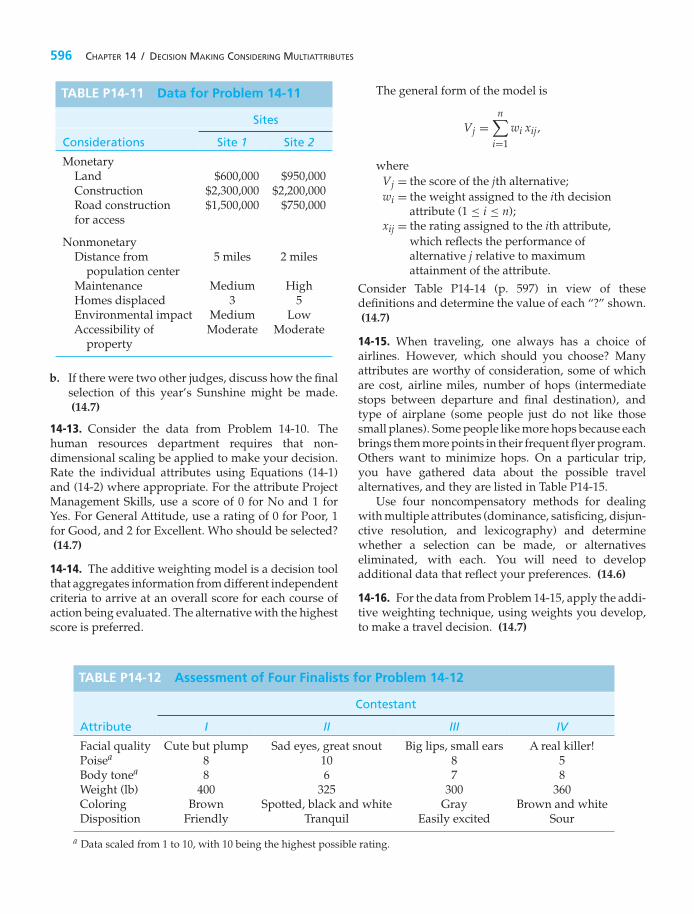
596 CHAPTER 14 / DECISION MAKING CONSIDERING MULTIATTRIBUTES

TABLE P14-11 Data for Problem 14-11

Sites

Considerations Site 1 Site 2

MonetaryLand $600,000 $950,000Construction $2,300,000 $2,200,000Road construction $1,500,000 $750,000for access

NonmonetaryDistance from 5 miles 2 miles

population centerMaintenance Medium HighHomes displaced 3 5Environmental impact Medium LowAccessibility of Moderate Moderate

property

b. If there were two other judges, discuss how the finalselection of this year’s Sunshine might be made.(14.7)

14-13. Consider the data from Problem 14-10. Thehuman resources department requires that non-dimensional scaling be applied to make your decision.Rate the individual attributes using Equations (14-1)and (14-2) where appropriate. For the attribute ProjectManagement Skills, use a score of 0 for No and 1 forYes. For General Attitude, use a rating of 0 for Poor, 1for Good, and 2 for Excellent. Who should be selected?(14.7)

14-14. The additive weighting model is a decision toolthat aggregates information from different independentcriteria to arrive at an overall score for each course ofaction being evaluated. The alternative with the highestscore is preferred.

TABLE P14-12 Assessment of Four Finalists for Problem 14-12

Contestant

Attribute I II III IV

Facial quality Cute but plump Sad eyes, great snout Big lips, small ears A real killer!Poisea 8 10 8 5Body tonea 8 6 7 8Weight (lb) 400 325 300 360Coloring Brown Spotted, black and white Gray Brown and whiteDisposition Friendly Tranquil Easily excited Sour

a Data scaled from 1 to 10, with 10 being the highest possible rating.

The general form of the model is

Vj =n∑

i=1

wi xij,

whereVj = the score of the jth alternative;wi = the weight assigned to the ith decision

attribute (1 ≤ i ≤ n);xij = the rating assigned to the ith attribute,

which reflects the performance ofalternative j relative to maximumattainment of the attribute.

Consider Table P14-14 (p. 597) in view of thesedefinitions and determine the value of each “?” shown.(14.7)

14-15. When traveling, one always has a choice ofairlines. However, which should you choose? Manyattributes are worthy of consideration, some of whichare cost, airline miles, number of hops (intermediatestops between departure and final destination), andtype of airplane (some people just do not like thosesmall planes). Some people like more hops because eachbrings them more points in their frequent flyer program.Others want to minimize hops. On a particular trip,you have gathered data about the possible travelalternatives, and they are listed in Table P14-15.

Use four noncompensatory methods for dealingwith multiple attributes (dominance, satisficing, disjun-ctive resolution, and lexicography) and determinewhether a selection can be made, or alternativeseliminated, with each. You will need to developadditional data that reflect your preferences. (14.6)

14-16. For the data from Problem 14-15, apply the addi-tive weighting technique, using weights you develop,to make a travel decision. (14.7)

SPREADSHEET EXERCISES 597

TABLE P14-14 Data for Problem 14-14

Alternative j

(1) (2)Keep Purchase

Existing a NewMachine Machine

i wi Rank Decision Attribute Tool Tool

1 1.0 1 Annual cost of ownership Rank ? ?(capital recovery cost) xij 1.0 0.7

2 ? 4 Flexibility in types of jobs scheduled Rank 2 1xij 0.8 1.0

3 0.8 2 Ease of training and operation Rank 1 2xij ? 0.5

4 0.7 ? Time savings per part produced Rank 2 1xij 0.7 1.0

Vj 2.69 2.30Vj (normalized) 1.00 ?

TABLE P14-15 Data for Problem 14-15

Alternatives

Attribute Fly-by-night Puddle Jumper Air ’R Us Hopwe Makit

Air fare $350 $280 $325 $300Number of stops 0 2 1 2Frequent flyer? Yes No Yes YesAirplane type Large Very small Small Small

14-17. “Paper or plastic?” asks a checkout clerkat your grocery store. According to Time

magazine (August 13, 2007, page 50), paper bags cost5.7 cents each as opposed to 2.2 cents per plastic bag.After leaving the store with several plastic bags, youdecide to do some research on paper versus plasticbags. The Time article goes on to inform you that theUnited States uses 12 million barrels of oil to produceits plastic bags consumed annually. Furthermore, paper

bags consumed in the United states equate to 14million trees a year. What other factors might gointo a multiattribute analysis of the pros and cons ofpaper versus plastic bags (e.g., littering, leak potential,biodegradability, transportation to landfills)? Use theadditive weighting technique to assess the impact ofimposing a 3 cent “finder’s fee” for returning plasticbags to an approved recycling center. (14.7)

Spreadsheet Exercises

14-18. Refer to Example 14-1. Mary Jones has beenenlightened at a recent seminar and now rates hypnosisas her highest choice of anesthesia. The remaininganesthesia methods retain their relative order, just

shifted down one. How does this impact the choiceof a dentist via the nondimensional scaling technique?(14.7)

APPENDIX A

Using Excel to SolveEngineering EconomyProblems

by James A. Alloway, Jr.EMSQ Associates

This appendix presents techniques and specific functions needed to formulatespreadsheet models for solving engineering economy problems. The spreadsheetexamples in the text use Microsoft Excel because of its widespread use. Otherspreadsheet software, such as Lotus 1-2-3 and Corel Quattro Pro, can be usedequally as well, with only minor changes to the formulas.

A.1 Spreadsheet BasicsThe basic spreadsheet components and notation are shown in Figure A-1. The rowimmediately above the worksheet column headings is the formula bar. The cell isthe basic building block of the spreadsheet and is identified by its column letterand row number. In Figure A-1, the text SAMPLE SPREADSHEET is in cell C2, theintersection of column C and row 2. The box on the left of the formula bar indicatesthe active cell, which in this case is C2. The contents of the active cell appear in thebox to the right of fx on the formula bar.

The other fundamental spreadsheet entity is the range, which can be a singlecell, a portion of a row or column, or any uniform rectangular region. A range isidentified by its first and last cells separated by a colon (e.g., H1:H7). A one-cellrange has the same starting and ending cell (e.g., B1:B1), while a rectangular rangeuses the top left and bottom right cells (e.g., A1:G7). When prompted for a rangeby Excel, move the cell pointer to the first cell in the range and anchor the rangeby pressing the colon key. Then move to the last cell in the range and press theEnter key.

598

SECTION A.2 / TYPES OF INPUT 599

Figure A-1 Sample Excel Worksheet Showing Basic Terms and Relationships

A.2 Types of InputA cell may contain numbers (e.g., −1.23, 123456789, 49E-15), formulas (e.g., =A23∗5, = 7+4∧2.3, = 5 + min(A1:A10)), or labels (e.g., Alternative Alpha). Cells canbe edited by moving to the desired cell and pressing the F2 key. The keyboard arrowkeys will now move the cursor within the expression. Use the Delete or Backspacekey to delete characters. The Insert key toggles between insert and type-over mode.

It is helpful to document the input values and results with explanatory labels,which are left-justified by default. In Figure A-1, cell D2 appears to containPREADSHEET, but in fact the cell is empty. This is because formulas that are longerthan the column width spill over to adjacent blank cells.

Numbers are right-justified by default and are entered without commasor currency signs. These features are added separately by using formattingcommands, which are described in Section A.4.

Formulas consist of algebraic expressions and functions. In Excel, the firstcharacter in the cell must be an equal (=) sign. Reference to other cells is doneby either (a) clicking the cell with the mouse, (b) pointing to the cell by using thefour keyboard arrow keys, (c) typing the cell address directly, or (d) entering therange name, if one has been assigned. Expressions are evaluated left to right andfollow typical precedence rules. Exponentiation is denoted in Excel with the hatsymbol (∧).

600 APPENDIX A / USING EXCEL TO SOLVE ENGINEERING ECONOMY PROBLEMS

A.3 Financial Function SummaryThe financial functions are based on the following assumptions, which agree withthose presented in the text:

(a) The per period interest rate, i, remains constant.(b) There is exactly one period between cash flows.(c) The period length remains constant.(d) The end of period cash-flow convention is utilized.(e) The first cash flow in a range occurs at the end of the first period.

The last assumption needs to be emphasized, since most problems involve aninvestment at k = 0, which is the beginning of the first period. This only affectsthe NPV function (see p. 609 for more details). Be sure to review the assumptionsmade in your particular spreadsheet package.

The most frequently used financial functions for engineering economy analysisare as follows:

PV(i, N, A) returns the present worth of an annuity.FV(i, N, A) returns the future worth of an annuity.PMT(i, N, P) returns an annuity-given a present worth.NPV(i, range) returns the present worth of any cash flow.IRR(guess, range) returns the internal rate of return for a range of cash flows.

There is no space preceding the left parenthesis in Excel functions. A, i, and Nare single values and have the same definitions as in Chapter 4. Range is the cash-flow range, and guess is a decimal estimate of the internal rate of return (IRR), whichis used internally by the IRR algorithm. The equivalent worth functions returnmonetary amounts, not the discount factor values. Other functions, includingdepreciation, are available. Check your particular spreadsheet program for theiravailability and usage.

A.4 Spreadsheet AppearanceBlank rows and columns are inserted into a worksheet with the commands Insert| Rows or Insert | Columns Rows and columns can be removed by highlightingtheir row identifier on the left and then using the Edit | Delete command. Becareful when deleting rows and columns: remember, rows are horizontal, columnsare vertical. Larger areas of the spreadsheet can be cleared by highlighting therange and using the Edit | Clear command. The dialog box allows one to delete cellcontents and/or cell formatting.

The appearance of numbers, such as the number of significant digits and thepresence of dollar and percent signs or commas, is changed with the Format| Cells command. Figure A-2 illustrates the results of several common formattingand alignment options.

Long text entries with nonblank cells to the right and large numbers mayrequire wider columns to display their results. This can be done for each columnindividually by using the Format | Column | Width command or by moving thecursor to the edge of the column heading (the mouse pointer will change to a

SECTION A.5 / CELL REFERENCING 601

Figure A-2 SampleScreen IllustratingTypical Text andNumeric FormattingOptions

double arrow) and dragging it in the appropriate direction. The alternative is toallow the text to wrap in the cell using Format | Cells | Alignment | Text and checkthe Wrap Text box. This will affect the row height.

A.4.1 Moving Cells

Cell contents are removed by highlighting the range and then using the Edit | Cutcommand. Cell contents are placed in a new location by highlighting the first cellin the new range and using the Edit | Paste command. Anything in the new rangewill be replaced with the new material.

The original location will be blank after the Cut command is issued. When aformula is cut and subsequently pasted to a new location, the cell references of theformula are automatically updated to reflect its new location. If a value is cut andpasted to a new location, all formulas that refer to it are automatically revised toreflect the new location.

A.4.2 Copying Cells

To copy the contents of a cell to a new location while leaving the original cell intact,highlight the cell or range and use the Edit | Copy command. Move the cursor tothe new location and use the Edit | Paste command. Formulas in copied cells aremodified, as described in section A.5.

A.5 Cell ReferencingThe manner in which cells in formulas are referenced internally provides the powerand flexibility of spreadsheet software. These features make it possible to constructcomplex models by using a minimal number of formulas and to get updated resultsas values change. Many problems encountered by novice spreadsheet users can betraced back to a lack of understanding of how formulas reference cells.

There are three methods to refer to the reference of a cell: relative, absolute,and mixed. The distinction between them becomes important only when copying

602 APPENDIX A / USING EXCEL TO SOLVE ENGINEERING ECONOMY PROBLEMS

formulas. If cell B5 contains the formula = A4 + 1 and cell A4 contains the value 7,then the result displayed in B5 is 8. Although the formula refers to cell A4, internallythe spreadsheet interprets it as “Add 1 to the contents of the cell that is one rowup and one column to the left of this cell.” This is relative referencing, which isthe default. When the formula in B5 is copied, the cell that receives the copy of theformula will display the sum of 1 plus the contents of the cell that is one row upand one column to the left of the new cell.

There are occasions when one always wants to refer to a specific cell, no matterwhere a formula is copied. The interest rate, i, is typically a value that is constantfor a problem. Absolute referencing (a $ in front of both the column and rowdesignation, e.g., $A$1) will always return the contents of that specific cell, nomatter where the formula is copied.

Sometimes it is necessary to hold either the row or the column constant andallow the other portion of the reference to vary. This is achieved with mixedreferencing. A $ is placed in front of the row or column that is to be kept constant.Thus, $A1 will make the column reference absolute and the row reference relative,while A$1 will make the row reference absolute and the column reference relative.

The F4 key can simplify the process of cell addressing. Each time the key ispressed, the highlighted cell reference cycles through absolute, mixed row, mixedcolumn, and relative addressing.

Figure A-3 illustrates the results of the cut, copy, and paste commands for thethree types of referencing. The range A5:C9 contains arbitrary values. Cells E5:E9contain formulas to compute the respective row totals. The actual formulas areshown in column F. Results of cut, copy, and paste actions are shown in rangeE13:E17, and the resulting formulas are in column F.

Figure A-3 Sample Screen Illustrating the Effects on Formula References of the Copyand Move Commands

SECTION A.6 / STRUCTURED SPREADSHEETS 603

A.6 Structured SpreadsheetsUsing a structured approach for model formulation reduces the chance ofoverlooking information, aids in locating errors and making revisions, and makesit easier for others to interpret your analysis. Taking a few minutes to organize thedata and plan the model prior to sitting down at the keyboard will reduce the totaldevelopment time. There is no single best format, but the following tips work wellin practice:

a. Treat everything as a variable, even if you do not expect it to change.Assign key parameters, such as the interest rate, life, and estimates of revenueand expenses, their own cells. Formulas should reference these cells, not the valuesthemselves. This way, if these values change, it is only necessary to revise thesefew cells rather than try to locate all of the formulas that contain these values. Ifthese cells are located in the upper left corner of the spreadsheet, you can return tothem from anywhere in the spreadsheet by pressing the keyboard Home key.

b. Next, divide the problem into segments. Combining several calculationsinto a single formula saves space, but such an approach makes it more difficultto verify results and locate errors. Each segment should provide an intermediateresult, which can be referenced in other segments and aids in isolating problems.This recommendation also applies for different types of cash flows. Rather thancombine revenues and expenses for each period prior to entry on the spreadsheet,list each type of cash flow in a column and sum them to get a net figure for eachperiod.

c. It is helpful to save each type of problem as a separate file, which is calleda template. When a similar problem is encountered in the future, the appropriatetemplate is retrieved, revised, and a new analysis is completed. If you are creatinga new spreadsheet from a template, be sure to change the file name the first timeyou save it, or the template will be overwritten.

d. It is possible to create new functions, automate commands, and createnew menus by using macros. These are beneficial if you will be using a templatefrequently, but macros are generally not productive in the classroom setting.

e. Range names are useful when entering long formulas and when using macros.They can be assigned to any valid range (including a single cell) with the commandInsert | Name. Range names can be made absolute by prefixing the name with adollar sign.

Three examples follow that illustrate useful spreadsheet commands andfunctions, in addition to basic model formulation techniques needed to solveengineering economy problems. Keep the following points in mind:

a. Remain familiar with the hand solutions so that the spreadsheet model canbe verified.

b. Understand the course material first, have a plan for solving the problem,and then use the spreadsheet to help with the calculations.

c. Try the examples in this appendix to verify that they are working properlywith your particular spreadsheet.

d. Blindly copying formulas and pressing keys without taking the time to lookat what is going on doesn’t aid learning.

604 APPENDIX A / USING EXCEL TO SOLVE ENGINEERING ECONOMY PROBLEMS

e. Graphing your results can reveal relationships that may not be easilydiscernable when looking at columns of numbers.

f. Save your work frequently and keep backups of your files.

EXAMPLE A-1

This example uses breakeven analysis to illustrate many basic spreadsheetfeatures. It includes examples of relative, mixed, and absolute cell addressing;a simple formula; the use of a spreadsheet function; and a graph. Spreadsheetcommands used include formatting, label alignment, and the copy command.Because of the copy command, only five unique formulas are required.

Consider two options, Alpha and Beta, each with its own set-up (fixed)cost and incremental (variable) cost. We wish to determine the least expensiveoption for a given production quantity. The total cost (TC) for Q units producedby either method is

TCm = FCm + ICm∗ Q,

where m is either Alpha or Beta, FC is the fixed cost, IC is the incremental cost,and Q is the number of units produced.

The spreadsheet for this problem is shown in Figure A-4. The data inputarea is at the top of the worksheet. Here, the specific fixed and variable costsare entered (cells B2 to C3), along with the name of each alternative underconsideration (in cells B1 and C1). Cells B6 and B7 contain values that will beused later to bracket the breakeven quantity.

The total cost formula is entered in cell B12, using mixed addressing,and copied to the range B12:C22. The choice of cell in which to enter theinitial formula is arbitrary, and any other cell (e.g., Z798) could have been usedas well.

The Units Produced column is created with two formulas. Cell A12 usesrelative addressing to refer to the starting value in cell B6. Cell A13 uses relativeaddressing to refer to the contents of the cell above it and absolute addressingto refer to the increment value to be added to it. While the start and incrementvalues could be entered directly in the formulas, the current approach providesgreater flexibility.

The general approach for solving a breakeven problem without using thesolver function is to set the start value to 0 and the increment value to some largevalue, say 100. You may need to go higher or try other values, depending onthe specifics of your particular problem. Once the breakeven point is bracketed,the start and increment values can be changed to get a more exact value. As thegraph in Figure A-5 indicates, the breakeven point occurs between 25 and 30, sothe start value can be changed to 25 and the increment reduced to 1 to locate theexact breakeven quantity.

An IF function is used in column D to make it easier to identify the breakevenpoint. It displays the name of the alternative with the lowest cost.

The graph is produced by highlighting the range A12:C22, then clicking onthe Chart Wizard and selecting the XY(Scatter) option.

SECTION A.6 / STRUCTURED SPREADSHEETS 605

= B$1

= B6

= B$2 + B$3 * $A12

= A12 + $B$7

= IF(B12 > C12, $C$1, $B$1)

Figure A-4 Spreadsheet and Unique Formulas for Example A-1

Figure A-5 Breakeven Graph for Example A-1

606 APPENDIX A / USING EXCEL TO SOLVE ENGINEERING ECONOMY PROBLEMS

Since all values are treated as variables, a high degree of flexibility isinherent in the spreadsheet. Note that, as you change values, the spreadsheet isautomatically revised, as is the graph. Even the labels in column D are updatedif the names of the alternatives change!

EXAMPLE A-2

Cash flows can take many forms, such as single unique values, annuities, andgradients. Single values are entered individually into their respective cells.Annuities are created by entering the first period amount and then using the copycommand to fill in the rest of the range. Both arithmetic and geometric gradientsare created in a spreadsheet with simple formulas and the copy command, asshown in Figure A-6.

The formula in B8 copies the starting amount from which both gradientsbuild. By using absolute addressing, we are able to apply the same startingamount to both columns. For an arithmetic gradient, cell B9 takes the amountin the cell above it and adds a fixed amount to it, as specified in B3. In ageometric gradient, cell C9 takes the cell above it and multiplies it by the fixedpercentage specified in B4. Note the use of absolute addressing in both gradientformulas to keep the gradient quantity constant as it is copied down each column.Finally, B15 calculates the present worth of the gradient series. Note that absoluteaddressing is used to hold the interest rate and base (year 0) amount constant. Toobtain a decreasing gradient, simply substitute a negative sign for the positivesign in the formulas in row 9.

= $B$2

= C8 + C8 * $B$4= B8 + $B$3

= NPV($B$1,B9:B13) + B8

Figure A-6 Spreadsheet and Unique Formulas for Example A-2

SECTION A.6 / STRUCTURED SPREADSHEETS 607

EXAMPLE A-3

Once the cash-flow values are entered into the spreadsheet, financial measuresof merit can be determined (see Figure A-7). The equivalent worth measures areobtained with the following combination of functions:

PW: = NPV(i, range) + P0

AW: = PMT(i, N, −PW)

FW: = FV(i, N, −AW)

IRR: = IRR(range, i)

Here, P0 refers to the cash flow at time 0, PW is the result of the NPV functionwith P0 added, AW is the result of the PMT function, and range is the cash-flowrange excluding the amount P0.

The NPV function is probably the most useful financial function. It workswith any cash flow; it is not restricted to be an annuity, as with PMT and FV,and provides a unique result regardless of the number of sign changes. Once wehave the PW, we can obtain any other equivalent worth measure.

In the past, many firms avoided the IRR method in project justificationbecause it is difficult to compute by hand. With the spreadsheet, IRR is actuallyeasier to compute than PW. The value i is an initial estimate of the IRR in decimal

= NPV (B1, B5:B9) + B4

= PMT (B1, A9, –C11)

= FV (B1, A9, –C12)

= IRR (B4:B9, B1)

Figure A-7 Spreadsheet and Unique Formulas for Example A-3

608 APPENDIX A / USING EXCEL TO SOLVE ENGINEERING ECONOMY PROBLEMS

form. MARR is usually a good guess. For a unique answer, there must be onlya single change of sign in the cash flow. The IRR function does not provide awarning if multiple rates of return exist.

A.7 Excel Formula SummaryABS(value)

Returns the absolute value of the argument.

AVERAGE(range)Returns the average of the values specified in range.

CEILING(number, significance)Rounds the specified number up to the significance specified. Significance istypically 1.

FV(i,N,A,{PW},type)Returns the future worth amount at the end of period N for an annuity A,beginning at the end of period 1. The interest rate is i per period. {PW} isoptional.

HLOOKUP(class life, table range, k)This function returns a value from a specific location in a table. The locationis specified by values in the header row and the number of rows below theheader.

IF(condition, true, false)Condition is a logical expression, containing a logical operator (<>, >, <,>=, <=). If the result of the condition is true, the value or label in the trueargument is returned. If the result is false, the value or label in the false argumentis returned.

IRR(range, guess)Returns the IRR for cash flows in the specified range. Recall that more thanone change of sign in the cash flow may generate multiple rates of return! Theguess argument is a starting point used by the internal algorithm and is oftenspecified as the MARR.

ISERR(cell)Computational errors, such as division by zero, display an error code in the cellcontaining the error and any cells that reference that cell. If the cell containsan error, this function returns a logical TRUE; otherwise, it returns a logicalFALSE.

MAX(range)Returns the maximum value in the range. Text and logical results are ignored.

SECTION A.7 / EXCEL FORMULA SUMMARY 609

MIN(range)Returns the minimum value in the range. Text and logical results are ignored.

NORMINV(number, mean; std dev)Returns the inverse cumulative distribution for a normal distribution with thespecified mean and standard deviation.

NPV(i,range)Computes present worth of any arbitrary cash flows in the specified range.Caution is required for handling the cash flow (P0) at T = 0. Let

P_range = range containing the cash flows at the end of periods 1, 2, . . . , N

F_range = range containing the cash flows at the end of periods 0, 1, . . . , N

Then the PW can be determined using either formula:

PW = P0 + NPV(i, P_range)

or

PW = NPV(i, F_range)∗(1 + i)

PMT(i,N,P,{F},type)Returns the annuity amount that is equivalent to P taken over N periods. {F}is optional. Type = 1 denotes beginning of period cash flows, type = 0 is end ofperiod. End of period cash flows are assumed if type is blank.

PV(i,N,A,{F},type)Returns the present worth amount of an annuity A, beginning at the end ofperiod 1 and continuing until the end of period N. The interest rate is i perperiod. {F} is optional. Note that this function works only with an annuity,while NPV works with any cash-flow pattern.

RAND()Returns a continuous uniform random variable on the interval (0, 1). Note thatthe parentheses are required, but there is no argument.

ROUND(number, digits)Rounds the specified value to the number of digits.

STDEV(range)Calculates the sample standard deviation (divisor = n − 1) for the valuesspecified in range.

SUM(range)Returns the sum of the values in the cells of the range specified.

VDB(B, SVN , N, start, end, percent, no_switch)Returns dk for the general declining balance depreciation method. The percentargument is 2 for double declining balance, 1.5 for 150% declining balance,and so on. If omitted, it is assumed to be 2 (200%). The start and end argumentspermit use of the half-year (and half month) conventions. To permit switchingto the straight-line method, set the switch argument to FALSE. A value of TRUEfor this argument disallows switching.

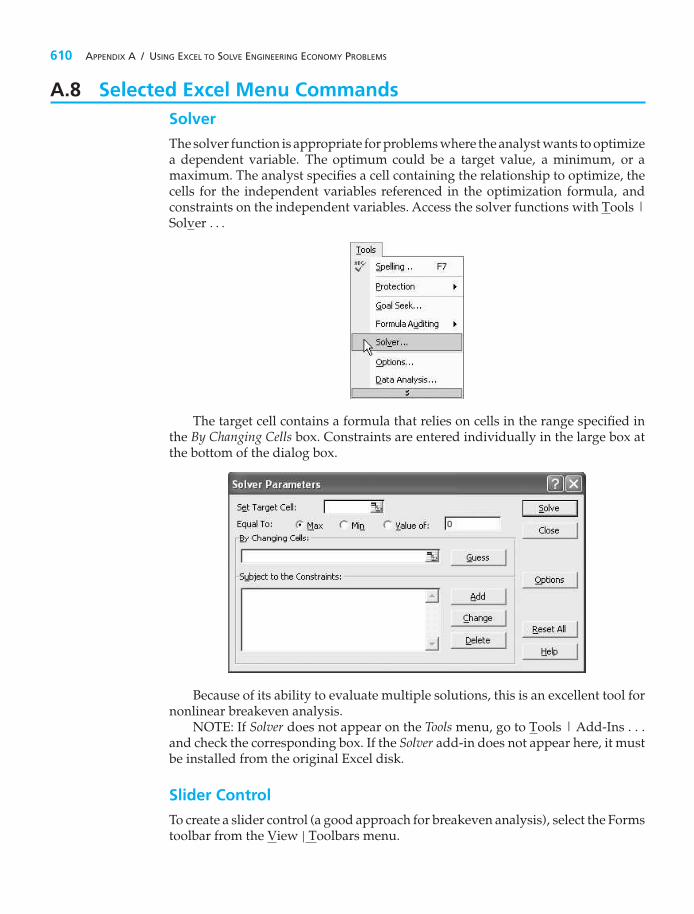
610 APPENDIX A / USING EXCEL TO SOLVE ENGINEERING ECONOMY PROBLEMS

A.8 Selected Excel Menu CommandsSolver

The solver function is appropriate for problems where the analyst wants to optimizea dependent variable. The optimum could be a target value, a minimum, or amaximum. The analyst specifies a cell containing the relationship to optimize, thecells for the independent variables referenced in the optimization formula, andconstraints on the independent variables. Access the solver functions with Tools |Solver . . .

The target cell contains a formula that relies on cells in the range specified inthe By Changing Cells box. Constraints are entered individually in the large box atthe bottom of the dialog box.

Because of its ability to evaluate multiple solutions, this is an excellent tool fornonlinear breakeven analysis.

NOTE: If Solver does not appear on the Tools menu, go to Tools | Add-Ins . . .and check the corresponding box. If the Solver add-in does not appear here, it mustbe installed from the original Excel disk.

Slider Control

To create a slider control (a good approach for breakeven analysis), select the Formstoolbar from the View | Toolbars menu.

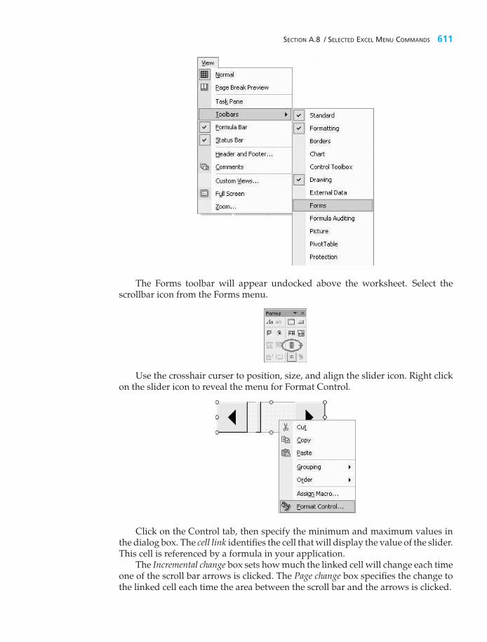
SECTION A.8 / SELECTED EXCEL MENU COMMANDS 611

The Forms toolbar will appear undocked above the worksheet. Select thescrollbar icon from the Forms menu.

Use the crosshair curser to position, size, and align the slider icon. Right clickon the slider icon to reveal the menu for Format Control.

Click on the Control tab, then specify the minimum and maximum values inthe dialog box. The cell link identifies the cell that will display the value of the slider.This cell is referenced by a formula in your application.

The Incremental change box sets how much the linked cell will change each timeone of the scroll bar arrows is clicked. The Page change box specifies the change tothe linked cell each time the area between the scroll bar and the arrows is clicked.

612 APPENDIX A / USING EXCEL TO SOLVE ENGINEERING ECONOMY PROBLEMS

Simple Linear Regression

Regression is a very useful estimation and prediction tool. To access it, select Tools| Data Analysis . . . | Regression.

The regression output from Excel includes the estimated regression parameters,correlation coefficient, and diagnostic statistics.

SECTION A.8 / SELECTED EXCEL MENU COMMANDS 613

The range of cells containing the dependent variable is specified in the InputY Range. The corresponding independent variable range goes in the Input X Rangebox. Recall that these values are paired, and corresponding X and Y values mustappear in the same row.

Residuals are diagnostic values used to assess how well the regressionassumptions are met by the data.

Histogram

Histograms provide a graphic summary showing the center, spread, and shape forlarge amounts of continuous numeric data. To access the histogram feature, usethe Tools | Data Analysis | Histogram menu.

614 APPENDIX A / USING EXCEL TO SOLVE ENGINEERING ECONOMY PROBLEMS

The Input Range contains the data for which you wish to create the histogram.The Bin Range can be left blank, and Excel will select the number of bins and thewidth of the bins to make the histogram look nice. You can exercise more controlover the appearance of the histogram by specifying values for the Bin Range.

Check the box for Chart Output to view the histogram. Right click on anyhistogram bar and select Format Data Series, then specify a Gap Width of 0 on theOptions tab to get a true histogram.

APPENDIX B

Abbreviations and Notation*

Chapter 2CF total fixed costCV total variable costcv variable cost per unitCT total costD demand for a product or service in unitsD∗ optimal demand or production volume that maximizes profitD′ breakeven pointD demand or production volume that will produce maximum revenue

Chapter 3In an unweighted or a weighted index number, dependent on the

calculationK the number of input resource units needed to produce the first output

unitu the output unit numberX cost-capacity factorZu the number of input resource units needed to produce output unit

number u

Chapter 4A equal and uniform end-of-period cash flows (or equivalent end-of-

period values)APR annual percentage rate (nominal interest)A1 end of period 1 cash flow in a geometric sequence of cash flowsEOY end of year∗ Listed by the chapter in which they first appear.

615

616 APPENDIX B / ABBREVIATIONS AND NOTATION

F a future equivalent sum of moneyf a geometric change from one time period to the next in cash flows

or equivalent valuesG an arithmetic (i.e., uniform) change from one period to the next

in cash flows or equivalent valuesI total interest earned or paid (simple interest)i effective interest rate per interest periodk an index for time periodsP principal amount of a loan; a present equivalent sum of moneyM number of compounding periods per yearN number of interest periodsr nominal interest rate per period (usually a year)r a nominal interest rate that is continuously compounded

Chapter 5AW(i%) equivalent uniform annual worth, computed at i% interest, of one

or more cash flowsCR(i%) equivalent annual cost of capital recovery, computed at i% interestCW(i%) capitalized worth (a present equivalent), computed at i% interest,

of cash flows occurring over an indefinite period of timeE equivalent annual expensesε external reinvestment rateERR external rate of returnEUAC(i%) equivalent uniform annual cost, calculated at i% interest, of one

or more cash flowsFW(i%) future equivalent worth, calculated at i% interest, of one or more

cash flowsI initial investment for a projectIRR internal rate of return, also designated i?%MARR minimum attractive rate of returnN the length of the study period (usually years)PW(i%) present equivalent worth, computed at i% interest, of one or more

cash flowsR equivalent annual revenues (or savings)S salvage (market) value at the end of the study periodθ payback periodθ ′ discounted payback periodVN value (price) of a bond N periods prior to redemptionZ face value of a bond

Chapter 6�(B − A) incremental net cash flow (difference) calculated from the cash flow

of Alternative B minus the cash flow of Alternative A (read: delta Bminus A)

APPENDIX B / ABBREVIATIONS AND NOTATION 617

Chapter 7ACRS accelerated cost recovery systemADS alternative depreciation systemATCF after-tax cash flowB cost basisBTCF before-tax cash flowBV book value of an assetd depreciation deductiond∗ cumulative depreciation over a specified period of timeE annual expenseea after-tax cost of equity capitalEVA economic value addedGDS general depreciation systemib before-tax interest paid on borrowed capitalλ fraction of capital that is borrowed from lendersMACRS modified accelerated cost recovery systemMV market value of an asset; the price that a buyer will pay for a particular

type of propertyN useful life of an asset (ADR life)NOPAT net operating profit after taxesR ratio of depreciation in a particular year to book value at the beginning

of the same yearR gross annual revenuerk MACRS depreciation rate (a decimal)SVN salvage value of an asset at the end of useful lifeT income taxest effective income tax rateWACC tax-adjusted weighted average cost of capital

Chapter 8A$ actual (current) dollarsb base time period indexej total price escalation (or de-escalation) rate for good or service je′

j differential price inflation (or deflation) rate for good or service jfe annual devaluation rate (rate of annual change in the exchange rate)

between the currency of a foreign country and the U.S. dollarf general inflation rateim market (nominal) interest rateifm rate of return in terms of a combined (market) interest rate relative to

the currency of a foreign countryir real interest rateius rate of return in terms of a combined (market) interest rate relative to

U.S. dollarsR$ real (constant) dollars

618 APPENDIX B / ABBREVIATIONS AND NOTATION

Chapter 9TCk total (marginal) cost for year k

Chapter 10B–C benefit–cost ratioB equivalent uniform annual benefits of a proposed project

Chapter 11EW equivalent worth (annual, present, or future)

Chapter 12E(X) mean of a random variableEVPI expected value of perfect informationf (x) probability density function of a continuous random variableF(x) cumulative distribution function of a continuous random variablep(x) probability mass function of a discrete random variablep(xi) probability that a discrete random variable takes on the value xiP(x) cumulative distribution function of a discrete random variablePr{· · ·} probability of the described event occurringSD(X) standard deviation of a random variableV(X) variance of a random variable

Chapter 13B∗ present worth of an investment opportunity in a specified budgeting

periodβM market risk levelβS contribution of stock S to market riskc cash outlay for expenses in capital allocation problemsCk maximum cash outlay permissible in period kCAPM capital asset pricing modelEBIT earnings before income taxesm number of mutually exclusive projects being consideredRF risk-free rate of returnRM market portfolio rate of returnRS stock S rate of returnSML security market lineXj binary decision variable (= 0 or 1) in capital allocation problems

Chapter 14r∗ dimensionality of a multiattribute decision problem

APPENDIX C

Interest and Annuity Tablesfor Discrete Compounding

For various values of i from 1/4% to 25%,

i = effective interest rate per period (usually one year);N = number of compounding periods;

(F/P, i%, N) = (1 + i)N ; (A/F, i%, N) = i(1 + i)N − 1

;

(P/F, i%, N) = 1(1 + i)N ; (A/P, i%, N) = i(1 + i)N

(1 + i)N − 1;

(F/A, i%, N) = (1 + i)N − 1i

; (P/G, i%, N) = 1i

[(1 + i)N − 1

i(1 + i)N − N(1 + i)N

];

(P/A, i%, N) = (1 + i)N − 1i(1 + i)N ; (A/G, i%, N) = 1

i− N

(1 + i)N − 1.

619

TABLE C-1 Discrete Compounding; i = 1/4%

Single Payment Uniform Series Uniform Gradient

Compound Present Compound Present Sinking Capital Gradient GradientAmount Worth Amount Worth Fund Recovery Present Worth Uniform SeriesFactor Factor Factor Factor Factor Factor Factor Factor

To Find F To Find P To Find F To Find P To Find A To Find A To Find P To Find AGiven P Given F Given A Given A Given F Given P Given G Given G

N F/P P/F F/A P/A A/F A/P P/G A/G N1 1.0025 0.9975 1.0000 0.9975 1.0000 1.0025 0.000 0.0000 12 1.0050 0.9950 2.0025 1.9925 0.4994 0.5019 0.995 0.4994 23 1.0075 0.9925 3.0075 2.9851 0.3325 0.3350 2.980 0.9983 34 1.0100 0.9901 4.0150 3.9751 0.2491 0.2516 5.950 1.4969 45 1.0126 0.9876 5.0251 4.9627 0.1990 0.2015 9.901 1.9950 5

6 1.0151 0.9851 6.0376 5.9478 0.1656 0.1681 14.826 2.4927 67 1.0176 0.9827 7.0527 6.9305 0.1418 0.1443 20.722 2.9900 78 1.0202 0.9802 8.0704 7.9107 0.1239 0.1264 27.584 3.4869 89 1.0227 0.9778 9.0905 8.8885 0.1100 0.1125 35.406 3.9834 9

10 1.0253 0.9753 10.1133 9.8639 0.0989 0.1014 44.184 4.4794 10

11 1.0278 0.9729 11.1385 10.8368 0.0898 0.0923 53.913 4.9750 1112 1.0304 0.9705 12.1664 11.8073 0.0822 0.0847 64.589 5.4702 1213 1.0330 0.9681 13.1968 12.7753 0.0758 0.0783 76.205 5.9650 1314 1.0356 0.9656 14.2298 13.7410 0.0703 0.0728 88.759 6.4594 1415 1.0382 0.9632 15.2654 14.7042 0.0655 0.0680 102.244 6.9534 15

16 1.0408 0.9608 16.3035 15.6650 0.0613 0.0638 116.657 7.4469 1617 1.0434 0.9584 17.3443 16.6235 0.0577 0.0602 131.992 7.9401 1718 1.0460 0.9561 18.3876 17.5795 0.0544 0.0569 148.245 8.4328 1819 1.0486 0.9537 19.4336 18.5332 0.0515 0.0540 165.411 8.9251 1920 1.0512 0.9513 20.4822 19.4845 0.0488 0.0513 183.485 9.4170 20

21 1.0538 0.9489 21.5334 20.4334 0.0464 0.0489 202.463 9.9085 2122 1.0565 0.9466 22.5872 21.3800 0.0443 0.0468 222.341 10.3995 2223 1.0591 0.9442 23.6437 22.3241 0.0423 0.0448 243.113 10.8901 2324 1.0618 0.9418 24.7028 23.2660 0.0405 0.0430 264.775 11.3804 2425 1.0644 0.9395 25.7646 24.2055 0.0388 0.0413 287.323 11.8702 25

30 1.0778 0.9278 31.1133 28.8679 0.0321 0.0346 413.185 14.3130 3036 1.0941 0.9140 37.6206 34.3865 0.0266 0.0291 592.499 17.2306 3640 1.1050 0.9050 42.0132 38.0199 0.0238 0.0263 728.740 19.1673 4048 1.1273 0.8871 50.9312 45.1787 0.0196 0.0221 1040.055 23.0209 4860 1.1616 0.8609 64.6467 55.6524 0.0155 0.0180 1600.085 28.7514 60

72 1.1969 0.8355 78.7794 65.8169 0.0127 0.0152 2265.557 34.4221 7284 1.2334 0.8108 93.3419 75.6813 0.0107 0.0132 3029.759 40.0331 84

100 1.2836 0.7790 113.4500 88.3825 0.0088 0.0113 4191.242 47.4216 100∞ 400.0000 0.0025 ∞

TABLE C-2 Discrete Compounding; i = 1/2%

Single Payment Uniform Series Uniform Gradient

Compound Present Compound Present Sinking Capital Gradient GradientAmount Worth Amount Worth Fund Recovery Present Worth Uniform SeriesFactor Factor Factor Factor Factor Factor Factor Factor

To Find F To Find P To Find F To Find P To Find A To Find A To Find P To Find AGiven P Given F Given A Given A Given F Given P Given G Given G

N F/P P/F F/A P/A A/F A/P P/G A/G N1 1.0050 0.9950 1.0000 0.9950 1.0000 1.0050 0.000 0.0000 12 1.0100 0.9901 2.0050 1.9851 0.4988 0.5038 0.990 0.4988 23 1.0151 0.9851 3.0150 2.9702 0.3317 0.3367 2.960 0.9967 34 1.0202 0.9802 4.0301 3.9505 0.2481 0.2531 5.901 1.4938 45 1.0253 0.9754 5.0503 4.9259 0.1980 0.2030 9.803 1.9900 5

6 1.0304 0.9705 6.0755 5.8964 0.1646 0.1696 14.655 2.4855 67 1.0355 0.9657 7.1059 6.8621 0.1407 0.1457 20.449 2.9801 78 1.0407 0.9609 8.1414 7.8230 0.1228 0.1278 27.176 3.4738 89 1.0459 0.9561 9.1821 8.7791 0.1089 0.1139 34.824 3.9668 9

10 1.0511 0.9513 10.2280 9.7304 0.0978 0.1028 43.387 4.4589 10

11 1.0564 0.9466 11.2792 10.6770 0.0887 0.0937 52.853 4.9501 1112 1.0617 0.9419 12.3356 11.6189 0.0811 0.0861 63.214 5.4406 1213 1.0670 0.9372 13.3972 12.5562 0.0746 0.0796 74.460 5.9302 1314 1.0723 0.9326 14.4642 13.4887 0.0691 0.0741 86.584 6.4190 1415 1.0777 0.9279 15.5365 14.4166 0.0644 0.0694 99.574 6.9069 15

16 1.0831 0.9233 16.6142 15.3399 0.0602 0.0652 113.424 7.3940 1617 1.0885 0.9187 17.6973 16.2586 0.0565 0.0615 128.123 7.8803 1718 1.0939 0.9141 18.7858 17.1728 0.0532 0.0582 143.663 8.3658 1819 1.0994 0.9096 19.8797 18.0824 0.0503 0.0553 160.036 8.8504 1920 1.1049 0.9051 20.9791 18.9874 0.0477 0.0527 177.232 9.3342 20

21 1.1104 0.9006 22.0840 19.8880 0.0453 0.0503 195.243 9.8172 2122 1.1160 0.8961 23.1944 20.7841 0.0431 0.0481 214.061 10.2993 2223 1.1216 0.8916 24.3104 21.6757 0.0411 0.0461 233.677 10.7806 2324 1.1272 0.8872 25.4320 22.5629 0.0393 0.0443 254.082 11.2611 2425 1.1328 0.8828 26.5591 23.4456 0.0377 0.0427 275.269 11.7407 25

30 1.1614 0.8610 32.2800 27.7941 0.0310 0.0360 392.632 14.1265 3036 1.1967 0.8356 39.3361 32.8710 0.0254 0.0304 557.560 16.9621 3640 1.2208 0.8191 44.1588 36.1722 0.0226 0.0276 681.335 18.8359 4048 1.2705 0.7871 54.0978 42.5803 0.0185 0.0235 959.919 22.5437 4860 1.3489 0.7414 69.7700 51.7256 0.0143 0.0193 1448.646 28.0064 60

72 1.4320 0.6983 86.4089 60.3395 0.0116 0.0166 2012.348 33.3504 7284 1.5204 0.6577 104.0739 68.4530 0.0096 0.0146 2640.664 38.5763 84

100 1.6467 0.6073 129.3337 78.5426 0.0077 0.0127 3562.793 45.3613 100∞ 200.0000 0.0050 ∞

TABLE C-3 Discrete Compounding; i = 3/4%Single Payment Uniform Series Uniform Gradient

Compound Present Compound Present Sinking Capital Gradient GradientAmount Worth Amount Worth Fund Recovery Present Worth Uniform SeriesFactor Factor Factor Factor Factor Factor Factor Factor

To Find F To Find P To Find F To Find P To Find A To Find A To Find P To Find AGiven P Given F Given A Given A Given F Given P Given G Given G

N F/P P/F F/A P/A A/F A/P P/G A/G N1 1.0075 0.9926 1.0000 0.9926 1.0000 1.0075 0.000 0.0000 12 1.0151 0.9852 2.0075 1.9777 0.4981 0.5056 0.985 0.4981 23 1.0227 0.9778 3.0226 2.9556 0.3308 0.3383 2.941 0.9950 34 1.0303 0.9706 4.0452 3.9261 0.2472 0.2547 5.853 1.4907 45 1.0381 0.9633 5.0756 4.8894 0.1970 0.2045 9.706 1.9851 5

6 1.0459 0.9562 6.1136 5.8456 0.1636 0.1711 14.487 2.4782 67 1.0537 0.9490 7.1595 6.7946 0.1397 0.1472 20.181 2.9701 78 1.0616 0.9420 8.2132 7.7366 0.1218 0.1293 26.775 3.4608 89 1.0696 0.9350 9.2748 8.6716 0.1078 0.1153 34.254 3.9502 9

10 1.0776 0.9280 10.3443 9.5996 0.0967 0.1042 42.606 4.4384 10

11 1.0857 0.9211 11.4219 10.5207 0.0876 0.0951 51.817 4.9253 1112 1.0938 0.9142 12.5076 11.4349 0.0800 0.0875 61.874 5.4110 1213 1.1020 0.9074 13.6014 12.3423 0.0735 0.0810 72.763 5.8954 1314 1.1103 0.9007 14.7034 13.2430 0.0680 0.0755 84.472 6.3786 1415 1.1186 0.8940 15.8137 14.1370 0.0632 0.0707 96.988 6.8606 15

16 1.1270 0.8873 16.9323 15.0243 0.0591 0.0666 110.297 7.3413 1617 1.1354 0.8807 18.0593 15.9050 0.0554 0.0629 124.389 7.8207 1718 1.1440 0.8742 19.1947 16.7792 0.0521 0.0596 139.249 8.2989 1819 1.1525 0.8676 20.3387 17.6468 0.0492 0.0567 154.867 8.7759 1920 1.1612 0.8612 21.4912 18.5080 0.0465 0.0540 171.230 9.2516 20

21 1.1699 0.8548 22.6524 19.3628 0.0441 0.0516 188.325 9.7261 2122 1.1787 0.8484 23.8223 20.2112 0.0420 0.0495 206.142 10.1994 2223 1.1875 0.8421 25.0010 21.0533 0.0400 0.0475 224.668 10.6714 2324 1.1964 0.8358 26.1885 21.8891 0.0382 0.0457 243.892 11.1422 2425 1.2054 0.8296 27.3849 22.7188 0.0365 0.0440 263.803 11.6117 25

30 1.2513 0.7992 33.5029 26.7751 0.0298 0.0373 373.263 13.9407 3036 1.3086 0.7641 41.1527 34.4468 0.0243 0.0318 524.992 16.6946 3640 1.3483 0.7416 46.4464 34.4469 0.0215 0.0290 637.469 18.5058 4048 1.4314 0.6986 57.5207 40.1848 0.0174 0.0249 886.840 22.0691 4860 1.5657 0.6387 75.4241 48.1734 0.0133 0.0208 1313.519 27.2665 60

72 1.7126 0.5839 95.0070 55.4768 0.0105 0.0180 1791.246 32.2882 7284 1.8732 0.5338 116.4269 62.1540 0.0086 0.0161 2308.128 37.1357 84

100 2.1111 0.4737 148.1445 70.1746 0.0068 0.0143 3040.745 43.3311 100∞ 133.3333 0.0075 ∞

TABLE C-4 Discrete Compounding; i = 1%

Single Payment Uniform Series Uniform Gradient

Compound Present Compound Present Sinking Capital Gradient GradientAmount Worth Amount Worth Fund Recovery Present Worth Uniform SeriesFactor Factor Factor Factor Factor Factor Factor Factor

To Find F To Find P To Find F To Find P To Find A To Find A To Find P To Find AGiven P Given F Given A Given A Given F Given P Given G Given G

N F/P P/F F/A P/A A/F A/P P/G A/G N1 1.0100 0.9901 1.0000 0.9901 1.0000 1.0100 0.000 0.0000 12 1.0201 0.9803 2.0100 1.9704 0.4975 0.5075 0.980 0.4975 23 1.0303 0.9706 3.0301 2.9410 0.3300 0.3400 2.922 0.9934 34 1.0406 0.9610 4.0604 3.9020 0.2463 0.2563 5.804 1.4876 45 1.0510 0.9515 5.1010 4.8534 0.1960 0.2060 9.610 1.9801 5

6 1.0615 0.9420 6.1520 5.7955 0.1625 0.1725 14.321 2.4710 67 1.0721 0.9327 7.2135 6.7282 0.1386 0.1486 19.917 2.9602 78 1.0829 0.9235 8.2857 7.6517 0.1207 0.1307 26.381 3.4478 89 1.0937 0.9143 9.3685 8.5660 0.1067 0.1167 33.696 3.9337 9

10 1.1046 0.9053 10.4622 9.4713 0.0956 0.1056 41.844 4.4179 10

11 1.1157 0.8963 11.5668 10.3676 0.0865 0.0965 50.807 4.9005 1112 1.1268 0.8874 12.6825 11.2551 0.0788 0.0888 60.569 5.3815 1213 1.1381 0.8787 13.8093 12.1337 0.0724 0.0824 71.113 5.8607 1314 1.1495 0.8700 14.9474 13.0037 0.0669 0.0769 82.422 6.3384 1415 1.1610 0.8613 16.0969 13.8651 0.0621 0.0721 94.481 6.8143 15

16 1.1726 0.8528 17.2579 14.7179 0.0579 0.0679 107.273 7.2886 1617 1.1843 0.8444 18.4304 15.5623 0.0543 0.0643 120.783 7.7613 1718 1.1961 0.8360 19.6147 16.3983 0.0510 0.0610 134.996 8.2323 1819 1.2081 0.8277 20.8109 17.2260 0.0481 0.0581 149.895 8.7017 1920 1.2202 0.8195 22.0190 18.0456 0.0454 0.0554 165.466 9.1694 20

21 1.2324 0.8114 23.2392 18.8570 0.0430 0.0530 181.695 9.6354 2122 1.2447 0.8034 24.4716 19.6604 0.0409 0.0509 198.566 10.0998 2223 1.2572 0.7954 25.7163 20.4558 0.0389 0.0489 216.066 10.5626 2324 1.2697 0.7876 26.9734 21.2434 0.0371 0.0471 234.180 11.0237 2425 1.2824 0.7798 28.2432 22.0232 0.0354 0.0454 252.895 11.4831 25

30 1.3478 0.7419 34.7849 25.8077 0.0287 0.0387 355.002 13.7557 3036 1.4308 0.6989 43.0769 30.1075 0.0232 0.0332 494.621 16.4285 3640 1.4889 0.6717 48.8863 32.8346 0.0205 0.0305 596.856 18.1776 4048 1.6122 0.6203 61.2226 37.9740 0.0163 0.0263 820.146 21.5976 4860 1.8167 0.5504 81.6697 44.9550 0.0122 0.0222 1192.806 26.5333 60

72 2.0471 0.4885 104.7099 51.1504 0.0096 0.0196 1597.867 31.2386 7284 2.3067 0.4335 130.6723 56.6485 0.0077 0.0177 2023.315 35.7170 84

100 2.7048 0.3697 170.4814 63.0289 0.0059 0.0159 2605.776 41.3426 100∞ 100.0000 0.0100 ∞

TABLE C-5 Discrete Compounding; i = 2%Single Payment Uniform Series Uniform Gradient

Compound Present Compound Present Sinking Capital Gradient GradientAmount Worth Amount Worth Fund Recovery Present Worth Uniform SeriesFactor Factor Factor Factor Factor Factor Factor Factor

To Find F To Find P To Find F To Find P To Find A To Find A To Find P To Find AGiven P Given F Given A Given A Given F Given P Given G Given G

N F/P P/F F/A P/A A/F A/P P/G A/G N1 1.0200 0.9804 1.0000 0.9804 1.0000 1.0200 0.000 0.0000 12 1.0404 0.9612 2.0200 1.9416 0.4950 0.5150 0.961 0.4950 23 1.0612 0.9423 3.0604 2.8839 0.3268 0.3468 2.846 0.9868 34 1.0824 0.9238 4.1216 3.8077 0.2426 0.2626 5.617 1.4752 45 1.1041 0.9057 5.2040 4.7135 0.1922 0.2122 9.240 1.9604 5

6 1.1262 0.8880 6.3081 5.6014 0.1585 0.1785 13.680 2.4423 67 1.1487 0.8706 7.4343 6.4720 0.1345 0.1545 18.904 2.9208 78 1.1717 0.8535 8.5830 7.3255 0.1165 0.1365 24.878 3.3961 89 1.1951 0.8368 9.7546 8.1622 0.1025 0.1225 31.572 3.8681 9

10 1.2190 0.8203 10.9497 8.9826 0.0913 0.1113 38.955 4.3367 10

11 1.2434 0.8043 12.1687 9.7868 0.0822 0.1022 46.998 4.8021 1112 1.2682 0.7885 13.4121 10.5753 0.0746 0.0946 55.671 5.2642 1213 1.2936 0.7730 14.6803 11.3484 0.0681 0.0881 64.948 5.7231 1314 1.3195 0.7579 15.9739 12.1062 0.0626 0.0826 74.800 6.1786 1415 1.3459 0.7430 17.2934 12.8493 0.0578 0.0778 85.202 6.6309 15

16 1.3728 0.7284 18.6393 13.5777 0.0537 0.0737 96.129 7.0799 1617 1.4002 0.7142 20.0121 14.2919 0.0500 0.0700 107.555 7.5256 1718 1.4282 0.7002 21.4123 14.9920 0.0467 0.0667 119.458 7.9681 1819 1.4568 0.6864 22.8406 15.6785 0.0438 0.0638 131.814 8.4073 1920 1.4859 0.6730 24.2974 16.3514 0.0412 0.0612 144.600 8.8433 20

21 1.5157 0.6598 25.7833 17.0112 0.0388 0.0588 157.796 9.2760 2122 1.5460 0.6468 27.2990 17.6580 0.0366 0.0566 171.380 9.7055 2223 1.5769 0.6342 28.8450 18.2922 0.0347 0.0547 185.331 10.1317 2324 1.6084 0.6217 30.4219 18.9139 0.0329 0.0529 199.631 10.5547 2425 1.6406 0.6095 32.0303 19.5235 0.0312 0.0512 214.259 10.9745 25

30 1.8114 0.5521 40.5681 22.3965 0.0246 0.0446 291.716 13.0251 3036 2.0399 0.4902 51.9944 25.4888 0.0192 0.0392 392.041 15.3809 3640 2.2080 0.4529 60.4020 27.3555 0.0166 0.0366 461.993 16.8885 4048 2.5871 0.3865 79.3535 30.6731 0.0126 0.0326 605.966 19.7556 4860 3.2810 0.3048 114.0515 34.7609 0.0088 0.0288 823.698 23.6961 60

72 4.1611 0.2403 158.0570 37.9841 0.0063 0.0263 1034.056 27.2234 7284 5.2773 0.1895 213.8666 40.5255 0.0047 0.0247 1230.419 30.3616 84

100 7.2446 0.1380 312.2323 43.0984 0.0032 0.0232 1464.753 33.9863 100∞ 50.0000 0.0200 ∞

TABLE C-6 Discrete Compounding; i = 3%

Single Payment Uniform Series Uniform Gradient

Compound Present Compound Present Sinking Capital Gradient GradientAmount Worth Amount Worth Fund Recovery Present Worth Uniform SeriesFactor Factor Factor Factor Factor Factor Factor Factor

To Find F To Find P To Find F To Find P To Find A To Find A To Find P To Find AGiven P Given F Given A Given A Given F Given P Given G Given G

N F/P P/F F/A P/A A/F A/P P/G A/G N1 1.0300 0.9709 1.0000 0.9709 1.0000 1.0300 0.000 0.0000 12 1.0609 0.9426 2.0300 1.9135 0.4926 0.5226 0.943 0.4926 23 1.0927 0.9151 3.0909 2.8286 0.3235 0.3535 2.773 0.9803 34 1.1255 0.8885 4.1836 3.7171 0.2390 0.2690 5.438 1.4631 45 1.1593 0.8626 5.3091 4.5797 0.1884 0.2184 8.889 1.9409 5

6 1.1941 0.8375 6.4684 5.4172 0.1546 0.1846 13.076 2.4138 67 1.2299 0.8131 7.6625 6.2303 0.1305 0.1605 17.955 2.8819 78 1.2668 0.7894 8.8923 7.0197 0.1125 0.1425 23.481 3.3450 89 1.3048 0.7664 10.1591 7.7861 0.0984 0.1284 29.612 3.8032 9

10 1.3439 0.7441 11.4639 8.5302 0.0872 0.1172 36.309 4.2565 10

11 1.3842 0.7224 12.8078 9.2526 0.0781 0.1081 43.533 4.7049 1112 1.4258 0.7014 14.1920 9.9540 0.0705 0.1005 51.248 5.1485 1213 1.4685 0.6810 15.6178 10.6350 0.0640 0.0940 59.420 5.5872 1314 1.5126 0.6611 17.0863 11.2961 0.0585 0.0885 68.014 6.0210 1415 1.5580 0.6419 18.5989 11.9379 0.0538 0.0838 77.000 6.4500 15

16 1.6047 0.6232 20.1569 12.5611 0.0496 0.0796 86.348 6.8742 1617 1.6528 0.6050 21.7616 13.1661 0.0460 0.0760 96.028 7.2936 1718 1.7024 0.5874 23.4144 13.7535 0.0427 0.0727 106.014 7.7081 1819 1.7535 0.5703 25.1169 14.3238 0.0398 0.0698 116.279 8.1179 1920 1.8061 0.5537 26.8704 14.8775 0.0372 0.0672 126.799 8.5229 20

21 1.8603 0.5375 28.6765 15.4150 0.0349 0.0649 137.550 8.9231 2122 1.9161 0.5219 30.5368 15.9369 0.0327 0.0627 148.509 7.3186 2223 1.9736 0.5067 32.4529 16.4436 0.0308 0.0608 159.657 9.7093 2324 2.0328 0.4919 34.4265 16.9355 0.0290 0.0590 170.971 10.0954 2425 2.0938 0.4776 36.4593 17.4131 0.0274 0.0574 182.434 10.4768 25

30 2.4273 0.4120 47.5754 19.6004 0.0210 0.0510 241.361 12.3141 3035 2.8139 0.3554 60.4621 21.4872 0.0165 0.0465 301.627 14.0375 3540 3.2620 0.3066 75.4012 23.1148 0.0133 0.0433 361.750 15.6502 4045 3.7816 0.2644 92.7199 24.5187 0.0108 0.0408 420.633 17.1556 4550 4.3839 0.2281 112.7969 25.7298 0.0089 0.0389 477.480 18.5575 50

60 5.8916 0.1697 163.0534 27.6756 0.0061 0.0361 583.053 21.0674 6080 10.6409 0.0940 321.3630 30.2008 0.0031 0.0331 756.087 25.0353 80

100 19.2186 0.0520 607.2877 31.5989 0.0016 0.0316 879.854 27.8444 100∞ 33.3333 0.0300 ∞

TABLE C-7 Discrete Compounding; i = 4%Single Payment Uniform Series Uniform Gradient

Compound Present Compound Present Sinking Capital Gradient GradientAmount Worth Amount Worth Fund Recovery Present Worth Uniform SeriesFactor Factor Factor Factor Factor Factor Factor Factor

To Find F To Find P To Find F To Find P To Find A To Find A To Find P To Find AGiven P Given F Given A Given A Given F Given P Given G Given G

N F/P P/F F/A P/A A/F A/P P/G A/G N1 1.0400 0.9615 1.0000 0.9615 1.0000 1.0400 0.000 0.0000 12 1.0816 0.9246 2.0400 1.8861 0.4902 0.5302 0.925 0.4902 23 1.1249 0.8890 3.1216 2.7751 0.3203 0.3603 2.703 0.9739 34 1.1699 0.8548 4.2465 3.6299 0.2355 0.2755 5.267 1.4510 45 1.2167 0.8219 5.4163 4.4518 0.1846 0.2246 8.555 1.9216 5

6 1.2653 0.7903 6.6330 5.2421 0.1508 0.1908 12.506 2.3857 67 1.3159 0.7599 7.8983 6.0021 0.1266 0.1666 17.066 2.8433 78 1.3686 0.7307 9.2142 6.7327 0.1085 0.1485 22.181 3.2944 89 1.4233 0.7026 10.5828 7.4353 0.0945 0.1345 27.801 3.7391 9

10 1.4802 0.6756 12.0061 8.1109 0.0833 0.1233 33.881 4.1773 10

11 1.5395 0.6496 13.4864 8.7605 0.0741 0.1141 40.377 4.6090 1112 1.6010 0.6246 15.0258 9.3851 0.0666 0.1066 47.248 5.0343 1213 1.6651 0.6006 16.6268 9.9856 0.0601 0.1001 54.455 5.4533 1314 1.7317 0.5775 18.2919 10.5631 0.0547 0.0947 61.962 5.8659 1415 1.8009 0.5553 20.0236 11.1184 0.0499 0.0899 69.736 6.2721 15

16 1.8730 0.5339 21.8245 11.6523 0.0458 0.0858 77.744 6.6720 1617 1.9479 0.5134 23.6975 12.1657 0.0422 0.0822 85.958 7.0656 1718 2.0258 0.4936 25.6454 12.6593 0.0390 0.0790 94.350 7.4530 1819 2.1068 0.4746 27.6712 13.1339 0.0361 0.0761 102.893 7.8342 1920 2.1911 0.4564 29.7781 13.5903 0.0336 0.0736 111.565 8.2091 20

21 2.2788 0.4388 31.9692 14.0292 0.0313 0.0713 120.341 8.5779 2122 2.3699 0.4220 34.2480 14.4511 0.0292 0.0692 129.202 8.9407 2223 2.4647 0.4057 36.6179 14.8568 0.0273 0.0673 138.128 9.2973 2324 2.5633 0.3901 39.0826 15.2470 0.0256 0.0656 147.101 9.6479 2425 2.6658 0.3751 41.6459 15.6221 0.0240 0.0640 156.104 9.9925 25

30 3.2434 0.3083 56.0849 17.2920 0.0178 0.0578 201.062 11.6274 3035 3.9461 0.2534 73.6522 18.6646 0.0136 0.0536 244.877 13.1198 3540 4.8010 0.2083 95.0255 19.7928 0.0105 0.0505 286.530 14.4765 4045 5.8412 0.1712 121.0294 20.7200 0.0083 0.0483 325.403 15.7047 4550 7.1067 0.1407 152.6671 21.4822 0.0066 0.0466 361.164 16.8122 50

60 10.5196 0.0951 237.9907 22.6235 0.0042 0.0442 422.997 18.6972 6080 23.0498 0.0434 551.2450 23.9154 0.0018 0.0418 511.116 21.3718 80

100 50.5049 0.0198 1237.6237 24.5050 0.0008 0.0408 563.125 22.9800 100∞ 25.0000 0.0400 ∞

TABLE C-8 Discrete Compounding; i = 5%

Single Payment Uniform Series Uniform Gradient

Compound Present Compound Present Sinking Capital Gradient GradientAmount Worth Amount Worth Fund Recovery Present Worth Uniform SeriesFactor Factor Factor Factor Factor Factor Factor Factor

To Find F To Find P To Find F To Find P To Find A To Find A To Find P To Find AGiven P Given F Given A Given A Given F Given P Given G Given G

N F/P P/F F/A P/A A/F A/P P/G A/G N1 1.0500 0.9524 1.0000 0.9524 1.0000 1.0500 0.000 0.0000 12 1.1025 0.9070 2.0500 1.8594 0.4878 0.5378 0.907 0.4878 23 1.1576 0.8638 3.1525 2.7232 0.3172 0.3672 2.635 0.9675 34 1.2155 0.8227 4.3101 3.5460 0.2320 0.2820 5.103 1.4391 45 1.2763 0.7835 5.5256 4.3295 0.1810 0.2310 8.237 1.9025 5

6 1.3401 0.7462 6.8019 5.0757 0.1470 0.1970 11.968 2.3579 67 1.4071 0.7107 8.1420 5.7864 0.1228 0.1728 16.232 2.8052 78 1.4775 0.6768 9.5491 6.4632 0.1047 0.1547 20.970 3.2445 89 1.5513 0.6446 11.0266 7.1078 0.0907 0.1407 26.127 3.6758 9

10 1.6289 0.6139 12.5779 7.7217 0.0795 0.1295 31.652 4.0991 10

11 1.7103 0.5847 14.2068 8.3064 0.0704 0.1204 37.499 4.5144 1112 1.7959 0.5568 15.9171 8.8633 0.0628 0.1128 43.624 4.9219 1213 1.8856 0.5303 17.7130 9.3936 0.0565 0.1065 49.988 5.3215 1314 1.9799 0.5051 19.5986 9.8986 0.0510 0.1010 56.554 5.7133 1415 2.0789 0.4810 21.5786 10.3797 0.0463 0.0963 63.288 6.0973 15

16 2.1829 0.4581 23.6575 10.8378 0.0423 0.0923 70.160 6.4736 1617 2.2920 0.4363 25.8404 11.2741 0.0387 0.0887 77.141 6.8423 1718 2.4066 0.4155 28.1324 11.6896 0.0355 0.0855 84.204 7.2034 1819 2.5270 0.3957 30.5390 12.0853 0.0327 0.0827 91.328 7.5569 1920 2.6533 0.3769 33.0660 12.4622 0.0302 0.0802 98.488 7.9030 20

21 2.7860 0.3589 35.7193 12.8212 0.0280 0.0780 105.667 8.2416 2122 2.9253 0.3418 38.5052 13.1630 0.0260 0.0760 112.846 8.5730 2223 3.0715 0.3256 41.4305 13.4886 0.0241 0.0741 120.009 8.8971 2324 3.2251 0.3101 44.5020 13.7986 0.0225 0.0725 127.140 9.2140 2425 3.3864 0.2953 47.7271 14.0939 0.0210 0.0710 134.228 9.5238 25

30 4.3219 0.2314 66.4388 15.3725 0.0151 0.0651 168.623 10.9691 3035 5.5160 0.1813 90.3203 16.3742 0.0111 0.0611 200.581 12.2498 3540 7.0400 0.1420 120.7998 17.1591 0.0083 0.0583 229.545 13.3775 4045 8.9850 0.1113 159.7002 17.7741 0.0063 0.0563 255.315 14.3644 4550 11.4674 0.0872 209.3480 18.2559 0.0048 0.0548 277.915 15.2233 50

60 18.6792 0.0535 353.5837 18.9293 0.0028 0.0528 314.343 16.6062 6080 49.5614 0.0202 971.2288 19.5965 0.0010 0.0510 359.646 18.3526 80

100 131.5013 0.0076 2610.0252 19.8479 0.0004 0.0504 381.749 19.2337 100∞ 20.0000 0.0500 ∞

TABLE C-9 Discrete Compounding; i = 6%Single Payment Uniform Series Uniform Gradient

Compound Present Compound Present Sinking Capital Gradient GradientAmount Worth Amount Worth Fund Recovery Present Worth Uniform SeriesFactor Factor Factor Factor Factor Factor Factor Factor

To Find F To Find P To Find F To Find P To Find A To Find A To Find P To Find AGiven P Given F Given A Given A Given F Given P Given G Given G

N F/P P/F F/A P/A A/F A/P P/G A/G N1 1.0600 0.9434 1.0000 0.9434 1.0000 1.0600 0.000 0.0000 12 1.1236 0.8900 2.0600 1.8334 0.4854 0.5454 0.890 0.4854 23 1.1910 0.8396 3.1836 2.6730 0.3141 0.3741 2.569 0.9612 34 1.2625 0.7921 4.3746 3.4651 0.2286 0.2886 4.946 1.4272 45 1.3382 0.7473 5.6371 4.2124 0.1774 0.2374 7.935 1.8836 5

6 1.4185 0.7050 6.9753 4.9173 0.1434 0.2034 11.459 2.3304 67 1.5036 0.6651 8.3938 5.5824 0.1191 0.1791 15.450 2.7676 78 1.5938 0.6274 9.8975 6.2098 0.1010 0.1610 19.842 3.1952 89 1.6895 0.5919 11.4913 6.8017 0.0870 0.1470 24.577 3.6133 9

10 1.7908 0.5584 13.1808 7.3601 0.0759 0.1359 29.602 4.0220 10

11 1.8983 0.5268 14.9716 7.8869 0.0668 0.1268 34.870 4.4213 1112 2.0122 0.4970 16.8699 8.3838 0.0593 0.1193 40.337 4.8113 1213 2.1329 0.4688 18.8821 8.8527 0.0530 0.1130 45.963 5.1920 1314 2.2609 0.4423 21.0151 9.2950 0.0476 0.1076 51.713 5.5635 1415 2.3966 0.4173 23.2760 9.7122 0.0430 0.1030 57.555 5.9260 15

16 2.5404 0.3936 25.6725 10.1059 0.0390 0.0990 63.459 6.2794 1617 2.6928 0.3714 28.2129 10.4773 0.0354 0.0954 69.401 6.6240 1718 2.8543 0.3503 30.9057 10.8276 0.0324 0.0924 75.357 6.9597 1819 3.0256 0.3305 33.7600 11.1581 0.0296 0.0896 81.306 7.2867 1920 3.2071 0.3118 36.7856 11.4699 0.0272 0.0872 87.230 7.6051 20

21 3.3996 0.2942 39.9927 11.7641 0.0250 0.0850 93.114 7.9151 2122 3.6035 0.2775 43.3923 12.0416 0.0230 0.0830 98.941 8.2166 2223 3.8197 0.2618 46.9958 12.3034 0.0213 0.0813 104.701 8.5099 2324 4.0489 0.2470 50.8156 12.5504 0.0197 0.0797 110.381 8.7951 2425 4.2919 0.2330 54.8645 12.7834 0.0182 0.0782 115.973 9.0722 25

30 5.7435 0.1741 79.0582 13.7648 0.0126 0.0726 142.359 10.3422 3035 7.6861 0.1301 111.4348 14.4982 0.0090 0.0690 165.743 11.4319 3540 10.2857 0.0972 154.7620 15.0463 0.0065 0.0665 185.957 12.3590 4045 13.7646 0.0727 212.7435 15.4558 0.0047 0.0647 203.110 13.1413 4550 18.4202 0.0543 290.3359 15.7619 0.0034 0.0634 217.457 13.7964 50

60 32.9877 0.0303 533.1282 16.1614 0.0019 0.0619 239.043 14.7909 6080 105.7960 0.0095 1746.5999 16.5091 0.0006 0.0606 262.549 15.9033 80

100 339.3021 0.0029 5638.3681 16.6175 0.0002 0.0602 272.047 16.3711 100∞ 16.6667 0.0600 ∞

TABLE C-10 Discrete Compounding; i = 7%

Single Payment Uniform Series Uniform Gradient

Compound Present Compound Present Sinking Capital Gradient GradientAmount Worth Amount Worth Fund Recovery Present Worth Uniform SeriesFactor Factor Factor Factor Factor Factor Factor Factor

To Find F To Find P To Find F To Find P To Find A To Find A To Find P To Find AGiven P Given F Given A Given A Given F Given P Given G Given G

N F/P P/F F/A P/A A/F A/P P/G A/G N1 1.0700 0.9346 1.0000 0.9346 1.0000 1.0700 0.000 0.0000 12 1.1449 0.8734 2.0700 1.8080 0.4831 0.5531 0.873 0.4831 23 1.2250 0.8163 3.2149 2.6243 0.3111 0.3811 2.506 0.9549 34 1.3108 0.7629 4.4399 3.3872 0.2252 0.2952 4.795 1.4155 45 1.4026 0.7130 5.7507 4.1002 0.1739 0.2439 7.647 1.8650 5

6 1.5007 0.6663 7.1533 4.7665 0.1398 0.2098 10.978 2.3032 67 1.6058 0.6227 8.6540 5.3893 0.1156 0.1856 14.715 2.7304 78 1.7182 0.5820 10.2598 5.9713 0.0975 0.1675 18.789 3.1465 89 1.8385 0.5439 11.9780 6.5152 0.0835 0.1535 23.140 3.5517 9

10 1.9672 0.5083 13.8164 7.0236 0.0724 0.1424 27.716 3.9461 10

11 2.1049 0.4751 15.7836 7.4987 0.0634 0.1334 32.467 4.3296 1112 2.2522 0.4440 17.8885 7.9427 0.0559 0.1259 37.351 4.7025 1213 2.4098 0.4150 20.1406 8.3577 0.0497 0.1197 42.330 5.0648 1314 2.5785 0.3878 22.5505 8.7455 0.0443 0.1143 47.372 5.4167 1415 2.7590 0.3624 25.1290 9.1079 0.0398 0.1098 52.446 5.7583 15

16 2.9522 0.3387 27.8881 9.4466 0.0359 0.1059 57.527 6.0897 1617 3.1588 0.3166 30.8402 9.7632 0.0324 0.1024 62.592 6.4110 1718 3.3799 0.2959 33.9990 10.0591 0.0294 0.0994 67.622 6.7225 1819 3.6165 0.2765 37.3790 10.3356 0.0268 0.0968 72.599 7.0242 1920 3.8697 0.2584 40.9955 10.5940 0.0244 0.0944 77.509 7.3163 20

21 4.1406 0.2415 44.8652 10.8355 0.0223 0.0923 82.339 7.5990 2122 4.4304 0.2257 49.0057 11.0612 0.0204 0.0904 87.079 7.8725 2223 4.7405 0.2109 53.4361 11.2722 0.0187 0.0887 91.720 8.1369 2324 5.0724 0.1971 58.1767 11.4693 0.0172 0.0872 96.255 8.3923 2425 5.4274 0.1842 63.2490 11.6536 0.0158 0.0858 100.677 8.6391 25

30 7.6123 0.1314 94.4608 12.4090 0.0106 0.0806 120.972 9.7487 3035 10.6766 0.0937 138.2369 12.9477 0.0072 0.0772 138.135 10.6687 3540 14.9745 0.0668 199.6351 13.3317 0.0050 0.0750 152.293 11.4233 4045 21.0023 0.0476 285.7495 13.6055 0.0035 0.0735 163.756 12.0360 4550 29.4570 0.0339 406.5289 13.8007 0.0025 0.0725 172.905 12.5287 50

60 57.9464 0.0173 813.5204 14.0392 0.0012 0.0712 185.768 13.2321 6080 224.2344 0.0045 3189.0627 14.2220 0.0003 0.0703 198.075 13.9273 80

100 867.7163 0.0012 12381.6618 14.2693 0.0001 0.0701 202.200 14.1703 100∞ 14.2857 0.0700 ∞

TABLE C-11 Discrete Compounding; i = 8%Single Payment Uniform Series Uniform Gradient

Compound Present Compound Present Sinking Capital Gradient GradientAmount Worth Amount Worth Fund Recovery Present Worth Uniform SeriesFactor Factor Factor Factor Factor Factor Factor Factor

To Find F To Find P To Find F To Find P To Find A To Find A To Find P To Find AGiven P Given F Given A Given A Given F Given P Given G Given G

N F/P P/F F/A P/A A/F A/P P/G A/G N1 1.0800 0.9259 1.0000 0.9259 1.0000 1.0800 0.000 0.0000 12 1.1664 0.8573 2.0800 1.7833 0.4808 0.5608 0.857 0.4808 23 1.2597 0.7938 3.2464 2.5771 0.3080 0.3880 2.445 0.9487 34 1.3605 0.7350 4.5061 3.3121 0.2219 0.3019 4.650 1.4040 45 1.4693 0.6806 5.8666 3.9927 0.1705 0.2505 7.372 1.8465 5

6 1.5869 0.6302 7.3359 4.6229 0.1363 0.2163 10.523 2.2763 67 1.7138 0.5835 8.9228 5.2064 0.1121 0.1921 14.024 2.6937 78 1.8509 0.5403 10.6366 5.7466 0.0940 0.1740 17.806 3.0985 89 1.9990 0.5002 12.4876 6.2469 0.0801 0.1601 21.808 3.4910 9

10 2.1589 0.4632 14.4866 6.7101 0.0690 0.1490 25.977 3.8713 10

11 2.3316 0.4289 16.6455 7.1390 0.0601 0.1401 30.266 4.2395 1112 2.5182 0.3971 18.9771 7.5361 0.0527 0.1327 34.634 4.5957 1213 2.7196 0.3677 21.4953 7.9038 0.0465 0.1265 39.046 4.9402 1314 2.9372 0.3405 24.2149 8.2442 0.0413 0.1213 43.472 5.2731 1415 3.1722 0.3152 27.1521 8.5595 0.0368 0.1168 47.886 5.5945 15

16 3.4259 0.2919 30.3243 8.8514 0.0330 0.1130 52.264 5.9046 1617 3.7000 0.2703 33.7502 9.1216 0.0296 0.1096 56.588 6.2037 1718 3.9960 0.2502 37.4502 9.3719 0.0267 0.1067 60.843 6.4920 1819 4.3157 0.2317 41.4463 9.6036 0.0241 0.1041 65.013 6.7697 1920 4.6610 0.2145 45.7620 9.8181 0.0219 0.1019 69.090 7.0369 20

21 5.0338 0.1987 50.4229 10.0168 0.0198 0.0998 73.063 7.2940 2122 5.4365 0.1839 55.4568 10.2007 0.0180 0.0980 76.926 7.5412 2223 5.8715 0.1703 60.8933 10.3711 0.0164 0.0964 80.673 7.7786 2324 6.3412 0.1577 66.7648 10.5288 0.0150 0.0950 84.300 8.0066 2425 6.8485 0.1460 73.1059 10.6748 0.0137 0.0937 87.804 8.2254 25

30 10.0627 0.0994 113.2832 11.2578 0.0088 0.0888 103.456 9.1897 3035 14.7853 0.0676 172.3168 11.6546 0.0058 0.0858 116.092 9.9611 3540 21.7245 0.0460 259.0565 11.9246 0.0039 0.0839 126.042 10.5699 4045 31.9204 0.0313 386.5056 12.1084 0.0026 0.0826 133.733 11.0447 4550 46.9016 0.0213 573.7702 12.2335 0.0017 0.0817 139.593 11.4107 50

60 101.2571 0.0099 1253.2133 12.3766 0.0008 0.0808 147.300 11.9015 6080 471.9548 0.0021 5886.9354 12.4735 0.0002 0.0802 153.800 12.3301 80

100 2199.7613 0.0005 27484.5157 12.4943 a 0.0800 155.611 12.4545 100∞ 12.5000 0.0800 ∞

a Less than 0.0001.

TABLE C-12 Discrete Compounding; i = 9%

Single Payment Uniform Series Uniform Gradient

Compound Present Compound Present Sinking Capital Gradient GradientAmount Worth Amount Worth Fund Recovery Present Worth Uniform SeriesFactor Factor Factor Factor Factor Factor Factor Factor

To Find F To Find P To Find F To Find P To Find A To Find A To Find P To Find AGiven P Given F Given A Given A Given F Given P Given G Given G

N F/P P/F F/A P/A A/F A/P P/G A/G N1 1.0900 0.9174 1.0000 0.9174 1.0000 1.0900 0.000 0.0000 12 1.1881 0.8417 2.0900 1.7591 0.4785 0.5685 0.842 0.4785 23 1.2950 0.7722 3.2781 2.5313 0.3051 0.3951 2.386 0.9426 34 1.4116 0.7084 4.5731 3.2397 0.2187 0.3087 4.511 1.3925 45 1.5386 0.6499 5.9847 3.8897 0.1671 0.2571 7.111 1.8282 5

6 1.6771 0.5963 7.5233 4.4859 0.1329 0.2229 10.092 2.2498 67 1.8280 0.5470 9.2004 5.0330 0.1087 0.1987 13.375 2.6574 78 1.9926 0.5019 11.0285 5.5348 0.0907 0.1807 16.888 3.0512 89 2.1719 0.4604 13.0210 5.9952 0.0768 0.1668 20.571 3.4312 9

10 2.3674 0.4224 15.1929 6.4177 0.0658 0.1558 24.373 3.7978 10

11 2.5804 0.3875 17.5603 6.8052 0.0569 0.1469 28.248 4.1510 1112 2.8127 0.3555 20.1407 7.1607 0.0497 0.1397 32.159 4.4910 1213 3.0658 0.3262 22.9534 7.4869 0.0436 0.1336 36.073 4.8182 1314 3.3417 0.2992 26.0192 7.7862 0.0384 0.1284 39.963 5.1326 1415 3.6425 0.2745 29.3609 8.0607 0.0341 0.1241 43.807 5.4346 15

16 3.9703 0.2519 33.0034 8.3126 0.0303 0.1203 47.585 5.7245 1617 4.3276 0.2311 36.9737 8.5436 0.0270 0.1170 51.282 6.0024 1718 4.7171 0.2120 41.3013 8.7556 0.0242 0.1142 54.886 6.2687 1819 5.1417 0.1945 46.0185 8.9501 0.0217 0.1117 58.387 6.5236 1920 5.6044 0.1784 51.1601 9.1285 0.0195 0.1095 61.777 6.7674 20

21 6.1088 0.1637 56.7645 9.2922 0.0176 0.1076 65.051 7.0006 2122 6.6586 0.1502 62.8733 9.4424 0.0159 0.1059 68.205 7.2232 2223 7.2579 0.1378 69.5319 9.5802 0.0144 0.1044 71.236 7.4357 2324 7.9111 0.1264 76.7898 9.7066 0.0130 0.1030 74.143 7.6384 2425 8.6231 0.1160 84.7009 9.8226 0.0118 0.1018 76.927 7.8316 25

30 13.2677 0.0754 136.3075 10.2737 0.0073 0.0973 89.028 8.6657 3035 20.4140 0.0490 215.7108 10.5668 0.0046 0.0946 98.359 9.3083 3540 31.4094 0.0318 337.8824 10.7574 0.0030 0.0930 105.376 9.7957 4045 48.3273 0.0207 525.8587 10.8812 0.0019 0.0919 110.556 10.1603 4550 74.3575 0.0134 815.0836 10.9617 0.0012 0.0912 114.325 10.4295 50

60 176.0313 0.0057 1944.7921 11.0480 0.0005 0.0905 118.968 10.7683 6080 986.5517 0.0010 10950.5741 11.0998 0.0001 0.0901 122.431 11.0299 80

100 5529.0408 0.0002 61422.6755 11.1091 a 0.0900 123.234 11.0930 100∞ 11.1111 0.0900 ∞

aLess than 0.0001.

TABLE C-13 Discrete Compounding; i = 10%Single Payment Uniform Series Uniform Gradient

Compound Present Compound Present Sinking Capital Gradient GradientAmount Worth Amount Worth Fund Recovery Present Worth Uniform SeriesFactor Factor Factor Factor Factor Factor Factor Factor

To Find F To Find P To Find F To Find P To Find A To Find A To Find P To Find AGiven P Given F Given A Given A Given F Given P Given G Given G

N F/P P/F F/A P/A A/F A/P P/G A/G N1 1.1000 0.9091 1.0000 0.9091 1.0000 1.1000 0.000 0.0000 12 1.2100 0.8264 2.1000 1.7355 0.4762 0.5762 0.826 0.4762 23 1.3310 0.7513 3.3100 2.4869 0.3021 0.4021 2.329 0.9366 34 1.4641 0.6830 4.6410 3.1699 0.2155 0.3155 4.378 1.3812 45 1.6105 0.6209 6.1051 3.7908 0.1638 0.2638 6.862 1.8101 5

6 1.7716 0.5645 7.7156 4.3553 0.1296 0.2296 9.684 2.2236 67 1.9487 0.5132 9.4872 4.8684 0.1054 0.2054 12.763 2.6216 78 2.1436 0.4665 11.4359 5.3349 0.0874 0.1874 16.029 3.0045 89 2.3579 0.4241 13.5795 5.7590 0.0736 0.1736 19.422 3.3724 9

10 2.5937 0.3855 15.9374 6.1446 0.0627 0.1627 22.891 3.7255 10

11 2.8531 0.3505 18.5312 6.4951 0.0540 0.1540 26.396 4.0641 1112 3.1384 0.3186 21.3843 6.8137 0.0468 0.1468 29.901 4.3884 1213 3.4523 0.2897 24.5227 7.1034 0.0408 0.1408 33.377 4.6988 1314 3.7975 0.2633 27.9750 7.3667 0.0357 0.1357 36.801 4.9955 1415 4.1772 0.2394 31.7725 7.6061 0.0315 0.1315 40.152 5.2789 15

16 4.5950 0.2176 35.9497 7.8237 0.0278 0.1278 43.416 5.5493 1617 5.0545 0.1978 40.5447 8.0216 0.0247 0.1247 46.582 5.8071 1718 5.5599 0.1799 45.5992 8.2014 0.0219 0.1219 49.640 6.0526 1819 6.1159 0.1635 51.1591 8.3649 0.0195 0.1195 52.583 6.2861 1920 6.7275 0.1486 57.2750 8.5136 0.0175 0.1175 55.407 6.5081 20

21 7.4002 0.1351 64.0025 8.6487 0.0156 0.1156 58.110 6.7189 2122 8.1403 0.1228 71.4027 8.7715 0.0140 0.1140 60.689 6.9189 2223 8.9543 0.1117 79.5430 8.8832 0.0126 0.1126 63.146 7.1085 2324 9.8497 0.1015 88.4973 8.9847 0.0113 0.1113 65.481 7.2881 2425 10.8347 0.0923 98.3471 9.0770 0.0102 0.1102 67.696 7.4580 25

30 17.4494 0.0573 164.4940 9.4269 0.0061 0.1061 77.077 8.1762 3035 28.1024 0.0356 271.0244 9.6442 0.0037 0.1037 83.987 8.7086 3540 45.2593 0.0221 442.5926 9.7791 0.0023 0.1023 88.953 9.0962 4045 72.8905 0.0137 718.9048 9.8628 0.0014 0.1014 92.454 9.3740 4550 117.3909 0.0085 1163.9085 9.9148 0.0009 0.1009 94.889 9.5704 50

60 304.4816 0.0033 3034.8164 9.9672 0.0003 0.1003 97.701 9.8023 6080 2048.4002 0.0005 20474.0021 9.9951 a 0.1000 99.561 9.9609 80

100 13780.6123 0.0001 137796.1234 9.9993 a 0.1000 99.920 9.9927 100∞ 10.0000 0.1000 ∞

aLess than 0.0001.

TABLE C-14 Discrete Compounding; i = 12%

Single Payment Uniform Series Uniform Gradient

Compound Present Compound Present Sinking Capital Gradient GradientAmount Worth Amount Worth Fund Recovery Present Worth Uniform SeriesFactor Factor Factor Factor Factor Factor Factor Factor

To Find F To Find P To Find F To Find P To Find A To Find A To Find P To Find AGiven P Given F Given A Given A Given F Given P Given G Given G

N F/P P/F F/A P/A A/F A/P P/G A/G N1 1.1200 0.8929 1.0000 0.8929 1.0000 1.1200 0.000 0.0000 12 1.2544 0.7972 2.1200 1.6901 0.4717 0.5917 0.797 0.4717 23 1.4049 0.7118 3.3744 2.4018 0.2963 0.4163 2.221 0.9246 34 1.5735 0.6355 4.7793 3.0373 0.2092 0.3292 4.127 1.3589 45 1.7623 0.5674 6.3528 3.6048 0.1574 0.2774 6.397 1.7746 5

6 1.9738 0.5066 8.1152 4.1114 0.1232 0.2432 8.930 2.1720 67 2.2107 0.4523 10.0890 4.5638 0.0991 0.2191 11.644 2.5515 78 2.4760 0.4039 12.2997 4.9676 0.0813 0.2013 14.471 2.9131 89 2.7731 0.3606 14.7757 5.3282 0.0677 0.1877 17.356 3.2574 9

10 3.1058 0.3220 17.5487 5.6502 0.0570 0.1770 20.254 3.5847 10

11 3.4785 0.2875 20.6546 5.9377 0.0484 0.1684 23.129 3.8953 1112 3.8960 0.2567 24.1331 6.1944 0.0414 0.1614 25.952 4.1897 1213 4.3635 0.2292 28.0291 6.4235 0.0357 0.1557 28.702 4.4683 1314 4.8871 0.2046 32.3926 6.6282 0.0309 0.1509 31.362 4.7317 1415 5.4736 0.1827 37.2797 6.8109 0.0268 0.1468 33.920 4.9803 15

16 6.1304 0.1631 42.7533 6.9740 0.0234 0.1434 36.367 5.2147 1617 6.8660 0.1456 48.8837 7.1196 0.0205 0.1405 38.697 5.4353 1718 7.6900 0.1300 55.7497 7.2497 0.0179 0.1379 40.908 5.6427 1819 8.6128 0.1161 63.4397 7.3658 0.0158 0.1358 42.998 5.8375 1920 9.6463 0.1037 72.0524 7.4694 0.0139 0.1339 44.968 6.0202 20

21 10.8038 0.0926 81.6987 7.5620 0.0122 0.1322 46.819 6.1913 2122 12.1003 0.0826 92.5026 7.6446 0.0108 0.1308 48.554 6.3514 2223 13.5523 0.0738 104.6029 7.7184 0.0096 0.1296 50.178 6.5010 2324 15.1786 0.0659 118.1552 7.7843 0.0085 0.1285 51.693 6.6406 2425 17.0001 0.0588 133.3339 7.8431 0.0075 0.1275 53.105 6.7708 25

30 29.9599 0.0334 241.3327 8.0552 0.0041 0.1241 58.782 7.2974 3035 52.7996 0.0189 431.6635 8.1755 0.0023 0.1223 62.605 7.6577 3540 93.0510 0.0107 767.0914 8.2438 0.0013 0.1213 65.116 7.8988 4045 163.9876 0.0061 1358.2300 8.2825 0.0007 0.1207 66.734 8.0572 4550 289.0022 0.0035 2400.0182 8.3045 0.0004 0.1204 67.762 8.1597 50

60 897.5969 0.0011 7471.6411 8.3240 0.0001 0.1201 68.810 8.2664 6080 8658.4831 0.0001 72145.6925 8.3324 a 0.1200 69.359 8.3241 80

100 83522.2657 a 696010.5477 8.3332 a 0.1200 69.434 8.3321 100∞ 8.3333 0.1200 ∞

aLess than 0.0001.

TABLE C-15 Discrete Compounding; i = 15%Single Payment Uniform Series Uniform Gradient

Compound Present Compound Present Sinking Capital Gradient GradientAmount Worth Amount Worth Fund Recovery Present Worth Uniform SeriesFactor Factor Factor Factor Factor Factor Factor Factor

To Find F To Find P To Find F To Find P To Find A To Find A To Find P To Find AGiven P Given F Given A Given A Given F Given P Given G Given G

N F/P P/F F/A P/A A/F A/P P/G A/G N1 1.1500 0.8696 1.0000 0.8696 1.0000 1.1500 0.000 0.0000 12 1.3225 0.7561 2.1500 1.6257 0.4651 0.6151 0.756 0.4651 23 1.5209 0.6575 3.4725 2.2832 0.2880 0.4380 2.071 0.9071 34 1.7490 0.5718 4.9934 2.8550 0.2003 0.3503 3.786 1.3263 45 2.0114 0.4972 6.7424 3.3522 0.1483 0.2983 5.775 1.7228 5

6 2.3131 0.4323 8.7537 3.7845 0.1142 0.2642 7.937 2.0972 67 2.6600 0.3759 11.0668 4.1604 0.0904 0.2404 10.192 2.4498 78 3.0590 0.3269 13.7268 4.4873 0.0729 0.2229 12.481 2.7813 89 3.5179 0.2843 16.7858 4.7716 0.0596 0.2096 14.755 3.0922 9

10 4.0456 0.2472 20.3037 5.0188 0.0493 0.1993 16.980 3.3832 10

11 4.6524 0.2149 24.3493 5.2337 0.0411 0.1911 19.129 3.6549 1112 5.3503 0.1869 29.0017 5.4206 0.0345 0.1845 21.185 3.9082 1213 6.1528 0.1625 34.3519 5.5831 0.0291 0.1791 23.135 4.1438 1314 7.0757 0.1413 40.5047 5.7245 0.0247 0.1747 24.973 4.3624 1415 8.1371 0.1229 47.5804 5.8474 0.0210 0.1710 26.693 4.5650 15

16 9.3576 0.1069 55.7175 5.9542 0.0179 0.1679 28.296 4.7522 1617 10.7613 0.0929 65.0751 6.0472 0.0154 0.1654 29.783 4.9251 1718 12.3755 0.0808 75.8364 6.1280 0.0132 0.1632 31.157 5.0843 1819 14.2318 0.0703 88.2118 6.1982 0.0113 0.1613 32.421 5.2307 1920 16.3665 0.0611 102.4436 6.2593 0.0098 0.1598 33.582 5.3651 20

21 18.8215 0.0531 118.8101 6.3125 0.0084 0.1584 34.645 5.4883 2122 21.6447 0.0462 137.6316 6.3587 0.0073 0.1573 35.615 5.6010 2223 24.8915 0.0402 159.2764 6.3988 0.0063 0.1563 36.499 5.7040 2324 28.6252 0.0349 184.1678 6.4338 0.0054 0.1554 37.302 5.7979 2425 32.9190 0.0304 212.7930 6.4641 0.0047 0.1547 38.031 5.8834 25

30 66.2118 0.0151 434.7451 6.5660 0.0023 0.1523 40.753 6.2066 3035 133.1755 0.0075 881.1702 6.6166 0.0011 0.1511 42.359 6.4019 3540 267.8635 0.0037 1779.0903 6.6418 0.0006 0.1506 43.283 6.5168 4045 538.7693 0.0019 3585.1285 6.6543 0.0003 0.1503 43.805 6.5830 4550 1083.6574 0.0009 7217.7163 6.6605 0.0001 0.1501 44.096 6.6205 50

60 4383.9987 0.0002 29219.9916 6.6651 a 0.1500 44.343 6.6530 6080 71750.8794 a 478332.5293 6.6666 a 0.1500 44.436 6.6656 80

100 1174313.4507 a 7828749.6713 6.6667 a 0.1500 44.444 6.6666 100∞ 6.6667 0.1500 ∞

aLess than 0.0001.

TABLE C-16 Discrete Compounding; i = 18%

Single Payment Uniform Series Uniform Gradient

Compound Present Compound Present Sinking Capital Gradient GradientAmount Worth Amount Worth Fund Recovery Present Worth Uniform SeriesFactor Factor Factor Factor Factor Factor Factor Factor

To Find F To Find P To Find F To Find P To Find A To Find A To Find P To Find AGiven P Given F Given A Given A Given F Given P Given G Given G

N F/P P/F F/A P/A A/F A/P P/G A/G N1 1.1800 0.8475 1.0000 0.8475 1.0000 1.1800 0.000 0.0000 12 1.3924 0.7182 2.1800 1.5656 0.4587 0.6387 0.718 0.4587 23 1.6430 0.6086 3.5724 2.1743 0.2799 0.4599 1.935 0.8902 34 1.9388 0.5158 5.2154 2.6901 0.1917 0.3717 3.483 1.2947 45 2.2878 0.4371 7.1542 3.1272 0.1398 0.3198 5.231 1.6728 5

6 2.6996 0.3704 9.4420 3.4976 0.1059 0.2859 7.083 2.0252 67 3.1855 0.3139 12.1415 3.8115 0.0824 0.2624 8.967 2.3526 78 3.7589 0.2660 15.3270 4.0776 0.0652 0.2452 10.829 2.6558 89 4.4355 0.2255 19.0859 4.3030 0.0524 0.2324 12.633 2.9358 9

10 5.2338 0.1911 23.5213 4.4941 0.0425 0.2225 14.353 3.1936 10

11 6.1759 0.1619 28.7551 4.6560 0.0348 0.2148 15.972 3.4303 1112 7.2876 0.1372 34.9311 4.7932 0.0286 0.2086 17.481 3.6470 1213 8.5994 0.1163 42.2187 4.9095 0.0237 0.2037 18.877 3.8449 1314 10.1472 0.0985 50.8180 5.0081 0.0197 0.1997 20.158 4.0250 1415 11.9737 0.0835 60.9653 5.0916 0.0164 0.1964 21.327 4.1887 15

16 14.1290 0.0708 72.9390 5.1624 0.0137 0.1937 22.389 4.3369 1617 16.6722 0.0600 87.0680 5.2223 0.0115 0.1915 23.348 4.4708 1718 19.6733 0.0508 103.7403 5.2732 0.0096 0.1896 24.212 4.5916 1819 23.2144 0.0431 123.4135 5.3162 0.0081 0.1881 24.988 4.7003 1920 27.3930 0.0365 146.6280 5.3527 0.0068 0.1868 25.681 4.7978 20

21 32.3238 0.0309 174.0210 5.3837 0.0057 0.1857 26.300 4.8851 2122 38.1421 0.0262 206.3448 5.4099 0.0048 0.1848 26.851 4.9632 2223 45.0076 0.0222 244.4868 5.4321 0.0041 0.1841 27.339 5.0329 2324 53.1090 0.0188 289.4945 5.4509 0.0035 0.1835 27.773 5.0950 2425 62.6686 0.0160 342.6035 5.4669 0.0029 0.1829 28.156 5.1502 25

30 143.3706 0.0070 790.9480 5.5168 0.0013 0.1813 29.486 5.3448 3035 327.9973 0.0030 1816.6516 5.5386 0.0006 0.1806 30.177 5.4485 3540 750.3783 0.0013 4163.2130 5.5482 0.0002 0.1802 30.527 5.5022 4045 1716.6839 0.0006 9531.5771 5.5523 0.0001 0.1801 30.701 5.5293 4550 3927.3569 0.0003 21813.0937 5.5541 a 0.1800 30.786 5.5428 50

60 20555.1400 a 114189.6665 5.5553 a 0.1800 30.847 5.5526 6080 563067.6604 a 3128148.1133 5.5555 a 0.1800 30.863 5.5554 80∞ 5.5556 0.1800 ∞

aLess than 0.0001.

TABLE C-17 Discrete Compounding; i = 20%Single Payment Uniform Series Uniform Gradient

Compound Present Compound Present Sinking Capital Gradient GradientAmount Worth Amount Worth Fund Recovery Present Worth Uniform SeriesFactor Factor Factor Factor Factor Factor Factor Factor

To Find F To Find P To Find F To Find P To Find A To Find A To Find P To Find AGiven P Given F Given A Given A Given F Given P Given G Given G

N F/P P/F F/A P/A A/F A/P P/G A/G N1 1.2000 0.8333 1.0000 0.8333 1.0000 1.2000 0.000 0.0000 12 1.4400 0.6944 2.2000 1.5278 0.4545 0.6545 0.694 0.4545 23 1.7280 0.5787 3.6400 2.1065 0.2747 0.4747 1.852 0.8791 34 2.0736 0.4823 5.3680 2.5887 0.1863 0.3863 3.299 1.2742 45 2.4883 0.4019 7.4416 2.9906 0.1344 0.3344 4.906 1.6405 5

6 2.9860 0.3349 9.9299 3.3255 0.1007 0.3007 6.581 1.9788 67 3.5832 0.2791 12.9159 3.6046 0.0774 0.2774 8.255 2.2902 78 4.2998 0.2326 16.4991 3.8372 0.0606 0.2606 9.883 2.5756 89 5.1598 0.1938 20.7989 4.0310 0.0481 0.2481 11.434 2.8364 9

10 6.1917 0.1615 25.9587 4.1925 0.0385 0.2385 12.887 3.0739 10

11 7.4301 0.1346 32.1504 4.3271 0.0311 0.2311 14.233 3.2893 1112 8.9161 0.1122 39.5805 4.4392 0.0253 0.2253 15.467 3.4841 1213 10.6993 0.0935 48.4966 4.5327 0.0206 0.2206 16.588 3.6597 1314 12.8392 0.0779 59.1959 4.6106 0.0169 0.2169 17.601 3.8175 1415 15.4070 0.0649 72.0351 4.6755 0.0139 0.2139 18.510 3.9588 15

16 18.4884 0.0541 87.4421 4.7296 0.0114 0.2114 19.321 4.0851 1617 22.1861 0.0451 105.9306 4.7746 0.0094 0.2094 20.042 4.1976 1718 26.6233 0.0376 128.1167 4.8122 0.0078 0.2078 20.681 4.2975 1819 31.9480 0.0313 154.7400 4.8435 0.0065 0.2065 21.244 4.3861 1920 38.3376 0.0261 186.6880 4.8696 0.0054 0.2054 21.740 4.4643 20

21 46.0051 0.0217 225.0256 4.8913 0.0044 0.2044 22.174 4.5334 2122 55.2061 0.0181 271.0307 4.9094 0.0037 0.2037 22.555 4.5941 2223 66.2474 0.0151 326.2369 4.9245 0.0031 0.2031 22.887 4.6475 2324 79.4968 0.0126 392.4842 4.9371 0.0025 0.2025 23.176 4.6943 2425 95.3962 0.0105 471.9811 4.9476 0.0021 0.2021 23.428 4.7352 25

30 237.3763 0.0042 1181.8816 4.9789 0.0008 0.2008 24.263 4.8731 3035 590.6682 0.0017 2948.3411 4.9915 0.0003 0.2003 24.661 4.9406 3540 1469.7716 0.0007 7343.8578 4.9966 0.0001 0.2001 24.847 4.9728 4045 3657.2620 0.0003 18281.3099 4.9986 0.0001 0.2001 24.932 4.9877 4550 9100.4382 0.0001 45497.1908 4.9995 a 0.2000 24.970 4.9945 50

60 56347.5144 a 281732.5718 4.9999 a 0.2000 24.994 4.9989 6080 2160228.4620 a 10801137.3101 5.0000 a 0.2000 25.000 5.0000 80∞ 5.0000 0.2000 ∞

aLess than 0.0001.

TABLE C-18 Discrete Compounding; i = 25%

Single Payment Uniform Series Uniform Gradient

Compound Present Compound Present Sinking Capital Gradient GradientAmount Worth Amount Worth Fund Recovery Present Worth Uniform SeriesFactor Factor Factor Factor Factor Factor Factor Factor

To Find F To Find P To Find F To Find P To Find A To Find A To Find P To Find AGiven P Given F Given A Given A Given F Given P Given G Given G

N F/P P/F F/A P/A A/F A/P P/G A/G N1 1.2500 0.8000 1.0000 0.8000 1.0000 1.2500 0.000 0.0000 12 1.5625 0.6400 2.2500 1.4400 0.4444 0.6944 0.640 0.4444 23 1.9531 0.5120 3.8125 1.9520 0.2623 0.5123 1.664 0.8525 34 2.4414 0.4096 5.7656 2.3616 0.1734 0.4234 2.893 1.2249 45 3.0518 0.3277 8.2070 2.6893 0.1218 0.3718 4.204 1.5631 5

6 3.8147 0.2621 11.2588 2.9514 0.0888 0.3388 5.514 1.8683 67 4.7684 0.2097 15.0735 3.1611 0.0663 0.3163 6.773 2.1424 78 5.9605 0.1678 19.8419 3.3289 0.0504 0.3004 7.947 2.3872 89 7.4506 0.1342 25.8023 3.4631 0.0388 0.2888 9.021 2.6048 9

10 9.3132 0.1074 33.2529 3.5705 0.0301 0.2801 9.987 2.7971 10

11 11.6415 0.0859 42.5661 3.6564 0.0235 0.2735 10.846 2.9663 1112 14.5519 0.0687 54.2077 3.7251 0.0184 0.2684 11.602 3.1145 1213 18.1899 0.0550 68.7596 3.7801 0.0145 0.2645 12.262 3.2437 1314 22.7374 0.0440 86.9495 3.8241 0.0115 0.2615 12.833 3.3559 1415 28.4217 0.0352 109.6868 3.8593 0.0091 0.2591 13.326 3.4530 15

16 35.5271 0.0281 138.1085 3.8874 0.0072 0.2572 13.748 3.5366 1617 44.4089 0.0225 173.6357 3.9099 0.0058 0.2558 14.109 3.6084 1718 55.5112 0.0180 218.0446 3.9279 0.0046 0.2546 14.415 3.6698 1819 69.3889 0.0144 273.5558 3.9424 0.0037 0.2537 14.674 3.7222 1920 86.7362 0.0115 342.9447 3.9539 0.0029 0.2529 14.893 3.7667 20

21 108.4202 0.0092 429.6809 3.9631 0.0023 0.2523 15.078 3.8045 2122 135.5253 0.0074 538.1011 3.9705 0.0019 0.2519 15.233 3.8365 2223 169.4066 0.0059 673.6264 3.9764 0.0015 0.2515 15.363 3.8634 2324 211.7582 0.0047 843.0329 3.9811 0.0012 0.2512 15.471 3.8861 2425 264.6978 0.0038 1054.7912 3.9849 0.0009 0.2509 15.562 3.9052 25

30 807.7936 0.0012 3227.1743 3.9950 0.0003 0.2503 15.832 3.9628 3035 2465.1903 0.0004 9856.7613 3.9984 0.0001 0.2501 15.937 3.9858 3540 7523.1638 0.0001 30088.6554 3.9995 a 0.2500 15.977 3.9947 4045 22958.8740 a 91831.4962 3.9998 a 0.2500 15.992 3.9980 4550 70064.9232 a 280255.6929 3.9999 a 0.2500 15.997 3.9993 50

60 652530.4468 a 2610117.7872 4.0000 a 0.2500 16.000 3.9999 60∞ 4.0000 0.2500 ∞

aLess than 0.0001.

APPENDIX D

Interest and Annuity Tablesfor Continuous Compounding

For various values of r from 8% to 20%,

r = nominal interest rate per period, compounded continuously;N = number of compounding periods;

(F/P, r%, N) = erN ;

(P/F, r%, N) = e−rN = 1erN ;

(F/A, r%, N) = erN − 1er − 1

;

(P/A, r%, N) = erN − 1erN (er − 1)

.

638

APPENDIX D / INTEREST AND ANNUITY TABLES FOR CONTINUOUS COMPOUNDING 639

TABLE D-1 Continuous Compounding; r = 8%Discrete Flows

Single Payment Uniform Series

Compound Present Compound PresentAmount Worth Amount WorthFactor Factor Factor Factor

To Find F To Find P To Find F To Find PGiven P Given F Given A Given A

N F/P P/F F/A P/A N1 1.0833 0.9231 1.0000 0.9231 12 1.1735 0.8521 2.0833 1.7753 23 1.2712 0.7866 3.2568 2.5619 34 1.3771 0.7261 4.5280 3.2880 45 1.4918 0.6703 5.9052 3.9584 5

6 1.6161 0.6188 7.3970 4.5771 67 1.7507 0.5712 9.0131 5.1483 78 1.8965 0.5273 10.7637 5.6756 89 2.0544 0.4868 12.6602 6.1624 9

10 2.2255 0.4493 14.7147 6.6117 10

11 2.4109 0.4148 16.9402 7.0265 1112 2.6117 0.3829 19.3511 7.4094 1213 2.8292 0.3535 21.9628 7.7629 1314 3.0649 0.3263 24.7920 8.0891 1415 3.3201 0.3012 27.8569 8.3903 15

16 3.5966 0.2780 31.1770 8.6684 1617 3.8962 0.2567 34.7736 8.9250 1718 4.2207 0.2369 38.6698 9.1620 1819 4.5722 0.2187 42.8905 9.3807 1920 4.9530 0.2019 47.4627 9.5826 20

21 5.3656 0.1864 52.4158 9.7689 2122 5.8124 0.1720 57.7813 9.9410 2223 6.2965 0.1588 63.5938 10.0998 2324 6.8120 0.1466 69.8903 10.2464 2425 7.3891 0.1353 76.7113 10.3817 25

26 8.0045 0.1249 84.1003 10.5067 2627 8.6711 0.1153 92.1048 10.6220 2728 9.3933 0.1065 100.776 10.7285 2829 10.1757 0.0983 110.169 10.8267 2930 11.0232 0.0907 120.345 10.9174 30

35 16.4446 0.0608 185.439 11.2765 3540 24.5325 0.0408 282.547 11.5172 4045 36.5982 0.0273 427.416 11.6786 4550 54.5982 0.0183 643.535 11.7868 5055 81.4509 0.0123 965.947 11.8593 55

60 121.510 0.0082 1446.93 11.9079 6065 181.272 0.0055 2164.47 11.9404 6570 270.426 0.0037 3234.91 11.9623 7075 403.429 0.0025 4831.83 11.9769 7580 601.845 0.0017 7214.15 11.9867 80

85 897.847 0.0011 10768.1 11.9933 8590 1339.43 0.0007 16070.1 11.9977 9095 1998.20 0.0005 23979.7 12.0007 95

100 2980.96 0.0003 35779.3 12.0026 100

640 APPENDIX D / INTEREST AND ANNUITY TABLES FOR CONTINUOUS COMPOUNDING

TABLE D-2 Continuous Compounding; r = 10%Discrete Flows

Single Payment Uniform Series

Compound Present Compound PresentAmount Worth Amount WorthFactor Factor Factor Factor

To Find F To Find P To Find F To Find PGiven P Given F Given A Given A

N F/P P/F F/A P/A N1 1.1052 0.9048 1.0000 0.9048 12 1.2214 0.8187 2.1052 1.7236 23 1.3499 0.7408 3.3266 2.4644 34 1.4918 0.6703 4.6764 3.1347 45 1.6487 0.6065 6.1683 3.7412 5

6 1.8221 0.5488 7.8170 4.2900 67 2.0138 0.4966 9.6391 4.7866 78 2.2255 0.4493 11.6528 5.2360 89 2.4596 0.4066 13.8784 5.6425 9

10 2.7183 0.3679 16.3380 6.0104 10

11 3.0042 0.3329 19.0563 6.3433 1112 3.3201 0.3012 22.0604 6.6445 1213 3.6693 0.2725 25.3806 6.9170 1314 4.0552 0.2466 29.0499 7.1636 1415 4.4817 0.2231 33.1051 7.3867 15

16 4.9530 0.2019 37.5867 7.5886 1617 5.4739 0.1827 42.5398 7.7713 1718 6.0496 0.1653 48.0137 7.9366 1819 6.6859 0.1496 54.0634 8.0862 1920 7.3891 0.1353 60.7493 8.2215 20

21 8.1662 0.1225 68.1383 8.3440 2122 9.0250 0.1108 76.3045 8.4548 2223 9.9742 0.1003 85.3295 8.5550 2324 11.0232 0.0907 95.3037 8.6458 2425 12.1825 0.0821 106.327 8.7278 25

26 13.4637 0.0743 118.509 8.8021 2627 14.8797 0.0672 131.973 8.8693 2728 16.4446 0.0608 146.853 8.9301 2829 18.1741 0.0550 163.298 8.9852 2930 20.0855 0.0498 181.472 9.0349 30

35 33.1155 0.0302 305.364 9.2212 3540 54.5981 0.0183 509.629 9.3342 4045 90.0171 0.0111 846.404 9.4027 4550 148.413 0.0067 1401.65 9.4443 5055 244.692 0.0041 2317.10 9.4695 55

60 403.429 0.0025 3826.43 9.4848 6065 665.142 0.0015 6314.88 9.4940 6570 1096.63 0.0009 10417.6 9.4997 7075 1808.04 0.0006 17182.0 9.5031 7580 2980.96 0.0003 28334.4 9.5051 80

85 4914.77 0.0002 46721.7 9.5064 8590 8103.08 0.0001 77037.3 9.5072 9095 13359.7 a 127019.0 9.5076 95

100 22026.5 a 209425.0 9.5079 100aLess than 0.0001.

APPENDIX D / INTEREST AND ANNUITY TABLES FOR CONTINUOUS COMPOUNDING 641

TABLE D-3 Continuous Compounding; r = 20%

Discrete Flows

Single Payment Uniform Series

Compound Present Compound PresentAmount Worth Amount WorthFactor Factor Factor Factor

To Find F To Find P To Find F To Find PGiven P Given F Given A Given A

N F/P P/F F/A P/A N1 1.2214 0.8187 1.0000 0.8187 12 1.4918 0.6703 2.2214 1.4891 23 1.8221 0.5488 3.7132 2.0379 34 2.2255 0.4493 5.5353 2.4872 45 2.7183 0.3679 7.7609 2.8551 5

6 3.3201 0.3012 10.4792 3.1563 67 4.0552 0.2466 13.7993 3.4029 78 4.9530 0.2019 17.8545 3.6048 89 6.0496 0.1653 22.8075 3.7701 9

10 7.3891 0.1353 28.8572 3.9054 10

11 9.0250 0.1108 36.2462 4.0162 1112 11.0232 0.0907 45.2712 4.1069 1213 13.4637 0.0743 56.2944 4.1812 1314 16.4446 0.0608 69.7581 4.2420 1415 20.0855 0.0498 86.2028 4.2918 15

16 24.5325 0.0408 106.288 4.3325 1617 29.9641 0.0334 130.821 4.3659 1718 36.5982 0.0273 160.785 4.3932 1819 44.7012 0.0224 197.383 4.4156 1920 54.5981 0.0183 242.084 4.4339 20

21 66.6863 0.0150 296.682 4.4489 2122 81.4509 0.0123 363.369 4.4612 2223 99.4843 0.0101 444.820 4.4713 2324 121.510 0.0082 544.304 4.4795 2425 148.413 0.0067 665.814 4.4862 25

26 181.272 0.0055 814.227 4.4917 2627 221.406 0.0045 995.500 4.4963 2728 270.426 0.0037 1216.91 4.5000 2829 330.299 0.0030 1487.33 4.5030 2930 403.429 0.0025 1817.63 4.5055 30

35 1096.63 0.0009 4948.60 4.5125 3540 2980.96 0.0003 13459.4 4.5151 4045 8103.08 0.0001 36594.3 4.5161 4550 22026.5 a 99481.4 4.5165 5055 59874.1 a 270426.0 4.5166 55

60 162755.0 a 735103.0 4.5166 60aLess than 0.0001.

APPENDIX E

Standard Normal Distribution

The standard normal distribution is a normal (Gaussian) distribution with a meanof 0 and a variance of 1. It is a continuous distribution with a range of −∞ to +∞.The tabled values denote the probability of observing a value from minus infinityto the z value indicated by the left column and top row. The z value is determinedby applying the following formula to the observed data:

z = (X − μ)

σ

Interested readers are referred to any introductory statistics textbook for an in-depth discussion of the use of the standard normal distribution function.

642

APPENDIX E / STANDARD NORMAL DISTRIBUTION 643

0 z

Area

TABLE E-1 Areas Under the Normal Curvez 0.00 0.01 0.02 0.03 0.04 0.05 0.06 0.07 0.08 0.09

−3.4 0.0003 0.0003 0.0003 0.0003 0.0003 0.0003 0.0003 0.0003 0.0003 0.0002−3.3 0.0005 0.0005 0.0005 0.0004 0.0004 0.0004 0.0004 0.0004 0.0004 0.0003−3.2 0.0007 0.0007 0.0006 0.0006 0.0006 0.0006 0.0006 0.0005 0.0005 0.0005−3.1 0.0010 0.0009 0.0009 0.0009 0.0008 0.0008 0.0008 0.0007 0.0007 0.0007−3.0 0.0013 0.0013 0.0013 0.0012 0.0012 0.0011 0.0011 0.0011 0.0010 0.0010−2.9 0.0019 0.0018 0.0017 0.0017 0.0016 0.0016 0.0015 0.0015 0.0014 0.0014−2.8 0.0026 0.0025 0.0024 0.0023 0.0023 0.0022 0.0021 0.0021 0.0020 0.0019−2.7 0.0035 0.0034 0.0033 0.0032 0.0031 0.0030 0.0029 0.0028 0.0027 0.0026−2.6 0.0047 0.0045 0.0044 0.0043 0.0041 0.0040 0.0039 0.0038 0.0037 0.0036−2.5 0.0062 0.0060 0.0059 0.0057 0.0055 0.0054 0.0052 0.0051 0.0049 0.0048−2.4 0.0082 0.0080 0.0078 0.0075 0.0073 0.0071 0.0069 0.0068 0.0066 0.0064−2.3 0.0107 0.0104 0.0103 0.0099 0.0096 0.0094 0.0091 0.0089 0.0087 0.0084−2.2 0.0139 0.0136 0.0132 0.0129 0.0125 0.0122 0.0119 0.0116 0.0113 0.0110−2.1 0.0179 0.0174 0.0170 0.0166 0.0162 0.0158 0.0154 0.0150 0.0146 0.0143−2.0 0.0228 0.0222 0.0217 0.0212 0.0207 0.0202 0.0197 0.0192 0.0118 0.0183−1.9 0.0287 0.0281 0.0274 0.0268 0.0262 0.0256 0.0250 0.0244 0.0239 0.0233−1.8 0.0359 0.0352 0.0344 0.0336 0.0329 0.0322 0.0314 0.0307 0.0301 0.0294−1.7 0.0446 0.0436 0.0427 0.0418 0.0409 0.0401 0.0392 0.0384 0.0375 0.0367−1.6 0.0548 0.0537 0.0526 0.0516 0.0505 0.0495 0.0485 0.0475 0.0465 0.0455−1.5 0.0668 0.0655 0.0643 0.0630 0.0618 0.0606 0.0594 0.0582 0.0571 0.0559−1.4 0.0808 0.0793 0.0778 0.0764 0.0749 0.0735 0.0722 0.0708 0.0694 0.0681−1.3 0.0968 0.0951 0.0934 0.0918 0.0901 0.0885 0.0869 0.0853 0.0838 0.0823−1.2 0.1151 0.1131 0.1112 0.1093 0.1075 0.1056 0.1038 0.1020 0.1003 0.0985−1.1 0.1357 0.1335 0.1314 0.1292 0.1271 0.1251 0.1230 0.1210 0.1190 0.1170−1.0 0.1587 0.1562 0.1539 0.1515 0.1492 0.1469 0.1446 0.1423 0.1401 0.1379−0.9 0.1841 0.1841 0.1788 0.1762 0.1736 0.1711 0.1685 0.1660 0.1635 0.1611−0.8 0.2119 0.2090 0.2061 0.2033 0.2005 0.1977 0.1949 0.1922 0.1894 0.1867−0.7 0.2420 0.2389 0.2358 0.2327 0.2296 0.2266 0.2236 0.2206 0.2177 0.2148−0.6 0.2743 0.2709 0.2676 0.2643 0.2611 0.2578 0.2546 0.2514 0.2483 0.2451−0.5 0.3085 0.3050 0.3015 0.2981 0.2946 0.2912 0.2877 0.2843 0.2810 0.2776−0.4 0.3446 0.3409 0.3372 0.3336 0.3300 0.3264 0.3228 0.3192 0.3156 0.3121−0.3 0.3821 0.3783 0.3745 0.3707 0.3669 0.3632 0.3594 0.3557 0.3520 0.3483−0.2 0.4207 0.4168 0.4129 0.4090 0.4052 0.4013 0.3974 0.3936 0.3897 0.3859−0.1 0.4602 0.4562 0.4522 0.4483 0.4443 0.4404 0.4364 0.4325 0.4286 0.4247−0.0 0.5000 0.4960 0.4920 0.4880 0.4840 0.4801 0.4761 0.4721 0.4681 0.4641

Source: From R. E. Walpole and R. H. Myers, Probability and Statistics for Engineers and Scientists, 2nded. (New York: Macmillan, 1978), 513.

644 APPENDIX E / STANDARD NORMAL DISTRIBUTION

0 z

Area

TABLE E-1 (Continued)z 0.00 0.01 0.02 0.03 0.04 0.05 0.06 0.07 0.08 0.09

0.0 0.5000 0.5040 0.5080 0.5120 0.5160 0.5199 0.5239 0.5279 0.5319 0.53590.1 0.5398 0.5438 0.5478 0.5517 0.5557 0.5596 0.5636 0.5675 0.5714 0.57530.2 0.5793 0.5832 0.5871 0.5910 0.5948 0.5987 0.6026 0.6064 0.6103 0.61410.3 0.6179 0.6217 0.6255 0.6293 0.6331 0.6368 0.6406 0.6443 0.6480 0.65170.4 0.6554 0.6591 0.6628 0.6664 0.6700 0.6736 0.6772 0.6808 0.6844 0.68790.5 0.6915 0.6950 0.6985 0.7019 0.7054 0.7088 0.7123 0.7157 0.7190 0.72240.6 0.7257 0.7291 0.7324 0.7357 0.7389 0.7422 0.7454 0.7486 0.7517 0.75490.7 0.7580 0.7611 0.7642 0.7673 0.7704 0.7734 0.7764 0.7794 0.7823 0.78520.8 0.7881 0.7910 0.7939 0.7967 0.7995 0.8023 0.8051 0.8078 0.8106 0.81330.9 0.8159 0.8186 0.8212 0.8238 0.8264 0.8289 0.8315 0.8340 0.8365 0.83891.0 0.8413 0.8438 0.8461 0.8485 0.8508 0.8531 0.8554 0.8577 0.8599 0.86211.1 0.8643 0.8665 0.8686 0.8708 0.8729 0.8749 0.8770 0.8790 0.8810 0.88301.2 0.8849 0.8869 0.8888 0.8907 0.8925 0.8944 0.8962 0.8980 0.8997 0.90151.3 0.9032 0.9049 0.9066 0.9082 0.9099 0.9115 0.9131 0.9147 0.9162 0.91771.4 0.9192 0.9207 0.9222 0.9236 0.9251 0.9265 0.9278 0.9292 0.9306 0.93191.5 0.9332 0.9345 0.9357 0.9370 0.9382 0.9394 0.9406 0.9418 0.9429 0.94411.6 0.9452 0.9463 0.9474 0.9484 0.9495 0.9505 0.9515 0.9525 0.9535 0.95451.7 0.9554 0.9564 0.9573 0.9582 0.9591 0.9599 0.9608 0.9616 0.9625 0.96331.8 0.9641 0.9649 0.9656 0.9664 0.9671 0.9678 0.9686 0.9693 0.9699 0.97061.9 0.9713 0.9719 0.9726 0.9732 0.9738 0.9744 0.9750 0.9756 0.9761 0.97672.0 0.9772 0.9778 0.9783 0.9788 0.9793 0.9798 0.9803 0.9808 0.9812 0.98172.1 0.9821 0.9826 0.9830 0.9834 0.9838 0.9842 0.9846 0.9850 0.9854 0.98572.2 0.9861 0.9864 0.9868 0.9871 0.9875 0.9878 0.9881 0.9884 0.9887 0.98902.3 0.9893 0.9896 0.9898 0.9901 0.9904 0.9906 0.9909 0.9911 0.9913 0.99162.4 0.9918 0.9920 0.9922 0.9925 0.9927 0.9929 0.9931 0.9932 0.9934 0.99362.5 0.9938 0.9940 0.9941 0.9943 0.9945 0.9946 0.9948 0.9949 0.9951 0.99522.6 0.9953 0.9955 0.9956 0.9957 0.9959 0.9960 0.9961 0.9962 0.9963 0.99642.7 0.9965 0.9966 0.9967 0.9968 0.9969 0.9970 0.9971 0.9972 0.9973 0.99742.8 0.9974 0.9975 0.9976 0.9977 0.9977 0.9978 0.9979 0.9979 0.9980 0.99812.9 0.9981 0.9982 0.9982 0.9983 0.9984 0.9984 0.9985 0.9985 0.9986 0.99863.0 0.9987 0.9987 0.9987 0.9988 0.9988 0.9989 0.9989 0.9989 0.9990 0.99903.1 0.9990 0.9991 0.9991 0.9991 0.9992 0.9992 0.9992 0.9992 0.9993 0.99933.2 0.9993 0.9993 0.9994 0.9994 0.9994 0.9994 0.9994 0.9995 0.9995 0.99953.3 0.9995 0.9995 0.9995 0.9996 0.9996 0.9996 0.9996 0.9996 0.9996 0.99973.4 0.9997 0.9997 0.9997 0.9997 0.9997 0.9997 0.9997 0.9997 0.9997 0.9998

APPENDIX F

Selected References

Au, T., and T.P. Au. Engineering Economics for Capital Investment Analysis, 2nd ed.(Boston: Allyn and Bacon, 1992).

Barish, N.N., and S. Kaplan. Economic Analysis for Engineering and ManagerialDecision Making (New York: McGraw-Hill, 1978).

Bierman, H., Jr., and S. Smidt. The Capital Budgeting Decision, 8th ed. (New York:Macmillan, 1993).

Blank, L.T., and A.J. Tarquin. Engineering Economy, 7th ed. (New York: McGraw-Hill, 2012).

Bodie, Z., and R.C. Merton, Finance (Upper Saddle River, NJ: Prentice Hall, 2000).Bowman, M.S. Applied Economic Analysis for Technologists, Engineers, and Managers,

2nd ed. (Upper Saddle River, NJ: Prentice Hall, 2003).Brimson, J.A. Activity Accounting: An Activity-Based Approach (New York: John

Wiley & Sons, 1991).Bussey, L.E., and T.G. Eschenbach. The Economic Analysis of Industrial Projects,

2nd ed. (Upper Saddle River, NJ: Prentice Hall, 1992).Campen, J.T. Benefit, Cost, and Beyond (Cambridge, MA: Ballinger Publishing

Company, 1986).Canada, J.R., and W.G. Sullivan. Economic and Multiattribute Analysis of Advanced

Manufacturing Systems (Upper Saddle River, NJ: Prentice Hall, 1989).Canada, J.R., W.G. Sullivan, D.J. Kulonda, and J.A. White. Capital Investment

Decision Analysis for Engineering and Management, 3rd ed. (Upper Saddle River,NJ: Prentice Hall, 2005).

Clark, J.J., T.J. Hindelang, and R.E. Pritchard. Capital Budgeting: Planning andControl of Capital Expenditures (Upper Saddle River, NJ: Prentice Hall, 1979).

Collier, C.A., and C.R. Gragada. Engineering Cost Analysis, 3rd ed. (New York:Harper & Row, 1998).

645

646 APPENDIX F / SELECTED REFERENCES

Engineering Economist, The. Aquarterly journal jointly published by the EngineeringEconomy Division of the American Society for Engineering Education and theInstitute of Industrial Engineers. Published by IIE, Norcross, GA.

Engineering News-Record. Published monthly by McGraw-Hill, New York.Eschenbach, T. Engineering Economy: Applying Theory to Practice, 2nd ed. (New York:

Oxford University Press, 2003).Fabrycky, W.J., G.J. Thuesen, and D. Verma. Economic Decision Analysis, 3rd ed.

(Upper Saddle River, NJ: Prentice Hall, 1998).Fleischer, G.A. Introduction to Engineering Economy (Boston, MA: PWS Publishing

Company, 1994).Goicoechea, A., D.R. Hansen, and L. Duckstein. Multiobjective Decision Analysis with

Engineering and Business Applications (New York: John Wiley & Sons, 1982).Grant, E.L., W.G. Ireson, and R.S. Leavenworth. Principles of Engineering Economy,

8th ed. (New York: John Wiley & Sons, 1990).Hartman, J.C. Engineering Economy and the Decision Making Process (Upper Saddle

River, NJ: Pearson Prentice Hall, 2007).Horngren, C.T., G.L. Sundem, and W.O. Stratton, Introduction to Management

Accounting, 11th ed. (Upper Saddle River, NJ: Prentice Hall, 1999).Hull, J.C. The Evaluation of Risk in Business Investment (New York: Pergamon Press,

1980).Industrial Engineering. A monthly magazine published by the Institute of Industrial

Engineers, Norcross, GA.Internal Revenue Service Publication 534. Depreciation. U.S. Government Printing

Office, revised periodically.Jelen, F.C., and J.H. Black. Cost and Optimization Engineering, 3rd ed. (New York:

McGraw-Hill, 1991).Jones, B.W. Inflation in Engineering Economic Analysis (New York: John Wiley & Sons,

1982).Kahl, A.L., and W.F. Rentz. Spreadsheet Applications in Engineering Economics

(St. Paul, MN West Publishing Company, 1992).Kaplan, R.S., and R. Cooper. The Design of Cost Management Systems (Upper Saddle

River, NJ: Prentice Hall, 1999).Keeney, R.L., and H. Raiffa. Decisions with Multiple Objectives: Preferences and Value

Trade-offs (New York: John Wiley & Sons, 1976).Lasser, J.K. Your Income Tax (New York: Simon & Schuster, 2007).Mallik, A.K. Engineering Economy with Computer Applications (Mahomet, IL:

Engineering Technology, 1979).Matthews, L.M. Estimating Manufacturing Costs: A Practical Guide for Managers and

Estimators (New York: McGraw-Hill, 1983).Michaels, J.V., and W.P. Wood. Design to Cost (New York: John Wiley & Sons, 1989).Merrett, A.J., and A. Sykes. The Finance and Analysis of Capital Projects (New York:

John Wiley & Sons, 1963).Mishan, E.J. Cost-Benefit Analysis (New York: Praeger Publishers, 1976).Morris, W.T. Engineering Economic Analysis (Reston, VA: Reston Publishing, 1976).

APPENDIX F / SELECTED REFERENCES 647

Newnan, D.G., T.G. Eschenbach, and J.P. Lavelle. Engineering Economic Analysis,11th ed. (New York: Oxford University Press, 2012).

Ostwald, P.F. Engineering Cost Estimating, 3rd ed. (Upper Saddle River, NJ: PrenticeHall, 1992).

Park, C.S. Contemporary Engineering Economics, 5th ed. (Upper Saddle River, NJ:Prentice Hall, 2011).

Park, C.S., and G.P. Sharp-Bette. Advanced Engineering Economics (New York: JohnWiley & Sons, 1990).

Park, W.R., and D.E. Jackson. Cost Engineering Analysis: A Guide to EconomicEvaluation of Engineering Projects, 2nd ed. (New York: John Wiley & Sons, 1984).

Porter, M.E. Competitive Strategy: Techniques for Analyzing Industries and Competitors(New York: The Free Press, 1980).

Riggs, H.E. Financial and Cost Analysis for Engineering and Technology Management(New York: John Wiley & Sons, 1994).

Riggs, J.L., D.D. Bedworth, and S.V. Randhawa. Engineering Economics, 4th ed.(New York: McGraw-Hill, 1996).

Sassone, Peter G., and William A. Schaffer. Cost-Benefit Analysis: A Handbook(New York: Academic Press, 1978).

Smith, G.W. Engineering Economy: The Analysis of Capital Expenditures, 4th ed. (Ames,IO: Iowa State University Press, 1987).

Steiner, H.M. Engineering Economic Principles, 2nd ed. (New York: McGraw-Hill,1996).

Stermole, F.J., and J.M. Stermole. Economic Evaluation and Investment DecisionMethods, 6th ed. (Golden, CO: Investment Evaluations Corp., 1987).

Stewart, R.D. Cost Estimating (New York: John Wiley & Sons, 1982).Stewart, R.D., R.M. Wyskida, and J.D. Johannes, eds. Cost Estimators? Reference

Manual, 2nd ed. (New York: John Wiley & Sons, 1995).Taylor, G.A. Managerial and Engineering Economy, 3rd ed. (New York: Van Nostrand

Reinhold, 1980).Thuesen, G.J., and W.J. Fabrycky. Engineering Economy, 9th ed. (Upper Saddle River,

NJ: Prentice Hall, 2001).VanHorne, J.C. Financial Management and Policy, 8th ed. (Upper Saddle River, NJ:

Prentice Hall, 1989).Weingartner, H.M. Mathematical Programming and the Analysis of Capital Budgeting

Problems (Englewood Cliffs, NJ: Prentice-Hall, 1975).White, J.A., K.E. Case, and D.B. Pratt. Principles of Engineering Economic Analysis,

5th ed. (New York: John Wiley & Sons, 2010).Woods, D.R. Financial Decision Making in the Process Industry (Englewood Cliffs, NJ:

Prentice-Hall, 1975).Zeleny, M. Multiple Criteria Decision Making (New York: McGraw-Hill, 1982).

APPENDIX G

Solutions to Try Your Skills

Chapter 1

1-A Other information needed includes total number of miles driven each yearand the gas consumption (miles per gallon) of the average delivery vehicle.

1-B Some nonmonetary factors (attributes) that might be important are asfollows:• Safety• Reliability (from the viewpoint of user service)• Quality in terms of consumer expectations• Aesthetics (how it looks, and so on)• Patent considerations

Chapter 2

2-A Fixed Cost Elements:• Executive salaries and the related cost of benefits• Salaries and other expenses associated with operating a legal department• Operation and maintenance (O&M) expenses for physical facilities

(buildings, parking lots, landscaping, etc.)• Insurance, property taxes, and any license fees• Other administrative expenses (personnel not directly related to produc-

tion; copying, duplicating, and graphics support; light vehicle fleet; etc.)• Interest cost on borrowed capital

Variable Cost Elements:

• Direct labor• Materials used in the product or service• Electricity, lubricating and cutting oil, and so on for equipment used to

produce a product or deliver a service

648

APPENDIX G / SOLUTIONS TO TRY YOUR SKILLS 649

• Replacement parts and other maintenance expenses for jigs and fixtures• Maintenance material and replacement parts for equipment used to

produce a product or deliver a service• The portion of the costs for a support activity (to production or service

delivery) that varies with quantity of output (e.g., for central compressedair support: electricity, replacement parts, and other O&M expenses)

2-B Let X = number of weeks to delay harvesting and R = total revenue as afunction of X

R = (1,000 bushels + 1,000 bushels × X)($3.00/bushel − $0.50/bushel × X)

R = $3,000 + $2,500X − $500X2

dRdX

= 2,500 − 1,000X = 0

Solving for X yields X∗ = 2.5 weeks

d2RdX2 = −1,000 so, we have a stationary point, X∗, that is a maximum.

Maximum revenue = $3,000 + $2,500(2.5) − 500(2.5)2 = $6,125

Chapter 3

3-A At a typical household, the cost of washing and drying a 12 pound load oflaundry would include water ($0.40), detergent ($0.25), washing machine –dryer equipment ($1.50), electric power ($0.75), and floor space ($0.10). Thistotals $3.00 for a load of laundry.

3-B The average compound rate of growth is 2.4% per year.

C2016 = C2014[(1 + 0.24)2] or C2014 = $10.2(1.0486) = $10.7 million

3-C Cost in 10 years =(

2,4002,000

)(400 lbs)($3.50/lb)(1.045)10 = $2,609

Chapter 4

4-A I = P(N)(i) = $10,000 (8.25 yrs) (0.10/yr) = $8,250

4-B Set up a table to determine how long it will take to retire the $30 million debtplus interest of 3% per year on the debt:

Amount Owed Annual Amount of Amount OwedEOY at BOY Interest Paid Principal Repaid at EOY

1 $30,000,000 $900,000 $5,000,000 $25,900,0002 25,900,000 777,000 5,000,000 21,677,0003 21,677,000 650,310 5,000,000 17,327,3104 17,327,310 519,819 5,000,000 12,847,1295 12,847,129 385,414 5,000,000 8,232,5436 8,232,543 246,976 5,000,000 3,479,5197 3,479,519 104,386 3,479,519 0

Therefore, it will take 7 years to repay the principal and interest on this loan.

650 APPENDIX G / SOLUTIONS TO TRY YOUR SKILLS

4-C F = $400 (F/P, 9%, 40) = $400 (31.4094) = $12,563.76

4-D P = $18,000 (P/F, 7%, 15) = $18,000(0.3624) = $6,523.20

4-E N = 2005 − 1981 = 24 yearsP = $67 (P/F, 3.2%, 24) = $67(1.032)−24 = $31.46

4-F $4,000 = $1,000 (F/P, 15%, N)4 = (1.15)N

N = log(4)/ log(1.15) = 9.9 or N = 10 yearsAlternative solution: 4 = (F/P, 15%, N) and from Table C-15, the value of Nis 10.

4-G $25,000(1 + i)225 = $400,000i = 225√16 − 1 = 0.0124 or 1.24% per year

4-H The $1,000 originally invested dollars doubles nine times in 36 years, so thestudent will gain ($1,000)(29) − $1,000 = $511,000 in 36 years.An alternate approach is to solve 2 = (F/P, i′, 4) for i′ = 18.921%. Then

F = $1,000 (F/P, 18.921%, 36) = $512,000.

Thus, the gain is $512,000 − $1,000 = $511,000.

4-I (a) $5,290 = $827 (F/P, i%, 23) i = 8.4% per year(b) $5,290 = $2,018 (F/P, i%, 12) i = 8.36% per year(c) 1982–2005: 198.1 = 96.5(1 + i)23 i = 3.18% per year

1993–2005: 198.1 = 144.5(1 + i)12 i = 2.66% per year

The cost of tuition and fees has risen 2.6 times faster than the CPI for the1993–2005 time period. Over the 1982–2005 period, they have risen morethan three times as fast.

4-J $15 = $6 (F/P, i%, 6); i = 16.5% per year. This is more than five times theannual inflation rate! Turn down the thermostat on your gas furnace.

4-K In the cash-flow diagram below, notice that the present equivalent, P, occursone time period (year) before the first cash flow of $20,000.

0

P � ?

1 532 4

A � $20,000

End of Year

APPENDIX G / SOLUTIONS TO TRY YOUR SKILLS 651

The increase in cash flow is $20,000 per year, and it continues for 5 years at15% annual interest. The upper limit on what we can afford to spend now is

P = $20,000 (P/A, 15%, 5)

= $20,000 (3.3522)

= $67,044.

4-L F = $100 (F/A, 30%, 25) = $100[

(1.3)25−10.30

]= $234,880

4-M F = $730 (F/A, 7%, 35) = $730 (138.2369) = $100,913. Of this amount,$730 × 35 = $25,550 is money you paid in and $75,363 is accumulated interest.

4-N P = $100,000 (P/A, 15%, 10) = $100,000 (5.0188) = $501,880

4-O F6 = $2,000 (F/A, 5%, 6) = $2,000 (6.8019) = $13,603.80F10 = F6 (F/P, 5%, 4) = $13,603.80 (1.2155) = $16,535.42

4-P

0

$100,000

1 432EOY

F4�?

A � $10,000

i � 15%/yr

Equivalent receipts = Equivalent expenditures

F4 + $10,000 (F/A, 15%, 4) = $100,000 (F/P, 15%, 4)

F4 = $100,000 (F/P, 15%, 4) − $10,000 (F/A, 15%, 4)

= $100,000 (1.7490) − $10,000 (4.9934)

= $174,900 − $49,934 = $124,966

4-Q Equivalent cash inflows = Equivalent cash outflowsUsing time 0 as the equivalence point and N = total life of the system:

$2,000(P/F, 18%, 1) + $4,000(P/F, 18%, 2)

+ $5,000(P/A, 18%, N − 2)(P/F, 18%, 2) = $20,000

$2,000(0.8475) + $4,000(0.7182) + $5,000(P/A, 18%, N − 2)(0.7182)

= $20,000

$5,000(P/A, 18%, N − 2)(0.7182) = $15,432.20

(P/A, 18%, N − 2) = 4.297

652 APPENDIX G / SOLUTIONS TO TRY YOUR SKILLS

From Table C-17, (P/A, 18%, 8) = 4.078 and (P/A, 18%, 9) = 4.303. Thus,(N − 2) = 9 and N = 11 years. Note that if the system lasts for only 10 years,the present equivalent of the cash inflows < present equivalent of the cashoutflows.

4-R A = $500 + $100(A/G, 8%, 20) = $500 + $100(7.0369) = $1,203.69

4-SPS1 = $1,000 + $1,000(1.05)[1 − (P/F, 10%, 5)(F/P, 5%, 5)]

0.10 − 0.05= $5,358.45

PS2 = $2,000[1 − (P/F, 10%, 5)(1 − 0.06)5]0.10 + 0.06

= $6,804

Choose S2.

4-T $1,304.35 (1 + f )10 = $5,276.82; Solving yields f = 15%

P−1 = $1,304.35[1 − (P/F, 20%, 11)(F/P, 15%, 11)]0.20 − 0.15

= $1,304.35[1 − (0.1346)(4.6524)]0.05

= $9,750.98

∴ P0 = $9,750.98 (F/P, 20%, 1) = $9,750.98 (1.20) = $11,701.18

∴ A = $11,701.18 (A/P, 20%, 10) = $11,701.18 (0.2385) = $2,790.73

4-U (a) r = 10%, M = 2/yr; i = [1 + r

M

]M − 1 =[1 + 0.1

2

]2 − 1 = 0.1025 = 10.25%

(b) r = 10%, M = 4/yr; i = [1 + r

M

]M − 1 =[1 + 0.1

4

]4 − 1 = 0.1038 = 10.38%

(c) r = 10%, M = 52/yr ; i = [1 + r

M

]M − 1 =[1 + 0.1

52

]52 − 1 = 0.1051= 10.51%

4-V (a) For a 30-year loan:

A = $300,000 (A/P, 0.5%, 360) = $300,000 (0.0060) = $1,800 per month

For a 50-year loan:

A = $300,000 (A/P, 0.5%, 600) = $300,000 (0.0053) = $1,590 per month

The difference is $210 per month.(b) 30-year: Total interest paid = $1,800 (360) − $300,000 = $348,000

50-year: Total interest paid = $1,590 (600) − $300,000 = $654,000Difference = $306,000

4-W The future lump-sum equivalent cost of the membership is:

F = $29 (F/A, 0.75%, 100) = $29 (148.1445) = $4,296.19

The manager is incorrect in his claim.

4-X Number of monthly deposits = (5 years)(12 months/yr) = 60$400,000 = $200,000(F/P, i′/month, 60) + $676(F/A, i′/month, 60)

APPENDIX G / SOLUTIONS TO TRY YOUR SKILLS 653

Try i′/month = 0.75%: $400,000 > $364,126.69, ∴ i′/month > 0.75%Try i′/month = 1%: $400,000 < $418,548.72, ∴ i′/month < 1%

Using linear interpolation:

i’/month − 0.75%$400,000 − $364,126.69

= 1% − 0.75%$418,548.72 − $364,126.69

; i′/month = 0.9148%

Therefore, i′/year = (1.009148)12 − 1 = 0.1155 or 11.55% per year

4-Y 0.35 = er − 1 er = 1.35r = ln(1.35)r = 30%

4-Z i = e0.06 − 1 = 0.0618 or 6.18% per year

Chapter 5

5-A No. A higher MARR reduces the present worth of future cash inflows createdby savings (reductions) in annual operating costs. The initial investment (attime 0) is unaffected, so higher MARRs reduce the price that a companyshould be willing to pay for this equipment.

5-B One of many formulations:

PW(10%) = −$50,000 + ($20,000 − $5,000) (P/A, 10%, 5)

− $1,000 (P/G, 10%, 5)

+ $11,000 (F/A, 10%, 5) (P/F, 10% 10)

+ $35,000(P/F, 10%, 10),

so we find that PW(10%) = $39,386, and this is a profitable undertaking.

5-C Assume a monthly compounding frequency to match the monthly savings of$31.25:

PW(1%) = $31.25 (P/A, 1%, 36)

= $31.25 (30.1075)

= $940.86

This is the amount you would pay now for a 760 FICO loan if your FICOscore is 660.

5-D Desired yield per quarter = 12%/4 = 3%; N = 4(10) = 40 quarters

VN = $10,000 (P/F, 3%, 40) + 0.02 ($10,000) (P/A, 3%, 40)

= $10,000 (0.3066) + $200 (23.1148)

= $7,688.96

5-E $1,000,000 + $500,000(P/F, 35%, 1) − $500,000(P/F, 35%, 2) = $Y0.35 (P/F, 35%,2)

$1,000,000 + $500,000(0.7407) − $500,000(0.5487) = 0.5487Y0.35

$1,096,000 = 1.5677YY = $699,113

654 APPENDIX G / SOLUTIONS TO TRY YOUR SKILLS

5-F AW(20%) = −$50,000 (A/P, 20%, 5) + $20,000 − $5,000 = −$1,720 < 0.Not a good investment.

5-G AW(18%) = −$15,000 (A/P, 18%, 2) + $10,000 − $3,000+ $10,000 (A/F, 18%, 2)

= $2,006.50 > 0.A good investment.

5-H Investment cost of new buses = 35 ($40,000 − $5,000) = $1,225,000Annual fuel + maintenance = $144,000 − $10,000 = $134,000EUAC(6%) = $1,225,000(A/P, 6%, 15) + $134,000 = $260,175

5-I PW = 0 = −$200,000 + ($100,000 − $64,000)(P/A, i′, 10)i′ = 12.4% > MARR; project is justified.

5-J Letting A = $200 per month, we solve for the unknown interest rate (IRR) asfollows:

4[ $200(120) ] = $200 (F/A, i′ per month, 120 months)

480 = [(1 + i′)120 − 1]/i′

Solving this, we find that i′ = 1.98% per month. The annual effective IRR is(1.0198)12 − 1 = 0.2653. Thus, IRR = 26.53% per year − not a bad return!

5-K Find the IRR:0 = −$200,000 (P/A, i′, 3) + $50,000 (P/F, i′, 4)

+ $250,000 (P/A, i′, 5)(P/F, i′, 4)

By trial and error, i′ = 17.65%, which is greater than the MARR. As a matterof interest, the PW(15%) = $51,094. But the simple payback period is 7 years,so the gamble in this firm is probably too great for a risk intolerant investor(like most of us).

5-L Because the face value (what a bond is worth at maturity) of a bond and itsinterest payout are fixed, the trading price of a bond will increase as interestrates go down. This is because people are willing to pay more money for abond to obtain the fixed interest rate in a declining interest rate market. Forinstance, if the bond pays 8% per year, people will pay more for the bondwhen interest rates in the economy drop from, for example, 6% to 5% peryear.

Chapter 6

6-A (a) Acceptable alternatives are those having a PW(15%) ≥ 0.

Alt I: PW (15%) = −$100,000 + $15,200 (P/A, 15%, 12)

+ $10,000 (P/F, 15%, 12)

= −$15,738

Alt II: PW(15%) = −$152,000 + $31,900 (P/A, 15%, 12)

= $20,917

APPENDIX G / SOLUTIONS TO TRY YOUR SKILLS 655

Alt III: PW(15%) = −$184,000 + $35,900 (P/A, 15%, 12)

+ $15,000 (P/F, 15%, 12)

= $13,403

Alt IV: PW(15%) = −$220,000 + $41,500 (P/A, 15%, 12)

+ $20,000 (P/F, 15%, 12)

= $8,693

Alternative I is economically infeasible, and Alternative II should beselected because it has the highest positive PW value.

(b) If total investment capital is limited to $200,000, Alternative II should beselected since it is within the budget and is also economically feasible.

(c) Rule 1; the net annual revenues are present and vary among thealternatives.

6-B 1 inch of insulation:

Investment cost = (1,000 feet)($0.60 per foot) = $600Annual cost of heat lost = ($2 per ft per yr)(1,000 feet)(1 − 0.88)

= $240 per yearAW(6%) = −$600 (A/P, 6%, 10) − $240 = −$321.54

2 inches of insulation:

Investment cost = (1,000 feet)($1.10 per foot) = $1,100Annual cost of heat lost = ($2 per ft per yr)(1,000 feet)(1 − 0.92)

= $160 per yearAW(6%) = −$1,100 (A/P, 6%, 10) − $160 = −$309.49

Two inches of insulation should be recommended.

6-C With a 20-year study period, we can compare the present worth of the twoalternatives.

Gas: PW(8%) = −$225,000 − $2,000 (P/A, 8%, 20)

− $5,000[1 − (P/F, 8%, 20) (F/P, 5%, 20)]0.08 − 0.05

= −$225,000 − $2,000(9.8181) − $5,000[1 − (0.2145)(2.6533)]0.03

= −$316,447

Geothermal: PW(8%) = −$200,000 − $10,000 (P/A, 8%, 20)

= −$200,000 − $10,000 (9.8181)

= −$298,181

656 APPENDIX G / SOLUTIONS TO TRY YOUR SKILLS

The lower cost (less negative PW) alternative is to select the geothermalheating option.

6-D Let’s use the EUAC method.

EUACA(8%) = $30,000 (A/P, 8%, 20) + X + $7,500 = $10,557 + XEUACB(8%) = $55,000 (A/P, 8%, 20) + X = $5,604.50 + XEUACC(8%) = $180,000 (A/P, 8%, 20) + X − $1,500 = $16,842 + X

Because X is equal for all fuel types, select B as the most economical.

6-E List the alternatives in increasing order of initial cost: DN, B, D, A, C.

In general, we have P = A (P/A, i′, 80) which becomes i′ = A/P when theMARR is 12% and N = 80 years, where i′ is the IRR of the project or theincremental cash flows. The incremental comparisons follow:

�(B−DN) = 8/52 = 0.154 (15.4%), so select B.�(D−B) = 1/3 = 0.333 (33.3%), so select D.�(A−D) = 1/7 = 0.143 (14.3%), so select A.�(C−A) = 10/88 = 0.114 (11.4%), so keep A.

Therefore, we recommend Alternative A even though it does not have thelargest IRR or the largest �IRR.

6-F Examine � (New Baghouse – New ESP):

Incremental investment = $147,500

Incremental annual expenses = $42,000 per year for 10 years

Therefore, by inspection, the extra investment required by the new baghouseis producing extra annual expenses, so the new ESP should be recommended.

Double check: PW(15%) for the new baghouse = −$1,719,671PW(15%) for the new ESP = −$1,359,876

The economic advantage of the ESP may not be sufficient enough to overcomeits inability to meet certain design specifications under varying operatingconditions.

6-G The cash flows for the difference between the two alternatives can be set equalto zero to determine the IRR on the increment:

0 = −$400 + $400 (P/F, i′, 5) + $200 (P/F, i′, 10)

Solving yields i′ = 6.44% per year. This is greater than 5%, so the Sauer 45 isthe preferred choice.

6-H AW2cm(15%) = −$20,000 (A/P, 15%, 4) + $5,000 = −$2,006 per yearAW5cm(15%) = −$40,000 (A/P, 15%, 6) + $7,500 = −$3,068 per year

Therefore, the 2 cm thickness should be recommended.

APPENDIX G / SOLUTIONS TO TRY YOUR SKILLS 657

6-I CR5cm(15%) = $40,000 (A/P, 15%, 6) = $10,568MV5cm after 4 years = $10,568 (P/A, 15%, 2) = $17,180

AW5cm(15%) = −$40,000 (A/P, 15%, 4) + $7,500 + $17,180 (A/F, 15%, 4)= −$3,071

Still recommend 2 cm thickness.

6-J Compare the annual worth of the two infinite series:

AWA(10%) = $1,000 + [$500/0.10](P/F, 10%, 10)(A/P, 10%, ∞) = $1,192.75AWB(10%) = $1,200 + [$100/0.10](P/F, 10%, 10)(A/P, 10%, ∞) = $1,238.55

Select Trust B.

6-K Assume repeatability.

AWA(10%) = −$30,000(A/P, 10%, 5) −$450 − $6,000 = −$14,364AWB(10%) = −$38,000(A/P, 10%, 4) −$600 − $4,000 = −$16,589

Recommend Proposal A, assuming a proposal must be chosen.

6-L Rank order: Gravity-fed (G), Vacuum-led (V)

The IRR of the gravity-fed exceeds 15%, so it is acceptable. We must nextconsider the incremental difference, � (V – G) as follows: 0 = −$13,400 +$24,500(P/F, i′, 5). The IRR on this increment is 12.8%, so we reject vacuum-ledand stick with gravity-fed as our choice.

6-M 15,000/5,000 = 3 oil changes / year × $30 / oil change = $9015,000/3,000 = 5 oil changes / year × $30 / oil change = $150

PW(savings) = $60(P/A, 10%, 6) = $261

6-N Bond: FW = $10,000 with certainty (IRR = 5.922%)

CD: FW = $7,500(F/P, 6.25%, 5) = $7,500(1.3541) = $10,155.80 (IRR = 6.25%)

The CD is better, assuming comparable risk in both investments.

Chapter 7

7-A Under MACRS, the ADS might be preferred to the GDS in several cases. Ifprofits are expected to be relatively low in the near future, but were going toincrease to a fairly constant level after that, the ADS would be a way to “saveup” depreciation for when it is needed later. In essence, income taxes wouldbe deferred until a later time when the firm is financially better able to paythem.

7-B t = 0.06 + 0.34(1 − 0.06) = 0.3796, or 37.96%t = 0.12 + 0.34(1 − 0.12) = 0.4192, or 41.92%

7-C t = 0.5 + (1 − 0.5)(0.39) = 0.4205 (effective income tax rate)After-tax MARR = 0.18(1 – 0.4205) = 0.1043 (10.43%)

658 APPENDIX G / SOLUTIONS TO TRY YOUR SKILLS

7-D Using Equation (7-15):

0.40 = 0.20 + federal rate(1 − 0.20)

federal rate = 0.25 or 25%

Select (b).

7-E

EOY BTCF Depreciation Taxable Income Income Tax ATCF

0 −$P — — — −$P1–5 $15,000 $P/5 $15,000 − $P/5 −$6,000 + 0.08P $9,000 + $0.08P

P ≤ $9,000(P/A, 12%, 5) + 0.08P(P/A, 12%, 5)P ≤ $32,443.20 + 0.2884PP ≤ $45,592 for the proposed system

7-F Assume repeatability.

Alternative A: Plasticd = ($5,000 − $1,000)/5 = $800

(A) (B) (C) = (A) − (B) (D) = −t (C) (E) = (A) + (D)EOY BTCF Depr. TI T (40%) ATCF

0 −$5,000 — — — − $5,0001–5 −$300 $800 −$1,100 $440 $1405 0 — −$1,000 $400 $400

AWA(12%) = −$5,000(A/P, 12%, 5) + $140 + $400(A/F, 12%, 5) = −$1,184

Alternative B: Copperd = ($10,000 − $5,000)/10 = $500

(A) (B) (C) = (A) − (B) (D) = −t (C) (E) = (A) + (D)EOY BTCF Depr. TI T (40%) ATCF

0 −$10,000 — — — − $10,0001−10 −$100 $500 −$600 $240 $140

10 0 — −$5,000 $2,000 $2,000

AWB(12%) = −$10,000(A/P, 12%, 10) + $140 + $2,000(A/F, 12%, 5) = −$1,516

Select Alternative A: Plastic.

APPENDIX G / SOLUTIONS TO TRY YOUR SKILLS 659

Chapter 8

8-A At 3% annual inflation, it will take 72/3 = 24 years to halve the value of today’smoney. At 4% annual inflation, it will take 72/4 = 18 years to dwindle to halfof today’s value.

8-B In 10 years, a service/commodity that increases at the 4% general inflationrate will cost (F/P, 4%, 10) = 1.4802 times its current cost. But health carecosts will increase to (F/P, 12%, 10) = 3.1058 times their current value. Theratio of 3.1058 to 1.4802 is 2.10, which means that health care will cost 210%more than an inflation-indexed service/commodity in 10 years.

8-C Situation a: FW5 (A$) = $2,500 (F/P, 8%, 5) = $2,500 (1.4693) = $3,673Situation b: FW5 (A$) = $4,000 (given)Choose situation b. (Note: The general inflation rate, 5%, is a distractor notneeded in the solution.)

8-D In 10 years, the investor will receive the original $10,000 plus interest that hasaccumulated at 10% per year, in actual dollars. Therefore, the market rate ofreturn (IRRm) is 10%.

Then, based on Equation (8-5), the real rate of return (IRRr) is:

i′r = im − f

1 + f= 0.0185, or 1.85% per year

8-E $1/0.55 pound = $1.82 per pound$1.82 per pound / 1.4 euro per pound = $1.30 per euro, or 1 U.S. dollar willbuy 0.77 euro.

INDEX

A

Abandonment 404, 421–422ABS(value) 608Accelerated Cost Recovery System (ACRS) 310Accounting

cost 61–64definition 59depreciation 309equation 59–61fundamentals 59as source of estimates 77

Accreditation Board for Engineering and Technology 2Actual dollars 370Additive weighting 587–592Adjusted (cost) basis 311After-tax cash flow (ATCF) analyses

general procedure for 337–341spreadsheet example 341–345

After-tax comparisonsequations for ATCF 338illustration using different methods 341–353

After-tax economic life 423–425After-tax MARR 332After-tax replacement analyses 427–430Allocation of capital 547–548, 565–571Alternative Depreciation System (ADS) 317–319Alternatives

comparison of 241, 349–351, 460with different useful lives 264by equivalent-worth method 247–253, 265by rate-of-return methods 254–264, 275

cost 242–244

coterminated assumption 246, 264, 268–269, 418–420,464

developmentof brainstorming 10Nominal Group Technique 10–11

do-nothing (no change) 4, 257, 461, 563investment 242–244mutually exclusive 241, 460–465repeatability assumption 246, 264, 265, 418–420rules for comparing by rate-of-return methods

254–264unequal lives 351–353

Analysis (study) period 187, 245–246Annual percentage rate (APR) 156–157Annual revenue and expenses 477Annual worth (AW) method 197–202, 248, 350

spreadsheet example 607unequal lives 275

Annuity 123deferred 135–137fixed and responsive 376–381ordinary 135

Arithmetic (uniform) sequencesmodeling expenses 272–274spreadsheet example 606

Assets 59–60, 336–337Assumed certainty 476, 503Attributes 576

choice of 578weighting of 587

Augmentation 404, 430AVERAGE(range) 608Avoidable difference 115

660

INDEX 661

B

Balance sheet 60, 63Base time period 371Basis (cost) 311Before-tax cash flow 338Before-tax MARR 331–332Benefit–cost (B–C) ratio method 452

added benefits versus reduced costs457–458

case study 465–467conventional ratio 452–454disbenefits 445, 456–457in independent projects evaluation 458–460modified ratio 452–454mutually exclusive alternatives 460–465spreadsheet example 463–464

Bond value 193–195Book cost 23, 311Borrowed capital 108, 332, 450, 549Borrowing–lending terminology 118Brainstorming 10Breakeven analysis 31, 37–38, 476–483, 604Breakeven life 217, 477Breakeven point 31–32, 37–38, 476Budget (semidetailed) estimates 76Burden 23Buy versus status quo 563–564

C

Capacity utilization 477Capital 108

allocation 547–548, 565–571borrowed 108, 332, 549budgets 562–563, 568debt 549–550equity 550–553financing 547–548gains and losses 336–337investment 27, 217, 242leasing decisions 563–565return to 108, 187sources 548–549weighted average cost of 550, 553

Capital asset pricing model (CAPM) 551–553Capital cost 195Capital investment 27, 218–219, 242

internal rate of return and 275real options and 535–536

Capital rationing 188, 458Capital recovery factor 128Capitalized-worth (CW) method 195–196

useful lives 269–270Case studies

benefit-cost ratio 465–467depreciation 326–330economic equivalence 163–166incremental analysis 281–283inflation 390–393present economy 49–51process yield 218–219replacement 430–433

Cash cost 23Cash flow(s) 11

after-tax 337–338arithmetic (uniform) sequences 143–148developing 70–72diagrams 113–116estimating 78geometric sequences 148–153tables 115–116uniform gradient of 143–148

CEILING(number, significance) 608Cell referencing 601–602Challengers 404

economic life of 408, 411–414, 422versus defenders 418–421

Class life 312, 317, 321Communication 561Comparison of alternatives 241, 349–352

with equal useful lives 246with unequal useful lives 264

Compensation and Liability Act(CERCLA) 67

Compensatory models 579, 584–592Competition 29–30Compound interest 110, 155

662 INDEX

Compoundingcontinuous, with discrete cash flows 160–163discrete 133more often than yearly 157–160

Constant dollars 370Constant percentage method 314Consumer goods and services 28Consumer price index (CPI) 369Continuous compounding

and discrete cash flows 160–163interest and annuity tables for 638

Continuous random variables 505–506projects evaluation with 517–522

Conventional B–C ratio 452–454Correlation coefficient 93Cost accounting 61–64Cost alternatives 242–244, 349–351Cost and revenue structure 70, 75Cost basis 311Cost driver 39, 84Cost estimating

by analogy 82bottom-up approach 68–69case study 94–96data (sources) 77–78Delphi method 78factor technique 81–83indexes 79–81integrated approach 70–78learning and improvement 86–89parametric 83–94power-sizing technique 84–86purpose of 76ratio technique 79relationships 83–84, 89–94spreadsheet example 88, 91technique (models) 70, 75, 78top-down approach 68–69unit technique 81ways to accomplish 78

Cost estimating relationships (CERs) 83–84development of 89–94power-sizing technique 84–86

Cost indexes (see Indexes)

Cost of capital 548–549debt 550equity 579weighted average 332, 550, 553

Cost-driven design optimization 38–43Cost(s)

basis 311book 23, 311capital recovery 198cash 23depreciation 310direct 23disposal 27driver 39, 84fixed 21incremental 21, 47index (see Indexes)indirect 23investment 27life cycle 25, 75, 578marginal 408, 411, 415, 423noncash 23, 310operation and maintenance 27opportunity 24–25, 47, 108, 407verhead 23prime 64standard 23sunk 24, 406variable 21

Coterminated assumption 246, 264, 268–269,418–421

Cumulative distribution function 504Current dollars 370

D

Data sources for cost estimation 77–78Debt capital 549–550Decision analysis, multiple objectives in 576Decision criterion 12Decision reversal 483–484Decision trees

defined 530deterministic example 531–532

INDEX 663

diagramming, general principles of 532–533with random outcomes 533–535

Decisions under certainty 476, 503Decisions under risk 503Decisions under uncertainty 503Declining-balance (DB) method 314Defender 404

after-tax investment value of 406, 425–427economic life of 408, 415–418, 422

Deferred annuities 135–137Definitive (detailed) estimates 76Deflation (general price) 369–371Delphi method 78Dependence between pairs of projects 559–560Depreciable life 312Depreciable property 310Depreciation 23–24, 61, 310

accounting for 309Alternative Depreciation System (ADS) 317, 318–319basis 311class lives (MACRS) 317, 321classical methods 310, 312comprehensive example 324–330constant percentage method 314declining-balance method 314General Depreciation System (GDS)

317–318half-year convention 319historical methods 310, 312illustration in after-tax analysis 341–353MACRS method 317Matheson formula 314present worth of 329–330, 341recapture 337, 342recovery period 312, 317recovery rate 312, 320straight-line method 312switchover option 315units-of-production method 315–316

Design (see Engineering design)Design for the Environment (DFE) 39Differential price inflation (deflation) rate 381Dimensionality 579Direct costs 23

Discounted cash flow method 202Discounted payback period 216Discrete compounding 133, 619Discrete random variables 505

project evaluation with 508–517Disjunctive resolution 579, 580Disposal cost 27Dollars

actual 370constant 370current 370real 370, 381

Dominance 579, 580Do-nothing (no change) alternative 4, 257, 461, 563

E

Economic breakeven analysis 31–32, 37–38,476–483, 604

Economic equivalence (case study) 163–166Economic life 405, 408

after-tax 423–425of challenger 408, 411–415of defender 408, 415–418spreadsheet example 413–414

Economic Recovery Tax Act of 1981 (ERTA) 310Economic value 576Economic value added (EVA) 353–355Economy

engineering (definition) 3, 26present studies 43–51

Effective income tax rate 332, 335corporate rates 333–334

Effective interest rate 155–157End-of-period cash flows 113Engineering, definition 2Engineering design

cost-driven optimization 38–43problem definition 8process 7

Engineering economic analysis procedure 7Engineering economy

definition 3, 26design process and 7–8interest rate to use 374

664 INDEX

Engineering economy (continued)principles of 3–6

Equipment life 477Equity capital 60, 550–553

capital asset pricing model (CAPM) 551–553cost estimation 553

Equivalence 110–112, 137case study 163–166terminology 118

Equivalent worth method 189, 198, 247–253, 265Equivalent uniform annual cost (EUAC) 405Esteem value 576Estimates

accounting records (as source) 77types of 76

Excel menu commandshistograms 613–614linear regression 612–613slider control 610–612solver 610

Exchange rates 385–389Excise taxes 331Expenses (see Cost(s))Experience curve 86Exponential model 84–86External rate of return (ERR) method 213–215,

263advantages over IRR method 214

F

Factor technique 85–87Financial function 600Financial leases 563Firm 59Fixed costs 21Full-dimension analysis 579Future worth (FW) method 196–197

spreadsheet example 607FV(i,N,A,{PW},type) 608

G

Gains and losses on capital 336–337General Depreciation System (GDS) 317–318

General economic environment 27–38General price inflation rate 369, 370, 382

calculation 369fixed and responsive annuities 376

Geometric sequences 124, 148–153, 391–392spreadsheet example 151–152, 606

Gradientsarithmetic (uniform) sequences 143–148,

272–274geometric sequences 148–153, 391–392to present equivalent conversion factor 144spreadsheet example 606

Green engineering 1, 39Gross income 332

H

HLOOKUP(class life, table range, k) 608Hurdle rate 188, 218Hurricane Katrina 575

I

IF(condition, true, false) 608Improvement (see Learning)Imputed market value 275–277Income statement 60, 63Income taxes 330

corporate federal tax rates 333–335effect on average cost of capital 332effective rate 335gains and losses 336–337and replacement studies 408

Inconsistent ranking problem 254Incremental analysis of alternatives 256–264

benefit-cost method 461case study 281–283rate of return methods 256–258spreadsheet example 262, 463–464unequal lives 275

Incremental cash flows 242, 243, 255, 257fundamental role 255

Incremental cost 21, 47Incremental revenue 21

INDEX 665

Independent projects 458–460Indexes 79–81Indirect costs 23Inflation 369

analogy to foreign exchange rates 385–389case study 390–393common errors 374fixed and responsive annuities 376–381general price (inflation) 369, 370interest rate in engineering economy studies

374modeling with geometric cash flow sequence

391–392relationship between actual dollars and real

dollars 371–373relationship between combined and real interest

rates 375spreadsheet example 383–385terminology and basic concepts 370–371

In-lieu payments 446Installment financing 208–213Intangible property 310Interest

combined (nominal) rate 370compound 110, 155factor relationships 134origin of 109real rate 370simple 109–110

Interest factorsfor continuous compounding 161for discrete compounding 134

Interest rateconstant 190effective 155–157inflation-free 370nominal 155–157public projects 450–451time varying 153–154

Interest symbols 134, 161Internal rate of return (IRR) 202–213, 255, 341

common errors 259drawbacks 212–213installment financing 208–212

modified 213multiple rate of return problem 213, 236–238spreadsheet example 205, 206, 207, 262, 607

Internal Revenue Service (IRS) 311Investment alternatives 242Investment-balance diagram 203, 208Investment cost 27Investment decisions, delegation plans for 560Investment proposal classification 558–559Investor’s method 202IRR(range, guess) 608ISERR(cell) 608

L

Learningcurve 86, 96–99improvement and 86–89

Leasing of assets 349–351, 563–565buy versus lease alternative 563–564equipment and financing decisions 563

Lexicography 579, 580–581Liabilities 60, 335–336Life

of challenger 408, 411–414of defender 408, 415–418depreciable 312economic 405, 408, 422ownership 405physical 405useful 246, 264, 312, 405

Life cycle 25, 75cost 25, 578perspective 38–39phases of 25–27relationship to design 27

Linear interpolation 204–206, 209Linear programming and capital allocation 567–571Loan repayment plans 111–112Luxuries 28–29

M

Making versus purchasing studies 47–48Marginal cost 408, 411, 415, 423

666 INDEX

Market competition 38Market interest rate 370Market premium 552Market value 312, 406, 407–408Markowitz, Harry 551Markowitz efficient market portfolio 551–552Material selection 44Mathematical expectation 506–507Matheson formula 312MAX(range) 608Measures of economic worth 28, 187Method of feasible ranges 580Method of least squares 90Minimum Attractive Rate of Return (MARR) 187,

188, 331–332, 477, 555–557opportunity cost principle 188, 556–557WACC and 555–556

MIN(range) 609Modified Accelerated Cost Recovery System (MACRS)

311, 317depreciation deductions 319flow diagram 322property class and recovery period

317–319recovery rates 319time conventions 319

Modified B–C ratio 452–454Modified internal rate of return (MIRR) 213Money 108Monopoly 30Monte Carlo simulation 522–526

computer and 526–530spreadsheet example 526–528

Multiattribute decisions 576–577compensatory models 584–592noncompensatory models 579–584

Multiple alternativesindependent 458–460mutually exclusive 460–465

Multiple internal rates of return 213,236–238

Multiple objectives 6Multiple-purpose projects 446–448Mutually exclusive alternatives 241, 460–465

analysis of (see Comparison of alternatives)ranking errors 255

Mutually exclusive combinations 566–567

N

Necessities 28–29Net cash flow 11, 113, 242Net operating profit after taxes (NOPAT) 353Net salvage value 312Net worth 60Nominal Group Technique (NGT) 10–11Nominal interest rate 155–157Noncash cost 23Noncompensatory models 579–584Nondimensional scaling 584–587Nonmonetary factors (attributes) 6, 12, 576

choice of 578measurement scale selection 578–579

NORMINV(number, mean; std dev) 609NPV(i, range) 609

O

Obsolescence 405Operation and maintenance cost (O&M) 27Opportunity cost 24–25, 47, 108

in determination of interest rates 188–189, 450–451in determination of MARR 556–557in replacement analysis 407

Optimistic-most likely-pessimistic (O-ML-P) technique490–492

Order-of-magnitude estimates 76Ordinary annuities 135Outsider viewpoint 406–408, 425Overhead costs 23Ownership life 405

P

Parametric cost estimating 83–94Payback (payout) period method 187, 215–219

determining 217discounted 216simple 215–216spreadsheet modeling 220–222

Perfect competition 29–30

INDEX 667

Perpetual series of uniform payments 195Personal finances 277–281Personal property 310Perspective (view point)

in engineering economy studies 4–5, 116life cycle 38–39outsider 406–408public projects 445systems 8

Physical life 405Planning horizon 187, 245–246PMT(i, N, P,{F},type) 609Portfolios 551, 567Postaudit reviews 284Postevaluation of results 6, 12–13Postmortem project review 561–562Postponement of investment 418Power-sizing technique 84–86Present economy studies 43

case study 49–51Present worth (PW) method 189–196, 247

assumptions of 193bond value 193–195capitalized-worth method 195–196spreadsheet example 342, 607

Price 28deflation 369demand and 28–29inflation 369

Primary cost driver 39Prime costs 64Principles of engineering economy 3–6Probabilistic risk analysis 503

decision trees 530–535distribution of random variables 504–508Monte Carlo simulation 522–530project evaluationwith continuous random variables 517–522with discrete random variables 508–517real option analysis 535–538uncertainty, sources of 504

Probability density function 504Probability mass function 504Probability trees 514–516

Problem-solving efficiency 8Producer goods and services 28Producer Price Index (PPI) 369Profit 32–36, 44, 46, 60, 108Profit and loss statement 60Profitability 187, 215, 330Profitability index 202Project selection 557–561Projects

benefit–cost ratio method in evaluating 452–458dependence between pairs of 559–560independent, comparisons among 458–460multiple-purpose 446–448public versus privately owned 444self-liquidating 446

Propertydepreciable 310intangible 310personal 310real 310tangible 310

Property class 317–319Property taxes 331Public projects 444

additional benefits versus reduced costs 457–458benefits 445costs 445difficulties inherent in 449–450disbenefits 445, 456–457interest rate 450–451multiple-purpose 446–448self-liquidating 446versus privately owned 444

PV(i,N,A,{F},type) 609

R

RAND 609Random normal deviates 523, 524Random variable(s) 503

continuous 505–506discrete 505distribution of 504–508

668 INDEX

Random variable(s) (continued)expected value 506multiplication by constant 507multiplication of two independent 507–508standard deviation 506–507variance 506

Rank ordering 256, 461Ranking errors among alternatives 461Rate-of-return methods 254–264, 477

external 213–215, 263internal 202–213, 254, 256

Ratio technique 79Real dollars 370, 381Real interest rate 370Real option analysis 535–538Real property 310Recaptured depreciation 337, 342Recovery period 312Recovery rate 312, 319, 320Reinvestment assumption 255Reinvestment rate 213Repeatability assumption 246, 264, 265, 418–420, 464Replacement

case studies 430–433challenger versus defender 430–433economic life 405, 408

after-tax 423–425of challenger 408, 411–414of defender 408, 415–418spreadsheet example 413–414

opportunity cost 407ownership life 405physical life 405reasons for 404–405sunk costs 406

Replacement studiesafter-tax 422–430before-tax 409–411case study 430–433of challenger 408different lives 418–421factors to be considered 405–408

Retirement without replacement 421–422Return to capital 108, 187

Revenuesalternatives with different 245, 247, 258alternatives with identical 245

Risk 108premium 552probabilistic analysis 502WACC and 555

Risk-free rate 552ROUND(number, digits) 609

S

Sales taxes 331Salvage value 198, 312Satisficing principle 580Saving-investment ratio (SIR) 452Security market line (SML) 551–552Self-liquidating projects 446Semidetailed (or budget) estimates 76Sensitivity 476

to capacity utilization 477to decision reversal 483–484

Sensitivity analysis 483multiple factor of 489–493spreadsheets example 485–486, 488

Separation principle 555Sequences of cash flows

arithmetic (uniform) 143–148geometric 148–153, 391–392

Simple interest 109–110Simple payback (payout) period 215–216Simulation (Monte Carlo) 522–530

spreadsheet example 526–528Single payment compound amount factor 117Single payment present worth factor 118Single-dimension analysis 579Sinking fund factor 128Social discount rate 451Spiderplot 483, 484–486Spreadsheet basics 598–599

appearance 600–601cell referencing 601–602copying cells 601excel formula summary 608–609

INDEX 669

excel menu commands 610–614input types 599financial functions 600moving cells 601tips for structured 603–604

Spreadsheet examplesafter-tax analyses 341–345benefit-cost ratio method 463–464breakeven analysis 481–482, 604combination of projects 566–567different reject rates 252–253economic life 413–414in engineering economic analysis 15equivalent worth method 251GDS recovery rates 324–326geometric gradient 151–152incremental analysis 262inflation 383–385internal rate of return 205, 206, 207, 262Monte Carlo simulation 526–528parametric cost estimating 88, 91project postevaluation 284–287rate-of-return methods 262sensitivity analysis 485–486, 488

Spreadsheet modelinglearning curve 96–98payback period method 220–222

Standard costs 23Standard deviation 506–507Standard error 93Standard normal distribution 642Statistical moments

expected value (mean) 506variance 506

Status quo 563–564STDEV(range) 609Straight-line depreciation method 312–313Strategic investment 558Study (analysis) period 187, 245–246SUM(range) 609Sunk cost 24

in replacement studies 406Superfund 67Systems perspective 8

T

Tactical investment 558Tangible property 310Tax Reform Act of 1986 311, 317, 331Taxable income 332–333Terminology

borrowing-lending 118cost 21–27equivalence 118

Time value of money 108, 245Total price escalation (or de-escalation)

rate 381Total revenue function 30–31Trade-offs 48–49, 529, 584

U

Unadjusted cost basis 311Unamortized values 406, 408Uncertainty 504Uniform gradient amount 143Uniform series 113, 123, 126

compound amount factor 124deferred 135–137perpetual 195present worth factor 126

Unit technique 81Units-of-production method 315–316Unrecovered investment balance 203, 208Use value 576Useful life 246, 312, 405

equal 247unequal 264

Usury 109Utiles 584Utility 28Utility equivalent 579

V

Value 28book 311definition 576economic 576esteem 576

670 INDEX

Value (continued)

market 312

salvage 312

use 576

Variable costs 21

Variance, statistical 506–507

VDB(B, SVN, N, start, end, percent, no_switch) 609

View point (perspective)

in engineering economy studies 4–5, 116

life cycle 38–39

outsider 406–408

public projects 445systems 8

W

Wealth accumulation 124Wealth creation 125Weighted average cost of capital (WACC) 354,

577–581relationship with MARR 339, 579–581risk and 579

Work breakdown structure (WBS) 70, 72–74Working capital 348, 349

This page intentionally left blank

Excel Formula SummaryABS(value)

Returns the absolute value of the argument.

AVERAGE(range)Returns the average of the values specified in range.

CEILING(number, significance)Rounds the specified number up to the significance specified. Significance istypically 1.

FV(i,N,A,{PW},type)Returns the future worth amount at the end of period N for an annuity A,beginning at the end of period 1. The interest rate is i per period. {PW} isoptional.

HLOOKUP(class life, table range, k)This function returns a value from a specific location in a table. The locationis specified by values in the header row and the number of rows below theheader.

IF(condition, true, false)Condition is a logical expression, containing a logical operator (<>, >, <,>=, <=). If the result of the condition is true, the value or label in the trueargument is returned. If the result is false, the value or label in the false argumentis returned.

IRR(range, guess)Returns the IRR for cash flows in the specified range. Recall that more thanone change of sign in the cash flow may generate multiple rates of return! Theguess argument is a starting point used by the internal algorithm and is oftenspecified as the MARR.

ISERR(cell)Computational errors, such as division by zero, display an error code in the cellcontaining the error and any cells that reference that cell. If the cell containsan error, this function returns a logical TRUE; otherwise, it returns a logicalFALSE.

MAX(range)Returns the maximum value in the range. Text and logical results are ignored.

MIN(range)Returns the minimum value in the range. Text and logical results are ignored.

NORMINV(number, mean; std dev)Returns the inverse cumulative distribution for a normal distribution with thespecified mean and standard deviation.

NPV(i,range)Computes present worth of any arbitrary cash flows in the specified range.Caution is required for handling the cash flow (P0) at T = 0. Let

P_range = range containing the cash flows at the end of periods 1, 2, . . . , N

F_range = range containing the cash flows at the end of periods 0, 1, . . . , N

Then the PW can be determined using either formula:

PW = P0 + NPV(i, P_range)

or

PW = NPV(i, F_range)∗(1 + i)

PMT(i,N,P,{F},type)Returns the annuity amount that is equivalent to P taken over N periods. {F}is optional. Type = 1 denotes beginning of period cash flows, type = 0 is end ofperiod. End of period cash flows are assumed if type is blank.

PV(i,N,A,{F},type)Returns the present worth amount of an annuity A, beginning at the end ofperiod 1 and continuing until the end of period N. The interest rate is i perperiod. {F} is optional. Note that this function works only with an annuity,while NPV works with any cash-flow pattern.

RAND()Returns a continuous uniform random variable on the interval (0, 1). Note thatthe parentheses are required, but there is no argument.

ROUND(number, digits)Rounds the specified value to the number of digits.

STDEV(range)Calculates the sample standard deviation (divisor = n − 1) for the valuesspecified in range.

SUM(range)Returns the sum of the values in the cells of the range specified.

VDB(B, SVN , N, start, end, percent, no_switch)Returns dk for the general declining balance depreciation method. The percentargument is 2 for double declining balance, 1.5 for 150% declining balance,and so on. If omitted, it is assumed to be 2 (200%). The start and end argumentspermit use of the half-year (and half month) conventions. To permit switchingto the straight-line method, set the switch argument to FALSE. A value of TRUEfor this argument disallows switching.