AALBORG UNIVERSITY

Classification using Hierachical

Naıve Bayes models

by

Helge Langseth and Thomas D. Nielsen

"

#

!TR-02-004 - REVISED VERSION July, 2004

To be referenced as:

Under review

Original release: October, 2002

Revised version: July, 2004

Department of Computer ScienceDecision Support Group

Fredrik Bajers Vej 7E — DK 9220 Aalborg — DenmarkTel.: +45 96 35 80 80 — Fax +45 98 15 98 89

Classification using Hierarchical Naıve Bayes models

Helge LangsethDepartment of Mathematical Sciences,

Norwegian University of Science and Technology,N-7491 Trondheim, Norway

Thomas D. NielsenDepartment of Computer Science,

Aalborg University,Fredrik Bajers Vej 7E, DK-9220 Aalborg Ø, Denmark

July, 2004

Abstract

Classification problems have a long history in the machine learning literature. One of thesimplest, and yet most consistently well performing set of classifiers is the Naıve Bayes models.However, an inherent problem with these classifiers is the assumption that all attributes usedto describe an instance are conditionally independent given the class of that instance. Whenthis assumption is violated (which is often the case in practice) it can reduce classificationaccuracy due to “information double-counting” and interaction omission.

In this paper we focus on a relatively new set of models, termed Hierarchical Naıve Bayesmodels. Hierarchical Naıve Bayes models extend the modelling flexibility of Naıve Bayesmodels by introducing latent variables to relax some of the independence statements in thesemodels. We propose a simple algorithm for learning Hierarchical Naıve Bayes models in thecontext of classification. Experimental results show that the learned models can significantlyimprove classification accuracy as compared to other frameworks. Furthermore, as a side-effect, the algorithm gives an explicit semantics for the latent structures (both variables andstates), which enables the user to reason about the classification of future instances andthereby boost the user’s confidence in the model learned.

1 Introduction

Classification is the task of predicting the class of an instance from a set of attributes describingthat instance, i.e., to apply a mapping from the attribute space into a predefined set of classes.When learning a classifier we seek to generate such a mapping based on a database of labelledinstances. Classifier learning, which has been an active research field over the last decades, cantherefore be seen as a model selection process where the task is to find a single model, from someset of models, with the highest classification accuracy. The Naıve Bayes (NB) models (Duda andHart 1973) is a set of particularly simple models which has shown to offer very good classificationaccuracy. NB models assume that all attributes are conditionally independent given the class.However, this assumption is clearly violated in many real world problems; in such situationsoverlapping information is counted twice by the classifier. To resolve this problem, methods forhandling the conditional dependence between the attributes have become a lively research area;these methods are typically grouped into three categories: Feature selection (Kohavi and John1997), feature grouping (Kononenko 1991; Pazzani 1996a), and correlation modelling (Friedmanet al. 1997).

1

The approach taken in this paper is based on correlation modelling using Hierarchical NaıveBayes (HNB) models (Zhang 2004; Zhang et al. 2003), see also Langley (1993), Spirtes et al.(1993), Martin and VanLehn (1994), and Pazzani (1996b). HNBs are tree-shaped Bayesian net-works, with latent variables between the class node (the root of the tree) and the attributes (theleaves), see Figure 1. The latent variables are introduced to relax some of the independence state-ments of the NB classifier. For example, in the HNB model shown in Figure 1, the attributes A1

and A2 are not independent given C because the latent variable L1 is unobserved. Note that ifthere are no latent variables in the HNB, it reduces to an NB model.

C

L1

A1 A2

A3 L3

A4 L2

A5 A6 A7

Figure 1: An HNB designed for classification. The class attribute C is the root, and the attributesA = {A1, . . . , A7} are leaf nodes. L1, L2 and L3 are latent variables.

The idea to use HNBs for classification was first explored by Zhang et al. (2003). However,they did not focus on classification, but rather the generation of interesting latent structures. Inparticular, Zhang et al. (2003) search for the model maximizing the BIC score (a form of penalizedlog likelihood (Schwarz 1978)), and such a global score function is not necessarily suitable forlearning a classifier.

In this paper we focus on learning HNBs for classification: We propose a computationallyefficient learning algorithm that is significantly more accurate than the system by Zhang et al.(2003) as well as several other state-of-the-art classifiers. As a side-effect the proposed algorithmalso provides the latent variables with an explicit semantics, including a semantics for the state-spaces: Informally, a latent variable can be seen as aggregating the information from its childrenwhich is relevant for classification. Such a semantic interpretation is extremely valuable for adecision maker employing a classification system, as she can inspect the classification model andextract the “rules” which the system uses for the classification task.

The remainder of this paper is organized as follows: In Section 2 we give a brief overview of someapproaches to Bayesian classification, followed by an introduction to HNB models in Section 3. InSection 4 we present an algorithm for learning HNB classifiers from data, and Section 5 is devotedto empirical results. We discuss some aspects of the algorithm in further detail in Section 6 andmake some concluding remarks in Section 7.

2 Bayesian classifiers

A Bayesian network (BN) (Pearl 1988; Jensen 2001) is a powerful tool for knowledge represen-tation, and it provides a compact representation of a joint probability distribution over a set ofvariables. Formally, a BN over a set of discrete random variables X = {X1, . . . ,Xm} is denotedby B = (BS ,ΘBS

), where BS is a directed acyclic graph and ΘBSis the set of conditional proba-

bilities. To describe BS , we let pa (Xi) denote the parents of Xi in BS , and ch (Xi) is the childrenof Xi in BS . We use sp (Xi) to denote the state-space of Xi, and for a set of variables we have

2

sp (X ) = ×X∈X sp (X). We use the notation Xi⊥⊥Xj to denote that Xi is independent of Xj

and Xi⊥⊥Xj |Xk for conditional independence of Xi and Xj given Xk. In the context of clas-sification, we shall use C to denote the class variable (sp (C) is the set of possible classes), andA = {A1, . . . , An} is the set of attributes describing the possible instances to be classified.

When doing classification in a probabilistic framework, a new instance (described by a ∈sp (A)) is classified to class c∗ according to:

c∗ = arg minc∈sp(C)

∑

c′∈sp(C)

L(c, c′)P (C = c′ |A = a),

where L(·, ·) defines the loss function, i.e., L(c, c′) is the cost of classifying an instance to class cwhen the correct class is c′. The most commonly used loss function is the 0/1-loss, defined s.t.L(c, c′) = 0 if c′ = c and 1 otherwise.

Since we rarely have access to P (C = c |A = a), learning a classifier amounts to estimatingthis probability distribution from a set of labelled training samples which we denote by DN =

{D1, . . . ,DN}; N is the number of training instances and Di =(c(i), a

(i)1 , . . . , a

(i)n

)is the class and

attributes of instance i, i = 1, . . . , N . Let P (C = c |A = a,DN ) be the a posteriori conditionalprobability for C = c given A = a after observing DN . Then an optimal Bayes classifier willclassify a new instance with attributes a to class c∗ according to (see, e.g., Mitchell (1997)):

c∗ = arg minc∈sp(C)

∑

c′∈sp(C)

L(c, c′)P (C = c′ |a,DN ).

An immediate approach to calculate P (C = c |A = a,DN ) is to use a standard BN learningalgorithm, where the training data is used to give each possible classifier a score which signalsits appropriateness as a classification model. One such scoring function is based on the minimumdescription length (MDL) principle (Rissanen 1978; Lam and Bacchus 1994):

MDL(B | DN ) =log N

2

∣∣∣ΘBS

∣∣∣−N∑

i=1

log(PB

(c(i),a(i)

∣∣∣ ΘBS

)).

That is, the best scoring model is the one that minimizes MDL(· | DN ), where ΘBSis the maximum

likelihood estimate of the parameters in the model, and∣∣∣ΘBS

∣∣∣ is the dimension of the parameter

space (i.e., the number of free parameters in the model). However, as pointed out by Greineret al. (1997) and Friedman et al. (1997) a “global” criterion like MDL may not be well suited forlearning a classifier, as:

N∑

i=1

log(PB

(c(i),a(i), ΘBS

))=

N∑

i=1

log(PB

(c(i)

∣∣∣ a(i), ΘBS

))+

N∑

i=1

log(PB

(a(i)1 , . . . , a(i)

n , ΘBS

)).

In the equation above, the first term on the right-hand side measures how well the classifierperforms on DN , whereas the second term measures how well the classifier estimates the jointdistribution over the attributes. Thus, only the first term is related to the classification task, andthe latter term will therefore merely bias the model search; in fact, the latter term will dominatethe score if n is large. To overcome this problem, Friedman et al. (1997) propose to replace MDLwith predictive MDL, MDLp, defined as:

MDLp(B | DN ) =log N

2

∣∣∣ΘBS

∣∣∣−N∑

i=1

log(PB

(c(i)

∣∣∣ a(i) , ΘBS

)). (1)

However, as also noted by Friedman et al. (1997), MDLp cannot be calculated efficiently in general.

3

The argument leading to the use of predictive MDL as a scoring function rests upon theasymptotic theory of statistics. That is, model search based on MDLp is guaranteed to selectthe best classifier w.r.t. 0/1-loss when N → ∞. Unfortunately, though, the score may not besuccessful for finite data sets (Friedman 1997). To overcome this potential drawback, Kohavi andJohn (1997) describe the wrapper approach. Informally, this method amounts to estimating theaccuracy of a given classifier by cross validation (based on the training data), and to use thisestimate as the scoring function. The wrapper approach relieves the scoring function from beingbased on approximations of the classifier design, but at the potential cost of higher computationalcomplexity. In order to reduce this complexity when learning a classifier, one approach is to focuson a particular sub-class of BNs. Usually, these sub-classes are defined by the set of independencestatements they encode. For instance, one such restricted set of BNs is the Naıve Bayes modelswhich assume that Ai⊥⊥Aj |C, i.e., that P (C = c|A = a) ∝ P (C = c)

∏n

i=1 P (Ai = ai|C = c).Even though the independence statements of the NB models are often violated in practice,

these models have shown to provide surprisingly good classification results. Recent research intoexplaining the merits of the NB model has emphasized the difference between the 0/1-loss functionand the log-loss, see e.g. Friedman (1997) and Domingos and Pazzani (1997). Friedman (1997, p.76) concludes:

Good probability estimates are not necessary for good classification; similarly, low clas-sification error does not imply that the corresponding class probabilities are being esti-mated (even remotely) accurately.

The starting point of Friedman (1997) is that a classifier learned for a particular domain is afunction of the training set. As the training set is considered a random sample from the domain,the classifier generated by a learner can be seen as a random variable; we shall use P (C = c |A)to denote the learned classifier. Friedman (1997) characterizes a (binary) classifier by its bias (i.e.,

EDN

[P (C |A)− P (C |A)

]) and its variance (i.e., VarDN

(P (C |A)

)); the expectations are taken

over all possible training sets of size N . Friedman (1997) shows that in order to learn classifierswith low 0/1-loss it may not be sufficient to simply focus on finding a model with negligibleclassifier bias; robustness in terms of low classifier variance can be just as important.

An example of a class of models where negligible asymptotic bias (i.e., fairly high model ex-pressibility) is combined with robustness is the Tree Augmented Naıve Bayes (TAN) models, seeFriedman et al. (1997). TAN models relax the NB assumption by allowing a more general corre-lation structure between the attributes. More specifically, a Bayesian network model is initiallycreated over the variables in A, and this model is designed s.t. each variable Ai has at most oneparent (that is, the structure is a directed tree). Afterwards, the class attribute is included in themodel by making it the parent of each attribute. Friedman et al. (1997) use an adapted versionof the algorithm by Chow and Liu (1968) to learn the classifier, and they prove that the structurethey find is the TAN which maximizes the likelihood of DN ; the algorithm has time complexityO

(n2(N + log(n))

).

3 Hierarchical Naıve Bayes models

A special class of Bayesian networks is the so-called Hierarchical Naıve Bayes (HNB) models(Zhang et al. 2003), see also Kocka and Zhang (2002), and Zhang (2004). An HNB is a tree-shaped Bayesian network, where the variables are partitioned into three disjoint sets: {C} is theclass variable, A is the set of attributes, and L is a set of latent (or hidden) variables. In thefollowing we use A to represent an attribute, whereas L is used to denote a latent variable; X andY denote variables that may be either attributes or latent variables. In an HNB the class variableC is the root of the tree (pa(C) = ∅) and the attributes are at the leaves (ch(A) = ∅,∀A ∈ A); thelatent variables are all internal (ch (L) 6= ∅, pa (L) 6= ∅, ∀L ∈ L). The use of latent variables allowsconditional dependencies to be encoded in the model (as compared to e.g. the NB model). Forinstance, by introducing a latent variable as a parent of the attributes Ai and Aj , we can representthe (local) dependence statement Ai 6⊥⊥Aj |C (see for instance A1 and A2 in Figure 1). Being

4

able to model such local dependencies is particularly important for classification, as overlappinginformation would otherwise be double-counted.

Example 1. Consider a domain consisting of two classes (C = 0 or C = 1), and two binaryattributes A1 and A2. Assume P (A1 = A2) = 1, and let P (Ai = k |C = k) = 3/5, for i = 1, 2,k = 0, 1, and P (C = 0) = 2/3. Consequently, we have P (C = 0 |A1 = 1, A2 = 1) > P (C =1 |A1 = 1, A2 = 1). On the other hand, if we were to attempt to encoded this domain in a NaıveBayes structure, we would get P (C = 0 |A1 = 1, A2 = 1) < P (C = 1 |A1 = 1, A2 = 1), whichwould revert the classification if 0/1-loss is used.

Note that the HNB model reduces to the NB model in the special case when there are no latentvariables.

When learning an HNB we can restrict our attention to the parsimonious HNB models; weneed not consider models which encode a probability distribution that is also encoded by anothermodel with fewer parameters. Formally, an HNB model, H = (BS ,ΘBS

), with class variable Cand attribute variables A is said to be parsimonious if there does not exist another HNB model,H ′ = (B′

S ,Θ′BS

), with the same class and attribute variables s.t.:

i) H ′ has fewer parameters than H, i.e., |ΘBS| > |Θ′

BS|.

ii) The probability distributions over the class and attribute variables are the same in the twomodels, i.e., P (C,A|BS ,ΘBS

) = P (C,A|B′S ,Θ′

BS).

In order to obtain an operational characterization of these models, Zhang et al. (2003) definethe class of regular HNB models. An HNB model is said to be regular if for any latent variable L,with neighbors (parent and children) X1,X2, . . . ,Xn, it holds that:

|sp(L)| ≤

∏n

i=1 |sp(Xi)|

maxi=1,...,n |sp(Xi)|; (2)

strict inequality must hold whenever L has only two neighbors and at least one of them is a latentnode.1

Zhang et al. (2003) show that i) any parsimonious HNB model is regular, and ii) for a givenset of class and attribute variables, the set of regular HNB model structures is finite. Observethat these two properties ensure that when searching for an HNB model we only need to considerregular HNB models and we need not deal with infinite search spaces.2

As opposed to other frameworks, such as NB or TAN models, an HNB can model any correlationamong the attribute variables given the class by simply choosing the state-spaces of the latentvariables large enough (although the encoding is not necessarily done in a cost-effective mannerin terms of model complexity); note that the independence statements are not always representedexplicitly in the graphical structure, but are sometimes only encoded in the conditional probabilitytables. On the other hand, the TAN model, for instance, is particular efficient for encoding suchstatements but may fail to represent certain types of dependence relations among the attributevariables.

Example 2. Consider the classification rule “C = 1 if and only if exactly two out of the threebinary attributes A1, A2 and A3 are in state 1”. Obviously, a Naıve Bayes model can not representthis statement, and neither can the TAN model; see Jaeger (2003) for a discussion regardingexpressibility of probabilistic classifiers.

On the other hand, a HNB can (somewhat expensively) do it as follows: As the only childof the binary class variable we introduce the latent variable L, with sp (L) = {0, 1, . . . , 7} andch (L) = {A1, A2, A3}. Aj (j = 1, 2, 3) is given deterministically by its parent, and its CPT is

1We will not consider regular HNB models with singly connected latent variables.2Note that Zhang et al. (2003) do not consider whether a regular model is parsimonious or not. When we later

search the space of all regular models looking for a “good” classifier we may therefore not use the smallest searchspace that define all HNB classifiers.

5

defined s.t. Aj = 1 iff bit j equals 1 when the value of L is given in binary representation. If, forinstance, L = 5 (101 in binary representation), then A1 = 1, A2 = 0, and A3 = 1 (with probability1). Thus, all information about the attributes are contained in L, and we can simply use theclassification rule C = 1 iff L ∈ {3, 5, 6}, which can be encoded by insisting that P (L = l|C = 0)is 0 for l ∈ {3, 5, 6} and strictly positive otherwise, whereas P (L = l|C = 1) is strictly positive iffl ∈ {3, 5, 6} and 0 otherwise.

More generally, by following the method above we see that any conditional correlation amongthe attributes can, in principle, be modelled by an HNB: simply introduce a single latent variableL having all the attributes as children and with the state space defined as sp (L) = ×n

i=1sp (Ai).Clearly, this structure can encode any conditional distribution over the attributes.

4 Learning HNB classifiers

Learning an HNB model for classification has previously been explored by Zhang et al. (2003),with the aim of finding a scientific model with an interesting latent structure. Their method isbased on a hill-climbing algorithm where the models are scored using the BIC score. However, adrawback of the algorithm is its high computational complexity, and, as discussed in Section 2, thetype of scoring function being used does not necessarily facilitate the identification of an accurateclassifier. In particular, Zhang et al. (2003) state that

[...] the primary goal of this paper is to discover interesting latent variables rather thanto improve classification accuracy.

We take a different approach, as we focus on learning HNB models with the sole aim of obtaininga good classifier. As a side-effect, the algorithm gives an explicit semantics to the latent variables.We also demonstrate the feasibility of the algorithm in terms of its computational complexity.

4.1 The main algorithm

Our search algorithm is based on a greedy search over the space of HNBs; we initiate the searchwith an HNB model, H0, and learn a sequence {Hk}, k = 1, 2 . . . of HNB models. The searchis conducted s.t. at each step we investigate the search boundary of the current model (denotedB (Hk)), i.e., the set of models that can be reached from Hk in a single step. From this set ofmodels the algorithm always selects a model with a higher score than the current one; if no suchmodel can be found, then the current model is returned (see Algorithm 1).

Algorithm 1. (Greedy search)

1. Initiate model search with H0.

2. For k = 0, 1, . . .

(a) Select H ′ = arg maxH∈B(Hk)

Score(H | DN ).

(b) If Score(H ′ | DN ) > Score(Hk | DN ) then:Hk+1 ← H ′; k ← k + 1

elsereturn Hk.

In order to make the above algorithm operational we need to specify the score functionScore(· | DN ) as well as the search operator (which again defines the search boundary).

The score-function is defined s.t. a high value corresponds to what is thought to be a struc-ture with good classification qualities (as measured by the average loss on unseen data), i.e.,Score(H | DN ) measures the “goodness” of H. In order to apply a score metric that is closelyrelated to what the search algorithm tries to achieve, we use the wrapper approach by Kohavi and

6

John (1997). That is, we use cross validation (over the training set DN ) to estimate an HNB’sclassification accuracy on unseen data; notice that the test-set (if specified) is not used by thelearner.

The search operator is defined s.t. the HNB structure is grown incrementally. More specifically,if Lk is the set of latent variables in model Hk, then the set of latent variables in Hk+1, is enlargeds.t. Lk+1 = Lk ∪ {L}, where L is a new latent variable. We restrict ourself to only consideringcandidate latent variables which are parents of two variables X and Y where {X,Y } ⊆ ch (C) inHk.3 Hence, we define Hk+1 as the HNB which is produced from Hk by including a latent variableL s.t. pa (L) = {C} and pa (X) = pa (Y ) = {L}; Hk+1 is otherwise structurally identical to Hk.Thus, the search boundary B(Hk) consists of all models where exactly one latent variable hasbeen added to Hk; there is one such model in B(Hk) for each possible definition of the state-spaceof each possible new latent variable. Finally, as our starting point, H0, we use the NB modelstructure; this implies that each Hk is a tree with a binary internal structure, i.e., any latent nodeL′ ∈ Lk has exactly two children but the class node C may have up to n children. It is obvious thatany conditional distribution P (A1, . . . , AN |C) is in principle reachable by the search algorithmbut, as the score function is multi-modal over the search space, the search will in general onlyconverge towards a local optimum.

4.2 Restricting the search boundary

Unfortunately, B(Hk) is too large for the search algorithm to efficiently examine all models. Toovercome this problem we shall instead focus the search by only selecting a subset of the models inB(Hk), and these models are then used to represent the search boundary. The idea is to pinpoint afew promising candidates in the search boundary without examining all models available. Basicallythe algorithm proceeds in two steps by first deciding where to include a latent variable, and thendefining the state-space of the new latent variable:4

1. Find a candidate latent variable.

2. Select the state-space of the latent variable.

Note that when using this two-step approach for identifying a latent variable, we cannot usescoring functions such as the wrapper approach, MDL, or MDLp in the first step; this step doesnot select a completely specified HNB.

Before describing the two steps in detail, recall that the algorithm starts out with a NB model,and that the goal is to introduce latent variables to improve upon that structure, i.e., to avoid“double-counting” of information when the independence statements of the NB model are violated.

4.2.1 Step 1: Finding a candidate latent variable

To facilitate the goal of the algorithm, a latent variable L is proposed as the parent of {X,Y } ⊆ch (C) if the data points towards X 6⊥⊥Y |C. That is, we consider variables that are strongly cor-related given the class variable as indicating a promising position for including a latent variable;from this perspective there is no reason to introduce a latent variable as a parent of X and Yif X⊥⊥Y |C. Hence, the variables that have the highest correlation given the class variable maybe regarded as the most promising candidate-pair. More specifically, we calculate the conditionalmutual information given the class variable, I(·, · |C), for all (unordered) pairs {X,Y } ⊆ ch (C).However, as I(X,Y |C) is increasing in both |sp (X)| and |sp (Y )| we cannot simply pick thepair {X,Y } that maximizes I(X,Y |C); this strategy would unintentionally bias the search to-wards latent variables with children having large state-spaces. Instead we utilize that under the

3Note that restricting the latent variables to only having two children does not affect the expressibility of themodels.

4Ideally, a candidate latent variable should be selected directly (that is, defining location and state-space at thesame time), but this is computationally prohibitive.

7

assumption that X⊥⊥Y |C we have:

2N · I(X,Y |C)L→ χ2

|sp(C)|(|sp(X)|−1)(|sp(Y )|−1),

whereL→ means convergence in distribution as N →∞, see e.g. Whittaker (1990). Finally, we let

i(X,Y ) be the estimated value of I(X,Y |C), and calculate

Q(X,Y | DN ) = P (Z ≥ 2N · i(X,Y )) , (3)

where Z is χ2 distributed with |sp (C)| (|sp (X)| − 1) (|sp (Y )| − 1) degrees of freedom, that is,Q(X,Y | DN ) gives the p-value of a hypothesis test of H0: X⊥⊥Y |C. The pairs {X,Y } areordered according to these probabilities, s.t. the pair with the lowest probability is picked out. Byselecting the pairs of variables according to Q(X,Y | DN ), the correlations are normalized w.r.t.the size differences in the state-spaces.

Unfortunately, to greedily select a pair of highly correlated variables as the children of a newlatent variable is not always the same as improving classification accuracy, as can be seen fromthe example below.

Example 3. Consider a classifier with binary attributes A = {A1, A2, A3} (all with uniformmarginal distributions) and target concept C = 1⇔ {A1 = 1 ∧A2 = 1}. Assume that A1 and A2

are marginally independent but that P (A2 = A3) = 0.99. It then follows that:

P (Q(A2, A3 | DN ) < Q(A1, A2 | DN ))→ 1

as N grows large (the uncertainty is due to the random nature of DN ). Hence, the heuristic willnot pick out {A1, A2} which in a myopic sense appears to be most beneficial w.r.t.˙ classificationaccuracy, but will propose to add a variable L′ with children ch (L′) = {A2, A3}. Luckily, as weshall see in the following section, this does not necessarily effect classification accuracy.

4.2.2 Step 2: Selecting the state-space

To find the cardinality of a latent variable L, we use an algorithm similar to the one by Elidan andFriedman (2001): Initially, the latent variable is defined s.t. |sp (L)| =

∏X∈ch(L) |sp (X)|, where

each state of L corresponds to exactly one combination of the states of the children of L. Let thestates of the latent variable be labelled l1, . . . , lt. We then iteratively collapse two states li and ljinto a single state l∗ as long as this is “beneficial”. Ideally, we would measure this benefit usingthe wrapper approach, but as this is computationally expensive we shall instead use the MDLp

score to approximate the classification accuracy. Let H ′ = (B′S ,ΘB′

S) be the HNB model obtained

from a model H = (BS ,ΘBS) by collapsing states li and lj . Then li and lj should be collapsed if

and only if ∆L(li, lj | DN ) = MDLp (H | DN )−MDLp (H ′ | DN ) > 0. For each pair (li, lj) of stateswe therefore compute:

∆L(li, lj | DN ) = MDLp(H|DN )−MDLp(H′|DN )

=log(N)

2

(|ΘBS

| −∣∣ΘB′

S

∣∣)

+

N∑

i=1

[log

(PH′(c(i)|a(i))

)− log

(PH(c(i)|a(i))

)].

For the second term we first note that:N∑

i=1

[log

(PH′(c(i)|a(i))

)− log

(PH(c(i)|a(i))

)]

=

N∑

i=1

logPH′(c(i)|a(i))

PH(c(i)|a(i))

=∑

D∈DN :f(D,li,lj)

logPH′

(cD|aD

)

PH (cD|aD),

8

where f(D, li, lj) is true if case D includes either {L = li} or {L = lj}; cases that do not includethese states cancel out. This is also referred to as local decomposability by Elidan and Friedman(2001), i.e., the gain of collapsing two states li and lj is local to those states and it does notdepend on whether or not other states have been collapsed. In order to avoid considering allpossible combinations of the attributes we approximate the difference in predictive MDL as thedifference w.r.t. the relevant subtree. The relevant subtree is defined by C together with thesubtree having L as root:5

∑

D∈DN :f(D,li,lj)

logPH′

(cD|aD

)

PH (cD|aD)

≈ log∏

c∈sp(C)

(N(c,li)+N(c,lj)

N(li)+N(lj)

)N(c,li)+N(c,lj)

(N(c,li)N(li)

)N(c,li)

·(

N(c,lj)N(lj)

)N(c,lj)

, (4)

where N(c, s) and N(s) are the sufficient statistics, e.g., N(c, s) =∑N

i=1 γ(C = c, L = s : Di);γ(C = c, L = s : Di) takes on the value 1 if (C = c, L = s) appears in case Di, and 0 otherwise;N(s) =

∑c∈sp(C) N(c, s). We shall return to the accuracy of the approximation later in this

section.States are collapsed in a greedy manner, i.e., we find the pair of states with highest ∆L(li, lj | DN )

and collapse those two states if ∆L(li, lj | DN ) > 0. This is repeated (making use of local decom-posability) until no states can be collapsed, see also Algorithm 2.

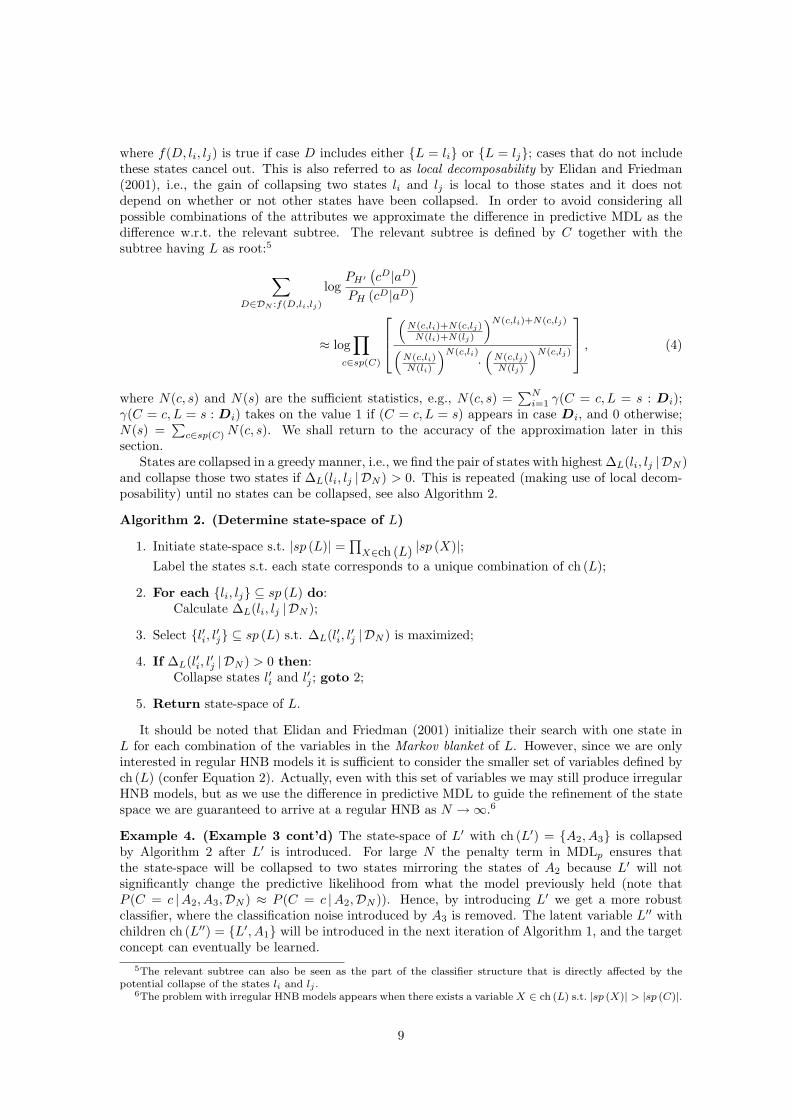
Algorithm 2. (Determine state-space of L)

1. Initiate state-space s.t. |sp (L)| =∏

X∈ch (L) |sp (X)|;

Label the states s.t. each state corresponds to a unique combination of ch (L);

2. For each {li, lj} ⊆ sp (L) do:Calculate ∆L(li, lj | DN );

3. Select {l′i, l′j} ⊆ sp (L) s.t. ∆L(l′i, l

′j | DN ) is maximized;

4. If ∆L(l′i, l′j | DN ) > 0 then:

Collapse states l′i and l′j ; goto 2;

5. Return state-space of L.

It should be noted that Elidan and Friedman (2001) initialize their search with one state inL for each combination of the variables in the Markov blanket of L. However, since we are onlyinterested in regular HNB models it is sufficient to consider the smaller set of variables defined bych (L) (confer Equation 2). Actually, even with this set of variables we may still produce irregularHNB models, but as we use the difference in predictive MDL to guide the refinement of the statespace we are guaranteed to arrive at a regular HNB as N →∞.6

Example 4. (Example 3 cont’d) The state-space of L′ with ch (L′) = {A2, A3} is collapsedby Algorithm 2 after L′ is introduced. For large N the penalty term in MDLp ensures thatthe state-space will be collapsed to two states mirroring the states of A2 because L′ will notsignificantly change the predictive likelihood from what the model previously held (note thatP (C = c |A2, A3,DN ) ≈ P (C = c |A2,DN )). Hence, by introducing L′ we get a more robustclassifier, where the classification noise introduced by A3 is removed. The latent variable L′′ withchildren ch (L′′) = {L′, A1} will be introduced in the next iteration of Algorithm 1, and the targetconcept can eventually be learned.

5The relevant subtree can also be seen as the part of the classifier structure that is directly affected by thepotential collapse of the states li and lj .

6The problem with irregular HNB models appears when there exists a variable X ∈ ch (L) s.t. |sp (X)| > |sp (C)|.

9

Note that Algorithm 2 will only visit a subset of the HNB-models in the search boundary,namely those where the latent variables are given (deterministically) by the value of their children.An important side-effect of this is that we can give a semantic interpretation to the state-spacesof the latent variables in the models the algorithm generates: L ∈ L aggregates the informationfrom its children which is relevant for classification. If, for example, L is the parent of two binaryvariables A1 and A2, then Algorithm 2 is initiated s.t. L’s state-space is sp (L) = {A1 = 0∧A2 =0, A1 = 0 ∧ A2 = 1, A1 = 1 ∧ A2 = 0, A1 = 1 ∧ A2 = 1}. When the algorithm collapses states,we can still maintain an explicit semantics over the state-space, e.g., if the first and second stateis collapsed we obtain a new state defined as (A1 = 0 ∧ A2 = 0) ∨ (A1 = 0 ∧ A2 = 1), i.e.,A1 = 0. Having such an interpretation can be of great importance when the model is put intouse: The semantics allows a decision maker to inspect the “rules” that form the basis of a givenclassification. Through this insight she can consider whether the classification of the system shouldbe overruled or accepted.7

Another important aspect of the semantic interpretation, is that it allows us to infer data forthe latent variables due to the deterministic relations encoded in the model. This fact providesus with a fast calculation scheme, as we “observe” all the variables in A and L. It therefore alsofollows that we can represent the HNB classifier using only the class variable and its children.Hence, the representation we will utilize is a Naıve Bayes structure where the “attributes” arerepresented by the variables which occur as children of the class variable in the HNB model. It issimple to realize that the number of free parameters required to represent this structure equals:

|ΘBS| = (|sp (C)| − 1) + |sp (C)|

∑

X∈ch (C)

(|sp (X)| − 1) ,

see also Kocka and Zhang (2002). Hence, the difference in predictive MDL (used in Algorithm 2)can be approximated by:

∆L(li, lj) ≈ log2(N)|sp (C)|

2(5)

−∑

c∈sp(C)

N(c, li) log2

(N(c, li)

N(c, li) + N(c, lj)

)

−∑

c∈sp(C)

N(c, lj) log2

(N(c, lj)

N(c, li) + N(c, lj)

)

+ N(li) log

(N(li)

N(li) + N(lj)

)+ N(lj) log

(N(lj)

N(li) + N(lj)

).

Let Di ⊆ DN (Dj ⊆ DN ) be the subset of the database for which L = li (L = lj). LetD = (aD, cD) be an observation, and let a

DL− be the part of the observed attributes which are

not in the relevant subtree of L. Now, it can be shown that the approximation of Equation (5) isexact if P

(ch (C) \ {L} |aD

L− , L = li)

= P(ch (C) \ {L} |aD

L− , L ∈ {li, lj})

for all D ∈ Di ∪ Dj .8

As a last remark we note that one may also consider other ways of determining the state-spaceof the latent variables. One immediate approach is to search for a suitable state-space by fixingthe number of states, and use some learning algorithm, see e.g., Dempster et al. (1977), Binderet al. (1997), or Wettig et al. (2003). This can be done greedily to maximize some performancecriteria, like BIC in Zhang et al. (2003). However, to reduce the computational complexity of thealgorithm, and at the same time to facilitate the semantic interpretation of the latent variables,we have not considered this any further.

7It should be clear that a semantic interpretation of the state-space is a side effect of the learning algorithm,and not a required feature of an HNB classifier. Furthermore, this semantic interpretation does not alter theclassification rules as it is simply a way for the user to understand how the classifier works. A detailed example isgiven in Section 5.

8Note that these probability distributions are degenerated.

10

4.2.3 The search boundary

By following the two-step procedure described above, the focusing algorithm produces a singlecandidate model H ′ ∈ B(Hk) to represent the search boundary. However, from our experimentswe have found that picking out a single model to represent the search boundary is not an adequaterepresentation of B(Hk). We can easily solve this drawback in at least two different ways:

i) Go through the candidate latent nodes one at a time in order of increasing Q(·, · | DN ), andaccept the first candidate model H ′′ ∈ B(Hk) for which Score(H ′′ | DN ) > Score(Hk | DN )in Step 2b of Algorithm 1.

ii) Limit the number of candidates used to represent the boundary to κ > 1 models, and do agreedy search over these models.

The first approach can be seen as a hill-climbing search, where we use Equation 3 to guide thesearch in the right direction. Step 2a will in this case not be a maximization over B(Hk), but merelya search for a model which can be accepted in Step 2b. In Step 2a the algorithm may have to visitall models in the boundary B′(Hk) ⊂ B(Hk), where B′(Hk) is defined s.t. each possible latent nodeis represented by exactly one state-space specification, i.e., a total of O(n2) models. On the otherhand, the second approach will only examine κ models in Step 2a. It follows that alternative i)has higher computational complexity; in fact we may have to inspect O(n3) candidates before thealgorithm terminates (Step 2 may be repeated n− 1 times), and since inspecting each candidatelatent variable involves costly calculations it may be computationally expensive. For the resultsreported in Section 5 we have therefore used the second alternative: A fixed number of candidatemodels (κ = 10) are selected from the search boundary, and the search proceeds as in Algorithm1. The computational complexity of this approach is detailed in Section 4.3.

An immediate approach for implementing this refined algorithm would be to: 1) pick out theκ node pairs that have the strongest correlation (according to Equation 3), 2) find the associatedstate-spaces, and 3) select the model with the highest score in Step 2a. However, to increasethe robustness of the algorithm (e.g. in case of outliers), we do it slightly differently: Initially,we randomly partition the training data DN into κ partly overlapping subsets, each containing(κ − 1)/κ of the training data, and then each of these subsets are used to approximate the best

model in the search boundary; this results in a list of up to κ different candidate models. We letthese models represent B(Hk), and continue as if this was the whole boundary: If the best modelamongst them (the one with the highest accuracy estimated by cross validation over the trainingdata) is better than the current model candidate, we select that one and start all over again. Ifthe best model is inferior to the current model, the search algorithm terminates, and the currentmodel is returned (see Algorithm 3).

Algorithm 3. (Find HNB classifier)

1. Initiate model search with H0;

2. Partition the training-set into κ partly overlapping subsets D(1), . . . , D(κ);

3. For k = 0, 1, . . . , n− 1

(a) For i = 1, . . . , κ

i. Let {X(i), Y (i)} = arg min{X,Y }⊆ch (C) Q

(X,Y | D(i)

)

(i.e.,{X(i), Y (i)

}⊆ ch (C) in Hk), and define the latent

variable L(i) with children ch(L(i)

)=

{X(i), Y (i)

};

ii. Collapse the state-space of L(i) (Algorithm 2 with D(i) usedin place of DN );

iii. Define H(i) by introducing L(i) into Hk;

(b) H ′ = arg maxi=1,...,κ

Score(H(i) | DN

);

11

(c) If Score(H ′ | DN ) > Score(Hk | DN ) then:Hk+1 ← H ′; k ← k + 1;

elsereturn Hk;

4. Return Hn;

4.3 Complexity analysis

The complexity can be analyzed by considering the three steps that characterize the algorithm:

1. Find a candidate latent variable.

2. Find the state-space of a candidate latent variable, and check if it is useful.

3. Iterate until no more candidate latent variables are accepted.

Part 1Proposing a candidate latent variable corresponds to finding the pair (X,Y ) of variables withthe strongest correlation (Equation 3). There are at most (n2 − n)/2 such pairs, where n is thenumber of attribute variables. By calculating the conditional mutual information for a pair ofvariables as well as sorting the pairs (for future iterations) according to this measure we get thetime complexity:. O(n2 · (N + log(n))) In the remainder of this analysis we shall assume thatlog(n) is negligible compared to N hence, for part 1 we get O(n2 · (N + log(n))) ≈ O(n2 ·N).

Part 2The time complexity of calculating the gain, ∆L(·, ·), of collapsing two states is simply O(N),see Equation 5. Due to local decomposability, the gain of collapsing two states has no effect oncollapsing two other states, and there are therefore at most (|sp (L)|2 − |sp (L)|)/2 such possiblecombinations to calculate initially. Next, when two states are collapsed, ∆L(·, ·) must be calculatedfor |sp (L)| − 1 new state combinations, and the collapsing is performed at most |sp (L)| − 1times. The time complexity of finding the state-space of a candidate latent variable is therefore

O(N · |sp (L)|2 + N · |sp (L)| (|sp (L)| − 1)/2

)= O(|sp (L)|2 ·N).

Having found the cardinality of a candidate variable, say L, we test whether it should beincluded in the model using the wrapper approach. From the rule-based propagation method it iseasy to see that the time complexity of this task is O(n ·N). Thus, the time complexity of Part 2

is O((n + |sp (L)|2) ·N).

Part 3Each time a latent variable is introduced we would in principle need to perform the above stepsagain, and the time complexity would therefore be n − 1 times the time complexities above.However, by exploiting locality some of the previous calculations can be reused.

Moreover, note that after having introduced a latent variable L with children X and Y , wecannot create another latent variable having either X or Y as a child (due to the structure of theHNB model). Thus, after having included a latent variable the cardinality of the resulting set ofcandidate pairs is reduced by n−1. This implies that we will perform at most n−2 re-initializations,thereby giving the overall time complexity O(n2·N+n·(n·N+(|sp (L)|2·N))) = O(n2·|sp (L)|2·N).

It is important to emphasize that the computational complexity is dependent on the cardinalityof the latent variables. In the worst case, if none of the states are collapsed, then the cardinality ofa latent variable L is exponential in the number of leaves in the subtree having L as root. However,this situation also implies that the leaves are conditionally dependent given the class variable, andthat the leaves and the class variable do not exhibit any type of context specific independence(Boutilier et al. 1996).

12

5 Empirical results

In this section we will investigate the merits of the proposed learning algorithm by using it tolearn classifiers for a number of different domains. All data-sets are taken from the Irvine MachineLearning Repository (Blake and Merz 1998), see Table 1 for a summary of the 22 datasets usedin this empirical study.

Dataset #Att #Cls Size Database #Att #Cls Sizepostop 8 3 90 cleve 13 2 296iris 4 3 150 wine 13 3 178monks-1 6 2 432 thyroid 5 3 215car 6 4 1728 ecoli 7 8 336monks-3 6 2 432 breast 10 2 683glass 9 7 214 vote 16 2 435glass2 9 2 163 crx 15 2 653diabetes 8 2 768 australian 14 2 690heart 13 2 270 chess 36 2 3199hepatitis 19 2 155 vehicle 18 4 846pima 8 2 768 soybean-large 35 19 562

Table 1: Datasets used in the experiments

A summary of the 22 databases used in the experiments: #Att indicates the number ofattributes; #Cls is the number of classes; Size is the number of instances. 5-fold crossvalidation was used for all datasets. Further details regarding the datasets can be found atthe UCI Machine Learning Repository.

We have compared the results of the HNB classifier to those of the Naıve Bayes model (Dudaand Hart 1973), the TAN model (Friedman et al. 1997), the original HNB algorithm (Zhang et al.2003), C5.0 (Quinlan 1998), a standard implementation of logistic regression and neural networkswith one hidden layer trained by back-propagation.9 As some of the learning algorithms requirediscrete variables, the attributes were discretized using the entropy-based method of Fayyad andIrani (1993). In addition, instances containing missing attribute-values were removed; all pre-processing was performed using MLC++ (Kohavi et al. 1994).

The accuracy-results are given in Table 2. For each dataset we have estimated the accuracyof each classifier (in percentage of instances which are correctly classified), and give a standarddeviation of this estimate. The standard deviations are the theoretical values calculated accordingto Kohavi (1995), and are not necessarily the same as the empirical standard deviations observedduring cross validation. In order to test whether a given classifier is better than another classifier wehave used Nadeau and Bengio (2003)’s corrected resampled t-test, which incorporates informationabout classifier accuracy on each cross-validation fold; the same cross-validation folds were givento all classification algorithms. The best result for each dataset is given in boldface. We notethat the proposed HNB classifier achieves the best result, among all the classification algorithms,for 12 of the 22 datasets, and is significantly poorer than the winner (at 10% level) for only twodatasets. See also Figure 2 for a graphical illustration of the accuracy results of the proposedalgorithm compared to the accuracy results of the algorithms mentioned above.

To help the interpretation of the results reported in Table 2 ran all algorithms in their “basic”configurations, i.e., no optimization was performed. One notable exception is the TAN model,which was run both in its basic form and with a damping-factor equal to 5 virtual counts (thisalgorithm is denoted TAN-5 in Table 2). The high computational complexity of the algorithmby Zhang et al. (2003) prevented us from obtaining results for this algorithm on the three most

9We used Clementine (SPSS Inc. 2002) to generate the C5.0, logistic regression and neural network models.

13

complex domains.We have also analyzed the effect which the size of training data has on the classification

accuracy of our learning algorithm. Let α(N) be the accuracy of a learning algorithm whentrained on a database of size N . We call a plot of N vs. α(N) the learning curve. The learningcurve can give important information about the workings of an algorithm; it is for instance wellknown that the Naıve Bayes algorithm learns fast (“high” accuracy compared to other learningalgorithms for “small” databases), but because of the strong learning bias it also has a tendency toconverge too quickly (meaning that the accuracy does not increase beyond a certain level even for“large” databases), see also Ng and Jordan (2002). To estimate the learning curve of Algorithm3, we have generated a random data set of a given size N by sub-sampling from a larger database,and used the remaining cases in the database as a test-set. This was repeated 10 times for eachN . We used the car database to generate the results shown in Figure 3.

The most important conclusion to draw from the results in Figure 3 is that the learningalgorithm introduced in this paper generates classifiers with the fast starting property of theNaıve Bayes models, and at the same time it avoids the premature convergence the NB modelsstruggle with. This also conforms with the intuition: as the HNB model is (in principle) capableof learning any classification system, it should not converge prematurely.

Next, we note that in some of the domains the learned HNB models contain an interestinglatent structure. For example, the car database is a synthetic data-set consisting of 1728 caseswhich describe the relationship between certain characteristics of a car and whether or not the caris “acceptable”. The states of the class attribute are unacceptable, acceptable, good and very-good,and the attributes describing the car are:

• Number of doors (Doors) with states 2,3,4 and 5-more.

• Capacity in term of persons (Persons) having states 2, 4 and more.

• Size of luggage boot (Lug boot) having states small, medium and big.

• Estimated safety of the car (Safety) having states low, medium and high.

• Buying price (Buying) having states low, medium, high and very-high.

• Price of maintenance (Maint) having states low, medium, high and very-high.

When applying the algorithm to this database we obtain the model illustrated in Figure 4.The nodes TechValue, SafetyPrDollar and Cost correspond to the latent variables identified

by the algorithm; the names of these variables have manually been deduced from their usage inthe model. For example, the node Cost summarizes the two types of monetary costs using thefour states Cost=very-high, Cost=high, Cost=medium and Cost=low. The state very-high encodesthe following configurations of the attributes Maint and Buying:

[(Maint = very-high) ∧ (Buying = very-high)]

∨

[(Maint = very-high) ∧ (Buying = high)]

∨

[(Maint = high) ∧ (Buying = very-high)]

Similar the state cost-low corresponds to the following configurations:

[(Maint = medium) ∧ (Buying = low)]

∨

[(Maint = low) ∧ (Buying = low)]

∨

[(Maint = low) ∧ (Buying = medium)]

14

Database NB TAN TAN-5 C5.0 NN Logistic Zhang et al. HNB #Latentpostop 64.25+/-5.0 63.03+/-5.1 ?62.09+/-5.1 67.31+/-4.9 67.31+/-4.9 66.26+/-5.0 68.94+/-4.9 68.95+/-4.9 [0; 1]iris 94.00+/-2.0 94.00+/-2.0 94.00+/-2.0 93.53+/-2.0 93.51+/-2.0 93.53+/-2.0 ◦86.81+/-2.8 94.00+/-2.0 [0; 1]monks-1 •75.00+/-2.2 100.0+/-0.1 100.0+/-0.1 100.0+/-0.1 ?95.65+/-1.0 •75.28+/-2.1 100.0+/-0.1 100.0+/-0.1 [2; 2]car •87.15+/-0.8 94.97+/-0.5 ?93.86+/-0.6 •92.21+/-0.6 ?93.65+/-0.6 ?94.23+/-0.6 •86.75+/-0.8 95.66+/-0.5 [2; 3]monks-3 ◦97.22+/-0.8 99.30+/-0.4 ?98.84+/-0.5 100.0+/-0.1 99.31+/-0.4 100.0+/-0.1 ◦97.22+/-0.8 100.0+/-0.1 [2; 2]glass 71.04+/-3.1 71.04+/-3.1 72.44+/-3.0 70.78+/-3.1 66.66+/-3.2 71.70+/-3.1 •53.45+/-3.4 71.04+/-3.1 [0; 0]glass2 81.61+/-3.0 81.69+/-3.0 82.29+/-3.0 ?79.18+/-3.2 82.23+/-3.0 81.02+/-3.1 •68.30+/-3.6 84.11+/-2.9 [0; 1]diabetes 75.65+/-1.5 75.25+/-1.6 75.51+/-1.6 73.21+/-1.6 ◦74.25+/-1.6 75.41+/-1.6 •65.83+/-1.7 75.25+/-1.6 [0; 1]heart 83.70+/-2.2 84.07+/-2.2 84.44+/-2.2 ◦80.00+/-2.4 ◦82.54+/-2.3 85.09+/-2.2 ◦81.26+/-2.4 85.93+/-2.3 [0; 3]hepatitis 92.34+/-2.1 87.25+/-2.7 87.27+/-2.7 ◦80.64+/-3.2 ◦81.11+/-3.1 ◦83.01+/-3.0 ?83.49+/-3.0 93.76+/-2.1 [0; 1]pima 76.17+/-1.5 ◦74.74+/-1.6 ◦74.87+/-1.6 ◦73.35+/-1.6 ◦74.13+/-1.6 76.07+/-1.5 •65.81+/-1.7 76.04+/-1.5 [0; 1]cleve 83.46+/-2.1 81.38+/-2.2 82.41+/-2.2 ?79.07+/-2.4 ?78.42+/-2.4 82.38+/-2.2 81.17+/-2.3 83.45+/-2.1 [0; 2]wine 98.30+/-1.0 ◦96.03+/-1.5 ◦96.03+/-1.5 ◦91.28+/-2.1 ◦93.41+/-1.9 ◦93.44+/-1.9 ◦89.19+/-2.3 98.86+/-0.8 [0; 1]thyroid 93.02+/-1.7 93.02+/-1.7 94.42+/-1.6 91.36+/-1.9 92.73+/-1.8 92.27+/-1.8 •80.73+/-2.7 93.02+/-1.7 [0; 1]ecoli 80.95+/-2.1 ?79.76+/-2.2 ?80.06+/-2.2 82.41+/-2.1 ◦77.14+/-2.3 ?78.89+/-2.2 •66.20+/-2.6 82.74+/-2.1 [0; 1]breast 97.36+/-0.6 ?96.19+/-0.7 96.78+/-0.7 ◦94.92+/-0.8 ◦95.64+/-0.8 ?96.08+/-0.7 ◦94.20+/-0.9 97.36+/-0.6 [0; 4]vote ?90.11+/-1.4 ?92.64+/-1.3 94.48+/-1.1 94.77+/-1.1 93.86+/-1.2 ?92.27+/-1.3 94.30 +/- 1.1 93.39+/-1.3 [0; 3]crx 86.22+/-1.3 ◦83.78+/-1.4 85.30+/-1.3 86.17+/-1.4 85.25+/-1.4 86.33+/-1.3 85.41 +/- 1.4 86.51+/-1.3 [0; 1]australian 85.80+/-1.3 ◦82.32+/-1.5 84.78+/-1.4 85.61+/-1.3 83.88+/-1.4 86.47+/-1.3 85.80 +/- 1.3 84.64+/-1.4 [0; 1]chess •88.02+/-0.6 •92.30+/-0.5 •92.30+/-0.5 99.32+/-0.1 99.13+/-0.2 •97.69+/-0.3 — •94.06+/-0.4 [2; 2]vehicle ◦59.09+/-1.7 68.79+/-1.6 69.50+/-1.6 67.78+/-1.6 67.10+/-1.6 69.22+/-1.6 — ?63.59+/-1.7 [0; 4]soybean-large 92.90+/-1.0 91.64+/-1.1 92.17+/-1.0 91.71+/-1.2 ◦64.86+/-2.0 ?88.69+/-1.3 — 92.89+/-1.1 [1; 4]

Table 2: Classifier accuraciesClassifiers accuracies: Calculated accuracy for the 22 datasets used in the experiments; the results are given together with their theoretical standard deviation.

The adjusted t-test of Nadeau and Bengio (2003) was used to compare the classifiers: Results that are significantly poorer than the best on a given dataset at

10%-level are marked with ‘?’. Results significant at 5%-level are marked with ‘◦’, and 1%-level with ‘•’. The right-most column (#Latent) shows the range

for the number of latent nodes inserted by Algorithm 3 during model search.

15

0 5

10 15 20 25 30 35 40 45

0 5 10 15 20 25 30 35 40 45

HN

B c

lass

ifica

tion

erro

r

NB classification error

0 5

10 15 20 25 30 35 40 45

0 5 10 15 20 25 30 35 40 45

HN

B c

lass

ifica

tion

erro

r

TAN classification error

a) NB vs. HNB b) TAN vs. HNB

0 5

10 15 20 25 30 35 40 45

0 5 10 15 20 25 30 35 40 45

HN

B c

lass

ifica

tion

erro

r

C5.0 classification error

0 5

10 15 20 25 30 35 40 45

0 5 10 15 20 25 30 35 40 45

HN

B c

lass

ifica

tion

erro

r

NN classification error

c) C5.0 vs. HNB d) NN vs. HNB

0 5

10 15 20 25 30 35 40 45

0 5 10 15 20 25 30 35 40 45

HN

B c

lass

ifica

tion

erro

r

Log.Reg. classification error

0 5

10 15 20 25 30 35 40 45

0 5 10 15 20 25 30 35 40 45

HN

B c

lass

ifica

tion

erro

r

Zhang et al.’s classification error

e) Logistic regression vs. HNB f) Zhang et al. vs. HNB

Figure 2: Scatter plot of classification error for HNB and a selection of other classification systems.In each plot, a point represents a dataset. The HNB’s classification error is given on the y-axis,whereas the other system’s error is given on the x-axis. Hence, data points below the diagonalcorresponds to datasets where the HNB is superior, whereas points above the diagonal are datasetswhere the HNB classifier is inferior to the other system.

16

70

75

80

85

90

95

100

0 200 400 600 800 1000 1200 1400 1600

Cla

ssifi

catio

n ac

cura

cy

Size of training set

Figure 3: The figure shows the estimated learning curves for Algorithm 3 when applied to the car

database (Straight line), TAN (Dashed) and Naıve Bayes (dotted).

MaintBuying

CostSafety

SafetyPrDollarLug boot

TechValue PersonsDoors

Class

MaintBuying

Safety

Lug boot

PersonsDoors

Class

Figure 4: The learned HNB model for the car database with three latent variables (left) and thecorresponding TAN model (right).

17

medium

highvery-high

high

medium

low

Maint

Buying

low

1

1

1

2

2

3 3

3 3

3

3 3

3

4

4 4very-high

1 - Cost=low

3 - Cost=high

2 - Cost=medium

4 - Cost=very-high

2 - SafetyPrDollar=low

4 - SafetyPrDollar=good

6 - SafetyPrDollar=very-high

1 - SafetyPrDollar=very-low

3 - SafetyPrDollar=medium

5 - SafetyPrDollar=high

medium

highvery-high

high

medium

low

Costlow

Safety

1 1 1 1

1

1

23

3

4

56

SafetyPrDollarvery-low

lowmedium

good

highvery-high

Lug boot

high

medium

small 1 1

1

1

2

2 2

2

2 2 2

3

3

3

4 4

4 4

1 - TechValue=low 2 - TechValue=medium

3 - TechValue=high 4 - TechValue=very-high

Figure 5: The figure illustrates the state spaces of the latent variables; the numbers correspondto specific states for each of the variables and indicate the relationship between a given latentvariable and its children.

The node SafetyPrDollar compares the safety level to the cost, and contains the six statesvery-high, high, good, medium, low and very-low. For instance, SafetyPrDollar=very-low specify[Safety = low ∨ Cost = very-high]. A graphical representation of the state spaces can be seen inFigure 5.

Finally Figure 6 shows the average number of latent variables inserted by the learning algorithmas a function of the size of the training set. Again, the results are averaged over 10 runs. We cansee that the algorithm has a built-in ability to avoid overfitting when working with this data-set;only a few latent variables are inserted when the size of the training set is small, and the algorithmseems to stabilize around 3 latent variables for N ≥ 1000 training cases.

6 Discussion

6.1 Parameter learning

The parameters in the model are estimated by their maximum likelihood values. This may not beoptimal for classification, and recent research by Wettig et al. (2003) has shown some improvementin classification accuracy when the parameters are chosen otherwise. However, to support theinterpretation of the empirical results in Section 5 we have deliberately not taken the opportunityof improving the classification accuracy further in this way.

18

0

0.5

1

1.5

2

2.5

3

3.5

0 200 400 600 800 1000 1200 1400 1600

No.

late

nt v

aria

bles

Size of training set

Figure 6: The number of latent variables inserted by Algorithm 3, as a function of the size of thetraining set (the numbers are from the car domain).

6.2 Inference and model structure

The algorithm for collapsing the state-space of a latent variable is the source of the semantics forthese nodes, and in turn the reason why we can represent the HNB as a Naıve Bayes model withaggregations in place of the attributes. This compact representation requires a “deterministicinference engine” to calculate P (C |a), because the aggregations defined by the semantics of thelatent variables can in general not be encoded by the conditional probability tables for the variables.Assume, for instance, that we have three binary variables L,X, Y , ch (L) = {X,Y }, and “L = 1if and only if X = Y ”. This relationship cannot be encoded in the model X ← L → Y , and toinfer the state of the latent variable L from X and Y we would therefore need to design a specialinference algorithm which explicitly uses the semantics of L. To alleviate this potential drawbackwe can simply re-define the network-structure: Introduce a new latent variable L′, and changethe network structure s.t. ch (L) = pa (X) = pa (Y ) = {L′}; L′ is equipped with at most onestate for each possible combination of its children’s states. This enlarged structure is capable ofencoding any relation between {X,Y } and L using the conditional probability tables only. Hence,the enlarged structure can be handled by any standard BN propagation algorithm and, since thestructure is still an HNB, the inference can be performed extremely fast.

7 Concluding remarks

In this paper we have used Hierarchical Naıve Bayes models for classification, and through experi-ments we have shown that the HNB classifiers offer results that are significantly better than thoseof other commonly used classification methods. Moreover, a number of existing tools may be ableto improve the classification accuracy even further. These include feature selection (Kohavi andJohn 1997), and supervised learning of the probability parameters (Wettig et al. 2003). Finally,the proposed learning algorithm also provides an explicit semantics for the latent structure of amodel. This allows a decision maker to easily deduce the rules which govern the classification ofsome instance hence, the semantics may also increase the user’s confidence in the model.

19

Acknowledgements

We have benefited from interesting discussions with the members of the Decision Support Systemsgroup at Aalborg University, in particular Tomas Kocka, and Jirı Vomlel. We thank Nevin L.Zhang for his valuable insight and for giving us access to his implementation of the HNB learningalgorithm by Zhang et al. (2003).

References

Binder, J., D. Koller, S. Russell, and K. Kanazawa (1997). Adaptive probabilistic networks withhidden variables. Machine Learning 29 (2–3), 213–244.

Blake, C. and C. Merz (1998). UCI repository of machine learning databases. http://www.ics.uci.edu/∼mlearn/MLRepository.html.

Boutilier, C., N. Friedman, M. Goldszmidt, and D. Koller (1996). Context-specific independencein Bayesian networks. In Proceedings of the Twelfth Conference on Uncertainty in Artificial

Intelligence, Portland, Oregon, pp. 115–123.

Chow, C. K. and C. Liu (1968). Approximating discrete probability distributions with depen-dence trees. IEEE Transactions on Information Theory 14, 462–467.

Dempster, A. P., N. M. Laird, and D. B. Rubin (1977). Maximum likelihood from incompletedata via the EM algorithm. Journal of the Royal Statistical Society, Series B 39, 1–38.

Domingos, P. and M. Pazzani (1997). On the optimality of the simple Bayesian classifier underzero-one loss. Machine Learning 29 (2–3), 103–130.

Duda, R. O. and P. E. Hart (1973). Pattern Classification and Scene Analysis. New York: JohnWiley & Sons.

Elidan, G. and N. Friedman (2001). Learning the dimensionality of hidden variables. In Proceed-

ings of the Seventeenth Conference on Uncertainty in Artificial Intelligence, San Francisco,CA., pp. 144–151. Morgan Kaufmann Publishers.

Fayyad, U. M. and K. B. Irani (1993). Multi-interval discretization of continuous-valued at-tributes for classification learning. In Proceedings of the Thirteenth International Joint Con-

ference on Artificial Intelligence, San Mateo, CA., pp. 1022–1027. Morgan Kaufmann Pub-lishers.

Friedman, J. H. (1997). On bias, variance, 0/1-loss, and the curse of dimensionality. Data Mining

and Knowledge Discovery 1 (1), 55–77.

Friedman, N., D. Geiger, and M. Goldszmidt (1997). Bayesian network classifiers. Machine

Learning 29 (2–3), 131–163.

Greiner, R., A. J. Grove, and D. Schuurmans (1997). Learning Bayesian nets that perform well.In Proceedings of the Thirteenth Conference on Uncertainty in Artificial Intelligence, SanFrancisco, CA., pp. 198–207. Morgan Kaufmann Publishers.

Jaeger, M. (2003). Probabilistic classifiers and the concepts they recognize. In Proceedings of the

Twentieth International Conference on Machine Learning, Menlo Park, pp. 266–273. TheAAAI Press.

Jensen, F. V. (2001). Bayesian Networks and Decision Graphs. New York: Springer-Verlag.

Kohavi, R. (1995). A study of cross-validation and bootstrap for accuracy estimation and modelselection. In Proceedings of the Fourteenth International Joint Conference on Artificial In-

telligence, San Mateo, CA., pp. 1137–1143. Morgan Kaufmann Publishers.

Kohavi, R., G. John, R. Long, D. Manley, and K. Pfleger (1994). MLC++: A machine learninglibrary in C++. In Proceedings of the Sixth International Conference on Tools with Artificial

Intelligence, pp. 740–743. IEEE Computer Society Press.

20

Kohavi, R. and G. H. John (1997). Wrappers for feature subset selection. Artificial Intelli-

gence 97 (1–2), 273–324.

Kononenko, I. (1991). Semi-naive Bayesian classifier. In Proceedings of Sixth European Working

Session on Learning, Porto, Portugal, pp. 206–219. Springer-Verlag.

Kocka, T. and N. L. Zhang (2002). Dimension correction for hierarchical latent class models.In Proceedings of the Eighteenth Conference on Uncertainty in Artificial Intelligence, SanFrancisco, CA., pp. 267–274. Morgan Kaufmann Publishers.

Lam, W. and F. Bacchus (1994). Learning Bayesian belief networks: An approach based on theMDL principle. Computational Intelligence 10 (4), 269–293.

Langley, P. (1993). Induction of recursive Bayesian classifiers. In Proceedings of the Fourth Euro-

pean Conference on Machine Learning, Volume 667 of Lecture Notes in Artificial Intelligence,pp. 153–164. Springer-Verlag.

Martin, J. D. and K. VanLehn (1994). Discrete factor analysis: Learning hidden variables inBayesian networks. Technical Report LRDC-ONR-94-1, Department of Computer Science,University of Pittsburgh. http://www.pitt.edu/∼vanlehn/distrib/Papers/Martin.pdf.

Mitchell, T. M. (1997). Machine Learning. Boston, MA.: McGraw Hill.

Nadeau, C. and Y. Bengio (2003). Inference for the generalization error. Machine Learn-

ing 52 (3), 239–281.

Ng, A. Y. and M. I. Jordan (2002). On discriminative vs. generative classifiers: A comparison oflogistic regression and naive Bayes. In Advances in Neural Information Processing Systems

15, Vancouver, British Columbia, Canada, pp. 841–848. The MIT Press.

Pazzani, M. (1996a). Searching for dependencies in Bayesian classifiers. In Learning from data:

Artificial Intelligence and Statistics V, New York, N.Y., pp. 239–248.

Pazzani, M. J. (1996b). Constructive induction of cartesian product attributes. In ISIS: Infor-

mation, Statistics and Induction in Science, Singapore, pp. 66–77. World Scientific.

Pearl, J. (1988). Probabilistic Reasoning in Intelligent Systems: Networks of Plausible Inference.San Mateo, CA.: Morgan Kaufmann Publishers.

Quinlan, R. (1998). C5.0: An informal tutorial. http://www.rulequest.com/see5-unix.html.

Rissanen, J. (1978). Modelling by shortest data description. Automatica 14, 465–471.

Schwarz, G. (1978). Estimating the dimension of a model. The Annals of Statistics 6, 461–464.

Spirtes, P., C. Glymour, and R. Scheines (1993). Causation, Prediction, and Search. New York:Springer-Verlag.

SPSS Inc. (2002). Clementine v6.5. http://www.spss.com/spssbi/clementine/.

Wettig, H., P. Grunwald, T. Roos, P. Myllymaki, and H. Tirri (2003). When discriminativelearning of Bayesian network parameters is easy. In Proceedings of the Eighteenth Interna-

tional Joint Conference on Artificial Intelligence, pp. 491–496. Morgan Kaufmann Publish-ers.

Whittaker, J. (1990). Graphical models in applied multivariate statistics. Chichester: John Wiley& Sons.

Zhang, N. L. (2004). Hierarchical latent class models for cluster analysis. Journal of Machine

Learning Research 5 (6), 697–723.

Zhang, N. L., T. D. Nielsen, and F. V. Jensen (2003). Latent variable discovery in classificationmodels. Artificial Intelligence in Medicine 30 (3), 283–299.

21