aalborg universitet non-gaussian, non-stationary and ...vbn.aau.dk/files/33922153/cl_thesis.pdf ·...

Aalborg Universitet

Non-Gaussian, Non-stationary and Nonlinear Signal Processing Methods - withApplications to Speech Processing and Channel EstimationLi, Chunjian

Publication date:2007

Document VersionEarly version, also known as pre-print

Link to publication from Aalborg University

Citation for published version (APA):Li, C. (2007). Non-Gaussian, Non-stationary and Nonlinear Signal Processing Methods - with Applications toSpeech Processing and Channel Estimation. Aalborg Universitet: Institut for Elektroniske Systemer, AalborgUniversitet.

General rightsCopyright and moral rights for the publications made accessible in the public portal are retained by the authors and/or other copyright ownersand it is a condition of accessing publications that users recognise and abide by the legal requirements associated with these rights.

? Users may download and print one copy of any publication from the public portal for the purpose of private study or research. ? You may not further distribute the material or use it for any profit-making activity or commercial gain ? You may freely distribute the URL identifying the publication in the public portal ?

Take down policyIf you believe that this document breaches copyright please contact us at [email protected] providing details, and we will remove access tothe work immediately and investigate your claim.

Downloaded from vbn.aau.dk on: juni 11, 2018

http://vbn.aau.dk/en/publications/nongaussian-nonstationary-and-nonlinear-signal-processing-methods--with-applications-to-speech-processing-and-channel-estimation(439cf6e0-cfdb-11dc-8dd8-000ea68e967b).html

Non-Gaussian, Non-stationary, andNonlinear Signal Processing

Methods

with Applications to Speech Processing andChannel Estimation

Ph.D. Thesis

CHUNJIAN LI

February, 2006

Chunjian Li

Non-Gaussian, Non-stationary, and Nonlinear Signal Processing methods

- with Applications to Speech Processing and Channel Estimation

Copyright c© 2006 Chunjian Li, except where otherwise stated.

All rights reserved. No part of this publication may be reproduced, stored in a retrieval system,or transmitted in any form or by any means, electronic, mechanical, photocopying, recording, orotherwise, without the prior written permission of the author.

ISBN 87-90834-90-9

ISSN 0908-1224

R06-1001

Department of Communication TechnologyAalborg UniversityFredrik Bajers Vej 7DK-9220 Aalborg Øst, DenmarkPhone: +45 9635 8650

This thesis was typeset using LATEX.

Printed by Uniprint, Aalborg, Denmark.

Abstract

The Gaussian statistic model, despite its mathematical elegance, is found to be too fac-titious for many real world signals, as manifested by its unsatisfactory performancewhen applied to non-Gaussian signals. Traditional non-Gaussian signal processingtechniques, on the other hand, are usually associated with high complexities and lowdata efficiencies. This thesis addresses the problem of optimum estimation of non-Gaussian signals in computation-efficient and data-efficient ways. The approaches thatwe have taken exploit the high temporal-resolution non-stationarity or the underlyingdynamics of the signals. The sub-topics being treated include: joint MMSE estimationof the signal DTFT magnitude and phase, high temporal-resolution Kalman filtering,blind de-convolution and blind system identification, and optimum non-linear estima-tion. Applications of the proposed algorithms to speech enhancement, non-Gaussianspectral analysis, noise-robust spectrum estimation, andblind channel equalization aredemonstrated.

The thesis consists of two parts, the Introduction and the Papers. The Introduc-tion gives background information of the problems at hand, states the motivation ofapproaches taken, summarizes the state-of-the-art in literature, and describes our con-tributions briefly. The Papers presents our contributions in the form of published papers.

The first part of the Papers (paper A and B) deals with the importance of phase innon-Gaussian signal estimation. Joint MMSE estimators of both magnitude spectra andphase spectra are developed. Application to the enhancement of noisy speech signalsresults in clearer sounds and higher SNR than frequency domain MMSE estimators.Here the non-Gaussianity of the speech signal is modeled by the linearity in the phasespectrum, and is enhanced by the joint estimator. This is in contrast to the spectraldomain MMSE estimator (e.g., the Wiener filter), which is zero-phase.

The second part of the Papers (paper C and D) attacks the non-Gaussian estimationproblem with a purely temporal domain approach. It is recognized that a temporal-domain high-resolution non-stationary LMMSE estimator isable to extract structuresin both magnitude and phase spectra at a lower complexity. For speech signals, thenon-Gaussianity is represented by an excitation sequence with a rapidly varying vari-

i

ance filtered by an all-pole filter. A Kalman filter with a time-varying system noise isideally suitable to this model. This so called high temporal-resolution Kalman filteringtechnique fully exploits the non-stationary processing capability of the Kalman filter,yet takes advantage of the fact that the all-pole filter changes slowly over time. This isin contrast to the conventional frame-based Kalman filtering, which presumes signalsto be stationary within a processing frame, and to the adaptive Kalman filtering whichadapts all system parameters in every time instant.

The third part of the Papers (paper E, F and G) sees the non-Gaussian estimationproblem from yet another angle. Her the non-Gaussian excitation is treated as a discrete-state finite-alphabet symbol sequence. The new model combines the HMM and theAR model to represent a wide range of signals, thus we call it the Hidden Markov-Autoregressive model (HMARM). The HMARM can efficiently extract the second or-der and higher order temporal structure with the two dynamicmodels respectively. Effi-cient ML system identification algorithms are derived basedon the EM methodology tojointly estimate the HMM parameters and the AR parameters. In paper F, the HMARMis extended to having a measurement noise at the output of theAR model. This exten-sion increases the estimation complexity significantly since the system output is nowhidden and the measurement noise variance need to be estimated jointly with otherparameters. A nonlinear MMSE estimator is incorporated into the EM algorithm toprovide the sufficient statistics for the learning. The HMARM and its extended ver-sion are applied to speech analysis, noise robust spectrum estimation, and blind channelequalization for PAM and PPM signals.

The proposed algorithms in this thesis only involve computations of the second or-der statistics explicitly. The higher order structure is though represented by the appro-priately chosen models. Thus the computational complexityis low and data efficiencyis high compared to Higher Order Statistics based methods, which require no signalmodels.

ii

List of Papers

The thesis is based on the following papers:

[A] Chunjian Li and Søren Vang Andersen, “Inter-frequency Dependency inMMSE Speech Enhancement”. InProceedings of the 6th Nordic Signal Pro-cessing Symposium, NORSIG-2004, pp. 200-203. June 9-11, 2004, Espoo,Finland.

[B] Chunjian Li and Søren Vang Andersen, “A Block Based Linear MMSE NoiseReduction with a High Temporal Resolution Modeling of the Speech Excita-tion”. In EURASIP Journal on Applied Signal Processing, Special Issue onDSP in Hearing Aids and Cochlear Implants, vol. 2005:18, pp. 2965-2978.October, 2005.

[C] Chunjian Li and Søren Vang Andersen, “Integrating Kalman filtering and multi-pulse coding for speech enhancement with a non-stationary model of the speechsignal”. In Proceedings of the Thirty-eighth Annual Asilomar Conference onSignals, Systems, and Computers, ASILOMAR-2004. November 7-11, 2004.Pacific Grove, California, USA.

[D] Chunjian Li and Søren Vang Andersen, “A new Iterative Speech EnhancementScheme Based on Kalman Filtering”. InProceedings of the 13th European Sig-nal Processing Conference, EUSIPCO-2005. September 9-11, 2005, Antalya,Turkey.

[E] Chunjian Li and Søren Vang Andersen, “Blind Identification of Non-GaussianAuto-regressive Models for Efficient Analysis of Speech Signals”. InProceed-ings of IEEE International Conference on Acoustics, Speech, and Signal Pro-cessing. May 14-19, 2006, Toulouse, France.

iii

[F] Chunjian Li and Søren Vang Andersen, “Efficient Blind System Identificationof Non-Gaussian Auto-Regressive Models with Dynamic Modeling”. Acceptedfor publication inIEEE Transactions on Signal Processing.

[G] Chunjian Li and Søren Vang Andersen, “Efficient Implementation of theHMARM Identification and Its Application in Spectral Analysis”. Submittedto Proceedings of IEEE International Conference on Acoustics, Speech, andSignal Processing, 2007.

The research that is documented in this thesis has lead to theprovisional filing of thefollowing patents:

[1] Chunjian Li and Søren Vang Andersen. A method for noise reduction using anon-Toeplitz temporal signal covariance matrix, 2005.

[2] Chunjian Li and Søren Vang Andersen. Efficient initialization of iterative pa-rameter estimation, 2005.

[3] Chunjian Li and Søren Vang Andersen. High temporal resolution estimation ofLPC excitation variance of signals, 2005.

[4] Chunjian Li and Søren Vang Andersen. A non-Gaussian signal analysis tech-nique, 2006.

iv

Preface

This thesis is submitted to the International Doctoral School of Technology and Sci-ence at Aalborg University as a partial fulfillment of the requirements for the degree ofDoctor of Philosophy. The work was carried out during the period March 1st, 2003 -February 28th, 2006 at the Department of Communication Technology at Aalborg Uni-versity, and was funded by The Danish National Centre for IT Research, Grant No. 329and Microsound A/S.

I would like to thank my primary supervisor Søren Vang Andersen for his profes-sional guidance and constant support. His encouragement has always strengthened mewhen I explored new ideas, and his broad knowledge has been animportant sourceof my learning and building my own competence. I would also like to thank my co-supervisors Søren Holdt Jensen, Per Rubak, and Uwe Hartmannfor many fruitful dis-cussions and valuable advices. I also appreciate the effortof Søren Louis Petersen atMicrosound A/S and Kjeld Hermansen in making the project a reality. I also thank themand other Microsound employees who have involved in the project for bringing in theirindustrial viewpoints and technical contributions, from which I have gotten inspirationsand insights.

Finally, I would like to acknowledge my colleagues and fellow Ph.D. students atAalborg University. Special thanks go to Karsten Vandborg Sørensen, who I have sharedroom and project with for the past three years, for giving me assistance that makesmy stay in Denmark easier; Mads Græsbøll Christensen, Xuefeng Yin, Morten HolmLarsen, Steffen Præstholm, Ingmar Land, Troels Pedersen, Joachim Dahl, Bin Hu, andChristoffer Asgaard Rødbro for many interesting discussions. Last, but not least, I thankmy friends and family for their support during my time at Aalborg University.

Chunjian LiAalborg, February 2006

v

Acronyms

AR auto-regressiveARMA auto-regressive moving averageARX auto-regressive with exogenous inputBLUE best linear unbiased estimatorE-HMARM extended hidden Markov auto-regressive modelDFT discrete Fourier transformEKF extended Kalman filterEM expectation-maximization algorithmGEM generalized EM algorithmGMM Gaussian mixture modelGSF Gaussian sum filterHMARM hidden Markov auto-regressive modelHMM hidden Markov modelHOS higher order statisticsi.i.d. independent and identically distributedISI inter-symbol interferenceKF Kalman filterLDA Levinson-Durbin algorithmLMMSE linear minimum mean square errorLPC linear predictive codingLS least squaresLTI linear time-invariantMAP maximum a posteriorML maximum likelihoodMP matching pursuitMPLPC multi-pulse linear predictive codingMMSE minimum mean squared errorMSE mean square errorPAM pulse amplitude modulation

vii

PDF probability density functionPPM pulse position modulationSKF switching Kalman filterSNR signal to noise ratioSVD Singular Value DecompositionTLS total least squaresXLS extended least squaresWF Wiener filterWSS wide sense stationary

viii

Contents

Abstract i

List of Papers iii

Preface v

Acronyms vii

I Introduction 11 Non-Gaussian time series and Bayesian estimation . . . . . . .. . . . 32 Temporal structures of non-Gaussian AR signals . . . . . . . . .. . . 93 Signal estimation . . . . . . . . . . . . . . . . . . . . . . . . . . . . . 11

3.1 Wiener filtering . . . . . . . . . . . . . . . . . . . . . . . . . . 123.2 Kalman filtering . . . . . . . . . . . . . . . . . . . . . . . . . 153.3 HMM filters and switching Kalman filters . . . . . . . . . . . . 16

4 Parameter estimation . . . . . . . . . . . . . . . . . . . . . . . . . . . 184.1 Least Squares methods . . . . . . . . . . . . . . . . . . . . . . 184.2 Bayesian analysis of dynamic systems . . . . . . . . . . . . . . 214.3 The Maximum Likelihood method . . . . . . . . . . . . . . . . 224.4 The Expectation-Maximization algorithm . . . . . . . . . . . .234.5 Higher Order Statistics based methods . . . . . . . . . . . . . . 26

5 Summary of contributions . . . . . . . . . . . . . . . . . . . . . . . . 27References . . . . . . . . . . . . . . . . . . . . . . . . . . . . . . . . . . . . 28

II Papers 37

Paper A: Inter-frequency Dependency in MMSE Speech Enhancement A11 Introduction . . . . . . . . . . . . . . . . . . . . . . . . . . . . . . . . A3

ix

2 Phase spectrum and inter-frequency dependency . . . . . . . . .. . . . A43 MMSE estimator with time and frequency envelopes . . . . . . . .. . A44 results . . . . . . . . . . . . . . . . . . . . . . . . . . . . . . . . . . . A75 Discussion . . . . . . . . . . . . . . . . . . . . . . . . . . . . . . . . . A8References . . . . . . . . . . . . . . . . . . . . . . . . . . . . . . . . . . . . A9

Paper B: A Block Based Linear MMSE Noise Reduction with a High TemporalResolution Modeling of the Speech Excitation B11 Abstract . . . . . . . . . . . . . . . . . . . . . . . . . . . . . . . . . . B32 Introduction . . . . . . . . . . . . . . . . . . . . . . . . . . . . . . . . B33 Background . . . . . . . . . . . . . . . . . . . . . . . . . . . . . . . . B6

3.1 Time domain LMMSE estimator . . . . . . . . . . . . . . . . . B63.2 Frequency domain LMMSE estimator and Wiener filter . . . . .B7

4 High temporal resolution modeling for the signal covariance matrix es-timation . . . . . . . . . . . . . . . . . . . . . . . . . . . . . . . . . . B84.1 Modeling signal covariance matrix . . . . . . . . . . . . . . . . B84.2 Estimating the spectral envelope . . . . . . . . . . . . . . . . . B94.3 Estimating the temporal envelope . . . . . . . . . . . . . . . . B10

5 The algorithm . . . . . . . . . . . . . . . . . . . . . . . . . . . . . . . B116 Reducing computational complexity . . . . . . . . . . . . . . . . . . .B127 Results . . . . . . . . . . . . . . . . . . . . . . . . . . . . . . . . . . . B158 Discussion . . . . . . . . . . . . . . . . . . . . . . . . . . . . . . . . . B19References . . . . . . . . . . . . . . . . . . . . . . . . . . . . . . . . . . . . B23

Paper C: Integrating Kalman Filtering and Multi-pulse Codin g for Speech En-hancement with a Non-stationary Model of the Speech Signal C11 introduction . . . . . . . . . . . . . . . . . . . . . . . . . . . . . . . . C32 Non-stationary signal modeling . . . . . . . . . . . . . . . . . . . . . .C43 Kalman filtering . . . . . . . . . . . . . . . . . . . . . . . . . . . . . . C54 Parameter estimation . . . . . . . . . . . . . . . . . . . . . . . . . . . C6

4.1 AR parameter estimation . . . . . . . . . . . . . . . . . . . . . C64.2 Estimating the excitation variance with high temporal resolution C7

5 experimental results . . . . . . . . . . . . . . . . . . . . . . . . . . . . C96 Conclusion . . . . . . . . . . . . . . . . . . . . . . . . . . . . . . . . C10References . . . . . . . . . . . . . . . . . . . . . . . . . . . . . . . . . . . . C11

Paper D: A New Iterative Speech Enhancement Scheme Based on Kalman Fil-tering D11 Introduction . . . . . . . . . . . . . . . . . . . . . . . . . . . . . . . . D32 The Kalman filter based iterative scheme . . . . . . . . . . . . . . . .. D5

x

3 Initialization and sequential approximation . . . . . . . . . .. . . . . . D64 Kalman filtering with high temporal resolution signal model . . . . . . D8

4.1 The Kalman filtering solution . . . . . . . . . . . . . . . . . . D84.2 Parameter estimation . . . . . . . . . . . . . . . . . . . . . . . D9

5 Experiments and results . . . . . . . . . . . . . . . . . . . . . . . . . . D106 Conclusion . . . . . . . . . . . . . . . . . . . . . . . . . . . . . . . . D12References . . . . . . . . . . . . . . . . . . . . . . . . . . . . . . . . . . . . D13

Paper E: Blind Identification of Non-Gaussian Autoregressive Models for Effi-cient Analysis of Speech Signals E11 Introduction . . . . . . . . . . . . . . . . . . . . . . . . . . . . . . . . E32 The Method . . . . . . . . . . . . . . . . . . . . . . . . . . . . . . . . E53 Experimental results . . . . . . . . . . . . . . . . . . . . . . . . . . . E94 Conclusion . . . . . . . . . . . . . . . . . . . . . . . . . . . . . . . . E10References . . . . . . . . . . . . . . . . . . . . . . . . . . . . . . . . . . . . E11

Paper F: Efficient Blind System Identification of Non-Gaussian Auto-RegressiveModels with Dynamic Modeling F11 Introduction . . . . . . . . . . . . . . . . . . . . . . . . . . . . . . . . F32 Method . . . . . . . . . . . . . . . . . . . . . . . . . . . . . . . . . . F5

2.1 The HMARM and its identification . . . . . . . . . . . . . . . F62.2 The Extended-HMARM and its identification . . . . . . . . . . F11

3 Applications and results . . . . . . . . . . . . . . . . . . . . . . . . . . F173.1 Efficient non-Gaussian speech analysis . . . . . . . . . . . . . F173.2 Blind channel equalization . . . . . . . . . . . . . . . . . . . . F213.3 Noise robust spectrum estimation for voiced speech . . . .. . . F263.4 Blind noisy channel equalization . . . . . . . . . . . . . . . . . F28

4 Conclusion . . . . . . . . . . . . . . . . . . . . . . . . . . . . . . . . F305 Appendix I . . . . . . . . . . . . . . . . . . . . . . . . . . . . . . . . F31References . . . . . . . . . . . . . . . . . . . . . . . . . . . . . . . . . . . . F32

Paper G: Efficient Implementation of the HMARM Model Identifica tion andIts Application in Spectral Analysis G11 Introduction . . . . . . . . . . . . . . . . . . . . . . . . . . . . . . . . G32 Covariance method for the HMARM . . . . . . . . . . . . . . . . . . . G43 HMARM for spectral analysis . . . . . . . . . . . . . . . . . . . . . . G7

3.1 Window design and covariance methods . . . . . . . . . . . . . G83.2 Avoiding spectral sampling effect . . . . . . . . . . . . . . . . G93.3 Avoiding over training . . . . . . . . . . . . . . . . . . . . . . G10

4 Conclusion . . . . . . . . . . . . . . . . . . . . . . . . . . . . . . . . G11

xi

References . . . . . . . . . . . . . . . . . . . . . . . . . . . . . . . . . . . . G11

xii

Part I

Introduction

1

Introduction

1 Non-Gaussian time series and Bayesian estimation

A time series is a sequence of observations that are orderly in time (or space). Most ofthe natural and man-made signals are time series, e.g. speech, images, and communica-tion signals. Many important time series exhibit certain temporal structures, or temporaldependencies. Temporal dependency in a time series is oftenmodeled by linear models,such as auto-regressive (AR), moving average (MA), and autoregressive-moving aver-age (ARMA) models, although nonlinear temporal dependencyis sometimes of interestand can be modeled by nonlinear models such as the Volterra series [1] [2] and neuralnetwork based models [3]. A linear model can be seen as a linear time invariant (LTI)filter excited by a stationary Gaussian process, whereas a nonlinear model can be seenas a nonlinear filter excited by either a Gaussian or a non-Gaussian process. In thiswork, we focus on LTI filters, especially the AR filters, excited by non-stationary ornon-Gaussian processes. The motivation is that linear filters are easier to analyze, and,as will be shown later on, the LTI filter model with a non-stationary/non-Gaussian inputis able to represent a wide range of nonlinear signals.

In the category of linear models, the AR model is the most frequently used in appli-cations. There are several reasons for its popularity: 1) the AR model can well representspectra with narrow peaks, and narrow band spectra are very common in practice [4]; 2)for a Gaussian process, the maximum entropy spectrum [5] is the spectrum given by ARmodeling [6]; 3) under the Gaussian assumption, the AR parameter estimation problemis linear while the MA and ARMA estimation problems are nonlinear. Moreover, theAR model with a sufficiently high order can be used to approximate any ARMA modelsarbitrarily well [7, p.52] [8, p.411].

Under the standard definition of the AR model, an AR process iscreated by filteringan independent, identically distributed (i.i.d.) sequence by an all-pole filter [9] [10]. Themost used distribution in the AR modeling is the Gaussian pdf. This model is, however,too restrictive to suit many important signals. As we will show later, voiced speech sig-nals and some communication signals are better modeled having non-Gaussian or non-

3

4

i.i.d. processes as inputs to the all-pole filters. In this thesis, we use a generalized ARmodel definition in which the input process to the all-pole filter can be non-Gaussian,non-stationary, and temporally dependent.

Definition 1 The process {Xt} is said to be a generalized AR(p) process if for everytit satisfies the difference equation

Xt − a1Xt−1 − · · · − apXt−p = Zt, (1)

whereZt is a random process that can take on any probability density function (pdf),can be non-stationary within the analysis frame, and can be temporally dependent.

Remark 1: The generalized AR model belongs to the big category of equation-error-type models, which is defined in [11, p.71, p.74]. All the AR models mentionedin the sequel are under this generalized definition.

Remark 2: This definition means that the input processZt can be any time series.This is especially useful for de-convolution problems.

When the excitation processZt in an AR model is stationary, white, and Gaus-sian, the model is known as the Gaussian AR model. The Gaussian AR model has beenwidely used in many signal processing fields including linear prediction [12] [13], spec-tral analysis [6] [14], and linear dynamical modeling [15, p.420] [16]. The identificationof the Gaussian AR model has also been extensively studied. Thanks to the stationary-white-Gaussian assumption, the Gaussian AR parameters canbe identified analyticallyusing, e.g. the Least Squares (LS) method [11] [15] [4].

When the excitation processZt is i.i.d. non-Gaussian, the model is known as thenon-Gaussian AR model. Non-Gaussian AR models have recently attracted an in-creased attention in the signal processing society. Many signals are found to be farfrom Gaussian [17] [18] [19]. In other words, for many signals, non-Gaussian stochas-tic models often outperform Gaussian models significantly and can be used to solveproblems that are unsolvable with the Gaussian models (e.g.Blind Source Separa-tion using Independent Component Analysis [20]). Major benefits of non-Gaussianestimation includes smaller estimation variance and bias [21] [22], robustness to out-liers [23], and efficient representation of signals [23] [24] [25]. Research works onnon-Gaussian AR modeling have appeared in image processing[26] [27] [28], speechprocessing [29] [23], medical signal processing [30], radar signals [31], navigation [32],econometrics [33], and communications signal processing [34].

When the excitation processZt is a non-stationary Gaussian process with possiblytemporal dependency, i.e., a non-i.i.d.1 Gaussian process, it is often treated as an i.i.d.non-Gaussian process too. Note that here, we are talking about a Gaussian process that

1Here, a non-i.i.d. process is referred to as a non-independent and/or non-identically distributed randomprocess.

1. NON-GAUSSIAN TIME SERIES AND BAYESIAN ESTIMATION 5

changes its mean and/or variance at every time instance, such that the usual short-timeprocessing techniques (based on the quasi-stationary assumption) are not applicable.

Similar generalizations of the linear time-invariant (LTI) system to accommodatingnon-Gaussian input process date back to the 60’s. Bartlett [35] in 1955 and Brillingeret al. [36] in 1967 analyzed the polyspectra for the i.i.d. non-Gaussian and non-i.i.d.processes excited linear systems (see [37]). In [11], ARMA models are generalizedsuch that the modeling errors are themselves AR or MA processes, therefore correlatederrors are introduced. In [38, Theorem 2], it is shown that a linear system with a non-i.i.d., non-Gaussian input process can be identified using higher order statistics. Thenon-i.i.d. Gaussian excited AR process, though, has received less research attentionthan the i.i.d. non-Gaussian excited AR process. In this work, we promote the use ofthe non-i.i.d. Gaussian excited AR process, and we give the following motivations for it:1) its optimum filtering problem can be solved analytically,with appropriate adaptationsto the classical optimum linear filters; 2) there is often rich temporal structures in theinput process which can be exploited to facilitate the identification of the underlyingdynamics of the non-stationary Gaussian process, while thei.i.d. non-Gaussian modelignores this temporal structure.

It is well known that a nonlinear transformation of an i.i.d.Gaussian process ingeneral results in an i.i.d. non-Gaussian process. We contend here that a non-stationary,though linear, transformation of a Gaussian process can also make an i.i.d. non-Gaussiandistribution if viewed as a static system. By non-stationary linear transform, we meanthe transform that changes its functional form or coefficients along time. As an example,

Y = atX + bt (2)

is such a transform, whereX is a stationary Gaussian process,at andbt are the trans-form coefficients that change over time. The resulting processY can be seen as eithera non-Gaussian process if assumed stationary, or a non-stationary process if assumedGaussian. In other words, the same set of data can be explained by either a statisticalstructure in a static view, or a temporal structure in a dynamical view. Fig. 1 shows therelations between the two transforms. The double-arrow in the center shows the duality,i.e., a process can be modeled as an i.i.d. non-Gaussian process by ignoring the tempo-ral structure in it, or modeled by a non-i.i.d. Gaussian process if the temporal structurecan be identified.

We prefer to use the dynamical view anywhere possible, sinceit allows analyticalsolution to the optimum estimation problem now that the Gaussian assumption is main-tained. Such observations are analogous to the time-variant linear system theory, whichlinearizes a nonlinear system along its trajectory and results in a time-variant linearsystem. The Extended Kalman filter (EKF) [39] is a good example of such a dynam-ical linearization. But unlike the EKF, the non-i.i.d. Gaussian AR model confines its

6

non-i.i.d.

Gaussian

non-i.i.d.

non-Gaussian

i.i.d.

Gaussian

i.i.d.

non-Gaussian

non-

stat

iona

rylin

ear

tran

sfor

m

stationary nonlinear transform

Figure 1: Non-Gaussianity, non-stationarity, and nonlinearity.

nonlinearity in the input process instead of the filter. Thisbrings several benefits:

1. The filter is linear and is easier to identify;

2. The nonlinearity of the input process is in the form of a non-Gaussian pdf, whichhas no problem of representing discontinuity such as switching effects. Whereasthe EKF requires the existence of derivatives of the nonlinear function.

3. This is useful in many de-convolution problems, where theinput to the filter hasnon-Gaussian structures.

The applicability of the dynamical view, however, requiresknowledge of the dy-namics of the input process. For example, in [18, p.145], a switching model in whichone of its constituent Gaussian sub-processes is selected at each instant is shown tohave a non-Gaussian pdf, since its switching is random. A switching process can notbe treated as a non-stationary Gaussian unless the switching is deterministic. In otherwords, if the switching mechanism is decoded, the switchingprocess can be modeledby a non-stationary Gaussian process without losing any information.

We are interested in two types of non-stationary Gaussian input processes: the Gaus-sian process with a time-varying variance, and the Gaussianprocess with a time-varyingmean. In contrast to the conventional AR model whose input process must be white,there can be temporal dependency in the input process of the generalized AR model.In fact, temporal dependency in the input process is welcomed in our models since itfacilitates the estimation of the temporal structure. An example of the non-stationary-in-variance Gaussian process with temporal dependency is aGaussian process with asmoothly varying variance. An example of the non-stationary-in-mean process with

1. NON-GAUSSIAN TIME SERIES AND BAYESIAN ESTIMATION 7

(A) (B)

Figure 2: (A) A non-stationary Gaussian process with a smoothly varying variance. The red curve is thescaling factor as a function of time. (B) The resulting histogram is non-Gaussian.

(A) (B)

Figure 3: (A) A non-stationary Gaussian process with a smoothly varying mean. The red curve is the meanas a function of time. (B) The resulting histogram is non-Gaussian.

temporal dependency is a Gaussian process with a smoothly varying mean. An exampleof the switching process with deterministic switching is a GMM or HMM process withdecoded states. Fig. 2 and Fig. 3 shows examples of non-Gaussian processes created byvarying the variance or mean of a Gaussian process, and Fig. 4shows a switching pro-cess with two Gaussian components. They all can alternatively be seen as non-Gaussianprocesses if viewed statically (by the histograms).

8

(A) (B)

Figure 4: (A) A switching process with deterministic switching states. (B) The resulting histogram is non-Gaussian.

Bayesian estimation of non-Gaussian signals

Despite the promising results given by non-Gaussian signalprocessing techniques, the-ories and methods in this field are still underdeveloped. Fundamental problems such asoptimum filtering of non-Gaussian signals and parameter estimation of non-Gaussianmodels are still difficult. The major difficulty is that optimum non-Gaussian estimationproblems are nonlinear. So either a nonlinear equation system needs to be solved (inestimating parameters), or numerical integration of an arbitrary pdf need to be eval-uated (in filtering). These problems become even more difficult when the signal is anon-Gaussian AR process instead of a non-Gaussian i.i.d. process, because the pdf ofthe non-Gaussian AR process evolves along time axis, unlikethe stable pdf in the i.i.d.case.

Recognizing the difficulty of the general non-Gaussian signal processing problem,we, in this thesis, avoid solving the problem in a general sense. Instead, we attack theproblem by taking on a particular type of signals that have powerful structures whichcan be exploited for efficient filtering and system identification. This class of signals arethe generalized AR signals with prominent temporal structures in their input processes.The signals that we treated in this thesis include voiced speech signals, Pulse AmplitudeModulation (PAM) signals and Pulse Position Modulation (PPM) signals with Inter-Symbol Interference (ISI). A wide range of other signals aresuitable for this model too,although not treated in this work, such as images, music, andradar signals.

Here we define the signal estimation process as the act of recovering a signal wave-form from its distorted or noisy observations. Any time series estimation problem canbe decomposed into three basic tasks: model design, estimation of model parameters,and estimation of the time series given the estimated model.In statistics and neural

2. TEMPORAL STRUCTURES OF NON-GAUSSIAN AR SIGNALS 9

networks literature, the last two tasks are also known as learning (of the model) andinference (of the data). These terms will be used interchangeably in the sequel.

In this work, we consider Bayesian estimation methods, in particular the MinimumMean Squared Error (MMSE) estimator, for the signal estimation problem. Bayesianestimation provides a convenient framework for exploitingprior knowledge of the signalstatistics in the estimation. The prior knowledge is represented by the prior probabilitydistribution. For a Gaussian AR process, the prior is a Gaussian pdf, while for a non-Gaussian AR process the prior takes the form of a non-Gaussian pdf. It is well knownthat the Bayesian methods result in linear estimators only if the signals are Gaussian.For arbitrary priors, the Bayesian estimators are generally nonlinear.

Established methods for solving non-Gaussian MMSE estimation problems can begrouped as follows:

1. integrating non-Gaussian parametric pdfs, which results in highly nonlinear equa-tions [40] [41];

2. approximating priors using Gaussian Mixture Models (GMM), which results inthe Gaussian Sum Estimator [42] [43];

3. using sampling techniques to approximate the pdf, which results in the MonteCarlo filters [44] [45] [46] [47] [48].

The problem with the first group of methods is that, the closedform nonlinear solutionsdo not generally exist. Even the proposed ones are obtained under very restrictive as-sumptions. For the Gaussian Sum Estimator, a major drawbackis that the number ofconstituent states grows exponentially with the time index, and so does the complexity.The Monte Carlo filters are also associated with high complexities since large numbersof samples need to be generated and their likelihood to be tested.

In the works included in this thesis, we adapt a general strategy different from theabove. Specifically, we extend the classic linear Gaussian models to accommodate non-Gaussian signals by exploiting special temporal structures in the signals. In this way, thecomplexity is maintained at a comparable level with the linear Gaussian methods, whilethe non-Gaussian features of the signals are faithfully represented. In the followingsections, the signal structures of interest are first introduced, then classic methods inBayesian signal estimation and parameter estimation will be briefly reviewed, and ourviews on how these problems should be approached in the non-Gaussian case will bebriefly introduced.

2 Temporal structures of non-Gaussian AR signals

A time series carries information in its temporal structure, eg. audio signals, images,and certain modulated signals used in communications, justto name a few. This is

10

in contrast with signals that carry information in the frequency of occurrence, eg. thefailure rate of a component, the bit-error rate of a communication system, results ofindependent experiments, the histogram of a random process, and etc. Thus in timeseries modeling, exploiting temporal structure is one of the key factors. Here the tem-poral structure is defined as any pattern exhibited by the signal in the time domain thatcan be described by a mathematical model with a small number of coefficients. Theconventional Gaussian AR model however,

1. only models the signal correlation, which is a second order dependency;

2. contributes all signal correlation to the all-pole filter, even though for some ARsignals the input processes are not white.

Many signals have prominent temporal structures in the input process when modeled bythe AR model. In this work, we study two important groups of signals: speech signalsand communications signals.

Specifically, the speech signals that are of interest here are the voiced speech signals,and the communication signals that are of interest are the PAM and PPM signals withISI. When modeled by the AR model, the residual of the voiced speech signal exhibitsan impulse train structure, as shown in Fig. 5. This structure has long been recognizedto be important to the speech quality in speech coding literature [49] [50]. In the filteringproblem, this structure is usually ignored due to the use of linear Gaussian models. Toexploit this structure, from a Bayesian optimum filtering point of view, the input processcan be modeled by a super-Gaussian pdf (e.g., Laplace distribution) [51] [52], due tothe large amplitude of the spikes. Solving for the MMSE estimate requires integratingthe non-Gaussian pdf, which is generally intractable for high-dimension problems. Inthe first part of the Papers, We propose to model the input process as a non-stationaryGaussian process with a constant mean and a time-dependent variance. The variancegoes up at the vicinity of an impulse and remains low between the impulses. Thus,the time-dependent variance can represent the temporal localization of the power in theinput process. As will be shown below, this high temporal resolution modeling bringsin many advantages for both the block-based spectral domainMMSE estimator and thetemporal domain sequential MMSE estimator.

In the second part of the Papers, we propose to model the inputprocess as a se-quence of discrete-valued symbols from a finite alphabet added with white Gaussiannoise. A Hidden Markov Model (HMM) is ideal for modeling sucha process, with theassumption that the temporal dependency is Markovian. The HMM can be seen as aKalman filter model with a simple nonlinearity [53]. It can also be seen as modeling aGaussian process with a mean controlled by a switching mechanism that is nonlinear.More about the HMM and nonlinear filtering will be introducedin Section 3.3. Whenthe HMM is cascaded with the AR model, they respectively extract the nonlinear tem-poral dependency and the linear dependency from the signal.This model can represent

3. SIGNAL ESTIMATION 11

(A) (B)

Figure 5: (A) LPC residual of the vowel /ae/. (B) The waveform of the speech.

a broader range of signals that have equivalent discrete input processes with temporaldependency. Besides the analysis of voiced speech signals,we have investigated thechannel equalization problem of PAM and PPM signals. Specifically, the ISI channel ismodeled as an AR filter, with or without additive measurementnoise, and the transmit-ted symbols are modeled by the HMM. If the transmitted sequence of symbols possessa certain dependency, the HMM can capture it and exploit it inthe filtering. The de-pendency between symbols is due to the special way the symbols are arranged, suchas the PPM signals, or is introduced into the sequence on purpose, such as the trellismodulated signals [54]. If the transmitted symbols are indeed i.i.d., such as ordinaryPAM signals, the HMM reduces to a Gaussian Mixture Model (GMM). Fig. 6 shows anexample of PPM signals.

3 Signal estimation

This section reviews the estimation of the signal waveform of an AR(p) process, assum-ing that the signal model and its parameters are known. For anAR(p) process we havethe following signal model

x(t) =

p∑

k=1

akx(t− k) + u(t), (3)

y(t) = x(t) + v(t), (4)

wherey(t) is the observation,x(t) is the clean signal,v(t) is the observation noise,u(t)is the excitation process to the AR(p) filter, andak are the AR coefficients. The signal

12

(A) (B)

Figure 6: (A) The transmitted symbol sequence of a combined PPM-PAM modulation. (B) The receivedwaveform, assuming the channel is AR(10).

model (3) and (4) are also known as the linear dynamic model.To simplify the presentation, we assume that the noisev(t) is an i.i.d. Gaussian pro-

cess. In the case that the additive noise is correlated in time or non-Gaussian, the noiseshould be treated as another signal, and optimum joint estimation of the two signalscan be done by generalizing the estimator to its vector form.This is more of a topic ofsource separation, which is not addressed in this thesis.

3.1 Wiener filtering

The causal Wiener filter (WF) is a Linear Minimum Mean Squared Error (LMMSE)estimator of the signalx(t) given the observationy(k) for −∞ < k 6 t. The causalWiener filter is rarely used in practice due to the difficulty of a required spectral fac-torization procedure [55, p.265]. Commonly used in practice is the non-causal Wienerfilter (or Wiener smoother). We will now review both filters.

Causal Wiener filters

The LMMSE estimator solves a special case of the MMSE estimation problem, in whichthe priors of the clean signal and the observation noise are assumed to be Gaussian. Weuse the Gaussian AR signal model (3) and (4) again. To be convenient, we re-write thesignal model in matrix form.

y = x + v, (5)

where the boldface letters representN dimensional vectors that contain the data fromtime 1 toN . The LMMSE estimate of the signalx can be shown to be the conditional


expectation of the signal given the observationy [15]:

x = E[x|y]

= CxyC−1yyy, (6)

whereCyy is theN×N covariance matrix ofy, andCxy is theN×N cross-covariancematrix of x andy. In practical problems, the covariance matrix of the clean signal isunknown and difficult to estimate. In the Wiener theory, the signal lengthN is assumedto be infinitely long, spanning from time−∞ to present time. Based on this assump-tion and the stationarity assumption, Wiener and Hopf proposed a spectral factorizationmethod to find the spectral response of the causal Wiener filter using power spectraldensity (psd) of the signal, which is much easier to estimatethan the covariance ma-trix [55, p.231] [10, p.417]. Notice that in this method, thesignal is assumed to be widesense stationary (WSS) in order to use the power spectral density, and the signal lengthis assumed to be semi-infinite.

Non-causal Wiener filters

The non-causal Wiener filter solves the problem by assuming the signal length and thefilter taps length to be infinite, in addition to the WSS assumption. Now, to minimize theMSE of the estimate by applying the orthogonality principle, one obtains the followingequation:

Ryx(t) =

+∞∑

k=−∞

h(k)Ryy(t− k) for all t, (7)

whereh(k) is thekth coefficient of the Wiener filter,Ryx(t) is the cross-correlationfunction of they(t) andx(t), Ryy(t) is the auto-correlation function ofy(t). Becauseof the infinite summation, taking the Fourier transform of both sides of (7) results in

Syx(f) = H(f)Syy(f), (8)

or

H(f) =Syx(f)

Syy(f), (9)

whereSyx(f) andSyy(f) are the psds, andH(f) is the frequency response of theWiener filter.

Extension to the Wiener filter

In both the causal and non-causal Wiener filter, it is assumedthat the signal is wide sensestationary and the signal length is infinite or semi-infinite. These assumptions are obvi-

14

ously inappropriate in practical problems. First, the observation data are often of shortlength. Short time processing is a common technique in many signal processing appli-cations, such as speech processing. When the length of the data frame is comparableto the correlation span of the signal, the stationarity assumption does not hold. Second,the local stationarity assumption rules out the possibility of modeling the dynamics ofthe signal within the processing frame. For a time series that has rich temporal struc-tures, the stationarity assumption is a major drawback. As consequences, the Wienerfilter 1) provides only trivial estimate of the phase spectrum; 2) does not exploit poten-tial inter-frequency correlation; 3) does not suppress noise power according to temporaldistribution of the signal power.

As an example, we consider the voiced speech signal. A frame of voiced speechcan be modeled by filtering a noisy impulse train by an AR filter. This is known as thespeech production model, or the source-filter model and is widely used in speech codingand speech synthesis [49]. It is obviously a non-Gaussian ARmodel, since the inputto the AR filter is super-Gaussian due to the large values of the impulses. Because ofthe mechanism of glottal folds movement, the excitation to the AR filter has an impulsetrain structure. Instead of modeling this temporal structure with a static super-Gaussianmodel, it is beneficial to model it as a non-stationary Gaussian process with rapidlyvarying variance. That is, between two impulses, the process has a low variance, andat the vicinities of the impulses, the process has large variances. The large variancerepresent the concentration of power at certain time points.

We show in paper A and B, that with a high temporal resolution modeling of theinput process, a block based LMMSE estimator can be obtained, which jointly estimatesthe phase and magnitude spectra of the signal, exploits inter-frequency correlation tohelp estimation of those spectral components with low localSNRs, and attenuates noisepower at the valleys between the excitation impulses.

Frequency domain methods

In the speech processing literature, estimation methods based on frequency domain ma-nipulations are dominant, e.g. the power spectral subtraction method [56], the MMSEshort-time spectral amplitude estimator [40], the MAP spectral amplitude estimator andMMSE spectral power estimator [57], and the MMSE estimator of magnitude-squaredDFT coefficients [41]. These estimators only estimate the spectral magnitude and havezero phase, and they all assume stationarity of the signal and independence betweenspectral components. Thus they share the same property of the non-causal Wiener filteras discussed above.


3.2 Kalman filtering

The Kalman filter is a very important extension to the Wiener filter within the LMMSEframework. The Kalman filter generalizes the LMMSE estimator to allow the parame-ters to evolve in time. This is possible because of the use of the state-space model andsequential estimation. Thanks to its capability of handling non-stationary signals, theKalman filter is ideal for our high temporal resolution modeling of the input processto the AR filter. Also, because the Kalman filter is a time domain method, it has nosuch problem as ignoring phase spectra as in the Wiener filter(Wiener filter is some-times referred to as a time domain method, whereas it is indeed solved in the spectraldomain).

The Gaussian AR signal model (3) and (4) can be written in the standard state-spaceform:

x(n) = Ax(n− 1) + bu(n)

y(n) = hx(n) + v(n),(10)

wherex is the state vector of the signal,u(n) is the process noise,y(n) is theobservation,v(n) is the observation noise,A is the state transition matrix, and

A =

0 1 0 · · · 0

0 0 1 · · · 0...

......

. . ....

0 0 0 · · · 1

ap ap−1 ap−2 · · · a1

, (11)

bT = h =[0 · · · 0 1

]. (12)

The Kalman filtering is first published in the 60s by Rudolf E. Kalman [58] [59]and since then has been extensively studied and applied in a large number of fields. TheKalman filter solutions can be found in many text books, e.g. [15]. For the fixed-intervalsmoothing problem, the Kalman theory also provides an interesting time-domain solu-tion. Basically, Kalman smoothers first do a forward filtering followed by a backwardfiltering, and then combine the two filtering results. In thiswork, we use a "two-pass"Kalman smoothing algorithm which combines the last two steps in one sweep [60,p.572].

Although having been recognized as one of the major features, the non-stationaryprocessing capability of the Kalman filter is, in many signalprocessing applications,not fully exploited. In speech processing, for example, thespeech signals are known ashighly non-stationary due to the fast movement of the articulators. The standard wayof handling this non-stationarity is via short time processing. That is, to segment a

16

long sequence of speech signal into small frames, and assumelocal stationarity withineach frame. As a consequence, the input process in the AR model is modeled as astationary Gaussian process. As we have pointed out before,the impulse train structurein the input process is important to a good representation ofthe signal and should bemodeled as either a non-Gaussian static process or a non-stationary Gaussian process.Thus we show, in paper C and D, that if the input process of voiced speech is modeledas a Gaussian process with rapidly varying variance, the Kalman filter (or smoother)can achieve a lower estimation MSE than the quasi-stationary Kalman filter. Differentmethods of estimating the slowly varying and fast varying parameters of the Kalmanfilter are also proposed in these two papers.

3.3 HMM filters and switching Kalman filters

The Hidden Markov Model (HMM) [61] [62] is a state-space model with discrete states.It is analogous to its continuous-state counterpart, the Kalman filter model in manyways. For example, both models use first-order Markovian dynamics to model stateevolutions, and both observation processes are linear and Gaussian. The HMM can beexpressed in a state-space form similar to the Kalman model (c.f. (10)), but with anonlinear system equation:

x(n) = f(x(n− 1)

)

y(n) = x(n) + v(n),(13)

wheref(·) is a nonlinear function. It is shown in [53] that thef(·) is a "winner-takes-all"nonlinearity, and that there is mapping between the representation using this nonlinear-ity and the one using a transition matrix. The HMM can also be seen as a Markovian-dynamical version of the Gaussian Mixture Model, which models non-Gaussianity witha sum of Gaussian pdfs. The HMM is widely used in modeling multi-mode systemswith temporal structures in the transition of modes. The standard HMM filter estimatesthe discrete-valued Markov sequence hidden in white Gaussian noise. The filtering orsmoothing is done with the forward-backward recursion [61].

Having the interesting capability of modeling the non-Gaussianity with a dynami-cal model, the HMM is ideal for modeling a non-Gaussian AR process with temporalstructures in the input process. We designed a Hidden Markov-Autoregressive Model(HMARM), which cascades the HMM with the AR model, to model the temporal de-pendency in the input process and the dependency caused by the AR filter respectively.The motivation is that the conventional AR model only modelscorrelation of the signal,which is a second order statistics, while the HMM can model higher order dependencythat exists in the input process. The HMARM can also be seen asan extension of theHMM to explicitly model time correlation in the emitted samples. The conventional


HMM assumes that the emitted sample is independent of the previous ones. In theHMARM, the emitted samples are allowed to have correlation and the correlation ismodeled by an AR(p) model. In this respect, a method in [63] provides an alternativeof achieving a similar goal. In [63], the emission probability is modeled as a correlatedmulti-variate Gaussian pdf, which takes into account the correlation between the currentsample and the previous one. This turns out to be a first order AR model.

The HMARM can be extended by introducing observation noise.We call it theExtended-HMARM (E-HMARM). When the signal is distorted by observation noise,the HMM filter alone is not sufficient, since it only deals withthe process noise in theHMARM. An optimum nonlinear smoothing scheme is now needed.We propose to usea variant of the Switching Kalman filter with soft switching.

Switching Kalman filter is the collective name given to a group of methods (see [64]for a review). Conceptually, a switching Kalman filter models a system with a bank oflinear models, and does optimum inference by switching between them or taking linearcombinations of them. The switching decision is based on theprobability of the hiddenstates that govern the linear models. Instead of switching all parameters of the systemat every time instant as in [65] [66], or switching only the ARparameters frame-wise asin [67] [68], we switch the parameter of the input process at every time instant and keepthe AR parameter constant within an analysis frame. In this way, the slowly varyingAR parameters and the fast varying input process are modeledmost efficiently (seeFig. 7). This is justified by our knowledge of many physical systems. For example,in the speech production system, the vocal tract (the filter)changes slowly compared tothe movement of the vocal folds (the source); in communication systems, the physicalchannel (the filter) changes slowly compared to the transmitted symbols (the source).

Z(1)t

Z(2)t

.

.

.

Z(M)t

qt

All-pole filterXt

Figure 7: The switching AR signal model, whereZMt is theM th constituent input process, andXt is the

observed signal. The state variableqt controls the switch to select one input process at each time instant.

In paper E, F and G, we present the HMARM and E-HMARM models andalgo-rithms for the filtering and system identification problems.Applications in speech anal-ysis, noise robust spectra estimation, and blind channel equalization are demonstrated.

18

4 Parameter estimation

Parameter estimation, or system identification, is the process of learning the parametersof a system model given the observations and other information about the system. Inthe previous section we discussed the optimum filtering (or smoothing) problems fornon-Gaussian AR signals, assuming known parameters. In practice, system parametersare generally unknown and need to be estimated before the signal can be estimated.

In the specific problem of AR model parameter estimation, theparameters can begrouped into two groups: the all-pole filter parameters and the excitation parameters.For a Gaussian AR model, the excitation process assumes an i.i.d. Gaussian pdf. Thusthe only excitation parameter is the variance. For the Gaussian AR model, the filterparameter estimation problem and the excitation parameterestimation problem are de-coupled. So all parameters can be estimated jointly. For non-Gaussian AR models, theexcitation processes usually assume more complex models, and the filter parametersestimation problem and excitation parameters estimation problem are usually coupled.Most non-Gaussian AR model estimation algorithms estimatethe two sets of param-eters separately in iterative manners to reduce complexity[69] [70] [71]. In paper Eand F, we show that the filter parameters and the excitation parameters can be jointlyestimated by appropriately constraining the model.

In the following, we will review several major techniques for optimum estimationof parameters.

4.1 Least Squares methods

Least Squares (LS) is one of the most often used criterion in mathematical optimization.The LS method tries to find a set of parameters of the selected model that best fit tothe measured data by minimizing the sum of the squares of the modeling error. It isshown by the Gauss-Markov theorem that the Least Squares estimator is the best linearunbiased estimator (BLUE) if the model is linear and if the modeling errors have zeromean and equal variance, and are uncorrelated. It is noteworthy that the LS criterion isa finite-sample approximate solution of the MSE criterion [4, p.91].

In the AR model parameter estimation problem, the optimum values for the param-etersap are to be chosen such that the sum of the squared errors between the signalx(t)and the predicted signalx(t) is minimized. The prediction here is a linear predictionusing the previousp samples. Thus the cost function to be minimized is

C(θ) =

N2∑

t=N1

[x(t) −

p∑

k=1

akx(t− k)]2

(14)

where theθ = [a1, · · · , ap]T . TheN1 andN2 are the indices of the boundary samples,

4. PARAMETER ESTIMATION 19

and the signal is assumed to be zeros outside of the boundaries. The vectorθ thatminimizes the cost function can be shown to be

θ = (X∗X)−1(X∗x) (15)

wherex = [x(N1), · · · , x(N2)]T , andX is a Toeplitz matrix with[0, x(N1), · · · , x(N2)]

T

as the first column. This result can also be obtained by writing the AR model in a matrixform:

x = Xθ + u (16)

where thex andX are defined as same as above, andu is the vector of residuals. Theresidual is assumed to be a stationary process, and thusu can be seen as a perturbationvector. The parameter vector can be estimated by solving theperturbed linear systemx ≈ Xθ with the pseudo inverse, which results in (15).

There are two major variants that differ from each other by the choice of the bound-aries: the autocorrelation method, which uses all available samples of the data frame informing theX, and the covariance method, which uses all samples except for the firstp samples in forming the matrixX. Notice that the matrixX∗X is equivalent to thefinite-sample estimate of the signal covariance matrix (up to a scaling factor).

The covariance method is found to be more accurate than the autocorrelation methodwhen the data length is small [14]. The autocorrelation method though, is more popu-lar in applications due to the existence of efficient implementation, e.g., the Levinson-Durbin algorithm (LDA) [72] [73]. An important observationhere is that the auto-correlation method and the well known Yule-Walker method [74] lead to the same setof equations. For a Gaussian AR signal, the Yule-Walker method solves the optimumlinear prediction problem by solving the Yule-Walker equations or normal equations:

r(0) r(−1) · · · r(−p)r(1) r(0)

......

. . . r(−1)

r(n) · · · r(0)

1

a1

...ap

=

σ2

0...0

(17)

wherer(k) is the autocorrelation at lagk, andσ2 is the variance of the input process.Due to the stationarity assumption, the autocorrelation matrix in the Yule-Walker systemof equations is Toeplitz and Hermitian. The LDA exploits this structure and solve (3) ina recursive manner.

Both variants of the Least Squares method, as said, is based on the stationarityassumption. When applied to non-Gaussian or non-stationarysignals, the bias andvariance of the LS estimates are higher than that of the non-Gaussian estimators [17,p.147]. The cause of large bias and variance is the mismatch of Gaussian models to

20

non-Gaussian signal structures. For example, in the LPC analysis of voiced speechsignals, the impulse train structure causes spectral sampling effects, which bias the es-timated spectral envelope upwards at the harmonic frequencies and downwards at otherfrequencies. In paper E and F, a multi-state version of the Gaussian AR model has beendeveloped, where the input process is modeled as several Gaussian processes controlledby a nonlinear switching mechanism. The resulting equationsystem is linear and canbe seen as a multi-state version of the LS solution in (15).

Nonlinear Least Squares

The regression is called nonlinear regression when the regression model is not a linearfunction of the parameters. The method for nonlinear regression with the least squarescriterion is called the Nonlinear Least Squares (NLS) method. The NLS method is oftenused in parameter estimation where the underlying nonlinear behavior of the process iswell known. In general, solving the NLS problem requires numerical minimizationtechniques [75] such as Gauss-Newton method and grid searching.

The Multi-Pulse Linear Predictive Coding (MPLPC) is an example of the NLSmethod. The MPLPC is originally proposed by Atal and Remde [76] to optimally de-termine the impulse position and amplitude of the input process to the AR filter in thecontext of analysis-by-synthesis linear predictive coding. The criterion of the optimalityis to minimize the sum of squares of modeling errors. Assuming thath(n) is the (trun-cated) impulse response of the AR filter, and there areM pulses located at positionsmi

with amplitudesgi, i ∈ [1,M ], the cost function can be written as

C(gi,mi) =

N∑

t=1

[x(t) −

M∑

i=1

gih(t−mi)]2

, (18)

whereN is the data frame length. Here the position parametermi is the nonlinearparameter. To solve the multi-dimensional nonlinear optimization (18) is difficult. Apopular sub-optimal technique for this kind of problem is the Matching Pursuit (MP)technique, which decomposes the problem into a sequence of one-dimension optimiza-tions. The MP finds the single best impulse, and subtract the effect of this impulsefrom the signal, and then find the next best impulse. Finding one impulse at a time iseasy since it can be casted to a linear problem. Continuing until the required number ofimpulses are found, one gets a sequence of impulses that minimizes the cost function(18).

The MPLPC method is used in paper B and paper C for the estimation of temporallocalization of power in the speech excitation. In using theMPLPC method for esti-mating the structure of the input process, the AR filter parameters need to be known orestimated first. The estimation of the AR parameters is done with the linear LS method


as introduced in the previous section. In paper B, the MPLPC model is modified suchthat the input process is a sum of a pulse train and a noise floorto better model theexcitation of speech signals. The noise sequence and its amplitude are optimized as partof the nonlinear optimization.

The Total Least Squares method

In many practical problems, the output of the AR filter is distorted by observation noise.It is thus preferable to distinguish system noise and measurement noise since they aregenerated by different mechanisms. The ordinary LS method though, attributes all per-turbations to the system noise. This can be seen clearly if the residual vectoru in (16)can be written as a perturbation vector ofx:

x + ∆x = Xθ. (19)

The Total Least Squares (TLS) is an extension to the LS methodwith an explicit pertur-bation to the signal matrixX:

x + ∆x = (X + ∆X)θ. (20)

The TLS problem can be solved by first finding the[X;x] that minimizes[∆X;∆x]

subject tox ∈ Range(X), and then solving for

x = Xθ. (21)

The minimization is usually done by finding the best lower rank approximation of theaugmented matrix[X+∆X;x+∆x], using the Singular Value Decomposition (SVD)technique.

It is shown in [77] (and the references therein) that the TLS estimator is a more ro-bust parameter estimator than the LS estimator in noisy environments. Whereas, due toits very simple model, the TLS estimator can not utilize prior knowledge of the probabil-ity distributions of the system noise and measurement noise. If the Gaussian assumptionis significantly violated, e.g., when outliers are present,the accuracy of the TLS deterio-rates considerably and may be quite inferior to that of the LSestimates [77, p.5]. In thisrespect, the Bayesian analysis based on dynamical system models is a good alternativesince it allows convenient modeling of system noise and measurement noise statistics.

4.2 Bayesian analysis of dynamic systems

One of the most popular dynamic model is the Kalman filter model, which is brieflyreviewed in Section 3.2. Like the TLS, the Kalman filter modelmodels both the system

22

noise and the measurement noise. But the Kalman filter model is more flexible in thatthe noise processes can be correlated, and non-stationary.More general dynamic modelseven allow non-Gaussian modeling of the noise, e.g., [78]. Some of the non-GaussianMMSE estimation techniques mentioned in Section 1 have beenor can be generalizedto the dynamic models. Bayesian analysis though, is more used for signal estimationthan parameter estimation, because the prior distributionof parameters are harder tolearn than that of the signal waveforms. Thus the system identifications of Bayesiandynamic models are often treated as hidden data problems, and are solved via the EMalgorithm. The principle is that, an MMSE estimator estimates the signal given the priordistributions of the system noise and the distribution of the measurement noise, and theparameters of the distributions of the noises are estimatedby Maximum Likelihoodestimators given the estimated clean signal. It can be shownthat the iterations increasethe likelihood function monotonically, so the resulting estimates of the parameters areequivalent to the ML estimates. The ML estimation and EM algorithm will be reviewedin the next section. Examples of identification of linear dynamic models can be foundin [79] [53] [80]. In paper E and F, we derived blind system identification algorithmsfor non-Gaussian and nonlinear dynamic systems based on theEM paradigm.

4.3 The Maximum Likelihood method

The LS estimator reviewed in the previous section belongs todeterministic estimatorssince there is no statistics involved explicitly in its model. Introducing statistical modelsinto the estimation is a way to improve estimation performance by exploiting statisticalstructure of the data. The Maximum Likelihood (ML) estimator is a popular statisticalestimator for estimating parameters of an underlying probability distribution of a givendata set.

In the ML estimation, the observation datax are assumed to be samples of a randomprocess whose probability distribution are parameterizedby a set of parametersθ. TheML estimator seeks the values ofθ that maximize the likelihood of the observationsgiven the model. The likelihood is defined as

L(θ) ∝ P (x|θ). (22)

The ML estimator is widely used in applications because it iseasy to use and it isasymptoticly consistent and efficient. Asymptotic consistency and efficiency means thatif the observation data length approaches infinity, the biasof the ML estimates approachzero and the variance approach the Cramer-Rao lower bound.

For the specific problem of ML estimation of Gaussian AR parameters, severalworks have been reported for the clean observation case [81][82] [83] [84]. Evenfor Gaussian AR models, the exact ML estimators are nonlinear [84] [17], and are often


solved by numerical optimization or approximate ML estimations [17].For the noisy observation case, the ML estimation of AR parameters are often

done with iterative algorithms. A powerful iterative ML estimation technique calledthe Expectation-Maximization (EM) algorithm will be reviewed in the next section.

4.4 The Expectation-Maximization algorithm

The Expectation-Maximization (EM) algorithm is an iterative computation techniquefor maximum likelihood estimation. It is most suitable for incomplete data, or hiddendata problems. Observation data corrupted by noise, or outputs of models whose latentvariables are of real interest are examples of incomplete data. For an estimation prob-lem that direct formulation of ML estimator is intractable or complicated, the problemcan often be casted into a complete-data problem by appropriately choosing the com-plete data set, for which the ML estimation is more efficient.For example, while themaximization of the likelihood of the observation data needto be solved by computa-tionally complex numerical optimizations, the maximization of the joint likelihood ofthe observation data and some other data can have a close formsolution. The obser-vation data and the extra data together are called the complete data. The extra data isusually unknowna priori, so the conditional mean (expectation) of the joint likelihoodis maximized instead. Thus the EM algorithm iterates between the two steps, the max-imization step (M-step) and the expectation step (E-step).The EM algorithm is shownto monotonically increase the likelihood at every iteration [85]. Thus it is an iterativeML estimator and enjoy the asymptotic property of the ML estimator.

Compared to other algorithms employing numerical optimization techniques such asgradient ascent methods and Newton type methods, the EM algorithm has the followingadvantages:

1. the EM algorithm has no such parameter as step size. Finding optimum time-dependent step size in the gradient ascent methods is a tricky and rather ad hocprocess.

2. No need of finding Hessian and inverting Hessian as is needed in every iterationof the Newton type methods.

3. The EM algorithm is numerically stable with each iteration monotonically in-creasing the likelihood.

4. The E-step and M-step equations of an EM algorithm often give intuitive insightsto the estimation problem, while the other numerical methods provide no suchinsight.

24

Generalized EM algorithms

In some problems, the M-step has no closed form solutions. Insuch cases, instead ofchoosing the parameters that maximize the expected likelihood of the complete data,the parameters can be chosen such that the expected likelihood is increased. It can beshown that this choice of parameters also increase the likelihood monotonically at eachiteration [86, p.84]. This is called the Generalized EM (GEM) algorithm. One line ofGEM algorithms use numerical maximization techniques in each M-step. Dependingon the numerical methods used for the maximization, there exist different variants ofGEM, such as the GEM Newton-Raphson algorithm [87] and the GEM gradient algo-rithm [88]. Another line of GEM uses the coordinate-ascent principle, which increasesthe multivariate likelihood function at each iteration by changing one parameter at atime [34]. If the free variable at each time is chosen to maximize the likelihood, thecoordinate ascent converges to a local maximum [89].

The GEM algorithms, being easy to implement, have slower convergence rates thanthe exact EM algorithms, if exist. Also notice that in every iteration of the GEM, theexpected likelihood is increased or locally maximized, unlike that in the exact EM theexpected likelihood is globally maximized. So the GEM is more sensitive to the initialcondition.

EM for parameter and signal estimation

In the application of EM algorithms to the estimation problem of noisy AR signals,the parameter estimation and signal estimation problems are integrated nicely in onetheoretical framework. For Gaussian signal and noise, the complete data is usuallydefined as the concatenation of the observation and the cleansignal. Using the signalmodel defined in (3) and (4), the complete data is denoted as

z =

[y

x

]. (23)

The parameters to be estimated, including the AR parameters[a1, · · · , ap]T , the process

noise variance, and the measurement noise variance are denoted by the parameter vectorθ.

In the M-step, the expected likelihood to be maximized is denoted by theQ-function

Q(θ,θ(l)) = E{log f(z|θ)|y}, (24)

whereθ(l) is the estimate ofθ at thel’th iteration, and the expectation is over the cleansignalx. TheQ-function is maximized with respect to the parameterθ, resulting in aset of linear equations.


In the E-step, the expectation in (24), or the sufficient statistics of the signal, is cal-culated. This is usually done with the non-causal Wiener filter or the Kalman smoother.

At the stationary point of the algorithm, the ML estimates ofall parameters and theMMSE estimates of the clean signal given the parameters are obtained.

Applying the EM algorithm to the estimation of Gaussian AR signals is first pro-posed by Feder, Oppenheim, and Weinstein [90] [91]. Though,a closely related iterativealgorithm due to Lim and Oppenheim appears much earlier [92].

For non-Gaussian AR signals, the model for the excitation process is more com-plex, and either the M-step or the E-step can be nonlinear. For example, in [34] thenon-Gaussian pdf is approximated by a mixture of Gaussian pdfs so that the filteringbecomes a linear combination of linear filters, but the M-step requires solving a set ofnonlinear equations. The solution in [34] is to use the generalized EM with coordinateascent as described earlier.

Our approaches in paper E and F, are to impose further constraints on the excitationmodel. We show that when the mixture of Gaussian pdfs are constrained to have equalvariance, the exact EM algorithm results in linear M-step and E-step. Further more, toexploit the temporal structure of the excitation process, we use an HMM to model thedynamics of the excitation process. It is shown that the EM identification algorithmfor the HMM combined with the AR model has better convergenceproperty and bet-ter estimation accuracy than the GMM ones for signals with temporal structure in theexcitations.

Approximate EM algorithms

In the speech enhancement literature, there is a group of algorithms that have similariterative structures to the EM algorithm. In [92] and [93], the algorithm iterates betweenthe estimation of AR parameters and the estimation of the signal using Wiener filtering.In [94] and [95], The iterations are between AR parameter estimation and the Kalmanfiltering. In [96], a model for the long term correlation in the pitch is introduced. Theparameters of the long term correlation model and the AR model are estimated from thenoisy signal and then the Kalman filtering is done based on theestimated parameters.The algorithm iterates until convergence criterion is met.These algorithms are notdesigned explicitly based on the EM theory, but they are closely related to the EMalgorithm and are conventionally seen as approximate EM algorithm.

In Paper D, we proposed an iterative algorithm based on Kalman filtering. Differentfrom the above mentioned quasi-stationary EM methods, thismethod uses a Kalmanfilter model that has a non-stationary system noise with a rapidly varying variance. Thismethod is an approximate EM algorithm. Another novelty is that the iteration is in aframe-wise sequential form. Instead of doing several iterations for each signal frame,the algorithm does the iterations along consecutive framesso that each frame is filtered

26

only once. The estimated spectrum of the previous frame is used in the initializationof the current frame estimation by a Weighted Power SpectralSubtraction (WPSS) ini-tialization scheme. The WPSS filter combines the estimate of the previous frame withthe current Power Spectral Subtraction estimate, much as the Decision-Directed methodused in [40]. But it has different property than the Decision-Directed method becausethe signal phase is enhanced during the iteration due to the high resolution excitationmodeling, while in the DD method phase is unprocessed. Due tothe strong correla-tion between signal spectra of consecutive frames, the algorithm filters each frame onlyonce and achieves the same gain as the conventional iterative scheme. In this way wecan also obtain a good initialization for the iteration which is very important in iterativealgorithms.

4.5 Higher Order Statistics based methods

Higher Order Statistics (HOS) based methods estimate modelparameters using cumu-lants and their fourier transforms, known as polyspectra. HOS parameter estimation ofLTI systems with non-Gaussian inputs has been extensively studied in the recent years.Works on AR estimation using HOS methods are found in [97] [38] [98] [37] [99]. Inaddition to the common properties of non-Gaussian processing techniques mentionedpreviously, major advantages of the HOS methods include:

1. The HOS based methods do not require a model for the pdf of the input process.Thus they are more general than methods assuming certain parametric forms forthe distributions of input processes.

2. The HOS based methods are immune to Gaussian measurement noise. Eitherwhite or colored Gaussian noise can not degrade the estimation accuracy.

On the other hand, drawbacks associated with HOS methods arealso significant:

1. HOS methods require longer data lengths than second-order method do. Thisis also a side effect of the non-parametric calculation of higher order statisticsfrom samples. For many fast varying non-stationary signals, the calculation ofhigh order cumulants are prohibitive in terms of data efficiency and computationefficiency.

2. HOS methods seldom use higher than 4th-order cumulants, because the higherthe moment, the higher the estimator’s variance will be [100] [38]. So they areunable to model nonlinearities higher than 4th-order.

In the speech processing literature, it is found that the higher order spectral analysisis associated with a higher spectral distortion compared tothe second order ones [101].This is due to the high variance of the HOS estimates given short frames of data. As

5. SUMMARY OF CONTRIBUTIONS 27

a principle, if any information/structure of the signal is knowna priori, one should tryto build it into a model, and then fit the model to the data. Goodmodels help reduceestimation variance without need of long data.

5 Summary of contributions

The works included in this thesis are dedicated to solving the signal estimation and pa-rameter estimation problems for non-Gaussian signals thatposses rich temporal struc-tures. We model such a signal as a stochastic process createdby filtering a non-Gaussianinput process with an all-pole filter. We term this model the generalized AR model sinceit resembles the standard AR model except that the input process can be of any prob-ability distribution and can be temporally dependent. Thismodel contains two parts:the all-pole filter with a moderate order models part of the temporal correlation of thesignal, and a dynamical model is used to model the non-Gaussianity and correlation ofthe input process. Optimum non-Gaussian signal estimationand parameter estimationare addressed. A brief summary of our contributions on this subject is depicted in Fig.8. Also shown in the diagram are the major established methods, and their positions inthe big picture of AR signal estimation.

In papers A, B, C, and D, the focuses are on the optimum filtering of the non-Gaussian AR signals, based on extensions to the classical linear Gaussian filtering theo-ries. We show that by treating the input process to the all-pole filter as a non-stationaryprocess (i.e., dispensing with the quasi-stationarity assumption imposed on the inputprocess), the temporal structures in the input process can be exploited for a better es-timation of the signal. Thus by viewing a non-Gaussian process as a non-stationaryGaussian process, this approach solves the non-Gaussian signal estimation problem bymodeling the non-stationarity. Specifically, the input process is modeled as a Gaus-sian process with zero-mean and a fast varying time-dependent variance. Parameters ofthe model are estimated before the filtering using the MPLPC technique, or using aniterative scheme, which iterates between parameter estimation and filtering.

In papers E, F and G, the non-Gaussianity of the input processis modeled by aGMM or an HMM model. The parameters of the GMM or the HMM, the all-pole filterparameters, and the measurement noise statistics are jointly estimated under the EMframework. The MMSE estimates of the non-Gaussian signal isobtained as a resultsof the E-step of the algorithm. The MMSE estimator we used here is a variant of theSwitching Kalman Filter. The SKF is a nonlinear filter which combines a number of lin-ear filters with a nonlinear switching function. When the GMM is used in the model, thenon-Gaussianity in the input process is modeled without temporal dependency. Whenthe HMM is used, the dynamics or the nonlinear temporal dependency in the inputprocess is modeled. Thus it is possible in the HMARM model that the temporal de-

28

pendency in the input process and the temporal correlation caused by the all-pole filterare distinguished by the system identification algorithm. This is especially useful forde-convolution and equalization problems. Applications in speech analysis and channelequalization are demonstrated in the papers.

In summary, we propose, in this thesis, several non-Gaussian signal processingmethods. These methods extend the classical linear Gaussian models in various waysto approach the non-Gaussian signal estimation problem with moderate additional com-plexities to the Gaussian ones by exploiting special signalstructures. In these methods,the non-stationarity is fully exploited to model structures used to be modeled by non-Gaussianity and non-linearity.

References

[1] E. Mumolo and A. Carini, “Volterra adaptive prediction of speech withapplication towaveform coding,”European Transactions on Telecommunications, vol. 6, No. 6, pp. 685–693, 1995.

[2] Y.-S. Zhang and D.-B. Li, “Volterra adaptive prediction of multipathfading channel,”Elec-tronics Letters, vol. 33, No. 9, pp. 754–755, 1997.

[3] S. Haykin, Neural networks: a comprehensive foundation. Englewood Cliffs, NJ:Macmillan Publishing Company, 1994.

[4] P. Stoica and R. Moses,Introduction to spectral analysis. Prentice Hall, 1997.

[5] J. Burg, “Maximum entropy spectral analysis,”PhD dissertation, 1975.

[6] D. B. Percival and A. T. Walden,Spectral analysis for physical applications: Multitaperand conventional univariate techniques. Cambridge, UK: Cambridge University Press,1993.

[7] G. P. Box and G. M. Jenkins,Time series analysis - Forecasting and control. San Fran-cisco, CA: Holden-Day, 1976.

[8] T. W. Anderson,The statistical analysis of time series. New York: John Wiley & Sons,1971.

[9] P. J. Brockwell and R. A. Davis,Time series - theory and methods. New York: Springer-Verlag, 1991.

[10] K. S. Shanmugan and A. M. Breipohl,Random Signals - detection, estimation and dataanalysis. John Wiley & Sons, Inc, 1988.

[11] L. Ljung, System identification - Theory for the user. Prentice Hall, Englewood Cliffs, NJ, 1987.

[12] B. Atal and M. Schroeder, “Adaptive predictive coding of speech signals,”The Bell SystemTechnical Journal, pp. 1973–1987, Oct. 1971.

[13] J. Makhoul, “Linear prediction: A tutorial review,”Proc. IEEE, pp. 561–580, Apr. 1995.

REFERENCES 29

[14] S. L. Marple,Digital spectral analysis with applications. Englewood Cliffs, NJ: PrenticeHall, 1987.

[15] S. M. Kay,Fundamentals of Statistical Signal Processing - Estimation Theory. PrenticeHall PTR, 1993.

[16] K. K. Paliwal and A. Basu, “A Speech Enhancement Method Based on Kalman Filtering,”Proc.of ICASSP 1987, vol. 12, pp. 177–180, Apr. 1987.

[17] S. Kay and D. Sengupta, “Recent advances in non-gaussian autoregressive processes,” inAdvances in spectrum analysis and array processing, vol.I, S. Haykin, Ed. EnglewoodCliffs, NJ: Prentice-Hall, 1991.

[18] M. Grigoriu,Applied non-Gaussian processes. Englewood Cliffs, NJ: PTR Prentice Hall,1976.

[19] G. K. Grunwald, R. J. Hyndman, L. Tedesco, and R. L. Tweedie, “Non-Gaussian condi-tional linear AR(1) models,”Australian & New Zealand Journal of Statistics, vol. 42, issue4, pp. 479–495, Dec. 2000.

[20] A. Hyvarinen, J. Karhunen, and E. Oja,Independent Component Analysis. John Wiley &Sons, Inc., 2001.

[21] D. Sengupta and S. Kay, “Efficient estimation of parameters for non-Gaussian autoregres-sive processes,”IEEE Trans. Acoustics, Speech and Signal Processing, vol. 37. No.6, pp.785–794, 1989.

[22] C. Li and S. V. Andersen, “Blind identification of non-Gaussian Autoregressive models forefficient analysis of speech signals,”Proceedings of ICASSP, 2006.

[23] C.-H. Lee, “Robust linear prediction for speech analysis,”IEEE Trans. on Acoustics,Speech and Signal Processing, vol. 12, pp. 289–292, Apr. 1987.

[24] B. Olshausen and D. Field, “Sparse coding with an overcomplete basis set: A strategyemployed by v1,”Vision Research, vol. 37, No.23, pp. 3311–3325, 1997.

[25] Y. Li, A. Cichocki, and S.-I. Amari, “Analysis of sparse representation and blind sourceseparation,”Neural Computation, vol. 16, pp. 1193–1234, 2004.

[26] R. C. Reininger and J. D. Gibson, “Distribution of the two-dimensional DCT coefficientsfor images,”IEEE Trans. Commun., vol. COM-31, pp. 835–839, 1983.

[27] S. R. Kadaba, S. B. Gelfand, and R. L. Kashyap, “Recursiveestimation of images us-ing non-Gaussian autoregressive models,”IEEE Trans. on Acoustics, Speech and SignalProcessing, vol. 7. Issue 10, pp. 1439 – 1452, Oct. 1998.

[28] W. D. Penny and S. J. Roberts, “Variational Bayes for non-Gaussian autoregressive mod-els,” IEEE intl. Workshop on Neural Networks for Signal Processing, vol. 1, pp. 135–144,2000.

[29] Y. Linde and R. M. Gray, “Fake process approach to data compression,” IEEE Trans.Commun., vol. COM-26, pp. 840–847, 1978.

[30] M. Shen and L. Sun, “The analysis and classification of phonocardiogram based on higher-order spectra,”IEEE Signal Processing Workshop on Higher-Oder Statistics, pp. 29–33,1997.

30

[31] S. Fang, W. Li, and D. Zhu, “Modeling and simulation of non-Gaussian correlated clutter,”Proc. of CIE Int. Conf. on Radar, pp. 195–199, 1996.

[32] D. A. Hsu, “Long-tailed distributions for position errors in navigation,” Jour. Roy. Statist.Soc. ser. C, vol. 28, pp. 62–72, 1979.

[33] G. Barnett, R. Kohn, and S. Sheather, “Bayesian estimation of an autoregressive modelusing Markov chain Monte Carlo,”Journal of Econometrics, vol. 74(2), pp. 237–254,1996.

[34] S. M. Verbout, J. M. Ooi, J. T. Ludwig, and A. V. Oppenheim, “Parameter estimation forautoregressive Gaussian-Mixture processes: the EMAX algorithm,”IEEE Trans. on SignalProcessing, vol. 46. No.10, pp. 2744–2756, 1998.

[35] M. S. Bartlett,An introduction to stochastic processes. London, UK: Cambridge Univer-sity Press, 1955.

[36] D. R. Brillinger and M. Rosenblatt, “Computation and interpretation of kth-order spectra,”in Spectral analysis of time series, B. Harris, Ed. New York: Wiley, 1967.

[37] J. M. Mendel, “Tutorial on higher-order statistics (spectra) in signal processing and systemtheory: Theoretical results and some applications,”Proceedings of the IEEE, vol. 79, No.3, pp. 278–305, 1991.

[38] G. B. Giannakis and J. M. Mendel, “Identification of non-minimum phase systems usinghigh-order statistics,”IEEE Trans. Acoust., Speech, Signal Processing, vol. 37, pp. 360–377, 1989.

[39] A. Gelb,Applied optimal estimation. Cambridge, Massachusetts: The M.I.T. Press, 1974.

[40] Y. Ephraim and D. Malah, “Speech Enhancement Using a Minimum Mean-Square ErrorShort-Time Spectral Amplitude Estimator,”IEEE Trans. on Acoustics, Speech, and SignalProcessing, vol. ASSP-32, pp. 1109–1121, Dec. 1984.

[41] C. Breithaupt and R. Martin, “MMSE estimation of magnitude-squared DFT coefficientswith supper Gaussian priors,”Proc.of ICASSP, vol. 1, pp. 848–851, 2003.

[42] H. W. Sorensen and D. L. Alspach, “Recursive Bayesian estimation using Gaussian sums,”Automatica, vol. 7, pp. 465–479, 1971.

[43] G. Kitagawa, “The two-filter formula for smoothing and an implementation of theGaussian-sum smoother,”Ann. Inst. Statist. Math., vol. 46, No.4, pp. 605–623, 1994.

[44] N. J. Gordon, D. J. Salmond, and A. F. M. Smith, “Novel approach to nonlinear/non-Gaussian Bayesian state estimation,”IEE Proceedings, vol. 140, No.2, pp. 107–113, Apr.1993.

[45] S. J. Godsill and P. J. Rayner, “Robust noise reduction for speech and audio signals,”ICASSP Proc., pp. 625–628, 1996.

[46] E. R. Beadle and P. M. Djuric, “Parameter estimation for non-Gaussian autoregressiveprocesses,”ICASSP Proc., vol. 5, pp. 3557–3560, Apr. 1997.

[47] R. Chen and J. S. Liu, “Mixture Kalman filters,”J. R. Statist. Soc. B, vol. 62, Part 3, pp.493–508, 2000.

REFERENCES 31

[48] P. M. Djuric, J. H. Kotecha, F. Esteve, and E. Perret, “Sequential parameter estimationof time-varying non-Gaussian Autoregressive processes,”EURASIP Journal on AppliedSignal Processing, vol. 8, pp. 865–875, 2002.

[49] J. R. Deller, J. H. L. Hansen, and J. G. Proakis,Discrete-Time Processing of Speech Sig-nals. Wiley-Interscience-IEEE, 1993.

[50] A. M. Kondoz,Digital Speech, Coding for Low Bit Rate Communications Systems. JohnWiley & Sons, 1999.

[51] E. Denoel and J.-P. Solvay, “Linear Prediction of Speech with a Least Absolute ErrorCriterion,” IEEE Trans. on Acoustics, Speech, and Signal Processing, vol. ASSP-33, No.6, pp. 1397–1403, 1985.

[52] M. Namba, H. Kamata, and Y. Ishida, “Neural Networks Learning with L1 Criteria andIts Efficiency in Linear Prediction of Speech Signals,”Proc. ICSLP ’96, vol. 2, pp. 1245–1248, 1996.

[53] S. Roweis and Z. Ghahramani, “A unifying review of linear Gaussian models,”NeuralComputation, vol. 11. No.2, 1999.

[54] J. G. Proakis,Digital Communications. New York: McGraw-Hill, Inc, 1995.

[55] T. Kailath, A. H. Sayed, and B. Hassibi,Linear estimation. Prentice Hall, 2000.

[56] S. F. Boll, “Suppression of Acoustic Noise in Speech Using Spectral Subtraction,”IEEETrans. Acoust., Speech, Signal Processing, vol. ASSP-27, No. 2, pp. 113–120, Apr. 1979.

[57] P. J. Wolfe and S. J. Godsill, “Simple alternatives to the Ephraim and Malah suppressionrule for speech enhancement,”Proc. IEEE signal processing workshop on statistical signalprocessing, pp. 496–499, Aug. 2001.

[58] R. E. Kalman, “A new approach to linear filtering and prediction problems,”J. Basic Engr.(ASME Trans.), vol. 82 D, pp. 35–45, 1960.

[59] ——, “New methods in Wiener filtering theory,”Proc. of the 1st. Symposium on Engineer-ing Applications of Random Function and Probability, pp. 270–388, 1963.

[60] G. Strang and K. Borre,Linear Algebra, Geodesy and GPS. Wellesley-Cambridge, U.S.,1997.

[61] L. R. Rabiner and B. H. Juang, “An introduction to Hidden Markov Model,” IEEE ASSPMagazine, pp. 4–16, Jan. 1986.

[62] L. R. Rabiner, “A tutorial on Hidden Markov Models and selected applications in speechrecognition,”Proceedings of the IEEE, pp. 257–286, Feb. 1989.

[63] C. J. Wellekens, “Explicit time correlation in hidden Markov models for speech recogni-tion,” ICASSP Proc., vol. 12, pp. 384–386, 1987.

[64] K. Murphy, “Switching Kalman filters,”Technical report, U. C. Berkeley, 1998.

[65] J. B. Kim, K. Y. Lee, and C. W. Lee, “On the applications of the Interacting Multiple Modelalgorithm for enhancing noisy speech,”IEEE Trans. on Speech and Audio Processing, vol.8, No.3, pp. 493–508, May 2000.

32

[66] J. Deng, M. Bouchard, and T. Yeap, “Speech enhancement using a switching Kalman filterwith a perceptual post-filter,”Proc. of ICASSP, vol. I, pp. 1121–1124, 2005.

[67] B.-H. Juang and L. R. Rabiner, “Mixture autoregressive Hidden Markov Models for speechsignals,”IEEE Trans. on Acoustics, Speech and Signal Processing, vol. ASSP-33. No.6,pp. 1404–1413, 1985.

[68] A. Poritz, “Linear predictive hidden Markov models and the speech signal,” ICASSP’82,vol. 7, pp. 1291–1294, 1982.

[69] S. Kay and D. Sengupta, “Statistically/computationally efficient estimation of non-Gaussian autoregressive processes,”ICASSP’87, vol. 12, pp. 45–48, 1987.

[70] D. Burshtein, “Joint modeling and maximum-likelihood estimation of pitch and linear pre-diction coefficient parameters,”Journal of Acoustic Society of America, vol. 91(3), pp.1531–1537, Mar. 1992.

[71] Y. Zhao, X. Zhuang, and S.-J. Ting, “Gaussian mixture density modeling of non-Gaussiansource for autoregressive process,”IEEE Trans. on Signal Processing, vol. 43. No.4, pp.894–903, 1995.

[72] N. Levinson, “The Wiener RMS (root mean square) criterion in filter design and predic-tion,” Journal of Math. and Physics, vol. 25, pp. 261–278, 1947.

[73] J. Durbin, “The fitting of time series models,”Rev. Inst. Int. Stat., vol. 28, pp. 233–244,1947.

[74] S. B. Kesler,Modern spectral analysis II. New York: IEEE Press, 1986.

[75] L. Ljung, “General structure of adaptive algorithms: adaptation and tracking,” inAdaptivesystem identification and signal processing algorithms, N. Kalouptsidis and S. Theodor-idis, Eds. UK: Prentice-Hall international, 1993.

[76] B. Atal and J. Remde, “A new model of LPC excitation for producing natural soundingspeech at low bit rates,”Proc. of ICASSP 1982, vol. 7, pp. 614–617, May 1982.

[77] S. V. Huffel and J. Vandewalle,The total least squares problem: computational aspectsand analysis. Philadelphia: Society for Industrial and Applied Mathematics, 1991.

[78] A. Pole, M. West, and P. J. Harrison, “Nonnormal and nonlineardynamic bayesian model-ing,” in Bayesian analysis of time series and dynamic models, J. C. Spall, Ed. New York:Marcel Dekker, Inc., 1988.

[79] Z. Ghahramani and G. E. Hinton, “Parameter estimation for linear dynamical systems,”Technical Report CRG-TR-96-2, University of Toronto, 1996.

[80] ——, “Variational Learning for Switching State-Space Models,”Neural Computation, vol.12. No.4, pp. 831–864, 2000.

[81] F. C. Schweppe, “Evaluation of likelihood functions for Gaussian signals,” IEEE Trans.Inform. Theory, vol. IT-11, pp. 61–70, 1965.

[82] J. P. Burg, D. G. Luenburger, and D. L. Wenger, “Estimation ofstructured covariancematrices,”Proc. IEEE, vol. 70, pp. 963–974, 1982.

REFERENCES 33

[83] T. Kailath, B. Levy, L. Ljung, and M. Morf, “Fast time invariant implementation of Gaus-sian signal detectors,”IEEE Trans. Inform. Theory, vol. IT-24, July 1978.

[84] L. T. McWhorter and L. L. Scharf, “Nonlinear Maximum Likelihoodestimation of Au-toregressive time series,”IEEE Trans. Signal Processing, vol. 43, No.12, pp. 2909–2919,Dec. 1995.

[85] A. P. Dempster, N. M. Laird, and D. B. Rubin, “Maximum likelihood from incompletedata via the EM algorithm,”J. R. Statist. Soc., Series B, p. 138, 1977.

[86] G. J. McLachlan and T. Krishnan,The EM algorithm and extensions. John Wiley & Sons,Inc., 1997.

[87] S. N. Rai and D. E. Matthews, “Improving the EM algorithm,”Biometrics, vol. 49, pp.587–591, 1993.

[88] K. Lange, “A gradient algorithm locally equivalent to the EM algorithm,” Journal of theRoyal Statistical Society, vol. B, 57, pp. 425–437, 1995.

[89] D. G. Luenberger,Linear and nonlinear programming, 2nd ed.Addison Wesley, 1984.

[90] M. Feder, A. V. Oppenheim, and E. Weinstein, “Maximum likelihood noise cancellationusing the EM algorithm,”IEEE Trans. on Acoustic, Speech and Signal Processing, vol. 37,no.2, pp. 204–216, 1989.

[91] E. Weinstein, A. V. Oppenheim, and M. Feder, “Signal enhancement using single andmulti-sensor measurements,”RLE Tech. Rep. 560, MIT, Cambridge, MA, vol. 46, pp. 1–14, 1990.

[92] J. S. Lim and A. V. Oppenheim, “All-pole Modeling of Degraded Speech,” IEEE Trans.Acoust., Speech, Signal Processing, vol. ASP-26, pp. 197–209, June 1978.

[93] J. H. L. Hansen and M. A. Clements, “Constrained Iterative Speech Enhancement withApplication to Speech Recognition,”IEEE Trans. Signal Processing, vol. 39, pp. 795–805,1991.

[94] J. D. Gibson, B. Koo, and S. D. Gray, “Filtering of colored noise for speech enhancement,”IEEE Trans. on Signal Processing, vol. 39, pp. 1732–1742, 1991.

[95] S. Gannot, D. Burshtein, and E. Weinstein, “Iterative and sequential Kalman filter-basedspeech enhancement algorithms,”IEEE Trans. on Speech and Audio, vol. 6, pp. 373–385,July 1998.

[96] Z. Goh, K. Tan, and B. T. G. Tan, “Kalman-filtering speech enhancement method basedon a voiced-unvoiced speech model,”IEEE Trans. on Speech and Audio Processing, vol.7, No.5, pp. 510–524, 1999.

[97] G. B. Giannakis, “On the identifiability of non-Gaussian ARMA models using cumulants,”IEEE Trans. Automat. Contr., vol. 35, pp. 18–26, 1990.

[98] A. Swami and J. M. Mendel, “ARMA parameter estimation using only output cumulants,”IEEE Trans. Acoust., Speech, Signal Processing, vol. 38, pp. 1257–1265, 1990.

[99] K. K. Paliwal and M. M. Sondhi, “Recognition of noisy speech usingcumulant-basedlinear prediction analysis,”Proc. ICASSP, vol. 1, pp. 429–432, 1991.

34

[100] K. S. Lii and M. Rosenblatt, “A fourth-order deconvolution technique for non-gaussianlinear processes,” inMultivariate Analysis-VI, P. R. Krishnaiah, Ed. New York: ElsevierScience, 1985, pp. 395–410.

[101] J. M. Salavedra, E. Masgrau, A. Moreno, J. Estarellas, and X. Jove, “Robust coefficients ofa higher order AR modeling in a speech enhancement system using parameterized Wienerfiltering,” Proc. 7th Mediterranean Electrotechnical Conference, vol. 1, pp. 69–72, 1994.

RE

FE

RE

NC

ES

35

Optimum estimationof AR signals

MMSE signal

estimation

Optimum parameterestimation

Gaussian signals Non-Gaussian signals

- Wiener filter

- Kalman filter- EKF- Gaussian Sum Filter- Monte Carlo method- WF with non-Toeplitzsignal covariance matrix- KF with high temporalresolution modeling- Switching KF withdynamic system noise

Gaussian signals Non-Gaussian signals

Without measurement

noise

With measurement

noise

Without measurement

noise

With measurement

noise

- LS

- ML

- TLS

- XLS

- EM [91]

- EMAX [34]

- HOS

- HMARM

- E-HMARM

- HOS

- Iterative KF

Figure

8:A

briefsumm

aryofm

ethodsforA

Rsignalestim

ation,andcontribu

tionsofthis

work

(inboldface).

Part II

Papers

37

Paper A

Inter-frequency Dependency in MMSE SpeechEnhancement

Chunjian Li and Søren Vang Andersen

The paper has been published inProceedings of the 6th Nordic Signal Processing Symposium, pp. 200-203.

June 9-11, 2004. Espoo, Finland.

1. INTRODUCTION A3

Abstract

In this paper an MMSE estimator of the complex short-time spectrum is considered foroptimum noise reduction of speech. The correlation betweenfrequency componentsis exploited to improve the estimation, especially of thosecomponents with low localSNR. Furthermore, by making use of both spectral envelope and time envelope, theestimator is able to suppress noise power in frequency domain and time domain simul-taneously. The performance of the resulting estimator is found to be superior to thenon-causal IIR Wiener filter. The enhanced signal suffers less spectral distortion, whileachieving a lower mean squared error than the Wiener filter.

1 Introduction

In recent years, several MMSE approaches to speech enhancement appeared, includ-ing the non-causal IIR Wiener filter [1], the MMSE STSA estimator [2], and MMSEestimator using non-Gaussian priors [3]. Most of them can becharacterized as short-time spectral amplitude estimators. A common characteristic of these methods is thatthey only process the spectral amplitude and use the noisy phase spectra to generatethe enhanced signals (except for [3], in which the real partsand imaginary parts of theDFT coefficients are independently estimated). As an example, take the non-causal IIRWiener filter with transfer function defined by

HWF (ω) =Pss(ω)

Pss(ω) + Pvv(ω)(1)

wherePss(ω) andPvv(ω) denote the power spectral density of the speech signal and theuncorrelated additive noise, respectively. Hereafter we refer to (1) as the Wiener filter orWF. The transfer function of the WF is of zero phase and therefore it leaves the phaseunprocessed. In addition, the WF does not exploit any inter-frequency dependency.This is a consequence of the stationarity assumption, and isanother common point ofthe established MMSE approaches. One reason for not processing the phase spectrum isthat phase is found to play a less important role in the human perception of speech [4].An approximate threshold of phase perception was found in [4] corresponding to alocal SNR of about 6 dB. If a frequency component in a frame hasa local SNR higherthan 6 dB, the phase distortion is not audible. The second common point comes asa consequence of assuming the speech frame to be infinitely long and stationary [5].Although speech signals are known to be non-stationary and short-time processing isapplied, this assumption is widely used in order to simplifythe estimator.

In this paper we show that if these two restrictions are removed, better estimatorsare obtained.

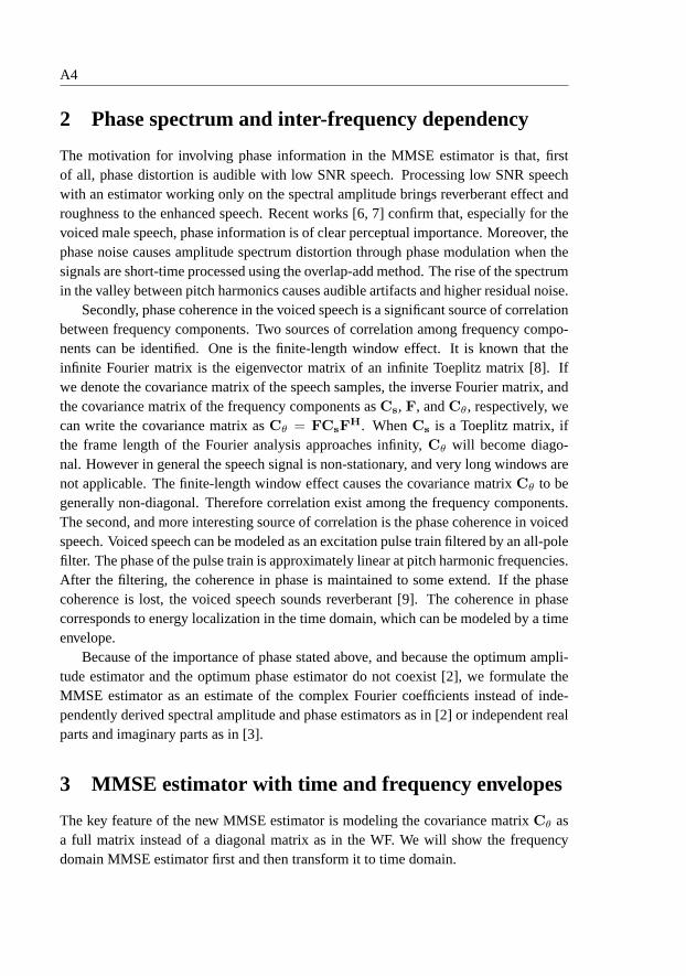
A4

2 Phase spectrum and inter-frequency dependency

The motivation for involving phase information in the MMSE estimator is that, firstof all, phase distortion is audible with low SNR speech. Processing low SNR speechwith an estimator working only on the spectral amplitude brings reverberant effect androughness to the enhanced speech. Recent works [6, 7] confirmthat, especially for thevoiced male speech, phase information is of clear perceptual importance. Moreover, thephase noise causes amplitude spectrum distortion through phase modulation when thesignals are short-time processed using the overlap-add method. The rise of the spectrumin the valley between pitch harmonics causes audible artifacts and higher residual noise.

Secondly, phase coherence in the voiced speech is a significant source of correlationbetween frequency components. Two sources of correlation among frequency compo-nents can be identified. One is the finite-length window effect. It is known that theinfinite Fourier matrix is the eigenvector matrix of an infinite Toeplitz matrix [8]. Ifwe denote the covariance matrix of the speech samples, the inverse Fourier matrix, andthe covariance matrix of the frequency components asCs, F, andCθ, respectively, wecan write the covariance matrix asCθ = FCsF

H. WhenCs is a Toeplitz matrix, ifthe frame length of the Fourier analysis approaches infinity, Cθ will become diago-nal. However in general the speech signal is non-stationary, and very long windows arenot applicable. The finite-length window effect causes the covariance matrixCθ to begenerally non-diagonal. Therefore correlation exist among the frequency components.The second, and more interesting source of correlation is the phase coherence in voicedspeech. Voiced speech can be modeled as an excitation pulse train filtered by an all-polefilter. The phase of the pulse train is approximately linear at pitch harmonic frequencies.After the filtering, the coherence in phase is maintained to some extend. If the phasecoherence is lost, the voiced speech sounds reverberant [9]. The coherence in phasecorresponds to energy localization in the time domain, which can be modeled by a timeenvelope.

Because of the importance of phase stated above, and becausethe optimum ampli-tude estimator and the optimum phase estimator do not coexist [2], we formulate theMMSE estimator as an estimate of the complex Fourier coefficients instead of inde-pendently derived spectral amplitude and phase estimatorsas in [2] or independent realparts and imaginary parts as in [3].

3 MMSE estimator with time and frequency envelopes

The key feature of the new MMSE estimator is modeling the covariance matrixCθ asa full matrix instead of a diagonal matrix as in the WF. We will show the frequencydomain MMSE estimator first and then transform it to time domain.

3. MMSE ESTIMATOR WITH TIME AND FREQUENCY ENVELOPES A5

We use the following statistical model and problem formulation. The DFT coef-ficients of each speech segment are modeled as complex Gaussian random variableswith zero mean and varying variance. Lety(n, k), s(n, k), v(n, k) denote then’th sam-ple of noisy observation, speech, and additive white Gaussian noise of thek’th frame,respectively. Then

y(n, k) = s(n, k) + v(n, k). (2)

Let θ(m, k) represent them’th DFT coefficient of thek’th frame, defined byθ(m, k) =∑N

n=0 s(n, k)exp(−j2πnm/N). For compactness we use vector representation andomit the index in the following discussion. Lety, θ, v, andF denote the vectors ofy,θ, v and the inverse Fourier matrix respectively. Then (2) can bewritten as

y = Fθ + v. (3)

The MMSE estimator can be shown to be the conditional mean [10]

θ = E(θ|y)

= CθFH(FCθF

H + Cv)−1y(4)

where(·)H denotes the Hermitian transpose andCv denotes the covariance matrix ofthe noisev. The covariance matrixCθ is generally unknown and must be replaced withan estimate. We propose here an approach to the estimation ofCθ from the all-polemodel of the speech. Letq/A(z) denote the transfer function of the all pole model. LetH be the corresponding synthesis filter matrix derived from the all-pole model, andrbe the residual vector, such that

s = Hr. (5)

Since the residual is a white noise sequence with unit variance (for voiced speech it isa few impulses present periodically in the white noise), thecovariance matrixCr of r

can be written as a diagonal matrix with the squared residualas the diagonal elements1. OnceCr is obtained,Cs andCθ can easily be found. We have

Cs = HCrHH (6)

Cθ = FHCsF. (7)

Inserting (7) in (4) gives the MMSE short-time spectral estimator.Fig.1 shows how the covariance matrixCθ estimated by this approach differs from

the diagonal matrix underlying the standard WF. We can see that the off-diagonal el-ements are generally non-zero. At the brims of the matrix thecross-correlations are

1Here we ignore the long term correlation of the residual.

A6

significant. This represents the windowing effect caused bythe high spectral powerat low frequencies. More interestingly, we see how inter-frequency dependency, espe-cially between neighboring formants show up as significant off-diagonal elements inthe covariance matrix. It is well known that a properly chosen window can reduce thecorrelation between frequency components but can not eliminate it. In Fig.1 a Hanningwindow is used, and we see that the remaining correlation is still significant and can beexploited to improve the estimator.

The frequency domain MMSE estimator given by (4) is mainly for the purposeof demonstrating the difference to the WF made by a full covariance matrix. In theestimation of the speech waveform, (4) is transformed back to time domain, giving thedesired time domain MMSE estimator,

s = Cs(Cs + Cv)−1y. (8)

Estimating the diagonal elements ofCr is equivalent to estimating the residualpower distribution over the time axis. It can also be seen as estimating phase fromthe residual, because the power spectrum of the residual is known to be white. Estimat-ing the squared residual from noisy observation is difficult. Our solution is to estimatethe time envelope of the squared residual with simple shapes, i.e. a constant floor plussome pulses located periodically. These varying variancesof residual represent timelocalization of energy. This is a major difference to the WF, which can be seen as us-ing constant residual variance because of the stationary assumption. We estimate theresidual envelope in a simple but effective way. The noisy speech signal is first lowpassfiltered with cut-off frequency of 800 Hz. A 3-tap whitening filter is found by applyinglinear prediction on the filtered signal. The output of the low pass filter is then filteredby the whitening filter to get a reference residual. The position of the maximum in thereference residual is chosen as the first impulse position ofthe estimated residual enve-lope. According to an estimate of the pitch period the positions of remaining impulsesare found. A pre-defined pulse shape is put on every impulse position. The pulse shapeis chosen to be wider and smoother than a true residual impulse in order to gain robust-ness against error in estimating the impulse positions. Therest of the residual will beapproximated with a constant whose amplitude is decided by keeping the average powerof the estimated residual equal to unity. The estimation of the residual envelope is onlyneeded for voiced frames. Fig.2 shows an example of the estimated residual envelope.

Because the above described MMSE estimator requires a spectral envelope and atemporal envelope as the prior knowledge, we hereafter refer to it as the Time-FrequencyEnvelope MMSE (TFE-MMSE) estimator.

4. RESULTS A7

10 20 30 40 50 60 70 80

10

20

30

40

50

60

70

80

−40

−20

0

Am

plitu

de [d

B]

Figure 1: Amplitude plot of the covariance matrixCθ . Matrix size is 160 by 160 (only one quarter of thematrix is shown).

0 20 40 60 80 100 120 140 1600

4

8

12

16

Pow

er

Figure 2: The squared residual (dashed) and the estimated envelope (solid).

4 results

We first compare the performance of the TFE-MMSE estimator and the WF based onknown spectral envelope of the signal. Since the purpose is to show that using the extrainformation about phase (or energy localization in time) itis possible to achieve lowermean squared error and lower spectral distortion at the sametime, we first use knownspectral envelopes for both estimators.

Both estimators run with 30 sentences from different speakers (15 male and 15female) from the TIMIT database added with artificial white Gaussian noise at a signal-to-noise ratio of 0 dB. All sentences are 16kHz sampled, and segmented into frames of160 samples. For the TFE-MMSE estimator, the time envelopesof the residual are esti-mated from noisy observations using the method described insection 3. For the outputof both estimators, the SNR, Segmental SNR (segSNR) and Log-Spectral Distortion(LSD) to the original signal spectrum are calculated. The SNR is defined as the ratio of

A8

the total signal power to the total noise power in the sentence. The segSNR is definedas the average ratio of signal power to noise power per frame,omitting frames with apower more than 30 dB below average power. The LSD is defined asthe distance be-tween two log-scaled DFT spectra summed over all frequencies. The LSD is calculatedonly for voiced frames since for the unvoiced frames both estimators are identical.

From Table 1 we see consistent improvement of the TFE-MMSE estimator over WFin all three measurements. Fig.3 shows the signal spectrum of a voiced frame comparingwith the spectrum of the output of the two estimators. Only the lower frequency halfis plotted to show the details of the harmonic structure. It is seen that the TFE-MMSEestimator preserves the harmonic structure better than theWF.

To verify the performance in a practical scenario, estimated LPC coefficients arealso used in the comparison. The LPC coefficients are estimated by a method similar tothe decision directed method in [2]. The experimental setupis identical to the above one,except that input SNR is now set to 10 dB. Table 2 shows the results. Significant im-provements are observed with the segSNR measurement. The LSD of the TFE-MMSEestimator also improves significantly over the WF. Informal listening experiments showthat the reduction of spectral distortion is significant.

Male FemaleSNR segSNR LSD SNR segSNR LSD

WF 10.73 5.21 290 10.57 5.59 347TFE-MMSE 11.24 5.48 265 10.85 5.71 315Improv. 0.51 0.27 25 0.28 0.12 32

Table 1: Performance of WF and the TFE-MMSE estimator with known AR coefficients. All SNR measuresare in dB. Input SNR is 0 dB. Results are averaged over 30 sentences (by 15 male and 15 female speakers).

Male FemaleSNR segSNR LSD SNR segSNR LSD

WF 15.65 8.73 245 15.38 9.30 303TFE-MMSE 16.71 9.42 183 16.48 9.83 231Improv. 1.06 0.70 62 1.10 0.53 72

Table 2: Performance of WF and the TFE-MMSE estimator with estimated AR coefficients. Input SNR is 10dB. Results are averaged over 30 sentences (by 15 male and 15 female speakers).

5 Discussion

In the first part of this paper we stated the motivation of formulating an MMSE joint es-timator of amplitude and phase spectrum, i.e., phase is of perceptual importance for lowSNR sources, and estimating phase provides the additional information about the corre-lation of DFT coefficients which improves the amplitude spectrum estimation in return.

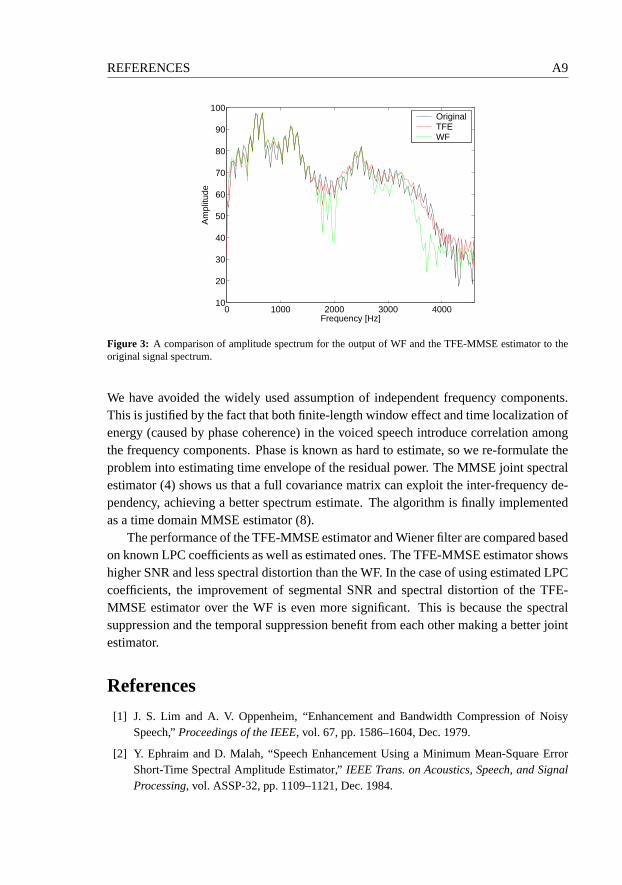
REFERENCES A9

0 1000 2000 3000 400010

20

30

40

50

60

70

80

90

100

Frequency [Hz]

Am

plitu

de

OriginalTFEWF

Figure 3: A comparison of amplitude spectrum for the output of WF and the TFE-MMSE estimator to theoriginal signal spectrum.

We have avoided the widely used assumption of independent frequency components.This is justified by the fact that both finite-length window effect and time localization ofenergy (caused by phase coherence) in the voiced speech introduce correlation amongthe frequency components. Phase is known as hard to estimate, so we re-formulate theproblem into estimating time envelope of the residual power. The MMSE joint spectralestimator (4) shows us that a full covariance matrix can exploit the inter-frequency de-pendency, achieving a better spectrum estimate. The algorithm is finally implementedas a time domain MMSE estimator (8).

The performance of the TFE-MMSE estimator and Wiener filter are compared basedon known LPC coefficients as well as estimated ones. The TFE-MMSE estimator showshigher SNR and less spectral distortion than the WF. In the case of using estimated LPCcoefficients, the improvement of segmental SNR and spectraldistortion of the TFE-MMSE estimator over the WF is even more significant. This is because the spectralsuppression and the temporal suppression benefit from each other making a better jointestimator.

References

[1] J. S. Lim and A. V. Oppenheim, “Enhancement and Bandwidth Compression of NoisySpeech,”Proceedings of the IEEE, vol. 67, pp. 1586–1604, Dec. 1979.


A10

[3] R. Martin, “Speech Enhancement Using MMSE Short Time SpectralEstimation WithGamma Distributed Speech Priors,”Proc.of ICASSP 2002, vol. 1, pp. 253–256, May 2002.

[4] P. Vary, “Noise Suppression By Spectral Magnitude Estimation - Mechanism and Theoreti-cal Limits,” Signal Processing 8, pp. 387–400, May 1985.

[5] W. B. Davenport and W. L. Root,An Introduction to the Theory of Random Signals andNoise. New York: McGraw-Hill, 1958.

[6] H. Pobloth and W. B. Kleijn, “On Phase Perception in Speech,”Proc.of ICASSP 1999, vol. 1,pp. 29–32, Mar. 1999.

[7] J. Skoglund, W. B. Kleijn, and P. Hedelin, “Audibility of Pitch-Synchronously ModulatedNoise,” Speech Coding For Telecommunications Proceeding, IEEE, vol. 7-10, pp. 51–52,Sept. 1997.

[8] R. M. Gray, “Toeplitz and Circulant Matrices: A review,”Foundations and Trends in Com-munications and Information Theory, vol. 2, Issue 3, pp. 155–239, 2006.

[9] T. F. Quatieri and R. J. McAulay, “Phase Coherence in Speech Reconstruction for Enhance-ment and Coding Applications,”Proc.of ICASSP 1989., vol. 1, pp. 207–210, May 1989.


Paper B

A Block Based Linear MMSE Noise Reduction with aHigh Temporal Resolution Modeling of the Speech

Excitation


The paper has been published inEURASIP Journal on Applied Signal Processing, Special Issue on DSP in Hearing

Aids and Cochlear Implants, vol. 2005:18, pp. 2965-2978, October 2005.

1. ABSTRACT B3

1 Abstract

A comprehensive Linear Minimum Mean Squared Error (LMMSE) approach for para-metric speech enhancement is developed. The proposed algorithms aim at joint LMMSEestimation of signal power spectra and phase spectra, as well as exploitation of correla-tion between spectral components. The major cause of this inter-frequency correlationis shown to be the prominent temporal power localization in the excitation of voicedspeech. LMMSE estimators in time domain and frequency domain are first formulated.To obtain the joint estimator, we model the spectral signal covariance matrix as a fullcovariance matrix instead of a diagonal covariance matrix as is the case in the Wienerfilter derived under the quasi-stationarity assumption. Toaccomplish this, we decom-pose the signal covariance matrix into a synthesis filter matrix and an excitation matrix.The synthesis filter matrix is built from estimates of the all-pole model coefficients, andthe excitation matrix is built from estimates of the instantaneous power of the excita-tion sequence. A decision-directed Power Spectral Subtraction method and a modifiedMulti-Pulse Linear Predictive Coding (MPLPC) method are used in these estimations,respectively. The spectral domain formulation of the LMMSEestimator reveals impor-tant insight about inter-frequency correlations. This is exploited to significantly reducecomputational complexity of the estimator. For resource-limited applications such ashearing aids, the performance-to-complexity tradeoff canbe conveniently adjusted bytuning the number of spectral components to be included in the estimate of each compo-nent. Experiments show that the proposed algorithm is able to reduce more noise than anumber of other approaches selected from the state-of-the-art. The proposed algorithmimproves the segmental SNR of the noisy signal by 13 dB for thewhite noise case withan input SNR of 0 dB.

2 Introduction

Noise reduction is becoming an important function in hearing aids in recent years thanksto the application of powerful DSP hardware and the progressof noise reduction algo-rithm design. Noise reduction algorithms with high performance-to-complexity ratiohave been the subject of extensive research study for many years. Among many differentapproaches, two classes of single-channel speech enhancement methods have attractedsignificant attention in recent years because of their better performance compared to theclassic spectral subtraction methods (A comprehensive study of Spectral Subtractionmethods can be found in [1]). These two classes are the frequency domain block basedMinimum Mean Squared Error (MMSE) approach and the signal subspace approach.The frequency domain MMSE approach includes the non-causalIIR Wiener filter [2],the MMSE Short-Time Spectral Amplitude (MMSE-STSA) estimator [3], the MMSELog-Spectral Amplitude (MMSE-LSA) estimator [4], the Constrained Iterative Wiener

B4

Filtering (CIWF) [5], and the MMSE estimator using non-Gaussian priors [6]. TheseMMSE algorithms all rely on an assumption of quasi-stationarity and an assumption ofuncorrelated spectral components in the signal. The quasi-stationarity assumption re-quires short time processing. At the same time, the assumption of uncorrelated spectralcomponents can be warranted by assuming the signal to be infinitely long and wide-sense stationary [7] [8]. This infinite data length assumption is in principle violatedwhen using the short-time processing, although the effect of this violation may be mi-nor (and is not the major issue this paper addresses). More importantly, the wide-sensestationarity assumption within a short frame does not well model the prominent tempo-ral power localization in the excitation source of voiced speech due to the impulse trainstructure. This temporal power localization within a shortframe can be modeled as anon-stationarity of the signal that is not resolved by the short-time processing. In [9],we show how voiced speech is advantageously modeled as non-stationary even withina short frame, and that this model implies significant inter-frequency correlations. Asa consequence of the stationarity and long frame assumptions, the MMSE approachesmodel the frequency domain signal covariance matrix as a diagonal matrix.

Another class of speech enhancement methods, the signal subspace approach, im-plicitly exploits part of the inter-frequency correlationby allowing the frequency do-main signal covariance matrix to be non-diagonal. This class includes the Time DomainConstraint (TDC) linear estimator and Spectral Domain Constraint (SDC) linear esti-mator [10], and the Truncated Singular Value Decomposition(TSVD) estimator [11].In [10], the TDC estimator is shown to be an LMMSE estimator with adjustable inputnoise level. When the TDC filtering matrix is transformed to the frequency domain,it is in general non-diagonal. Nevertheless, the known signal subspace based methodsstill assume stationarity within a short frame. This can be seen as follows. In TDC andSDC the noisy signal covariance matrices are estimated by time averaging of the outerproduct of the signal vector, which requires stationarity within the interval of averaging.The TSVD method applies singular value decomposition to thesignal matrix instead.This can be shown to be equivalent to the eigen decompositionof the time averagedouter product of signal vectors. Compared to the mentioned frequency domain MMSEapproaches, the known signal subspace methods implicitly avoid the infinite data lengthassumption, so that the inter-frequency correlation caused by the finite length effect isaccommodated. However, the more important cause of inter-frequency correlation, i.e.,the non-stationarity within a frame is not modeled.

In terms of exploiting the masking property of the human auditory system, the abovementioned frequency domain MMSE algorithms and signal subspace based algorithmscan be seen as spectral masking methods without explicit modeling of masking thresh-olds. To see this, observe that the MMSE approaches shape theresidual noise (theremaining background noise) power spectrum to one more similar to the speech powerspectrum, thereby facilitating a certain degree of maskingof the noise. In general, the

2. INTRODUCTION B5

MMSE approaches attenuate more in the spectral valleys thanthe spectral subtractionmethods do. Perceptually, this is beneficial for high pitch voiced speech, which hassparsely located spectral peaks that are not able to mask thespectral valley sufficiently.The signal subspace methods in [10] are designed to shape theresidual noise powerspectrum for a better spectral masking, where the masking threshold is found exper-imentally. Auditory masking techniques have received increasing attention in recentresearch of speech enhancement [12–14]. While the majority of these works focus onspectral domain masking, the work in [15] shows the importance of the temporal mask-ing property in connection with the excitation source of voiced speech. It is shownthat noise between the excitation impulses is more perceivable than noise close to theimpulses, and this is especially so for the low pitch speech for which the excitation im-pulses locates temporally sparsely. This temporal maskingproperty is not employed bycurrent frequency domain MMSE estimators and the signal subspace approaches.

In this paper, we develop an LMMSE estimator with a high temporal resolutionmodeling of the excitation of voiced speech, aiming for modeling a certain non-stationarityof the speech within a short frame, which is not modeled by quasi-stationarity basedalgorithms. The excitation of voiced speech exhibits prominent temporal power local-ization, which appears as an impulse train superimposed with a low level noise floor.We model this temporal power localization as a non-stationarity. This non-stationaritycauses significant inter-frequency correlation. Our LMMSEestimator therefore avoidsthe assumption of uncorrelated spectral components, and isable to exploit the inter-frequency correlation. Both the frequency domain signal covariance matrix and filteringmatrix are estimated as complex-valued full matrices, which means that the informationabout inter-frequency correlation are not lost and the amplitude and phase spectra areestimated jointly. Specifically, we make use of the linear prediction based source-filtermodel to estimate the signal covariance matrix, upon which atime domain or frequencydomain LMMSE estimator is built. In the estimation of the signal covariance matrix,this matrix is decomposed into a synthesis filter matrix and an excitation matrix. Thesynthesis filter matrix is estimated by a smoothed power spectral subtraction methodfollowed by an autocorrelation Linear Predictive Coding (LPC) method. The excitationmatrix is a diagonal matrix with the instantaneous power of the LPC residual as its diag-onal elements. The instantaneous power of the LPC residual is estimated by a modifiedMulti-Pulse Linear Predictive Coding (MPLPC) method. Having estimated the signalcovariance matrix, we use it in a vector LMMSE estimator. We show that by doingthe LMMSE estimation in the frequency domain instead of in time domain, the com-putational complexity can be reduced significantly due to the fact that the signal is lesscorrelated in the frequency domain than in the time domain. Compared to several quasi-stationarity based estimators, the proposed LMMSE estimator results in a lower spectraldistortion to the enhanced speech signal while having higher noise reduction capability.The algorithm applies more attenuation in the valleys between pitch impulses in time

B6

domain, while small attenuation is applied around the pitchimpulses. This arrangementexploits the temporal masking effect, and results in a better preservation of abrupt riseof the waveform amplitude while maintaining a large amount of noise reduction.

The rest of this paper is organized as follows. In Section 3 the notations and as-sumptions used in the derivation of LMMSE estimators are outlined. In Section 4, thenon-stationary modeling of the signal covariance matricesis described. The algorithm issummarized in Section 5. In Section 6, the computational complexity of the algorithmis reduced by identifying an interval of significant correlation and by simplifying themodified MPLPC procedure. Experimental settings, objective, and subjective resultsare given in Section 7. Finally, Section 8 discusses the obtained results.

3 Background

In this section, notations and statistic assumptions for the derivation of LMMSE esti-mators in time and frequency domain are outlined.

3.1 Time domain LMMSE estimator

Let y(n, k), s(n, k), v(n, k) denote then’th sample of noisy observation, speech, andadditive noise (uncorrelated with the speech signal) of thek’th frame, respectively. Then

y(n, k) = s(n, k) + v(n, k).

Alternatively, in vector form we have

y = s + v, (1)

where boldface letters represent vectors and the frame indices are omitted to allow acompact notation. For exampley = [y(1, k), y(2, k), · · · , y(N, k)]T is the noisy signalvector of thek’th frame, whereN is the number of samples per frame.

To obtain linear MMSE estimators, we assume zero mean Gaussian PDF’s for thenoise and the speech processes. Under this statistic model the LMMSE estimate of thesignal is the conditional mean [16]

s = E[s|y]

= Cs(Cs + Cv)−1

y,(2)

whereCs andCv are the covariance matrices of the signal and the noise, respectively.The covariance matrix is defined asCs = E[ssH ], where(·)H denotes Hermitian trans-position andE[·] denotes the ensemble average operator.

3. BACKGROUND B7

3.2 Frequency domain LMMSE estimator and Wiener filter

In the frequency domain the goal is to estimate the complex DFT coefficients given aset of DFT coefficients of the noisy observation. LetY (m, k), θ(m, k), andV (m, k)

denote them’th DFT coefficient of thek’th frame of the noisy observation, the signal,and the noise, respectively. Due to the linearity of the DFT operator, we have,

Y (m, k) = θ(m, k) + V (m, k). (3)

In vector form we haveY = θ + V, (4)

where again boldface letters represent vectors and the frame indices are omitted. As anexample, the noisy spectrum vector of thek’th frame is arranged as

Y = [Y (1, k), Y (2, k), · · · , Y (N, k)]T

where the number of frequency bins is equal to the number of samples per frameN .We again use the linear model.Y, θ, andV are assumed to be zero-mean complex

Gaussian random variables andθ andV are assumed to be uncorrelated to each other.The LMMSE estimate is the conditional mean

θ = E[θ|Y]

= Cθ(Cθ + CV)−1Y,(5)

whereCθ andCV are the covariance matrices of the DFT coefficients of the signal andthe noise, respectively. By applying inverse DFT to each side, (5) can be easily shownto be identical to (2).

The relation between the two signal covariance matrices in time and frequency do-main is

Cθ = FCsF−1, (6)

whereF is the Fourier matrix. If the frame was infinitely long and thesignal wasstationary,Cs would be an infinitely large Toeplitz matrix. The infinite Fourier matrixis known to be the eigenvector matrix of any infinite Toeplitzmatrix [8]. Thus,Cθ

becomes diagonal and the LMMSE estimator (5) reduces to the non-causal IIR Wienerfilter with the transfer function

HWF (ω) =Pss(ω)

Pss(ω) + Pvv(ω), (7)

wherePss(ω) andPvv(ω) denotes the power spectral density (PSD) of the signal andthe noise, respectively. In the sequel we refer to (7) as the Wiener filter or WF.

B8

4 High temporal resolution modeling for the signal co-variance matrix estimation

For both time and frequency domain LMMSE estimators described in Section 3, theestimation of the signal covariance matrixCs is crucial. In this work, we assume thenoise to be stationary. For the signal, however, we propose the use of a high temporalresolution model to capture the non-stationarity caused bythe excitation power varia-tion. This can be explained by examining the voice production mechanism. In the wellknown source-filter model for voiced speech, the excitationsource models the glottalpulse train, and the filter models the resonance property of the vocal tract. The vocaltract can be viewed as a slowly varying part of the system. Typically in a duration of20 to 30 ms it changes very little. The vocal folds vibrate at afaster rate producingperiodic glottal flow pulses. Typically there can be 2 to 8 glottal pulses in 20 ms. Inspeech coding, it is common practice to model this pulse train by a long-term correla-tion pattern parameterized by a long-term predictor [17] [18] [19]. However, this modelfails to describe the linear relationship between the phases of the harmonics. That is,the long term predictor alone does not model the temporal localization of power in theexcitation source. Instead, we apply a time envelope that captures the localization andconcentration of pitch pulse energy in the time domain. This, in turn, introduces anelement of non-stationarity to our signal model because theexcitation sequence is nowmodeled as a random sequence with time varying variance, i.e., the glottal pulses aremodeled with higher variance and the rest of the excitation sequence is modeled withlower variance. This modeling of non-stationarity within ashort frame implies a tem-poral resolution much finer than that of the quasi-stationarity based algorithms. Thelatter has a temporal resolution equal to the frame length. Thus we term the former thehigh temporal resolution model. It is worth noting that someunvoiced phonemes, suchas plosives, have very fast changing waveform envelopes, which also could be modeledas non-stationarity within the analysis frame. In this paper, however, we focus on thenon-stationary modeling of voiced speech.

4.1 Modeling signal covariance matrix

The signal covariance matrix is usually estimated by averaging the outer product of thesignal vector over time. As an example this is done in the signal subspace approach [10].This method assumes ergodicity of the autocorrelation function within the averaginginterval.

Here we propose the following method of estimatingCs with the ability to modela certain element of non-stationarity within a short frame.The following discussion isonly appropriate for voiced speech. Letr denote the excitation source vector, andH

denote the synthesis filtering matrix corresponding to the vocal tract filter such as

4. HIGH TEMPORAL RESOLUTION MODELING FOR THE SIGNALCOVARIANCE MATRIX ESTIMATION B9

H =

h(0) 0 0 · · · 0

h(1) h(0) 0...

h(2) h(1) h(0)...

.... . . 0

h(N − 1) h(N − 2) · · · h(0)

,

whereh(n) is the impulse response of the LPC synthesis filter. We then have

s = Hr, (8)

and thereforeCs = E[ssH ] = HCrH

H , (9)

whereCr is the covariance matrix of the model residual vectorr. In (9) we treatH as adeterministic quantity. This simplification is common practice also when the LPC filtermodel is used to parameterize the power spectral density in classic Wiener filtering[20] [5]. Section 4.2 addresses the estimation ofH. Note that (8) does not take intoaccount the zero-input response of the filter in the previousframe. Either the zero-input response can be subtracted prior to the estimation of each frame, or a windowedoverlap-add procedure can be applied to eliminate this effect.

We now modelr as a sequence of independent zero mean random variables. Thecovariance matrixCr is therefore diagonal with the variance of each element ofr asits diagonal elements. For voiced speech, except for the pitch impulses, the rest ofthe residual is of very low amplitude and can be modeled as constant variance randomvariables. Therefore, the diagonal ofCr takes the shape of a constant floor with a fewperiodically located impulses. We term this the temporal envelope of the instantaneousresidual power. This temporal envelope is an important partof the new MMSE estima-tor because it provides the information of uneven temporal power distribution. In thefollowing two subsections, we will describe the estimationof the spectral envelope andthe temporal envelope respectively.

4.2 Estimating the spectral envelope

In the context of LPC analysis, the synthesis filter has a spectrum that is the envelope ofthe signal spectrum. Thus, our goal in this subsection is to estimate the spectral envelopeof the signal. We first use the Decision Directed method [3] toestimate the signal powerspectrum and then use the autocorrelation method to find the spectral envelope.

The noisy signal power spectrum of thek’th frame|Y(k)|2 is obtained by applyingthe DFT to thek’th observation vectory(k) and squaring the amplitudes. The Decision

Directed estimate of the signal power spectrum of thek’th frame,| ˆθ(k)|2, is a weighted

B10

sum of two parts, the power spectrum of the estimated signal of the previous frame,|θ(k − 1)|2, and the power-spectrum-subtraction estimate of the current frame’s powerspectrum:

| ˆθ(k)|2 = α|θ(k − 1)|2 + (1 − α)max(|Y(k)|2 − E[|V(k)|2], 0), (10)

whereα is a smoothing factorα ∈ [0, 1], andE[|V(k)|2] is the estimated noise powerspectral density. The purpose of such a recursive scheme is to improve the estimateof the power spectrum subtraction method by smoothing out the random fluctuation inthe noise power spectrum, thus reduce the “musical noise” artifact [21]. Other iterativeschemes with similar time or spectral constraints are applicable in this context. For acomprehensive study of constraint iterative filtering techniques, readers are referred to[5]. We now take the square-root of the estimated power spectrum and combine it withthe noisy phase to reconstruct the so called intermediate estimate, which has the noise-reduced amplitude spectrum but noisy phase. An autocorrelation method LPC analysisis then applied to this intermediate estimate to obtain the synthesis filter coefficients.

4.3 Estimating the temporal envelope

We propose to use a modified MPLPC method to robustly estimatethe temporal en-velope of the residual power. MPLPC is first introduced by Atal and Remde [17] tooptimally determine the impulse position and amplitude of the excitation in the con-text of analysis-by-synthesis linear predictive coding. The principle is to represent theLPC residual with a few impulses in which the locations and amplitudes (gains) of theimpulses are chosen such that the difference between the target signal and the synthe-sized signal is minimized. In the noise reduction scenario,the target signal will be thenoisy signal and the synthesis filter must be estimated from the noisy signal. Here, thesynthesis filter is treated as known. For the residual of voiced speech, there is usuallyone dominating impulse in each pitch period. We first determine one impulse per pitchperiod, then model the rest of the residual as a noise floor with constant variance. InMPLPC the impulses are found sequentially [22]. The first impulse location and ampli-tude is found by minimizing the distance between the synthesized signal and the targetsignal. The effect of this impulse is subtracted from the target signal and the same pro-cedure is applied to find the next impulse. Because this way offinding impulses does nottake into account the interaction between the impulses, re-optimization of the impulseamplitudes is necessary every time a new impulse is found. The number of pitch im-pulsesp in a frame is determined in the following way.p is first assigned an initial valueequal to the largest number of pitch periods possible in a frame. Thenp impulses aredetermined using the above mentioned method. Only the impulses with an amplitudelarger than a threshold are selected as pitch impulses. In our experiment, the threshold

5. THE ALGORITHM B11

is set to 0.5 times the largest impulse amplitude in this frame. Having determined theimpulses, a white noise sequence representing the noise floor of the excitation sequenceis added into the gain optimization procedure together withall the impulses. We use acodebook of 1024 white Gaussian noise sequences in the optimization. The white noisesequence that yields the smallest synthesis error to the target signal is chosen to be theestimate of the noise floor. This procedure is in fact a multi-stage coder withp impulsestages and one Gaussian codebook stage, with a joint re-optimization of gains. Detailedtreatment of this optimization problem can be found in [23].After the optimization,we use a flat envelope equal to the square of the gain of the selected noise sequence tomodel the variance of the noise floor. Finally, the temporal envelope of the instanta-neous residual power is composed of the noise floor variance and the squared impulses.When applied to noisy signals, the MPLPC procedure can be interpreted as a non-linearLeast Square fitting to the noisy signal, with the impulse positions and amplitudes asthe model parameters.

5 The algorithm

Having obtained the estimate of the temporal envelope of theinstantaneous residualpower and the estimate of the synthesis filter matrix, we are able to build the signalcovariance matrix in (9). The covariance matrix is used in the time LMMSE estimator(2) or in the spectral LMMSE estimator (5) after being transformed by (6).

The noise covariance matrix can be estimated using speech absent frames. Here,we assume the noise to be stationary. For the time domain LMMSE estimator (2), ifthe noise is white, the covariance matrixCv is diagonal with the noise variance asits diagonal elements. In the case of colored noise, the noise covariance matrix is nolonger diagonal and it can be estimated using the time averaged outer product of thenoise vector. For the spectral domain LMMSE estimator (5),CV is a diagonal matrixwith the power spectral density of the noise as its diagonal elements. This is due tothe assumed stationarity of the noise1. In the special case where the noise is white, thediagonal elements all equal the variance of the noise.

We model the instantaneous power of the residual of unvoicedspeech with a flatenvelope. Here, voiced speech is referred to as phonemes that require excitation fromthe vocal folds vibration, and unvoiced speech consists of the rest of the phonemes. Weuse a simple voiced/unvoiced detector that utilize the factthat voiced speech usuallyhas most of its power concentrated in the low frequency band,while unvoiced speechhas a relatively flat spectrum within0 to 4kHz. Every frame is low pass filtered and

1In modeling the spectral covariance matrix of the noise we haveignored the inter-frequency correlationscaused by the finite-length window effect. With typical window length, e.g.15 to 30ms, the inter-frequencycorrelations caused by the window effect is less significantthan those caused by the non-stationarity of thesignal. This can be easily seen by examining a plot of the spectral covariance matrix.

B12

Algorithm 1 TFE-MMSE estimator

1: Take thek’th frame,2: Estimate the noise PSD from the latest speech-absent frame.3: Calculate the power spectrum of the noisy signal.4: Do power spectrum subtraction estimation of the signal PSD,and refine the estimate

using Decision-Directed smoothing (eq.(10)).5: Reconstruct the signal by combining the amplitude spectrumestimated by 4 and

the noisy phase.6: Do LPC analysis to the reconstructed signal. Obtain the synthesis filter coefficients,

and form the synthesis matrixH.7: IF the frame is voiced

Estimate the envelope of the instantaneous residual power using the modifiedMPLPC method.

8: IF the frame is unvoicedUse a constant envelope for the instantaneous residual power.

9: ENDIF10: Calculate the residual covariance matrixCr.11: Form the signal covariance matrixCs = HCrH

H (eq.(9)).12: IF time domain LMMSE:

s = Cs(Cs + Cv)−1

y (eq.(2)).13: IF frequency domain LMMSE:

transformCs to frequency domainCθ = FCsF−1,

filter the noisy spectrumθ = Cθ(Cθ + CV)−1Y (eq.(5)),obtain the signal estimate by inverse DFT.

14: ENDIF15: Calculate the power spectrum of the filtered signal,|θ(k − 1)|2, for use in the PSD

estimation of next frame.16: k = k + 1 and go to 1.

then the filtered signal power is compared with the original signal power. If the powerloss is more than a threshold, the frame is marked as an unvoiced frame, and vice versa.Note however, that even for the unvoiced frames, the spectral covariance matrix is non-diagonal because the signal covariance matrixCs, built in this way, is not Toeplitz.Hereafter, we refer to the proposed approach as the Time-Frequency-Envelope MMSEestimator (TFE-MMSE), due to its utilization of envelopes in both time and frequencydomain. The algorithm is summarized in Algorithm 1.

6 Reducing computational complexity

The TFE-MMSE estimators require inversion of a full covariance matrixCs or Cθ.This high computational load prohibits the algorithm from real time application in hear-

6. REDUCING COMPUTATIONAL COMPLEXITY B13

ing aids. Noticing that both covariance matrices are symmetric and positive definite,Cholesky factorization can be applied to the covariance matrices, and the inversion canbe done by inverting the Cholesky triangle. A careful implementation requiresN3/3

operations for the Cholesky factorization [24] and the algorithm complexity isO(N3).Another computation intensive part of the algorithm is the modified MPLPC method.In this section we propose simplifications to these two parts.

Further reduction of complexity for the filtering requires understanding of the inter-frequency correlation. In the time domain the signal samples are clearly correlated witheach other in a very long span. However, in the frequency domain, the correlation spanis much smaller. This can be seen from the magnitude plots of the two covariancematrices (see Fig.1).

20 40 60 80 100 120−2000

−1000

0

1000

2000

3000

4000

Sample

Am

plitu

de

(a) Voiced speech waveform

30 40 50 60

Sample

Sam

ple

20 40 60 80 100 120

20

40

60

80

100

120

Frequency bin

Fre

quen

cy b

in

20 40 60 80 100 120

20

40

60

80

100

120

0 20 40 60

dB dB

(b) covariance matrix in time domain (left) and spectral domain (right)

Figure 1: The voiced speech waveform and its time domain and frequency domain (amplitude) covariancematrices estimated with the non-stationary model. Frame lengthis 128 samples.

For the spectral covariance matrix, the significant values concentrate around thediagonal. This fact indicates that a small number of diagonals capture most of the inter-

B14

frequency correlation. The simplified procedure is as follows. Half of the spectrumvectorθ is divided into small segments ofl frequency bins each. The sub-vector start-ing at thej’th frequency is denoted asθsub,j , wherej ∈ [1, l, 2l, · · · , N/2] andl ≪ N .The noisy signal spectrum and the noise spectrum can be segmented in the same waygivingYsub,j andVsub,j . The LMMSE estimate ofθsub,j needs only a block of the co-variance matrix, which means that the estimate of a frequency component benefits fromits correlations withl neighboring frequency components instead of all components.This can be written as

θsub,j = Cθsub,j(Cθsub,j

+ CVsub,j)−1Ysub,j . (11)

The first half of the signal spectrum can be estimated segmentby segment. The sec-ond half of the spectrum is simply a flipped and conjugated version of the first half.The segment length is chosen to bel = 8, which in our experience does not degradeperformance noticeably when compared with the use of the full matrix. Other segmen-tation schemes are applicable, such as overlapping segments. It is also possible to usea number of surrounding frequency components to estimate a single component at atime. We use the non-overlapping segmentation because it iscomputationally less ex-pensive while maintaining good performance for smalll. When the signal frame lengthis 128 samples and the block length isl = 8, using this simplified method requiresonly 8×83

1283 = 1512 times of the original complexity for the filtering part of thealgorithm

with an extra expense of FFT operations to the covariance matrix. When l is set tovalues larger than 24, very little improvement in performance is observed. Whenl isset to values smaller than 8, the quality of enhanced speech degrades noticeably. Bytuning the parameterl, an effective trade-off between the enhanced speech quality andthe computational complexity is adjusted conveniently.

In the MPLPC part of the algorithm, the optimization of the impulse amplitude andthe gain of the noise floor brings in heavy computational load. It can be simplified byfixing the impulse shape and the noise floor level. In the simplified version, the MPLPCmethod is only used for searching the locations of thep dominating impulses. Once thelocations are found, a predetermined pulse shape is put at each location. An envelope ofthe noise floor is also predetermined. The pulse shape is chosen to be wider than an im-pulse in order to gain robustness against estimation error of the impulse locations. Thisis helpful as long as noise is present. The pulse shape used inour experiment is a raisedcosine waveform with a period of 18 samples and the ratio between the pulse peak andthe noise floor amplitude is experimentally determined to be6.6. Finally, the estimatedresidual power must be normalized. Although the pulse shapeand the relative level ofthe noise floor are fixed for all frames, experiments show thatthe TFE-MMSE estimatoris not sensitive to this change. The performance of both the simplified procedure andthe optimum procedure are evaluated in Section 7. Fig.2 shows the estimated envelopes

7. RESULTS B15

of residual in the two ways.

20 40 60 80 100 1200

0.05

0.1

Sample

Mag

nitu

de

True residualEstimate

(a) Complete MPLPC method

20 40 60 80 100 1200

0.05

0.1

Sample

Mag

nitu

de

True residualEstimate

(b) Simplified MPLPC method

Figure 2: Estimated magnitude envelopes of the residual by the MPLPC method and the simplified MPLPCmethod.

7 Results

Objective performance of the TFE-MMSE estimator is first evaluated and comparedwith the Wiener filter [2], the MMSE-LSA estimator [4], and the signal subspace methodTDC estimator [10]. For the TFE-MMSE estimator, both the complete algorithm andthe simplified algorithms are evaluated. For all estimatorsthe sampling frequency is8kHz, and the frame length is 128 samples with 50% overlap. Inthe Wiener filter weuse the same Decision Directed method as in the MMSE-LSA and the TFE-MMSEestimator to estimate the PSD of the signal. An important parameter for the DecisionDirected method is the smoothing factorα. The larger theα is, the more noise is re-moved and more distortion imposed to the signal, because of more smoothing made tothe spectrum. In the MMSE-LSA estimator with the aforesaid parameter setting, wefound experimentallyα = 0.98 to be the best trade-off between noise reduction andsignal distortion. We use the sameα for the WF and the TFE-MMSE estimator as forthe MMSE-LSA estimator. For the TDC, the parameterµ (µ ≧ 1) controls the degreeof over suppression of the noise power [10]. The larger theµ is, the more attenuation

B16

to the noise but larger distortion to the speech. We chooseµ = 3 in the experiments bybalancing the noise reduction and signal distortion.

All estimators run with 32 sentences from different speakers (16 male and 16 fe-male) from the TIMIT database [25] added with white Gaussiannoise, pink noise, andcar noise in SNR ranging from 0 dB to 20 dB. The white Gaussian noise is computergenerated, and the pink noise is generated by filtering whitenoise with a filter having a3 dB per octave spectral power descend. The car noise is recorded inside a car with aconstant speed. Its spectrum is more low pass than the pink noise. The quality measuresused include the SNR, the segmental SNR, and the Log-Spectral Distortion (LSD). TheSNR is defined as the ratio of the total signal power to the total noise power in the sen-tence. The segmental SNR (segSNR) is defined as the average ratio of signal power tonoise power per frame. To prevent the segSNR measure from being dominated by a fewextreme low values, since the segSNR is measured in dB, it is common practice to applya lower power thresholdǫ to the signals. Any frame that has an average power lowerthanǫ is not used in the calculation. We setǫ to 40dB lower than the average power ofthe utterance. The segSNR is commonly considered to be more correlated to perceivedquality than the SNR measure. The LSD is defined as [26]:

LSD =1

K

K∑

k=1

[1

M

M∑

m=1

(20log10

|X(m, k)| + ǫ

|X(m, k)| + ǫ

)2] 12

, (12)

whereǫ is to prevent extreme low values. We again setǫ to 40 dB lower than theaverage power of the utterance. Results of the white Gaussian noise case are givenin Fig. 3. TFE-MMSE1 is the complete algorithm, and TFE-MMSE2 is the one withsimplified MPLPC and reduced covariance matrix (l = 8). It is observed that the TFE-MMSE2, although a result of simplification of TFE-MMSE1, hasbetter performancethan the TFE-MMSE1. This can be explained as follows: 1) Its wider pulse shape ismore robust to the estimation error of impulse positions, and 2) the wider pulse shapecan model to some extent the power concentration around the impulse peaks, whichis overlooked by the spiky impulses. For this reason, in the following evaluations weinvestigate only the simplified algorithm.

Informal listening tests reveal that, although the speech enhanced by the TFE-MMSE algorithm has a significantly clearer sound (less muffled than the reference al-gorithms), the remaining background noise has musical tones. A solution to the musicalnoise problem is to set a higher value to the smoothing factorα. Using a largerα sacri-fices the SNR and LSD slightly at high input SNR’s, but improves the SNR and LSD atlow input SNR’s, and generally improves the segSNR significantly. The musical tonesare also well suppressed. By settingα = 0.999, the residual noise is greatly reduced,while the speech still sounds less muffled than for the reference methods. The referencemethods can not use a smoothing factor as high as the TFE-MMSE: experiments show

7. RESULTS B17

0 5 10 15 201

2

3

4

5

6

7

8

9

Input SNR (dB)

SN

R g

ain

(dB

)TFE−MMSE1TFE−MMSE2TFE−MMSE3MMSE−LSAWFTDC

(a) SNR gain, male speech.

0 5 10 15 202

3

4

5

6

7

8

9

10

Input SNR (dB)

SN

R g

ain

(dB

)

TFE−MMSE1TFE−MMSE2TFE−MMSE3MMSE−LSAWFTDC

(b) SNR gain, female speech

0 5 10 15 202

3

4

5

6

7

8

9

10

11

12

13

14

Input SNR (dB)

segS

NR

gai

n (d

B)


(c) segSNR gain, male speech.

0 5 10 15 203

4

5

6

7

8

9

10

11

12

13

Input SNR (dB)

segS

NR

gai

n (d

B)


(d) segSNR gain, female speech

0 5 10 15 20−14

−13

−12

−11

−10

−9

−8

−7

−6

−5

−4

−3

−2

Input SNR (dB)

LSD

gai

n (d

B)


(e) Log-Spectral Distortion gain, male speech.

0 5 10 15 20−14

−13

−12

−11

−10

−9

−8

−7

−6

−5

−4

−3

−2

Input SNR (dB)

LSD

gai

n (d

B)


(f) Log-Spectral Distortion gain, female speech.

Figure 3: SNR gain, segSNR gain, and Log-Spectral Distortion gain forthe white Gaussian noise case.

that atα = 0.999 the MMSE-LSA and the WF result in extremely muffled sounds. TheTDC also suffers from a musical residual noise. To suppress its residual noise level to

B18

as low as that of the TFE-MMSE withα = 0.999, the TDC requires aµ lager than8. This causes a sharp degradation of the SNR and LSD, and results in very muffledsounds. The TFE-MMSE2 estimator with a large smoothing factor (α = 0.999) is here-after termed TFE-MMSE3 and its objective measures are also shown in the figures. Toverify the perceived quality of the TFE-MMSE3 subjectively, preference test betweenthe TFE-MMSE3 and the WF, and between the TFE-MMSE3 and the MMSE-LSAare conducted. The WF and the MMSE-LSA use their best value of smoothing factor(α = 0.98). The test is confined to white Gaussian noise and a limited range of SNR’s.Three sentences by male speakers and three by female speakers at each SNR level areused in the test. Eight unexperienced listeners are required to vote for their preferredmethod based on the amount of noise reduction and speech distortion. The utterancesare presented to the listeners by a high quality headphone. The clean utterance is firstplayed as a reference, and the enhanced utterances are played once, or more if the lis-tener finds this necessary. The results in Table 1 and 2 show that: 1) at 10 dB and 15 dBthe listeners clearly prefer the TFE-MMSE over the two reference methods, while at 5dB the preference on the TFE-MMSE is unclear; 2) the TFE-MMSEmethod has a moresignificant impact on the processing of male speech than on the processing of femalespeech. At 10 dB and above, the speech enhanced by TFE-MMSE3 has barely audi-ble background noise, and the speech sounds less muffled thanthe reference methods.There is one artifact heard in rare occasions that we believeis caused by remaining mu-sical tones. It is of very low power and occur some times at speech presence. The tworeference methods have higher residual background noise and suffer from muffling andreverberance effects. When SNR is lower than 10 dB, a certain speech dependent noiseoccurs at speech presence in the TFE-MMSE3 processed speech. The lower the SNRis, the more audible this artifact is. Comparing the male andfemale speech processedby the TFE-MMSE3, the female speech sounds a bit rough.

The algorithms are also evaluated for pink noise and car noise cases. The objectiveresults are shown in Fig. 4 and 5. In these results the TDC algorithm is not includedbecause the algorithm is proposed based on the white Gaussian noise assumption. In-formal listening test shows that the perceptual quality in the pink noise case for all thethree algorithms are very similar to the white noise case, and that in the car noise case alltested methods have very similar perceptual quality due to the very low pass spectrumof the noise.

A comparison of spectrograms of a processed sentence (male "only lawyers lovemillionaires") is shown in Fig. 6.

8. DISCUSSION B19

Table 1: Preference test between WF and TFE-MMSE3 with additive whiteGaussian noise.15 dB 10 dB 5 dB

Malespeaker

WF 8% 7% 37%TFE 92% 83% 63%

Femalespeaker

WF 37% 33% 58%TFE 63% 67% 42%

Table 2: Preference test between MMSE-LSA and TFE-MMSE3 with additive white Gaussian noise.15 dB 10 dB 5 dB

Malespeaker

LSA 4% 25% 46%TFE 96% 75% 54%

Femalespeaker

LSA 25% 42% 50%TFE 75% 58% 40%

8 Discussion

The results show that for male speech, the TFE-MMSE3 estimator has the best perfor-mance in all the three objective measures (SNR, segSNR, and LSD). For female speech,the TFE-MMSE3 is the second in SNR, the best in LSD, and among the best in segSNR.The TFE-MMSE3 estimator allows a high degree of suppressionto the noise whilemaintaining low distortion to the signal. The speech enhanced by the TFE-MMSE3has a very clean background and a certain speech dependent residual noise. When theSNR is high (10 dB and above), this speech dependent noise is very well masked bythe speech, and the resulting speech sounds clean and clear.As spectrograms in Fig. 6indicates, the clearer sound is due to a better preserved signal spectrum, and a moresuppressed background noise. At SNR lower than 5 dB, although the background stillsounds clean, the speech dependent noise becomes audible, and perceived as a distor-tion to the speech.The listeners preference start shiftingfrom the TFE-MMSE3 towardsthe MMSE-LSA that has a more uniform residual noise, although the noise level is high.The conclusion here is that at high SNR, it is preferable to remove background noisecompletely using the TFE-MMSE estimator without major distortion to the speech.This could be especially helpful at relieving listening fatigue for the hearing aid user.Whereas, at low SNR it is preferable to use a noise reduction strategy that producesuniform background noise, such as the MMSE-LSA algorithm.

The fact that female speech enhanced by the TFE-MMSE estimator sounds a littlerougher than the male speech is consistent with the observation in [15], where malevoiced speech and female voiced speech are found to have different masking proper-ties in the auditory system. For male speech, the auditory system is sensitive to highfrequency noise in the valleys between the pitch pulse peaksin the time domain. Forthe female speech, the auditory system is sensitive to low frequency noise in the valleysbetween the harmonics in the spectral domain. While the time domain valley for the

B20

0 5 10 15 202

3

4

5

6

7

8

9

10

Input SNR (dB)

SN

R g

ain

(dB

)

TFE−MMSE3MMSE−LSAWF


0 5 10 15 204

5

6

7

8

9

10

Input SNR (dB)

SN

R g

ain

(dB

)



0 5 10 15 202

4

6

8

10

12

14

Input SNR (dB)

segS

NR

gai

n (d

B)



0 5 10 15 204

6

8

10

12

14

Input SNR (dB)

segS

NR

gai

n (d

B)



0 5 10 15 20−10

−9

−8

−7

−6

−5

−4

−3

−2

−1

Input SNR (dB)

LSD

gai

n (d

B)



0 5 10 15 20−11

−10

−9

−8

−7

−6

−5

−4

−3

−2

Input SNR (dB)

LSD

gai

n (d

B)



Figure 4: SNR gain, segSNR gain, and Log-Spectral Distortion gain forthe pink noise case.

male speech is cleaned by the TFE-MMSE estimator, the spectral valleys for the femalespeech are not attenuated enough; a comb filter could help to remove the roughness in

8. DISCUSSION B21

0 5 10 15 206

7

8

9

10

11

12

13

14

15

16

Input SNR (dB)

SN

R g

ain

(dB

)TFE−MMSE3MMSE−LSAWF


0 5 10 15 2010

11

12

13

14

15

16

Input SNR (dB)

SN

R g

ain

(dB

)



0 5 10 15 206

8

10

12

14

16

18

Input SNR (dB)

segS

NR

gai

n (d

B)



0 5 10 15 209

10

11

12

13

14

15

16

17

Input SNR (dB)

segS

NR

gai

n (d

B)



0 5 10 15 20−2.2

−2

−1.8

−1.6

−1.4

−1.2

−1

−0.8

Input SNR (dB)

LSD

gai

n (d

B)



0 5 10 15 20−3.5

−3

−2.5

−2

Input SNR (dB)

LSD

gai

n (d

B)



Figure 5: SNR gain, segSNR gain, and Log-Spectral Distortion gain forthe car noise case.

the female voiced speech.In the TFE-MMSE estimator, we apply a high temporal resolution non-stationary

B22

40

50

60

70

80

90

Time (Sec)

Fre

quen

cy (

kHz)

Clean

0.5 1 1.5 2

4

3

2

1

040

50

60

70

80

90

Time (Sec)

Fre

quen

cy (

kHz)

Noisy

0.5 1 1.5 2

4

3

2

1

0

40

50

60

70

80

90

Time (Sec)

Fre

quen

cy (

kHz)

TDC

0.5 1 1.5 2

4

3

2

1

040

50

60

70

80

90

Time (Sec)

Fre

quen

cy (

kHz)

TFE−MMSE3

0.5 1 1.5 2

4

3

2

1

0

40

50

60

70

80

90

Time (Sec)

Fre

quen

cy (

kHz)

MMSE−LSA

0.5 1 1.5 2

4

3

2

1

040

50

60

70

80

90

Time (Sec)

Fre

quen

cy (

kHz)

WF

0.5 1 1.5 2

4

3

2

1

0

(dB) (dB)

(dB)

(dB) (dB)

(dB)

Figure 6: Spectrograms of enhanced speech. Input SNR is 10 dB.

model to explain the pitch impulses in the LPC residual of voiced speech. This enablesthe capture of abrupt changes in sample amplitude that are not captured by an AR linearstochastic model. In fact, the estimate of the residual power envelope contains infor-mation about the uneven distribution of signal power in timeaxis. In Fig.7 the originalsignal waveform, the WF enhanced signal waveform and the TFE-MMSE enhancedsignal waveform of a voiced segment are plotted. It can be observed in this figure thatby a better model of temporal power distribution the TFE-MMSE estimator representsthe sudden rises of amplitude better than the Wiener filter.

1 50 100 150 200

−600

−400

−200

0

200

400

600

800

1000

1200

Time [samples]

Am

plitu

de

Figure 7: Comparison of waveforms of enhanced signals and the original signal. Dotted line: original, solidline: TFE-MMSE, dashed line: WF.

Noise in the phase spectrum is reduced by the TFE-MMSE estimator. Although

REFERENCES B23

human ears are less sensitive to phase than to power, it is found in recent work [27] [28][29] that phase noise is audible when the source SNR is very low. In [27] a thresholdof phase perception is found. This phase-noise tolerance threshold corresponds to anSNR threshold of about 6 dB, which means for spectral components with local SNRsmaller than 6 dB, it is necessary to reduce phase noise. The TFE-MMSE estimatorhas the ability of enhancing phase spectra because of its ability to estimate the temporallocalization of residual power. It is the linearity in the phase of harmonics in the residualthat makes the power be concentrated at periodic time instances, thus producing pitchpulses. Estimating the residual power temporal envelope enhances the linearity of thephase spectrum of the residual and therefore reduces phase noise in the signal.

References

[1] S. F. Boll, “Suppression of Acoustic Noise in Speech Using SpectralSubtraction,”IEEETrans. Acoust., Speech, Signal Processing, vol. ASSP-27, No. 2, pp. 113–120, Apr. 1979.



[4] ——, “Speech Enhancement Using a Minimum Mean-Square Error Log-Spectral Ampli-tude Estimator,”IEEE Trans. on Acoustics, Speech, and Signal Processing, vol. ASSP-33,pp. 443–445, Apr. 1985.


[6] R. Martin, “Speech Enhancement Using MMSE Short Time SpectralEstimation WithGamma Distributed Speech Priors,”Proc.of ICASSP 2002, vol. 1, pp. 253–256, May 2002.

[7] W. B. Davenport and W. L. Root,An Introduction to the Theory of Random Signals andNoise. New York: McGraw-Hill, 1958.

[8] R. M. Gray, “Toeplitz and Circulant Matrices: A review,”Foundations and Trends in Com-munications and Information Theory, vol. 2, Issue 3, pp. 155–239, 2006.

[9] C. Li and S. V. Andersen, “Inter-frequency Dependency in MMSE Speech Enhancement,”Proceedings of the 6th Nordic Signal Processing Symposium, June 2004.

[10] Y. Ephraim and H. L. V. Trees, “A Signal Subspace Approach for Speech Enhancement,”IEEE Tran. Speech and Audio Processing, vol. 3, pp. 251–266, July 1995.

[11] M. Dendrinos, S. Bakamidis, and G. Carayannis, “Speech Enhancement from Noise: ARegenerative Approach,”Speech Communication, vol. 10, pp. 45–57, Feb. 1991.

B24

[12] D. Tsoukalas, J. Mourjoupoulos, and G. Kokkinakis, “Speech enhancement based on audi-ble noise suppression,”IEEE Trans. on Speech and Audio Processing, vol. 5(6), pp. 497–514, Nov. 1997.

[13] N. Virag, “Single channel speech enhancement based on masking properties of the humanauditory system,”IEEE Trans. on Speech and Audio Processing, vol. 7,no.2, pp. 126–137,1999.

[14] K. Arehart, J. Hansen, S. Gallant, and L. Kalstein, “Evaluation of an auditory masked thresh-old noise suppression algorithm in normal-hearing and hearing impaired listeners,”SpeechCommunications, vol. 40, no.4, pp. 575–592, Sept. 2003.

[15] J. Skoglund and W. B. Kleijn, “On Time-Frequency Masking in Voiced Speech,”IEEETrans. Speech and Audio Processing, vol. 8, No.4, pp. 361–369, July 2000.


[17] B. Atal and J. Remde, “A new model of LPC excitation for producing natural soundingspeech at low bit rates,”Proc. of ICASSP 1982, vol. 7, pp. 614–617, May 1982.

[18] B. Atal, “Predictive Coding of Speech at Low Bit Rate,”IEEE Trans. on Comm., pp. 600–614, Apr. 1982.

[19] B. S. Atal and M. R. Schroeder, “Adaptive predictive coding ofspeech signals,”Bell Syst.Techn. J., vol. 49, pp. 1973–1986, 1970.


[21] O. Cappé, “Elimination of the Musical Phenomenon with the Ephraim and Malah NoiseSuppressor,”IEEE Trans. Acoust., Speech, Signal Processing, vol. 2, pp. 345–349, Apr.1994.


[23] N. Moreau and P.Dymarski, “Selection of excitation vectors for theCELP coders,”IEEETrans. on Speech and Audio Processing, vol. 2, no. 1, pp. 29–41, January 1994.

[24] G. H. Golub and C. F. V. Loan,Matrix Computations. The Johns Hopkins University Press,1996.

[25] “DARPA TIMIT Acoustic-Phonetic Continuous Speech Corpus,” CD-ROM, NTIS, 1990.

[26] J.-M. Valin, J. Rouat, and F. Michaud, “Microphone array post-filter for seperation of si-multaneous non-stationary source,”ICASSP 2004, pp. I–221, 2004.

[27] P. Vary, “Noise Suppression By Spectral Magnitude Estimation - Mechanism and Theoreti-cal Limits,” Signal Processing 8, pp. 387–400, May 1985.

[28] H. Pobloth and W. B. Kleijn, “On Phase Perception in Speech,”Proc.of ICASSP 1999, vol. 1,pp. 29–32, Mar. 1999.

[29] J. Skoglund, W. B. Kleijn, and P. Hedelin, “Audibility of Pitch-Synchronously ModulatedNoise,” Speech Coding For Telecommunications Proceeding, IEEE, vol. 7-10, pp. 51–52,Sept. 1997.

Paper C

Integrating Kalman Filtering and Multi-pulse Codingfor Speech Enhancement with a Non-stationary Model

of the Speech Signal


The paper has been published inProceedings of the Thirty-eighth Annual Asilomar Conference on Signals, Systems,

and Computers.November 7 - November 10, 2004, Pacific Grove, California, USA.

1. INTRODUCTION C3

Abstract

In this paper, speech enhancement via Kalman filtering is considered. A non-stationarysignal model for the speech signal is first described. This model consists of a slowlyvarying AR model and an excitation source that exhibits a rapidly time-varying vari-ance. The AR model and the excitation model fit nicely into theKalman filtering frame-work, fully exploiting the capability of the Kalman filter toprocess non-stationary sig-nals in an LMMSE optimum manner. The AR-model coefficients are estimated by adecision-directed type Power Spectral Subtraction methodfollowed by an LPC analysis.For the robust estimation of the rapidly time-varying excitation model in the presence ofnoise, we propose the use of a Multi-Pulse Linear PredictiveCoding (MPLPC) basedmethod. The Kalman filtering algorithm based on the non-stationary signal model isable to partially avoid the commonly used quasi-stationarity assumption of the speech.Therefore the non-stationarity of the signal is fully exploited in suppressing the noisepower that is more stationary. Our experiments show that theKalman filter with rapidlytime-varying variance modeling using the proposed MPLPC based method brings sig-nificant performance improvement both when compared to a baseline Kalman filter-ing method with quasi-stationarity assumption and when compared to the well-knownMMSE Log-Spectral Amplitude estimator (MMSE-LSA).

1 introduction

Kalman filters have been applied to speech enhancement in thelast two decades. Anearly proposal can be dated back to Paliwal and Basu in the late 80’s [1]. The Kalmanfilter can be seen as a generalization of the Wiener filter. It therefore has importantproperties that are superior to those of the Wiener filter. One of the most fundamentaldifferences between the Wiener filter and the Kalman filter isthe ability of the lat-ter to accommodate non-stationary signals. However, most Kalman filters previouslyproposed for speech enhancement have not fully exploited this aspect. On the con-trary, it is common practice to simply segment the speech into short frames and assumethe signal to be stationary within each frame [1–3]. This is also known as the quasi-stationarity assumption. Thus, the modeling of signal non-stationarity in these methodsis not significantly different from common practice for Wiener filtering [4] and SpectralSubtraction [5] based speech enhancement methods.

The speech signal is known to be non-stationary due to the movement of the articu-lators consisting of the vocal tract and the vocal folds. Theshort time processing usuallysegments signals into frames with length of about 20 ms. Thistemporal resolution isgood enough to resolve the movement of the vocal tract, but not enough to resolve themovement of the vocal folds. Reducing the frame length is in general undesirable be-cause it undermines the capability of averaging that every spectral estimator relies on.

C4

Therefore, for voiced speech, a model with high temporal resolution is desired to fullyexploit the non-stationarity of the signal.

A Kalman filter with modeling of non-stationarity is proposed by Popescu andZeljkovic [6]. This filter aims at modeling non-stationarity of the noise but still as-sumes the speech to be stationary within the analysis frame.Lee et al. proposed anEM-based noise reduction approach [7], in which the excitation source of an AR filteris modeled as an outcome from one of two Gaussian processes. These processes dif-fer by having a low and a high variance, respectively. This isin contrast to the singlevariance used in other proposed Kalman filters. Goh et al. proposed another EM-basedalgorithm with a voiced-unvoiced speech model that is able to model the periodicityor long-term correlation in the excitation of the voiced speech [8]. This model is still aquasi-stationary model since the long-term correlation alone can not model the temporalpower concentration in the excitation source.

In this paper, we present a Kalman filter based approach with an explicit effort toestimate the time varying variance of the excitation source. This is achieved by mod-eling the excitation as a combination of sparse impulses anda noise component withlow variance. To robustly identify the locations of these pulses, we propose the use of amodified Multi-Pulse Linear Predictive Coding (MPLPC) method, which was originallyproposed for lossy compression of speech by Atal and Remde [9]. The AR parametersare estimated in a recursive manners similar to the decisiondirected method in [10]. Aforward-backward Kalman filtering using the estimated hightemporal resolution exci-tation variance and the AR model is then applied to obtain a final estimate of the signal.

2 Non-stationary signal modeling

In [11] we show that voiced speech can be advantageously modeled as non-stationaryeven within a short analysis frame. Examining the speech production mechanism re-veals that for voiced speech the vocal tract filter is slowly varying while the excitationsource produced by the vocal folds exhibits rapid variationin power. An all-pole filterestimated by the Linear Predictive Coding (LPC) method excited by the LPC residual isa good mathematical model of speech production. With this model, the high temporalresolution estimation and robust spectral envelope estimation are divided into separateproblems: the LPC residual exhibits rapid power variation,thus requires a high tempo-ral resolution modeling; the all-pole filter represents thespectral envelope of the signal,thus demands large data length for a robust estimation. Therefore, our non-stationarysignal model consists of an all-pole filter that is invariantwithin the span of a frame,and an excitation sequence modeled byN Gaussian random variables with zero meansand varying variances, whereN is the frame length. This is different from the quasi-stationary model, which models the excitation source as having a constant variance

3. KALMAN FILTERING C5

within a frame. This signal model partially avoids the quasi-stationarity assumption,therefore is termed non-stationary signal model.

3 Kalman filtering

The non-stationary signal model is most suitable for Kalmanfiltering because of theKalman filter’s capability to handle non-stationarity. To fully utilize the data bufferedin frames, as is the case in many applications, we choose to use a forward-backwardKalman filtering formulation.

We use the following state space model:

x(n) = Ax(n− 1) + bu(n)

y(n) = hx(n) + v(n),(1)

wherex is the state vector of the speech signal,u(n) is the process noise,y(n) isthe observation,v(n) is the observation noise,A is the state transition matrix, and

A =

0 1 0 · · · 0

0 0 1 · · · 0...

......

. . ....

0 0 0 · · · 1

ap ap−1 ap−2 · · · a1

, (2)

bT = h =[0 · · · 0 1

]. (3)

The Kalman forward filtering solution is summarized as follows:

x(n|n− 1) = Ax(n− 1|n− 1) (4)

M(n|n− 1) = AM(n− 1|n− 1)AT + σ2u(n)bbT (5)

K(n) =M(n|n− 1)hT (n)

σ2v + h(n)M(n|n− 1)hT

(6)

x(n|n) = x(n|n− 1)+

K(n)[y(n) − h(n)x(n|n− 1)] (7)

M(n|n) = [I − K(n)h(n)]M(n|n− 1). (8)

C6

The backward filtering solution can be shown to be [12]:

x(n− 1|N) =x(n− 1|n− 1)+

F(n− 1)[x(n|N) − x(n|n− 1)] (9)

F(n− 1) = M(n− 1|n− 1)AT M−1(n|n− 1). (10)

In the equations listed above,x(n|n− 1) denotes the forward prediction ofx(n) usingprevious data up to timen− 1, andx(n|n) denotes the forward filtering estimate usingdata up to timen. Likewise,M(n|n−1) andM(n|n) are the forward prediction and fil-tering estimate MSE matrix, respectively. The vectorx(n−1|N) denotes the backwardprediction ofx(n−1) using future data from timen to the end of the frame. The matrixF(n − 1) denotes the backward prediction MSE matrix. The filtering first goes for-ward obtaining the forward estimate and forward MSE matrix,then goes backward andcombine the forward-backward estimate by eq.(9). The unknown parameters need to beestimated before the filtering, which includesA, σ2

u(n), andσ2v . The observation noise

are assumed to be white Gaussian in this work. Its varianceσ2v is time invariant and can

be estimated using the speech absent frames. The variance ofthe processing noise, onthe other hand, is time varying. The estimation ofA andσ2

u(n) will be presented in thefollowing section.

4 Parameter estimation

4.1 AR parameter estimation

The estimate of AR coefficients is needed in building the state transition matrix of theKalman filter. Since the AR model represents the spectral envelope of the signal, it isconvenient to estimate the signal spectrum first and then estimate its envelope. To esti-mate the signal spectrum robustly and efficiently, we use thePower Spectral Subtractionmethod in a time-recursive manner similar to the decision directed method used in [13].Denote the DFT spectrum of the speech in thekth frame by a vectorθ(k). The current

estimate of the signal power spectrum of thek’th frame, | ˆθ(k)|2, is a weighted sumof two parts, the power spectrum of the estimated signal of the previous frame and thepower-spectral-subtraction estimate of the current frame’s power spectrum:

| ˆθ(k)|2 =α|θ(k − 1)|2+(1 − α)max(|Y(k)|2 − E[|V(k)|2], 0), (11)

whereα is a smoothing factor,|Y(k)|2 is the noisy power spectrum ofk’th frame,|θ(k − 1)|2 is the power spectrum of the estimated signal of the(k − 1)’th frame and

4. PARAMETER ESTIMATION C7

E[|V(k)|2] is the estimated noise power spectral density. The smoothing factorα con-trols the degree of smoothing over time. Such a smoothing scheme has been shown tobe effective in reducing musical noise artifact. We take thesquare-root of the estimatedsignal power spectrum and combine it with the noisy phase to obtain an intermediateestimate of the signal. An auto-correlation type LPC analysis is then applied to theintermediate estimate to obtain the estimate of the AR modelcoefficients.

4.2 Estimating the excitation variance with high temporal resolu-tion

The conventional quasi-stationarity based algorithms estimate the excitation source vari-ance by explicitly or implicitly averaging the power of the estimate of the excitationsource over the whole frame. In our non-stationary model, inorder to resolve the rapidpower variation of the excitation of the voiced speech, the variance must be estimatedwithin smaller intervals. Acknowledging the impulse trainstructure of the LPC resid-ual (see Figure 1), a time varying variance can be found by first estimating the resid-ual instantaneous power and then doing smoothing to the instantaneous power withless smoothing around the impulses and more smoothing between the impulses. Thesmoothed instantaneous power is our estimate of the variance. In this way, the onsetof the power rise at the impulse is preserved, and the variance estimate between theimpulses are robust to outliers because of higher degree of smoothing. Since impulsesare of high amplitudes and easier to estimate than the floor between the impulses, whennoise is present, we propose the following simplified procedure, which does not requireestimating all samples of the excitation source. The positions of the impulses are first es-timated, then a pre-determined pulse shape is put on every impulse position. A constantnoise floor with an amplitude that is proportional to the pulse peak is put on, togetherwith the pulses, to form an envelope of the instantaneous power of the excitation. Theenvelope is finally scaled to ensure that its total energy equals the estimated energy ofthe excitation. The pulse shape and the amplitude ratio are determined by experiments.We choose a raised cosine waveform with a period of 18 samplesas the pulse shape, andthe amplitude ratio is set to 6.6. To robustly estimate the impulse positions, we proposeto use the Multi-Pulse Linear Predictive Coding (MPLPC) method. The basic MPLPCmethod is originally proposed by Atal and Remde [9] for determining the impulse posi-tion and amplitude of the excitation in linear predictive coding (LPC) applications. TheMPLPC procedure finds the optimum position and amplitude of the excitation impulsesthat minimize the distance between the target signal waveform and the synthesized sig-nal waveform. In our noise reduction application, the target signal is the noisy speechsignal. The impulses are estimated in a sequential way: every time an impulse has beendetermined, its contribution to the waveform is subtractedand a search for the next im-pulse is started. The search continues until the amplitude of the newest impulse gets

C8

below a certain threshold. We choose the threshold to be 0.5 times the highest impulseamplitude. Any new impulse smaller than this threshold is not regarded as a pitch im-pulse. The following is a brief description of the MPLPC optimization procedure. Fordetails the reader is referred to [14].

The squared error between the synthesized signal using the first impulse and thenoisy signal can be written as

e =

N∑

n=1

[y(n) − gh(n−m)]2, (12)

whereN is the frame length,g andm are the amplitude and location of the impulserespectively, andh(n) is the impulse response of the synthesis filter. By differentiating(12) with respect tog and setting the derivative to zero, the optimum amplitude isfoundto be

g =

∑N

n=1 y(n)h(n−m)∑N

n=1 h2(n−m)

(13)

and the optimum value form can be shown to be

m∗ = arg maxm

(∑N

n=1 y(n)h(n−m))2∑N

n=1 h2(n−m)

, (14)

wherem∗ denotes the optimum position of the impulse. After the estimation of all thepitch impulses sequentially, only the position information is used in constituting theenvelope, as described previously. An example of the estimated envelope is shown inFigure 1.

50 100 150 200 250 300−5000

0

5000

50 100 150 200 250 300

0

2000

4000

50 100 150 200 250 300

2000

4000

Figure 1: Top: a segment of voiced speech waveform; middle: the LPC residual of the speech waveform;bottom: the instantaneous magnitude of the residual (thin line) and the estimated amplitude envelope (thickline).

5. EXPERIMENTAL RESULTS C9

5 experimental results

To evaluate the performance of the proposed Non-stationaryKalman filter (NSK), wecompare it with two reference methods, the conventional Kalman filter (CK) based onquasi-stationary assumption, and the MMSE-LSA estimator [10]. In CK, the all-polemodel is estimated by the decision directed power subtraction method as same as theone used in the MMSE-LSA, followed by an LPC analysis. The smoothing factorα inall three algorithms is set to 0.98. All algorithms run with 32 sentences from the TIMITdatabase corrupted by white Gaussian noise at different SNR. The sampling frequencyis 8 kHz and the frame length is 128 samples with 50% overlap. The comparison is onobjective measures including SNR gain and Log-Spectral Distortion (LSD). The SNRis defined as the ratio between the total signal power and the noise power. The LSD isdefined as the distance between log-scaled DFT spectra for the clean and the processedspeech summed over all frequencies and divided by the numberof frequency bins. Com-parison of spectrograms, and informal listening test are also performed. Figure 2 and 3show the results for SNR gain and LSD, respectively.

0 5 10 15 200

1

2

3

4

5

6

7

8

9

Input SNR (dB)

SN

R g

ain

(dB

)

NSKMMSE−LSACK

Figure 2: Comparison of SNR gain.

It is observed that the proposed NSK has constantly the highest SNR gain amongthe three algorithms, and has the lowest spectral distortion except for 0 dB input SNR.In Figure 4, the spectrograms of the processed speech by the three algorithms are com-pared. Here we clearly see that the NSK preserves the harmonic structure of the voicedspeech better than all the other algorithms. Finally, informal listening test shows thatthe NSK results in a less muffled sound than the other two algorithms, as is evident fromthe spectrogram plots.

C10

0 5 10 15 201

1.5

2

2.5

3

3.5

4

4.5

5

Input SNR (dB)

LSD

(dB

)

NSKMMSE−LSACK

Figure 3: Comparison of LSD.

−10

0

10

20

30

40

Time (Sec)

Fre

quen

cy (

kHz)

Clean

0.8 1.6 2.4

4

3

2

1

0 −10

0

10

20

30

40

Time (Sec)

Fre

quen

cy (

kHz)

NSK

0.8 1.6 2.4

4

3

2

1

0

−10

0

10

20

30

40

Time (Sec)

Fre

quen

cy (

kHz)

MMSE−LSA

0.8 1.6 2.4

4

3

2

1

0 −10

0

10

20

30

40

Time (Sec)

Fre

quen

cy (

kHz)

CK

0.8 1.6 2.4

4

3

2

1

0

Figure 4: Comparison of spectrograms.

6 Conclusion

In this paper, we proposed a non-stationary signal model that is able to model the rapidpower variation in the excitation source of the voiced speech signals. This model es-timates the variance of the excitation source with a high temporal resolution by fittingan envelope to the instantaneous power of the LPC residual. The envelope is designed

REFERENCES C11

to emphasize the temporal power concentration at the impulses while reducing noisepower between the impulses. Locating the impulses is done byan MPLPC optimizationprocedure. The Kalman filter with this non-stationary signal model shows better SNRgain and suffers from lower spectral distortion than the quasi-stationarity based Kalmanfilter and MMSE-LSA estimator.

References

[1] K. K. Paliwal and A. Basu, “A Speech Enhancement Method Basedon Kalman Filtering,”Proc.of ICASSP 1987, vol. 12, pp. 177–180, Apr. 1987.




[5] S. F. Boll, “Suppression of Acoustic Noise in Speech Using SpectralSubtraction,”IEEETrans. Acoust., Speech, Signal Processing, vol. ASSP-27, No. 2, pp. 113–120, Apr. 1979.

[6] D. C. Popescu and I. Zeljkovic, “Kalman filtering of colored noise for speech enhancement,”Proc. ICASSP, vol. 2, pp. 997–1000, 1998.

[7] B. G. Lee, K. Y. Lee, and S. Ann, “An EM-based approach for parameter enhancement withan application to speech signals,”Signal Processing, vol. 46, pp. 1–14, 1995.

[8] Z. Goh, K. Tan, and B. T. G. Tan, “Kalman-filtering speech enhancement method basedon a voiced-unvoiced speech model,”IEEE Trans. on Speech and Audio Processing, vol. 7,No.5, pp. 510–524, 1999.

[9] B. Atal and J. Remde, “A new model of LPC excitation for producingnatural soundingspeech at low bit rates,”Proc. of ICASSP 1982, vol. 7, pp. 614–617, May 1982.

[10] Y. Ephraim and D. Malah, “Speech Enhancement Using a Minimum Mean-Square ErrorLog-Spectral Amplitude Estimator,”IEEE Trans. on Acoustics, Speech, and Signal Pro-cessing, vol. ASSP-33, pp. 443–445, Apr. 1985.


[12] H. Rauch, “Solutions to the linear smoothing problem,”IEEE Trans. on Automatic Control,vol. AC-8, 1963.



Paper D

A New Iterative Speech Enhancement Scheme Based onKalman Filtering


The paper has been published inProceedings of the 13th European Signal Processing Conference.

September 9-11, 2005, Antalya, Turkey.

1. INTRODUCTION D3

Abstract

A new iterative speech enhancement scheme that can be seen asan approximation tothe Expectation-Maximization (EM) algorithm is proposed.The algorithm employs aKalman filter that models the excitation source as a spectrally white process with arapidly time-varying variance, which calls for a high temporal resolution estimation ofthis variance. A Local Variance Estimator based on a Prediction Error Kalman Fil-ter is designed for this high temporal resolution variance estimation. To achieve fastconvergence and avoid local maxima of the likelihood function, a Weighted Power Spec-tral Subtraction filter is introduced as an initialization procedure. Iterations are thenmade sequential inter-frame, exploiting the fact that the AR model changes slowly be-tween neighboring frames. The proposed algorithm is computationally more efficientthan a baseline EM algorithm due to its fast convergence. Performance comparisonshows significant improvement over the baseline EM algorithm in terms of three objec-tive measures. Listening test indicates an improvement in subjective quality due to asignificant reduction of musical noise compared to the baseline EM algorithm.

1 Introduction

Single channel noise reduction of speech signals using iterative estimation methodshas been an active research area for the last two decades. Most of the known iterativespeech enhancement schemes are based on, or can be interpreted as, the Expectation-Maximization (EM) algorithm or a certain approximation to it. Proposals of the EMalgorithms for speech enhancement can be found in [1] [2] [3][4] [5]. Some otheriterative speech enhancement techniques can be seen as approximations to the EM al-gorithm, see e.g. [6] [7] [8] [9]. A paradigm of these EM basedapproaches is to iteratebetween an expectation step comprising Wiener or Kalman filtering given the currentestimate of signal model parameters, and a maximization step comprising the estimationof the parameters given the filtered signal. By doing so, the conditional likelihood of theestimated parameters and the signal increases monotonically until a certain convergencecriterion is reached.

Evolution of these EM approaches is seen in the underlying signal models. In earlyproposals [6] [1] [7], the non-causal IIR Wiener filter (WF) isused, where the signal ismodeled as a short-time stationary Gaussian process. This is a rather simplified model,where the speech is assumed to be stationary and the voiced and unvoiced speech sharethe same Gaussian model even though voiced speech is known tobe far from Gaussian.The time domain formulation in [2] uses the Kalman smoother in place of the WF,which allows the signal to be modeled as non-stationary but still uses one model for bothvoiced and unvoiced speech. In [3], the speech excitation source is modeled as a mixtureof two Gaussian processes with differing variances. For voiced speech, the process with

D4

higher variance models the impulses and the one with lower variance models the restof the excitation sequence. The detection of the impulse is done by a likelihood testat every time instant. In [4], an explicit model of speech production is used, wherethe excitation of voiced speech is modeled as an impulse train superimposed in whitenoise. The impulse parameters (pitch period, amplitude, and phase) and the noise floorvariance are estimated iteratively by an inner loop in everyiteration. In [9], the long termcorrelation in voiced speech is explicitly modeled. To accomplish this, the instantaneouspitch period and the degree of voicing need to be estimated inevery frame. In general,using finer models has the potential to improve the enhanced speech quality, but alsoraises the concern of complexity and robustness, since the decision on voicing and otherpitch related parameters are difficult to extract from noisyobservations.

Another line of development in speech enhancement employing fine models of thevoiced speech production mechanism puts effort into modeling the rapidly varying vari-ance of the excitation source of voiced speech signals undera Linear Minimum MeanSquared-Error Estimator (LMMSE) framework [10] [11] [12].It is shown that theprominent temporal localization of power in the excitationsource of voiced speech isa major source of correlation between spectral components of the signal. An LMMSEestimator with a signal model that models this non-stationarity can achieve both higherSNR gain and lower spectral distortion. It is well known thatthe Kalman filter pro-vides a more convenient framework for modeling signal non-stationarity than the WF:the WF assumes the signal to be wide-sense stationary; while the Kalman filter allowsfor a dynamic mean, which is modeled by the state transition model, and a dynamicsystem noise variance, which is assumed to be knowna priori. Whereas, in most ofthe proposed Kalman filtering based speech enhancement approaches, the system noisevariance is modeled as constant within a short frame, thus animportant part of the non-stationarity is not modeled. In [12], the temporal localization of power in the excitationsource is estimated by a modified Multi-pulse LPC method, andthe Kalman filter usingthis dynamic system noise variance gives promising results.

In this paper, we propose a new iterative approach employingKalman filtering witha signal model comprising a rapidly time-varying excitation variance. The proposedalgorithm consists of three steps in every iteration, i.e.,the estimation of the auto-regressive (AR) parameters, the excitation source variance estimation with high tem-poral resolution, and the Kalman filtering. The high temporal resolution estimation ofthe excitation variance is performed by a combination of a prediction-error Kalman fil-ter and a spline smoothing method. By employing an initialization procedure calledWeighted Spectral Power Subtraction, the convergence is achieved in one iteration perframe. The iterative scheme thus becomes frame-wise sequential, because the esti-mation in the current frame is based on the filtered signal of the previous frame. Inconstrast with the aforementioned EM approaches with fine speech production models,this approach has the advantages of simplicity and robustness since it requires no ex-

2. THE KALMAN FILTER BASED ITERATIVE SCHEME D5

plicit estimation of pitch related parameters neither voiced/unvoiced decisions. The lowcomputational complexity is also attributed to its fast convergence.

2 The Kalman filter based iterative scheme

It is convenient to introduce the overall scheme before going into detailed discussion.Figure 1 shows the function blocks of the proposed algorithm. The noisy signal issegmented into non-overlapping short analysis frames. We denote thenth sample ofthe speech signal, the additive noise, and the noisy observation of the kth frame ass(n, k), v(n, k) andy(n, k), respectively. At the first iteration of thekth frame, thenoisy signal is first filtered by a Weighted Power Spectral Subtraction (WPSS) filter asan initialization step. The WPSS does a Power Spectral Subtraction (PSS) estimation ofthe signal spectrum, and combines it with the estimated power spectrum of the previousframe. The filtered signalspss(n, k) is then synthesized using the combined spectrumand the noisy phase, and is fed into an LPC analysis (by closing the switch to the WPSSoutput) to estimate the AR coefficients. A Prediction Error Kalman filter (PEKF) takesthe spss(n, k) as input and estimates the system noiseu(n, k). The time dependentvariance of the excitation,σ2

u(n, k), is estimated by a Local Variance Estimator (LVE)that locally smoothes the instantaneous power of theu(n, k). A second Kalman filterthen filters the noisy signal to get the final signal estimate,using the estimated SRcoefficients and system noise variance. The signal estimates(n, k) is used by the LPCblock in the next iteration (by closing the switch to the feedback link) to improve theestimation of the AR coefficients.

The iterations can be made sequential on a frame-to-frame basis by fixing the num-ber of iterations to one, and closing the switch to the WPSS permanently. This is aframe-wise-sequential approximation to the original iterative algorithm, with the pur-pose of reducing computational complexity, exploiting thefact that the spectral enve-lope of the speech signal changes slowly between neighboring frames. As is shownin the experiment section, with an appropriate parameter setting of the WPSS proce-dure, the iterative algorithm can achieve convergence in the first iteration with an evenhigher SNR gain. For comparison, the block diagram of the iterative-batch EM ap-proach (IEM) [2] [5] that is used as a baseline algorithm in our work is shown in Figure2 (A). Note that for the IEM, the system noise variance is onlydependent on the frameindexk, while for the proposed algorithm, it is dependent on bothk andn. The twonew functional blocks in the proposed algorithm are the WPSS and the High TemporalResolution Modeling (HTRM) block. The function of the WPSS isto improve the ini-tialization of the iterative scheme to achieve fast convergence. Section 3 addresses theinitialization issue in details. The HTRM block estimates the system noise variance ina high temporal resolution, in contrast to the IEM where the system noise variance is

D6

s(n, k)

LVEu(n, k)

σ2u(k)

LPC coef.

PEKF

KF

LPC

HTRM

y(n, k)

WPSSspss(n, k)

SW

s(n, k − 1)

σ2u(n, k)

Figure 1: Block diagram of the proposed algorithm

s(n, k − 1)

(B)(A)

LPC coef.

LPC coef.

KFKF

s(n, k)

s(n, k)

LPC

LPCσ2u(k)

σ2u(k)

spss(n, k)

y(n, k)y(n, k) WPSSSW

SW

Figure 2: Block diagrams of the IEM algorithm (A), and the IEM with WPSS initialization (B) .

constant within a frame. The formulation of the Kalman filtering with high temporalresolution modeling is treated in section 4.

3 Initialization and sequential approximation

The Weighted Power Spectral Subtraction procedure combines the signal power spec-trum estimated in the previous frame and the one estimated bythe Power Spectral Sub-traction method in the current frame, so that the iteration of the current frame is startedwith the result of the previous iteration as well as the new information in the currentframe. The weight of the previous frame is set much larger than the weight of thecurrent frame because the signal spectrum envelope varies slowly between neighboring

3. INITIALIZATION AND SEQUENTIAL APPROXIMATION D7

frames. The WPSS combines the spectrum estimates as follows:

| ˆθ(k)|2 = α|θ(k − 1)|2 + (1 − α)max(|Y(k)|2 − E[|V(k)|2], 0), (1)

where| ˆθ(k)|2 is the estimate of thekth frame’s power spectrum at the output of theWPSS,α is the weighting for the previous frame,|θ(k − 1)|2 is the power spectrumof the estimated signal of the previous frame,|Y(k)|2 is the power spectrum of thenoisy signal, andE[|V(k)|2] is the Power Spectral Density (PSD) of the noise. Herewe use bold face letters to represent vectors. The WPSS then takes the square-root ofthe weighted power spectrum and combines it with the noisy phase to form its outputspss(n, k). The LPC block uses thespss(n, k) to estimate the AR coefficients of thesignal.

The WPSS procedure pre-processes the noisy signal so that theiteration starts ata point close to the maximum of the likelihood function, and is thus an initializationprocedure. Initialization is crucial to EM approaches. A good initialization can makethe convergence faster and prevent converging into a local maxima of the likelihoodfunction. Several authors have suggested using an improvedinitial estimate of the pa-rameters at the first iteration. In [4], Higher Order Statistics is used in the first estimationof AR parameters in order to improve the immunity to Gaussiannoise. In [9], the noisyspectrum is first smoothed before the iteration begins. The initialization that is usedhere can be understood as using the likelihood maximum foundin the previous frameas the starting point in the search of the maximum in the current frame, at the same timeadapts to changes by incorporating new information from thePSS estimate. It can alsobe understood as a smoothed Power Spectral Subtraction method, noting the similaritybetween (1) and the Decision-Directed method used in [13]. Our experiments show thatwith this initialization procedure, an EM based approach can achieve faster convergenceand higher SNR gain when theα is set appropriately.

Other authors have suggested sequential EM approaches in, e.g. [2] [3] [4] [5] [9].These methods are sequential on a sample-to-sample basis. Thus the AR coefficientsand the residual related parameters need to be estimated at every time instant. Our newalgorithm is sequential frame-wise. This reduces computational complexity by exploit-ing the slow variation of the spectral envelopes (represented by the AR model). Thesystem noise variance, on the other hand, needs a high temporal resolution estimation,and is discussed in the next section.

D8

4 Kalman filtering with high temporal resolution signalmodel

Speech signals are known as non-stationary. Common practice is to segment the speechinto short frames of 10 to 30 ms and assume a certain stationarity within the frame.Thus the temporal resolution of such a quasi-stationarity based processing equals theframe length. For voiced speech, the system noise usually exhibits large power varia-tion within a frame (due to the impulse train structure), thus a much higher temporalresolution is desired. In this work, we allow the variance ofthe system noise to be in-deed time variant. We estimate it by locally smoothing an estimate of the instantaneouspower of the system noise.

4.1 The Kalman filtering solution

We use the following signal model,

s(n) =

p∑

i=1

ais(n− i) + u(n)

y(n) = s(n) + v(n)

(2)

where the speech signals(n) is modeled as apth-order AR process, andy(n) is theobservation,ai is theith AR parameter, the system noiseu(n) and the observation noisev(n) are uncorrelated Gaussian processes. The system noiseu(n) models the excitationsource of the speech signal and is assumed to have a time dependent varianceσ2

u(n)

that needs to be estimated. The observation noise varianceσ2v is assumed to change

much slower, such that it can be seen as time invariant in the duration of interest andcan be estimated from speech pause. In this work, we further assume that it is known.Equation (2) can be represented by the state space model

x(n) = Ax(n− 1) + bu(n)

y(n) = hx(n) + v(n)(3)

where boldface letters represent vectors or matrices.This is a standard state space model for the speech signal. Details about the state

vector arrangement and the recursive solution equations are omitted here for brevity.Interested readers are referred to the classic paper [14]. We use the Kalman fixed-lag smoother in our experiment since it obtains the smoothing gain at the expense ofdelay only (again, see [14]. Though, note that in the proposed algorithm the systemnoise variance is truly time variant, whereas in the conventional Kalman filtering basedspeech enhancement the system noise variance is quasi-stationary).

4. KALMAN FILTERING WITH HIGH TEMPORAL RESOLUTION SIGNALMODEL D9

4.2 Parameter estimation

The AR coefficients and the excitation variance should ideally be estimated jointly.However, this turns out to be a very complex problem. Here we also take an iterativeapproach. The AR coefficients are first estimated as described in Section 3, and thenthe excitation and its rapidly time-varying variance are estimated by the HTRM block,given the current estimate of the AR coefficients. The Kalmanfilter then uses the currentestimate of the AR coefficients and the excitation variance to filter the noisy signal. Thespectrum of the filtered signal is used in the next iteration to improve the estimate of theAR coefficients. It is again an approximation to the Maximum Likelihood estimationof the parameters, in which every iteration increases the conditional likelihood of theparameters and the signal.

The time-varying residual variance is estimated by the HTRMblock. Given the ARcoefficients, a Kalman filter takes thespss as input and estimate the system noise, whichis essentially the linear prediction error of the clean signal. To distinguish this operationfrom the second Kalman filter, we call it the Prediction ErrorKalman filter (PEKF).Instead of using a conventional linear prediction analysisto find the linear predictionerror, we propose to use the PEKF because it has the capability to estimate the excitationsource for the clean signal given an explicit model of noise in the observations. Notingthat spss is the output of a smoothed Power Spectral Subtraction estimator, it containsboth remaining noise and signal distortion. We model the joint contribution of theremaining noise and the signal distortion by a white Gaussian noisez(n). The PEKFthus assumes the following state space model:

x(n) = Ax(n− 1) + bu(n)

spss(n) = hx(n) + z(n).(4)

Comparing with (3), the differences are: 1) now thespss becomes the observation, 2)the system noiseu(n) is now modeled as a Gaussian process withconstant variancewithin the frame, 3) the observation noisez(n) has a smaller variance thanv(n) becausethe WPSS procedure has removed part of the noise power. The same Kalman solution asstated before is used to evaluate the prediction,x(n|n− 1), and the filtered estimation,x(n|n). The prediction error is defined ase(n) = x(n|n) − x(n|n − 1). The reasonthat in the PEKF the system noise variance is modeled as constant within a frame is thatwe only use it as an initial estimate, and a finer estimate of the time variant varianceis obtained at the output of the HTRM block. This is necessarysince we can not usethe estimate of theσ2

u(n) in the previous frame as the initialization, due to the fact thatthe proposed processing framework is not pitch-synchronous. We assumez(n) to bezero-mean Gaussian with varianceσ2

z = βσ2v , whereβ is a fractional scalar determined

by experiments.

D10

The high temporal resolution estimate of the system noise varianceσ2u(n) is ob-

tained by local smoothing of the instantaneous power ofe(n). By a moving averagesmoothing using 2 or 3 points at each side of the current data point we get a quite goodresult. However, we found that a cubic spline smoothing yields better performance.The reason could be that the spline smoothing smoothes more in the valleys betweentwo impulses than at the impulse peaks because of the large difference between theamplitudes of the impulse and the noise floor. This property of spline smoothing is de-sirable for our purpose since we want to maintain the dynamicrange of the impulse asmuch as possible while smoothing out noise in the valleys. The cubic spline smoothingis implemented using the Matlab routinecsaps with the smoothing parameter set to0.1.

5 Experiments and results

We first define three objective quality measures used in this section, i.e., the signal tonoise ratio (SNR), segmental SNR (segSNR), and Log-Spectral Distortion (LSD). TheSNR is defined as the ratio of the total signal power to the total noise power in theutterance. SNR provides a simple error measure although itssuitability for perceptualquality measure is questioned since it equally weights the frames with different energywhile noise is known to be especially disturbing in low energy parts of the speech. Wemainly use SNR as a convergence measure. Segmental SNR is defined as the averageratio of signal power to noise power per frame, and is regarded to be better correlatedwith perceptual quality than the SNR. The LSD is defined as thedistance between twolog-scaled DFT spectra averaged over all frequency bins [15]. We measure the LSD onvoiced frames only. Common parameters are set as follows: the sampling frequency is8 kHz, the AR model order is10, the frame length is160 samples. We aim at removingbroad band noise from speech signals. In the experiments, the speech is contaminatedby computer generated white Gaussian noise. The algorithm can be easily extended forthe colored noise by augmenting the signal state vector and the transition matrix withthe ones of the noise [8].

PP

PP

PIter.

α0.0 0.8 0.9 0.95 0.96 0.97 0.98 0.99IEM

1 9.45 10.39 10.86 11.22 11.3111.38 11.41 11.33 10.362 10.57 11.07 11.26 11.36 11.3711.37 11.33 11.21 11.063 10.94 11.12 11.20 11.22 11.22 11.20 11.17 11.0611.174 10.99 11.06 11.09 11.09 11.08 11.07 11.05 10.9711.11

Table 1: Output SNR of IEM+WPSS at differentα and IEM.

We then compare the performance of the IEM with and without WPSS initializa-tion, in order to show the effectiveness of the WPSS initialization. The two system

5. EXPERIMENTS AND RESULTS D11

configurations are as in Fig. 2. When it is without the WPSS, the IEM is initializedby estimating the AR coefficients from the noisy signal. In the original IEM [2], theobservation noise variance is estimated iteratively as part of the EM estimation and thesystem noise variance is obtained from the variance of the LPC residual. In this work,the observation noise variance is estimated from the speechpause. Utilizing this in-formation, for the IEM, the initial estimate of the system noise variance is obtained bysubtracting the noise variance from the LPC residual variance. We found that this mod-ification improves the SNR gains by about 2 dB. In the sequel, we refer to the modifiedversion as the IEM. Table 1 shows the output SNR of the IEM withWPSS initialization(IEM+WPSS) at differentα and the IEM versus the number of iterations. The input sig-nal is 3.6 seconds of male speech corrupted by white Gaussiannoise at 5 dB SNR. Bythe SNR measure, the IEM converges at the third iteration. While for the IEM+WPSS,the iteration of convergence is dependent ofα. Whenα is greater than0.96, the al-gorithm achieves convergence at the first iteration. Withα larger than0.98 the SNRimprovement decreases. Experiments on more speech samplesand SNR levels show aconsistent trend. Thus theα is decided to be0.98. The result shows that the IEM withWPSS initialization (α = 0.98) can achieve convergence at the first iteration and obtaineven higher SNR gain than the IEM with three iterations.

Next, to determine the values of the weighting factorα and the remaining-noise-factorβ for the proposed iterative Kalman filtering (IKF) algorithm, the algorithm isapplied to 16 sentences from the TIMIT corpus added with white Gaussian noise at 5 dBSNR with various values ofα andβ. As is for the IEM+WPSS, the number of iterationsneeded for convergence of IKF is dependent of the parameters. The combination ofαandβ that makes convergence at the first iteration and gives the best result is chosen.By balancing the noise reduction and signal distortion, we choose the combination:α = 0.95, β = 0.5.

It is observed in this experiment that for anα smaller than0.98, settingβ to a valuelarger than0 results in a great improvement in the SNR, segSNR, and LSD, incompari-son to whenβ is 0. Note that whenβ equals0, the PEKF is reduced to the conventionallinear prediction error filter. This suggests that the prediction-error Kalman filter suc-ceeds in modeling and reducing the remaining noise in the excitation source that can notbe modeled by the linear prediction error filter. When theα is larger than0.98, settingβto a positive value does not improve the SNR and LSD, but stillsignificantly improvesthe segSNR.

Now we compare the IKF with the base line IEM, and the IEM+WPSS algorithm.The results averaged on 30 TIMIT sentences (the training setused in the parameter se-lection is not included) are listed in Table 2. Significant improvement in all the threeperformance measures is observed, especially the segmental SNR. The only exceptionis the LSD at 0 dB. To confirm the subjective quality improvement, we apply a Degra-dation Mean Opinion Score (DMOS) test on the enhanced speechby the IKF and IEM,

D12

with 10 untrained listeners. The result is shown in Tab 3. Thelistening test reveals thatthe background noise level in the IKF output is perceived to be significantly lower thanthe IEM. Besides, the low score of IEM is attributed to the annoying musical artifact,which is greatly reduced in the IKF. At input SNR higher than 15 dB, the backgroundnoise in the IKF enhanced speech is reduced to almost inaudible without introducingany major artifact.

Input Methods SNR[dB] segSNR[dB] LSD[dB]

20dBIKF 23.13 12.60 1.89

IEM+WPSS 22.75 11.42 2.08IEM 22.72 11.61 2.07

15dBIKF 19.16 9.48 2.46

IEM+WPSS 18.74 7.79 2.68IEM 18.69 8.13 2.65

10dBIKF 15.37 6.65 3.15

IEM+WPSS 14.96 4.36 3.33IEM 14.85 4.76 3.30

5dBIKF 11.71 4.07 4.06

IEM+WPSS 11.40 1.13 3.96IEM 11.18 1.56 3.97

0dBIKF 8.25 1.81 5.24

IEM+WPSS 8.11 -1.95 4.54IEM 7.81 -1.44 4.67

Table 2: Performance comparison. White Gaussian noise.

15dBIKF 3.92

10dBIKF 3.12

5dBIKF 2.14

IEM 2.25 IEM 1.98 IEM 1.64noisy 2.11 noisy 1.79 noisy 1.63

Table 3: DMOS scores.

6 Conclusion

In this paper, a new iterative Kalman filtering based speech enhancement scheme ispresented. It is an approximation to the EM algorithm embracing the maximum likeli-hood principle. A high temporal resolution signal model is used to model voiced speechand the rapidly varying variance of the excitation source isestimated by a prediction-error Kalman filter. Distinct from other algorithms utilizing fine models for voicedspeech, this approach avoids any voiced/unvoiced decisionand pitch related parameterestimation. The convergence of the algorithm is obtained atthe first iteration by intro-ducing the WPSS initialization procedure. Performance evaluation shows significantimprovements in three objective measures. Furthermore, informal listening indicates asignificant reduction of musical noise. This result is confirmed by a DMOS subjectivetest.

REFERENCES D13

References

[1] M. Feder, A. V. Oppenheim, and E. Weinstein, “Maximum likelihood noise cancellationusing the EM algorithm,”IEEE Trans. on Acoustic, Speech and Signal Processing, vol. 37,no.2, pp. 204–216, 1989.

[2] E. Weinstein, A. V. Oppenheim, and M. Feder, “Signal enhancement using single and multi-sensor measurements,”RLE Tech. Rep. 560, MIT, Cambridge, MA, vol. 46, pp. 1–14, 1990.

[3] B. G. Lee, K. Y. Lee, and S. Ann, “An EM-based approach for parameter enhancement withan application to speech signals,”Signal Processing, vol. 46, pp. 1–14, 1995.

[4] S. Gannot, “Algorithms for single microphone speech enhancement,” M.Sc. thesis, Tel-AvivUniversity, Apr. 1995.





[9] Z. Goh, K. Tan, and B. T. G. Tan, “Kalman-filtering speech enhancement method basedon a voiced-unvoiced speech model,”IEEE Trans. on Speech and Audio Processing, vol. 7,No.5, pp. 510–524, 1999.


[11] ——, “A Block-based Linear MMSE noise reduction with a high temporal resolution mod-eling of the speech excitation,”EURASIP Journal on Applied Signal Processing, vol. 18,pp. 2965–2978, 2005.

[12] ——, “Integrating Kalman filtering and multi-pulse coding for speech enhancement with anon-stationary model of the speech signal,”Proceedings of the 39th Asilomar Conferenceon Signals, Systems, and Computers, June 2004.

[13] Y. Ephraim and D. Malah, “Speech Enhancement Using a Minimum Mean-Square ErrorLog-Spectral Amplitude Estimator,”IEEE Trans. on Acoustics, Speech, and Signal Pro-cessing, vol. ASSP-33, pp. 443–445, Apr. 1985.

[14] K. K. Paliwal and A. Basu, “A Speech Enhancement Method Based on Kalman Filtering,”Proc.of ICASSP 1987, vol. 12, pp. 177–180, Apr. 1987.

[15] S. R. Quackenbush, T. P. Barnwell, and M. A. Clements,Objective Measures of SpeechQuality. Prentice Hall, 1988.

Paper E

Blind Identification of Non-Gaussian AutoregressiveModels for Efficient Analysis of Speech Signals


The paper has been published inProceedings, 2006 IEEE International Conference on Acoustics, Speech, and Signal

Processing.May 14-19, 2006, Toulouse, France.

1. INTRODUCTION E3

Abstract

Speech signals, especially voiced speech, can be better modeled by non-Gaussian au-toregressive (AR) models than by Gaussian ones. Non-Gaussian AR estimators areusually highly non-linear and computationally prohibitive. This paper presents an effi-cient algorithm that jointly estimates the AR parameters and the excitation statistics anddynamics of voiced speech signals. A model called the HiddenMarkov-Autoregressivemodel (HMARM) is designed for this purpose. The HMARM modelsthe excitation tothe AR model using a Hidden Markov Model with two Gaussian states that have, re-spectively, a small and a large mean but identical variances. This formulation enablesa computationally efficient exact EM algorithm to learn all parameters jointly, insteadof resorting to pure numerical optimization or relaxed EM algorithms. The algorithmconverges in typically 3 to 5 iterations. Experimental results show that the estimatedAR parameters have much lower bias and variance than the conventional Least Squaressolution. We also show that the new estimator has a very good shift-invariance propertythat is useful in many applications.

1 Introduction

Autoregressive (AR) modeling has been one of the most important techniques in speechsignal processing. While the classical Least Squares (LS) solution, also known as LPCanalysis, is computationally simple, it relies on a Gaussian AR model assumption.However, many important natural signals, including speechsignals, are found to befar from Gaussian. The mismatch of a Gaussian model to a non-Gaussian signal causesan unnecessarily large variation in the estimates. This is supported by the fact that theCramer-Rao bound for the variances of the AR estimators is lower in the non-Gaussiancase than in the Gaussian case [1]. Smaller variances of AR estimators are desirablein many speech processing applications. As an example, in linear predictive coding,when a sustained vowel is segmented into overlapping framesthat are subsequently en-coded, small variance and shift-invariance property of theestimates of AR parametersare very beneficial in reducing the entropy and thus the needed bit rate for encodingthe AR parameters. Non-Gaussian modeling of speech signalsalso reduces the bias ofthe AR estimator caused by the spectral sampling effect of the impulse train in voicedspeech excitations. Applications in speech synthesis, speech recognition, and speechenhancement can benefit from these properties of non-Gaussian AR modeling.

We see the non-Gaussian AR model estimation problem as a blind system identi-fication problem since the AR parameters and the non-Gaussian statistics of the exci-tation need to be estimated jointly. Reported works in this field include Higher OrderStatistics (HOS) based methods (see [2] for a comprehensivereview), Gaussian Mix-ture Model (GMM) based methods [1, 3, 4] and non-linear dynamical methods [5].

E4

The HOS-based methods do not require explicit knowledge of the excitation probabil-ity density function (pdf), but tend to produce high-variance estimates when the lengthof the data record is small [3] and are associated with high computational complexitydue to the bispectrum calculation. The GMM-based methods estimate their parametersusing the Maximum Likelihood (ML) criterion. Since the exact ML solution for non-Gaussian signals typically involves solving a set of highlynon-linear equations, it hasto be solved by computationally complex numerical algorithms, or by solving for anapproximation of the ML solution. In [1], the ML solution is solved by a conventionalNewton-Raphson optimization algorithm. In [4], the AR parameters and the excita-tion probability density function (pdf) are separately estimated in a recursive mannerto approximate the joint estimation in a tractable way. In [3], the AR parameters andthe excitation pdf are estimated by a generalized EM (GEM) algorithm, which relaxesfrom the standard EM algorithm by breaking the multi-dimensional optimization intorecursive one-dimensional optimizations. The price to payfor the GEM is a slower con-vergence rate than the EM. The non-linear dynamic method proposed in [5] estimatesthe coefficients of an inverse filter by minimizing a dynamic-based complexity measurecalled phase space volume (PSV). This method does not assumeany structure of theexcitation, but the computation of PSV is rather involved.

Most of the reported non-Gaussian AR modeling techniques are for general pur-poses. While being applicable to any probability distribution, this also makes them lessefficient in handling speech signals, whose production mechanism is well known andimplies powerful structures in the signal. In this paper, wepropose an algorithm thatis designed to exploit the structure of voiced speech signals, aiming at better computa-tional efficiency and data efficiency. The algorithm jointlyestimates the AR parametersand the excitation statistics and dynamics based on a ML criterion. Here the voicedspeech signal is modeled by a Hidden Markov-AutoregressiveModel (HMARM), wherethe excitation sequence is modeled by a Hidden Markov Model (HMM) that has twostates with Gaussian emission densities of different meansbut same variances and thenconvolved with an AR filter. The HMARM parameters can be learned efficiently byan exact EM algorithm consisting of a set of linear equations. This model is differentfrom the Linear Predictive HMM (LP-HMM), or AutoregressiveHMM (AR-HMM)used in [6] and [7]. The AR-HMM applies its dynamic modeling on tracking the ARmodel variation along frames, while the proposed HMARM applies dynamic modelingon tracking the impulse train structure of the excitation within a frame.

The remainder of this paper is organized as follows. Section2 describes the problemformulation and derives the EM algorithm. The algorithm is evaluated with syntheticsignals and speech signals in Section 3. Conclusion is made in Section 4.

2. THE METHOD E5

2 The Method

The speech production mechanism is well modeled by the excitation-filter model, wherean AR(p) filter models the vocal tract resonance property and an impulse train modelsthe excitation of voiced speech. To improve naturalness of the speech, a white noisecomponent is added to the impulse train. This can be expressed in the following equa-tions:

x(t) =

p∑

k=1

g(k)x(t− k) + r(t) (1)

r(t) = v(t) + u(t), (2)

wherex(t) is the signal,g(k) is thekth AR coefficient, andr(t) is the excitation. Theexcitation sequence is the sum of an impulse trainv(t) and a white Gaussian noisesequenceu(t) with zero mean and varianceσ2. This noisy impulse train structure isperfectly suitable for stochastic dynamic modeling. We design a two-state HMARMwhose diagram is shown in Fig.1. The stateqt at timet selects according to the statetransition probabilityaqt−1qt

one of two states. The emission pdfs of the two states areGaussian pdfs with identical variancesσ2, and a small meanmr(1) and a large meanmr(2) respectively. The small mean is close to zero, and the large mean is equal to theamplitude of the impulses. The emission outcome constitutes the excitation sequencer(t), which is independent ofr(l) for l 6= t and only dependent on the stateqt. Theexcitationr(t) is then convolved with an AR(p) filter with coefficients[g(1), · · · , g(p)]to produce the observation signalx(t). The objective of the algorithm is to learn themodel parametersφ = [A,mr(1),mr(2), σ2, g(1), · · · , g(p)] given a frame of signalx with lengthT , where the state transition matrixA = (aij), with i, j ∈ (1, 2).

N`

r(t); mr(j), σ2´

qt

r(t)

aqt−1qt

1G(z)

hidden unit

visible unit

intermediate unit

x(t)

Figure 1: A generative data structure of the HMARM.

We now define the notations for the HMARM model. Letα(j, t) andβ(i, t) de-note the forward and backward likelihoods as defined in the standard HMM [8],aij

E6

denote the state transition (statei to statej) probability,br(j, t) denote the observationpdf (emission pdf) of the excitationr(t) given the stateqt = j, which is a Gaussiandistribution

br(j, t) = N(r(t);mr(j), σ

2), (3)

andbx(j, t) denote the observation pdf of the signalx(t) given the stateqt = j. From (1)and (3),bx(j, t) can be shown to be a Gaussian process with a varying meanmx(j, t),

bx(j, t) = N(x(t);mx(j, t), σ2

), (4)

where

mx(j, t) =

p∑

k=1

g(k)x(t− k) +mr(j). (5)

The forward and backward likelihood inductions are given by

α(j, t) =

[ N∑

i=1

α(i, t− 1)aij

]bx(j, t), (6)

β(i, t) =

[ N∑

j=1

aijbx(j, t+ 1)β(j, t+ 1)

], (7)

respectively. Now defineξ(i, j, t) to be the probability of being in statei at timet andin statej at timet + 1, i.e. ξ(i, j, t) = p(qt = i, qt+1 = j|x,φ). One can evaluateξ(i, j, t) by

ξ(i, j, t) =α(i, t)aijbx(j, t+ 1)β(j, t+ 1)∑T−1

t=0 aqtqt+1bx(qt+1, t+ 1)

. (8)

Defineγ(i, t) =∑N

j=1 ξ(i, j, t). It can then be shown that the quantity∑T−1

t=1 γ(i, t)

represents the expected number of transitions made from state i, and∑T−1

t=1 ξ(i, j, t)

represents the expected number of transitions from statei to statej [8].Now we derive the EM algorithm. Let bold face lettersx andq denote a frame of

signal and the state vector of the corresponding frame of excitation, respectively. We de-fine the complete data to be(x,q). Instead of maximizing the log-likelihood logp(x|φ)

directly, we maximize the expectation of the complete data likelihood logp(x,q|φ)

over the statesq given the datax and current estimate ofφ, denoted byφ. So the

2. THE METHOD E7

function to be maximized in each iteration is written as:

Q(φ, φ) =∑

q

p(x,q|φ)

p(x|φ)log p(x,q|φ) (9)

=∑

q

p(x,q|φ)

p(x|φ)

( T∑

t=1

log aqt−1qt

+

T∑

t=1

log bx(qt, x(t)

))(10)

=∑

i

∑

j

∑

t

p(x, qt−1 = i, qt = j|φ)

p(x|φ)log aqt−1qt

+∑

j

∑

t

p(x, qt = j|φ)

p(x|φ)log bx

(qt, x(t)

), (11)

where (10) follows from the identity

p(x,q|φ) =

T∏

t=1

aqt−1qtbx

(qt, x(t)

),

and (11) follows from the first order Markov assumption. The first term in (11) concernsonly aij and the second term concerns the rest of the parameters. Thusthe optimizationcan be done on the two terms separately. The re-estimation equation ofaij is foundby the Lagrange multiplier method, and is identical to the standard Baum-Welch re-estimation algorithm:

aij =

∑T−1t=1 p(x, qt−1 = i, qt = j|φ)∑T−1

t=1 p(x, qt−1 = i|φ)=

∑T−1t=1 ξ(i, j, t)

∑T−1t=1 γ(i, t)

. (12)

We denote the second term of (11) byQ(φ, b). Following (1) and (4) we can write

Q(φ, b) =∑

j

T−1∑

t=1

p(x, qt = j|φ)

p(x|φ)

(log

1√2πσ2

− 1

2σ2

(x(t) −mx(j, t)

)2). (13)

The re-estimation equations of the rest of the parameters are found by setting the par-tial derivatives of (13) to zero, and solving the equation system. Forg(k), we havep

E8

equations:

∑

j

T−1∑

t=1

γ(j, t)(x(t) −mx(j, t)

)x(t− k) = 0, k = 1, · · · , p. (14)

whereγ(j, t) = p(x,qt=j|φ)

p(x|φ)is now interpreted as the posterior of statej at timet given

the observationx andφ. Formr(j), we get two equations:

T−1∑

t


)= 0, j = 1, 2. (15)

Forσ2, we get

σ2 =

∑j

∑T−1t γ(j, t)

(x(t) −mx(j, t)

)2

∑j

∑T−1t=1 γ(j, t)

. (16)

Equation (14) and (15) formp + 2 coupled linear equations which can be solved ana-lytically. Then (16) can be solved by inserting the estimated g(k) andmr(j).

In this model,mx(j, t) can be interpreted as the linear prediction ofx(t) takinginto account the excitation dynamics, as shown in (5). The re-estimation equations alsohave intuitive interpretations. In (12),aij equals the expected number of transitionsfrom statei to statej divided by the expected number of transitions made from state i;Equation (14) is a multi-state version of the orthogonalityprinciple; Equation (15) tellsthat the prediction error weighted by state posterior is of zero mean; and (16) calculatesthe mean of the prediction error power weighted by the state posterior as the varianceof the stochastic element of the signal.

The existence of linear solutions to the maximization of theQ function makes fastconvergence. This is a direct benefit from our proposed signal model. Compared to theGMM-based method in [3], which has no analytical solution tothe maximization ofQfunction, the HMM in our model is constrained to have states with identical emissionvariance. It is this constraint that renders the set of non-linear equations linear, withoutcompromising the validity of the model.

A GMM with similar constraint can be used in place of the HMM inour signalmodel, and the EM equations can be derived in the same way as shown above withproper changes in the definition ofα andβ (andξ(i, j, t) is not needed in the GMM). Inour experience, this constrained GMM-AR model results in a slower convergence rateand slightly worse estimation accuracy than the HMARM. Thisis expected since theGMM lacks capability of dynamic modeling, while the impulsetrain does show a cleardynamic structure.

Finally, we point out an implementation issue of the HMARM estimation. Since

3. EXPERIMENTAL RESULTS E9

the signal model is a causal dynamic model and the analysis isusually frame-based,the ringing from the last impulse of the previous frame has anundesired impact onthe current frame estimates. This is because the estimator does not see the previousimpulse but its effect is there. This could sometimes degrade the performance mildly.We therefore suggest to do a pre-processing that removes theringing from the previousframe, or simply set the signal before the first impulse to zeros. The latter is used in ourexperiments.

3 Experimental results

We now experimentally compare the spectral distortion, thevariance, and the bias ofthe AR parameters estimated by the proposed HMARM analysis and the LPC analysis.To get different realizations of an AR process, we shift a rectangular window along along segment of the signal by one sample each time. Every shift produces a differentrealization frame of the AR process. A small variance of the estimates based on shiftedrealizations is also known as the shift-invariance property. The LPC analysis has apoor shift-invariance property when it is applied to voicedspeech. This is because itsunderlying Gaussian model does not fit the non-Gaussian nature of the excitation of thevoiced speech.

First, to have access to the true values of the AR parameters of a signal, we usea synthetic signal that mimics a voiced speech signal. The signal is analyzed by theHMARM and the LPC analysis respectively for 50 realizationswith a frame length of320 samples. The 50 realizations of estimated AR spectra arecompared to the trueAR parameters and the difference is measured by the Log-Spectral Distortion (LSD)measure. The LSD versus the shift is shown in Fig 2. It is clearthat the proposed methodhas a flat distortion surface and this surface is lower than the LPC’s. It is important tonote that the LPC analysis encounters huge deviation from the true values in the secondhalf of the plot. This is where a large “hump” in the signal comes into the analysisframe. The large humps in the signal are caused by the impulses in the excitation,which represent the non-Gaussian structure of the signal. The bias is0.092 for theHMARM analysis, and compared to the0.197 for the LPC analysis, accounts for animprovement of more than 6 dB. The variance is0.128 for the HMARM and9.69 forthe LPC analysis, representing a variance reduction of18 dB.

Second, we test the shift-invariance property with true speech signals. The ARspectra of four different sustained voiced phonemes are estimated 50 times with onesample shift each time. The frame length is set to 256 samples. The spectra are plottedin Fig 3. The estimates by the HMARM show good consistency, while the LPC analysisappears to be poor. In Fig. 4 we show the prediction residualsof the signal using theAR parameters estimated by the HMARM and the LPC respectively. It is clear that

E10

0 5 10 15 20 25 30 35 40 45 500.1

0.15

0.2

0.25

0.3

0.35

Shift (sample)

LSD

HMARMLPC

(a)

0 50 100 150 200 250 300 350 400−20

−10

0

10

20

Time (sample)

Am

plitu

de

(b)

Figure 2: (a): The Log-Spectral Distortion of the AR spectra. (b): thesynthetic signal waveform used in thetest.

the residual of the HMARM has more prominent impulses, and less correlation in thevalleys. From, as one example, a speech coding point of view,the lower variance ofthe AR estimates reduces the entropy of the AR parameters, and the more impulsiveresidual is also easier to code.

As it is well known that a properly chosen window can reduce the variance ofthe LPC estimates, we also conducted comparisons between the HMARM analysisand the Hamming-windowed LPC analysis. For the synthetic signal, the variance ofthe Hamming-windowed LPC is1.197, which is still 9.7 dB higher than that of theHMARM. Although its variance is reduced, the Hamming-windowed LPC in generalsuffers from larger bias and lower spectral resolution. Dueto space limit, more resultswill be presented in a following paper.

4 Conclusion

A non-Gaussian AR model is proposed to model the voiced speech signal. This modelenables an efficient EM algorithm that consists of a set of linear equations. The algo-rithm jointly estimates the AR parameters of the signal and the dynamics of the exci-

REFERENCES E11

Spectrum − proposed method

Spectrum − LPC

Signal

(a) Vowel /o/ in “short”.


Spectrum − LPC

Signal

(b) Vowel /e/ in “red”.


Spectrum − LPC

Signal

(c) Vowel /a/ in “began”.


Spectrum − LPC

Signal

(d) Vowel /ou/ in “shoulder”

Figure 3: The AR spectra estimated by HMARM and LPC analysis.

tation that is highly non-Gaussian in the voiced speech case. The experimental resultsusing synthetic signals and real speech signals show that the algorithm has a good shift-invariance property, and the variance and bias are significantly smaller than the classicalLPC analysis.

References

[1] D. Sengupta and S. Kay, “Efficient estimation of parameters for non-Gaussian autoregressiveprocesses,”IEEE Trans. Acoustics, Speech and Signal Processing, vol. 37. No.6, pp. 785–794, 1989.

[2] C. L. Nikias and M. R. Raghuveer, “Bispectrum estimation: a digital signal processing frame-work,” Proc. IEEE, vol. 75, pp. 869–891, 1987.

E12

20 40 60 80 100 120 140 160 180 200−1000

−500

0

500

1000

1500Residual − HMARM

20 40 60 80 100 120 140 160 180 200−1000

0

1000

Residual − LPC

20 40 60 80 100 120 140 160 180 200−5000

0

5000Signal waveform

Figure 4: Prediction residuals by the HMARM and the LPC analysis.


[4] Y. Zhao, X. Zhuang, and S.-J. Ting, “Gaussian mixture density modeling of non-Gaussiansource for autoregressive process,”IEEE Trans. on Signal Processing, vol. 43. No.4, pp.894–903, 1995.

[5] H. Leung, S. Wang, and A. M. Chan, “Blind identification of an autoregressive system usinga non-linear dynamical approach,”IEEE Trans. on Signal Processing, vol. 48. No.11, pp.3017–3027, 2000.

[6] A. Poritz, “Linear predictive hidden Markov models and the speechsignal,” ICASSP’82,vol. 7, pp. 1291–1294, 1982.

[7] B.-H. Juang and L. R. Rabiner, “Mixture autoregressive HiddenMarkov Models for speechsignals,”IEEE Trans. on Acoustics, Speech and Signal Processing, vol. ASSP-33. No.6, pp.1404–1413, 1985.


Paper F

Efficient Blind System Identification of Non-GaussianAuto-Regressive Models with Dynamic Modeling


The paper has been accepted for publication inIEEE Transactions on Signal Processing, 2006

1. INTRODUCTION F3

Abstract

We have previously proposed a blind system identification method that exploits the un-derlying dynamics of non-Gaussian signals in [1]. The signal model being identified isan Auto-Regressive (AR) model driven by a discrete-state Hidden Markov process. Anexact EM algorithm was derived for the joint estimation of the AR parameters and theHMM parameters. In this paper, we extend the system model by introducing an addi-tive measurement noise. The identification of the extended system model becomes muchmore complicated since the system output is now hidden. We propose an exact EM al-gorithm that incorporates a novel Switching Kalman Smoother, which obtains optimumnonlinear MMSE estimates of the system output based on the state information givenby the HMM filter. The exact EM algorithms for both models are obtainable only byappropriate constraints in the model design, and have better convergence propertiesthan algorithms employing generalized EM algorithm or empirical iterative schemes.The proposed methods also enjoy good data efficiency since only second order statisticsis involved in the computation. The signal models are general and suitable to numer-ous important signals, such as speech signals and base-bandcommunication signals.This paper describes the two system identification algorithms in an integrated form, andprovides supplementary results to the noise-free model andnew results to the extendedmodel with applications in speech analysis and channel equalization.

1 Introduction

One of the recent trends in signal processing is to exploit non-Gaussianity or non-stationarity of the signals to accomplish tasks that are generally impossible for tradi-tional linear estimators, e.g., blind source separation, blind channel equalization, andblind system identification. Blind system identification (BSI) solves the fundamentalproblem residing in most signal processing fields: estimating the system parametersfrom system output only. In this definition of BSI, the model selection is a prelimi-nary step to the actual identification process. Model selection is usually done accordingto prior knowledge of the underlying physics of the system. So the task of the BSIis to extracta posteriori information from the system output. A good model selec-tion should facilitate the identification process without compromising the validity of themodel much.

In this work, we present two signal models that have efficientidentification solu-tions. On one hand, they are general enough to accommodate many important signalssuch as speech signals and base band communications signalswith the presence ofInter-Symbol Interference (ISI). On the other hand, the efficiency of the algorithmscomes from the prior knowledge of the specific signal structure carried by the model.

The first system model consists of a linear time-invariant ARfilter excited by a

F4

first-order discrete-state Hidden Markov process. In the speech analysis application,the AR filter models the resonant property of the vocal tract,and a two-state HiddenMarkov process models the excitation to the filter as a noisy impulse train. The task ofsystem identification here is to jointly estimate the AR coefficients and the excitationdynamics, which contains information about the impulse position, the impulse ampli-tude, and the noise variance, under a certain optimum criterion. By the joint estimation,the highly non-Gaussian impulse train structure of the excitation no longer affects theAR estimation as it does in the classic Least Squares (LS) solution. The LS methods,such as the auto-correlation method, a.k.s. the LPC analysis, assumes a Gaussian signalmodel. The consequence of the mismatch of Gaussian model to non-Gaussian signalsis an unnecessarily large variation in the estimates. This is supported by the fact that theCramer-Rao bound for the variances of the AR estimators is lower in the non-Gaussiancase than in the Gaussian case [2]. Estimating the AR parameters taking into accountthe impulse structure of the excitation can also reduce bias. This bias is present in theLPC analysis because of the spectral sampling effect of the impulse train. We will showthat the AR spectra estimated by our method have smaller variance and bias and a bettershift invariance property than the LPC analysis. These properties are useful in a widerange of speech processing fields, such as speech coding, pitch modification, speechrecognition, and speech synthesis. The identification is done through an exact EM al-gorithm that consists of forward-backward calculations ofstate posterior and solving asmall linear equation system iteratively. Initialized with the LPC estimates, using onlya few dozens of samples, the algorithm converges in typically 3 to 5 iterations.

Application of this model to the blind channel equalizationproblem is also demon-strated in this paper. To combat ISI in a dispersive channel,channel equalizers are usedin many communication systems before decoding the signal. When neither the chan-nel response nor the transmitted-symbol statistics are known a priori, hence the nameblind equalization, the channel response and transmitted symbols need to be estimatedjointly. Most established blind equalization methods presume the channel to be FIR.Our blind equalization method, instead, is based on an assumption of an IIR all-polechannel model with the following arguments: 1) The use of an AR channel model canreduce the computational complexity dramatically by exploiting the Markovian prop-erty of the channel; 2) In channels that exhibit resonance property, such as wirelinechannels, an AR model is probably more realistic than an FIR model; 3) An AR modelwith a sufficiently high order can approximate any ARMA or MA model very well. Tobe specific, the AR filter models the channel response, and theHidden Markov processmodels the sampled base-band signals. The algorithm exploits the underlying dynam-ics and non-Gaussianity of the finite alphabet symbol sequence to accomplish systemidentification. An example of equalizing an MA channel is also demonstrated.

In the second system model, observation noise is taken into account. Now, the modelconsists of a linear time-invariant AR filter excited by a first-order discrete-state Hidden

2. METHOD F5

Markov process, and the measurements of the system output are perturbed by whiteGaussian noise. The identification algorithm must jointly estimate the AR parameters,the excitation dynamics, and the measurement noise variance. The introduction of mea-surement noise complicates the problem significantly. Thisis because that the simplicityof the first algorithm partly comes from the fact that the AR model aggregates the stateinformation in the most recent system output samples, whichare not directly observablenow due to the presence of measurement noise. We adopted a layered data structure withMarkov property between layers, which is analogous to the one used in the IndependentFactor Analysis [3]. The EM algorithm thus involves a nonlinear MMSE smoother,which provides estimates of the conditional first and secondmoments of the systemoutput needed in the parameter estimations. We propose a nonlinear MMSE smootherthat can be seen as a variant of the soft-decision Switching Kalman Filter [4], wherethe states control the discrete inputs to the AR filter, and the switching relies on theaposteriori probability of states estimated by a forward-backward algorithm. The EMalgorithm thus iterates between the nonlinear MMSE smoothing and the ML parameterestimations.

The introduction of measurement noise modeling in the second system model is amajor extension to the first system model. The second method is thus noise robust andapplicable in adverse environments, although with a price of higher computational com-plexity. In its application to robust spectrum estimation of speech signals, the algorithmgives better estimates of the signal spectra than referencemethods do, under moderatenoise conditions. Established iterative estimators basedon Gaussian AR models areknown to have convergence problems, thus an empirical termination is required [5] [6].They also require prior knowledge of measurement noise statistics. The proposed al-gorithm does not require prior knowledge of the noise statistics, and its convergence isguaranteed. Applications to channel equalization under moderate noise conditions arealso demonstrated. Simulations show that the proposed algorithm has better estimatesof the channel response and the transmitted symbols than theLeast Squares method.

The remainder of the paper is organized in the following way:Section 2 introducesthe two signal models and derives the EM algorithms for blindsystem identification. InSection 3 the proposed algorithms are applied to solving problems in speech analysis,noise robust spectrum estimation, and blind channel equalizations with and withoutmeasurement noise. We conclude in Section 4.

2 Method

We consider the stochastic source-filter model, in which a linear time invariant (LTI)filter is excited by a stochastic process with a certain statistic property. When the ex-citation is stationary and Gaussian, the Least Squares method provides an optimum

F6

solution to the system identification problem. Nevertheless, many important signals arefar from Gaussian. Voiced speech signals and modulated communication signals trans-mitted through a dispersive channel are just two examples ofsuch signals. A commoncharacteristic of the above mentioned two non-Gaussian signals is that the excitationcan be viewed as a sequence of symbols drawn from a finite alphabet, with possibly ad-ditive noise. More specifically, for voiced speech, the excitation is well modeled by animpulse train with additive white Gaussian noise [7]. This noisy impulse train structurecan be characterized by a two-state symbol sequence. While anM -ary Pulse Ampli-tude Modulation (PAM) signal can be characterized by anM -state symbol sequence.The probability distribution functions (pdfs) of these discrete state excitations are thusmulti-modal, and possibly asymmetric (as is for the impulsetrain). Based on this obser-vation, either a Gaussian Mixture Model (GMM) or a Hidden Markov Model (HMM)with discrete states is suitable to characterize the statistics of such excitations. Whensuch non-Gaussian excitations are filtered by an AR filter, weterm the system modela Hidden Markov-Auto Regressive Model (HMARM) or a GaussianMixture-Auto Re-gressive model (GMARM), respectively. We will show in the following sections thatwhen the emission pdfs of all states are constrained to be Gaussian pdfs with identi-cal variance, both the HMARM and the GMARM have exact EM algorithms for theiridentifications. Whereas, the HMM is preferable in modeling the excitation becauseof its capability of modeling the underlying temporal structure that is not captured bythe GMM, which is still a static statistical model. Therefore, the following presentationwill mainly focus on the HMARM with a brief discussion on the advantage of the HMMover the GMM in modeling temporal structure.

In Section 2.1, we present the HMARM and its identification without measurementnoise. Section 2.2 deals with the identification of HMARM with its output perturbed bywhite Gaussian noise, which is termed the Extended-HMARM.

2.1 The HMARM and its identification

For an AR(p) filter excited by a Hidden Markov sequence, we have the following systemmodel:

x(t) =

p∑

k=1

g(k)x(t− k) + r(t) (1)

r(t) = v(t) + u(t), (2)

wherex(t) is the observed signal (system output),g(k) is thekth AR coefficient, andr(t) is the excitation. The excitation is a Hidden Markov process, i.e., a first orderMarkov chainv(t) plus white Gaussian noiseu(t) with zero mean and varianceσ2.A diagram of the data structure of the HMARM is shown in Fig. 1,which adopts a

2. METHOD F7

layered data structure analogous to the one used in [3]. The stateqt at timet selectsaccording to the state transition probabilityaqt−1qt

one ofM states. The emission pdfsof the states are Gaussian pdfs with thesame varianceσ2, and meansmr(j), j ∈(1, · · · ,M), respectively. The emission outcome constitutes the excitation sequencer(t), which is independent ofr(l) for l 6= t and only dependent on the stateqt. Theexcitationr(t) is then convolved with an AR(p) filter with coefficients[g(1), · · · , g(p)]to produce the observationx(t). The objective of the identification algorithm is to learnthe model parametersφ = [A,mr(1), · · · ,mr(M), σ2, g(1), · · · , g(p)] given a frameof signal with lengthT , where the state transition matrix is denoted byA = (aij),i, j ∈ (1, · · · ,M).

N`

r(t); mr(j), σ2´

qt

r(t)

aqt−1qt

1G(z)

hidden data layer

observation data layer

intermediate data layer

x(t)

Figure 1: A generative data structure of the HMARM.

We now define some HMM type notations. Letα(j, t) andβ(i, t) denote the forwardand backward likelihoods as defined in [8], andaij denote the state transition probability(from stateqt = i to stateqt+1 = j), andbr(j, t) denote the emission pdf of stateqt = j

observed at the intermediate layerr(t). Follows from (2), the emission pdfbr(j, t) takeson a Gaussian distribution

br(j, t) = N(r(t);mr(j), σ

2). (3)

Now, let bx(j, t) denote the emission pdf of stateqt = j observed at the observationdata layerx(t). It is difficult to deduce this pdf from top layer down to the bottom layerbecause of the filtering. But we can use the autoregressive property of the filter, i.e.,the p most recent system outputs and the current input state definethe current outputuniquely. From (1), (2) and (3),bx(j, t) can be shown to be a Gaussian pdf with atimevaryingmeanmx(j, t),

bx(j, t) = N(x(t);mx(j, t), σ2

), (4)

F8

where

mx(j, t) =

p∑

k=1

g(k)x(t− k) +mr(j). (5)

The forward and backward likelihood inductions are given by

α(j, t) =

[ M∑

i=1

α(i, t− 1)aij

]bx(j, t), (6)

β(i, t) =

[ M∑

j=1

aijbx(j, t+ 1)β(j, t+ 1)

], (7)

respectively. Now defineξ(i, j, t) to be the probability of being in statei at timet andin statej at timet + 1, i.e. ξ(i, j, t) = p(qt = i, qt+1 = j|x,φ). One can evaluateξ(i, j, t) by

ξ(i, j, t) =α(i, t)aijbx(j, t+ 1)β(j, t+ 1)∑T−1

t=1 aqtqt+1bx(qt+1, t+ 1)

, t ∈ [1, T − 1]. (8)

Defineγ(i, t) =∑M

j=1 ξ(i, j, t). It can then be shown that the quantity∑T−1

t=1 γ(i, t)

represents the expected number of transitions made from state i, and∑T−1

t=1 ξ(i, j, t)

represents the expected number of transitions from statei to statej [8].Now we are ready to derive the EM algorithm for identification. Let bold face

lettersx andq denote a frame of signal and the state vector of the corresponding frameof excitation, respectively. We define the complete data to be the concatenation of theobservation data and the hidden data(x,q), as indicated in Fig. 1. The excitationr(t)can not be treated as hidden data because once the parametersφ are known,r(t) islinearly dependent on the observation data. Hence we term itthe intermediate data.Following the EM paradigm [9], we maximize, instead of the log-likelihood logp(x|φ)

directly, the expectation of the complete data likelihood logp(x,q|φ) over the statesq given the observationx and current estimate ofφ, which is denoted byφ. So the

2. METHOD F9

function to be maximized in each iteration is written as1:

Q(φ, φ) =∑

q

p(q|x, φ)log p(x,q|φ) (9)

=∑

q

p(x,q|φ)

p(x|φ)log p(x,q|φ) (10)

=∑

q

p(x,q|φ)

p(x|φ)

(∑

t

log aqt−1qt+

∑

t

log bx(qt, x(t)

))(11)

=∑

i

∑

j

∑

t

p(x, qt−1 = i, qt = j|φ)

p(x|φ)log aqt−1qt

+∑

j

∑

t

p(x, qt = j|φ)

p(x|φ)log bx

(qt, x(t)

), (12)

where (11) follows from the identity

p(x,q|φ) =

T∏

t=1

aqt−1qtbx

(qt, x(t)

),

and (12) follows from the first order Markov assumption. The first term in (12) concernsonly aij and the second term concerns the rest of the parameters. Thusthe optimizationcan be done on the two terms separately. The re-estimation equation ofaij is foundby the Lagrange multiplier method, and is identical to the standard Baum-Welch re-estimation algorithm [10]:

aij =

∑T−1t=1 p(x, qt−1 = i, qt = j|φ)∑T−1

t=1 p(x, qt−1 = i|φ)=

∑T−1t=1 ξ(i, j, t)

∑T−1t=1 γ(i, t)

. (13)

We denote the second term of (12) byQ(φ, b). Following (1) and (4) we can write

Q(φ, b) =∑

j

T−1∑

t=1

p(x, qt = j|φ)

p(x|φ)

(log

1√2πσ2

− 1

2σ2

(x(t) −mx(j, t)

)2). (14)

The re-estimation equations of the rest of the parameters are found by setting the partialderivatives of (14) w.r.t. the parameters to zero, and solving the equation system. Define

1In the following, the notation of summation is abbreviated to showing only the variable’s name if thesummation interval is over the whole range of the variable. In other case the summation interval will beshown explicitly.

F10

γ(j, t) = p(x,qt=j|φ)

p(x|φ), which is now interpreted as the posterior of statej at timet given

the observationx andφ. Forg(k), we havep equations:

∑

j

T−1∑

t=1


)x(t− k) = 0, k = 1, · · · , p. (15)

Formr(j), we haveM equations:

T−1∑

t=1


)= 0, j = 1, · · · ,M. (16)

Forσ2, we get

σ2 =

∑j

∑T−1t γ(j, t)

(x(t) −mx(j, t)

)2

∑j

∑T−1t=1 γ(j, t)

. (17)

Equation (15) and (16) formp + M coupled linear equations which can be solvedanalytically, whereinmx(j, t) is calculated by (5). Then (17) can be solved by insertingthe estimatedg(k) andmr(j).

In this model,mx(j, t) can be interpreted as the linear prediction ofx(t) taking intoaccount the mean of the stateqt = j. The re-estimation equations also have intuitive in-terpretations. In (13),aij equals the expected number of transitions from statei to statej divided by the expected number of transitions made from state i; Equation (15) is amulti-state version of the orthogonality principle; Equation (16) tells that the predictionerror weighted by state posterior is of zero mean; and (17) calculates the mean of theprediction error power weighted by the state posterior as the variance of the stochasticelement of the signal.

The existence of linear solutions to the maximization of theQ function makes fastconvergence. This is a direct benefit from the HMM modeling ofthe excitation, wherethe HMM is constrained to have states with identical emission variance. Without thisconstraint, the resulting maximization equations would bea set of nonlinear equations.GMM-based, general purpose identification methods do not have this constraint, e.g.[11]. Thus they have to resort to numerical maximization of theQ function, which isknown as the Generalized EM algorithm.

A GMM with similar constraint can be used in place of the HMM inour signalmodel, and the EM equations can be derived in the same way as shown above withproper changes in the definition ofα andβ (theξ(i, j, t) used in the HMM is not neededin the GMM). The derivation of the GMARM is briefly described in Appendix 5. Theadvantage of the GMARM is a lighter computational load than that of the HMARM.Whereas, the lack of dynamic modeling makes the GMARM converge slower and es-

2. METHOD F11

timate less accurately than the HMARM when there is a discrete temporal structure inthe excitation that is ignored by the GMM, since the GMM is still a static model. Ex-amples of this discrete temporal structure include the impulse train structure in voicedspeech signals and Pulse Position Modulation (PPM) signals, and trellis-coded modu-lation signals. They all have inherent temporal structuresthat can be well modeled bya state transition matrix. The GMARM on the other hand, can not exploit this usefulinformation in its estimation. For excitations that have notemporal structure, the twoalgorithms perform similarly.

Remark: An advantage of this two-layer structure is that the AR modelextractsthe linear temporal structure from the signal, and the HMM takes care of the nonlineartemporal structure overlooked by the AR model. Thus it is a more efficient way ofmodeling complex temporal structures than using AR model orHMM alone.

2.2 The Extended-HMARM and its identification

In the previous signal model, the output of the AR filter is assumed to be exactly mea-surable. In many applications, however, measurement noiseis inevitable. To be robustagainst noise, the signal model need to be extended to incorporate a noise model. As-suming stationary white Gaussian measurement noise, we have a new system modelwhose structure is depicted in Fig. 2. We term this model the Extended-HMARM(E-HMARM).

N`

y(t); my(j, t), σ2

y|qt

´

N`

r(t); mr(j), σ2´

qt

r(t)

1G(z)

top hidden data layer

intermediate data layer

x(t)

y(t) observation data layer

bottom hidden data layer

aqt−1qt

Figure 2: A generative data structure of the E-HMARM.

In this extended data model, we define two hidden data layers:the stateqt and thefilter outputx(t). Observe thatr(t) is not hidden because it is linearly dependent on

F12

x(t). The system model can be expressed in the following equations:

x(t) =

P∑

k=1

g(k)x(t− k) + r(t) (18)

r(t) = v(t) + u(t) (19)

y(t) = x(t) + z(t), (20)

wherey(t) is the observations,z(t) is the measurement noise,g(k) is thekth AR co-efficient, andr(t) is the non-Gaussian process noise, or, the filter excitation. We writer(t) as the sum ofv(t), a sequence ofM -state symbols, and a white Gaussian noisesequenceu(t) with zero mean and varianceσ2

u. Thus the excitationr(t) is actuallya Hidden Markov process withM states. In HMM terms, these states have Gaussianemission pdfs with meanmr(j), j ∈ [1, · · · ,M ], and identical varianceσ2

u. The statetransition matrix is denoted byA = (ai,j). The observation noise is assumed to bewhite Gaussian noise with zero mean and varianceσ2

z .The HMM used here is different from the standard HMM and the HMM used in the

HMARM in that, the emission pdf of the stateqt = j observed at the observation datalayer is a Gaussian pdf with atime varying meanmy(j, t) and atime varyingvarianceσ2

y|qt. This can be written as:

byt|qt,y(j, t) = N(y(t);my(j, t), σ2

y|qt

). (21)

From (20), the mean ofy(t) should bex(t) if x(t) was known. But sincex(t) is notavailable, a proper choice of the mean ofy(t) will be the mean ofx(t) given y. Somy(j, t) can be obtained by calculating the smoothing estimate ofx(t) using the obser-vationsy and the current stateqt. The variance of the emission pdf is therefore the sumof the smoothing error variance and the measurement noise variance. The smoothingestimates and the error variance can be calculated with a nonlinear MMSE smoother,which will be described later. It can be summarized as follows:

my(j, t) =⟨x(t)|y, φ

⟩, (22)

σ2y|qt

= σ2xp

(j, t) + σ2z , (23)

with σ2xp

(j, t) being the smoothing error variance ofx(t) givenqt = j. In (22) and in thefollowing, we use the angle bracket〈ψ|ϕ〉 to denote the expectation ofψ conditionedonϕ. The forward and backward likelihood denoted byα(j, t) andβ(j, t) are definedin the same way as in the HMARM, and can be calculated recursively.

The parameters to be estimated areφ = [A,mr(1), · · · ,mr(M), σ2u, σ

2z , g(1), · · · , g(p)].

2. METHOD F13

Applying the EM methodology again, we write theQ function as follows:

Q(φ, φ) =∑

q

∫

x

p(q,x|y, φ) log p(q,x,y|φ)dx (24)

=∑

q

p(q|y, φ) log p(q|φ) +∑

q

p(q|y, φ)

∫

x

p(x|q,y, φ) log p(x|q, φ)dx

+

∫

x

p(x|y, φ) log p(y|x,φ)dx. (25)

Equation (25) follows from the first order Markovian property of the layered data model:

p(q,x,y|φ) = p(q|φ)p(x|q,φ)p(y|x,φ). (26)

Denote the first, second, and third term in (25) asQT ,QB , andQV , respectively. ThusQT involves only the top hidden layer parameters,QB involves only the bottom hiddenlayer parameters, andQV involves only the visible (observation) layer parameters.Themaximization of theQ function can now be done by maximizing the three terms in (25)separately.

According to the Gaussian assumption of the observation noise,QV can be writtenas:

QV =

∫

x

p(x|y, φ)∑

t

[log

1√2πσ2

z

− 1

2σ2z

(y(t) − x(t)

)2]dx (27)

=∑

t

∫

x(t)

p(x(t)|y, φ)

[log

1√2πσ2

z

− 1

2σ2z

(y(t) − x(t)

)2]dx(t) (28)

=∑

t

log1√2πσ2

z

− 1

2σ2z

∑

t

(y2(t) − 2y(t)〈x(t)|y〉 + 〈x2(t)|y〉

). (29)

Note that all the conditioned mean should also be conditioned on φ, but it is omittedhere and in the sequel for brevity.

F14

From (18) and (25),QB can be written as:

QB =∑

q

p(q|y, φ)

∫

x

p(x|q,y, φ)∑

t

[log

1√2πσ2

u

− 1

2σ2u

(x(t)

−P∑

k=1

g(k)x(t− k) −mr(j)

)2]dx

=∑

t

∑

j

p(qt|y, φ)

∫

x(t)

p(x(t)|qt,y, φ)

[log

1√2πσ2

u

− 1

2σ2u

(x(t)

−P∑

k=1


)2]dx(t)

=∑

t

∑

j

p(qt|y, φ)

[log

1√2πσ2

u

− 1

2σ2u

⟨(x(t)

−P∑

k=1


)2

|qt,y⟩], (30)

whereqt = j, andj ∈ (1, · · · ,M). Here, the posterior mean is conditioned on both thestate at present timeqt and the observationy.

QT can be written as:

QT =∑

q

p(q|y, φ)∑

t

log aqt−1qt

=∑

t

∑

j

p(qt = j|y, φ)log aqt−1qt, (31)

whereaqt−1qtis the state transition probability (from stateqt−1 to qt).

Now we maximize theQ functions by setting the derivatives with respect to theparameters to zeros. Forσ2

z we get equations:

∂QV

∂σ2z

= − T

2σ2z

+1

2(σ2z)2

∑

t

[y2(t) − 2y(t)

⟨x(t)|y

⟩+

⟨x2(t)|y

⟩] .= 0,

from which we get

σ2z =

∑

t

[y2(t) − 2y(t)

⟨x(t)|y

⟩+

⟨x2(t)|y

⟩]/T. (32)

2. METHOD F15

For the AR parametersg(k), we get:

∂QB

∂g(k)=

T−1∑

t=1

∑

j

p(qt = j|y, φ)

[1

σ2u

⟨(x(t) −

P∑

c=1

g(k)x(t− c)

−mr(j))x(t− k)

∣∣∣qt = j,y

⟩]

=1

σ2u

T−1∑

t=1

∑

j

p(qt = j|y, φ)

[⟨x(t)x(t− k)|qt = j,y

⟩

−P∑

c=1

g(c)⟨x(t− c)x(t− k)|qt = j,y

⟩

−mr(j)⟨x(t− k)|qt = j,y

⟩].= 0, k = 1, · · · , P (33)

Here,p(qt = j|y, φ) is the posterior probability of the state beingj at timet, and is tobe denoted in the sequel byγ(t, j) = p(qt = j|y, φ). In (33), the sum of the posteriormean〈 · |qt = j,y〉 over the state weighted by the state posterior can be expressed asthe posterior mean conditioned only ony. That is,

∑

j

γ(t, j)〈 · |qt,y〉 = 〈 · |y〉. (34)

Therefore, (33) can be re-written as

T−1∑

t=1

[⟨x(t)x(t− k)

∣∣∣y⟩−

P∑

c=1

g(c)⟨x(t− c)x(t− k)

∣∣∣y⟩

−∑

j

γ(t, j)mr(j)⟨x(t− k)

∣∣∣qt = j,y⟩]

= 0. (35)

Formr(j) we have

∂QB

∂mr(j)=

T−1∑

t=1

γ(t, j)

[− 1

2σ2u

⟨2(x(t) −

P∑

c=1

g(c)x(t− c) −mr(j))(−1)

∣∣∣qt = j,y⟩]

=1

σ2u

T−1∑

t=1

γ(t, j)

[⟨x(t)|qt = j,y

⟩−

P∑

c=1

g(c)⟨x(t− c)|qt = j,y

⟩

−mr(j)

].= 0, j = 1, · · · ,M. (36)

F16

Forσ2u, we have

∂QB

∂σ2u

=

T−1∑

t=1

∑

j

γ(t, j)

[− 1

2σ2u

+1

2(σ2u)2

⟨(x(t) −

P∑

c=1

g(c)x(t− c)

−mr(j)

)2∣∣∣qt = j,y

⟩].= 0, (37)

from which we get

σ2u =

T−1∑

t=1

∑

j

γ(t, j)

[⟨(x(t) −

P∑

c=1

g(c)x(t− c) −mr(j)

)2∣∣∣qt = j,y

⟩

︸︷︷︸W

]

/ T−1∑

t=1

∑

j

γ(t, j), (38)

where

W =⟨x2(t)

∣∣∣qt = j,y⟩− 2mr(j)

⟨x(t)

∣∣∣qt = j,y⟩

+m2r(j)

− 2

P∑

c=1

g(c)⟨x(t)x(t− c)

∣∣∣qt = j,y⟩

+ 2mr(j)

P∑

c=1

g(c)⟨x(t− c)

∣∣∣qt = j,y⟩

+

P∑

c=1

P∑

d=1

g(c)g(d)⟨x(t− c)x(t− d)

∣∣∣qt = j,y⟩. (39)

The transition probability can be estimated in the same way as in the standard HMM:

aij =

∑T−1t=1 p(x, qt−1 = i, qt = j|φ)∑T−1

t=1 p(x, qt−1 = i|φ)=

∑T−1t=1 ξ(i, j, t)

∑T−1t=1 γ(i, t)

, (40)

whereξ(i, j, t) andγ(i, t) are defined in the same way as in the HMARM.Equation (32), (35), and (36) consist of a set of1 + P + M linear equations and

can be solved by matrix inversion. Then (38) can be solved by inserting the newlyupdated parameter estimates. The quantities needed in these equations include: the stateposteriorsξ(i, j, t) andγ(i, t), which are calculated by the forward-backward algorithm;the first and second moments ofx(t), which are estimated by a nonlinear MMSE fixed-interval smoother.

The nonlinear MMSE smoother consists of a forward sweep and abackward sweep.In the forward sweep, at timet, a Kalman filter producesM estimates of the mean andcorrelation matrix ofx(t) conditioned onqt = j, j = 1, · · · ,M , andy. We com-

3. APPLICATIONS AND RESULTS F17

bine theM estimates weighted by the statea posterioriprobabilities,γ(i, t), to get anMMSE filtering estimate conditioned only ony. Then the backward sweep calculatesthe smoothing estimates and MSE matrices using the filteringestimates and MSE ma-trices obtained in the forward sweep. The backward sweep equations are identical tothose of the two-pass Kalman smoother, and can be found in, e.g., [12, p.572]. Thealgorithm thus iterates between the nonlinear MMSE smoother, and the estimation ofφandγ(i, t).

The algorithm stacks two dynamic state estimators together, i.e., the nonlinear MMSEsmoother and the HMM estimator. A unifying view of the Kalman-type state estimatorand the HMM state estimator can be found in [13]. The nonlinear smoother uses a con-tinuous state model, where the state vector is the output of the AR(P ) filter, x|t−P+1:t,and the state transition is ruled by the auto-regressive property of the AR(P ) filter. TheHMM uses a discrete state model, where the states are the input symbols, and the statetransition is ruled by the underlying mechanism that produces the symbols.

Remark:The proposed nonlinear MMSE smoother falls in the category of Switch-ing Kalman Filter (SKF) with soft-decision, as is defined in [4]. Different from thetypical SKFs whose control mechanism switches the AR filter coefficients and/or thesystem-noise variance over segments of data, the proposed SKF switches its system-noise mean from sample to sample.

3 Applications and results

We apply the proposed system models and their identificationalgorithms to tackle prob-lems in speech analysis and channel equalization. In the speech analysis examples, weshow that the proposed non-Gaussian AR system identification method can provide bet-ter estimates of the AR coefficients, and better structured residual, than those given bythe classical LPC analysis. We also show that under mild noise conditions, robust ARanalysis can be achieved without knowing the noise variance. In the channel equal-ization examples, we show that joint channel estimation andsymbol estimation can bedone efficiently to a high accuracy when SNR is high. When SNR ismoderate, the jointestimation can be done with extra computational complexity.

3.1 Efficient non-Gaussian speech analysis

In a vast variety of speech processing applications, AR coefficients or AR spectra, andlinear prediction residual need to be calculated. Least Squares methods, such as the LPCanalysis (implemented as an autocorrelation method), havebeen the standard methodsof analyzing AR models. The Gaussian assumption taken by theLS method results insimple analytic solutions. But when applied to non-Gaussian signals such as voicedspeech signals, the mismatch of assumption brings in undesirably large variance and

F18

bias. The large variance implies a bad shift-invariance property of the LPC analysis.This means that, when a sustained vowel is segmented into several frames, the LPCestimates of the AR parameters for each frame can be very different. This causes, as anexample, in a CELP coding application, more bits than necessary to be transmitted, andin a packet loss concealment application, difficulty to interpolate a missing frame. Herewe apply the HMARM method to AR analysis, and compare the biasand the varianceof the estimates to those given by the LPC analysis.

First, we use a synthetic signal that resembles a sustained voiced speech signal. Thesynthetic signal is made by filtering a noisy impulse train with an AR(10) filter. 50realizations of this signal are analyzed. To get the 50 realizations we shift a rectangularwindow along the signal one sample each time 50 times. The window length is 320samples. The estimated AR spectra of the 50 realizations arecompared to the trueAR spectrum, and the difference is measured by the Log-Spectral Distortion (LSD)measure. The LSD is defined as follows:

LSD =1

L

[ L∑

l=1

(20log10

|X(l)||X(l)|

)2] 12

, (41)

whereL is the number of spectral bins. The LSD versus the shift is shown in Fig 3. Itis clear that the proposed method has a flat distortion surface and this surface is lowerthan the LPC’s. It is important to note that the LPC estimatesencounter huge deviationfrom the true values in the second half of the plot. This is where a large “hump” inthe signal comes into the analysis frame. The large humps in the signal are causedby the impulses in the excitation, which represent the non-Gaussian/nonlinear structureof the signal. The bias and variance of the estimates are alsocalculated using samplemean and sample variance. The bias is0.092 for the HMARM analysis, and comparedto the0.197 for the LPC analysis, accounts for an improvement of more than 5 dB.The variance is0.128 for the HMARM and9.69 for the LPC analysis, representing avariance reduction of18.8 dB.

Now, we test the shift-invariance property with true speechsignals. For real speechsignals, there is an implementation issue needed to be pointed out. Since the HMARMis a causal dynamic model, and the analysis is usually frame-based, the ringing fromthe last impulse of the previous frame has an undesired impact on the current frameestimates. This is because the estimator does not see the previous impulse but its effectexists. This could sometimes degrade the performance mildly. We therefore suggestto do a pre-processing that removes the ringing from the previous frame, or simply setthe signal before the first impulse to zero. The latter is usedin our experiments. TheAR spectra of four different voiced phonemes are estimated 50 times with one sampleshift each time. The frame length is set to 256 samples. The spectra are plotted in Fig4. The estimates by the HMARM show good consistency, while the consistency of the


0 10 20 30 40 500

0.02

0.04

0.06

0.08

0.1

Shift (sample)

LSD

HMARMLPC

(a)

0 50 100 150 200 250 300 350 400−20

−10

0

10

20

Time (sample)

Am

plitu

de

(b)

Figure 3: (a): The Log-Spectral Distortion of the AR spectra of the 50 shifted frames. (b): the syntheticsignal waveform used in the experiment.

LPC analysis appears to be poor. We observed the same tendency when we varied thesegment length and compared the estimates from different data length. These resultsshow that, the LPC analysis is sensitive to the difference inthe waveforms of differentrealizations of the same process, while the HMARM is significantly less sensitive. Theresidual of the HMARM analysis also has different properties than the LPC analysis. InFig. 5 we show the prediction residual of a voiced speech signal using the AR param-eters estimated by the HMARM and the LPC respectively. It is clear that the residualof the HMARM has more prominent impulses, and the noise between the impulses ap-pears to be less correlated. In general, the residual of HMARM has a smaller L1 normthan that of the LPC analysis. From a sparse coding point of view, the proposed methodprovides a sparser representation of the voice signal than the one given by LPC analysis.Traditionally, sparse representation is achieved by minimizing L1-norm with numericaloptimizations (see [14] for a review, and [15] for application in speech analysis), or us-ing Bayesian inference with a super Gaussian pdf as prior [16]. The HMARM methodproposed here provides a computationally simple alternative to the sparse coding ofvoiced speech signals.

In the experiments described above, the analysis window is arectangular window.As it is well known that an appropriately chosen window can reduce the variance of

F20

the LPC estimates, we also conducted comparisons between the HMARM analysisand the Hamming-windowed LPC analysis. For the synthetic signal, the variance ofthe Hamming-windowed LPC is1.197, which is still 9.7 dB higher than that of theHMARM. Although its variance is reduced, the Hamming-windowed LPC in generalsuffers from lower spectral resolution due to the large mainlobe of the Hamming win-dow. We show in Fig. 6 that the Hamming-windowed LPC analysisfails to resolve twoclosely located spectral peaks, while the HMARM succeeds. The signal used herein isa synthetic signal, which is made by filtering a noisy impulsetrain with an AR filterwith order 40. Windowing technique can sometimes cause large bias because it altersthe signal waveform significantly, especially when the datasequence is short. We showin Fig. 7 the difference in spectrum caused by windowing. By reducing the amplitudeof the last peak, the Hamming window changes the waveform andthus the spectrumsignificantly.

Another known LS method is the covariance method [17, Ch. 5.3]. The covariancemethod is known to give more accurate estimates of the AR coefficients than the au-tocorrelation method when the data length is small. In our experiments, it is so whenthe analysis window is rectangular. When a Hamming window is used, the covariancemethod gives similar results as the autocorrelation method.



Spectrum − LPC

Signal

(a) Vowel /o/ in “short”.


Spectrum − LPC

Signal

(b) Vowel /e/ in “red”.


Spectrum − LPC

Signal

(c) Vowel /a/ in “began”.


Spectrum − LPC

Signal

(d) Vowel /ou/ in “shoulder”

Figure 4: The AR spectra estimated by HMARM and LPC analysis.

3.2 Blind channel equalization

We consider a discrete-time communication channel model asshown in Fig. 8, wherethe channel response has included the response of the transmitter filter, the medium, thereceiver filter, and the symbol-rate sampler. We assume thatthe channel can be wellcharacterized by an AR model, and no measurement noise is present (or, the channelhas a very high SNR). The transmitted symbols are quaternaryPAM symbols. At thereceiver end, the channel distortion is compensated and thetransmitted symbols aredecoded. The receiver has no prior knowledge about the channel, the alphabet of thetransmitted symbols, and the probability distribution of the symbols.

Using the HMARM, the equalization and decoding are done jointly. In the firstexperiment, 200 symbols generated randomly using a four-symbol alphabetA={ -3,-

F22

20 40 60 80 100 120 140 160 180 200−1000

−500

0

500

1000

1500Residual − HMARM

20 40 60 80 100 120 140 160 180 200−1000

0

1000

Residual − LPC

20 40 60 80 100 120 140 160 180 200−5000

0

5000Signal waveform

Figure 5: Prediction residuals by the HMARM and the LPC analysis.


Spectrum − Hamming windowed LPC

True spectrum

Signal waveform

Figure 6: Spectral resolution comparison using a synthetic signal. The AR model order is 40.

1,1,3} are transmitted. The channel is AR(10) with coefficients

A = [1,−1.223,−0.120, 1.016, 0.031,−0.542,−0.229, 0.659, 0.307,−0.756, 0.387].

The received signal waveform, the equalizer output, and theestimated channel spectra


Spectrum − LPC with Hamming window

Spectrum − HMARM

Spectrum − LPC without Hamming window

Signal waveform

Figure 7: Using Hamming window on a short frame alters the spectrum.

X S

Received symbol sequence

Z

White Gaussian noise

Transmitted symbol sequence

AR(p) channel

Figure 8: The discrete-time channel model.

are shown in Fig. 9 Fig. 10 and Fig. 11, respectively. Here we again use the LSmethod as the reference method. It is clear from the figures that the recovered symbolsequence by the HMARM method coincides with the transmittedsymbols very well,and the spectrum estimated by the HMARM method completely overlaps with the truechannel spectrum. Whereas the LS method has a much larger estimation error on boththe recovered symbols and the channel spectrum. More precisely, the estimation errorvariance of the recovered symbol sequence is1.06 × 10−26 for the HMARM methodand0.36 for the LS method, which represents a255 dB gain of the HMARM methodover the LS method.

In the second experiment, we consider an FIR channel model. In most of the chan-nel equalization literature, channels are modeled by MA models. A major advantage ofMA modeling in channel equalization is the simplicity in algorithm design. Whereas,most realistic channels have both an MA part and an AR part. When the channel re-sponse is IIR, the drawback of an MA model is obvious: it requires a very large numberof coefficients to approximate an IIR channel, while the AR model can approximate anMA channel with a mildly larger order. Equalization of MA channel using AR model

F24

0 50 100 150 200−30

−20

−10

0

10

20

30

Sample number

Am

plitu

de

Figure 9: The received signal waveform. The channel is AR(10).

20 40 60 80 100 120 140 160 180 200

−4

−3

−2

−1

0

1

2

3

4

Sample number

Am

plitu

de

Figure 10: The recovered symbol sequences. Dots: the transmitted symbols, circles: the recovered symbolsby the HMARM, stars: the recovered symbols by the LS method.

0.25 0.5

−10

0

10

20

30

Normalized frequency

Mag

nitu

de (

dB)

True spectrumHMARMLeast Squares

Figure 11: The true and estimated spectra. Note that the HMARM spectrum overlaps the true spectrum.

has been shown before, e.g. [11]. In this example we use the same experimental setupas in [11] to demonstrate the applicability of our method to the MA channel equaliza-tion. The alphabetA is the same as before, and the 3rd order MA channel coefficients


areB = [1.0,−0.65, 0.06, 0.41]. The received signal waveform is shown in Fig. 12.The recovered symbol sequence and the estimated channel spectrum are shown in Fig.13 and Fig. 14, respectively. The estimation error varianceof the recovered symbolsequence is0.0023 for the HMARM method, and0.4212 for the LS method. The gainof the HMARM method over the LS method is22.6 dB.

0 50 100 150 200−10

−5

0

5

10

Sample number

Am

plitu

de

Figure 12: The received signal waveform. The channel is MA(3).

20 40 60 80 100 120 140 160 180 200−4

−3

−2

−1

0

1

2

3

Sample number

Am

plitu

de

Figure 13: The recovered symbol sequences. Dots: the transmitted symbols, circles: the recovered symbolsby the HMARM, stars: the recovered symbols by the LS method.

When there exists white Gaussian measurement noise in the system, the perfor-mance of the HMARM method degrades. For a channel SNR of 60 dB,50 dB, and 40dB, the gain of the HMARM method over the LS method are 27.5 dB,17.5 dB, and 8dB, respectively. From 30 dB down, the performance of HMARM is similar to that ofthe LS method.

F26

0.25 0.5

−10

−5

0

5

Normalized Frequency

Mag

nitu

de (

dB)

True spectrumHMARMLeast Squares

Figure 14: The true and estimated spectra.

3.3 Noise robust spectrum estimation for voiced speech

When measurement noise is present in an AR system, the classicLeast Squares methodperforms poorly because there is no noise modeling in it. TheLS method can be ex-tended to modeling both process noise and measurement noise. This is known as theExtended Least Squares (XLS) method [18]. Examples of Gaussian AR model identi-fication are given in [18]. On another thread, EM-type AR model estimations in noisyenvironments have been extensively studied, especially inthe speech processing litera-ture. Pioneered by Lim and Oppenheim [5], and followed by Hansen and Clements [19],Weinstein and Oppenheim [20], Gannot [21], and etc., the paradigm of EM-type al-gorithms is an iterative ML or MAP estimation. These algorithms are all based onGaussian signal assumption and succeed in achieving noise robust AR estimation withlow complexities. Yet a common drawback of the Gaussian EM-type algorithm is thatconvergence is not guaranteed. Often an empirical stop criterion is needed, or certainconstraints based on knowledge of speech signals are needed[19].

Using the E-HMARM method, we show that the observation noisestrength, the ARparameters, and the excitation statistics of voiced speechsignal can be jointly estimated,and the convergence is guaranteed.

The synthetic signal used in Section 3.1 is added with white Gaussian noise, suchthat the SNR equals 15 dB and 20 dB. Fig. 15 and Fig. 16 show the signal spectrumand the estimated spectra by the E-HMARM and LS, respectively. Table 1 shows theaveraged values of parameters of 50 estimations. The results show that the E-HMARMalgorithm gives much better estimates of the signal spectrathan the LS method. Theestimates of the impulse amplitude and measurement noise variance are also quite ac-curate. The estimated process noise variance is always larger than the true value, espe-cially when the SNR is low. This is because in the E-HMARM algorithm, the modelingerror is included as part of the process noise.


0.25 0.5

−10

0

10

20

30


Mag

nitu

de (

dB)

E−HMARMTrue spectrumLeast Squares

Figure 15: The true and estimated spectra. The SNR is 15 dB.

0.25 0.5−15

−10

−5

0

5

10

15

20

25

30


Mag

nitu

de (

dB)

E−HMARMTrue spectrumLeast Squares


Table 1: The true and estimated parameters. Results are the average of 50 estimations.AR(10) filter coefficients σ2

z σ2u mr(1) mr(2)

True values[1, -1.223, -0.120, 1.016, 0.031, -0.543, 1.43a

0.22 0 10-0.229, 0.660 , 0.307, -0.756, 0.387] 0.45b

E-HMARM(15 dB)

[1, -1.164, -0.144, 0.916, 0.078, -0.438,1.36 0.57 -0.03 10.25

-0.286, 0.601, 0.316, -0.678, 0.334]E-HMARM(20 dB)

[1, -1.210, -0.126, 0.975, 0.044, -0.475,0.51 0.27 -0.03 10.23

-0.290, 0.646, 0.335, -0.759, 0.375]

LS (15 dB)[1, -0.838, -0.150, 0.425, 0.184, -0.041,

- - - --0.119, 0.109, 0.237, -0.098, 0.075]

LS (20 dB)[1, -1.012, -0.143, 0.650, 0.140, -0.211,

- - - --0.200, 0.266, 0.327, -0.341, 0.155]

a15 dBb20 dB

Like all EM-type algorithms, it is possible for the E-HMARM algorithm to con-

F28

verge towards a local maxima. A good initialization can prevent converging to the localmaxima. In our implementation of the E-HMARM algorithm, theLS estimates of theAR coefficients are used as initial values. The convergence criterion is set such thatthe iteration stops when the norm of the difference in the parameter vectors is smallerthan10−4. No divergence has ever been observed under extensive experiments. TheE-HMARM algorithm works best at SNRs above 15 dB. From 10 dB and below, thealgorithm converges to the LS solution.

3.4 Blind noisy channel equalization

In Section 3.2 we have shown the performance of the HMARM blind channel equaliza-tion in a high SNR communication system. We now show that at a lower SNR range,the E-HMARM algorithm can do the job better.

In this example, we consider a Pulse Position Modulation (PPM) signal. PPM is amodulation scheme in whichM messages are encoded by transmitting a single pulse inone ofM possible time-shifts in a time frame. PPM is typically used in optical com-munications and recently in ultra-wide-band (UWB) systems [22] and indoor infraredcommunications [23]. PPM is known to be vulnerable to ISI because of its very largesignal bandwidth, and equalization is necessary for high speed transmission. Differentfrom the white spectrum of the PAM symbol sequence, the spectrum of a PPM sym-bol sequence is high pass and has a strong DC component2. The smaller theM , themore high pass the spectrum. This imposes a difficulty to the system identification, i.e.,the auto-correlation in the symbol sequence can be absorbedinto the AR spectrum es-timates resulting in biased estimates of the channel response. In the E-HMARM, thisdifficulty can be circumvented by exploiting the known symbol amplitudes. That is,if the transmitted symbol amplitudes are known to the receiver, as is the case in mostcommunication systems, we can constrain themr to be equal to the known values. Thisnot only speeds up the convergence, but also makes the algorithm robust against thenon-whiteness of the symbol sequence.

In the experiment, the transmitted symbols are randomly generated from anM -aryalphabet withM = 8. A signal frame thus has 8 time slots, each corresponding to onesymbol in the alphabet. When thekth symbol is to be transmitted, a pulse is put at thekth time slot, and zeros elsewhere. We again use an equivalentdiscrete-time channelmodel to simplify the analysis. Without loss of generality,the transmitted signal ismodeled as a "1" at the symbol position and "0" at the other 7 positions. The channel ismodeled as an AR(10) filter. White Gaussian noise is added to the output of the AR(10)filter. The E-HMARM equalizer estimates the channel response and the noise variance,

2Instead of defining the whole frame as a symbol, here we treat thepulse duration as the symbol duration.Thus a time frame consists ofM symbols, and the sampler at the receiver samplesM times per frame. Thisis why the received symbol sequence has a strong DC component and a high pass spectrum.


and does inverse filtering to recover the transmitted symbols. The standard LS methodis used as a reference method. It is shown in Fig. 17 that the recovered symbol sequenceby the E-HMARM method has much smaller error variance than that of the LS method.In Fig. 18 it is shown that the E-HMARM gives a very good estimate of the channelspectrum, while the LS estimate is far off. The channel SNR inthis example is 18 dB,and the signal length is 400 samples. The E-HMARM equalizer works best at SNRsabove 18 dB. At SNRs below 18 dB its performance degrades fast. At SNRs below 15dB the E-HMARM algorithm converges to the LS solution.

50 100 150 200 250 300 350 400

−0.5

0

0.5

1

1.5

Sample number

Am

plitu

de

Figure 17: The recovered symbol sequence. Dots: the transmitted symbols,circles: the recovered symbolsby the HMARM, stars: the recovered symbols by the LS method. TheSNR is 18 dB.

0.25 0.5−20

−10

0

10

20

30

Radian frequency

Mag

nitu

de (

dB)

True spectrumE−HMARMLeast Squares


Next, we consider a combined PAM-PPM modulation with a smallerM . A timeframe has nowM = 4 pulse positions. Only one of the positions has an impulse, andthe other positions have zeros. The impulse can have an amplitude of either "1" or"2". So the alphabet still has 8 symbols, but the time frame isshorter and thus the high

F30

pass effect of the symbol sequence is more severe. Fig. 19 shows the spectrum of atransmitted symbol sequence. The LS equalizer mistakes thehigh pass characteristicsof the transmitted symbol sequence as part the channel distortion, and results in a biasedspectrum estimate, as shown in Fig. 20. In the same figure, thespectrum estimate bythe E-HMARM method is shown, and its curve overlaps the true spectrum. Fig. 21shows the recovered symbol sequence. It shows clearly that the E-HMARM gives amuch lower estimation error variance than the LS method. In this experimental setup,the E-HMARM works best at SNRs above 23 dB.

0.25 0.5

−5

0

5

10

15

20

25


Mag

nitu

de (

dB)

Figure 19: The spectrum of the transmitted symbol sequence.

0.25 0.5 −20

−10

0

10

20

30


Mag

nitu

de (

dB)

True spectrumE−HMARMLeast Squares


4 Conclusion

In this paper we have presented two blind system identification algorithms for two non-Gaussian AR systems. The algorithms combine an AR model and an HMM such thatsecond order temporal structure (auto-correlation) and higher order temporal structure(abrupt changes and discrete dynamics) in the signals can beextracted efficiently by the

5. APPENDIX I F31

50 100 150 200 250 300 350 400−1

−0.5

0

0.5

1

1.5

2

Sample number

Am

plitu

de

Figure 21: The recovered symbol sequence. Dots: the transmitted symbols,circles: the recovered symbolsby the HMARM, stars: the recovered symbols by the LS method. TheSNR is 23 dB.

two models, respectively. By constraining the variance of the HMM emission pdfs tobe identical, the algorithms have analytical solutions to the maximization of theQ func-tions in each iteration, which results in faster convergence than numerical optimizationmethods. In the case that measurement noise is present, a nonlinear MMSE smoother isintegrated into the EM algorithm. This smoother obtains optimum MMSE estimates ofthe non-Gaussian signal at a complexity comparable toM Kalman smoothers. At mod-erate noise levels, the algorithm gives accurate estimatesof the parameters of the HMM,the AR model, and the measurement noise variance. Applications of the algorithms inspeech analysis and channel equalization are demonstrated.

5 Appendix I

Here we show how to combine a GMM with an AR model in the two-layer data struc-ture. The forward-backward algorithm used in the HMM parameter learning is a conve-nient and insightful way of calculating the state posteriorprobability. So we can modifythe HMM learning algorithm to obtain a GMM learning algorithm.

Assume the GMM hasM Gaussian terms. Denote the vector of the weights forGaussian terms byA = [ai], wherei ∈ 1, · · · ,M . Denote the emission pdf given thestateqt = j by bx(j, t). Define the forward and backward likelihoodα(j, t) andβ(i, t)

as same as in the HMM. So the induction equations can be written, analogous to those

F32

of the HMM, as:

α(j, t) =∑

i

[α(i, t− 1)

]ajbx(j, t)

= ajbx(j, t), (42)

and

β(i, t) =∑

j

[aibx(j, t+ 1)β(j, t+ 1)

]. (43)

Now, we can derive the EM algorithm. TheQ function can be written as

Q(φ, φ) =∑

q

p(q|x, φ)log p(x,q|φ) (44)

=∑

q

p(x,q|φ)

p(x|φ)

( T∑

t=1

log aqt+

T∑

t=1

log bx(qt, x(t)

))(45)

=∑

j

T∑

t=1

p(x, qt = j|φ)

p(x|φ)log aqt

+∑

j

T∑

t=1

p(x, qt = j|φ)

p(x|φ)log bx

(qt, x(t)

).

(46)

Comparing (46) with (12), only the first terms are different.So all the re-estimationequations are identical except for the one foraj . For aj we have the following re-estimation equation:

aj =

∑T

t=1 p(x, qt = j|φ)∑

j

∑T

t=1 p(x, qt = j|φ)

=

∑T

t=1 α(j, t)β(j, t)∑

j

∑T

t=1 α(j, t)β(j, t). (47)

This GMARM algorithm has a lighter computational load than the HMARM pre-sented in Section 2.1 since the calculation of the state posterior probability has a simplerform.

References


REFERENCES F33

[2] D. Sengupta and S. Kay, “Efficient estimation of parameters for non-Gaussian autoregres-sive processes,”IEEE Trans. Acoustics, Speech and Signal Processing, vol. 37. No.6, pp.785–794, 1989.

[3] H. Attias, “Independent factor analysis,”Neural Computation, vol. 11, no. 4, pp. 803–851,1999.

[4] K. Murphy, “Switching Kalman filters,”Technical report, U. C. Berkeley, 1998.



[7] J. R. Deller, J. H. L. Hansen, and J. G. Proakis,Discrete-Time Processing of Speech Signals.Wiley-Interscience-IEEE, 1993.


[9] A. P. Dempster, N. M. Laird, and D. B. Rubin, “Maximum likelihood from incomplete datavia the EM algorithm,”J. R. Statist. Soc., Series B, p. 138, 1977.

[10] L. E. Baum and T. Petrie, “Statistic inference for probabilistic functions of finite stateMarkov chains,”Ann. Math. Stat., vol. 37, pp. 1554–1563, Mar. 1966.


[12] G. Strang and K. Borre,Linear Algebra, Geodesy and GPS. Wellesley-Cambridge, U.S.,1997.

[13] S. Roweis and Z. Ghahramani, “A unifying review of linear Gaussian models,”Neural Com-putation, vol. 11. No.2, 1999.

[14] Y. Li, A. Cichocki, and S.-I. Amari, “Analysis of sparse representation and blind sourceseparation,”Neural Computation, vol. 16, pp. 1193–1234, 2004.

[15] M. Namba, H. Kamata, and Y. Ishida, “Neural Networks Learning with L1 Criteria and ItsEfficiency in Linear Prediction of Speech Signals,”Proc. ICSLP ’96, vol. 2, pp. 1245–1248,1996.

[16] B. Olshausen and D. Field, “Sparse coding with an overcomplete basis set: A strategyemployed by v1,”Vision Research, vol. 37, No.23, pp. 3311–3325, 1997.

[17] J. R. Deller, J. H. L. Hansen, and J. G. Proakis,Discrete-time processing of speech signals.Wiley Interscience, 2002.

[18] A. Yeredor, “The extended least squares criterion: minimization algorithms and applica-tions,” IEEE Trans. on Signal Processing, vol. 49. No.1, pp. 74–86, 2000.


F34

[20] E. Weinstein, A. V. Oppenheim, and M. Feder, “Signal enhancement using single and multi-sensor measurements,”RLE Tech. Rep. 560, MIT, Cambridge, MA, vol. 46, pp. 1–14, 1990.


[22] K. Siwiak, P. Withington, and S. Phelan, “Ultra-wide band radio: Theemergence of animportant new technology,”IEEE Proc. Veh. Tech. Conf., vol. 2, pp. 1169–1172, 2001.

[23] M. D. Audeh, J. M. Kahn, and J. R. Barry, “Performance of Pulse-Position Modulation onmeasured non-directed indoor infrared channels,”IEEE Trans. Communications, vol. 44,No. 6, pp. 654–659, 1996.

Paper G

Efficient Implementation of the HMARM ModelIdentification and Its Application in Spectral Analysis


The paper has been submitted toProceedings, 2007 IEEE International Conference on Acoustics, Speech, and Signal

Processing.2007.

1. INTRODUCTION G3

Abstract

The Hidden Markov Auto-Regressive model (HMARM) has recently been proposed tomodel non-Gaussian Auto-Regressive signals with hidden Markov-type driving noise.This model has been shown to be suitable to many signals, including voiced speech anddigitally modulated signals received through ISI channels. The HMARM facilitates ablind system identification algorithm that has a good computational efficiency and dataefficiency. In this paper, we solve an implementation issue of the HMARM identification,which can otherwise degrade the efficiency of the model and hinder extensive evalua-tions of the algorithm. Then we study in more detail the properties associated with theautoregressive (AR) spectral analysis for signals of interest.

1 Introduction

Exploiting the non-Gaussianity of signals in spectral analysis can often offer signifi-cant improvements in estimation accuracy over traditionalGaussianity based methods.In [1] and [2], we show that specially designed non-Gaussianmodels for specific typesof signals can exploit the structures in the signals and achieve higher computational anddata efficiency than general purpose non-Gaussian methods such as the higher orderstatistics methods and Gaussian Mixture Model based methods. The Hidden MarkovAuto-Regressive model (HMARM) proposed by the authors in [1] is tailored for sig-nals generated by exciting an autoregressive (AR) filter with either a finite-alphabetsymbol sequence or a hidden Markov sequence. Due to the non-Gaussian nature ofthe excitation, this type of signal belongs to the class of non-Gaussian AR signals. Weproposed an efficient learning algorithm for the HMARM to jointly estimate the ARcoefficients and the excitation symbols or the parameters ofthe hidden Markov se-quence. The joint estimation is what distinguishes the method from other identificationalgorithms of models that have similar source-filter structure: most known methods es-timate the source parameters and the filter parameters in a sequential way, resulting inlower efficiencies. The HMARM algorithm is an exact EM algorithm, which solves fora set of linear equations iteratively and converges in a few iterations. It is shown thatcompared to the classical autocorrelation method of AR spectral analysis, the HMARMhas a smaller bias, a smaller variance, and a better shift invariance property. In [2], theHMARM is extended for robust analysis of noisy signals by introducing an observationnoise model to the system. At moderate noise levels, the algorithm achieves a highestimation accuracy withouta priori knowledge of the noise variance. Applications ofthe model to different signals, including noise robust spectral analysis of speech signalsand blind channel estimation, are demonstrated in [1] [2], and promising results areobtained.

One critical issue in the frame based implementation of the HMARM algorithm

G4

in [1] is that, if a signal is segmented into frames, the HMARMcould have problemsestimating the parameters for those frames that do not contain the onset of the signal.This is because when estimating the AR parameters of the current frame, the estimatorhas no knowledge about the excitation in the previous frame,but the large impulses inthe previous excitation can cause large "ripples" in the beginning of the current frame,which then causes the state estimator in the HMARM to make wrong decisions. Sincethe parameter estimations are based on the state decisions,these estimates become er-roneous too. In the previous papers, this problem is solved by pre-processing the frameto remove the "ripples" caused by the previous frame. For simplicity of that approach,all samples before the first impulse in the current frame are set to zero. This solutionis somewhat troublesome since it requires an impulse detector in the residual domain,whose accuracy affects the performance of the whole system.This and other ways ofsubtracting the ripples also lower the computation efficiency and data efficiency, sincethey add extra complexity and discard data samples. In this paper, we address thisproblem by exploiting the Markovian property of the AR modelin a way analogous tothe covariance method for AR spectral analysis. Our proposed solution costs no extracomplexity, and is highly reliable.

The rest of the paper is organized as follows. Section 2 describes the covarianceimplementation, and discusses its benefits. Then, in Section 3, we investigate someinteresting properties of the HMARM using our new proposed implementation in ap-plication to spectral analysis.

2 Covariance method for the HMARM

The causality problem associated with the frame based implementation1 of the HMARMis functionally different from the boundary problem in the least-squares (LS) method.The classical LS solution to the AR spectral analysis assumes the excitation to the ARfilter to be a stationary white Gaussian sequence. With this assumption, the only pa-rameter of the excitation statistics, the variance, is decoupled from the estimation ofthe AR filter coefficients. Therefore, the excitation has no effect on the AR filter esti-mates. However, the HMARM has a more sophisticated model forthe excitation, andthe estimations of the excitation parameters and the AR parameters affect each other.Specifically, the HMARM models the excitation as a hidden Markov sequence. Duringthe estimation, the states of the excitation sequence at each time instant are first esti-mated by calculating the state probabilities. Based on the state decisions, the AR filtercoefficients and the parameters of the hidden Markov model are estimated by a set ofcoupled linear equations, c.f. [1] and [2] for derivations.For convenience, we list belowthe signal model and the final equations of the estimator.

1In this context, the frames have no overlap.

2. COVARIANCE METHOD FOR THE HMARM G5

For a signal generated by the following model,

x(t) =

p∑

k=1

g(k)x(t− k) + r(t) (1)

r(t) = v(t) + u(t), (2)

wherex(t) is the signal,g(k) is thekth AR coefficient, andr(t) is the excitation se-quence consisting of a Markovian sequencev(t) and additive white Gaussian noiseu(t),the estimates of the parameters are obtained from solving the following p + m equa-tions, wherep is the order of the AR model, andm is the number of states of the HMM.Fork = 1, · · · , p, andj = 1, · · · ,m:

mX

j

T−1X

t=1

γ(j, t)“

x(t) − mx(j, t)”

x(t − k) = 0, (3)

T−1∑

t


)= 0, (4)

Here,γ(j, t) is the posterior probability of the states, and

mx(j, t) =

p∑

k=1

g(k)x(t− k) +mr(j), (5)

wheremr(j) is the mean of statej.The state posteriorγ(j, t) is estimated by a forward-backward induction, based on

an initial estimate of the AR coefficients. The LS estimates of the AR coefficients areused as the initialization. With the voiced speech signal asan example, the voicedspeech can be modeled as a noisy impulse train filtered by a vocal tract filter, and atwo-state HMM is sufficient for representing the impulse train: a state with a meanequal to the magnitude of the impulses, and a state with a zeromean. For a frame thatdoes not contain the onset of the impulse train, there must beripples, or ringing, atthe beginning of the frame, which is originated from an impulse in the previous frame.If the ringing is large enough, it will be erroneously interpreted by the algorithm ashaving a non-zero-mean state at the beginning of the frame although the true state is azero-mean state. The wrong decision on the state certainly has a negative impact on thesubsequent estimation of parameters. To illustrate the problem, in Fig. 1, we plot thelog-spectral distance (LSD) between an estimated spectrumand the true spectrum forframes of signal beginning at different time instants. The signal is a synthetic speechsignal, generated by filtering a noisy impulse train with a10th order AR filter (the first200 samples of the signal and its excitation are shown in Fig.2). The first impulse,i.e. the onset, is located at the50th sample. A hundred frames with length of 320

G6

0 10 20 30 40 50 60 70 80 90 1000

0.02

0.04

0.06

0.08

0.1

0.12

Frame number

LSD

HMARM−aLS

Figure 1: The log-spectral distances between the true AR spectrum andthe estimates.

0 50 100 150 200 250 300−20

0

20

Samples

Am

plitu

de

0 50 100 150 200 250 300−10

0

10

20

Samples

Am

plitu

de

Figure 2: The synthetic signal waveform (upper panel) and its excitation (lower panel).

samples are taken from the signal by shifting the frame one sample each time. Thefigure shows that for the first 50 frames, i.e. all the frames that contain the onset, thespectral distortions of the HMARM spectra are low and constant. In the rest 50 frames,where the onset impulse is absent, the distortion is generally much higher. Also shownin Fig. 1 are the distortion curve for the LS spectral estimates. These curves show thatthe problem with the LS method is of another kind, which was pointed out in [1].

The results of the HMARM shown in Fig. 1 are without any preprocessing. Toavoid the problem, in [1] and [2], a preprocessor detects theposition of the first impulseof the excitation in the current frame, and sets all samples before this position to zero,such that large ripples trailing from the previous frame areremoved. The problem withthis solution is that removing samples reduces data efficiency of the algorithm. Thereliability of the impulse detector is also a concern. Another solution is to calculate theripples from the previous frame, using the estimated AR filter and the impulses of theprevious frame, and subtract it from the current frame. Thissolution also reduces dataefficiency, since a certain part of the signal energy is discarded, which could have beenused by the estimator. Furthermore, the ringing will be subtracted using an inaccurateestimate of the AR coefficients. Moreover, these solutions add extra complexity to thealgorithm.

3. HMARM FOR SPECTRAL ANALYSIS G7

The solution we propose in this paper is based on the observations that the HMARMhas a built in linear predictor, i.e. (5), and that an AR(p) process is a Markovian processwith vector states ofp-dimension. So, instead of calculate the long trailing ripplesfrom the previous frame using estimated parameters and subtract it from the followingframes, it is better to initialize the predictor of the current frame with thep samples inthe end of the previous frame, which gives the state estimator all the information aboutthe past. therefore the causality problem is avoided.

To implement this solution, we only have to change the way thedata matrix and thep covariance vectors are populated. They are used in the matrix form of the predictor(5) and the equations system (??) in the following forms:

x0 x−1 x−2 · · · x−p+1

x1 x0 x−1 · · · x−p+2

x2 x1 x0 · · · x−p+3

......

......

...xT−1 xT−2 xT−3 · · · xT−p

, (6)

whereT is the frame length, and

[x1x1−k, x2x2−k, · · · , xTxT−k

]t, k = 1, · · · , p. (7)

In the frame based implementation the samples with negativeindices are of value zero.To provide the estimator a correct starting state, the samples in the previous frame mustbe put into the appropriate positions of the matrices. In thecase that the previous frameis missing, the firstp rows of the matrices in (6) and (7) must be removed, so thatthere is no un-populated elements (the zeros) in the matrices. This is formally similarto the covariance method of the LS analysis of AR models [3]. Therefore, we term itthe covariance method HMARM, and the original implementation the autocorrelationmethod HMARM. The LSD of the two implementations are plottedin Fig. 3 for com-parison. It is clear from this figure that the covariance method HMARM maintains itsgood performance for all frames. Notice that for frames thatcontain the onset impulse,the performance of the covariance method HMARM is similar tothe autocorrelationmethod HMARM. This is in contrast to the LS, whose covariancemethod always out-performs its autocorrelation method, given that the signallength is small.

3 HMARM for spectral analysis

Now, we discuss some properties of the HMARM that can be beneficial in the AR spec-tral analysis. The HMARM hereafter refers to the covariancemethod implementation.

G8

0 10 20 30 40 50 60 70 80 90 1000.01

0.02

0.03

0.04

0.05

0.06

0.07

0.08

Frame number

LSD

HMARM−aHMARM−c

Figure 3: The log-spectral distances between the true AR spectrum andthe estimates. HMARM-a: theautocorrelation method of the HMARM; HMARM-c: the covariance method of the HMARM.

3.1 Window design and covariance methods

As shown in [1] and [2], the HMARM estimate of the AR spectrum has significantlylower bias and variance than the LPC analysis, which is an autocorrelation LS method.The variance studied therein is the shift variance, where the set of realizations of anAR process is generated by shifting a time window many times with one sample as theshift step length. Other known methods for reducing the shift variance of the LS anal-ysis are the window design and the covariance method LS. In [1], it has been shownthat applying a Hamming window reduces the shift variance ofthe LPC analysis, butthe reduced variance is still significantly larger than thatof the HMARM. Besides, anywindow other than the rectangular window has the side effectof reduced spectral res-olutions. Here, we discuss the covariance method LS analysis, and compare the threemethods under a more general variance analysis.

The covariance method LS reduces the shift variance by avoiding the boundary ef-fect. This is done by feeding a number of samples preceding the current frame to thedata matrix. In this way, the covariance matrix of the signalbecomes non-Toeplitz, andthus the assumption of the signal being stationary is avoided, whereas it is still basedon the assumption that the excitation is white stationary Gaussian. Therefore, for thesignals of interest in this work, the large variance caused by the mismatch between theassumption and the signal is still there. To reveal a more general statistics than only theshift variance, we let the sliding window shift so many timesthat the beginning framesand the ending frames contain completely different samples. In this way, it is possibleto show a variance consisting of both the shift variance and the variance due to differentrealizations. We investigate the statistical properties of the three estimators, with a syn-thetic speech signal and a bipolar signal received through an AR channel. The syntheticspeech signal is the one used in the previous example (Fig. 2), and the received bipolarsignal is generated by filtering a random [-1,1] sequence with an AR filter. They arethe two typical non-Gaussian AR signals with different characteristics: the excitation ofthe speech signal is spectrally colored due to the periodic impulses, and has a Gaussian

3. HMARM FOR SPECTRAL ANALYSIS G9

Speech Bipolarbias variance bias variance

HMARM-c 0.0861 27.68 8.8 × 10−15 4.7 × 10−24

LS-c 0.1524 169.39 0.1595 190.41LS-a-w 0.1276 185.90 0.1862 560.95LS-a 0.1879 179.22 0.3100 160.46

Table 1: Comparison of biases and variances. HMARM-c: the covariancemethod HMARM, LS-c: thecovariance method LS, LS-a-w: the autocorrelation method LS with Hamming window, LS-a: the autocorre-lation method LS.

component due to the noise; while the transmitted bipolar sequence is spectrally white,and very non-Gaussian since there is no Gaussian noise in it.Tab. 1 shows the biasesand variances of the three methods. The statistics are obtained from estimating 600frames of an AR process, and the frames are obtained by movinga 320-sample window600 times by one sample each time.

The results show that: 1) the HMARM has a far smaller variancethan the auto-correlation method LS, especially for the signal that has noGaussian componets, and2) generally, the Hamming windowing and the covariance method do not reduce thevariance of an LS AR analysis.

3.2 Avoiding spectral sampling effect

Having a more sophisticated model for the excitation makes the estimation accuracy ofthe HMARM superior to the traditional Gaussian AR model whenapplied to spectralanalysis of certain non-Gaussian signals. This is because the excitation to an AR filteris often not spectrally white and/or non-Gaussian. With theHMARM, correlation inthe excitation can be separated from that caused by the AR filter. Thus the estimatesof the AR spectral envelop are not affected by the excitation. An example of relatedproblems for the Gaussian AR model is the spectral sampling effect due to the impulsetrain structure in voiced speech.

A voiced speech signal is commonly modeled by AR filtering of an impulse train.The impulse train has a comb-shape spectrum. Although the LPC analysis is intendedfor estimating the spectral envelop of the signal, which models the vocal tract reso-nance property, the comb-shape excitation spectrum has a spectral sampling effect onthe estimated spectral envelop. This causes the following problems. Firstly, when aformant peak happens to locate at one of the harmonic frequencies of the impulsetrain, the estimated spectral envelop will have an abnormally sharp peak. This is awell known problem for the LPC analysis in speech coding, especially for high pitchspeech [4] [5]. Secondly, in the case that the formant peaks do not locate at a harmonicfrequency, the peaks of the estimated spectral envelope tend to drift to the neighboringharmonic frequencies. This effect is undesired in applications such as speech synthesis

G10

Figure 4: The AR spectra estimated by the HMARM (upper) and the LPC (middle), and the true spectrum(lower). The vertical bars show the harmonic frequencies. The pitch frequency is 133Hz.

Figure 5: The AR spectra estimated by the HMARM (upper) and the LPC (middle), and the true spectrum(lower). The vertical bars show the harmonic frequencies. The pitch frequency is 200Hz.

and prosody manipulation. We compare the spectral envelopes estimated by the LPCand the HMARM, using two synthetic speech signals with pitchfrequencies of 133Hzand 200Hz. Fig. 4 shows that the LPC spectral envelope has an abnormally sharp peak,while the HMARM estimate does not have the problem. Fig. 5 shows that the spectralpeaks of the LPC estimate drift towards the harmonic frequencies, while the HMARMestimate has the peaks in correct positions.

3.3 Avoiding over training

Another problem associated with parametric modeling is known as over training, orover fitting. In the specific case of AR spectral analysis, over training is referred to thephenomena that when modeling the signal with a model order larger than the true order,the AR spectrum tends to fit to the FFT spectrum instead of the spectral envelope. Here

4. CONCLUSION G11

Figure 6: The AR spectra estimated by the HMARM (upper) and the LPC (middle) with order 40, and thetrue spectrum of order 10 (lower).

we take the bipolar signal as an example. The transmitted signal is a randomly generatedbipolar signal with a white spectrum. The signal is convolved by an AR channel beforeit is received. The receiver tries to de-convolve the channel distortion by first estimatingthe channel. In general, the model order is unknown, and using a larger model ordercould risk over training. In Fig. 6 we show that the HMARM largely avoids the effectof over training, while the LPC spectral envelope starts representing the random peaksdue to the spectrum of the transmitted signal.

4 Conclusion

In this paper, we propose a covariance method type implementation of the HMARMsystem identification algorithm. The method solves the causality problem that can causethe state estimator to fail in a frame based HMARM analysis. The proposed methodcosts no additional complexity to the system, and is proven by extensive experimentsto be highly reliable. Based on the results of the covarianceimplementation, a fewinteresting issues concerning the AR spectral analysis areaddressed. Examples aregiven for speech and digitally modulated signals with promising results.

References


[2] ——, “Efficient blind identification of non-Gaussian Autoregressivemodels with HMMmodeling of the excitation,”IEEE Trans. on Signal Processing, 2006, accepted for publi-cation.

[3] P. Stoica and R. L. Moses,Spectral Analysis of Signals. Prentice Hall, 2005.

G12

[4] L. A. Ekman, W. B. Kleijn, and M. N. Murthi, “Spectral envelope estimation and regulariza-tion,” Proc. ICASSP, pp. I245–I248, 2006.

[5] M. N. Murthi, “Regularized linear prediction all-pole models,”Proc. IEEE Workshop onSpeech Coding, pp. 96–98, 2000.

aalborg universitet non-gaussian, non-stationary and ...vbn.aau.dk/files/33922153/cl_thesis.pdf ·...

Documents