aalborg universitet fault detection and isolation in ...vbn.aau.dk/files/501583/thesis-1a.pdf ·...
TRANSCRIPT

Aalborg Universitet
Fault Detection and Isolation in Centrifugal Pumps
Kallesøe, Carsten
Publication date:2005
Document VersionPublisher's PDF, also known as Version of record
Link to publication from Aalborg University
Citation for published version (APA):Kallesøe, C. (2005). Fault Detection and Isolation in Centrifugal Pumps. Aalborg: Department of ControlEngineering, Aalborg University.
General rightsCopyright and moral rights for the publications made accessible in the public portal are retained by the authors and/or other copyright ownersand it is a condition of accessing publications that users recognise and abide by the legal requirements associated with these rights.
? Users may download and print one copy of any publication from the public portal for the purpose of private study or research. ? You may not further distribute the material or use it for any profit-making activity or commercial gain ? You may freely distribute the URL identifying the publication in the public portal ?
Take down policyIf you believe that this document breaches copyright please contact us at [email protected] providing details, and we will remove access tothe work immediately and investigate your claim.
Downloaded from vbn.aau.dk on: juli 14, 2018
Fault Detection and Isolation
inCentrifugal Pumps
Ph.D. Thesis
Carsten Skovmose KallesøeGrundfos Management A/S
Aalborg University
Institute of Elec. Systems Dept. of Control Eng.

ISBN 87-90664-22-1March 2005
Copyright 2002–2005c©Carsten Skovmose Kallesøe
Printing: Budolfi tryk ApS
ii

To my wife Susanneand
my three sons Emil, Mikkel and Andreas.
iii

iv

Preface and Acknowledgements
This thesis is submitted as partly fulfillment of the requirements for the Doctor of Phi-losophy at the Department of Control Engineering at the Institute of Electronic Systems,Aalborg University, Denmark. The work has been carried out in the period January2002 to January 2005 under the supervision of Associate Professor Henrik Rasmussen,Associate Professor Roozbeh Izadi-Zamanabadi, and Chief Engineer Pierré Vadstrup.
The subject of the thesis is fault detection and identification in centrifugal pumps.The thesis is mainly aimed to investigate the newest accomplishments in fault detectionand identification, in order to obtain robust and realiable detection schemes for the cen-trifugal pump. Even though the main focus is on the application, a number of theoreticalcontributions are also obtained. These are mainly in the area of robustness analysis inevent based detection schemes, and the realization of subsystems identified using Struc-tural Analysis.
I would like to thank my supervisors Associate Professor Henrik Rasmussen, As-sociate Professor Roozbeh Izadi-Zamanabadi, and Chief Engineer Pierré Vadstrup fortheir good and constructive criticism during the whole project. A special thank shouldbe given to Roozbeh Izadi-Zamanabadi for many valuable and inspiring discussionsduring the project. Furthermore, I would like to thank Karen Drescher for her help intransforming the thesis into readable english. Also, I would like to thank my wife Su-sanne for her patience and support during the whole project period, and for her help withmy english writing.
A sincere thanks goes to Dr. Vincent Cocquempot at the USTL-LAIL in Lille,France, for letting me visit the university, and our inspiring discussions during my staythere. I am also grateful to the staff at the Department of Control Engineering, and mycolleagues at Grundfos for providing a pleasant and inspiring working environment, andtheir helpfulness throughout the whole project.
Finally, I want to acknowledge the financial support from The Danish Academy ofTechnical Sciences (ATV) and Grundfos Management A/S.
Aalborg University, January 2005Carsten Skovmose Kallesøe
v

Preface and Acknowledgements
vi
Summary
The main subject of this thesis is Fault Detection and Identification (FDI) in centrifugalpumps. Here, it is assumed that an induction motor is driving the centrifugal pump, andthat only electrical and hydraulic quantities are measured. A state of the art analysisof the topic has shown that signal-based approaches are the most used approaches forFDI in centrifugal pumps. Robustness is seldom considered in these approaches. How-ever, robustness is a very important aspect when it comes to implementation in real lifeapplications. Therefore, special focus is put on robustness in this thesis.
The signal-based approaches are utilizing signal processing and/or artificial intelli-gence to obtain knowledge about the faults in the pump. To analyse robustness in thesesystems, a combination of the Failure Mode and Effect Analysis (FMEA) and the FaultPropagation Analysis (FPA) is proposed. To enable robustness analysis using the FMEAand FPA a so-called disturbing event is introduced. Moreover, one of the manual stepsin the FPA is automated, using an algorithm developed in this thesis. The proposed anal-ysis method is used to identify a set of signal events, which can be used for robust FDIin the centrifugal pump. This shows the usability of the proposed method, not only foranalysis purpose, but also as a part of the design of signal-based fault detection schemes.
The most common fault in submersible pump applications is stator burnout. In thestate of the art analysis it is argued that this kind of fault is often initiated by an inter-turnshort circuit inside the stator. To understand the impact of this short circuit, a model of aninduction motor, including an inter-turn short circuit, is derived. This model is utilizedin the design of an adaptive observer, which can estimate the states of the motor, thespeed, and the inter-turn short circuit simultaneously. The observer is incorporated in adetection scheme, by which the size of the inter-turn short circuit and the phase, affectedby the short circuit, can be found. The detection scheme is tested on an industrial test-bench showing the capabilities of the detection scheme on a real application.
Structural Analysis (SA) is utilized in the design of residual generators for FDI in themechanical and hydraulic part of the centrifugal pump. The use of the SA is two folded.Firstly, it is used to divide the centrifugal pump model into two cascade-connected sub-parts, enabling the design of residual generators. Secondly, it is used to identify subsys-tems, which can be used in the derivation of residual generators.
Traditionally, the results of the SA are used in the derivation of Analytical Redundant
vii

Summary
Relations (ARR). However, here a novel realization approach is proposed. With thisapproach the subsystems, found using SA, are transformed into nonlinear state spacedescriptions suitable for observer designs. All unknown variables, except for the states,are eliminated in this state space description, leaving only the stability problem to beconsidered in the observer design.
The proposed realization approach is used in the derivation of three residual gener-ators for FDI in the mechanical and hydraulic parts of the pump. The obtained residualobservers are tested on an industrial test-bench, showing that the observers are robust,with respect to changes in the operating conditions of the pump. Likewise, the testsshows that the observers are able to detect and identify 5 different faults in the mechan-ical and hydraulic part of the pump.
In many real life centrifugal pump applications, only slow bandwidth sensors areavailable. This means that FDI schemes, based on dynamic models of the system, are notusable. Therefore, a detection scheme, based on the steady state model of the centrifugalpump, is proposed. This detection scheme is derived using SA to obtain ARR’s. Robust-ness, with respect to parameter variation, is incorporated in the detection scheme, withthe utilization of the set-valued approach. This algorithm is also tested on an industrialtest-bench, and is also shown to be able to detect 5 different faults in the mechanical andhydraulic part of the centrifugal pump. Moreover, the algorithm is shown to be robustto the operating conditions of the pump, but not to transient changes in these operatingconditions.
viii
Sammenfatning
Hovedemnet for denne afhandling er Fejl Detektering og Identifikation (FDI) i centrifu-galpumper. Her antages det, at centrifugalpumperne er drevet af induktionsmotorer ogat kun elektriske og hydrauliske værdier måles. En state of the art analyse af området harvist, at signalbaserede metoder er de mest brugte til fejl detektering i centrifugalpumper.Der tages sjældent hensyn til robusthed i designet af disse metoder. Imidlertid er ro-busthed et meget vigtigt aspekt, når FDI algoritmer skal implementeres i de færdigeprodukter. Derfor vil der blive lagt specielt vægt på robusthed i denne afhandling.
I designet af de signalbaserede metoder, benyttes signalbehandling og/eller kunstigintelligens til at uddrage fejlinformation fra pumpen. Til analyse af robusthed i dissemetoder, foreslås en kombination af en "Failure Mode and Effect Analysis" (FMEA) ogen "Fault Propagation Analysis" (FPA). For at gøre det muligt at bruge FMEA’en ogFPA’en til analyse af robusthed, er et såkaldt forstyrrelses event foreslået. Derudover eren af de manuelle opgaver i FPA’en automatiseret via en algoritme opbygget i projektet.Den foreslåede metode er benyttet til identifikation af en række signal events, som kanbenyttes til robust FDI i centrifugalpumper. Dette viser brugbarheden af den foreslåedemetode i såvel analyse som design af signalbaserede FDI algoritmer.
En af de mest almindelige fejl i dykpumpeapplikationer er stator sammenbrud. Istate of the art analysen argumenteres der for, at en stor del af disse fejl starter som ko-rtslutninger mellem enkelte vindinger i statoren. For at forstå betydningen af sådannekortslutninger, er der opbygget en model af en induktionsmotor med denne type kortslut-ning i statoren. Denne model er efterfølgende benyttet i designet af en adaptiv observer,som på samme tid kan estimere de elektriske tilstande, hastigheden og kortslutningeni motoren. Denne observer er indbygget i en FDI algoritme, som både kan estimerekortslutningen og identificere fasen, som er påvirket af denne. Brugbarheden af FDIalgoritmen er påvist på en testopstilling, opbygget til dette formål.
I designet af residualgeneratorer til detektering af fejl i den mekaniske og hy-drauliske del af pumpen, er Struktur Analyse (SA) benyttet. Brugen af SA har to formål.Det første formål er at opdele modellen af centrifugal pumpen i to cascade-koblede sys-temer. Denne opdeling er foretaget for at muliggøre design af residualgeneratorer. Detandet formål er identifikation af delsystemer, som kan bruges i designet af residualgen-eratorer.
ix

Sammenfatning
Traditionelt bruges resultaterne af SA’en til at udlede Analytiske Redundante Rela-tioner (ARR). Imidlertid benyttes her i stedet en ny realisationsmetode udviklet i pro-jektet. Med denne metode kan de delsystemer, der er fundet via SA, omskrives til til-standsmodeller, som er velegnede til observer design. De eneste ukendte signaler i dissetilstandsmodeller er tilstandene i modellen. Det betyder, at kun stabilitetsproblemet skalbehandles i observer designet.
Den udviklede realisationsmetode er i afhandlingen brugt til design af tre residualobservere til FDI i den mekaniske og hydrauliske del af pumpen. De udviklede residualobservere er testet på en industriel testopstilling, hvormed det er vist, at observerne errobuste overfor ændringer i pumpens driftspunkt. Derudover er det vist, at observernekan bruges til identifikation af 5 forskellige fejl i den mekaniske og hydrauliske del afpumpen.
I mange industrielle applikationer forefindes der kun sensorer med en lav bånd-bredde. Det betyder, at FDI algoritmer, opbygget på baggrund af dynamiske modeller,ikke kan bruges. Derfor er der i denne afhandling udviklet en algoritme baseret på enligevægts model af pumpen. Til udvikling af denne algoritme er SA brugt til at findetre ARR’er. Robusthed er inkorporeret i algoritmen ved brug af en "set-valued" metode.Herved er algoritmen gjort robust overfor parametervariationer i pumpen. Denne algo-ritme er også testet på en industriel testopstilling, hvor det er vist, at algoritmen kandetektere 5 forskellige fejl i den mekaniske og hydrauliske del af pumpen. Ydermere,er det vist, at algoritmen er robust overfor driftspunktet for pumpen, men ikke overfortransiente ændringer i driftspunktet.
x
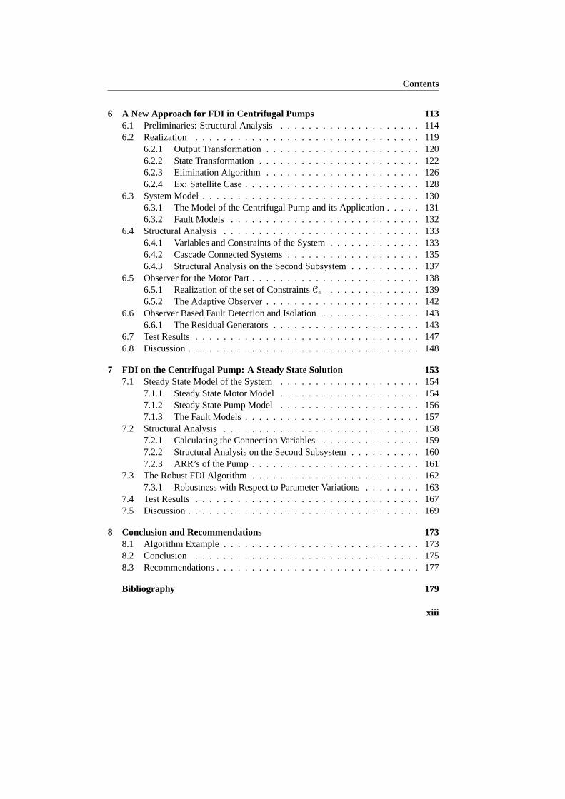
Contents
Nomenclature xv
1 Introduction 11.1 Background and Motivation . . . . . . . . . . . . . . . . . . . . . . . 11.2 Objectives . . . . . . . . . . . . . . . . . . . . . . . . . . . . . . . . . 31.3 Contributions . . . . . . . . . . . . . . . . . . . . . . . . . . . . . . . 31.4 Outline of the Thesis . . . . . . . . . . . . . . . . . . . . . . . . . . . 5
2 Fault Detection and Isolation in Pump Systems 72.1 Fault Detection and Isolation . . . . . . . . . . . . . . . . . . . . . . . 8
2.1.1 Signal-Based Approach . . . . . . . . . . . . . . . . . . . . . 92.1.2 Model-Based Approach . . . . . . . . . . . . . . . . . . . . . 102.1.3 Parameter Estimation Approach . . . . . . . . . . . . . . . . . 122.1.4 Residual Evaluation . . . . . . . . . . . . . . . . . . . . . . . 12
2.2 FDI in the Induction Motors . . . . . . . . . . . . . . . . . . . . . . . 122.2.1 Mechanical Faults in the Motor . . . . . . . . . . . . . . . . . 132.2.2 Electrical Faults in the Motor . . . . . . . . . . . . . . . . . . 14
2.3 FDI in Centrifugal Pumps . . . . . . . . . . . . . . . . . . . . . . . . . 152.3.1 Detection of Caviation . . . . . . . . . . . . . . . . . . . . . . 152.3.2 Performance Monitoring and Fault Detection . . . . . . . . . . 16
2.4 Discussion . . . . . . . . . . . . . . . . . . . . . . . . . . . . . . . . . 17
3 Model of the Centrifugal Pump 193.1 The Construction of the Centrifugal Pump . . . . . . . . . . . . . . . . 203.2 Model of the Electrical Motors . . . . . . . . . . . . . . . . . . . . . . 21
3.2.1 The Induction Motor Model inabc-coordinates . . . . . . . . . 223.2.2 Transformation to Stator Fixeddq0-coordinates . . . . . . . . . 243.2.3 Grid Connections . . . . . . . . . . . . . . . . . . . . . . . . . 253.2.4 The Torque Expression . . . . . . . . . . . . . . . . . . . . . . 28
3.3 The Hydraulic Part of the Centrifugal Pump . . . . . . . . . . . . . . . 283.3.1 The Principle of the Centrifugal Pump Dynamics . . . . . . . . 29
xi

Contents
3.3.2 The Torque Expression . . . . . . . . . . . . . . . . . . . . . . 313.3.3 The Head Expression . . . . . . . . . . . . . . . . . . . . . . . 343.3.4 Leakage Flow and Pressure Losses in the Inlet and Outlet . . . . 353.3.5 Multi Stage Pumps . . . . . . . . . . . . . . . . . . . . . . . . 38
3.4 The Mechanical Part of the Centrifugal Pump . . . . . . . . . . . . . . 393.5 Final Model of the Centrifugal Pump . . . . . . . . . . . . . . . . . . . 403.6 Discussion . . . . . . . . . . . . . . . . . . . . . . . . . . . . . . . . . 42
4 System Analysis and Fault Modelling 434.1 Method for Fault Analysis . . . . . . . . . . . . . . . . . . . . . . . . 44
4.1.1 Preliminaries: The FMEA and FPA . . . . . . . . . . . . . . . 454.2 Automated FPA . . . . . . . . . . . . . . . . . . . . . . . . . . . . . . 48
4.2.1 The Automated FPA Algorithm . . . . . . . . . . . . . . . . . 484.2.2 Sensor Configuration and Disturbing Events . . . . . . . . . . . 57
4.3 Pump Applications . . . . . . . . . . . . . . . . . . . . . . . . . . . . 614.3.1 Component Identification in the Centrifugal Pump . . . . . . . 624.3.2 FMEA on the System Components . . . . . . . . . . . . . . . 634.3.3 Identifying Interesting Faults . . . . . . . . . . . . . . . . . . . 694.3.4 FPA on the General Pump System . . . . . . . . . . . . . . . . 714.3.5 Sensor Configuration Analysis . . . . . . . . . . . . . . . . . . 74
4.4 Detection Algorithm for the Centrifugal Pump . . . . . . . . . . . . . . 774.4.1 Decision Logic . . . . . . . . . . . . . . . . . . . . . . . . . . 784.4.2 Test Results . . . . . . . . . . . . . . . . . . . . . . . . . . . . 79
4.5 Discussion . . . . . . . . . . . . . . . . . . . . . . . . . . . . . . . . . 80
5 A New approach for Stator Fault Detection in Induction Motors 855.1 Model of the Stator Short Circuit . . . . . . . . . . . . . . . . . . . . . 86
5.1.1 TheY-connected Motor inabc-coordinates . . . . . . . . . . . 875.1.2 The∆-connected Motor inabc-coordinates . . . . . . . . . . . 885.1.3 Transformation to a Stator fixeddq0-frame . . . . . . . . . . . 895.1.4 Grid Connections . . . . . . . . . . . . . . . . . . . . . . . . . 905.1.5 Torque Expression . . . . . . . . . . . . . . . . . . . . . . . . 92
5.2 An Adaptive Observer for Inter-turn Fault Detection . . . . . . . . . . . 935.2.1 The Adaptive Observer . . . . . . . . . . . . . . . . . . . . . . 955.2.2 Calculation of the Observer Gain . . . . . . . . . . . . . . . . 995.2.3 Identification of the Faulty Phase . . . . . . . . . . . . . . . . 102
5.3 Test Results . . . . . . . . . . . . . . . . . . . . . . . . . . . . . . . . 1035.3.1 Test of Identification Capabilities . . . . . . . . . . . . . . . . 1055.3.2 Test of Estimation Capabilities . . . . . . . . . . . . . . . . . . 106
5.4 Conclusion . . . . . . . . . . . . . . . . . . . . . . . . . . . . . . . . 107
xii
Contents
6 A New Approach for FDI in Centrifugal Pumps 1136.1 Preliminaries: Structural Analysis . . . . . . . . . . . . . . . . . . . . 1146.2 Realization . . . . . . . . . . . . . . . . . . . . . . . . . . . . . . . . 119
6.2.1 Output Transformation . . . . . . . . . . . . . . . . . . . . . . 1206.2.2 State Transformation . . . . . . . . . . . . . . . . . . . . . . . 1226.2.3 Elimination Algorithm . . . . . . . . . . . . . . . . . . . . . . 1266.2.4 Ex: Satellite Case . . . . . . . . . . . . . . . . . . . . . . . . . 128
6.3 System Model . . . . . . . . . . . . . . . . . . . . . . . . . . . . . . . 1306.3.1 The Model of the Centrifugal Pump and its Application . . . . . 1316.3.2 Fault Models . . . . . . . . . . . . . . . . . . . . . . . . . . . 132
6.4 Structural Analysis . . . . . . . . . . . . . . . . . . . . . . . . . . . . 1336.4.1 Variables and Constraints of the System . . . . . . . . . . . . . 1336.4.2 Cascade Connected Systems . . . . . . . . . . . . . . . . . . . 1356.4.3 Structural Analysis on the Second Subsystem . . . . . . . . . . 137
6.5 Observer for the Motor Part . . . . . . . . . . . . . . . . . . . . . . . . 1386.5.1 Realization of the set of ConstraintsCe . . . . . . . . . . . . . 1396.5.2 The Adaptive Observer . . . . . . . . . . . . . . . . . . . . . . 142
6.6 Observer Based Fault Detection and Isolation . . . . . . . . . . . . . . 1436.6.1 The Residual Generators . . . . . . . . . . . . . . . . . . . . . 143
6.7 Test Results . . . . . . . . . . . . . . . . . . . . . . . . . . . . . . . . 1476.8 Discussion . . . . . . . . . . . . . . . . . . . . . . . . . . . . . . . . . 148
7 FDI on the Centrifugal Pump: A Steady State Solution 1537.1 Steady State Model of the System . . . . . . . . . . . . . . . . . . . . 154
7.1.1 Steady State Motor Model . . . . . . . . . . . . . . . . . . . . 1547.1.2 Steady State Pump Model . . . . . . . . . . . . . . . . . . . . 1567.1.3 The Fault Models . . . . . . . . . . . . . . . . . . . . . . . . . 157
7.2 Structural Analysis . . . . . . . . . . . . . . . . . . . . . . . . . . . . 1587.2.1 Calculating the Connection Variables . . . . . . . . . . . . . . 1597.2.2 Structural Analysis on the Second Subsystem . . . . . . . . . . 1607.2.3 ARR’s of the Pump . . . . . . . . . . . . . . . . . . . . . . . . 161
7.3 The Robust FDI Algorithm . . . . . . . . . . . . . . . . . . . . . . . . 1627.3.1 Robustness with Respect to Parameter Variations . . . . . . . . 163
7.4 Test Results . . . . . . . . . . . . . . . . . . . . . . . . . . . . . . . . 1677.5 Discussion . . . . . . . . . . . . . . . . . . . . . . . . . . . . . . . . . 169
8 Conclusion and Recommendations 1738.1 Algorithm Example . . . . . . . . . . . . . . . . . . . . . . . . . . . . 1738.2 Conclusion . . . . . . . . . . . . . . . . . . . . . . . . . . . . . . . . 1758.3 Recommendations . . . . . . . . . . . . . . . . . . . . . . . . . . . . . 177
Bibliography 179
xiii
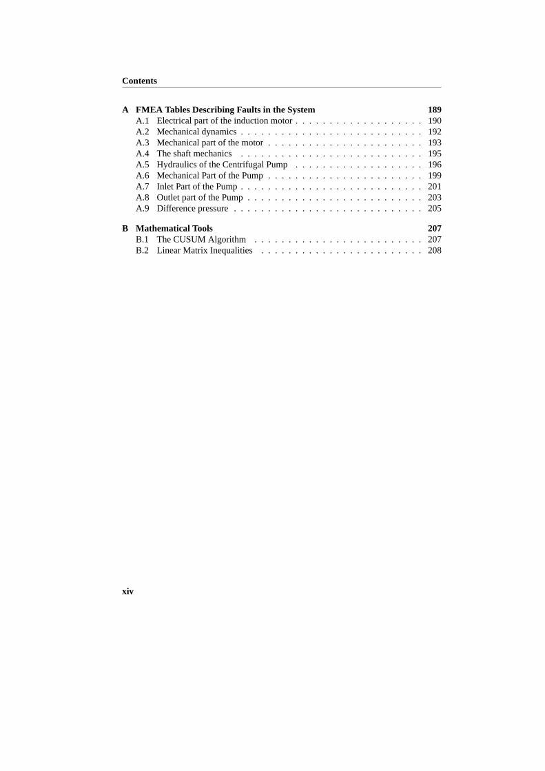
Contents
A FMEA Tables Describing Faults in the System 189A.1 Electrical part of the induction motor . . . . . . . . . . . . . . . . . . . 190A.2 Mechanical dynamics . . . . . . . . . . . . . . . . . . . . . . . . . . . 192A.3 Mechanical part of the motor . . . . . . . . . . . . . . . . . . . . . . . 193A.4 The shaft mechanics . . . . . . . . . . . . . . . . . . . . . . . . . . . 195A.5 Hydraulics of the Centrifugal Pump . . . . . . . . . . . . . . . . . . . 196A.6 Mechanical Part of the Pump . . . . . . . . . . . . . . . . . . . . . . . 199A.7 Inlet Part of the Pump . . . . . . . . . . . . . . . . . . . . . . . . . . . 201A.8 Outlet part of the Pump . . . . . . . . . . . . . . . . . . . . . . . . . . 203A.9 Difference pressure . . . . . . . . . . . . . . . . . . . . . . . . . . . . 205
B Mathematical Tools 207B.1 The CUSUM Algorithm . . . . . . . . . . . . . . . . . . . . . . . . . 207B.2 Linear Matrix Inequalities . . . . . . . . . . . . . . . . . . . . . . . . 208
xiv

Nomenclature
Symbols
In this thesis all matrices and vectors are written with bold letters, to distinguish thesefrom scalar values.
Symbols and parameters used in connection with the motor modelvtdq dq-transformed voltages at the terminals of the induction motor,vtdq =
(vtd vtq)T .itdq dq-transformed currents at the terminals of the induction motor,itdq =
(itd itq)T .vsdq dq-transformed stator voltages of the induction motor,vsdq = (vsd vsq).isdq dq-transformed stator currents of the induction motor,isdq = (isd isq).i′sdq Deriveddq-transformed stator current,i′sdq = isdq −Tdqγif .irdq dq-transformed rotor currents of the induction motor,irdq = (ird irq).γ Among of turns involved in the stator short circuit,γ = (γa γb 0)T .if Current in the short circuit loop of the stator.Te Torque generated by the electrical circuit of the motor.Tdq0(θ) Transformation matrix given byxdq0 = Tdq0(θ)xabc, whereTdq0(θ) =
23
cos(θ) cos(θ + 23π ) cos(θ + 4
3π )sin(θ) sin(θ + 2
3π ) sin(θ + 43π )
12
12
12
.
Tdq0 Transformation matrix given byTdq0 = Tdq0(0).Tdq Matrix consisting of the two first rows ofTdq0.T−1
dq Matrix consisting of the two first columns ofT−1dq0.
J 2× 2 skew inverse matrix given byJ =[0 −11 0
].
xv
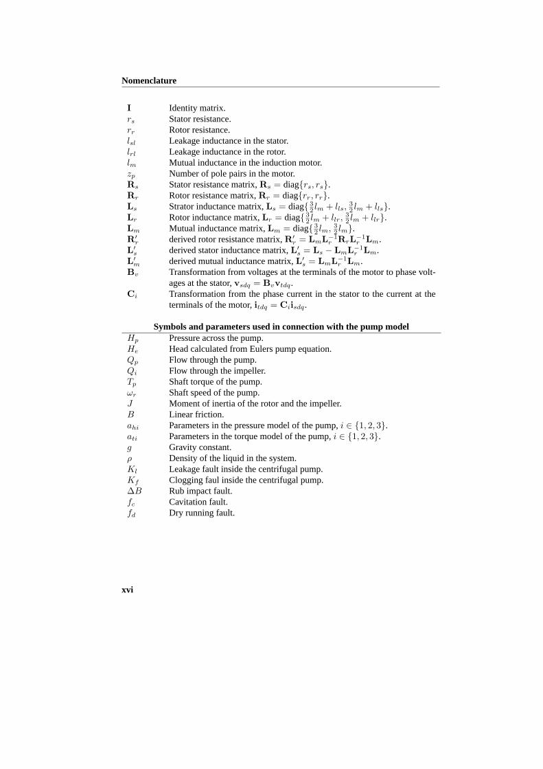
Nomenclature
I Identity matrix.rs Stator resistance.rr Rotor resistance.lsl Leakage inductance in the stator.lrl Leakage inductance in the rotor.lm Mutual inductance in the induction motor.zp Number of pole pairs in the motor.Rs Stator resistance matrix,Rs = diag{rs, rs}.Rr Rotor resistance matrix,Rr = diag{rr, rr}.Ls Strator inductance matrix,Ls = diag{ 3
2 lm + lls,32 lm + lls}.
Lr Rotor inductance matrix,Lr = diag{ 32 lm + llr,
32 lm + llr}.
Lm Mutual inductance matrix,Lm = diag{ 32 lm, 3
2 lm}.R′
r derived rotor resistance matrix,R′r = LmL−1
r RrL−1r Lm.
L′s derived stator inductance matrix,L′s = Ls − LmL−1r Lm.
L′m derived mutual inductance matrix,L′s = LmL−1r Lm.
Bv Transformation from voltages at the terminals of the motor to phase volt-ages at the stator,vsdq = Bvvtdq.
Ci Transformation from the phase current in the stator to the current at theterminals of the motor,itdq = Ciisdq.
Symbols and parameters used in connection with the pump modelHp Pressure across the pump.He Head calculated from Eulers pump equation.Qp Flow through the pump.Qi Flow through the impeller.Tp Shaft torque of the pump.ωr Shaft speed of the pump.J Moment of inertia of the rotor and the impeller.B Linear friction.ahi Parameters in the pressure model of the pump,i ∈ {1, 2, 3}.ati Parameters in the torque model of the pump,i ∈ {1, 2, 3}.g Gravity constant.ρ Density of the liquid in the system.Kl Leakage fault inside the centrifugal pump.Kf Clogging faul inside the centrifugal pump.∆B Rub impact fault.fc Cavitation fault.fd Dry running fault.
xvi

Nomenclature
Symbols used in connection with the FMEA and FPAF Finite set of all event vectors in the system.Fi Finite set of all event vectors in theith component in the system.Ff Finite set of all fault event vectors.Fd Finite set of all disturbing event vectors.If Finite set of all fault event vectors with only one non zero element.f Vector of fault events.d Vector of disturbing events.Aj
fiPropagation matrix from the faults defined in theith component to theeffects defined in thejth component.
Aji Propagation matrix from the effects defined in theith component to the
effects defined in thejth component.Af Propagation matrix from the faults to the end-effects in the system.Ad Propagation matrix from the disturbing events to the end-effects in the
system.Gf , Df GraphGf and corresponding adjacency matrixDf describing the con-
nection between faults and components in the FPA diagram.Ge, De GraphGe and corresponding adjacency matrixDe describing the struc-
ture of the effect propagation in the FPA diagram.
Symbols used in connection with the SA and realizationS Dynamic system.O Observer design based on the dynamic systemS.C Set of constraints.Z Set of variables.S System composed of a set of constraints and a set of variables, i.e.S =
(C, Z).K Set of known variables, i.e.K ⊂ Z.X Set of unknown variables, i.e.X ⊂ Z.xd State vector of the dynamic systemS.xa Algebraic variables of the dynamic systemS.c Constraint which links a subset of the variables inZ.d Constraint on the formxd = dxd
dt , wherexd, xd ∈ X.fx,mx,hx Vector field, algebraic constraints, and output maps of the dynamic system
S.fo,ho Vector field and output maps of an output transformed system.fz,hz Vector field and output maps of a state transformed system.
xvii

Nomenclature
Symbols used in connection with the steady state FDIVrms RMS value of the supply voltage.Irms RMS value of the supply current.ωe Frequency of the supply voltage.φ Angle between the supply voltage and supply current.V e
sd Stator voltage used in the steady state model of the motor.V e
sq Stator voltage used in the steady state model of the motor.Iesq Stator current used in the steady state model of the motor.
Iemd Magnetizing current used in the steady state model of the motor.
Iemq Magnetizing current used in the steady state model of the motor.
r Residual.R Set of residual values.
Mathematical SymbolsÂ,≺ Positive and negative definit respectively.>,< Larger than and smaller than respectively.→ Logical expression to the left implies logical expression to the right.∨ Logical or operator.∧ Logical and operator.x Maximum value ofx.x Minimum value ofx.R The reals.R+ The positive reals including zero, i.e.R+ = {x ∈ R | x ≥ 0}.
Abbreviations
FDI Fault Detection and Identification.SA Structural Analysis.ARR Analytical Redundant Relation.FMEA Failure Mode and Effect Analysis.FPA Fault Propagation Analysis.Model-based FDI FDI approaches based on mathematical models of the applica-
tion.Signal-based FDI FDI approaches based on signal processing and classifing tech-
niques.
xviii

Chapter 1
Introduction
This thesis considers the analysis and design of algorithms for Fault Detection and Iden-tification (FDI) in centrifugal pumps. The aim has been to investigate methods for FDIin centrifugal pumps, with special focus on the robustness and usability of the obtainedalgorithms. This means that the algorithms must be able to detect faults under changingoperating conditions, and should be robust with respect to disturbances in the system.
1.1 Background and Motivation
This project was founded by Grundfos, which is a multi-national company with pro-duction and sale facilities in around 50 different countries all over the world. Grundfosis producing pumps for a variety of different applications. Still, most of the producedpumps are for use in water treatment and aqueous solutions. In these applications thecentrifugal pump is the most used pump type. This is due to its simple constructionwith few moving parts, making it very reliable and robust. In this thesis especially cen-trifugal pumps for use in industrial applications, submersible applications, water supplyapplications, and sewage applications are of interest.
In many of these applications it is crucial that the pumps are working all the time.Moreover, the size of the pumps makes maintenance costly, in many cases. In addi-tion to that, the applications are often situated in remote places, when it comes to watersupply and sewage treatment. This means that maintenance becomes even more costly.Therefore, in these applications supervision, including fault detection and in speciallyfault prediction, is very interesting. Equally interesting is supervision in industrial appli-cations. Here, the need is initiated by the ongoing demand for production improvement,meaning that it is crucial that the pumps are only stopped when absolutely necessary.Therefore, the use of a monitoring system, which includes supervision of the pumps,would be beneficial in many of these applications. This implies, that monitoring sys-tems can be expected to be a growing competition parameter in the following years.
1

Chapter 1: Introduction
This project was initiated by a growing need, inside Grundfos, for knowledge aboutthe newest methods for detection of events and faults in pumps and pump systems. Thisneed is based on the expectation that monitoring and control systems will be commonlyused for supervision and control, of especially larger pumps, in the future. Besides that,pumps are sometimes returned on warranty where it has been impossible to reproducethe fault. In these cases it would be of great interest to know what the pump has been ex-posed to before it is returned. This knowledge could be used to improve the constructionof the pumps and user manuals to avoid unnecessary returns on warranty, and therebyunnecessary inconveniencies for the costumer.
The most common maintenance problems and faults expected in centrifugal pumpscan be divided into three main categories,
• Maintenance, such as cleaning of the pump.
• Faults which demands maintenance, such as bearing faults, and leakage due tosealing faults.
• Severe faults, which demand replacement, such as stator burnouts, and damagedimpeller.
The first item covers normal maintenance, which, to some extend, is necessary in anyapplication. Likewise, the second item covers replacement of wearing parts, which alsoshould be expected in any pump setup, when running for long time periods. The last itemcovers severe damages, normally caused by unexpected faults or by lack of maintenance.
A well designed monitoring system will be able to help a user, exposed to faults,in any of the three mentioned categories. Traditionally, the first two categories are,in large pump applications, handled by doing scheduled maintenance on the plant. Atthese scheduled maintenance procedures, a set of predetermined wearing parts are oftenexchanged to avoid future breakdowns. When using a monitoring system, maintenancecan be done on demand, which will save costs for unnecessary replacement parts, andmore important, the pump only has to be stopped for maintenance when really necessary.For the last category, a monitoring system would be able to detect and stop the pumpbefore a given fault causes total breakdown of the pump. In larger pumps this wouldmake repair possible, meaning that a replacement of the whole pump is saved.
Different sets of sensors could be used as inputs to such a monitoring system. Forcentrifugal pumps the following sensors are interesting; vibration sensors, current andvoltage sensors, absolute pressure and pressure difference sensors, flow sensors, andtemperature sensors. Of these, the current and voltage sensors, and the flow and pressuredifference sensors have been considered in this project. These sensors are all reasonablycheep and are often already mounted in a pump system. Therefore, by using only thesesensors, no additional hardware is needed for the proposed algorithms to work. There-fore, the implementation costs for the system is reduced considerably.
2

Section 1.2: Objectives
1.2 Objectives
The aim of the Thesis is to investigate different methods for their usability in analyz-ing and designing FDI algorithms for centrifugal pumps. In the investigation, specialemphasis is layed on the robustness and practical usability of the obtained algorithms.
In (Åström et al., 2001) it is argued that methods for FDI can be divided into twomain groups, namely the model-based and signal-based approaches. Here, the signal-based approaches are approaches, in which signal processing and/or artificial intelli-gence are utilized to obtain knowledge about faults in a given system. The model-basedapproaches are, on the other hand, utilizing system theory to obtain knowledge about thefaults. In this thesis special focus will be put on the use of the model-based approaches,as these approaches have inherent methods for handling disturbances. Hereby, increasedrobustness of the algorithms can be obtained. However, signal-based approaches havebeen widely used for fault detection in centrifugal pumps and their applications. SeeChapter 2 concerning the state of the art of the area. In most of these cases robustnesshas not been considered. Therefore, a method for analyzing robustness in signal-basedFDI systems, is also considered.
1.3 Contributions
The contributions of the Thesis can be divided into two groups. The first group containscontributions to FDI in the centrifugal pumps. The second group contains theoreticalcontributions, mainly on robustness analysis of signal-based fault detection schemesand the realization of subsystems found using Structural Analysis. In this section, firstthe theoretical contributions are listed, followed by the contribution to FDI in centrifugalpumps.
The main contributions in the theoretical areas are:
• A new algorithm for cutting loops in a Fault Propagation Analysis (FPA) graph isproposed in Chapter 4. With this algorithm and a theorem also proposed in thisthesis, the FPA is automated. This means that the only manual step is to setup theevent model.
• A disturbing event is introduced as a part of the FPA in Chapter 4. With this eventit is possible to analyse the robustness of signal-based fault detection algorithms.Two theorems are formulated, aimed to analyse robustness, based on this idea.
• A new adaptive observer, for a particular kind of bilinear system, is proposed inChapter 5. With this observer it is possible to explore the parameter structure inthe system. Observability of the known part of the system is not necessary. Thegain matrix of the observer can be analysed, and in some cases calculated, usingthe proposed Linear Matrix Inequalities (LMI).
3
Chapter 1: Introduction
• A novel transformation method is proposed in Chapter 6. With this transfor-mation, minimal over-constraint subsystems, identified using Structural Analysis(SA), can be transformed into state space descriptions. The method includes twotransformations; an output transformation, and a state transformation. These areformulated in two theorems. The state transformation is submitted for publication(Kallesøe and Izadi-Zamanabadi, 2005).
• As a part of the derivation of a set-valued residual expression, the Taylor Seriesexpantion is proposed in Chapter 7. The Taylor Series expantion is used on theparameter expression to include a linear approximation of the nonlinear depen-dency of the parameters. This has been submitted for publication (Kallesøe et al.,2004a).
The main contributions to FDI in the centrifugal pumps are:
• A fault propagation model of the faults, expected to happen in centrifugal pumps,is derived in Chapter 4. This model has been used to analyse different sensorcombinations aimed for robust signal-based fault detection.
• A new model of an inter-turn short circuit in the stator of an induction motor isderived in Chapter 5. The model is derived for bothY- and∆-connected motors,and has a nice structure, which has similarities to models of motors not affected byinter-turn short circuits. The model of theY-connected motor has been publishedin (Kallesøe et al., 2004c).
• An adaptive observer for estimating inter-turn short circuit faults in the stator ofan induction motor is proposed in Chapter 5. This has been published in (Kallesøeet al., 2004c).
• An example of using SA to divide a complex system into two cascade-connected,less complex, subsystems is shown in Chapter 6. This enables possibilities foreasy observer designs. The idea has been used for solving the nonlinear FDIproblem in the centrifugal pump, using only electrical and hydraulic measure-ments. This has been submitted for publication (Kallesøe et al., 2004a).
• A model-based FDI scheme, for FDI in centrifugal pumps, is proposed in Chapter6. The FDI scheme is based on measurements of the electrical quantities and thehydraulic quantities only. Here, the electrical quantities are the motor voltagesand currents, and the hydraulic quantities are the pressure and volume flow. Partsof the approach have been published in (Kallesøe et al., 2004b).
• A robust FDI scheme, based on the steady state model of the pump and set-valuedalgebra, is derived in Chapter 7. The obtained algorithm depends on steady statemeasurements only, making it useful in cost sensitive products.
4

Section 1.4: Outline of the Thesis
1.4 Outline of the Thesis
The thesis is organized as follows,
Chapter 1: Introduction
Chapter 2: Fault Detection and Isolation in Pump Systems
The purpose of this chapter is two-folded. Firstly, the most important ideas and termsused in the area of Fault Detection and Identification (FDI) are introduced. Secondly,state of the art on FDI in centrifugal pumps, as well as in induction motors, is considered.This includes contributions from the academic world and products already on the market.
Chapter 3: Model of the Centrifugal Pump
This chapter introduces the mathematical model of the centrifugal pump. This includesa model of the induction motor driving the pump, and models of the mechanical andhydraulic parts of the pump. The presented models are lumped parameter models, whichespecially are suitable for use in model-based FDI design. Special emphasize is put onthe dynamics of the hydraulic part. Here, it is shown that the energy conversion frommechanical to hydraulic energy, is described by a purely algebraic equation. Moreover,it is shown that the pump dynamics can be described by adding extra mass to the rotatingparts of the pump, i.e. increasing the moment of inertia of the rotating parts of pump.The derived model is valid under two assumptions, also stated in the chapter.
Chapter 4: System Analysis and Fault Modelling
In this chapter the use of Failure Mode and Effect Analysis (FMEA) and Fault Propaga-tion Analysis (FPA) in the design of signal-based fault detection algorithms is explored.The FMEA and the FPA are well known analysis tools, and have been proposed as ananalysis tool in the design Fault Tolerant Control, as well as in FDI algorithms. A newalgorithm for automating parts of the FPA is proposed in this chapter. Moreover, byintroducing a so-called disturbing event in the FPA, it is shown that the robustness ofsignal-based FDI algorithms can be analysed.
The chapter includes an FMEA of a general centrifugal pump, meaning that the con-ceptual faults, expected in centrifugal pumps, are identified and analyzed. The outcomeof the FMEA is a list of possible faults in centrifugal pumps. 11 of these faults aregrouped into 7 fault groups. These 7 faults found the basis for the FDI algorithms de-signed in this thesis. Using the FPA, different sensor combinations are analysed, aimedto find a set of signals, which can be used in a signal-based fault detection scheme. Oneof these sensor configurations is proven to work on a special designed test setup.
5

Chapter 1: Introduction
Chapter 5: A New Approach for Stator Fault Detection in Induction Motors
This chapter introduces a new approach for inter-turn short circuit detection in the statorof an induction motor. In the design, an adaptive observer approach is used, utilizingonly electrical measurements. The observer is based on a model of the induction motor,in which a description of the inter-turn short circuit is included. This model is derivedin the beginning of the chapter. With the designed observer it is possible to estimatethe states of the motor, the speed, and the inter-turn short circuit simultaneously. Theobserver is shown to work on a special designed motor, where it is possible to simulateinter-turn short circuit faults. Likewise, it is shown that it is possible to identify thephase, affected by the inter-turn short circuit. The adaptive observer, used in the pro-posed design, is formulated in general terms, and could therefore be used in a numberof other applications.
Chapter 6: A New Approach for FDI in Centrifugal Pumps
The topic of this chapter is FDI on the hydraulic and mechanical parts of the centrifugalpump. The model-based approach is used for this purpose. This means that residual gen-erators are developed, based on the model of the centrifugal pump, presented in Chapter3. In the design of the residual generators, subsystems, which are robust with respectto disturbances and unknown model parts, are identified using Structural Analysis (SA)(Blanke et al., 2003). These subsystems are then transformed into state space form,enabling residual observer designs. The transformation from subsystems, identified us-ing SA, into state space descriptions is novel, and is described in general terms in thebeginning of the chapter.
Chapter 7: FDI on the Centrifugal Pump: A Steady State Solution
In this chapter a FDI algorithm, based on a steady state model of the pump, is developed.The FDI algorithm is developed using Structural Analysis, in order to obtain three An-alytical Redundant Relations, each used in the calculation of a residual. The algorithmis shown to enable detection and identification of five different faults in the hydraulicpart of the pump. Robustness of the algorithm is insured using a set-valued approach,making it possible to in-count parameter variations in the FDI algorithm.
Chapter 8: Conclusion and Recommendations
6

Chapter 2
Fault Detection and Isolation inPump Systems
The purpose of this chapter is two-folded. Firstly, a short introduction to the most im-portant ideas and terms used in the area of Fault Detection and Identification (FDI) isincluded. Secondly, a state of the art analysis on FDI in centrifugal pump applicationsis presented. The first part is included to lighten readers of the thesis not familiar withthe concept of FDI. The second part includes both a state of the art analysis of FDI inthe centrifugal pump itself, and on the induction motor drive by which centrifugal pumpis driven. Moreover, the analysis includes contributions from both the academic worldand products already on the market.
In Section 2.1, where the concept of FDI is introduced, three different approaches toFDI are considered. First of all, distinguishing between model-based and signal-basedFDI is considered (Åström et al., 2001), and the main ideas behind both methods aredescribed. This is followed by an introduction of the parameter adaptation approach,and finally the concept of residual evaluation is introduced.
In Sections 2.2 and 2.3 state of the art of FDI in respectively induction motors andcentrifugal pumps is considered. A number of different faults and detection methodshave been treated in both the induction motor and in the centrifugal pump. However,considerable more work is done in the area of FDI on induction motors compared to thework done on centrifugal pumps. This is mainly because of the widespread use of themotor type. The state of the art analysis is followed by some concluding remarks, whichend the chapter.
7

Chapter 2: Fault Detection and Isolation in Pump Systems
2.1 Fault Detection and Isolation
To understand the concept of FDI, first it has to be defined what is meant by faults, andwhich information is expected to be available for detection of these. To explain this,let the structure of a system with inputsu(t) ∈ Rm, outputsy(t) ∈ Rd be definedas shown in Fig. 2.1. Here, a fault affecting the system is symbolized byf . This
System u y
f
Figure 2.1: System with inputsu, outputsy and a faultf affecting the system.
fault is interpreted as an unwanted event creating abnormal operation of the system.Faults can affect the operation of a system in different ways. Normally, these faulteffects are divided into two sub-groups, which are denotedmultiplicative faultsandadditive faultsrespectively. Multiplicative faults influence the system as a product, likefor example parameter variations, and additive faults influence the system by an addedterm (Isermann and Balle, 1997).
As an example of a system affected by faults, consider the following linear system,which is affected by both multiplicative and additive faults.
dxdt = A(θf )x + B(θf )u + E1d + F1fy = C(θf )x + D(θf )u + E2d + F2f .
(2.1)
In this systemx(t) ∈ Rn contains the states,u(t) ∈ Rp contains the inputs,y(t) ∈ Rd
contains the outputs, andd(t) ∈ Rl contains disturbances, which can be interpretedas unknown or unmeasurable inputs. This system is affected by the faultsf(t) ∈ Rh
affecting the system by an added term, and the parametersθf ∈ Rk affecting the sys-tem in multiplicative manner. Here the multiplicative faults are seen as changes of theparameter values in the system. Besides the multiplicative and additive fault effects, afault can change the structure of a system, meaning that the system becomes a so-calledhybrid system, where the state change is caused by the given fault.
Having the above described system in mind the fault detection problem is the taskof detecting that a faultf ∈ F has occurred in a given system, whereF is the set of allpossible faults in the system, i.e. it contains all faults inf andθf . The solution to thefault detection problem is based on the set of measurementsy and possibly the set ofknown input signalsu. When a fault is detected it is possible to state that something iswrong in the system but not what is wrong. However, sometimes it is possible to isolatethe fault, meaning that faultfi can be distinguished for the set of possible faultsF inthe system. When a fault is isolated it is possible to state where and what is wrong in
8

Section 2.1: Fault Detection and Isolation
the system (Chen and Patton, 1999; Gertler, 1998). The problem of both detection andisolation of a fault is called the Fault Detection and Isolation (FDI) problem. If it is notonly possible to isolate the faultfi in the setF , but also possible to estimate the size ofthis faultfi, the fault is said to be estimated. The three levels of complexity in the faultdetection problem, described above, are summarized below.
Fault Detection: An abnormality in a system is detected, but the type and size are un-known.
Fault Isolation: The faultfi is identified in the set of all possible faultsF . Hereby thetype of the fault is known but the size remains unknown.
Fault Estimation: The size of the faultfi ∈ F is estimated.
Different methods can be used for detecting a faultf ∈ F . The choice of methodshould be based on the type of fault, which has to be detected, and which measurementsare available. Below three main groups of approaches are described.
2.1.1 Signal-Based Approach
In the Signal-Based approach, characteristics in the measured signalsy containing in-formation about the health of the system are utilized (Åström et al., 2001). A blockdiagram of a FDI system based on the signal-based approach is shown in Fig. 2.2. From
System u y Signal
processing
r Residual evaluation
f
v
Fault detection and isolation
Fault scenario
database
Figure 2.2: Structure of a signal based fault detection and isolation system (Åströmet al., 2001).
this figure it is seen that the fault detection algorithm consists of three blocks. In thefirst block,signal processing, methods from signal processing theory are utilized to ex-tract information about the health of the system from the measured signals. The outputfrom the signal-processing block is sent to a unit consisting of a database and somesorts of artificial intelligence. In Fig. 2.2 this is theresidual evaluationblock and thefault scenario databaseblock. This part of the algorithm compares the output from the
9
Chapter 2: Fault Detection and Isolation in Pump Systems
signal-processing block with predefined data sets from the database, each describing thecharacteristics of a given fault. From this comparison the FDI algorithm decides if thesystem is affected by a fault and if so, which one it is.
The signal-processing block often consists of frequency spectrum analysis such asFFT-algorithms, wavelets, or higher order statistic (HOS) tools. However, it could alsobe a simple limit check on the measured signal. In the decision unit, i.e. the faultscenario database and the residual evaluation block, all kinds of methods for data evalu-ation are used. Of these clustering techniques, neural networks, and fuzzy logic shouldbe mentioned. All of these are sophisticated methods for data mining. However, in mostreal applications simple forms of decision logic are used.
Now considering the advantages and disadvantages of the signal-based method asthe author see it. First of all, a mathematical model is not used in this approach, which isa huge advantage, as such a model can be difficult and even in some cases impossible toderive. However, the drawback is the need for data from the system when it is affectedby faults, as these data should be used in the development of the fault scenario database.Moreover, it can be difficult to ensure robustness of the FDI algorithm, as in theory allpossible operation conditions should be tested, before robustness is ensured. Of course,simulations can solve some of these problems, but then a model is needed, underminingone of the advantages of the approach. Considering these characteristics, this approachmust be considered most suitable for systems, which are difficult or in particular casesimpossible to describe with a mathematical model.
2.1.2 Model-Based Approach
The model-based approach utilizes analytical redundancy to extract information aboutfaults in the system. When using analytical redundancy one utilizes physical bindingsbetween inputs and outputs and between different outputs of the system to describe nor-mal operation conditions. The physical bindings are here denoted analytical relations.Faults are then detected when the analytical relation is not fulfilled. When this is thecase the system is operating under abnormal operation conditions, which are exactly thedefinition of a fault. The analytical relations, utilized in this approach, are described us-ing mathematical models. The relations described by these models are compared to thephysical relations in the real system, revealing abnormal operation if a difference exists.
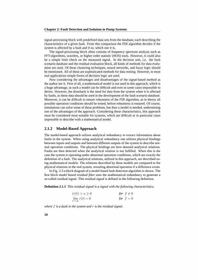
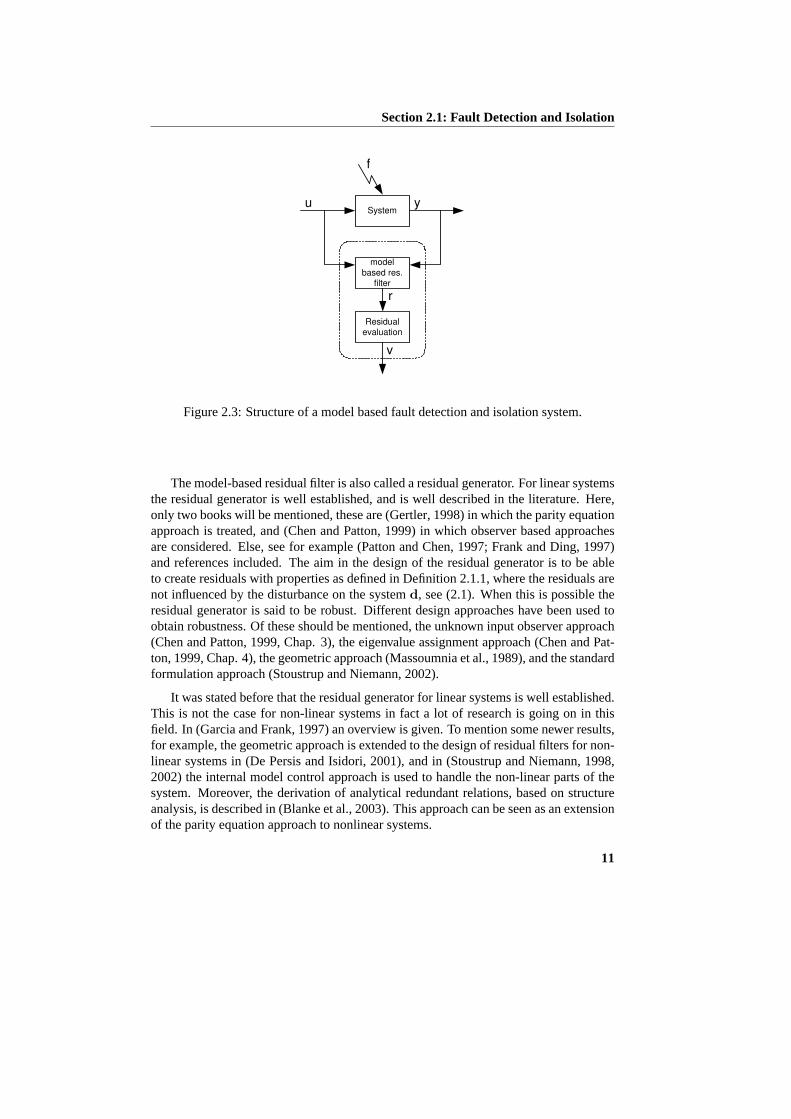
In Fig. 2.3 a block diagram of a model-based fault detection algorithm is shown. Thefirst block model based residual filteruses the mathematical redundancy to generate aso-called residual signal. This residual signal is defined in the following definition.
Definition 2.1.1 This residual signal is a signal with the following characteristics,
|r(t)| > κ ≥ 0 for f 6= 0lim
t→∞r(t) = 0 for f = 0
wheref is a fault in the system andr is the residual signal.
10
Section 2.1: Fault Detection and Isolation
System u y
f
model
based res. filter
Residual evaluation
r
v
Figure 2.3: Structure of a model based fault detection and isolation system.
The model-based residual filter is also called a residual generator. For linear systemsthe residual generator is well established, and is well described in the literature. Here,only two books will be mentioned, these are (Gertler, 1998) in which the parity equationapproach is treated, and (Chen and Patton, 1999) in which observer based approachesare considered. Else, see for example (Patton and Chen, 1997; Frank and Ding, 1997)and references included. The aim in the design of the residual generator is to be ableto create residuals with properties as defined in Definition 2.1.1, where the residuals arenot influenced by the disturbance on the systemd, see (2.1). When this is possible theresidual generator is said to be robust. Different design approaches have been used toobtain robustness. Of these should be mentioned, the unknown input observer approach(Chen and Patton, 1999, Chap. 3), the eigenvalue assignment approach (Chen and Pat-ton, 1999, Chap. 4), the geometric approach (Massoumnia et al., 1989), and the standardformulation approach (Stoustrup and Niemann, 2002).
It was stated before that the residual generator for linear systems is well established.This is not the case for non-linear systems in fact a lot of research is going on in thisfield. In (Garcia and Frank, 1997) an overview is given. To mention some newer results,for example, the geometric approach is extended to the design of residual filters for non-linear systems in (De Persis and Isidori, 2001), and in (Stoustrup and Niemann, 1998,2002) the internal model control approach is used to handle the non-linear parts of thesystem. Moreover, the derivation of analytical redundant relations, based on structureanalysis, is described in (Blanke et al., 2003). This approach can be seen as an extensionof the parity equation approach to nonlinear systems.
11
Chapter 2: Fault Detection and Isolation in Pump Systems
2.1.3 Parameter Estimation Approach
In the parameter estimation approach parameters are estimated, which contains fault in-formation. The estimated parameter values are then compared to the expectation valuesof these parameters, resulting in a set of residuals, as shown below,
r = θ0 − θ ,
whereθ0 are the expected parameter values andθ are the estimated values. The param-eters can either be estimated by an extended Kalman filter (Del Gobbo et al., 2001) orby means of adaptive observers (Xu and Zhang, 2004; Jiang and Staroswiecki, 2002).With both of these approaches the states of the system and the parameters containingfault information are estimated simultaneously. System identification, as it is presentedin (Ljung, 1999), can also be used to estimate the parameter values of the system online.This approach is explored in for example (Isermann, 1997).
2.1.4 Residual Evaluation
From the definition of the residual signal given in Definition 2.1.1 the residualr shouldbe smaller than a predefined threshold valueκ, when no fault has happened in the sys-tem. However, it can be difficult or even impossible to find aκ, which is smaller than|r|if a fault has happened and larger then|r| at all times in the no fault case. This is becausethe residualr will be corrupted by model errors, un-modelled disturbances, and noise inreal life application. To overcome this problem different methods are developed. Twoof these are mentioned here.
To overcome the model error problem it is possible to derive an adaptive thresholdκ(t) on the residual signal. If for example the model is poor under transient phases, thethreshold could be increased during this phase. This is called adaptive residual eval-uation (Frank and Ding, 1997). To overcome the noise problem statistical test can beused. Especially the CUSUM algorithm is often used for testing changes in the residualsignals when it is affected by noise (Basseville and Nikiforov, 1998).
2.2 FDI in the Induction Motors
Fault detection and identification in induction motors have gained a lot of attention inthe resent years. Here all kind of faults in induction motors are considered. However, in(Kliman et al., 1996) it is argued that the main causes of faults in induction motors canbe divided into the following three groups,
40-50% Bearing faults.
30-40% Stator faults.
5-10% Rotor faults.
12

Section 2.2: FDI in the Induction Motors
Even though most faults fall into one of these three groups, mechanical faults such asmiss alignment and rub impact between stator and rotor are also considered. In thefollowing two sections detection of mechanical faults are considered first, followed byan analysis of the used method in detection of electrical faults.
2.2.1 Mechanical Faults in the Motor
As stated before, most mechanical breakdowns of motors are due to bearing faults. Thisis especially a problem if a voltage inverter supplies the motor. If this is the case, largehigh frequency voltage components will cause circulating current through the bearings.This current will eventually destroy the bearings. Even though bearing faults are themost common mechanical faults, also other kind of faults such as for example bend shaftor rub impact between stator and rotor can happen. For the whole group of mechanicalfaults the most used detection schemes fall into two groups,
• Spectrum analysis of motor currents.
• Spectrum analysis of vibration signals.
The current spectrum analysis is explored in (Eren and Devaney, 2001; Schoen et al.,1995; Benbouzid, 2000). In (Eren and Devaney, 2001) Wavelets are used for analysingthe stator current at start up, to detect bearing faults, and in (Schoen et al., 1995) thecurrent spectrum, during steady state operation, is used for the same purpose. In (Ben-bouzid, 2000) an overview is given over different signal analysis methods for currentspectrum analysis. Here such different methods as the FFT, wavelets, and Higher OrderSpectrum (HOS) analyses are considered. The obtained current spectrums are used inthe detection of bearing faults and other mechanical faults.
The spectrum analysis of vibrations is explored in (Li et al., 2000; Chow and Tan,2000; Stack et al., 2002). In (Li et al., 2000) the signal of vibrations is transformedinto a frequency spectrum, creating attributes used as input to a neural network. Theneural network is then used to map the attributes into fault types. In (Chow and Tan,2000; Stack et al., 2002) Higher Order Spectrum (HOS) analysis is used to extract faultinformation from the signal of vibrations. Also model-based methods have been usedin the detection of mechanical faults. This is explored in (Loparo et al., 2000) where amathematical model of the mechanical part of the motor is developed, and used in a FDIscheme.
In commercial products the analysis of the vibration spectrum is the mostly usedapproach for detection of mechanical faults. Companies such asSKF, andBrüel & Kjæroffer hand held or stationary vibration analysers, for use by the maintenance staff. Herethe spectrum of vibrations is shown, leaving it to the user to interpret the signal, andthereby conclude if there is a fault in the motor or not. To help the maintenance staffsupervising the frequency spectrum, it is normally possible to set alarm thresholds onparts of this spectrum.
13
Chapter 2: Fault Detection and Isolation in Pump Systems
Even though, analysis of vibration signals is considered the most used method fordetection of mechanical faults in electrical motors, advanced motor protection units candetect mechanical faults to some extend too. Such motor protection units are offered byfor exampleSiemens, Rockwell Automation, andABB. With these motor protection unitsit is possible to detect faults such as blocked rotor, and high temperature, which couldbe caused by mechanical faults.
2.2.2 Electrical Faults in the Motor
Both stator and rotor faults are denoted electrical faults. These faults are responsible foraround 35-50% of the faults in induction motors. The only referred electrical fault in therotor is broken rotor bar. However, in the stator three main fault groups are considered.These are; inter-turn short circuits, phase to phase short circuits, and phase to groundfaults. Of these the inter-turn short circuit fault has gained most attention. This couldbe explained by referring to (Bonnett and Soukup, 1992; Kliman et al., 1996), where itis argued that phase to phase or phase to ground faults often start by an inter-turn shortcircuit in one of the stator phases.
The detection of inter-turn short circuits in a stator is explored in a large number ofpapers. In (García et al., 2004) the voltage between line neutral and the star point ofthe motor is used for detection. This is shown theoretical using a model of the motorin (Tallam et al., 2002). An inter-turn short circuit will cause imbalance in the stator.This imbalance is used in the detection schemes proposed in (Trutt et al., 2002; Leeet al., 2003), where the negative sequence impedance is estimated, and used as faultindicator. When there is an imbalance in the motor a negative sequence current willbe created. This current is used for fault detection in (Kliman et al., 1996; Arkan et al.,2001; Tallam et al., 2003). In (Arkan et al., 2001) robustness, with respect to imbalancedvoltage supply, is added to the approach by using an estimate of the negative impedancein the motor. Oscillations in the Park transformed current, due to the motor imbalanceare used for detection in (Cruz and Cardoso, 2001), and in (Kostic-Perovic et al., 2000)the so-called space vector fluctuations of the current are used.
Also frequency spectrum approaches have be proposed for the detection of inter-turn short circuit faults (Joksimovic and Penman, 2000; Perovic et al., 2001). In theseFFT as well as Wavelet Package transformations have be used together with some sortof classifier. Higher Order Statistics (HOS) has also be used for extracting knowledgeabout faults in the stator (Chow and Tan, 2000; Arthur and Penman, 2000). In boththe frequency spectrum based methods, and in the HOS based methods steady stateconditions are assumed on the motor. This assumption is relaxed in (Nandi and Toliyat,2002) where the frequency spectrum of the voltage after having the supply switchedoff is used to extract fault information. In (Backir et al., 2001) a parameter estimationapproach is used, also relaxing the steady state assumption.
All the references mentioned until now have been dealing with stator faults, but alsothe detection of rotor faults is considered in the literature. For example in (Trzynad-
14

Section 2.3: FDI in Centrifugal Pumps
lowski and Ritchie, 2000) and in (Bellini et al., 2001) the FFT of the Park transformedcurrent, is used to extract fault information. However, not only the FFT is used in signal-based detection of rotor faults. For example in (Ye et al., 2003; Ye and Wu, 2001; Cu-pertino et al., 2004) the discrete Wavelet and the Wavelet Package transforms are usedfor analysing the motor current.
In industry intelligent motor protection units are commercial available. These Motorprotection units can detect ground faults and overcurrent, which again can be initiatedby inter-turn short circuits. These kinds of motor protection units are available from forexampleSiemens, Rockwell Automation, andABB. Moreover, offline analysis tools areavailable from for exampleBaker Instrument Company, which is able to detect inter-turnshort circuits in stators of electrical machines, directly.
2.3 FDI in Centrifugal Pumps
The most referred fault in the hydraulic part of centrifugal pumps is cavitation. Cavi-tation is the phenomenon, that cavities are created in the liquid if the pressure, at somepoints inside the pump, decreases below the vapor pressure of the liquid. When thisphenomenon occurs the impeller erodes and in extreme cases it vanishes totally afterjust a short time of duty.
Even though cavitation is the most referred fault other faults are also treated in theliterature. The most important of these are mentioned here,
• Obstruction inside the pump or in the inlet or outlet pipe.
• Leakage from the pump or from the inlet or outlet pipe.
• Leakage flow inside the pump.
• Bloked impeller.
• Defect impeller.
• Bearing faults.
In the two following subsections, detection of caviation is considered first, followed byan overview of the most interesting approaches for detection of the faults listed above.
2.3.1 Detection of Caviation
The cavitation phenomenon has been known for decades, and is treated in most booksdealing with centrifugal pumps, see for example (Stepanoff, 1957) and (Sayers, 1990).Even though the phenomenon has been known for a long time it is still a topic of re-search. Especially detecting cavitation and designing pumps to avoid cavitation hasachieved attention. Here, only the problem of detecting the phenomenon is addressed.
15

Chapter 2: Fault Detection and Isolation in Pump Systems
As described before cavitation is the phenomenon of cavities created by vaporiza-tion of the liquid, due to local pressure drops below the vapor pressure inside the pump.When the cavities, due to the vaporization, implode large pressure shocks are created.These pressure shocks will destroy the pump over time. Cavitation has traditional beendefined at the point where the pressure delivered by the pump has dropped 3%. How-ever, the degradation of the pump has started long before this point. Therefore, onlymethods aimed to detect cavitation before the 3% limit are considered here. Differentapproaches are proposed for cavitation detection. These are based on different signals,such as; mechanical vibrations, high frequency pressure vibrations, high frequency cur-rent oscillations, acoustic noise, and vision.
The mechanical vibration signal is investigated in (Lohrberg et al., 2002; Lohrbergand Stoffel, 2000), and the power spectrum of the signal of mechanical vibrations iscompared to the power spectrum of the high frequency pressure signal in (Parrondoet al., 1998). Here it is argued that the pressure signal has the favour of the signal ofvibrations. The high frequency pressure signal is also considered in (Friedrichs andKosyna, 2002), where a connection between cavitation inside the pump and pressurevibrations is established based on experiments presented in the paper. The same is ob-tained in (Neill et al., 1997) where controlled cavitation tests, in a special designedpipeline, are explored. More sophisticated methods are considered in (Cudina, 2003;Baldassarre et al., 1998). In (Cudina, 2003) audio microphones are placed around thepump, collecting the audio noise created by cavitation, and in (Baldassarre et al., 1998)a vision camera is placed inside the pump filming the bobbles created during cavitations.
In the following subsection references, which treat the fault detection and identifi-cation problem in a more general framework, are presented. However, in almost all ofthese references, the problem of cavitation detection has also been considered.
2.3.2 Performance Monitoring and Fault Detection
In the start of this section a number of possible faults in a centrifugal pump applicationare listed. These faults can be as important as cavitation to detect in real life applications.Therefore, the detection and identification of these faults have also be considered in theliterature. Some of the references concerned with this fault detection and identificationproblem are presented in this subsection.
The signal of mechanical vibration has been proposed for general fault detectionin centrifugal pumps in (Surek, 2000; Bleu Jr. and Xu, 1995; Kollmar et al., 2000b).In (Surek, 2000) it is argued that a change in the level of vibrations of the pump canbe used as an indication for need of maintenance. In (Bleu Jr. and Xu, 1995) a so-call spick energy approach is proposed for signal processing, and in (Kollmar et al.,2000b) the FFT spectrum of the vibration signals is used as input to a classifier for faultidentification. In this case the classification is based on machine learning techniques.
The current signal has also been used for detection and identification of a num-ber of faults in centrifugal pumps (Perovic et al., 2001; Müller-Petersen et al., 2004;
16
Section 2.4: Discussion
Kenull et al., 1997). In (Perovic et al., 2001) the current spectrum is used as input toa fuzzy Logic based classifier. This classifier is used for identification of cavitation,clogging, and damaged impeller. In (Müller-Petersen et al., 2004; Kenull et al., 1997)fault detection in submersible pumps is considered, based on different signal processingphilosophies.
Also the model-based approach has been used for fault detection in centrifugalpumps (Dalton et al., 1996; Liu and Si, 1994; Wolfram et al., 2001). In (Liu and Si,1994) a linearised model of the pump is used in the design, and the considered faultsare; motor faults and the efficiency of the pump hydraulic. In (Dalton et al., 1996)also a linearised model of the pump is used. In this case a two-pump system is treated.Clogging faults and faults in connection with the valves in the two pump system areconsidered. In (Wolfram et al., 2001) a nonlinear model of the pump, described by aNeuro-Fuzzy model, is used in the design. Here, faults such as various sensor faults,leakage, clogging, cavitation, bearings faults, and impeller faults are considered.
Different protection units are commercial available. For example the monitoringunit CU3 for protection of submersible application is offered byGrundfos. However,this is not the only commercial available monitoring unit, as bothKSBand ITT offermonitoring units, too.KSBhas just launched thePumpExpertunit, which enables detec-tion of cavitation, bearing faults and worn impeller. Moreover, dry running protectionis included. The identification approach is based on a fault tree as described in (Koll-mar et al., 2000a). Likewise,ITT has launched a set of monitoring units with the brandPumpSmart. This monitoring unit is based on power level protection, and does not in-clude adjustment to different operating points of the pump. With the adjusted alarmlevels it is only possible to detect faults with major impact on the power level. Besidethese advanced monitoring units,ABB offers a system for data collection in pump ap-plication. With this system data measured at any given application location is madeavailable on a website, and evaluations of trend curves are performed.
Also special sensors for seal protection exist.Burgmann, a seal producing company,offers a life protection system for their special designed seals, andGrundfosoffers thehumidity sensorLiqTec, for protecting water lubricated seals. The companyWilo is alsoworking in this area, as the publication (Greitzke and Schmidthals, 2000) describes aproposed seal protection system.
Beside the products mentioned above, most centrifugal pumps with imbedded elec-tronic control units, do offer some kind of fault detection and protection. Likewise, forlarger pump systems customized designed monitoring systems can be available.
2.4 Discussion
In this chapter the FDI problem is introduced. Two different approached are considered,these are the signal-based fault detection approach and the model-based fault detectionapproach. It is argued that the signal-based approach has its advantages when a modelof the system is not available. However, robustness properties are difficult to establish.
17
Chapter 2: Fault Detection and Isolation in Pump Systems
For the model-based approach it is argued that the advantages are in its ability to obtainrobustness from theoretical consideration, and the drawback is the need for reasonablegood models.
This introduction is followed by a state of the art analysis of Fault Detection andIdentification (FDI) in centrifugal pump applications. Centrifugal pumps are mostlydriven by induction motors, therefore state of the art in the area of FDI in inductionmotors is also considered. Here, it is stated that the most common faults in inductionmotors are bearing faults. However, from internal data at Grundfos it is known that statorburnouts are one of the main reason for faults in submersible pumps. Both signal-basedand model-based approaches have been used for detecting stator faults. The signal-based approaches are mostly concerned in finding fault signatures in the stator current.The model-based approaches are mostly based on steady state impedance models of themachine. This basically means that robustness with respect to dynamic changes in themotor speed and motor current is not considered.
From the state of the art analysis of FDI in centrifugal pumps it is seen that differ-ent centrifugal pump faults are considered, and that different methods are used for theirdetection. However, the model-based approach is fare less used than signal-based meth-ods. This might be due to the nonlinear nature of the centrifugal pump model. It is wellknown that frequency converters, making it possible to optimize the operating point ofthe pump, are used more and more often as drives for centrifugal pumps. However, thismeans that the detection algorithms should not only be robust with respect to changes inthe hydraulic resistance, i.e. the flow through the pump, but also to speed changes. Thishas not be considered in any of the presented papers.
18
Chapter 3
Model of the Centrifugal Pump
In this chapter the mathematical model of the centrifugal pump is presented. The chapterstarts by describing the mechanical construction of a standard centrifugal pump. Here itis argued that the model of the pump can be divided into three subparts,
• The induction motor driving the pump.
• The hydraulics of the pump.
• The mechanical parts of the pump.
The induction motor is modelled using a so-calleddq-model of the motor dynamics.This type of model is extensively described in the literature. The description presentedhere is based on (Krause et al., 1994; Kazmierkowski, 1994; Novotny and Lipo, 1996).
The steady state performance of the hydraulics of the centrifugal pump is extensivelydescribed in the literature too, (Sayers, 1990; Stepanoff, 1957) and others. Here thissteady state description is extended to cover the dynamics of the centrifugal pump aswell as the steady state operation, making it particular suitable in model based FDIalgorithms. The same approach is in (Gravdahl and Egeland, 1999) used for modellinga centrifugal compressor, but here the dynamics are neglected. Dynamics of centrifugalpumps are treated in for example (Bóka and Halász, 2002).
In this work the model is derived using the control volume approach (Roberson andCrowe, 1993). The derived model expresses the theoretical performance of the impeller.To obtain a model describing the performance of a real pump extra pressure losses areadded to the theoretical model (Sayers, 1990; Stepanoff, 1957). The obtained modeldescribes the performance of a single impeller. However, it is shown that the samemodel structure also describes the performance of a multi stage pump.
The mechanical part of the pump is modelled using simple considerations based onNewton’s second law. The frictions losses in the bearing and seals are modelled by asimple linear friction term, as the friction losses are very small compared to the torquenecessary the drive the pump, and therefore are not important in the model.
19

Chapter 3: Model of the Centrifugal Pump
The first section of this chapter contains a description of the mechanical constructionof the centrifugal pump. The second section describes the induction motor model, andthe third section contains the derivation of the model modelling the hydraulics of thecentrifugal pump. The fourth section presents the mechanical model, and in the fifthsection each of the submodels, derived in the previous sections, are composed into thefinal nonlinear state space model of the centrifugal pump. Finally, concluding remarksend the chapter.
3.1 The Construction of the Centrifugal Pump
In this section the mechanical components of the centrifugal pump are described. Thisis done in order to give an overview over the construction of the pump. This descriptionis included to help the reader to follow the model derivations presented in the followingparts of this chapter.
In Fig. 3.1 a CR5-10 Grundfos centrifugal pump is shown. This centrifugal pumpcontains the same set of components as almost all other centrifugal pumps, and is inthis section used as an example of a standard centrifugal pump. In Fig. 3.1 the pump issliced revealing the inside of the pump. The CR5-10 pump is a multistage centrifugalpump, meaning that the pressure is increased using a set of identical impellers, see Fig.3.1. The impellers are the rotating part of the pump, which increase the pressure by theutilization of the centrifugal force induced by the rotation. This effect is formalized insection 3.3.
The pump is driven by an 1.5 [KW] induction motor, which is connected to the pumpby a shaft connection, see Fig. 3.1. This is a typical way to drive centrifugal pumps inthe rang from 50 [W] up till several hundreds [KW]. The pumps considered in this thesishave the same structure as the one shown in Fig. 3.1.
A signal flow diagram of such a centrifugal pump is shown in Fig. 3.2. Here thepump is divided into four subsystems. These subsystems are,
• The electrical part of the induction motor. This part converts electrical energy intomechanical energy.
• The mechanical part of the induction motor and the pump. This part connects theimpeller to the rotor of the induction motor.
• The hydraulic part of the pump. This part converts mechanical energy into hy-draulic energy.
• The hydraulic application. This part absorbs the hydraulic energy delivered by thepump.
The first three of these are parts of the centrifugal pump itself, and the last part is theapplication in which the pump is placed. As the topic of this thesis is FDI on centrifugalpumps only the first three parts are considered in the following.
20

Section 3.2: Model of the Electrical Motors
Electrical motor
Shaft connection
Centrifugal pump
Impellers
Inlet Outlet
Figure 3.1: A multistage centrifugal pump driven by an induction motor.
3.2 Model of the Electrical Motors
In this section modelling of the energy conversion from electrical to mechanical energyin the induction motor is considered. The presented model is described in the so-calleddq0-coordinates as it is shown in (Krause et al., 1994), but with the coordinate systemoriented as in (Leonhard, 1996; Kazmierkowski, 1994; Novotny and Lipo, 1996). Thesefour references contain good descriptions of the induction motor model and form thefoundation for the model presented in this section. Only the stator fixeddq0-coordinatesare treated in this work. This is so because the observer designs, for which the model isused in this work, are all based on stator fixed models.
In the model derivations described in this section the following set of assumptionsare used, (Kazmierkowski, 1994),
• The motor is symmetrical and contains three phases.
• Only the basic harmonic is considered, while higher harmonics in the field distri-bution and in the magnetomotive force are neglected.
• The distributed windings in the stator and the rotor cage are replaced by concen-trated coils.
• The permeability of the iron parts are assumed infinite, meaning that the effect ofmagnetic saturation is neglected, hereby the magnetic circuit becomes linear.
21
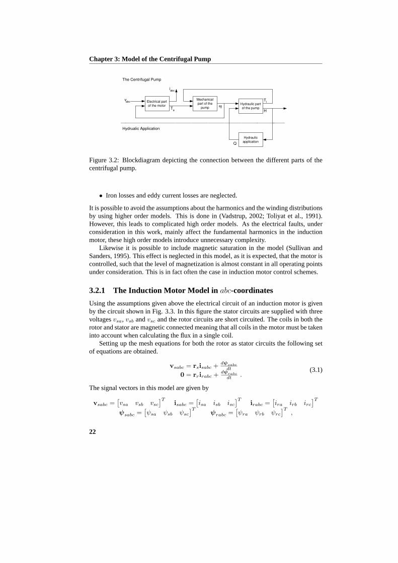
Chapter 3: Model of the Centrifugal Pump
Electrical part
of the motor
Mechanical
part of the
pump
v abc
i abc
H T
e
T l
ω r
Hydraulic part
of the pump
Hydraulic
application Q
The Centrifugal Pump
Hydrualic Application
Figure 3.2: Blockdiagram depicting the connection between the different parts of thecentrifugal pump.
• Iron losses and eddy current losses are neglected.
It is possible to avoid the assumptions about the harmonics and the winding distributionsby using higher order models. This is done in (Vadstrup, 2002; Toliyat et al., 1991).However, this leads to complicated high order models. As the electrical faults, underconsideration in this work, mainly affect the fundamental harmonics in the inductionmotor, these high order models introduce unnecessary complexity.
Likewise it is possible to include magnetic saturation in the model (Sullivan andSanders, 1995). This effect is neglected in this model, as it is expected, that the motor iscontrolled, such that the level of magnetization is almost constant in all operating pointsunder consideration. This is in fact often the case in induction motor control schemes.
3.2.1 The Induction Motor Model in abc-coordinates
Using the assumptions given above the electrical circuit of an induction motor is givenby the circuit shown in Fig. 3.3. In this figure the stator circuits are supplied with threevoltagesvsa, vsb andvsc and the rotor circuits are short circuited. The coils in both therotor and stator are magnetic connected meaning that all coils in the motor must be takeninto account when calculating the flux in a single coil.
Setting up the mesh equations for both the rotor as stator circuits the following setof equations are obtained.
vsabc = rsisabc + dψsabc
dt
0 = rrirabc + dψrabc
dt .(3.1)
The signal vectors in this model are given by
vsabc =[vsa vsb vsc
]Tisabc =
[isa isb isc
]Tirabc =
[ira irb irc
]T
ψsabc =[ψsa ψsb ψsc
]Tψrabc =
[ψra ψrb ψrc
]T,
22

Section 3.2: Model of the Electrical Motors
+
-
v sb
r s
d ψ
dt sb i sb
v sa
r s
d ψ
dt sa
+
-
i sa
+
-
v sc i sc
r s
d ψ
dt sc
r r
r r
r r
d ψ
dt rb
d ψ
dt ra
d ψ
dt rc
i rb
i rc
i ra
z p θ r
Figure 3.3: The electrical circuit diagram of the induction motor, placed in the mechan-ical structure of the induction motor. The three outer circuits are the circuits of the threephases of the stator and the inner circuit is the rotor circuit.
and the parameter matrices are
rs = rsI rr = rrI ,
wherers andrr are the electrical resistances in respectively the stator and rotor coils,see Fig. 3.3.
The flux linkagesψsabc andψrabc in (3.1) are given by the following expression.Here the assumption concerning saturation, described in the start of this section, is used.
ψsabc = lsisabc + lm(zpθr)irabc
ψrabc = lrirabc + lm(zpθr)T isabc .(3.2)
The parameter matricesls andlr are defined by
ls = llsI + lm(0) lr = llrI + lm(0) ,
wherells and llr are the leakage inductances in the stator and rotor windings respec-tively, andlm is the mutual inductance and is given by
lm(θe) = lm
cos(θe) cos(θe + 2π3 ) cos(θe + 4π
3 )cos(θe + 4π
3 ) cos(θe) cos(θe + 2π3 )
cos(θe + 2π3 ) cos(θe + 4π
3 ) cos(θe)
, (3.3)
wherelm is a constant andθe = zpθr is the electrical angle between the stator and rotorphases, see Fig. 3.3.
23
Chapter 3: Model of the Centrifugal Pump
3.2.2 Transformation to Stator Fixeddq0-coordinates
From the model described in theabc-coordinates it is seen that the mutual inductancematrix (3.3) is a function ofzpθr. This dependency can be removed using a variabletransformation from theabc-coordinates of the stator and rotor variables respectively tostator fixeddq0-coordinates. This variable transformation is given by
xsdq0 = Tdq0(0)xsabc xrdq0 = Tdq0(−zpθr)xrabc , (3.4)
where subscripts andr denote the stator variables and rotor variables respectively, andzpθr is the electrical angle between the stator and rotor circuit, see Fig. 3.3. In thistransformationsTdq0 is given by
Tdq0(θ) =23
cos(θ) cos(θ + 23π ) cos(θ + 4
3π )sin(θ) sin(θ + 2
3π ) sin(θ + 43π )
12
12
12
.
Equations (3.1) and (3.2), describing the electrical and magnetic system of the in-duction motor respectively, are transformed using the transformation (3.4). Hereby thefollowing description of the induction motor is obtained,
vsdq = Rsisdq + dψsdq
dt
vs0 = rsis0 + dψs0dt
0 = Rrirdq + dψrdq
dt − zpωrJψrdq
0 = rrir0 + dψr0dt ,
(3.5)
wherezpωr = dzpθr
dt , asθr is a function of time. The flux linkages in these equationsare given by
ψsdq = Lsisdq + Lmirdq
ψs0 = llsis0ψrdq = Lrirdq + Lmisdq
ψr0 = llrir0 .
(3.6)
In (3.5) and (3.6) thedq0-space is split intodq-coordinates and0-coordinates of reasons,which will become obvious in the following. The parameter matricesRs, Rr, Ls Lr,andLm do all have a diagonal structure, and are given by,
Rs = diag{rs, rs} Rr = diag{rr, rr}Ls = diag{3
2 lm + lls,32 lm + lls}
Lr = diag{32 lm + llr,
32 lm + llr}
Lm = diag{ 32 lm, 3
2 lm}J =
[0 1−1 0
].
24

Section 3.2: Model of the Electrical Motors
Rewriting (3.5) and (3.6), and using the magnetizing currentimdq defined such thatit fulfils the equationψrdq = Lmimdq, the induction motor model becomes
L′sdisdq
dt=− (Rs + R′
r) isdq + (R′r − zpωrJL′m) imdq + vsdq (3.7a)
llsdis0dt
=− rsis0 + vs0 (3.7b)
L′mdimdq
dt=R′
risdq − (R′r − zpωrJL′m) imdq (3.7c)
llrdψr0
dt=− rrψr0 , (3.7d)
where
R′r = LmL−1
r RrL−1r Lm L′s = Ls − LmL−1
r Lm L′m = LmL−1r Lm ,
meaning that the new matrices retain the diagonal structure.Equation (3.7d) shows thatlimt→∞ ψr0 = 0 for every possible operating conditions.
Moreoverψr0 is not influencing the rest of the model equations. Therefore, (3.7d) canbe excluded from the final induction motor model.
3.2.3 Grid Connections
The stator windings described in (3.1) can either be connected in aY- or ∆-connection
as shown in Fig. 3.4. In this figure only the terminal voltagesvtabc =[vta vtb vtc
]T
r s
i sa
+
-
v ta
+
-
v tb
+
-
v tc
i sb
i sc
i =0 0
i ta i tb i tc
d ψ
dt sa d ψ
dt sb d ψ
dt sc
+
- - -
+
+
v sa
v sb
v sc
+
-
v 0
r s r s
(a) Y-connection.
i ta
i tb
i tc
v tc
v ta
+
+
-
-
v tb
+ -
i sa
i sb
i sc
d ψ
dt sc
d ψ
dt sa
d ψ
dt sb
+
-
v sc
+ - v sa
+
-
v sb
r s
r s
r s
(b) ∆-connection.
Figure 3.4: Example of the stator windings connected in aY- and∆-connection respec-tively. The stator circuit in this figure is the same as the one shown in figure 3.3.
and the terminal currentsitabc =[ita itb itc
]Tare measurable. Therefore a relation-
ship between the voltages and currents at the terminals of the motor, and the voltagesand currents in (3.1) must be defined. This relationship is, in the following, establishedfor aY- and∆-connected motor respectively.
25

Chapter 3: Model of the Centrifugal Pump
The Y-connected induction motor
In the case of aY-connected stator, the mappings between the stator variables and theterminal variables are given by,
vtabc = vsabc + 1v0 itabc = Iisabc ,
where1 =[1 1 1
]T, andv0 is the voltage between the star point of the supply and
the star point of the stator circuit, see Fig. 3.4(a). Transforming these equations todq0-coordinates the description becomes,
vsdq = vtdq itdq = isdq
vs0 = vt0 − v0 it0 = is0 .
Moreover it is seen from Fig. 3.4(a) that the relationsship0 = isa + isb + isc must holdfor this circuit, therefore the currentsis0 = it0 = 0.
Using the expressionvs0 = vt0 − v0, obtained above, and the fact theis0 = 0, theexpression of the zero sequence quantities described by (3.7b) becomes,
0 =vt0 − v0 . (3.8)
This shows that (3.7b) has no impact on the motor performance, therefore it can beexcluded from the final model of aY-connected induction motor.
From the above argumentation theY-connected induction motor is modelled by thefollowing set of equations,
L′sdisdq
dt=− (Rs + R′
r) isdq + (R′r − zpωrJL′m) imdq + vtdq (3.9a)
L′mdimdq
dt=R′
risdq − (R′r − zpωrJL′m) imdq , (3.9b)
where the measurable terminal currentitdq is given by,
itdq = isdq . (3.9c)
Remark 3.2.1 From the expression of the star point voltage (3.8) it is seen that thestart point voltage of the induction motorv0 equals the star point voltage of the supplyvt0 in the no-fault case. This can be used for fault detection inY-connected inductionmotors, whenever the star point voltage of the motor is measured. This scheme uses that∫
T(vs0 − vt0)2dt 6= 0 when a fault has happend in the motor, and in the no-fault case∫
T(vs0 − vt0)2dt = 0 (Tallam et al., 2002).
26

Section 3.2: Model of the Electrical Motors
The ∆-connected induction motor
In the case of a∆-connected stator the mappings between the stator variables and theterminal variables are given by,
vsabc = K∆vtabc itabc = KT∆isabc ,
where the linear mappingK∆ is given by,
K∆ =
1 −1 00 1 −1−1 0 1
.
Transforming these equations todq0-coordinates the description becomes,
vsdq0 = Tdq0K∆T−1dq0vtdq0 itdq0 = Tdq0KT
∆T−1dq0isdq0 .
The structures of these linear mappings are,
[vsdq
vs0
]=
[Bv 00 0
] [vtdq
vt0
] [itdq
it0
]=
[Ci 00 0
] [isdq
is0
].
This shows thatvs0 = 0 despite of the value ofvtdq0, andit0 despite of the value ofisdq0.
Using the factvs0 = 0 in (3.7b) it becomes,
llsdis0dt
=− rsis0 .
This shows thatlimt→∞ is0 = 0 for every possible operating conditions. Moreoveris0is not affecting the rest of the model equations. Therefore (3.7b) can be excluded fromthe final model of a∆-connected induction motor.
From the above argumentation the∆-connected induction motor is modelled by thefollowing set of equations,
L′sdisdq
dt=− (Rs + R′
r) isdq + (R′r − zpωrJL′m) imdq + Bvvtdq (3.10a)
L′mdimdq
dt=R′
risdq − (R′r − zpωrJL′m) imdq , (3.10b)
where the measurable terminal currentitdq is given by,
itdq = Ciisdq . (3.10c)
27

Chapter 3: Model of the Centrifugal Pump
3.2.4 The Torque Expression
From energy consideration it is shown, in (Krause et al., 1994), that the torque producedby the induction motor is given by,
Te = iTsabc
∂lm(zpθr)∂θr
irabc ,
whereisabc is the current of the stator windings andirabc is the current in the rotor.Including the transformations (3.4) into this expression it becomes,
Te = (Tdq0(0)−1isdq0)T ∂lm(zpθr)∂θr
(Tdq0(−zpθr)−1irdq0) .
Simplifying the expression and usingLmimdq = Lrirdq + Lmisdq the following torqueexpression is obtained,
Te =32zpL
′m (imdisq − imqisd) , (3.11)
whereL′m = L2m/Lr, meaning thatL′m is the diagonal element ofL′m.
3.3 The Hydraulic Part of the Centrifugal Pump
This section is concerned with modelling the hydraulic part of the centrifugal pump.The hydraulic part of the centrifugal pump consists of the inlet and outlet of the pump,and the impeller and the diffuser inside the pump. These components are all shown inFig. 3.5. The impeller is the rotating part of the pump, which induces a rotational speedinto the liquid. This speed is transformed into a static pressure in the diffuser and volute.Hereby a pressure difference between the impeller eye and the outlet of the volute isobtained. This will be formulized in this section.
The model, presented in this section, describes the pressure and torque of the pumpas functions of the flow and speed respectively. This means that the obtained model hasa structure as shown in Fig. 3.6. In this figureωr is the angular speed of the impeller,Qp is the volume flow, andHp andTp are the pressure and torque produced by the pumprespectively.
In the literature a polynomial model of the centrifugal pump can be found (Sayers,1990; Stepanoff, 1957). This model describes the torque load of the centrifugal pumpunder steady state operation. Here, the aim is to derive a dynamic model of the pump.Such a model is needed in the design of FDI observers. Fortunately, it is well knowfrom the literature that a control volume approach can be used in the derivation of thedynamics of a hydraulic system (Roberson and Crowe, 1993). This approach is used inthis section to obtain a model describing the dynamics as well as the steady state opera-tion of the centrifugal pump. The obtained model has a nonlinear but simple structure,which is usable in model based FDI algorithms.
28
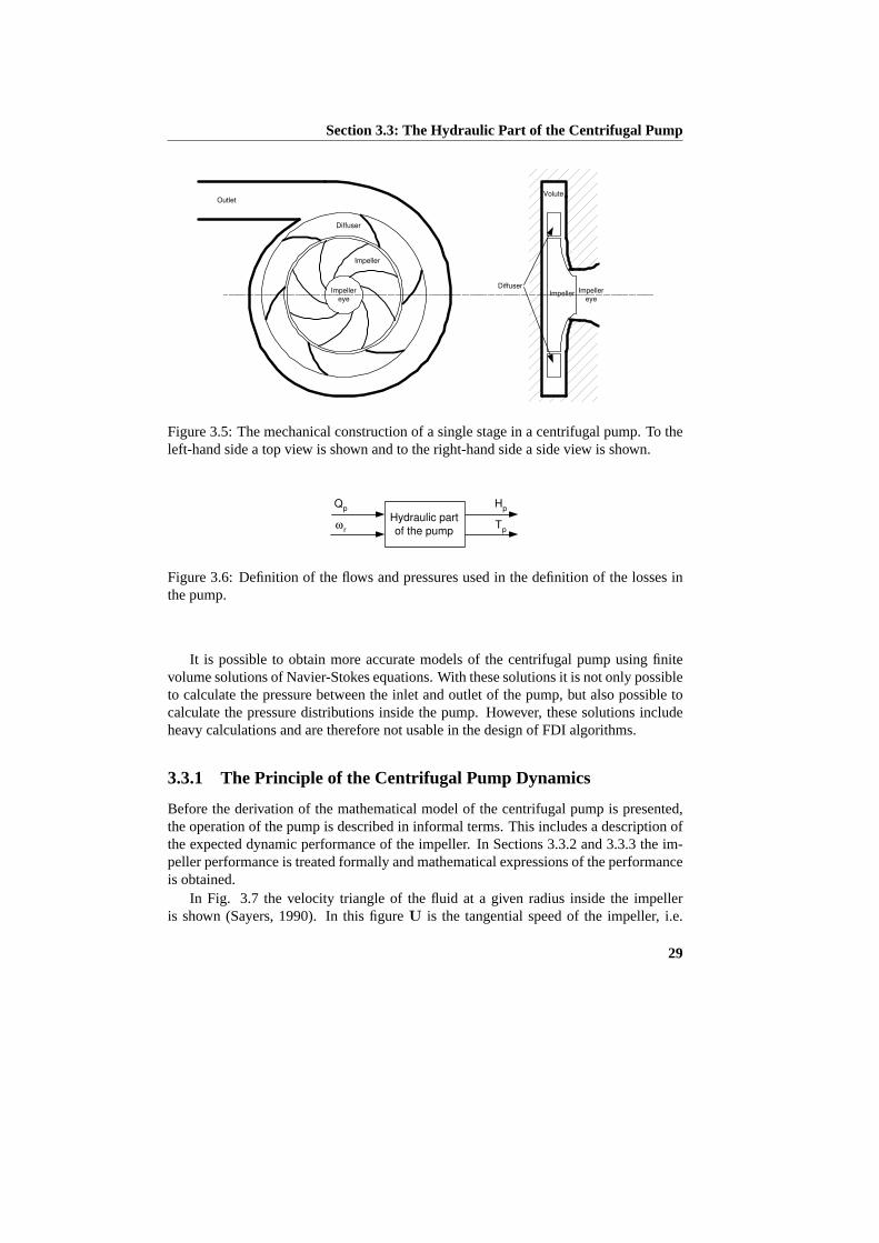
Section 3.3: The Hydraulic Part of the Centrifugal Pump
Impeller
Diffuser
Volute
Impeller eye ���������������������������Impeller Impeller
eye
Diffuser
Outlet
Figure 3.5: The mechanical construction of a single stage in a centrifugal pump. To theleft-hand side a top view is shown and to the right-hand side a side view is shown.
H p
T p
Q p
ω r
Hydraulic part
of the pump
Figure 3.6: Definition of the flows and pressures used in the definition of the losses inthe pump.
It is possible to obtain more accurate models of the centrifugal pump using finitevolume solutions of Navier-Stokes equations. With these solutions it is not only possibleto calculate the pressure between the inlet and outlet of the pump, but also possible tocalculate the pressure distributions inside the pump. However, these solutions includeheavy calculations and are therefore not usable in the design of FDI algorithms.
3.3.1 The Principle of the Centrifugal Pump Dynamics
Before the derivation of the mathematical model of the centrifugal pump is presented,the operation of the pump is described in informal terms. This includes a description ofthe expected dynamic performance of the impeller. In Sections 3.3.2 and 3.3.3 the im-peller performance is treated formally and mathematical expressions of the performanceis obtained.
In Fig. 3.7 the velocity triangle of the fluid at a given radius inside the impelleris shown (Sayers, 1990). In this figureU is the tangential speed of the impeller, i.e.
29
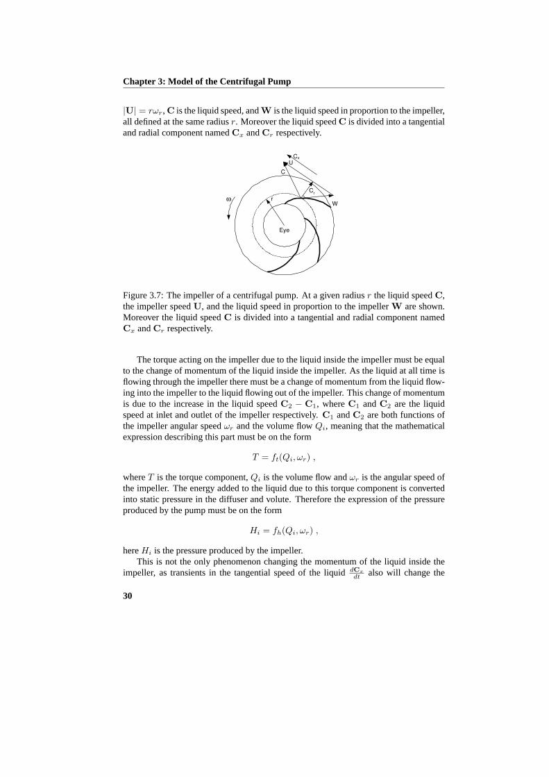
Chapter 3: Model of the Centrifugal Pump
|U| = rωr, C is the liquid speed, andW is the liquid speed in proportion to the impeller,all defined at the same radiusr. Moreover the liquid speedC is divided into a tangentialand radial component namedCx andCr respectively.
ω
C x
C
U
W
C r
r
Eye
Figure 3.7: The impeller of a centrifugal pump. At a given radiusr the liquid speedC,the impeller speedU, and the liquid speed in proportion to the impellerW are shown.Moreover the liquid speedC is divided into a tangential and radial component namedCx andCr respectively.
The torque acting on the impeller due to the liquid inside the impeller must be equalto the change of momentum of the liquid inside the impeller. As the liquid at all time isflowing through the impeller there must be a change of momentum from the liquid flow-ing into the impeller to the liquid flowing out of the impeller. This change of momentumis due to the increase in the liquid speedC2 − C1, whereC1 andC2 are the liquidspeed at inlet and outlet of the impeller respectively.C1 andC2 are both functions ofthe impeller angular speedωr and the volume flowQi, meaning that the mathematicalexpression describing this part must be on the form
T = ft(Qi, ωr) ,
whereT is the torque component,Qi is the volume flow andωr is the angular speed ofthe impeller. The energy added to the liquid due to this torque component is convertedinto static pressure in the diffuser and volute. Therefore the expression of the pressureproduced by the pump must be on the form
Hi = fh(Qi, ωr) ,
hereHi is the pressure produced by the impeller.This is not the only phenomenon changing the momentum of the liquid inside the
impeller, as transients in the tangential speed of the liquiddCx
dt also will change the
30
Section 3.3: The Hydraulic Part of the Centrifugal Pump
momentum. Now recognizing that the velocity triangle in Fig. 3.7 will be fulfilled atall time, and that the direction of the liquid speed in proportion to the impellerW isfixed due to the impeller blades. This means that changes of the tangential speed ofthe impellerU will induce changes inCx, and therefore the momentum of the liquidinside the impeller is changed. Moreover,Cx will also change if the radial speed of theliquid Cr is changed. This change is explained by the velocity triangle, which has to befulfilled all the time. This means that a change in the volume flowQi will change themomentum of the liquid inside the impeller, asCr is proportional toQi.
From the above consideration the model describing the torque acting on the impellerdue to the liquid, must be on the form,
Ti = ft(Qi, ωr) + f ′t(Qi, ωr,dωr
dt ) + f ′′t (Qi, ωr,dQi
dt ) ,
whereTi is the impeller torque,Qi is the volume flow,ωr is the angular speed of theimpeller andfh, f ′h andf ′′h are functions to be decided. In fact in Section 3.3.2 thecontrol volume approach is used to derived an expression of the torque. Here it is shownthat the torque is described by,
Ti =(−at2Q
2i + at1ωrQi + at0ω
2r
)+ JMv
dωr
dt−KQ
dQi
dt,
whereat2, at1, at0, JMv andKQ are constants described in Section 3.3.2. An expressionof the pressure produced by the pump is derived in Section 3.3.3. Here it is shown thatthe pressure expression becomes,
Hi = ρg(−ah2Q2i + ah1ωrQi + ah0ω
2r) ,
whereah2, ah1 andah0 are constants described in Section 3.3.3.
3.3.2 The Torque Expression
In this section an expression of the torque acting on the impeller is derived using con-trol volume considerations. In (Roberson and Crowe, 1993, p. 242) a control volumeequation is derived, describing the torque properties of the given control volume. Theobtained equation is (Roberson and Crowe, 1993, p. 243),
∑
j
Tj =∫
cs
(r× c)ρC • dA +d
dt
∫
cv
(r× c)ρdV , (3.12)
where allTj are external torques on the control volume,r is a radius vector, andc is thefluid speed at the radius vectorr. C is the fluid speed in proportion to a infinitesimalcontrol surfacedA anddA is an infinitesimal area vector describing the direction andsize of the infinitesimal control surfacedA. Finally ρ is the mass density of the liquidanddV is an infinitesimal volume. The subscribescs andcv on the intergrals denotethe control surface and the control volume respectively. The first term on the right-hand
31
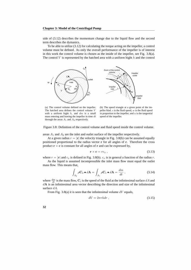
Chapter 3: Model of the Centrifugal Pump
side of (3.12) describes the momentum change due to the liquid flow and the secondterm describes the dymanics.
To be able to utilize (3.12) for calculating the torque acting on the impeller, a controlvolume must be defined. As only the overall performance of the impeller is of interestin this work the control volume is chosen as the inside of the impeller, see Fig. 3.8(a).The controlV is represented by the hatched area with a uniform highth and the control������������
dm
ω
C 2
C 1
dm
dm
R 1
R 2
V
Inlet
outlet
A 1
A 2
(a) The control volume defined on the impeller.The hatched area defines the control volumeVwith a uniform hight h, and dm is a smallmass entering and leaving the impeller in timedtthrough the areasA1 andA2 respectively.
����������������U
C x C
W
C r
β
Impeller
inlet
Impeller
outlet
Zoom of the control
volume
Impeller
blad
r
(b) The speed triangle at a given point of the im-peller blad.c is the fluid speed,w is the fluid speedin proportion to the impeller, andu is the tangentialspeed of the impeller.
Figure 3.8: Definition of the control volume and fluid speed inside the control volume.
areasA1 andA2 are the inlet and outlet surface of the impeller respectively.At a given radiusr = |r| the velocity triangle in Fig. 3.8(b) can be assumed equally
positioned proportional to the radius vectorr for all angles ofr. Therefore the crossproductr× c is constant for all angles ofr and can be expressed by,
r× c = rcx , (3.13)
wherer = |r| andcx is defined in Fig. 3.8(b).cx is in general a function of the radiusr.As the liquid is assumed incompressible the inlet mass flow must equal the outlet
mass flow. This means that,∫
A2
ρC2 • dA =∫
A1
ρC1 • dA =dm
dt, (3.14)
wheredmdt is the mass flow,Ci is the speed of the fluid at the infinitesimal surfacedA and
dA is an infinitesimal area vector describing the direction and size of the infinitesimalsurfacedA.
From Fig. 3.8(a) it is seen that the infinitesimal volumedV equals,
dV = 2πrhdr , (3.15)
32
Section 3.3: The Hydraulic Part of the Centrifugal Pump
wherer is the radius at a given slice of the disc forming the impeller with highth.Using (3.13), (3.14), and (3.15) in (3.12), the torque expression is reduced to,
Ti =dm
dt(r2cx2 − r1cx1) +
d
dt2πhρ
∫ R2
R1
r2cx(r)dr , (3.16)
whereTi is the component of the shaft torque created by the fluid inside the impeller.In (3.16) the first term on the right-hand side describes the time derivative of the changeof momentum between the liquid entering and leaving the impeller. This term is thepressure or head producing part and is in the following denoted the steady state torqueterm. The second term on the right-hand side describes the torque necessary to changethe speed of the impeller when the mass of the impeller itself is not taken into account.This term is in the following denoted the transient torque term.
The steady state torque expression
From Fig. 3.8(b) it is seen that the speedcx = u − cr cot(β), whereu is the tangentialspeed of the impeller and is given byu = rωr. Moreover, if the area of a slice of theimpeller with radiusr is defined asAr = 2πrh, then the volume flow inside the impelleris given byQi = crAr. Using these considerations the following expressions ofcx areobtained,
cx = u− cr cot(β) = rωr − Qi
Arcot(β) = rωr − Qi
2πrhcot(β) . (3.17)
Using (3.17) at the inlet and outlet of the impeller to obtain an expression ofcx1 andcx2.Then used these expressions in the first term on the right-hand side of (3.16) to obtainthe following expression for the steady state torque,
Ti = ρ(r22 − r2
1
)Qiωr − ρ
(r2 cot(β2)
A2− r1 cot(β1)
A1
)Q2
i , (3.18)
where the mass flowdmdt is replaced byρQi. Equation (3.18) models the steady state
torque load of the impeller.Beside the torque described by (3.18) and extra torque termTf = Knω2
r (Sayers,1990) is added. This term models the hydraulic friction due to liquid between the voluteand the impeller, see Fig. 3.5. Adding this term the final steady state expression of thetorque becomes,
Tp =− at2Q2i + at1ωrQi + at0ω
2r , (3.19)
where,
at2 = ρ
(r2 cot(β2)
A2− r1 cot(β1)
A1
)at1 = ρ
(r22 − r2
1
)at0 = Kn .
33

Chapter 3: Model of the Centrifugal Pump
The transient torque expression
The transient torque component is given by the second term on the right-hand side of(3.16). Using (3.17) to describecx in this expression the following expression is ob-tained,
Tt = JMv
dωr
dt−KQ
dQi
dt, (3.20)
whereJMv andKQ are constants and represent the moment of inertia of the water insidethe impeller, and the effects of flow changes on the impeller torque respectively. Theseconstants are given by,
JMv= 2πhρ
∫ R2
R1
r3dr KQ = ρ
∫ R2
R1
r cot(β(r))dr .
The first term on the right-hand side of (3.20) describes the change of momentum of theliquid inside the impeller due to changes in the impeller speed. The second term on theright-hand side describes the tangential change of liquid speed due to flow changes. Asit is a change of speed in the tangential direction it will affect the transient componentof the shaft torque, as it is shown in (3.20).
The combined torque expression
From (3.19) and (3.20) the final expression of the external torque on the impeller isfound,
Tp = −at2Q2i + at1ωrQi + at0ω
2r + JMv
dωr
dt−KQ
dQi
dt, (3.21)
whereTp is the external torque on the impeller.
3.3.3 The Head Expression
In this section an expression of the head is derived from the torque expression (3.18),presented in the previous section. Head is defined by,
Hp = ρgH ,
whereH is the head andHp is the pressure. The theoretical headHe is given byHe =P/(Qiρg), whereg is the gravity andP = Tiωr is the power. Including this in (3.18)the following expression is obtained,
He =(
r22
g− r2
1
g
)ω2
r −(
r2
gA2cot(β2)− r1
gA1cot(β1)
)ωrQi . (3.22)
34

Section 3.3: The Hydraulic Part of the Centrifugal Pump
The head described by (3.22) is the theoretical obtainable head of the impeller. This headis not equal to the head between the inlet and outlet of the pump due to head losses. Thefollowing types of head losses are expected to influence the theoretical head (Sayers,1990),
• Slip factor, here namedσs.
• Shock losses, here namedhs.
• Friction losses, here namedhf .
The slip factor is an empirical factor used to account for re-circulating flow inside theimpeller. The two last head losses are due to friction and shock losses inside the impellerand at the inlet of the impeller respectively. The head losses affect the theoretical headas shown in the following equation,
H + hs + hf = σsHe , (3.23)
whereH is the head between the inlet and outlet of the pump. The shock and frictionlosses are given by,
hs = Ks(Qi −Qd)2 hf = KfQ2i ,
whereQd is the design flow, which is a linear expression of the angular velocity e.i.Qd = Kdωr. Ks, Kf andKd are all constants. When including these expressions in(3.23) the model describing the head becomes,
H = −ah2Q2i + ah1ωrQi + ah0ω
2r , (3.24)
whereH is the head produced by the pump,ωr is the impeller speed, andQi is thevolume flow through the impeller. The parameters in the expression are given by,
ah2 = Ks + Kf ah1 = σs
(r2
gA2cot(β2)− r1
gA1cot(β1)
)−KsK
2d
ah0 = 2KsKd − σs
(r22
g− r2
1
g
).
The slip factorσs in the expression above is, as explained before, an empirical scalingfactor and is in general a non-linear function of the flow and the angular velocity, (Say-ers, 1990). However, if this factor is assumed constant the parametersah2, ah1 andah0
are also constants.
3.3.4 Leakage Flow and Pressure Losses in the Inlet and Outlet
The model equations derived in the previous part of this section describe the relationsbetween the speed and flow of the impeller, and the pressure generated by the impeller.
35

Chapter 3: Model of the Centrifugal Pump
The impeller is not the only component affecting the hydraulic performance of the pump,as the fluid also passes through the inlet, the diffuser, the volute and the outlet on its waythrough the pump, see Fig. 3.6. To have a complete model of the hydraulic performanceof the pump, leakage flow and pressure losses caused by these components must beconsidered.
In Fig. 3.9 the leakage flowq, the inlet and outlet flowQp, and the impeller flowQi
are presented.
Outlet
Inlet Q
p
Q p Q i q q
-
+ ������������� ���������������aH i
H i
H inlet
H outlet
+ + + - - -
Figure 3.9: Sketch of the flows inside the centrifugal pump.Qp is the main flow com-ponent andq is the leakage flow between the pressure and suction side of the impeller.
The leakage flowq in this figure is calculated using,
KJd
dtq = aρgHi −Klq
2 ,
whereKJ is a constant depending on the mass of the fluid involved in the leakage,a isa scaling constant taking into account that the pressure acting on leakage flow is not thesame as the pressure delivered by the impeller, and finallyKl models pressure losses inthe loop of the leakage flowq.
The pressure lossesHinlet andHoutlet in Fig. 3.9, at the inlet and outlet of thepump respectively, are modelled by adding an extra pressure loss termKc in the flowQp. These pressure losses are called casing losses, as the pressure losses are caused bythe casing of the pump.
If each of the pressure losses are symbolized as valves, and the theoretical pressureρgHe is symbolized as a pump without losses, the diagram in Fig. 3.10 describes theoperation of the centrifugal pump.
Pump model including leakage flow
Including the description of the lekage flowq in the expressions of the impeller head andtorque in (3.24) and (3.21) respectively, the following model of the centrifugal pump is
36

Section 3.3: The Hydraulic Part of the Centrifugal Pump
q
Q
Q i
K s (Q
i -K
d ω
r ) 2
K f Q
i 2
K Q c
2
K q l
2
H
H i
σ ρ g H e
Figure 3.10: Diagram of the centrifugal pump. The valves describe the losses inside thecentrifugal pump, and the pump symbol symbolizes generated pressure without losses.
obtained,
KJdqdt = ρg(−ah2(Qp + q)2 + ah1(Qp + q)ωr + ah0ω
2r)−Klq
2
Hp = ρg(−ah2(Qp + q)2 + ah1(Qp + q)ωr + ah0ω2r)−KcQ
2p
Tp = −at2(Qp + q)2 + at1(Qp + q)ωr + at0ω2r + JMv
dωr
dt −KQ
(dQp
dt + dqdt
),
(3.25)
whereHp is the pressure generated by the pump,Tp is the impeller torque andQp =Qi − q is the inlet flow of the pump.
Simplified pump model
When the leakage flowq in Fig. 3.10 can be neglected a simplified model of the pumpcan be used. The leakage flow can be neglected when Assumption 3.3.1 holds.
Assumption 3.3.1 For most centrifugal pumps the following assumptions hold in the nofault case,
1. The dynamics of the leakage flowq is at least a decade faster than the main dy-namics of the system, i.e.dq
dt ≈ 0 almost all the time.
2. |q| << |Qp| meaning thatQp ≈ Qi.
3. When 2 does not holdTp ≈ at0ω2r in (3.25).
When these assumptions hold the effect of the leakage flow on the pump performance isneglible.
37
Chapter 3: Model of the Centrifugal Pump
When Assumption 3.3.1 holds the model (3.25) can be simplified to become,
Hp = ρg(−(ah2 + Kc)Q2p + ah1ωrQp + ah0ω
2r)
Tp = −at2Q2p + at1ωrQp + at0ω
2r + JMv
dωr
dt −KQdQp
dt .(3.26)
3.3.5 Multi Stage Pumps
To be able to increase the pressure generated by the pump without increasing the diam-eter of the pump, normally a set of pump stages are connected in series. Hereby thepressure across the pump becomes,
H = H1 + H2 + · · ·+ Hn (3.27)
wheren is the number of pump stages. If thesen pump stages are identical, meaningthat Hi = Hi1 = · · · = Hin and q = q1 = · · · = qn the model of a multi stagecentrifugal pump is given by the sum of each stage,
nKJdqdt = nρg
(−ah2(Qp + q)2 + ah1(Qp + q)ωr + ah0ω2r
)− nKlq2
Hp = nρg(−ah2(Qp + q)2 + ah1(Qp + q)ωr + ah0ω
2r
)− nKcQ2p −K ′
cQ2p
Tp = n(−at2(Qp + q)2 + at1(Qp + q)ωr + at0ω
2r
)+
nJMv
dωr
dt − nKQ
(dQp
dt + dqdt
).
In this modelnKc expresses the pressure losses due to the guidens of the flow from onestage to the next. Therefore, an extra casing loss termK ′
c is added to model losses at theinlet and outlet of the pump.
If Assumption 3.3.1 still holds, which is normally the case, this model can be reducedto,
Hp = ρg(− (n(ah2 + Kc) + K ′
c) Q2p + nah1ωrQp + nah0ω
2r
)
Tp = −nat2Q2p + nat1ωrQp + nat0ω
2r + nJMv
dωr
dt − nKQdQp
dt .
From this it is seen that the structure of the model is the same for a serie connected setof identical stages, as for a single stage centrifugal pump.
Pump curves
Normally centrifugal pumps are described by two so-called pump curves. This isthrough for both multi stage and single stage pumps. The two curves depict the vol-ume flow versus the pressure and the power of the pump respectively. Normally thecurves are only depitch for one particular speed value, which is denoted the norminalspeed. An example of these pump curves is shown in Fig. 3.11.
38
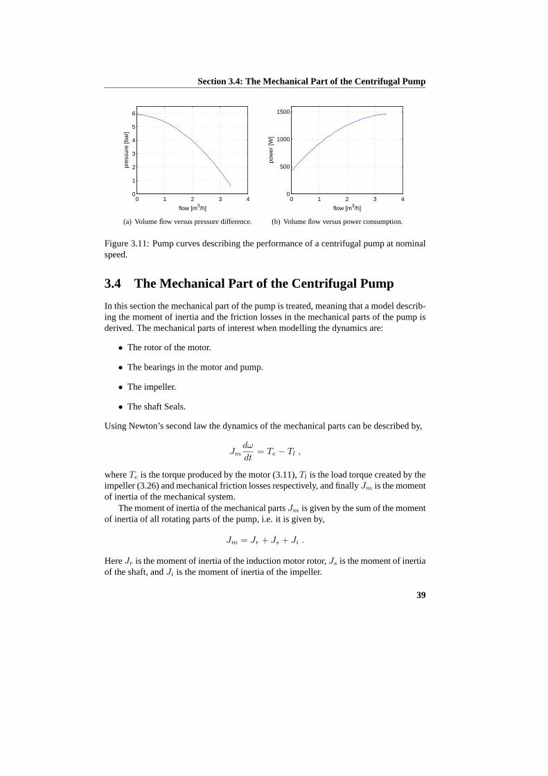
Section 3.4: The Mechanical Part of the Centrifugal Pump
0 1 2 3 40
1
2
3
4
5
6
pres
sure
[bar
]
flow [m3/h]
(a) Volume flow versus pressure difference.
0 1 2 3 40
500
1000
1500
pow
er [W
]
flow [m3/h]
(b) Volume flow versus power consumption.
Figure 3.11: Pump curves describing the performance of a centrifugal pump at nominalspeed.
3.4 The Mechanical Part of the Centrifugal Pump
In this section the mechanical part of the pump is treated, meaning that a model describ-ing the moment of inertia and the friction losses in the mechanical parts of the pump isderived. The mechanical parts of interest when modelling the dynamics are:
• The rotor of the motor.
• The bearings in the motor and pump.
• The impeller.
• The shaft Seals.
Using Newton’s second law the dynamics of the mechanical parts can be described by,
Jmdω
dt= Te − Tl ,
whereTe is the torque produced by the motor (3.11),Tl is the load torque created by theimpeller (3.26) and mechanical friction losses respectively, and finallyJm is the momentof inertia of the mechanical system.
The moment of inertia of the mechanical partsJm is given by the sum of the momentof inertia of all rotating parts of the pump, i.e. it is given by,
Jm = Jr + Js + Ji .
HereJr is the moment of inertia of the induction motor rotor,Js is the moment of inertiaof the shaft, andJi is the moment of inertia of the impeller.
39

Chapter 3: Model of the Centrifugal Pump
If the friction lossesTf of the bearings and shaft seals are assumed linear, i.e.Tf =Bωr, the load torque is given by,
Tl = Bωr +(−at2Q
2p + at1ωrQp + at0ω
2r
)+ JMv
dωr
dt−KQ
dQp
dt.
In this equation the first term on the right-hand side models the mechanical frictionlosses, and the last term models the load torque of the impeller (3.21).
Including the load torque expression in the mechanical equations the model of themechanical system is obtained,
Jdωr
dt= Te −Bωr −
(−at2Q2p + at1ωrQp + at0ω
2r
)+ KQ
dQp
dt,
whereJ = Jm +JMv . The termdQp
dt in the above expression means that the mechanicalsystem depends upon the dynamics of the hydraulic application. This dependency is inalmost all applications very small, meaning that the following assumption holds foralmost all applications.
Assumption 3.4.1 It is assumed that the dynamics of the hydraulic application, inwhich the pump is placed, is such that,
∣∣∣∣KQdQp
dt
∣∣∣∣ <<∣∣−at2Q
2p + at1ωrQp + at0ω
2r
∣∣ ,
at all time. When this assumption holds it means that the application dynamics is soslow that its effect on the pump dynamics is negliable.
Using this assumption the mechanical expression becomes,
Jdωr
dt= Te −Bωr −
(−at2Q2p + at1ωrQp + at0ω
2r
).
3.5 Final Model of the Centrifugal Pump
The model derived in the previous sections is described on state space form by the fol-lowing system,
x = f(x) + Gu + m(x,w)y = h(x,w) .
(3.28)
In this system the state vector is,
x =[isd isq imd imq ωr
]T,
40

Section 3.5: Final Model of the Centrifugal Pump
whereisd andisq are the motor currents in adq-frame fixed on the stator,imd andimq arethe magintizing currents described in the same frame, and finallyωr is the mechanicalspeed of the pump.
The inputs of the system consist of the known input vectoru and the unknown inputvectorw, given by,
u =[vsd vsq
]Tw =
[Qp
]T,
wherevsd andvsq are the supply voltages of the motor described in the samedq-frameas the motor currents, and the unknown input is the volume flowQp through the pump.
Except for the known inputs it is assumed that three variables are measured. Theseare the motor currents and the pump pressure respectively. Therefore, the measurementvectory in (3.28) is given by,
y =[isd isq Hp
]T.
The matrixG, the vector fieldsf(x) andm(x,w) and the mappingh(x,w) in (3.28)are presented below,
f(x) =
−Rs+R′rL′s
isd + R′rL′s
imd − zpωrL′mL′s
imq
−Rs+R′rL′s
isq + zpωrL′mL′s
imd + R′rL′s
imq
R′rL′m
isd − R′rL′m
imd + zpωrimq
R′rL′m
isq − zpωrimd − R′rL′m
imq1J
32zpLm (imdisq − imqisd)− B
J ωr
G =
1L′s
00 1
L′s0 00 00 0
m(x,w) =
0000
− 1J fT (Qp, ωr)
h(x,w) =
isd
isq
fH(Qp, ωr)
,
where the first four rows in the model represent the electrical part of the induction motorand the fifth row describes the mechanical part of the pump.
In this model the expressionfH(Qp, ωr) describes the pressure produced by thepump, and the expressionfT (Qp, ωr) describes the load torque of the pump. Theseexpressions are derived in Section 3.3, and are given by,
fH(Qp, ωr) = ρg(−ah2Q
2p + ah1Qpωr + ah0ω
2r
)fT (Qp, ωr) = −at2Q
2p + at1Qpωr + at0ω
2r ,
(3.29)
41
Chapter 3: Model of the Centrifugal Pump
whereah2, ah1, ah0 andat2, at1, at0 are constant parameters found from the physicalproperties of the pump, see Section 3.3.
The model presented above is not valid in the whole state space since the functionsfH(Qp, ωr) andfT (Qp, ωr) are only valid for positive flow and speed. Therefore, thestate space of interest for this system is given byD = {(x,w)|(x1, · · · , x4) ∈ R4, x5 ∈R+, w ∈ R+}, wherex1, · · · , x5 are states in the state vector andw is the unknowninput signal.
3.6 Discussion
In this chapter a model of the centrifugal pump including an induction motor drive isderived. The obtained model is a fifth-order lumped parameter system, making FaultDetection and Identification designs, based on this model, possible. However, the modelis very nonlinear, therefore a linearized version of the model is only expected to workin a small neighborhood around the point of linearization. The model is composed ofthree sub-models describing the electrical part of the motor, the mechanical parts of thesystem and the hydraulic parts of the system respectively.
In the derivation of the model the dynamics is taking into account. It is shown thatunder two assumptions given in the chapter, and if the mass of the liquid inside theimpeller is added to the mass of the impeller itself, the model of the hydraulics becomespurely algebraic. This means that the liquid inside the impeller affects the moment ofinertial in the mechanical description of the pump, and that no additional dynamics areadded to the model due to the hydraulics of the pump.
The obtained model or sub-models will in the following be used in the derivationof FDI-algorithms. Moreover, the understanding of the system obtained through themodel, is used in the design of a test setup, where a number of hydraulic, mechanicaland electrical faults can be simulated.
42
Chapter 4
System Analysis and FaultModelling
In (Jørgensen, 1995), (Bøgh, 1997) and (Izadi-Zamanabadi, 1999) systematic methodsfor developing fault detection, isolation and accommodation algorithms are presented.These systematic methods include analysis tools aimed to identify faults and their causesin physical systems. Failure Mode and Effect Analysis (FMEA) and Fault PropagationAnalysis (FPA) are proposed, as a way to start the development of these fault detection,isolation and accommodation algorithms. These analysis tools will in this chapter beused to analyse the centrifugal pump, resulting in a list of faults, which are expected tohappend in centrifugal pumps. A subset of these faults are chosen for futher investiga-tion.
In Chapter 2 two basically different approaches to the fault detection and isolation(FDI) problem were introduced. The first of these approaches is the signal-based ap-proach, where a set of events are extracted from the set of measurements on the system.The second approach is the model-based approach, where a model of the system is usedto extract knowledge of abnormal operation of the system. In Chapter 2 it is argued thatrobustness is treated extensively in the second approach, but is hardly considered in thefirst approach.
The model obtained using the FMEA and FPA is a logical model connecting faultsin the system with a set of effects chosen by the user. In this chapter a method for usingthis model to analyse the robustness of signal based fault detection schemes is proposed.This is done by defining a set of disturbing events, which are treated in the same wayas the faults in the FEMA and FPA. Hereby a model connecting both the faults anddisturbing events to the chosen set of end effects is obtained. The robustness of thesignal-based fault detection scheme is then obtained by analysing the connection amongfaults, disturbing events and end-effects, where the end-effects are chosen as a subset ofthe measurable events in the system. To help doing this a set of definitions and theorems
43

Chapter 4: System Analysis and Fault Modelling
are developed.By including the notation of disturbing events in the FPA, the use of the approach
is extended to handle robustness of signal-based fault detection schemes. However, itdoes not solve the problem with the manual steps in the analysis. One of these manualsteps is the cutting of loops inherent in the system under investagation (Bøgh, 1997).In this chapter an automated way of handling these loops is proposed, meaning that theremaining manual step is to setup the event model.
The chapter starts by presenting some preliminaries on the FMEA and FPA and theiruse in connection with fault detection, isolation and accommodation in Section 4.1. Theremaining parts of the chapter are devoted to the presentation of the contributions on theFMEA and FPA obtained in this work. First, the theoretical contributions are presented,followed by the FMEA and FPA results on the centrifugal pump. In Section 4.2 thetheoretical results are presented. They are obtained using FMEA and FPA for robustnessanalysis of signal-based fault detection schemes. In Section 4.3 the results obtained byusing the ideas, developed in Section 4.2, on the centrifugal pump are presented. Thisincludes a list of faults expected in the system, a FMEA and FPA model of the system,and an analysis of the signal based detection possibilities. Finally, the chapter endswith a presentation of test results obtained on a test setup particular developed for thispropose, and some concluding remarks. This is in Section 4.4 and 4.5 respectively.
4.1 Method for Fault Analysis
In (Izadi-Zamanabadi, 1999) a structured method for developing fault detection, isola-tion and accommondation algorithms is described. The method includes 8 steps wherestep numbers 1, 2 and 6 are interesting from a fault detection and isolation point of view.These steps are shortly described here:
Fault modeling - step 1: In this step a qualitative model of the faults in each componetof the system is made. This is done by dividing the system into suitable compo-nents. In each of these components the faults and their effects are identified anddescribed. This is done using the Failure Mode and Effect Analysis (FMEA).
Fault propagation analysis (FPA)- step 2: In this step the propagation of the identi-fied faults through the component of the systems is analysed. The result of thisanalysis is a description of the connection between the faults in the system and aset of interesting effects. This analysis is called Fault Propagation Analysis (FPA),and is performed by first identifing the functional connection between the com-ponents of the system, ending with a functional diagram (Bøgh, 1997). After thatthis diagram is used for the fault propagation analysis.
Detector design - step 6:In this step detectors for detecting the fault in the system aredeveloped. Different approaches have be used in this step. The state of the arton the area of fault detection and isolation in pumps is presented in Chapter 2.
44

Section 4.1: Method for Fault Analysis
In (Izadi-Zamanabadi, 1999) an extension to this step is proposed using structuralanalysis. Structural analysis will also be used in this thesis as a tool for analysingthe model structure of the system before designing residual generators.
In this chapter the two first steps are performed on the centrifugal pump, while the restof the thesis is devoted to the last step.
From the above list it is seen that FMEA and FPA are used in steps 1 and 2. Theseanalysis tools form a systematic way of creating a high level qualitative model of thesystem under consideration. The model needs only to be descriptive for the behaviourunder faulty conditions, which allow the model to be simple compared to dynamicalmodels.
Traditionally the FMEA and FPA have been used for analysing the fault behaviourof a system, and to identify reconfiguration possiblities. Hereby the conditions for faultrobust control of the given system are obtained (Blanke et al., 2003). However, in thiswork the purpose of introducing the FMEA and FPA is different. Here these analysistools are used as a first step in developing FDI algorithms. The purpose of using FMEAand FPA is two folded, as it is used for both identifing the set of most important faultsin the system, and analysing different combinations of sensors for detection possiblities.These sensor combinations are in this thesis denoted sensor configurations. The first ofthese purposes is the normal outcome of a FMEA analysis when used in the design offault robust control algorithms (Blanke et al., 2003) and qualitative analysis of products.
4.1.1 Preliminaries: The FMEA and FPA
This section contains a short presentation of the FMEA and FPA, and their utilizationsin developing Fault Robust Control algorithms. This presentation is included for readersnot familiar with these analysis tools, and their use in the area of fault detection andaccommodation.
FMEA is a tool originally developed by reliability engineers to analyse componentsof a system for possible failures, and their causes and effects (Blanke et al., 2003).This tool is for analysing single components of a system, therefore the first step in aFMEA is to identify these components in the system. Each of the components is thenanalysed resulting in a set of tables including information about the failure modes, failurecauses, failure effects and risk assessment for each component. An example of such atable is shown in Table 4.1.1, where a pressure sensor is considered. The table can alsoinclude risk code and actions required. But this information is not used, when the FMEAis utilized for designing fault detection and accommodation algorithms, therefore it isomitted here.
This FMEA table includes information of the importance of each of the faults in therisk assessmentcolumn, and the connection between the failure modes and the failure ef-fects can be deduced from theFailure modeandFailure Effectcolumn. Mathematricallythis connection can be expressed via the fault propagation matrix defined in Definition4.1.1.
45
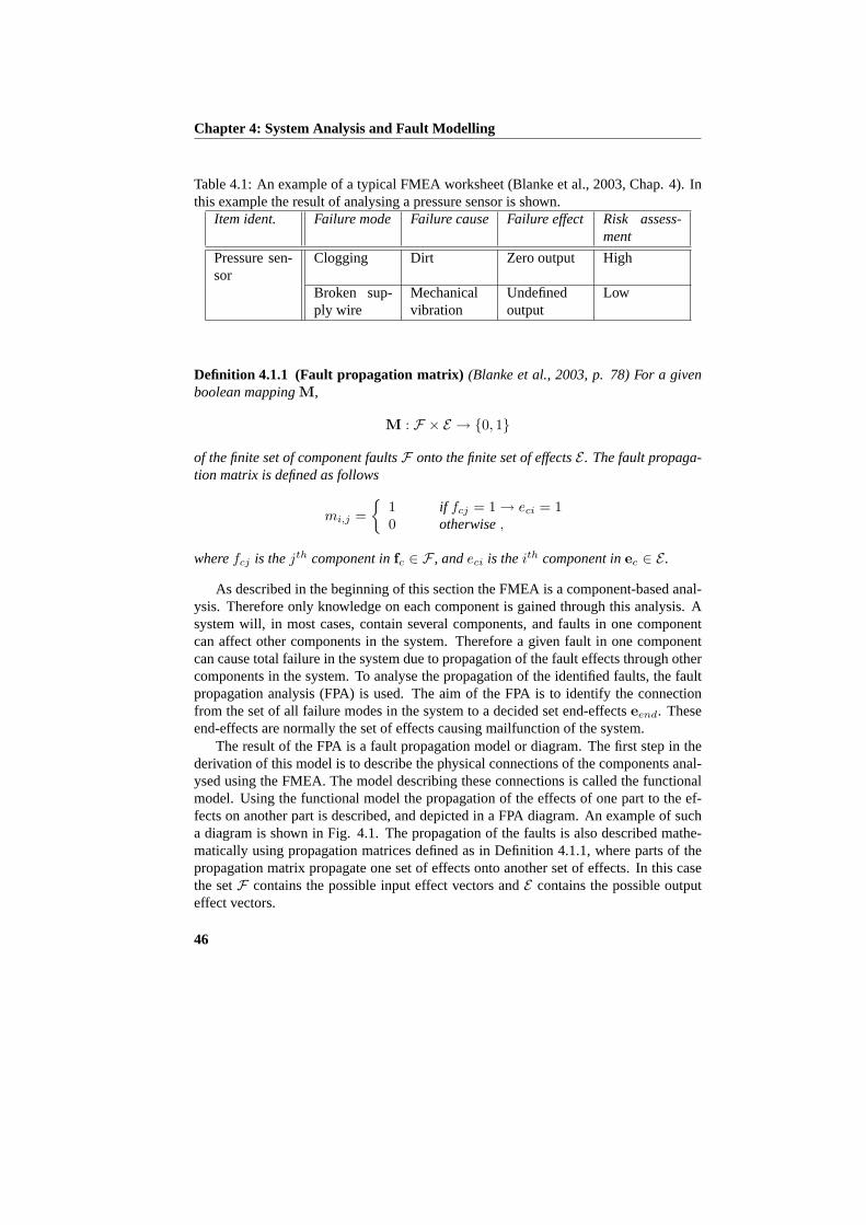
Chapter 4: System Analysis and Fault Modelling
Table 4.1: An example of a typical FMEA worksheet (Blanke et al., 2003, Chap. 4). Inthis example the result of analysing a pressure sensor is shown.
Item ident. Failure mode Failure cause Failure effect Risk assess-ment
Pressure sen-sor
Clogging Dirt Zero output High
Broken sup-ply wire
Mechanicalvibration
Undefinedoutput
Low
Definition 4.1.1 (Fault propagation matrix) (Blanke et al., 2003, p. 78) For a givenboolean mappingM,
M : F × E → {0, 1}
of the finite set of component faultsF onto the finite set of effectsE . The fault propaga-tion matrix is defined as follows
mi,j ={
1 if fcj = 1 → eci = 10 otherwise,
wherefcj is thejth component infc ∈ F , andeci is theith component inec ∈ E .
As described in the beginning of this section the FMEA is a component-based anal-ysis. Therefore only knowledge on each component is gained through this analysis. Asystem will, in most cases, contain several components, and faults in one componentcan affect other components in the system. Therefore a given fault in one componentcan cause total failure in the system due to propagation of the fault effects through othercomponents in the system. To analyse the propagation of the identified faults, the faultpropagation analysis (FPA) is used. The aim of the FPA is to identify the connectionfrom the set of all failure modes in the system to a decided set end-effectseend. Theseend-effects are normally the set of effects causing mailfunction of the system.
The result of the FPA is a fault propagation model or diagram. The first step in thederivation of this model is to describe the physical connections of the components anal-ysed using the FMEA. The model describing these connections is called the functionalmodel. Using the functional model the propagation of the effects of one part to the ef-fects on another part is described, and depicted in a FPA diagram. An example of sucha diagram is shown in Fig. 4.1. The propagation of the faults is also described mathe-matically using propagation matrices defined as in Definition 4.1.1, where parts of thepropagation matrix propagate one set of effects onto another set of effects. In this casethe setF contains the possible input effect vectors andE contains the possible outputeffect vectors.
46
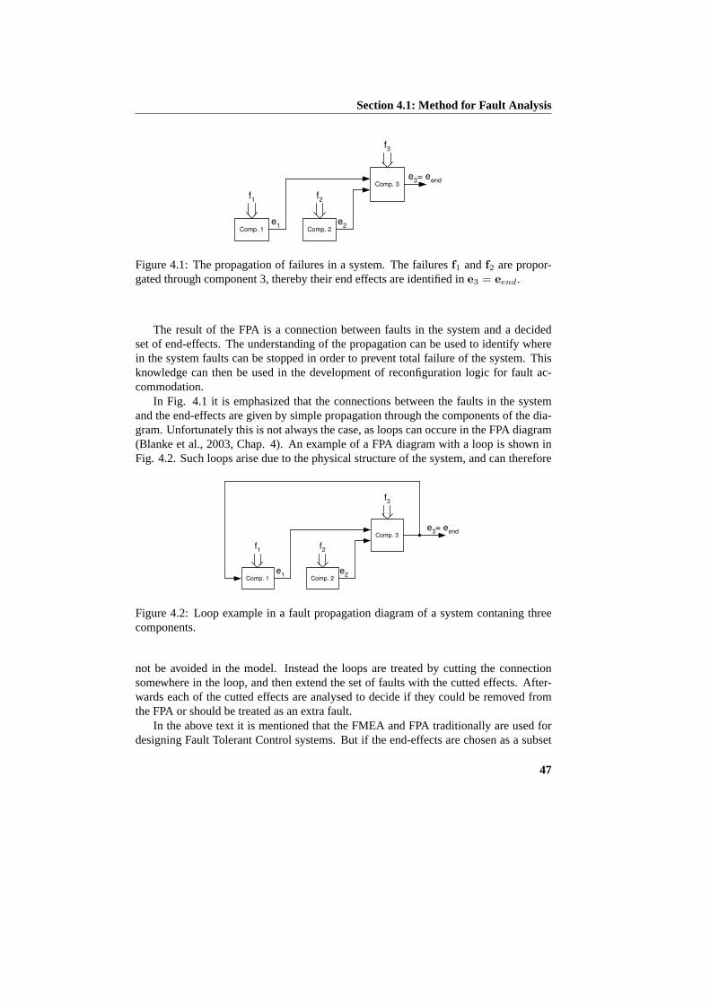
Section 4.1: Method for Fault Analysis
Comp. 1
f 1
e 1
Comp. 2
f 2
e 2
Comp. 3
f 3
e 3 = e
end
Figure 4.1: The propagation of failures in a system. The failuresf1 andf2 are propor-gated through component 3, thereby their end effects are identified ine3 = eend.
The result of the FPA is a connection between faults in the system and a decidedset of end-effects. The understanding of the propagation can be used to identify wherein the system faults can be stopped in order to prevent total failure of the system. Thisknowledge can then be used in the development of reconfiguration logic for fault ac-commodation.
In Fig. 4.1 it is emphasized that the connections between the faults in the systemand the end-effects are given by simple propagation through the components of the dia-gram. Unfortunately this is not always the case, as loops can occure in the FPA diagram(Blanke et al., 2003, Chap. 4). An example of a FPA diagram with a loop is shown inFig. 4.2. Such loops arise due to the physical structure of the system, and can therefore
Comp. 1
f 1
e 1
Comp. 2
f 2
e 2
Comp. 3
f 3
e 3 = e
end
Figure 4.2: Loop example in a fault propagation diagram of a system contaning threecomponents.
not be avoided in the model. Instead the loops are treated by cutting the connectionsomewhere in the loop, and then extend the set of faults with the cutted effects. After-wards each of the cutted effects are analysed to decide if they could be removed fromthe FPA or should be treated as an extra fault.
In the above text it is mentioned that the FMEA and FPA traditionally are used fordesigning Fault Tolerant Control systems. But if the end-effects are chosen as a subset
47

Chapter 4: System Analysis and Fault Modelling
of the measurable effects in the system, the FPA can be used in the development ofFDI algorithms. An example of this is shown in (Thomsen, 2000). Here the FPA isused for analysing sensor configurations, revealing the connection between the faults inthe system and the set of measurable signals. Hereby the usability of different sensorconfiguration can be analysed. In the following this approach is further developed tohandle robustness with respect to events in the system, which should not be consideredas faults. Finally, the developed approach is used in the analysis of the centrifugal pump.
4.2 Automated FPA
This section is concerned with the theoretical contributions to the FMEA and FPA, whenused in connection with FDI design. Firstly, an algorithm is proposed, which automatesthe cutting of loops in the FPA diagram. Secondly, robustness of the chosen signal eventsis considered.
4.2.1 The Automated FPA Algorithm
From the FPA diagram in Fig. 4.1 it is seen that a general component of this diagramhas a structure as shown in Fig. 4.3. Herefi is a vector containing the possible faults
Comp. i
f i
e i
e j
Figure 4.3: A single component in a FMEA.fi is the possible failures of the component,ej is effects affecting the component andei is the effects on the component performancedue tofi andej respectively.
in the component,ej contains the effects affecting the component, andei contains theeffects on the component due tofi andej respectively. The component shown in Fig. 4.3implies that a component in the FPA diagram can be described as defined in definition4.2.1.
Definition 4.2.1 (Component description)Theith componentci in the systemS con-taningn components, i.e.S =
⋃ni=1 ci, is described by,
ei ← Aifi· fi +
i−1∑
j=1
Aij · ej +
n∑
j=i+1
Aij · ej , (4.1)
where
48
Section 4.2: Automated FPA
• Aifi
: Fi × Ei → {0, 1} andAij : Ej × Ei → {0, 1} are propagation matrices on
form described in Definition 4.1.1.
• fi ∈ Fi = {0, 1}ni is the set of faults associated withith component.
• ej ∈ Ej = {0, 1}mj is the set of effects associated withjth component.
• + is the boolean disjunction operator∨ and· is the boolean conjunction operator∧. Both defined as vector operators.
Remark 4.2.1 In Definition 4.2.1Aij = 0 means that there does not exist a connection
from componentj to componenti in the FPA diagram. AndAifi
= 0 means that nofaults affect theith component.
Remark 4.2.2 This description is similar to the one used in (Jørgensen, 1995; Blankeet al., 2003) except for opertator and matrix notation. In (Blanke et al., 2003, Chap.4) all the matricesAi
fiandAj
i are lumped into one matrixMfi . An example of such a
matrix is shown below,
ei ← Mfi ⊗
fie1
e2
...en
=(Mf
i,f Mfi,e1
Mfi,e2
. . . Mfi,en
)⊗
fie1
e2
...en
,
whereAif = Mf
i andAij = Mf
i,ejin Definition 4.2.1.
The component description in Definition 4.2.1 is slightly different from the conventionalone as seen in Remark 4.2.2. The reason for this will be obvious later in this section.
In Definition 4.2.1 a description of each component in the FPA diagram is defined.Moreover the structure of the diagram is implicit given by the set of propagation matri-ces, which equals0. An example of a FPA diagram is shown in Fig. 4.1. The structureof this diagram can be described by a graphGe and a graphGf , whereGe contains thestructure of the propagation of the effects in the system, andGf contains the structureof the propagation from the fault vectorsfi to the effect vectorsei ∀i ∈ {1, 2, · · · , n}.The graphsGe andGf are defined as in Definition 4.2.2.
Definition 4.2.2 (Graph representation)A graph representation of a FPA diagram isdefined by two graphs, namely a directed graph (digraph)Ge and a bi-partite graphGf . The digraphGe is a graph withn verticesY. Where the vertexyi ∈ Y is associatedwith the effect vectorsei. The edges ofGe are defined by the following rule,
• A directed edge exists fromyi to yj if the matrixAji 6= 0, where the matrixAj
i isdefined in Definition 4.2.1.
49
Chapter 4: System Analysis and Fault Modelling
The bi-partite graphGf is a graph withm verticesU andn verticesY. Where the vertexui ∈ U is associated with the fault vectorfi and the vertexyj ∈ Y is associated with theeffect vectorej . The edges ofGf are defined by the following rule,
• An edge exists betweenui andyj if the matrixAifj6= 0, where the matrixAi
fjis
defined in Definition 4.2.1.
A example of the graphs defined in Definition 4.2.2 are shown in Figs. 4.4 and 4.5.The above definition defines a general graph representation of the FPA diagram. Theadjacency matrixDe associeated withGe includes the structure of the FPA diagram,meaning that loops in the FPA diagram are seen in this matrix. Using this graph repre-sentation it is possible to define the properties for the system to be on calculable form.This is formulated in Defintion 4.2.3. Here the calculability is defined from the structureof the adjacency matrixDe of Ge.
Definition 4.2.3 (Calculable graph reprecentation)The system described by thegraph representation in Definition 4.2.2 is on calculable form if then vertices inYare ordered, e.i.Y = {y1, y2, · · · , yn}, such that the adjacency matrixDe associatedwith Ge has the following structure,
De =
0 0 . . . 0 0 0d2,1 0 . . . 0 0 0d3,1 d3,2 . . . 0 0 0
......
.. ....
......
dn−1,1 dn−1,2 . . . dn−1,n−2 0 0dn,1 dn,2 . . . dn,n−2 dn,n−1 0
,
wheredi,j ∈ {0, 1}. Moreover the vertex representing the end-effecteend must be thelast vertex inY, i.e. the vertexyn is associated witheend.
All FPA diagrams with a graph representation as defined in Defintion 4.2.2, which donot contain loops, can be transformed to this form by changing the order of the verticesin Y (Shih, 1999).
If the graph representation is on the form defined in Definition 4.2.3 the followingtheorem can be used for calculating the connection between faults and end-effects.
Theorem 4.2.1 Let the graph representation of a system be on the form defined in Def-inition 4.2.3, withn vertrices inY andm vertices inU . Then by association of the edge
di,j in De with Aij , the connection between the faultsf =
(fT1 fT
2 · · · fTm
)Tand
the end-effect vectoren is given by,
en ←[T1 T2 . . . Tn−1 I
] ·Af · f (4.2)
50

Section 4.2: Automated FPA
where,
Tn−1 = Ann−1
Tn−k = Ann−k +
k−1∑
i=1
Tn−i ·An−in−k
and
Af =
A1f1
A1f2
· · · A1fm
A2f1
A2f2
· · · A2fm
......
. .....
Anf1
Anf2
· · · Anfm
.
In Af the submatrixAifj6= 0 if there is an edge from the vertexuj ∈ U to the vertex
yi ∈ Y elseAifj
= 0.
Proof: If the graphGe of a system, defined as in Definition 4.2.2, is on the form defined inDefinition 4.2.3 the logical structure of the system is given by,
e1 = A1f · f
e2 = A21 · e1 + A2
f · fe3 = A3
1 · e1 + A32 · e2 + A3
f · f...
en−1 = An1 · e1 + An
2 · e2 + · · ·+ Ann−2 · en−2 + An−1
f · fen = An
1 · e1 + An2 · e2 + · · ·+ An
n−2 · en−2 + Ann−1 · en−1 + An
f · f
(4.3)
where eachAji corresponds todj,i in the adjacency matrixDe of the digraphGe, and f =(
fT1 fT
2 · · · fTm
)T, wherem is the number of components affected by faults.
We search for a solution ofen on the form,
en =[T1 T2 · · · Tn−1 Tn
] ·Af · f (4.4)
whereAf is given by,
Af =[A1
fT
A2f
T · · · Anf
T]T
.
The structure ofAf corresponds to the structure of the adjacency matrixDf : F → E of thebigraphGf .
From (4.3) and (4.4) it is seen thatTn propagates the effects fromAnf · f to en, thereforeTn
can be found by settingAif = 0 for all i 6= n. From (4.3) it is seen that allej for j < n are equal
to zeros in this case. This implies that,
en = Tn ·Anf · f = I ·An
f · f
51

Chapter 4: System Analysis and Fault Modelling
meaning that,
Tn = I (4.5)
Tn−1 is found by settingAif = 0 for all i 6= n− 1. From (4.3) and (4.4) it is seen that allej
for j < n− 1 are equal to zeros in this case, anden−1 = An−1f · f . This implies that,
en = Tn−1 ·An−1f · f = An
n−1 · en−1
meaning that,
Tn−1 = Ann−1 (4.6)
whereTn−1 propagates the effect vectoren−1 to en.Choosek ∈ {2, 3, · · · , n − 1} and assuming that allTn−i are known fori < n − k, then
Tn−k is found by settingAif = 0 for all i 6= n− k. From (4.3) and (4.4) it is seen that allej for
j < n− k are equal to zeros in this case, anden−k = An−kf · f . This means that,
en = Tn−k ·An−kf · f =
(An
n−k + Tn−(k−1) ·An−(k−1)n−k + · · ·+ Tn−1 ·An−1
n−k
)· en−k
whereTn−i propagates the effect vectoren−i to en. From this equations it is seen that,
Tn−k = Ann−k + Tn−(k−1) ·An−(k−1)
n−k + · · ·+ Tn−1 ·An−1n−k
Tn−k = Ann−k +
k−1∑i=1
Tn−i ·An−in−k (4.7)
which complets the proof.¤
The above theorem represents a simple solution for finding the connection between faultand end-effects in the system. The theorem uses Definition 4.2.3, which is the sameas assuming that no loops exist in the FPA diagram. Therefore, loops must be cuttedbefore the theorem can be used. This is a well known problem and is described in(Blanke, 1996; Blanke et al., 2003; Bøgh, 1997). In these references it is suggested thata solution to the loop problem is to cut loops at places, which are sensible in a physicalsense.
However, it can be argued that optimal cuts would be the set of cuts, which maxi-mizes the number of faults seen in the chosen end-effects. By intuition these cuts wouldbe placed such that the backward walk from the end-effect to the cut is as long as pos-sible. As an example see Fig. 4.4, wherey4 is chosen as the vertex associated with theend-effect vector.
In this figure the edgesd2, d3 andd4 form a loop. This loop can be cutted at eachof these edges. But by cuttingd4 all faults associated with the vertisesy2 andy3 canbe seen in the effects associated with the vertexy4. This is not the case if the loop iscutted at eitherd2 or d3. By doing this either all effects associated withy2 andy3, orthe effects associated withy2 can not be seen in the effects ofy4. Whend4 is cutted itis possible to do the backward walky4 → y3 → y2, whereas in the other two cases the
52
Section 4.2: Automated FPA
y 1
y 2
y 3 y
4
d 1
d 2
d 3
d 4
Figure 4.4: An example of the graphGe from Definition 4.2.2. This graph representsthe structure of the FPA diagram.
backward walk would bey4 → y3 andy4 respectively. This confirms the connectionbetween faults seen in the end-effect and the possible steps in the backward walk.
In the following an algorithm is presented. This algorithm is designed to sort out theset of vertricesY and cut edges inGe such that the possible backward walks inGe aremaximized andDe is on the form defined in Definition 4.2.3. When an edge is cutted itmeans that the propagation of an effect vector is removed from the analysis. In (Blankeet al., 2003) it is argued that the cutted effects should be added to the fault vector, andthereby treated as additional faults. In the following algorithm this is done by addingvertices to the setU and edges toGf corresponding to each cutted effect. As the setof verticesU corresponds to the faults in the system, the set of cutted effects are herebyadded to the set of faults as argued in (Blanke et al., 2003). The algorithm is given below,and an example of using this algorithm is shown in the example ending this section.
Algorithm 4.2.1 (The cutting algorithm) Assuming that a system is described by twographs, as defined in Definition 4.2.2, withn verticesyi ∈ Y andm verticesui ∈ U ,whereY andU are ordered sets. LetDf : U → Y be the adjacency matrix associatedwith the graphGf andDe : Y → Y be the adjacency matrix associated with the graphGe. Then the algorithm is as follows:
Initialization: TransformDf andDe such that the vertex inY associated with the end-effecteend is the last vertexY, and for all vertices at position1 to n − 1 in Y;remove all vertices with zero colomns inDe recusively, and seti = n′ such thatthe vertexyi is associated witheend, wheren′ is the number of vertices afterremoving zero colomns.
Step 1: If there are non-zero elements above the diagonal element in theith colomn ofDe then, set these equal to zero and add the vertexyi to the set of verticesU andadd a colomn inDf corresponding to this new vertexyi ∈ U . This new colomnmust have zero elements at positioni to n′ and a structure corresponding to theith colomn ofDe at position1 to i− 1.
53
Chapter 4: System Analysis and Fault Modelling
Step 2: Sort out the vertices at possition1 to i− 1 in Y such that the vertex at positioni − 1 is the vertex with edges incident to one or more of the vertices at positionito n′ and with fewest edges incident to the vetices at position1 to i− 1.
Step 3: Seti := i− 1 and go to step 1.
Using this algorithm on a given graph representation, the graphsGf andGe are forcedto have a structure as defined in Definition 4.2.3. Therefore Theorem 4.2.1 states theconnection between fault and end-effects. The obtained logical expression is on theform,
eend ← A · f . (4.8)
In this expressionf contains both the faults in the system, and the effects cutted usingthe cutting Algorithm 4.2.1. As it is argued in (Blanke et al., 2003; Bøgh, 1997), eachof the cutted effects should be analysed to check if they can be omitted in the analysis,or should be treated as an additional fault.
Remark 4.2.3 It would be possible to define the two graphs in Definition 4.2.3 suchthat each vertex inU is associated with a single faultfi and not a fault vectorfi, andlikewise each vertexY is associated with a single effectei and not a vector of effectsei. This approach is not chosen here as the physical meaning is somewhat lost by doingthat.
In the following example the result of using this algorithm on a small system containingonly four components is shown.
Example
Using Definition 4.2.1 a system containing 4 components is shown in Table 4.2.1. Here
Table 4.2: An example of a system containing 4 components.fi contains failure modesandei contains failure effects in thei’th component, andAi
fiandAi
j are fault propaga-tion matrices.
Part Name Failures Effects Transformationsc1 Comp. 1 f1 e1 A1
f1,A1
4
c2 Comp. 2 0 e2 A23
c3 Comp. 3 f3 e3 A3f3
,A31,A
32
c4 Comp. 4 f4 e4 A4f4
,A41,A
43
it is seen that each componentci is described by the propagation matricesAifi
andAij .
TheAij = 0 is omitted in the system representation.
54
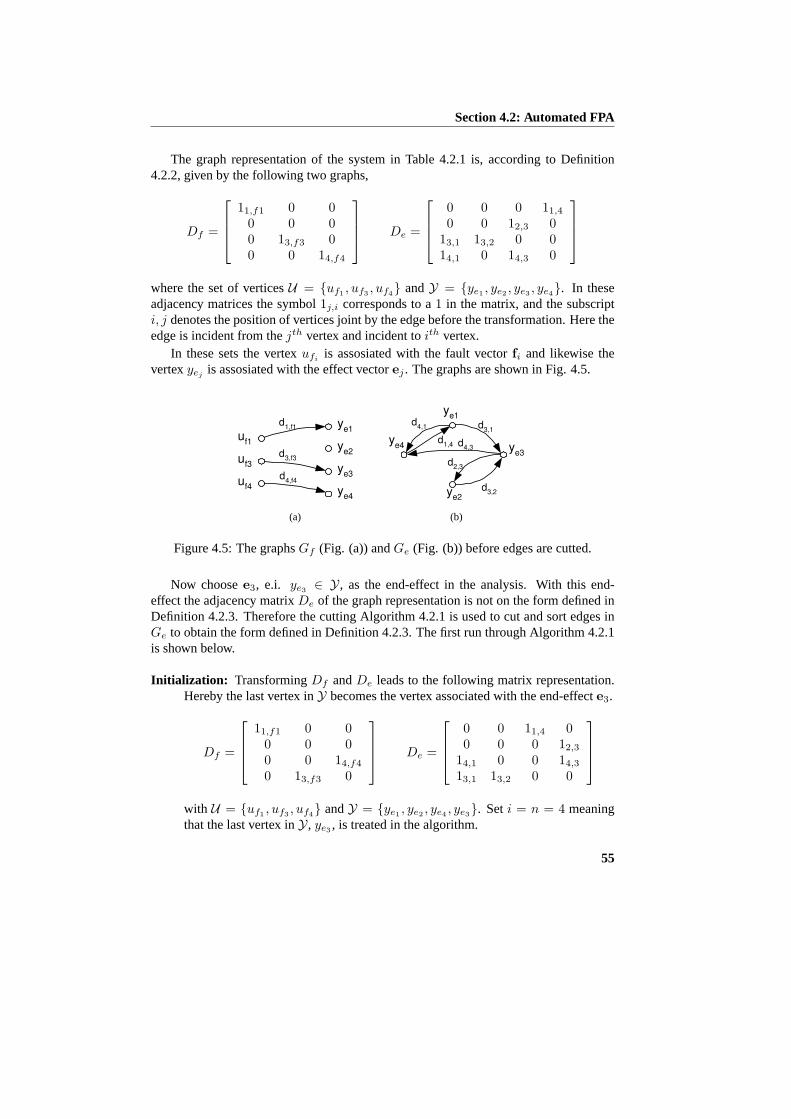
Section 4.2: Automated FPA
The graph representation of the system in Table 4.2.1 is, according to Definition4.2.2, given by the following two graphs,
Df =
11,f1 0 00 0 00 13,f3 00 0 14,f4
De =
0 0 0 11,4
0 0 12,3 013,1 13,2 0 014,1 0 14,3 0
where the set of verticesU = {uf1 , uf3 , uf4} andY = {ye1 , ye2 , ye3 , ye4}. In theseadjacency matrices the symbol1j,i corresponds to a1 in the matrix, and the subscripti, j denotes the position of vertices joint by the edge before the transformation. Here theedge is incident from thejth vertex and incident toith vertex.
In these sets the vertexufiis assosiated with the fault vectorfi and likewise the
vertexyejis assosiated with the effect vectorej . The graphs are shown in Fig. 4.5.
y e 1
y e2
y e3
y e4
d 1 ,f1
u f1
u f3
u f4
d 3 ,f3
d 4 ,f4
(a)
y e 1
d 3,2 y
e2
y e3
y e4
d 2 ,3
d 4 ,3
d 1 ,4
d 4 ,1 d
3 ,1
(b)
Figure 4.5: The graphsGf (Fig. (a)) andGe (Fig. (b)) before edges are cutted.
Now choosee3, e.i. ye3 ∈ Y, as the end-effect in the analysis. With this end-effect the adjacency matrixDe of the graph representation is not on the form defined inDefinition 4.2.3. Therefore the cutting Algorithm 4.2.1 is used to cut and sort edges inGe to obtain the form defined in Definition 4.2.3. The first run through Algorithm 4.2.1is shown below.
Initialization: TransformingDf andDe leads to the following matrix representation.Hereby the last vertex inY becomes the vertex associated with the end-effecte3.
Df =
11,f1 0 00 0 00 0 14,f4
0 13,f3 0
De =
0 0 11,4 00 0 0 12,3
14,1 0 0 14,3
13,1 13,2 0 0
with U = {uf1 , uf3 , uf4} andY = {ye1 , ye2 , ye4 , ye3}. Seti = n = 4 meaningthat the last vertex inY, ye3 , is treated in the algorithm.
55

Chapter 4: System Analysis and Fault Modelling
Step 1: Cut the edges above theith diagonal element, add theith vertex ofY to U , andthe cutted edges toGf , e.i. Df . This results in,
Df =
11,f1 0 0 00 0 0 12,3
0 0 14,f4 14,3
0 13,f3 0 0
De =
0 0 11,4 00 0 0 0
14,1 0 0 013,1 13,2 0 0
with U = {uf1 , uf3 , uf4 , ue3} andY = {ye1 , ye2 , ye4 , ye3}.Step 2: Sorting outDe such that the vertex at positioni− 1 is a vertex with edges inci-
dent to theith vertex, and as few as possible no zero elements above the diagonalin De. This results in,
Df =
1f1,1 0 0 00 0 1f4,4 13,4
0 0 0 13,2
0 1f3,3 0 0
De =
0 11,4 0 014,1 0 0 00 0 0 0
13,1 0 13,2 0
with U = {uf1 , uf3 , uf4 , ue3} andY = {ye1 , ye4 , ye2 , ye3}.Step 3: Seti := i − 1 and return to step 1. This means that the vertexye2 is treated in
the next run through the algorithm.
After 5 cycils of the algorithm the following two adjact matrices are obtained,
Df =
0 14,f4 0 14,3 14,1
11,f1 0 0 0 00 0 0 12,3 00 0 13,f3 0 0
De =
0 0 0 011,4 0 0 00 0 0 00 13,1 13,2 0
whereU = {uf1 , uf3 , uf4 , ue3 , ue1} andY = {ye4 , ye1 , ye2 , ye3}. The resulting graphsare depicted in Fig. 4.6.
These are on the form defined in Definition 4.2.3, hence Theorem 4.2.1 can be usedto obtain relations between the faults and the end-effects. In this example the followingconnection between the extended fault vector and the end-effects is obtained,
e3 ←[A3
1A1f1
A3f3
A31A
14A
4f4
(A32A
23 + A3
1A14A
43) A3
1A14A
41
] ·
f1f3f4e3
e1
.
The remaining task is to analyse each cut to validate the results against the physicalproporties of the system.
56

Section 4.2: Automated FPA
y e 1
y e2
y e3
y e4
d 1 ,f1 u
f1
u f3
u f4
d 3 ,f3
d 4 ,f4
y e1
y e3
d 4 ,3
d 2 ,3
d 4 ,1
(a)
y e 1
d 3,2 y
e2
y e3
y e4
d 1 ,4
d 3 ,1
(b)
Figure 4.6: The graphsGf (Fig (a)) andGe (Fig. (b)) after edges are cutted.
4.2.2 Sensor Configuration and Disturbing Events
In the previous section analysis tools was derived, which can establish an expressionbetween faults and end-effects in a system. Using these analysis tools it is possible toobtain knowledge about the effects of faults in any component of the system. This is nor-mally used to identify the effects of the faults on the overall performance of the system.However, the analysis tools could also be used to identify the connection between faultsand the measurable effects in a given system. If the identification of these connectionsis the goal of the analysis, the end-effect should be chosen as a subset of the measurableeffects in the system. This subset should be interpreted as a given sensor configuration,which hereby is analysed. The result of the analysis can in this case be used to developa logical detection scheme based on events extracted from measurements.
If the analysis tools are used for evaluating detection capabilities of different sensorconfigurations, it is important to take disturbing events in the system into account. Heredisturbing events are defined as events, which affect the system, but should not be de-tected. This means that the only difference between faults and disturbing events is thatthe faults should be detected and the disturbing events should not. As the only differencebetween faults and disturbing events is their interpretation, it is possible to use the anal-ysis tools presented in the previous section, for analysing system with disturbing events.This is done by extending the faults vector with the set of disturbing events. Duing this,the end-effects are given by the following expression,
eend ←(Af Ad
) ·(
fd
), (4.9)
wheref is the set of faults in the system,d is the set of disturbing events, andAf ,Ad are logical matrices defined as in Definition 4.1.1. This means that (4.9) is only afactorization of (4.8). The factorization intof andd of the fault vector is formilized inthe following definition.
57

Chapter 4: System Analysis and Fault Modelling
Definition 4.2.4 (Faults and Disturbing Events)Define the set of all possible eventsin (4.8) asF =
⋃ni=1 Fi where eachFi is the set of events associated with theith
component andn is the number of components in the system. This set can be split intoa set which should be detectedFf ⊆ F and a set which should notFd ⊆ F , whereFf ∩ Fd = ∅. Fd andFf denote the set of disturbing events and faults repectively.
From (4.9) it is seen that the end-effects are given byedi ← Ad · di in the no faultcase, i.e.f = 0. Hereedi is the effect vector generated by theith disturbing event vectordi ∈ Fd. Likewise, it is seen that the end-effects are given byefj ← Af · fk + Ad · dj
in the case of the fault vectorfk ∈ Ff and thejth disturbing event vectordj ∈ Fd. Fora fault vectorfk to distinguishable from the no fault case all possible effect vectors inthe faulty caseefj must be different from all possible effect vectors in the no fault caseedi, i.e.
efj 6= edi ∀di,dj ∈ Fd (4.10)
whereefj ← Af · fk + Ad · dj andedi ← Ad · di. If this expression is true forall di,dj ∈ Fd the given faultfk is said to be detectable in a logical sense. This isformalized in the following definition.
Definition 4.2.5 (Logical Robust Fault Detectability) The fault vectorfk ∈ Ff is log-ical detectable if the effect vectoreend in the case of the fault vectorfk is different fromthe effect vectoreend in the no fault case. This must be true for all possible combinationsof disturbing events in both the fault and in the no fault case.
From (4.10) it is seen that for a fault to be logical detectable in a robust manner,it is necessary that at least one of the effects of the fault cannot be corrupted by anydisturbing events. The following theorem states the conditions for this to be possible.
Theorem 4.2.2 (Logical Robust Fault Detectability)LetIf be the set of vectors withonly 1 element different from zero. Letfk ∈ If be a vector with only thekth elementdifferent from zero, and letAf andAd be defined as in (4.9). Let(Af )j,k be thej, kth
element inAf and likewise for(Ad)j,k, then the fault described byfk is logically de-tectable iff,
∃ j ∈ {1, 2, · · · , ne} : (Af )j,k = 1 andnd∑
i=1
(Ad)j,i = 0 (4.11)
wherene is the number of end-effects andnd is the number of disturbing events. Thisis the same as saying thatfk can be distinguished from all possible combinations ofdisturbing events.
Proof: (Af )j,k = 1 implies that thejth element ofefk ← Af fk is equal to 1 forfk ∈ Ff .Moreover,
∑ndi=1(Ad)j,i = 0 implies that thejth element ined ← Add is equal to zero for
58
Section 4.2: Automated FPA
all d ∈ Fd, i.e. thejth element ofe will always be equal to zero in the no fault case. Thisagain implies that, only faults can affect thejth element ine. Therefore, if thejth element ofe ← Af f + Add is different from zero it must be due tof . fk will cause thejth element ine tobe different from zero, therefore (4.11) implies thatfk is robust detectable.
Now assume thatefk 6= ed, where
efk ← Af · fk + Ad · d (4.12a)
ed ← Ad · d . (4.12b)
This implies that there exists an elementj in efk anded, such that thejth element inefk isdifferent from thejth element ined. For this to be true thejth element ined must be equal tozero, as the termAd · d is part of both (4.12a) and (4.12b). Fored to be zero for alld ∈ Fd thejth row of Ad must equal zero, i.e.
∑ndi=1(Ad)j,i = 0. Therefore, for thejth element ofefk to
be different from thejth element ofed, thejth element ofefk must be different from zero. Thisimplies that(Af )j,k = 1 for the faultfk to be detectable.¤
Remark 4.2.4 From Theorem 4.2.2 it is seen that ifFd = ∅, meaning that no disturbingevents exist in the system, then the demand for detectability offk reduces to(Af )j,k = 1for somej ∈ {1, 2, · · · , ne}.If Theorem 4.2.2 is fulfilled for a given fault in a system, then this fault is detectabledespite of the disturbing events affecting the system.
In some cases not all disturbing events are independent. As an example there couldexist two disturbing eventsd1 andd2; d1 saying that an input to a given component isincreasing andd2 saying that the same input is decreasing. In this cased1 andd2 aremutually excluded ord1 = 1 → d2 = 0 andd2 = 1 → d1 = 0. When this is the caseTheorem 4.2.2 is too restrictive.
In general such dependencies between disturbing events can be described by,
di1 = 1, di2 = 1, · · · , diα = 1 → dj1 = 0, dj2 = 0, · · · , djβ= 0 (4.13)
where there areα disturbing eventsdi1 to diα , which excludeβ disturbing eventsdj1
to djβ. The following Corollary relaxes the demands for logical robust fault detection,
whenh dependencies on the form (4.13) are assumed.
Corollary 4.2.1 (Logical Robust Fault Detectability) For thecth dependency expres-sion on the form (4.13), defineα + 1 fault propagation matrices, whereα matrices areformed by setting theithl column equal 0,l ∈ {1, 2, · · · , α}, and one matrix is formedby setting thejth
1 , jth2 , · · · , jth
β columns equal 0. These matrices form the set,
Ac = {Ad,i1 ,Ad,i2 , · · · ,Ad,iα ,Ad,j} . (4.14)
If there areh dependency expression there existA1 toAh of this sets each correspondingto one dependency expression. This means that there existsh′ =
∏hx=1(αc +1) different
59
Chapter 4: System Analysis and Fault Modelling
combinations given by the set,
Ah =
{Ah | Ah =
h∧c=1
Ac, Ac ∈ Ac
}.
Iff Theorem 4.2.2 holds for a faultfk ∈ If for all Ah ∈ Ah, then the fault is logicaldetectable.
Proof: Before stating the proof a set of disturbing event vectors is defined. From Theorem 4.2.2it is obvious that all end-effects, which can be affected by disturbing events, will be affected if allelements ind is equal to 1. Let this worst case vector be given by1d. When there are mutualexcluded disturbing events, as given in (4.13), the vector1d becomes too restictive. In this casethe vectors with the maximal possible number of elements equal to one, must form the set of worstcase vectors. Let this set be given by,
Dc = {d1,d2, · · · ,dm}Examining (4.13) the firstm − 1 vectors must be formed by setting one of the elementsi1 to iαequal to zero. Themth vector is formed by setting the elementsj1, · · · , jβ equal to zero. Fromthis it is deduced that there existm = α + 1 independent vectors inDc describing the possibleworst case disturbing event vectors, when the mutual exclusion (4.13) exists. If there existh ofthese mutual exclusions, formingh sets of vectorsD1,D2, · · · ,Dh all possible worst case vectorscan be defined as,
D = {d | d = d1 ∧ d2 ∧ · · · ∧ dh, whered1 ∈ D1, d2 ∈ D2, · · · ,dh ∈ Dh}where∧ is the logical "and" operator. Each of the elements inD is formed byαc + 1 vectors,meaning that the total number of vectors becomesΠh
c=1(αc + 1).To prove Corollary 4.2.1 recognise that Theorem 4.2.2 holds for allAh ∈ Ah. This implies
that fk is logical robust detectable with respect to eachAh ∈ Ah, which again implies thatef 6= ed whereef ← Af fk + Ahd anded ← Ahd. Ah =
∧hc=1 Ac, whereAc ∈ Ac is on
the form described in the corollary. From the definition ofAc it is seen that for eachAc ∈ Ac
there corresponds exactly onedc ∈ Dc such thatAc1d = Addc. Using this the following is truefor eachAh ∈ Ah,
Ah1d =
(h∧
c=1
Ac
)1d =
(h∧
c=1
Ac1d
)=
(h∧
c=1
Addc
)= Ad
(h∧
c=1
dc
)= Add
whered ∈ D. Due to the one to one correspondency betweendc ∈ Dc andAc ∈ Ac the aboveequation implies that if Theorem 4.2.2 hold for eachAh ∈ Ah, thenfk is logical robust detectablefor every disturbing event vectord ∈ D. In the start of the proof it was argued that all worst casedisturbing event vectors are contained inD. Therefore,fk is detectable for all possible disturbingevent vectors.
To show sufficiency just reverse the proof.¤
Theorem 4.2.2 and alternatively Corollay 4.2.1 states the demands for a fault to berobust detectable in a logical sense. If this is the case for a set of faults in a system, it
60
Section 4.3: Pump Applications
is interesting to know if the faults in this set can be distinguished from each other i.e.efk
6= efi wheneverfk 6= fi wherefk, fi ∈ If . The following theorem states thedemands for this to be possible,
Theorem 4.2.3 (Logical Fault Identification)Let If be the set of vectors with only 1element different from zero. Letfk ∈ If be the vector describing thekth fault and let(Af )k denote thekth column inAf then the fault described byfk can be distinguishedfrom all otherf ∈ If in a logical sense iff,
(Af )k 6= (Af )i ∀i 6= k, i ∈ {1, 2, · · · , n} . (4.15)
Proof: Two faults fk and fi (fk 6= fi, fk, fi ∈ If ) are distinguishable ifefk 6= efi , whereefk ← Af fk andefi ← Af fi. Let fk be a vector with only thekth element different from zero.Thenefk equals thekth column inAf , i.e. (Af )k. Likewise, letfi be a vector with only theith
element different from zero. Thenefi equals theith column inAf , i.e. (Af )i. From this it isimmediately seen that (4.15) implies thatefk 6= efi wheneverfk 6= fi, wherefk, fi ∈ If . Thiscompletes the proof.¤
Remark 4.2.5 It should be noted that the effects used for fault identification must notbe corrupted by disturbing events. Therefore if there are disturbing events in the systemonly the end-effectsej associated with
∑nd
i=1(Ad)j,i = 0 should be used in Theorem4.2.3.
Remark 4.2.6 In (Blanke et al., 2003) a methods for defining the logical connectionfrom the effects to the faults is given, i.e.f ← B ¯ e where¯ is a special operatordefined in (Blanke et al., 2003). Using this expression it is possible to identify a givenfault from the measurable effects, whenever Theorem 4.2.3 is fulfilled for the system.
If both Theorems 4.2.2 and 4.2.3 are fulfilled for a set of faults in a system, then this setof faults are said to be robust identifiable in a logical sense. Whenever this is the case itis possible to measure a set of effect in the system, and from these measurements detectand isolate the faults.
Unfortunately for many systems it is not possible to find a set of measurable effectswhere both Theorems 4.2.2 and 4.2.3 are fulfilled. However, in many cases Theorem4.2.3 is fulfilled but not Theorem 4.2.2. In these cases the problem is that the disturbingevents cannot be distinguished from the faults in a logical sense. However, it mightstill be possible to quantitatively decouple the disturbing events from the faults usingmodel-based techniques.
4.3 Pump Applications
In this section first the FMEA technique will be used for analysing the centrifugal pump,and second the algorithm presented in the previous section will be utilized for analysing
61

Chapter 4: System Analysis and Fault Modelling
sensor configuration on the centrifugal pump. In the first subsection the division of thesystem into useful components is described. In the second subsection each of thesecomponents are then analysed for their faults and fault effects. This is done by usingthe FMEA. The result of this analysis is a set of possible faults in the system. 7 ofthese faults are chosen for further investigation. Using this subset, different sensor con-figurations are analysed, showing their capability in fault detection and isolation, whensignal-based fault detection methods are used.
The centrifugal pump under investigation in this section should be seen as a generalcentrifugal pump, meaning that the faults identified are general centrifugal pump faults.Therefore in real application only a subset of these faults will occur in practice. Eventhough no particular type of pump is chosen in the investigation, a CR5-10 Grundfospump is used as an example, whenever it can illustrate the presented ideas.
4.3.1 Component Identification in the Centrifugal Pump
The FMEA and FPA are component based analysis tools, therefore the first step is to di-vide the system, in this case the centrifugal pump, into suitable components. In (Bøgh,1997) three approaches are proposed for this division. These are the component hier-archy model, the physical structure model, and the functional structure model. In thefirst approach, the system is divided into components based on the functionality of thecomponents, and in the physical structure model, physical components are identified. Inthe last approach the functionality of the components is identified, meaning that a modelof the functional connection between the components is obtained.
In this work the physical structure model is used to identify components for theFMEA, whereas the functional structure model is used for the FPA. In Fig. 4.7 a com-ponent diagram of the pump is shown. In this diagram 7 physical components are iden-tified. In Fig. 4.8 each of these components are identified on a CR 5-10 Grundfos pump.
In the middle of Fig. 4.8 the centrifugal pump is shown, and each component, iden-tified in Fig. 4.7, is shown in separate subfigures. On the top left corner the inductionmotor, driving the pump, is shown. In the physical structure diagram this motor is againdivided into an electrical and a mechanical component.
Below the motor, the centrifugal pump is shown. The centrifugal pump is also di-vided into two components in the physical structure diagram, namely a hydraulic and amechanical component. The hydraulic component covers the parts directly involved inthe energy transfer from mechanical to hydraulic energy, and the mechanical componentcovers the remeaning parts. The middel figure to the left is a zoom of the hydraulic parts.Here the impeller and the guide vanes are seen.
On the top to the right the shaft is shown. The CR5-10 Grundfos pump has a shortshaft connection. In other pumps this can be longer and often positioned horisontal andnot vertical as in the CR5-10 case. The two last figures show the inlet and outlet part ofthe pump. In some pump applications the inlet part can be equiped with a filter to avoid
62

Section 4.3: Pump Applications
Pump Motor
Shaft
Hydraulics
Mechanical parts of the motor
Shaft mechanics
Electrical parts of the motor
Inlet parts
Outlet parts
Mechanical parts of the centrifugal
pump
Hydraulic parts of the centrigfugal
pump
Figure 4.7: Physical structure diagram of the centrifugal pump. First the pump is dividedinto three components; the motor, the shaft, and the hydraulics. These components areagain divided into 7 components.
large impurities to enter the pump.The functional connection between the identified components, shown in Fig. 4.7,
is presented in Fig. 4.9. To cover the functionality of the pump two extra non physicalcomponents are added. These are, a component covering the dynamics of the mechanicalparts of the pump, and a component deriving the pressure difference produced by thepump. Each component is named in Table 4.3.
Each of the components in Table 4.3 will in the next subsection be analysed usingthe FMEA.
4.3.2 FMEA on the System Components
Each of the components identified in the previous section, see Table 4.3, is in this sectiondescribed with respect to the functionality of the components, the faults in the compo-nents, and the disturbing events affecting the components. Here a fault denotes an eventcausing malfunction of a given component, and therefore should be detected. Whereasa disturbing event is an event affecting the component, but should not be detected. Thefaults and disturbing events, and their effects on each component are analysed using theFMEA. The full result of this analysis is presented in Appendix A, whereas only thefaults and disturbing events are presented in this section. Beside the faults, disturbing
63

Chapter 4: System Analysis and Fault Modelling
Electrical and mechanical
part of the motor.
Hydraulic and mechanical
part of the pump
The shaft
One of the impellers and
guide vanes
Inlet part
Outlet part
Figure 4.8: A real pump example of the component chosen for the FMEA. The pump isa CR5-10 Grundfos pump drived by a 1.5 [KW] induction motor.
events, and their effects on the components, the propagation matrices are presented inAppendix A.
c1: Electrical part of the induction motor
This component contains the electrical parts of the induction motor driving the centrifu-gal pump. This includes the grid connections, the stator windings, and the rotor bars.This component converts electrical energy from the grid to mechanical energy on theshaft of the pump. The faults identified in the component are,
fem1 Loss of one or more phases of the supply voltage.
fem3 Short circuit between windings in the motor.
64
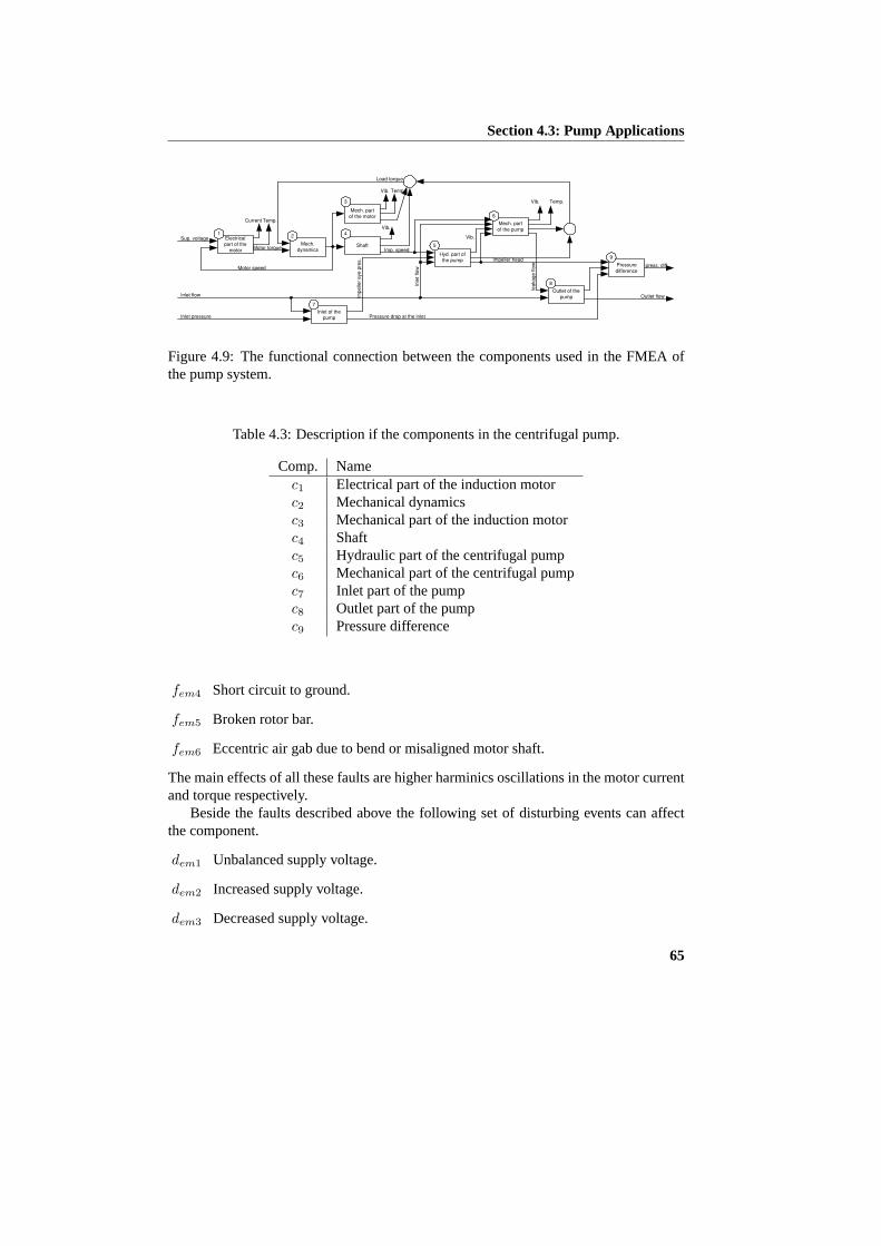
Section 4.3: Pump Applications
Electrical part of the
motor
Outlet of the pump
Sup. voltage
Load torque
Inlet flow
press. diff.
Vib.
Inle
t flow
Temp.
Motor torque Mech.
dynamics Shaft
Motor speed
Imp. speed Hyd. part of the pump
Mech. part of the motor
Mech. part
of the pump
Vib.
Current
Temp.
Temp.
leakage flo
w
Vib.
Inlet of the pump
Impelle
r eye p
res.
Pressure drop at the inlet Inlet pressure
Outlet flow
Vib.
Impeller head Pressure
difference
1 2
3
4
7
5
6
8
9
Figure 4.9: The functional connection between the components used in the FMEA ofthe pump system.
Table 4.3: Description if the components in the centrifugal pump.
Comp. Namec1 Electrical part of the induction motorc2 Mechanical dynamicsc3 Mechanical part of the induction motorc4 Shaftc5 Hydraulic part of the centrifugal pumpc6 Mechanical part of the centrifugal pumpc7 Inlet part of the pumpc8 Outlet part of the pumpc9 Pressure difference
fem4 Short circuit to ground.
fem5 Broken rotor bar.
fem6 Eccentric air gab due to bend or misaligned motor shaft.
The main effects of all these faults are higher harminics oscillations in the motor currentand torque respectively.
Beside the faults described above the following set of disturbing events can affectthe component.
dem1 Unbalanced supply voltage.
dem2 Increased supply voltage.
dem3 Decreased supply voltage.
65

Chapter 4: System Analysis and Fault Modelling
dem4 Increased supply frequency with constant V/f relationship.
dem5 Decreased supply frequency with constant V/f relationship.
c2: Mechanical dynamics
This component contains the mass of all rotating parts in the pump. It is introducedin the functional model to cover the convertion from torque to speed. As it is not aphysical component, but a functional signal transformation, no faults are identified inthe component.
c3: Mechanical part of the induction motor
This component contains the ball bearings and the shaft of the motor. The functionalityof the component is to transfer torque produced by the electrical part of the motor tothe shaft connecting the centrifugal pump and the motor. The faults identified on thecomponent are:
fmm1 Ware of the bearings in the motor.
fmm2 Rub impact between the stator and the rotor due to a bend or misaligned motorshaft.
The main effect of these faults is vibrations in the mechanical structure of the motor,beside that small torque oscillation can occur.
c4: Shaft mechanics
This component contains the shaft and the shaft connection attaching the motor andpump shaft. The functionality of the component is to transfer the torque on the motorshaft to torque on the pump shaft. The faults identified on the component are,
fsh1 Broken shaft.
fsh2 Misalignment between the motor and pump.
fsh3 Bend shaft.
The main effect of these faults are mechanical vibrations and, in the case of the last twofaults, torque oscillations.
c5: Hydraulics of the centrifugal pump
This component contains the impeller, the diffuser, the volute, and the guide vanes ofthe centrifugal pump. The component converts mechanical energy from the shaft tohydraulic energy induced into the liquid pumped by the pump. The faults identified inthe component are the following,
66

Section 4.3: Pump Applications
fi1 Dry running.
fi2 Impurities fixed on the impeller, causing inbalance.
fi3 Wear of the impeller.
fi4 Blocked or partial blocked flow field inside the impeller.
fi5 Blocked impeller rotation.
fi6 Wear of the sealing ring.
fi7 Missing sealing ring.
fi8 Loss of the impeller.
The main effects of these faults are changes in the value of pressure and the load torquegenerated by the impeller at a given flow. Moreover some of the faults can induce pres-sure oscillations. These pressure oscillations can be either harmonics of the rotationalfrequency, or noise like signals covering a larger frequency span.
Beside the faults described above the following set of disturbing events can affectthe component.
di1 Decreased flow through the pump.
di2 Increased flow through the pump.
c6: Mechanical part of the pump
This component contains those mechanical parts of the pump not directly involved inthe energy transformation from mechanical to hydraulic energy (the parts involved inthe energy transformation are contained in componentc5, hydraulics of the centrifugalpump). This means that parts such as the shaft of the pump, bearings inside the pump,and the casing are included in this component. The functionality of the component is tosecure the hydraulic parts in the right possition, and to lead the liquid to and from thehydraulic part of the pump. The faults identified in the component are the following:
fmp1 Dry running.
fmp2 Inlet flow equal to zero.
fmp3 Ware of the bearings in the pump.
fmp4 Ware of seals.
fmp5 Rub impact between the impeller and the cassing.
67

Chapter 4: System Analysis and Fault Modelling
The first two of these faults are connected to the cooling of the pump, and therefore themain effect of these faults is an increased temperature of the pump. The main effects ofthe last four faults are mechanical vibrations and leakages from the pump casing.
Beside the faults described above the following set of disturbing events can affectthe component.
dmp1 Decreased flow through the pump.
dmp2 Increased flow through the pump.
c7: Inlet of the pump
This component includes the inlet parts of the pump, which can contain a suction pipeand/or a filter. The functionality of the component is to lead the liquid to the impeller.The faults identified in the part are the following,
fip2 Low pressure at the inlet of the pump.
fip3 Opstruction of the inlet of the pump.
The main effect of these faults is that the inlet pressure to the impeller becomes too low.Beside the faults described above the following set of disturbing events can affect
the component.
dip1 Decreased flow through the pump.
dip2 Increased flow through the pump.
dip3 High frequency pressure oscillations.
c8: Outlet of the pump
This component includes the outlet part of the pump, which can contain an outlet pipeor a riser pipe. The length of this pipe is defined by the two points where the pressuredifference generated by the pump is measured. The component is leading the liquidfrom the pump to a given distination. The faults identified in this component are:
fop2 Leakage on the outlet pipe.
fop3 Opstruction of the outlet pipe.
The main effects of these faults are leakages from the system and decreased pressureproduced by the pump.
Beside the faults described above the following set of disturbing events can affectthe component.
dip1 Decreased flow through the pump.
dip2 Increased flow through the pump.
68

Section 4.3: Pump Applications
c9: Generated differential pressure
This component is not a physical component, but a collection of the pressure effectsaffecting the pressure difference across the pump. The component is necessary in thefunctional model as the effects on the pressure difference is a function of head losses inthe inlet and the outlet components and the hydraulics of the centrifugal pump.
Sensor components
This work is not concerned with sensor faults, even though it is an important field.Instead sensors are seen as components, which are able to measure special effects on thesystem. Hence, they collect the end-effects used in the sensor analysis.
The list of possible sensors is long, some of the most important, with respect to thecentrifugal pump applications, are the following,
• Current sensors.
• Voltage sensors.
• Vibration sensors on the stator and/or the pump mechanics.
• Pressure difference sensor (between outlet and inlet).
• Absolute pressure sensor at the inlet and/or the outlet of the pump.
• Flow sensor at the inlet and/or the outlet of the pump.
• Temperature sensors inside the stator, bearings and/or seals.
• Speed sensors, on the motor and/or the pump shaft.
Of these especially the pressure difference sensor is often used for control purposes.Likewise, if the speed of the motor is controlable normally expressions of the currentsand the voltages of the motor are also available. If the system is equipped with a surveil-lance system, a subset of all the sensor information can be available. Unfortunately, thisis only the case in very few centrifugal pump applications.
4.3.3 Identifying Interesting Faults
Normally, in the FMEA it is common to include risk assessments and frequencies forthe faults expected in the given component. These risk assessments and frequencies areattached to a given product. In this work no specific centrifugal pump is chosen, insteadthe general components forming a centrifugal pump is analysed. Therefore, it has notbeen possible to make a risk assessment and even less possible to include frequencies ofthe faults. Instead the FMEA has be used to identify a set of common faults in centrifugalpumps, and their effects on the component under investagation. The obtained set canthen be used as a gross set when analysing a specific centrifugal pump.
69

Chapter 4: System Analysis and Fault Modelling
As neither risk assessments nor frequencies are identified for the faults on the cen-trifugal pump these cannot be used as guidelines for choosing faults for further investa-gation. Instead a set of fault is chosen using the following criteria:
• The fault must be expected to happen in real life applications.
• It must be possible to simulate the fault on a test-bench without changing compo-nents in the pump.
The first of these criteria is included to insure the relavance of the faults from an indus-trial point of view. The second criterion is included to make it possible to simulate thefault behaviour in real time on a test-bench.
Using these criteria the following set of faults is chosen for futher investagation,
Fault Group Faults Fault Descriptionfe1 fem3 Short circuit between stator windings.fh1 fi4 Inc. hydraulic resistance inside the pump.fh2 fip3 Inc. hydraulic resistance at inlet.fh3 fi6 fi7 Wear of or missing sealing ringfm1 fmp5 Rub impact between impeller and casingfin1 fi1 fmp1 fip1 fop1 Dry running.fin2 fip2 Too low inlet pressure. Can cause cavita-
tion.
Of these faultsfi1 , fmp1 , fip1 , fop1 , and fip2 are input faults meaning that they arecaused by unsuitable operation of the application in which the pump is placed. Thesetype of faults are also called external faults. Even though these faults are not dirrectlyconnected to the components of the pump, they are very important to detect. The reasonis that dry running will destroy the bearings of the pump in a few seconds, and toolow inlet pressure will cause cavitation inside the pump, which again will destroy theimpeller over time.
Beside these faults of course all disturbing events affecting the system must be takeninto account in the following analysis. The disturbing events are,
Dist. Group Dist. Dist. descriptionde1 dem1 Unbalanced supply voltage.de2 dem2 Increased supply voltage.de3 dem3 Decreased supply voltage.de4 dem4 Increased supply freq. with const. V/f.de5 dem5 Decreased supply freq. with const. V/f.dh1 di1 dmp1 dip1 dip1 Decreased flow through the pump.dh2 di2 dmp2 dip2 dip2 Increased flow through the pump.dh3 dip3 High frequency pressure oscillations.
70

Section 4.3: Pump Applications
Collecting the chosen fault and disturbing events the following logical fault vector isobtained,
fe =(fT dT
)T(4.16)
where,
f =(fe1 fh1 fh2 fh3 fm1 fin1 fin2
)d =
(de1 de2 de3 de4 de5 dh1 dh2 dh3
).
(4.17)
In the next section the effects of this fault vector on different measureable signals areanalysed.
4.3.4 FPA on the General Pump System
In Section 4.2.1 it is argued that logical models of the components forming the systemcan be described as defined in Definition 4.2.1. Using this definition the componentmodel of the centrifugal pump, presented in Section 4.3.1, is given in Table 4.4.
Table 4.4: The component description of the centrifugal pump. The structure of each ofthe logical matrices is given in Appendix A.
Comp. Faults Effects Transformationsc1 fem eem Aem
f ,Aemdy
c2 0 edy Adyem,Ady
mm,Adysh,Ady
mp,Adyi
c3 fmm emm Ammf ,Amm
dy
c4 fsh esh Ashf ,Ash
dy
c5 fi ei Aif ,Ai
sh,Aiip
c6 fmp emp Ampf ,Amp
sh ,Ampi
c7 fip eip Aipf
c8 fop eop Aopf ,Aop
mp
c9 0 edh Adhi ,Adh
op ,Adhip
Having a model on this form Algorithm 4.2.1 and Theorem 4.2.1 can be used to de-rived the connection from the faults and disturbing events, to any effect vectore in thesystem. Therefore, by identifing all measureable effects of interest it is possible to estab-lish a connection between faults and disturbing events, and a subset of the measurableeffects. This connection can then be used to evaluate the usability of the given sensorconfiguration, when the design of signal-based fault detection schemes is considered.
In the previous section a list of sensors used on centrifugal pumps is presented.Moreover, it is argued that some of these sensors are only used in special applications.The most frequently used sensors are the electrical sensors and the pressure difference
71

Chapter 4: System Analysis and Fault Modelling
sensor. Therefore these should attend special attention when developing intelligent FDIalgorithms. The electrical and pressure sensors are often used for control purposes inhydraulic applications, and are therefore often available for other purposes too. Thismeans that the cost of implementing a supervision system is reduced considerably byusing only these sensors as input to the FDI algorithms.
Beside the sensors just mentioned, the flow sensor is considered. Flow sensors arenormally expensive, but by using the newest micro technology it is possible to reducethe cost considerably. This means that this sensor will become interesting in even smallcentrifugal pump applications. Also a sensor measuring the impeller eye pressure isconsidered. The flow sensor and the impeller eye pressure sensor are considered to beadditional sensors and are therefore increasing the cost of implementing the supervisionsystem.
To summarize; the effects seen in the following sensors are analysed using the FPA,
• Current sensors.
• Voltage sensors.
• pressure difference sensor (between outlet and inlet).
• Flow sensor.
• Impeller eye pressure sensor.
The results of the FPA using these sensors are presented in the following, where each ofthe logical matrices are obtained by using Algorithm 4.2.1.
Effects on the electrical part of the motor
The effects measurable using the current and voltage sensors are all found in componentc1 Electrical Part of the Motor. The measurable effects on this component are,
eem,i1 ∼ Increased current.eem,i2 ∼ Decreased current.eem,i3 ∼ Oscillations in the length of the pack transform current.eem,i4 ∼ Unbalanced stator current.eem,v1 ∼ Zero voltage in one or more of the phases.eem,v2 ∼ Oscillations in the length of the pack transform voltage.
72

Section 4.3: Pump Applications
The connection between these effects and the faults and disturbing events in the systemis given by the following logical equation,
eem,i1
eem,i2
eem,i3
eem,i4
eem,v1
eem,v2
←
1 0 0 1 1 0 0 0 1 0 0 1 0 1 00 1 1 0 0 1 1 0 0 1 1 0 0 0 11 1 0 0 1 0 0 1 0 0 0 0 0 0 00 0 0 0 0 0 0 0 0 0 0 0 0 0 00 0 0 0 0 0 0 0 0 0 0 0 0 0 00 0 0 0 0 0 0 1 0 0 0 0 0 0 0
(fd
)
(4.18)
wheref is the fault vector andd is disturbing event vector, both defined in (4.17).
Effects on the pressure difference generated by the pump
The effects measuable using the pressure difference sensor are all found in componentc9 Pressure Difference. The measurable effects on this component are,
eop,h1 ∼ Increased pressure difference across the pump.eop,h2 ∼ Decreased pressure difference across the pump.eop,h3 ∼ Zero pressure difference across the pump.eop,h4 ∼ Harmonic oscillations in the pressure difference signal.eop,h5 ∼ High frequence oscillations in the pressure difference signal.eop,h6 ∼ Pressure difference across the pump is not defined.
The connection between these effects and the faults and disturbing events in the systemis given by the following logical equation,
edh1
edh2
edh3
edh4
edh5
edh6
←
0 0 0 0 0 0 0 0 0 0 1 0 0 1 00 1 1 1 1 0 1 0 0 0 0 1 0 0 10 0 0 0 0 1 0 0 0 0 0 0 0 0 00 1 0 0 1 0 0 0 0 0 0 0 0 0 00 0 1 0 1 0 1 0 0 0 0 0 1 0 00 0 0 0 0 1 0 0 0 0 0 0 0 0 0
(fd
)
(4.19)
wheref is the fault vector andd is disturbing event vector, both defined in (4.17).
Effects on the flow measurement
Using a flow sensor it is possible to measure effects on the flow input, meaning that theeffects of the input faults and disturbing events, which are associated with the flow, aremeasurable with this sensor. The measurable effects on this component are,
73
Chapter 4: System Analysis and Fault Modelling
eq1 ∼ Increased floweq2 ∼ Decreased floweq3 ∼ Not defined
The connection between these effects, and the faults and disturbing events in the systemis given by the following logical equation,
eq1
eq2
eq3
←
0 0 0 0 0 0 0 0 0 0 0 0 0 1 00 0 0 0 0 0 0 0 0 0 0 0 1 0 00 0 0 0 0 1 0 0 0 0 0 0 0 0 0
(fd
)
(4.20)
wheref is the fault vector andd is disturbing event vector, both defined in (4.17).
Effects on the impeller eye pressure measurement
It is well known that the inlet pressure has large impact on the pump performance, ascavitation will occur if this pressure becomes too low. If cavitation does occure it willdestroy the pump over time. Therefore, by measuring the pressure at the impeller eye itmight be possible to detect decreases in this pressure and thereby detect the possibilitiesfor cavitation. Moreover measuring the pressure at the impeller eye pressure noise dueto cavitation might be measurable. The effects in the impeller eye pressure are found incomponentc7 Inlet of the Pumpandc5 Hydraulic part of the centrifugal pump, wherethe mean pressure is coming fromc7 and the pressure noise due to cavitation is comingfrom c5. The measurable effects are,
eeh1 ∼ Noise like pressure oscillationseeh2 ∼ Impeller eye pressure not definedeeh3 ∼ Impeller eye pressure too low
The connection between these effects and the faults and disturbing events in the systemis given by the following logical equation,
eeh1
eeh2
eeh3
←
0 0 1 0 1 0 1 0 0 0 0 0 1 0 00 0 0 0 0 1 0 0 0 0 0 0 0 0 00 0 1 0 0 0 1 0 0 0 0 0 0 0 0
(fd
)
(4.21)
4.3.5 Sensor Configuration Analysis
In this section different combinations of the proposed sensors are analysed with repectto logical robustness and identification. This is done by analysing the logical connectionbetween the measurable effects in each sensor and the faults in the system. In this anal-ysis both logical robustness and identification possibilities are considered. The logical
74

Section 4.3: Pump Applications
connections between faults and effects were established for each of the sensors in theprevious section.
The robustness of the different sensor configurations could be analysed using Theo-rem 4.2.2, but by looking at the description of the disturbing events in Section 4.3.3 thefollowing mutually exclusive expressions of the disturbing events are recognized,
de2 = 1 → de3 = 0 de3 = 1 → de2 = 0de4 = 1 → de5 = 0 de5 = 1 → de4 = 0dh2 = 1 → dh1 = 0 dh1 = 1 → dh2 = 0
asde2, de4 anddh2 are increased voltage, frequency and flow respectively, andde3, de5
anddh1 are decreased voltage, frequency and flow. These dependencies are taken intoaccount using Corollary 4.2.1. When the robustness properties are establised the pos-sibilities for fault identification of the detectable fault can be analysed, using Theorem4.2.3.
The results are presented in two logical vectorsRr andRi, whereRr containsthe results of the robustness analysis, andRi contains the results of the identificabilityanalysis. Such that,
if the property holds forfj thenrj := 1 ,elserj := 0
wherefj is thejth component in the fault vectorf andrj is thejth component in eitherRr orRi dependent on which property is analysed. The fault vectorf is given by,
f =(
fe1 fh1 fh2 fh3 fm1 fin1 fin2
)
where eachfj is described in Section 4.3.3. Three sensor configurations are consideredin the following, these are,
1. Sensors measuring the electrical quantities, e.i. the voltage and current measure-ments.
2. Sensors measuring the electrical quantities and the pressure difference across thepump.
3. Sensors measuring the electrical quantities, the pressure difference and the volumeflow.
4. Sensors measuring the electrical quantities, the pressure difference, the volumeflow and the impeller eye pressure.
The results of the analysis of these different sensor configurations are presented in thefollowing.
75
Chapter 4: System Analysis and Fault Modelling
Electrical measurements
Firstly, only the effects in the electrical measurements are considered, e.i. the effectsmeasurable using the current and voltage sensors. The connection from the faults anddisturbing events, to their effect on the electrical quantities is given by (4.18). Thisequation is on the form,
e ← [Af Ad
] ·[fd
]
meaning that Theorem 4.2.2 and Corollary 4.2.1 can be used to establish the logicalrobust fault detection possibilities. The result of this analysis is shown below,
Rr =(0 0 0 0 0 0 0
). (4.22)
FromRr it is seen that it is not possible to distinguish any of the faults from possiblelogical combinations of disturbing events. This means that non of these effects can beused in a robust signal-based fault detection scheme.
Electrical and pressure difference measurements
Secondly, consider the effects on the electrical measurements and the pressure differencemeasurement. These are given by (4.18) and (4.19). The result of this analysis is shownbelow,
Rr =(0 1 0 0 1 1 0
). (4.23)
Here it is seen that 3 of the 6 faults are detectable using signal-based methods.Normally it is impossible to measure the high frequency components in the pressure
signal using standard pressure sensors. To analyse the detection properties under thisassumption, the high frequency pressure componenteop,h5 is removed from the analy-sis. Moreover it is assumed that the pressure value is always available, meaning that theeffect eop,h6 is also removed. The result of this test is shown below,
Rr =(0 1 0 0 1 1 0
). (4.24)
By comparing this result with the result from the analysis including the high frequencycomponents, it is seen that all the fault information, not corrupted by disturbing events,is contained in the low frequency parts of the pressure signal.
Electrical, pressure difference and flow measurements
In the third analysis the electrical measurements are combined with both a pressuremeasurement containing high frequency components and a flow measurement. Theseare given by (4.18), (4.19) and (4.20) repectively. The result of this test is shown below,
Rr =(0 1 0 0 1 1 0
). (4.25)
76

Section 4.4: Detection Algorithm for the Centrifugal Pump
Comparing these results, with the results of the analysis where only the electrical mea-surements and the pressure sensor are considered, it is seen that no addition informationis added using the flow sensor. This is in fact true when only logical combinations areconsidered. But, as it will be shown in Chapter 6, The flow sensor can be used for dis-turbance decoubling, when model-based methods are used. Hereby, it becomes possibleto detect the faultfh3 corresponding to increased leakage flow inside the pump.
Electrical, pressure difference, flow and impeller eye pressure measurements
As the last analysis a pressure sensor measuring the impeller eye pressure is added. Thismeans that effect in the electrical quantities, the pressure difference, the volume flow,and the impeller eye pressure are assumed known. These are given by (4.18), (4.19),(4.20) and (4.21) respectively. The result of this analysis is shown below,
Rr =(0 1 1 0 1 1 1
). (4.26)
Here it is seen that only the faultsfe1 andfh1 corresponding to inter-turn short circuitand leakage flow are undetectable. To check the possibilities for identification of thethe 5 detectable faults, the effects not corrupted by disturbing events are analysed usingTheorem 4.2.3. The logical expression of the faults is given by the following expression.
eem,i4
eem,v1
edh3
edh4
edh6
eq3
eeh2
eeh3
←
0 0 0 0 0 0 00 0 0 0 0 0 00 0 0 0 0 1 00 1 0 0 1 0 00 0 0 0 0 1 00 0 0 0 0 1 00 0 0 0 0 1 00 0 1 0 0 0 1
· (f) .
In this expression the effects, which can be corrupted by disturbing events, are removed.The result of the detectability analysis is shown below,
Ri =(x 0 0 x 0 1 0
)(4.27)
wherex corresponds to the fault not robust detectable. Here it is seen that only one faultis distinguishable from the other faults, when all the effects corrupted by disturbingevents are removed.
4.4 Detection Algorithm for the Centrifugal Pump
In this section an example of a robust signal-based detection scheme is developed. Theobtained detection scheme is tested on a test-bench particular developed for this purpose.
77
Chapter 4: System Analysis and Fault Modelling
4.4.1 Decision Logic
In the analysis presented in the previous section the system was assumed to be disturbedby 8 different disturbing events, see Section 4.3.3. If this assumption is relaxed byremoving the disturbing eventde1 the robust detection properbilities are increased. Re-moving this disturbing event is the same as assuming that the supply voltage is balancedat all times. Now consider the sensor configuration including the following sensors,
• Current sensors.
• Voltage sensors.
• Low bandwide pressure difference sensor.
With this sensor configuration the result of the FPA is the following,
Rr =(1 1 0 0 1 1 0
) Ri =(1 0 x x 0 1 x
)
where thex’s inRi indicates that the given fault is not robust detectable (the interpreta-tion ofRr andRi is described in Section 4.3.5). FromRr it is seen that four faults arelogical robust detectable. This means that the following fault vector is detectable usingthe considered sensor configuration,
f =(
fe1 fh1 fm1 fin1
).
The connection between the measurable effects, and the faults and disturbing events isin this particular case given by the following logical equation,
eem,i3
edh3
edh4
←
1 1 1 00 0 0 10 1 1 0
fe1
fh1
fm1
fin1
, (4.28)
where the measurable effects not in use are removed. From (4.28) it is easy to see thatthe faultsfh1 andfm1 are indistinguishable as they affect the same measurable effect.This is also shown inRi. Likewise it is seen inRi that the faultsfe1 andfin1 can bedistinguished from the remaining two faults. This is confirmed by examination of (4.28).The detection logic is very simple in this case, and is given by,
eem,i3 → fe1
eem,i3 ∨ edh4 → fh1
eem,i3 ∨ edh4 → fm1
edh3 → fin1 .
(4.29)
In this expressioneem,i3 indicates frequency components of the length of the Park trans-formed motor currents, where the length of the Park current vector is given by,
‖isdq‖ = ‖Tdqisabc‖ .
78

Section 4.4: Detection Algorithm for the Centrifugal Pump
In this expression the same notation as in Chapter 3 is used. The effectedh3 correspondsto zero difference pressure, when the pump is running. Finally, the effectedh4 corre-sponds to low freqency harmonic oscillations in the pressure measurements. Here lowfrequency components correspond to frequencies larger than 0 [Hz] and up to 2-4 timesthe supply voltage frequency.
4.4.2 Test Results
To test the validity of the decision logic, derived in the previous subsection, data sets ob-tained by simulating faults on a centrifugal pump is analysed. These data are obtained byrunning tests on a test-bench particular developed for testing fault detection algorithmsin this project. A sketch of the test-bench is shown in Fig. 4.10. The pump used in thetest-bench is a Grundfos 1.5(KW ) CR5-10 pump.
V 1
V 2
V c
pipe
pump
M
motor
shaft
T e
H p
tank
V 3
V l
Q p
Figure 4.10: Sketch of the test-bench. The measurements are the electrical quantities,the pressure differenceHp delivered by the pump and the volume flow through the pumpQp.
In the tank and pipe system, connected to this pump, the valveV1 is used to modeldisturbances in the system. The inter-turn short circuit is simulated by shorting windingsin phasea in the costimized designed stator particular developed for this purpose. Dryrunning is simulated by closingV2 and openingV3, and rub impact is simulated byadding an extra force on the shaft. During the test, presented here, this is done bymounting twist on the shaft, which rubs against the mechanical connection between thepump and motor. Hereby an oscilating force, similar to the one expected in a pumpduring faultfm1, is added. Finally, clogging inside the pump can be simulated by theclosing valveVc. However, this valve simulates clogging of for example an inlet filter,
79

Chapter 4: System Analysis and Fault Modelling
Table 4.5: Summing of the test results. Here, the faults denoted inter-turn, Dry-running,and rub-impact corresponds tofe1, fm1, andfin1 respectively. Likewise, and increase inσis, andσh corresponds toeem,i3, andedh4 respectively. Finally, whenµh approximatezero it corresponds toedh3.
Normal Inter-turn Rub-impact Dry-runningµis 2.7366 5.2066 4.6263 2.0450σis 0.0037 0.4954 0.0141 0.0041µh 2.2178 2.2561 1.6402 0.1054σh 0.0003 0.0006 0.0067 0.0010
and not clogging in one of the channels in the impeller, which was assumed in the logicalanalysis. Therefore, results from this test are not considered here.
The measurable effects considered in these tests are affecting the current and thepressure measurements, therefore only these will be analysed in the following test re-sults. To evaluate the robustness of the approach, signals obtained on the pump at con-stant speed and at different positions of valveV1 are analysed. The different valve po-sitions simulates the no fault condition at different hydraulic loads. Results from thistest are shown in Fig. 4.11. From these test results it is obvious that the DC-level ofthe considered signals are not usable for fault detection. This was also predicted by theFPA-analysis performed in Section 4.4.1.
Figs. 4.12, 4.13, and 4.14 depitch the current and pressure signals when the pumpis exposed to the three faultsfe1, fm1, andfin1 denoting inter-trun short circuit, rubimpact, and dry running respectively. The results of these tests are summarized in Table4.5. In the evaluation of the resultsσis andσh are used as measurements of the end-effectseem,i1 and eh4 respectively. The end-effectedh3 is assumed triggered whenµh ≈ 0.
Considering the results presented in Table 4.5 it is seen thatσis is increased consid-erably in the case of the inter-turn faultfe1 and the rub-impact faultfm1. Comparingthese results with the decision logic in (4.29), and rembering thatσis is a measure ofthe end-effecteem,i1 it fits perfectly. Likewise, by usingσh as a measure of theedh4
it is seen that the rub-impact faultsfm1 is the only fault which increasesσh. This alsofits the results of (4.29) perfectly. Finally, the only fault forcingµh close to zero is thedry-running faultfin1. As µh ≈ 0 is considered a measure ofedh1 this also fits theresults of (4.29).
4.5 Discussion
In the literature it is described how Failure Mode and Effect Analysis (FMEA) and FaultPropagation Analysis (FPA) are used in the design of Fault Tolerant Control (FTC).However, these tools are general analysis tools, and could as well be used in the design
80

Section 4.5: Discussion
0 2 4 6 8 10 12 14 160
1
2
3
4
Cur
rent
[A]
Time [sec]
µ = 2.7366σ = 0.0037
→ ←
(a) Length of the Park current vector.
0 2 4 6 8 10 12 14 160
1
2
Pre
ssur
e [b
ar]
Time [sec]
µ = 2.2178σ = 0.0003
→ ←
(b) Pressure difference across the pump.
Figure 4.11: Results obtained when running the pump at constant speed and differentpositions of valveV1. The change in valve position simulates different load condition ofthe pump.
0 5 10 15 200
2
4
6
Cur
rent
[A]
µ = 5.2066σ = 0.4954
→ ←
(a) Length of the Park current vector.
0 5 10 15 200
1
2
Pre
ssur
e [b
ar]
Time [sec]
µ = 2.2561σ = 0.0006
→ ←
(b) Pressure difference across the pump.
Figure 4.12: Results obtained when introducing an inter-turn short circuit in phasea ofthe induction motor stator. The fault is introduced at time 6.05 [sec] and removed at time5.75 [sec]. The mean and variance of the two presented signals are calculted from databetween the two indicator lines. During the test the pump is running at constant speedand with valveV1 fixed at a constant position.
81
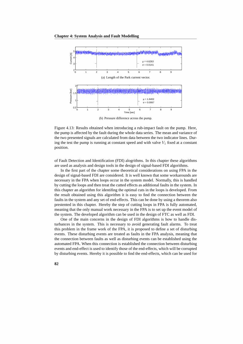
Chapter 4: System Analysis and Fault Modelling
0 1 2 3 4 5 6 7 8 92
3
4
5
Cur
rent
[A]
µ = 4.6263σ = 0.0141
→ ←
(a) Length of the Park current vector.
0 1 2 3 4 5 6 7 8 90.5
1
1.5
2
Pre
ssur
e [b
ar]
Time [sec]
µ = 1.6402σ = 0.0067
→ ←
(b) Pressure difference across the pump.
Figure 4.13: Results obtained when introducing a rub-impact fault on the pump. Here,the pump is affected by the fault during the whole data series. The mean and variance ofthe two presented signals are calculated from data between the two indicator lines. Dur-ing the test the pump is running at constant speed and with valveV1 fixed at a constantposition.
of Fault Detection and Identification (FDI) alogrithms. In this chapter these algorithmsare used as analysis and design tools in the design of signal-based FDI algorithms.
In the first part of the chapter some theoretical considerations on using FPA in thedesign of signal-based FDI are considered. It is well known that some workarounds arenecessary in the FPA when loops occur in the system model. Normally, this is handledby cutting the loops and then treat the cutted effects as additional faults in the system. Inthis chapter an algorithm for identifing the optimal cuts in the loops is developed. Fromthe result obtained using this algorithm it is easy to find the connection between thefaults in the system and any set of end-effects. This can be done by using a theorem alsoprestented in this chapter. Hereby the step of cutting loops in FPA is fully automated,meaning that the only manual work necessary in the FPA is to set up the event model ofthe system. The developed algorithm can be used in the design of FTC as well as FDI.
One of the main concerns in the design of FDI algorithms is how to handle dis-turbances in the system. This is necessary to avoid generating fault alarms. To treatthis problem in the frame work of the FPA, it is proposed to define a set of disturbingevents. These disturbing events are treated as faults in the FPA analysis, meaning thatthe connection between faults as well as disturbing events can be established using theautomated FPA. When this connection is established the connection between disturbingevents and end-effect is used to identify those of the end-effects, which will be corruptedby disturbing events. Hereby it is possible to find the end-effects, which can be used for
82
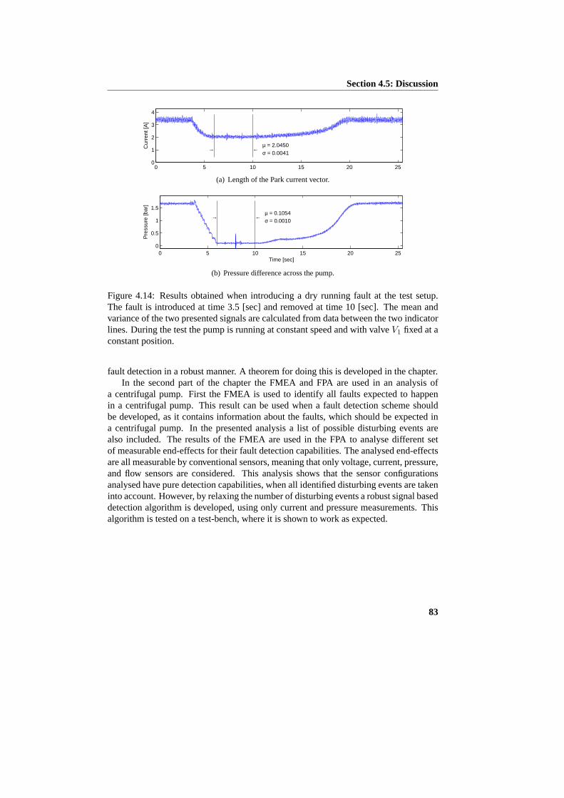
Section 4.5: Discussion
0 5 10 15 20 250
1
2
3
4
Cur
rent
[A]
µ = 2.0450σ = 0.0041
→ ←
(a) Length of the Park current vector.
0 5 10 15 20 250
0.5
1
1.5
Pre
ssur
e [b
ar]
Time [sec]
µ = 0.1054σ = 0.0010
→ ←
(b) Pressure difference across the pump.
Figure 4.14: Results obtained when introducing a dry running fault at the test setup.The fault is introduced at time 3.5 [sec] and removed at time 10 [sec]. The mean andvariance of the two presented signals are calculated from data between the two indicatorlines. During the test the pump is running at constant speed and with valveV1 fixed at aconstant position.
fault detection in a robust manner. A theorem for doing this is developed in the chapter.In the second part of the chapter the FMEA and FPA are used in an analysis of
a centrifugal pump. First the FMEA is used to identify all faults expected to happenin a centrifugal pump. This result can be used when a fault detection scheme shouldbe developed, as it contains information about the faults, which should be expected ina centrifugal pump. In the presented analysis a list of possible disturbing events arealso included. The results of the FMEA are used in the FPA to analyse different setof measurable end-effects for their fault detection capabilities. The analysed end-effectsare all measurable by conventional sensors, meaning that only voltage, current, pressure,and flow sensors are considered. This analysis shows that the sensor configurationsanalysed have pure detection capabilities, when all identified disturbing events are takeninto account. However, by relaxing the number of disturbing events a robust signal baseddetection algorithm is developed, using only current and pressure measurements. Thisalgorithm is tested on a test-bench, where it is shown to work as expected.
83

Chapter 4: System Analysis and Fault Modelling
84

Chapter 5
A New approach for Stator FaultDetection in Induction Motors
Stator faults are according to (Kliman et al., 1996) the most common electrical faultsin electrical motors. Moreover according to (Bonnett and Soukup, 1992) most of thesefaults start as an inter-turn short circuit in one of the stator coils. The increased heat dueto this short circuit will eventually cause turn to turn or turn to ground faults, and finallylead to a breakdown of the stator, (Wiedenbrug et al., 2003) and references included. Thetime, from an inter-turn short circuit has occurred to breakdown of the stator, can be veryshort. In (Gerada et al., 2004) it is argued that the time from an inter-turn short circuithas occured to the temperature in the short circuit exceed the breakdown temperature ofthe insulation can be as small as 1 to 2 [sec].
Inter-turn short circuits are caused by several different influences on the stator. Forexample mechanical stress during assembling or during operation can create scratchesin the insulation, which again can cause short circuits. If the motor is placed in wetenvironment, moisture can cause flow of current from scratch to scratch, which canmake a hot spot and thereby destroy the insulation. Moreover, if the motor is suppliedwith a PWM voltage source, partial discharges due to very high amplitude alternatingvoltage between the turns can degrade the insulation over time and cause a short circuits.
In the literature different approaches are proposed for detection of inter-turn shortcircuits. In (Cruz and Cardoso, 2001) the stator currents are transformed using the Parktransformation. Second order harmonics in the length of the transformed current vectoris then used for fault detection. In (Cash, M. A. et al., 1997; García et al., 2004) oscilla-tions in the voltage between the line neutral and the star point of the motor are used asa fault indicators. This is also shown in (Tallam et al., 2002) using a model of a faultymotor. In (Lee et al., 2003) estimation of the negative impedance of the motor is usedas a fault indicator, and in (Arkan et al., 2001) the negative sequence current is used forthe same purpose. In (Briz et al., 2003) high frequency voltage injection in the supply
85
Chapter 5: A New approach for Stator Fault Detection in Induction Motors
voltage is utilized to create a response on the motor current. This response containsinformation of the inter-turn short circuit fault.
In this chapter a model-based approach is proposed. The proposed approach is basedon a model of the induction motor including an inter-turn fault in the stator. Differentapproaches for modelling inter-turn short circuits in the stator windings are found in theliterature. In (Joksimovic and Penman, 2000) a higher order model is used. This modelis an extension of the model presented in (Luo et al., 1995). This type of model is usedfor simulating higher order effects in the motor, but the obtained model is of high order.The inter-turn short circuit fault has its main harmonics in the lower frequency range.Therefore observers designed on the basis of this type of model will be of unnecessaryhigh order for this kind of fault. In (Williamson and Mirzoian, 1985) a steady statemodel of both inter-turn and turn-turn faults in an induction motor is developed using alow order model. In (Tallam et al., 2002) a transient model of the same order as the onepresented in (Williamson and Mirzoian, 1985) is developed. This model describes anY-connected induction motor with an inter-turn short circuit in phasea.
In this chapter an adaptive observer is proposed for estimation of the inter-turn shortcircuit fault. Theoretical considerations on adaptive observers can for example be foundin (Besancon, 2000; Rajamani and Hedrick, 1995; Cho and Rajamani, 1997). Based onthese contributions a new observer scheme is proposed, specially designed for handlingbi-linear systems. The observer is formulated in general terms, hence is usable in otherapplications. The proposed observer is capable of simultaneously estimating the speedof the motor, the amount of turns involved in the short circuit, and an expression of thecurrent in the short circuit. The observer is based on a model, developed particular forthis purpose. This model is based on the same ideas as the model described in (Tallamet al., 2002). However, the model developed in this chapter is valid for bothY- and∆-connected induction motors, and does includes both inter-turn and turn-turn shortcircuits. Moreover, the model has a more useful structure compared to (Tallam et al.,2002). Using three copies of the designed adaptive observer the phase affected by theinter-turn short circuit is identified using an approach described in (Zhang, 2000).
As a model-based approach for fault estimation is proposed in this chapter, the chap-ter starts by deriving a model of the induction motor with an inter-turn short circuit inSection 5.1. This model is in Section 5.2 used in the design of the proposed adaptiveobserver. In Section 5.3 test results from tests on a customized designed motor are pre-sented. Finally concluding remarks end the chapter.
5.1 Model of the Stator Short Circuit
As described in the introduction, this chapter is concerned with detection of inter-turnshort circuit faults. In this work the model-based approach is used, meaning that amodel of the motor is needed in the derivation of the FDI algorithm. The derivation ofthis model is considered in this section, meaning that a model of an induction motorincluding a stator fault is derived.
86

Section 5.1: Model of the Stator Short Circuit
A turn-turn short circuit denotes a short circuit between windings in two differentphases of the stator, see Fig. 5.1. Here a short circuit between phasea and b in aY-connected and a∆-connected stator is shown.
a
b
c
i f
i sa
i sb
i sc
v sa + - -
+
v sc
-
+
v sb
(a) Short circuit between turns in phasea andb in aY-connected stator.
a
c
b i f i
sa
i sc
i sb
v sa + -
v sb
-
+
+
v sc
-
(b) Short circuit between turns in phasea andb in a∆-connected stator.
Figure 5.1: Simplified electrical diagram of a three phaseY-connected and∆-connectedstator with a turn-turn short circuit between phasea andb.
An inter-turn fault is, in contrast with the turn-turn fault, a short circuit betweenwindings in the same phase coil. However, an inter-turn fault can be treated as a specialcase of the turn-turn fault, as it can be modelled by assuming that no turns, of for ex-ample phaseb, are involved in the short circuit. However, it can be argued that this is arather limited model assumption for the inter-turn fault, because the short circuit alwaysmust be connected to the end point of the phase coil in this case. But, if the electricalcircuit is assumed linear, all short circuits in a coil can be represented by a short circuitconnected to the end point of the given coil. This new short circuit must of cause havethe same amount of turns as the real short circuit.
In the following, a model of an induction motor, including a turn-turn short circuitbetween phasea andb, is developed. The model is developed under the assumption thatthe short circuit does not affect the overall angular position of the coil in the motor.
5.1.1 The Y-connected Motor inabc-coordinates
First theY-connected motor is considered. Setting up the mesh equations for theY-connected motor shown in Fig. 5.1(a) and rearranging these equations, a model de-scribing a motor with a short circuit between phasea andb is found. Using the matrix
87

Chapter 5: A New approach for Stator Fault Detection in Induction Motors
notation presented in Chapter 3 this model is given by the following set of equations,
vsabc = rs(isabc − γif ) +dψsabc
dt(5.1a)
γT vsabc = rf if + lfdifdt
(5.1b)
0 = rrirabc +dψrabc
dt(5.1c)
ψsabc = ls(isabc − γif ) + lm(θ)irabc (5.1d)
ψrabc = lrirabc + lm(θ)(isabc − γif ) , (5.1e)
where (5.1a) and (5.1d) describe the voltages and the flux linkages in each of the statorphases, (5.1c) and (5.1e) describe the voltages and the flux linkages in each of the rotorphases, and finally (5.1b) describes the current in the short circuit. In these equationsvsabc contains the voltages across each stator phase,isabc is the current running intoeach stator phase, andif is the current in the short circuit. The matricesrs, rr, ls, lr,andlm(θ) have the same form as in the case of a motor with no faults. These matricesare given in Section 3.2.1.
The vectorγ in (5.1a) to (5.1e) represents the position and the amount of turns in theshort circuit. The vector is, in the case of a short circuit between phasea andb, given by
γ =[γa −γb 0
]T, (5.2)
whereγa is the amount of turns affected in phasea, andγb is the amount of turns affectedin phaseb by the short circuit. The inductor and the resistor in (5.1b) are given by
lf = (γa(1− γa) + γb(1− γb)) lls, rf = (γa(1− γa) + γb(1− γb)) rs + ri (5.3)
wherers is the stator resistance,lls is the leakage inductance of the stator, andri is theresistance in the insulation break.ri = ∞ means that no short circuit has occurred andri 6= ∞ means that a leakage current is flowing. The evolution fromri = ∞ to ri = 0is very fast in most insulating materials, meaning that the value ofri can be assumed toequal either∞ or 0 in most cases.
5.1.2 The∆-connected Motor inabc-coordinates
To set up the model of the∆-connected induction motor the same procedure as used inthe case of aY-connected motor is used.
Setting up the mesh equations for the∆-connected motor depicted in Fig. 5.1(b)and rearranging these equations, a model describing the∆-connected motor with a shortcircuit between phasea andb is obtained. Using the same matrix notation as used in the
88

Section 5.1: Model of the Stator Short Circuit
previous section the following set of equations is obtained,
vsabc = rs(isabc − γif ) +dψsabc
dt(5.4a)
γT vsabc = rf if + lfdifdt
(5.4b)
0 = rrirabc +dψrabc
dt(5.4c)
ψsabc = ls(isabc − γif ) + lm(θ)irabc (5.4d)
ψrabc = lrirabc + lm(θ)(isabc − γif ) . (5.4e)
This model has the same structure as the one modelling theY-connected motor. More-over the parametersrs, rr, rf , ls, lr, lm andlf in this model have the same values as inthe model of theY-connected motor. The only difference is the vectorγ modelling theamount of turns involved in the short circuit, which in this case is given by
γ =[γa γb 0
]T. (5.5)
5.1.3 Transformation to a Stator fixeddq0-frame
Comparing the models developed in the two previous sections it is seen that the modelof theY-connected and∆-connected motor has the same structure. This model structurewill in this section be transformed to a stator fixeddq0-frame.
Using thedq0-transformationTdq0(θ) presented in Section 3.2.2 the models pre-sented in (5.1) and (5.4) are transformed into the following,
vsdq = Rs(isdq −Tdqγif ) + dψsdq
dt
vs0 = rs(is0 − 13T
T0 γif ) + dψs0
dt
0 = Rrirdq + dψrdq
dt − zpωrJψrdq
0 = rrir0 + dψr0dt
lfdif
dt = −rf if + γT T−1dq0vsdq0 ,
(5.6)
where the flux linkages are given by
ψsdq = Ls(isdq −Tdqγif ) + Lmirdq
ψs0 = lls(is0 − 13T
T0 γif )
ψrdq = Lrirdq + Lm(isdq −Tdqγif )ψr0 = llrir0 .
(5.7)
In these expressionsTdq contains the two first rows andT0 contains the last row ofTdq0. The parameter matrices in this modelRs, Rr, Ls Lr, andLm do all have diagonalstructures, and are given in Section 3.2.2.
From (5.6) and (5.7) it is seen that it is convenient to define a new current vectori′sdq0 = isdq0 − Tdq0γif . This current equals the amount of the stator current, which
89

Chapter 5: A New approach for Stator Fault Detection in Induction Motors
generates air gab flux. Rewriting (5.6) and (5.7) using the same procedure as describedin Section 3.2, and introducing the currenti′sdq0 the induction motor model becomes,
L′sdi′sdq
dt = −(Rs + R′r)i
′sdq + (R′
r − zpωrJL′m)imdq + vsdq
llsdi′s0dt = −rsi
′s0 + vs0
L′mdimdq
dt = R′ri′sdq − (R′
r − zpωrJL′m)imdq
lfdif
dt = −rf if + γT T−1dq0vsdq0 ,
(5.8)
where
R′r = LmL−1
r RrL−1r Lm L′s = Ls − LmL−1
r Lm L′m = LmL−1r Lm ,
meaning that the new matrices retain the diagonal structure.
5.1.4 Grid Connections
In the model presented in (5.8) the voltagesvsdq0 and the currentsisdq0 are defined asthe quantities related to each phase in the motor. These are in general not measurable,therefore the connection between these quantities and the quantities of the terminal ofthe motor must be establised. This is done in Section 3.2.3 in Chapter 3 for an inductionmotor without stator faults. In the following the connection established in Section 3.2.3is used to obtain the final model of theY- and∆-connected induction motors with aninter-turn short circuit in the stator.
The Y-connected Case
From Section 3.2.3 the relationships between the phase quantities and the measurablequantities are given by
vsdq = vtdq itdq = isdq
vs0 = vt0 − v0 it0 = is0 ,
where quantities with subscripts are related to the phases of the motor, and quantitieswith subscriptt are related to the terminals of the motor, and are therefore measurable.Moreover in theY-connected caseis0 = it0 = 0. Introducing these relationships in(5.8) the model of theY-connected induction motor with a stator short circuit becomes
L′sdi′sdq
dt= −(Rs + R′
r)i′sdq + (R′
r − zpωrJL′m)imdq + vtdq (5.9a)
llsdi′s0dt
= −rsi′s0 + (vt0 − v0) (5.9b)
L′mdimdq
dt= R′
ri′sdq − (R′
r − zpωrJL′m)imdq (5.9c)
lfdifdt
= −rf if + γT T−1dq0(vtdq0 − v0) , (5.9d)
90

Section 5.1: Model of the Stator Short Circuit
and the measurable currents are given by
itdq0 = i′sdq0 + Tdq0γif . (5.9e)
From (5.9e) it is seen thati′s0 = − 13 (γa − γb)if asit0 = 0 in the Y-connected case.
Using this expression in (5.9b), and using the obtained expression to eliminatevt0 − v0
in (5.9d) a new expression of the short circuit currentif is found. This expression isgiven by
Lfdif
dt = −Rf if + γT T−1dq vtdq , (5.10)
whereT−1dq is a matrix consisting of the two first columns ofT−1
dq0, andLf andRf arescalars and are given by
Lf = lf + 13 (γa − γb)2lls Rf = rf + 1
3 (γa − γb)2rs .
The final model of theY-connected induction motor then becomes
L′sdi′sdq
dt = −(Rs + R′r)i
′sdq + (R′
r − zpωrJL′m)imdq + vtdq
L′mdimdq
dt = R′ri′sdq − (R′
r − zpωrJL′m)imdq
Lfdif
dt = −Rf if + γT T−1dq vtdq
itdq = i′sdq + Tdqγif ,
(5.11)
whereγ =(γa −γb 0
)T.
The ∆-connected Case
From Section 3.2.3 the relationships between the phase quantities and the measurablequantities in the∆-connected case are given by,
[vsdq
vs0
]=
[Bv 00 0
] [vtdq
vt0
] [itdq
it0
]=
[Ci 00 0
] [isdq
is0
],
here again quantities with subscripts are related to the phases of the motor, and quanti-ties with subscriptt are related to the terminals of the motor, and are therefore measur-able. Introducing these relationships in (5.8) the model of the∆-connected inductionmotor with a stator short circuit becomes
L′sdi′sdq
dt= −(Rs + R′
r)i′sdq + (R′
r − zpωrJL′m)imdq + Bvvtdq (5.12a)
llsdi′s0dt
= −rsi′s0 (5.12b)
L′mdimdq
dt= R′
ri′sdq − (R′
r − zpωrJL′m)imdq (5.12c)
lfdifdt
= −rf if + γT T−1dq0
[Bv
0
]vtdq , (5.12d)
91

Chapter 5: A New approach for Stator Fault Detection in Induction Motors
and the measurable currents are given by
itdq =[Ci 0
] (i′sdq0 + Tdq0γif
). (5.12e)
In the∆-connected case the currenti′s0 = is0 − 13 (γa − γb)if . From (5.12b) it is seen
thati′s0 → 0 ast → ∞, meaning thatis0 → 13 (γa − γb)if ast → ∞. This shows that
the circulating current in the∆-connected motor will be proportional to the current inthe short circuitif .
The final model of the∆-connected induction motor with a short circuit fault be-comes
L′sdi′sdq
dt = −(Rs + R′r)i′sdq + (R′
r − zpωrJL′m)imdq + Bvvtdq
L′mdimdq
dt = R′ri′sdq − (R′
r − zpωrJL′m)imdq
lfdif
dt = −rf if + γT T−1dq Bvvtdq
itdq = Cii′sdq + CiTdqγif ,
(5.13)
whereγ =(γa γb 0
)Tin the∆-connected case, andT−1
dq consists of the two first
columns ofT−1dq0 as in theY-connected case.
5.1.5 Torque Expression
An expression of the torque developed by an induction motor, not affected by faults,is derived in Section 3.2.4. In the following the same approach is used to derive anexpression of the torque developed by an induction motor affected by a turn-turn shortcurcuit fault in the stator. This torque expression is based on the same idea as used in(Tallam et al., 2002). From (Krause et al., 1994) the torque produced by the inductionmotor is given by
Te = zpiTs∂lfm(θ)
∂θir , (5.14)
whereis is the current in the stator windings andir is the current in the rotor. In the caseof a stator with faults, the current in each part of the faulty windings must be defined.In the case of a stator with a single turn-turn short circuit between phasea andb, thecurrentsis andir are given by
is =[isa isa − sign(γ1)if isb isb − sign(γ2)if isc
]T
ir =[ira irb irc
]T,
where γ1 and γ2 are the first and second elements inγ respectively. The matrixlfm(zpθr) is the mutual inductance matrix between the stator and rotor.lfm(zpθr)
92
Section 5.2: An Adaptive Observer for Inter-turn Fault Detection
is in the case of a turn-turn fault between phasea andb given by,
lfm(θ) = lm
(1− γa) cos(θ) (1− γa) cos(θ + 2π3 ) (1− γa) cos(θ − 2π
3 )γa cos(θ) γa cos(θ + 2π
3 ) γa cos(θ − 2π3 )
(1− γb) cos(θ − 2π3 ) (1− γb) cos(θ) (1− γb) cos(θ + 2π
3 )γb cos(θ − 2π
3 ) γb cos(θ) γb cos(θ + 2π3 )
cos(θ + 2π3 ) cos(θ − 2π
3 ) cos(θ)
.
The torque expression in (5.14) can be rearranged to become
Te = zp (isabc − γif )T ∂lm(zpθr)∂θ
irabc , (5.15)
whereγ is given by (5.2) and (5.5) in theY- and∆-connected cases respectively.lm(θ)has the same structure as in the no fault case, and is given in Section 3.2.1.
Transforming the torque expression in (5.15) using the transformationTdq0 and us-ing thatLmimdq = Lrirdq + Lmisdq, the following torque expression is obtained,
Te =32zpL
′m
(imdi
′sq − imqi
′sd
)
whereL′m = L2m/Lr, meaning thatL′m is the diagonal element ofL′m.
Remark 5.1.1 By examining the electrical model of an induction motor with an inter-turn short circuit (5.11) or (5.13) and the torque expression given above, it can be seenthat no torque ripples should be expected, if the load is constant at a given speed andthe motor is supplied with a balanced three phase sinusoidal voltage.
5.2 An Adaptive Observer for Inter-turn Fault Detec-tion
According to (Bonnett and Soukup, 1992) most stator burnouts start as an inter-turnshort circuit in one of the stator coils. The increased heat due to this short circuit willeventually cause turn to turn and turn to ground faults and finally lead to a burnout ofthe stator. In (Gerada et al., 2004) the time, from an inter-turn short circuit has occuredto an insulation breakdown due to heat, is investagated on a 15 [KW] motor. Here it isshown that this time slot can be as short as 2 [sec]. This means that a fast and reliabledetection scheme is necessary, but also that the most important of the inter-turn and theturn-turn faults are the inter-turn faults. Therefore, a detection scheme, which can detectinter-turn short circuits in the stator of an induction motor, is considered in this section.
The considered detection scheme is based on the model developed in the previoussection. This model is used in the derivation of an observer which can estimate the inter-turn short circuit faults. Only inter-turn short circuits in phasea are considered, as three
93

Chapter 5: A New approach for Stator Fault Detection in Induction Motors
identical observers, which can detect faults in phasea, b andc respectively, can be usedfor identification. The approach used for this is described at the end of this section andis based on (Zhang, 2000).
In the model developed in the previous section an inter-turn short circuit in phaseais modelled by settingγb = 0 in the vectorγ. Doing this the parametersRf andLf inboth theY- and∆-connected motors can be expressed by
Rf = f(γa)rs + ri Lf = f(γa)lls ,
wheref(γa) equalsγa(1 − 23γa) and γa(1 − γa) in the Y- and ∆-connected cases
respectively. In section 5.1.1 it is argued that the resistorri in the expression ofRf isalmost always either equal to∞ or 0. Therefore the assumption thatri = 0 is almostalways true if a short circuit has occurred. Using this and consideringγa as a state in thesystem the model of both theY- and∆-connected motors with an inter-turn short circuitcan be expressed as
L′sdi′sdq
dt = −(Rs + R′r)i
′sdq + (R′
r − zpωrJL′m)imdq + Bvvtdq
L′mdimdq
dt = R′ri′sdq − (R′
r − zpωrJL′m)imdq
dif
dt = − rs
llsif + 1
lls
[γa
f(γa) 0]Bvvtdq
dγa
dt = 0 ,
(5.16a)
where the measurable outputs are given by
itdq = Ci
(i′sdq +
[23γa
0
]if
). (5.16b)
The only differences between the model of theY- and∆-connected induction motorsare the structures ofBv, Ci, andf(γa). In theY-connected caseBv = Ci = I and inthe∆-connected caseBv andCi are given in Section 3.2.3 of Chapter 3.
The model in (5.16) represents an induction motor with an inter-turn short circuit inthe stator. However, by settingγa = 0 a motor not affected by a fault can be modelled.This is true because settingγa = 0 represents a short circuit involving 0 turns, whichhave the same effect on the motor performance as when no short cicuits have occured.To ensure the validity of this model the termγa
f(γa) must be bounded whenγa → 0. Theterm is given by
γa
f(γa)=
γa
γa(1− aγa),
wherea equals23 and1 in theY- and∆-connected cases respectively. From this expres-
sion it is seen that γa
f(γa) is bounded on the set{γa : 0 ≤ γa < 1}, which contains allpossible values ofγa.
A surprising fact when modelling the no fault case by settingγa = 0 is that the faultcurrentif is not equal to zero in the no fault case. This is because the model expresses
94
Section 5.2: An Adaptive Observer for Inter-turn Fault Detection
the limit of the fault current whenγa → 0, when the no fault case is modelled in thisway. The model is still correct in the no fault case, as the fault current only affects theremaining model in the output expression (5.16b), and here the fault current is multipliedwith γa which is equal to zero.
From (5.16) it is seen that the model of the induction motor contains one unknownvariableωr, which represents the speed of the rotor. If this variable is modelled as anunknown but constant parameter, an adaptive observer approach can be used for stateestimations, and thereby estimation of the fault. The design of this adaptive observer isconsidered in Section 5.2.1. The design of the feedback gain in the adaptive observeris considered in Section 5.2.2, and finally the identification of the phase affected by agiven inter-turn short circuit fault is considered in Section 5.2.3.
5.2.1 The Adaptive Observer
An adaptive observer exists for the system in (5.16) if it can be transformed into theadaptive observer form defined in Definition 5.2.1. This definition is a bilinear versionof the general nonlinear definition given in (Besancon, 2000).
Definition 5.2.1 Consider a system on the form
dzdt = A(u, θ)z + Buy = Cz ,
(5.17)
wherez(t) ∈ Rn contains the states of the system,y(t) ∈ Rd contains the meassurableoutputs,θ ∈ Rk contains unknown but constant parameters andC =
[I 0
]. This
system is said to be on bilinear adaptive form if,
1. A(u, θ) is bounded for allθ ∈ Dθ ⊆ Rk andu(t) ∈ U ⊆ Rm, whereDθ is theparameter space andU is the input space,
2. the set(A(u, θ),C) is an observable pair for everyθ ∈ Dθ andu(t) ∈ U ,
3. Aθ1(u) to Aθk(u) are linear independent matrices for everyu(t) ∈ U ,
4. Im{Aθi(u)}⋂Ker{C} = 0 ∀ i ∈ {1, 2, · · · , k},
where
A(u, θ) = A0(u) +k∑
i=1
θiAθi(u) .
Remark 5.2.1 Item Number 4 in Definition 5.2.1 means that the only states, which canbe directly affected byθi, are the measurable states, and thatAθi(u) has the followingstructure
Aθi(u) =[A′
θi(u)
0
]
95

Chapter 5: A New approach for Stator Fault Detection in Induction Motors
due to the structure ofC =[I 0
].
For systems on the form defined by Definition 5.2.1 an adaptive observer exists accord-ing to the following proposition.
Proposition 5.2.1 For a system of the form defined in Definition 5.2.1 an adaptive ob-server exists and has the following form,
dzdt = A(u, θ)z + Bu + K(u)(y −Cz)
dθi
dt = κizT A′θi
(u)T (y −Cz) ∀ i ∈ {1, · · · , k} ,(5.18)
whereκi > 0, i ∈ {1, · · · , k} are design constants,A(u, θ) is a copy of the systemmatrix defined in Definition 5.2.1 andA′
θi(u) is a submatrix given by
Aθi(u) =
[A′
θi(u)
0
].
If there exists aK(u) stabilizing the system for everyθ ∈ Dθ andu ∈ U , i.e. thereexists aP(θ) fulfilling the following Matrix Inequality (MI),
(A(u, θ)−K(u)C)T P(θ) + P(θ) (A(u, θ)−K(u)C) ≺ 0−P(θ) ≺ 0 .
(5.19)
Proof: Defining the state estimation error asez = z− z, and the parameter estimation errors aseθi = θi − θi, the dynamics of the errors become
ez = (A(u, θ)−K(u)C) ez +∑k
i=1 Aθi zeθi
eθi = −κizT AT
θiez ∀i ∈ {1, 2, · · · , k} ,
where it is used thateθi = − ˙θi asθi = 0. This error equation can be reformulated by defining
the following parameter error vector and matrix,
eθ =[eθ1 eθ2 · · · eθk
]TAθ(z) =
[Aθ1 z Aθ2 z · · · Aθk z
].
Using this vector and matrix in the description of the error system it becomes,[ez
eθ
]=
[(A(u, θ)−K(u)C) Aθ(z)
−κAθ(z)T 0
] [ez
eθ
]
=
[I 00 κ
] [(A(u, θ)−K(u)C) Aθ(z)
−Aθ(z)T 0
] [ez
eθ
], (5.20)
whereκ = diag{κ1, κ2, · · · , κn}, meaning that
[I 00 κ
]=
[I 00 κ
]T
 0. Now definee =
[eT
z eTθ
]Tand let the following quadratic function be a Lyapunov function candidate for the
error system (5.20),
V = eT
[P(θ) 0
0 I
]e ,where
[P(θ) 0
0 I
]Â 0 .
96

Section 5.2: An Adaptive Observer for Inter-turn Fault Detection
Taking the derivative along the trajectory of (5.20) and recognizing that
eT
[( [I 00 κ
] [0 Aθ(z)
−Aθ(z)T 0
] )T [P(θ) 0
0 I
]+
[P(θ) 0
0 I
] (∗
)]e = 0
for all e ∈ Rn+k. This is true as the matrix in the expression is skew symmetric. Moreover,dP(θ)
dt= 0 asθ = 0. Using these statements the derivative of the Lyapunov function candidate
becomes,
V = eTz
((A(u, θ)−K(u)C)T P(θ) + P(θ) (A(u, θ)−K(u)C)
)ez .
This shows thatez → 0 ast → ∞ if (5.19) is fulfilled for everyu ∈ U andθ ∈ Dθ. To showthat the error of the parameter estimate also tends to zero the La-Salle’s theorem is used (Khalil,2002). This theorem can be used to state that an error system as (5.20) is asymptotic stable if theonly positive invariant space with respect to (5.20) inE ⊂ Rn+k is e = 0, whereE is the spaceof all error vectorse, which makeV = 0. Now consider (5.20) whenV = 0,
ez = Aθ(z)eθ =∑k
i=1 Aθi zeθi
eθ = 0 .
This shows that the positive invariant spaceE is given byez = 0 and∑k
i=1 Aθi zeθi = 0. FromDefinition 5.2.1 it is known that{Aθ1 ,Aθ1 , · · · ,Aθk} are linearly independent. Therefore, theremust exist time seriesz(t), t ∈ [t0, t0 + T ], which guarantees that
∑ki=1 Aθi zeθi = 0 implies
thateθ = 0. This leads to the following persistently of excitation demand,
∃α1, α2, T : α1I ≤∫ t0+T
t0
Aθ(z(t))T Aθ(z(t))dt ≤ α2I .
¤
Using a nonlinear transformationΦ on (5.16), this system is transformed into a form,which fulfills Definition 5.2.1. The transformationΦ : x → z maps the original states
x =[i′Tsdq iTmdq if γa
]T
(5.21)
into the new statesz ∈ R6, and is given by
Φ(x) =
i′sdq +[
23γa
0
]if
L′m−1L′si
′sdq + imdq + L′m
−1L′s
[23γa
0
]if
23γaif
γ2a
llsf(γa)
. (5.22)
When this transformation is used on system (5.16) it is transformed into a bilinear systemon the form,
dzdt = (A0 + ωrAωr + vsdAvsd
)z + Buy = Cz ,
(5.23)
97

Chapter 5: A New approach for Stator Fault Detection in Induction Motors
where the input vectoru = vtdq, the output vectory = itdq, and the matrices in (5.23)are given by
A0 =
−L′s−1(Rs + R′
r)− L′m−1R′
r L′s−1R′
r
[Rs+R′r
L′s− rs
lls
0
]0
L′m−1Rs 0
[ Rs
L′m− rs
lls
0
]0
0 0 − rs
lls0
0 0 0 0
Aωr=
zpJ −zpJL′s−1L′m 0 0
0 0 0 00 0 0 00 0 0 0
Avsd
=
0 0 0[
23lls0
]
0 0 0[
2(lm+lls)3Lmlls
0
]
0 0 0 23lls
0 0 0 0
B =
L′s−1
L′m−1
00
Bv C = Ci
[I 0 0 0
].
If ωr is treated as an unknown but constant parameter, system (5.23) fulfills Definition5.2.1 except for the observability condition whenvsd = 0. However, it can be arguedthat, when the induction motor is running, the fraction of time wherevsd = 0 tends tozero. This is so becausevsd passes zero but does never stay there during normal oper-ation. Therefore the system described by (5.23) is observable at all the times, meaningthat Definition 5.2.1 is fulfilled.
As (5.23) fulfills Definition 5.2.1 an adaptive observer is given by Proposition 5.2.1.This observer becomes
Oa :
dzdt = (A0 + ωrAωr + vsdAvsd
)z + Bu + K(u)(y −Cz)dωr
dt = κ(y −Cz)T Aωr zx = Φ−1(z) .
(5.24)
In this designK(u) is the stabilizing feedback gain and0 < κ is the adaptation gain.κ should be chosen such that the adaptation speed is suitable.K(u) should be chosenaccording to Proposition 5.2.1. The calculation ofK(u) is considered in the followingsection.
98
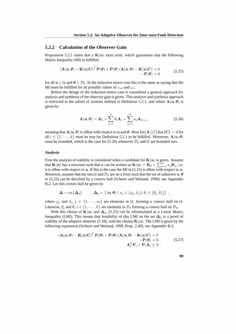
Section 5.2: An Adaptive Observer for Inter-turn Fault Detection
5.2.2 Calculation of the Observer Gain
Proposition 5.2.1 states that aK(u) must exist, which guarantees that the followingMatrix Inequality (MI) is fulfilled,
(A(u,θ)−K(u)C)T P(θ) + P(θ) (A(u, θ)−K(u)C) ≺ 0−P(θ) ≺ 0
(5.25)
for all u ∈ U andθ ∈ Dθ. In the induction motor case this is the same as saying that theMI must be fulfilled for all possible values ofvsd andωr.
Before the design of the induction motor case is considered a general approach foranalysis and synthesis of the observer gain is given. This analysis and synthesis approachis restricted to the subset of systems defined in Definition 5.2.1, and whereA(u, θ) isgiven by
A(u, θ) = A0 +k∑
i=1
θiAi +m∑
j=1
ujAk+j , (5.26)
meaning thatA(u,θ) is affine with respect tou andθ. Here Im{Ai}⋂
Ker{C} = 0 forall i ∈ {1, · · · , k} must be true for Definition 5.2.1 to be fulfilled. Moreover,A(u,θ)must be bounded, which is the case for (5.26) wheneverDθ andU are bounded sets.
Analysis
First the analysis of stability is considered when a candidate forK(u) is given. AssumethatK(u) has a structure such that it can be written asK(u) = K0 +
∑mj=1 ujKj , i.e.
it is affine with respect tou. If this is the case the MI in (5.25) is affine with respect tou.Moreover, assume that the setsU andDθ are on a form such that the set of unknownu, θin (5.25) can be descibed by a convex hull (Scherer and Weiland, 1999), see AppendixB.2. Let this convex hull be given by
∆ = co{∆0} , ∆0 ={(u, θ) | uj ∈ {uj , uj}, θi ∈ {θi, θi}
},
whereuj and uj j ∈ {1, · · · ,m} are elements inU , forming a convex hull onU .Likewise,θi andθi i ∈ {1, · · · , k} are elements inDθ forming a convex hull onDθ.
With this choise ofK(u) and∆0, (5.25) can be reformulated as a Linear MatrixInequality (LMI). This means that feasibility of this LMI on the set∆0 is a proof ofstability of the adaptive observer (5.18), with the chosenK(u). The LMI is given by thefollowing expression (Scherer and Weiland, 1999, Prop. 2.40), see Appendix B.2,
(A(u, θ)−K(u)C)T P(θ) + P(θ) (A(u,θ)−K(u)C) ≺ 0−P(θ) ≺ 0
ATi Pi + PiAi º 0 ,
(5.27)
99

Chapter 5: A New approach for Stator Fault Detection in Induction Motors
which must be fulfilled for all(u,θ) ∈ ∆0 and alli ∈ {1, · · · , k}. In this LMI P(θ) ison the formP(θ) = P0 +
∑ki=1 θiPi.
The feasability of this LMI states that the adaptive observer in Proposition 5.2.1is stable for the givenK(u). However, if there are limits on the change rate of thesupply signalsu, this rate limit can be incorporated in the stability analysis, relaxing thecondition. To see this, letu be contained in the setΛ given by
Λ = co{Λ0} , Λ0 = co{u | uj ∈ {λj , λj}
},
and letP in (5.27) be an affine function of bothθ andu. Then the stability conditioncan be formulated by the following LMI (Scherer and Weiland, 1999, Prop. 2.43), seeAppendix B.2,
(A(u, θ)−K(u)C)T P(θ,u) + P(θ,u) ( ∗ ) + P(0, λ) ≺ P0
−P(θ,u) ≺ 0AT
i Pi + PiAi º 0 ,
(5.28)
where∗ denotes a copy of the contents of the previous bracket andP(θ,u) is on theform P(θ,u) = P0 +
∑ki=1 θiPi +
∑mj=1 ujPj+k. The LMI must be fulfilled for all
(u,θ) ∈ ∆0, λ ∈ Λ0 and alli ∈ {1, · · · , k + m}.Remark 5.2.2 The LMI’s presented in (5.27) or (5.28) are not the only LMI formulationfor stability analysis of (5.18). The problem can also be transformed to the standardformulation used in the robust control community. Doing this performance demandsdefined in the frequency domaín can be included in the analysis. However, this approachis not prestented here, as it is the author oppinion that (5.27) and (5.28) are easier tofollow, due to the straightforward connection to Lyapunov stability.
Synthesis
The LMI presented in (5.27) and (5.28) can only be used for analysis, becauseP is afunction ofθ ∈ Dθ andu ∈ U . However, introducing the restriction thatP is constantoverDθ andU , the LMI is made solvable forK(u) = K0 +
∑mj=1 ujKj . Introducing
this restriction in (5.25) it becomes
(A(u, θ)−K(u)C)T P + P (A(u,θ)−K(u)C) ≺ 0−P ≺ 0 ,
(5.29)
which must be fulfilled for all(u,θ) ∈ ∆0. Using the transformationsLj = KjPj ∈ {0, 1, · · · ,m}, (5.29) can be rewritten to become
(P
(A0 +
∑ki=1 θkAi
)− L0C
)T
+(∗
)+
∑mj=1 uj
[(PAk+j − LjC
)T
+(∗
)]≺ 0
−P ≺ 0 ,
(5.30)
100
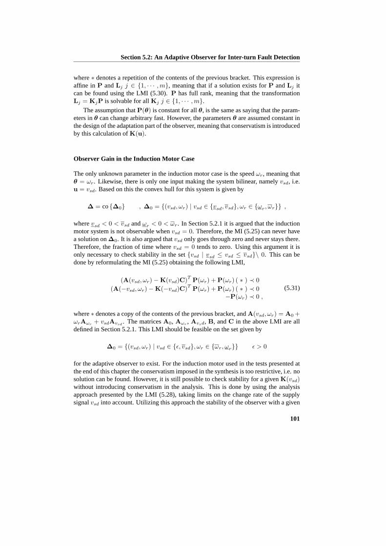
Section 5.2: An Adaptive Observer for Inter-turn Fault Detection
where∗ denotes a repetition of the contents of the previous bracket. This expression isaffine inP andLj j ∈ {1, · · · , m}, meaning that if a solution exists forP andLj itcan be found using the LMI (5.30).P has full rank, meaning that the transformationLj = KjP is solvable for allKj j ∈ {1, · · · ,m}.
The assumption thatP(θ) is constant for allθ, is the same as saying that the param-eters inθ can change arbitrary fast. However, the parametersθ are assumed constant inthe design of the adaptation part of the observer, meaning that conservatism is introducedby this calculation ofK(u).
Observer Gain in the Induction Motor Case
The only unknown parameter in the induction motor case is the speedωr, meaning thatθ = ωr. Likewise, there is only one input making the system bilinear, namelyvsd, i.e.u = vsd. Based on this the convex hull for this system is given by
∆ = co{∆0} , ∆0 = {(vsd, ωr) | vsd ∈ {vsd, vsd}, ωr ∈ {ωr, ωr}} ,
wherevsd < 0 < vsd andωr < 0 < ωr. In Section 5.2.1 it is argued that the inductionmotor system is not observable whenvsd = 0. Therefore, the MI (5.25) can never havea solution on∆0. It is also argued thatvsd only goes through zero and never stays there.Therefore, the fraction of time wherevsd = 0 tends to zero. Using this argument it isonly necessary to check stability in the set{vsd | vsd ≤ vsd ≤ vsd}\ 0. This can bedone by reformulating the MI (5.25) obtaining the following LMI,
(A(vsd, ωr)−K(vsd)C)T P(ωr) + P(ωr) ( ∗ ) ≺ 0(A(−vsd, ωr)−K(−vsd)C)T P(ωr) + P(ωr) ( ∗ ) ≺ 0
−P(ωr) ≺ 0 ,
(5.31)
where∗ denotes a copy of the contents of the previous bracket, andA(vsd, ωr) = A0 +ωrAωr + vsdAvsd
. The matricesA0, Aωr , Avsd, B, andC in the above LMI are alldefined in Section 5.2.1. This LMI should be feasible on the set given by
∆0 = {(vsd, ωr) | vsd ∈ {ε, vsd}, ωr ∈ {ωr, ωr}} ε > 0
for the adaptive observer to exist. For the induction motor used in the tests presented atthe end of this chapter the conservatism imposed in the synthesis is too restrictive, i.e. nosolution can be found. However, it is still possible to check stability for a givenK(vsd)without introducing conservatism in the analysis. This is done by using the analysisapproach presented by the LMI (5.28), taking limits on the change rate of the supplysignalvsd into account. Utilizing this approach the stability of the observer with a given
101
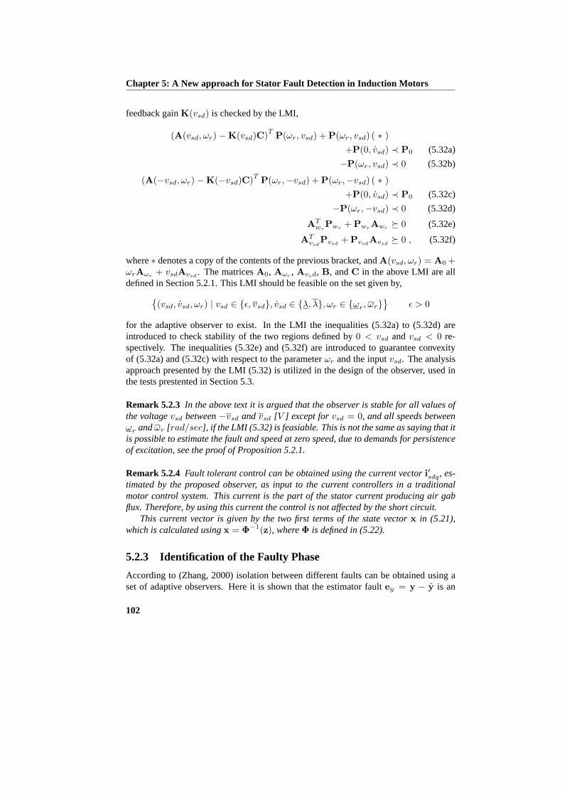
Chapter 5: A New approach for Stator Fault Detection in Induction Motors
feedback gainK(vsd) is checked by the LMI,
(A(vsd, ωr)−K(vsd)C)T P(ωr, vsd) + P(ωr, vsd) ( ∗ )+P(0, vsd) ≺ P0 (5.32a)
−P(ωr, vsd) ≺ 0 (5.32b)
(A(−vsd, ωr)−K(−vsd)C)T P(ωr,−vsd) + P(ωr,−vsd) ( ∗ )+P(0, vsd) ≺ P0 (5.32c)
−P(ωr,−vsd) ≺ 0 (5.32d)
ATwr
Pwr+ Pwr
Awrº 0 (5.32e)
ATvsd
Pvsd+ Pvsd
Avsdº 0 , (5.32f)
where∗ denotes a copy of the contents of the previous bracket, andA(vsd, ωr) = A0 +ωrAωr
+ vsdAvsd. The matricesA0, Aωr
, Avsd, B, andC in the above LMI are alldefined in Section 5.2.1. This LMI should be feasible on the set given by,
{(vsd, vsd, ωr) | vsd ∈ {ε, vsd}, vsd ∈ {λ, λ}, ωr ∈ {ωr, ωr}
}ε > 0
for the adaptive observer to exist. In the LMI the inequalities (5.32a) to (5.32d) areintroduced to check stability of the two regions defined by0 < vsd andvsd < 0 re-spectively. The inequalities (5.32e) and (5.32f) are introduced to guarantee convexityof (5.32a) and (5.32c) with respect to the parameterωr and the inputvsd. The analysisapproach presented by the LMI (5.32) is utilized in the design of the observer, used inthe tests prestented in Section 5.3.
Remark 5.2.3 In the above text it is argued that the observer is stable for all values ofthe voltagevsd between−vsd andvsd [V ] except forvsd = 0, and all speeds betweenωr andωr [rad/sec], if the LMI (5.32) is feasiable. This is not the same as saying that itis possible to estimate the fault and speed at zero speed, due to demands for persistenceof excitation, see the proof of Proposition 5.2.1.
Remark 5.2.4 Fault tolerant control can be obtained using the current vectori′sdq, es-timated by the proposed observer, as input to the current controllers in a traditionalmotor control system. This current is the part of the stator current producing air gabflux. Therefore, by using this current the control is not affected by the short circuit.
This current vector is given by the two first terms of the state vectorx in (5.21),which is calculated usingx = Φ−1(z), whereΦ is defined in (5.22).
5.2.3 Identification of the Faulty Phase
According to (Zhang, 2000) isolation between different faults can be obtained using aset of adaptive observers. Here it is shown that the estimator faultey = y − y is an
102
Section 5.3: Test Results
indicator of the correctness of the model used in the observer design. This means thatwhen only one of the observer faults approximate zero it indicates that the fault modelledby this particular observer has happened in the system. This approach can, in the caseof the induction motor, be used if three identical observers are designed, each detectinga stator winding fault in one of the three phases. This is considered in the following.
The adaptive observerOa in (5.24), is capable of estimating an inter-turn fault inphasea. However, the same observer can be used to estimate a fault in phaseb andcby using another phase sequence as argument in the transformationTdq0. To estimate afault in phaseb the following transformation must be used,
vsdq0 = Tdq0vsbca isdq0 = Tdq0isbca ,
wherexsbca =[xsb xsc xsa
]Tandx ∈ {v, i}. When these signal vectors are used
as input to the observer in (5.24), the observer can estimate faults in phaseb, and istherefore calledOb. Likewise, an observerOc for estimating inter-turn faults in phasecis found by using yet another phase sequence resulting in the following transformations,
vsdq0 = Tdq0vscab isdq0 = Tdq0iscab .
Using these transformations in the approach presented in (Zhang, 2000) the overall struc-ture of the fault identification and estimation algorithm becomes as depitched in Fig. 5.2.Here the error signalseya, eyb andeyc are used for identification of the phase affectedby a inter-turn fault, andxa, xb and xc are the estimates of the states including theestimates of the fault currentif and the fault sizeγ.
The affected phase is in this work identified by comparing the square error, of eacherror signaleya, eyb andeyc, with a predefined threshold value. The square error iscalculated usingeT
i ei.
Remark 5.2.5 The approach used here is based on a predefined threshold value. Thisthreshold must be chosen as a trade-off between how small a fault can be detected androbustness in the system. However, the problem of choosing this threshold can be over-come by comparing the square error of the three error signalseya, eyb, andeyc. If thelevels of these error signals are alike no fault has occurred, and if a fault has occuredit is identified by the signal with the smallest square error. However, using these ap-proaches you cannot be sure to identify the correct fault, you will just identify the faultmost likely to have occured among the modelled faults.
5.3 Test Results
In this section the identification and estimation approaches described in the previoussection are tested on an induction motor setup, where inter-turn stator faults can be sim-ulated. The electrical circuit of the stator is shown in Fig. 5.3. The motor used in the
103

Chapter 5: A New approach for Stator Fault Detection in Induction Motors
Motor Pump
ω r
T l
Q,H V
s i s
Software algorithm
Real world
Observer
O b
Observer
O c
abc
abc
abc
bca
abc
cab
i s
x b
i s
x c
-
-
e yb
e yc
Observer
O a
i s
x a
- e ya
Figure 5.2: The structure of the identification algorithm for identification and estimationof inter-turn short circuits. Hereeya, eyb and eyc are used for identification of theaffected phase, andxa, xb andxc are the estimates of the states including the estimatesof the fault currentif and the fault sizeγ.
tests is a 1.5 [KW] customized Grundfos motor, supplied with a Danfoss frequency con-verter. The speed, the three phase currents, and the three phase voltages are available atthe test setup. The voltage to the motor is controlled using a linear voltage to frequencyrelation, with a voltage boost at low frequencies. All tests are preformed at supply fre-quencies around 30 [Hz] to avoid too large short circuit currents and thereby burnout ofthe motor during the tests. The tests are performed with the induction motor connectedin a ∆-connection as it is shown Fig. 5.3. However, similar results can be found for aY-connected motor in (Kallesøe et al., 2004c).
In the first, of the two following subsections, the identification capabilities of theproposed algorithm are tested. In the second subsection the estimation capabilities of theadaptive observer are tested. In these tests the algorithm is tested against three differentoperating conditions. These are,
• Constant speed at 25 [Hz] supply frequency and balanced supply voltage.
• Speed changes at every 1 second between 25 and 40 [Hz] and balanced supplyvoltage.
• Constant speed at 25 [Hz] supply frequency and a 5 % voltage decrease in phase
104
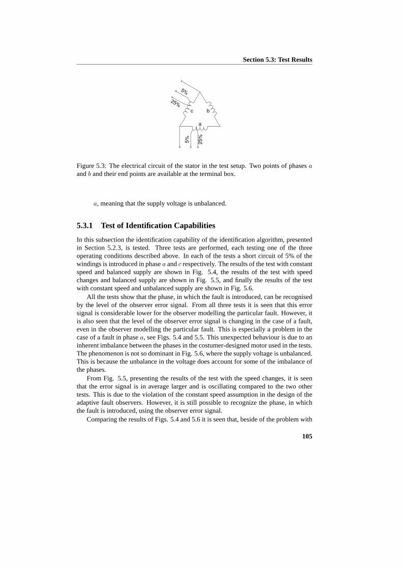
Section 5.3: Test Results
a
25%
5%
25%
5%
b c
Figure 5.3: The electrical circuit of the stator in the test setup. Two points of phasesaandb and their end points are available at the terminal box.
a, meaning that the supply voltage is unbalanced.
5.3.1 Test of Identification Capabilities
In this subsection the identification capability of the identification algorithm, presentedin Section 5.2.3, is tested. Three tests are performed, each testing one of the threeoperating conditions described above. In each of the tests a short circuit of 5% of thewindings is introduced in phasea andc respectively. The results of the test with constantspeed and balanced supply are shown in Fig. 5.4, the results of the test with speedchanges and balanced supply are shown in Fig. 5.5, and finally the results of the testwith constant speed and unbalanced supply are shown in Fig. 5.6.
All the tests show that the phase, in which the fault is introduced, can be recognisedby the level of the observer error signal. From all three tests it is seen that this errorsignal is considerable lower for the observer modelling the particular fault. However, itis also seen that the level of the observer error signal is changing in the case of a fault,even in the observer modelling the particular fault. This is especially a problem in thecase of a fault in phasea, see Figs. 5.4 and 5.5. This unexpected behaviour is due to aninherent imbalance between the phases in the costumer-designed motor used in the tests.The phenomenon is not so dominant in Fig. 5.6, where the supply voltage is unbalanced.This is because the unbalance in the voltage does account for some of the imbalance ofthe phases.
From Fig. 5.5, presenting the results of the test with the speed changes, it is seenthat the error signal is in average larger and is oscillating compared to the two othertests. This is due to the violation of the constant speed assumption in the design of theadaptive fault observers. However, it is still possible to recognize the phase, in whichthe fault is introduced, using the observer error signal.
Comparing the results of Figs. 5.4 and 5.6 it is seen that, beside of the problem with
105

Chapter 5: A New approach for Stator Fault Detection in Induction Motors
0 5 10 150
1
2
3
4
e A
0 5 10 150
1
2
3
4
e B
0 5 10 150
1
2
3
4
e C
time [sec]
Turn fault
in phase a
Turn fault
in phase c
Figure 5.4: The mean square error of the observersOa, Ob, andOc respectively. Inthis test the speed is constant and the supply voltage is balanced, and faults are imposedseperately in phasea andc.
the inherent imbalance in the phases, the results are comparable. This shows that thealgorithm is able to handle unbalanced supply conditions, which also was expected asno assumption were put on the supply voltage in the design. This means that the observercan manage any distortion of the supply voltage as long as it does not introduce too largeoscillations in the speed.
5.3.2 Test of Estimation Capabilities
In this subsection the estimation capability of the adaptive observer, derived in the pre-vious section, is tested. The observer is tested under the three different operating con-ditions described in the start of this section. In each of the tests the algorithm is testedwith no short circuit, 5% of the windings short circuited, and 25% of the windings shortcircuited in phasea. The results of the test with constant speed and balanced supplyare shown in Fig. 5.7(a) and 5.7(b). The results of the test with speed changes and bal-anced supply are shown in Fig. 5.8(a) and 5.8(b), and finally the results of the test withconstant speed and unbalanced supply are shown in Fig. 5.9(a) and 5.9(b).
All the tests have shown that the observer is stable. From the first test, presented inFig. 5.7(a) and 5.7(b), it is seen that the speed is estimated without any bias. It is alsoseen that there is a bias on the estimated fraction of turns in the short circuit. This bias is
106

Section 5.4: Conclusion
0 5 10 150
1
2
3
4
e A
0 5 10 150
1
2
3
4
e B
0 5 10 150
1
2
3
4
e C
time [sec]
Turn fault
in phase a
Turn fault
in phase c
Figure 5.5: The mean square error of the observersOa, Ob, andOc respectively. Inthis test the speed is variating and the supply voltage is balanced, and faults are imposedseperately in phasea andc.
partly due to noise on the measurements, partly due to mismatch between the real motorparameters and the motor parameters used in the observer, and partly due to the initialimbalance between the three stator phases. This bias is repeated in each of the threetests.
Results from the second test, presented in 5.8(a) and 5.8(b), show that the observeris capable of estimating the wanted quantities despite of speed changes. Still it is seenthat the speed changes affect the estimated amount of turns in the short circuit. This isbecause of the constant speed assumption used in the design. It is, however, still possibleto use the estimate of the fault.
From the results of the last test, presented in 5.9(a) and 5.9(b), it is seen that anunbalanced supply of 5% is not affecting the performance of the observer.
5.4 Conclusion
An adaptive observer for simultaneous estimation of the motor states, the speed, andthe amount of turns in an inter-turn short circuit is proposed. The observer is testedon a customized designed induction motor. The tests have shown that the observer canestimate an inter-turn fault despite of speed changes and unbalanced supply conditions.
107

Chapter 5: A New approach for Stator Fault Detection in Induction Motors
0 5 10 150
1
2
3
4
e A
0 5 10 150
1
2
3
4
e B
0 5 10 150
1
2
3
4
e C
time [sec]
Turn fault
in phase a
Turn fault
in phase c
Figure 5.6: The mean square error of the observersOa,Ob, andOc respectively. In thistest the speed is constant and the supply voltage is unbalanced, and faults are imposedseperately in phasea andc.
This makes the estimation scheme usable in inverter feed induction motor drives, or inmotor applications supplied by a bad grid. Using three of these observers it is shownthat it is possible to identify the phase affected by a given inter-turn short circuit.
The adaptive observer is based on a model of an induction motor including an inter-turn short circuit. This model is a simplification of the model presented in the start ofthis chapter, as the derived model describes the motor behaviour in both the inter-turnand the turn-turn short circuit cases. Moreover, the model describes the motor when itis connected in aY-connection as well as a∆-connection.
Comparing the approach presented here with traditional approaches, the main ad-vance is that the obtained observer is based on a dynamic model of the system. Thismeans that the detection capabilities are not affected by dynamic changes in the elec-trical system. The main drawback of the proposed approach is the need for the motorparameters. However, in the cases where the approach is used in a frequency converterapplication, this problem can be solved by parameter identification methods at start up(Rasmussen, 1995).
The proposed adaptive observer can be used for fault-tolerant control of the inductionmotor, as the impact of the inter-turn short circuit is estimated. This is so because it ispossible to obtain control in the case of an inter-turn short circuit, meaning that it ispossible to control the process, driven by the motor, to a fail-safe mode, or to reduce the
108
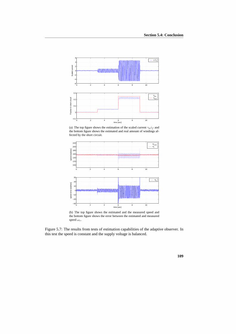
Section 5.4: Conclusion
0 2 4 6 8 10−6
−4
−2
0
2
4
6
Sca
led
curr
ent
γ ⋅ if
0 2 4 6 8 10−0.1
0
0.1
0.2
0.3
Frac
tion
in s
hort
circ
uit
time [sec]
γest
γreal
(a) The top figure shows the estimation of the scaled currentγaif andthe bottom figure shows the estimated and real amount of windings af-fected by the short circuit.
0 2 4 6 8 10
100
120
140
160
180
200
220
spee
d [r
ad/s
ec]
ωr,est
ωr
0 2 4 6 8 10−30
−20
−10
0
10
20
30
spee
d er
ror
[rad
/sec
]
time [sec]
ωe
(b) The top figure shows the estimated and the measured speed andthe bottom figure shows the error between the estimated and measuredspeedωe.
Figure 5.7: The results from tests of estimation capabilities of the adaptive observer. Inthis test the speed is constant and the supply voltage is balanced.
109

Chapter 5: A New approach for Stator Fault Detection in Induction Motors
0 2 4 6 8 10−8
−6
−4
−2
0
2
4
6
8
Sca
led
curr
ent
γ ⋅ if
0 2 4 6 8 10−0.1
0
0.1
0.2
0.3
Frac
tion
in s
hort
circ
uit
time [sec]
γest
γreal
(a) The top figure shows the estimation of the scaled currentγaif andthe bottom figure shows the estimated and real amount of windings af-fected by the short circuit.
0 2 4 6 8 10
150
200
250
300
350
spee
d [r
ad/s
ec]
ωr,est
ωr
0 2 4 6 8 10−30
−20
−10
0
10
20
30
spee
d er
ror
[rad
/sec
]
time [sec]
ωe
(b) The top figure shows the estimated and the measured speed andthe bottom figure shows the error between the estimated and measuredspeedωe.
Figure 5.8: The results from tests of estimation capabilities of the adaptive observer. Inthis test the speed is variating and the supply is balanced.
110

Section 5.4: Conclusion
0 2 4 6 8 10−6
−4
−2
0
2
4
6
Sca
led
curr
ent
γ ⋅ if
0 2 4 6 8 10−0.1
0
0.1
0.2
0.3
Frac
tion
in s
hort
circ
uit
time [sec]
γest
γreal
(a) The top figure shows the estimation of the scaled currentγaif andthe bottom figure shows the estimated and real amount of windings af-fected by the short circuit.
0 2 4 6 8 1080
100
120
140
160
180
200
220
spee
d [r
ad/s
ec]
ωr,est
ωr
0 2 4 6 8 10−30
−20
−10
0
10
20
30
spee
d er
ror
[rad
/sec
]
time [sec]
ωe
(b) The top figure shows the estimated and the measured speed andthe bottom figure shows the error between the estimated and measuredspeedωe.
Figure 5.9: The results from tests of estimation capabilities of the adaptive observer. Inthis test the speed is constant and the supply voltage is unbalanced.
111

Chapter 5: A New approach for Stator Fault Detection in Induction Motors
level of the current in the short circuit, and thereby increase the time from the occurrenceof the inter-turn short circuit to a stator burnout.
112

Chapter 6
A New Approach for FDI inCentrifugal Pumps
The topic of this chapter is FDI on the hydraulic and mechanical part of the centrifugalpump. The model-based approach is used for this purpose, meaning that a set of residualgenerator are developed, each based on the centrifugal pump model presented in Chapter3. The centrifugal pump model is highly nonlinear, which is why methods based ona linearization of the model will, in general, fail to work on a larger area around theoperating point of the linearization. Therefore nonlinear methods should be considered,when the operating point is changed frequently or is unknown. In a lot of applicationsthis is infact the case.
Beside robustness with respect to the operating point, it is important that the algo-rithms do not depend on knowledge of the application of the pump. This means that thedeveloped algorithms should work in spite of the hydraulic system in which the pumpis placed. The Structural Analysis (SA) (Blanke et al., 2003; Izadi-Zamanabadi, 2001;Izadi-Zamanabadi and Staroswiecki, 2000) is a tool designed to identify subsystems,which are independent of the rest of the system. Therefore this tool will be chosen foridentification of subsystems, which can be used for FDI on the centrifugal pump in arobust manner.
The common way to obtain residual generators from subsystem identified using SAis to derive Analytical Redundance Relations (ARR) (Blanke et al., 2003). Unfortu-nately, in general the derived ARR’s are functions of the derivatives of the measurementsin the system. These are normally not known and are difficult to calculate. To overcomethis problem a novel method to derived state space realizations of the subsystems iden-tified using SA is developed in this chapter. Using this method the obtained state spacerealizations are decoupled from any unknown algebraic variables or inputs. Therefore,the decoupling problem is solved and the only remaining problem is to design a stableresidual observer.
113

Chapter 6: A New Approach for FDI in Centrifugal Pumps
The chapter starts by presenting some preliminaries on SA in Section 6.1. Then thestate space realization, developed in this work, is described in Section 6.2. After that FDIon the centrifugal pump is considered. This is done by presenting the model of the pumpin Section 6.3, followed by the results obtained using SA in Section 6.4. One of the re-sults of the SA is that the system can be splitted into two cascade connected subsystems,of which only the second is affected by the mechanical and hydraulic faults consideredin this chapter. Therefore only an observer has to be considered for the first subsys-tem. This observer must observe the connecting variables between the two subsystems.The design of this observer is described in Section 6.5. In Section 6.6 the design of theresidual observers are considered. These observers are based on results obtained usingSA on the second subsystem, and the realization theory developed in Section 6.2 of thechapter. Test results obtained on an industrial test-bench, which has been particularlydeveloped for this purpose, are presented in Section 6.7. Finally, concluding remarksend the chapter.
6.1 Preliminaries: Structural Analysis
Structural Analysis (SA) is the study of the system properties, which are independentof the actual values of the parameters. Only links between the variables and parametersare represented in this analysis. These links result from the operating model and arecalled relations or constraints. They are independent of the operating model and arethus independent of the form under which this operating model is expressed (qualitativeor quantitative data, analytical or non-analytical relations). The links are representedby a graph, on which a structural analysis is performed (Blanke et al., 2003; Izadi-Zamanabadi, 2001; Izadi-Zamanabadi and Staroswiecki, 2000). In this section some ofthe most important definitions and theorems of SA are presented. The presentation isbased on (Blanke et al., 2003).
In SA a system is described by a set of variablesZ and a set of constraintsC. Eachconstraint inC describes the connection between a subset of the variables inZ, mean-ing that the equations and differential equations describing the system form the set ofconstraints. The definition of a system of this form is given below.
Definition 6.1.1 (System structure)(Blanke et al., 2003) A systemS is defined by twosetsC andZ, where,
• Z is the set of variables in the system.
• C is the set of constains in the system connecting the variables of the system.
The following three assumptions must hold on the constraintsC in S for the SA al-gorithms to work. Before these assumptions are presented, letZc = Q(c) denote thevaribles constrained byc and letnc = |Q(c)| be the number of variables inc.
114

Section 6.1: Preliminaries: Structural Analysis
c 1
c 2
c 3
x 1
x 1
x 2
x 2
u
c 4
(a) Graph representation.
K X
u x1 x1 x2 x2
c1 1 1c2 1 1c3 1 1c4 1 1 1 1
(b) Table representation.
Figure 6.1: Structural representation of the connection between set of equations denotedconstraintc1 to c4, and the set of variablesZ = {u, x1, x1, x2, x2}. HereK = {u} isthe known variable, andX = {x1, x1, x2, x2} is the set of unknown variables.
Assumption 6.1.1 (Blanke et al., 2003, Ass. 5.1) Any algebraic constraintc ∈ C definesa manifold of dimensionnc − 1 in the space of the variablesQ(c).
Assumption 6.1.2 (Blanke et al., 2003, Ass. 5.2) All the constraints inC are compati-ble.
Assumption 6.1.3 (Blanke et al., 2003, Ass. 5.3) All the constraints inC are indepen-dent.
The structural model ofS, defined in Definition 6.1.1, is a model describing the connec-tion between the variablesZ and the constraints inC by a bi-partite graph. This graph isdefined in the following definition.
Definition 6.1.2 (Structural model) (Blanke et al., 2003, Sec. 5.2) The structuralmodel (or the structure) of the system(C, Z) is a bi-partite graph(C, Z, E) whereE ⊆ C× Z is the set of edges defined by:
(ci, zj) ∈ E if the variablezj ∈ Z appears in the constaintci ∈ C.
An example of such a bi-partite graph is shown in Fig. 6.1. Both a graphical and a tablerepresentation of the the graph are shown here. Using the bi-partite graphs defined inDefinition 6.1.2 the structure of the model equations forming the set of constraintsC canbe analysed. Two important properties in this analysis areReachabilityandMatching.These are defined in the following definitions.
Definition 6.1.3 (Reachability)(Blanke et al., 2003, Def. 5.8) A variablez2 is reach-able from a variablez1 if there exists an alternated chain fromz1 to z2 in the graph(C, Z,E). A variablez2 is reachable from a subsetX ⊆ Z\{z2} if the existsz1 ∈ X
115

Chapter 6: A New Approach for FDI in Centrifugal Pumps
such thatz2 is reachable fromz1. A subset of variablesZ2 is reachable from a subset ofvariablesZ1 if any variable ofZ2 is reachable fromZ1.
Definition 6.1.4 (Matching) (Blanke et al., 2003) A matchingM is a subset of theedgesE such that the endpoints of the edges have no common vertices, i.e.
∀ei, ej ∈M : ei = (a, b), ej = (α, β), thena 6= α, b 6= β.
Definition 6.1.5 (Complete matching)(Blanke et al., 2003) A matching is called com-plete with respect toC if |M| = |C| holds. A matching is called complete with respectto Z if |M| = |Z|.When there exist a complete matching with respect to the unknown variablesX ⊂ Z
in the system, it means that, in almost all cases, these variables can be eliminated byrewriting the system equations. To ensure this property the notation of calculability isused. Calculability is defined in the following definition.
Definition 6.1.6 (Calculability) (Izadi-Zamanabadi and Staroswiecki, 2000) Letzi,i = 1, · · · , p, · · · , n be variables, which are related through a constraintci, e.g.ci(z1, · · · , zn). The variablezp is calculable if its value can be determined throughthe constraintci under the condition that the values of the other variableszj , j =1, · · · , n , j 6= p are known.
When a matching of an unknown variable is done under the calculability constraint itis possible to calculate the given unknown variable in the space where the calculabil-ity condition is fulfilled. Unfortunately, this is not enough to state that a matching,where all the unknown variables are calculable, implies that all unknown variables canbe eliminated. This fact will be considered later when the notation of causal matches isconsidered.
To connect the definitions given above to a system description as known from systemtheory, let a dynamic systemS be described by the following set of equations,
S :
Cf : xd = fx(xd,xa,u)Cm : 0 = mx(xd,xa,u)Ch : y = hx(xd,xa,u)Cd : dxd
dt = xd
, (6.1)
where the set of variablesZ = xd ∪ xd ∪ xa ∪ u ∪ y. Z can be decomposed into aset of unknown variablesX = xd ∪ xd ∪ xa and a set of known variablesK = u ∪ y.The constaintsC of system (6.1) are given by the setC = Cf ∪ Cm ∪ Ch ∪ Cd. Thestructural model of this system is shown in Table 6.1. HereG, Fi,Mi,Hi are booleanmatrices describing the connections between the variablesZ and the constaintsC. I isthe identity matrix andX is a diagonal matrix denoting thatxd can only be calculatedform xd up to an unknown but constant offset.
116

Section 6.1: Preliminaries: Structural Analysis
Table 6.1: Incident matrix of a structural graph. This structural graph is a graph of aminimal over-constrained system, which can be a subsystem of a larger system.
yT uT xTd xT
d xTa
fx 0 G I F1 F2
mx 0 M3 0 M1 M2
hx I H3 0 H1 H2
dx 0 0 I X 0
The structural model presented in Table 6.1 of the systemS can have, but does notalways have, one of following three properties,
Definition 6.1.7 (Over-constrained graph)(Blanke et al., 2003, Def. 5.9) A graph(C, Z,E) is called over-constained if there is a complete matching on the variablesZ
but not on the constaintsC.
Definition 6.1.8 (Just-constrained graph)(Blanke et al., 2003, Def. 5.10) A graph(C, Z,E) is called just-constained if there is a complete matching on the variablesZ
and on the constaintsC.
Definition 6.1.9 (Under-constrained graph)(Blanke et al., 2003, Def. 5.11) A graph(C, Z,E) is called under-constained if there is a complete matching on the constaintsC
but not on the variablesZ.
In the cases where the systemS fails to conform to any of the three above properties,it can be proven that there exists a unique decomposition ofS into three subsystems(Blanke et al., 2003),
S+ = (C+, Z+)S0 = (C0, Z+ ∪ Z0)S− = (C−,Z+ ∪ Z0 ∪ Z−),
whereC = C− ∪ C0 ∪ C+ andZ = Z− ∪ Z0 ∪ Z+. For this decomposition the sub-systems(C+,Z+), (C0, Z0), and(C−, Z−) are over-constrained, just-constrained, andunder-constrained respectively. On the over-constrained and just-constrained subsys-tems the notion of causality is important, as it is used to state the conditions for structuralobservability. Causality is defined in the following definition.
Definition 6.1.10 (Causality)(Blanke et al., 2003) A subsystem is called causal if thereexists an alternating chain fromki ∈ K to xj ∈ X for all reachablexj ∈ X and thischain is composed of only calculable matchings.
117
Chapter 6: A New Approach for FDI in Centrifugal Pumps
A special and very important over-constrained subsystem is defined in the followingdefinition.
Definition 6.1.11 (Minimal over-constrained subsystem)(Izadi-Zamanabadi, 2001,Def. 4) A minimal over-constrained subsystem,Smin = (Cmin, Zmin) is an over-constrained subsystem with the following property:
|Cmin| = 1 + |Xmin| (6.2)
whereXmin ⊆ Zmin are the unknown variables contained in the set of constraintsCmin. Additionally,Cmin ⊆ C andZmin ⊆ Z.
Such a minimal over-constrained subsystem contains information enough to derived ex-actly one residual. Therefore, if a set of minimal over-constrained subsystems is identi-fied in a system, and the matchings, which define each of these subsystems, are causal,a set of residual generators can be derived. When the residual generators are derivedby eliminating all unknown variables in the subsystem they are called Analytical Re-dundant Relations (ARR). If each of these residual generators are sensitive to differentsubsets of the faults affecting the system this can be used for fault identification. This isformalized in the following two theorems.
Theorem 6.1.1 (Structural observability)(Blanke et al., 2003, The. 5.2) A necessaryand sufficient condition for system (6.1) to be structural observable is that, under deriva-tive causality
1. all the unknown variablesX are reachable from the known ones,
2. the over-constrained and the just-constrained subsystems are causal,
3. the under-constrained subsystem is empty.
For systems which are structural observable as stated in Theorem 6.1.1, and where theover-constraint subsystem is non empty, it is always possible to identify a number ofminimal over-constraint subsystems, as defined in Definition 6.1.11.
Let one of the constraintsϕ ∈ C be corrupted by a fault. Let the unknown variablescontainted in the constraint be given byXϕ = Q(ϕ). Then the following theorem statesthe conditions for the fault corrupting the constraintϕ to be monitorable or detectable.
Theorem 6.1.2 (Monitorability) (Blanke et al., 2003, The. 5.3) Two equivalent neces-sary conditions for a faultϕ to be monitorable are:
(i) Xϕ is structural observable - according to Theorem 6.1.1 - in the system(C\{ϕ}, Z),
(ii) ϕ belongs to the structurally observable over-constrained part of the system(C,Z).
118

Section 6.2: Realization
Algorithms exist, which can decompose a systemS into all possible minimal over-constraint subsystems. For each of these minimal over-constraint subsystems the con-nectionnc = nx +1 holds, wherenc = |C| is the number of constraints andnx = |X| isthe number of unknown variables in these constraints (Izadi-Zamanabadi, 2001; Izadi-Zamanabadi and Staroswiecki, 2000). It is possible to derive an Analytical RedundantRelation (ARR) for each of these subsystems. Each of these ARR can be used to gen-erate one residual, which is sensitive to a subset of the faults in the systemS (Blankeet al., 2003). The connection between the subsystem used in the derivation of a givenARR and the faults is described by Theorem 6.1.2.
6.2 Realization
Realization denotes the task of finding a description of an over-constrained subsystem,identified using SA, which can be used for residual generation. A straightforward wayto find such a residual generator, is to solve the set of constraintsC, forming the sub-system, for the unknown variablesX in this set of constraints. The solution obtainedusing this approach is an Analytical Redundant Relation (ARR) (Blanke et al., 2003).Unfortunately in general the obtained ARR’s are functions of the derivatives of the mea-surements, which are in general not calculable due to measurement noise.
To overcome the problem with the derivatives in the ARR’s, a new approach is devel-oped here. The main idea is to find a state space description of the subsystem identifiedusing SA, meaning that the subsystem can be described on the form,
dzdt = fz(z,y,u)
gz(y,u) = hz(z,y,u) ,(6.3)
wherez contains the states of the system, andu andy contain the known signals in thesystem. If a state space description (6.3) exists it can be used in the development of anobserver, which enables residual generation. The decoupling of unknown inputs has notto be considered in this observer design, as this problem is already solved using SA andthe realization techniques presented here.
Assuming that an over-constrained subsystem identified using SA is described bythe following set of equations,
Sx :
xd = fx(xd,xa,u)0 = mx(xd,xa,u)y = hx(xd,xa,u)
dxd
dt = xd
, (6.4)
wherexd(t), xd(t) ∈ Rn, xa(t) ∈ Rl, u(t) ∈ Rp andy(t) ∈ Rd. fx, mx, andhx aresufficiently smooth maps.fx is denoted a map, as thexd is considered a free variableconstraint by the derivative constraintdxd
dt = xd, in SA. Finally,u andy are the knowninput and output signals respectively, andxd, xd, andxa are unknown signals.
119

Chapter 6: A New Approach for FDI in Centrifugal Pumps
Let the subsystem, identified using SA, be given by(C, Z), then each equation in(6.4) is given by a constraint inC. Likewise, the variablesu,y ⊂ K andxd, xd,xa ⊂ X
are the known and unknown variables respectively. These variables form the setZ, i.e.Z = K ∪ X. The graph representation of this system is shown in Table 6.2, where
Table 6.2: Incident matrix of a structural graph. This structural graph is a graph of aminimal over-constrained system, which can be a subsystem of a larger system.
y u xd xd xc
fx 0 G I F1 F2
mx 0 M3 0 M1 M2
hx I H3 0 H1 H2
dx 0 0 I X 0
G,Fi,Mi, Hi are boolean matrices describing the connection between the variablesZ
and the constaintsC. I is the identity matrix andX is a diagonal matrix denoting thatxd can only be calculated formxd up to a constant offset.
In the following a method is presented, which can be used to obtain the state spacedescription (6.3) from the over-constraints subsystem (6.4). To obtain this state spacedescription all the unknown algebraic variablesxa must be eliminated, or in other wordsa state and/or output transformation must be found such that the unknown signalsxa aredecoupled from the residual output. When such a state space description exists a residualobserver or residual filter of the following form can be obtained,
dzdt = fz(z,y,u)− k(z,y,u)(gz(y,u)− hz(z,y,u))r = q(gz(y,u)− hz(z,y,u)) .
Here it is assumed that a stabilizing feedbackk can be found. In the above equationris the set of residual outputs,u is a set of known signals defined as input in the originalsystem,y is the set of known signals defined as outputs in the original system, andzcontains the states of the residual filter. If the subsystem is a minimal over-constraintsubsystem the residualr becomes a scalarr. This is infact normally the case.
In the following, first an output transformation is considered, eliminating a part ofthe algebraic variablesxa. The remaining algebraic variables are eliminated using astate transformation. This is considered in Section 6.2.2. Finally, the two eliminationapproaches are composed into one algorithm in Section 6.2.3.
6.2.1 Output Transformation
In this subsection the eliminations of the algebraic variablesxa, using only the algebraicconstraints of system (6.4), is considered, i.e. the set of constraints formed bymx andhx are used. If the causal match, found using SA, shows that a subset of the variables in
120
Section 6.2: Realization
xa denotedxa1 and a subset of the variablesxd denotedxd1 are matched usingmx andhx. Then there must exist an explicite solution to these variables usingmx andhx. Letthis solution be given by,
(xa1
xd1
)=
(g1(xd2,xa2,y,u)g2(xd2,xa2,y,u)
),
wherexa,xd are partitioned such thatxa =(xT
a1 xTa2
)T, xd =
(xT
d1 xTd2
)T. This
proves the following lemma.
Lemma 6.2.1 Letxa =(xT
a1 xTa2
)Tandxd =
(xT
d1 xTd2
)Tbe partitioned such that
xa1 andxd1 are the unknown variables matched by the set of constraintsmx ∪hx, thenthere must exist explicite solutions forxa1 andxd1. Let these solutions be denoted by,
xa1 = g1(xd2,xa2,y,u)xd1 = g2(xd2,xa2,y,u) ,
(6.5)
The above Lemma states that a solution exists for a subset of the algebraic variablesxa
and a subset of the state variablesxd in the system, without introducing derivatives ofany known variables, i.e. variables inK. This solution can be used for elimination ofthese variables. Moveover under the following assumption an output transformation canbe found, which has the property that the known and unknown variables in the outputexpression are separated.
Assumption 6.2.1 It is assumed that the expressiong2 in Lemma 6.2.1 exists and canbe rewritten to become,
ho(xd) = go(y,u) , xd =(xT
d1 xTd2
)T. (6.6)
Assumption 6.2.1 states that the algebraic variables matched by the algebraic constraintsmx andhx can be eliminated using these. For linear systems, this is the same as assum-ing that disturbances in the output equation are decoupled using a transformation of theoutput, e.i.Qy = QCx + QEdd whereQEd = 0.
Under Assumption 6.2.1 the following theorem can be used to derive a state spacedescription where all unknown algebraic variables are contained in the differential equa-tions.
Theorem 6.2.1 (Output Transformation)If a causal match exists on an over-constrainedsubsystem on the form given in (6.4), then if Assumption 6.2.1 holds for this system, itcan be rewritten to the following form,
So :{
dxd
dt = fo(xd,xa2,y,u)go(y,u) = ho(xd) ,
(6.7)
wherexa2 is a vector of algebraic variables.
121

Chapter 6: A New Approach for FDI in Centrifugal Pumps
Proof: Using Lemma 6.2.1 and Assumption 6.2.1 the set of constraintsmx∪hx can be rewrittento become,
xa1 = g1(xd2,xa2,y,u)ho(xd) = go(y,u) ,
(6.8)
wherexa =(xT
a1 xTa2
)Tandxd =
(xT
d1 xTd2
)T. Using the first expression (6.8) to eliminate
the variablesxa1 in fx in (6.4) it becomes,
dxddt
= fo(xd,xa2,y,u).
Choose the second expression in (6.8) as the output equation, system (6.7) is obtained.¤
In some cases all the algebraic variables in the vectorxa are match using the set ofconstraintsmx ∪ hx. When this is the case all the algebraic variables can be eliminatedusing the output transformation given in Theorem 6.2.1. This is stated in the followingcorollary.
Corollary 6.2.1 (Output Transformation) If a causal match exists on an over-constrained subsystem on the form given in (6.4), then if Assumption 6.2.1 holds forthis system and all algebraic variblesxa are matched usingmx andhx, then the systemcan be rewritten to become,
So :{
dxd
dt = fo(xd,y,u)go(y,u) = ho(xd) .
(6.9)
6.2.2 State Transformation
The theorem and corollary, presented in the previous subsection, deal with the elim-ination of the algebraic variables, using the algebraic constraintsmx and the outputmapshx. In general, it is not possible to eliminate all algebraic variables using theseconstraints. In order to eliminate the remaining algebraic variables a state space trans-formation is required, hence proposed. To be able to perform the state transformationit is required that system (6.7) admits a simpler form as specified by the following as-sumption.
Assumption 6.2.2 The state space description of system (6.7) is of the following form
dxd
dt = f ′o(xd,y,u) + Go(xd)xa2
go(y,u) = ho(xd) ,(6.10)
whereGo(xd) is a(n× l2) matrix with full column rank for allxd ∈ Dxd. It is assumed
thatn > l2 wherel2 is the number of elements inxa2.
122
Section 6.2: Realization
Later, in the proof of the main theorem in this subsection, it will be shown that, for theover-constrained subsystems,Go has full rank always.
The elimination of the algebraic variablesxa2 in (6.10) are dealt with in the follow-ing Lemma.
Lemma 6.2.2 Eliminating algebraic variablesxa2 from the state space description ofsystem (6.10) results in a new system on the form
D(xd)dxd
dt = f ′o(xd,y,u) , (6.11)
whereD is an(n− l2)× n matrix of function ofxd with full row rank.
Proof: Let the state space system (6.10) be scaled by an arbitrary(n× n) matrixD(xd), whichis full rank for allxd ∈ Dxd ⊆ Rn. UsingD on (6.10) the system becomes,
D(xd) dxddt
= D(xd)f ′o(xd,y,u) + D(xd)Go(xd)xa2 .
Design the scaling matrixD such that the following condition is fulfilled,
D(xd)Go(xd) =
[0
Il2×l2
]. (6.12)
The solution can easily be found using the Gauss-Jordan elimination method on the system,
[In×n Go(xd)
] →[
D(xd)
[0
Il2×l2
] ].
When the scaling matrixD is used on the system, it becomes,
D(xd) dxddt
= D(xd)f ′o(xd,y,u) +
[0(n−l2)×l2
Il2×l2
]xa2 . (6.13)
In this expression the first(n − l2) rows are independent ofxa2. This means thatxa2 has beeneliminated in this part of the system. Using the first(n− l2) rows in (6.13) the final expression isobtained,
D(xd) dxddt
= D(xd)f ′o(xd,y,u) = f ′o(xd,y,u)
The matrixD(xd) is formed by the first(n− k2) rows of the matrixD(xd). ¤
The following additional assumption, that is required to prove the main theorem, isintroduced.
Assumption 6.2.3 The following condition for system (6.10) is fulfilled:
Span{∂ho
∂xd(xd)T } ⋃
Ker{Go(xd)T
}(6.14)
must spanRn for all xd ∈ Dxd.
123

Chapter 6: A New Approach for FDI in Centrifugal Pumps
Remark 6.2.1 A linear version of (6.10) is given by the following state space model
dxd
dt = Axd + Bu + Gxa2
y = Cxd .(6.15)
Comparing this expression with (6.10) it is seen that∂ho
∂xd(xd) and Go(xd) in (6.10)
corresponds toC andG in (6.15) respectively. Using these relations Assumtion 6.2.3implies that rank{CG} = rank{G}, which is exactly the demand for existence of anunknown input observer for linear systems (Chen and Patton, 1999, chap. 3).
In the following the main theorem of this section is presented. Using this theorem it ispossible to eliminate the remaining algebraic variablesxa2 in system (6.10).
Theorem 6.2.2 (Realization)By a state transformation, system (6.10) can, under as-sumption 6.2.3, be transformed into a new system of the following form
dzdt = fz(z,y,u) = µ(xd)f ′o(xd,y,u)|xd=Ψ(z,y,u)
go1(y,u) = hz(z,y,u) = ho1(xd)|xd=Ψ(z,y,u) .(6.16)
The inverse state transformationxd = Ψ(z,y,u) is obtained as the local solution to(go2(y,u)
z
)=
(ho2(xd)Φ(xd)
), (6.17)
with output map organized as
go(y,u) = ho(xd) ⇔(go1(y,u)go2(y,u)
)=
(ho1(xd)ho2(xd)
).
The transformationz = Φ(xd) is given by the partial differential equation (p.d.e.),
µ(xd)D(xd) =∂Φ∂xd
, (6.18)
whereD is given by Lemma 6.2.2 andµ(xd) is a l2 × l2 scaling matrix with full rankfor all xd ∈ Dxd
⊆ Rn.
Proof: The proof is done in two steps. In the first step it is shown that allxa2 can be eliminatedin (6.10). In the second step it is shown that under Assumption 6.2.3 there exists a transformationtransforming system (6.10) into (6.16).
Step 1:First it is shown that (6.10) is on a form such that Lemma 6.2.2 can be used in theelimination of the unknown algebraic variablesxa2. To show this, it must be proven thatGo(xd)has full column rank and that the number of rows exceed the number of columns.
System (6.7) is by definition a over-constrained subsystem with the set of constraintsCmin =do ∪ fo ∪ ho and the set of unknown variablesXmin = xd ∪ xd ∪ xa2. Using Definition 6.1.7the following property must hold for (6.7)
|do|+ |fo|+ |ho| = |xd|+ |xd|+ |xa2|+ k ,
124
Section 6.2: Realization
where| · | is the number of elements in the given vector anddo is the set of differential constraints(arranged in a vector) as described in Section 6.1. By definition|do| = |xd|. Moreover, someof the elements inxd must be matched usingho. Let these elements be denotedxd1. Since allconstraints inho are matched we have|xd1| = |ho|, and we get
|fo| = |xd2|+ |xa2|+ k , (6.19)
wherexd =(xT
d1 xTd2
)T. Under Assumption 6.2.2 (6.7) is restricted to be on the form (6.10).
Here the number of columns inGo are given byl2 = |xa2| and the number of rows are given by|f ′o| = |fo|, which is strictly larger than|xa2|, see (6.19). Moreover from the match obtained fromSA it is known thatxa2 can be calculated usingfo, which implies thatGo must have full columnrank. Therefore, using Lemma 6.2.2 system (6.10) can be rewritten to,
D(xd) dxddt
= f ′o(xd,y,u)g(y,u) = ho(xd) .
(6.20)
A method for calculatingD is given in the proof of Lemma 6.2.2. Multiplying the differentialequation (6.20) with the scaling matrixµ, we obtain an expression fordz
dt
dz
dt= µ(xd)D(xd)
dxd
dt= µ(xd)f ′o(xd,y,u) . (6.21)
From this equation it is seen thatΦ is given by the p.d.e.
∂Φ
∂xd= µ(xd)D(xd).
Step 2.:Next it is shown that there exists an expression on the form
(go2(y,u)
z
)=
(ho2(xd)Φ(xd)
), (6.22)
wherego2(y,u) = ho2(xd) contains a subpart of the rows ingo(y,u) = ho(xd). This expres-sion must be solvable for allxd in the system, i.e. a local solution must exists. For this to be truethe inverse function theorem states that the Jacobian determinant of (6.22) must be different fromzero, e.i.
∂
∂xd
(ho2(xd)Φ(xd)
)=
(∂ho2(xd)
∂xd
µ(xd)D(xd)
)(6.23)
must have full rank for allxd ∈ Dxd .Using the proof of Lemma 6.2.2 it can be deduced that Span{(µ(xd)D(xd))T } =
Span{D(xd)T } = Ker{Go(xd)T
}, and thatD(xd) has full row rank for allxd ∈ Dxd . Using
Assumption 6.2.3 it is guaranteed that there exists aho2 ⊆ ho such that∂ho2(xd)∂xd
span thel2
dimensional row space not spanned byD(xd). This implies that the matrix in (6.23) has full rankfor all xd ∈ Dxd , i.e. (6.22) can be solved forxd. Let the solution ofxd be given by
xd = Ψ(z,y,u).
125

Chapter 6: A New Approach for FDI in Centrifugal Pumps
Using this expression in (6.21) the final model becomes
dzdt
= µ(xd)f ′o(xd,y,u)|xd=Ψ(z,y,u)
go1(y,u) = ho1(xd,y,u)|x=Ψ(z,y,u) .
¤
Remark 6.2.2 The question arise about the existence of the solutionz = Φ(x) thatsatisfies (6.18). InR2 the problem can be formilized by
∂Φ∂x
= µ(x)D(x) ⇔ (∂Φ∂x1
∂Φ∂x2
)= µ(x)
(d1(x) d2(x)
)
which implies that,
∂2Φ∂x1∂x2
− ∂2Φ∂x1∂x2
= ∂µd1∂x2
− ∂µd2∂x1
= 0
This expression can be solved forµ (in theR2 case) using the intergrating factor ap-proach (Nagle and Saff, 1996, chap. 2). Whenµ is knownΦ can be found by simpleintergration (this approach is used in the example in Section 6.2.4).
The expression described above, can inR3 be described by
∇Φi(x) = [µ(x)f(x)]i
wherei denotes theith row in (6.18). Using the∇ operator the following expressioncan be obtained
∇×∇Φi(x) = ∇× [µ(x)f(x)]i = 0
Unfortunately, no procedure exists for findingµ(x) in R3.
Remark 6.2.3 In general the existence of a solution to the p.d.e. (6.18) can be treatedusing Frobenius theorem (Isidori, 1995). A discussion on this approach is found in (Friskand Åslund, 2003), which treats the solution to problems similar to (6.18).
6.2.3 Elimination Algorithm
To summarize the results obtained in the previous two subsections, an algorithm isprestented below. This algorithm presents the steps necessary to obtain a state spacedescription of (6.4).
1. First use Theorem 6.2.1 to eliminate a subset of the unknown algebraic variablesxa. If all the algebraic variables can be eliminated using this approach Corollary6.2.1 states the final solution. If this is not the case go to step 2.
126

Section 6.2: Realization
2. Check if Assumptions 6.2.2 and 6.2.3 holds for the system. If it holds go to step 3,else it is not possible to transform the system into a state space description usingthe approach given here.
3. Use Theorem 6.2.2 to obtain the state transformationΨ, and derive the trans-formed system.
4. Finally, to design a residual observer, find a stabilizing feedback for the trans-formed system. This is not treated here.
In this section ideas for developing residual observers using over-constrainted subsys-tems found using SA are presented. Even though deriving residual observers were theaim of the section, it is possible to use the same ideas to identify subsystems which canbe used in the development of reduced order observers. The following theorem can beused to formulate a necessary condition for this to be possible.
Theorem 6.2.3 (Observability and over-constraint subsystems)If a system given by
dxdt = f(x)y = h(x)
(6.24)
is observable for allx ∈ Dx, then there exists an over-constrained match of the unknownvariablesX = x ∪ x using the system constraintsC = h ∪ f ∪ d.
Proof: A necessary but not sufficent condition for system (6.24) to be observable is,
rank
(∂f∂x
(x)∂h∂x
(x)
)= n ∀x ∈ Dx .
This implies that, when (6.24) is observable then allxi i ∈ {1, · · · , n} are containted in eitherf or h. This implies that there exist a match of allxi. When this match existxi can be matchusing the differential constraintsd. The length of bothf andd is n, and the number of unknownvariablesX is 2n. Therefore, there exist|h| more constraints than unknown variables, i.e. thesystem is over-constraint. This completes the proof.¤
Remark 6.2.4 Theorem 6.2.3 states that if system (6.24) is observable, then there existand over-constrained match on the system. Reversing this argument, it can be saidthat if there does not exist an over-constraints subsystem, then there does not exist anobservable state space description of the system.
Remark 6.2.5 The arguments presented in this section does not garantee the existenceof a residual observer or a reduced order observer, as the stability of an observer imple-mentation is not considered here.
127
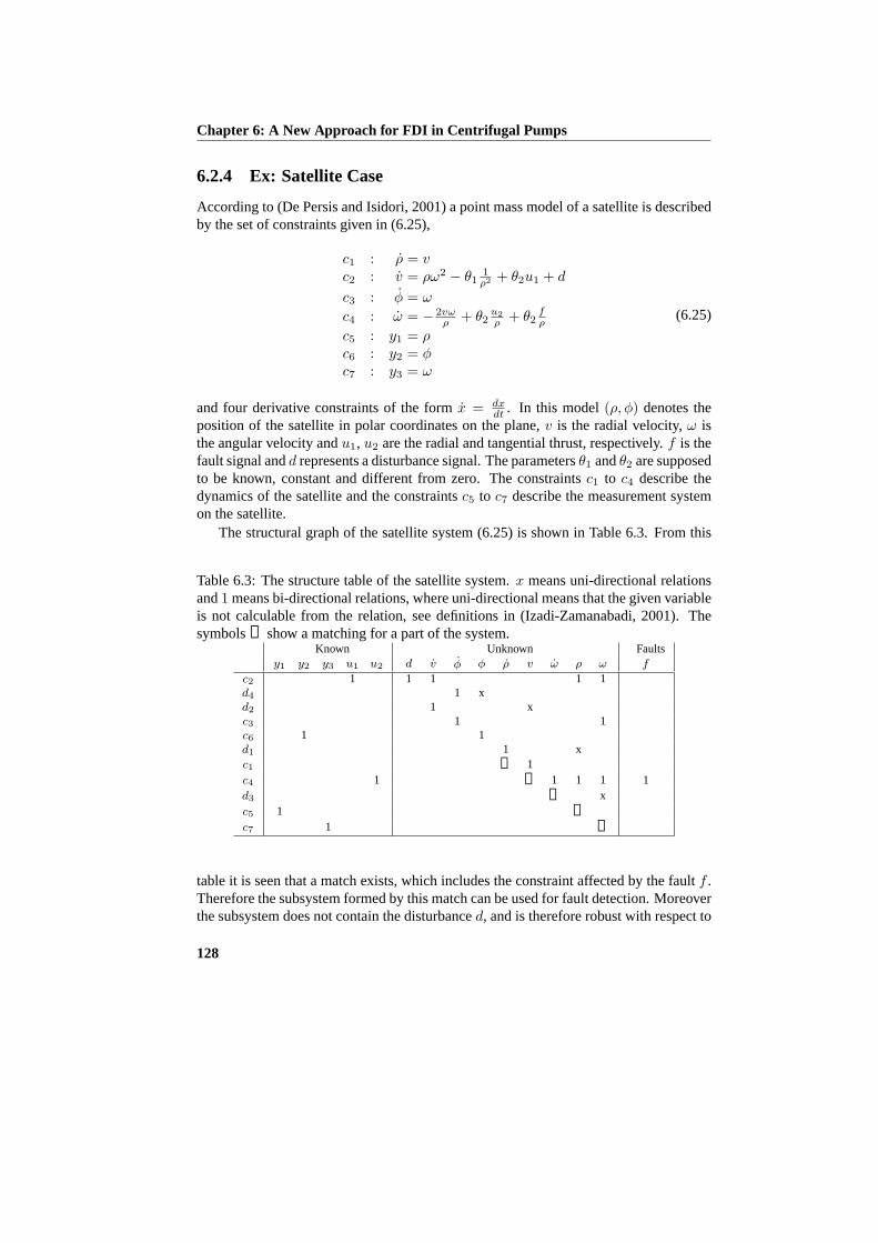
Chapter 6: A New Approach for FDI in Centrifugal Pumps
6.2.4 Ex: Satellite Case
According to (De Persis and Isidori, 2001) a point mass model of a satellite is describedby the set of constraints given in (6.25),
c1 : ρ = vc2 : v = ρω2 − θ1
1ρ2 + θ2u1 + d
c3 : φ = ω
c4 : ω = − 2vωρ + θ2
u2ρ + θ2
fρ
c5 : y1 = ρc6 : y2 = φc7 : y3 = ω
(6.25)
and four derivative constraints of the formx = dxdt . In this model(ρ, φ) denotes the
position of the satellite in polar coordinates on the plane,v is the radial velocity,ω isthe angular velocity andu1, u2 are the radial and tangential thrust, respectively.f is thefault signal andd represents a disturbance signal. The parametersθ1 andθ2 are supposedto be known, constant and different from zero. The constraintsc1 to c4 describe thedynamics of the satellite and the constraintsc5 to c7 describe the measurement systemon the satellite.
The structural graph of the satellite system (6.25) is shown in Table 6.3. From this
Table 6.3: The structure table of the satellite system.x means uni-directional relationsand1 means bi-directional relations, where uni-directional means that the given variableis not calculable from the relation, see definitions in (Izadi-Zamanabadi, 2001). Thesymbols➀ show a matching for a part of the system.
Known Unknown Faultsy1 y2 y3 u1 u2 d v φ φ ρ v ω ρ ω f
c2 1 1 1 1 1d4 1 xd2 1 xc3 1 1c6 1 1d1 1 xc1 ➀ 1c4 1 ➀ 1 1 1 1d3 ➀ xc5 1 ➀c7 1 ➀
table it is seen that a match exists, which includes the constraint affected by the faultf .Therefore the subsystem formed by this match can be used for fault detection. Moreoverthe subsystem does not contain the disturbanced, and is therefore robust with respect to
128
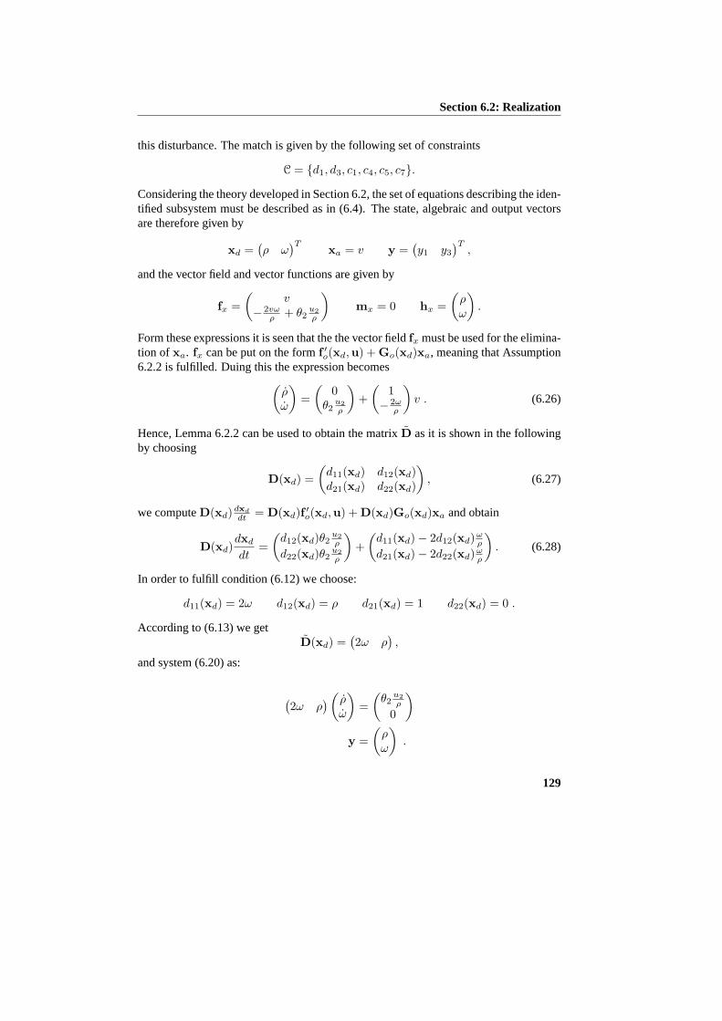
Section 6.2: Realization
this disturbance. The match is given by the following set of constraints
C = {d1, d3, c1, c4, c5, c7}.Considering the theory developed in Section 6.2, the set of equations describing the iden-tified subsystem must be described as in (6.4). The state, algebraic and output vectorsare therefore given by
xd =(ρ ω
)Txa = v y =
(y1 y3
)T,
and the vector field and vector functions are given by
fx =(
v− 2vω
ρ + θ2u2ρ
)mx = 0 hx =
(ρω
).
Form these expressions it is seen that the the vector fieldfx must be used for the elimina-tion of xa. fx can be put on the formf ′o(xd,u) + Go(xd)xa, meaning that Assumption6.2.2 is fulfilled. Duing this the expression becomes
(ρω
)=
(0
θ2u2ρ
)+
(1
− 2ωρ
)v . (6.26)
Hence, Lemma 6.2.2 can be used to obtain the matrixD as it is shown in the followingby choosing
D(xd) =(
d11(xd) d12(xd)d21(xd) d22(xd)
), (6.27)
we computeD(xd)dxd
dt = D(xd)f ′o(xd,u) + D(xd)Go(xd)xa and obtain
D(xd)dxd
dt=
(d12(xd)θ2
u2ρ
d22(xd)θ2u2ρ
)+
(d11(xd)− 2d12(xd)ω
ρ
d21(xd)− 2d22(xd)ωρ
). (6.28)
In order to fulfill condition (6.12) we choose:
d11(xd) = 2ω d12(xd) = ρ d21(xd) = 1 d22(xd) = 0 .
According to (6.13) we getD(xd) =
(2ω ρ
),
and system (6.20) as:
(2ω ρ
) (ρω
)=
(θ2
u2ρ
0
)
y =(
ρω
).
129
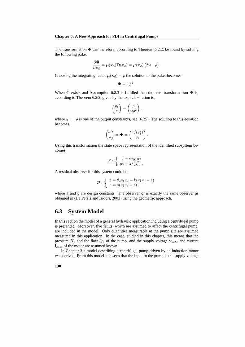
Chapter 6: A New Approach for FDI in Centrifugal Pumps
The transformationΦ can therefore, according to Theorem 6.2.2, be found by solvingthe following p.d.e.
∂Φ∂xd
= µ(xd)D(xd) = µ(xd)(2ω ρ
).
Choosing the integrating factorµ(xd) = ρ the solution to the p.d.e. becomes
Φ = ωρ2 .
WhenΦ exists and Assumption 6.2.3 is fulfilled then the state transformationΨ is,according to Theorem 6.2.2, given by the explicit solution to,
(y1
z
)=
(ρ
ωρ2
),
wherey1 = ρ is one of the output constraints, see (6.25). The solution to this equationbecomes,
(ωρ
)= Ψ =
(z/(y2
1)y1
).
Using this transformation the state space representation of the identified subsystem be-comes,
S :{
z = θ2y1u2
y3 = z/(y21) .
A residual observer for this system could be
O :{
z = θ2y1u2 + k(y21y3 − z)
r = q(y21y3 − z) ,
wherek andq are design constants. The observerO is exactly the same observer asobtained in (De Persis and Isidori, 2001) using the geometric approach.
6.3 System Model
In this section the model of a general hydraulic application including a centrifugal pumpis presented. Moreover, five faults, which are assumed to affect the centrifugal pump,are included in the model. Only quantities measurable at the pump site are assumedmeasured in this application. In the case, studied in this chapter, this means that thepressureHp and the flowQp of the pump, and the supply voltagevsabc and currentisabc of the motor are assumed known.
In Chapter 3 a model describing a centrifugal pump driven by an induction motorwas derived. From this model it is seen that the input to the pump is the supply voltage
130

Section 6.3: System Model
Centrifugal
pump
Application
H p
Q p
d
v sabc
Figure 6.2: The centrifugal pump placed in a hydraulic application. The inputs to thecentrifugal pump are the supply voltagevsabc and the volume flowQp and the output isthe pressure differenceHp. The inputs to the application are a set of unknown inputsdand the pressure difference of the pumpHp, and the output is the volume flowQp.
vsabc and the volume flowQp, and the output is the pressure differenceHp delivered bythe pump. This input/output structure is depicted in Fig. 6.2 where it is connected to ageneral hydraulic application. The inputs to this application are a set of unknown inputsd and the pressure differenceHp of the pump, and the output is the volume flowQp.The model of the system, depiced in Fig. 6.2, is formalized in the following subsections.
6.3.1 The Model of the Centrifugal Pump and its Application
It is assumed that the application is a dynamic system, which can be modelled by a setof first order ordinary differential equations. The structure of a model describing such asystem is shown below,
dxQ
dt = fA(xQ,Hp,d)Qp= hA(xQ) ,
(6.29)
wherexQ is a vector containing the states of the hydraulic application and the vectordrepresents the unknown inputs to this application.Hp andQp are the pressure outputand the volume flow of the centrifugal pump respectively.
The model of the centrifugal pump, presented in Chapter 3, is connected in a feed-back loop with the application model, as it is depiced in Fig. 6.2. This results in thefollowing model,
dxd
dt = fx(xd,u,d)y= hx(xd) ,
where the state vectorxd is given by,
xd =[isd isq imd imq ωr xT
Q
]T,
and the input vectoru and the output vectory are given by,
u =[vsd vsq
]Ty =
[isd isq H Q
]T.
131

Chapter 6: A New Approach for FDI in Centrifugal Pumps
Finally, the unknown input vectord is the same vector as the unknown input vectorprestented in (6.29). The vector fieldfx of the system is described by the following setof equations,
fx(xd,u,d) =
−Rs+R′rL′s
isd + R′rL′s
imd − zpωrL′mL′s
imq + 1L′s
vsd
−Rs+R′rL′s
isq + zpωrL′mL′s
imd + R′rL′s
imq + 1L′s
vsq
R′rL′m
isd − R′rL′m
imd + zpωrimq
R′rL′m
isq − zpωrimd − R′rL′m
imq1J
32zpL
′M (imdisq − imqisd)− B
J ωr − fT (h(xQ), ωr)fA(xQ,H,d)
,
wherefH(Q,ωr) andfT (Q,ωr) are given by,
fH(Q,ωr) = −ah2Q2 + ah1Qωr + ah0ω
2r
fT (Q,ωr) = −at2Q2 + at1Qωr + at0ω
2r
. (6.30)
The output map of the system is given by,
hx(x) =
isd
isq
fH(hA(xQ), ωr)
.
This model represents the behaviour of the system when no fault has occured. In thefollowing the effect of faults on the centrifugal pump is described.
6.3.2 Fault Models
Five faults are considered in this chapter, these are,
1. clogging inside the pump,
2. increased friction due to either rub impact or bearing faults,
3. increased leakage flow,
4. performance degradation due to cavitation,
5. dry running.
The first three faults are internal faults caused by impurities in the liquid and wear re-spectively. The fourth fault, cavitation, is caused by too low inlet pressure, meaningthat the fault is external. Finally, the last fault, dry running, is a phenomenon caused byfaults in the surrounding system, hence it is also an external fault. Even though it is nota fault in the pump, this fault is important to detect as sealing rings and bearings will bedestroyed when the pump is running without water for only a few seconds.
132
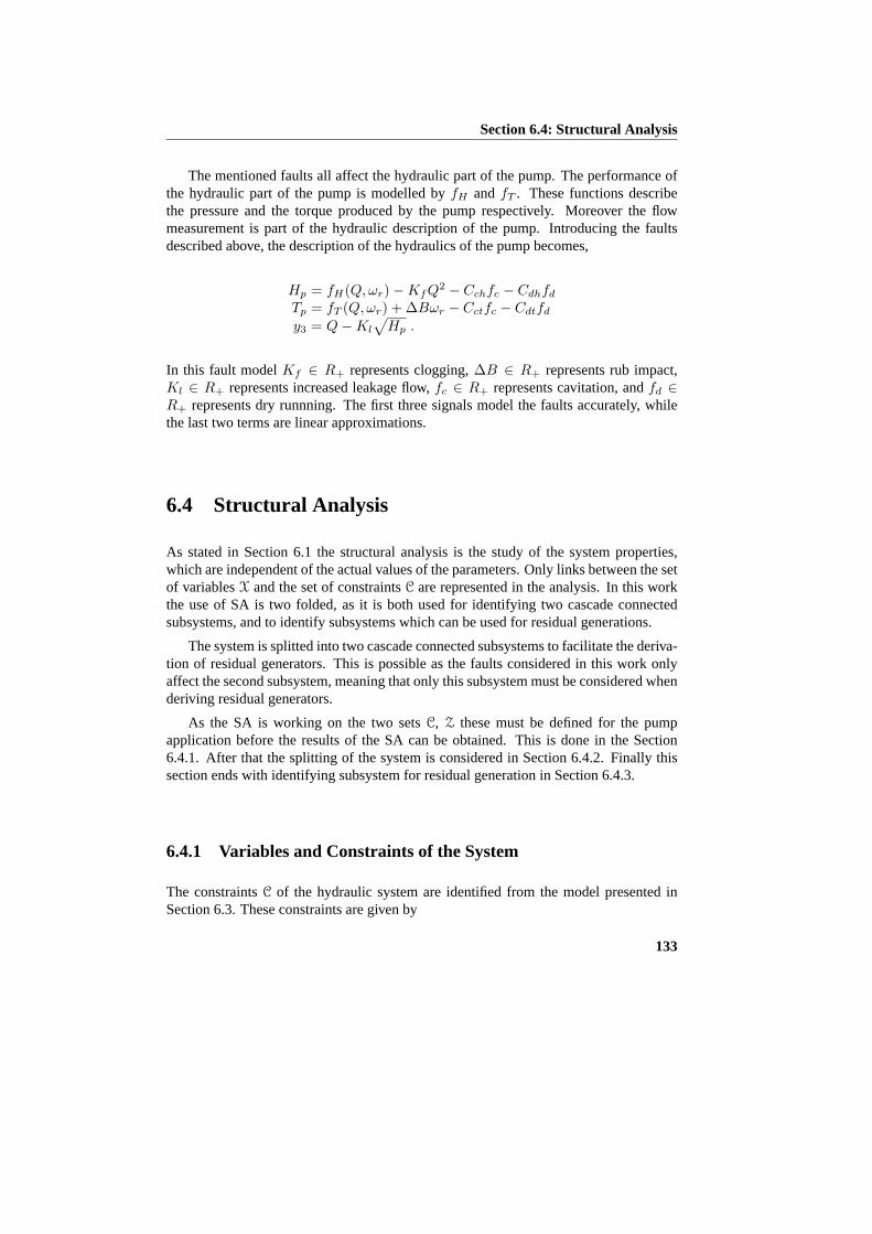
Section 6.4: Structural Analysis
The mentioned faults all affect the hydraulic part of the pump. The performance ofthe hydraulic part of the pump is modelled byfH andfT . These functions describethe pressure and the torque produced by the pump respectively. Moreover the flowmeasurement is part of the hydraulic description of the pump. Introducing the faultsdescribed above, the description of the hydraulics of the pump becomes,
Hp = fH(Q,ωr)−KfQ2 − Cchfc − Cdhfd
Tp = fT (Q,ωr) + ∆Bωr − Cctfc − Cdtfd
y3 = Q−Kl
√Hp .
In this fault modelKf ∈ R+ represents clogging,∆B ∈ R+ represents rub impact,Kl ∈ R+ represents increased leakage flow,fc ∈ R+ represents cavitation, andfd ∈R+ represents dry runnning. The first three signals model the faults accurately, whilethe last two terms are linear approximations.
6.4 Structural Analysis
As stated in Section 6.1 the structural analysis is the study of the system properties,which are independent of the actual values of the parameters. Only links between the setof variablesX and the set of constraintsC are represented in the analysis. In this workthe use of SA is two folded, as it is both used for identifying two cascade connectedsubsystems, and to identify subsystems which can be used for residual generations.
The system is splitted into two cascade connected subsystems to facilitate the deriva-tion of residual generators. This is possible as the faults considered in this work onlyaffect the second subsystem, meaning that only this subsystem must be considered whenderiving residual generators.
As the SA is working on the two setsC, Z these must be defined for the pumpapplication before the results of the SA can be obtained. This is done in the Section6.4.1. After that the splitting of the system is considered in Section 6.4.2. Finally thissection ends with identifying subsystem for residual generation in Section 6.4.3.
6.4.1 Variables and Constraints of the System
The constraintsC of the hydraulic system are identified from the model presented inSection 6.3. These constraints are given by
133

Chapter 6: A New Approach for FDI in Centrifugal Pumps
c1 : L′sisd = −(Rs + R′r)isd + A1 + vsd
c2 : L′sisq = −(Rs + R′r)isq + A2 + vsq
c3 : L′mimd = −A1 + R′risd
c4 : L′mimq = −A2 + R′risq
c5 : Jωr = Te −Bωr − Tp
c6 : xQ = fA(xQ,Hp,uQ)c7 : A1 = R′rimd + zpωrL
′mimq
c8 : A2 = R′rimq − zpωrL′mimd
c9 : Te = 32zpL
′m (imdisq − imqisd)
c10 : Hp = −ah2Q2p + ah1Qpωr + ah0ω
2r
c11 : Tp = −at2Q2p + at1Qpωr + at0ω
2r
c12 : Qp = hA(xQ)c13 : y1 = isd
c14 : y2 = isq
c15 : y3 = Hp
c16 : y4 = Qp ,
(6.31)
where the constraintsc7 andc8 are included to make the constraintsc1 to c4 independent.Hereby Assumption 6.1.3 is fulfilled globally (Blanke et al., 2003).
In (6.31) the constraintsc1 to c4 and c7 to c8 describe the electrical part of theinduction motor,c5 describes the mechanical dynamics of the pump, andc6 describesthe dynamics of the hydraulic applications.c9, c10 andc11 describe the torque generatedby the induction motor, the pressure difference generated by the centrifugal pump, andthe load torque of the centrifugal pump respectively.c12 describes the volume flowthrough the pump and finallyc13 to c16 describe the measurements on the system.
Two extra constraints can be deduced by differentatingc7 and c8 with respect totime. Doing this the following additional constraints are obtained,
cd7 : A1 = R′r imd + zpωrL′mimq + zpωrL
′mimq
cd8 : A2 = R′r imq − zpωrL′mimd − zpωrL
′mimd .
(6.32)
Beside the constrains presented above, there is a differential constraint for each variablexd, meaning that a constraint on the form,
di :dxdi
dt= xdi, (6.33)
exists for each element inxd. In this expressioni denotes theith element inxd.From the constraints presented in (6.31) and (6.32) the set of variables are identified.
These are given by,
Z = xd ∪ xd ∪ xa ∪ u ∪ y
134

Section 6.4: Structural Analysis
whereX = xd ∪ xd ∪ xa are the unknown variables, which must be matched, andK = u ∪ y are the known variables.xd, xa, u, andy are given by,
xd =[isd isq imd imq ωr A1 A2 xT
Q
]T
xc =[Hp Qp Tp dT
]Tu =
[vsd vsq
]Ty =
[y1 y2 y3 y4
]T.
6.4.2 Cascade Connected Systems
From the model of the system presented in Section 6.3 it is seen that the system is non-linear. Therefore, traditionally a nonlinear transformation is required to enable a designof a residual observer (Garcia and Frank, 1997). This transformation is not easy to finddue to the nonlinear nature of the system. Moreover, developing Analytical RedundancyRelations (ARR’s), using for example Groebner basis (Cox et al., 1997) for variableeliminations, have not given any usable result. This is also due to the nonlinear natureof the system. Therefore, the system is divided into two cascade-connected subsystemsby using structural consideration on the system (Blanke et al., 2003; Izadi-Zamanabadiand Staroswiecki, 2000).
Using SA it is shown that it is in fact possible to make this split. By analysing therelation describing the electrical part of the induction motor, it is seen from Table 6.4 thatthese constraints form an over-constraint system, see Definition 6.1.7. Therefore fromTheorem 6.1.1 the system is structural observable, meaning that the set of constrainsCe
form an observable subsystem for almost all parameters. This set is given by,
Ce = {d1, d2, dd7, dd8, c1, c2, c3, c4, c7, c8, c9, cd7, cd8, c13, c14} , (6.34)
Ce is defined as the first subsystem. The remaining relations are defined as the secondsubsystem, meaning that the constrains of this subsystem are given by,
Cm = {d5, d6, c5, c6, c10, c11, c12, c15, c16}. (6.35)
The connecting variables between the two subsystems are in this work defined as theestimates ofωr andTe, and will in the following be denotedωr andTe respectively.
It is also seen from the column at the right hand side of Table 6.4 that the faultstreated in this chapter are not affecting the relations in the first subsystem. Therefore, itis only necessary to consider the second subsystem when designing residual generatorsfor FDI on the system. Hence, the fault detection algorithm can be divided into two partsas shown in Fig. 6.3.
Using the relations describing the first part, an adaptive observer is designed. Thisobserver observes the variablesωr andTe connecting the two parts. The design of thisobserver is considered in Section 6.5. But first SA is used to identify minimal over-constrained subsystems (see Definition 6.1.11) in the system formed by the constraintsCm. The obtained results are presented in the following subsection,
135
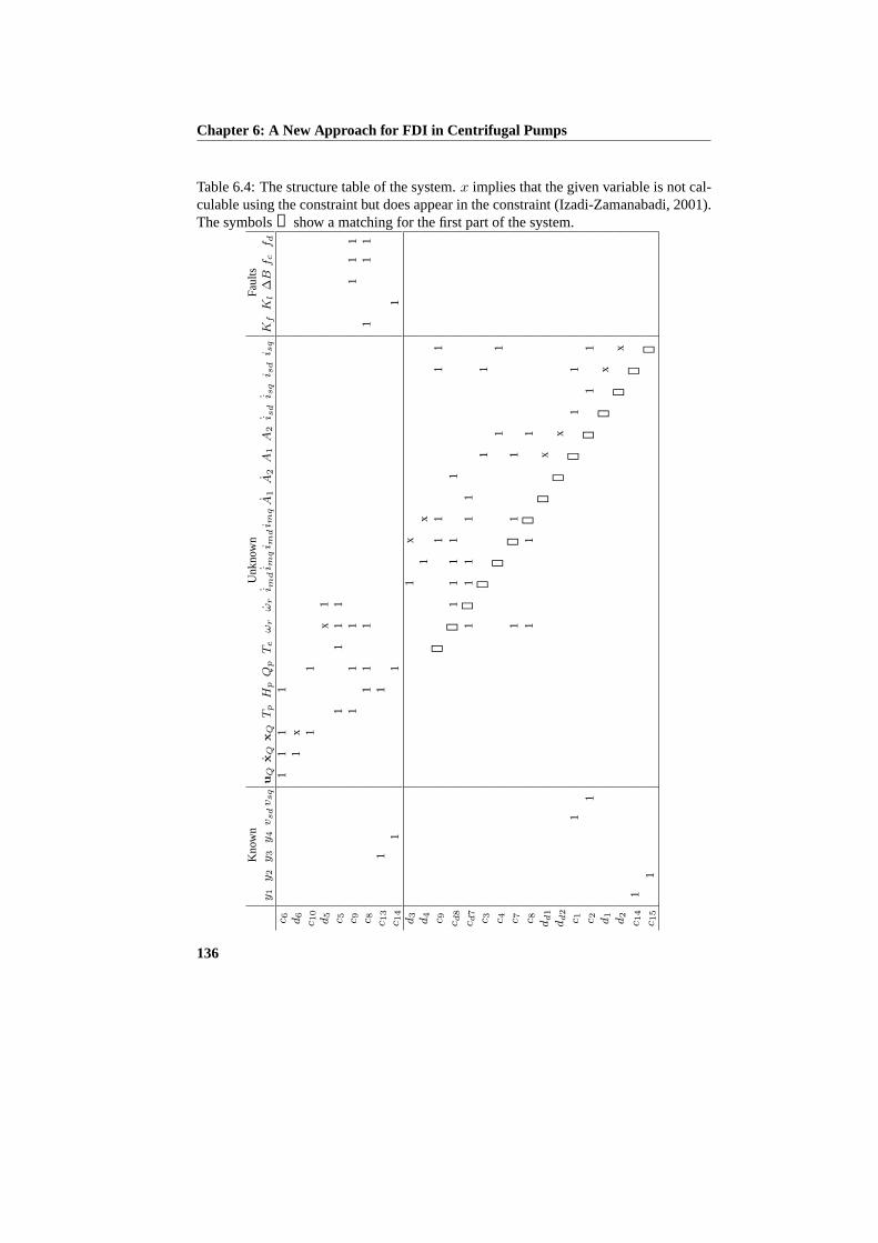
Chapter 6: A New Approach for FDI in Centrifugal Pumps
Table 6.4: The structure table of the system.x implies that the given variable is not cal-culable using the constraint but does appear in the constraint (Izadi-Zamanabadi, 2001).The symbols➀ show a matching for the first part of the system.
Kno
wn
Unk
now
nF
aults
y1
y2
y3
y4
vsd
vsq
uQ
xQ
xQ
Tp
Hp
Qp
Te
ωr
ωr
i mdi m
qi m
di m
qA
1A
2A
1A
2i s
di s
qi s
di s
qK
fK
l∆
Bf
cf
d
c 61
11
1d6
1x
c 10
11
d5
x1
c 51
11
1c 9
11
11
11
c 81
11
11
1c 1
31
1c 1
41
11
d3
1x
d4
1x
c 9➀
11
11
c d8
➀1
11
11
c d7
1➀
11
11
c 3➀
11
c 4➀
11
c 71
➀1
1c 8
11
➀1
dd1
➀x
dd2
➀x
c 11
➀1
1c 2
1➀
11
d1
➀x
d2
➀x
c 14
1➀
c 15
1➀
136
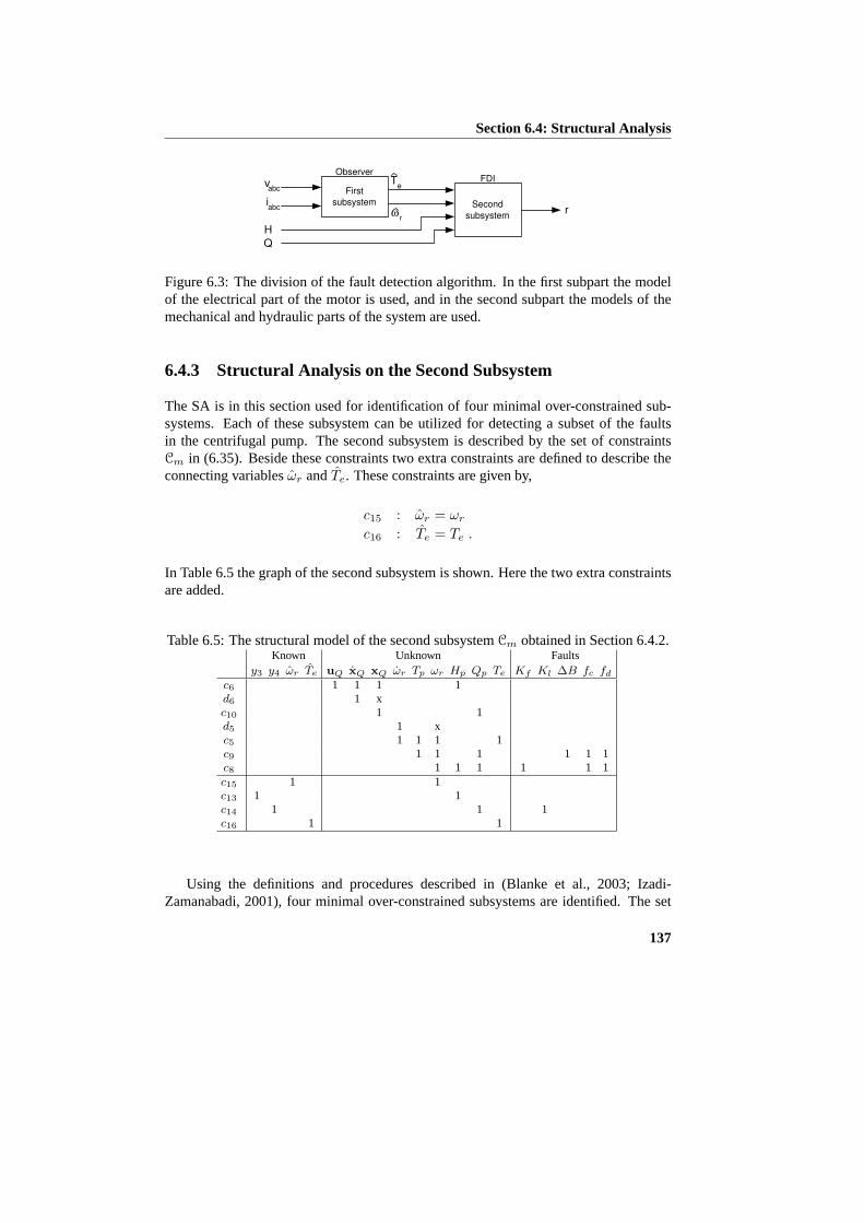
Section 6.4: Structural Analysis
First
subsystem Second
subsystem r
v abc
i abc
ω r
T e
H
Observer FDI
Q
Figure 6.3: The division of the fault detection algorithm. In the first subpart the modelof the electrical part of the motor is used, and in the second subpart the models of themechanical and hydraulic parts of the system are used.
6.4.3 Structural Analysis on the Second Subsystem
The SA is in this section used for identification of four minimal over-constrained sub-systems. Each of these subsystem can be utilized for detecting a subset of the faultsin the centrifugal pump. The second subsystem is described by the set of constraintsCm in (6.35). Beside these constraints two extra constraints are defined to describe theconnecting variablesωr andTe. These constraints are given by,
c15 : ωr = ωr
c16 : Te = Te .
In Table 6.5 the graph of the second subsystem is shown. Here the two extra constraintsare added.
Table 6.5: The structural model of the second subsystemCm obtained in Section 6.4.2.Known Unknown Faults
y3 y4 ωr Te uQ xQ xQ ωr Tp ωr Hp Qp Te Kf Kl ∆B fc fd
c6 1 1 1 1d6 1 xc10 1 1d5 1 xc5 1 1 1 1c9 1 1 1 1 1 1c8 1 1 1 1 1 1c15 1 1c13 1 1c14 1 1 1c16 1 1
Using the definitions and procedures described in (Blanke et al., 2003; Izadi-Zamanabadi, 2001), four minimal over-constrained subsystems are identified. The set
137

Chapter 6: A New Approach for FDI in Centrifugal Pumps
of constraints contained in each of these system are given by,
Cm1 = {d5, c5, c9, c14, c15, c16}Cm2 = {c8, c13, c14, c15}Cm3 = {d5, c5, c8, c9, c13, c15, c16}Cm4 = {d5, c5, c8, c9, c13, c14, c16} .
(6.36)
From these four minimal over-constrained subsystems, it is seen that the constraintsd6,c6, andc10 are not contained in any of the matchings. These constraints describe theapplication in which the pump is placed. Therefore, when these are not used in a matchit means that the matching is independent of the application model, and therefore noknowledge about the application is necessary for the algorithm to work.
Looking at the column to the right in table 6.5 the faults affecting each of the sub-systemsCmi can be identified. The connections between the faults and the subsystemsare shown below,
Cm1 : {Kl, ∆B, fc, fd}Cm2 : {Kf ,Kl, fc, fd}Cm3 : {Kf ,∆B, fc, fd}Cm4 : {Kf ,Kl,∆B, fc, fd} .
(6.37)
These connections show that the given faults areStructurally monitorablefrom the givenset of constraints, see Theorem 6.1.2 (Blanke et al., 2003).
From the connection in (6.37) it is seen that the faultsfc andfd are indistinguish-able from a structural point of view, meaning that isolation of these faults is impossibleusing residual generator built on these sets of constraints. Moreover, it is seen that noadditional information is added usingCm4. Therefore the set,
{Cm1, Cm2, Cm3} ,
contains the obtainable information about the faults in the system. The last relationCm4
could be used for validation in a robust fault detection scheme.
6.5 Observer for the Motor Part
In Section 6.4.2 it is shown, using SA, that the model of the centrifugal pump can besplitted into two subsystems, where the first system isstructurally observable, see The-orem 6.1.1 (Blanke et al., 2003). When this is the case the behaviour model of thesystem is also observable for almost all parameters (Blanke et al., 2003). Therefore, itshould be possible to derive an expression of the measurements and their derivatives forcalculating the connecting variables.
Unfortunately, the derivatives of the measurements are not known. Therefore, anobserver solution is investigated in this section. In the first part of the section a statespace description of the system is derived from the constraintsCe. In the last part anadaptive observer for observing the connecting variables is presented.
138

Section 6.5: Observer for the Motor Part
6.5.1 Realization of the set of ConstraintsCe
One approach for developing an observer to observe the speed and torque is to derive adynamic description of the set of constraints using the theory presented in Section 6.2.The obtained dynamic description can then be used in the design of an observer.
In Section 6.4.2 the set of constraintsCe is identified. This set forms a match ofthe two connecting variablesωr andTe. From Table 6.4 it is seen that the constraintc9 is used to match the variableTe, which is not used in any other constraints inCe.Therefore,c9 is not necessary in a match of the speedωr. However, it is seen that, whenthe speed is matched,c9 can be used to calculateTe, as all variables exceptTe is matchedin c9. Therefore, when an expression for calculatingωr is derived, then the derivationof an expression for calculatingTe is just a matter of form.
Based on the above argumentation only the calculation ofωr is considered in thefollowing. In Remark 6.2.4 it is argued that an observable state space description onlyexists if the given subsystem is over-constrained, which is not the case for the setCe.Therefore, by adding an extra constraint toCe making the new set over-constraint andremovingc9, the following set is obtained
C′e = (Ce\c9) ∪ d3 , (6.38)
which fulfills the demand of existence given in Remark 6.2.4. The new setC′e is formedby the following constraints,
c1 : L′sisd = −(Rs + R′r)isd + A1 + vsd
c2 : L′sisq = −(Rs + R′r)isq + A2 + vsq
c3 : L′mimd = −A1 + R′risd
c4 : L′mimq = −A2 + R′risq
c7 : A1 = R′rimd + zpωrL′mimq
c8 : A2 = R′rimq − zpωrL′mimd
c13 : y1 = isd
c14 : y2 = isq
cd7 : A1 = R′r imd + zpωrL′mimq + zpωrL
′mimq
cd8 : A2 = R′r imq − zpωrL′mimd − zpωrL
′mimd .
In this set the unknown variablesxd ∪ xa and the known variablesu ∪ y are given by,
xd =[isd isq imd A1 A2
]Txa =
[imq imq ωr ωr
]T
u =[vsd vsq
]Ty =
[y1 y2
]T.
Comparing the set (6.38) with the general system given by (6.4) the vector fieldfx, thealgebraic mapsmx and the output mapshx are constructed using the set of constraints{c1, c2, c3, cd7, cd8}, {c4, c7, c8}, and{c13, c14} respectively. According to Theorem6.2.1 and the match shown in Table 6.4, it is possible to eliminate a subset of the alge-braic variablesxa in the system using the vector functionmx. From the match presented
139

Chapter 6: A New Approach for FDI in Centrifugal Pumps
in Table 6.4 it is seen that the two algebraic variablesimq andimq should be eliminatedusingmx. By eliminating these the following system is obtained,
dxd
dt = f ′o(xd,xa2,u)go(y) = ho(xd,xa2) ,
(6.39)
wherexa2 =[ωr ωr
]Tand,
fo =
−Rs+R′rL′s
isd + 1L′s
A1 + 1L′s
vsd
−Rs+R′rL′s
isq + 1L′s
A2 + 1L′s
vsq
− 1L′m
A1 + R′rL′m
isd
R′rL′m
(R′risd −A1) + zpωr
(L′mR′r
A2 + zpωrL′m
2
R′rimd
)+ zpωr(R′risq −A2)
− R′rL′m
A2 + R′r2
L′misq − zpωrL
′mimd − zpωr(R′risd −A1)
go =
0y1
y2
ho =
(R′r + z2
pω2r
L′m2
R′r
)imd + zpωr
L′mR′r
A2 −A1
isd
isq
.
The next step in the derivation of a state space description is to use the approach de-scribed in Theorem 6.2.2 to eliminate the algebraic variablesxa2 in (6.39). Unfortu-nately, doing this the expression becomes huge, making it very difficult to find the statetransformationΦ, see Theorem 6.2.2. This makes the obtained expression useless.
However, by eliminating the variables inxa2 in two steps an useful expressionis obtained. To see this firstωr is eliminated in (6.39), and then the state trans-formation T : x, ωr → xd is used to transform the obtained system. Herex =[isd isq imd imq
]TandT is given by
T(x, ωr) =
isd
isq
imd
R′rimd + zpωrL′mimq
R′rimq − zpωrL′mimd
,
Doing this the traditional description of the electrical part of an induction motor is ob-tained, i.e. the transformed model has the following form
dxdt = fx(x, ωr,u)y = hx(x) ,
(6.40)
140
Section 6.5: Observer for the Motor Part
where
fx(x, ωr,u) =
−Rs+R′rL′s
isd + R′rL′s
imd − zpωrL′mL′s
imq + 1L′s
vsd
−Rs+R′rL′s
isq + zpωrL′mL′s
imd + R′rL′s
imq + 1L′s
vsq
R′rL′m
isd − R′rL′m
imd + zpωrimq
R′rL′m
isq − zpωrimd − R′rL′m
imq
hx(x) =(
isd
isq
).
As the second step the approach presented in Theorem 6.2.2 is used ones again. Thistime to eliminateωr in (6.40). Hereby the following state space description is obtained,
dzdt = fz(z,u′)
y = hz(z,u′) ,(6.41)
wherez ∈ Dz ⊂ R3 andu′ =[vsd vsq y2
]T. The vector fieldfz and the nonlinear
maphz in this expression are given by,
fz(z,u′) =
−Rs
L′sz1 + Rs
√2L′mz3−z2
2+2z2L′sy2−L′s2y2
2L′s
+ vsd
−Rsy2 + vsq
−2R′rL′s+R′rL′mL′sL′m
z3 + R′rL′mL′s
z22 − R′r
L′mz2y2 + R′r
√2L′mz3−z2
2+2z2L′sy2−L′s2y2
2z1
L′mL′s
hz(z,u′) =(
1L′s
z1 −√
2L′mz3−z22+2z2L′sy2−L′s
2y22
L′s
).
The system (6.41) is a state space realization of the set of constraintsC′e, where allalgebraic variables are eliminated. The speed of the motor can be calculated from thestates of (6.41) using the following expression,
ωr =R′rL′m
z2+vsq−L′sy2−(
Rs+R′rL′sL′m
+R′r
)y2
zp
√2L′mz3−z2
2+2z2L′sy2−L′s2y2
2
,
from which it is seen thatωr is a function ofy2, which in general is not known. Eventhough this expression is not usable for estimating the speedωr, the following remarkon this system should be considered.
Remark 6.5.1 If an observer can be found based on system (6.41), then this observeris a residual observer for the induction motor, which is independent of the speedωr.
In this section it is argued that it is not possible to estimate the speed of the motor withoutknowing the derivative of at least one of the measurements. However, it is also shownthat the subsystem identified using SA corresponds to the electrical part of an inductionmotor, see (6.40). Therefore, all the methods, described in the literature, for speedand torque estimation based on the electrical model can be used. In the following theadaptive observer, developed in Section 5.2.1, is utilized for estimating the connectingvariables, i.e. motor speed and torque.
141

Chapter 6: A New Approach for FDI in Centrifugal Pumps
6.5.2 The Adaptive Observer
In most pump applications the speed is either constant most of the time or changingslowly over time. Therefore the speed can be assumed constant in the observer design,meaning that an adaptive observer can be used for estimating the states and speed of themotor simultaneously. This approach, of course, has the drawback that, when transientphases occurs, short time errors in the estimated signals must be expected.
Considering the motor description (6.40) obtained in the previous section, it is seenthat this system can be rewritten to be on the following form
dxdt = (A0 + ωrAωr )x + Buy = Cx ,
(6.42)
where the state vectorx, the input vectoru and the output vectory are given by
x =[isd isq imd imq
]T
u =[vsd vsq
]Ty =
[isd isq
]T,
and the matrices in (6.42) are
A0 =
−Rs+R′rL′s
0 R′rL′s
0
0 −Rs+R′rL′s
0 R′rL′s
R′rL′m
0 − R′rL′m
0
0 R′rL′m
0 − R′rL′m
Aωr =
0 0 0 −zpL′mL′s
0 0 zpL′mL′s
00 0 0 zp
0 0 −zp 0
B =
1L′s
00 1
L′s0 00 0
C =
[1 0 0 00 1 0 0
].
If the speed is assumed constant, this system is a linear system with one unknown butconstant parameter. Using the transformationx = Tz given by
T =
1 0 0 00 1 0 0
− L′sL′m
0 1 0
0 − L′sL′m
0 1
the system (6.42) is tranformed to the adaptive observer form defined in Definition 5.2.1in Section 5.2.1, whereA(u,θ) = A(θ) andθ = ωr. This means that an adaptive
142
Section 6.6: Observer Based Fault Detection and Isolation
observer is given by Proposition 5.2.1. Using this proposition the adaptive observer forthe induction motor becomes
Oe :
dzdt = (A′
0 + ωrA′ωr
)z + B′u + K(y −C′z)dωr
dt = κ(y −C′z)T A′′ωr
zx = Tz ,
(6.43)
wherez ∈ R4 contains the observer states, andωr is the estimated speed. The matricesin the observer are
A′0 = T−1A0T A′
ωr= T−1Aωr
TB′ = T−1B C′ = CT ,
and A′′ωr
is a matrix composed by the two first rows ofA′ωr
. K and κ are designconstants.K is chosen such that the LMI (5.27), described in Section 5.2.2, is feasible,andκ is chosen such that the convegence speed ofωr is suitable.
The connecting variables between the two subsystems are the speed and torque. Ofthese only the speed is directly available from the observer (6.43). However, usingc9
the torque can be calculated whenever the states of the motor are known. When theestimates of the states are usedc9 becomes,
c9 : Te = 1.5zpL′m
(imdisq − imq isd
),
whereisd, isq, imd and imq are estimates of states in the original system presented in(6.42).
This observer is, as mentioned in the beginning of this subsection, developed underthe assumption that the speed is constant i.e.dωr
dt = 0. This assumption is not correctduring transient phases, therefore it is expected that problems can arise when transientsoccur in the speed.
6.6 Observer Based Fault Detection and Isolation
In this section one ARR and three residual observers are designed. These are based onthe four minimal over-constrained subsystems identified in Section 6.4.3. The designof the observers is partly based on the theory presented in Section 6.2, and partly basedon a proposition presented in this section, which states the stability condition for theobservers. Results obtained using the developed residual observers on the test setup arepresented in Section 6.7.
6.6.1 The Residual Generators
Looking at the constraints forming the setCm2 = {c8, c13, c14, c15} it is seen that nodifferential constraints are included in this. Therefore an ARR obtained from this set
143

Chapter 6: A New Approach for FDI in Centrifugal Pumps
does not include derivatives. The ARR is given by,
r2 = −ah2y24 + ah1ωry4 + ah0ω
2r − y3 . (6.44)
It is also possible to obtain ARR’s from the setsCm1, Cm3 andCm4, but because adifferential constraint is used in each of these sets, it is necessary to use derivatives ofthe output in these cases. To avoid this, three residual observers are developed in thefollowing. The constraints contained in the setsCm1, Cm3 andCm4 are given by (6.36),and are reproduced below for convenience,
Cm1 = {d5, c5, c9, c14, c15, c16}Cm3 = {d5, c5, c8, c9, c13, c15, c16}Cm4 = {d5, c5, c8, c9, c13, c14, c16} ,
where the constraints are given by,
d5 : ωr = dωr
dtc5 : Jωr = Te −Bωr − Tp
c8 : Hp = −ah2Q2p + ah1Qpωr + ah0ω
2r
c9 : Tp = −at2Q2p + at1Qpωr + at0ω
2r
c13 : y3 = Hp
c14 : y4 = Qp
c15 : ωr = ωr
c16 : Te = Te .
Comparing the setsCm1, Cm3 andCm4 with the structure of (6.4), the vector fieldfxis formed by the constraintc5, the mapmx is formed by a subset of{c8, c9}, and themaphx is formed by a subset of{c13, c14, c15, c16}. Using Corollary 6.2.1 on these setsit is shown that the setsCm1, Cm3 andCm4 all can be transformed to systems with thefollowing structure,
dxd
dt = axd + fx(xd, v1, u) + e1(xd, v1, u, f)g(v1, v2, u) = h(xd) + e2(xd, v1, v2, u, f) ,
(6.45)
where the state of the systemxd = ωr, the inputu = Te, the outputsv1, v2 ∈{ωr, y3, y4}, andf is a vector containing the fault signals. This shows that the alge-braic variables in systemCm1, Cm3 andCm4 can be decoupled using a transformationof the output equations only. For the three obtained systems the following assumptionholds.
Assumption 6.6.1 It is assumed that in the case where no faults have occurred, i.e.f = 0, the output maph in (6.45) can be solved forxd locally. Let this solution be givenby,
xd = g(v1, v2, u) . (6.46)
144

Section 6.6: Observer Based Fault Detection and Isolation
Using the above assumption the following proposition describes a residual observerfor the system described by (6.45).
Proposition 6.6.1 Under Assumption 6.6.1 the following observer is a residual ob-server for systems described by (6.45),
xd
dt = axd + fx(g(v1, v2, u), v1, u) + k(g(v1, v2, u)− xd)r = q(g(v1, v2, u)− xd)
. (6.47)
The residual observer is asymptotical stable ifa−k < 0. The fault input to this observeris given by,
ff =(fx(xd, v1, u)− fx(xd + δxf , v1, u)) + e1(xd, v1, u, f)− kδxf ,
whereff is a derived fault signal, which is strongly detectable. In the expression offf
the signalδxf is given by,
δxf = h−1(g(v1, v2, u)− e2(xd, v1, v2, u, f))− g(v1, v2, u) .
Proof: In the no fault casef = 0 the observer error equation becomes,
e = (axd + fx(xd, v1, u))− (axd + fx(xd, v1, u) + k(xd − xd))
e = (a− k)e (6.48)
where (6.46) is used in the observer expression (6.47), meaning thatg(v1, v2, u) = xd. Equation(6.48) shows that the error dynamic of the observer is asymptotical stable ifa− k < 0.
The expression of the derived fault signalff is obtained in the following by introducing thefault signals in the error equation of the observer. First, an expression of the fault when mappedthroughg is obtained. To this end define the functiongf as,
gf (v1, v2, u) = g(v1, v2, u)− e2(xd, v1, v2, u, f) = h(xd)
From this expression it is seen that the functiongf must be used to obtain a map from the mea-surementsv1 andv2 to the statexd if a fault f has occured, i.e.
xd = gf (v1, v2, u) = h−1(g(v1, v2, u)− e2(xd, v1, v2, u, f))
Defineδxf andxf asδxf = xd−xf andδxf = gf (y1, y2, u)− g(y1, y2, u) respectively. Usingthese signals the observer error equation, in the faulty case, i.e.f 6= 0, becomes,
e =ae + fx(xd, y1, u)− fx(xf , y1, u) + e1(x, y1, f)− k(xf − x)
e =(a− k)e + (fx(xd, y1, u)− fx(xd − δxf , y1, u)) + e1(x, y1, f)− kδxf (6.49)
From this expression the following nonlinear expression of the fault can be identified,
ff =(fx(xd, y1, u)− fx(xd + δxf , y1, u)) + e1(x, y1, f)− kδxf
145

Chapter 6: A New Approach for FDI in Centrifugal Pumps
Including this fault expression in the error equation (6.49) it becomes,
e = (a− k)e + ff
r = qe
From this expression it is seen that the derived fault signalff is strongly detectable.¤
Remark 6.6.1 The derived faultff is strongly detectable using this observer. This isnot the case for the faults inf , as the nonlinear expression offf can equal zero eventhough one of the entries inf is different from zero.
Remark 6.6.2 The observer described by Proposition 6.6.1 is designed under the as-sumption that a perfect model exists, and that the measurements are not affected bynoise. This is, of course, not fulfilled in real life applications. To overcome this the gaink of the observer is chosen such that errors due to small model mismatchs and noise willbe suppressed.
Using Corollary 6.2.1 and Proposition 6.6.1 on the three over-constrained subsystemsCm1, Cm3, andCm4, the following three residual observers are obtained,
Om1 :{
J dxd
dt = −Bxd − fT (y4, ωr) + Te + k1 (ωr − xd)r1 = q1 (ωr − xd)
(6.50)
Om3 :{
J dxd
dt = −Bxd − fT (g3(ωr, y3), ωr) + Te + k3 (ωr − xd)r3 = q3 (ωr − xd)
(6.51)
Om4 :{
J dxd
dt = −Bxd − fT (y4, g4(y3, y4)) + Te + k4 (g4(y3, y4)− xd)r4 = q4 (g4(y3, y4)− xd)
(6.52)
whereki is designed according to Proposition 6.6.1 andqi is chosen such that the resid-uals have a reasonable value in the case of faults. The functionfT is given by
fT (Qp, ωr) = −at2Q2p + at1Qpωr + at0ω
2r ,
and the functionsg3 andg4 are derived from the output maph in (6.45), and are givenby,
g3(ωr, y3) =ah1ωr +
√a2
h1ω2r − 4ah2(y3 − ah0ω2
r)2ah2
g4(y3, y4) =−ah1y4 +
√a2
h1y24 + 4ah0(y3 + ah2y2
4)2ah0
.
These expressions are valid forωr, y4 ∈ R+ when the parameters of the pump used inthe test are considered. Therefore the expressions are valid in the state spaceωr, Q ∈R+, which is exactly the state space in which the model is valid, see Section 3.5.
146
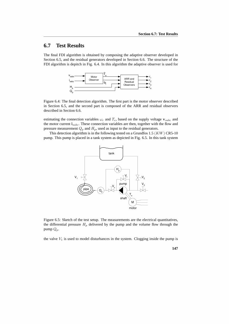
Section 6.7: Test Results
6.7 Test Results
The final FDI algorithm is obtained by composing the adaptive observer developed inSection 6.5, and the residual generators developed in Section 6.6. The structure of theFDI algorithm is depitch in Fig. 6.4. In this algorithm the adaptive observer is used for
Motor
Observer ARR and
Residual
Observers
r 1
ω r
T e
H p
r 2
r 3
r 4
v sabc
i sabc
Q p
Figure 6.4: The final detection algorithm. The first part is the motor observer describedin Section 6.5, and the second part is composed of the ARR and residual observersdescribed in Section 6.6.
estimating the connection variablesωr andTe, based on the supply voltagevsabc andthe motor currentisabc. These connection variables are then, together with the flow andpressure measurementQp andHp, used as input to the residual generators.
This detection algorithm is in the following tested on a Grundfos 1.5(KW ) CR5-10pump. This pump is placed in a tank system as depicted in Fig. 6.5. In this tank system
V 1
V 2
V c
pipe
pump
M
motor
shaft
T e
H p
tank
V 3
V l
Q p
Figure 6.5: Sketch of the test setup. The measurements are the electrical quantitatives,the differential pressureHp delivered by the pump and the volume flow through thepumpQp.
the valveV1 is used to model disturbances in the system. Clogging inside the pump is
147
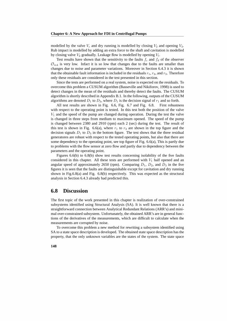
Chapter 6: A New Approach for FDI in Centrifugal Pumps
modelled by the valveVc and dry running is modelled by closingV2 and openingV3.Rub impact is modelled by adding an extra force to the shaft and cavitation is modelledby closing valveV2 gradually. Leakage flow is modelled by openingVl.
Test results have shown that the sensitivity to the faultsfc andfd of the observerOm4 is very low. Infact it is so low that changes due to the faults are smaller thanchanges due to noise and parameter variations. Moreover in Section 6.4.3 it is shownthat the obtainable fault information is included in the residualsr1, r2, andr3. Thereforeonly these residuals are considered in the test presented in this section.
Since the tests are performed on a real system, noise is expected on the residuals. Toovercome this problem a CUSUM algorithm (Basseville and Nikiforov, 1998) is used todetect changes in the mean of the residuals and thereby detect the faults. The CUSUMalgorithm is shortly described in Appendix B.1. In the following, outputs of the CUSUMalgorithms are denotedD1 to D3, whereD1 is the decision signal ofr1 and so forth.
All test results are shown in Fig. 6.6, Fig. 6.7 and Fig. 6.8. First robustnesswith respect to the operating point is tested. In this test both the position of the valveV1 and the speed of the pump are changed during operation. During the test the valveis changed in three steps from medium to maximum opened. The speed of the pumpis changed between 2380 and 2910 (rpm) each 2 (sec) during the test. The result ofthis test is shown in Fig. 6.6(a), wherer1 to r3 are shown in the top figure and thedecision signalsD1 to D3 in the bottom figure. The test shows that the three residualgeneratores are robust with respect to the tested operating points, but also that there aresome dependency to the operating point, see top figure of Fig. 6.6(a), This is partly dueto problems with the flow sensor at zero flow and partly due to dependency between theparameters and the operating point.
Figures 6.6(b) to 6.8(b) show test results concerning isolability of the five faultsconsidered in this chapter. All these tests are performed withV1 half opened and anangular speed of approximately 2650 (rpm). ComparingD1, D2, andD3 in the fivefigures it is seen that the faults are distinguishable except for cavitation and dry runningshown in Fig.6.8(a) and Fig. 6.8(b) respectively. This was expected as the structuralanalysis in Section 6.4.3 already had predicted this.
6.8 Discussion
The first topic of the work presented in this chapter is realization of over-constrainedsubsystems identified using Structural Analysis (SA). It is well known that there is astraightforward connection between Analytical Redundant Relations (ARR’s) and mini-mal over-constrained subsystem. Unfortunately, the obtained ARR’s are in general func-tions of the derivatives of the measurements, which are difficult to calculate when themeasurements are corrupted by noise.
To overcome this problem a new method for rewriting a subsystem identified usingSA to a state space description is developed. The obtained state space description has theproperty, that the only unknown variables are the states of the system. The state space
148
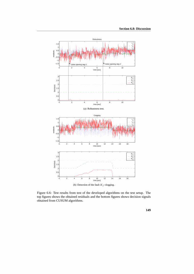
Section 6.8: Discussion
0 2 4 6 8 10
−1.5
−1
−0.5
0
0.5
1
1.5
Robustness
time [sec]
resi
dual
s
r1
r2
r3
0 2 4 6 8 100
0.5
1
1.5
2
2.5
3
time [sec]
Dec
isio
ns
D1
D2
D3
Valve opening step 1 Valve opening step 2
(a) Robustness test.
0 2 4 6 8 10 12 14 16 18
−1.5
−1
−0.5
0
0.5
1
1.5
Clogging
time [sec]
resi
dual
s
r1
r2
r3
0 2 4 6 8 10 12 14 16 180
0.5
1
1.5
2
2.5
3
time [sec]
Dec
isio
ns
D1
D2
D3
(b) Detection of the faultKf clogging.
Figure 6.6: Test results from test of the developed algorithms on the test setup. Thetop figures shows the obtained residuals and the bottom figures shows decision signalsobtained from CUSUM algorithms.
149

Chapter 6: A New Approach for FDI in Centrifugal Pumps
0 2 4 6 8 10
−2
−1
0
1
2
Leakage Flow
time [sec]
resi
dual
s
r1
r2
r3
0 2 4 6 8 100
0.5
1
1.5
2
2.5
3
time [sec]
Dec
isio
ns
D1
D2
D3
(a) Detection of the faultKl leakage flow.
0 2 4 6 8 10 12 14 16
−2
−1
0
1
2
Rub Impact
time [sec]
resi
dual
s
r1
r2
r3
0 2 4 6 8 10 12 14 160
0.5
1
1.5
2
2.5
3
time [sec]
Dec
isio
ns
D1
D2
D3
(b) Detection of the fault∆B rub impact.
Figure 6.7: Test results from test of the developed algorithms on the test setup. Thetop figures shows the obtained residuals and the bottom figures shows decision signalsobtained from CUSUM algorithms.
150
Section 6.8: Discussion
0 2 4 6 8 10 12 14 16 18
−5
0
5
Cavitation
time [sec]
resi
dual
s
r1
r2
r3
0 2 4 6 8 10 12 14 16 180
0.5
1
1.5
2
2.5
3
time [sec]
Dec
isio
ns
D1
D2
D3
End of cavitation
(a) Detection of the faultfc cavitation.
0 2 4 6 8 10 12 14 16 18−15
−10
−5
0
5
10
15Dry Running
time [sec]
resi
dual
s
r1
r2
r3
0 2 4 6 8 10 12 14 16 180
0.5
1
1.5
2
2.5
3
time [sec]
Dec
isio
ns
D1
D2
D3
Air valve opened Air valve closed
(b) Detection of the faultfd dry running.
Figure 6.8: Test results from test of the developed algorithms on the test setup. Thetop figures shows the obtained residuals and the bottom figures shows decision signalsobtained from CUSUM algorithms.
151

Chapter 6: A New Approach for FDI in Centrifugal Pumps
description can then be used for derivation of residual observers. In the design of theseobservers decoupling of unknown inputs has not to be considered, as the only unknownvariables are the states of the system. The method is tested on a satellite model, showingthat a residual observer can be obtained using this approach. Moreover the method isused to develop residual observer for the centrifugal pump application, which is thesecond topic of the chapter.
The second topic of the chapter is fault detection and isolation in a centrifugal pumpplaced in an arbitrary hydraulic application. An algorithm, which is capable of detectionand isolation of five faults in a centrifugal pump, is developed. The proposed alogrithmis independent of the application in which the pump is placed. This makes the algorithmrobust and usable in a wide range of applications, such as submersible application, wastewater application, and heating application.
Tests have shown that it is possible to distinguish between four of the five faults un-der consideration, using three chosen residuals. But it is also shown that the algorithm issensitive to the operating point. This is partly due to dependency between the operatingpoint and the parameters in the model and partly due to flow sensor problems at zeroflow. Even though the algorithm has a small inherent dependency of the operating point,it still performs considerably better than algorithms built on a linearized model, whenthe operating point is changed.
152

Chapter 7
FDI on the Centrifugal Pump: ASteady State Solution
In this chapter Structural Analysis (SA) is utilized to derive Analytical Redundant Re-lations (ARR’s), which can be used for fault detection. The concept of SA is describedin Section 6.1 in the previous chapter. The obtained ARR’s are based on a steady statemodel of the pump. Here a steady state model denotes a model describing the pumpunder constant speed, pressure and flow conditions. The developed detection algorithmis only using electrical measurements on the motor, and the pressure and flow measure-ments on the centrifugal pump. The electrical measurements are in this case Root MeanSquare (RMS) measurements of the voltage and current, the voltage frequency, and theelectrical angle between the voltage and current. These measurements become constantwhen the system is running under steady state conditions, and can therefore be sampledat any given sample rate, provided the steady state conditions. Therefore, by using onlythese measurements the microprocessor load of the derived algorithm can be chosenfreely. Moreover, the steady state measurements of the electrical signals are sometimesmade available by modern motor protection units. All in all this makes the algorithmsuitable for implementation in cost sensitive products.
The obtained algorithm is robust with respect to parameter variations and the oper-ating point of the pump respectively, making it usable in real life applications. In thedevelopment of the FDI algorithm, the approach, presented in Section 6.4, of dividingthe system into two cascade-connected subsystems is used. This is done to avoid twolarge residual expressions. The first of these subsystems consists of the electrical partof the induction motor driving the pump, and the second subsystem consists of the me-chanical and hydraulic part of the pump. Theoretical considerations regarding to Struc-tural Analysis (SA) are, among others, found in (Blanke et al., 2003; Izadi-Zamanabadi,2001).
The faults, which only affect the second subsystem, are detected using Analytical
153

Chapter 7: FDI on the Centrifugal Pump: A Steady State Solution
Redundancy Relations (ARR’s). These relations are obtained through the utilization ofstructural analysis (Blanke et al., 2003) and the Groebner basis algorithm (Cox et al.,1997). Using this approach the obtained ARR’s are polynomial. This is utilized inthe development of a detection algorithm, which is robust with respect to parametervariations. Theoretical results on using the Groebner basis are given in (Staroswieckiand Comtet-Varga, 2001). Moreover, an overview of model-based methods using ARR’sis given in (Staroswiecki, 2000).
This chapter starts by presenting the steady state model of a centrifugal pump placedin an arbitrarily hydraulic application. This is done in Section 7.1. Structural analysis onthe derived steady state model is considered in Section 7.2, which includes; the divisionof the system into two suitable subsystems, derivation of an expression for calculatingthe connecting variables, and ARR expressions for fault detection. In Section 7.3 amethod for robust fault detection using ARR’s is considered. Section 7.4 presents sometest results obtained on the industrial test bench, which also was used to obtain the testresults presented in Chapter 6. Finally concluding remarks end the chapter.
7.1 Steady State Model of the System
In this section, the model of the centrifugal pump derived in Chapter 3, is reformulatedto describe the pump under steady state conditions, only. The section is divided intothree subsections, where the first one is concerned with the steady state model of themotor. The second one is concerned with the steady state model of the mechanical andhydraulic parts of the pump, and finally the last one is concerned with fault modelling.The obtained model will in the following be used in the derivation of a FDI algorithmbased on low bandwidth measurements, such as Root Mean Square (RMS) measurementof the electrical quantities.
7.1.1 Steady State Motor Model
The model of the induction motor is described in Section 3.2. In this section both amodel of aY-connected and a∆-connected motor is derived. The obtained models areprestented in (3.9) and (3.10) respectively. Comparing these models it is seen that thefollowing equations describe the motor in both cases,
L′sdisdq
dt =− (Rs + R′r) isdq + (R′
r − zpωrJL′m) imdq + vsdq
L′mdimdq
dt =R′risdq − (R′
r − zpωrJL′m) imdq .(7.1)
The variablesvsdq, isdq, andimdq are in general unknown. However, in theY-connectedcase the measurable electrical quantities at the terminals of the motoritdq and vtdq
equalsisdq andvsdq respectively. In the∆-connected case these currents and voltagesare given by the transformationsitdq = Ciisdq andvsdq = Bvvtdq respectively, seeSection 3.2.3.
154

Section 7.1: Steady State Model of the System
To obtain a steady state model of the motor, a transformation of the motor states isused. This transformation takes the states described in the stator fixed reference framexdq and transform these to an arbitrary frame. In this case the arbitrary frame rotateswith the frequency of the supply voltageωe. The new states are denotedxe
dq. Thetransformation is given byxdq = T(θe)xe
dq, whereθe is the angle between the statorfixed frame and the arbitrary rotating frame.T is given by
T(θe) =[cos(θe) − sin(θe)sin(θe) cos(θe)
], (7.2)
whereθe is a function of time. Using this transformation to transformvsdq, isdq, andimdq, a new model is obtained with the property that all states are constant during steadystate operation. Setting the derivatives of the states equal to zero, the following steadystate model of the motor is obtained,
−ωeL′sI
esq = −(Rs + R′r)Ie
sd + (R′rIemd − zpωrL
′mIe
mq) + V esd
ωeL′sI
esd = −(Rs + R′r)I
esq + (R′rI
emq + zpωrL
′mIe
md) + V esq
−ωeL′mIe
mq = −(R′rIemd − zpωrL
′mIe
mq) + R′rIesd
ωeL′mIe
md = −(R′rIemq + zpωrL
′mIe
md) + R′rIesq .
Defining Iesd = 0 in the above model, meaning that the rotating reference frame is
aligned with the currentIesq, the final steady state model of the motor is obtained,
−ωeL′sI
esq = (R′rIe
md − zpωrL′mIe
mq) + V esd
0 = −(Rs + R′r)Iesq + (R′rI
emq + zpωrL
′mIe
md) + V esq
−ωeL′mIe
mq = −(R′rIemd − zpωrL
′mIe
mq)ωeL
′mIe
md = −(R′rIemq + zpωrL
′mIe
md) + R′rIesq .
(7.3)
The torque expression of the motor is given in (3.11) and repeated here for the sake ofconvenience,
Te =32zpL
′m (imdisq − imqisd) .
Using the transformationT, given in (7.2), a torque expression of the new variables isobtained. The expression becomes
Te =32zpL
′m
(IemdI
esq
). (7.4)
Equations (7.3) and (7.4) form the model of the induction motor during steady state op-erations. However, the electrical quantitiesV e
sd, V esq, andIe
sq are not directly measurable.Therefore, a connection between these quantities and the measurable quantities must beestablished. The measurable quantities are the RMS values of the supply voltageVrms
and currentIrms, the supply frequencyωe and the electrical angle between the voltage
155

Chapter 7: FDI on the Centrifugal Pump: A Steady State Solution
and currentφ. The angleφ is in this case defined as the angle between the voltage vec-
tor Vetdq =
[V e
td V etq
]T, and the current vectorIe
tdq =[0 Ie
tq
]T, where subscriptt
denotes quantities available at the terminals of the motor. The Euclidean length of thevectorsVe
tdq andIetdq is connected to the RMS values of the measurable electrical quan-
tities by|Vetdq| =
√2Vrms and|Ie
tdq| =√
2Irms. Using the RMS valuesVrms andIrms
and the angleφ the voltagesV etd andV e
tq, and the currentIetq can be calculated using
V etd = −
√2Vrms sin(φ) V e
tq =√
2Vrms cos(φ) Ietq =
√2Irms . (7.5)
In the case of aY-connected motor the electrical quantities at the motor terminalsV etd,
V etq, andIe
tq and the quantitiesV esd, V e
sq, andIesq in (7.3) are equivalent. However, in
the case of a∆-connected motor the transformation matricesBv andCi have to beconsidered. These matrices are defined in Section 3.2.3. It can be shown that
Bv =√
3T∆ C−1i =
1√3T∆ ,
whereT∆ is a rotation matrix. Using these expressions in (7.1) to obtain the steadystate model, it is seen that (7.3) can be used to model the steady state operation of themotor when it is connected in a∆-connection if the following scalings of the electricalquantities are used,
V etd =
√3V e
td V etq =
√3V e
tq Iesq =
1√3Ietq . (7.6)
7.1.2 Steady State Pump Model
The hydraulic and the mechanical parts of the pump are derived in Section 3.4 andSection 3.3 respectively. Moreover, a model of a general hydraulic application is givenin Section 6.3.2. In Section 3.4 it is shown that the mechanical part is described by thefollowing differential equation,
Jdωr
dt= Te −Bωr − Tp
whereTe is the torque produced by the motor,ωr is the speed of the shaft, andTp theload torque produced by the pump. Under steady state operation the speed is constant,i.e. dωr
dt = 0, meaning that the steady state model of the mechanical part becomes,
0 = Te −Bωr − fT (Qp, ωr) . (7.7)
The hydraulic parts of the pump is considered as the parts involved with the energytransformation from mechanical to hydraulic energy. In the model derived in Section3.3 this energy transformation is described by two maps given by
Tp = fT (Qp, ωr) Hp = fH(Qp, ωr) , (7.8)
156

Section 7.1: Steady State Model of the System
whereTp andHp are the load torque and pressure produced by the pump respectively.The arguments of the mapsfT andfH in (7.8) are the volume flowQp and the speed ofthe pumpωr. The mapsfT andfH are given by,
fH(Qp, ωr) = ρg(−ah2Q
2p + ah1Qpωr + ah0ω
2r
)fT (Qp, ωr) = −at2Q
2p + at1Qpωr + at0ω
2r .
A general model of a hydraulic application of a centrifugal pump is given in Sec-tion 6.3.1. Here it is argued that such a model, in most cases, can be described by thefollowing state space model,
xQ= fA(xQ,Hp,d)Qp= hA(xQ) ,
wherexQ is the state vector of the application model,Hp andQp are the pressure andvolume flow of the centrifugal pump, andd is a vector containing some unknown inputsignals to the application. If it is assumed that the derivative of the statesxQ equals zeroduring steady state operation, the steady state model becomes,
0= fA(xQ, Hp,d)Qp= hA(xQ) .
(7.9)
7.1.3 The Fault Models
In Section 6.3.2 five faults are included in the centrifugal pump model. These faults areall affecting the hydraulic part of the pump. The faults are,
1. clogging inside the pump,
2. increased friction due to either rub impact or bearing faults,
3. increased leakage flow,
4. performance degradation due to cavitation,
5. dry running.
In the model of the system used here, the hydraulic part of the pump is modelled bythe mapsfH , fT and the flow measurement. Introducing the faults described above, thedescription of the hydraulic part of the pump becomes,
Hp = fH(Q,ωr)−KfQ2 − Cchfc − Cdhfd
Tp = fT (Q,ωr) + ∆Bωr − Cctfc − Cdtfd
y3 = Q−Kl
√Hp .
In this fault modelKf ∈ R+ represents clogging,∆B ∈ R+ represents rub impact,Kl ∈ R+ represents increased leakage flow,fc ∈ R+ represents cavitation andfd ∈ R+
represents dry runnning. The first three signals model the faults accurately, while the lasttwo terms are linear approximations.
157
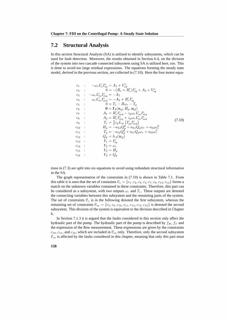
Chapter 7: FDI on the Centrifugal Pump: A Steady State Solution
7.2 Structural Analysis
In this section Structural Analysis (SA) is utilized to identify subsystems, which can beused for fault detection. Moreover, the results obtained in Section 6.4, on the divisionof the system into two cascade connected subsystem using SA is utilized here, too. Thisis done to avoid too large residual expressions. The equations forming the steady statemodel, derived in the previous section, are collected in (7.10). Here the four motor equa-
c1 : −ωeL′sI
esq = A1 + V e
sd
c2 : 0 = −(Rs + R′r)Iesq + A2 + V e
sq
c3 : −ωeL′mIe
mq = −A1
c4 : ωeL′mIe
md = −A2 + R′rIesq
c5 : 0 = Te −Bωr − Tp
c6 : 0 = fA(xQ,Hp,uQ)c7 : A1 = R′rI
emd − zpωrL
′mIe
mq
c8 : A2 = R′rIemq + zpωrL
′mIe
md
c9 : Te = 32zpLm
(IesqI
emd
)c10 : Hp = −ah2Q
2p + ah1Qpωr + ah0ω
2r
c11 : Tp = −at2Q2p + at1Qpωr + at0ω
2r
c12 : Qp = hA(xQ)c13 : Y1 = Ie
sq
c14 : Y2 = ωe
c15 : Y3 = Hp
c16 : Y4 = Qp
(7.10)
tions in (7.3) are split into six equations to avoid using redundant structural informationin the SA.
The graph representation of the constraints in (7.10) is shown in Table 7.1. Fromthis table it is seen that the set of constaintsCe = {c1, c2, c3, c4, c7, c9, c13, c14} forms amatch on the unknown variables contained in these constraints. Therefore, this part canbe considered as a subsystem, with two outputsωr andTe. These outputs are denotedthe connecting variables between this subsystem and the remaining parts of the system.The set of constraintsCe is in the following denoted the first subsystem, whereas theremaining set of constraintsCm = {c5, c6, c10, c11, c12, c15, c16} is denoted the secondsubsystem. This division of the system is equivalent to the division described in Chapter6.
In Section 7.1.3 it is argued that the faults considered in this section only affect thehydraulic part of the pump. The hydraulic part of the pump is described byfH , fT andthe expression of the flow measurement. These expressions are given by the constraintsc10, c11, andc16, which are included inCm only. Therefore, only the second subsystemCm is affected by the faults considered in this chapter, meaning that only this part must
158

Section 7.2: Structural Analysis
Table 7.1: The structure table of the centrifugal pump system under steady state condi-tions. The symbols➀ show a matching for the first part of the system.
Known UnknownY1 Y2 V e
sd V esq Y3 Y4 xQ uQ Tp Hp Qp Te ωr Ie
mdIemq A1 A2 Ie
sq ωe
c6 1 1 1c12 1 1c5 1 1 1c11 1 1 1c10 1 1 1c15 1 1c16 1 1c8 1 1 1 1c9 ➀ 1 1c7 ➀ 1 1 1c4 ➀ 1 1 1c3 ➀ 1 1c1 1 ➀ 1 1c2 1 ➀ 1c13 1 ➀c14 1 ➀
be considered when FDI is applied.
7.2.1 Calculating the Connection Variables
The SA showed that the connecting variablesωr andTe should be calculable using theset of constraints,
Ce = {c1, c2, c3, c4, c7, c9, c13, c14} .
Rewriting these constraints the following expression of the speedωr is obtained,
ωr =L′mω2
eL′sIesq + L′mωeV
esd −R′rRsI
esq + R′rV
esq
L′mzp(ωeL′sIesq + V e
sq), (7.11)
whereV esd, V e
sq, Iesq = Y1, andωe = Y2 are assumed known. The torqueTe is also
obtained by rewritingCe resulting in the following expression,
Te =3zpI
esq(I
esqRs − V e
sq)2ωe
. (7.12)
As in the above expressionV esq, Ie
sq = Y1, andωe = Y2 are assumed known in the torqueexpression.
In the speed and torque expression (7.11) and (7.12) the voltagesV esd, V e
sq, and thecurrentIe
sq are calculated using the RMS values of the supply voltageVrms, supplycurrentIrms, and angle between the voltage and currentφ, defined in Section 7.1.1.This is done using (7.5), and in the case of a∆-connected motor (7.6).
159

Chapter 7: FDI on the Centrifugal Pump: A Steady State Solution
7.2.2 Structural Analysis on the Second Subsystem
The second subsystem is described by the set,
Cm1 = {c5, c6, c10, c11, c12, c15, c16} .
Beside these constraints two extra constraints are added to model the estimation of theconnecting variablesωr andTe. These constraints are given by
c17 : Te = Te
c18 : ωr = ωr .(7.13)
Table 7.2 is a representation of the graph describing the structure of the second subsys-tem. In this table the column at the right hand side is added to show the connectionbetween the faults in the system and the constraints. Using SA three minimal over-
Table 7.2: The structure table of the second system. The first two columns describethe structural connection between the constraints and the known and unknown variablesrespectively. Whereas the last column describes the connection between the constraintsand the faults in the system.
Known Unknown FaultsY3 Y4 Te ωr xQ uQ Tp Hp Qp Te ωr Kf Kl ∆B fc fd
c6 1 1 1c12 1 1c5 1 1 1c11 1 1 1 1 1 1c10 1 1 1 1 1 1c15 1 1c16 1 1c17 1 1c18 1 1 1
constraint subsystems are identified. These are given by the following three sets,
Cm1 = {c5, c11, c16, c17, c18}Cm2 = {c5, c10, c11, c15, c16, c17}Cm3 = {c10, c15, c16, c18} .
(7.14)
The connections between these sets and the faults in the system are given by
Cm1 : {Kl, ∆B, fc, fd}Cm2 : {Kf ,∆B, fc, fd}Cm3 : {Kf ,Kl, fc, fd} .
(7.15)
160
Section 7.2: Structural Analysis
7.2.3 ARR’s of the Pump
The constraintsc6 andc12, describing the application in which the pump is placed, arenot included in any of the set of constraintsCm1, Cm2, andCm3. Hence, any ARRbased on these sets will not be affected by the application in which the pump is placed,i.e. it will be robust with respect to the application of the pump. The next step in thedevelopment of an ARR is to eliminate all unknown variables in this set. Although itcould be done by hand, here the Groebner basis algorithm is used to guarantee residualexpressions that are on polynomial form. The polynomial characteristic is utilized innext section to derive an algorithm, which takes parameter variations into account. In(Staroswiecki and Comtet-Varga, 2001) the Groebner basis is also used as a part of analgorithm to obtain ARR’s.
The ARR obtained using the Groebner basis algorithm on the setsCm1, Cm2, andCm3 are used to establish residual expressions on the following form,
rpi= fpi
(ypi)T api
(θpi) i ∈ {1, 2, 3}
whereθpi is the parameter vector andypi is the measurement vector. In this expressionboth api(θ) and fpi(y) contain polynomial functions. In the following the parameterand measurement vectorsθpi andypi , and the polynomial vector functionsfpi andapi
are given for each set of constraintsCm1, Cm2, andCm3.
ARR based on the set of constraintsCm1
The set of constraintsCm1 contains the following parameters and measurements de-scribed on vector form,
θp1 =(at2 at1 at0
)Typ1 =
(Te ωr Y4
)T.
The polynomial vector functionsfp1 andap1 are given by
ap1(θp1) =
1at2
−at1
−at0
fp1(yp1) =
Te −Bωr
Y 24
Y4ωr
w2r
.
ARR based on the set of constraintsCm2
The set of constraintsCm2 contains the following parameters and measurements de-scribed on vector form,
θp2 =(ah2 ah1 ah0 at2 at1 at0
)Typ2 =
(Te ωr Y3
)T.
161

Chapter 7: FDI on the Centrifugal Pump: A Steady State Solution
The polynomial vector functionsfp2 andap2 are given by
ap2(θp2) =
a2h2
a2t2
ah2at1ah1 − at2a2h1 + 2a2
h2at0 − 2ah2ah0at2
a1(θ) + a2(θ)2ah2at2at0 + ah2a
2t1 − 2ah0a
2t2 − ah1at2at1
2ah2at2
,
where
a1(θ) = at2(a2h0at2 + ah0ah1at1 − at0a
2h1)
a2(θ) = ah2(a2t0ah2 + at0at1ah1 − ah0a
2t1 − 2ah0at2at0) ,
and
fp1(yp1) =
B2ω2r − 2BTeωr + T 2
e
Y 23
Bω3r − Teω
2r
ω4r
Y3ω2r
−Y3Te + BY3ωr
.
ARR based on the set of constraintsCm3
The set of constraintsCm3 contains the following parameters and measurements de-scribed on vector form,
θp3 =(ah2 ah1 ah0
)Typ3 =
(ωr Y3 Y4
)T.
The polynomial vector functionsfp3 andap3 are given by
ap3(θp3) =
−1−at2
at1
at0
fp3(yp3) =
Y3
Y 24
Y4ωr
ω2r
.
7.3 The Robust FDI Algorithm
The ARR’s developed in the previous section depend on the parameters describing thepump. As the application treated in this work is a real system the model parameters arenot matching the real parameters exactly over the whole operating range of the pump.
162

Section 7.3: The Robust FDI Algorithm
Moreover, the density of the liquid is not constant due to temperature changes and im-purities in the liquid. This density affects the value of the parameters in the hydraulicmodel of the pump given by (3.29). Therefore, parameter variations must be taken intoaccount, for the developed algorithms to be robust and thereby usable in real applica-tions.
7.3.1 Robustness with Respect to Parameter Variations
The residuals are in this case calculated using functions on the formr = f(y)T a(θ) asseen in Section 7.2.3. In these equationsr = 0 when the parameter vectorθ = θ0 andno fault has occured in the system. Hereθ0 is the parameter vector used in the designof the residual generators. Robustness is now formulated as the problem of handlingthe residual generation problem whenθ ∈ Θ, whereΘ is the set of possible parametervalues includingθ0. This means thatr = 0 is not necessary fulfilled in the no fault caseanymore. However, in all real life systems it is assumed thatr is bounded on the setΘ.
One way to treat the parameter variation problem, sketched above, is the use of a set-valued approach, as presented in for example (Tornill et al., 2000; Idrissi et al., 2001).When using this approach a set of possible residual values is obtained. If0 is not in thisset it can be concluded that there is a fault in the system in spite of parameter variations.This is formalized in the following definition,
Definition 7.3.1 The set of possible residual valuesR has the following properties,
• If the system is not affected by faults i.e.e = 0 then0 ∈ R.
• If 0 /∈ R then there are faults in the system i.e.e 6= 0
wheree is a given fault vector andR ⊂ R is a connected set.
Now let r = g(y, θ) be an ARR describing the behaviour of a given system, whereycontains the measurements andθ contains the parameters in the ARR. For this ARRronly equals0 in the no fault case, if the structure and parameters of the system are knownexactly. When, for such a system, parameter uncertainties are taken into account the setof possible residualsR defined in Definition 7.3.1 is given by the following lemma,
Lemma 7.3.1 If the set of possible parametersΘ is a compact set, given by
Θ = {θ|θi = [θi, θi], i = 1, · · · , n} , (7.16)
whereθ ∈ Rn, and the residual functiong : Y ×Θ → R is continuous onΘ for ally ∈ Y ⊂ Rm, then the set of possible residual values, in the no fault case, is defined bythe maximum valuer and minimum valuer ofR. These maximum and minimum valuesare given by
r = maxθ∈Θ
g(y, θ)
r = minθ∈Θ
g(y, θ) .
163

Chapter 7: FDI on the Centrifugal Pump: A Steady State Solution
This is a well known fact from mathematical analysis and the proof can be found in(Apostol, 1974). Using this lemma the boundaries ofR can be calculated. Unfortunatelyit is not straightforward to calculate these maximum and minimum values. However,in the case treated in this work the functiong can be separated into a function of theparameters and a function of the measurements i.e.g(y, θ) = f(y)T a(θ). When this isthe case it is easy to see that one set of boundaries on the residual setR is given by
r ≤ rmax =k∑
i=1
maxθ∈Θ
(ai(θ)fi(y))
r ≥ rmin =k∑
i=1
minθ∈Θ
(ai(θ)fi(y)) .
From these expression it is seen that onlyai i = 1, · · · , k is a function of the parametersθ. The maximum and minimum ofai can be calculated offline, leaving only a sign checkof fi to be done online. This is expressed in the following lemma.
Lemma 7.3.2 If r = f(y)T a(θ) wherea and f are two vector functions, which arecontinuous on respectivelyΘ andY, then an upper (lower) boundary ofr (r) is givenby
r ≤ rmax =∑
i
ri,max r ≤ rmin =∑
i
ri,min ,
where
ri,max ={
fi(y) maxθ∈Θ (ai(θ)) if fi(y) > 0fi(y)minθ∈Θ (ai(θ)) otherwise
ri,min ={
fi(y)minθ∈Θ (ai(θ)) if fi(y) > 0fi(y) maxθ∈Θ (ai(θ)) otherwise .
The upper and lower boundaries, found using this lemma, are fast and easy to calculateonline, as the hard part of the calculations can be done offline. Unfortunately, the foundupper and lower boundaries are in general not very tight. However, if the residual ex-pressionr = g(y,θ) is affine with respect to the parametersθ an exact solution exists.If g is affine with respect to the parametersθ it can be rewritten to be come,
r = g(y, θ) = G0(y) + Gl(y)θ . (7.17)
For an expression of this form the upper and lower boundaries can be found on aninterval setΘ using interval algebra (Boukhris et al., 1998). Using this approach theexact maximum and minimum values of (7.17) can be calculated, in the no fault case,using the following lemma.
164

Section 7.3: The Robust FDI Algorithm
Lemma 7.3.3 For the parameter affine system (7.17) the maximum and minimum valuesof the residual setR can be calculated exactly, and are given by
r = G0(y) + Gl(y)θ0 + |Gl(y)| (θ − θ0)r = G0(y) + Gl(y)θ0 + |Gl(y)| (θ − θ0) ,
whereθ0 = 12 (θ + θ).
This is a well-known fact from interval analysis (Boukhris et al., 1998; Moore, 1979).In the following, Lemma 7.3.2 and 7.3.3 are used to calculate an upper and a lowerboundary of the residual expressions found in the previous section.
All the residual expressions derived in Section 7.2.3 are on the form
r = f(y)T a(θ) ,
where botha andf are vector functions with only polynomial nonlinearities inθ andy. As this is a nonlinear expression, Lemma 7.3.2 could be used to find upper andlower boundaries of the residual set. However, these upper and lower boundaries are ingeneral far from the real maximum and minimum values ofR, which is also the case incentrifugal pumps. Therefore, the linear dependency between the parameters is extractedusing a first order Taylor Series expansion ofa(θ). This Taylor Series expansion is givenby
a(θ) = a(θ0) +[
∂a∂θi
(θ0)](θ − θ0) + O(θ − θ0) .
When this expression is used in the residual equation the residual is calculated by thesum of two termsr = rl + rO. These terms are given by
rl(y) =(f(y)T a(θ0)
)+
(f(y)T
[∂a∂θi
(θ0)])
θ (7.18a)
rO(θ,y) = f(y)T(O(θ)
), (7.18b)
whereθ = θ − θ0, andθ0 is chosen such thatθ0 = 12 (θ − θ). It is immediately seen
that (7.18a) has the same structure as (7.17), meaning that Lemma 7.3.3 can be usedto calculate the maximum and minimum values ofr1 in the no fault case. This doeshowever not form the boundaries onr because of the higher order termsO(θ−θ0). Thedependency onr of these terms is described by (7.18b). This expression is a nonlinearexpression on the form treated in Lemma 7.3.2, which therefore gives the upper andlower boundaries on this expression.
Using interval algebra it is easy to find the boundaies ofr from the boundaries ofrl andrO. This is formalized in the following algorithm, which is used for robust faultdetection.
165

Chapter 7: FDI on the Centrifugal Pump: A Steady State Solution
1. At each new sampley computef(y), G0(y) = f(y)T a(θ0) andGl(y) = f(y)T
[∂a∂θi
(θ0)].
2. Compute the maximum and minimum valuesrl and rl usingLemma (7.3.3).
3. Compute the boundariesrO,min andrO,max using Lemma 7.3.2.
4. Compute the boundaries of the residual set using,
r ≥ rmin = rl + rO,min
r ≤ rmax = rl + rO,max
5. Compute the decision signalD using,
D ={
0 if rmin ≤ 0 ≤ rmax
1 otherwise
Remark 7.3.1 This algorithm can calculate the boundaries of the residual set of onesingle residual expression. However, parameter dependencies between residuals, whenmore than one residual is considered, are not taken into account. Therefore, the identi-fication of incipient faults can create problems in some cases.
Interpretation of the algorithm
The idea of the algorithm is to find the possible variation on the residual value, whichcan be caused by parameter divergence form the nominal parameter values. This isillustrated in Fig. 7.1.
+ y i
θ 1
θ 2
Θ
r
r l
r
r l
y i
r max
r min
r O , max
r O , min
Figure 7.1: Illustration of the different boundary values in the proposed algorithm.
To the left of Fig. 7.1 the set of possible parameter valuesΘ is shown. At eachmeasurement vectoryi this set of parameter values is mapped into a set of possible
166
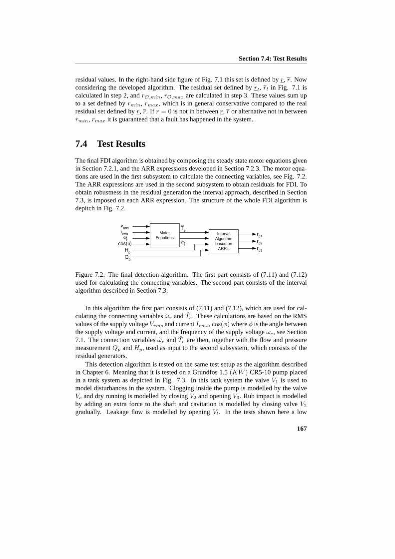
Section 7.4: Test Results
residual values. In the right-hand side figure of Fig. 7.1 this set is defined byr, r. Nowconsidering the developed algorithm. The residual set defined byrl, rl in Fig. 7.1 iscalculated in step 2, andrO,min, rO,max are calculated in step 3. These values sum upto a set defined byrmin, rmax, which is in general conservative compared to the realresidual set defined byr, r. If r = 0 is not in betweenr, r or alternative not in betweenrmin, rmax it is guaranteed that a fault has happened in the system.
7.4 Test Results
The final FDI algorithm is obtained by composing the steady state motor equations givenin Section 7.2.1, and the ARR expressions developed in Section 7.2.3. The motor equa-tions are used in the first subsystem to calculate the connecting variables, see Fig. 7.2.The ARR expressions are used in the second subsystem to obtain residuals for FDI. Toobtain robustness in the residual generation the interval approach, described in Section7.3, is imposed on each ARR expression. The structure of the whole FDI algorithm isdepitch in Fig. 7.2.
Motor
Equations Interval
Algorithm
based on
ARR's
r p 1
ω r
T e
H p
r p 2
r p3
v rms
i rms
Q p
cos( φ )
ω e
Figure 7.2: The final detection algorithm. The first part consists of (7.11) and (7.12)used for calculating the connecting variables. The second part consists of the intervalalgorithm described in Section 7.3.
In this algorithm the first part consists of (7.11) and (7.12), which are used for cal-culating the connecting variablesωr andTe. These calculations are based on the RMSvalues of the supply voltageVrms and currentIrms, cos(φ) whereφ is the angle betweenthe supply voltage and current, and the frequency of the supply voltageωe, see Section7.1. The connection variablesωr andTe are then, together with the flow and pressuremeasurementQp andHp, used as input to the second subsystem, which consists of theresidual generators.
This detection algorithm is tested on the same test setup as the algorithm describedin Chapter 6. Meaning that it is tested on a Grundfos 1.5(KW ) CR5-10 pump placedin a tank system as depicted in Fig. 7.3. In this tank system the valveV1 is used tomodel disturbances in the system. Clogging inside the pump is modelled by the valveVc and dry running is modelled by closingV2 and openingV3. Rub impact is modelledby adding an extra force to the shaft and cavitation is modelled by closing valveV2
gradually. Leakage flow is modelled by openingVl. In the tests shown here a low
167
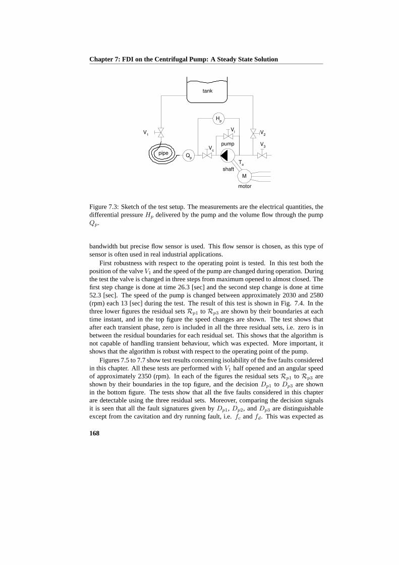
Chapter 7: FDI on the Centrifugal Pump: A Steady State Solution
V 1
V 2
V c
pipe
pump
M
motor
shaft
T e
H p
tank
V 3
V l
Q p
Figure 7.3: Sketch of the test setup. The measurements are the electrical quantities, thedifferential pressureHp delivered by the pump and the volume flow through the pumpQp.
bandwidth but precise flow sensor is used. This flow sensor is chosen, as this type ofsensor is often used in real industrial applications.
First robustness with respect to the operating point is tested. In this test both theposition of the valveV1 and the speed of the pump are changed during operation. Duringthe test the valve is changed in three steps from maximum opened to almost closed. Thefirst step change is done at time 26.3 [sec] and the second step change is done at time52.3 [sec]. The speed of the pump is changed between approximately 2030 and 2580(rpm) each 13 [sec] during the test. The result of this test is shown in Fig. 7.4. In thethree lower figures the residual setsRp1 toRp3 are shown by their boundaries at eachtime instant, and in the top figure the speed changes are shown. The test shows thatafter each transient phase, zero is included in all the three residual sets, i.e. zero is inbetween the residual boundaries for each residual set. This shows that the algorithm isnot capable of handling transient behaviour, which was expected. More important, itshows that the algorithm is robust with respect to the operating point of the pump.
Figures 7.5 to 7.7 show test results concerning isolability of the five faults consideredin this chapter. All these tests are performed withV1 half opened and an angular speedof approximately 2350 (rpm). In each of the figures the residual setsRp1 to Rp3 areshown by their boundaries in the top figure, and the decisionDp1 to Dp3 are shownin the bottom figure. The tests show that all the five faults considered in this chapterare detectable using the three residual sets. Moreover, comparing the decision signalsit is seen that all the fault signatures given byDp1, Dp2, andDp3 are distinguishableexcept from the cavitation and dry running fault, i.e.fc andfd. This was expected as
168

Section 7.5: Discussion
0 10 20 30 40 50 60 70
200
250
300
Spe
ed [r
ad/s
ec]
0 10 20 30 40 50 60 70
−0.5
0
0.5R
p1
0 10 20 30 40 50 60 70−0.02
0
0.02
Rp2
0 10 20 30 40 50 60 70
−0.1
0
0.1
time [sec]
Rp3
Figure 7.4: Robustness test. The top figure shows the speed steps, and the three lowerfigures show the residual boundaries for each of the three residual setsRp1 toRp3.
the structural analysis in Section 7.2.2 already had predicted this.Both the appearance and the disappearance of the considered faults, except from
the dry running faultfd, are detected. From Fig. 7.7 the problem of detecting thedisappearance of the dry running fault is seen. This problem is due to air bobbles in thesystem imposed by the dry running fault, which disturbs the flow sensor used in this test.
7.5 Discussion
The topic of this chapter is fault detection in a centrifugal pump based on steady statemeasurements only. Here the steady state measurements are Root Mean Square (RMS)measurement of the voltage and current, the voltage frequency, the electrical angle be-tween the voltage and current, and the pressure and volume flow of the pump. Threeresiduals are derived form the steady state model of the pump, using Structural Analy-sis and Analytical Redundant Relations (ARR’s). The faults under consideration in thischapter are only affecting the second subsystem. Hence the ARR’s are only developedfor this part. The connecting variables between the two subsystems are calculated usinga steady state model of the motor.
Structural analysis has been used to analyse the system. As a result of this analysisthe system is divided into two cascade-connected subsystems simplifying the derivationof the Analytical Redundancy Relation (ARR) considerably. The first subsystem con-sists of the induction motor model, and the mechanical and hydraulic parts of the pump
169
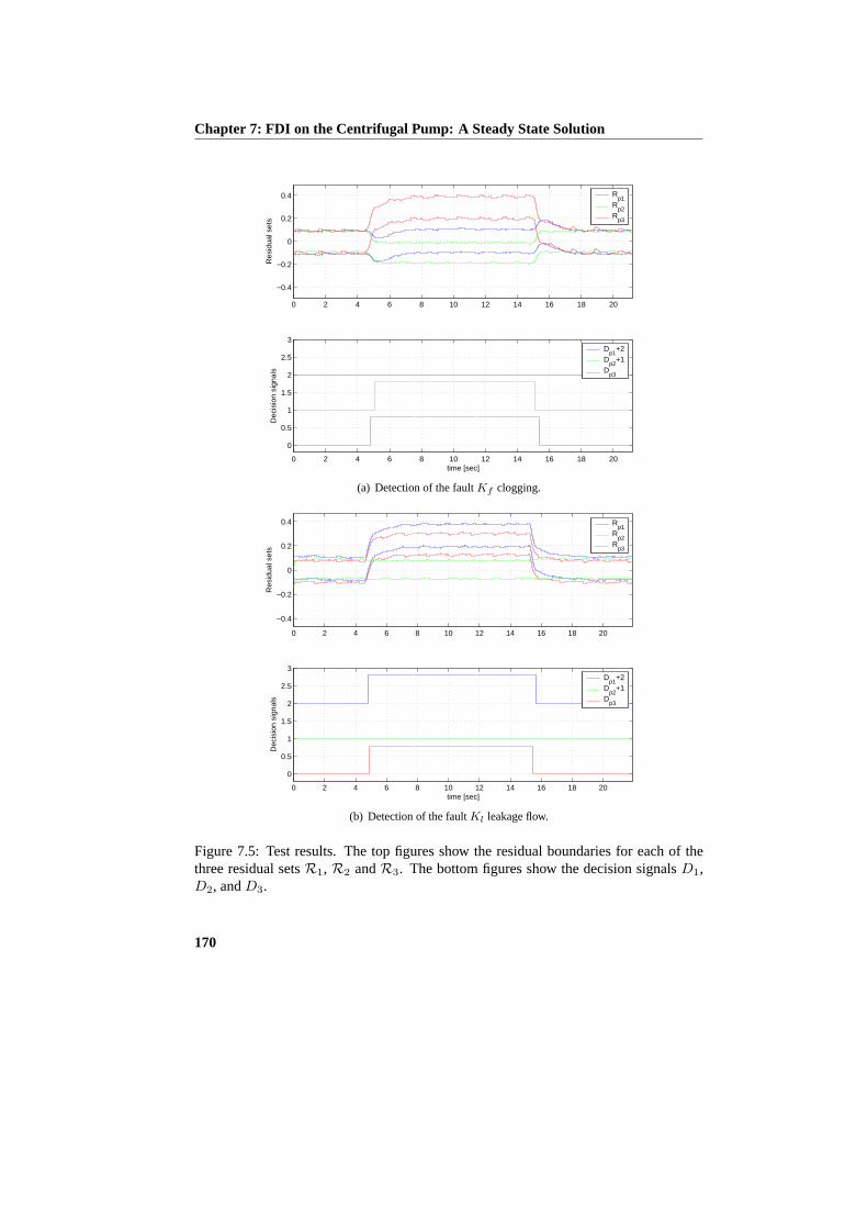
Chapter 7: FDI on the Centrifugal Pump: A Steady State Solution
0 2 4 6 8 10 12 14 16 18 20
−0.4
−0.2
0
0.2
0.4
Res
idua
l set
s
Rp1
Rp2
Rp3
0 2 4 6 8 10 12 14 16 18 20
0
0.5
1
1.5
2
2.5
3
Dec
isio
n si
gnal
s
time [sec]
Dp1
+2D
p2+1
Dp3
(a) Detection of the faultKf clogging.
0 2 4 6 8 10 12 14 16 18 20
−0.4
−0.2
0
0.2
0.4
Res
idua
l set
s
Rp1
Rp2
Rp3
0 2 4 6 8 10 12 14 16 18 20
0
0.5
1
1.5
2
2.5
3
Dec
isio
n si
gnal
s
time [sec]
Dp1
+2D
p2+1
Dp3
(b) Detection of the faultKl leakage flow.
Figure 7.5: Test results. The top figures show the residual boundaries for each of thethree residual setsR1, R2 andR3. The bottom figures show the decision signalsD1,D2, andD3.
170
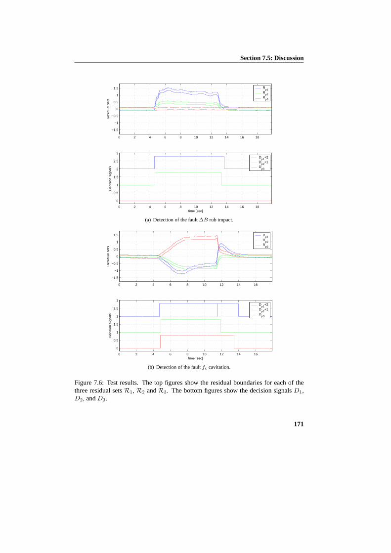
Section 7.5: Discussion
0 2 4 6 8 10 12 14 16 18
−1.5
−1
−0.5
0
0.5
1
1.5
Res
idua
l set
s
Rp1
Rp2
Rp3
0 2 4 6 8 10 12 14 16 18
0
0.5
1
1.5
2
2.5
3
Dec
isio
n si
gnal
s
time [sec]
Dp1
+2D
p2+1
Dp3
(a) Detection of the fault∆B rub impact.
0 2 4 6 8 10 12 14 16
−1.5
−1
−0.5
0
0.5
1
1.5
Res
idua
l set
s
Rp1
Rp2
Rp3
0 2 4 6 8 10 12 14 16
0
0.5
1
1.5
2
2.5
3
Dec
isio
n si
gnal
s
time [sec]
Dp1
+2D
p2+1
Dp3
(b) Detection of the faultfc cavitation.
Figure 7.6: Test results. The top figures show the residual boundaries for each of thethree residual setsR1, R2 andR3. The bottom figures show the decision signalsD1,D2, andD3.
171

Chapter 7: FDI on the Centrifugal Pump: A Steady State Solution
0 5 10 15 20
−2
−1
0
1
2
Res
idua
l set
s
Rp1
Rp2
Rp3
0 5 10 15 20
0
0.5
1
1.5
2
2.5
3
Dec
isio
n si
gnal
s
time [sec]
Dp1
+2D
p2+1
Dp3
Figure 7.7: Test results showing detection of the faultfd dry running. The top figuresshow the residual boundaries for each of the three residual setsR1, R2 andR3. Thebottom figures show the decision signalsD1, D2, andD3.
form the second subsystem. The approach of dividing the system into two cascade-connected subsystems was also utilized in Chapter 6. Parameter variations are onlyconsidered for the second subsystem, with the drawback that the algorithm can handleonly parameter variations in the hydraulic part of the pump. However, the possibilityof handling parameter variations in the hydraulic part can be used to obtain a simpleand logical way of setting alarm levels for a user of the system, as these can be defineddirectly on pump curves, as those shown in Section 3.3.5.
The residuals obtained from the ARR’s are made robust with respect to parame-ter variations in the centrifugal pump model by using the set-valued approach. It isshown that linearization of the parameter function can be used to calculate relativelytight boundaries of the residual in the centrifugal pump case. Using the set-valued ap-proach the set of possible residual values are changed as a function of the operatingpoint of the pump. This could be compared to a residual with an adaptive threshold. Thepresented method has the advantage of connecting the physics of the pump and the setof residuals in a straightforward manner.
172
Chapter 8
Conclusion andRecommendations
In this thesis different aspects of Fault Detection and Identification (FDI) in centrifugalpumps were considered. Special focus was put on the robustness of the FDI algorithms.In this connection an analysis method for analysing robustness in signal-based faultdetection schemes was proposed. In most model-based fault detection schemes, robust-ness considerations are a part of the design. Therefore, the possibilities of using theseapproaches on the centrifugal pump were investigated too, ending up with three new FDIalgorithms. Here, a small example of connecting these algorithms into one FDI schemeis given. This example is followed by a conclusion and a number of recommendationsfor further research.
8.1 Algorithm Example
In the thesis four different FDI algorithms were considered. One of these was based onthe signal-based approach, and the remaining three on the model-based approach. Inthe design of the three model-based algorithms, a subset of the following 6 faults wereconsidered.
1. Inter-turn short circuit in the stator of the induction motor.
2. Clogging inside the pump.
3. Increased friction due to either rub impact or bearing faults.
4. Increased leakage flow.
5. Performance degradation due to cavitation.
173
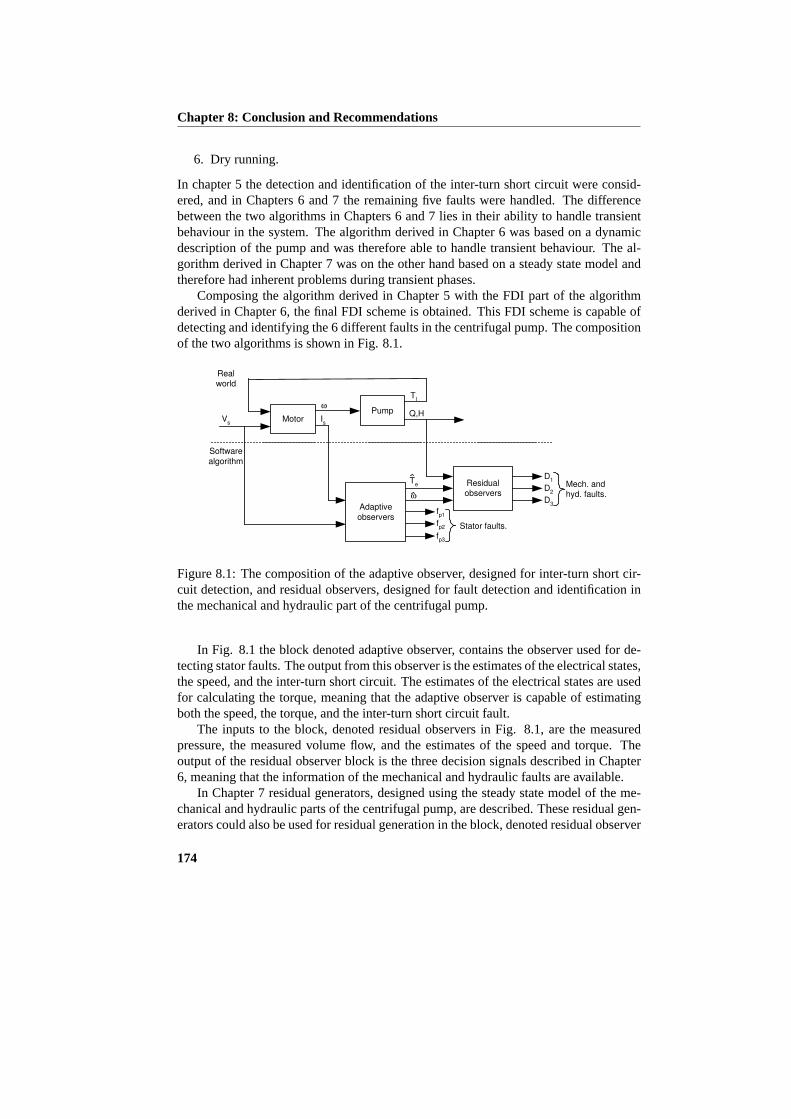
Chapter 8: Conclusion and Recommendations
6. Dry running.
In chapter 5 the detection and identification of the inter-turn short circuit were consid-ered, and in Chapters 6 and 7 the remaining five faults were handled. The differencebetween the two algorithms in Chapters 6 and 7 lies in their ability to handle transientbehaviour in the system. The algorithm derived in Chapter 6 was based on a dynamicdescription of the pump and was therefore able to handle transient behaviour. The al-gorithm derived in Chapter 7 was on the other hand based on a steady state model andtherefore had inherent problems during transient phases.
Composing the algorithm derived in Chapter 5 with the FDI part of the algorithmderived in Chapter 6, the final FDI scheme is obtained. This FDI scheme is capable ofdetecting and identifying the 6 different faults in the centrifugal pump. The compositionof the two algorithms is shown in Fig. 8.1.
Motor Pump
ω
T l
Q,H V
s I s
ω
Software
algorithm
Real world
T e Residual
observers
D 1
D 2
D 3
f p1
f p2
f p3
Adaptive
observers Stator faults.
Mech. and hyd. faults.
Figure 8.1: The composition of the adaptive observer, designed for inter-turn short cir-cuit detection, and residual observers, designed for fault detection and identification inthe mechanical and hydraulic part of the centrifugal pump.
In Fig. 8.1 the block denoted adaptive observer, contains the observer used for de-tecting stator faults. The output from this observer is the estimates of the electrical states,the speed, and the inter-turn short circuit. The estimates of the electrical states are usedfor calculating the torque, meaning that the adaptive observer is capable of estimatingboth the speed, the torque, and the inter-turn short circuit fault.
The inputs to the block, denoted residual observers in Fig. 8.1, are the measuredpressure, the measured volume flow, and the estimates of the speed and torque. Theoutput of the residual observer block is the three decision signals described in Chapter6, meaning that the information of the mechanical and hydraulic faults are available.
In Chapter 7 residual generators, designed using the steady state model of the me-chanical and hydraulic parts of the centrifugal pump, are described. These residual gen-erators could also be used for residual generation in the block, denoted residual observer
174

Section 8.2: Conclusion
in Fig. 8.1. However, by using these residual generators, problems will arise duringtransient phases.
8.2 Conclusion
The following conclusions are drawn on the accomplishments and contributions of thethesis:
• The dynamics of the centrifugal pump were considered in the development of thecentrifugal pump model in Chapter 3. Two assumptions were given, under whichalgebraic maps can be used for describing the energy conversion from mechani-cal to hydraulic energy, and the pressure of the centrifugal pump. Moreover, thedynamics of the hydraulic part can be described by an added mass to the impeller,which is corresponding to the mass of the liquid inside the impeller. This meansthat, when the mechanical and hydraulic part of the centrifugal pump is consid-ered, the dynamics of the pump is described by a first order system. The algebraicmaps describing the energy conversion and the pressure generation are polyno-mial of second order. This makes the model of the system a nonlinear lumpedparameter model. As the model is a lumped parameter model, it is well suited foruse in model-based designs, both when it comes to control and to FDI.
• The most used methods for FDI in centrifugal pumps are, according to the stateof the art analysis, presented in Chapter 2, based on the signal-based approaches.Normally robustness is not considered when FDI algorithms are derived usingsignal-based approaches. Therefore, it was found that a method, which can beused for robustness analysis, was needed. In Chapter 4 a combination of the Fail-ure Mode and Effect Analysis (FMEA) and Fault Propagation Analysis (FPA) isproposed for the robustness analysis of signal-based FDI algorithms. The pro-posed method can be used in the design, as well as in the analysis. In additionto the robustness analysis method, an algorithm for automating one of the manualsteps in the FPA was proposed. Using the improvements of the FMEA and FPA,the proposed analysis method was used to analyse different sensor configurationson the centrifugal pump. Also it was used in the design of a detection scheme,based on one particular sensor configuration. Test results on an industrial test-bench showed that 3 out of 7 chosen faults could be detected in a robust mannerwith this sensor configuration. This showed the usability of the proposed analysisand design method. However, the result obtained in Chapters 6 and 7 showed that,using the model-based approach, 5 different faults were detected using the samesensor configuration. This shows the drawback of the signal-based approacheswhen used on centrifugal pumps.
• One of the faults considered in this work was the inter-turn short circuits in thewindings of the induction motor driving the pump. In the state of the art analysis
175

Chapter 8: Conclusion and Recommendations
in Chapter 2, it was argued, that this fault is often the initiator of a stator burnout.To understand the nature of the inter-turn short circuit fault, a dynamic modelof the fault was derived in Chapter 5. A model was established for bothY- and∆-connected induction motors. One remarkable result was shown by this model,namely that torque ripple should not be expected when an inter-turn short circuithas occurred. That is, if the motor is supplied with a balanced sinusoidal supplyvoltage, and a constant torque load. This fact was indirectly shown in the test,presented in the end of Chapter 5, as the level of oscillations in the real speed didnot change when introducing the inter-turn short circuit fault.
• In Chapter 5, the model of the induction motor, including an inter-turn short cir-cuit, was used in the derivation of an adaptive observer. In real applications, onlythe electrical quantities are normally available. Therefore, the derived adaptiveobserver was only using these quantities. The obtained observer was capable ofestimating an inter-turn short circuit fault in one of the phases, the electrical states,and the speed of the induction motor simultaneously. The design of the observerwas based on a dynamic model of the induction motor, with the speed assumedconstant. Therefore, the observer was capable of detecting the faults during tran-sient behaviour, when the constant speed assumption was not violated too much.This makes the algorithm very useful in real applications. Especially for inductionmotors supplied with a frequency converter, as transients are expected to occurfrequently in these applications. The drawback of the algorithm is the need forthe motor parameters, which are not always known in real life applications.
• In Chapter 3 it was shown that the model of the centrifugal pump is highly non-linear, meaning that model-based approaches, based on nonlinear models, shouldbe considered when the operating point of the pump is changed frequently or isunknown. This is actually the case in many centrifugal pump applications. Here,Structural Analysis (SA) was chosen as the first step in the derivation of residualgenerators. The only straightforward way to use the results of the SA, in orderto obtain residual generators, is the derivations of Analytical Redundant Relations(ARR’s). These ARR’s can, and in general do, contain derivatives of the measuredsignals. To overcome this problem, a novel realization approach was proposed inChapter 6. With this approach, it is possible to obtain a nonlinear state space de-scription from the results of the SA. The obtained state space description does notinclude unknown variables, except for the states of the system. The approach wastested on three applications; a satellite case borrowed from (De Persis and Isidori,2001), the induction motor, and the hydraulic part of the centrifugal pump. Therealization method is based on a solution to a partial differential equation, whichis the main problem with this approach. This is, however, a known problem con-cerning nonlinear state transformations on general nonlinear systems, as it is thecase in the proposed realization approach.
• Based on the results obtained using SA and the realization approach developed in
176

Section 8.3: Recommendations
Chapter 6, three residual observers and an ARR were derived for the centrifugalpump. Tests, on a test-bench developed particularly for this purpose, were per-formed, showing the capabilities of the observers and the ARR. The tests showedthat the observers and the ARR were robust, with respect to changes in the operat-ing point of the pump. Moreover, the tests showed that 5 different faults, affectingthe hydraulic and mechanical parts of the pump, were detectable with this ap-proach. This shows the superiority of the model-based approach compared to thesignal-based approach, when it comes to robustness.
• In Chapter 6, the algorithm, developed for detecting faults in the mechanical andhydraulic part of the centrifugal pump, was based on a dynamic model of the sys-tem. This means that the involved signals were expected to have a bandwidthcovering the dynamics of the system. These high bandwidth signals are often notavailable in real life centrifugal pump applications. However, low bandwidth sig-nals are often available. Therefore, an algorithm based on a steady state modelof the centrifugal pump was proposed in Chapter 7. This algorithm was shownto be able to detect 5 different faults in the mechanical and hydraulic parts ofthe centrifugal pump. The algorithm was made robust with respect to parameteruncertainties, using a set-valued approach. The need for only low bandwidth sen-sors and the robustness considerations, makes the algorithm appropriate for im-plementation in cost sensitive applications, where the necessary sensors alreadyare available.
8.3 Recommendations
The following topics are not covered in this thesis, but it is believed that future investi-gations could be beneficial.
• In Chapter 5 an adaptive observer is designed for simultaneous estimation of theelectrical states, the speed, and the inter-turn short circuit of the induction mo-tor. In the design proposed here, the parameters of the motor are assumed known.However, an adaptive observer is used. Therefore it should be possible to finda transformation of the induction motor model, making it possible for the adap-tive observer to adapt to the motor parameters. If this is possible, the proposedalgorithm becomes parameter independent.
• In Chapter 5 also a Linear Matrix Inequality (LMI) approach was used for bothanalysis and synthesis of the observer gain in the proposed adaptive observer. Itcould be interesting to include the concept of LMI regions in the proposed analysisand synthesis. Hereby, it would be possible to state demands on the damping ratioin the system, as well as the convergence rate.
• In Chapter 6 a new concept, for realization of subsystems identified using Struc-tural Analysis, was presented. This concept should be further investigated. Es-
177

Chapter 8: Conclusion and Recommendations
pecially Assumption 6.2.3, stating the condition for the existence of a state spacetransformation, should be considered.
• In Chapter 7 a detection scheme, based on the steady state model of the pump,was proposed. Because of the steady state model, transient phases can force theresidual to be different from zero, even in the no fault cases. Therefore, means fordetecting these transient conditions, must be established before implementing thealgorithm in real life applications.
• A set-valued approach was proposed for obtaining robustness in the residual gen-eration in Chapter 7. This approach utilizes interval models. Extending the set-valued approach, to include interval models of each fault case, it might be possibleto state which fault has happened in a robust manner. Hereby robustness is intro-duced in the identification of incipient faults.
178

Bibliography
Tom M. Apostol.Mathematical Analysis, second edition. Addison-Wesley PublishingCompany, Inc., 1974. ISBN 0-201-00288-4.
M. Arkan, D. K. Perovic, , and P. Unsworth. Online stator fault diagnosis in inductionmotors.IEE proceedings on electrical power applications, Vol. 148, No. 6, 2001.
Neil Arthur and Jim Penman. Induction machine condition monitoring with higherorder spectra.IEEE Transaction on Industrial Electronics, Vol. 47, No. 5, 2000.
S. Backir, S. Tnani, T. Poinot, and J. C. Trigeassou. Stator fault diagnosis in inductionmachines by parameter estimation.IEEE, International Symposium on Diagnostics,Grado, Italy, 2001.
Antonio Baldassarre, Maurizio De Lucia, and Paolo Nesi. Real-time detection of cav-itation for hydraulic turbomachines.Real-Time Imaging 4, Page 403 - 416, 1998.
Michele Basseville and Igor V. Nikiforov.Detection of Abrupt Changes - Theory andApplication. www.irisa.fr/sigma2/kniga/, 1998.
Alberto Bellini, Fiorenzo Filippetti, Giovanni Franceschini, Carla Tassoni, and Ger-ald B. Kliman. Quantitative evaluation of induction motor broken bars by means ofelectrical signature analysis.IEEE Transaction on Industry Applications, Vol. 37, No.5, 2001.
Mohamed El Hachemi Benbouzid. A review of induction motors signature analysis asa midium for faults detection.IEEE Transactions on industrial electronics vol. 47 no.5, 2000.
Gildas Besancon. Remarks on nonlinear adaptive observer design.ELSEVIER, System& Control Letters, Vol. 41, No. 4, 2000.
Søren Abildsten Bøgh.Fault Tolerant Control Systems - a Development Method andReal-Life Case Study. PhD thesis, Aalborg University, Department of Control Engi-neering, 1997.
179

Bibliography
Péter Bóka and Gábor Halász. Dynamic behaviour of centrifugal pumps.Proceedingsof the XXIst IAHR Symposium on Hydraulic Machinery and Systems, Lausanne, 2002.
Mogens Blanke. Consistent design of dependable control systems.Control Eng. Prac-tice, Vol. 4, No. 9, 1996.
Mogens Blanke, Michel Kinnaert, Jan Lunze, and Marcel Starowiecki.Diagnosis andFault-Tolerant Control. Springer Verlag, 2003. ISBN 3-540-01056-4.
Julien Le Bleu Jr. and Ming Xu. Vibration monitoring of sealess pumps using spikeenergy.Sound and Vibration, Vol. 29, No. 12, 1995.
Austin H. Bonnett and George C. Soukup. Cause and analysis of stator and rotorfailures in three-phase squirrel-cage induction motors.IEEE Transaction on IndustryApplications, Vol. 28, No. 4, 1992.
A. Boukhris, D. Mandel, and J. Ragot. Data validation using interval algebra.UKACCInternational Conference on Control, CONTROL’98, 1998.
Fernando Briz, Michael W. Degner, Antonio Zamarron, and Juan M. Guerrero. Onlinestator winding fault diagnosis in inverter-fed ac machines using high-frequency signalinjection. IEEE Transactions on Industry Applications, Vol. 39, No. 4., 2003.
Cash, M. A., Habetler, T. G., and Kliman, G. B. Insulation failure prediction in in-duction machines using line-neutral voltages.IEEE Industry Applications Conference,Thirty-Second IAS Annual Meeting, IAS ’97, 1997.
Jie Chen and R. J. Patton.Robust Model-Based Fault Diagnosis for Dynamic Systems.Kluwer Academic Publishers, 1999. ISBN 0-7923-8411-3.
Young Man Cho and Rajesh Rajamani. A systematic approach to adaptive observersynthesis for nonlinear systems.IEEE Transactions on Automatic Control, Vol. 42, No.4, 1997.
Tommy W. S. Chow and Hong-Zhou Tan. Hos-based nonparametric and parametricmethodologies for machine fault detection.IEEE Transaction on Industrial Electron-ics, Vol. 47, No. 5, 2000.
David Cox, John Little, and Donal O’Shea.Ideals, Varieties, and Algorithms, Anintroduction to computational algebraic geometry and comutative algebra. Springer-Verlag Inc., 1997. ISBN 0-387-94680-2.
Sergio M. A. Cruz and A. J. Marques Cardoso. Stator winding fault diagnosis in three-phase synchronous and asynchronous motors, by the extended park’s vector approach.IEEE Transaction on Industrial Applications, Vol. 37, No. 5, 2001.
M. Cudina. Detection of cavitation phenomenon in centrifugal pump using audiblesound.Mechanical Systems and Signal Processing, Vol. 17, No. 6, 2003.
180

Bibliography
Francesco Cupertino, Elisabetta de Vanna, Luigi Salvatore, and Silvio Stasi. Analysistechniques for detection of im broken rotor bars after supply disconnection.IEEETransactions on Industry Applications, Vol. 40, No. 2., 2004.
Tracy Dalton, Ron J. Patton, and J. Chen. Application of eigenstructure assignment torobust residual design for FDI.UKACC International Conference on Control, CON-TROL ’96, 1996.
Claudio De Persis and Alberto Isidori. A geometric approach to nonlinear fault detec-tion and isolation.IEEE Transaction on Automatic Control, Vol. 46 No. 6, 2001.
Diego Del Gobbo, Marcello Napolitano, Parviz Famouri, and Mario Innocenti. Expe-rimantal application of extended kalman filtering for sensor valitation.IEEE Transac-tions on Control Systems Technology, Vol 9. No 2., 2001.
Levent Eren and Michael J. Devaney. Motor bearing damage detection via waveletanalysis of the starting current transient.IEEE Instrumentation and Measurement Tech-nology Conference, 2001.
P. M. Frank and X. Ding. Survey of robust residual generation and evaluation methodsin observer-based fault detection systems.Journal of Proces Control, Vol. 7, No. 6,1997.
Jens Friedrichs and Günter Kosyna. Rotating cavitation in a centrifugal pump impellerof low specific speed.Transactions of the ASME, Journal of Fluid Engineering, Vol.124, No. 2, 2002.
Erik Frisk and Jan Åslund. Lowering orders of derivatives in non-linear consistencyrelations - theory and simulation examples. Technical Report LiTH-R-2547, Dept. ofElectrical Engineering, Linköping University, Sweden, 2003.
Pablo García, Fernando Briz, Michael W. Degner, and Alberto B. Diez. Diagnosticsof induction machines using the zero sequence voltage.Proceedings of the IEEE39th
IAS Annual Meeting, Seattle, Washington, 2004.
E. Alcorta Garcia and P. M. Frank. Deterministic nonlinear observer-based approachesto fault diagnosis: A survey.Control Eng. practice, Vol. 5 No. 5, 1997.
C. Gerada, K. J. Bradley, M. Sumner, P. Wheeler, S. Pickering, J. Clare, C. Whitley,and G. Towers. The implications of winding faults in induction motor drives.Proceed-ings of the IEEE39th IAS Annual Meeting, Seattle, Washington, 2004.
Janos J. Gertler.Fault Detection and Diagnosis in Engineering Systems. MarcelDekker, Inc., 1998. ISBN 0-8247-9427-3.
Jan Tommy Gravdahl and Olav Egeland. Centrifugal compressor surge and speed con-trol. IEEE Transactions on Control System Technology, vol. 7, No. 5, 1999.
181

Bibliography
S. Greitzke and C. Schmidthals. Principles and application of a diagnosis system formechanical seals.Pump Users International Forum 2000, Karlsruhe, 2000.
Janati Idrissi, Olivier Adrot, and Jose Ragot. Multi-fault detection of systems withbounded uncertainties.Proceedings of the 40th IEEE Conference on Decision andControl, Orlando, Florida USA, 2001.
R. Isermann. Supervision fault-detection and fault-diagnosis methods - an introduction.Control Eng. Practice, vol. 5, No. 5, 1997.
R. Isermann and P. Balle. Trends in the application of model-based fault detection anddiagnosis of technical processes.Control Eng. Practice, vol 5, No. 5, 1997.
Alberto Isidori.Nonlinear Control Systems, third edition. Springer-Verlag, 1995. ISBN3-540-19916-0.
Roozbeh Izadi-Zamanabadi.Fault-tolerant Supervisory Control - System Analysis andLogic Design. PhD thesis, Aalborg University, Department of Control Engineering,1999.
Roozbeh Izadi-Zamanabadi. Structural analysis approach for fault diagnosis and dis-turbance decoupling. Technical report, Institute of Electronic Systems, Aalborg Uni-versitet, Denmark, 2001.
Roozbeh Izadi-Zamanabadi and Marcel Staroswiecki. A structural analysis methodformulation on fault-tolerant control system design.Proc. of the39th IEEE Conferenceon Decision and Control, Sydney, Austrailia, 2000.
Bin Jiang and Marcel Staroswiecki. Adaptive observer design for robust fault estima-tion. International Journal of Systems Science, Vol. 33, No. 9, 2002.
Gojko M. Joksimovic and Jim Penman. The detection of inter-turn short circuits in thestator windings of operating motors.IEEE Transaction on Industrial Electronics, Vol.47, No. 5, 2000.
Rikke Bille Jørgensen.Development and Test of Methods for Fault Detection andIsolation. PhD thesis, Aalborg University, Department of Control Engineering, 1995.
Carsten Skovmose Kallesøe, Vincent Cocquempot, and Roozbeh Izadi-Zamanabadi.Model based fault detection in a centrifugal pump application.Submitted in 2004 toIEEE Transactions on Control Systems Technology, 2004a.
Carsten Skovmose Kallesøe and Roozbeh Izadi-Zamanabadi. A realization approachfor residual expressions.Submitted to the joint 44th IEEE Conference on Decision andControl and European Control Conference ECC 2005, 2005.
182
Bibliography
Carsten Skovmose Kallesøe, Roozbeh Izadi-Zamanabadi, Vincent Cocquempot, andHenrik Rasmussen. Model based fault diagnosis in a centrifugal pump applicationusing structural analysis.Proceedings of the IEEE International Conference on ControlApplications, Taipei, Taiwan, 2004b.
Carsten Skovmose Kallesøe, Henrik Rasmussen, Pierre Vadstrup, and Roozbeh Izadi-Zamanabadi. Estimation of stator winding faults in induction motors using an adaptiveobserver scheme.Proceedings of the IEEE39th IAS Annual Meeting, Seattle, Wash-ington, 2004c.
Marian P. Kazmierkowski.Automatic Control of Converter-Fed Drives. PWN-PolishScientific Publishers, Warszawa, 1994.
T. Kenull, G. Kosyna, and P. U. Thamsen. Diagnostics of submersible motor pumps bynon-stationary signals in motorcurrent.The 1997 ASME Fluids Engineering DivisionSummer Meeting, FEDSM’97, 1997.
Hassan K. Khalil.Nonlinear Systems. Prentice-Hall, Inc., 2002. ISBN 0-13-067389-7.
G. B. Kliman, W. J. Premerlani, R. A. Koegl, and D. Hoeweler. A new approachto on-line turn fault detection in ac motors.IEEE Industry Applications Conference,Thirty-First IAS Annual Meeting, IAS ’96, 1996.
D. Kollmar, D. H. Hellman, and S. Brodersen. Intelligent standardized chemicalpumps, a chance for pump users?Pump Users International Forum 2000, Karlsruhe,2000a.
D. Kollmar, D. H. Hellman, and F. W. Hennecke. An early failure detection systememerging from laboratory into plant.Pump Users International Forum 2000, Karl-sruhe, 2000b.
Dragica Kostic-Perovic, Muslum Arkan, and Peter Unsworth. Induction motor faultdetection by space vector angular fluctuation.Proceedings of the IEEE35th IAS AnnualMeeting, 2000.
P. C. Krause, O. Wasynczuk, and S. D. Sudhoff.Analysis of Electric Machinery. IEEEPress, 1994.
Sang-Bin Lee, Rangarajan M. Tallam, and Thomas G. Habetler. A robust, on-line turn-fault detection technique for induction machines based on monitoring the sequencecomponent impedance matrix.IEEE Transactions on Power Electronics, Vol. 18, No.3, 2003.
Werner Leonhard.Control of Electrical Drives. Springer-Verlag Berlin HeidelbergNew York, 1996. ISBN 3-540-13650-9.
183

Bibliography
Bo Li, Mo-Yuen Chow, Yodyium Tipsuwan, and James C. Hung. Neural-network-based motor rolling bearing fault diagnosis.IEEE Transactions on industrial electron-ics vol. 47 no. 5, 2000.
Linfan Liu and Jennie Si. Fault isolation filter design for linear systems.Digital Avion-ics Systems Conference, 13th DASC., AIAA/IEEE, 1994.
Lennart Ljung. System Identification, Theory for the User, Second edition. PrenticeHall Inc., 1999. ISBN 0-13-656695-2.
Henrik Lohrberg and Bernd Stoffel. Measurement of cavitation erosive aggressivenessby means of structure born noise.IFAC 2000, 2000.
Henrik Lohrberg, Burkart Voss, Bernd Stoffel, and Manfred Glesner. Impeller inte-grated measurement of cavitation erosive aggressiveness.Mechatronic, Vol. 12, No. 8,2002.
Kenneth A. Loparo, M. L. Adams, Wei Lin, M. Farouk Abdel-Magied, and NadarAfshari. Fault detection and diagnosis of rotating machinery.IEEE Transactions onindustrial electronics vol. 47 no. 5, 2000.
Xiaogang Luo, Yuefeng Liao, Hamid A. Toliyat, Ahmed El-Antably, and Thomas A.Lipo. Multiple coupled circuit modeling of induction machines.IEEE Transactions onIndustry Applications, Vol. 31, No. 2, 1995.
Mohammad-Ali Massoumnia, George C. Verghese, and Alan S. Willsky. Fault de-tection and identification.IEEE Transactions on Automatic Control, Vol. 34, No. 3,1989.
R. Müller-Petersen, Th. Kenull, and G. Kosyna. Condition monitoring of pumps bymotor current analysis in a field test.Pump Users International Forum 2004, Karl-sruhe, 2004.
Ramon E. Moore.Methods and Applications of Interval Analysis. SIAM, Philadelphia,1979. ISBN 0-89871-161-4.
Kent R. Nagle and Edward B. Saff.Fundamentals of Differential Equations andBoundary Balue Problems, Second edition. Addison-Wesley, 1996. ISBN 0-201-80879-X.
Subhasis Nandi and Hamid A. Toliyat. Novel frequency-domain-based technique todetect stator interturn faults in induction machines using stator-induced voltages afterswitch-off. IEEE Transactions on Industry applications, Vol. 38, No. 1, 2002.
G. D. Neill, R. L. Reuben, E. R. Brown, and J. A. Steel. Detection of incipient cavi-tation in pumps using acoustic emission.Proceedings of the Institution of MechanicalEngineers, Vol. 211, Part E, 1997.
184

Bibliography
D. W. Novotny and T. A. Lipo.Vector Control and Dynamics of AC Drives. OxfordUniversity Press Inc., New York, 1996.
Jorge L. Parrondo, Sandra Velarde, and Carlos Santolaria. Development of a predic-tive maintenance system for a centrifugal pump.Journal of Quality in MaintenanceEngineering, Vol. 4, No. 3, 1998.
R. J. Patton and J. Chen. Observer-based fault detection and isolation: Robustness andapplications.Control Eng. Practice, Vol. 5, No. 5, 1997.
S. Perovic, P. J. Unsworth, and E. H. Higham. Fuzzy logic system to detect pump faultsfrom motor current spectra.IEEE, Industry Applications Conference Thirty-Sixth IASAnnual Meeting, 2001.
Rajesh Rajamani and J. Karl Hedrick. Adaptive observers for active automotive sus-pensions: Theory and experiment.IEEE Transactions on Control Systems Technology,Vol. 3, No. 1, 1995.
Henrik Rasmussen.Self-tuning Torque Control of Induction Motors for High Perfor-mance Applications. PhD thesis, Aalborg University, Department of Control Engineer-ing, 1995.
John A. Roberson and Clayton T. Crowe.Engineering Fluid Mechanics, Fifth Edition.Houghton Mifflin Company, 1993. ISBN 0-395-66161-7.
A. T. Sayers.Hydraulic and Compressible flow Turbomachines. McGraw-Hill BookCompany, 1990.
Carsten Scherer and Siep Weiland. Lecture note disc course on linear matrix inequal-ities in control, version 2.0. Technical report, Delft University of Technology, Delft,The Netherlands, 1999. Available on the homepage of Carsten W. Scherer.
Randy R. Schoen, Thomas G. Habetler, Farrukh Lamran, and Robert G. Bartheld. Mo-tor bearing damage detection using stator current monitoring.IEEE Transactions onindustry Applications vol. 31 no. 6, 1995.
Mau-Hsiang Shih. Solution of the boolean markus-yamabe problem.Advances inApplied Mathematics, Vol. 22, No. 1, 1999.
Jason R. Stack, Ronald G. Harley, and Thomas G. Habetler. An amplitude modulationdetector for fault diagnosis in rolling element bearings.Proceedings of 28th AnnualConference of the IEEE Industrial Electronics Society, 2002.
M. Staroswiecki. Quantitative and qualitative models for fault detection and isolation.Mechanical Systems and Signal Processing, Vol. 14, No. 3, 2000.
M. Staroswiecki and G. Comtet-Varga. Analytical redundancy relations for fault de-tection and isolation in algebraic dynamic systems.Automatica, Vol. 37, No. 5, 2001.
185
Bibliography
A. J. Stepanoff.Flow Pumps, Design and Application. John Wiley & sons, 1957. ISBN0 471 82137 3.
Jakob Stoustrup and Henrik Niemann. Fault detection for nonlinear systems - a stan-dard problem approach.Proceedings of the 37th IEEE Conference on Decision &Control., 1998.
Jakob Stoustrup and Henrik Niemann. Fault estimation - a standard problem approach.International Journal of Robust and Nonlinear Control, Vol. 12, No. 8, 2002.
Karl Åström, Pedro Albertos, Mogens Blanke, Alberto Isidori, Walter Schaufelberger,and Ricardo Sanz.Control of Complex Systems. Springer-Verlag, 2001. ISBN 1-85233-324-3.
Charles R. Sullivan and Seth R. Sanders. Models for induction machines with magneticsaturation of the main flux path.IEEE Transactions on Industrial Applications, Vol 31,No. 4, 1995.
D. Surek. Pump monitoring by measurement of the case vibrations.Pump UsersInternational Forum 2000, 2000.
Rangarajan M. Tallam, Thomas G. Habetler, and Ronald G. Harley. Transient modelfor induction machinces with stator winding turn faults.IEEE Transactions on IndustryApplications, Vol. 38, No. 3, 2002.
Rangarajan M. Tallam, Thomas G. Habetler, and Ronald G. Harley. Stator windingturn-fault detection for closed-loop induction motor drives.IEEE Transactions on In-dustry Applications, Vol. 39, No. 3, 2003.
Jesper Sandberg Thomsen. A fault tolerant electronic steering system for a fork lifttruck. Technical report, Institute of Electronic Systems, Aalborg Universitet, Denmark,2000.
Hamid A. Toliyat, Thomas A. Lipo, and J. Coleman White. Analysis of a concen-trated winding induction machine for adjustable speed drive applications part 1 (motoranalysis).IEEE Transactions on Energy Conversion, Vol 6, No. 4, 1991.
Sebastian Tornill, Teresa Escobet, and Vicenc Puig. Fault detection using intervalmodels.SafeProcess ’2000, IFAC, Budapest, 2000.
Frederik C. Trutt, Joseph Sottile, and Jeffery L. Kohler. Online condition monitoringof induction motors.IEEE Transactions on Industry Applications, Vol. 38, No. 6, 2002.
Andrzej M. Trzynadlowski and Ewen Ritchie. Comparative investigation of diagnosticmedia for indiction motors, a case of rotor cage faults.IEEE Transaction on IndustrialElectronics, Vol. 47, No. 5, 2000.
186

Bibliography
Pierre Vadstrup. Multiwinding modelling of induction motors. Technical report,Grundfos Mangement A/S, 2002. Internal technical rapport at Grunfos, not available.
E. Wiedenbrug, G. Frey, and J. Wilson. Impulse testing and turn insulation deterio-ration in electric motors.IEEE Pulp and Paper Industry Technical Conference ’03,2003.
S. Williamson and K. Mirzoian. Analysis of cage induction motors with stator windingsfaults. IEEE Transactions on Power Apparatus and Systems, Vol. Pas-104, Issue. 7,1985.
Armin Wolfram, Dominik Fussel, Torsten Brune, and Rolf Isermann. Component-based multi-model aproach for fault detection and diagnosis of a centrifugal pump.IEEE Proceedings of American Control Conference, ACC-2001, 2001.
Aiping Xu and Qinghua Zhang. Nonlinear system fault diagnosis based on adaptiveestimation.Automatica, Vol. 40, No. 7, 2004.
Zhongming Ye and Bin Wu. Online rotor bar breakage detection of three phase induc-tion motors by wavelet packet decomposition and artificial neural network.IEEE 32ndAnnual Power Electronics Specialists Conference, 2001.
Zhongming Ye, Bin Wu, and A. R. Sadaghian. Current signature analysis of induc-tion motor mechanical faults by wavelet packet decomposition.IEEE Transactions onIndustrial Electronics, Vol. 50, No. 6., 2003.
Qinghua Zhang. A new residual generation and evaluation method for detection andisolation of faults in non-linear systems.International Journal of Adaptive Control andSignal Processing, Vol. 14, No. 7, 2000.
187

Bibliography
188

Appendix A
FMEA Tables Describing Faultsin the System
This appendix contains tables describing the fault modes of the pump system. The pumpsystem is in Chapter 4 devided into 7 components. These are,
• Electrical part of the induction motor.
• Mechanical part of the induction motor.
• Shaft.
• Hydraulic part of the centrifugal pump.
• Mechanical part of the centrifugal pump.
• Inlet of the pump.
• Outlet of the pump.
In each Section of this appendix one of the above components is analysed. This meansthat a FMEA table is given and that the disturbing events affecting the component arelisted. The FMEA tables contain the following information; thename of the fault mode,the causes of the fault, and thethe effect of the fault. Here, the general components,forming a centrifugal pump, are analysed. This means that no failure information of aparticular product is used. This information is necessary to include risk assessment andfrequency of the faults in the FMEA, and are therefore omitted here. The tables andmatrices in this appendix are the results of the FMEA described in Chapter 4.
189
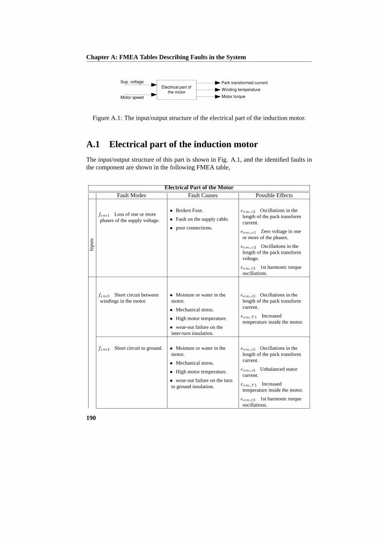
Chapter A: FMEA Tables Describing Faults in the System
Electrical part of the motor
Sup. voltage
Winding temperature
Motor speed
Park transformed current
Motor torque
Figure A.1: The input/output structure of the electrical part of the induction motor.
A.1 Electrical part of the induction motor
The input/output structure of this part is shown in Fig. A.1, and the identified faults inthe component are shown in the following FMEA table,
Electrical Part of the MotorFault Modes Fault Causes Possible Effects
fem1 Loss of one or morephases of the supply voltage.
• Broken Fuse.
• Fault on the supply cable.
• poor connections.
eem,i3 Oscillations in thelength of the pack transformcurrent.
eem,v1 Zero voltage in oneor more of the phases.
eem,v2 Oscillations in thelength of the pack transformvoltage.
eem,t3 1st harmonic torqueoscillations.
Inpu
ts
fem3 Short circuit betweenwindings in the motor.
• Moisture or water in themotor.
• Mechanical stress.
• High motor temperature.
• wear-out failure on theinter-turn insulation.
eem,i3 Oscillations in thelength of the pack transformcurrent.
eem,T1 Increasedtemperature inside the motor.
fem4 Short circuit to ground. • Moisture or water in themotor.
• Mechanical stress.
• High motor temperature.
• wear-out failure on the turnto ground insulation.
eem,i3 Oscillations in thelength of the pack transformcurrent.
eem,i4 Unbalanced statorcurrent.
eem,T1 Increasedtemperature inside the motor.
eem,t3 1st harmonic torqueoscillations.
190

Section A.1: Electrical part of the induction motor
Par
ts
fem5 Broken rotor bar. • Poor production.
• Mechanical stress.
eem,i3 Oscillations in thelength of the pack transformcurrent.
eem,t4 higher harmonictorque oscillations.
fem6 Eccentric air gab due tobend or misaligned motorshaft.
• Poor production.
• Mechanical stress.
eem,i4 Unbalanced statorcurrent.
eem,t3 1st harmonic torqueoscillations.
The propagation matrix representation of the component is given by the following logi-cal expression,
eem ← Aemfem
fem + Aemdy edy (A.1)
where the fault vectorfem and the effect vectoreem equals,
f ′em =(
fem1 fem2 fem3 fem4 fem5 fem6
)T
eem =(
eem,i1 eem,i2 eem,i3 eem,i4 eem,v1 eem,v2
eem,T1 eem,t1 eem,t2 eem,t3 eem,t4
)T
A description of each fault and effect is found in the above FMEA table. The faultpropargation matrixAem
femin (A.1) is just a matrix representation of the connections
between the faults and the effects described in the FMEA table presented in this section.The propagation matrixAem
dy is defined below,
Aemdy =
0 1 0 0 0 0 01 0 0 0 0 0 00 0 1 0 0 0 00 0 1 0 0 0 0
T
To cover the disturbances affecting this component, the fault vector is extended witha set of disturbing events. These are,
191
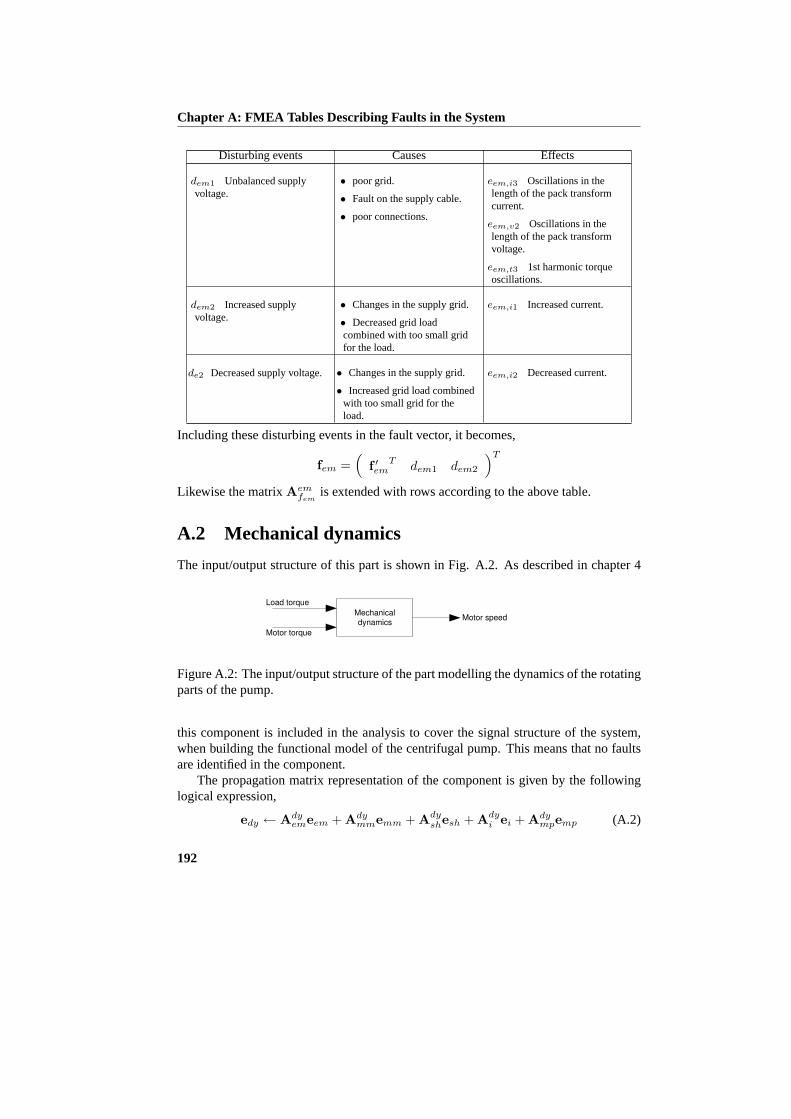
Chapter A: FMEA Tables Describing Faults in the System
Disturbing events Causes Effects
dem1 Unbalanced supplyvoltage.
• poor grid.
• Fault on the supply cable.
• poor connections.
eem,i3 Oscillations in thelength of the pack transformcurrent.
eem,v2 Oscillations in thelength of the pack transformvoltage.
eem,t3 1st harmonic torqueoscillations.
dem2 Increased supplyvoltage.
• Changes in the supply grid.
• Decreased grid loadcombined with too small gridfor the load.
eem,i1 Increased current.
de2 Decreased supply voltage.• Changes in the supply grid.
• Increased grid load combinedwith too small grid for theload.
eem,i2 Decreased current.
Including these disturbing events in the fault vector, it becomes,
fem =(
f ′emT
dem1 dem2
)T
Likewise the matrixAemfem
is extended with rows according to the above table.
A.2 Mechanical dynamics
The input/output structure of this part is shown in Fig. A.2. As described in chapter 4
Mechanical dynamics
Load torque
Motor speed
Motor torque
Figure A.2: The input/output structure of the part modelling the dynamics of the rotatingparts of the pump.
this component is included in the analysis to cover the signal structure of the system,when building the functional model of the centrifugal pump. This means that no faultsare identified in the component.
The propagation matrix representation of the component is given by the followinglogical expression,
edy ← Adyemeem + Ady
mmemm + Adyshesh + Ady
i ei + Adympemp (A.2)
192

Section A.3: Mechanical part of the motor
The resulting effect vectoredy in this expression is given by,
edy =(
edy,n1 edy,n2 edy,n3 edy,n4
)T
where the effects in this vector are,
edy,n1 ∼ Increased speed.edy,n2 ∼ Decreased speed.edy,n3 ∼ 1st harmonic speed oscillations.edy,n4 ∼ higher harmonic speed oscillations.
The propagation matricesAdyem, Ady
mm, Adysh, Ady
i , andAdymp in (A.2) are defined below,
Adyem =
0 0 0 0 0 0 0 1 0 0 00 0 0 0 0 0 0 0 1 0 00 0 0 0 0 0 0 0 0 1 00 0 0 0 0 0 0 0 0 0 1
Adymm =
0 1 0 0 0 0 01 0 0 0 0 0 00 0 1 0 0 0 00 0 0 1 0 0 0
Adysh =
0 0 0 0 0 0 0 0 00 0 0 0 0 0 0 0 00 0 0 0 0 1 0 1 00 0 0 0 0 0 1 0 1
Adyi =
0 0 0 0 0 0 1 1 0 0 0 00 0 0 0 0 1 0 0 0 0 0 00 0 0 0 0 0 0 0 1 0 0 00 0 0 0 0 0 0 0 0 1 0 0
Adymp =
0 1 0 0 0 0 0 0 01 0 0 0 0 0 0 0 00 0 1 0 0 0 0 0 00 0 0 1 0 0 0 0 0
A.3 Mechanical part of the motor
The input/output structure of this part is shown in Fig. A.3, and the identified faults inthe component are shown in the following FMEA table,
193

Chapter A: FMEA Tables Describing Faults in the System
Mechanical part of the motor
Motor speed Bearing temperature
Mechanical vibrations
Load torque
Figure A.3: The input/output structure of the mechanical part of the induction motor.
Mechanical Part of the MotorFault Modes Fault Causes Possible Effects
fmm1 Ware of the bearingsin the motor.
• Ware-out faults due to along running period.
• Impurities in the bearings.
• Water in the bearing oil.
emm,t4 higher harmonictorque oscillations.
emm,T1 Increased bearingtemperature.
emm,v2 Increased higherharmonic vibrations.
Par
ts
fmm2 Rub impact betweenthe stator and the rotor due toa bend or misaligned motorshaft.
• Production fault.
• Overload due to suddentblocked rotor.
emm,t1 Increased torqueload from mechanical parts inthe motor.
emm,t3 1st harmonic torqueoscillations.
emm,v1 Increased 1stharmonic vibrations.
The propagation matrix representation of the component is given by the following logi-cal expression,
emm ← Ammfmm
fmm + Ammdy edy (A.3)
where the fault vectorfmm and the effect vectoremm equals,
fmm =(
fmm1 fmm2
)T
emm =(
emm,t1 emm,t2 emm,t3 emm,t4 emm,T1 emm,v1 emm,v2
)T.
A description of each fault and effect is found in the above FMEA table. The faultpropargation matrixAmm
fmmin (A.3) is just a matrix representation of the connections
between the faults and the effects described in the FMEA table presented in this section.The propagation matrixAmm
dy is defined below,
Ammdy =
1 0 0 0 0 0 00 1 0 0 0 0 00 0 1 0 0 1 00 0 0 1 0 0 1
T
194
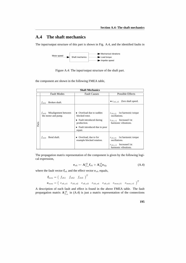
Section A.4: The shaft mechanics
A.4 The shaft mechanics
The input/output structure of this part is shown in Fig. A.4, and the identified faults in
Shaft mechanics Load torque Motor speed
Mechanical vibrations
Impeller speed
Figure A.4: The input/output structure of the shaft part.
the component are shown in the following FMEA table,
Shaft MechanicsFault Modes Fault Causes Possible Effects
fsh1 Broken shaft. • esh,s5 Zero shaft speed.
Par
ts
fsh2 Misalignment betweenthe motor and pump.
• Overload due to suddenblocked rotor.
• Fault introduced duringproduction.
• Fault introduced due to poorrepair.
esh,t1 1st harmonic torqueoscillations.
esh,v1 Increased 1stharmonic vibrations.
fsh3 Bend shaft. • Overload, due to forexample blocked rotation.
esh,t1 1st harmonic torqueoscillations.
esh,v1 Increased 1stharmonic vibrations.
The propagation matrix representation of the component is given by the following logi-cal expression,
esh ← Ashfsh
fsh + Ashdyedy (A.4)
where the fault vectorfsh and the effect vectoresh equals,
fmm =(
fsh1 fsh2 fsh3
)T
emm =(
esh,s1 esh,s2 esh,s3 esh,s4 esh,s5 emm,t1 emm,v1
)T
A description of each fault and effect is found in the above FMEA table. The faultpropargation matrixAsh
fshin (A.4) is just a matrix representation of the connections
195

Chapter A: FMEA Tables Describing Faults in the System
between faults and the effects described in the FMEA table presented in this section.The propagation matrixAsh
dy is defined below,
Ammdy =
1 0 0 0 0 0 00 1 0 0 0 0 00 0 1 0 0 0 00 0 0 1 0 0 0
T
A.5 Hydraulics of the Centrifugal Pump
The input/output structure of this part is shown in Fig. A.5, and the identified faults in
Electrical part of the motor
Impeller speed
Torque load Eye pressure Mechanical vibrations
Impeller pressure Inlet flow
Figure A.5: The input/output structure of the part describing the hydraulics of the cen-trifugal pump.
the component are shown in the following FMEA table,
Hydraulics of the Centrifugal PumpFault Modes Fault Causes Possible Effects
Inpu
ts
fi1 Dry running. • Error in the hydraulicsystem in which the pump isplaced.
ei,h3 Zero pressure.
ei,t3 Zero torque load fromthe impeller.
fi2 Impurities fixed on theimpeller, causing inbalance.
• Impurities in the water. ei,h4 Harmonic pressureoscillations.
ei,t4 1st harmonic torqueoscillations.
ei,t5 higher harmonic torqueoscillations.
ei,v1 Increased 1st harmonicvibrations.
ei,v2 Increased higherharmonic vibrations.
196

Section A.5: Hydraulics of the Centrifugal Pump
Par
ts
fi3 Wear of the impeller. • Sand and other impurities inthe water.
ei,h2 Decreased pressure.
ei,h4 Harmonic pressureoscillations.
ei,t2 Decreased torque loadfrom the impeller.
ei,t4 1st harmonic torqueoscillations.
ei,t5 higher harmonic torqueoscillations.
ei,v1 Increased 1st harmonicvibrations.
ei,v2 Increased higherharmonic vibrations.
fi4 Blocked or partialblocked flow field inside theimpeller.
• Larges obstical in the liquid. ei,h2 Decreased pressure.
ei,h4 Harmonic pressureoscillations.
ei,t2 Decreased torque loadfrom the impeller.
ei,t4 1st harmonic torqueoscillations.
ei,t5 higher harmonic torqueoscillations.
ei,v1 Increased 1st harmonicvibrations.
ei,v2 Increased higherharmonic vibrations.
fi5 Blocked impellerrotation.
• Sand and other impurities inthe water.
ei,h3 Zero pressure.
ei,t1 Increased torque loadfrom the impeller.
fi6 Wear of the sealing ring. • Long running time / normalwear.
• Overheated, due to forexample dry running.
ei,h2 Decreased pressure.
ei,t2 Decreased torque loadfrom the impeller.
fi7 Missing sealing ring. • Production error. ei,h2 Decreased pressure.
ei,t2 Decreased torque loadfrom the impeller.
197
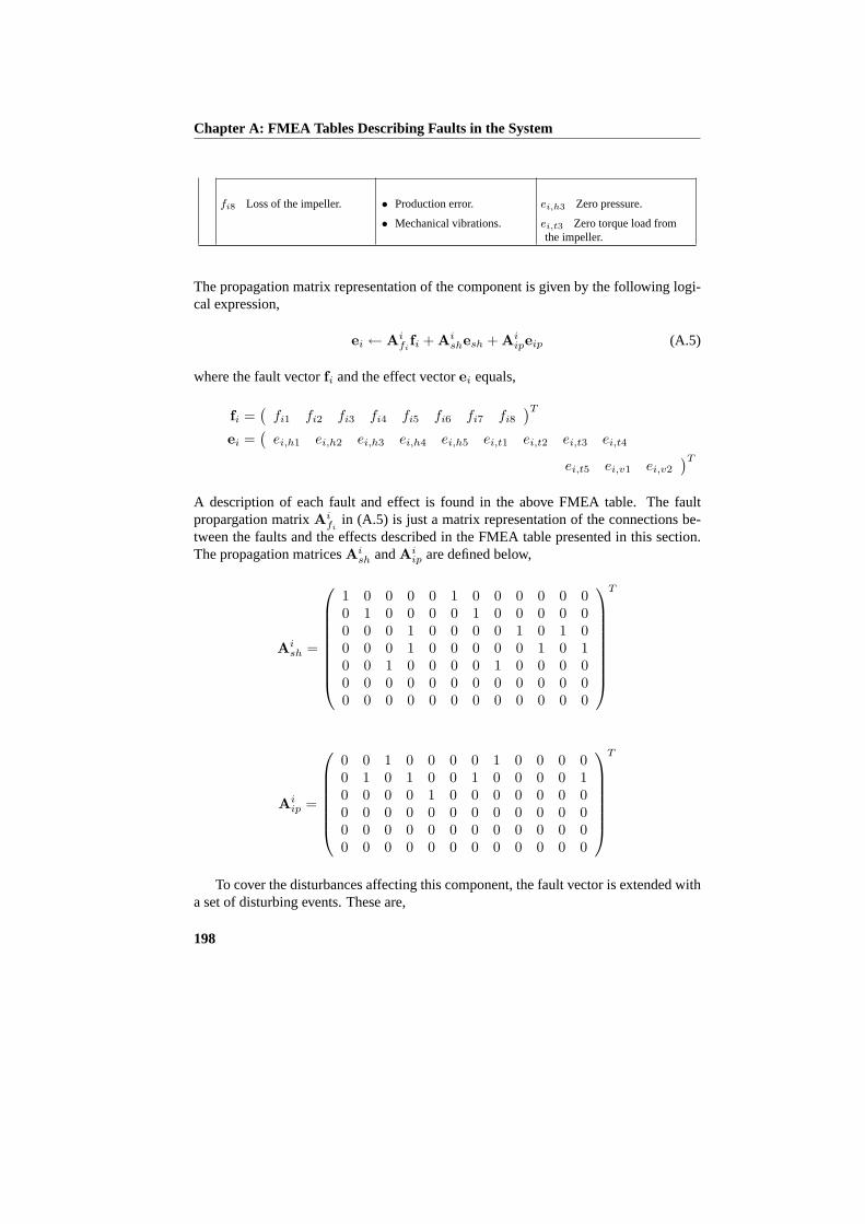
Chapter A: FMEA Tables Describing Faults in the System
fi8 Loss of the impeller. • Production error.
• Mechanical vibrations.
ei,h3 Zero pressure.
ei,t3 Zero torque load fromthe impeller.
The propagation matrix representation of the component is given by the following logi-cal expression,
ei ← Aififi + Ai
shesh + Aiipeip (A.5)
where the fault vectorfi and the effect vectorei equals,
fi =(
fi1 fi2 fi3 fi4 fi5 fi6 fi7 fi8
)T
ei =(
ei,h1 ei,h2 ei,h3 ei,h4 ei,h5 ei,t1 ei,t2 ei,t3 ei,t4
ei,t5 ei,v1 ei,v2
)T
A description of each fault and effect is found in the above FMEA table. The faultpropargation matrixAi
fiin (A.5) is just a matrix representation of the connections be-
tween the faults and the effects described in the FMEA table presented in this section.The propagation matricesAi
sh andAiip are defined below,
Aish =
1 0 0 0 0 1 0 0 0 0 0 00 1 0 0 0 0 1 0 0 0 0 00 0 0 1 0 0 0 0 1 0 1 00 0 0 1 0 0 0 0 0 1 0 10 0 1 0 0 0 0 1 0 0 0 00 0 0 0 0 0 0 0 0 0 0 00 0 0 0 0 0 0 0 0 0 0 0
T
Aiip =
0 0 1 0 0 0 0 1 0 0 0 00 1 0 1 0 0 1 0 0 0 0 10 0 0 0 1 0 0 0 0 0 0 00 0 0 0 0 0 0 0 0 0 0 00 0 0 0 0 0 0 0 0 0 0 00 0 0 0 0 0 0 0 0 0 0 0
T
To cover the disturbances affecting this component, the fault vector is extended witha set of disturbing events. These are,
198

Section A.6: Mechanical Part of the Pump
Disturbing events Causes Effects
di1 Decreased flow throughthe pump.
• Changes in the hydraulicsystem in which the pump isplaced.
ei,h1 Increased pressure.
ei,t2 Decreased torque loadfrom the impeller.
di2 Increased flow throughthe pump.
• Changes in the hydraulicsystem in which the pump isplaced.
ei,h2 Decreased pressure.
ei,t1 Increased torque loadfrom the impeller.
Including these disturbing events in the fault vector, it becomes,
fi =(
f ′iT
di1 di2
)T
Likewise the matrixAifi
is extended with rows according to the above table.
A.6 Mechanical Part of the Pump
The input/output structure of this part is shown in Fig. A.6, and the identified faults in
Mechanical part of the pump
Impeller speed
Torque load
Inlet flow Mechanical vibrations
Leakage flow Imp. pressure Mech. vibrations
Cassing Temp.
Figure A.6: The input/output structure of the part including all mechanical componentsin the pump, not directly involved in the pressure generation.
the component are shown in the following FMEA table,
Mechanical Part of the PumpFault Modes Fault Causes Possible Effects
fmp1 Dry running. • Error in the hydraulicsystem in which the pump isplaced.
emp,tp1 Increased bearingtemperature.
Inpu
ts
fmp2 Inlet flow equal to zero. • Error in the hydraulicsystem in which the pump isplaced.
emp,tp1 Increased bearingtemperature.
199

Chapter A: FMEA Tables Describing Faults in the System
fmp3 Ware of the bearings inthe pump.
• Sand in the liquid.
• Wear out due to long runingtime.
emp,t3 1st harmonic torqueoscillations.
emp,t4 higher harmonictorque oscillations.
emp,tp1 Increased bearingtemperature.
emp,v1 Increased 1stharmonic vibrations.
Par
ts
fmp4 Ware of seals. • Over heated seals, due to forexample dry running or zeroflow.
• Wear out due to long runingtime.
emp,q1 Leakage flow fromthe pump.
fmp5 Rub impact betweenthe impeller and the cassing.
• Dirte fixed between therotating and stationary parts ofthe pump.
• Bend shaft due to overload,cause by for example largeobsticals in the liquid.
emp,t1 Increased torque loadfrom the mechanical parts ofthe pump.
emp,t3 1st harmonic torqueoscillations.
emp,v1 Increased 1stharmonic vibrations.
The propagation matrix representation of the component is given by the following logi-cal expression,
emp ← Ampfmp
fmp + Ampsh esh + Amp
i ei (A.6)
where the fault vectorfmp and the effect vectoremp equals,
fmp =(
fmp1 fmp2 fmp3 fmp4 fmp5
)T
emp =(
emp,t1 emp,t2 emp,t3 emp,t4 emp,T5 emp,v1 emp,v2 emp,q1
)T
A description of each fault and effect is found in the above FMEA table. The faultpropargation matrixAmp
fmpin (A.6) is just a matrix representation of the connections
between the faults and the effects described in the FMEA table presented in this section.
200

Section A.7: Inlet Part of the Pump
The propagation matricesAmpsh andAmp
i are defined below,
Ampsh =
1 0 0 0 0 0 0 00 1 0 0 0 0 0 00 0 1 0 0 0 0 00 0 0 1 0 0 0 00 1 0 0 0 0 0 00 0 0 0 0 0 0 00 0 0 0 0 0 0 0
T
Ampi =
0 0 0 0 0 0 0 00 0 0 0 0 0 0 00 0 0 0 0 0 0 00 0 0 0 0 1 1 00 0 0 0 0 0 1 00 0 0 0 0 0 0 00 0 0 0 0 0 0 00 0 0 0 0 0 0 00 0 0 0 0 0 0 00 0 0 0 0 0 0 00 0 0 0 0 1 0 00 0 0 0 0 0 1 0
T
A.7 Inlet Part of the Pump
The input/output structure of this part is shown in Fig. A.7, and the identified faults in
Inlet part of the pump
Pressure drop at inlet
Inlet flow
Inlet pressure
Impeller eye pressure
Figure A.7: The input/output structure of the part including the component forming theinlet of the pump.
the component are shown in the following FMEA table,
201

Chapter A: FMEA Tables Describing Faults in the System
Inlet part of the pumpFault Modes Fault Causes Possible Effects
fip1 Dry running. • Application error. eip,e1 The pressure atimpeller eye is not defined.
eip,h1 The pressure drop atthe inlet part is not defined.
Inpu
ts
fip2 Low pressure at the inletof the pump.
• Poor dimensioned system.
• Low water level in the inlettank or well.
eip,e2 To low impeller eyepressure.
Par
ts
fip3 Opstruction of the inletof the pump.
• Clogging in the inlet part,due to impurities in the water.
eip,e2 To low impeller eyepressure.
eip,h2 The pressure drop atthe inlet part is increased.
The propagation matrix representation of the component is given by the following logi-cal expression,
eip ← Aipfip
fip (A.7)
where the fault vectorfip and the effect vectoreip equals,
f ′ip =(
fip1 fip2 fip3
)T
eip =(
eip,e1 eip,e2 eip,e3 eip,h1 eip,h2 eip,h3
)T
A description of each fault and effect is found in the above FMEA table. The faultpropargation matrixAip
fipin (A.7) is just a matrix representation of the connections
between the faults and the effects described in the FMEA table presented in this section.To cover the disturbances affecting this component, the fault vector is extended with
a set of disturbing events. These are,
Disturbing events Causes Effects
dip1 Decreased flow throughthe pump.
• Changes in the hydraulicsystem in which the pump isplaced.
eip,h3 The pressure drop atthe inlet part is decreased.
dip2 Increased flow throughthe pump.
• Changes in the hydraulicsystem in which the pump isplaced.
eip,h2 The pressure drop atthe inlet part is increased.
202

Section A.8: Outlet part of the Pump
dip3 High frequency pressureoscillations.
• High frequency pressurenoise, due to for examplecavitation in valves.
eip,e3 High frequencypressure oscillations at theimpeller eye.
Including these disturbing events in the fault vector, it becomes,
fip =(
f ′ipT
dip1 dip2 dip3
)T
Likewise the matrixAipfip
is extended with rows according to the above table.
A.8 Outlet part of the Pump
The input/output structure of this part is shown in Fig. A.8, and the identified faults in
Outlet part of the pump
Outlet flow
Leakage flow
Inlet flow
Pressure drop at outlet
Figure A.8: The input/output structure of the part including the component forming theoutlet of the pump.
the component are shown in the following FMEA table,
Outlet part of the pumpFault Modes Fault Causes Possible Effects
fop1 Dry running. • Application error. eop,h1 The pressure drop atthe outlet part is not defined.
eop,q1 The outlet flow is notdefined.
Inpu
ts
fop2 Leakage on the outletpipe.
• Waer of the outlet part. eop,q2 The outlet flow isdescreased.
Par
ts
fop3 Opstruction of the outletpipe.
• Clogging in the outlet part,due to impurities in the warter.
eop,h2 The pressure drop atthe outlet part is increased.
203
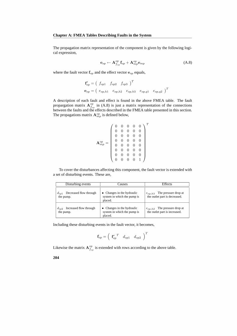
Chapter A: FMEA Tables Describing Faults in the System
The propagation matrix representation of the component is given by the following logi-cal expression,
eop ← Aopfop
fop + Aopmpemp (A.8)
where the fault vectorfop and the effect vectoreop equals,
f ′op =(
fop1 fop2 fop3
)T
eop =(
eop,h1 eop,h2 eop,h3 eop,q1 eop,q2
)T
A description of each fault and effect is found in the above FMEA table. The faultpropargation matrixAop
fopin (A.8) is just a matrix representation of the connections
between the faults and the effects described in the FMEA table presented in this section.The propagations matrixAop
mp is defined below,
Aopmp =
0 0 0 0 00 0 0 0 00 0 0 0 00 0 0 0 00 0 0 0 00 0 0 0 00 0 0 0 00 0 0 0 1
T
To cover the disturbances affecting this component, the fault vector is extended witha set of disturbing events. These are,
Disturbing events Causes Effects
dip1 Decreased flow throughthe pump.
• Changes in the hydraulicsystem in which the pump isplaced.
eop,h3 The pressure drop atthe outlet part is decreased.
dip2 Increased flow throughthe pump.
• Changes in the hydraulicsystem in which the pump isplaced.
eop,h2 The pressure drop atthe outlet part is increased.
Including these disturbing events in the fault vector, it becomes,
fop =(
f ′opT
dop1 dop2
)T
Likewise the matrixAopfop
is extended with rows according to the above table.
204

Section A.9: Difference pressure
Outlet part of the pump
Impeller pressure
Outlet pressure drop Difference pressure Inlet pressure drop
Figure A.9: The input/output structure of the part modelling the dynamics of the rotatingparts of the pump.
A.9 Difference pressure
The input/output structure of this part is shown in Fig. A.9. As described in chapter4 this component is included in the analysis to cover the signal structure of the systemwhen building the functional model of the centrifugal pump. This means that no faultsare identified in the component.
The propagation matrix representation of the component is given by the followinglogical expression,
edy = Adhi ei + Adh
ip eip + Adhopeop (A.9)
The resulting effect vectoredh in this expression is given by,
edh =(
edh,h1 edh,h2 edh,h3 edh,h4 edh,h5 edh,h6
)T
where the effects in this vector are,
eop,h1 ∼ Increased pressure difference across the pump.eop,h2 ∼ Decreased pressure difference across the pump.eop,h3 ∼ Zero pressure difference across the pump.eop,h4 ∼ Harmonic oscillations in the pressure difference signal.eop,h5 ∼ High frequence oscillations in the pressure difference signal.eop,h6 ∼ Pressure difference across the pump is not defined.
205
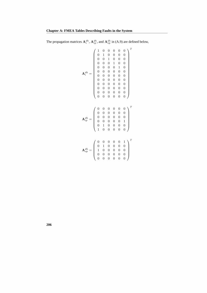
Chapter A: FMEA Tables Describing Faults in the System
The propagation matricesAdhi , Adh
ip , andAdhop in (A.9) are defined below,
Adhi =
1 0 0 0 0 00 1 0 0 0 00 0 1 0 0 00 0 0 1 0 00 0 0 0 1 00 0 0 0 0 00 0 0 0 0 00 0 0 0 0 00 0 0 0 0 00 0 0 0 0 00 0 0 0 0 00 0 0 0 0 0
T
Adhip =
0 0 0 0 0 00 0 0 0 0 00 0 0 0 0 00 0 0 0 0 10 1 0 0 0 01 0 0 0 0 0
T
Adhop =
0 0 0 0 0 10 1 0 0 0 01 0 0 0 0 00 0 0 0 0 00 0 0 0 0 0
T
206

Appendix B
Mathematical Tools
This appendix contains a short presentation of two mathematical tools used in this thesis.These are a CUSUM alogithm, and some notes on Linear Matrix Inequalities (LMI).
B.1 The CUSUM Algorithm
The cumulative sum (CUSUM) algorithm is a statistical tool to identify changes in thestatistical properties of a signal. The algorithm is described in (Basseville and Nikiforov,1998, Sec. 2.2). This presentation is based of one particular version of the CUSUMAlgorithm also presented in (Basseville and Nikiforov, 1998).
The CUSUM algorithm is based on the log-likelihood ratiolnpθ1 (yk)
pθ0 (yk) , which can beused to measure the likelihood of two different hypothesesH0 andH1 described by theparameterθ, i.e.
H0 : θ = θ0
H1 : θ = θ1
These hypotheses can be tested using a recursive algorithm called the CUSUM algo-rithm. One from of this algorithm is given by,
gk =
gk−1 + ln pθ1 (yk)
pθ0 (yk) if gk−1 + ln pθ1 (yk)
pθ0 (yk) > 0
0 if gk−1 + ln pθ1 (yk)
pθ0 (yk) ≤ 0(B.1)
whereg0 = 0. The interpretation of the variablegk, compared to the hypothesisH0 andH1, is given by the decision signalD,
D ={
1 if gk ≥ h0 otherwise
207

Chapter B: Mathematical Tools
whereh is a predefined threshold value. IfD = 1 the hypothesesH1 is most likely tohave occurred and otherwise ofD = 0.
In this work the CUSUM algorithm is used to statistical evaluation of residual sig-nals. Here it is assumed that the residual signals are normal distributed, meaning thattheir distribution is given by,
pµ(y) =1
σ√
2πe−
(y−µ)2
2σ2
whereµ is the mean value of the residual. Therefore it can be deduced thatµ = µ0 = 0in the no fault case, andµ = µ1 6= 0 in the faulty case. It is assumed that the variancesof the residual signals are known and do not change due to faults, i.e.σ in the aboveexpression is constant and known. When these properties are fulfilled the log-likelihoodin the CUSUM algorithm (B.1) is given by,
lnpµ1(yk)pµ0(yk)
= − (yk − µ1)2
2σ2+
y2k
2σ2= −µ1
σ2
(yk − µ1
2
)
The signalgk in the CUSUM algorithm (B.1) is bounded from below by0. In thealgorithm used in this work the signalgk is also bounded from above byh, resulting inthe following algorithm,
gk =
0 if gk−1 − θ1σ2
(yk − θ1
2
) ≤ 0h if gk−1 − θ1
σ2
(yk − θ1
2
) ≥ h
gk−1 − θ1σ2
(yk − θ1
2
)otherwise
(B.2)
This algorithm is a discrete algorithm. However, only continuous systems are consideredin this work. Therefore, for the sake of cosistency a continuous version of (B.2) is givenbelow. Heres(t) = −µ1
σ2
(y(t)− µ1
2
)is used.
dg
dt=
{0 if (g(t) = 0 ∧ s(t) ≤ 0) ∨ (g(t) = h ∧ 0 ≤ s(t))
s(t) otherwise(B.3)
where∧ and∨ denotes the logicalandandor operator respectively.
B.2 Linear Matrix Inequalities
In this appendix some general remarks on Linear Matrix Inequalities (LMI)’s and thereuse in connection with parameter variating systems are presented. The presentation isbased on (Scherer and Weiland, 1999). First the consept of LMI’s is defined, followedby three proporsitions dealing with stability of parameter variating system. These pro-porsitions are in Section 5.2.2 used in the analysis and synthesis of the feedback gain inthe proposed adaptive observer.
208

Section B.2: Linear Matrix Inequalities
A LMI is an expression on the form,
F(x) = F0 +m∑
i=1
xiFi ≺ 0 (B.4)
where
• x =[x1 x2 · · · xm
]is a vector of real numbers.
• F0, · · · ,Fm are real symmetric matrices, i.e.Fi = FTi ∈ Rn×n, i = 1, · · · ,m
for somen ∈ Z+.
• The inequality≺ 0 in (B.4) means positive definite, i.e.uT F(x)u < 0 for allu ∈ Rn. Equivalently, the largest eigenvalue ofF(x) is negative.
This is stated in slightly more general in the following definition.
Definition B.2.1 (Linear Matrix Inequality) (Scherer and Weiland, 1999, Sec. 1.3) ALinear Matrix Inequality (LMI) is an inequality,
F(X) ≺ 0 (B.5)
whereF is an affine function mapping a finit dimensional vector spaceV to the setSn = {M | M = MT ∈ Rn×n}, n > 0 of real symmetric matrices.
The feasibility of the LMI defined in Definition B.2.1 denotes the existence of at leastoneX which fulfills (B.5). Likewise the LMI is infeasible if such anX does not exist.If an affine performance function on the formc(X) is defined, algorithms exists whichcan solve the minimization problemminX c(X) constrainted by (B.5).
LMI’s as defined in Definition B.2.1 can be used for checking stability of linearsystems with unknown and variating parameters. Such a system is shown below,
x = A(δ(t))x (B.6)
where the state matrixA(δ(t)) is a function of the real valued parameter vectorδ. In allphysical system this parameter vector belongs to a bounded set∆, i.e. δ ∈ ∆.
Suppose that the state matrixA(δ(t)) is an affine function of the parameters, i.e.A(δ(t)) = A0 +
∑kj=1 δj(t)Aj for all δ ∈ ∆, then (B.6) is refered to as anaffine
parameter dependent model. Suppose that the unknown parametersδj j = 1, · · · , k inthis expression are bounded on an interval, i.e.δj ∈ [δj , δj ]. If the unknown parametersare bounded on this interval thecornersof the uncertainty region is given by the set,
∆0 ={δ = (δ1, · · · , δk) | δj ∈ {δj , δj}
}(B.7)
Then the uncertainty region∆ = co{∆0}, whereco denotes the convex hull of thegenerators∆0 (Scherer and Weiland, 1999).
The stability of (B.6), whenA(δ(t)) is an affine parameter dependent model, isformulated by an LMI in the following proposition.
209

Chapter B: Mathematical Tools
Proposition B.2.1 (Scherer and Weiland, 1999, Sec. 2.4) if (B.6) is an affine parameterdependent model then it is quadratically stable if and only of there existsP Â 0 suchthat
A(δ)T P + PA(δ) ≺ 0
for all δ ∈ ∆0, where∆0 contains the generators of the convex hull, i.e.∆ = co{∆0}.This proposition is motivated by the Lyapunov stability criterion. When PropositionB.2.1 holds, system (B.6) is stable for arbitrary fast variations ofδ. However, if theparameters are unknown and bounded on a set, but not variating Proposition B.2.1 is torestricted, i.e. system (B.6) can be stable for allδ ∈ ∆ even though Proprosition B.2.1does not hold.
The following proposition states the stability conditions for (B.6) if the parametervector is assumed constant, i.e.δ = 0.
Proposition B.2.2 (Scherer and Weiland, 1999, Page 62) If (B.6) is an affine parameterdependent model and∆ ⊂ Rk is the uncertainty set given by∆ = co{∆0}, where∆0
is defined in (B.7), then system (B.6) is affinely quadralically stable if there exist realmatricesP0, · · · ,Pk such that,
A(δ)T P(δ) + P(δ)A(δ) ≺ 0 ∀δ ∈ ∆0 (B.8a)
P(δ) Â 0 ∀δ ∈ ∆0 (B.8b)
ATj Pj + PjAj º 0 for j = 1, · · · , k (B.8c)
Here,A(δ) = A0 +∑k
j=1 δjAj andP(δ) = P0 +∑k
j=1 δjPj . Moreover, in that
caseV (x, δ) := xT P(δ)x is a quadratic parameter-dependent Lyapunov function forthe system.
Proposition B.2.1 states the stability conditions for system (B.6) for abitraly variatingparametersδ ∈ ∆ and Proposition B.2.2 stated the stability condition for the samesystem when the parametersδ ∈ ∆ are constant. The following proporsition states thestability conditions in the case where the parameters are variating, but with a limet onthe variation rate, i.e.δi = λi ∈ [λi, λi]. If each variation rate is limited to this set, thecornersof the uncertainty region of the variations rates is given by,
Λ0 = {λ = (λ1, · · · , λk) | λi ∈ [λi, λi]} (B.9)
Then the uncertainty regionΛ = co{Λ0} is the set of possible variation rates of theparametersδ. When the variation rates are limited on this set the following propositionstates the stability conditions for system (B.6).
Proposition B.2.3 (Scherer and Weiland, 1999, Page 64) If (B.6) is an affine parameterdependent model and∆ ⊂ Rk is the uncertainty set given by∆ = co{∆0}, where∆0
210

Section B.2: Linear Matrix Inequalities
is defined in (B.7), then system (B.6) is affinely quadralically stable if there exist realmatricesP0, · · · ,Pk such that,
A(δ)T P(δ) + P(δ)A(δ) + P(λ) ≺ P0 ∀ δ ∈ ∆0 andλ ∈ Λ0 (B.10a)
P(δ) Â 0 ∀ δ ∈ ∆0 (B.10b)
ATj Pj + PjAj º 0 for j = 1, · · · , k (B.10c)
Here,A(δ) = A0 +∑k
j=1 δjAj andP(δ) = P0 +∑k
j=1 δjPj . Moreover, in that
caseV (x, δ) := xT P(δ)x is a quadratic parameter-dependent Lyapunov function forthe system.
211