aace international recommended practice no. 29r-03
TRANSCRIPT
Copyright 2007 AACE, Inc. AACE International Recommended Practices
AACE International Recommended Practice No. 29R-03
FORENSIC SCHEDULE ANALYSIS
TCM Framework: 6.4 – Forensic Performance Assessment
Acknowledgments: Kenji P. Hoshino, PSP CFCC (Author) Robert B. Brown, PE John J. Ciccarelli, PE CCE PSP Gordon R. Costa, PSP CFCC Michael S. Dennis, CCC Edward E. Douglas, III CCC PSP Philip J. Farrocco, PE Sidney J. Hymes, CFCC John C. Livengood, PSP Mark F. Nagata, PSP Jeffery L. Ottesen, PE PSP CFCC
Thomas F. Peters, PE CFCC Keith Pickavance Dr. Anamaria I. Popescu, PE Jose F. Ramirez, CCE Mark C. Sanders, PE CCE PSP Takuzo Sato L. Lee Schumacher, PSP Robert Seals, PSP Ronald M. Winter, PSP James G. Zack, Jr. CFCC
Copyright 2007 AACE International, Inc. AACE International Recommended Practices
AACE International Recommended Practice No. 29R-03 FORENSIC SCHEDULE ANALYSIS TCM Framework: 6.4 – Forensic Performance Assessment
June 25, 2007
CONTENTS 1. ORGANIZATION AND SCOPE 1.1 Introduction 1.2. Basic Premise and Assumptions 1.3. Scope and Focus 1.4. Taxonomy and Nomenclature
A. Layer 1: Timing 1. Prospective 2. Retrospective
B. Layer 2: Basic Methods 1. Observational 2. Modeled
C. Layer 3: Specific Methods 1. Observational Methods
a. Static Logic Observation b. Dynamic Logic Observation
2. Modeled Methods a. Additive Modeling b. Subtractive Modeling
D. Layer 4: Basic Implementation 1. Gross Mode or Periodic Mode 2. Contemporaneous / As-Is or Contemporaneous / Split 3. Modified or Recreated 4. Single Base, Simulation or Multi Base, Simulation
E. Layer 5: Specific Implementation 1. Fixed Periods vs. Variable Periods / Grouped Periods 2. Global (Insertion or Extraction) vs. Stepped (Insertion or Extraction)
1.5. Underlying Fundamentals and General Principles
A. Underlying Fundamentals B. General Rules
1. Use CPM Calculations 2. Concept of Data Date Must be Used 3. The As-Built Critical Path Cannot be Calculated by CPM Alone 4. Shared Ownership of Network Float 5. Update Float Preferred Over Baseline Float. 6. Sub-Network Float Values 7. Delay Must Affect the Critical Path
2. SOURCE VALIDATION 2.1. Baseline Schedule Selection, Validation, and Rectification (SVP 2.1)
A. General Considerations B. Recommended Protocol C. Recommended Enhanced Protocol

Copyright 2007 AACE International, Inc. AACE International Recommended Practices
Forensic Schedule Analysis
June 25 2007
2 of 105
D. Special Procedures 1. Summarization of Schedule Activities 2. Reconstruction of a Computerized CPM Model from a Hardcopy 3. De-statusing a Progressed Schedule to Create a Baseline 4. Software Format Conversions
2.2. As-Built Schedule Sources, Reconstruction, and Validation (SVP 2.2) A. General Considerations B. Recommended Protocol C. Recommended Enhanced Protocol D. Special Procedures
1. Creating an Independent As-Built from Scratch 2. Validating a Progressed Update / Creating a Progressed Baseline 3. Determination of ‘Significant’ Activities for Inclusion in an As-Built 4. Collapsible As-Built CPM Schedule 5. Summarization of Schedule Activities
2.3. Schedule Updates: Validation, Rectification, and Reconstruction (SVP 2.3) A. General Considerations B. Recommended Protocol C. Recommended Enhanced Protocol D. Special Procedures
1. After-the-Fact Statusing & Destatusing a. Hindsight Method b. Blinders Method
2. Bifurcation: Creating a Progress-Only Half-Step Update
2.4. Identification and Quantification of Discrete Delay Events and Issues (SVP 2.4) A. General Considerations
1. ‘Delay’ Defined a. Activity-Level Variance (ALV) b. Distinguished from Project-Level Variance (PLV) c. Distinguished Delay-Cause from Delay-Effect d. Characterization as Delay is Independent of Responsibility
2. Identifying and Collecting Delays a. Two Main Approaches to Identification & Collection b. Criticality of the Delay
3. Quantification of Delay Durations and Activity Level Variances 4. Causation Analysis 5. Assigning or Assuming Responsibility
B. Recommended Protocol C. Recommended Enhanced Protocol D. Special Procedures
1. Duration & Lag Variance Analysis 3. METHOD IMPLEMENTATION 3.1. Observational / Static / Gross (MIP 3.1)
A. Description B. Common Names C. Recommended Source Validation Protocols D. Enhanced Source Validation Protocols E. Recommended Implementation Protocols F. Enhanced Implementation Protocols

Copyright 2007 AACE International, Inc. AACE International Recommended Practices
Forensic Schedule Analysis
June 25 2007
3 of 105
1. Daily Delay Measure G. Identification of Critical and Near-Critical Paths H. Identification & Quantification of Concurrent Delays & Pacing I. Determination & Quantification of Excusable and Compensable Delay
1. Excusable & Compensable Delay (ECD) 2. Excusable & Non-Compensable Delay (END)
J. Identification & Quantification of Mitigation / Constructive Acceleration K. Specific Implementation Procedures & Enhancements L. Advantages & Disadvantages
3.2. Observational / Static / Periodic (MIP 3.2) A. Description B. Common Names C. Recommended Source Validation Protocols D. Enhanced Source Validation Protocols E. Recommended Implementation Protocols F. Enhanced Implementation Protocols 1. Daily Delay Measure G. Identification of Critical & Near-Critical Paths H. Identification & Quantification of Concurrent Delays & Pacing I. Determination & Quantification of Excusable and Compensable Delay
1. Excusable & Compensable Delay (ECD) 2. Excusable & Non-Compensable Delay (END)
J. Identification & Quantification of Mitigation / Constructive Acceleration K. Specific Implementation Procedures & Enhancements
1. Fixed Periods 2. Variable Periods
L. Advantages & Disadvantages 3.3. Observational / Dynamic / Contemporaneous As-Is (MIP 3.3)
A. Description B. Common Names C. Recommended Source Validation Protocols D. Enhanced Source Validation Protocols E. Recommended Implementation Protocols F. Enhanced Implementation Protocols
1. Daily Progress Method G. Identification of Critical & Near-Critical Paths H. Identification & Quantification of Concurrent Delays & Pacing I. Determination & Quantification of Excusable and Compensable Delay
1. Non-Excusable & Non-Compensable Delay (NND) 2. Excusable & Compensable Delay (ECD) 3. Excusable & Non-Compensable Delay (END)
J. Identification & Quantification of Mitigation / Constructive Acceleration K. Specific Implementation Procedures & Enhancements
1. All Periods 2. Grouped Periods 3. Blocked Periods
L. Advantages & Disadvantages 3.4. Observational / Dynamic / Contemporaneous Split (MIP 3.4)
A. Description B. Common Names C. Recommended Source Validation Protocols D. Enhanced Source Validation Protocols

Copyright 2007 AACE International, Inc. AACE International Recommended Practices
Forensic Schedule Analysis
June 25 2007
4 of 105
E. Recommended Implementation Protocols F. Enhanced Implementation Protocols
1. Daily Progress Method G. Identification of Critical & Near-Critical Paths H. Identification & Quantification of Concurrent Delays & Pacing I. Determination & Quantification of Excusable and Compensable Delay J. Identification & Quantification of Mitigation / Constructive Acceleration K. Specific Implementation Procedures & Enhancements
1. All Periods 2. Grouped Periods 3. Blocked Periods 4. Bifurcation: Creating a Progress-Only Half-Step Update
L. Advantages & Disadvantages 3.5. Observational / Dynamic / Modified or Recreated (MIP 3.5)
A. Description B. Common Names C. Recommended Source Validation Protocols D. Enhanced Source Validation Protocols E. Recommended Implementation Protocols F. Enhanced Implementation Protocols
1. Daily Progress Method G. Identification of Critical & Near-Critical Paths H. Identification & Quantification of Concurrent Delays & Pacing I. Determination & Quantification of Excusable and Compensable Delay J. Identification & Quantification of Mitigation / Constructive Acceleration K. Specific Implementation Procedures & Enhancements
1. Fixed Periods 2. Variable Periods 3. All-Periods vs. Grouped-Periods
L. Advantages & Disadvantages 3.6. Modeled / Additive / Single Base (MIP 3.6)
A. Description B. Common Names C. Recommended Source Validation Protocols D. Enhanced Source Validation Protocols E. Recommended Implementation Protocols F. Enhanced Implementation Protocols G. Identification of Critical & Near-Critical Paths H. Identification & Quantification of Concurrent Delays & Pacing I. Determination & Quantification of Excusable and Compensable Delay
1. Excusable & Compensable Delay (ECD) 2. Non-Excusable & Non-Compensable Delay (NND) 3. Excusable & Non-Compensable Delay (END)
J. Identification & Quantification of Mitigation / Constructive Acceleration K. Specific Implementation Procedures & Enhancements
1. Global Insertion 2. Stepped Insertion
L. Advantages & Disadvantages 3.7. Modeled / Additive / Multiple Base (MIP 3.7)
A. Description B. Common Names C. Recommended Source Validation Protocols

Copyright 2007 AACE International, Inc. AACE International Recommended Practices
Forensic Schedule Analysis
June 25 2007
5 of 105
D. Enhanced Source Validation Protocols E. Recommended Implementation Protocols F. Enhanced Implementation Protocols G. Identification of Critical & Near-Critical Paths H. Identification & Quantification of Concurrent Delays & Pacing I. Determination & Quantification of Excusable and Compensable Delay
1. Excusable & Compensable Delay (ECD) 2. Non-Excusable & Non-Compensable Delay (NND) 3. Excusable & Non-Compensable Delay (END)
J. Identification & Quantification of Mitigation / Constructive Acceleration K. Specific Implementation Procedures & Enhancements
1. Fixed Periods 2. Variable Periods 3. Global Insertion 4. Stepped Insertion
L. Advantages & Disadvantages 3.8. Modeled / Subtractive / Single Simulation (MIP 3.8)
A. Description B. Common Names C. Recommended Source Validation Protocols D. Enhanced Source Validation Protocols E. Recommended Implementation Protocols F. Enhanced Implementation Protocols G. Identification of Critical & Near-Critical Paths H. Identification & Quantification of Concurrent Delays & Pacing I. Determination & Quantification of Excusable and Compensable Delay
1. Excusable & Compensable Delay (ECD) 2. Non-Excusable & Non-Compensable Delay (NND) 3. Excusable & Non-Compensable Delay (END)
J. Identification & Quantification of Mitigation / Constructive Acceleration K. Specific Implementation Procedures & Enhancements
1. Choice of Extraction Modes a. Global Extraction b. Stepped Extraction
2. Creating a Collapsible As-Built CPM Schedule 3. Identification of the Analogous Critical Path (ACP)
L. Advantages & Disadvantages 4. ANALYSIS EVALUATION 4.1. Excusability and Compensability of Delay
A. General Rules B. Accounting for Concurrent Delay C. Equitable Symmetry of the Concept
4.2. Identification and Quantification of Concurrent Delay
A. Identification & Quantification of Concurrency 1. Literal Concurrency vs. Functional Concurrency 2. Cause of Delay vs. Effect of Delay 3. Frequency, Duration and Placement of Analysis Intervals
a. Frequency & Duration b. Chronological Placement
4. Order of Insertion or Extraction in Stepped Implementation
Copyright 2007 AACE International, Inc. AACE International Recommended Practices
Forensic Schedule Analysis
June 25 2007
6 of 105
5. Hindsight vs. ‘Blind-sight’ B. Concept of Pacing C. Demonstrating Pacing
1. Existence of the Parent Delay 2. Showing of Contemporaneous Ability to Resume Normal Pace 3. Evidence of Contemporaneous Intent
4.3. Critical Path and Float
A. Identifying the Critical Path 1. Critical Path: Longest Path School vs. Total Float Value School 2. Negative Float: Zero Float School vs. Lowest Float Value School
B. Quantifying ‘Near-Critical’ 1. Duration of Discrete Delay Events 2. Duration of Each Analysis Interval 3. Historical Rate of Float Consumption 4. Amount of Time or Work Remaining on the Project
C. Identifying the As-Built Critical Path D. Critical Path Manipulation Techniques
1. Resource Leveling & Smoothing 2. Multiple Calendars 3. Precedence Logic / Lead & Lag 4. Start & Finish Constraints 5. Various Calculation Modes
a. Schedule Calculation b. Duration Calculation c. Float Calculation
6. Use of Data Date 7. Judgment Calls during the Forensic Process
E. Ownership of Float 4.4. Delay Mitigation and Constructive Acceleration
A. Definitions B. General Considerations
1. Differences between Acceleration, Constructive Acceleration and Delay Mitigation. 2. Acceleration and Compensability 3. Delay Mitigation and Compensability
C. Elements of Constructive Acceleration 1. Contractor Entitlement to an Excusable Delay 2. Contractor Requests and Establishes Entitlement to a Time Extension 3. Owner Failure to Grant a Timely Time Extension 4. Implied Order by the Owner to Complete More Quickly 5. Contractor Notice of Acceleration 6. Proof of Damages
5. CHOOSING A METHOD 5.1 Factor 1: Contractual Requirements 5.2 Factor 2: Purpose of Analysis 5.3 Factor 3: Source Data Availability and Reliability 5.4 Factor 4: Size of the Dispute
Copyright 2007 AACE International, Inc. AACE International Recommended Practices
Forensic Schedule Analysis
June 25 2007
7 of 105
5.5 Factor 5: Complexity of the Dispute 5.6 Factor 6: Budget for Forensic Schedule Analysis 5.7 Factor 7: Time Allowed for Forensic Schedule Analysis 5.8 Factor 8: Expertise of the Forensic Schedule Analyst and Resources Available 5.9 Factor 9: Forum for Resolution and Audience 5.10 Factor 10: Legal or Procedural Requirements 5.11 Factor 11: Past History/Methods and What Method the Other Side Is Using REFERENCES CONTRIBUTORS

Copyright 2007 AACE International, Inc. AACE International Recommended Practices
Forensic Schedule Analysis
June 25 2007
8 of 105
1. ORGANIZATION AND SCOPE 1.1. Introduction The purpose of this AACE International (AACE) Recommended Practice on Forensic Schedule Analysis (FSA) is to provide a unifying technical reference for the forensic application of critical path method (CPM) of scheduling. Forensic1 scheduling analysis refers to the study and investigation of events using CPM or other recognized schedule calculation methods for potential use in a legal proceeding. It is the study of how actual events interacted in the context of a complex model for the purpose of understanding the significance of a specific deviation or series of deviations from some baseline model and their role in determining the sequence of tasks within the complex network. Forensic scheduling analysis, like many other technical fields, is both science and art. As such, it relies on professional judgment and expert opinion and usually requires many subjective decisions. The most important of these decisions is what technical approach should be used to measure or quantify delay and to identify affected activities to focus on causation, and how the analyst should apply the chosen method. The desired objective of this Recommended Practice is to reduce the degree of subjectivity involved in the current state of the art. This is with the full awareness that there are certain types of subjectivity than cannot be minimized let alone be eliminated. Professional judgment and expert opinion ultimately rests on subjectivity. But that subjectivity must be based on diligent factual research and analyses whose procedures can be objectified. For these reasons, the Recommended Practice will focus on minimizing procedural subjectivity. It will do this by defining terminology, identifying the methodologies currently being used by forensic scheduling analysts, classifying them, and setting recommended procedural protocols for the use of these techniques. By describing uniform procedures that increase transparency of the analysis method and the analyst’s thought process, the guidelines established herein will increase accountability and testability of an opinion and minimize the need to contend with “black-box” or “voodoo” analyses. It is hoped that the implementation of this Recommended Practice will result in minimizing disagreements over technical implementation of accepted techniques and allow the providers and consumers of these services to concentrate on resolving disputes over substantive or legal issues. 1.2. Basic Premise and Assumptions
a. Forensic scheduling is a technical field that is associated with, but distinct from, project planning and
scheduling. It is not just a subset of planning and scheduling. b. Protocols that may be sufficient for the purpose of project planning, scheduling and controls may not
necessarily be adequate for forensic schedule analysis. c. It is assumed that this document will be used by practitioners to foster consistency of practice and in
the spirit of logical and intellectual honesty. d. All methods are subject to manipulation. They all involve judgment calls by the analyst whether in
preparation or in interpretation.
1 The word ‘forensic’ is defined as: 1. Relating to, used in, or appropriate for courts of law or for public discussion or argumentation. 2. Of, relating to, or used in debate or argument; rhetorical. 3. Relating to the use of science or technology in the investigation and establishment of facts or evidence in a court of law: a forensic laboratory.[9]
Copyright 2007 AACE International, Inc. AACE International Recommended Practices
Forensic Schedule Analysis
June 25 2007
9 of 105
e. No forensic schedule analysis method is exact. The level of accuracy of the answers produced by each method is a function of the quality of the data used by the method and the accuracy of the assumptions and the subjective judgments made by the forensic schedule analyst.
f. Schedules are a project management tool that, in and of themselves, do not demonstrate root
causation or responsibility for delays. Legal entitlement to delay damages should be distinct and apart from the forensic schedule analysis methodologies contained in this RP.
1.3. Scope and Focus The scope and focus of this Recommended Practice are: a. This Recommended Practice (RP) covers the technical aspects of forensic schedule analysis
methods. It will identify, define and describe the usage of various forensic schedule analysis methods in current use. It is not the intent of the RP to exclude or to endorse any method over others. However, it will offer caveats for usage and cite the best current practices and implementation for each method.
b. The focus of the document will be on the technical aspects of forensic scheduling as opposed to the
legal aspects. This RP is not intended to be a primary resource for legal theories governing claims related to scheduling, delays and disruption. However, relevant legal principles will be discussed to the extent that they would affect the choice of techniques and their relative advantages and disadvantages.
c. Accordingly, the RP will primarily focus on the use of forensic scheduling techniques and methods for
factual analysis and quantification as opposed to assignment of delay responsibility. This, however, does not preclude the practitioner from performing the analysis based on certain assumptions regarding liability.
d. This RP is not intended to be a primer on forensic schedule analysis. The reader is assumed to have
advanced, hands-on knowledge of all components of CPM analysis and a working experience in a contract claims environment involving delay issues.
e. Nor is this RP intended to be an exhaustive treatment of CPM scheduling techniques. While the RP
explains how schedules generated by the planning and scheduling process become the source data for forensic schedule analysis, it is not intended to be a manual for basic scheduling. Please refer to other sources for further information about basic schedule analysis methods and techniques.
f. This RP is not intended to override contract provisions regarding schedule analysis methods or other
mutual agreement by the parties to a contract regarding same. However this is not an automatic, blanket endorsement of all methods of delay analysis by the mere virtue of their specification in a contract document. It is noted that contractually specified methods often are appropriate for use during the project in a prospective mode but may be inappropriate for retrospective use.
g. It is not the intent of this RP to intentionally contradict or compete with other similar protocols2. All
effort should be made by the user to resolve and reconcile apparent contradictions. AACE requests and encourages all users to notify AACE and bring errors, contradictions and conflict to its attention.
h. This RP deals with CPM-based schedule analysis methods. Other RPs will address scheduling
methods other than simple CPM such as linear scheduling and heuristic leveling. However it is not the intent of the RP to exclude analyses of simple cases where explicit CPM modeling may not be necessary and mental calculation is adequate for analysis and presentation. The delineation between
2 The only other similar protocol known at this time is the “Delay & Disruption Protocol” issued in October 2002 by the Society of Construction Law of the United Kingdom[1]. The DDP has a wider scope than this RP.
Copyright 2007 AACE International, Inc. AACE International Recommended Practices
Forensic Schedule Analysis
June 25 2007
10 of 105
simple and complex is admittedly blurry and subjective. For this purpose, a ‘simple case’ is defined as any CPM network model that can be subjected to mental calculation whose reliability cannot be reasonably questioned and allows for effective presentation to lay persons using simple reasoning and intuitive common sense.
i. Finally, the RP is an advisory document to be used in conjunction with professional judgment based
on adequate working experience and knowledge of the subject matter. It is not intended to be a prescriptive document that can be applied without exception. The recommended protocols will aid the practitioner in creating a competent work product, some cases require additional steps and some require less. Thus, a departure from the recommended protocols should not be automatically treated as an error or a deficiency as long as such departure is based on a conscious and sound application of schedule analysis principles.
1.4. Taxonomy and Nomenclature The industry knows the forensic schedule analysis methods and approaches described herein by various common names. Current usage of these names throughout the industry is loose and undisciplined. It is not the intent of this document to enforce more disciplined use of the common names. Instead, the RP will correlate the common names with a taxonomic classification. This taxonomy will allow for the freedom of regional, cultural and temporal differences in the use of common names for these methods. As described herein, the RP correlates the common names for the various methods to taxonomic names much like the biosciences use Latin taxonomic terms to correlate regionally diverse common names of plants and animals. This allows the variations in terminology to coexist with a more objective and uniform language of technical classification. For example, the implementation of time impact analysis (TIA) has a bewildering array of regional variations. Not only that, the method undergoes periodic evolutionary changes while maintaining the same name. By using taxonomic classifications, it hoped that the discussion of the various forensic analysis methods will become more specific and objective. Thus, the RP will not provide a uniform definition for the common names of the various methods, but it will instead describe in detail the taxonomic classification in which they belong. Table 1 – Nomenclature Correspondence, shows the commonly associated names for each of the taxonomic classifications. The RP’s taxonomy is a hierarchical classification system of known methods of schedule impact analysis techniques and methods used to analyze how delays and disruptions affect entire CPM networks. For example, you will find methods like the window analysis or collapsed as-built classified here. Procedures such as fragnet modeling, bar charting and linear graphing, are tools, and not methods. Therefore, they are not classified under this taxonomy. The RP’s taxonomy is a hierarchical classification system comprising the five layers: timing, basic and specific methods, and the basic and specific implementation of each method. Please refer to Figure 1 – Taxonomy of Forensic Schedule Analysis for a graphic representation of the taxonomy. The elements of the diagrams are explained below.

Copyright 2007 AACE International, Inc. AACE International Recommended Practices
Forensic Schedule Analysis
June 25 2007
11 of 105
Footnotes 1. Contemporaneous or Modified / Reconstructed 2. The single base can be the original baseline or an update
Table 1 – Nomenclature Correspondence
Figure 1 – Taxonomy of Forensic Schedule Analysis
A. Layer 1: Timing The first hierarchy layer distinguishes the timing of when the analysis is performed, consisting of two branches, prospective and retrospective.
1. Prospective analyses are performed in real-time, prior to the delay event, or where the analysis takes place, in real-time, contemporaneous with the delay event. In all cases prospective analysis consists of the analyst’s best estimate of future events. Prospective analysis occurs while the project is still underway and may not evolve into a forensic context.
2. Retrospective analyses are performed after the delay event has occurred and the impacts are known. The timing may be soon after the delay event but prior to the completion of the overall project, or after the completion of the entire project. Note that forward-looking analysis (such as ‘additive modeling’) performed after project completion is still retrospective in terms of timing.
2

Copyright 2007 AACE International, Inc. AACE International Recommended Practices
Forensic Schedule Analysis
June 25 2007
12 of 105
What is classified here is the real-time point-of-view of the analyst, and not the mode of analysis (forward-looking or hindsight). In other words even forward-looking analysis methods implemented retrospectively has the full benefit of hindsight at the option of the analyst.
This distinction in timing is one of the most significant factors in the choice of methods. For example, contract provisions prescribing methods of delay analysis typically contemplate the preparation of such analysis in the prospective context, in order to facilitate the evaluation of time extensions. Therefore a majority of contractually specified methods, often called the time impact analysis, consists of the insertion of delay events into the most current schedule update that existed at the time of the occurrence of the event: a prospective method. At the end of the project the choices of analysis methods are expanded with the full advantage of hindsight offered by the various forms of as-built documentation. In addition, if as-built documentation is available the best evidence rule demands that all factual investigation use the as-built as the primary source of analysis. Also the timing distinction is often mirrored by a change in personnel. That is, often the forensic schedule analyst who typically works in the retrospective context is not the same person as the project scheduler who worked under the prospective context.
B. Layer 2: Basic Methods The second hierarchy layer is the basic method, consisting of two branches, observational and modeled. The distinction drawn here is whether the analyst’s expertise is utilized for the purpose of interpretation and evaluation of the existing scheduling data only, or for constructing simulations and the subsequent interpretation and evaluation of the different scenarios created by the simulations. The distinction between the two basic methods becomes less defined in cases where the identity of the forensic analyst and the project scheduler rest in the same person.
1. Observational The observational method consists of analyzing the schedule by examining a schedule, by itself or in comparison with another, without the analyst making any changes to the schedule to simulate a certain scenario. Contemporaneous period analysis and as-built vs. as-planned are common examples that fall under the observational basic method. 2. Modeled Unlike the observational method, the modeled method calls for intervention by the analyst beyond mere observation. In preparing a modeled analysis the analyst inserts or extracts activities representing delay events from a CPM network and compares the calculated results of the ‘before’ and ‘after’ states. Common examples of the modeled method are the collapsed as-built, time impact analysis and the impacted as-planned.
C. Layer 3: Specific Methods
At the third layer are the specific methods.
1. Observational Methods
Copyright 2007 AACE International, Inc. AACE International Recommended Practices
Forensic Schedule Analysis
June 25 2007
13 of 105
Under the observational method, further distinction is drawn on whether the evaluation considers just the original schedule logic or the additional sets of progressive schedule logic that were developed during the execution of the project, often called the dynamic logic.
a. Static Logic Observation A specific subset of the observational method, the static logic variation compares a plan consisting of one set of network logic to the as-built state of the same network. The term, ‘static’ refers to the fact that observation consists of the comparison of an as-built schedule to just one set of as-planned network logic. The as-planned vs. as-built is an example of this specific method. b. Dynamic Logic Observation In contrast with the static logic variation, the dynamic logic variation typically involves the use of schedule updates whose network logic may differ to varying degrees from the baseline and from each other. This variation considers the changes in logic that were incorporated during the project. The contemporaneous period analysis is an example of this specific method. Note that this category does not occur under the prospective timing because the use of past updates indicates that the analysis is performed using retrospective timing.
2. Modeled Methods The two distinctions under the modeled method are whether the delays are added to a base schedule or subtracted from a simulated as-built.
a. Additive Modeling The additive modeling method consists of comparing a schedule with another schedule that the analyst has created by adding schedule elements (i.e. delays) to the first schedule for the purpose of modeling a certain scenario. You will find under this variation, the impacted as-planned, and some forms of the window analysis method. The time impact analysis can also be classified as an additive modeling method. But be aware that this term or its equivalent, time impact evaluation (TIE) has been used in contracts and specifications to refer to other basic and specific methods as well. b. Subtractive Modeling The subtractive modeling method consists of comparing a CPM schedule with another schedule that the analyst has created by subtracting schedule elements (i.e. delays) from the first schedule for the purpose of modeling a certain scenario. The collapsed as-built is one example that is classified under the subtractive modeling method.
D. Layer 4: Basic Implementation The fourth layer consists of the differences in implementing the methods outline above. The static logic method can be implemented in a gross mode or periodic mode. The progressive logic method can be implemented as contemporaneous: as-is, contemporaneous: split, modified, or recreated. The
Copyright 2007 AACE International, Inc. AACE International Recommended Practices
Forensic Schedule Analysis
June 25 2007
14 of 105
additive or subtractive modeling method can be implemented as a single base with simulation or a multiple base with simulation.
1. Gross Mode or Periodic Mode The first of the two basic implementations of the static logic variation of the observational method is the gross mode. Implementation of the gross mode considers the entire project duration as one whole analysis period without any segmentation. The alternate to the gross mode is the periodic mode. Implementation of the periodic mode breaks the project duration into two or more segments for specific analysis focusing on each segment. Because this is an implementation of the static logic method, the segmented analysis periods are not associated with any changes in logic that may have occurred contemporaneously with these project periods. 2. Contemporaneous / As-Is or Contemporaneous / Split This basic implementation pair occurs under the dynamic logic variation of the observation method. Both choices contemplate the use of the schedule updates that were prepared contemporaneously during the project. However the as-is implementation evaluates the differences between each successive update in its unaltered state, while the split implementation bifurcates each update into the pure progress and the non-progress revisions such as logic changes. The purpose of the bifurcation is to isolate the schedule slippage (or recovery) caused solely by work progress based on existing logic during the update period from that caused by non-progress revisions newly inserted (but not necessarily implemented) in the schedule update. 3. Modified or Recreated This pair, also occurring under the dynamic logic variation of the observational method, also involves the observation of updates. Unlike the contemporaneous pair, however, this implementation involves extensive modification of the contemporaneous updates, as in the modified implementation, or the recreation of entire updates where no contemporaneous updates exist, as in the recreated implementation. 4. Single Base, Simulation or Multi Base, Simulation This basic implementation pair occurs under the additive and the subtractive modeling methods. The distinction is whether when the modeling (either additive or subtractive) is performed, the delay activities are added to or extracted from a single CPM network or multiple CPM networks. For example, a modeled analysis that adds delays to a single baseline CPM schedule is a single base implementation of the additive method, whereas one where delays are extracted from several as-built simulations is a multi base simulation implementation of the subtractive method. A single base additive modeling method is typically called the impacted as-planned. Similarly the single simulation subtractive method is called the collapsed as-built. The multi base, simulation variations are called window analysis.
E. Layer 5: Specific Implementation
1. Fixed Periods vs. Variable Periods / Grouped Periods
Copyright 2007 AACE International, Inc. AACE International Recommended Practices
Forensic Schedule Analysis
June 25 2007
15 of 105
These specific implementations are the two possible choices for segmentation under all basic implementations except gross mode and the single base / simulation basic implementations. They are not available under the gross mode because the absence of segmentation is the distinguishing feature of the basic gross mode. They are not available under the single base / simulation basic implementation because segmentation assumes a change in network logic for each segment; the single base, simulation uses only one set of network logic for the model. In the fixed period specific implementation, the periods are fixed in date and duration by the data dates used for the contemporaneous schedule updates, usually in regular periods such as monthly. Each update period is analyzed. The act of grouping the segments for summarization after each segment is analyzed is called blocking. In the prospective timing mode, since there is usually only one forward looking set of network logic, be it the baseline or the current update, there is only one fixed period. Upon the creation of subsequent updates, by definition, the use of previous updates brings the analysis under the retrospective timing mode. The variable period, grouped period specific implementation establishes analysis periods other than the update periods established during the project by the submission of regular schedule updates. The grouped period implementation groups together the pre-established update periods while the variable windows implementation establishes new periods whose lines of demarcation may not coincide with the data dates used in the pre-established periods and/or which can be determined by changes in the critical path or by the issuance of revised or recovery baseline schedules. This implementation is one of the primary distinguishing features of the window analysis method. 2. Global (Insertion or Extraction) vs. Stepped (Insertion or Extraction) This specific implementation pair occurs under the single base, simulation basic implementation, which in turn occurs under the additive modeling and the subtractive modeling specific methods. Under the global implementation delays are either inserted or extracted all at once, while under the stepped implementation the insertion or the extraction is performed sequentially (individually or grouped). Although there are further variations in the sequence of stepping the insertions or extractions, usually the insertion sequence is from the start of the project towards the end, whereas stepped extraction starts at the end and proceeds towards the start of the project.
1.5. Underlying Fundamentals and General Principles
A. Underlying Fundamentals
At any given point in time on projects, certain work must be completed at that point in time so the completion of the project does not slip later in time. The industry calls this work, “critical work.” Project circumstances that delay critical work will extend the project duration. Critical delays are discrete, happen chronologically and accumulate to the overall project delay at project completion. When the project is scheduled using CPM scheduling, the schedule typically identifies the critical work as the work that is on the “longest” or “critical path” of the schedule’s network of work activities. The performance of non-critical work can be delayed for a certain amount of time without affecting the timing of project completion. The amount of time that the non-critical work can be delayed is “float” or “slack” time.
Copyright 2007 AACE International, Inc. AACE International Recommended Practices
Forensic Schedule Analysis
June 25 2007
16 of 105
A CPM schedule for a particular project generally represents only one of the possible ways to build it. Therefore, in practice, the schedule analyst must also consider the assumptions (work durations, logic, sequencing and labor availability) that form the basis of the schedule when performing a forensic schedule analysis. This is particularly true when the schedule contains preferential logic (i.e., sequencing which is not based on physical or safety considerations) and resource assumptions. This is because both can have a significant impact on the schedule’s calculation of the critical path and float values of non-critical work at a given point in time. CPM scheduling facilitates the identification of work as either critical or non-critical. Thus, at least in theory, CPM schedules give the schedule analyst the ability to determine if a project circumstance delays the project or if it just consumes float in the schedule. For this reason, delay evaluations utilizing CPM scheduling techniques are now preferred for the identification and quantification of project delays. The critical path and float values of uncompleted work activities in CPM schedules change over time as a function of the progress (or lack of progress) on the critical and non-critical work paths in the schedule network. For this reason, only project circumstances that delay work that is critical when the circumstances occur extend the overall project duration. Thus, when quantifying project delay, schedule analysts must evaluate the impact of potential causes of delay within the context of the schedule at the time when the circumstances happen.
B. General Rules
1. Use CPM Calculations Calculation of the critical path and float must be based on a CPM schedule with proper logic (see 2.1.) 2. Concept of Data Date Must be Used The CPM schedule used for the calculation must employ the concept of the data date. Note that the critical path and float can be computed only for the portion of the schedule forward (future) of the data date. 3. The As-Built Critical Path Cannot be Calculated by CPM Alone The as-built critical path cannot be determined by conventional CPM calculation alone. The as-built portion is behind (past side of) the data line, which is prior in time to the point from which CPM calculations are performed. 4. Shared Ownership of Network Float In the absence of contrary contractual language, network float, as opposed to project float, is a shared commodity between the owner and the contractor. 5. Update Float Preferred Over Baseline Float. If reliable updates exist, float values for activities in those updates at the time the schedule activity was being performed are considered more reliable compared to float values in the baseline for those same activities. 6. Sub-Network Float Values What is critical in a network model may not be critical when a part of that network is evaluated on its own, and vice versa. The practical implication of this rule is that what is considered critical to a

Copyright 2007 AACE International, Inc. AACE International Recommended Practices
Forensic Schedule Analysis
June 25 2007
17 of 105
subcontractor in performing its own scope of work may not be critical in the master project network. Similarly, a schedule activity on the critical path of the general contractor’s master schedule may carry float on a subcontractor’s sub-network when considered on its own. 7. Delay Must Affect the Critical Path In order for a claimant to be entitled to an extension of contract time for a delay event (and further to be considered compensable), the delay must affect the critical path. This is because before a party is entitled to compensation for damages it must show that it was actually damaged. Because conventionally, a contractor’s delay damages are a function of the overall duration of the project, there must be an increase in the duration of the project.
2. SOURCE VALIDATION The intent of the source validation protocols (SVP) is to provide guidance in the process of assuring the validity of the source input data that forms the foundation of the various forensic schedule analysis methodologies discussed in section 3. Any analysis method, no matter how reliable and meticulously implemented, can fail if the input data is flawed. The primary purpose of the SVP is to minimize the failure of an analysis method based upon the flawed use of source data. The approach of the SVP is to maximize the reliable use of the source data as opposed to assuring the underlying reliability or accuracy of the substantive content of the source data. The best accuracy that an analyst can hope to achieve is the faithful reflection of the facts as represented in contemporaneous project documents, data and witness statements. Whether that reflection is an accurate model of reality is almost always a matter of debatable opinion. Source validation protocols consist of the following:
2.1. Baseline Schedule Selection, Validation and Rectification (SVP 2.1) 2.2. As-Built Schedule Sources, Reconstruction, and Validation (SVP 2.2) 2.3. Schedule Updates: Validation, Rectification, and Reconstruction (SVP 2.3) 2.4. Identification and Quantification of Discrete Impact Events and Issues (SVP 2.4)
2.1. Baseline Schedule Selection, Validation, and Rectification (SVP 2.1)
A. General Considerations The baseline schedule is the starting point of most types of forensic schedule analysis. Even methods that do not directly use the baseline schedule, such as the modeled subtractive method, often refer to the baseline for activity durations and initial schedule logic. Hence assuring the validity of the baseline schedule is one of the most important steps in the analysis process. Note that validation for forensic purposes may be fundamentally different from validation for purposes of project controls. What may be adequate for project controls may not be adequate for forensic scheduling, and vice versa. Thus the initial focus here is in assuring the functional utility of the baseline data as opposed to assuring the reasonableness of the information that is represented by the data or optimization of the schedule logic. So, for example, the validation of activity durations against quantity estimates is probably not something that would be performed as part of this protocol. The test is, if it is possible to build the project in the manner indicated in the schedule and still be in compliance with the contract, then do not make any subjective changes to improve it or make it more reasonable.

Copyright 2007 AACE International, Inc. AACE International Recommended Practices
Forensic Schedule Analysis
June 25 2007
18 of 105
The obvious exception to the above would be where the explicit purpose of the investigation is to evaluate the reasonableness of the baseline schedule for planning, scheduling and project controls purposes. For those guidelines please refer to other Recommended Practices published by AACE3. The recommended protocol outlined below assumes that the forensic analysis contemplates the investigation of schedule deviations at the level 3 (project controls) degree of detail. The user is cautioned that an investigation of schedule deviations at level 1 or 2 may require less detail. Similarly investigation of schedule deviations at level 4 may require verification at a higher level of detail. The recommended protocol below is worded as a set of investigative issues that should be addressed. If the baseline schedule is to be used in an observational analysis, the forensic schedule analyst may simply note the baseline’s schedule’s compliance – or non compliance with the various protocols below. If however, the baseline schedule is to be used in a modeled analysis, the various protocols below form the basis for documented alterations so that the adjusted baseline schedule both reflects its original intent as closely as possible and still meets the procedural elements of the recommended protocol. SVP 2.1 also forms the basis of SVP 2.3, which deals with the validation and rectification of schedule updates, since early updates are based almost entirely on the baseline schedule. B. Recommended Protocol CAVEAT: When implementing MIP 3.3 or 3.4, baseline validation protocols involving changes to logic or calendars should not be implemented. 1. Ensure that the data date is set at notice-to-proceed (or earlier) with no progress data for any
schedule activity that occurred after the data date. 2. Ensure that there is at least one continuous critical path, using the longest path criterion that
starts at the earliest occurring schedule activity in the network (start milestone) and ends at the latest occurring schedule activity in the network (finish milestone).
3. Ensure that all activities have at least one predecessor, except for the start milestone, and one
successor, except for the finish milestone. 4. Ensure that the full scope of the project/contract is represented in the schedule. 5. Investigate and document the basis of any milestones dates that violate the contract provisions. 6. Investigate and document the basis of any other aspect of the schedule that violates the contract
provisions. 7. Document and provide the basis for each change made to the baseline for purposes of
rectification. 8. Ensure that the calendars used for schedule calculations reflect actual working day constraints
and restrictions actually existing at the time when the baseline schedule was prepared. 9. Document and explain the software settings used for the baseline schedule. C. Recommended Enhanced Protocol
3 AACE International’s Planning & Scheduling Committee is developing an RP that includes an extensive discussion on the baseline schedule.

Copyright 2007 AACE International, Inc. AACE International Recommended Practices
Forensic Schedule Analysis
June 25 2007
19 of 105
CAVEAT: When implementing MIP 3.3 or 3.4, baseline validation protocols involving changes to logic or calendars should not be implemented. 1. The level of detail is such that no one schedule activity carries a value of more than one half of
one percent (½%) of project contract value per unit of activity duration, and no more than five percent (5%) of project contract value per schedule activity.
2. Split activities that contain scope of work performed by more than one subcontractor. 3. Document the basis of all controlling and non-controlling constraints. 4. Replace controlling constraints, except for the start milestone and the finish milestone, with logic
and/or activities. D. Special Procedures
1. Summarization of Schedule Activities a. Ensure that summarization is restricted to activities that do not fall on the critical or near-
critical paths. b. Organize the full-detail source schedule so that the identity of the activities comprising the
summary schedule activity can be determined using:
i. Summarizing or hammocking. ii. Work breakdown structure (WBS). iii. Coding of the detail activities with the summarized activity ID.
c. Restrict the summarization to logical chains of activities with no significant predecessor or
successor logic ties to activities outside of the summarized detail. d. Restrict the summarization to logical chains of activities that are not directly subject to delay
impact evaluation or modeling.
2. Reconstruction of a Computerized CPM Model from a Hardcopy a. The recommended set of hardcopy data necessary for an accurate reconstruction is:
i. Predecessor & successor listing with logic type and lag duration, preferably sorted by activity ID. ii. Tabular listing of activities showing duration, calendar ID, early and late dates, preferably sorted by activity ID. iii. Detailed listing of working days for each calendar used.
b. The recommended level of reconstruction has been reached when the reconstructed model
and the hardcopy show matching data for:
i. Early start & early finish. ii. Late start & late finish.

Copyright 2007 AACE International, Inc. AACE International Recommended Practices
Forensic Schedule Analysis
June 25 2007
20 of 105
c. A graphic logic diagram alone is not a reliable hardcopy source to reconstruct an accurate copy of a schedule.
3. De-statusing a Progressed Schedule to Create a Baseline If a baseline schedule is not available, but a subsequent CPM update exists, the progress data from the update can be removed to create a baseline schedule. Also, the schedule that is considered to be the baseline schedule may contain some progress data or even delays that occurred prior to the preparation or the acceptance of the baseline schedule. The general procedure consists of the following: a. For each schedule activity with any indicated progress, remove actual start (AS) and actual
finish (AF) dates. b. For each schedule activity with any indicated progress, set completion percentage to 0%. c. For each schedule activity with any indicated progress, set remaining duration (RD) equal to
original duration (OD).
i. The OD should be based on the duration that was thought to be reasonable at the time of NTP. If the update is one that was prepared relatively early in the project, it is likely that the OD is the same as the OD used in the baseline schedule.
ii. The OD should not be based on the actual duration of the schedule activity from
successive updates. d. Set the schedule data date (DD) to the start of the project, usually the notice-to-proceed or
some other contractually recognized start date. e. Review the scope of the progressed schedule to determine whether it contains additions to or
deletions from the base contract scope. If so, modify the schedule so it reflects the base contract scope.
4. Software Format Conversions a. Document the exact name, version and release number of the software used for the source
data which is to be converted. b. If available, use a built-in automatic conversion utility for the initial conversion and compare
the recalculated results to the source data for:
i. Early start & early finish. ii. Late start & late finish.
c. Manually adjust for an exact match of the early and late dates by adjusting:
i. The lag value of a controlling predecessor tie. ii. The relationship type of a controlling predecessor tie. iii. Activity duration. iv. Constraint type and/or date.

Copyright 2007 AACE International, Inc. AACE International Recommended Practices
Forensic Schedule Analysis
June 25 2007
21 of 105
d. Document all manual adjustments made and explain and justify if those adjustments have a significant effect on the network.
2.2. As-Built Schedule Sources, Reconstruction, and Validation (SVP 2.2)
A. General Considerations Along with the baseline schedule, the as-built schedule is the most important source data for most types of forensic schedule analysis methods. Even methods that do not directly use the as-built schedule, such as the modeled additive methods, often refer to the as-built to test the reasonableness of the model. As with the baseline, assuring the validity of the as-built schedule is one of the most important steps in the analysis process. It is important to accept the fact that the accuracy and the reliability of as-built data are never going to be perfect. Rather than insisting on increasing the accuracy, it is better to recognize uncertainty and systematize the measurement of the level of uncertainty of the as-built data and document the source data. One of the simplest systems is to call all uncertainty in favor of the adverse party. However, it may be more defensible to use a set of consistent set of documentation for the as-built. Of course the most reasonable solution may be for both parties is to agree on a set of as-built dates prior to proceeding with the analysis and the resolution of the dispute. This is especially true if both sides to the dispute are using the same practice of calling grays in favor of the other party. There are two different approaches to creating an as-built schedule. The first one is to create an as-built schedule from scratch using various types of progress records, for example, the daily log. The resulting schedule is defined by and potentially constrained by the level of detail and the scope of information available in the progress records used to reconstruct the as-built. The second approach is to adopt the fully progressed update as the basic as-built schedule and modify or augment it as needed. Often a fully progressed update is not available and the analyst must complete the statusing of the schedule using progress records. A subset of this approach is to create a fully progressed baseline schedule from progress records. In implementing this approach it is important to understand the exact scope of the activities in the baseline schedule before verifying or researching the actual start and finish dates. The subtractive modeling methods require an as-built schedule with complete logic as the staring point. Note that the preparation of the model requires not only the validation of as-built dates but also creating a network model based on actual durations and sequences. To qualify as an as-built schedule the cause of delays need not be explicitly shown so long as the delay effect is shown. For example if an schedule activity that was planned to be complete in ten days took thirty days and is shown as such, the cause of the delay need not be shown for it to be a proper as-built. However, as the analysis progresses, eventually the delay causation would need to be addressed and made explicit in some form. Note that if the analyst chooses to explicitly show delays, SVP 2.4 covers the subject of identification and quantification of delays. The as-built critical path, as defined by total float value, cannot be directly computed using software CPM logic alone on the past portion (left) of the data date. Because of this technical reason, often the critical set of as-built activities is called the controlling activities as opposed to critical activities. Objective identification of the controlling activities is difficult, if not impossible, without the benefit of any schedule updates or at least a baseline CPM schedule with logic. Therefore, in the absence of competent schedule updates the analyst must err on the side of over-inclusion in selecting the controlling set of as-built activities. The determination must be a composite process based on multiple sources of project data including the subjective opinion of the percipient witnesses.
Copyright 2007 AACE International, Inc. AACE International Recommended Practices
Forensic Schedule Analysis
June 25 2007
22 of 105
Contemporaneous perception of criticality by the project participants is just as important as the actual fact of criticality because important project execution decisions are often made based on perceptions. The recommended protocol outline below assumes that the forensic analysis contemplates the investigation of schedule deviations at level 3 (project controls) degree of detail. The user is cautioned that an investigation of schedule deviations at level 1 or 2 may require less detail. Similarly, an investigation of schedule deviations at level 4 may require verification at a higher level of detail. B. Recommended Protocol 1. If a schedule update is the primary source of as-built dates, perform a check of the dates using
the source deemed most reliable other than the update itself. 2. Perform a check of all critical and near-critical activities as defined by this RP and a random 10%
sampling of all activities against the reliable alternate source to determine whether a more extensive check is necessary.
3. Dates of significant activities should be accurate to 1 working day and dates of all other activities
should be accurate to 5 working days or less. 4. Contractual dates such as notice-to-proceed, milestones and completion dates should be
accurate to the exact date. Should those dates be subject to dispute, the justification for the selection of the dates should be clearly stated.
C. Recommended Enhanced Protocol 1. Tabulate all sources of as-built schedule data and evaluate each for reliability. 2. If a baseline schedule exists, create a fully progressed baseline schedule that allows for a one-to-
one, planned versus actual comparison for each baseline schedule activity. 3. Show discrete activities for delay events and delaying influences
D. Special Procedures
1. Creating an Independent As-Built from Scratch a. An as-built record of the work on a project is often necessary to verify the accuracy of the
CPM dates reflected in the various schedule updates and to identify and correlate events inside a single CPM schedule activity. This identification of events inside a CPM schedule activity is essential to particularize possible shifts in the schedule and explain responsibility for any delays.
b. The best source for as-built data is a continuous daily history of events on the project
developed and maintained by persons working on the project. Traditionally, there are contractor’s daily reports, but they may be owner’s daily inspection reports, or a scheduler’s daily progress report. These daily records can be augmented as required by other primary sources such as completion certificates, inspection reports, incident reports and start-up reports. Secondary sources such as weekly meeting minutes, or progress reports can also provide insight into what happened.
c. It is often best to develop the daily specific as-built using a database where every entry in the
daily report is separately listed as a record. Such a database would allow for the complete history of each schedule activity over time, or an electronic version of the daily report coded

Copyright 2007 AACE International, Inc. AACE International Recommended Practices
Forensic Schedule Analysis
June 25 2007
23 of 105
for activities worked on a particular day. Notes on the daily reports such as problems or delays can be listed as additional activities.
d. It is important to develop a correlation between as-planned activities and as-built activities.
Baseline schedule activities usually include descriptions sufficient to distinguish them from other similar activities. The as-built schedule is coded to the same activities included in the baseline schedule. It is frequently the case that there is not a perfect match between the activities of the two schedules. Some of the as-planned activities do not appear in the as-built, and, more frequently, there are significant as-built activities that are either in greater detail than the as-planned, or simply do not appear in the as-planned.
i. Activity in the baseline schedule, but not the as-built schedule. There are generally three
reasons for an activity to appear in the baseline schedule but not the as-built schedule. The first and most likely reason is that the as-built is not sufficiently detailed. This is usually because the work depicted in detail in the baseline schedule is described more generically in the as-built. In this case, the preferred method would be to divide the as-built activity into two constituent parts if contemporaneous notes permit. If this is not possible, then the two represented activities in the baseline schedule should be combined. The second reason could be that the schedule activity was deleted by change order and thus does not appear in the as-built. If this is the case, it is generally not appropriate to modify the baseline schedule. Rather, the lack of an as-built activity will have to be evaluated in light of successor work. The third reason rarely occurs. The contractor may not have performed a specific aspect of the work, even though it is required. In such a situation the longer duration of the predecessor or successor must be considered in light of the “missing” schedule activity.
ii. Activity in the as-built schedule, but not the baseline schedule. There generally are three
reasons for an activity appearing in the as-built schedule but not the baseline schedule: 1) the first and most likely possibility is that the actual activity is simply reported in more detail in the as-built than in the as-planned. In this situation, it is generally better to combine the more detailed as-built data into a schedule activity that is reflected in the as-planned. However, this extra detail from the as-built may be necessary in performing a responsibility analysis. 2) The second reason could be that the activity was new - it was added by a change order. If this is the case, it is generally again not appropriate to modify the baseline schedule. Rather the new as-built activity should be treated simply as additional work and coded in such a manner as to indicate this situation and permit the analysis to properly consider it. 3) The third reason is that the baseline schedule might not completely reflect the actual scope of contractual work. Again, it is probably best not to alter the baseline schedule, but rather to reflect the actual work activity in its proper logical as-built sequence. This should not occur if the analysis is utilizing a properly validated baseline schedule (see SVP 2.1).
e. Line up the as-built and baseline schedule. This step can be performed either in a large
database with graphical output, or can be done in a more personal/mechanical manner by hand.
i. Using a database. By using a database, the analyst can arrange or cluster the activities
according to whatever sequence seems most appropriate. For example, it may be useful on a multi-building project to review the data by building. Alternatively, if the performance of a particular trade is important, then the review could be performed based on trade. It is possible through export from a database to a graphical program to plot the baseline schedule data (early/late start/finish) directly against the as-built record.
ii. By hand. (A.k.a. X-chart or Dot-chart). On small projects it is possible to simply plot the
data graphically by hand, a technique called the “X-chart”, because the analyst placed an
Copyright 2007 AACE International, Inc. AACE International Recommended Practices
Forensic Schedule Analysis
June 25 2007
24 of 105
“X” in the appropriate date and activity of a chart with dates, along the X-axis and activities along the Y-axis. This pre-computer technique is still useful for smaller projects or partial analysis.
f. Identify the true “start” of an activity. It is usually relatively easy to identify from the as-built
data the start of an activity, but not always. It is recommended that the start of an activity be considered the first date associated with a series of substantive work days on the activity.
g. Identify the true “finish” of an activity. The same logic as above applies to the finish dates.
Generally the analyst, absent specific data to the contrary, should assume that when the period of concentrated work is completed on an activity, the activity is complete. Another possible criterion is that an activity can be considered logically complete when a successor tied with a simple FS logic is able to start substantive work.
2. Validating a Progressed Update / Creating a Progressed Baseline a. Because delay scenarios often involve factors external to the original contract assumptions
when the baseline was created, it may be necessary to add activities or enhance the level of detail beyond that contained in the baseline.
b. Recognize the importance of understanding the exact scope and the assumptions underlying
each baseline schedule activity so that the as-built data is a reflection of the same scope and assumptions.
c. If the description of the schedule activity is too general or vague to properly ascertain the
scope, the schedule activity should be subdivided into detailed components using other progress records.
d. Interview the project scheduler or other persons-most-knowledgeable for update data
collection and data entry procedures to evaluate the reliability of the statusing data.
3. Determination of ‘Significant’ Activities for Inclusion in an As-Built Many CPM schedules in current use contain hundreds, if not thousands of activities. While that level of detail may be necessary to keep track of performance and progress for the purpose of project controls, the facts of the dispute may not require the analysis of each and every activity in a forensic context. This section offers guidelines for streamlining and economizing the as-built analysis process without compromising the quality of the process and the reliability of the results. Because this step typically occurs early in the analysis process, the analyst may not have a full understanding of the project and the issues. Therefore the criterion is prima facie significance. In other words, if in doubt, consider it significant. As a result, it is possible that at the end of the analysis some of the selected activities are considered insignificant. But that is better than discovering at the end of the analysis that some significant activities and key factors were not considered. This is a multi-iterative process that requires continuous refinement of the set of significant activities during the analysis process. The main factor for significance is criticality. The procedure for determining the as-built critical path is discussed in section 4.3.C and the procedure for determining the significant activities includes the procedure set forth in 4.3.C. However, in addition to those items the following items are recommended for inclusion in the significant set: • Suspected concurrent delays including those alleged by the opposing party
Copyright 2007 AACE International, Inc. AACE International Recommended Practices
Forensic Schedule Analysis
June 25 2007
25 of 105
• Activity paths for which time extensions were granted
• Delay event and all activities on the logical path(s) those events lie on
• All milestones used in the schedule
• High-value (based on pay loading) activities
• High-effort (based on resource loading) activities Note that in many cases some significant activities are not discretely and explicitly contained in the CPM model. Obviously, these extraneous activities must also be considered in the as-built.
4. Collapsible As-Built CPM Schedule The fundamental difference between a fully progressed CPM and a collapsible as-built CPM schedule is in the schedule logic. The fully progressed CPM schedule can graphically illustrate the as-built condition using the actual start and actual finish dates assigned to each schedule activity. However, the schedule cannot be used for calculation because it has been fully progressed. Therefore the activity duration (OD) and the logic ties are no longer controlling the network calculation. On the other hand, the collapsible as-built is a CPM model of the as-built condition. The schedule logic is revised by assigning actual durations to the activities and tying them together with actual relationships so that the actual start and the actual finish dates are simulated in the schedule as calculated start and finish dates. For a step-by-step procedure please refer to MIP 3.8.
5. Summarization of Schedule Activities a. Ensure that summarization is restricted to activities that do not fall on the critical or near-
critical paths. b. Organize the full-detail source schedule so that the identity of the activities comprising the
summary schedule activity can be determined using:
i. Summarizing or hammocking. ii. Work breakdown structure (WBS). iii. Coding the detail activities with the summarized activity ID.
c. Restrict the summarization to logical chains of activities with no significant predecessor or
successor logic ties to activities outside of the summarized detail. d. Restrict the summarization to logical chains of activities that are not directly subject to delay
impact evaluation or modeling. 2.3. Schedule Updates: Validation, Rectification, and Reconstruction (SVP 2.3)
A. General Considerations SVP 2.3 discusses issues involved in evaluating the project schedule updates for use in forensic schedule analysis.

Copyright 2007 AACE International, Inc. AACE International Recommended Practices
Forensic Schedule Analysis
June 25 2007
26 of 105
A schedule update consist of the as-built portion on the past side (left side) of the data date, the as-planned portion on the future side (right side) of the data date, and the data date itself. Because SVP 2.1 addresses the issues relevant to the as-planned portion, and 2.2 addresses the issues relevant to the as-built portion, the focus of SVP 2.3 is on the practice of updating the schedule with progress information and the reliable use of that progress data.
B. Recommended Protocol 1. Assemble all schedule updates so that they cover the entire project duration from the start to
finish or up to the current real-time data date. 2. Use officially submitted schedule updates 3. Ensure that the update chain starts with a recognized baseline. 4. Check on the consistency of the actual start and finish dates assigned to each schedule activity
from update to update. 5. Document the calculation mode (e.g. retained logic, progress override, etc.) of each schedule
update and ensure consistency from update to update. 6. Document and provide the basis for each update, changes made that extends, reduces or
changes the longest path or the critical path. 7. If other progress records are available, check the remaining duration and percentage complete
values for accuracy and reasonableness. C. Recommended Enhanced Protocol 1. Implement SVP 2.1 for the as-planned portion of each schedule update, including the baseline. 2. Implement D.2. (see below) to bifurcate the pure-progress step form the logic revision step in
each update.
D. Special Procedures
1. After-the-Fact Statusing & Destatusing There are two main schools of thought on recreating a partially statused schedule. The first school of thought, called the hindsight method, states that since the forensic scheduler is performing the analysis after the job has been completed, he or she can use the actual performance dates and durations to recreate the updates. The second school of thought, called the blinders or the blind-sight method, requires the analyst to pretend that he or she does not have access to actual performance data and simulate the project scheduler’s mindset at the time the update was actually being prepared. Therefore, the analyst needs to ask him or herself what the scheduler would have assigned as the remaining duration for that schedule activity at that time. If the analyst cannot logically make that guess, he or she needs to be as objective as possible and follow a remaining duration formula. Outlined below are two methods
a. Hindsight Method In this method, the actual status of the schedule activity in the succeeding scheduling update

Copyright 2007 AACE International, Inc. AACE International Recommended Practices
Forensic Schedule Analysis
June 25 2007
27 of 105
time is used to calculate the remaining duration of the previous update schedule. This is delineated in the formula below:
i. RD = actual duration of succeeding update - (data date - actual start of activity) where the data date is the data date of the existing schedule update that needs to be statused.
b. Blinders Method In this method, it as assumed that the expert does not have the update schedule for the succeeding period and therefore must put him or herself in the shoes of the scheduler at the time of the project. Note that the progress curve created by this method assumes is a straight line.
i. IF: data date (DD) - actual start of the activity (AS) < original duration (OD), THEN: remaining duration (RD) = OD - (DD - AS)
ii. IF: DD - AS > OD, THEN: RD = 1
2. Bifurcation: Creating a Progress-Only Half-Step Update Bifurcation (a.k.a. half-stepping or two-stepping) is a procedure to segregate progress reporting from various non-progress revisions inherent in the updating process. This should not be considered a revision or modification of the update schedules but rather a procedure that examines selected data, namely logic changes, which are inherent in the updates of record. For a step-by-step implementation of the bifurcation process please refer to MIP 3.4
2.4. Identification and Quantification of Discrete Delay Events and Issues (SVP 2.4)
A. General Considerations SVP 2.4 discusses the compilation of information regarding delay events, activities and influences that are inserted or extracted in modeled methods or used in evaluating the observational methods. As stated in the introduction to the SVP, the approach of the SVP is to maximize the reliable use of the source data as opposed to assuring the reliability or the accuracy of the substantive content of the source data. The best accuracy that a non-percipient analyst can hope to achieve is the faithful reflection of the facts as represented in document, data and witness statement. Whether that reflection is an accurate model of reality is almost always a matter of debatable opinion. This is especially true in assembling delay data and making the causal connection between the delay event or influence and the impacted activity.
1. ‘Delay’ Defined For the purpose of this section, the term, ‘delay’, is considered neutral in terms of liability. Delay simply means a state of extended duration of an activity, or a state prevention of an activity from starting or finishing on time, relative to its predecessor.
a. Activity-Level Variance (ALV) Delays that are the initial focus of forensic delay analysis are schedule variances for each individual schedule activity, called activity-level variances (ALV). Variances consist of either waiting (absence of work) or the performance of additional of work. For example a delayed start of an activity awaiting a response to an RFI is absence of work. Whereas a delayed start

Copyright 2007 AACE International, Inc. AACE International Recommended Practices
Forensic Schedule Analysis
June 25 2007
28 of 105
due to the performance of a scope of work that was missed at bid time is the performance of addition of work. Given these variations there are two main manners in which ALVs are expressed in a CPM schedule: i. Delayed Relative Start. This is the variance between the planned point of start relative to
the planned controlling predecessor to the actual point of start. Because this is a relative measure, it cannot be determined by the simple comparison of planned date (either early or late) to the actual, which would yield a cumulative delay figure. This means that all of the necessary predecessor activities must have been at a level of completion where the delayed activity could have commenced.
ii. Extended Duration. An extended duration delay occurs when the activity duration
exceeds the planned or reasonable duration required to perform the described activity. The extension may be due to performance of extra work, intermittent work disruptions caused by recurring problems. Unless the delay is a discretely identifiable period of exclusive extra work performance, quantification of this type of delay requires some estimating on the part of the analyst, as opposed to documentary analysis.
• Due to Continuous Impact • Due to Intermittent Impact / Stop-and-Go • Due to Discrete Period of Added Work or Suspension
b. Distinguished from Project-Level Variance (PLV) The ALV should be distinguished from the project-level variance (PLV) which is also a variance but at the overall project level. Thus while the ALVs occur close in time to the causes, the PLV may be months apart form the cause(s). PLV is the result of the aggregation of ALV’s after taking into account network float. Within the context of this RP, ALVs are considered ‘delays’ regardless of the amount of float they carry.
c. Distinguished Delay-Cause from Delay-Effect It is important to be able to distinguish the cause of delay from the resulting effect. For example, a fully updated schedule may show extended activities and delayed start of activities relative to its controlling predecessor. Those are delay-effects or ALVs. There is a misconception that unless delay activities are inserted, a fully updated schedule cannot show delays. While the cause may not be apparent, a competent statusing of the schedule will show the delay-effects. What caused the ALVs often does not appear on the schedule but must be investigated and researched using project documents, data and witness interviews. The identification of delay-causes is a focus in the latter phases of delay analysis, during causation analysis.
d. Characterization as Delay is Independent of Responsibility Also, ALV’s are considered “delays” independent of the responsibility for those variances. Thus an ALV can be contractor-caused or owner-caused, but it is still a delay. Similarly, the characterization of delays as ‘excusable’, ‘compensable’, ‘concurrent’ and ‘paced’ are attributes that are assigned well after the initial delay analysis starts by examining ALVs.
2. Identifying and Collecting Delays
a. Two Main Approaches to Identification & Collection

Copyright 2007 AACE International, Inc. AACE International Recommended Practices
Forensic Schedule Analysis
June 25 2007
29 of 105
i. Cause-Based Approach: This approach starts with the collection of suspected causes of delays and then determining the effect they had on the base schedule. It is a ‘causes in search of effects’ approach. This is often used in the additive modeling methods.
ii. Effect-Based Approach: This is the opposite of the cause-based approach. It starts
by compiling a set of ALV’s and then identifies the causes of those variances. This is used in the observational and the subtractive modeling methods. In most cases, of the two, this is the more economical approach.
b. Criticality of the Delay Do not prejudge criticality, nor limit the collection process to only those delays perceived to be critical, especially if the delays are being identified for a modeled method. The ultimate critical path quantification of the effect of each delay will eventually be determined in the modeling process. Also float consumption and ownership can be relevant where issues involve disruption and construction acceleration
3. Quantification of Delay Durations and Activity Level Variances
There are two fundamentally different methods for quantifying delay durations. They are the variance method and the independent method. a. The variance method is a comparative method that determines the delay duration by
computing the variance in duration between the as-built activity duration and the unimpacted or planned activity duration obtained from the baseline schedule, an updated schedule or other non-CPM sources such as a measured mile analysis or some reasoned estimate. In most cases where the variance is obtained using the planned duration from the baseline or an updated schedule, the resulting figure or a portion thereof must be tied to a proximate cause. On the other hand, if the variance is obtained from a competent measured mile analysis or some other reasoned estimate a prima facie causation has been established.
b. In contrast, the independent method is not comparative. The delay duration is determined
from project documentation that contemporaneously chronicled or otherwise recorded the occurrence of the delay or quantified the impact resulting from a delay event. Under this method, the answer to the question whether causation has been established or not depends on the type and content of the documentation that was used for the quantification. For example, if the documentation consists of a daily diary entry that states the activity was suspended for that day pending an investigation of a differing site condition, there is prima facie establishment of causation. But if the documentation is a letter stating that, “during the previous month many activities experienced extensive delays due to Owner-changes, resulting in an overall slippage of the critical path by fifteen days,” further analysis to determine proximate cause may be warranted.
4. Causation Analysis What caused the variances often does not appear on the schedule but must be investigated and researched using project documents, data and witness interviews. In researching, evaluating and modeling the cause-and-effect relationships, be aware that these relationships are often successively linked into a chain of alternating causes and effects.
5. Assigning or Assuming Responsibility Where the forensic schedule analyst does not possess adequate expertise to make a determination of responsibility for the delay, he or she may have to proceed with the analysis

Copyright 2007 AACE International, Inc. AACE International Recommended Practices
Forensic Schedule Analysis
June 25 2007
30 of 105
using responsibility assignment based on an assumption. Such assumption should be noted and clearly stated as part of the final analysis product. a. A contractor-delay is any delay event caused by the contractor, or the risk of which has been
assigned solely to the contractor4. Typical examples of contractor-delay events include, but are not limited to delays caused by rework resulting from poor workmanship, inefficient as-planned logic, insufficient labor, management and coordination problems, failure to order necessary materials and failure to secure contractual approvals.
b. An owner-delay is any delay event caused by the owner, or the risk of which has been
assigned solely to the owner5. Examples of owner-delay events include, but are not limited to delays resulting from change orders, extended submittal review, directed suspension of work, delayed owner-furnished equipment and defective contract documents.
c. A force majeure delay is any delay event caused by something or someone other than the
owner (including its agents) or the contractor (or its agents), or the risk of which has not been assigned solely to the owner or the contractor. Examples of force majeure delays include, but are not limited to, delays caused by acts of god, inclement weather, acts of war, extraordinary economic disruptions, strikes and other events not foreseeable at the time of contract. Many contracts specifically define force majeure events. Although strictly not a ‘force majeure’ event, delays caused by parties external to the contract may also be classified under this category if there are no contractual risk assignment to the contractor or the owner for such delays.
B. Recommended Protocol 1. Determine the delay identification and collection approach to be used. 2. Tabulate all sources of delay data and evaluate each for reliability. 3. Identify the specific actual start date and actual finish date for each delay along with the events
that occurred on those dates and their significance in relation to the delay. 4. Identify and tabulate all significant activity-level variances. 5. Determine the criticality of those significant ALVs. 6. Determine the causation of those significant ALVs. 7. Determine responsibility or proceed based on assumed allocation of responsibility. 8. Quantify the claim portion of each ALVs for which causation analysis determined.
a. If the delay is not a complete stoppage and or continuous throughout the period identified in (B), quantify the net delay duration during the period.
b. For each delay issue, if applicable, distinguish the informational delay portion from the actual
performance of disputed/extra work. c. For each discrete delay activity, identify the activity ID number of the schedule activity that
was impacted by the delay. 4 The SCL Delay & Disruption Protocol calls this a Contractor Risk Event which is defined as an event or cause of delay which under the contract is at the risk and responsibility of the Contractor. SCL also calls it a non-compensable event.[1] 5 The SCL Delay & Disruption Protocol calls this an Employer Risk Event which is defined as an event or cause of delay which under the contract is at the risk and responsibility of the employer (owner). SCL also calls it a compensable event.[1]

Copyright 2007 AACE International, Inc. AACE International Recommended Practices
Forensic Schedule Analysis
June 25 2007
31 of 105
C. Recommended Enhanced Protocol 1. Establish the activity coding structure for various attributes of delays, such as responsibility, issue
grouping and documentation source so that different scenarios can be analyzed. 2. For each delay issue, if applicable, document and reconcile the claimed delay duration against
any contract time extensions received for that issue.
D. Special Procedures
1. Duration & Lag Variance Analysis a. Prepare a table comparing the planned duration of a schedule activity to the actual duration
and determine the cause for each significant variance. b. Prepare a table comparing the planned controlling predecessor logic of schedule activity to
the actual controlling predecessor logic and determine the cause for each significant variance.
3. METHOD IMPLEMENTATION The intent of the method implementation protocols (MIP) is to describe each forensic schedule analysis method identified in the Taxonomy and to provide guidance in implementing these methods. The user is reminded that the focus of this RP is on procedure as opposed to substance. Adopting a method and using the recommended procedures do not, on their own, assure soundness of substantive content. The use of the Source Validation Protocols (SVP) discussed in section 2 is integral to the implementation guidelines discussed here. Therefore a thorough understanding of the SVP is a prerequisite to the competent use of the MIP. Method implementation protocols consist of the following:
3.1. Observational / Static / Gross (MIP 3.1) 3.2. Observational / Static / Periodic (MIP 3.2) 3.3. Observational / Dynamic / Contemporaneous As-Is (MIP 3.3) 3.4. Observational / Dynamic / Contemporaneous Split (MIP 3.4) 3.5. Observational / Dynamic / Modified or Recreated (MIP 3.5) 3.6. Modeled / Additive / Single Base (MIP 3.6) 3.7. Modeled / Additive / Multiple Base (MIP 3.7) 3.8. Modeled / Subtractive / Single Simulation (MIP 3.8)
3.1. Observational / Static / Gross (MIP 3.1)
A. Description MIP 3.1 is an observational technique that compares the baseline or other planned schedule to the as-built schedule or a schedule update that reflects progress. In its simplest application the method does not involve any explicit use of CPM logic and can simply be an observational study start and finish dates of various activities. It can be performed using a simple graphic comparison of the as-planned schedule to the as-built schedule. A more sophisticated implementation compares the dates and the relative sequences of the activities and tabulates the

Copyright 2007 AACE International, Inc. AACE International Recommended Practices
Forensic Schedule Analysis
June 25 2007
32 of 105
differences in activity duration, and logic ties and seeks to determine the causes and explain the significance of each variance. In its most sophisticated application it can identify on a daily basis the most delayed activities and candidates for the as-built critical path.
Delayed Completion
Early Start
Early Completion
Overall Delay
Delayed Start
As-Planned
As-Built
Delayed Completion
Early Start
Early Completion
Overall Delay
Delayed Start
As-Planned
As-Built
Figure 2 – Observational, Static, Gross Analysis Method Graphic Example 3.1 is classified as a static logic method because it primarily relies on the single set of CPM logic underlying the baseline or other planned schedule. The method is classified as gross as opposed to periodic, because the analysis is performed on the entire project against a single baseline or other planned schedule rather than in periodic segments.
B. Common Names 1. As-planned vs. as-built. 2. AP vs. AB. 3. Planned vs. actual. 4. As-planned vs. update.
C. Recommended Source Validation Protocols 1. Implement SVP 2.1 (baseline validation) and, 2. Implement SVP 2.2 (as-built validation) or, 3. Implement SVP 2.3 (update validation) and, 4. Implement SVP 2.4 (delay ID & quantification)
D. Enhanced Source Validation Protocols [Not used.]
E. Recommended Implementation Protocols The application of this methodology involves the sequential comparison of individual activities planned start and finish dates with actual start and finish dates. Through this comparison a detailed

Copyright 2007 AACE International, Inc. AACE International Recommended Practices
Forensic Schedule Analysis
June 25 2007
33 of 105
summary of the delays and/or accelerations of activities can be identified. Generally, it is best to compare the LATE planned dates from a CPM schedule rather than the early dates. While contractors usually intend to perform their work in accordance with the early dates, delay to an activity cannot be measured until the activity is actually delayed – is later than the planned late dates. The basic steps in the analysis are as follows: 1. Identify the baseline or other schedule that will form the as-planned schedule. Ideally, this
schedule reflects a schedule that has been approved or accepted by both parties and reflects the full scope of the work, includes proper logic from the start of the project through completion, and reflects neither progress nor post-commencement mitigations of delay. This schedule is usually a CPM model, so that even without functioning CPM logic and modeling, the original planned logic should be used in analysis and interpretation. Alternatively, a simple comparison can be performed using graphic time-scaled diagrams. In this situation no explicit schedule logic is evident, although the sequence and timing will imply certain logical connections.
2. The comparison progresses from the earliest activities planned dates to later dates. Generally,
this comparison sequence should follow the logic in the original as-planned schedule. Thus, at least until the first significant delays, the focus will be on the as-planned critical and near-critical paths.
3. The analysis should advance through the comparison by identifying for each activity: (a) delayed
starts; (b) extended durations; and, (c) delayed finishes. Since the as-built analysis is performed using a 7-day calendar, it is important that all durations be in calendar days. In this manner it is possible to identify where the most significant delays occurred, where there were mitigations of delay through implementation of out-of-sequence logic, and possible accelerations through shorter than planned durations.
4. Arithmetic calculations performed at the start and completion of each as-built activity provides a
detailed view of the relative delay of every as-built activity. The most delayed series of activities can be ascertained using this method. The most delayed series of activities can often be used as a starting point for identifying the as-built critical path. Expert judgment is required to identify the as-built critical path, based on industry experience and contemporaneous evidence as discussed in section 4.3.C, from the various set of most delayed activities at any particular time.
5. Simultaneous delays, whether they are pacing delays (see section 4.2.B) or concurrent delays
(see section 4.2.A), should be identified and confirmed as being on the critical path. 6. As the analysis continues and advances through the as-planned schedule it is likely that it will
become less accurate since contemporaneous adjustments to the contractor’s plan will supersede the original logic. For this reason, particular care must be exercised during the analysis of the later stages of the project.
7. Extended durations for any activity should be examined for the cause. This will allow
determination of cause of the delays along the critical path. 8. Similarly, any duration with shorter than planned durations may indicate reductions in work scope
or acceleration by the contractor. 9. If time extensions have been granted, they should be considered both at the time they were
granted and at the end of the analysis. Time extensions should be considered when evaluation of the reasons for delayed performance is identified through the comparison as well as identification of the as-built critical path. Time extensions will change the overall delay to the project and may therefore override apparent delays to specific activities.
Copyright 2007 AACE International, Inc. AACE International Recommended Practices
Forensic Schedule Analysis
June 25 2007
34 of 105
If the baseline schedule has both early and late dates, the analysis should be performed using late dates unless a review of the late dates reveal that the logic associated with the late dates is significantly different than the logic of the early dates. In this situation, the analysis should be performed using early dates with the understanding that adjustments for available float may need to be considered. A schedule with logic that is incomplete or significantly different from the logic associated with the early dates should be considered for correction is accordance with section 2.1.B. The bare minimum implementation of this method is applicable only to relatively simple cases and should not be used for long duration cases or where there are significant changes between the original planned work scope and the final as-built scope. For the purpose of this MIP, a ‘simple case’ is defined as one in which there is a single clearly defined chain of activities on the longest path that stayed as the longest path throughout the performance of the project.
F. Enhanced Implementation Protocols
1. Daily Delay Measure The as-planned vs. as-built methodology can be used in more complicated cases if the data is available. Since the basic implementation protocol is applicable only for very simple cases, this more advanced method should be used if possible. However, even this more enhanced implementation is useful only for simple projects where the sequence of work did not vary significantly from the baseline schedule. a. The as-built should be a fully progressed baseline schedule allowing for a one-to-one
comparison of each schedule activity. This is essential as activity descriptions and ID numbers often change as the project advances.
b. On larger schedules and projects that are activate for long periods of time it is often desirable
to use a database comparison between actual dates determined from the as-built analysis with the LATE planned dates. This comparison will allow the selection of the more significant activities for graphical comparison. Prepare a table comparing the planned duration or a schedule activity to the actual duration and determine the cause for each significant variance.
c. Prepare a table comparing the planned controlling predecessor logic of schedule activity to
the actual controlling predecessor logic and determine the cause for each significant variance.
d. If an edited baseline schedule was used, the analysis should proceed using both the
unaltered baseline as well as the modified baseline. A comparison between the two sets of results will assist the analysis in identifying the likely and realistic progress of the job.
e. Arithmetic calculations performed on a daily basis can provide significantly more accurate
information if the as-built date is available at the appropriate level of detail. This method is called daily delay measure (DDM). DDM is an enhanced variation for the identification of activities that are candidates for critical and near critical paths. DDM compares late start and finish dates with as-built start and finish dates.
• It can be done on a daily, weekly, or any other periodic basis. By depicting the number of
days a schedule activity is ahead or behind the planned late dates, a determination of any point of the status of any schedule activity is possible.
• While the comparison can be made between the early start/finish dates and the actual dates, it is better to compare late start/finish dates with actual dates. By using late dates, any delay indicated by the comparison is a true delay rather than consumption of float. As a result of that exercise, any float associated with the duration of a schedule activity is excluded. Activities that have float and accordingly, are not on the as-planned critical

Copyright 2007 AACE International, Inc. AACE International Recommended Practices
Forensic Schedule Analysis
June 25 2007
35 of 105
path, will generally not appear to have been delayed during the early stages of analysis, since they will under DDM, at least appear to be “ahead” of schedule because of their float. As the analysis progresses through a project’s performance, however, the activities which initially had float, if they were delayed for duration in excess of the value of that float, can become critical, thus overtaking one or more of those activities originally on the project’s as-planned critical path. While late dates are preferred in performing the analysis, in some CPM schedules, late dates do not represent a consistent or practical plan for execution of the work even if the early dates do. In these cases, it is better to use early dates.
• The DDM can also identify possible changes in the as-built critical path if the analysis is done on a frequent, possible daily basis, even within the actual duration of activities. In this case there are several alternative assumptions that can be made to identify progress within an activity duration: (1) if accurate progress data is available on a regular basis, this regular progress can be used (realistically this is very rare in most construction projects); (2) progress can be assumed to advance at an equal rate each period, for example, a 10-day activity would be assumed to advance 10 percent each day; or (3) a different progress rate, perhaps conforming to a more typical bell-curve distribution.
G. Identification of Critical and Near-Critical Paths In this method, the emphasis should be on the as-built critical path as opposed to the baseline critical path. Since this methodology does not use a computational CPM, the methodology relies more extensively on expert evaluation. • Identify and understand all related contractual language. • From the fully populated baseline schedule, identify the calculated critical path of the baseline
using the longest path and the lowest total float concept of the validated baseline. • From the fully populated as-built schedule, identify the near-critical path using the procedure in
section 4.3.C. for identifying the as-built critical path. • Confirm and cross check these results by tracing the delays through the as-planned critical path
and near critical paths based on late as-planned dates. • Identify the most delayed activities at every measuring point. • Review the planned logic and evaluate any likely changes based on contemporaneous evidence.
H. Identification & Quantification of Concurrent Delays & Pacing • Identify and understand all related contractual language. • Determine whether literal or functional concurrency theory is to be used. • If applicable, determine the near-critical threshold (see 4.3.) • If applicable, determine the frequency, duration and placement of the analysis intervals. • Determine whether there are two simultaneous delays to activities on the critical path or two
simultaneous causes of delay to a single activity on the as-built critical path. • Determine the day each commenced. • Determine the contractually responsible party for each delay by the contractor or owner at issue.
Copyright 2007 AACE International, Inc. AACE International Recommended Practices
Forensic Schedule Analysis
June 25 2007
36 of 105
• For each delay event, distinguish the cause from the effect of delay. • Identify and explain all relative delayed starts and extended duration of activities that are critical
or near-critical. • For each suspected pacing delay event, identify the parent delay(s) and establish the order of
precedence between the parent delay and the pacing delay. • For each suspected pacing delay event, evaluate whether enough resources could have been
realistically employed to perform the paced activity within its original planned duration.
I. Determination & Quantification of Excusable and Compensable Delay First and foremost, identify and understand all contractual language related to delay apportionment and determine whether the contractual language would override any determination of excusability and compensability based on findings resulting from analyses performed under this RP. Absent such overriding language, use the following procedure:
1. Excusable & Compensable Delay (ECD) Each incremental delay along the as-built critical path should be independently quantified and the cause of the delay identified. Then, determine the sum of the individual delays that were the responsibility of the owner, and delayed the completion date of the project and were not concurrent with delays the responsibility of the contractor is excusable and compensable. 2. Excusable & Non-compensable Delay (END) Each incremental delay along the as-built critical path should be independently quantified and the cause of the delay identified. Then, determine the sums of the individual delays that were concurrent or force majeure and delayed the completion date of the project and were not the responsibility of the contractor are excusable, but not compensable.
J. Identification & Quantification of Mitigation / Constructive Acceleration Observational / static analysis methods can note differences in logic but cannot directly quantify net critical path impact. However, there may be evidence of reduced individual activity duration, which when coupled with detailed records of increased man-hours would serve as adequate proof of acceleration. Note that the acceleration would be evident in both critical path and non-critical path activities.
K. Specific Implementation Procedures & Enhancements [Not Used]
L. Advantages & Disadvantages 1. Strengths & Advantages • Easy to understand. • Based on as-built critical path. • Technically simple to perform.

Copyright 2007 AACE International, Inc. AACE International Recommended Practices
Forensic Schedule Analysis
June 25 2007
37 of 105
• Can be performed with very rudimentary schedules. • Can be performed with very little as-built data. • Closely related to actual events. 2. Weaknesses & Disadvantages • Not suitable for projects of extended duration. • Not applicable to projects built in a manner significantly different than planned. • Not suitable for complicated projects with multiple planned critical paths. • Less accurate at the analysis advances through the project. • Relatively time-consuming when implemented correctly.
3.2. Observational / Static / Periodic (MIP 3.2)
A. Description Like MIP 3.1, 3.2 is an observational technique that compares the baseline or other planned schedule to the as-built schedule or a schedule update that reflects progress. But this method analyzes the project in multiple segments rather than in one whole continuum. Because this is essentially an enhancement of 3.1, as a practical matter the implementation of 3.2 would require that prerequisites for 3.1 be implemented first.
Figure 3 – Observational, Static, Periodic Method Graphic Example In its range of implementation from simple to sophisticated it shares the characteristics of 3.1. In its simplest application the method does not involve any explicit use of CPM logic and can be simply an observational study start and finish dates of various activities. It can be performed using a simple graphic comparison of the as-planned schedule to the as-built schedule. A more sophisticated implementation compares the dates and the relative sequences of the activities and tabulates the

Copyright 2007 AACE International, Inc. AACE International Recommended Practices
Forensic Schedule Analysis
June 25 2007
38 of 105
differences in activity duration, and logic ties and seeks to determine the causes and explain the significance of each variance. In its most sophisticated application it can identify on a daily basis the most delayed activities and candidates for the as-built critical path. The advantage of performing this analysis in two or more time periods is that the identification of delays or accelerations can be more precisely identified to particular events. Generally the more time periods, the more closely related the analysis is too the events that actually occurred. The fact that the analysis is segmented into periods does not significantly increase or decrease the technical accuracy of this method when compared to 3.1 because the comparison remains between the as-built and baseline or original as-planned schedule. However, the segmentation is useful in enhancing the organization of the analysis process and enables prioritization. It also may add to the effectiveness of the presentation of the analysis. 3.2 is classified as a static logic method because it primarily relies on the single set of CPM logic underlying the baseline schedule or other planned schedule. Note that a similar method as described in 3.3 is classified as a dynamic logic method because that method uses a series of updates schedule with logic that may be different from the baseline and from each other. 3.2 is distinguished from 3.3 in that while the analysis is performed in segments, they are segments of the as-built without reference to schedule updates that are contemporaneous to those segments. The method is classified as periodic because the analysis is performed in periodic segments rather than in one continuous project period.
B. Common Names 1. As-planned vs. as-built 2. AP v AB 3. Planned vs. actual 4. As-planned vs. update 5. Window analysis 6. Windows analysis
C. Recommended Source Validation Protocols 1. Implement SVP 2.1 (baseline validation) and, 2. Implement SVP 2.2 (as-built validation) or, 3. Implement SVP 2.3 (update validation) and, 4. Implement SVP 2.4 (delay ID & quantification)
D. Enhanced Source Validation Protocols [Not used.]
E. Recommended Implementation Protocols

Copyright 2007 AACE International, Inc. AACE International Recommended Practices
Forensic Schedule Analysis
June 25 2007
39 of 105
The procedures below are essentially those of 3.1, but are applied only for a specific time period less than the overall duration of the project. Selection of the time periods should follow section 3.2.A. In this method however, the selection is primarily made for clarity of conclusions, not for greater accuracy of analysis. The results of this analysis are summed at the end of each time analysis period. The application of this methodology involves the sequential comparison of individual activities planned start and finish dates with actual start and finish dates. Through this comparison a detailed summary of the delays and/or accelerations of activities can be identified. Generally, it is best to compare the LATE planned dates from a CPM schedule rather than the early dates. While contractors usually intend to perform their work in accordance with the early dates, delay to an activity cannot be measured until the activity is actually delayed – is later than the planned late dates. The basic steps in the analysis are as follows: 1. Identify the baseline or other schedule that will form the as-planned schedule. Ideally this
schedule reflects a schedule that has been approved or accepted by both parties and reflects the full scope of the work, includes proper logic from the start of the project through completion, and reflects neither progress nor post-commencement mitigations of delay. This schedule is usually a CPM model, so that even without functioning CPM logic and modeling, the original planned logic should be used in analysis and interpretation. Alternatively, a simple comparison can be performed using graphic time-scaled diagrams. In this situation no explicit schedule logic is evident, although the sequence and timing will imply certain logical connections.
2. The comparison progresses from the earliest activities planned dates to later dates. Generally,
this comparison sequence should follow the logic in the original as-planned schedule. Thus, at least until the first significant delays, the focus will be on the as-planned critical and near-critical paths.
3. The analysis should advance through the comparison by identifying for each activity: (a) delayed starts; (b) extended durations; and, (c) delayed finishes. Since the as-built analysis is performed using a 7-day calendar, it is important that all durations be in calendar days. In this manner it is possible to identify where the most significant delays occurred, where there were mitigations of delay through implementation of out-of-sequence logic, and possible accelerations through shorter than planned durations.
4. Arithmetic calculations performed at the start and completion of each as-built activity provides a
detailed view of the relative delay of every as-built activity. The most delayed series of activities can be ascertained using this method. The most delayed series of activities can often be used as a starting point for identifying the as-built critical path. Expert judgment is required to identify the as-built critical path, based on industry experience and contemporaneous evidence as discussed in section 4.3.C, from the various set of the most delayed activities at any particular time.
5. Simultaneous delays, whether they are pacing delays (see section 4.2.B), or concurrent delays
(see section 4.2.A) should be identified and confirmed as being on the critical path. 6. As the analysis continues and advances through the as-planned schedule it is likely that it will
become less accurate since contemporaneous adjustments to the contractor’s plan will supersede the original logic. For this reason, particular care must be exercised during the analysis of the later stages of the project.
7. Extended durations for any activity should be examined for the cause. This will allow
determination of cause of the delays along the critical path. 8. Similarly, any duration with shorter than planned durations may indicate reductions in work scope
or acceleration by the contractor.
Copyright 2007 AACE International, Inc. AACE International Recommended Practices
Forensic Schedule Analysis
June 25 2007
40 of 105
9. If time extensions have been granted, they should be considered both at the time they were
granted and at the end of the analysis. Time extensions should be considered when evaluation the reasons for delayed performance identified through the comparison as well as identification of the as-built critical path. Time extensions will change the overall delay to the project and may therefore override apparent delays to specific activities.
10. Prepare a tabulation that summarizes the variances quantified for each analysis period and
reconcile the total to the result that would be obtained by a competent implementation of method 3.1. This is intended to eliminate the possibility of skewing the result of the analysis through the use of variable periods.
If the baseline schedule has both early and late dates, the analysis should be performed using late dates unless a review of the late dates reveal that the logic associated with the late dates is significantly different than the logic of the early dates. In this situation, the analysis should be performed using early dates with the understanding that adjustments for available float may need to be considered. A schedule with logic that is incomplete or significantly different from the logic associated with the early dates should be considered for correction is accordance with section 2.1.B. The bare minimum implementation of this method is applicable only to relatively simple cases and should not be used for long duration cases or where there are significant changes between the original planned work scope and the final as-built scope. For the purpose of this MIP, a ‘simple case’ is defined as one in which there is a single clearly defined chain of activities on the longest path that stayed as the longest path throughout the performance of the project.
F. Enhanced Implementation Protocols
1. Daily Delay Measure The as-planned vs. as-built methodology can be used in more complicated cases if the data is available. Since the basic implementation protocol is applicable only for very simple cases, this more advanced method should be used if possible. However, even this more enhanced implementation is useful only for simple projects where the sequence of work did not vary significantly from the baseline schedule. a. The as-built should be a fully progressed baseline schedule allowing for a one-to-one
comparison of each schedule activity. This is essential as activity descriptions and ID numbers often change as the project advances.
b. On larger schedules and projects that are activate for long periods of time it is often desirable
to using a database comparison between actual dates determined from the as-built analysis with the LATE planned dates. This comparison will allow the selection of the more significant activities for graphical comparison. Prepare a table comparing the planned duration or a schedule activity to the actual duration and determine the cause for each significant variance.
c. Prepare a table comparing the planned controlling predecessor logic of schedule activity to
the actual controlling predecessor logic and determine the cause for each significant variance.
d. If an edited baseline schedule was used, the analysis should proceed using both the
unaltered baseline as well as the modified baseline. A comparison between the two sets of results will assist the analysis in identifying the likely and realistic progress of the job.
e. Arithmetic calculations performed on a daily basis can provide significantly more accurate
information if the as-built date is available at the appropriate level of detail. This method is

Copyright 2007 AACE International, Inc. AACE International Recommended Practices
Forensic Schedule Analysis
June 25 2007
41 of 105
called daily delay measure (DDM). DDM is an enhanced variation for the identification of activities that are candidates for critical and near critical paths. DDM compares late start and finish dates with as-built start and finish dates.
• It can be done on a daily, weekly, or any other periodic basis. By depicting the number of
days a schedule activity is ahead or behind the planned late dates, a determination at any point of the status of any schedule activity is possible.
• While the comparison can be made between the early start/finish dates and the actual dates, it is better to compare late start/finish dates with actual dates. By using late dates, any delay indicated by the comparison is a true delay rather than consumption of float. As a result of that exercise, any float associated with the duration of a schedule activity is excluded. Activities that have float and accordingly, are not on the as-planned critical path, will generally not appear to have been delayed during the early stages of analysis, since they will under DDM, at least appear to be “ahead” of schedule because of their float. As the analysis progresses through a project’s performance, however, the activities which initially had float, if they were delayed for duration in excess of the value of that float, can become critical, thus overtaking one or more of those activities originally on the project’s as-planned critical path. While late dates are preferred in performing the analysis, in some CPM schedules, late dates do not represent a consistent or practical plan for execution of the work even if the early dates do. In these cases, it is better to use early dates.
• The DDM can also identify possible changes in the as-built critical path if the analysis is done on a frequent, possible daily basis, even within the actual duration of activities. In this case there are several alternative assumptions that can be made to identify progress within an activity duration: (1) if accurate progress data is available on a regular basis, this regular progress can be used (realistically this is very rare in most construction projects); (2) progress can be assumed to advance at an equal rate each period, for example a 10-day activity would be assumed to advance 10 percent each day; or (3) a different progress rate, perhaps conforming to a more typical bell-curve distribution.
G. Identification of Critical & Near-Critical Paths In this method, the emphasis should be on the as-built critical path as opposed to the baseline critical path. Since this methodology does not use a computational CPM, the methodology relies more extensively on expert evaluation. • Identify and understand all related contractual language. • From the fully populated baseline schedule, identify the calculated critical path of the baseline
using the longest path and the lowest total float concept of the validated baseline. • From the fully populated as-built schedule, identify the near-critical path using the procedure in
section 4.3.C. for identifying the as-built critical path. • Confirm and cross check these results by tracing the delays through the as-planned critical path
and near critical paths based on late as-planned dates. • Identified the most delayed activities at every measuring point. • Review the planned logic and evaluate any likely changes based on contemporaneous evidence.
H. Identification & Quantification of Concurrent Delays & Pacing • Identify and understand all related contractual language.

Copyright 2007 AACE International, Inc. AACE International Recommended Practices
Forensic Schedule Analysis
June 25 2007
42 of 105
• Determine whether literal or functional concurrency theory is to be used. • If applicable, determine the near-critical threshold (see 4.3.) • If applicable, determine the frequency, duration and placement of the analysis intervals. • Determine whether there are two simultaneous delays to activities on the critical path or two
simultaneous causes of delay to a single activity on the as-built critical path. • Determine the day each commenced. • Determine the contractually responsible party for each delay by the contractor or owner at issue. • For each delay event, distinguish the cause from the effect of delay. • Identify and explain all relative delayed starts and extended duration of activities that are critical
or near-critical. • For each suspected pacing delay event, identify the parent delay(s) and establish the order of
precedence between the parent delay and the pacing delay. • For each suspected pacing delay event, evaluate whether enough resources could have been
realistically employed to perform the paced activity within its original planned duration.
I. Determination & Quantification of Excusable and Compensable Delay First and foremost, identify and understand all contractual language related to delay apportionment and determine whether the contractual language would override any determination of excusability and compensability based on findings resulting from analyses performed under this RP. Absent such overriding language, use the following procedure.
1. Excusable & Compensable Delay (ECD) Each incremental delay along the as-built critical path should be independently quantified and the cause of the delay identified. Then, determine the sum of the individual delays that were the responsibility of the owner, and delayed the completion date of the project and were not concurrent with delays the responsibility of the contractor is excusable and compensable.
2. Excusable & Non-Compensable Delay (END) Each incremental delay along the as-built critical path should be independently quantified and the cause of the delay identified. Then, determine the sums of the individual delays that were concurrent or force majeure and delayed the completion date of the project and were not the responsibility of the contractor are excusable, but not compensable.
J. Identification & Quantification of Mitigation / Constructive Acceleration Observational / Static analysis methods can note differences in logic but cannot directly quantify net critical path impact. However, there may be evidence of reduced individual activity duration, which when coupled with detailed records of increased man-hours would serve as adequate proof of acceleration. Note that the acceleration would be evident in both critical path and non-critical path activities.

Copyright 2007 AACE International, Inc. AACE International Recommended Practices
Forensic Schedule Analysis
June 25 2007
43 of 105
K. Specific Implementation Procedures & Enhancements
1. Fixed Periods The analysis periods are of virtually identical widths (duration) and may coincide with regular schedule update periods. 2. Variable Periods The analysis periods are of varying widths (duration) and are characterized by their different natures such as the type of work being performed, the types of delaying influences, significant events, changes to the critical path, revised baseline schedules and/or the operative contractual schedule under which the work was being performed.
Fixed periods have the advantage of providing regular measurements and are thus easier to track progress through the project. However, variable periods identified by major events on the project are often more useful since they will relate status of the delay to a specific known event.
L. Advantages & Disadvantages 1. Strengths & Advantages • Easy to understand. • Based on as-built critical path. • Technically simple to perform. • Related to time periods within project. • Can be performed with very rudimentary schedules. • Can be performed with very little as-built data. • Closely related to actual events. 2. Weaknesses & Disadvantages • Not suitable for projects of extended duration. • Not applicable to projects built in a manner significantly different than planned. • Not suitable for complicated projects with multiple planned critical paths. • Less accurate at the analysis advances through the project. • Relatively time-consuming when implemented correctly. • Provides illusion of greater accuracy (as opposed to detail) than 3.1 where none exists.
3.3. Observational / Dynamic / Contemporaneous As-Is (MIP 3.3)
A. Description
Copyright 2007 AACE International, Inc. AACE International Recommended Practices
Forensic Schedule Analysis
June 25 2007
44 of 105
3.3 is retrospective technique that uses the project schedule updates to quantify the loss or gain of time along a logic path and identify the causes. Although this method is a retrospective technique, it relies on the forward-looking calculations made at the time the updates were prepared. That is, it primarily uses the information to the right of the updates’ data date. 3.3 is an observational technique since it does not involve the insertion or deletion of delays, but instead is based on the observing the behavior of the network from update to update and measuring schedule variances based on unaltered, existing logic models. Because the method uses schedule updates whose logic may have changed from the previous updates as well as from the baseline, it is considered a dynamic logic method. It is labeled contemporaneous because the updates it relies on were prepared contemporaneously with the project execution as opposed to reconstructed after the fact as in MIP 3.5. Finally, the ‘as-is’ label distinguishes this method from 3.4 by the fact that the updates are evaluated completely untouched or ‘as is’. While rare, it is possible that the contemporaneous updates never made any non-progress revisions throughout the project. Under this situation, technically, the method is not a dynamic logic method but a static logic method that relies completely on the initial baseline logic.
B. Common Names 1. Contemporaneous period analysis 2. Contemporaneous project analysis 3. Observational CPA 4. Update analysis 5. Month-to-month 6. Window analysis 7. Windows analysis C. Recommended Source Validation Protocols 1. Implement SVP 2.1 (baseline validation) and, 2. Implement SVP 2.3 (update validation)
D. Enhanced Source Validation Protocols 1. Implement SVP 2.2 (as-built validation)
E. Recommended Implementation Protocols 1. Recognize all contract time extensions granted. 2. Identify the critical path activity that will be used to track the loss or gain of time for the overall
network.

Copyright 2007 AACE International, Inc. AACE International Recommended Practices
Forensic Schedule Analysis
June 25 2007
45 of 105
3. Separately identify activities that will be used to track intra-network time losses and gains, such as on interim milestones.
4. Use the longest path and the least float criteria to identify the controlling chain of activities.
F. Enhanced Implementation Protocols
1. Daily Progress Method The application of this methodology involves identifying the delay or savings in time attributable to the project’s progress between the updates by chronologically tracking progress along the critical path on a unit basis (typically the smallest planning unit used in executing the project; for example, daily) by comparing the planned timing of the activities in the first update to their actual progress as depicted in the second and identifying the resulting effect of the project’s progress. The following steps outline the application of this methodology: a. Identify the consecutive schedules that will be used to measure the delay or savings in time.
For example, update No. 1 and update No. 2. b. Using a copy of the first update, insert the progress made on day 1 of the update period, as
depicted in the second update, and re-status the progressed update with a data date of the next calendar day.
c. Compare the critical paths of the first update and the progressed update to identify the
activity(s) whose progress or lack of progress affected the project’s milestones. d. Separately measure the effect of the responsible the critical activity(s) to the project
milestones. In doing so, the analyst should separately identify the critical activity(s) that cause delay and other critical activities that may make out-of-sequence progress resulting in a savings in time to the project milestones.
e. Repeat this procedure of inserting the project’s progress on a daily basis for every calendar
day between the updates, while identifying and measuring the effect of progress on the critical paths of consecutive calendar days until reaching the data date of the second update.
f. This step concludes with the creation of a totally-progressed version of the first update, with the second update’s data date, that contains all of the progress contained in the second update and that depicts the status of the project before the development of the second update.
The distribution of progress to activities that made progress between the updates can determine whether an activity becomes critical and potential delay the project. For example, assume an activity start before the update period, made five workdays of progress during the update period, and was not completed during the update period. If there are no contemporaneous documents to identify when those five workdays of progress occurred, then analyst has to decide when and how to depict the work occurring between the updates. The analyst could assume that the progress occurred within the first available five workdays of the period or the last available workdays of the period or in some other fashion between the updates. Regardless of which method is chosen to distribute progress between the updates, the analyst should consistently apply the chosen method throughout the entire analysis and be able to explain why the method was chosen. Upon completion of these steps, the analyst will be able to specifically identify the activities that were responsible for the delay or savings in time to the project’s milestones during the update period and assign the resultant delay or savings to those same activities caused by the progress

Copyright 2007 AACE International, Inc. AACE International Recommended Practices
Forensic Schedule Analysis
June 25 2007
46 of 105
made between the updates. Additionally, by tracking the progress along the critical path between the updates that analyst will be able to identify shifts in the critical path. This process is performed between all consecutive updates throughout the entire project duration.
G. Identification of Critical & Near-Critical Paths • Identify and understand all related contractual language. • Identify the negative float theory being used by the opposing analyst. • For each analysis interval, identify the calculated critical path using the longest path and the
lowest total float concept of the validated update(s) corresponding to the analysis interval. • The near-critical activity-set in each analysis interval is the one that yields the most number of
activities using one of the following methods: • lowest float value in the update PLUS the average duration of all discrete delay events contained
in whole or in part inside the analysis interval, or • lowest float value in the update PLUS duration of the analysis interval.
H. Identification & Quantification of Concurrent Delays & Pacing
• Determine whether compensable delay by contractor or owner is at issue.
• Identify and understand all related contractual language.
• For each delay event, distinguish the cause from the effect of delay.
• Determine whether literal or functional concurrency theory is to be used.
• If applicable, determine the near-critical threshold (see 4.3.)
• If applicable, determine the frequency, duration and placement of the analysis intervals.
• For each analysis interval, identify the critical path(s) and the near-critical path(s) and explain all
relative delayed starts and extended duration of activities that occurred in the previous analysis interval on the same chains of activities.
• For each suspected pacing delay event, identify the parent delay(s) and establish the order of
precedence between the parent delay and the pacing delay.
• For each suspected pacing delay event, evaluate whether enough resources could have been realistically employed to perform the paced activity within its original planned duration.
I. Determination & Quantification of Excusable and Compensable Delay
First and foremost, identify and understand all contractual language related to delay apportionment and determine whether the contractual language would override any determination of excusability and compensability based on findings resulting from analyses performed under this RP. Absent contract language or other agreements, use the following procedure to determine the net total delay apportionment:
Copyright 2007 AACE International, Inc. AACE International Recommended Practices
Forensic Schedule Analysis
June 25 2007
47 of 105
1. Non-Excusable & Non-Compensable Delay (NND)
a. For each period analyzed, determine the longest-path delay attributable to events that are contractor-caused, that occurred between the current data date and the last data date.
b. For each period analyzed, determine the longest-path gains attributable to contractor-initiated
schedule mitigation that was actually implemented, and then add the resulting values together.
c. Make adjustment for concurrent delays due to owner-caused and force majeure-caused
events using the selected concurrency analysis method. 2. Excusable & Compensable Delay (ECD) a. For each period analyzed, determine the longest-path delay attributable to events that are
owner-caused, that occurred between the current data date and the last data date. b. For each period analyzed, determine the longest-path gains attributable to owner-initiated
schedule mitigation that was actually implemented, and then add the resulting values together.
c. Make adjustment for concurrent delays due to contractor-caused and force majeure-caused
events using the selected concurrency analysis method. 3. Excusable & Non-Compensable Delay (END) a. Total network delay less total NND, less total ECD is the total END.
J. Identification & Quantification of Mitigation / Constructive Acceleration
The observational / dynamic analysis methods are especially well-suited for identifying and quantifying acceleration and delay mitigation through the use of logic changes. These methods allow the analyst to not only quantify the acceleration, but also determine whether the acceleration was achieved by current, actually implemented measures, or by logic changes representing promise of future acceleration. With 3.3 acceleration or delay mitigation is identified by comparing the completion date of the longest path of the previous period with that of the current period. A current date that is earlier than the previous date suggests acceleration. However, note that the value is a net number potentially representing both slippage and gain, where the gain was greater than the slippage. Thus a detailed examination of the longest path and the near-longest path surrounding the data date is necessary along with the examination of the logic changes between the last and the current periods along those paths are necessary for a competent identification and quantification of acceleration and delay mitigation. In order to determine whether the promised future acceleration was actually implemented, it will be necessary to compare the proposed accelerated fragnet with an as-built of the same activities. The process can become complicated if the actual execution of the accelerated scenario was hampered by delays that occurred subsequent to the formulation of the acceleration scenario.
K. Specific Implementation Procedures & Enhancements
1. All Periods

Copyright 2007 AACE International, Inc. AACE International Recommended Practices
Forensic Schedule Analysis
June 25 2007
48 of 105
The analysis is performed for each and all contemporaneous updates. Whether the periods are of fixed or variable width is dictated by the frequency of the contemporaneous updates, not by the forensic analyst.
2. Grouped Periods The analysis is performed for grouped periods where each group may contain updates between two or more updates with the same planned critical path being compared for variance calculation. So for example, a group may be the period starting with the January update and ending with the May update, and contain three other updates (February, March, April). The three updates are not ignored but may not be directly utilized in quantifying the variance.
3. Blocked Periods The individual periods, whether prepared in the all-periods mode or the grouped-periods mode can be gathered into blocks for summarization. Blocking is mentioned here to distinguish the practice from grouping.
The all-periods implementation yields more information than the grouped-periods implementation, and is considered more precise. Also the grouped-periods implementation allows the analyst to skip over periods that may be unfavorable to the party for which the analysis is being performed.
L. Advantages & Disadvantages 1. Strengths & Advantages • Allows the forensic analyst to claim objectivity, because it relies on the contemporaneous
schedules to identify and measure delays or gains instead relying on the analyst’s after-the-fact analysis model.
• Considers the real-time perspective of project conditions, the state of mind, and knowledge of the
project participants during each update period. • Uses as the primary tool a set of schedules that are already familiar to the parties at dispute,
thereby minimizing surprises and fundamental disagreements over source data. • Considers the dynamic nature of the critical path because it identifies shifts in the critical path
between the updates. • Delays or savings in time can be assigned to specific activities. • Data preparation process is quicker than other methods that require an as-built schedule.
2. Weaknesses & Disadvantages
• Cannot be implemented if contemporaneous schedule updates do not exist. • Relies on the validity of the contemporaneous schedule updates. • Must show that the project participants used the contemporaneous schedules to plan and
construct the project. • Except with very simple network models, it may become extremely difficult to distinguish schedule
variances caused by non-progress revisions from schedule variances caused purely by progress or lack thereof. Consider method 3.4 to overcome this challenge.
Copyright 2007 AACE International, Inc. AACE International Recommended Practices
Forensic Schedule Analysis
June 25 2007
49 of 105
• If date constraints were liberally used in the update schedules, analysis may be very difficult.
Consider removing these constraints per method 3.5. 3.4. Observational / Dynamic / Contemporaneous Split (MIP 3.4)
A. Description
MIP 3.4 is identical to 3.3 in all respects except that for each update an intermediate file is created between the current update and the previous update consisting of progress information without any non-progress revisions. Generally the process involves updating the previous update with progress data from the current update and recalculating the previous update using the current data date. This is the intermediate schedule or the half-step schedule. The process allows the analyst to bifurcate the update-to-update schedule variances based on pure progress by evaluating the difference between the previous update and the half-step, and then the variance based on non-progress revisions by observing the difference between the half-step and the current update. As with 3.3, 3.4 is retrospective technique that uses the project schedule updates to quantify the loss or gain of time along a logic path and identify the causes. Although this method is a retrospective technique, it relies on the forward-looking calculations made at the time the updates were prepared. That is, it primarily uses the information to the right of the updates’ data date. 3.4 is an observational technique since it does not involve the insertion or deletion of delays, but instead is based on observing the behavior of the network from update to update and measuring schedule variances based on unaltered, existing logic models. Because the method uses schedule updates whose logic may have changed from the previous updates as well as from the baseline, it is considered a dynamic logic method. It is labeled contemporaneous because the updates it relies on were prepared contemporaneously with the project execution as opposed to reconstructed after the fact as in MIP 3.5. Although the contemporaneous updates are used to generate the new, intermediate, progress-only updates, the contemporaneous schedules themselves are not changed in any way. The ‘split’ label distinguishes this method from 3.3 by the fact that the updates are evaluated after the bifurcation process that splits the pure progress update from the non-progress revisions. While rare, it is possible that the contemporaneous updates never made any non-progress revisions throughout the project. Under this situation, technically, the method is not a dynamic logic method but a static logic method that relies completely on the initial baseline logic. Also in this situation, the 3.4 method would yield the same end product as the 3.3 method.
B. Common Names
1. Contemporaneous period analysis
2. Contemporaneous project analysis
3. Contemporaneous schedule analysis
4. Bifurcated CPA
5. Half-stepped update analysis
Copyright 2007 AACE International, Inc. AACE International Recommended Practices
Forensic Schedule Analysis
June 25 2007
50 of 105
6. Two-stepped update analysis
7. Month-to-month
8. Window analysis
9. Windows analysis
C. Recommended Source Validation Protocols
1. Implement SVP 2.1 (baseline validation)
2. Implement SVP 2.3 (update validation) and,
3. Implement SVP 2.2 D.2 (as-built validation)
D. Enhanced Source Validation Protocols
1. Implement SVP 2.2 (as-built validation)
E. Recommended Implementation Protocols
1. Recognize all contract time extensions granted. 2. Identify the critical path activity that will be used to track the loss or gain of time for the overall
network. 3. Separately identify activities that will be used to track intra-network time losses and gains, such
as on interim milestones. 4. Use both the longest path and the least float criteria to identify the controlling chain of activities.
F. Enhanced Implementation Protocols
1. Daily Progress Method
The first step identifies the delay or savings in time attributable to the project’s progress between the updates by chronologically tracking progress along the critical path on unit basis (typically the smallest planning unit used in executing the project; for example, daily) by comparing the planned timing of the activities in the first update to their actual progress as depicted in the second and identifying the resulting effect of the project’s progress. The following steps, which are identical to the methodology associated with 3.3, should be followed when applying the first step of this method:
a. Identify the consecutive schedules that will be used to measure the delay or savings in time.
For example, update No. 1 and update No. 2. b. Using a copy of the first update, insert the progress made on day 1 of the update period, as
depicted in the second update, and re-status the progressed update with a data date of the next calendar day.
c. Compare the critical paths of the first update and the progressed update to identify the
activity(s) whose progress or lack of progress affected the project’s milestones.

Copyright 2007 AACE International, Inc. AACE International Recommended Practices
Forensic Schedule Analysis
June 25 2007
51 of 105
d. Separately measure the effect of the responsible the critical activity(s) to the project milestones. In doing so, the analyst should separately identify the critical activity(s) that cause delay and other critical activities that may make out-of-sequence progress resulting in a savings in time to the project milestones.
e. Repeat this procedure of inserting the project’s progress on a daily basis for every calendar
day between the updates, while identifying and measuring the effect of progress on the critical paths of consecutive calendar days until reaching the data date of the second update.
f. This step concludes with the creation of a totally-progressed version of the first update, with
the second update’s data date, that contains all of the progress contained in the second update and that depicts the status of the project before the development of the second update.
The distribution of progress to activities that made progress between the updates can determine whether an activity becomes critical and potential delay the project. For example, assume an activity start before the update period, made five workdays of progress during the update period, and was not completed during the update period. If there are no contemporaneous documents to identify when those five workdays of progress occurred, then analyst has to decide when and how to depict the work occurring between the updates. The analyst could assume that the progress occurred within the first available five workdays of the period or the last available workdays of the period or in some other fashion between the updates. Regardless of which method is chosen to distribute progress between the updates, the analyst should consistently apply the chosen method throughout the entire analysis and be able to explain why the method was chosen. Upon completion of these steps, the analyst will be able to specifically identify the activities that were responsible for the delay or savings in time to the project’s milestones during the update period and assign the resultant delay or savings to those same activities caused by the progress made between the updates. Additionally, by tracking the progress along the critical path between the updates that analyst will be able to identify shifts in the critical path. The second step identifies the delay or savings in time attributable to non-progress revisions included in the second update. This step involves comparing the totally-progressed version of the first update to the second update to identify if any non-progress schedule revisions made contemporaneously to the second update that resulted in a delay or savings in time to the project milestones. This process is performed between all consecutive updates throughout the entire project duration.
G. Identification of Critical & Near-Critical Paths
• Identify and understand all related contractual language. • Identify the negative float theory being used by the opposing analyst. • For each analysis interval, identify the calculated critical path using the longest path and the
lowest total float concept of the validated update(s) corresponding to the analysis interval. • The near-critical activity-set in each analysis interval is the one that yields the most number of
activities using one of the following methods:
• lowest float value in the update PLUS the average duration of all discrete delay events contained in whole or in part inside the analysis interval, or
Copyright 2007 AACE International, Inc. AACE International Recommended Practices
Forensic Schedule Analysis
June 25 2007
52 of 105
• lowest float value in the update PLUS duration of the analysis interval.
H. Identification & Quantification of Concurrent Delays & Pacing
• Determine whether compensable delay by contractor or owner is at issue.
• Identify and understand all related contractual language.
• For each delay event, distinguish the cause from the effect of delay.
• Determine whether literal or functional concurrency theory is to be used. .
• If applicable, determine the near-critical threshold (see 4.3.)
• If applicable, determine the frequency, duration and placement of the analysis intervals.
• For each analysis interval, identify the critical path(s) and the near-critical path(s) and explain all relative delayed starts and extended duration of activities that occurred in the previous analysis interval on the same chains of activities.
• For each suspected pacing delay event, identify the parent delay(s) and establish the order of
precedence between the parent delay and the pacing delay.
• For each suspected pacing delay event, evaluate whether enough resources could have been realistically employed to perform the paced activity within its original planned duration.
I. Determination & Quantification of Excusable and Compensable Delay
(See method 3.3.)
J. Identification & Quantification of Mitigation / Constructive Acceleration The observational / dynamic analysis methods are especially well-suited for identifying and quantifying acceleration and delay mitigation through the use of logic changes. These methods allow the analyst to not only quantify the acceleration, but also determine whether the acceleration was achieved by current, actually implemented measures, or by logic changes representing promise of future acceleration. The difference between this method and 3.3 is that the bifurcation of each update into half-steps in 3.4 make it much easier to identify acceleration and delay mitigation that results from logic changes. As with 3.3, in 3.4 acceleration or delay mitigation is identified by comparing the completion date of the longest path of the previous period with that of the current period. A current date that is earlier than the previous date suggests acceleration. However, note that the value is a net number potentially representing both slippage and gain, where the gain was greater than the slippage. Thus a detailed examination of the longest path and the near-longest path surrounding the data date is necessary along with the examination of the logic changes between the last and the current periods along those paths are necessary for a competent identification and quantification of acceleration and delay mitigation. In order to determine whether the promised future acceleration was actually implemented, it will be necessary to compare the proposed accelerated fragnet with an as-built of the same activities. The process can become complicated if the actual execution of the accelerated scenario was hampered by delays that occurred subsequent to the formulation of the acceleration scenario.

Copyright 2007 AACE International, Inc. AACE International Recommended Practices
Forensic Schedule Analysis
June 25 2007
53 of 105
K. Specific Implementation Procedures & Enhancements
1. All Periods The analysis is performed for each and all contemporaneous updates. Whether the periods are of fixed or variable width is dictated by the frequency of the contemporaneous updates, not by the forensic analyst. 2. Grouped Periods The analysis is performed for grouped periods where each group may contain updates between the two updates being compared for variance calculation. So for example, a group may be the period starting with the January update and ending with the May update, and contain three other updates (February, March, April). The three updates are not ignored but may not be directly utilized in quantifying the variance. 3. Blocked Periods The individual periods, whether prepared in the all-periods mode or the grouped-periods mode can be gathered into blocks for summarization. Blocking is mentioned here to distinguish the practice from grouping.
The all-periods implementation yields more information than the grouped-periods implementation, and is considered more precise. Also the grouped-periods implementation allows the analyst to skip over periods that may be unfavorable to the party for which the analysis is being performed.
4. Bifurcation: Creating a Progress-Only Half-Step Update
Bifurcation (a.k.a. half-stepping or two-stepping) is a procedure to segregate progress reporting from various non-progress revisions inherent in the updating process. Elements that are considered to be non-progress revisions include:
• Addition or deletion of activities. • Split or combined activities, using new activity IDs. • Addition or deletion of logic links. • Changes to lag value of logic links. • Addition, deletion or changes to constraints. • Changes to OD. • Increase in RD such that RD becomes greater than OD. • Changes to calendar assignments. • Changes to holiday assignments within a pre-existing calendar.
The following is one of several step-by-step procedures used to perform the bifurcation:
a. Make a copy of the baseline or an update schedule that you want to half-step. The original
baseline or update will be referred herein as 01 and the copy as H1.
Copyright 2007 AACE International, Inc. AACE International Recommended Practices
Forensic Schedule Analysis
June 25 2007
54 of 105
b. Update the copy, H1, using the progress data from the next schedule update [referred herein as 02] for the following fields:
i. Actual start ii. Actual finish iii. Increased percent complete iv. Decreased remaining duration
c. Recalculate schedule H1 by setting the data date6 to that used by 02.
d. The variance between the completion date of H1 compared to that of 01 represents the
slippage or gain due to progress during the update period.
e. The variance between the completion date of H1 compared to that of 02 represents the slippage or gain due to non-progress revisions made in 02.
f. These two variance values add up to the variance between 01 and 02.
g. The validity of the H1 file should be checked by comparing the duration of the update period
(that is, the difference between the two data dates) to the progress variance. If the progress variance value is greater than the duration of the update period, there are two possible explanations.
i. The first one is that there is a ‘pseudo-non-progress revision’ such as an increase in RD-
value found itself in the H1 file. This needs to be fixed. ii. The second possibility is that the lack of progress during the update period pushed
subsequent activities into a period of no-work defined by the calendar. This does not need to be fixed.
h. Elements that are considered to be nuisances or complications that require case-by-case
intervention by the analyst include:
i. Significant changes in activity descriptions to an schedule activity occupying a preexisting activity ID.
ii. Assignments of a different activity ID to a preexisting schedule activity. iii. Changes in actual start or actual finish values previously reported. iv. Any change in calculation mode such as progress override and retained logic. v. Reversal of previously reported progress (i.e. deprogressing) by either increasing the
value of remaining duration of the activity over the previously stated value or decreasing the percentage-complete value under what was previously reported.
L. Advantages & Disadvantages
1. Strengths & Advantages
6 Note that in some software packages, for example Microsoft Project, you have to change the default setting to recognize the concept of the data date.

Copyright 2007 AACE International, Inc. AACE International Recommended Practices
Forensic Schedule Analysis
June 25 2007
55 of 105
• Allows the forensic analyst to claim objectivity, because it relies on the contemporaneous schedules to identify and measure delays or gains instead relying on the analyst’s after-the-fact analysis model.
• Considers the real-time perspective of project conditions, the state of mind, and knowledge of the
project participants during each update period. • Uses as the primary tool a set of schedules that are already familiar to the parties at dispute,
thereby minimizing surprises and fundamental disagreements over source data. • Considers the dynamic nature of the critical path because it identifies shifts in the critical path
between the updates. • Delays or savings in time can be assigned to specific activities. • Data preparation process is quicker than other methods that require an as-built schedule. • Allows for easier identification of schedule slippage and gains due to logic changes compared to
method 3.3.
2. Weaknesses & Disadvantages
• Cannot be implemented if contemporaneous schedule updates do not exist. • Relies on the validity of the contemporaneous schedule updates. • Must show that the project participants used the contemporaneous schedules to plan and
construct the project. • If date constraints were liberally used in the update schedules, analysis may be very difficult.
Consider removing these constraints per method 3.5. 3.5. Observational / Dynamic / Modified or Recreated (MIP 3.5)
A. Description
3.5 looks like 3.3 or 3.4 except that it uses contemporaneous schedule updates that were extensively modified or ‘updates’ that were completely recreated. 3.5 is usually implemented when contemporaneous updates are not available or never existed. The fact that it does not use the contemporaneous updates places this method in a fundamentally different category from the standpoint of the nature of source input data. It is a retrospective technique that uses the modified or recreated schedule updates to quantify the loss or gain of time along a logic path and identify the causes. Although this method is a retrospective technique, it relies on the forward-looking calculations made at the time the updates would have been prepared. That is, it primarily uses the information to the right of the updates’ data date. While 3.5 is still categorized as an observational technique since it does not involve the insertion or deletion of delays, it is not purely observational when seen in the context of the level of data intervention by the analyst. 3.3 and 3.4 are purely observation in a sense that the analyst is interpreting what is observed in the behavior of the network from update to update and measuring schedule variances based on unaltered, existing logic models. Because of extensive data intervention by the analyst in using 3.5, the observation is made on the behavior of the networks on which the analyst had significant control.

Copyright 2007 AACE International, Inc. AACE International Recommended Practices
Forensic Schedule Analysis
June 25 2007
56 of 105
If there were non-progress revisions to the baseline during the project, the method must recognize those non-progress revisions. Otherwise the modification or the reconstruction is not complete or proper. As such, a properly implemented 3.5 is considered a Dynamic Logic method. If non-progress revisions did not occur on the project, the results of 3.5 would be very similar to one that would result from 3.2. 3.5 can be implemented with or without the half-step process. But unlike the contemporaneous methods 3.3 and 3.4, because the modification or reconstruction is under the control of the analyst, the label ‘as-is’ in distinction to the ‘split’ is irrelevant.
B. Common Names
1. Update analysis
2. Reconstructed update analysis
3. Modified update analysis
4. Month-to-month
5. Window analysis
6. Windows analysis
C. Recommended Source Validation Protocols
1. Implement SVP 2.3 (update validation) and, 2. Implement SVP 2.3 D.1 or D.2 (reconstruction) and, 3. Implement SVP 2.1 (baseline validation).
D. Enhanced Source Validation Protocols
1. Implement SVP 2.2 (as-built validation)
E. Recommended Implementation Protocols
1. Recognize all contract time extensions granted.
2. Identify the critical path activity that will be used to track the loss or gain of time for the overall
network.
3. Separately identify activities that will be used to track intra-network time losses and gains, such as on interim milestones.
4. Use both the longest path and the least float criteria to identify the controlling chain of activities.
F. Enhanced Implementation Protocols
1. Daily Progress Method
(See method 3.3.)

Copyright 2007 AACE International, Inc. AACE International Recommended Practices
Forensic Schedule Analysis
June 25 2007
57 of 105
G. Identification of Critical & Near-Critical Paths
• Identify and understand all related contractual language.
• Identify the negative float theory being used by the opposing analyst.
• For each analysis interval, identify the calculated critical path using the longest path and the lowest total float concept of the validated update(s) corresponding to the analysis interval.
• The near-critical activity-set in each analysis interval is the one that yields the most number of
activities using one of the following methods:
• lowest float value in the update PLUS the average duration of all discrete delay events contained in whole or in part inside the analysis interval, or
• lowest float value in the update PLUS duration of the analysis interval.
H. Identification & Quantification of Concurrent Delays & Pacing
• Determine whether compensable delay by contractor or owner is at issue. • Identify and understand all related contractual language. • For each delay event, distinguish the cause from the effect of delay. • Determine whether literal or functional concurrency theory is to be used. • If applicable, determine the near-critical threshold (see 4.3.) • If applicable, determine the frequency, duration and placement of the analysis intervals. • For each analysis interval, identify the critical path(s) and the near-critical path(s) and explain all
relative delayed starts and extended duration of activities that occurred in the previous analysis interval on the same chains of activities.
• In cases where difference in full-hindsight approach versus ‘blind-sight’ approach results in a
significance variance, use both approaches for evaluation of concurrency. • For each suspected pacing delay event, identify the parent delay(s) and establish the order of
precedence between the parent delay and the pacing delay. • For each suspected pacing delay event, evaluate whether enough resources could have been
realistically employed to perform the paced activity within its original planned duration.
I. Determination & Quantification of Excusable and Compensable Delay
(See method 3.3.) J. Identification & Quantification of Mitigation / Constructive Acceleration (See method 3.3.)
K. Specific Implementation Procedures & Enhancements
1. Fixed Periods
Copyright 2007 AACE International, Inc. AACE International Recommended Practices
Forensic Schedule Analysis
June 25 2007
58 of 105
The analysis periods are of virtually identical widths (duration) and may coincide with regular schedule update periods. Note that the fixed period implementation can be further processed into Grouped or Blocked implementation as described in 3.3 and 3.4.
2. Variable Periods
The analysis periods are of varying widths (duration) and are characterized by their different natures such as the type of work being performed, the types of delaying influences or the operative contractual schedule under which the work was being performed.
3. Fixed-Periods vs. Variable-Periods Similar to the comparison between the all-periods implementation and the grouped-periods implementation for 3.3 and 3.4, a frequent-fixed-periods implementation yields more information than the infrequent-variable-periods implementation, and is considered more precise. The infrequent-variable-periods implementation allows the analyst to skip over periods that may be unfavorable to the party for which the analysis is being performed.
L. Advantages & Disadvantages
1. Strengths & Advantages • Considers the dynamic nature of the critical path because it identifies shifts in the critical path
between the updates. • Allows the consideration of dynamic changes to the critical path even if reliable contemporaneous
schedule updates do not exist. • Delays or savings in time can be assigned to specific activities.
2. Weaknesses & Disadvantages
• In case of a fully reconstructed implementation, it is perceived to be an after-the-fact analysis that
fails to consider logic changes that would have been incorporated in view of contemporaneous project circumstances.
• In case of a modified-record implementation, it is perceived to be an after-the-fact analysis that
contradicts logic changes that were incorporated in view of contemporaneous project circumstances.
• Requires, at least, a fully-updated schedule with CPM logic with reliable as-built dates. • Relatively time consuming and therefore costly to implement compared to 3.3 or 3.4.
3.6. Modeled / Additive / Single Base (MIP 3.6)
A. Description
3.6 is a modeled technique since it relies on a simulation of a scenario based on a CPM model. The simulation consists of the insertion or addition of activities representing delays or changes into a network analysis model representing a plan to determine the impact of those inserted activities to the network. Hence it is an additive model.

Copyright 2007 AACE International, Inc. AACE International Recommended Practices
Forensic Schedule Analysis
June 25 2007
59 of 105
Figure 4 – Graphic Example: Modeled, Additive, Single Base 3.6 is a single base method, distinguished from 3.7 as a multiple base method. The additive simulation is performed on one network analysis model representing the plan. Hence it is a static logic method as opposed to a dynamic logic method. 3.6 can be used prospectively or retrospectively. Prospectively it can be used to forecast future impacts. Retrospectively, it relies on the forward-looking calculations to the right of the data date.
B. Common Names
1. Impacted as-planned (IAP) 2. Impacted baseline (IB) 3. Plan plus delay 4. Impacted update analysis 5. Time impact analysis (TIA) 6. Time impact evaluation (TIE) 7. Fragnet insertion 8. Fragnet analysis C. Recommended Source Validation Protocols
1. Implement SVP 2.1 (baseline validation) or,

Copyright 2007 AACE International, Inc. AACE International Recommended Practices
Forensic Schedule Analysis
June 25 2007
60 of 105
2. Implement SVP 2.3 (update validation) and, 3. Implement SVP 2.4 (delay ID and quantification).
D. Enhanced Source Validation Protocols
1. Implement SVP 2.2 (as-built validation) E. Recommended Implementation Protocols
1. Recognize all contract time extensions granted. 2. Has at least one continuous critical path, using the longest path criterion that starts at NTP or
some earlier start milestone and ends at a finish milestone which is the latest occurring schedule activity in the network, after the insertion of delay activities.
3. Each change made to the baseline to create the impacted as-planned is tabulated and justified. 4. Use both the longest path and the least float criteria to identify the controlling chain of activities. F. Enhanced Implementation Protocols
1. Analysis accompanied by a listing of known significant delays not incorporated into the model. 2. Compare the impacted schedule to the as-built and explain the variances between the two
schedules for all significant chains of activities. G. Identification of Critical & Near-Critical Paths
• Identify and understand all related contractual language. • Identify the negative float theory being used by the opposing analyst. • From the baseline schedule, identify the calculated critical path of the baseline using the longest
path and the lowest total float concept of the validated baseline. • The near-critical activity-set is the one that yields the most number of activities using one of the
following methods:
• the lowest float value in the pre-insertion baseline network PLUS the maximum duration of all the inserted delays, or
• the float value of the pre-insertion baseline longest path PLUS the maximum duration of all
the inserted delays, or
• the lowest float value in the pre-insertion baseline PLUS the average duration of the periods of schedule updates or revisions generated during the project
• Stepped insertion should be in chronological order of the occurrence of the delay event. H. Identification & Quantification of Concurrent Delays & Pacing

Copyright 2007 AACE International, Inc. AACE International Recommended Practices
Forensic Schedule Analysis
June 25 2007
61 of 105
In its minimum implementation, concurrency cannot be evaluated by this method. The procedure below outlines some enhancements over the minimum implementation that would allow limited evaluation of concurrent delays using this method.
• Determine whether compensable delay by contractor or owner is at issue. • Identify and understand all related contractual language. • For each delay event, distinguish the cause from the effect of delay. • Determine whether literal or functional concurrency theory is to be used. • If applicable, determine the near-critical threshold (see 4.3.) • If applicable, determine the frequency, duration and placement of the analysis intervals. • Compare the pre-insertion baseline to the as-built and discretely identify and classify by causation
all delays on those chains of activities that are near-critical in the pre-insertion baseline schedule. • Insert the delays found in the previous step into the pre-insertion baseline and compare the result
with the impacted baseline that resulted from the insertion of the claimed delays. • For each suspected pacing delay event, identify the parent delay(s) and establish the order of
precedence between the parent delay and the pacing delay. • For each suspected pacing delay event, evaluate whether enough resources could have been
realistically employed to perform the paced activity within its original planned duration. I. Determination & Quantification of Excusable and Compensable Delay
First and foremost, identify and understand all contractual language related to delay apportionment and determine whether the contractual language would override any determination of excusability and compensability based on findings resulting from analyses performed under this RP. Absent contract language or other agreements, use the following procedure to determine the net total delay apportionment:
1. Excusable & Compensable Delay (ECD)
An additive-modeled schedule by itself does not account for concurrent delays and is therefore unsuitable for determining compensability. However, it is possible to analyze for approximate concurrency by comparing two additive-modeled schedules. To do this: a. Create one additive model by inserting all owner-caused impact events into the baseline. b. Create another additive model by inserting all contractor-caused and force majeure-caused
impact events into the baseline. c. Compare the two resulting schedules. To the extent that the net delay-effect beyond the
baseline completion date overlaps there is concurrency. d. The extent to which the completion date of the additive model with the owner-impact is later
than that of the other additive model with the contractor-impact, may be the quantity of ECD, but only to the extent that the impacted completion date does not exceed the actual completion date.
Copyright 2007 AACE International, Inc. AACE International Recommended Practices
Forensic Schedule Analysis
June 25 2007
62 of 105
2. Non-Excusable & Non-Compensable Delay (NND)
An additive-modeled schedule by itself does not account for concurrent delays and is therefore unsuitable for determining liquidated damages. However, it is possible to analyze for approximate concurrency by comparing two additive-modeled schedules. To do this: a. Create one additive model by inserting all owner-caused and force majeure-caused impact
events into the baseline. b. Create another additive model by inserting all contractor-caused impact events into the
baseline. c. Compare the two resulting schedules. To the extent that the net delay-effect beyond the
baseline completion date overlaps there is concurrency. d. The extent to which the completion date of the additive model with the contractor-impact is
later than that of the other additive model with the owner-impact, may be the quantity of NND, but only to the extent that the impacted completion date does not exceed the actual completion date.
3. Excusable & Non-Compensable Delay (END)
a. Insert all owner-caused and force majeure-caused impact events into the baseline and
recalculate the schedule. b. The difference between the baseline completion of the longest path and the completion of the
longest path in the additive model is the END. c. If the completion of the longest path in the additive model is later than the actual completion
date, the END is the difference between the baseline completion and the actual completion dates.
J. Identification & Quantification of Mitigation / Constructive Acceleration
The comparison between the completion date of the longest path of the additive model and the actual completion date will provide a gross approximation of acceleration or delay mitigation. This is based on the theory that if non-contractor delays inserted into the baseline yields a completion date that is later than that actually achieved, it must have resulted from shortening of actual performance duration and/or the sue of more aggressive logic. Note that the gross comparison does not provide the detail necessary in order to address the issue of who gets the credit for the acceleration.
K. Specific Implementation Procedures & Enhancements
1. Global Insertion All the delay events and influences are added together and the impact is determined on the combined effect of the added delays.
2. Stepped Insertion The delays are added individually or in groups and the impact is determined after each iterative insertion.
L. Advantages & Disadvantages

Copyright 2007 AACE International, Inc. AACE International Recommended Practices
Forensic Schedule Analysis
June 25 2007
63 of 105
1. Strengths & Advantages • Intuitively easy to understand. • Does not require an as-built schedule. • Can be implemented relatively easily and quickly compared to other methods.
2. Weaknesses & Disadvantages • Because it does not rely on an as-built schedule it is perceived as an analysis based on a purely
hypothetical model. • 3.6 cannot, by itself, account for concurrent delays.
3.7. Modeled / Additive / Multiple Base (MIP 3.7)
A. Description
3.7 is a modeled technique since it relies on a simulation of a scenario based on a CPM model. The simulation consists of the insertion or addition of activities representing delays or changes into a network analysis model representing a plan to determine the impact of those inserted activities to the network. Hence it is an additive model. 3.7 is a multiple base method, distinguished from 3.6 as a single base method. The additive simulation is performed on multiple network analysis models representing the plan, typically an update schedule, contemporaneous, modified contemporaneous or recreated. Each base model creates a period or a window of analysis that confines the quantification of delay impact. Because the updates typically reflect non-progress revisions, it is a dynamic logic method as opposed to a static logic method. 3.7 is a retrospective analysis since the existence of the multiple periods means the analyst has the benefit of hindsight.
B. Common Names
1. Window analysis 2. Windows analysis 3. Impacted update analysis 4. Time impact analysis (TIA) 5. Time impact evaluation (TIE) 6. Fragnet insertion 7. Fragnet analysis
C. Recommended Source Validation Protocols
Copyright 2007 AACE International, Inc. AACE International Recommended Practices
Forensic Schedule Analysis
June 25 2007
64 of 105
1. Implement SVP 2.1 (baseline validation) and, 2. Implement SVP 2.3 (update validation) and, 3. Implement SVP 2.4 (delay ID and quantification)
D. Enhanced Source Validation Protocols
1. Implement SVP 2.2 (as-built validation)
E. Recommended Implementation Protocols
1. Recognize all contract time extensions granted.
2. Has at least one continuous critical path, using the longest path criterion that starts at NTP or
some earlier start milestone and ends at a finish milestone which is the latest occurring schedule activity in the network, after the insertion of delay activities.
3. Each change made to the base model to create the impacted schedule is tabulated and justified. 4. Use both the longest path and the least float criteria to identify the controlling chain of activities. . 5. A new analysis period to be established with each significant change in the critical path chain of
activities. 6. Prepare a tabulation that summarizes the variances quantified for each analysis period and
reconcile the total to the result that would be obtained by a competent implementation of method 3.1.
F. Enhanced Implementation Protocols
1. Analysis accompanied by a listing of known significant delays not incorporated into the model. 2. Compare the impacted schedule to the as-built and explain the variances between the two
schedules for all significant chains of activities. 3. Use of accepted baseline, updates and schedule revisions.
G. Identification of Critical & Near-Critical Paths
• Identify and understand all related contractual language. • Identify the negative float theory being used by the opposing analyst. • For each analysis interval, identify the calculated critical path using the longest path and the
lowest total float concept of the pre-insertion validated update(s) corresponding to the analysis interval.
• The near-critical activity-set in each analysis interval is the one that yields the most number of
activities using one of the following methods:
• float value of the longest path in the pre-insertion validated update PLUS the maximum duration of all discrete delay events inserted in whole or in part inside the analysis interval, or

Copyright 2007 AACE International, Inc. AACE International Recommended Practices
Forensic Schedule Analysis
June 25 2007
65 of 105
• lowest float value in the pre-insertion validated update PLUS the maximum duration of all discrete delay events inserted in whole or in part inside the analysis interval, or
• lowest float value in the update PLUS duration of the analysis interval.
• Stepped insertion should be in chronological order of the occurrence of the delay event.
H. Identification & Quantification of Concurrent Delays & Pacing
• Determine whether compensable delay by contractor or owner is at issue. • Identify and understand all related contractual language. • For each delay event, distinguish the cause from the effect of delay. • Determine whether literal or functional concurrency theory is to be used. • If applicable, determine the near-critical threshold (see 4.3.) • If applicable, determine the frequency, duration and placement of the analysis intervals. • For each analysis interval, compare the pre-insertion schedule update(s) corresponding to the
analysis interval, to the as-built and discretely identify and classify by causation all delays on those chains of activities that are near-critical in the pre-insertion schedule update.
• Insert those discrete delay activities into the pre-insertion update and compare the result with the
impacted schedule for that analysis interval that resulted from the insertion of the claimed delays. • Compare the longest path of the impacted schedule for the analysis interval with the longest path
of the same schedule recalculated with the progress data and the data date of the subsequent analysis interval.
• If the longest path and the overall completion dates are the same, the predictive model
generated for the analysis period is reasonably accurate . • If the longest path is the same but the overall completion date of the progressed version is
later, the delay predicted for the longest path was, in actuality, worse or additional delay events occurred on the longest path.
• If the longest path is the same but the overall completion date of the progressed version is
earlier, there was acceleration or some other delay mitigation on the delays on the longest path.
• If the longest path and the overall completion dates are the same but an additional path is
also the longest path, some activity or delay event on that additional longest path may be concurrent with the claimed delay.
• If the longest path had changed but the overall completion date is the same, some activity or
delay event on the new longest path may be partially or completely concurrent with the claimed delay on the former longest path.
• If the longest path had changed but the overall completion date is earlier, some activity or
delay event on that new longest path may be partially or completely concurrent with the claimed delay on the former longest path.

Copyright 2007 AACE International, Inc. AACE International Recommended Practices
Forensic Schedule Analysis
June 25 2007
66 of 105
• If the longest path had changed but the overall completion date is later, some activity or delay event on that new longest path may be partially or completely concurrent with the claimed delay on the former longest path.
• Compare the longest path of the progressed version of the analysis interval with the longest path
of the pre-insertion baseline of the subsequent analysis interval. Any differences are the result of non-progress revisions implemented in the pre-insertion baseline of the subsequent analysis interval, and should be identified and explained.
• Repeat process until there are no more analysis intervals. • For each suspected pacing delay event, identify the parent delay(s) and establish the order of
precedence between the parent delay and the pacing delay. • For each suspected pacing delay event, evaluate whether enough resources could have been
realistically employed to perform the paced activity within its original planned duration.
I. Determination & Quantification of Excusable and Compensable Delay
First and foremost, identify and understand all contractual language related to delay apportionment and determine whether the contractual language would override any determination of excusability and compensability based on findings resulting from analyses performed under this RP. Note that this method or a variation of this is often specified as the method of choice in many construction contracts, including specific procedural steps for implementation. Therefore the following procedure should be applied only in absence of contract language or other agreements.
1. Excusable & Compensable Delay (ECD)
An additive-modeled schedule by itself does not account for concurrent delays and is therefore unsuitable for determining compensability. However, it is possible to analyze for concurrency by comparing two additive-modeled schedules. The reliability of this quantification method is inversely proportional to the duration of the analysis periods. In other words, the shorter the period duration, the more reliable the quantification. To do this, for each analysis period: a. Create one additive model by inserting the subject owner-caused impact events into the
update with the data date closes in time prior to the commencement of the impact event. b. Create a separate additive model by inserting the contractor-caused and force majeure-
caused impact events into the same update chosen for the owner-impact model. c. Compare the two resulting schedules. To the extent that the net delay-effect beyond the
baseline completion date overlaps there is concurrency. d. The extent to which the completion date of the additive model with the owner-impact is later
than that of the other additive model with the contractor-impact, may be the quantity of ECD, but only to the extent that the impacted completion date does not exceed the actual completion date.
2. Non-Excusable & Non-Compensable Delay (NND)
An additive-modeled schedule by itself does not account for concurrent delays and is therefore unsuitable for determining compensability. However, it is possible to analyze for concurrency by comparing two additive-modeled schedules. The reliability of this quantification method is

Copyright 2007 AACE International, Inc. AACE International Recommended Practices
Forensic Schedule Analysis
June 25 2007
67 of 105
inversely proportional to the duration of the analysis periods. In other words, the shorter the period duration, the more reliable the quantification. To do this, for each analysis period: a. Create one additive model by inserting the subject contractor-caused impact events into the
update with the data date closes in time prior to the commencement of the impact event. b. Create a separate additive model by inserting the owner-caused and force majeure-caused
impact events into the same update chosen for the owner-impact model. c. Compare the two resulting schedules. To the extent that the net delay-effect beyond the
baseline completion date overlaps there is concurrency. d. The extent to which the completion date of the additive model with the contractor-impact is
later than that of the other additive model with the owner-impact, may be the quantity of NND, but only to the extent that the impacted completion date does not exceed the actual completion date.
3. Excusable & Non-Compensable Delay (END)
a. Insert the owner-caused and force majeure-caused impact events into the update with the
data date closes in time prior to the commencement of the impact event. b. The difference between the completion of the longest path prior to the insertion and the
completion of the longest path after the insertion is the END. c. The post-insertion schedule can be further analyzed by inserting actual progress data. If the
resulting completion date is shorter than that indicated in the post-insertion schedule prior to actual progressing, it may be proper to reduce the amount of END accordingly.
J. Identification & Quantification of Mitigation / Constructive Acceleration
In 3.7, after inserting delays into the update closest in time preceding the delay, the identity and the movement of the critical path is monitored. Then when the update is progressed with actual progress data and the same logic path reexamined, if the that logic path is shorter than that which was calculated prior to adding actual progress, there was acceleration or schedule recovery during the period for which actual progress was entered. K. Specific Implementation Procedures & Enhancements
1. Fixed Periods
The analysis periods are of virtually identical widths (duration) and may coincide with regular schedule update periods.
2. Variable Periods
The analysis periods are of varying widths (duration) and are characterized by their different natures such as the type of work being performed, they types of delaying influences, significant project events, changes to the critical path, revised baseline schedules, and/or the operative contractual schedule under which the work was being performed.
3. Global Insertion
Copyright 2007 AACE International, Inc. AACE International Recommended Practices
Forensic Schedule Analysis
June 25 2007
68 of 105
All the delay events and influences are added together and the impact is determined on the combined effect of the added delays.
4. Stepped Insertion
The delays are added individually or in groups and the impact is determined after each iterative insertion. Note that stepping is different from windowing in that windows create a straight, vertical delineation of analysis periods, whereas delays for each step insertion may not fit neatly into an existing analysis period.
L. Advantages & Disadvantages
1. Strengths & Advantages • Intuitively easy to understand • Does not require an as-built schedule • Can be implemented relatively easily and quickly compared to other methods.
2. Weaknesses & Disadvantages • Because it does not rely on an as-built schedule it is perceived as an analysis based on a purely
hypothetical model. • 3.7 cannot, by itself, account for concurrent delays.
3.8. Modeled / Subtractive / Single Simulation (MIP 3.8)
A. Description
3.8 is a modeled technique relying on a simulation of a scenario based on a CPM model. The simulation consists of the extraction or subtraction of activities representing delays or changes from a network analysis model representing the as-built schedule to determine the impact of those subtracted activities to the network. Hence it is a subtractive model.

Copyright 2007 AACE International, Inc. AACE International Recommended Practices
Forensic Schedule Analysis
June 25 2007
69 of 105
Figure 5 – Graphic Example: Modeled, Subtractive, Single Simulation The subtractive simulation is performed on one network analysis model representing the as-built. Because it uses one network analysis model, it is technically a static logic method as opposed to a dynamic logic method. But recall that the significance of the distinction rests in the fact that as the project undergoes non-progress revisions reflecting the as-built conditions in contrast to the original baseline logic. And in view of that, a method that dynamically considers how the original logic changed is thought to be more forensically accurate than that which statically relies solely on the baseline logic. Therefore in that context, the distinction in case of 3.8 is irrelevant since it relies on the as-built as the starting point. 3.8 can be used prospectively or retrospectively, but when it is used prospectively the subtraction is made from a network model that represents a plan rather than an as-built.
B. Common Names
1. Collapsed as-built (CAB) 2. But-for analysis 3. As-built less delay 4. Modified as-built
C. Recommended Source Validation Protocols
1. Implement SVP 2.2 (as-built validation) and, 2. Implement SVP 2.3 (update validation) and, 3. Implement SVP 2.4 (delay ID and quantification) D. Enhanced Source Validation Protocols
Copyright 2007 AACE International, Inc. AACE International Recommended Practices
Forensic Schedule Analysis
June 25 2007
70 of 105
1. Implement SVP 2.1 (baseline validation)
E. Recommended Implementation Protocols
1. Recognize all contract time extensions granted. 2. Each change made to the base impacted model to create the unimpacted schedule is tabulated
and justified. 3. The base impacted model from which the delays are extracted is CPM logic-driven as opposed to
a graphic as-built schedule and the unimpacted schedule should also be CPM logic-driven. 4. The base impacted model should contain:
a. As-built critical path activities found in implementing AIP 4.3 including near-critical and near-longest paths.
b. Baseline critical path and longest path. c. All contractual milestones and their predecessor chains. d. All chains of activities alleged by the respondent to have constituted concurrent delays due to
specific fault of the claimant. e. All delays for which contract time extensions were granted.
5. The collapse process should not involve any adjustment to logic or removal of constraints unless
each instance of such adjustment is specifically tabulated and the basis of such adjustment explained.
6. Perform a constructability analysis of the resulting collapsed as-built schedule.
F. Enhanced Implementation Protocols
1. Reconcile the as-built and the collapsed as-built to the as-planned schedule. 2. Use all schedule activities found in the baseline schedule. 3. Use a calendar simulating actual weather conditions to account for periods during which work
could not have progressed under the collapsed scenario.
G. Identification of Critical & Near-Critical Paths
Pure computation of the criticality of an schedule activity under the collapsed as-built method is neither practical nor necessary prior to the extraction of delays. To fully verify the quantum of compensable delays and to fully account for non-compensable concurrencies the analyst must consider and extract the delays and then assess the criticality of the delay. The critical path identified after the extraction process is called the analogous critical path. Identification of the near-controlling path at this stage is not necessary if the significant set of as-built activities were properly selected when the as-built model was prepared. The checklist for the identification of critical and near-critical paths is as follows:
• Identify and understand all related contractual language.

Copyright 2007 AACE International, Inc. AACE International Recommended Practices
Forensic Schedule Analysis
June 25 2007
71 of 105
• Identify the negative float theory being used by the opposing analyst.
• If necessary, identify the as-built controlling path(s) using section 4.3.C.
• After extraction of delays, identify the analogous critical path (see section 3.8.K.3.).
H. Identification & Quantification of Concurrent Delays & Pacing Even in its minimum implementation, concurrency analysis is built into this method. Since the as-built, by definition, contains all delays that occurred on the activity paths modeled, to the extent that as subset of those delays are extracted, the post-extraction schedule still contains the impact of those delays that were left in the model, thereby accounting for the concurrent impact of those delays. Because of this, often the evaluation of pacing delays is a part of the extraction process. To what extent concurrent delays are evaluated is directly related to the significant set of activities that was integrated into the as-built model. The checklist for the identification of critical and near-critical paths is as follows: • Determine whether compensable delay by contractor or owner is at issue. • Identify and understand all related contractual language. • For each delay event, distinguish the cause from the effect of delay. • Determine whether literal or functional concurrency theory is to be used. • In a stepped extraction implementation, begin extraction with the delay event that is latest in time. • Reconcile the total net variance between the as-built and the collapsed state of the model by
identifying the analogous critical path (section 3.8.K.3.) • For each suspected pacing delay event, identify the parent delay(s) and establish the order of
precedence between the parent delay and the pacing delay. • For each suspected pacing delay event, evaluate whether enough resources could have been
realistically employed to perform the paced activity within its original planned duration.
I. Determination & Quantification of Excusable and Compensable Delay
First and foremost, identify and understand all contractual language related to delay apportionment and determine whether the contractual language would override any determination of excusability and compensability based on findings resulting from analyses performed under this RP. Absent such overriding language, use the following procedure.
1. Excusable & Compensable Delay (ECD)
The difference between the as-built completion date and the collapsed as-built completion date resulting from the extraction of all owner-caused delays is the total ECD.
2. Non-Excusable & Non-Compensable Delay (NND)
The difference between the as-built completion date and the collapsed as-built completion date resulting from the extraction of all contractor-caused delays is the total ECD.

Copyright 2007 AACE International, Inc. AACE International Recommended Practices
Forensic Schedule Analysis
June 25 2007
72 of 105
3. Excusable & Non-Compensable Delay (END)
This method is not the best tool for determining END since it automatically accounts for concurrency. Entitlement to END does not require that concurrency be analyzed. Thus, it can be said that the difference between the as-built completion date and the collapsed as-built completion date resulting from the extraction of all owner-caused delays is at least the total END.
J. Identification & Quantification of Mitigation / Constructive Acceleration
The subtractive modeling methods are not the best tools for identifying and quantifying specific instances of acceleration and delay mitigation, since the methods start with the as-built schedule that already incorporates all acceleratory measures to the extent that they were actually implemented. When the delays are subtracted the resulting schedule still retains all acceleratory measures that were built into the as-built. Therefore the resulting comparison is that of one accelerated schedule to another, albeit one without delays. However, the subtractive modeling methods are one of the only tools to identify and quantify the overall extent to which the contractor’s actual performance would have resulted in a project duration shorter than the baseline schedule, but for the delays. If the completion date of the subtractive model is earlier than that of the original baseline schedule it can be claimed by the contractor that if allowed to proceed unhindered by delays, it was possible to finish earlier than originally planned. Whether the contractor would have decided to actually incur the necessary expenses to implement the acceleratory measures absent delays must be proven independent of the schedule analysis.
K. Specific Implementation Procedures & Enhancements
1. Choice of Extraction Modes
a. Global Extraction All the delay events and influences are extracted together and the impact is determined on the combined effect of the extracted delays.
b. Stepped Extraction The delays are extracted individually or in groups, and the impact is determined after each iterative extraction. Stepped extraction should be in reverse chronological order of the occurrence of the delay event. This is the reverse of the order recommended for the additive methods, 3.6 and 3.7. In the additive methods, the base schedule contains no delays, so it makes sense to start the additive process chronologically. In the 3.8 the base schedule already contains all the delays. If extraction is performed chronologically, the iterative results would make no sense. For example, extracting the earliest delay first would create a schedule that still contains all the delays that occurred after the first delay.
2. Creating a Collapsible As-Built CPM Schedule
a. The first step in modeling the as-built CPM is to determine the actual duration of each
schedule activity. In assigning actual durations and actual lead-lag values, use a 7-day week calendar which allows all duration units to be in calendar days rather than working days. The main reason being that often project documentation will reveal that work was performed on some days that were planned to be non-working days. The spillover advantage of using a 7-day calendar is that it significantly simplifies the reconciliation of the calculated results. This system may sometimes produce anomalous results. For example, if work started on Friday and completed on the next Monday, the duration assignment will be four days although only

Copyright 2007 AACE International, Inc. AACE International Recommended Practices
Forensic Schedule Analysis
June 25 2007
73 of 105
two were actually worked. Then in the collapse, if the same activity happens to start on the first day of a four-day holiday weekend, it will show to continue through the holiday weekend and complete on the last day of the holiday. However, the system tends to balance itself out because it is equally likely that an activity which started on a Friday and finished on the following Monday (a 2 workday activity taking 4 calendar days) would show up as occupying four workdays from a Monday through Thursday in the collapsed as-built. The counterbalancing rule is applicable to both work activities and no-work durations. And hence the 7-day calendar is used for assigning actual durations to both types of activities.
b. The completed bar-chart is then converted into a CPM schedule by incorporating actual and
underlying unimpacted logic relationships. The purpose of this is to allow the CPM schedule to simulate the actual activity durations and sequences solely by CPM computation using the logic ties and actual durations. The four-series diagram below illustrates this concept.
AS-PLAN LOGIC WITH AS-PLANNED DURATIONS
4
5
AS-PLAN LOGIC WITH PROGRESSED ACTUAL DATES
AS-PLAN LOGIC WITH AS-BUILT DURATIONS (WRONG)5
7
AS-BUILT LOGIC WITH AS-BUILT DURATIONS (RIGHT)5
7
4
5
FS0
FS0
FS0
SS3
AS: 1/1/95 AF: 1/5/95
AS: 1/4/95 AF: 1/10/95
ES: 1/1/95
EF: 1/9/95
EF: 1/4/95
ES: 1/5/95
ES: 1/1/95 EF: 1/5/95
ES: 1/6/95 EF: 1/12/95
ES: 1/1/95 EF: 1/5/95
ES: 1/4/95 EF: 1/10/95 Figure 6 – Conversion of As-Planned Logic to As-Built Logic
c. Be aware that in many cases an activity should have more than one predecessor. For example, suppose that the start of wire pulling in building B was controlled by the completion of wire pulling in building A. In such a case there would be a finish-to-start (FS) relationship with a zero lag value from “pull wire building A” to “pull wire building B”. But you will need to

Copyright 2007 AACE International, Inc. AACE International Recommended Practices
Forensic Schedule Analysis
June 25 2007
74 of 105
tie the installation of conduit in building B as a logical predecessor to wire pulling, even if that activity may not have been the controlling factor. This non-controlling relationship may become the controlling relationship if the wire pulling for building A collapses to an earlier date than conduit installation for building B.
d. Depending on the level to which the as-built logic has been developed, the activity float value,
in and of itself, may not be the true computed delineation of the as-built controlling path. This is illustrated in the diagrams below.
ACTIVITY 1 (DUR=5 TF=0)
ACTIVITY 2 (DUR=5 TF=4)
ACTIVITY 3 (DUR=7 TF=0)
ACTIVITY 4 (DUR=2 TF=0)
SS2
SS5
FS0 w/ FLOAT=4
Figure 7 – As-Built Logic Showing Activity 2 Not Critical
e. The focus is on activity #2. This first model shows a FS0 logic tie from activity #2 to activity #4, allowing activity #2 to carry a float value of 4. The diagram below shows that a change to the successor logic of activity #2 to a FF5 to activity #3 will not change the dates but makes activity #2 critical.
ACTIVITY 1 (DUR=5 TF=0)
ACTIVITY 2 (DUR=5 TF=0)
ACTIVITY 3 (DUR=7 TF=0) ACTIVITY 4 (DUR=2 TF=0)
SS5
SS2
FF5 FLOAT=0
LOGIC CHANGED
Figure 8 – Logic Change to Make Activity 2 Critical
f. Another way of looking at this FF5 logic is to model the 5 days of lag as an explicit schedule activity and tie that to activity #4 with an FS0. By adopting a policy to replace all non-zero lag values with explicit activities and restrict all relationship ties to FS0 may simplify the logic and debugging process but will greatly increase the number of activities to be processed.
g. If the logic change is more reflective of what actually took place, the second model is superior
to the first model, and is further along in the modeling process. This does not make the first model wrong because the validity of the as-built dates is intact, just the logic and the calculated float have changed. But to rely solely on the float value of a less developed as-built model may invite error in the determination of the controlling path.
h. In most cases, simulating the actual performance of work using CPM logic requires the use of
logic ties other than standard, simple, consecutive finish-to-start ties (FS0). The following is a set of guidelines to be used in assigning CPM logic ties to simulate as-built performance:

Copyright 2007 AACE International, Inc. AACE International Recommended Practices
Forensic Schedule Analysis
June 25 2007
75 of 105
i. Replace with an schedule activity any FS logic with lag values 50% or longer than the duration of its predecessor or its successor.
ii. Replace with an schedule activity any SS Logic with lag values 50% or longer than the
duration of the predecessor. iii. Replace with an schedule activity any FF Logic with lag values 50% or longer than the
duration of the successor. iv. Replace FS logic with negative lag values whose absolute value is larger than one unit of
duration with another type of logic with a zero or a positive lag that does not violate the rules stated above.
v. Replace SS or FF logic with negative lag values whose absolute value is larger than one
unit of duration with another type of logic with a zero or a positive lag that does not violate the rules stated above.
vi. Where more than one type of logic ties is applicable, use the type that would use the
smallest absolute lag value as the controlling logic tie.
i. This highlights the importance of this logic process, but do not expect to perfect the logic at this stage. This is because the collapsed as-built method is most efficiently implemented as a multi-iterative process involving rapid modeling and a subsequent trial collapse which reveals faulty or incomplete as-built logic. This is repeated until the model is debugged. However, this does not excuse the analyst from using a judicious combination of expert judgment, common sense and extensive input from project personnel with first-hand knowledge of the day-to-day events during this step of the process.
3. Identification of the Analogous Critical Path (ACP)
The analogous critical path, or ACP, is determined by transferring the calculated critical path of the collapsed as-built onto the analogous logic path on the as-built schedule. The analogous critical path allows the analyst to reconcile the total delta between the collapsed state and the as-built state with the sum of those delays, whole or in part, lying on the analogous path. Because the collapsed as-built schedule is the residual schedule after the extraction of delay activities at issue, a comparison of the critical path of the collapsed as-built with the same logic path on the as-built will yield the list of delays whose discrete durations add up to the net difference in overall duration between the two schedules. The ACP may or may not be identical to the controlling path. The paths are identical if the sum of the delays along the controlling path is equal to the duration difference between the as-built and the collapse. A rule that can be derived from this is that the sum of delays along the ACP is equal to or less than those on the controlling path, but never more. The converse of this rule is that if a delay that does not lie on the ACP but is on the controlling path was not extracted out of the as-built, a full collapse may not be achieved to the extent the duration of the particular delay exceeds the arithmetic difference between the sum of the delays on the ACP and the sum of all delays on the subject controlling path.
L. Advantages & Disadvantages
1. Strengths & Advantages • Concept behind the method is intuitively easy to understand.
Copyright 2007 AACE International, Inc. AACE International Recommended Practices
Forensic Schedule Analysis
June 25 2007
76 of 105
• Utilizes only records of actual events. • Proof of reasonableness of baseline schedule not necessary. • Can be implemented without any baseline or update schedules.
2. Weaknesses & Disadvantages • Perceived to be purely an after-the-fact reconstruction of events that does not refer to schedule
updates used during the project • Relatively few practitioners with significant, hands-on experience in preparing this analysis • Cannot, by itself, be used to identify the as-built critical path.
4. ANALYSIS EVALUATION
4.1 Excusability and Compensability of Delay 4.2 Identification and Quantification of Concurrency of Delay 4.3 Critical Path and Float 4.4 Delay Mitigation & Constructive Acceleration
The ultimate conclusion sought in forensic schedule analysis involving delay disputes is the determination and quantification of excusable delays along with the compensability of such delays. The analysis methods outlined in section 3 are the tools used in reaching this ultimate conclusion7. This section describes the procedures for interpreting the results obtained from the use of the methods described in section 3. The process of segregating non-excusable, excusable and compensable delays is referred herein as apportionment of the responsibility for delay. Many jurisdictions in the United States and other common law countries prefer the use of critical path method (CPM) techniques for the purpose of apportionment. This is in distinction to the use of other techniques such as bar-charts without network logic or by gross allocation of fault by percentage, often called the pie-chart method. Subsection 4.1 was placed first so that the reader can gain an overview before delving into the underlying technical bases. You must be familiar with the concepts of concurrency of delay (section 4.2), criticality and float (subsection 4.3) in order to fully understand the concepts in the first subsection, 4.1. Therefore for issues involving delay, the actual order of performance of the analysis interpretation protocol would be subsection 4.3 first, then 4.2 followed by 4.1. Constructive acceleration, along with recovery schedules, disruption and delay mitigation are addressed in subsection 4.4. Even if the project did not result in actual slippage of the completion date, these issues still generate disputes. Because the issues are intertwined with excusability of delay they are discussed here in section 4. Be advised that difference in analysis methods combined with differences in concurrency and float theories may result in conflicting ultimate conclusions. The primary purpose of this section is to describe and explain the different theories in order to aid in the reconciliation of the conflicting conclusions. 4.1. Excusability and Compensability of Delay 7 As a practical matter, delay analysis is just an intermediate step towards the ultimate question of financial liability. Thus, if agreement can be reached directly on the question of financial liability, the forensic schedule analysis leading to an apportionment of delay liability is moot.
Copyright 2007 AACE International, Inc. AACE International Recommended Practices
Forensic Schedule Analysis
June 25 2007
77 of 105
A. General Rules8
Excusability exists where there is contractual or equitable justification in a claimant’s request for a contract time extension for relief from the potential claim for liquidated or actual delay damages by the owner. The showing of excusability does not necessarily mean that the claimant is also entitled to compensation for the delay. Conversely, delay is non-excusable when such justification does not exist. Compensability or compensable delay exists where the claimant is entitled to recover not only a time extension but compensation for expenses associated with the extension of completion date or the prolongation of the duration of work. Excusability is a prerequisite to compensability. Therefore where compensability can be established, excusability is assumed.
B. Accounting for Concurrent Delay
In the absence of any contractual language or other agreements, the conventional rule governing compensability is that the claimant must first account for concurrent delays (see subsection 4.2) in quantifying the delay duration to which compensation applies. That is, the contractor is barred from recovering delay damages to the extent that concurrent contractor-caused delays offset owner-caused delays, and the owner is barred from recovery liquidated or actual delay damages to the extent that concurrent owner-caused delays offset contractor-caused delays. The evaluation proceeds in two distinct steps. First, the liability for each delay event is individually analyzed9. The classification is made primarily according to the responsibility for the cause of the delay, but may also consider the contractual risk allocation of the delay event regardless of the party who caused such delay. The second step consists of evaluating whether each delay event is concurrent with other types of delays to arrive at the final conclusion of compensability, excusability or non-excusability. As evident from the list of existing definitions, the current, common usage of the terms compensable, excusable and non-excusable is confusing because it often uses those terms to characterize the assignment of liability performed in the first step. For the purpose of this RP the delays identified in the first step will be classified as: contractor-delay, owner-delay or force majeure delay. A contractor-delay is any delay event caused by the contractor, or the risk of which has been assigned solely to the contractor10. If the contractor-delay is on the critical path, in absence of other types of concurrent delays, contractor is granted neither an extension of contract time nor additional compensation for delay related damages. An owner-delay is any delay event caused by the owner, or the risk of which has been assigned solely to the owner11. If the owner-delay is on the critical path, in absence of other types of concurrent delays, the contractor is granted both an extension of contract time and additional compensation for delay related damages. A force majeure delay is any delay event caused by something or someone other than the owner (including its agents) or the contractor (or its agents), or the risk of which has not been assigned
8 The contracting parties are free to depart from the general rule by mutual agreement as long as such agreement does not violate public policy. 9 Note that the forensic scheduling analyst may not possess the skill, knowledge or experience to independently determine the legal liability for an event. In such a case the first step consists of making a reasoned assumption of liability, subject to verification by those with the requisite expertise. 10 The SCL Delay & Disruption Protocol calls this a contractor risk event which is defined as an event or cause of delay which under the contract is at the risk and responsibility of the contractor. SCL also calls it a non-compensable event.[1] 11 The SCL Delay & Disruption Protocol calls this an employer risk event which is defined as an event or cause of delay which under the contract is at the risk and responsibility of the employer (owner). SCL also calls it a compensable event.[1]

Copyright 2007 AACE International, Inc. AACE International Recommended Practices
Forensic Schedule Analysis
June 25 2007
78 of 105
solely to the owner or the contractor. If the force majeure delay is on the critical path, in absence of other types of concurrent delays, the contractor is granted an extension of contract time, but does not receive additional compensation for delay related damages. After liability is determined in the first step the second step calls for the determination of concurrency in accordance with subsection 4.2. The various permutations of concurrency scenarios are summarized below in Table 2 – Net Effect Matrix.
Delay Event Concurrent with Net Effect
Owner Delay Another Owner Delay or Nothing
Compensable to Contractor, Non-Excusable to Owner
Contractor Delay Another Contractor Delay or Nothing
Non-Excusable to Contractor, Compensable to Owner
Force Majeure Delay Another Force Majeure Delay or Nothing
Excusable but Not Compensable to Either Party
Owner Delay Contractor Delay Excusable but Not Compensable to Either Party
Owner Delay Force Majeure Delay Excusable but Not Compensable to Either Party
Contractor Delay Force Majeure Delay Excusable but Not Compensable to Either Party
Table 2 – Net Effect Matrix – Concurrent Delay If there are more than two parties among which the delay must be apportioned, first determine whether the additional parties are distinct signatories to the subject contract or parties subsumed under the two primary parties. Under the first case, there would be another factor added to the above matrix. But the principle used to derive the net effect would be the same. Namely, in order to be entitled to compensation, the party must not have caused or otherwise be held accountable for any concurrent delay and concurrent force majeure delays. Under the second scenario involving agents to the two primary parties such as subcontractors, suppliers, architects and construction management firms, the net effect equation should be solved first between the two primary parties. This is followed by a subsidiary analysis apportioning the quantified delay allocation established by the first analysis.
C. Equitable Symmetry of the Concept
Note that the terms, compensable, excusable and non-excusable, in current industry usage, are from the viewpoint of the contractor. That is, a delay that is deemed compensable is compensable to the contractor, but non-excusable to the owner. Conversely, a non-excusable delay is a compensable delay to the owner since it results in the collection of liquidated damages. A neutral perspective on the usage of the terms often aids understanding of the parity and symmetry of the concepts12. Thus entitlement to compensability, whether it applies to the contractor or the owner, requires that the party seeking compensation show a lack of concurrency. But for entitlement to excusability without compensation, whether it applies to the contractor or the owner, it only requires that the party seeking excusability show that a delay by the other party impacted the critical path.
12 In the absence of contractual provisions to the contrary. For example, depending on the contract language and applicable law, the applicable tests for the recovery of actual delay damages may be different from that applicable to the owner’s right to liquidated damages.

Copyright 2007 AACE International, Inc. AACE International Recommended Practices
Forensic Schedule Analysis
June 25 2007
79 of 105
Based on the symmetry of the concept, one can say that entitlement to a time extension does not automatically entitle the contractor to delay compensation. In addition to showing that an owner-delay impacted the critical path, the contractor would have to show the absence of concurrent delays caused by a contractor-delay or a force majeure delay in order to be entitled to compensation. One can also say that the existence of concurrent contractor-delay does not automatically negate the contractor’s entitlement to a time extension. In fact, if a party is not seeking compensation for the delay, be it the contractor forgoing delay damages and seeking only a time extension, or the owner forgoing liquidated damages and only defending the contractor’s compensable delay claim, that party need not concern itself with its own concurrent delays. This means that a single contractor-delay concurrent with many owner-delays would negate the contractor’s entitlement to delay compensation. Similarly, one owner-delay concurrent with many contractor-delays would negate the owner’s entitlement to delay compensation, including liquidated damages. While, in such extreme cases, the rule seems draconian, it is a symmetrical rule that applies to both the owner and the contractor and hence ultimately equitable.
4.2. Identification and Quantification of Concurrent Delay
A. Identification & Quantification of Concurrency
This is the most contentious technical subject in forensic schedule analysis. Because of this, it is important that both sides, if possible, agree on the theory employed in the identification and quantification of concurrency. Failing that, the analyst should be aware of the theory adopted by the adversary. There is no consensus on many of these factors affecting the identification and quantification of concurrency. The one thing that seems to be universally accepted is that reliable identification and quantification of concurrency must be based on CPM concepts. Gross concurrency, or the method of counting concurrent delay events based purely on contemporaneous occurrence without regard to CPM principles, is not adequate basis in negating compensability. Contractual definition is one major factor having significant impact on the determination of concurrency. As stated in the previous subsections, contracting parties are free to mutually agree on any method or procedure as long as those agreements do not violate public policy. Therefore the general rules, exceptions and considerations in this RP are applicable to the extent that they do not directly contradict contractual definitions and specifications. While it is beyond the scope of this document to catalogue the variations in contractual specifications, one relatively common definition is worth mentioning. Some contracts include in the definition of concurrent delay that it be a critical path delay. The requirement that the concurrent delay be critical, in effect, excludes other delay events with float values greater than the critical path from being evaluated for offsets against compensable delays. Absent such contract definition, non-critical delays can be used to offset compensable delay on a day-for-day basis after the expenditure of relative float against the critical path. In addition to the contractual variable, there are at least five factors that influence the identification and quantification of concurrency:
• Whether concurrency is determined literally or functionally. • Whether concurrency is determined on the cause or the effect of delay.

Copyright 2007 AACE International, Inc. AACE International Recommended Practices
Forensic Schedule Analysis
June 25 2007
80 of 105
• The frequency, duration and placement of the analysis interval • The order of delay insertion or extraction in a stepped implementation. • Whether the analysis is done using full hindsight or based on knowledge-at-the-time.
1. Literal Concurrency vs. Functional Concurrency
The difference here is whether delays have to be literally concurrent in time, as in “happening at the same time”, or they need to be functionally concurrent so that only the separate network paths on which the delays reside be concurrently impacting the completion date. Note that absolute, literal concurrency is an unachievable goal since time is infinitely divisible. It is more a function of the planning unit used by the schedule or the verification unit used in the review of the as-built data. For example, upon further examination, a pair of events that were determined to have occurred concurrently on a given day may not be literally concurrent because one occurred in the morning and the other in the afternoon. Implicit in this difference is the conflicting views on whether float value is an attribute possessed by each individual activity (literal theory) or an attribute that each activity inherits from the network path on which it resides (functional theory). While both theories have their merits, the functional theory is more attuned to the workings of the critical path method. Of the two, the functional theory is more liberal in identifying and quantifying concurrency. The assumption made by the functional theory practitioner is that most delays have the potential of becoming co-critical, once float on the path it resides have been consumed. In other words, delays are assumed guilty of concurrency until proven innocent by float analysis. Whereas the practice based on the literal theory will result in far fewer identification of concurrent delays, since delays are dropped from the list of suspects if they do not share real-time concurrency. If the literal theory practice is combined with the contractual definition of concurrent delay as a critical path delay, the finding of concurrency becomes exceedingly rare. The difference in outcome is significant. Given the same network model, the literal theory practitioner will find many more compensable delays for both parties. Because of the potential for more compensability for both parties, the resolution process tends to be more emotionally charged. Whereas the functional theory practitioner will find many of those delays to be concurrent and hence be excusable but non-compensable for both parties. But note that the ultimate outcome may be similar, since when the compensation due for both sides under the literal theory model are combined for a net calculation, they may also cancel each other out. The only significant difference despite the fact that the canceling effect operates under both theories is the timing of the canceling effect and its implication concerning damage calculation. Under the literal theory, an owner-delay and a contractor-delay of equal duration, occurring at different times are calculated as a period of compensable delay for the owner and a separate period of compensable delay of equal length for the contractor. The two periods will cancel each other out in time, but not necessarily money, since more likely that not the owner’s liquidated damages rate will not be equal to the contractor’s extended project rate. So despite the canceling effect, there is still potential of award of compensability to one side or the other. In contrast, under the functional theory, the canceling effect is realized before calculation of damages; hence there will be no offsetting calculation for damages.

Copyright 2007 AACE International, Inc. AACE International Recommended Practices
Forensic Schedule Analysis
June 25 2007
81 of 105
The practical effect is that the use of literal theory will benefit the owner if the liquidated damages or actual delay damages rate is greater than the delay damages rate used by the contractor. Conversely, if the contractor’s rate is greater than the owner’s the literal theory will benefit the contractor. In contrast, the functional theory tends to minimize compensable delay to both sides by concentrating on the detection of functionally concurrent periods and removing them from consideration of delay damages.
2. Cause of Delay vs. Effect of Delay
Another philosophical dichotomy that complicates the evaluation of concurrency is the difference between the proximate13 cause of the delay and effect of the delay. For example a schedule activity with a planned duration of five days experiences work suspensions on the second day and the fifth day, thereby extending the duration by two days. The delay-cause is on the second and the fifth day, but the delay-effect is on the sixth and the seventh day. The differences become much larger on activities with longer planned duration that experiences extended delays. A good example would be delayed approval of a submittal that stretches for weeks and months. The philosophical difference rests on the observation by the delay-effect adherents that there is no ‘delay’ until the planned duration has been exhausted. In contract the delay-cause adherents maintain that the identification of delay should be independent of planned or allowed duration, and instead should be driven by the nature of the event. The disadvantage of the delay-cause theory is that if there are no discrete events that cause an schedule activity to exceed its planned duration, it would have to fall back to the delay-effect method of identifying the delay. Conversely, in cases where the delay was a result of a series of discrete events, the delay-effect method of chronological placement of delay would often be at odds with contemporaneous documentation of such discrete events. The difference in outcome is pronounced under the literal theory, since it affects whether or not a delay is identified as concurrent. Under the functional theory the significance to the outcome depends on whether the analyst is using a static method (3.1, 3.6 or 3.8) or a dynamic method (3.2, 3.3, 3.4, 3.5, 3.7 or 3.8). Using a static method, the cause-effect dichotomy makes no difference because the entire project is one networked continuum. But using a dynamic method, it does make a difference because the chronological difference between the cause and effect may determine the analysis interval in which the delay is analyzed. At the individual activity level, there are logical bases for the application of both theories of thinking. But at the overall project level, the delay-effect theory makes very little sense because it simplifies the entire network into one summary bar and evaluates the net effect of various delay scenarios by comparing the length of the bars. In effect, it reduces concurrency analysis to a measuring exercise requiring only a ruler or an accurate eye. The best practice that incorporates the best features of both theories is to use the cause theory where discrete delay events exist and to use the effect theory where there are no discrete events that led to the delay. But note that in many cases the identification of discrete causes is a function of diligence in factual research, which is in turn dictated by time and budget allowed for the analysis.
3. Frequency, Duration and Placement of Analysis Intervals
Analysis interval refers to the individual time periods14 used in analyzing the schedule under the various dynamic methods (3.2, 3.3, 3.4, 3.5, and 3.7). The frequency, duration and the placement
13 The cause in question is the proximate cause as opposed to an ultimate or root cause. 14 Also called ‘windows’.
Copyright 2007 AACE International, Inc. AACE International Recommended Practices
Forensic Schedule Analysis
June 25 2007
82 of 105
of the analysis intervals are the most significant technical factors that influence the determination of concurrency. The significance of the analysis interval concept is also underscored by the fact that it creates the distinction in the taxonomy between the static versus the dynamic methods. The static method has just one analysis interval, namely the entire project, whereas the dynamic model segments the project into multiple analysis intervals.
a. Frequency & Duration
The variables of frequency and duration are related to each other and are dependent on the overall duration of the project. A thousand-day project can be segmented into ten equal analysis intervals of a hundred days each; and a seven-day project can be segmented into two analysis intervals consisting of two days and five days. While prevailing conventional wisdom states that the accuracy of the analysis is enhanced by increasing the frequency of analysis intervals, the number of intervals must be considered in relation to the duration of each of the intervals. The caveat is applicable in evaluating any dynamic method (subsections 3.3, 3.4, 3.5, and 3.7) but would also apply when evaluating static methods. For example, a periodic implementation of the static observational method (3.2) that evaluated the as-built in relation to the as-planned in daily increments may be a much better analysis than an implementation of the dynamic observational method using reconstructed updates (3.5) where there are only three ‘windows’, each containing several months. Concurrency is evaluated discretely for each analysis interval. That is, at the end of each period, accounting of concurrency is closed, and a new one opened for the next period. This is especially significant when analysis proceeds under the functional theory of concurrency in cases where two functionally concurrent delay events, one owner-delay and the other a contractor-delay, are separated into separate periods. If those delay events were contained in one period, they would be accounted together and offset each other. When they are separated, they would each become compensable to the owner and the contractor respectively, thereby, in essence, forcing the functional theory to behave like a literal theory. However, the distinction between the functional and the literal theories do not disappear automatically with the use of multiple analysis intervals. Two delay events separated by time within one analysis interval will still be treated differently depending on which theory is used. The distinction becomes virtually irrelevant only when the duration of the analysis interval is reduced to one day. When multiple analysis intervals are used an additional dimension is added to the canceling effect that was discussed in the comparison of the literal theory to the functional theory. As stated above, the separation of two potential concurrent delay events into different analysis intervals causes the functional theory to behave like the literal theory. Because the change from one period to another closes analysis for that period and mandates the identification and quantification of excusable, compensable and non-excusable delays for that period, it is only after all the analysis intervals, covering the entire duration of the project, are evaluated that reliable results can be obtained by performing a ‘grand total’ calculation. In other words, the ultimate conclusion cannot be reached by selective evaluation of some, but not all, analysis intervals.
b. Chronological Placement
The general rule that all the intervals must be evaluated will assure the reliability of the net result. But the analyst can still influence the characterization of the delays by determining the chronological placement of the boundaries of the intervals, or the cut-off dates. There are two main ways that the analysis intervals are placed. The first method is to adopt the update periods used during the project by using the data dates of the updates, which are

Copyright 2007 AACE International, Inc. AACE International Recommended Practices
Forensic Schedule Analysis
June 25 2007
83 of 105
usually monthly or some other regular periods dictated by reporting or payment requirement15. The other is the event-based method in which the cut-off dates are determined by key project events such as the attainment of a project milestone, occurrence of a major delay event, change in the project critical path based on progress (or lack thereof), or a major revision of the schedule. Event-based cut-off dates may not necessarily coincide with any update period. The most distinguishing feature of the event-based placement of cut-off dates is that there is significant judgment exercised by the forensic analyst. Because the cut-off date is equivalent to the data date used for CPM calculation, it heavily influences the determination of criticality and float, and hence the identification and quantification of concurrent delays. Also, as stated above, the placement of cut-off date plays a major role in how the canceling effect operates.
4. Order of Insertion or Extraction in Stepped Implementation
In a stepped insertion (3.6, and 3.7) or extraction (3.8) implementation, the order of the insertion or extraction of the delay will affect the identity of potentially concurrent delays and the quantification of such concurrency. As a general rule, for additive modeling methods where results are obtained by the forward pass calculation, the order of insertion should be from the earliest in time to the latest in time. For subtractive modeling methods the order is reversed so that the stepped extraction starts with the latest delay event and proceeds in reverse chronological order. There are other systems, such as inserting delays in the order that the change orders were processed, or extracting delays grouped by subcontractors responsible for the delays. In all these seemingly logical schemes if chronological order of the delay events is ignored, the resulting float calculation for each step may not yield the data necessary for reliable determination of concurrent delays. 5. Hindsight vs. ‘Blind-sight’
The difference between the prospective and the retrospective modes was addressed in section 1. This RP deals primarily with the retrospective mode of analysis. Suffice to say that a determination of concurrency made prospectively during the project may be correct at the time, but may be incorrect in hindsight using retrospective information. Thus, in the context of forensic schedule analysis, the analyst must be aware of the difference when reconciling the results of the retrospective analysis utilizing full hindsight with findings made during the project when future was unknown. The one place where this difference becomes technically relevant in the practice of forensic schedule analysis is in rectifying and reconstructing schedule updates (3.5). Specifically, the assignment of remaining duration to each partially progressed activity is highly dependent on whether the approach is hindsight or ‘blind-sight’. And because CPM calculation of schedule updates depends, in part, on the value of remaining duration of activities at the data date, the difference in approach will affect the identification and quantification of concurrent delays. There is no prevailing practice, let alone agreement, on which practice ought to be used in the reconstruction of schedule updates. On one hand, the hindsight supporters maintain that it serves no purpose to ignore best available evidence and recreate updates, pretending that the as-built information does not exist. On the other hand, the ‘blind-sight’ supporters argue that the very purpose of reconstructing schedule updates is to replicate the state of mind of the project
15 Sometimes called the recording interval.

Copyright 2007 AACE International, Inc. AACE International Recommended Practices
Forensic Schedule Analysis
June 25 2007
84 of 105
participants at the time of the update, because project decisions were made based on best available information at the time. For the time being, it is recommended that in cases where difference in approach results in a significance variance, both approaches be evaluated.
B. Concept of Pacing
Concurrent delay occurs where another activity independent of the subject delay is also delaying the ultimate completion of the chain of activities. Pacing delay occurs when the delay in the independent activity is the result of a conscious and contemporaneous decision to pace progress against the subject delay. The quality that distinguishes pacing from concurrent delay is the fact that while the former is a result of conscious choice by the performing party to pace the work, in the latter case, the work is involuntarily delayed by factors independent of any problems arising from the subject delay. Pacing delay is a real-life manifestation of the principle that work durations expand to fill the time available to perform them. It can take many forms. Work can be slowed down, resulting in extended work durations, or temporarily suspended, or performed on an intermittent basis. Whatever form it takes, the key is that it results from the performing party’s reasoned decision to keep pace with another activity, which is called the parent delay, which is experiencing a delay. By pacing the work, the performing party is exercising its option to reallocate its resources in a more cost effective manner in response to the changes in the schedule caused by the parent delay and thereby mitigating or avoiding the cost associated with the resource demands if one were to ‘hurry up and wait’. In other words it is consumption of float created16 by the occurrence of the parent delay. Pacing is seen by most contractors as an integral part of the detailed implementation of their means and methods. Pacing is done because it is believed that it will result in savings of money or effort to the pacing party without any penalty of net loss of time. There are two distinct circumstances to which the term, pacing delay, is often applied. The first circumstance, often referred to as direct pacing, occurs where the duration of an schedule activity is extended due to a delay in a predecessor activity on which the progress of the subject activity is directly dependent. An example would be the pacing of electrical conduit rough-in when the duration of metal stud installation is extended by delays. In such a case, because there is not enough work to sustain the continuous utilization of a full crew, the electrical subcontractor may order a crew size reduction, by temporarily reassigning some workers to other areas, slowing the progress. In either case it extends the overall duration of electrical rough-in. Although this is definitely pacing, it is not considered a pacing delay because it is usually not seen as concurrent delay. Pacing delay is the second type where the paced activity has no direct dependency on the parent delay activity, often called indirect pacing. The fact that it shares the same time frame is a function of schedule timing as opposed to construction logic. An example of this type of pacing would be the landscaping subcontractor who demobilizes its crew and returns at a later time because critical-path work in the building has been delayed.
In this type of pacing, the sole relationship of the paced activity to the parent delay is the fact that the parent delay creates additional relative total float available for consumption by the paced activity. The deceleration is achieved typically by reassignment or reduction of resources or entirely foregoing the procurement of resources that would have been otherwise necessary. It should be clear that where the pacing defense is raised in answer to the identification of a potential concurrent delay, the pacing delay is not a distinct delay event but an alternate characterization or
16 The term ‘creation’ should not be interpreted to mean that total float is increased. In fact, the opposite is true. The parent delay adversely impacts the overall critical path of the project, thereby decreasing total float. What it creates (increases) is relative total float on the path of the paced activity relative to the total float on the path carrying the parent delay.

Copyright 2007 AACE International, Inc. AACE International Recommended Practices
Forensic Schedule Analysis
June 25 2007
85 of 105
‘label’ to describe and explain the concurrent delay event. Therefore, the pacing issue is relevant only to the extent that concurrency of delays is an issue. If there has been no potential concurrently delays identified, pacing is irrelevant. In the United States and in some common law jurisdictions, the contractor’s right to pace its work in reaction to a critical path delay is a generally accepted concept. Thus, the contractor will not be penalized for pacing its work. This is consistent with the majority view that float, a shared commodity, is available for consumption on a ‘first come first served’ basis. What has not been explicitly settled by case law is the issue of compensability. The courts’ recognition of the contractors’ right to pace failed to directly address the question of whether that recognition should lead to the compensability of the parent delay. But since pacing is irrelevant without the initial assertion of concurrent delay, and since concurrent delay is irrelevant where compensability is not at issue, the general acceptance of pacing strongly suggests that the contractor’s right to pace would remove the owner’s defense of concurrent delay, and thereby make an otherwise non-compensable parent delay a compensable one.
Viewed in the context of the net effect matrix, pacing has the following effect:
Delay Event Concurrent with Net Effect
Owner Delay Another Owner Delay or Nothing
Compensable to Contractor, Non-Excusable to Owner
Contractor Delay Another Contractor Delay or Nothing
Non-Excusable to Contractor, Compensable to Owner
Force Majeure Delay Another Force Majeure Delay or Nothing
Excusable but Not Compensable to Either Party
Owner Delay Contractor Delay Compensable to Contractor, Non-Excusable to Owner
Owner Delay Force Majeure Delay Excusable but Not Compensable to Either Party
Contractor Delay Force Majeure Delay Excusable but Not Compensable to Either Party
Table 3 –Net Effective Matrix – Pacing Delay – Contractor Perspective Using symmetrical logic, the same could be said on the owner’s side. If pacing is a practical use of shared float, the owner can also pace. The owner’s legitimate pacing would remove the contractor’s defense of concurrent delay, and thereby make an otherwise excusable contractor delay a non-excusable one. In this case the net effect matrix would look like the one below:
Contractor Pacing
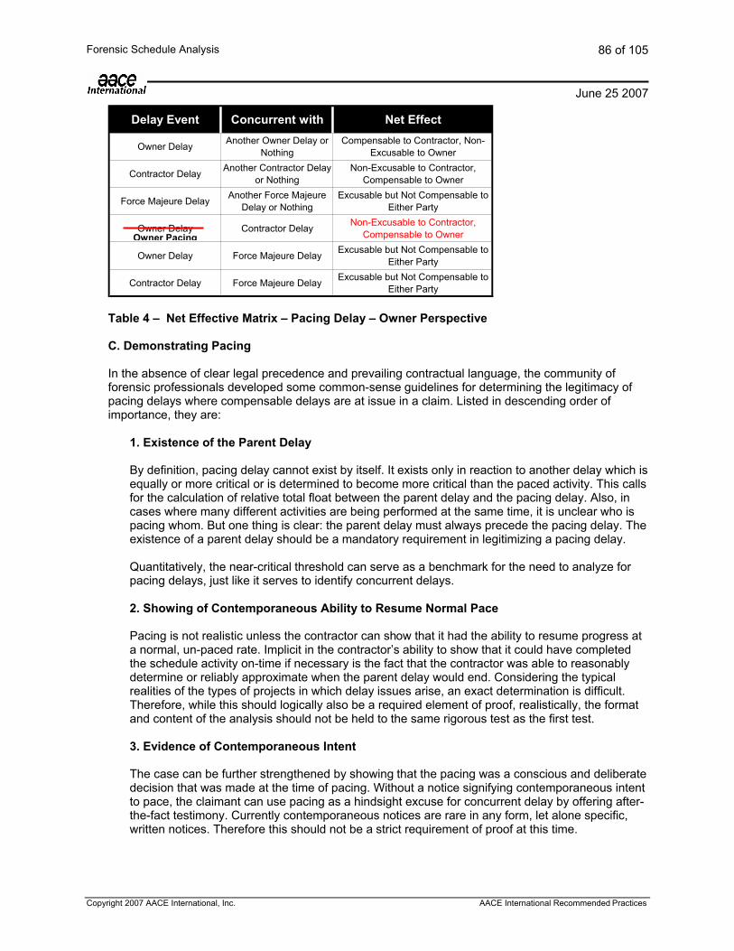
Copyright 2007 AACE International, Inc. AACE International Recommended Practices
Forensic Schedule Analysis
June 25 2007
86 of 105
Delay Event Concurrent with Net Effect
Owner Delay Another Owner Delay or Nothing
Compensable to Contractor, Non-Excusable to Owner
Contractor Delay Another Contractor Delay or Nothing
Non-Excusable to Contractor, Compensable to Owner
Force Majeure Delay Another Force Majeure Delay or Nothing
Excusable but Not Compensable to Either Party
Owner Delay Contractor Delay Non-Excusable to Contractor, Compensable to Owner
Owner Delay Force Majeure Delay Excusable but Not Compensable to Either Party
Contractor Delay Force Majeure Delay Excusable but Not Compensable to Either Party
Table 4 – Net Effective Matrix – Pacing Delay – Owner Perspective
C. Demonstrating Pacing In the absence of clear legal precedence and prevailing contractual language, the community of forensic professionals developed some common-sense guidelines for determining the legitimacy of pacing delays where compensable delays are at issue in a claim. Listed in descending order of importance, they are:
1. Existence of the Parent Delay By definition, pacing delay cannot exist by itself. It exists only in reaction to another delay which is equally or more critical or is determined to become more critical than the paced activity. This calls for the calculation of relative total float between the parent delay and the pacing delay. Also, in cases where many different activities are being performed at the same time, it is unclear who is pacing whom. But one thing is clear: the parent delay must always precede the pacing delay. The existence of a parent delay should be a mandatory requirement in legitimizing a pacing delay. Quantitatively, the near-critical threshold can serve as a benchmark for the need to analyze for pacing delays, just like it serves to identify concurrent delays.
2. Showing of Contemporaneous Ability to Resume Normal Pace Pacing is not realistic unless the contractor can show that it had the ability to resume progress at a normal, un-paced rate. Implicit in the contractor’s ability to show that it could have completed the schedule activity on-time if necessary is the fact that the contractor was able to reasonably determine or reliably approximate when the parent delay would end. Considering the typical realities of the types of projects in which delay issues arise, an exact determination is difficult. Therefore, while this should logically also be a required element of proof, realistically, the format and content of the analysis should not be held to the same rigorous test as the first test. 3. Evidence of Contemporaneous Intent The case can be further strengthened by showing that the pacing was a conscious and deliberate decision that was made at the time of pacing. Without a notice signifying contemporaneous intent to pace, the claimant can use pacing as a hindsight excuse for concurrent delay by offering after-the-fact testimony. Currently contemporaneous notices are rare in any form, let alone specific, written notices. Therefore this should not be a strict requirement of proof at this time.
Owner Pacing

Copyright 2007 AACE International, Inc. AACE International Recommended Practices
Forensic Schedule Analysis
June 25 2007
87 of 105
4.3. Critical Path and Float
A. Identifying the Critical Path
1. Critical Path: Longest Path School vs. Total Float Value School In the early days of the development of the CPM, the longest path was the path with the lowest float. Using simple network logic (finish-to-start) only, the critical path of an un-progressed CPM network calculated using the longest path criterion or the lowest float value criterion is the same. It is only when some advanced scheduling techniques17 are applied to the network model that the paths identified using these different criteria diverge. Most practitioners would agree that the longest path is the true critical path. Even with the use of advanced techniques, if basic network rules (see section 2.1) are observed the total float value is a reasonably accurate way of identifying the critical path. But note that float values are displayed using workday units defined by the underlying calendar assigned to the schedule activity instead of in 7-day calendar units so that activities on a chain with uniform network tension may display different float values.
2. Negative Float: Zero Float School vs. Lowest Float Value School
When a project is behind schedule, the network model may display negative values for float. Technically, this results from the fact that the earliest possible dates of performance for the activities are later than the latest dates by which they must be performed in order for the overall network to complete by a constrained finish date. Thus the negative value is a direct indication of how many work days the schedule activity is behind schedule. There are two schools of thought in interpreting the criticality of activity paths carrying negative float values. One school, which will be called the zero float school, maintains that all activities with negative float are, by definition, critical; assuming the definition of critical path is anything less than total float of one unit. The other school, which will be called the lowest value school, insists that only the activity paths that carry the lowest value are critical. In the context of the two critical path schools, longest path versus total float value, the total float value adherents tend to align with the zero float thinking while the longest path adherents tend to think along the lines of the lowest float value school. However, neither one of these philosophical alignments are guaranteed, nor are they logically inconsistent. Which one is correct depends on which principles are considered. If only CPM principles are used to evaluate the theories, the lowest value school is correct. The zero float school may have an arguable point if contractual considerations are brought into play, since all paths showing negative float are impacting (albeit not equally) the contractual completion date. For the purpose of this RP, the procedures and methods use the lowest value theory as the valid criterion for criticality where negative float is shown. Thus the true float value of an schedule activity carrying negative float will be calculated as the relative total float against the lowest float value in the network. For example if the lowest float value in the network is minus 100, and another schedule activity shows a value of negative 20, the true float for that schedule activity, based on relative total float, is 80. The potential also exists for fragnets of activities to have lower total float than the project longest or critical path. This occurs when activities are tied to intermediate project milestones (and not to overall project completion). If such a scenario is
17 For examples of these advanced techniques refer to section 4.3.D.

Copyright 2007 AACE International, Inc. AACE International Recommended Practices
Forensic Schedule Analysis
June 25 2007
88 of 105
observed, the analysis should also consider the contractual relationship or requirement for the intermediate milestones.
B. Quantifying ‘Near-Critical’
The purpose of quantifying the near-critical path is to reduce the effort of identifying and analyzing potential concurrent delays. A rational system of identifying all activities and delays that are near-critical is the first step in objectively streamlining the process of evaluating the schedule for concurrent delays. Thus, if you choose to analyze all delays and activities on a network, the quantification of near-critical is unnecessary. But in most cases analyzing all activities, especially on large complex schedule is excessively time consuming and unnecessary. Near-critical delays have the greatest potential of becoming concurrent delays. This is because a near-critical delay, upon consumption of relative float against the critical path delay, will become critical. Therefore the near-critical delays are the most likely suspects of concurrency, and therefore must be analyzed for partial concurrency to the extent that the net effect of that delay may exceed such relative float. The determination of what a ‘near critical’ activity is depends on the following factors:
1. Duration of Discrete Delay Events The insertion or extraction of delays affects the CPM calculations of a network model. Specifically, the duration of delays modeled in the analysis is directly proportional to the impact such delays have on the underlying network. Because the effect results from insertion or extraction of delay, this is of obvious relevance to the modeled methods (3.6, 3.7, and 3.8). But it is also relevant to the dynamic observation methods where the underlying schedule updates were prepared during the project by inserting delay events. The maximum duration of the set of all delay events would measure the greatest potential effect resulting from insertion or extraction. Averaging the duration of the set of all delay events would provide a less rigorous average measure. The maximum or the average measure is added to the value of the float value of the critical path to yield the near-critical threshold. Any schedule activity or path carrying a float value between that threshold and the value of the critical path is considered near-critical. The practical effect is that the greater the duration of the delay events used in the model the greater the number of activities that must be considered near-critical and subjected to concurrency evaluation. Under this criterion, the most obvious way of minimizing the number of near-critical activities is to minimize the duration of the delay events. That is, a delay event of relatively long duration can be segmented into smaller sub-events for analysis and documentation. While ensuring a finer granularity of delay events gives rise to added work in modeling and documenting those delay events, the trade-off is less number of activities to analyze for concurrency. 2. Duration of Each Analysis Interval The duration of the analysis interval is the length of time from the start of the segment of analysis to the end of that segment. In the dynamic methods (3.2, 3.3, 3.4, 3.5, and 3.7) where the analysis is segmented into multiple analysis intervals, the measure would be the duration of each
Copyright 2007 AACE International, Inc. AACE International Recommended Practices
Forensic Schedule Analysis
June 25 2007
89 of 105
period or window. In the static methods (3.1, 3.218, 3.6 and 3.8) the duration of the analysis interval is the duration of the entire project or whatever segment of the project represented by the schedule used for the analysis. Although this would mean that the static methods would have to perform a concurrency analysis on the entire network, it is both impractical and unnecessary to do so. Thus for methods that use the as-built as a component (3.1, 3.2, and 3.8), determination of near criticality can be made pursuant the procedure established in 4.3.C below regarding the as-built critical path.
The concept underlying this criterion is the fact that the potential change in the critical path due to slippage or gain caused by progress (or lack thereof) during the analysis interval is equal to the duration of that interval. Thus, if the interval is one month, the maximum slippage that can occur, excluding non-progress revisions and delay insertions, is one month. Hence near-criticality threshold would be set by adding 30 calendar days to the float value of the critical path. This criterion is most relevant with the dynamic methods (3.2, 3.3, 3.4, 3.5, and 3.7) that use the concept of analysis intervals. An implementation that uses large windows would have to consider more activities near-critical than one that uses many small windows. An extreme example of the latter is an as-planned versus as-built analysis that analyzes progress on a daily basis (3.2). This would have a near-critical threshold value of one day over the critical path. The practical tradeoff is by increasing the number of analysis intervals one can reduce the work load of concurrency analysis, and vice-versa.
3. Historical Rate of Float Consumption To augment the previous analysis interval criterion, the rate at which float is being consumed on a given activity-chain over time is worthy of consideration. The rate of consumption should be no more than the duration of the analysis interval per interval. Thus, where the interval is one month, if an activity chain is outside the near-critical threshold but is consuming more than 30 calendar days of float per month in the past updates19, the trend indicates that it would become near-critical in the next period. Therefore it should be considered near-critical even though it carries more relative float than the duration of the interval. 4. Amount of Time or Work Remaining on the Project As the project approaches completion, CPM may not be the best tool to assess criticality. This is true especially in a problem project where many activities are being performed out-of-sequence in an attempt to meet an aggressive deadline. Even on a normal project, as the work transitions from final finishes to punch list work, CPM updates may be abandoned in favor of a list or matrix format of work scheduling. It is often said that near the end ‘everything is critical’. Reduced to an equation, the percentage of activities remaining on the network that should be considered near-critical is proportional to the degree of completion of the schedule. Therefore after 90 to 95 percent of the base scope and change order work are complete, you may want to consider all activities on the schedule as near-critical regardless of float.
C. Identifying the As-Built Critical Path
As stated in section 2.2, the as-built critical path cannot be directly computed using CPM logic since networked computations that generate float values can be generated only to the future (right) of the
18 Method 3.2 appears in both classifications because under some (but not all) implementations of 3.2, the segmentation is merely a graphical tool for presenting a conclusion derived from a non-periodic analysis. Please refer to that subsection for details. 19 Obviously this would be caused by reasons beyond just pure slippage. An example would be insertion of activities or a change to more restrictive logic.
Copyright 2007 AACE International, Inc. AACE International Recommended Practices
Forensic Schedule Analysis
June 25 2007
90 of 105
data date. Because of this technical reason, the critical set of as-built activities is often called the controlling activities as opposed to critical activities. Even in a modeled collapsible as-built (3.8) float is not a relevant indicator of criticality because the late dates are not used in modeling the as-built schedule. The closest the analyst can come to a direct computational determination is to cumulatively collect from successive schedule updates the activities that reside on the critical path between the data date and the data date of the subsequent update. The same technique can be used to determine the as-built near-critical activities. If the updates are available, the following is the recommended protocol.
a. Use all the critical and near-critical activities in the baseline schedule. If modifications were made
to the baseline for analysis purposes use both sets of critical activities, before and after the modification.
b. For each schedule update, use the critical and near-critical chains of activities starting
immediately to the right of the data date. c. Also use the predecessor activities to the left of the data date that precede the chains found in (b)
above. d. Use the longest path and near-longest path criteria in addition to the lowest float path criterion in
identifying the activities. e. If weather or other calendar factors are at issue, also use a baseline recalculated with an
alternate calendar reflecting actual weather or other factors to gather critical and near-critical activities.
An enhanced protocol would add the following sets to the recommended protocol.
f. If appropriate, perform (b) through (d) above using different calculation modes20 if they are
available. g. Where significant non-progress revisions were made during the updating process, repeat (b)
through (d) using the progress-only, bifurcated schedules (see subsection 2.3.D.) h. If appropriate, examine the resource-leveled critical path as opposed to hard-tied sequences,
sometimes called preferential logic, based solely on resources. i. Conversely, if resource constraint is at issue and the schedule logic does not reflect the
constraint, insert resource-based logic to obtain a critical path that considers all significant constraints.
But objective identification of the controlling activities is difficult, if not impossible, without the benefit of any schedule updates or at least a baseline CPM schedule with logic. Therefore, in the absence of competent schedule updates the analyst must err on the side of over-inclusion in selecting the controlling set of as-built activities. The determination must be a composite process based on multiple sources of project data including the subjective opinion of the percipient witnesses. All sources used to identify the as-built controlling path should be tabulated and evaluated for reliability. Contemporaneous perception of criticality by the project participants is just as important as the actual fact of criticality because important project execution decisions are often made based on perceptions. Perceived or subjective as-built critical paths can be based on:
• Interview of the hands-on field personnel.
20 For example, in Primavera Project Planner: retained logic and progress override modes.

Copyright 2007 AACE International, Inc. AACE International Recommended Practices
Forensic Schedule Analysis
June 25 2007
91 of 105
• Interview of the project scheduler. • Contemporaneous non CPM documentation such as:
• monthly update reports
• meeting minutes
• daily reports
D. Critical Path Manipulation Techniques
There are various ways of creating, erasing, decreasing, inflating or hiding float and manipulating the critical path of a CPM network. These manipulation techniques can be used prospectively during the preparation of the baseline and the project updates as well as in the process of preparing the forensic models (3.6, 3.7, and 3.8). This does not mean that the observational methods (3.1, 3.2, 3.3, 3.4, and 3.5) are immune from manipulation. Since they rely on the baseline and the updates, the source schedules must be checked for manipulation prior to use in the forensic process. Also, during the forensic process, the dynamic methods are subject to manipulation through the frequency, duration and placement of analysis intervals (section 4.3.B.2) and through subjective assignment of progress data in reconstructing updates (section 3.5). The use of these techniques per se is not evidence of intentional manipulation. It must be stressed that there are legitimate uses and good reasons, albeit limited, for these features; otherwise they would have never found their way into the software. Even in the absence of ‘good reason’, the feature could have resulted from laziness or even misguided attempts to improve the schedule. At any rate, schedules used for forensic schedule analysis must minimize the use of these techniques (see section 2.1). The policy of this RP is to be ‘software neutral’. This means that procedures and recommendations are made without regard to the brand or version of software used for analysis. However, the examples of techniques used to manipulate results, listed below, contain descriptions of the features taken directly from the software manufacturer’s manual in order to accurately represent the techniques which are software-dependent. Two major software products, Primavera Project Planner (P3) and Microsoft Project (MSP), representing a significant market share of the scheduling trade were used as references.
1. Resource Leveling & Smoothing This technique uses available float to balance the resources necessary for executing the schedule. Some analysts maintain that resource leveling is the technical embodiment of pacing (see 4.4). Software Definitions
• Resource leveling is the process of determining and minimizing the effect of low resource
availability on the schedule. Use resource leveling to resolve resource conflicts by rescheduling activities to times when sufficient resources are available. Split activities to work around times when resources are not available; stretch activity durations to reduce their resource per time period requirements; or compress activity durations to take advantage of ample resource supplies. Resource leveling uses the normal and maximum limits established in the resource dictionary. The normal limit is used during resource-constrained leveling to

Copyright 2007 AACE International, Inc. AACE International Recommended Practices
Forensic Schedule Analysis
June 25 2007
92 of 105
take advantage of positive float within the network. During forward leveling, activities may be shifted to a later date (the leveled date). In backward leveling, activities may be moved earlier in time. If an activity cannot be scheduled without exceeding the normal limit and without exhausting all positive float, P3 increases the resource availability limit to the maximum level. A resource leveling analysis report details the reasons activities are rescheduled. [2]
• Resource smoothing is an optional resource leveling method that resolves resource conflicts by delaying activities that have positive float. Resource smoothing uses the available positive float and incrementally increases the availability limits in ten equal steps from normal to maximum. P3 smoothes only those activities that will be delayed beyond their calculated early start date due to insufficient resources. This method minimizes peaks and valleys in the resource usage profile. [2]
2. Multiple Calendars
Float values are displayed using workday units defined in the underlying work-day calendar assigned to the activity instead of in calendar-day units so that activities on a chain with identical network tension may display different float values. All things being equal, activities using a more restrictive work-day calendar, such as one that excludes the winter months for work, carry less float than if those activities used a less restrictive work-day calendar. Thus by building in or removing a few holidays in the calendar, float can be manipulated. While highly impractical, the only way to avoid gaps, discontinuities and work-day conversions is to use only one calendar consisting of a seven-day week.
Software Definitions
• The work periods and holidays defined for the project determine when P3 can schedule
activities and resources. P3 allows up to 31 base (activity) calendars per project. Once you add and define project base calendars, use the calendar ID to assign the appropriate calendar to each activity. Define calendars in planning units of hours, days, weeks, or months. Define an unlimited number of resource calendars, using any base calendar as a template for each one. [2]
• The scheduling mechanism that determines working time for resources and tasks. Microsoft
Project uses four types of calendars: base calendar, project calendar, resource calendar & task calendar. [3]
3. Precedence Logic / Lead & Lag Simple logic is finish-to-start with a lag value of zero, denoted as FS0. Other known types of logic are start-to-start (SS), finish-to-finish (FF) and start-to-finish (SF). Most software allows the use of these logic types along with the use of lead and lag values other than zero, including negative values. The use of lag values greater than zero with FS-type of logic absorbs otherwise available float. It is possible to assign lag values that are less than zero, called negative lags. Negative lags associated with the FS-type of logic have the effect of overlapping the associated schedule activities, thereby increasing float.
Software Definitions
• Lag: An offset or delay from an activity to its successor. Lag can be positive or negative; it is
measured in the planning unit for the project and based on the calendar of the predecessor activity. Lag cannot exceed 32,000 time periods or be less than -9999 time periods. Lag

Copyright 2007 AACE International, Inc. AACE International Recommended Practices
Forensic Schedule Analysis
June 25 2007
93 of 105
decreases as you record progress (actual start). When P3 calculates a schedule, it subtracts from the lag value the number of work periods between the project data date and the actual start date of the predecessor activity. [2]
• Lead Time: An overlap between tasks that have a dependency. For example, if a task can
start when its predecessor is half finished, you can specify a finish-to-start dependency with a lead time of 50 percent for the successor task. You enter lead time as a negative lag value. [3]
• Lag Time: A delay between tasks that have a dependency. For example, if you need a two-
day delay between the finish of one task and the start of another, you can establish a finish-to-start dependency and specify a two-day lag time. You enter lag time as a positive value. [3]
4. Start & Finish Constraints
Setting a start constraint to a date that is later than what would be allowed by a controlling predecessor would decrease the float on the schedule activity. Similarly, setting a finish constraint to a date that is earlier than what would be allowed by a controlling predecessor would also decrease float on the schedule activity. Both techniques can be used to force activity paths to carry negative float. There are also features that force the schedule activity to carry no total float21 or no free float22. Also certain types constraints23 force the assignment of zero float value by fixing dates on which the activity will be performed, overriding associated precedence logic.
Software Definitions
• A scheduling restriction you impose on the start or finish of an activity. Use constraints to
reflect real project requirements; for example, all outdoor activities must be completed by the beginning of winter. [2]
• A restriction or limitation that you or Microsoft Project set on the start or finish date of a task.
For example, you can specify that a task must start on a particular date or finish no later than a particular date. When you add a new task to a project that is scheduled from the start date, Microsoft Project automatically assigns the “as soon as possible” constraint. Conversely, when you add a new task to a project that is scheduled from the finish date, Microsoft Project automatically assigns the “as late as possible” constraint. [3]
5. Various Calculation Modes
Fundamental schedule and float calculation methods can be selected by the user, further complicating the effort to identify the critical path and quantify float. Below are examples related to various methods of schedule calculation, duration calculation, and float calculation.
a. Schedule Calculation
• Retained Logic: 1) One of two types of logic used to calculate a schedule in P3. If you
select retained logic in the schedule/level calculation options dialog box, P3 schedules an activity with out-of-sequence progress according to the network logic. P3 allows the activity to begin out of sequence, but the remaining duration for the activity cannot be completed until all its predecessors complete. [This is the default setting] [2] 2) One of two types of logic used to handle activities that occur out of sequence. When used,
21 Zero total float (ZTF) constraint in Primavera. 22 Zero free float (ZFF) constraint in Primavera. 23 Mandatory start (MS) and mandatory finish (MF) constraints in Primavera.

Copyright 2007 AACE International, Inc. AACE International Recommended Practices
Forensic Schedule Analysis
June 25 2007
94 of 105
scheduling software schedules the remaining duration of an out-of-sequence activity according to current network logic - after its predecessors. [4]
• Progress Override: 1) One of two types of logic used to calculate a schedule in P3.
Progress override ignores logic and affects the schedule only if out-of-sequence progress occurs. If you select progress override in the schedule/level calculation options dialog box, P3 treats an activity with out-of-sequence progress as though it has no predecessors and can progress without delay. [This is the alternate setting] [2] 2) One of two types of scheduling software logic used to handle activities that occur out of sequence. When specified, it treats an activity with out-of-sequence progress as though it has no predecessor constraints; its remaining duration is scheduled to start immediately, rather than wait for the activities predecessors to complete. [4]
b. Duration Calculation
• Continuous Activity Duration: One of two types of activity-duration logic used by P3 to
calculate schedules. Contiguous activity duration requires that work on an activity occur without interruption. For early dates, this type of logic affects how P3 schedules the start dates for an activity when the finish dates are delayed by a finish relationship from a preceding activity or by a finish constraint. If you select contiguous logic, and finish dates of an activity are delayed, the start dates are delayed also. [This is the default setting] [2]
• Interruptible Activity Duration: One of two types of activity duration logic P3 uses to
calculate a schedule. For early dates, interruptible scheduling affects how P3 schedules start dates of an activity when the finish dates are delayed by a finish relationship from a preceding activity or by a finish constraint. If you select interruptible scheduling, and the finish dates of an activity are delayed, the start dates are not delayed. P3 stretches the duration of the activity, allowing the work to be interrupted along the way. [This is the alternate setting] [2]
c. Float Calculation
• Show Open Ends As: Choose “critical” to show open-ended activities as critical; choose
“non-critical” if you do not want activities with open ends to be considered critical. [2] • Calculate Total Float As: Choose the method P3 uses to calculate total float for all
activities. “Start float” is the difference between the early and late start dates; “finish float” is the difference between the early and late finish dates; and “most critical float” is the least (most critical) of the start or finish floats. [2]
6. Use of Data Date
Reliable calculation of schedule updates requires the use of the concept of data date. Some software ships with the feature turned off and require that the featured be manually activated as an option. Software Definitions • The date P3 uses as the starting point for schedule calculations. Change the data date to the
current date when you record progress. [In P3, data date is a built-in default feature that cannot be deactivated.] [2]
7. Judgment Calls during the Forensic Process

Copyright 2007 AACE International, Inc. AACE International Recommended Practices
Forensic Schedule Analysis
June 25 2007
95 of 105
Any of the above techniques can be abused to affect discretionary decisions by the forensic analyst to influence the analysis in favor of the client. There are two instances in the forensic process that are especially sensitive to such influence because they directly affect the schedule variables at the data line. They are: • Frequency, duration, and placement of analysis Intervals (see 4.2.A.3).
• Hindsight vs. blind-sight update reconstruction (see 4.2.A.5).
E. Ownership of Float
In the absence of contrary contractual language, network float is a shared commodity between the owner and the contractor. Conventional interpretation of the principle of shared float allows the use of float on a first-come-first-serve basis, thereby allowing the owner to delay activities on that path up to the point where float is consumed. Therefore, as a corollary, if pacing is defined as the consumption of float, it follows that both owners and contractors are allowed to pace non-critical work. Project float is the time between the last schedule activity on the baseline schedule and the contractual completion date where the contractual completion date is later than the scheduled completion date. In this case, in the absence of contrary contractual language, project float is owned solely by the contractor.
4.4. Delay Mitigation and Constructive Acceleration
A. Definitions
Acceleration: Work by the contractor that is required to complete all or a portion of the contracted scope earlier than scheduled. The accelerated work may be required as a result of: a) direction of the owner or its agents (directed acceleration); b) conduct of the owner or its agents without explicit direction (constructive acceleration); or c) events within the responsibility of the contractor resulting in possible delay that the contractor decides to mitigate. Acceleration has a cost associated with its performance. Directed Acceleration: Formal instruction by the owner directing the contractor to: (1) complete all or a portion of the work earlier than scheduled; (2) which directs the contractor to undertake additional work; or, (3) perform other actions so as to yet complete all, or a portion, of the contract scope of work in the previously scheduled timeframe. This could include mitigation efforts that usually have no costs associated with them. Constructive Acceleration: 1) A contractor’s acceleration efforts to maintain scheduled completion date(s) undertaken as a result of an owner’s action or inaction and failure to make a specific direction to accelerate; [4] 2) Constructive acceleration generally occurs when five criteria are met: a) the contractor is entitled to an excusable delay; b) the contractor requests and establishes entitlement to a time extension; c) the owner fails to grant a timely time extension; d) the owner or its agent specifically orders or clearly implies completion within a shorter time period than is associated with the requested time extension; and, e) the contractor provides notice to the owner or its agent that the contractor considers this action an acceleration order. [4] 3) Acceleration is said to have been constructive when the contractor claims a time extension but the owner denies the request and affirmatively requires completion within the original contract duration, and it is later determined that the contractor was entitled to the extension. The time extension can be for either additional work or delayed original work. [5] 4) Constructive acceleration occurs when the contractor is forced by the owner to complete all or a portion of its work ahead of a properly adjusted progress schedule. This may mean the contractor suffers an excusable delay but is not granted a time extension for the delay. If ordered to complete performance within the originally specified completion period, the contractor is

Copyright 2007 AACE International, Inc. AACE International Recommended Practices
Forensic Schedule Analysis
June 25 2007
96 of 105
forced to complete the work in a shorter period either than required or to which he is entitled. Thus, the contractor is forced to accelerate the work. [6] 5) Acceleration following failure by the employer to recognize that the contractor has encountered employer delay for which it is entitled to an EOT (extension of time) and which failure required the contractor to accelerate its progress in order to complete the works by the prevailing contract completion date. This situation may be brought about by the employer’s denial of a valid request for an EOT or by the employer’s late granting of an EOT. This is not (currently) a recognized concept under English law. [1] 6) constructive acceleration is caused by an owner failing to promptly grant a time extension for excusable delay and the contractor accelerating to avoid liquidated damages. [7]
Disruption: 1) An interference (action or event) with the orderly progress of a project or activity(ies). Disruption has been described as the effect of change on unchanged work which manifests itself primarily as adverse labor productivity impacts. [4] 2) Schedule disruption is any unfavorable change to the schedule that may, but does not necessarily, involve delays to the critical path or delayed project completion. Disruption may include, but is not limited to, duration compression, out-of-sequence work, concurrent operations, stacking of trades and other acceleration measures. [8] Out-of-Sequence Progress: Work completed for an activity before it is scheduled to occur. In a conventional relationship, an activity that starts before its predecessor completes shows out-of-sequence progress. [2] Delay Mitigation: A contractor’s or owner’s efforts to reduce the effect of delays already incurred or anticipated to occur to activities or groups of activities. Mitigation often includes revising the project's scope, budget, schedule or quality, preferably without material impact on the project's objectives, in order to reduce possible delay. Mitigation usually has no associated costs. [4] Recovery Schedule: A special schedule showing special efforts to recover time lost for delays already incurred or anticipated to occur when compared to a previous schedule. Often a recovery schedule is a contract requirement when the projected finish date no longer indicates timely completion. [4]
B. General Considerations
1. Differences between Acceleration, Constructive Acceleration and Delay Mitigation.
In practice there are subtle distinctions between acceleration, constructive acceleration and delay mitigation. For example, acceleration cost implies additional expenditure or money for recovery of either incurred or projected delay, and efforts to complete early. The term constructive acceleration applies to expenditure of money for efforts to recover either incurred or projected delay. Delay mitigation, refers to no-cost recovery efforts for incurred or projected delay. In the case of acceleration, constructive acceleration, and delay mitigation, affected activities are usually on the projected critical path, thus the objective of most acceleration or mitigation is to recover for anticipated delay to project completion. However, acceleration, constructive acceleration and mitigation can occur with regard to activities that are not on the critical path. For example, an owner might insist that a certain portion of the work be made available prior to the scheduled date for completion of that activity. The contractor may mitigate non-critical delay by resequencing a series of non-critical activities to increase the available float. There are circumstances in which acceleration measures are used in an attempt to complete the project earlier than planned. Those circumstances are usually classified as: (1) directed acceleration where the owner directs such acceleration and usually pays for the associated additional cost; or (2) voluntary acceleration in which the contractor implements the plan on its own initiative in the hope of earning an early completion bonus. Contractor efforts undertaken

Copyright 2007 AACE International, Inc. AACE International Recommended Practices
Forensic Schedule Analysis
June 25 2007
97 of 105
during the course of the project to recover from its own delays to activities are generally not considered acceleration. The causative link between a delay event and cost associated with constructive acceleration is diagramed below. The root cause of the impact results in a construction delay or projects a construction delay. This, in turn, results in the contractor identifying that it needs a time extension and requesting a time extension. The owner denies the time extension request but the need for recovery from the delay remains. The contractor then undertakes acceleration measures that could include increased labor. Increased labor, without a time extension can result in loss of productivity.
Figure 9 – Constructive Acceleration Flow Chart A contractor’s cost for acceleration, whether directed or constructive, is generally associated with its effort to engage more resources to perform the work during a unit of time than it had planned. These increased resources fall into the following major categories: (1) increased management resources; (2) increased equipment usage; (3) increased material supply; and (4) increased labor. The greatest cost associated with acceleration is usually labor. Since the amount of actual work remains unchanged in most acceleration efforts (the planned scope of work has not increased), the increase in labor cost is a result of a decrease in labor productivity. Decreased labor productivity is caused by disruption to the planned sequence and pace of the labor. The greater the disruption to the work, the greater the inefficiency. Disruption is the result of having more men working in the planned area during a specific time, or loss of productivity associated with individual workers working more hours than planned.
2. Acceleration and Compensability
Directed acceleration is always compensable to the contractor, although the parties may disagree on quantum. This is true regardless of whether the contractor is accelerating to overcome an owner-caused delay, or to recover from a force majeure event. Constructive acceleration follows this same pattern. If entitlement to constructive acceleration is established, the contractor may recover for a delay caused by the owner that the owner has refused to acknowledge and also for a force majeure event. This is different than the normal rule concerning damages associated with force majeure events. Typically, force majeure events entitle the contractor to time but no money. In a constructive acceleration situation, however, the owner has refused to acknowledge a delay, so the contractor has no choice but to accelerate so as to avoid the delay. As a result, the contactor is entitled to recover its cost for that constructive acceleration.
3. Delay Mitigation and Compensability
Delay mitigation is generally achieved through non-compensable efforts. These efforts are usually associated with changes in preferential logic so as to perform the work in a shorter timeframe.
Root Cause
Construction Delay
Need For Time Extension
Extension NotAvailable
Need For Acceleration
Acceleration Measures
Loss of Productivity

Copyright 2007 AACE International, Inc. AACE International Recommended Practices
Forensic Schedule Analysis
June 25 2007
98 of 105
Mitigation applies to either incurred or predicted delays. There is no mitigation associated with efforts to complete early. Delay mitigation does have a small cost that is usually ignored. This cost is associated with the contractor’s management of the schedule and the overall project and is generally considered minimal and, therefore, not compensable.
C. Elements of Constructive Acceleration
1. Contractor Entitlement to an Excusable Delay
The contractor must establish entitlement to an excusable delay. The delay can be caused by an action or inaction on the part of the owner that results in delay and would be considered compensable, or if can be a force majeure event. Generally, the contemporaneous development of a schedule that reasonably shows the basis for the entitlement to the delay. In theory, a contractor can recover for constructive acceleration for work yet-to-be done. In this situation the owner takes some action that will result in the contractor expending acceleration costs to recover from the delay. The contractor could assert its entitlement even though the actual acceleration has yet-to occur and the actual acceleration costs have yet-to occur. In practice, since constructive acceleration occurs after the owner has denied a time extension, it is almost always resolved after the acceleration is complete and the contactor usually is arguing that it was actually accelerated.
2. Contractor Requests and Establishes Entitlement to a Time Extension
The contractor must ask for a time extension associated with the owner’s action or the force majeure event. In that request, or associated with that request, the contractor must establish that it is entitled to a time extension. The owner must have the opportunity to review the contractor’s request and act upon it. If the contractor fails to submit proof of its entitlement to a time extension, the owner is able to argue that it was never given the opportunity to properly decide between granting a time extension or ordering acceleration. The level of proof required to be submitted must in the end be sufficient to convince the eventual trier of fact that the contractor “established” its entitlement. In certain situations, it is possible that actions of the owner may negate the requirement for the contractor to request a time extension or establish its entitlement. In this situation, the theory is that the owner has made clear through its actions that it will absolutely not grant a time extension. Such cases are difficult to establish.
3. Owner Failure to Grant a Timely Time Extension The owner must unreasonably fail to grant a time extension. This is closely related to the requirement that the contractor establish its entitlement to a time extension. If the owner reasonably denies a request for time, as eventually decided by the trier of fact, then by definition the contractor has failed to prove entitlement. Therefore, the owner’s decision not to grant a time extension must be unreasonable.
4. Implied Order by the Owner to Complete More Quickly
The owner must also, by implication or direction, require the contractor to accelerate. There are several different factual alternatives possible . First, a simple denial of a legitimate time extension, by implication, requires timely completion and thus acceleration. If this denial is timely given, the contractor can proceed. However, the best proof for the contractor is a statement or action by the owner that specifically orders the contactor meet a date that requires acceleration. Second, the owner could deny the time extension request and remind the contractor that he needs to complete on time. This is better than the first alternative above, but not as strong as the next alternative. Third, the owner could deny the time extension request and advise the contractor that

Copyright 2007 AACE International, Inc. AACE International Recommended Practices
Forensic Schedule Analysis
June 25 2007
99 of 105
any acceleration is the contractor’s responsibility. This is probably the best proof for this aspect of constructive acceleration. All three of these alternatives meet the test for an owner having instructed acceleration. Examples of owner actions that meet this requirement include: (1) a letter from the owner informing the contractor that he must meet a completion date that is accelerated; (2) an owner demand for a schedule that recovers the delay; or (3) the owner threatening to access LDs unless the completion date is maintained. The fourth alternative arises when the owner is presented with a request for a time extension but fails to respond. The contractor is faced with either assuming it will be granted a time extension, or accelerating. Under this alternative, the owner’s failure to timely decide, functions as a denial.
5. Contractor Notice of Acceleration
The contractor must provide notice of acceleration. As with any contract claim for damages, the owner must be provided notice of the claim. Even though the contractor has requested and supported its application for a time extension, the contractor must still notify the owner of its intent to accelerate or is actually experiencing ongoing acceleration. This is so the owner can decide if it actually desired acceleration to occur or instead the owner may decide to grant a time extension.
6. Proof of Damages
The contractor must establish its damages. For loss of productivity claims, the contractor is faced with developing convincing proof of decreased productivity. Actual acceleration is not required. A valid contractor effort to accelerate, supported by contemporaneous records, is sufficient to establish constructive acceleration. It is quite common that contractors accelerate to overcome delays but continue to be impacted and delayed by additional events and impacts that actually result in further delay to the project.
5. CHOOSING A METHOD This part of the Recommended Practice discusses the choice of forensic schedule analysis methodology. Each claim is somewhat unique in that each deals with a different project, different contract documents, different legal jurisdictions, and different dispute resolution mechanisms among other project execution factors. Likewise, each method discussed in this RP is somewhat different and each has certain advantages and disadvantages. Forensic scheduling analysts generally agree that there are a number of qualitative reasons, beyond technical schedule analysis reasons, that should be included in determining which forensic schedule analysis method is to be used for a particular claim. This part of the RP discusses eleven factors that should be considered by the forensic schedule analyst when making a recommendation to the client and its legal counsel concerning this decision. The forensic schedule analyst ought to consider each of these factors, reach a conclusion, and offer a recommendation with supporting rationale on methodology to the client and legal counsel in order to obtain agreement prior to proceeding with the work. 5.1 Factor 1: Contractual Requirements When a project is executed under a contract which specifies or mandates a specific schedule delay analysis method, then the choice of methodology is largely taken out of the hands of the forensic schedule analyst and contract compliance is the prevailing factor. Many contracts in the United States, for example, now require that all requests for time extension (either during the life of the project or at the end of the job) be substantiated through the use of a time impact analysis (TIA). As noted in this RP, several methods of forensic schedule analysis fall under this generic terminology. Most likely, the forensic schedule analyst will be required to use one of the additive modeling methods, either single base or multiple base, unless there are persuasive reasons why a different method would yield a more credible result.
Copyright 2007 AACE International, Inc. AACE International Recommended Practices
Forensic Schedule Analysis
June 25 2007
100 of 105
On the other hand, if the contract documents are silent on which schedule delay analysis method is to be used when requesting a time extension, then the forensic schedule analyst is free to use any of the methods identified in this RP to support requests for time extensions and additional time related compensation. However, even when the contract is silent on methodology, contract language may still constrain the forensic schedule analyst’s choice of methods. For example, some contracts contain language requiring that all time extension requests document that the event “…impacted the critical path of the project schedule” or “…caused or will cause the end date of the project schedule to be later than the current contract completion date.” Thus, while this language does not dictate a schedule delay analysis method, it probably requires the forensic schedule analyst to use one of the observational dynamic, additive modeling, or subtractive modeling techniques. Also, it precludes the use of any method which does not identify or analyze a critical path such as a listing of delay events or a bar-chart analysis. Thus, the first factor to be considered is the contract’s requirements (if any) for supporting documentation for time extension requests. Forensic schedule analysts must adhere to the requirements of the contract. However, it is not uncommon that requirements set forth in contracts are unclear or ambiguous (such as a “but for TIA”) or patently erroneous (such as an “impacted as-built analysis”). The forensic schedule analyst may want to use this RP as a mechanism to advise the client, legal counsel and the other parties and help all focus on an appropriate method to be used. It is also believed that adoption and use of the terminology contained in this RP may help prevent such situations in the future.
5.2 Factor 2: Purpose of Analysis Generally, the purpose of forensic schedule analysis is to quantify delay, determine causation, and assess responsibility for such delay. Forensic schedule analysis studies how specific events impact a project schedule. Thus, the forensic schedule analyst uses contemporaneous project documentation to determine which events may have caused delay (including event identification, start and complete dates, activities impacted by the event, etc.). The forensic schedule analyst then applies these events in some orderly manner to the schedule employed on the project. Once the events are added to, removed from or otherwise identified in the schedule, then a determination can be made concerning whether any or all of the events caused the project to complete later than planned. From this determination, assessment of causation and liability can be made based on the terms and conditions and the law of the contract. With respect to a particular project, the purpose of forensic schedule analysis is to determine which party is entitled to time extensions as a result of certain events. Once the forensic schedule analyst has assessed the events that occurred on the project then consideration must be given to issues such as concurrent delay, pacing delay, delay mitigation, etc. If the forensic schedule analyst, for example, is investigating whether concurrent delay is a major factor in the analysis of project delay, then the choice of method will be limited to those methods, which specifically provide for concurrent delay identification and analysis. The forensic schedule analyst may be more likely to recommend one of the observational dynamic or modeled methods. If the purpose of the forensic schedule analysis is to demonstrate only excusable, non-compensable delay, numerous methods are available since the forensic schedule analyst will probably not need to deal with concurrent delay. If the purpose is to demonstrate compensable delay, other methods may be more appropriate. If the forensic schedule analyst needs to document the contractor’s ability to complete work early in order to document a delayed early completion claim, again some schedule delay analysis methods may be better than others. Even more specific purposes for forensic schedule analysis may be required. For example, the forensic schedule analysis may be required to justify entitlement to a time extension resulting from a particular change order. A request for equitable adjustment may require a detailed forensic schedule analysis when it is to be presented to a dispute review board or as part of a rebuttal response to claims by another party.

Copyright 2007 AACE International, Inc. AACE International Recommended Practices
Forensic Schedule Analysis
June 25 2007
101 of 105
3.1 3.2 3.3 3.4 3.5 3.6 3.7 3.8
Non-Compensable Time Extension OK OK OK OK OK OK OK OK
Compensable Delay OK OK OK OK OK OK
Right to Finish Early Compensable Delay OK
Entitlement to Early Completion Bonus OK OK OK OK OK OK OK OK
Disruption Without Project Delay OK OK OK OK OK OK OK
Constructive Acceleration OK OK OK
Forensic Use of Analysis
M E T H O D
Table 5 –Some Methods are Better Suite for Certain Purposes Than Others
5.3 Factor 3: Source Data Availability and Reliability
As discussed in this RP and emphasized heavily in the source validation protocols, the choice of a particular forensic scheduling methodology is substantially influenced by the availability of source data which can be validated and determined reliable. If, for example, the project records show that there exists only a baseline schedule but no schedule updates for the duration of the project, then the observational methods 3.3 and 3.4 cannot be utilized As a result, it is incumbent on the forensic schedule analyst to first determine the amount of contemporaneous project documentation available. As a second step, the forensic scheduler needs to review a sufficiently large sampling of the project documentation to determine if the data is reliable. Once these two reviews have been completed, then the forensic scheduler can formulate a plan for the forensic scheduling effort and make a recommendation concerning which forensic schedule analysis method should be employed on the claim.
3.1 3.2 3.3 3.4 3.5 3.6 3.7 3.8
Baseline Schedule Need Need Need Need
Schedule Updates Need Need
As-Built Record Need Need Need Need
Source Schedules or Data
M E T H O D
Table 6 – Source Data Validation Needed for Various Methods 5.4 Factor 4: Size of the Dispute

Copyright 2007 AACE International, Inc. AACE International Recommended Practices
Forensic Schedule Analysis
June 25 2007
102 of 105
One of the primary factors the forensic scheduler must keep in mind is the size of the dispute or the amount in controversy. In most situations, the choice of the forensic schedule analyst is constrained by how much a client is prepared to spend to increase the probability of successful resolution of the dispute. This is most often determined by how much money is at stake. For example, if the delay damages being sought by the client are approximately US$100,000 then the forensic schedule analyst should recommend a relatively inexpensive forensic scheduling method which is still effective for its intended purpose. On the other hand, if the delay damages sought are US$50,000,000 then the range of methods to be considered is substantially expanded because of the greater scope and costs associated with analyzing a substantially larger claim. The forensic schedule analyst needs to recommend a forensic schedule analysis method that is both cost effective and suitable for the size of the dispute. 5.5 Factor 5: Complexity of the Dispute When considering a forensic schedule analysis method, the forensic schedule analyst must do so with some knowledge of the complexity of the dispute in question and the number of events to be included in the forensic scheduling effort. For example, if the project in question is a linear project of relatively short duration and only three specific delay events need to be considered, then a simple comparison of the baseline with the as-built schedule may be appropriate. On the other hand, if the project was a complex process facility, with a 5,000+ activity network, and a hundred or so discrete events occurring over a five year period, the forensic schedule analyst may need to recommend one of the observational or modeled methods which divides the project duration into smaller analysis periods to isolate and explain controlling delays. In this context, the forensic schedule analyst must also distinguish between the complexity of the dispute and the complexity of the forensic analysis. Some complex disputes can still be analyzed with a less complex analytical technique. And, some of the methods contained in this RP may not require analysis of every activity on the schedule but can be focused on the critical path and sub-critical paths or on key events and activities only, to reduce both the cost and the complexity of the analysis. 5.6 Factor 6: Budget for Forensic Schedule Analysis Hand in glove with the size and the complexity of the dispute is the client’s budget for the forensic schedule analysis. That is, what can the client afford to spend on forensic schedule analysis? The forensic schedule analyst needs to determine any budget constraints prior to making a recommendation on forensic schedule analysis methodology. The forensic schedule analyst must also keep in mind the overall cost of the various forensic scheduling methods when making a recommendation. For example, if the delay analysis method requires the testimony of ten or fifteen percipient witnesses in order to properly lay the groundwork for the analysis in arbitration or litigation, this cost too, must be taken into account. If the law of the contract has a prevailing legal fees provision, then clients and their counsel may be willing to spend more on forensic schedule analysis than if the contract is under the “American Rule” where each party pays their own cost, regardless of outcome. If the client is prepared to spend only a small amount for a forensic schedule analysis effort, then the forensic schedule analyst should only recommend less expensive forensic scheduling methods or alternatives which will reduce cost – such as using the client’s in-house staff for certain tasks rather than outside consultant staff. Or, the forensic schedule analyst may find a method contained in this RP which is appropriate for the situation, but which does not require that all of the validation protocols be performed. Knowing that the client has a fixed or limited budget, it would be inappropriate, and perhaps even unethical, for a forensic schedule analyst to recommend a method which they know will cost more than the agreed upon budget. If the forensic schedule analyst is required to work with a very tight budget the forensic schedule analyst should advise the client and its legal counsel of the potential risks of proceeding in this manner. 5.7 Factor 7: Time Allowed for Forensic Schedule Analysis

Copyright 2007 AACE International, Inc. AACE International Recommended Practices
Forensic Schedule Analysis
June 25 2007
103 of 105
There may be occasions when the amount of time available to perform and produce a complete forensic schedule analysis is limited. If the contract contains a fast track arbitration clause which requires that hearings begin within ninety days of the filing of the arbitration demand, and all material to be used in the arbitration is to be exchanged with the other side no less than two weeks prior to the first hearing date, the forensic schedule analyst may be limited to a sixty day timeframe in which to perform the scope of work. In many situations, the need for forensic schedule analysis is not made early enough to allow complete flexibility in the choice of an analytical method or is made at the last minute due to time limitations designating testifying experts. In either situation, the forensic schedule analyst may have a very limited timeframe in which to complete their work. Should this be the case, then the forensic schedule analyst is constrained to recommend a method which can be completed in far less time than other forensic scheduling methods in order to meet the time available to perform the work. Again, the forensic schedule analyst should point out the risks of proceeding in this manner. 5.8 Factor 8: Expertise of the Forensic Schedule Analyst and Resources Available If the forensic schedule analyst has experience with only two or three of the methods identified in this RP and may be subject to challenge from the other side either during voir dire the forensic schedule analyst may be compelled to recommend use only of methods with which they have experience. Additionally, if the forensic schedule analyst is to perform all analytical work individually with no assistance, they may be constrained to recommend simpler methods which can be performed individually and not require a staff of additional people processing data, making computer runs, etc. 5.9 Factor 9: Forum for Resolution and Audience During initial discussions concerning the potential engagement, the forensic schedule analyst needs to seek advice from the client and its legal counsel on the most likely dispute resolution forum. Regardless of the dispute resolution requirements mandated in the contract documents, what the forensic schedule analyst must seek is an opinion from those involved in the project, and their legal counsel, on whether the claim is likely to settle in negotiation, mediation, arbitration (and if so, under what rules) or litigation (and if so, in which court). If there is good reason to believe that all issues are likely to be settled at the bargaining table, or in mediation, then the range of options for forensic scheduling methods is wide open as the audience is only the people on the other side. Almost any option which appears persuasive is legitimately open for consideration. On the other hand, if legal counsel believes that the issue will end up in a federal court or a federal board of contract appeals, then the range of options available is considerably narrowed because the Boards of Contract Appeals have, for nearly two decades, insisted that delay issues presented to them must rest on CPM scheduling. Therefore, any forensic schedule analysis method that does not appear to be a CPM-based analysis is unlikely to prevail. Further, if the claim is likely to end up before a board of contract appeals, the forensic schedule analyst must recognize that the audience is the trier of fact, likely to be fairly sophisticated in dealing with schedule delay issues, and likely also to be an experienced user of schedules for delay analysis purposes. Therefore, the forensic schedule analyst should recommend a more thorough method. 5.10 Factor 10: Legal or Procedural Requirements Depending upon the forum for the dispute and the jurisdiction, the forensic schedule analyst must be aware of or ask about any contractual, legal, or procedural requirements that may impact the forensic analysis. For example, any forensic schedule analysis which is, or appears to be, a total time claim in many jurisdictions must meet the following four tests to be determined persuasive: • The forensic scheduler must demonstrate that the as-planned or baseline schedule was reasonable,
achievable and free of material errors;

Copyright 2007 AACE International, Inc. AACE International Recommended Practices
Forensic Schedule Analysis
June 25 2007
104 of 105
• The forensic scheduler must demonstrate that the client followed the logic and sequence of the schedule at least until intervening events precluded the client from doing so;
• The forensic scheduler must demonstrate that the client mitigated damages to the other side to the
extent practicable; and, • The forensic scheduler must demonstrate that the other side was responsible for all delaying events
on the project and that the client caused none. There may be other contractual, legal, or procedural rules impacting forensic scheduling that the forensic scheduling analyst must consider when making a recommendation concerning which forensic scheduling methodology to use on a particular claim. Consultation with the client’s legal counsel on these issues is essential.
5.11 Factor 11: Past History/Methods and What Method the Other Side Is Using
The final factor to be considered is past history and methods. Presumably a forensic schedule analyst is not engaged until after preliminary negotiations have failed. Thus, the forensic schedule analyst needs to consider what delay analysis method was employed by the client and its staff earlier during the project, which was not acceptable to the other side in prior negotiations. Knowing this, the forensic schedule analyst should not recommend use of this technique as it has already proven unsuccessful, unless the scheduler can determine that the client staff performed the method erroneously in its early efforts. Additionally, the forensic scheduler should take into consideration the method being employed, if known, when making a recommendation concerning the method they want to employ. Not all of the above factors will be applicable to all delay claims, obviously. But a prudent forensic schedule analyst should consider each of the above factors, as well as any other relevant factors that emerge, to determine which apply to the claim at hand. Once these are identified, including their potential synergistic effect upon each other, the forensic schedule analyst should discuss each applicable factor with the client and its legal counsel prior to making a recommendation as to which method should be employed for the delay analysis. Failure to consider these factors could lead to substantial difficulties later on in claim settlement negotiations, arbitration or litigation. REFERENCES 1. SCL Delay and Disruption Protocol, Society of Construction Law, Oxon, United Kingdom, 2002 2. Primavera Project Planner – on-line software glossary 3. Microsoft Project – on-line software glossary 4. AACE International Recommended Practice No 10S-90 “Cost Engineering Terminology”, AACE
International, Morgantown, WV, 2004 5. Construction Delay Claims, Third Edition, Barry B. Bramble, Esq., Michael T. Callahan, Esq., Aspen
Publishers, New York, NY, 2006 6. Construction Scheduling: Preparation, Liability & Claims, Second Edition, Jon M. Wickwire, Esq.,
Thomas J. Driscoll, Stephen B. Hurlbut, Esq., Scott B. Hillman, Esq., Aspen Publishers, New York, NY, 2006
7. How to Get Paid for Construction Changes: Preparation and Resolution Tools and Techniques, Steven S. Pinnell, McGraw-Hill, New York, NY, 1998
8. Proposed Specification Language Regarding Pacing, Kenji P. Hoshino, AACE International Annual Meeting, 2006
9. The American Heritage® Dictionary of the English Language, Fourth Edition, Houghton Mifflin Company, Boston, MA, 2006

Copyright 2007 AACE International, Inc. AACE International Recommended Practices
Forensic Schedule Analysis
June 25 2007
105 of 105
CONTRIBUTORS Kenji P. Hoshino, PSP CFCC (Author) Robert B. Brown, PE John J. Ciccarelli, PE CCE PSP Gordon R. Costa, PSP CFCC Michael S. Dennis, CCC Edward E. Douglas, III CCC PSP Philip J. Farrocco, PE Sidney J. Hymes, CFCC John C. Livengood, PSP Mark F. Nagata, PSP Jeffery L. Ottesen, PE PSP CFCC Thomas F. Peters, PE CFCC Keith Pickavance Dr. Anamaria I. Popescu, PE Jose F. Ramirez, CCE Mark C. Sanders, PE CCE PSP Takuzo Sato L. Lee Schumacher, PSP Robert Seals, PSP Ronald M. Winter, PSP James G. Zack, Jr. CFCC