A wavelet filter enhancement scheme with a

fast integral B-wavelet transform and

pyramidal multi-B-wavelet algorithm

James D. B. Nelson1

Applied Mathematics and Computing group, Cranfield University, Cranfield,

MK43 OAL

Abstract

A construction paradigm is proposed to refine a class of wavelet bases such that thefilter characteristics are enhanced. In particular, it is shown that the entire Mthorder B-wavelet family belong to this class. Exploiting some recent work, a fastintegral wavelet transform is found for the refined B-wavelet family. Moreover, thisrefined basis can be placed into the setting of a multiresolution analysis that has amultiplicity greater than one. Accordingly, a fast, discrete, pyramidal algorithm isrealised.

Key words: Multiwavelet, wavelet modification, fast continuous wavelettransform, lifting scheme, filter characteristic

1 Introduction

With the advent of the lifting scheme came a general approach to modifywavelets such that a selection of their properties could be systematically al-tered. We propose a disparate, specialised approach to mitigate the side lobesof a wavelet filter characteristic whilst preserving differentiability, symmetry,anti-symmetry, compact support, and the existence of an analytical expres-sion.

Devised by Sweldens [12], the lifting scheme can be used to emend an exist-ing wavelet and scaling function basis to produce so called second generationwavelets. Such wavelets are not necessarily formed by dilations and transla-tions of a single scalar function. A distinctive feature of the scheme is that the

1 E-mail: j.nelson@cranfield.ac.uk

Preprint submitted to Elsevier Science 17 August 2012

wavelet construction uses a linear combination of the initial scaling functionsat the same scale level as the wavelet, whereas an orthodox wavelet construc-tion uses scaling functions at the next finest level. To paraphrase Sweldens[13], the lifting scheme uses the ‘aunt’ scaling functions rather than the ‘sis-ter’ scaling functions. Aside from giving rise to a new class of wavelets, thelifting scheme offers a custom based design as well as a means to contrivealgorithms that outperform the classical fast wavelet transform.

Although our modification scheme can give rise to second generation wavelets,it differs from the lifting scheme because a linear combination of integer di-lated and translated ‘sister’ scaling functions are employed as the buildingblocks of the wavelet. The principal aim of the construction is to minimise theside lobe to main lobe power and magnitude ratios of the filter characteris-tic about carefully chosen sub-intervals such that differentiability, symmetry,anti-symmetry, compact support, and the existence of an analytical expressionare all preserved.

Section 2 describes some measures that assess the efficacy of wavelet filtercharacteristics. We generalise these measures and, in Section 3, some numeri-cal results illustrate that our modification scheme achieves enhanced charac-teristics for the B-wavelet family. Adapting recent work by by Munoz et al.[11] and Unser et al. [14], Section 4 shows how a fast integral wavelet trans-form can be formulated for the modified B-wavelets. First realised by Alpert[1] and Geronimo et al. [6], the multi-scaling function is discussed in Section5. Finally, we consider the modified B-wavelet construction in the setting ofa multiresolution analysis generated by a multi-scaling function.

2 Measures for the frequency characteristic of a wavelet

For α, τ ∈ R, the integral wavelet transform of a function f ∈ L2(R) takes theform

(Wψf)(α, τ) = |α|−1/2∫

R

f(x)ψ(τ − x

α

)dx. (1)

That is (Wψf)(α, τ) = (f∧Ψ∧α)

∨ (τ), with Ψα :=√2π |α|−1/2 ψ(α−1·), and

where ∧ and ∨ denote the Fourier, and inverse Fourier, transform operations.Accordingly, Ψ∧

α can be thought of as a filter transfer function with a nor-malised filter characteristic |ψ∧|. Invertibility of the integral wavelet transformrequires that the wavelet satisfies the admissability condition, namely

∫

R

|ψ∧(ξ)|2 dξ|ξ| <∞.

Since it follows that ψ∧(0) = 0, wavelets are often thought of in the contextof band pass filters. A critical feature of the wavelet transform is that the

2

width of the time or space window narrows when the wavelet is assessingthe high frequency content of f , and it expands when assessing the lowerfrequencies. One is therefore left with the problem of constructing a functionthat is, in some sense, well localised in both time and frequency. However,except from the trivial example of zero, functions cannot have compact supportin both time and frequency. Consequently, a more meaningful measure of time-frequency localisation is employed, as follows.

Definition 2.1 Suppose h(x), |x|1/2 h(x), xh(x) ∈ L2(X). Then the centre ofh on X is defined as

x∗X(h) :=

∥∥∥|x|1/2 h(x)∥∥∥2

L2(X)

‖h(x)‖2L2(X)

and the radius of h is defined as

∆X(h) :=‖(x− x∗X(h))h(x)‖L2(X)

‖h(x)‖L2(X)

.

The uncertainty of a wavelet, U(ψ) := ∆R(ψ)∆R+(ψ∧) is proportional to thearea of the time-frequency window and is bounded from below by the wellknown Heisenberg-Weyl uncertainty condition U(ψ) ≥ 1/2. The uncertaintymeasure gives a broad indication of how well localised a wavelet is. Morespecific measures exist that are used to appraise the filter characteristic of awavelet. Two such methods of measurement, discussed below, recognise that,in order to perform a band pass operation efficiently, the power in the mainlobe must be significantly greater than the side lobes. Such an observation isnot lost on Dovis et al. [5], who discuss the virtues of low side lobes in thecontext of digital communications. In the following we denote those zeros ofψ∧(ξ) that lie on the positive half of the frequency axis as 0 < ξ0 < ξ1 < . . . .The first measure takes the ratio of the power of all the side lobes and dividesit by the power of the main lobe [2].

Definition 2.2 The side lobe/main lobe power ratio of the filter characteristic|ψ∧| is defined as

Mψ :=‖ψ∧‖2L2(ξ0,∞)

‖ψ∧‖2L2(0,ξ0)

.

The second measure compares the maximum taken at the main lobe and themaximum at the neighbouring lobe. Indeed, as Chui, [2] points out, this com-parison is favoured in many engineering applications such as antenna design.

Definition 2.3 The maximal side lobe/main lobe ratio of the filter character-

3

istic |ψ∧| is defined as

M∗ψ :=‖ψ∧‖L∞(ξ0,ξ1)

‖ψ∧‖L∞(0,ξ0)

.

We propose a generalisation of both measures. The ratio in Definition 2.2 canbe localised by taking the side lobe power over a finite interval Ω instead ofthe interval (ξ0,∞).

Definition 2.4 The localised side lobe/main lobe power ratio of the filtercharacteristic |ψ∧| is defined as

MΩψ :=‖ψ∧‖2L2(Ω)

‖ψ∧‖2L2(0,ξ0)

for some interval Ω ⊆ R+∗ := R

+ \ 0.

In particular, this measure can be calculated over the first N side lobes bychoosing Ω = (ξ0, ξN). It can be seen immediately that Definition 2.2 is aspecific case of MΩ, with Ω = (ξ0,∞). Alternatively, the ratio in Definition2.3 can be extended by replacing the numerator with an average of the firstN side lobe maxima.

Definition 2.5 Let Ωn = (ξn, ξn+1), and ξ−1 = 0. The globalised maxima sidelobe/main lobe ratio of the filter characteristic |ψ∧| is defined as

M∗Nψ := N ‖ψ∧‖−1

L∞(Ω−1)

N−1∑

n=0

‖ψ∧‖L∞(Ωn).

When N = 1, this reduces to Definition 2.3. To construct wavelets whichperform efficiently with respect to such measures, it is clearly necessary toconcentrate upon reducing the side lobe power in some neighbourhood aboutthe main lobe.

3 Modifying wavelet bases to optimise frequency localisation

The following method is proposed as a means of altering an existing waveletbasis such that the side lobe/main lobe measures of a wavelet are enhanced.The technique modifies a wavelet by adding dilated versions of the waveletto itself. These linear combinations are constructed such that the power as-sociated with the side lobes of the filter characteristic is attenuated. After ageneral construction is introduced, the application to the B-wavelet family isdiscussed.

4

3.1 Construction

A wavelet ψ is considered with suppψ ⊆ [0, X). The following constructionwill make use of dilated, periodically extended versions of ψ onto the interval[0, X). Let the set of integers dj, with d1 = 1, be defined by

dj+1 = minn∈2N−1

n > dj and max

nα|dα = 1

,

for all j = 1, . . . , J , and

d :=J∏

j=1

dj,

and where a | b denotes the condition that a divides b. We define the operatorsTj : [0, X) 7→ [0, X) by

Tjψ :=X(dj−1)∑

n=0

ψ(dj · −n).

The modified wavelet, denoted by ψJ , is defined in terms of the operators Tjas follows:

ψJ :=J∑

j=1

µ(dj)ΓjTjψ, (2)

where µ : N 7→ 0,±1 is the Mobius arithmetic function, given by

µ(n) :=

1, if n = 1

(−1)k, if n is the product of k distinct primes

0, otherwise

,

and the Γj comprise a set of suitably chosen coefficients. The Mobius functionis employed here due to the utility afforded by the following result, taken fromNumber Theory.

Lemma 3.1 Let µ denote the Mobius function. Then, for n ∈ N,

∑

d|n

µ(d) =

1, for n = 1

0, otherwise.

In view of our aim to attenuate the wavelet filter characteristic side lobe power,we present the following result.

Theorem 3.2 Consider the modified wavelet ψJ , as defined by (2) with the

5

set djJ1 and, for any k,m, n ∈ Z, assume that

ψ∧(2nπ)

ψ∧(2nmπ)=

ψ∧(2kπ)

ψ∧(2kmπ), if ψ∧(2nmπ)ψ∧(2kmπ) 6= 0. (3)

Then Γj can be chosen such that

ψJ∧(2nπ) = 0, 1 < n ≤ dJ .

Proof The filter characteristic of ψJ is determined by

(Tjψ)∧(ξ) =1

djψ∧

(ξ

dj

)Kj(ξ)

with

Kj(ξ) =X(dj−1)∑

r=0

e−irξ/dj =1− e−i(djX−X+1)ξ/dj

1− e−iξ/dj.

Note that Kj(2djπ) = Kj(2nπ)|dj |n, and assumption (3) implies that

ψ∧(2djπ)

ψ∧(2π)=

ψ∧(2nπ)

ψ∧(2nd−1j π)

∣∣∣∣∣dj |n

.

It follows that choosing Γj to be

Γj =djψ

∧(2djπ)

Kj(2djπ)ψ∧(2π),

ensures that, for n ∈ djN, we have

ψJ∧ (2nπ) = ψ∧(2nπ)dJ∑

dj |n

µ(dj).

Lemma 3.1 concludes the proof.

Therefore, given a wavelet basis ψ, this process will introduce zeros into themodified frequency characteristic |ψJ∧|. Of particular relevance are the zerosat ξ = 2nπ for 1 < n ≤ dJ which may help to reduce the power ratiosintroduced in Definitions 2.4 and 2.5.

It should be noted that this refinement technique does not necessarily guar-antee that ψJ can be generated from a multiresolution analysis. Furthermore,the scheme is only relevant for the class of wavelets that satisfies the con-dition stipulated by (3). However, since this process involves forming linearcombinations of dilated versions of a wavelet, it will preserve the symmetry,anti-symmetry, differentiability, and support of the original wavelet.

6

3.2 B-splines and B-wavelets

The refinement method will now be applied to the family of B-wavelets. Aquantitative comparison is then made between the frequency characteristicsof the original wavelets and those of the modified wavelets.

We let φM and ψM denote the Mth order B-spline and the associated Mthorder B-wavelet, constructed by Chui and Wang [3]. Let χΩ denote the char-acteristic, or indicator, function on some interval Ω. The first order B-spline isthe Haar scaling function defined by φ1 := χ[0,1) and the first order B-waveletis the Haar wavelet ψ1 = χ[0,1/2) − χ[1/2,1). Other members of the B-splinefamily are generated by forming an (M − 1)-fold convolution with φ1. That is

φM := φ1 ∗ φM−1. (4)

The two-scale relation for φ1 can be expressed in the frequency domain as

φ∧1 = H(z)φ∧

1

( ·2

),

with H(z) = (1 + z)/2, and z = z(ξ) := e−iξ/2. Hence, taking the Fouriertransform of both sides of (4) leads to the two-scale relation for φM , namely

φ∧M =

(1 + z

2

)Mφ∧M

( ·2

).

The B-wavelets are constructed in the multiresolution analysis generated bythe B-splines. In the original domain, the B-wavelets can be expressed as

ψM =√2∑

k

gM(k)φM(2 · −k), (5)

and in the Fourier domain we have

ψ∧M(ξ) =

1√2

∑

k

gM(k)zkφ∧M

(ξ

2

)=: GM(z)φ∧

M

(ξ

2

). (6)

Following the treatment of Chui [2], the non-zero coefficients of gM(k) can becalculated by

gM(k) =(−1)k

2M−1√2

M∑

ℓ=0

(M

ℓ

)φ2M(k − ℓ+ 1), k = 0, . . . , 3M − 2,

together with the recursive scheme

φj(n) =n

j − 1φj−1(n) +

j − n

j − 1φj−1(n− 1), j = 3, . . . , 2M,

7

with φ2(n) = δn,1, for n ∈ Z. Given the B-wavelet family above, we requirethe coefficients Γj in order to apply the refinement process. Recall

Γj = djK−1j

ψ∧(2nπ)

ψ∧(2nπ/dj). (7)

By using the two-scale relation (6), the fraction involving the function ψ in(7) can be simplified by putting k = n/dj. We have

ψ∧(2nπ)

ψ∧(2nπ/dj)=G(e−idjkπ

)

G (e−ikπ)

φ∧(nπ)

φ∧(nπ/dj)=

φ∧(nπ)

φ∧(nπ/dj).

For the Mth order B-wavelets this ratio is

φ∧M(nπ)

φ∧M(nπ/dj)

=φ∧M(djkπ)

φ∧M(kπ)

=

(φ∧1 (djkπ)

φ∧1 (kπ)

)M

=

(1− z(2djkπ)

idjkπ

)M (1− z(2kπ)

ikπ

)−M

= d−Mj .

The support of the Mth order B-wavelet is [0, 2M −1). Hence the coefficientsΓj associated with the Mth order B-wavelets are

Γj =d1−Mj

(2M − 1)(dj − 1) + 1.

Figures 1, 2, and 3 show the original wavelets and the first two refinementstogether with the corresponding filter characteristics.

Example 3.3 Choosing J = 1 implies that no modification takes place andψ1 = ψ, whereas choosing J = 2 implies d2 = 3, d = 3. Hence, the enhancedHaar wavelet ψ2

1 is

ψ21 := ψ1 −

1

3

(ψ1(3·) + ψ1(3 · −1) + ψ1(3 · −2)

).

Choosing J = 3 gives d2 = 3, d3 = 5, and d = 15. And so on.

8

0 0.2 0.4 0.6 0.8 1

−1

−0.5

0

0.5

1

x

ψ11

0 20 40 60 800

0.5

1

ξ

Filter Characteristic

0 0.2 0.4 0.6 0.8 1

−1

−0.5

0

0.5

1

x

ψ12

0 20 40 60 800

0.5

1

ξ

J=1J=2

0 0.2 0.4 0.6 0.8 1

−1

−0.5

0

0.5

1

x

ψ13

0 20 40 60 800

0.5

1

ξ

J=1J=3

Fig. 1. Left: The modified Haar wavelet ψJ1 , for J = 1, 2, and 3. Right: The filtercharacteristics

∣∣ψJ∧1∣∣, for J = 1, 2, and 3.

0 1 2 3−0.5

0

0.5

1

x

ψ21

0 20 40 60

10

20

30

40

50

ξ

Filter Characteristic (Db)

0 1 2 3−0.5

0

0.5

1

x

ψ22

0 20 40 60

10

20

30

40

50

ξ

J=1J=2

0 1 2 3−0.5

0

0.5

1

x

ψ23

0 20 40 60

10

20

30

40

50

ξ

J=1J=3

Fig. 2. Left: The modified linear B-spline wavelet ψJ2 , for J = 1, 2, and 3. Right:The filter Characteristics

∣∣ψJ∧2∣∣, for J = 1, 2, and 3, measured in Db.

9

1 2 3 4 5

−0.2

0

0.2

x

ψ31

0 10 20 30 40 50

−20

0

20

ξ

Filter Characteristic (Db)

1 2 3 4 5

−0.2

0

0.2

x

ψ32

0 10 20 30 40−10

0

10

20

30

ξ

J=1J=2

1 2 3 4 5

−0.2

0

0.2

x

ψ33

10 20 30 40

0

10

20

30

ξ

J=1J=3

Fig. 3. Left: The modified quadratic B-spline wavelet ψJ3 , for J = 1, 2, and 3. Right:The filter Characteristics

∣∣ψJ∧3∣∣, for J = 1, 2, and 3, measured in Db.

3.3 Frequency characteristic measures for the refined B-wavelet bases

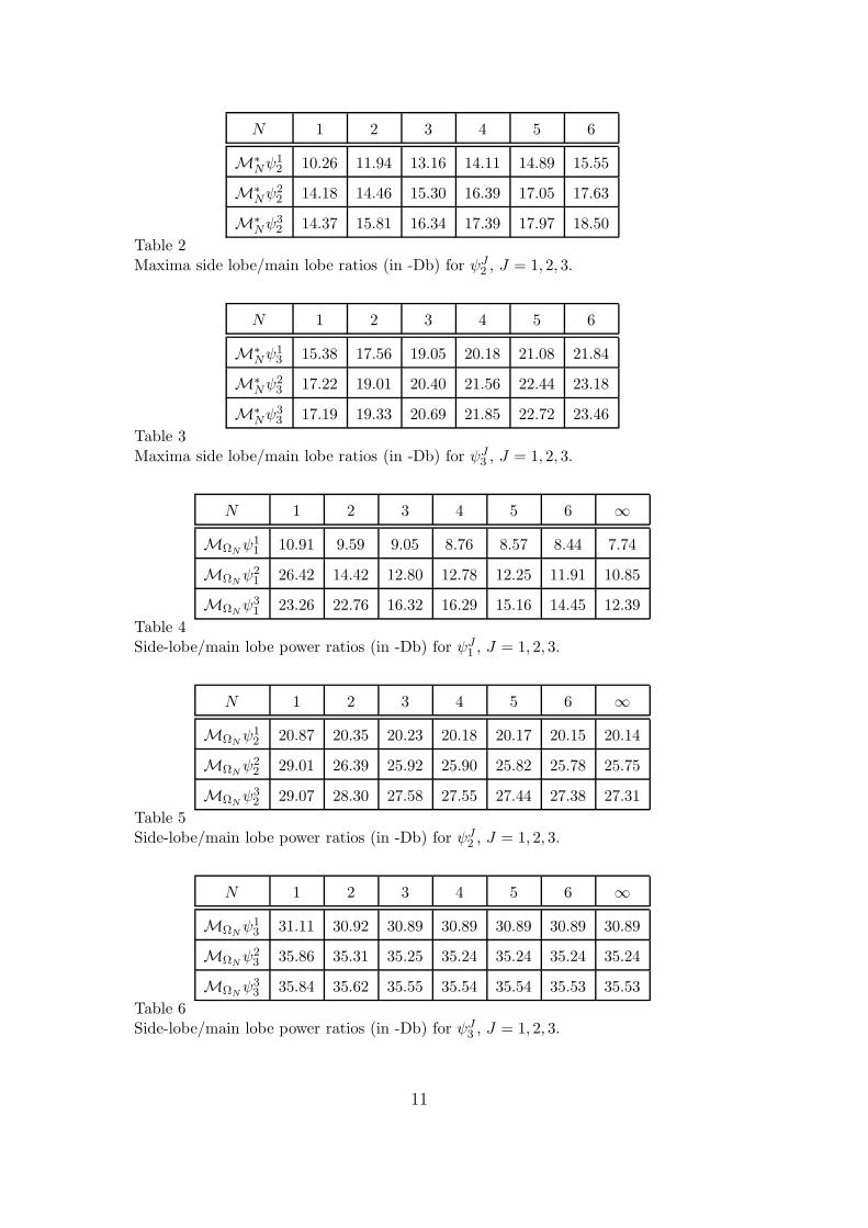
The enhanced filter characteristic of the modified B-wavelet bases is now il-lustrated by calculating the measures from Definitions 2.4 and 2.5.

The filter characteristic of the original B-wavelets have zeros at ξ = 4nπ, forn ∈ Z. By virtue of Theorem 3.2, the modified basis ψJM has extra zeros at2nπ, for 1 < n ≤ dJ .

We compare the filter characteristics |ψM∧(ξ)| and∣∣∣ψJM

∧(ξ)∣∣∣ by considering

their power and maxima over the intervals ΩN = (4π, 4(N+1)π). The measuresare calculated for the original and refined versions of the Haar, linear, andquadratic B-wavelets, and are presented in Tables 1 – 6. For completeness,

N 1 2 3 4 5 6

M∗Nψ

11 5.28 6.26 7.00 7.59 8.09 8.52

M∗Nψ

21 12.32 9.03 8.94 10.00 10.13 10.32

M∗Nψ

31 10.38 12.10 10.63 11.63 11.40 11.36

Table 1Maxima side lobe/main lobe ratios (in -Db) for ψJ1 , J = 1, 2, 3.

10

N 1 2 3 4 5 6

M∗Nψ

12 10.26 11.94 13.16 14.11 14.89 15.55

M∗Nψ

22 14.18 14.46 15.30 16.39 17.05 17.63

M∗Nψ

32 14.37 15.81 16.34 17.39 17.97 18.50

Table 2Maxima side lobe/main lobe ratios (in -Db) for ψJ2 , J = 1, 2, 3.

N 1 2 3 4 5 6

M∗Nψ

13 15.38 17.56 19.05 20.18 21.08 21.84

M∗Nψ

23 17.22 19.01 20.40 21.56 22.44 23.18

M∗Nψ

33 17.19 19.33 20.69 21.85 22.72 23.46

Table 3Maxima side lobe/main lobe ratios (in -Db) for ψJ3 , J = 1, 2, 3.

N 1 2 3 4 5 6 ∞

MΩNψ11 10.91 9.59 9.05 8.76 8.57 8.44 7.74

MΩNψ21 26.42 14.42 12.80 12.78 12.25 11.91 10.85

MΩNψ31 23.26 22.76 16.32 16.29 15.16 14.45 12.39

Table 4Side-lobe/main lobe power ratios (in -Db) for ψJ1 , J = 1, 2, 3.

N 1 2 3 4 5 6 ∞

MΩNψ12 20.87 20.35 20.23 20.18 20.17 20.15 20.14

MΩNψ22 29.01 26.39 25.92 25.90 25.82 25.78 25.75

MΩNψ32 29.07 28.30 27.58 27.55 27.44 27.38 27.31

Table 5Side-lobe/main lobe power ratios (in -Db) for ψJ2 , J = 1, 2, 3.

N 1 2 3 4 5 6 ∞

MΩNψ13 31.11 30.92 30.89 30.89 30.89 30.89 30.89

MΩNψ23 35.86 35.31 35.25 35.24 35.24 35.24 35.24

MΩNψ33 35.84 35.62 35.55 35.54 35.54 35.53 35.53

Table 6Side-lobe/main lobe power ratios (in -Db) for ψJ3 , J = 1, 2, 3.

11

the measures M over R+∗ are also given.

The tables offer clear evidence that the refinement technique significantly im-proves the filter characteristic of the B-wavelets about an arbitrarily largelocalised band-region. In fact, an improvement can be seen over the entirefrequency domain.

For the Haar and quadratic wavelet, it can be seen that ψ3 has slightly poorerperformance than ψ2 over the interval Ω1. Generally, however, the filter char-acteristics of ψJ will improve with larger J .

4 Fast integral wavelet transforms

The integral transform, given by Equation (1) can be written as the convolu-tions (Wψf)(α, τ) = (f ∗Ψα)(τ). In practice the transform is calculated over adiscrete set of α, and τ . For N data points, a verbatim calculation of (1) incursO(N2) computational complexity per scale. Alternatively, via the fast Fouriertransform, (Wψf)(α, τ) = (f∧Ψ∧

α)∨(τ) requires O(N logN) complexity per

scale.

Of course, wavelets obtained from a multiresolution analysis can be calculatedover the dyadic lattice (αj , τk) = (2j , 2jk), for j, k ∈ Z with an overall com-plexity of O(N), via Mallat’s fast wavelet transform algorithm [10]. Likewise,zero-padding the input samples and using the algorithme a trous [9] returnsthe wavelet coefficients over the semi-dyadic lattice (2j, k) with O(N) com-plexity per scale.

Restricting the choice of wavelet to those generated by B-splines, Unser et al.[14] proposed an algorithm for the integer lattice (αj , τk) = (j, k) with O(N)complexity per scale. This result was extended recently by Munoz et al. [11]for arbitrary scales, again with O(N) complexity per scale.

A brief discussion of these fast integral wavelet transforms, as derived in [14]for integer scales, and [11] for arbitrary scales, will be given below. This isfollowed by the application of the fast transform to our modified wavelet,defined by (2). Both Unser et al. and Munoz et al. used splines centred aboutthe origin. However, their theory is easily adapted to the so called non-causalsplines that are defined over the positive half of the real line.

12

4.1 Integer scale B-wavelets

The fast algorithm of Unser et al. [14] is facilitated by the following self simi-larity property of the B-splines.

Proposition 4.1 (Unser et al.) For α ∈ Z, there exists a sequence ηαM(k)kin ℓ2(Z), such that

φM(α−1·) =∑

k∈Z

ηαM(k)φM(· − k).

Proof Clearly φ1(α−1·) = ∑α−1

k=0 φ1(· − k) =: ηα1 ∗ φ1 with ηα1 (k) = 1, for all0 ≤ k < α. Define ηαM := α−1ηα1 ∗ ηαM−1. An (M − 1)-fold convolution of bothsides completes the proof.

It follows from Proposition 4.1 and the two-scale relation (5) that

ψM(α−1·) =∑

k,ℓ∈Z

gM(ℓ)ηαM(k)φM(2 · −k − αℓ),

that is

ψM(α−1·) =∑

k∈Z

(g↑αM ∗ ηαM

)(k)φM(2 · −k),

where the symbol ↑ indicates the up-sampling operator:

g↑m(n) =

g(n/m), m | n0, otherwise

, m, n ∈ Z.

Hence, the integral wavelet transform of f , evaluated over the integer lattice(α, τ) with α, τ ∈ Z, can be written as

(WψMf)(α, τ) = (f ∗Ψα;M)(τ) =

(g↑αM ∗ ηαM ∗ 〈f, φM(2 · −k)〉L2

)(τ).

Unser et al. [15] propose the following algorithm:

• Perform the initialisation f 1M(k) = 〈f, φM(2 · −k)〉L2

.

• For each α ∈ N, calculate fαM = ηαM ∗f 1M = α−Mf 1

M

M∗j=1

ηα1 where each moving

average operation (ηα1 ∗ ·) is implemented recursively via:

fαM(k) = fαM(k − 1) +fα−1M (k + α)− fα−1

M (k)

α.

• (WψMf)(α, τ) =

(g↑αM ∗ fαM

)(τ).

13

In such a manner, each point fα(k) can be calculated with 2M additions.Since the sequence gM is symmetric or anti-symmetric and has length 3M−1,the final convolution will require ⌈(3M − 1)/2⌉ multiplications and 3M − 2additions per value of τ .

4.2 Arbitrary scale B-wavelets

The algorithm of Munoz et al. [11] admits arbitrary scales. They define ∆M

as the M-th fold finite difference operator:

∆M :=M∑

k=0

(M

k

)(−1)kδ(· − k),

where δ is Dirac’s delta. Accordingly, ∆−M denotes the inverse of ∆M and isequivalent to the Mth iteration of ∆−1 =

∑n≥0 δ(x− n). The values

wαM =∑

k

(gM(ℓ) ∗

(M

ℓ

)(−1)ℓ

)(k)δ(· − αk) ∗ φM(2·)

are calculated prior to run time and stored in a look table. Denoting φM asthe scaling function, biorthonormal to φM , the initialisation stage

cM(k) = ∆−M ∗ 〈f, φM(2 · −k)〉L2,

is followed by the calculation

(WψMf)(α, τ) = wαM ∗ cM ,

for each α in some subset of R. Although this algorithm is not quite as efficientas the first for integer scales, it still manages O(N) complexity per scale andis obviously more versatile.

4.3 Fast algorithms for the modified B-wavelet

The fast integral wavelet transform algorithms can be adapted for the modifiedB-wavelets. Since the modified wavelets comprise sums of integer dilated andshifted versions of the original wavelet, the adaptation is quite natural. Recallthat the modified B-wavelet is given as

ψJM =J∑

j=1

µ(dj)Γj

X(dj−1)∑

n=0

ψM(dj · −n).

14

With respect to the dilated B-splines, this is

ψJM =J∑

j=1

µ(dj)Γj∑

k∈Z

gM ;j(k)φM(2dj · −k), (8)

with

gM ;j(k) :=X(dj−1)∑

n=0

gM(k − 2n).

For integer scales α ∈ Z, we note that

φM(djα−1·) =

∑

k∈Z

ηαM(k)φM(dj · −k)

is a corollary of Proposition 4.1. From the definition of the modified wavelet(2), it follows that

ψJM (α−1·) =J∑

j=1

µ(dj)Γj∑

k∈Z

(g↑αM ;j ∗ ηαM

)(k)φM(2dj · −k),

and similar to the original scheme, the algorithm is initialised with

f 1M ;j(k) = 〈f, φM(2dj · −k)〉L2

,

for j = 1, . . . , J . Next, fαM ;j = ηαM ∗ f 1M ;j is calculated recursively. Finally, for

α, τ ∈ Z

(WψMf)(α, τ) =

J∑

j=1

µ(dj)Γj(g↑αM ;j ∗ fαM ;j

)(τ).

Although clearly slower than the unmodified B-wavelet case, the algorithmstill retains O(N) complexity per scale. Similarly, for arbitrary scales α ∈ R

we put

wαM ;j :=∑

j=1

µ(dj)Γj∑

k

(gM ;j(ℓ) ∗

(M

ℓ

)(−1)ℓ

)(k)δ(· − αk) ∗ φM(2dj·)

and calculate the initialisation stage

cM(k) = ∆−M ∗ 〈f, φM(2 · −k)〉L2,

followed by

(WψMf)(α, τ) = wαM ∗ cM .

Again, this is slower than the original algorithm but shares the O(N) com-plexity per scale property.

15

5 Multi-scaling functions and the modified wavelets

The construction of a multiresolution analysis (MRA) not only facilitateswavelet design but also raises the opportunity to perform fast discrete wavelettransforms via pyramidal algorithms [10]. Early multiresolution analyses weregenerated by dyadic dilations and translations of a single scaling functionφ ∈ L2(R). A natural extension of this theory to the case of multi-scalingfunctions φ = (φ0, . . . , φR−1)T , with φr ∈ L2(R), for r = 0, . . . , R − 1, waspioneered by Alpert [1], Geronimo et al. [6], and Goodman et al. [7], [8]. Ac-cordingly, R-many scaling functions and R-many wavelet functions are usedto construct a basis for L2.

Multi-wavelets hold certain advantages over single, so called scalar, wavelets.Daubechies [4] proved that an orthogonal, finitely supported, symmetric, scalarwavelet could not have an approximation order greater than one. However,Geronimo et al. [6] managed to circumvent this restriction by considering amultiwavelet design.

Like the scalar case, the multi-scaling functions give rise to a fast, pyramidalwavelet transform algorithm. This motivates us to place the modified waveletsinto the setting of a MRA, generated by a multi-scaling functions. To this end,the following notation will be useful:

ℓR2 (Z) =c = (c0, . . . , cR−1)

T : cj ∈ ℓ2(Z), 0 ≤ j < R

ℓR×R2 (Z) =C = (Cj,k)

R−1j,k=0 : Cj,k ∈ ℓ2(Z), 0 ≤ j, k < R

LR2 (R)=f = (f0, . . . , fR−1)

T : fj ∈ L2(R), 0 ≤ j < R.

That is, ℓR2 (Z) comprises R dimensional vectors of square summable sequences,whereas ℓR×R2 (Z) comprises R-by-R matrices of square summable sequences,and LR2 (R) comprises R dimensional vectors of square integrable functions.

Definition 5.1 Let φ := (φ0, . . . , φR−1)T ∈ LR2 (R). For j ∈ Z, define

Vj(φ) := clos span2j/2φr(2j · −k) : 0 ≤ r < R, k ∈ Z.

Then φ is a multiscaling function that generates the MRA Vj(φ) of multi-plicity R if all of the following properties are satisfied.

(1) Vj(φ) ⊂ Vj+1(φ), ∀j ∈ Z.(2) f ∈ Vj(φ) ⇔ f(2·) ∈ Vj+1(φ), ∀j ∈ Z.(3) clos

⋃j∈Z Vj(φ) = L2(R).

(4)⋂j∈Z Vj(φ) = 0.

(5) The set φr(· − k) : 0 ≤ r < R, k ∈ Z forms a Riesz basis for V0(φ).

16

Commonly, the multi-scaling function is used to define a multiwavelet. Here,however, we take a different approach. We construct a scalar wavelet from themulti-scaling function. This allows the modified wavelet to be described in thecontext of a MRA, with multiplicity R.

Definition 5.2 The function ψ ∈ L2(R) is said to be generated by a MRAVj(φ) of multiplicity R, with φ = (φ0, . . . , φR−1)T ∈ LR2 (R) if there existssome (g0(k), . . . , gR−1(k))Tk∈Z ∈ ℓR2 (Z), such that

ψ =∑

0≤r<Rk∈Z

gr(k)φr(2 · −k). (9)

Using vector notation, define g(k) := (g0(k), . . . , gR−1(k))T . Then (9) can bewritten as a natural extension of the two scale relation for scalar functions(5):

ψ =∑

k∈Z

g(k)Tφ(2 · −k).

5.1 Modified B-wavelet construction

Recall the Mth order B-spline function φM and the Mth order modifiedwavelet ψJM . Define the multi-scaling function φJM := (φJ,0M , . . . , φJ,d−1

M )T , with

φJ,rM := φM(d · −r), where dj+1 = minn∈2N−1

n > dj and maxnα|d α = 1

for

j = 2, . . . , J, and d1 := 1, and d :=∏Jj=1 dj .

Furthermore, recall that φM is the scaling function, biorthonormal to φM .That is 〈φM(· −m), φM(· − n)〉 = δm,n. Some results are now established forthe modified B-wavelets in the setting of a MRA of multiplicity d. This willexpedite the pyramidal algorithm, discussed below in Section 5.3.

Theorem 5.3 There exists a d-by-d matrix of sequences HJM ∈ ℓd×d2 (Z) such

that φJM =∑k∈Z H

JM(k)φJM(2 · −k).

Proof For the B-splines there exists hM(k)k∈Z ∈ ℓ2(Z) such that

φM =∑

k∈Z

hM(k)φM(2 · −k).

That is

17

φJ,rM =∑

k∈Z

hM(k)φM(2d · −2r − k)

=∑

k∈Z

d−1∑

s=0

hM(s− 2r + kd)φJ,sM (2 · −k).

Define the sth column and rth row of HJM(k) as hM(s − 2r + kd), such that

hM(k) = 0 for k < 0 and k > M .

Example 5.4 Choose J = 2, and M = 1. For then, φ21 = (φ2,1

1 )2j=0 with

φ2,j1 := φ1(3 · −j) and

H21(0) =

1 1 0

0 0 1

0 0 0

, H2

1(1) =

0 0 0

1 0 0

0 1 1

.

Theorem 5.5 There exists a vector of functions φJ

M := ((φJ,rM (·−n))d−1r=0)

T in

Ld2(R), with V0(φJ

M) ⊃ V0(φM) such that, for f ∈ V0(φM) we have

f =∑

k∈Z

(φJ

M(· − k))T (PJMf)(k),

where the mapping PJM : V0

(φM

)7→ ℓd2(Z) is defined by

(PJMf

)(k)

k∈Z:=(⟨

f, φJ,0M (· − k)⟩, . . . ,

⟨f, φJ,d−1

M (· − k)⟩)T

k∈Z.

Proof Firstly, we prove that PJM is a bounded and boundedly invertible linear

operator. From Proposition 4.1 it follows that there exists ηdM ∈ ℓ2(Z) suchthat

φM =∑

k∈Z

ηdM(k)φM(d · −k)

=∑

k∈Z

d−1∑

r=0

ηdM(r + kd)φJ,rM (· − k).

Therefore, f =∑n∈Z〈f, φM(· − n)〉φM(· − n) ∈ V0(φM) can be expressed as

f =∑

n,k∈Z

φM(· − n)(ηdM(d(k − n)), . . . , ηdM(d(k − n+ 1)− 1)

)(PJ

Mf)(k).

Now, clearly φJ,rM =∑n∈Z η

dM(r − nd)φM(· − n) ∈ V0(φM).

18

Theorem 5.6 There exists a sequence gJM ∈ ℓd2(Z) such that the two scalerelation ψJM =

∑k∈Z g

JM(k)TφJM(2 · −k) holds.

Proof From (8) we have:

ψJM =J∑

j=1

∑

k∈Z

µ(dj)ΓjgM ;j(k)φM(2dj · −k).

Proposition 4.1 implies φM(dj·) =∑M(d∗

j−1)

k=0 ηd∗j

M (n)φM(d ·−k), with d∗j := d/dj.Hence

ψJM =J∑

j=1

∑

k∈Z

M(d∗j−1)∑

n=0

µ(dj)ΓjgM ;j(k)ηd∗j

M (n)φM(2d · −n− kdj).

Put r+ qd := n+ kd∗j , with 0 ≤ r < d. That is q = qj(n, k) := ⌊d−1(n+ kd∗j)⌋,and r = rj(n, k) := n + kdj − qd. We now have

ψJM =J∑

j=1

∑

k∈Z

M(d∗j−1)∑

n=0

µ(dj)ΓjgM ;j(k)ηd∗j

M (n)φJ,rj(n,k)M (2 · −qj(n, k)),

which is of the form ψJM =∑q,r g

J,rM (q)φJ,rM (2 · −q).

Example 5.7 Choosing J = 2 and M = 1, yields g21(0) = (1, 2, 1)T , and

g21(1) = −(1, 2, 1)T .

5.2 Multi-wavelet algorithms

Mallat’s scalar wavelet pyramidal algorithm was extended to the multiwaveletcase by Xia et al [16]. A brief synopsis of the algorithm is given before weadapt the idea to the modified B-wavelet.

Consider the multi-scaling functions φj,n := (2j/2φr(2j · −n))R−1r=0 , the

multiwavelet functions ψj,n := (2j/2ψr(2j · −n))R−1r=0 , and their two scale

equations given by

φj−1,n=∑

k∈Z

H(k − 2n)φj,k

ψj−1,n=∑

k∈Z

G(k − 2n)φj,k,

where H,G ∈ ℓR×R2 (Z) . Let λj,nn∈Z, γj,nn∈Z ∈ ℓR2 (Z). A function f in

19

V0(φ), can be expressed as

f =∑

k∈Z

λT0,kφ0,k,

where the rth element of λ0,k is found by calculating 〈f, φr(2 ·−k)〉L2. Accord-

ingly, the coefficients λj,nj<0 of f at the larger scales can be calculated byrecursively applying

λj−1,n =∑

k∈Z

H(k − 2n)λj,k.

Similarly, the associated wavelet decomposition coefficients γj,nj<0 of f canbe calculated recursively via

γj−1,n =∑

k∈Z

G(k − 2n)λj,k.

5.3 Multi-B-wavelet recursive algorithm

Let H ∈ ℓR×R2 (Z), λj,nn∈Z, g ∈ ℓR2 (Z), and γj,nn∈Z ∈ ℓ2(Z). We define

φJM ;j,n := ((2j/2φJ,rM (2j · −n))R−1r=0 )

T , and φJ

M ;j,n := ((2j/2φJ,rM (2j · −n))R−1r=0 )

T .

For f ∈ V0(φM), Theorems 5.3 and 5.5 imply that we can write

f =∑

k∈Z

λT0,kφJ

M ;0,k,

with

λ0,k =(〈f, φJ,0M (2 · −k)〉, . . . , 〈f, φJ,d−1

M (2 · −k)〉)T, (10)

such that the two scale relation

λj−1,n =∑

k∈Z

HJM(k − 2n)

Tλj,k (11)

is satisfied. From Theorem 5.6 it follows that

γj−1,n =∑

k∈Z

gJM(k − 2n)Tλj,k. (12)

Herewith the possibility arises to implement a fast discrete multiwavelet trans-form for our modified wavelets. The coefficients are initialised by (10). Theλj,n are computed recursively with (11). Consequently, the wavelet coefficientsare found via (12).

20

References

[1] B. K. Alpert. Wavelets and other bases for fast numerical linear algebra. In:Wavelets- A Tutorial in Theory and Applications, pages 181–216. C. K. Chui,editor, Academic Press, 1992.

[2] C.K. Chui. Wavelets: a mathematical tool for signal analysis. SIAM, Texas,1997.

[3] C.K. Chui and J.Z. Wang. On compactly supported spline-wavelets and aduality principle. Trans. Amer. Math. Soc., 330:903–915, 1992.

[4] I. Daubechies. Orthonormal bases of compactly supported wavelets. Comm.

Pure and Appl. Math., 41:909–996, 1988.

[5] F. Dovis, M. Mondin, and F. Daneshgaran. The modified gaussian: A novelwavelet with low sidelobes with applications to digital communications. IEEE

Trans. on Communications Letters, 2(8):208–210, 1998.

[6] J. S. Geronimo, D. P. Hardin, and P. R. Massopust. Fractal functions andwavelet expansions based on several scaling functions. J. Approx. Theory,78:373–401, 1994.

[7] T. N. T. Goodman and S. L. Lee. Wavelets of multiplicity r. Trans. Amer.

Math. Soc., 342:307–324, 1994.

[8] T. N. T. Goodman, S. L. Lee, and W. S. Tang. Wavelets in wandering subspaces.Trans. Amer. Math. Soc., 338:639–654, 1993.

[9] M. Holschneider, R. Kronland-Martinet, J. Morlet, and P. Tchamitchian. Areal-time algorithm for signal analysis with the help of the wavelet transform.In: Wavelets, time-frequency methods and phase space, pages 286–297. Springer,Berlin, 1989.

[10] S.G. Mallat. A theory for multiresolution signal decomposition: the waveletrepresentation. IEEE Trans. Pattern Anal. Mach. Intell., 11:674–693, 1989.

[11] A. Munoz, M. Unser, and R. Ertle. Continuous wavelet transform with arbitraryscales and O(N) complexity. Signal Processing, 82:749–757, 2002.

[12] W. Sweldens. The lifting scheme: A custom-design construction of biorthogonalwavelets. Journal of Appl. and Comput. Harmonic Analysis, 3(2):186–200, 1996.

[13] W. Sweldens. The lifting scheme: A construction of second generation wavelets.SIAM Journal on Mathematical Analysis, 29(2):511–546, 1998.

[14] M. Unser, A. Aldroubi, and J. Schiff. Fast implementation of the continuouswavelet transform with integer scales. IEEE Trans. Signal Processing,42(12):3519–3523, 1994.

[15] M. Vrhel, Chulhee Lee, and M. Unser. Fast continuous wavelet transform.International Conference on Acoustics, Speech, and Signal Processing, 2:1165–1168, 1995.

21

[16] X. G. Xia, J. S. Geronimo, D.P. Hardin, and B. W. Suter. Design of prefiltersfor discrete multiwavelet transforms. IEEE Trans. Signal Processing, 44:25–35,1996.

22