a viscoelastic model for the long-term deflection of segmental prestressed box … ·...

A viscoelastic model for the long-term deflection of prestressed box girders

1

A viscoelastic model for the long-term deflection of

segmental prestressed box girders

Angela Beltempo, Oreste S. Bursi*, Carlo Capello, Daniele Zonta

Department of Civil, Environmental and Mechanical Engineering (University of Trento), Via Mesiano 77, 38123 Trento, Italy

&

Massimiliano Zingales

Department of Civil, Environmental, Aerospace, Materials Engineering (University of Palermo), Viale delle Scienze Ed.8,

90128 Palermo, Italy

Abstract: Most of segmental prestressed concrete box

girders exhibit excessive multidecade deflections

unforeseeable by past and current design codes. In order

to investigate such a behavior, mainly caused by creep

and shrinkage phenomena, an effective FE formulation

is presented in this paper. This formulation is developed

by invoking the stationarity of an energetic principle for

linear viscoelastic problems and relies on the Bazant

creep constitutive law. A case study representative of

segmental prestressed concrete box girders susceptible

to creep is also analyzed in the paper, i.e. the Colle

Isarco viaduct. Its FE model, based on the

aforementioned energetic formulation, was successfully

validated through the comparison with monitoring field

data. As a result, the proposed 1D FE model can

effectively reproduce the past behavior of the viaduct

and predict its future behavior with a reasonable run

time, which represents a decisive factor for the model

implementation in a decision support system.

Nomenclature

𝐴 cross section area

C costs

𝐶0(𝑡, 𝑡′) compliance function for basic creep

𝐶𝑑(𝑡, 𝑡′, 𝑡0) compliance function for drying

𝑫 derivative operator

𝐸28 Young’s modulus at 28 days

𝐹(𝑢, 𝑣) extension of the total potential energy

𝑯 operator of the assembled structure

𝐼 momentum of inertia

𝐽𝐵3(𝑡, 𝑡′) compliance function of Model B3

𝑲 elastic stiffness operator

𝑳 extended stiffness operator

𝐿 beam length

𝑴(𝑡) operator of time shape functions

𝑵(𝑥) operator of spatial shape functions

𝑅(𝑥, 𝑡′, 𝑡′) generic relaxation function evaluated at

𝑡′

𝑅𝐵3(𝑡, 𝑡′) relaxation function of Model B3

aopt economically optimal choice

𝑎 𝑐⁄ aggregate-cement ratio

𝒇 vector of nodal forces

𝑓�̅� cylinder compression strength

𝒈 extended vector of equivalent nodal

forces

i index to indicate the generic iteration

step

n index to indicate the current time step

𝑝(𝑥, 𝑡) longitudinal distributed load

p(θ) prior probability of parameter

p(S) prior probability of possible structural

conditions

�̂�(𝑥, 𝑡) fictitious longitudinal distributed load

𝑞(𝑥, 𝑡) transversal distributed load

�̂�(𝑥, 𝑡) fictitious transversal distributed load

𝑞1 first parameter of Model B3

𝑞2 second parameter of Model B3

𝑞3 third parameter of Model B3

𝑞4 forth parameter of Model B3

𝑞5 fifth parameter of Model B3

𝒓(𝑡) vector of nodal DoFs

𝒓𝒖 vector of extensional DoFs

𝒓𝒗 vector of bending DoFs

𝑡 generic time

𝑡0 time when drying starts

𝑡′ loading time

𝑢(𝑥, 𝑡) longitudinal displacement

Beltempo et al. 2

�̂�(𝑥, 𝑡) fictitious longitudinal displacement of

the auxiliary elastic problem

𝑣(𝑥, 𝑡) transversal displacement

�̂�(𝑥, 𝑡) fictitious transversal displacement of the

auxiliary elastic problem

𝑤 𝑐⁄ water-cement ratio

𝑥 beam longitudinal axis

y SHM measurements

∆𝑇 temperature variation

𝛼 thermal expansion coefficient

𝜶(𝑡) vector of spatial displacement unknowns

�̂�(𝑡) vector of fictitious displacement

unknowns

𝜷 vector of time displacement unknowns

𝜀(𝑡) total strain evaluated at time t

𝜀𝑐𝑟 creep strain

𝜀𝑠ℎ(𝑡) shrinkage strain evaluated at time t

𝜀𝑠ℎ∞ shrinkage strain at infinity

𝝐 tolerance vector

𝜎 constant stress

θ vector of generic parameters

1 INTRODUCTION

1.1 Background and motivation

“Clarification of the causes of major disasters and

serviceability losses has been, and will always be, a prime

opportunity for progress in structural engineering”

(Bazant et al., 2012). This need always arises behind

important upgrades in design codes and is followed by

many researchers for a better understanding of complex

phenomena.

According to that need, this study will cover a specific

class of bridges, i.e. prestressed concrete box girders,

which reveal excessive multidecade deflections

unforeseeable by past and current design codes. For

instance, let us examine the Koror-Babelthuap Bridge in

Palau, depicted in Figure 1(a)-(b), which collapsed in

1996 mainly due to an excessive creep deflection

recorded at midspan; or other four segmental prestressed

box girders in Japan, which exhibited a similar behavior

(Koshirazu, Tsukiyono, Konaru, and Urado) (Bazant et

al., 2012). An example in Europe, proving once more that

the multidecade deflections are not unique occurrences

for the Koror-Babelthuap Bridge, is represented by the

Colle Isarco viaduct, shown in Figure 1(c)-(d), which still

constitutes a strategic link in the highway corridor

connecting Northern Italy with Germany.

Specifically, the excessive multidecade deflections of

the aforementioned box girders and many others bridges

spread throughout the world may be due to the

combination of several factors (Beltempo et al., 2015)

listed herein: i) the cast-in-place segmental method used

for construction; ii) creep deformation; iii) losses of pre-

tensioning force in tendons; and iv) differential shrinkage

between top and bottom slabs. However, with regard to

the Colle Isarco viaduct, i.e. the case study of this paper,

any attempt to investigate the midspan deflection drift

using the classical CEB-FIP creep and shrinkage models

(CEB, 2008) -those currently recognized by Eurocode 2

(CEN, 2004)- failed to provide a convincing

explanation/prediction. In fact, according to the CEB-FIP

model, creep effects become negligible 20 years after

concrete casting, whilst the Colle Isarco viaduct

experiences a deflection still growing 40 years after its

construction. Thus, the hyperbolic law exploited in

Eurocode 2 creep models clearly exhibits limitations to its

applicability. Bazant et al. (2012), focusing on Koror-

Babelthuap Bridge, also demonstrated that classical CEB-

FIP shrinkage and creep models are clearly not suited for

reproducing the long-term deflection of large-span

segmentally-erected box girders and recommended the

use of creep Model B3 (Bazant & Baweja, 1995), which

has been recently improved in Model B4 (Wendner et al.,

2015). Unlike CEB-FIP models, both Model B3 and

Model B4 consider a creep component whose effect

persists even many decades after concrete casting.

Moreover, they properly take into account difference in

shrinkage between top and bottom slabs of the box girder,

a phenomenon that could strongly influence the deflection

trend. Model B4 includes two major improvements with

respect to Model B3: the first is the inclusion of

temperature effects in the creep function; the second

concerns the separation of the drying and the autogenous

components of shrinkage, particularly important for high

strength concrete.

An innovative approach to investigate excessive

deflections in massive concrete structures could be the

introduction of fractional (real-order) operators into the

creep constitutive law (Di Paola & Zingales, 2012, Di

Paola et al., 2013). Specifically, the use of fractional

operators could bring significant computational savings to

model calibration due to the reduced number of

parameters -about three- involved into the formulation.

However, both Di Paola & Zingales (2012) and Di Paola

et al. (2013) applied fractional operators to hereditary

materials, e.g. polymers, and not to ageing materials like

concrete. Therefore, in this research work we focus on

Model B3 mainly because its creep and relaxation

functions (Bazant & Baweja,1995, Bazant et al.,2013),

can be fitted by fractional operators. Moreover, a reliable

relaxation function is not yet available for Model B4 and,

therefore, Model B3 is preferred.


3

Significant aspects relative to monitoring and

modelling of segmental box girders should worthy of

investigation. In fact, in most cases, the inexplicable

behavior of this specific class of structures led to the

installation of efficient structural health monitoring

(SHM) systems and to the development of FE models.

This is the case of the Colle Isarco viaduct, for which both

field data -revealed to assess the effectiveness of the last

maintenance work undertaken in 2014- and FE model

predictions were used to provide information on future

structural performance and to support decisions

concerning the viaduct management. The SHM system

installed on the Colle Isarco viaduct includes: i) fiber-

optic sensors based on fiber Bragg gratings (Balageas et

al., 2010; Glisic & Inaudi 2007) to measure strains of top

and bottom slabs; ii) PT100 resistance thermometers to

acquire temperature variations along the whole structure;

and iii) a topographic network with prisms to measure

displacements. This fusion of data coming from different

sensors certainly reduces uncertainties regarding

structural behavior (Han et al., 2017), helps the bridge

manager to identify causes of possible anomalies and

improves his or her capability to take optimal decisions

(Cappello et al., 2016).

As further support for computational frameworks for

Bayesian inference and bridge maintenance decisions, a

1D FE model of the Colle Isarco viaduct, which is

presented in this paper, was also developed. Along the

same lines, Caracoglia et al. (2009) developed a time-

domain FE model to better interpret the behavior of long-

span modern bridges under vortex shedding-induced

loads. Torbol et al. (2013) used a FE analysis to evaluate

bridge fragility throughout its service life. Shapiro (2007)

built a FE model of the Interstate Highway 565 Bridge in

Huntsville (Alabama), to investigate the main causes of

cracking phenomena observed just after the construction

of the bridge. The main difference between the

aforementioned models and the model of the Colle Isarco

viaduct is that they are all available in commercial

software, mainly ANSYS or OpenSEES (Mazzoni, 2006);

conversely, the Colle Isarco’s model is implemented in

MATLAB and relies on an energetic formulation for

linear viscoelastic problems (Carini et al., 1995). Another

important aspect is its reduced run time, which is

determinant for both stochastic computations and model

implementation in a Decision Support System (DSS). In

sum, to the authors’ knowledge, there is a paucity of

papers dealing with modelling of creep and shrinkage

phenomena for simple yet effective FE simulations of

complex segmental prestressed concrete box girders; box

girders that, in addition, are subjected to complex loading

histories. These are the important issues that the paper

explores further.

1.2 Scope

This paper presents the main issues regarding the

modelling of creep and shrinkage phenomena for a

specific class of bridges, i.e. segmental prestressed

concrete box girders subjected to complex loading

histories. It also shows how a reliable SHM system

coupled to an effective FE model can be used to

investigate the past behavior and predict the short- and

long-term deflection of such complex structures,

considering, as representative case study, the Colle

Isarco viaduct.

According to this aim, we organize the paper as

follows. Firstly, Section 2 describes an energetic

formulation and a creep constitutive law suitable for the

problem under investigation. Section 3 introduces a

segmental prestressed concrete box girder, i.e. the Colle

Isarco viaduct, focusing on the main structural

characteristics and the SHM system installed on the

viaduct in 2014. Section 4 provides details about the

implementation of the viaduct geometry and the whole

load history into the FE formulation, together with model

results. Moreover, an overview of the conceived DSS as

further development of this research work can be found

in Section 5. Finally, we present conclusions and future

developments in Section 6.

2 A FE FORMULATION FOR PRESTRESSED

CONCRETE BOX GIRDERS

In this section, we propose an effective way to model

segmental prestressed concrete box girder deflection

and, generally, all structures highly sensitive to creep,

without resorting to commercial software analyses.

Hence, we present a 1D FE formulation by invoking the

stationarity of a functional for linear viscoelastic

problems, which relies on the creep constitutive law of

Bazant (Bazant & Baweja, 1995).

Hereinafter, we recall the Bazant’s creep law, known

in the literature as Model B3 (Bazant & Baweja, 1995);

and present, in greater detail, an energetic formulation

for concrete (aging) materials derived from a previous

formulation proposed by Carini et al. (1995).

2.1 A constitutive creep model: Model B3

In its most general form, Model B3 (Bazant & Baweja,

1995) assumes that, for a constant stress σ applied at

age 𝑡′, the resulting strain 𝜀(𝑡) at time t can be expressed

as

𝜀(𝑡) = 𝐽𝐵3(𝑡, 𝑡′) ∙ 𝜎 + 𝜀𝑠ℎ(𝑡) + 𝛼 ∙ ∆𝑇(𝑡) (1)

Beltempo et al. 4

in which 𝐽𝐵3(𝑡, 𝑡′) defines the compliance function, i.e.

strain at time 𝑡 caused by a unit uniaxial constant stress

at 𝑡′, 𝜀𝑠ℎ is the shrinkage strain, ∆𝑇 defines the

temperature variation, and 𝛼 the thermal expansion

coefficient. Furthermore, we can conceive the

compliance function as the sum of three components,

𝐽𝐵3(𝑡, 𝑡′) = 𝑞1 + 𝐶0(𝑡, 𝑡′) + 𝐶𝑑(𝑡, 𝑡′, 𝑡0) (2)

where 𝑞1 defines the instantaneous strain due to a unit

stress, 𝐶0 is the compliance function for basic creep,

meaning the creep at constant moisture content and no

moisture movement through the material, and 𝐶𝑑 defines

the compliance function for drying starting at time 𝑡0.

The basic creep compliance can be further broken

down into

𝐶0(𝑡, 𝑡′) = 𝑞2𝑄(𝑡, 𝑡′) + 𝑞3 𝑙𝑛[1 + (𝑡 − 𝑡′)𝑛] +

𝑞4𝑙𝑛 (𝑡

𝑡′) (3)

where function 𝑄 is discussed in more detail in Bazant &

Baweja (1995). The terms in (3) containing 𝑞2, 𝑞3, 𝑞4

represent the aging viscoelastic compliance, non-aging

viscoelastic compliance and flow compliance,

respectively, as deduced from the solidification theory.

The drying compliance 𝐶𝑑 reads

𝐶𝑑(𝑡, 𝑡′, 𝑡0) = 𝑞5[𝑒−8𝐻(𝑡) − 𝑒−8𝐻(𝑡0′ )]

1 2⁄ (4)

where H is the hydraulic radius of the section, i.e. the

volume-to-surface ratio and 𝑡0′ = max (𝑡′, 𝑡0). Evidently,

a) b)

c) d)

Figure 1. (a) The Koror-Babelthuap Bridge in Palau; (b) the Koror-Babelthuap Bridge failure;

(c) the central span of the Colle Isarco viaduct in Italy; (d) northern lateral spans of the Colle Isarco viaduct


5

Equation (4) is valid for t > 𝑡0′ , otherwise it is equal to

zero. The five parameters of Model B3 can be either

treated as statistical variables or estimated through the

following formulas, valid only for certain ranges of

material mechanical properties (Bazant & Baweja,

1995), i.e.

𝑞1 = 0,6 ∙ 106 𝐸28 𝐸28 = 4734√𝑓�̅� (5)

𝑞2 = 185.4 𝑐0.5 𝑓�̅�−0.9

(6)

𝑞3 = 0.29 (𝑤 𝑐)⁄ 4𝑞2 (7)

𝑞4 = 20.3 (𝑎 𝑐)⁄ −0.7 (8)

𝑞5 = 7.57 ∙ 105𝑓�̅�−1

|𝜀𝑠ℎ∞|−0.6 (9)

All the formulas above are given in SI (metric) units

(MPa, m). In addition, 𝐸28 is the Young’s modulus at 28

days, 𝑓�̅� defines the cylinder compression strength, 𝑤 𝑐⁄

is water-cement ratio, 𝑎 𝑐⁄ is aggregate-cement ratio, and

𝜀𝑠ℎ∞ is the shrinkage strain at infinity.

Once the compliance function and its five parameters

are known, it is also possible to estimate the

corresponding relaxation function 𝑅𝐵3 through the

following approximate formula (Bazant et al., 2013):

𝑅𝐵3(𝑡, 𝑡′) =1

𝐽𝐵3(𝑡,𝑡′)[1 +

𝑐1𝛼(𝑡,𝑡′)𝐽𝐵3(𝑡,𝑡′)

𝑞𝐽𝐵3(𝑡,𝑡−𝜂)]

−𝑞

(10)

where

𝑐1 = 0.0119 ln(𝑡′) + 0.08 𝑞 = 10 (11)

𝛼(𝑡, 𝑡′) =𝐽(𝑡′+𝜖,𝑡′)

𝐽(𝑡,𝑡−𝜖)− 1 (12)

𝜖 =𝑡−𝑡′

2 𝜂 = 1 (13)

Unlike the formula developed in 1979 by Bazant and

Kim (Bazant & Kim, 1979), Equation (10) prevents any

violation of the thermodynamic requirement of negatives

of 𝑅𝐵3(𝑡, 𝑡′). Therefore, (10) can be utilized to describe

the long-time relaxation phenomenon of concrete loaded

at a young age; for this reason, it is particularly useful for

compliance functions that correctly describe

multidecade creep, which is the case of the Model B3

compliance function.

In summary, Model B3 depends on five different

terms, controlled by parameters 𝑞1, 𝑞2, 𝑞3, 𝑞4, and 𝑞5.

The first three components roughly reproduce the same

effect as the classical CEB-FIP model (CEB, 2008) and

have no impact on the long-term behavior. In contrast,

the flow compliance term, including q4, is unique to

Model B3 and to the aforementioned Model B4

(Wendner et al., 2015); it depends on the logarithm of

time and, thus, keeps producing its effects in the long

term. Lastly, the term involving q5, which depends on the

effective thickness H, allows us to properly take into

account the differential drying rate of the two

(bottom/top) slabs of box girders.

2.2 FE viscoelastic formulation

In order to take into account creep effects, we start

from the classical total potential energy with an

additional integration over time. Moreover, we assume

the classical hypotheses of Bernoulli-Navier and first-

order beam theories, denoting with 𝑥 the coordinate of

the beam longitudinal axis, 𝑢(𝑥, 𝑡) the longitudinal

displacement, and 𝑣(𝑥, 𝑡) the transversal displacement of

the generic point of the beam. Hence, 𝑥 defines the local

axis of the beam and, in the case under investigation, it

matches the global axis.

The extension of the total potential energy functional

to viscoelasticity reads,

𝐹(𝑢, 𝑣) =1

2∫ ∫ 𝑅(𝑥, 𝑡′, 𝑡′) [𝐴 (

𝜕�̂�(𝑥,𝑡)

𝜕𝑥)

2

+𝐿

0

𝑡

𝑡′

𝐼 (𝜕2�̂�(𝑥,𝑡)

𝜕𝑥2 )2

] 𝑑𝑥 𝑑𝑡 − ∫ ∫ 𝑝(𝑥, 𝑡)�̂�(𝑥, 𝑡)𝐿

0

𝑡

𝑡′𝑑𝑥 𝑑𝑡 −

∫ ∫ 𝑞(𝑥, 𝑡)�̂�(𝑥, 𝑡)𝐿

0

𝑡

𝑡′𝑑𝑥 𝑑𝑡 (14)

where [𝑡′, 𝑡] is the time interval, 𝑅(𝑥, 𝑡′, 𝑡′) defines the

viscous relaxation kernel evaluated at 𝑡′, and 𝑝(𝑥, 𝑡) and

𝑞(𝑥, 𝑡) are the longitudinal and transversal components

of distributed load, respectively; whereas, �̂�(𝑥, 𝑡) and

�̂�(𝑥, 𝑡) define the solution of the auxiliary problem.

Figure 2. DoFs of a plane beam finite element

Now, among the admissible displacement fields, the

solution of the viscoelastic problem, in the given time

interval, is the field that makes the functional minimum.

The admissible displacement fields are intended as those

that satisfy both compatibility equations and the

Dirichelet boundary condition.

Due to the double dimension of the integral, we need

to introduce into (14) both space and time discretization.

For the spatial discretization, beam finite elements with

three DoFs per node are considered. Figure 2 depicts a

single beam finite element with its six DoFs. In addition,

Beltempo et al. 6

we take into account the classical linear shape functions

for the extensional DoFs 𝒓𝒖 = [u1 u2]T, and the classical

cubic shape functions for the bending DoFs 𝒓𝒗 = [v1 θ1

v2 θ2]T. The shape functions, referring to each node of the

mesh, are collected into the operator 𝑵(𝑥) and the

corresponding nodal DoFs into the vector 𝒓(𝑡). Thus, we

can express the displacement vector 𝒖 = [𝑢 𝑣]𝑻 as

follows:

𝒖 = [𝒏𝒖

𝑻 𝟎𝑻

𝟎𝑻 𝒏𝒗𝑻] [

𝒓𝒖

𝒓𝒗] = 𝑵(𝑥)𝒓(𝑡) (15)

𝒓(𝑡) = 𝑨𝜶(𝑡) (16)

where 𝑨 denotes the coordinate transformation operator

and 𝜶(𝑡) the vector of nodal DoFs. With regard to the

time discretization, the vector 𝜶(𝑡) reads

𝜶(𝑡) = 𝑴(𝑡)𝜷 (17)

It expresses the product of time shape functions,

collected into the operator 𝑴(𝑡), and time DoFs,

collected into the vector 𝜷. For each spatial DoF, we

consider two linear time shape functions, for a total of 12

DoFs per beam finite element. The first time shape

function is 0 at the beginning of the time step and 1 at the

end of the time step, whilst the second is 1 at the

beginning and 0 at the end.

The discretized form of (14) reads

𝐹(𝑢, 𝑣) =1

2∫ �̂�𝑻(𝑡) {∫ 𝑅(𝑥, 𝑡′, 𝑡′) [𝐴 (

𝑑𝒏𝒖(𝑥)

𝑑𝑥) (

𝑑𝒏𝒖(𝑥)

𝑑𝑥)

𝑇

+𝐿

0

𝑡

𝑡′

𝐼 (𝑑2𝒏𝒗(𝑥)

𝑑𝑥2 ) (𝑑2𝒏𝒗(𝑥)

𝑑𝑥2 )𝑇

] 𝑑𝑥} �̂�(𝑡) 𝑑𝑡 −

∫ �̂�𝑻(𝑡) {∫ 𝒏𝒖(𝑥)𝑝(𝑥, 𝑡)𝐿

0𝑑𝑥}

𝑡

𝑡′ �̂�(𝑡)𝑑𝑡 −

∫ �̂�𝑻(𝑡) {∫ 𝒏𝒗(𝑥)𝑞(𝑥, 𝑡)𝐿

0𝑑𝑥}

𝑡

𝑡′�̂�(𝑡) 𝑑𝑡 (18)

The vector �̂�(𝑡) of the ‘fictitious’ displacement

unknowns can be obtained by means of the

aforementioned auxiliary elastic problem with the

following longitudinal and transversal distributed loads:

�̂�(𝑥, 𝑡) = −𝜕

𝜕𝑥(𝑅(𝑥, 𝑡, 𝑡′)𝐴

𝜕𝑢(𝑥,𝑡)

𝜕𝑥) −

𝜕

𝜕𝑥∫ (𝑅(𝑥, 𝑡, 𝜏)𝐴

𝜕𝑑𝑢(𝑥,𝜏)

𝜕𝑥)

𝑡

𝑡′ (19)

�̂�(𝑥, 𝑡) =𝜕2

𝜕𝑥2 (𝑅(𝑥, 𝑡, 𝑡′)𝐼𝜕2𝑣(𝑥,𝑡)

𝜕𝑥2 ) +

𝜕2

𝜕𝑥2 ∫ (𝑅(𝑥, 𝑡, 𝜏)𝐼𝜕2𝑑𝑣(𝑥,𝜏)

𝜕𝑥2 )𝑡

𝑡′ (20)

named ‘fictitious’ loads by Carini et al. (1995). Invoking

the stationarity of the classical total potential energy

functional, we reach the following resolving system for

the auxiliary problem,

𝑲�̂�(𝑡) = 𝑯𝜷 (21)

with 𝑲 the well-known elastic stiffness operator of the

assembled structure and, 𝑯, an operator depending on

both the relaxation kernel and the time shape functions.

Hence, we can derive the vector �̂�(𝑡) from (21) and,

then, introducing its expression into (18), its minimum is

reached when 𝜷 corresponds to the solution of the

following linear system:

𝑳𝜷 = 𝒈 (22)

where 𝑳 is the extended stiffness operator and 𝒈 is the

extended vector of equivalent nodal forces.

In order to specialize the solution to the case of ageing

materials, it is necessary to consider a proper creep

model into the formulation. For instance, according to

the reasoning set out in Section 1 for box girders under

investigation, the relaxation function of Model B3 (10)

has to be replaced into (19) and (20). Moreover, the

subdivision of the whole time step into small

subintervals will further improve the proposed

formulation. As a result, a sequence of smaller problems

can be solved and, at every step, the calculation is

accomplished by starting from the results available from

previous steps. A pseudocode, summarizing the whole

FE viscoelastic formulation, is reported in the Appendix.

3 THE CASE STUDY OF THE COLLE ISARCO

VIADUCT

3.1 Bridge structural characteristics

The Colle Isarco viaduct is an example of segmental

prestressed concrete box girder that experienced

excessive multidecade deflections just after its

construction. It was designed by engineers Bruno and

Lino Gentilini and erected between 1968 and 1971

(Gentilini & Gentilini, 1972). Overall, the viaduct

comprises two structurally independent decks, the so-

called North and South carriageways, with 13 spans, for

a total length of 1028.2 m. The main span of the viaduct,

163 m long, consists of two symmetric reinforced

concrete Niagara box girders, which support a suspended

beam of 45 m, as depicted in Figure 3. Each box girder

ends with a 59m-long cantilever, counterbalanced by a

back arm with a length of 91 m. Moreover, each box

girder is composed of 33 box-girder cast-in-place

segments with a depth varying from 10.93 m, at the pier,


7

to 2.57 m, at the edge. The thickness of the top slab of

the box girder is constant at 0.29 m, whilst the bottom

slab varies from 0.99 m to 0.12 m. A concrete of nominal

class Rck = 450 kg/cm2 (C35/45 according to the current

CEN (2004)) was used for all cast-in-place elements of

piers and girders. The initial prestressing was applied

through 32 mm diameter Dywidag ST 85/105 threaded

bars, with 1030 MPa nominal tensile strength and an

initial jacking tension of 720 MPa. For each 59m-long

cantilever, the longitudinal force above the pier was

about 120 MN and was provided by a total of 266 cables.

As mentioned in Section 1, after only a few years from

the viaduct opening, monitoring field data started to

exhibit a deflection drift that cannot be explained using

classical creep models such as those found in most

design codes, e.g. CEN (2004). In this respect, Figure 4

depicts the deflection trend recorded at cross section A

of Figure 3(a). In stark contrast with the design

prediction (CEN, 2004) of 160 mm in 1988, the actual

deflection reached 230 mm with an apparent rate of 8

mm/year. A similar behavior was also observed for the

other three box girders. These first observations

prompted the owner to undertake, between 1988 and

1989, a radical intervention. Specifically, 10 cm of road

pavement was removed from the cantilever arms and the

suspended central beam, and replaced with a thinner

layer of lightweight asphalt. The effect of this work is

evident in Figure 4 through the immediate recovery of 70

mm in deflection and the disappearance of the deflection

drift for a few years after the intervention. A second

major maintenance activity was accomplished between

1998 and 1999, with the aim of repairing the concrete

cover of the top slab, heavily deteriorated by the

extensive use of salt during winter. The repair consisted

of a scarification of the damaged concrete, replacement

of corroded unprestressed bars, and restoration of the

damaged concrete cover. In the following years, dumpy

level measurements showed once more an increase in

deflection drift. Therefore, another important

intervention followed in 2014, which mainly involved

the installation of an external post-tensioning system

within the four box girders. The retrofit was designed by

the Autostrada del Brennero SpA technical office in

collaboration with an engineering consultant, SEICO

SRL. The additional prestress was provided by a total of

212 0.6” diameter compact strands, with a jacking load

of 213 kN. The additional longitudinal force produced

above the pier was about 45 MN, which is almost 40%

of the original prestress. To compensate the additional

post-tensioning force, the thickness of the top slab of the

box girder was increased from 260 mm to 290 mm. This

last intervention led to a recovery of 80 mm in deflection

and a change from negative to positive deflection slope.

Other minor work was carried out along with the post-

tensioning. Details of the retrofit work can be found in

the relevant design documentation (Autostrada del

Brennero SpA, 2013).

Figure 4. Comparison between monitoring data (black

dots) and design prediction of CEN (2004) (red line)

relevant to cross section A of Figure 3(a)

a)

b)

Figure 3. (a) Elevation of the three main spans of the viaduct and (b) generic cross section of the box-girder.

Dimensions in m

C B A

Beltempo et al. 8

3.2 SHM system for field data acquisition

The SHM system recently installed on the viaduct

consists of three different sets of instruments, each based

on a different technology. The first set is made of two

Leica TM50 topographic total stations and 72 GPR112

prisms. It was installed and activated in early 2014, so it

managed to record the effects of the retrofit intervention.

The total stations can detect the position of each prism

with a precision in the range of 2 to 20 mm, every hour.

The second and third set of the system were installed in

June 2016 but have not yet been activated. These are

made of 56 fiber optic sensors (FOSs) implementing

fiber Bragg gratings (FBGs) and 74 PT100 platinum

resistance thermometers connected to their respective

reading units. The topographic network was designed to

monitor the deflection of the decks between Pier #7 and

#10 during the structural intervention and afterwards.

The total stations were installed on a 1.50 m-high

concrete pile and protected by low-iron glass, a type of

glass that minimizes the measurement error due to

refraction. The location of the two stations was chosen

both to ensure stability and to maximize the precision of

the measurements. In general, the latter is enhanced by

placing the measurement points and the benchmarks at

approximately the same distance from the total stations

and at the same altitude. The location of the 60 prisms

used as measurement points and the 12 benchmarks is

depicted in Figure 5. In order to reduce the uncertainty

(Kirkup & Frenkel 2010), 6 benchmarks were used for

each total station and were positioned in sparse locations

around the Isarco Valley.

The systems based on FOSs and PT100 sensors were

designed to monitor the long-term effects of the recent

post-tensioning intervention and to assist the

investigation into possible structural anomalies. These

systems record the strain of both the top and bottom slabs

of the box girders and the temperature pattern between

Piers #7 and #10. The FBGs sensors measure the average

uniaxial strain with a base of 2.00 m, whilst the PT100

resistance thermometers measure local temperature.

Each instrumented section contains 4 FOSs, 2 for each

deck, 1 for each slab, whilst 4 acquisition units are

located near Piers #8 and #9. In total, 14 sections are

measured using the FOSs. The temperature field is

measured in 10 sections: 16 PT100 sensors, 8 for each

deck, are devoted to cross sections C5 and C7, see Figure

6, whilst 6 PT100 sensors, 3 for each deck, are devoted

to each of the remaining sections. The strategy consists

in accurately measuring the temperature pattern in cross

sections C5 and C7, and then obtaining the pattern in the

remaining sections by using the temperatures provided

by the 3 sensors as boundary conditions. Since the units

that record data from the PT100 sensors can acquire

measurements from 4 different sensors at most, 4

acquisition units are installed in cross sections C5 and

C7, and 2, one for each deck, in the others. Each

acquisition unit has an RJ-45 interface and is connected

to an industrial PC by means of a TCP/IP protocol.

The total stations started acquiring data on June 9,

2014. Figure 7 shows the vertical displacement of prisms

8N1N and 8N1S, along with the air temperature,

recorded from August 4 to 9, 2014. These prisms are

placed at the edge of the north girders, i.e. a location that

is sensitive to variations in loads, temperature and

mechanical properties. By observing these

measurements, we can conclude that the behavior of the

two decks before post-tensioning was similar, and

mostly affected by temperature rather than live loads.

Based on Figure 7, we can also argue that when the air

temperature increases in the morning, the edge of each

deck moves down, with a short time delay. This occurs

because the source of heat, i.e. the sun, increases the

temperature of the top slab more than that of the bottom

slab, and so leads the top slab to elongate more than the

bottom one.

In Figure 8, we show the instant effects of post-

tensioning. The figure displays one measurement per

day, acquired from 5 am to 7 am -when a measurement

exists within this interval-. Three phenomena can be

observed in Figure 8:

i. from July 31 to August 11, 2014, part of the top slab

belonging to the girder bearing the southbound

carriageway was removed and new concrete was cast

to the required thickness; this weakened the

corresponding deck, leading it to behave differently

from the girder bearing the northbound carriageway;

ii. from November 25 to December 3, 2014, the external

cables installed in the girder bearing the southbound

carriageway were tensioned, causing the same deck to

rise by about 70 mm;

iii. the behavior of the southbound deck after post-

tensioning in 2014 was different from the other, as its

deflection clearly increased more over time than that

of the northbound carriageway.

In addition, Figure 8 also shows the influence of the

environmental temperature. In particular, we can notice

that whereas the measurements of Figure 7 are strongly

influenced by the hourly effects of the sun, which causes

the edge of the cantilever to lower, the deflection

displayed in Figure 8 seems to increase with the

temperature. The reason for this is that measurements

shown in Figure 7 were recorded before sunrise, i.e.


9

when the temperature of the two slabs should be about

the same and close to the average temperature of the air

in the early morning. Based on this reasonable

assumption, a global increase in temperature of the

structure increases the size of the whole viaduct, in

particular of the piers, resulting in larger measurements

of the edge deflection.

Finally, Figure 8 shows that the effect of every stage

of the 2014 intervention was monitored with a good

precision and that measurements agree well with first

principles and engineering judgement.

Figure 5. Configuration of prisms between Piers #8 and

#9. Dimensions in m

Figure 6. Configuration of FOSs and PT100 sensors

Figure 7. Time histories of deflection and temperature

field data

Figure 8. Measured deflection at prisms 8N1N and

8N1S and air temperature field data

4 FE MODELLIIN OF THE COLLE ISARCO

VIADUCT

A realistic FE model of the Colle Isarco viaduct may

be useful not only for the investigation of the main

causes of its past behavior, but also to estimate future

deflections, to detect the effectiveness of the last

intervention, and to provide a useful means for the

development of a DSS, resulting in significant cost

savings in future maintenance.

Therefore, in the sequel, we present two separate FE

models. The first is a refined 3D model that we used to

perform local analyses only; in fact, the run time required

for analyses of the whole structure appeared to be

excessive. The second is a simpler 1D model, based on

the formulation presented in Section 2 and conceived to

perform rapid and accurate creep analyses on the main

box girders. To the best of authors’ knowledge, this is the

first time that an energetic formulation for linear

viscoelastic problems is developed and applied to a

realistic structure subjected to such a complex loading

history.

Beltempo et al. 10

4.1 3D FE model

We developed a 3D FE model of the Colle Isarco

viaduct in ANSYS v. 12.1. The concrete structure of the

viaduct was implemented using SOLID186 elements,

whereas the 414 cables were modeled with 8059

BEAM188 Timoshenko beam elements, for a total of

260000 degrees of freedom (DoFs). With regard to the

prestressing load, each cable was placed into the model

at its proper longitudinal and transversal position,

simulating the prestress friction losses by applying an

equivalent thermal gradient between the two edges of

each cable. The geometrical characteristics considered in

the model reproduce the actual geometry of the viaduct,

as well as the mechanical properties of materials. We

summarize both geometrical and mechanical properties

in Table 1 and Table 2, where 2.38÷10.80 m indicates

that the cross-section depth varies from 2.38 m at section

A of Figure 3a to 10.80 m at Pier #8 as well as for the

lower slab thickness.

Table 1. Geometrical characteristics

Cross section properties

Cross section depth 2.38÷10.80 m

Upper slab width 11.00 m

Lower slab width 6.00 m

Upper slab thickness 0.26 m

Lower slab thickness 0.12÷0.99 m

Lateral slab thickness 0.40 m

Table 2. Mechanical properties

Concrete

Compression strength 45 MPa

Young’s modulus 31043 MPa

Poisson’s ratio 0.2

Density 2500 kg/m3

Dywidag bars

Yield strength 850 MPa

Young’s modulus 210000 MPa

Poisson’s ratio 0.3

Density 7850 kg/m3

With regard to the constitutive law of Bazant, ANSYS

allows users to redefine the mechanical constitutive

behavior of materials through User Programmable

Features (UPF). Thus, Model B3 was implemented in

FORTRAN language as an external user-defined

subroutine with two outputs: i) the incremental creep

strain at the current time step; ii) the corresponding time

derivative. According to Equations (2)-(4), these two

strain quantities are functions of five parameters, which

were estimated through a Bayesian analysis (Bolstad,

2010) and read: 𝑞1 =19.33𝜇𝜀, 𝑞2 =129.93𝜇𝜀,

𝑞3 =0.56𝜇𝜀, 𝑞4 =10.09 𝜇𝜀 and 𝑞5=19352.92𝜇𝜀 ∙ 𝜀𝑠ℎ∞.

Regardless of the constitutive law considered in

the model, ANSYS can analyze creep phenomena by

means of two different integration methods.

Figure 9. Phases of displacement evolution of upper

point at cross section B of Figure 3(a) during

construction estimated by a 3D FE simulation

The first is the explicit forward Euler method, whilst

the second corresponds to the implicit backward Euler

method. The explicit method is widely used in creep

analysis because of simplicity, and its accuracy depends

on the time-step size. Furthermore, it is conditionally

stable, which means that its stability is restricted to small

time steps. On the other hand, the implicit Euler method

is numerically unconditionally stable, which implies that

it does not require as small a time step as the explicit

creep method, so it is much faster overall. However, the

price for the unconditional stability is the need to solve

non-linear equations at each time step. The computation

of the creep strain, 𝜀𝑐𝑟 , through the implicit integration

method, i.e. the method selected for modelling the Colle

Isarco viaduct, follows the algorithm summarized in

Table 3. Therein, we use n to indicate the current time

step, i the iteration step, 𝑫 the derivative operator, 𝑲 the

stiffness operator, and 𝝐 a tolerance vector.

As clearly shown in Table 3, the accuracy and

effectiveness of the implicit method depend on both the

chosen tolerance and the convergence ratio of the fixed

point iterations. A drawback that might occur in this type

of analysis concerns the slow convergence of the fixed

point iterations. Therefore, if the desired accuracy is not

reached within 3-4 iterations, the time-step size will be

decreased and calculations repeated starting from Step 1.

For instance, in the case of the Colle Isarco viaduct

30 40 50 60 70 80 900

0.02

0.04

0.06

0.08

0.1

0.12

Load Step

[

m]

New Segment cast

Post-tension

TEMPORARY SUPPORT

FINAL SUPPORT


11

model, due to the heavier deformation gradient occurring

within the first few days after load application, we

divided initial time steps into several small subintervals.

Table 3. Algorithm for the evaluation of creep strains

implemented in the ANSYS software

Implicit creep method

Set 𝑖 ≔ 0; 𝜺𝑛+1𝑐𝑟𝑖

= 𝜺𝑛𝑐𝑟 ; 𝝈𝑛+1

𝑖 = 𝝈𝑛

1 Subroutine computes ∆𝜺𝑛𝑐𝑟𝑖

; 𝜺𝑛+1𝑐𝑟𝑖+1

= 𝜺𝑛𝑐𝑟 + ∆𝜺𝑛

𝑐𝑟𝑖

If |𝜺𝑛+1𝑐𝑟𝑖+1

− 𝜺𝑛+1𝑐𝑟𝑖

| > 𝝐 then

solve: 𝑫𝑲𝑫𝑻𝒖𝑛+1𝑖+1 = −𝒇 + 𝑫𝑲𝜺𝑛+1

𝑐𝑟𝑖+1+ 𝑫𝑲𝜺𝑛+1

𝑡ℎ𝑖+1

calculate: 𝝈𝑛+1𝑖+1 = 𝑲(𝑫𝑻𝒖𝑛+1

𝑖+1 − 𝜺𝑛+1𝑐𝑟𝑖+1

)

set 𝑖 ≔ 𝑖 + 1 and go to 1

else

set 𝜺𝑛+1𝑐𝑟 = 𝜺𝑛+1

𝑐𝑟𝑖+1

end

The 3D model accounts for all variations in loading,

geometry and boundary conditions. Furthermore, it can

reproduce both bridge history and construction stages

with optimal accuracy. For instance, Figure 9 shows the

principal construction phases tracked by ANSYS in

terms of deflection at cross section B, specified in Figure

3(a). In particular, the box girder deck was erected in

alternate segments launched each side of Pier #8, known

in the technical literature as balanced construction. As a

result, after a new segment cast, indicated in red in the

curve of Figure 9, the post tension followed, whose

deflection is depicted in blue, in the same curve. Then,

because of the different lengths of the cantilever arm (59

m) and the back arm (91 m), the balanced construction

required the erection of a temporary support at cross

section C of Figure 3(a). After the construction of the

back arm, the temporary support was removed, reaching

its final configuration.

We employed the same 3D FE model to perform a

creep analysis from 1969 to 2016; anyhow it did not lead

to satisfactory results due to: i) the huge simulation time,

more than 15 days with an 8-core machine -32 GB of

RAM and 2.10 GHz of CPU frequency-; ii) the amount

of memory required to complete the analysis. Given this

computational burden, we mainly used the ANSYS

model to perform 3D elastic analyses; moreover, the

extent of local stresses at the anchorage blocks of the

post-tensioning systems and at other critical parts of the

structure were estimated.

4.2 1D FE model

Owing to the drawbacks of the 3D ANSYS model, the

1D model was then selected for non-linear simulations

accounting for: i) the construction stages of the viaduct;

ii) its geometry; iii) the prestress loadings; iv) the tension

losses; v) and major maintenance work. Accordingly, we

describe herein the main input data for the FE

formulation anticipated in Subsection 2.2.

As depicted in Figure 10, we divided the box girder

into 48 segments. Hence, 49 nodes, with three DoFs per

node, characterize the 1D FE model, for a total number

of 147 DoFs against the 260000 DoFs of the 3D model.

In order to take into account the exact assembly of the

segments and the change of constraint configuration, we

redefine the geometric input data at each time step within

the interval 0 days (start of construction on May 1969) to

731 days (end of construction on May 1971), with a time-

step size equal to 1 day. After the construction end, the

static configuration of the box girder was left unchanged.

Thus as depicted in Figure 3(a), the final configuration

of each single box girder consists of a roller at Pier #7

and a pin at Pier #8.

Other important input data provide information about

the number of upper and lower pretensioning cables, the

homogenized area, the homogenized moment of inertia,

and the volume-to-surface ratio at each cross section of

mesh; all assigned according to the technical reports of

Autostrada del Brennero SpA. In detail, the area and

moment of inertia are two fundamental quantities for the

determination of the element stiffness operator Ke,

whereas the volume-to-surface ratio is utilized to

compute the drying compliance of Model B3. All

additional information useful for estimating the five

parameters of Model B3 through Equations (5)-(9), i.e.

cement content, aggregate content, water content,

environmental relative humidity, and other mechanical

properties of materials, are directly included into the

Figure 10. Discetization of the box girder under exam

Beltempo et al. 12

MATLAB code. As previously discussed, we reassigned

these geometric input data, i.e. number of cables, area,

moment of inertia, and volume-to-surface ratio, at each

time step within the first 731 days and during the last

maintenance work in 2014. For instance, Table 4 collects

geometric input data and information about the Model

B3 parameters at Pier #8, where ‘o’ indicates the

characteristics of the old concrete C35/45 and ‘n’

indicates the characteristics of the new layer of concrete

C45/55 added at the top of the upper slab during the last

maintenance work (2014). In addition, it is important to

underline that we set the final values of Model B3

parameters through a proper calibration process; it was

accomplished by varying the main quantities related to

shrinkage phenomena, i.e. relative humidity and volume-

to-surface ratio. Since they are taken into account by

parameter q5, it affected the most the creep response of

the structure.

Table 4. Geometrical characteristics and Model B3

parameters of the cross section at Pier #8, where ‘o’

indicates the characteristics of old concrete and ‘n’

indicates the characteristics of the new layer of concrete

Characteristics of the cross section at Pier #8

Cross section depth 10.80 m

Upper slab width 11.00 m

Lower slab width 6.00 m

Upper slab thickness 0.26 m

New upper slab thickness 0.09 m

Lower slab thickness 0.99 m

Lateral slab thickness 0.40 m

Number of upper cables 260

Number of lower cables 0

Homogenized area 18.13 m2

Homogenized inertia 340.43 m4

Volume-surface ratio (o) 0.22 m

Volume-surface ratio (n) 0.09 m

𝑞1,𝑜 19.33 𝜇𝜀

𝑞2,𝑜 143.90 𝜇𝜀

𝑞3,𝑜 1.07 𝜇𝜀

𝑞4,𝑜 9.22 𝜇𝜀

𝑞5,𝑜 323.47 𝜇𝜀

𝑞1,𝑛 17.41 𝜇𝜀

𝑞2,𝑛 101.43 𝜇𝜀

𝑞3,𝑛 0.75 𝜇𝜀

𝑞4,𝑛 6.99 𝜇𝜀

𝑞5,𝑛 304.79 𝜇𝜀

Table 5. Load history at Pier #8 during main

interventions

Date M [kN m] P [kN]

16/05/1971 -8.66∙105 1.09∙105

15/03/1988 -7.06∙105 9.94∙104

24/11/2014 -7.60∙105 9.64∙104

04/10/2015 -7.60∙105 1.40∙105

Both the dead loads and the prestress loads were

assigned at each time step. A total of 1373 time steps

were assigned until year 2040, in terms of bending

moment M and concentrated force P. Table 5 reports the

load history of the cross section at Pier #8 relative to the

dates of main interventions. Moreover, in order to

guarantee the compatibility of displacements between

the old and new slab after the intervention of 2014, we

considered a horizontal force applied at the interface. We

evaluated this horizontal force by simply subtracting the

increment of creep-shrinkage deformation of the new

layer to the increment of creep-shrinkage deformation of

the old upper slab; then, we multiplied this difference by

the Young’s modulus and the cross section area of the

new layer.

4.3 1D model validation and prediction

In this section, we discuss the validation of the 1D FE

formulation through comparison between field data and

the simulated time-deflection profile. Moreover, we also

present the prediction made by the 1D model.

Figure 11. Comparison between 1D FE model

predictions and field data of time-deflection profile

relevant to cross section A of Figure 3(a)

With regard to model validation, Figure 11 depicts the

deflection trend at cross section A of Figure 3(a), from

the construction of the viaduct in 1969 up to 2016. The

first part of the simulation curve is characterized by a

slope very similar to the one acquired by dumpy level

measurements. We can also observe a high level of

accuracy in reproducing the elastic recoveries during the

two maintenance interventions, in 1988 and 2014,

respectively. A slight deviation between field data and

the FE model occurs from 1989 to 1996; however, this


13

mismatch vanishes a few years after 1996. Overall, we

estimated a RMSE equal to 5.7 % between the results of

1D FE model and measured field data. Therefore, it is

evident that the proposed FE model can capture the past

behavior of the viaduct with a favorable accuracy.

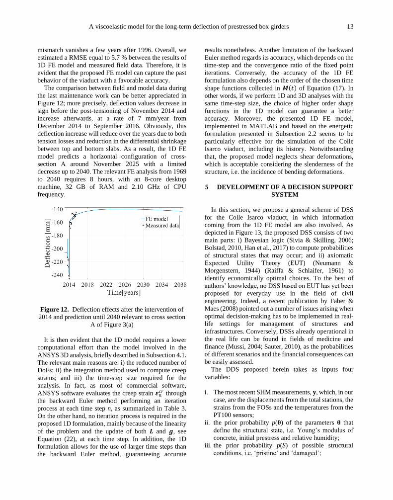
The comparison between field and model data during

the last maintenance work can be better appreciated in

Figure 12; more precisely, deflection values decrease in

sign before the post-tensioning of November 2014 and

increase afterwards, at a rate of 7 mm/year from

December 2014 to September 2016. Obviously, this

deflection increase will reduce over the years due to both

tension losses and reduction in the differential shrinkage

between top and bottom slabs. As a result, the 1D FE

model predicts a horizontal configuration of cross-

section A around November 2025 with a limited

decrease up to 2040. The relevant FE analysis from 1969

to 2040 requires 8 hours, with an 8-core desktop

machine, 32 GB of RAM and 2.10 GHz of CPU

frequency.

Figure 12. Deflection effects after the intervention of

2014 and prediction until 2040 relevant to cross section

A of Figure 3(a)

It is then evident that the 1D model requires a lower

computational effort than the model involved in the

ANSYS 3D analysis, briefly described in Subsection 4.1.

The relevant main reasons are: i) the reduced number of

DoFs; ii) the integration method used to compute creep

strains; and iii) the time-step size required for the

analysis. In fact, as most of commercial software,

ANSYS software evaluates the creep strain 𝜺𝑛𝑐𝑟 through

the backward Euler method performing an iteration

process at each time step n, as summarized in Table 3.

On the other hand, no iteration process is required in the

proposed 1D formulation, mainly because of the linearity

of the problem and the update of both 𝑳 and 𝒈, see

Equation (22), at each time step. In addition, the 1D

formulation allows for the use of larger time steps than

the backward Euler method, guaranteeing accurate

results nonetheless. Another limitation of the backward

Euler method regards its accuracy, which depends on the

time-step and the convergence ratio of the fixed point

iterations. Conversely, the accuracy of the 1D FE

formulation also depends on the order of the chosen time

shape functions collected in 𝑴(𝑡) of Equation (17). In

other words, if we perform 1D and 3D analyses with the

same time-step size, the choice of higher order shape

functions in the 1D model can guarantee a better

accuracy. Moreover, the presented 1D FE model,

implemented in MATLAB and based on the energetic

formulation presented in Subsection 2.2 seems to be

particularly effective for the simulation of the Colle

Isarco viaduct, including its history. Notwithstanding

that, the proposed model neglects shear deformations,

which is acceptable considering the slenderness of the

structure, i.e. the incidence of bending deformations.

5 DEVELOPMENT OF A DECISION SUPPORT

SYSTEM

In this section, we propose a general scheme of DSS

for the Colle Isarco viaduct, in which information

coming from the 1D FE model are also involved. As

depicted in Figure 13, the proposed DSS consists of two

main parts: i) Bayesian logic (Sivia & Skilling, 2006;

Bolstad, 2010, Han et al., 2017) to compute probabilities

of structural states that may occur; and ii) axiomatic

Expected Utility Theory (EUT) (Neumann &

Morgenstern, 1944) (Raiffa & Schlaifer, 1961) to

identify economically optimal choices. To the best of

authors’ knowledge, no DSS based on EUT has yet been

proposed for everyday use in the field of civil

engineering. Indeed, a recent publication by Faber &

Maes (2008) pointed out a number of issues arising when

optimal decision-making has to be implemented in real-

life settings for management of structures and

infrastructures. Conversely, DSSs already operational in

the real life can be found in fields of medicine and

finance (Mussi, 2004; Sauter, 2010), as the probabilities

of different scenarios and the financial consequences can

be easily assessed.

The DDS proposed herein takes as inputs four

variables:

i. The most recent SHM measurements, y, which, in our

case, are the displacements from the total stations, the

strains from the FOSs and the temperatures from the

PT100 sensors;

ii. the prior probability p(θ) of the parameters θ that

define the structural state, i.e. Young’s modulus of

concrete, initial prestress and relative humidity;

iii. the prior probability p(S) of possible structural

conditions, i.e. ‘pristine’ and ‘damaged’;

Beltempo et al. 14

iv. the costs C corresponding to each possible event, i.e.

costs of using a damaged structure -including indirect

costs- and costs of inspection.

The DSS contains a Bayesian inference module and a

decision-analysis module. In order to calculate the

probability p(S|y) of each possible state of the viaduct,

given the updated observations y, the former module

implements a numerical Bayesian inference such as the

Metropolis-Hastings algorithm (Cappello et al., 2015)

and Monte Carlo importance sampling (Evans & Swartz,

1995). In order to identify the economically optimal

choice aopt for the detected structural behavior, the

decision-analysis module takes into account costs C,

(Cappello et al., 2016). Typical choices to be considered

are: ‘do nothing’, ‘close the bridge’ and ‘send an

inspector’. The optimal action aopt corresponds to the

maximum expected utility, calculated by applying the

EUT axioms.

In this framework, the 1D FE model proposed in

Subsection 4.2 is used to train the Bayesian inference

module depicted in Figure 13. The objective of the

Bayesian module is to identify which structural condition

S -‘pristine’ or ‘damaged’- agrees with the measurements

best; therefore, it must contain the response predicted by

the FE model in both conditions. During training, the

structural behavior is simulated using the FE model for

different realizations of structural condition S and for

different realizations of state parameters θ. The need to

perform a number of simulations that is significant from

a statistical viewpoint made it necessary to develop an

extremely efficient structural model. Straub (Straub,

2014) estimated that 102 to 103 simulations are required

to accurately calculate structural reliability. Relevant

simulation results are stored in a lookup table, which

provides the structural response of the viaduct for the

realizations of S and θ not considered during training.

The use of a lookup table reduces the execution time of

the Bayesian inference algorithm within the DSS, and

therefore, expedites the identification of the optimal

action aopt that is recommended to the bridge manager.

6 CONCLUSIONS AND FUTURE

PERSPECTIVES

In this paper, we have presented the conception and

development of effective FE-based tools to model, in

general, segmental prestressed concrete box girders

susceptible to creep and, in particular, the significant

Colle Isarco viaduct. We have also shown the recordings

from the structural health monitoring system recently

installed on the viaduct, thus highlighting its key role in

both model validation and interpretation of the structural

behavior of the viaduct.

Figure 13. The architecture of the decision support

system

Two different FE models of the Colle Isarco viaduct

were presented, both based on the creep constitutive law

proposed by Bazant and co-workers. The first is a 3D FE

model developed in a commercial software, utilized to

perform elastic analyses only, due to the excessive

simulation time required to perform creep analyses. The

second is a 1D FE model conceived through an energetic

formulation for linear viscoelastic problems, used to

estimate the deflection trend at the tip of the longest

cantilever, from viaduct construction in 1969 up to 2040.

Unlike the 3D FE model, the 1D FE formulation relies

on an extension of the classical total potential energy and

is particularly convenient for accomplishing creep

analyses mainly due to its reduced run time.

Furthermore, it simulates the past behavior of the viaduct

with a good level of accuracy and provides a satisfactory

prediction of its long-term behavior up to 2040, with a

clear change in the deflection trend at the end of 2025.

The results of the 1D FE model were validated using

both field data from the old dumpy level acquisition

method until 2013 and from the new structural health

monitoring system, afterwards. Moreover, the structural

health monitoring system not only provides accurate and

reliable data for validation of the proposed 1D FE model,

but also successfully records the response of the viaduct

during the last maintenance work in 2014.

The obvious exploitation of both the 1D FE model and

monitoring field data, presented above as an effective

tool for future risk estimation and viaduct management,

is their use into the context of Bayesian inference for the

implementation of an efficient decision support system.

Finally, further run time savings can be achieved in the

1D FE model by parallelizing the algorithm solution for

different load applications and by replacing the 5-

parameter Bazant model creep constitutive law with

three parameters fractional-based real-order operators.

Observations y

Prior probability p(θ)

p(S)

Bayesian inference

EUT-based decision analysis

p(θ|y)

p(S|y) Costs

C

Choice aopt


15

ACKNOWLEDGMENTS

The work presented in this paper was carried out under

the research agreement between Autostrada del Brennero

SpA/Brennerautobahn AG and the University of Trento.

The financial contribution of Autostrada del Brennero is

acknowledged. The authors also wish to thank all those

who contributed to this project, in particular C. Costa, W.

Pardatscher, P. Joris, S. Vivaldelli, (Autostrada del

Brennero SpA); M. Vivaldi (SEICO srl); A. Bonelli, D.

Trapani (University of Trento).

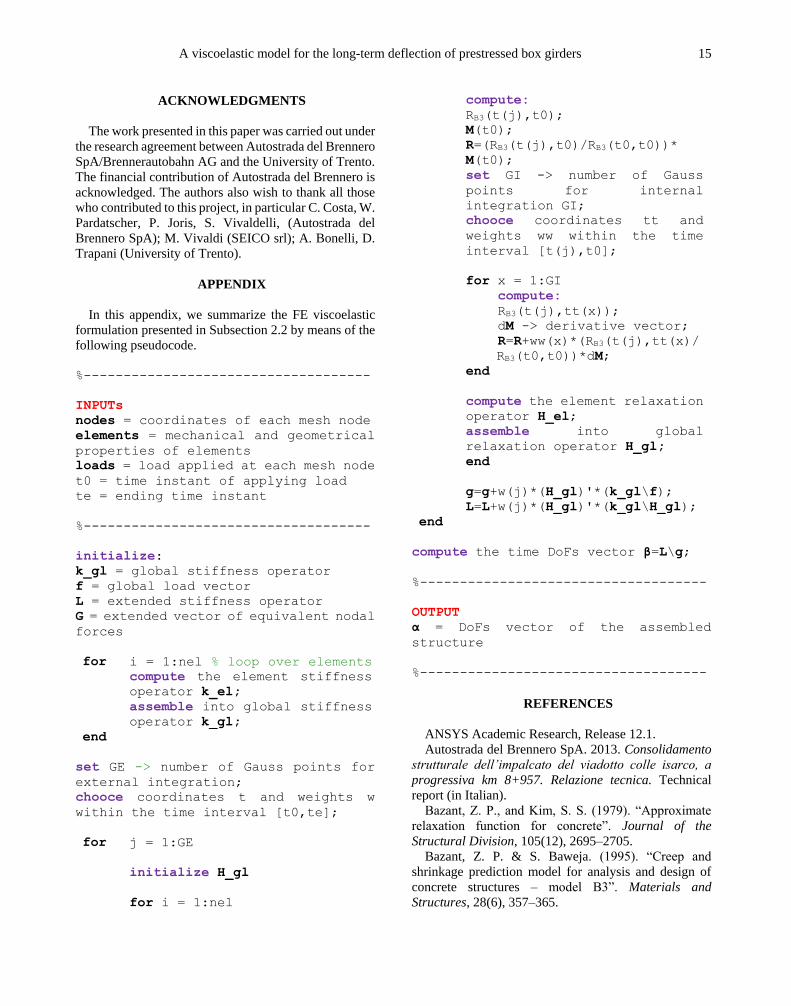
APPENDIX

In this appendix, we summarize the FE viscoelastic

formulation presented in Subsection 2.2 by means of the

following pseudocode.

%------------------------------------

INPUTs

nodes = coordinates of each mesh node

elements = mechanical and geometrical

properties of elements

loads = load applied at each mesh node

t0 = time instant of applying load

te = ending time instant

%------------------------------------

initialize:

k_gl = global stiffness operator

f = global load vector

L = extended stiffness operator

G = extended vector of equivalent nodal

forces

for i = 1:nel % loop over elements

compute the element stiffness

operator k_el;

assemble into global stiffness

operator k_gl;

end

set GE -> number of Gauss points for

external integration;

chooce coordinates t and weights w

within the time interval [t0,te];

for j = 1:GE

initialize H_gl

for i = 1:nel

compute:

RB3(t(j),t0);

M(t0);

R=(RB3(t(j),t0)/RB3(t0,t0))*

M(t0);

set GI -> number of Gauss

points for internal

integration GI;

chooce coordinates tt and

weights ww within the time

interval [t(j),t0];

for x = 1:GI

compute:

RB3(t(j),tt(x));

dM -> derivative vector;

R=R+ww(x)*(RB3(t(j),tt(x)/

RB3(t0,t0))*dM;

end

compute the element relaxation

operator H_el;

assemble into global

relaxation operator H_gl;

end

g=g+w(j)*(H_gl)'*(k_gl\f);

L=L+w(j)*(H_gl)'*(k_gl\H_gl);

end

compute the time DoFs vector β=L\g;

%------------------------------------

OUTPUT

α = DoFs vector of the assembled

structure

%------------------------------------

REFERENCES

ANSYS Academic Research, Release 12.1.

Autostrada del Brennero SpA. 2013. Consolidamento

strutturale dell’impalcato del viadotto colle isarco, a

progressiva km 8+957. Relazione tecnica. Technical

report (in Italian).

Bazant, Z. P., and Kim, S. S. (1979). “Approximate

relaxation function for concrete”. Journal of the

Structural Division, 105(12), 2695–2705.

Bazant, Z. P. & S. Baweja. (1995). “Creep and

shrinkage prediction model for analysis and design of

concrete structures – model B3”. Materials and

Structures, 28(6), 357–365.

Beltempo et al. 16

Bazant, Z. P., Q. Yu and G. Li (2012). “Excessive

Long-Time Deflections of Prestressed Box Girders. I:

Record-Span Bridge in Palau and Other Paradigms”.

Journal of Structural Engineering, 138, 676–686.

Bazant, Z. P., Mija Hubler, Milan Jirásek (2013).

“Improved Estimation of Long-Term Relaxation

Function from Compliance Function of Aging

Concrete”. Journal of Engineering Mechanics, 139(2),

146–152.

Balageas, D., C.P: Fritzen, A. Guemes. (2010).

Structural Health Monitoring. John Wiley & Sons.

Beltempo, A., C. Cappello, D. Zonta, A. Bonelli,

O.S.Bursi, C. Costa, W. Pardatscher. (2015). “Structural

Health Monitoring of the Colle Isarco Viaduct”. IEEE

Workshop on Environmental, Energy and Structural

Monitoring Systems (EESMS).

Bolstad, W. M. (2010). Understanding Computational

Bayesian Statistics. New York City: Wiley.

Cappello, C., Zonta, D., Pozzi, M., & Zandonini, R.

(2015). “Impact of prior perception on bridge health

diagnosis”. Journal of Civil Structural Health

Monitoring, 5(4), 509–525.

Cappello, C., D. Zonta, and B. Glisic (2016).

“Expected Utility Theory for Monitoring-Based

Decision-Making”. Proceedings of the IEEE, 104(8),

1647–1661.

Caracoglia, L., S. Noè, and V. Sepe (2009).

“Nonlinear Computer Model for the Simulation of Lock-

in Vibration on Long-Span Bridges”. Computer-Aided

Civil and Infrastructure Engineering, 24, 130–144.

Carini, A., P. Gelfi, and E. Marchina (1995). “An

energetic formulation for the linear viscoelastic problem.

part I: Theoretical results and first calculations”.

International Journal for Numerical Methods in

Engineering, 38(1), 37–62.

CEB (Comité Euro-International du Béton) (2008).

CEB-FIP model code 1990. London: Thomas Telford

Ltd.

CEN (European Committee for Standardization)

(2004). Eurocode 2: Design of concrete structures – Part

1-1: General rules and rules for buildings.

Di Paola, M. & M. Zingales (2012). “Exact

mechanical models of fractional hereditary materials”.

Journal of Rheology, 56, 983–1004.

Di Paola, M., F. Pinnola, and M. Zingales (2013).

“Fractional differential equations and related exact

mechanical models”. Computer and Mathematics with

Applications, 66, 608–620.

Evans, M., & Swartz, T. (1995). Methods for

approximating integrals in statistics with special

emphasis on Bayesian integration problem. Statistical

Science, 10(3), 254–272.

Faber, M. H. & M. A. Maes (2008). “Issues in societal

optimal engineering decision making”. Structure and

Infrastructure Engineering, 4(5), 335–351.

Gentilini, B. & L. Gentilini (1972). “Il viadotto di

Colle Isarco per l’Autostrada del Brennero.” L’Industria

Italiana del Cemento, 5, 318–334 (in Italian).

Glisic, B. & D. Inaudi (2007). Fiber Optic Methods

for Structural Health Monitoring. Chichester: John

Wiley & Sons.

Han, B., Xiang, T-Y and Xie, H-B, (2017). “A

Bayesian inference framework for predicting the long-

term deflection of concrete structures caused by creep

and shrinkage”, Engineering Structures, 142, 46-55.

Kirkup, L. & R. Frenkel (2010). An introduction to

uncertainty in measurement. Oxford: Cambridge

University Press.

MATLAB Release 2015b, The MathWorks, Inc.,

Natick, Massachusetts, United States.

Mazzoni, S. OpenSees command language manual.

PEER Center, 2006

Mussi, S. (2004). Putting value of information theory

into practice: a methodology for building sequential

decision support systems. Expert Systems, 21 (2), 92–

103.

Neumann, J. & O. Morgenstern (1944). Theory of

Games and Economic Behavior. New York, NY, USA:

Wiley.

Raiffa, H. & R. Schlaifer (1961). Applied Statistical

Decision Theory. Boston, MA, USA: Clinton.

Shapiro, K. A. (2007). Finite-Element Modeling of a

Damagd Prestressed Concrete Bridge. Doctoral Thesis,

Auburn University.

Sauter, V. L. (2010). Decision Support Systems for

Business Intelligence. New York City: Wiley.

Sivia, D., & Skilling, J. (2006). Data Analysis: a

Bayesian Tutorial. Oxford: Oxford University Press.

Straub, D. (2014). Value of information analysis with

structural reliability methods. Structural Safety, 49, 74–

85.

Torbol, M., H. Gomez, and M. Feng (2013). “Fragility

Analysis of Highway Bridges Based on Long-Term

Monitoring Data”. Computer-Aided Civil and

Infrastructure Engineering, 28, 178–192.

Wendner, R., Zdenek Bazant, Mija Hubler (2015).

“Statistical justification of Model b4 for multi-decade

concrete creep using laboratory and bridge databases and

comparisons to other models”. Materials and Structures,

48, 797–814.

a viscoelastic model for the long-term deflection of segmental prestressed box … ·...

Documents