A Virtual Structure Approach to Formation Control of Unicycle

Mobile Robots

T.H.A. van den Broek ∗, N. van de Wouw, H. Nijmeijer

Department of Mechanical Engineering, Eindhoven University of Technology,

PO Box 513, 5600 MB Eindhoven, The Netherlands

Abstract

In this paper, the formation control problem for unicycle mobile robots is studied. A

virtual structure control strategy with mutual coupling between the robots is proposed.

The rationale behind the introduction of the coupling terms is the fact that these introduce

additional robustness with respect to perturbations as compared to typical leader-follower

approaches. The applicability of the proposed approach is shown in experiments with a

group of wirelessly controlled mobile robots.

1 Introduction

In this paper, the formation control problem (i.e. cooperative control problem) for unicycle

mobile robots is considered. Formation control problems arise when groups of mobile robots

are employed to jointly perform certain tasks. The benefits of exploiting groups of robots, as

opposed to a single robot or a human, become apparent when considering spatially distributed

tasks, dangerous tasks, tasks which require redundancy, tasks that scale up or down in time

or tasks that require flexibility. Various areas of application of cooperative control of mobile

robots are e.g. simultaneous localization and mapping [12], automated highway systems [6],

payload transportation [30], RoboCup [17], enclosing an invader [31] and the exploration of

an unknown environment [7]. In [2] and [18], an overview is given of what has been achieved

with respect to cooperative control and the control of nonholonomic unicycle mobile robots,

respectively.

∗Corresponding author. E-mail addresses: thijs.vandenbroek@tno.nl, {n.v.d.wouw,h.nijmeijer}@tue.nl

1

Before a wide application of cooperative mobile robotics will become feasible, many tech-

nical and scientific challenges must be faced such as the development of cooperative and

formation control strategies, control schemes robust to communication constraints, the local-

ization of the robot position, sensing and environment mapping, etc. In the current paper, the

focus is on the aspect of cooperative control. In the recent literature, see e.g. [4, 8, 9, 11, 26],

three different approaches towards the cooperative control of mobile robots are described: the

behaviour-based approach, the leader-follower approach and the virtual structure approach.

In the behaviour-based approach, a so-called behaviour (e.g. obstacle avoidance, target seek-

ing) is assigned to each individual robot [3]. This approach can naturally be used to design

control strategies for robots with multiple competing objectives. Moreover, it is suitable for

large groups of robots, since it is typically a decentralized strategy. A disadvantage is that the

complexity of the dynamics of the group of robots does not lend itself for simple mathematical

stability analysis. To simplify the analysis, the dynamics of individual robots are commonly

simplified as being described by a single integrator. Clearly, even kinematic models of mobile

robots is more complex, limiting the applicability of this approach in practice.

In the leader-follower approach some robots will take the role of leader and aim to track

predefined trajectories, while the follower robots will follow the leader according to a relative

posture [5, 8, 9, 10, 13, 20, 28, 29, 32]. An advantage of this approach is the fact that it

is relatively easy to understand and implement. A disadvantage, however, is the fact that

there is no feedback from the followers to the leaders. Consequently, if a follower is being

perturbed, the formation cannot be maintained and such a formation control strategy lacks

robustness in the face of such perturbations.

A third approach in cooperative control is the virtual structure approach, in which the

robots’ formation no longer consists of leaders nor followers, i.e. no hierarchy exists in the

formation. In [27], a general controller strategy is developed for the virtual structure approach.

Using this strategy, however, it is not possible to consider formations which are time-varying.

Moreover, the priority of the mobile robots, either to follow their individual trajectories or

to maintain the groups formation, can not be changed. In [11], a virtual structure controller

is designed for a group of unicycle mobile robots using models involving the dynamics of the

2

robots. Consequently, the controller design tends to be rather complex, which is unfavorable

from an implementation perspective, especially when kinematic models suffice. An advantage

of the virtual structure approach is, as we will show in this paper, that it allows to attain a

certain robustness of the formation to perturbations on the robots.

In this paper the design of a virtual structure controller is considered, which guarantees

stability of the formation error dynamics for a group of nonholonomic unicycle mobile robots.

To limit the complexity of the virtual structure controller, the controller design is based on

the kinematics of unicycle mobile robots. Moreover, so-called mutual coupling terms will

be introduced between the robots to ensure robustness of the formation with respect to

perturbations. Finally, the control design is validated in an experimental setting.

This paper is organized as follows. In Section 2, preliminary technical results needed in

the remainder of the paper are presented. The virtual structure control design, which uses

the tracking controller of [14] as a stepping stone, and a stability proof for the formation

error dynamics is given in Section 3. In Section 4, experiments are presented validating the

proposed approach in practice. Section 5 present concluding remarks.

2 Preliminaries

Consider the following linear time-varying system

x = A(t)x + B(t)u

y = C(t)x,(1)

where matrices A(t), B(t), C(t) are matrices of appropriate dimensions whose elements are

piecewise continuous functions of time. Let Φ(t, t0) denote the state-transition matrix for the

system x = A(t)x.

Definition 2.1. [19] The pair (A(t), C(t)) is uniformly completely observable (UCO) if con-

stants δ, ǫ1, ǫ2 > 0 exist such that ∀t > 0:

ǫ1In ≤∫ t

t−δΦT (τ, t − δ)CT (τ)C(τ)Φ(τ, t − δ)dτ ≤ ǫ2In. (2)

3

Definition 2.2. [19] A continuous function ω : R+ → R is said to be persistently exciting

(PE) if ω(t) is bounded, Lipschitz, and constants δc > 0 and ǫ > 0 exist such that

∀t ≥ 0,∃s : t − δc ≤ s ≤ t such that |ω(s)| ≥ ǫ. (3)

The following corollary is based on Theorem 2.3.3, presented in [19], and will be used in

the proof of Lemma 2.6.

Corollary 2.3. Consider the linear time-varying system

x = A(ω(t))x + Bu

y = Cx,(4)

where A(ω) is continuous and ω : R → R is continuous. Assume that for all s 6= 0 the pair

(A(s), C) is observable. If ω(t) is persistently exciting, see Definition 2.2, then the system (4)

is uniformly completely observable.

Consider the system z = f(t, z), z ∈ Rn+m, which is decomposed as follows:

z1 = f1(t, z1) + g(t, z1, z2)z2,

z2 = f2(t, z2),(5)

where z1 ∈ Rn, z2 ∈ R

m, f1(t, z1) is continuously differentiable in (t, z1) and f2(t, z2),

g(t, z1, z2) are continuous in their arguments, and locally Lipschitz in z2 and (z1, z2), re-

spectively, and (z1, z2) = (0, 0) is an equilibrium point of (5) ∀t.

Assumption 2.4. [22] Assume that there exist continuous functions k1, k2 : R+ → R such

that

‖g(t, z1, z2)‖F ≤ k1(‖z2‖2) + k2(‖z2‖2)‖z1‖2, ∀t ≥ t0, (6)

where ‖g(t, z1, z2)‖F denotes the Frobenius norm of the matrix g(t, z1, z2). The Frobenius

norm is defined as ‖A‖F =[ n∑

j=1

m∑

i=1

|aij |2]1/2

.

Then the following corollary can be derived from Theorem 1 in [23].

4

Corollary 2.5. The equilibrium point of the cascaded system of (5) is locally exponentially

stable if the equilibrium point z1 = 0 of z1 = f1(t, z1) is globally exponentially stable, g(t, z1, z2)

satisfies Assumption 2.4 and the equilibrium point z2 = 0 of z2 = f2(t, z2) is locally exponen-

tially stable.

In the next result a sufficient condition is provided for the global exponential stability of

the equilibrium point of a specific linear time-varying system, which will be used in Appendix

B.

Lemma 2.6. The equilibrium point x = 0 of the system

x =

−g1 g2ωd(t) g3 −g4ωd(t)

−ωd(t) 0 0 0

g3 −g4ωd(t) −g1 g2ωd(t)

0 0 −ωd(t) 0

x (7)

is globally exponentially stable if −g1 + g3 < 0, −g1 − g3 < 0, g2 6= g4, g2 6= −g4 and ωd(t) is

persistently exciting.

Proof. See Appendix A.

3 Virtual Structure Formation Control with Mutual Coupling

In Section 3.1, the kinematic model of a unicycle mobile robot is presented. In Section 3.2, a

generic virtual structure formation controller, with mutual coupling between the robots, will

be presented, which is based on the kinematic model of a unicycle. Moreover, in Section 3.3,

a stability result for the formation error dynamics for the case of two robots is given.

5

ydi

yi

yei

xdixi

xei

φi

φdiφei

~e 01

~e 02

~e i1

~e i2

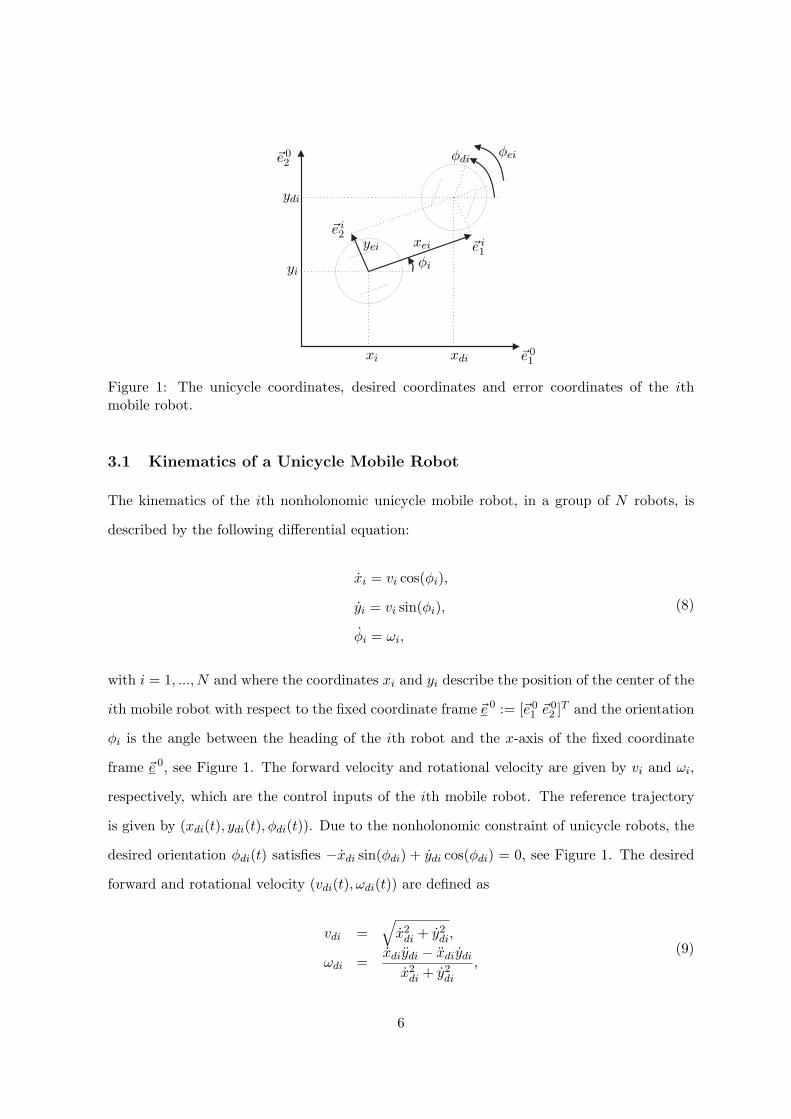
Figure 1: The unicycle coordinates, desired coordinates and error coordinates of the ithmobile robot.

3.1 Kinematics of a Unicycle Mobile Robot

The kinematics of the ith nonholonomic unicycle mobile robot, in a group of N robots, is

described by the following differential equation:

xi = vi cos(φi),

yi = vi sin(φi),

φi = ωi,

(8)

with i = 1, ..., N and where the coordinates xi and yi describe the position of the center of the

ith mobile robot with respect to the fixed coordinate frame ~e 0 := [~e 01 ~e 0

2 ]T and the orientation

φi is the angle between the heading of the ith robot and the x-axis of the fixed coordinate

frame ~e 0, see Figure 1. The forward velocity and rotational velocity are given by vi and ωi,

respectively, which are the control inputs of the ith mobile robot. The reference trajectory

is given by (xdi(t), ydi(t), φdi(t)). Due to the nonholonomic constraint of unicycle robots, the

desired orientation φdi(t) satisfies −xdi sin(φdi) + ydi cos(φdi) = 0, see Figure 1. The desired

forward and rotational velocity (vdi(t), ωdi(t)) are defined as

vdi =√

x2di + y2

di,

ωdi =xdiydi − xdiydi

x2di + y2

di

,(9)

6

for xdi, ydi 6= 0. Define the tracking error coordinates (xei, yei, φei) as follows:

xei

yei

φei

=

cos(φi) sin(φi) 0

− sin(φi) cos(φi) 0

0 0 1

xdi − xi

ydi − yi

φdi − φi

, (10)

see also Figure 1. We will exploit these error coordinate definitions in the stability proof of

the formation error dynamics in Section 3.3.

3.2 Virtual Structure Control Design

We design a virtual structure controller, with mutual coupling between N individual robots,

such that a desired formation is achieved. The main goals of the virtual structure controller are

twofold. Firstly, the formation as a whole should follow a predefined trajectory; i.e. a so-called

virtual center should follow a predefined trajectory and the i-th unicycle robot, i ∈ {1, . . . , N ,

should follow at a certain predefined, and possibly time-varying, location (lxi, lyi)~ei relative to

the virtual center. Secondly, if the individual robots suffer from perturbations, the controller

should mediate between keeping formation and ensuring the tracking of the individual robots’

desired trajectories, which is facilitated by introducing mutual coupling between the robots.

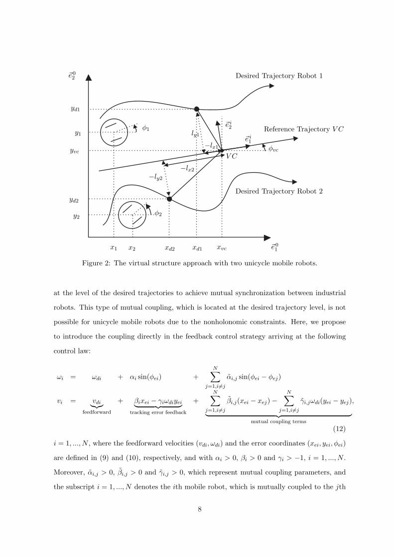
In Figure 2, for the purpose of illustration two mobile robots and the virtual center V C

of the formation are shown. The reference trajectory of the virtual center is described by

the coordinates (xvc(t), yvc(t)) defining the position of the virtual center with respect to the

fixed coordinate frame ~e 0. The desired trajectories of the individual robots (xdi(t), ydi(t)),

i = 1, ..., N , are described as

xdi(t)

ydi(t)

=

xvc(t)

yvc(t)

+

cos(φvc(t)) − sin(φvc(t))

sin(φvc(t)) cos(φvc(t))

lxi(t)

lyi(t)

, (11)

where φvc(t) is the orientation of the virtual center along its trajectory and (lxi(t), lyi(t))~ei is

possibly time-varying to allow for time-varying formation shapes. Now, the tracking controller

of [14] is expanded with so-called mutual coupling terms. In [25], such terms were introduced

7

yd1

y1

yd2

y2

yvc

x1 x2 xd1xd2 xvc

φ1

φ2

φvc

~e 01

~e 02

~e i1

~e i2

Desired Trajectory Robot 1

Desired Trajectory Robot 2

Reference Trajectory V C

V C

−lx1

−lx2

ly1

−ly2

Figure 2: The virtual structure approach with two unicycle mobile robots.

at the level of the desired trajectories to achieve mutual synchronization between industrial

robots. This type of mutual coupling, which is located at the desired trajectory level, is not

possible for unicycle mobile robots due to the nonholonomic constraints. Here, we propose

to introduce the coupling directly in the feedback control strategy arriving at the following

control law:

ωi = ωdi + αi sin(φei) +N∑

j=1,i6=j

αi,j sin(φei − φej)

vi = vdi︸︷︷︸

feedforward

+ βixei − γiωdiyei︸ ︷︷ ︸

tracking error feedback

+N∑

j=1,i6=j

βi,j(xei − xej) −N∑

j=1,i6=j

γi,jωdi(yei − yej)

︸ ︷︷ ︸

mutual coupling terms

,

(12)

i = 1, ..., N , where the feedforward velocities (vdi, ωdi) and the error coordinates (xei, yei, φei)

are defined in (9) and (10), respectively, and with αi > 0, βi > 0 and γi > −1, i = 1, ..., N .

Moreover, αi,j > 0, βi,j > 0 and γi,j > 0, which represent mutual coupling parameters, and

the subscript i = 1, ..., N denotes the ith mobile robot, which is mutually coupled to the jth

8

mobile robot, j = 1, ..., N .

Before a stability proof for the formation error dynamics of a group of unicycles under

application of the virtual structure controller of (12) is presented in the next section, let

us explain the working principle of the controller in (12). For the sake of simplicity, we

limit ourselves to the case of two mobile robots. Assume that robot 2 resides on its desired

trajectory, i.e. (xe2, ye2, φe2) = 0. According to (12) this results in the following individual

control inputs of robots 1 and 2:

ω1 = ωd1 + α1 sin(φe1) + α1,2 sin(φe1),

v1 = vd1 + β1xe1 − γ1ωd1ye1 + β1,2xe1 − γ1,2ωd1ye1,(13)

and

ω2 = ωd2 − α2,1 sin(φe1),

v2 = vd2 − β2,1xe1 + γ2,1ωd2ye1,(14)

respectively. Moreover, it is assumed that robot 1 is not on its desired trajectory, e.g.

xe1, ye1, φe1 > 0. Note that the terms −α2,1 sin(φe1), −β2,1xe1 and γ2,1ωd2ye1 in (14), with

xe1, ye1, φe1 > 0, have a similar effect as terms α2 sin(φe2), β2xe2 and −γ2ωd2ye2 would, with

xe2, ye2, φe2 < 0. In other words, the mutual coupling terms are acting as if robot 2 is behind

its desired trajectory (i.e. as if xe2 < 0), below its desired trajectory (i.e. as if ye2 < 0) and

orientated in clockwise direction relative to the desired trajectory (i.e as if φe2 < 0). Conse-

quently, the controller for robot 2 will try to compensate for these errors, which results in the

fact that the formation will remain (partly) intact. The second effect of the mutual coupling

term is that robot 1 in this case is subject to effective gains α1 + α1,2, β1 + β1,2 and γ1 + γ1,2

in (13).

3.3 Stability Analysis of the Formation Error Dynamics

In this section, the stability of the resulting formation error dynamics under application of

the controller (12) is analyzed for the specific case of a formation of two mobile robots. The

formation error dynamics of two mobile robots, described by (8) and the controller (12), can

9

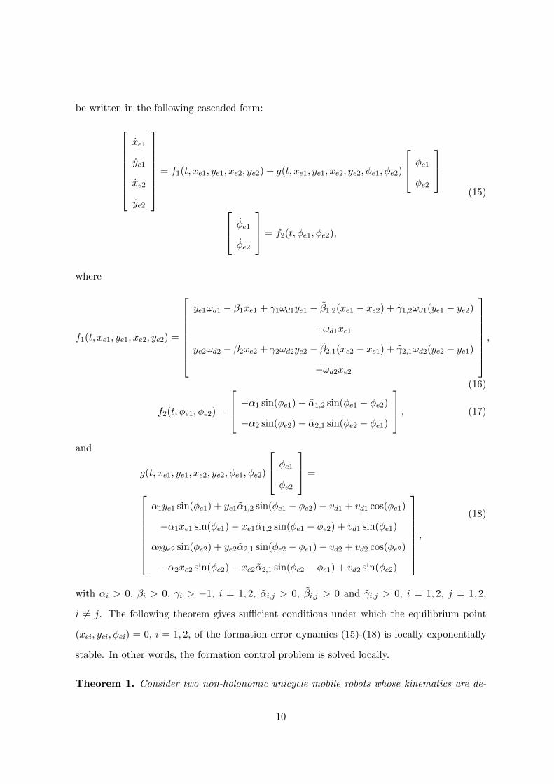
be written in the following cascaded form:

xe1

ye1

xe2

ye2

= f1(t, xe1, ye1, xe2, ye2) + g(t, xe1, ye1, xe2, ye2, φe1, φe2)

φe1

φe2

φe1

φe2

= f2(t, φe1, φe2),

(15)

where

f1(t, xe1, ye1, xe2, ye2) =

ye1ωd1 − β1xe1 + γ1ωd1ye1 − β1,2(xe1 − xe2) + γ1,2ωd1(ye1 − ye2)

−ωd1xe1

ye2ωd2 − β2xe2 + γ2ωd2ye2 − β2,1(xe2 − xe1) + γ2,1ωd2(ye2 − ye1)

−ωd2xe2

,

(16)

f2(t, φe1, φe2) =

−α1 sin(φe1) − α1,2 sin(φe1 − φe2)

−α2 sin(φe2) − α2,1 sin(φe2 − φe1)

, (17)

and

g(t, xe1, ye1, xe2, ye2, φe1, φe2)

φe1

φe2

=

α1ye1 sin(φe1) + ye1α1,2 sin(φe1 − φe2) − vd1 + vd1 cos(φe1)

−α1xe1 sin(φe1) − xe1α1,2 sin(φe1 − φe2) + vd1 sin(φe1)

α2ye2 sin(φe2) + ye2α2,1 sin(φe2 − φe1) − vd2 + vd2 cos(φe2)

−α2xe2 sin(φe2) − xe2α2,1 sin(φe2 − φe1) + vd2 sin(φe2)

,

(18)

with αi > 0, βi > 0, γi > −1, i = 1, 2, αi,j > 0, βi,j > 0 and γi,j > 0, i = 1, 2, j = 1, 2,

i 6= j. The following theorem gives sufficient conditions under which the equilibrium point

(xei, yei, φei) = 0, i = 1, 2, of the formation error dynamics (15)-(18) is locally exponentially

stable. In other words, the formation control problem is solved locally.

Theorem 1. Consider two non-holonomic unicycle mobile robots whose kinematics are de-

10

scribed by (8). Suppose that the desired tracking state trajectories of the individual robots

(xdi(t), ydi(t)), i = 1, 2, are given by (11) for a given trajectory (xvc(t), yvc(t)) for the virtual

center. Moreover, the desired orientations φdi(t), i = 1, 2, are imposed by the non-holonomic

constraint. Consider controller (12) for N = 2, with the feedforwards vdi, ωdi, i = 1, 2,

satisfying (9). If

• the desired rotational velocities ωdi, i = 1, 2, of both mobile robots are persistently ex-

citing and identical, i.e. ωd1 = ωd2;

• the control parameters αi > 0, i = 1, 2, β1 = β2 > 0 and γ1 = γ2 > −1;

• the coupling parameters αi,j > 0, for i = 1, 2, j = 1, 2, i 6= j, β1,2 = β2,1 > −β1

2and

γ1,2 = γ2,1 6= −1−γ1

2,

then the equilibrium point (xe1, ye1, φe1, xe2, ye2, φe2) = 0 of the formation error dynamics

(15)-(18) is locally exponentially stable.

Proof. See Appendix B.

Remark I. In practice we typically choose the coupling parameters such that αi,j > 0, βi,j > 0,

γi,j > 0 (which reflect more strict conditions than those in the theorem), because if we would

opt for −β1

2< βi,j ≤ 0 and (γi,j ≤ 0) ∧ (γi,j 6= −1−γ1

2), then (although stability is not

endangered) undesirable transient behaviour of the formation may be induced.

Remark II. Simulations, with more than two robots, moving with different desired rotational

velocities ωdi, different control parameters (βi, γi) and different coupling parameters (βi,j , γi,j),

show that the error dynamics of the virtual structure controller is stable in a more general

setting. In the current paper, we refrain from such technical extensions, but rather focus on

the experimental validation of the proposed approach, which is shown in the next section.

4 Experiments

In this section experiments are performed to validate in practice the controller design, pro-

posed in the previous section. In Section 4.1, the experimental setup is presented and exper-

imental results are discussed in Section 4.2.

11

4.1 Experimental Setup

The experimental setup is shown in Figure 3. The experiments are performed with two E-Puck

CameraE-Pucks ArenaPC

Figure 3: The experimental setup, with two E-Pucks driving in the arena, a camera whichdetermines the position of the robot and a PC which sends new information to the robots.

mobile robots [21]. The E-Puck robot has two driven wheels, which are individually actuated

by means of stepper motors. Velocity control commands are sent to both stepper motors over

a wireless BlueTooth connection. The absolute position measurement of the mobile robots

is performed using a Firewire camera AVT Guppy F-080b b/w [1], in combination with

reacTIVision software [15]. We note that the achieved position and orientation accuracy of

these position measurements are 0.0019 m in x- and y-direction and 0.0524 rad in φ-direction,

and the driving area of the mobile robots is 1.75 by 1.28 m. The sample rate is given as 25

Hz. Both signal processing and controller implementation is executed in Python [24].

4.2 Experimental Results

In this section, the results of an experiment with two mobile robots driving in formation are

discussed. The trajectory of the virtual center is given by xvc(t) = 0.9 + 0.3 cos(2π0.02t)

12

[m] and yvc(t) = 0.6 + 0.3 sin(2π0.02t) [m]. The desired trajectories of the mobile robots

are defined according to (11), with lx1 = 0.1 m, ly1 = 0.1 m, lx2 = −0.1 m and ly2 = 0

m, respectively. In other words, the virtual center moves in a circular motion, robot 1 is

positioned ahead and left of the virtual center and robot 2 is positioned behind the virtual

center. The controllers of both robots are of the form (12), where the control and coupling

parameters satisfy the conditions of Theorem 1 and given by αi = 0.3, βi = 0.275, γi = 1.3,

i = 1, 2, αi,j = 3, βi,j = 2.75 and γi,j = 13, i = 1, 2, j = 1, 2, i 6= j. The control and coupling

parameters are tuned to demonstrate the main goal of the experiment, which is to illustrate

that the two mobile robots attain formation asymptotically and prefer to maintain formation,

as opposed to following their individual desired trajectories. This type of behaviour is due

to the relatively strong coupling parameters (αi,j , βi,j , γi,j). Two types of perturbations are

applied to illustrate the behaviour of the mobile robots in the face of perturbations. The first

perturbation involves both the forward velocity v1 and rotational velocity ω1 of robot 1 as

follows:

ω1 = ωd1 + α1 sin(φe1) + α1,2 sin(φe1) + 0.5,

v1 = vd1 + β1xe1 − γ1ωd1ye1 + β1,2xe1 − γ1,2ωd1ye1 + 0.3,(19)

for t ∈ [35, 36] s. The second perturbation takes place at t = 56 s; here, robot 1 is repositioned

manually. In Figure 4, the desired trajectories and actual trajectories of robots 1 and 2 are

shown. Robot 1 initially moves backwards and away from its desired trajectory, thereby

aiming to achieve the desired formation with robot 2 as fast as possible. A closer inspection

of the trajectory of robot 2 reveals that the effects of the disturbances on robot 1 are clearly

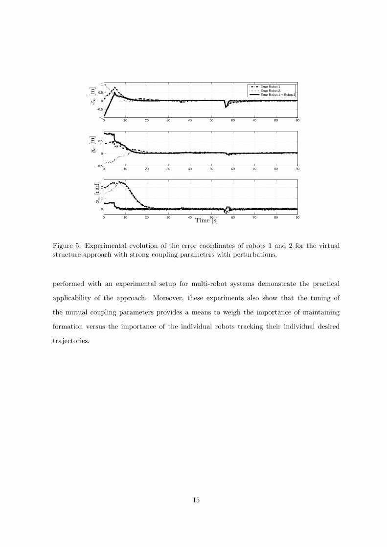
noticeable in the behaviour of robot 2. In Figure 5, the error coordinates of the individual

robots (xe1, ye1, φe1, xe2, ye2, φe2) and the error coordinates of the formation (xe1 − xe2, ye1 −

ye2, φe1 − φe2) are shown. This figure clearly shows that the robots converge to the desired

formation within 15 s. Within 25 s, the robots have also converged to their desired trajectories.

Clearly, both in transients and after perturbations the robots first converge to their desired

formation, and then converge to their desired trajectories. This behaviour is due to the choice

for strong coupling parameters, i.e. the robots priority is to maintain the formation. In Figure

6 (a zoomed version of Figure 5), the error coordinates of robots 1 and 2 are displayed for the

13

0.4 0.6 0.8 1 1.20.2

0.3

0.4

0.5

0.6

0.7

0.8

0.9

1Desired Trajectory Robot 1

Trajectory Robot 1

0.4 0.6 0.8 1 1.20.2

0.3

0.4

0.5

0.6

0.7

0.8

0.9

1

Desired Trajectory Robot 2

Trajectory Robot 2

x[m

]

y [m]y [m]

Perturbation 1

Perturbation 2

Figure 4: The actual trajectories and desired trajectories of robots 1 and 2 in the virtualstructure approach with strong coupling parameters and perturbations.

time interval t ∈ [30, 90] s. During the perturbations, robot 2 is reacting to the error of robot

1, thereby trying to remain in formation. Clearly, this experiment shows that the mutual

coupling terms in the proposed controlled strategy provides robustness to the formation in

the face of perturbations. Moreover, the tuning of the coupling control gains provides a means

to mediate between the individual tracking of the robots’ desired trajectories and the goal of

achieving formation.

5 Conclusions

In this paper a virtual structure controller is designed for the formation control of unicycle

mobile robots. We have proposed a controller, which introduces mutual coupling between

the individual robots, thereby providing more robustness to the formation in the face of

perturbations as compared to leader-follower (i.e. master-slave) type approaches. Moreover,

an explicit stability proof is given for the case of two cooperating mobile robots. Experiments

14

0 10 20 30 40 50 60 70 80 90−1

−0.5

0

0.5

1

Error Robot 1Error Robot 2Error Robot 1 − Robot 2

0 10 20 30 40 50 60 70 80 90−0.5

0

0.5

0 10 20 30 40 50 60 70 80 90

0

1

2

xe

[m]

ye

[m]

φe

[rad

]

Time [s]

Figure 5: Experimental evolution of the error coordinates of robots 1 and 2 for the virtualstructure approach with strong coupling parameters with perturbations.

performed with an experimental setup for multi-robot systems demonstrate the practical

applicability of the approach. Moreover, these experiments also show that the tuning of

the mutual coupling parameters provides a means to weigh the importance of maintaining

formation versus the importance of the individual robots tracking their individual desired

trajectories.

15

30 40 50 60 70 80 90−0.4

−0.3

−0.2

−0.1

0

Error Robot 1Error Robot 2Error Robot 1 − Robot 2

30 40 50 60 70 80 90

−0.05

0

0.05

30 40 50 60 70 80 90

−0.4

−0.2

0

0.2

xe

[m]

ye

[m]

φe

[rad

]

Time [s]

Figure 6: Experimental evolution of the error coordinates of robots 1 and 2 for the virtualstructure approach with strong coupling parameters with perturbations for the time ∈ [30, 90]s.

Appendices

A Proof of Lemma 2.6

Here, it is shown that the equilibrium point x = 0 of the following system (system (7) in

Lemma 2.6) is globally exponentially stable (GES):

x =

−g1 g2ωd(t) g3 −g4ωd(t)

−ωd(t) 0 0 0

g3 −g4ωd(t) −g1 g2ωd(t)

0 0 −ωd(t) 0

x =: G(t)x. (20)

16

Apply a coordinate transformation x = Uz with the following well-defined transformation

matrix U :

U =

0 12

√g2 − g4 −1

20

−12√

g2+g4

0 0 12

0 12

√g2 − g4

12

0

12√

g2+g4

0 0 12

. (21)

With this change of coordinates the following system dynamics results:

z =

0 0 −a1ωd(t) 0

0 −a2 0 a3ωd(t)

a1ωd(t) 0 −a4 0

0 −a3ωd(t) 0 0

z =: A(t)z, (22)

where a1 =√

g2 + g4, a2 = g1 − g3, a3 =√

g2 − g4 and a4 = g1 + g3. Note that the system

matrix A(t) in (22) is skew-symmetric.

The following quadratic candidate Lyapunov function

V = zT Pz =1

2z21 +

1

2z22 +

1

2z23 +

1

2z24 , (23)

with P = 12I, is differentiated along the solutions of (22) to obtain

V = zT (AT (t)P + PA(t))z = (−g1 + g3)z22 + (−g1 − g3)z

23 . (24)

Consequently, V is negative semi-definite if −g1 + g3 < 0 and −g1 − g3 < 0.

Let us first show that the following inequality holds:

zT (AT (t)P + PA(t))z ≤ −zT CT Cz, (25)

17

for

C =

[

0 12

√g1 − g3

12

√g1 + g3 0

]

. (26)

Clearly, zT CT Cz = 14(g1 − g3)z

22 + 1

2

√g1 − g3

√g1 + g3z2z3 + 1

4(g1 + g3)z

23 ≥ 0, and using the

fact that 12

√g1 − g3

√g1 + g3z2z3 ≤ 1

4(g1 − g3)z

22 + 1

4(g1 + g3)z

23 , we obtain

−zT CT Cz ≥ −12(g1 − g3)z

22 − 1

2(g1 + g3)z

23

≥ (−g1 + g3)z22 + (−g1 − g3)z

23 .

(27)

Combining (24) and (27) proves the validity of inequality (25). Furthermore, using Corollary

2.3 it can easily be shown that system (22) is uniformly completely observable. The latter fact,

together with the satisfaction of inequality (25), implies that z = 0 is a globally exponentially

stable equilibrium point of (22), see e.g. [16]. Consequently, x = 0 is a globally exponentially

stable equilibrium point of (20). This completes the proof.

B Proof of Theorem 1

Note that the formation error dynamics of both robots can be described by (15)-(18). Note,

moreover, that (15) is of the form (5) and Corollary 2.5 will be exploited to show that the

equilibrium point (xe1, ye1, φe1, xe2, ye2, φe2) = 0 of the error dynamics (15)-(18) is locally ex-

ponentially stable. First, the global exponential stability of the f1(t, xe1, ye1, xe2, ye2) part of

the (xe1, ye1, xe2, ye2)-dynamics, see (16), is proven. Second, the local exponential stability of

the (φe1, φe2)-dynamics of (17) is proven. Third, it is shown that g(t, xe1, ye1, xe2, ye2, φe1, φe2)

as in (18) satisfies Assumption 2.4. According to Corollary 2.5 the satisfaction of these three

conditions implies that the equilibrium point (xei, yei, φei) = 0, i = 1, 2, of the formation error

dynamics is locally exponentially stable.

A. Global exponential stability of the f1(t, xe1, ye1, xe2, ye2) part of the (xe1, ye1, xe2, ye2)-

dynamics

18

Consider the linear time-varying system [xe1, ye1, xe2, ye2]T = f1(t, xe1, ye1, xe2, ye2), with

f1(t, xe1, ye1, xe2, ye2) =

−β1 − β1,2 (1 + γ1 + γ1,2)ωd1(t) β1,2 −γ1,2ωd1(t)

−ωd1(t) 0 0 0

β2,1 −γ2,1ωd2(t) −β2 − β2,1 (1 + γ2 + γ2,1)ωd2(t)

0 0 −ωd2(t) 0

xe1

ye1

xe2

ye2

.

(28)

Since β1 = β2 > 0, β1,2 = β2,1 > −β1

2, γ1 = γ2 6= −1, γ1,2 = γ2,1 6= −1−γ1

2and ωd1(t) = ωd2(t)

is persistently exciting, Lemma 2.6 can be directly exploited to prove that the origin of the

system [xe1, ye1, xe2, ye2]T = f1(t, xe1, ye1, xe2, ye2), with f1(t, xe1, ye1, xe2, ye2) as in (28), is

globally exponentially stable.

B. Local exponential stability of the (φe1, φe2)-dynamics

Note that φe = (φe1, φe2)T = 0 is an equilibrium point of the (φe1, φe2)-dynamics in (15) with

f2(t, φe1, φe2) as defined in (17). If these dynamics are linearized around this equilibrium

point we obtain linear time-invariant dynamics with the following system matrix:

A =∂f2

∂φe(φe)

∣∣∣φe=0

=

−α1 − α1,2 α1,2

α2,1 −α2 − α2,1

, (29)

which is Hurwitz for αi > 0, i = 1, 2 and αi,j > 0 for i, j = 1, 2 and i 6= j. Consequently,

φe = 0 is a locally exponentially stable equilibrium point of the φe-dynamics for αi > 0,

i = 1, 2, and αi,j > 0 for i, j = 1, 2 and i 6= j.

C. Matrix g(t, xe1, ye1, xe2, ye2, φe1, φe2) satisfies Assumption 2.4

The matrix g(t, xe1, ye1, xe2, ye2, φe1, φe2), as defined in (18), can be written as follows:

g(t, xe1, ye1, xe2, ye2, φe1, φe2)

φe1

φe2

=

g11 g12

g21 g22

φe1

φe2

, (30)

19

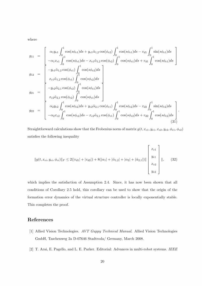
where

g11 =

α1ye1

∫ 1

0

cos(sφe1)ds + ye1α1,2 cos(φe2)

∫ 1

0

cos(sφe1)ds − vd1

∫ 1

0

sin(sφe1)ds

−α1xe1

∫ 1

0

cos(sφe1)ds − xe1α1,2 cos(φe2)

∫ 1

0

cos(sφe1)ds + vd1

∫ 1

0

cos(sφe1)ds

g12 =

−ye1α1,2 cos(φe1)

∫ 1

0

cos(sφe2)ds

xe1α1,2 cos(φe1)

∫ 1

0

cos(sφe2)ds

g21 =

−ye2α2,1 cos(φe2)

∫ 1

0

cos(sφe1)ds

xe2α2,1 cos(φe2)

∫ 1

0

cos(sφe1)ds

g22 =

α2ye2

∫ 1

0

cos(sφe2)ds + ye2α2,1 cos(φe1)

∫ 1

0

cos(sφe2)ds − vd2

∫ 1

0

sin(sφe2)ds

−α2xe2

∫ 1

0

cos(sφe2)ds − xe2α2,1 cos(φe1)

∫ 1

0

cos(sφe2)ds + vd2

∫ 1

0

cos(sφe2)ds

.

(31)

Straightforward calculations show that the Frobenius norm of matrix g(t, xe1, ye1, xe2, ye2, φe1, φe2)

satisfies the following inequality

‖g(t, xei, yei, φei)‖F ≤ 2(|vd1| + |vd2|) + 8(|α1| + |α1,2| + |α2| + |α2,1|)‖

xe1

ye1

xe2

ye2

‖, (32)

which implies the satisfaction of Assumption 2.4. Since, it has now been shown that all

conditions of Corollary 2.5 hold, this corollary can be used to show that the origin of the

formation error dynamics of the virtual structure controller is locally exponentially stable.

This completes the proof.

References

[1] Allied Vision Technologies. AVT Guppy Technical Manual. Allied Vision Technologies

GmbH, Taschenweg 2a D-07646 Stadtroda/ Germany, March 2008.

[2] T. Arai, E. Pagello, and L. E. Parker. Editorial: Advances in multi-robot systems. IEEE

20

Transactions on Robotics and Automation, pages 655–661, Oct 2002.

[3] R. C. Arkin. Behavior-based robotics. MIT Press, London, 1998.

[4] R. W. Beard, J. Lawton, and F. Y. Hadaegh. A feedback architecture for formation

control. In Proceedings of the American Control Conference, pages 4087–4091, June

2000.

[5] E. Bicho and S. Monteiro. Formation control for multiple mobile robots: a nonlinear

attractor dynamics approach. IEEE/RSJ International Conference on Intelligent Robots

and Systems, pages 2016–2022, 2003.

[6] R. Bishop. Intelligent vehicle technology and trends. Artech House, Norwood, 2005.

[7] W. Burgard, M. Moors, C. Stachniss, and F. Schneider. Coordinated multi-robot explo-

ration. IEEE Transactions on Robotics, 21(3):376–386, 2005.

[8] R. Carelli, C. de la Cruz, and F. Roberti. Centralized formation control of non-holonomic

mobile robots. Latin American Applied Research, pages 63–69, June 2006.

[9] L. Consolini, F. Morbidi, D. Prattichizzo, and M. Tosques. On the control of a leader-

follower formation of nonholonomic mobile robots. IEEE Conference on Decision and

Control, pages 5992–5997, 2006.

[10] J. P. Desai, J. P. Ostrowski, and V. Kumar. Modeling and control of formations of

nonholonomic mobile robots. IEEE Transactions on Robotics and Automation, pages

905–908, Dec 2001.

[11] K. Do and J. Pan. Nonlinear formation control of unicycle-type mobile robots. Robotics

and Autonomous Systems, pages 191–204, 2007.

[12] H. Durrant-Whyte and T. Bailey. Simultaneous localization and mapping: Part i. IEEE

Robotics & Automation Magazine, pages 99–108, June 2006.

[13] T. Ikeda, J. Jongusuk, T. Ikeda, and T. Mita. Formation control of multiple nonholo-

nomic mobile robots. Electrical Engineering in Japan, pages 81–88, 2006.

21

[14] J. Jakubiak, E. Lefeber, K. Tchon, and H. Nijmeijer. Two observer-based tracking

algortihms for a unicycle mobile robot. International Journal of Applied Mathematical

and Computer Science, pages 513–522, 2002.

[15] M. Kaltenbrunner and R. Bencina. Reactivision: A computer-vision framework for table-

based tangible interaction. In Proceedings of the first international conference on ”Tan-

gible and Embedded Interaction”, 2007.

[16] H. K. Khalil. Nonlinear Systems. Prentice Hall, New Jersey, 3 edition, 2002.

[17] H. Kitano, M. Asada, Y. Kuniyoshi, I. Noda, E. Osawa, and H. Matsubara. Robocup:

A challenge problem for AI. AI Magazine, 18(1):73–85, 1997.

[18] I. Kolmanovsky and N. H. McClamroch. Developments in nonholonomic control prob-

lems. IEEE Control Systems Magazine, pages 20–36, 1995.

[19] A. A. J. Lefeber. Tracking control of nonlinear mechanical systems. PhD thesis, Univer-

siteit Twente, 2000.

[20] N. E. Leonard and E. Fiorelli. Virtual leaders, artifical potentials and coordinated control

of groups. Proc. 40th IEEE Conference Decision and Control, pages 2968–2973, 2001.

[21] F. Mondada and M. Bonani. E-puck education robot, 2007. http://www.e-puck.org/.

[22] E. Panteley, E. Lefeber, A. Lorıa, and H. Nijmeijer. Exponential tracking control of

a mobile car using a cascaded approach. In Proceedings IFAC Workshop on Motion

Control, pages 221–226, 1998.

[23] E. Panteley and A. Lorıa. On global uniform asymptotic stability of nonlinear time-

varying systems in cascade. Systems and Control Letters, pages 131–138, 1998.

[24] Python. Python Programming Language, 2008. http://www.python.org/.

[25] A. Rodriguez-Angeles and H. Nijmeijer. Mutual synchronization of robots via estimated

state feedback: A cooperative approach. IEEE Transactions on Control Systems Tech-

nology, 12:542–554, July 2004.

22

[26] H. Takahashi, H. Nishi, and K. Ohnishi. Autonomous decentralized control for formation

of multiple mobile robots considering ability of robot. IEEE Transactions on Industrial

Electronics, pages 1272–1279, Dec 2004.

[27] K.-H. Tan and M. A. Lewis. Virtual structures for high-precision cooperative mobile

robot control. Autonomous Robots, 4:387–403, 1997.

[28] H. G. Tanner, G. J. Pappas, and V. Kumar. Leader-to-formation stability. IEEE Trans-

actions on Robotics and Automation, pages 443–455, June 2004.

[29] R. Vidal, O. Shakernia, and S. Sastry. Formation control of nonholonomic mobile ro-

bots with omnidirectional visual servoing and motion segmentation. IEEE International

Conference on Robotics and Automation, pages 584–589, 2003.

[30] Z. Wang, Y. Takano, Y. Hirata, and K. Kosuge. Decentralized cooperative object trans-

portation by multiple mobile robots with a pushing leader. In Distributed Autonomous

Robotic Systems 6, pages 453–462. Springer Japan, 2007.

[31] H. Yamaguchi. A cooperative hunting behavior by mobile-robot troops. International

Journal of Robotics Research, 18(9):931–940, 1999.

[32] D. Yanakiev and I. Kanellakopoulos. A simplified framework for string stability analysis

in AHS. Preprints of the 13th IFAC World Congress, pages 177–182, July 1996.

23