a vector and tensor analysis in turbomachinery fluid mechanics978-3-642-24675-3/1.pdf · a vector...

A Vector and Tensor Analysis in TurbomachineryFluid Mechanics

A. 1 Tensors in Three-Dimensional Euclidean Space

In this section, we briefly introduce tensors, their significance to turbomachinery fluiddynamics and their applications. The tensor analysis is a powerful tool that enablesthe reader to study and to understand more effectively the fundamentals of fluidmechanics. Once the basics of tensor analysis are understood, the reader will be ableto derive all conservation laws of fluid mechanics without memorizing any singleequation. In this section, we focus on the tensor analytical application rather thanmathematical details and proofs that are not primarily relevant to engineeringstudents. To avoid unnecessary repetition, we present the definition of tensors froma unified point of view and use exclusively the three-dimensional Euclidean space,with N = 3 as the number of dimensions. The material presented in this chapter hasdrawn from classical tensor and vector analysis texts, among others those mentionedin References. It is tailored to specific needs of turbomchinery fluid mechanics andis considered to be helpful for readers with limited knowledge of tensor analysis.

The quantities encountered in fluid dynamics are tensors. A physical quantitywhich has a definite magnitude but not a definite direction exhibits a zeroth-ordertensor, which is a special category of tensors. In a N-dimensional Euclidean space,a zeroth-order tensor has N0 = 1 component, which is basically its magnitude. Inphysical sciences, this category of tensors is well known as a scalar quantity, whichhas a definite magnitude but not a definite direction. Examples are: mass m, volumev, thermal energy Q (heat), mechanical energy W (work) and the entire thermo-fluiddynamic properties such as density , temperature T , enthalpy h, entropy s , etc.

In contrast to the zeroth-order tensor, a first-order tensor encompasses physicalquantities with a definite magnitude with components and a definitedirection that can be decomposed in directions. This special category oftensors is known as vector. Distance X, velocity V, acceleration A, force F andmoment of momentum M are few examples. A vector quantity is invariant withrespect to a given category of coordinate systems. Changing the coordinate systemby applying certain transformation rules, the vector components undergo certainchanges resulting in a new set of components that are related, in a definite way, tothe old ones. As we will see later, the order of the above tensors can be reducedif they are multiplied with each other in a scalar manner. The mechanical energy

A Vector and Tensor Analysis in Turbomachinery686

Fig. A.1: Vector decomposition in a Cartesian coordinate system

W = F.X is a representative example, that shows how a tensor order can be reduced.The reduction of order of tensors is called contraction.

A second order tensor is a quantity, which has definite components and definite directions (in three-dimensional Euclidean space: ). General stresstensor , normal stress tensor , shear stress tensor , deformation tensor D androtation tensor are few examples. Unlike the zeroth and first order tensors (scalarsand vectors), the second and higher order tensors cannot be directly geometricallyinterpreted. However, they can easily be interpreted by looking at their pertinent forcecomponents, as seen later in section A.5.4

A.1.1 Index Notation

In a three-dimensional Euclidean space, any arbitrary first order tensor or vector canbe decomposed into 3 components. In a Cartesian coordinate system shown in Fig.A.1, the base vectors in x1, x2, x3 directions e1, e2, e3 are perpendicular to each otherand have the magnitude of unity, therefore, they are called orthonormal unit vectors.Furthermore, these base vectors are not dependent upon the coordinates, therefore,their derivatives with respect to any coordinates are identically zero. In contrast, ina general curvilinear coordinate system (discussed in Appendix A) the base vectors

A Vector and Tensor Analysis in Turbomachinery 687

(A.1)

(A.2)

(A.3)

(A.4)

(A.5)

(A.6)

(A.7)

do not have the magnitude of unity. They depend on the curvilinear coordinates, thus,their derivatives with respect to the coordinates do not vanish.

As an example, vector A with its components A1, A2 and A3 in a Cartesiancoordinate system shown in Fig. A.1 is written as:

According to Einstein's summation convention, it can be written as:

The above form is called the index notation. Whenever the same index (in the aboveequation i) appears twice, the summation is carried out from 1 to N (N = 3 forEuclidean space).

A.2 Vector Operations: Scalar, Vector and Tensor Products

A.2.1 Scalar Product

Scalar or dot product of two vectors results in a scalar quantity . We applythe Einstein’s summation convention defined in Eq.(A.2) to the above vectors:

we rearrange the unit vectors and the components separately:

In Cartesian coordinate system, the scalar product of two unit vectors is calledKronecker delta, which is:

with ij as Kronecker delta. Using the Kronecker delta, we get:

The non-zero components are found only for i = j, or ij = 1, which means in theabove equation the index j must be replaced by i resulting in:

with scalar C as the result of scalar multiplication.


(A.8)

(A.9)

Fig. A.2: Permutation symbol, (a) positive , (b) negative permutation

(A.10)

(A.11)

A.2.2 Vector or Cross Product

The vector product of two vectors is a vector that is perpendicular to the planedescribed by those two vectors. Example:

with C as the resulting vector. We apply the index notation to Eq. (A.8):

with ijk as the permutation symbol with the following definition illustrated in Fig.A.2:

ijk = 0 for i = j, j = k or i = k: (e.g. 122)ijk = 1 for cyclic permutation: (e.g. 123)ijk = -1 for anti-cyclic permutation: (e.g.132)

Using the above definition, the vector product is given by:

A.2.3 Tensor Product

The tensor product is a product of two or more vectors, where the unit vectors are notsubject to scalar or vector operation. Consider the following tensor operation:


(A.12)

(A.13)

(A.14)

(A.15)

(A.16)

(A.17)

The result of this purely mathematical operation is a second order tensor with ninecomponents:

The operation with any tensor such as the above second order one acquires a physicalmeaning if it is multiplied with a vector (or another tensor) in scalar manner. Consider the scalar product of the vector C and the second order tensor . The resultof this operation is a first order tensor or a vector. The following example shouldclarify this:

Rearranging the unit vectors and the components separately:

It should be pointed out that in the above equation, the unit vector ek must bemultiplied with the closest unit vector namely ei

The result of this tensor operation is a vector with the same direction as vector B.Different results are obtained if the positions of the terms in a dot product of a vectorwith a tensor are reversed as shown in the following operation:

The result of this operation is a vector in direction of A. Thus, the products is different from

A.3 Contraction of Tensors

As shown above, the scalar product of a second order tensor with a first order one isa first order tensor or a vector. This operation is called contraction. The trace of asecond order tensor is a tensor of zeroth order, which is a result of a contraction andis a scalar quantity.

As can be shown easily, the trace of a second order tensor is the sum of the diagonalelement of the matrix ij. If the tensor itself is the result of a contraction of twosecond order tensors and D:


(A.18)

(A.19)

(A.20)

(A.21)

(A.22)

then the Tr( ) is:

A.4 Differential Operators in Fluid Mechanics

In fluid mechanics, the particles of the working medium undergo a time dependentor unsteady motion. The flow quantities such as the velocity V and the thermo-dynamic properties of the working substance such as pressure p, temperature T,density or any arbitrary flow quantity Q are generally functions of space and time:

During the flow process, these quantities generally change with respect to time andspace. The following operators account for the substantial, spatial, and temporal changes of the flow quantities.

A.4.1 Substantial Derivatives

The temporal and spatial change of the above quantities is described mostappropriately by the substantial or material derivative. Generally, the substantialderivative of a flow quantity Q, which may be a scalar, a vector or a tensor valuedfunction, is given by:

The operator D represents the substantial or material change of the quantity Q, thefirst term on the right hand side of Eq. (A.20) represents the local or temporal changeof the quantity Q with respect to a fixed position vector x. The operator d symbolizesthe spatial or convective change of the same quantity with respect to a fixed instantof time. The convective change of Q may be expressed as:

A simple rearrangement of the above equation results in:

The scalar multiplication of the expressions in the two parentheses of Eq. (A.22)results in Eq. (A.21)


(A.23)

(A.24)

Fig. A.3: Physical explanation of the gradient of scalar field

A.4.2 Differential Operator

The expression in the second parenthesis of Eq. (A.22) is the spatial differentialoperator (Nabla, del) which has a vector character. In Cartesian coordinate system,the operator Nabla is defined as:

Using the above differential operator, the change of the quantity Q is written as:

The increment dQ in Eq. (A.24) is obtained either by applying the product , orby taking the dot product of the vector dx and Q. If Q is a scalar quantity, then Qis a vector or a first order tensor with definite components. In this case , Q is called


(A.25)

(A.26)

(A.27)

(A.28)

(A.29)

the gradient of the scalar field. Equation (A.24) indicates that the spatial change ofthe quantity Q assumes a maximum if the vector Q (gradient of Q ) is parallel to thevector dx. If the vector Q is perpendicular to the vector dx, their product will bezero. This is only possible, if the spatial change dx occurs on a surface with Q =const. Consequently, the quantity Q does not experience any changes. The physicalinterpretation of this statement is found in Fig. A.3. The scalar field is represented bythe point function temperature that changes from the surfaces T to the surface T + dT.In Fig. A.3, the gradient of the temperature field is shown as T, which isperpendicular to the surface T = const. at point P. The temperature probe located atP moves on the surface T = const. to the point M, thus measuring no changes intemperature ( = /2, cos = 0). However, the same probe experiences a certainchange in temperature by moving to the point Q, which is characterized by a highertemperature T + dT ( 0 < < /2 ). The change dT can immediately be measured, ifthe probe is moved parallel to the vector T. In this case, the displacement dx (seeFig. A.3) is the shortest ( = 0, cos = 1). Performing the similar operation for avector quantity as seen in Eq.(A.21) yields:

The right-hand side of Eq. (A.25) is identical with:

In Eq. (A.26) the product can be considered as an operator that is applied to thevector V resulting in an increment of the velocity vector. Performing the scalarmultiplication between dx and gives:

with Vas the gradient of the vector field which is a second order tensor. To performthe differential operation, first the operator is applied to the vector V, resulting ina second order tensor. This tensor is then multiplied with the vector dx in a scalarmanner that results in a first order tensor or a vector. From this operation, it followsthat the spatial change of the velocity vector can be expressed as the scalar productof the vector dx and the second order tensor V, which represents the spatial gradientof the velocity vector. Using the spatial derivative from Eq. (A.27), the substantialchange of the velocity is obtained by:

where the spatial change of the velocity is expressed as :

Dividing Eq. (A.29) by dt yields the convective part of the acceleration vector:


(A.30)

(A.31)

(A.32)

(A.33)

(A.34)

The substantial acceleration is then:

The differential dt may symbolically be replaced by Dt indicating the materialcharacter of the derivatives. Applying the index notation to velocity vector and Nablaoperator, performing the vector operation , and using the Kronecker delta, the indexnotation of the material acceleration A is:

Equation (A.32) is valid only for Cartesian coordinate system, where the unit vectors do not depend upon the coordinates and are constant. Thus, their derivatives withrespect to the coordinates disappear identically. To arrive at Eq. (A.32) with a unifiedindex i, we renamed the indices. To decompose the above acceleration vector intothree components, we cancel the unit vector from both side in Eq. (A.32) and get:

To find the components in xi -direction, the index i assumes subsequently the valuesfrom 1 to 3, while the summation convention is applied to the free index j. As a resultwe obtain the three components:

A.5 Operator Applied to Different Functions

This section summarizes the applications of nabla operator to different functions. Asmentioned previously, the spatial differential operator has a vector character. If itacts on a scalar function, such as temperature, pressure, enthalpy etc., the result is avector and is called the gradient of the corresponding scalar field, such as gradientof temperature, pressure, etc. (see also previous discussion of the physicalinterpretation of Q). If, on the other hand, acts on a vector, three different casesare distinguished.


(A.35)

x1

x2

x3

dxV11

V 11

dxx 2

V2V 2

2

V dxV33

33

2V

3V

n

V

ds

ds

V

n

n

V

V

out

out

in

S

S

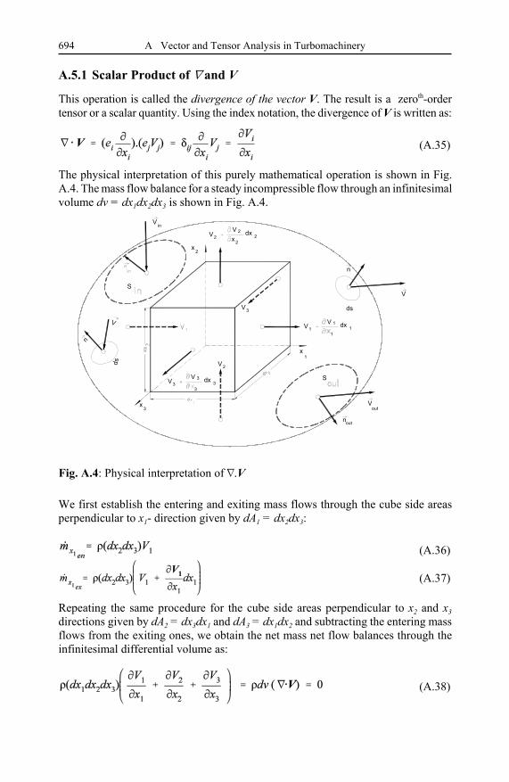
Fig. A.4: Physical interpretation of .V

(A.36)

(A.37)

(A.38)

A.5.1 Scalar Product of and V

This operation is called the divergence of the vector V. The result is a zeroth-ordertensor or a scalar quantity. Using the index notation, the divergence of V is written as:

The physical interpretation of this purely mathematical operation is shown in Fig.A.4. The mass flow balance for a steady incompressible flow through an infinitesimalvolume dv = dx1dx2dx3 is shown in Fig. A.4.

We first establish the entering and exiting mass flows through the cube side areasperpendicular to x1- direction given by dA1 = dx2dx3:

Repeating the same procedure for the cube side areas perpendicular to x2 and x3directions given by dA2 = dx3dx1 and dA3 = dx1dx2 and subtracting the entering massflows from the exiting ones, we obtain the net mass net flow balances through theinfinitesimal differential volume as:


(A.39)

(A.40)

(A.41)

(A.42)

(A.43)

The right hand side of Equation (A.38) is a product of three terms, the density , thedifferential volume dv and the divergence of the vector V. Since the first two termsare not zero, the divergence of the vector must disappear. As result, we find:

Equation (A.39) expresses the continuity equation for an incompressible flow, as wewill saw in Chapter 3.

A.5.2 Vector Product

This operation is called the rotation or curl of the velocity vector V. Its result is a first-order tensor or a vector quantity. Using the index notation, the curl of V iswritten as:

The curl of the velocity vector is known as vorticity, . As we will see later, thevorticity plays a crucial role in fluid mechanics. It is a characteristic of a rotationalflow. For viscous flows encountered in engineering applications, the curl isalways different from zero. To simplify the flow situation and to solve the equationof motion, as we discusseded in Chapter 3 later, the vorticity vector , canunder certain conditions, be set equal to zero. This special case is called theirrotational flow.

A.5.3 Tensor Product of and V

This operation is called the gradient of the velocity vector V. Its result is a secondtensor. Using the index notation, the gradient of the vector V is written as:

Equation (A.41) is a second order tensor with nine components and describes thedeformation and the rotation kinematics of the fluid particle. As we saw previously,the scalar multiplication of this tensor with the velocity vector, resulted in theconvective part of the acceleration vector, Eq. (A.32). In addition to the applicationswe discussed, can be applied to a product of two or more vectors by using theLeibnitz's chain rule of differentiation:

For U = V, Eq. (A.42) becomes or


Fig. A.5: Fluid element under a general three-dimensional stress condition

Equation (A.43) is used to express the convective part of the acceleration in terms ofthe gradient of kinetic energy of the flow.

A.5.4 Scalar Product of and a Second Order Tensor

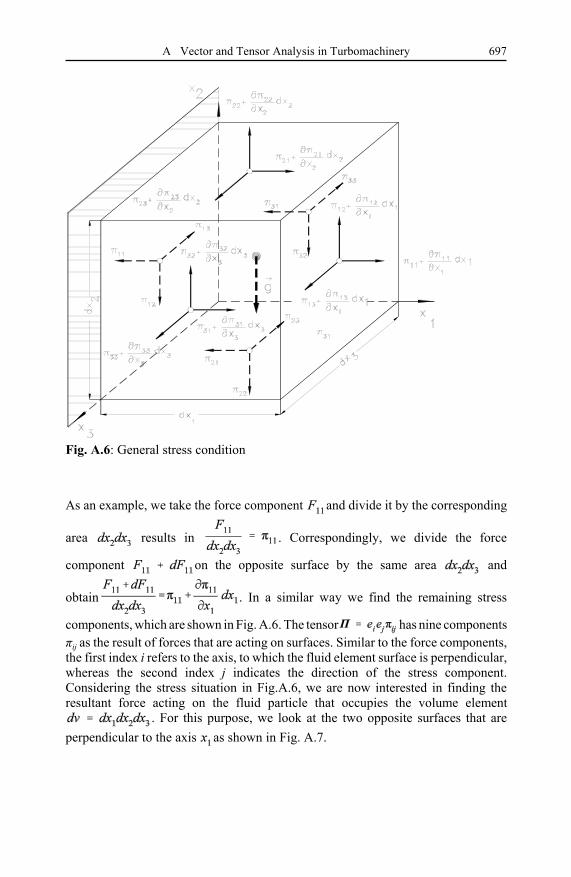
Consider a fluid element with sides dx1, dx2, dx3 parallel to the axis of a Cartesiancoordinate system, Fig.A.5. The fluid element is under a general three-dimensionalstress condition. The force vectors acting on the surfaces, which are perpendicular tothe coordinates x1, x2, and x3 are denoted by F1, F2, and F3,. The opposite surfaces aresubject to forces that have experienced infinitesimal changes F1 + dF1, F2 + dF2, andF3 + dF3. Each of these force vectors is decomposed into three components Fijaccording to the coordinate system defined in Fig. A.5. The first index i refers to theaxis, to which the fluid element surface is perpendicular, whereas the second indexj indicates the direction of the force component. We divide the individual componentsof the above force vectors by their corresponding area of the fluid element side. Theresults of these divisions exhibit the components of a second order stress tensorrepresented by as shown in Fig. A.6.


Fig. A.6: General stress condition

As an example, we take the force component and divide it by the corresponding

area results in . Correspondingly, we divide the force

component on the opposite surface by the same area and

obtain . In a similar way we find the remaining stress

components, which are shown in Fig. A.6. The tensor has nine componentsij as the result of forces that are acting on surfaces. Similar to the force components,

the first index i refers to the axis, to which the fluid element surface is perpendicular,whereas the second index j indicates the direction of the stress component. Considering the stress situation in Fig.A.6, we are now interested in finding theresultant force acting on the fluid particle that occupies the volume element

. For this purpose, we look at the two opposite surfaces that areperpendicular to the axis as shown in Fig. A.7.


Fig. A.7: Stresses on two opposite walls

As this figure shows, we are dealing with 3 stress components on each surface, fromwhich one on each side is the normal stress component such as and

. The remaining components are the shear stress components such as

and . According to Fig. A.7 the force balance in -directions is:

and in -direction, we find


(A.44)

(A.45)

(A.46)

Similarly, in , we obtain

Thus, the resultant force acting on these two opposite surfaces is:

In a similar way, we find the forces acting on the other four surfaces. The totalresulting forces acting on the entire surface of the element are obtained by adding the nine components. Defining the volume element , we divide the resultsby and obtain the resulting force vector that is acting on the volume element.

Since the stress tensor is written as:

it can be easily shown that:

The expression is a scalar differentiation of the second order stress tensor andis called the divergence of the tensor field . We conclude that the force vector actingon the surface of a fluid element is the divergence of its stress tensor. The stresstensor is usually divided into its normal- and shear stress parts. For an incompressiblefluid it can be written as


(A.47)

(A.48)

(A.49)

(A.50)

(A.51)

(A.52)

(A.53)

(A.54)

with Ip as the normal and T as the shear stress tensor. The normal stress tensor is aproduct of the unit tensor and the pressure p. Inserting Eq. (A.47) into(A.46) leads to

Its components are

A.5.5 Eigenvalue and Eigenvector of a Second Order Tensor

The velocity gradient expressed in Eq. (A.41) can be decomposed into a symmetric deformation tensor D and an antisymmetric rotation tensor :

A scalar multiplication of D with any arbitrary vector A may result in a vector, whichhas an arbitrary direction. However, there exists a particular vector V such that itsscalar multiplication with D results in a vector, which is parallel to V but has different magnitude:

with V as the eigenvector and the eigenvalue of the second order tensor D. Sinceany vector can be expressed as a scalar product of the unit tensor and the vector itself

, we may write:

Equation (A.52) can be rearranged as:

and its index notation gives:

or


(A.55)

(A.56)

(A.57)

(A.58)

(A.59)

(A.60)

(A.61)

(A.62)

(A.63)

Expanding Eq. (A.55) gives a system of linear equations,

A nontrivial solution of these Eq. (A.56) is possible if and only if the followingdeterminant vanishes:

or in index notation:

Expanding Eq. (A.58) results in

After expanding the above determinant, we obtain an algebraic equation in in thefollowing form

where and are invariants of the second order tensor D defined as:

The roots of Eq. (A.60) are known as the eigenvalues of the tensor D. Thesuperscript refers to the roots of Eq. (A.60) - not to be confused with thecomponent of a vector.


References

1. Aris, R.: Vector, Tensors and the Basic Equations of Fluid Mechanics. Prentice-Hall, Englewood Cliffs (1962)

2. Brand, L.: Vector and Tensor Analysis. John Wiley and Sons, New York (1947)3. Klingbeil, E.: Tensorrechnung für Ingenieure. Bibliographisches Institut,

Mannheim (1966)4. Lagally, M.: Vorlesung über Vektorrechnung, 3rd edn. Akademische Verlags-

gesellschaft, Leipzig (1944)5. Vavra, M.H.: Aero-Thermodynamics and Flow in Turbomachines. John Wiley &

Sons, Chichester (1960)

(B.1)

(B.2)

(B.3)

B Tensor Operations in Orthogonal CurvilinearCoordinate Systems

B.1 Change of Coordinate System

The vector and tensor operations we have discussed in the foregoing chapters wereperformed solely in rectangular coordinate system. It should be pointed out that wewere dealing with quantities such as velocity, acceleration, and pressure gradient thatare independent of any coordinate system within a certain frame of reference. In thisconnection it is necessary to distinguish between a coordinate system and a frame ofreference. The following example should clarify this distinction. In an absoluteframe of reference, the flow velocity vector may be described by the rectangularCartesian coordinate xi:

It may also be described by a cylindrical coordinate system, which is a non-Cartesiancoordinate system:

or generally by any other non-Cartesian or curvilinear coordinate system i thatdescribes the flow channel geometry:

By changing the coordinate system, the flow velocity vector will not change. Itremains invariant under any transformation of coordinates. This is true for any otherquantities such as acceleration, force, pressure- or temperature gradient. The conceptof invariance, however, is generally no longer valid if we change the frame ofreference. If, for example, the flow particles leave the absolute frame of reference(such as turbine or compressor stator blade channels) and enter a relative frame, forexample rotating turbine or compressor blade channels, its velocity will experiencea change as seen in Chapter 3. In this Chapter, we will pursue the concept of quantityinvariance and discuss the fundamentals needed for understanding the coordinatetransformation.

B Tensor Operations in Orthogonal Curvilinear Coordinate Systems704

(B.4)

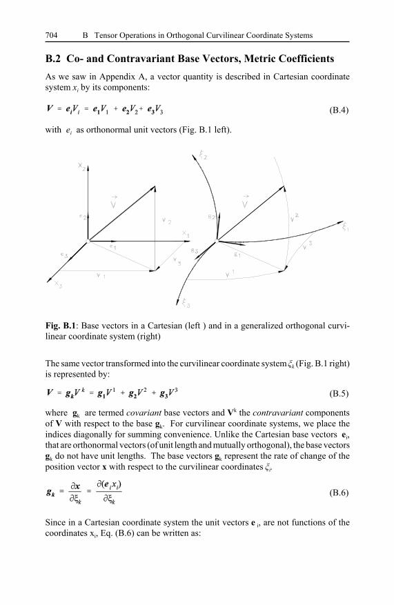
Fig. B.1: Base vectors in a Cartesian (left ) and in a generalized orthogonal curvi-linear coordinate system (right)

(B.5)

(B.6)

B.2 Co- and Contravariant Base Vectors, Metric CoefficientsAs we saw in Appendix A, a vector quantity is described in Cartesian coordinatesystem xi by its components:

with ei as orthonormal unit vectors (Fig. B.1 left).

The same vector transformed into the curvilinear coordinate system k (Fig. B.1 right)is represented by:

where gk are termed covariant base vectors and Vk the contravariant componentsof V with respect to the base gk. For curvilinear coordinate systems, we place theindices diagonally for summing convenience. Unlike the Cartesian base vectors ei,that are orthonormal vectors (of unit length and mutually orthogonal), the base vectorsgk do not have unit lengths. The base vectors gk represent the rate of change of theposition vector x with respect to the curvilinear coordinates i.

Since in a Cartesian coordinate system the unit vectors e i, are not functions of thecoordinates xi, Eq. (B.6) can be written as:

B Tensor Operations in Orthogonal Curvilinear Coordinate Systems 705

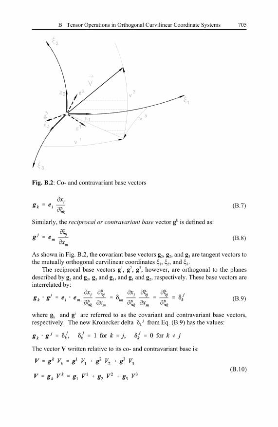
Fig. B.2: Co- and contravariant base vectors

(B.7)

(B.8)

(B.9)

(B.10)

Similarly, the reciprocal or contravariant base vector gk is defined as:

As shown in Fig. B.2, the covariant base vectors g2, g2, and g3 are tangent vectors tothe mutually orthogonal curvilinear coordinates 1, 2, and 3.

The reciprocal base vectors g1, g2, g3, however, are orthogonal to the planesdescribed by g2 and g3, g3 and g1, and g1 and g2, respectively. These base vectors areinterrelated by:

where gk and gj are referred to as the covariant and contravariant base vectors,respectively. The new Kronecker delta k

j from Eq. (B.9) has the values:

The vector V written relative to its co- and contravariant base is:


(B.11)

(B.12)

(B.13)

(B.14)

(B.15)

(B.16)

(B.17)

(B.18)

(B.19)

(B.20)

with the components Vk and V k as the covariant and contravariant components, respectively. The scalar product of covariant respectively contravariant base vectorsresults in the covariant and covariant metric coefficients:

The mixed metric coefficient is defined as

Using in curvilinear coordinate systems, its is often necessary to express the covariantbase vectors in terms of the contravariant ones and vice versa. To do this, we first assume that:

Generally the contravariant base vector can be written as

To find a direct relation between the base vectors, first the coefficient matrix Aij mustbe determined. To do so, we multiply Eq. (B.14) with gk scalarly:

This leads to . The right hand side is different from zero only if j = k, which means:

Introducing Eq. (B.16) into (B.14) results in a relation that expresses the contravariantbase vectors in terms of covariant base vectors:

The covariant base vector can also be expressed in terms of contravariant base vectorsin a similar way:

Multiply Eq. (B.l8) with (B.17) establishes a relationship between the covariant andcontravariant metric coefficients:

Applying the Kronecker delta on the right hand side results in:


(B.21)

(B.22)

(B.23)

(B.24)

(B.25)

(B.26)

(B.27)

B.3 Physical Components of a Vector

As mentioned previously, the base vectors gi or gj are not unit vectors. Consequentlythe co- and contravariant vector components Vj or Vj do not reflect the physicalcomponents of vector V. To obtain the physical components, first the correspondingunit vectors must be found. The covariant unit vectors are determined from:

Similarly, the contravariant unit vectors are:

where gi*, represents the unit base vector, gi the absolute value of the base vector.

The expression (ii) denotes that no summing is carried out, whenever the indices areenclosed within parentheses. The vector can now be expressed in terms of its unitbase vectors and the corresponding physical components:

Thus the covariant and contravariant physical components can be easily obtainedfrom:

B.4 Derivatives of the Base Vectors, Christoffel Symbols

In a curvilinear coordinate system, the base vectors are generally functions of thecoordinates itself. This fact must be considered while differentiating the base vectors. Consider the derivative:

The comma in Eq. (B.25) followed by the lower index j represents the derivative ofthe covariant base vector gi with respect to the coordinate j. Similar to Eq.(B.7), theunit vector ek can be written as:

Introducing Eq. (B.26) into (B.25) yields:

with ijn, and i jn as the Christoffel symbol of first and second kind, respectively

with the definitions:


(B.28a)

(B.28b)

(B.29)

(B.30a)

(B.30b)

(B.31)

It follows from (B.28a) that the Christoffel symbols of the second kind are related tothe first kind by:

Because of (B.28b) and, for the sake of simplicity, in what follows, we will use theChristoffel symbol of second kind . Thus, the derivative of the contravariant base

vector reads:

The Christoffel symbols are then obtained by expanding Eq. (B.28a):

The fact that the only non-zero elements of the matrix are the diagonal elementsallows the modification of Eq. (B.30a) to:

In Eq. (B.30a), the Christoffel symbols are symmetric in their lower indices. Again,note that a repeated index in parentheses in an expression such as g(kk) does notsubject to summation.

B.5 Spatial Derivatives in Curvilinear Coordinate System

The differential operator is in curvilinear coordinate system defined as:

In this Chapter, the operator will be applied to different arguments such as zeroth,first and second order tensors.

B.5.1 Application of to Zeroth Order Tensor Functions

If the argument is a zeroth order tensor which is a scalar quantity such as pressure ortemperature, the results of the operation is the gradient of the scalar field which is avector quantity:


(B.32)

(B.33a)

(B.33b)

(B.34a)

(B.34b)

The abbreviation “,i ” refers to the derivative of the argument, in this case p, withrespect to the coordinate i .

B.5.2 Application of to First and Second Order Tensor Functions

Scalar Product: If the argument is a first order tensor such as a velocity vector, theorder of the resulting tensor depends on the operation character between the operator

and the argument. If the argument is a product of two or more quantities, chain ruleof differentiation is applied. Thus, the divergence of the vector filed V is:

Implementing the Christoffel symbol from (B.27), the results of the above operationsare the divergence of the vector V. It should be noticed that a scalar operation leadsto a contraction of the order of tensor on which the operator is acting. The scalaroperation in (B.33a) leads to:

Cross Product: This vector operation yields the rotation or curl of a vector field as:

Because of the antisymmetric character of a cross product and the symmetry of theChristoffel symbols in their lower indices, the second term on the right-hand side of (B.34a), namely . As a result, we find

with as the permutation symbol that functions similar to the one for Cartesiancoordinate system withe the difference that:


(B.35)

(B.36)

(B.37)

(B.38)

(B.39)

(B.40)

with as the determinant of the matrix of covariant metric coefficients.

Tensor Product: The gradient of a first order tensor such as the velocity vector V isa second order tensor. Its index notation in a curvilinear coordinate system is:

Divergence of a Second Order Tensor: A scalar operation that involves and asecond order tensor, such as the stress tensor or deformation tensor D, results in afirst order tensor which is a vector:

The right hand side of (B.37) is reduced to:

By calculating the shear forces using the Navier-Stokes equation, the secondderivative, the Laplace operator , is needed:

This operator applied to the velocity vector yields:

B.6 Application Example 1: Inviscid Incompressible Flow Motion

As the first application example, the equation of motion for a steady, incompressibleand inviscid flow is transformed into a cylindrical coordinate system, where it isdecomposed into components in r, and z-directions. Neglecting the gravitationalforce , the coordinate invariant version of the equation is written as:


(B.41)

(B.42)

(B.43)

(B.44)

(B.45)

(B.46)

(B.47)

(B.48)

(B.49)

The transformation and decomposition procedure is shown in the following steps.

B.6.1 Equation of Motion in Curvilinear Coordinate Systems

The second order tensor on the left hand side can be obtained using Eq. (B.35):

The scalar multiplication of (B.42) with the velocity vector V leads to:

Introducing the mixed Kronecker delta into (B.43), we get:

For an orthogonal curvilinear coordinate system the mixed Kronecker delta is:

Taking this into account, Eq. (B.43)

and rearranging the indices, we obtain the convective part of the Navier-Stokesequations as:

The pressure gradient on the right hand side of Eq. (B.40) is calculated form Eq. (B.32):

Replacing the contravariant base vector with the covariant one using Eq. (B.17) leadsto:


(B.50)

(B.51)

(B.52)

(B.53)

(B.54)

(B.55)

(B.56)

Incorporating Eqs. (B.46) and (B.49) into Eq. (B.40) yields:

In i-direction, the equation of motion is:

B.6.2 Special Case: Cylindrical Coordinate System

To transfer Eq. (B.40) into any arbitrary orthogonal curvilinear coordinate system,first the coordinate system must be specified. The cylindrical coordinate system isrelated to the Cartesian coordinate system by:

The curvilinear coordinate system is represented by:

B.6.3 Base Vectors, Metric Coefficients

The base vectors are calculated from Eq. (B.7).

Equation (B.54) decomposed in its components yields:

Performing the differentiation of the terms in Eq. (B.55) yields:


(B.57)

(A.57a)

(A.57b)

(B.59)

(B.60)

(B.61)

The co- and contravariant metric coefficients are:

The contravariant base vectors are obtained from:

Since the mixed metric coefficient are zero, (B.57a) reduces to:

B.6.4 Christoffel Symbols

The Christoffel symbols are calculated from Eq. (B.30b)

To follow the calculation procedure, one zero- element and one non-zero element arecalculated:

All other elements are calculated similarly. They are shown in the following matrices:


(B.62)

(B.63)

(B.64)

(B.65)

(B.66)

(B.67)

(B.68)

(B.69)

(B.70)

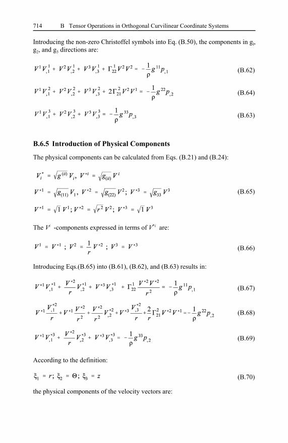
Introducing the non-zero Christoffel symbols into Eq. (B.50), the components in gl,g2, and g3 directions are:

B.6.5 Introduction of Physical Components

The physical components can be calculated from Eqs. (B.21) and (B.24):

The Vi -components expressed in terms of V*i are:

Introducing Eqs.(B.65) into (B.61), (B.62), and (B.63) results in:

According to the definition:

the physical components of the velocity vectors are:


(B.71)

(B.72)

(B.73)

(B.74)

and insert these relations into Eqs. (B.66) to (B.68), the resulting components in r, ,and z directions are:

B.7 Application Example 2: Viscous Flow Motion

As the second application example, the Navier-Stokes equation of motion for asteady, incompressible flow with constant viscosity is transferred into a cylindricalcoordinate system, where it is decomposed into its three components r, , z. Thecoordinate invariant version of the equation is written as:

The second term on the right hand side of Eq. (B.73) exhibits the shear stress force. It was treated in section B.5, Eq. (B.39) and is the only term that has been added tothe equation of motion for inviscid flow, Eq. (B.40).

B.7.1 Equation of Motion in Curvilinear Coordinate Systems

The transformation and decomposition procedure is similar to the example in sectionB. 6. Therefore, a step by step derivation is not necessary.


(B.75)

(B.76)

B.7.2 Special Case: Cylindrical Coordinate System

Using the Christoffel symbols from section B.6.4 and the physical components fromB.6.5, and inserting the corresponding relations these relations into Eq. (B.74), theresulting components in r, , and z directions are:

References

1. Aris, R.: Vector, Tensors and the Basic Equations of Fluid Mechanics. Prentice-Hall, Inc., Englewood Cliffs (1962)

2. Brand, L.: Vector and Tensor Analysis. John Wiley & Sons, New York(1947)

3. Klingbeil, E.: Tensorrechnung für Ingenieure. Bibliographisches Institut, Mann-heim (1966)

4. Lagally, M.: Vorlesung über Vektorrechnung, 3rd edn. Akademische Verlags-gesellschaft, Leipzig (1944)

5. Vavra, M.H.: Aero-Thermodynamics and Flow in Turbomachines. John Wiley& Sons, Chichester (1960)

Index

1/7-th boundary layerdisplacement thickness 631energy deficiency thickness 631,

633integral equation 635length scale 670momentum deficiency thickness

631re-attachment 661, 664, 667,

668, 670separation 667wall influence 655

Algebraic Model 585Baldwin-Lomax 585Cebeci-Smith 584Prandtl Mixing Length 578

Anemometer 519Averaging 560

conservation equations 561continuity equation 561mechanical energy equation 562Navier-stokes equation 561total enthalpy equation 565

Axial vector 24

Base vectors 704, 707contravariant 704covariant 704reciprocal 704

Becalming 535Bernoulli equation 39, 584Bio-Savart law 195Blade design 267

Assessment of 289Bézier 285camberline coordinates 285

conformal transformation 267Blade design using Bézier function

283Blade force, inviscid flow

circulation 145–149, 162–164,168, 171

lift coefficient 149, 153,155–158, 166, 168

lift force 145–149, 153Blade force, viscous flow

drag coefficient 153, 157drag force 152, 153drag-lift ratio 157, 158lift coefficient 149, 153,

155–158, 166, 168lift force 145–149, 153lift-solidity coefficient 153–155,

162–164, 166–171no-slip condition 150optimum solidity 158, 160periodic wake flow 150total pressure loss coefficient

150Blending function 590Boundary layer 580

buffer layer 580bypass 517experimental simulation of

unsteady 527intermittency function 519logarithmic layer 580natural 535outer layer 581transitional 581unsteady Boundary 525viscous sublayer 580von Karman constant 583

Index718

wake function 581wake induced 535

Boundary layer theoryBlasius solution 624concept of 619viscous layer 619

Boussinesq 577relationship 577

Bypass transition 517

Calmed region 532Cascade process 546Cauchy-Poisson law 35Circulation function 389Co- and contravariant Base Vectors

703Combustion chamber 80, 84, 341, 346,

348, 372chamber heat transfer 376mass flow transients 373temperature transients 374

Compound lean 309–311, 313–315Compression waves 100Compressor corrections

blade thickness effect 408circulation function 389–396,

408Mach number effect 394, 407maximum velocity 386,

389–391, 393, 395optimum flow condition 389profile losses 385, 396, 407, 408Reynolds number effect 408secondary flow losses 385, 403,

406shock losses 384, 385, 397, 400,

403Compressor blade design 2, 265, 272,

273, 275, 279base profile 2, 265, 276–279,

281, 285, 286DCA, MCA 2, 267, 272, 273,

279, 281double circular arc (DCA) 272for High Subsonic Mach Number

279graphic design of camberline 284induced velocity 274, 275

Joukowsky transformation 267maximum thickness 273, 277,

278, 285multi-circular arc (MCA) profiles

272NACA-67 profiles 2, 272, 274subsonic compressor 271, 273,

279summary, simple compressor

blade design steps 279superimposing the base profile

276, 278supersonic compressor 282vortex distribution 274

Compressor diffusion factorcompressibility effect on, 393,

395, 396, 403diffusion factor 385–388,

391–393, 395–397, 403–408,415, 416, 420, 422

modified diffusion factor 385,391, 403–405, 415, 416

Compressor stage 341, 348, 353Conformal transformation

circle-cambered AirfoilTransformation 271

circle-ellipse Transformation 268circle-symmetric Airfoil

Transformation 269Convergent nozzle 91, 92Cooled turbine 60, 82Coriolis acceleration 51Correlations

autocorrelation 549coefficient 548osculating parabola 553single point 548tensor 548two-point correlation 548

Covariance 549Critical state 88, 97, 103Cross-section change 93Curvilinear coordinate Systems 703,

712base vectors 712metric coefficients 712spatial Derivatives 708

Index 719

Deformation 34, 700Density change 91Derivative 690

material 690substantial 690temporal 690

Description 15Lagrangian description 16material 15spatial 15

Diabatic expansion 351Diabatic processes 351Diabatic turbine module 467Differential operator 691Differential operators 690Diffusers 220

concave and convex 225configurations 221conversion coefficient 224induced Velocity 194opening angle 226pressure recovery 220, 222recovery factor 224vortex generator edges 226

Diffusivity 546Direct Navier-Stokes simulations 577Dissipation 575, 576, 577

dissipation 564energy 545equation 554exact derivation of 577function 43kinetic Energy 576parameter 557range 556turbulence 554turbulent 564viscous 564

Eddy viscosity 578Effect of stage parameters on

degree of reaction 130, 131,133–135, 137, 139, 140

flow coefficient 129, 137, 139,140, 142

load coefficient 129, 130,136–143

Efficiency 452

Efficiency of multi-stageturbomachines 233

heat recovery 233, 234, 237, 239infinitesimally small expansion

235isentropic efficiency 239–242polytropic efficiency 233, 235,

239–242recovery factor 236–239reheat 233, 234, 240, 241reheat factor 240, 241

Einstein summation convention 37Einstein’s summation 687Energy balance in stationary frame 42

dissipation function 43mechanical energy 42thermal energy balance 45

Energy cascade process 546, 547Energy spectral function 558Energy spectrum 555

dissipation range 556large eddies 555

Energy transfer 123–125compressor stage 123, 125,

127–129, 137, 139, 143Euler turbine equation 127turbine row 127, 128, 136turbine stage 124, 127, 128,

135–137, 139Ensemble averaging 530Entropy balance 49Equation 570

turbulence kinetic Energy 570Euler equation of motion 38Expansion waves 98, 100, 121Expansion

adiabatic 348

Falkner-Skan equation 629Fanno 101, 106–109Fanno line 101, 106–109Faulkner-Skan equation 628Flow coefficients 453Fluctuation kinetic energy 566Frame indifferent quantities 34Free turbulent flow 545Friction stress tensor 35Frozen turbulence 551

Index720

Gas dynamic functions 97Gas turbines

components 473compressed air storage 473design 473dynamic 473multi-spool 475performance 473power generation 473process 473shutdown 495single spool 500startup 495three-spool 493twin-spool 473ultra high efficiency 485

Gaussian distribution 534Generalized lift-solidity coefficient

162, 166lift-solidity coefficient 153–155,

162–164, 166–171turbine rotor 163, 168, 170turbine stator 159, 162–164, 166

Generic component configurationadiabatic compressor 348adiabatic turbine 349, 350compressor 341, 342, 346, 348,

350–355diabatic turbine 350heat exchangers 346inlet, exhaust, pipe 345schematic 350, 353, 355turbine 341–343, 347–356

Generic modelingcomponents 2heat exchangers 346inlet, exhaust, pipe 345

Geometry parameter 458

Heat transfer 376conduction 376convection 373Nusselt number 660radiation 376Stanton number 660thermography 660

Hot wire anemometry 653aliasing effect 656

analog/digital converter 656constant current (CC) mode 654constant-temperature (CT) mode

654cross-wire 654folding frequency 656Nyquist-frequency 656sample frequency 656sampling rate 656signal conditioner 656single wire 653single, cross and three-wire

probes 653single-wire 653three-wire 654

Incidence and deviation 241cascade parameters 255complex plane 242complex velocity potential 243conformal transformation 241,

242, 244, 250, 261deviation 241, 255, 256,

258–261, 263infinitely thin circular arc 250optimum incidence 256, 257,

259singularities 244, 247transformation function 244, 247

Incompressibility condition 31Index Notation 686, 687Integral balances 59

axial moment 70energy 72, 73, 75, 77, 78linear momentum 59, 61mass flow 60moment of momentum 66, 68,

70, 71, 73reaction force 65, 66, 68shaft power 75, 78, 101

Intermittency 533averaged 534curved plate 521ensemble-averaged 533flat plate 524function 653Intermittency into Navier Stokes

Equations 536

Index 721

maximum 533minimum 534modeling 524

Irreversibility 72, 79, 84total pressure loss 79, 86, 87

Isentropic row load coefficients 452Isotropic turbulence 560Isotropy 547

Jacobian 16–21, 25, 26function 16–19, 21, 25, 26functional determinant 19material derivative 17, 19, 26transformation vector 16, 17,

18,19–21, 25Joukowsky transformation 265

Kinematics of fluid motion 15deformation tensor 21material volume 17, 18, 20, 25rotation tensor 24, 25rotation vector 24, 25translation 21, 23

Kinetic energy 556, 560, 566Kolmogorov 546

eddies 546first hypothesis 556hypothesis 546inertial subrange 555, 556length scale 555scales 555second hypothesis 557time scale 555universal equilibrium 546velocity scale 555

Kronecker delta 705Kronecker tensor 35Kutta-Joukowsky Transformation 268

Laminar Boundary 624Blasius equation 625Faulkner-Skan equation 628Hartree 628Polhausen Approximate 629

Laval nozzle 95, 96, 98, 109Linear wall function 580Losses due to blade profile

diffusion factor 185

effect of Reynolds number 186integral equation 179, 181momentum equation 187–189,

205, 212, 214profile loss 176–178, 182,

184–186, 192, 217total pressure loss 176, 182, 183,

190, 194, 197, 198, 200, 201,203, 205, 223, 227

Losses due to exit kinetic energy,effect of

degree of reaction 208–212exit flow angle 176, 177, 203,

211–213, 216, 222stage load coefficient 209–211

Losses due to leakage flow in shrouds 204

induced drag 194, 196–199, 201load function 198–200losses due to secondary flows

192mixing loss 190–192, 217–219

Losses due to trailing edge ejectionmixing loss 190–192, 217–219optimum mixing losses 219

Mach number 88Material acceleration 692Material derivative 17Metric coefficients 703

contravariant 705covariant 705mixed metric coefficient 705

Mixing length hypothesis 578Modeling 372

combustion chambers 372Modeling of inlet, exhaust, and pipe

system 357continuity 358inlet 357momentum 358physical and mathematical 357pipe 357, 358, 361, 362total pressure 358, 359

Modeling the compressor dynamicperformance

active surge prevention 430

Index722

module level 2: row-by-rowadiabatic calculation 429

module level 3: row-by-rowdiabatic compression 436

simulation example 427, 431simulation of compressor surge

432Modeling turbomachinery components

combustion chambers 341, 346,348

high pressure compressor 342,351, 354, 355

high pressure turbine 341, 342low pressure compressor 342,

353, 355low pressure turbine 342, 348,

354modular configuration 342, 351,

353, 355, 356recuperators 346twin-spool engine 342

Modular configuration 2, 342, 351,353, 355, 356

control systems 342, 352shafts 352, 355valves 342, 352

Momentum balance in stationary frame 32

Natural transition 517Navier-Stokes 569

equations 547, 548, 552, 561,569, 570

operator 569Navier-Stokes equation for

compressible fluids 36Newtonian fluids 35Nnormal shock 99, 109–115, 117Nonlinear dynamic simulation 323

numerical treatment 339one-dimensional approximation

331Predictor-corrector 339Runge-Kutta 339thermo-fluid dynamic equations.

328

time dependent equation ofcontinuity 331

time dependent equation ofenergy 334

time dependent equation ofmotion 332

Numerical treatment 330, 339Nusselt number 660

Oblique shock 109, 115, 116, 118, 121Orthonormal vectors 704Osculating parabola 553Over expansion 98

Peclet number 651effective 652turbulent 651

Physical components of a Vector 706Physical components of vector 706Plenum 343Pohlhausen 629

profiles 630slope of the velocity profiles 630velocity profiles 630

Polytropic load coefficients 452Power law 647Prandtl 619

1/7–th power lawboundary layer 619boundary layer approximation

619boundary layer theory 624effective Prandtl number 652experimental observations 619mixing length 650mixing length model 653molecular Prandtl number 652number 651turbulent Prandtl number 651

Prandtl mixing length hypothesis 580Prandtl number 651

effective 652turbulent 651

Preheater 367Principle of material objectivity 34

Index 723

Radial equilibrium 291, 295, 298–300,309, 316

derivation of equilibriumequation 292

free vortex flow 291, 316, 317Rayleigh 101, 103–106, 108, 109Recuperator 346, 369

heat Transfer Coefficient 371recuperators 367

Reynolds transport theorem 25, 27Richardson energy cascade 547Rotating frame

continuity equation in 52energy equation in 55equation of motion in 53

Rotation 700Rotation tensor 34

Scalar product of 693Scales of turbulence

length 547of the smallest eddy 547time 547time scale 546time scale of eddies 548

Shear viscosity 36Shock tube, dynamic behavior 359

mass flow transients 361, 364pressure transients 361, 362shock tube dynamic behavior

361temperature transients 362–364

Shocks 98, 101, 113, 115, 117detached shock 117Hugoniot relation 111–113normal shock wave 99, 109, 115oblique shock wave 115Prandtl-Meyer expansion 118,

121strong shock 112, 114, 115, 117weak shock 114, 117

Similarity condition 627Spatial differential 691Spectral tensor 558Stage parameters 129, 138, 140

circumferential velocity ratio 139, 141

degree of reaction 130, 131,133–135, 137, 139, 140

flow coefficient 129, 137, 139,140, 142

load coefficient 129, 130,136–143

meridional velocity ratio 139,141

Stage-by-stage and row-by-rowadiabatic compression 409

calculation of compressionprocess 409

generation of steady stateperformance map 418

off-design efficiency calculation 415

rotating stall 420–423, 430–433row-by-row adiabatic

compression 409, 411, 423surge 385, 420–424, 428–434surge limit 420, 422, 423, 428,

434Stanton number 660Streamline curvature method 291, 292,

300, 301, 306, 309, 310, 312, 313application of 292, 300, 310derivation of equilibrium

equation 292examples 306forced vortex flow 317free vortex flow 291, 316special cases 292, 316step-by-step solution procedure

302Stress tensor 34

apparent 547Substantial change 690

Taylor 553eddies 551frozen turbulence 551hypothesis 551micro length scale 553time scale 553

Temporal change 690Tensor 568, 685

contraction 686, 689

Index724

deformation 573eigenvalue 700eigenvector 700first-order 685friction 569friction stress 563principal Axis 700product 687, 678Reynolds stress 568rotation 585second order 686zeroth-order 685

Tensor product of and V 695, 702Thermal efficiency of gas turbines

477, 478, 482–484, 508, 509improvement of 483UHEGT 508

Transition 535Turbine 123–143, 445

adiabatic design 447adiabatic expansion 449axial 123, 124, 128, 129, 131,

132, 137–140, 142blade design 283blade design using Bezier curve

285design and off-design behavior

459expansion process 448extreme low mass flows 456modeling 462off-design efficiency calculation

454off-design performance 447off-design primary loss

coefficient 454radial 128, 131, 132, 134, 137,

139, 140, 143row-by-row diabatic expansion

465stage 123–125, 127–131,

133–143, 342, 348–350stage-by-stage 447velocity parameter 461

Turbulence 547anisotropic 555convective diffusion 575

correlations 548diffusion 546free turbulence 545homogeneous 547isotropic 547, 556kinetic energy 571length and time Scales 547production 575production of turbulence kinetic

energy 575type of 545, 547viscous diffusion 546viscous dissipation 575wall turbulence 545

Turbulence length 578Turbulence model 545, 578

algebraic model 578Baldwin-lomax algebraic model

585Cebeci-smith algebraic model

584one-equation model by prandtl

586Prandtl mixing length 578standard k- vs k- 595two-equation k- model 587two-equation k- -model 589two-equation k- -sst-model 590

Turbulent flow 581fully developed 581

Turbulent kinetic energy 571

Universal equilibrium 546Unsteady boundary layer 657

Strouhal number 661wake generator 661

Variation of 670Length Scale 670Pressure Gradient 671

Vector 685cross product 687scalar product 687tensor product 688

Vector product 695Velocity scales 578Velocity spectrum tensor 558

Index 725

Ventilation power 457Viscous diffusion 546Viscous sublayer 580von Kármán 635

integral equation 635von Kármán constant 583

Vortex 547Vorticity, 695

Wave number space 558, 559Weinig, conformal transformation 241

Zweifel number 161

a vector and tensor analysis in turbomachinery fluid mechanics978-3-642-24675-3/1.pdf · a vector...

Documents