A User’s Guide to Support Vector Machines

Asa Ben-HurDepartment of Computer Science

Colorado State University

Jason WestonNEC Labs America

Princeton, NJ 08540 USA

Abstract

The Support Vector Machine (SVM) is a widely used classifier. And yet, obtaining the bestresults with SVMs requires an understanding of their workings and the various ways a user caninfluence their accuracy. We provide the user with a basic understanding of the theory behindSVMs and focus on their use in practice. We describe the effect of the SVM parameters on theresulting classifier, how to select good values for those parameters, data normalization, factorsthat affect training time, and software for training SVMs.

1 Introduction

The Support Vector Machine (SVM) is a state-of-the-art classification method introduced in 1992by Boser, Guyon, and Vapnik [1]. The SVM classifier is widely used in bioinformatics (and otherdisciplines) due to its high accuracy, ability to deal with high-dimensional data such as gene ex-pression, and flexibility in modeling diverse sources of data [2].

SVMs belong to the general category of kernel methods [4, 5]. A kernel method is an algorithmthat depends on the data only through dot-products. When this is the case, the dot product canbe replaced by a kernel function which computes a dot product in some possibly high dimensionalfeature space. This has two advantages: First, the ability to generate non-linear decision boundariesusing methods designed for linear classifiers. Second, the use of kernel functions allows the user toapply a classifier to data that have no obvious fixed-dimensional vector space representation. Theprime example of such data in bioinformatics are sequence, either DNA or protein, and proteinstructure.

Using SVMs effectively requires an understanding of how they work. When training an SVMthe practitioner needs to make a number of decisions: how to preprocess the data, what kernel touse, and finally, setting the parameters of the SVM and the kernel. Uninformed choices may resultin severely reduced performance [6]. We aim to provide the user with an intuitive understandingof these choices and provide general usage guidelines. All the examples shown were generatedusing the PyML machine learning environment, which focuses on kernel methods and SVMs, andis available at http://pyml.sourceforge.net. PyML is just one of several software packages thatprovide SVM training methods; an incomplete listing of these is provided in Section 9. Moreinformation is found on the Machine Learning Open Source Software website http://mloss.organd a related paper [7].

1

w

wTx + b < 0

wTx + b > 0

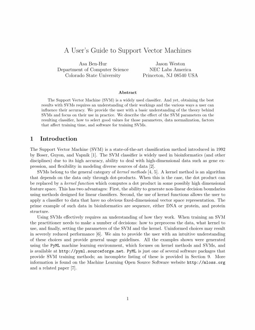
Figure 1: A linear classifier. The decision boundary (points x such that wTx + b = 0) divides theplane into two sets depending on the sign of wTx + b.

2 Preliminaries: Linear Classifiers

Support vector machines are an example of a linear two-class classifier. This section explainswhat that means. The data for a two class learning problem consists of objects labeled withone of two labels corresponding to the two classes; for convenience we assume the labels are +1(positive examples) or −1 (negative examples). In what follows boldface x denotes a vector withcomponents xi. The notation xi will denote the ith vector in a dataset {(xi, yi)}ni=1, where yi is thelabel associated with xi. The objects xi are called patterns or examples. We assume the examplesbelong to some set X . Initially we assume the examples are vectors, but once we introduce kernelsthis assumption will be relaxed, at which point they could be any continuous/discrete object (e.g.a protein/DNA sequence or protein structure).

A key concept required for defining a linear classifier is the dot product between two vectors,also referred to as an inner product or scalar product, defined as wTx =

∑iwixi. A linear classifier

is based on a linear discriminant function of the form

f(x) = wTx + b. (1)

The vector w is known as the weight vector, and b is called the bias. Consider the case b = 0first. The set of points x such that wTx = 0 are all points that are perpendicular to w and gothrough the origin — a line in two dimensions, a plane in three dimensions, and more generally, ahyperplane. The bias b translates the hyperplane away from the origin. The hyperplane

{x : f(x) = wTx + b = 0} (2)

divides the space into two: the sign of the discriminant function f(x) denotes the side of thehyperplane a point is on (see 1). The boundary between regions classified as positive and negative

2

is called the decision boundary of the classifier. The decision boundary defined by a hyperplane issaid to be linear because it is linear in the input examples (c.f. Equation 1). A classifier with alinear decision boundary is called a linear classifier. Conversely, when the decision boundary of aclassifier depends on the data in a non-linear way (see Figure 4 for example) the classifier is saidto be non-linear.

3 Kernels: from Linear to Non-Linear Classifiers

In many applications a non-linear classifier provides better accuracy. And yet, linear classifiers haveadvantages, one of them being that they often have simple training algorithms that scale well withthe number of examples [9, 10]. This begs the question: Can the machinery of linear classifiers beextended to generate non-linear decision boundaries? Furthermore, can we handle domains suchas protein sequences or structures where a representation in a fixed dimensional vector space is notavailable?

The naive way of making a non-linear classifier out of a linear classifier is to map our data fromthe input space X to a feature space F using a non-linear function φ : X → F . In the space F thediscriminant function is:

f(x) = wTφ(x) + b. (3)

Example 1 Consider the case of a two dimensional input-space with the mapping

φ(x) = (x21,√

2x1x2, x22)T,

which represents a vector in terms of all degree-2 monomials. In this case

wTφ(x) = w1x21 +√

2w2x1x2 + w3x22,

resulting in a decision boundary for the classifier, f(x) = wTx+b = 0, which is a conic section (e.g.,an ellipse or hyperbola). The added flexibility of considering degree-2 monomials is illustrated inFigure 4 in the context of SVMs.

The approach of explicitly computing non-linear features does not scale well with the numberof input features: when applying the mapping from the above example the dimensionality of thefeature space F is quadratic in the dimensionality of the original space. This results in a quadraticincrease in memory usage for storing the features and a quadratic increase in the time required tocompute the discriminant function of the classifier. This quadratic complexity is feasible for lowdimensional data; but when handling gene expression data that can have thousands of dimensions,quadratic complexity in the number of dimensions is not acceptable. Kernel methods solve thisissue by avoiding the step of explicitly mapping the data to a high dimensional feature-space.Suppose the weight vector can be expressed as a linear combination of the training examples, i.e.w =

∑ni=1 αixi. Then:

f(x) =n∑i=1

αixTi x + b.

In the feature space, F this expression takes the form:

f(x) =n∑i=1

αiφ(xi)Tφ(x) + b.

3

The representation in terms of the variables αi is known as the dual representation of the decisionboundary. As indicated above, the feature space F may be high dimensional, making this trickimpractical unless the kernel function k(x,x′) defined as

k(x,x′) = φ(x)Tφ(x′)

can be computed efficiently. In terms of the kernel function the discriminant function is:

f(x) =n∑i=1

αik(x,xi) + b . (4)

Example 2 Let’s go back to the example of φ(x) = (x21,√

2x1x2, x22)T, and show the kernel asso-

ciated with this mapping:

φ(x)Tφ(z) = (x21,√

2x1x2, x22)T(z2

1 ,√

2z1z2, z22)

= x21z

21 + 2x1x2z1z2 + x2

2z22

= (xTz)2.

This shows that the kernel can be computed without explicitly computing the mapping φ.

The above example leads us to the definition of the degree-d polynomial kernel:

k(x,x′) = (xTx′ + 1)d. (5)

The feature space for this kernel consists of all monomials up to degree d, i.e. features of the form:xd11 x

d22 · · ·xdm

m where∑m

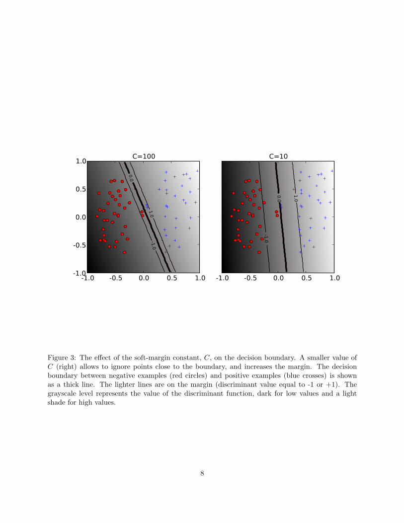
i=1 di ≤ d. The kernel with d = 1 is the linear kernel, and in that case theadditive constant in Equation 5 is usually omitted. The increasing flexibility of the classifier as thedegree of the polynomial is increased is illustrated in Figure 4. The other widely used kernel is theGaussian kernel defined by:

k(x,x′) = exp(−γ||x− x′||2) , (6)

where γ > 0 is a parameter that controls the width of Gaussian. It plays a similar role as the degreeof the polynomial kernel in controlling the flexibility of the resulting classifier (see Figure 5).

We saw that a linear decision boundary can be “kernelized”, i.e. its dependence on the datais only through dot products. In order for this to be useful, the training algorithms needs tobe kernelizable as well. It turns out that a large number of machine learning algorithms can beexpressed using kernels — including ridge regression, the perceptron algorithm, and SVMs [5, 8].

4 Large Margin Classification

In what follows we use the term linearly separable to denote data for which there exists a lineardecision boundary that separates positive from negative examples (see Figure 2). Initially we willassume linearly separable data, and later indicate how to handle data that is not linearly separable.

4

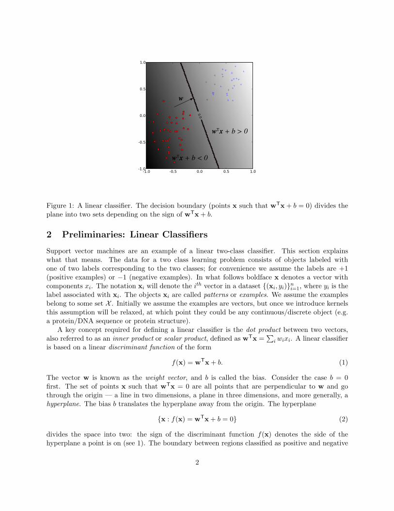
margin

Figure 2: A linear SVM. The circled data points are the support vectors—the examples that areclosest to the decision boundary. They determine the margin with which the two classes areseparated.

4.1 The Geometric Margin

In this section we define the notion of a margin. For a given hyperlane we denote by x+(x−) theclosest point to the hyperpalne among the positive (negative) examples. The norm of a vector wdenoted by ||w|| is its length, and is given by

√wTw. A unit vector w in the direction of w is given

by w/||w|| and has ||w|| = 1. From simple geometric considerations the margin of a hyperplane fwith respect to a dataset D can be seen to be:

mD(f) =12wT(x+ − x−) , (7)

where w is a unit vector in the direction of w, and we assume that x+ and x− are equidistant fromthe decision boundary i.e.

f(x+) = wTx+ + b = a

f(x−) = wTx− + b = −a (8)

for some constant a > 0. Note that multiplying our data points by a fixed number will increasethe margin by the same amount, whereas in reality, the margin hasn’t really changed — we justchanged the “units” with which we measure it. To make the geometric margin meaningful we fixthe value of the decision function at the points closest to the hyperplane, and set a = 1 in Eqn. (8).Adding the two equations and dividing by ||w|| we obtain:

mD(f) =12wT(x+ − x−) =

1||w||

. (9)

5

4.2 Support Vector Machines

Now that we have the concept of a margin we can formulate the maximum margin classifier. Wewill first define the hard margin SVM, applicable to a linearly separable dataset, and then modifyit to handle non-separable data. The maximum margin classifier is the discriminant function thatmaximizes the geometric margin 1/||w|| which is equivalent to minimizing ||w||2. This leads to thefollowing constrained optimization problem:

minimizew,b

12 ||w||

2

subject to: yi(wTxi + b) ≥ 1 i = 1, . . . , n . (10)

The constraints in this formulation ensure that the maximum margin classifier classifies each ex-ample correctly, which is possible since we assumed that the data is linearly separable. In practice,data is often not linearly separable; and even if it is, a greater margin can be achieved by allowingthe classifier to misclassify some points. To allow errors we replace the inequality constraints inEqn. (10) with

yi(wTxi + b) ≥ 1− ξi i = 1, . . . , n ,

where ξi ≥ 0 are slack variables that allow an example to be in the margin (0 ≤ ξi ≤ 1, also calleda margin error) or to be misclassified (ξi > 1). Since an example is misclassified if the value of itsslack variable is greater than 1,

∑i ξi is a bound on the number of misclassified examples. Our

objective of maximizing the margin, i.e. minimizing 12 ||w||

2 will be augmented with a term C∑

i ξito penalize misclassification and margin errors. The optimization problem now becomes:

minimizew,b

12 ||w||

2 + C∑n

i=1 ξi

subject to: yi(wTxi + b) ≥ 1− ξi, ξi ≥ 0. (11)

The constant C > 0 sets the relative importance of maximizing the margin and minimizing theamount of slack. This formulation is called the soft-margin SVM, and was introduced by Cortesand Vapnik [11]. Using the method of Lagrange multipliers, we can obtain the dual formulationwhich is expressed in terms of variables αi [11, 5, 8]:

maximizeα

∑ni=1 αi −

12

∑ni=1

∑nj=1 yiyjαiαjx

Ti xj

subject to:∑n

i=1 yiαi = 0, 0 ≤ αi ≤ C. (12)

The dual formulation leads to an expansion of the weight vector in terms of the input examples:

w =n∑i=1

yiαixi. (13)

The examples xi for which αi > 0 are those points that are on the margin, or within the marginwhen a soft-margin SVM is used. These are the so-called support vectors. The expansion in termsof the support vectors is often sparse, and the level of sparsity (fraction of the data serving assupport vectors) is an upper bound on the error rate of the classifier [5].

The dual formulation of the SVM optimization problem depends on the data only through dotproducts. The dot product can therefore be replaced with a non-linear kernel function, thereby

6

performing large margin separation in the feature-space of the kernel (see Figures 4 and 5). TheSVM optimization problem was traditionally solved in the dual formulation, and only recently it wasshown that the primal formulation, Equation (11), can lead to efficient kernel-based learning [12].Details on software for training SVMs is provided in Section 9.

5 Understanding the Effects of SVM and Kernel Parameters

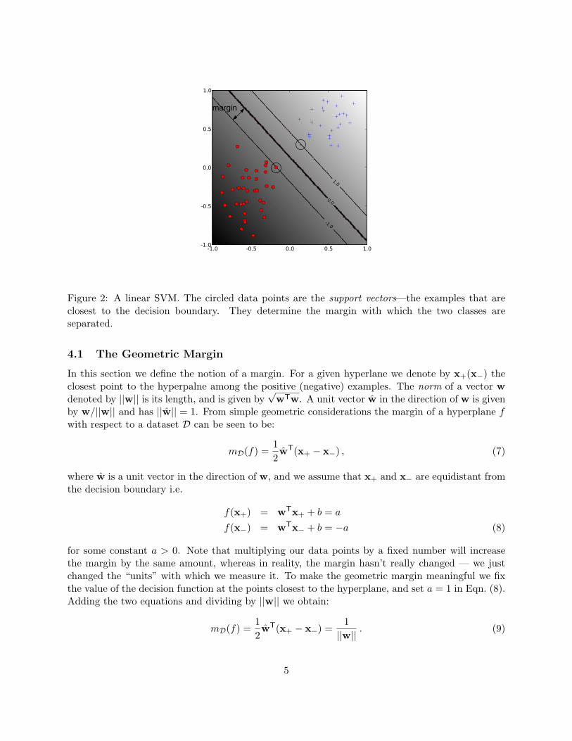
Training an SVM finds the large margin hyperplane, i.e. sets the parameters αi and b (c.f. Equa-tion 4). The SVM has another set of parameters called hyperparameters: The soft margin constant,C, and any parameters the kernel function may depend on (width of a Gaussian kernel or degree ofa polynomial kernel). In this section we illustrate the effect of the hyperparameters on the decisionboundary of an SVM using two-dimensional examples.

We begin our discussion of hyperparameters with the soft-margin constant, whose role is il-lustrated in Figure 3. For a large value of C a large penalty is assigned to errors/margin errors.This is seen in the left panel of Figure 3, where the two points closest to the hyperplane affectits orientation, resultinging in a hyperplane that comes close to several other data points. WhenC is decreased (right panel of the figure), those points become margin errors; the hyperplane’sorientation is changed, providing a much larger margin for the rest of the data.

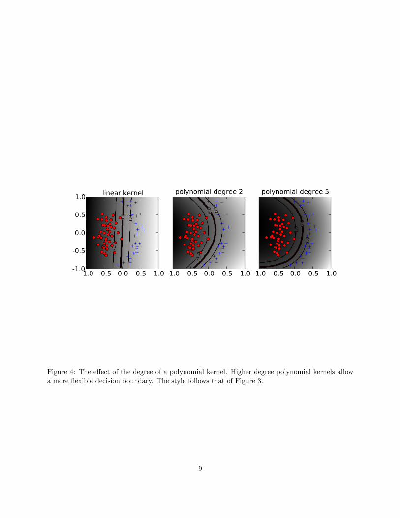
Kernel parameters also have a significant effect on the decision boundary. The degree of thepolynomial kernel and the width parameter of the Gaussian kernel control the flexibility of theresulting classifier (Figures 4 and 5). The lowest degree polynomial is the linear kernel, whichis not sufficient when a non-linear relationship between features exists. For the data in Figure 4a degree-2 polynomial is already flexible enough to discriminate between the two classes with asizable margin. The degree-5 polynomial yields a similar decision boundary, albeit with greatercurvature.

Next we turn our attention to the Gaussian kernel: k(x,x′) = exp(−γ||x−x′||2). This expressionis essentially zero if the distance between x and x′ is much larger than 1/

√γ; i.e. for a fixed x′

it is localized to a region around x′. The support vector expansion, Equation (4) is thus a sumof Gaussian “bumps” centered around each support vector. When γ is small (top left panel inFigure 5) a given data point x has a non-zero kernel value relative to any example in the set ofsupport vectors. Therefore the whole set of support vectors affects the value of the discriminantfunction at x, resulting in a smooth decision boundary. As γ is increased the locality of the supportvector expansion increases, leading to greater curvature of the decision boundary. When γ is largethe value of the discriminant function is essentially constant outside the close proximity of theregion where the data are concentrated (see bottom right panel in Figure 5). In this regime of theγ parameter the classifier is clearly overfitting the data.

As seen from the examples in Figures 4 and 5 the γ parameter of the Gaussian kernel and thedegree of polynomial kernel determine the flexibility of the resulting SVM in fitting the data. Ifthis complexity parameter is too large, overfitting will occur (bottom panels in Figure 5).

A question frequently posed by practitioners is “which kernel should I use for my data?” Thereare several answers to this question. The first is that it is, like most practical questions in machinelearning, data-dependent, so several kernels should be tried. That being said, we typically followthe following procedure: Try a linear kernel first, and then see if we can improve on its performanceusing a non-linear kernel. The linear kernel provides a useful baseline, and in many bioinformaticsapplications provides the best results: The flexibility of the Gaussian and polynomial kernels often

7

-1.0 -0.5 0.0 0.5 1.0-1.0

-0.5

0.0

0.5

1.0

-1.0

0.0

1.0

C=100

-1.0 -0.5 0.0 0.5 1.0

-1.0

0.0

1.0

C=10

Figure 3: The effect of the soft-margin constant, C, on the decision boundary. A smaller value ofC (right) allows to ignore points close to the boundary, and increases the margin. The decisionboundary between negative examples (red circles) and positive examples (blue crosses) is shownas a thick line. The lighter lines are on the margin (discriminant value equal to -1 or +1). Thegrayscale level represents the value of the discriminant function, dark for low values and a lightshade for high values.

8

-1.0 -0.5 0.0 0.5 1.0-1.0

-0.5

0.0

0.5

1.0

-1.0

0.0

1.0

linear kernel

-1.0 -0.5 0.0 0.5 1.0

-1.0

0.0

1.0

polynomial degree 2

-1.0 -0.5 0.0 0.5 1.0

-1.0

0.0

1.0

polynomial degree 5

Figure 4: The effect of the degree of a polynomial kernel. Higher degree polynomial kernels allowa more flexible decision boundary. The style follows that of Figure 3.

9

-1.0

-0.5

0.0

0.5

1.0-1

.0

0.0 1.0

gaussian, gamma=0.1

-1.0

0.01.0

gaussian, gamma=1

-1.0 -0.5 0.0 0.5 1.0-1.0

-0.5

0.0

0.5

1.0

-1.0

0.0

1.0

1.0

gaussian, gamma=10

-1.0 -0.5 0.0 0.5 1.0

-1.0

-1.0

0.0

0.0

gaussian, gamma=100

Figure 5: The effect of the inverse-width parameter of the Gaussian kernel (γ) for a fixed valueof the soft-margin constant. For small values of γ (upper left) the decision boundary is nearlylinear. As γ increases the flexibility of the decision boundary increases. Large values of γ lead tooverfitting (bottom). The figure style follows that of Figure 3.

10

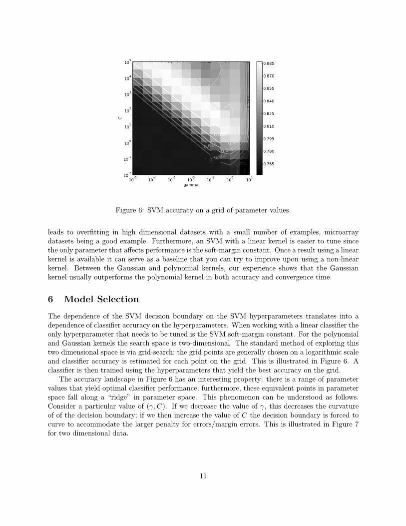
Figure 6: SVM accuracy on a grid of parameter values.

leads to overfitting in high dimensional datasets with a small number of examples, microarraydatasets being a good example. Furthermore, an SVM with a linear kernel is easier to tune sincethe only parameter that affects performance is the soft-margin constant. Once a result using a linearkernel is available it can serve as a baseline that you can try to improve upon using a non-linearkernel. Between the Gaussian and polynomial kernels, our experience shows that the Gaussiankernel usually outperforms the polynomial kernel in both accuracy and convergence time.

6 Model Selection

The dependence of the SVM decision boundary on the SVM hyperparameters translates into adependence of classifier accuracy on the hyperparameters. When working with a linear classifier theonly hyperparameter that needs to be tuned is the SVM soft-margin constant. For the polynomialand Gaussian kernels the search space is two-dimensional. The standard method of exploring thistwo dimensional space is via grid-search; the grid points are generally chosen on a logarithmic scaleand classifier accuracy is estimated for each point on the grid. This is illustrated in Figure 6. Aclassifier is then trained using the hyperparameters that yield the best accuracy on the grid.

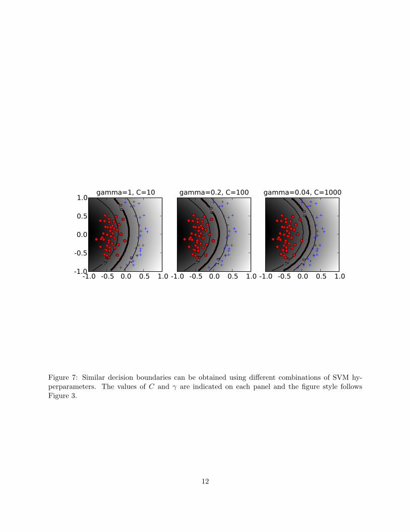
The accuracy landscape in Figure 6 has an interesting property: there is a range of parametervalues that yield optimal classifier performance; furthermore, these equivalent points in parameterspace fall along a “ridge” in parameter space. This phenomenon can be understood as follows.Consider a particular value of (γ,C). If we decrease the value of γ, this decreases the curvatureof of the decision boundary; if we then increase the value of C the decision boundary is forced tocurve to accommodate the larger penalty for errors/margin errors. This is illustrated in Figure 7for two dimensional data.

11

-1.0 -0.5 0.0 0.5 1.0-1.0

-0.5

0.0

0.5

1.0

-1.0

0.0

1.0

gamma=1, C=10

-1.0 -0.5 0.0 0.5 1.0

-1.0

0.0

1.0

gamma=0.2, C=100

-1.0 -0.5 0.0 0.5 1.0-1

.0

0.0

1.0

gamma=0.04, C=1000

Figure 7: Similar decision boundaries can be obtained using different combinations of SVM hy-perparameters. The values of C and γ are indicated on each panel and the figure style followsFigure 3.

12

7 SVMs for Unbalanced Data

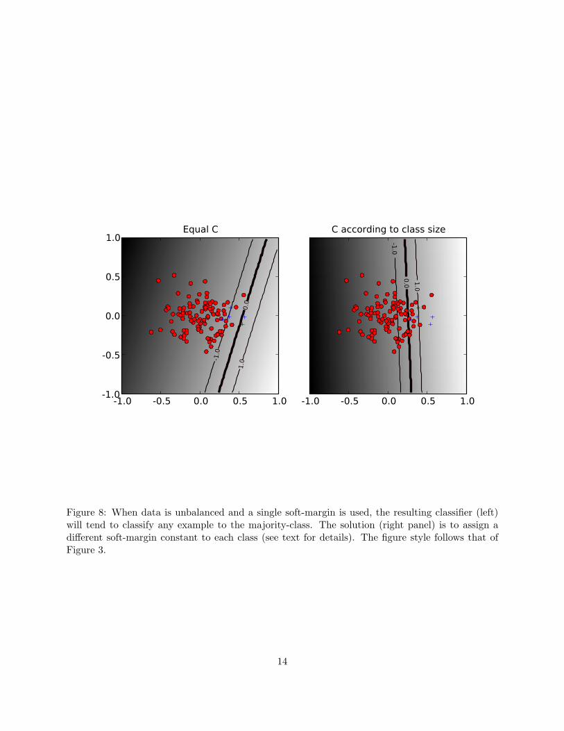
Many datasets encountered in bioinformatics and other areas of application are unbalanced, i.e.one class contains a lot more examples than the other. Unbalanced datasets can present a challengewhen training a classifier and SVMs are no exception — see [13] for a general overview of the issue. Agood strategy for producing a high-accuracy classifier on imbalanced data is to classify any exampleas belonging to the majority class; this is called the majority-class classifier. While highly accurateunder the standard measure of accuracy such a classifier is not very useful. When presented withan unbalanced dataset that is not linearly separable, an SVM that follows the formulation Eqn. 11will often produce a classifier that behaves similarly to the majority-class classifier. An illustrationof this phenomenon is provided in Figure 8.

The crux of the problem is that the standard notion of accuracy (the success rate, or fractionof correctly classified examples) is not a good way to measure the success of a classifier applied tounbalanced data, as is evident by the fact that the majority-class classifier performs well under it.The problem with the success rate is that it assigns equal importance to errors made on examplesbelonging the majority class and errors made on examples belonging to the minority class. Tocorrect for the imbalance in the data we need to assign different costs for misclassification to eachclass. Before introducing the balanced success rate we note that the success rate can be expressedas:

P (success|+)P (+) + P (success|−)P (−) ,

where P (success|+) (P (success|−)) is an estimate of the probability of success in classifying positive(negative) examples, and P (+) (P (−)) is the fraction of positive (negative) examples. The balancedsuccess rate modifies this expression to:

BSR = (P (success|+) + P (success|−))/2 ,

which averages the success rates in each class. The majority-class classifier will have a balanced-success-rate of 0.5. A balanced error-rate is defined as 1 − BSR. The BSR, as opposed to thestandard success rate, gives equal overall weight to each class in measuring performance. A similareffect is obtained in training SVMs by assigning different misclassification costs (SVM soft-marginconstants) to each class. The total misclassification cost, C

∑ni=1 ξi is replaced with two terms, one

for each class:

C

n∑i=1

ξi −→ C+

∑i∈I+

ξi + C−∑i∈I−

ξi ,

where C+ (C−) is the soft-margin constant for the positive (negative) examples and I+ (I−) arethe sets positive (negative) examples. To give equal overall weight to each class we want the totalpenalty for each class to be equal. Assuming that the number of misclassified examples from eachclass is proportional to the number of examples in each class, we choose C+ and C− such that

C+n+ = C−n− ,

where n+ (n−) is the number of positive (negative) examples. Or in other words:

C+

C−=n−n+

.

This provides a method for setting the ratio between the soft-margin constants of the two classes,leaving one parameter that needs to be adjusted. This method for handling unbalanced data isimplemented in several SVM software packages, e.g. LIBSVM [14] and PyML.

13

-1.0 -0.5 0.0 0.5 1.0-1.0

-0.5

0.0

0.5

1.0

-1.0

0.0

1.0

Equal C

-1.0 -0.5 0.0 0.5 1.0

-1.0

0.0 1.0

C according to class size

Figure 8: When data is unbalanced and a single soft-margin is used, the resulting classifier (left)will tend to classify any example to the majority-class. The solution (right panel) is to assign adifferent soft-margin constant to each class (see text for details). The figure style follows that ofFigure 3.

14

8 Normalization

Large margin classifiers are known to be sensitive to the way features are scaled [14]. Therefore itis essential to normalize either the data or the kernel itself. This observation carries over to kernel-based classifiers that use non-linear kernel functions: The accuracy of an SVM can severely degradeif the data is not normalized [14]. Some sources of data, e.g. microarray or mass-spectrometrydata require normalization methods that are technology-specific. In what follows we only considernormalization methods that are applicable regardless of the method that generated the data.

Normalization can be performed at the level of the input features or at the level of the kernel(normalization in feature space). In many applications the available features are continuous values,where each feature is measured in a different scale and has a different range of possible values. Insuch cases it is often beneficial to scale all features to a common range, e.g. by standardizing the data(for each feature, subtracting its mean and dividing by its standard deviation). Standardization isnot appropriate when the data is sparse since it destroys sparsity since each feature will typicallyhave a different normalization constant. Another way to handle features with different ranges is tobin each feature and replace it with indicator variables that indicate which bin it falls in.

An alternative to normalizing each feature separately is to normalize each example to be a unitvector. If the data is explicitly represented as vectors you can normalize the data by dividing eachvector by its norm such that ||x|| = 1 after normalization. Normalization can also be performedat the level of the kernel, i.e. normalizing in feature-space, leading to ||Φ(x)|| = 1 (or equivalentlyk(x,x) = 1). This is accomplished using the cosine kernel which normalizes a kernel k(x,x′) to:

kcosine(x,x′) =k(x,x′)√

k(x,x)k(x′,x′). (14)

Note that for the linear kernel cosine normalization is equivalent to division by the norm. The useof the cosine kernel is redundant for the Gaussian kernel since it already satisfies K(x,x) = 1. Thisdoes not mean that normalization of the input features to unit vectors is redundant: Our experienceshows that the Gaussian kernel often benefits from it. Normalizing data to unit vectors reducesthe dimensionality of the data by one since the data is projected to the unit sphere. Therefore thismay not be a good idea for low dimensional data.

9 SVM Training Algorithms and Software

The popularity of SVMs has led to the development of a large number of special purpose solversfor the SVM optimization problem [15]. One of the most common SVM solvers is LIBSVM [14].The complexity of training of non-linear SVMs with solvers such as LIBSVM has been estimatedto be quadratic in the number of training examples [15], which can be prohibitive for datasets withhundreds of thousands of examples. Researchers have therefore explored ways to achieve fastertraining times. For linear SVMs very efficient solvers are available which converge in a time whichis linear in the number of examples [16, 17, 15]. Approximate solvers that can be trained in lineartime without a significant loss of accuracy were also developed [18].

There are two types of software that provide SVM training algorithms. The first type are spe-cialized software whose main objective is to provide an SVM solver. LIBSVM [14] and SVMlight [19]are two popular examples of this class of software. The other class of software are machine learn-ing libraries that provide a variety of classification methods and other facilities such as methods

15

for feature selection, preprocessing etc. The user has a large number of choices, and the fol-lowing is an incomplete list of environments that provide an SVM classifier: Orange [20], TheSpider (http://www.kyb.tuebingen.mpg.de/bs/people/spider/), Elefant [21], Plearn (http://plearn.berlios.de/), Weka [22], Lush [23], Shogun [24], RapidMiner [25], and PyML (http://pyml.sourceforge.net). The SVM implementation in several of these are wrappers for theLIBSVM library. A repository of machine learning open source software is available at http://mloss.org as part of a movement advocating distribution of machine learning algorithms asopen source software [7].

10 Further Reading

We focused on the practical issues in using support vector machines to classify data that is alreadyprovided as features in some fixed-dimensional vector space. In bioinformatics we often encounterdata that has no obvious explicit embedding in a fixed-dimensional vector space, e.g. protein orDNA sequences, protein structures, protein interaction networks etc. Researchers have developeda variety of ways in which to model such data with kernel methods. See [2, 8] for more details.The design of a good kernel, i.e. defining a set of features that make the classification task easy, iswhere most of the gains in classification accuracy can be obtained.

After having defined a set of features it is instructive to perform feature selection: removefeatures that do not contribute to the accuracy of the classifier [26, 27]. In our experience featureselection doesn’t usually improve the accuracy of SVMs. Its importance is mainly in obtainingbetter understanding of the data—SVMs, like many other classifiers, are “black boxes” that do notprovide the user much information on why a particular prediction was made. Reducing the set offeatures to a small salient set can help in this regard. Several successful feature selection methodshave been developed specifically for SVMs and kernel methods. The Recursive Feature Elimination(RFE) method for example, iteratively removes features that correspond to components of the SVMweight vector that are smallest in absolute value; such features have less of a contribution to theclassification and are therefore removed [28].

SVMs are two-class classifiers. Solving multi-class problems can be done with multi-class exten-sions of SVMs [29]. These are computationally expensive, so the practical alternative is to converta two-class classifier to a multi-class. The standard method for doing so is the so-called one-vs-the-rest approach where for each class a classifier is trained for that class against the rest of the classes;an input is classified according to which classifier produces the largest discriminant function value.Despite its simplicity, it remains the method of choice [30].

Acknowledgements

The authors would like to thank William Noble for comments on the manuscript.

References

[1] B. E. Boser, I. M. Guyon, and V. N. Vapnik. A training algorithm for optimal margin classifiers.In D. Haussler, editor, 5th Annual ACM Workshop on COLT, pages 144–152, Pittsburgh, PA,1992. ACM Press.

16

[2] B. Scholkopf, K. Tsuda, and J.P. Vert, editors. Kernel Methods in Computational Biology.MIT Press series on Computational Molecular Biology. MIT Press, 2004.

[3] W.S. Noble. What is a support vector machine? Nature Biotechnology, 24(12):1564–1567,2006.

[4] J. Shawe-Taylor and N. Cristianini. Kernel Methods for Pattern Analysis. Cambridge UP,Cambridge, UK, 2004.

[5] B. Scholkopf and A. Smola. Learning with Kernels. MIT Press, Cambridge, MA, 2002.

[6] Chih-Wei Hsu, Chih-Chung Chang, and Chih-Jen Lin. A practical guide to support vectorclassification. Technical report, Department of Computer Science, National Taiwan University,2003.

[7] S. Sonnenburg, M.L. Braun, C.S. Ong, L. Bengio, S. Bottou, G. Holmes, Y. LeCun, K Muller,F Pereira, C.E. Rasmussen, G. Ratsch, B. Scholkopf, A. Smola, P. Vincent, J. Weston, andR.C. Williamson. The need for open source software in machine learning. Journal of MachineLearning Research, 8:2443–2466, 2007.

[8] N. Cristianini and J. Shawe-Taylor. An Introduction to Support Vector Machines. CambridgeUP, Cambridge, UK, 2000.

[9] T. Hastie, R. Tibshirani, and J.H. Friedman. The Elements of Statistical Learning. Springer,2001.

[10] C.M. Bishop. Pattern Recognition and Machine Learning. Springer, 2007.

[11] C. Cortes and V. Vapnik. Support vector networks. Machine Learning, 20:273–297, 1995.

[12] O. Chapelle. Training a support vector machine in the primal. In L. Bottou, O. Chapelle,D. DeCoste, and J. Weston, editors, Large Scale Kernel Machines. MIT Press, Cambridge,MA., 2007.

[13] F. Provost. Learning with imbalanced data sets 101. In AAAI 2000 workshop on imbalanceddata sets, 2000.

[14] C-C. Chang and C-J. Lin. LIBSVM: a library for support vector machines, 2001. Softwareavailable at http://www.csie.ntu.edu.tw/~cjlin/libsvm.

[15] L. Bottou, O. Chapelle, D. DeCoste, and J. Weston, editors. Large Scale Kernel Machines.MIT Press, Cambridge, MA., 2007.

[16] T. Joachims. Training linear SVMs in linear time. In ACM SIGKDD International ConferenceOn Knowledge Discovery and Data Mining (KDD), pages 217 – 226, 2006.

[17] V. Sindhwani and S. S. Keerthi. Large scale semi-supervised linear svms. In 29th annualinternational ACM SIGIR Conference on Research and development in information retrieval,pages 477–484, New York, NY, USA, 2006. ACM Press.

[18] A. Bordes, S. Ertekin, J. Weston, and L. Bottou. Fast kernel classifiers with online and activelearning. Journal of Machine Learning Research, 6:1579–1619, September 2005.

17

[19] T. Joachims. Making large-scale support vector machine learning practical. In B. Scholkopf,C. Burges, and A. Smola, editors, Advances in Kernel Methods: Support Vector Machines.MIT Press, Cambridge, MA, 1998.

[20] J. Demsar, B. Zupan, and G. Leban. Orange: From Experimental Machine Learning to Inter-active Data Mining. Faculty of Computer and Information Science, University of Ljubljana,2004.

[21] K. Gawande, C. Webers, A. Smola, S.V.N. Vishwanathan, S. Gunter, C.H. Teo, J.Q. Shi,J. McAuley, L. Song, and Q. Le. ELEFANT user manual (revision 0.1). Technical report,NICTA, 2007.

[22] I. H. Witten and E. Frank. Data Mining: Practical machine learning tools and techniques.Morgan Kaufmann, 2nd edition edition, 2005.

[23] L. Bottou and Y. Le Cun. Lush Reference Manual, 2002.

[24] S. Sonnenburg, G. Raetsch, C. Schaefer, and B. Schoelkopf. Large scale multiple kernel learn-ing. Journal of Machine Learning Research, 7:1531–1565, 2006.

[25] I. Mierswa, M. Wurst, R. Klinkenberg, M. Scholz, and T. Euler. YALE: Rapid prototyping forcomplex data mining tasks. In Proceedings of the 12th ACM SIGKDD International Conferenceon Knowledge Discovery and Data Mining, 2006.

[26] I. Guyon, S. Gunn, M. Nikravesh, and L. Zadeh, editors. Feature extraction, foundations andapplications. Springer Verlag, 2006.

[27] I. Guyon and A. Elisseeff. Special issue on variable and feature selection. Journal of MachineLearning Research, 3, March 2003.

[28] I. Guyon, J. Weston, S. Barnhill, and V. Vapnik. Gene selection for cancer classification usingsupport vector machines. Machine Learning, 46(1-3):389–422, 2002.

[29] J. Weston and C. Watkins. Multi-class support vector machines. Royal Holloway TechnicalReport CSD-TR-98-04, 1998.

[30] R. Rifkin and A. Klautau. In defense of one-vs-all classification. Journal of Machine LearningResearch, 5:101–141, 2004.

18