a uniform description of riemannian symmetric spaces as ...leung/phd students/thesis yong dong...
TRANSCRIPT

A Uniform Description of Riemannian
Symmetric Spaces as Grassmannians Using
Magic Square
HUANG, Yongdong
A Thesis Submitted in Partial Fulfilment
of the Requirements for the Degree of
Doctor of Philosophy
in
Mathematics
c©The Chinese University of Hong Kong
May 2007
The Chinese University of Hong Kong holds the copyright of this thesis. Any
person(s) intending to use a part or whole of the materials in the thesis in a
proposed publication must seek copyright release from the Dean of the Graduate
School.

Symmetric Spaces as Grassmannians Using Magic Square 1
Abstract
In this thesis we introduce and study the (i) Grassmannian, (ii) Lagrangian
Grassmannian and (iii) double Lagrangian Grassmannian of subspaces in (A⊗ B)n,
where A and B are normed division algebras, i.e. R, C, H or O.
We show that every irreducible compact Riemannian symmetric space X must
be one of these Grassmannian spaces (up to a finite cover) or a compact simple
Lie group. Furthermore, its noncompact dual symmetric space is the open sub-
manifold of X consisting of spacelike linear subspaces, at least in the classical
cases.
This gives a simple and uniform description of all symmetric spaces. This is
analogous to Tits magic square description for simple Lie algebras.

Symmetric Spaces as Grassmannians Using Magic Square 2
ACKNOWLEDGMENTS
I wish to express my gratitude to my supervisor Prof. Naichung Conan Leung,
whose expertise, understanding, and patience, added considerably to my graduate
experience. I appreciate his vast knowledge and skill in many areas, and his
assistance in writing this thesis. I would express my thanks to my teacher Prof.
Zhi-Jie Chen, Prof. Sheng-Li Tan and Prof. Kang Zuo, they led me to the
learning of algebraic geometry. I would give my thanks to Prof. Weiping Li,
Prof. Jianghua Lu, Prof. Xiaowei Wang, and Prof. Siye Wu, they give me great
help to my graduate studies. I would also thank Kwok Wai Chan, Chang Zhen
Li, Mao Sheng and Jia Jin Zhang, they give me the chances to discuss problems
with them and help to my thesis.
I would give my thanks to the department of mathematics and IMS of CUHK.
I would also like to thank my family for the support they provided me through
my entire life and in particular, I must acknowledge my wife, without whose love
and encouragement, I would not have finished this thesis.

Contents
1 Introduction 5
1.1 Main Result – Compact Case . . . . . . . . . . . . . 6
1.2 Main Result – Noncompact Case . . . . . . . . . . . 8
2 Magic Square from Complex and Symplectic Point
of Views 13
2.1 Magic Square . . . . . . . . . . . . . . . . . . . . . . 14
2.1.1 Magic square of 3× 3 matrices . . . . . . . . 16
2.1.2 Magic square of 2× 2 matrices . . . . . . . . 18
2.1.3 Symmetry of the magic square . . . . . . . . . 19
2.2 Doubling Construction . . . . . . . . . . . . . . . . . 21
2.3 Noncompact Magic Square . . . . . . . . . . . . . . . 23
2.3.1 The case of m = 0 . . . . . . . . . . . . . . . 25
2.3.2 The case of m = 1, l = 0 . . . . . . . . . . . . 26
2.3.3 The case of m = l = 1 . . . . . . . . . . . . . 26
2.3.4 The case of m = 1, l = 2 . . . . . . . . . . . . 27
2.3.5 The case of m = 2 . . . . . . . . . . . . . . . 28
3

Symmetric Spaces as Grassmannians Using Magic Square 4
3 Compact Riemannian Symmetric Spaces 35
3.1 Definitions and First Properties . . . . . . . . . . . . 35
3.2 Grassmannians . . . . . . . . . . . . . . . . . . . . . 43
3.3 Lagrangian Grassmannians . . . . . . . . . . . . . . . 46
3.4 Double Lagrangian Grassmannians . . . . . . . . . . 48
3.5 Compact Simple Lie Groups . . . . . . . . . . . . . . 52
4 Noncompact Riemannian Symmetric Spaces 55
4.1 Dual Riemannian Symmetric Spaces and
Borel Embedding . . . . . . . . . . . . . . . . . . . . 55
4.2 An Embedding of Noncompact Symmetric Space into
Its Compact Dual . . . . . . . . . . . . . . . . . . . . 56
Bibliography 63

Chapter 1
Introduction
Riemannian symmetric spaces are important model spaces in geometry. They are
classified in terms of symmetric Lie algebras. Every compact symmetric space
has a noncompact dual and vice versa. Examples of compact symmetric spaces
include Grassmannians of k-planes in n-dimensional vector spaces over R, C, or
evenH. Symbolically, we write these symmetric spaces as O (n) /O (k) O (n− k) =Rk ⊂ Rn
, U (n) /U (k) U (n− k) =
Ck ⊂ Cn
and so on. There are also
Lagrangian Grassmannians in Cn and Hn, which we write as U (n) /O (n) =
Rn ⊂ Cn and Sp (n) /U (n) = Cn ⊂ Hn. Of course, compact Lie groups
are also examples of compact symmetric spaces. For example O (n) = O (n) ×O (n) /O (n) is the set of all maximally isotropic subspaces in Rn ⊕ Rn with
respect to a symmetric 2-tensor g′ of type (n, n). Taking g′-orthogonal comple-
ment defines an involution σg′ on the Grassmannian and we have O(n) = Rn ⊂Rn ⊕ Rnσg′ .
Classical compact Lie groups include SO (n), SU (n) and Sp (n) . Roughly
speaking, they are groups of isometries of Rn, Cn and Hn respectively. There are
also five exceptional Lie groups, namely G2, F4, E6, E7 and E8. If we include
the largest normed division algebra O, the octonion, also known as the Cayley
number Ca, then we can obtain G2 and F4 as well. Since O is not associative,
5
Symmetric Spaces as Grassmannians Using Magic Square 6
On does not make sense at all. However, if n ≤ 3 then it is possible to define
the group of symmetries of On using exceptional Jordan algebras (see e.g. [13]).
For the remaining groups, Freudenthal [8] and Tits [15] introduced the magic
square to describe every type of compact Lie algebras in a uniform manner by
considering (A⊗ B)n with both A and B normed division algebras. In particular,
using the magic square, we can realize the Lie algebra of E6, E7 and E8 as roughly
the Lie algebras of infinitesimal isometries of (C⊗O)3, (H⊗O)3 and (O⊗O)3
respectively.
1.1 Main Result – Compact Case
For compact Riemannian symmetric spaces, there are many more exceptional
cases. At first sight, it seems hard to imagine that they can all be described in a
simple and uniform manner. By realizing the symmetry of the magic square as a
mirror duality between complex geometry and symplectic geometry, we generalize
the magic square and succeed in giving a simple and uniform description of all
compact Riemannian symmetric spaces. Among them, the most nontrivial ones
are E6/Sp (4) and E7/SU (8) , which will be described as the Grassmannians
of double Lagrangian subspaces Λ2 (R⊗H)4 in (C⊗O)3 and Λ2 (C⊗H)4 in
(H⊗O)3 respectively!
Main result - compact case: A description of four types of Grassmannian
spaces which include every type of compact symmetric spaces.
First type: Compact (semi)simple Lie groups
G = (A⊗ B)n ⊂ (A⊗ B)n ⊕ (A⊗ B)nσg′ ,
here σg′ is an involution induced by a canonical symmetric 2-tensor on (A⊗B)n⊕(A ⊗ B)n. These spaces are given in the following table (with the Abelian part
taken away). 1
1For all tables in this paper, n is assumed to be 3 when A or B equals O.

Symmetric Spaces as Grassmannians Using Magic Square 7
A\B R C H O
R SO(n) SU(n) Sp(n) F4
C SU(n) SU(n)2 SU(2n) E6
H Sp(n) SU(2n) SO(4n) E7
O F4 E6 E7 E8
(Table: C1)
On the Lie algebra level, it coincides with the magic square.
Recall that the compact Lie group G2 is the automorphism group of O, in
fact it is of the first type for n = 1 and A is O, B is R, or vice versa, i.e. it can
be realized as O ⊂ O⊕O invariant under g′.
Second type: Grassmannians
GrAB (k, n) =
(A⊗ B)k ⊂ (A⊗ B)n
.
A\B R C H O
RO(n)
O(k)O(n− k)
U(n)
U(k)U(n− k)
Sp(n)
Sp(k)Sp(n− k)
F4
Spin(9)
CU(n)
U(k)U(n− k)
U(n)2
U(k)2U(n− k)2
U(2n)
U(2k)U(2n− 2k)
E6
Spin(10)U(1)
HSp(n)
Sp(k)Sp(n− k)
U(2n)
U(2k)U(2n− 2k)
O(4n)
O(4k)O(4n− 4k)
E7
Spin(12)Sp(1)
OF4
Spin(9)
E6
Spin(10)U(1)
E7
Spin(12)Sp(1)
E8
SO(16)(Table: C2)
Third type: Lagrangian Grassmannians (with the Abelian part taken away)
LGrAB (n) =
(A2⊗B
)n
⊂ (A⊗ B)n
,
where A2
denotes R,C and H when A is C,H and O respectively.

Symmetric Spaces as Grassmannians Using Magic Square 8
A\B R C H O
CSU(n)
SO(n)
SU(n)2
SU(n)
SU(2n)
Sp(n)
E6
F4
HSp(n)
U(n)
SU(2n)
S(U(n)2)
SO(4n)
U(2n)
E7
E6U(1)
OF4
Sp(3)Sp(1)
E6
SU(6)Sp(1)
E7
Spin(12)Sp(1)
E8
E7Sp(1)(Table: C3)
The compact symmetric space G2/Sp (1) Sp (1) is a Lagrangian Grassmannian
for n = 1 and A is O, B is R, i.e. it can be realized as H ⊂ O.
Fourth type: Double Lagrangian Grassmannians (with the Abelian part taken
away)
LLGrAB =
(A2⊗ B
2
)n
⊕(
j1A2⊗ j2
B2
)n
⊂ (A⊗ B)3
,
where j1 and j2 are elements of A and B respectively, such that j21 = j2
2 = −1
and A = A2
+ j1A2
and B = B2
+ j2B2.
A\B C H O
CSU(n)2
SO(n)2
SU(2n)
SO(2n)
E6
Sp(4)
HSU(2n)
SO(2n)
SO(4n)
S(O(2n)2)
E7
SU(8)
OE6
Sp(4)
E7
SU(8)
E8
SO(16)(Table: C4)
1.2 Main Result – Noncompact Case
As a corollary, we can also give a simple and uniform description of all Rieman-
nian symmetric spaces of noncompact type. Recall that any noncompact sym-
metric space has a compact dual X. From the above main result, X parametrizes
certain linear subspaces P in a fixed “vector space” V ' (A⊗ B)n. If we fix one

Symmetric Spaces as Grassmannians Using Magic Square 9
such subspace P0 and write V as an orthogonal decomposition V = P0 ⊕ P⊥0 .
We change the positive definite inner product gV = gP0 ⊕ gP⊥0on V to an in-
definite inner product gV = gP0 ⊕(−gP⊥0
). Then the noncompact symmetric
space X consists precisely of those subspaces P in V which are of spacelike, i.e.
gV (v, v) > 0 for any nonzero vector v in P . Furthermore, this inclusion X ⊂ X
is an open embedding for at least any pair of dual symmetric spaces of classical
types, i.e. the symmetric spaces whose isometry groups are classical groups.
Main result - noncompact case: A description of four types of spacelike
Grassmannian spaces which include every type of noncompact symmetric spaces.
First type: Noncompact dual to compact Lie groups GC/G.
A\B R C H O
R SO(n,C)/SO(n) SL(n,C)/SU(n) Sp(2n,C)/Sp(n) FC4 /F4
C SL(n,C)/SU(n) SL(n,C)2/SU(n)2 SL(2n,C)/SU(2n) EC6 /E6
H Sp(2n,C)/Sp(n) SL(2n,C)/SU(2n) SO(4n,C)/SO(4n) EC7 /E7
O FC4 /F4 EC6 /E6 EC
7 /E7 EC8 /E8
(Table: N1)
Second type: Spacelike Grassmannians Gr+AB (k, n) .
A\B R C H O
RO(k, n− k)
O(k)O(n− k)
U(k, n− k)
U(k)U(n− k)
Sp(k, n− k)
Sp(k)Sp(n− k)
F4(−20)
Spin(9)
CU(k, n− k)
U(k)U(n− k)
U(k, n− k)2
U(k)2U(n− k)2
U(2k, 2n− 2k)
U(2k)U(2n− 2k)
E6(−14)
Spin(10)U(1)
HSp(k, n− k)
Sp(k)Sp(n− k)
U(2k, 2n− 2k)
U(2k)U(2n− 2k)
O(4k, 4n− 4k)
O(4k)O(4n− 4k)
E7(−5)
Spin(12)Sp(1)
OF4(−20)
Spin(9)
E6(−14)
Spin(10)U(1)
E7(−5)
Spin(12)Sp(1)
E8(8)
SO(16)(Table: N2)

Symmetric Spaces as Grassmannians Using Magic Square 10
Remark 1.2.1 Here we use the same notation to denote the identity connected
component of O(k, n− k)/O(k)O(n− k), and similarly in the other cases.
Where −20 in the group F4(−20) is the signature of the Killing form of the
noncompact Lie group F4(−20), the other cases are similar.
Third type: Spacelike Lagrangian Grassmannians LGr+AB (n) (with the Abelian
part taken away).
A\B R C H O
CSL(n,R)
SO(n)
SL(n,C)
SU(n)
SL(n,H)
Sp(n)
E6(−26)
F4
HSp(2n,R)
U(n)
SU(n, n)
S(U(n)2)
SO∗(4n)
U(2n)
E7(−25)
E6U(1)
OF4(4)
Sp(3)Sp(1)
E6(2)
SU(6)Sp(1)
E7(−5)
Spin(12)Sp(1)
E8(−24)
E7Sp(1)(Table: N3)
Fourth type: Spacelike Double Lagrangian Grassmannians LLGr+AB (with the
Abelian part taken away).
A\B C H O
CSL(n,R)2
SO(n)2
SL(2n,R)
SO(2n)
E6(6)
Sp(4)
HSL(2n,R)
SO(2n)
SO(2n, 2n)
S(O(2n)2)
E7(7)
SU(8)
OE6(6)
Sp(4)
E7(7)
SU(8)
E8(8)
SO(16)(Table: N4)
Remark 1.2.2 A Riemannian symmetric space G/K admits a G-invariant com-
plex structure precisely when K has a U (1)-factor. Such spaces are called Her-
mitian symmetric spaces and they play very important roles in many different
branches of mathematics. From the above tables we know that Hermitian sym-
metric spaces are precisely those grassmannians parametrizing certains types of

Symmetric Spaces as Grassmannians Using Magic Square 11
(A⊗ B)k in W = (D⊗ E)n where A or B equals the complex numbers C, with
only one exception O(2, n)/O(2)O(n).
In the remainder of this section, we give an intuitive explanation of the origin
of these four types of Grassmannians, we first recall that all normed division
algebras A can be obtained from a doubling construction starting from R, the
Cayley-Dickson process: R Ã C Ã H Ã O. For any “vector space” V over R,
this doubling procedure can be viewed in two different ways: (i) complexification
V 7−→ (TV, J) and (ii) symplectification V 7−→ (T ∗V, ω). The corresponding
semi-simple part of Lie algebras of infinitesimal symmetries of these doublings
are (i) sl (n,R) 7−→ sl (n,C) 7−→ sl (n,H) and (ii) sl (n,R) 7−→ sp (2n,R) 7−→sp (2n,C). The octonion case is more complicated which we will deal with in the
next section via the magic square. Combining both of them gives the following
table of Lie algebras.
A\B R C H
R sl(n,R) sl(n,C) sl(n,H)
C sp(2n,R) su(n, n) so∗(4n)
H sp(2n,C) sl(2n,C) so(4n,C)
(Table: T1)
If we also require these symmetries to preserve the metric g on V , then they
reduce to the maximal compact (modulo center) subalgebras and we obtain the
magic square
A\B R C H
R so(n) su(n) sp(n)
C su(n) su(n)2 su(2n)
H sp(n) su(2n) so(4n)
(Table: T2)

Symmetric Spaces as Grassmannians Using Magic Square 12
The symmetry of the magic square along the diagonal is closely related to the
formula
g (Ju, v) = ω (u, v) ,
which says that complex structure and symplectic structure determine each other
when a matric is given.
Notice that every symplectic form ω on V determines an involution σω on
the Grassmannian of linear subspaces P ⊂ V by σω (P ) = P⊥ω whose fix points
are precisely Lagrangian subspaces in (V, ω). This is analogous to every complex
structure J on V determines an involution σJ on the Grassmannian by σJ (P ) =
JP whose fix points are precisely complex linear subspaces in (V, J).
Suppose that V ' (A⊗ B)n with A, B normed division algebras. Then the
Grassmannian of all real linear subspaces P in V which are σJ -invariant for
every J coming from either A or B is precisely our compact symmetric space
of type I, GrAB (k, n). Similarly, if we require P to be σω-invariant, instead of
σJ -invariant, for one J coming from A, then we obtain the Lagrangian Grassman-
nians LGrAB (n). Furthermore, if we do this to both A and B, then we obtain the
double Lagrangian Grassmannian LLGrAB(n).
Recall that the canonical symplectic form ω on T ∗V = V ⊕ V ∗ is the skew-
symmetric component of a two tensor induced from the natural pairing between
V and V ∗. The symmetric component of this tensor is an indefinite inner product
h on V ⊕ V ∗ with signature (N,N), where N is the dimension of V over R. If
we replace σω by σh in the definition of LGrAB (n), then we obtain the list of
compact Lie groups G.
In conclusion, every irreducible compact symmetric space is a Grassmannian
of linear subspaces in W ' (A⊗ B)n which are invariant under involutions σJ ,
σω or σh.

Chapter 2
Magic Square from Complex and
Symplectic Point of Views
Complex simple Lie algebras are completely classified. The classical ones are
complexification of so(n), su(n) and sp(n), which are Lie algebras of isometry
groups (modulo center) of Rn, Cn and Hn respectively. They can also be identified
as derivation algebras of Jordan algebras of rank n Hermitian matrices over R, C
and H respectively. Namely so(n) = DerHn(R), su(n) = DerHn(C) and sp(n) =
DerHn(H). The rest are five exceptional Lie algebras, g2, f4, e6, e7 and e8. To
define them, we need to include the non-associative normed division algebra O,
the octonion or the Cayley number. For instance g2 = DerO and f4 = DerH3(O).
Even though On can not be defined properly due to the non-associative nature
of O, nevertheless, the Jordan algebra Hn(O) has a natural interpretation as the
exceptional Jordan algebra when n = 3 (see e.g. [10]).
Tits [15] observed that we can have a uniform description of all simple Lie
algebras, including e6, e7 and e8, if we use any two normed division algebras A,
B ∈ R,C,H,O and define
L3(A,B) = DerH3(A)⊕ (H ′3(A)⊗ ImB)⊕Der(B),
where H ′3(A) is the subset of trace zero Hermitian matrices in H3(A).
13

Symmetric Spaces as Grassmannians Using Magic Square 14
2.1 Magic Square
Let K be an algebra over R with a quadratic form x 7→ |x|2 and associated bilinear
form 〈x, y〉. If the quadratic form satisfies
|xy|2 = |x|2|y|2, ∀x, y ∈ K,
then K is a composition algebra. A division algebra is an algebra in which
xy = 0 ⇒ x = 0 or y = 0.
This is true in a composition algebra if the quadratic form |x|2 is positive definite.
By Hurwitz’s theorem [12], the only such algebras are R,C,H andO. The positive
definite quadratic form is also called a norm on K, hence K is also called a normed
division algebra. These algebras can be obtained by the Cayley-Dickson process
[12]. We consider R to be embedded in K as the set of scalar multiples of the
identity element, and denote by ImK the subspace of K orthogonal to R, so that
K = R ⊕ ImK. We write x = Rex + Imx with Rex ∈ R and Imx ∈ ImK. The
conjugation of x is x = Rex− Imx, satisfies
xy = y x,
and
xx = |x|2.
The inner product in K is given in terms of this conjugation as
〈x, y〉 = Re(xy) = Re(xy).
Let Mn(K) be the algebra of all n× n matrices with entries in K, where K is
a normed division algebra, i.e. R,C,H or O.
For A ∈ Mn(K), let At and A denote the transpose and conjugate of A
respectively, defined as
(At)ij = Aji

Symmetric Spaces as Grassmannians Using Magic Square 15
and
(A)ij = Aij.
By using these notations, the hermitian conjugate of the matrix A is At.
Let I denote the identity matrix (of a size which will be clear from the context).
We use U(s, t) (SU(s, t)) for the pseudo-unitary (unimodular pseudo-unitary)
group,
U(s, t) =
A ∈ Mn(C) : AGAt= G
where G = diag(1, ..., 1,−1, ...,−1) with s + signs and t − signs; Sp(n) for the
group of antihermitian quaternionic matrices A,
Sp(n) =
A ∈ Mn(H) : AAt= I
;
and Sp(2n,K) for the symplectic group of 2n×2n matrices with entries in K, i.e.
Sp(2n,K) =A ∈ Mn(K) : AωAt = ω
where ω =
0 I
−I 0
. We also have O(s, t), the pseudo-orthogonal group,
given by
O(s, t) =AGAt = G
where G is defined as before. We will denote the Lie algebras of SU(s, t), Sp(n),
Sp(2n,K) and O(s, t) as su(s, t), sp(n), sp(2n,K) and so(s, t) respectively. When
s or t is zero, the groups U(s, t) (SU(s, t)) and O(s, t) become the normal unitary
and orthogonal groups U(n) (SU(n)) and O(n) respectively.
A Jordan algebra J is defined to be a commutative algebra (over a field K) in
which all products satisfy the Jordan identity
(xy)x2 = x(yx2).
Let Hn(K) and An(K) be the sets of all hermitian and antihermitian matrices
with entries in K respectively. We denote by H ′n(K), A′
n(K) and M ′n(K) the

Symmetric Spaces as Grassmannians Using Magic Square 16
subspaces of traceless matrices of Hn(K), An(K) and Mn(K) respectively. If we
define
X · Y = XY + Y X,
then Hn(K) is a Jordan algebra for K = R,C,H for all n and for K = O when
n = 2, 3.
For any algebra A, we define the derivation algebra Der(A) as
Der(A) = D | D(xy) = D(x)y + xD(y) ∀x, y ∈ A .
The derivation algebras of the four normed division algebras are as follows:
Der(R) = Der(C) = 0,
Der(H) = Ca | a ∈ ImH, Ca(q) = aq − qa ∼= sp(1),
Der(O) ∼= g2,
where g2 is the compact exceptional Lie algebra of type G2.
2.1.1 Magic square of 3× 3 matrices
The following is the Tits original constructions of the magic square.
Let A and B be normed division algebras, define
L3(A,B) = DerH3(A)⊕H ′3(A)⊗ ImB⊕Der(B).
This is a Lie algebra with Lie subalgebras DerH3(A) and Der(B) when taken with
the brackets
[D,A⊗ x] = D(A)⊗ x
[E, A⊗ x] = A⊗ E(x)
[D,E] = 0
[A⊗ x,B ⊗ y] =1
6〈A,B〉Dx,y + (A ∗B)⊗ 1
2[x, y]− 〈x, y〉[LA, LB]

Symmetric Spaces as Grassmannians Using Magic Square 17
with D ∈ DerH3(A); A,B ∈ H ′3(A); x, y ∈ ImB and E ∈ Der(B). These brackets
are obtained from Schafer’s description of the Tits construction [12]. We explain
these operations as follows. 〈A,B〉 and 〈x, y〉 denote the symmetric bilinear forms
on H3(A) and B respectively, given by
〈A,B〉 = Re(tr(A ·B)) = 2Re(tr(AB)),
〈x, y〉 =1
2(|x + y|2 − |x|2 − |y|2) = Re(xy).
The derivation Dx,y is defined as
Dx,y = [Lx, Ly] + [Lx, Ry] + [Rx, Ry] ∈ Der(B),
where Lx, Rx are maps of left and right multiplication by x respectively. Finally
(A ∗B) is the traceless part of the Jordan product of A and B,
A ∗B = A ·B − 1
3tr(A ·B).
Tits [15] showed that this gives a unified construction leading to the so-called
magic square of Lie algebras of 3× 3 matrices as follows.
A\B R C H O
R so(3) su(3) sp(3) f4
C su(3) su(3)2 su(6) e6
H sp(3) su(6) so(12) e6
O f4 e6 e7 e8
Remark 2.1.1 There are several versions of the magic square:
1. The Vinberg’s version [16]
L3(A,B) = Der(A)⊕ Der(B)⊕ A′3(A⊗ B),
where A′n(A ⊗ B) is the trace zero skew hermitian matrix of rank n with
entries in A⊗ B;

Symmetric Spaces as Grassmannians Using Magic Square 18
2. The Barton-Sudbery version [4]
L3(A,B) = tri(A)⊕ tri(B)⊕ (A⊗ B)3,
where tri(A) is the triality algebra of A, which by definition is a lie subalgebra
of so(A)⊕ so(A)⊕ so(A), satisfying
A(xy) = x(By) + (Cx)y, ∀x, y ∈ A,
for any (A,B,C) ∈ tri(A), where so(A) is the Lie algebra of the unimodular
orthogonal group SO(A), where A viewed as a real vector space.
2.1.2 Magic square of 2× 2 matrices
The Tits construction can also be adapted for 2× 2 matrix algebras. In this case
the underlying vector space is
L2(A,B) = DerH2(A)⊕H ′2(A)⊗ ImB⊕ so(ImB),
which admits a Lie algebra structure with the Lie brackets given as follows,
[D,A⊗ x] = D(A)⊗ x
[E, A⊗ x] = A⊗ E(x)
[D,E] = 0
[A⊗ x,B ⊗ y] =1
4〈A,B〉Dx,y − 〈x, y〉[RA, RB]
where the symbols used in this set of brackets are defined in the same way as the
ones used in the 3×3 case. This gives the compact magic square for 2×2 matrix
algebras
L2(A,B) = so(ν1 + ν2),
where ν1, ν2 are the dimensions of A,B over R. The magic square is as follows

Symmetric Spaces as Grassmannians Using Magic Square 19
A\B R C H O
R so(2) so(3) so(5) so(9)
C so(3) so(4) so(6) so(10)
H so(5) so(6) so(8) so(12)
O so(9) so(10) so(12) so(16)
Remark 2.1.2 As a matter of fact, Ln(A,B) can be defined for any n as long
as A, B ∈ R,C,H. The following is the table of magic square:
A\B R C H
R so(n) su(n) sp(n)
C su(n) su(n)2 su(2n)
H sp(n) su(2n) so(4n)
Freudenthal [8] also found a very different version to construct the magic
square in about 1958.
2.1.3 Symmetry of the magic square
A surprising fact of the magic square is the symmetry in A and B. For example
Ln(R,R) = DerHn(R) = so (n) is the space of infinitesimal isometries of V ∼=Rn. Ln(C,R) = DerHn(C) = su (n) is the space of infinitesimal isometries of
V ⊗R C = V ⊕ V = TV which also preserve the natural complex structure J on
TV , the tangent bundle of V . On the other hand, any symmetric matrix A =
(Aij) ∈ H ′n (R) ⊆ Ln(R,C) induces a natural transformation φA on V ⊕V ∗ = T ∗V
preserving the canonical symplectic structure on the cotangent bundle,
ω =∑n
i=1dxi ∧ dyi,
where xini=1 and yin
i=1 are dual coordinates on V and V ∗ respectively. Here
φA (xi) = xi and φA (yi) = yi + ΣjAijxj. Using the metric to identify V and V ∗,
the complex and symplectic structures on TV = T ∗V are related by the formula

Symmetric Spaces as Grassmannians Using Magic Square 20
ω (u, v) = g (Ju, v). Thus we obtain the first symmetry Ln(C,R) = Ln(R,C) in
the magic square. By repeating this doubling process, we obtain other symmetries
in the magic square.
We will also define noncompact Lie algebra nn(A,B), which contains Ln(A,B)
as its maximal compact Lie subalgebra (modulo center), by not requiring its
elements to preserve the inner product. We will discuss this noncompact magic
square and its properties in section 2.3.
In the next section, we will apply this construction to study the classification of
symmetric spaces, we will identify any irreducible symmetric spaces as all (multi-
complex) Grassmannian-Lagrangian linear cycles in the constructed spaces.

Symmetric Spaces as Grassmannians Using Magic Square 21
2.2 Doubling Construction
Definition 2.2.1 Given any real vector space V, we define inductively V [m,l]
by (i) V [0,0] = V and (ii) V [m,l] = TV [m,l−1] = T ∗V [m−1,l], together with the l
canonical complex structuresJR
1 , ..., JRl
and m canonical symplectic structures
ωL
1 , ..., ωLm
defined as below.
To explain the complex and symplectic structures we assume that V is a 2n
dimensional real vector space together with a complex structure and a symplectic
structure as follows,
J1 =∑
(∂xi ⊗ dxn+i − ∂xn+i ⊗ dxi),
ω1 =∑
(dxi ∧ dxn+i),
where xi2ni=1 are the real coordinates of V , ∂xi = ∂
∂xi .
1. On TV, besides the canonical complex structure J2, we also have a natural
complex structure and a symplectic structure induced by J1 and ω1 given
as follows, which we still use the same notations.
J1 =∑
(∂xi ⊗ dxn+i − ∂xn+i ⊗ dxi)−∑
(∂yi⊗ dyn+i − ∂yn+i
⊗ dyi),
J2 =∑
(∂xi ⊗ dyi − ∂yi ⊗ dxi),
ω1 =∑
(dxi ∧ dxn+i + dyi ∧ dyn+i),
where yi2ni=1 are the fiber coordinates of
∑yi∂xi on the tangent bundle.
2. On T ∗V, besides the canonical symplectic structure ω2, we also have a nat-
ural complex structure and a symplectic structure induced by J1 and ω1
given as follows, which we still use the same notations.
J1 =∑
(∂xi ⊗ dxn+i − ∂xn+i ⊗ dxi) +∑
(∂ui⊗ dun+i − ∂un+i
⊗ dui),
ω1 =∑
(dxi ∧ dxn+i − dui ∧ dun+i),
ω2 =∑
(dxi ∧ dun+i),

Symmetric Spaces as Grassmannians Using Magic Square 22
where ui2ni=1 are the fiber coordinates of
∑uidxi on the cotangent bundle.
Proposition 2.2.1 Above complex and symplectic structures on TV and T ∗V
satisfy the following conditions.
J1J2 = −J2J1,
ωi(Jj(·), Jj(·)) = ωi(·, ·),ι−1ω1 ιω2 = −ι−1
ω2 ιω1 .
Here ιω : V → V ∗ is defined as ιω(v) = vy ω = ω(v, ·).
This proposition can be easily proven by simple calculations.

Symmetric Spaces as Grassmannians Using Magic Square 23
2.3 Noncompact Magic Square
Given a vector space V = V [0,0] ∼= Rn, its group of automorphisms is GL (n,R).
Recall that V [0,1] (resp. V [1,0]) carries a natural complex (resp. symplectic)
structure and its group of automorphisms is GL (n,C) (resp. Sp (2n,R)). If
we restrict our attentions to only isometries, then both GL (n,C) and Sp (2n,R)
reduce to U (n), which is also their common maximal compact subgroup. If
we only look at semi-simple parts of these reductive groups, then they become
SL (n,C), Sp (2n,R) and SU (n) respectively. The following definitions generalize
these to a general V [m,l].
Definition 2.3.1 Given a real vector space V ∼= Rn, we denote by Nn(m, l) ⊂GL
(n · 2m+l,R
)the connected maximal semisimple subgroup of the group of all
automorphisms of V [m,l] which preserve the canonical complex structures JR1 , ..., JR
l
and symplectic structures ωL1 , ..., ωL
m on V [m,l]. We denote the maximal com-
pact subgroup of Nn(m, l) as Gn(m, l), and the maximal semisimple subgroup of
Gn(m, l) as Gsn(m, l).
The Lie algebras of Nn(m, l) and Gn(m, l) are denoted as nn(m, l) and gn(m, l)
respectively.
Recall the Tits definition for Ln(A,B), in fact Ln(A,B) is just the Lie alge-
bra of Gsn(m, l), where A and B are division algebras of dimension 2m and 2l
respectively.
The main result in this section is the following theorem.
Theorem 2.3.2 The groups Nn(m, l), Gn(m, l) and Gsn(m, l) satisfy the follow-
ing properties:
(i) Nn(0, l)/Gn(0, l) is the noncompact dual to Gsn(1, l)/Gn(0, l).
(ii) Nn(2, l) is the complexification of Nn(1, l).
(iii) Nn(1, l)/Gn(1, l) is the noncompact dual to Gsn(2, l)/Gn(1, l).

Symmetric Spaces as Grassmannians Using Magic Square 24
If we restrict our attention to 0 ≤ m, l ≤ 2, then the Lie algebra of Gsn(m, l)
is the same as the corresponding Lie algebra Ln(A,B) in the Tits magic square
where dimRA = 2m and dimRB = 2l. Then we are naturally led to extend our
definitions to N3(m, 3), using (i), (ii) and (iii) in theorem 2.3.2. Thus we have
the following table for Nn(m, l).
m\l 0 1 2 3 (n = 3)
0 SL(n,R) SL(n,C) SL(n,H) E6(−26)
1 Sp(2n,R) SU(n, n) SO∗(4n) E7(−25)
2 Sp(2n,C) SL(2n,C) SO(4n,C) E7C
Recall that suppose A is a linear transformation of a vector space V . We say
(i) A preserves a complex structure J on V if A J = J A and (ii) A preserves
a symplectic structure ω on V if ω (Au,Av) = ω (u, v) for any u, v in V . The
following lemma expresses this condition in terms of the isomorphism ιω.
Lemma 2.3.1 Suppose (V, ω) is a symplectic vector space and A ∈ End (V ).
Then A preserves ω if and only if ιω A = A∗ ιω, where A∗ ∈ End (V ∗) is the
adjoint of A.
Proof. Replacing v by A−1v, A preserves ω implies
ω(Au, v) = ω(u,A−1v).
For any u, v ∈ V ,
((ιω A)u)(v) = ω(Au, v),
((A∗ ιω)u)(v) = ιω(u)(A−1v)
= ω(u,A−1v),
so
ιω A = A∗ ιω.

Symmetric Spaces as Grassmannians Using Magic Square 25
is equivalent to A preserves ω. ¤
Now we consider the group Nn(m, l) for m, l = 0, 1, 2.
2.3.1 The case of m = 0
The case for m = 0 is obvious SL(n,K), where K is R, C, H when l = 0, 1, 2
respectively. The reason is that we can view TV = V [0,1] and T (TV ) = V [0,2]
together with the canonical complex structures as Cn and Hn respectively since
the two complex structures on T (TV ) are anti-commutative:
JR1 JR
2 = −JR2 JR
1 .
Before we consider the other cases we first identify V [m,l] together with m
symplectic structures and l complex structures as (T ∗)mKn with m symplectic
structures, where K is R, C, H when l = 0, 1, 2 respectively. Then we view any
A ∈ Nn(m, l) as K-linear transformation A ∈ SL(n,K) preserving ωLi . In terms
of matrices with entries in K, this means
AωLi A
t= ωL
i ,
which deduced from
ωLi (JR
j (·), JRj (·)) = ωi(·, ·).
At the Lie algebra level it is
AωLi + ωL
i At= 0,
where A ∈ sl(n,K). From now on we identify Nn(m, l) as the maximal semisimple
subgroup of all K-linear transformations of (T ∗)mKn which preserve ωLi (i =
1, ..., m).
Symmetric Spaces as Grassmannians Using Magic Square 26
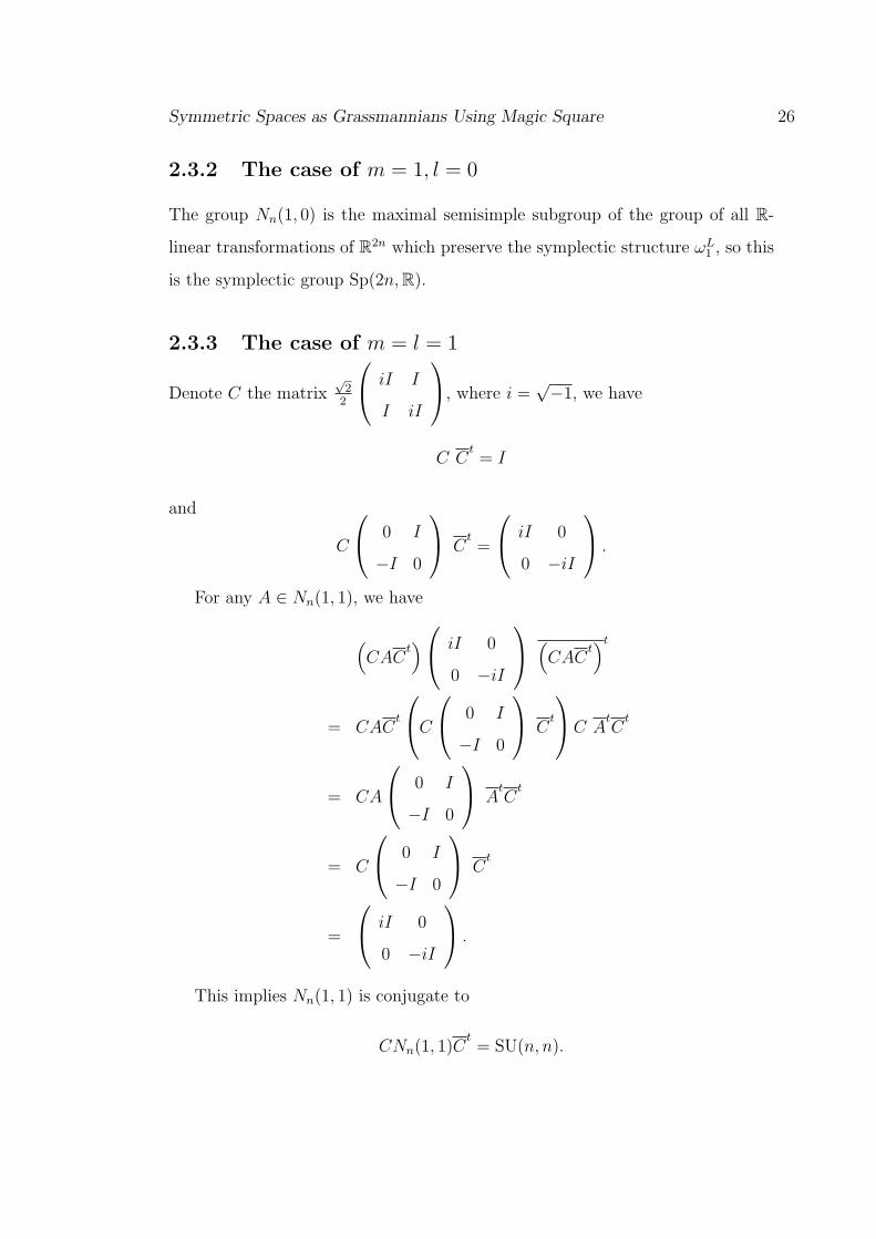
2.3.2 The case of m = 1, l = 0
The group Nn(1, 0) is the maximal semisimple subgroup of the group of all R-
linear transformations of R2n which preserve the symplectic structure ωL1 , so this
is the symplectic group Sp(2n,R).
2.3.3 The case of m = l = 1
Denote C the matrix√
22
iI I
I iI
, where i =
√−1, we have
C Ct= I
and
C
0 I
−I 0
C
t=
iI 0
0 −iI
.
For any A ∈ Nn(1, 1), we have
(CAC
t)
iI 0
0 −iI
(CAC
t)t
= CACt
C
0 I
−I 0
C
t
C A
tC
t
= CA
0 I
−I 0
A
tC
t
= C
0 I
−I 0
C
t
=
iI 0
0 −iI
.
This implies Nn(1, 1) is conjugate to
CNn(1, 1)Ct= SU(n, n).

Symmetric Spaces as Grassmannians Using Magic Square 27
2.3.4 The case of m = 1, l = 2
Nn(1, 2) is the group of all H-linear transformations of H2n, which preserve the
symplectic structure ωL1 .
Nn(1, 2) =
A + jB ∈ SL(2n,H) | (A + jB)
0 I
−I 0
(
A + jB)t
=
0 I
−I 0
Denote C the matrix 12
(i + j)I (−1− k)I
(−1 + k)I (i− j)I
, we have
C Ct= I
and
C
0 I
−I 0
C
t= −j
I 0
0 I
.
So the group Nn(1, 2) is conjugate to
CNn(1, 2)Ct=
A + jB ∈ SL(2n,H) | (A + jB) jI
(A + jB
)t= jI
.
We use the embedding
SL(2n,H) −→ SL(4n,C)
A + jB 7→ A −B
B A
,
any element A + jB ∈ CNn(1, 2)Ct
corresponds to
A −B
B A
∈ SL(4n,C),
which satisfies
A −B
B A
0 −I
I 0
A −B
B A
t
=
0 −I
I 0
.

Symmetric Spaces as Grassmannians Using Magic Square 28
By elementary calculation this is equivalent to
A
0 −I
I 0
A
t=
0 −I
I 0
,
AAt = I,
where A ∈ SL(4n,C). That is A ∈ SO∗(4n). (See [9] p.445)
2.3.5 The case of m = 2
First we introduce the following three properties.
Let (g, σ) be an orthogonal symmetric Lie algebra of noncompact semisimple
type with standard decomposition
g = k + m.
This implies that k is the maximal compact Lie subalgebra of g. We define a real
subspace g∗ of the complexification gC of g by
g∗ = k∗ + m∗, where k∗ = k, m∗ =√−1m,
and σ∗ a real linear map of g∗ into itself defined by
σ∗(X + Y ) = X − Y, (X ∈ k∗, Y ∈ m∗).
Then (g∗, σ∗) is an orthogonal symmetric Lie algebra of compact type, which is
the compact dual to (g, σ). g∗ is also a maximal compact Lie subalgebra of gC.
In the following we consider this on the Lie group level. If G is a Lie group of
noncompact type with g as its Lie algebra, and the maximal compact subgroup
K with k as its Lie algebra, then G/K is the noncompact dual to Gc/K, where Gc
with gc as its Lie algebra is the maximal compact subgroup of the complexification
of G.

Symmetric Spaces as Grassmannians Using Magic Square 29
Proposition 2.3.1 Nn(0, l)/Gn(0, l) is the noncompact dual to Gsn(1, l)/Gn(0, l).
Proof. Consider V [1,l] together with the complex structures J1, ..., Jl and
symplectic structure ω (in the proof of this and next propositions we omit R and
L in JRj and ωL
i respectively),
ω(Jiu, Jiv) = ω(u, v)
induces
ιω Ji = J∗i ιω.
Let g be the standard Euclidean metric, by simple calculation we have
g(Jiu, Jiv) = g(u, v),
this induces
Ji ι−1g = ι−1
g J∗i .
We define a complex structure J (this is obvious a complex structure) by
ω(u, v) = g(Ju, v),
i.e.
J = ι−1g ιω.
It is easy to check that
Ji J = Ji ι−1g ιω
= ι−1g J∗i ιω
= ι−1g ιω Ji
= J Ji,
so
Ji (J A) = (J A) Ji.

Symmetric Spaces as Grassmannians Using Magic Square 30
This implies that the subgroup of the special linear group of V [1,l] whose elements
preserve J1, ..., Jl and J is the complexification of the subgroup of the special
linear group of V [o,l] whose elements preserve J1, ..., Jl, i.e.
SL(V [1,l], J1, ..., Jl, J) = SL(V [0,l], J1, ..., Jl)C.
For any A ∈ SL(V [1,l], J1, ..., Jl), if g(Au,Av) = g(u, v), then
A∗ ιω = ιω A
⇔ A ι−1g ιω = ι−1
g A∗ ιω = ι−1g ιω A
⇔ AJ = JA
This implies
SL(V [1,l], J1, ..., Jl, J, g) = SL(V [1,l], J1, ..., Jl, ω, g).
So
Gn(1, l) = SL(V [1,l], J1, ..., Jl, ω, g)
= SL(V [1,l], J1, ..., Jl, J, g)
= maximal compact subgroup of SL(V [1,l], J1, ..., Jl, J)
= maximal compact subgroup of SL(T lV, J1, ..., Jl)C,
this implies our result. ¤
Proposition 2.3.2 Nn(2, l) is the complexification of Nn(1, l).
Proof. Let J ′ be ι−1ω1 ιω2 , it is a complex structure since
(J ′)2 = (ι−1ω1 ιω2)(ι
−1ω1 ιω2)
= (−ι−1ω2 ιω1)(ι
−1ω1 ιω2) (by preposition 2.2.1)
= −ι−1ω2 ιω2
= −I.

Symmetric Spaces as Grassmannians Using Magic Square 31
For any A ∈ SL(V [2,l], J1, ..., Jl, ω1),
ιω2 A = A∗ ιω2
⇔ A ι−1ω1 ιω2 = ι−1
ω1 A∗ ιω2 = ι−1
ω1 ιω2 A
⇔ AJ ′ = J ′A
implies
SL(V [2,l], J1, ..., Jl, ω1, ω2) = SL(V [2,l], J1, ..., Jl, ω1, J′).
Next we check SL(V [2,l], J1, ..., Jl, ω1, J′) is a complex Lie group, i.e. we need
to check
JiJ′ = J ′Ji, for any i = 1, ..., l
and
ω1(J′u, J ′v) = −ω1(u, v), for any u, v ∈ V [2,l].
First JiJ′ = J ′Ji follows from
ι−1ω1 ιω2 Ji = ι−1
ω1 J∗i ιω2 = Ji ι−1
ω1 ιω2 .
The following calculation
ω1(J′u, J ′v) = ω1(ι
−1ω1 ιω2(u), ι−1
ω1 ιω2(v))
= ιω1(ι−1ω1 ιω2(u))(ι−1
ω1 ιω2(v))
= ιω2(u)(ι−1ω1 ιω2(v))
= ω2(u, ι−1ω1 ιω2(v))
= −ω2(ι−1ω1 ιω2(v), u)
= −ιω2(ι−1ω1 ιω2(v))(u)
= −ιω2(−ι−1ω2 ιω1(v))(u) (by proposition 2.2.1)
= ιω1(v)(u)
= −ω1(u, v)

Symmetric Spaces as Grassmannians Using Magic Square 32
implies
ω1(J′u, J ′v) = −ω1(u, v).
Unify the above discussion we have
Nn(l, 2) = SL(V [2,l], J1, ..., Jl, ω1, ω2)
= SL(V [2,l], J1, ..., Jl, ω1, J′)
= SL(V [1,l], J1, ..., Jl, ω1)C,
i.e. Nn(2, l) is the complexification of Nn(1, l). ¤
Proposition 2.3.3 Nn(1, l)/Gn(1, l) is the noncompact dual of Gsn(2, l)/Gn(1, l).
Proof. This property is a direct corollary of 2.3.2. ¤
Use proposition 2.3.2 we have the following table for Nn(m, l)
A\B R C H
R SL(n,R) SL(n,C) SL(n,H)
C Sp(2n,R) SU(n, n) SO∗(4n)
H Sp(2n,C) SL(2n,C) SO(4n,C)
The maximal compact (semisimple) subgroups Gsn(m, l) of Nn(m, l) are
A\B R C H
R SO(n) SU(n) Sp(n)
C SU(n) SU(n)2 SU(2n)
H Sp(n) SU(2n) SO(4n)
At the Lie algebra level we also have the tables (T1) and (T2) in the introduc-
tion for the noncompact Lie algebras nn(m, l) and compact Lie algebras Ln(A,B)
respectively.
If we use the above properties 2.3.1, 2.3.2 and 2.3.3 to extend the above
noncompact square to the fourth column, we have the table of noncompact square
for Nn(m, l) as in theorem 2.3.2.

Symmetric Spaces as Grassmannians Using Magic Square 33
Remark 2.3.1 Now we will use the above properties to give another way to for-
mulate the construction of the noncompact magic square of Lie groups.
In the above construction we view Nn(m, l) as the connected maximal semisim-
ple subgroup of the group of all B-linear transformations of (T ∗)mBn which pre-
serve ωLi (where i = 1, ..., m).
According to the proof of proposition 2.3.2, by introducing the complex struc-
ture JL1 = J ′ = ι−1
ωL1 ιωL
2(only when m = 2), (T ∗)mBn can be identified as
A2⊗B-linear subspace (A
2⊗B)2n when we only consider R-linear transformations
of (T ∗)mBn which preserve the complex structures JL1 (only when m = 2), JR
j = Jj
(where j = 1, ..., l) and ωLm.
Now we view Nn(m, l) as the connected maximal semisimple subgroup of the
group of all A2⊗B-linear transformations of (A
2⊗B)2n which preserve ωL
m, where
ωLm is viewed as a 2n× 2n matrix with entries in A
2⊗ B.
For any A ∈ Nn(m, l), we identify A ∈ SL(2n, A2⊗ B), which satisfies
AωLmAt = ωL
m,
where ˜ is the conjugation with respect to the right side of the tensor product,
that is the conjugation of B.
At the Lie algebra level, for any element A ∈ nn(m, l), identify A ∈ M2n(A2⊗
B), the Lie algebra of 2n× 2n matrix with entries in A2⊗ B, which satisfies
AωLm + ωL
mAt = 0.
So by proper choosing of coordinates (such that ωLm is of the form
0 I
−I 0
as a 2n× 2n matrix with entries in A2⊗B), any element of nn(l, m) has the form
A B
C −At
,
where A,B,C ∈ Mn(A2⊗B), the algebra of n× n matrices with entries in A
2⊗B,
and Bt = B, Ct = C.

Symmetric Spaces as Grassmannians Using Magic Square 34
Remark 2.3.2 If we equip (A2⊗ B)2n with the standard Euclidean metric, the
symplectic structure ωLm induces a complex structure JL
m, the maximal compact
subgroup Gn(m, l) of Nn(m, l) can be viewed as the group of all A ⊗ B-linear
transformations of (A⊗ B)n in Nn(m, l) which preserve the standard metric.
From now on we consider (A⊗B)n instead of (A2⊗B)2n unless stated otherwise,
and use the above formulation of Gn(m, l).

Chapter 3
Compact Riemannian Symmetric
Spaces
3.1 Definitions and First Properties
Let (M, g) be a Riemannian manifold. Let p ∈ M and let Br(p) be a normal
coordinate ball around p. The diffeomorphism of Br(p)
σp = Expp (−Ip) Exp−1p ,
is called the geodesic symmetry at p, where Expp is the exponential map at p and
Ip is the identity map of TpM , the tangent space of M at p.
Definition 3.1.1 The Riemannian manifold (M, g) is said to be Riemannian
locally symmetric if for each p ∈ M there is a suitable Br(p) such that the geodesic
symmetry σp is an isometry of Br(p) relative to the metric induced by g.
Definition 3.1.2 A Riemannian manifold (M, g) is a Riemannian symmetric
space if each point p ∈ M is an isolated fix point of an involutive isometry σp of
M .
Here “involutive” means that the square is the identity map and σp is called
the symmetry at p. In this case, the differential (σp)∗p is an linear isomorphism
35

Symmetric Spaces as Grassmannians Using Magic Square 36
of TpM which has no nonzero fixed vector, it must coincide with −Ip. Thus σp is
the geodesic symmetry on every normal coordinate ball Br(p). Hence (M, g) is
locally symmetric.
A topological space M is said to be simply connected if it is path connected
and the fundamental group of M is trivial. A Riemannian manifold (M, g) is
complete if it is complete as a metric space, i.e. every Cauchy sequence in M is
a convergent sequence.
The following theorem gives a characterization of a Riemannian locally sym-
metric space in terms of the Riemannian curvature tensor field and a sufficient
condition for a Riemannian locally symmetric space to be Riemannian symmetric.
Theorem 3.1.3 Let (M, g) be a Riemannian manifold, D the Riemannian con-
nection, and R the Riemannian curvature tensor field.
1. For (M, g) to be Riemannian locally symmetric it is necessary and sufficient
for R to be parallel relative to D : DR = 0.
2. If (M, g) is a Riemannian locally symmetric space which is simply connected
and complete, then it is Riemannian symmetric.
The completeness assumption of the above theorem cannot be dropped, as we
will see in the following theorem.
Theorem 3.1.4 Let (M, g) be a Riemannian symmetric space. Then
1. (M, g) is complete.
2. (M, g) is Riemannian homogeneous.
3. The universal Riemannian covering manifold (M, g) of (M, g) is Rieman-
nian symmetric.

Symmetric Spaces as Grassmannians Using Magic Square 37
Two Riemannian manifolds (M1, g1) and (M2, g2) are said to be locally iso-
metric if their universal Riemannian covering manifolds are isometric. In this
thesis we will give a uniform description of Riemannian symmetric spaces up to
local isometry. By theorem 3.1.4 this is equivalent to classifying simply connected
Riemannian symmetric spaces up to isometry.
A simply connected Riemannian symmetric space (M, g) is uniquely decom-
posed as the direct product
(M, g) = (M0, g0)× (M1, g1),
where (M0, g0) is a Euclidean space and (M1, g1) is a simply connected Rieman-
nian symmetric space of semisimple type, which by definition has no parallel
vector field, that is, the only smooth vector field on M1 that is parallel relative
to the Riemannian connection D is the zero vector field.
Because of the following de Rham decomposition, we can concentrate our
attention on the irreducible Riemannian symmetric space.
Definition 3.1.5 A Riemannian symmetric space (M, g) is said to be irreducible
if, for each p ∈ M , the holonomy algebra h(p) acts on TpM irreducibly and
nontrivially.
Theorem 3.1.6 (de Rham decomposition) A simply connected Riemannian
symmetric space (M, g) is the direct product
(M, g) = (M0, g0)× (M1, g1)...× (Mm, gm),
where (M0, g0) is a Euclidean space and each (Mi, gi) is a simply connected irre-
ducible Riemannian symmetric space. The decomposition is unique up to order
of irreducible factors.
Let (M, g) be a connected Riemannian symmetric space, by theorem 3.1.4
(M, g) is Riemannian homogeneous. Let G be the identity component of the

Symmetric Spaces as Grassmannians Using Magic Square 38
isometry group of (M, g), which acts transitively on M , K the isotropy subgroup
of a fixed point p ∈ M . Hence M can be identified with the quotient space G/K
together with the action of G by the correspondence
gK 7→ g(p)
for g ∈ G.
The most well-known example of Riemannian symmetric space is the real
Grassmannian GrR(k, W ), i.e. the space of all k-dimensional linear subspaces in
a real vector space W . In this case, σP (P ′) is the reflection of the k-dimensional
subspace P ′ along P . Other Riemannian symmetric spaces can be constructed
using (multi-)complex and (multi-) symplectic structures on W .
Recall when A,B ∈ R,C,H and we write dimRA = 2m, dimRB = 2l, then
W = (A ⊗ B)n can be identified as a real vector space together with complex
structures JLi and JR
j , where i = 1, ..., m and j = 1, ..., l. If we equip W with the
standard Euclidean metric g, then each complex structure JLi (respectively JR
j )
induces a symplectic structure ωLi (respectively ωR
j ) on W . Let GrR(W ) denote
the space of all R-linear subspaces of W , i.e.,
GrR(W ) =N∐
k=0
GrR(k, W )
=N∐
k=0
O(N)/O(k)O(N − k),
where N = dimRW .
Each complex structure J on W induces an involution σJ on GrR(W ), given
by
σJ : GrR(W ) → GrR(W ),
σJ(P ) = J(P ) = J(v)|v ∈ P ,
for any R-linear subspace P ⊂ W . Its fix point set
GrR(W )σJ = P ∈ GrR(W ) | J(P ) = P

Symmetric Spaces as Grassmannians Using Magic Square 39
is simply the union of complex Grassmannians of J-complex linear subspaces in
W , i.e.
GrR(W )σJ ∼=N∐
k=1
U(N)
U(k)U(N − k),
where 2N = dimRW .
Similarly, any symplectic structure ω on W induces a map σω on GrR(W ),
σω : GrR(W ) → GrR(W ),
σω(P ) = P⊥ω = v ∈ W |ω(v, w) = 0, for any w ∈ P ,
for any R-linear subspace P ⊂ W . Non-degeneracy of ω implies that
dimRP + dimRσω(P ) = dimRW.
Together with the simple fact P ⊂ (P⊥ω)⊥ω , they imply that σω is also an invo-
lution, i.e. (σω)2 = id. Observe that σω(P ) = P if and only if P is a Lagrangian
subspace of W . Namely P is a half dimensional subspace such that ω vanishes
on P . Hence the fix point set of σω can be identified as the Lagrangian Grass-
mannian, i.e.
GrR(W )σω ∼= U(N)
O(N).
Proposition 3.1.1 Given any Hermitian vector space (W, g, J, ω) of dimension
2n, the involutions σJ and σω are isometries on GrR(2k, W ) (k = 1, ..., n) and
GrR(n,W ) respctively.
Proof. Take an orthonormal real basis e1, e2, ..., e2n of W , such that
Je2i−1 = e2i, Je2i = −e2i−1,
for i = 1, ..., n. For any A ∈ O(2n), define
σJ : GrR(2k, W ) → GrR(2k, W ),
σJ(AK) = AJK,

Symmetric Spaces as Grassmannians Using Magic Square 40
where K is O(2k)O(2n − 2k). σJ is well-defined because the linear subspaces
generated by e1, e2, ..., e2k and e2k+1, e2k+2, ..., e2n are complex. Since J ∈O(W ), and O(W ) is the isometry group of GrR(2k, W ), this implies σJ is an
isometry with respect to the invariant metric of GrR(2k, W ).
For σω, we choose an orthonormal basis such that ω (as a non-degenerate two
form) is of the form 0 I
−I 0
.
For any A ∈ O(2n), define
σω : GrR(n,W ) → GrR(n,W ),
σω(AK) = ωAω−1K,
where K = O(n)O(n). It is easy to check σω is also well-defined.
ω(A(e1, ..., e2n)t, ωAω−1(e1, ..., e2n)t)
= Aω(ωAω−1)t
= ω
=
0 I
−I 0
.
Here we view the upper n rows of A as a basis of the linear subspace corresponding
to A, this implies that for any linear subspace P corresponding to A, σω(P ) = P⊥ω
is represented by ωAω−1, i.e. the upper n rows of ωAω−1 is a basis of the linear
subspace P⊥ω . As a matrix ω is in O(2n), this implies σω is an isometry on
GrR(n,W ). ¤
The following lemma enables us to construct many symmetric spaces from the
real Grassmannian using involutive isometries induced by complex and symplectic
structures on W .

Symmetric Spaces as Grassmannians Using Magic Square 41
Lemma 3.1.1 Let M be a Riemannian symmetric space and Σ = σ1, σ2, ..., σsbe a collection of involutive isometries, then the fix point set
MΣ =⋂σ∈Σ
Mσ
with the induced Riemannian metric is again a Riemannian symmetric space.
Proof. Without loss of generality we may assume that MΣ is connected. First
it is easy to see that Mσ is a closed submanifold of M for any σ in Σ. If we can
show that the second fundamental form B of the Levi-Civita connection D is zero,
then Mσ is a totally geodesic submanifold, so MΣ (intersection of totally geodesic
submanifolds) is also a totally geodesic submanifold. Every geodesic in M which
passes through a point x in MΣ with the tangent in TxMΣ is still a geodesic in
MΣ, this implies that MΣ is a locally symmetric space with the induced metric.
For any geodesic isometry σx of M , where x ∈ MΣ, σx(MΣ) ⊂ MΣ (because σx
is just reverse the geodesic) and MΣ is closed in M , so MΣ is a global symmetric
space.
Now we prove the second fundamental form B is zero. For any point x ∈ Mσ,
we have the decomposition of vector space TxM = TxMσ ⊕Nx, where Nx is the
normal vector space of Mσ at x. σ is an isometry, so
DX(Y ) = σ∗(DX(Y )) = Dσ∗X(σ∗Y ),
where X,Y are vectors of M at x. Denote D′, D′′ as the connections induced by
D on TMσ and the normal bundle N of Mσ in M , and e, f as the basis of TMσ
and N respectively, we have D′
e(e) Be(f)
−Btf (e) D′′
f (f)
=
D′
e(e) −Be(f)
−(−Btf (e)) D′′
f (f)
.
This obviously implies B = 0, i.e. the second fundamental form is zero. ¤
Back to W = (A⊗B)n, we denote the set of its canonical complex structures
induced by A as ΣL =JL
1 , ..., JLl−1, J
Ll
. We also define ΣL =
JL
1 , ..., JLl−1, ω
Ll

Symmetric Spaces as Grassmannians Using Magic Square 42
and we have ΣR and ΣR defined in a similar fashsion using complex and symplectic
structures induced from B. They define involutive isometries σ’s on GrR (W )
whose fixed points correspond to complex subspaces or Lagrangian subspaces in
W .
Definition 3.1.7 Let W = (A⊗ B)n, where A,B ∈ R,C,H.
1. Grassmannians GrAB(k, n): The connected component containing (A⊗B)k
of⋂
I∈ΣL∪ΣR
GrR(k · 2m+l,W )σI .
2. Lagrangian Grassmannians LGrAB(n): The connected component contain-
ing (A2⊗ B)n of (with the Abelian part taken away)
⋂
I∈ΣL∪ΣR
GrR(n · 2m+l−1,W )σI .
3. Double Lagrangian Grassmannians LLGrAB(n): The connected component
containing (A2⊗ B
2)n ⊕ (j1
A2⊗ j2
B2)n of (with the Abelian part taken away)
⋂
I∈ΣL∪ΣR
GrR(n · 2m+l−1,W )σI .
By lemma 3.1.1, these Grassmannians, Lagrangian Grassmannians and Dou-
ble Lagrangian Grassmannians are Riemannian symmetric spaces.

Symmetric Spaces as Grassmannians Using Magic Square 43
3.2 Grassmannians
GrAB(k, n) can be viewed as the connected component containing (A⊗B)k of the
space of all A⊗B-linear subspaces P in W = (A⊗B)n with dimA⊗BP = k, where
A,B ∈ R,C,H.
Proposition 3.2.1 When A,B ∈ R,C,H, GrAB(k, n) are given by the spaces
in the table (C2) in the introduction.
Proof. Denote the invariant subspace (A⊗ B)k by P0. It is easy to see that
for any A ∈ Gn(m, l), A · P0 is also an invariant linear subspace under all of the
involutions, because A preserves all these complex structures. The Gn(m, l) orbit
of P0 is connected. Note O(n)/O(k)O(n − k) is connected though O(n) is not
connected. So the Gn(m, l) orbit of P0 is contained in GrAB(k, n). Therefore, it
is enough to show that both have the same dimension.
Let (I B
)
be the coordinates of a point in GrAB(k, n) (k row vectors in (A⊗B)n as a basis of
an invariant subspace), so B is a k×(n−k) matrix with entries in A⊗B. This im-
plies that the dimension of GrAB(k, n) is the same as the dimension of the Gn(m, l)
orbit. It is easy to see that the isotropy subgroup of P0 is Gk(m, l)Gn−k(m, l).
¤
Corollary 3.2.1 When A,B ∈ R,C,H, we have
GrAB(k, n) = G/K,
where
Lie (G) = gn(m, l), and
Lie (K) = gk(m, l)⊕ gn−k(m, l).

Symmetric Spaces as Grassmannians Using Magic Square 44
When A or/and B equals O, GrAB(k, n) need to be defined with more care
because of the non-existence of On. Nevertheless, with the help of Jordan alge-
bras, we can make sense of the Lie algebra Ln(O) of infinitesimal symmetries of
it when n = 2 or 3. Namely they are Spin(9) and F4 respectively. Similarly, using
the magic square, we can define the corresponding Lie algebra Ln(A,B) for any
normed division algebras A and B, provided that n = 2, 3. It is therefore natural
to extend the definition of GrAB(k, n) to include the octonion numbers as below:
Theorem 3.2.1 (Definition-Theorem): Suppose A and B are any normed divi-
sion algebras.
We define GrAB(k, n) to be the symmetric space G/K with
Lie (G) = Ln(A,B) = Der(A)⊕ Der(B)⊕ A′n(A⊗ B), and
Lie (K) = Der(A)⊕ Der(B)⊕ A′k(A⊗ B)⊕ A′
n−k(A⊗ B)⊕ Im(A)⊕ Im(B),
such that if A,B ∈ R,C,H, then GrAB(k, n) is
⋂
I∈ΣL∪ΣR
GrR(k, (A⊗ B)n
)σI
containing (A⊗ B)k. Here k = dimR(A⊗ B)k = k · 2m+l.
If A or B equals O, then we assume that n equals 3.
Remark 3.2.1 Here we use the Vinberg’s version of the magic square [16], and
similar in the subsequence.
Proof. This follows immediately from proposition 3.2.1 and its corollary
3.2.1. ¤
Remark 3.2.2 These types of exceptional symmetric spaces are described as pro-
jective planes over A⊗B (see [3]). In fact we can construct the projective planes
OP2 and (C⊗O)P2 by using Jordan algebras over R and C respectively, but there
is no geometric construction for (H⊗O)P2 and (O⊗O)P2 because H,O are not
fields, thus these is no Jordan algebra defined over them.

Symmetric Spaces as Grassmannians Using Magic Square 45
Theorem 3.2.2 For any normed division algebras A,B ∈ R,C,H,O, GrAB(k, n)
are given by the spaces in the table (C2) in the introduction.

Symmetric Spaces as Grassmannians Using Magic Square 46
3.3 Lagrangian Grassmannians
LGrAB(n) can be viewed as the connected component containing(A
2⊗ B)n
of the
space of all A2⊗ B-linear subspaces P in W = (A ⊗ B)n with dimA
2⊗BP = n
invariant under σωLm, where A ∈ C,H and B ∈ R,C,H.
Proposition 3.3.1 When A ∈ C,H and B ∈ R,C,H, LGrAB(n) are given
by the spaces in the table (C3) in the introduction.
Proof. Recall LGrAB(n) is the space of all R-linear subspaces of W invariant
under the involutions σJLi, σJR
jand σωL
m, where i = 1, ..., m−1, j = 1, .., l. Denote
the invariant subspace(A
2⊗ B)n
by P0. As in the Grassmannians case, we prove
that the Gsn(m, l) orbit of P0 is the connected component containing P0. The
orbit of P0 is obviously contained in the connected component, thus it is enough
to show that both have same dimension.
Let (I, jB
)
be the coordinates of a point in LGrAB(n) (n row vectors in W =(A
2⊗ B)n ⊕
(j · A
2⊗ B)n
as a basis of an invariant subspace P ), where jB is a n × n matrix
with entries in j · A2⊗ B. We have
(I, jB) ωLm
(I, jB
)t
= 0,
where B ∈ Mn
(A2⊗ B)
, it implies:
Bt = B.
So the dimension of this component is the same as the Gsn(m, l) orbit (see remark
2.3.1). ¤
Corollary 3.3.1 When A ∈ C,H and B ∈ R,C,H, we have
LGrAB(n) = G/K,

Symmetric Spaces as Grassmannians Using Magic Square 47
where
Lie (G) = Ln(A,B), and
Lie (K) = Ln
(A2
,B)⊕ Im
(A2
).
When A or/and B equals O, the definition for LGrAB(n) is naturally extended
as below.
Theorem 3.3.1 (Definition-Theorem): Suppose A and B are any normed divi-
sion algebras and A is not R.
We define LGrAB(n) to be the symmetric space G/K with
Lie (G) = Ln(A,B) = Der(A)⊕ Der(B)⊕ A′n(A⊗ B), and
Lie (K) = Ln
(A2
,B)⊕ Im
(A2
),
such that if A,B ∈ R,C,H, then LGrAB(n) is the connected component con-
taining(A
2⊗ B)n
of (with the Abelian part taken away)
⋂
I∈ΣL∪ΣR
GrR(k, (A⊗ B)n
)σI,
where k = dimR(A⊗B)n
2= n · 2m+l−1.
If A or B equals O, then we assume that n equals 3.
Proof. This follows immediately from proposition 3.3.1 and its corollary
3.3.1. ¤
Theorem 3.3.2 For any normed division algebra A ∈ C,H,O and B ∈ R,C,
H,O, LGrAB(n) are given by the spaces in the table (C3) in the introduction.

Symmetric Spaces as Grassmannians Using Magic Square 48
3.4 Double Lagrangian Grassmannians
LLGrAB(n) can be viewed as the connected component containing(A
2⊗ B
2
)n ⊕(j1A2⊗ j2
B2
)nof the space of all A
2⊗B
2-linear subspaces P in W = (A⊗B)n invariant
under σωLm
and σωRl
with dimA2⊗ B
2P = 2n, where A ∈ C,H and B ∈ C,H.
Proposition 3.4.1 When A,B ∈ C,H, LLGrAB(n) are given by the spaces in
the table (C4) in the introduction.
Proof. The Gsn(m, l) orbit of P0 =
(A2⊗ B
2
)n ⊕ (j1A2⊗ j2
B2
)nis contained in
LLGrAB(n) since A · P0 is also an invariant subspace in W for any A ∈ Gsn(m, l).
Thus we only need to prove both have same dimensions as before.
First we determine the Lie algebra k of the isotropy subgroup of P0 in GrR(k, W
),
it is easy to see that k is
An
(A2⊗ B
2
)⊕ An
(j1A2⊗ j2
B2
).
1. When m = l = 1, k is obvious so(n)2.
2. When m = 1, l = 2. Any element of An(C ⊗ R) ⊕ An(jC ⊗ iR) can be
represented as
A · 1⊗ 1 + B · i⊗ 1 + C · j ⊗ i + D · k ⊗ i,
where A,B,C,D ∈ Mn(R). These can be identify as
A−D C −B
C + B A + D
.
It is not difficult to check that this is an element in so(2n,R), so An(C ⊗R)⊕ An(jC⊗ iR) is isomorphic to so(2n).
3. When m = 2, l = 1, this is the same case as m = 1, l = 2.

Symmetric Spaces as Grassmannians Using Magic Square 49
4. When m = l = 2, k is An(C⊗C)⊕An(jC⊗ jC). C⊗C can be identified as
C⊕ C,
this implies that k is isomorphic to
(An(C)⊕ An(j ⊗ j · C))⊕ (An(C)⊕ An(j ⊗ j · C)).
Then any element of k can be represented as
A + B · i + C · j ⊗ j + D · k ⊗ j,
where A,B,C,D ∈ Mn(R), then identify this to A−D C −B
C + B A + D
,
so k is isomorphic to so(2n)2.
To show that the orbit is the connected component we only need to consider
the dimensions of the orbit and the component because the orbit is contained in
the connected component.
We use x, y, z, w to denote the coordinates of W with respect to the follow-
ing decomposition:(A2⊗ B
2
)n
⊕(
j1A2⊗ j2
B2
)n
⊕(
j1A2⊗ B
2
)n
⊕(A2⊗ j2
B2
)n
.
We use I 0 j1B1 0
0 I 0 j2B2
to denote any point P near P0, where B1, B2 ∈ Mn
(A2⊗ B
2
). Since P is an
invariant subspace, we have the following conditions: I 0 j1B1 0
0 I 0 j2B2
ωL
m
I 0 j1B1 0
0 I 0 j2B2
t
= 0,
I 0 j1B1 0
0 I 0 j2B2
ωR
l
I 0 j1B1 0
0 I 0 j2B2
t
= 0.

Symmetric Spaces as Grassmannians Using Magic Square 50
Under the above coordinates, ωRl , ωL
m is represented by the following matrices:
ωRl =
0 0 0 I
0 0 −I 0
0 I 0 0
−I 0 0 0
, ωLm =
0 0 I 0
0 0 0 −I
−I 0 0 0
0 I 0 0
.
Denote
P1 =
0 I
−I 0
, P2 =
I 0
0 −I
,
so we have
B · P1 + P1 · Bt = 0, P2 · Bt = B · P2.
By simple calculation we have
B =
B1 B2
−B2 −Bt1
,
where Bt1 = B1, B
t2 = B2.
When m = l = 1, the dimension is n2 − n.
When m = 1, l = 2 or m = 1, l = 2, we have
JRi B1 = B1J
Ri , JL
j B1 = B2JLj ,
so
B1 =
a b
b −a
,
where at = a, bt = b, so the dimension of B1 is n2 + n. By the same way, the
dimension of B2 is n2, so the result is true.
For m = l = 2, the case is similar. ¤
Corollary 3.4.1 When A,B ∈ C,H, we have
LLGrAB(n) = G/K,

Symmetric Spaces as Grassmannians Using Magic Square 51
where
Lie (G) = Ln(A,B), and
Lie (K) = An
(A2⊗ B
2
)⊕ An
(j1A2⊗ j2
B2
).
When A or/and B equalsO, the definition for LLGrAB(n) is naturally extended
as below.
Theorem 3.4.1 (Definition-Theorem): Suppose A and B are any normed divi-
sion algebras except R.
We define LLGrAB(n) to be the symmetric space G/K with
Lie (G) = Ln(A,B) = Der(A)⊕ Der(B)⊕ A′n(A⊗ B), and
Lie (K) = Der
(A2
)⊕ Der
(B2
)⊕ An
(A2⊗ B
2
)⊕ An
(j1A2⊗ j2
B2
),
such that if A,B ∈ C,H, then LLGrAB(n) is the connected component contain-
ing(A
2⊗ B
2
)n ⊕ (j1A2⊗ j2
B2
)nof (with the Abelian part taken away)
⋂
I∈ΣL∪ΣR
GrR(k, (A⊗ B)n
)σI,
where k = dimR(A⊗B)n
2= n · 2m+l−1.
If A or B equals O, then we assume that n equals 3.
Proof. This follows immediately from proposition 3.4.1 and its corollary
3.4.1. ¤
Theorem 3.4.2 For any normed division algebras A,B ∈ C,H,O, LLGrAB(n)
are given by the spaces in the table (C4) in the introduction.
Remark 3.4.1 When n = 3, the double Lagrangian Grassmannians can be viewed
as
LLGrAB =
2∧ (
A2⊗B
2
)4
⊂ (A⊗ B)3
.

Symmetric Spaces as Grassmannians Using Magic Square 52
3.5 Compact Simple Lie Groups
Let W = (A ⊗ B)n with complex structures JLi , JR
j as before, T ∗W = W + W ∗
is a vector space with the induced complex structures JLi , JR
j and a symplectic
structure ω = dx∧dy (here x, y denote the coordinates of W and the cotangent
space respectively). But here we consider the symmetric tensor (non-definite)
g′ = dx⊗ dy
rather than the skew-symmetric structure ω.
As in the case of ω, g′ induces an involution on GrR(T∗W ),
σg′ : GrR(T∗W ) → GrR(T
∗W ),
σg′(P ) = P⊥g′ = v ∈ T ∗W |g′(v, w) = 0, for any w ∈ P ,
for any real linear subspace P ⊂ T ∗W .
Let N be the dimension of W over R, for any A ∈ O(2N), σg′ is defined as
σg′(AK) = g′Ag′−1K,
where K is O(N)O(N) and g′ is the matrix
0 I
I 0
, where I is the identity
matrix in O(N). So σω is also well-defined and is an isometry on GrR(N, 2N).
Denote the connected component containing W (with the Abelian part taken
away) of the space of all linear subspaces of T ∗W which are invariant under the
involutive isometries σJLi, σJR
jand σg′ as GAB(n), where i = 1, ..., m, j = 1, ..., l.
Proposition 3.5.1 When A,B ∈ R,C,H, GAB(n) is the space in the table
(C1) in the introduction.
Remark 3.5.1 These symmetric spaces are compact (semi)simple Lie groups.

Symmetric Spaces as Grassmannians Using Magic Square 53
Proof. Take the coordinate transformation
u =1√2(x + y),
v =1√2(x− y),
the symmetric tensor becomes
g′ = du2 − dv2,
and the standard metric is
g = dx2 + dy2 = du2 + dv2.
The group of all A ⊗ B-linear transformations of T ∗W which preserve g′ and
the standard metric g is isomorphic to Gn(m, l)2, the isotropy subgroup of W is
obvious the group of all A⊗ B-linear transformations of W , that is Gn(m, l). So
the Gn(m, l)2 orbit of W (with the Abelian part taken away) is the space in the
table (C1) in the introduction.
Now We prove that the orbit is the connected component which contains W .
Obviously the orbit is contained in the connected component, we only need to
compare their dimensions. W is characterized by (I, I) under the coordinates
u, v, a point (I B
),
is invariant under σg′ implies
(I, B)g′(I, B
)t= 0,
where B ∈ Mn(A⊗ B). By simple calculation we have
BBt= I.
This implies that the dimension of the Gn(m, l)2 orbit is the same as the connected
component. ¤

Symmetric Spaces as Grassmannians Using Magic Square 54
Corollary 3.5.1 When A,B ∈ R,C,H, we have
GAB(n) = G/K,
where
Lie (G) = (gn(m, l))2, and
Lie (K) = gn(m, l).
When A or/and B equals O, the definition for GAB(n) is naturally extended
as below.
Theorem 3.5.1 (Definition-Theorem): Suppose A and B are any normed divi-
sion algebras.
We define GAB(n) to be the symmetric space G/K with
Lie (G) = Ln(A,B)2 = (Der(A)⊕ Der(B)⊕ A′n(A⊗ B))2
Lie (K) = Ln(A,B),
such that if A,B ∈ R,C,H, then GAB(n) is the connected component containing
(A⊗ B)n of (with the Abelian part taken away)
⋂
I∈ΣL∪ΣR∪σg′GrR
(k, T ∗(A⊗ B)n
)σI,
where k = dimRT ∗(A⊗B)n
2= n · 2m+l.
If A or B equals O, then we assume that n equals 3.
Proof. This follows immediately from proposition 3.5.1 and its corollary
3.5.1. ¤
Theorem 3.5.2 For any normed division algebras A,B ∈ R,C,H,O, GAB(n)
are given by the spaces in the table (C1) in the introduction.

Chapter 4
Noncompact Riemannian
Symmetric Spaces
4.1 Dual Riemannian Symmetric Spaces and
Borel Embedding
Riemannian symmetric spaces of semisimple type come in pairs. Given any simply
connected Riemannian symmetric space X = G/K, we have a decomposition of
its orthogonal symmetric Lie algebra g = k⊕p. Then g∗ = k⊕√−1p ⊆ gC is also
an orthogonal symmetric Lie algebra and its corresponding symmetric space X is
called the dual of X. Furthermore X is compact if and only if X is noncompact
and vice versa. Another amazing property is the existence of a natural embedding
X ⊂ X as an open submanifold if X is a hermitian symmetric space, which is
called the Borel embedding. For example, when X = SU(n)/S(U(k)U(n − k)),
then we have X = SU(k, n− k)/S(U(k)U(n− k)).
In this chapter we want to generalize the Borel embedding to other cases of
pairs of Riemannian symmetric spaces.
55

Symmetric Spaces as Grassmannians Using Magic Square 56
4.2 An Embedding of Noncompact Symmetric
Space into Its Compact Dual
In fact, for any symmetric space X, (not necessary hermitian) there exists a
natural embedding X ⊂ X as an open submanifold, at least for the classical cases.
For example, when X is the Grassmannian GrR (k, W ) = O (N) /O (k) O (N − k),
then we have X = O (k, N − k) /O (k) O (N − k). In fact X is the Grassmannian
of spacelike linear subspaces in W . To explain it, we need the following definitions.
Definition 4.2.1 We assume W is a real vector space with a positive definite
inner product gW . Given a fixed linear subspace P0 in W , which corresponds to
an element P0 in GrR (k, W ), we have an orthogonal decomposition W = P0⊕P⊥0
with respect to gW . This determines an indefinite inner product gW on W given
by
gW = gW |P0 − gW |P⊥0 .
(i) An element P in GrR (k, W ) is called spacelike if the restriction of gW to
P is positive definite, i.e. gW |P > 0.
(ii) We denote Gr+R (k, W ) the space of all spacelike elements in GrR (k, W ).
(iii) For any subspace X of GrR (k, W ) containing P0, we define X+ = X ∩Gr+
R (k, W ).
It is not difficult to see that the noncompact dual to the Grassmannian is
precisely given by
Gr+R (k, W ) ∼= O (k, N − k) /O (k) O (N − k) .
In this section, we are going to apply our descriptions of compact symmetric
spaces as certain types of Grassmannians, we will show that under the above em-
bedding the noncompact dual to any compact symmetric space X always consists
of spacelike elements in X.

Symmetric Spaces as Grassmannians Using Magic Square 57
The following theorem generalizes the Borel embedding to any pair of Rie-
mannian symmetric spaces of semisimple type in the classical cases.
Theorem 4.2.2 Let W = (A⊗ B)n, where A,B ∈ R,C,H.(1) For any Grassmannian GrAB(k, n) ⊂ GrR(k · 2m+l,W ), we consider P0 =
(A ⊗ B)k ⊂ W , then Gr+AB(k, n) is the noncompact dual to GrAB(k, n) and the
natural inclusion Gr+AB(k, n) ⊂ GrAB(k, n) is an open embedding.
(2) For any Lagrangian Grassmannian LGrAB(n) ⊂ GrR(n · 2m+l−1,W ), we
consider P0 = (A2⊗B)n ⊂ W , then LGr+
AB(n) is the noncompact dual to LGrAB(n)
and the natural inclusion LGr+AB(n) ⊂ LGrAB(n) is an open embedding.
(3) For any Double Lagrangian Grassmannian LLGrAB(n) ⊂ GrR(n·2m+l−1,W ),
we consider P0 = (A2⊗ B
2)n ⊕ (j1
A2⊗ j2
B2)n, then LLGr+
AB(n) is the noncompact
dual to LLGrAB(n) and the natural inclusion LLGr+AB(n) ⊂ LLGrAB(n) is an
open embedding.
(4) For any compact Lie group G = GAB(n) ⊂ GrR(n·2m+l, T ∗W ), we consider
P0 = W , then G+AB(n) is the noncompact dual to GAB(n), and the natural inclusion
G+AB(n) ⊂ GAB(n) is an open embedding.
Proof. Let X be a compact Riemannian symmetric space, recall that X is
the fix point set of some involutive isometries of GrR(k, W ). We want to prove
1. These involutions can be restricted to Gr+R (k, W ).
2. These involutions are isometries on Gr+R (k, W ) with respect to the invariant
metric on Gr+R (k, W ).
Then 1 and 2 implies that M+ is a noncompact Riemannian symmetric space
sitting in M as an open subset by lemma 3.1.1.
Recall the involutive isometries which we used in chapter 3 are σJ σω and
σg′ , we will prove these two facts for σJ σω and σg′ separately. To simplify the
notations in the proof we assume that the dimension of W is 2n in the cases of

Symmetric Spaces as Grassmannians Using Magic Square 58
σJ and σω and the dimension of T ∗W is 2n in the case of σg′ , the dimension of
P0 is 2k in the case of σJ and n in the cases of σω and σg′ .
1. For the involution σJ induced by a complex structure J , take an orthogonal
bases e1, e2, ..., e2n of W , such that for each i, Je2i−1 = e2i, Je2i = −e2i−1.
Then as a matrix J ∈ O(2k)O(2n−2k). For any A ∈ O(2k, 2n−2k), define
σJ : Gr+R (2k, W ) → Gr+
R (2k, W ),
σJ(AK) = AJK,
where K is O(2k)O(2n − 2k). It is easy to check σJ is well-defined. The
following natural embedings
O(2n) → GL(2n,R)
and
O(2k, 2n− 2k) → GL(2n,R)
induce the natural embeddings
O(2k, 2n− 2k)/O(2k)O(2n− 2k) → GL(2n,R)/P
and
O(2n)/O(2k)O(2n− 2k) → GL(2n,R)/P,
where
P =
a b
0 c
∈ GL(2n,R) | a, b, c ∈ Mn(R)
.
For any matrix A in GL(2n,R), one can use the Gram-Schmidt process
to find a matrix B in P , such that AB is an orthogonal matrix. This
implies that the above last embedding is surjective, i.e. GL(2n,R)/P can

Symmetric Spaces as Grassmannians Using Magic Square 59
be identified as O (2n) /O (2k) O (2n− 2k). Let B′ = J−1BJ ∈ P ,
σJ(ABK) = ABJK (in O (2n) /O (2k) O (2n− 2k))
= AJB′K (in O (2n) /O (2k) O (2n− 2k))
= AJP (in GL(2n,R)/P )
= AJK (in O (2k, 2n− 2k) /O (2k) O (2n− 2k))
= σJ(AK) (in O (2k, 2n− 2k) /O (2k) O (2n− 2k)),
this implies σJ = σJ |Gr+R (k,W ). σJ is isometry on Gr+
R (k, W ) because J is a
matrix in O(2k)O(2n− 2k).
2. For the involution σω induced by a symplectic structure ω, take an orthog-
onal bases e1, e2, ..., e2n of W , such that ω is of the form
0 I
−I 0
as a
non-degenerate tow form. Denote by D the matrix
0 I
I 0
, where I is
the identity matrix of rank n. For any A ∈ O(n, n), define
σω : Gr+R (n,W ) → Gr+
R (n,W ),
σω(AK) = DAD−1K,
where K is O(n)O(n). σω is well-defined.
A in O(n, n) means
A
I 0
0 −I
At =
I 0
0 −I
.
The Gram-Schmidt process asserts that there is a matrix B in P such that
AB is an orthogonal matrix, that is
(AB)t(AB) = I.
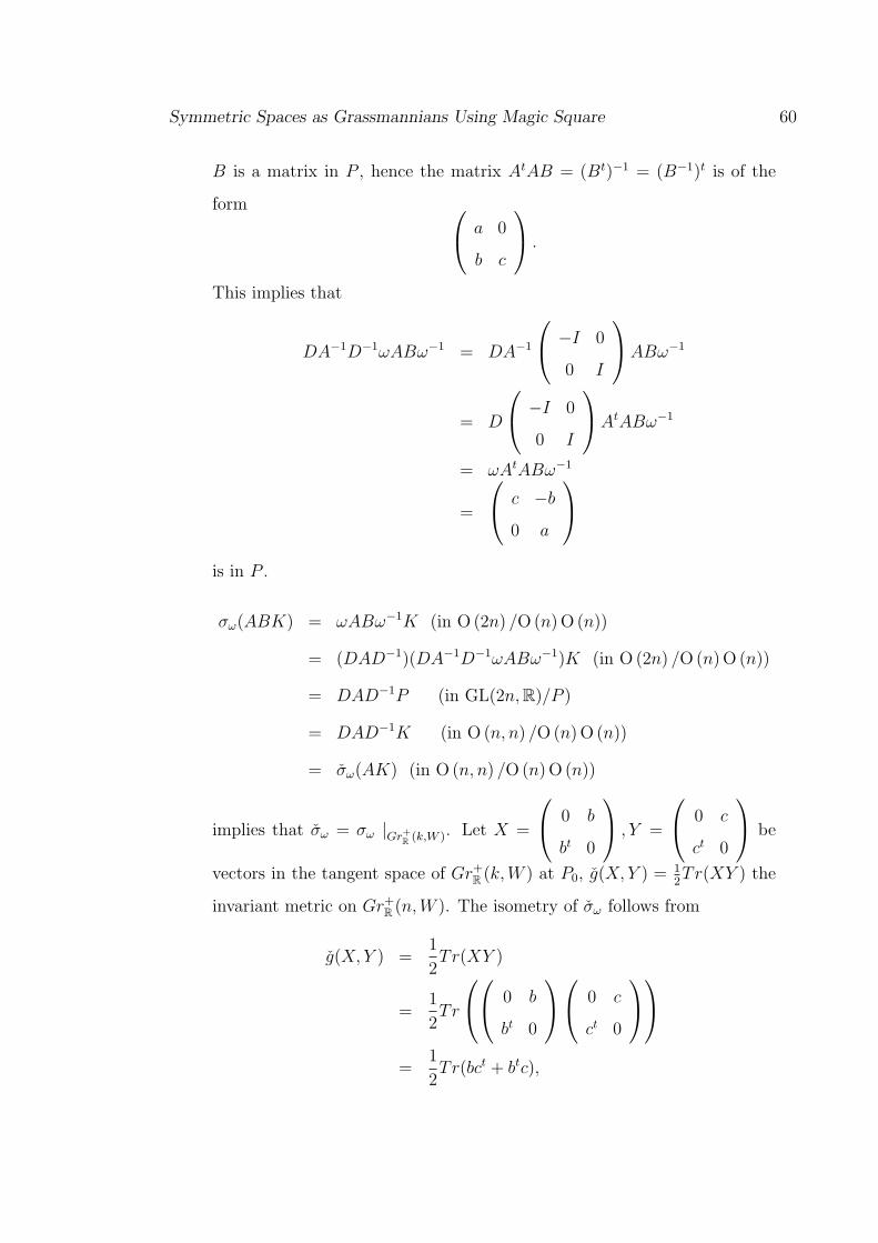
Symmetric Spaces as Grassmannians Using Magic Square 60
B is a matrix in P , hence the matrix AtAB = (Bt)−1 = (B−1)t is of the
form a 0
b c
.
This implies that
DA−1D−1ωABω−1 = DA−1
−I 0
0 I
ABω−1
= D
−I 0
0 I
AtABω−1
= ωAtABω−1
=
c −b
0 a
is in P .
σω(ABK) = ωABω−1K (in O (2n) /O (n) O (n))
= (DAD−1)(DA−1D−1ωABω−1)K (in O (2n) /O (n) O (n))
= DAD−1P (in GL(2n,R)/P )
= DAD−1K (in O (n, n) /O (n) O (n))
= σω(AK) (in O (n, n) /O (n) O (n))
implies that σω = σω |Gr+R (k,W ). Let X =
0 b
bt 0
, Y =
0 c
ct 0
be
vectors in the tangent space of Gr+R (k, W ) at P0, g(X,Y ) = 1
2Tr(XY ) the
invariant metric on Gr+R (n,W ). The isometry of σω follows from
g(X,Y ) =1
2Tr(XY )
=1
2Tr
0 b
bt 0
0 c
ct 0
=1
2Tr(bct + btc),

Symmetric Spaces as Grassmannians Using Magic Square 61
and
g((σω)∗X, (σω)∗Y ) =1
2Tr((σω)∗(X) · (σω)∗(Y ))
=1
2Tr
0 bt
b 0
0 ct
c 0
=1
2Tr(btc + bct).
3. For the involution σg′ induced by a symmetric 2-tensor g′, take an orthog-
onal bases e1, e2, ..., e2n of T ∗W , such that g′ is of the form
0 I
I 0
.
Denote
0 I
−I 0
by Ω, where I is the identity matrix of rank n. For
any A ∈ O(n, n), define
σg′ : Gr+R (n, T ∗W ) → Gr+
R (n, T ∗W ),
σg′(AK) = ΩAΩ−1K,
where K is O(n)O(n) . σg′ is well-defined. Use the notations as above,
σg′(ABK) = g′ABg′−1K (in O (2n) /O (n) O (n))
= (ΩAΩ−1)(ΩA−1Ω−1g′ABg′−1)K (in O (2n) /O (n) O (n))
= (ΩAΩ−1)(g′AtABg′)K (in O (2n) /O (n) O (n))
= (ΩAΩ−1)
c b
0 a
K (in O (2n) /O (n) O (n))
= ΩAΩ−1P (in GL(2n,R)/P )
= ΩAΩ−1K (in O (n, n) /O (n) O (n))
= σg′(AK) (in O (n, n) /O (n) O (n))
implies that σg′ = σg′ |Gr+R (k,W ). Let X,Y be the above tangent vectors of
Gr+R (k, W ) at P0, g(X,Y ) the invariant metric as before. The isometry of

Symmetric Spaces as Grassmannians Using Magic Square 62
σg′ follows from
g((σg′)∗X, (σg′)∗Y ) =1
2Tr((σg′)∗(X) · (σg′)∗(Y ))
=1
2Tr
0 −bt
−b 0
0 −ct
−c 0
=1
2Tr(btc + bct)
= g(X,Y ). ¤

Bibliography
[1] J. F. Adams, Lectures on exceptional Lie groups. University of Chicago Press,
Chicago, 1996.
[2] M. Atiyah, J. Berndt, I., Projective planes, Severi varieties and spheres,
Surveys in Differential Geometry VIII, Papers in Honor of Calabi, Lawson,
Siu and Uhlenbeck (International Press, Somerville, MA, 2003) 1-27.
[3] J. C. Baez, The octonions, Bull. Amer. Math. Soc. 39 (2002), 145-205. Errata
in Bull Amer. Math. Soc. 42 (2005), 213.
[4] C. H. Barton, A. Sudbery, Magic squares of Lie algebras, Ph.D thesis, Uni-
versity of York (2000) and math.RA/0001083
[5] C. H. Barton, A. Sudbery, Magic squares and matrix models of Lie algebras,
Adv. in Math. 180 (2003), 596-647.
[6] R. B. Brown, Groups of type E7, Jour. Reine Angew. Math. 236 (1969),
79-102.
[7] E. Cardan, Sur une classe remarquable d’espaces de Riemann, Bull. Soc.
Math. France 55 (1927), 114-134.
[8] H. Freudenthal, Beziehungen der e7 und e8 zur Oktavenebene, I, II, Indag.
Math. 16 (1954), 218-230, 363-368. III, IV, Indag. Math. 17 (1955), 151-
157, 277-285. V-IX, Indag. Math. 21 (1959), 165-201, 447-474; X, XI, Indag.
Math. 25 (1963), 457-487.
63

Symmetric Spaces as Grassmannians Using Magic Square 64
[9] S. Helgason, Differential geometry Lie groups, and symmetric spaces. Aca-
demic Press, 1978.
[10] P. Jordan, J. von Neumann, E. Wigner, On an algebraic generalization of
the quantum mechanical formalism, Ann. Math. 35 (1934), 29-64.
[11] N. C. Leung, Riemannian geometry over different normed division algebra,
Journal of Differential Geometry 61 (2002), no. 2, 289-333.
[12] R. D. Schafer, Introduction to non-associative algebras. Academic Press,
1966.
[13] T. A. Springer and F. D. Veldkamp, Octonions, Jordan algebras and excep-
tional groups. Springer, Berlin, 2000.
[14] M. Ise, M. Takeuchi, Lie groups I, M. Takeuchi, Lie groups II. Iwanami
Shoten, Publishers, Tokyo, 1978.
[15] J. Tits, Algebres alternatives, algebres de Jordan et algebres de Lie excep-
tionnelles, Indag. Math. 28 (1966), 223-237.
[16] E. B. Vinberg, A construction of exceptional simple Lie groups (Russian),
Tr. Semin. Vektorn. Tensorn. Anal. 13 (1966), 7-9.