a unified approach to subdivision algorithms near...

~ N,~._~ COMPUTER ~_~ AIDED GEOMETRIC

DESIGN ELSEV1ER Computer Aided Geometric Design 12 (1995) 153-174

A unified approach to subdivision algorithms near extraordinary vertices

U l r i c h R e i f * Mathematisches lnstitut A, Universitgit Stuttgart, Pfaffenwaldring 57, 70511 Stuttgart, Germany

Received April 1993; revised January 1994

Abstract

We present a unified approach to subdivision algorithms for meshes with arbitrary topology which admits a rigorous analysis of the generated surface and give a sufficient condition for the regularity of the surface, i.e. for the existence of a regular smooth parametrization near the extraordinary point. The criterion is easily applicable to all known algorithms such as those of Doo-Sabin and Catmull-Clark, but will also be useful to construct new algorithms like interpola- tory subdivision schemes.

Keywords: Subdivision; Arbitrary topology; Regular surface; Characteristic map; Extraordinary vertex

1. Introduct ion

Subdivision algorithms are a powerful tool in CAGD and have been well understood for tensor product surfaces for a long time. Usually, the principle is to describe a given surface over a refined control net where "refined" means in general that the scale is bisected. When a subdivision process is iterated, the control net will contain more and more vertices which converge under well-known conditions to the originally described surface. On the other hand, one can define a subdivision process by an arbitrary linear map in the space of control points without knowing something a priori about a surface. If the sequence of control nets converges in a certain sense, one can use this procedure to generate surfaces.

A combination of these two ideas can help to deal with the problem of filling an n-sided hole or, equivalently, to define surfaces over meshes with arbitrary topology. The first algorithms of this type were given by Doo and Sabin (1978) and by Catmull

* Email: [email protected].

0167-8396/95/$09.50 (~) 1995 Elsevier Science B.V. All rights reserved SSDI 0 1 6 7 - 8 3 9 6 ( 9 4 ) 0 0 0 0 7 - F

154 U. Reif/Computer Aided Geometric Design 12 (1995) 153-174

Fig. 1. Refining a mesh by subdivision.

and Clark (1978). The idea is the following: in general, a control net will consist of large regular regions, where standard C-conditions can be used to describe a smooth surface, and isolated irregular regions, where these conditions are too restrictive. Thus, the resulting surface has gaps, also called n-sided holes, corresponding to the irregular regions and these gaps can be filled gradually by subdivision. To achieve this, the key observation is that subdivision enlarges the regular regions of the control net and shrinks the irregular regions. Number and type of the irregular regions are not changed, but the scale is halved, cf. Fig. 1.

Now it is required that the subdivision process reproduces the original surface completely on the common domain. But, moreover, since parts of the former irregular regions are now regular, it is possible to prolong the original surface. In the space of control points, this means that most of the new ones are determined uniquely from the repro- duction condition, but those corresponding to the new parts of the surface can be chosen rather arbitrarily. Usually, they are computed as a linear combination of old control points near the irregular region. The associated matrix is called the subdivision matrix

and it turns out that a proper choice of this matrix leads in the limit to smooth surfaces when the subdivision process is iterated.

Doo-Sabin and Catmull-Clark suggested particular subdivision matrices where the coefficients were determined by some ad hoc generalizations of the regular case and after that some modified algorithms were proposed. But not before 1986, Ball and Storry (1986; 1988) made a first serious attempt to prove convergence to smooth surfaces for subdivision schemes of Catmull-Clark type. However, a detailed analysis of their proof reveals that it is incomplete as it is exclusively based on the analysis of the eigenproperties of the subdivision matrix and does not take the properties of the basis functions into account. But this is indispensable as will be shown in particular by the examples in the fourth section. The point is that the process of normalizing the sequence of normal vectors can fail if a certain regularity condition is violated. But even if this gap is filled (which can be done), the problem remains that Ball and Storry only try to prove tangent plane continuity near the extraordinary point. However, the existence of a limit for the normal vectors is a rather weak smoothness category since local self- intersections of the surface are still possible. Smoothness in the sense of differential geometry (and, of course, from the point of view of the designer) requires the existence of a regular smooth parametrization for the surface near the point in question.

Recently, Halstead et al. (1993) used Catmull-Clark surfaces to construct surfaces which interpolate the vertices of a given mesh of arbitrary topological type subject to the minimization of a certain fairness functional. In this paper, a short proof for the

U. Reif/Computer Aided Geometric Design 12 (1995) 153-174 155

smoothness of the surfaces is given, but the same remarks as for the Ball and Storry proof apply.

In this paper, we give a new unified approach to the topic which will be carried out for surfaces based on quadrilaterals, but will work in exactly the same way for surfaces based on triangles. Our main result is that all properties of a subdivision algorithm, especially the existence of a smooth regular parametrization for the generated surface near the limit point, can be detected from the leading eigenvalues of the subdivision matrix and an associated characteristic map.

The paper is organized as follows: In Section 2, we formulate the problem and define the setup; in Section 3, we present some theorems on the smoothness properties of the generated surfaces; and in Section 4, we give an example. In the appendix, we outline the proof of two lemmas needed in Section 3. Although they are crucial for the proof of our main theorem, the proofs were diverted to the appendix, since they are somewhat technical.

2. Definitions and formulation of the problem

In practice, subdivision is carried out in the space of control points corresponding to some basis functions. Nevertheless, it is more convenient to start our considerations in the space of patches which make up the surface.

Let X be a parametrically smooth spline surface x consisting of rectangular patches xJ , j c J, with a single n-sided hole. For convenience, we shall assume that X is an infinite surface with the n-sided hole as its only boundary in order to avoid a formal discussion of the outer boundary of the surface. The parameter space J2 := w × J consists of # J copies of the unit square ~o provided with a neighborhood relation. A representation of ,(7 is a map

q b : ( w , j ) ~-+q~'J(6o) 6 R 2, j E J. (2.1)

from s2 to R 2, where the functions q~ are smooth injective maps in R 2 with the property that pieces of boundary curves identified by the neighborhood relation have a common image. Otherwise, the image is supposed to be unique. The resulting mesh F := q~(s'2) is regular, what means that every vertex in the interior of F is shared by exactly four patches. It is well known that this topology admits the generation of smooth surfaces with parametrically smoothness conditions between the patches. On the other hand, a mesh F as shown in Fig. 2 is maximal in the sense that one cannot add further patches inside the n-sided hole without breaking symmetry or regularity.

One possibility to fill the gap is the application of a subdivision process S: We replace every oJ by four new squares and obtain a new parameter space ,(2; the new neighborhood relations are obvious, see Fig. 3.

The: new mesh P := ~ ( ,0 ) generated by some representation ~b has an important property: it can be prolonged by a layer p r (F ) of patches such that the mesh

i We do not distinguish explicitly between a surface viewed as a map or as a point set in ~3. It will be clear

from the context what is meant.


1

¢ x J > p

Fig. 2. Representation of the parameter space.

> 1

) i

S >

Fig. 3. Subdivision of the parameter space.

(daahed) C F (aolid) S ( F ) = F O p t ( r )

Fig. 4. Subdivision and prolongation.

S(F) := / " U p r ( / ' ) (2.2)

is still regular, cf. Fig. 4. In fact, it has exactly the same topological structure as the original mesh F. Thus, we can think of S(F) =: S ( ~ ) ( f 2 ) as a new representation S(@) of the original parameter space /'2 reflecting the fact that the parameter space contains only information on the topology but not on the scale of the mesh.

Now it will be possible to find a parametrically smooth surface S(X) over S(F) with the property that the restriction .~ := S(X)IP of S(X) to the mesh P coincides with the

original surface X (viewed as point sets in •3). The new part of the surface

p r (X) := S(X) \ X = S(X)lpr(r ) (2.3)

is called a prolongation of X. Of course, it is not unique, since the only requirement a priori is that it joins smoothly with the original surface X, but once an algorithm to compute the prolongation has been established, it will not be changed (in a sense that will become clearer soon), when the subdivision process is iterated.

To keep things as simple as possible, assume that

p r (S (X) ) = p r (pr (X) ) = pr2(X), (2.4)


in other words, the prolongation of a surface should depend only on the inner layer of patches of the given surface. This is not an essential loss of generality since one can think of any finite number of layers of patches as a single layer of macro patches.

When the subdivision process is iterated, more and more new layers arise which, in the limit, will fill the n-sided hole completely if the prolongation procedure is properly chosen. The object in question is the surface

e :-- U SIn(X) \ X-- U pr"(X), mEN mEN

(2.5)

whose properties must be analyzed in dependence on the particular subdivision process. To this end, we start with some definitions.

Definition 2.1. A subdivision procedure S is said to be convergent, if there is a unique limit point p with

lira x,,, = p

for any sequence of points Xm E pr" (X) .

This means that the closure

[9 := c losure(P) = P U p

is a surface without gaps.

(2.6)

Definition 2.2. The surface P is called tangent plane continuous, if S converges and if there is a unique limit n ( p ) for any sequence of normal vectors

lim n(x,, ,) = n ( p ) , Xm C prm(X).

Remark . n ( p ) is just the name of the limit of the normal vectors and not necessarily the normal vector of P at p which might not even exist.

Definition 2.3. The surface P is called regular at p, if there is a regular smooth parametrization o f / 9 near p.

It is important to notice that regularity is essentially more than tangent plane continuity. Interestingly enough, the question of regularity has (as far as we know) never been investigated for subdivision algorithms. To demonstrate the difference, consider the surface F shown in Fig. 5. This surface is tangent plane continuous with limr--0 n( r , t) -- (0 ,0 , 1 ), but not regular at the origin since the projection of F on the xy-plane is not injective.

Now we turn towards a more precise description of the surface P: First, note that every prolongation prm(X) has the same parameter domain h =: ~o x J, where J C ,1 is the subset of the index set J corresponding to the inner layer of patches, cf. Fig. 6. With the notations from above, we have ~ = (Sm ( ~ ) ) - 1 (pr m ( F ) ) for all m E N.

158 U. Reif / Computer Aided Geometric Design 12 (1995) 153-174

08"

0.4"

-0.4-

-0.8"

Fig. 5. F : (r,t) H (rcos3t, rsin3t, r2sint), (r,t) C [0,11 x 10,27r).

I

x J )

s~(e) ~ - ( r )

Fig. 6. Representation of the prolongation.

Further, it is required that the surfaces pl'm(X) can be written m the form

K

prm(X) : (u,u,j) ~ xJ (u,u) := Z bk(u,v,j)Bk m, k=-I

(u,u) E w, j E J,

or in vector notation

xJ(u,v) =b(u,u,j)Bm (2.7)

with a row vector b(u, u,j) of functions and a column vector Bm of points 2 in N 3. The functions b~ are supposed to lie in C l ( ~ ) , the space of parametrically smooth

functions over S) and to form a partition of unity, i.e.

K

Z bk(u,v,j) =-- 1. k=l

(2.8)

2 The points i tself are row vectors with three entries for the coordinates of the point. Thus, Bm can be viewed either as a column vector of points in N 3 or as a K × 3-matrix of reals.


We refer to the bk as basis functions and to the B~m E R 3 as control points. The crucial point is that the basis functions do not depend on m. This seems to be very restrictive at first sight, but many ways of generating surfaces, and in particular B-splines, fit into this concept.

Further, we assume that the subdivision process is linear and stationary, i.e. it is a linear map in the space of control points and does not depend on m. We write in vector notation

B,,,+I = ABm, B,,, = AmBo (2.9)

with some matrix A which is called the subdivision matrix. A basic property of A is that all rows have sum 1, since the subdivision process is supposed to be affine invariant. Then some entries of A are determined by the condition that consecutive layers must join smoothly, but other ones can be chosen arbitrarily reflecting the fact that the prolongation of a given surface is not unique. Usually, there are some other requirements on A such as positivity or periodicity, but we do not need them in the further analysis. The problem to be solved is to find easily applicable criteria correlating a given subdivision matrix with the regularity properties of the generated surfaces.

3. Sufficient smoothness conditions

In ~his section we shall show that the smoothness properties of the surface P can be detected from the leading eigenvalues of the subdivision matrix A and an associated characteristic map ~ . We start with a simple lemma from linear algebra.

L e m m a 3.1. Denote the eigenvalues o f A by ~ 1 , "~'2 . . . . . /~K with

la,I > la21 > - . . > I&l

and let c'l, u2 . . . . . c'K be a system of real vectors spanning the corresponding invariant sut?spaces. I f IAt, I > fat,+ll, then

A"v,t=o(A;",') as m --+ ~ for all q > p.

Remark . Omitting for simplicity the usual notation of the absolute value in the argument of the: order function, a sequence rl , r2 . . . . in R K is said to be of order o(am), if

IIr,,,ll , , l im ~ = 0

with respect to some norm II • It in R K. For sequences of functions the convergence is always uniform since all domains are compact in this context.

Proot: The proof follows immediately from the fact that there is a norm in IRK-/', with respect to which the associated matrix norm differs from the spectral radius of the matrix by an arbitrarily small e > 0. []


Now we give a first theorem which provides a sufficient criterion for the convergence of a subdivision algorithm.

Theorem 3.2. A subdivision algorithm converges, if 1 =/~1 > IA2I.

Proof. All rows of A sum up to 1, so A] = 1 is always an eigenvalue of A and Vl = [1 . . . . . 1 ]T is the corresponding eigenvector. We can write the sequence of vectors of control points in the form

K

B O = Z u i p i, Bm=vlpl + O ( 1 ) (3.1) i=l

with coefficients Pl . . . . . PK E R 3 and obtain

K

X ~ ( U , U ) = Z b ( u ' u ' j ) u i P i ' i=1

x J ( u , v ) = b (u ,v , j ) v lp l + o ( 1 ) =Pl + o ( 1 ) , (3.2)

where we have used that the functions in b(u, v , j ) form a partition of unity. Since the order function converges uniformly in (u, v), we finally obtain

lim xJ,(u, v) = p~ (3.3) m---* Oo

and p := Pl is the limit point in the sense of Definition 2.1. []

It turns out that the further smoothness properties of the surface P can be derived from the leading eigenvalues of A and a map 9' from ~ to ~;~2 which depends only on the corresponding eigenvectors of A and the basis functions. Therefore, g ' is called the characteristic map of the subdivision process.

Definition 3.3. For a subdivision matrix A with 1 > I,~21 = IA3I > IA4I, the characteristic map ~ : f2 ~ R 2 is defined by

~ : ( u , u , j ) ~ b ( u , v , j ) V := b(u,v , j )[u2, v3],

where V is a K × 2 matrix with the vectors v2 and v3 as its columns. ~ is called regular, if d ( u , v , j ) :=de tO~(u , v , j ) / a (u , v ) 4= 0 for all (u , v , j ) C i2.

Note that the characteristic map can be viewed as a two-dimensional spline function with two-dimensional control points given by the rows of the matrix V. In Section 4, this fact will be used for visualization purposes.

Of course, the characteristic map is subject to the ambiguity in the choice of the vectors v2 and v3, however, all of its crucial properties are well defined. This is shown in the following lemma.

L e m m a 3.4. (i) lnjectivity and regularity of the characteristic map do not depend on the particular choice of the vectors u2 and v3.


(ii) If q z is regular, then

# ( A ) := inflA[ > 0. il

Proof. Denote by V := [~2,~3] another feasible matrix. Its columns span the same linear space as those of the given matrix V and so it can be written as

') = Vir

with T some regular 2 x 2-matrix. This implies

~P'(u,t;,j) := b(u ,c , , j )¢ /= qZ(u,c , , j )T (3.4)

and

.d(u, t,, j ) = A(u, c , j ) detT, (3.5)

Now, the first statement follows from (3.4) and (3.5) whereas the second statement is an immediate consequence of the continuity of A for fixed j E ] and the compactness of w. []

The next theorem gives a sufficient condition for the tangent plane continuity of a subdivision algorithm.

Theorem 3.5. If A2 = A3, 1 > IA2I > IA4I, is a real eigenvalue with algebraic and geometric multiplicity 2 and if the characteristic map is regular, then P is tangent plane continuous for almost every initial vector Bo of control points.

Proof. We have

and

B,,, = t.~lPl + A~z(v2P2 + v3P3) -F o(A~') (3.6

x)~,(u, t,) = Pl + A~'b(u, t~,j)(v2P2 + c'3P3) + o(A~'),

x[,,..(u, L,) = a~'b,,(u, v , j ) (v2P2 + v3P3) + o( a ' ) ,

x.~,,,.(u, l,) = Ar~'b,.(u, c,,j) (v2P2 + u3P3) + o(A~'). (3.7

For the cross product of the partial derivatives we find

x~,., × x./1,. ,, = 3.~m(A(u,v, j )p2 x P3 + o ( 1 ) ) . (3.8

A is nonzero and the cross product of p? and P3 has a positive norm for almost cvery choice of control points B0. So, the normalized normal vector is given by

' j

XJm,u X Xm,t, P2 x P3 o( 1 )

,,,,,(l,,~,.j) = IIx~,,. × x~,,~,ll - IIp2 × p311 -I- la(u.~,,j)l IIp2 × p3t] (3 .9)

162 U. Reif /Computer Aided Geometric Design 12 (1995) 153-174

1

>

1 tL

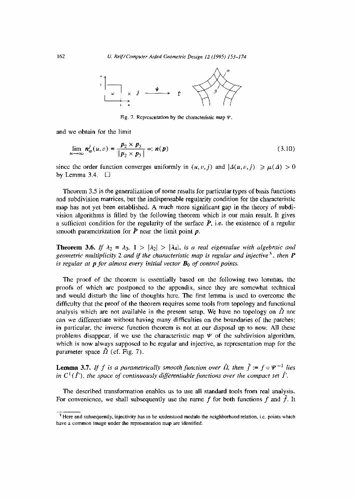
Fig. 7. Representation by the characteristic map ~.

and we obtain for the limit

P2 x P3 =: n(p) (3.10) ,lirnoo nJm(u, v) - liP2 × p3 II

since the order function converges uniformly in (u , v , j ) and la (u ,v , j ) l >1 m(a) > 0 by Lemma 3.4. []

Theorem 3.5 is the generalization of some results for particular types of basis functions and subdivision matrices, but the indispensable regularity condition for the characteristic map has not yet been established. A much more significant gap in the theory of subdivision algorithms is filled by the following theorem which is our main result. It gives a sufficient condition for the regularity of the surface P, i.e. the existence of a regular smooth parametrization for ]) near the limit point p.

Theorem 3.6. If A2 = A3, 1 > ]A21 > IA41, is a real eigenvalue with algebraic and geometric multiplicity 2 and if the characteristic map is regular and injective 3, then P is regular at p for almost every initial vector Bo of control points.

The proof of the theorem is essentially based on the following two lemmas, the proofs of which are postponed to the appendix, since they are somewhat technical and would disturb the line of thoughts here. The first lemma is used to overcome the difficulty that the proof of the theorem requires some tools from topology and functional analysis which are not available in the present setup. We have no topology on ~ nor can we differentiate without having many difficulties on the boundaries of the patches; in particular, the inverse function theorem is not at our disposal up to now. All these problems disappear, if we use the characteristic map ~ of the subdivision algorithm, which is now always supposed to be regular and injective, as representation map for the parameter space .0 (cf. Fig. 7).

L e m m a 3.7. If f is a parametrically smooth function over f2, then f := f o # - I lies in c l(/~), the space of continuously differentiable functions over the compact set [~.

The described transformation enables us to use all standard tools from real analysis. For convenience, we shall subsequently use the name f for both functions f and f . It

3 Here and subsequently, injectivity has to be understood modulo the neighborhood relation, i.e. points which have a common image under the representation map are identified.


will come clear from the arguments (typically stand r/), when we refer to the transformed function. The characteristic map itself, for instance, will be written in the form

q-' (~:, ~7) = (~, z/) (3.11)

as it is transformed to the identity on F. Further, we need the following lemma from functional analysis.

L e m m a 3.8. The set of all regular injective functions is open in C 1 (if').

Now we can give the

P roof of T h e o r e m 3.6. First, we transform the problem to the canonical form

Pl = o , P2 = e l , P3 = e 2

by an affine change of coordinates, where (e l , e2, e3) are the unit vectors and 0 is the origin of the new coordinate system. This leads to

{ x ( u , v , j , m ) ) /h'~b(u,v,j)v2 + o ( . ~ n ) ) x J , (u ,v ) =: ~y(u,v , j ,m) = [a~b(u,v, j)v3+o(A~ n) (3.12)

\ z (u , v , j ,m) \ o(a~ ' )

or in the transformed form to

x ( ' , r l : m ) ) / A ' ~ ' + ° ( A ' ~ ) ~ y ( ( , r / m) = { A ~ ' r / + o ( . ~ ' ) ] . (3.13) z((,rl , m ) \ o(A~') J

By Theorem 3.5, n(p) = e3 is the limit of the normal vectors. Therefore, we try to parametrize the surface P over the xy-plane in the form z = h(x, y) in a neighborhood of the origin. This is possible, if there is an M C N such that the map

FM : ( ( , z / , m ) H (x((,~7, m), y((,Tl, m) ), (~,~7) E F, m >I M (3.14)

is injective, because then we can set z = h(x, y) := z (FM 1 (x, y ) ) . Since both the functions b(u, v, j ) and their partial derivatives are bounded over the

compact set F, the order functions converge with respect to the Cl-norm. Hence

,,lirno~ IIAymFM(', m) - ~llc'(/') = 0 (3.15)

and q~ is regular and injective by assumption. Thus, by Lemma 3.8, there is an M C 1N with the property that FM is injective for arbitrary but fixed m ~> M, i.e.

FM(~,rl, m) = FM(£-,~I,m) ~ (s~,r/) = ( ~ , ~ ) . (3.16)

It remains to show that the images of the maps FM(', m) are essentially disjoint, where "essentially" means that the intersection of the images of consecutive maps consists exactly of the common boundary curve. To this end, we define a natural partial order


for closed curves without self-intersections in N 2. Denote by I(c) the interior of such a curve c, then we set

cj < c2 ¢~ c7 C I (c2 ) . (3.17)

Now P has two closed disjoint boundary curves, we call the outer curve a and the inner curve /3 (cf. Fig. 7). The boundary of FM(.,m) consists exclusively of the disjoint curves FM(a, m) and FM(/3, m). This follows from the regularity of FM(.,m) and the inverse function theorem. Since FM(a, m) and FM(/3, m) are the only boundary curves of the compact and connected set F(F,m) , we have either

FM(a,m) < FM(/3, m) or FM(/3, m) < FM(ce, m)

and all function values of FM(',m) lie in the strip between the two curves. From the fact that/3 < a and

,~i~m~ IIA-''FM(a'm)-cellc'(P~= m---*oc~lim IlA-'FM(/3, m)- /3lIc , ( t~=O (3.18)

one easily concludes that the second case must hold if M is large enough. Now consider the sequence

FM(a,M), FM(t3, M) = FM(a,M + I), FM(/3, M + I) = FM(ee, M + 2) . . . .

of boundary curves. It is strictly monotone decreasing and converges to the origin. Each strip corresponds exactly to the image of FM for some fixed m and thus FM is injective.

The image ~-M of FM is the interior of the outermost curve FM(a, M) with exception of the origin, i.e.

~M = I(FM(a,M)) \ {(0 ,0)} (3.19)

and 5CM t2 { (0 ,0)} is a neighborhood of the origin. There the surface P can be parametrized by

z =h(x ,y ) := {~ (FMI(x'y)) for (x,y) C f'M, for (x,y) = (0,0) , (3.20)

where the function h is continuously differentiable for (x ,y ) 4: (0,0) since P is a smooth surface. Finally, we obtain for the normal vector n of P by Theorem 3.5

[ -hx ( x , y)'~ lim n ( x , y ) = lim 1 I - h y ( x , y ) l =e3. (3.21)

(x ,,)~(0,0) (x,~)-~(0 0)v/1 + I[Vh(x,y)lj2

Thus, the limit of the gradient

lim Vh(x , y) = (0, 0) (x,y)~(0,0)

exists and consequently h is continuously differentiable for all (x, y) E .T'M U { (0, 0)} as a simple consequence of the mean value theorem. []


B j, 7 /" \ \

B "/'8 //X x B j'6

t t¢ / ",, i t ~'\\\

/, \J /\ - B~+~'5 =. B j~'9.

w+,. ~ , j , L , , , \ X ,N / ' -'v-,, , " ' -

laa+t . / . t,6

B.~ +1, ~11]

Fig. 8. Labeling of the control points.

4. An example

It is not the purpose of this section to discuss particular subdivision algorithms in detail, but to show some generic phenomena and how they fit into the theory which has been developed in the preceding sections. We skip many computational details and all proofs and restrict ourselves to the results and some hints, how they can be obtained. Providing the arguments should be easy for anyone who is familiar with B-spline theory and the discrete Fourier analysis of cyclic systems. The use of a computer algebra system is helpful, since the computations are rather extensive.

We shall examine some subdivision schemes for biquadratic B-splines near a six-sided hole. The general case of an n-sided hole is not more difficult, but we make this choice in order to keep things as simple and concrete as possible. For the same reason, we shall discuss only some particular subdivision matrices and avoid the use of parameters as much as possible. A more general discussion is beyond the scope of this paper.

The inner layer of patches of a biquadratic B-spline surface is defined by a vector B of control points which consists of 6 blocks B1 . . . . . B 6 with 9 elements each,

B : = [ B ° . . . . . B5] T, B k : = [ B k'l . . . . . Bk'9] T, k = 0 . . . . . 5, (4.1)

cf. Fig. 8. Note: Subsequently, the index k always runs from 0 to 5 and has to be understood

modulo 6. A subdivision process

Bo := B, Bm+l := ABm (4.2)


should have no preference for a particular side of the hole, hence the subdivision matrix is supposed to be cyclic in blocks of 9 x 9 matrices A ° . . . . . A s. We have

where

5 B,k,+l = ~ A~- ' iB~,

j--0

/a ° 0 0 0 ~

r s O 0

r S t S

r 0 0 s

s r 0 0

s r s t

t s r s

s t s r

s 0 0 r

A 1 , 1 : 9 , 1 : 4 =

A 0 1 : 9 , 1 : 4 =

/a I 0 0 O~

s 0 0 t

0 0 0 0

0 0 0 0

t 0 0 s

0 0 0 0

0 0 0 0

0 0 0 0

o o o o j

A 5 , 1 : 9 , 1 : 4 =

[a 5 0 0 O\

0 0 0 0

0 0 0 0

s t 0 0

0 0 0 0

0 0 0 0

0 0 0 0

0 0 0 0

t s 0 0

(4.3)

with r = 9 /16 , s = 3 /16 and t = 1/16, all other entries being zero. Except for the first rows, the matrices are uniquely determined by the condition that consecutive layers must join smoothly. The weights r, s and t coincide with those of the subdivision scheme for biquadratic tensor product surfaces. The entries in the first rows are at our disposal and the first simplification is to set most of them to zero. The present form implies that the innermost ring of control points depends only on the innermost ring of the preceding stage. This will be illustrated by figures of the type shown in Fig. 9.

a 5 a4

a° ~ a3

a I a ~ Fig. 9. Free parameters of the subdivision matrix.

For symmetry reasons we require

a 1 = a s, a 2 = a 4 (4.5)

and since the rows of A must sum up to 1 we have

a ° + 2a I + 2 a 2 + a 3 = 1. (4.6)

Apply ing the discrete Fourier transformation

5 13~ = ~ w - J k p j , ¢o := exp(27r i /6) (4.7)

.j=o

A 2 A 3 A 4 = a 4 (4.4) 1,1 = a2, 1,1 = a3, 1,1

U. Reif/Computer Aided Geometric Design 12 (1995) 153-174

to the system yields the diagonal ized form

Bin+ 1 A Bm

with

' 1:9,1:4 =

[ hk 0 0 0 "~

r + sw -k s 0 tw -k r s t s

r + sw k tw k 0 s

s + to) - k r 0 so) -k

s r s t

t s r s

s t s r s + tw k sw k 0 r

167

(4.8)

(4.9)

The eigenvalues # I . . . . . /z9 ~ of Ak are also eigenvalues of A. We find

/zf = &k, /z~ = 1/4, #~ = /z4 ~ = 1/8, /z~ . . . . . #~ = 0, (4 .10)

where

ih ° = 1, &l = ~ 5 = a 0 + a l _ a 2 _ a 3,

i h 2 = & a = a ° - a 1 - a 2 + a 3, & 3 = a ° - 2 a J + 2 a 2 - a 3. (4 .11)

What happens if we apply different subdivis ion matrices to a B-spl ine surface with a 6-sided hole? The fo l lowing four cases reveal a completely different behavior.

1/8 1/8

1/z ~ ~ ~ o

x/8 1/8

Fig. lO. Weights for Case I.

Case 1 (see Fig. 10). We have &0 = 1, &l = &3 = &5 = 1 /2 and •2 = t~4 = 1/4 and

obtain for the leading eigenvalues of A

,~1 = l , /~2 = /~3 = ,~4 = 1 / 2 , A5 = 1 / 4 . ( 4 . 1 2 )

Accord ing to Theorem 3.2 we can expect a convergent algorithm, but no smooth surface. This is i l lustrated in Fig. 11.4 The hole is filled gradually, but the different shades near the l imi t point indicate that there is no l imit for the normal vectors.

4 All surfaces shown in Figs. 11, 14, 17 and 20 were generated from the same set of initial data. The pictures on the left-hand side show the first few steps for the given algorithm and those on the right-hand side a magnification of the region near the limit point. Different shades correspond to different normal vectors, the white lines indicate boundaries of consecutive layers.


Fig. I 1. Surface for Case 1 and 1000-fold magnification.

1/12 1/12

1/2 ~ 1/6

1/12 1/12

Fig. 12. Weights for Case 2.

Case 2 (see Fig. 12). We have ~0 = l, &l =~3 =~5 = 1/3 and ~2 =~4 = 1/2 and obtain for the leading eigenvalues of A

//1 = 1, ,t2 = ,~3 = 1 / 2 , ,~4 = 1 / 3 . ( 4 . 1 3 )

The eigenvectors v2 = [v ° . . . . . v~] T and v3 = [v ° . . . . . v35] T are given by

v~ = Re(w2k~), v3 k = Im(w2kb), (4.14)

where

~ 3 = [ 1 4 , 2 1 , 3 6 , 2 1 , 2 8 , 4 5 , 5 8 , 4 5 , 2 8 ] + 7 v ~ i [ 0 , - 1 , 0 , 1 , - 2 , - 1 , 0 , 1 , 2 ] (4.15)

is an eigenvector of ~2 and ~4. We find

v2k=v~ +3, v3k=v3 k+3, (4.16)

from which follows that the characteristic map is not injective. As mentioned above, the rows of the matrix V = [v2,v3] serve as two-dimensional control points for the characteristic map. Fig. 13 shows on the left-hand side a plot of these control points connected by dashed lines according to the structure defined in Fig. 8. The right-hand side shows the corresponding characteristic map g~ where the images of a 7 × 7 grid parallel to the edges of the unit square w are plotted with thin lines. The thicker lines indicate the patch boundaries. The image consists of 18 patches, but in fact one can see only 9 patches since always two copies of w have a common image.

3 0

- - 3 0

U. Reif/Computer Aided Geometric Design 12 (1995) 153-174

I ~ t

. t

t i / I

6 - - - , 6 - - - 4

t x R

o I

I I

- - 3 0 0

t x i

,i ;,( x I •

x x

3 0

0

- - 3 ( ]

[ I I 310 30 - - 3 0 0

Fig. 13. Eigenvectors and characteristic map for Case 2.

169

Fig. 14. Surface for Case 2 and lO00-fold magnification.

A numerical or analytical computation of the Jacobian of the characteristic map qt shows that q~ is regular and thus the surfaces generated by the given algorithm are tangent plane continuous by Theorem 3.5. Nevertheless, self-intersections will lead to a non-regular limit point. This is shown in Fig. 14.

The', non-injectivity of the characteristic map in Case 2 is rather obvious, since the dominant eigenvalues occur in the blocks k = 2 and k = 4 of the Fourier transformed system. But even if the dominant eigenvalues come from the blocks k = 1 and k = 5, things can go wrong. This is shown by the next case as well as the fact that the regularity of the characteristic map is an indispensable condition for generating smooth surfaces.

Case 3 (see Fig. 15). We have &0 = l, ~1 =~/5 = - 3 / 4 , gfl =&4 = 1/4 and &3 = 0 and obtain for the leading eigenvalues of A


--8

[ I I

II

'~,, ~ ,~

, / 4

0 1/4

o ~ 1/2

0 1/4

Fig. 15. Weights for Case 3.

,7 t I

I l / l

t,',?

K

,: Ib

- - 4

I I I

I I I I I I --8 0 8 --4 0 4

Fig. 16. Eigenvectors and characteristic map for Case 3.

A1 = 1, A2 = A3 = - 3 / 4 , •4 = 1/4. (4.17)

In this case one can show that the characteristic map is not regular and indeed it looks rather strange, see Fig. 16.

The generated surfaces are not tangent plane continuous and far from being well shaped, as can be seen in Fig. 17.

One could object that the dominant eigenvalues are negative and that it is rather obvious that this algorithm cannot work. However, following the arguments of Ball and Storry it would have been found to be tangent plane continuous.

Finally, here is a suitable algorithm for generating regular surfaces:

Case 4 (see Fig. 18). We have ~o = I, ~1 = ~5 = 1/2 and b 2 = ~3 = ~4 = 0 and obtain for the leading eigenvalues of A

A1 = 1, A2 = A3 = 1/2, A4 = 1/4. (4.18)

The eigenvectors v2 = [v ° . . . . . v~] T and v3 = [v ° . . . . . v35]T are given by

v~ = Re(wkb), v3 k = Im(wkD), (4.19)

where

b = [14 ,35 ,48 ,35 ,56 ,67 ,82 ,67 ,56] + 7v/3i[0, - 1 , 0 , 1 , - 2 , - 1 , 0 , 1 , 2 ] (4.20)

ug[sop lensn oql ol dn soAt.I tuqB..IO~'llZ oql l'eql soll3.tlsnl[l 0g "~.lq 'poopuI "soa-ej.lns .lleln~'o.l qlootus saleaaua~ tuql!ao~Ie aql pue PallrJlnJ aae 9"E tuaaoaq.l jo suo[.ldtunsse ii e 'snq2 '

• aeln~aa s! di 113ql ~oqs ol lua!uaguoa OSle s! ttuoj aa!zg~ t aq,L ',~laadoM llnq xaAuoa aql aSh pue uuoj aa!zpfl u! ah 01!a~a ',~l!A!laa.fu! leqoI ~ aql aAoad oi "aA!laa[u! st. qal-ed ai~u!s eol df detu a!ls!aalaeaeqa aql jo uo!la!alsaa aql leql u/~oqs aq ,q!sea uea 1I "~y pue ~V jo aolaaAUa~!a ue s~

17 aseD aoj detu a!lsuolaexeqa pue saolaoAUag!~/ 61 ~!d Dc~ 0 0~--

Oc~--

0(2 0 Og--

/

,. .., -,, ,,- ,< ;o "~." %/., ~. "',,." .~"

'e oseD aoj slq~!oA~ "81 "~!d

:) ~/t

Og--

O~

• uo!l~ag!u~em ploJ-o0£ pue EaseD Joj aae~n s %1 '~!a

• /

?

J

, ,, ;, ....

i :

t

/ ]

/

[L 1 PZ I-U2I (~66 l) Zl uX~.saG abtlalUOaD pap!v .lalndwoD/fta~t "/1


Fig. 20. Surface for Case 4 and 1000-fold magnification.

standards in CAGD.

Finally, we want to mention that exactly the same characteristic map as in the last case is found for the Doo-Sab in weights given in Fig. 21.

1/6 1/12

11/24 ~ 1/24

1/6 ]/12

Fig. 21. Doo-Sabin weights.

Here we have ho = 1,~1 = ~5 = 1/2 and &2 = &3 = ~4 __ 1/4 and it can easily be seen that the eigenvectors v2 and v3 depend only on the value of &l = ~5.

Appendix

L e m m a 3.7. If f is a parametrically smooth function over" ~2, then f := f o gt-I lies in C 1 ( ~.), the space of continuously differentiable functions over the compact set I'.

Proof. Parametrical smoothness means that the cross boundary derivatives of f at a common boundary of two patches are equal up to sign. More precisely, assume without loss of generality that for some patches j and k the boundary curves ( [0 , 1], 0 , j ) and ( [0 , 1 ] , 0, k) are identified by the neighborhood relation. Then we have for u E [0, 1 ]

f ( u , O , j ) = f ( u , O , k ) , D f ( u , O , j ) = D f ( u , O , k ) O , (A.1)

where D f denotes the matrix of partial derivatives with respect to ( u , v ) and Q is a diagonal 2 × 2-matrix with entries 1 and - 1. In particular, we obtain for the characteristic map


c(u) := ~ ( u , 0 , j ) = qr (u ,0 , k) , DqZ(u,O,j) =Dqs(u,O,k)Q. (A.2)

Now it mus! be shown that D f is a continuous function over F. qr is smoothly invertible in the interior of the patches and the chain rule implies there

D f ( x , y ) = D f (gr- l (x , y) ) (Dg'(~F-l(x, y)) - ' (A.3)

If (x, y) is approaching the boundary curve c(u) from either the patch j or k, we obtain in the limit

D f ( c ( u ) ) = Df (u ,O , j ) (Dq~(u ,O , j ) ) -1 (A.4)

o r

D f ( c ( u ) ) = D f ( u , O, k) (Dq~(u, O, k) ) - '

The right-hand sides coincide since

D f ( u , O,j) ( D ~ ( u , O , j ) ) - 1 = (Df (u ,O, k)Q) (Q-I ( D~(u,O, k) )-1)

= D f ( u , 0, k) (Dq.'(u, 0, k) ) -n

and thus, D f is well defined on P and continuous by the mean value theorem.

L e m m a 3.8. The set of regular injective functions is open in C 1 ( f l ) .

(A.5)

(A.6)

[]

for all functions g E C I ( F ) . If a function f E C 1 ( F ) is regular and injective, then it can be inverted and f - I E C l ( f ( F ) ) C C °'1 ( f ( F ) ) . Thus,

II.f-~llco.,(f(r)) := sup I l f -~(y) - f-~(Y)ll2 y ~ef(/) I l y - Ytl2 = : K < oo (A.8)

and consequently

in f I I f ( x ) - f ( 2 ) l l z = 1/K. (A.9)

Now we find for some function f := f + g

inf k l f ( x ) -- f (~ )112 ~,~c f" I I x - - ~112

/> inf [ I f (x ) -- f(2)112 _ sup IIg(x) -g(2)112 x,~U" I I x - ~112 x,~cr IIx - ~112

>> 1/K - [Igllco,~r,)/> 1/K - MIIgllc,(f,>. (A.10)

] ] g ( x ) - g(.~)112 sup =: Ilgllco,,(r~ ~< Mltg[lc,¢p) (A.7)

x , ~ r I I x - ~ l 1 2

Proof. The proof is based on the continuous embedding of C I ( F ) in C °'1 ( f l ) , the space of Lipschitz continuous functions, i.e. there is a constant M E R such that

174 u. Reif / Computer Aided Geometric Design 12 (1995) 153-174

Thus f is inject ive, i f Ilgllc,<p) = I[f- fllc,(h < 1 / ( M K ) . One can show by a s imple

cont inui ty a rgument that f is also regular, i f [ I f - fllc,(p~ is small enough and so the p r o o f is comple te . []

References

Ball, A.A. and Storry, D.J.T. (1986), A matrix approach to the analysis of recursively generated B-spline surfaces, Computer-Aided Design 18, 437-442.

Ball, A.A. and Storry, D.J.T. (1988), Conditions for tangent plane continuity over recursively generated B-spline surfaces, ACM Trans. Graph. 7(2), 83-102.

Catmull, E. and Clark, J. (1978), Recursively generated B-spline surfaces on arbitrary topological meshes, Computer-Aided Design 10, 350-355.

Doo, D. and Sabin, M.A. (1978), Behaviour of recursive division surfaces near extraordinary points, Computer- Aided Design 10, 356-360.

Loop, Ch.T. (1987), Smooth Subdivision for Surfaces Based on Triangles, Master Thesis, Univ. of Utah, Salt Lake City.

Nasri, A.H. (1987), Polyhedral subdivision methods for free-form surfaces, ACM Trans. Graph. 6( 1 ) 29-73. Reif, U. (1993), Neue Aspekte in der Theofie der Freiformfl~ichen beliebiger Topologie, Thesis, Universit~it

Stuttgart Halstead, M., Kass, M. and DeRose, T.D. (1993), Efficient, Fair interpolation using Catmull-Clark surfaces,

in: SIGGRAPH '93, ACM Press, New York, 35-44.

a unified approach to subdivision algorithms near...

Documents