a unified robust bootstrap method for sharp/fuzzy mean...
TRANSCRIPT
arX
iv:1
702.
0443
0v2
[st
at.M
E]
24
Feb
2017
A Unified Robust Bootstrap Method for Sharp/Fuzzy
Mean/Quantile Regression Discontinuity/Kink Designs
Harold D. Chiang∗ Yu-Chin Hsu† Yuya Sasaki‡
February 28, 2017
Abstract
Computation of asymptotic distributions is known to be a nontrivial and delicate task for the
regression discontinuity designs (RDD) and the regression kink designs (RKD). It is even more
complicated when a researcher is interested in joint or uniform inference across heterogeneous sub-
populations indexed by covariates or quantiles. Hence, bootstrap procedures are often preferred
in practice. This paper develops a robust multiplier bootstrap method for a general class of local
Wald estimators. It applies to the sharp mean RDD, the fuzzy mean RDD, the sharp mean RKD,
the fuzzy mean RKD, the sharp quantile RDD, the fuzzy quantile RDD, the sharp quantile RKD,
and the fuzzy quantile RKD, to list a few examples, as well as covariate-indexed versions of them.
In addition to its generic applicability to a wide variety of local Wald estimators, our method
also enjoys robustness against large bandwidths commonly used in practice. This robustness is
achieved through a bias correction approach incorporated into our multiplier bootstrap framework.
We demonstrate the generic applicability of our theory through ten examples of local Wald esti-
mators including those listed above, and show by simulation studies that it indeed performs well,
robustly, and uniformly across different examples. All the code files are available upon request.
Keywords: bias correction, local Wald estimator, multiplier bootstrap, quantile, regression dis-
continuity design, regression kink design, robustness
JEL Codes: C01, C14, C21
∗Harold D. Chiang: [email protected]. Department of Economics, Johns Hopkins University.†Yu-Chin Hsu: [email protected]. Institute of Economics, Academia Sinica.‡Yuya Sasaki (Corresponding Author): [email protected]. Department of Economics, Johns Hopkins University.
1

1 Introduction
Empirical researchers have used many different versions of local Wald estimators. Of mostly wide use
are the local Wald estimators for the regression discontinuity design (RDD). More recently, researchers
also use local Wald ratios of derivative estimators for the regression kink design (RKD). Furthermore,
local Wald ratios of conditional cumulative distribution functions and their variants are used for
estimation of quantile treatment effects. For all of these different versions of local Wald estimators,
computation of asymptotic distributions – and thus computation of standard errors – is known to be a
nontrivial and delicate task to varying extents. Because of this undesired feature, bootstrap methods
that circumvent the necessity to calculate complicated covariance matrices/functions are preferred
in practice, but their availability is surprisingly limited in the existing literature. In this paper, we
propose a general multiplier bootstrap framework, which uniformly applies to all of the commonly
used versions of local Wald estimators. In addition to its generic applicability, our method enjoys
robustness against practically used bandwidth choice rules. Therefore, the proposed method is readily
applicable to most, if not all, types of empirical research based on local Wald estimators.
We are not the first to develop a bootstrap- or simulation-based method of inference for local
Wald estimators, but no existing method shares the generic applicability and the robustness that our
method enjoys. A couple of important references are Qu and Yoon (2015b) and Bartalotti, Calhoun,
and He (2016). Qu and Yoon (2015b) propose a simulation method with bias corrections to achieve
robustness, specifically for the sharp quantile RDD. Bartalotti, Calhoun, and He (2016) propose a
wild bootstrap method with bias corrections to achieve robustness, specifically for the sharp mean
RDD. To our knowledge, on the other hand, there is no robust bootstrap method proposed for any
of the other versions of local Wald estimators, such as the fuzzy mean RDD, the sharp mean RKD,
the fuzzy mean RKD, the fuzzy quantile RDD, the sharp quantile RKD, and the fuzzy quantile RKD.
Instead of proposing a robust bootstrap method which specifically applies to each single version of
local Wald estimators, we propose one generic multiplier bootstrap framework that uniformly applies
2

to most, if not all, versions of the local Wald estimators including the sharp mean RDD, the fuzzy
mean RDD, the sharp mean RKD, the fuzzy mean RKD, the sharp quantile RDD, the fuzzy quantile
RDD, the sharp quantile RKD, and the fuzzy quantile RKD, to list a few most popular examples used
in empirical research.
Our contributions consist of the robustness and the generic applicability as argued above. We
achieve the robustness against practically used bandwidth choice rules through higher-order bias cor-
rections following Calonico, Cattaneo, and Titiunik (2014), as Qu and Yoon (2015b) and Bartalotti,
Calhoun, and He (2016) do in their respective contexts. We achieve the generic applicability by taking
advantage of the fact that all of the commonly used versions of local Wald estimators share a common
basic form of Bahadur representations (BR). Notably, the insight of Porter (2003; Proof of Theorem
3) allows us to derive the BR for higher-order local polynomials which we require for robustness, and
we further develop the uniform validity of the BR similar to Qu and Yoon (2015a; Theorem 1). We
first establish the validity of the multiplier bootstrap with this common basic form of BR following
Kosorok (2003, 2008), and then apply the functional delta method to both of the BR and the multiplier
bootstrap processes. Thereby, we achieve the generic applicability through a single unified framework,
with only the variable definitions and the Hadamard derivatives having to be changed across different
versions of the local Wald estimators.
This paper is organized as follows. After reviewing the literature in Section 2, we first present a
general framework of local Wald estimands in Section 3, with ten examples (Sections 3.1–3.10). Section
4 proposes general multiplier bootstrap processes, and establishes the validity of the general multiplier
bootstrap method. We then demonstrate its applications to the aforementioned ten examples in
Section 5, and conduct simulation studies in Section 6. Proofs and mathematical details are delegated
to Section A in the appendix. We provide some practical guide for bandwidth choice in Section B in
the appendix.
3

2 Relation to the Literature
In this section, we overview the most relevant parts of the existing literature. Because of the breadth
of the related literature, what we write below is far from being exhaustive.
Literature on Local Designs: The idea of the RDD is introduced by Thistlethwaite and Camp-
bell (1960). There is a vast literature on the RDD today. Instead of enumerating all papers, we refer
the readers to a collection of surveys, including Cook (2008), the special issue of Journal of Economet-
rics edited by Imbens and Lemieux (2008), Imbens and Wooldridge (2009; Sec. 6.4), Lee and Lemieux
(2010), and Volume 38 of Advances in Econometrics edited by Cattaneo and Escanciano (2016), as
well as the references cited therein. For technical matters, we mainly refer to Porter (2003) for its con-
venience in deriving the general BR for higher-order local polynomials. While it mostly evolved around
the RDD, recent additions to this local design literature include the RKD (e.g., Nielsen, Sørensen,
and Taber, 2010; Landais, 2015; Simonsen, Skipper, and Skipper, 2015; Card, Lee, Pei, and Weber,
2016; Dong, 2016) and quantile extensions (e.g., Frandsen, Frolich, and Melly, 2012; Qu and Yoon,
2015b). We emphasize once again that all these different frameworks are uniformly encompassed by
the general framework developed in this paper.
Literature on Bandwidth and Robustness: Calonico, Cattaneo, and Titiunik (2014) intro-
duce bias correction for the purpose of achieving the robustness of asymptotic inference against large
bandwidths. This innovation paves the way for empirical practitioners to obtain valid standard errors
for their estimates under popular data-driven methods of bandwidths (e.g., Imbens and Kalyanara-
man, 2012; Calonico, Cattaneo and Titiunik, 2014; Arai and Ichimura, 2016; Calonico, Cattaeneo,
and Farrell, 2016ab). Bartalotti, Calhoun, and He (2016) adopt this idea of bias correction in a wild
bootstrap method of inference for the sharp mean RDD. Qu and Yoon (2015b) adopt this idea of bias
correction in a simulation-based method of inference for the sharp quantile RDD. We adopt this idea of
bias correction in a multiplier bootstrap method of inference that uniformly applies to the sharp mean
RDD (Section 3.2), the fuzzy mean RDD (Section 3.1), the sharp mean RKD (Section 3.4), the fuzzy
4

mean RKD (Section 3.3), the sharp quantile RDD (Section 3.6), the fuzzy quantile RDD (Section
3.7), the sharp quantile RKD (Section 3.9), and the fuzzy quantile RKD (Section 3.8), among others.
Furthermore, Calonico, Cattaneo, and Farrell (2016ab) propose a coverage-probability optimal band-
width selector and provide a rule of thumb adjustment method to convert MSE-optimal bandwidths
into the coverage-probability optimal ones. We also take advantage of these recent innovations.
Literature on Uniform Bahadur Representation: The Bahadur representation is a key to
asymptotic distributional results. As we aim to cover uniform inference over a general index set,
uniform validity of Bahadur representation over the set is essential for our method. For classes of
nonparametric kernel regressions on which our method relies, Masry (1996) and Kong, Linton, and
Xia (2010) develop uniform Bahadur representations over regressors. Furthermore, Guerre and Sabbah
(2012) and Qu and Yoon (2015a) develop uniform validity over quantiles as well. We take advantage
of and extend this existing idea in deriving the uniform validity of our Bahadur representation. In
order to deal with a more general class of complexity rather than just quantiles, we use a new maximal
inequality (van der Vaart and Wellner, 2011; Chernozhukov, Chetverikov, and Kato, 2014).
Literature on Multiplier Bootstrap: The multiplier bootstrap for Donsker and other weakly
convergent classes is first studied by Ledoux and Talagrand (1988) and Gine and Zinn (1990). Our
results are based on a more general version developed more lately by Kosorok (2003, 2008), that works
for triangular arrays of row-independent non-identically distributed stochastic processes. This version
provides a conditional-weak-convergence counterpart of the functional central limit theorem for row-
independent arrays (Pollard, 1990). To our knowledge, use of the multiplier bootstrap in econometrics
dates back to Hansen (1996). This method proves particularly useful for uniform inference on CDFs,
for its convenience of not having to estimate a gigantic covariance matrix to approximate a covariance
function. Barrett and Donald (2003) use the multiplier bootstrap for uniform inference on uncondi-
tional CDFs. More recently, Donald, Hsu, and Barrett (2012) use the multiplier bootstrap with kernel
weights for uniform inference on conditional CDFs. In this paper, we use the multiplier bootstrap
5

with one-sided kernel weights for uniform inference on a generalized class of local Wald estimators.
In particular, our examples include uniform inference on conditional CDFs of potential outcomes
(Section 3.5) as well as uniform inference on conditional quantile treatment effects via inversions of
conditional CDFs (Sections 3.6–3.7). With all these preceding papers on the multiplier bootstrap, we
want to emphasize on our own theoretical contributions. We face an extra challenge that the existing
researches did not face. Namely, we need to allow for a more general assumption to uniformly deal
with complexities of processes across different estimators to accommodate all the relevant examples.
In addition, we need to take into account the variability of the estimates for unknowns in the operators
of local Wald ratios in many examples that we consider. To deal with these issues, we develop new
proofs for the validity of the multiplier bootstrap in a different way from those of the existing literature
– we elaborate on this point in Section 4.4.
3 The General Framework and Ten Examples
Let (Y,D,X) be a random vector defined on a probability space (Ωx,Fx,Px), where Y contains
an outcome vector, D contains a treatment vector, and X is a running variable or an assignment
variable. We denote their supports as Y , D and X , respectively. Suppose that a researcher observes
n independent copies (Yi,Di,Xi)ni=1 of (Y,D,X).
Consider some subsets of some finite dimensional Euclidean spaces Θ1, Θ2, Θ′1, Θ
′2, and Θ′′. We
will use them to denote sets of indices. Let Θ = Θ1×Θ2, and let g1 : Y ×Θ1 → R and g2 : D×Θ2 → R
be functions to be defined in various contexts of empirical research designs – concrete examples are
suggested in the ten subsections below. When we discuss the continuity of gk in θk, we consider Θ1
and Θ2 with the topologies they inherit from the finite dimensional Euclidean spaces they reside in.
We write µ1(x, θ1) = E[g1(Yi, θ1)|Xi = x] and µ2(x, θ2) = E[g2(Di, θ2)|Xi = x]. Their v-th order
partial derivatives with respect to x are denoted by µ(v)1 = ∂v
∂xvµ1 and µ(v)2 = ∂v
∂xvµ2. We also denote
b′ = ddxb for a function b : X 7→ R. For a set T , we denote C1(T ) as the collection of all real-valued
6

functions on T that are continuously differentiable, and ℓ∞(T ) is the collection of all bounded real-
valued functions on T . With suitable operators φ : ℓ∞(Θ1) → ℓ∞(Θ′1), ψ : ℓ∞(Θ2) → ℓ∞(Θ′
2), and
Υ : ℓ∞(Θ′1 ×Θ′
2) → ℓ∞(Θ′′), a general class of local Wald estimands can be expressed in the form of
τ(θ′′) = Υ
(φ(limx↓0 µ
(v)1 (x, ·)
)(·)− φ
(limx↑0 µ
(v)1 (x, ·)
)(·)
ψ(limx↓0 µ
(v)2 (x, ·)
)(·)− ψ
(limx↑0 µ
(v)2 (x, ·)
)(·)
)(θ′′). (3.1)
for all θ′′ ∈ Θ′′. This class of local Wald estimands encompasses a wide array of design-based estimands
used by empirical practitioners. We list examples in the ten subsections below (Sections 3.1–3.10).
Throughout this paper, we normalize the cutoff value of the running variable to x = 0.
3.1 Example: Fuzzy Mean RDD
We do not need index sets for fuzzy RDD, and so let Θ1 = Θ2 = Θ′1 = Θ′
2 = Θ′′ = 0 for simplicity.
Set g1(Yi, θ1) = Yi and g2(Di, θ2) = Di. Note that µ1(x, θ1) = E[g1(Yi, θ1)|Xi = x] = E[Yi|Xi = x]
and µ2(x, θ2) = E[g2(Di, θ2)|Xi = x] = E[Di|Xi = x]. Let φ and ψ be the identity operators, and let
Υ(µ1(x,·)µ2(x,·)
)(θ′′) = µ1(x,θ′′)
µ2(x,θ′′)∀θ′′ ∈ Θ′′. The local Wald estimand (3.1) with v = 0 in this setting becomes
τ(θ′′) =limx↓0 E[Yi|Xi = x]− limx↑0 E[Yi|Xi = x]
limx↓0 E[Di|Xi = x]− limx↑0 E[Di|Xi = x](3.2)
for all θ′′ ∈ Θ′′ = 0. This estimand τ(0) will be denoted by τFMRD for Fuzzy Mean RD design.
3.2 Example: Sharp Mean RDD
Sharp RDD is a special case of fuzzy RDD, where Di = 1Xi ≥ 0. Thus, we can write µ2(x, θ2) =
E[Di|Xi = x] = 1x ≥ 0, and the local Wald estimand (3.1) of the form (3.2) further reduces to
τ(θ′′) = limx↓0
E[Yi|Xi = x]− limx↑0
E[Yi|Xi = x]
for all θ′′ ∈ Θ′′ = 0. This estimand τ(0) will be denoted by τSMRD for Sharp Mean RD design. For
this estimand, Bartalotti, Calhoun, and He (2016) propose a robust bootstrap method of inference,
and hence we are not the first to propose a robust bootstrap method for τSMRD. The benefit of our
method is its applicability not only to τSMRD, but also to many other estimands of the form (3.1).
7

3.3 Example: Fuzzy Mean RKD
Define Θ1,Θ2,Θ′1,Θ
′2,Θ
′′, g1, g2, φ, ψ, and Υ as in Section 3.1. The local Wald estimand (3.1) with
v = 1 in this setting becomes
τ(θ′′) =limx↓0
∂∂x E[Yi|Xi = x]− limx↑0
∂∂x E[Yi|Xi = x]
limx↓0∂∂x E[Di|Xi = x]− limx↑0
∂∂x E[Di|Xi = x]
(3.3)
for all θ′′ ∈ Θ′′ = 0. This estimand τ(0) will be denoted by τFMRK for Fuzzy Mean RK design. See
Card, Lee, Pei, and Weber (2016) for a causal interpretation of this estimand.
3.4 Example: Sharp Mean RKD
Sharp RKD is a special case of fuzzy RKD where the treatment is defined by E[g2(Di, θ2)|Xi] = b(Xi)
through a known function b. Thus, the local Wald estimand (3.1) of the form (3.3) further reduces to
τ(θ′′) =limx↓0
∂∂x E[Yi|Xi = x]− limx↑0
∂∂x E[Yi|Xi = x]
limx↓0 b′(x)− limx↑0 b′(x)
for all θ′′ ∈ Θ′′ = 0. This estimand τ(0) will be denoted by τSMRK for Sharp Mean RK design. See
Card, Lee, Pei, and Weber (2016) for a causal interpretation of this estimand.
3.5 Example: CDF Discontinuity and Test of Stochastic Dominance
Let Θ1 = Θ′1 = Θ′′ = Y for Y ⊂ R, and let Θ2 = Θ′
2 = 0. Set g1(Yi, θ1) = 1Yi ≤ θ1 and
g2(Di, θ2) = Di, where Di = 1Xi ≥ 0 holds under the sharp RD design. Note that µ1(x, θ1) =
E[g1(Yi, θ1)|Xi = x] = FY |X(θ1|x) and µ2(x, θ2) = E[g2(Di, θ2)|Xi = x] = E[Di|Xi = x] = 1x ≥ 0.
Let φ and ψ be the identity operators, and let Υ(µ1(x,·)µ2(x,·)
)(θ′′) = µ1(x,θ′′)
µ2(x,0)∀θ′′ ∈ Θ′′. The local Wald
estimand (3.1) with v = 0 in this setting becomes
τ(θ′′) = limx↓0
FY |X(θ′′|x)− limx↑0
FY |X(θ′′|x)
for all θ′′ ∈ Θ′′ = Y ⊂ R. This estimand τ will be denoted by τSCRD for Sharp CDF RD design. This
estimand may be useful to test the hypothesis of stochastic dominance (τ(θ′′) ≤ 0 for all θ′′ ∈ Θ′′).
See Shen and Zhang (2016) for this estimand and hypothesis testing.
8

3.6 Example: Sharp Quantile RDD
Denote QY |X(θ′′) := infy ∈ Y : FY |X(y) ≥ θ′′, fix an a ∈ (0, 1/2), ε > 0 and let Y1 = [QY |X(a|0−)−
ε,QY |X(1− a|0−) + ε] ∪ [QY |X(a|0+)− ε,QY |X(1− a|0+) + ε].
Let Θ1 = Y1, Θ′1 = Θ′′ = [a, 1−a] and Θ2 = Θ′
2 = 0. Set g1(Yi, θ1) = 1Yi ≤ θ1 and g2(Di, θ2) =
Di, where Di = 1Xi ≥ 0 holds under the sharp RDD. Note that µ1(x, θ1) = E[g1(Yi, θ1)|Xi = x] =
FY |X(θ1|x) and µ2(x, θ2) = E[g2(Di, θ2)|Xi = x] = E[Di|Xi = x] = 1x ≥ 0. Let φ(FY |X(·|x))(θ′) =
infθ1 ∈ Θ1 : FY |X(θ1|x) ≥ θ′ ∀θ′ ∈ Θ′1, ψ(1x ≥ 0)(θ′) = 1x ≥ 0 ∀θ′ ∈ Θ′
2 = 0, and
let Υ(µ1(x,·)µ2(x,·)
)(θ′′) = µ1(x,θ′′)
µ2(x,0)∀θ′′ ∈ Θ′′. The local Wald estimand (3.1) with v = 0 in this setting
becomes
τ(θ′′) = limx↓0
QY |X(θ′′|x)− limx↑0
QY |X(θ′′|x)
for all θ′′ ∈ Θ′′ = [a, 1 − a], where QY |X(θ′′|x) := infθ1 ∈ Θ1 : FY |X(θ1|x) ≥ θ′′ for a short-hand
notation. This estimand τ will be denoted by τSQRD for Sharp Quantile RD design. For this estimand,
Qu and Yoon (2015b) propose a method of uniform inference based on uniform random sampling, and
hence we are not the first to propose a bootstrap method for τSQRD. Our method adds the property
of robustness to this existing method, besides the main result that it applies to other estimands too.
3.7 Example: Fuzzy Quantile RDD
Frandsen, Frolich and Melly (2012) propose the following estimand to identify the conditional CDF
of potential outcome Y di under each treatment status d ∈ 0, 1 given the event C of compliance.
FY d|C(y) =limx↓0E[1Y ∗
i ≤ y · 1D∗i = d|Xi = x]− limx↑0E[1Y ∗
i ≤ y · 1D∗i = d|Xi = x]
limx↓0E[1D∗i = d|Xi = x]− limx↑0E[1D∗
i = d|Xi = x]
(3.4)
Further, they propose to identify the local quantile treatement effect by F−1Y 1|C −F−1
Y 0|C . This estimand
also fits in the general framework (3.1). Denote QY d|C(θ′′) = infy ∈ Y : FY d|C(y) ≥ θ′′. We first fix
an a ∈ (0, 1/2), ε > 0 and let Y1 = [QY 1|C(a)−ε,QY 1|C(1−a)+ε]∪[QY 0|C(a)−ε,QY 0|C(1−a)+ε]. Let
9

Θ1 = Θ′1 = Y1×D and Θ2 = Θ′
2 = D for D = 0, 1, and let Θ′′ = [a, 1−a] for a constant a ∈ (0, 1/2).
Let Yi = (Y ∗i ,D
∗i ) and Di = D∗
i . Set g1((Y∗i ,D
∗i ), (y, d)) = 1Y ∗
i ≤ y · 1D∗i = d and g2(D
∗i , d) =
1D∗i = d. Note that µ1(x, y, d) = E[g1((Y
∗i ,D
∗i ), y, d)|Xi = x] = E[1Y ∗
i ≤ y · 1D∗i = d|Xi = x]
and µ2(x, d) = E[g2(D∗i , d)|Xi = x] = E[1D∗
i = d|Xi = x]. Let φ and ψ be the identity operators,
and let Υ be defined by Υ(FY ·|C)(θ′′) = infy ∈ Y : FY 1|C(y) ≥ θ′′ − infy ∈ Y : FY 0|C(y) ≥ θ′′.
The local Wald estimand (3.1) with v = 0 in this setting becomes
τ(θ′′) = QY 1|C(θ′′)−QY 0|C(θ
′′)
for all θ′′ ∈ Θ′′ = [a, 1−a], where QY d|C(θ′′) := infy ∈ Y : FY d|C(y) ≥ θ′′ for a short-hand notation,
and FY d|C(y) is given in (3.4) for all (y, d) ∈ Y × D . This estimand τ will be denoted by τFQRD for
Fuzzy Quantile RD design.
3.8 Example: Fuzzy Quantile RKD
Let Y1 = [QY |X(a|0)− ε,QY |X(1−a|0)+ ε], Θ1 = Y1, Θ′1 = Θ′′ = [a, 1−a] for a constant a ∈ (0, 1/2),
and Θ2 = Θ′2 = 0. We set g1(Yi, θ1) = 1Yi ≤ θ1 and g2(Di, θ2) = Di. Note that µ1(x, θ1) =
E[g1(Yi, θ1)|Xi = x] = FY |X(θ1|x) and µ2(x, θ2) = E[g2(Di, θ2)|Xi = x] = E[Di|Xi = x]. With the
short-hand notations fY |X = ∂∂yFY |X and F
(1)Y |X := ∂
∂xFY |X , let
φ(F ′Y |X(·|x))(θ′) := −
F(1)Y |X(infθ ∈ Θ1 : FY |X(θ|0) ≥ θ′|x)fY |X(infθ ∈ Θ1 : FY |X(θ|0) ≥ θ′|x) ∀θ′ ∈ Θ′
1,
let ψ be the identity operator, and let Υ(µ1(x,·)µ2(x,·)
)(θ′′) = µ1(x,θ′′)
µ2(x,0)∀θ′′ ∈ Θ′′. We emphasize that
F(1)Y |X(·|x) does not map to fY |X(·|0) or FY |X(·|0) in the definition of φ; instead fY |X(·|0) and FY |X(·|0)
are embedded in the definition of φ. It will be shown that that φ(F(1)Y |X(·|x))(θ′′) = ∂
∂xQY |X(θ′′|x).
The local Wald estimand (3.1) with v = 1 in this setting becomes
τ(θ′′) =limx↓0
∂∂xQY |X(θ′′|x)− limx↑0
∂∂xQY |X(θ′′|x)
limx↓0ddx E[Di|Xi = x]− limx↑0
ddx E[Di|Xi = x]
(3.5)
for all θ′′ ∈ Θ′′ = [a, 1− a]. This estimand τ will be denoted by τFQRK for Fuzzy Quantile RK design.
See Chiang and Sasaki (2016) for its causal interpretation.
10

3.9 Example: Sharp Quantile RKD
Sharp quantile RKD is a special case of fuzzy quantile RKD where the treatment is defined by
Di = b(Xi) as a known function b of Xi. Thus, the local Wald estimand (3.1) of the form (3.5)
further reduces to
τ(θ′′) =limx↓0
∂∂xQY |X(θ′′|x)− limx↑0
∂∂xQY |X(θ′′|x)
limx↓0 b′(x)− limx↑0 b′(x)
for all θ′′ ∈ Θ′′ = [a, 1− a]. This estimand τ will be denoted by τSQRK for Sharp Quantile RK design.
See Chiang and Sasaki (2016) for its causal interpretation.
3.10 Example: Group Covariate and Test of Heterogeneous Treatment Effects
Suppose that a researcher wants to make a joint inference for the average causal effects across ob-
served heterogeneous groups Gi taking categorical values in Θ1 = Θ2 = Θ′1 = Θ′
2 = Θ′′ = 1, · · · ,K
by RDD. Let Yi = (Y ∗i , Gi) and Di = (D∗
i , Gi). Set g1((Y∗i , Gi), θ1) = Y ∗
i · 1Gi = θ1 and
g2((D∗i , Gi), θ2) = D∗
i · 1Gi = θ2. Note that µ1(x, θ1) = E[g1((Y∗i , Gi), θ1)|Xi = x] = E[Y ∗
i · 1Gi =
θ1|Xi = x] and µ2(x, θ2) = E[g2((D∗i , Gi), θ2)|Xi = x] = E[D∗
i · 1Gi = θ2|Xi = x]. Let φ and ψ be
the identity operators, and let Υ(µ1(x,·)µ2(x,·)
)(θ′′) = µ1(x,θ′′)
µ2(x,θ′′)∀θ′′ ∈ Θ′′. The local Wald estimand (3.1)
with v = 0 in this setting becomes
τ(θ′′) =limx↓0E[Y ∗
i · 1Gi = θ′′|Xi = x]− limx↑0E[Y ∗i · 1Gi = θ′′|Xi = x]
limx↓0E[D∗i · 1Gi = θ′′|Xi = x]− limx↑0E[D∗
i · 1Gi = θ′′|Xi = x]
for all θ′′ ∈ Θ′′ = 1, · · · ,K. This estimand τ will be denoted by τGFMRD for Group Fuzzy Mean
RD design. This estimand may be useful to test the hypotheses of heterogeneous treatment effects
(τ(θ′′1) 6= τ(θ′′2) for some θ′′1 , θ′′2 ∈ Θ′′) or unambiguous treatment significance (τ(θ′′) > 0 for all
θ′′ ∈ Θ′′). While we introduced this group estimand for the fuzzy mean regression discontinuity
design, we remark that a similar estimand can be developed for any combinations of sharp/fuzzy
mean/quantile regression discontinuity/kink designs.
11

3.11 Notations
We introduce some short-hand notations for conservation of space. Let
Ek(y, d, x, θ) = gk(y, θk)− µk(x, θk)
for (θ1, θ2) ∈ Θ, k ∈ 1, 2, y ∈ Y , d ∈ D , and x ∈ X . Let
σkl(θ, ϑ|x) = E[Ek(Yi,Di,Xi, θ) El(Yi,Di,Xi, ϑ)|Xi = x]
denote the conditional covariance of residuals for each θ = (θ1, θ2), ϑ = (ϑ1, ϑ2) ∈ Θ. Also define the
product space T = Θ×1, 2 = (Θ1×Θ2)×1, 2. We will also use the following short-hand notations
for functions at right and left limits: µ(v)k (0+, θ) = limx↓0 µ
(v)k (x, θ) and µ
(v)k (0−, θ) = limx↑0 µ
(v)k (x, θ)
for k = 1, 2. The composite notation µ(v)k (0±, θ) is used to collectively refer to µ
(v)k (0+, θ) and
µ(v)k (0−, θ). Let rp(x) = (1, x, ..., xp)′. Let K denote a kernel function, and let (h1,n(θ1), h2,n(θ2))
denote bandwidth parameters that depend on θ = (θ1, θ2) ∈ Θ and the sample size n ∈ N. We write
Γ±p =
∫R±
K(u)rp(u)r′p(u)du and Λ±
p,q =∫R±
uqK(u)rp(u)du.
The notation will be used to denote weak convergence andp ξ
for the notation of conditional
weak convergence (convergence of the conditional limit laws of bootstraps), as defined in Section 2.2.3
of Korosok (2008). See Section A.2 in the Mathematical Appendix for more details. We use C, C1,
C2,... to denote constants that are positive and independent of n. The values of C may change at
each appearance but C1, C2,... are fixed. Let v, p, q ∈ T+ with v ≤ p < q. We will use v for the order
of derivative of interest as in (3.1), and p stands for the order of local polynomial fitting to estimate
(3.1).
4 The General Results
4.1 The Local Wald Estimator
We first develop an estimator for the nonparametric components µ(v)k (0±, ·), k ∈ 1, 2, of the local
Wald estimand (3.1) based on local polynomial fitting with the bias correction approach proposed by
12

Calonico, Cattaneo and Titiunik (2014). Under proper smoothness assumptions to be formally stated
below, the p-th order approximations
µk(x, θk) ≈ µk(0+, θk) + µ
(1)k (0+, θk)x+ ...+
µ(p)k (0+, θk)
p!xp = rp(x/h)
′αk+,p(θk) x > 0
µk(x, θk) ≈ µk(0−, θk) + µ
(1)k (0−, θk)x+ ...+
µ(p)k (0−, θk)
p!xp = rp(x/h)
′αk−,p(θk) x < 0
hold for each k ∈ 1, 2, where αk±,p(θ) = [µk(0±, θk)/0!, µ
(1)k (0±, θk)h/1!, ..., µ
(p)k (0±, θk)hp/p!], h > 0
and rp(x) = [1, x, x2, ..., xp]′. To estimate αk±,p(θk), we solve the one-sided local weighted least squares
problems
α1±,p(θk) = arg minα∈Rp+1
n∑
i=1
δ±i
(g1(Yi, θ1)− rp(
Xi
h1,n(θ1))′α)2K
(Xi
h1,n(θ1)
)(4.1)
α2±,p(θ2) = arg minα∈Rp+1
n∑
i=1
δ±i
(g2(Di, θ2)− rp(
Xi
h2,n(θ2))′α)2K
(Xi
h2,n(θ2)
)(4.2)
for each k ∈ 1, 2, where δ+i = 1Xi ≤ 0 and δ−i = 1Xi ≥ 0. We let the coordinates of these
estimates be written by
αk±,p(θk) = [µk,p(0±, θk)/0!, µ
(1)k,p(0
±, θk)hk,n(θk)/1!, ..., µ(p)k,p(0
±, θ)hpk,n(θk)/p!]′.
With these component estimates, the local Wald estimand (3.1) is in turn estimated by plug in.
τ(θ′′) = Υ
(φ(µ(v)1,p(0
+, ·))(·)− φ
(µ(v)1,p(0
−, ·))(·)
ψ(µ(v)2,p(0
+, ·))(·)− ψ
(µ(v)2,p(0
−, ·))(·)
)(θ′′) for each θ′′ ∈ Θ′′. (4.3)
The rest of this section develops a method to approximate the asymptotic distribution of the process
√nh1+2v
n [τ(·)− τ(·)] for the local Wald estimator. In order to translate the nonparametric estimators,
µ(v)1,p(0
±, ·) and µ(v)2,p(0±, ·), into a bootstrap framework, we first derive uniform Bahadur representations
(BR) of them in Section 4.2. In Section 4.3, we define estimated multiplier processes (EMP) based
on the uniform BR. The validity of the bootstrap is then established in Section 4.4 by the weak
convergence of the BR and the conditional weak convergence of the EMP. Finally, the functional delta
method and functional chain rule establish the bootstrap validity for the process√nh1+2v
n [τ(·)− τ(·)]
of interest.
13

4.2 Uniform Bahadur Representations
The following set of assumptions is used to develop uniform BR.
Assumption 1 (Uniform Bahadur Representation). Let x < 0 < x,
(i) (a) (Yi,Di,Xi)ni=1 are n independent copies of random vector (Y,D,X) defined on a probability
space (Ωx,Fx,Px); (b) X has a density function fX which is continuously differentiable on [x, x], and
0 < fX(0) <∞.
(ii) For each k = 1, 2, (a) the collections of real-valued functions, x 7→ µk(x, θk) : θk ∈ Θk, y 7→
g1(y, θ1) : θ1 ∈ Θ1, and d 7→ g2(d, θ2) : θ2 ∈ Θ2, are of VC type with a common integrable envelope
FE such that∫Y ×D×[x,x] |FE (y, d, x)|2+ǫdPx(y, d, x) < ∞ for some ǫ > 0; (b) µ
(j)k is Lipschitz on
[x, 0)×Θk and (0, x]×Θk for j = 0, 1, 2, ..., p+1; (c) For any (θ, k), (ϑ, l) ∈ T, we have σkl(θ, ϑ| · ) ∈
C1([x, x]\0) with bounded derivatives in x and σkl(θ, ϑ|0±) <∞; (d) For each y ∈ Y , g1(y, ·) is left-
or right-continuous in each dimension. Similarly, for each d ∈ D , g2(d, ·) is left- or right-continuous
in each dimension.
(iii) There exist bounded Lipschitz functions c1 : Θ1 → [c, c] ⊂ (0,∞) and c2 : Θ2 → [c, c] ⊂ (0,∞)
such that h1,n(θ1) = c1(θ1)hn and h2,n(θ2) = c2(θ2)hn hold for hn satisfying hn → 0, nh2n → ∞ and
nh2p+3n → 0 for some h0 <∞.
(iv) (a) K : [−1, 1] → R+ is bounded and continuous; (b) K(·/h) : h > 0 is of VC type. (c) Γ±p is
positive definite.
Condition (i) requires a random sampling of (Y,D,X) and sufficient data at X = 0. Regarding
condition (ii), a sufficient condition for x 7→ µk(x, θk) : θk ∈ Θk to be of VC type class is, for
example, the existence of some non-negative functionMk : X → R+ such that |µk(x, θk)−µk(x, θk)| ≤
Mk(x)|θk − θk| for all θk, θk ∈ Θk for each k = 1, 2. Analogous remarks apply to y 7→ g1(y, θ1) : θ1 ∈
Θ1 and d 7→ g2(d, θ2) : θ2 ∈ Θ2 as well. Another sufficient condition is the case when a class of
functions is of variations bounded by one, e.g. in the case of CDF estimation, y 7→ 1y ≤ y′ : y′ ∈ Y
satisfies the VC type condition. Also notice that the common integrable envelope FE in condition (ii)
14

is satisfied if all the classes of functions are uniformly bounded, but does not rule out some cases that
some of these classes of functions are unbounded.
In Section 5, we will check these high-level assumptions with primitive sufficient assumptions for
each of the ten specific example presented in Sections 3.1–3.10. Condition (iii) specifies admissible
rates of bandwidths, which are consistent with common choice rules to be presented in Section B.
Condition (iv) is satisfied by common kernel functions, such as uniform, triangular, biweight, triweight,
and Epanechnikov kernels to list a few examples, while the normal kernel is obviously ruled out. Under
this set of assumptions, we obtain the uniform BR of the local polynomial estimators µ(v)1,p(0
±, ·) and
µ(v)2,p(0
±, ·) presented in the following lemma – see Section A.1 for a proof.
Lemma 1 (Uniform Bahadur Representation). Under Assumption 1, we have:
√nh1+2v
k,n (θk)(µ(v)k,p(0
±, θk)− µ(v)k (0±, θk)− hp+1−v
k,n (θk)e′v(Γ
±p )
−1Λ±p,p+1
(p+ 1)!µ(p+1)k (0±, θk)
)
= v!n∑
i=1
e′v(Γ±p )
−1Ek(Yi,Di,Xi, θ)rp(Xi
hk,n(θk))K( Xi
hk,n(θk))δ±i√
nhk,n(θk)fX(0)+ oxp(1)
uniformly for all θk ∈ Θk for each k ∈ 1, 2.
Notice that the leading bias terms on the left-hand side of the equations in this lemma are of the
(p + 1)-st order. Thus, the asymptotic distributions of the Bahadur representation take into account
the p-th order bias reduction. This property is the key to develop a method of inference which is
robust against large bandwidth parameter choices.
4.3 Multiplier Bootstrap: Multiplier Processes
We now propose the multiplier bootstrap processes. Write the BR in Lemma 1 by
ν±n (θ, k) = v!n∑
i=1
e′v(Γ±p )
−1Ek(Yi,Di,Xi, θ)rp(Xi
hk,n(θk))K( Xi
hk,n(θk))δ±i√
nhk,n(θk)fX(0)
for each (θ, k) ∈ T. We also write νn(·) = ν+n (·)− ν−n (·).
To simulate the limiting process of the BR, we use the pseudo random sample ξini=1 drawn from
the standard normal distribution, independently from the data (Yi,Di,Xi)ni=1. Precisely, ξini=1 is
15

defined on (Ωξ,Fξ ,Pξ), a probability space that is independent of (Ωx,Fx,Px) – this condition will
be formally stated in Assumption 2 (v) below. With this pseudo random sample, define the multiplier
processes (MP)
ν±ξ,n(θ, k) = v!
n∑
i=1
ξie′v(Γ
±p )
−1Ek(Yi,Di,Xi, θ)rp(Xi
hk,n(θk))K( Xi
hk,n(θk))δ±i√
nhk,n(θk)fX(0)
for each (θ, k) ∈ T. We also write νξ,n(·) = ν+ξ,n(·)− ν−ξ,n(·).
In practice, we need to replace Ek and fX by their estimates. Let fX be an estimate of fX .
For estimation of Ek, since every component in the BR is multiplied by the kernel K supported
on [−1, 1], we only need to consider Ek(Yi,Di,Xi, θ)1|Xi/hk,n(θk)| ≤ 1. Write its estimate by
Ek(Yi,Di,Xi, θ)1|Xi/hk,n(θk)| ≤ 1 which has µk,p replaced by some estimate µk,p of µk,p. Section
A.4 discusses the effects of these first-stage estimates. Substituting these estimated components in
the MP, we define the estimated multiplier processes (EMP)
ν±ξ,n(θ, k) = v!
n∑
i=1
ξie′v(Γ
±p )
−1Ek(Yi,Di,Xi, θ)rp(Xi
hk,n(θk))K( Xi
hk,n(θk))δ±i√
nhk,n(θk)fX(0)
for each (θ, k) ∈ T. We also write νξ,n(·) = ν+ξ,n(·)− ν−ξ,n(·).
4.4 Multiplier Bootstrap: Uniform Validity
In this section, we derive the asymptotic distribution of the BR, ν±n (·), and show that the EMP, ν±ξ,n(·),
can be used to approximate this asymptotic distribution, i.e., the uniform validity of the multiplier
bootstrap is established. By the functional delta method, these asymptotic distributions translate
into the asymptotic distribution of the process√nh1+2v
n [τ(·)− τ(·)] for the local Wald estimator. For
convenience of writing, we introduce the notation
W =φ(µ
(v)1 (0+, ·))− φ(µ
(v)1 (0−, ·))
ψ(µ(v)2 (0+, ·))− ψ(µ
(v)2 (0−, ·))
for the intermediate local Wald estimand. We invoke the following two sets of assumptions.
Assumption 2 (Conditional Weak Convergence).
(i) ψ, φ and Υ are Hadamard differentiable at µ(v)1 (0±, ·), µ(v)2 (0±, ·), and W , respectively, tangentially
16

to some subspaces of their domains, with their Hadamard derivatives denoted by φ′µ(v)1 (0±,·)
, ψ′µ(v)2 (0±,·)
,
and Υ′W , respectively.
(ii) infθ′2∈Θ′2|ψ(µ(v)2 (0+, ·))(θ′2)− ψ(µ
(v)2 (0−, ·))(θ′2)| > 0.
(iii) nh1+2vn → ∞ as n→ ∞.
(iv) ξini=1 is an independent standard normal random sample defined on (Ωξ,Fξ ,Pξ), a probability
space that is independent of (Ωx,Fx,Px).
Assumption 3 (First Stage Estimation). µk,p(x, θk)1|x/hk,n(θk)| ≤ 1 is uniformly consistent for
µk(x, θk)1|x/hk,n(θk)| ≤ 1 on ([x, x]\0) ×T. fX(0) is consistent for fX(0).
Primitive conditions for Assumption 2 will be discussed for each of the ten examples in Section
5. We will propose µk in Section A.4 to satisfy Assumption 3 under Assumptions 1 and 2. At the
current level of generality, we state these high-level assumptions. The following theorem states the
main general results of this paper.
Theorem 1. Under Assumptions 1 and 2(i)-(iii), we have the following results.
(i) ν±n GH± , where GH± are zero mean Gaussian processes GH± : Ωx 7→ ℓ∞(T) with covariance
function
H±((θ, k), (ϑ, l)) =σkl(θ, ϑ|0±)e′v(Γ±
p )−1Ψ±
p ((θ, k), (ϑ, l))(Γ±p )
−1ev√ck(θk)cl(ϑl)fX(0)
where
Ψ±p ((θ, k), (ϑ, l)) =
∫
R±
rp(u/ck(θk))r′p(u/cl(ϑl))K(
u
ck(θ1))K(
u
cl(ϑl))du
for each θ = (θ1, θ2), ϑ = (ϑ1, ϑ2) ∈ Θ. Therefore,
√nh1+2v
n [τ − τ ]
Υ′W
( [ψ(µ(v)2 (0+, ·)) − ψ(µ(v)2 (0−, ·))]G′(·, 1) − [φ(µ
(v)1 (0+, ·)) − φ(µ
(v)1 (0−, ·))]G′(·, 2)
[ψ(µ(v)2 (0+, ·)) − ψ(µ
(v)2 (0−, ·))]2
),
17

where G′ : Ωx 7→ ℓ∞(T) is defined as
G′(·, 1)
G′(·, 2)
=
φ′µ(v)1 (0+,·)
(GH+(·, 1)/
√c1+2v1 (·)
)(·)− φ′
µ(v)1 (0−,·)
(GH−(·, 1)/
√c1+2v1 (·)
)(·)
ψ′µ(v)2 (0+,·)
(GH+(·, 2)/
√c1+2v2 (·)
)(·)− ψ′
µ(v)2 (0−,·)
(GH−(·, 2)/
√c1+2v2 (·)
)(·)
.
(ii) If Assumptions 2(iv) and 3 also hold in addition, then ν±ξ,n(·)p ξGH±(·), and therefore
Υ′W
( [ψ(µ(v)2 (0+, ·)) − ψ(µ(v)2 (0−, ·))]X′
n(·, 1) − [φ(µ(v)1 (0+, ·))− φ(µ
(v)1 (0−, ·))]X′
n(·, 2)(ψ(µ
(v)2 (0+, ·))− ψ(µ
(v)2 (0−, ·))2
)
p ξΥ′
W
( [ψ(µ(v)2 (0+, ·)) − ψ(µ(v)2 (0−, ·))]G′(·, 1) − [φ(µ
(v)1 (0+, ·)) − φ(µ
(v)1 (0+, ·))]G′(·, 2)
(ψ(µ(v)2 (0+, ·)) − ψ(µ
(v)2 (0−, ·))2
),
whereX′
n(·, 1)
X′n(·, 2)
=
φ′µ(v)1 (0+,·)
(ν+ξ,n(·, 1)/
√c1+2v1 (·)
)(·)− φ′
µ(v)1 (0−,·)
(ν−ξ,n(·, 1)/
√c1+2v1 (·)
)(·)
ψ′µ(v)2 (0+,·)
(ν+ξ,n(·, 2)/
√c1+2v2 (·)
)(·)− ψ′
µ(v)2 (0−,·)
(ν−ξ,n(·, 2)/
√c1+2v2 (·)
)(·)
.
See Section A.3 for a proof. In part (i), we first derive the asymptotic distributions of the BR,
ν±n (·). By the functional delta method, these asymptotic distributions translate into the asymptotic
distribution of the process√nh1+2v
n [τ (·)−τ(·)] for the local Wald estimator. In part (ii), we show that
the EMP, ν±ξ,n(·), can be used to approximate this asymptotic distribution, i.e., the uniform validity of
the multiplier bootstrap is established. Therefore, using the functional delta method again, we propose
to let the transformed EMP approximate the asymptotic distribution of the process√nh1+2v
n [τ (·) −
τ(·)] for the local Wald estimator.
Remark 1. As mentioned in Section 2, we develop proofs differently from those of the existing liter-
ature. We elaborate on two pieces of our theoretical innovations here. We need to allow for a more
general assumption to uniformly deal with complexities of processes across different estimators to ac-
commodate all the relevant examples. To deal with this issue, we show that Vapnik-Chervonenkis (VC)
type class provides a convenient notion of complexity that is sufficient in most examples. In addition,
we need to take into account the variability of the estimates for unknowns in the operators of local
Wald ratios in many examples that we consider. To deal with this issue, we combine Theorem 2 of
Kosorok (2003) and our Lemma 4 to show that the estimated multiplier process conditional on the
18

data can accurately characterizes the covariance structure of sample paths and thus can be used for
inference on the limiting Gaussian processes of interest provided that the unknowns can be uniformly
consistently estimated.
Part (i) of the Theorem further implies the following useful asymptotic identities. Because these
implications themselves prove useful when we apply Theorem 1 to the ten aforementioned examples,
we state them as corollaries below for convenience of later references.
Corollary 1. Under Assumptions 1 and 2, µ(v)l,p (0
±, ·)− µ(v)k (0±, ·) p→
x0 uniformly.
Corollary 2. Under Assumption 1 and 2, φ(µ(v)l,p (0
±, ·)) − φ(µ(v)k (0±, ·)) p→
x0 uniformly.
Assumption 2(iv) further implies that the modep→x
of convergence in the above corollaries can be
replaced by the modep→
x×ξof convergence.
5 Applications of the General Results to the Ten Examples
In this section, we apply the general results of Section 4 to the ten examples introduced in Sections
3.1–3.9. Throughout this section, we present our assumptions for the case of p = 2. We remark that,
however, using a different order p of local polynomial fitting is also possible by similar arguments.
5.1 Example: Sharp Mean RDD
Consider Θ1, Θ2, Θ′1, Θ
′2, Θ
′′, g1, g2, φ, ψ, and Υ defined in Section 3.2. Recall that we denote the
local Wald estimand (3.1) with v = 0 in this setting by τSMRD. We also denote the analog estimator
(4.3) with v = 0 in this setting by
τSMRD = µ1,2(0+, 0) − µ1,2(0
−, 0).
For this application, we consider the following set of assumptions.
19

Assumption SMRD.
(i) (a) (Yi,Xi)ni=1 are n independent copies of the random vector (Y,X) defined on a probability
space (Ωx,Fx,Px). (b) X has a density function fX which is continuously differentiable on [x, x] that
contains 0 in its interior and satisfies 0 < fX(0) <∞.
(ii) (a) E[|Y |2+ǫ|X = ·] < ∞ on [x, x]\0 for some ǫ > 0. (b) ∂j
∂xjE[Y |X = ·] is Lipschitz on [x, 0)
and (0, x] for j = 0, 1, 2, 3.
(iii) hn satisfies hn → 0, nh7n → 0 and nh2n → ∞.
(iv) (a) K : [−1, 1] → R+ is bounded and continuous. (b) K(·/h) : h > 0 is of VC type. (c) Γ±2 is
positive definite.
(v) V (Y |X = ·) ∈ C1([x, x] \ 0) with bounded derivative in x and 0 < V (Y |X = 0±) <∞
(vi) ξini=1 are independent standard normal random variables defined on (Ωξ,Fξ ,Pξ), a probability
space that is independent of (Ωx,Fx,Px).
Define the EMP
ν±ξ,n =n∑
i=1
ξie′0(Γ
±2 )
−1[Yi − µ1,2(Xi, 0)]r2(Xi
hn)K(Xi
hn)δ±i√
nhnfX(0),
where µ1,2 is defined in the statement of Lemma 9. Our general result applied to the current case
yields the following corollary.
Corollary 3 (Example: Sharp Mean RDD). Suppose that Assumption SMRD holds.
(i) There exists σSMRD > 0 such that
√nhn[τSMRD − τSMRD] N(0, σ2SMRD)
(ii) Furthermore, with probability approaching to one,
ν+ξ,n − ν−ξ,np ξN(0, σ2SMRD).
A proof is provided in Section A.6.1. Perhaps the most practically relevant application of this
corollary is the test of the null hypothesis of treatment nullity:
H0 : τSMRD = 0.
20

To test this hypothesis, we can use√nhn |τSMRD| as the test statistic, and use
∣∣∣ν+ξ,n − ν−ξ,n
∣∣∣ to simulate
its asymptotic distribution.
5.2 Example: Sharp Mean RKD
Consider Θ1, Θ2, Θ′1, Θ
′2, Θ
′′, g1, g2, φ, ψ, and Υ defined in Section 3.4. Recall that we denote the
local Wald estimand (3.1) with v = 1 in this setting by τSMRK . We also denote the analog estimator
(4.3) with v = 1 in this setting by
τSMRK =µ(1)1,2(0
+, 0)− µ(1)1,2(0
−, 0)
b′(0+)− b′(0−).
For this application, we consider the following set of assumptions.
Assumption SMRK.
(i) (a) (Yi,Xi)ni=1 are n independent copies of the random vector (Y,X) defined on a probability
space (Ωx,Fx,Px). (b) X has a density function fX which is continuously differentiable on [x, x] that
contains 0 in its interior and satisfies 0 < fX(0) <∞.
(ii) (a) E[|Y |2+ǫ|X = ·] < ∞ on [x, x]\0 for some ǫ > 0. (b) ∂j
∂xjE[Y |X = ·] is Lipschitz on [x, 0)
and (0, x] for j = 0, 1, 2, 3.
(iii) hn satisfies hn → 0, nh3n → ∞ and nh7n → 0.
(iv) (a) K : [−1, 1] → R+ is bounded and continuous. (b) K(·/h) : h > 0 is of VC type. (c) Γ±2 is
positive definite.
(v) V (Y |X = x) ∈ C1([x, x] \ 0) with bounded derivative in x and 0 < V (Y |X = 0±) <∞
(vi) ξini=1 are independent standard normal random variables defined on (Ωξ,Fξ ,Pξ), a probability
space that is independent of (Ωx,Fx,Px).
(vii) b is continuously differentiable on I \ 0 and b′(0+)− b′(0−) 6= 0.
Define the EMP
ν±ξ,n =
n∑
i=1
ξie′1(Γ
±2 )
−1[Yi − µ1,2(Xi, 0)]r2(Xi
hn)K(Xi
hn)
√nhnfX(0)
,
21

where µ1,2 is defined in the statement of Lemma 9. Our general result applied to the current case
yields the following corollary.
Corollary 4 (Example: Sharp Mean RKD). Suppose that Assumption SMRK holds.
(i) There exists σSMRK > 0 such that
√nh3n[τSMRK − τSMRK ] N(0, σ2SMRK).
(ii) Furthermore, with probability approaching to one,
ν+ξ,n − ν−ξ,nb′(0+)− b′(0−)
p ξN(0, σ2SMRK).
This corollary can be proved similarly to Corollary 3. Perhaps the most practically relevant
application of this corollary is the test of the null hypothesis of treatment nullity:
H0 : τSMRK = 0.
To test this hypothesis, we can use√nh3n |τSMRK | as the test statistic, and use
∣∣∣∣ν+ξ,n
−ν−ξ,n
b′(0+)−b′(0−)
∣∣∣∣ to
simulate its asymptotic distribution.
5.3 Example: Fuzzy Mean RDD
Consider Θ1, Θ2, Θ′1, Θ
′2, Θ
′′, g1, g2, φ, ψ, and Υ defined in Section 3.1. Recall that we denote the
local Wald estimand (3.1) with v = 1 in this setting by τFMRD. We also denote the analog estimator
(4.3) with v = 1 in this setting by
τFMRD =µ1,2(0
+, 0) − µ1,2(0−, 0)
µ2,2(0+, 0) − µ2,2(0−, 0).
For this application, we consider the following set of assumptions.
Assumption FMRD.
(i) (a) (Yi,Xi,Di)ni=1 are n independent copies of the random vector (Y,X,D) defined on a prob-
ability space (Ωx,Fx,Px). (b) X has a density function fX which is continuously differentiable on
22

[x, x] that contains 0 in its interior and satisfies 0 < fX(0) <∞.
(ii) (a) E[|Y |2+ǫ|X = ·] <∞ on [x, x]\0 for some ǫ > 0. (b) ∂j
∂xjE[Y |X = ·] and ∂j
∂xjE[D|X = ·] are
Lipschitz on [x, 0) and (0, x] for j = 0, 1, 2, 3. (d) E[D|X = 0+] 6= E[D|X = 0−].
(iii) The baseline bandwidth hn satisfies hn → 0, nh2n → ∞, nh7n → 0. There exist constants c1, c2
such that h1,n = c1hn and h2,n = c2hn.
(iv) (a) K : [−1, 1] → R+ is bounded and continuous. (b) K(·/h) : h > 0 is of VC type. (c) Γ±2 is
positive definite.
(v) V (Y |X = ·), V (D|X = ·) ∈ C1([x, x] \ 0) with bounded derivatives in x and 0 < V (Y |X =
0±) <∞
(vi) ξini=1 are independent standard normal random variables defined on (Ωξ,Fξ ,Pξ), a probability
space that is independent of (Ωx,Fx,Px).
For k ∈ 1, 2, define
X′n(0, k) =
1√ck
[ν+ξ,n(0, k) − ν−ξ,n(0, k)],
where the EMP is given by
ν±ξ,n(0, 1) =n∑
i=1
ξie′0(Γ
±2 )
−1[Yi − µ1,2(0±, 0)]r2(
Xi
h1,n)K( Xi
h1,n)
√nh1,nfX(0)
ν±ξ,n(0, 2) =n∑
i=1
ξie′0(Γ
±2 )
−1[Di − µ2,2(0±, 0)]r2(
Xi
h2,n)K( Xi
h2,n)
√nh2,nfX(0)
and µk,2(0±, 0) is defined in Lemma 9. Our general result applied to the current case yields the
following corollary.
Corollary 5 (Example: Fuzzy Mean RDD). Suppose that Assumption FMRD holds.
(i) There exists σFMRD > 0 such that
√nhn[τFMRD − τFMRD] N(0, σ2FMRD).
(ii) Furthermore, with probability approaching to one,
(µ2,2(0+, 0)− µ2,2(0
−, 0))X′n(0, 1) − (µ1,2(0
+, 0) − µ1,2(0−, 0))X′
n(0, 2)
(µ2,2(0+, 0)− µ2,2(0−, 0))2p ξN(0, σ2FMRD).
23

A proof is provided in Section A.6.2. Perhaps the most practically relevant application of this
corollary is the test of the null hypothesis of treatment nullity:
H0 : τFMRD = 0.
To test this hypothesis, we can use√nhn |τFMRD| as the test statistic, and use
∣∣∣∣∣(µ2,2(0
+, 0) − µ2,2(0−, 0))X′
n(0, 1) − (µ1,2(0+, 0)− µ1,2(0
−, 0))X′n(0, 2)
(µ2,2(0+, 0) − µ2,2(0−, 0))2
∣∣∣∣∣
to simulate its asymptotic distribution.
5.4 Example: Fuzzy Mean RKD
Consider Θ1, Θ2, Θ′1, Θ
′2, Θ
′′, g1, g2, φ, ψ, and Υ defined in Section 3.3. Recall that we denote the
local Wald estimand (3.1) with v = 1 in this setting by τFMRK . We also denote the analog estimator
(4.3) with v = 1 in this setting by
τFMRK =µ(1)1,2(0
+, 0)− µ(1)1,2(0
−, 0)
µ(1)2,2(0
+, 0)− µ(1)2,2(0
−, 0)
For this application, we consider the following set of assumptions.
Assumption FMRK.
(i) (a) (Yi,Xi,Di)ni=1 are n independent copies of the random vector (Y,X,D) defined on a prob-
ability space (Ωx,Fx,Px). (b) X has a density function fX which is continuously differentiable on
[x, x] that contains 0 in its interior and satisfies 0 < fX(0) <∞.
(ii) (a) E[|Y |2+ǫ|X = ·] <∞ and E[|D|2+ǫ|X = ·] <∞ on [x, x]\0 for some ǫ > 0. (b) ∂j
∂xjE[Y |X = ·]
and ∂j
∂xjE[D|X = ·] are Lipschitz on [x, 0) and (0, x] for j = 0, 1, 2, 3. (c) ∂∂xE[D|X = 0+] 6=
∂∂xE[D|X = 0−].
(iii) The baseline bandwidth hn satisfies hn → 0, nh3n → ∞, nh7n → 0. There exist constant c1, c2
such that h1,n = c1hn and h2,n = c2hn.
(iv) (a) K : [−1, 1] → R+ is bounded and continuous. (b) K(·/h) : h > 0 is of VC type. (c) Γ±2 is
24

positive definite.
(v) V (Y |X = ·), V (D|X = ·) ∈ C1([x, x] \ 0) with bounded derivatives in x and 0 < V (Y |X =
0±) <∞
(vi) ξini=1 are independent standard normal random variables defined on (Ωξ,Fξ ,Pξ), a probability
space that is independent of (Ωx,Fx,Px).
For k ∈ 1, 2, define
X′n(0, k) =
1√c3k
[ν+ξ,n(0, k) − ν−ξ,n(0, k)],
where the EMP is given by
ν±ξ,n(0, 1) =n∑
i=1
ξie′1(Γ
±2 )
−1[Yi − µ1,2(0±, 0)]r2(
Xi
h1,n)K( Xi
h1,n)
√nh1,nfX(0)
ν±ξ,n(0, 2) =n∑
i=1
ξie′1(Γ
±2 )
−1[Di − µ2,2(0±, 0)]r2(
Xi
h2,n)K( Xi
h2,n)
√nh2,nfX(0)
and µk,2(0±, 0) is defined in Lemma 9. Our general result applied to the current case yields the
following corollary.
Corollary 6 (Example: Fuzzy Mean RKD). Suppose that Assumption FMRK holds.
(i) There exists σFMRK > 0 such that
√nh3n[τFMRK − τFMRK ] N(0, σ2FMRK).
(ii) Furthermore, with probability approaching to one,
(µ(1)2,2(0
+, 0) − µ(1)2,2(0
−, 0))X′n(0, 1) − (µ
(1)1,2(0
+, 0)− µ(1)1,2(0
−, 0))X′n(0, 2)
(µ(1)2,2(0
+, 0)− µ(1)2,2(0
−, 0))2p ξN(0, σ2FMRK).
This corollary can be proved similarly to Corollary 5. Perhaps the most practically relevant
application of this corollary is the test of the null hypothesis of treatment nullity:
H0 : τFMRK = 0.
25

To test this hypothesis, we can use√nh3n |τFMRK | as the test statistic, and use
∣∣∣∣∣(µ
(1)2,2(0
+, 0) − µ(1)2,2(0
−, 0))X′n(0, 1) − (µ
(1)1,2(0
+, 0)− µ(1)1,2(0
−, 0))X′n(0, 2)
(µ(1)2,2(0
+, 0) − µ(1)2,2(0
−, 0))2
∣∣∣∣∣
to simulate its asymptotic distribution.
5.5 Example: Group Covariate and Test of Heterogeneous Treatment Effects
Consider Θ1, Θ2, Θ′1, Θ
′2, Θ
′′, g1, g2, φ, ψ, and Υ defined in Section 3.10. Recall that we denote the
local Wald estimand (3.1) with v = 1 in this setting by τGFMRD. We also denote the analog estimator
(4.3) with v = 1 in this setting by τGFMRD.
τGFMRD(θ′′) =
µ1,2(0+, θ′′)− µ1,2(0
−, θ′′)µ2,2(0+, θ′′)− µ2,2(0−, θ′′)
For this application, we consider the following set of assumptions.
Assumption GFMRD.
(i) (a) (Yi,Xi,Di)ni=1 are n independent copies of the random vector (Y,X,D) defined on a proba-
bility space (Ωx,Fx,Px) and supported in Y ×X ×D ⊂ R5. (b) X has a density function fX which
is continuously differentiable on [x, x] that contains 0 in its interior, and 0 < fX(0) <∞.
(ii) (a) E[|Y |∗2+ǫ · 1G = θ′′|X = ·] < ∞ on [x, x]\0 for some ǫ > 0 for θ′′ ∈ 1, ...,K. (b)
∂j
∂xjE[Y ∗ · 1G = θ′′|X = ·] < C and ∂j
∂xjE[D∗ · 1G = θ′′|X = ·] are Lipschitz on [x, 0) and (0, x]
for j = 0, 1, 2, 3. (c) E[D∗ · 1G = θ′′|X = 0+] 6= E[D∗ · 1G = θ′′|X = 0−] for θ′′ ∈ 1, ...,K. (d)
E[1G = θ′′|X = ·] > 0 for all θ′′ ∈ Θ′′
(iii) The baseline bandwidth hn satisfies hn → 0, nh2n → ∞, nh7n → 0. There exist functions c1,
c2 : 1, ...,K → [c, c] ⊂ (0,∞) such that h1,n(θ′′1) = c1(θ
′′1)hn and h2,n(θ
′′2) = c2(θ
′′2)hn.
(iv) (a) K : [−1, 1] → R+ is bounded and continuous. (b) K(·/h) : h > 0 is of VC type. (c) Γ±2 is
positive definite.
(v) V (Y ∗ · 1G = θ′′|X = x), V (D∗ · 1G = θ′′|X = x) ∈ C1([x, x] \ 0) and 0 < V (Y ∗ · 1G =
θ′′|X = 0±) with derivatives in x all bounded on [x, x]\0. Furthermore, 0 < V (D∗ ·1G = θ′′|X =
26

0±) for θ′′ ∈ 1, ...,K.
(vi) ξini=1 are independent standard normal random variables defined on (Ωξ,Fξ ,Pξ), a probability
space that is independent of (Ωx,Fx,Px).
For k ∈ 1, 2 and θ′′ ∈ 1, ...,K, define
X′n(θ
′′, k) =1√ck
[ν+ξ,n(θ′′, k)− ν−ξ,n(θ
′′, k)],
where the EMP is given by
ν±ξ,n(0, 1) =n∑
i=1
ξie′0(Γ
±2 )
−1[Yi − µ1,2(0±, θ′′1)]r2(
Xi
h1,n(θ′′1 ))K( Xi
h1,n(θ′′1 ))
√nh1,n(θ
′′1)fX(0)
ν±ξ,n(0, 2) =n∑
i=1
ξie′0(Γ
±2 )
−1[Di − µ2,2(0±, θ′′2)]r2(
Xi
h2,n(θ′′2 ))K( Xi
h2,n(θ′′2 ))
√nh2,n(θ
′′2)fX(0)
and µk,2(0±, θ′′k) are defined in Lemma 9. Our general result applied to the current case yields the
following corollary.
Corollary 7 (Example: Group Covariate). Suppose that Assumption GFMRD holds.
(i) There exists a symmetric positive definite K-by-K matrix ΣGFMRD such that
√nhn[τGFMRD − τGFMRD] N(0,ΣGFMRD)
(ii) Furthermore, with probability approaching one,
(µ2,2(0+, ·)− µ2,2(0
−, ·))X′n(·, 1) − (µ1,2(0
+, ·)− µ1,2(0−, ·))X′
n(·, 2)(µ2,2(0+, ·)− µ2,2(0−, ·))2
p ξN(0,ΣGFMRD).
A proof is provided in Section A.6.3. One of the practically most relevant applications of this
corollary is the test of the null hypothesis of joint treatment nullity:
H0 : τFMRD(θ′′) = 0 for all θ′′ ∈ 1, ...,K.
To test this hypothesis, we can use maxθ′′∈1,...,K√nhn |τGFMRD(θ
′′)| as the test statistic, and use
maxθ′′∈1,...,K
∣∣∣∣∣(µ2,2(0
+, θ′′)− µ2,2(0−, θ′′))X′
n(θ′′, 1)− (µ1,2(0
+, θ′′)− µ1,2(0−, θ′′))X′
n(θ′′, 2)
(µ2,2(0+, θ′′)− µ2,2(0−, θ′′))2
∣∣∣∣∣
27

to simulate its asymptotic distribution.
Another one of the practically most relevant applications of the above corollary is the test of the
null hypothesis of treatment homogeneity across the covariate-index groups:
H0 : τFMRD(θ′′) = τFMRD(θ
′′′) for all θ′′, θ′′′ ∈ 1, ...,K.
To test this hypothesis, we can use maxθ′′∈1,...,K√nhn
∣∣∣τGFMRD(θ′′)−K−1
∑Kθ′′′=1 τGFMRD(θ
′′′)∣∣∣ as
the test statistic, and use
maxθ′′∈1,...,K
∣∣∣∣∣(µ2,2(0
+, θ′′)− µ2,2(0−, θ′′))X′
n(θ′′, 1) − (µ1,2(0
+, θ′′)− µ1,2(0−, θ′′))X′
n(θ′′, 2)
(µ2,2(0+, θ′′)− µ2,2(0−, θ′′))2
− 1
K
K∑
θ′′′=1
(µ2,2(0+, θ′′′)− µ2,2(0
−, θ′′′))X′n(θ
′′′, 1)− (µ1,2(0+, θ′′′)− µ1,2(0
−, θ′′′))X′n(θ
′′′, 2)(µ2,2(0+, θ′′′)− µ2,2(0−, θ′′′))2
∣∣∣∣∣
to simulate its asymptotic distribution.
5.6 Example: CDF Discontinuity and Test of Stochastic Dominance
Consider Θ1, Θ2, Θ′1, Θ
′2, Θ
′′, g1, g2, φ, ψ, and Υ defined in Section 3.5. Recall that we denote the
local Wald estimand (3.1) with v = 1 in this setting by τSCRD. We also denote the analog estimator
(4.3) with v = 1 in this setting by
τSCRD(θ′′) = FY |X(θ′′|0+)− FY |X(θ′′|0−) = µ1,2(0
+, θ′′)− µ1,2(0−, θ′′).
For this application, we consider the following set of assumptions.
Assumption SCRD.
(i) (a) (Yi,Xi)ni=1 are n independent copies of the random vector (Y,X) defined on a probability
space (Ωx,Fx,Px); (b) X has a density function fX which is continuously differentiable on [x, x] that
contains 0 in its interior, and 0 < fX(0) <∞.
(ii) ∂j
∂xj FY |X is Lipschitz in x on Y × [x, 0) and Y × (0, x] for j = 0, 1, 2, 3.
(iii) hn satisfies hn → 0, nh7n → 0, and nh2n → ∞.
(iv) (a) K : [−1, 1] → R+ is bounded and continuous. (b) K(·/h) : h > 0 is of VC type. (c) Γ±2 is
28

positive definite.
(v) ξini=1 are independent standard normal random variables defined on (Ωξ,Fξ,Pξ), a probability
space that is independent of (Ωx,Fx,Px).
Let the EMP be given by
ν±ξ,n(θ′′) =
n∑
i=1
ξie′0(Γ
±2 )
−1[1Yi ≤ θ′′ − FY |X(θ′′|Xi)]r2(Xi
hn)K(Xi
hn)δ±i√
nhnfX(0),
where FY |X(θ′′|x) = µ1,2(x, θ′′)1|x/hn| ∈ [−1, 1], and µ1,2 is defined in the statement of Lemma 9.
Our general result applied to the current case yields the following corollary. A proof is provided in
Section A.6.4.
Corollary 8 (Example: CDF Discontinuity). Suppose that Assumption SCRD holds.
(i) There exists a zero mean Gaussian process G′SCRD : Ωx 7→ ℓ∞(Y ) such that
√nhn[τSCRD − τSCRD] G
′SCRD.
(ii) Furthermore, with probability approaching one,
ν+ξ,n − ν−ξ,np ξG
′SCRD.
One of the most common applications of weak convergence results for CDFs as stated in this
corollary is the test of the stochastic dominance:
H0 : τSCRD(θ′′) ≤ 0 ∀θ′′ ∈ Θ′′.
See McFadden (1989). To test this hypothesis, we can use supθ′′∈Θ′′
√nhnmaxτSCRD(θ
′′), 0 as the
test statistic, and use supθ′′∈Θ′′
√nhnmaxν+ξ,n(θ′′)− ν−ξ,n(θ
′′), 0 to simulate its asymptotic distribu-
tion.
29

5.7 Example: Sharp Quantile RDD
Consider Θ1, Θ2, Θ′1, Θ
′2, Θ
′′, g1, g2, φ, ψ, and Υ defined in Section 3.6. Recall that we denote the
local Wald estimand (3.1) with v = 1 in this setting by τSQRD. We also denote the analog estimator
(4.3) with v = 1 in this setting by
τSQRD(θ′′) = QY |X(θ′′|0+)− QY |X(θ′′|0−) = φ(µ1,p(0
+, ·))(θ′′)− φ(µ1,p(0−, ·))(θ′′)
for θ′′ ∈ [a, 1− a] ⊂ (0, 1). For this application, we consider the following set of assumptions.
Assumption SQRD.
(i) (a) (Yi,Xi)ni=1 are n independent copies of the random vector (Y,X) defined on a probability
space (Ωx,Fx,Px). (b) X has a density function fX which is continuously differentiable on [x, x] that
contains 0 in its interior, and 0 < fX(0) <∞.
(ii) (a) ∂j
∂xjFY |X is Lipschitz in x on Y1 × [x, 0) and Y1 × (0, x] for j = 0, 1, 2, 3. (b) fY |X(y|x) is
Lipschitz in x and 0 < C < fY |X < C ′ <∞ on Y1 × [x, 0) and Y1 × (0, x].
(iii) hn satisfies hn → 0, nh7n → 0, and nh2n → ∞.
(iv) (a) K : [−1, 1] → R+ is bounded and continuous. (b) K(·/h) : h > 0 is of VC type. (c) Γ±2 is
positive definite.
(v) ξini=1 are independent standard normal random variables defined on (Ωξ,Fξ,Pξ), a probability
space that is independent of (Ωx,Fx,Px).
(vi) There exists fY |X(y|0±) such that supy∈Y1|fY |X(y|0±)− fY |X(y|0±)| = oxp(1).
We state (vi) as a high level assumption to accommodate a number of alternative estimators. An
example and sufficient conditions for (vi) is given above Lemma 13 in section A.5.2 in the Mathematical
Appendix.
30

Define
φ′FY |X(·|0±)(ν±ξ,n)(θ
′′) = −ν±ξ,n(QY |X(θ′′|0±))
fY |X(QY |X(θ′′|0±)|0±)
= −n∑
i=1
ξie′0(Γ
+2 )
−1[1Yi ≤ QY |X(θ′′|0±) − FY |X(QY |X(θ′′|0±)|Xi)]r2(Xi
hn)K(Xi
hn)
√nhnfX(0)fY |X(QY |X(θ′′|0±)|0±)
where FY |X(y|x) = µ1,2(x, y)1|x/hn| ≤ 1, and µ1,2 is defined in the statement of Lemma 9. Our
general result applied to the current case yields the following corollary.
Corollary 9 (Example: Sharp Quantile RDD). Suppose that Assumption SQRD holds.
(i) There exists a zero mean Gaussian process G′SQRD : Ωx 7→ ℓ∞([a, 1 − a]) such that
√nhn[τSQRD − τSQRD] G
′SQRD.
(ii) Furthermore, with probability approaching one,
φ′FY |X(·|0+)(ν+ξ,n)− φ′FY |X(·|0−)(ν
−ξ,n)
p ξG
′SQRD.
A proof is provided in Section A.6.5. One of the practically most relevant applications of this
corollary is the test of the null hypothesis of uniform treatment nullity:
H0 : τSQRD(θ′′) = 0 for all θ′′ ∈ Θ′′ = [a, 1− a].
See Koenker and Xiao (2002), Chernozhukov and Fernandez-Val (2005), and Qu and Yoon (2015b).
To test this hypothesis, we can use supθ′′∈[a,1−a]
√nhn |τSQRD(θ
′′)| as the test statistic, and use
supθ′′∈[a,1−a]
∣∣∣φ′FY |X(·|0+)(ν+ξ,n)(θ
′′)− φ′FY |X(·|0−)(ν−ξ,n)(θ
′′)∣∣∣
to simulate its asymptotic distribution.
Another one of the practically most relevant applications of the above corollary is the test of the
null hypothesis of treatment homogeneity across quantiles:
H0 : τSQRD(θ′′) = τSQRD(θ
′′′) for all θ′′, θ′′′ ∈ Θ′′ = [a, 1− a].
31

We again refer to the list of references in the previous paragraph. To test this hypothesis, we can use
supθ′′∈[a,1−a]
√nhn
∣∣∣τSQRD(θ′′)− (1− 2a)−1
∫[a,1−a] τSQRD(θ
′′′)dθ′′′∣∣∣ as the test statistic, and use
supθ′′∈[a,1−a]
∣∣∣φ′FY |X(·|0+)(ν+ξ,n)(θ
′′)− φ′FY |X(·|0−)(ν−ξ,n)(θ
′′)
− 1
1− 2a
∫
[a,1−a]
(φ′FY |X(·|0+)(ν
+ξ,n)(θ
′′′)− φ′FY |X(·|0−)(ν−ξ,n)(θ
′′′))dθ′′′
∣∣∣∣∣
to simulate its asymptotic distribution.
Remark 2. It may happen that FY |X(·|0±) is not monotone increasing in finite sample. We may
monotonize the estimated CDFs by re-arrangements following Chernozhukov, Fernandez-Val, Galichon
(2010). This does not affect the asymptotic properties of the estimators, while allowing for inversion
of the CDF estimators.
5.8 Example: Sharp Quantile RKD
Consider Θ1, Θ2, Θ′1, Θ
′2, Θ
′′, g1, g2, φ, ψ, and Υ defined in Section 3.9. Recall that the operator φ
is defined by
φ(F(1)Y |X(·|x))(θ′′) = −
F(1)Y |X(QY |X(θ′′|x)|x)fY |X(QY |X(θ′′|x)|x) (5.1)
where F(1)Y |X(y|x) = ∂
∂xF (y|x) and QY |X(θ′|x) = infθ ∈ Θ1 : FY |X(θ|x) ≥ θ′. Also recall that the
local Wald estimand (3.1) with v = 1 in this setting is denoted by τSQRK . We denote the analog
‘intermediate’ estimator (4.3) with v = 1 in this setting by
τSQRK(θ′′) =φ(F
(1)Y |X(·|0+))(θ′′)− φ(F
(1)Y |X(·|0−))(θ′′)
b′(0+)− b′(0−)
for θ′′ ∈ [a, 1 − a] ⊂ (0, 1). This is intermediate because the operator φ contains unknowns, fY |X(·|x)
and QY |X(·|x). In practice, we need to also estimate this operator φ by replacing these unknowns by
uniformly consistent estimators. Thus, a feasible analog estimator is denoted by
τSQRK(θ′′) :=φ(F
(1)Y |X(·|0+))(θ′′)− φ(F
(1)Y |X(·|0−))(θ′′)
b′(0+)− b′(0−)
32

where
φ(F(1)Y |X(·|0±))(θ′′) = −
F(1)Y |X(QY |X(θ′′|0)|0±)fY |X(QY |X(θ′′|0)|0)
for QY |X(θ′′|x) = infθ ∈ Θ1 : FY |x(θ|x) ≥ θ′′ and φ(F(1)Y |X(·|x))(θ′′) := −F
(1)Y |X
(QY |X(θ′′|x)|x)fY |X(QY |X(θ′′|x)|x) . For this
application, we consider the following set of assumptions.
Assumption SQRK.
(i) (a) (Yi,Xi)ni=1 are n independent copies of the random vector (Y,X) defined on a probability
space (Ωx,Fx,Px). (b) X has a density function fX which is continuously differentiable on [x, x] that
contains 0 in its interior, and 0 < fX(0) <∞.
(ii) (a) ∂j
∂xjFY |X is Lipschitz in x on Y1 × [x, 0) and Y1 × (0, x] for j = 0, 1, 2, 3. (b) fY |X is Lipschitz
in x and 0 < C < fY |X(y|x) < C ′ <∞ on Y1 × [x, x].
(iii) hn satisfies hn → 0, nh7n → 0, and nh3n → ∞.
(iv) (a) K : [−1, 1] → R+ is bounded and continuous. (b) K(·/h) : h > 0 is of VC type. (c) Γ±2 is
positive definite.
(vi) ξini=1 are independent standard normal random variables defined on (Ωξ,Fξ ,Pξ), a probability
space that is independent of (Ωx,Fx,Px).
(v) b′ is continuous on [x, x]\0 and limx↓0 b′(x) 6= limx↑0 b′(x).
(vi) supy∈Y1|√nh3n[fY |X(y|0)− fY |X(y|0)]| p→
x0
We state part (vi) of this assumption at this high-level in order to accommodate a number of
alternative estimators. Above Lemma 14 in Section A.5.2, we propose one particular such estimator
which satisfies (vi).
We defined the operator φ for τSQRK with φ in (5.1) without a formal justification. Now that
Assumption SQRK is stated, we can now provide the following lemma for a justification.
Lemma 2. Suppose that Assumption SQRK (i) and (ii) hold. Then, we have
∂
∂xQY |X(θ′′|0±) = −
F(1)Y |X(QY |X(θ′′|0)|0±)fY |X(QY |X(θ′′|0)|0) = φ(F
(1)Y |X(·|0±)).
33

To state the result of this subsection, define the following objects.
φ′FY |X(·|0±)(ν±ξ,n)(θ
′′) = −ν±ξ,n(QY |X(θ′′|0±))fY |X(QY |X(θ′′|0)|0)
= −n∑
i=1
ξie′1(Γ
±2 )
−1[1Yi ≤ QY |X(θ′′|0) − FY |X(QY |X(θ′′|0)|Xi)]r2(Xi
hn)K(Xi
hn)δ±i√
nhnfX(0)fY |X(QY |X(θ′′|0)|0)
φ′FY |X(·|0±)(ν±ξ,n)(θ
′′) = −ν±ξ,n(QY |X(θ′′|0±))fY |X(QY |X(θ′′|0)|0)
= −n∑
i=1
ξie′1(Γ
±2 )
−1[1Yi ≤ QY |X(θ′′|0) − FY |X(QY |X(θ′′|0)|Xi)]r2(Xi
hn)K(Xi
hn)δ±i√
nhnfX(0)fY |X(QY |X(θ′′|0)|0)
where F (y|x) = µ1,2(x, y)1|x/hn| ≤ 1 with µ1,2 defined in the statement of Lemma 9. Our general
result applied to the current case yields the following corollary.
Corollary 10 (Example: Sharp Quantile RKD). Suppose that Assumption SQRK holds.
(i) There exists a zero mean Gaussian process G′SQRK : Ωx 7→ ℓ∞([a, 1− a]) such that
√nh3n[τSQRK − τSQRK] G
′SQRK ,
and thus
√nh3n[τSQRK − τSQRK] G
′SQRK .
(ii) Furthermore, with probability approaching one,
φ′FY |X(·|0+)(ν+ξ,n)− φ′FY |X(·|0−)(ν
−ξ,n)
b′(0+)− b′(0−)p ξG
′SQRK ,
and thus
φ′FY |X(·|0+)(ν+ξ,n)− φ′FY |X(·|0−)(ν
−ξ,n)
b′(0+)− b′(0−)p ξG
′SQRK .
A proof is provided in Section A.6.6. One of the practically most relevant applications of this
corollary is the test of the null hypothesis of uniform treatment nullity:
H0 : τSQRK(θ′′) = 0 for all θ′′ ∈ Θ′′ = [a, 1− a].
To test this hypothesis, we can use supθ′′∈[a,1−a]
√nh3n |τSQRK(θ′′)| as the test statistic, and use
supθ′′∈[a,1−a]
∣∣∣∣∣∣
φ′FY |X(·|0+)(ν+ξ,n)(θ
′′)− φ′FY |X(·|0−)(ν−ξ,n)(θ
′′)
b′(0+)− b′(0−)
∣∣∣∣∣∣
34

to simulate its asymptotic distribution.
Another one of the practically most relevant applications of the above corollary is the test of the
null hypothesis of treatment homogeneity across quantiles:
H0 : τSQRK(θ′′) = τSQRK(θ′′′) for all θ′′, θ′′′ ∈ Θ′′ = [a, 1 − a].
To test this hypothesis, we can use supθ′′∈[a,1−a]
√nh3n
∣∣∣τSQRK(θ′′)− (1− 2a)−1∫[a,1−a] τSQRK(θ′′′)dθ′′′
∣∣∣
as the test statistic, and use
supθ′′∈[a,1−a]
∣∣∣∣∣∣
φ′FY |X(·|0+)(ν+ξ,n)(θ
′′)− φ′FY |X(·|0−)(ν−ξ,n)(θ
′′)
b′(0+)− b′(0−)
− 1
1− 2a
∫
[a,1−a]
φ′FY |X(·|0+)(ν+ξ,n)(θ
′′′)− φ′FY |X(·|0−)(ν−ξ,n)(θ
′′′)
b′(0+)− b′(0−)dθ′′′
∣∣∣∣∣∣
to simulate its asymptotic distribution.
5.9 Example: Fuzzy Quantile RDD
Consider Θ1, Θ2, Θ′1, Θ
′2, Θ
′′, g1, g2, φ, ψ, and Υ defined in Section 3.7. Recall that we denote the
local Wald estimand (3.1) with v = 1 in this setting by τFQRD. We also denote the analog estimator
(4.3) with v = 1 in this setting by
τFQRD(θ′′) = Υ(FY ·|C)(θ
′′),
where
FY 1|C(y) =µ1,2(0
+, y, 1)− µ1,2(0−, y, 1)
µ2,2(0+, 1)− µ2,2(0−, 1)and
FY 0|C(y) =µ1,2(0
+, y, 0)− µ1,2(0−, y, 0)
µ2,2(0+, 0)− µ2,2(0−, 0).
By van der Vaart and Wellner (1996; Lemma 3.9.23) and van der Vaart (1998; Theorem 20.9), Υ is
Hadamard differentiable at (FY ·|C), and the Hadamard derivative is
Υ′W (g·)(·) =: Υ′
FY ·|C(g·)(·) = −
g1(QY 1|C(·))fY 1|C(QY 1|C(·))
+g0(QY 0|C(·))
fY 0|C(QY 0|C(·))
35

tangential to C(Y1 ×D) under the assumptions to be stated below. For this application, we consider
the following set of assumptions.
Assumption FQRD.
(i) (a) (Y ∗i ,D
∗i ,Xi)ni=1 are n independent copies of the random vector (Y ∗,D∗,X) defined on a
probability space (Ωx,Fx,Px). (b) X has a density function fX which is continuously differentiable
on [x, x] that contains 0 in its interior, and 0 < fX(0) <∞.
(ii) (x, y, d) 7→ ∂j
∂xjE[1Y ∗i ≤ y,D∗
i = d|Xi = x] is Lipschitz in x on [x, 0) × Θ1 and (0, x] × Θ1 for
j = 0, 1, 2, 3, and (x, d) 7→ ∂j
∂xjE[1D∗i = d|Xi = x] is Lipschitz in x on [x, 0)×Θ2 and (0, x]×Θ2 for
j = 0, 1, 2, 3.
(iii) The baseline bandwidth hn satisfies hn → 0 and nh2n → ∞, nh7n → 0. There exist bounded
constants 0 < c1, c2 <∞ such that h1,n = c1hn and h2,n = c2hn.
(iv) (a) K : [−1, 1] → R+ is bounded and continuous. (b) K(·/h) : h > 0 is of VC type. (c) Γ±p is
positive definite.
(v) |Px(Di = 1|Xi = 0+)− Px(Di = 1|Xi = 0−)| > 0.
(vi) ξini=1 are independent standard normal random variables defined on (Ωξ,Fξ ,Pξ), a probability
space that is independent of (Ωx,Fx,Px).
(vii) FY 1|C , FY 0|C ∈ C1(Y1), and fY 1|C and fY 0|C are bounded away from 0 on Y1.
(viii) There exists fY |XD(y|0±, d) such that sup(y,d)∈Y1×D |fY |XD(y|0±, d) − fY |XD(y|0±, d)| = oxp(1).
We state part (viii) of this assumption at this high-level in order to accommodate a number of
alternative estimators. In Lemma 15 above Section A.5.2, we propose one particular such estimator
which satisfies (viii).
The next lemma, which follows from Theorem 1 (i), shows the weak convergence in probability of
the estimators of the local conditional quantiles of the potential outcomes. A proof of the lemma is
provided in Section A.5.4.
Lemma 3. Suppose that Assumption FQRD holds. Then, supY1|QY d|C −QY d|C |
p→x×ξ
0 for d = 1, 0.
36

This lemma will be used in proving the result of this subsection below. Define the EMP by
ν±ξ,n(y, d1, d2, 1) =n∑
i=1
ξie′0(Γ
±2 )
−1[1Y ∗i ≤ y,D∗
i = d1 − µ1,p(Xi, y, d1)]r2(Xi
hn)K(Xi
hn)δ±i√
nhnfX(0)
ν±ξ,n(y, d1, d2, 2) =n∑
i=1
ξie′0(Γ
±2 )
−1[1D∗i = d2 − µ2,p(Xi, d2)]r2(
Xi
hn)K(Xi
hn)δ±i√
nhnfX(0)
X′n(y, d1, d2, k) = ν+ξ,n(y, d1, d2, k)/
√ck − ν−ξ,n(y, d1, d2, k)/
√ck
for each (y, d1, d2, k) ∈ T = Y1 × D × D × 1, 2. An estimated Hadarmard derivative is given by
Υ′W (Yn)(θ
′′)
=[µ2,2(0
+, 1)− µ2,2(0−, 1)]X′
n(QY 1|C(θ′′), 1, 1, 1)− [µ1,2(0
+, QY 1|C(θ′′), 1)− µ1,2(0
−, QY 1|C(θ′′), 1)]X′
n(QY 1|C(θ′′), 1, 1, 2)
fY 1|C(QY 1|C(θ′′))[µ2,2(0+, 1)− µ2,2(0−, 1)]2
− [µ2,2(0+, 0)− µ2,2(0
−, 0)]X′n(QY 0|C(θ
′′), 0, 0, 1)− [µ1,2(0+, QY 0|C(θ
′′), 0)− µ1,2(0−, QY 0|C(θ
′′), 0)]X′n(QY 0|C(θ
′′), 0, 0, 2)
fY 0|C(QY 0|C(θ′′))[µ2,2(0+, 0)− µ2,2(0−, 0)]2
Our general result applied to the current case yields the following corollary.
Corollary 11 (Example: Fuzzy Quantile RDD). Suppose that Assumptions FQRD holds.
(i) There exists a zero mean Gaussian process G′FQRD : Ωx 7→ ℓ∞([a, 1 − a]) such that
√nhn[τFQRD − τFQRD] G
′FQRD.
(ii) Furthermore, with probability approaching one,
Υ′W (Yn)
p ξG
′FQRD.
A proof is provided in Section A.6.7. One of the practically most relevant applications of this
corollary is the test of the null hypothesis of uniform treatment nullity:
H0 : τFQRD(θ′′) = 0 for all θ′′ ∈ Θ′′ = [a, 1− a].
To test this hypothesis, we can use supθ′′∈[a,1−a]
√nhn |τFQRD(θ
′′)| as the test statistic, and use
supθ′′∈[a,1−a]
∣∣∣Υ′W (Yn)(θ
′′)∣∣∣
to simulate its asymptotic distribution.
37

Another one of the practically most relevant applications of the above corollary is the test of the
null hypothesis of treatment homogeneity across quantiles:
H0 : τFQRD(θ′′) = τFQRD(θ
′′′) for all θ′′, θ′′′ ∈ Θ′′ = [a, 1− a].
To test this hypothesis, we can use supθ′′∈[a,1−a]
√nhn
∣∣∣τFQRD(θ′′)− (1− 2a)−1
∫[a,1−a] τFQRD(θ
′′′)dθ′′′∣∣∣
as the test statistic, and use
supθ′′∈[a,1−a]
∣∣∣Υ′W (Yn)(θ
′′) − 1
1− 2a
∫
[a,1−a]Υ′
W (Yn)(θ′′′)dθ′′′
∣∣∣∣∣
to simulate its asymptotic distribution.
Remark 3. In practice, we may encounter the situation that for a fixed n, fY d|C(y) < 0 at some y.
We may make use of a sequence ln > 0, ln → 0 as n → ∞ and define the estimator as fY d|C(y) =
maxfY d|C(y), ln to avoid this problem.
5.10 Example: Fuzzy Quantile RKD
Consider Θ1, Θ2, Θ′1, Θ
′2, Θ
′′, g1, g2, φ, ψ, and Υ defined in Section 3.8. Recall that we denote the
local Wald estimand (3.1) with v = 1 in this setting by τFQRK . We also denote the analog estimator
(4.3) with v = 1 in this setting by
τFQRK(θ′′) =φ(F
(1)Y |X(·|0+))(θ′′)− φ(F
(1)Y |X(·|0−))(θ′′)
µ(1)2,2(0
+, 0) − µ(1)2,2(0
−, 0),
where φ(F(1)Y |X(·|0±))(θ′′) := F
(1)Y |X(QY |X(·|0)|0±)/fY |X(QY |X(·|0)|0). We further define
φ′F
(1)Y |X
(·|0±)(ν±ξ,n(·, 1)/
√c31)(·)
= −n∑
i=1
ξie′1(Γ
±2 )
−1[1Yi ≤ QY |X(·|0) − FY |X(QY |X(·|0)|Xi)]r2(Xi
h1,n)K( Xi
h1,n)δ±i√
c31nh1,nfX(0)fY |X(QY |X(·|0)|0),
ψ′µ(1)2 (0±,0)
((·, 2)/√c32)(·) =
n∑
i=1
ξie′1(Γ
±2 )
−1[Di − µ2(Xi, 0)]r2(Xi
h2,n)K( Xi
h2,n)δ±i√
c32nhnfX(0),
X′n(·, 1) = φ′FY |X(·|0+)(ν
+ξ,n(·, 1)/
√c31)(·) − φ′FY |X(·|0−)(ν
−ξ,n(·, 1)/
√c31)(·), and
X′n(·, 2) = ψ′
µ(1)2 (0+,0)
(ν+ξ,n(·, 2)/√c32)(·)− ψ′
µ(1)2 (0−,0)
(ν−ξ,n(·, 2)/√c32)(·),
38

where FY |X(y|x) = µ1,2(x, y)1|x/h1,n| ≤ 1. For this application, we consider the following set of
assumptions.
Assumption FQRK.
(i) (a) (Yi,Di,Xi)ni=1 are n independent copies of the random vector (Y,D,X) defined on a prob-
ability space (Ωx,Fx,Px). (b) X has a density function fX which is continuously differentiable on
[x, x] that contains 0 in its interior, and 0 < fX(0) <∞.
(ii)(a) ∂j
∂xjFY |X is Lipschitz on Y1 × [x, 0) and Y1 × (0, x] in x for j = 0, 1, 2, 3. ∂j
∂xjE[D|X = ·]
is Lipschitz continuous on [x, 0) and (0, x] in x for j = 0, 1, 2, 3. (b) fY |X is Lipschitz in x and
0 < C < fY |X(y|x) < C ′ <∞ on Y1 × ([x, x] \ 0).
(iii) The baseline bandwidth hn satisfies hn → 0, nh7n → 0, and nh3n → ∞, and there exist constants
c1, c2 ∈ (0,∞) such that hk,n = ckhn.
(iv) (a) K : [−1, 1] → R+ is bounded and continuous. (b) K(·/h) : h > 0 is of VC type. (c) Γ±2 is
positive definite.
(vi) ξini=1 are independent standard normal random variables defined on (Ωξ,Fξ ,Pξ), a probability
space that is independent of (Ωx,Fx,Px).
(v) E[D|X = 0+] 6= E[D|X = 0−].
(vi) supy∈Y1|√nh3n[fY |X(y|0)− fY |X(y|0)]| p→
x0
Our general result applied to the current case yields the following corollary.
Corollary 12 (Example: Fuzzy Quantile RKD). Suppose that Assumptions FQRK holds.
(i) There exists a zero mean Gaussian process G′FQRK : Ωx 7→ ℓ∞([a, 1 − a]) such that
√nh3n[τFQRK − τFQRK ] G
′FQRK
(ii) Furthermore, with probability approaching one,
[µ(1)2,2(0
+, 0)− µ(1)2,2(0
−, 0)]X′n(·, 1) − [φ(F
(1)Y |X(·|0+))(·) − φ(F
(1)Y |X(·|0−))(·)]X′
n(·, 2)
[µ(1)2,2(0
+, 0)− µ(1)2,2(0
−, 0)]2p ξG
′FQRK(·)
39

This corollary can be proved similarly to Corollary 10. One of the practically most relevant
applications of this corollary is the test of the null hypothesis of uniform treatment nullity:
H0 : τFQRK(θ′′) = 0 for all θ′′ ∈ Θ′′ = [a, 1− a].
To test this hypothesis, we can use supθ′′∈[a,1−a]
√nh3n |τFQRK(θ′′)| as the test statistic, and use
supθ′′∈[a,1−a]
∣∣∣∣∣∣
[µ(1)2,2(0
+, 0) − µ(1)2,2(0
−, 0)]X′n(θ
′′, 1) − [φ(F(1)Y |X(·|0+))(·) − φ(F
(1)Y |X(·|0−))(·)]X′
n(θ′′, 2)
[µ(1)2,2(0
+, 0)− µ(1)2,2(0
−, 0)]2
∣∣∣∣∣∣
to simulate its asymptotic distribution.
Another one of the practically most relevant applications of the above corollary is the test of the
null hypothesis of treatment homogeneity across quantiles:
H0 : τSQRK(θ′′) = τSQRK(θ′′′) for all θ′′, θ′′′ ∈ Θ′′ = [a, 1 − a].
To test this hypothesis, we can use supθ′′∈[a,1−a]
√nh3n
∣∣∣τSQRK(θ′′)− (1− 2a)−1∫[a,1−a] τSQRK(θ′′′)dθ′′′
∣∣∣
as the test statistic, and use
supθ′′∈[a,1−a]
∣∣∣∣∣∣
[µ(1)2,2(0
+, 0) − µ(1)2,2(0
−, 0)]X′n(θ
′′, 1) − [φ(F(1)Y |X(·|0+))(·)− φ(F
(1)Y |X(·|0−))(·)]X′
n(θ′′, 2)
[µ(1)2,2(0
+, 0)− µ(1)2,2(0
−, 0)]2
− 1
1− 2a
∫
[a,1−a]
[µ(1)2,2(0
+, 0)− µ(1)2,2(0
−, 0)]X′n(θ
′′′, 1)− [φ(F(1)Y |X(·|0+))(·) − φ(F
(1)Y |X(·|0−))(·)]X′
n(θ′′′, 2)
[µ(1)2,2(0
+, 0)− µ(1)2,2(0
−, 0)]2dθ′′′
∣∣∣∣∣∣
to simulate its asymptotic distribution.
6 Simulation Studies
We conduct simulation studies to demonstrate the robustness and unified applicability of our general
multiplier bootstrap method. Each of the ten examples covered Sections 3.1–3.10 and Sections 5.1–
5.10 are tested, except for the example of CDF discontinuity – this example is omitted because it is
a less complicated form of the sharp Quantile RDD without CDF inversions. The concrete bootstrap
procedures outlined in Section 5 are used in the respective subsections below. We follow the procedure
outlined in Section B for choices of bandwidths in finite sample. Other details are discussed in each
example subsection below.
40

6.1 Example: Sharp Mean RDD
Consider the case of sharp RDD presented in Sections 3.2 and 5.1. We generate an i.i.d. sample
(Yi,Di,Xi)ni=1 through the following data generating process:
Yi = α0 + α1Xi + α2X2i + β1Di + Ui,
Di = 1Xi ≥ 0,
(Xi, Ui)′ ∼ N(0,Σ),
where α0 = 1.00, α1 = 0.10, α2 = 0.01, β1 is to be varied across simulation sets, Σ11 = σ2X = 1.02,
Σ22 = σ2U = 1.02, and Σ12 = ρXU · σX · σU = 0.5 · 1.02. In this setup, we have
Treatment Effect = β1.
We simulate the 95% test for the null hypothesis H0 : τSMRD = 0 of treatment nullity using
the procedure described in the last paragraph of Section 5.1. Table 1 shows simulated acceptance
probabilities based on 2,500 multiplier bootstrap replications for 2,500 Monte Carlo replications for
each of the sample sizes n = 1, 000, 2, 000, and 4, 000. The first column under β1 = 0.00 shows that
simulated acceptance probabilities are close to the designed nominal probability, 95%. The next four
columns show that the acceptance probability decreases in β1, and the rate of decrease is higher for
the larger sample sizes. These results evidence the power as well as the size correctness.
6.2 Example: Sharp Mean RKD
Consider the case of sharp RKD presented in Sections 3.4 and 5.2. We generate an i.i.d. sample
(Yi,Di,Xi)ni=1 through the following data generating process:
Yi = α0 + α1Xi + α2X2i + β1Di + Ui,
Di = Xi · (2 · 1Xi ≥ 0 − 1) ,
(Xi, Ui)′ ∼ N(0,Σ),
41

where α0 = 1.00, α1 = 0.10, α2 = 0.01, β1 is to be varied across simulation sets, Σ11 = σ2X = 1.02,
Σ22 = σ2U = 1.02, and Σ12 = ρXU · σX · σU = 0.5 · 1.02. In this setup, we have
Treatment Effect = β1.
We simulate the 95% test for the null hypothesis H0 : τSMRK = 0 of treatment nullity using
the procedure described in the last paragraph of Section 5.2. Table 2 shows simulated acceptance
probabilities based on 2,500 multiplier bootstrap replications for 2,500 Monte Carlo replications for
each of the sample sizes n = 1, 000, 2, 000, and 4, 000. The results, exhibiting the same qualitative
features as those in the previous subsection, evidence the power as well as the size correctness.
6.3 Example: Fuzzy Mean RDD
Consider the case of fuzzy RDD presented in Sections 3.1 and 5.3. We generate an i.i.d. sample
(Yi,Di,Xi)ni=1 through the following data generating process:
Yi = α0 + α1Xi + α2X2i + β1Di + Ui,
Di = 12 · 1Xi ≥ 0 − 1 ≥ Vi,
(Xi, Ui, Vi)′ ∼ N(0,Σ),
where α0 = 1.00, α1 = 0.10, α2 = 0.01, β1 is to be varied across simulation sets, Σ11 = σ2X = 1.02,
Σ22 = σ2U = 1.02, Σ33 = σ2V = 0.52, Σ12 = ρXU ·σX ·σU = 0.5 ·1.02, Σ13 = ρXV ·σX ·σV = 0.0 ·1.0 ·0.5,
and Σ23 = ρUV · σU · σV = 0.5 · 1.0 · 0.5. In this setup, we have
Treatment Effect = β1.
We simulate the 95% test for the null hypothesis H0 : τFMRD = 0 of treatment nullity using
the procedure described in the last paragraph of Section 5.3. Table 3 shows simulated acceptance
probabilities based on 2,500 multiplier bootstrap replications for 2,500 Monte Carlo replications for
each of the sample sizes n = 1, 000, 2, 000, and 4, 000. The results, exhibiting the same qualitative
features as those in the previous subsections, evidence the power as well as the size correctness.
42

6.4 Example: Fuzzy Mean RKD
Consider the case of fuzzy RKD presented in Sections 3.3 and 5.4. We generate an i.i.d. sample
(Yi,Di,Xi)ni=1 through the following data generating process:
Yi = α0 + α1Xi + α2X2i + β1Di + Ui,
Di = Xi · (2 · 1Xi ≥ 0 − 1) + Vi,
(Xi, Ui, Vi)′ ∼ N(0,Σ),
where α0 = 1.00, α1 = 0.10, α2 = 0.01, β1 is to be varied across simulation sets, Σ11 = σ2X = 1.02,
Σ22 = σ2U = 1.02, Σ33 = σ2V = 0.12, Σ12 = ρXU ·σX ·σU = 0.5 ·1.02, Σ13 = ρXV ·σX ·σV = 0.0 ·1.0 ·0.1,
and Σ23 = ρUV · σU · σV = 0.5 · 1.0 · 0.1. In this setup, we have
Treatment Effect = β1.
We simulate the 95% test for the null hypothesis H0 : τFMRK = 0 of treatment nullity using
the procedure described in the last paragraph of Section 5.4. Table 4 shows simulated acceptance
probabilities based on 2,500 multiplier bootstrap replications for 2,500 Monte Carlo replications for
each of the sample sizes n = 1, 000, 2, 000, and 4, 000. The results, exhibiting the same qualitative
features as those in the previous subsections, evidence the power as well as the size correctness.
6.5 Example: Group Covariate and Test of Heterogeneous Treatment Effects
Consider the case of fuzzy RDD with heterogeneous groups presented in Sections 3.10 and 5.5. We
generate an i.i.d. sample (Y ∗i ,D
∗i , Gi,Xi)ni=1 through the following data generating process:
Y ∗i = α0 + α1Xi + α2X
2i + β1D
∗i · 1Gi = 1+ β2D
∗i · 1Gi = 2 + Ui,
D∗i = 12 · 1Xi ≥ 0 − 1 ≥ Vi,
Gi ∼ Bernoulli(π) + 1,
(Xi, Ui, Vi)′ ∼ N(0,Σ),
43

where α0 = 1.00, α1 = 0.10, α2 = 0.01, β1 or β2 is to be varied across simulation sets, π = 0.5,
Σ11 = σ2X = 1.02, Σ22 = σ2U = 1.02, Σ33 = σ2V = 0.52, Σ12 = ρXU · σX · σU = 0.5 · 1.02, Σ13 =
ρXV · σX · σV = 0.0 · 1.0 · 0.5, and Σ23 = ρUV · σU · σV = 0.5 · 1.0 · 0.5. In this setup, we have
Treatment Effect =
β1 if Gi = 1
β2 if Gi = 2
.
First, we simulate the 95% test for the null hypothesis H0 : τGFMRD(1) = τGFMRD(2) = 0 of
joint treatment nullity using the procedure described in the second to the last paragraph of Section
5.5. Part (A) of Table 5 shows simulated acceptance probabilities based on 2,500 multiplier bootstrap
replications for 2,500 Monte Carlo replications for each of the sample sizes n = 1, 000, 2, 000, and
4, 000. The first column under β1 = 0.00 shows that simulated acceptance probabilities are close to
the designed nominal probability, 95%. The next four columns show that the acceptance probability
decreases in β1, and the rate of decrease is higher for the larger sample sizes. These results evidence
the power as well as the size correctness for the test of joint treatment nullity.
We next simulate the 95% test for the null hypothesis H0 : τGFMRD(1) = τGFMRD(2) of treatment
homogeneity using the procedure described in the last paragraph of Section 5.5. Part (B) of Table
5 shows simulated acceptance probabilities based on 2,500 multiplier bootstrap replications for 2,500
Monte Carlo replications for each of the sample sizes n = 1, 000, 2, 000, and 4, 000. The first column
under β1 = 0.00 shows that simulated acceptance probabilities are close to the designed nominal
probability, 95%. The next four columns show that the acceptance probability decreases in β1, and
the rate of decrease is higher for the larger sample sizes. These results evidence the power as well as
the size correctness for the test of treatment homogeneity.
44

6.6 Example: Sharp Quantile RDD
Consider the case of sharp quantile RDD presented in Sections 3.6 and 5.7. We generate an i.i.d.
sample (Yi,Di,Xi)ni=1 through the following data generating process:
Yi = α0 + α1Xi + α2X2i + β1Di + (γ0 + γ1Di) · Ui,
Di = 1Xi ≥ 0,
(Xi, Ui)′ ∼ N(0,Σ),
where α0 = 1.00, α1 = 0.10, α2 = 0.01, β1 is to be varied across simulation sets, γ0 = 1, γ1 is to be
varied across simulation sets, Σ11 = σ2X = 1.02, Σ22 = σ2U = 1.02, and Σ12 = ρXU · σX · σU = 0.5 · 1.02.
In this setup, we have
θ-th Conditional Quantile Treatment Effect at x = 0 = β1 + γ1F−1U |X(θ|0).
We set Θ′′ = [a, 1 − a] = [0.20, 0.80] as the set of quantiles on which we conduct inference. We
use a grid with the interval size of 0.02 to approximate the continuum Θ′′ for numerical evaluation of
functions defined on Θ′′. First, we simulate the 95% test for the null hypothesis H0 : τSQRD(θ′′) =
0 ∀θ′′ ∈ [a, 1− a] of uniform treatment nullity using the procedure described in the second to the last
paragraph of Section 5.7. Next, we simulate the 95% test for the null hypothesis H0 : τSQRD(θ′′) =
τSQRD(θ′′′) ∀θ′′, θ′′′ ∈ [a, 1 − a] of treatment homogeneity using the procedure described in the last
paragraph of Section 5.7.
Table 6 show simulated acceptance probabilities based on 2,500 multiplier bootstrap replica-
tions for 2,500 Monte Carlo replications for each of the sample sizes n = 1, 000, 2, 000, and 4, 000.
Part (A) reports results for the test of uniform treatment nullity and part (B) shows results for
the test of treatment homogeneity. The top panel (I) presents results across alternative values of
β1 ∈ 0.00, 0.25, 0.50, 0.75, 1.00 while fixing γ1 = 0. The bottom panel (II) presents results across
alternative values of γ1 ∈ 0.00, 0.25, 0.50, 0.75, 1.00 while fixing β1 = 0. The nominal acceptance
probability is 95%.
45

The first column of each part of the table shows that simulated acceptance probabilities are close
to the designed nominal probability, 95%. The next four columns in parts (I) (A) and (II) (A) of
the table show that the acceptance probability decreases in β1 and γ1, respectively, and the rate of
decrease is higher for the larger sample sizes. These results evidence the power as well as the size
correctness for the test of uniform treatment nullity. In part (I) (B), all the simulated acceptance
probabilities are close to the designed nominal probability, 95%. This is consistent with the fact that
β1 does not contribute to treatment heterogeneity. On the other hand, part (II) (A) of the table
shows that the acceptance probability decreases in γ1, and the rate of decrease is higher for the larger
sample sizes. These results evidence the power as well as the size correctness for the test of treatment
homogeneity.
6.7 Example: Sharp Quantile RKD
Consider the case of sharp quantile RKD presented in Sections 3.9 and 5.8. We generate an i.i.d.
sample (Yi,Di,Xi)ni=1 through the following data generating process:
Yi = α0 + α1Xi + α2X2i + β1Di + (γ0 + γ1Di) · Ui,
Di = Xi · (2 · 1Xi ≥ 0 − 1) ,
(Xi, Ui)′ ∼ N(0,Σ),
where α0 = 1.00, α1 = 0.10, α2 = 0.01, β1 is to be varied across simulation sets, γ0 = 1, γ1 is to be
varied across simulation sets, Σ11 = σ2X = 1.02, Σ22 = σ2U = 1.02, and Σ12 = ρXU · σX · σU = 0.5 · 1.02.
θ-th Conditional Quantile Treatment Effect at x = 0 = β1 + γ1F−1U |X(θ|0).
We set Θ′′ = [a, 1 − a] = [0.20, 0.80] as the set of quantiles on which we conduct inference. We
use a grid with the interval size of 0.02 to approximate the continuum Θ′′ for numerical evaluation of
functions defined on Θ′′. First, we simulate the 95% test for the null hypothesis H0 : τSQRK(θ′′) =
0 ∀θ′′ ∈ [a, 1− a] of uniform treatment nullity using the procedure described in the second to the last
46

paragraph of Section 5.8. Next, we simulate the 95% test for the null hypothesis H0 : τSQRK(θ′′) =
τSQRK(θ′′′) ∀θ′′, θ′′′ ∈ [a, 1 − a] of treatment homogeneity using the procedure described in the last
paragraph of Section 5.8.
Table 7 show simulated acceptance probabilities based on 2,500 multiplier bootstrap replica-
tions for 2,500 Monte Carlo replications for each of the sample sizes n = 1, 000, 2, 000, and 4, 000.
Part (A) reports results for the test of uniform treatment nullity and part (B) shows results for
the test of treatment homogeneity. The top panel (I) presents results across alternative values of
β1 ∈ 0.00, 0.25, 0.50, 0.75, 1.00 while fixing γ1 = 0. The bottom panel (II) presents results across
alternative values of γ1 ∈ 0.00, 0.25, 0.50, 0.75, 1.00 while fixing β1 = 0. The nominal acceptance
probability is 95%. The results, exhibiting the same qualitative features as those in the previous sub-
section, evidence the power as well as the size correctness for both of the tests of uniform treatment
nullity and treatment homogeneity.
6.8 Example: Fuzzy Quantile RDD
Consider the case of fuzzy quantile RDD presented in Sections 3.7 and 5.9. We generate an i.i.d.
sample (Yi,Di,Xi)ni=1 through the following data generating process:
Yi = α0 + α1Xi + α2X2i + β1Di + (γ0 + γ1Di) · Ui,
Di = 12 · 1Xi ≥ 0 − 1 ≥ Vi,
(Xi, Ui, Vi)′ ∼ N(0,Σ),
where α0 = 1.00, α1 = 0.10, α2 = 0.01, β1 is to be varied across simulation sets, γ0 = 1, γ1
is to be varied across simulation sets, Σ11 = σ2X = 1.02, Σ22 = σ2U = 1.02, Σ33 = σ2V = 0.52,
Σ12 = ρXU ·σX ·σU = 0.5·1.02 , Σ13 = ρXV ·σX ·σV = 0.0·1.0·0.5, and Σ23 = ρUV ·σU ·σV = 0.5·1.0·0.5.
θ-th Conditional Quantile Treatment Effect at x = 0 = β1 + γ1F−1U |X(θ|0).
We set Θ′′ = [a, 1 − a] = [0.20, 0.80] as the set of quantiles on which we conduct inference. We
47

use a grid with the interval size of 0.02 to approximate the continuum Θ′′ for numerical evaluation of
functions defined on Θ′′. First, we simulate the 95% test for the null hypothesis H0 : τFQRD(θ′′) =
0 ∀θ′′ ∈ [a, 1− a] of uniform treatment nullity using the procedure described in the second to the last
paragraph of Section 5.9. Next, we simulate the 95% test for the null hypothesis H0 : τFQRD(θ′′) =
τFQRD(θ′′′) ∀θ′′, θ′′′ ∈ [a, 1 − a] of treatment homogeneity using the procedure described in the last
paragraph of Section 5.9.
Table 8 show simulated acceptance probabilities based on 2,500 multiplier bootstrap replica-
tions for 2,500 Monte Carlo replications for each of the sample sizes n = 1, 000, 2, 000, and 4, 000.
Part (A) reports results for the test of uniform treatment nullity and part (B) shows results for
the test of treatment homogeneity. The top panel (I) presents results across alternative values of
β1 ∈ 0.00, 0.25, 0.50, 0.75, 1.00 while fixing γ1 = 0. The bottom panel (II) presents results across
alternative values of γ1 ∈ 0.00, 0.25, 0.50, 0.75, 1.00 while fixing β1 = 0. The nominal acceptance
probability is 95%. The results, exhibiting the same qualitative features as those in the previous
two subsections, evidence the power as well as the size correctness for both of the tests of uniform
treatment nullity and treatment homogeneity.
6.9 Example: Fuzzy Quantile RKD
Consider the case of fuzzy quantile RKD presented in Sections 3.8 and 5.10. We generate an i.i.d.
sample (Yi,Di,Xi)ni=1 through the following data generating process:
Yi = α0 + α1Xi + α2X2i + β1Di + (γ0 + γ1Di) · Ui,
Di = Xi · (2 · 1Xi ≥ 0 − 1) + Vi,
(Xi, Ui, Vi)′ ∼ N(0,Σ),
where α0 = 1.00, α1 = 0.10, α2 = 0.01, β1 is to be varied across simulation sets, γ0 = 1, γ1
is to be varied across simulation sets, Σ11 = σ2X = 1.02, Σ22 = σ2U = 1.02, Σ33 = σ2V = 0.12,
48

Σ12 = ρXU ·σX ·σU = 0.5·1.02 , Σ13 = ρXV ·σX ·σV = 0.0·1.0·0.1, and Σ23 = ρUV ·σU ·σV = 0.5·1.0·0.1.
θ-th Conditional Quantile Treatment Effect at x = 0 = β1 + γ1F−1U |X(θ|0).
We set Θ′′ = [a, 1 − a] = [0.20, 0.80] as the set of quantiles on which we conduct inference. We
use a grid with the interval size of 0.02 to approximate the continuum Θ′′ for numerical evaluation of
functions defined on Θ′′. First, we simulate the 95% test for the null hypothesis H0 : τFQRK(θ′′) =
0 ∀θ′′ ∈ [a, 1− a] of uniform treatment nullity using the procedure described in the second to the last
paragraph of Section 5.10. Next, we simulate the 95% test for the null hypothesis H0 : τFQRK(θ′′) =
τFQRK(θ′′′) ∀θ′′, θ′′′ ∈ [a, 1 − a] of treatment homogeneity using the procedure described in the last
paragraph of Section 5.10.
Table 9 show simulated acceptance probabilities based on 2,500 multiplier bootstrap replica-
tions for 2,500 Monte Carlo replications for each of the sample sizes n = 1, 000, 2, 000, and 4, 000.
Part (A) reports results for the test of uniform treatment nullity and part (B) shows results for
the test of treatment homogeneity. The top panel (I) presents results across alternative values of
β1 ∈ 0.00, 0.25, 0.50, 0.75, 1.00 while fixing γ1 = 0. The bottom panel (II) presents results across
alternative values of γ1 ∈ 0.00, 0.25, 0.50, 0.75, 1.00 while fixing β1 = 0. The nominal acceptance
probability is 95%. The results, exhibiting the same qualitative features as those in the previous
three subsections, evidence the power as well as the size correctness for both of the tests of uniform
treatment nullity and treatment homogeneity.
7 Summary
The availability of bootstrap methods is desired for empirical research involving local Wald estimators
due to the difficulty in computing asymptotic distributions for those estimators. In this paper, we
develop a unified robust multiplier bootstrap method of inference which generically applies to a wide
variety of local Wald estimators. Examples include the sharp mean RDD, the fuzzy mean RDD, the
sharp mean RKD, the fuzzy mean RKD, the CDF discontinuity, the sharp quantile RDD, the fuzzy
49

quantile RDD, the sharp quantile RKD, the fuzzy quantile RKD, and covariate-index versions of them.
We achieve robustness against practically employed large bandwidths by incorporating a higher-order
bias correction in our multiplier bootstrap framework. We achieve the generic applicability by taking
advantage of the fact that all of the commonly used versions of local Wald estimators share a common
basic form of BR. As such, the validity of the multiplier bootstrap is developed only for a single unified
framework, with only the variable definitions and the Hadamard derivatives having to be changed
across different versions of the local Wald estimators. We demonstrate applications of our unified
theoretical results to ten examples including those listed above. The simulation studies demonstrate
that the proposed method indeed performs well, robustly, and uniformly across the different examples.
Finally, we are happy to share all the readers with the bootstrap code files which we wrote for each
example – please contact the corresponding author.
A Mathematical Appendix
We use a . b to denote the relation that there exists C, 0 < C <∞, such that a ≤ Cb. We will borrow
the following notations from empirical process theory. For more detail, we refer the reader to Gine and
Nickl (2016), Kosorok (2003) and van der Vaart and Wellner (1996), to name a few references. For
an arbitrary semimetric space (T, d), define the covering number N(ǫ, T, d) to be the minimal number
of closed d-balls of radius ǫ required to cover T . We further define the Uniform Entropy Integral
J(δ,F , F ) = supQ∫ δ0
√1 + logN(ǫ ‖F‖Q,2 ,F , ‖·‖Q,2)dǫ, where ‖·‖Q,2 is the L2 norm with respect to
measure Q and the supremum is taken over all probability measure over (Ωx,Fx).
A class of measurable functions F is called a VC (Vapnik-Chervonenkis) type with respect to a
measurable envelope F of F if there exist finite constants A ≥ 1, V ≥ 1 such that for all probability
measures Q on (Ωx,Fx), we have N(ǫ ‖F‖ ,F , ‖·‖Q,2) ≤ (Aǫ )V , for 0 < ǫ ≤ 1.
50

A.1 Proof of Lemma 1 (BR)
Proof. In this proof, we will show the first result for the case of k = 1 and ± = +. All the other
results can be shown by similar lines of proof. As in Section 1.6 of Tsybakov (2003), the solution to
(4.2) can be computed explicitly as
α1+,p(θ1) =[µ1,p(0±, θ1), µ
(1)1,p(0
±, θ1)h1,n(θ1), ..., µ(p)1,p(0
±, θ1)hp1,n(θ1)/p!]
′
=[ 1
nh1,n(θ1)
n∑
i=1
δ+i K(Xi
h1,n(θ1))rp(
Xi
h1,n(θ1))r′p(
Xi
h1,n(θ1))]−1
·
[ 1
nh1,n(θ1)
n∑
i=1
δ+i K(Xi
h1,n(θ1))rp(
Xi
h1,n(θ1))g1(Yi, θ1)
]
For each data point Xi > 0, a mean value expansion by Assumption 1 (ii)(b) gives
g1(Yi, θ1) = µ1(Xi, θ) + E1(Yi,Di,Xi, θ)
= µ1(0, θ) + µ(1)1 (0+, θ1)Xi + ...+ µ
(p)1 (0+, θ1)
Xpi
p!+ µ
(p+1)1 (x∗ni, θ1)
X(p+1)i
(p + 1)!+ E1(Yi,Di,Xi, θ)
= r′p(Xi
h1,n(θ1))α1+,p(θ1) + µ
(p+1)1 (x∗ni, θ1)h
p+11,n (θ1)
( Xi
h1,n(θ1))(p+1)
(p+ 1)!+ E1(Yi,Di,Xi, θ)
51

for an x∗ni ∈ (0,Xi]. Substituting this expansion in the equation above and multiplying both sides by
√nh1,n(θ1)e
′v , we obtain
√nh1,n(θ1)µ
(v)1 (0+, θ1)h
v1,n(θ1)/v!
=√nh1,n(θ1)e
′v
[ 1
nh1,n(θ1)
n∑
i=1
δ+i K(Xi
h1,n(θ1))rp(
Xi
h1,n(θ1))r′p(
Xi
h1,n(θ1))]−1
·
[ 1
nh1,n(θ1)
n∑
i=1
δ+i K(Xi
h1,n(θ1))rp(
Xi
h1,n(θ1))g1(Yi, t)
]
=√nh1,n(θ1)e
′v
[ 1
nh1,n(θ1)
n∑
i=1
δ+i K(Xi
h1,n(θ1))rp(
Xi
h1,n(θ1))r′p(
Xi
h1,n(θ1))]−1
·
[ 1
nh1,n(θ1)
n∑
i=1
δ+i K(Xi
h1,n(θ1))rp(
Xi
h1,n(θ1))(r′p(
Xi
h1,n(θ1))α1+,p(θ1)
+ µ(p+1)1 (x∗ni, θ1)h
p+1l,n (θ1)
( Xi
h1,n(θ1))p+1
(p+ 1)!+ E1(Yi,Di,Xi, θ)
)]
=√nh1,n(θ1)e
′vα1+,p(θp)
+e′v[ 1
nh1,n(θ1)
n∑
i=1
δ+i K(Xi
h1,n(θ1))rp(
Xi
h1,n(θ1))r′p(
Xi
h1,n(θ1))]−1
·
1√nh1,n(θ1)
n∑
i=1
δ+i K(Xi
h1,n(θ1))rp(
Xi
h1,n(θ1))µ
(p+1)1 (x∗ni, θ1)h
p+1l,n (θ1)
( Xi
h1,n(θ1))p+1
(p+ 1)!
+e′v[ 1
nh1,n(θ1)
n∑
i=1
δ+i K(Xi
h1,n(θ1))rp(
Xi
h1,n(θ1))r′p(
Xi
h1,n(θ1))]−1
·
1√nh1,n(θ1)
n∑
i=1
δ+i K(Xi
h1,n(θ1))rp(
Xi
h1,n(θ1))E1(Yi,Di,Xi, θ)
=√nh1,n(θ1)µ
(v)1 (0+, θ1)h
v1,n(θ1)/v! + (a) + (b)
where
(a) = e′v[ 1
nh1,n(θ1)
n∑
i=1
δ+i K(Xi
h1,n(θ1))rp(
Xi
h1,n(θ1))r′p(
Xi
h1,n(θ1))]−1
·
1√nh1,n(θ1)
n∑
i=1
δ+i K(Xi
h1,n(θ1))rp(
Xi
h1,n(θ1))µ
(p+1)1 (x∗ni, θ1)h
p+11,n (θ1)
( Xi
h1,n(θ1))p+1
(p+ 1)!
52

and
(b) = e′v[ 1
nh1,n(θ1)
n∑
i=1
δ+i K(Xi
h1,n(θ1))rp(
Xi
h1,n(θ1))r′p(
Xi
h1,n(θ1))]−1
·
1√nh1,n(θ1)
n∑
i=1
δ+i K(Xi
h1,n(θ1))rp(
Xi
h1,n(θ1))E1(Yi,Di,Xi, θ)
We will show stochastic limits of the (a) and (b) terms above.
Step 1 First, we consider their common inverse factor. Specifically, we show that
[1
nh1,n(θ1)
n∑
i=1
δ+i K(Xi
h1,n(θ1))rp(
Xi
h1,n(θ1))r′p(
Xi
h1,n(θ1))]−1 p−→ (Γ+
p )−1/fX(0) (A.1)
uniformly in θ1. Note that by Minkowski’s inequality
∣∣∣[ 1
nh1,n(θ1)
n∑
i=1
δ+i K(Xi
h1,n(θ1))rp(
Xi
h1,n(θ1))r′p(
Xi
h1,n(θ1))]−1 − (Γ+
p )−1/fX(0)
∣∣∣Θ1
≤∣∣∣[ 1
nh1,n(θ1)
n∑
i=1
δ+i K(Xi
h1,n(θ1))rp(
Xi
h1,n(θ1))r′p(
Xi
h1,n(θ1))]−1
−E[[1
nh1,n(θ1)
n∑
i=1
δ+i K(Xi
h1,n(θ1))rp(
Xi
h1,n(θ1))r′p(
Xi
h1,n(θ1))]−1]
∣∣∣Θ1
+∣∣∣E[[
1
nh1,n(θ1)
n∑
i=1
δ+i K(Xi
h1,n(θ1))rp(
Xi
h1,n(θ1))r′p(
Xi
h1,n(θ1))]−1]− (Γ+
p )−1/fX(0)
∣∣∣Θ1
where the first term on the right hand side is stochastic while the second term is deterministic. First,
regarding the deterministic part, we have
E[1
nh1,n(θ1)
n∑
i=1
δ+i K(Xi
h1,n(θ1))rp(
Xi
h1,n(θ1))r′p(
Xi
h1,n(θ1))] = fX(0)Γ+
p +O(h1,n(θ1))
uniformly by Assumption 1 (i), (iii), and (iv). For the stochastic part, we will show that each entry
of such a matrix converges in probability with respect to Px uniformly. we may write
Fr = x 7→ 1x ≥ 0K(ax)(ax)r1ax ∈ [−1, 1] : a > 1/h0
Fn,r = x 7→ 1x ≥ 0K(x/h1,n(θ1))(x/h1,n(θ1))r : θ1 ∈ Θ1
for each integer r such that 0 ≤ r ≤ 2p. By Lemma 8, each Fr is of VC type (Euclidean) with envelope
F = ‖K‖∞ under Assumption 1 (iii) and (iv)(a) and (b), i.e., there exists constants k, v <∞ such that
53

supQ logN(ǫ ‖F‖Q,2 ,Fr, ‖·‖Q,2) ≤ (kǫ )v for 0 < ǫ ≤ 1 and for all probability measures Q supported on
[x, x]. This implies J(1,Fr , F ) = supQ∫ 10
√1 + logN(ǫ ‖F‖Q,2 ,Fr, ‖·‖Q,2)dǫ <∞. Since F ∈ L2(P ),
we can apply Theorem 5.2 of Chernozhukov, Chetverikov and Kato (2014) to obtain
E
[supf∈Fr
∣∣∣∣1√n
n∑
i=1
(f(Xi)− Ef
)∣∣∣∣]≤ CJ(1,Fr, F ) ‖F‖P,2 +
‖K‖∞ J2(1,Fr , F )
δ2√n
<∞
for a universal constant C > 0. Note that Fn,r ⊂ Fr for all n ∈ N. Multiplying both sides by
[√nh1,n(θ1)]
−1 yields
E
[sup
θ1∈Θ1
∣∣∣∣1
nh1,n(θ1)
n∑
i=1
δ+i K(Xi
h1,n(θ1))(
Xi
h1,n(θ1))s
− 1
nh1,n(θ1)
n∑
i=1
E[δ+i K(Xi
h1,n(θ1))(
Xi
h1,n(θ1))s)]
∣∣∣∣]
≤ 1√nh1,n(θ1)
CJ(1,Fr, F ) ‖F‖P,2 +BJ2(1,Fr , F )
δ2√n
=O(1√nhn
)
The last line goes to zero uniformly under Assumption 1(iii). Finally, Markov’s inequality gives the
uniform convergence of the stochastic part at the rate Oxp(
1√nhn
). Consequently, we have the uniform
convergence in probability for each r ∈ 0, ..., 2p. Assumption 1 (iv)(c) and the continuous mapping
theorem concludes (A.1).
Step 2 For term (a), we may again use Minkowski’s inequality under supremum norm as in Step
1 to decompose
∣∣∣ 1√nh1,n(θ1)
n∑
i=1
δ+i K(Xi
h1,n(θ1))rp(
Xi
h1,n(θ1))µ
(p+1)1 (x∗ni, θ1)h
p+11,n (θ1)
( Xi
h1,n(θ1))p+1
(p+ 1)!− 0∣∣∣Θ1
≤∣∣∣ 1√
nh1,n(θ1)
n∑
i=1
δ+i K(Xi
h1,n(θ1))rp(
Xi
h1,n(θ1))µ
(p+1)1 (x∗ni, θ1)h
p+11,n (θ1)
( Xi
h1,n(θ1))p+1
(p+ 1)!
− E[1√
nh1,n(θ1)
n∑
i=1
δ+i K(Xi
h1,n(θ1))rp(
Xi
h1,n(θ1))µ
(p+1)1 (x∗ni, θ1)h
p+11,n (θ1)
( Xi
h1,n(θ1))p+1
(p+ 1)!]∣∣∣Θ1
+∣∣∣E[
1√nh1,n(θ1)
n∑
i=1
δ+i K(Xi
h1,n(θ1))rp(
Xi
h1,n(θ1))µ
(p+1)1 (x∗ni, θ1)h
p+11,n (θ1)
( Xi
h1,n(θ1))p+1
(p+ 1)!]− 0
∣∣∣Θ1
54

Under Assumption 1(i),(ii)(b),(iii),(iv)(a), standard calculations show that the deterministic part
E[1√
nh1,n(θ1)
n∑
i=1
δ+i K(Xi
h1,n(θ1))rp(
Xi
h1,n(θ1))µ
(p+1)1 (x∗ni, θ1)h
p+11,n (θ1)
( Xi
h1,n(θ1))p+1
(p+ 1)!]
=hp+11,n (θ1)Λ
+p,p+1√
nh1,n(θ1)(p+ 1)!fX(0)µ
(p+1)1 (0+, θ1) +O(
hp+2n√nh1,n
)
=O(
√h2p+1n
n)
uniformly in θ1.
As for the stochastic part, first note that under Assumption 1(ii), we know that for a Lipschitz
constant L such that 0 ≤ L <∞, it holds uniformly in θ1 that
∣∣∣ 1√nh1,n(θ1)
n∑
i=1
δ+i K(Xi
h1,n(θ1))rp(
Xi
h1,n(θ1))hp+1
1,n (θ1)( Xi
h1,n(θ1))p+1
(p+ 1)![µ
(p+1)1 (x∗ni, θ1)− µ
(p+1)1 (0+, θ1)]
∣∣∣
.n max1≤i≤n
∣∣∣ 1√nh1,n(θ1)
δ+i K(Xi
h1,n(θ1))rp(
Xi
h1,n(θ1))hp+1
1,n (θ1)( Xi
h1,n(θ1))p+1
(p + 1)![µ
(p+1)1 (x∗ni, θ1)− µ
(p+1)1 (0+, θ1)]
∣∣∣
.nmax1≤i≤n |µ(p+1)
1 (x∗ni, θ1)− µ(p+1)1 (0+, θ1)|hp+1
1,n (θ1)√nhn
≤nLhp+2n√nhn
= Oxp (
√nh2p+3
n )
The second inequality holds since δ+i K( Xi
h1,n(θ1))rp(
Xi
h1,n(θ1))(
Xih1,n(θ1)
)p+1
(p+1)! is bounded under Assumption
1(iii) and (iv)(a), the third one is due to Assumption 1(ii). It is then sufficient to consider the
asymptotic behavior of
1√nh1,n(θ1)
n∑
i=1
δ+i K(Xi
h1,n(θ1))rp(
Xi
h1,n(θ1))µ
(p+1)1 (0+, θ1)h
p+11,n (θ1)
( Xi
h1,n(θ1))p+1
(p+ 1)!
Note that rp(x/h)(x/h)p+1 = [(x/h)p+1, ..., (x/h)2p+1]′. So we may let
Fs = x 7→ 1x ≥ 0K(ax)(ax)s+p+1µp+11 (0+, θ1)1ax ∈ [−1, 1] : a ≥ 1/h0, θ1 ∈ Θ1
Fn,s = x 7→ 1x ≥ 0K(x/h1,n(θ1))(x/h1,n(θ1))s+p+1µp+1
1 (0+, θ1) : θ1 ∈ Θ1
for each integer s such that 0 ≤ s ≤ p. Since (ax)s+p+11ax ∈ [−1, 1] is Lipschitz continuous
for each a ≥ 1/h0 and bounded by 1. Applying Lemma 7, it is also of VC type. We then ap-
ply Lemma 8 to show that for each 0 ≤ s ≤ p, Fs is a VC type class with envelope Fs(x) =
55

‖K‖∞∫Y×D Fǫ(y, d
′, x)dPx(y,D = d′|x), which is integrable under Assumption 1(ii)(b) and (iv)(a).
By Assumption 1 (iii) and (iv)(a), Fn,s ⊂ Fs for all n ∈ N, thus a similar argument as the one above
with Theorem 5.2 of Chernozhukov, Chetverikov and Kato (2014) shows that for each 0 ≤ s ≤ p
E[ supf∈Fs
| 1√n
n∑
i=1
(f(Xi)− Ef(Xi))|] = O(1) (A.2)
To prove the uniform convergence of the part of (a) outside the inverse sign, it suffices to show that
for each s
supf∈Fs
| 1√nhn
n∑
i=1
(f(Xi)h
p+1n − E[f(Xi)h
p+1n ]
)| p→
x0
multiply both sides of equation (A.2) by hp+1n /
√hn and apply Markov’s inequality as in Step 1, we
have
supf∈Fs
| 1√nhn
n∑
i=1
(f(Xi)hp+1n − Ef(Xi)h
p+1n )| = Ox
p (
√h2p+1n
n) (A.3)
which converges to zero in probability (Px) under Assumption 1(iii). To conclude, we have shown
1√nh1,n(θ1)
n∑
i=1
δ+i K(Xi
h1,n(θ1))rp(
Xi
h1,n(θ1))µ
(p+1)1 (x∗ni, θ1)h
p+11,n (θ1)
(Xi/hl,n(θ1))p+1
(p+ 1)!
=O(
√h2p+1n
n) +Ox
p (
√nh2p+3
n ) +Oxp (
√h2p+1n
n)
uniformly in θ1. Finally, the continuous mapping theorem gives (a)p−→(O(hn)+O
xp (
1√nhn
))(O(
√h2p+1n
n )+
Oxp (√nh2p+3
n ) +Oxp (
√h2p+1n
n ))= oxp(1) uniformly in θ1.
Step 3 For term (b), Minkowski’s ineqaulity under supremum norm implies
∣∣∣ 1√nh1,n(θ1)
n∑
i=1
δ+i K(Xi
h1,n(θ1))rp(
Xi
h1,n(θ1))E1(Yi,Di,Xi, θ)
∣∣∣Θ1
≤∣∣∣ 1√
nh1,n(θ1)
n∑
i=1
δ+i K(Xi
h1,n(θ1))rp(
Xi
h1,n(θ1))E1(Yi,Di,Xi, θ)
− E[1√
nh1,n(θ1)
n∑
i=1
δ+i K(Xi
h1,n(θ1))rp(
Xi
h1,n(θ1))E1(Yi,Di,Xi, θ)]
∣∣∣Θ1
+∣∣∣E[
1√nh1,n(θ1)
n∑
i=1
δ+i K(Xi
h1,n(θ1))rp(
Xi
h1,n(θ1))E1(Yi,Di,Xi, θ)]− 0
∣∣∣Θ1
56

By construction, local polynomial regression satisfies E[E1(Yi,Di,Xi, θ)|X] = E[g(Yi, θ1)−µ1(Xi, θ1)|X] =
0, thus by the law of iterated expectations, we have
E[1√
nh1,n(θ1)
n∑
i=1
δ+i K(Xi
h1,n(θ1))rp(
Xi
h1,n(θ1))E1(Yi,Di,Xi, θ)]
=E[1√
nh1,n(θ1)
n∑
i=1
δ+i K(Xi
h1,n(θ1))rp(
Xi
h1,n(θ1))E[E1(Yi,Di,Xi, θ)|X]] = 0.
Therefore, in the light of (A.1), in order to show (b)p−→∑n
i=1
(Γ+p )−1δ+i K(
Xih1,n(θ1)
)rp(Xi
h1,n(θ1))E1(Yi,Di,Xi,θ)√
nh1,n(θ1)fX(0)
uniformly in θ1, it remains to show that for each coordinate 0 ≤ s ≤ p
supθ1∈Θ1
∣∣∣ e′s√nh1,n(θ1)
n∑
i=1
δ+i K(Xi
h1,n(θ1))rp(
Xi
h1,n(θ1))E1(Yi,Di,Xi, θ)
∣∣∣ = Oxp (1)
First note that under Assumptions 1(i),(ii)(c),(iii),(iv) and
supθ1∈Θ1
E[e′s√
nh1,n(θ1)
n∑
i=1
δ+i K(Xi
h1,n(θ1))rp(
Xi
h1,n(θ1))E1(Yi,Di,Xi, θ)]
2
= supθ1∈Θ1
E[1
h1,n(θ1)δ+i E[E2
1 (Yi,Di,Xi, θ)|Xi]K2(
Xi
h1,n(θ1))e′srp(
Xi
h1,n(θ1))r′p(
Xi
h1,n(θ1))es]
= supθ1∈Θ1
∫
R+
σ11(θ1, θ1|uh1,n(θ1))K2(u)e′srp(u)r′p(u)esfX(uh1,n(θ1))du
= supθ1∈Θ1
∫
R+
σ11(θ1, θ1|0+)K2(u)e′srp(u)r′p(u)esfX(0+)du+Ox
p(hn)
≤fX(0)e′sΨ+p es sup
θ1∈Θ1
σ11(θ1, θ1|0+) +Oxp (hn)
.fX(0)e′sΨ+p es +Ox
p(hn)
where the right hand side is bounded and does not depend on θ1. Using Markov’s inequality, we know
that for some constant that doesn’t depend on n, for each M > 0
Px(∣∣∣ e′s√
nh1,n(θ1)
n∑
i=1
δ+i K(Xi
h1,n(θ1))rp(
Xi
h1,n(θ1))E1(Yi,Di,Xi, θ)
∣∣∣ > M)≤C[fX(0)e′sΨ
+p es + hn]
M2
Since the right hand side can be made arbitrarily small by choosing M , it is bounded in probability
uniformly in θ1, which concludes the proof.
57

A.2 Auxiliary Lemmas for the General Result
Since we are working on two probability spaces, (Ωx,Fx,Px) and (Ωξ,Fξ ,Pξ), we use the following
notations to clarify the sense of various modes of convergence and expectations. We letp→•
denote the
convergence in probability with respect to the probability measure P•, let Eξ|x denote the conditional
expectation with respect to the product probability measure Px×Pξ given the events in Fx, and let Ex
denote the expectation with respect to the probability measure Px. Following Section 1.13 of van der
Vaart and Wellner (1996), we define the conditional weak convergence in probability, or convergence of
the conditional limit laws of bootstraps, denoted by Xnp ξX, by suph∈BL1
|Eξ|xh(Xn)−Eh(X)| p→x
0,
where BL1 is the set of functions with Lipschitz constant and supremum norm bounded by 1. We
state and prove the following lemma, which can be seen as a conditional weak convergence analogy of
Theorem 18.10 (iv) of van der Vaart (1998).
The following lemma is used for the purpose of bounding estimation errors in the EMP to approx-
imate the MP.
Lemma 4. Let (Ωx×Ωξ,Fx⊗Fξ,Px×ξ) be the product probability space of (Ωx,Fx, P x) and (Ωξ,Fξ, P ξ),
where Fx ⊗ Fξ stands for the product sigma field of Fx and Fξ. For a metric space (T, d), consider
Xn, Yn, X : Ωx × Ωξ → T, n = 1, 2, .... If Xnp ξX and d(Yn,Xn)
p→x×ξ
0, then Ynp ξX.
Proof. For each h ∈ BL1, we can write
|Eξ|xh(Yn)−Eh(X)| ≤ |Eξ|xh(Yn)− Eξ|xh(Xn)|+ |Eξ|xh(Xn)− Eh(X)|.
For the second term on the right-hand side, |Eξ|xh(Xn)−Eh(X)| p→x
0 by the assumption Xnp ξX and
the definition of BL1. To analyze the first term on the right-hand side, note that for any ε ∈ (0, 1),
we have
|Eξ|xh(Yn)− Eξ|xh(Xn)| ≤ εEξ|x1d(Xn, Yn) ≤ ε+ 2Eξ|x1d(Xn, Yn) > ε.
The first part can be set arbitrarily small by letting ε→ 0. To bound the second part, note first that
the assumption of d(Yn,Xn)p→
x×ξ0 yields limn→∞Px×ξ(d(Xn, Yn) > ε) = limn→∞E[1d(Xn, Yn) >
58

ε] = 0. By the law of iterated expectations and the dominated convergence theorem, we obtain
limn→∞
E[1d(Xn, Yn) > ε] = limn→∞
Ex[Eξ|x[1d(Xn, Yn) > ε]] = Ex[ limn→∞
Eξ|x[1d(Xn, Yn) > ε]] = 0
In other words, limn→∞Eξ|x[1d(Xn, Yn) > ε] = 0 Px-almost surely.
The following lemma will be used for deriving the weak convergence of Wald type statistics from
joint weak convergence results for the numerator and denominator processes. It can be easily checked
by using definition of Hadamard differentiation, and so we omit a proof.
Lemma 5. Let (A(·), B(·)) ∈ ℓ∞(Θ) × ℓ∞(Θ), if B(θ) > C > 0 on Θ, then (F,G)Φ7→ F/G is
Hadamard differentiable at (A,B) tangentially to ℓ∞(Θ) with the Hadamard derivative Φ′(A,B) given
by Φ′(A,B)(g, h) = (Bg −Ah)/B2.
We restate the Functional Central Limit Theorem of Pollard as the following lemma, which plays a
pivotal role in the proof of our main Theorem. To cope with some measurability issues, we present the
version with sufficient conditions for measurability by Kosorok (Lemma 1; 2003). See also Theorem
10.6 of Pollard (1990).
Lemma 6 (Pollard (1990); Kosorok (2003)). Denote outer expectation, as defined in Section 1.2 of
van der Vaart and Wellner (1996), by E∗. Let a triangular array of almost measurable Suslin (AMS)
stochastic processes fni(t) : i = 1, ...n, t ∈ T be row independent and define νn(t) =∑n
i=1[fni(t) −
Efni(·, t)]. Define ρn(s, t) = (∑n
i=1[fni(s) − fni(t)]2)1/2. Suppose that the following conditions are
satisfied.
1. the fni are manageable, with envelope Fni which are also independent within rows;
2. H(s, t) = limn→∞Eνn(s)νn(t) exists for every s, t ∈ T ;
3. lim supn→∞∑n
i=1E∗F 2
ni <∞;
4. limn→∞∑n
i=1E∗F 2
ni1Fni > ǫ = 0 for each ǫ > 0;
59

5. ρ(s, t) = limn→∞ ρn(s, t) exists for every s, t ∈ T , and for all deterministic sequences sn and
tn in T , if ρ(sn, tn) → 0 then ρn(sn, tn) → 0.
Then T is totally bounded under the ρ pseudometric and Xn converges weakly to a tight mean zero
Gaussian process X concentrated on z ∈ ℓ∞(T ) : z is uniformly ρ-continuous, with covariance
H(s, t).
Remark 4. The AMS condition is technical and thus we refer the readers to Kosorok (2003). In this
paper, we will make use of the following separability as a sufficient condition for AMS (Lemma 2;
Kosorok (2003)):
Denote P∗ as outer probability, as defined in Section 1.2 of van der Vaart and Wellner (1996). A
triangular array of stochastic processes fni(t) : i = 1, ...n, t ∈ T is said to be separable if for every
n ≥ 1, there exists a countable subset Tn ⊂ T such that
P∗(supt∈T
infs∈Tn
n∑
i=1
(fni(s)− fni(t))2 > 0
)= 0
Checking the manageability in condition 1 above is usually not straightforward. In practice, we use
VC type as a sufficient condition. We state Proposition 3.6.12 of Gine and Nickl (2016) as a lemma
below, which is used for establishing VC type of functions we encounter.
Lemma 7. Let f be a function of bounded p-variation, p ≥ 1. Then, the collection F of translations
and dilation of f , F = x 7→ f(tx− s) : t > 0, s ∈ R is of VC type.
We also cite some results of Chernozhukov, Chetverikov and Kato (2014) as the following lemma,
which shows the stability of VC type classes under element-wise addition and multiplication.
Lemma 8. Let F and G be of VC type with envelopes F and G respectively. Then the collection
of element-wise sums F + G and the collection of element-wise products FG are of VC type with
envelope F +G and FG, respectively.
The first one is a special case of Lemma A.6 of Chernozhukov, Chetverikov and Kato (2014). The
second one is proven in Corollary A.1 of Chernozhukov, Chetverikov and Kato (2014).
60

A.3 Proof of Theorem 1 (The Main Result)
Proof.
Part (i) For (θ, k) ∈ T, we define
fni(θ, k) =e′v(Γ
+p )
−1rp(Xi
hk,n(θk))
√nhk,n(θk)fX(0)
Ek(Yi,Di,Xi, θ)K(Xi
hk,n(θk))δ+i ,
=a0 + a1(
Xi
ck(θk)hn) + ...+ ap(
Xi
ck(θk)hn)p
√nck(θk)hnfX(0)
Ek(Yi,Di,Xi, θ)K(Xi
ck(θk)hn)δ+i and
ν+n (θ, k) =
n∑
i=1
[fni(θ, k)− Efni(θ, k)].
By Assumption 1 (i)(a), the triangular array fni(θ, k) is row independent. The separability follows
from the same argument as in the proof of Theorem 4 in Kosorok (2003) and the left or right continuity
(in both θ1 and θ2) of the process fni(θ, k), which followings from Assumption 1 (ii)(d),(iii) and (iv).
We claim that it satisfies the conditions required by Lemma 6
For condition 1, we note that Ek(Yi,Xi, ·) is a VC type (Euclidean) class with envelope 2FE by
Assumption 1(ii)(a) and Lemma 8. Notice that for a fixed n, denote δ+x = 1x > 0, both
x 7→(a0 + a1(
xck(θk)hn
) + ...+ ap(x
ck(θk)hn)p)1|x| ≤ chnδ+x√
nck(θk)hnfX(0): (θ, k) ∈ T and
x 7→ K(x
ck(θk)hn) : (θ, k) ∈ T
are of VC type with envelopes C1√nhn
1|x| ≤ chn and 1|x| ≤ chn ‖K‖∞, respectively, under As-
sumptions 1(i),(iii) and (iv) and Lemma 7. By Lemma 8, their product is a VC type class with
envelope
Fni(y, d, x) =C3√nhn
FE(y, d, x)1C2x
hn∈ [−1, 1].
Applying Lemma 9.14 (iii) and Theorem 9.15 of Kosorok (2008), we obtain that fni is a bounded
uniform entropy integral class with row independent envelopes Fni. Theorem 1 of Andrews (1994)
then implies that fni is manageable with respect to the envelope Fni, and therefore condition 1
is satisfied.
61

To check condition 2, notice that
E[ν+n (θ, k)ν+n (ϑ, l)] =n∑
i=1
Efni(θ, k)fni(ϑ, l)− (n∑
i=1
Efni(θ, k))(n∑
i=1
Efni(ϑ, l)).
Under Assumptions 1(i)(b),(ii)(c),(iii),(iv)(a) we can write
n∑
i=1
Efni(θ, k)fni(ϑ, l)
=E[e′v(Γ
+p )
−1rp(x/ck(θk)hn)r′p(x/cl(ϑl)hn)(Γ
+p )
−1ev√ck(θk)cl(ϑl)hnf
2X(0)
σkl(θ, ϑ|Xi)K(Xi
ck(θk)hn)K(
Xi
cl(ϑl)hn)δ+i ]
=
∫
R+
e′v(Γ+p )
−1rp(u/ck(θ1))r′p(u/cl(ϑl))(Γ
+p )
−1ev√ck(θk)cl(ϑl)f
2X(0)
σkl(θ, ϑ|uhn)K(u
ck(θk))K(
u
cl(ϑl))fX(uhn)du
=σkl(θ, ϑ|0+)e′v(Γ+
p )−1Ψ+
p ((θ, k), (ϑ, l))(Γ+p )
−1ev√ck(θk)cl(ϑl)fX(0)
+O(hn).
Ψ+p ((θ, k), (ϑ, l)) exists under Assumptions 1(iii) and (iv)(a). All entries in the matrix part are bounded
under Assumption 1(iii),(iv)(a)(c). In the last line, n enters only through O(hn). Therefore, by
Assumption 1(iii), the limit exist and is finite. Thus, limn→∞∑n
i=1Efni(θ1, l1)fni(θ2, l2) exists. Since
Efni(θ1, l1) = 0 implies limn→∞(∑n
i=1Efni(θ, k))(∑n
i=1Efni(ϑ, l)) = 0, and condition 2 is satisfied.
Under Assumption 1 (i)(a), (ii)(a), (iii), and (iv)(a), it is clear that
n∑
i=1
E∗F 2ni =
n∑
i=1
EF 2ni .
∫
Y ×D×X
F 2E (y, d, uhn)1C2u ∈ [−1, 1]dPx(y, d, uhn) + o(hn) <∞
as n→ ∞. This shows condition 3.
To show condition 4, note that for any ǫ > 0
limn→∞
n∑
i=1
E∗F 2ni1Fni > ǫ
= limn→∞
n∑
i=1
EF 2ni1Fni > ǫ
. limn→∞
∫
Y ×D×X
F 2E (y, d, uhn)1
C3√nhn
FE (y, d, uhn)1C2u ∈ [−1, 1] > ǫdPx(y, d, uhn)
=
∫
Y ×D×X
F 2E (y, d, uhn) lim
n→∞1 C3√
nhnFE (y, d, uhn)1C2u ∈ [−1, 1] > ǫdPx(y, d, uhn)
=0
by the dominated convergence theorem under Assumption 1(ii)(a), (iii).
62

To show condition 5, note that we can write
ρ2n((θ, k), (ϑ, l)) =n∑
i=1
E[fni(θ, k)− fni(ϑ, l)]2
= nE[f2ni(θ, k) + f2ni(ϑ, l)− 2fni(θ, k)fni(ϑ, l)].
From our calculations on the way to show condition 2, we know that each term exists on the right-hand
side. Since n enters the expression only through the O(hn) part, for all deterministic sequences sn
and tn in T, ρ2(sn, tn) → 0 implies ρ2n(sn, tn) → 0.
Now, applying Lemma 6, we have ν+n (·) converging weakly to a tight mean-zero Gaussian process
GH+(·) with covariance function
H+((θ, k), (ϑ, l)) =σ(θ, ϑ|0)e′v(Γ+
p )−1Ψ+((θ, k), (ϑ, l))(Γ+
p )−1ev√
ck(θk)cl(ϑl)fX(0).
Slutsky’s Theorem and Assumption 1(iv) then give
√nh1+2v
n
µ(v)1,p(0
+, ·)− µ(v)1 (0+, ·)
µ(v)2,p(0
+, ·)− µ(v)2 (0+, ·)
GH+(·, 1)/
√c1+2v1 (·)
GH+(·, 2)/√c1+2v2 (·)
Applying the functional delta method under Assumption 2(i), we then have
√nh1+2v
n
φ(µ
(v)1,p(0
+, ·))(·) − φ(µ(v)1 (0+, ·))(·)
ψ(µ(v)2,p(0
+, ·))(·) − ψ(µ(v)2 (0+, ·))(·)
φ′µ(v)1 (0+,·)
(GH+(·, 1)/
√c1+2v1 (·)
)(·)
ψ′µ(v)2 (0+,·)
(GH+(·, 2)/
√c1+2v2 (·)
)(·)
All arguments above can be replicated for the left limit objects, and thus by Assumption 1(i)(a),
we obtain
√nh1+2v
n
(φ(µ
(v)1,p(0
+, ·))− φ(µ(v)1,p(0
−, ·)))(·)−
((φ(µ
(v)1 (0+, ·)) − φ(µ
(v)1 (0−, ·))
)(·)
(ψ(µ
(v)2,p(0
+, ·)) − ψ(µ(v)2,p(0
−, ·)))(·)−
((ψ(µ
(v)2 (0+, ·))− ψ(µ
(v)2 (0−, ·))
)(·)
φ′µ(v)1 (0+,·)
(GH+(·, 1)/
√c1+2v1 (·)
)(·)− φ′
µ(v)1 (0−,·)
(GH−(·, 1)/
√c1+2v1 (·)
)(·)
ψ′µ(v)2 (0+,·)
(GH+(·, 2)/
√c1+2v2 (·)
)(·)− ψ′
µ(v)2 (0−,·)
(GH−(·, 2)/
√c1+2v2 (·)
)(·)
=
G′(·, 1)
G′(·, 2)
.
Finally, by another application of the functional delta method, chain rule for the functional delta
method (Lemma 3.9.3 of van der Vaart and Wellner(1996)), and Lemma 5 under Assumption 2(i) and
63

(ii), we obtain
√nh1+2v
n [τ (·)− τ(·)] =√nh1+2v
n [Υ( φ(µ(v)1,p(0
+, ·))− φ(µ(v)1,p(0
−, ·))ψ(µ
(v)2,p(0
+, ·))− ψ(µ(v)2,p(0
−, ·))
)(·)−Υ
( φ(µ(v)1 (0+, ·)) − φ(µ(v)1 (0−, ·))
ψ(µ(v)2 (0+, ·)) − ψ(µ
(v)2 (0−, ·))
)(·)]
Υ′W
( [ψ(µ(v)2 (0+, ·)) − ψ(µ(v)2 (0−, ·))]G′(·, 1) − [φ(µ
(v)1 (0+, ·)) − φ(µ
(v)1 (0−, ·))]G′(·, 2)
(ψ(µ(v)2 (0+, ·))− ψ(µ
(v)2 (0−, ·)))2
)(·).
Part (ii) We introduce the following notations.
ν+ξ,n(θ, k) =
n∑
i=1
ξie′v(Γ
+p )
−1rp(Xi
hk,n(θk))
√nck(θk)hnfX(0)
Ek(Yi,Di,Xi, θ)K(Xi
ck(θk)hn)δ+i
ν+ξ,n(θ, k) =n∑
i=1
ξie′v(Γ
+p )
−1rp(Xi
hk,n(θk))
√nck(θk)hnfX(0)
Ek(Yi,Di,Xi, θ)K(Xi
ck(θk)hn)δ+i
Applying Theorem 2 of Kosorok (2003) (same as Theorem 11.19 of Kosorok (2008)), we have ν+ξ,np ξ
B+H . In order to apply Lemma 4, we need to show
sup(θ,k)∈T
|ν+ξ,n(θ, k)− ν+ξ,n(θ, k)|p→
x×ξ0.
We will show for k = 1 and same argument applies to k = 2 and thus the above holds. Note that
64
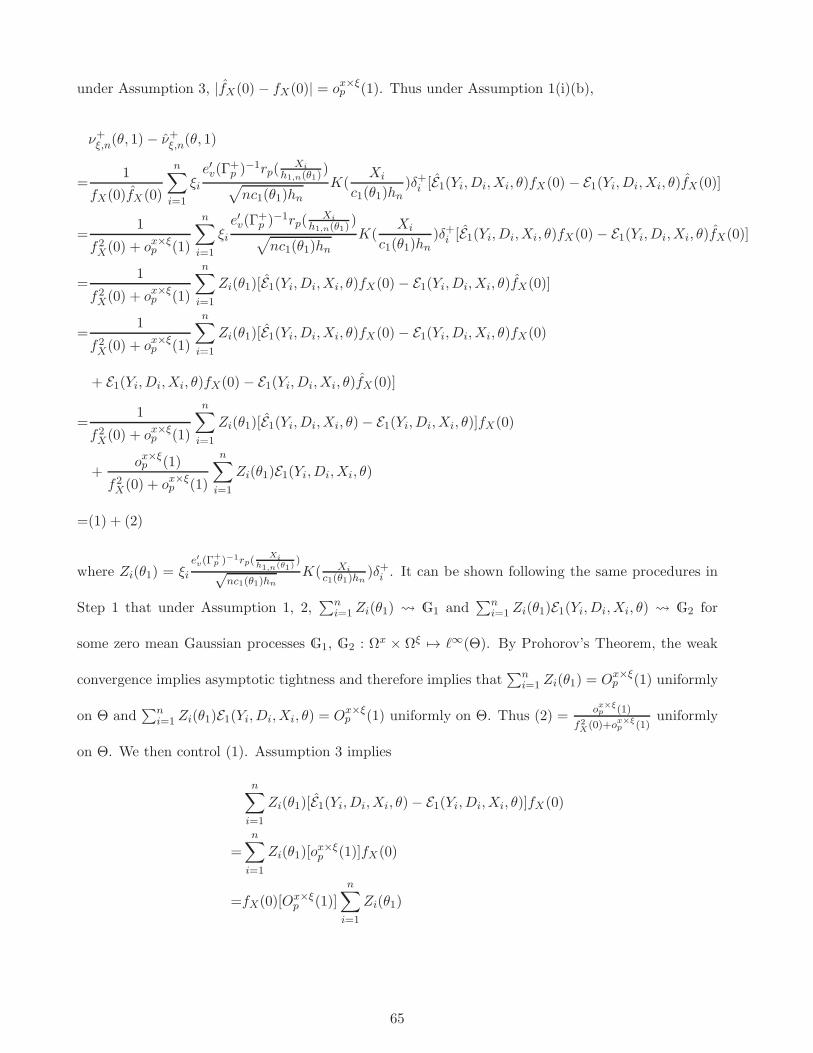
under Assumption 3, |fX(0) − fX(0)| = ox×ξp (1). Thus under Assumption 1(i)(b),
ν+ξ,n(θ, 1)− ν+ξ,n(θ, 1)
=1
fX(0)fX(0)
n∑
i=1
ξie′v(Γ
+p )
−1rp(Xi
h1,n(θ1))
√nc1(θ1)hn
K(Xi
c1(θ1)hn)δ+i [E1(Yi,Di,Xi, θ)fX(0) − E1(Yi,Di,Xi, θ)fX(0)]
=1
f2X(0) + ox×ξp (1)
n∑
i=1
ξie′v(Γ
+p )
−1rp(Xi
h1,n(θ1))
√nc1(θ1)hn
K(Xi
c1(θ1)hn)δ+i [E1(Yi,Di,Xi, θ)fX(0)− E1(Yi,Di,Xi, θ)fX(0)]
=1
f2X(0) + ox×ξp (1)
n∑
i=1
Zi(θ1)[E1(Yi,Di,Xi, θ)fX(0)− E1(Yi,Di,Xi, θ)fX(0)]
=1
f2X(0) + ox×ξp (1)
n∑
i=1
Zi(θ1)[E1(Yi,Di,Xi, θ)fX(0)− E1(Yi,Di,Xi, θ)fX(0)
+ E1(Yi,Di,Xi, θ)fX(0)− E1(Yi,Di,Xi, θ)fX(0)]
=1
f2X(0) + ox×ξp (1)
n∑
i=1
Zi(θ1)[E1(Yi,Di,Xi, θ)− E1(Yi,Di,Xi, θ)]fX(0)
+ox×ξp (1)
f2X(0) + ox×ξp (1)
n∑
i=1
Zi(θ1)E1(Yi,Di,Xi, θ)
=(1) + (2)
where Zi(θ1) = ξie′v(Γ
+p )−1rp(
Xih1,n(θ1)
)√
nc1(θ1)hn
K( Xi
c1(θ1)hn)δ+i . It can be shown following the same procedures in
Step 1 that under Assumption 1, 2,∑n
i=1 Zi(θ1) G1 and∑n
i=1 Zi(θ1)E1(Yi,Di,Xi, θ) G2 for
some zero mean Gaussian processes G1, G2 : Ωx × Ωξ 7→ ℓ∞(Θ). By Prohorov’s Theorem, the weak
convergence implies asymptotic tightness and therefore implies that∑n
i=1 Zi(θ1) = Ox×ξp (1) uniformly
on Θ and∑n
i=1 Zi(θ1)E1(Yi,Di,Xi, θ) = Ox×ξp (1) uniformly on Θ. Thus (2) =
ox×ξp (1)
f2X(0)+ox×ξ
p (1)uniformly
on Θ. We then control (1). Assumption 3 implies
n∑
i=1
Zi(θ1)[E1(Yi,Di,Xi, θ)− E1(Yi,Di,Xi, θ)]fX(0)
=n∑
i=1
Zi(θ1)[ox×ξp (1)]fX(0)
=fX(0)[Ox×ξp (1)]
n∑
i=1
Zi(θ1)
65

uniformly on Θ. Therefore, we have
sup(θ,k)∈T
|ν+ξ,n(θ, k)− ν+ξ,n(θ, k)|p→
x×ξ0,
And thus we can apply Lemma 4 to conclude ν+ξ,np ξG
+H . With similar arguments, we can derive that
ν−ξ,np ξG
−H .
The continuous mapping theorem for bootstrap (Kosorok,2008; Proposition 10.7) and the conti-
nuity of the Hadamard derivatives imply
X′
n(·, 1)
X′n(·, 2)
=
φ′µ(v)1 (0+,·)
(ν+ξ,n(·, 1)/
√c1+2v1 (·)
)(·)− φ′
µ(v)1 (0−,·)
(ν+ξ,n(·, 1)/
√c1+2v1 (·)
)(·)
ψ′µ(v)2 (0+,·)
(ν+ξ,n(·, 2)/
√c1+2v2 (·)
)(·)− ψ′
µ(v)2 (0−,·)
(ν+ξ,n(·, 2)/
√c1+2v2 (·)
)(·)
p ξ
G′(·, 1)
G′(·, 2)
Recursively applying Functional Delta for Bootstrap (Theorem 2.9 of Kosorok (2008)) then gives
Υ′W
( [ψ(µ(v)2 (0+, ·)) − ψ(µ(v)2 (0−, ·))]X′
n(·, 1) − [φ(µ(v)1 (0+, ·))− φ(µ
(v)1 (0−, ·))]X′
n(·, 2)[ψ(µ
(v)2 (0+, ·))− ψ(µ
(v)2 (0+, ·)]2
)
p ξΥ′
W
( [ψ(µ(v)2 (0+, ·)) − ψ(µ(v)2 (0+, ·))]G′(·, 1) − [φ(µ
(v)1 (0+, ·)) − φ(µ
(v)1 (0−, ·))]G′(·, 2)
[ψ(µ(v)2 (0+, ·)) − ψ(µ
(v)2 (0−, ·)]2
)
This completes the proof.
A.4 First Stage Estimators
To estimate MP, we replace µk(x, θ)1|x/hk,n(θk)| ≤ 1 by its estimate µk,p(x, θ)1|x/hk,n(θk)| ≤ 1
which is uniformly consistent across (x, θ). Lemma 9 below proposes such a uniformly consistent
estimator without requiring to solve an additional optimization problem; by a mean-value expansion
and uniform boundedness of µ(p+1)k , we can reuse the first stage local polynomial estimates of µ
(v)l,p (0
±, θ)
for all v ≤ p. This auxiliary result will prove useful when we apply Theorem 1 to specific examples.
In fact, we will prove a more general result that allows us to use any first r terms of our p-th order
polynomial estimator for a t such that 0 ≤ t ≤ p.
Lemma 9. Fix an integer t such that 0 ≤ t ≤ p. Suppose that Assumptions 1 and 2(i)-(iii) are
satisfied. Let E1(y, d, x, θ) = g1(y, θ1) − µ1(x, θ1), E2(y, d, x, θ) = g2(d, θ2)− µ2(d, θ2), δ+x = 1x ≥ 0
66

and δ−x = 1x ≤ 0. Define
µ1,t(x, θ1) = rt(x/h1,n(θ1))′α1+,t(θ1)δ
+x + rt(x/h1,n(θ1))
′α1−,t(θ1)δ−x and
µ2,t(x, θ2) = rt(x/h2,n(θ2))′α2+,t(θ2)δ
+x + rt(x/h2,n(θ2))
′α2−,t(θ2)δ−x
Then we have
E1(y, d, x, θ) = [g1(y, θ1)− µ1,t(x, θ1)]1|x/h1,n(θ1)| ≤ 1 and
E2(y, d, x, θ) = [g2(d, θ2)− µ2,t(x, θ2)]1|x/h2,n(θ2)| ≤ 1
are uniformly consistent for E1(y, d, x, θ)1|x/h1,n(θ1)| ≤ 1 and E2(y, d, x, θ)1|x/h2,n(θ2)| ≤ 1 on
[x, x]× Y × D , respectively.
Proof. We will show the 1+ part only, since the other parts can be shown similarly. Recall that
E1(y, d, x, θ) = g1(y, θ1)− µ1(x, θ1). If x > 0,
µ1(x, θ1)1|x/h1,n(θ1)| ≤ 1 =
(µ1(0
+, θ1) + µ(1)1 (0+, θ1)x+ ...+ µ
(t)1 (0+, θ1)
xt
t!+ µ
(t+1)1 (x∗ni, θ1)
x(t+1)
(t+ 1)!
)1|x/c1(θ)hn| ≤ 1.
By Corollary 1, µ(v)1,t (0
±, θ1) is uniformly consistent for µ(v)1 (0±, θ1), v = 0, 1, ..., t. Thus,
[E1(y, d, x, θ)− E1(y, d, x, θ)]1|x/h1,n(θ)| ≤ 1
=(µ1,t(0
+, θ1) + µ(1)1,t (0
+, θ1)x+ ...+ µ(t)1,t(0
+, θ1)xt
t!
)1|x/h1,n(θ)| ≤ 1−
(µ1(0
+, θ1) + µ(1)1 (0+, θ1)x+ ...+ µ
(t)1 (0+, θ1)
xt
t!+ µ
(t+1)1 (x∗, θ1)
x(t+1)
(t+ 1)!
)1|x/h1,n(θ1)| ≤ 1
=oxp(1) − µ(t+1)1 (x∗, θ1)
x(t+1)
(t+ 1)!1|x| ≤ h1,n(θ) = oxp(1) +O(hn),
where the last equality is by Assumption 1(iii) and by the uniform boundedness of µ(t+1) under
Assumption 1 (ii)(a).
67

A.5 Auxiliary Lemmas for the Ten Examples
A.5.1 Lemmas Related to Asymptotic Equicontinuity
The following Lemma establish the relationship between convergence in probability in supremum norm
and convergence in probability with respect to the semi-metric ρ induced by the limiting Gaussian
process. We use this lemma in the corollary below to ensure that the asymptotically equicontinuous
process, ν±ξ,n, evaluating QY |X(·|0±) can nicely approximate this process evaluating QY |X(·|0±).
Lemma 10. Suppose that Assumption SQRD holds. Define
ρ(QY |X(θ′′|0±), QY |X(θ′′|0±)) = limn→∞
( n∑
i=1
E|fni(QY |X(θ′′|0±))− fni(QY |X(θ′′|0±))|2)1/2
,
where
fni(y) =e′0(Γ
±2 )
−1r2(Xi
hn)K(Xi
hn)[1Yi ≤ y − FY |X(y|Xi)]δ
±i√
nhnfX(0).
Then,∥∥∥QY |X(·|0±)−QY |X(·|0±)
∥∥∥[a,1−a]
p→x
0 implies supθ′′∈[a,1−a] ρ(QY |X(θ′′|0±), QY |X(θ′′|0±)) p→x0.
Proof. We will show the claim for the + side only. The case of the − side can be similarly proved.
Notice that by Law of Iterated Expectations and calculations under Assumption SQRD (i) (a), (i)
(b), (iii), and (iv),
ρ2(QY |X(θ′′|0+), QY |X(θ′′|0+))
= limn
n∑
i=1
E[E[(e′0(Γ+
2 )−1r2(
Xi
hn)K(Xi
hn)δ+i√
nhnfX(0)
[1Yi ≤ QY |X(θ′′|0+) − FY |X(QY |X(θ′′|0+)|Xi)− 1Yi ≤ QY |X(θ′′|0+)+ FY |X(QY |X(θ′′|0+)|Xi)])2
|Xi]]
= limnE[e′0(Γ
+2 )
−1Ψ+(Γ+2 )
−1e0fX(0)
E[(1Yi ≤ QY |X(θ′′|0+) − FY |X(QY |X(θ′′|0+)|Xi)
− 1Yi ≤ QY |X(θ′′|0+)+ FY |X(QY |X(θ′′|0+)|Xi))2|Xi]]
It then suffices to show that
E[(1Yi ≤ QY |X(θ′′|0+) − FY |X(QY |X(θ′′|0+)|Xi)− 1Yi ≤ QY |X(θ′′|0+)+ FY |X(QY |X(θ′′|0+)|Xi))2|Xi]
p→x
0
68

uniformly in θ′′. We write
(1Yi ≤ QY |X(θ′′|0+) − FY |X(QY |X(θ′′|0+)|Xi)− 1Yi ≤ QY |X(θ′′|0+)+ FY |X(QY |X(θ′′|0+)|Xi))2
=([1Yi ≤ QY |X(θ′′|0+) − 1Yi ≤ QY |X(θ′′|0+)]− [FY |X(QY |X(θ′′|0+)|Xi)− FY |X(QY |X(θ′′|0+)|Xi)])2
=[1Yi ≤ QY |X(θ′′|0+) − 1Yi ≤ QY |X(θ′′|0+)]2 + [FY |X(QY |X(θ′′|0+)|Xi)− FY |X(QY |X(θ′′|0+)|Xi)]2
− 2[1Yi ≤ QY |X(θ′′|0+) − 1Yi ≤ QY |X(θ′′|0+)][FY |X(QY |X(θ′′|0+)|Xi)− FY |X(QY |X(θ′′|0+)|Xi)]
=(1) + (2)− (3).
The conditional expectation of part (1) is
E[(1)|Xi] = FY |X(QY |X(θ′′|0+)|Xi) + FY |X(QY |X(θ′′|0+)|Xi)− 2FY |X(QY |X(θ′′|0+) ∧QY |X(θ′′|0+)|Xi)
p→x
0
uniformly by the uniform consistency∥∥∥QY |X(·|0±)−QY |X(·|0±)
∥∥∥[a,1−a]
p→x0 and the continuous map-
ping theorem under Assumption SQRD (ii) (a). The uniform convergence in probability of other parts,
(2) and (3), can be concluded similarly.
Similar results hold in the cases of Sharp FQRK, Fuzzy FQRK and Fuzzy FQRD as the following
Lemma 11. Suppose that Assumption SQRK or FQRK holds. Define
ρ(QY |X(θ′′|0), QY |X(θ′′|0)) = limn→∞
( n∑
i=1
E|fni(QY |X(θ′′|0)) − fni(QY |X(θ′′|0))|2)1/2
,
where
fni(y) =e′1(Γ
±2 )
−1r2(Xi
hn)K(Xi
hn)[1Yi ≤ y − FY |X(y|Xi)]δ
±i√
nhnfX(0).
Then,∥∥∥QY |X(·|0) −QY |X(·|0)
∥∥∥[a,1−a]
p→x
0 implies supθ′′∈[a,1−a] ρ(QY |X(θ′′|0), QY |X(θ′′|0)) p→x
0.
Lemma 12. Suppose that Assumption FQRD holds. Define
ρ(QY d|C(θ′′), QY d|C(θ
′′)) = limn→∞
( n∑
i=1
E|fni(QY d|C(θ′′), d) − fni(QY d|C(θ
′′), d)|2)1/2
,
69

where
fni(y, d) =e′1(Γ
±2 )
−1r2(Xi
hn)K(Xi
hn)[1Y ∗
i ≤ y,D∗i = d − µ1(Xi, y, d)]δ
±i√
nhnfX(0).
Then,∥∥∥QY d|C(θ
′′)−QY d|C(θ′′)∥∥∥[a,1−a]×0,1
p→x
0 implies sup(θ′′,d)∈[a,1−a]×0,1 ρ(QY d|C(θ′′), QY d|C(θ
′′))p→x
0.
Since the proofs are mostly identical to Lemma 10, we omit them.
A.5.2 Lemmas for Uniform Consistency of Estimators for Conditional Densities
Recall that in Section 5.7, the existence of an uniform consistency estimator is assumed in Assumption
5.7 (vi) An example of estimators fY |X(y, 0±) that satisfy Assumption 5.7 (vi) are
fY |X(y|0±) =1
na2n
∑ni=1K(Yi−y
an)K(Xi
an)δ±i
1nan
∑ni=1K(Xi
an)δ±i
=gY X(y, 0±)gX(0±)
The following result gives the sufficient conditions for fY |X(y|0±) to satisfy Assumption 5.7 (vi).
Lemma 13. Assuming Assumption 5.7. In addition, let fY X be continuously differentiable on Y1 ×
[x, 0), and Y1 × (0, x] with bounded partial derivatives and assume kernel K be symmetric. Let an
be such that an → 0, nan → ∞, na2n| log an| → ∞, | log an|
log log an→ ∞, and a2n ≤ ca22n for some c > 0. then
fY |X(y|0±) such that supy∈Y1|fY |X(y|0±)− fY |X(y|0±)| = oxp(1).
Proof. We will show only for 0+. The other side follows similarly. Note the denominator gX(0+) =
12fX(0+) + oxp(1) and fX(0) is bounded away from 0 under Assumption 1(ii).
Thus, it suffices to show supy∈Y1|gY X(y, 0+)−1
2fY X(y, 0+)| = oxp(1). Note |gY X(y, 0+)−12fY X(y, 0+)| ≤
|gY X(y, 0+)− EgY X(y, 0+)|+ |EgY X(y, 0+)− 12fY X(y, 0+)|. To control the stochastic part, Theorem
2.3 of Gine and Guillou (2002) suggests that
supy∈Y1
|gY X(y, 0+)− EgY X(y, 0+)| = Oxa.s.(
√log 1
an
na2n).
70

For the deterministic part, under the smoothness assumptions made on fY X , a mean value expansion
gives
E[gY X(y, 0+)]
=
∫
R
∫
R+
K(u)K(v)(fY X(y, 0+) +∂
∂yfY X(y∗, x∗)uan +
∂
∂xfY X(y∗, x∗)van)dudv
=1
2fY X(y, 0+) +O(an)
uniformly on Y1, where (y∗, x∗) is a linear combination of (y, 0) and (y + uhn, vhn). This concludes
the proof.
In Section 5.8, we assumed the existence of an estimator that satisfies Assumption 5.8. Define
fY |X(y|0) =1
na2n
∑ni=1K(Yi−y
an)K(Xi
an)
1nan
∑ni=1K(Xi
an)
=fY X(y, 0)
fX(0)
The following lemma provides such estimator.
Lemma 14. Assume Assumption SQRK (i) (a), (i) (b), and (ii) (b) hold. In addition, if the joint
density fY X(y, x) is twice continuously differentiable on Y2 × [x, x] with bounded partial derivatives
for some open set Y2 such that Y1 ⊂ Y2 ⊂ Y . Let K be a bounded kernel function such that
x 7→ K(x− x′/a) : a > 0, x′ ∈ R forms a VC type class (e.g. Epanechnikov) and∫RuK(u)du = 0,
∫Ru2K2(u)du < 0. The bandwidth an → 0 satisfies na2n
| log an| → ∞, | log an|log log an
→ ∞, and a2n ≤ ca22n for
some c > 0,h3n log 1
an
a2n→ 0 and nh3na
4n → 0. Then, supy∈Y1
√nh3n|fY |X(y|0) − fY |X(y|0)| p→
x0. Thus,
Assumption SQRK (vi) is satisfied.
We remark that the conditionh3n log 1
an
a2n→ 0 is easily satisfied by the bandwidth selectors hMSE
1,n ∝
n−1/5 and hROT1,n ∝ n−1/4 proposed in Section B along with a Silverman’s rule of thumb an ∝ n−1/6.
Proof. First note that the denominator is essentially fX(0) + oxp(1) and fX(0) > C > 0. It then
suffices to show that the numerator fY X(y, 0) satisfies supy∈Y1
√nhn|fY X(y, 0) − fY X(y, 0)| = oxp(1).
Write |fY X(y, 0) − fY X(y, 0)| ≤ |fY X(y, 0) − EfY X(y, 0)| + |EfY X(y, 0) − fY X(y, 0)|. To control the
71

stochastic part, Theorem 2.3 of Gine and Guillou (2002) suggests that
supy∈Y1
|fY X(y, 0)− EfY X(y, 0)| = Oxa.s.(
√log 1
an
na2n).
For the deterministic part, a mean value expansion gives
E[fY X(y, 0)]
=
∫
R
∫
R
K(u)K(v)(fY X(y, 0) +∂
∂yfY X(y, 0)uan +
∂
∂xfY X(y, 0)van
+∂
∂y
∂
∂yfY X(y∗, x∗)uva2n +
1
2
∂2
∂y2fY X(y∗, x∗)u2a2n +
1
2
∂2
∂x2fY X(y∗, x∗)v2a2n)dudv
=fY X(y, 0) +O(a2n)
uniformly on Y1, where (y∗, x∗) is a linear combination of (y, 0) and (y+uhn, vhn). Thus, the conclusion
follows fromlog 1
anh3n
a2n→ 0 and nh3na
4n → 0.
In Section 5.9, the densities in the denominator can be estimated in the following manner. Define
fY d|C(y) =fY |XD(y|0+, d)µ2,2(0+, d) − fY |XD(y|0−, d)µ2,2(0−, d)
µ2,2(0+, d) − µ2,2(0−, d),
where fY |XD(y|0±, 1) =1
na2n
∑ni=1 K(
Xian
)K(Yi−y
an)Diδ
±i
1nan
∑ni=1 K(
Xian
)Diδ±i
, fY |XD(y|0±, 0) =1
na2n
∑ni=1 K(
Xian
)K(Yi−y
an)(1−Di)δ
±i
1nan
∑ni=1 K(
Xian
)(1−Di)δ±i
,
with bandwidths an. The following lemma shows uniform consistency of these estimators.
Lemma 15. Suppose that Assumption FQRD holds, in addition, for each d = 0, 1, let fY X|D(·, ·|d) be
continuously differentiable on Y1 × [x, 0), and Y1 × (0, x] with bounded partial derivatives and assume
kernel K be symmetric. Let an be such that an → 0, nan → ∞, na2n| log an| → ∞, | log an|
log log an→ ∞,
and a2n ≤ ca22n for some c > 0. Then, supy∈Y |fY 0|C(y) − fY 0|C(y)| = oxp(1) and supy∈Y |fY 1|C(y) −
fY 1|C(y)| = oxp(1).
Proof. Note that
fY 1|C(y) =∂
∂yFY 1|C(y) =
∂∂yµ1(0
+, (y, 1)) − ∂∂yµ1(0
−, (y, 1))
µ2(0+, 1)− µ2(0−, 1)
72

The numerator can be estimated consistently with the local quadratic regression defined above. For
the denominator, we have
∂
∂yµ1(0
+, (y, 1)) =∂
∂yE[1Yi ≤ y1Di = 1|Xi = 0+]
=∂
∂y
(E[1Yi ≤ y|Xi = 0+,Di = 1]Px(Di = 1|Xi = 0+) + 0
)
=∂
∂yFY 1|XD(y|0+, 1)µ2(0+, 1)
=fY 1|XD(y|0+, 1)µ2(0+, 1)
Uniform consistency of fY 1|X,D(y|0±, 1) can be shown by applying Theorem 2.3 of Gine and Guillou
(2002), as in Lemma 13. Also µ2,p(0±) is uniformly consistent by Corollary 1. Corresponding result
for fY 0|C(y) can be shown similarly.
A.5.3 Proof of Lemma 2
Proof. The Hadamard differentiability of the left-inverse operator and a mean value expansion give
∂
∂xQY |X(θ′′|0+) = lim
δ↓0
QY |X(θ′′|δ) −QY |X(θ′′|0+)δ
= limδ↓0
Φ(FY |X(·|δ)
)(θ′′)− Φ
(FY |X(·|0+)
)(θ′′)
δ
= limδ↓0
Φ((FY |X(·|0+) + δ ∂
∂xFY |X(·|x∗))(θ′′)− Φ
(FY |X(·|0+)
)(θ′′)
δ
= Φ′FY |X(·|0)
( ∂∂xFY |X(·|0+)
)(θ′′)
= −F
(1)Y |X(QY |X(θ′′|0)|0+)fY |X(QY |X(θ′′|0)|0)
= φ(F(1)Y |X(·|0+))(θ′′)
by the definition of Hadamard Derivative and then Lemma 3.9.23 (i) of van der Vaart and Wellner
(1996).
73

A.5.4 Proof of Lemma 3
Proof. Write Φ(FY d|C)(θ′′) := infy ∈ Y1 : FY d|C(y) ≥ θ′′ for θ′′ ∈ [a, 1 − a]. The weak convergence
of ν±n from Theorem 1 (i), Lemma 3.9.23 (i) of van der Vaart and Wellner (1996), and the functional
delta method yield
√nhn[QY d|C(·)−QY d|C(·)] =
√nhn[Φ(FY d|C)(·) − Φ(FY d|C)(·)] = Ox
p (1)
The result follows from Assumption FQRD (vi) and Slutsky’s lemma.
A.6 Proofs of Corollaries for the Ten Examples
We use G and G± to denote generic zero mean Gaussian processes that appear in some intermediate
steps in the proofs without having to specify their covariance structure. They differ across different
examples, but are fixed within each one.
A.6.1 Proof of Corollary 3
Proof. It suffices to show that Assumption SMRD implies Assumptions 1, 2, and 3. Most of these
implications are direct. For Assumption 1 (ii)(a), note that µ1(x, 0) : [x, x] 7→ R is a singleton, and
therefore forms a VC type class with its sole element serving as an envelope, which is integrable by
Assumption SMRD (ii)(a). Assumption 3 follows from Lemma 9.
A.6.2 Proof of Corollary 5
Proof. To check the Assumptions required by Theorem 1, for Assumption 1(ii)(a), notice that
µ2(x, 0) : [x, x] 7→ R is a singleton, and therefore forms a VC type class with envelope 1. Assumption
3 follows from Lemma 9. Other conditions can be checked as before. Applying Theorem 1 gives
(µ2(0+, 0) − µ2(0
−, 0))X′n(0, 1) − (µ1(0
+, 0)− µ1(0−, 0))X′
n(0, 2)
(µ2(0+, 0) − µ2(0−, 0))2 N(0, σ2FMRD)
74

with probability approaching to one. According to Lemma 4, it remains to show
(µ2(0+, 0) − µ2(0
−, 0))X′n(0, 1) − (µ1(0
+, 0) − µ1(0−, 0))X′
n(0, 2)
(µ2(0+, 0)− µ2(0−, 0))2
−(µ2,2(0+, 0) − µ2,2(0
−, 0))X′n(0, 1) − (µ1,2(0
+, 0)− µ1(0−, 0))X′
n(0, 2)
(µ2,2(0+, 0) − µ2,2(0−, 0))2= ox×ξ
p (1).
This is the case due to the uniform consistency of µ1,2(0±, 0), µ2,2(0±, 0) that follows from Corollary 1,
the independence between data and ξi under Assumption FMRD (vi), and the fact that |µ2(0+, 0) −
µ2(0−, 0)| > 0 under Assumption FMRD (ii) (d).
A.6.3 Proof of Corollary 7
Proof. It is direct to show that Assumption GFMRD and Lemma 9 together imply the three assump-
tions required by Theorem 1. Note for k = 1, 2, µk(·, θ) : [x, x] 7→ R : θ ∈ 1, ...,K has finite
elements and therefore is of VC-subgraph class with envelope maxθ∈1,...,K
µk(x, θ) and Assumption 1
(ii)(a) is satisfied. The theorem then gives
(µ2(0+, ·) − µ2(0
−, ·))X′n(·, 1) − (µ1(0
+, ·)− µ1(0−, ·))X′
n(·, 2)(µ2(0+, ·)− µ2(0−, ·))2
N(0,ΣGFMRD)
with probability approaching to one. Lemmas 4 and 9 then give the desired result.
A.6.4 Proof of Corollary 8
Proof. We check that Assumption SCRD implies the assumptions required by Theorem 1. Most are di-
rect, and we only need to check the following three points. For Assumption 1 (ii) (a), x 7→ FY |X(θ′′|x) :
θ′′ ∈ Y1 and y′ 7→ 1y′ ≤ θ′′ : θ′′ ∈ Y1 are increasing stochastic processes bounded by one, and
they are of VC-subgraph classes according to Lemma 9.10 of Kosorok (2008), and thus of VC type.
For Assumption 1 (ii)(c), note that E[(1Yi ≤ y1 − FY |X(y1|Xi))(1Yi ≤ y2 − FY |X(y2|Xi))|Xi] =
FY |X(y1∧y2|Xi)−FY |X(y1|Xi)FY |X(y2|Xi) and thus it follows from Assumption SCRD (ii). Assump-
tion 1 (ii) (d) is implied by the right continuity of y′ 7→ 1y ≤ y′.
Assumption 3 is implied by Lemma 9. The result then follows from Theorem 1.
75

A.6.5 Proof of Corollary 9
Proof. We need to check that Assumption SQRD implies all the three Assumptions required by The-
orem 1. The only non-trivial ones are Assumptions 1 (ii) (a), (d) 2 (i), and 3. For Assumptions 1 (ii)
(a) and 3 (i), note that y′ 7→ 1y′ ≤ y : y ∈ Y1 and x 7→ FY |X(y|x) : y ∈ Y1 are collections of
increasing stochastic processes, and Lemma 9.10 of Kosorok (2008) suggests that they are of VC-class
and thus VC type with envelope one. Assumption 1 (ii) (d) is implied by the right continuity of
y′ 7→ 1y ≤ y′. Assumption 2 (i) follows from Lemma 3.9.23 (i) of van der Vaart and Wellner (1996)
and Assumption 5.7 (ii). Assumption 3(b) is implied by Lemma 9.
By Theorem 1 (i), we have√nhn[τSQRD(·)− τSQRD(·)] G′
SQRD, where
G′SQRD(·) =φ′FY |X(·|0+)
(GH+
)(·)− φ′FY |X(·|0−)
(GH−
)(·)
=−GH+(QY |X(·|0+))
fY |X(QY |X(·|0+)|0+) +GH−(QY |X(·|0−))
fY |X(QY |X(·|0−)|0−) .
Also, by Theorem 1 (ii), φ′FY |X(·|0+)(ν+ξ,n)− φ′FY |X(·|0−)(ν
−ξ,n)
p ξG′
SQRD, where
φ′FY |X(·|0±)(ν±ξ,n)(θ
′′) = −ν±ξ,n(QY |X(θ′′|0±))
fY |X(QY |X(θ′′|0±)|0±) .
In the EMP, we replace fY |X(·|0±), QY |X(·|0±) by their uniformly consistent estimators fY |X(·|0±),
QY |X(·|0±), where the uniform consistency of the former follows from Assumption 5.7 (vi) (see Lemma
10) and the uniform consistency of the latter follows from Corollary 2.
By Lemma 4, it suffices to show that supθ′′∈[a,1−a]
∣∣∣(φ′FY |X(·|0+)(ν
+ξ,n)(θ
′′)− φ′FY |X(·|0−)(ν−ξ,n)(θ
′′))−
(φ′FY |X(·|0+)(ν
+ξ,n)(θ
′′)− φ′FY |X(·|0−)(ν−ξ,n)(θ
′′))∣∣∣ p→
x×ξ0. We first show
∥∥∥φ′FY |X(·|0+)(ν+ξ,n(QY |X(·|0+)))− φ′FY |X(·|0+)(ν
+ξ,n(QY |X(·|0+)))
∥∥∥[a,1−a]
=
∥∥∥∥∥−ν+ξ,n(QY |X(·|0+))
fY |X(QY |X(·|0+)|0+)+
ν+ξ,n(QY |X(·|0+))fY |X(QY |X(·|0+)|0+)
∥∥∥∥∥[a,1−a]
p→x×ξ
0.
Lemma 10 and Corollary 2 along with the asymptotic equicontinuity of ν+ξ,n implied by its weak conver-
gence in Theorem 1 (i) suggest that ν+ξ,n(QY |X(·|0+))− ν+ξ,n(QY |X(·|0+)) p→x×ξ
0 uniformly. Assumption
76

SQRD (ii)(b) and the uniform consistency of both QY |X(·|0+) and fY |X(·|0+) shows that fY |X(·|0+)
is bounded away from 0 uniformly, and with probability approaching one
supθ′′∈[a,1−a]
|fY |X(QY |X(θ′′|0+)|0+)− fY |X(QY |X(θ′′|0+)|0+)|
≤ supy∈Y1
|fY |X(y|0+)− fY |X(y|0+)|+ supθ′′∈[a,1−a]
L|QY |X(θ′′|0+)−QY |X(θ′′|0+)| = oxp(1) + oxp(1)
for a Lipschitz constant L > 0. Thus,
∥∥∥∥−ν+ξ,n
(QY |X(·|0+))
fY |X(QY |X(·|0+)|0+)+
ν+ξ,n
(QY |X(·|0+))
fY |X(QY |X(·|0+)|0+)
∥∥∥∥[a,1−a]
p→x×ξ
0.
Similar lines show∥∥∥φ′FY |X(·|0−)(ν
−ξ,n(QY |X(·|0−)))− φ′FY |X(·|0−)(ν
−ξ,n(QY |X(·|0−)))
∥∥∥[a,1−a]
p→x×ξ
0 as
well. Therefore, we have
supθ′′∈[a,1−a]
∣∣∣(φ′FY |X(·|0+)(ν
+ξ,n)(θ
′′)−φ′FY |X(·|0−)(ν−ξ,n)(θ
′′))−(φ′FY |X(·|0+)(ν
+ξ,n)(θ
′′)−φ′FY |X(·|0−)(ν−ξ,n)(θ
′′))∣∣∣ p→
x×ξ0.
We then apply Lemma 4 to conclude the proof.
A.6.6 Proof of Corollary 10
Proof. For the unconditional weak convergence, the assumptions required by Theorem 1 can be checked
as in Corollary 9 except for Assumption 2(i) now follows from Assumption 5.8 (ii)(a). Applying
Theorem 1 (i), we have√nh3n[τSQRK − τSQRK] GSQRD. It then suffices to show
√nh3n ‖τSQRK − τSQRK‖Θ′′ = oxp(1)
By definition, we only need to show
√nh3n
∥∥∥φ(F (1)Y |X(·|0±))− φ(F
(1)Y |X(·|0±))
∥∥∥Θ′′
=−√nh3n
∥∥∥∥∥∥
F(1)Y |X(QY |X(θ′′|0±)|0)fY |X(QY |X(θ′′|0)|0)
−F
(1)Y |X(QY |X(θ′′|0±)|0)fY |X(QY |X(θ′′|0)|0)
∥∥∥∥∥∥Θ′′
= oxp(1). (A.4)
We first claim that
√nh3n[F
(1)Y |X(QY |X(θ′′|0)|0±)− F
(1)Y |X(QY |X(θ′′|0)|0±)] = oxp(1)
respectively. Then by Assumption SQRK (ii) (b) and uniform super-consistency of fY |X(·|0) and
QY |X(·|0), supθ′′∈[a,1−a] |fY |X(QY |X(θ′′|0)|0) − fY |X(QY |X(θ′′|0)|0)| = oxp(1) and∣∣∣ 1fY |X(QY |X(θ′′|0)|0)
∣∣∣ <
C <∞. We can thus conclude that equation (A.4) is true.
77

To prove the claim, notice that
√nh3n[F
(1)Y |X(QY |X(θ′′|0)|0±)− F
(1)Y |X(QY |X(θ′′|0)|0±)]
≤√nh3n[F
(1)Y |X(QY |X(θ′′|0)|0±)− F
(1)Y |X(QY |X(θ′′|0)|0±)]
+√nh3n[F
(1)Y |X(QY |X(θ′′|0)|0±)− F
(1)Y |X(QY |X(θ′′|0)|0±)]
+√nh3n[F
(1)Y |X(QY |X(θ′′|0)|0±)− F
(1)Y |X(QY |X(θ′′|0)|0±)]
=(1) + (2) + (3)
From Theorem 1(i) and the Hadamard differentiability of left inverse operator, we have√nhn[QY |X(θ′′|0)−
QY |X(θ′′|0)] = Oxp (1) uniformly. An application of Slutsky’s lemma implies |QY |X(θ′′|0)−QY |X(θ′′|0)| =
Ox( 1√nhn
). This and Assumption 5.8(ii)(a) imply (2) = oxp(1) uniformly in θ′′. From Lemma 1, (3) =
−ν±n (QY |X(θ′′|0))+oxp(1) and (1) = ν±n (QY |X(θ′′|0))+oxp(1) = ν±n (QY |X(θ′′|0))+oxp(1) uniformly in θ′′,
where the last equality is due to Lemma 11 and asymptotic ρ−equicontinuity of ν±n implied by its weak
convergence from Theorem 1(i). Thus we have√nh3n[F
(1)Y |X(QY |X(θ′′|0)|0±)−F (1)
Y |X(QY |X(θ′′|0)|0±)] =
oxp(1).
As for the conditional weak convergence part of the statement, Theorem 1(ii) shows
φ′FY |X(·|0±)(ν±ξ,n)(·) = −
ν±ξ,n(QY |X(·|0))fY |X(QY |X(·|0))
p ξ−
G±(QY |X(·|0))fY |X(QY |X(·|0)|0)
Uniform consistency of fY |X(·|0), QY |X(·|0), Assumption SQRK (ii), asymptotic ρ−equicontinuity of
ν±ξ,n, Lemmas 11, 4 and 14 then imply
φ′FY |X(·|0±)(ν±ξ,n)(·) = −
ν±ξ,n(QY |X(·|0))fY |X(QY |X(·|0))
p ξ−
G±(QY |X(·|0))fY |X(QY |X(·|0)|0)
and thus by Assumption 5.8 (i)(a) and the continuous mapping theorem, we conclude
φ′FY |X(·|0+)(ν+ξ,n)(·)− φ′FY |X(·|0−)(ν
−ξ,n)(·)
b′(0+)− b′(0−)=
1
b′(0+)− b′(0−)[−
ν+ξ,n(QY |X(·|0))fY |X(QY |X(·|0)|0)
+ν−ξ,n(QY |X(·|0))fY |X(QY |X(·|0)|0)
]
p ξG
′SQRK(·)
78

A.6.7 Proof of Corollary 11
Proof. We first verify that the Assumptions required by Theorem 1 are satisfied.
To show Assumption 1(ii)(a), it is true that the subgraphs of (y, d) 7→ 1y ≤ y′ : y′ ∈ Y1 and
(y, d) 7→ 1d = d′ : d′ ∈ D can not shatter any two-point sets (for definition, see Section 9.1.1
of Kosorok(2008)); to see this, let (y1, d1, r1), (y2, d2, r2) ∈ Y1 × D × R with y1 ≤ y2. Notice that
(y1, d1, r1) can never be picked out by any function in either of the classes. Therefore they are of
VC-subgraph classes with VC index of 2. This implies that they are of VC type and Lemma 8 implies
that the set of products (t, y) 7→ 1y ≤ y′t : y′ ∈ Y1 is of VC type with square integrable constant
function 1 as its envelope. On the other hand, x 7→ E[1Yi ≤ y1t = d|Xi = x] : (y, d) ∈ Y1×D is
of VC type with square integrable envelope 1 because of Example 19.7 of van der Vaart (1998) under
boundedness of Y1 and Lipschitz continuity from Assumption FQRD (i) (a) and (ii). Assumption
1(ii)(c) follows from Assumption FQRD (ii) since for any (y1, d1), (y2, d2) ∈ Y × D , if d1 = d2 = d
E[1Y ≤ y1,D = d1Y ≤ y2,D = d|X = x] = E[1Y ≤ y1 ∧ y2,D = d|X = x] and It equals zero
if d1 6= d2. Assumption 1 (ii) (d) is implied by the right continuity of (y′, d′) 7→ 1y ≤ y′, d = d′
on Y1 × 0, 1 in y for each d. Assumption 3 is implied by Lemma 9. Assumption FQRD (vii) and
Lemma 3.9.23 of van der Vaart and Wellner (applicable under Assumption FQRD (ii), (v) and (vii))
implies Hadamard differentiability of Assumption 2(i).
The rest are directly implied by Assumption FQRD. Thus we may apply Theorem 1(i) and acquire
νn G := G+ −G− for a zero mean Gaussian process G, where
νn(y, d1, d2, 1)
νn(y, d1, d2, 2)
=
√nhn[(µ1,2(0
+, y, d1)− µ1,2(0−, y, d1))− (µ1(0
+, y, d1)− µ1(0−, y, d1))]
√nhn[(µ2,2(0
+, d2)− µ2,2(0−, d2))− (µ2(0
+, d2)− µ2(0−, d2))]
79

Theorem 1(i) further implies
√nh(τFQRD(·)− τFQRD(·))
G′FQRD(·)
:=Υ′W
( [µ2(0+, d)− µ2(0−, d)]G(·, ·, ·, 1) − [µ1(0
+, y, d) − µ1(0−, y, d)]G(·, ·, ·, 2)
[µ2(0+, d)− µ2(0−, d)]2
)(·)
=−[µ2(0
+, d) − µ2(0−, d)]G(QY 1|C(·), 1, 1, 1) − [µ1(0
+, QY 1|C(·), 1) − µ1(0−, QY 1|C(·), 1)]G(QY 1|C(·), 1, 1, 2)
fY 1|C(QY 1|C(·))[µ2(0+, 1)− µ2(0−, 1)]2
+[µ2(0
+, d) − µ2(0−, d)]G(QY 0|C(·), 0, 0, 1) − [µ1(0
+, QY 0|C(·), 0) − µ1(0−, QY 0|C(·), 0)]G(QY 1|C(·), 0, 0, 2)
fY 0|C(QY 0|C(·))[µ2(0+, 0)− µ2(0−, 0)]2
For the conditional weak convergence part of the proof, define
Υ′W (Yn)(θ
′′) =
−[µ2(0
+, 1)− µ2(0−, 1)]X′
n(QY 1|C(θ′′), 1, 1, 1) − [µ1(0
+, QY 1|C(θ′′), 1) − µ1(0
−, QY 1|C(θ′′), 1)]X′
n(QY 1|C(θ′′), 1, 1, 2)
fY 1|C(QY 1|C(θ′′))[µ2(0+, 1)− µ2(0−, 1)]2
+[µ2(0
+, 0)− µ2(0−, 0)]X′
n(QY 0|C(θ′′), 0, 0, 1) − [µ1(0
+, QY 0|C(θ′′), 0) − µ1(0
−, QY 0|C(θ′′), 0)]X′
n(QY 0|C(θ′′), 0, 0, 2)
fY 0|C(QY 0|C(θ′′))[µ2(0+, 0)− µ2(0−, 0)]2
Theorem 1(ii) then suggests that Υ′W (Yn)
p ξG′
FQRD. Thus it suffices to show
supθ′′∈[a,1−a]
|Υ′W (Yn)(θ
′′)−Υ′W (Yn)(θ
′′)| p→x×ξ
0
which is true by the asymptotic ρ−equicontinuity of X′n (which is inherited from the conditional weak
convergence of νξ,n), the uniform consistency of QY d|C and fY d|C for d = 1, 0 by Lemmas 15, 3 and
12.
B Bandwidth Choice in Practice
While our theory prescribes asymptotic rates of bandwidths, empirical practitioners need to choose
bandwidth for each finite n. In this section, we provide a guide for this matter. We emphasize that our
robust inference procedure allows for large bandwidths such as the ones based on the MSE optimality.
Following the bias-robust approach from Calonico, Cattaneo and Titiunik (2014), we increment the
degree of local polynomial estimation by one or more to p for the purpose of bias correction while using
80

the optimal bandwidths for the correct order s. For instance, if we are interested in the local linear
model (s = 1), then we run a local quadratic regression (p = 2) while using the optimal bandwidths for
the local linear model (s = 1). Generally, when we want to estimate the v-th order derivative via a local
s-th order polynomial estimation, we fix the degree p such that 0 ≤ v ≤ s ≤ p, and additionally s < p
if one wants to implement a bias correction. We now remind the readers of the following short-hand
notations: Ψs =∫Rrs(u)r
′s(u)K
2(u)du, Ψ±s =
∫R±
rs(u)r′s(u)K
2(u)du, Γs =∫RK(u)rs(u)r
′s(u)du,
Γ±s =
∫R±
K(u)rs(u)r′s(u)du, Λs,s+1 =
∫Rus+1rs(u)K(u)du, and Λ±
s,s+1 =∫R±
us+1rs(u)K(u)du.
For the main local polynomial estimation, we first derive the oracle MSE-optimal bandwidths for
the v-th order derivative based on a local polynomial estimation of the s-th degree. For the numerator,
we have
horac1,n (θ1|s, v) =(
2v + 1
2s+ 2− 2v
C ′1,θ1,s,v
C21,θ1,s,v
)1/(2s+3)
n−1/(2s+3),
where C ′1,θ1,s,v
and C21,θ1,s,v
are given by the leading terms of bias and variance, respectively:
C1,θ1,s,v =Bias(µ
(v)1 (0+, θ1)− µ
(v)1 (0−, θ1))
hs+1−v1,n (θ1)
= e′v
[(Γ+
s )−1Λ+
s,s+1
(s+ 1)!µ(s+1)1 (0+, θ1)−
(Γ−s )
−1Λ−s,s+1
(s+ 1)!µ(s+1)1 (0−, θ1)
]
C ′1,θ1,s,v = nh2v+1
1,n (θ1)V ar(µ(v)1 (0±, θ1)− µ
(v)1 (0−, θ1)) =
e′v [σ11(θ1, θ1|0+)(Γ+s )
−1Ψ+s ((θ1, 1)(θ1, 1))(Γ
+s )
−1 + σ11(θ1, θ1|0−)(Γ−s )
−1Ψ−s ((θ1, 1)(θ1, 1))(Γ
−s )
−1]evfX(0)
Likewise, for the denominator, we have
horac2,n (θ2|s, v) =(
2v + 1
2s+ 2− 2v
C ′2,θ2,s,v
C22,θ2,s,v
)1/(2s+3)
n−1/(2s+3)
where C ′2,θ2,s,v
and C22,θ2,s,v
are given by the leading terms of bias and variance, respectively:
C2,θ2,s,v =Bias(µ
(v)2 (0+, θ2)− µ
(v)2 (0−, θ2))
hs+1−v2,n (θ2)
= e′v
[(Γ+
s )−1Λ+
s,s+1
(s+ 1)!µ(s+1)2 (0+, θ2)−
(Γ−s )
−1Λ−s,s+1
(s+ 1)!µ(s+1)2 (0−, θ2)
]
C ′2,θ2,s,v = nh2v+1
2,n (θ2)V ar(µ(v)2 (0+, θ2)− µ
(v)2 (0−, θ2)) =
e′v [σ22(θ2, θ2|0+)(Γ+s )
−1Ψ+s ((θ2, 2)(θ2, 2))(Γ
+s )
−1 + σ22(θ2, θ2|0−)(Γ−s )
−1Ψ−s ((θ2, 2)(θ2, 2))(Γ
−s )
−1]evfX(0)
In practice, the unknowns in the above bandwidth selectors need to be replaced by their consistent
estimates. We propose the following three-step procedure.
81

Step 1: Estimate fX(0) by the kernel density estimator
fX(0) =1
ncn
n∑
i=1
K(Xi
cn)
with the bandwidth cn determined by Silverman’s rule of thumb
cn = 1.06σXn−1/5,
where σX is the standard deviation of the sample Xini=1. We then compute the preliminary band-
widths for first-stage estimates, µ(v)k , k = 1, 2, by
h01,n = (2v + 1
2s+ 2− v
C ′1,0
C21,0
)1/5n−1/5,
h02,n = (2v + 1
2s+ 2− v
C ′2,0
C22,0
)1/5n−1/5,
where the constant terms
Ck,0 = e′v[(Γ+
s )−1Λ+
s,s+1
(s+ 1!)µ(s+1)k,+ −
(Γ−s )
−1Λ−s,s+1
(s+ 1)!µ(s+1)k,− ]
C ′k,0 = e′v[σ
2k,+(Γ
+s )
−1Ψ+s (Γ
+s )
−1 + σ2k,−(Γ−s )
−1Ψ−s (Γ
−s )
−1]ev/fX(0)
depend on the preliminary estimates µ(s+1)k,± and σ2k,± for µ
(v)k and σkk, respectively. These preliminary
estimates may be obtained by global parametric polynomial regressions of order greater or equal to
s + 1 and the sample variance of µ(s+1)k,± . Through simulations to be presented below, we find that
simply setting µ(s+1)k,± and σ2k,± to one in this first step also yields fine results, whereas fX(0) should
not be substituted by an arbitrary constant.
Step 2 Using the preliminary bandwidths obtained in Step 1, we next obtain the first stage
estimates [µk(0±, θk), ..., µ
(s)k (0±, θk)]′ = α′
k±,sdiag[1, 1!/h0k,n, .., s!/(h
0k,n)
s] as follows. Solve
α′1±,s := arg min
α∈Rs+1
n∑
i=1
δ±i (g1(Yi|θ1)− rs(Xi/h0,n)′α)K(
Xi
h01,n),
α′2±,s := arg min
α∈Rs+1
n∑
i=1
δ±i (g2(Di, θ2)− rs(Xi/h0,n)′α)K(
Xi
h02,n).
82

Using these estimates of the local polynomial coefficients, we in turn compute first stage estimates
based on s-th order expansion
µk(x, θk) =[µk(0+, θk) + µ
(1)k (0+, θk)x+ ...+ µ
(s)k (0+, θk)
xs
s!]δ+x
+[µk(0−, θk) + µ
(1)k (0−, θk)x+ ...+ µ
(s)k (0−, θk)
xs
s!]δ−x ,
for k = 1, 2. The covariance estimates are in turn computed by
σ11(θ1, θ1|0±) =(∑n
i=1(g1(Yi, θ1)− µ1(Xi, θ1))2K( Xi
h01,n
)δ±i∑n
i=1K( Xi
h01,n
)δ±i
)1/2,
σ22(θ2, θ2|0±) =(∑n
i=1(g2(Di, θ2)− µ2(Xi, θ2))2K( Xi
h02,n
)δ±i∑n
i=1K( Xi
h02,n
)δ±i
)1/2.
The uniform consistency of µk(x, θk)1|x| ≤ h0k,n in (x, θk) is implied by Lemma 9 with bandwidths
h1,n(θ1) = h2,n(θ2) = h0,n selected in Step 1 under r = s. This further implies the uniform consistency
of σkk for k = 1, 2.
Step 3: We are now ready to derive a feasible version of the main bandwidths. Let
hMSEk,n (θ1|s, v) =
(2v + 1
2s+ 2− 2v
C ′k,θk,s,v
C2k,θk,s,v
)1/(2s+3)
n−1/(2s+3)
where C1,θ1,s,v, C′1,θ1,s,v
, C2,θ2,s,v and C ′2,θ2,s,v
are replaced by their estimates:
C1,θ1,s,v = e′v
[(Γ+
s )−1Λ+
s,s+1
(s+ 1)!µ(s+1)s,1 (0+, θ1)−
(Γ−s )
−1Λ−s,s+1
(s+ 1)!µ(s+1)s,1 (0−, θ1)
],
C ′1,θ1,s,v =
e′v [σ11(θ1, θ1|0+)(Γ+s )
−1Ψ+s (Γ
+s )
−1 + σ11(θ1, θ1|0−)(Γ−s )
−1Ψ−s (Γ
−s )
−1]ev
fX(0)
C2,θ2,s,v = e′v
[(Γ+
s )−1Λ+
s,s+1
(s+ 1)!µ(s+1)2 (0+, θ2)−
(Γ−s )
−1Λ−s,s+1
(s+ 1)!µ(s+1)2 (0−, θ2)
],
C ′2,θ2,s,v =
e′v [σ22(θ2, θ2|0+)(Γ+s )
−1Ψ+s (Γ
+s )
−1 + σ22(θ2, θ2|0−)(Γ−s )
−1Ψ−s (Γ
−s )
−1]ev
fX(0),
respectively. To these feasible MSE-optimal choices, we further apply the rule of thumb (ROT)
bandwidth algorithm for optimal coverage error following Calonico, Cattaneo, and Farrell (2016ab):
hROT1,n (θ1|s, v) = hMSE
1,n (θ1|s, v)n−s/(2s+3)(s+3),
hROT2,n (θ2|s, v) = hMSE
2,n (θ2|s, v)n−s/(2s+3)(s+3).
83

References
Arai, Yoichi, and Hidehiko Ichimura (2016) “Optimal bandwidth selection for the fuzzy regression
discontinuity estimator.” Economics Letters, Vol 141, pp. 103–106.
Barrett, Garry F., and Stephen G. Donald (2003) “Consistent tests for stochastic dominance.” Econo-
metrica Vol. 71, No.1, pp. 71–104.
Bartalotti, Otvio C., Gray Calhoun, and Yang He (2016) “Bootstrap Confidence Intervals for Sharp Re-
gression Discontinuity Designs with the Uniform Kernel.” in Advances in Econometrics: Regression
Discontinuity Designs: Theory and Applications, Vol. 38 (ed. M. Cattaneo and J. C. Escanciano).
Calonico, Sebastian, Matias D. Cattaneo, and Max Farrell (2016a) “Coverage Error Optimal Confi-
dence Intervals for Regression Discontinuity Designs,” Working paper.
Calonico, Sebastian, Matias D. Cattaneo, and Max Farrell (2016b) “On the Effect of Bias Estimation
on Coverage Accuracy in Nonparametric Inference,” Journal of the American Statistical Association,
forthcoming.
Calonico, Sebastian, Matias D. Cattaneo, and Rocio Titiunik (2014) “Robust Nonparametric Confi-
dence Intervals for Regression Discontinuity Designs,” Econometrica, Vol. 82, No. 6, pp. 2295–2326.
Card, David, David S. Lee, Zhuan Pei, and Andrea Weber (2016) “Inference on causal effects in a
generalized regression kink design.” Econometrica Vol. 83, No. 6, pp. 2453–2483.
Cattaneo, Matias D., and Juan Carlos Escanciano (2016) “Regression Discontinuity Designs: Theory
and Applications,” Advances in Econometrics, Vol. 38 (Forthcoming)
Chernozhukov, Victor, Denis Chetverikov, and Kengo Kato (2014) “Gaussian Approximation of
Suprema of Empirical Processes,” The Annals of Statistics, Vol. 42, No. 4, pp. 1564–1597.
84

Chernozhukov, Victor and Ivan Fernandez-Val (2005) “Subsampling Inference on Quantile Regression
Processes,” Sankhya: The Indian Journal of Statistics, Vol. 67, No. 2, pp. 253–276.
Chernozhukov, Victor, Ivan Fernandez-Val and Alfred Galichon (2010) “Quantile and Probability
Curves without Crossing,” Econometrica, Vol. 78, No. 3, pp. 1093–1125.
Chiang, Harold D. and Yuya Sasaki (2016) “Quantile Regression Kink Designs,” Working paper, Johns
Hopkins University.
Cook, Thomas D. (2008) “Waiting for life to arrive: a history of the regression-discontinuity design
in psychology, statistics and economics.” Journal of Econometrics, Vol. 142, No. 2, pp. 636–654.
Donald, Stephen G., Yu-Chin Hsu, and Garry F. Barrett (2012) “Incorporating covariates in the
measurement of welfare and inequality: methods and applications.” The Econometrics Journal Vol.
15, No. 1, pp. C1-C30.
Dong, Yingying (2016) “Jump or Kink? Identification of Binary Treatment Regression Discontinuity
Design without the Discontinuity.” working paper.
Dony, Julia, Uwe Einmahl and David M. Mason (2006) “Uniform in Bandwidth Consistency of Local
Polynomial Regression Function Estimators,” Austrian Journal of Statistics, Vol. 35, pp. 105–120.
Frandsen, Brigham R., Markus Frolich and Blaise Melly (2012) “Quantile Treatment Effects in the
Regression Discontinuity Design,” Journal of Econometrics, Vol. 168, No.2 pp. 382-395.
Gine, Evarist, and Armelle Guillou (2002) “Rates of Strong Uniform Consistency for Multivariate
Kernel Density Estimators,” Annales de l’Institut Henri Poincare, Probabilites et Statistiques, Vol.
38. No. 6. pp. 907–921.
Gine, Evarist and Richard Nickl (2016) “Mathematical Foundations of Infinite-Dimensional Statistical
Models,” Cambridge University Press: Cambridge.
85

Gine, Evarist, and Joel Zinn. (1990) “Bootstrapping general empirical measures,” The Annals of
Probability, Vol. 18, No. 2, pp. 851–869.
Guerre, Emmanuel and Camille Sabbah (2012) “Uniform Bias Study and Bahadur Representation for
Local polynomial Estimators of the Conditional Quantile Function,” Econometric Thoery, Vol. 26,
No. 5, pp. 1529-1564.
Hansen, Bruce E. (1996) “Inference when a nuisance parameter is not identified under the null hy-
pothesis.” Econometrica, Vol. 64, No. 2, pp. 413–430.
Imbens, Guido, and Karthik Kalyanaraman. “Optimal bandwidth choice for the regression disconti-
nuity estimator.” The Review of Economic Studies, Vol. 79, No. 3, pp. 933–959.
Imbens, Guido and Thomas Lemieux (2008) “Special Issue Editors’ Introduction: The Regression
Discontinuity Design – Theory and Applications,” Journal of Econometrics, Vol. 142, No. 2, pp.
611–614.
Imbens, Guido W., and Jeffrey M. Wooldridge (2009) “Recent developments in the econometrics of
program evaluation.” Journal of Economic Literature, Vol. 47, No. 1, pp. 5–86.
Koenker, Roger and Zhijie Xiao (2002) “Inference on the quantile regression process,” Econometrica,
Vol. 70, No. 4, pp.1583–1612.
Kong, Efang, Oliver B. Linton, and Yingcun Xia (2010) “Uniform Bahadur Representation for Local
Polynomial Estimates of M-Regression and its Application to the Additive Model?,” Econometric
Thoery, Vol. 26, No. 5, pp. 1529–1564.
Kosorok, Michael R. (2003) “Bootstraps of sums of independent but not identically distributed stochas-
tic processes.” Journal of Multivariate Analysis, Vol 84, No. 2, pp. 299–318.
Kosorok, Michael R. (2008) “Introduction to Empirical Processes and Semiparametric Inference
Springer: New York.” (2008).
86

Landais, Camille (2015) “Assessing the Welfare Effects of Unemployment Benefits Using the Regression
Kink Design,” American Economic Journal: Economic Policy, Vol. 7, No. 4, pp. 243–278.
Ledoux, Michel, and Michel Talagrand. (1988) “Un critere sur les petites boules dans le thoreme limite
central.” Probability Theory and Related Fields, Vol. 77, No. 1, pp. 29–47.
Lee, David S., and Thomas Lemieux (2010) “Regression Discontinuity Designs in Economics,” Journal
of Economic Literature, Vol. 48, No. 2, pp. 281–355.
Masry, Elias (1996) “Multivariate local polynomial regression for time series: uniform strong consis-
tency and rates.” Journal of Time Series Analysis, Vol. 17, No. 6, pp. 571–599.
McFadden, Daniel (1989) “Testing for Stochastic Dominance,” in Studies in the Economics of Uncer-
tainty: In Honor of Josef Hadar, ed. by T. B. Fomby and T. K. Seo, Springer.
Nielsen, Helena Skyt, Torben Sørensen, and Christopher Taber (2010) “Estimating the Effect of
Student Aid on College Enrollment: Evidence from a Government Grant Policy Reform,” American
Economic Journal: Economic Policy, Vol. 2, No. 2, pp. 185–215.
Pollard, David (1990) “Empirical Processes: Theory and Applications. NSF-CBMS Regional Confer-
ence Series in Probability and Statistics Vol. 2
Porter, Jack (2003). “Estimation in the regression discontinuity model.” Unpublished Manuscript,
Department of Economics, University of Wisconsin at Madison.
Qu, Zhongjun and Jungmo Yoon (2015a) “Nonparametric Estimation and Inference on Conditional
Quantile Processes,” Journal of Econometrics, Vol. 185, No.1, pp. 1–19.
Qu, Zhongjun and Jungmo Yoon (2015b) “Uniform Inference on Quantile Effects under Sharp Re-
gression Discontinuity Designs,” Working Paper, 2015.
Shen, Shu and Xiaohan Zhang (2016) “Distributional Tests for Regression Discontinuity: Theory and
Empirical Examples,” Review of Economics and Statistics, Vol. 98, No. 4, pp. 685–700.
87

Simonsen, Marianne, Lars Skipper, and Niels Skipper (2015) “Price sensitivity of demand for prescrip-
tion drugs: Exploiting a regression kink design,” Journal of Applied Econometrics, Forthcoming.
Tsybakov, Alexandre B. (2000) “Introduction to Nonparametric Estimation,” Springer Series in Statis-
tics.
van der Vaart, Aad W. (1998) “Asymptotic Statistics,” Cambridge University Press: Cambridge.
van der Vaart, Aad W. and Jon A. Wellner (1996) “Weak Convergence and Empirical Processes,”
Springer-Verlag: New York.
Van Der Vaart, Aad, and Jon A. Wellner (2011). “A local maximal inequality under uniform entropy.”
Electronic Journal of Statistics, Vol. 5, pp. 192–203.
Tables
88

Table 1: Simulated acceptance probabilities for treatment nullity under the sharp RDD across alter-
native values of β1 ∈ 0.00, 0.25, 0.50, 0.75, 1.00. The nominal acceptance probability is 95%.
n β1
0.00 0.25 0.50 0.75 1.00
1000 0.939 0.842 0.641 0.366 0.190
2000 0.949 0.812 0.481 0.204 0.075
4000 0.955 0.738 0.304 0.082 0.019
Table 2: Simulated acceptance probabilities for treatment nullity under the sharp RKD across alter-
native values of β1 ∈ 0.00, 0.25, 0.50, 0.75, 1.00. The nominal acceptance probability is 95%.
n β1
0.00 0.25 0.50 0.75 1.00
1000 0.914 0.843 0.731 0.598 0.469
2000 0.917 0.812 0.641 0.465 0.324
4000 0.932 0.772 0.516 0.348 0.194
89
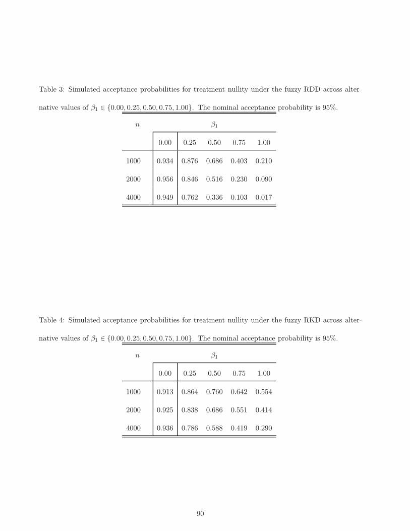
Table 3: Simulated acceptance probabilities for treatment nullity under the fuzzy RDD across alter-
native values of β1 ∈ 0.00, 0.25, 0.50, 0.75, 1.00. The nominal acceptance probability is 95%.
n β1
0.00 0.25 0.50 0.75 1.00
1000 0.934 0.876 0.686 0.403 0.210
2000 0.956 0.846 0.516 0.230 0.090
4000 0.949 0.762 0.336 0.103 0.017
Table 4: Simulated acceptance probabilities for treatment nullity under the fuzzy RKD across alter-
native values of β1 ∈ 0.00, 0.25, 0.50, 0.75, 1.00. The nominal acceptance probability is 95%.
n β1
0.00 0.25 0.50 0.75 1.00
1000 0.913 0.864 0.760 0.642 0.554
2000 0.925 0.838 0.686 0.551 0.414
4000 0.936 0.786 0.588 0.419 0.290
90

Table 5: Simulated acceptance probabilities for (A) joint treatment nullity and (B) treatment
homogeneity under the fuzzy RDD with group covariate across alternative values of β1 ∈
0.00, 0.25, 0.50, 0.75, 1.00 while fixing β2 = 0. The nominal acceptance probability is 95%.
(A) Joint Treatment Nullity (B) Treatment Homogeneity
n β1 n β1
0.00 0.25 0.50 0.75 1.00 0.00 0.25 0.50 0.75 1.00
1000 0.980 0.971 0.957 0.940 0.885 1000 0.972 0.966 0.964 0.944 0.919
2000 0.977 0.959 0.942 0.881 0.803 2000 0.971 0.964 0.951 0.913 0.867
4000 0.972 0.959 0.902 0.786 0.601 4000 0.971 0.965 0.925 0.855 0.762
91

Table 6: Simulated acceptance probabilities for (A) uniform treatment nullity and (B) treatment
homogeneity under the sharp quantile RDD. The top panel (I) presents results across alternative values
of β1 ∈ 0.00, 0.25, 0.50, 0.75, 1.00 while fixing γ1 = 0. The bottom panel (II) presents results across
alternative values of γ1 ∈ 0.00, 0.25, 0.50, 0.75, 1.00 while fixing β1 = 0. The nominal acceptance
probability is 95%.
(I) (A) Joint Treatment Nullity (I) (B) Treatment Homogeneity
n β1 n β1
0.00 0.25 0.50 0.75 1.00 0.00 0.25 0.50 0.75 1.00
1000 0.966 0.917 0.798 0.620 0.484 1000 0.967 0.967 0.965 0.954 0.963
2000 0.959 0.859 0.633 0.414 0.269 2000 0.959 0.959 0.966 0.955 0.958
4000 0.950 0.740 0.400 0.161 0.074 4000 0.950 0.946 0.958 0.948 0.947
(II) (A) Joint Treatment Nullity (II) (B) Treatment Homogeneity
n γ1 n γ1
0.00 0.25 0.50 0.75 1.00 0.00 0.25 0.50 0.75 1.00
1000 0.966 0.928 0.842 0.742 0.647 1000 0.967 0.920 0.808 0.698 0.574
2000 0.959 0.866 0.669 0.500 0.378 2000 0.959 0.855 0.625 0.446 0.327
4000 0.950 0.718 0.362 0.206 0.138 4000 0.950 0.693 0.327 0.170 0.116
92

Table 7: Simulated acceptance probabilities for (A) uniform treatment nullity and (B) treatment
homogeneity under the sharp quantile RKD. The top panel (I) presents results across alternative values
of β1 ∈ 0.00, 0.25, 0.50, 0.75, 1.00 while fixing γ1 = 0. The bottom panel (II) presents results across
alternative values of γ1 ∈ 0.00, 0.25, 0.50, 0.75, 1.00 while fixing β1 = 0. The nominal acceptance
probability is 95%.
(I) (A) Joint Treatment Nullity (I) (B) Treatment Homogeneity
n β1 n β1
0.00 0.25 0.50 0.75 1.00 0.00 0.25 0.50 0.75 1.00
1000 0.930 0.928 0.906 0.881 0.851 1000 0.927 0.936 0.945 0.936 0.940
2000 0.941 0.917 0.883 0.850 0.837 2000 0.932 0.930 0.929 0.929 0.928
4000 0.941 0.902 0.850 0.835 0.829 4000 0.929 0.930 0.918 0.936 0.924
(II) (A) Joint Treatment Nullity (II) (B) Treatment Homogeneity
n γ1 n γ1
0.00 0.25 0.50 0.75 1.00 0.00 0.25 0.50 0.75 1.00
1000 0.930 0.954 0.955 0.943 0.936 1000 0.927 0.938 0.939 0.921 0.911
2000 0.941 0.931 0.936 0.926 0.902 2000 0.932 0.932 0.923 0.901 0.875
4000 0.941 0.931 0.928 0.905 0.879 4000 0.929 0.920 0.885 0.861 0.816
93
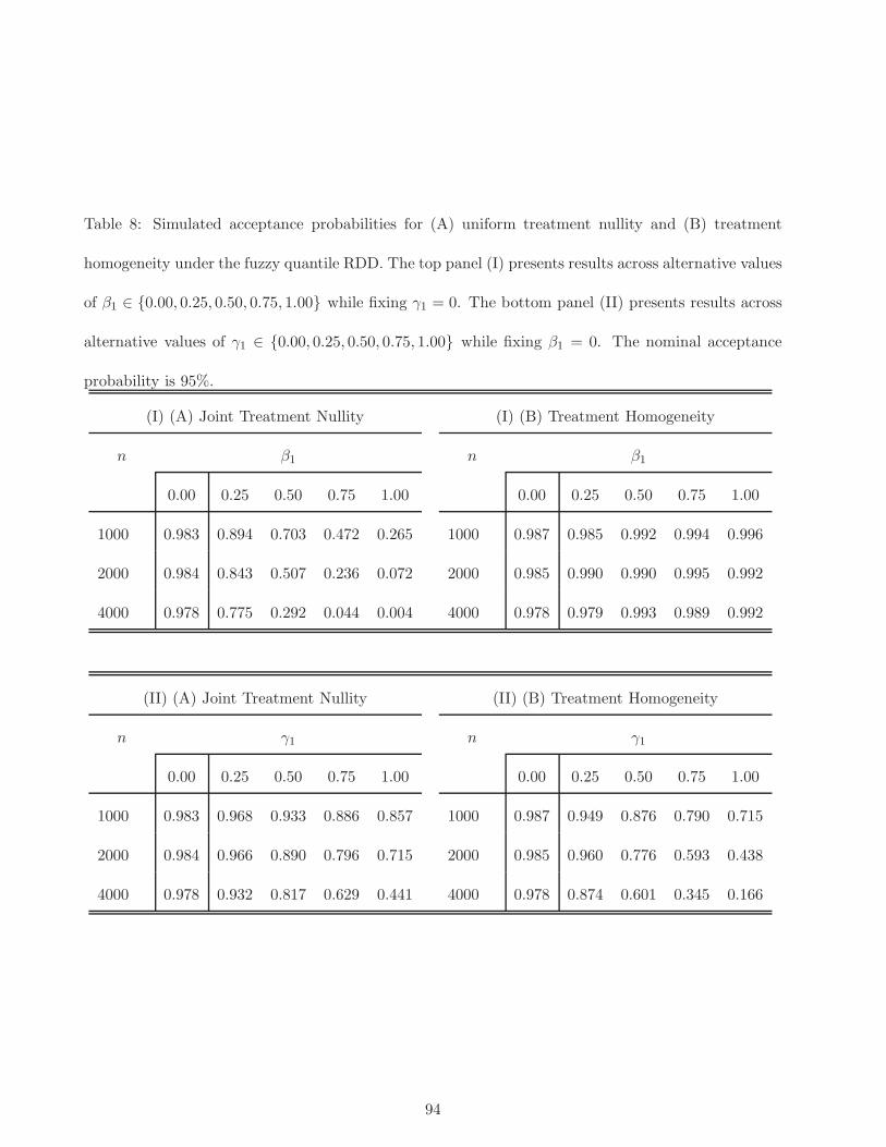
Table 8: Simulated acceptance probabilities for (A) uniform treatment nullity and (B) treatment
homogeneity under the fuzzy quantile RDD. The top panel (I) presents results across alternative values
of β1 ∈ 0.00, 0.25, 0.50, 0.75, 1.00 while fixing γ1 = 0. The bottom panel (II) presents results across
alternative values of γ1 ∈ 0.00, 0.25, 0.50, 0.75, 1.00 while fixing β1 = 0. The nominal acceptance
probability is 95%.
(I) (A) Joint Treatment Nullity (I) (B) Treatment Homogeneity
n β1 n β1
0.00 0.25 0.50 0.75 1.00 0.00 0.25 0.50 0.75 1.00
1000 0.983 0.894 0.703 0.472 0.265 1000 0.987 0.985 0.992 0.994 0.996
2000 0.984 0.843 0.507 0.236 0.072 2000 0.985 0.990 0.990 0.995 0.992
4000 0.978 0.775 0.292 0.044 0.004 4000 0.978 0.979 0.993 0.989 0.992
(II) (A) Joint Treatment Nullity (II) (B) Treatment Homogeneity
n γ1 n γ1
0.00 0.25 0.50 0.75 1.00 0.00 0.25 0.50 0.75 1.00
1000 0.983 0.968 0.933 0.886 0.857 1000 0.987 0.949 0.876 0.790 0.715
2000 0.984 0.966 0.890 0.796 0.715 2000 0.985 0.960 0.776 0.593 0.438
4000 0.978 0.932 0.817 0.629 0.441 4000 0.978 0.874 0.601 0.345 0.166
94
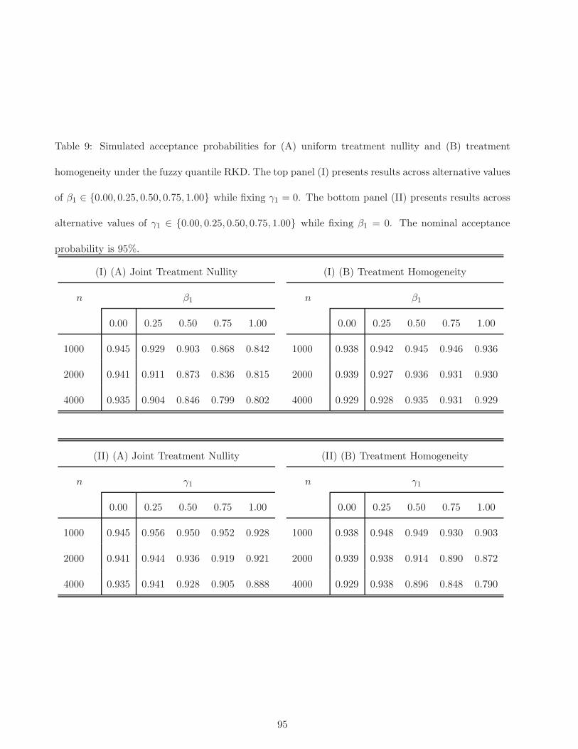
Table 9: Simulated acceptance probabilities for (A) uniform treatment nullity and (B) treatment
homogeneity under the fuzzy quantile RKD. The top panel (I) presents results across alternative values
of β1 ∈ 0.00, 0.25, 0.50, 0.75, 1.00 while fixing γ1 = 0. The bottom panel (II) presents results across
alternative values of γ1 ∈ 0.00, 0.25, 0.50, 0.75, 1.00 while fixing β1 = 0. The nominal acceptance
probability is 95%.
(I) (A) Joint Treatment Nullity (I) (B) Treatment Homogeneity
n β1 n β1
0.00 0.25 0.50 0.75 1.00 0.00 0.25 0.50 0.75 1.00
1000 0.945 0.929 0.903 0.868 0.842 1000 0.938 0.942 0.945 0.946 0.936
2000 0.941 0.911 0.873 0.836 0.815 2000 0.939 0.927 0.936 0.931 0.930
4000 0.935 0.904 0.846 0.799 0.802 4000 0.929 0.928 0.935 0.931 0.929
(II) (A) Joint Treatment Nullity (II) (B) Treatment Homogeneity
n γ1 n γ1
0.00 0.25 0.50 0.75 1.00 0.00 0.25 0.50 0.75 1.00
1000 0.945 0.956 0.950 0.952 0.928 1000 0.938 0.948 0.949 0.930 0.903
2000 0.941 0.944 0.936 0.919 0.921 2000 0.939 0.938 0.914 0.890 0.872
4000 0.935 0.941 0.928 0.905 0.888 4000 0.929 0.938 0.896 0.848 0.790
95