a two-dinsionsional finite-volume hydrodynamic · pdf filea two-dimensional finite-volume...
TRANSCRIPT

A TWO-DIMENSIONAL FINITE-VOLUME HYDRODYNAMIC MODEL
FOR COASTAL WETLANDS
Final Report
December 2003
JHR 03-294 Project 93-4
by
J. D. Lin, Kejian Qiu and Wengen Liao Department of Civil and Environmental Engineering
and
Michael W. Lefor
Department of Geography
The University of Connecticut Storrs, Connecticut
This research was sponsored by the Joint Highway Research Advisory Council (JHRAC) of the University of Connecticut and the Connecticut Department of Transportation and was carried out through the Connecticut Transportation Institute of the University of Connecticut. The contents of this report reflect the views of the authors who are responsible for the facts and accuracy of the data presented herein. The contents do not necessarily reflect the official views or policies of the University of Connecticut or the Connecticut Department of Transportation. This report does not constitute a standard, specification, or regulation.
i
Technical Report Documentation Page1. Report No. 2. Government Accession No. 3. Recipient’s Catalog No.
JHR 03-294 N/A N/A 4. Title and Subtitle
5. Report Date
December 2003
6. Performing Organization Code
A Two-Dimensional Finite-Volume Hydrodynamic Model for Coastal Wetlands
N/A
7. Author(s)
8. Performing Organization Report No.
J.D. Lin, Kejian Qiu, Wengen Liao, Michael W. Lefor JHR 03-294 9. Performing Organization Name and Address 10. Work Unit No. (TRAIS)
N/A 11. Contract or Grant No.
University of Connecticut Connecticut Transportation Institute Storrs, CT 06269-5202 N/A 12. Sponsoring Agency Name and Address 13. Type of Report and Period Covered
FINAL
14. Sponsoring Agency Code
Connecticut Department of Transportation 280 West Street Rocky Hill, CT 06067-0207
N/A
15. Supplementary Notes
N/A
16. Abstract This project was initiated in 1993 for the purpose of developing hydrodynamic models of tidal flow in coastal river-marsh systems. These models can be used as an analytical framework to address the need for environmental assessment for permit applications as well as for use in the design and maintenance of highway structures for the Connecticut Department of Transportation. In the initial phase of the project, a pseudo-2D hydrodynamic model was developed. The field data collected at the Oyster River marsh site was used for the model calibration and validation. It was followed up by the development of a two-dimensional finite-volume hydrodynamic model and by an extensive field work conducted at the Menunketesuck River marsh in Westbrook, Connecticut and a wind tunnel study of the characteristics of friction drag of marsh vegetation in the laboratory. The finite-volume approach used in this model can handle the complex topographic features of coastal marshes and various discontinuity of flow caused by hydraulic structures. The model was calibrated and validated by using the observed data from the Menunketesuck River site. The model was later applied to study the tidal flushing of the Farm River marsh in East Haven, Connecticut. These models will provide an analytical tool for the highway engineer to assess the impacts of highway structures on tidal flushing.
17. Key Words 18. Distribution Statement
Hydrodynamics, Model, Tidal Flow, Marsh
No restrictions. This document is available to the public through the National Technical Information Service Springfield, Virginia 22161
19. Security Classif. (of this report) 20. Security Classif. (of this page) 21. No. of Pages 22. Price
Unclassified Unclassified 83 N/A
Form DOT F 1700.7 (8-72) Reproduction of completed page authorized
ii

Acknowledgments
This work is sponsored by the Connecticut Department of Transportation under project JHRAC 93-4, “Hydrodynamic and Transport Models of Coastal Water for Use in Design and Management of Highway Structures.” Field survey was conducted and maps were made by Roger Ferguson and Phil Caron. We thank Bruce Davies, U.S. Geological Survey, Connecticut Field Office for use of the stream gauging equipment. The cooperation of W.J. Kolodnicki, Refuge Manager, at Stewart B. McKinney National Wildlife Refuge and Fish Service, Department of Interior in our field work at the Menunketesuck salt marsh is gratefully acknowledged. The topographic survey of the Farm River marsh in East Haven, Connecticut was conducted by Milone & MacBroom, Engineers, Cheshire, Connecticut.
iii
iv

Table of Contents
Title Page ................................................................................................................................... i Technical Report Documentation Page ..................................................................................... ii Acknowledgments...................................................................................................................... iii Modern Metric Conversion Factors........................................................................................... iv Table of Contents.......................................................................................................................v List of Figures ............................................................................................................................vii List of Tables .............................................................................................................................x 1. INTRODUCTION .................................................................................................................1 2. 2-D FINITE-VOLUME HYDRODYNAMIC MODEL FOR COASTAL WETLANDS.....2 2.1 Background.....................................................................................................................2 2.2 Formulation and Numerical Method...............................................................................2
2.3 Wetting and Drying in Control Volumes........................................................................8
2.4 Computer Program..........................................................................................................9 2.5 Model Setup and Operation ............................................................................................9 3. FIELD WORK .......................................................................................................................11 3.1 Description of the Research Site.....................................................................................11 3.2 Geology...........................................................................................................................11 3.3 General Features .............................................................................................................12 3.4 Vegetation.......................................................................................................................13 3.5 Establishment of Survey Control and Elevations...........................................................13 3.6 The 2-D Grid System and Locations of Staffs ...............................................................17 3.7 Field Measurements ........................................................................................................18
v

4. MODEL CALIBRATION AND SIMULATION .................................................................19 4.1 Calibration of Manning’s Roughness Coefficient .........................................................20 4.2 Comparisons of Simulation Results with Measured Data ..............................................25
4.3 Tidal Velocity Field of Simulation Results on 3/18/99..................................................50 4.4 Discussion of Results .....................................................................................................60 5. APPLICATION OF THE MODEL TO THE FARM RIVER MARSH, EAST HAVEN, CONNECTICUT ...................................................................................................................61 5.1 Description of the Site ....................................................................................................61 5.2 Field Work......................................................................................................................64 5.3 Model Simulation ...........................................................................................................65 5.4 Simulation Results and Comparison with Observations ................................................67 6. SUMMARY AND CONCLUSIONS....................................................................................71 REFERENCES ..........................................................................................................................72
vi
List of Figures 2.1 A Control Volume in FVM................................................................................................3 2.2 Integration Path in OS Scheme..........................................................................................7 3.1 Location of the Menunketesuck Site in Connecticut .........................................................15 3.2 Aerial View of the Site ......................................................................................................16 3.3 Sketch of the Site ...............................................................................................................16 3.4 2-D Grid System and the Staff Locations ..........................................................................17 4.1 Influence of Channel n on Water Elevation at Staff #8 in Run #9 ....................................21 4.2 Influence of Channel n on Water Elevation at Staff #15 in Run #9 (Ditch n=0.05) .........22 4.3 Influence of Marsh n on Water Elevation at Staff #8 in Run #9 (Channel n=0.025) ........23 4.4 Influence of Marsh n on Water Elevation at Staff #15 in Run #9 (Ditch n=0.05) ............24 4.5 Influence of Ditch n on Water Elevation at Staff #15 in Run #9.......................................25 4.6 Comparison of Water Elevations at Staff #14, Run #1 (07/04/1996)................................26 4.7 Comparison of Water Elevations at Staff #15, Run #1 (07/04/1996)................................27 4.8 Comparison of Water Elevations at Staff #14, Run #2 (07/05/1996)................................28 4.9 Comparison of Water Elevations at Staff #10, Run #2 (07/05/1996)................................29 4.10 Comparison of Water Elevations at Staff #14, Run #3 (08/04/1996)................................30 4.11 Comparison of Water Elevations at Staff #15, Run #3 (08/04/1996)................................31 4.12 Comparison of Water Elevations at Staff #10, Run #3 (08/04/1996)................................32 4.13 Comparison of Water Elevations at Staff #14, Run #4 (10/26/1996)................................33 4.14 Comparison of Water Elevations at Staff #15, Run #4 (10/26/1996)................................34 4.15 Comparison of Water Elevations at Staff #10, Run #4 (10/26/1996)................................35 4.16 Comparison of Water Elevations at Staff #14, Run #5 (10/27/1996)................................36
vii

4.17 Comparison of Water Elevations at Staff #15, Run #5 (10/27/1996)................................37 4.18 Comparison of Water Elevations at Staff #10, Run #5 (10/27/1996)................................38 4.19 Comparison of Water Elevations at Staff #14, Run #6 (12/13/1997)................................39 4.20 Comparison of Water Elevations at Staff #8, Run #7 (06/04/1998)..................................40 4.21 Comparison of Water Elevations at Staff #15, Run #7 (06/04/1998)................................41 4.22 Comparison of Water Elevations at Staff #10, Run #7 (06/04/1998)................................42 4.23 Comparison of Water Elevations at Staff #8, Run #8 (03/18/1999)..................................43 4.24 Comparison of Water Elevations at Staff #15, Run #8 (03/18/1999)................................44 4.25 Comparison of Water Elevations at Staff #10, Run #8 (03/18/1999)................................45 4.26 Comparison of Water Elevations at Staff #8, Run #9 (04/15/1999)..................................46 4.27 Comparison of Flow Velocities at Staff #8, Run #9 (04/15/1999) ....................................47 4.28 Comparison of Water Elevations at Staff #15, Run #9 (04/15/1999)................................48 4.29 Comparison of Flow Velocities at Staff #15, Run #9 (04/15/1999) ..................................49 4.30 Simulated Flow Field on March 18, 1999 at 9 am.............................................................51 4.31 Simulated Flow Field on March 18, 1999 at 10 am...........................................................52 4.32 Simulated Flow Field on March 18, 1999 at 11 am...........................................................53 4.33 Simulated Flow Field on March 18, 1999 at 12 pm ..........................................................54 4.34 Simulated Flow Field on March 18, 1999 at 1 pm ............................................................55 4.35 Simulated Flow Field on March 18, 1999 at 2 pm ............................................................56 4.36 Simulated Flow Field on March 18, 1999 at 3 pm ............................................................57 4.37 Simulated Flow Field on March 18, 1999 at 4 pm ............................................................58 4.38 Simulated Flow Field on March 18, 1999 at 4:35 pm .......................................................59 5.1 Location of the Farm River Marsh, East Haven, Connecticut...........................................62
viii

5.2 2-D Grid System and the Staff Locations ..........................................................................63 5.3 Staff Readings at Staff #16 on July 11, 1999.....................................................................66 5.4 Staff Readings at Staff #5 on July 11, 1999.......................................................................67 5.5 Comparison of Simulation Results of the Observations at Staff #7 ..................................68 5.6 Comparison of Simulation Results of the Observations at Staff #1 ..................................69 5.7 Comparison of Simulation Results of the Observations at Staff #2 ..................................70
ix

List of Tables
2.1. Expressions of Oscher's Numerical Fluxes..........................................................................8
3.1 Summary of Field Measurements ........................................................................................18
4.1 Summary of Field Surveys and Calculations.......................................................................19 5.1 Time Lags and Tidal Amplitudes on August 19, 1997........................................................64 5.2 High Tide Time Lags on July 11, 1999 ...............................................................................65
x
1. INTRODUCTION
Coastal salt marshes have a broad global distribution (Chapman, 1974), forming a rich biological ecosystem because of their interaction with flow of nutrients between the terrestrial and marine environment. Water a the primary conveyor of nutrient and salt, and a thorough knowledge of marsh hydrology is vital to understanding the transport mechanism involved and the environmental characteristics in the coastal marsh (Price and Woo, 1988). The Connecticut shore of Long Island Sound is one of the most developed coastal zones in the United States. Our coastal waters, including estuaries, harbors, coves and tidal wetlands, are used for transportation, fisheries, and as receiving waters for domestic and industrial effluents. Long Island Sound’s water quality (badly impacted by excess nutrients) and the long-term ecology of its coastal wetlands have become sensitive environmental concerns, along with the ever-increasing social and environmental pressures from increasing population. On the other hand, there has been a continuing demand for maintenance, reconstruction, and new construction of highway facilities. The highway engineers not only has to deal with conventional design concerns, but also has to face problems of the environmental impacts of highways on coastal wetlands, tidal channels, and estuaries, especially in the process of applying for permits from state and federal environmental regulatory agencies.
Many projects along the Connecticut coast involve tidal marsh. Environmentalists charge
that restricted tidal openings imposed by highway and rail right-of-way facilities negatively impact flora fauna because they alter tidal regimes. Today, secondary roads, State routes, U.S. Route 1, Interstate 95, and the ConnRail (AmTrak) coastal rail corridor form a series of braided obstructions perpendicular to the Connecticut’s natural drainages into Long Island Sound. There is a large number of river, stream, and wetland crossings that significantly restrict the full exchange of tidal waters in coastal salt marshes, further complicated by changes in the hydrographs of these streams and rivers due to filling, dredging, and diking of marshes. Salts and estuarine marshes are a vital part of the ecology of Long Island Sound and its water quality; their annual cycle of growth and decay rests on the type of vegetation they support and is principally linked to the elevation and frequency of flooding by tidal waters (Lefor et al., 1997; Miller and Egler, 1950). The slightest change in ambient surface elevation of tidal regime or marsh surface itself alters the vegetation and therefore the productivity of the system. The tidal salt waters of Long Island Sound are the principal and essential environmental factor in the existence of valuable salt marsh ecosystems in Connecticut.
In 1993, the Joint Highway Research Advisory Council (JHRAC) of the University of
Connecticut awarded us a research grant to develop hydrodynamic medals of tidal flows as an analytical frame work to address the need for environmental assessment for permit applications as well as for use in the design and maintenance of highway structures. In the first phase of the development a pseudo-2D hydrodynamic model was developed (Lin, et al., 1997; Lin et al., 1998). This final report is focused primarily on the presentation of the two-dimensional, finite-volume hydrodynamic model developed in the second phase of the project. Two companion documentations for the two-dimensional hydrodynamic model, User’s Manual (Lin et al., 2002) and Tutorial (Lin et al., 2002), have been published. These documents will facilitate users to understanding and executing the model.
1
2. 2-D FINITE-VOLUME HYDRODYNAMIC MODEL FOR COASTAL WETLANDS
2.1 Background
The numerical model for river-basin simulation should possess the following features:
Ability to handle complex topography;
Simulation of sub-critical or supercritical flow;
Simulation of steady or unsteady flow;
Simulation of smooth flow or discontinuous flow as in dam break or hydraulic jump;
Ability to handle wetting or drying of floodplain;
Simulation of flows through structures such as weirs, gates, culverts and bridges;
Ability to handle tributary and slough inflows.
The finite difference method does not have the ability to handle complex topography, and when dealing with wetting or drying of flood plain it is very slow. This might because that the differential form of shallow-water equations is not valid at discontinuities where the solution is not differentiable.
The integral form of the shallow-water equations is valid both at discontinuities and in
the smooth part of the flow field. Thus, it will be better to base the discretization on the integral form of the shallow-water equation.
In Finite Volume Method (FVM), the discretization scheme is constructed on the basis of
conservation laws in integral form, as is different from the FDM. The formulas for the transported physical variables can be established naturally, so that conservation can be followed satisfactorily.
2.2 Formulation and Numerical Method
First of all, the Finite Volume Method is formulated for the equation, integrating over the time-space sub-domain yields,
2

According to the mean-value theorem, select a mean value of over the interval , we have
With the notion , express its time integral over the interval by a time-weighted average
we have
The FVM scheme is explicit when θ = 0, whereas it is implicit when 0 < θ < 1, and fully implicit when θ = 1.
The advantages of the FVM can be seen more clearly, when a non-rectangular mesh is adopted in the multi-dimensional case.
Figure 2.1 A Control Volume in FVM A planar computational domain with a complicated geometric shape is partitioned into arbitrary quadrilaterals (Figure 2.1), called finite volumes. The vertices of the quadrilaterals may be either distributed irregularly (unstructured mesh), or taken as the nodes of a curvilinear mesh (structured mesh). However, only the coordinates of the vertices and centroids of the quadrilaterals enter into computation, so it is unnecessary to write the differential equations in the curvilinear coordinate form.
Suppose the given differential conservation law is expressed as then for each finite volume we have the integral conservation law
3
where Σe, Γe are domain and boundary of finite volume respectively, and N is a unit outward vector normal to Γe. Take mean value of ω and F over Σe, denoted by ωe and Fe. Denote the area of Σe by Ae and the outward flux passing through side AB by EAB, a line integral along the path AB of a scalar product of the vector (G, H) and vector N. Thus, we have
(1.1)
which is an ODE in ωe. By approximating the fluxes EAB, etc., with an explicit difference scheme, and performing time-integration, the variation of ω with time can obtained. Here, EAB can be estimated by the formula (those for other fluxes are similar)
where GAB is the mean value of G over AB, and ∆xAB = xB - xA, ∆yAB = yB - yA.
If the nodes are determined by a curvilinear mesh, the finite volumes can be numbered as in the case of rectangular mesh, e.g., (i, j) denotes the volume on the ith roe and the jth column. Then a centered approximation
or a biased approximation (0 < α < 1) may be adopted
Eq.1 can be solved either by using an explicit or implicit scheme, or by a predictor-corrector two-step scheme, depending on the discretization of time-derivative.
The method has several advantages: (i) The underlying principle is simple and intuitive. (ii) It is possible to use a flexible mesh composed of arbitrary triangles or quadrilaterals, which suits problems with a complicated geometric shape. (iii) As integral conservation law is used, the solution may be either a smooth or a discontinuous flow. Therefore, in the recent thirty years, the finite volume method is always one of the effective methods.
Osher-Solomon Scheme and Its Application to the Solution of 2-D Shallow Water Equations
The conservation form of the 2D shallow-water equations are given by
4
where, q = [h, hu, hv]T = conserved physical vector, quantity, F(q) = [hu, hu2+gh2/2, huv]T = flux vector in the x direction; and G(q) = [hv, huv, hv2+gh2/2]T = flux vector in the y direction. The quantity h = water depth; u and v = depth-averaged velocity components in the x and y directions, respectively; and g = gravitational acceleration. The source/sink term B(q) is
where, s0x s0y and sfx sfy are bed slope and friction slope in x and y direction, respectively. The friction slope is estimated by Manning's equation. Other external forces, such as wind or eddy viscosity, can be accounted for in the source/sink term also.
Under a rotational transformation of the coordinate system, for all ϕ = angle between vector and x axis (counterclockwise from x axis), we have where,
Then the integral form of the system can be written as
where a control volume ω is taken from the computational domain Ω, and ϕ is the directional angle of a normal to the boundary ∂ω. Obviously, the integrate of the second term has the meaning of normal flux vector, so the 2-D problem can be locally treated as a 1-D problem.
Select a structured curvilinear mesh, with quadrilaterals (Figure 1) as its cells, each of
which has four adjacent neighbors. Denote by ϕi+1/2, j the directional angle of the outward normal to the interface ∂ωi+1/2, j between the control volumes ωij and ωi+1, j. Then, the second term in the last equation can be expanded into
with the notation Ti+1/2, j = T (ϕi+1/2, j). The first integral on the right-hand side can be approximated by
5
li+1/2, j is the length of ∂ωi+1/2, j, while f(qL, qR) is the flux vector across that interface, which can be obtained by solving a 1-D Rieman problem in the normal direction.
1-D Riemann Problem
1-D Riemann problem is the solution of the hyperbolic system
where vectors qL and qR are fixed states vectors.
For the 2-D shallow water equations, we have
where , rk is the right eigenvector associated with the eigenvalue λk; ψk(i) is a Riemann
invariant associated with the eigenvalue λk. Riemann invariant will keep constant if the hyperbolic system is homogeneous and A is function of q only.
When q can be expressed as a function of one scalar parameter ξ, q = q(ξ), we call the solution of the hyperbolic system a simple wave. In this case, qt must be a product of qx and a scalar, and both derivatives are eigenvector of A. An integral curve in q-space defined by
is called the wave path. Each point on the path corresponds to a state q(ξ), a right eigenvector rk (ξ) and a eigenvalue λk(ξ), one each. Meanwhile, we draw a straight line dx/dt = λk(ξ) in the t-x plane, on which q is constant, qt + λk qx = 0. Then it is seen that a wave path must intersect a
6
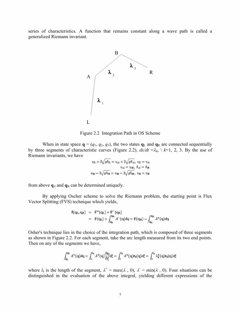
series of characteristics. A function that remains constant along a wave path is called a generalized Riemann invariant.
Figure 2.2 Integration Path in OS Scheme
When in state space q = (q1, q2, q3), the two states qL and qR are connected sequentially by three segments of characteristic curves (Figure 2.2), dx/dt =λk, \ k=1, 2, 3. By the use of Riemann invariants, we have
from above qA and qB can be determined uniquely.
By applying Oscher scheme to solve the Riemann problem, the starting point is Flux Vector Splitting (FVS) technique which yields,
Osher's technique lies in the choice of the integration path, which is composed of three segments as shown in Figure 2.2. For each segment, take the arc length measured from its two end points. Then on any of the segments we have,
where lk is the length of the segment, λ+ = max(λ , 0), λ- = min(λ , 0). Four situations can be distinguished in the evaluation of the above integral, yielding different expressions of the
7

numerical flux,
where qS is determined by the condition λ(qS) = 0. When k = 2, as ψ21 = u = λ2 = const, λ does
not change sign on arc AB; when k = 1 or 3, λ changes sign at most once. Based on the above equation, the expressions of the numerical flux f(qL, qR) can be distinguished in sixteen cases, depending on the flow regime. (Table 2.1)
Table 2.1 Expressions of Oscher's Numerical Fluxes
The space of independent variables (t, x, y) is called definition space. The x-y plane is called the physical plane. The space of dependent variables (u, v, h) or (q1,, q2, q3) is called the state space. There are three kinds of boundary condition on the boundary of a computational domain associated with the shallow water problems. The first kind is a prescribed time series of water surface elevation or depth, h, at the boundary, such as the variation of the diurnal tide at the mouth of an estuary or river. The second kind is a prescribed time series of flow velocity (u ,v) at a point or discharge, q, across a section of the boundary at the edge of a marsh, the upstream of a river or the entrance of a tributary. The third kind is a combination of above two in terms of a functional relationship of (u, v, h) or (q, h), for example, at the boundary between a channel and its bank when the level of water in the channel becomes lower than that over marsh surface during the period of ebb tide. The free-fall condition may be described by a formula derived for the critical flow condition from the open-channel flow theory. One will find that all three kinds of boundary condition exist in tidal regimes in a river-marsh system.
2.3 Wetting and Drying in Control Volumes
The drying and wetting cycles of a portion of the river basin are calculated according to the hydraulic condition of the control volume under consideration and its adjacent control
8

volumes. In the drying cycle, the wet control volume undergoes the conditions from being wet to partially dry due to decrease in water depth through water discharge into adjacent control volumes and could finally become an entirely dry control volume when the water depth decreases further below a certain threshold depth. In the wetting cycle, an entirely dry control volume becomes a partially dry control volume because of increase of water depth through mass flux from adjacent control volumes and becomes a wet control volume if its water depth exceeds a certain threshold depth.
Internally in the model, when a control volume is entirely dry, then the control volume is
not considered in the computation for that time step. When the control volume is partially dry, the computations at that control volume are based only on a mass balance equation. Therefore, momentum exchange in and out of the control volume is neglected.
When the water depth in a control volume is less than a pre-determined first-level water
depth, i.e. the dry depth, the control volume is considered dry. When the water depth in a control volume is greater than the dry depth but less than a pre-determined second-level water depth, i.e. the wet depth, then the control volume is considered partially dry. The momentum flux is assumed negligible so that only the mass balance equation is evaluated. In that case, the mass flux, that is, the amount flowing through the side of a control volume f(qI, qO) is estimated according to the boundary condition specified for that side, where qI is inside the computation domain and qO is outside the computation domain. The possibilities are as follows:
For the first kind boundary condition, the water stage is given at the boundary, qO is
estimated using the given water stage and the flow velocities of qI.
For second kind boundary condition, the flow velocities is given at the boundary, qO is
estimated using the given flow velocities and the water stage of qI. If the cell on the other side is dry, then f(qI, qO) = 0.
If the bottom elevations between two adjacent control volumes are significantly different, then f(qI, qO) across one cell of higher elevation to the cell with lower elevation is calculated as a critical flow.
2.4 Computer Program
The core of this 2-D Finite Volume Hydrodynamic Model (FVHM) was first written in FORTRAN. Then the graphical interface was first written in Borland C++ and then ported to Microsoft Visual C++.
2.5. Model Setup and Operation Model setup and operation are described in detail the User’s Manual (Lin, et al. 2002a) and the Tutorial (Lin, et al., 2002b). After a study site has been chosen, a modeling or computational domain should be delineated in the area. All topographical features in the interior and on the boundary of the computational domain must be identified, such as natural and man-
9

made channels, lakes or reservoirs, man-made structures, etc. The model requires a set of topographical data as input. The accuracy of model results depends critically on the quality and density of these data. In additional, the operation of the model needs a time series of hydraulic data on certain parts of the boundary, such as water surface elevation, flow rate or a relation between the water level and flow rate. Installation
FVHM model installation package contains one zip file. In the zip file, there are 7 files in the main directory, estu.exe, model.dll, dialogs.dll, oscher.dll, utility.dll, estu.cnt, and estu.hlp. There are a User’s menu documentation in the Documents subdirectory and 7 Tutorial files under the Tutorials directory. Unzip the files into a directory and keep the subdirectory hierarchy. Please refer to the User’s Menu (Lin et al., 2002) for more details. Running the model
Double click estu.exe would start the model. From there you can either Open a project file that already exists or start a new one. Grid Generation
When start a new grid, the first thing need to do is to use Project Options dialog and
specify the configuration data for the site. Then you will be able to start setting up grids. The graphical user interface of FVHM model makes it easy for grid generation. Using the
mouse, right click inside the workspace to bring up the context menu and select ‘New Cell” menu item. Then continue left click inside the workspace to form a closed cell shape. Then you can adjust cell corner positions to the exact location using the “Edit Grid…” menu selection. If the grid being generated contains same size and shaped cells, you can do a select of one or more cells then copy and paste to a new location to speed up the process. Input Data
After grid set up, one can specify initial condition and boundary conditions. To specify
initial condition, one can right click inside a cell and select “Edit Grid…” menu item and specify the initial condition for that one cell. Or one can right click and select “Select” menu item, then left click the center of the cells that you want to specify the same initial condition. After select all the cell you want, right click and select “Edit Grid…” menu item, then specify the initial condition for all the cells you selected in the dialog that comes up.
To specify boundary condition, you will have to use boundary condition data input file.
Please refer to User’s Menu (Lin et al., 2002) and Tutorial (Lin et al., 2002) for the detailed information on the format and naming convention of the boundary condition data input file as well as how to input the boundary conditions into the grids.
10

Calculation Procedure
After setting up the grid with initial and boundary conditions, it is the time to run the model simulation.
Use Run Project menu item to start the execution. The Modeling Options dialog that
comes up allows you to set the start and ending date and time as well as couple of other important parameters. Click ‘Ok’ to close the Options dialog will start the simulation. You can view the results while the model is running or you can disable the real time refresh and view the result after finish.
Presentation of Results
If you choose to have result output into disk file, you can then replay the results in an animated fashion just like real time refresh but faster. The result can be viewed in different ways, such as water surface elevation, water depth, depth averaged velocity vector field, and Froude Number distribution. Results can also be output to disk files for further processing.
Please refer User’s Manual (Lin et al., 2002) and Tutorial (Lin et al., 2002) for all the
details on the model operations. 3. FIELD WORK 3.1 Description of the Research Site
The Menunketesuck River marshes in the study area are located in the Town of Westbrook, Connecticut, north of U. S. Route 1 and south of the ConnRail railroad tracks (Figs. 3.1 and 3.3). They appear on the southwestern quadrant of the U. S. G. S. 7.5 minute topographic mapping, Essex quadrangle (USGS, 1995). Based on its geology, soils, climate, and vegetation, the study site lies within Eco-region V-B, the Eastern Coastal Eco-region. The marshes of the study site are part of the Stewart B. McKinney National Wildlife Refuge System of coastal marshes and islands in Connecticut, and are vigorously kept free of human disturbance, except as noted. (See Acknowledgements). The specific research area lies adjacent to the west side of the Menunketesuck, and extends westward for a distance of approx. 1500 ft. It is fed with tidal waters from the Menunketesuck directly; via a tributary drainage channel leading westward from the River, and by an extensive system of mosquito ditches.
3.2 Geology
The area is underlain by bedrock of the Monson Gneiss formation, which generally
trends downward northwest to southeast at an inclination of 40-70° in the vicinity of the site. Surface elevations of exposed bedrock material range from zero to 100 ft. NGVD. Surface deposits in the marsh proper consist of peaty swamp deposits accreted over sorted and unsorted glacial tills from the Wisconsinian glaciation of 20,000 - 8,000 yrs B.P. These deposits are on the order of 0 - 15 ft. thick, and in the Menunketesuck marshes, have a general surface elevation of approximately 2. 5 ft. above MHT as measured on the site.
11

The Menunketesuck extends northward from its mouth at Long Island Sound for about
8.3mi., and drains portions of the towns of Westbrook, Clinton, and Old Saybrook. Development patterns are such that although drainages in coastal Connecticut run
generally north-south, roads and railroads run perpendicularly across drainages east-west. The topography along the coast consists of flat area of salt marsh , beaches, and glacial outwash deposits interspersed with bedrock headlands. Progressing northward, one finds a surface comprising north-south trending small eroded till-covered hills interspersed with glacial outwash drainages and small streams, with their associated floodplains, swamps, and marshes (Bell, 1985).
Land-use is mixed, ranging from the moderately-developed commercial sections of Rte. 1
to single--family residential suburban lands to rural-residential sections further inland, interspersed with 50 - 100 yrs. old secondary (or tertiary) mixed hardwood forest. Past land-use was largely agricultural inland, with a variety of small mills running from impoundments placed in sequence upstream on most of the local rivers. Marine-related industries populated the coastal towns (fishing, ship-building, etc.) until the centralization of activities engendered by the industrial revolution forced the closure of many of these small enterprises. Another factor in the tightly developed smaller coastal towns was the silting of the small estuaries, once adequate for the passage of marine commerce (Bell, 1985). Costs of dredging and spoil disposal soon placed the maintenance of these small harbors out of the range of small operators.
Another factor in the history and development of the coastal zone was the construction of
the coastal rail corridor in the 1850's. This massive linear east-west element of the landscape was constructed across regional drainages, and supplied with numerous small under-drains, impeding coastward flows and impounding (and in some cases, draining) local fresh and brackish marshes. Where the rail route crossed over tidal marsh deposits, the marsh peat was dug out and (or) filled with rock from upland cuts, thus intercepting and occasionally diverting subsurface flows in marshes (an item deserving much further investigation as it related to subsurface flows in salt marshes). Evidence of this activity can be seen in the shallow secondary road underpasses below the railroad tracks in many coastal towns. Some of these flood at highest high tides via their catch basins.
Although there have been recent increases in preserved lands (due partly to a healthy
economy), the area is fairly rapidly undergoing suburban “sprawl” with the concomitant increase in impervious surface. The resulting increases in amounts of fresh-water runoff and flashier hydrographs will continue to be seen in the vegetation of coastal marshes and estuaries. 3.3 General Features
Like many of Connecticut’s coastal marshes, those of the Menunketesuck system have
been mosquito-ditched and(or) provided with tide-gates. Ditching began in the late 1600's with European colonization when the marshes were used for salt hay production. Ditching was accomplished by hand or with horse-drawn plows, and continues to the present. Many marshes that had not been ditched by the end of the 19th century were first ditched under the WPA
12
programs of the Great Depression of the 1920's and later, and almost all of Connecticut’s marshes were ditched by the 1950's. In the 1980's the Connecticut Department of Health Services purchased an amphibious rotary ditching device, and cleaned and reconfigured the ditches in many of Connecticut’s marshes, a program that continues today under the Tidal Wetland Restoration Program of the Department of Environmental Protection - Office of Long Island Sound Programs. During re-ditching, the amphibious rotary ditcher cleaned out and re-dug existing ditches to a standard width of ca. 2 ft., and a depth of 4 - 6 ft. Excavated material is chopped up by the cutter head and cast over the surface of the marsh, to be carried away by the next high tide. Elsewhere some ditches were plugged at one end to adjust circulation patterns; plugged at both ends to retain high tide water and trap small fish that feed on mosquito larvae; or filled completely to the level of adjacent marsh. Figure 3 shows an aerial view of present ditch patterns and Figure 4 is a diagrammatic representation of marsh features.
3.4 Vegetation The existing vegetation of the Menunketesuck River marshes examined in this study is of
the so-called “High Marsh” type (Miller & Egler, 1950), interspersed with areas of “Low Marsh”, a cover-type which has been increasing in Connecticut in recent times, possibly in response to sea-level rise. The Menunketesuck marshes exhibit a typical morphology of levees along the Main Channel and the Main Tributary Channel (see Figs. 3.3 and 3.4), with interior portions of the marsh generally flat and somewhat lower. The levees are dominated by High Marsh Spartina patens - Distichlis spicata - Juncus gerardi (Salt meadow grass, Spike Grass, Black-grass), with interspersed individuals and(or) patches of Limonium carolinianum (Sea-lavender), Aster tenuifolius (Salt Marsh Aster) and Plantago spp. (Salt Marsh Plantains). Less disturbed areas of the marsh farther west of the Main Channel are delimited by mosquito-ditches, and are dominated by Spartina patens High Marsh or Spartina alterniflora - short form (Salt Marsh Cord Grass),with other salt marsh species interspersed. Here and there areas of greater apparent decomposition rates support Spartina alterniflora short form low marsh, and the tall form of S. alterniflora occupies its typical position lining channels and ditches. The channel-ward margin of the marsh system is eroding in typical fashion due to ice scour and wave action. At the westernmost extremity of the marsh and here and there along its borders, one finds the Common Reed, Phragmites australis, a typical salt marsh species. This plant can become rapidly invasive in areas of tidal restriction or increased fresh-water input in salt marshes, but here does not seem to have grown “out of bounds.” Patches of Reed are found here and there along the railroad embankment and along the southerly edge of the marsh adjacent to Oak-Hickory coastal woodland— second growth forest. A large portion of this area is currently under construction for single-family houses, but a buffer strip of forest remains. The marsh is home to a wide variety of birds (including an active Osprey platform), and an island of upland (see Figs 3.3 and 3.4) provides further habitat diversity. The usual suburban mammals or their signs were observed. 3.5 Establishment of Survey Control and Elevations
During 1997 - 1998 Extensive surveying was carried out on the Menunketesuck site by C. Roger Ferguson , P.E., L.S., of The University of Connecticut’s Department of Civil and Environmental Engineering, aided by project personnel. Surveying apparatus used was a Laser
13

Theodolite and appurtenances. Salt marshes are notoriously difficult to survey accurately due to the compressible substrate, and indeed it has not been since the development of laser-guided instruments of this sort that accurate elevations and distances have been gathered with regularity and with minimum damage to the marsh surface.
Three base stations were established and marked with galvanized iron pipe and were
referenced to a USGS - Connecticut State Highway Department (ConnDOT) NGVD benchmark located on the northeasterly base of the railing on the Rte. 1 bridge over the Menunketesuck. Note that this bridge is scheduled to be torn down and reconstructed: the benchmark will be moved and re-established.
Manor features of the marsh were surveyed for x, y, z including the locations of ditches
(ends and mouths), channel cross-sections, marsh cross-sections, marsh boundaries, channel boundaries, three marsh vegetation distribution quadrants, tide staffs, current measurement stations, island and upland boundaries, bridges, and certain other landmarks, e. g. rocks and utility poles that appear in aerial photographs used in the project. All survey data were entered into an AutoCAD data base for automated mapping and retrieval. Aerial photograph of the Connecticut over-flight (Lockwood, Kessler, & Bartlett, Syosset, L. I, 1995, 1:12,000 contact scale) was used in photo interpretation and field work.
14

SITE
Figure 3.1 Location of the Menunketesuck Site in Connecticut
15

Figure 3.2 Aerial View of the Site
E
F
Menunketesuck R.
Dredged basins
N
“Island”
Upland Edge andComputational Boundary
MainTributaryChannel
RailroadBridge
ConnRail Tracks
Mosquito Ditch (typ.)
Figure 3.3 Sketch of the Site
16

3.6 The 2-D Grid System and Locations of Staffs
Figure 3.4 2-D Grid System and the Staff Locations
17
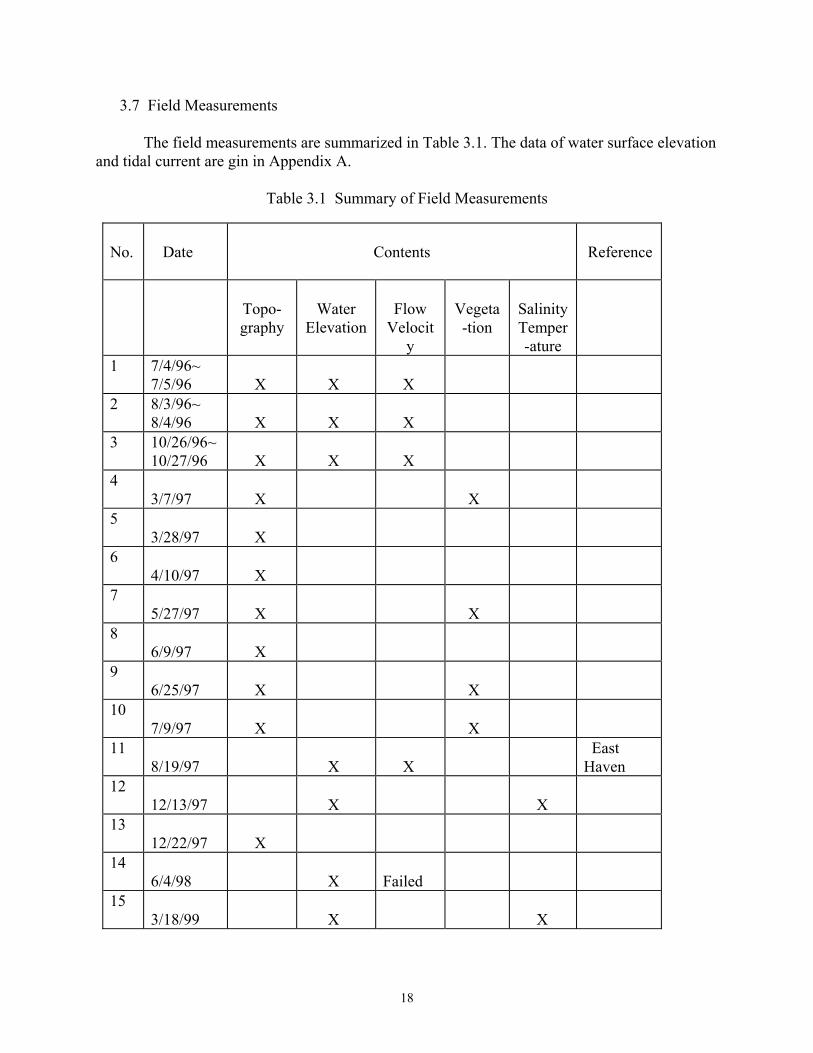
3.7 Field Measurements
The field measurements are summarized in Table 3.1. The data of water surface elevation and tidal current are gin in Appendix A.
Table 3.1 Summary of Field Measurements
No.
Date
Contents
Reference
Topo-graphy
Water
Elevation
Flow
Velocity
Vegeta-tion
Salinity Temper-ature
1 7/4/96~ 7/5/96
X
X
X
2 8/3/96~ 8/4/96
X
X
X
3 10/26/96~ 10/27/96
X
X
X
4 3/7/97
X
X
5 3/28/97
X
6 4/10/97
X
7 5/27/97
X
X
8 6/9/97
X
9 6/25/97
X
X
10 7/9/97
X
X
11 8/19/97
X
X
East Haven
12 12/13/97
X
X
13 12/22/97
X
14 6/4/98
X
Failed
15 3/18/99
X
X
18

16 4/15/99
X
X
X
X
X
17 7/11/99~ 7/12/99
X
East Haven
4. MODEL CALIBRATION AND SIMULATION
The diurnal tidal flow in the Menunketesuck River and its salt marshes at Westbrook, Connecticut, which are described in detail in the previous chapter, was used for calibration of this model and the simulation study. Since there are no interior structures, Manning’s roughness coefficient was the only calibration parameter. Table 4.1, Summary of Field Observation and Model Calculation, lists all field observations of tidal flow which were conducted at this site. Based on the length of observation and the integrity of survey data, the measurement results of Run no. 9 on April 15, 1999 in Table 4.1 were chosen as the basis for calibration. Other runs were used for model simulation.
Table 4.1 Summary of Field Surveys and Calculations
Run No. Date Refer to
Run # 1 07/04/1996 Figure 4.6 Comparison of Water Elevations at Staff #14, Run #1 (07/04/1996)
Figure 4.7 Comparison of Water Elevations at Staff #15, Run #1 (07/04/1996)
Run # 2 07/05/1996 Figure 4.8 Comparison of Water Elevations at Staff #14, Run #2 (07/05/1996)
Figure 4.9 Comparison of Water Elevations at Staff #10, Run #2 (07/05/1996)
Run # 3 08/04/1996 Figure 4.10 Comparison of Water Elevations at Staff #14, Run #3 (08/04/1996)
Figure 4.11 Comparison of Water Elevations at Staff #15, Run #3 (08/04/1996)
Figure 4.12 Comparison of Water Elevations at Staff #10, Run #3 (08/04/1996)
Run # 4 10/26/1996 Figure 4.13 Comparison of Water Elevations at Staff #14, Run #4 (10/26/1996)
Figure 4.14 Comparison of Water Elevations at Staff #15, Run #4 (10/26/1996)
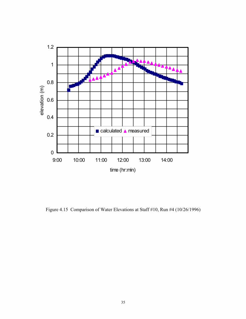
Figure 4.15 Comparison of Water Elevations at Staff #10, Run #4 (10/26/1996)
Run # 5 10/27/1996 Figure 4.16 Comparison of Water Elevations at Staff #14, Run #5 (10/27/1996)
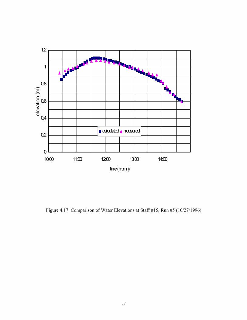
Figure 4.17 Comparison of Water Elevations at Staff #15, Run #5 (10/27/1996)
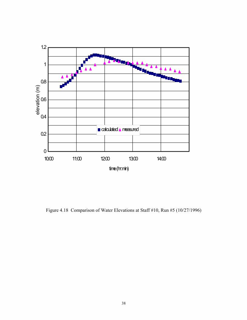
Figure 4.18 Comparison of Water Elevations at Staff #10, Run #5 (10/27/1996)
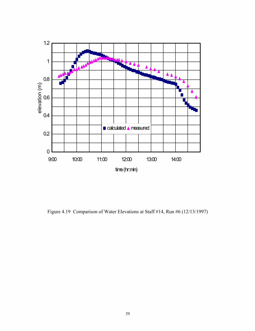
Run # 6 12/13/1997 Figure 4.19 Comparison of Water Elevations at Staff #14, Run #6 (12/13/1997)
Run # 7 06/04/1998 Figure 4.20 Comparison of Water Elevations at Staff #8, Run #7 (06/04/1998)
19
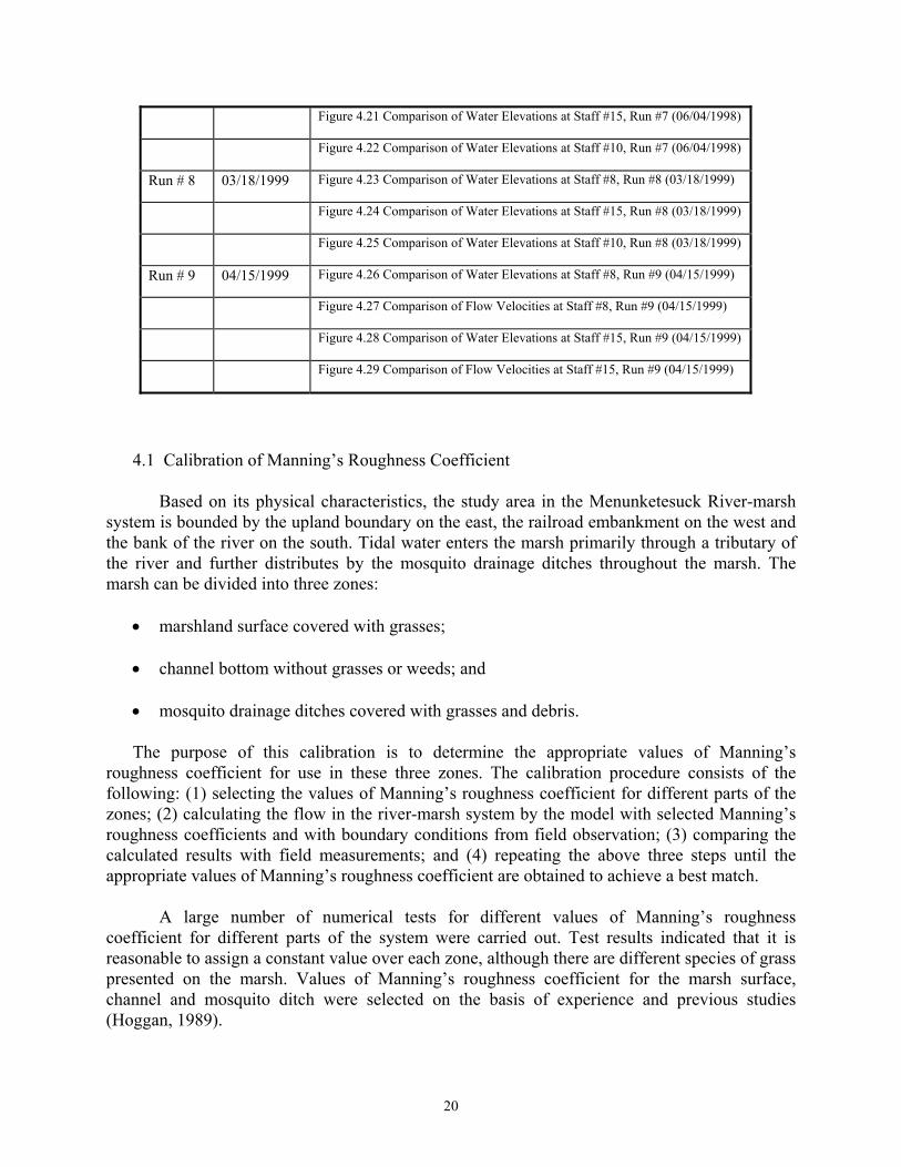
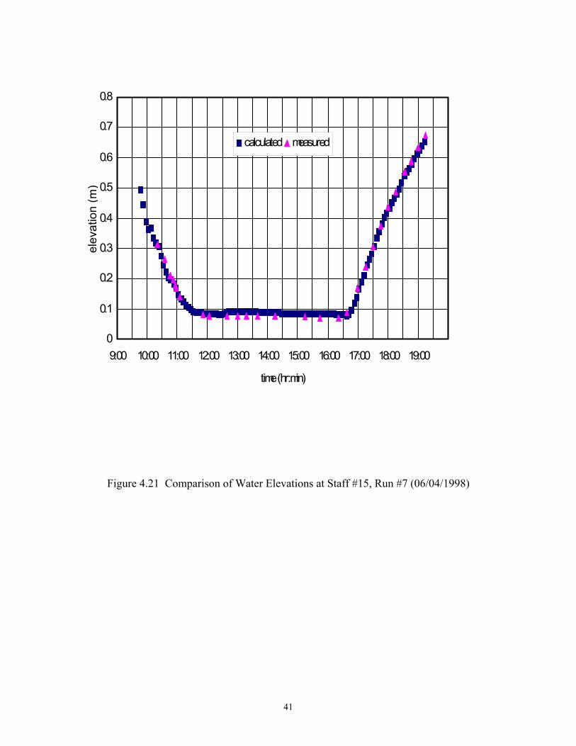
Figure 4.21 Comparison of Water Elevations at Staff #15, Run #7 (06/04/1998)
Figure 4.22 Comparison of Water Elevations at Staff #10, Run #7 (06/04/1998)
Run # 8 03/18/1999 Figure 4.23 Comparison of Water Elevations at Staff #8, Run #8 (03/18/1999)
Figure 4.24 Comparison of Water Elevations at Staff #15, Run #8 (03/18/1999)
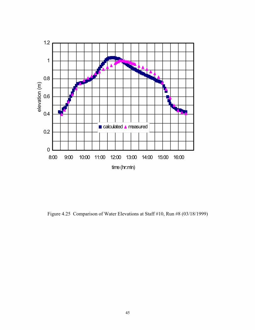
Figure 4.25 Comparison of Water Elevations at Staff #10, Run #8 (03/18/1999)
Run # 9 04/15/1999 Figure 4.26 Comparison of Water Elevations at Staff #8, Run #9 (04/15/1999)
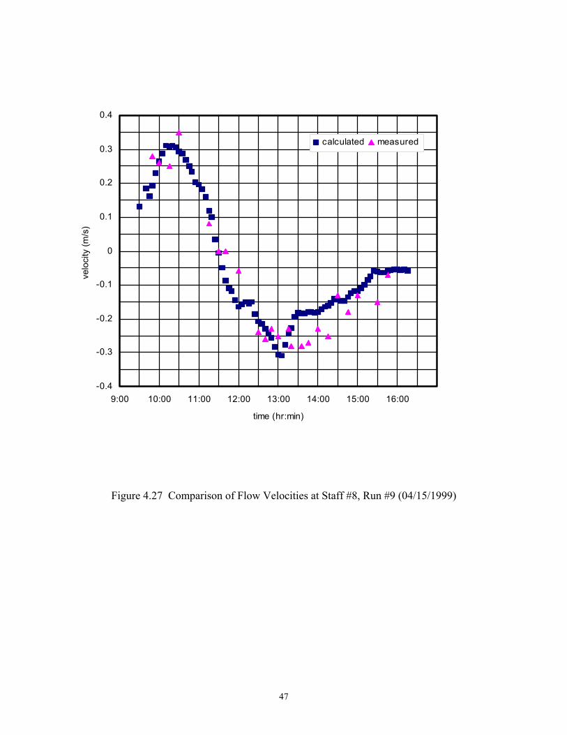
Figure 4.27 Comparison of Flow Velocities at Staff #8, Run #9 (04/15/1999)
Figure 4.28 Comparison of Water Elevations at Staff #15, Run #9 (04/15/1999)
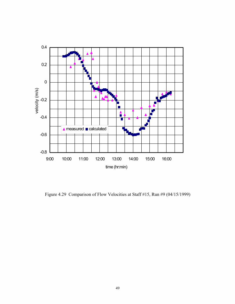
Figure 4.29 Comparison of Flow Velocities at Staff #15, Run #9 (04/15/1999)
4.1 Calibration of Manning’s Roughness Coefficient
Based on its physical characteristics, the study area in the Menunketesuck River-marsh system is bounded by the upland boundary on the east, the railroad embankment on the west and the bank of the river on the south. Tidal water enters the marsh primarily through a tributary of the river and further distributes by the mosquito drainage ditches throughout the marsh. The marsh can be divided into three zones:
• marshland surface covered with grasses;
• channel bottom without grasses or weeds; and
• mosquito drainage ditches covered with grasses and debris.
The purpose of this calibration is to determine the appropriate values of Manning’s roughness coefficient for use in these three zones. The calibration procedure consists of the following: (1) selecting the values of Manning’s roughness coefficient for different parts of the zones; (2) calculating the flow in the river-marsh system by the model with selected Manning’s roughness coefficients and with boundary conditions from field observation; (3) comparing the calculated results with field measurements; and (4) repeating the above three steps until the appropriate values of Manning’s roughness coefficient are obtained to achieve a best match.
A large number of numerical tests for different values of Manning’s roughness
coefficient for different parts of the system were carried out. Test results indicated that it is reasonable to assign a constant value over each zone, although there are different species of grass presented on the marsh. Values of Manning’s roughness coefficient for the marsh surface, channel and mosquito ditch were selected on the basis of experience and previous studies (Hoggan, 1989).
20

In general, the calibration results indicated that the tidal flow in the channel is not sensitive to the change of value of Manning’s roughness coefficient. An increase in the value for the channel from 0.025 to 0.05 does not change the water elevation significantly as shown in Figure 4.1.
-0.4
-0.2
0
0.2
0.4
0.6
0.8
1
1.2
9:00 10:00 11:00 12:00 13:00 14:00 15:00 16:00
time (hr:min)
elev
atio
n (m
)
calculated (channel n=0.025) calculated (channel n=0.05) measured
Figure 4.1 Influence of Channel n on Water Elevation at Staff #8 in Run #9
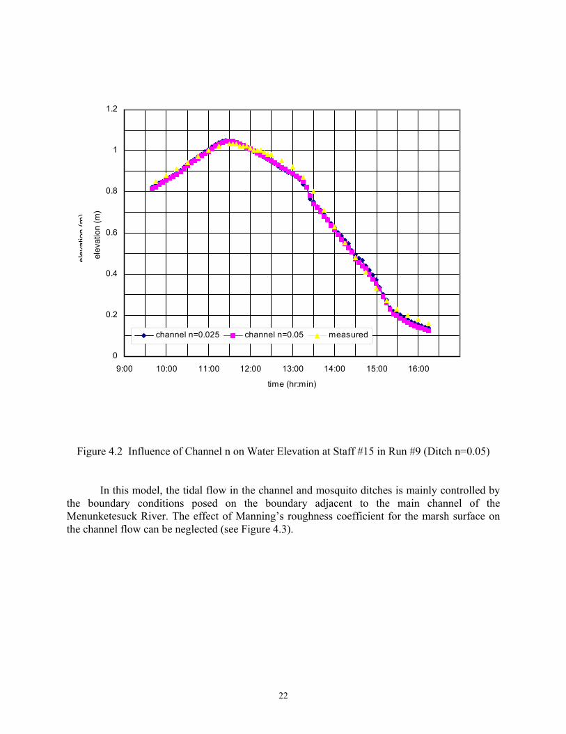
The effect of the change of value of Manning’s n in the mosquito ditches during the ebb tide is more pronounce than during the flood tide. The tidal flow in the ditches is not sensitive within a large range of values of Manning’s n as in the tributary channel because the length of channel in the model area for this study is relatively short (see Figure 4.2).
21
0
0.2
0.4
0.6
0.8
1
1.2
9:00 10:00 11:00 12:00 13:00 14:00 15:00 16:00
time (hr:min)
elev
atio
n (m
)
channel n=0.025 channel n=0.05 measured
0
0.2
0.4
0.6
0.8
1
1.2
9:00 10:00 11:00 12:00 13:00 14:00 15:00 16:00
time (hr:min)
elev
atio
n (m
)
channel n=0.025 channel n=0.05 measured
Figure 4.2 Influence of Channel n on Water Elevation at Staff #15 in Run #9 (Ditch n=0.05)
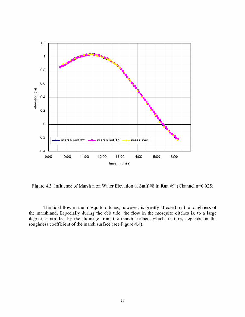
In this model, the tidal flow in the channel and mosquito ditches is mainly controlled by the boundary conditions posed on the boundary adjacent to the main channel of the Menunketesuck River. The effect of Manning’s roughness coefficient for the marsh surface on the channel flow can be neglected (see Figure 4.3).
22
-0.4
-0.2
0
0.2
0.4
0.6
0.8
1
1.2
9:00 10:00 11:00 12:00 13:00 14:00 15:00 16:00
time (hr:min)
elev
atio
n (m
)
marsh n=0.025 marsh n=0.05 measured
Figure 4.3 Influence of Marsh n on Water Elevation at Staff #8 in Run #9 (Channel n=0.025)
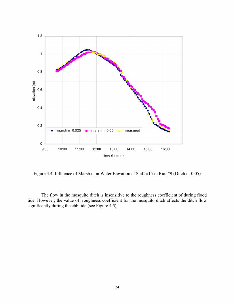
The tidal flow in the mosquito ditches, however, is greatly affected by the roughness of the marshland. Especially during the ebb tide, the flow in the mosquito ditches is, to a large degree, controlled by the drainage from the march surface, which, in turn, depends on the roughness coefficient of the marsh surface (see Figure 4.4).
23
0
0.2
0.4
0.6
0.8
1
1.2
9:00 10:00 11:00 12:00 13:00 14:00 15:00 16:00
time (hr:min)
elev
atio
n (m
)
marsh n=0.025 marsh n=0.05 measured
Figure 4.4 Influence of Marsh n on Water Elevation at Staff #15 in Run #9 (Ditch n=0.05)
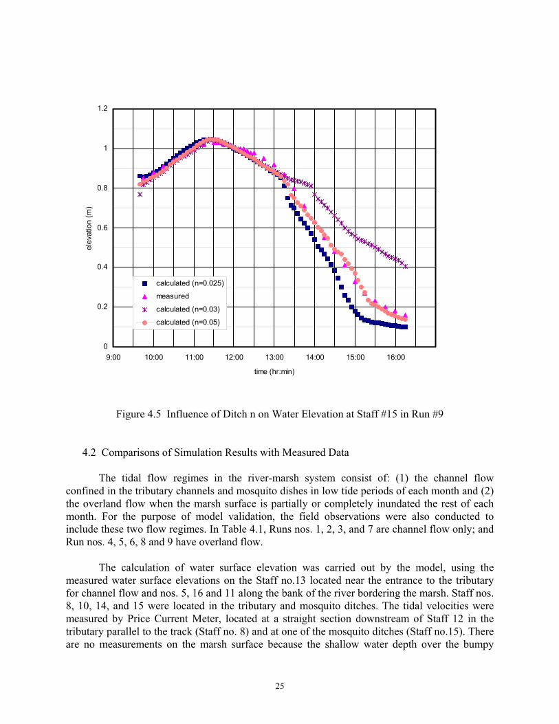
The flow in the mosquito ditch is insensitive to the roughness coefficient of during flood tide. However, the value of roughness coefficient for the mosquito ditch affects the ditch flow significantly during the ebb tide (see Figure 4.5).
24
0
0.2
0.4
0.6
0.8
1
1.2
9:00 10:00 11:00 12:00 13:00 14:00 15:00 16:00
time (hr:min)
elev
atio
n (m
)
calculated (n=0.025)
measured
calculated (n=0.03)
calculated (n=0.05)
Figure 4.5 Influence of Ditch n on Water Elevation at Staff #15 in Run #9 4.2 Comparisons of Simulation Results with Measured Data
The tidal flow regimes in the river-marsh system consist of: (1) the channel flow confined in the tributary channels and mosquito dishes in low tide periods of each month and (2) the overland flow when the marsh surface is partially or completely inundated the rest of each month. For the purpose of model validation, the field observations were also conducted to include these two flow regimes. In Table 4.1, Runs nos. 1, 2, 3, and 7 are channel flow only; and Run nos. 4, 5, 6, 8 and 9 have overland flow.
The calculation of water surface elevation was carried out by the model, using the
measured water surface elevations on the Staff no.13 located near the entrance to the tributary for channel flow and nos. 5, 16 and 11 along the bank of the river bordering the marsh. Staff nos. 8, 10, 14, and 15 were located in the tributary and mosquito ditches. The tidal velocities were measured by Price Current Meter, located at a straight section downstream of Staff 12 in the tributary parallel to the track (Staff no. 8) and at one of the mosquito ditches (Staff no.15). There are no measurements on the marsh surface because the shallow water depth over the bumpy
25

marsh surface provides a lot of difficulty to obtain meaningful results. Unsuccessful attempts were made to measure the velocity over the marsh surface by various methods. Again, the shallowness of depth, bumpy surface, and the presence of grass and the wind induced surface current make velocity measurements very difficult. The values of Manning’s roughness coefficient n are derived from the calibration, using the data of Run no.9.
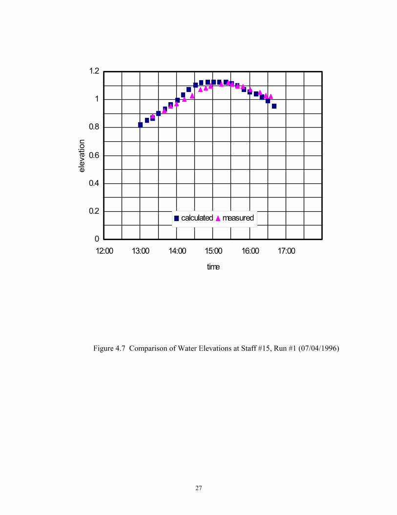
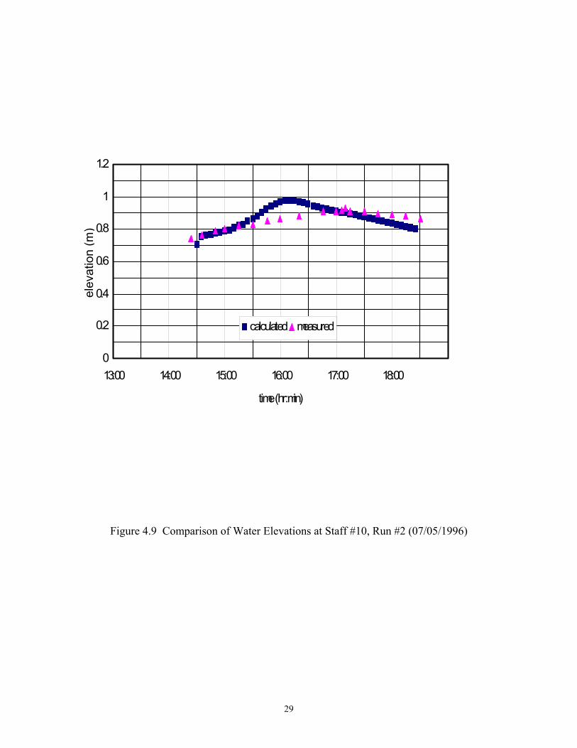
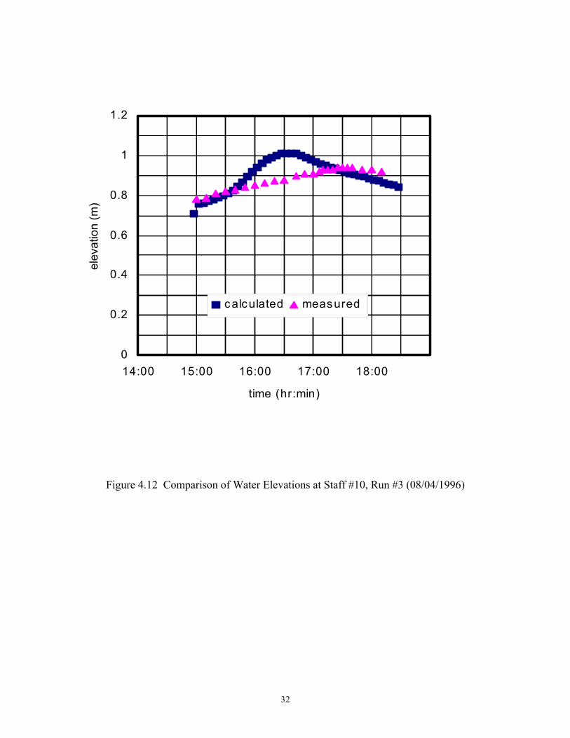
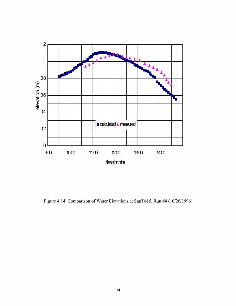
Comparisons of water surface elevations of the simulation results and field measurements
for these runs are shown in Figures 4.6 to 4.26 and Figure 4.28. Comparisons of tidal velocities at the sections on the tributary (Staff #8) and a mosquito channel (Staff #15) are shown in Figures 4.27 and 4.29, respectively.
0
0.2
0.4
0.6
0.8
1
1.2
12:00 13:00 14:00 15:00 16:00 17:00
time (hr:min)
elev
atio
n (m
)
calculated meaured
Figure 4.6 Comparison of Water Elevations at Staff #14, Run #1 (07/04/1996)
26
0
0.2
0.4
0.6
0.8
1
1.2
12:00 13:00 14:00 15:00 16:00 17:00
time
elev
atio
n
calculated measured
Figure 4.7 Comparison of Water Elevations at Staff #15, Run #1 (07/04/1996)
27

0
0.2
0.4
0.6
0.8
1
1.2
14:00 15:00 16:00 17:00 18:00
time (hr:min)
elev
atio
n (m
)
calculated measured
Figure 4.8 Comparison of Water Elevations at Staff #14, Run #2 (07/05/1996)
28
0
0.2
0.4
0.6
0.8
1
1.2
13:00 14:00 15:00 16:00 17:00 18:00
time (hr:min)
elev
atio
n (m
)
calculated measured
Figure 4.9 Comparison of Water Elevations at Staff #10, Run #2 (07/05/1996)
29

0
0.2
0.4
0.6
0.8
1
1.2
14:00 15:00 16:00 17:00 18:00
time (hr:min)
elev
atio
n (m
)
calculated measured
Figure 4.10 Comparison of Water Elevations at Staff #14, Run #3 (08/04/1996)
30

0
0.2
0.4
0.6
0.8
1
1.2
14:00 15:00 16:00 17:00 18:00 19:00
time (hr:min)
elev
atio
n (m
)
calculated measured
Figure 4.11 Comparison of Water Elevations at Staff #15, Run #3 (08/04/1996)
31
0
0.2
0.4
0.6
0.8
1
1.2
14:00 15:00 16:00 17:00 18:00
time (hr:min)
elev
atio
n (m
)
c alculated measured
Figure 4.12 Comparison of Water Elevations at Staff #10, Run #3 (08/04/1996)
32

0
0.2
0.4
0.6
0.8
1
1.2
9:00 10:00 11:00 12:00 13:00 14:00
time (hr:min)
elev
atio
n (m
)
calculated measured
Figure 4.13 Comparison of Water Elevations at Staff #14, Run #4 (10/26/1996)
33
0
0.2
0.4
0.6
0.8
1
1.2
9:00 10:00 11:00 12:00 13:00 14:00
time (hr:min)
elev
atio
n (m
)
calculated measured
Figure 4.14 Comparison of Water Elevations at Staff #15, Run #4 (10/26/1996)
34
0
0.2
0.4
0.6
0.8
1
1.2
9:00 10:00 11:00 12:00 13:00 14:00
time (hr:min)
elev
atio
n (m
)
calculated measured
Figure 4.15 Comparison of Water Elevations at Staff #10, Run #4 (10/26/1996)
35

0
0.2
0.4
0.6
0.8
1
1.2
10:00 11:00 12:00 13:00 14:00
time (hr:min)
elev
atio
n (m
)
calculated measured
Figure 4.16 Comparison of Water Elevations at Staff #14, Run #5 (10/27/1996)
36
0
0.2
0.4
0.6
0.8
1
1.2
10:00 11:00 12:00 13:00 14:00
time (hr:min)
elev
atio
n (m
)
calculated measured
Figure 4.17 Comparison of Water Elevations at Staff #15, Run #5 (10/27/1996)
37
0
0.2
0.4
0.6
0.8
1
1.2
10:00 11:00 12:00 13:00 14:00
time (hr:min)
elev
atio
n (m
)
calculated measured
Figure 4.18 Comparison of Water Elevations at Staff #10, Run #5 (10/27/1996)
38
0
0.2
0.4
0.6
0.8
1
1.2
9:00 10:00 11:00 12:00 13:00 14:00
time (hr:min)
elev
atio
n (m
)
calculated measured
Figure 4.19 Comparison of Water Elevations at Staff #14, Run #6 (12/13/1997)
39

-0.4
-0.2
0
0.2
0.4
0.6
0.8
9:00 10:00 11:00 12:00 13:00 14:00 15:00 16:00 17:00 18:00 19:00
time (hr:min)
elev
atio
n (m
)
calculated measured
Figure 4.20 Comparison of Water Elevations at Staff #8, Run #7 (06/04/1998)
40
0
0.1
0.2
0.3
0.4
0.5
0.6
0.7
0.8
9:00 10:00 11:00 12:00 13:00 14:00 15:00 16:00 17:00 18:00 19:00
time (hr:min)
elev
atio
n (m
)
calculated measured
Figure 4.21 Comparison of Water Elevations at Staff #15, Run #7 (06/04/1998)
41

0
0.1
0.2
0.3
0.4
0.5
0.6
0.7
9:00 10:00 11:00 12:00 13:00 14:00 15:00 16:00 17:00 18:00 19:00
time (hr:min)
elev
atio
n (m
)
calculated measured
Figure 4.22 Comparison of Water Elevations at Staff #10, Run #7 (06/04/1998)
42

-0.4
-0.2
0
0.2
0.4
0.6
0.8
1
1.2
8:00 9:00 10:00 11:00 12:00 13:00 14:00 15:00 16:00
time (hr:min)
elev
atio
n (m
)
calculated measured
Figure 4.23 Comparison of Water Elevations at Staff #8, Run #8 (03/18/1999)
43

0
0.2
0.4
0.6
0.8
1
1.2
8:00 9:00 10:00 11:00 12:00 13:00 14:00 15:00 16:00
time (hr:min)
elev
atio
n (m
)
calculated measured
Figure 4.24 Comparison of Water Elevations at Staff #15, Run #8 (03/18/1999)
44
0
0.2
0.4
0.6
0.8
1
1.2
8:00 9:00 10:00 11:00 12:00 13:00 14:00 15:00 16:00
time (hr:min)
elev
atio
n (m
)
calculated measured
Figure 4.25 Comparison of Water Elevations at Staff #10, Run #8 (03/18/1999)
45

-0.4
-0.2
0
0.2
0.4
0.6
0.8
1
1.2
9:00 10:00 11:00 12:00 13:00 14:00 15:00 16:00
time (hr:min)
velo
city
(m/s
)
calculated measured
Figure 4.26 Comparison of Water Elevations at Staff #8, Run #9 (04/15/1999)
46
-0.4
-0.3
-0.2
-0.1
0
0.1
0.2
0.3
0.4
9:00 10:00 11:00 12:00 13:00 14:00 15:00 16:00
time (hr:min)
velo
city
(m/s
)
calculated measured
Figure 4.27 Comparison of Flow Velocities at Staff #8, Run #9 (04/15/1999)
47

0
0.2
0.4
0.6
0.8
1
1.2
9:00 10:00 11:00 12:00 13:00 14:00 15:00 16:00
time (hr:min)
elev
atio
n (m
)
calculated (n=0.025)measuredcalculated (n=0.03)calculated (n=0.05)
Figure 4.28 Comparison of Water Elevations at Staff #15, Run #9 (04/15/1999)
48
-0.8
-0.6
-0.4
-0.2
0
0.2
0.4
9:00 10:00 11:00 12:00 13:00 14:00 15:00 16:00
time (hr:min)
velo
city
(m/s
)
measured calculated
Figure 4.29 Comparison of Flow Velocities at Staff #15, Run #9 (04/15/1999)
49

4.3 Tidal Velocity Field of Simulation Results on 3/18/99 In the process of simulation of the runs shown in the previous section, the tidal velocity fields on the marsh surface and in the channels were recorded at a pre-selected time interval over the entire tidal cycle. The simulation results of March 18, 1999 provides as an example of the tidal velocity field of the overland flow over the marsh throughout the tidal cycle. The velocity vector of a cell is represented by a bar radiating from the center of the cell. The length of the bar is scaled to the magnitude of velocity. Figs. 4.30 to 4.38 depicts a sequence of hourly velocity fields on the marsh throughout the cycle on March 18, 1999. At the low tide, the flow mainly confines within the channel and the overland flow starts to spread over the area with low elevation as shown in Fig. 4.30. The overland flow continues to increase to the maximum tidal velocity (not shown here) before the large flow field shown at 11:00 a.m. in Fig. 4.32. The peak tidal amplitude reaches approximately at 11.45 a.m. as seen in Figs. 4.23-4.25. The tidal velocity practically vanishes for most of the area and the overland flow starts to drain toward the channel in areas with low elevation in the marsh as shown in Fig. 4.33. The tidal velocity on the marsh exhibits a strong asymmetry as shown in Figs. 4.27 and 4.29. A prolong overland drainage with a smaller velocity during the ebb tide is evident in Figs. 4.34 through 4.38.
50

Figure 4.30 Simulated Flow Field on March 18, 1999 at 9 am
51

Figure 4.31 Simulated Flow Field on March 18, 1999 at 10 am
52

Figure 4.32 Simulated Flow Field on March 18, 1999 at 11 am
53

Figure 4.33 Simulated Flow Field on March 18, 1999 at 12 pm
54

Figure 4.34 Simulated Flow Field on March 18, 1999 at 1 pm
55

Figure 4.35 Simulated Flow Field on March 18, 1999 at 2 pm
56
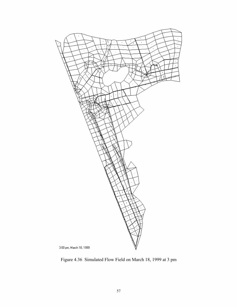
Figure 4.36 Simulated Flow Field on March 18, 1999 at 3 pm
57

Figure 4.37 Simulated Flow Field on March 18, 1999 at 4 pm
58
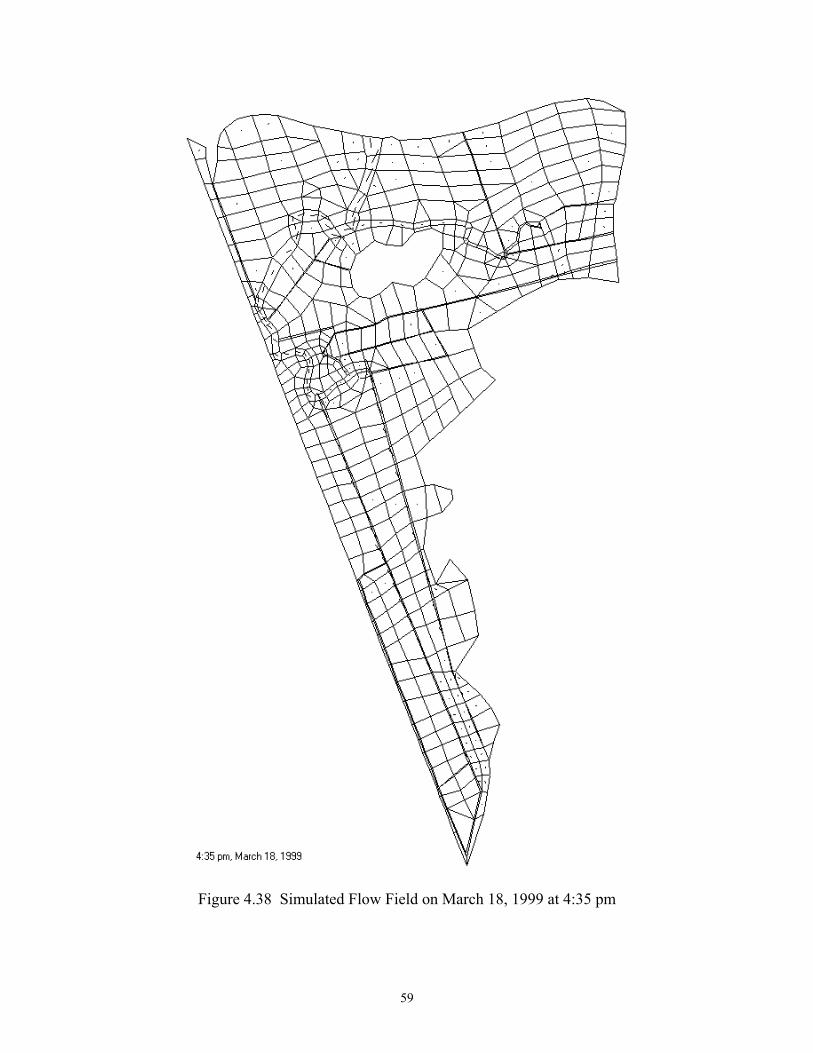
Figure 4.38 Simulated Flow Field on March 18, 1999 at 4:35 pm
59
4.4 Discussion of Results
The calibration procedure of the model as shown in Section 4.2 involves only a single parameter, surface roughness coefficient n. Normally, only two values of n are used: one for the channel and another for the marsh surface. Although there are various species of vegetation existed at this site as we discussed in Section 3.1; however, the tidal regime in this system is such that the overland flow is always at a shallow depth and the density of plant for these species are similar. In any case, the model could accommodate the use of different values of n according to the species of vegetation in each area. However, if there were lack of a rational method to determine the value of n associated with each species, the procedure for calibration would become more complicated, and perhaps more elaborated. A research to quantify the plant physical characteristics, such as the plant density distribution, stem and leaf area index, and then to correlate these parameters with drag and friction coefficients is needed for a rational approach to any modeling effort, including this model.
In the simulation study, the results presented in Section 4.2 include the model being
applied to both the flow confined only in the main channel and tributaries and the regime with overland flow over the marsh. The comparisons between the simulated results and observed data depicted in Figures 4.6 to 4.26 and Figure 4.28 for the water surface elevation at the staffs at different locations throughout the marsh show reasonable agreement despite the fact that the marsh surface and channel cross sections are highly irregular. Particularly, at shallow depths of submergence, there exist many pools and discontinuity of water surface beyond the resolution of the model.
Many attempts have been tried to measure the velocity of the overland flow over the
marsh surface, including a technique using the combination of video cameras and neutrally buoyant beads. Unfortunately, the shallowness of water, irregularity of surface, presence of plant, and usually strong wind over the marsh present too much obstacles to overcome. We can only validate the tidal flow in the model by means of the traditional method of current meter in the channel. Figures 4.27 and 4.29 are the comparisons at a section on the tributary at Staff #8 and at a mosquito channel at Staff #15, respectively.
A sequence of velocity fields over the marsh during a tidal cycle is an important tool for
an engineer or environmentalist to visualize how structures or man-made changes affect the pattern of tidal flow over marshes. The sequence of flow fields shown in Figures 4.30 to 4.38 is a typical output from the results of simulation. In addition to the velocity distributions over the whole marsh, they also show the drying and wetting of the marsh surface and the channels during the tidal cycle. Further analysis can be made to determine the duration pf submergence and volume of salt-water exchange at location where these parameters influence the health of marsh vegetation.
60

5. APPLICATION OF THE MODEL TO THE FARM RIVER MARSH, EAST HAVEN, CONNECTICUT
5.1 Description of the Site
The Farm River marsh is located in East Haven, Connecticut s shown in Figs. 3.1 and 5. The site for this study (see Fig. 5.2) starts at a section of the river (Staff #16) approximately ¾ of a mile from the Farm River Gut and Kelsey Island in the Long Island Sound and extends northeasterly to about a mile. The east bank of the marsh is narrow and the west edge is limited by Route 142 or Hemingway Avenue with a maximum width about 6/10 of a miles. A tributary meanders through the major portion of the marsh and intersects Route 142 (Staffs #1 and #2). It enters to a small inland marsh through a culvert under Route 142. The river in the site ends at a bridge near Shore Line Trolley Museum (Staff #5). The condition of heavy silting and debris is apparent in the tributary. The vegetation in the marsh is dominated by Reed (Phragmites australis), which forms dense patches near the edge of the marsh and most of the inland marsh.
61

Figure 5.1 Location of the Farm River Marsh, East Haven, Connecticut
62

Figure 5.2 2-D Grid System and the Staff Locations
63

5.2 Field Work
The simulation study requires topographic and tidal cycle data. The topographic data consists of the location and elevation of a sufficient number of points on the surface of the marsh including the boundary of the site and on the cross sections of channel. The topographic survey of the marsh surface is conducted by Milone & MacBroom, Engineers, Cheshire, Connecticut. The data provides the coordinates and elevation of selected points on the marsh surface. We measured the elevations at selected cross sections along the channel. For water surface elevations, there are five staffs located along the main channel and the tributary as follows (see Figure 5.2). Staff #16 at the entrance of the river to the site provides the forcing boundary condition for the model. Staff #5 on a bridge near the Shore Line Trolley Museum provides another boundary condition. Staff #7 at the junction of the main channel and the tributary and Staffs #1 and #2 at the upstream and downstream sides of the culvert under Route 142 provide the observed tidal elevations for comparison with the results of model simulation. In addition, the discharge through the culvert versus the differential elevations of Staffs #1 and #2 were measured for the calibration of the discharge coefficient of the culvert. The measurements of water surface elevation were conducted for the tidal cycle of August 20, 1997. Both water surface elevations and flow through the culvert were measured for the tidal cycle of July 11 and 12, 1999. These data are presented in Appendix B. The site represents a small coastal river-marsh system subject to significant environmental interference, which is evident from the lag of the high tide time and the attenuation of tidal amplitude at various locations in the marsh. Table 5.1 on August 19, 1997 and Table 5.2 on July 11, 1999.
Table 5.1 Time Lags and Tidal Amplitudes on August 19, 1997
Staff # High Tide Time Time Lag (min)
relative to #1 staff
Tidal Amplitude (ft)
13 13:30 6.84 16 14:40 70 4.33 1 14:37~14:42 67~72 3.67 2 14:44~15:00 74~90 2.91 3 15:40 130 1.42 5 15:32~15:37 122~127 2.67
Note: Staff #0 located at the Condominium/marina on Route 100
Staff #3 located at the center of the inland marsh upstream of the culvert
64
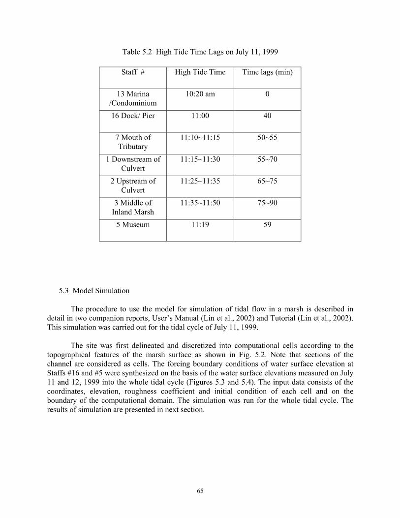
Table 5.2 High Tide Time Lags on July 11, 1999
Staff # High Tide Time Time lags (min)
13 Marina /Condominium
10:20 am 0
16 Dock/ Pier 11:00 40
7 Mouth of Tributary
11:10~11:15 50~55
1 Downstream of Culvert
11:15~11:30 55~70
2 Upstream of Culvert
11:25~11:35 65~75
3 Middle of Inland Marsh
11:35~11:50 75~90
5 Museum 11:19 59
5.3 Model Simulation The procedure to use the model for simulation of tidal flow in a marsh is described in detail in two companion reports, User’s Manual (Lin et al., 2002) and Tutorial (Lin et al., 2002). This simulation was carried out for the tidal cycle of July 11, 1999. The site was first delineated and discretized into computational cells according to the topographical features of the marsh surface as shown in Fig. 5.2. Note that sections of the channel are considered as cells. The forcing boundary conditions of water surface elevation at Staffs #16 and #5 were synthesized on the basis of the water surface elevations measured on July 11 and 12, 1999 into the whole tidal cycle (Figures 5.3 and 5.4). The input data consists of the coordinates, elevation, roughness coefficient and initial condition of each cell and on the boundary of the computational domain. The simulation was run for the whole tidal cycle. The results of simulation are presented in next section.
65

Figure 5.3 Staff Readings at Staff #16 on July 11, 1999
66
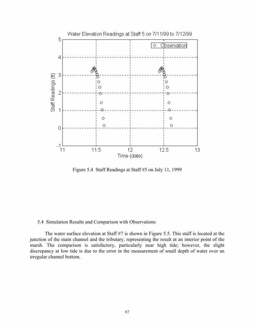
Figure 5.4 Staff Readings at Staff #5 on July 11, 1999
5.4 Simulation Results and Comparison with Observations
The water surface elevation at Staff #7 is shown in Figure 5.5. This staff is located at the junction of the main channel and the tributary, representing the result at an interior point of the marsh. The comparison is satisfactory, particularly near high tide; however, the slight discrepancy at low tide is due to the error in the measurement of small depth of water over an irregular channel bottom.
67

Figure 5.5 Comparison of Simulation Results of the Observations at Staff #7
The comparisons of Staff #1 at the downstream and of Staff #2 at the upstream of the culvert under Route 142 are reasonable. The discrepancy appears to be over-predicting of the time at the high tide. As a result, the water surface elevation is under-predicted during the flood tide and over-predicted during the ebb tide. The discrepancy could be due to the roughness coefficient used in the channel or the irregularity if the channel bottom leading to the culvert. It also indicated that the calculation of the flow through the culvert is reasonable.
68

Figure 5.6 Comparison of Simulation Results of the Observations at Staff #1
69

Figure 5.7 Comparison of Simulation Results of the Observations at Staff #2
70

6. SUMMARY AND CONCLUSIONS
The project has developed two hydrodynamic models for tidal flushing in coastal river-marsh systems. The Pseud-2D Hydrodynamic Model for a Tidal-Wetland System (Lin et al., 1996) is a tidal flow model by superimposing a one-dimensional lateral overland flow over the marsh on a one- dimensional open-channel along the main channel of a costal river. It is a simple model for applications to a tidal river with a narrow marsh, which requires less topographic and hydraulic data than the two-dimensional model. A research site at the Oyster River marsh, Old Saybrook, Connecticut was chosen for model calibration and validation. Field observations were conducted at this site for topographic, hydraulic and vegetation data. Development of The Two-dimensional Finite-Volume Hydrodynamic Model for Coastal Wetlands has been completed, including User’s Manual and Tutorial (Lin et al., 2002a,b). Model calibration and validation were carried out at the Menunketesuck River marsh, Westbrook, Connecticut. Extensive fieldwork has been conducted at this site for studying of marsh topography and vegetation, and hydraulic measurements. The model was successively applied to the investigation of tidal flushing at the Farm River marsh, East Haven, Connecticut. These models should provide Connecticut Department of Transportation an analytical tool for assessment of environmental impacts of highway structures on coastal waters.
71

REFERENCES
Bell, M. M., 1985. The Face of Connecticut: People, Geology, and the Land. State Geological and Natural History Survey of the State, Bull. 110, 196 pp.
Bloom, A. W., & C. W. Ellis, Jr., 1965. Postglacial Stratigraphy and Morphology of Coastal Connecticut State Geol. & Nat. Hist. Surv. of Connecticut, Guidebook. no. 1. 10 pp. Chapman, V. J., 1974. Salt Marshes and Salt Deserts of the World. Cramer & Lehre, 392 pp. State of Conn. Dept. Envtl. Protection–Natural resources Data Center, Rept. Investigs. No. 6.
137 pp. Dowhan, J. J., & R. J. Craig, 1976. Rare and Endangered Species of Connecticut and their
Habitats. Hill, D. E., & A. E. Shearin, 1970. Tidal Marshes of Connecticut and Rhode Island. Connecticut
Agr. Exp. Sta., New Haven, Bull. 709. 4 pp.
Lefor, M. W., W. C. Kennard and D. L.Civco, 1987. On the Relationship of Salt Marsh Plant Distributions to Tidal Levels in Connecticut, U. S. A. Envtl. Mgmnt. Vol. 11, pp. 61-68. Lin, J. D., Liao, Lefor, M. W., Hua, J. S, W. G., Qiu, K-J and W. G. Liao, 19970. A Pseudo- 2D
Hydrodynamic Model for a Tidal River-Wetland System, JHR 96-253, December, 1996. Lin, J. D., Liao, Lefor, M. W., Hua, J. S, W. G., Qiu, K-J and W. G. Liao, 19970. A Pseudo- 2D Hydrodynamic Model for a Tidal River-Wetland System. Presented at Connections 98: Wetlands, Transportation, and the Environment, New Bern, NC, September 17, 1998. Lin, J. D., Liao, W. G., Qiu, K-J, and M. W. Lefor, 2000. A Two-dimensional Hydrodynamic Model for Coastal River-Marsh Systems: Tutorial, Version 1.0, Report No. JHR 02-277, June, 2002. Lin, J. D., Liao, W. G., Qiu, K-J, and M. W. Lefor, 2002. A Two-dimensional Hydrodynamic Model for Coastal River-Marsh Systems: User’s Manual, Version 1.0,
Report No. JHR 02-275, June, 2002. Lundgren, L., Jr., 1964. The Bedrock Geology of the Essex Quadrangle, with Map. State Geol.
& Nat. Hist. Surv. Connecticut, Quadrangle Rept. no. 15. 38 pp. Miller, W. R. and F. E. Egler, 1950. Vegetation of Wequetequock Tidal Marshes, Connecticut
Ecol. Monogr. 20(2): pp. 142-172.
72

73
Price, J. S. and M-K. Woo, 1988. Studies of a Subarctic Marsh, II. Salinity. Journal of Hydrology, No.103, pp. 293-307.
USGS, 1995. Digital Orthophotographic 7.5 min. Quarter-Quadrangle, Essex Quadgrangle.
.