All of us

We should have a mission.

We should have a purpose.

It’s in our bones.

What’s a man

If he has no ambition?

A truncated vision.

He’s a man alone.

This is the story of a generation

An ageless nation. Are we alone?

The days and weeks have started bleeding.

We’re in dire need of something bold.

All of us

We should have a mission!

We should have a purpose!

- The Phenomenauts (Man Alone)

Finding Terrestrial Exoplanets With Synthetic Radial Velocity

Datasets

Benjamin Nelson

Faculty advisor: Gregory Laughlin

Lick Observatory, University of California, Santa Cruz, CA 95064

Department of Astronomy and Astrophysics, University of California, Santa Cruz, CA

95064

ABSTRACT

Within the past couple of years, our technology has become so precise that

we have been able to unveil terrestrial planets inhabiting outside solar systems.

Though we are currently unable to detect planets with Earth-like orbital prop-

erties, we can nonetheless contemplate what we might discover in the next few

years. Utilizing the known distribution of extrasolar planets today and a variable

meter that controls the likelihood of finding extraterrestrial planets, an numer-

ical algorithm was developed allowing extrasolar enthusiasts to create batches

of artificial planetary systems in the form of radial velocity (RV) datasets, that

span over the course of a couple years, in a matter of seconds. The datasets are

currently generated through Simple Keplerian Integrations while modeling an

observatory on Earth in order to replicate a more realistic time sampling. Once

polished, this program will become a major extension for the Systemic Console

for both amateur and professional astronomers to use in their planet detection

simulations. With this tool at hand, we can discuss what strategies to take in

order to find planets lurking beneath the current error threshold. A couple sam-

ple datasets will be analyzed as mere examples of plausible systems that this

program is capable of generating.

1. Introduction and Background

This project deals with our current capability to detect extrasolar planets, planets which

orbit other stars or star systems. The first extrasolar planet orbiting a main sequence star

was announced in late 1995 by Dr. Michel Mayor and his Ph. D student at the time, Didier

Queloz, at the University of Geneva in Switzerland. The planet was found around the star

– 3 –

51 Pegasi, a 1.06 solar-mass star (M) barely visible to the naked eye (5.49 Magnitude)

found within the Pegasus constellation between the saddle (α) and the leg (β), and it was

appropriately labeled 51 Pegasi b (Mayor et al., 1995). It was a breakthrough for two reasons:

not only was this the first planet to exist outside the Solar System but it also reformulated

our understanding of how planets formed. It had a near circular orbit of roughly 4 days, an

orbit well within that of Mercury (≈88 days). Being so close to its parent star, it came as

quite a shock when they found that the planet was over 150 Earth-masses (M⊕), nearly half

of a Jupiter-mass (MJ) (Mayor et al., 1995). This was the first case of a “hot Jupiter” but

certainly not the last. Most of the 340 or so planets currently contained in the Extrasolar

Planet Encyclopedia, found at http://www.exoplanet.eu, are on the order of a Jupiter-mass,

and most have orbital periods considerably less than that of Jupiter.

Eccentricity, e, is another orbital element, besides planet mass, m, and orbital period,

T , that plays a crucial role in basic planetary dynamics. It is a dimensionless number

representing how much an orbit deviates from being circular, where 0 is a perfect circle and

1 is a parabola. Anything in between is defined as an ellipse and numbers greater than

1 are treated as hyperbolas. For stable planetary systems, we only consider bound orbits,

0 < e < 1, which is the range we will utilize here and henceforth. Mercury held the record

for most eccentric planet in the Solar System, e ≈ 0.206, but was quickly overthrown upon

the discovery of extrasolar planets. The ∼4 MJ planet HD80606b is the leading contender

for most wild orbit, with a whopping eccentricity of 0.93 (Moutou et al., 2009). A decent

model for this planet’s orbital behavior is much like a ball thrown straight up from the Earth

with a 111 day hang time. Its perihelion, the point of closest approach, is 0.03AU (Mercury’s

perihelion is about 10 times this) and swings into an aphelion, the farthest point from the

host star, of 0.84AU, a distance comparable to that of the Earth-Sun distance (Moutou et al.,

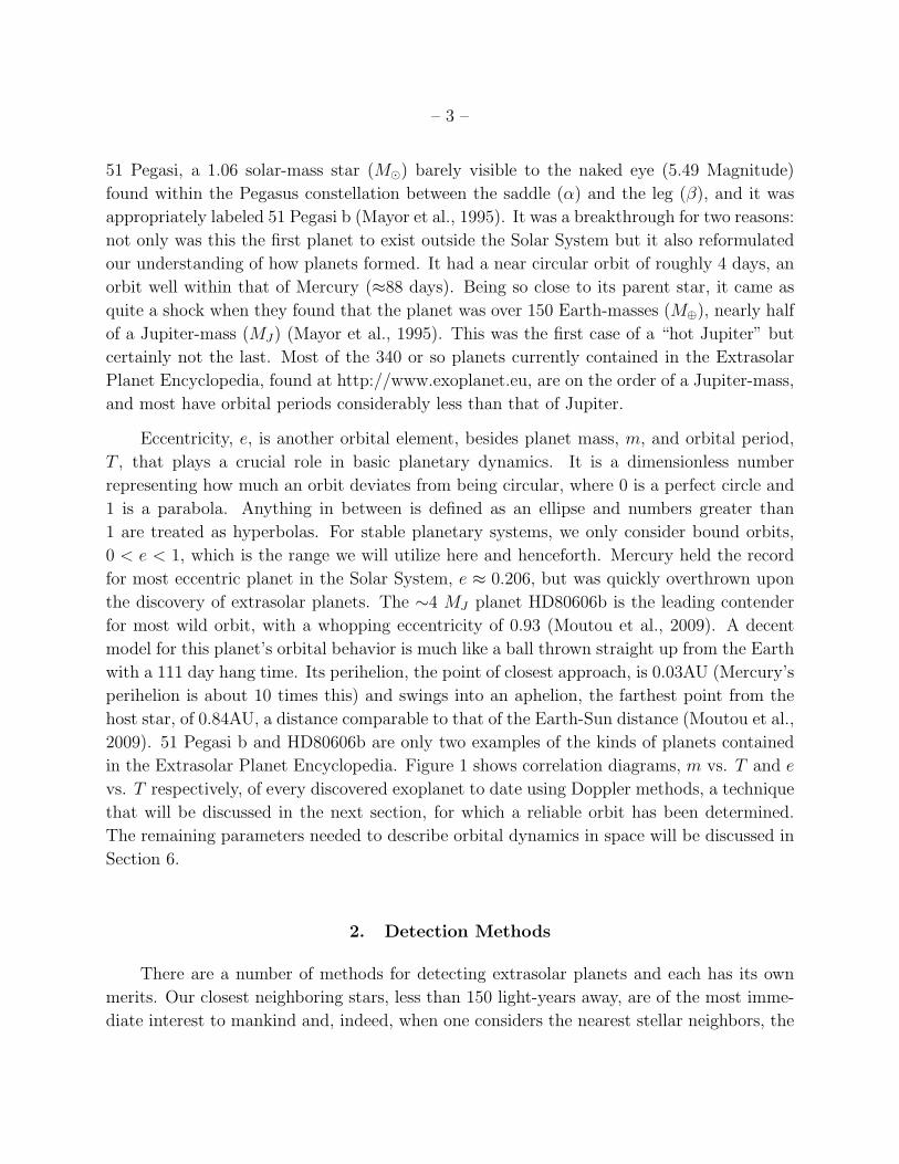
2009). 51 Pegasi b and HD80606b are only two examples of the kinds of planets contained

in the Extrasolar Planet Encyclopedia. Figure 1 shows correlation diagrams, m vs. T and e

vs. T respectively, of every discovered exoplanet to date using Doppler methods, a technique

that will be discussed in the next section, for which a reliable orbit has been determined.

The remaining parameters needed to describe orbital dynamics in space will be discussed in

Section 6.

2. Detection Methods

There are a number of methods for detecting extrasolar planets and each has its own

merits. Our closest neighboring stars, less than 150 light-years away, are of the most imme-

diate interest to mankind and, indeed, when one considers the nearest stellar neighbors, the

– 4 –

0.001

0.01

0.1

1

10

0.1 1 10 100 1000 10000

Mas

s [J

upite

r]

Period [Days]

(a)

Jupiter

Earth

0

0.1

0.2

0.3

0.4

0.5

0.6

0.7

0.8

0.9

1

0.1 1 10 100 1000 10000

Ecc

entr

icity

Period (Days)

(b)

Earth

Jupiter

Fig. 1.— The current known exoplanet distribution correlating orbital period with (a) mass and (b)eccentricity. Most discovered planets do not normally exceed a 1000 day orbit, since it would take a fewyears to see a full period in the dataset. Note how periods less than 10 days are roughly circular whilelonger orbits have more flexibility to be eccentric. The properties of the Earth and Jupiter are also shownfor reference.

mind leaps to consider the possibility of communication with other worlds. More practically,

these stars will generally be brighter due to their close proximity, and good astrophysical

data depend on high luminosities.

The most common and noteworthy method, and also the basis for this entire paper,

– 5 –

is Radial Velocity/Doppler method (Lunine et al., 2008). Just as the name implies, this

method detects the variations in the line-of-sight speed of a star as it moves toward or away

from the Earth. By working out a simple 2-body problem involving a single planet-star

system, it is easy to deduce that both objects orbit about the system’s barycenter with

the same orbital period. Assuming the orbital trajectory is a perfectly flat plane and is

not significantly inclined, we set up a Cartesian coordinate system centered at the system’s

barycenter and arbitrarily put the Earth some very large distance along the negative y

direction. An observer on Earth could detect velocity fluctuations along the y-axis using the

RV method. Astrometry is very similar to RV detection but rather than finding changes in

the line-of-sight velocity, it finds positional changes in the plane of the sky relative to much

further stars (Lunine et al., 2008). As long as there are enough sufficiently bright and distant

background stars and as long as proper motion is corrected for, an observer can center in

on a star and detect any significant deviations in its position from the center, which would

imply a planetary system. If no planetary system existed, the star would forever stay within

the crosshairs. One advantage in using either of these methods is that both are independent

of distance (Lunine et al., 2008); as long as the star is above a critical luminosity, it can be

considered a worthy candidate for observation.

For orbital elements unobtainable by either astrometry or RV detection, gravitational

microlensing and transit methods have shown promise. The former is normally used to

determine the mass of stars by observing their effects on background light sources. The

gravity of such a body will act as a lens by magnifying and distorting the image of background

stars or dust. Even less massive objects, such as planets, will also affect the background

image as well, and we currently have the technology to find such objects below an Earth-

mass (Lunine et al., 2008). Unlike Doppler or astrometry, GM actually excels at detecting

planets on long periodic orbits, since any background light sources would be bent solely by

the planet, rather than the planet-star pair. Though it is great for detecting low mass, cold

bodies, it is not easily repeatable since the background star/dust alignment will never be

the same as the one observed (Lunine et al., 2008), which also means the eccentricity is

difficult to obtain. Only a dozen or so planets have been uncovered with this method all

on 1000+ day orbits, and while the detection techniques are quite onerous mathematically,

microlensing has shown promise especially in finding terrestrial planets.

Transits occur when a planet eclipses its parent star relative to the Earth. This is de-

tected through a dip in the star’s luminosity as the planet traverses across the star. Once

the change in luminosity is known and assuming both the sun and planet are roughly spher-

ical entities, it is possible to obtain the planet’s radius, a parameter unobtainable by the

other mentioned means of detection. Since many Neptune-mass planets and Super-Earths

(terrestrial planets of multiple Earth-masses) weigh on the same order of magnitude, it is

– 6 –

difficult to distinguish between the two unless the radius is known. Transits are very rare

encounters, however. The orbital plane must cross the star-Earth line-of-sight, which in

space, is probabilistically not in our favor. The transit does not have to cross equatorially,

but there is little room for error.

There have recently been a number of cases where young, still warm exoplanets have

been detected directly. An example that received a lot of attention in the media was the

planetary system around the star Fomalhaut, which was directly imaged with the Hubble

Space Telescope. The star is very close (25 light years) and quite visible to the naked eye (1.73

Magnitude), which made it an exceptional candidate for direct imaging. The planet itself

has a gigantic semi-major axis, 119 AU, which implies an orbital period of over 3×105days,

quite an extraordinary orbit compared to that of our farthest orbiting planet, Neptune (30

AU, 6×104days). The Fomalhaut b was found by slight changes in its orbital behavior over

the course of nearly two years (Kalas et al. 2008). While this method is specially equipped

for finding planets with extremely high periodicity, it generally takes a lot of space telescope

time to find any minor phase difference in the orbit, and the planet must radiate enough

light in order to see it (Kalas et al. 2008).

3. The Threshold and .VELS File

Since precision in any experiment is never infinite, it should be realize that RV detection

has its limitations. Referring back to the two-body problem, both objects orbit barycenter

with the same orbital period but with different amplitudes, or in this case semi-major axes,

depending on the mass of each object. The heavier object, the star, will orbit at a smaller

semi-major axis since it is closer to barycenter. Its average orbital speed will be much smaller

than its planet. From here, we must ask ourselves: how well can we pinpoint a star’s radial

velocity and what does this mean in terms of the planets we are currently able to detect?

Today, our RV threshold lies at ∼3m/s (Laughlin, G.P. 2009); as a guide marker, Earth

has imparts a radial velocity of 6cm/s onto the Sun. A civilization on a nearby extrasolar

world with similar technology would therefore not be able detect the Earth using our present-

day state-of-the-art Doppler methods. They would only see Jupiter as it is the only detectable

planet, imparting a radial velocity of 12m/s. Saturn arrives in at second place barely below

the threshold yet still not detectable by today’s means (2.7m/s).

To answer the second part of our question, we can look towards Kepler’s Laws to

understand what species of planets would lie above the threshold. Kepler’s Third Law

– 7 –

of Planetary Motion, (T

2π

)2

=a3

G(M? +m)(1)

where M? is the stellar mass and G is the gravitational constant, 6.673 × 10−11m3kg−1s−2,

states that the square of the orbital period of a planet is directly proportional to the cube

of the semi-major axis, a. Therefore, short orbits will impart a greater radial velocity than

longer ones. This relation also depends on the planetary mass, and while Super-Earths

have been detected, they normally have orbital periods that last no more than two weeks.

An equation for calculating these radial velocity half amplitudes, K, will be derived in the

Section 6.

-150

-100

-50

0

50

100

150

0 50 100 150 200 250 300 350 400

Rad

ial V

eloc

ity [m

/s]

Time [Days]

(a)

-150

-100

-50

0

50

100

150

0 50 100 150 200 250 300 350 400

Rad

ial V

eloc

ity [m

/s]

Time [Days]

(b)

-150

-100

-50

0

50

100

150

0 50 100 150 200 250 300 350 400

Rad

ial V

eloc

ity [m

/s]

Time [Days]

(c)

-150

-100

-50

0

50

100

150

0 50 100 150 200 250 300 350 400

Rad

ial V

eloc

ity [m

/s]

Time [Days]

(d)

Fig. 2.— A 1 MJ planet on a 100 orbit. The different values for e and $ are (a) 0.2, 0; (b) 0.4, 60; (c)0.6, 120; and (d) 0.8, 180 respectively.

The RV data is normally compiled into a dataset with the extension .VELS, for velocity,

which is composed of three columns: the time at which the measurement was taken, the

observed radial velocity, and the associated error. Like in many astronomical datasets, time

is measured in Julian Days, the number of days after 12:00 January 1, 4713 BC Greenwich

– 8 –

Mean Time (GMT). The decimal of the Julian day denotes the time of day (0.0=noon and

0.5=midnight), making it easier to find time sums and differences than using calendar dates.

If M? is known, a plot of the velocity with respect to time is all that is needed to

extract the necessary orbital elements of that star system, even in cases where the plot

seems hopelessly scattered to the naked eye. Well defined RV plots will normally exhibit

sinusoidal or periodic behavior, so it is rather easy to determine T in such datasets. For

datasets that hide their secret from the casual glance of the scientist, there are a number of

numerical methods that can scan for notable periodic signals. As for the rest of the orbital

elements, m has an effect solely on the amplitude of sinusoid; e is interesting as it deforms

the RV curve into shapes that sometimes resemble delta or sawtooth functions when paired

with another parameter called the argument of pericenter ($). Figure 2 demonstrates the

effect that a linear scaling of both e and $ have on regular sinusoidal curves.

4. The Systemic Console

To explore how these orbital elements affect graphical shapes, we can make use of a

radial velocity fitting program, in this case the Systemic Console. The console is a program

designed to help find the best fit to RV datasets in order to determine what planets could

inhabit those systems. The beta was released in November 2005 by a team of astronomers at

UC Santa Cruz, notably Professor Greg Laughlin with his graduate team, Stefano Meschiari,

Eugenio Rivera, and Paul Shankland, as well as undergraduate Aaron Wolf. The console is

written in Java so it can be easily run on any operating system. It is available for the public

to download at http://www.oklo.org, either as a Java Applet or a .JAR file that can be run

from a home computer. It is also used as a learning tool for undergraduate and graduate

astronomy/planetary science courses at universities all over the world.

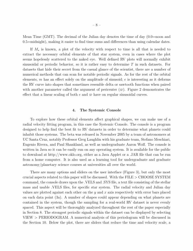
There are many options and sliders on the user interface (Figure 3), but only the most

crucial aspects related to this paper will be discussed. With the FILE > CHOOSE SYSTEM

command, the console draws upon the .VELS and .SYS file, a text file consisting of the stellar

mass and usable .VELS files, for specific star system. The radial velocity and Julian day

values are plotted against each other on the y and x axis respectively with error bars placed

on each data point (3a). A number of shapes could appear depending on what planets are

contained in the system, though the sampling for a real-world RV dataset is never evenly

spaced. This aspect will be thoroughly analyzed throughout the rest of the paper especially

in Section 8. The strongest periodic signals within the dataset can be displayed by selecting

VIEW > PERIODOGRAM. A numerical analysis of this periodogram will be discussed in

the Section 10. Below the plot, there are sliders that reduce the time and velocity scale, a

– 9 –

great tool for examining closely knit clusters of points. Below that, in the bottom half of

the UI, there are rows of 5 different sliders, each one associating with an orbital element

of a single planet(from left to right): period, mass, mean anomaly (M), eccentricity, and

argument of pericenter (3c). Varying these parameters will alter the theoretical curve as

well as the Orbital View, a window displaying the physical appearance of the system (3d).

A small window outside of the console, entitled Palette, gives the fit properties including

the goodness fit variable (χ2) (3e). The small circles to the right of each slider polishes

that parameter to give the smallest χ2. While the lowest value for χ2 might not necessarily

imply the correct properties of that system, there are active forums where users can compare

results from the console and contribute to a better understanding of these systems.

Fig. 3.— The user interface for the Systemic Console. (a) Plot of radial velocity [m/s] vs. time [JulianDays]. (b) Selection tab for integration method. (c) Various sliders for orbital elements. Each row representsa different planet. (d) The orbital view of the fitted system. This properties of this image will change as theorbital parameters are varied. (e) The separate window, Palette. The top number is the goodness of the fit,χ2.

– 10 –

Depending on how the true nature of the system is constructed, there are a number of

integration methods available. Some methods, such as Runge Kutta or 4th Order Hermite,

can account for close encounter or crossing orbits (3b). Because these methods are compli-

cated and mathematically much more rigorous than a Simple Keplerian Integration, it takes

considerably longer to perform such fits, but the result will be much more accurate. Once

the user is satisfied, the fitting can be saved into a .FIT file, incorporating all the information

needed to redo the fitting, including the .VELS file used, M?, and orbital elements of each

planet. This way, fits can be uploaded and modified if need be.

5. Synthetic Radial Velocity Datasets

With over 340 known planets today and a threshold crossing into terrestrial territory,

we can begin to make predictions to what we will see in the future as well as determine what

stars are worth looking at in hopes of finding rocky planets. It hasn’t been until these last

couple of years where planets on the order of an Earth mass have been discovered, and we

would ultimately love to hunt for Earths in habitable zones, a narrow orbital band in every

star system ideal for supporting multicellular life (also referred to as the Goldilocks Zone,

because it is “just right”). The number of telescopes in the world, and time to observe for

that matter, is limited, so for the impatient, we can do the next best thing: simulate two

years worth of data in a fraction of a second.

The program essentially makes theoretical planetary systems by constructing artificial

.VELS files that span a maximum of two years using a Monte-Carlo routine, a method that

relies on random draws to perform and yield results. In order to determine what planets

inhabit such a dataset, we begin with an empty extrasolar system of 1 M and determine

what planets to tack on through a three step process.

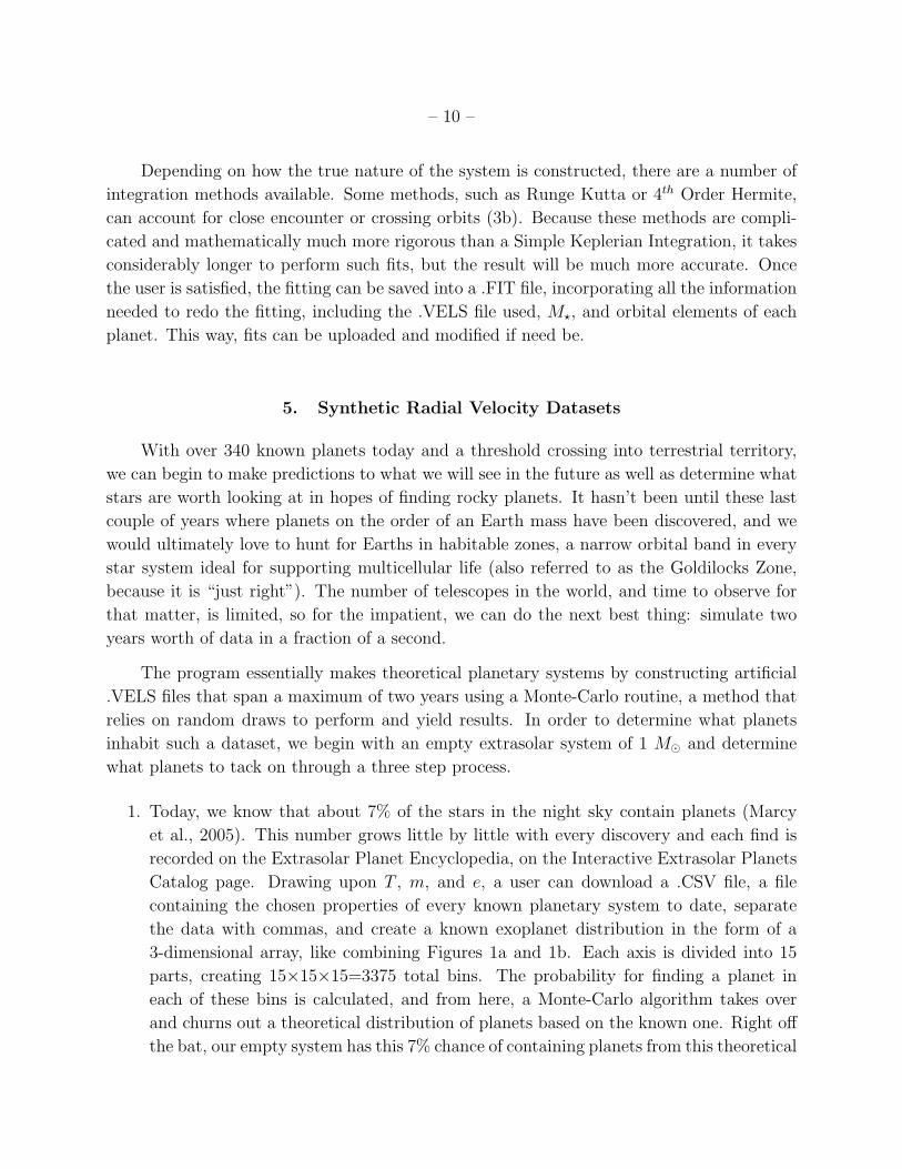
1. Today, we know that about 7% of the stars in the night sky contain planets (Marcy

et al., 2005). This number grows little by little with every discovery and each find is

recorded on the Extrasolar Planet Encyclopedia, on the Interactive Extrasolar Planets

Catalog page. Drawing upon T , m, and e, a user can download a .CSV file, a file

containing the chosen properties of every known planetary system to date, separate

the data with commas, and create a known exoplanet distribution in the form of a

3-dimensional array, like combining Figures 1a and 1b. Each axis is divided into 15

parts, creating 15×15×15=3375 total bins. The probability for finding a planet in

each of these bins is calculated, and from here, a Monte-Carlo algorithm takes over

and churns out a theoretical distribution of planets based on the known one. Right off

the bat, our empty system has this 7% chance of containing planets from this theoretical

– 11 –

distribution, so we are not drawing upon the same planets every run. The distribution

is still young and grows with every find, so the file often needs to be redownloaded

to account for new or updated planet discoveries. The most recent .CSV file for this

project was used on February 14th, 2009. Just like many of the known systems, most

of these datasets contain 1 − 2 planets and very rarely do we encounter a 3+ planet

system.

2. A fairly recent paper (Mayor et al. 2008) was published on the discovery of three

Super-Earths orbiting the star HD 40307. At the end of the paper, Mayor inquires the

frequency of Neptunes or Earths orbiting stars about as massive as our own (G and

K dwarfs). He estimated, based on the HARPS high-precision survey, a frequency of

30±10% with orbits shorter than 50 days. Though this is a rather large range, Neptune

mass planets are only just coming within our detectable threshold, so this estimation

has been implemented as the second step of the program: every system has a 30±10%

of a chance of obtaining a Neptune mass planet, which I define to be in the range of

10 and 20 M⊕ (Neptune is about 17 M⊕).

3. The last, yet probably the most interesting, step in generating these planetary systems

is the Astrobiology Knob. As one of the ultimate goals in planet hunting, we wish

to find terrestrial planets and, furthermore, planets capable of supporting intelligent

life. Since we are uncertain of the abundance (or lack thereof) of extrasolar planets,

the final step is an optimism parameter, a variable probability of 1 − 10 M⊕ planets

existing. Details behind this variable meter will be broken down in Section 9.

In the last two steps, the period (0 to 1000 days) and eccentricity (0 to 1) are randomly

generated on a logarithmic probability scale. With this, most orbits should fall under 50 days

and be roughly circular but will certainly not discount the possibility of large periodic orbits

or highly eccentric ones. If, by chance, our star system remains empty after the three steps,

the system is rerun through the program until at least one planetary companion is found.

As of now, the result, after running through the three steps, is a batch of 100 synthetic

planetary systems, each consisting of a .VELS, .SYS, and text file containing the orbital

properties of each planet, much like the .FIT file. Rerunning the entire program will simply

write over the previous set of systems. With these tools at hand, we can begin to examine

these simulated systems and discuss what strategies to use to find those planets currently

invisible to us. The .VELS dataset calculations will be discussed in the following section. A

couple noteworthy multi-planet systems generated through this program, testsystem18 and

testsystem69, will be investigated in each section. Their orbital elements are contained in

Table 1.

– 12 –

Table 1: Orbital Elements of Two Synthetic Planetary Systems

Planet T (days) m (MJ) M0 () e $ ()

testsystem18a 9.3953 0.0534 117.6178 0.2539 213.3232

testsystem18b 199.7527 0.0174 183.8270 0.0003 260.9201

testsystem69a 1.5046 0.0063 51.0006 0.2811 153.0978

testsystem69b 4.5826 0.0551 313.2331 0.1443 215.5691

testsystem69c 26.8316 0.5029 177.8364 0.0132 299.3562

testsystem69d 236.0574 0.9512 334.5467 0.2726 324.2928

6. Equations of Motion

The properties of a planet can be decomposed into seven orbital elements. Several of

these elements have already been discussed: the orbital period (T ) (which is commonly used

in place of the semi-major axis (a)), eccentricity (e), and mass of a planet (m), which all

affect the radial velocity of its parent star. For an orbit in space, the argument of pericenter

(ω), inclination (i), and longitude of ascending node (Ω) represent angular shifts along each

axis in Cartesian space, as shown in Figure 4.

Fig. 4.— A diagram representing how the argument of pericenter (ω), inclination (i), and longitude ofascending node (Ω) shift an orbit in space, where the Y-axis is the reference direction.

– 13 –

The last element references where along the elliptical trajectory the planet resides, and

there are three variables that can be used. The true anomaly (ν) is the angle at which

a line connecting a point on the ellipse and focus makes with the semi-major axis. If we

consider circumscribed circle concentric with our ellipse and draw a line perpendicular to

the semi-major axis, through the orbital point, and ending on the circle itself, we can call

the angle this point makes with the center of the ellipse the eccentric anomaly (E). A clear

visual for these two angles is shown in Figure 5. The mean anomaly (M) is not a physical

angle, but it is easy to work with in that it scales linearly with time. M0 would be position

of the planet at the chosen epoch. There is a very nice boundary condition that f = E = M

for any integer multiple of π and at any time for circular orbits (e = 0), as will be made

apparent shortly.

Eν

F

Orbit

Circumscribed Circle

a

O

Fig. 5.— A circle, circumscribed and concentric with the orbital ellipse with focal point F , and the relationbetween the true anomaly, ν, and eccentric anomaly, E.

We begin this derivation by considering a star-planet pair with the equation of an ellipse

and equations provided exclusively by Murray & Dermott (1999).

r =a(1− e2)

1 + e cos(ν)(2)

As the resulting case for the 2-body problem, both orbits mirror each other about the center

– 14 –

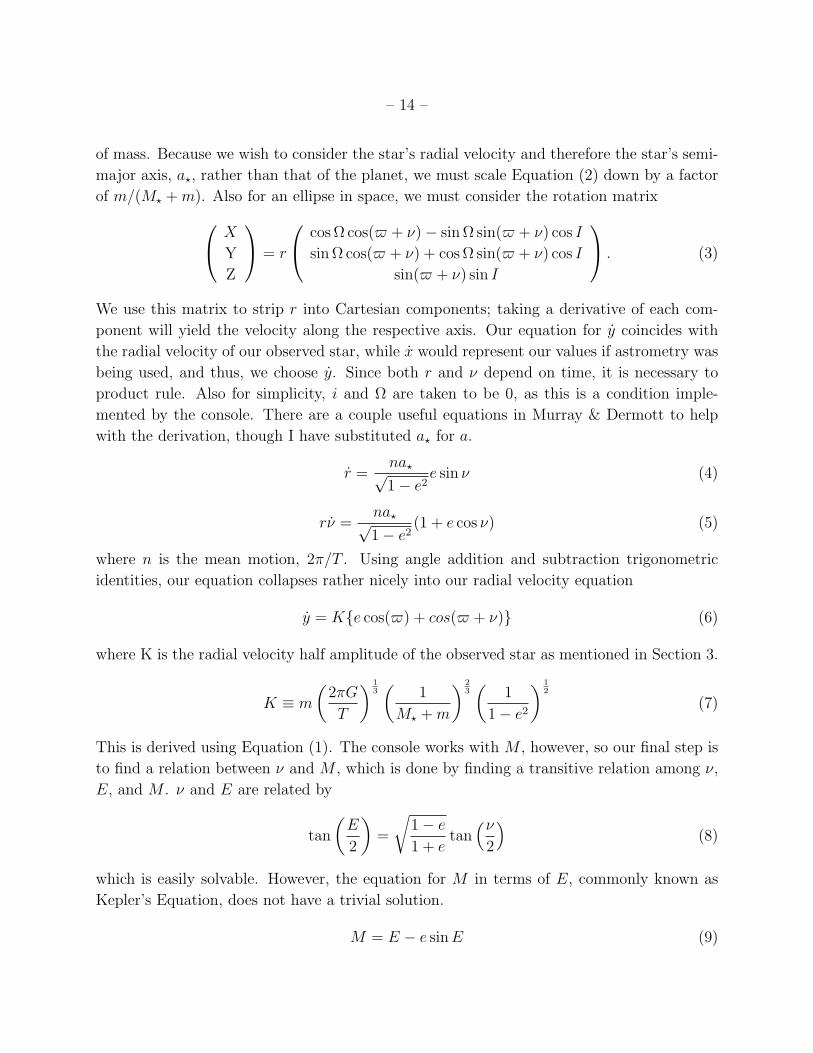
of mass. Because we wish to consider the star’s radial velocity and therefore the star’s semi-

major axis, a?, rather than that of the planet, we must scale Equation (2) down by a factor

of m/(M? +m). Also for an ellipse in space, we must consider the rotation matrix X

Y

Z

= r

cos Ω cos($ + ν)− sin Ω sin($ + ν) cos I

sin Ω cos($ + ν) + cos Ω sin($ + ν) cos I

sin($ + ν) sin I

. (3)

We use this matrix to strip r into Cartesian components; taking a derivative of each com-

ponent will yield the velocity along the respective axis. Our equation for y coincides with

the radial velocity of our observed star, while x would represent our values if astrometry was

being used, and thus, we choose y. Since both r and ν depend on time, it is necessary to

product rule. Also for simplicity, i and Ω are taken to be 0, as this is a condition imple-

mented by the console. There are a couple useful equations in Murray & Dermott to help

with the derivation, though I have substituted a? for a.

r =na?√1− e2

e sin ν (4)

rν =na?√1− e2

(1 + e cos ν) (5)

where n is the mean motion, 2π/T . Using angle addition and subtraction trigonometric

identities, our equation collapses rather nicely into our radial velocity equation

y = Ke cos($) + cos($ + ν) (6)

where K is the radial velocity half amplitude of the observed star as mentioned in Section 3.

K ≡ m

(2πG

T

) 13(

1

M? +m

) 23(

1

1− e2

) 12

(7)

This is derived using Equation (1). The console works with M , however, so our final step is

to find a relation between ν and M , which is done by finding a transitive relation among ν,

E, and M . ν and E are related by

tan

(E

2

)=

√1− e1 + e

tan(ν

2

)(8)

which is easily solvable. However, the equation for M in terms of E, commonly known as

Kepler’s Equation, does not have a trivial solution.

M = E − e sinE (9)

– 15 –

There are multiple ways to solve this, though I stuck with a simple iterative method. We

can define a function f(E).

f(E) = E − e sinE −M (10)

Setting f(E) equal to 0 is the same as simply subtracting M from both sides of Equation

(9), but this definition for f(E) allows us to perform Newton-Raphson iterations to solve for

E in terms of M .

Ei+1 = Ei −f(Ei)

f ′(Ei)(11)

where f ′(Ei) = df(Ei)/dEi = 1− e cosEi. In order to begin these iterations, we must begin

with a suitable E0. A good approximation for near circular orbits is E0 ∼ M0, but this

breaks down for significant eccentricities. In order to consider this, we can better guess our

starting point by modifying our approximation.

E = M + sign(sinM × ke) (12)

where k is a constant which Murray & Dermott recommend to be 0.85. Since we wish to

parameterize M , simply substitute M0+2πt/T for M . The result is a mess on paper, but less

than ten iterations will get accuracy one part in 10−15, a more than decent approximation

for this project.

Now that we have derived the radial velocity equation in terms of the Systemic Con-

sole’s variables, we can create our synthetic datasets. The RV curve for testplanet18 and

testplanet69 are shown in Figures 6(a) and 6(b) respectively. The equation for y describes

radial velocity of a star with a single planet orbiting it. For more interesting 2+ planet

systems, there are more suitable integration methods for more accurate fits. However, I have

chosen to only consider multi-planet systems in which the planets have negligible gravita-

tional interaction, meaning I will use a Simple Keplerian Integration. All that this entails is

calculating y of each star-planet pair and adding them together at every timestep. Therefore,

our final equation for y for N bodies (with central body m0=M? and N − 1 planets orbiting

M?) in terms of ν is a simple summed version of Equation (6).

y =N−1∑

1

Kj (ej cos($j) + cos($j + νj)) (13)

This may change in a future update, but that will be addressed in Section 12. The velocity

is then perturbed by noise equal to a number near the threshold, around 3-6 m/s, times a

draw from a Gaussian distribution. The starting time and date should have no effect on a

dataset’s periodogram, so I arbitrarily assigned it to the Winter Solstice of 2000, December

21st 2000, at noon GMT (2451899.500 in Julian Days).

– 16 –

-25

-20

-15

-10

-5

0

5

10

15

20

25

2451900.0 2452100.0 2452300.0 2452500.0

Rad

ial V

eloc

ity [m

/s]

Time [Julian Days]

(a)

-80

-60

-40

-20

0

20

40

60

80

2451900.0 2452100.0 2452300.0 2452500.0

Rad

ial V

eloc

ity [m

/s]

Time [Julian Days]

(b)

Fig. 6.— Radial velocity plots of (a) testsystem18 and (b) testsystem69. Neither show any apparentsinusoidal trend.

7. Stability

For astrobiological purposes, it is best that the terrestrial planets we hope to find orbit

in a somewhat stable manner. In a recent paper, Batygin & Laughlin (2008) showed the

Solar System may not be as stable in the long term as we once thought. Much of the

paper discussed the fate of the terrestrial planets, especially Mercury due to its low mass

and relatively high eccentricity, since the gas giants were undisturbed by any chaotic nature

– 17 –

in the extremely long run. Possible outcomes included Mercury spiraling into the Sun,

Mercury getting ejected from the Solar System, and Mercury colliding with Venus resulting

in Mars’s ejection, all happening before the Sun reaches its Red Giant phase. This was found

using synthetic secular perturbation theory, where a planet, Mercury, in resonance with a

more massive planet, in this case Jupiter, becomes increasingly unstable over the course of

hundreds of millions of years. Though this might be important in determining the outcome

of extrasolar systems, we know the bodies of the Solar System to a much higher precision

and can account for every minor change over a large timespan. Also, the Solar System has

been stable enough since it first formed to have had intelligent life form on Earth, so we wish

to look for extrasolar systems that will not produce any immediate chaotic nature, arguing

in favor for a Simple Keplerian form of behavior.

It is important to know how the mutual gravitational fields of multiple planet systems

may complicate the development of life. In one extreme, the gravitational interaction between

two planets may cause overlaps in their orbits, commonly called a crossing orbit. They are

not uncommon occurrences in nature; Neptune and Pluto exchange radial positions in the

Solar System every few hundred years. Planets with such close interactions with other large

objects would not be ideal places for life to develop. Though some such worlds out there may

be lucky enough to harness multicellular organisms, we would have better odds finding life

on a planet whose orbit is not significantly perturbed for a very long time. The calculation

for crossing orbits is simple: the periastron of a larger semi-major axis must be smaller

than the apastron of the smaller semi-major axis. In mathematical terms, this means that

a0(1 + e0) < a1(1− e1). It is possible to disobey this rule and still have a non-crossing orbit,

one unlikely example being two focal centric ellipses of equal e and approximately equal $

(almost like the vertical cross section of two Russian Nesting Dolls).

However, two orbits do not need to cross in order to induce eventual chaos. Simply

being close to each other will trigger the gravitational fields between two planets. So now

we must ask: how close can we bring two planets together before their mutual gravitational

interaction is no longer negligible? It would certainly have to depend on the mass of both

planets as well as their respective semi-major axes. Gladman (1987) derived the equation

for a critical close encounter.

4 > 2.4

(m1 +m0

M?

) 13

(14)

that is, the percent difference in the semi-major axes, 4, must be greater than some value

that is dependent on both the planetary and stellar masses in order to consider their mutual

gravitational interaction non-significant. This equation might seem confusing at first, since

it does not account for eccentricity. It only considers near circular orbits and will break

down if significant eccentricities are involved. I modified the equation a bit by substituting

– 18 –

Fig. 7.— The orbital views of (a) testsystem18 and (b) testsystem69 to scale. Refer to Table 1 for theorbital properties.

a0(1 + e0) for a0 and a1(1 − e1) for a1, that is replacing the larger semi-major axis with

its orbital periastron and the smaller one with its apastron. This new equation essentially

accounts for the “worst case close encounter scenario” and treats highly eccentric orbits as

circular ones at the supposed extremes. In turn, this may create a stability band between two

planets, a zone where an orbiting planet below some critical mass would be gravitationally

unaffected by any neighboring planets in the short run. This stability clause is implemented

– 19 –

for all three steps of the program, so if more than two planets are present, then it will

consider every possible pair of planets to ensure a non-interacting system. The overhead

orbital views of the two selected synthetic systems are shown in Figure 7.

8. Uneven Time Sampling

Since stars are only viewable during certain times of the year (and day, for that matter),

the radial velocity datasets are not smooth, evenly distributed curves. The error for each

data point depends partially on where the target star is relative to the horizon; the lower

on the horizon, the greater the error, since the light is traversing through more atmosphere

to reach the observer. One condition for these datasets is that as long as our target star is

not too low on the horizon (> 25), we can assume our observed data during that time are

usable. An observer’s position on the Earth, in latitude and longitude, will also affect ob-

servation times, so in order to make these datasets as realistic as possible, we must simulate

plausible observing situations. By treating the Earth as a stationary object, we can create

a 2-dimensional clock, with the Earth in the center and fixed at some latitude and longi-

tude (which for creating these datasets, I made our very own Lick Observatory, 3720′35′′N

12138′14′′W), where the Sun revolves every 24 hours and the position of the target star

every 24 hours and 4 minutes (since any point in the sky moves approximately 2 hours every

month). As time goes on, our datasets will have giant gaps where no data was taken for that

point on the Earth, which is entirely expected and consistent with the current, real datasets.

As long as the target star lies within a conal field of view of 130, which comes from being

25 above the clock’s diameter in both directions (roughly 10 and 2 o’clock), and the Sun is

outside this view, then that data point is usable. In the clock model, we consider the radius

of the Earth to be negligible compared to the Earth-star distance on the celestial sphere, so

an angle made with respect to the diameter of the clock and one made with respect to a line

tangent to the surface of the Earth are approximately equal. However, we must put further

restrictions on the location of the Sun, as it requires some time to move below the horizon

for the sky to fade to black. Two hours after sunset (30), on most parts of the Earth, is

generally enough time this to happen. For these conditions to work at all, our target star

must be assigned a declination and right ascension on the range of −90 to +90 and 0 to 24

hours respectively. If by chance the star is never within viewing range, the program simply

restarts from the beginning without writing any output files for that system.

Other factors that prevent data taking may include administrative problems or financial

insufficiencies, but weather is something out of human control. Observatories are normally

placed in the most optimal environments for data taking, usually atop a large mountain or a

– 20 –

dry area with little or no nearby sources of light pollution. However, rainstorms, snowstorms,

or any form of strong atmospheric turbulence can shut down an entire night of observation.

Our very own Lick Observatory in the Diablo range east of San Jose reports about 300

clear nights per year (82%) on average. The weather patterns vary all over the world, so

this program incorporates a good weather probability, a percent chance for an observable

night. For all other problems that may delay or disrupt observation and can not be easily

programmed, I created a variable timestep, beginning with one day and tacking on a draw

from the absolute value of a Gaussian distribution. This will create an even more uneven

data distribution without any accidental backwards timesteps.

Cadances are the last factor contributing an uneven sampling. In many cases, observers

are allotted enough telescope time to take multiple data points. The advantage is that the

relative error decreases by a factor of the square root of the number of data points taken.

However, one obvious trade off is that this makes it difficult to view multiple stars in one

night. In the code, every observation time has a chance to enter a cadance stage, where

another data point is taken 10 minutes after the initial one. It is not uncommon to find four

data points in a row in a real dataset. Cadanced data is especially helpful in finding highly

eccentric planets, when the radial velocity of the star suddenly spikes upward or downward

such as Figure 2d. This may seem like a lot of effort to create unevenly spaced data, but it

is important to account for as many outside effects as possible to ensure the periodograms

behave as they would with a real dataset.

9. The Astrobiology Knob

Wolszcan & Frial (1992) were responsible for finding the first terrestrial planets. The

two planets circularly orbiting the pulsar PSR B1257+12 were on the order of a few Earth-

masses, and this predated the discovery of 51 Pegasi b! However if we ultimately want to

find extraterrestrial life, intelligent or not, it is in our best interests to find terrestrial planets

that orbit actual main sequence stars. When a hefty list of Earth-mass planets is eventually

compiled, we can begin to filter out those in inhabitable systems and carefully study those

that satisfy habitable zone conditions. Though a fair number of Earth-mass bodies have

already been discovered and cataloged, it is still unknown how common terrestrial planets

are. For that, we can consider a variable meter for our confidence that terrestrial planets

exist in other star systems. Enter the Astrobiology Knob (ABK).

There are two well defined boundary conditions for the ABK: when the meter is set to

0, then the chance that we find terrestrial planets is essentially null. If the ABK is cranked

up to 10, nearly every star system will contain an Earth or Super-Earth. Thus, we can say

– 21 –

the probability of detecting these planets at the mentioned settings is 0 and 1 respectively.

There has to be some function that satisfies these conditions, in the domain 0 to 10, but there

are several to choose from. Linear? Exponential? Logarithmic or an N root? Even then,

there are theoretically an infinite number of functions for each of these categories that could

fulfill the boundary conditions. Nonetheless, there is actually a safe choice that considers

most graphical shapes.

0

0.1

0.2

0.3

0.4

0.5

0.6

0.7

0.8

0.9

1

0 1 2 3 4 5 6 7 8 9 10

AB

K(X

) (P

roba

bilit

y of

Get

ting

Ter

rest

rial P

lane

t)

X (Astrobiology Knob Setting)

Fig. 8.— The Astrobiology Knob Function. A list of values is charted in Table 2.

f(x) =1√

2πσ2exp

(−(x− µ)2

2σ2

)(15)

Simply put, this is the equation for a Gaussian distribution, sometimes called a probability

density function. The plot of this function contains linear, concave up, and concave down

chunks. By simply altering the standard deviation, σ2, mean, µ, and scale of the Gaussian

in the proper manner, we can obtain any reasonable graphical shape we desire. The function

for my ABK is as follows:

ABK(x) =9√18π

exp

(−(x− 12)2

18

)(16)

– 22 –

The values for σ2 and µ are 9 and 12 respectively, and the function was scaled by a factor

of 9 as well. The graphical representation for this function is shown in Figure 8. There

were a few reasons for choosing this shape. It roughly satisfies the boundary conditions with

ABK(0) ≈ 4× 10−4 and ABK(10) ≈ 0.958. Now consider the number 5, a confidence right

between complete pessimism and optimism. If the function was linear, ABK(5) would lie at

50%. Is this a reasonable value or should it be different? In the latter case, should the value

be higher or lower?

Table 2: Astrobiology Knob Values

Setting (X) Probability (%)

0 0.040

1 0.144

2 0.463

3 1.330

4 3.419

5 7.867

6 16.20

7 29.84

8 49.20

9 72.59

10 95.83

In my personal opinion, a value much lower than 0.5 suits this probability distribution

better. If half of all observable stars contain at least one terrestrial planet, and considering

that less than 10% of all known star systems contain detectable planets, that is certainly

good news for the extrasolar community, at least an 8 on the ABK. Furthermore, the great

thing about Gaussian distributions is that they are easily manipulable. By shifting the

Gaussian parameters around, it is possible to make an entirely different function that also

roughly obeys the boundary conditions. If I wish to change the ABK function on a whim,

I simply assign new parameter values without having to rewrite the entire function itself.

Table 2 shows the ABK at integer values from 0 to 10. I have tinkered with the ABK values

to explore different outcomes, but the batch that created testsystem18 and testsystem69,

the ABK was set at 7, not for any particular reason.

– 23 –

10. The Lomb Scargle Periodogram

Data hardly ever come in convenient distributions, especially in astronomy. Telescope

time is expensive, and even with exclusive access to an instrument, daytime inevitably arrives

and prevents sampling all together. Examining the timesteps of any .VELS file, it is readily

apparent that the data points are often clumped together while others are randomly scattered

throughout the dataset with no real consistent pattern, making it hard to determine the

shape of the graph, and thus, the orbital periods of possible planetary inhabitants.

With our observed velocities, Xj, we can find both the mean and variance of our dataset,

since they are independent of time, given by

X =1

N

N∑Xj (17)

and

σ2 =1

N − 1

N∑(Xj − X) (18)

respectively, where N is the number of data points.

In 1982, Scargle developed a specialized method in accounting for uneven sampling using

his Lomb-Scargle Periodogram, which we will use to investigate the amorphous RV plots that

are testsystem18 and testsystem69. The equation for the normalized periodogram is

PN(ω) =1

2σ2

[∑N(Xj − X) cosω(tj − τ)

]2∑N cos2 ω(tj − τ)

+

[∑N(Xj − X) sinω(tj − τ)]2

∑N sin2 ω(tj − τ)

(19)

where tj is the associated observation time in Julian Days and ω is just 2π/T , which is a

substitution we would like to make in order to view the power spectrum vs. the period rather

than the frequency. The variable τ , defined by

τ =1

2ω

∑N sin 2ωtj∑N cos 2ωtj(20)

allows our sampling to be invariant of time. If all the values for Xj and the sampling were

fixed, then the starting time should not affect the appearance of the periodogram. These

equations might be perplexing at first, because they are independent of error. Wouldn’t one

think that the quality of a data point should affect the periodogram itself? The problem

with the above equations is that they are only valid for equally weighted data. Gilliland &

Baluinas (1987) describe a modified version of the LS Periodogram to account for unequal

– 24 –

weights.

Px(ω) =N

2∑N Wj

[∑N XjWj cosω(tj − τ)

]2∑N XjWj cos2 ω(tj − τ)

+

[∑N XjWj sinω(tj − τ)]2

∑N XjWj sin2 ω(tj − τ)

(21)

whereWj are the individual weights calculated by the inverse error squared. τ is also modified

a little bit.

τ =1

2ω

∑N Wj sin 2ωtj∑N Wj cos 2ωtj(22)

If all the weights are the same, they end up canceling, which returns a non-normalized

version of Scargle’s original periodogram. To normalize Px, simply divide by σ2. As we

sweep through different values of ω (for our case, T ), we see various peaks where the function

begins to resonate with the data sampling; a significant resonance at some value of T will

yield a notable peak, which could imply a planet with such orbital period. Though due to

the uneven sampling, some of these peaks may simply be the sum of a periodic signal and

pure Gaussian noise (Press et al., 1992), but this is something we can be tested. We can

ask if there is a chance that noise fluctuations are responsible for generating these peaks. It

would be convenient to have some quantitative way of verifying the significance of any peak.

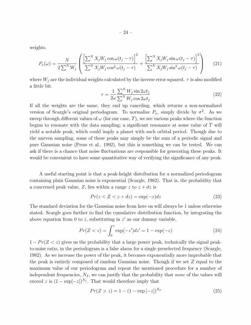
A useful starting point is that a peak-height distribution for a normalized periodogram

containing plain Gaussian noise is exponential (Scargle, 1982). That is, the probability that

a concerned peak value, Z, lies within a range z to z + dz is

Pr(z < Z < z + dz) = exp(−z)dz (23)

The standard deviation for the Gaussian noise from here on will always be 1 unless otherwise

stated. Scargle goes further to find the cumulative distribution function, by integrating the

above equation from 0 to z, substituting in z′ as our dummy variable.

Pr(Z < z) =

∫ z

0

exp(−z′)dz′ = 1− exp(−z) (24)

1−Pr(Z < z) gives us the probability that a large power peak, technically the signal peak-

to-noise ratio, in the periodogram is a false alarm for a single preselected frequency (Scargle,

1982). As we increase the power of the peak, it becomes exponentially more improbable that

the peak is entirely composed of random Gaussian noise. Though if we set Z equal to the

maximum value of our periodogram and repeat the mentioned procedure for a number of

independent frequencies, Nf , we can justify that the probability that none of the values will

exceed z is (1− exp[−z])Nf . That would therefore imply that

Pr(Z > z) = 1− (1− exp [−z])Nf (25)

– 25 –

0

2

4

6

8

10

12

1 10 100 1000 10000

Pow

er S

pect

rum

Period (Days)

(a)

0.01

0.050.1

0.5

0

2

4

6

8

10

12

1 10 100 1000 10000

Pow

er S

pect

rum

Period [Days]

(b)

0.5

0.10.05

0.01

Fig. 9.— Normalized LS Periodograms of testsystem18 that are (a) unweighted and (b) weighted alongwith several FAP values. The signal for 18a remained strong after weighting, but 18b refuses to show itself.

This equation is the “false alarm probability”, commonly referred to as the FAP. Basically,

this is the chance that peak just as high or higher than our target peak happens to appear in

the periodogram due to the Gaussian noise (a false alarm), so if the FAP is small, it means

the peak in question is highly legitimate. We can calculate the FAP once a number for Nf

is known, though this is not as trivial as it sounds.

Finding Nf can be tricky. To begin, Nf will never come out exactly the same every

time it is calculated, which will be made apparent when the derivation method is discussed.

However, this may not even be that important: how precisely do we need to know Nf? We

can approximate small values of the FAP by expanding (1− exp [−z])Nf .

Pr(Z > z) ≈ Nf exp(−z) (26)

– 26 –

0

2

4

6

8

10

12

1 10 100 1000 10000

Pow

er S

pect

rum

Period (Days)

(a)

0.01

0.050.1

0.5

0

2

4

6

8

10

12

1 10 100 1000 10000

Pow

er S

pect

rum

Period [Days]

(b)

0.5

0.10.05

0.01

Fig. 10.— Normalized LS Periodograms of testsystem69 that are (a) unweighted and (b) weighted withthe same significance levels as Figure 9. 69b and 69c gain signal strength after weighting, while 69d shranka minor amount. Even as close as 69a is, it too shies away due to its low K.

Due to the nature of our function, the FAPs would be evenly spaced on a logarithmic scale

if we kept Nf fixed. Answering our question, Nf does not have to be very accurate, since

the exponential is the dominant variable for the FAP.

There are a number of methods to calculate Nf , though the program utilizes a simple

Monte-Carlo routine as described by Press et al., 1992. This is done by keeping the data

sampling times fixed and replacing the RV values with Gaussian noise. We attain the highest

peak value from each periodogram and repeat the process for as many times as there are data

points, eventually obtaining N numbers. These numbers are then compiled into a histogram

and normalized, so the area under the curve yields unity, which is done by dividing by N.

This is fit to Equation (25) for different values of Nf using a χ2 test, associating our Nf with

– 27 –

the lowest value of χ2.

Figures 9 and 10 display the effects of both weighting and not weighting normalized

LS Periodograms for testsystem18 and testplanet69 respectively along with several FAPs

for various peaks. With all the nitty-gritty mathematics done, we examine our FAP values

and determine which peaks are worth analyzing. If the FAP value for a hypothetical peak

is determined to be 0.5, it would insinuate that the peak is a coin flip’s chance of being

legitimate. Strong signals typically have FAPs that are less than 0.01.

11. Results and Analysis

Generating these batches of planetary systems spawns some interesting talking points,

though first, it would be best to provide a quick summary of what was done. Using a Simple

Keplerian Integration method, we can create sets of 100 non-interacting planetary systems

in less than a couple seconds per run. These systems are based on the known exoplanet

distribution, Mayor’s prediction on the possible number of Neptune-mass planets, and a

variable confidence in the abundance of terrestrial planets embodied by the Astrobiology

Knob. A Lomb-Scargle Periodogram was also written into the program to aid in the detection

of periodic signals that are hard to eyeball.

In one random batch atABK(7), I chose two particularly interesting systems. testsystem18

contains two planets: a ≈1 Neptune-mass planet (18a) on an orbit a little more than a week

and a ≈5.5 M⊕ planet (18b) with an orbit a bit less than Venus (224.7 days). The eccentric-

ity of the former is on par with that of Mercury while the latter is almost a perfect circle,

but they are hardly close enough to even refer back to Equation (14). testsystem69 is a

4-planet system comprised of two from the distribution (69c and 69d), both under MJ and

almost in 1:2 resonance, another 1 Neptune-Mass (69b), and a 2 M⊕ planet (69a) with a

36 hour orbital period. The smallest two both have unignorable eccentricities, yet they are

unusually non-interacting. Using Equation (14), 4 must be above ≈9.32%, which is due to

their relatively low masses, and even if the difference in their argument of pericenters was

180 so their orbits would eventually have the greatest close encounter, 4 would still be over

4 times the necessary orbital separation. This demonstrates how undetected Earths may be

happily residing in stability bands of an already well known exoplanetary systems.

Though their RV plots look rather scattered, their respective Lomb-Scargle Periodograms

both depict some interesting behavior. The strongest peak in testsystem18 resides where

18a should be, but 18b, due to its smaller mass and greater orbital period, is obscured by

noise and unable to be detected. testsystem69 should show stronger signals due the two gas

– 28 –

giants inhabiting the system, but its periodogram is rather noisy in the < 10 day region.

There are many peaks in the range of 1-10 days especially between 1 and 2, since these can

be in resonance with the true periods of the system. This makes it hard to find planets on

orbits less than a week long in a multiple planet system. 69b is slightly heavier and closer to

its parent star than 18a, so its peak should be apparent and well defined, which it is though

its uncomfortably close to a supposed ∼6 day entity, which we know is a false alarm peak.

Though 69a is much, much closer to its host star than 18b, its peak is still absent. We can

refer back to Equation (7) to calculate that K for 69a is barely above 1m/s; though our

incapability in detecting these boiling hot rocks seems quite demoralizing, this could imply

an abundance of extremely short orbit Earth-mass objects that have yet to be exposed. Yet,

one would have to take at least 10 cadenced observations in order to cut the relative error

down to a third. Alone, lots of data points will not flush out these terrestrial planets from

the dataset; there must be technological advancements as well that continue to lower the

threshold. Even if two .VELS files can never fully describe the overall portrait of extrasolar

planets, this is merely an example of the potential this tool has to describe possible systems.

12. Future Updates

Not every nearby star has been surveyed yet. The Extrasolar Planet Encyclopedia

will continue to grow and eventually become a well defined distribution. Hopefully this

program will provide the extrasolar community with a means of understanding how various

time samplings affect LS Periodograms and what other planets could exist in an already

discovered system. At the moment, I am working with Stefano Meschiari to build a user

interface that will probably look similar to the Systemic Console. Furthermore, there are a

few interesting ideas that could further improve upon this program for future updates.

Many of the RV datasets need something more than just a Simple Keplerian Integration.

We are bound to discover more systems that inhibit mutual gravitational interactions and

that require much more mathematically tedious and time consuming integrations such as

Runge Kutta. In order to consider such a situation, it is necessary to dismantle the current

equations of motion and stability clauses and make way for an interacting N -body map, most

likely in Jacobian coordinates. A detailed explanation is provided by Murray & Dermott, so

I will only briefly discuss the setup for the mapping.

Consider an N body problem composed of a central object of mass m0, in this case M?,

and N − 1 planetary bodies m1, m2,...,mn−1. Now consider the position vector of mi, ri,

with respect to some arbitrary origin, O. The position vector of the center of mass, with

– 29 –

respect to O, for all the bodies up to the index i is given by

Ri =1

ηi

i∑j=0

mjrj (27)

where ηi is the total mass up to the ith body. RN−1 would denote the barycenter for the

entire system. A vector denoting the position vector of the mi with respect to the mi−1, ...,m0

system center of mass is given by

ri = ri −Ri−1 (28)

The radial velocity trend would not follow a regular Keplerian Method like the program

currently employs, but it will account for constantly changing position vector of the center

of mass as the planets orbit M?. This already considers gravitational interactions between

planets, but then a new set of stability clauses must be erected and obeyed to prevent possible

collisions or ejections.

As more discoveries are made, it is possible that we find many systems like HD 40307,

where every known planet contained within the system on the order of M⊕. However, the

ABK only can apply a single terrestrial planet and still needs a method to account for a

possible multiple terrestrial planet system. I plan to implement the “11” option, which is

ABK(10) with an extra kick! It incorporates the added effect of a system possibly containing

2+ terrestrial planets. As the known terrestrial planet distribution builds upon itself, we

can modify the ABK to exclusively assign habitable planets, a more narrow set of terrestrial

planets where conditions are comparable to that of Earth.

Finally, there is extensive code already written that takes an already well known plan-

etary system and inserts Neptunes and Earths into possible stability bands. This works

exactly like the program at hand, but rather than drawing random planets from the theo-

retical distribution, it considers actual planetary systems themselves. In the end, a hybrid

planetary system, composed of the real system and various synthetic low mass planets, is

created, where upon the user can find how the added Earths alter the original periodogram

and determine whether the system is worth further study.

I thank Patrick Niemeyer and Jonathon Knudsen for their helpful book Learning Java,

as well as Professor Greg Laughlin, Professor Adriane Steinacker, and Arthur von Nagel for

helpful talks and insights. This project was funded by NSF Career Grant #AST-0449986 to

Greg Laughlin.

– 30 –

REFERENCES

Batygin K., Laughlin G. 2008, The Astrophysical Journal, 683, 1207

Gladman, B. 1993, Icarus, 106, 247

Gilliland R. L., Baliunas S.L. 1987, The Astrophysical Journal, 314, 766

Kalas et al. 2008, Science, 322, 1345

Laughlin, G.P. 2009, personal communication

Lunine et al. 2008, Report of the ExoPlanet Task Force: Worlds Be-

yond: A Strategy for the Detection and Characterization of Exoplanets,

http://www.nsf.gov/mps/ast/aaac/exoplanet task force/reports/exoptf final re-

port.pdf/

Marcy et al. 2005, Progress in Theoretical Physics, 158, 24

Mayor et al. 1995, Nature, 378, 355

Mayor et al. 2008, Astronomy & Astrophysics, 493, 639

Moutou et al. 2009, Astronomy & Astrphysics, http://arxiv.org/abs/0902.4457v1

Murray C. D., Dermott, S. F. 1999 Solar System Dynamics (Cambridge: Cambridge Uni-

versity Press)

Press W. H., Teukolsky S. A., Vetterling W. T., Flannery B. P. 1992, Numerical recipes in

C: The art of scientific computing (Cambridge: Cambridge University Press)

Scargle, J.D. 1982, Astrophysical Journal, 263, 835

Wolszczan A., Frail D. 1992, Nature, 355, 145

This preprint was prepared with the AAS LATEX macros v5.2.