a thin film fluid structure interaction model for the
TRANSCRIPT

HAL Id: hal-02472899https://hal.archives-ouvertes.fr/hal-02472899
Submitted on 10 Feb 2020
HAL is a multi-disciplinary open accessarchive for the deposit and dissemination of sci-entific research documents, whether they are pub-lished or not. The documents may come fromteaching and research institutions in France orabroad, or from public or private research centers.
L’archive ouverte pluridisciplinaire HAL, estdestinée au dépôt et à la diffusion de documentsscientifiques de niveau recherche, publiés ou non,émanant des établissements d’enseignement et derecherche français ou étrangers, des laboratoirespublics ou privés.
A Thin Film Fluid Structure Interaction Model for theStudy of Flexible Structure Dynamics in Centrifugal
PumpsAbdulaleem Albadawi, Mathieu Specklin, R. Connolly, Yan Delauré
To cite this version:Abdulaleem Albadawi, Mathieu Specklin, R. Connolly, Yan Delauré. A Thin Film Fluid Struc-ture Interaction Model for the Study of Flexible Structure Dynamics in Centrifugal Pumps. Jour-nal of Fluids Engineering, American Society of Mechanical Engineers, 2018, 141 (6), pp.500 - 600.�10.1115/1.4041759�. �hal-02472899�

A. AlbadawiSchool of Mechanical and
Manufacturing Engineering,
Dublin City University,
Glasnevin,
Dublin D9, Ireland
e-mail: [email protected]
M. SpecklinSulzer Pump Solutions Ireland Ltd.,
School of Mechanical and
Manufacturing Engineering,
Dublin City University,
Glasnevin,
Dublin D9, Ireland
e-mail: [email protected]
R. ConnollyGlobal Technology,
Pumps Equipment,
Sulzer Pump Solutions Ireland Ltd.,
Clonard Road,
Wexford Y35 YE24, Ireland
e-mail: [email protected]
Y. Delaur�eSchool of Mechanical and
Manufacturing Engineering,
Dublin City University,
Glasnevin,
Dublin D9, Ireland
e-mail: [email protected]
A Thin Film Fluid StructureInteraction Model for the Studyof Flexible Structure Dynamicsin Centrifugal PumpsThis paper describes a fluid-structure interaction (FSI) model for the study of flexible cloth-like structures or the so-called rags in flows through centrifugal pumps. The struc-tural model and its coupling to the flow solver are based on a Lagrangian formulation combining structural deformation and motion modeling coupled to a sharp interface immersed boundary model (IBM). The solution has been implemented in the open-source library OpenFOAM relying in particular on its PIMPLE segregated Navier–Stokes pres-sure–velocity coupling and its detached eddy simulation (DES) turbulence model. The FSI solver is assessed in terms of its capability to generate consistent deformations and transport of the immersed flexible structures. Two benchmark cases are covered and both involve experimental validation with three-dimensional (3D) structural deformations of the rag captured using a digital image correlation (DIC) technique. Simulations of a rag transported in a centrifugal pump confirm the suitability of the model to inform on the dynamic behavior of immersed structures under practical engineering conditions.
1 Introduction
The focus of the present fluid structure interaction (FSI) studyis the transport of immersed structures in centrifugal pumpsdesigned for waste water systems. These pumps typically need tohandle particle-laden flow but also thin flexible cloth-like struc-tures or the so-called rags. Their accumulation within the voluteaffects hydraulic efficiency but can also quickly lead to a fullpump blockage. The issue can cause severe disruption to sewagedistribution networks and has motivated continued research inhydraulic design. Pump optimization for this type of applicationoften involves some form of compromise between hydraulic effi-ciency and anticlogging performances. A few studies [1–5] haveattempted to characterize and quantify experimentally the mecha-nisms that lead to blockage and their impact on pump hydraulicperformance. It has proven very difficult, however, to understandthe behavior of thin flexible structures, so that the effectivenessand consequences of more subtle pump design changes are diffi-cult to assess. The aim of this study is to propose and validate acomputational model capable of capturing both solid and liquidphases to characterize their interaction with the pump impeller.There is very limited evidence of published research having beencarried out on such computational modeling to date. The morerecent work by Jensen et al. [6,7] for the study of clogging inwaste water pumps based on a discrete element method is onenotable exception to this. In this method, interparticles forcesapproximate the real strain–stress characteristics of the rag. Com-putational fluid dynamics simulations of centrifugal pumps wereperformed in Refs. [8,9] and [10,11] where FSI modeling has
been used to study the impeller vibrations induced by nonsymmet-rical hydrodynamic loads. The Design of Experiments study of asingle blade impeller pump of Ref. [12], the Constant-Velocityvolute analysis of Ref. [13], and the validation of computationalfluid dynamics simulations of Ref. [14] are to be noted for thedevelopment and design of pump impellers and volutes. However,none of these investigations consider the transport of secondaryflexible objects through the pump.
The present study relies on a model which couples the sharpinterface immersed boundary method (IBM) of Specklin andDelaur�e [15] to capture moving rigid boundaries with the diffuseimmersed boundary (IB) FSI model of Refs. [16–20] forimmersed flexible structures. The FSI and collision models havepreviously been partially validated by considering two sets ofwell-documented experimental benchmark cases characterized byhighly dynamic response of the flexible structure where oscilla-tions are promoted by the choice of bending and torsion rigidityfor the material [21]. The first set concerns one-dimensional fila-ments oscillating under the effect of gravity with and withoutinteraction with external flow [16]. The second involves the sus-tained flapping of a two-dimensional thin flexible membrane inexternal crossflow and has been extensively used in the literature[17,22–24]. This analysis confirmed that predictions of the struc-tures’ oscillations are in good agreement with experimental andnumerical data available from the literature, and the reader isreferred to Ref. [21] for a detailed assessment. Two new valida-tion cases are proposed in the present article. Both rely on theexperimental characterization of three-dimensional (3D) structuraldeformations for comparison with model predictions and considertwo types of boundary conditions for the immersed structure (freeand imposed rigid body motion with two-way coupling). The aimis to assess the model’s behavior and accuracy with material prop-erties that are more representative of those tested with real pumps.

The use of IBM to capture the pump’s impeller is justified by ref-erence to the pump performance curves. The models are thenadapted to simulate the interaction of an immersed rag with thepump volute and the rotating impeller at two different flow rates.
The paper is divided into four sections in addition to the intro-duction. Section 2 describes the formulation of the problem. Themodel is then assessed in Sec. 3 for both flag oscillations and ragtransport in freestreams. This analysis relies on experimentalmeasurements of three-dimensional deformations of the immersedstructure obtained with a digital image correlation (DIC) tech-nique. A brief description of the experimental system is also pro-vided in this section. Finally, the simulation of flow in centrifugalpumps with and without FSIis discussed in Sec. 4 in part todescribe the processes leading to clogging of centrifugal pump.The conclusions and findings of the paper are presented in Sec. 5.
2 Theoretical Background
2.1 Governing Equations. The model solves the three-dimensional incompressible Navier–Stokes equations on an Euler-ian mesh (Eqs. (2) and (1)) for the flow velocity u and pressure pand the structure motion equation (Eq. (3)) on a Lagrangian two-dimensional mesh (with curvilinear coordinates (s1, s2)) to updatethe Lagrangian point positions X
qf
@u
@tþ u ��u
� �¼ ��pþ l�2
uþ f ibm þ f fsi (1)
� � u ¼ 0 (2)
q1
@2X
@t2¼X2
i;j¼1
@
@sirij@X
@sj
� �� @2
@si@sjcij
@2X
@si@sj
!" #þ q1g� Ffsi
þ Fc
(3)
where qf and l are the fluid density and the dynamic viscosity,respectively, and q1 ¼ qs � qf c is the difference between thesolid mass per unit surface area qs and the fluid density multipliedby the thickness of the flexible structure c. Neutrally buoyantcases (q1¼ 0) are not considered here and a gravity term isincluded (q1g). The sharp interface IBM method of Specklin andDelaur�e [15] is adopted to account for the effect of immersedsurfaces from rigid bodies. It defines the momentum source f ibm
in Eq. (1) to correct the pressure and velocity boundary conditionstaking account of the position and orientation of the immersedsurface. The motion equation determines the acceleration ofLagrangian points in response to internal structural stresses andinteractions of the immersed flexible object with the fluid (Ffsi)and all rigid boundaries through a collision term (Fc). Internalstresses include tension and bending with the terms rij ¼uijðTij � T0
ijÞ and cij ¼ fijðBij � B0ijÞ, respectively. The variable
Tij ¼ ð@X=@siÞ � ð@X=@sjÞ models stretching when i¼ j and shear-ing when j 6¼ j, while Bij ¼ ð@2X=@si@sjÞ � ð@2X=@si@sjÞ repre-sents bending when i¼ j and twisting when j 6¼ j. The rigidity totension and bending are determined by the proportionality con-stants uij and fij, respectively. The superscript 0 denotes the initialtime.
The test cases studied rely on three types of boundary condi-tions on Lagrangian points which are the (i) fixed condition(X¼ constant, @2X=@si
2¼ (0,0) for i¼ 1 or 2), (ii) clamped condi-tion (X¼ constant, @X=@si¼ constant for i¼ 1 or 2), and (iii)free end condition @2X=@s2
i ¼ ð0; 0Þ; @3X=@s3i ¼ ð0; 0Þ and
rij¼ 0,cij¼ 0 for i,j¼ 1 or 2.
2.2 Discretization Technique and Solution Solver. Thefluid flow is solved using the open source library OpenFOAM-2.3.1 [25] and its PIMPLE pressure–velocity coupling method
which is an iterative implementation of the pressure-implicit withsplitting of operators (PISO) scheme [26]. The Euler implicitscheme is used for time advancement. The Gauss’ theorem isapplied to express the divergence terms as flux summations overthe bounding cell faces. Momentum fluxes are treated usingOpenFOAM’s linear-upwind stabilized transport scheme definedas a blend of the unbounded second-order central differencingscheme weighted at 0.75 and a second-order central differencebounded scheme based on the normalized variable diagram [27].The scheme has been shown to stabilize grid-sensitive spuriousoscillations associated with the Central Differencing scheme. In acomparison with Bounded and Filtered Central Differencingscheme, it was found to be the most effective at suppressing pres-sure oscillations in scale-resolved large eddy simulations (LES) ofsubcritical external slightly compressible flow past a cylinder[28]. It should be noted that the improved stability is achieved atthe cost of increased numerical dissipation as discussed by Kras-tev and Bella in their analysis of detached eddy simulation (DES)wall bounded flow simulations [29]. All other convective fluxes(e.g., �t and ~�) are interpolated using the bounded central schemewithout blending. The Laplacian terms are again treated using theGauss’ theorem to express the volume integral as a sum of diffusivefluxes approximated in this case using a central differencing scheme.The second-order approximation is achieved, in this case, by using adeferred correction to account for nonorthogonal components.
The motion equation for the flexible immersed object is discre-tized following the finite difference approach introduced by Ref.[18]. Numerical tests indicated that stable solution can beachieved with the following time-step constraint: Ds=Dt � 100,where Ds and Dt are the Lagrangian space step size and the time-step size, respectively. The following discretized equation issolved on a staggered and uniform initial grid where bendingcoefficients are defined at the Lagrangian points, while the tensioncoefficients are defined at the midpoint between the Lagrangianpoints
q1I � Dt2K þ Dtk2
� �Xnþ1 ¼ 2q1ð ÞXn � q1 � Dt
k2
� �Xn�1
þ Dt2qg� Dt2Fnfsi þ Dt2Fn
C (4)
2.3 Fluid Structure Interaction Coupling. The couplingbetween the flow and structural solvers is defined by f fsi and Ffsi
following the diffuse IBM of Refs. [17] and [18] as detailed inRef. [21] and summarized below:
� Update the position of internal immersed rigid surfaces andassociated Lagrangian points (X) before calculating the IBMforce f ibm from Eq. (9).
� The forcing term, Ffsi, in the Lagrangian motion equation(Eq. (4)) is defined implicitly using two sets of Lagrangianpoints: the immersed boundary points (Xib) calculateddirectly from the local fluid velocity Uib and the structurepoints (X) obtained from the solution of the flag motionequation
Ffsi ¼ �KfsiðXnþ1ib � 2Xn þ Xn�1Þ (5)
where Xnþ1ib ¼ Xn
ib þ UnibDt is the new estimated position of
the Lagrangian points. The velocity Unib at the position Xn
ib isobtained using linear interpolation from the velocity value at theclosest cell center on the Eulerian frame. The superscript n representsthe time step. The term Kfsi is a large penalization constant [18].� The Lagrangian forcing Ffsi is transferred to the Eulerian
grid, using a smoothed three-dimensional Dirac function, todefine ffsi in Eq. (1)
d Xð Þ ¼ 1
h3u
x
h
� �u
y
h
� �u
z
h
� �(6)

u rð Þ ¼
1
83� 2jrj þ
ffiffiffiffiffiffiffiffiffiffiffiffiffiffiffiffiffiffiffiffiffiffiffiffiffiffiffiffiffiffiffi1þ 4jrj � 4jr2j
p� �0 � jrj < 1
1
85� 2jrj þ
ffiffiffiffiffiffiffiffiffiffiffiffiffiffiffiffiffiffiffiffiffiffiffiffiffiffiffiffiffiffiffiffiffiffiffiffiffi�7þ 12jrj � 4jr2j
p� �1 � jrj < 2
0 2 � jrj
8>>>>><>>>>>:
(7)
where h is the Eulerian mesh size. With this diffuse IBM, theEulerian momentum source is influenced by all Lagrangian pointswhich satisfy simultaneously x/h< 2, y/h< 2, and z/h< 2. Thesource is determined from a surface integral over the Immersedsurface C
fnfsi ¼
ðC
FnfsiðC; tÞdðx� XnðC; tÞÞdC (8)
where x is the position of the Eulerian cell center.� The updated pressure and velocity fields at step nþ 1 are
obtained from the solution of the transient Navier–Stokesequation using the PIMPLE pressure velocity coupling.
� The motion equation (Eq. (4)) is solved for the solid posi-tions at time nþ 1 giving Xnþ1.
� Correct the Lagrangian point positions (X) to account forcollision using Eq. (11).
� Iterate through time.
2.4 Sharp Interface Immersed Boundary Model forImmersed Rigid Surfaces. The sharp immersed boundarymethod from Ref. [15] has been integrated with the diffuse IBMto also model static and moving surfaces from rigid immersedobjects. The method is based on a penalization approach. TheIBM penalization constant Kibm represents the permeability of theimmersed object and must be set to a very small value to modelsolids (Kibm � 1). The immersed boundary force in Eq. (1) iswritten as
f ibm ¼ vlf
Kibm
u� uribð Þ (9)
where the vector urib is the prescribed velocity of rigid immersedboundary. The constant v is a characteristic function defined as
vðx; tÞ ¼ 1 if x is inside rigid domain
0 if x is inside fluid domain
(10)
In all cases considered in this paper, the penalization coefficientKibm is defined implicitly using a single constant penalizationKibm¼ 1� 10�6
2.5 Collision Model. Collision between flexible immersedstructures and rigid boundaries (whether they are modeled by thesharp IBM method or as a wall boundary) is handled by maintain-ing a liquid film between the two surfaces. The position of theLagrangian points (flexible object) is corrected if the minimumdistance �c between the flexible object and the closest rigid bound-ary is less than a specific threshold dt. The following correction isapplied only for the Lagrangian points which satisfy thisthreshold:
Xnþ1c ¼ Xnþ1 þ nwðdt � �cÞ (11)
where nw is the unit normal to the rigid surface and Xnþ1c is the
position of the Lagrangian point after correction.Self-collision arising from the folding of the rag has not been
observed in any of the simulations performed. Lower structuralrigidity, stronger flow mixing, and larger flexible structures maycombine to create conditions which are favorable to more
complex structural deformation including the formation of self-intersecting manifolds. Although this would not be strictly incom-patible with the Lagrangian model, it is likely to create sharpgradients and generate unstable conditions. It would be advisablein this case to adapt the collision model to include self-collision.The same general approach can be used. In this case, however, thecorrective displacement would have to be spread between collid-ing Lagrangian points.
2.6 Turbulence Modeling. A DES model is coupled to thepresent Immersed Boundary Method, as described in Ref. [15] tomodel turbulence. The model implemented is the Spalart–Allmaras(SA) DES model of Ref. [30] which relies Reynolds-averagedNavier–Stokes modeling in the vicinity of wall boundaries but pro-vides LES modeling capability in the rest of the flow domain. Thisis achieved by substituting ~d ¼ d � fdmaxð0; lSA � ldes) for theReynolds-averaged Navier–Stokes length scale lSA¼ d which isbased, in the SA model, on the wall distance d alone. ldes ¼ cdesD isthe LES length scale defined by D ¼ ðDxDyDzÞ1=3
. The turbulentinlet boundary condition is specified in terms of the modified turbu-lent viscosity with ~�=� ¼ 3. It should be noted that immersed rigidsurfaces (pump impeller or immersed obstacles) and outer rigid(wall) boundaries are treated differently. The latter is handled usinga boundary formulation. For turbulent flow, this involves imposinga Dirichlet condition for the modified viscosity ~� ¼ 0. In addition,Spalding’s law of the wall was included to model momentum trans-fer at rigid wall boundaries [31]. For immersed rigid surfaces, thesame condition for ~� is imposed using in this case the sharp IBMreconstruction detailed in Ref. [15]. No turbulence correction hasbeen specified for immersed flexible structures due to the diffusenature of the IB method.
3 Benchmark Cases
The test cases considered here were selected to complement theprevious validation detailed in Ref. [21] by covering materialproperties and flow conditions that are more relevant to the caseof flow in centrifugal pumps. These conditions will be determinedin terms of the Reynolds number Re ¼ qf UL=l, the nondimen-sional bending rigidity KB ¼ f=q1U2L2, the nondimensional ten-sion coefficient KT ¼ u=q1U2, and the nondimensional mass ratioq ¼ q1=qf L, where L is the flag length and U is the flow meanvelocity. In all cases considered here, the gravitational accelera-tion is applied along the vertical direction and its magnitude istaken as 9.81 m2/s.
3.1 Pendulum Oscillation in Air. The FSI model is validatedhere against experimental results for oscillations in air. The thinflexible structure is a paper sheet of know mechanical properties.It is clamped at the bottom of a 10 cm long bar connected by astraight arm to a horizontal axis with a bearing to minimize fric-tion. The paper sheet is initially flat and is released from an initialinclination of 30 deg. After the release, the bar oscillates freelyunder the action of gravity and the only source of damping isassumed to be due to drag induced by FSI between the paper sheetand surrounding air. A sketch illustrating the experimental setupis shown in Fig. 1. The main purpose of these experimental meas-urements is to provide a qualitative assessment of the model pre-diction with structural constants determined from the firstprinciple. The tension and bending coefficients can be obtainedfrom the Young’s modulus E, the thickness �, and the Poisson’sratio � of the rag, as u¼E� and f ¼ E�3=12ð1� �2Þ. The rectan-gular flag is cut from an A4 sheet of paper with the dimensions(0:1 m� 0:05 m). The flag has a thickness of 100 lm and a sur-face density of 80 g/m2. The carrier phase is air (with density1.25 kg/m3 and dynamic viscosity of 2� 10�5 m2/s). The proper-ties of the paper are provided in Table 1. The bending rigidityconsidered for this study is in agreement with values reported inthe literature which varies from 1� 10�4 N�m for a paper of 80 g/

m2 [32] to values up to 1.7� 10�3 N�m for a paper of 120 g/m2
[33]. Eulerian and Lagrangian mesh step sizes are 0.004 m in adomain of dimensions (0.5 m� 0.2 m� 0.3 m). The flag is cen-trally positioned within the domain. The FSI constant Kfsi used forthe coupled fluid flag interaction is set at 2� 105 which is of thesame order as reported in Refs. [17] and [18]. It is interesting tonote that a one order of magnitude increase in the penalizationconstant was previously shown to have a non-negligible impacton both the magnitude and the period of oscillations in the case ofa clamped rag in crossflow [21]. This classical oscillating flagproblem is highly dynamic in the sense that oscillations are sus-tained by strong feedback between fluid and structure. No suchinteraction exists in the present case where the flag is driven bythe free pendulum oscillations in a quiescent flow. The primaryeffect of the FSI forces is to dampen the oscillations. In thefollow-on cases, the rag motion is determined primarily by thefluid that is with little or no interference with solid boundaries andwithout a clamping constraint the FSI feedback can again beassumed limited. In both cases, the penalization constantKfsi¼ 2� 105 was chosen to ensure that the immersed structureresponded quickly to changes in the flow. Sensitivity tests will bediscussed in Sec. 3.2. For the setup of the numerical boundarycondition of the flag, the position of the top edge attached to therigid oscillating object is recorded experimentally and imposed atthe clamped edge of the numerically modeled flag.
Digital image correlation method is used to analyze the experi-mental optical images. The system and analysis rely on stereo-scopic imaging of the structure to derive three-dimensional strainsand displacements [34,35]. The two imaging sensors are locatedat specific distance with two different orientation angles so thatthe target flag is within the field of view with sufficient pixelationto capture the displacement at any point on the flag surface. Thecalculation of each point is obtained with the knowledge of twoparameter sets: intrinsic parameters (principal point, focal length,and distortion parameters) and extrinsic parameters (rotationmatrix and translation vector which are determined from the
position of the two cameras with respect to each other). The DICsystem employed for the optical measurement is Q-400 withGigE_Camera 2Mpx provided by Dantec Dynamics GmbH, Ulm,Germany. The lens on each camera is 16 mm. A stochastic specklepattern is printed on the A4 sheets used in the experiments inorder to allow for good quality gray value digital images to beused in the calculation of the displacement. Prior to performingthe oscillation tests, the DIC system setup is calibrated and testedfor a simple controlled translational and rotational motion andacceptable results were found. For all the experimental tests, anaccurate correlation is considered when the residuum is below 0.2pixels. The captured images are correlated against an initial posi-tion with the flag at its vertical equilibrium position. The imageswere recorded during the test at a frequency of 50 Hz. During thepostprocessing stage, the evaluation of the captured images is per-formed using a facet size of 17 pixels with grid spacing of14 pixels.
The position of the center point at the free edge is trackednumerically and compared to computational simulations in Figs. 2and 3 for the normal and the longitudinal directions, respectively.The asymmetrical nature of the oscillations can be explained bythe fact that the flag is off-set by a distance of 1 cm from the verti-cal equilibrium plane passing through the axis of rotation (seeFig. 1). A maximum error of 7% and 9% is observed but this isconfined to the peak of the oscillations. Both sets of results clearly
Table 1 Parameters for the pendulum case
q1 (kg/m2) u (N/m) f (N�m) Kfsi Dt (s)
0.08 100 1� 10�4 2� 105 5� 10�5
Fig. 2 Time history of the free edge center point displacementin the normal direction
Fig. 1 Schematic of the pendulum rig
Fig. 3 Time history of the free edge center point displacementin the longitudinal direction

confirm the effect of damping on the oscillations with a gradualdecrease in the amplitudes, and, in general, the FSI solver isshown to provide numerical results that are in close agreementwith experimental results both in terms of phase, period, andamplitude of oscillations.
3.2 Free Rag Motion. The aim of this section is to confirmthe suitability of the diffuse penalty based IBM to simulate thetransport of a free flowing rag. This is achieved by studying themotion and dynamics of a rag in a nonuniform channel flow.Physically, the coupling between the fluid and free flexible objectsis affected by both the shear and pressure stresses based on thedirection of the fluid flow relative to the surface of the deformableobject. When the rag orientation is parallel to the fluid flow, shearstress is the predominant driving force. For more complicatedbehaviors characterized by arbitrary deformations of the rag, thecoupling is affected by both the pressure and shear forces.Numerically, the coupling between the flexible object and thefluid in the FSI solver is represented by an artificial force.
This type of IBM coupling enforces the no-slip and no-penetration conditions at the immersed surface. This is achievedby tuning Kfsi constant to accelerate the fluid in response to struc-tural deformations. Because the source term is applied to the fullfluid cell, the no-slip condition does not necessarily need to bestrictly enforced in particular when the structure thickness ismuch smaller than the cell characteristic size. A momentumsource defined in terms of the shear stress instead of an arbitraryconstant would better capture the underlying physics. On the otherhand, the flow should respond very rapidly to the no-penetrationcondition so that a large Kfsi constant is justified for this condition.As a result, it is expected that the model will not capture correctdynamic responses when the predominant force acting on theimmersed surface is due to shear stresses. This, however, wouldonly occur when the slender structure is broadly aligned withstreamlines, a condition which is unlikely to prevail in flow withsignificant mixing and significant dynamic response of thestructure.
The test case covered in this section considers the transport of aquasi-neutrally buoyant rag (with qs � qf c < 0:01 kg=m2 and asolid density qs ¼ 0:08 kg=m2) released in the wake of a cylindri-cal pole with flow confined in a water tunnel with a square crosssection of dimensions L� H � w ¼ 0:8 m� 0:15 m� 0:15 m.The numerical domain extends 0.2 m upstream of the pole axisand 0.6 m downstream. The Reynolds number studied here is
Re¼ 0.69� 105. The blockage due to the pole creates a stream-jetbetween the lower wall boundary of the tunnel and the pole itself,as illustrated by the numerical results in Fig. 4. The formation ofthis jet enhances the mixing in the channel and promotes the rota-tion and deformation of the rag.
The DIC method is used to capture the three-dimensional dis-placement as shown in Fig. 5. The images were recorded duringthe test at a frequency of 50 Hz. The rag is positioned so that it isinitially parallel to the xz plane behind the flag pole, which has adiameter of 0.016 m and a height of 0.14 m and which is locatedat 0.1 m away from the inlet boundary. Its initial shape is rectan-gular with dimensions 0.1 m� 0.05 m and aligned with the meanflow direction.
For the simulations, both Eulerian and Lagrangian domains arediscretized using uniform structured grids with size Dx¼ 0.004 m.The density and the kinematic viscosity of the fluid domain(water) were taken as 1000 kg/m3 and 1� 10�6 m2/s, respectively.The Dirichlet boundary condition is considered at the inflowboundary with a nonzero velocity applied only in the x-direction(ux¼U, uy¼ 0, where U is the area average streamwise velocity).A constant pressure boundary condition is applied at the outletand a no-slip wall boundary condition is applied at the top andbottom sides of the numerical domain. The rag free boundary con-dition is applied at all the sides of the flexible rag so that it moves
Fig. 4 Snapshots of the rag superimposed on contour plot of flow velocity magnitude from numerical simulations
Fig. 5 Schematic diagram of the water tunnel and DIC mea-surement system

freely under the effect of the fluid flow. The properties of the ragmaterials are based on properties of paper and are provided inTable 2 along with the flow characteristics. Numerical tests wereperformed to determine Kfsi constant over a range varying from104 to 106. This involved testing its impact on the terminal veloc-ity and acceleration of a quasi-neutrally buoyant rag placed paral-lel to a uniform rectilinear flow. The sensitivity analysis showedthat with a Kfsi greater than 1� 105, changes to the accelerationmeasured as the time to reach the terminal velocity remainedwithin 0.5% of the reference time. Kfsi was set at 2.5� 105 for thepresent case. This large value can be expected to overpredict theacceleration in a flow driven predominantly by shear stress whichmay be the case at the initial stage of release but not anymoreonce the rag starts deforming and rotating.
A precursor simulation without the rag but including the cylin-drical pole was run to determine the initial pressure and velocityconditions before placing the rag in the flow domain. The initialrag deformation and the dynamic characteristics of its motion(acceleration) were not reproduced in the numerical simulations.As a result, these cannot be expected to capture the exact samedynamic rag response, and the comparison between experimentaland numerical results is only intended to assess the time averagedtrends while also providing some qualitative descriptions of therag behavior. A more detailed experimental investigation relying
on simultaneous DIC and particle image velocimetry measure-ments to allow for a more precise comparison of initial conditionsis planned as part of follow-on research. The time sequencedepicting the simulated and measured motions of the rag after itsrelease is shown in Figs. 4 and 6, respectively. One notable differ-ence between the two results is the initial position of the rag. Adelayed release at the lower edge of the rag in the experimentsmeans that it is initially tilted downward due to gravity. This canbe expected to lead to stronger interaction with the jet formed atthe lower end of the pole.
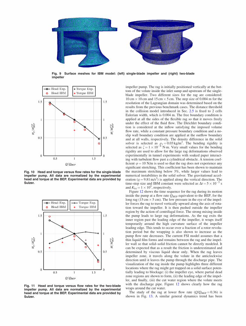
The experimental and numerical rag mean streamwise and ver-tical velocities and positions are compared in Figs. 7 and 8, wheret*¼ t/U, x*¼ x/L, y*¼ y/L, and u*¼ u/U. (x, u) and (y, v) are thestreamwise and vertical positions and velocities of the centroid ofthe rag’s upstream edge, and t*¼ 0 marks the time of releasewhen the upstream rag edge fully detached from the pole.
A comparison between experimental observations and numeri-cal predictions confirms that several key response characteristicsare in good agreement. First, the rag is shown to rotate counter-clockwise as its tip interacts with the jet formed at the lower endof the flagpole after release. The initial dipping of the flagobserved experimentally is due to a delayed release at its lowerend which is not modeled numerically. Following release, the ragdoes not remain in the plane of symmetry of the tunnel and experi-ences some bending so that the flow streamlines do not remainparallel to rag surface. As these deformations develop, the numeri-cal and experimental transport velocities are shown to converge.These results do indeed suggest that acceleration is overpredictedin shear-dominated flow but that as soon as the rag deforms a bet-ter agreement can be expected. For example, u* approaches 1 att*¼ 0.69. Further downstream, Figs. 4 and 6 show that the rag
Fig. 6 Transported rag shown with contour plot of transverse displacement obtained by DIC(experimental tests). The flagpole is visible on the left. The nondimension time t* is shown oneach frame.
Table 2 Parameters for the free rag motion case
q1 (kg/m2) u (N/m) f (N�m) Kfsi Dt (s)
(0.03, 0.08) 200 1� 10�4 2.5� 105 4� 10�5
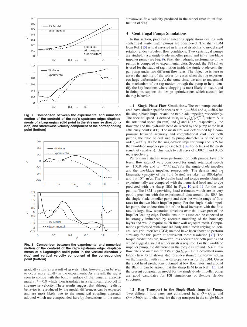
gradually sinks as a result of gravity. This, however, can be seento occur more rapidly in the experiments. As a result, the rag isseen to collide with the bottom surface of the tunnel at approxi-mately t*¼ 0.8 which then translates in a significant drop off instreamwise velocity. These results suggest that although realisticbehavior is reproduced by the model, differences can be expectedand are most likely due to the numerical coupling approachadopted which are compounded here by fluctuations in the mean
streamwise flow velocity produced in the tunnel (maximum fluc-tuation of 5%).
4 Centrifugal Pumps Simulations
In this section, practical engineering applications dealing withcentrifugal waste water pumps are considered. The sharp IBMfrom Ref. [15] is first assessed in terms of its ability to model rigidrotation under turbulent flow conditions. Two centrifugal pumpsare studied: (i) a single-blade impeller pump and (ii) a two-bladeimpeller pump (see Fig. 9). First, the hydraulic performance of thepumps is compared to experimental data. Second, the FSI solveris used for the study of rag motion inside the single-blade centrifu-gal pump under two different flow rates. The objective is here toassess the stability of the solver for cases when the rag experien-ces large deformations. At the same time, we aim to understandthe mechanism of the rag motion through the pump to help iden-tify the key locations where clogging is most likely to occur, andin doing so, support the design optimizations which account forthe rag behavior.
4.1 Single-Phase Flow Simulations. The two pumps consid-ered have similar specific speeds with ns¼ 56.4 and ns¼ 50.6 forthe single-blade impeller and the two-blade impeller, respectively.The specific speed is defined as ns ¼ N
ffiffiffiffiQp
=ðHÞ0:75, where N is
the rotational speed (in rpm) and Q and H are, respectively, theflow rate and the hydraulic head delivered by the pump at the bestefficiency point (BEP). The mesh size was determined by a com-promise between accuracy and computational cost. For bothpumps, the ratio of cell size to pump diameter is of the sameorder, with 1/100 for the single-blade impeller pump and 1/75 forthe two-blade impeller pump (see Ref. [36] for details of the meshsensitivity analysis). This leads to cell sizes of 0.002 m and 0.005m, respectively.
Performance studies were performed on both pumps. Five dif-ferent flow rates Q were considered for single rotational speedsx¼ 150.8 rad/s and x¼ 77.45 rad/s for the single-blade impellerand the two-blade impeller, respectively. The density and thekinematic viscosity of the fluid (water) are taken as 1000 kg/m3
and 1� 10�6 m2/s. The hydraulic head and torque results obtainedexperimentally are compared with the numerical head and torquepredicted with the sharp IBM in Figs. 10 and 11 for the twopumps. The IBM is providing head estimates which are in verygood agreement with the experimental data around the BEP forthe single-blade impeller pump and over the whole range of flowrates for the two-blade impeller pump. For the single-blade impel-ler pump, the underestimation of the head increases with the flowrate as large flow separation develops over the lower part of theimpeller leading edge. Predictions in this case can be expected tobe strongly influenced by accurate modeling of the boundarylayers and would require much finer wall adjacent mesh. Compu-tations performed with standard body-fitted mesh relying on gen-eralized grid interface (GGI) method have been shown to performsimilarly for this pump at equivalent mesh resolution [37]. Thetorque predictions are, however, less accurate for both pumps andwould suggest also that a finer mesh is required. For the two-bladeimpeller pump, the difference in the torque is around 16% at lowflow rate and increases to 33% at Q/QBEP¼ 1.6. Body-fitted simu-lations have been shown also to underestimate the torque actingon the impeller, with similar discrepancies as for the IBM. Giventhe good head predictions obtained at low flow rates, and aroundthe BEP, it can be argued that the sharp IBM from Ref. [15] andthe present computation model for the single-blade impeller pumpare good candidates for FSI simulations of flexible slenderstructures.
4.2 Rag Transport in the Single-Blade Impeller Pump.Two different flow rates are considered here, Q¼QBEP andQ¼ 0.36QBEP, to characterize the rag transport in the single-blade
Fig. 8 Comparison between the experimental and numericalmotion of the centroid of the rag’s upstream edge: displace-ments of a Lagrangian solid point in the vertical direction y(top) and vertical velocity component of the correspondingpoint (bottom)
Fig. 7 Comparison between the experimental and numericalmotion of the centroid of the rag’s upstream edge: displace-ments of a Lagrangian solid point in the streamwise direction x(top) and streamwise velocity component of the correspondingpoint (bottom)
impeller pump. The rag is initially positioned vertically at the bot-tom of the volute inside the inlet sump and upstream of the single-blade impeller. Two different sizes for the rag are considered:10 cm� 10 cm and 15 cm� 5 cm. The step size of 0.004 m for theresolution of the Lagrangian domain was determined based on theresults from the previous benchmark cases. The distance thresholdin the collision model introduced in Sec. 2.5 is fixed to 2 cellsEulerian width, which is 0.004 m. The free boundary condition isapplied at all the sides of the flexible rag so that it moves freelyunder the effect of the fluid flow. The Dirichlet boundary condi-tion is considered at the inflow satisfying the imposed volumeflow rate, while a constant pressure boundary condition and a no-slip wall boundary condition are applied at the outflow boundaryand at all walls, respectively. The density difference in the solidsolver is selected as q1¼ 0.03 kg/m2. The bending rigidity isselected as f¼ 1� 10�8 N�m. Very small values for the bendingrigidity are used to allow for the large rag deformations observedexperimentally in tunnel experiments with soaked paper interact-ing with turbulent flow past a cylindrical obstacle. A tension coef-ficient u¼ 10 N/m is used so that the rag does not experience anysignificant stretching. This coefficient has been shown to maintainthe maximum stretching below 3%, while larger values lead tonumerical instabilities in the solid solver. The gravitational accel-eration (g¼ 9.81 m/s2) is applied along the vertical direction. Thetime-step size and IBM constant were selected as Dt¼ 5� 10�5 sand Kfsi¼ 1� 105, respectively.
Figure 12 shows the time sequence for the rag during its motioninside the pump at a flow rate QBEP equivalent to the BEP, for thelong rag (15 cm� 5 cm). The low pressure in the eye of the impel-ler forces the rag to travel vertically upward along the axis of rota-tion toward the impeller. It is then pushed outside the impellerregion by the action of centrifugal force. The strong mixing insidethe pump leads to large rag deformations. As the rag exits theinner region past the leading edge of the impeller, it wraps itselftemporarily around the high curvature surface of the impellerleading edge. This tends to occur over a fraction of a rotor revolu-tion period but the wrapping is also shown to increase as thepump flow rate decreases. The current FSI model assumes that athin liquid film forms and remains between the rag and the impel-ler wall so that solid–solid friction cannot be directly modeled. Itcan be expected that as a result the friction is underestimated anddetermined by viscous liquid shear only. When the rag leavesimpeller zone, it travels along the volute in the anticlockwisedirection until it leaves the pump through the discharge pipe. Thevisualization of the rag inside the pump highlights three differentlocations where the rag might get trapped on a solid surface poten-tially leading to blockage: (i) the impeller eye, where partial deadzone regions are shown to form, (ii) the leading edge of the impel-ler, and finally, (iii) the cut water region where the volute meetswith the discharge pipe. Figure 12 shows clearly how the ragwraps around the cut water.
The study of the rag at lower flow rate (Q/QBEP¼ 0.36) isshown in Fig. 13. A similar general dynamics trend has been
Fig. 9 Surface meshes for IBM model: (left) single-blade impeller and (right) two-bladeimpeller
Fig. 10 Head and torque versus flow rates for the single-bladeimpeller pump. All data are normalized by the experimentalhead and torque at the BEP. Experimental data are provided bySulzer.
Fig. 11 Head and torque versus flow rates for the two-bladeimpeller pump. All data are normalized by the experimentalhead and torque at the BEP. Experimental data are provided bySulzer.
observed in this case compared to the BEP. However, three differ-ences have been observed compared to the previous case. First,the rag wraps around the leading edge at a different height. Sec-ond, the rag does not collide against the cut water region
indicating the strong sensitivity of the results to the initial andboundary conditions. Finally, there is a significant delay in thetime required for the rag to leave the impeller region, and there-fore, the pump. This can be inferred to increase the likelihood of
Fig. 12 Visualization of the deformed rag surface at eight suc-cessive times after the release for Q/QBEP 5 1. The cross sectionof the pump volute and impeller is shown in gray.
Fig. 13 Visualization of the deformed rag surface at eight suc-cessive times after the release for Q/QBEP 5 0.36. The cross sec-tion of the pump volute and impeller is shown in gray.

the rag being wrapped around the leading edge for a long timeallowing for multiple rags to accumulate. At Q/QBEP¼ 0.36, therag remains around the leading edge for approximately 50% of thesimulation time (or approximately 2.4 periods of revolution)instead of 30% at QBEP (or 1.5 periods of revolution). Hence, therag takes only 0.1 s to reach the cut water region at the BEP com-pared to 0.14 s at the lower flow rate. Similar conclusions regard-ing the probability of clogging were obtained experimentally inRef. [4]. Inspection of the flow in Ref. [38] suggests that changingthe flow rate leads to a change in fluid incident angle relative tothe impeller leading edge. Increasing the flow generates area ofincreased radial velocity and decreased tangential velocity, asobserved also in Ref. [39].
Figure 14 shows the position of the rag at the impeller leadingedge for three different rags: the results show that wide rags aremore likely to find themselves wrap around the whole leadingedge. In contrast, long narrow rag wraps around a small region ofthe leading edge. For the BEP, the rag wraps around the top sideof the leading edge close to the hub. In contrast, the wrap movesaround the bottom side at smaller flow rates. These observationshighlight the strong sensitivity of rag dynamics to the size of therag and the value of the flow rate, and hence, the importance of aholistic approach to design optimization if clogging dynamics isto be accounted for. It is also worth noting that experimentalobservations from high-speed camera imaging of rag flow at theinlet sump of the same reference pump confirmed that rags thatremain within the pump volute tend to wrap around the leadingedge of the impeller. This behavior was observed from visualiza-tion tests obtained with high-speed cameras and confirmed follow-ing the dismantling of the impeller. Statistical assessment ofexperimental studies have indicated that the likelihood of block-age is based on several factors which include the rag initial loca-tion, the fluid inlet boundary conditions, the geometricalparameters for the pump hydraulic parts, and the rag geometricaland physical properties.
5 Conclusion
A FSI solver based on IBMs has been described and validatedfor multiple interactions between flows from low to high Reynoldsnumbers, flexible slender structures, and rigid moving bodies. Thesolver couples a diffuse IBM with a finite difference solution of
the motion equation of a two-dimensional elastic solid and a sharpIBM for rigid body motion including a collision model to accountfor interactions with moving immersed objects. It has beenassessed with a range of benchmark cases including a highlydynamic system at different flow regimes. Comparisons with thepreviously published FSI solvers based on IBMs and new experi-mental tests presented in this paper indicate that stable, robust,and accurate or physically realistic predictions can be achieved.The solver was then applied to study the transport of flexiblestructures through a centrifugal pump and describe the processesthat may lead to accumulation of rags around impeller. Resultsclearly highlight the influence of two key parameters which arethe rag length and the pump flow rate on the positioning of the ragwithin the volute and around the impeller providing for the firsttime some insight in the dynamics of the rag and its sensitivity toflow conditions.
Acknowledgment
The authors would like to thank the staff of Sulzer pump Wex-ford for their support in selecting suitable test cases and providingexperimental validation data. All numerical simulations were per-formed on the FIONN cluster of the Science Foundation Ireland/Higher Education Authority (SFI/HEA) Irish Centre for High-EndComputing (ICHEC). ICHEC support through the dceng002b anddceng005b Class B Projects is gratefully acknowledged.
Funding Data
� Enterprise Ireland (EI) (IP/2014/0359).� Irish Research Council (IRC) (EBPPG 2013 63).
References[1] Gerlach, S., and Thamsen, P. U., 2017, “Cleaning Sequence Counters
Clogging: A Quantitative Assessment Under Real Operation Conditions of aWastewater Pump,” ASME Paper No. FEDSM2017-69020.
[2] Jensen, A. L., Gerlach, S., Lykholt-Ustrup, F., Sørensen, H., Rosendahl, L., andThamsen, P. U., 2017, “Investigation of the Influence of Operating Point on theShape and Position of Textile Material in the Inlet Pipe to a Dry-InstalledWastewater Pump,” ASME Paper No. FEDSM2017-69298.
[3] P€ohler, M., H€ochel, K., and Gerlach, S., 2017, “Linking Efficiency to Func-tional Performance by a Pump Test Standard for Wastewater Pumps,” ASMEPaper No. AJKFluids2015-33763.
[4] Connolly, R., 2017, “An Experimental and Numerical Investigation Into FlowPhenomena Leading to Wastewater Centrifugal Pump Blockage,” ME thesis,Dublin City University, Dublin, Ireland.
[5] Jensen, A. L., Sørensen, H., Rosendahl, L., and Thamsen, P. U., 2018,“Characterisation of Textile Shape and Position Upstream of a WastewaterPump Under Different Part Load Conditions,” Urban Water J., 15(2), pp.132–137.
[6] Jensen, A. L., Sørensen, H., and Rosendahl, L., 2016, “Towards Simulation ofClogging Effects in Wastewater Pumps: Modelling of Fluid Forces on a Fiberof Bonded Particles Using a Coupled CFD-DEM Approach,” InternationalSymposium on Transport Phenomena and Dynamics of Rotating Machinery(ISROMAC 2016), Honolulu, HI, Apr. 10–15, pp. 1–6.
[7] Jensen, A. L., Sørensen, H., Rosendahl, L., Adamsen, P., and Lykholt-Ustrup,F., 2016, “Investigation of Drag Force on Fibres of Bonded Spherical ElementsUsing a Coupled CFD-DEM Approach,” Ninth International Conference onMultiphase Flow (ICMF), Firenze, Italy, May 22–27, Paper No. 1922.
[8] Yao, Z.-F., Yang, Z.-J., and Wang, F.-J., 2016, “Evaluation of Near-Wall Solu-tion Approaches for Large-Eddy Simulations of Flow in a Centrifugal PumpImpeller,” Eng. Appl. Comput. Fluid Mech., 10(1), pp. 454–467.
[9] Posa, A., Lippolis, A., and Balaras, E., 2016, “Investigation of Separation Phe-nomena in a Radial Pump at Reduced Flow Rate by Large-Eddy Simulation,”ASME J. Fluids Eng., 138(12), p. 121101.
[10] Pei, J., Yuan, S., Benra, F.-K., and Dohmen, H., 2012, “Numerical Predictionof Unsteady Pressure Field Within the Whole Flow Passage of a Radial Single-Blade Pump,” ASME J. Fluids Eng., 134(10), p. 101103.
[11] Pei, J., Dohmen, H., Yuan, S., and Benra, F.-K., 2012, “Investigation ofUnsteady Flow-Induced Impeller Oscillations of a Single-Blade Pump UnderOff-Design Conditions,” J. Fluids Struct., 35, pp. 89–104.
[12] Souza, B. D., and Niven, A., 2008, “Single Blade Impeller DevelopmentThrough the Use of the Design of Experiments Method in Combination WithNumerical Simulation,” International Symposium on Transport Phenomena andDynamics of Rotating Machinery (ISROMAC 2008), Honolulu, HI, Feb.17–22, pp. 1–8.
Fig. 14 Visualization of the rag (shown in red) as it wraps itselfaround the impeller (shown in blue): square 10 cm 3 10 cm ragat Q/QBEP 5 1 (top), rectangular 15 cm 3 5 cm rag at Q/QBEP 5 1(middle), and rectangular 15 cm 3 5 cm rag at Q/QBEP 5 0.36(bottom)

[13] de Souza, B., Niven, A., and McEvoy, R., 2010, “A Numerical Investigation ofthe Constant-Velocity Volute Design Approach as Applied to the Single BladeImpeller Pump,” ASME J. Fluids Eng., 132(6), p. 061103.
[14] Stephen, C., Yuan, S., Pei, J., and Cheng, G. X., 2017, “Numerical Flow Predic-tion in Inlet Pipe of Vertical Inline Pump,” ASME J. Fluids Eng., 140(5), p.051201.
[15] Specklin, M., and Delaur�e, Y., 2018, “A Sharp Immersed Boundary MethodBased on Penalisation and Its Application to Moving Boundaries and TurbulentRotating Flows,” Eur. J. Mech./B Fluids, 70, pp. 130–147.
[16] Huang, W.-X., Shin, S. J., and Sung, H. J., 2007, “Simulation of Flexible Fila-ments in a Uniform Flow by the Immersed Boundary Method,” J. Comput.Phys., 226(2), pp. 2206–2228.
[17] Huang, W.-X., and Sung, H. J., 2010, “Three-Dimensional Simulation of aFlapping Flag in a Uniform Flow,” J. Fluid Mech., 653, pp. 301–336.
[18] Huang, W.-X., and Sung, H. J., 2009, “An Immersed Boundary Method forFluid Flexible Structure Interaction,” Comput. Methods Appl. Mech. Eng.,198(33–36), pp. 2650–2661.
[19] Ryu, J., Park, S. G., and Sung, H. J., 2018, “Flapping Dynamics of InvertedFlags in a Side-by-Side Arrangement,” Int. J. Heat Fluid Flow, 70, pp.131–140.
[20] Park, S. G., and Sung, H. J., 2018, “Hydrodynamics of Flexible Fins Propelledin Tandem, Diagonal, Triangular and Diamond Configurations,” J. Fluid Mech.,840, pp. 154–189.
[21] Albadawi, A., Marry, S., Breen, B., Connolly, R., and Delaur�e, Y., 2016, “AnIBM-FSI Solver of Flexible Objects in Fluid Flow for Pumps CloggingApplications,” Ninth International Conference on Computational Fluid Dynam-ics (ICCFD9), Istanbul, Turkey, July 11–15, pp. 1–22.
[22] Tian, F.-B., Dai, H., Luo, H., Doyle, J. F., and Rousseau, B., 2014, “Fluid-Structure Interaction Involving Large Deformations: 3D Simulations and Appli-cations to Biological Systems,” J. Comput. Phys., 258, pp. 451–469.
[23] Lee, I., and Choi, H., 2015, “A Discrete-Forcing Immersed Boundary Methodfor the Fluid-Structure Interaction of an Elastic Slender Body,” J. Comput.Phys., 280, pp. 529–546.
[24] de Tullio, M., and Pascazio, G., 2016, “A Moving-Least-Squares ImmersedBoundary Method for Simulating the Fluid-Structure Interaction of ElasticBodies With Arbitrary Thickness,” J. Comput. Phys., 325, pp. 201–225.(August),
[25] OpenCFD, 2016, “The Open Source Computational Fluid Dynamics (CFD)Toolbox,” ESI Group, Paris, France, http://openfoam.com/
[26] Issa, R., 1986, “Solution of the Implicitly Discretised Fluid Flow Equations byOperator-Splitting,” J. Comput. Phys., 62(1), pp. 40–65.
[27] Weller, H., 2012, “Controlling the Computational Modes of the ArbitrarilyStructured c Grid,” Mon. Weather Rev., 140(10), pp. 3220–3234.
[28] Lysenko, D. A., and Rian, K. R., 2014, “Large-Eddy Simulation of the FlowOver a Cylinder at Reynolds Number 2� 104,” Flow Turbul. Combust., 92(3),pp. 673–698.
[29] Krastev, V., and Bella, G., 2012, “A Zonal Turbulence Modeling Approach forIce Flow Simulation,” SAE Int. J. Engines, 9(3), pp. 1425–1436.
[30] Spalart, P. R., Jou, W.-H., Strelets, M., and A, S. R., 1997, “Comments on theFeasibility of LES for Wings and on a Hybrid RANS/LES Approach,” Advan-ces in DNS/LES: Proceedings of the First AFOSR International Conference onDNS/LES, Louisiana Tech University, Ruston, Louisiana, USA, August 4–8,1997, Greyden Press, Columbus, OH.
[31] Spalding, D., 1961, “A Single Formula for the Law of the Wall,” ASME J.Appl. Mech., 28(3), pp. 455–458.
[32] F€allstr€om, K. E., Gren, P., and Mattsson, R., 2002, “Determination of PaperStiffness and Anisotropy From Recorded Bending Waves in Paper Subjected toTensile Forces,” NDT and E Int., 35(7), pp. 465–472.
[33] Virot, E., Amandolese, X., and H�emon, P., 2013, “Fluttering Flags: An Experi-mental Study of Fluid Forces,” J. Fluids Struct., 43, pp. 385–401.
[34] Siebert, T., and Crompton, M. J., 2013, “Application of High Speed DigitalImage Correlation for Vibration Mode Shape Analysis,” Application of ImagingTechniques to Mechanics of Materials and Structures, Vol. 4, Springer, Berlin,pp. 291–298.
[35] Tabandeh-Khorshid, M., Schultz, B., Rohatgi, P., and Elhajjar, R., 2016, “TheDiametrically Loaded Cylinder for the Study of Nanostructured Aluminum-Graphene and Aluminum-Alumina Nanocomposites Using Digital ImageCorrelation,” Front. Mater., 3, p. 22.
[36] Specklin, M., 2018, “On the Assessment of Immersed Boundary Methods for Fluid-Structure Interaction Modelling: Application to Waste Water Pumps Design and theInherent Clogging Issues,” Ph.D. thesis, Dublin City University, Dublin, Ireland.
[37] Specklin, M., 2018, “A Versatile Immersed Boundary Method for PumpDesign,” Sulzer Management Ltd., Winterthur, Switzerland, White Paper,1/2018.
[38] G€ulich, J. F., 2008, Centrifugal Pumps, Springer, Berlin.[39] Feng, J., Benra, F. K., and Dohmen, H. J., 2009, “Unsteady Flow Visualization
at Part-Load Conditions of a Radial Diffuser Pump: By PIV and CFD,” J.Visualization, 12(1), pp. 65–72.