a thesis submitted for the award of master of science
TRANSCRIPT

Measuring Protein Diffusion in
Living Cells by Raster Image
Correlation Spectroscopy (RICS)
A Thesis Submitted for the Award ofMaster of Science
Raz Shimoni
CENTRE OF MICRO-PHOTONICS
The Faculty of Engineering and Industrial Sciences (FEIS)
Swinburne University of Technology, Melbourne, Australia
PETER MACCALLUM CANCER CENTRE
St Andrews Place, East Melbourne, Australia
Supervised By: Prof. Sarah Russell, Dr. Ze’ev Bomzon, Prof. Min Gu
January 2010

Dedicated to my partner Olga

iii
”Anyone who has never made a mistake hasnever tried anything new.”
-Albert Einstein(1879-1955)

iv
Abstract
T ime-lapse fluorescence imaging has revolutionized studies of biology in the
last 15 years. In addition to the now routine tracking of bulk fluorescence, for
instance of a protein moving into the nucleus in response to an extracellular signal,
technologies are now emerging that enable much more sophisticated analysis of
the motion and interactions of proteins within living cells. The potential of these
approaches to elucidate biological processes is clear, but they have not yet been
developed and validated for broad use by biologists.
This thesis describes the adaptation of a recently introduced method, Raster
Image Correlation Spectroscopy (RICS). RICS is a novel approach to assess the
dynamic properties of fluorescent macromolecules in solutions and within living
cells by confocal laser scanning microscopy. Based on RICS theory, we developed
novel software with which to analyse confocal images and to measure diffusion
coefficients of the fluorophores. This new software has several advantages
compared with published RICS software, and its ability to give accurate diffusion
coefficient values was characterized under a range of settings.
Once a RICS routine was established, it was applied to measure the diffusion
coefficient of PAK-interacting exchange factor (βPIX) within living fibroblast
cells as a paradigm for RICS analysis. The interaction between βPIX and
the adaptor protein, Scribble, plays a critical role in cell polarity and actin
polymerization. These preliminary measurements indicate the potential of RICS
in elucidating the dynamics of proteins within living cells, and demonstrate how
the use of RICS will open new opportunities in the cell biology research.

Acknowledgments
The last two years have been an amazing experience for me. I have been
introduced to novel technologies in the BioPhotonics field, interacted with leading
biologists and physicists, met new friends from different nationalities and travelled
extensively around beautiful Australia. It was a great honour for me to be a part of
the Centre of Micro-Photonics (CMP) at Swinburne University of Technology and
I am grateful for this opportunity. I would like to thank my research supervisors-
Professor Sarah Russell, the group leader of Immune Signalling at the Peter
MacCallum Cancer Centre and the head of the Cell Biology group in the CMP
and Dr. Zeev Bomzon for this opportunity and for their kind support along the
way. Of course, without financial support all this could not be possible. For the
generous financial support that allowed me to conduct my research I would like to
thank Professor Min Gu- the Director of the CMP and the Faculty of Engineering
and Industrial Sciences (FEIS) at Swinburne University of Technology.
v

vi
I would like to acknowledge the contribution of my supervisor Dr. Zeev
Bomzon to the RICSIM. Dr. Bomzon built the initial stage of the RICSIM GUI,
including the image-processing filters procedures.
I would like to thank Mandy Ludford-Menting the senior research assistant
from Sarah Russell‘s lab at Peter MacCallum Cancer Centre for teaching me to
generate and to validate the cell lines that were used for this thesis, and
I thank Kim Pham, a PhD student from the CMP for providing the EYFP-
βPIX∆CT construct and the EYFP-βPIX cells.
I would also like to thank Dr. Andrew Clayton and Dr. Noga Kozer from
Ludwig Institute for Cancer Research for supplying BaF3 cell lines including
supportive materials, GFP samples, and for our fruitful discussions.
I thank the Nanostructured Interfaces and Materials Group at the department
of Chemical and Biomolecular Engineering, the University of Melbourne, for
contributing the PVPON.
For the microscopy training and for taking care that the microscope equipment
is in the best condition - I would like to thank Sarah Ellis, the core manager of the
microscopy unit at the Peter MacCallum Cancer Centre.
For his professional help with the flow cytometry and our interesting conversa-
tions, I would like to thank Ralph Rossi from the Peter MacCallum Cancer Centre.
I would like to extend my thanks to all the CMP members and my colleagues
from Russell’s group for providing a supportive intellectually environment with a
friendly atmosphere.
Finally, I would like to thank my family and close friends in Israel and
Australia who supported and encouraged me throughout this research.

vii
Declaration
I declare that:
n This thesis contains no material of any other degree or diploma, except
where due reference is made in the text of the thesis.
n To the best of my knowledge, this thesis contains no material previously
published or written by another person except where due reference is made
in the text of the thesis.
n Contributions of respective workers are mentioned in this thesis.
Raz Shimoni

Abbreviations
1-D One-dimensional
2-D Two-dimensional
3-D Three-dimensional
A/D Analog-to-Digital
ACF Autocorrelation Function
AF488 Alexa R© Fluor dye 488 nm
AOBS Acoustic Optical Beam Splitter
AOTF Acoustic Optical Tuneable Filters
APD Avalanche Photodiode Detector
ATP Adenosine Triphosphate
βPIX Beta PAK- Interacting Exchange Factor
βPIX∆CT βPIX mutant that lack (-TNL)
BSA Bovine Serum Albumin
c Speed of light (≈3×10⁸ m·s−1)
C Concentration
CHO Chinese Hamster Ovary
CLSM Confocal Laser Scanning Microscopy
viii

ix
D Diffusion coefficient (µm2/s)
DLS Dynamic Light Scattering
DMEM Dulbecco’s Modified Essential Medium
DMSO Dimethyl Sulphoxide
Dstop βPIX∆CT
ECL Enhanced Chemiluminescence
EDTA Ethylenediamietetraacetate
EGF Epidermal Growth Factor
EGFP Enhance-Green-Fluorescence Protein
EGFR EGF-Receptor
EYFP Enhance-Yellow-Fluorescence Protein
f Fourier Transform
f−1 Inverse Fourier Transform
FACS Fluorescence Activated Cell Sorting
FCS Fluorescence Correlation Spectroscopy
FFS Fluorescence Fluctuation Spectroscopy
FFT Fast Fourier Transform
fl femtoliter (10−15 liter)
FRAP Fluorescence Recovery After Photobleaching
FRET Fluorescence Resonance Energy Transfer
G(0,0) amplitude of 2-D ACF before normalization
g(0,0) amplitude of 2-D normalized ACF
g(ξ,0) horizontal vector of the normalized ACF
g(0,ψ) vertical vector of the normalized ACF
GDP Guanosine diphosphate
GEF Guanine nucleotide Exchange Factors
GFP Green Fluorescence Protein
GTP Guanosine triphosphate
GUI Graphical User Interface

x
h Planck constant (≈6.62×10⁻³⁴ J·s)
HRP Horse Radish Peroxidase
I(X,Y) Intensity of pixel at coordinates (X,Y) in 2-D matrix
I(t) Intensity value at time in a vector
ICM Image Correlation Microscopy
ICS Image Correlation Spectroscopy
ICCS Image Cross Correlation Spectroscopy
IF ImmunoFluorescence
ii index image from series
jj index counter
KB Boltzmann constant (≈1.38×10⁻²³ J·K−1)
kDa Kilo Dalton
µg micro-gram (10−6 gram)
µl micro-liter (10−6 liter)
µM microMolar
µs micro-second (10−6 second)
M Molarity
MEF Mouse Embryonic Fibroblasts
mg milli-gram (10−3 gram)
ml milli-liter (10−3 liter)
mM milli-Molar (10−3 Molar)
mQ H2O milliQ water
ms milli-second (10−3 second)
MSD Mean Square Displacement
N Number of particles
n length of discrete intervals refractive index
NA Numerical Aperture
Na Avogadro constant (≈6.02×10²³ mol−1)
nM nano-Molar (10−9 Molar)

xi
ns nano-second (10−9 second)
PAK p21-activated serine threonine kinase
PAO Phenylarsine oxide
PBS Phosphate Buffer Saline
PCH Photon Counting Histogram
pH Power of Hydrogen
PMT Photomultiplier Tube
PSD Power Spectrum Density
PSF Point Spread Function
PVPON Poly(N-vinyl pyrrolidone)
Q Quantum yield
r radius
rcf relative centrifugal force
RICS Raster Image Correlation Spectroscopy
ROI Region of Interest
RPMI Roswell Park Memorial Institute medium
RT Room Temperature
s seconds
S/N, SNR Signal to Noise ratio
SPT Single-Particle Tracking
STICS Spatial-Temporal Image Correlation Spectroscopy
T absolute Temperature (K)
t time, index image from series
Tiff Tagged Image File
V Volt, Volume
Veff effective volume
WT Wild Type
X height of an image in pixels
X(t) trajectories of individual particle
Y width of an image in pixels

xii
Symbols
δ fluctuation
ε excitation efficiency
γ correction shape factor
η signal-to-noise ratio constant
ι instrumental counting efficiency
λ wavelength
µ micro (10−9)
ν viscosity
π mathematical constant (π≈3.14159)
θ angular aperture
ρ density of material
τ lag time (characteristic delay time)
τD diffusion time
τ l line time
τ p pixel time
ξ spatial displacement along X-axis
ψ spatial displacement along Y-axis
ωxy XY-waist of the PSF (µm)
ωz Z-waist of the PSF (µm)

Contents
Abstract iv
Acknowledgments v
List of Abbreviations viii
Contents xvii
List of Figures xx
1 Introduction- The Biological Context 1
1.1 βPIX and Scribble in Cell Polarity . . . . . . . . . . . . . . . . . 2
1.2 βPIX-Scribble Interaction in RAC1/Cdc42
Mediated Actin Polymerization . . . . . . . . . . . . . . . . . . . 4
1.3 The Research Questions and an Outline of the Chosen Methodology 7
2 Theoretical Background 10
2.1 Introduction . . . . . . . . . . . . . . . . . . . . . . . . . . . . . 10
2.1.1 The diffusion coefficient in cell biology . . . . . . . . . . 13
Fick’s 1st law for diffusion . . . . . . . . . . . . . . . . . 13
Brownian motion and Einstein-Smoluchowski equation . . 15
The Stokes-Einstein relation . . . . . . . . . . . . . . . . 18
2.1.2 The principles of fluorescence . . . . . . . . . . . . . . . 20
xiii

CONTENTS xiv
2.1.3 Fluorescence proteins technology and traditional
respective fluorescence based techniques . . . . . . . . . . 21
Time-lapse fluorescence microscopy . . . . . . . . . . . . 23
Computational image analysis of fluorescence microscopy
images . . . . . . . . . . . . . . . . . . . . . . 23
Single-particle tracking . . . . . . . . . . . . . . . . . . . 24
Fluorescence Recovery After Photobleaching (FRAP) . . 24
Forster Resonance Energy Transfer (FRET) . . . . . . . . 26
Summary . . . . . . . . . . . . . . . . . . . . . . . . . . 27
2.2 Principles of Fluorescence Correlation
Spectroscopy (FCS) . . . . . . . . . . . . . . . . . . . . . . . . . 28
2.2.1 The theory behind FCS . . . . . . . . . . . . . . . . . . . 28
2.2.2 The ACF . . . . . . . . . . . . . . . . . . . . . . . . . . 32
2.2.3 FCS fitting model for Brownian motion . . . . . . . . . . 34
2.2.4 FCS in cell biology . . . . . . . . . . . . . . . . . . . . . 42
2.3 Principles of Image Correlation Spectroscopy (ICS) . . . . . . . . 43
2.3.1 ICS is based on raster CLSM . . . . . . . . . . . . . . . . 43
2.3.2 The 2-D ACF . . . . . . . . . . . . . . . . . . . . . . . . 45
2.3.3 ICS fitting model . . . . . . . . . . . . . . . . . . . . . . 46
2.3.4 Advances in Image Correlation Spectroscopy . . . . . . . 47
2.4 Principles of Raster Image Correlation
Spectroscopy (RICS) . . . . . . . . . . . . . . . . . . . . . . . . 48
2.4.1 Time and space domains in RICS . . . . . . . . . . . . . . 52
2.4.2 RICS fitting model for Brownian motion . . . . . . . . . . 52
2.4.3 Advances in RICS . . . . . . . . . . . . . . . . . . . . . 53
2.4.4 Cross correlation approach in FFS . . . . . . . . . . . . . 55
2.5 Summary . . . . . . . . . . . . . . . . . . . . . . . . . . . . . . 56

CONTENTS xv
3 Materials and Methods 57
3.1 Conditions for Cell Maintenance . . . . . . . . . . . . . . . . . . 57
3.2 Plasmid DNA . . . . . . . . . . . . . . . . . . . . . . . . . . . . 58
3.3 Antibiotic Titration . . . . . . . . . . . . . . . . . . . . . . . . . 58
3.4 Cell Transfection . . . . . . . . . . . . . . . . . . . . . . . . . . 59
3.5 Preparation of Cell Lines . . . . . . . . . . . . . . . . . . . . . . 59
3.6 Western Blotting . . . . . . . . . . . . . . . . . . . . . . . . . . 60
3.7 Antibodies . . . . . . . . . . . . . . . . . . . . . . . . . . . . . . 62
3.8 Preparation of Microscope Samples . . . . . . . . . . . . . . . . 62
3.9 Microscope Setup . . . . . . . . . . . . . . . . . . . . . . . . . . 65
3.10 Data Processing and Manipulation . . . . . . . . . . . . . . . . . 68
4 Computational Implementation of RICS by the RICSIM software 70
4.1 Introduction . . . . . . . . . . . . . . . . . . . . . . . . . . . . . 70
4.2 General RICS Procedure . . . . . . . . . . . . . . . . . . . . . . 73
4.3 The RICSIM Process Scheme . . . . . . . . . . . . . . . . . . . . 82
4.3.1 Control modes in RICSIM . . . . . . . . . . . . . . . . . 83
4.3.2 Threshold algorithm (6) . . . . . . . . . . . . . . . . . . . 87
4.3.3 Photobleaching correction algorithm (7) . . . . . . . . . . 87
4.3.4 Normalization (8) . . . . . . . . . . . . . . . . . . . . . . 89
4.3.5 Input User Selection (9) . . . . . . . . . . . . . . . . . . . 90
4.3.6 Fitting (10) . . . . . . . . . . . . . . . . . . . . . . . . . 91
4.4 Summary . . . . . . . . . . . . . . . . . . . . . . . . . . . . . . 92
5 Experimental Studies and Validation
of RICS 93
5.1 Introduction . . . . . . . . . . . . . . . . . . . . . . . . . . . . . 93
5.2 Validation of RICS with Microspheres . . . . . . . . . . . . . . . 94
5.2.1 Estimation of the PSF waist by microspheres scanning . . 94
CONTENTS xvi
5.2.2 Effect of viscosity on the ACF of diffusing microspheres . 97
5.2.3 Effect of viscosity on the ACF of diffusing microspheres . 98
5.2.4 Effect of scanning speed on the ACF of
diffusing microspheres . . . . . . . . . . . . . . . . . . . 104
5.3 ACF Studies by Using PVPON Solutions . . . . . . . . . . . . . 106
5.3.1 Effect of laser power . . . . . . . . . . . . . . . . . . . . 107
5.3.2 Effect of scan speed . . . . . . . . . . . . . . . . . . . . . 112
5.3.3 Effect of pinhole . . . . . . . . . . . . . . . . . . . . . . 115
5.3.4 Effect of viscosity . . . . . . . . . . . . . . . . . . . . . . 119
5.4 ACF of Diffusing GFP in Isotropic Solutions . . . . . . . . . . . . 122
5.4.1 Effect of the scanning direction in RICS . . . . . . . . . . 124
5.5 The Effect of Immobile Fraction Removal on RICS measurements 126
5.6 Discussion . . . . . . . . . . . . . . . . . . . . . . . . . . . . . . 134
6 RICS Measurements in 3T3 Cells 139
6.1 Introduction . . . . . . . . . . . . . . . . . . . . . . . . . . . . . 139
6.2 Validation of Cell Lines . . . . . . . . . . . . . . . . . . . . . . . 141
6.3 Calibration of RICS to 3T3 Cells . . . . . . . . . . . . . . . . . . 144
6.3.1 RICS measurements in Fixed Cells . . . . . . . . . . . . . 144
6.3.2 Workflow of RICS experiments . . . . . . . . . . . . . . . 145
6.3.3 Adjustment of the scanning speed . . . . . . . . . . . . . 146
6.3.4 Determination of the optimal pixel size . . . . . . . . . . 147
6.3.5 Determination of the pinhole diameter and laser power . . 147
6.3.6 The effect of the ROI Size on the ACF . . . . . . . . . . . 149
6.3.7 Effect of removing data points before fitting the ACF . . . 151
6.3.8 Adjustment of the MA subtraction . . . . . . . . . . . . . 152
6.3.9 Adjustment of the cut-off frequency of high pass filter . . . 153
6.3.10 Summary . . . . . . . . . . . . . . . . . . . . . . . . . . 157

CONTENTS xvii
6.4 Measurements Under Optimal Conditions . . . . . . . . . . . . . 157
6.4.1 Spatial Diffusivity of βPIX in living cells . . . . . . . . . 157
6.4.2 Measurements of diffusion coefficients for a
large population . . . . . . . . . . . . . . . . . . . . . . . 165
6.5 Summary . . . . . . . . . . . . . . . . . . . . . . . . . . . . . . 170
7 Conclusions and Future Work 172
7.1 Conclusions and Outlook . . . . . . . . . . . . . . . . . . . . . . 173
7.2 Recommendations for Future Work . . . . . . . . . . . . . . . . . 175
Bibliography 202
Appendices: 202
A Theoretical Studies of the ACF 203
A.1 Simulation of diffusion . . . . . . . . . . . . . . . . . . . . . . . 203
A.2 The effect of the number of particles on the statistical distribution . 205
A.3 Effect of number of particles on the ACF . . . . . . . . . . . . . . 207
A.4 ACF of FCS Change as function of diffusion . . . . . . . . . . . . 210
A.5 ACF of RICS Change as function of diffusion . . . . . . . . . . . 212
B List of lab recipes 214
C Classes in RICSIM 217
D RICSIM GUI 218
E Photobleaching curve for a ROI 220
F Spatial correlation at the cell edges 221

List of Figures
1.1 The cycle of actin polarization during cell motility . . . . . . . . . 5
1.2 Proposed model for the βPIX-Scribble interaction in RAC1/Cdc42
mediated actin polymerization . . . . . . . . . . . . . . . . . . . 6
2.1 Diffusing particle enters the observation volume . . . . . . . . . . 12
2.2 Diffusion of particles resulting from a concentration gradient . . . 14
2.3 Illustration of random one-dimensional motion of a particle . . . . 16
2.4 Brownian motion of diffusing particles . . . . . . . . . . . . . . . 17
2.5 Liquid molecules pass part of their momentum to diffusing parti-
cles through collusion impact . . . . . . . . . . . . . . . . . . . . 18
2.6 Jablonski diagram . . . . . . . . . . . . . . . . . . . . . . . . . . 20
2.7 Graph of FRAP experiment . . . . . . . . . . . . . . . . . . . . . 25
2.8 Scheme for a standard FCS experimental set up . . . . . . . . . . 30
2.9 Convolution of point source in raster LSCM . . . . . . . . . . . . 44
2.10 RICS is a combination between ICS and FCS . . . . . . . . . . . 48
2.11 The principle behind RICS . . . . . . . . . . . . . . . . . . . . . 51
3.1 βPIX and βPIX∆CT plasmids . . . . . . . . . . . . . . . . . . . 58
3.2 Molecular structure of PVPON . . . . . . . . . . . . . . . . . . . 63
3.3 Scheme of Leica TCS SP5 components . . . . . . . . . . . . . . . 67
4.1 An example of the RICS analysis for EYFP expressed in living
3T3 cell . . . . . . . . . . . . . . . . . . . . . . . . . . . . . . . 74
xviii

LIST OF FIGURES xix
4.2 RICSIM fitting flowchart . . . . . . . . . . . . . . . . . . . . . . 79
4.3 Fitting the experimental ACF to theoretical RICS equation . . . . 81
4.4 RICSIM process scheme. . . . . . . . . . . . . . . . . . . . . . . 83
4.5 Effect of averaging on the ACF . . . . . . . . . . . . . . . . . . . 85
4.6 Interpolated detailed Diffusion maps for EYFP cell . . . . . . . . 86
5.1 ACF map of freely diffusing fluorescence microspheres . . . . . . 95
5.2 Average grid of ACF map obtained from diffusing microspheres . 96
5.3 Diffusing microspheres in glycerol/water solutions . . . . . . . . 99
5.4 ACF of diffusing microspheres in glycerol/water solutions . . . . 100
5.5 Horizontal and vertical ACF curves of diffusing microspheres in
glycerol . . . . . . . . . . . . . . . . . . . . . . . . . . . . . . . 101
5.6 Horizontal and vertical ACF curves of diffusing microspheres
imaged using various scanning speeds . . . . . . . . . . . . . . . 105
5.7 Effect of laser power on the ACF measured with PVPON . . . . . 108
5.8 Photobleaching of PVPON-Alexa at different laser power . . . . . 109
5.9 Photobleaching of PVPON-Alexa at different scanning speeds . . 110
5.10 Photobleaching of PVPON-Alexa at different viscosities . . . . . 112
5.11 Effect of scanning speed on the ACF measured with PVPON . . . 113
5.12 Effect of scanning speed on the ACF measured with adjustable gain 114
5.13 Effect of pinhole diameter on the ACF measured with PVPON . . 117
5.14 Effect of pinhole diameter on the ACF measured with adjustable
gain . . . . . . . . . . . . . . . . . . . . . . . . . . . . . . . . . 118
5.15 Effect of glycerol concentration on the accumulating intensity
distribution histogram . . . . . . . . . . . . . . . . . . . . . . . . 119
5.16 Effect of viscosity on the ACF measured with PVPON . . . . . . 121
5.17 Horizontal ACF of diffusing GFP in PBS and glycerol . . . . . . . 122
5.18 Unsuccessful fitting of ACF describing PVPON . . . . . . . . . . 123

LIST OF FIGURES xx
5.19 The effect of scanning direction on the ACF in RICS . . . . . . . 125
5.20 Starved BaF3 cells expressing EGFP-EGFR . . . . . . . . . . . . 128
5.21 Measuring Diffusion of EGFP-EGFR in BaF3 cells with RICS . . 131
5.22 Graphical illustration of the effect of the function of the cut-off
frequency of high pass filter on the ACF . . . . . . . . . . . . . . 133
6.1 EYFP-βPIX and EYFP-βPIX∆CT FACS profile . . . . . . . . . 142
6.2 EYFP-βPIX and EYFP-βPIX∆CT are expressed in the trans-
fected 3T3 cell lines . . . . . . . . . . . . . . . . . . . . . . . . . 143
6.3 ACF of fixed fibroblast cells expressing EYFP-βPIX∆CT and EYFP145
6.4 The effect of pinhole and laser on the diffusion values . . . . . . . 148
6.5 Effect of ROI size. . . . . . . . . . . . . . . . . . . . . . . . . . 150
6.6 ACF under different numbers of ignored pixels . . . . . . . . . . 152
6.7 Effect of Moving average subtraction on the diffusion values . . . 154
6.8 Effect of high pass filter on the ACF . . . . . . . . . . . . . . . . 155
6.9 Effect of high pass filter on the calculated diffusion coefficients . . 156
6.10 Interpolated detailed Diffusion maps for EYFP cell . . . . . . . . 159
6.11 Interpolated detailed Diffusion maps for EYFP-βPIX cell . . . . . 160
6.12 Interpolated detailed Diffusion maps for EYFP-βPIX∆CT cell . . 161
6.13 Histograms of diffusion maps . . . . . . . . . . . . . . . . . . . . 163
6.14 Horizontal and vertical ACF vectors for large population of cells . 166
6.15 Diffusion coefficients of cell populations . . . . . . . . . . . . . . 169

Chapter 1Introduction- The Biological Context
Living cells can be characterized by different shape properties, which are
commonly connected with the biological activity and function of the cells. While
many different cell shapes can be defined, this thesis emphasizes one particular
phenomenon in cell shape that is known as cell polarity. Cell polarity describes the
asymmetrical cell geometry and asymmetrical distribution of cellular components
such as proteins, carbohydrates, cytoskeleton structures and lipids [1–4]. The
importance of cell polarity derives from its connection to biological functions and
from a potential connection to tumor development [5, 6].
Recent experiments have revealed a family of scaffolding proteins that contain
PDZ domains, and regulate cell polarity. The PDZ domains are protein-protein
recognition domains that target the associated proteins to specific cell membranes
and play an important role by assembling proteins into localized signalling
complexes [7, 8]. The PDZ-containing proteins can interact with actin, Rho
GTPases proteins and Rho Guanine nucleotide Exchange Factors (GEF) proteins
[9, 10].
1

1.1. βPIX and Scribble in Cell Polarity 2
Rho GTPases proteins are members of the Ras super-family, which serve as a
biomolecular switch by cycling between active (bound to Guanosine-triphosphate
(GTP)) and inactive (bound to Guanosine diphosphate (GDP)) states [9, 11, 12].
This cycle is regulated by GEFs, which stimulate the release of GDP and allow
binding of GTP [13, 14]. More than twenty different mammalian Rho GTPases
have been identified, among them RAC1 and Cdc42 [10, 15]. It is now becoming
apparent that the activity of many Rho GTPases is controlled by interactions with
the PDZ-containing polarity proteins [16].
1.1 βPIX and Scribble in Cell Polarity
Scribble is a polarity protein
Scribble is a cytosolic scaffolding protein and a member of the PDZ-containing
family, which contains multiple PDZ domains and has an important role in the
regulation of cell polarity [8, 17, 18]. Deficiency in Scribble impairs many
aspects of cell polarity and cell movement [19], and has an important role during
tumourigenesis [16]. The mechanisms by which Scribble regulates cell migration
are unclear, but one downstream effector that has the potential to link Scribble
with Rho GTPase function is the Rho GEF, beta PAK-interacting exchange factor
(βPIX) [6].
βPIX is a GEF
βPIX (also called cool-1) is a cytosolic protein that upon stimulation is recruited
by Scribble to the plasma membrane and the leading edge, where it plays an
important role in cell polarity [6, 20]. Once βPIX is localized by Scribble, it can
interact with GIT1 [21, 22]. It is thought that GIT1 has no affinity for Scribble, but

1.1. βPIX and Scribble in Cell Polarity 3
by directly binding to βPIX, a complex of βPIX-Scribble-GIT1 is formed [20, 23].
Consequently, βPIX can serve as a GEF for the small GTPases Cdc42 and RAC1
[24]. RAC1 and Cdc42 are cytoplasmic proteins that can be recruited to the
plasma membrane under certain conditions, and are linked to the regulation of cell
morphology and division cycle [13, 25]. In particular RAC1 and Cdc42 control
the actin cytoskeleton in protrusions, as demonstrated with 3T3 fibroblast cells
[14, 26]. It is important to note that there is evidence that βPIX does not activate
RAC1 directly, but rather may be involved in controlling RAC1 localization at the
leading edge where it is needed [6, 27].
βPIX and Scribble interaction
The last 15 amino acid residues at the carboxyl terminus in βPIX contain the PDZ
binding motif, a -Threonine-Asparagine-Leucine sequence (-TNL) that interacts
strongly with the PDZ domain of Scribble to form a complex [20]. Using GST
pull-down and two-hybrid assays, it was proven that the (-TNL) motif is sufficient
for the interaction with the PDZ domain of Scribble but not with the PDZ domains
of other polarity proteins such as Erbin, Dlg, AF6, PICK1, PAR3, and PAR6
[20]. Removal of the (-TNL) motif in βPIX peptide abrogated the interaction
with Scribble and affected βPIX localization[20].
The βPIX-Scribble complex was found in cellular lysates by using tandem
mass spectroscopy [28], and biochemical assays [20]. It was shown that Scribble
controls βPIX recruitment to the leading edge in migrating astrocytes, and
perturbation of Scribble localization or βPIX-Scribble interaction inhibits the
polarization of βPIX as shown by immunofluorescence localization experiments
[29]. Furthermore, there was a difference in localization between βPIX and a
βPIX mutant that cannot interact with Scribble in neuronal cells [20].
1.2. βPIX-Scribble Interaction in RAC1/Cdc42Mediated Actin Polymerization 4
βPIX enables RAC1/Cdc42 mediated actin
polymerization
Activation of Cdc42 by βPIX leads to the auto-phosphorylation of PAK (p21-
activated serine threonine kinase), which dissociates from the βPIX-Scribble
complex [6, 30–32]. Since PAK competes with RAC1 to bind to βPIX [6, 33],
once PAK is released, βPIX can recruit and activate RAC1, as demonstrated in
membrane ruffles of fibroblasts [34]. Finally, activation of RAC1 enables RAC1-
Cdc42 mediated actin polymerization at the plasma membrane, protrusions, and
focal adhesions [28].
Actin polymerization is important in many cell polarization processes. One
example of the role of actin in polarity is in migration of fibroblastic and epithelial
cells, which is enabled by crawling motility. This motility is facilitated by
extending filopodia or protrusions that start from the front of the cell and extrude
in the direction of migration [35], and by periodic lamellipodial contractions that
are substrate-dependent [35]. This dynamics requires actin polymerization, and
consequently may required activation of RAC1/Cdc42- βPIX dependent signalling
pathway βPIX [23].
1.2 βPIX-Scribble Interaction in RAC1/Cdc42
Mediated Actin Polymerization
The major structural component of the filopodia is filamentous actin (F-actin),
which is made of polymerized actin monomer subunits (G-actin). The actin
monomers diffuse to the leading edge to be assembled in an actin network, and
to extend the filopodia. As the cell progresses forward, the actin filaments move
to the rear of the cell to be disassembled [36]. Simultaneously, the filopodia

1.2. βPIX-Scribble Interaction in RAC1/Cdc42Mediated Actin Polymerization 5
elongation continues, and the required actin monomers diffuse back to the front of
the cell to be assembled again [37], as shown by Figure 1.1.
Figure 1.1: The cycle of actin polarization during cell motility.While a fibroblast cell moves to the left, an asymmetrical cell shapebetween the two opposite edges of the cell is formed. The red net resemblesthe branched network of polymerized actin filaments at the leading edgeand the red dots resemble the actin monomers. The black arrows illustratethe flow direction of the actin subunits to the leading edge from the rearof the cell. The white arrows illustrate the flow direction of filamentousactin back to the rear of the cell where they disassemble to monomers. Theextension of the filopodia protrusion requires actin polymerization at theleading edges. [37, 38].
The importance of βPIX in the asymmetric organization during migration
was demonstrated by reducing the expression of βPIX in fibroblasts. As a
result, there was a decrease in actin-based protrusions and migration [27, 39].
Figure 1.2 shows the proposed model for the role of βPIX-Scribble interaction in
mediating RAC1/Cdc42 GIT1/βPIX/PAK dependent signalling pathway during
cell migration.

1.2. βPIX-Scribble Interaction in RAC1/Cdc42Mediated Actin Polymerization 6
Figure 1.2: Proposed model for the βPIX-Scribble interaction in RAC1/Cdc42mediated actin polymerization.1.Scribble recruits βPIX to the leading edges by forming a tight complex,and localizes βPIX where it is required in the asymmetric organization ofthe actin network. 2. Once βPIX is directed to the leading edges, it binds toGIT1 and a complex of βPIX-Scribble-GIT1 is formed. 3. βPIX activatesthe small GTPase Cdc42 and regulates a Cdc42 dependent polarizationpathway. 4. Activation of Cdc42 by βPIX leads to the auto phosphorylationof PAK which dissociates from βPIX. 5. RAC1 replaces PAK. 6. Thisprocess activates RAC1 and enables RAC1-mediated actin polymerizationat the plasma membrane and focal adhesion.

1.3. The Research Questions and an Outline of the Chosen Methodology 7
1.3 The Research Questions and an Outline of the
Chosen Methodology
The data presented in the previous sections shows the important role of the βPIX-
Scribble complex in polarity processes. Thus, many questions remain open, as:
• Where is the complex between βPIX and Scribble initiated?
• What is the mechanism by which Scribble recruits βPIX? Is it due to random
motion that drives the βPIX-Scribble to where its biological activity is
needed, or is there an active transport mechanism involved? What is the
time scale of this process?
• Does Scribble remain in the complex once βPIX is localized in the
protrusions and leading edges?
• Does Scribble remain in the complex while βPIX activates Cdc42?
The questions mentioned above are all related in one way or another to protein
motion within living cells. While various biochemical and biomolecular tech-
niques such as immunolocalization, pull-down assays, and immunoprecipitation
have been extensively used to demonstrate protein-protein interactions, they are
limited to cell extracts and fixed cells [40]. Hence, it is difficult to use these
techniques to study the time-dependent processes. Time-lapse imaging with
fluorescent proteins including optical and image process computing are reliable
techniques that offer new opportunities to study such biological questions by
monitoring the dynamic properties of proteins inside living cells [41].

1.3. The Research Questions and an Outline of the Chosen Methodology 8
One of the most basic properties of mobile proteins within living cells is the
diffusion coefficient, which is a physical value that describes the rate of protein
random motion. Hence, measuring the diffusion coefficient of βPIX in living cells
might be an important key to answer these questions. Here we show non-invasive
measurements of the diffusion coefficient of βPIX by applying a novel technique
known as Raster Image Correlation Spectroscopy (RICS). The analysis of βPIX
serves as a paradigm for the use of RICS to study any protein-based biological
process.
The primary aim of this thesis was to establish a RICS routine to measure
diffusion coefficients of proteins in living 3T3 fibroblast cells. Once this aim was
achieved, this routine was applied to monitor the interaction between βPIX and
Scribble indirectly by measuring the diffusion coefficients of βPIX Wild Type
(WT) in fibroblast cells, and comparing it to the diffusion coefficient of a βPIX
mutant that is unable to bind to Scribble. Given that the molecular weight of the
WT and the mutant is almost identical, the assumption of this thesis is that the
diffusion coefficient of βPIX can be related to the molecular interaction between
βPIX and Scribble. For instance, the molecular weight of βPIX-Scribble complex
is larger than the molecular weight of βPIX alone. Since there is a connection
between the molecular weight and the diffusion coefficient of a diffusing molecule,
an interaction with Scribble might reduce the measured diffusion coefficient of
βPIX. It is important to note that the investigation of the interaction between
βPIX and Scribble could be done with complementary strategies such as mutating
Scribble and measuring the diffusing coefficient of WT βPIX. Such measurements
are out of the scope of this thesis but may be done in future work.

1.3. The Research Questions and an Outline of the Chosen Methodology 9
To explore possible differences in diffusion between WT and mutant βPIX the
following steps were performed:
1. The theoretical background behind the autocorrelation analysis approach, as
well as literature review in this field were performed. (Chapter 2)
2. An automated RICS software was created especially for this thesis to deal
with the challenge of diffusion coefficient measurements. (Chapter 4)
3. The experimental setup was characterized and validated with diffusing
fluorophores in isotropic solutions and EGFP-EGFR in living BaF3 cells.
These validations discovered effects in RICS that have not been reported
in any published RICS literature, but were discussed in similar techniques
based upon fluorescence correlation spectroscopy. In addition, it raises the
requirement to optimize the acquisition parameters.(Chapter 5)
4. The effect of photobleaching was supported by using fixed transfected
fibroblast 3T3 cells expressing Enhanced Yellow Fluorescence Protein
(EYFP) as control. Living 3T3 cells expressing EYFP were used to
indentify the optimal framework for accurate RICS measurements, which
was used to compare between the diffusion coefficient of WT βPIX and the
mutant βPIX. (Chapter 6)

Chapter 2Theoretical Background
2.1 Introduction
Biological functions in living cells require localization and intracellular redis-
tribution of proteins between subcellular regions [42]. For instance, redistribution
of different proteins in specific regions of the cell is necessary for the assembly
and disassembly of biomolecular complexes [43–45]. These processes can play
important roles in various cellular functions such as cellular motility, cellular
signalling [46], and cell polarity as explained in Chapter 1.
various mechanisms control the molecular movement of proteins within
the cell, and can involve either active or passive transport [47–49]. While
passive transport occurs spontaneously, active transport is usually characterized
by fast and specific directional mobility that requires energy exchange [47, 50].
One common type of passive transport is diffusion, whereby molecules move
spontaneously down their concentration gradient due their random motion [47].
10

2.1. Introduction 11
An example of a process that involves both passive and active transport is the
transport of G-actin during actin polymerization. This transport can be facilitated
by translational diffusion, or can be carried out by active transport to regions that
already contain an excess of G-actin [51, 52]. Active transport in cells usually
involves motor proteins, which commonly mediate active transport processes
by hydrolysis of Adenosine Triphosphate (ATP) or GTP and by converting the
released energy from this reaction to mechanical movement [42, 53].
Since protein-protein interactions and interactions of proteins with various
cellular components can alter the diffusion coefficient of proteins in living cells
[54–56], measuring the rates of diffusion can provide indications of biological
activity, and can provide an important method for understanding many phenomena
in cell biology [57]. Recently, major developments in a broad collection of
microfluorimetric techniques known as Fluorescence Fluctuation Spectroscopy
(FFS) have significantly enhanced our capabilities to measure diffusion. These
techniques enable study of the molecular motion of fluorophores by illuminating
a defined volume with a laser beam, and by characterizing the frequency of the
fluctuations in the emission intensity collected from this volume. The measured
fluctuations are indicative of how the fluorophores are being transported, and can
be analysed quantitatively to give the dynamic motion of the fluorophores.
Figure 2.1 illustrates the principle behind FFS methods. A laser is focused
into a solution to define a small optical detection volume with a size usually
on the scale of a femtoliter. Since the solution contains diffusing fluorophores,
fluorophores will eventually enter to this volume. When a fluorophore enters
the observation volume, it will begin to fluoresce. When it exits the volume,
it will stop fluorescing. Thus, the fluorescent signal will fluctuate in a random
manner that reflects the entrance and exit of particles to and from the volume. The
probability for a particle to enter or exit the volume will depend on its average rate

2.1. Introduction 12
of movement, which is related to its diffusion coefficient. Thus, the statistics of
the fluctuations in fluorescence (which reflect the probability of particles to enter
and exit the volume) will depend on the diffusion coefficient of the fluorophores.
FFS techniques utilize statistical methods and mathematical models to derive the
diffusion characteristics of the fluorophores from the measured fluctuations in
fluorescence.
Figure 2.1: Diffusing particle enters the observation volume. Diffusing fluorescentmolecules moving in and out of the focal volume causes a temporalchange in the concentration, and as a result, there are fluctuations in thecollected fluorescence intensity. Quantitative analysis of the frequency ofthese fluctuations can give information about how fast the fluorophores aremoving into the focal volume. If the sample is homogenous, the dynamicsof the fluorophores inside the focal volume gives statistical information forthe all sample.
In 2005 a new FFS technique was introduced by E. Gratton and M. Digman
(University of California, Irvine, CA), who demonstrated how a standard confocal
microscope can be used to accurately measure the diffusion coefficient of fluo-
rophores [58]. This development was based on two previous FFS techniques- Flu-
orescence Correlation Spectroscopy (FCS) and Image Correlation Spectroscopy
(ICS), and was used to measure diffusion coefficient of proteins in solutions and
within living cells [58–67].

2.1. Introduction 13
In this thesis, we utilized Raster Image Correlation Spectroscopy (RICS) in
order to characterize βPIX-Scribble interactions in fibroblasts.
In order to provide an insight into RICS, this chapter provides a comprehensive
explanation of its principles. Section 2.1.1 begins with a theoretical overview of
the diffusion coefficient and its importance in cell biology field. Sections 2.1.3
and 2.1.3 explain the principles of fluorescence phenomena and show a number of
fluorescence-based techniques in the emerging interdisciplinary field of Photonics
in the cell biology research. Since RICS is based on concepts that originated in
FCS and ICS, these techniques are explained in sections 2.2 and 2.3. Finally,
section 2.4 explains RICS and shows its applications.
2.1.1 The diffusion coefficient in cell biology
Fick’s 1st law for diffusion
A concentration gradient of a solute exists if the particles of that solute are not
equally distributed over space. If the particles are free to move spontaneously (for
example, in the case of particles in liquid), there will be a thermodynamic force
that will act to make the particle distribution uniform. The phenomenon by which
mass is passively transported through thermodynamic forces from a region of high
concentration to a region of low concentration is known as diffusion.
Mathematical quantification of the diffusion process is possible by using Fick’s
1st law (2.1), which describes the flux of particles across a defined area over time,
as a function of the diffusion coefficient and the concentration gradient of the
particles:

2.1. Introduction 14
~F = −D~∇C(~r, t)
D − diffusion coefficient
~∇C(~r, t) − concentration gradient
(2.1)
Figure 2.2 illustrates diffusion of small solid particles in a liquid down their
concentration gradient.
NA NB
NA>NB
NANB
NA=NB
Figure 2.2: Diffusion of particles resulting from a concentration gradient.
At the beginning of the process, the number of particles in the left tank(NA) is larger than the number of particles in the right tank (NB). Both ofthe tanks have the same size, and therefore the number of particles in eachtank is equivalent to the concentration of particles in the tank. When thebarrier between the tanks is removed, the particles are free to move betweenthe two tanks. This results in a net flux of particles from tank A to tank B.This flux will decrease to zero when the concentration of particles in tankB is equal to the concentration of particles in tank A. The hashed line is animaginary border between the two sides of the tanks, which is removed toenable diffusion. Fick’s 1st law can be used to calculate the flux of particlesfrom tank A to tank B at any given time after the boundary is removed.

2.1. Introduction 15
Although Fick’s first law describes diffusive processes, it does not provide
insight into the physical mechanisms that cause diffusion. We will discuss these
mechanisms in the following few sections.
Brownian motion and Einstein-Smoluchowski equation
If you suspend dust in a cup of water, you will notice that the dust specks tend to
move around in a random manner. The phenomenon by which small particles
suspended in liquid move around in a random manner is known as Brownian
motion. It was first reported in the middle of the 19th century by the botanist
Robert Brown who made careful observations with small particles resuspended in
solutions with a light microscope [68]. A computer simulation that demonstrates
Brownian motion is shown in Appendix A.1.
Since at any given time the direction of particles undergoing Brownian motion
is random, the path followed by the particles will be erratic [69]. If the path is
divided into small intervals, the total displacement of the particle at time t, ∆X(t),
is the sum of the motion over all small intervals up to time t [69]. Because at
any time point there is an even chance for the particle to move in any direction,
it is possible to prove mathematically that the mean displacement over any time
increment will be equal to zero. This becomes evident if you consider a one-
dimensional (1-D) case in which the particle is limited to moving along a line.
Since at any time there is an equal probability to find the particle on the right
as there is to find it on the left (or up and down), then the mean displacement is
equal to zero. However, it is possible to show that the probability of finding the
particle at its point of origin decreases with time. In fact, it is possible to show
that the expected value (mean) of the distance travelled by a particle will increase
with time. Thus the Mean Squared Displacement (MSD), which is the mean of
the square of the displacement of an ensemble of diffusing particles, will increase

2.1. Introduction 16
over time. Figure 2.3 illustrate random 1-D motion of a particle, and the concept
of the MSD. It provides an intuitive explanation about why the MSD increases
with time.
up
down
up
down
up
down
up
up
down
up
down
up
down
up
down
up
down
up
down
up
down
up
down
up
down
up
down
up
down
up
down
up
down
up
down
down
up
down
up
down
up
down
up
up
down
up
down
up
down
up
up
down
up
down
up
down
up
down
up
up
up
down
up
down
up
down
up
down
up
up
down
up
down
up
down
up
down
up
down
up
down
up
down
up
down
up
down
up
down
up
down
up
down
up
down
up
down
up
down
up
down
Loca
tion
Time
Figure 2.3: Illustration of random one-dimensional motion of a particle. Theparticle is limited to move randomly along a line up and down. Since atany time there is an equal probability that the particle will move up, asthere is that the particle will move down, and then the mean displacementis equal to zero. However, the probability of finding the particle at zerodecreases with time.
The Mean Square Displacement (MSD) of the particles (the square of the
displacement is always positive) is used to describe the average distance of a
randomly moving particle from the starting point at time t. The MSD of a particle
undergoing Brownian motion (free diffusion) will increase linearly with time and
the rate at which the MSD increases depends on the diffusion coefficient. This is

2.1. Introduction 17
expressed in the Einstein-Smoluchowski equation:
for 1D : 〈X2(t)〉 = 2 ·D · t
for 2D : 〈X2(t)〉 = 4 ·D · t
for 3D : 〈X2(t)〉 = 6 ·D · t
〈X2(t)〉 − mean of the squared displacement
D − translational diffusion coefficient
(2.2)
This equation shows that the larger the diffusion coefficient, the larger the
MSD of the particles at any given time. This random motion is the source of the
diffusion, as can be seen in Figure 2.4.
NA NB
NA>NB
Figure 2.4: Brownian motion of diffusing particles. When small particles areimmersed into a liquid, they do not remain stationary. If you were toobserve the individual particles, you would notice that they move about ina random manner. This movement is responsible for the diffusion definedin Fick’s 1st law.
However, two questions remain open:
(a) What causes the random movement of each individual particle?

2.1. Introduction 18
(b) What are the factors that affect the diffusion coefficient?
These two questions are addressed in the next sub-section.
The Stokes-Einstein relation
By the beginning of the 20th century, the kinetic theory of gases and liquids was
already established and it was well known that the atoms (or molecules) in a gas or
liquid move about in a random fashion similar to the Brownian motion described
above. If small particles are placed into the liquid then the molecules of the liquid
will collide with them, and a transfer of momentum from the liquid to the particles
will occur. Since the collisions between the atoms and the particles are random,
the movement of the particles are random as well (Figure 2.5).
Figure 2.5: Liquid molecules pass part of their momentum to diffusing particlesthrough collision impact.
As the temperature of the liquid increases, the kinetic energy of the liquid
atoms (or molecules) increases. Consequently, the liquid molecules will collide
with the particles more frequently and the exchange of momentum will increase.
The increased rate of momentum exchange between liquid and particles, leads to
an increase in the MSD of the particles over a given time. Since the diffusion

2.1. Introduction 19
coefficient is proportional to the MSD, we can conclude that a rise in temperature
causes an increase in the diffusion coefficient. Similarly, we might conclude that
larger liquid viscosity and larger particle sizes will increase the drag experienced
by the particles moving about in the liquid. Thus, larger viscosities and particle
sizes will tend to reduce the MSD, and therefore reduce the diffusion coefficient
of the particles in the liquid.
In 1905 Einstein formulated the relationships mentioned above into a mathe-
matical formula, known as the Stokes-Einstein relationship [70]. This relationship
expresses the diffusion coefficient of a spherical particle in liquid in terms of
the temperature and viscosity of the liquid and the hydrodynamic radius of the
particle:
D =KBT
6πνRH
KB − Botzmann‘s constant
T − absolute temperature
ν − viscosity
RH − hydrodynamic radius
(2.3)
The upper term in the Stokes-Einstein relation is the temperature-dependent
driving force of the liquid molecules on the particles. This force is derived from
the relation between the thermal energy and the motion of the liquid molecules as
a function of temperature. The lower term expresses the drag force experienced
by the diffusing particle. We thus conclude that random forces originating from
the thermodynamic kinetics of the solute in which the diffusion occurs cause
diffusion. We also conclude that the diffusion coefficient is determined by the
temperature of the solute, the viscosity of the solute and the hydrodynamic radius
of the diffusing particle.

2.1. Introduction 20
In addition to diffusion, the next physical effect that is involved in RICS is
fluorescence. Sections 2.1.2 and 2.1.3 explain the principles of fluorescence,
explain how fluorescence proteins can be used to monitor proteins in living cells,
and show how advanced technologies from non-biological fields can be used to
monitor protein dynamics in living cells.
2.1.2 The principles of fluorescence
The principles of fluorescence can be explained by the Jablonski diagram (2.6). In
brief, when a photon strikes a fluorophore, there is a statistical probability that the
molecule will absorb the photon energy (h·cλ
, where λ is wavelength, h is Planck’s
constant, and c is the speed of light). As a result, the electronic ground state of
the molecule will be excited to a high-energy state. Since the high-energy state is
unstable, it subsequently returns spontaneously to the ground state, followed by
fluorescence emission of the energy that was absorbed by the molecule.
Absorption(~fs)
S*
S
Irreversiblephotobleaching
Fluorescence(~ns)
Intersystemcrossing(~µs-ms)
T*
Figure 2.6: Jablonski diagram for the energy states.The time scales of each physical process mentioned in the brackets. S, S∗,and T∗ resemble the ground state, excited state, and triplet state (explainedin 2.4.3), respectively. Figure was adopted from [71].

2.1. Introduction 21
Since energy is lost due to vibrations and heat transfer during the fluorescence
process, the wavelengths of the emission are longer than the excitation wave-
lengths [72]. This shift in fluorescence spectra is termed the Stokes-shift. The
Stokes-shift of a specific molecule is like the fingerprint of the molecule, and it
is associated with the molecular structure of the molecule and its conformation.
In addition, the Stokes-shift allows spectral separation between the emitted
fluorescence from the specimen and the excitation light source in fluorescence
microscopy. Illumination of the specimen with specific wavelengths that can be
absorbed by the specimen, and analysis of the emitted light from the specimen is
one of the most basic principles behind any fluorescent-based technique.
Exciting fluorophores with high illumination intensity increases the probability
that the fluorescent molecules irreversibly lose their characteristic fluorescence.
With a laser as an excitation source, this phenomenon so-called photobleaching,
can occur in as little time as a few microseconds [73]. A more detailed description
about the photobleaching effect can be read somewhere else [74, 75]. A major
breakthrough in the field of molecular biology field was achieved at the beginnings
of the 90s, when fluorescent protein technology emerged. This technology enabled
fluorescence labelling of specific proteins within live cells, thereby enabling
scientists to monitor their protein of interest in a specific and efficient manner [76].
A brief introduction about the fluorescence protein technology and its contribution
to cell biology research is presented in section 2.1.3.
2.1.3 Fluorescence proteins technology and traditional
respective fluorescence based techniques
The first naturally fluorescent protein to be identified and purified was derived
from the jellyfish Aequorea victoria by O. Shimomura 50 years ago [77]. This

2.1. Introduction 22
protein has a special molecular structure, which is characterized by a barrel shape
core that serves as a fluorophore. Since its fluorescence emission is in the lower
green portion of the visible spectrum (∼500 nm), it was later termed as Green
Fluorescent Protein (GFP). The GFP was firstly cloned and sequenced by Prasher
and co-workers [78] and expressed in E. coli and C. elegans by M. Chalfie [79].
Because GFP is genetically encoded, the encoding DNA can be fused with that of
any other protein of interest. Once transfected into a cell, this DNA will then be
transcribed and translated into a fusion protein where the fluorescence of the GFP
effectively reports the expression, localization and movement of the protein of
interest [80]. In 1995 R. Tsien succeeded for the first time to genetically engineer
a new variant of GFP [81, 82]. Since then, many GFP variants have been created
with improved properties, such as photo-stability, pH-stability and temperature-
stability and various spectral properties (For instance- EGFP (Enhanced GFP),
EYFP that was used in this study, and many more.) [83].
In recent years there has been a huge acceleration in the use of fluorescent pro-
tein technology to provide unprecedented insight into specific processes involving
proteins. Genetic modifications of GFP are commonly used as standard tools
in cell, developmental and molecular biology as reporters of protein expression.
Combined with novel microscopy and other photonic techniques, fluorescent
proteins technologies allow mapping of the stoichiometry and interactions of
proteins non-invasively within living cells [77, 84, 85].

2.1. Introduction 23
The power of this technology was acknowledged in 2008 when the Nobel Prize
in chemistry was awarded to Shimomura, Tsien, and Chalfie for the discovery
of GFP, and the development of related technologies. A concise overview of a
number of fluorescence-based techniques relevant to this thesis is given in the
following subsections:
Time-lapse fluorescence microscopy
Time-lapse microscopy is based on the capacity to record sequences of microscope
images of a cell or a group of cells at constant time intervals and to analyse
those images to give information about dynamic cellular processes. At the
crudest level, combining the power of fluorescence microscopy and time-lapse
microscopy allows, for instance, tracking of bulk flow of a protein into the nucleus
to mediate transcriptional regulation upon activation of a signalling pathway.
More sophisticated analysis can allow single-molecule fluorescence tracking of,
for instance, the motion of motor proteins within living cells [86]. Moreover,
biomolecular processes within the cell can be correlated with the trajectory
analysis of individual cells to give data about the activity of specific proteins
during cell migration [87, 88].
Computational image analysis of fluorescence microscopy images
Data analysis and image processing can be applied to describe biophysical effects
and biological processes quantitatively by using mathematical algorithms [89].
Computational methods automatically quantify objects, distances, concentrations,
and velocities of cells and sub-cellular structures [90]. An example of how
image processing algorithms can play a role in cell biology is the generation
of quantitative spatial-temporal maps of F-actin localization and velocity during
migration of Keratocytes (fish epithelial cells) [91].

2.1. Introduction 24
Single-particle tracking
Using mathematical algorithms to analyse the trajectories of single particles such
as small fluorophores, organelles, viruses or colloidal microspheres is known by
the term Single-Particle Tracking (SPT) [92]. Once the trajectory of the particle is
recorded over time, its MSD can be calculated to measure the diffusion coefficient
and velocity [[89, 93]. Although SPT is an extremely useful method, its limitations
should be considered. Firstly, individual particles have to be distinguishable.
Evidently, applying SPT to βPIX conjugated to fluorescence protein requires ultra-
sensitive optical equipment. Next, there is a requirement that the trajectories of the
particles can be recorded over enough time points. Finally, merging and splitting
trajectories can make it difficult to quantify the physical motion of the practices
[92].
Fluorescence Recovery After Photobleaching (FRAP)
While photobleaching is usually an undesired effect in fluorescence microscopy
measurements, as it decreases the signal intensity and lowers the Signal to
Noise ratio (S/N) [94], it can also be exploited as an extremely useful tool for
measuring the mobility of fluorophores from time-lapse fluorescence microscopy
by a technique known as FRAP. The principle of FRAP is that a defined
volume within the sample is photobleached by exciting the fluorophores with
high illumination intensity. The photobleaching results in a fast decline in the
total fluorescence intensity that is collected from the bleached volume. Once
the volume has been significantly photobleached, the laser power is reduced, so
that no further bleaching occurs. Subsequently, there is a measurable recovery
in the fluorescence intensity of the volume due to the diffusion of unbleached
fluorophores from other areas in the sample. The rate of recovery strongly
depends on the rate of fluorophore diffusion, Hence by fitting the experimental

2.1. Introduction 25
recovery curve to a physical model that describes the mobility properties of
the fluorophores, quantitative information about the diffusion coefficient and
the fraction of immobile fluorophores in the sample can be obtained [95, 96].
Recently, several FRAP methods that consider recovery of fluorophores during
photobleaching were developed [97–99]. A schematic diagram explaining the
concept of FRAP is shown in Figure 2.7.
Percent fluorescence
Recovery
Pre-
photobleach
Time
Photobleach
Partial Recovery
XY
Bleached area
100%
0%
Figure 2.7: Graph of FRAP experiment.Graph describes recovery of fluorescence intensity collected from a definedarea during a FRAP experiment. X is the fluorescence intensity before itwas bleached. After the area was photobleached, the intensity is drasticallyreduced. If there is no significant recovery of un-bleached molecule duringthe photobleaching process, the area is photobleached very fast and asharp curve will form. Once most of the fluorophores in the defined areaare irreversibly photobleached, the defined area is stopped being exposeto excitation light. Therefore, there is a recovery in the fluorescenceintensity as unbleached fluorophores diffuse into the area, taking the placeof photobleached fluorophores. The value of Y is the intensity where therecovery is stabilized. The ratio between Y and X gives the percentage ofrecovery, which is proportional to the percentage of immobile components.The time it takes for the intensity to reach Y gives the diffusion coefficient

2.1. Introduction 26
Although FRAP is a very useful technique and has been used extensively
in cell biological studies, its resolution is limited, as the measured diffusion
coefficient describes the average value of diffusion for all molecules within the
photobleached region, which is usually several square microns in size. Another
problem arises from the difficulty to predict the exact model that describes the
dynamic property of the fluorophores due to the complex behaviour of proteins
within living cells [100, 101]. As will be explained in section 2.2 this is
also a problem in several FFS techniques that also requires fitting models. In
addition, FRAP cannot measure interactions between two different species directly
[102, 103].
Forster Resonance Energy Transfer (FRET)
FRET is based on energy transfer between an excited molecule (the donor) to a
coupled acceptor fluorophore (the quencher), which absorbs the energy released
from the donor while its energetic level returns to ground state. This mechanism
requires an overlap between the emission spectrum of the donor and the absorption
spectrum of the acceptor, and a distance that is typically not greater than 10 nm
between the two-coupled fluorophores. When the acceptor quenches the donor
there is a reduction in the donor emission (if the donor is also a fluorophore)
and an increase in the acceptor emission. Since the energy transfer depends on
the proximity between the two fluorophores, visualization of the donor-acceptor
fluorescence with appropriate filters can give information about their complex
formation [104, 105]. However, FRET also suffers from several limitations.
For example, FRET is sensitive to concentration. If the ratio between the
concentrations of the acceptor/donor is not approximately equal, high background
fluorescence will hamper the sensitivity of the FRET measurements and will make
it difficult to detect shifts in fluorescence spectra that indicate an interactions

2.1. Introduction 27
between the proteins [85].
Summary
In summary, the methods mentioned above are extraordinarily powerful in study-
ing the properties of proteins in cells. They are now standard tools in many areas
of cell biology. However, given the heterogeneity of mammalian cells, and the fact
that any given protein within a cell can demonstrate multiple different properties
depending upon, for instance, interactions with other proteins, posttranslational
modifications, and intracellular localization, other complimentary approaches that
can measure diffusion with a higher spatial or temporal resolution are also called
for. FFS techniques are ideal for this purpose.

2.2. Principles of Fluorescence CorrelationSpectroscopy (FCS) 28
2.2 Principles of Fluorescence Correlation
Spectroscopy (FCS)
2.2.1 The theory behind FCS
When a beam of light passes through a colloidal suspension, the incident light
is scattered by spontaneously moving particles. As a result, there are stochastic
fluctuations in the intensity of the scattered light. The connection between the
intensity fluctuations and the concentration of the moving particles was established
by Smoluchowski and Einstein [106] as the “fluctuation theory of light scattering”.
This connection can be formulated through the Autocorrelation Function (ACF),
which is a mathematical function that is used in signal processing and stochastic
systems as a statistical tool for measuring the self-similarity of fluctuating signals.
The ACF is an extremely useful tool in the field of physics and is the
cornerstone for many fluctuation based techniques. One of the first fluctuation
based techniques to be introduced was Dynamic Light Scattering (DLS), which
could be used to accurately measure diffusion coefficient values of macromolec-
ular solutions using an optical system. The development of DLS through the
pioneering work of Pecora, Cummins and Dubin [69, 107, 108] was enabled due
to improvements in optical instrumentation that occurred in the early 1960s, in
particular the invention of the laser, electronic correlators, and sensitive detectors.
By using coherent and monochromatic light, such as the light emitted from a laser,
DLS has the capability to measure the fluctuations in the intensity of the scattered
light that is collected from a defined observation volume. Since the fluctuations are
influenced by both the optical system and the dynamic properties of the particles,
by calculating the ACF of the intensity fluctuations, and by fitting the derived
ACF to a physical model, information about the physical values of the molecular

2.2. Principles of Fluorescence CorrelationSpectroscopy (FCS) 29
movement (i.e. - diffusion coefficient) can be obtained [105].
FCS was developed in the early 1970s as the fluorescence analogue to
DLS. It was developed by Magde, Elson and Web who showed the first FCS
measurements of thermodynamic kinetic rates [109], diffusion coefficients of
diffusing fluorescent particles [110, 111] and velocity of fluid solutions [112].
Although FCS and DLS are based on a similar concept, instead of using
fluctuations in the scattered light, FCS utilizes fluctuations in the collected
fluorescence intensity. The fact that FCS utilizes fluorescence means that it can be
used to monitor specific fluorophores in heterogeneous populations of molecules.
Furthermore, the use of fluorescence allows filtering of noise by using an emission
bandpass filter. In addition, the use of a laser for FCS enables the focusing of a
high intensity beam to a near diffraction-limited spot [113] thereby improving the
sensitivity of the method.
Figure 2.8 illustrate a typical FCS setup. A laser beam is focused into the
sample, which contain diffusing fluorophores. The movement of the fluorophores
in and out of the focal volume cause fluctuations in the fluorescent intensity.
These fluctuations are subsequently picked up on a detector. Only the fluorescence
from the objective focal volume is confocal with the pinhole and therefore passes
through the pinhole aperture, while most of the out-of-focus light is blocked by
the pinhole and therefore cannot be received by the detector. Each photon from the
emission that passes through the pinhole strikes the photocathode of the detector
and has a statistical probability to produce a single photoelectron. The electronic
signal is amplified about a million times by charge multiplication, and the current
is then converted into an analogue electrical signal. The Analogue-to-Digital (A/D
converter) processing algorithm converts the analogue signal into discrete digital
increments, which are correlated by hardware processors or software correlators
to yield the autocorrelation function (ACF).

2.2. Principles of Fluorescence CorrelationSpectroscopy (FCS) 30
1
2
4
3
5
6
7
89
10
12
APD
11
Figure 2.8: Scheme for a standard FCS experimental set up. Excitation light arrivesfrom the Laser source (1), collimated by lenses (2), and reflected on thedichroic mirror (3). The laser beam is focused into the sample (4) by theobjective (5), and the diffusing fluorophores in the sample are excited. Theemitted fluorescence is collected by the objective and is transmitted onto thedichroic mirror through the emission bandpass filter (6). The emission isfocused by a lense (7) through the pinhole (8), and continues to the detector(10) via an optic fiber (9). The detector (10) translates the fluctuations inthe emission intensity into an electronic signal. Finally, computer software(or electronic hardware) calculates the ACF from the electronic signal. Aphysical model is fitted to the ACF, and information about the dynamicproperties of the fluorophores is derived.
.

2.2. Principles of Fluorescence CorrelationSpectroscopy (FCS) 31
The ACF is then fitted to a mathematical model to yield the diffusion
coefficient of the fluorophore. It is important to note that FCS involves the analysis
of a continuous voltage stream that corresponds to variations in light intensity
collected. Thus, it FCS cannot be strictly classified as single-molecule methods
because the signal is averaged over thousands of molecules. Nevertheless, FCS
is based upon the contribution of small number of molecules in a defined volume
[114].
A couple of brute force methods are commonly used to calculate the ACF, and
are based on the idea that shifting the intensity vector, and multiplying it with the
un-shifted vector, gives the ACF, as described in (2.4).
G(τ) ∼= 1n
∑nii=1 I(ii) · I(ii+ n)
n− length of discrete intervals
I(ii)− value of vector at the iith interval
I(ii+ n)− value of vector at the (ii + n)th interval
(2.4)
Another way is to use the Fast Fourier Transform (FFT) of the intensity power
spectrum, as can be seen in Equation (2.9):
G(τ) = f−1([f(I(t))] · [f(I(t))])
f − Fourier transform
f−1 − inverse Fourier transform
f(I(t)) − complex conjugate of the transform
(2.5)
FCS measurements can be performed by using either a designated setup for
FCS, or with a modern commercial system that offers a Confocal Laser Scanning
Microscope (CLSM) combined with FCS.

2.2. Principles of Fluorescence CorrelationSpectroscopy (FCS) 32
2.2.2 The ACF
In order to obtain quantitative information on the frequency of the fluctuations
in the collected intensity signal, which is directly connected to the diffusion
coefficient of the fluorophores, the experimental ACF has to be fitted to a
theoretical model by computational curve fitting. The fitting model has to consider
the following:
o The properties of the experimental system.
o The type of motion that the detected particles are expected to exhibit.
o Biophysical characteristics of the fluorophore and photophysical effects that
can influence the ACF.
The difficulty in developing such models is derived from the large number of
parameters and complex interactions between them. What follows is a brief
overview of how the ACF is calculated and how it can be fitted to a mathematical
model to yield diffusion coefficients of fluorophores in solution.
Equation (2.6) expresses the one-dimensional second-order ACF as an integra-
tion of the function multiplied by itself in lag time, τ .
G(τ) = limT→∞
1T
∫ T0I(t)I(t+ τ)dt
τ lag time(2.6)
As τ increases, I(t+τ ) is shifted more before being multiplied by the function
I(t), and the deviation of I(t+τ ) from I(t) increases. In this manner, the decay of
the ACF characterizes the similarity between the function at different lag times, or
in other words, how strong the correlation of elements within the function is. The

2.2. Principles of Fluorescence CorrelationSpectroscopy (FCS) 33
rate and shape of the decay of the ACF, G(τ) provide statistical information about
the duration and form of the random signal, I(t+τ ). For instance, the G(τ ) of a
rapidly fluctuating random process will decrease faster than the G(τ ) of a slowly
fluctuating random process [69].
In Equation (2.6) the integral limits are between 0 and ∞, and the G(τ ) is
a symmetric function with the axis of symmetry at τ=0. Since the function is
symmetric, it is sometimes more convenient to use integral limits between 0 and
∞. Although the pattern of the signal fluctuation is random, if the function
is integrated over a sufficiently long time (much longer that the period of the
fluctuations) the average of two different times will give the same value. Hence:
〈I(t)〉 = limT→∞
1T
∫ T0I(t)dt
〈I(t)〉 −mean vector(2.7)
Another common notation of the ACF:
G(τ) = 〈I(t) · I(t+ τ)〉 = limT→∞
1T
∫ T0I(t)I(t+ τ)dt (2.8)
where the brackets <> symbolizes the time average over the fluorescence signal.
The amplitude of the ACF at the lag zero (G(0)) is the average of the
function multiplied with itself and is equal to the average intensity of the signal.
Normalizing the ACF with the average intensity, as shown in Equation (2.9), yields
a function. g(/tau) for which g(0)=1. This normalization makes it possible to
compare the frequencies of fluctuating signals with different average intensities.
g(τ) = G(τ)
〈I(t)〉2 − 1 = 〈I(t)·I(t+τ)〉−〈I(t)〉2
〈I(t)〉2(2.9)

2.2. Principles of Fluorescence CorrelationSpectroscopy (FCS) 34
The fluctuations in the signal are equal to the signal at a specific time from
which the average of the signal is subtracted. Therefore:
δI(t) = I(t)− 〈I(t)〉
δI(t+ τ) = I(t+ τ)− 〈I(t+ τ)〉(2.10)
where δ stands for fluctuations in the signal. Using the last equation gives one
more useful notation for the normalized ACF:
g(τ) = 〈δI(t)·δI(t+τ)〉〈I(t)〉2
(2.11)
2.2.3 FCS fitting model for Brownian motion
As an example of how FCS is used to derive quantitative information about
diffusive processes, we now show how an FCS model for single-component three-
dimensional Brownian motion is developed. This model assumes:
1. Free diffusion of fluorophores as a result of Brownian motion, without the
presence of flow dynamics.
2. That the observation volume has an ellipsoidal 3-D Gaussian intensity
profile.
3. That the fluctuations in the fluorescence intensity are only due to temporal
changes in the number of particles and their locations within the focal
volume as a result of the fluorophore diffusion.
The first assumption is usually valid for an isotropic macromolecular solution,
and when motion due to active transport or unidirectional flow can be discounted.

2.2. Principles of Fluorescence CorrelationSpectroscopy (FCS) 35
However, in many cases this assumption is not entirely realistic, as dynamics
that are more complex can be found in living cells. For instance anomalous
diffusion, hop diffusion and confined diffusion all commonly occur in cells [115].
As a result, there is not necessarily a linear relationship between the MSD
of intracellular macromolecules and their diffusion coefficient as predicated by
Equation (2.2) for free diffusion [93]. Therefore, integrating models that can
account for other diffusion behaviour into the FCS model can correct inaccuracies
[116].
The geometry of the observation volume is defined by a combination of the
illumination and collection point spread functions (PSF) of the optical system.
The PSF is determined by the confocal pinhole and the illumination profile of the
laser beam [117]. For most of the confocal microscopes and FCS systems, the
assumption that the observation volume has an ellipsoidal 3-D Gaussian shape
is correct [118]. The PSF usually has the shape of an airy disk modified with
a Gaussian profile as the result of the Fraunhofer diffraction of the focused
laser illumination passing through a circular aperture. It is common practice to
characterize the beam by its waist, which is defined as the distance between the
maximum intensity of the beam and the point at which the beam drops to e−2 of
its maximum intensity [119].
The third assumption comes to simplify the mathematical model. It forms
the basis for most FCS measurements. More complicated FCS models do exist.
For example, models that consider the contribution of photophysical effects into
intensity fluctuations have been derived [118]. However, the derivation of these
models is based on the same formulas used to derive the model based on the
assumptions mentioned above. Furthermore, these assumptions are the basis
for the standard RICS model, which is developed using a similar mathematical
procedure. Therefore, an outline of how the basic FCS equations are derived is

2.2. Principles of Fluorescence CorrelationSpectroscopy (FCS) 36
presented. A more detailed description of this model can be found in [118, 120]).
Abstract computer simulations demonstrating the concepts of the autocorrelation
analysis in FCS for these assumptions are shown in Appendix A.
When the assumptions mentioned above are used, then the intensity of light
that is incident on the detector is given by Equation (2.12):
for dn :I(t) = α∫RnW (~r) · C(~r, t)dnr
n − number of dimensions
W (~r) − exciting radiation
C(~r, t) − concentration
α = ιεQ
ι − instrumental counting efficiency
ε − excitation efficiency
Q − quantum yield of the molecules
(2.12)
The meaning of Equation (2.12) is that the collected intensity at time t is the
sum of the collected intensities emitted from all the fluorescent particles in the
excitation volume. The collected intensity of each individual particle depends on
the excitation radiation, fluorophore concentration and the detection efficiency (in-
strumental counting efficiency, pinhole, gain, and detector sensitivity), excitation
efficiency, and the quantum yield of the molecule (the ratio between the particle
fluorescence intensity and the excitation intensity). The excitation intensity of
the particles is weighted with the laser profile at the location of the particle at
time t. When the particles are moving in and out of the excitation volume, and
within the excitation volume, the collected intensity fluctuates as a result of the
differences in the excitation intensity. Note that I(t) can also represent the current
registered by the PMT. In this case, the PMT gain voltage will be accounted for in
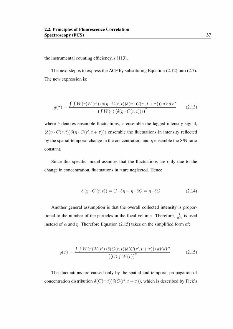
2.2. Principles of Fluorescence CorrelationSpectroscopy (FCS) 37
the instrumental counting efficiency, ι [113].
The next step is to express the ACF by substituting Equation (2.12) into (2.7).
The new expression is:
g(τ) =
∫ ∫W (r)W (r′) 〈δ(η · C(r, t))δ(η · C(r′, t+ τ))〉 dV dV ′(∫
W (r) 〈δ(η · C(r, t))〉)2 (2.13)
where δ denotes ensemble fluctuations, τ ensemble the lagged intensity signal,
〈δ(η · C(r, t))δ(η · C(r′, t+ τ))〉 ensemble the fluctuations in intensity reflected
by the spatial-temporal change in the concentration, and η ensemble the S/N ratio
constant.
Since this specific model assumes that the fluctuations are only due to the
change in concentration, fluctuations in η are neglected. Hence
δ (η · C (r, t)) = C · δη + η · δC = η · δC (2.14)
Another general assumption is that the overall collected intensity is propor-
tional to the number of the particles in the focal volume. Therefore, 1〈C〉 is used
instead of α and η. Therefore Equation (2.15) takes on the simplified form of:
g(τ) =
∫ ∫W (r)W (r′) 〈δ(C(r, t))δ(C(r′, t+ τ))〉 dV dV ′(
〈C〉∫W (r)
)2 (2.15)
The fluctuations are caused only by the spatial and temporal propagation of
concentration distribution δ(C(r, t))δ(C(r′, t + τ)), which is described by Fick’s

2.2. Principles of Fluorescence CorrelationSpectroscopy (FCS) 38
2nd law:
∂C(~r, t)
∂t= D · ∇2C(~r, t) (2.16)
Solving Equation (2.16) for a simple case of Brownian motion gives:
for 1d : C(r, t) = N
(4·π·D·τ)1/2e
[−x24·D·t
]
for 2−D : C(r, t) = N4·π·D·te
[−r24·D·t
]
for 3−D : C(r, t) = N
8·(π·D·t)3/2e
[−r24·D·t
]
t − time
N − number of particles
D − diffusion coefficient
x − position
(2.17)
where C(r,t) expresses the probability that a particle originally located at r=0 and
t=0 can be found in location r at time t. This probability has a Gaussian shape
[121, 122].
The Equation (2.17) can replace the concentration fluctuation term in Equation
(2.15), as demonstrated for 2-D diffusion in Equation (2.18):
〈δC(~r, t)t · δC(~r, t)t+τ 〉 = C4·π·D·τ e
[−(~r−~rτ )2
4·D·τ
](2.18)
And the new expression is:
g(τ) = 14·π·D·τ ·〈C〉
∫ ∫W (r)W (r′)e
[−(~r−~rτ )2
4·D·τ
]dV dV ′
(∫W (r)dV )
2(2.19)

2.2. Principles of Fluorescence CorrelationSpectroscopy (FCS) 39
The effective detection function describes the optical combination between
the PSF and the pinhole. Its exact shape is largely determined by the numerical
aperture (NA) of the objective lenses:
NA = n · sin(θ)
θ − angular aperture
n − refractive index of the medium
(2.20)
where n denotes the refractive index of the medium, and θ denotes the half angle
of the cone from which the objective is able to collect light. The waist of the
effective detection function are described in Equation (2.21):
ωxy(confocal) ' 0.44·λNAobjective
ωz(approximated) ' 3 · ωxy
λ − excitation wavelength
(2.21)
where the 0.44 value in Equation (2.21) is flexible and dependent on the charac-
terization of the optical setup.
Equation (2.22) shows the excitation radiation for a Gaussian focal spot in the
cases of 2-D and 3-D diffusion. For 2-D diffusion, there is no contribution to
the intensity fluctuations from the Z direction. Since the particles diffuse in the
XY-plane, the weighted excitation intensity is also planar. This is in contrast to
3-D diffusion where the particles can diffuse in and out of the XYZ-plane and
detection is 3-D. In such a case, the waist of the focal volume in the Z-plane, ωz,
has to be considered. The ratio between ωz and ωxy depends on the experimental

2.2. Principles of Fluorescence CorrelationSpectroscopy (FCS) 40
system and the objective [123].
for 2−D : W (~r) = W0 · e−2
[X2+Y 2
ω2xy
]
for 3−D : W (~r) = W0 · e−2
[X2+Y 2
ω2xy
+Z2
ω2z
]
W (0) − maximum excitation
X, Y, Z − cartezian coordinates
(2.22)
For an ellipsoidal 3-D Gaussian profile, the last equation can be expressed with
the next simple formula ([118]):
1Veff
=∫ ∫
W (r)W (r′)dV dV ′
(∫W (r)dV )
2
Veff−for Gaussian V olume = π32 · ω2
xy · ωzωxy − radial waist
ωz − axial waist
(2.23)
And the ACF will take the shape:
g(τ) = 1Veff ·〈C〉
· 14·π·D·τ
∫ ∫e
[−(~r−~r′)2
4·D·τ
]dV dV ′ (2.24)
The limits of integration take the definition of the observed volume into
account (W(r)=0 outside the observed volume [113]. Therefore, the integral in
Equation (2.19) can be solved analytically to yield:
g(τ) = 1Veff ·〈C〉︸ ︷︷ ︸
1〈Np〉
·
(1
1+ττD
)
τD − diffusion time
(2.25)

2.2. Principles of Fluorescence CorrelationSpectroscopy (FCS) 41
Equation (2.25) gives two useful parameters. The first parameter is the mean
number of particles in the focal volume, 1〈Np〉 , which is the amplitude of the
normalized ACF. The normalized ACF is expressed by:
g(τ) = 〈δI(t)·δI(t+τ)〉〈I(t)〉2
〈δI(t) · δI(t)〉− variance of intensity
〈I(t)〉−mean of intensity
and for τ = 0 :
g(0) = 〈δI(t)·δI(t)〉〈I(t)〉2
(2.26)
Assuming that the number of particles observed in the focal volume has a
Poisson distribution, and therefore the variance of the collected intensity is equal
to the mean of the intensity, and assuming that the overall collected intensity is
proportional to the number of particles, I∝<Np>∝<C>, when τ = 0 the ACF
amplitude is proportional to the average concentration of the particles:
Assuming Poisson probability, var(I) = mean(I) :
g(0) ∝ 1〈I(t)〉
Assuming I ∝ 〈Np〉 ∝ 〈C〉 :
g(0) ∝ 1〈Np〉 , g(0) ∝ 1
〈C〉
(2.27)
The second parameter is the diffusion time, τD, which is the time molecules
spend on the average in the observation volume [117]. The diffusion time is
proportional to the half-maximal of the maximum ACF value. For the simple
case of 2-D diffusion, the diffusion time is defined as:

2.2. Principles of Fluorescence CorrelationSpectroscopy (FCS) 42
for 2−D : τD = ω2
4·D (2.28)
Hence, measurement of fluctuations in fluorescence within a focal volume
and calculation of the ACF can be used to measure the diffusion time. Thereby
knowing the ωxy and the characteristic diffusion time providing useful knowledge
about the dynamic properties of the fluorophore, and can give the diffusion
coefficient of a specific fluorophore.
2.2.4 FCS in cell biology
The first FCS setups lacked the ability to measure diffusion in living cells.
The difficulty in adopting FCS for cell biology begins when trying to measure
the intensity fluctuation in single spots with a volume of only few femtolitres.
Selecting the location of this observation spot has enormous importance as the
cell dynamics and structure are very heterogeneous. More problems can arise
in the presence of autofluorescence, photobleaching and blinking. Finally, the
interpolation of the ACF to derive the exact value of the diffusion requires
sensitive FCS setup and knowledge about the size and shape of the PSF. Some
of these difficulties have been overcame in the last 10 years, and these days
FCS has the potential to become a major biophysical technique for studying
molecular interactions in living biological specimens [114, 124–127]. Moreover,
by modelling FCS fitting models that consider more complex dynamic properties,
FCS can be used to measure molecular distribution, direct flow, give information
about binding kinetics, and about multiple component interactions of expressed
labelled proteins in living cells [120, 128–132]. .

2.3. Principles of Image Correlation Spectroscopy (ICS) 43
2.3 Principles of Image Correlation Spectroscopy
(ICS)
2.3.1 ICS is based on raster CLSM
When a single point source with a size that is smaller than the PSF is visualized by
raster CLSM, the point source is excited by the laser beam, and the emitted fluores-
cence is detected and translated to electronic signal. In confocal microscopy, the
resolution limit is determined by the waists of the observation volume (or simply
the PSF), ωxy and ωz, as defined by the Rayleigh criterion (Equation (2.21)). This
means that the smallest object in the reconstructed confocal image is actually
the convolution of the point source with the PSF, and that information below the
resolution criteria cannot be resolved between adjacent pixels. Thus, information
below the resolution criteria will be correlated between close pixels.
The concept that there is hidden correlated information between the pixels was
introduced by Petersen and Wiseman in 1993, who introduced a technique known
as Image Correlation Spectroscopy (ICS) (known also as Image Correlation
Microscopy (ICM)). By using computer analysis of the 2-D ACF of images
acquired by raster CLSM, ICS was shown to give statistical information about
the number of particles in the sample [133].
Figure 2.9 shows a schematic illustration of convolution by raster LSCM.

2.3. Principles of Image Correlation Spectroscopy (ICS) 44
Raster scan
Smoothed Image
Reconstructed image
Figure 2.9: Convolution of point source in raster LSCM.The laser beam horizontally scans the sample that contains a fixed pointsource (the red diamond shape). The point source is excited, and theemitted fluorescence is detected and translated to an electronic signal. Sincethe mirrors that control the raster scan are coordinated with the collectedintensity at any specific time, computer software divides the intensity intodiscernments, and gives each pixel a value. Pixel by pixel the confocalimage is reconstructed, and the point source is spread over a number ofpixels (the pixelated shape in the middle of the figure) as a consequence ofthe convolution. Over sampling (i.e. - capturing a series of images overtime and averaging the series) will give a smoother image with a perfectairy-disk shape as predicted by Rayleigh criterion. The figure was adoptedfrom [74].

2.3. Principles of Image Correlation Spectroscopy (ICS) 45
2.3.2 The 2-D ACF
The 2-D ACF is the extension of the 1-D ACF presented in FCS (section 2.2).
While in FCS the 1-D ACF describes the temporal laser signal, in ICS the 2-D
ACF describes images, which can also be regarded as a 2-D matrix:
G(ξ, ψ) = 〈δI(X, Y ) · δI(X + ξ, Y + ψ)〉
I(X, Y ) − detected intensity at each pixel from matrix (image/ROI)
δI(X, Y ) − fluctuations around the mean intensity of the image
(2.29)
Similar to FCS, the 2-D ACF can be calculated in two manners: brute force
and through the 2-D Fast Fourier Transform. When brute force is used to calculate
the 2-D ACF is represented by:
for specific t :
g(ξ, ψ)t =1
X·Y∑Xk=1
∑Yl=1 I(X,Y )I(X+ξ,Y+ψ)[
1X·Y
∑Xk=1
∑Yl=1 I(X,Y )
]2 − 1
t − frame number
(2.30)
This matrix is shifted relative to the original image and the shifted and original
images are multiplied and the result summed. Where X-axis is the horizontal
axis (parallel with the scanning direction), and Y-axis is the vertical axis. This
process is repeated for all possible magnitudes of shift (the maximum magnitude
of shift is limited to the largest dimension of the image) in all possible directions.
The complete expression of the ACF after its normalization with the spatial mean
intensity is:
g(ξ, ψ) =G(ξ, ψ)
< I(X, Y ) >2− 1 (2.31)

2.3. Principles of Image Correlation Spectroscopy (ICS) 46
A more convenient way to calculate the 2-D ACF is to use the 2D-FFT. This
method also has the advantage that it enables application of frequency filters which
are essential for RICS (Equation (2.32)):
G(ξ, ψ) = f−1(
[f (I(X, Y ))] ·[(f (I(X, Y )))
])(2.32)
Generally, it is better to minimize the noise originating from the contribution
of random correlations to obtain an accurate estimate of the ACF. This can be
achieved by averaging the normalized ACF over a number of images [134]. In
contrast to the spatial correlation due to the effect of the convolution by PSF,
random shot noise is not correlated between adjacent pixels, and appears at zero
time lag [135]. Therefore, by fitting the ACF to a theoretical shape which is
dictated by the PSF, random noise can be discounted.
2.3.3 ICS fitting model
The two-dimensional ACF in ICS gives the dominant spatial correlation in the
image which is the result of the convolution of the point sources with the shape
of the focal volume, which is commonly assumed to have a Gaussian shape.
Therefore, the normalized ACF has to be fitted to a Gaussian shape:
g(ξ, ψ) = g(0, 0)e−(
(ξ2+ψ2)ω2xy
)+ g∞ (2.33)
where g∞ express the offset constant for the possibility of long range spatial
correlation. The peak of the ACF after the fitting gives the number of particles
without counting the noise in the image (Equation (2.34)).

2.3. Principles of Image Correlation Spectroscopy (ICS) 47
g(0, 0) = limξ→0
limψ→0
g(ξ, ψ) = 1Veff ·〈C〉︸ ︷︷ ︸
1〈Np〉
(2.34)
The ACF amplitude, the g(0,0), is equivalent to the g(0) in FCS ((2.25)), and
is proportional to the inverse of the average number of the particles in the image.
2.3.4 Advances in Image Correlation Spectroscopy
ICS provides information about the number of particles within an image. How-
ever, it does not provide information about the dynamic properties of the fluo-
rophores in the sample. However, in the last 10 years there has been extensive
development of ICS-based techniques to exploit the spatial-temporal correlation
in images from commercial CLSM to retrieve quantitative information about the
fluorophores dynamics. These concepts were mainly contributed by Wiseman
and coworkers (McGill University, Montreal, Quebec, Canada), who developed
a series of ICS-based techniques.
An example of an ICS-based technique is Spatial-Temporal Image Correlation
Spectroscopy (STICS), which gives spatial-temporal maps of macromolecules
dynamics by calculating the temporal correlation of the spatial correlation of
aggregations of fluorescence proteins within living cells. If the motion of the
molecules is non-isotropic (i.e. - directed flow), STICS can extract the directional
information over time points. It has been used to generate velocity maps of α-
actinin in living CHO (Chinese Hamster Ovary) cells, were arrows gives the speed
and direction of the α-actinin flow [136].

2.4. Principles of Raster Image CorrelationSpectroscopy (RICS) 48
2.4 Principles of Raster Image Correlation
Spectroscopy (RICS)
Firstly, RICS was introduced by E. Gratton and M. Digman who noticed that
there is an additional component to the ACF of ICS, in which the apparent
diffusion coefficient of the fluorophores increases while the laser beam raster
scans the sample. Briefly, this additional component was formulated and the
RICS technique was than introduced with the aptitude to combine the capability
of FCS to measure fast diffusion with the capability of ICS to obtain quantitative
information about molecules from confocal images. Unlike STICS, RICS does
not measure the direction of the flow, but rather measures the average diffusion
coefficient due to Brownian motion of the fluorophores. Figure 2.10 illustrates the
advantage of RICS through integration of FCS and ICS. While FCS is based on
the 1-D ACF from single point locations, RICS is based on the ACF analysis from
CLSM images in 2-D.
LimitationData from single point
AdvantageMeasure temporal correlation
of dynamic movement
AdvantageData is in 2D from CLSM
LimitationOnly spatial correlation
RICSMeasure 2D spatio-temporal correlation of dynamic
from CLSM images
ICSFCS
STICSspatio-temporal 2-D ACF
between the framesmovement between pixels
Figure 2.10: RICS is a combination between ICS and FCS.
RICS has the capability to provide temporal and spatial information about the
diffusion coefficients and concentration of fluorophores in solutions. Like FCS,

2.4. Principles of Raster Image CorrelationSpectroscopy (RICS) 49
it is a non-contact measurement technique, and therefore is a non-invasive tool
for studying dynamic processes within living cells. Evidently, RICS does inherit
some of its limitations from FCS. Measurements in cell edges, the movement
of the cells, and the dependency of the measurements on the size and shape of
the observation volume all have a strong effect on the ACF (and the calculated
diffusion coefficients). However, RICS also has some advantages over FCS.
For instance, RICS has a better capability to filter out the immobile fraction.
Moreover, it allows mapping the diffusion coefficient within living cells by
generating spatial-temporal plots.
While STICS can also give spatial-temporal plots, there is a major difference
between these two approaches. While STICS is based on temporal correlation
between the ACF of a defined region over consecutive confocal images and
therefore is limited to measuring relatively slow dynamics, RICS is based on the
correlation of fluctuation between successive pixels and is used for faster diffusion
coefficients.
The principle of RICS is that the ACF of the image collected by CLSM
contains correlated information about diffusing fluorescence molecules in time
and space domains. The key to understanding RICS is to note that CLSMs create
images by raster-scanning the sample and collecting the intensity emitted from
each point in a sequential manner. Hence, different points on the image are
actually acquired at different times. Thus, if the CLSM picks up a molecule at
a certain point I(X,Y) then there is a finite probability that the laser will pick up
the same molecule at a later point delta I(X+ξ ,Y+ψ). The probability to detect
the molecule depends on the PSF, scanning speed of the CLSM and the diffusion
coefficient of the particle. Thus, analysing the statistics of the fluctuations in a
CLSM image could provide information about the diffusion of the particles being
imaged. RICS is a method for deriving this information by analysing the ACF of

2.4. Principles of Raster Image CorrelationSpectroscopy (RICS) 50
the confocal image. If the fluorophores are not moving, the ACF will correlate
only the spatial correlation due to convolution with the point source. Under
constant scanning speed, as the diffusion coefficient of the fluorophores increases,
the probability to detect the same particle at a different point will change. The
ACF reflects the probability of imaging the same diffusing particles at two or more
different points in the image. This probability depends on the diffusion coefficient
of the particle. Hence, fitting the ACF to a RICS equation can give the diffusion
coefficient.
Figure 2.11 shows a schematic illustration of the principle behind RICS.

2.4. Principles of Raster Image CorrelationSpectroscopy (RICS) 51
Particle diffusing during raster scan
Smoothed ACF
Reconstructed image
The probability to detect the particle is correlated in the ACF
Less probability to detect the
particle in parallel lines
Figure 2.11: The principle behind RICS.Similar to ICS, the laser beam raster scans the sample, which containsfluorescence particles. However, in RICS the assumption is that thefluorophore randomly diffuses and therefore its probability to be detectedis correlated between adjacent pixels. This correlation is translated byusing the ACF, and can be fitted to the theoretical RICS model to give thephysical value of the diffusion coefficient.

2.4. Principles of Raster Image CorrelationSpectroscopy (RICS) 52
2.4.1 Time and space domains in RICS
The Time domain in RICS is controlled by the scanning speed of the microscope.
Since the ACF in RICS is two dimensional, the lag time accounts for the difference
in time between the horizontal line and the vertical line (Equation (2.35)) [66].
τ(ξ, ψ) = τpξ + τlψ
ξ − spatial displacements along X direction
ψ − spatial displacements along Y direction
(2.35)
Rather than using the lag time, τ , which is used in the 1-D ACF, τ l and τ p are
multiplied in ξ and ψ, respectively. The pixel dwell time, τ p, indicates the time in
which the signal to the detector is integrated to be displayed as a single point in
the resulting image [74, 137]. The line time, τ p, is the time that it takes the laser
beam to complete a scan of the full line.
2.4.2 RICS fitting model for Brownian motion
The 2-D experimental ACF has to be fitted to the RICS model in order to yield the
diffusion coefficient and concentration. The standard RICS model makes the same
assumptions as the standard FCS model discussed in section 2.2. The RICS model
has two components. The first RICS component assumes that the location of
fluorophores changes in space and time, therefore the collected intensity fluctuates
over time while the image is being reconstructed.
When the laser beam scans the sample with a suitable speed, each pixel gets
a value that is different from the values of the pixels before and after it, but there
is still correlated information between adjacent pixels, as explained in ICS for a
case where the particles are fixed. As the diffusion coefficient of the fluorophores

2.4. Principles of Raster Image CorrelationSpectroscopy (RICS) 53
is faster, there is less correlation between adjacent pixels and the frequency of
fluctuation will increase, as in FCS (Equation ((2.25) ). Equation (2.36) expresses
the RICS Equation for a single photon laser and 3-D diffusion.
GD(ψ, ψ) = 1Veff ·〈C〉︸ ︷︷ ︸
1〈Np〉
·(
1 + 4D(τpξ+τlψ)
ω2xy
)−1 (1 + 4D(τpξ+τlψ)
ω2z
)−1/2
(2.36)
The second component is the correlation due to the raster scans and due to the
spatial differences in concentrations, in a similar way to ICS but considering that
diffusion can cause a broadening of the PSF (Equation (2.37)):
S(ξ, ψ) = exp
− 12[(2ξδrwxy
)2 + (2ψδrwxy
)2]
(1 + 4D(τpξ+τlψ)
w2xy
)
(2.37)
The overall RICS expression that was used in this thesis is:
G(ξ, ψ) = GD(ξ, ψ) · S(ξ, ψ) (2.38)
A graphical 2-D image that illustrates this function is presented in Appendix
A.5.
2.4.3 Advances in RICS
Returning back to the Jablonski diagram, the fluorophores can also go through
a process that is known as intersystem crossing, which means a nonradiative
transition between different electronic spins. This process leads to a triplet

2.4. Principles of Raster Image CorrelationSpectroscopy (RICS) 54
electronic energy level, and results from saturation in the total number of high-
energy states, which leads to energetic instability. The duration of this transition
is in µs-ms, and it causes the fluorophore to blink. [118, 138].
Several improvements and extensions have been made to the RICS technique
in the last two years. For instance, a third component known as the ”time
dependent” component was introduced by Digman et al. in 2009 [66] to consider
the contribution of additional fluctuations in fluorescence while the molecules
enter and leave their triplet states. Equation (2.39) expresses the time dependent
component:
GT (ξ, ψ) = 1 + Ae−(τpξ+τlψ)/τ
A − fraction of blinking molecules
τ − characteristic time
(2.39)
The temporal change in the intensity of the fluorophore can occur either due
to conformational changes of the molecule that alter its fluorescence, or due to
blinking, which naturally occurs in some fluorophores. For example, quantum
dots exhibit significant blinking when they fluoresce [139]. The ”time dependent”
component was not applied in this thesis. However, it does emphasize the idea
that the standard RICS model is not always sufficient, that there is still a place
for improvements and considerations of biophysical effects, and that modelling of
correction factors is a standard procedure. As will be shown next in this thesis, a
similar idea of applying RICS in conjunction with photobleaching phenomena
to detected fluorophores diffusion can be applied by using more sophisticated
modelling.
Another improvement was introduced in 2008 by Digman et al. who demon-
strated that by dividing an image into a grid of overlapping regions and applying

2.4. Principles of Raster Image CorrelationSpectroscopy (RICS) 55
RICS to each region, they could create spatial-temporal maps of diffusion of
EGFP-paxillin in Chinese Hamster Ovary cells [60]. These results were verified
by using complementary techniques such as: scanning FCS, temporal ICS and
Photon Counting Histogram analysis (PCH)[60].
2.4.4 Cross correlation approach in FFS
One particular development in FFS is the highly desirable approach of Fluores-
cence Cross Correlation Spectroscopy (FCCS) technique to measure functional
associations of two different fluorophores by correlating their two ACFs, and its
biological applications to measure protein-protein interactions within living cells
[125, 140–143]. Image Cross Correlation Spectroscopy (ICCS) is the analogous
to FCCS based on the 2-D ACF similar to ICS. ICCS was used to generate
spatial maps of the dynamic interaction between actin and its bundled protein,
α-actinin, to the leading edge of a migrating cell [144]. In more recent times cross
correlation between vinculin, focal adhesion kinase (FAK), and paxillin tagged
with fluorescence proteins within living Mouse Embryonic Fibroblasts (MEF)
cells was demonstrated by employing Cross Correlation RICS (cc-RICS) to study
protein complexes [66, 67]. Although very novel, cc-RICS is likely to prove
extremely powerful in dissecting the relationships between protein interactions
and biological processes. As compared with the often-misleading observations of
co-localization of two proteins, finding that diffusion properties are identical in a
given region of the cells is likely to be very strong evidence that they physically
interact.

2.5. Summary 56
2.5 Summary
The importance of fluorescent imaging to study biological questions by using
fluorescence proteins was emphasized. In addition, the advantages of several
FFS were discussed. Yet, more advances in this field are required before it will
become a standard routine in cell biology, and will reach to its maximum potential.
RICS was introduced as a novel technique, and its principles were explained. This
theoretical background helps to understand the concept of this thesis.

Chapter 3Materials and Methods
3.1 Conditions for Cell Maintenance
3T3 cells (fibroblast cells from mouse embryo tissue) were maintained in
humidified, 10% CO2 at 37◦C in standard Dulbecco’s Modified Essential Medium
(DMEM) supplemented with 10% v/v Fetal Bovine Serum (FBS) and a final
concentration of 3 mM GlutaMAX (Glutamine, Gibco BRL, Invitrogen Corp.
Life Technologies, CA, USA). Cells were harvested with trypsin and passaged
to maintain exponential growth. BaF3 cells (naive pro B cells) were maintained
in humidified, 5% CO2 at 37◦C in RPMI medium (GIBCO,11875-093) supple-
mented with 10% Fetal Bovine Serum (FBS), 10% v/v WEHI 3BD conditioned
medium (contains IL-3, supplied by Andrew Clayton from Ludwig Institute for
Cancer Research) and 1.5 mg/ml geneticin (G418, Gibco). The cells were frozen
in FBS containing 10% Dimethyl sulphoxide (DMSO, Sigma), stored in liquid
nitrogen, and were thawed and cultured for a week prior to any experiment.
57

3.2. Plasmid DNA 58
3.2 Plasmid DNA
The DNA was extracted from E.coli and was purified with a Qiagen plasmid
maxi kit (Qiagen GmbH, Hilden, Germany) by Kim Pham from Peter MacCallum
Cancer Centre, Melbourne, Australia. pEYFP-βPIX and pEYFP-βPIX∆CT (also
known as pEYFP-βPIX-DSTOP) plasmids were constructed by Kim Pham and
the pEYFP plasmid was purchased from Clontech (Clontech Laboratories, USA).
Figure 3.1: βPIX and βPIX∆CT plasmids.The βPIX plasmid has three Src homology domains (SH3) that interactwith sequences rich in proline residues of PAK, GIT and PLC. The DHis Dbl homology domain that interacts with Cdc42 and RAC. PH is Plechomology domain. T1 domain inhibits GEF activity. PR is proline-richregion. GBD is GIT binding domain. CC domain contain leucine zipperthat mediates βPIX dimerization. The last domain is the PDZ domain-binding motif that interacts with the PDZ domain of Scribble is located atthe carboxyl terminus. While the wt-βPIX has the (-TNL) site, βPIX∆CTstops at (-D) and lacks the (-TNL) site of binding to Scribble. The domainmap was adapted from [23]
3.3 Antibiotic Titration
The pEYFP, pEYFP-βPIX and pEYFP-βPIX∆CT plasmids contain the gene for
neomycin resistance for positive selection with G418. In order to determine the
optimal concentration of G418 for selection of transfected cells, cells were plated
at 1×10⁵ cells/well in a Cellstar R© 6-well plate (Greiner bio-one, Frickenhausen,

3.4. Cell Transfection 59
Germany) and cultured for at least 24 hours to achieve 80% confluency. G418 was
added at different concentrations and was refreshed every two days. The cultures
were checked daily under transmission light microscope and the survival rates
of the cells was assessed by subjective judgment of the cells appearance. The
optimal concentration of G418 that achieved rapid killing of the cells was 1000
µg/ml. This optimal concentration of G418 was determined to be sufficient to use
for selection of transfected cells.
3.4 Cell Transfection
3T3 cells were plated at 1×10⁵ cells/well in a Cellstar R© 6-well plate and were
cultured for at least 24 hours to achieve 80% confluency under same condition as
the culture at the section 3.1.
Transfections were achieved by using metafectene (Biontex Laboratories
GmbH Munich, Germany) at a 1:3 ratio of DNA to metafectene, respectively.
Metafectene was incubated with DMEM (not supplemented) for 5 minutes at
Room Temperature (RT) and 500 ng of DNA was added to the metafectene mix,
followed by another 15 minute of incubation in RT. The diluted mixture was added
drop wise to the plated cells. After one hour, G418 was added for positive selection
and was refreshed every two days.
3.5 Preparation of Cell Lines
The transfected cell lines were cultured with G418 until they reached 100%
confluence then sorted by Fluorescent Activated Cell Sorting (FACS) for YFP
fluorescence expression level on DiVa (Becton Dickinson, NJ, USA) for two
rounds of sorting. The bulk population of βPIX∆CT was single cell cloned in 96

3.6. Western Blotting 60
flat-well cell culture plates. When the cultures reached 80% confluence, random
clones were selected and expanded. Expression levels of the clones were checked
by DiVa FACS and analysed using Flow Cytometry Software (FCS express v3.0
software, Becton Dickinson). At the end of the process, FACS and Western blot
were used to characterize the three cell lines.
3.6 Western Blotting
Sample preparation
Whole cell extracts were prepared from 106 to 107 cells/ml of media. The
cells were incubated in NETN lysis buffer (see appendix B) that contained
(1 tablet/10 ml) Complete Mini protease inhibitor cocktail (Roche Diagnostics
Australia, NSW, Australia) for 15 minute on ice. The lysates were cleared by
centrifugation at 15.7×10³ relative centrifugal force (rcf) for 15 minutes at 4◦C
and the supernatants were aliquoted into clean Eppendorf tubes. The supernatants
were used immediately or stored at -80◦C.
Determination of protein concentration
A colorimetric assay was used to determine protein concentration in the super-
natant using the Bio-Rad DC Protein Assay Reagent kit, according to manufac-
turer’s instructions (BIO-RAD laboratories, Hercules, Canada). The absorbance
was read by spectrophotometer at 650 nm and the protein concentrations were cal-
culated with SoftMax Pro v5.2 software (Molecular Devices Corp., Downington,
PA).

3.6. Western Blotting 61
Gel electrophoresis and transfer
Lysates were diluted with lysis buffer to generate equivalent concentrations of 30
mg protein per loading well in the SDS gel. Reducing 5×loading buffer (see
appendix B) was added to the dilution (in 5:1 ration v/v). This mixture was
incubated for 5 minutes at 95◦C and then was loaded to 9% SDS PAGE (see
appendix B). The proteins were resolved for 1 hour in 100 Volts at RT with
SeeBlue R© Plus2 (Invitrogen) as a pre-stained standard.
Transfer
The proteins were transferred for one hour in 100V at 4◦C in wet Bio-rad elec-
trophoretic transfer cell containing transfer buffer (see appendix B) to Immobulon-
P (PVDF) membrane (Millipore Corp., MA, USA) wetted with methanol.
Detection
Membranes were blocked in blocking solution (5% w/v Skim milk powder
(Diploma, Mount Waverly, Australia) in PBS that contained 0.05% v/v Tween-
20 (Polysorbate 20, Sigma-Aldrich, MO, USA)) for one hour rotating at RT.
Membranes were probed with the appropriate primary antibodies (see Table 3.1)
in blocking solution for one hour at RT or overnight at 4◦C. The membranes were
washed in 0.05% v/v Tween-20 in PBS three times over 15 minutes and incubated
with cognate Horse Radish Peroxidase (HRP) linked secondary antibody (see
Table 3.2) in blocking solution for 30 minutes at RT. The membranes were washed
in 0.05% v/v Tween-20 in PBS three times over 15 minutes.
The proteins were detected by using Enhanced Chemiluminscence (ECL)
western blotting detection kit (GE Healthcare, Buckinghamshire, UK) according

3.7. Antibodies 62
to manufacturer’s instructions and visualized by autoradiography using X-ray film
(Fujifilm Europe GmbH, Heesenstrasse, Germany).
3.7 Antibodies
Both primary and secondary antibodies for Western Blot (WB) were diluted in
western blocking solution (PBS contained 5% w/v Skim milk powder and 0.05%
v/v Tween-20). The antibodies dilutions are presented in Table 3.1.
Table 3.1: Primary antibodies
Antigen Source Supplier WB
βPIX Rabbitpolyclonal
Chemicon Int.,Billerica, MA
1:200
GFP Rabbitpolyclonal
Supplier 1:3000
α-tubulin Mousemonoclonal
Supplier 1:1500
Table 3.2: Secondary antibodies
Reactivity Fluorochrome Supplier WBsheep anti mouse HRP GE Health care 1:10000
Donkey anti rabbit HRP GE Health care 1:10000
3.8 Preparation of Microscope Samples
Preparation of fluorescent samples
A template of wells was punched in a double-sided sticky tape that was attached
onto 25 mm×75 mm×1 mm glass microscope slides (Esco, Biolab Scientific).

3.8. Preparation of Microscope Samples 63
Each well was used to contain 6.5 µl fluorescent solution sample for microscope
imaging. The slide was sealed with 24 mm×50 mm glass covered slips (Esco).
Three kinds of samples were prepared:
1. GFP (molecular weight of ≈27 kDa, Invitrogen) diluted in PBS-glycerol
solution, final concentration 44 nM at pH=7.4 . The collected emission
wavelengths for the GFP sample were chosen automatically by λ-scan
emission spectra with increments of 10 nm.
2. Poly(N-vinyl pyrrolidone) (PVPON, molecular weight of 21 kDa, con-
tributed by Melbourne University, VIC, AU). PVPON was covalent bonded
to Alexa R© Fluor dye 488 nm, (molecular weight of ≈0.64 kDa, Molecular
Probes, Invitrogen), and diluted in dH2O, final concentration 5 µM. The
collected emission wavelengths for the Fluor dye 488 nm were chosen
according to the manufacturer’s instructions.
Figure 3.2: Molecular structure of PVPON.
Polymer chain of PVPON covalent bonded to Alexa R© Fluor dye 488 nm(AF488) to one of its attachment sites.
3. Green-yellow fluorescent polystyrene sub-resolution 0.1 µm diameter mi-
crospheres (Duke Scientific Corp., Palo Alto, California, USA) were diluted
in dH2O or glycerol-dH2O solution to a final concentration containing
7.8×10⁻³% solid (1:128 dilution between the stock (containing 1% solid)
and dH2O/glycerol-dH2O solution, respectively. Excitation maxima λ=468

3.8. Preparation of Microscope Samples 64
nm, emission maxima λ=508 nm. The density of microspheres is 1.05
g/cm3.
In order to control the solutions viscosity, the solutions were made in different
concentrations of glycerol (LabServ Biolab). The viscosity of water/glycerol
mixture was interpolated from the Dorsey sheet [145]. Samples were assumed
to be at 37◦C. Prior to imaging, the samples were stored at 4◦C in the dark to
prevent photobleaching.
Preparation of biological samples
3T3 cells were plated at 5×10³ cells/well on 35 mm optic glass bottom dishes
(Matek, MA) and were cultured for 24 or 48 hours as in 3.1.
BaF3-EGFR-EGFP is a cell line that over expresses EGFR (epidermal growth
factor receptors) fused by its carboxyl terminus to EGFP. This line was supplied
by Andew Clayton from Ludwig Institute for Cancer Research. The cells were
grown at a concentration of 1×10⁶ cells/ml, and were serum-starved for 5 hours
prior to the experiment. Cells were collected by centrifugation, and resuspended
at 1.25×10⁶ cells/well. To immobilize the cells, 5×10⁴ cells/ml were transferred
onto 35 mm optic glass bottom dishes (Matek) containing soft agarose mix (0.8%
w/v agarose (Promega, Corp., Madison Wl, USA) and 1% w/v BSA in PBS.
This concentration of agarose was found to restrict cellular movement without
compromising cell viability. The ratio between the medium and agarose mix was
1:5 respectively. The agarose mix was pre-warmed in a microwave to 45◦C and
then cooled to 37◦C before the cells were pipetted to the bottom of the dishes
to penetrate the agarose layer. The cells which were located between the glass
and the agarose were randomly chosen for RICS measurements. The BaF3 were
imaged under similar conditions as the 3T3 with three exceptions: Firstly, since

3.9. Microscope Setup 65
movement of large receptor aggregations (larger then the PSF) were observed, the
focus was manually adjusted to be at the cell membrane ring (the cross section was
exactly at the centre of the cell). Secondly, the zoom factor was increased as the
BaF3 are smaller then 3T3, allowing to increase the resolution into approximately
30 nm pixel widths. Finally, both the excitation line and emission spectrum were
chosen differently, as the BaF3 expressed EGFP and not EYFP as in the 3T3 lines.
3.9 Microscope Setup
Data for RICS experiments was acquired with a Leica TCS SP5 multispectral
commercial CLSM (Leica Microsystems CMS GmbH, Germany) in direct mode,
controlled by LAS AF v2.0 software interface. It is multispectral in the sense
that it contains optical components that enables the user many degrees of freedom
in determining the spectra of the excitation illumination and detected emission.
The unique components incorporated in the system enable fast switching between
different excitation sources and flexible determination of the spectra detected
on each of the five PMTs in the system. Thus, the SP5 can provide detailed
information on the spectrum of fluorescent emission thereby enabling FRET, and
possibly cc-RICS measurements in the future.
Three special optical components allow the Leica SP5 its special feature of
multispectral confocal imaging: an Optical Tuneable Filter (AOTF), an Acoustic
Optical Beam Splitter (AOBS), and the Spectrophotometer detection apparatus
(SP) [146, 147]. These components are coupled and work synchronously together,
as shown in Figure 3.3.
Both the AOTF and the AOBS are based on the same approach of generating
an acoustic-optical field within piezoelectric crystal (i.e.-quartz) while the poly-
chromatic light is passing through the crystal. When the crystal is excited by

3.9. Microscope Setup 66
a modulated ultrasonic wave field, local changes in its refractive index result in
the formation of an effective diffraction grating that deflects the passing light in
a wavelength-dependent manner. A wavelength is deflected, dependent on the
period of the grating, which is determined by the frequency and intensity of the
ultrasonic excitation. Thus, by controlling the ultrasonic frequency and intensity
within the crystal, and selecting the light deflected at a certain angle from the
crystal, it is possible to select the wavelength of choice. [74].
The AOTF is an adjustable quartz crystal that is acoustic-optically modulated
to select the specific wavelengths of the excitation. One important advantage of
the AOTF is that it can be switched very rapidly, thereby enabling the selection of
multiple active excitation laser lines for acquisition of a single frame. Secondly,
the AOTF can be used to adjust the percentage of the laser intensity passing
through. It is important to note, that the AOTF control does not affect the laser
power from its source [74, 146].
The AOBS is a novel beam splitter that was introduced in 2002 by Leica to
replace the dichroic mirror and to improve the separation between the illumination
and the detection paths [146]. It works by exciting the piezoelectric crystal with a
signal that is the sum of several specific frequencies, thereby enabling diffraction
of several wavelengths simultaneously. Thus, the AOBS allows simultaneous
detection in multi fluorescence channels [146].
The last optical apparatus that allows of multispectral detection is the spec-
trophotometer detection module. This module comprises a prism that disperses
the emission into a moveable mirror that directs the light into tuneable slits placed
in front of the PMTs. These slits are mechanically adjustable to any position in
the spectrum. By adjusting the width of the slits, it is possible to determine the
spectral band to be collected by the PMTs [148].

3.9. Microscope Setup 67
Figure 3.3: Scheme of Leica TCS SP5 components relevant to this thesis work.Excitation light arrives from the Laser sources (1-3) and its intensityis controlled by an Acoustic Optical Tuneable Filter (AOTF), which iscontrolled by the LAS AF v2.0 software(4-6). The laser beam is reflectedby an Acoustic Optical Beam Splitter (AOBS) (8) and scan the samplethrough the scanner and calibration target units (10-11). The beam isfocused into the sample by the objective and the emitted fluorescence lightis collected by the same objective. The collected light passes througha pinhole (16), which eliminates all light emitted from outside the focalvolume. After passing the detection pinhole, the light emitted from thefocal plane is passed through a spectrophotometer prism (19). The lightcontinues from there to the PMTs, which are mounted with slits that can bewidened or narrowed to determine the portion of the spectrum collected byeach (PMT) (20-24). Figure was printed from [123] with permission.
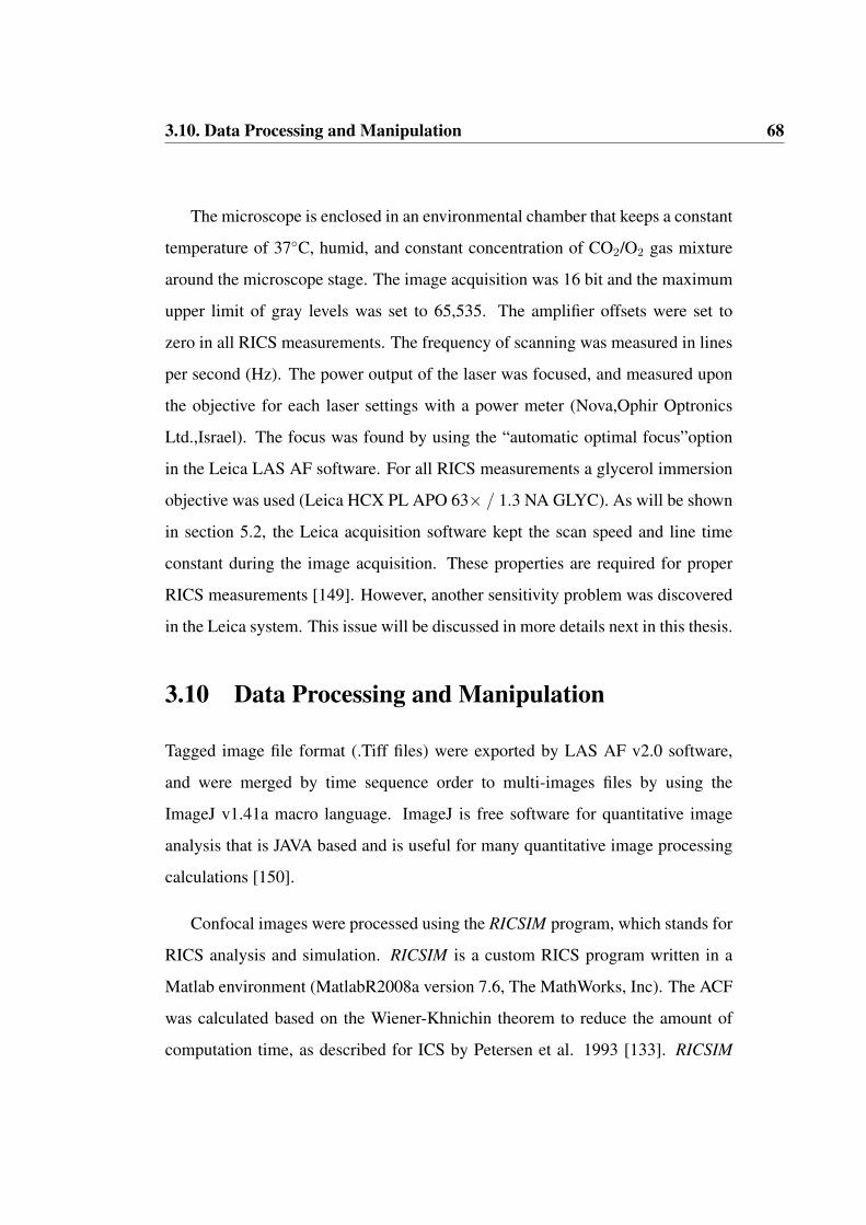
3.10. Data Processing and Manipulation 68
The microscope is enclosed in an environmental chamber that keeps a constant
temperature of 37◦C, humid, and constant concentration of CO2/O2 gas mixture
around the microscope stage. The image acquisition was 16 bit and the maximum
upper limit of gray levels was set to 65,535. The amplifier offsets were set to
zero in all RICS measurements. The frequency of scanning was measured in lines
per second (Hz). The power output of the laser was focused, and measured upon
the objective for each laser settings with a power meter (Nova,Ophir Optronics
Ltd.,Israel). The focus was found by using the “automatic optimal focus”option
in the Leica LAS AF software. For all RICS measurements a glycerol immersion
objective was used (Leica HCX PL APO 63× / 1.3 NA GLYC). As will be shown
in section 5.2, the Leica acquisition software kept the scan speed and line time
constant during the image acquisition. These properties are required for proper
RICS measurements [149]. However, another sensitivity problem was discovered
in the Leica system. This issue will be discussed in more details next in this thesis.
3.10 Data Processing and Manipulation
Tagged image file format (.Tiff files) were exported by LAS AF v2.0 software,
and were merged by time sequence order to multi-images files by using the
ImageJ v1.41a macro language. ImageJ is free software for quantitative image
analysis that is JAVA based and is useful for many quantitative image processing
calculations [150].
Confocal images were processed using the RICSIM program, which stands for
RICS analysis and simulation. RICSIM is a custom RICS program written in a
Matlab environment (MatlabR2008a version 7.6, The MathWorks, Inc). The ACF
was calculated based on the Wiener-Khnichin theorem to reduce the amount of
computation time, as described for ICS by Petersen et al. 1993 [133]. RICSIM

3.10. Data Processing and Manipulation 69
implements the RICS technique with a Graphical User Interface (GUI) based on
Matlab-GUIDE especially for this thesis. A screen capture of the RICSIM GUI
can be seen in appendix D. An explanation about how RICSIM works is presented
in the next chapter. The Matlab toolboxes that were used in RICSIM are the
Image Processing Toolbox for the background and cells filters, the Optimization
Toolbox for fitting procedures and the Spline Toolbox for polynomial fitting to
generate smoothed diffusion maps. Calculations were performed on a personal
laptop equipped with a 2 GHz Intel CoreTM 2 Duo processor and 3GB of
RAM. Calculation time for generating a smoothed diffusion map of cells and for
calculating the average diffusion coefficient for a group of 10 cells is between 5
and 10 minutes, depending on the available computer resources.

Chapter 4Computational Implementation of
RICS by the RICSIM software
4.1 Introduction
Previous RICS measurements were achieved by using commercial CLSMs,
such as the- FV300 and FV1000 systems (Olympus Inc, Japan), and the LSM
510 META (Carl Zeiss Inc, Germany), all in analogue mode employed with
standard PMTs [58, 65]. These studies showed that RICS is not a straightforward
technique, and several aspects regarding its sensitivity have to be considered
before it can be applied to more precise measurements. For instance, the accuracy
of the autocorrelation analysis was shown to be dependent on the system setup.
Calculating the ACF under several different experimental conditions and fitting
the corresponding ACF to RICS equation yielded dramatically different apparent
diffusion times [61, 135]. In addition, the PMTs of both the FV300 and the LSM
510 META systems have an inherent residual that is correlated in the ACF, and
70

4.1. Introduction 71
might affect the apparent diffusion time. This effect was mainly in the central
horizontal (X direction) and vertical (Y direction) ACF pixels, and was noticed to
increase with the scanning speed [61, 65, 135].
Recently, it was also reported by Gielen et al. (2009) that it might be
better to utilize Avalanche photodiode detectors (APD) rather than PMTs for
RICS measurements [65]. PMTs have a high dynamic range and noise-free
signal amplification and are generally the standard detectors in many research
laboratories, while APDs are usually used in FCS applications due to their superior
sensitivity over the PMTs [151]. However, the installation of APDs on commercial
confocal systems is not practical in many labs, and therefore other approaches are
required to gain more accuracy in RICS measurements using the PMTs in a direct
analogue mode.
Hence, in the absence of published data about RICS measurements with the
Leica SP5 (to our knowledge), it was a requirement to characterize the ACF
obtained by the Leica SP5, and to establish a RICS routine that will allow precise
measurements of diffusion coefficients within living cells. Such a characterization
was even more necessary because of the sensitivity limit when performing RICS
with the Leica SP5 was stated by E. Gratton, the inventor of RICS [152]. While
the first problem that was mentioned in the RICS literature describes ”over-
correlation”, potentially due to the sensitivity of the PMT detector, our Leica SP5
system had the opposite trend, and did not gave enough correlated pixels. As
explained in Chapter 2 RICS relies on the relative intensity fluctuations generated
by each single molecule. Consequently, such an effect will probably abate its
sensitivity for RICS measurements. One possible explanation for the insufficient
number of correlated pixels in the ACF is that while the Leica SP5 raster scans the
sample in direct analogue mode by using standard PMT, fluctuations in intensity
of the collected emission are partly averaged due to the detector time response,
4.1. Introduction 72
software manipulation, or possibly non-linear response of the detector [152].
Although the exact source of this problem has not been verified, we developed
an approach to overcome this problem, as will be shown next in this thesis.
Measuring and characterizing intracellular diffusion in living cells presents
additional challenges from both the biology and methodology aspects. For
instance, the values of the diffusion coefficients for different membrane proteins
in different cells are highly variable [55], and therefore a large number of repeats
is required to increase the accuracy of these measurements. Moreover, spatial
correlations due to cell components can control the spatial-temporal correlation
and therefore can interfere with accurate measurements [61].
To handle these challenges, we had to gain a better understanding of the
precision limitations of our SP5 system when used for RICS measurements.
Therefore, we aimed to develop generic procedures that would enable us to derive
quantitative data from RICS-like analysis of images acquired with the SP5. At the
same time, we wanted to identify factors related to imaging and image processing
that might introduce artifacts into RICS measurements in general, and develop
imaging and image processing techniques that would help to negate these effects.
Since our ultimate aim was to perform RICS measurements in living cells, the
methodologies we used were developed to enable efficient examination of artifacts
that could arise when testing cellular samples.
The methodologies we developed involved statistical analysis of RICS-like
measurements performed on large image sets of cells and well-characterized
fluorescent solutions. RICSIM is a software package we developed to perform the
autocorrelation analysis in automated manner. It implements the RICS theory and
has the ability to efficiently handle large data sets, thereby enabling rapid analysis
of the large image sets we used in this study. The aim of this chapter is to describe

4.2. General RICS Procedure 73
the general RICS procedures we used and the computational implementation of
RICS by RICSIM.
Section 4.2 of this chapter will describe the general routine for RICS analysis
that we adapted to measure diffusion within living cells. This routine will be
used to measure diffusion coefficients EGF-EGFR in BaF3 Cells in section 5.5,
and to measure diffusion coefficients of EYFP, EYFP-βPIX and EYFP-βPIX∆CT
within a 3T3 cells in Chapter 6. We will also provide a detailed description of the
(RICSIM) package and its algorithms that were designed to solve problems that
are specific for living cells in section 4.3.
4.2 General RICS Procedure
The first step in the RICS analysis was to load a sequential series of 2-D images of
the sample. As an example, a representative frame from an image series of a 3T3
cell expressing EYFP is presented in Figure 4.1a. The acquisition of the images
had to be under an optimal RICS measurement framework, which usually required
a high NA objective. Further discussions about optimal setup are in Chapter 6.
Figure 4.1 demonstrates the RICS routine we used on living 3T3 cells expressing
EYFP.
Tiff images are exported into RICSIM for analysis. Tiffs are high-quality
graphics files that can contain multiple images (referred also as stack files). Tiff
files contain the raw data in a lossless compression format, which is important
as RICS relies on small fluctuations that would be smoothed out if a lossy
compression algorithm were applied to the images. Next, a Region Of Interest
(ROI) within the images is chosen for analysis. Figure 4.1a shows an image of the
EYFP fluorescence intensity expressed in a 3T3 cell with a blue square defining
the ROI to be analysed. A magnified image of the ROI is shown in Figure 4.1b.

4.2. General RICS Procedure 74
(a) EYFP cell (b) Selected ROI
(c) After subtraction (d) ACF of ROI
Figure 4.1: An example of the RICS analysis for EYFP expressed in living 3T3 cell.(a) representative frame out of a series of a 3T3 cell expressing EYFP;(b) the ROI that was selected by the user is reflected by the blue borderedsquare at (a); (c) image after applying immobile subtraction; and, (d) ACFfor the selected ROI. Images were collected using:Laser power (Multi-ion Argon, visible): 50%. AOTF (λexcitation=514nm): 40% [90 mW]. Emission band collected:523-537 nm. Gain: 1000V. Pinhole diameter: 130 µm. Objective: 63× 1.3 NA. Pixel resolution xand y, δr= 60 nm × 60 nm [zoom factor of 8]. Images size: 512 × 512pixels [30.8 µm × 30.8 µm]. Pixel dwell time, τp=19.5 µs and Line time,τ l=10 ms [scanning speed: 100 Hz]. MA subtraction: 10/15. Total time:73.4 s. Resolution: 16 bits.

4.2. General RICS Procedure 75
The ROI has to be 2n × 2n pixels in size, where 2n is limited by the number
of pixels in the image. The reason for this requirement will be explained later in
this section.
When working with living cells, the ACF contains the intensity correlation that
arises from the fluctuations of the moving molecules together with the immobile
structures component. It is a requirement to filter out the spatial correlation due
to the immobile structures prior to the RICS analysis; otherwise, the obtained
diffusion coefficient will be lower than the real value [58, 59].
The next step of RICS analysis is to apply an immobile subtraction algorithm
to filter out cellular components such as cell organelles (i.e. - mitochondria,
endosmose, Golgi) and cell structures (i.e.- cell edges, protrusions, protein
aggregations, large multimolecule complexes, internal networks), which have
spatial structures that could dominate the ACF if not removed properly. This can
be achieved by using the next two complementary filtering stages:
The first filtering stage is called Moving Average (MA) subtraction. Each
processed frame for the entire stack file is calculated by subtracting its value with
the updated cumulative Moving Average subtraction of (ii-1)/2 frames, where ii is
the index image before and after the current frame (the MA value). The MA value
has to be adjusted accordingly to the cells movement: if the cell movement is fast
it is less likely that cell will stay at the same position between successive frames.
Therefore, there is no point to subtract many images before and after the index
image, and smaller MA value should be applied. The internal loop (jj) is used
to calculate the updated cumulative MA subtraction. The average pixel of the
updated cumulative MA subtraction is added to the subtracted frame to prevent
decreasing of intensity in the obtained image [61]. Although the amplitude of
the ACF is normalized after the MA subtraction ends, it was found that adding

4.2. General RICS Procedure 76
the average pixel of the updated Moving Average subtraction is essential for
appropriate subtraction. Mathematically, it is expressed by:
I =∑N−MA value
2
ii=MA value2
∑ii+MA value
jj=ii+MA value2
I(ii) −〈I(jj−1)〉+Ijj
JJ+
⟨⟨〈I(jj−1)〉+Ijj
JJ
⟩⟩I− subtracted stack
ii, jj− Image index
N− Nuber of images
MA value− user input
I(ii)− image ii before subtraction
〈I(jj−1)〉+IjjJJ
− updated moving average⟨⟨〈I(jj−1)〉+Ijj
JJ
⟩⟩− average pixel for moving average
(4.1)
Figure 4.1c shows a representative image out of the new subtracted series.
It can be seen that the cell looks uniform with fewer visible cell components.
While the spatial correlation due to the cell components was mostly eliminated,
the fluctuations due to the diffusion are mostly kept. However, some components
are still visible in the image, and could influence the ACF, which is the basis
for deriving diffusion coefficients using RICS. Therefore, additional filtering to
eliminate the unwanted correlation due to cellular features is required.
To this end, we note that RICS is based on analysis of fluctuations in intensity
that occurs on the scale of several pixels, whereas the cellular features appear on
much larger scales. Hence, RICS analysis is based on the analysis of high-spatial
frequencies within images, whereas the background features appear in lower
spatial frequencies. Hence, it should be possible to filter out the background by
applying a high-pass filter to the images. This filter will suppress all low frequency

4.2. General RICS Procedure 77
components in the image, thereby suppressing all cellular components. If designed
properly it should leave all the information required for RICS unscathed. The first
step in applying such a filter is to determine its cut-off frequency, which is the
frequency below which the filter suppresses all spatial frequencies.
One method for determining this frequency is to observe the Power Spectrum
Density (PSD) of the image. The PSD shows the distribution of spatial frequencies
within an image. It is calculated by multiplying the Fourier Transform of an
image with its complex conjugate, to give frequency domain images. The power
spectrum is widely used in image analysis. It is one of the most powerful tools
used in RICSIM. It can be used to determine a cut-off frequency, below which
all spatial frequencies present in the image are set to zero, thereby eliminating
residual cellular structures that could affect RICS measurements. In the RICSIM
software, as the cut-off frequency increases, more points from the central power
spectrum (low frequencies) are ignored. This comprises the second filtering stage,
in which we apply a high pass filter to the acquired images (also named as high
spatial frequency mask)[153]. An example of an image of cell after high pass
filtering will be shown in section 6.3.9.
When no high pass filter is applied to images, the ACF will be dominated
by the shape of the cell. For example, the ACF of BaF3 cells will be round,
while the ACF of 3T3 cell will be less defined. From experience after adjusting
the cut-off frequency to around 1000 pixels (the 1000 central pixels from the
power spectrum were set to 0) for a 512 ×512 pixels image, the dominant shape
of the cell and the characteristic spatial correlation of the receptor aggregations
are removed from the ACF (section 5.5). For cytoplasm proteins in 3T3, it was
found that by setting the cut-off frequency value to approximately between 400
to 500 pixels we eliminate most of spatial correlation due to cell components
(section 6.3.9). On the other hand, increasing the cut-off frequency value gives

4.2. General RICS Procedure 78
higher diffusion coefficients than expected. Hence, adjustment with a well-known
standard is required. Experience showed that applying this filter is a requirement
for accurate measurements, as will be shown in section 5.5.
The next step in the RICS analysis is to calculate the ACF according to the
Wiener-Khinchin theory (Eqation 2.32). Once the low frequency has been filtered
from the power spectrum, the real part of the Inverse FFT2 of the filtered power
spectrum gives the ACF. To shift the zero-frequency component to the centre of
the spectrum, the Matlab function FFTSHIFT is used. This ensures consistency
between different ACFs, which will allow a quantitative fitting procedure and
easier comparison. As noted above, there is a requirement for the region of interest
to be 2n × 2n pixels size, where is n=5,6,7 This requirement is derived from the
quadratic operation of FFTSHIFT that centres the ACF on the symmetry axes of
the image. Figure 4.1d shows the corresponding ACF of the selected ROI. Figure
4.2 illustrate RICSIM fitting flowchart.

4.2. General RICS Procedure 79
RICSIM flowchart
InputMicroscopy Images (*.Tiff)
User selectionImages to correlate
Immobile filters:
· MA subtraction· High pass filterGrids size
ROI size
Microscopic parameters
· Pixel size· Line time· Pixel time· Estimated Diffusion· PSF waist
Calculate 2D ACFinside_power=fft2(RREAD).*conj(fft2(RREAD));
ACF=fftshift(real(ifft2(inside_power)));
FittingLeast-squares fitting with Matlab lsqcurvefit function
User selectionParameters:
· Normalization mode· Pixels to ignore· Pixels to fitFitting mode
· Original RICS· Original RICS+ blinking (+ find A and tau) Type of fitting
· 2-D surface· Horizontal ACF (X axis)· Vertical ACF (Y axis)
DiffusionResidual, R-squared
Figure 4.2: RICSIM fitting flowchart.Tiff images of diffusing fluorophores visualized by confocal images areexported. By knowing the properties of the confocal system that wasused while the image acquisition, and by fitting the experimental ACF intotheoretical RICS model, information about the diffusion of the fluorophorescan be derived.

4.2. General RICS Procedure 80
The last step in RICS analysis is to fit the ACF to the assumed RICS model
that gives the physical values of the diffusion coefficient. However, in some cases
fitting the experimental ACF to the theoretical model is not a straightforward
procedure, and the assumptions of the dynamic properties of the fluorophores and
the geometry of the detection region that were shown in section 2.2.3 for FCS can
lead to inaccuracies [154]. Figure 4.2 shows the fitting flowchart of RICSIM. The
result of the fitting gives the average diffusion of the fluorophores in the ROI.
Similar to Globals for Images, RICS gives the user the ability to define the type
of fitting to be used- entire surface, vertical/horizontal ACF. Currently, three fitting
modes exists in RICS- the original RICS equation; the original RICS equation with
a blinking component; and the original RICS equation with a blinking component
while the variables of the blinking components are not fixed during the fitting
operation. The power value is regarded as the number of pixels masked from the
power spectrum when the high pass filter is applied. Figure 4.3 shows fitting of the
obtained ACF from Figure 4.1c with the standard RICS model (Equation 2.38).
Fitting the experimental ACF gives the diffusion coefficient and the residual
between the experimental and the theoretical model. As can be seen there is a
significant residual in the central horizontal axis, indicating a deviation between
the experimental ACF and the used model. Nevertheless, the calculated diffusion
value was close to the theoretical diffusion of freely diffusing fluorescent protein
in living cells (around 20 µm2/s [155]). This deviation and more accurate
measurements are shown in Chapter 6.4.
The accuracy of the fit relies heavily on the assumptions used and on how well
they reflect the dynamic properties of the fluorophores and the geometry of the
detection region [154]. In addition, the contribution of biophysical effects and
the experimental setup have to be considered [118]. While many FCS models

4.2. General RICS Procedure 81
Figure 4.3: Fitting the experimental ACF to theoretical RICS equation.The upper surface is a 2-D plot of the experimental ACF that was calculatedat 4.1. The red mesh is the residual between the experimental andtheoretical ACF according to the RICS equation at each pixel.
have been extensively investigated over the last 30 years, and several experimental
factors that can affect the ACF were characterized, RICS is very limited in known
models. This raises two major questions: How well does the ACF describe
the dynamic properties of the fluorophore? Moreover, how can we increase the
accuracy of measurement? The former question was partly answered by Brown
et al. in 2008, who demonstrated the rule that system adjustment is critical to
increase the statistical accuracy of the ACF [61]. The second question is asking
how to decode the ACF correctly to get quantitative measurements of diffusion
coefficient.
A systematic study of the questions mentioned above requires software for
performing RICS that allows interactive adaptation of all parameters related to the
analysis steps mentioned in section 4.2. We found that Globals for Images, which
is the software used in most of the published RICS measurements was difficult
to adapt for this purpose. Therefore, we decided to write our own RICS code

4.3. The RICSIM Process Scheme 82
in Matlab, and base the algorithms on the RICS theory. This software has some
procedures that overlap with procedures available in Globals for Images, as well
as new additions that allow handling of large datasets. Another essential property
of RICSIM is its ability to support the RICS analysis with interactive tools that
allow the user to track each step during the analysis process. In addition Globals
for Images is already compiled and therefore the code is not accessible, whereas
RICSIM is in-house software with open code and can be adjusted by demand, and
can contribute to the understanding of less familiar users.
4.3 The RICSIM Process Scheme
RICSIM consists of three main elements. The first element calculates the ACF,
and is composed of five different control modes that determine the degree of
automation. The second element is the fitting procedure, and the third element
contains different tools that allow interactive screening of the data. A schematic
representation of the RICSIM process scheme is shown in Figure 4.4.

4.3. The RICSIM Process Scheme 83
RICSIM- process flowchart
AC
F-m
anua
l th
resh
AC
F fo
r RO
IA
CF
for g
roup
AC
F fo
r hig
h re
s-m
apM
anua
l con
trol
Select and open file
Filters options:WienerTophat
Thresh-background
ACF curser
Thresh-background (option)
Bleaching correction(option)
2D ACFHigh pass filternormalization
Manually thresh To binary
Select ACF for high resolution map method
Select ACF for group method
Select ACF for ROI method
Select manual thresh method
Moving AverageImobbile filter
ACF vs. Intensity map/group
Fitting parameters
2D ACFHigh pass filternormalization
2D ACFHigh pass filternormalization
2D ACFHigh pass filternormalization
2D ACFHigh pass filternormalization
Smooth diffusion map
diffusion map
diffusion map
List Fitting
Roi Fitting
Map Fitting
High-res Map Fitting
Map Fitting diffusion map
Fit of ROI
Map Fitting
Roi Fitting Fit of ROI
Diffusion Histogram
Load tif files of microscope
images
Export data as fig/emf/jpg
Load 2D ACF in fig format
(1)
(2)
(3)
(4)
(5)
(6)(7)
(8)
(8)
(8)
(8)
(8)
(10) Fitting
(9)
Figure 4.4: RICSIM process scheme(1-5) Different control modes that allow various automation lev-els. (6) threshold algorithm to subtract the background of the cell(7)Photobleaching correction algorithm for the image series (8) Calculationof the ACF and normalization (9) Input user selection that is required forthe fit (10) Fitting the ACF into theoretical RICS model.
The next sections provides an overview of various features of RICSIM:
4.3.1 Control modes in RICSIM
1. Manual Control : The most basic operation while performing RICS
analysis is to specify the ROI by using the cursor dragging box that define
the ROI location over the image. For example, the main method of Globals

4.3. The RICSIM Process Scheme 84
for Images works by using this principle.
2. ACF manual threshold : This mode works similar to the manual control
mode with one exception. In this mode, the ROI is cross-divided into small
square region (grids) to give ACF and diffusion maps. For living cells, the
ROI can be weighted with a thresholded image of the cell. This gives the
ability to ignore the background of the cell (the surrounding media). Such
diffusion maps were recently described by [60, 65]. Figure 4.6 shows an
example of a diffusion map of EYFP expressed in 3T3 cells.
3. ACF for ROI : Works similar to the ACF manual threshold mode, but the
background filters are adjusted automatically.
4. ACF for group : In order to achieve higher accuracy in the analysis, there
is a need to enlarge the statistics by using stacks of frames that are taken over
time, or by using relatively large ROIs [156]. The original approach that is
shown in this thesis is that the ACF can be averaged not only over space and
time, but also over a whole cell population. In the ”ACF for group” mode, a
group of files is loaded from a whole cell population, and the ACF for each
individual cell is calculated. This fast RICS calculation allows processing
of much data in a short time, allowing better statistics for large populations
of cells in an elegant way. The output can be ACF, ACF map or the selected
ROI. The user controls the type of the output that will be collected into
the collection box. Figure 4 demonstrates the new approach of RICSIM to
achieve more accurate ACF by averaging the ACF for a population of 3T3
cells. A group of 10 cells expressing EYFP was visualized under suitable
setup for RICS, and the ACF for a ROI of both 64 × 64 and 512 × 512
pixels were calculated for each cell. The ACFs of the entire group were
averaged and were compared to a representative ACF of one cell from the
group.

4.3. The RICSIM Process Scheme 85
Figure 4.5: Effect of averaging on the ACF.A. ACF of one cell, ROI size: 64 × 64. B. Averaged ACF of 10 cells, ROIsize: 64× 64. C. ACF of one cell, ROI size: 512× 512. D. Averaged ACFof 10 cells, ROI size: 512 × 512. The small difference between C. andD. indicates a small variation between the ACF of one cell and the averageACF for the all group. The larger variation between A. and B. suggest thata ROI of 64 × 64 pixels does not give the average diffusion coefficient ofthe all cell population. Fitting of the ACFs will be shown in Chapter 6.Images were collected using the parameters :Laser power (Multi-ion Argon, visible): 20%. AOTF (λexcitation=514 nm):60% [60 mW]. Emission collected: 531-591 nm. Detector gain was setto: 1200 V. Pinhole diameter: 160 µm. Objective: 63× 1.3 NA. Pixelresolution in the x and y, δr= 68 nm×68 nm [zoom factor of 8]. Imagessize: 512 × 512 pixels [35.2 µm ×35.2 µm]. Pixel dwell time, τp=19.5µs and Line time, τ l=10 ms [scanning speed: 100 Hz]. Total time: 73.4 s.Resolution: 16 bits
5. High-resolution diffusion maps : In order to improve the resolution of
the diffusion map, sequential grids are shifted and overlapped to generate
an averaged ACF map. The resolved diffusion map is than interpolated by
using the function SPLINE in Matlab.

4.3. The RICSIM Process Scheme 86
Figure 4.6: Interpolated detailed Diffusion maps for EYFP cell.Images were collected using the parameters :Laser power (Multi-ion Argon, visible): 50%. AOTF (λexcitation= 514nm):40% [90mW]. Emission band collected:523-537 nm. Gain: 1000 V.Pinhole diameter: 130 µm. Objective: 63× 1.3 NA. Pixel resolution xand y, δr= 60 nm × 60 nm [zoom factor of 8]. Images size: 512 × 512pixels [30.8 µm × 30.8 µm]. Pixel dwell time, τp=19.5 µs and Line time,τ l=10 ms [scanning speed: 100 Hz]. MA subtraction: 10/15. Total time:73.4 s. Resolution: 16 bits. a. Fluorescence image. The color bar mapsthe intensity in pseudocolor scale from 0 to 65535. b. Color bar maps thediffusion values in pseudocolors from 0 to 40. Grids size: 32 × 32 pixelswith an overlap of 8 pixels.

4.3. The RICSIM Process Scheme 87
The important computational components in the RICSIM process scheme are
discussed next.
4.3.2 Threshold algorithm (6)
The morphological threshold algorithm was written especially for living cells and
uses a combination of Matlab built-in functions to threshold the space between
the cell and the background. In the first stage the images are converted to binary
images, based on Otsu‘s method [157] to automatically choose the threshold value
that gives minimum interclass variance of the black and white pixels. Pixels
identified as background are set to zero, while the pixels indentified as the cell
are set to one in the reconstructed binary image. Next, the binary image is dilated
with squared structure elements with a size of four pixels and then eroded with
larger square structure elements with a size of five pixels. This step is repeated
consecutively three times, and each time the size of the structure elements is
enlarged by one pixel. Finally, the structure is eroded with a structural element
of 8 square pixels. This feature is used in particular for generating diffusion
maps, where an overlap of 8 square pixels between the grids is required. At the
end of this process, small objects are removed from the image, and small gaps
are morphologically closed. The image is then converted back to 8-bit or 16-
bit greyscale image, depending on the original type of the input images. It is
important to mention that since RICSIM is an open code program, the structure
elements can be easily adjusted by size and shape for performing RICS analysis
with different cell shapes.
4.3.3 Photobleaching correction algorithm (7)
One artifact that we noticed is that photobleaching affects RICS measurements. In
fact, we found that under certain conditions, inducing high excitation intensities

4.3. The RICSIM Process Scheme 88
during RICS measurements might enhance the accuracy of the technique. This is
the topic of discussion in section 5.3.1, where PVPON (Poly(N-vinyl pyrrolidone),
3.8), was used to study how the intensity of the excitation laser affects the
ACF. Consequently, we incorporated a photobleaching correction algorithm into
RICSIM. This algorithm can correct for the decreasing fluorescence intensity
between successive images because of the fluorophore photobleaching over time
[158]. More specifically, when photobleaching occurs the first images in a series
are brighter than the later images, leading to biases towards the earlier images
when the immobile subtraction algorithm described in section 4.1 is applied. This
is more of a problem in cells than large bulk of solution because of the limited
pool of fluorophores [135].
The photobleaching correction algorithm is designed to compensate for this
effect. The first step in the algorithm is to determine the bleaching kinetics. For
this purpose, the intensities of pixels within the ROI or cell are measured over
time for each image of the series. Background intensity is subtracted and values of
pixels outside the ROI/cell are set to zero, therefore the total frame intensity comes
only from the ROI/cell. The total frame intensity is divided by the size of the
ROI/cell in the same frame and a graph of the normalized ROI/cell intensity over
time is plotted. Fitting the intensity graph to a mono or bi-exponential decay gives
the photobleaching coefficients without the filtered noise. Normally, the mono-
exponential approach considers a homogeneous fluorophore population, while the
bi-exponential models consider two different populations [159]. However, it was
decided to use the bi-exponential model as it gave smaller residuals. The intensity
for each frame is then corrected by using the inverse of the average between the
photobleaching coefficients. (Curve fitting of photobleaching measured from the
ROI in Figure 4.1 is shown in Appendix E). Finally, it is also suggested that the
use of the photobleaching correction algorithm means that there is not actually
4.3. The RICSIM Process Scheme 89
upper concentration limit of fluorophores for our RICS measurements. This aspect
should be investigated in future work.
4.3.4 Normalization (8)
G(0,0) is proportional to the inverse number of fluorescent molecules in the focal
volume (1/N). Since the effective focal volume is constant during ICS/RICS
experiments, the number of particles (N) is proportional to the concentration of
particles in the sample [133]. In RICSIM the ACF for RICS is calculated as in
ICS, as introduced by D. Kolin [134], but instead of normalizing the ACF with the
average temporal intensity, the ACF was normalized to have a maximum value of
1. Because of normalization, the concentration cannot be measured and the only
output is the diffusion coefficient. This is for five main reasons:
1. Experiments with different dilutions of fluorescence microspheres showed
that although there was a trend of increasing detection of number of particles
as the concentration of particles increased, this trend was not linear (data is
not shown). This data indicated that there is a certain systematic error in
generating concentration measurements with the current system.
2. A constant g(0,0) gives a more stable curve/surface fitting procedure as there
is one parameter less in the least square fitting.
3. In absence of a RICS equation that considers many other types of dynamics,
plotting different ACFs in the same graph and comparing the horizontal
(g(ξ,0)) and vertical (g(0,ψ)) vectors gives an indication of the relationship
between the diffusion coefficient even without the fitting process. For
example, if one horizontal ACF vector declines faster than the other does,
it suggests that the fluorophore represented by the faster decaying curve
is diffusing faster than the fluorophore represented by the curve with the

4.3. The RICSIM Process Scheme 90
slower decay. Since it is easier to compare two ACF decays if they both
start from the same point, normalization is useful.
4. The autocorrelation amplitude can be affected by the presence of photo-
bleaching, as reported in FCS [160].
5. Finally, the g(0,0) is affected by the immobile subtraction. Although it is
possible to compensate the Moving Average subtraction filter by adding the
average intensity of the updated Moving Average subtraction in Equation
(4.1), there is no standard method to compensate for the use of the high pass
filter in RICS, which manipulates the amplitude of the ACF [65].
4.3.5 Input User Selection (9)
Before fitting the ACF to the RICS equation there is a need to enter the physical
variables and analysis parameters as follows:
Pixel size: δr, the plain size of the pixels in the image in µm.
Pixels to fit: Define the number of pixels to be used when forming horizontal
or vertical line fitting.
Diffusion: The estimated diffusion coefficient for fitting in µm2/sec.
Pixel time: τ p the exposure time of individual pixel to the laser beam in µs.
Line time: τ l, the time that takes the laser to scan one line in ms.
ROI size: The number of pixels along the sides of the ROI.
Grid size: In order to create a diffusion map in the ROI, the ROI is cross-
divided into grids with the same size. The Grid size parameter refers to the number
of pixels along sides of the grids. The grids have to be 2nx2n size.

4.3. The RICSIM Process Scheme 91
Grids jump: The distance between adjacent grids in pixels. Increasing the
overlapping will increase both the resolution and calculation time.
g∞: The convergence value of the ACF for long times in ICS and RICS in
the fitting model(the interception of the minimum value in the experimental ACF
image with the fit).
Fit size: The size of the ACF surface to be fitted.
Spap: To create smoothed topographic maps of the diffusion coefficients the
parameters of the cubic polynomials matrix (the diffusion map before it was
smoothed) has to be interpolated. The SPLINE function is used to obtain the
piecewise polynomial form of the cubic spline interpolation, taking the spap
parameter as an input to determine the degree of interpolation [161].
4.3.6 Fitting (10)
The Matlab function LSQCURVEFIT is used to determine how various factors
contribute quantitatively to the RICS curve by comparing the experimental
ACF to the theoretical ACF as presented in Section 2.4. LSQCURVEFIT is
a nonlinear curve-fitting solver in the least-squares sense that also returns the
residual curve/surface for each pixel in the fit, in addition to the R squared value
that defines if the fit is optimal or unsatisfactory. The mathematical operation of
LSQCURVEFIT is described as [161]:
12
∑mi=1 F (x, xdatai)− ydatai)2
x : initial guess
ydatai: experimental ACF
xdatai : RICS ACF
(4.2)

4.4. Summary 92
4.4 Summary
RICSIM is new RICS software that contains original routines as described in
this chapter. It imparts some of the Matlab advantages and provides the user
with efficient data manipulation and visualization tools. RICSIM uses built-in
filters to ignore the background and the cell edges, and has a convenient and
stable Graphical User Interface that is user-friendly. Writing RICSIM as open-
code provides accessibility of modifications to its mathematical and programming
operations. Those modifications could include the incorporation of other fitting
equations, different cell segmentation, and averaging algorithms.
A major part of RICS involves fitting the ACF to a mathematical model. It is
important to note that although fitting the experimental ACF to the RICS equation
is essential for quantitative information, it is definitely not essential for gaining
half- quantitative information. For instance, comparison of the experimental ACF
of an unknown sample to an ACF of a well-characterized standard can provide
information about the diffusion within the unknown sample as long as imaging of
both samples was performed under the same conditions. For this propose, RICSIM
has some unique features that were built in order to gain better control over the
analysis process. This is achieved by giving the user the ability to screen and
compare interactively the ACF without the fitting procedure. In addition, RICSIM
improve the experimental statistics by automatically calculating the diffusion
coefficient of a large population. It also provides statistical analysis of these results
and can generate ACF plots for multiple positions and organize ACF vectors as
functions of the ROIs intensities. At the same time, RICSIM can give the user full
manual control over each step in the analysis of the ACF obtained from confocal
images. For example, it provides the user with the ability to adjust the high pass
filter and the Moving Average subtraction algorithm separately.

Chapter 5Experimental Studies and Validation
of RICS
5.1 Introduction
The computational implementation and the use of RICSIM as a new program
to handle the complexity involved in RICS analysis within living cells is discussed
in Chapter 4. In order to ensure that the performance of RICSIM is satisfactory,
and to demonstrate that performing RICS measurements with the Leica SP5 by
using a PMT is possible, RICSIM had to be validated experimentally before any
measurements within living cells. We now show the experimental studies and the
validation of RICSIM accordingly with the RICS theory.
93

5.2. Validation of RICS with Microspheres 94
Characterization studies using fluorescence microspheres diffusing in solu-
tions are shown in section 5.2 of this thesis. To evaluate a number of effects
that influence the ACF and have to be considered in RICS measurements section
5.3 shows ACFs under changeable settings of visualized freely diffusing polymer.
The capability of RICSIM to measure qualitative diffusion of fluorescent proteins
from the autocorrelation function is shown in section 5.4. These measurements, in
addition to the measurements in section 5.5 will show measurements within living
cells by fitting the derived ACF into a RICS model, and in particular the effect of
the high pass filter on the apparent diffusion coefficients.
5.2 Validation of RICS with Microspheres
5.2.1 Estimation of the PSF waist by microspheres scanning
The XY-axial waist of the PSF, ωxy, is one of the parameters that influences
the shape of the autocorrelation function. More specific, ωxy is of the same
magnitude of the length of g(ξ,0), and therefore it is an important parameter in
the RICS fitting equation (as can be seen in Equation (2.21). To measure (ωxy)
during RICS experiments and to validate that the laser beam scans the image in a
uniform fashion, a series of 25 images of diffusing sub-resolution 100 nm diameter
green-yellow fluorescence microspheres suspended in a viscous solution (aqueous
solution containing 75% glycerol w/w) was acquired at a fast scanning speed of
1400 Hz (1400 lines per second). The series was cross-divided into grids of 64×64
pixels per grid, and the ACFs were calculated for each grid yielding a new series
of ”ACF maps”, showing the ACFs calculated in each grid. A final ACF map
describing the average ACF for each crossed-grid was created by averaging over
the entire series of ACF maps. Figure 5.1 shows a map of the averaged ACF for
each grid.

5.2. Validation of RICS with Microspheres 95
(a) 0% Glycerol
(b) 75% Glycerol
Figure 5.1: ACF map of freely diffusing fluorescence microspheres.To evaluate the uniformity of the beam scanning across the images, a mapof freely diffusing fluorescent microspheres was generated by using thenext parameters:Laser power (Multi-ion Argon, visible): 20%. AOTF (λexcitation=488nm): 15% [7 mW]. Emission collected:500-550 nm. Detector gain wasset to: 1193 V. Pinhole diameter: 103 µm. Objective: 63× 1.3 NA. Pixelresolution x and y, δr= 50 nm×50 nm [zoom factor of 39]. Images size:128 × 128 pixels [6.3 µm×6.3 µm]. Pixel dwell time, τp=5.6 µs and Linetime, τ l=0.71 ms [scanning speed: 1400 Hz]. Moving Average subtraction:0/200. Total time: 20 s. Resolution: 8 bits.

5.2. Validation of RICS with Microspheres 96
It can be seen from Figure 5.1 that the ACF map is relatively homogenous,
confirming that the Leica SP5 acquisition software kept the scan speed and line
time constant during the image acquisition. Assuming that the PSF in our system
has a Gaussian shape, the average grid from Figure 5.1 was calculated, and the
horizontal ACF vector was curve-fitted to a Gaussian profile. The beam waist was
estimated as the distance from the peak of the Gaussian to the points where the
intensity had dropped to e−2 of the maximum intensity at g(0,0).
Figure 5.2: Average grid of ACF map obtained from diffusing microspheres.2-D pseudocolor image of the average grid (left) and a graph that shows thefirst five horizontal ACF curves (right).
Figure 5.2 shows the average ACF of the ACF map obtained from the
diffusing microspheres. The beam waist was measured to be approximately 5.2
pixels, which is equivalent to 0.26 µm. This value matched the manufacturer‘s
information about the specific objective that was used for green excitation [162].
Since the emission of the fluorescence microspheres was in the green-yellow
spectrum (500-550 nm), and because the evaluation of the PSF is actually from
the emission rather the excitation, it was decided to use this beam waist for all
RICS measurements. It is important to note however, that small variations in the
laser beam radius are common, and that ideally, the exact value of the beam radius
would be determined at the beginning of each experiment.

5.2. Validation of RICS with Microspheres 97
5.2.2 Effect of viscosity on the ACF of diffusing microspheres
Performing measurements on well-characterized samples is a standard procedure
for validating RICS systems [58, 65]. To validate our RICS approach and more
particularly to estimate the accuracy of our system, control measurements of
diffusing sub-resolution microspheres in solutions with known viscosities were
performed. These solutions were prepared by mixing glycerol into water at
different concentrations and adding fluorescent microspheres with a diameter of
100 nm as explained in section 3.8.
Since the diffusion coefficient of microspheres in a solution can be calculated
using the Stokes-Einstein relationship, performing these experiments enabled us
to estimate the accuracy of RICS measurements with our setup. By repeating
the measurements on several image sequences and examining the spread of the
measurements, it was possible to estimate the repeatability of the system and the
error in measurement.
Figure 5.2 shows the average grid of the ACF map obtained from the diffusing
microspheres. The beam waist found from this ACF was measured to be
approximately 5.2 pixels, which was equivalent to 0.26 µm. This value matched
the manufacturer’s information about the specific objective that was used for green
excitation [162]. Since the emission of the fluorescence microspheres was in the
green-yellow spectrum (500-550 nm), and because the evaluation of the PSF is
actually from the emission rather the excitation, it was decided to use this beam
waist for all RICS measurements. It is important to note, that small variations in
the laser beam radius are common, and that it was better to determined at the start
of each day the exact value of the beam radius. Therefore, it is pointed out that
inaccuracy can be contributed to the following measurements.

5.2. Validation of RICS with Microspheres 98
5.2.3 Effect of viscosity on the ACF of diffusing microspheres
Performing measurements on well-characterized samples is a standard procedure
for validating RICS systems [58, 65]. To validate our RICS approach and more
particularly to estimate the accuracy of our system, control measurements of
diffusing sub-resolution microspheres in solutions with known viscosities were
performed. These solutions were prepared by mixing glycerol into water at
different concentrations and adding fluorescent microspheres with a diameter of
100 nm as explained in section 3.8.
Since the diffusion coefficient of microspheres in a solution can be calculated
using the Stokes-Einstein relationship, performing these experiments enabled us
to estimate the accuracy of RICS measurements with our setup. By repeating
the measurements on several image sequences and examining the spread of the
measurements, it was possible to estimate the repeatability of the system and the
error in measurement.
Figure 5.3 shows representative images of the diffusing fluorescence micro-
spheres in three different glycerol concentrations (0%, 50% and 75% w/w). The
higher the glycerol concentration, the higher the viscosity of the solution as
predicted by the Dorsey table [145]. Therefore, the smallest diffusion coefficient
is expected in the 75% w/w glycerol solution. Although the microsphere con-
centration in all of the images in Figure 5.3 is the same, there are distinguishable
differences in the patterns visible in the images. The difference in the patterns is
caused by the different diffusion rates of the microspheres in the solutions. When
diffusion is faster, individual microspheres appear more elongated because they
move larger distances as a single frame is being acquired. This is reminiscent of
the ”smudging” that occurs in photographs of rapidly moving objects. There is
an asymmetry in the apparent elongation of the microspheres because horizontal

5.2. Validation of RICS with Microspheres 99
lines are scanned faster than vertical lines.
(a) 0% Glycerol (b) 50% Glycerol (c) 75% Glycerol
Figure 5.3: Diffusing microspheres in glycerol/water solutions.Images were collected using the parameters :Laser power (Multi-ion Argon, visible): 20%. AOTF ((λexcitation=488nm): 15% [7 mW]. Emission collected:500-550 nm . Detector gain wasset to: 1193 V. Pinhole diameter: 103 µm. Objective: 63× 1.3 NA.Images size: 128 × 128 pixels [6.3 µm×6.3 µm]. Pixel dwell time, τp=39µs and Line time, τ l=5 ms [scanning speed: 200 Hz]. Moving Averagesubtraction: 0/200. Total time: 139.3 s. Resolution: 8 bits.
Each image out of the image series above was processed to give its correspond-
ing ACF. The ACFs were averaged for 0%, 50%, 75% w/w glycerol to give the
dominant correlation for each viscosity. Figure 5.4 shows the average ACF for
each solution.

5.2. Validation of RICS with Microspheres 100
Figure 5.4: ACF of diffusing microspheres in glycerol/water solutionsThe ACFs were derived from Figure 5.3
From Figure 5.4 it can be seen that the shape of the experimental ACF changes
as the diffusion coefficient of the beads changes as predicted by the RICS equation.
In order to compare more precisely the dependence of the ACF on viscosity, the
central horizontal normalized ACF vector, g(ξ,0), and the vertical ACF vector,
g(0,ψ), were plotted. Figure 5.5 shows that the normalized ACF curves decline
slower with increases in the glycerol concentration.

5.2. Validation of RICS with Microspheres 101
(a) Horizontal ACF
(b) Vertical ACF
Figure 5.5: Horizontal and vertical ACF curves of diffusing microspheres inglycerol/water mixtures.The dependency of the ACF in the viscosity shown at the horizontal andvertical ACF profiles: (a) Horizontal ACF; (b) Vertical ACF.

5.2. Validation of RICS with Microspheres 102
This is in agreement with the RICS theory that assumes that a decrease in
the rate of Brownian motion of the particles causes a reduction in the number
of correlated pixels, particularly in the vertical direction. The ACFs were fitted
to the standard RICS equation, and were compared with the expected diffusion
coefficients as defined by Stokes-Einstein relation (Equation (2.3)). The obtained
values are presented in Table 5.1.
The experimental diffusion coefficient values were between ±7% and ±23%
of the theoretical values. The experimental error as estimated from the standard
deviation of the measurements was of the order of between ±15% and ±0.027%.
The higher deviations of the experimental measurements from the theory were
observed in the low percentage glycerol mixtures. This is most likely because
of a mismatch in refractive index between the non-glycerol solutions (n≈1.33),
and the glycerol solution in the objective immersion solution which was 80% w/w
(n≈1.45).
The refractive index mismatch induces spherical aberrations on the focused
beam, altering its PSF. There are reports that such aberrations can affect FCS
measurement and can lead to an increased diffusion time and thus to a decreased
apparent diffusion coefficients [163]. Similar to FCS, RICS may also be affected
since the spherical aberrations might cause the experimental ACF of a source point
Table 5.1: Effect of viscosity on the diffusion coefficient of diffusing microspheres.a Calculated by Stokes-Einstein relation. b Uncertainties are reported asstandard errors.
Experimental D compared with theoreticala
Glycerol Concentration ν DTheoretical DExperimentalb
(w/w) (Centipoises/mPa·s) (µm2/s) (µm2/s)0% 0.7 3.2 2.15±0.34
50% 3.4 0.66 0.52±0.0475% 16 0.14 0.15±0.004

5.2. Validation of RICS with Microspheres 103
(in this case, the microspheres) to appear axially elongated or compressed [164]
and may result impreciseness in RICS measurments.
Although this objective has a correction ring to correct focus changes due to
the thickness of the cover slip or due to small changes in the NA as a result of
different concentrations of glycerol/dH2O in the immersion solution [162], turning
the correction ring can compensate for index variations between 1.447 and 1.455
[162]. These values are still far above the 1.33 refractive index of water. However,
it is important to note that the objective that was used for these measurements has
a refractive index specific for microscopy of living cells, as the aim of this study
is to implement RICS for cell biology research. Therefore, the refractive index
mismatch is less of a problem in living cells as the refractive index within cells is
closer to glycerol than water, and common mounting media have refractive indices
of about 1.45 [154].
To summarize, these measurements demonstrate the potential of RICS not only
to biology but also to other research areas, such as the capability to measure
viscosities of very small samples (in µm scale) can be extremely useful in
rheological studies as shown by Raub et al. (2008) who studied the viscosity
of Collagen by using CLSM [153].

5.2. Validation of RICS with Microspheres 104
5.2.4 Effect of scanning speed on the ACF of
diffusing microspheres
The basis for RICS is that the shape of the ACF in confocal images is influenced by
the diffusion coefficient of the particle being imaged. In particular, the horizontal
and vertical slopes of the ACF change in a systematic manner, which is indicative
of the diffusion coefficient. The same effects in the ACF can be obtained by
imaging a sample at different scan rates. Figure 5.6 shows the horizontal and
vertical central ACF curves of images of a microsphere solution obtained at
different scanning speeds.
It can be seen that increasing the scanning speed resulted in a slower decay
in both in the horizontal and vertical curves of the ACF, with a faster decay in
the vertical ACF, as predicted by the RICS equation. As the laser beam scans the
sample faster, the relative motion of the diffusing particles is reduced relative to
the movement of the laser beam.
As expected, higher scanning modes showed experimental ACFs that are
equivalent to slower diffusion. In fact if the scan rate is too fast relative to the
diffusion coefficient, then the ACF will resemble the ACF of a fixed particle,
and it will be impossible to derive quantitative information about diffusion from
the images. Similarly, if the scan rate is too slow, then the decay rate along the
horizontal axis will approach zero, and derivation of information through the RICS
procedure will not be possible. This leads to the conclusion that there must be an
optimal range of scanning speeds with which to perform RICS. How to identify
this range will be discussed in section 5.3.2 (with PVPON), and in section 6.3.3
with living cells.

5.2. Validation of RICS with Microspheres 105
(a) Horizontal ACF
(b) Vertical ACF
Figure 5.6: Horizontal and vertical ACF curves of diffusing microspheres imagedusing various scanning speedsThe dependency of the ACF in the scanning speed shown at the horizontaland vertical ACF profiles: (a) Horizontal ACF; (b) Vertical ACF

5.3. ACF Studies by Using PVPON Solutions 106
5.3 ACF Studies by Using PVPON Solutions
In section 5.2 we showed that the SP5 could be used to measure the diffusion
coefficients of microspheres in solution. However, microspheres are large relative
to the proteins that we aim to characterize. Furthermore, their fluorescence is
bright and the S/N in the resulting images is high. Hence, the fact that our system
can be used for accurate RICS measurements on microspheres solutions might not
be indicative of its capability to measure diffusion of proteins in solutions. In order
to test and characterize the performance of our system under more challenging
conditions, we chose to measure the diffusion coefficients of PVPON in solution.
Poly(N-vinyl pyrrolidone) (called also PVP, or PVPON) is a water-soluble,
non-toxic, non-charged, biocompatible and FDA approved polymer, which is
made from monomer N-vinylpyrrolidone [165]. PVPON was especially selected
for the following measurements because it has two covalent attachment sites that
can bind two Alexa R© Fluor dye molecules for each polymer chain, as shown in
section 3.8. This provides PVPON the ability to be attached to two different dyes
with different emission spectra, and therefore to be used in future work to develop
cc-RICS protocols using the promising multispectral characteristics of the Leica
SP5. Moreover, it is possible that PVPON may be employed in other emerging
applications, as FRET, due its capability to be linked with both the acceptor and
donor of each polymer molecule. The next sections show an investigation of the
ACF obtained from diffusing PVPON and how the ACF is affected by different
imaging conditions, and support the theory that quantitative information about rate
of diffusion can be extracted from the ACF.

5.3. ACF Studies by Using PVPON Solutions 107
5.3.1 Effect of laser power
To study the effect of the excitation intensity on the ACF, images of freely
diffusing PVPON polymer in aqueous isotropic solutions were collected at several
different excitation intensities ranging from 15 mW to 160 mW. To compensate for
changes in detection efficiency at different illumination intensities the PMT gain
was adjusted manually to 1210, 1129, 977, 925, and 918 V. These gain values gave
relatively close values of intensity histograms for all samples. Figure 5.7a shows
the horizontal vector curve of the normalized ACF, g(ξ,0), at different excitation
intensities. Figure 5.7a shows the distribution of the pixels intensities as a function
of excitation intensity.
Increasing the laser power output results in a slower decline of g(ξ,0). There
are several factors that could contribute to the consistent relationship between the
laser power and the ACF, including photobleaching and non-linear response of
the detectors. In addition, it is possible that the effects on the ACF are due to
photobleaching. It is also important to note that above 100 mW, instability of
the measured laser excitation was observed. Inconsistency in the laser intensity
may cause an artifact in the RICS measurements. However, since we performed
RICS within living cells in less than 100 mW, and since the aim was not to show
quantitative measurements with PVPON, this limitation is acceptable.
In order to determinate whether photobleaching might affect the ACF, we first
aimed to establish that photobleaching does occur in our samples and that the rate
of photobleaching is influenced by diffusion. This was done by plotting the change
in the average intensities in time-sequences of the same images that were used in
Figure 5.3.1. Figure 5.8 shows the photobleaching curves as a function of laser
power versus the frame number according to the acquisition order.

5.3. ACF Studies by Using PVPON Solutions 108
(a)
(b)
Figure 5.7: The effect of laser power on the ACF measured with PVPON.
(a) The effect of various laser powers on the intensity distributionhistogram were checked with: Laser power (Multi-ion Argon, visible):λexcitation=488 nm. Laser power: 15, 24, 75, 130, and 160 mW.Subsequently, the PMT gain was adjusted manually to 1210, 1129, 977,925, and 918 V, respectively with the laser power. The histograms describethe distribution of the pixels intensities of the average image for each series,binned by a vector from 0 to 512. (b) The corresponding horizontal ACFcurve, g(ξ,0), is affected by the change in the illumination intensity.Images were collected using the parameters :Emission collected:505-565 nm. Pinhole diameter: 130 µm. Objective:63× 1.3 NA. Pixel resolution x and y, δr= 32 nm×32 nm [zoom factor of15]. Images size: 512×512 pixels [16.4 µm×16.4 µm]. Pixel dwell time,τp=19.5 µs and Line time, τ l=10 ms [scanning speed: 100 Hz]. MovingAverage subtraction: 0/30. Total time: 152 s. Resolution: 16 bits.

5.3. ACF Studies by Using PVPON Solutions 109
Figure 5.8: Photobleaching of PVPON-Alexa at different laser power.The normalized intensity is given on an arbitrary scale between 1 (theintensity before photobleaching) and 0.945 (94.5% of the maximumintensity before photobleaching) in arbitrary units (a.u.).
It can be seen that higher laser power yields a faster decline in the normalized
intensity. The most likely reason is that higher laser power raises the probability of
each fluorophore in the focal volume to be bleached. Thus, photobleaching does
occur in this system and is influenced by laser power.
The next parameter that was studied in this thesis was the effect of scanning
speed on the rate of photobleaching. Since higher excitation intensity is required
to photobleach a photostable molecule like the Alexa-488 (up to 500 mW, while
photobleaching of GFP can be achieved in 25 mW [76]) high laser power was
applied in this experiment.
Figure 5.9 shows the average intensity over time in sequences of images of
PVPON acquired at several different scanning speeds. The excitation time is
determined by the scanning speed of the laser beam. Thus higher scanning speeds
result in shorter effective excitation times, which lead to less photobleaching
([137, 166]). However, since there is a recovery of unbleached particles during the

5.3. ACF Studies by Using PVPON Solutions 110
scan, the recovery of the fluorescence is less at high higher scanning speed. The
net effect is a faster photobleaching decay as demonstrated in the figure. Hence,
the principle of fluorescence recovery while the laser raster scans the sample was
demonstrated.
Figure 5.9: Photobleaching of PVPON-Alexa at different scanning speeds.

5.3. ACF Studies by Using PVPON Solutions 111
Finally, we examined whether diffusion rates could influence the rate of
photobleaching within images. Figure 5.10 shows the average intensity over time
in sequences of images of PVPON solutions with different viscosities. It can be
seen that when the diffusion was predicted to be fast (in low concentrations of
glycerol), the photobleaching decay is slow. Hence, this proves that the dynamic
property of the PVPON is reflected by the dynamics of the photobleaching. The
most likely reason for this effect is that fast diffusion allows fast recovery and a
compensation of the photobleached molecules by new molecules. In addition,
because fast diffusing molecules spend less time within a focal volume than
slow diffusing particles, they will be exposed to smaller doses of light. Hence,
individual molecules will be less likely to undergo photobleaching.
To summarize, we have shown that in confocal microscopy the rate of
photobleaching is influenced by diffusion. Thus, it might be possible to use the
rate of photobleaching in confocal images to quantitatively measure diffusion.
Since the diffusion of particles is reflected in photobleaching kinetics, it is
likely that photobleaching will also affect the ACF, and hence influence RICS
measurements when high intensity illumination is used.

5.3. ACF Studies by Using PVPON Solutions 112
Figure 5.10 shows the photobleaching curve of PVPON solutions contained
different glycerol concentrations imaged at same scan speeds. Clearly, the
viscosity of the solutions affects the photobleaching curve exactly the opposite
as described for Figure 5.9. This demonstrates the rule that fast diffusion and fast
scan is equivalent to slow diffusion and slow scan, and therefore scanning speed
has to be adjusted to the diffusion coefficient of the particles.
Figure 5.10: Photobleaching of PVPON-Alexa at different viscosities.
5.3.2 Effect of scan speed
In order to validate that this is not an artifact of a potential relationship between the
intensity distribution histogram and the ACF, the gain was manually adjusted (as
in Figure 5.14a). Comparison between Figure 5.11a and Figure 5.12a shows the
gain was successfully adjusted and the intensity histograms for different scanning
speeds are approximately the same range.
Figure 5.12b shows that the ACF was not sensitive to the gain adjustment and
therefore the relationship between the ACF and the scan speed was validated to be
an important parameter that has to be considered during RICS measurements.

5.3. ACF Studies by Using PVPON Solutions 113
(a)
(b)
Figure 5.11: The effect of scanning speed on the ACF measured with PVPON.(a) The effect of various scanning speeds on the intensity histogram werechecked with: [100, 200, 400 and 700 Hz, which are equivalent to Pixeldwell time of 19.5, 9.75, 4.8 and 2.44 µs, and line time of 10, 5, 2.5 and1.25 ms, respectively]. The total experiment time was: 152, 76, 38.14and 21.8 s, respectively with the scanning speed. (b) The correspondinghorizontal ACF curves.Images were collected using the parameters :Laser power (Multi-ion Argon, visible): 50%. AOTF ((λexcitation=488nm): 100% [130 mW]. Emission collected:505-565 nm. Detector gainwas set to: 850 V. Pinhole diameter: 130 µm. Objective: 63× 1.3 NA.Pixel resolution x and y, δr= 32 nm×32 nm [zoom factor of 15]. Imagessize: 512 × 512 pixels [16.4 µm×16.4 µm]. Moving average subtraction:0/30. Resolution: 16 bits.

5.3. ACF Studies by Using PVPON Solutions 114
(a)
(b)
Figure 5.12: The effect of scanning speed on the ACF measured with adjustablegain.(a) The effect of various scanning speed on the intensity distributionhistogram were checked with: 100, 200, 400, and 700 Hz. The PMTgain was adjusted manually to values between 925 and 940 V. (b) Thecorresponding horizontal ACF curves.Images were collected using the parameters :Laser power (Multi-ion Argon, visible): 50%. AOTF ((λexcitation=488nm): 100% [130 mW]. Emission collected:505-565 nm. Pinholediameter: 130 µm. Objective: 63× 1.3 NA. Pixel resolution x and y,δr= 32 nm× 32 nm [zoom factor of 15]. Images size: 512 × 512 pixels[16.4 µm×16.4 µm]. Moving Average subtraction: 0/30. Resolution: 16bits.

5.3. ACF Studies by Using PVPON Solutions 115
5.3.3 Effect of pinhole
We now continue to characterize the effect of the pinhole diameter on the ACF.
When the pinhole size is optimal, background fluorescence and scattered laser
light out of the confocal volume cannot pass through the pinhole. In the absence of
adequate pinhole adjustment, most of the desired signal will be rejected, leading
to a low S/N ratio. In contrast, if the pinhole diameter is widely opened, the
emission outside the focal plane will be correlated, and the ACF will be noisier
and less defined.
To study the effect of pinhole diameter on the ACF, a series of images of
freely diffusing PVPON in aqueous solution was imaged under different pinhole
diameters. Figure 5.13b shows the g(ξ,0) at different pinhole diameters. Figure
5.13a shows the distribution of fluorescence intensity under different pinhole
settings. It can be seen that increasing the pinhole diameter shifts the histogram
of intensity distribution to higher values as a result of additional photons that pass
through the pinhole. The corresponding ACF shows that increasing the pinhole
diameter results in a slower decay of the ACF curve. We offer three theoretical
explanations for the dependence of the ACF on the pinhole diameter:
1. Opening the pinhole may lead to over-saturation of the detector. However,
since the peaks of intensity histograms were around the middle of the
number of greyscales that was used, this explanation is unlikely.
2. The detection volume depends on the pinhole diameter. Since the ACF
is strongly dependent on the detection profile, the corresponding ACF
changes. This effect is well known to be an acceptable limitation in the FCS
literature. For example, for specific FCS systems different pinhole settings
can give up to 25% deviation in the apparent diffusion time [167].

5.3. ACF Studies by Using PVPON Solutions 116
3. Increasing the pinhole diameter may be translated into less pixel variations
in the image. Since the decay of the ACF curve indicates the frequency
of the fluctuations in the collected intensity (as illustrated in Appendix A),
it might be suggested that increasing the pinhole diameter consequently
affects the ACF
The last explanation would be a major concern. If the distribution of the
pixel intensities has a strong effect on the ACF, it can cause severe artifact in any
measurements. In order to check this explanation, the gain was manually adjusted
for achieving relatively constant intensity histograms (Figure 5.14a).
As can be seen in Figure 5.14b, there was not a significant change in the ACF
with and without gain adjustments, indicating that the effect of the pinhole is not
an artifact, but a real physical phenomena probably related to the increase in the
size of the PSF caused by opening the pinhole. Hence, as is the case for FCS,
we must accept a potential deviation in measurement from the absolute diffusion
coefficient when the pinhole diameter is not optimal. Thus, adjusting the pinhole
diameter by using a well-known standard is essential for obtaining reliable RICS
measurements in cells, as will shown in section 6.3.5.

5.3. ACF Studies by Using PVPON Solutions 117
(a)
(b)
Figure 5.13: The effect of pinhole diameter on the ACF measured with PVPON.(a) The effect of various pinhole diameters on the intensity distributionhistogram were checked with: 70, 100, 130, 160, and 190 µm. (b) Thecorresponding horizontal ACF curve.Images were collected using the parameters:Laser power (Multi-ion Argon, visible): 50%. AOTF (λexcitation=488nm): 100% [130 mW]. Emission collected:505-565 nm. Detector gainwas set to: 850 V. Objective: 63× 1.3 NA. Pixel resolution x and y, δr=32 nm×32 nm [zoom factor of 15]. Images size: 512 × 512 pixels [16.4µm×16.4 µm]. Pixel dwell time, τp=19.5 µs and Line time, τ l=10 ms[scanning speed: 100 Hz]. Moving Average subtraction: 0/30. Total time:152 s. Resolution: 16 bits.

5.3. ACF Studies by Using PVPON Solutions 118
(a)
(b)
Figure 5.14: The effect of pinhole diameter on the ACF measured with adjustablegain.(a) The effect of different pinhole diameters on the intensity distributionhistogram were checked with: 70, 100, 130, 160, and 190 µm. ThePMT gain was adjusted manually: [1250, 1047.5, 926, 871, and 825 V]respectively with Pinhole diameters. (b) The corresponding horizontalACF curves.Images were collected using the parameters:Laser power (Multi-ion Argon, visible): 50%. AOTF (λexcitation=488nm): 100% [130 mW]. Emission collected:505-565 nm. Objective: 63×,1.3 NA Glycerol. Pixel resolution x and y, δr= 32 nm× 32 nm [zoomfactor of 15]. Images size: 512 × 512 pixels [16.4 µm×16.4 µm]. Pixeldwell time, τp=19.5 µs and Line time, τ l=10 ms [scanning speed: 100Hz]. Moving Average subtraction: 0/30. Total time: 152 s. Resolution:16 bits.

5.3. ACF Studies by Using PVPON Solutions 119
Once the complexity of measuring the diffusion coefficient was demonstrated,
and some of the imaging parameters that influence the ACF were studied, the next
step was to prove that such measurements could be obtained. This will be achieved
in the next section by using the same strategy that was shown in section 5.2.3 of
using different glycerol concentrations with diffusing PVPON.
5.3.4 Effect of viscosity
In order to study the influence of viscosity on the ACF, a series of different
glycerol concentrations with PVPON was visualized. To compare between the
widths of the different intensity distribution histograms, accumulated histograms
were plotted from the normalized histogram. Figure 5.15 shows the accumulated
histograms as a function of different glycerol concentration. Slight differences in
the gradients can be noticed, with a consistency with the glycerol concentrations.
The relationship between the intensity distribution histogram and the diffusion
coefficient is described by Vukojevic et al. (2008) who developed an alternative
method to RICS based on statistical analysis of the intensity distribution [151].
Figure 5.15: Effect of glycerol concentration on the accumulating intensitydistribution histogram.
Figure 5.16a shows the intensity histograms several solution viscosities.

5.3. ACF Studies by Using PVPON Solutions 120
Figure 5.16b shows the corresponding horizontal ACF curves. Since faster
estimated diffusion coefficients gave faster decline ACF, as predicted by the
theory, we conclude that although our system does not always enable quantitative
measurement of diffusion coefficients, comparing decline rates of the ACFs of
different samples under the same imaging conditions can be used to determine the
relationship of rates of diffusion between samples. Comparison between Figure
5.16b and Figure 5.5a shows exactly the opposite trend in that the horizontal ACF
decays faster for high glycerol concentrations using the microspheres (5.5a) but
slower for high glycerol concentrations when using PVPON (Figure 5.16b). We
offer that two distinct types of RICS experiments are possible: In the first case
we consider bright and large particles (but still smaller than the PSF), as sub-
resolution beads or receptor aggregations. We offer that in such a case, RICS
measurements should be more robust, as shown in section 5.2. The second case
describes many fluorescent proteins or dyes in solution or within cells, where
the contribution of each particle to the over fluctuation in the recorded intensity
is important. In this case, the results are more sensetive to changes in the
experimental system. As mentioned in section 5.3, we noticed that high excitation
intensity gives more correlated pixels. This technique was used to enhance the
ACF for the second case, which is actually the case that this thesis deals with.
A more detailed theoretical explanation about how the use of high excitation
intensity can possibly enhance the ACF is discussed later in this chapter.

5.3. ACF Studies by Using PVPON Solutions 121
(a)
(b)
Figure 5.16: The effect of viscosity on the ACF measured with PVPON.(a) The effect of various solution viscosities on the intensity distributionhistogram were checked with: [0, 5, 10, 15, and 20% glycerol solution,which are equivalent to approximated viscosity of 0.7, 0.8, 0.9, 1, and 1.15Centipoises, respectively]. (b) The corresponding horizontal ACF curve.Images were collected using the parameters :Laser power (Multi-ion Argon, visible,λexcitation=488 nm): 130 mW.Emission collected:505-565 nm. Detector gain was set to: 850 V. Pinholediameter: 130 µm. Objective: 63× 1.3 NA. Pixel resolution x and y, δr=32 nm× 32nm. Images size: 512× 512 pixels [16.4 µm×16.4 µm]. Pixeldwell time, τp=19.5 µs and Line time, τ l=10 ms [scanning speed: 100Hz]. Moving Average subtraction: 0/30. Total time: 152 s. Resolution:16 bits.
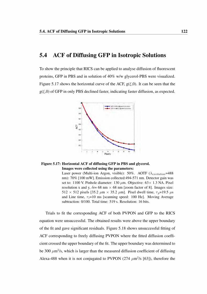
5.4. ACF of Diffusing GFP in Isotropic Solutions 122
5.4 ACF of Diffusing GFP in Isotropic Solutions
To show the principle that RICS can be applied to analyse diffusion of fluorescent
proteins, GFP in PBS and in solution of 40% w/w glycerol-PBS were visualized.
Figure 5.17 shows the horizontal curve of the ACF, g(ξ,0). It can be seen that the
g(ξ,0) of GFP in only PBS declined faster, indicating faster diffusion, as expected.
Figure 5.17: Horizontal ACF of diffusing GFP in PBS and glycerol.Images were collected using the parameters:Laser power (Multi-ion Argon, visible): 50%. AOTF (λexcitation=488nm): 70% [100 mW]. Emission collected:494-571 nm. Detector gain wasset to: 1100 V. Pinhole diameter: 130 µm. Objective: 63× 1.3 NA. Pixelresolution x and y, δr= 68 nm × 68 nm [zoom factor of 8]. Images size:512 × 512 pixels [35.2 µm × 35.2 µm]. Pixel dwell time, τp=19.5 µsand Line time, τ l=10 ms [scanning speed: 100 Hz]. Moving Averagesubtraction: 0/100. Total time: 519 s. Resolution: 16 bits.
Trials to fit the corresponding ACF of both PVPON and GFP to the RICS
equation were unsuccessful. The obtained results were above the upper boundary
of the fit and gave significant residuals. Figure 5.18 shows unsuccessful fitting of
ACF corresponding to freely diffusing PVPON where the fitted diffusion coeffi-
cient crossed the upper boundary of the fit. The upper boundary was determined to
be 300 µm2/s, which is larger than the measured diffusion coefficient of diffusing
Alexa-488 when it is not conjugated to PVPON (274 µm2/s [63]), therefore the

5.4. ACF of Diffusing GFP in Isotropic Solutions 123
diffusion coefficient could not been resolved. A possible explanation for this
failure is that the fast diffusion of PVPON in solution crossed the sensitivity limit
of our system.
Figure 5.18: Unsuccessful fitting of ACF describing PVPON.
In summary, although we were not always able to obtain quantitative mea-
surements of diffusion coefficients, we were always able to identify trends and
compare diffusion coefficients in samples imaged under the same conditions. Such
comparisons, rather than measurement of absolute values of diffusion are the
goal of our cellular studies, so these findings confirmed the likely utility of our
approach. Although further work involving production of more viscous samples
is required to determine the parameter limit for RICS measurements of GFP in
solution, these data indicate that a high diffusion coefficient gives correlation
only in the horizontal ACF vector. Fitting only the horizontal pixels along the
line of the ACF to the theoretical RICS equation was found to be much less
accurate then full-surface ACF. This indicates that there is an upper limit of
diffusion coefficient possible to quantitative measure with our system. However,
the diffusion coefficients of cytoplasmic proteins in living cells are estimates in
range from 1 to 30 µm2/s, and even smaller diffusion coefficients as 0.1 - 1 µm2/s

5.4. ACF of Diffusing GFP in Isotropic Solutions 124
are expected for membrane proteins such as integrins [135]. Therefore, this upper
limit should not affect measurements within living cells.
5.4.1 Effect of the scanning direction in RICS
Many microscopes can perform more than one scanning mode. For this thesis,
the horizontal scan along the X-axis was used. The connection between the
scanning direction (vertically/horizontally raster scan) and the ACF is considered
in Equation 2.35, where ξ is multiplied with τ p, and ψ is multiplied with τ l.
In order to demonstrate this connection, the average ACF was calculated from
a series of images describing diffusing sub-resolution microspheres in water. The
whole stack was then rotated 90◦, and the average ACF was calculated again.
Figure 5.19 shows a representative image from the stack before and after
rotation, and the corresponding ACFs. It can be clearly seen that the central line
of the ACF before rotation is along the X-axis due to the horizontal scanning
direction, and after rotating the images, the ACF was rotated. This indicates
that the calculated ACF is an experimental result, and not an artifact due to data
manipulation. Insignificant difference is observed between Figure 5.19c and 5.19d
indicates that the ACF is appropriately calculated. In addition, it demonstrates the
dependency of the ACF on the scanning mode as a parameter for RICS equation.
The reason the ACF becomes narrower along the X-axis direction is due to
the direction of the raster scanning, supporting the theory of RICS as shown in
Chapter 2.

5.4. ACF of Diffusing GFP in Isotropic Solutions 125
(a) Before rotation. (b) After rotating 90◦ right.
(c) ACF before rotation. (d) ACF after rotation.
Figure 5.19: The effect of scanning direction on the ACF in RICS.The ACF of diffusing microspheres in water were calculated before andafter rotating the images. (a) representative frame out of a series of imagesbefore rotation; (b) representative frame out of a series of images after allstack was rotated.; (c) ACF before rotation with a horizontal dominantACF; and, (d) dominant vertical ACF correspond with the rotation.Images were collected using the parameters :Laser power (Multi-ion Argon, visible): 20%. AOTF (λexcitation=488nm): 15% [7mW]. Emission collected:494-571 nm. Detector gain was setto: 1193 V. Pinhole diameter: 103 µm. Objective: 63× 1.3 NA Glycerol.Pixel resolution x and y, δr= 50 nm×50 nm [zoom factor of 39]. Imagessize: 128 × 128 pixels [6.3 µm×6.3 µm]. Pixel dwell time, τp=39 µsand Line time, τ l=5 ms [scanning speed: 200 Hz]. Moving Averagesubtraction: 0/200. Total time: 139.3 s. Resolution: 8 bits.
5.5. The Effect of Immobile Fraction Removal on RICS measurements 126
5.5 The Effect of Immobile Fraction Removal on
RICS measurements
Once we showed that our system could be used to perform RICS measurements in
isotropic solutions, the next step was to apply RICS measurements to living cells,
and to try to identify trends in diffusion during biological activity. As explained
in Chapter 4, working with cells is more complicated than working with solutions
because of the lower signal to noise ratio, the heterogeneity in cell structure and
in types of motion, and because of the presence of a large immobile fraction.
One of the methods we used for removing the immobile fraction from images,
was to apply a high pass filter to the images with a cut-off frequency determined
from the power spectrum (see section 4.2). To determine if the new RICS
modification can enhance the accuracy of RICS measurements in living cells and
to study the influence of the cut-off frequency on the ACF, we performed RICS
measurements in diffusing EGFP-EGFR in living BaF3 cells. During the analysis,
we applied high pass filters to the images with different cut-off frequencies using
the procedure described in section 4.3 and evaluated their effects on the apparent
diffusion coefficients.
The BaF3 cell line had been characterized by Clayton et al., who used ICS to
count EGFR-EGFP clusters and demonstrated that in the absence of EGF in the
media, EGFR had an average of 2.2 receptors per cluster, and after activation with
EGF the average number of receptors per cluster increased to 3.7 [168]. The
proposed model is that the activation induces dimerization or oligomerization
of receptors at the cell surface [168]. By using flow cytometry it was also
demonstrated that the fluorescent intensity of the cells was constant, indicating
that the total number of receptors remains relatively constant [168]. Using FCS,

5.5. The Effect of Immobile Fraction Removal on RICS measurements 127
the diffusion coefficient of EGFP-EGFR was measured to be approximately 0.25
µm2/s in CHO cells [169]. Since the hydrodynamic radius of the dimer is larger
than the monomer, it is predicted that the diffusion coefficient of EGFR should
be smaller in activated cells than it is in non-activated cells [170]. Therefore,
comparison of activated and un-activated EGFR-EGFP is a perfect candidate for
RICS calibration and validation. In addition, the fact that the spatial correlation
of EGF receptor in fixed cells (where the diffusion coefficient can be regarded as
zero) was measured by ICS [133, 168, 171] gives a good opportunity to study how
this spatial correlation can be eliminated by using the high pass filter.
The standard technique to activate the cells is by adding EGF to the media.
However, due to the difficulty of preventing receptor internalization and at the
same time performing RICS on relatively immobile cells, this technique proved
impractical. As an alternative, two populations of BaF3 cells were cultured under
different conditions: the first group was cultured in RPMI containing 10% FBS
and 10% conditioned medium, while the second group was starved without FBS
and conditioned medium to create conditions in which EGF is absent, therefore
a different state of activation might be expected. Validating any differences in
activation between the samples was beyond the scope of this thesis, but might
involve assessment of receptor phosphorylation. Further work might also test
whether inhibition of the internalization by using Phenylarsine oxide (PAO) as
reported by Clayton et al. (2008) [172] can significantly reduce the obtained
diffusion coefficient.

5.5. The Effect of Immobile Fraction Removal on RICS measurements 128
(a)
(b)
Figure 5.20: Starved BaF3 cells expressing EGFP-EGFR.(a): Starved BaF3 cells expressing EGFR-EGFP in micro grids. (b): Crosssection of starved BaF3 cell expressing EGFR-EGFP in soft agarose.Images were collected using the parameters :Laser power (Multi-ion Argon, visible): 50%. AOTF (λexcitation=488nm): 10% [5m W]. Emission collected:505-565 nm. Detector gain wasset to: 1250 V. Pinhole diameter: 160 µm. Objective: 63× 1.3 NA. Pixelresolution in the x and y size, δr= 32 nm×32 nm [zoom factor of 15].Images size: 512× 512 pixels [16.4 µm×16.4 µm]. Scanning speed: 10Hz. Resolution: 16 bits.

5.5. The Effect of Immobile Fraction Removal on RICS measurements 129
To accommodate the slow diffusion of the receptors we tried to minimize the
movement of the cell as much as possible. The best scanning mode for such a
slow diffusion is 10Hz, which is the slowest scanning mode in the Leica SP5.
At scan speed of 10 Hz, the time taken to scan one frame is 51.2 s. Since the
BaF3 cells are not adherent cells, individual cells starved in micro-grids (Figure
5.20a) were shown to move significantly (up to approximately 3 µm/min). In
order to immobilize the cells in such a way that the viability was not affected,
the soft agarose method was applied. Very briefly, soft agarose is a method to
culture eukaryotic cells in a viscous gel environment that holds the cells in their
position, while enabling cell viability. The viscosity of the soft agarose rises with
the increasing concentration of the agarose. The optimal agarose concentration
was determined to be approximately 0.8% w/v, whereas higher concentrations
lead to deformation of cells. Individual cells were randomly selected, and were
imaged at a magnification that allowed the entire cell to be fitted into the image
frame.
The diameter of the receptor aggregations has an important effect in any
ICS-based measurements. Ideally, the diameter of the aggregation would be
homogeneous and smaller then ωxy. ICS measurements of the BaF3 are out of the
scope of this thesis, but importantly, we did see a large variance in the diameter
of the receptor (as indicated by variation in the intensity and size of receptor
aggregates).
Receptor aggregates were seen to move relatively fast at the surface of the
cells, possibly because of the rotational motion of the cells within the gel. In
order to minimize any inaccuracy in RICS measurements that may be caused
either by the heterogeneity in the diameter or the movement of the aggregation,
the optical section was focused on an interior plane of the cell, where fluorescence
at the cortex was visible as a ”cell ring”. Receptor aggregations were observed

5.5. The Effect of Immobile Fraction Removal on RICS measurements 130
as bright spots on the ”cell ring” and within the cells, potentially as a result of
internalization. Since most fluorescence is at the cell membrane, it is assumed
that the contribution of the internalization to the apparent diffusion coefficient is
negligible.
Sets of time-lapse images from 15 living cells were obtained for both starved
and non-starved cells and the average ACFs for each series were calculated. In
order to quantify the effect of the cut-off frequency and to determine the optimal
cut-off frequency value, the vertical ACF vector from each cell was fitted to the
RICS equation under different cut-off frequency values. Figure 5.21a shows
the values of the apparent diffusion coefficients versus the number of points
eliminated from the PSD.
As explained in section 5.5, the effect of the immobile fraction filtering
is to eliminate cellular components and immobile structures from the apparent
diffusion coefficient. Proportions between the graphs that quantify the effects
of the immobile fraction removal on the diffusion coefficients for the three cell
lines were found to be almost constant. However, the scales of the apparent
diffusion values were different, suggesting that it is hard to neglect all the other
parameters while testing a specific parameter because of the complex relationship
between them. Yet, it clearly demonstrates the effects of the immobile filtering on
the apparent diffusion coefficient. Since the apparent diffusion coefficient of the
EYFP cells was close to the reference when the cut-off frequency was between
400 and 600 pixels, it was decided to adjust the cut-off frequency to this range of
values.
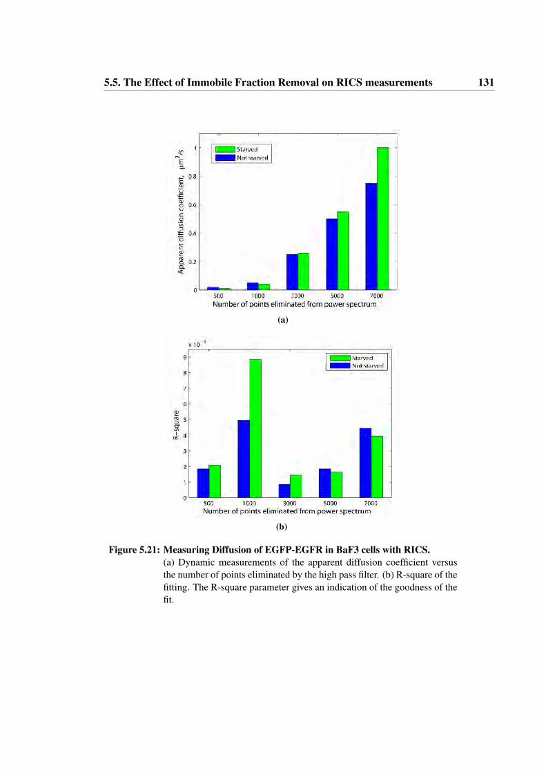
5.5. The Effect of Immobile Fraction Removal on RICS measurements 131
(a)
(b)
Figure 5.21: Measuring Diffusion of EGFP-EGFR in BaF3 cells with RICS.(a) Dynamic measurements of the apparent diffusion coefficient versusthe number of points eliminated by the high pass filter. (b) R-square of thefitting. The R-square parameter gives an indication of the goodness of thefit.
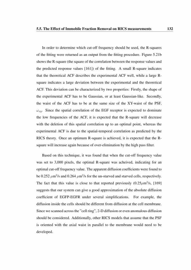
5.5. The Effect of Immobile Fraction Removal on RICS measurements 132
In order to determine which cut-off frequency should be used, the R-squares
of the fitting were returned as an output from the fitting procedure. Figure 5.21b
shows the R-square (the square of the correlation between the response values and
the predicted response values [161]) of the fitting. A small R-square indicates
that the theoretical ACF describes the experimental ACF well, while a large R-
square indicates a large deviation between the experimental and the theoretical
ACF. This deviation can be characterized by two properties: Firstly, the shape of
the experimental ACF has to be Gaussian, or at least Gaussian-like. Secondly,
the waist of the ACF has to be at the same size of the XY-waist of the PSF,
ωxy. Since the spatial correlation of the EGF receptor is expected to dominate
the low frequencies of the ACF, it is expected that the R-square will decrease
with the deletion of this spatial correlation up to an optimal point, whereas the
experimental ACF is due to the spatial-temporal correlation as predicted by the
RICS theory. Once an optimum R-square is achieved, it is expected that the R-
square will increase again because of over-elimination by the high pass filter.
Based on this technique, it was found that when the cut-off frequency value
was set to 3,000 pixels, the optimal R-square was acheived, indicating for an
optimal cut-off frequency value. The apparent diffusion coefficients were found to
be 0.252 µm2/s and 0.264 µm2/s for the un-starved and starved cells, respectively.
The fact that this value is close to that reported previously (0.25µm2/s, [169]
suggests that our system can give a good approximation of the absolute diffusion
coefficient of EGFP-EGFR under several simplifications. For example, the
diffusion inside the cells should be different from diffusion at the cell membrane.
Since we scanned across the ”cell ring”, 2-D diffusion or even anomalous diffusion
should be considered. Additionally, other RICS models that assume that the PSF
is oriented with the axial waist in parallel to the membrane would need to be
developed.

5.5. The Effect of Immobile Fraction Removal on RICS measurements 133
Figure 5.22: Graphical illustration of the effect of the cut-off frequency of highpass filter on the ACF.The effect of the immobile fraction filtering on the horizontal vector of thenormalized ACF. As more immobile fraction is removed, the horizontalACF projection becomes narrower, with a diameter closer to the diameterof the PSF. However, at some point over-elimination will lead to over-estimation of the diffusion coefficient. This effect was quantified usingthe automated RICS approach.
Here we determined semi-quantitatively the effect of the high pass filter
on the apparent diffusion time: higher cut-off frequency values give higher
apparent diffusion coefficients. A full analysis involving additional strategies and
complementary techniques such as ICS and FCS is not within the scope of this
thesis but would confirm the obtained results. Meanwhile, these measurements
show that the establishment of the high pass filter methodology can separate
between the spatial correlation due to the cell structure and the faster fluctuation
due to the dynamic properties of the proteins. Once again, it is important to note
that this parameter is only one from a full list of parameters that needs to be
optimized in order to perform accurate RICS measurements of cells. Since the
focus of this thesis is in βPIX-Scribble interaction and not the EGFR, in-depth
analysis of EYFP-βPIX expressed in 3T3 cells will be presented in section 6.3.

5.6. Discussion 134
5.6 Discussion
RICS measurements were validated by using microspheres in glycerol solutions
with different viscosities. However, when the particles were much smaller than
microspheres (PVPON, fluorescence proteins) it was found that the experimental
ACF did not entirely match the theoretical ACF predicted by the standard
RICS equation, and fitting the experimental ACF to the theoretical ACF gave
a characteristic residual. This effect was probably caused by using high laser
intensity to overcome the sensitivity limitation of the Leica SP5 that was reported
previously [152].
The mechanism by which high intensity illumination enhanced our RICS
measurements is not clear. One possible mechanism by which this could occur
is photobleaching, the rate of which we showed to be influenced by the diffusion
coefficient in section 5.3. Currently we lack a mathematical model to describe this
effect. Therefore, we cannot fully validate this hypothesis. We propose two ways
in which photobleaching could influence the ACF:
1. Short-term photobleaching: Since fluorophores that spend a large time in the
beam are bleached, then the probability of measuring specific fluorophores
at two points will decrease with the distance between them. Therefore,
high laser intensities might give a faster decline in both g(ξ,0) and g(0,ψ).
Since there is a connection between the diffusion time (the average time
the fluorophore stays in the effective volume) and the probability of each
individual fluorophore to be photobleached, it is theoretically possible to
derive information about the diffusion coefficient from the experimental
ACF.
2. Long-term photobleaching: If the scanning speed is slower then the critical

5.6. Discussion 135
velocity Vc =2D/ωxy, high excitation intensity can create a progressive
decrease in the total number of fluorescent particles (termed ”photobleach-
ing hole”), and create a non-uniform concentration of fluorophores [173].
The spatial-temporal correlation of the distribution of photobleached fluo-
rophores in the sample describes the average photobleaching rate for the
detection volume, the scanning speed, and the diffusion coefficient of the
fluorophores.
We assume that a correction factor for RICS under short term photobleaching
should be easier to derive than for long term photobleaching. For example,
Satsoura et al. 2007 [173] introduced a modified expression for ACF under short
term photobleaching in a case of line scan. Since the transition between the
short-term and long-term photobleaching is dependent on the scanning speed, it
would be useful to adjust the scanning speed up to a point where only short-term
photobleaching occurs.
A similar effect of high laser intensity on the ACF was reported during
FCS of rhodamine 6G in aqueous solutions [174]. Moreover, Widengren et
al demonstrated that in order to obtain optimal conditions during FCS it is
necessary to apply excitation intensities that lead to photophysical alterations
in the fluorophore [174]. In the case of rhodamine 6G, the mechanism that is
responsible for this effect is a contribution to fluctuations from the triplet state
(blinking). In such a system, the fluctuations in intensity are caused both by the
dynamic properties of the fluorophores and by the kinetic rates of its triplet state.
More recently, a system that combines FCS with photophysical processes was
reported, in addition to modelling and formulations that consider blinking in the
fitting procedure [166].
Since the laser illumination that was used in this thesis was strong enough

5.6. Discussion 136
for photobleaching (as seen in Figure 5.8), it is suggested that increasing the
excitation intensity increases the weight of the photobleaching effect in the ACF
in RICS. This effect had an indirect influence on the apparent diffusion time and
the diffusion coefficient values, and should be considered.
The principle that the ACF is sensitive to photobleaching is also well character-
ized in the FCS literature, and is expressed in FCS correction models [175, 176].
Moreover, this effect can be also exploited, as demonstrated by Wachsmuth
et al. [177], and by Delon et al. [178, 179]. In such a system, the ACF
contains correlations due to the probability of detection of the fluorophores, the
probability to photobleach each single fluorophore and the dynamic movement of
the fluorophores. The probability of each single fluorophore to be photobleached
is also complex and dependent on the number of photons striking the fluorophore
and the sensitivity of the fluorophore to photobleaching, which in some cases can
also be dependent on the conditions of the surrounding environment.
The concept of using photobleaching with a laser scanning confocal mi-
croscope was recently described by Braeckmans et al. who showed accurate
measurements of diffusion coefficients by scanning rapidly along a line segment
with a scanning laser beam while allowing continuous recovery of fluorescence
throughout the photobleached line [97]. This recovery resulted from diffusion
of surrounding non-bleached fluorophores into the bleached area while the laser
beam was continuously changing its position. Hence, the distribution of the
bleached and un-bleached fluorophores in the surrounding bulk is dependent
on the rate of recovery, which is characterized by the dynamic property of the
fluorophores, for instance the diffusion coefficient (long-term photobleaching). It
is worth mentioning that integrating the advantage of the photobleaching effect
was also demonstrated in FRET by Zal et al. who developed a photobleaching
correction factor for FRET and used this technique to study protein-protein

5.6. Discussion 137
interactions in the immunological synapse in living T-cells by analysing time-lapse
imaging [180].
All these data support the idea that photophysical effects, and photobleaching
in particular, can be exploited to improve current technologies in the biophysics
field. As a new member of the FFS family, RICS is still open for new
improvements and modifications. We propose that our data on photobleaching
in RICS presents both a problem and an opportunity. It presents a problem
since it suggests that the ACF contains not only correlations due to fluctuations
in the temporal change in the concentration (as assumed in the original RICS
equation), but also fluctuations due to photobleaching. A correction model is
required to account for these effects to allow more quantified interpretation of
the ACF. However, there is currently no available RICS model that considers
photobleaching, therefore fitting the experimental ACF to the original RICS
equation creates a dominant residual that interferes with the RICS analysis.
Conversely, it also presents an opportunity since performing RICS with high
intensity excitation might provide a method to enhance the ACF by giving more
correlated pixels, and to overcome the sensitivity problem of the SP5. A simple
calculation reveals that even the slowest scanning speed in the Leica software
(10Hz), is above the critical velocity, indicating that short-term bleaching is
the mechanism we deal with. Yet, the validity of this assumption should be
investigated as part of any RICS work in the future.
As with FCS, better physical equations are required in RICS to increase the
sensitivity of the fitting. Moreover, our measurements show that a number of
parameters, which are not easy to formulate into a single biophysical model,
influence RICS analysis. Since RICS is such a novel technique, it is still not
clear if some of the effects we measured are exclusive to the Leica SP5 system, or
whether they are generic to all RICS measurement systems. Future work involving

5.6. Discussion 138
other optical settings and other confocal microscopes is necessary to answer this
critical question. Nevertheless, our measurements showed the establishment of
new strategies to handle effectively some of these factors, including qualitative
measurements and theoretical suggestions that can explain these very important
issues in any FCS based techniques, and in particular in RICS.
Since the phenomena of photobleaching is much more established in FCS
then in RICS, and since the Leica SP5 microscope is commercial available with
integrated FCS system, we offer that future work should correlate the information
derived from both our RICS modification with FCS measurements. This can give
extremely important information about our system, for instance, to quantify the
effect of photobleaching in RICS, to enhance the sensitivity of the SP5 for RICS
measurements, and to create standard solution curve by using series of solutions
with increasing viscosities to optimize the precision of our measurements.

Chapter 6RICS Measurements in 3T3 Cells
6.1 Introduction
Chapter 5 showed that RICS measurements are influenced by a variety of
parameters, which significantly affect the apparent diffusion time (Figure 5.5),
or caused a characteristic residual in the fitting procedure (Figures 4.3 and
5.18). Since the original RICS equation does not consider these effects, and
in the absence of available correction models, it can be hard to interpolate the
ACF precisely. Hence, careful control of acquisition and analysis parameters
throughout the ACF analysis are required. Thus, it is important to develop
a standardized methodology that enables consistent calibration of the system.
This methodology is presented in this chapter, in addition to more precise
measurements of diffusion coefficients of EYFP-βPIX and EYFP-βPIX∆CT
within 3T3 cells once the system setup is achieved.
139

6.1. Introduction 140
Originally, RICS was shown to give absolute diffusion coefficients without
the use of well-known standards for calibration. However, the consequence of the
photobleaching modification to overcome the sensitivity problem in the SP5 is that
the use of well-known standard is a requirement. Ideally, it would be better to have
a ”standard solution” with well-known diffusion coefficients. However, solutions
can not mimic the diffusion of protein within cells. The interior of the cell is
very heterogeneous, and the environment of the cell cytoplasm is very different
from dilute solution for several biophysical properties such as pH, concentrations,
type of diffusion, viscosity. The following measurements in this chapter were
calibrated by using freely diffusing EYFP within living cells as a standard to
compare the apparent diffusion coefficients under identical experimental and post
acquisition analysis parameters as EYFP-βPIX and EYFP-βPIX∆CT.
Previous RICS analysis that were held in CHO cells expressing EGFP, showed
that EGFP is uniformly distributed as a monomer with a large variety in the
measured diffusion coefficient [155], and with an average value of approximately
20 µm2/s [60]. In addition, diffusion coefficients of enhanced cyan mutant of
green fluorescent protein (ECFP) were shown to give close values [181]. Since
the molecular structure of EGFP, ECFP and EYFP is very similar [83, 182], it is
assumed that EYFP is also freely diffusing in 3T3 cells with a diffusion coefficient
in the same range.
The hypothesis to be tested is that the binding of βPIX to partner-proteins
during biological activities has a strong effect on its diffusion coefficient. Since
the (-TNL) motif responsible for the interactions between βPIX and Scribble,
and the absence of the (-TNL) motif in βPIX∆CT abrogates its interaction with
Scribble, the hypothesis is that the diffusion coefficient of EYFP-βPIX and EYFP-
βPIX∆CT will be different.

6.2. Validation of Cell Lines 141
To test this hypothesis, 3T3 fibroblast cell lines expressing EYFP, EYFP-βPIX
and EYFP-βPIX∆CT were generated and the averaged diffusion coefficients
within these cells were measured by RICS. Validation of these cell lines is
shown in section 6.2. Section 6.3 shows several effects that can influence the
experimental ACF, as shown in Chapter 5 and determines the optimal framework
for this analysis. Based on these measurements, section 6.4 describes the
comparison of diffusion coefficients of EYFP, EYFP-βPIX and EYFP-βPIX∆CT
within living cells, and shows diffusion maps of these proteins in living cells.
6.2 Validation of Cell Lines
Cell lysates from the transfected cells were assessed for EYFP, EYFP-βPIX and
EYFP-βPIX∆CT expression by western blot (Figure 6.2 ). The membranes were
incubated with antibodies specific for the detection of endogenous and transfected
βPIX (A), and GFP (detects EYFP) (B). The two membranes were also probed
with antibody specific for tubulin to control for protein loading.
The first lane was loaded with untransfected (UT) cells for negative control.
The second lane was loaded with EYFP-expressing cells as positive control. The
third and forth lanes are 3T3 cells expressing EYFP-βPIX and EYFP-βPIX∆CT,
respectively. Band are detected at approximately 98 kDa by antibodies to GFP and
βPIX only in the third and forth lanes. These bands indicates a stable expression
of EYFP-βPIX and EYFP-βPIX∆C in the transfected cells. Bands above 148
kDa are shown in the third and forth lanes. These bands are likely to represent
dimerized βPIX. The only band at approximately 27 kDa was detected in the
cells expressing EYFP alone, indicating that the only free EYFP can be found in
the control cells. Approximately equal bands were detected at 64 kDa in all lanes
by βPIX antibodies, indicating equal expression of endogenous βPIX.

6.2. Validation of Cell Lines 142
Figure 6.1: EYFP-βPIX and EYFP-βPIX∆CT FACS profile.
To confirm the western blot results, the cell lines were checked by FACS for
YFP fluorosence. Figure 6.1 shows the FACS analysis. It can be seen that there
are significant percentages of positive transfected populations, indicating that the
transfections were successful, and stable cell lines were achieved. Future studies
will assess populations with varying expression levels, but these cell lines provided
a suitable stable population on which to apply RICS.

6.2. Validation of Cell Lines 143
EYFP
Tubulin
EYFP-βPIX
EYFP3T3UT
EYFP-βPIX
EYFP-βPIXΔCT
98kDa
50kDa
36kDa
148kDa
Primary Abs:
anti Tubulinanti GFP
(a) anti GFP and anti tubulin
EYFP-βPIXΔCT
EYFP EYFP-βPIX
Primary Abs:
anti Tubulinanti βPIX
148kDa
98kDaEYFP-βPIX
64kDa
50kDa
βPIX
Tubulin
3T3UT
(b) anti βPIX and anti tubulin
Figure 6.2: EYFP-βPIX and EYFP-βPIX∆CT are expressed in the transfected3T3 cell lines(a) Anti GFP and anti tubulin. The only band around 36 kDa ( 27 kDa)is in the EYFP cells. (b) Anti βPIX and anti tubulin. The bands at 50kDa indicate tubulin protein and show that approximately equal amountsof protein was loaded in each lane.

6.3. Calibration of RICS to 3T3 Cells 144
6.3 Calibration of RICS to 3T3 Cells
6.3.1 RICS measurements in Fixed Cells
As a validation procedure, cells expressing EYFP-βPIX∆CT and EYFP were
fixed with fixation solution (Appendix B), and the diffusion coefficient of EYFP
and EYFP-βPIX∆CT were measured. It is assumed that fixation of the cells
reduces dramatically the diffusion of the protein within the cells, causing the
difference in the molecular weight between EYFP-βPIX∆CT and EYFP (as
shown in Figure 6.2) to have an insignificant effect on the diffusion coefficient.
Figure 6.3 shows the averaged normalized ACF for each cell. As can be seen,
there is no distinguishable difference between the ACF of EYFP-βPIX∆CT and
EYFP, supporting the hypothesis that fixing the cells results in equal diffusion
coefficients (very close to zero).
Comparing Figure 6.3 with Figure A.5a (Appendix A) shows that the obtained
ACFs for the fixed cells are different from theoretical ACF when the diffusion
coefficient is equal to zero. As discussed before, the optimal framework for
RICS is a combination of parameters. One example for a possible factor that can
affect the ACF is photobleaching of the fluorophores due to high laser excitation
intensity. Several additional effects that were shown with PVPON, and factors
that are specific to living cells all have to be characterized. In order to define the
optimal setup for RICS measurements under the Leica SP5 microscope, and to
obtain the best analysis parameters to use, RICS measurements were performed in
3T3 cells expressing EYFP as a control under changeable image acquisition and
analysis settings.

6.3. Calibration of RICS to 3T3 Cells 145
Figure 6.3: ACF of fixed fibroblast cells expressing EYFP-βPIX∆CT and EYFP.Images were collected using the parameters : Laser power (Multi-ion Argon, visible): 50%. AOTF (λexcitation=514 nm): 40% [90 mW].Emission collected: 537-595 nm. Detector gain was set to: 1250 V. Pinholediameter: 160 µm. Objective: 63×, 1.3 NA. Pixels resolution in the x andy directions size, δr= 60 nm×60 nm [zoom factor of 8]. Images size: 512× 512 pixels [30.8 µm×30.8 µm]. Pixel dwell time, τp=19.5 µs and Linetime, τ l=10 ms [scanning speed: 100 Hz]. MA subtraction: 3/5 as there isno cell movement. Total time: 21 s. Resolution: 16 bits.
6.3.2 Workflow of RICS experiments
3T3 cells were plated at 5×10³ cells/well on 35 mm optic glass bottom dishes
(Matek, MA) and were cultured for 24 or 48 hours before each experiment as in
3.1. The environmental chamber of the Leica SP5 enabled constant temperature
of 37◦C, humidity, and a constant concentration of CO2/O2 gas mixture. To
select the optimal conditions for imaging the cells, our approach was first to
adjust the experimental conditions, and later the post acquisition parameters. The
first experimental condition is the scanning speed, which is proportional to the
movement of the cell and to the expected diffusion coefficient of the protein of
interest. Next, the pixel size has to be adjusted according to the size of the cell.

6.3. Calibration of RICS to 3T3 Cells 146
Once the scan speed and pixel size is adjusted, the laser power has to be adjusted.
Since high laser has to be applied, the next parameter to be determined is the
pinhole diameter to prevent saturation. Next, the post-acquisition parameters have
to be adjusted: the size of the ROI, the number of data points eliminated before
fitting the ACF (”jumping pixels”), and the immobile subtraction filtering. The
order of adjustment of the post-acquisition parameters is less important, but since
there is a complex relationship between them, we found that this adjustment is
not a simple matter. In fact this was one of the reasons that we developed the
automated RICS approach, to systematically scan for the optimal combinations
that give a good approximation between the apparent diffusion coefficients of the
standard.
6.3.3 Adjustment of the scanning speed
It has been reported that when high scanning speeds are applied, the detector
cannot reset itself properly and can result in false correlation between successive
pixels [61, 65]. This bleed-through noise caused by the limitation of detector
electronics was found to be a major problem in other confocal microscopes
[61, 65]. Therefore, it was decided to work with a slow detection mode.
A scanning speed of 10 Hz under the specific magnification and objective used
here was shown to be too slow for RICS measurements (data not shown). This
was because of significant 3T3 cell movement, especially at the cellular edge and
cell protrusions. Scanning speeds faster than 100 Hz gave a low S/N ratio, and
pixelated corresponding ACF (very few correlated pixels) so they were not ideal
for quantitative analysis. Therefore, it was decided to use a scanning speed of 100
Hz. This scanning speed is equivalent to a pixel dwell time, τ p, of 19.5 µs and
Line scan time τ l, of 10 ms when the size of the image is 512 × 512 pixels.

6.3. Calibration of RICS to 3T3 Cells 147
6.3.4 Determination of the optimal pixel size
This is important to have enough correlated pixels in the ACF for accurate fitting
of the data [61]. Although the average size and shape of 3T3 cells is varied, the
average 3T3 cell can generally fit within a frame size of 50 µm × 50 µm. Since
the size of the images is 512 × 512 pixels, this equals a pixel size of 0.08 µm.
However, such a pixel size gives small insufficient number of correlated pixels,
which is equal to the beam waist divided by the pixel size. Therefore, it was
decided to finding a pixel size that allows over-sampling of the confocal PSF so
that that it contains enough detail to enable easy analysis. At the same time, the
chosen pixel size allows a maximum cell part to be fitted into the image frame.
Therefore, the optimal pixel size was found to be between 0.06 and 0.065 µm.
6.3.5 Determination of the pinhole diameter and laser power
As demonstrated with PVPON in sections 5.3.3 and 5.3.1, the intensity of the
laser excitation and the pinhole diameter alter the ACF. In addition, increasing the
laser illumination power and the pinhole size gives higher S/N ratios and fewer
images are required. Figure 6.4a shows the apparent diffusion coefficients for
different combinations of pinhole and laser power settings. The average ACFs
of three cells from each cell line were calculated, and the diffusion coefficient
values were obtained by fitting the ACFs to the RICS equation. The images were
captured using different pinhole and laser intensity. The Cut-off frequency was set
to 500 pixels, the total time was 73.4 s, and the resolution was 16 bit. To avoid
the negative effect of saturation during image acquisition the histograms of image
intensity were used to assess the level of saturation, as shown with PVPON.
6.3. Calibration of RICS to 3T3 Cells 148
(a)
(b)
Figure 6.4: The effect of pinhole and laser on the diffusion values.(a) Apparent diffusion coefficient versus the number of points eliminated bythe high pass filter. (b) Each measurement describe the average apparentdiffusion coefficient for each cells. The error bars correspond to thestandard deviation of the three cells analysed for each cell line. The laserpower was 33 mW and pinhole diameter was 130 µm. λexcitation=514 nm.Emission: 531-591 nm. Gain: 1200 V. δr= 60 nm×60 nm. Images size:512 × 512 pixels. τp=19.5 µs, τ l=10 ms. MA: 13/15.

6.3. Calibration of RICS to 3T3 Cells 149
Figure 6.4a shows that when the laser power was set to 60 mW under these
settings, the ACF cannot be fitted properly. One possible explanation why strong
excitation intensity gives an over estimation of the diffusion coefficient is that
the contribution of the correlated fluctuations results partly from photobleaching
and the recovery of diffusing fluorophores. As the photobleaching process
is stronger, the ACF will contain more information about the photobleaching
process and describe the effect of diffusion less, and therefore the standard RICS
equation can not be used anymore. Another possible explanation is the effect
of oversaturation in the detection. In addition, the optical relation between the
pinhole diameter and the PSF diameter is a complex matter. Future work should
thoroughly investigate the affects above in addition to generating more accurate
measurements. Despite the issues described above, the average ACF for the EYFP
cell line gave reasonable apparent diffusion coefficients (when the pinhole was
adjusted to 130 µm (approximately 1.3 airy disks by the Leica LAS AF software)
and the laser power 33 mW), indicating that under specific pinhole and laser
power settings, a good experimental framework exists. The deviation of this result
is shown in Figure 6.4b. Once the acquisition settings were adjusted, the cells
were imaged under these settings, and the next post acquisition parameters were
adjusted by using RICSIM software:
6.3.6 The effect of the ROI Size on the ACF
The ROI size is an important factor that influences the accuracy of the RICS
analysis. A larger ROI gives an ACF that contains more information with a
higher S/N ratio. Conversely, larger ROI also describes a larger averaged space
and therefore the overall size of the cell can be divided into a smaller number of
grids. Thus, the resolution of the analysis within the cell decreases as the ROI size
increases. Brown et al. ([61] previously showed that a ROI with a size of 32 × 32

6.3. Calibration of RICS to 3T3 Cells 150
pixels, where the pixel size is approximately 65 nm × 65 nm (2 × 2 µm2), is the
smallest ROI size that gives sufficient statistical accuracy for their RICS system.
To demonstrate the principle that the ROI size has an strong effect on the ACF,
ACFs were calculated from several different ROI sizes. It can be seen that as the
lower g∞ decreases as the size of the ROI increases, with more correlated pixels
along the g(ξ,0). Therefore, the corresponding ACF is better defined, and with
higher SNR.
Figure 6.5: Effect of ROI size.ACF were calculated from ROIs taken from same location but with differentsizes: a. 16 × 16 pixels. b. 32 × 32 pixels c. 64 × 64 pixels. d. 128 ×128 pixels. The axes symbolize the pixels coordinates in the ACF, g(ξ,ψ) .Applying size of 128× 128 pixels provide sharper image, while ROI with asize of 16×16 leads in losing information. Axes symbolize the pixels alongg(ξ,ψ).
6.3. Calibration of RICS to 3T3 Cells 151
6.3.7 Effect of removing data points before fitting the ACF
As discussed in the beggining of Chapter 4.1, in some CLSM systems, under
certain conditions the detector does not completely reset itself before new data
points arrive. As a result, there is a residual signal from the previous data points
that contributes correlated shot-noise to the ACF [65]. This noise can lower the
S/N ratio and damage the accuracy of the fitting.
Collecting images while the microscope is set to the eyepiece and no light
can go through to the PMTs, and calculating the corresponding ACF from these
images was reported by Brown et al. as a standard procedure to estimate this effect
on the ACF [61]. The shot-noise was found to be dependent on the digitization rate
of the detector (i.e. scanning speed, gain and offset), and does not depend on the
objective configuration, focusing, pixels resolution in the x and y directions and
laser intensity [61]. Thus, sensitive consideration in choosing the optimal number
of pixels to ignore is required. The standard procedure to overcome this unwanted
correlation was simply not to use the first correlated pixels to the fit [61, 135].
In our system, we noticed that the central pixel in the ACF matrix, the g(0,0),
is very dominant and it has to be removed before fitting the ACF to the RICS
equation. Possible reasons for the large value of g(0,0) in the ACF matrix is
that the ACF contains much un-correlated shot noise, in addition to possible
contributions of spatial correlation and other noise factors. To eliminate these
effects, it was decided to ignore this pixel in the fitting procedures, and the ACF
was normalized with the value of g(1,0). It can be seen that by ignoring more
pixels in the x direction, the weight of the values in the sides of the ACF rises.
However, over-elimination of the central pixels can be also a problem as the
noise around the ACF sides can dominate the ACF. Therefore, it was decided
to eliminate the central pixel, g(0,0), and to normalize the ACF to g(1,0).

6.3. Calibration of RICS to 3T3 Cells 152
Figure 6.6: ACF under different numbers of ignored pixels.
A. Selected ROI from 3T3 express EYFP. B. ACF of the ROI. The ACF isnormalized with g(0,0). C. ACF after ignoring the first central peak. TheACF is normalized with g(1,0). D. ACF after ignoring the three centralpeaks. The axes symbolize the pixels coordinates in the ACF, g(ξ,ψ)
6.3.8 Adjustment of the MA subtraction
As explained in Chapter 4, the Moving Average (MA) subtraction has to be
adjusted correspondingly to the movement of the cells. To quantify the effect
of the immobile fraction filtering on the apparent diffusion coefficients, the
corresponding ACFs were averaged for each cell line, and then were fitted to
the standard RICS equation. Figure 6.7 shows a graph of the dependence of
the apparent diffusion coefficient on the MA value. It can be seen that there

6.3. Calibration of RICS to 3T3 Cells 153
is an increase in the apparent diffusion coefficient with the increasing MA
value. This might be a result of the elimination of cellular components and
immobile structures. However, it suggests that the MA value should be chosen
carefully, as over subtraction could add artifacts due to elimination of correlated
information that truly describes the dynamic property of the proteins. When the
MA subtraction value was above 10, the apparent diffusion coefficient of EYFP
was close to the reference, indicating a good range.
In addition, it can be seen that when the total number of images in the series
was 15, there was a well-defined corresponding ACF. This number of images is
smaller than the minimal number of images that was reported for the original
RICS by Gielen et al. who reported just recently that a number of 15 images is
insufficient to give accurate results [65]. At this point, it is still not clear if the
small number of images required here is due to the high laser intensities that were
used. In addition it is important to note that although high laser illumination can
cause phototoxicity to the cells [74], it is assumed that in this short experiment
time (around 70 seconds), it is unlikely that phototoxicity can influence cell
activity. Whether high laser intensities can increase the detection efficiency and
minimize noise in the ACF, and if there is a phototoxicity process during this
short experiment time, should be verified in the future. Determination of cell
viability can be achieved, for example, by using mitochondrial staining [183].
Nevertheless, these observations combined indicate that, with the appropriate
settings reasonably accurate diffusion values can be obtained.
6.3.9 Adjustment of the cut-off frequency of high pass filter
The role of the high pass filter in reducing the contribution of cell components was
explained in section 4.2. Figure 6.8 demonstrates the effect of the high pass filter
on the ACF. While a cut-off frequency of zero gives ACF of the entire cell structure

6.3. Calibration of RICS to 3T3 Cells 154
Figure 6.7: Effect of Moving average subtraction on the diffusion values. Diffusioncoefficient values were calculated from the average ACF for three cellsfor the three cell lines. The ACFs were calculated by using different MAsubtraction values, in units of the number of frames in a window over whichaveraging is performed. An increment in the apparent diffusion coefficientas function of the MA value was observed. Images were collected usingthe parameters :Laser power (Multi-ion Argon, visible): 20%. AOTF (λexcitation=514 nm):60% [60 mW]. Emission collected: 531-591 nm. Detector gain was setto: 1200 V. Pinhole diameter: 160 µm. Objective: 63× 1.3 NA. Pixelsresolution in the x and y directions size, δr= 60 nm×60 nm [zoom factor of8]. Images size: 512 × 512 pixels [30.8 µm × 30.8 µm]. Pixel dwell time,τp=19.5 µs and Line time, τ l=10 ms [scanning speed: 100 Hz]. Cut-offfilter:500 pixels. Total time: 73.4 s. Resolution: 16 bits.
that cannot be resolved, applying a cut-off frequency of 500 pixels gives ACF only
due to the fast fluctuations representing the dynamics of the fluorophores.
To formally test the effect of the cut-off frequency of the spatial filter on RICS
measurements quantitatively, the apparent diffusion coefficients were calculated
after the high pass filter was applied with various cut-off frequencies. The graphs
that quantify the effect of the high pass filter on the apparent diffusion coefficients

6.3. Calibration of RICS to 3T3 Cells 155
Figure 6.8: Effect of high pass filter on the ACF.A. 3T3 cell express EYFP. B. ACF for the cell. The cut-off frequency wasset to: 0. C. ACF with dominant correlation in the horizontal axis but stillvery noisy. The cut-off frequency was set to: 100 pixels. D. Very cleanACF. (The cut-off frequency was set to: 500 pixels.) In order to filter outcellular structures from the ACF there is a requirement that approximately500 central pixels will be masked out from the power spectrum.Images were collected using the parameters :Laser power (Multi-ion Argon, visible): 20%. AOTF (λexcitation=514 nm):60% [60 mW]. Detector gain was set to: 1200 V. Emission collected: 531-591 nm. Pinhole diameter: 160 µm. Objective: 63× 1.3 NA. Pixelsresolution in the x and y directions size, δr= 60 nm×60 nm [zoom factorof 8]. Images size: 512 × 512 pixels [30.8 µm × 30.8 µm]. Pixel dwelltime, τp=19.5 µs and Line time, τ l=10 ms [scanning speed: 100 Hz]. MAsubtraction: 13/15. Total time: 73.4 s. Resolution: 16 bits
were generated in the same manner as for Figure 6.7. The corresponding ACFs
for three cells from each cell line were averaged for each cell line, and then were
fitted to the standard RICS equation. The ROI was defined as the total size of the
image (512 × 512 pixels), as shown in Figure 6.8. For each point in the graph,
the cut-off frequency value was adjusted in RICSIM prior to the ACF calculation.
As shown in section 5.5, there is a consistent increment in the calculated diffusion
coefficients as a function of the cut-off frequency.
We offer that the effect of the immobile fraction filtering eliminate cellular

6.3. Calibration of RICS to 3T3 Cells 156
Figure 6.9: Effect of high pass filter on the calculated diffusion coefficients.Theaverage ACF for three cells from each cell line were calculate usingdifferent cut-off frequencies. The ACFs were fitted into RICS equationto give the diffusion coefficient values.
components and immobile structures. In addition, it is suggested that both the
MA value and the cut-off frequency should be chosen carefully, as over subtraction
could add artifacts due to elimination of correlated information that truly describes
the dynamic property of the proteins. The proportions between the diffusion
coefficients of the three cell lines were found to be almost constant but show
different scale of diffusion coefficients, suggesting that it is hard to neglect all the
other parameters while testing the effect of specific parameter due to the complex
relationship between them. Yet, it clearly demonstrates the effects of the immobile
filtering on the apparent diffusion coefficient as explained in sections 4.2 and
5.5. Since the apparent diffusion coefficient of the EYFP cells was close to the
reference when the cut-off frequency was between 400 and 600 pixels, it was
decided to adjust the cut-off frequency to this range of values.

6.4. Measurements Under Optimal Conditions 157
6.3.10 Summary
In summary, it is suggested that once the scanning speed is adjusted according to
the estimated diffusion coefficient of the fluorophores, the next parameter that
should be determined is the laser power. The laser power should be adjusted
corresponding to the concentration of the fluorophores and the sensitivity of the
fluorophores to photobleaching. Next, there is a requirement to adjust the recorded
intensity to avoid over-saturation. As can be seen in Figure 6.4a, adjustment of
the pinhole size affects the apparent diffusion coefficient. This can be explained
by the fact that changing the pinhole size also affects the PSF. Therefore, our
data indicates an advantage in adjusting the recorded intensity using the PMT
gain. Finally, the automated RICS approach should be used to adjust the cut-
off frequency of the high pass filter and the MA subtraction under the selected
ROI size. This combination of parameters is not easy, especially since there is
complex relationship between them. This complexity and the hard work involving
this adjustment is one of the major limitations that our system suffers from. Yet,
once this process is complete and the optimal settings is achieved, measurements
in sub-resolution scale within living cells can be achieved, as demonstrated in the
following section.
6.4 Measurements Under Optimal Conditions
6.4.1 Spatial Diffusivity of βPIX in living cells
Fitting the ACF from images that describe EYFP diffusing in living cells gave
a characteristic residual that could not be eliminated. However, in the previous
section it was shown that the characteristic residual could be minimized under
a certain combination of parameters, and the calculated diffusion coefficient gave

6.4. Measurements Under Optimal Conditions 158
reasonable values. This means that the optimal setup was successfully established.
The next section shows precise diffusion coefficient measurements that were
obtained using this optimal framework.
The fluorescence intensity of EYFP-βPIX was shown by fast time-lapse fluo-
rescence microscopy to distribute homogeneously within the cytoplasm and that
EYFP-βPIX was excluded from the nucleus. To determine whether intracellular
localization influenced diffusion, the cell images were divided into small grids,
with a size of 32 × 32 pixels as explained in section 6.3.6. The diffusion
coefficient of each grid was calculated as explained in section 4.3. The upper
limit of the fitting procedure was set in perspective to the measured diffusion
coefficients to threshold outer values. Finally, the diffusion map is smoothed as
explained in section 4.3.
Figure 6.10 shows spatial-temporal diffusion maps in a living EYFP cell,
which was used as validation for the diffusion maps of EYFP-βPIX (Figure 6.11)
and for EYFP-βPIX∆CT (Figure 6.12) under similar conditions .

6.4. Measurements Under Optimal Conditions 159
(a) Fluorescence image
(b) Diffusion mapFigure 6.10: Interpolated detailed Diffusion maps for EYFP cell.
Laser power:90 mW. λexcitation=514 nm. λemission=:523-537 nm. Gain:1000 V. Pinhole: 130 µm. Objective: 63× 1.3 NA. Pixel resolution xand y, δr= 60 nm × 60 nm. Images size: 512 × 512 pixels. Pixel dwelltime, τp=19.5 µs and Line time, τ l=10 ms [scanning speed: 100 Hz].MA:10/15. Time: 73.4 s. Resolution: 16 bits. a. Fluorescence image.The colour bar maps the intensity. b. Colour bar maps the diffusioncoefficients. Grids: 32 × 32 pixels with an overlap of 8 pixels.

6.4. Measurements Under Optimal Conditions 160
(a) Fluorescence image
(b) Diffusion mapFigure 6.11: Interpolated detailed Diffusion maps for EYFP-βPIX cell. The cells
was cultured and imaged at the same conditions as in Figure 6.10

6.4. Measurements Under Optimal Conditions 161
(a) Fluorescence image
(b) Diffusion mapFigure 6.12: Interpolated detailed Diffusion maps for EYFP-βPIX∆CT cell. The
cells was cultured and imaged at the same conditions as in Figure 6.10.

6.4. Measurements Under Optimal Conditions 162
It was reported previously that possible artifacts are expected to give higher
diffusion coefficients near bright spots or at the cell perimeter [65]. However,
we found that near the cell perimeter the obtained diffusion coefficients are
actually slower than expected due to the dominant structure of the cell edges.
Although it is possible to eliminate the spatial correlation of the cell edges by
applying an immobile filter for each grid, determination of the cut-off frequency
caused a difficulty for such a calculation. Since there is no available method to
determine automatically the cut-off frequency for each grid, and because the cut-
off frequency is currently constant for all the grids once the user of RICSIM selects
it, we chose simply to eliminate the cell edges from the diffusion maps. Therefore,
a space with a size of 8 × 8 pixels in the border between the edge of the cell and
the media background was thresholded out before generation of the diffusion map.
Future work can investigate how it is possible to overcome this kind of data loss by
developing a method to determinate the cut-off frequency automatically for each
grid. An example of the dominant structure of the cell edges is shown in Appendix
F.
The overall similarity between Figure 6.10 and the diffusion maps published
by Dross et al. (2009) [155] confirming the diffusion values shown in our diffusion
maps. The fact that there is no correlation between the fluorescence intensity
and the diffusion coefficient supporting that our measurements are not artifacts
due to intensity changes within the images. In addition, the variability in the
measured diffusion coefficient between different cell regions probably reflects
different biological activities at the sub-cellular level with different viscosities, and
providing proof of principle that RICS can indicate the influence of intracellular
localization on protein diffusion.
The diffusion maps for each cell line were uniformly thresholded, and the
mean diffusion coefficient per pixel squared was calculated for each diffusion map.

6.4. Measurements Under Optimal Conditions 163
Figure 6.13 shows the diffusion coefficients distribution histogram from Figures
6.10, 6.11, and 6.12 before the smoothing operation.
Figure 6.13: Histograms of diffusion maps.
As can be seen in Figure 6.13, there is a significant difference between the
histograms and the mean diffusion coefficients of EYFP and both EYFP-βPIX
and EYFP-βPIX∆CT. However, considering that even the accuracy of RICS
measurements that have been taken under perfect conditions is still not ideal (a
large variance as 30% for measurements within cells and between 80 to 90 %
accuracy [135]), the accuracy of these maps needs to be improved. Furthermore,
we note that the following simplifications contribute to the inaccuracy of our
diffusion maps: Firstly, the photobleaching of EYFP has some dependency on

6.4. Measurements Under Optimal Conditions 164
the pH and concentration [184]. Next, it is important to consider the possibility
of anomalous diffusion. For instance, the diffusion of GFP in the nucleus can
be described as anomalous, while normal diffusion is observed in the cytosol
[185]. Finally, the presence of potential quenchers can be also heterogeneously
distributed.
Improving the accuracy of these maps is out of the scope of this thesis, but
it is clear that trends do exist, suggesting that this approach will yield relevant
diffusion maps of EYFP-βPIX and EYFP-βPIX∆CT in the near future. Since we
aim to get data for a large population, this future work should give the average
diffusion coefficient per sub-region per cell line.
One important question relates to whether the differences in localization
between EYFP-βPIX and EYFP-βPIX∆CT can affect their diffusion behaviour.
As mentioned in section 6.1, the intracellular bulk has heterogeneous spatial
features, such as pH, concentrations of the fluorophores, type of diffusion and
viscosity. These features can significantly alter the diffusion coefficients of
proteins within the cells. For instance, if the WT and the mutant are localized
in different concentrations, reduced diffusion might be found as a consequence
of molecular crowding [186]. In brief, molecular crowding is a phenomenon by
which the diffusion of the particles exhibits different diffusion properties when
the concentration of the particles becomes high, and the diffusion due to the
Brownian motion is transformed to anomalous diffusion as the molecules collide
with each other and affect each others trajectories [187] . In addition, different
distribution patterns have a strong effect on the binding properties of the protein.
For example, when paxillin localizes in the cytoplasm close to adhesions, its
diffusion coefficient was measured be much slower than in the general cytosol
as a result of binding to larger complexes [60].

6.4. Measurements Under Optimal Conditions 165
In order to investigate this important question we suggest an approach to
quantify the correlation between the differences in localization and diffusion
coefficient. This solution is based on the ability of RICS to generate diffusion
maps, and the multispectral ability of the Leica SP5. Firstly, a new cell line
expressing both the WT conjugated to ECFP and the mutant conjugated to EYFP
has to be generated. Next, the diffusion map of each species has to be generated by
RICS. Finally, the diffusion coefficients of each species have to be characterized
for each distinct cellular compartment
6.4.2 Measurements of diffusion coefficients for a
large population
Preliminary data (Figure 6.4b) showed that EYFP-βPIX∆CT has smaller diffu-
sion coefficient then EYFP-βPIX. In order to perform precise measurements of
diffusion coefficients with better statistics for the three cell lines, the average
diffusion coefficient for a population of 12 cells from each cell line was measured.
Each cell was subdivided into 64 × 64 pixel grids (total area size of 17.3 µm2),
and the corresponding ACF for all the grids were averaged. The reason for this
selection was to eliminate the contribution of the cell edges, and to apply a cut-off
frequency that considers the size of the cell in the image, rather than using the same
cut-off frequency to the entire grids in the diffusion map. To determine the spatial
filter cut-off frequency for each grid, EYFP was used for calibration. Figure 6.14a
shows the difference between the corresponding horizontal ACF curve, g(ξ,0) and
6.14b the vertical ACF curve, g(0,ψ).

6.4. Measurements Under Optimal Conditions 166
(a) [Horizontal ACF for large population of cells
(b) Vertical ACF for large population of cells
Figure 6.14: Horizontal and vertical ACF vectors for large population of cellsHorizontal and vertical of the average ACF for 12 cells from each line.Images were collected using the parameters:Laser power:90 mW. λexcitation=514 nm. λemission=:523-537 nm. Gain:1000 V. Pinhole: 130 µm. Objective: 63× 1.3 NA. Pixel resolution xand y, δr= 60 nm × 60 nm. Images size: 512 × 512 pixels. Pixel dwelltime, τp=19.5 µs and Line time, τ l=10 ms [scanning speed: 100 Hz].MA:10/15. Time: 73.4 s. Resolution: 16 bits. Grids size of 64×64 pixelswith no overlap between the grids.

6.4. Measurements Under Optimal Conditions 167
There was a distinguishable difference in the vertical and horizontal ACF
curves of the three cell lines. The ACF declined fastest for EYFP diffusing alone,
indicating faster diffusing coefficient of EYFP, while the diffusion coefficient of
EYFP-βPIX∆CT was the lowest. The average ACFs from each cell was fitted to
give the representative diffusion coefficient of each cell line.
Balanced one-way Analysis Of Variance (ANOVA test) was performed by
Matlab ANOVA1 function to show the mean diffusion coefficients for each cell
line and to determine whether the differences in the diffusion coefficients between
EYFP, EYFP-βPIX and EYFP-βPIX∆CT were statistically significant. The p-
value gives the probability that the average diffusion coefficient of the cell lines is
significantly different. Common significance levels are under p<0.05 [161].
The ratio between the measured diffusion coefficient of both EYFP-βPIX
and EYFP-βPIX∆CT and the measured diffusion coefficient of EYFP was ap-
proximately1
4.5. EYFP-βPIX and EYFP-βPIX∆CT were both clearly shown to
diffuse differently than EYFP alone (p=1×10⁻¹²), but there was not a convincing
difference between EYFP-βPIX and EYFP-βPIX∆ (p=0.05). As can be seen from
Equation (6.1), in the case of free diffusion resulted by Brownian motion (Eq.
2.3) without any binding interactions the ratio in diffusion coefficients between
proteins with different molecular weight should be proportional to the cube root
of the ratio in their molecular weights. Since the molecular weight EYFP-βPIX
and EYFP-βPIX∆CT is approximately 98kDa, the theoretical ratio between the
diffusion coefficient of both EYFP-βPIX and EYFP-βPIX∆CT with EYFP should
be approximately1
1.5, which is about 3 times larger than the measured ratios.
One explanation for this result is that the biological activity of proteins can
alter their diffusion coefficient [54–56]. Therefore, the significant difference
between the expected and experimental ratio is probably resulted from the

6.4. Measurements Under Optimal Conditions 168
biological activity of both WT and the mutant. Since the relationship between the
hydrodynamic radius and the diffusion is linear in case of pure Brownian motion of
(Eq. 2.3), this proportion should be constant for the measured diffusion coefficient
((6.1)):
Rh =3
√0.75
(MwNa )π·ρ
Mw − Molecular weight
Na− Avogadro number (6.02 · 1023 mol−1)
ρ− 1.2 grcm3 for protein
⇒ D1
D2∝= 3
√Mw1
Mw2
(6.1)
Farther work is required to characterize even larger populations and to interpret
the biological aspect of these results.

6.4. Measurements Under Optimal Conditions 169
(a) Diffusion coefficients for the three cell lines
(b) ANOVA plot
Figure 6.15: Diffusion coefficients of cell populations.
(a) shows diffusion coefficients for a group of cells. shows ANOVA box-plot for comparison of the diffusion coefficients of the three cell lines.Each the median diffusion coefficients and the standard deviation for eachcell are mention for each cell line. The edges of the boxes ensemble the25th and 75th percentiles. The whiskers extend to the most extreme datapoints not considered outer values, which appeared only for the EYFP cellline.

6.5. Summary 170
6.5 Summary
In summary, when RICS is applied, it is important to work in a suitable framework
that gives extractable ACF. By using EYFP as a well-known standard, the optimal
framework for RICS within living cells was shown to be determined by the
microscopy acquisition settings adjustment, and by the post-acquisition settings
adjustment. While working at the optimal framework, the ACF provides precise
measure of the diffusion coefficient. By using the automatic RICS approach, we
showed an effective way to analyse a full list of different factors that have an effect
on the ACF. In addition, more advantages are derived for using the automated
RICS approach. From the biological aspect, statistical data are required for
characterization of biological phenomena. From the physical aspect, the accuracy
of the ACF analysis increases with the number of repeats. This approach may
be useful to investigate the limitations of different LCSM setups, and to test
concentration limits of different fluorophores for RICS measurements.
Once this optimal framework was achieved, RICS measurements were applied
to measure the diffusion coefficients of EYFP-βPIX and EYFP-βPIX∆CT, both
were clearly shown to diffuse differently than EYFP (p<1×10⁻¹²), but there was
not a significant difference between EYFP-βPIX and EYFP-βPIX∆CT. Given that
βPIX∆CT is different in only four out of 646 amino acids [188], it is not surprising
that the diffusion characteristics are comparable.
Whether the subtle differences in diffusion between EYFP-βPIX and EYFP-
βPIX∆CT (p=0.05) are biologically relevant will require future investigation.
This result might indicate that Scribble has a negligible effect on βPIX diffusion,
or might indicate that more complex analyse are required to elucidate the effect of
Scribble binding to βPIX. For example, it is possible that the diffusion of βPIX is
mostly determined by associated proteins other than Scribble. Since interactions

6.5. Summary 171
of proteins with large complexes can slow their diffusion [56], the absence of the (-
TNL) motif in EYFP-βPIX∆CT may be insignificant. Alternatively, it is possible
that over expression of EYFP-βPIX and EYFP-βPIX∆CT may cause artifacts in
localization or diffusion that obscure the effect of the absence of the (-TNL) motif
in EYFP-βPIX∆CT. If the number of EYFP-βPIX bound by Scribble is small
relative to the total number of EYFP-βPIX molecules in the cytoplasm, there will
be a small effect on the average diffusion coefficient measured for the all EYFP-
βPIX∆CT pool.
The last two assumptions can be checked by, for instance, comparing the
diffusion coefficient of EYFP-βPIX to EYFP-βPIX∆CT only in regions where
Scribble is present. This can be achieved by generating cells that overexpress
Scribble, and to activate the recruitment of βPIX to the plasma membrane and the
leading edge by adding EGF to the media as shown previously [20, 34].

Chapter 7Conclusions and Future Work
This thesis studies new RICS applications and brings original data that extends
the RICS frontier. By applying a new RICS modification, this thesis overcomes
the sensitivity barrier and succeeds to measure diffusion coefficients of proteins
in living cells by using the Leica SP5. The achievements that have been
accomplished in this thesis can be divided into three parts:
The creation of the RICSIM program
Much work has gone into designing the interface of RICSIM to be a stable
and efficient platform. RICSIM provides a number of advantages over
other publically available software as described earlier, and can be used in
the future for the application of RICS measurements to many biological
questions.
Offering a new avenue for RICS measurements
This thesis highlights the potential of performing RICS analysis with high
intensity laser excitation, which was shown to enhance the measured ACF.172

7.1. Conclusions and Outlook 173
It is unclear why high intensity enhances the ACF, but it is possible that this
is due to photobleaching effects. This improvement was applied to enhance
the sensitivity of the Leica SP5 to RICS, and to allow accurate quantitative
measurements under defined settings. Furthermore, by using high intensity
excitation, we showed that fewer images are required in comparison to
the original RICS in isotropic solutions and living cells. However, one
limitation for every FRAP based technique that should be considered is that
overexposure to excitation light can manipulate the biological behaviour of
the sample and to cause phototoxicity [189].
Measurements of diffusion coefficient in living cells
This thesis describes preparation of stable cell lines expressing EYFP-
βPIX and EYFP-βPIX∆PIX, and preliminary measurements of diffusion
coefficient within these cells. Although the accuracy of these RICS
measurements have to be validated by complementary techniques, by using
EYFP as a standard trends of small difference in the apparent diffusion
coefficient were identified. These results bring new and original information
about the dynamic properties of βPIX in living cells, and have the potential
to improve our understanding of how βPIX and Scribble interact with
each other in the future. A quantitative description of the spatial-temporal
behaviour of βPIX in living cells demonstrates the ability of RICS to detect
the dynamics of protein within living cells, and promise a wide range of
opportunities in cell biology research.
7.1 Conclusions and Outlook
The ACF was found to depend on a combination of different experimental
parameters such as the excitation intensity, the pinhole diameter, and the scanning

7.1. Conclusions and Outlook 174
speed. The precision of the fitting procedure was also found to be dynamic,
and its dependence on the experimental setup was demonstrated. These effects
were found to be significant, and required careful optimization through the ACF
analysis. At this point, it is still not clear if these effects are exclusive to the
Leica SP5 system, or can be found in any standard RICS measurement with
other systems. Future work should continue to characterize more potential effects
that were partly shown in this thesis. In addition, characterization experiments
involving other optical settings and other confocal microscopes are necessary to
answer this critical question.
Nevertheless, trends in the ACF of solutions with different viscosities were
consistent. This consistency suggests that it can be possible to give the absolute
physical values of the diffusion coefficient by considering the effects mentioned
above. This can be achieved for each RICS experiment in two steps: The first step
is to adjust the experimental setup to an optimum point by which the residual is
minimized (and therefore can be neglected in the fitting procedure). The second
step is to use well-characterized samples as a standard for each experiment, and to
calibrate the system setup to a point that gives its accurate diffusion coefficients,
which were found to be 6.7±0.8 µm2 for EYFP-βPIX and 5.5±1.8 µm2 for EYFP-
βPIX∆CT, when the diffusion coefficient of EYFP was used as a calibration
standard with a measured value of 28.5±6.1 µm2.
Since more complex biophysical processes such as photobleaching can con-
tribute to the shape of the ACF, it is advisable to use a transfected fluorescence
protein (i.e. - EGFP, EYFP) with well known diffusion coefficients in the same
cells as the proteins of interest. This, in addition to the use of other complimentary
techniques as FCS (as described previously) and FRAP should be used in
future work to validate our RICS modification. Although our measurements
lack this important validation, with the approach of using EYFP as standard,

7.2. Recommendations for Future Work 175
our measurements reveal that the diffusion coefficient of both than EYFP-
βPIX and EYFP-βPIX∆CT were lower than expected when simple Brownian
motion is assumed. This suggests that their biological function and protein-
protein interactions impede their diffusion. In addition, EYFP-βPIX gave slightly
higher diffusion coefficients than EYFP-βPIX∆CT. Once again, the significant
variance with these results suggests that further measurements and the use of
complimentary techniques such as FRET, FCS and FRAP, in addition to more
biomolecular techniques are necessary to understand these results.
Overall, although our RICS modification contains limitations, such as sensi-
tivity issues, possible phototoxicity derived from photobleaching, and the lack of
proper fitting models, it also contains major advantages over existing techniques.
In addition, by using RICS we demonstrated the ability to generate non-invasive
diffusion maps of proteins in living cells. We anticipate that this extraordinary
ability will be used in future in protein-protein interaction studies within living
cells, and possible publications about our RICS modification and about the
biological aspect of our study.
7.2 Recommendations for Future Work
Future work should focus on:
• Improving RICS models- Formulating new RICS correction factors that
account for the effects that were described in this thesis work, in addition to
further investigation for possible unknown biophysical/biological/experimental
effects.
• Further validation- To continue to study the effect of the photobleaching
in RICS by using complementary techniques such as FRAP, FRET and FCS

7.2. Recommendations for Future Work 176
to provide full information about the studied system.
• Scrambling technique in RICS- Investigating another RICS modification
that may allow to measure diffusion at the focal adhesions and cell edges.
This potential RICS-modification is based on the scrambling technique
that was described previously in the ICCS literature [144]. The idea of
the scrambling technique is that by collecting a large number of smaller
grids close to edges and scrambling the order of these grids to form a new
rectangular larger grid, the ACF close to cell edges can be estimated. The
ACF of the reconstructed grid may be fitted to a modified and suitable
RICS equation, to give the diffusion coefficient for sub-cellular close to cell
protrusions and edges, which currently cannot be calculated.
• Cross-Correlation-RICS - The diffusion coefficient measurements of
EYFP-Scribble are essential to complete the data about βPIX and Scribble
interaction. Although a cell line of 3T3 expressing the EYFP-Scribble con-
struct was generated and validated as part of this thesis, due to insufficient
time no RICS measurements were performed. In addition, by exploiting the
spectroscopic features of the Leica SP5 to perform cc-RICS measurements
between βPIX and Scribble, extremely useful information may be gained.

Bibliography
[1] D. G. DRUBIN. Cell Polarity. Oxford University Press, 320 pp., New York,
USA, 2000.
[2] R. LI AND G. G. GUNDERSEN. Beyond polymer polarity: how the
cytoskeleton builds a polarized cell. Nature Reviews Molecular Cell
Biology, 9:860–873, 2008.
[3] S. IDEN AND J. G. COLLARD. Crosstalk between small GTPases and
polarity proteins in cell polarization. Nature Reviews — Molecular Cell
Biology, 9:846–859, 2008.
[4] F. SANCHEZ-MADRID AND J. M. SERRADOR. Bringing up the rear:
defining the roles of the uropod. Nature Reviews Molecular Cell Biology,
10:353–359, 2009.
[5] A. WODARZ AND I. NATHKE. Cell polarity in development and cancer.
Nature Cell Biology, 9:1016–1024, 2007.
[6] S. ETIENNE-MANNEVILLE. Polarity proteins in migration and
invasion. Oncogene, 27(55):6970–6980, 2008.
177

BIBLIOGRAPHY 178
[7] B. Z. HARRIS AND A. L. WENDELL. Mechanism and role of PDZ
domains in signaling complex assembly. Journal of Cell Science,
114:3219–3231, 2001.
[8] R. TONIKIAN, Y. ZHANG, S. L. SAZINSKY, B. CURRE, J. H. YEH,
B. REVA, H.A. HELD, B. A. APPLETON, COWORKERS, AND S. S.
SIDHU. A specificity map for the PDZ domain family. PLOS Biology,
6(9):2043–2059, 2008.
[9] S. ETIENNE MANNEVILLE. Cdc42- the centre of polarity. Journal of
Cell Science, 117:1291–1300, 2004.
[10] P. G. CHREST AND R. A. FIRTEL. Big roles for small GTPases in the
control of directed cell movement. Biochemical Journal, 401:377–390,
2007.
[11] A. L. BISHOP AND A. HALL. Rho GTPases and their effector proteins.
Biochemical Journal, 348:241–255, 2000.
[12] P. K. MATTILA AND P. LAPPALAINEN. Filopodia: molecular
architecture and cellular functions. Nature Reviews Molecular Cell
Biology, 9:446–454, 2008.
[13] E. MANSER. RHO family GTPases. Dordrecht : Springer, Landes
Bioscience, Plenum Publishers, 296 pp., Georgetown, London, UK, 2005.
[14] A. J. RIDLEY, H. F. PATERSON, C. L. JOHNSTON, D. DIEKMANN,
AND A. HALL. The small GTP-binding protein RAC regulates growth
factor-induced membrane ruffling. Cell, 70(3):401–410, 1992.
[15] S. J. HEASMAN A. J. RIDLEY. Mammalian Rho GTPases: new insights
into their functions from in vivo studies. Nature Reviews Molecular Cell
Biology, 9:690–701, 2008.

BIBLIOGRAPHY 179
[16] P. O. HUMBERT, N. A. GRZESCHIK, A. M. BRUMBY, R. GALEA,
I. ELSUM, AND H. E. RICHARDSON. Control of tumourigenesis by the
Scribble/Dlg/Lgl polarity module. Oncogene, 27:6888–6907, 2008.
[17] D. BILDER, M. LI, AND N. PERRIMON. Cooperative regulation of
cell polarity and growth by Drosophila tumor suppressors. Science,
289(5476):113–116, 2000.
[18] P. HUMBERT AND L. E. DOW S. M. RUSSELL. The Scribble and Par
complexes in polarity and migration: friends or foes? Trends in Cell
Biology, 16(12):622–630, 2006.
[19] L. DOW. The role of Scribble in polarity, migration and tumourigenesis.
PhD Dissertation. Department of Biochemistry and Molecular Biology
University of Melbourne, Melbourne, Australia, 2006.
[20] S. AUDEBERT, C. NAVARRO, C. NOURRY, AND CHASSEROT-GOLAZ.
Mammalian Scribble Forms a Tight Complex with the βPIX Exchange
Factor. Current Biology, 14(11):987–995, 2004.
[21] K. P. NEIL AND M. JONES. Studies of distribution, location and
dynamic properties of EGFR on the cell surface measured by image
correlation spectroscopy. Molecular and Cellular Biology, 27(16):5790–
5805, 2007.
[22] O. SCHLENKER AND K. RITTINGER. Structures of dimeric GIT1
and trimeric βPIX and implications for GIT-PIX complex assembly.
Journal of Molecular Biology, 386(2):280–289, 2009.
[23] S. R. FRANK AND S. H. HANSEN. The PIX-GIT complex: a G
protein signaling cassette in control of cell shape. Seminars in Cell and
Developmental Biology, 19(3):234–244, 2008.

BIBLIOGRAPHY 180
[24] M. W. MAYHEW, E. D. JEFFERY, N. E. SHERMAN, K. NELSON, J. M.
POLEFRONE, S. J. PRATT, J. SHABANOWITZ, J. T. PARSONS, J. W. FOX,
D. F. HUNT, AND A. F. HORWITZ. Identification of phosphorylation
sites in βPIX and PAK1. Journal of Cell Science, 120:3911–3918, 2007.
[25] S. ETIENNE MANNEVILLE AND A. HALL. Rho GTPases in cell biology.
Nature, 420:629–635, 2002.
[26] V. SMALL, T. STRADALB, E. VIGNALA, AND K. ROTTNER. The
lamellipodium: where motility begins. Trends in Cell Biology,
12(3):112–120, 2002.
[27] J. CAU AND A. HALL. Cdc42 controls the polarity of the actin and
microtubule cytoskeletons through two distinct signal transduction
pathways. J. Cell Sci., 118(12):2579–2587, 2005.
[28] J. P. TEN-KLOOSTER, Z. M. JAFFER, J. CHERNOFF, AND P. L.
HORDIJK. Targeting and activation of Rac1 are mediated by the
exchange factor βPIX. J. Cell Biol., 172(5):759–769, 2006.
[29] N. OSMANI, N. VITALE, J. P. BORG, AND S. ETIENNE-MANNEVILLE.
Scrib controls Cdc42 localization and activity to promote cell
polarization during astrocyte migration. Current Biology, 16:2395–
2405, 2006.
[30] H. R. MOTT, D. NIETLISPACH, K. A. EVETTS, AND D. OWEN.
Structural analysis of the SH3 domain of βPIX and Its interaction with
R-p21 Activated Kinase (PAK). Biochemistry, 44:10977–10983, 2005.
[31] R. STOCKTON, J. REUTERSHAN, D. SCOTT, J. SANDERS, K. LEY, AND
M. A. SCHWARTZ. Induction of vascular permeability βPIX and GIT1

BIBLIOGRAPHY 181
scaffold the activation of extracellular signal-regulated kinase by PAK.
Molecular biology of the Cell, 18:2346–2355, 2007.
[32] S.B. NOLA, M. SEBBAGH, S. MARCHETTO, N. OSMANI, C. NOURRY,
S.P. AUDEBERT, C. NAVARRO, R. RACHEL, M. MONTCOUQUIOL,
N. SANS, S. ETIENNE-MANNEVILLE, J. P. BORG, AND M. J. SANTONI.
Scrib regulates PAK activity during the cell migration process. Human
Molecular Genetics, 17(22):3552–3565, 2008.
[33] C. FUMIN, C. A. LEMMON, D. PARK, AND L. H. ROMER. FAK
potentiates Rac1 Activation and localization to matrix adhesion sites:
a role for βPIX. Molecular Biology of the Cell, 18:253–264, 2007.
[34] E. Y. SHIN, K . N. WOO, C. S. LEE, S. H. KOO, Y. G. KIM, W. J. KIM,
C. D. BAE, S. I. CHANG, AND E. G. KIM. Basic fibroblast growth factor
stimulates activation of RAC1 through a p85 αPIX phosphorylation-
dependent pathway. Journal of Biological Chemistry, 279(3):1994–2004,
2004.
[35] C. W. WOLGEMUTH. Lamellipodial Contractions during Crawling and
Spreading. Biophysical Journal, 89:16431649, 2005.
[36] T. D. POLLARD AND G. G. BORISY. Cellular motility driven by
assembly and disassembly of actin filaments. Cell, 112(4):453–465,
2003.
[37] M. S. BRETSCHER. Getting membrane flow and the cytoskeleton to
cooperate in moving cells. Cell, 87(4):601–606, 1996.
[38] R. J. PETRIE, A. D. DOYLE, AND K. M. YAMADA. Random versus
directionally persistent cell migration. Nature Reviews Molecular Cell
Biology, 10:538–549, 2009.

BIBLIOGRAPHY 182
[39] J. P. TEN-KLOOSTER, I. V. LEEUWEN, N. SCHERES, E. C. ANTHONY,
AND P. L. HORDIJK. Rac1-induced cell migration requires membrane
recruitment of the nuclear oncogene SET. EMBO J., 26(2):336–345,
2007.
[40] P. A. VIDI AND V. J. WATTS. Fluorescent and Bioluminescent Protein-
fragment Complementation Assays in the Study of G Protein-coupled
Receptor Oligomerization and Signaling. Molecular Pharmacology,
53819:1–22, 2009.
[41] S. S. VOGEL, C. THALER, AND S. V. KOUSHIK. Fanciful FRET. Science
STKE, 301:re2, 2006.
[42] B. C. S. CROSS, I. SINNING, J. LUIRINK, AND S. HIGH. Delivering
proteins for export from the cytosol. Nature Reviews Molecular Cell
Biology, 10:255–264, 2009.
[43] D.J. WEBB, J. T. PARSONS, AND A. F. HORWITZ. Adhesion assembly,
disassembly and turnover in migrating cells - over and over and over
again. Nature Cell Biology, 4:E97–E100, 2002.
[44] T. YANAGIDA AND Y. ISHII. Revealing protein dynamics by
photobleaching techniques. Wiley-VCH, 346 pp., 2009.
[45] H. WOLFENSON, A. LUBELSKI, T. REGEV, J. KLAFTER, Y. I. HENIS,
AND B. GEIGER. A role for the juxtamembrane cytoplasm in the
molecular dynamics of focal adhesions. PLOS One, 4(1):e4304, 2009.
[46] A. J. RIDLEY, M. A. SCHWARTZ, K. BURRIDGE, R. A. FIRTEL,
M. H. GINSBERG, G. BORISY, J. T. PARSONS, AND A. R. HORWITZ.
Cell migration: integrating signals from front to back. Science,
302(5651):1704–1709, 2003.

BIBLIOGRAPHY 183
[47] M. H FRIEDMAN. Principles and Models of Biological Transport.
Springer, 2nd edition., 512 pp., 2008.
[48] B. ALBERTS, A. JOHNSON, J. LEWIS, M. RAFF, K. ROBERTS, AND
P. WALTER. Molecular Biology of the Cell. Garland Science; 5th edition ,
1392 pp., Oxford, UK, 2008.
[49] H. LODISH, A. BERK, P. MATSDUAIRA, AND C. A. KAISER. Molecular
Cell Biology. W.H. Freeman and Company, 6th edition, 973 pp., New York,
USA, 2008.
[50] I. SANTAMARIA-HOLEKA, M. H. VAINSTEINB, J.M. RUBI, AND
F.A. OLIVEIRAB. Protein motors induced enhanced diffusion in
intracellular transport. Physica A: Statistical Mechanics and its
Applications, 388(8):1515–1520, 2009.
[51] D. A. LAUFFENBURGER AND A. F. HORWITZ. Cell migration: a
physically integrated molecular process. Cell, 84(3):359–369, 1996.
[52] S. A. KOESTLER, K. ROTTNER, F. LAI, J. BLOCK, M. VINZENZ, AND
J. V. SMALL. F- and G-Actin concentrations in lamellipodia of moving
cells. PLOS One, 4(3):E4810, 2009.
[53] R. D. VALE. The molecular motor toolbox review for intracellular
transport. Cell, 112:467–480, 2003.
[54] P. I.H. BASTIAENS AND R. PEPPERKOK. Observing proteins in their
natural habitat: the living cell. Trends in Biotechnology, 25(12):631–
637, 2000.
[55] K. LUBY-PHELPS. Cytoarchitectural and physical properties of
cytoplasm: volume, viscosity, diffusion, intracellular surface area.
International Review of Cytology, 192:931–946, 2000.
BIBLIOGRAPHY 184
[56] M. WEISS, H. HASHIMOTO, AND T. NILSSON. Anomalous
protein diffusion in living cells as seen by fluorescence correlation
spectroscopy. Biophysical Journal, 84:4043–4052, 2003.
[57] E.A.J. REITS AND J. J. NEEFJES. From fixed to FRAP: measuring
protein mobility and activity in living cells. Nature Cell Biology, 3:145–
147, 2001.
[58] M. A. DIGMAN, C. M. BROWN, P. SENGUPTA, P. W. WISEMAN, A. R.
HORWITZ, AND E. GRATTON. Measuring fast dynamics in solutions and
cells with a laser scanning microscope. Biophysical Journal, 89(2):1317–
1327, 2005.
[59] M. A. DIGMAN, P. SENGUPTA, P. W. WISEMAN, C. M. BROWN, A. R.
HORWITZ, AND E. GRATTON. Fluctuation correlation spectroscopy
with a laser-scanning microscope: exploiting the hidden time structure.
Biophysical Journal, 88(5):33–36, 2005.
[60] M. A. DIGMAN, C. M. BROWN, A. R. HORWITZ, W. W. MANTULIN,
AND E. GRATTON. Paxillin dynamics measured during adhesion
assembly and disassembly by correlation spectroscopy. Biophysical
Journal, 94(7):2819–2831, 2008.
[61] C. M. BROWN, R. B. DALAL, B. HEBERT, M. A. DIGMAN, A. R.
HORWITZ, AND E. GRATTON. Raster image correlation spectroscopy
(RICS) for measuring fast protein dynamics and concentrations with a
commercial laser scanning confocal microscope. Journal of Microscopy,
229(1):78–91, 2008.
[62] H. SANABRIA, M. DIGMAN, E. GRATTON, AND M. N. WAXHAM. Spa-
tial diffusivity and availability of intracellular calmodulin. Biophysical
Journal, 95(12):6002–6015, 2008.

BIBLIOGRAPHY 185
[63] M. VENDELIN AND R. BIRKEDAL. Anisotropic diffusion of
fluorescently labeled ATP in rat cardiomyocytes determined by raster
image correlation spectroscopy. American Journal of Cell Physiology,
295:1302–1315, 2008.
[64] N. B. WATSON, E. NELSON, M. DIGMAN, J. A. THORNBURG, B. W.
ALPHENAA, AND W. G. MCGREGOR. RAD18 and associated proteins
are immobilized in nuclear foci in human cells entering S-phase with
ultraviolet light-induced damage. Mutation Research - Fundamental and
Molecular Mechanisms of Mutagenesis, 648(1-2):23–31, 2008.
[65] E. GIELEN, N. SMISDOM, M. VANDEVEN, B. D. CLERCQ, E. GRAT-
TON, M. DIGMAN, J.M RIGO, J. HOFKENS, Y. ENGELBORGHS, AND
M. AMELOOT. Measuring diffusion of lipid-like probes in artificial
and natural membranes by Raster Image Correlation Spectroscopy
(RICS): use of a commercial laser-scanning microscope with analog
detection. American Chemical Society, 25(9):5209–5218, 2009.
[66] M. A. DIGMAN, P. W. WISEMAN, A. R. HORWITZ, AND E. GRATTON.
Detecting protein complexes in living cells from laser scanning confocal
image sequences by the cross correlation raster image spectroscopy
method. Biophysical Journal, 96(2):707–716, 2009.
[67] M. A. DIGMAN AND E. GRATTON. Fluorescence correlation
spectroscopy and fluorescence cross-correlation spectroscopy. Wiley
Interdisciplinary Reviews: Systems Biology and Medicine, 96(2):707–716,
2009.
[68] R. BROWN. Brief account of microscopical observations, made in the
months of June, July and August (1827), on the particles, contained

BIBLIOGRAPHY 186
in the pollen of plants and in general existence of active molecules in
organic and inorganic matter. Ray Society, 1:456–486, 1866.
[69] B. J. BERNE AND R. PECORA. Dynamic Light Scattering With
Applications to Chemistry, Biology, and Physics. Dover Publications INC,
376 pp., Mineola, New-York, 2000.
[70] A. EINSTEIN. On the motion-required by the molecular kinetic theory
of heat-of small particles suspended in stationary liquid. Annalen der
Physik. [in German], 17:549–560, 1905.
[71] A. JABLONSKI. Z. Phys. 94:38–64, 1935.
[72] J. R. ALBANI. Structure and dynamics of macromolecules: absorption
and fluorescence studies. Elsevier Science, 94:2–8, 2004.
[73] L. SONG, E. J. HENNINK, AND H. J. TANK. Photobleaching kinetics
of fluorescein in quantitative fluorescence microscopy. Biophysical
Journal, 68:25588–2600, 1995.
[74] J. B. PAWLEY. Handbook of Biological Confocal Microscopy. Springer
Science+Business Media LLC, New York, USA, third edition, 998 pp.
edition, 2006.
[75] E. M. GOLDYS. Fluorescence Applications in Biotechnology and the Life
Sciences. John Wiley and Sons, 367 pp., New-Jersey,USA, 2009.
[76] R. D. GOLDMAN AND D. L. SPECTOR. Live cell imaging: a laboratory
manual. Cold Spring Harbor Laboratory Press, 631 pp., Cold Spring
Harbor, New-York, 2005.
[77] M. CHALFIE AND S. KAIN. Green Fluorescent Protein, Properties,
Applications, and Protocols. John Wiley and Sons Inc, 385 pp., New-York,
1998.
BIBLIOGRAPHY 187
[78] D. PRASHER, V. ECKENRODE, W. WARD, F. PRENDERGAST, AND
M. CORMIER. Primary structure of the Aequorea Victoria green-
fluorescent protein. Gene, 111(2):229–233, 1992.
[79] M. CHALFIE, Y. TU, G. EUSKIRCHEN, W. WARD, AND D. PRASHER.
Green fluorescent protein as a marker for gene expression. Science,
263(5148):802–805, 1994.
[80] I. U. RAFALSKA-METCALF AND S. M. JANICKI. Show and tell:
visualizing gene expression in living cells. Journal of Cell Science,
120:2301–2307, 2007.
[81] R. HEIM, A. CUBITT, AND R. TSIEN. Improved green fluorescence.
Nature, 6516:663–664, 1994.
[82] R. HEIM AND R. TSIEN. Engineering green fluorescent protein for
improved brightness, longer wavelengths and fluorescence resonance
energy transfer. Current Biology, 6(2):178–182, 1996.
[83] M. V. MATZ, K. A. LUKYANOV, AND S. A. LUKYANOV. Family of
the green fluorescent protein: Journey to the end of the rainbow.
BioEssays, 24(10):953–959, 2003.
[84] N. C. SHANER, P. A. STEINBACH, AND R. Y. TSEIN. A guide to
choosing fluorescent proteins. Nature Methods, 2(12):905–909, 2005.
[85] C. JOO, BALCI H, Y. ISHITSUKA, C. BURANACHAI, AND T. HA.
Advances in single-molecule fluorescence methods for molecular
biology. Annual Review of Biochemistry, 77:51–76, 2008.
[86] E. J. G. PETERMAN, H. SOSA, AND W. E. MOERNER. Single-molecule
fluorescence spectroscopy and microscopy of biomolecular motors.
Annual Review Physical Chemistry, 55:79–96, 2004.

BIBLIOGRAPHY 188
[87] J. S. FOTOS, V. P. PATEL, N. J. KARIN, M. K. TEMBURNI, J. T. KOH,
AND D. S. GSLILIEO. Automated time-lapse microscopy and high-
resolution tracking of cell migration. Cytotechnology, 51:7–19, 2006.
[88] E. NICOLAS, N. CHENOUARD, J. C. OLIVO-MARIN, AND A. GUICHET.
A Dual role for actin and microtubule cytoskeleton in the transport
of golgi units from the nurse cells to the oocyte across ring canals.
Molecular Biology of the Cell, 20(1):556–568, 2009.
[89] Z. BOMZON, M. KNIGHT, D. L. BADER, AND E. KIMMEL. Mitochon-
drial dynamics in chondrocytes and their connection to the mechanical
properties of the cytoplasm. Journal of biomechanical engineering,
128(5):674–679, 2006.
[90] R. EILS AND C. ATHALE. Computational imaging in cell biology.
Biopolymers, 161,3:1477–481, 2003.
[91] P. T. YAM, C. A. WILSON, L. JI, B. HEBERT, E. L. BARNHART,
N. A. DYE, P. W. WISEMAN, G. DANUSER, AND J. A. THERIOT.
Actin-myosin network reorganization breaks symmetry at the cell rear
to spontaneously initiate polarized cell motility. The Journal of Cell
Biology, 178178(7):1207–1221, 2007.
[92] M. J. SAXTON. Single-particle tracking: connecting the dots. Nature
methods, 5:671–672, 2008.
[93] M. J. SAXTON. Single-particle tracking: applications to membrane
dynamics. Annual Review Biophysicical Bimolecular Structure, 26:373–
399, 1997.

BIBLIOGRAPHY 189
[94] Z. PETRASEK AND P. SCHWILLE. Fluctuations as a source of
information in fluorescence microscopy. Journal of the Royal Society
Interface, 6:S15–S25, 2008.
[95] G. CARREROA, D. MCDONALDB, E. CRAWFORDB, G. VRIES, AND
M. J. HENDZEL. Using FRAP and mathematical modeling to determine
the in vivo kinetics of nuclear proteins. Methods, 29(1):14–28, 2003.
[96] D. AXELROD, D. E. KOPPEL, J. SCHLESSINGER, E. ELSON, AND
W. W. WEBB. Mobility measurement by analysis of fluorescence
photobleaching recovery kinetics. Biophysical Journal, 16:1055–1069,
1976.
[97] K. BRAECKMANS, K. REMAUT, R. E. VANDENBROUCKE, B. LUCAS,
S. C. DE SMEDT, AND J. DEMEESTER. Line FRAP with the confocal
laser scanning microscope for diffusion measurements in small regions
of 3-D Samples. Biophysical Journal, 92:2172–2183, 2007.
[98] K. BRAECKMAN. Photobleaching with the confocal laser scanning
microscope for mobility measurements and the encoding of microbeads.
Faculty pharmaceutical Wetenschappen Ghent University, Ghent, Belgium,
2004.
[99] J. BRAGA, J. M.P. DESTERRO, AND M. CARMO-FONSECA. Intracellu-
lar macromolecular mobility measured by fluorescence recovery after
photobleaching with confocal laser scanning microscope. Molecular
Biology of the Cell, 15:4749–4760, 2004.
[100] M. WEISS. Challenges and artifacts in quantitative photobleaching
experiments. Traffic, 5:662–671, 2004.

BIBLIOGRAPHY 190
[101] R. N. DAY AND F. SCHAUFELE. Imaging molecular interactions in
living cells. Molecular Endocrinology, 19(7):1675–1686, 2005.
[102] J. LIPPINCOTT-SCHWARTZ, N. ALTAN-BONNET, AND G. H. PATTER-
SON. Photobleaching and photoactivation: following protein dynamics
in living cells. Nature review- Imaging in Cell Biology, 25:S1–S13, 2003.
[103] P. S. JAMES, C. HENNESSY, T. BERGE, AND R. JONES. Compartmen-
talization of the sperm plasma membrane: a FRAP, FLIP and SPFI
analysis of putative diffusion barriers on the sperm head. Journal of
Cell Science, 117:6485–6495, 2004.
[104] A.D ELDER, A. DOMIN, G. S. KAMINSKI-SCHIERLE, C. LINDON,
J. PINES, A. ESPOSITO, AND C.F KAMINSKI. A quantitative
protocol for dynamic measurements of protein, interactions by Forster
resonance energy transfer-sensitized fluorescence emission. J. R. Soc.
Interface, 6:59–81, 2009.
[105] V. N. UVERSKY AND E. A. PERMYAKOV. Methods in protein structure
and stability analysis. Nova Biomedical Books, 372 pp., New York, USA,
2007.
[106] A. EINSTEIN. Ann. Physik, 33:1275, 1910.
[107] H. Z. CUMMINS AND K. N. YEH. Observation of diffusion broadening
of Rayleigh scattered light. Physical Review Letters, 12:150–153, 1964.
[108] S. B. DUBIN. Quasielastic Light Scattering From Macromolecules. PhD
Dissertation. Massachusetts Institute of Technology, Massachusetts, USA,
1970.
[109] D. MAGDE, E. L. ELSON, AND W. W. WEBB. Thermodynamic
fluctuations in a reacting system; Measurement by fluorescence

BIBLIOGRAPHY 191
correlation spectroscopy. Physical Review Letters, 29(11):705–708,
1972.
[110] E. L. ELSON AND D. MAGDE. Fluorescence correlation spectroscopy.
I. Conceptual basis and theory. Biopolymers, 13:1–27, 1974.
[111] D. MAGDE, W. W. WEBB, AND E. L. ELSON. Fluorescence correlation
spectroscopy. II. An experimental realization. Biopolymers, 13(1):29–
61, 1974.
[112] D. MAGDE, W. W. WEBB, AND E. L. ELSON. Fluorescence correlation
spectroscopy. III. Uniform translation and laminar flow. Biopolymers,
17:361–376, 1978.
[113] E. L. ELSON AND W. W. WEBB. Concentration correlation
spectroscopy. Annual Review of Biophysics and Bioengineering, 4:311–
334, 1975.
[114] P. R. SELVIN AND T. HA. Single-Molecule Techniques, A Laboratory
Manual. Cold Spring Harbor Laboratory Press, 507 pp., New-York, 2007.
[115] K. RITCHIE, X.Y. SHANA, J. KONDOA, K. IWASAWAA, T. FUJIWARAA,
AND A. KUSUMIA. Detection of non-Brownian diffusion in the cell
membrane in single molecule tracking. Biophysical Journal, 88(3):2266–
2277, 2008.
[116] J. WU AND K. M. BERLAND. Propagators and time-dependent
diffusion coefficients for anomalous diffusion. Biophysical Journal,
95(4):2049–2052, 2008.
[117] S. T. HESS AND W. W. WEBB. Focal volume optics and experimental
artifacts in confocal fluorescence correlation spectroscopy. Biophysical
Journal, 83:2300–2317, 2002.

BIBLIOGRAPHY 192
[118] R. RIGLER AND E. S. ELSON. Fluorescence correlation spectroscopy,
theory and applications. Springer Series in Chemical Physics, 487 pp.,
Berlin, Germany, 2001.
[119] R. RIGLER, U. METS, J. WIDENGREN, AND P. KASK. Fluores-
cence Correlation Spectroscopy with High Count Rate and Low-
Background-Analysis of Translational Diffusion. European Biophysics
Journal with Biophysics Letters, 22(3):169–175, 1993.
[120] P. SCHWILLE AND E. HAUSTEIN. Fluorescence Correlation Spectroscopy
An Introduction to its Concepts and Applications. Experimental Biophysics
Group Max-Planck-Institute for Biophysical Chemistry, 33 pp., Gottingen,
Germany, 2004.
[121] C. KITELL. Elementary Statistical Physics. John Wiley and Sons Inc, 228
pp., New York, USA, 1958.
[122] J. CRANK. The Mathematics of Diffusion. Oxford University Press, USA,
second edition,424 pp. edition, 1975.
[123] GERMANY LEICA MICROSYSTEMS CMS GMBH. MATLAB ICS Tutorial.
Leica Microsystems official website, www.leica-microsystems.com.
[124] E. HAUSTEIN AND P. SCHWILEE. Ultrasensitive investigations of
biological systems by fluorescence correlation spectroscopy. Methods,
29(2):153–166, 2003.
[125] K. BACIA, S. A. KIM, AND P. SCHWILLE. Fluorescence cross-
correlation spectroscopy in living cells. Nature Methods, 3:83–89, 2006.
[126] S. A. KIM, K. G. HEINZE, AND P. SCHWILLE. Fluorescence correlation
spectroscopy in living cells. Nature methods, 4:963–973, 2007.

BIBLIOGRAPHY 193
[127] P. MCCORMICK. Introduction to FCS and FRAP. Univeristy of
Edinburgh, 2008. Leica Microsystems.
[128] Y. CHEN, J. D. MULLER, K. M. BERLAND, AND E. GRATTON.
Fluorescence fluctuation spectroscopy. Methods, 18(2):234–252, 1999.
[129] Y. CHEN, L. N. WEI, AND J. D. MULLER. Probing protein oligomer-
ization in living cells with fluorescence fluctuation spectroscopy. PNAS,
100(26):15492–15497, 2003.
[130] E. HAUSTEIN AND P. SCHWILEE. Fluorescence correlation spec-
troscopy: Novel variations of an established technique. Annual review
of biophysics and biomolecular structure, 36:151–169, 2007.
[131] Y. CHEN AND J. D. MULLER. Determining the stoichiometry of
protein heterocomplexes in living cells with fluorescence fluctuation
spectroscopy. PNAS, 104(9):3142–3152, 2007.
[132] J. W. SCHWARTZ B. D. SLAUGHTER AND R. LI. Mapping
dynamic protein interactions in MAP kinase Signaling using live-
cell fluorescence fluctuation spectroscopy and imaging. PNAS,
104(51):20320–20325, 2007.
[133] N. O. PETERSEN, P. L. HODDELIUS, P. W. WISEMAN, O. SEGER
ANDO., AND K.MAGNUSSON. Quantitation of membrane receptor dis-
tributions by image correlation spectroscopy: concept and application.
Biophysical Journal, 65(3):1135–1146, 1993.
[134] D. KOLIN. MATLAB ICS Tutorial. Cell Migration Consortium (CMC)
website, Nature, www.cellmigration.org/resource/imaging/icsmatlab.

BIBLIOGRAPHY 194
[135] R. B. DALAL. Fluctuation Analysis Reveals Protein Concentration,
Mobility, and Aggregation States in Cells. PhD Dissertation. Department
of Biomedical Engineering University of Verginia, Verginia, USA, 2008.
[136] B. HEBERT, S. CONSTANTINO, AND P. W. WISEMAN. Spatio-temporal
image correlation spectroscopy (STICS): theory, verification and
application to protein velocity mapping in living CHO cells. Biophysical
Journal, 88:3601–3614, 2005.
[137] R. T. BORLINGHAUS. MRT Letter: high speed scanning has the
potential to increase fluorescence yield and to reduce photobleaching.
MICROSCOPY RESEARCH AND TECHNIQUE, 69:689–692, 2006.
[138] A. D. MCQUARRIE AND J. D. SIMON. Physical Chemistry: A Molecular
Approach. Sausalito, Calif. : University Science Books, 1st edition ,1360
pp., 1997.
[139] D. L. KOLIN, D. RONIS, AND P. W. WISEMAN. k-Space
image correlation spectroscopy: A method for accurate transport
measurements independent of fluorophore photophysics. Biophysical
Journal, pages 3061–3075, 2006.
[140] K. BACIA AND P. SCHWILLE. A dynamic view of cellular processes by
in vivo fluorescence auto- and cross-correlation spectroscopy. Methods,
29(1):74–85, 2003.
[141] E. THEWS, M. GERKEN, R. ECKERT, J. ZAPFEL, C. TIETZ, AND
J. WRACHTRUP. Cross talk free fluorescence cross correlation
spectroscopy in live cells. Biophysical Journal, 89:2069–2076, 2005.

BIBLIOGRAPHY 195
[142] A. E. MILLER, C. W. HOLLARS, S. M. LANE, AND TE. A. LAURENCE.
Fluorescence cross-correlation spectroscopy as a universal method for
protein detection with low false positives. Analytical Chemistry, 81.
[143] T. SUDHAHARAN, P. LIU, Y. H. FOO, W. BU, K. B. LIM, T. WOHLAND,
AND S. AHMED. Determination of in Vivo Dissociation Constant, KD,
of Cdc42-Effector Complexes in Live Mammalian Cells Using Single
Wavelength Fluorescence Cross-correlation Spectroscopy. Journal
Biological Chemistry, 284(20):13602–13609, 2009.
[144] J. W. D. COMEAU, D. L. KOLIN, AND P. W. WISEMAN. Accurate
measurements of protein interactions in cells via improved spatial
image cross-correlation spectroscopy. Molecular Biosystems, 4:672–685,
2008.
[145] E. N. DORSEY. The Properties of Ordinary Water Substance. Reinhold
Pub. Corp, 673 pp., New York, USA, 1940.
[146] R. T. BORLINGHAUS. The AOBS: Acousto optical beam splitter. G.I.T.
Imaging and Microscopy, 3:10–12, 2002.
[147] V. SEYFRIED, H. BIRK, R. STORZ, AND H. ULRICH. Advances in
multispectral confocal imaging. Progress in biomedical optics and imaging,
SPIE The international Society of optical engineering, Munich, Germany,
2003.
[148] R. T. BORLINGHAUS. Colours Count: how the Challenge of
Fluorescence was solved in Confocal Microscopy. Modern Research and
Educational Topics in Microscopy, pages 890–899, 2007.
[149] R. B. DALAL, M. A. DIGMAN, A. F. HORWITZ, V. AVETRI, AND
E. GRATTON. Determination of particle number and brightness using

BIBLIOGRAPHY 196
a laser scanning confocal microscope operating in the analog mode.
Microscopy Research and Technique, 71:69–81, 2008.
[150] NATIONAL INSTITUTES OF HEALTH. ImageJ. USA,
www.arsb.info.nih.gov/ij.
[151] V. VUKOJEVIC, M. HEIDKAMPB, Y. MINGA, B. JOHANSSONA,
L. TERENIUSA, AND R. RIGLERC. Quantitative single-molecule
imaging by confocal laser scanning microscopy. PNAS, 105(47):18176–
18181, 2008.
[152] E. GRATTON. Imaging molecules at work in live cells, conference
discussions, 1st Advanced Fluorescence Bio-Imaging Workshop. Con-
focal Bio-Imaging Facility (CBIF),Hawkesbury Campus, University of
Western Sydney. 2008.
[153] C. B. RAUB, J. UNRUH, V. SURESH, T. KRASIEVA, T. LINDMO,
E. GRATTON, B. J. TROMBERG, AND S. C. GEORGE. Image
correlation spectroscopy of multiphoton images correlates with
collagen mechanical properties. Biophysical Journal, 9(6):2361–2373,
2008.
[154] J. ENDERLEIN, I. GREGOR, D. PATRA, AND J. FITTER. Art
and artefacts of fluorescence correlation spectroscopy. Current
Pharmaceutical Biotechnology, 5:155–161, 2004.
[155] N. DROSS, C. SPRIET, M. ZWERGER, G. MULLER, W. WALDECK, AND
J. LANGOWSLI. Mapping EGFP oligomer mobility in living cells nucli.
PLOS One, 4(4):1–13, 2009.

BIBLIOGRAPHY 197
[156] M. SERGEEV, S. COSTANTINO, AND P. W. WISEMAN. Measurement
of monomer-oligomer distributions via fluorescence moment image
analysis. Biophysical Journal, 91:3884–3896, 2006.
[157] N. OTSU. A threshold selection method from gray-level histograms.
IEEE Transactions on Systems, Man, and Cybernetics, 9,1:62–66, 1979.
[158] L. HODGSON, P. NALBANT, F. SHEN, AND K. HAHN. Imaging and
photobleach correction of Mero-CBD, sensor of endogenous Cdc42
activation. Methods in Enzymology, 406:140–156, 2006.
[159] N. B. VICENTE, J. E. DIAZ ZAMBONI, J. F. ADUR, E. V. PARAVANI,
AND V. H. CASCO. Photobleaching correction in fluorescence mi-
croscopy images. Journal of Physics: Conference Series, 90(012068):1–8,
2007.
[160] P.S. DITTRICH AND P. SCHWILLE. Photobleaching and stabilization
of fluorophores used for single-molecule analysis with one- and two-
photon excitation. Applied Physics B., 73:829–837, 2001.
[161] MATLAB. The MathWorks Inc. MA, USA, www.mathworks.com/support.
[162] LEICA MICROSYSTEMS HEIDELBERG GMBH. Glycerol objective, Leica
HCX PL APO 63x, user manuals. Confocal Application Letter, 7 pp.,
Mannheim, Germany, 2004.
[163] T. DERTINGER, B. EWERS, I. V.D. HOCHT, AND J. ENDERLEIN.
Two-Focus fluorescence correlation spectroscopy. PicoQuant GmbH,
Application note, pages 1–7, 2007.
[164] N. MARTINI, J. BERWERSDORF, AND S. W. HELL. A new high-aperture
glycerol immersion objective lens and its application to 3D-fluorescence
microscopy. Journal of Microscopy, 206(2):146–151, 2002.

BIBLIOGRAPHY 198
[165] A. N. ZELIKIN, G. K. SUCH, A. POSTMA, AND F. CARUSO.
Poly(vinylpyrrolidone) for bioconjugation and surface ligand immobi-
lization. Biomacromolecules, 8:2950–2953, 2007.
[166] G. PERSSON. Temporal Modulation in Fluorescence Spectroscopy
and Imaging for Biological Applications. PhD Dissertation. AlbaNova
University Center, Stockholm, Sweden, 2009.
[167] M. LEUTENEGGER, M. GOSCH, A. PERENTES, P. HOFFMANN, O. J. F.
MARTIN, AND T. LASSER. Confining the sampling volume for
fluorescence correlation spectroscopy using a sub-wavelength sized
aperture. OPTICS EXPRESS, 14(2):956–969, 2006.
[168] A. H. CLAYTON, F. WALKER, S. G. ORCHARD, C. HENDERSON,
D. FUCHS, J. ROTHACKER, E. C. NICE, AND A. W. BURGESS.
Ligand-induced dimer-tetramer transition during the activation of
the cell surface epidermal growth factor receptor-A multidimensional
microscopy analysis. Journal of Biological Chemistry, 280(34):30392–
30399, 2005.
[169] S. SAFFARIAN, Y. LI, E. L. ELSON, AND L. J. PIKE. Oligomerization
of the EGF receptor investigated by Live Cell fluorescence intensity
distribution analysis. Biophysical Journal, 93(3):1021–1031, 2007.
[170] P. G. SAFFMAN AND M. DELBRUCK. Brownian motion in biological
membranes. PNAS, 72(8):3111–3113, 1975.
[171] P. W. WISEMAN AND N. O . PETERSEN. Image correlation
spectroscopy. II. optimization for ultrasensitive detection of preexisting
platelet-derived growth factor-b receptor Oligomers on Intact Cells.
Biophysical Journal, 76:963–977, 1999.
BIBLIOGRAPHY 199
[172] A. H. CLAYTON, S. G. ORCHARD, E. C. NICE, R. G. POSNER, AND
A. W. BURGESS. Predominance of activated EGFR higher-order
oligomers on the cell surface. Growth Factors, 26(6):316–324, 2008.
[173] D. SATSOURA, B. LEBER, D. W. ANDREWS, AND C. FRADIN. Circum-
vention of Fluorophore Photobleaching in Fluorescence Fluctuation
Experiments: a Beam Scanning Approach. ChemPhysChem, 8:834848,
2007.
[174] P. WIDENGREN AND R. RIGLER. Mechanisms of photobleaching
investigated by fluorescence correlation spectroscopy. Bioimaging,
4(3):149–157, 1996.
[175] P. SCHWILLE, U. HAUPTS, S. MAITI, AND W. W. WEBB. Molecular dy-
namics in living cells observed by fluorescence correlation spectroscopy
with one- and two-photon excitation. Biophysical Journal, 77(4):2251–
2265, 1999.
[176] P. WIDENGREN AND P. THYBERG. FCS cell surface measurements -
Photophysical limitations and consequences on molecular ensembles
with heterogenic mobilities. Cytometry Part A, 68A(2):101–112, 2006.
[177] M. WACHSMUTH, T. WEIDEMANN G. MULLER, U. W. HOFFMANN-
ROHRER, T. A. KNOCH, W. WALDECK, AND J. LANGOWSKI. Analyzing
intracellular binding and diffusion with continuous fluorescence
photobleaching. Biophysical Journal, 84(5):3353–3363, 2003.
[178] A. DELON, Y. USSON, J. DEROUARD, T. BIBEN, AND C. SOUCHIER.
Photobleaching, mobility, and compartmentalisation: inferences
in fluorescence correlation spectroscopy. Journal of Fluorescence,
14(3):255–267, 2004.

BIBLIOGRAPHY 200
[179] A. DELON, Y. USSON, J. DEROUARD, T. BIBEN, AND C. SOUCHIER.
Continuous photobleaching in vesicles and living cells: A measure of
diffusion and compartmentation. Journal of Fluorescence, 90:2548–
2562, 2006.
[180] T. ZAL AND N. R. J. GASCOIGNE. Photobleaching-corrected FRET
efficiency imaging of live cells. Biophysical Journal, 86(6):3923–3939,
2004.
[181] Z. WANG, J. V. SHAH, Z. C. C.H. SUN, AND M. W. BERNS.
Fluorescence correlation spectroscopy investigation of a GFP mutant-
enhanced cyan fluorescent protein and its tubulin fusion in living cells
with two photon excitation. Journal of Biomedical Optics, 9(2):395–403,
2004.
[182] G. JACH, M. PESCH, K. RICHTER, SABINE FRINGS, AND J. F.
UHRIG. An improved mRFP1 adds red to bimolecular fluorescence
complementation. Nature Methods, 3:597 – 600, 2006.
[183] A. W. HAYES. Principles and methods of toxicology. CRC Press, Taylor
and Francis group, 5th edition, 2270 pp., USA, 2007.
[184] T. B. MCANANEY, W. ZENG, C. F. E. DOE, N. BHANJI, S. WAKE-
LINAND, D. S. PEARSON, P. ABBYAD, X. SHI, S. G. BOXER, AND
C. R. BAGSHAW. Protonation, Photobleaching, and Photoactivation
of Yellow Fluorescent Protein (YFP 10C): A Unifying Mechanism.
Biochemistry, 44(14):5510–5524, 2005.
[185] M. WACHSMUTH, W. WALDECK, AND J. LANGOWSKI. Anomalous
diffusion of fluorescent probes inside living cell nuclei investigated by
spatially-resolved fluorescence correlation spectroscopy. J. Mol. Biol.,
298:677–689, 2000.

BIBLIOGRAPHY 201
[186] E. DAUTY AND A. S. VERKMAN. Molecular crowding reduces to
a similar extent the diffusion of small solutes and macromolecules:
measurement by fluorescence correlation spectroscopy. MJournal of
Molecular Recognition, 17(5):441–447, 2004.
[187] D. S. BANKS AND C. FRADIN. Anomalous Diffusion of Proteins Due to
Molecular Crowding. Biophysical Journal, 89(5).
[188] THE SIGNALING GATEWAY UCSD NATURE. Arhgef7. NPG Nature
Publishing Group, www.signaling-gateway.org.
[189] M. M. FRIGAULT, J. LACOSTE, J. L. SWIFT, C. M. BROWN, P. K.
MATTILA, AND P. LAPPALAINEN. Live-cell microscopy tips and tools.
Journal of Cell Science, 122(6):753–767, 2009.
[190] C. SANTIAGO, J. W. D. COMEAU, D. L. KOLIN, AND P. W. WISEMAN.
Accuracy and dynamic range of spatial image correlation and cross-
correlation spectroscopy. Biophysical Journal, 89:1251–1260, 2005.
[191] D. L. KOLIN, C. SANTIAGO, AND P. W. WISEMAN. Sampling effects,
noise, and photobleaching in temporal image correlation spectroscopy.
Biophysical Journal, 90(2):628–639, 2006.
[192] I. KAJ AND R. GAIGALAS. multibbm.m. Department of Mathematics, Up-
psala University, Sweden, www.math.uu.se/research/telecom/software.
[193] W. R GILKS AND D. J. SPIEGELHALTER. Markov chain Monte Carlo in
practice. Chapman and Hall/CRC Interdisciplinary Statistics Series, 486
pp., Oxford, UK, 1996.
[194] E. R. WEEKS. Soft jammed materials. Emory University, Atlanta, GA,
USA, 2007.
BIBLIOGRAPHY 202
[195] A. J. BERGLUND AND H. MABUCHI. Tracking-FCS: Fluorescence
Correlation Spectroscopy of individual particles. Optical Society of
America, 13(20):8069–8082, 2005.
[196] M. SERGEEV. High order autocorrelation analysis in image correlation
spectroscopy. MSc Dissertation. McGill University, Montreal, Quebec,
Canada, 2004.
[197] O. KRICHEVSKY AND G. BONNET. Fluorescence correlation
spectroscopy: the technique and its applications. Rep. Prog. Phys,
65(2):251–297, 2002.
[198] S. SAFFARIAN AND E. L. ELSON. Statistical analysis of fluorescence
correlation spectroscopy: The standard deviation and bias. Biophysical
Journal, 84(3):2030–2042, 2003.
[199] A. DIAMOND. magnifyrecttofig3.m. EnVision Systems LLC,
www.mathworks.com/matlabcentral/fileexchange.
Appendix ATheoretical Studies of the ACF
This appendix presents theoretical studies of the ACF that were performed using
computer simulations. These simulations demonstrate the relationship between
the fluctuations in the collected emission intensity and the ACF. Studying physical
effects using computational approaches is standard in the FFS field. For example-
simulations of ICS have been used to show the absolute value of the relative
error in ICS analysis [190]. Simulations of the ACF dependence on experimental
effects were shown for STICS measurements [191], simulations of the effect of
anomalous diffusion in living cells on the ACF in FCS [56], and simulations that
describe the dependence of the two-dimensional ACF on the anisotropic diffusion
coefficient according to RICS theory [63] have also been performed.
A.1 Simulation of diffusion
Simulations of two-dimensional diffusion were generated to demonstrate
effects in FCS that can influence the ACF. The particles were simulated as dots
with a negligible size that do not collide. Therefore, the diffusion can be assumed
203

A.1. Simulation of diffusion 204
as a free diffusion resulting from Brownian motion, and there is no correlation
between the trajectories of individual particles.
MATLAB code for Monte-Carlo simulation of branching Brownian motion
in the XY-plane was adopted from multibbm.m by I. Kaj and R. Gaigalas [192],
and was modified for FCS simulation. To simulate the erratic motion of diffusing
particles, the trajectories of each individual particle at time t were calculated by
[192, 193]:
X(t) = X(t− 1) + cos(2π · randn(1)) ·√
4 ·D · t
Y (t) = Y (t− 1) + sin(2π · randn(1)) ·√
4 ·D · t(A.1.1)
(A.1.1) shows stochastic movement in each direction of the local Cartesian frame.
The trajectories of individual particles ∆(X(t) − X(t − 1)) were governed by
the diffusion coefficient according to the Einstein-Smoluchowski equation. Each
increment was generated randomly from a Gaussian distribution by using the
Matlab command RANDN [161], and increments over displacement intervals
were independent [192]. Figure A.1 shows an example of the trajectories of a
single particle undergoing Brownian motion over time in a planar surface.
Since the change in the position of the particle in X direction during time
interval ∆t is ∆X, and similarly for Y:
D =〈(∆X)2〉+〈(∆Y )2〉
4·∆t
Where :
∆X = X(t)−X(t− 1)
∆Y = Y (t)− Y (t− 1)
(A.1.2)
where ∆t is the time increments (s), ∆X and ∆Y, and the angle brackets denote
time averaging over the sample trajectory, sectioned into bins of size ∆t [195].

A.2. The effect of the number of particles on the statistical distribution 205
Figure A.1: Trajectories of a single diffusing particle over time.Random movement of an individual particle in space and time. Theaverage distance the particle travelled from its starting point (thedisplacement), is proportional to the square root of the time and itsdiffusion coefficient. The position of the particle at each time point wasmarked in black dots and the path between 2,000 time points was coloredin different colors to emphasize the particle progress over time. Thiscomputer simulation was performed in the same manner as shown byWeeks [194].
A.2 The effect of the number of particles on the
statistical distribution
According to the Einstein-Smoluchowski equation for Brownian motion, the MSD
increases linearly with the diffusion coefficient. Therefore, the radius of the
particle‘s distribution increases with the diffusion coefficient. In section 2.2 the
solution of Fick’s 2nd law (Equation (2.16)) gave the gaussian probability that
a particle originally located at r=0 and t=0 can be found in location r at time t
(Equation (2.17)). This gaussian probability is also equivalent to the particles
distribution in space and time, and is usually referred as Green’s function for

A.2. The effect of the number of particles on the statistical distribution 206
diffusion [121, 122, 196]. Since both FCS and RICS consider the gaussian
shape of Green’s shape, it is important to validate that the simulations behave
as predicted by this law.
In order to simulate Green’s function for diffusion, the distribution of the
particle trajectories was visualized as a two-dimensional matrix. To examine the
influence of the number of particles on the particle distribution, the number of the
particles in the matrix was changed, as can be seen in Figure A.2.
Figure A.2: Distribution of diffusing particles as function of particles number.The trajectories of the particles were summed and normalized to themaximum value of each matrix to form a distribution image of theparticles. The particles were diffused in a blocked area for 2,000 timeintervals.A. Distribution of only one particle. There is not any defined shape. B.Averaged distribution of 100 particles. A defined shape is starting to form.C. Averaged distribution of 10,000 particles with a symmetric Gaussianshape. As the number of the particles increases, the distribution of theparticles is more statistically accurate and therefore more symmetric.
It can be seen that a perfect geometric distribution was achieved when the
number of the diffusing particles was 10,000, and there were 2,000 time intervals,
while for smaller numbers of particles, the distribution was not gaussian. This

A.3. Effect of number of particles on the ACF 207
means that when performing FCS or RICS experiments there is a requirement for
a minimal number of particles that will give sufficient statistical accuracy to be
measured.
A.3 Effect of number of particles on the ACF
Simulations of FCS were generated to study the influence of the number of
particles in the focal volume on the fluctuations. FCS simulations were generated
by counting the diffusing particles in each time interval weighted with the gaussian
geometry of the PSF located at the centre of the XY-plane. The XY-plane
resembles the sample bulk, and particles initially are distributed according to a
Poisson probability by using the Matlab function POISSRND [161, 192]. The
gaussian geometry was modeled as a 2-D matrix, where each pixel gives its value.
The simulation assumes that the intensity of the particles is equal and constant,
and that the particles are diffusing in a Brownian fashion. The number of
particles in the sample was statistically proportional to the number of particles
in the focal volume, which is equivalent to the concentration in the case of an
isotropic solution. The collected intensity at each time interval was the sum
of all the weighted particles inside the circle of the focal volume. Therefore,
the contribution of intensity from each particle is dependent only on its planar
coordinates. Such dynamics occur, for example, in thin solutions and membranes
[118].
Several simulations were performed for different numbers of particles. For
each simulation, the total intensity was normalized by dividing it with its average.
Figure A.3a shows the normalized intensities plotted as a function of time. Figure
A.3b shows the corresponding ACFs plotted as a function of the number of
particles in the sample.

A.3. Effect of number of particles on the ACF 208
(a) Normalized collected intensity.
(b) ACF curve.
Figure A.3: FCS simulation of various particles number.(a) The simulated intensity for a various particles numbers in the sampleat the first 300 s of the total simulation time, normalized and given on anarbitrary scale. (a) The corresponding ACF. Simulations were createdusing the next parameters : Defined area size: 512 × 512 pixels. Pixelresolution in x and y: 0.06 µm, ωxy: 0.26 µm, total time: 1000 s. Diffusioncoefficient: 2 µm2/s

A.3. Effect of number of particles on the ACF 209
Figure A.3a shows that there is an observable connection between the simu-
lated intensity and the number of particles in the sample. The relative fluctuations
in the signal increases with a decreasing average number of particles. When the
total number of the particles in the defined area was 20,000, there were very
little fluctuations in intensity whilst when the number of particles was 1,000 the
intensity fluctuated very rapidly.
Quantification of the fluctuations was achieved by using the ACF to give a
statistical analysis of the frequencies of the fluctuating signal. Figure A.3b shows
that the normalized ACF declines slower with the increase in the number of
particles in the defined area. The reason for this behavior is that the contributed
signal from each individual diffusing particle is minor in comparison to the overall
super-position of total contribution from all the particles.
Such an outcome means that there is a sensitivity limit for the number of
particles in the focal volume, and therefore a limit on the dynamic range of
concentrations that can be measured with FCS. Having a small number of particles
per focal volume increases the required measurement time for accurate data with
sufficient S/N ratio, while increasing the concentration of molecules will decrease
the detected relative fluctuations up to a saturation level that cannot provide a
satisficatory ACF.
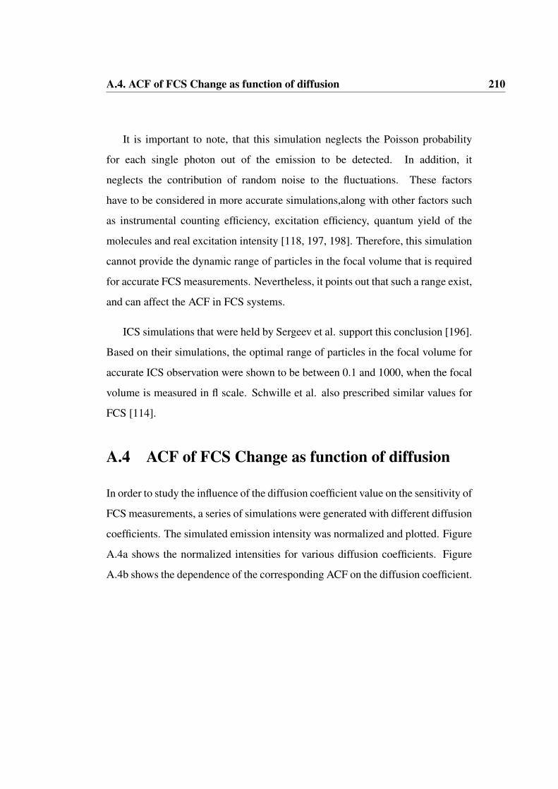
A.4. ACF of FCS Change as function of diffusion 210
It is important to note, that this simulation neglects the Poisson probability
for each single photon out of the emission to be detected. In addition, it
neglects the contribution of random noise to the fluctuations. These factors
have to be considered in more accurate simulations,along with other factors such
as instrumental counting efficiency, excitation efficiency, quantum yield of the
molecules and real excitation intensity [118, 197, 198]. Therefore, this simulation
cannot provide the dynamic range of particles in the focal volume that is required
for accurate FCS measurements. Nevertheless, it points out that such a range exist,
and can affect the ACF in FCS systems.
ICS simulations that were held by Sergeev et al. support this conclusion [196].
Based on their simulations, the optimal range of particles in the focal volume for
accurate ICS observation were shown to be between 0.1 and 1000, when the focal
volume is measured in fl scale. Schwille et al. also prescribed similar values for
FCS [114].
A.4 ACF of FCS Change as function of diffusion
In order to study the influence of the diffusion coefficient value on the sensitivity of
FCS measurements, a series of simulations were generated with different diffusion
coefficients. The simulated emission intensity was normalized and plotted. Figure
A.4a shows the normalized intensities for various diffusion coefficients. Figure
A.4b shows the dependence of the corresponding ACF on the diffusion coefficient.

A.4. ACF of FCS Change as function of diffusion 211
(a) Normalized collected intensity
(b) ACF
Figure A.4: FCS simulation for a various diffusion coefficients.(a) shows the collected intensity for a various diffusion coefficients at thefirst 200 s of the simulation time, normalized and given on an arbitraryscale. (a) shows the normalized ACF for (a).Simulations were created using the next parameters:Area size:512 × 512 pixels. Pixel resolution in x and y: 0.06µm, ωxy:0.26µm, total time: 2,000 s. Number of particles: 5,000.

A.5. ACF of RICS Change as function of diffusion 212
Figure A.4a shows that the ACF curve declines faster with increasing diffusion
coefficient of the particles. Therefore, the simulated ACF successfully described
the dynamic properties of the simulated particles and supports the use of the
autocorrelation approach to investigate the diffusion coefficient of diffusing
particles.
A.5 ACF of RICS Change as function of diffusion
Matlab code describing the RICS equations illustrate the ACF behavior and the
dependence of the ACF shape on the diffusion, beam waist, scanning speed and
pixel resolution in the X and Y directions. This Matlab code was connected with
the GUI of RICSIM, to give the user convenient accessibility to modify the input
parameters from 4.3.5.
To validate the RICS equation that is used for the fitting in RICSIM, the
theoretical ACF was compared when the diffusion coefficient was set to zero, and
when the diffusion coefficient was larger than 0. Figure A.5 shows the theoretical
ACF according the RICS equation.
It can be seen that for D=0 the ACF has a perfect gaussian shape, which is
similar to the ACF in ICS, and for D>0 the ACF became less gaussian-elliptical
and narrower with faster decay as a result of more rapidly fluctuations as a result
of the diffusion of the particles. Similar to FCS, demonstration of the dependence
of the ACF in RICS exhibits the same effect as in the FCS simulations that are
shown in Appendix A.4.

A.5. ACF of RICS Change as function of diffusion 213
(a) D=0
(b) D>0
Figure A.5: Theoretical ACF according RICS equation.The theoretical ACF was simulated using the next parameters :Defined area size: 512 × 512 pixels. Pixel resolution in x and y , δr=37nm × 37nm , Wxy: 0.26µm

Appendix BList of lab recipes
Standard NETN buffer pH 8.0
Reagent Concentration Provider
NP40 0.5% v/v Amresco,
Denver, Colorado
EDTA 1mM Amresco
Tris-Cl 20mM Amresco
NaCl 100mM Amresco
Permeabilisation solution
Reagent Concentration Provider
TritonX-100 0.1% v/v Sigma
BSA 0.5% w/v Sigma
in PBS
214
Appendix B. List of lab recipes 215
Materials for separating SDS PAGE (1 gel)
Reagent Concentration Provider Information
Acryl-40 1800µl Amresco 40% w/v pure Acry-
lamide in H2O
Bis-2 360µl Amresco 2% w/v Bis-Acrylamid
in H2O
Temed 30µl Amresco TetraMethyl Ethylene
Diamine
APS 60µl Amresco 10% w/v Ammonium
Persulfate in H2O
Separating buffer 2000µl
dH20 4000µl
Materials for stacking SDS PAGE (1 gel)
Reagent Concentration Provider Information
Acryl-40 4800µl Amresco 40% w/v pure Acry-
lamide in H2O
Bis-2 280µl Amresco 2% w/v Bis-Acrylamid
in H2O
Temed 30µl Amresco TetraMethyl Ethylene
Diamine
APS 80µl Amresco 10% w/v Ammonium
Persulfate in H2O
Separating buffer 500µl
dH20 2600µl

Appendix B. List of lab recipes 216
5xloading buffer (In H2O)
Reagent Concentration Provider Information
2-ME 0.1% v/v Sigma 2-Mercaptoethanol
14M
Bromophenol
blue
0.25% v/v Sigma
SDS 10% v/v Amresco Sodium Dodecyl
Sulfate
Glycerol 50% v/v Biolab,Clyton, VIC
Tris 250mM Amresco
Transfer buffer(In H2O)
Reagent Concentration Provider
Methanol 10% v/v Amresco
Glycine 1.74% w/v Amresco
Tris 0.58% w/v Amresco
PEMED buffer pH 7 (in PBS)
Reagent Concentration Provider
PIPES 100mM Sigma
EGTA 10mM Sigma
MgSO4 5mM Sigma
DTT 2mM Sigma
Fixation solution
Reagent Concentration Provider
Paraformaldehyde 3.7% w/v BDH Analar, Biolab
in PEMED buffer

Appendix CClasses in RICSIM
Class Name Description
load tiff Import .Tiff into the listbox
Load selected file Read selected file
Thresh background Set the background of the cell to zero
Moving Average Perform moving average subtruction
Choose ROI Define the ROI
ACF of ROI up/ down Present ACF of ROI in upper/bottom axes
ACF for ROI Calculate ACF map from grids for ROI
ACF for multi files Calculate ACF maps for a list of files
stack threshed filter Thresh stack file based on cells filter
cells filter In house threshold filter of cells
stack bleaching correction Perform bleaching correction to stack
Calculate ACF map Calculate ACF map from stack/matrix
magnifyrecttofig3 Modified imagnifyrecttofig from [199] for ROI
217

Appendix DRICSIM GUI
Figure D.1: Screen Shot of RICSIM GUI- a. Data windows.
218

Appendix D. RICSIM GUI 219
Figure D.2: Screen Shot of RICSIM GUI- b. User controls.
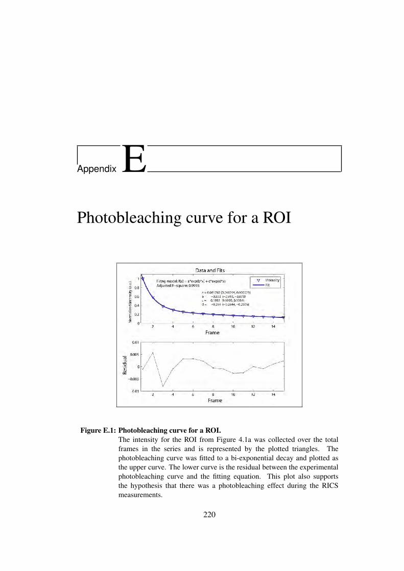
Appendix EPhotobleaching curve for a ROI
Figure E.1: Photobleaching curve for a ROI.The intensity for the ROI from Figure 4.1a was collected over the totalframes in the series and is represented by the plotted triangles. Thephotobleaching curve was fitted to a bi-exponential decay and plotted asthe upper curve. The lower curve is the residual between the experimentalphotobleaching curve and the fitting equation. This plot also supportsthe hypothesis that there was a photobleaching effect during the RICSmeasurements.
220

Appendix FSpatial correlation at the cell edges
221

Appendix F. Spatial correlation at the cell edges 222
(a) Fluorescence intensity
(b) Corresponding ACF map
Figure F.1: ACF map of freely diffusing EYFP expressed in 3T3 cell revealsadditional spatial correlation at cell edges that is created by thedominant structure of the cell edges. The immobile filtering was notapplied intentionally.