a theory of renewable energy from natural evaporation
TRANSCRIPT

A Theory of Renewable Energy from
Natural Evaporation
Ahmet-Hamdi Çavuşoğlu
Submitted in partial fulfillment of the
requirements for the degree of
Doctor of Philosophy
in the Graduate School of Arts and Sciences
COLUMBIA UNIVERSITY
2017

© 2017
Ahmet-Hamdi Çavuşoğlu
All Rights Reserved

Abstract A Theory of Renewable Energy from Natural Evaporation
Ahmet-Hamdi Çavuşoğlu
About 50% of the solar energy absorbed at the Earth’s surface is used to drive evaporation,
a powerful form of energy dissipation due to water’s large latent heat of vaporization. Evaporation
powers the water cycle that affects global water resources and climate. Critically, the evaporation
driven water cycle impacts various renewable energy resources, such as wind and hydropower. While
recent advances in water responsive materials and devices demonstrate the possibility of converting
energy from evaporation into work, we have little understanding to-date about the potential of
directly harvesting energy from evaporation.
Here, we develop a theory of the energy available from natural evaporation to predict the
potential of this ubiquitous resource. We use meteorological data from locations across the USA to
estimate the power available from natural evaporation, its intermittency on varying timescales, and
the changes in evaporation rates imposed by the energy conversion process. We find that harvesting
energy from natural evaporation could provide power densities up to 10 W m-2 (triple that of present
US wind power) along with evaporative losses reduced by 50%. When restricted to existing lakes
and reservoirs larger than 0.1 km2 in the contiguous United States (excluding the Great Lakes), we
estimate the total power available to be 325 GW. Strikingly, we also find that the large heat capacity
of water bodies is sufficient to control power output by storing excess energy when demand is low.
Taken together, our results show how this energy resource could provide nearly continuous
renewable energy at power densities comparable to current wind and solar technologies – while
saving water by cutting evaporative losses. Consequently, this work provides added motivation for
exploring materials and devices that harness energy from evaporation.

i
Table of Contents
List of Charts, Graphs, Illustrations ................................................................................................................ ii
Acknowledgements ........................................................................................................................................... iv
Dedication .......................................................................................................................................................... vi
Preface ............................................................................................................................................................... vii
Chapter 1 Natural Evaporation and Renewable Energy .............................................................................. 1
Chapter 2 Thermodynamics of Water Vapor Engines ............................................................................... 11
Chapter 3 Transport Phenomena of Evaporation in Nature .................................................................... 25
Chapter 4 Steady State Energy Harvesting from Natural Evaporation ................................................... 42
Chapter 5 Regulating Natural Evaporation Energy via Heat Storage ...................................................... 60
Chapter 6 Summary and Future Research .................................................................................................... 78
References ......................................................................................................................................................... 86

ii
List of Charts, Graphs, Illustrations
Figure 1-1 | The global mean energy budget of the Earth. ......................................................................... 2
Figure 1-2 | The global water cycle of the Earth. ......................................................................................... 4
Figure 1-3 | Natural evaporation – via the water cycle – impacts renewable energy. ............................. 5
Figure 1-4 | The distribution of wind and solar power across the contiguous United States. .............. 6
Figure 1-5 | The duck curve of renewable power in California. ................................................................ 8
Figure 2-1 | Examples of natural and synthetic water-responsive materials. ......................................... 12
Figure 2-2 | Chemical potential difference as a driving force. ................................................................. 15
Figure 2-3 | Conceptual mechanochemical work cycle projected on the μN and PV planes. ............ 22
Figure 3-1 | The surface boundary layer and typical wind, temperature, and humidity profiles ......... 28
Figure 3-2 | Unstable density, temperature, and humidity profiles causes free convection cells ........ 32
Figure 3-3 | Circuit analogies for various resistance models of evaporation ......................................... 39
Figure 4-1 | The energy balance in the absence and presence of an evaporation-driven engine. ....... 45
Figure 4-2 | Effective engine resistance and the effect on the evaporation rate and power. .............. 50
Figure 4-3 | Steady state power generation and effects on evaporative losses. ..................................... 51
Figure 4-4 | Distribution of weather conditions that affect potential power and water savings. ........ 54
Figure 4-5 | Geographic distributions of available power generation and water savings. .................... 56
Figure 5-1 | Demand variability, energy storage, and lake stratification. ................................................ 61
Figure 5-2 | Dynamic power generation model converges toward steady state predictions. .............. 64
Figure 5-3 | Simulation model of a controlled evaporation driven engine. ............................................ 67
Figure 5-4 | Matching demand in Southern California by controlling heat storage. ............................. 72
Figure 5-5 | Power quality from natural evaporation varies with climate and demand strength. ....... 73
Figure 5-6 | Trends between demand, output, reliability, and steady state. ........................................... 75
Figure 5-7 | Water savings trends between demand and steady state. .................................................... 76

iii
Figure 6-1 | Performance falls as the water vapor transport resistance of the engine increases. ........ 83
Table 4-1 | Statistics of potential power generation from natural evaporation by US State. ……… 58

iv
Acknowledgements
First, I must thank my family for their love and support over the years. I would not have the
opportunity to go on this journey of the mind without your support, patience, and encouragement.
To my mother, Robin, thank you for nurturing my passion for discovery. To my father, Hüseyin,
thank you for encouraging me to be resilient. You both have sacrificed so much, and I can only
hope I can be strong enough to make such sacrifices in the future. To my siblings, Gülsün, Celil, and
Zeynep: growing up – together and apart – has been a fascinating journey so far and I look forward
to what the future will bring us all. You all are strong individuals who inspire me. To Münevver,
Özbek, and their mother, Zeynep: even though you are far away, you are very near to my heart.
I must also thank my current academic mentor and advisor. Without you, I would not have
made it this far on this journey. To Professor Özgür Şahin: thank you for being such an excellent
mentor. You are an amazing role-model and your excitement for research and life is inspiring. When
I joined your lab back in September of 2013, I was lucky to join such a dynamic laboratory with such
a variety of exciting projects and a dynamic team of young researchers. It is with your patient
encouragement, support, and guidance that I have been able to complete this work.
I must also thank my past and present committee members. To Professor Pierre Gentine:
thank you for being such a receptive and enthusiastic collaborator. Having the chance to learn about
atmospheric science and modeling from you has been a critical part of my development. To
Professor Christopher Durning, Professor Sanat Kumar, and Professor Daniel Esposito: thank you
all for taking the time to discuss my research, critique my work, guide my development, and provide
words of support. To Professor Jeffery Koberstein: thank you for serving on my proposal
committee and being a thoughtful supporter of my journey through research here at Columbia. To
Professor Ben O’Shaughnessy: thank you for encouraging me to ask the difficult questions about
myself and the world around me.

v
I also must thank members of the Şahin Lab, who over the years have helped me in so many
ways. To Prof. Xi Chen: thank you for being a great scientist, collaborator, and friend. To Michael
DeLay: our open-ended discussions on research and life is one of the biggest highlights of my time
in the lab. To Zhenghan Gao, John Jones Molina, Ju Yang, and Dr. Onur Çakmak, Dr. Süleyman
Üçüncüoğlu, and Dr. Nicola Mandriota: thank you all for providing help and feedback over the
years to help me improve as a researcher and team member.
Additionally, I could not have made it this far without a wide and evolving network of
friends and colleagues from the world over. I have had an adventure of a lifetime here in New York,
and it could not have happened without such a strong group of friends. When I was burned out, I
had the chance to relax by going to weekly dinners with friends or explore the music and arts that
New York has to offer. I am especially grateful to my closest friends: Chinua Green, Constantin
Sabet d’Acre, Douglas McPherson, Hamid Palo, Liza Wiley, Michael Laha, Nicolas Gortzounian,
Asia Wrzaszczyk, İpek Ensari, Prakhar Agarwal, and Yuxi Lin. Without you, I would not be who I
am today. Thank you all so much.
I would also like to quickly thank the wide range of organizations at Columbia and New
York that I have worked with over the past seven years: Columbia Technology Ventures, the
Graduate Student Advisory Council, Entrepreneurship@Columbia, the Columbia-Coulter
Biomedical Accelerator, and the New York Academy of Sciences.
Finally, I must thank Alexandra Campbell, my partner and a source of immense support
during the past five years. This journey has been full of both exciting adventures and unexpected
detours. You have been there to help me breathe when I have lost my breath and to celebrate with
me when I have found success. You make me laugh harder, work better, think faster, and fight to
become stronger. I could not have completed this without you and your love and support.
vi
Dedication
I would like to dedicate this thesis to the memory of my grandparents:
Ahmet-Hamdi and Münevver Çavuşoğlu
Patricia Morag and Robert Albert Skinner
The universe is change; our life is what our thoughts make it.

vii
Preface
The purpose of this dissertation is to introduce a model of the potential renewable energy
available from the environment by tapping into the natural flow of water vapor from a water
reservoir into the atmosphere. Chapters 2 and 3 consists of brief surveys of current knowledge in
the fields of ideal isothermal chemical engines and the kinetics of natural evaporation, respectively.
Chapter 4 develops a new model that predicts the energy available from natural evaporation using a
steady state approximation along with exploring the limit of this new renewable energy resource.
Chapter 5 develops a model of a natural evaporation power plant with control and investigates the
range of power reliability in three major US electrical markets. Chapter 6 provides a discussion of
the implications of this work and directions on improving the work’s principal assumptions.
Chapters 4 and 5 have been submitted for publication and are under review as of May 1,
2017. Data supporting the findings in Chapters Chapter 4 and Chapter 5 have been uploaded to a
public repository (figshare) as of May 1, 2017.
This work should be of interest to members of the materials science community studying
evaporation powered devices because it provides an estimate of the limit of energy availability in
these systems. This work should also be of interest to scholars of renewable energy modeling
because of the potential for this renewable energy resource to exhibit lower intermittency than wind
or solar photovoltaic systems. Finally, this work should be of interest to environmental and climate
scientists, because it delivers a model for using water-responsible materials as a measurement device
of local evapotranspiration, thereby extending the predictive power of available data.
This research was conducted at Columbia University and supported by awards to Dr. Özgür
Şahin from the Department of Energy and Packard Foundation.

1
Chapter 1 Natural Evaporation and Renewable Energy
Imagine filling a glass jar halfway with liquid water, sealing the lid immediately, and then
placing the jar on a windowsill with the blinds pulled down. Some of the water molecules at the
liquid surface will have enough energy to escape the liquid phase and enter the gas phase in the jar,
thus evaporating. The reverse also occurs – water molecules from the gas collide with and then enter
the liquid in the jar as condensate. As long as the partial pressure of water vapor in the gas is below
the saturation pressure, the net transfer rate will be from the liquid into the gas. When water vapor
saturates the gas above the liquid, this glass jar system reaches equilibrium and the net exchange of
mass and energy between the liquid and gas is zero.
This equilibrium changes as we add and remove energy from the jar. When we raise the
blinds of the window, sunlight now enters our system, heating the water. This raises the saturation
pressure, leading to increased evaporation until equilibrium is reached again. When the sun sets, we
lose heat due to radiative and convective cooling around the jar. As the jar cools, water begins to
condense as the saturation pressure falls, again moving towards equilibrium.
If we open the jar, we bring the water in contact with the air. As long as the relative humidity
– the ratio of the partial pressure of water in the air to the saturation pressure of water – is below
100%, water will continue to evaporate into the air. As evaporation occurs, the water in the jar will
cool until a steady state is reached where the heat leaving the water is equal to the heat entering the

2
water in the jar. Note that the total evaporation scales with the exposed surface area of the water – a
wide jar will exhibit more evaporation than a narrow one. Evaporation will continue to occur in this
dry, sub-saturated air until all the liquid has evaporated. We can further change the rate of
evaporation by opening the window – by introducing an air flow across the top of the jar, we can
accelerate the mass transfer of water vapor away from the jar and increase the evaporation rate.
Like the jar on the windowsill, evaporation is ubiquitous on Earth. Natural evaporation (the
evaporation of water that occurs in nature) is a powerful process – studies of the global mean energy
budget show that about 50% of the solar energy absorbed at the Earth’s surface drives natural
evaporation (see Figure 1-1) [1-7]. Natural evaporation is such a powerful form of solar energy
Figure 1-1 | The global mean energy budget of the Earth.
The global mean energy budget as reported in 2013. Numbers represent the predicted energy flux magnitude in W m–2. Numbers in parentheses cover the range of observed values. Reprinted from [5]. These fluxes are time-averaged over 24 hours over the entire Earth’s surface, with 340 W m–2 incoming solar radiation at the top of the atmosphere (TOA) fueling the energy fluxes through Earth’s climate and surface.

3
dissipation because of the immense amount of energy required to evaporate water. The energy
required to drive the evaporation of water from liquid to vapor is called the latent heat of
vaporization, which is about 2,230 J/g or 40,200 J/mol. This latent heat is considerably larger than
the specific heat capacity of air, which is about 1 J/g per degree Celsius increase in temperature at
constant pressure. Thus, the sensible (convective) heat flux – the energy transfer that results in a
measurable temperature change – is only about 25% as large as the latent heat flux due to natural
evaporation (Figure 1-1).
Both the latent heat (natural evaporation) and sensible heat (convective heat) fluxes are
critical components of the tightly coupled transport phenomena of mass (water vapor), energy
(heat), and momentum (wind). At the simplest level, the latent heat flux of evaporation is
proportional to the vapor pressure deficit between the water surface and the atmosphere, whereas
the sensible heat flux of convection is proportional to the temperature difference between the water
surface and the atmosphere. The magnitudes of these two energy fluxes also depend upon the
transport characteristics of the air, which is expressed as a transport coefficient. As shown in
Chapter 3, there is both free (buoyancy-driven) and forced (wind-driven) convection over time,
requiring the use of empirical transport coefficients to adequately model these mass and transport
phenomena in nature.
Looking closer at the surface heat budget in Figure 1-1, we see how the energy balance
between net radiation (short and long wave) primarily governs the evaporation rate E and heat losses
due to turbulent convection (sensible heat flux). By combining this surface energy balance with
models of heat and mass transfer, we can predict the evaporation rate E over a saturated water
surface from weather data alone [8]. In other words, the evaporation rate E can be predicted as a
function of net solar radiation, relative humidity, wind speed, air temperature, and pressure – all

4
without needing data about the surface temperature of the water. Over 60 years later, this method is
still used to predict the evaporation rate over large scales of space (>1km2) and time (24 hours and
greater) from weather and climate data. This model has been adapted to understand and predict
changes in the naturally occurring evaporation rate over surfaces unlike a saturated water surface –
such as plants [9] and soil [10, 11].
Natural evaporation – powered primarily by the sun – drives the global water cycle [12] (see
Figure 1-2). The water cycle transports and redistributes energy, salts, nutrients, and minerals all
across Earth’s climate system. The water that evaporates from the land and ocean rises into the
atmosphere as water vapor and is carried around the Earth by winds. This water vapor eventually
Figure 1-2 | The global water cycle of the Earth.
The global water cycle – also known as the hydrological cycle – as reported in 2007. Normal font represents estimates of the primary reservoirs of water (103 km3). Italic font represents estimates of the flow rates of water through the system (103 km3 yr−1). Reprinted from [12].

5
cools and condenses to form clouds and ultimately returns to the Earth’s surface via precipitation.
Precipitation over land generates runoff that forms streams and rivers that discharge into oceans and
reservoirs, completing the global water cycle.
The water cycle shapes and affects the Earth's climate. The energy that evaporates water is
released into the atmosphere as kinetic energy and heat when water condenses to form clouds. This
energy transport can be viewed as a heat engine in the atmosphere, which generates kinetic energy
by transporting heat from warmer regions with evaporation to colder regions with condensation [13,
14]. This atmospheric heat engine analogy can be used to understand and predict various
Figure 1-3 | Natural evaporation – via the water cycle – impacts renewable energy.
a, Smokey Hills Wind Farm in Kansas has a mean generation of 1 W m-2 and capacity factor of 42% due to changing wind patterns. b, Nellis Solar Power Plant in Nevada has a mean generation of 6 W m-2 and a capacity factor of 26% due to changing cloud patterns. c-e, Changing rainfall patterns, climate variability, high levels of evaporation, reduced snow melt runoff, and current water use patterns impacts water management at Lake Mead as the water and power demands increase [21]. c, Lake Mead on July 6, 2000 versus d, July 24, 2015 illustrates how drastic a 50% reduction in water capacity can reshape the coastline. e, red areas illustrate the change in water surface area from 2010 to 2015. Scale bar = 15 km. Adapted from [22].

6
atmospheric phenomena, such as the global circulation of the atmosphere [15] and the formation of
storm systems like hurricanes [16] and tornados [17]. Thus, natural evaporation – via the water cycle
– inexorably affects the weather and climate [14, 18-22].
Critically, this evaporation-driven water cycle influences many of the renewable energy
resources and technologies used today (see Figure 1-3). Spatial and temporal changes in the latent
heat and sensible heat fluxes lead to changes in air pressure, generating the wind that power wind
turbines [23]. Clouds scatter and reflect sunlight, altering the solar radiation that power solar
photovoltaic systems [24]. Precipitation and runoff refill the water reservoirs that power
hydroelectric dams and provides water needed to grow biofuel crops [25-28]. Alternatively, droughts
slowly drain those same reservoirs and dry those same crops.
Just as the water cycle is distributed geographically, renewable energy resources are
heterogeneously distributed [29]. The advantage of dispersed energy resources is that they enable
distributed power generation at the location of consumers, thereby reducing the cost and complexity
associated with power transmission and distribution. Today, we can map where these renewable
resources can be optimally harnessed because the theories grounding these renewable energy
technologies are well explored and the availability of these renewable energy resources are well
Figure 1-4 | The distribution of wind and solar power across the contiguous United States.
Maps of a, Wind Power Class and b, TILT Solar Irradiance. A Wind Power Class of 3 or higher is considered viable for utility scale power generation. Data is from the Solar and Wind Energy Resource Assessment (SWERA) and the National Renewable Energy Library [29]

7
studied (Figure 1-4). Of all this energy that is available, renewable energy (e.g., wind, solar,
hydroelectric) makes up 17% of the total electric energy capacity in the United States as of 2015 [30].
This underwhelming figure is a result of several challenges to renewable energy adoption.
A primary hurdle for renewable energy power plants that hinders widespread adoption is
intermittency, where the power plant exhibits undesired or uncontrolled changes in power output.
Part of this issue is due to the power grid being designed for large electric power plants – such as
coal, natural gas, hydroelectric, and nuclear power – to provide electricity to end-users. To provide
uninterrupted electric energy, grid operators today control power plants by planning across three
different time spans. The time spans of electrical power demand and control are real-time regulation
(seconds to minutes), demand load balancing (minutes to hours), and scheduling (hours to days).
Intermittent power sources – such as renewables – pose a challenge because they disturb the
standard planning procedures for electrical grid operators. Since renewable resources tend to exhibit
fluctuations over multiple time scales, grid operators are forced to adjust operations across all three
time-spans. Intermittency can be predictable and grid operators can plan for this. For example, PV
solar panels only generate energy between sunrise and sunset. However, intermittency can also be
hard to predict – for example, the power from a single turbine varies as local wind speeds change.
A metric commonly used to describe intermittency is a capacity factor. The capacity factor is
a dimensionless ratio of the net electrical energy output to the maximum possible energy output
over a given time period. The capacity factors for coal and natural gas tend to hover near 50-60%,
due to shutdowns for plant maintenance (coal power plants) and varying electricity demands (natural
gas power plants) [30]. The respective capacity factors for wind and solar photovoltaic power
systems hover near 40% and 20 %, due to the intermittency of their respective natural resources.

8
Due to this intermittency, many renewable energy systems can typically not be turned on or
off with respect to the demand for power such that the supply matches market demand; that is to
say, they are not dispatchable. For example, natural gas power plants are highly dispatchable since
they can be switched on and off rapidly while coal and nuclear power plants take several hours to
cool down or come online. However, grid operators cannot just ‘turn on’ wind or solar resources to
match consumer demand. In other words, we cannot simply will the sun to shine or the wind to
blow when we wish.
This has a drastic impact on matching power demand, as shown by the ‘duck curve’ – the
graph resembles a duck silhouette – illustrating the drop and steep rise in non-renewable power
generation due to solar power in California. As Figure 1-5 shows, California has a considerable level
of solar power capacity and generates vast amounts of power during the day (yellow curve). Since
the peak demand occurs after sunset (around 9 PM) when solar power is no longer available, the
power that must be generated from sources other than wind or solar (green curve) increases rapidly
Figure 1-5 | The duck curve of renewable power in California.
On Sunday April 9, 2017, the California Independent System Operator (CAISO) reports a peak generation of 8.58 GW of solar power along with 3.01 GW of wind power. However, generation is not distributed evenly with respect to demand load. The Total Load, less Wind and Solar curve (green) shows there is a steep ramp up of power load demand (>2.5 GW per hour) between 4 PM and 8 PM Pacific Standard Time. CAISO matches this demand by importing electricity and dispatching natural gas power plants.

9
near sunset. To prevent a power outage, operators and computers at the California Independent
System Operator (CASIO) typically dispatch natural gas power plants and increase energy imports.
Interestingly, natural evaporation occurs consistently over the entire day [31]. In fact, plants
use and control evaporation to grow through a process called transpiration. Transpiration is the flow
of water from the soil through a vascular plant to evaporate into the air and represents 80 – 90% of
natural evaporation that occurs over land [32]. The mechanism of transpiration is described by the
cohesion-tension model, first proposed by Dixon and Joly in 1894 [33]. In this model, water from
the soil is drawn up the xylem to the leaves where it evaporates through the stomata. Guard cells on
the stomata control this final step of transpiration by opening and closing to allow gas exchange. In
C3 [34] and C4 [35] plants, the guard cells are open during the day, allowing evaporation to occur,
and close at night. Alternatively, the guard cells of CAM plants (a group of desert plants) open at
night to allow evaporation and stay closed during the day to prevent excessive evaporation losses
through the plant [36].
Recent research into bio-mimetic systems demonstrates our growing ability to use and
control evaporation from fabricated materials. For example, Wheeler and Stroock demonstrate the
design and operation of a synthetic microfluidic system in a hydrogel that mimics the process of
transpiration in a tree [37]. Additional materials advances demonstrate the ability to convert energy
from evaporation into work. Many of these water-responsive materials generate mechanical work
through a cycle of absorbing and rejecting water via evaporation. Examples of purely synthetic
materials that can generate mechanical work from evaporation include polypyrrole [38-40] and
functionalized carbon [41-48]. Another interesting avenue includes bio-composite materials made
from cellulose [49-53] or bacterial spores [54, 55]. On the other hand, some of these materials
generate electrical work through a flow process [56-58]. These water-responsive materials and

10
devices can harness energy when placed above a body of evaporating water. With improvements in
energy conversion efficiency, such devices could harvest energy from natural evaporation.
However, we have little theoretical understanding to-date about the potential of directly
harvesting energy from natural evaporation – specifically, the power availability, intermittency, and
the impact on water resources. In this work, we estimate the power available from natural
evaporation from open bodies of freshwater, such as lakes and water reservoirs, by modeling the
effects of an evaporation-driven engine on the energy balance and coupled heat and mass transport.
Ultimately, this work provides an estimate of the upper theoretical limit of performance and output
for any evaporation driven engine operating from evaporation from an open water surface,
analogous to the work by Shockley-Queisser on their theory of solar photovoltaic devices [59].
While there may be a large range of uncertainty involved with the approximations and assumptions
needed for this work, the value of this theory is critical in guiding the future development of this
nascent class of materials and devices.
To accomplish this, we will first construct a model of an ideal water vapor engine in Chapter
2 to understand the thermodynamic limits of such an engine. We will then study the range of natural
evaporation models in Chapter 3 to understand how evaporation in nature occurs and how it is
predicted. We will then develop a model of a steady state evaporation driven engine in Chapter 3 to
predict where (and how well) these engines could operate best in nature. Then in Chapter 5 we will
develop a dynamic model of the evaporation driven engine, and evaluate how such an engine could
potentially be controlled to deliver dispatchable power generation. Finally, in Chapter 6 we will
briefly explore the implications of this work and potential future avenues of research.

11
Chapter 2 Thermodynamics of Water Vapor Engines
Advances in water responsive materials [38, 41, 55, 60] and devices [54, 61] exhibit the ability to convert
energy from water absorption and desorption into work. This work is due to a difference in chemical potential. These
water-responsive materials can be incorporated into evaporation-driven engines that harness energy when placed above a
body of evaporating water. These materials generate work from this chemical potential through a sorption / expansion
/ desorption / compression work cycle. With improvements in energy conversion efficiency, such devices could become an
avenue to harvest energy from natural evaporation. In this chapter, we will briefly explore the thermodynamic principles
and work cycle of a water-responsive engine.
An interesting property of many materials in nature is their ability to move and perform
mechanical work at constant temperature and pressure. This is in stark contrast with many modern
engines that perform work by changing temperatures and pressures, which is often wasteful and
promotes dangerous combustion-related byproducts. Biological actuators feature fast and consistent
responses coupled with large-scale displacements – such as the twitching muscles a baseball player
uses to swing a bat. Early studies that isolated myosin proteins from muscles [62-65] kick-started
research activity studying biological motor proteins, with over 15,000 publications listed in PubMed
studying myosin over the past decade. Thus, these naturally contractile systems continue to be of
interest to scientists and engineers as model systems. These early model systems laid the groundwork

12
needed to understand how such materials could generate mechanical work while operating at
constant temperatures and pressures [62, 66-71].
To capitalize on the advantages cultivated by nature after eons of evolution, similar
properties are eagerly sought after in synthetic materials and systems, with studies of fabricated
materials that generate mechanical work through isothermal work cycles being of long-standing
interest [72-75]. Recently, significant research efforts have been focused upon hygroscopic actuators
– materials that change shape and size as they absorb water vapor – as a possible avenue to achieve
biological-like performance in synthetic systems. These recent research efforts have resulted
understanding the performance of these naturally water-responsive materials and developing
synthetic analogs that move and change shape due to changes in ambient humidity (see Figure 2-1)
[38, 53, 54, 76-81]. These hygroscopic materials that perform work by undergoing changes in shape
in response to changes in ambient humidity could provide a potential avenue to capture energy from
Figure 2-1 | Examples of natural and synthetic water-responsive materials.
a, Cone from Picea abies in its wet (closed) and dry (open) state. Adapted from [100]. b, Seed pod from wheat awn in a wet (closed) and dry (open) state. Cycling through ambient humidity conditions causes the wheat awn to ‘dig’ itself into the ground. Adapted from [81]. c, Representative images of a PEE-PPY film’s multistage motion on top of a moist surface. Adapted from [38]. d, Photos of hygroscopy-driven artificial muscles (HYDRAs) that are designed to create linear actuators that are wet (open,long) and dry (closed,short). Parallel HYDRAs can lift weights. Adapted from [54].

13
natural evaporation, a long-neglected yet powerful and readily available natural flux found practically
everywhere on Earth.
The actuators described thus far – both biological and synthetic – are examples of
mechanochemical systems. A mechanochemical system is capable of transforming chemical energy
directly into mechanical work. This is in contrast to the indirect transformation of chemical energy
into work – seen in systems such as the steam engine where combustion generates heat that is then
used to perform work. One example of a simple mechanochemical process is the swelling of a gel.
Consider a polymer gel laying at rest. When is it is exposed to a favorable solvent, the gel will absorb
some of the solvent molecules and swell (i.e., expand in volume). If the total system – gel plus
solvent – is adequately large, this swelling will occur at a constant temperature and pressure. This
change in volume may be used to create work – such as lifting a stone placed on top of the gel.
J. Willard Gibbs – building upon the foundations of Carnot, Mayer, Joule, Clausius, and
Kelvin – pioneered the first studies on the fundamental thermodynamics processes concerning the
absorption of fluids by a system under stress in his seminal paper The Equilibrium of Heterogeneous
Substances [82] and simplified by subsequent commentary [83]. Barkas applied Gibb’s thermodynamic
models to wood absorbing water vapor [84-86], and these early models were further extended by
Warburton [87] and Gurney [88]. Several models established by Gee [89] and Treloar [90] proved
useful for interpreting experiments studying the behavior of swollen polymer gels under stress.
Work by Hermans further studied the underlying thermodynamics of swollen gels undergoes
infinitesimal deformation [91]. Further work by Hill [70] and White [92] studied the absorption of
these swollen gels under finite strain, developing methods to understand the experimental data
better. All of these studies provide the crucial elements needed to describe the individual
thermodynamic processes of a mechanochemical work cycle.

14
Knowledge and information about the mechanochemical work cycle were then combined to
create descriptions and working prototypes of cyclically operating mechanochemical engines.
Biochemical research in 1952 by Morales – along with Botts and Hill – specified the requirements
for the mechanochemical cycle in actomyosin muscles [93, 94]. These studies included both
thermodynamic and kinetic limits but were not able to represent the characteristics of any possible
mechanochemical system. It was Katchalsky and colleagues who pioneered the early study and
construction of working engines that operated on a mechanochemical cycle (see Figure 2-2a) [95-
100]. These mechanochemical engines consisted of re-formed collagen fibers – and other
polyelectrolyte gels – that would stretch and shrink in response to changing salt and pH levels.
Similar synthetic and biological materials have been incorporated into devices and engines
that use the chemical potential gradient of water vapor to generate work. For example, Okuzaki et al.
designed a rotor made out of polypyrrole that operated due to absorbing and desorbing water vapor
[40]. This concept was improved by Ma et al. by designing a polypyrrole-polyol composite material
[38]. Alternatively, Wheeler and Stroock designed a biomimetic hydrogel ‘tree-on-a-chip’ that can
pump water along a chemical gradient similar to how trees undergo transpiration due to cohesion-
tension [37]. Xue et al. replicated this phenomenon with nanostructured carbon materials to
generate electrical power [56]. Recently, Chen et al. have explored using biosynthetic composites
made out of Bacillus spores to generate mechanical work from the evaporation of water [54, 55].
Fundamentally, all of these devices are limited due to thermodynamic considerations. Our
thermodynamic study of evaporation driven engines in this chapter is focused on expressing the
conditions necessary for predictable performance. By using the historically simple parameters of
mass, energy, and entropy balances, we will show that extracting work from a chemical potential
gradient is largely predictable under a specific range of conditions. We will then adapt classical

15
thermodynamic concepts and equations to the study the thermodynamic work cycle of these
evaporation driven engines and explore the possible limitations of each step in the engine cycle.
It is critical to note that many processes involved in any of these systems – such as the
muscle twitch of the baseball player [69] – are irreversible and generate additional losses due to
entropy. This irreversibility will inevitably occur in a real evaporation driven engine. In order to
develop a simpler description of the complicated phenomena involved in an evaporation driven
engine, we will treat these idealized engines as reversible. A reversible process is where every
consecutive state is in equilibrium and the maximum work is obtained from this ideal process. Thus,
the evaporation of water against a pressure just equal to its vapor pressure is reversible, and the work
done by the water vapor is the reversible work. Understanding the principles of a reversible engine
will let us set a benchmark of performance and identify possible limiting conditions.
Figure 2-2 | Chemical potential difference as a driving force.
a, Photograph of an experimental mechanochemical engine that uses formaldehyde-tanned collagen tape to pump LiBr salt from a high concentration (lower basin) to a low concentration (upper basin) while generating useful work. Adapted from [97]. b, Time-lapse images of cellulose film water vapor engine cycle (similar to a) and force balance diagram. Adapted from [53]. c, Photo of a device that exhibit self-starting oscillatory movement when placed above water. Adapted from [54]. d, The flow diagram of a mechanochemical engine.
16
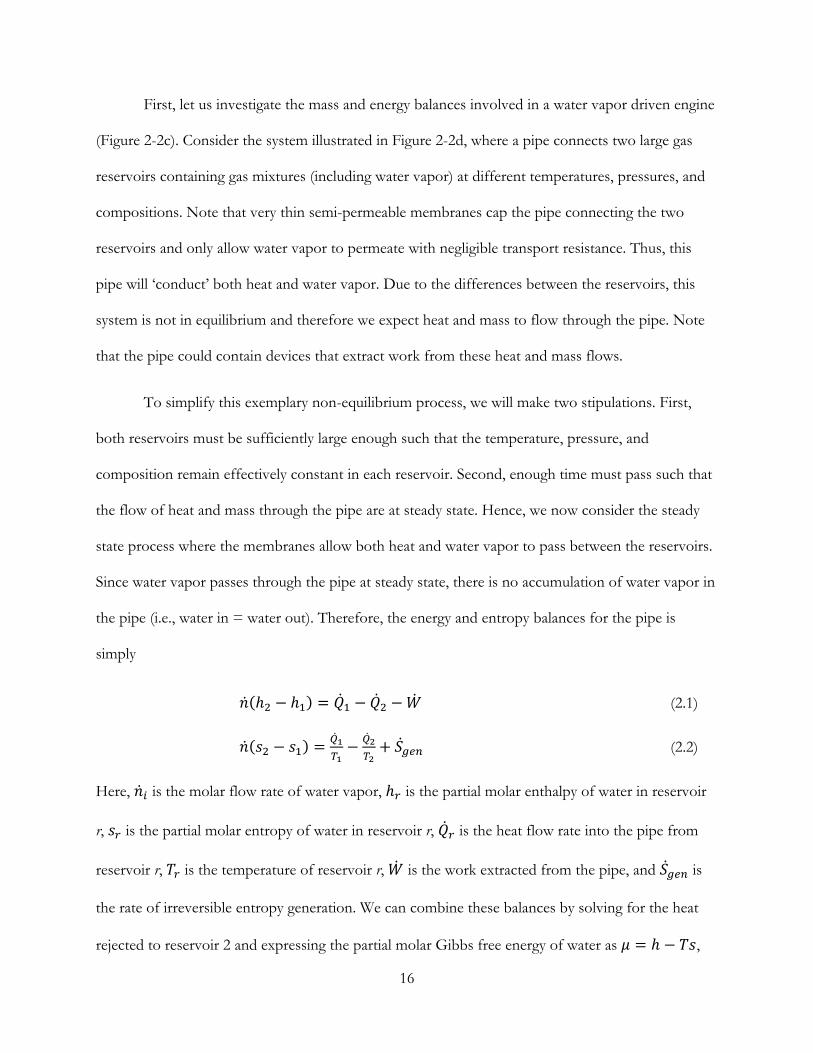
First, let us investigate the mass and energy balances involved in a water vapor driven engine
(Figure 2-2c). Consider the system illustrated in Figure 2-2d, where a pipe connects two large gas
reservoirs containing gas mixtures (including water vapor) at different temperatures, pressures, and
compositions. Note that very thin semi-permeable membranes cap the pipe connecting the two
reservoirs and only allow water vapor to permeate with negligible transport resistance. Thus, this
pipe will ‘conduct’ both heat and water vapor. Due to the differences between the reservoirs, this
system is not in equilibrium and therefore we expect heat and mass to flow through the pipe. Note
that the pipe could contain devices that extract work from these heat and mass flows.
To simplify this exemplary non-equilibrium process, we will make two stipulations. First,
both reservoirs must be sufficiently large enough such that the temperature, pressure, and
composition remain effectively constant in each reservoir. Second, enough time must pass such that
the flow of heat and mass through the pipe are at steady state. Hence, we now consider the steady
state process where the membranes allow both heat and water vapor to pass between the reservoirs.
Since water vapor passes through the pipe at steady state, there is no accumulation of water vapor in
the pipe (i.e., water in = water out). Therefore, the energy and entropy balances for the pipe is
simply
(2.1)
(2.2)
Here, is the molar flow rate of water vapor, is the partial molar enthalpy of water in reservoir
r, is the partial molar entropy of water in reservoir r, is the heat flow rate into the pipe from
reservoir r, is the temperature of reservoir r, is the work extracted from the pipe, and is
the rate of irreversible entropy generation. We can combine these balances by solving for the heat
rejected to reservoir 2 and expressing the partial molar Gibbs free energy of water as ,

17
1 (2.3)
It is trivial to note that the right-hand side of this equation vanishes in the case of thermal and
chemical equilibrium, where and .
We can use equation (2.3) to understand the interplay between coupled heat and mass
transport and the ideal limits of work generation. When the pipe is completely irreversible such that
no power is extracted from the pipe 0 , the entropy generation is maximized
0 (2.4)
We can interpret this entropy generation in terms of thermodynamic potentials and related fluxes.
The two potentials in the pipe are the reduced chemical potential gradient and the inverse
temperature gradient . The respective fluxes due to these potentials are the water flow
and the energy flow , .1
Now let us consider the limit of work that can be extracted from the temperature and
chemical potential gradients in the pipe. The maximum power generation occurs when the pipe is
completely reversible 0 . In the case of a reversible and closed 0 pipe, equation (2.3)
simplifies to the solution of an ideal Carnot heat engine – which is driven by the temperature
gradient alone – and the power generated is proportional to the heat flow into the pipe and the
sensible thermal efficiency limit 1 .
1 Aside to readers: While modelling of this irreversible process is outside the scope of this work, it is interesting to note that this relationship is important to understand the transport laws imposed by this open system. Note that the mass transfer of water in this pipe will occur due to a pressure gradient (Darcy’s Law) or concentration gradient (Fick’s Law). Additionally, mass transfer can also occur in response to a thermal gradient (Soret effect of thermodiffusion). Likewise, while heat transfer primarily occurs due to a thermal gradient, it may also occur due to pressure or concentration gradients (Dufour effect).

18
Alternatively, for a reversible, isothermal , and open pipe, the power in
equation (2.3) is proportional to the mass (water vapor) flow through the pipe and the chemical
potential drop across the pipe. We define the chemical potential as ln , where
is the standard chemical potential, R is the gas constant, Tr is the vapor temperature in the reservoir,
and ar is the thermodynamic activity of water vapor in the reservoir. The activity is proportional to
the fugacity (i.e., the effective partial pressure) at constant pressure and temperature – and for an
ideal gas, the activity is the partial pressure [101, 102]. Since the reduced pressure for water vapor at
typical atmospheric pressures and temperatures is well below 0.01, we will use the ideal gas law with
acceptable accuracy. Hence, the activity of water vapor can be defined as a ratio of the partial
pressure of water vapor in a reservoir (pr) to a standard reference pressure (p0). We can express the
chemical potential drop (work per mole of water vapor) from reservoir 1 to 2 as
(2.5)
Equation (2.5) can be further simplified by describing a relationship between the vapor
pressure in each reservoir. Each reservoir has a specific dew point – the temperature at which the
reservoir must be cooled to become saturated with water vapor. The Clausius–Clapeyron equation
describes how the saturated vapor pressure increases non-linearly with temperature. For water vapor
with a constant latent heat of vaporization L:
(2.6)
Here, R is the molar gas constant and is the saturated partial pressure of water vapor at – the
dew point temperature in this case. By integrating equation (2.6), we find
(2.7)

19
Here, and are the dew point temperatures in reservoir 1 and 2, respectively. Thus, we can
rewrite equation (2.5) as
(2.8)
Let us now consider this hypothetical pipe system of Figure 2-2d placed over a lake or any
other natural body of water. Now reservoir 1 is the liquid-vapor interface of the lake at while
reservoir 2 is at the sub-saturated vapor pressure of water in the atmosphere at , and the pipe
connecting the two is at the temperature of the water surface, . Equation (2.8) shows that the
isothermal chemical potential drop from reservoir 1 to 2 is proportional to the inverse dew point
temperature gradient between the reservoirs. In this case, the dew point temperature of reservoir 1 is
equal to the surface temperature, . Therefore, we can rewrite equation (2.3) as
1 (2.9)
Equation (2.9) shows that the reversible power available from water vapor moving through a semi-
permeable, isothermal pipe is proportional to the latent heat flow rate into the pipe and the latent
thermal efficiency limit 1 .2
Now that we have investigated the mass and energy balances involved in an ideal water
vapor driven engine, let us investigate the engine cycle found inside this hypothetical pipe. For
example, consider the engine shown in Figure 2-2c – and illustrated in Figure 2-3 – where this
working mechanochemical engine cyclically returns to its original state as water evaporates through
2 Aside to readers: If you had found yourself in Death Valley, California at 4 PM PST on June 30th, 2013, you would have experienced one of the hottest and driest days ever in the United States (46 oC, 2 oC dew point, 7% relative humidity). If you had this hypothetical pipe that reversibly and isothermally extracts energy from the flow of evaporating water from a saturated surface through the pipe, the ideal latent work efficiency would be 16%.

20
the engine. Remember that a mechanochemical system transforms chemical energy into mechanical
work directly. In an ideal situation, this cycle consists of the following steps:
1. Water vapor from the water surface enters the engine chamber and absorbs into
the water responsive, mechanochemical ‘working’ material, causing it to swell.
2. The engine is then isolated from the water surface as the ‘working’ material is
adjusted to prepare for water vapor ejection.
3. The engine is then opened to the air, allowing water vapor to leave the ‘working’
material by evaporating away, generating contractile work.
4. The engine is then again isolated from the air as the ‘working’ material is restored
to absorb water vapor again to complete the cycle
As shown through our exercise of the hypothetical pipe, essential to all isothermal water
vapor driven engine cycles is the absorption of water into the system at high chemical potential, the
subsequent ejection of water to the surroundings at a lower chemical potential, and the generation of
work. As stated earlier, the two chemical potential levels, which characterize the operation of these
water vapor engines, are maintained by the vapor reservoirs – large enough to supply or absorb
unlimited quantities of water vapor without changing temperature or vapor pressure.
Importantly, this ideal water vapor engine should be able to reciprocate between the vapor
reservoirs at different chemical potential levels. In order to sustain the chemical potential difference
and prevent the water vapor from spontaneously – and irreversibly – moving between the reservoirs,
the reservoirs must be isolated from one another. In other words, water vapor can only pass
between the reservoirs by going through the ideal engine alternating between contacting each
reservoir. In the case of Figure 2-3, this isolating mechanism is the shutters that isolate the water
responsive material from the water reservoir below and the air above. It must be stressed that in

21
certain stages of this cycle, the engine is an open system – while in other stages the engine is a closed
system. The distinction between open and closed thermodynamic processes is essential.
Let us consider the differential change in internal energy for this water vapor engine,
assuming that only thermal and chemical effects generate work. Thus, the Gibbs equation [103] is:
(2.10)
Here, is the change in the engine’s internal energy, is the heat added to the engine, is
the work performed by the engine, and is the amount of water vapor entering the engine at the
chemical potential . We can then integrate equation (2.10) over the path of a complete engine cycle
at constant temperature
∮ ∮ ∮ ∮ (2.11)
By observing that the integrals of state functions are zero in a completely reversible cycle and that
this cycle is operating at steady state, we find
∮ ∮ (2.12)
Equation (2.12) replicates the result of equation (2.9): in order to get work, there must be a
gradient of chemical potential across the engine. In other words, this chemical engine cannot operate
between two reservoirs of equal chemical potentials. This is equivalent to the Kelvin-Planck
statement of the second law of thermodynamics that no thermal engine can operate between two
reservoirs of equal temperature.
Equation (2.12) also suggests that we can impose a degree of control on this engine. By
varying the workload on the engine cycle with a fixed exchange of Δ water molecules, we will be
able to control the chemical potential drop . Note, we have not yet defined the type of work
that could be extracted by this cycle. Many water vapor engines constructed to-date generate

22
mechanical work from the chemical potential drop across the engine. Mechanical work can be
generated across three space dimensions. For a fiber (one-dimensional), the differential work is
proportional to the change in fiber length and the force on the fiber [61]. For a surface
(two-dimensional), such as a bilayer, the differential work is proportional to the change in surface
area and the stress on the surface [104]. And for a volume (three-dimensional), such as
a piston, the differential work is proportional to the change in volume and the pressure on the
volume [105]. It is also possible to generate non-mechanical forms of work from this
cycle, such as electromagnetic work [56].
For convenience, let us study the one-dimensional case of an isothermal water vapor engine
constructed of fibers and examine each stage of the work cycle. During Stage I, the engine is in
contact with the water surface reservoir and the fiber absorbs water molecules 0 at a high
chemical potential as the fiber expands in length 0 . Throughout Stage II, the engine is
isolated from the water surface reservoir 0 as the fiber is stretched 0 to lower the
Figure 2-3 | Conceptual mechanochemical work cycle projected on the μN and PV planes.
a, The conceptual work cycle of an engine operating between the high chemical potential source s to the low chemical potential exhaust e. The four stages are 1) iso-potential absorption, 2) isothermal expansion to, 3) iso-potential rejection, and 4) isothermal compression to the initial state. b, A projection of this work cycle on the -N plane, where the area inside the curve is the extracted work from the cycle. c, A projection of this work cycle on the f-L plane, where the area inside the curve is the extracted work from the cycle.

23
chemical potential of water from to . Then at Stage III, the engine is in contact with the vapor
sink and the fiber desorbs water molecules 0 at the lower chemical potential as the fiber
contracts in length 0 . At Stage IV, the engine is again isolated from the vapor sink reservoir
0 as the fiber is relaxed 0 to raise the chemical potential of water from to to
begin the cycle again.
We can project this cycle onto the vs. plane and the vs. plane to understand the
mechanical and chemical properties of each stage.3 For stages I and III, the vs. curves at constant
represent isopotential processes. All points along an isopotential can be obtained by conducting a
stress-strain absorption isotherm experiment in a large vapor reservoir of constant vapor pressure
[106]. Similarly for stages II and IV, the vs. curves at constant represent a closed isothermal
processes. These curves represent the behavior of an isolated stress-strain experiment while
measuring the change in vapor pressure – which represents the change in chemical potential for an
ideal gas, as shown in equation (2.5). Looking at the vs. plane, the isopotential and isothermal
curves are perpendicular to each other, similar to how the isothermal and adiabatic curves are
perpendicular to each other in a Carnot cycle projected on the vs. plane.
Now that we have constructed this ideal cycle, let us reflect back on equations (2.9) and
(2.12). Equation (2.9) provides a relationship for the power output from this ideal engine when the
chemical potential drop and molar flow rate is known. However, equation (2.12) only provides a
relationship for the work output. In fact, since an ideal work cycle takes an infinite number of
3 Aside to readers: Interestingly, we can restate the performance of this engine cycle based on the observed mechanical properties. The slopes of the isopotential and isothermal curves represent the elastic response of the material under conditions of constant chemical potential and constant temperature and chemical loading. The area within the engine cycle is non-zero if, and only if, the slopes of the two curves are not equivalent. In other words, the engine material will possess two distinct elastic moduli: one for absorbing water molecules at constant chemical potential and another for closed system stretching.

24
reversible steps that are in quasi-equilibrium with each other, the true power output of this ideal
work limit is zero. Therefore, there will inevitably be irreversible losses due to the flow of water
vapor through the engine.
The critical question is which stage of this engine cycle will limit the molar flow rate, thus
limiting the power output? It is possible that water transport within the material can limit the
performance of this system [39]. For the sake of simplicity, let us stipulate that our engine is made of
an ideal material that is chemically and thermally thin such that the respective water concentration
and temperature profiles can be assumed effectively constant throughout the material’s volume at
any time. In other words, the Biot numbers for mass and heat transfer are
both much less than 0.1. Therefore, external transport resistances dominate this model.
This means that our engine will be limited by the flow of water into or out of the engine.
Since we are interested in the molar flow rate of water vapor through the engine, we can narrow our
focus onto Stages I and III, where the engine absorbs and desorbs water. Absorption in Stage I can
be accelerated by immersing – or quenching – the engine material in liquid water, which is in
equilibrium with the water vapor in the high potential reservoir. Desorption in Stage III is limited by
the rate of water vapor transport away from the material surface into the reservoir. If the convective
mass transfer coefficient is small, the engine will need to desorb at a chemical potential much higher
than the potential in the vapor sink. With a higher transport coefficient, the engine will become
more efficient. Therefore, for an engine powered by the evaporation of water in nature, the rate of
water vapor transport away from the engine into the atmosphere will dictate the power limit of this
engine. By exploring how an ideal hygroscopic evaporation engine can be coupled to natural
evaporation, we can finally begin to understand the potential of this intriguing class of materials.

25
Chapter 3 Transport Phenomena of Evaporation in Nature
Evaporation is a powerful process in nature [1, 2, 5] with an average global energy flux of ~80 W m-2 that
impacts ecosystems, water resources, weather, and climate [14, 18-20]. The evaporation rate E from a water body is
balanced between net incoming radiation and heat losses due to convection. By combining this balance with equations of
heat and mass transfer, we can predict E over a saturated water surface from meteorological data (i.e., net solar
radiation, relative humidity, air temperature, and wind speed) [8]. This model has been modified to understand
changes in E due to varying surface conditions such as plants [9] and soil [10, 11]. In this chapter, we will review the
driving factors of evaporation and how it is studied and predicted in our natural environment.
As shown in Chapter 1, evaporation is a powerful transport process since the latent heat of
vaporization for water is so large. This powerful heat transport process is of great interest to
engineers. For example, homeowners in arid climates (such as Arizona) frequently use evaporative
coolers as an alternative to vapor-compression refrigeration (air conditioning) since evaporative
coolers cost less to operate [107]. Process engineers also design evaporative cooling towers to
remove heat from the heat exchangers used in power plants, refineries, and other industrial facilities
[108]. Food engineers can control the size of salt crystals by controlling the evaporation rate. These
processes exemplify how we can predict and control the evaporation rate of water for residential and
industrial applications. However, natural variations in the climate and weather found outdoors cause
variability in evaporation rates that are not so easy to control or predict.

26
While evaporation in nature is difficult to control or predict, it is of critical importance due
to natural evaporation being an important part of the water cycle [109]. Evaporation also plays a
critical component in our weather and climate [110]. For example, farmers use predicted evaporation
rates to determine their water needs for crops during a growing season [111]. Over longer time
scales, evaporation impacts the formation of soil, watersheds, and coastlines [112]. Importantly, the
rate of evaporation in nature will limit renewable energy potential from evaporation-driven engines.
Simple observations plainly illustrate how spatial and temporal energy imbalances can lead to
varying evaporation rates – warm, windy, and dry days produce greater evaporation than cool, calm,
and moist days. Pre-19th-century efforts to predict evaporation focused on individual components,
such as air temperature, sunlight, or wind speed alone. However, these correlation studies do not
fully capture the physical phenomena, nor do they provide enough temporal or spatial resolution to
provide important predictions, such as how much water will evaporate from a farm over a given day.
John Dalton conducted some of the earliest studies on evaporation [113, 114], marking the
transition of meteorology into a field of serious scientific study. Dalton first estimated the annual
evaporation from Great Britain based on the difference between rainfall and river discharge. This
was done by repurposing catchment areas (ditches that direct water runoff to a central location) and
then studying the effect of soil surfaces and environmental variations on evaporation. This particular
technique still provides useful experimental data on natural evaporation [115-118].
Critically, Dalton first described the physical principles of evaporation from open water: that
the air above a water surface can only contain a limited amount of water vapor that depends on
temperature – a maximum partial pressure of saturation. Moreover, when the partial pressure above
a water surface was not saturated, then evaporation would occur at a rate directly proportional to the
vapor pressure difference and a ‘constant’ that increased with stronger wind speeds.

27
(3.1)
In equation (3.1), the evaporation flux E (volume of liquid water lost to evaporation per area per
time) is equal to the vapor pressure deficit between the water surface and two meters above
ground4 and the mass transport coefficient .
Since the evaporation of water requires energy (i.e., the latent heat per mole of water, L) to
drive the phase change, the evaporation rate in equation (3.1) can be rewritten as a latent heat flux:
(3.2)
Here in equation (3.2), we define the latent heat transport coefficient as equal to / ,
where L is the molar heat of vaporization, is the liquid density of water, is the molecular
weight of water, and is the mass transport coefficient.
Importantly, note how the form of the latent heat flux in equation (3.2) mimics Newton’s
Law of Cooling [119], where the heat loss rate is proportional to a drop in temperature:
(3.3)
Here in equation (3.3), the sensible heat flux C is equal to the temperature drop between the
water surface and two meters above ground and the sensible heat transport coefficient .
Equations (3.1) through (3.3) represent a system of equations expressing the macroscopic
balance of heat and mass for a body of water evaporating in nature. In these models, the flux of heat
or water vapor is linearly proportional to the change in temperature or vapor pressure from the
water surface to the air. The coefficients of proportionality in these equations are the transport
4 Aside to readers: Measuring the temperature and humidity suitably far from the surface in the 18th and 19th century involved using a sling psychrometer. This device uses thermometers attached to a length of rope and spun in the air for about a minute to measure both the dry bulb and wet bulb temperature to determine the air temperate and partial pressure of water. 2 meters above the surface is the approximate height of this device as it is spun above a scientist’s head.

28
coefficients, which represent how rapidly these systems try to reach equilibrium. By knowing both
the transport characteristics of the air above the water and the boundary conditions – the
temperature and vapor pressure in the air and at the water surface – we can predict the convective
flux of heat and water vapor.
The transport of heat and mass in fluids (such as air) occurs due to both advection (bulk
fluid motion) and diffusion (random motion of molecules). This transport mechanism is called
convection. Convection is flow-dependent, increasing dramatically as the flow transitions from
laminar to turbulent. There are two limiting classes of convective transport. Free convection drives
the flow of momentum, heat, and mass due to changes in density. Forced convection drives the flow
of momentum, heat, and mass due to changes in pressure. Mixed convection, where both density
and pressure gradients are present, is in between these two limits and frequently occurs in nature.
Let us consider the flow of wind over a lake as a representative case of forced convection.
As the wind blows, a boundary layer naturally develops above the lake (Figure 3-1a). This boundary
layer can be decomposed into several regions above the surface of the lake. For simplicity, we will
treat the water surface as stagnant and apply a no-slip boundary condition. This assumption is
obviously very poor based on the simple observation that ripples form on water surfaces as the wind
Figure 3-1 | The surface boundary layer and typical wind, temperature, and humidity profiles
a, Horizontal profile of the boundary layer of forced convection forming over a flat surface, transitioning from laminar to turbulent flow. The critical length for transition to turbulence depends upon the Reynolds number. b, Vertical profile of the time averaged horizontal wind speed (green), air temperature (red), and water vapor faction (blue). Time averaged values are critical when modeling transport in a turbulent system.

29
blows. However, this is adequate for representing a microporous surface (e.g., soil, plant,
evaporation driven engine) losing heat and water to a moving airstream.
The wind flows at a bulk velocity with a bulk temperature and a bulk water vapor
content . At the water surface, the velocity is zero, the temperature is , and the water vapor
content is . The profile of each quantity varies with the height above the lake z and the distance
along the lake x (Figure 3-1b). The velocity, thermal, and water vapor boundary layers are defined as
, , 0.99 (3.4)
, , 0.99 (3.5)
, , 0.99 (3.6)
The values , , and define the respective velocity, thermal, and water vapor boundary layer
heights where ′ , , ′ , , and ′ , are respectively equal to 0.99.
As shown in the development of the boundary layer over the lake illustrated in Figure 3-1a.,
the initial flow above the lake is laminar and transitions to a turbulent flow some critical distance
away from the leading edge of the lake. Turbulence greatly enhances the convection of momentum,
heat, and mass, resulting in a mixed layer where the turbulent eddy diffusion dominates transport.
The transition from laminar to turbulent flow is ultimately due to a balance between the inertial
forces that amplify chaotic turbulence and viscous forces that dampen turbulence. The Reynolds
number defines the dimensionless ratio of inertial to viscous forces.
(3.7)
In equation (3.7), is the bulk velocity, is the distance away from the leading edge of the lake
and is the kinematic viscosity, or momentum diffusivity, of the air (approximately 1.5 10

30
m2/s). Above a critical Reynolds number, the inertial forces dominate the viscous forces, causing the
onset of observable turbulence. This critical Reynolds number is approximately 10 based on
observation.
Just as the Reynolds number provides information on the momentum transport and onset of
turbulence in the air, we can find similar information from dimensionless ratios representing the
heat and moisture transport properties of the air. For heat transport, the applicable dimensionless
ratio is the Prandtl number Pr . This number characterizes the ratio of the momentum
diffusivity to the thermal diffusivity and specifies the relative ease of momentum and energy
transport. The analogous ratio for mass transport is the Schmidt number Sc . This number
signifies the ratio of the momentum diffusivity to the water vapor diffusivity and identifies the
relative ease of momentum and mass transport.
These ratios also indicate the relative sizes of the boundary layers , , and . If the
Prandtl number is greater than unity, then > . And if the Prandtl number is less than unity,
then < . This behavior holds between and for the Schmidt number. Finally, if Pr and Sc
are both equal to unity, then all three boundary layers are the same thickness. For gases such as air,
Pr and Sc are similar (~0.7) and thus the transport of fluid, heat, and mass are of similar scale. Note
that researchers occasionally assume both Pr and Sc as unity to develop tractable analytical solutions
for cases of convection with simple geometries. This is called the Reynolds analogy.
Just as the Prandtl and Schmidt numbers relate the diffusive behavior of momentum, heat,
and mass, we can study the relative contribution of advection to diffusion for heat and mass
transport through similar dimensionless groups. These dimensionless groups are the Nusselt (Nu)
and Sherwood (Sh) numbers for heat and mass transfer, respectively.

31
(3.8)
(3.9)
In equations (3.8) and (3.9), is the characteristic length (ratio of the area to the perimeter) in
meters, is the thermal conductivity of the air in W/m/K, is the heat transfer coefficient in
W/m2/K, is the binary diffusion coefficient of water vapor in air in m2/s, and is the mass
transport coefficient in m/s. From dimensional analysis, it can be shown that the Nusselt number
represents the dimensionless surface heat flux while the Sherwood number represents the
dimensionless surface vapor transport flux.
Note that the local features of lakes can be irregular due to shorelines, rivers, trees, and other
natural or fabricated structures. This makes it considerably difficult to develop analytical solutions to
heat and mass transport, even if one uses simplifying assumptions such as the no-slip boundary
condition and the Reynolds analogy. Therefore, researchers develop empirical correlations of the
Nusselt and Sherwood numbers as functions of relevant dimensionless quantities. For the forced
convection case illustrated in Figure 3-1, the Nusselt number over the lake is a function of the
Prandtl number and the Reynolds number Nu Re , Pr . Similarly, the Sherwood number
is a function of the Schmidt number and the Reynolds number Sh Re , Sc . Both
empirical correlations depends upon if the boundary layer is laminar or turbulent. Considering that
the characteristic length of lakes and reservoirs larger than 0.1 km2 is at least 180 meters, a majority
of the airflow across the lake will be turbulent if wind speeds are greater than 0.2 m/s.
While the preceding analysis focused on how the flow of wind creates forced convection,
there are occasionally calm days where wind speeds are less than 0.2 m/s. Even on such days,
convection still occurs due to buoyancy-driven flow from unstable density gradients (see Figure 3-2).

32
These unstable gradients can arise due to temperature (hotter air is less dense than cooler air) and
composition (humid air is less dense than dry air). This buoyancy-driven flow develops the diurnal
circulation of the lake and sea breezes between land and water.
Similar to forced convection, turbulence can also happen in free convection flow, ultimately
due to the balance between buoyancy forces and viscous forces. Analogous to the Reynolds number,
the Grashof number defines the dimensionless ratio of buoyancy to viscous forces.
(3.10)
In equation (3.10), is the characteristic length of free convection in meters, is the gravitational
acceleration in m/s2, Δ is the change in density between the water surface and the reference level in
kg/m3, ̅ is the mean film density between the boundaries in kg/m3, and is the kinematic viscosity
in m2/s. In other words, represents the body forces acting on a parcel of air of size across
a normalized density gradient while represent the viscous forces acting on the same parcel.
Similar to the Reynolds number, turbulence occurs above a critical Grashof number. This critical
Grashof number is approximately 10 based on observation.
Figure 3-2 | Unstable density, temperature, and humidity profiles causes free convection cells
a, Horizontal profile of the unstable air density (green) layer due to local temperature (red) and water content (blue). This unstable layer results in free convections where denser, cooler, drier air falls as lighter, warmer, wetter air rises over a flat surface. b, Time averaged projections of the convection cells that can form near the shoreline due to spatial differences in temperature. This is primarily due to the heat capacity of water.

33
There are also empirical correlations of the Nusselt and Sherwood numbers in the case of
free convection, analogous to the force convection correlations. In this case, the Nusselt number
over the lake is now a function of the Prandtl number and the Grashof number Nu Gr, Pr .
Similarly, the Sherwood number is a function of the Schmidt number and the Grashof number
Sh Gr, Sc . Parallel to the forced convection scenario, each empirical correlations depends
upon if the free convection boundary layer is laminar or turbulent. Note that while forced
convection depends on the size of the surface, the characteristic length of free convection from a
horizontal surface may not be related to the total surface area evaporation. At large Gr, the
convective fluid develops random local eruptions of buoyant eddies, producing turbulent jets within
the boundary layer. These plumes can eventually form semi-regular convection cells, where the
Nusselt number becomes dependent on the aspect ratio of circulation.
In nature, both free and forced convection occur at the same time, increasing the complexity
of modeling the transport of heat and water vapor in the atmosphere. We call this process mixed
convection. In this situation, the Nusselt and Sherwood numbers are dependent on the shape and
orientation of both free and forced convection. The Nusselt and Sherwood number correlations for
mixed convection are described by the system geometry as well as the Reynolds, Grashof, Prandtl,
and Schmidt numbers Nu Re, Gr, Pr , Sh Re, Gr, Sc . We can identify the relative
importance of convection modes by the studying the ratio between the free buoyancy effects and
the forced inertial effects: free convection dominates when Gr Re ≫ 1, forced convection
dominates when Gr Re ≪ 1, and the regime is mixed when Gr Re 1.
To reduce the complexity involved in modeling convection, researchers commonly use
diagnostic models of the form Nu Nu , Nu , and Sh Sh , Sh , as a

34
first approximation of the relevant transport coefficients. Here, the best correlation of data is seen
for 3 for the most general cases. Since there is a limited range of characteristic length scales and
air densities compared to the range of observed wind speeds, researchers use simplified empirical
correlations for the transport coefficients for equations (3.1) though (3.3) [120, 121].
32.93 17.65 (3.11)
74.43 39.89 (3.12)
(3.13)
In equations (3.11) through (3.13), the wind speed u at two meters above the surface is in m/s, is
in mm3/s/kPa, is in W/m2/kPa, and is in W/m2/kPa. Since the fundamental mechanisms of
heat and mass transport in the air as similar, the sensible heat transport coefficient is proportional to
the latent heat transport coefficient, as shown in equation (3.13). Here, the psychrometric constant γ
(units kPa K-1) represents the ratio between the heat capacity of moist air to the latent heat of water
7.260 10 .
Note that these convection-driven transport models require information on the boundary
conditions of the system. In practice, the boundaries are the evaporating water surface and a
reference level of two to ten meters above the surface [111]. The temperature of the evaporating
surface is measured with thermometers while the air at the surface is assumed to be at saturation.
Field researchers far away from nearby weather stations use a sling hygrometer to determine the wet
and dry bulb temperatures of the air [122]. The dry bulb provides a measurement of the reference
level temperature while the wet bulb would provide information about the partial pressure of water
through psychrometric calculations [123]. Typically, we express the partial pressure as a fraction of
the saturated partial pressure (i.e., relative humidity). We can then express the vapor pressure deficit

35
Δp from equations (3.1) and (3.2) as the difference in vapor pressures between the saturated water
surface (ps) and the sub-saturated atmosphere (RHpa).
Historically, both wet bulb and surface temperature measurements suffer from low
measurement accuracy. Wet bulbs tend to be significantly less accurate than electronic sensors [124,
125]. This is because the wet bulb depends upon on a number of factors beyond relative humidity,
such as ventilation, atmospheric pressure, the thermometer diameter, the water film thickness
around the thermometer, and the arrangement of the wet and dry bulbs [122, 126]. Similarly,
consistent data from the water surface is difficult to acquire due to changes in water depth and
quality as well as variations in local heat transport [127]. The complexity inherent in measuring the
wet bulb and surface temperature limits the accuracy of the data needed to predict evaporation.
Hence, scientists spent considerable effort during the 20th century to develop alternative methods to
predict evaporation that is not dependent upon temperature data from the surface or wet bulb.
One method to predict evaporation that gained prominence in the early 20th century uses
data from the energy balance when researchers began to understand that radiative energy is a critical
component of the global energy budget [128-131]. Researchers distinguish radiation between
shortwave (0.1 – 5 microns) and longwave (greater than 5 microns). Shortwave radiation (observed
via pyranometers) varies with surface albedo (reflectivity), cloud cover, and the solar zenith.
Longwave radiation (defined by the Stefan-Boltzmann law) varies with the thermodynamic
temperatures and the emissivity between the surface and the air. Thus, researchers can define the net
radiation at the Earth’s surface as the sum of the absorbed solar shortwave radiation plus the
balance of the longwave radiation exchanged between the surface and sky.
Looking back at the energy balance in Figure 1-1, we see that the net radiation provides the
energy that drives the latent and sensible heat fluxes at the Earth’s surface. With this added

36
information about the radiative energy that drives evaporation, we can use a macroscopic energy
balance to reduce the need for information about the boundary conditions. This model eliminates
the need for observed relative humidity data and now predicts evaporation as a function of net
radiation, air temperature, surface temperature, wind speed, and air pressure. For a lake at steady
state, the incoming energy from net radiation leaves the water body via convection (sensible heat),
evaporation (latent heat), and horizontal heat conduction through the soil. Over long time scales
(~24 hr), the average heat loss due to soil conduction is zero. Thus, the energy balance is
(3.14)
Here, the balance between net radiation energy I into a body of water against the energy losses
through convective heat flux C defines the evaporative latent heat flux F. As radiation detectors
improved, the energy balance method in equation (3.14) became a more accurate alternative to using
a sling hygrometer to solve for the latent heat flux directly with equation (3.2).
While both the aerodynamically driven convective model and the energy balance model can
separately predict evaporation rates, they require accurate surface temperature data. However,
gathering reliable and consistent surface temperature data is difficult. This is primarily due to
seasonal changes in water height and quality. While it would be simple to design a floating
thermometer, the growth of biofilms can alter the local heat transfer characteristics, requiring
frequent recalibration of the thermometer. Due to these challenges, surface temperature data is not
widely available, unlike meteorological data like air temperature and wind speed.
As more accurate humidity sensors were developed, interest arose to develop a predictive
model of evaporation that eliminates the need for surface temperature data by re-incorporating data
on the relative humidity of the air. Penman first pioneered this approach in 1948 [8]. By combining
both approaches (convection and energy balance) into a single model, Penman eliminated the need
for surface temperature data. Researchers use the Penman model to make predictions of evaporation

37
rates from standard and widely available meteorological data (net radiation, air temperature, wind
speed, relative humidity, and air pressure).
We can summarize the Penman model as follows. Because of the similarity in the
relationships between the latent heat flux F and the convective heat flux C, we can express C as a
ratio to F. This is known as the Bowen ratio [130]
(3.15)
Remember that the psychrometric constant γ represents the ratio of the sensible heat transfer
coefficient to the latent heat transfer coefficient . We can now rewrite the energy balance from
equation (3.14) as I = F (1 + B).
To reduce the need for surface information, we estimate the secant (ps – pa)/(Ts – Ta) by the
Clausius–Clapeyron relation Δ, which is the slope of the vapor pressure vs. temperature curve as
shown in equation (2.6)
≡ (3.16)
We can now estimate the temperature difference between the surface and the atmosphere by using
(ps – pa)/Δ, thus eliminating the need to know the surface temperature to predict the temperature
difference in equation (3.15). We can now rewrite the Bowen ratio from equation (3.15) as
(3.17)
However, we still need a relationship to eliminate our dependence on surface vapor pressure data.
To address this challenge, we introduce the latent heat flux of the atmosphere
(3.18)
Here, we replace the surface vapor pressure ps for Δp in equation (3.2) with the saturated vapor
pressure of the atmosphere pa. Thus, Fa represents the drying power of the sub-saturated atmosphere
if the surface was at the same temperature as the air. We can then define the ratio of Fa to F as

38
1 (3.19)
We can use the ratio Fa/F in equation (3.17) to estimate the ratio between the saturation vapor
pressure deficit due to temperature differences (ps – pa) and the true vapor pressure deficit between
the saturated water surface and the sub-saturated atmosphere (ps – RHpa), thus eliminating the need
to know the surface temperature to predict the vapor pressure gradient.
By re-writing the Bowen ratio from equation (3.17) with this new information from equation
(3.19), we get
1 (3.20)
We now use equations (3.18) and (3.20) to solve I = F (1 + B) and get the Penman combination
equation
1 (3.21)
Here, is the transport coefficient from equation (3.12), I is the net radiation, Δ is the Clausius–
Clapeyron relationship, γ is the psychrometric constant, RH is the relative humidity of the air, and pa
is the saturated vapor pressure of water at the air temperature.
There is an important requirement to the Penman model – we need to choose a temperature
at which to first evaluate Δ in equation (3.16) to estimate the ratio of the saturation vapor pressure
deficit (ps – pa) to the thermal gradient (Ts – Ta). We address this issue through an iterative approach.
For the first iteration, we approximate Δ at the air temperature. After determining F, we re-
approximate the surface temperature Ts by using the aerodynamic equation for the convective heat
flux C in equation (3.3) and the Bowen ratio shown in equation (3.20)
(3.22)

39
This is an improved estimate of the surface temperature. Next, we can calculate the mean
temperature between the air and surface, Tm = (Ts + Ta)/2, and repeat our calculation for Δ in
equation (3.16). This provides a better estimate of the ratio between the saturation vapor pressure
deficit (ps – pa) and the thermal gradient (Ts – Ta). With these improvements, we can iterate between
the Penman model in equation (3.21) and equation (3.22) until the surface temperature converges
toward a solution.
The Penman combination model in equation (3.21) neatly illustrates the conditions necessary
for evaporation. We see that evaporation still occurs even when the air is saturated with water (100%
relative humidity). This is due to net radiation heating the water and local air, increasing the surface
vapor pressure. Conversely, we see that evaporation occurs even when the net radiation is zero, as
long as the relative humidity of the air is not completely saturated. Under this condition, the drying
power of the sub-saturated atmosphere (the remaining term in the parenthesis) drives evaporation.
The transport resistance of this sub-saturated drying is inversely proportional to .
Figure 3-3 | Circuit analogies for various resistance models of evaporation
a, A representative circuit model of evaporation from an open water surface. Due to convection within the top layer of water, the average temperature is constant for some depth. This is the epilimnion layer. The transport resistance in this scenario is inversely proportional to the transport coefficient b, A representative model of evaporation from plants growing from saturated soil. Some of the water flows through plants directly (transpiration) while some the water leaves the soil directly, but meets entrainment that slows mass transport until it is above the vegetation level. This creates several pathways for evaporation. c, A representative model of evaporation occurring in water limited system of dry soil. There is added resistance here due to water evaporating at the water table level and moving through the soil to the top surface. A chemical potential drop can model the flow resistance across the drier soil layers.

40
Penman’s combination equation remains a robust method for predicting potential
evaporation from saturated surfaces such as lakes and well-watered (i.e., saturated) soil, while
remaining flexible enough for further adoption and refinement to model other systems, such as
plants, regions with low moisture stress, and varying matric pressure head (Figure 3-3). One of the
earliest adoptions is the Penman-Monteith model, illustrated in Figure 3-3b, that extends the
evaporation estimates to vegetated land areas (evapotranspiration) [9]. This model divides the path
of vapor diffusion into two: 1) the path of water from the soil to the leaf surface via vegetation, or 2)
the path of water evaporating from the soil through the still air near the vegetation. These two paths
‘meet’ above the vegetation surface, where moisture is carried away due to eddy diffusion. Thus, the
Penman-Monteith model modifies the Penman model with parallel resistance analogy.
Further modification of the Penman equation by Priestley and Taylor in 1972 simplifies the
Penman model to conditions where evapotranspiration is limited by soil water supply, not
atmospheric eddy diffusion [132]. In other words, the soil resistance to water vapor transport is
significantly larger than the resistance due to atmospheric eddy diffusion. The Priestley-Taylor
equation presents α, the Priestley-Taylor coefficient, as a method of approximating evaporation rates
where the soil aridity is known, yet detailed meteorological measurements for RH and wind speed is
unknown. To determine the evaporation rate, one only needs the net radiation, soil heat flux, mean
air temperature, and soil water content (to approximate the Priestley-Taylor coefficient). When used
in areas with low to moderate aridity, the Priestley-Taylor model estimates are within ~5% of
observation, demonstrating the acceptable reliability of this phenomenological model [133].
Researchers further improve upon the Priestly-Taylor model by explicitly modeling the effect
of soil resistance on evaporation (Figure 3-3c). The Richards model is one such model of water
transport resistance in soil [134]. Richards predicted that the pressure head, along with the capillary
flow, within the soil dictates the flow of water in unsaturated and porous soils. Simulations by Milly

41
suggests that the conservation laws imposed by Richards’ equation lead to a suppression of vapor
pressure at the soil surface under arid conditions, resulting in evaporation suppression [135]. This
disruption of vapor diffusion and evaporation correlates well with observed disruptions in the
diurnal pattern of evaporation in arid climates [136-139]. This process can be approximated as an
additional chemical potential gradient that water must move across, restricting the evaporation rate.
The work in this chapter provides the groundwork for predicting evaporation based on
weather (i.e., meteorological) data. As shown in Chapter 2, we can extract work from the flow of
water vapor across a drop in chemical potential through an evaporation-driven engine. With an
ideally thin engine with relatively insignificant resistance to water vapor transport, the engine is
effectively ‘choked’ by the resistance to evaporation from the atmosphere. The models shown here
in Chapter 3 can allow us to predict empirically the evaporation rate due to turbulent, well-mixed
convection. Additionally, the work of Penman provides a way to predict evaporation without
needing surface temperature data. By combining the models shown in Chapter 2 and Chapter 3, we
can potentially predict how these evaporation-driven engines perform in the natural environment.

42
Chapter 4 Steady State Energy Harvesting from Natural Evaporation
In this chapter, we combine work from Chapter 2 and Chapter 3 to develop a model to predict the
performance of an evaporation-driven engine that is driven by steady state evaporation in the natural environment
(natural evaporation). The model demonstrates that natural evaporation is reduced in the presence of an evaporation-
driven engine and that there is an optimal workload for any specific weather condition. By using a data set of typical
meteorological conditions across the United States, we predict a range of areal power densities and corresponding water
savings due to reductions in evaporation rates at optimal power conditions.
As shown in Chapter 1 and Chapter 3, evaporation – with an average global energy flux of
about 80 W m-2 – is a powerful process in nature [1, 2, 5] that affects ecosystems, water resources,
weather, and climate [14, 18-20]. Recent advances in water responsive materials [38, 41, 55, 60] and
devices [54, 56, 61, 140] demonstrate the ability to convert energy from evaporation into work. As
shown in Chapter 2, these materials perform work through a cycle of absorbing and rejecting water
via evaporation. These water-responsive materials can be incorporated into evaporation-driven
engines that harness energy when placed above a body of evaporating water (Figure 4-1a-c). With
improvements in energy conversion efficiency, such devices could become an avenue to harvest
energy via natural evaporation from water reservoirs. However, little is currently known about the
potential of natural evaporation as a renewable energy source – such as when or where power is
available and the potential impact on water resources.

43
As shown in Chapter 3, the evaporation rate E is governed by the surface energy balance
between net radiation and heat losses due to turbulent convection and evaporation (Figure 4-1d).
Combining this energy balance with equations of heat and mass transfer can predict E over a
saturated water surface from meteorological data (i.e., net solar radiation, relative humidity, air
temperature, and wind speed) [8]. This model by Penman has been adapted to understand changes
in E over varying surfaces, such as plants [9] and soil [10, 11]. In this chapter, we estimate the power
available from natural evaporation by modeling the effects of an evaporation-driven engine on the
energy balance and coupled heat and mass transport (Figure 4-1e).
An evaporation-driven engine placed just above the water surface is powered by absorbing
water at a high chemical potential, s, and releasing it at a lower chemical potential, e, to the
atmosphere, a (s > e > a) (Figure 4-1e). As shown in Chapter 2, for a reversible and isothermal
engine, the power output depends on the evaporation rate E and the work done per mole of
evaporating water w = s – e. However, one cannot simply multiply existing E data by w, as the
energy conversion process alters the evaporation rate. Therefore, predicting the power available
from natural evaporation requires a relationship between w and E.
E is affected by w in two ways. First, the chemical potential drop w across the engine results
in a reduction in water vapor pressure across the engine, which reduces the mass transport. In the
case of an ideal gas [37], w is -RTs ln(), where R is the molar gas constant, Ts is the temperature of
the surface, and is the ratio of the vapor pressures above and below the engine. Note that the air
immediately above the water surface is saturated with water vapor, therefore the ratio is also the
relative humidity at the top of the engine (in dimensionless units 0.00 – 1.00) [141]. We can rewrite
as follows:
(4.1)

44
Because the evaporation rate depends on the vapor pressure deficit between the engine surface and
the atmosphere, an increase in w causes a reduction in evaporation rate.
Second, the total energy required to evaporate water through, and extract energy from, an
evaporation-driven engine is the sum of the latent heat L and the work energy w. We define the ratio
of this total energy to the unperturbed case as :
(4.2)
Here, L is the molar latent heat of vaporization of water in J/mol. Thus, represents the energy
penalty for evaporating water through an evaporation-driven engine versus the case with no engine.
Consequently, w affects the energy balance between net radiation and heat loss due to convection
and evaporation, because some portion of the energy from net radiation is now removed from the
system as work.
Using parameters and , it is possible to derive a model that predicts the evaporation rate
and power generated from it. Note that w can be dynamically adjusted during operation by varying
the resistance of the load such that the water responsive material in the engine must exert a larger
force on the load. Thus, it is possible to control and . In this new model, the incoming energy
from net radiation leaves the water surface via convection, evaporation (i.e., latent heat), and power
generation. The convective heat flux is proportional to the temperature difference between the
surface and the atmosphere, whereas the latent heat flux is proportional to the difference in vapor
pressures between the surface and the atmosphere. The magnitudes of these two energy fluxes also
depend on the heat and mass transport characteristics of the air, which is primarily determined by
turbulence and wind speed.
For steady state evaporation, the incoming energy from net radiation leaves the water surface
via convection and evaporation (i.e., latent heat). The energy flux due to convection is proportional

45
to the temperature difference between the surface and the atmosphere, whereas the energy flux due
to evaporation is proportional to the difference in vapor pressures between the surface and the
atmosphere. We can eliminate the need to have surface temperature data by combining these fluxes
with the energy balance.
By introducing the power output due to water evaporating through an evaporation driven
engine placed above a water surface, this new energy balance is
(4.3)
The energy balance between net radiation energy I (solar plus longwave) into a body of water against
the energy losses through evaporative latent heat flux F, power density W, and convective heat flux
C now describes this system.
Figure 4-1 | The energy balance in the absence and presence of an evaporation-driven engine.
a, The net radiative energy into a water body is balanced by convection and evaporation. b, An example of an evaporation-driven engine, incorporating water-responsive materials, placed at the water surface can harness energy from evaporation. c, Such an engine harnesses energy from evaporation through a 4 stage cycle: (I) With the upper shutters (gray jagged line) closed, the water-responsive material (green block) swells, absorbing water vapor at the high chemical potential s. (II) At maximum absorption, the upper shutters open as the bottom shutters close. (III) With the upper shutter open, the water-responsive material shrinks, releasing water that evaporates away into the atmosphere at a lower chemical potential e. (IV) At maximum desorption, the upper shutters close as the bottom shutters open, restarting the engine cycle. d, The flows between the water body and the atmosphere occur along a thermal gradient between Ts and Ta for convection and along a chemical gradient between s to a for evaporation. e, The new energy balance can be illustrated between net incoming radiation, convection, evaporation, and work extracted between s and e..

46
The latent heat flux F is proportional to the vapor pressure deficit between the top surface
of the evaporation driven engine and the atmosphere and a mass transfer coefficient
(4.4)
Here, is the empirical transport coefficient from equation (3.12) and αps – RHpa is the vapor
pressure deficit between the engine surface (αps) and the sub-saturated atmosphere (RHpa). We use
the integrated Clausius–Clapeyron model to find the saturation vapor pressure p at T, which yields
the following approximate form when the molar latent heat of vaporization L is assumed to be
constant
18.317 (4.5)
Here, p is in kPa and T is in K. A more accurate relationship is given by the Antoine equation;
however, differences are negligible for the temperature ranges involved in this analysis.
The convective heat flux is proportional to the temperature difference between the engine
and the atmosphere and a heat transfer coefficient
(4.6)
Here, the psychrometric constant γ (units kPa K-1) represents the ratio between the heat capacity of
moist air to the latent heat of water, and combined with fe represents the heat transport coefficient
[130]. The similarity in the relationships between F and C is because the fundamental mechanisms of
heat and mass transport are essentially the same for water vapor in the air.
We can couple F, C, and W together to simplify the right-hand side of the energy balance in
equation (4.3) as a function of the latent heat flux F. By our definition of in equation (4.2) as the
ratio of the total engine energy to latent heat, F + W = F. Likewise, because of the similarity in the
relationships between the latent heat flux F and the convective heat flux C, we can express C as a
ratio to F [130]

47
(4.7)
We can now rewrite the energy balance as I = F ( + B). However, this equation still
requires currently unknown surface temperature data to solve. To reduce the need for surface
temperature data, we use the Clausius–Clapeyron relation Δ, which is the slope of the vapor
pressure vs. temperature curve
≡ (4.8)
We can now estimate the temperature difference between the surface and the atmosphere by using
(ps – pa)/Δ, thus eliminating the need to know the surface temperature to predict the thermal
gradient in equation (4.7). We can now rewrite the Bowen ratio from equation (4.7) as
(4.9)
However, we still need a relationship to eliminate our dependence on surface vapor pressure data.
To address this challenge, we introduce the latent heat flux of the atmosphere
(4.10)
Here, the surface vapor pressure ps for F in equation (4.4) is replaced by the saturated vapor pressure
of the atmosphere pa. Thus, Fa represents the drying power of the sub-saturated atmosphere if the
surface was at the same temperature as the air. Therefore, the ratio of Fa to F is
1 (4.11)
We can use Fa/F in equation (4.11) to estimate the ratio between the saturation vapor pressure
deficit due to temperature differences (ps – pa) and the true vapor pressure deficit between the engine
and the sub-saturated atmosphere (ps – RHpa), thus eliminating the need to know the surface
temperature to predict the vapor pressure gradient.
By re-writing the Bowen ratio from equation (4.9) with this new information, we get

48
1 (4.12)
We use equations (4.10) & (4.12) to solve I = F ( + B) and get an expression for F
(4.13)
Here, is the transport coefficient of water vapor as a function of wind-speed u, I is the net
radiation, Δ is the slope of the saturation vapor pressure vs. temperature curve, γ is the
psychrometric constant, RH is the relative humidity of the air, and pa is the saturated vapor pressure
of water at the air temperature.
Once F is calculated, the evaporation rate E can be obtained from the relationship F =
ELMv, where and Mv, are the respective liquid density and molecular weight of water. Finally, the
areal power density W is given by W = F w/L.
The model in equation (4.13) neatly illustrates the behavior of evaporation in the presence of
an evaporation driven engine. We see that evaporation – and therefore power generation – occurs
even when the net radiation is zero, as long as the surface relative humidity is greater than the
relative humidity of the air. Under this condition, the drying power of the sub-saturated atmosphere
drives evaporative power generation. Conversely, we see that evaporation could still occur even
when is equal to the relative humidity of the air. This is due to the flux of net radiation heating the
water, increasing the surface temperature – and concurrently increasing the vapor pressure – below
the engine to drive the sensible and latent heat fluxes.
There are two important caveats to this model. First, we have not truly eliminated the need
to know the surface temperature for this model, since it is used to set in equation (4.1). Second,
we need to choose a temperature to evaluate Δ in equation (4.8) to estimate the ratio of the
saturation vapor pressure deficit (ps – pa) to the thermal gradient (Ts – Ta).

49
As shown in Chapter 3, we can address both issues through an iterative approach. For the
first iteration, we approximate both and Δ at the air temperature. After determining F, we re-
approximate the surface temperature Ts by using the aerodynamic equation for the convective heat
flux C in equation (4.6) and the Bowen ratio shown in equation (4.12)
(4.14)
This is an improved estimate of the surface temperature for . Next, we calculate the mean film
temperature of the air and surface, Tm = (Ts + Ta)/2, for solving Δ in equation (4.8). This provides a
better estimate of the ratio between the saturation vapor pressure deficit (ps – pa) and the thermal
gradient (Ts – Ta). With these improvements, we can iterate through equations (4.1), (4.13), and
(4.14) until the surface temperature converges toward a solution.
We can illustrate the behavior of this evaporation driven engine with a circuit analogy (see
Figure 4-2). Consider the case of increasing the workload w for a fixed weather condition, where wI
< wII < wIII. We expect that an increase in w will result in a decrease in the vapor pressure deficit
between the top surface of the engine and the atmosphere. This decrease in the vapor pressure
deficit will result in a decrease in the evaporation rate, all other things remaining fixed. As a rule of
conservation, the flux of water vapor through the engine must be equal to the flux of water vapor
evaporating away. We can expect that at a high enough w, evaporation will stop since the vapor
pressure deficit will become zero, eliminating the potential for evaporation. At this point, the system
dissipates all of the incoming heat as sensible heat. To maintain a steady state, the surface
temperature must increase (see Figure 4-2d). As we plot the evaporation rate from equation (4.13) as
shown in Figure 4-2b, we observe this decrease in the evaporation rate with an increase in w.
The plot of the evaporation rate E versus the workload w in Figure 4-2b is strikingly similar
to the current-voltage plots used to characterize solar photovoltaic panels. In this case, the

50
evaporation rate E represents the ‘current’ of water through the engine while w represents the
‘voltage’ (i.e., potential) across the engine. Since the areal power density W is defined as F w/L =
EMvw, we can plot rectangles under the E curve in Figure 4-2b to determine the areal power
density for each w (see Figure 4-2c). We see that W peaks a certain workload. Graphically, this
represents the largest rectangle that will fit under the E vs. w/L curve.
Figure 4-2 | Effective engine resistance and the effect on the evaporation rate and power.
a, A representative circuit model of evaporation through an evaporation driven engine above an open water surface with increasing workload w. (I) With a low engine load, there is a small drop in chemical potential inside the engine and the vapor pressure deficit between the engine surface and atmosphere is high, leading to a high evaporation rate. (II) As the engine load increases, there is a smaller vapor pressure deficit between the engine surface and atmosphere, leading to a lower evaporation rate. To maintain steady state, a higher surface temperature is needed to dissipate the net radiation into the water/engine system. (III) At even higher engine loads, the vapor pressure deficit becomes even smaller, approaching a point of no evaporation, along with no work. At this point, all of the heat is dissipated as sensible heat (thermal energy). b, Evaporation rate, c, areal power density, and d, surface temperature as a function of w/L for weather conditions of 200 W m-2 I, 16 oC Ta, 101.3 kPa P, 2.7 m s-1 (6 mph) u, and 10% relative humidity. Points along b represent the three stages shown in a. The area of the rectangles formed at each point are proportional to the areal power density shown in c. The increasing engine load of a results in higher surface temperatures, shown in d.

51
Figure 4-3 illustrates how the areal power density W and the evaporation E varies with
changes in weather conditions and workload. Figure 4-3a-c illustrates how W, E, and Ts vary as a
function of β as the relative humidity (RH) increases from 10% for the mild weather condition
shown in Figure 4-2b-d. As w increases, the surface temperature rises while the evaporation rate
gradually falls. As expected from our circuit analogy, as the RH increases, the vapor pressure deficit
between the engine and the atmosphere decreases, resulting in a decrease in the evaporation rate and
available power densities. Concurrently, we find higher surface temperatures at these more humid
conditions, necessary to drive the sensible heat flux to maintain the steady state heat balance. We
also see that the critical w value at which evaporation ultimately stops falls with an increase in the
Figure 4-3 | Steady state power generation and effects on evaporative losses.
a, Energy fluxes, b, evaporation rates, and c, surface temperatures are calculated as a function of β(w,Ts) for weather conditions of 200 W m-2 I, 16 oC Ta, 101.3 kPa P, and 2.7 m s-1 (6 mph) u at 5 values of RH (mild conditions). d, e, f are the respective energy fluxes, evaporation rates, and surface temperatures for the same conditions plotted as functions of (w,Ts). g, Maximum energy flux and h, water saved from evaporation at cool (pale, 12 oC, 150 W m-2), mild (neutral, 16 oC, 200 W m-2), and warm (dark, 20 oC, 250 W m-2) weather conditions and three wind speeds: 1.8 (4 mph, solid), 2.7 (6 mph, dashed), and 3.6 m s-1 (8 mph, dotted).

52
humidity of the air, at which point heat is released primarily as sensible heat C. Importantly, the peak
W value decreases with increasing humidity and occurs at decreasing values of w. We also plot W, E,
and Ts as a function of in Figure 4-3d-e, as is a variable of convenience that represents the
imposed relative humidity at the surface of the engine facing the atmosphere.
Just as we design solar photovoltaic cells to operate near the predicted peak power point, we
expect to operate these steady state evaporation driven engines near their peak power. To better
understand how changes in weather affect the optimal power density, we plot the optimal power
densities as a function of relative humidity for a range of weather conditions (see Figure 4-3f). We
find that peak power output increases in a super-linear fashion with decreasing relative humidity.
Interestingly, we find that the optimal power density varies weakly with wind speed; a doubling in
mean wind speed – which causes a 68% increase in based upon the model in equation (3.12) –
causes at most a 20% change in the optimal peak power output. As expected, the optimal power
densities grow with increases in air temperature and net radiation.
Notably, the evaporation rate at the optimal power density is significantly lower than the
natural evaporation rate with no engine load (w = 0). In fact, we can make a simple geometrical
argument from Figure 4-3b that the peak power output from any given E vs. w curve (or E vs. β, in
this case) occurs at approximately half of the zero load evaporation rate since that where the largest
rectangle can fit under the curve. We now define the difference between the natural evaporation rate
and the corresponding evaporation rate at peak power as ΔE, which represents the potential water
savings due to a reduction in evaporation rate through an evaporation driven engine. We find that
the potential water savings ΔE increases with increasing wind speed and decreasing relative
humidity. The results suggest peak power densities of up to 15 W m-2 and parallel water savings of
up to 7.5 mmH20 day-1 at some of the warmest, driest, and windiest conditions.

53
While these trends help to illustrate the best conditions for power harvesting from
evaporation, we can make better predictions about the feasibility of such evaporation driven engines
by using real weather data. Many various weather database products are available today, such as the
real-time weather provided by the National Center for Atmospheric Research (NCAR) or weather
forecasts generated by The Dark Sky Company.
However, there are several challenges to using such databases. Many of weather databases
use remote sensing to obtain weather information by using signals obtained from satellites and
aircraft. These remote sensing database products typically strike a compromise between high spatial
and high temporal resolution. Additionally, the size of these databases can become prohibitively
large and expensive to access when there are more than several hundred data calls for days or
locations. Finally, real-time and forecasted weather data can vary widely and may not represent
typical climatic conditions. To address these challenges, researchers use typical meteorological year
(TMY) data sets, which represent both the range and annual averages of weather phenomena that
are consistent with the long-term observation for a particular location. Critically, many researchers
modeling renewable energy systems commonly use TMY data sets [142-146].
Here, we will use the TMY3 data set provided by the Department of Energy’s (DOE)
National Renewable Energy Labs (NREL) [147]. The TMY3 dataset uses input data gathered
between 1976 and 2005. This dataset provides hourly weather values that epitomize typical
conditions at various weather stations across the USA over a span of 10 to 30 years. This dataset has
natural diurnal and seasonal variations and represents a year of typical weather conditions for each
location in the database. Note that this dataset does not contain extreme events and therefore will
not be suitable for predicting worst-case scenarios. However, TMY3 results can provide insight to
the typical performance of these evaporation driven engines.

54
The TMY for a specific location is a concatenation of 12 typical meteorological months
(January through December) to form a single year (8760 hours) of complete weather data. Note that
some hourly records may contain filled or interpolated data for periods when original observations
are missing or corrupted from the data archive. The NREL uses a statistical method to select each
typical month from a pool of 10 to 24 years [148]. For example, for a sample of 24 Januarys, we
examine all 24 samples and we select the most typical January to be included in the TMY. In this
case, a typical month means that the cumulative distributions of weather data for that month are
closest to the long-term distributions in the data pool. We repeat this procedure for the remaining
11 months, and then we concatenate the 12 selected typical months to form a complete typical year.
Since adjacent months (e.g., May, June, July) may be selected from different years, discontinuities at
the month interfaces are smoothed for 6 hours on each side.
Figure 4-4 | Distribution of weather conditions that affect potential power and water savings.
a, Distributions of (I) relative humidity, (II) global horizontal irradiance, and (III) air temperature for Daggett-Barstow, CA along with (IV) daily WMax (red line) and corresponding ΔE (blue line) predicted by equation (4.13) by using daily mean I, Ta, P, u, and RH values from the TMY3 dataset for the Daggett-Barstow, CA. b, illustrates the data (I – III) and results (IV) for Midland, TX. c, illustrates the data (I – III) and results (IV) for Newark, NJ.

55
We can use this data to understand how conditions vary over time and location (Figure 4-4).
Figure 4-4a illustrates the distribution of daily average values of (I) relative humidity, (II) global
horizontal irradiance (i.e., net radiation), and (III) air temperature for a semi-arid climate at Daggett-
Barstow, CA. For example, this data shows that the number of days where the relative humidity falls
below 40% occurs about 65% of the time at Daggett-Barstow, CA. We can use this daily data (along
with wind speed and air pressure data) to determine the daily peak power output and corresponding
water savings across the entire year, as shown in Figure 4-4aIV. We can repeat this procedure for
multiple locations; Figure 4-4b illustrates the data and findings for Midland, TX (another semi-arid
climate) and Figure 4-4c illustrates the same for Newark, NJ (a humid subtropical climate near New
York, NY). As one can expect from intuition, we find that the semi-arid climates in California and
Texas have higher power generation and water savings potential compared to the humid climate
found in New York / New Jersey. Additionally, we find that summer months will provide higher
potential power and water savings than winter months. Therefore, one has to take into account
variability of weather conditions to determine the average power available.
Using this regional meteorological dataset, our model can also provide insight into the
geographical distribution of power densities and water savings available. For our steady state model,
we generate daily mean I, Ta, RH, u, and P values at each TMY3 station in the contiguous USA (925
total stations) and calculate the maximum power output and corresponding water savings for that
day. We repeat this calculation for all 365 days at each location. We then determine the annual mean
peak power output and corresponding water savings for each location by averaging across all 365
samples. We use natural neighbor interpolation to generate contour maps of annual mean peak
power potential and water savings. In brief, natural neighbor interpolation is a method of producing
a C1 smooth map via Voronoi tessellation, a compromise between linear and cubic [149]. This
interpolation produces 5’ resolution maps of power density and parallel water savings in Figure 4-5.

56
These maps illustrate the range of annual peak power and corresponding water savings
across the United States. As expected, the arid locations in the Southwest have a higher potential for
peak power and water savings than the humid locations found in New England. Since the primary
source of energy driving evaporation is solar radiation, this map is similar to the solar power map in
Figure 1-4a. These results suggest average annual power densities and corresponding water savings
Figure 4-5 | Geographic distributions of available power generation and water savings.
a, Maximum power density available and b, total decrease in evaporation rate due to power harvesting across the contiguous United States of America. Maps calculated using data from 925 weather stations to calculate WMax and corresponding ΔE at each location from equation (4.13) with Natural Neighbor Interpolation and Linear Extrapolation to generate a 5’ resolution map.

57
up to 10.49 W m-2 and 5.95 mmH20 day-1, respectively. These maximums are located at Needles
Airport in California, only 11 km from Goose Lake and 47 km from Lake Havasu. This result is
particularly striking since the locations of peak power potential and water savings occur all together
in the US Southwest, a region that frequently suffers from water scarcity. As a point of reference,
the mean total area power densities for current US wind (as of 2009) and photovoltaic installations
(as of 2013) are 2.90 W m-2 and 8.06 W m-2, respectively [150, 151].
While the data in Figure 4-5 illustrate the geographical distributions of potential power
densities and water savings available from evaporation, there is no information about the absolute
potential possible from open water surfaces. We can make a prediction about the power and water
savings potential for evaporation driven engines by incorporating data on the location and sizes of
open bodies of water. Similar to the conundrum with weather databases, there is a wide range of
products available today. While many incorporate data from remote sensing, few databases identify
the difference between different water body types correctly and are recently being developed [152].
To address this challenge quickly, we use a global database of open water bodies that is
publically available [153]. We identify the location and size of each contiguous lake and reservoir
larger than 0.1 km2 within the contiguous United States found in the Global Lakes and Wetlands
Database. We identify a total of 11,048 candidate lakes and reservoirs, excluding the Great Lakes.
We then interpolate between our data from Figure 4-5 to calculate the total power generation and
corresponding annual water savings possible for that location if the entire water body was covered
with an evaporation driven engine. In Table 4-1, we group the results by US state as well as provide
data on the net energy generation rate for 2015 [30] and annual freshwater withdrawal rate for 2010
[108].
Our analysis reveals that 325 GW (2.85 million MWh per year) is potentially available by
covering lakes and reservoirs larger than 0.1 km2 across the contiguous US (excluding the Great

58
Lakes). Additionally, an additional 96.4 billion cubic meters of water could be recovered each year
due to lower evaporation rates. Our results indicate that potential power available exceeds demand
US State
Open Water Surface Area
(103 km2)
Potential Power Available
(GW)
Potential Water Savings
(109 m3 / year)
Net Energy Generation Rate
(GW)
Freshwater Withdrawals
(109 m3 / year)Utah 8.393 47.201 10.541 4.789 5.711 ‡California 4.845 27.551 6.376 22.455 43.049 §Texas 5.835 21.558 7.105 51.350 31.330 Minnesota 8.996 19.252 6.651 6.505 5.279 ‡Florida 5.779 18.516 6.555 27.102 8.573 §Louisiana 4.414 14.353 4.704 12.307 11.804 §Nevada 1.710 12.292 2.586 4.457 3.614 §Oklahoma 2.729 9.832 3.160 8.691 2.455 ‡Oregon 2.383 8.994 2.333 6.606 9.313 §Montana 2.854 8.628 2.615 3.345 10.546 §Maine 4.029 8.358 2.845 1.340 0.565 ‡South Dakota 3.031 7.617 2.762 1.100 0.865 ‡Tennessee 2.435 7.472 2.301 8.586 10.645 Idaho 1.817 6.897 1.795 1.788 23.806 §North Dakota 2.832 6.834 2.425 4.242 1.567 ‡North Carolina 2.260 6.759 2.301 14.656 15.295 Alabama 2.096 6.744 2.081 17.406 13.815 Wisconsin 2.874 6.461 2.213 7.575 8.511 Wyoming 1.420 6.005 1.543 5.590 6.414 §Arkansas 1.694 5.725 1.743 6.342 15.665 Georgia 1.658 5.431 1.726 14.705 6.130 Washington 1.887 5.280 1.616 12.476 6.809 New York 2.459 5.231 1.872 15.825 7.919 Missouri 1.602 5.153 1.609 9.548 11.854 South Carolina 1.504 4.889 1.596 11.020 9.374 Michigan 2.000 4.318 1.542 12.900 14.925 New Mexico 0.599 3.735 0.874 3.733 4.367 §Virginia 1.154 3.429 1.138 9.636 6.130 Arizona 0.403 3.408 0.710 12.916 8.412 Colorado 0.634 2.918 0.736 5.981 15.172 Kansas 0.899 2.796 0.976 5.197 5.538 Vermont 1.247 2.776 1.019 0.226 0.596 ‡Illinois 0.972 2.620 0.887 22.141 18.009 Kentucky 0.851 2.504 0.769 9.537 5.982 Mississippi 0.703 2.421 0.753 7.392 5.329 Nebraska 0.635 2.081 0.677 4.553 11.114 New Hampshire 0.586 1.434 0.457 2.285 0.507 Iowa 0.535 1.285 0.464 6.468 4.243 Ohio 0.507 1.165 0.428 13.915 13.075 Massachusetts 0.500 1.118 0.407 3.663 1.468 Pennsylvania 0.456 1.105 0.375 24.495 11.249 Indiana 0.422 1.067 0.371 11.874 11.952 Maryland 0.278 0.771 0.265 4.151 2.035 New Jersey 0.258 0.705 0.245 8.517 2.677 Connecticut 0.157 0.354 0.126 4.277 1.129 West Virginia 0.112 0.298 0.091 8.253 4.885 Rhode Island 0.043 0.098 0.036 0.792 0.186 Grand Total 95.487 325.434 96.404 462.709 419.888
Table 4-1 | Statistics of potential power generation from natural evaporation by US State
The table is sorted in descending order of potential power available by steady state peak power harvesting from all water bodies greater than 0.1 km2 within each state. § highlights states where the potential power available is greater than the net energy generation rate (in GW) for 2015. ‡ highlights a state where the power generation and potential water savings are greater than the net energy generation rate (in GW) for 2015 and the freshwater withdrawal rate (in billion of cubic meters per year) for 2010.
59
in 15 of 47 US states studied [30], and saves more freshwater than consumed in 7 of those 15 US
states [108].
It is important to note that there are certain caveats to the results displayed in Table 4-1.
One example is that lake sizes vary over time [152]. Another example is that these predictions only
consider evaporation from open water surfaces, not other sources of evaporation such as farms,
forests, or rivers. This is because the model assumes that the engine is covering an evaporating
surface of pure water. To predict the potential from other sources of evaporation would require
incorporating an additional evaporation transport resistance to the model. For example, predicting
evaporation from a body of water with high salinity (such as a salt lake or the sea) would require
incorporating the colligative property of vapor pressure depression for a salt-water solution. This is a
simple, but non-trivial, problem to solve.
The work in this chapter constructs a steady state model of an evaporation-driven engine,
with predictions made based on weather variables only. With this model, we study how changes in
weather conditions could potentially affect an ideal evaporation driven engine. We find that the
relative humidity, net radiation, and air temperature significantly affect the predicted performance of
these engines. Using this model, we have mapped the optimal geographic locations for such engines,
and we predict that over 325 GW of power is available from open water surfaces alone in America.
However, this model is not complete. While the model described by equation (4.13) allows
us to estimate the power density and its dependence on weather variables, our ability to make
predictions at short timescales (i.e., hours) are limited due to the approximation that the net heat
storage in the body of water is negligible. Evaluating the effect of heat storage on the variability of
evaporation is crucial to understand the potential of evaporation as a renewable energy source.
Especially since many renewable energy technologies suffer from intermittent availability.

60
Chapter 5 Regulating Natural Evaporation Energy via Heat Storage
In this chapter, we extend the work from Chapter 3 to develop a model of a natural evaporation power plant.
We derive a dynamic model of the power plant and show that it converges towards the steady state model shown in
Chapter 3. We then develop a feedforward model that leads to zero evaporation as our point of maximal energy
storage. This model is then combined with a proportional-integral (PI) feedback controller to match the power output of
this model to set power demands. This control model is then used to estimate the typical reliability of an ideal natural
evaporation power plant in three major US electrical energy markets.
Electrical power demand varies continuously due to human activity (Figure 5-1a). Unlike
other commodities, grid-scale electricity is not easily stored or delivered to match changes in supply
and demand. Electricity must be produced at the level of demand at any given moment, and demand
changes continually. Without stored electricity to call on, electric grid operators must vary generation
to match demand in order to maintain acceptable levels of power quality and reliability.
Many renewable energy resources – such as photovoltaic and wind – pose a challenge to grid
operators because they are intermittent and not dispatchable (Figure 1-5). Renewable resources tend
to exhibit fluctuations over multiple time scales, and grid operators cannot control when the sun will
shine or when the wind will blow. To handle these changes in generation, grid operators typically use

61
natural gas fired peak power plants. However, economic storage of electrical energy could reduce or
eliminate the need for peak power plants to supply dispatchable power.
Various types of storage technologies are adapted for different purposes (Figure 5-1b).
Electrical storage technologies respond to changes in demand on varying timescales. At longer
timescales – such as daily, weekly, and seasonal – electrical demand is largely predictable. At shorter
timescales – from seconds to minutes – electrical demand fluctuates significantly. To maintain a
prescribed level of power quality while delivering substantial amounts of electrical power, grid
operators use pumped storage of water (pumped hydro) to store and deliver electric power
Pumped hydro is capable of delivering high capacity electric power, reducing the need for
reserve power capacity [154]. In pumped hydro, we pump water from a lower elevation reservoir to
a higher elevation to store energy when excess, low-cost, and off-peak electric power is available.
When electrical demand increases, we release the stored water to produce electric power. The round-
trip energy efficiency of pumped hydro varies between 70 – 80% since pumping consumes energy
Figure 5-1 | Demand variability, energy storage, and lake stratification.
a, Electrical power demand in 2010 for the Eastern-Central region of CAISO for 3 representative two-week periods in December (winter), September (later summer), and June (early summer). b, Diagram of the characteristics of various grid-scale energy storage technologies. c, Temperature profile of a thermally stratified lake due to convection (red). The top (teal, epilimnion) and bottom (purple, hypolimnion) nearly-isothermal layers are separated by an intermixed layer (blue, metalimnion).

62
[30]. Pumped-storage hydroelectricity allows energy from intermittent renewable sources (e.g., wind,
solar PV) to be saved for periods of higher demand. As of 2017, pumped storage of hydroelectric
power accounts for over 90% of grid-scale energy storage (over 95 GW as of 2009) [155].
Similar to pumped hydroelectric storage, these evaporation driven engines could conceivably
provide controlled energy storage and delivery. Remember that w can be dynamically adjusted during
operation by varying the resistance of the load on the evaporation driven engine. As shown in Figure
4-2d, the water surface temperature rises as w increases. This is because of the need to satisfy the
steady-state energy balance on the evaporation engine system; with less heat leaving the system via
evaporation or work, the temperature increases such that more heat leaves the system via sensible
heat. However, an immediate change in w will result in breaking the energy balance shown in
equation (4.3). In this chapter, we will explore the dynamic energy balance of an evaporation driven
engine over a body of water and how it could be harnessed to provide controllable power delivery.
To understand the dynamic performance of this proposed evaporation driven engine, we
must understand how water responds to energy imbalances. As shown in Figure 5-1c, lakes and
reservoirs in nature undergo thermal stratification into three distinct layers [156, 157]. The top most
layer is the epilimnion, where water tends to be warmest. The bottom most layer is the hypolimnion,
where water remains near 4 °C all year. Between the two is the thermocline, which is classified by
rapid temperature changes with depth.
Stratification arises for two reasons. The first reason involves how water absorbs incoming
radiation. A portion of the net incoming radiation is absorbed by the water surface while the
remainder is absorbed exponentially beneath the surface. This absorption behavior results in only
the topmost layer of water absorbing most of the incoming radiative energy. Second, stratification
occurs because of how the density of water changes with temperature. The density of water varies
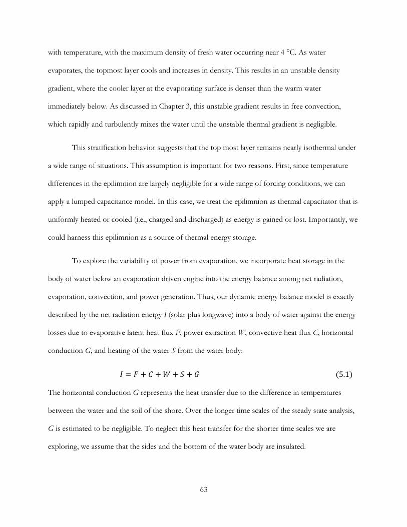
63
with temperature, with the maximum density of fresh water occurring near 4 °C. As water
evaporates, the topmost layer cools and increases in density. This results in an unstable density
gradient, where the cooler layer at the evaporating surface is denser than the warm water
immediately below. As discussed in Chapter 3, this unstable gradient results in free convection,
which rapidly and turbulently mixes the water until the unstable thermal gradient is negligible.
This stratification behavior suggests that the top most layer remains nearly isothermal under
a wide range of situations. This assumption is important for two reasons. First, since temperature
differences in the epilimnion are largely negligible for a wide range of forcing conditions, we can
apply a lumped capacitance model. In this case, we treat the epilimnion as thermal capacitator that is
uniformly heated or cooled (i.e., charged and discharged) as energy is gained or lost. Importantly, we
could harness this epilimnion as a source of thermal energy storage.
To explore the variability of power from evaporation, we incorporate heat storage in the
body of water below an evaporation driven engine into the energy balance among net radiation,
evaporation, convection, and power generation. Thus, our dynamic energy balance model is exactly
described by the net radiation energy I (solar plus longwave) into a body of water against the energy
losses due to evaporative latent heat flux F, power extraction W, convective heat flux C, horizontal
conduction G, and heating of the water S from the water body:
5.1
The horizontal conduction G represents the heat transfer due to the difference in temperatures
between the water and the soil of the shore. Over the longer time scales of the steady state analysis,
G is estimated to be negligible. To neglect this heat transfer for the shorter time scales we are
exploring, we assume that the sides and the bottom of the water body are insulated.

64
The remaining energy flows out of the body of water is power, evaporation, and convection.
The evaporative heat flux F is defined in equation (4.4), the convective heat flux C is defined in
equation (4.6), and the power density W is defined as F w/L = F (β – 1). The final remaining item in
the energy balance is the heat storage term S. We describe S with a lumped capacitance model. In
this model, the energy storage capability of the body of water is proportional to the heat capacity of
water and the change in temperature over time
5.2
Figure 5-2 | Dynamic power generation model converges toward steady state predictions.
a, Energy fluxes, b, evaporation rates, and c, surface temperatures as function of time along with the t → ∞ values of d, energy fluxes, e, evaporation rates, and f, surface temperatures as functions of α (w) for three selected conditions (colors) and water depth (line dashes). Steady state predictions are dashed black lines in d,e,f. The dynamic model results converge toward steady state predictions. The convergence time depends upon water body depth. Results are calculated for cool (pale, 12 oC, 45% RH, 150 W m-2), mild (neutral, 16 oC, 35% RH, 200 W m-2), and warm (dark, 20 oC, 25% RH, 250 W m-2) weather conditions at 2.7 m s-1 (6 mph). For d,e,f, the solid lines show the convergence of a dynamic model initialized at a surface temperature of 288 K with an isothermal depth of 5 m. The relaxation times of the surface temperature is plotted as a function of isothermal water depth f, for ten selected depths (circles) and interpolated (dashed line) at mild (16 oC, 35% RH, 200 W m-2) conditions.

65
Here, ρ is the density of water, d is the epilimnion depth of water (the warmest, near isothermal,
upper layer of a body of water), cw is the heat capacity of water, and ∂Ts/∂t is the rate of change in
water temperature over time due to heat storage/loss.
By substituting our expressions for F, C, W, and S, we rearrange the energy balance of
equation (5.1) to produce equation (5.3)
5.3
Here, the rate of heat storage is balanced by incoming net radiation (I) and outgoing convective heat
losses (C) and the sum of latent heat flux (F) and power output (W). Note that F = F+W. Thus,
the energy balance of equation (5.3) allows us to predict the water temperature Ts, the latent heat
flux F, and the power density W as a function of the chemical potential drop w and changing
weather conditions over time.
Since our hypothetical body of water is losing water to evaporation and is otherwise isolated
from below and to the side, the heat balance in equation (5.3) must be coupled with a mass balance.
The mass balance for this body of water evaporating is simply , where is the density of
water and is the evaporation rate given in equation (4.1). While incorporating this mass balance
would be straightforward, it ignores the fact that rivers fill lakes and reservoirs with water.
Therefore, a more exact model would include the mass and energy due to river flow. However, to
simplify our models, we assume that the mass flow rate of water being added back into the system is

66
equal to and that the water temperature is exactly equal to the surface temperature, reducing the
mass balance to zero and the energy balance to the one shown in equation (5.3).5
The model in equation (5.3) should converge toward our predictions from our steady state
model in Chapter 4. To check, we run a series of simulations for a range of fixed weather conditions
and initial conditions for the surface temperatures. Each simulation uses the Runge-Kutta (RK4)
method to approximate the solution of the ordinary differential equation in equation (5.3). Each
simulation runs for ten million (107) time steps and each step is one second in length. A few
examples of the simulation results are shown in Figure 5-2a-c. In these examples, we have chosen to
fix = 0.4 as representative of the workload of the evaporation driven engine. Since surface
temperature is changing as a function of time, so does the workload w. As expected for a lumped
capacitance model, each simulation evolves in time to decay exponentially towards a stable and final
steady state.
In Figure 5-2d-f, we confirm that the dynamic energy balance defined by equation (5.3) does
converge toward the steady state energy balance of equation (4.13) shown as dashed black lines. The
gray dots on Figure 5-2d-f represent the final state of the simulations shown in Figure 5-2a-c. Due to
the storage term S, the water epilimnion temperature depends on the history of the energy balance,
thus exhibiting a memory effect. The time needed for the system to forget the past is called the
relaxation time, which is strongly dependent on the depth of isothermal water d, with some weaker
effects due to the wind speed u and the workload w. An example of the importance of the depth of
the epilimnion is shown for the family of warm weather conditions in Figure 5-2a-c. As the water
5 Aside to readers: This is possible by using a small portion of the water surface as a solar water heater. The water temperature from this co-localized solar water heater would match or exceed the water temperature below the evaporation driven engine. The excess temperature of the solar can be cooled using river inflow.

67
depth increases from 0.5 to 5.0 meters, the relaxation time for the system increases ten-fold. This
strong effect of epilimnion depth on the relaxation time is shown in Figure 5-2g.
The relaxation times in Figure 5-2g illustrate an opportunity to control the level of energy
storage by effectively tuning the depth of the water. A deeper layer of isothermal water would store
more energy than a shallower layer of water, with all other variables held constant. However, this
same property would affect the ‘charging’ rate; a deeper layer of water would take considerably more
time to charge. Additionally, if the water temperature is considerably higher than the air temperature,
then energy is continuously being lost due to sensible heat loss (thermal heat transport) into the
atmosphere since this model does not consider any changes in heat transport due to the presence of
an evaporation driven engine. A thicker epilimnion layer (i.e., a larger thermal capacitator) with a
Figure 5-3 | Simulation model of a controlled evaporation driven engine.
a, Process model for an evaporation energy harvesting power plant and b, the control model for varying the output of the power plant W(t) to match a varying power demand set point PD(t).

68
higher charging time and no thermal insulation may exhibit a lower ‘round-trip’ efficiency than a
thinner epilimnion layer with thermal insulation. Finally, excessively large epilimnion depths are
unrealistic since the penetration depth of radiation and water layer convection limit the formation
and depth of the top epilimnion layer. Observations of epilimnion depths in nature range from 0.7
to 20 meters, with thicker depths in lakes and reservoirs with clearer water and larger surface areas
[158, 159]. We estimate that the mean epilimnion depth is 5 meters based upon the distribution of
lake sizes reported in the Global Lakes and Wetlands Database and the observed trends in
epilimnion depths versus surface area.
Importantly, w can be independently controlled. This feature might allow us to control
power generation, potentially mitigating the effect of changing weather conditions. To demonstrate
this, we develop a control system that adjusts w to match a power demand target over time (Figure
5-3a). To control the power delivery of the model system in Figure 5-3a, we design a combined
feedback and feedforward controller with saturation limits, shown in Figure 5-3b.
To design our control model, we must re-investigate the behavior of power output, the
system output we wish to control, in response to changes in the workload w. By looking at Figure
4-3a-c, it is evident that operating on the high w (high β and low ) side of the W curve would result
in lower evaporation rates and therefore greater water savings. More importantly, operating at high w
will provide higher thermal energy storage, with a penalty of sensible heat loss. For convenience, we
choose to manipulate in our control model to set w.
To achieve this maximum storage set point, we design a feedforward model where the
required for zero evaporation, 0, is defined at any moment by knowing the current surface
temperature Ts, air temperature Ta, and relative humidity RH. 0 is then defined as the ratio between

69
the sub-saturated vapor pressure in the air and the saturation vapor pressure at the water surface
below the engine:
5.4
We then set 0 = FF. This solution also determines the w0 required for zero evaporation:
1 5.5
Parallel with this feedforward control, we also implement an ideal Proportional-Integral (PI)
controller scheme. The proportional control accounts for real-time deviations from the changing
power demand set point while the integral control accounts for past deviations from the power
demand set point. We choose to ignore using any derivative action in the controller since the hourly
fluctuations in weather conditions can be so drastic as to induce frequent controller overshoot. The
standard PI control model is then simply
5.6
Here, is the controller gain, is the integral frequency (where and is the integral time),
and is the error signal that tells the feedback controller how far away the
system is from the desired power output to match power demand.
Since the feedforward model in equation (5.4) sets the controller at 0, the feedback control
must increase to produce more work. Thus, the final control output is the sum of FF and FB.
The non-linear characteristics demonstrated by the power density vs. surface vapor pressure curve in
Figure 5-2d can be adequately linearized near the zero-evaporation and zero work condition (0).
Thus, we tune the gain for the feedback controller to the inverse slope of W () at 0

70
| 5.7
Since 0 is always less than unity, log(0) is negative and the resulting gain is positive. However, to
reduce the computational time, we use an estimated gain of 0.0015 m2 W-1 in this work. The integral
time is tuned to the time step of the simulation (one second).
However, at higher power density levels, there is a risk of the controller going ‘over the hill’
and leading to a catastrophic failure of the PI control scheme. To avoid this, we use saturation
controls to design a relatively safe controller at the cost of losing out on the maximum power
potential of the system. A saturation range of 0.0 – 0.2 is applied to the feedback controller to
prevent controller overshoot due to this non-linearity characteristic of the system. A final saturation
control range of 0.0001 – 1.0 is applied to the sum of the feedforward and feedback controllers to
prevent non-physical controller values.
An important concern with using a PI controller with saturation limits is controller windup,
also known as integral windup. If the error signal increases rapidly because of physical limits, such as
the saturation limits, the integral term can continue to accumulate an ever-larger error signal, causing
windup that causes the controller to become unstable until this accumulated error is eliminated. To
address this issue, we use the clamping anti-windup method provided by MATLAB-Simulink to
prevent controller overshoot due to saturation [160]. In brief, the clamping method performs
conditional integration where integration is disabled when the controller is saturated.
With the system model and controller appropriately described and designed, we can begin to
simulate the potential of regulating the power delivery from an evaporation driven engine operating
in nature. To run these simulations, we need to choose which locations to study. We chose to
examine three test locations. We selected Daggett-Barstow, CA because it is near Los Angeles as
well as many large solar PV systems such that we could potentially compare our results to nearby PV

71
farms. We selected Midland, TX because it is near many large wind farms (e.g., the Roscoe Wind
Farm). We selected New York, NY because it is a major metropolitan location with large and
consistent power demands.
With our three test locations selected, we need to gather data about the weather conditions
at those locations as well as representative power demand for those locations. Conveniently, we can
reuse the typical meteorological year data (TMY3) used in Chapter 4. Here, we use station data from
Daggett-Barstow Airport (723815), Midland International Airport (722650), and Newark
International Airport (725020) to provide hourly typical meteorological data for our three respective
test locations.
We are also able to gather power demand data from various independent system operators
(ISOs) across the United States. Each ISO coordinates, controls, and monitors the operation of the
electrical power system. Here, we gather hourly power demand data for 2010 from the California
Independent System Operator (CAISO) [161], the Electric Reliability Council of Texas (ERCOT)
[162], and the New York Independent System Operator (NYISO) [163]. For each power demand
data set, we restrict our analysis to the appropriate sub-regions for each test location: South-East
Central California for Daggett-Barstow, North Central Texas for Midland, and New York City for
New York.
Because the power output of an evaporation driven engine scales with area, we are most
interested in the relative variations in power generation and demand over time, rather than absolute
values. Thus, we normalize each power demand curve by the respective mean power load for 2010.
We can then re-scaled these demand curves by a pre-factor to gauge the potential power density of
this power system. We linearly interpolate our hourly data to generate one-second samples for
calculations, and we sample our output data at one-hour intervals to reduce the size of our results.

72
With our input data, we can now run simulations for our three test locations. We run each
simulation for three simulation years (94,608,000 sample seconds) to adequately ‘forget’ the water
Figure 5-4 | Matching demand in Southern California by controlling heat storage.
Results for the final year of a simulation run for South-East Central California from Daggett Barstow, CA. From inside-out: Hourly 1) I (yellow, W m-2), 2) RH (blue, %), 3) Ta (red, oC), 4) u (cyan, m s-1), 5) WPD (gray, W m-2) and predicted WO (green dots, W m-2), and 6) four 3-day zoomed in samples of hourly WPD (gray, W m-2) and predicted WO (green dots, W m-2). Meteorological data and power demand data is from publically available databases. Annual data is evenly divided by hourly data.

73
temperature initial condition. We confirm this by finding no differences between the results for year
two and year three. Figure 5-4 and Figure 5-5a illustrates the results of a simulation year in Daggett-
Barstow with a target mean power demand of 2 W m-2. The results show that power generation
matches the demand curve 95% of the time, exhibiting some shortages on winter days where net
radiation and air temperatures are low and relative humidity is high. Similarly in Midland (Figure
5-5b), with a target annual mean power demand of 2 W m-2, power generation matches demand 93%
of the time. Again, these power failures are due to the cooler, darker, and wetter winter days. Once
Figure 5-5 | Power quality from natural evaporation varies with climate and demand strength.
The demand (gray line) and generation for a,b,c, 2 W m-2 (green dots) and d,e,f, 10 W m-2 (green dots) annual demand targets for the final simulation year in California (a,d), Texas (b,e), and New York (c,f). In a, generation matches demand 95% of the time with 99% annual generation to demand ratio. In b, generation matches demand 93% of the time with 98% annual generation to demand ratio. In c, generation matches demand over 38% of the time with 80% annual generation to demand ratio. In d, generation matches demand 48% of the time with 83% annual generation to demand ratio. In e, generation matches demand over 10% of the time with 50% annual generation to demand ratio. In f, generation matches demand 1% of the time with 24% annual generation to demand ratio.

74
more for New York (Figure 5-5c), we find power generation matches demand over 38% of the time,
again exhibiting significant power failures on winter days, as well as during the frequent high
humidity days found during the early spring and late fall.
As the annual mean power demand increases, the frequency of power shortages increases
despite an increase in the mean power generation. We can illustrate this aspect by comparing the 2
W m-2 mean power demand simulations (Figure 5-5a-c) discussed earlier to a situation where the
mean power demand is now 10 W m-2 (Figure 5-5d-f). As this comparison shows, the 10 W m-2
condition suffers from more frequent power shortages during cooler months. For example, this
system is now only able to match demand in California 48% of the time (Figure 5-5d). Note that
some power is still being generated during these cooler months, resulting in an annual generation-to-
demand ratio of 83%.
To understand the relationship between generation and demand better, we repeat these
calculations for a range of mean power demands. Figure 5-6a plots the mean generation versus the
mean demand at each test location along with a generation-to-demand ratio heat map. As demand
increases, the control system eventually saturates and the system is no longer able to provide any
more additional generation. These simulations predict a maximum generation of 2.4, 5.1, and 8.4 W
m-2 for the respective New York, Texas, and California test locations.
Figure 5-6b compares the behavior of these dynamic simulations to the behavior predicted
by the annual steady state calculations (map in Figure 4-5a) by re-normalizing the demand set point
and the generation to the respective steady-state prediction for each simulation location. This plot
reveals two regimes. When the mean demand set point is below the predicted steady state maximum
(PD/SS < 1), the average generation of the control model is approximately 80% of the demand set
point. When the demand set point is above the steady state prediction (PD/SS > 1), the generation

75
from the control model quickly saturates. The level of saturation varies between the semi-arid test
locations and the humid test location. For relatively humid New York, the control model saturates
and delivers approximately 85% of the steady state power predicted by equation (4.13) (2.8 W m-2).
This is due to the saturation range for the feedback controller, where the 0.2 level is much too high.
This causes controller overshoot and for power to be lost. For the semi-arid California and Texas
locations, the control model delivers over 95% of the steady-state prediction as demand increases
(8.4 and 5.3 W m-2, respectively).
Figure 5-6 | Trends between demand, output, reliability, and steady state.
a, Predicted average power generation as a function of target power demand for California (circles), Texas (triangles), and New York (squares) test locations. The overlaid contour map is the resulting generation to demand ratios at each power demand condition for that specific average power generation. b, Demand and Generation can re-scaled with respect to the annual steady state predictions for each location. When the mean demand set-point is set at the level of the steady state prediction of equation (4.13), the dynamic model generates ~80% of the power predicted by the steady state model. c, Predicted fraction of time that generation matches demand during an entire year as a function of target power demand. d, Demand matching re-scaled with respect to the annual steady state prediction for each location. The semi-arid locations (California and Texas) demonstrate higher reliability than the humid location (New York)

76
Importantly, as we reduce the imposed demand set point, the ability of the control system to
match power demand increases. Figure 5-6c plots the fraction of time for an entire simulation year
where generation matches the demand set point (within a 1% error tolerance), which serves as a
measure of reliability. As expected from the plots shown in Figure 5-5, the simulations with a mean
2 W m-2 demand set point can match demand more reliably than the 10 W m-2 set points.
Additionally, the warmer and more arid locations demonstrate greater reliability on average than the
cooler and humid conditions found in New York. This distinction between arid and humid vanishes
when we re-normalizing the demand with respect to the steady-state prediction for each simulation
location (Figure 5-6d), again illustrating the importance of the appropriately tuning the level of
sustainable demand to the potential resources available.
Figure 5-7 illustrates the water savings behavior of the power plant model as the level of
power demand varies. Similar to the plot shown in Figure 5-6a, at high power demand levels, the
control system is saturated and the water savings plateaus. When we reduce the mean demand set
point, we potentially save more water each day. This is due to the feedforward design constraint
Figure 5-7 | Water savings trends between demand and steady state.
a, Predicted water savings rate as a function of target power demand for California (circles), Texas (triangles), and New York (squares) test locations. b, Demand and water savings can re-scaled with respect to the annual steady state predictions for each location. When the mean demand set-point is set at the steady state level of equation (4.13), the dynamic model generates ~40% more water savings than predicted by the steady state model.

77
where no evaporation is allowed when the power demand is zero. We can also produce a similar
normalization procedure to the one shown in Figure 5-6b to see the behavior of water savings
(Figure 5-7b). We find that our dynamic model simulations could provide an additional 40% more
water savings when the demand level is set at the predicted steady-state potential. This behavior
could be due to the conservative saturation level of 0.2 set on the feedback controller, causing a
reduction in power output and evaporation rate.
The analyses here in Chapter 5 shows that the energy storage capability of naturally available
water bodies is potentially sufficient to match realistic power demand variability. This is a dramatic
result for a renewable energy source that depends on variable environmental conditions. For
comparison, wind and solar photovoltaic power have little to no control over power output without
incorporating external energy storage systems. By developing a control mechanism that takes
advantage of the relationship between the power output W and the workload w, we can potentially
optimize an evaporation driven power plant (an evaporation farm).
Taken together with the results in Chapter 4, these findings suggest that evaporation could
potentially be a widely available and flexible form of renewable energy. In principle, materials that
perform work due to changing relative humidity [38, 41, 55, 60, 104] can be incorporated into
evaporation-driven engines that harness energy when placed above a body of water [54]. With
improvements in energy conversion efficiency, such devices could become an avenue to harvest
energy from natural evaporation. This work provides added motivation to develop materials and
devices that are efficient at converting energy from evaporation.
78
Chapter 6 Summary and Future Research
This dissertation aims to understand the potential performance of evaporation driven
engines – made from hygroscopic actuators – to generate renewable energy from the evaporation of
water in nature. As discussed in Chapter 2, these hygroscopic materials perform work by changing
shape in response to variations in ambient humidity. Recent research efforts studying this class of
materials identify that the work from these materials and devices are due to changes in the chemical
potential in water vapor [38, 54, 76-79]. To understand the performance limits of such materials, we
constructed an ideal work cycle of a water vapor driven engine that extracts energy from a drop in
chemical potential. Equation (2.9) described how the power output from this ideal engine is
proportional to the drop in chemical potential across the engine and the molar flow rate of water
vapor through the engine.
At the end of Chapter 2, we made a critical assumption that an ideal evaporation engine
would present no resistance to the flow rate of water vapor through the engine. Therefore, the
engine would be limited due to either the intake of water vapor into the engine or the exhaust of
water vapor away from the engine. For an evaporation driven engine in nature, we assume that water
is abundantly available (such as from the surface of a lake) and that the exhaust rate – the rate of
evaporation in nature – would effectively ‘choke’ the performance of this new class of engine. In

79
order to model the performance of such an engine effectively, we would need to understand what
limits evaporation in nature.
With this limit in mind, we set out in Chapter 3 to explore the convective transport
phenomena that set the rate of evaporation in nature. Since evaporation requires latent heat to drive
the phase change of water from liquid to vapor and a drop in vapor pressure to drive the flux of
water vapor away from the water surface, we find two classical approaches to predict evaporation.
Researchers would either measure the vapor pressure deficit between the water surface and the
atmosphere or measure the energy imbalance at the water surface between incoming radiation and
outgoing sensible heat transfer. Both methods require surface temperature data, which is not widely
available.
By simultaneously solving both models, and incorporating radiation data with an estimate of
the vapor pressure deficit, Penman provided the first method to predict evaporation without
needing information about the surface. Penman’s combination model shown in equation (3.21)
allows for the prediction of evaporation rates based on weather data alone. Since weather data is
much more widely available compared to surface temperature data, this method widely increases the
geographical range of predictions that can be made. Critically, this combination method is versatile
enough to be adapted for a variety of alternative evaporating surfaces.
By combining the models shown in Chapter 2 and Chapter 3, we begin to predict how these
evaporation-driven engines perform in the natural environment in Chapter 4. We begin Chapter 4 by
constructing a steady state model of an evaporation-driven engine, whereby the workload of the
engine w reduces the vapor pressure deficit and increases the total heat needed to evaporate a unit of
water. The model shown in equation (4.13) enables us to make quantitative predictions based on
weather variables only. With this model, combined with typical meteorological data provided by the

80
DOE, we find that the warmer, drier, sunnier climate of the American Southwest could provide
optimal levels of power generation, along with potential water savings due to covering previously
open water surfaces with this hypothetical engine.
However, the model in equation (4.13) is a steady state approximation and is unable to make
predictions at short timescales (i.e., hours). This is due to the approximation that the net heat storage
in the body of water below the engine is negligible. To model and evaluate the dynamic performance
of an evaporation-fueled power plant, we develop a differential heat budget model in Chapter 5, as
shown in equation (5.3), which incorporates the heat storage effect of water on the evaporative
energy balance. Noticeably, since the workload w can be independently controlled, we are able to
construct a control model to vary the output of this potential evaporation power plant. The studies
in Chapter 5 show that the natural thermal energy storage capability of water is potentially sufficient
to match realistic power demand variability with power from evaporation in nature. Since many
renewable energy technologies suffer from intermittent availability, this is a vivid result for a
renewable energy source. For comparison, wind and solar photovoltaic power have little to no
control over power output without incorporating external energy storage systems.
The findings presented in this dissertation suggest that natural evaporation could potentially
be a widely available and flexible source of renewable energy. We can tap into this source of
renewable energy by placing evaporation-driven engines – made from materials that perform work
due to changing relative humidity – above a body of water. With improvements in energy
conversion efficiency, such devices could become an avenue to harvest energy from natural
evaporation. This work provides added motivation to develop materials and devices that are efficient
at converting energy from evaporation.

81
While the idealized models presented in this dissertation are helpful in predicting an upper
limit of efficiency and performance for this nascent class of hygroscopic actuators, there is a wide
range of future work needed to confirm the assumptions made in this dissertation and advance the
state-of-the-art. For example, experimental data on the internal transport resistances of these engines
would provide greater insight into how such engines would respond to changes in weather and
power demand. Our current ideal model is limited since it assumes an infinitesimally thin engine that
reversibly modifies the vapor pressure and latent heat of vaporization as it harvests energy.
Future work can begin to account for the non-infinitesimal thickness of an engine above a
body of water and the transport kinetics within the water responsive materials that make up the
engine. Let us first consider the hygroscopic actuators that could power such an engine. These
actuators would have a characteristic length defined by the ratio of the absorptive material
volume divided by the exposed surface area for absorption. They would also have a characteristic
permeability to water vapor , which is dependent upon the sorption equilibrium and the water
diffusivity of the material. We can model the flux of water vapor as
6.1
Here, Δ represents the vapor pressure drop that drives the flow of water into and out of the spore
engine (where represents the sorption of water vapor into the actuator while
describes the desorption of water vapor to the atmosphere). The difference is now the
vapor pressure drop due to extracting energy from evaporation. Note that
is a necessarily condition for an evaporation driven actuator to extract work. This model is
similar to equation (3.1), where the evaporation rate is proportional to the vapor pressure deficit
between the water surface and the atmosphere and the mass transfer coefficient .

82
Just as we defined as the ratio of vapor pressure drop from to due to the chemical
potential drop w, we can construct similar relationships for the changes in vapor pressure due to
transport losses and work. We can quickly define these vapor pressure ratios as
, , , 6.2
, , , 6.3
, , , 6.4
Here, represents the vapor pressure drop ratio due to actual work extraction while and
represent the ratios due to absorption and desorption, respectively. Thus, the total vapor pressure
ration is now defined as , allowing us to re-use the model for F in equation (4.13), while
redefining the power output as .
Critically, must equal for an evaporation driven engine operating at steady state. We can
use this behavior to redefine the mass transfer Biot number as /
. This
dimensionless ratio re-enforces the need for low Biot numbers for our models to remain valid (see
Figure 6-1). As this mass transfer Biot number increases, there is a greater relative resistance to water
vapor transport due to the engine. In other words, the water vapor gradients within the material can
no longer be neglected at high Biot numbers because a greater portion of the chemical potential
drop w is being used to drive the irreversible flow of water vapor through the engine. This causes the
engine’s performance to be ‘choked’ due to the engine characteristics, rather than the atmosphere.
Interestingly, this re-defined mass transfer Biot number touches upon another assumption
used in Chapter 3, the use of an empirical mass transfer coefficient. While many researchers use the
models shown in equations (3.11) through (3.13) for first-order estimates of potential evaporation in

83
nature, these transport coefficients are only diagnostic in nature. More appropriate transport
coefficients are location specific and incorporate more input, such as observations of gradients in
temperature and air composition that would give rise to buoyancy-induced eddies. Such data is
gathered by micrometeorological sites, such as FLUXNET [164] and AmeriFlux [165]. Additional
considerations would involve the real engineering and deployment of evaporation driven engines
since they would likely change the surface roughness of any surface and perturb the boundary layer.
Figure 6-1 | Performance falls as the water vapor transport resistance of the engine increases.
As the engine’s resistance to water vapor transport increases relative to the air, the performance of the engine falls. Here, we use the conditions from Figure 4-2 to illustrate this issue, while still assuming a thermally thin system. a, At a mass transfer Biot number of 0.1, where the resistance of the air is ten times greater than the engine, this system is nearly ideal, with relatively little transport losses in the workload w. b, When the engine resistance is equal to the resistance of the air, more of the chemical potential is ‘spent’ moving water vapor through the engine, reducing the available w for work extraction. c, At high Biot, much more of the chemical potential is spent, severely limiting hypothetical engine performance.

84
Beyond these model considerations, there is an on-going need to improve the input data for
the steady state and dynamic models shown in this dissertation. For example, the results shown in
Table 4-1 are based on data from a study published in 2004 [153], which was based on even older
records of water reservoir geography. It is readily apparent in nature that lake sizes vary over time
[152]. Between 1984 and 2015, permanent surface water bodies have recessed by over 90 thousand
square kilometers while 184 thousand square kilometers of new permanent surface water bodies
have formed globally. It would appear that being limited to typical weather data from the United
States could have handicapped the predictions made in this dissertation.
Another example is that these predictions only consider typical weather conditions. Without
accounting for atypical (i.e., extreme) weather events, the model shown in Chapter 5 cannot provide
predictions about planning for potential worst-case scenarios. Thus, it could be of value to perform
a range of simulations incorporating real weather to identify real-time energy performance. It may
also be of value to investigate alternative control methods to improve the output of the proposed
power plant system further. The control model shown in Figure 5-3b incorporates only feedback
and feedforward control based on matching varying power demand. Interestingly, many electric
grids now incorporate variable pricing, and it may be valuable to design an economic pricing model
to regulate the delivery of power from evaporation for optimal revenue. Additionally, better forward
predictive models (forecasts of weather and electric demand) could be used to make the control
system more resilient against changes in seasonal climate.
While there is a range of assumptions to continue validating and future work to accomplish,
this dissertation has set out to provide the first quantitative predictions about the potential for
harvesting renewable energy from evaporation in nature. In principle, materials that perform work
due to changing relative humidity can be incorporated into evaporation-driven engines that harness

85
energy when placed above a body of water. These findings suggest that evaporation could potentially
be a widely available and flexible form of renewable energy. Additionally, we find that the energy
storage capability of naturally available water bodies is potentially sufficient to match realistic power
demand variability. With improvements in energy conversion efficiency, such devices could become
an avenue to harvest energy from natural evaporation. This work provides added motivation to
develop materials and devices that are efficient at converting energy from evaporation.

86
References
1. Trenberth, K.E., J.T. Fasullo, and J. Kiehl, Earth's Global Energy Budget. Bulletin of the American Meteorological Society, 2009. 90(3): p. 311-323.
2. Stephens, G.L., et al., An update on Earth's energy balance in light of the latest global observations. Nature Geoscience, 2012. 5(10): p. 691-696.
3. Stephens, G.L., et al., The global character of the flux of downward longwave radiation. Journal of Climate, 2012. 25(7): p. 2329-2340.
4. Stevens, B. and S.E. Schwartz, Observing and Modeling Earth’s Energy Flows. Surveys in Geophysics, 2012. 33(3-4): p. 779-816.
5. Wild, M., et al., The global energy balance from a surface perspective. Climate Dynamics, 2013. 40(11-12): p. 3107-3134.
6. L’Ecuyer, T.S., et al., The Observed State of the Energy Budget in the Early Twenty-First Century. Journal of Climate, 2015. 28(21): p. 8319-8346.
7. Stephens, G.L. and T. L'Ecuyer, The Earth's energy balance. Atmospheric Research, 2015. 166: p. 195-203.
8. Penman, H.L., Natural evaporation from open water, bare soil and grass. Proc R Soc Lond A Math Phys Sci, 1948. 193(1032): p. 120-45.
9. Monteith, J.L., Evaporation and environment. Symp Soc Exp Biol, 1965. 19: p. 205-34. 10. Jarvis, P.G., The Interpretation of the Variations in Leaf Water Potential and Stomatal Conductance Found in
Canopies in the Field. Philosophical Transactions of the Royal Society of London B: Biological Sciences, 1976. 273(927): p. 593-610.
11. Barton, I.J., Parameterization of the Evaporation from Non-Saturated Surfaces. Journal of Applied Meteorology, 1979. 18(1): p. 43-47.
12. Trenberth, K.E., et al., Estimates of the Global Water Budget and Its Annual Cycle Using Observational and Model Data. Journal of Hydrometeorology, 2007. 8(4): p. 758-769.
13. Barry, L., G.C. Craig, and J. Thuburn, Poleward heat transport by the atmospheric heat engine. Nature, 2002. 415(6873): p. 774-7.
14. Laliberte, F., et al., Atmospheric dynamics. Constrained work output of the moist atmospheric heat engine in a warming climate. Science, 2015. 347(6221): p. 540-3.
15. Lorenz, E.N., Available Potential Energy and the Maintenance of the General Circulation. Tellus, 1955. 7(2): p. 157-167.
16. Emanuel, K.A., The dependence of hurricane intensity on climate. Nature, 1987. 326(6112): p. 483-485. 17. Renno, N.O., A thermodynamically general theory for convective vortices. Tellus A, 2008. 60(4): p. 688-699. 18. Huntington, T.G., Evidence for intensification of the global water cycle: Review and synthesis. Journal of
Hydrology, 2006. 319(1-4): p. 83-95. 19. Worden, J., et al., Importance of rain evaporation and continental convection in the tropical water cycle. Nature,
2007. 445(7127): p. 528-32.

87
20. Miralles, D.G., et al., El Niño–La Niña cycle and recent trends in continental evaporation. Nature Climate Change, 2014. 4(2): p. 122-126.
21. Moreo, M.T. and A. Swancar, Evaporation from Lake Mead, Nevada and Arizona, March 2010 through February 2012. 2013.
22. Marston, L., et al., Virtual groundwater transfers from overexploited aquifers in the United States. Proc Natl Acad Sci U S A, 2015. 112(28): p. 8561-6.
23. Neelin, J.D., I.M. Held, and K.H. Cook, Evaporation-Wind Feedback and Low-Frequency Variability in the Tropical Atmosphere. Journal of the Atmospheric Sciences, 1987. 44(16): p. 2341-2348.
24. Wetherald, R.T. and S. Manabe, Cloud Feedback Processes in a General-Circulation Model. Journal of the Atmospheric Sciences, 1988. 45(8): p. 1397-1415.
25. Payne, J.T., et al., Mitigating the effects of climate change on the water resources of the Columbia River Basin. Climatic Change, 2004. 62(1-3): p. 233-256.
26. Betts, A.K., Land-Surface-Atmosphere Coupling in Observations and Models. Journal of Advances in Modeling Earth Systems, 2009. 1(3): p. n/a-n/a.
27. Hohenegger, C., et al., The Soil Moisture-Precipitation Feedback in Simulations with Explicit and Parameterized Convection. Journal of Climate, 2009. 22(19): p. 5003-5020.
28. Schar, C., et al., The soil-precipitation feedback: A process study with a regional climate model. Journal of Climate, 1999. 12(3): p. 722-741.
29. Solar and Wind Energy Resource Assessment (SWERA) Data from the National Renewable Energy Library and the United Nations Environment Program (UNEP). Medium: ED.
30. Administration, E.I., Annual Energy Outlook 2016 With Projections to 2040. 2016, ; USDOE Energy Information Administration (EI), Washington, DC (United States). Office of Energy Analysis. p. Medium: ED; Size: 256 p.
31. Singh, V., Dependence of evaporation on meteorological variables at different time-scales and intercomparison of estimation methods. Hydrological processes, 1998. 12(3): p. 429-442.
32. Jasechko, S., et al., Terrestrial water fluxes dominated by transpiration. Nature, 2013. 496(7445): p. 347-50. 33. Dixon, H.H. and J. Joly, On the ascent of sap. Annals of Botany, 1894. 8(32): p. 468-470. 34. West-Eberhard, M.J., J.A.C. Smith, and K. Winter, Photosynthesis, Reorganized. Science, 2011.
332(6027): p. 311-312. 35. Edwards, E.J., et al., The Origins of C<sub>4</sub> Grasslands: Integrating Evolutionary and Ecosystem
Science. Science, 2010. 328(5978): p. 587-591. 36. Winter, K. and J.A.C. Smith, Crassulacean acid metabolism: biochemistry, ecophysiology and evolution. Vol. 114.
2012: Springer Science & Business Media. 37. Wheeler, T.D. and A.D. Stroock, The transpiration of water at negative pressures in a synthetic tree. Nature,
2008. 455(7210): p. 208-12. 38. Ma, M., et al., Bio-inspired polymer composite actuator and generator driven by water gradients. Science, 2013.
339(6116): p. 186-9. 39. Okuzaki, H., T. Kuwabara, and T. Kunugi, Theoretical study of sorption-induced bending of polypyrrole films.
Journal of Polymer Science Part B: Polymer Physics, 1998. 36(12): p. 2237-2246. 40. Okuzaki, H., T. Kuwabara, and T. Kunugi, A polypyrrole rotor driven by sorption of water vapour. Polymer,
1997. 38(21): p. 5491-5492. 41. Arazoe, H., et al., An autonomous actuator driven by fluctuations in ambient humidity. Nat Mater, 2016.
15(10): p. 1084-9. 42. Zhao, F., et al., Highly efficient moisture-enabled electricity generation from graphene oxide frameworks. Energy &
Environmental Science, 2016. 43. Weng, M., et al., Multiresponsive Bidirectional Bending Actuators Fabricated by a Pencil-on-Paper Method.
Advanced Functional Materials, 2016: p. n/a-n/a. 44. Kim, S.S., et al., High‐Fidelity Bioelectronic Muscular Actuator Based on Graphene‐Mediated and TEMPO‐
Oxidized Bacterial Cellulose. Advanced Functional Materials, 2015. 45. Zhu, C., et al., Highly compressible 3D periodic graphene aerogel microlattices. Nat Commun, 2015. 6: p. 6962. 46. Zhao, F., et al., Direct Power Generation from a Graphene Oxide Film under Moisture. Adv Mater, 2015.
27(29): p. 4351-7.

88
47. Han, D.D., et al., Bioinspired Graphene Actuators Prepared by Unilateral UV Irradiation of Graphene Oxide Papers. Advanced Functional Materials, 2015. 25(28): p. 4548-4557.
48. Mu, J., et al., Origami-inspired active graphene-based paper for programmable instant self-folding walking devices. Science Advances, 2015. 1(10): p. e1500533-e1500533.
49. Hamedi, M.M., et al., Electrically Activated Paper Actuators. Advanced Functional Materials, 2016: p. n/a-n/a.
50. Zhang, K., et al., Moisture-responsive films of cellulose stearoyl esters showing reversible shape transitions. Sci Rep, 2015. 5: p. 11011.
51. Li, S. and J. Huang, Cellulose-Rich Nanofiber-Based Functional Nanoarchitectures. Advanced Materials, 2015: p. n/a-n/a.
52. Erb, R.M., et al., Self-shaping composites with programmable bioinspired microstructures. Nat Commun, 2013. 4: p. 1712.
53. Geng, Y., et al., A cellulose liquid crystal motor: a steam engine of the second kind. Scientific Reports, 2013. 3: p. 1028.
54. Chen, X., et al., Scaling up nanoscale water-driven energy conversion into evaporation-driven engines and generators. Nat Commun, 2015. 6: p. 7346.
55. Chen, X., et al., Bacillus spores as building blocks for stimuli-responsive materials and nanogenerators. Nat Nanotechnol, 2014. 9(2): p. 137-41.
56. Xue, G., et al., Water-evaporation-induced electricity with nanostructured carbon materials. Nat Nanotechnol, 2017. advance online publication.
57. Ding, T., et al., All-Printed Porous Carbon Film for Electricity Generation from Evaporation-Driven Water Flow. Advanced Functional Materials, 2017: p. 1700551.
58. Borno, R.T., J.D. Steinmeyer, and M.M. Maharbiz, Charge-pumping in a synthetic leaf for harvesting energy from evaporation-driven flows. Applied Physics Letters, 2009. 95(1).
59. Shockley, W. and H.J. Queisser, Detailed Balance Limit of Efficiency of p‐n Junction Solar Cells. Journal of Applied Physics, 1961. 32(3): p. 510-519.
60. Zhang, L., et al., Photogated humidity-driven motility. Nat Commun, 2015. 6: p. 7429. 61. Kim, S.H., et al., Bio-inspired, Moisture-Powered Hybrid Carbon Nanotube Yarn Muscles. Sci Rep, 2016. 6: p.
23016. 62. Huxley, A., Progress in Biophysics and Biophysical Chemistry, JAV Butler and B. Katz, Eds. 1957, Pergamon
Press, New York. 63. Weber, H.H., The biochemistry of muscle. Annu Rev Biochem, 1957. 26(1): p. 667-98. 64. Helander, E., On quantitative muscle protein determination; sarcoplasm and myofibril protein content of normal and
atrophic skeletal muscles. Acta Physiol Scand Suppl, 1957. 41(141): p. 1-99. 65. Mommaerts, W. and J. Warren, Methods in Medical Research, vol. 7. 1958, Yearbook Publishers, Chicago. 66. Riseman, J. and J.G. Kirkwood, Remarks on the physico-chemical mechanism of muscular contraction and
relaxation. J Am Chem Soc, 1948. 70(8): p. 2820-2. 67. Pryor, M.G., Heat exchanges of a muscle model. Nature, 1953. 171(4344): p. 213. 68. Pryor, M., Progress in biophysics. Edited by JAV Butler and JT Randall. London: Butterworth and
Springer, 1950: p. 216-268. 69. Hill, A.V., The thermodynamics of elasticity in resting striated muscle. Proc R Soc Lond B Biol Sci, 1952.
139(897): p. 464-97; passim. 70. Hill, T.L., Statistical mechanics of adsorption. X. Thermodynamics of adsorption on an elastic adsorbent. The
Journal of Chemical Physics, 1950. 18(6): p. 791-796. 71. Klotz, I.M. and M.G. Horowitz, Electrochemical Basis for a Contractile Mechanism and Some Related Cellular
Phenomena. Science, 1957. 126(3262): p. 26-26. 72. Kuhn, H., Elektronengasmodell zur quantitativen Deutung der Lichtabsorption von organischen Farbstoffen I.
Helvetica chimica acta, 1948. 31(6): p. 1441-1455. 73. Meyer, K.H., The microstructure, tensile strength and contractility of animal tissue. Experientia, 1951. 7(10): p.
361-71. 74. Basu, S. and P.R. Chaudhury, Studies on mechanochemical systems. Part I. Journal of Colloid Science, 1957.
12(1): p. 19-24.

89
75. Yuki, H., et al., Synthetic Amphoteric Polypeptide. II. Synthesis and Some Properties of a Reversibly Contractile Amphoteric Polypeptide. Bulletin of the Chemical Society of Japan, 1956. 29(6): p. 664-669.
76. Andres, C.M., et al., Shape-morphing nanocomposite origami. Langmuir, 2014. 30(19): p. 5378-85. 77. Zhao, Q., et al., An instant multi-responsive porous polymer actuator driven by solvent molecule sorption. Nat
Commun, 2014. 5: p. 4293. 78. Reichert, S., A. Menges, and D. Correa, Meteorosensitive architecture: Biomimetic building skins based on
materially embedded and hygroscopically enabled responsiveness. Computer-Aided Design, 2015. 60: p. 50-69. 79. Menges, A. and S. Reichert, Performative Wood: Physically Programming the Responsive Architecture of the
HygroScope and HygroSkin Projects. Architectural Design, 2015. 85(5): p. 66-73. 80. Elbaum, R., S. Gorb, and P. Fratzl, Structures in the cell wall that enable hygroscopic movement of wheat awns. J
Struct Biol, 2008. 164(1): p. 101-7. 81. Elbaum, R., et al., The Role of Wheat Awns in the Seed Dispersal Unit. Science, 2007. 316(5826): p. 884-
886. 82. Gibbs, J.W., The scientific papers of J. Willard Gibbs. Vol. 1. 1906: Longmans, Green and Company. 83. Gibbs, J.W., F.G. Donnan, and A.E. Haas, A Commentary on the Scientific Writings of J. Willard Gibbs.
1936: Yale University Press. 84. Barkas, W.W., Sorption, swelling and elastic constants of the cell wall material in wood. Transactions of the
Faraday Society, 1946. 42: p. B137-B150. 85. Barkas, W.W., Wood water relationships - VII. Swelling pressure and sorption hysteresis in gels. Transactions of
the Faraday Society, 1942. 38: p. 0194-0208. 86. Barkas, W.W., Wood water relationships. VIII. Some elastic constants and swelling pressures of natural wood and of
its gel material. Transactions of the Faraday Society, 1942. 38: p. 447b-462. 87. Warburton, F.L., Some Thermodynamic Relations of Rigid Hygroscopic Gels. Proceedings of the Physical
Society of London, 1946. 58(329): p. 585-597. 88. Gurney, C., Thermodynamic relations for two phases containing two components in equilibrium under generalized
stress. Proceedings of the Physical Society, 1947. 59(4): p. 629. 89. Gee, G., The interaction between rubber and liquids. IX. The elastic behaviour of dry and swollen rubbers.
Transactions of the Faraday Society, 1946. 42: p. 585-598. 90. Treloar, L. The equilibrium swelling of cross-linked amorphous polymers. in Proceedings of the Royal Society of
London A: Mathematical, Physical and Engineering Sciences. 1950. The Royal Society. 91. Hermans, J.J., Flow properties of disperse systems. 1953. 92. White Jr, H.J., Thermodynamics of Sorption by Solids under Finite Strain with Particular Reference to Fibers. The
Journal of Chemical Physics, 1955. 23(8): p. 1491-1498. 93. Morales, M. and J. Botts, A model for the elementary process in muscle action. Arch Biochem Biophys, 1952.
37(2): p. 283-300. 94. Hill, T.L. and M.F. Morales, The thermodynamics of free energy transfer in certain models of muscle action. Arch
Biochem Biophys, 1952. 37(2): p. 425-41. 95. Katchalsky, A., Solutions of Polyelectrolytes and Mechanochemical Systems. Journal of Polymer Science, 1951.
7(4): p. 393-412. 96. Sussman, M.V. and A. Katchalsky, Mechanochemical turbine: a new power cycle. Science, 1970. 167(3914): p.
45-7. 97. Steinberg, I.Z., A. Oplatka, and A. Katchalsky, Mechanochemical Engines. Nature, 1966. 210(5036): p.
568-+. 98. Katchalsky, A. and M. Zwick, Mechanochemistry and Ion Exchange. Journal of Polymer Science, 1955.
16(82): p. 221-234. 99. Kuhn, W., et al., Reversible Dilation and Contraction by Changing the State of Ionization of High-Polymer Acid
Networks. Nature, 1950. 165(4196): p. 514-516. 100. Katchalsky, A., Rapid swelling and deswelling of reversible gels of polymeric acids by ionization. Experientia,
1949. 5(8): p. 319. 101. Lewis, G.N., The Osmotic Pressure of Concentrated Solutions, and the Laws of the Perfect Solution. Journal of
the American Chemical Society, 1908. 30(5): p. 668-683.

90
102. Lewis, G.N., Outlines of a New System of Thermodynamic Chemistry. Proceedings of the American Academy of Arts and Sciences, 1907. 43(7): p. 259.
103. Gibbs, J.W., On the equilibrium of heterogeneous substances. American Journal of Science, 1878(96): p. 441-458.
104. Reyssat, E. and L. Mahadevan, Hygromorphs: from pine cones to biomimetic bilayers. J R Soc Interface, 2009. 6(39): p. 951-7.
105. Bachhuber, C., Energy from the evaporation of water. American Journal of Physics, 1983. 51(3): p. 259-264. 106. Ciferri, A. and P.J. Flory, Stress‐Strain Isotherm for Polymer Networks. Journal of Applied Physics, 1959.
30(10): p. 1498-1507. 107. Banfi, S., et al., Willingness to pay for energy-saving measures in residential buildings. Energy Economics, 2008.
30(2): p. 503-516. 108. Maupin, M.A., et al., Estimated use of water in the United States in 2010. 2014. 109. Oki, T. and S. Kanae, Global Hydrological Cycles and World Water Resources. Science, 2006. 313(5790): p.
1068-1072. 110. Chahine, M.T., The hydrological cycle and its influence on climate. Nature, 1992. 359(6394): p. 373-380. 111. Allen, R.G. and Food and Agriculture Organization of the United Nations., Crop evapotranspiration :
guidelines for computing crop water requirements. FAO irrigation and drainage paper,. 1998, Rome: Food and Agriculture Organization of the United Nations. xxvi, 300 p.
112. Wang, D. and N. Alimohammadi, Responses of annual runoff, evaporation, and storage change to climate variability at the watershed scale. Water Resources Research, 2012. 48(5): p. n/a-n/a.
113. Dalton, J., Meteorological observations and essays. By John Dalton, professor of mathematics and natural philosophy, at the New College, Manchester [electronic resource]. 1793, London: Printed for W. Richardson, under the Royal Exchange; J. Phillips, George-Yard; and W. Penningtion, Kendal.
114. Dalton, J., Observations in Meteorology, particularly with Regard to the Dew-point, or Quantity of Vapour in the Atmosphere; Made on the Mountains in the North of England. Memoirs and Proceedings of the Manchester Literary and Philosophical Society, 1824. 9: p. 104.
115. Morton, F.I., Catchment evaporation and potential evaporation further development of a climatologic relationship. Journal of Hydrology, 1971. 12(2): p. 81-99.
116. Doyle, P., Modelling catchment evaporation: An objective comparison of the Penman and Morton approaches. Journal of Hydrology, 1990. 121(1-4): p. 257-276.
117. Zhang, Y.Q., et al., Estimating catchment evaporation and runoff using MODIS leaf area index and the Penman-Monteith equation. Water Resources Research, 2008. 44(10): p. n/a-n/a.
118. Brutsaert, W., Catchment-scale evaporation and the atmospheric boundary layer. Water Resources Research, 1986. 22(9S): p. 39S-45S.
119. Newton, I., Scala Graduum Caloris. Calorum Descriptiones & Figna. Philosophical Transactions of the Royal Society of London, 1700. 22(260-276): p. 824-829.
120. Shuttleworth, W.J., Putting the 'vap' into evaporation. Hydrology and Earth System Sciences, 2007. 11(1): p. 210-244.
121. Rohwer, C., Evaporation from free water surfaces. Technical bulletin / United States Department of Agriculture ;no. 271. 1931, Washington: U.S. Dept. of Agriculture. 96 p., [7] leaves of plates.
122. Wiederhold, P.R., Water vapor measurement: methods and instrumentation. Vol. 1. 1997: CRC Press. 123. Lawrence, M.G., The Relationship between Relative Humidity and the Dewpoint Temperature in Moist Air: A
Simple Conversion and Applications. Bulletin of the American Meteorological Society, 2005. 86(2): p. 225-233.
124. Ustymczuk, A. and S.A. Giner, Relative humidity errors when measuring dry and wet bulb temperatures. Biosystems Engineering, 2011. 110(2): p. 106-111.
125. Toida, H., et al., A Method for measuring Dry-bulb Temperatures during the Operation of a Fog System for Greenhouse Cooling. Biosystems Engineering, 2006. 93(3): p. 347-351.
126. Powell, R.W., The use of thermocouples for psychrometric purposes. Proceedings of the Physical Society, 1936. 48(3): p. 406-414.
127. Juday, C., The Annual Energy Budget of an Inland Lake. Ecology, 1940. 21(4): p. 438-450.

91
128. Ångström, A. and A. Angstrom, Applications of Heat Radiation Measurements to the Problems of the Evaporation from Lakes and the Heat Convection at Their Surfaces. Geografiska Annaler, 1920. 2: p. 237.
129. Cummings, N., The Relative Importance of Wind, Humidity and Solar Radiation in Determining Evaporation from Lakes. Phys. Rev, 1925. 25: p. 721.
130. Bowen, I.S., The ratio of heat losses by conduction and by evaporation from any water surface. Physical Review, 1926. 27(6): p. 779-787.
131. Cummings, N.W. and B. Richardson, Evaporation from Lakes. Physical Review, 1927. 30(4): p. 527-534. 132. Priestley, C.H.B. and R.J. Taylor, On the Assessment of Surface Heat Flux and Evaporation Using Large-Scale
Parameters. Monthly Weather Review, 1972. 100(2): p. 81-92. 133. Shuttleworth, W.J. and I.R. Calder, Has the Priestley-Taylor equation any relevance to forest evaporation?
Journal of Applied Meteorology, 1979. 18(5): p. 639-646. 134. Richards, L.A., Capillary Conduction of Liquids through Porous Mediums. Physics, 1931. 1(5): p. 318. 135. Milly, P.C.D., A Simulation Analysis of Thermal Effects on Evaporation From Soil. Water Resources
Research, 1984. 20(8): p. 1087-1098. 136. Dai, A., F. Giorgi, and K.E. Trenberth, Observed and model-simulated diurnal cycles of precipitation over the
contiguous United States. Journal of Geophysical Research, 1999. 104(D6): p. 6377. 137. Dai, A., K.E. Trenberth, and T.R. Karl, Effects of Clouds, Soil Moisture, Precipitation, and Water Vapor on
Diurnal Temperature Range. Journal of Climate, 1999. 12(8): p. 2451-2473. 138. Dai, A., Global Precipitation and Thunderstorm Frequencies. Part II: Diurnal Variations. Journal of Climate,
2001. 14(6): p. 1112-1128. 139. Trenberth, K.E., et al., The Changing Character of Precipitation. Bulletin of the American Meteorological
Society, 2003. 84(9): p. 1205-1217. 140. Ni, G., et al., Steam generation under one sun enabled by a floating structure with thermal concentration. Nature
Energy, 2016. 1(9): p. 16126. 141. Rawlins, S., Theory of thermocouple psychrometers for measuring plant and soil water potential. Psychrometry in
water relations research. University Logan Utah Agricultural Experiment Station, Utah State, USA, 1972: p. 43-50.
142. Hart, E.K. and M.Z. Jacobson, A Monte Carlo approach to generator portfolio planning and carbon emissions assessments of systems with large penetrations of variable renewables. Renewable Energy, 2011. 36(8): p. 2278-2286.
143. Fumo, N., A review on the basics of building energy estimation. Renewable and Sustainable Energy Reviews, 2014. 31: p. 53-60.
144. Wagner, S.J. and E.S. Rubin, Economic implications of thermal energy storage for concentrated solar thermal power. Renewable Energy, 2014. 61: p. 81-95.
145. Braff, W.A., J.M. Mueller, and J.E. Trancik, Value of storage technologies for wind and solar energy. Nature Climate Change, 2016. 6(10): p. 964-+.
146. Rao, Z., et al., A Geospatial Comparison of Distributed Solar Heat and Power in Europe and the US. PLoS ONE, 2014. 9(12): p. e112442.
147. Wilcox, S. and W. Marion, Users Manual for TMY3 Data Sets (Revised). 2008. p. 58 pp. 148. Hall, I.J., et al., Generation of a typical meteorological year. Conference: Analysis for solar heating and
cooling, San Diego, CA, USA, 27 Jun 1978. 1978: ; Sandia Labs., Albuquerque, NM (USA). Medium: X; Size: Pages: 3.
149. Sibson, R., A brief description of natural neighbor interpolation. Interpreting multivariate data, 1981: p. 21-36.
150. Denholm, P., et al., Land Use Requirements of Modern Wind Power Plants in the United States. 2009. p. 46 pp.
151. Ong, S., et al., Land-Use Requirements for Solar Power Plants in the United States. 2013. p. 47 pp. 152. Pekel, J.F., et al., High-resolution mapping of global surface water and its long-term changes. Nature, 2016.
540(7633): p. 418-422. 153. Lehner, B. and P. Doll, Development and validation of a global database of lakes, reservoirs and wetlands.
Journal of Hydrology, 2004. 296(1-4): p. 1-22.

92
154. Rehman, S., L.M. Al-Hadhrami, and M.M. Alam, Pumped hydro energy storage system: A technological review. Renewable and Sustainable Energy Reviews, 2015. 44: p. 586-598.
155. Roberts, B., Capturing grid power. IEEE Power and Energy Magazine, 2009. 7(4): p. 32-41. 156. Hutchinson, G.E. and H. Loffler, The Thermal Classification of Lakes. Proc Natl Acad Sci U S A, 1956.
42(2): p. 84-6. 157. Dake, J.M.K. and D.R.F. Harleman, Thermal stratification in lakes: Analytical and laboratory studies. Water
Resources Research, 1969. 5(2): p. 484-495. 158. Mazumder, A. and W.D. Taylor, Thermal Structure of Lakes Varying in Size and Water Clarity. Limnology
and Oceanography, 1994. 39(4): p. 968-976. 159. Downing, J.A., et al., The global abundance and size distribution of lakes, ponds, and impoundments. Limnology
and Oceanography, 2006. 51(5): p. 2388-2397. 160. Astrom, K. and T. Hagglund, Advanced PID Control. ISA-The Instrumentation Systems and Automation
Society. Research Triangle Park, NC 27709, 2005. 161. California Independent System Operator (CAISO). Open Access Same-time Information System (OASIS).
2014 [cited 2014 1 Mar]; Available from: http://oasis.caiso.com/mrioasis/logon.do. 162. Electric Reliability Council of Texas (ERCOT). Hourly Load Data Archives. 2014 [cited 2014 1 Mar];
Available from: http://www.ercot.com/gridinfo/load/load_hist/. 163. New York Independent System Operator (NYISO). NYISO Decision Support System (DSS) Custom
Reports. 2014 [cited 2014 1 Mar]; Available from: http://www.nyiso.com/public/markets_operations/market_data/custom_report/index.jsp.
164. Baldocchi, D., et al., FLUXNET: A New Tool to Study the Temporal and Spatial Variability of Ecosystem–Scale Carbon Dioxide, Water Vapor, and Energy Flux Densities. Bulletin of the American Meteorological Society, 2001. 82(11): p. 2415-2434.
165. Hargrove, W.W., F.M. Hoffman, and B.E. Law, New analysis reveals representativeness of the AmeriFlux network. Eos, Transactions American Geophysical Union, 2003. 84(48): p. 529.