1

A Theory of Non-Deterministic Networks

Alan Mishchenko and Robert Brayton Department of EECS, UC Berkeley, Berkeley, CA 94720 Phone: 510-525-7179. Fax: 510-642-5745. {alanmi, brayton}@eecs.berkeley.edu

Abstract

Both non-determinism and multi-level networks can be used to compactly characterize logic structures as well as all the flexibilities allowed for optimizing them. Synthesis results can be improved by allowing the manipulation of a larger class of networks, called ND networks. These are multi-level logic networks which embody both non-determinism and multi-valued signals, and thus enhance compactness and expressiveness. We develop a complete theory for representing and manipulating ND networks. It is shown that an ND network’s behavior can be classified into at least three types, all of which coalesce when the network becomes deterministic. The theory addresses the classical transformations commonly applied to optimize deterministic binary networks, such as node minimization, elimination, and decomposition. These are analyzed with respect to their effects on each type of network behavior, leading to modifications of some operations to make them safe, i.e. guaranteeing that the new behavior remains within the network’s specification. Finally, it is proved that all three types of behaviors can be used in a hierarchical synthesis paradigm.

1 Introduction

The broad goal of this paper is to develop and document a complete theory for non-deterministic networks. The need for this was motivated first during our implementation of a new logic synthesis system, MVSIS, which supports the manipulation and synthesis of multi-valued networks. Non-determinism arises naturally in such networks since the maximum flexibility derived when optimizing a node is non-deterministic; in the binary case this non-determinism is derived from don’t cares and gives rise to incompletely specified functions (ISFs). This flexibility can be used to create a minimum deterministic or non-deterministic replacement for the node. During the development and debugging of MVSIS, the need for a better understanding of such networks became apparent after encountering problems that appeared to be coding errors. These turned out to be misunderstandings about how ND networks should behave during some of the classical methods of manipulating logic networks.

A non-deterministic (ND) network is similar to a deterministic Boolean (binary) network. In both cases, each node has a single output. The ND networks are different in the following ways:

(1) a node can have a multi-valued (MV) output (instead of a binary output), and

(2) a node’s functionality is represented by a non-deterministic relation (instead of a completely specified logic function).

A single-output non-deterministic relation is such that there can be several output values for the same input minterm. In the binary case, an input minterm whose output can take any value, {0,1}, is called a don’t care and gives rise to ISFs. If, in the binary case, a node function is an ISF, then the binary network is non-deterministic. In the multi-valued case, a don’t care is a limited form of non-determinism where the output for a don’t care input can take any value allowed for that variable. If the output can take any value in a strict subset containing more than one value, it is called a partial care; the resulting function could be called a partially specified MV function.

A concept close to a non-deterministic relation is that of a Boolean relation, which arises only when multiple-output binary functions are considered. Similar to an ND relation, for each minterm, a Boolean relation can evaluate to one of a set of output vectors. If each possible output vector of the Boolean relation is decoded uniquely to one of a set of multiple values, then a Boolean relation becomes a single-output multi-valued ND relation. For example, output vector (101) might be decoded into output value 5. If for a minterm, the Boolean relation can evaluate to (011) or (101), then the ND relation would non-deterministically evaluate to either 3 or 5.

The generalization from a single Boolean relation to a set of Boolean relations was discussed in [36]. Sakallah [31] discusses a generalizastion from a single binary function to a set of binary functions. Such a set was called a partially specified Boolean function. These arise when one chooses to ignore functional dependence on certain variables (functional abstraction). Operations (conjunction, disjunction, substitution) are provided for manipulating such partial functions. However, arbitrary sets of functions or relations are impractical since there is no compact way of representing them. On the other hand, a single ISF, an ND relation, or a Boolean relation can represent a set of functions compactly. For example, an ISF is a set of functions in a function interval and can be represented by the least function and the greatest one, or by the onset and the offset.

2

An ND relation with k output values can be represented by k functions, one for each output value indicating when that value can occur. Networks where the output of a node, module or black box is only partially specified as a function of its inputs have been used in the verification community to provide abstractions. For example, uninterpreted functions have been used to model memory and datapaths [7]. In Section 3.5, we comment further on the relation between ND networks, and equivalence or CTL model checking for incomplete binary-valued designs as studied in [26][28][34]. Optimization of networks with black boxes was considered in [17] and [14].

As mentioned, the proposed theory applies to binary networks containing ISFs. ISFs occur in the initial specification of some RTL designs because internal nodes are allowed to have don’t cares. Don’t cares can also be computed for an internal node using its surrounding environment or they may exist due to user-specified constraints between internal signals. Similarly, a Boolean relation for a set of nodes can be computed from its surrounding network. Non-determinism can be used to model incomplete designs (e.g. designs with black boxes), which occur in the early stages of a design process where some components in a hierarchy have not been designed yet. The treatment of the equivalence checking of incomplete designs in [34] uses two notions of simulation, which are limited forms of two of the simulation types defined in the present paper (see Section 3.5).

Non-determinism also arises naturally in a sequential synthesis setting. For example, a system’s specification may be given by an FSM (possibly non-deterministic), along with a set of known components (possibly non-deterministic if they are not fully specified). To be synthesized is an unknown component that interacts with the known parts to provide a combined behavior that satisfies an external specification. The set of all permissible sequential behaviors of the unknown component can be derived compactly as a single ND automaton, using classical methods of complementation and composition for automata [38]. Although this derivation is not detailed in the present paper, it is remarkably similar to the derivation of the maximum flexibility (see Section 4) for a node as an ND relation.

In the future, an interesting application of ND network theory might provide a way of treating circuits where the network is subject to extreme process and environmental variations as is predicted for DSM technologies. Such variations might be modeled usefully with non-determinism.

Logic synthesis deals with the manipulation of logic networks to obtain smaller, faster, more efficient ones, which finally are mapped into netlists of logic gates (e.g. standard cells, FPGAs, etc.) for implementation in hardware.1 When synthesis concepts are generalized to account for non-determinism and multi-valuedness, operations for manipulating such networks must be generalized. Even though the final synthesis target still may be binary-valued hardware, the use of multi-valued ND networks can lead to smaller final deterministic binary implementations because they allow optimization algorithms to explore larger spaces [21].

In developing our theory for ND networks, we found that

1 The target implementation can be software [2][13] also. Software is

more naturally multi-valued than hardware, and logic synthesis has been shown to be useful in this context.

1. the definition of the “behavior” of an ND network is not obvious,

2. the changes in behavior caused by logic synthesis operations in the presence of ND nodes need to be understood, and

3. some operations need to be modified or controlled to account for the presence of non-determinism.

The results of this paper clarify all of these issues. A behavior (of a network) is defined to be the set of all primary-

input/primary-output (PI/PO) pairs of minterms, which can occur during the “simulation” of a network. A simulation starts with an evaluation (minterm) at the primary inputs and in topological order evaluates each node in the network. Since a node can be non-deterministic, its evaluation can have different interpretations. Unlike the case for deterministic (completely specified) nodes, non-determinism allows several possible PO minterms for the same PI minterm. We will discuss three types of network simulation models (NS, NSC, SS) for ND networks2, which lead to three interpretations of a network’s behavior. We will refer to these as the network’s B-behavior, { , , }B NS NSC SS∈ . All the types of behaviors reduce to the same unique behavior if the network is deterministic. Depending on the application, any one of these can be appropriate, but in most cases, NS is the natural interpretation (each node randomly chooses an allowed value) while the other two can be seen as over-approximations that are easier to manipulate.

We prove results about how an ND network’s B-behavior can change under the classical logic network operations, such as decompose, substitute, eliminate, collapse, node minimize, and merge [35]. We also study the limits for changing the relation at a node in an ND network (its flexibility, which is like don’t cares for binary networks) without violating the external specification of the network. We provide algorithms for computing the maximum relation representing the complete flexibility (CF) of a node. The CF depends on the type of simulation or behavioral model that is being used; hence we obtain B-CFs,

{ , , }B NS NSC SS∈ . We prove that the B-CF contains all behaviors (including ND behaviors) allowed at the node that are permissible in the sense that the resulting network’s B-behavior satisfies the external specification.

The derivation of the complete flexibility relation at a node leads to the problem of finding a small implementation of an ND relation. We provide a new method to find an exact minimum ND representation of a given ND relation, analogous to the Quine-McCluskey procedure for finding a minimum SOP for a binary ISF. This is useful since ND representations are often substantially smaller than the exact minimum deterministic ones. This fact is another reason that motivates allowing ND relations at nodes in a network.

It is advantageous if a theory can deal with hierarchy; this allows smaller parts of a network to be synthesized separately and then re-composed to create a network that still satisfies its specification. We show that all B-behaviors can be used in a hierarchical manner when manipulating and optimizing ND networks. In particular, we prove that if the NS or NSC behavior of a sub-part of a hierarchical design is not increased by a set of

2 In the binary case, one of these simulation models (SS) is analogous to

ternary-valued simulation using values {0,1,X} [1].

3

synthesis operations, then the corresponding behavior of the whole design is not increased. Therefore, conformance to the external specification of the overall network is maintained. For SS, a slight modification (detailed in Section 9) of a sub-network’s SS-behavior (considering its PIs to be set inputs) makes SS appropriate for use in hierarchical synthesis.

In this paper, the development of the theory is interspersed with a few informal observations about implementation issues and observed runtimes that we experienced with MVSIS [25] for the various methods and choices of how to interpret different forms of non-deterministic behavior. However, the details of these implementations are not in the scope of the present manuscript.

The paper is organized as follows. In Section 2, an ND network is defined and some notation is provided. Section 3 discusses the three methods of simulation for interpreting the behavior of an ND network. Section 4 provides methods for computing the different complete flexibilities (B-CFs) at a node. Section 4.3 develops several methods for finding a minimum well-defined (possibly non-deterministic) sub-relation of a relation; Section 4.3.3 presents a method for finding a small deterministic sub-relation. Section 5 discusses the node elimination operation. Section 6 considers division, which includes extraction, decomposition, and merging. Section 7 compares the relative merits of the three simulation methods. Since some operations may cause some B-behaviors to increase, possibly causing the network to violate its external specification, Section 8 provides methods to control this, so that all operations are safe. Section 9 analyzes how the theory applies in a hierarchical setting. Section 10 concludes the paper, summarizing the contributions and listing longer-term goals for applying this theory.

2 ND Networks

Definition: An ND network is a directed acyclic graph (DAG). A node represents an ND relation between the node’s inputs and its single multi-valued output. An edge is directed from node i to j if the relation at node j depends syntactically on the variable yi associated with node i. The output of node i can take values from domain {0, , 1}= −!i iD n .

The difference between an ND network and a Boolean network is that the latter has only binary signals and has functions at the logic nodes, instead of ND relations.

Primary input nodes (PI) are those with no inputs. Primary output nodes (PO) are those observable by the environment. Single input and output storage nodes have the latch input (LI) variables as inputs, and the latch output (LO) variables as outputs. Since this paper is concerned only with the combinational portion of an ND network, the set {PI, LO} will be denoted just by PI and represented by the vector X, and the set {PO, LI} will be denoted by PO and represented by the vector Z. An assignment of values to a vector, Y, is called a minterm and is denoted Ym .

An ND relation can be represented by a single characteristic function relating its inputs and outputs. An external specification of a network is given by a characteristic relation ( , )specR X Z , which describes the set of all acceptable (PI,PO) minterm pairs, ( , )X Zm m , i.e. ( , ) 1=spec

X ZR m m if Zm is allowed at the PO when the PI is Xm .

Definition: A relation is well-defined if for each input minterm, there exists at least one output minterm in the relation.

A relation where all the variables are binary has been called a Boolean relation [36]. A “compatible”, or output-symmetric, relation has an additional “symmetry” restriction.

Definition: Let {( ) | ( , ) 1}Xmi Z i X ZS m R m m= = . ( , )R X Z is

output-symmetric in Xm if

1 | |[( , ) ( , )] X Xm mX Z Z Zm m R X Z m S S∈ ⇔ ∈ × ×! .

Example. Consider a network with two binary outputs, z1 and z2. Suppose, for some input minterm m, the values the outputs can take are {00, 01}. The relations R(X, Z) is output-symmetric for this minterm, because 1 {0}mS = and

2 {0,1}mS = , and every combination from the set {0}×{0,1}={00, 01} belongs to the relation. If the same outputs take values {00, 01, 11} for another minterm, it would not be output-symmetric because 1 {0,1}mS = and

2 {0,1}mS = ; thus there would exist a combination {10} in {0,1}×{0,1}={00, 01, 10, 11}, which is not in the relation.

An output-symmetric relation has been called “compatible”3 because the choice of value at one output can be made independently of the choice at any other output. In contrast, for a general relation, once a choice is made at one output for a minterm, the choices at another output may be restricted for that minterm. Output-symmetric relations have the advantage that a set of individual single-output relations, one for each PO, can be used to represent them. Otherwise, a single monolithic relation must be used, which can easily become too large.

For implementation as well as conceptual purposes, it is often convenient to represent a node’s relation as a set of deterministic binary-output functions, such that the ith function takes value 1 for the input minterms producing value i at the output. These functions are called the i-sets of the (single-output) relation and can be represented as multi-valued sums-of-products (MVSOPs), as multi-valued decision diagrams (MDDs), etc.

In single-output binary relations, the overlap between the 0-set and the 1-set is called the don’t care set. For completely specified functions, the 0-set is typically the default i-set.

In synthesis, often we are concerned with representing a node’s functionality in a way that correlates well with some implementation. Sometimes a smaller representation can be obtained by designating one of the i-sets as the default. In many cases, there is no need to represent the default i-set, since it can be implemented by an invertor or NOR gate as the complement of the union of the other i-sets. However, not all ND relations can be represented this way because this representation requires that the default i-set be disjoint from all the rest.

Definition: An ND network conforms with its external specification ( , )specR X Z if, when the network is simulated with each possible input Xm , any possible output minterm Zm that

can be produced, satisfies ( , ) ( , )∈ specX Zm m R X Z .

3 An output-symmetric Boolean (binary) relation can be expressed using

compatible don’t cares.

4

We define three types, or models, of simulations of an ND network: {NS, NSC, SS}, all of which are the same as the usual notion of simulation when the network is deterministic. These simulation models differ in how the choice allowed by a non-deterministic node is generated and propagated to its fanouts. Note that the definition of conformance is with respect to a given simulation model. A network that conforms is also said to be compliant.

Definition: The B-behavior of an ND network is the set of all input-output pairs that can be simulated using the simulation of type { , , }B NS NSC SS∈ .

The behavior of a network with respect to the simulation of type B is denoted ( , )BR X Z .

Definition: A network B-conforms with the external specification if ( , ) ( , )B specR X Z R X Z⊆ .

For ease of notation, the arguments of a relation are often used to identify it, e.g. ( , )jR X Y and ( , )j jR Y y denote different relations, even though each is named R. The relation at a node j in an ND network is a relation between its immediate inputs (fanins)

jY and its output jy It is denoted ( , )j j jR Y y .

A binary-output, multi-valued-input function can be minimized effectively using a program such as Espresso-MV [4][30]. This results in a minimized MV sum-of-products (MVSOP) expression for the function.

Definition: An MVSOP is a disjunction of MV-products. An MV-product is a conjunction of MV-literals. An MV-literal of an MV variable, say y, is the binary function Sy , which is 1 whenever y takes any value from the subset S of the range of y, and 0 otherwise.

For example, if the range of y is {0,1,2,3,4,5,6} and {0,3,5}S = , then the MV-literal, {0,3,5}y , has value 1 if and only

if y = 0 or y = 3 or y = 5.

3 Different Types of Behaviors of ND Networks

A behavior (or complete behavior)4 of a network is defined to be the complete set of all input/output minterms that can occur. As stated above, it is not obvious how an ND network should choose an output value at an ND node and propagate this choice to its fanouts. Different interpretations associated with different ways to simulate an ND network can be used to define different behaviors. We will discuss three methods of simulation, some of which have an analogy with similar concepts existing in the literature for binary circuits. These methods are listed in the order of increasing amount of behavior:

1. Behavior by normal simulation (NS-behavior). 2. Behavior by normal simulation made compatible (NSC-

behavior). 3. Behavior by set simulation (SS-behavior).

4 We will use the term “behavior “ when complete behavior is meant, but

also sometimes write “complete behavior” to emphasize this point.

We define each simulation model and discuss its relative merits. Each of the three types of behaviors is treated equally, since no one dominates the others in terms of usefulness. Conceptually, and based on most applications, it is appropriate to view NS as the real behavior, and the others as easier-to-compute over-approximations. Thus, NS is the most realistic and the tightest one, while SS is the easiest to compute but it is also the loosest. NSC fits in between. In the future, different behaviors may dominate as the most useful in different applications and algorithmic developments.

Besides the above three, other interpretations of simulation can be proposed; an example, scattered simulation, is outlined in Section 3.3.3. In this paper, we do not pursue other types of simulations because the ones that we have examined appear to be less intuitive and/or harder to compute.

In manipulating and optimizing a network, it is typical to compare its behavior periodically with the external specification, e.g. to check the containment ( , ) ( , )B specR X Z R X Z⊆ . Any simulation model can be used in this. However, the same model should be used consistently during synthesis since an ND network may conform under one simulation type but not under another. Switching between behavior types could lead to non-conformance.5

In the following, we discuss each of the three behaviors, and state and prove theorems related to computing their complete behaviors efficiently.

3.1 Behavior by Normal Simulation (NS) NS is the most intuitive and realistic simulation of an ND

network. It proceeds in topological order starting with a minterm, Xm , at the PIs. At each ND node, j, the simulation non-

deterministically selects one of the choices of output values allowed by the minterm at its fanins,

jYm . This choice of value is

propagated to all the nodes in the fanout of j. The next node, k, in topological order has at the time of evaluation, a minterm,

kYm , at its fanins, and hence the simulation can proceed.

For NS, it is easy to simulate single pairs ( , )X Zm m of (PI, PO) minterms. However, it is much more difficult to obtain all pairs that could ever be simulated, which is often required. In fact, of the three methods, NS seems to be the most computationally complex simulation on to use in practice.

The complete NS-behavior can be given by the MV Boolean relation,

internal nodes( , ) ( , )

i

NSj j jy

j

R X Z R Y y∈

≡ ∃ ∏ . (3.1a)

This is not easy to compute, and cannot be obtained by the classical elimination of nodes in some order (which is how it is done for Boolean networks) since here, an existential quantification on an internal node variable has the effect of creating a relation which merges all fanout nodes into a single multi-output node; thus a (multi-output) Boolean relation must be

5 Usually, as synthesis proceeds, the network is continuously refined

leading to less and less non-determinism, until the final network is deterministic. Hence, the final conformance check is independent of the behavior used.

5

derived for this new node. After all quantifications are completed, the result is one monolithic MV Boolean relation (3.1a) for the entire circuit. A pair ( , )X Zm m is in the MV Boolean relation

( , )NSR X Z precisely if mX is given at the PI, and at each node there exists a choice that is propagated to its fanouts, such that finally the vector mZ appears at the POs.

Although “early” quantification can be used to make the computation of (3.1a) more efficient, it is still problematic since finally there is a single relation, which relates all PIs with all POs. In contrast, we will see that the other two types of behaviors, NSC and SS, can be represented by N independent relations, each connecting PI vectors, Xm , with only one PO, , {1, , }∈ !kz k N . Since they will be shown to be output-symmetric, the set of output vectors of POs related to Xm can be obtained as the cross product of the sets of values at the individual POs related to Xm .

3.1.1 Input Determinization (ID) Since the computation of the NS behavior is difficult, we

propose a simpler method, which is also better from a conceptual point of view. Non-determinism is similar to randomness and can be interpreted using additional inputs. These are called pseudo-inputs and lead to the concept of input determinization used for binary networks with don’t cares as well as in formal verification. We generalize this concept to ND networks. An MV pseudo-input variable pi is introduced at each ND node yi, where the range of pi is the same as that of yi. Then the relation at the node is made deterministic using ip to control the choice of the output value.6 The new relation at the node is simply,

( , , ) ( , )( )i i i i i i i i iR Y p y R Y y p y= =" ,

where { } { }{0} {0}( ) p pk ki i i i i ip y p y p y= ≡ + +! . We observe that

( , ) ( , , )ii i i p i i i iR Y y R Y p y= ∃ " . (3.1b)

Example: Let the range of yi be {0,1,2,3} and let {0,2} be the allowed output values for a fanin minterm

iYm . Thus, {0,2}( , ) ( , )∈

iY i i i im y R Y y . This relation is input-determinized by adding pi to control the ND choice, replacing

{0,2}( , )iY im y with {0} {0} {2} {2}( , )

iY i i i im p y p y+ . Note that the

function is not defined for input {1,3}( , )iY im p , i.e. there is

not output value iym associated with these inputs.

After input-determinization of just the ND nodes, the circuit is completely deterministic although only partially defined. If the circuit is now collapsed,7 a global partial (not well-defined) MV function is obtained at each output kz in terms of X and the vector of pseudo-inputs P; ( , )k kz G X P= . This is precisely what can be

6 Another way to think about ip is that it remembers the value of iy

chosen at the ND node. Later ip coordinates the value to be the same at all POs when existential quantification is done in Equation 3.1c.

7 Collapsing means that all internal nodes are eliminated in some order. For deterministic networks, the order of elimination is immaterial. A more general elimination procedure applicable to ND networks is discussed in Section 5, but roughly it is the process of substituting a node’s relation into its fanouts’ relations.

simulated in the NS mode, since at each internal ND node i, the output, controlled by ip , can take all permissible values. For a value of iy that is not permissible, the function is not defined. Thus, it can be easily proved that

1

( , ) ( ( , ))N

NSP k k

k

R X Z z G X P=

= ∃ =∏ . (3.1c)

3.2 Behavior by NS made Compatible (NSC) This kind of simulation logically comes next since its behavior

contains NS and is contained in SS. The NSC simulation model is the same as NS, except that it treats each PO independently, one at a time. At the end for each minterm, each PO has a set of values obtained. The full behavior for the entire network for that minterm is defined as the cross product of all the sets at the outputs. The resulting behavior is output-symmetric.

Since each PO is NS-simulated separately, we can use input determinization, as with NS, but each output can be converted into a separate relation to obtain a set of compatible relations:

( , ) ( ( , ))= ∃ =NSCk k P k kR X z z G X P (3.2)

for each PO, 1, ,= !k N . This increases the behavior over NS since the existential quantification of P is done independently at each PO; there is no correlation between POs. Equation (3.2) represents a behavior called NSC-behavior. Thus, if there is only one PO, then NS and NSC are the same.

Compared to NS, NSC is relatively easier to compute. Theorem 3.1: The NSC-behavior is equivalent to collapsing the network in reverse topological order.

Proof. The proof is by induction in reverse topological order. According to Equation 3.1b, the relation at the output of each node in the network is the same whether the relation is determinized first, followed by existential quantification of the pseudo-inputs, or left alone.

Assume that after n steps of elimination in reverse topological order, the relation at each PO k also has this property; it is the same, whether input determinization is used or not. Let ( , )n

k k kR Y z be the relation at PO k after the n steps with no input determinization. The next node to be eliminated, fans out only to PO nodes (since elimination is in reverse topological order) and, in particular, suppose to node k. Elimination of node i into fanout k yields,

( , ) ( , )∃i

ny i i i k k kR Y y R Y z .

On the other hand, with input determinization, we get ( , , ) ( , , )n i i

n np y i i i i k k kP

R Y p y R Y P z∃ ∃ ∃ " "

where ( , , )i i i iR Y p y" is the determinization of ( , )i i iR Y y using the pseudo-input ip , and Pn is the vector of pseudo-inputs introduced in the first n nodes eliminated. Interchanging the quantifiers, using (3.1b) and the induction hypothesis,

( , , ) ( , )nn n nk k k k k kP

R Y P z R Y z∃ =" , we get at output k the same result as eliminating yi in fanout zk. Thus, by induction, collapsing an output in reverse topological order is the same as introducing pseudo-inputs, collapsing that output and then eliminating the pseudo-inputs. Since input determinization followed by collapsing

6

provides the NSC-behavior, collapsing reverse topological order also does the same.

Q.E.D. Theorem 3.1 reveals that input determinization is not necessary

if NSC-behavior is used. Another property (not proved here) is that collapsing in reverse topological order yields the smallest output-symmetric relation that contains the NS behavior of the network. Since collapsing is a relatively straight-forward operation, NSC is an easy-to-compute over-approximation of NS. The output-symmetric property makes it easy to use since each PO can be represented separately in the computations.

An easy way to view NSC behavior is to consider the fanin cone of each PO output as being cut away from the network and simulated independently by NS. The set of values of an internal node during NSC simulation by a PI vector Xm is exactly the set of values that the node can assume during NS, since for any PO, this set is the same.

The difference between NS and NSC is that NSC simulation of the whole network allows different fanouts of an internal node i to have different values propagated to their fanouts during the same simulation cycle as long as these values propagate along paths to different POs. If the fanouts of node i go ultimately to different POs, then NSC has the effect that different values may appear on the fanouts of i during the same simulation round.

Let image be the set of all possible assignments of some set of internal variables under all possible PI minterms Xm . We observe that the image for set of fanins Yi of a node i is the same for both the NSC and NS models since NSC is simply NS done each output at a time. This observation is used later in computing the flexibility of a node.

The next theorem will be useful reducing the size of a network and will help in proving some later results. Theorem 3.2: The NS and NSC behaviors of a network are not changed by eliminating a deterministic node. Proof. Let N denote the original network and N" the result of eliminating a deterministic node i into node k. Suppose, in an NS simulation, node i produces value id in N. Let kY" be the set of

fanins of node k in N" . Under this simulation, the values kD" of ˆ( \ )k k i i k iY Y y Y Y Y= ∪ ≡ ∪" are the same in N and N" . Since

( , ) ( , ) ( , )ik k k y i i i k k kR Y y R Y y R Y y= ∃" " " " and ( , )i i iR Y y is deterministic,

then ˆ ˆ ˆ( , ) ( , ) ( , , ) ( , , ) ( , , )k k k i i i k k i k k k i k k k i kR D y R D d R D d y R D d y R D d y= = =" " " " "

Thus the values of and k ky y" are the same in both networks

proving that all values in N and N" are the same. Since NSC is NS performed one output at a time, and the NS-

behavior is unchanged, then the NSC-behavior is unchanged, too. Q.E.D.

3.3 Behavior by Set Simulation (SS) The last simulation considered is set simulation, which was

inspired by several concepts from classical logic synthesis. One is ternary-valued simulation, used in testing and timing analysis. The third value, X, represents the set of values {0,1}. We will prove that SS-behavior contains the other two types of behavior.

Set simulation is performed as follows. Every signal will be assigned a set value instead of a single value. The simulation starts at the PIs. For each PI minterm mX to be simulated, PI xk is assigned the singleton set {( ) }X km . The simulation proceeds in topological order. The next node to be evaluated then has each of its fanins assigned a set of values. The output of the node is the set of all values possible under all inputs in the cross-product of the input sets. For example, suppose each input has a set of values,

kiS . The output of a node i is evaluated as the following set,

1 2 | |{ | ( , ) 1, }

Yii i i i i i iS v R V v V S S S= = ∈ × × ×! .

Each fanout edge i j→ is assigned the set iS and the computation continues in a topological order. When the sets for all POs have been computed, the cross product of the PO sets forms the set of minterms { Zm } allowed for Xm . Such a pair ( , )X Zm m is in the SS-behavior of the network.8

The SS-behavior is an output symmetric relation since it is formed as the cross-product of sets obtained at the POs. Thus, it can be represented by a set of independent single output relations, one for each output.9 Similar to NSC, a key advantage of SS is that the network can be manipulated as a network of single-output MV nodes. In contrast, NS-behavior leads either to multi-output nodes and MV Boolean relations at these nodes, or leads to introducing a potentially large number of pseudo-inputs, which eventually need to be quantified out.

3.3.1 Binary Interpretation A useful way to view SS-behavior is to consider the ND

network as a set of binary deterministic nodes, one for each i-set of each MV node in the network. For example, a node j with 3 values has a 0-set, a 1-set and a 2-set. Each is represented by an MV-input binary-output SOP (MVSOP). In the binary network interpretation, each internal MV signal and each PO is replaced by a bundle of binary signals, one for each i-set. Each literal in any MVSOP is converted to a sum of binary literals, e.g.

{1,3,5}1 3 5= + +y y yy b b b , where y

jb is the binary signal controlled by the jth i-set of y; it is 1 whenever y = j and 0 otherwise. This resulting network is deterministic and can be manipulated like any other Boolean network.10 Theorem 3.3: The SS-behavior of an ND network is obtained by 1. treating each i-set as a separate binary function, 2. collapsing the network (in any order), and 3. merging the appropriate sets of binary outputs to form the MV

outputs.

8 Set simulation is similar to ternary simulation where values 0,1,X are

propagated. X stands for the set {0,1}. Using X is similar to propagating the set of both values. The truth table for each gate is made conservative; a logic function produces X only if the vector of inputs with non-X values can determine the output value unambiguously, i.e. they are a controlling set. It is easy to see that this is the same as selecting inputs minterms from the cross product of the input sets and producing, as the output set, all values that can be obtained this way.

9 Hence each output can be represented by its deterministic i-sets. 10 The PI are still MV, but could have been converted in a similar

manner to binary signals. It was not done here because it is not necessary for the arguments.

7

Proof. To show that the behavior of the original MV ND network and the resulting binary network is the same, we show that any PI/PO combination of minterms appearing in one of them can also appear in the other.

Suppose the PI minterm mx was applied to the original network and produced the PO minterm mz. Suppose each internal node j has the value set {si}. If some value v belongs to {si}, it means that this value was produced by node j under the given combination of the node inputs, using the SS model. This means that the sets of allowed values at the inputs of node j contain an input minterm, for which the v-th i-set of node j takes value 1. According to the construction of the binary network, in this case, the v-th binary output of node j will also produce value 1. Thus, for each node, the binary network will have the corresponding combination of variables at each internal node. In particular, the outputs of the binary network will contain a minterm, which corresponds to the minterm of the original network.

The proof in the other direction is similar. Q.E.D.

Theorem 3.3 leads to a very efficient way of computing the SS-behavior of a network and corresponds to the implementation done in MVSIS.

3.3.2 Elimination in Topological Order Like NSC, SS-behavior can be computed by collapsing the

network, but in a different order.11 We will discuss later why SS is easier to compute than NSC even though each is related to collapsing the network. Theorem 3.4: The SS-behavior of a network is exactly that obtained by eliminating the nodes in topological order.

Proof. We prove first that eliminating one node i into another j has the same effect as creating a new copy of i, say ij and assigning the fanout i j→ to this copy, i.e. i j→ is eliminated and ij j→ is created. Let the relation of the copy be ( , )i i ijR Y y .

Then eliminating this leads to ˆ( , ) ( , ) ( , )ijj j j y i i ij j j jR Y y R Y y R Y y= ∃" "

where ˆjY is the same as jY but with iy replaced with ijy . This is

the same as ( , ) ( , )iy i i i j j jR Y y R Y y∃ , i.e. that of eliminating i into j.

Since the nodes are eliminated in topological order, at each elimination step, all fanins of the node i to be eliminated next, are PIs. The elimination results in a new relation

( , ) ( , ) ( , )ij j j y i i j j jR Y y R X y R Y y= ∃" "

where i jy Y∈ . Since this is done independently at each fanout of

iy , the effect is to make a different “copy” of ( , )i iR X y for each of its fanouts. Although the “copies” are simulated with identical PI input values, if i is an ND node, the effect on relations

( , )j j jR Y y" " is as if each fanout of iy receives an independent set of values. This is precisely set simulation where a set is broadcast to each fanout but there is no correlation about how the values in each of the sets are used in the next node. Thus the behavior of the network is preserved when iy is eliminated. It follows that

11 This illustrates a difference between ND and deterministic networks,

where for the latter, one gets the same behavior independent of the order in which internal nodes are eliminated.

eliminating nodes in topological order preserves the network’s SS-behavior.

Q.E.D. The same effect can be obtained by unfolding the network; in

reverse topological order, each multiple fanout node is duplicated where each copy has exactly one fanout. When an ND node is encountered in this process, each fanout has a unique path to some PO. Since eliminating the ND node is the same as making a copy for each fanout, the effect that an ND node can have on the SS-behavior is directly related to the set of all paths from the ND node to the POs. This observation often provides good intuition about SS-behavior.

3.3.3 Scattered Simulation It is possible to come up with other ways of simulating the ND

network leading to other behaviors. Another simulation, which we studied, is briefly described in this section. We mention it here to illustrate other simulation possibilities.

“Scattered” simulation is seemingly related to SS,. In contrast to SS, which propagates a subset of output values for all fanouts, scattered simulation chooses randomly only one value for each fanout. Thus, each fanout can have a different value in the same simulation round, unlike NS which has the same value for all fanouts (also chosen randomly). It might seem that this independent random choice on each fanout would have the same effect as propagating the set of values.

Figure 1. An ND network used for illustration.

Example. The network in Figure 1 illustrates that SS and scattered simulation are different. The two-input node on the right is an XOR gate while the left-most node is a single-input ND node, producing 0 when its input is 0 and {0,1}, when its input is 1. Under scattered simulation, for any input, the output of the circuit is 1. Under SS, for input 1, the output is the set {0,1}. Note that the buffer plays an important role in this example. If the buffer is removed, the two fanouts of the ND node could receive different values during scattered simulation, which will make the total behavior the same as in the case of SS.

Scattered simulation gives a behavior between NSC and SS,

NSC SCAT SS⊆ ⊆ , but it is not clear how to compute the corresponding behavior, nor does it appear to be useful in practice. We do not consider scattered simulation in the rest of the paper.

3.4 External Specification A network’s external specification provides the set of allowed

network behaviors as observed from the outside; any behavior of a synthesized network should be well-defined and be contained in the specification. The specification can be output-symmetric (composed of independent relations for each output, which are similar to compatible don’t cares) or general (an MV-Boolean relation relating all outputs at once). Another situation of an

8

external specification is related to hierarchical specification and is discussed in Section 9. Some operations on an ND network can change some or all of its B-behaviors. Any decrease in behavior is always allowed as long as it remains well-defined, but an increase is not allowed if it is not contained in the specification. Thus the specification provides the upper bound while well-definedness provides the lower bounds.

Output-symmetric specifications are easier to use, since they can be stored individually for each output, e.g. as a set of binary-output i-set functions. Such specifications occur when compatible don’t cares are given for each PO. Non-output-symmetric specifications may require a single global Boolean relation, relating all inputs and outputs, which can easily become too large. Although Boolean relations can be determinized using pseudo-inputs and, therefore, stored individually at each output, many pseudo-inputs might be required, making this representation cumbersome. If the external specification is not output-symmetric, an option is to under-approximate it with an output-symmetric relation; this leads to a sound but conservative approach.

We saw that NSC-behavior can be defined in terms of NS-behavior: ( , ) ( , , )= ∃NSC NS

k k P k kR X z R X P z . Thus, NS-behavior is contained in NSC-behavior. Also, NSC is a subset of the SS-behavior, since in NSC some copies of ND relations, which lead to the same PO, are kept correlated (by the parameters P) during the collapsing process. On the other hand, with SS, all correlations between different fanouts of an ND node are lost when the node is eliminated since independent copies are made. Defining for the entire network,

( , ) ( , )NSC NSCk k

k PO

R X Z R X z∈

≡ ∏ ,

we have the observation that ( , ) ( , ) ( , )⊆ ⊆NS NSC SSR X Z R X Z R X Z . (3.3)

In Section 4, it is shown that this ordering has the reverse effect on a node’s optimization potential since any behavior is checked for containment in the external specification. Then, for example, if SS-behavior is used, it is larger and harder to contain. Therefore, use of SS behavior would lead to less flexibility in implementing a node that if NSC of NS behavior were used.

3.5 Additional Observations A parallel development [34] discusses equivalence checking for

incomplete binary-valued designs. They treat multiple output nodes and introduce two types of simulations.

The first type, called Z-simulation, treats the node as completely unspecified and effectively replaces all outputs of a multi-output node by a single output. Then, the simulation proceeds as X-simulation (or ternary-valued simulation), which is equivalent to SS-simulation for binary circuits. This is conservative because ternary simulation is used and the multiple outputs are replaced by a single one.

The second type of simulation, called iZ -simulation, treats each output i of a multi-output node separately and introduces a corresponding value iZ . In addition, a correlation is kept, unlike X-simulation. For example, if both inputs of an XOR gate have value iZ , the output of the XOR is 0. iZ -simulation is the same as that obtained by,

1. replacing each output by a node i and 2. introducing pseudo-inputs ip for each of the nodes to

“input-determinize” it (as in Section 3.1.1), 3. setting the node function to be i iX p= .

iZ -simulation is a limited form of NS-simulation because each signal is binary and the only form of non-determinism is to have nodes that are a don’t-care for all input minterms. Thus, Z-simulation is a form of SS-simulation, and iZ -simulation is a form of NS-simulation. Recently these two types of simulation were applied to CTL model checking [26][28].

All behaviors can be viewed from the point of view of quantifying out internal variables in different orders.

1. NS: conjoin all relations and existentially quantify all internal variables:

internal( , )

ij j jy

j

R Y y∈∃ ∏ .

2. NSC: intermix the products and existential quantifications independently for each output cone, so that the quantifications are done in reverse topological order. Thus the same variable may be quantified several times.

3. SS: intermix the products and existential quantifications independently for each output cone, so that the quantifications are done in topological order. The same variable may be quantified several times.

Finally, we prove some additional useful results. Theorem 3.5: If every node in a network is well-defined then the network is well-defined.

Proof. A network is well-defined if for each PI minterm Xm , there exists at least one PO minterm Zm such that

( , ) ( , )∈ BX Zm m R X Z . Since ⊆ ⊆NS NSC SSR R R , it is only

necessary to prove that NSR is well-defined. For this, we determinize the network by introducing pseudo-inputs P. This deterministic network is well-defined as a function of the input variables (X,P) because all internal nodes are well-defined. Therefore collapsing the network creates well-defined output nodes, which are functions of X and P only. This network has the NS-behavior of the original network, so the original is well-defined.

Q.E.D. Theorem 3.6: For an ND leaf-DAG12 network, the NS, NSC and SS behaviors coincide.

Proof. Since a leaf-DAG only one output, the NS and NSC behaviors are the same. Since inputs are deterministic and except for the inputs the leaf-DAG is a tree, it is easy to see that eliminating in topological order and reverse topological order are the same (no copies are needed). Hence, the SS-behavior also coincides with the NS-behavior.

Q.E.D.

12 A leaf-DAG is a single rooted tree except for the leaf nodes which can

have multiple fanout.

9

4 Node Minimization

In the next four sections, we will analyze the common network operations (node minimization, elimination, and division) and study how they may change each of the three B-behaviors of the overall network. Section 7 summarizes these results (Table 1).

Node minimization is a powerful but complicated operation that can be used to optimize a network. This operation consists of a) deriving a flexibility (don’t cares, for binary circuits) for the

node being minimized, and b) replacing the current logic representation at the node with a

smaller well-defined one contained in the flexibility. We first examine a) how a flexibility is computed for each B-

behavior, and then the changes possible when the current representation is replaced by a well-defined sub-relation of the flexibility. Step b), finding a minimum well-defined contained relation, is the subject of Section 4.3.

In general, a node flexibility is a non-deterministic relation. Figure 2(a) shows the initial function at a node in a multi-valued network. The node has two MV inputs with ranges {0,1,2,3} and {0,1,2,3,4}, and the MV output with range {0,1,2,3,4,5,6,7}. Represented using algebraic notation, the relation is

{0} {3} {1} {1} {0} {3} {2} {0} {0}

{3} {0,1,2} 1} {4} {3} {0,2,3,4} {5} {1,2} {3}

{6} {1,2} {0} {7} {1,2} {2,4}

z x y z x y z x yz x y z x y z x yz x y z x y

= = =

= = =

= =

Using the program MVSIS [25], the maximum flexibility for this node in its network was computed, shown in Figure 2(b).

x\y 0 1 2 3 4 0 2 3 3 1 3 1 6 3 7 5 7 2 6 3 7 5 7 3 4 0 4 4 4

(a) original multi-valued function at a node in MV-ND network

x\y 0 1 2 3 4 0 012345 012345 01234567 012345 135 1 6 135 7 1357 67 2 6 135 1357 1357 67 3 024 024 0246 4 012345

(b) maximum flexibility of this node as a non-deterministic function

x\y 0 1 2 3 4 0 5 5 5 5 5 1 6 5 7 7 7 2 6 5 7 7 7 3 4 4 4 4 4

(c) a possible new function after minimization

Figure 2. Illustration of node minimization using internal flexibilities.

Figure 2(c) shows a possible result of node minimization using

the flexibility. Note that the result reduced the range {4,5,6,7} of the node and its table structure is simplified considerably. Using algebraic notation, the result is,

{4} {3} {5} {0} {0,1,2} {1}

{6} {1,2} {0} {7} {1,2} {2,3,4}

z x z x x yz x y z x y

= = +

= =

Note that using only don’t cares, of which only one occurs at (x,y) = (0,2), the function in Figure 2(a) cannot be minimized.

4.1 Deriving Complete (Maximum) Flexibilities For any of the types of behaviors, there exists a maximum one

in the sense that all other flexibilities of that type are contained in it. The computation of the maximum or complete flexibility, CF, at a node iy in an ND network can be described generically for the NS and NSC behaviors, since these are similar in many ways. The case for SS is more complicated and is described in Section 4.1.2.

4.1.1 Flexibilities for NS and NSC The following definition is needed to present the computation of

the complete flexibility (CF) in MV ND networks. Definition. The network cut at node i (or cut network) is the

network derived from the original network by replacing the output node i by the new variable yi and adding variable yi as an additional (independent) PI iy .

The computation of the complete flexibility is based on the requirement that the B-behavior of the cut network, ( , , )B

iR X y Z ,

complies with the network specification, ( , )specR X Z . The ( , )iX y conditions under which this holds is captured in the following relation,

( , ) ( ( , , ) ( , ))B B speci Z iR X y R X y Z R X Z≡ ∀ ⇒ . (4.1)

This relation can be called the Observability Partial Cares (OPCs) for the node, in analogy with the observability don’t care set for a node in a binary network.

The following theorem proves that this relation is globally maximum in the sense that all other valid relations must be contained in this one. Theorem 4.1: For { , }B NS NSC∈ , ( , )B

iR X y is maximum, in the sense that if a deterministic function ( )=i iy f X is used to

replace node i such that ( ( )) ( , )= ⊄ Bi i iy f X R X y , then in the new

network N" , ( , ) ( , )B specR X Z R X Z⊄" .

Proof. Suppose there exists a minterm Xm , such that

( )=iy i Xm f m , but ( , ) 0=

i

BX yR m m . Let Zm be any output

minterm, such that ( , ) 1BX ZR m m =" ( R" is the B behavior of N" ).

Since ( )=i iy f X is deterministic and ( , ) 1BX ZR m m =" , the cut

network of N" also satisfies ( , , ) 1i

BX y ZR m m m =" . Since this is the

same as the original cut network, ( , , ) 1=i

BX y ZR m m m . Using this,

Equation 4.1, and ( , ) 0=i

BX yR m m we get ( , ) 0spec

X ZR m m = and

thus the B-behavior of N" does not satisfy the specification.

10

Q.E.D. Note that from Equations 3.3 and 4.1 it follows that,

( , ) ( , )NSC NSi iR X y R X y⊆ . (4.2)

Next we bring in the “satisfiability don’t cares” (SDC) to derive a local maximum (“complete”) flexibility (CF). Define

( , )BiM X Y as the relation (or image) between PI minterms and

vectors of values that the fanin variables of iy , iY , can take during B-simulation of the network.13 Using this, the CF is computed as

( , ) ( ( , ) ( , ))= ∀ ⇒B B Bi i X i iR Y y M X Y R X y . (4.3)

Using (4.2) and NSC NSM M= , ( , ) ( , )NSC NS

i i i iR Y y R Y y⊆ . (4.4)

In general, the CFs, ( , )Bi iR Y y , are ND relations, and since the

current relation, ( , )i i iR Y y , is well-defined and

( , ) ( , )⊆ Bi i i i iR Y y R Y y 14, then also ( , )B

i iR Y y is well-defined.

In Section 2, it is shown that NS (NSC) allows the current relation to be replaced by any well-defined sub-relation of NS-CF (NSC-CF). The situation for SS is different. Using Equations 4.1 and 4.3 with B=SS would also define a type of CF (call it SS’-CF). Unfortunately, this has the property that even if a deterministic function contained in the SS’-CF is used to replace the relation at node i, in general the resulting network’s SS-behavior may not conform to the specification. In the next section, Equation 4.1 is modified to obtain ( , )SS

jR X y . When this is used

with Equation 4.3, ( , )SSi iR Y y is obtained (the SS-CF) which has

the desired property, i.e. it allows any well-defined ND sub-relation to be used as the new representation of the node with conformance to the specification maintained . Thus Equation 4.3 is common for all three behaviors; it is just Equation 4.1 needs to be modified for SS.

4.1.2 Flexibility for SS The problem with Equation 4.1 when used with SS-behavior is

that, when computing ( , , )SSj kR X y z for the cut network, the

variable yj should represent a set of the output values of node j. This is what occurs at the output of node j during SS-simulation of the original network. If we were to use Equation 4.1 as it is, the cut signal jy would be treated like any PI and would take only one value at a time, not more generally a set of values.

To correct this, we introduce a set of new binary variables { }jb to encode subsets of the domain jD of jy . For example, if there

are three values in the domain jD , three binary signals

0 1 2{ , , }j j jb b b would be used as additional inputs to the cut network, e.g. values (1,0,1) of these variables encode the set of output

13 Note that ( , ) ( , )NS NSC

i iM X Y M X Y= since NSC is just NS done one output at a time (see comment in Section 3.2 on images).

14 This assumes that the current network conforms to the specifications. If the B-behavior of the current network does not conform, then

( , )Bi iR Y y may not be well-defined (see Theorem 10.1).

values {0,2}. By cutting the network at jy and introducing a new

MV-output node, say jn , with inputs 0 1 2{ , , }j j jb b b (treated as PIs)

and with output jy fanning out to the fanouts of node j, we obtain

the the possibility of having a set at jy . The node relation at node

jn , ( , )set jjR b y , is the relation that translates the 0 1 2{ , , }j j j jb b b b≡

into subsets of jD .

Example: (0,1,1,1) and (0,1,1,2) are in 0 1 2( , , , )set j j jjR b b b y ,

but (0,1,1,0) is not, because (0,1,1) is the encoding of the set {1,2}.

The complete flexibility in the global space is derived as the multi-output Boolean relation, relating the global minterms with the combinations of variable bj allowed for these minterms:

( , ) ( ( , , ) ( , ))k

SS j SS j specz k k kR X b R X b z R X z= ∀ Π ⇒ .

This equation is analogous to (4.1). Relation ( , )SS jR X b relates minterms in the PI space, X , with the allowed subsets of jD .

Since, for a given minterm Xm , ( , ) ( , )jSS j

X bm m R X b∈ may not

be unique, there may be several maximal subsets associated with Xm .

Example: Consider the circuit in Figure 1 and assume that the external specification is constant 1 for all inputs. If we compute ( , )SS jR X b for the single-input node on the left, for input 1 there are two possible maximal output sets: {0} and {1}. In each case, the output is constant 1. However, the set {0,1} does not belong to ( , )SS jR X b . In terms of variables bi, {0} = (10) and {1} = (01) are in

( , )SS jR X b , while {0,1} = (11) is not. This is different from that encountered previously, where the set

output of a node during SS-simulation is unique. To use the relation to compute an SS-CF, it is necessary to choose one of its maximal subsets, say ( , )SS jR X b" . This choice, combined with

( , )set jjR b y

( , ) ( , ) ( , )jSS set j SS j

j jbR X y R b y R X b= ∃ "

thereby transforms the result into a single-output MV relation, ( , )SS

jR X y . However, because of the choice of the maximal set, this may lead to some loss of flexibility. Thus we can’t state a result similar to Theorem 4.1 claiming the maximality of the result.

The final step in computing SS-CF is to use Equation 4.3 with B = SS.

4.1.3 Relationship with SDCs Satisfiability don’t cares, SDCs, are derived from the transitive

fanin of a node and are effectively are added via Equation 4.3 in those cases where a fanin minterm,

jYm , cannot appear during a

B-simulation (assuming the B-behavior) when Xm is applied at the PIs. In this case, for fanin minterm

jYm , the node iy can be

allowed to produce any value in the range of jy , and thus such a

jYm is a don’t care. Since, in general, ( , )BjM X Y is ND,

11

( , )BX jM m Y may produce a set of values,

jYS , and similarly

( , )BX jR m y may produce a set

jyS of values for yj. To better

understand the effect these have, consider Equation 4.3 in double complemented form,

( , ) ( , ) ( , )B B Bj j X j jR Y y M X Y R X y= ∃ ∩ .

The expression under the outer complement relates for each Xm ,

j jY Ym S∈ with the values jyS not allowed for iy . Then, all the

pairs ( , )j jY ym v that are not so related are put in ( , )B

j jR Y y . Thus,

increasing ( , )BjM X Y (e.g. by making some nodes ND, or

changing from NS to NSC to SS behaviors) causes two effects; 1. it decreases the SDC, and 2. it puts more values in the sets

jYS thereby increasing the

pairing of values with jyS and thus reducing the number of pairs in the complement.

4.1.4 Compatibility A classical method of node minimization for binary circuits, has

been to compute compatible don’t cares (CODCs). The main advantage was that these could be computed more efficiently than computing maximum don’t cares. Here we discuss compatibility for ND networks and relate this to the classical CODC computations. This leads to a new method for compatible don’t cares in binary networks.

CODC background: A CODC computation starts at the POs and computes a global CODC at each node in reverse topological order. Although the CODCs are usually expressed in terms of the fanins of the fanout cone for each node j, for purposes of comparison, we can assume that the CODCs are computed in terms of the cutset (X, jy ). The result is analogous to ( , )B

jR X y .

When CODCs have been computed for all nodes, a forward traversal is made in topological order, to compute the local don’t care at each node. Then, this is used to minimize the node function. The local don’t care computation derives the image of the complement of the CODC for that node into the local fanin space and thereby derives the local care set of the node. Note that, unlike ND networks, the image computation is done for a deterministic network.

The computation of the global CODCs guarantees compatibility of the resulting CODCs [5]. Compatibility means that each node can be changed within the CODC flexibility without changing the validity of the other CODCs. As a result, the CODCs of other nodes do not have to be recomputed when a node changes. However, compatibility holds only for the global CODCs, since the local DCs are based on an image computation. The image depends on the node representations in the fanin cone at the time of the computation. Thus, if a node changes in the fanin cone, it may change the local DC of the node. Thus local DCs are not compatible.

CODCs in Binary ND Networks: A mechanism for computing compatible local DCs has never been developed. Using the theory developed for ND networks, a method to compute compatible local DCs (CLDCs) can be proposed. In this, the global CODCs (GODCs) are computed (for a binary circuit) at each node. Then,

each node is visited in some order and the following computation is performed:

( , ) ( ( , ) ( , ))B Bi i i X i iCL Y y M X Y GODC X y= ∀ ⇒

Note that this is the same computation as discussed in Section 4.x except that the GODC of the node is used in place of the maximum global flexibility, ( , )B

iR X y . The GODC acts like the specification for the output of the node. This computation yields an ISF (binary case) which is used to replace the function at node i. At the instant when a node is visited, some of its TFI may hve been replaced by an ISF (i.e. ND relations). Thus, the computation of BM , which is an image computation, takes this into account. When all the nodes have been visited, the ISFs at the nodes form a set of compatible local don’t cares (CLDCs) because the non-determinism of the nodes in the TFI of a node at the time when its CL was computed was accounted for during the image computation of BM . Thus, at this point, any node can be changed within its CL, while the network as well as all the other CLs would remain valid.

It should be noted that computing the B-CFs (or CLs) and leaving them at the nodes reduces the amount of flexibility left for other nodes. Like any CODC computation it is is order dependent; the nodes whose CLs are computed at the beginning will have larger CLs than those computed later. Therefore, flexibilities are computed and deposited at the earlier nodes “at the expense” of the flexibilities at the later nodes.

In the above scenario, we computed a CL for a node and used it to replace the node function. Note that the same could be done for computing and leaving the B-CF at any node. In either case, compatibility can be seen as a way of reserving flexibility for later use. Once a node is replaced by a non-deterministic relation (in either the binary or MV case) subsequent computations must honor this and guarantee that whatever is done, should be valid for all choices of this non-determinism.

4.2 Using Different Flexibilities In this section, we discuss how the flexibility may be used for

the various CSs, both local and global, for the three types of simulation. In all cases, we use N to denote the original network, and N" to denote a network created from N by replacing the node relation at j by a new relation contained in a flexibility. Relations for N will be denoted by R and relations for N" will be denoted by R" . The terminology B-conforms is used if the B-behavior of a network is contained in the specification, i.e.

( , ) ( , )B specR X Z R X Z⊆" . In this case, the network is said to be compliant. We also provide some comments on our experience with the practical implementation of the various flexibility computations.

Note that many of the theorems below have very similar statements and sometimes, similar proofs. However, there are subtleties that cannot be handled by stating that the proof is similar for that case. For completeness and accuracy, we include all the theorems and proofs, since this manuscript is meant to be a reference source for the theory.

12

4.2.1 NS Behavior Theorem 4.2 discusses the case for the global NS-CF and

Theorem 4.3 the case for the local NS-CF. The theorems in the next three subsections discuss the legitimacy of replacing any node relation by any well-defined sub-relation contained in a CF. For each behavior we discuss this first for the global CF and then the local CF. Theorem 4.2: If a well-defined ND relation contained in global NS-CF, ( , )NS

jR X y , replaces the relation at node jy , and the

original network NS-conforms, then the resulting network N" also NS-conforms.

Proof. Suppose ( , )NSjR X y is used to replace the relation at

jy and assume there exists a minterm Xm , which produces an

output Zm i.e. ( , ) 1NSX ZR m m =" but ( , ) 0spec

X ZR m m = . Let jv be

a value obtained for jy in N" during NS-simulation when

( , )X Zm m appears at the PIs and POs. Thus, ( , ) 1NSX jR m v = and,

for the cut network, ( , , ) 1NSX j ZR m v m = . Using

( , ) ( ( , , ) ( , ))NS NS specj Z jR X y R X y Z R X Z≡ ∀ ⇒ ,

we get ( , ) 1specX ZR m m = , which is a contradiction. It follows also

that any well-defined sub-relation of ( , )NSiR X y keeps the

network compliant. Q.E.D.

Note that this theorem says nothing about the case where ( , )NS

jR X y is not well-defined, which could happen if the original network does not conform with respect to NS-simulation (see Theorem 8.1, which shows how use of various flexibilities can cause the network to conform anyway). Theorem 4.3: If a well-defined ND relation contained in local NS-CF, ( , )NS

j jR Y y , replaces the relation at node j, and the

original network NS-conforms, then N" , NS-conforms.

Proof. Let N" be the network with the relation at node j replaced by ( , )NS

j jR Y y . Suppose for some Xm , there exists Zm

such that ( , ) 1NSX ZR m m =" but ( , ) 0spec

X ZR m m = . Let jYm and

jym be a pair produced during NS simulation when Xm is applied

to N" and Zm is the output. Then ( , ) 1=j j

NSY yR m m and

( , ) 1=j

NSX YM m m . From Equation (4.3),

( , ) ( ( , ) ( , ))NS NS NSi i X i iR Y y M X Y R X y= ∀ ⇒ ,

which implies that ( , ) 1=j

NSX yR m m . Since the two networks cut

at jy are the same and ( , , ) 1j

NSX y ZR m m m =" , then

( , , ) 1j

NSX y ZR m m m = . Since

( , ) ( ( , , ) ( , ))NS NS specj Z jR X y R X y Z R X Z⇒∀ ⇒ ,

then ( , ) 1specX ZR m m = . This is a contradiction, and hence no

violation can exist. Clearly, if the relation at j is replaced by any

well-defined sub-relation of ( , )NSj jR Y y , the non-violation still

holds. Q.E.D.

Comments on the Computation with NS The computation of ( , )NS

jM X Y can be done efficiently by an image computation using input and output cofactoring [12]. After

( , )NSi iR Y y is minimized, a new minimum well-defined sub-

relation is inserted at the node. If the minimized relation is ND, then a new pseudo-input needs to be introduced if NS-behavior is used during the synthesis process. As the manipulation continues, the set of pseudo-inputs, Q, may be different from those P of the original network. Checking that the new network conforms to its specification requires verifying that

( , ) ( ( , )) ( , )NS specQ k k

k

R X Z z R X Q R X Z≡ ∃ = ⊆∏" .

Thus, the verification problem would seem to be a difficult one, since two Boolean relations, each relating all PI to all PO, must be compared.

Even though we have not tested this in an implementation, we sketch here how the verification problem can be solved using Boolean satisfiability for binary networks as shown, for example, in [19]. Further experiments might make the use of NS more competitive in practice.

To construct the SAT instance, convert N" and the specification into deterministic binary networks composed of the nodes representing i-sets of MV nodes of N" and the specification, as described in Section 3.3.1. Represent the binary networks as it is done for SAT-based verification [3], but for each pair of the corresponding outputs use an AND gate with a complemented input, to express the containment of values sets and a final AND gate. It can be shown that this formulation of the verification problem corresponds to verifying the containment of NS behaviors. By applying this procedure separately to the logic cones of the corresponding output pairs, the containment of NSC behaviors can be checked.

Example. Consider the network in Figure 1 with the specification equal to the constant 1 Boolean function. Suppose the ND node is a black box and we are computing the NS-CF for this box. (The NSC-CF is the same as NS-CF because the network has only one output.) The NS-CF of the box is the relation producing values {0,1} for any input because no matter what is the output of the black box, with NS only one value is propagated along both fanins of the EXOR gate. Since one of the fanins complements the value, the output value of the EXOR gate is always 1 and hence contained in the specification.

4.2.2 NSC Behavior Theorem 4.4: If a well-defined ND relation contained in the global NSC-CF, ( , )NSC

jR X y , is inserted at node j, then

( , ) ( , )NSC speck kR X z R X z⊆" , for all ( )k TFO j∈ .

Proof. Consider the network N" , where the relation ( , )NSC

jR X y replaces the old relation at node j. The NSC-behavior of this network can be obtained by collapsing in reverse

13

topological order. Because the new node j has only PI fanins X,15 it can be eliminated last. When node j is about to be eliminated, the relation at each fanout is ( , , )k j kR X y z , which is the same as

for the cut network, ( , , )NSCj kR X y z . Eliminating yj yields

( , ) ( , ) ( , , )j

NSC NSC NSCk y j j kR X z R X y R X y z= ∃" .

On the other hand, using Equation 4.1, ( , ) [ ( , , ) ( , )]NSC NSC spec

j j k kR X y R X y v R X v⇒ ⇒

for any value kv in the range of kz . Thus

( , ) ( , , ) ( , )NSC NSC specj j k kR X y R X y v R X v⇒ .

Since this holds for any value that jy can take, and kv is an

arbitrary value for kz , then ( , ) ( , )NSC speck kR X z R X z⇒" .Since this

holds for any PO in TFO(j), N" is NSC-compliant for those outputs. Clearly, if any well-defined sub-relation of ( , )NSC

jR X y is put at node j, the same statement holds.

Q.E.D. Note that the statement Theorem 4.4 only specifies compliance

for the POs in the TFO(j) . If at the other POs we had compliance in N, then N" is compliant. Now we prove a similar theorem for the local CF. Theorem 4.5: If a well-defined ND relation contained in local the NSC-CF, ( , )NSC

j jR Y y , is inserted at node j, then

( , ) ( , )NSC speck kR X z R X z⊆" , for all ( )k TFO j∈ .

Proof. Consider the network N" , where the relation ( , )NSC

j jR Y y is placed at node j. Suppose for some Xm , there is a

violation for N" at some PO kz in TFO(j) such that

( , ) 1k

NSCX zR m m =" but ( , ) 0

k

specX zR m m = . Let

jYm and jym be a

pair produced during NS-simulation when Xm is applied to N"

and when kzm is the output at kz . Then ( , ) 1=

j j

NSCY yR m m and

( , ) 1j

NSCX YM m m = . These imply that ( , ) 1=

j

NSCX yR m m , since

( , ) ( ( , ) ( , ))NSC NSC NSCi i X i iR Y y M X Y R X y= ∀ ⇒ .

Since the two networks cut at jy are the same and

( , , ) 1j k

NSCX y zR m m m =" , then ( , , ) 1=

j k

NSCX y zR m m m . Since

( , ) ( ( , , ) ( , ))k

NSC NSC specj z j k kR X y R X y z R X z⇒∀ ⇒ ,

then ( , ) 1k

specX zR m m = . This is a contradiction and hence no

violation can exist at any PO in TFO(j). Clearly, if the relation at j is replaced by any well-defined sub-relation of ( , )NSC

j jR Y y , the non-violation still holds. Q.E.D. Comments on the Computation with NSC

NSC-behavior is computationally easier than NS, since it is equivalent to collapsing in reverse topological order, and hence there is no need for introducing pseudo-inputs. Alternately, it is

15 Its relation is ( , )NSC

jR X y .

possible to perform collapsing in forward topological order, if some additional manipulations were done.

For each ND node, η , with reconvergent fanout, the i-sets in the fanout cone are computed by forward collapsing as global functions in terms of the PI and temporary (pseudo-input) MV variables representing the ND nodes in TFI(η ). When the forward collapsing reaches the final re-convergence point of η (called the assembly point of η ), it is possible to eliminate yη in the global relation of the assembly node by substituting instead of yη the i-sets of η expressed in terms of the PIs and other temporary variables. The temporary variable is used to synchronize the behavior of the ND node along the reconvergent paths. The resulting behavior is compatible with the NSC model.

This procedure was implemented, but so far it has not been successful in making NSC computations competitive with SS. The difference shows when the network has many ND nodes. In this case, the NSC computation requires using many intermediate pseudo-inputs while SS computation can be performed without them and is, therefore, more efficient.

Another problem is the following. In computing and using the NSC-CF, a comparison to ( , )specR X Z is required. If this is given as a Boolean relation, it is best to project the specification to an output-symmetric form a priori, by computing ( , )spec

kR X z such

that ( , ) ( , )⊆∏ spec speck

k

R X z R X Z . The computation for the

observability partial cares at a node then becomes,

1

( , ) ( ( ( , , ) ( , ))).k

NNSC NSC spec

j z k j k kk

R X y R X y z R X z=

= ∀ ⇒∏

Note that in computing ( , )NSCj jR Y y , we can use the fact that

( , ) ( , )=NS NSCj jM X Y M X Y and well-known image computation

techniques can be used.

4.2.3 SS Behavior Theorem 4.7: Let ˆ ( , )SS jR X b be any well-defined deterministic relation contained in global SS-CF ( , )SS jR X b . If this is inserted to the input to ( , )set j

jR b y at node j, the new network N" satisfies

( , ) ( , )SS speck kR X z R X z⊆" , for all ( )k TFO j∈ .

Proof: Let ˆ ( , )SS jR X b be the relation used at the jb inputs to create N" . Assume there exists a minterm Xm , which produces an

output Zm i.e. ( , ) 1k

SSX zR m m =" for all ( )k TFO j∈ but

( , ) 0k

specX zR m m = for some output ( )k TFO j∈ . Let jv be the

value16 obtained for jb in N" during SS-simulation when ( , )

kX zm m appears at the PIs and POs. Thus, ˆ ( , ) 1SS jXR m v = and,

for the cut network, ( , , ) 1k

SS jX zR m v m = . Using

16 We do not get a set value during SS-simulation, since ˆ ( , )SS jR X b is

deterministic.

14

ˆ ( , ) ( ( , , ) ( , ))k

SS j SS j specz k k kR X b R X b z R X z⊆ ∀ Π ⇒ ,

we get ( , ) 1k

specX zR m m = , which is a contradiction. It follows that

any well-defined deterministic sub-relation of ( , )SS jR X b keeps the network SS-compliant for those POs in TFO(j).

Q.E.D. Theorem 4.8: Assume that for the current node relation

( , ) ( , )SSj j j jR Y y R Y y⊆ . If any well-defined sub-relation of

( , )SSj jR Y y is put at node j, then for all ( )k TFO j∈ ,

( , ) ( , )SS speck kR X z R X z⊆" .

Proof: Suppose ( , )SSj jR Y y is used at node j. We will show that

N" satisfies the specification at POs ( )k TFO j∈ for any PI

minterm Xm . Let kzS" be the set at output ( )kz TFO j∈ obtained

during SS-simulation of N" under Xm . Thus ( , ) 1k

SSX zR m S ="" .

Let jYS be the set of vectors obtained at the fanins jY of node j

under input Xm . Thus ( , ) ( , ) 1j j

SS SSX Y X YM m S M m S= =" , since

this is the same sub-network in both and N N" . Let jyS" be the set

output at node j in N" ; thus ( , ) 1j j

SSY yR S S =" . Since

( , ) ( ( , ) ( , ))SS SS SSj j X j jR Y y M X Y R X y= ∀ ⇒ ,

in particular, it holds for Xm and thus

( , ) ( ( , ) ( , ))j j j j

SS SS SSY y X Y X yR S S M m S R m S= ⇒" " .

Thus ( , ) 1j

SSX yR m S =" . Let jb

m" be the binary encoding for jyS" ,

i.e. ( , ) 1j j

setyb

R m S ="" . Using

( , ) ( , ) ( , )jSS set j SS j

j jbR X y R b y R X b≡ ∃ ,

and the fact jbm" is the unique encoding for the set

jyS" , we have

1 ( , ) ( , ) ( , )j jj j

SS set SSX y y Xb b

R m S R m S R m m= =" "" "

or ( , ) 1jSS

X bR m m =" .

In N, let jyS be the set obtained at node j using SS-simulation

under PI Xm and kzS be the set obtained at output kz ; thus

( , ) 1k

SSX zR m S = . Let jb

m be the encoding of jyS ; thus

( , , ) 1j k

SSX zb

R m m S = . Now observe that if the set corresponding

to jbm is contained in the set corresponding to jb

m" , then

( , , ) ( , , )j jSS SS

X k X kb bR m m z R m m z⊆ " .

Since ( , ) ( , )SSj j j jR Y y R Y y⊆ , then

j jy yS S⊆ " and thus

( , , ) 1jk

SSX zb

R m m S ="" . Using

( , ) ( ( , , ) ( , ))k

SS j SS j specz k kR X b R X b z R X z≡ ∀ ⇒ ,

we have,

( , ) ( ( , , ) ( , ))j jk k

SS SS specX X z X zb b

R m m R m m S R m S= ⇒" "" " .

Since ( , , ) 1jk

SSX zb

R m m S ="" and ( , ) 1jSS

X bR m m =" , then

( , ) 1k

specX zR m S =" . Hence N satisfies the specification for any

minterm mX and any output ( )kz TFO j∈ . In addition, if any

relation ( , ) ( , )SSj j j jR Y y R Y y⊆" is put at node j it can only

decrease the output set kzS" at kz , and therefore the specification

will also continue to hold. Q.E.D.

Comments: Unlike ( , )SSjR X y , well-defined ND sub-relations of

( , )SSj jR Y y can be used at node j. Also the computation for the

modification required for the correct SS-CF (in contrast with using Equation 4.1 directly), gives a smaller flexibility, since the SS-CF requires that the network specification be satisfied under a larger set of values at the outputs.

Example. Consider the network in Figure 1 with the specification equal to the constant 1 Boolean function. Suppose the ND node is a black box and we are computing the SS-CF for this box. The SS-CF is the multi-output relation R(x,b0,b1) where b0 and b1 are two binary outputs representing output values of the node. In this example, R(x,b0,b1) is equal to (01,10) for any input x because when only one value is propagated along both fanins of the EXOR gate, the output value of the EXOR is 1. If we allow a set of inputs {0,1} to propagate, with SS the output is {0,1}. This set is not contained in the spec, which is {1} for any input. This example illustrates the difference between a single-output MV relation NS-CF and a multi-output relation with binary outputs SS-CF. We can symmetrize SS-CF by choosing only one pair of output values, for example, (10). In this case, the corresponding single-output relation is 0 for any input x. This example shows that, in general, we cannot make SS-CF a single-output MV relation without loss of flexibility. In this example, the output values 0 and 1 are mutually exclusive and one of them should be omitted during symmetrization.

4.3 MVSOP Minimizing an ND Relation Given a flexibility at a node, the minimization problem is to

construct a well-defined sub-relation which can be represented by an MVSOP with the minimum number of cubes. This is analogous to the classical SOP minimization problem for binary logic functions, except that the result may be non-deterministic. Of course, the minimum number of cubes is simply an approximate measure of the complexity of implementing the node. A factored form is a better measure, but this is obtained typically by first minimizing the SOP and then factoring the result.

Definition: The i-set of an ND relation, ( , )R Y y , is the set of minterms that can produce the value i, i.e. { } ( , )iy

R Y y . The

essential i-set is the set of minterms that can produce value i only, i.e. are not part of any other i-set.

We discuss the solution of this problem for two cases: where the solution is required to be deterministic and where it is allowed to be non-deterministic. The deterministic requirement seems to make the solution process much more complicated, although the

15

complexity for this is not known. For the ND case, we shall see that it can be related to classical SOP minimization for which complexity issues are known.

Example. Consider the ternary MV relations, shown in Figure 3. Relation R1 is non-deterministic and has a non-deterministic cover composed of four cubes. The second relation R2 is a determinised version of the first. It requires at least 5 cubes to cover all its i-sets.

R1 R2 a\b 0 1 2 a\b 0 1 2 0 0 0 2 0 0 0 2 1 0 0,1 1 1 0 1 1 2 2 1 1 2 2 1 1

Figure 3. Relations used in the example.

4.3.1 Deterministic MV-SOP Minimization We do not know how to solve this problem exactly (other than

brute-force enumeration of possible solutions) and, as far as we know, it is an open problem. We discuss one heuristic approach.

To find a well-defined small deterministic sub-relation, one heuristic computation is as follows. 1. Order the i-sets (heuristically) 2. In increasing order, delete the minterms of the i-set already

covered by the i-set covers already computed. 3. Minimize the remaining i-set minterms using the essential i-

set as the on-set, and uncovered non-essential minterms in the i-set as the don’t-care set.

Since the i-set cover computed in each step does not overlap with the covers selected for the previous i-sets, the resulting MV-SOPs are disjoint and therefore the resulting cover is deterministic.

We pose the following challenge for finding an exact solution for a slightly simplified but related problem.

Problem: Let f and g be two functions where f g∩ ≠ ∅ . Find SOP covers F and G such that F G∩ =∅ , F G f g∪ = ∪ and | | | |F G+ is minimum.

4.3.2 Non-Deterministic MVSOP Minimization We discuss both heuristic and exact minimization for this case.

As with the binary case, a heuristic method can be more efficient and may give acceptable results. Heuristic Minimization:

To find a small non-deterministic well-defined sub-relation, one computation proceeds as follows.

1. Minimize the essential part of each i-set as the onset using the rest of that i-set as don’t-care. Computed this way, the i-sets are allowed to overlap resulting possibly in an ND cover.

2. If all minterms are covered at this point, the algorithm has computed the exact minimum cover.17

17 Provided that the MV-input binary-output cover for each i-set has

been minimized exactly, which can be done using ESPRESSO-Exact. Surprisingly, in our experience, this is the case for about 90% of MV-SOP minimization problems that we have experienced in the simplification of ND networks.

3. If there are remaining uncovered minterms, and there is at least one output value common to all remaining minterms, then include all these in that value; thus only one i-set is increased, the others remain the same and are minimum.18 We have experienced this situation in about 9% of the cases, leaving only about 1% to be processed further.

4. If further processing is required, a simple greedy approach is taken; consider values one by one in some heuristic order, and add as many minterms as possible to each of the successive i-sets.

Exact ND MV-SOP Minimization:

Surprisingly, unlike the deterministic case, the problem of finding a minimum ND cover can be solved exactly, using a modified Quine-McCluskey procedure.

Procedure 1:

1. For each i-set, generate its set of all primes. 2. Form a combined covering table where the set of

minterms to be covered (the rows) is the entire input space and the union of primes of all i-sets is the set of covering cubes (the columns).

3. Solve the unate covering problem (UCP) for this table to obtain a minimum cover. Each prime chosen in the minimum cover is put into its appropriate i-set MVSOP to form the minimum i-set covers.

Theorem 4.9: The above procedure gives a set of i-set covers which has the minimum number of cubes. Each i-set cover is prime and irredundant.

Proof. Suppose it is not minimum. Then there is another set of i-set covers with a smaller total number of cubes. We can assume that each such cube in the cover is prime. So each cube is one of the primes generated. However this cover is smaller than the minimum cover of the UCP solution obtained by our procedure, leading to a contradiction.

Q.E.D. A common situation is that a default i-set is used since its output

can be implemented easily using a NOR gate.19 Then a slightly modified problem is to find a minimum i-set cover of a well-defined ND sub-relation when one of the i-sets is not counted. Thus, the problem is to select the default i-set in such a way that the remaining i-sets can be covered with the minimum number of cubes. This can be solved as follows.

Procedure 2:

1. For each j, form the covering table as in Theorem 4.9, with the following modifications:

a. do not use the primes of the jth i-set and b. do not include in the covering table the minterms in

this i-set. The measure of the solution obtained is

18 We have experienced this situation in about 9% of the cases, leaving

only about 1% to be processed further. 19 In binary logic synthesis, we usually only implement the onset of a

node; if the offset is required, it is produced by an invertor.

16

the number of cubes in the resulting cover, not counting those in the jth ith set.

2. Do this for each j and choose the one, k, that leads to the smallest measure.

3. This k is chosen as the default i-set while the cubes in the minimum solution of the kth covering problem, constitute the final cover.

Theorem 4.10: The above procedure determines a default value and leads to the minimum set of i-set covers when the default cover is not counted.

Proof. We only have to cover the minterms not in the default i-set. Suppose there is a solution with a smaller number of cubes. Then it must be a solution for some other value designated as the default. The fact that we have obtained the minimum solutions of these problems for all j (Theorem 4.9), and taken the best, contradicts that a smaller solution exists.

Q.E.D. In some cases, it is desirable that the number of values produced

by the cover is minimum (value-reducing minimization). This can be done by solving the following covering problem.

Procedure 3:

1. For each i-set, create one column in the covering table, which has a 1 in it if the minterm is in the i-set.

2. A minimum cover of this table gives a minimum set of values.

3. Now restrict to the i-sets in this minimum cover, and find a minimum set of i-set covers for these using either Theorem 4.9 or Theorem 4.10.

4. If there are several sets of minimum values, choose the set that leads to the minimum i-set covers.

When the minimum value subsets are found, the MVSOP

minimization problem is solved for each of them. This is done by simply deleting the primes that are not in the value sets selected and using the procedure of either Theorem 4.9 or Theorem 4.10. The set of all minimum value sets can be obtained by finding the complement of the unate function associated with the covering table and choosing the primes with the least number of literals.

4.3.3 Final Determinization In some applications, the final implementation must have every

node deterministic and well-defined. One way to achieve this is to re-derive the CF for each node and use the procedure of Section 4.3.1

Another method is to use binary encoding to convert the network into a binary one [11]. Then the network consists of only binary nodes, and each node can be minimized using its CF. The default for each binary node is chosen as the one with the largest i-set cover (the 0-set or the 1-set). The other i-set is implemented, and since the default i-set is defined as the complement of the other, the node is deterministic. The encoding problem for ND relations is discussed in [21], but there is no really good method for finding the best encoding.

4.4 Lower Bounds So far, we have considered two simulation methods, NSC and

SS, which provide upper bounds for the NS-behavior. There are cases when a lower bound of the NS-behavior or a Boolean relation is required. Examples occur when

1. a given ND circuit is to serve as the specification, 2. an RTL specification is incomplete, or 3. a sub-component in a hierarchy is to be synthesized.

As we have seen, one use of the external specification is to extract the CF for a node. In the CF computation, the specification serves as the upper bound for the behavior. Therefore, approximating a circuit’s behavior with an upper bound and then using it as the specification in the CF computation would lead to an error; on the other hand, approximating the specification with a lower bound lead to correct but conservative results.

If an internal node has don’t cares associated with it in the RTL specification, they can be used in two contexts. They can be given implicitly as constraints on local variables, e.g. 1xy xy+ = , which is a one-hot specification for x and y. If a CF computation is restricted to a local window around the node to be minimized [23] and the window includes the nodes producing x and y, then it is easy to include the constraints directly in a SAT based NS-CF computation. In a larger context, an NS computation becomes infeasible and approximations must be used. In this case, a lower bound of the specification is required since the RTL will be used as the specification. Since the NSC and SS behaviors are computationally tractable, output-symmetric lower bound of the NS behavior is required.

We give here one method, based on CODC computations, for computing an output-symmetric lower bound of the NS-behavior of a network.

1. Apply input determinization to the ND network, using pseudo-inputs P along with primary inputs X as in Section 3.1.1, and collapse the circuit, i.e. compute the global function ( , )kf X P of each PO.

2. Compute the NS-behavior of the network, ( , ) [ ( , )]NS

P k kk POR X Z z f X P

∈= ∃ Π = .

3. Imagine a binary-output sink node, η , with X and { }kz

as inputs and with 1( , , )NSmR X z z… as its node function.

4. Order the POs in some order (for illustration use the natural order) and compute recursively, for each fanin edge kz , a compatible ODC (see e.g. [5] and [12].

The computation gives a set { }kzCODC η→ for each PO. These

form an output-symmetric specification, which is a lower bound for the NS-behavior of the network. It is output-symmetric since it is compatible.

The above computations can be made more efficient by using early quantification techniques and taking advantage of the form of the dependency of ( , ) [ ( , )]NS

P k kk POR X Z z f X P

∈= ∃ Π = on kz .

17

5 Elimination

Even though we have discussed elimination in previous sections, we define elimination here precisely. Then the effects that elimination may have on each of the behaviors is discussed. As will be seen, elimination is safe in that it cannot increase behavior for SS, but this is not the case for NS and NSC. The process of elimination is illustrated in Figure 4 where node A is eliminated into node D. We observe that the number of paths between any pair of nodes can never increase due to elimination.

Figure 4. Elimination of A into D. Definition: Let the relation at node i be ( , )i i iR Y y and suppose k is a fanout of i with a relation Rk. Then, eliminating i into k yields the new relation at k, ( , ) ( , )∃

iy i i i k k kR Y y R Y y , which then replaces

Rk. After Ri has been eliminated into all its fanouts, iy can be removed from the network, since it is not used anywhere; Hence node i is eliminated.

We emphasize that this kind of elimination is different from first input-determinizing the node and then eliminating it. The latter would generate correlations between the fanout nodes because they would share a common pseudo-input. In contrast, elimination is done on each fanout independently and thus the fanout nodes are independent and uncorrelated.

In the following sections, we state and prove results characterizing the effect of an elimination step on the various behaviors.

5.1 NS Behavior Theorem 5.1: Eliminating a node i into a node j cannot decrease the NS or NSC behavior of a network.

Proof: Let N and N" be the networks before and after elimination respectively. Elimination is defined as

( , ) ( , ) ( , ).iy i i i j j j j j jR Y y R Y y R Y y∃ = " " "

Let , , ,i j j iY Y y ym m m m be a set of minterms produced during an NS

simulation of N using PI minterm Xm . Under the same PI

minterm Xm , N" can produce the same , \i jY Y im m y since the

two networks are the same between the PIs and the nodes i and j. Since ( , ) ( , ) 1,

i i j jY y Y yR m m R m m= = then ( , ) 1.jj yYR m m ="

" Thus,

under the same simulation input, N" can produce any value at j that N can produce. Therefore, the NS-behavior of N" is not decreased. Since NSC is NS at each PO simulated separately, the NSC-behavior is not decreased.

Q.E.D. Theorem 5.2: Eliminating a node can increase the NS-behavior of a network if and only if the node being eliminated is ND and has more than one fanout.

Proof: (⇒ ) If the node i to be eliminated is deterministic, then by Theorem 3.2, elimination cannot change the NS-behavior of the network. If i has only one fanout, k, then the fanout node’s relation in the new network is the same as the two nodes in combination, since

( , ) ( , ) ( , )ik k k y i i i k k kR Y y R Y y R Y y= ∃" " .

Suppose in the original network i iy d= , i iY D= and k kY D=

during an NS-simulation. Then kY" has values ( , )ik k iD D D=" 20.

Since ( , ) 1i i iR D d = , then ( , ) ( , )k k k k k kR D y R D y=" " . Hence any value of ky produced in the original network can be produced in the eliminated network. Since this is the only place where the networks differ, the two networks have the same NS-behavior.

(⇐ ) Assume node i is ND. Eliminating i has the effect of producing multiple copies of the node i. Thus the behavior could increase.

Q.E.D. As already discussed, we can manipulate NS-behavior by input-

determinizing the network first. Suppose a fanout j is given by the function ( , , )j j j jR Y p y and similarly for node i. Then the new function at j, after node i is eliminated into it, is

( , , , ) ( , , ) ( , , )ij j i j j y i i i i j j j jR Y p p y R Y p y R Y p y= ∃" "

and thus j now has two pseudo-inputs. Existentially quantifying out pi and pj leads to the same result as elimination without input-determinization. Note that pi and pj cannot be replaced with a single pseudo-input at node j because this would cause the loss of any correlation with a different fanout of node i (through the parameter ip ). Thus, in general, as the network is manipulated, the nodes in the network will depend on an increasing number of pseudo-inputs. Although the determinized elimination process done this way will not increase the NS-behavior of the network, it is more expensive computationally.

20 The fanins of k in the new network is the union of the fanins of k and i

in the old network, less iy , so ikD represents the fanin values of node k ,

kD less the value of node i.

AA B

C D

AA B

C D

18

5.2 NSC Behavior Theorem 5.3: Eliminating a node can increase a network’s NSC behavior if and only if the node is ND and has reconvergent fanout.

Proof: Since NSC is NS for each PO done separately and with only one PO, multiple fanout is the same as reconvergent fanout, the result follows from Theorem 5.2.

Q.E.D. Since elimination can cause NSC-behavior (NS-behavior) to

increase, the new network could become non-compliant. However, this could be controlled by making an ND node with reconvergent (multiple) fanout deterministic before it is eliminated (see Section 4.3.3) or by introducing pseudo-input synchronizing variables (see the end of Section 4.2.2).

5.3 SS Behavior SS-behavior was motivated initially by the fact that it is safe under elimination. Theorem 5.4: Eliminating a node cannot increase the SS-behavior of the network.

Proof. Elimination of a node has the same effect on a network as making an independent copy for each fanout of the node being eliminated. Since the inputs to all these copies are the same, the copies will produce the same set of values at their outputs. Therefore, at the fanout outputs, the sets in the new network cannot be greater than that for the old network. Thus, since internal sets cannot be increased, the sets at the POs cannot be increased.

Q.E.D. Some sets at the fanout outputs can be synchronized due to

common inputs, as shown for node A in Figure 5. This is why the behavior might reduce. Theorem 5.5: Eliminating a node A can decrease the SS-behavior of a network if only if

1. A has an ND node B in its TFI and 2. in the TFO of B there is a fanin of A which reconverges

at a fanout of A. (See Figure 5). Proof: (⇐ ) Figure 5 shows the topology of the case where

behavior could decrease. Eliminating A will decrease the number of paths from B to a PO. Thus when collapsing the network in topological order (to obtain the SS-behavior), effectively fewer copies of B will be made than if A is not eliminated first. Thus eliminating A could lead to less SS-behavior.

(⇒ ) Assume the negation of 1., that there are no ND nodes in the TFI of A. Eliminate all the nodes in TFI(A). Since all nodes in this sub-network are deterministic, its (unique) behavior is unchanged, and thus the resulting B-behaviors of the eliminated network are unchanged. Elimination of A at this point does not change the SS-behavior since A has only PI inputs and can be eliminated first in a topological order. Thus the SS-behavior does not change.

Now assume the negation of 2., that there is no fanin of A which reconverges at a fanout of A. We will show that a fanout node of A following A in a topological order, say E, has the same global SS-relation (that obtained by collapsing its TFI in topological order) in both networks, the one N with A in it, and the one NA

with A eliminated. We use the notation iG to denote the global SS-relation at node i. Clearly nodes not in the TFO of A have the same global relations in both networks. In NA, node E has been changed; its local relation is given by (here illustrated with a specific number of inputs)

1 2 3 4 5 6 1 2 3 4 5 6( , , , , , , ) ( , , , ) ( , , , , )AaR y y y y y y e R y y y a R a y y y e= ∃ .

Note that the inputs of A and E are disjoint by assumption. Then the global relation of EA in NA is

1 2 3 4 5 6

1 2 3 4 5 6

4 5 6 1 2 3

4 5 6

1 2 3 4 5 6 1 2 3 4 5 6

1 2 3 4 5 6 1 2 3 4 5 6

, 4 5 6 1 2 3 1 2 3 4 5 6

, 4 5 6

( , , , , , , )

( ( , , , ) ( , , , , ))

{[ ( , , , )][ ( , , , , )]}

{[ ][ (

A

AN A

y y y y y yE

y y y y y y a

a y y y y y y

a y y y A

G G G G G G G R y y y y y y a

G G G G G G R y y y a R a y y y e

G G G G G G R y y y a R a y y y e

G G G G R a

= ∃

= ∃ ∃

= ∃ ∃

= ∃ 4 5 6, , , , )]}

E

y y y e

G=The legality of the interchanges of the product of global relations and the existential quantifications is based on some of the relations being independent of some of the variables. By induction on the topological order, we conclude that the global SS-relations at the outputs are the same in both networks.

Q.E.D.

Figure 5. Topology where the number of paths from B to an output can decrease if A is eliminated before B.

Example: Consider the network in Figure 6. There is a reconvergent fanout from node 4. Suppose 2 and 3 are eliminated first and then node 4. After eliminating 2 and 3, node 4 has only one fanout, so intuitively only one copy is made during collapsing. In contrast, if 4 is eliminated first, two copies of 4 are made.

Figure 6. An ND network.

Eliminating 2 and 3 first has the same effect as simulating the network with a single value on the fanouts of 4. This may lead to losing the part of the SS-behavior where the two fanouts of 4 have different values (assuming that 4 is ND). This can be seen by observing the relation at 1 resulting from different orders of elimination. The elimination using order 4-3-2 yields the relation

2 3 4 4 3 1 4 4 2( ( ( ) )( ))∃ ∃ ∃ ∃y y y R R R y R R (5.1)

4

2

1

A 3

AA B

C

19

and for order 3-2-4 it becomes

4 2 3 3 1 2 4( ( ( ) ) )∃ ∃ ∃y y y R R R R

In the first expression, there are two uncorrelated existential quantifications on y4. Note that collapsing in topological order is not necessary to preserve behavior, since in the above example we could eliminate in the order of 3-4-2 because this would lead to

2 4 3 3 1 4 4 4 2( ( ( ) )( ))∃ ∃ ∃ ∃y y y R R R y R R , which can be obtained from Equation 5.1.

6 Division

The classical operations of extraction, decomposition and division/substitution are similar operations used in logic synthesis; essentially they involve dividing one node into another. In this section, we define division precisely and analyze the effect a division step on the various behaviors. Definition: Division of relation ( , )j j jR Y y by ( , )i i iR Y y is any operation such that

( , ) ( , ) ( , , )ij j j y i i i j j i jR Y y R Y y R Y y y⊇ ∃ " "

where ( , , )j j i jR Y y y" " is well-defined. If the containment is equivalence, the division is said to be exact; otherwise inexact.

Decomposition and extraction differ in that the first creates divisors for a single node at a time, while the second creates a divisor that fans out to a set of nodes. In either case, the new fanout node(s) are the result of dividing each fanout by the divisor. In what follows, we will use the generic term, “division”, to refer to any of the above operations.

Note that inexact division can directly decrease any of the B-behaviors of a network. Therefore in the discussion that follows, results about an operation causing a decrease in a behavior will be restricted to exact division. Definition: A division is called non-disjoint if it results in a network where a fanin of the divisor is also a fanin of the result. Otherwise, it is disjoint.

6.1 NS and NSC Behavior Theorem 6.1: Division cannot increase the NS and NSC behaviors of an ND network.

Proof. A division operation on a network N creates a new network N" where a set of nodes {j} has been changed and possibly a new node i has been created. Division has the property that

%( , ) ( , ) ( , , ) ( , )ij j j y i i i j j i j j j jR Y y R Y y R Y y y R Y y≡ ∃ ⊆" "

where 1( , )i j iR Y y is the relation of the new node. By Theorem 5.1,

the NS and NSC-behaviors of the network N̂ can’t decrease from that of N" . Thus ˆ ( , ) ( , ), { , }.B BR X Z R X Z B NS NSC⊇ ∈"

Q.E.D. Theorem 6.2: Exact division can decrease the NS (NSC) behaviors of an ND network if and only if the divisor is ND and after division has multiple (reconvergent) fanout.

Proof. Exact division by a node i 21 into a node j is by definition the inverse of elimination:

( , ) ( , ) ( , , )ij j j y i i i j j i jR Y y R Y y R Y y y≡ ∃ " " ,

where ( , )i i iR Y y is the relation of the divisor, ( , )j j jR Y y the

relation of the dividend, and ( , , )j j i jR Y y y" " is the result of division. Thus, eliminating the divisor into the result yields the old relation. Therefore, exact division can increase or decrease behavior precisely when elimination can decrease of increase behavior. By Theorems 5.1 (5.2) the result follows.

Q.E.D.

6.2 SS Behavior Theorem 6.3: Exact division cannot decrease the SS-behavior of the network.

Proof. The proof follows by Theorem 5.4 and the fact that exact division is the inverse of elimination.

Q.E.D. Theorem 6.4: Division by a node A can increase the SS-behavior of a network if and only if A is ND or

1. A has an ND node B in its TFI and 2. B has in its TFO a node that is both a fanin of A and a fanin

of a fanout of A. Proof: The SS-behavior of a network can increase if and only if

the number of paths from an ND node to the POs increases. Clearly if A is ND, the division will result in an increase in the number of paths. The other case follows from Theorem 5.5 and the fact that division is the inverse of elimination. Another way of looking at it is to observe that the paths from B to a PO would increase under Condition 2.

Q.E.D. Example: A non-disjoint division can increase the number of paths as shown in the network of Figure 7.

Figure 7. Non-disjoint division of A into C.

The division of A into C is non-disjoint because the inputs of the divisor A are not disjoint from the inputs of result C’. Thus, the number of paths from B to C has increased. If A is non-deterministic or there is an ND node in TFI(A), then the SS-behavior could increase.

21 Typically, decomposition/extraction creates a new node for a divisor,

but for the purposes of this discussion, we can assume that the divisor already exists in the network, perhaps with no fanouts.

B

A

C B

A

C’

20

6.3 Merging Merging is the process of combining two or more nodes (the

merging set) into a single node with more values [25]. A constraint on the merging set is that after merging, the network should remain acyclic. The i-sets of the new node are composed of intersections of the i-sets of the set of nodes being merged.

Example: Suppose two nodes are to be merged with ranges 3 and 5 respectively. Then the 0-set of the new node is the intersection of the 0-sets of the two relations, the 1-set is the intersection of the 0-set and the 1-set, the 2-set the intersection of the 0-set and 2-set, etc, and the 14-set is the intersection of the 2-set and the 4-set.

The second step of merging involves dividing the new MV node into each node that is a fanout of the merging set. The overall effect of merging is like dividing each merged node of the merged set into the fanouts of the other nodes in the merged set. Hence any behavior changes due to merging will be the same as for division.

7 Comparing Behaviors

Comparison leads to the following statements. 1. SS and NSC behaviors lead to output-symmetric relations at

the POs. 2. The computation of SS-behavior using multi-valued decision

diagrams (MDDs) is the simplest computational method since collapsing in topological order allows for building global MDDs using only the PI variables. NSC is the next simplest since it can be done by collapsing in reverse topological order. NS is the most complex since pseudo-inputs must be introduced.

3. A SAT-based computation for both NSC and SS can be performed using the approach presented in [23]. This should yield a method that is competitive in efficiency with the MDD-based method.

4. The SAT-based computation for NS is more complex because it involves the whole network rather than the iteration over the pairs of primary outputs in the TFO of the given node. The procedure is outlined in Section 4.2.1.

5. All methods lead to network operations that are similar to those used for binary networks, allowing operations on single nodes at a time.

6. Manipulations of the network possibly cause changes in any of the behaviors. These changes have been analyzed for the conditions under which a change can happen.

7. In terms of behavior, NS NSC SS⊆ ⊆

8. In terms of flexibility, - - -SS CF NSC CF NS CF⊆ ⊆ 9. Use of any of the methods may cause the network to become

non-compliant in one or more of the behaviors. Each type of behavior has only one operation that can cause non-compliance; elimination for NS and NSC, and division/merging for SS.

The theory based on SS-behavior is the one currently implemented in MVSIS, because it is the most computationally efficient.

Table 1 compares NSC-behavior with SS-behavior in terms of possible increases of the network behavior after the corresponding operation. An increase in behavior could cause non-compliance and hence any operation that can cause this is unsafe.

Operation SS-behavior NSC-behavior NS-behavior Elimination can’t increase may increase may increase Division may increase can’t increase can’t increase Merging may increase can’t increase can’t increase Minimization can’t increase can’t increase can’t increase B-CF smallest intermediate largest

Table 1. Comparing possible increases in behaviors.

In Section 8, we discuss methods for ensuring that a network does not become non-compliant due to an unsafe operation. It is also interesting that node minimization can be used to correct a non-compliant network. This leads to the possibility of a non-traditional logic synthesis scenario, in which a network’s behavior is allowed to become temporarily out-of-spec in order to explore a larger optimization space. In Section 8, we discuss how this process can be controlled, while ultimately satisfying the original specifications.

8 Managing Unsafe Operations

We have seen that for any type of B-simulation behavior there is a classical operation that is not guaranteed to preserve the B-compliance of the network. However, from the analysis of the previous sections, we know precisely the conditions when a network operation can change a type of network simulation behavior. Table 1 lists the various network operations that can cause an ND network to increase its B-behavior, possibly causing the network to become B-non-compliant.

Typically, the goal in manipulating an ND network is to derive an efficient well-defined network representation contained in the original ND specification.22 Typically, this is done by modifying the current network (called the cover network) incrementally so that its B-behavior continues to be contained in the external specification.

The following theorem shows that a well-defined B-CF and the network being B-compliant are related. Theorem 8.1: The B-CF for node j is well-defined if and only if there exists a relation for node j such that the resulting network B-conforms for all the POs in TFO(j).23

By B-conforms , ( )iz iz TFO j∀ ∈ we mean that B-behavior is

contained in the specification for the POs in the TFO(j). However, nothing is implied for other POs.

Proof: We prove the theorem for { , }B NS NSC∈ . The case for B = SS is slightly more complicated, because of the introduction of the temporary variables, jb , but the argument is analogous.

22 In some applications, we want finally a deterministic representation in

order to implement each node as a digital circuit. However, intermediate steps can take advantage of the compactness and generality of ND representations. A final determinization can be done using the procedures of Section 4.3.3.

23 We assume that the specification is output-symmetric.

21

(⇒ ) Consider the computation for the NS-CF and NSC-CF:

( , ) ( ( , , ) ( , ))B B specj Z jR X y R X y Z R X Z≡ ∀ ⇒

( , ) ( ( , ) ( , ))B B Bj j X j jR Y y M X Y R X y= ∀ ⇒ .

Assume that ( , )Bj jR Y y is well-defined. Put this relation at node j.

Suppose that the resulting network N" does not B-conform at some ( )iz TFO j∈ . Then for N" , there exists Xm ,

jYm , jym and

Zm such that ( , ) 1j

BX YM m m = , ( , ) 1

j j

BY yR m m = ,

( , , ) 1j

BX y ZR m m m = , but ( , ) 0spec

X ZR m m = . However, from the

above equations, ( , ) 1j

BX yR m m = , and hence ( , ) 1spec

X ZR m m = , a

contradiction. Hence the resulting network {NS, NSC}-conforms , ( )

iz iz TFO j∀ ∈ .

(⇐ ) Assume that there exists a relation, say ( , )j j jR Y y , which can be put at node j so that the resulting network B-conforms

, ( )iz iz TFO j∀ ∈ . Suppose there exists

jYm such that

( , ) 0j j

BY yR m m = for all values

jym , i.e. ( , ) 0Bj jR Y y = is not

well-defined. Then there must exist Xm such that

( , ) 1j

BX YM m m = and ( , ) 0

j

BX yR m m = for all values

jym . Thus

for all values of jym there exists Zm such that

( , , ) 1j

BX y ZR m m m = and ( , ) 0spec

X ZR m m = . However, for N"

with ( , )j j jR Y y at node j the assumption is that the network B-

conforms , ( )iz iz TFO j∀ ∈ . This means that the B-simulation can

never produce a discrepancy on these outputs. Hence ( , ) 1

j

BX YM m m = , ( , , ) 1

j

BX y ZR m m m =" , ( , ) 1

j jj Y yR m m =" for some

jym" and ( , ) 1specX ZR m m = , , ( )

iz iz TFO j∀ ∈ a contradiction.

Thus ( , )Bj jR Y y is well-defined.

Q.E.D. Theorem 8.1 leads to a method for partially repairing a network

by changing one node. Consider a network that has become non-compliant, i.e. there is a subset of POs that have values simulated that are not allowed by the external specification for a particular set of PI minterms. Apply node minimization to the network. During this, the B-CF is derived at each node. There are two cases.

1. RB(Y,y) for the node is well-defined. Then, by Theorem 8.1, a sub-function can be chosen, which corrects part24 of the non-compliance problem.

2. RB(Y,y) for the node is not well-defined (this is easy to detect). Then, by Theorem 8.1, not all non-conformance in the POs in the TFO of the present node can be corrected by changing only this node.25

24 Only those POs that are in the TFO of the node being minimized can

be corrected. 25 However, it may be that non-compliance at some of the POs can be

corrected, but we do not know exactly how this should be done. One possibility is to minimize the CF and then make it well-defined by using

An experiment with the ability of node minimization to repair a circuit, was done using MVSIS [25] and B = SS. Non-compliance (due to the division operation) was allowed to occur during an extraction step. Then, node minimization was applied. If a node was encountered that did not have a well-defined SS-CF, the current node relation was left unchanged. We found that in many cases, the network became out-of-spec temporarily, but was always automatically corrected by the node minimization process.

However, although this kind of single node at a time operation may be effective, it cannot guarantee to repair the network. In the following sections, we discuss some modifications of the operations so that non-compliance can’t happen. The modifications are based on the use of node minimization and the use of determinization, i.e. making nodes less non-deterministic.

In addition for SS, we show that it is possible to use unmodified division operations followed by a new procedure of determinizing some nodes in the network, and that this always results in an SS-compliant network.

8.1 NS and NSC-Behavior The only network operation that can cause the NS/NSC behavior

to increase is elimination, and then only if an ND node with reconvergent fanout is eliminated. Thus, a technique for ensuring continued NS/NSC-conformance is:

During elimination, 1. check the node to be eliminated for being both ND and

having reconvergent fanout (for NS, multiple fanout); 2. if both conditions hold, then

a. determinize the node relation before elimination, or b. for NSC, if all nodes between the ND node and its

reconvergence point are to be eliminated, collapse the node at the reconvergence point in reverse order down to the ND node.

Since all other network operations cannot increase the NS/NSC-

behavior, the resulting ND network is NS/NSC-compliant.

8.2 SS-Behavior Division is the only operation that can increase the SS-behavior.

It is possible only if the network contains ND nodes. By Theorem 6.3, division can increase SS-behavior only if the divisor node was ND or had an ND node in its TFI and the division was non-disjoint. Thus, the following procedure, which would be a modification of the division operations, is suggested.

At each division step,

1. Check if the division is disjoint or if the divisor has no ND node in its TFI. If either of the conditions is true, accept the division, and continue to the next division. If both of the conditions are not true, continue to Point 2.

2. Apply node minimization to the divisor node in the new network.

the values of the old relation at the node for the minterms that are not well-defined.

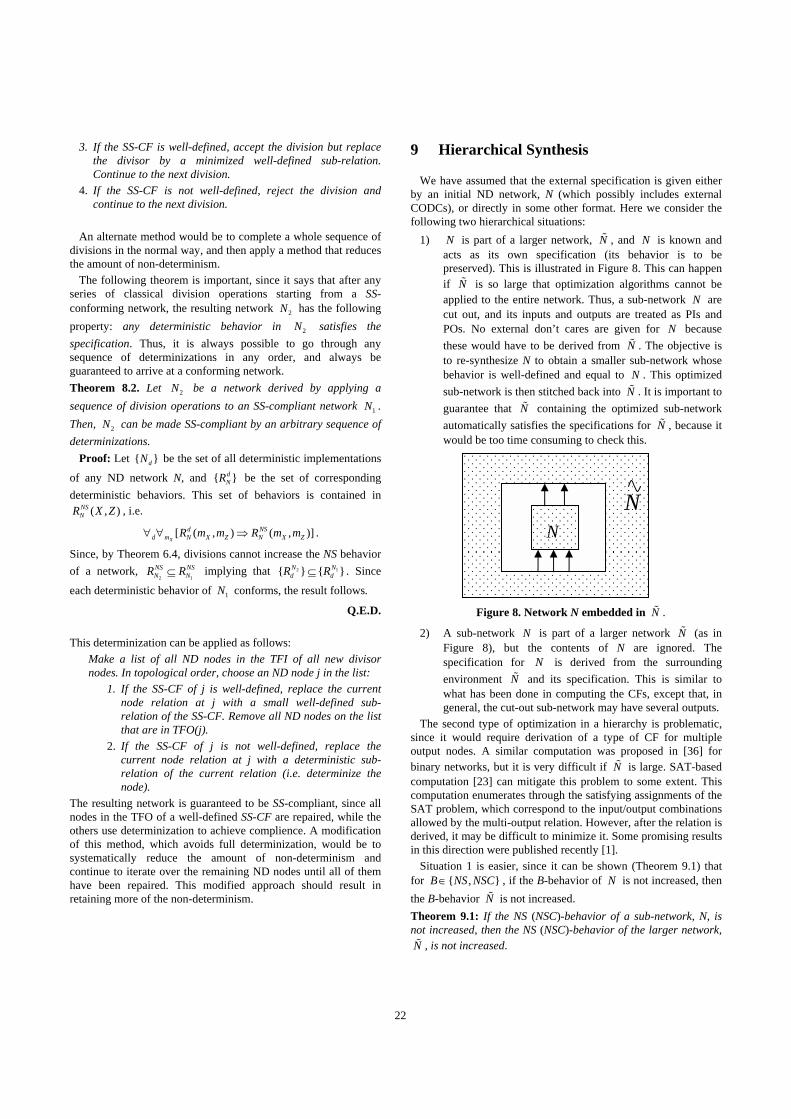
22

3. If the SS-CF is well-defined, accept the division but replace the divisor by a minimized well-defined sub-relation. Continue to the next division.

4. If the SS-CF is not well-defined, reject the division and continue to the next division.

An alternate method would be to complete a whole sequence of

divisions in the normal way, and then apply a method that reduces the amount of non-determinism.

The following theorem is important, since it says that after any series of classical division operations starting from a SS-conforming network, the resulting network 2N has the following property: any deterministic behavior in 2N satisfies the specification. Thus, it is always possible to go through any sequence of determinizations in any order, and always be guaranteed to arrive at a conforming network. Theorem 8.2. Let 2N be a network derived by applying a sequence of division operations to an SS-compliant network 1N . Then, 2N can be made SS-compliant by an arbitrary sequence of determinizations.

Proof: Let { }dN be the set of all deterministic implementations

of any ND network N, and { }dNR be the set of corresponding

deterministic behaviors. This set of behaviors is contained in ( , )NS

NR X Z , i.e.

[ ( , ) ( , )]X

d NSd m N X Z N X ZR m m R m m∀ ∀ ⇒ .

Since, by Theorem 6.4, divisions cannot increase the NS behavior of a network,

2 1

NS NSN NR R⊆ implying that 2 1{ } { }N N

d dR R⊆ . Since

each deterministic behavior of 1N conforms, the result follows.

Q.E.D. This determinization can be applied as follows:

Make a list of all ND nodes in the TFI of all new divisor nodes. In topological order, choose an ND node j in the list:

1. If the SS-CF of j is well-defined, replace the current node relation at j with a small well-defined sub-relation of the SS-CF. Remove all ND nodes on the list that are in TFO(j).

2. If the SS-CF of j is not well-defined, replace the current node relation at j with a deterministic sub-relation of the current relation (i.e. determinize the node).

The resulting network is guaranteed to be SS-compliant, since all nodes in the TFO of a well-defined SS-CF are repaired, while the others use determinization to achieve complience. A modification of this method, which avoids full determinization, would be to systematically reduce the amount of non-determinism and continue to iterate over the remaining ND nodes until all of them have been repaired. This modified approach should result in retaining more of the non-determinism.

9 Hierarchical Synthesis

We have assumed that the external specification is given either by an initial ND network, N (which possibly includes external CODCs), or directly in some other format. Here we consider the following two hierarchical situations:

1) N is part of a larger network, N" , and N is known and acts as its own specification (its behavior is to be preserved). This is illustrated in Figure 8. This can happen if N" is so large that optimization algorithms cannot be applied to the entire network. Thus, a sub-network N are cut out, and its inputs and outputs are treated as PIs and POs. No external don’t cares are given for N because these would have to be derived from N" . The objective is to re-synthesize N to obtain a smaller sub-network whose behavior is well-defined and equal to N . This optimized sub-network is then stitched back into N" . It is important to guarantee that N" containing the optimized sub-network automatically satisfies the specifications for N" , because it would be too time consuming to check this.

Figure 8. Network N embedded in N" .

2) A sub-network N is part of a larger network N" (as in Figure 8), but the contents of N are ignored. The specification for N is derived from the surrounding environment N" and its specification. This is similar to what has been done in computing the CFs, except that, in general, the cut-out sub-network may have several outputs.

The second type of optimization in a hierarchy is problematic, since it would require derivation of a type of CF for multiple output nodes. A similar computation was proposed in [36] for binary networks, but it is very difficult if N" is large. SAT-based computation [23] can mitigate this problem to some extent. This computation enumerates through the satisfying assignments of the SAT problem, which correspond to the input/output combinations allowed by the multi-output relation. However, after the relation is derived, it may be difficult to minimize it. Some promising results in this direction were published recently [1].

Situation 1 is easier, since it can be shown (Theorem 9.1) that for { , }B NS NSC∈ , if the B-behavior of N is not increased, then the B-behavior N" is not increased. Theorem 9.1: If the NS (NSC)-behavior of a sub-network, N, is not increased, then the NS (NSC)-behavior of the larger network, N" , is not increased.

N N

23

Proof: Consider the NS (NSC) simulation of N" . Assume that this is done in a particular topological order where all nodes of

\N N" in the TFI of N are evaluated before any node in N, and any node of \N N" in the TFO of N is evaluated after any node of N. When nodes in N are to be evaluated, the NS (NSC) presents a single vector to the PIs of N. After evaluation of N, a vector of outputs is presented at the POs of N. Since each of such PI/PO vector pairs is in the behavior of the sub-network and its NS (NSC)-behavior is not increased, then the set of possible PO vectors of the sub-network during its NS (NSC) simulation of N" is not increased when N is replaced by a modified network. Continuing the simulation, we conclude that the vector of possible outputs at the POs of the modified N" is not increased and hence the modified N" has a conforming NS (NSC)-behavior.

Q.E.D. To use SS-behavior in hierarchical synthesis, we must allow for

set inputs instead of scalar inputs at the PIs of the sub-network, similarly to how it was done in Section 4.1.2. Referring to Figure 8, the inputs to N would appear as sets during a set simulation of N" . Recall that this requires introducing binary PIs to simulate

arbitrary set inputs. To prevent misunderstanding, we refer to the resulting behavior as bSS simulation.

Given this modification, we can also conclude that SS is also suitable for hierarchical synthesis methods. Theorem 9.2: If the bSS -behavior of a sub-network, N, is not increased, then SS-behavior of the larger network, N" , is not increased.

Proof: The bSS -behavior of N serves as the specification for re-synthesizing N. This is conservative since the exact subsets that can be produced during SS-simulation of N" are not known. Denote the re-synthesized N by N̂ . Hence, N̂ must produce at its POs, only subsets that can be produced by bSS -simulation of N. This simulates all possible subset inputs. For subset inputs that do occur, the output subsets produced by N̂ will be a subset of the correct ones, i.e. those produced by N. For other subset inputs, it is immaterial what is produced by N̂ . In particular, the subsets produced by N are valid. Since for subsets at the PIs of N that are produced by SS-simulating N" modified with N̂ are the same as before modification and the corresponding subsets produced at the POs of N̂ are subsets produced of those produced by N, the SS-behavior of the modified N" is contained in the original.

Q.E.D. Theorems 9.1 and 9.2 imply that all the B-behaviors are suitable

for sub-network optimization in a hierarchical design.

10 Conclusions

In this paper, a theory of non-deterministic networks was developed and the effects of various classical network operations were analyzed under the following three definitions of behavior: normal simulation (NS), normal simulation made compatible (NSC), and set simulation (SS). NS is similar to a random simulation of a network where there is some randomness of the

node functionalities. The other two can be viewed as upper bound behaviors which are easier to compute. The theory generalizes the classical theory of binary deterministic logic networks and clarifies how the different types of behaviors are altered by the classical logic synthesis operations. The theory applies to binary designs that are specified with internal nodes represented with incompletely specified functions. Like all consistent theories, it works for a composition of ND networks in the hierarchical synthesis setting.

The theory allows for leaving a ND relation temporarily at a node during logic synthesis, even though finally a deterministic network may be the objective. This approach can be used to reserve some local flexibility for later use, instead of forcing a choice early. In this way, flexibility can be “borrowed” from non-critical regions and reserved for re-synthesizing a critical path.

We discussed how to compute a smallest ND representation for a node’s functionality. Replacing a node with its smallest ND relation is a useful heuristic for guiding the synthesis to a smaller solution just as node minimization is also a heuristic. In general, postponing the choice of deterministic behavior can lead to better solutions because more freedom is given for optimization. In addition, although the theory applies to functional randomness, it might be useful for and give insight into timing randomness, which is one of the directions of future work.

So far, experimentation has been done exclusively using SS-behavior, since it seems to be the easiest to compute with in practice. In our implementation in the prototype system MVSIS [25], we observed the runtimes on binary MCNC benchmarks where merging of binary nodes was done to produce MV nodes. Other examples were taken from an MV benchmark suite [26]. Non-deterministic nodes were produced naturally during the normal node simplification process as discussed in Section 4. Using binary encoding, we were able to compare runtimes on binary example that were equivalent to the MV examples. Our observations were that the computations required for dealing with networks with multi-valued and non-deterministic nodes was only marginally slower, compared to the computation for binary deterministic networks. Generally the differences seemed to be within 10-20%. Thus, the impact of using ND networks is not a practical factor for efficiency.

Future work on MVSIS is aimed at developing a number of semi-algebraic and Boolean operations in ND networks, taking advantage of new methods (e.g. SAT-based methods and use of AND-INV graphs [19]) for computing complete flexibilities as well as performing other logic operations. One goal is to enhance binary optimizations by allowing various optimization algorithms to work in a larger space. In a related work, [24], the ND network manipulations were used to operate on ND regular automata to derive sequential flexibility with the goal of improving sequential synthesis operations.

Acknowledgements The first author was supported partially by a research grant from

Intel and began this work while affiliated with Portland State University. The second author acknowledges the generous long-term support of the SRC under contract 683.004, as well as the GSRC. We gratefully acknowledge the support of the California Micro program and our associated industrial sponsors, Cadence,

24

Synplicity, Fujitsu, Intel, and Magma. Finally, we would like to thank the anonymous reviewers whose suggestions helped us improve the paper.

References

[1] D. Bañeres and J. Cortadella, “A recursive paradigm to solve Boolean relations”, Proc. DAC ’04, pp. 416-421.

[2] G. Berry, A. Bouali, X. Fornari, E. Ledinot, E. Nassor, R. DeSimone. “Esterel: A formal method applied to avionic software development”. Science of Computer Programming, 36(1), Jan. 2000, pp. 5-25.

[3] D. Brand, “Verification of large synthesized designs”, Proc. ICCAD ’93, pp. 456-459.

[4] R. K. Brayton, G. D. Hachtel, C. T. McMullen, A. L. Sangiovanni-Vincentelli, Logic Minimization Algorithms for VLSI Synthesis. Kluwer Academic Publishers, Dordrecht, 1984.

[5] R. K. Brayton, “Compatible observability don’t-cares revisited”, Proc. IWLS ’01. pp. 121-126.

[6] R. E. Bryant, “Boolean analysis of MOS circuits”, IEEE Trans. CAD, vol. 6(4), July 1987, pp. 634-649.

[7] R. E. Bryant , S. German , M. N. Velev, “Processor verification using efficient reductions of the logic of uninterpreted functions to propositional logic”, ACM Transactions on Computational Logic (TOCL), vol.2(1), Jan. 2001, pp. 93-134.

[8] E. Dubrova, Y. Jiang, R. Brayton, “Minimization of multi-valued functions in Post algebra”, Proc. IWLS ’01, pp. 132-137.

[9] C. M. Files and M. A Perkowski, “Multi-valued functional decomposition as a machine learning method”, Proc. ISMVL '98, pp. 173 -178.

[10] C. M. Files and M.A Perkowski, “New multi-valued functional decomposition algorithms based on MDDs”. IEEE Trans. CAD. Vol. 19(9), Sept. 2000, pp. 1081-1086.

[11] J.-H. Jiang, Y. Jiang, R. Brayton, “An implicit method for multi-valued network encoding”, Proc. IWLS ’01, pp. 127-131.

[12] Y. Jiang and R. Brayton, “Don’t-cares and multi-valued logic network optimization”, Proc. ICCAD ’00, pp. 520-525.

[13] Y. Jiang and R. Brayton, “Software synthesis from synchronous specifications using logic simulation techniques”. Proc. DAC ’02, pp. 319-124.

[14] Y. Jiang and R. K. Brayton, “Don't-care computation in minimizing extended finite-state machines with Presburger arithmetic”, Proc. IWLS ’02, pp. 327-332.

[15] Y. Li and R. Brayton, “Multi-valued logic optimization of Post networks”, UC Berkeley internal report, June 2002.

[16] B. Lin and A. R. Newton, “Efficient symbolic manipulation of equivalence relations and classes”, Proc. Int. Workshop on Formal Methods in VLSI Design, Jan. 1991.

[17] T. Liu, A. Aziz, V. Singhal, “Optimising designs containing black boxes”, ACM Transactions on Design Automation of Electronic Systems, 6(4), 2001.

[18] T. Kam, T. Villa, R. Brayton, A. Sangiovanni-Vincentelli. Synthesis of Finite State Machines: Functional optimization. Kluwer 1997 (See discussion on pp. 69-71.)

[19] A. Kuehlmann, V. Paruthi, F. Krohm, M. K. Ganai, “Robust boolean reasoning for equivalence checking and functional property verification”, IEEE Trans. CAD, vol. 21(12), Dec 2002, pp. 1377-1394.

[20] A. Mishchenko, B. Steinbach, M. Perkowski, ”Bi-decomposition of multi-valued relations”. Proc. IWLS’01, pp. 35-40.

[21] A. Mishchenko and R. Brayton, “A Boolean paradigm for multi-valued logic synthesis”, Proc. IWLS’02, pp. 173-177.

[22] A. Mishchenko and R. Brayton, ”Simplification of non-deterministic multi-valued networks”, Proc. ICCAD ‘02, pp.557-562.

[23] A. Mishchenko and R. Brayton, ”SAT-based complete don’t-care computation for network optimization”, Proc. DATE ‘05.

[24] A. Mishchenko, R. Brayton, J-H Jiang, T. Villa, N. Yevtushenko, “Efficient solution of language equations using partitioned representations”, Proc. IWLS ’04, pp. 401-408

[25] MVSIS Group. MVSIS. UC Berkeley. http://www-cad.eecs.berkeley.edu/mvsis/

[26] MVSIS Group. Multi-Valued Benchmarks. http://www-cad.eecs.berkeley.edu/~alanmi/research/bench/mv_benchmarks.zip

[27] T. Nopper and C. Scholl, “Symbolic model checking for incomplete designs”, Proc. IWLS ‘04, pp. 377-384.

[28] T. Nopper and Ch. Scholl, “Symbolic model checking for incomplete designs”. Report N201, Albert-Ludwigs-University, May 2004.

[29] M. Perkowski, M. Marek-Sadowska, L. Jozwiak, T. Luba, S. Grygiel, M. Nowicka, R. Malvi, Z. Wang, J. S. Zhang, “Decomposition of multiple-valued relations”. Proc. ISMVL ’97, pp. 13-18.

[30] R. L. Rudell and A. Sangiovanni-Vincentelli, “Multiple-valued minimization for PLA optimization”. IEEE Trans. CAD, vol. 6(5), Sep. 1987, pp. 727-750.

[31] K. Sakallah, “Functional abstraction and partial specification of Boolean functions”, University of Michigan Technical Report, CSE-TR-255-95, Aug. 9, 1995.

[32] H. Savoj and R. K. Brayton, “The use of observability and external don’t-cares for the simplification of multi-level networks”, Proc. DAC’ 90, pp. 297-301.

[33] H. Savoj Don't Cares in Multi-Level Network Optimization. Ph.D. dissertation, UC Berkeley, May 1992.

[34] C. Scholl and B. Becker, “Checking equivalence for partial implementations”. Proc. DAC ‘01, pp. 238-243.

[35] E. Sentovich et al, “SIS: A system for sequential circuit synthesis”, Tech. Rep. UCB/ERI, M92/41, ERL, Dept. of EECS, Univ. of California, Berkeley, 1992.

[36] E. Sentovich, V. Singhal, R. K. Brayton, “Multiple Boolean relations”, Proc. IWLS ’93.

[37] Y. Watanabe, L. Guerra, R. K. Brayton, “Logic optimization with multi-output gates”, Proc. ICCD ‘93, pp. 416-420.

[38] N. Yevtushenko, T. Villa, R. K. Brayton, A. Petrenko, A. L. Sangiovanni-Vincentelli, “Solution of parallel language equations for logic synthesis”, Proc. ICCAD ’01, pp. 103-111.