a theoretical study on a two-dimensional flap-type wavemaker
TRANSCRIPT
A THEORETICAL STUDY ON ATWO-DIMENSIONAL FLAP-TYPE WAVEMAKER
Final ProjectProposed as a requirement for an undergraduate degree
by
Natanael Karjanto10197045
DEPARTMENT OF MATHEMATICSFACULTY OF MATHEMATICS AND NATURAL SCIENCES
BANDUNG INSTITUTE OF TECHNOLOGY2001
arX
iv:2
001.
0585
4v1
[ph
ysic
s.fl
u-dy
n] 1
1 Ja
n 20
20

A THEORETICAL STUDY ON ATWO-DIMENSIONAL FLAP-TYPE WAVEMAKER
Approval Page
It has been examined and approved by the Supervisor:
Dr. AndonowatiNIP. 131803263
and Examiners:
Prof. Dr. M. Ansjar Dr. Wono Setya BudhiNIP. 130143972 NIP. 131284801

For my beloved father, mother, and sister.

AbstractA mathematical model for unidirectional wave generation explained in this study.
The model consists of Laplace’s equation in the semi-infinite two-dimensional water in-terior, dynamic and kinematic boundary conditions at the free surface, lateral boundarycondition on the wavemaker, and fixed wall at the bottom. The model is for a flap-type wavemaker that is commonly used in a towing tank of a hydrodynamic laboratory.To simplify the problem, some assumptions are made, namely that water is an idealfluid. Linear wavemaker theory is used and a generation of monochromatic wave (sin-gle frequency) is considered. The relation between the wavenumber, wave height, andwavemaker stroke is further derived.
Keywords: ideal fluid, wavemaker, Laplace equation, kinematic free surface, dynamicfree surface, linear wavemaker theory, monochromatic wave, wavenumber, wave height,and wavemaker stroke.
ForewordThank you to the readers who take the time to open this final project report. First
of all, allow me to thank God Almighty for blessing me to complete this project and tofinish my undergraduate degree. I am also grateful to the following individuals whohave supported me during my study.
1. Dr. Andonowati who was willing and patiently supervised this project.
2. Professor Dr. M. Ansjar and Dr. Wono Setya Budhi who have become the examin-ers for the project presentation on 15 December 2000. I thank Professor Ansjar fortrusting me as his teaching assistant in Mathematical Methods during Fall/Autumn2000. I am grateful to Dr. Wono for patiently teaching me Maple and LATEX so thatthis report can be completed nicely.
3. Dr. Nana Nawawi Gaos for being my academic adviser during Common First Year1997/1998 and Intensive Semester of 1998.
4. Dr. Ahmad Muchlis for being my academic advisor during my sophomore until senioryears. Thank you for motivating me to complete my undergraduate study in threeand half a year.
5. Warsoma Djohan M.Si. for delegating me as his teaching assistant for Calculus 1 dur-ing Fall 1999 and Fall 2000. I thank Dr. Jalina Widjaja for having me as her teachingassistant in Engineering Mathematics, Matrix and Vector Spaces and Calculus 1 aswell as Dr. Nuning Nuraini whom I assist in her Calculus 2 course. I would not for-get Koko Martono M.Si. for delegating me as his teaching assistant in MultivariableCalculus and Complex Function as well as training me to write scientific articles. I ac-knowledge other instructors and professors who have contributed me in developingmy mathematical maturity.
6. My parents who have supported me financially and their incessant prayer during mystudy. My beloved sister who has supported and motivated me to study diligently.
7. Hadi Susanto for being my friend, both in good and bad times, particularly beforehe departed to the Netherlands. Ik wil U bedanken omdat U mij heel goed heeftgemotiveend om extra hard te studeren. Bedankt, Hadi!
8. Maykel, Luis, Dina, Ety, Sica, Anna, Sondang, Rilyovira and other friends from theClass of 1997 whom I could not mention individually. Thanks for our friendship. Ialso thank both my seniors and juniors who have assisted me during my study.
9. Toto Nusantara (MA-S3), Lylye Sulaeman (P4M) and Surya (MA96) who have helpedme in TEX, LATEX, and Scientific Work Place to type this report.
10. Wili (MA97), Henry (FI97), Albert(TF97), Wila (TI97), Aan (TK97), Faiq (TG97),Krshna (EL97), Fitra (TA98), Dindin (TL98), Hidayat (FA98), Dwi Susanti (FA98),Mia (KI99), Erika (FA99), Dwi Hesti (TG2000) and other friends as well as juniorsfrom SMA Negeri 4 Bandung who have motivated and supported me to complete mystudy in less than eight semesters. I am grateful to you all!
vi

Experientia est optima rerum magistra is a well-known Latin expression for “Experi-ence is the best teacher”. Like other events in life, completing the undergraduate studyas well as finishing this report is a unique and interesting experience for me, become a‘teacher’ in happiness and sorrow. I have learned many things when writing this report,not only academically but also growing mature thinking.
With a humble heart, I am fully aware that as a person, I am merely an individualfrom a crowd who comes and goes and attempts to imprint an academic achievementat this department and university. Although I might not be able to present my best forthe progress of the department, I have striven to do my best in completing this project.I also hope that this ‘tiny’ writing could become creme de la creme from all the work thatI have made albeit there are many limitations in various aspects.
Therefore, I would like to take this opportunity to apologize to the readers of thisfinal project report. I hope this piece of work could be beneficial not only for interestedreaders but also for the progress of Mathematics.
Bandung, mid-January 2001
Natanael Karjanto
vii

Table of Contents
Abstract iv
Foreword vi
Table of Contents ix
List of Figures xi
1 Introduction 11.1 Background and Problem Formulation . . . . . . . . . . . . . . . . . . . 1
1.1.1 Background . . . . . . . . . . . . . . . . . . . . . . . . . . . . . . 11.1.2 Problem Formulation . . . . . . . . . . . . . . . . . . . . . . . . . 1
1.2 Study Coverage . . . . . . . . . . . . . . . . . . . . . . . . . . . . . . . . 21.3 Purpose . . . . . . . . . . . . . . . . . . . . . . . . . . . . . . . . . . . . 21.4 Basic Assumptions . . . . . . . . . . . . . . . . . . . . . . . . . . . . . . 21.5 Hypothesis . . . . . . . . . . . . . . . . . . . . . . . . . . . . . . . . . . 21.6 Research Methodology . . . . . . . . . . . . . . . . . . . . . . . . . . . . 2
1.6.1 Methodology . . . . . . . . . . . . . . . . . . . . . . . . . . . . . 21.6.2 Data Collection . . . . . . . . . . . . . . . . . . . . . . . . . . . . 3
1.7 Discussion Flow . . . . . . . . . . . . . . . . . . . . . . . . . . . . . . . . 3
2 Ideal Fluid Flow 42.1 Fluid Physical Characteristics . . . . . . . . . . . . . . . . . . . . . . . . 42.2 The Laws of Mass and Momentum Conversation . . . . . . . . . . . . . . 4
2.2.1 The Law of Conservation of Mass . . . . . . . . . . . . . . . . . . 42.2.2 The Law of Conservation of Momentum . . . . . . . . . . . . . . 5
2.3 Transport Theorem . . . . . . . . . . . . . . . . . . . . . . . . . . . . . . 62.4 Continuity Equation . . . . . . . . . . . . . . . . . . . . . . . . . . . . . 72.5 Euler’s Equation . . . . . . . . . . . . . . . . . . . . . . . . . . . . . . . . 92.6 Bernoulli’s Equation . . . . . . . . . . . . . . . . . . . . . . . . . . . . . 9
3 Two-Dimensional Wavemaker Theory 123.1 Simplified Wavemaker Theory . . . . . . . . . . . . . . . . . . . . . . . . 123.2 Linear Wavemaker Theory . . . . . . . . . . . . . . . . . . . . . . . . . . 13
3.2.1 Lateral boundary condition at the wavemaker(pseudo-boundary) . . . . . . . . . . . . . . . . . . . . . . . . . . 14
ix

TABLE OF CONTENTS x
3.2.2 Boundary condition at the bottom of the towing tank (kinematiccondition) . . . . . . . . . . . . . . . . . . . . . . . . . . . . . . . 15
3.2.3 Boundary conditions at the water surface . . . . . . . . . . . . . 153.3 Solutions for the Governing Differential Equation . . . . . . . . . . . . . 18
4 Numerical Simulation 224.1 Calculating the Progressive Wavenumber . . . . . . . . . . . . . . . . . . 224.2 Calculating Standing Wave Wavenumbers . . . . . . . . . . . . . . . . . 224.3 Monochromatic Wave Profiles . . . . . . . . . . . . . . . . . . . . . . . . 23
4.3.1 Two Wave Profiles with Distinct Wave Height H . . . . . . . . . . 234.3.2 Two Wave Profiles with Distinct Angular Frequency ω . . . . . . . 25
5 Conclusion and Suggestion 295.1 Conclusion . . . . . . . . . . . . . . . . . . . . . . . . . . . . . . . . . . 295.2 Suggestion . . . . . . . . . . . . . . . . . . . . . . . . . . . . . . . . . . 29
A Material Derivative 30
B Newton-Raphson Iteration 32
C Hydrodynamics Laboratories 34
References 37
List of Figures
3.1 A schematic diagram for a flap-type wavemaker. . . . . . . . . . . . . . . 133.2 A schematic diagram for a wavemaker with a governing equation and its
boundary conditions. . . . . . . . . . . . . . . . . . . . . . . . . . . . . . 173.3 A graph for the progressive wave dispersion relationship. . . . . . . . . . 183.4 A graph for the standing wave dispersion relationship. . . . . . . . . . . 193.5 A graph for the ratios between the wave height H and the stroke S with
respect to the relative depth kp h. . . . . . . . . . . . . . . . . . . . . . . 21
4.1 Maximum strokes from the wavemaker flap which produce two wave-profiles with different wave height. . . . . . . . . . . . . . . . . . . . . . 24
4.2 Shapes of surface water wave elevation for two distinct wave heights. . . 254.3 The maximum strokes from the flap which produce two wave-profiles
with distinct frequency. . . . . . . . . . . . . . . . . . . . . . . . . . . . . 264.4 Water wave surface graphs at t = 3. . . . . . . . . . . . . . . . . . . . . . 274.5 Water wave surface graphs at t = 5. . . . . . . . . . . . . . . . . . . . . . 274.6 Water wave surface graphs at t = 10. . . . . . . . . . . . . . . . . . . . . 274.7 Water wave surface graphs at t = 15. . . . . . . . . . . . . . . . . . . . . 274.8 Water wave surface graphs at t = 17. . . . . . . . . . . . . . . . . . . . . 284.9 Water wave surface graphs at t = 25. . . . . . . . . . . . . . . . . . . . . 284.10 Water wave surface graphs at t = 30. . . . . . . . . . . . . . . . . . . . . 284.11 Water wave surface graphs at t = 34. . . . . . . . . . . . . . . . . . . . . 28
xi

Chapter 1
Introduction
1.1 Background and Problem Formulation
1.1.1 Background
As a nation progresses, the need for research in science and technology is increasing aswell. More than two-thirds of the Indonesian territory consists of seas with abundantnatural resources. Indonesia has been known as a maritime nation since ancient times.As science and technology progress, there is a need for research in the maritime area.
In Ocean Engineering, the need to model phenomena in the open ocean mathemat-ically motivates the research in this area. This leads to interdisciplinary collaborationamong various fields of science and engineering. Mathematics as the queen and servantof science has the powerful ability to model many natural phenomena. In this finalproject report, we will discuss a theoretical study for a wave generation in a towingtank.∗
Modeling the wave generation process in a hydrodynamic laboratory is useful forship testing as if the ship is sailing in the open ocean. For example, a ship that plans tosail in the Javanese Sea should be tested with the ocean waves characterizing the onesin the Javanese Sea. Keeping this in mind, we could obtain information on how strongthe ocean waves are and this translates to building a strong ship that could handle thepressure from those ocean waves.
1.1.2 Problem Formulation
Based on the above background, we propose a mathematical model for ocean wavesusing the wavemaker theory utilized in a laboratory. We would like to investigate howlarge we should deviate the wavemaker if we wish a wave profile with particular waveheight. Additionally, we would like to examine the resulting wave profile if we movethe wavemaker with a particular frequency. Hence, we could formulate a mathematicalmodel for water wave evolution in a towing tank.
∗A towing tank is a facility in a hydrodynamic laboratory, the long pond contains water with a wave-maker on one side and a wave absorber on the other side. Some examples are listed in Appendix C.
1
CHAPTER 1. INTRODUCTION 2
1.2 Study Coverage
Based on the above problem formulation, the study coverage of this report is proposinga simple mathematical model of a two-dimensional flap-type wavemaker in a towingtank. We will adopt relevant assumptions to simplify the problems. We only considerthe output of monochromatic waves. Using computer software, a simple simulationdescribing the wave evolution will be presented.
1.3 Purpose
A subjective purpose of writing this final project report is fulfilling the requirementfor completing an undergraduate degree at the Department of Mathematics, Faculty ofMathematics and Natural Sciences, Bandung Institute of Technology. The meeting forthe degree conferring was held on 24 January 2001.
An objective purpose of this writing is to deepen the study of Mathematics, partic-ularly its applications in physical problems. Additionally, by modeling problem fromoutside Mathematics, the insight regarding the interconnection of science and technol-ogy will also be expanded.
1.4 Basic Assumptions
The proposed model depends on the following factors:
• The assumption of fluid characteristics leads to mathematical formulation.
• There exists a governing differential equation with several boundary conditions.
• An assumption regarding the type and the characteristics of the output waves.
1.5 Hypothesis
If we adopt an assumption that water is an ideal fluid, then we could obtain a partialdifferential equation with several boundary conditions as a governing differential equa-tion. If we also adopt another assumption that the output wave is monochromatic andperiodic, then we could propose a linear, two-dimensional wave generation theory.
1.6 Research Methodology
1.6.1 Methodology
We implement the theoretical and analytical methodology. This means analyzing theo-retically a model related to the wave generation and deriving equations related to thismodel. We also implement computational analysis methodology to analyze and solveproblems using a computer.
CHAPTER 1. INTRODUCTION 3
1.6.2 Data Collection
Data collection includes literature study and regular meetings with the supervisor. Aliterature study covers independent learning references related to Fluid Mechanics andMathematical Modeling, particularly related to wave generation theory. The list of ref-erences can be found in the References for this report. The supervising activity in-cludes reading assignments, discussion and problem-solving. Presentations were alsoconducted regularly.
1.7 Discussion Flow
After this introduction, we will discuss the characteristics of ideal fluid flow. Chapter 2also explains the physical characteristics of the fluid, the derivation of the continuityequation, Euler’s equation, and Bernoulli’s equation using the Laws of Mass and Mo-mentum Conservation, as well as using the Transport Theorem. Several assumptionsand equations covered in this chapter will be utilized in the subsequent chapters.
Chapter 3, the main part of this report, covers the problem formulation and the studycoverage. We will not only discuss the simplified wave generation theory but also morerealistic linear theory by solving the Laplace equation as the governing equation with alateral boundary condition at the wavemaker, a boundary condition at the bottom of thetowing tank, and boundary conditions at the surface of the water. The latter includeskinematics and dynamic boundary conditions.
While the theoretical approach and derivation dominate the preceding chapters,Chapter 4 explains computer simulation using Maple V Release 5. We calculate thevalues of progressive and traveling wavenumbers. We will display some figures relatedto the movement of the wavemaker and the produced monochromatic wave profiles.
The final chapter concludes this final project report. We also provide practical sug-gestions for friends and anyone interested to continue research in this area.

Chapter 2
Ideal Fluid Flow
2.1 Fluid Physical Characteristics
Due to its ability to move, it is interesting to observe fluids. A fluid is a substance thatdoes not experience resistance when it experiences deformation and will continue tochange when it is given pressures or forces. It does not have a regular shape and alwaysfollows the space it places. Under the influence of a force, a fluid will deform continuallyto form a flow.
Fluids can be categorized as liquid and gas. A liquid has a characteristic of rela-tively incompressible and possesses a free surface. A gas has a characteristic of readilycompressible and does not possess a free surface. In this chapter, we will discuss liq-uid fluid, particularly water. The property of water in our context belongs to the idealfluid, i.e., incompressible and inviscid fluid. This choice of assumptions will be used asa fundamental flow problem that we will discuss later [14, 17].
2.2 The Laws of Mass and Momentum Conversation
The laws of conservation for a system of particles in Physics can also be applied to fluidssince fluids are a collection of particles. Based on this, we focus on a collection of fluidparticles or a fluid material volume so that we always examine an identical particlegroup.
For easier symbolic writing, we express the Cartesian coordinates as the index (1, 2, 3)with a convention that x = x1, y = x2, and z = x3. The same convention also appliesfor the velocity components, i.e. u = u1, v = u2, and w = u3.
2.2.1 The Law of Conservation of Mass
The law of conservation of mass states that the total mass of a system composed of acollection of particles is always constant, it neither increases nor decreases.
In other words, there exists no fluid mass that can be created not annihilated. Thechange of mass within a domain is due to the mass flow passing through a boundary.Based on this restriction, we define fluid volume V (t) bounded by a surface S. If thefluid has a density ρ, then the total fluid mass in that volume is given by the triple
4

CHAPTER 2. IDEAL FLUID FLOW 5
integral∫∫∫
ρ dV . In our formulation, the law of mass conservation states that the totalfluid mass with density ρ and volume V is constant. Stated differently, this law gives arequirement that the triple integral is constant:
∫∫∫
V
ρ dV = constant (2.1)
ord
dt
∫∫∫
V
ρ dV
= 0. (2.2)
2.2.2 The Law of Conservation of Momentum
The law of conservation of momentum states that the total momentum of a systemcomposed by a collection of interacting particles is constant, as long as there is noexternal force acting to the system.
Similarly, the density of fluid-particle momentum is ρu with components ρ ui. Inour context, the law of conservation of momentum requires that the total forces actingon a fluid volume equals the rate of change of the fluid momentum. According to theNewtonian frame of reference, we can express the law of conservation of momentum asfollows:
d
dt
∫∫∫
V
ρ ui dV
=
∫∫
S
τij nj dS +
∫∫∫
V
Fi dV, (2.3)
where ρ ui denotes the component of fluid particles momentum density, τij denotes thepressure tensor acting on the fluid volume, nj denotes the unit normal vector componenton the fluid surface, and Fi denotes an external force working on the fluid particles. Thesurface integral is the i-th component from the surface forces acting on the surface S andthe final triple integral is the sum from external body force, including the gravitationalforce.
Using the Divergence Theorem,∗ the first term on the right-hand side of (2.3) can beexpressed as a triple integral of a divergence of a vector field covering the correspondingsurface ∫∫
S
Q · n dS =
∫∫∫
V
∇ ·Q dV. (2.4)
Written in component form, this equation can be expressed as∫∫
S
Qi ni dS =
∫∫∫
V
∂Qi
∂xidV. (2.5)
Here, Q denotes an arbitrary continuous and differentiable vector field in the volumeV and the unit normal vector n denotes the normal vector going in the outer directionfrom V on the surface S.
∗In Western countries, this theorem is known as Gauss Theorem, while in the Eastern Block territory,the theorem is known as Ostrogradsky Theorem, based on the name of one Russian mathematician [16].

CHAPTER 2. IDEAL FLUID FLOW 6
Using (2.5) to transform the surface integral to (2.3), we obtain
d
dt
∫∫∫
V
ρ ui dV
=
∫∫∫
V
(∂τij∂xj
+ Fi
)dV. (2.6)
Equations (2.2) and (2.6) express the Laws of Conservation of Mass and Momentum forthe fluid integrated over the arbitrary material volume V (t), respectively.
2.3 Transport Theorem
Let a general form of the volume integral be expressed as follows:
I(t) =
∫∫∫
V (t)
f(x, t) dV. (2.7)
Here, f denotes an arbitrary differentiable scalar function that depends on the positionx and time t integrated over the volume V (t), for which the latter can also change intime. Hence, the surface S of the volume boundary will change in time as well and itsnormal velocity is denoted by Un.
Using a common techniques employed in basic Calculus, consider the following dif-ference:
∆I = I(t+ ∆t)− I(t) =
∫∫∫
V (t+∆t)
f(x, t+ ∆t) dV −∫∫∫
V (t)
f(x, t) dV. (2.8)
From the Taylor series of f(x, t+ ∆t), we have
f(x, t+ ∆t) = f(x, t) + ∆t∂f(x, t)
∂t+
1
2!(∆t)2 ∂
2f(x, t)
∂t2+ · · · . (2.9)
Neglecting the terms proportional to the order of (∆t)2 and higher, we attain
f(x, t+ ∆t) = f(x, t) + ∆t∂f(x, t)
∂t. (2.10)
We can apply a similar analysis to the material volume V (t)
V (t+ ∆t) = V (t) + ∆tdV
dt+
1
2!(∆t)2 d
2V
dt2+ · · · . (2.11)
Neglecting the higher-order terms, we obtain
∆V = V (t+ ∆t)− V (t). (2.12)
Thus, V (t + ∆t) differs from V (t) a thin volume ∆V included insides the boundarysurfaces S(t+ ∆t) and S(t) and is proportional with ∆t. From (2.8), we obtain
∆I =
∫∫∫
V+∆V
(f + ∆t
∂f
∂t
)dV −
∫∫∫
V
f dV (2.13)
= ∆t
∫∫∫
V
∂f
∂tdV +
∫∫∫
∆V
f dV +O[(∆t)2
], (2.14)

CHAPTER 2. IDEAL FLUID FLOW 7
where the final term denotes the second order error proportional to (∆t)2.To evaluate the integral over the tiny volume ∆V , we notice that this thin solid has
the same thickness as the distance between S(t) and S(t + ∆t). This thickness equalsto the normal component from the distance covered by S(t) in time ∆t, which is theproduct Un ∆t. Thus, the integral of the second term only contributes to the first order,which is proportional to ∆t. The degree of accuracy of the integrand function f can beassumed to be constant throughout the thin solid in the direction of the normal fromthe surface S. Integrating only in this direction, we have the following:
∆I = 4t∫∫∫
V
∂f
∂tdV +
∫∫
S
(Un4t) f dS +O[(4t)2
]. (2.15)
Finally, we obtain the desired result by dividing both sides of the equation by ∆t andtake the limit by allowing ∆t approaching zero
dI
dt= lim
∆t→0
4I4t =
∫∫∫
V
∂f
∂tdV +
∫∫
S
f Un dS. (2.16)
Equation (2.16) is known as the Transport Theorem or the Transport Equation. Thesurface integral in this equation states the transport quantity f moving out from thevolume V as a result of the moving boundary. In the special case when S is fixed andUn = 0, equation (2.16) reduces to a simple form where the differential operator can bepulled out from the integral sign. For a complete explanation, please consult [13].
We have another interesting case. Since the material volume V is always composedby identical fluid particles, then the surface S moves with the same normal velocity withthe one of the fluid itself and Un = u · n = ui ni. In this case, applying the DivergenceTheorem to equation (2.4), then we can express equation (2.16) in the following form:
dI
dt=
d
dt
∫∫∫
V (t)
f dV
=
∫∫∫
V (t)
∂f
∂tdV +
∫∫
S
f ui ni dS (2.17)
=
∫∫∫
V (t)
∂f
∂tdV +
∫∫∫
V (t)
∂
∂xi(f ui) dV (2.18)
=
∫∫∫
V (t)
[∂f
∂t+
∂
∂xi(f ui)
]dV. (2.19)
2.4 Continuity Equation
This equation is closely related to the Law of Conservation of Mass and the TransportTheorem since it can be derived from these two equations. Look again equation (2.2)
CHAPTER 2. IDEAL FLUID FLOW 8
for the Law of Conservation of Mass. Using the result of the Transport Theorem (2.19),we obtain
d
dt
∫∫∫
V
ρ dV
=
∫∫∫
V
[∂ρ
∂t+
∂
∂xi(ρ ui)
]dV = 0. (2.20)
Since the last integral is evaluated at a fixed instantaneous time, the difference that Vis material volume is not necessary at this stage. Furthermore, that particular volumecan be composed of a group of arbitrary fluid particles. Hence, the integrand above isidentically zero throughout the whole fluid. Therefore, the volume integral in (2.20)can be replaced by a partial differential equation expressing the Law of Conservation ofMass in the following form:
∂ρ
∂t+
∂
∂xi(ρ ui) = 0. (2.21)
Written in a three-dimensional component form, this equation reads
∂ρ
∂t+∂ρu
∂x+∂ρv
∂y+∂ρw
∂z= 0, (2.22)
or written in a differential form∂ρ
∂t+∇ · (ρu) = 0. (2.23)
This important equation is known as the condition for the Law of Conservation ofMass or the continuity equation for incompressible fluid flow. Equation (2.22) describesthe mean rate of change of mass density at a fixed point as a result of the change in themass velocity vector ρu. By expanding the terms containing the product of density andthe velocity components, we can derive a different form of the continuity equation
∂ρ
∂t+ u
∂ρ
∂x+ ρ
∂u
∂x+ v
∂ρ
∂y+ ρ
∂v
∂y+ w
∂ρ
∂z+ ρ
∂w
∂z= 0 (2.24)
(∂ρ
∂t+ u
∂ρ
∂x+ v
∂ρ
∂y+ w
∂ρ
∂z
)+ ρ
(∂u
∂x+∂v
∂y+∂w
∂z
)= 0. (2.25)
Using the material or the total derivative operator (See Appendix A), equation (2.25)can be written as follows:
Dρ
Dt+ ρ (∇ · u) = 0. (2.26)
For a steady flow, i.e., a time-independent flow, it follows that ∂ρ∂t
= 0 and hence thecontinuity equation reduces to ∇ · (ρu) = 0. Using the assumption that water is incom-pressible fluid, i.e., having a constant mass rate ρ, then the continuity equation (2.25)reduces to
∂u
∂x+∂v
∂y+∂w
∂z= 0. (2.27)
We obtain the following expression in the vector form, which can also be derived directlyfrom equation (2.26):
∇ · u = 0. (2.28)
This relationship is known as the condition of incompressibility. This condition statesthe fact that the balance between outflow and inflow for a volume element or materialvolume is zero for all time.

CHAPTER 2. IDEAL FLUID FLOW 9
2.5 Euler’s Equation
While the continuity equation is related to the Law of Conservation of Mass, Euler’sequation is related to the Law of Conservation of Momentum and the Transport Theo-rem since its derivation makes use of these two equations. Look again equation (2.6)for the Law of Conservation of Momentum. Using the result from the Transport Theo-rem (2.19), we obtain
∫∫∫
V
[∂ρui∂t
+∂
∂xj(ρ ui uj)
]dV =
∫∫∫
V
(∂τij∂xj
+ Fi
)dV. (2.29)
Since these integrals are calculated over an identical volume, then the equation for theintegrand parts of (2.29) must be satisfied as well, it is given as follows:
∂
∂t(ρ ui) +
∂
∂xj(ρ ui uj) =
∂τij∂xj
+ Fi. (2.30)
Next, by expanding the derivatives of the left-hand side of (2.30) using the Chain Rule,we obtain
ui∂ρ
∂t+ ρ
∂ui∂t
+ uiuj∂ρ
∂xj+ ρuj
∂ui∂xj
+ ρui∂uj∂xj
=∂τij∂xj
+ Fi. (2.31)
Using the assumption that the observed fluid is incompressible and possesses constantmass density ρ, using the result of the continuity equation (2.28), we obtain Euler’sequation,∗ also known as the momentum equation
∂ui∂t
+ uj∂ui∂xj
=1
ρ
(∂τij∂xj
+ Fi
). (2.32)
Using the material derivative operator (see again Appendix A), Euler’s equation (2.32)can be expressed as follows:
DuiDt
=1
ρ(∇ · τi + Fi) . (2.33)
2.6 Bernoulli’s Equation
Consider again equation (2.32). In a frictionless flow, there exists neither shear stressnor normal stress for isotropic fluid flow. We adopt a convention that the normal stressesτ11, τ22, and τ33 have positive orientation if they are tensions. Since we assume thatwater is inviscid fluid, then the stress tensor τ has only the normal components fromthe pressure. For further explanation, please consult [8, 10, 13]. We set as follows
τ11 = τ22 = τ33 = − p, (2.34)∗Euler, Leonhard (1707-83). Swiss mathematician with a calm mind who fundamentally and mean-
ingfully contributed to various branches of mathematics and their applications, including but not limitedto, differential equations, infinite series, complex analysis, mechanics and hydrodynamics, as well as cal-culus of variations. He was also influential in promoting the use and the understanding of analysis. [9]

CHAPTER 2. IDEAL FLUID FLOW 10
so that the momentum equation becomes
∂ui∂t
+ uj∂ui∂xj
=1
ρ
(∂p
∂xj+ Fi
), (2.35)
or in a vector notationDu
Dt=
1
ρ(−∇p+ F) , (2.36)
where u = (u, v, w), F = (0, 0, −ρ g), and p is the pressure. Hence,
∂u
∂t+ (u · ∇)u = −∇
(p
ρ+ g z
). (2.37)
From a vector identity, we have
u× (∇× u) = (u · ∇)u−∇(
1
2|u|2). (2.38)
If we also assume that water is irrotational fluid,∗, then ∇ × u = 0, and thus (u ·∇)u = ∇
(12|u|2). Due to this assumption, the vector velocity u can be expressed as the
gradient of the scalar or velocity potential, i.e., u = ∇φ. (For a detailed explanation,please see [3] and [11].) The reason we implemented this simplification is for easieranalysis since in general, scalar quantities are less complicated to investigate than vectorquantities.
Therefore,∂∇φ∂t
+∇(
1
2|u|2)
= −∇(p
ρ+ g z
), (2.39)
or
∇(∂φ
∂t+
1
2|u|2 +
p
ρ+ g z
)= 0. (2.40)
If we integrate equation (2.40) throughout the entire space, then we will obtain Bernoulli’sequation∗∗
∂φ
∂t+
1
2|u|2 +
p
ρ+ g z = constant ≡ f(t). (2.41)
∗Irrotational fluid in this context refers to the absence of eddy or whirlpool.∗∗Bernoulli, Daniel (1700-82). This Dutch-born scientist is a member of a famous Swiss family who
consists of ten mathematicians (fathers, sons, uncles, cousins). He is well-known for his works on fluidflow and the kinetic theory of gases. His equation for fluid flow was first published in 1783. He alsopursued the study and research of astronomy and magnetism and was the first scientist who solved theRiccati equation [9].

CHAPTER 2. IDEAL FLUID FLOW 11
A schematic diagram for an ideal fluid interconnectivity.
Mass Conservation Law Momentum Conservation Law
Transport Equation
Continuity equation Euler’s equation
Bernoulli’s equation
++

Chapter 3
Two-Dimensional Wavemaker Theory
In this chapter, we are going to compare two wavemaker theories in which the corre-sponding mathematical models have been proposed and investigated. The first part is asimplified theory. A basic idea comes from a displaced volume of water by a flap-typewavemaker in a towing tank. The second part covers a more detailed theory for theflap-type wavemaker. From these two theoretical approaches, we will observe the ratiobetween the wave amplitude H with the maximum stroke of the wavemaker S.
In the context of this report, the more detailed theory is based on the linear wavetheory developed by Airy∗ around 160 years ago, when he analyzed the behavior ofocean waves [1].
3.1 Simplified Wavemaker Theory
For shallow-water waves, simple theory for the propagation of a wave profile producedby a wavemaker was first developed by Galvin in 1964. He reasoned that the displacedwater by a wavemaker equals the volume of the top part from the propagated wave.Consider a flap-type wavemaker with a fixed bottom end and possesses a maximumstroke S. The water depth in the towing tank is h. The displaced water volume bythe flap deviation is 1
2S h. See Figure 3.1. Meanwhile, the top part of water volume is∫ 1
2L
012H sin(k x) dx, where k = 2π/L is the wavenumber. Hence,
∫ 12L
0
1
2H sin(k x) dx =
∫ 12L
0
1
2H sin
(2 π
Lx
)dx (3.1)
=H L
2 π(3.2)
=H
k(3.3)
By equating the two volumes, we have
1
2S h =
H
k= H
L
2 π=H
2
(L
2
)2
π
∗Airy, Sir George Biddle (1801–1892). English mathematician and physicist, who became a RoyalAstronomer for 46 years. He contributed not only to the theory of light and astronomy but also to gravity,magnetism, sound, wave propagation, and tidal wave [9].
12

CHAPTER 3. TWO-DIMENSIONAL WAVEMAKER THEORY 13
where the factor 2/π, also known as the area factor, indicates the ratio between the areaformed by the wave profile with the rectangle circumscribed it. From the relationship12S h = H
k, we can find out the ratio between the wave height H and the stroke S,
namelyH
S=
1
2k h.
This relationship is only valid for the shallow-water waves, i.e., for k h < 110π.
Figure 3.1: A schematic diagram for a flap-type wavemaker.
3.2 Linear Wavemaker Theory
According to the assumption that water is an incompressible fluid, then from the resultof equation (2.28) in Section 2.4, we have ∇ · u = 0. Additionally, another adoptedassumption is the absence of water whirlpool, in other words, the water flow is irrota-tional. Based on this assumption, from the explanation in Section 2.6, we have obtainedu = ∇φ. Combining these two equations, we obtain ∇ · ∇φ = ∇2φ = 0. This equationis known as Laplace’s equation∗, and it plays a role as a governing differential equationfor the velocity potential φ. In the two-dimensional Cartesian coordinates–the x- andz-axes in the horizontal and vertical directions, respectively–Laplace’s equation can bewritten as follows:
∇2φ =∂2φ
∂x2+∂2φ
∂z2= 0, (3.4)
and it is valid for −h ≤ z ≤ η(x, t), and 0 ≤ x ≤ ∞.
∗Laplace, Marquis Pierre Simon de (1749-1827). French mathematical-physicist who contributed tothe study of celestial mechanics, particularly in explaining the orbit of planets Jupiter and Saturn. Healso developed an idea in using potential and orthogonal functions, as well as introduced their integraltransformations. He also played an important role in the development of probability theory.

CHAPTER 3. TWO-DIMENSIONAL WAVEMAKER THEORY 14
The boundary value problem in this context is the one for two-dimensional wavepropagation in an ideal fluid. We will solve the problem using several boundary con-ditions that are suitable for the situation in the towing tank. We have at least threeboundary conditions as auxiliary equations in solving the governing equation. Whatfollows is the boundary conditions related to the physical condition of the towing tank.
3.2.1 Lateral boundary condition at the wavemaker(pseudo-boundary)
Let the function describing a horizontal movement at the wavemaker surface be givenas follows:
F (x, z, t) = x− 1
2S(z) sin(ω t) = 0, (3.5)
then by applying a total differential to F (x, z, t), we obtain
DF
Dt=∂F
∂t+∂F
∂x
dx
dt+∂F
∂z
dz
dt(3.6)
0 = −1
2ω S(z) cos(ω t) + v − 1
2w
dS(z)
dzsin(ω t) (3.7)
v − 1
2w
dS(z)
dzsin(ω t) =
1
2ω S(z) cos(ω t) on F (x, z, t) = 0 (3.8)
where v and w are the velocity components in the x and z directions, respectively.(Remember that u = (v, w) is the two-dimensional velocity vector.) Equation (3.8) canalso be written as follows:
φx =1
2[φz S
′(z) sin(ω t) + ω S(z) cos (ω t)] . (3.9)
For the sufficiently small stroke movement S(z) and stroke velocity, we could lin-earize equation (3.8) by neglecting the second term of the left-hand side. Similar towhat is applied to a free surface, we can express conditions at the moving lateral bound-ary in terms evaluated at the mean position, i.e., at x = 0. We proceed it by expandingthe condition as a truncated Taylor series, or more precisely, in a truncated Maclaurinseries(φx −
1
2ω S(z) cos(ω t)
)∣∣∣∣x= 1
2S(z) sin(ω t)
=
(φx −
1
2ω S(z) cos(ω t)
)∣∣∣∣x=0
+1
2S(z) sin(ω t)
∂
∂x
(φx −
1
2ω S(z) cos(ω t)
)∣∣∣∣x=0
+ . . . . (3.10)
It should be obvious that only the first term from the above expansion is linear in φx andS(z), while other terms can be neglected since they are assumed to be tiny. Therefore,the final lateral boundary condition as a consequence of the linearization process is thefollowing equation:
u(0, z, t) = φx =1
2ω S(z) cos(ωt). (3.11)

CHAPTER 3. TWO-DIMENSIONAL WAVEMAKER THEORY 15
3.2.2 Boundary condition at the bottom of the towing tank (kine-matic condition)
Since there is no water flowing through the bottom of the towing thank, then the fluidvelocity in the vertical direction at the bottom is zero
φz =∂φ
∂z= 0, at z = −h. (3.12)
3.2.3 Boundary conditions at the water surface
• Free-surface kinematic boundary condition
At every boundary, irrespective of whether it is free, such as at the water surface,or fixed, such as at the bottom of a pond, the fluid velocity must satisfy a number ofphysical requirements. Under the influence of a force, this boundary might experience adeformation. All requirements which act upon the water particle kinematics are knownas kinematics boundary conditions. At each fluid surface or interface, there exists noflow passing through the interface, otherwise, the interface itself does not exist in thefirst place. This occurrence is obvious for the case of an impermeable fixed surface, suchas a sheet pile seawall [3].
Let the water surface function be given as follows:
G(x, z, t) = z − η(x, t) = 0, (3.13)
where η(x, t) denotes the wave elevation, also known as the water surface elevation,which indicates the distance of a point in a wave surface from the mean free surface.Then, the total differential of the above function gives
DG
Dt=∂G
∂t+∂G
∂x
dx
dt+∂G
∂z
dz
dt(3.14)
0 = −∂η∂t
+
(−∂η∂x
)v + w (3.15)
orηt = w − v ηx. (3.16)
Since u = (v, w) = (φx, φz) = ∇φ, then equation (3.16) can be written as follows:
ηt = φz − φx ηx. (3.17)
Now define ϕ(x, t) = φ(x, z, t)|z=η(x, t) = φ(x, η(x, t), t). By differentiating it with
respect to x, we now have∂ϕ
∂x=∂φ
∂x+∂φ
∂η
∂η
∂x. We write a notation ∂φ
∂η= γ. Hence, this
equation becomes ϕx = φx + γ ηx. By substituting φη = ∂φ∂η
= γ dan φx = ϕx− γ ηx to theequation above we obtain the following equation
ηt = γ − (ϕx − γ ηx) ηx = γ − ϕx ηx + γ η2x (3.18)
ηt =(1 + η2
x
)γ − ϕx ηx. (3.19)
This is the free surface kinematic boundary condition, a condition that states the factthat there is no fluid particle passes through the free surface.

CHAPTER 3. TWO-DIMENSIONAL WAVEMAKER THEORY 16
• Free-surface dynamic boundary condition
A “free” water surface, such as the interface between air and water, cannot sustainthe pressure difference along the boundary and thus must respond to receive a uniformpressure. Dynamic boundary condition describes a pressure distribution that acts uponthe boundaries such as free surface and interface.
From Bernoulli’s equation for unsteady flow, we already have the equation∂u
∂t+
∇(p
ρ+ g z +
1
2|u|2)
= 0. By assuming that the free atmospheric pressure above the
water layer bounded by only the free surface, this equation can be written as follows:
∂φ
∂t+ g η +
1
2|∇φ|2 = 0, at z = η(x, t). (3.20)
We first calculate 12|∇φ|2 to find out its representation in the form of its partial
derivatives. We also know that
1
2|∇φ|2 =
1
2(∇φ · ∇φ) =
1
2[ (φx, φz) · (φx, φz) ]
=1
2
(φ2x + φ2
z
)=
1
2
(φ2x + γ2
). (3.21)
By substituting φx = ϕx − γ ηx to this equation, we arrive at
1
2|∇φ|2 =
1
2
[(ϕx − γ ηx)2 + γ2
]
=1
2
(ϕ2x − 2γ ϕx ηx + γ2 η2
x + γ2). (3.22)
Thus,1
2|∇φ|2 =
1
2ϕ2x − γ ϕx ηx +
1
2
(1 + η2
x
)γ2.
From ϕ(x, t) = φ(x, η(x, t), t), a partial differentiation with respect to t gives∂ϕ
∂t=
∂φ
∂t+∂φ
∂η
∂η
∂t=⇒ ϕt = φt + γ ηt =⇒ φt = ϕt − γ ηt.
Substituting to Bernoulli’s equation (3.20) yields
ϕt − γ ηt +1
2ϕ2x − γ ϕx ηx +
1
2
(1 + η2
x
)γ2 + g η = 0. (3.23)
To obtain a simplified form, we substitute ηt = (1 + η2x) γ−ϕx ηx which is obtained from
the kinematic boundary condition. Consequently,
ϕt − γ[(
1 + η2x
)γ − ϕx ηx
]+
1
2ϕ2x − γ ϕx ηx +
1
2
(1 + η2
x
)γ2 + g η = 0 (3.24)
ϕt −(1 + η2
x
)γ2 + ϕx ηx γ +
1
2ϕ2x − γ ϕx ηx +
1
2
(1 + η2
x
)γ2 + g η = 0 (3.25)
ϕt −1
2
(1 + η2
x
)γ2 +
1
2ϕ2x + g η = 0. (3.26)
Finally, we obtain ϕt =1
2
(1 + η2
x
)γ2 − 1
2ϕ2x − g η. This equation is known as the free
surface dynamic boundary condition.
CHAPTER 3. TWO-DIMENSIONAL WAVEMAKER THEORY 17
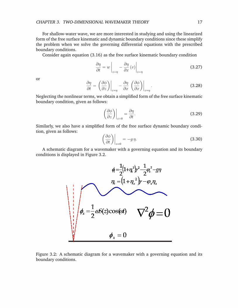
For shallow-water wave, we are more interested in studying and using the linearizedform of the free surface kinematic and dynamic boundary conditions since these simplifythe problem when we solve the governing differential equations with the prescribedboundary conditions.
Consider again equation (3.16) as the free surface kinematic boundary condition
∂η
∂t= w
∣∣∣∣z=η
− ∂η
∂x(v)
∣∣∣∣z=η
(3.27)
or∂η
∂t=
(∂φ
∂z
)∣∣∣∣z=η
− ∂η
∂x
(∂φ
∂x
)∣∣∣∣z=η
. (3.28)
Neglecting the nonlinear terms, we obtain a simplified form of the free surface kinematicboundary condition, given as follows:
(∂φ
∂z
)∣∣∣∣z=0
=∂η
∂t. (3.29)
Similarly, we also have a simplified form of the free surface dynamic boundary condi-tion, given as follows: (
∂φ
∂t
)∣∣∣∣z=0
= −g η. (3.30)
A schematic diagram for a wavemaker with a governing equation and its boundaryconditions is displayed in Figure 3.2.
Figure 3.2: A schematic diagram for a wavemaker with a governing equation and itsboundary conditions.
CHAPTER 3. TWO-DIMENSIONAL WAVEMAKER THEORY 18
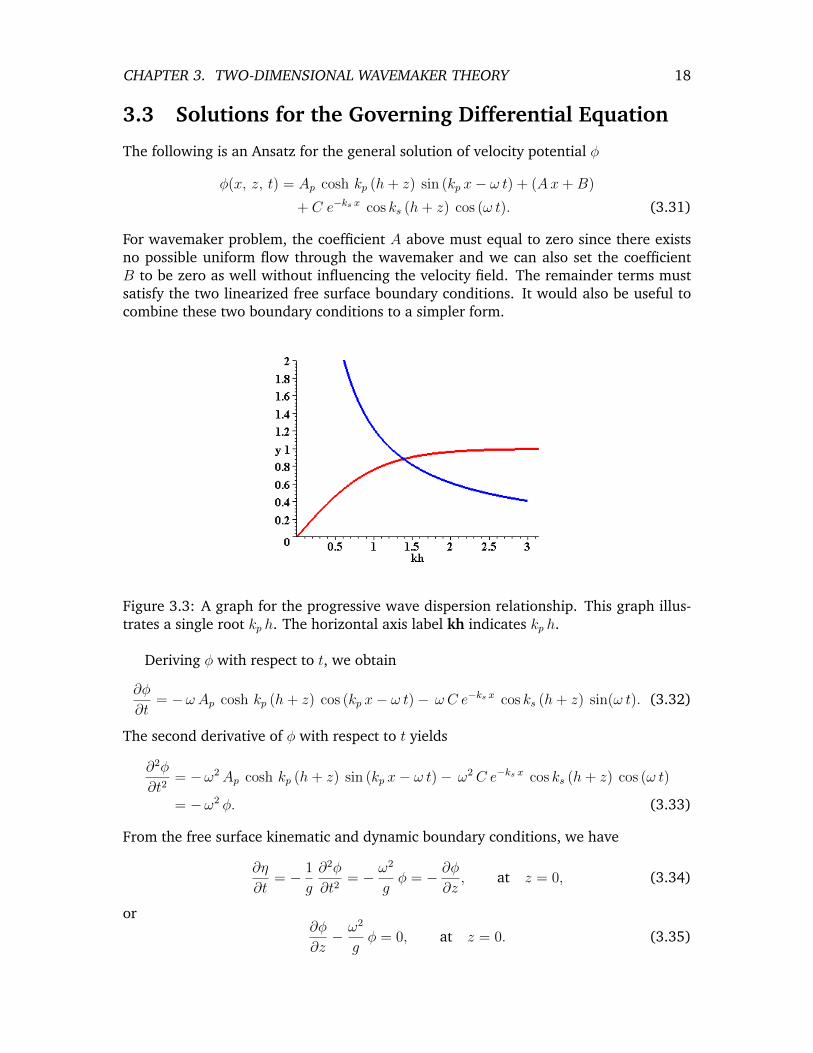
3.3 Solutions for the Governing Differential Equation
The following is an Ansatz for the general solution of velocity potential φ
φ(x, z, t) = Ap cosh kp (h+ z) sin (kp x− ω t) + (Ax+B)
+ C e−ks x cos ks (h+ z) cos (ω t). (3.31)
For wavemaker problem, the coefficient A above must equal to zero since there existsno possible uniform flow through the wavemaker and we can also set the coefficientB to be zero as well without influencing the velocity field. The remainder terms mustsatisfy the two linearized free surface boundary conditions. It would also be useful tocombine these two boundary conditions to a simpler form.
Figure 3.3: A graph for the progressive wave dispersion relationship. This graph illus-trates a single root kp h. The horizontal axis label kh indicates kp h.
Deriving φ with respect to t, we obtain
∂φ
∂t= −ω Ap cosh kp (h+ z) cos (kp x− ω t)− ω C e−ks x cos ks (h+ z) sin(ω t). (3.32)
The second derivative of φ with respect to t yields
∂2φ
∂t2= −ω2Ap cosh kp (h+ z) sin (kp x− ω t)− ω2C e−ks x cos ks (h+ z) cos (ω t)
= −ω2 φ. (3.33)
From the free surface kinematic and dynamic boundary conditions, we have
∂η
∂t= − 1
g
∂2φ
∂t2= − ω
2
gφ = − ∂φ
∂z, at z = 0, (3.34)
or∂φ
∂z− ω2
gφ = 0, at z = 0. (3.35)

CHAPTER 3. TWO-DIMENSIONAL WAVEMAKER THEORY 19
By substituting the Ansatz (3.31) to this equation, we obtain
ω2 = g kp tanh (kp h) (3.36)
andω2 = −g ks tan (ks h) . (3.37)
The former (3.36) is a dispersion relationship for the progressive wave. By rewritingthis equation as follows:
ω2 h
g kp h= tanh (kp h) (3.38)
and sketch each term with respect to kp h for a particular value ofω2 h
g, then we are able
to discover the solution for the dispersion relationship (3.36) as depicted in Figure 3.3.The latter (3.37), which relates ks with the wavemaker frequency ω, determines
the wavenumber for the standing wave with an amplitude decaying exponentially as ittravels far away from the wavemaker. By rewriting this equation as follows:
ω2 h
g ks h= − tan (ks h) (3.39)
we can sketch its graph and observe that it possesses an infinite numbers of solution.The solutions of this problem can be observed from the graph for its dispersion relation-ship, as depicted in Figure 3.4.
Figure 3.4: A graph for the standing wave dispersion relationship. This graph illustratesinfinitely many compound roots ks(n)h. The horizontal axis label kh means ks h.
Each solution is expressed in terms of ks(n), where n ∈ N. The final form for thevelocity potential is given as follows:
φ(x, z, t) = Ap cosh kp (h+ z) sin (kp x− ω t)
+∞∑
n=1
Cn e−ks(n)x cos ks(n) (h+ z) cos(ω t). (3.40)

CHAPTER 3. TWO-DIMENSIONAL WAVEMAKER THEORY 20
The first term indicates the progressive wave produced by the wavemaker, while theseries terms expresses decaying standing waves as they travel far away from the wave-maker.
To obtain a complete wave solution, we need to determine the coefficients Ap andCn. We can calculate these values using the wavemaker lateral boundary condition,namely
u(0, z, t) =
(∂φ
∂x
)∣∣∣∣x=0
=1
2ω S(z) cos(ω t). (3.41)
By finding the first derivative of velocity potential φ with respect to x and evaluating itat x = 0, we attain
1
2ω S(z) cos(ω t) = Ap kp cosh kp (h+ z) cos(ω t)
−∞∑
n=1
Cn ks(n) cos ks(n) (h+ z) cos(ω t) (3.42)
or1
2ω S(z) = Ap kp cosh kp (h+ z)−
∞∑
n=1
Cn ks(n) cos ks(n) (h+ z). (3.43)
We now possess a function in the z-variable which equals to a series of trigonometricfunctions on the right-hand side, a situation similar to a Fourier series. We also havethe fact that the set of functions {cosh kp (h+ z), cos [ks(n) (h+ z)]}∞n=1 forms a com-plete harmonic series orthogonal functions. Any arbitrary continuous function can beexpanded in terms of the series.
To find the coefficientsAp, therefore, we multiple the above equation with cosh kp (h+z) and integrate it with respect to the variable z from −h until 0. We now acquire
∫ 0
−h
1
2ω S(z) cosh kp (h+ z) dz =
∫ 0
−hAp kp cosh k2
p (h+ z) dz
−∫ 0
−h
∞∑
n=1
Cn ks(n) cos [ks(n) (h+ z)] cosh kp (h+ z) dz. (3.44)
Applying the orthogonality property, the last term vanishes and consequently
Ap =
1
2ω
∫ 0
−hS(z) cosh kp (h+ z) dz
kp
∫ 0
−hcosh k2
p (h+ z) dz
. (3.45)
For a flap-type wavemaker, the stroke function S can be specifically expressed as follows:
S(z) = S(
1 +z
h
). (3.46)
Employing a simple calculus, we could express the coefficient Ap explicitly without theintegral sign, given as follows:
Ap =2ω S
k2p h
kp h sinh kp h− cosh kp h+ 1
sinh 2 kp h+ 2 kp h. (3.47)

CHAPTER 3. TWO-DIMENSIONAL WAVEMAKER THEORY 21
Similarly, we can obtain the coefficient C(n) by multiplying (3.43) with cos [ks(n) (h+z)] and integrate it with respect to the variable z over the water depth from z = −h untilz = 0. We attain
Cn =
−1
2ω
∫ 0
−hS(z) cos ks(n) (h+ z) dz
ks(n)
∫ 0
−hcos2 [ks(n) (h+ z)] dz
(3.48)
or, by employing a little bit of integration process, we arrive at the following result:
Cn =−2ω S
[ks(n)]2 h
[ks(n)h] sin [ks(n) , h] + cos [ks(n)h]
sin [2 ks(n)h] + 2 ks(n)h. (3.49)
The wave height H for the progressive wave can be determined by evaluating ηsufficiently far from the wavemaker
η = −1
g
(∂φ
∂t
)∣∣∣∣z=0
=Apgω cosh kp h cos (kp x− ω t)
=H
2cos (kp x− ω t) for x� h. (3.50)
By substituting the values Ap obtained previously, we can acquire the ration betweenthe wave height H and the stroke S. It reads
H
S= 4
(sinh kp h
kp h
) (kp h sinh kp h− cosh kp h+ 1
sinh 2 kp h+ 2 kp h
). (3.51)
The graph for the ratios between H and S for the (shallow-water wave) simplifiedtheory and for a more complete linear wavemaker theory are depicted in Figure 3.5.
Figure 3.5: A graph for the ratios between the wave height H and the stroke S withrespect to the relative depth kp h. The horizontal axis label kh refers to kp h, while thevertical axis label H S refers to H/S.

Chapter 4
Numerical Simulation
In this chapter, we will discuss several results by selecting particular values from thewave-related quantities. Using the computer software Maple V Release 5, we couldalso observe an animation for the resulting monochromatic waves when we move thewavemaker with a particular stroke.
4.1 Calculating the Progressive Wavenumber
Consider again equation (3.36) which expresses the dispersion relationship for progres-sive waves
ω2 = g kp tanh kp h. (4.1)
Since we are not able to calculate the exact value of the wavenumber kp, we needto calculate it numerically. We use the following values: monochromatic frequencyω = 2 rad/s, gravitational acceleration constant g = 9.8 m/s2, and the water depthof the towing tank h = 3 m. Employing the Newton-Raphson iteration, we seek thevalue kp given an initial guess p0 by finding the roots of f(kp) = 0, where f(kp) =ω2 − g kp tanh kp h. Please see Appendix B for more information on the algorithm forthe Newton-Raphson iteration. By choosing error values of δ = 10−9, ε = 10−9, andsmall = 10−9, as well as the maximum iteration = 5000, then using the initial guessp0 = 0.5, we obtain kp = 0, 4624593666. For ω = 1, the obtained value for the progressivewavenumber is kp = 0, 1943823443. See again the graph in Figure 3.3.
4.2 Calculating Standing Wave Wavenumbers
Consider again equation (3.37) which expresses the dispersion relationship for standingwaves
ω2 = −g ks tan ks h. (4.2)
Similar as previously, since we cannot calculate exact values of the wavenumber ks,we calculate them numerically. We take identical values as previously: monochromaticfrequency ω = 2 rad/s, gravitational acceleration constant g = 9.8 m/s2, and the waterdepth of the towing tank h = 3 m. Employing the Newton-Raphson iteration, we seekthe values ks given an initial guess p0 by finding the roots of g(ks) = 0, where g(ks) =
22

CHAPTER 4. NUMERICAL SIMULATION 23
ω2 + g ks tan ks h. Please consult Appendix B for more detailed information on thealgorithm for the Newton-Raphson iteration. The selected error values are δ = 10−5,ε = 10−5, and small = 10−5 with the maximum iteration of 10000. Since the graphin the dispersion relationship produces infinitely many intersections, i.e., the values ofstanding wave wavenumbers, then the values for an initial guess also vary according tothe computational need, p0 = 1, 2, 3, · · · . For a practical purpose, we only select severalsuccessive wavenumber values, given as follows:
ks(1) = 0.906121231;
ks(2) = 2.028197863;
ks(3) = 3.097926261;
ks(4) = 4.156159228;
ks(5) = 5.209926525;
ks(6) = 6.261487236;
ks(7) = 7.311794624;
ks(8) = 8.361321437;
ks(9) = 9.410329031.
See again the graph in Figure 3.4.Similarly, using various values for the initial guess, we obtain the following wavenum-
ber values corresponding to the standing waves for ω = 1:
ks(1) = 1.013758189;
ks(2) = 2.078040121;
ks(3) = 3.130732073;
ks(4) = 4.180655871.
4.3 Monochromatic Wave Profiles
4.3.1 Two Wave Profiles with Distinct Wave Height H
Consider again the velocity potential equation (3.40) describing a water wave producedby the wavemaker
φ(x, z, t) = Ap cosh kp (h+ z) sin (kp x− ω t)
+∞∑
n=1
Cn e−ks(n)x cos ks(n) (h+ z) cos(ω t). (4.3)
Using equations (3.47) and (3.51), we can express the coefficient Ap in terms of ω, H,kp, and h, i.e.,
Ap =ωH
2 kp sin kp h. (4.4)
By substituting the values ω = 2, kp = 0, 4624593666, and h = 3, then

CHAPTER 4. NUMERICAL SIMULATION 24
• for H = 0.5, we have Ap = 1.099621133; and
• for H = 0.75, we have Ap = 1.649431700.
To obtain the maximum stroke S, we use equation (3.51), i.e.,
S =
(H kp h
4 sinh kp h
) (sinh 2 kp h+ 2 kp h
kp h sinh kp h− cosh kp h+ 1
). (4.5)
Substituting the values we have chosen, it yields
• for H = 0.5, we obtain S = 0.2908632665; and
• for H = 0, 75, we obtain S = 0.4362948995.
The wavemaker movement profile when it reaches the maximum stroke can beviewed in Figure 4.1.
Figure 4.1: Maximum strokes from the wavemaker flap which produce two wave-profiles with different wave height.
To find the coefficients for the standing wave Cn, we use (3.49), namely
Cn =−2ω S
[ks(n)]2 h
[ks(n)h] sin [ks(n)h] + cos [ks(n)h]
sin [2 ks(n)h] + 2 ks(n)h. (4.6)
We have already selected four values of ks(n). For larger values of n, the effect of Cn tothe wave profile solution is relatively small so that it can be neglected.
• For S = 0.2908632665, the coefficient values are C1 = 0.08013595964, C2 = 0.00976252019,C3 = 0.001714039296, and C4 = 0.001110132786.
• For S = 0.4362948995, the coefficient values are C1 = 0.1202039395, C2 = 0.01464378027,C3 = 0.002571058938, and C4 = 0.001665199177.

CHAPTER 4. NUMERICAL SIMULATION 25
Using equation (3.30)
η(x, t) = −1
g
(∂φ
∂t
)∣∣∣∣z=0
(4.7)
we are able to discover an equation for the shape of the formed water wave elevation.We can also display this surface elevation using computer software. The simulationresult for the water surface with two distinct wave heights is displayed in Figure 4.2.
Figure 4.2: Shapes of surface water wave elevation for two distinct wave heights.
4.3.2 Two Wave Profiles with Distinct Angular Frequency ω
In this subsection, we implement an identical technique as in the previous subsection.The water depth in the towing tank is also h = 3 m and the desired wave height profileis H = 0.5 m. The angular frequencies are ω = 2 and ω = 1. Employing the Newton-Raphson iteration toward both the progressive wave and the standing wave dispersionrelationships, we could attain the values kp and ks(n) for these frequencies. We haveobtained these results in Sections 4.1 and 4.2. We tabulate them again in this section.Additionally, we also list the coefficients for the velocity potential related to the valuesof ω, i.e., Ap and Cn.
The following provides results obtained by the computer software Maple V Release 5.
a. For ω = 2.
• A wavenumber for the progressive wave kp = 0.4624593666.
• Wavenumbers for the standing wave:ks(1) = 0.9061212307, ks(2) = 2.028197863,ks(3) = 3.0979262610, ks(4) = 4.156159228.
• The coefficient Ap = 1.099621133.
• The maximum stroke S = 0.2908632665.
• The coefficients Cn areC1 = 0.801359596400, C2 = 0.009762520190,C3 = 0.001714039296, C4 = 0.001110132786.
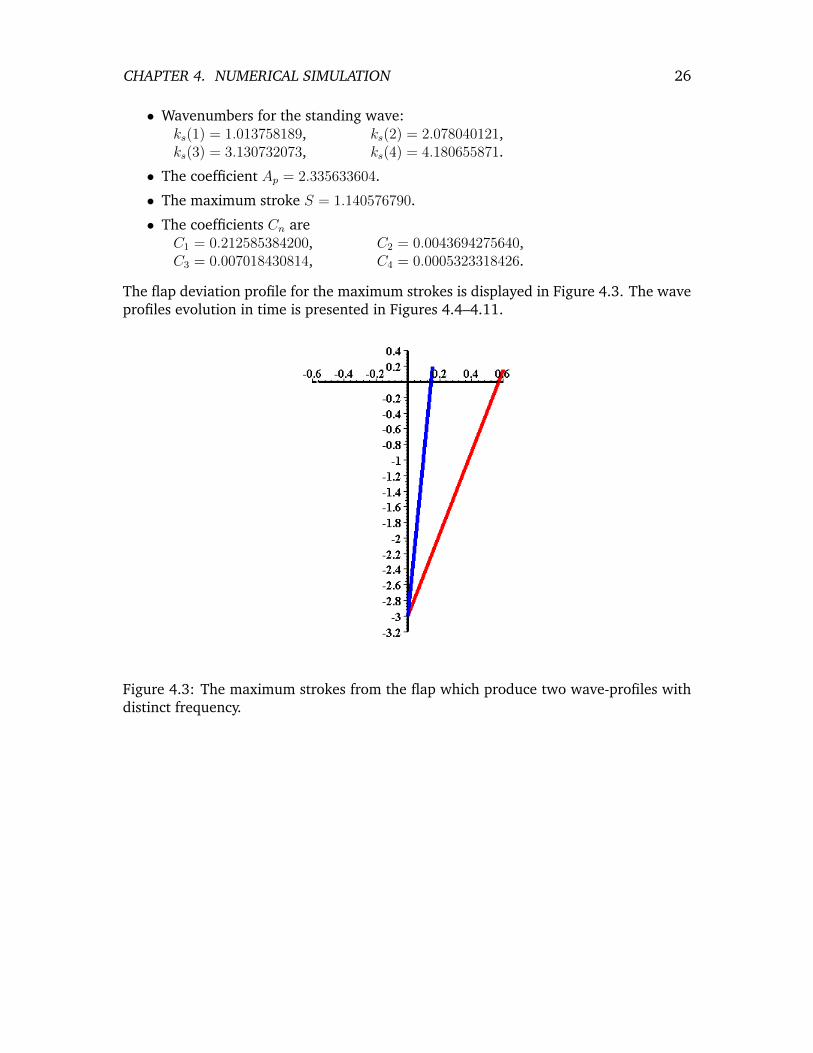
b. For ω = 1.
• A wavenumber for the progressive wave kp = 0.1943823443.
CHAPTER 4. NUMERICAL SIMULATION 26
• Wavenumbers for the standing wave:ks(1) = 1.013758189, ks(2) = 2.078040121,ks(3) = 3.130732073, ks(4) = 4.180655871.
• The coefficient Ap = 2.335633604.
• The maximum stroke S = 1.140576790.
• The coefficients Cn areC1 = 0.212585384200, C2 = 0.0043694275640,C3 = 0.007018430814, C4 = 0.0005323318426.
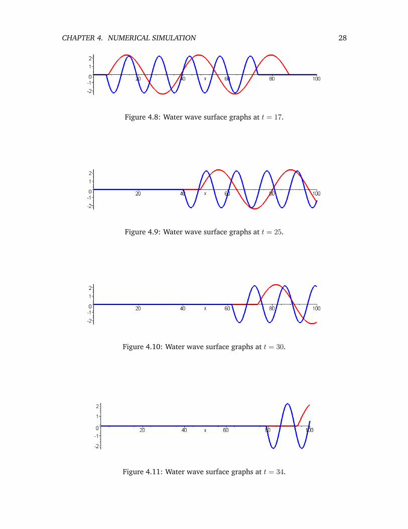
The flap deviation profile for the maximum strokes is displayed in Figure 4.3. The waveprofiles evolution in time is presented in Figures 4.4–4.11.
Figure 4.3: The maximum strokes from the flap which produce two wave-profiles withdistinct frequency.

CHAPTER 4. NUMERICAL SIMULATION 27
Figure 4.4: Water wave surface graphs at t = 3.
Figure 4.5: Water wave surface graphs at t = 5.
Figure 4.6: Water wave surface graphs at t = 10.
Figure 4.7: Water wave surface graphs at t = 15.
CHAPTER 4. NUMERICAL SIMULATION 28
Figure 4.8: Water wave surface graphs at t = 17.
Figure 4.9: Water wave surface graphs at t = 25.
Figure 4.10: Water wave surface graphs at t = 30.
Figure 4.11: Water wave surface graphs at t = 34.

Chapter 5
Conclusion and Suggestion
5.1 Conclusion
The following presents conclusion for this final project report:
a. We have adopted ideal fluid assumptions for wave generation modeling.
b. We have implemented linear wave theory for solving the governing differential equa-tions obtained from part (a).
c. We were able to derive the relationship among the wavenumber, wave height, andwavemaker stroke from the theory developed in part (b).
d. For shallow-water waves, both the simplified and the linear wave theories producean identical result, while for deeper-water waves, both theories provide differentresults.
5.2 Suggestion
The following presents suggestion for another final project or further research:
a. The wave theory can be extended to nonlinear theory and three-dimensional wave-maker theory.
b. The type of waves can be expanded to include random and irregular waves.
c. Adding a beach can be utilized to replace a semi-infinite domain.
29

Appendix A
Material Derivative
The operatorD
Dt=
∂
∂t+ u · ∇ (A.1)
is known as the material derivative, total derivative, substantial derivative, or Lagrange
derivative. In generalD
Dtis a vector operator. As a consequence,
D
Dtcomponents acts
on a vector will not be equal with the ones act on a scalar component of a vector, exceptin the Cartesian coordinates system. The material derivative can also be applied toa scalar quantity, such as temperature. Physically, it states the rate of change of thatquantity with respect to time, where the observer moves along with the measured fluidat a particular location in space and instant time when that derivative is evaluated.
This operator is the total derivative with respect to time acting on a fluid element,which can be viewed as follows. Let ξ be a spatial coordinate describing the fluid atan initial fixed instant t = 0, let also x be the spatial coordinate providing the locationduring time t of a fluid element for which it is ξ when t = 0. We have x = x(ξ, τ). TheEulerian derivative with respect to time is given by
∂
∂t=
∂
∂t
∣∣∣∣fixed x
, (A.2)
while the derivative which plays a role as Lagrangian derivative is given by
D
Dt=
∂
∂t
∣∣∣∣fixed ξ
. (A.3)
Employing the Chain Rule, we obtain
D
Dt=
∂
∂t
∣∣∣∣fixed ξ
=∂
∂t
∣∣∣∣fixed x
+∂xi∂t
∣∣∣∣fixed ξ
∂
∂t,
which results equation (A.1) since∂x
∂t
∣∣∣∣ξ
= u.
This operator is also used in the Navier-Stokes equation which states the total accel-eration of a particle as follows:
a =Du
Dt=∂u
∂t+
(u∂u
∂x+ v
∂u
∂y+ w
∂u
∂z
). (A.4)
30

APPENDIX A. MATERIAL DERIVATIVE 31
The first term on the right-hand side of (A.4) indicates a local acceleration, which iszero for the steady-state flow. The other terms express convective acceleration, whichshow that the fluid flow has a different velocity at a different position. For more detailedexplanation, please consult [5, 8].

Appendix B
An Algorithm for the Newton-RaphsonIteration
#
"
!Searching the root of f(x) = 0 given an initial guess p0 using the iteration
pn = pn−1 −f(pn−1)
f ′(pn−1)for n = 1, 2, 3, . . . .
Algorithm:δ := 10−6, ε := 10−6, small:= 10−6
{ several error values, can be adjusted according to the need }maks:= 99 { the maximum number of iterations }kond:= 0 { the condition for a loop termination }INPUT P0 { P0 must be sufficiently close with the desired root }Y0 := F (P0) { calculating a value of the function }
DO FOR N := 1 TO maks UNTIL kond 6= 0
Df := F ′(P0) { calculating the derivative }IF Df = 0 THEN
{ checking whether there exists any division by zero }kond:= 1Dp := 0
ELSE
Dp := Y0/DfENDIF
P1 := P0 −Dp { new iteration }Y1 := F (P1) { the value of a new function }RelErr:= 2 ∗ |Dp|/(|P1|+ small) { relative error }IF RelErr < δ AND |Y1| < ε THEN
IF kond 6= 1 THEN kond:= 2 { checking convergence }P0 := P1; Y0 := Y1 { replacing with new values }
PRINT ‘The value of the n-th iteration is’ P1 { ouput }
32
APPENDIX B. NEWTON-RAPHSON ITERATION 33
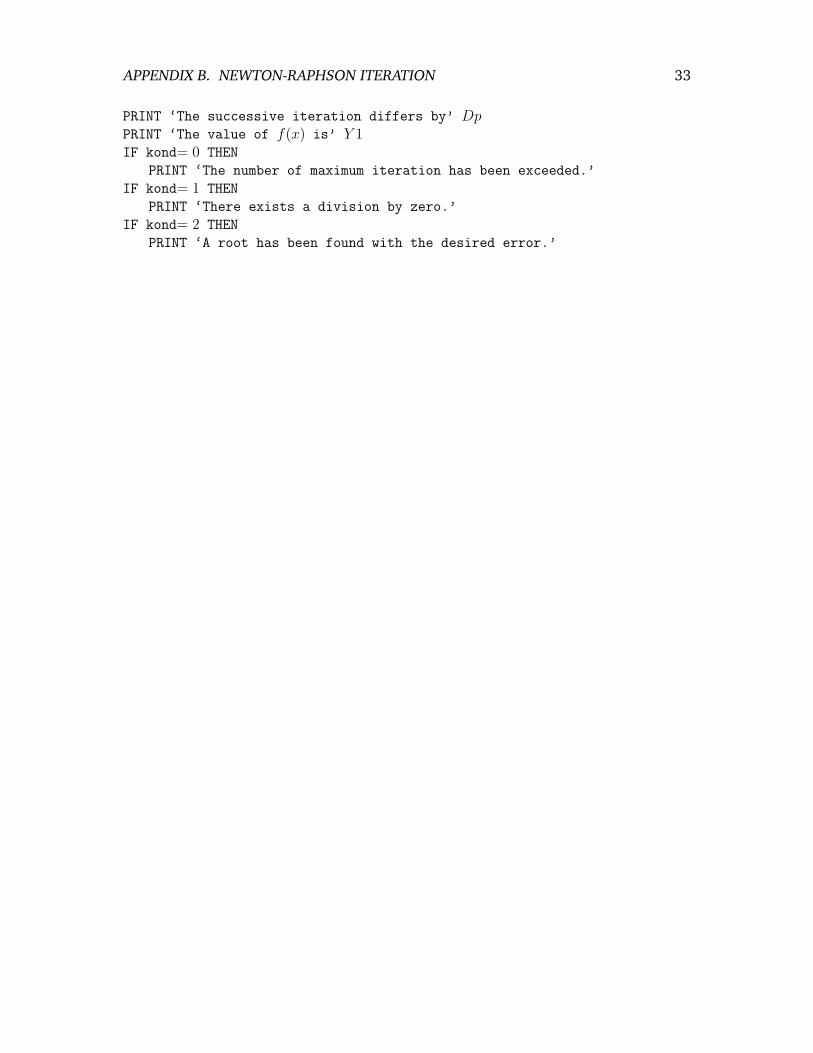
PRINT ‘The successive iteration differs by’ DpPRINT ‘The value of f(x) is’ Y 1IF kond= 0 THEN
PRINT ‘The number of maximum iteration has been exceeded.’
IF kond= 1 THEN
PRINT ‘There exists a division by zero.’
IF kond= 2 THEN
PRINT ‘A root has been found with the desired error.’

Appendix C
Hydrodynamics Laboratories Aroundthe World
This appendix lists hydrodynamic laboratories in various parts of the world. Some ofthem are used commercially and for marine structure defense. For detailed information,please consult [2] or the International Towing Tank Conference association. Otherwiseindicated, the size of the tank refers to the length, width, and depth, respectively.
a. Institute of Marine Dynamics Towing Tank, St. John’s, Newfoundland, CanadaFacility: Deep-water tankTank size: 200 m × 12 m × 7 mCarrier speed: 10 m/sWave type: Regular and irregular; 1 mWavemaker: Double flap-typeBeach: Surging wave bottom.
b. Offshore Model Basin, Escondido, California, United States (US)Tank size: 90 m × 14.6 m × 4.6 mDeeper part: Circular hole with 9 m depthCarrier speed: 6 m/sWave type: Regular and irregular; 0.74 mWavemaker: Single-flap boardBeach: Metal shaved.
c. Offshore Technology Research Center, Texas A&M, College Station, Texas, USTanks size: 45.7 m × 30.5 m × 5.8 mDeeper part: 16.7 m hole with adjustable floorWavemaker: Flap-type with hydraulic hinge controlMaximum wave height: 80 cmPeriod range: 0.5–4.0 sBeach: Metal panel
34

APPENDIX C. HYDRODYNAMICS LABORATORIES 35
d. David Taylor Research Center, Bethesda, Maryland, USFacility: Maneuvering and Seakeeping Facilities (MASK)Tank size: 79.3 m × 73.2 m × 6.1 mWavemaker: Total of 21 pneumatic-typeWave: Multidirectional, regular and irregular; maximum height 0.6 m;
and wavelength 0.9–12.2 mBeach: Wave absorberCarrier speed: 7.7 m/s.
Facility: Deep-Water BasinTank size: 846 m × 15.5 m × 6.7 mWave: Maximum height 0.6 m and wavelength 1.5–12.2 mCarrier speed: 10.2 m/s.
Facility: High-Speed BasinTank size: 79.3 m × 73.2 m × 6.1 mWave: Maximum height 0.6 m and wavelength 0.9–12.2 mCarrier speed: 35.8–51.2 m/s.
e. Maritime Research Institute (MARIN), the NetherlandsFacility: Seakeeping BasinTank size: 100 m × 24.5 m × 2.5 mDeeper part: Hole with 6 m depthWave: Regular and irregular; maximum height 0.3 m; and period range 0.7–3.0 sCarrier speed: 4.5 m/s.
Facility: Wave and Current BasinsTank size: 60 m × 40 m × 1.2 mDeeper part: Hole with 3 m depthWave: Regular and irregularCarrier speed: 3 m/sSpeed range: 0.1–0.6 m/s.
Facility: Deep-Water Towing TankTank size: 252 m × 10.5 m × 5.5 mCarrier speed: 9 m/s.
Facility: High-Speed Towing TankTank size: 220 m × 4 m × 4 mWavemaker: Hydraulic flap-typeWave: Regular and irregular; maximum height 0.4 m; and period range 0.3–5 sCarrier: Motor and jet controlsCarrier speed: 15 m/s and 30 m/sBeach: Circular arc lattices.
f. Danish Maritime Institute, Lyngby, DenmarkTank size: 240 m × 12 m × 5.5 mWavemaker: Hydraulic double-flap type controlled numericallyWave: Regular and irregular; maximum wave 0.4 m; and period range 0.5–7 sCarrier speed: 0–11 m/s (accurate ± 2%).

APPENDIX C. HYDRODYNAMICS LABORATORIES 36
g. Danish Hydraulic Institute, Horsholm, DenmarkTank size: 30 m × 20 m × 3 mDeeper part: 12 m in the middleWavemaker: 60 Hydraulic flaps controlled by a mini-computer on one sideWave: Maximum height ∼= 0.6 m and period range ∼= 0.5–4 s.
h. Norwegian Hydrodynamic Laboratory (MARINTEK), Trondheim, NorwayFacility: The Ocean BasinTank size: 80 m × 50 m × 10 mWavemaker: Hinged double-flap type, 144 self-control; Hydraulic controlled hinge-typeWave: Regular and irregular; maximum height 0.9 mWave speed: Maximum speed 0.2 m/s.

References
[1] Azoury, P. H., Engineering Applications of Unsteady Fluid Flow, John Wiley &Sons, 1992. (ISBN 0 471 92968 9; 97/602; 620.1’064 AZO).
[2] Chakrabarti, S. K., Offshore Structure Modelling, World Scientific, 1994. (ISBN981-02-1513-4; 96/5715; 627.98 CHA)
[3] Dean, R. G., Dalrymple, R. A., Water Wave Mechanics for Engineers and Scien-tists, World Scientific, 1991. (ISBN 9810204205-9810204213; 627’.042-dc20)
[4] Dingemans, M. W. Water Wave Propagation Over Uneven Bottoms, Part 1 - LinearWave Propagation, World Scientific, 1997. (ISBN 981-02-3393-9)
[5] Fowler, A. C., Mathematical Models in the Applied Sciences, Cambridge Univer-sity Press, 1997.
[6] Groesen, E. van, Lecture Notes Computational Fluid Dynamics, Research Work-shop, University of Twente, 1997.
[7] Hooft, J. P., Advanced Dynamics of Marine Structures, John Wiley & Sons, 1982.(ISBN 0-471-03000-7; 87/2262; 627’.042 HOO)
[8] Hughes, W. F., Brighton, J. A., Theory and Problems of Fluid Dynamics, 2nd
Edition, Schaum’s Outline Series, McGraw–Hill, Inc., 1991. (ISBN 0-07-112632-5;94/501; 532-05 HUG)
[9] Johnson, R. S., A Modern Introduction to the Mathematical Theory of WaterWaves, Cambridge University Press, 1997 (ISBN 0 521 59832 X)
[10] Keener, J. P., Principles of Applied Mathematics — Transformation and Approxi-mation, Addison–Wesley Publishing Company, 1988.
[11] Landau, L. D., Lifshitz, E. M., Fluid Mechanics (Mekhanika Sploshnykh Sred), 2nd
English Edition, Volume 6 of Course of Theoretical Physics (Teoreticheskaia Fizika),Translated from the Russian by J. B. Sykes and W. H. Reid, Pergamon Press, 1987.
[12] Mathews, J. H., Numerical Methods for Mathematics, Science, and Engineering,2nd Edition, Prentice-Hall, 1992. (ISBN 0-13-624990-6)
[13] Newman, J. N., Marine Hydrodynamics, MIT Press, 1977. (ISBN 0-262-14026-8)
[14] Ramamrutham, S., Fluid Mechanics, Hydraulics, and Fluid Machines, DhanpatRai & Sons, 1986. (90/522; 620.106 RAM)
37

REFERENCES 38
[15] Round, G. F., Garg, V. K., Applications of Fluid Dynamics, Edward Arnold, 1986.(ISBN 0-7131-3546-8; 87/1153; 620.1’064 ROU)
[16] Thomas, Jr. G. B., Finney, R. L., Calculus and Analytic Geometry, 9th Edition,Addison–Wesley Publishing Company, 1996. (ISBN 0-201-40015-4; 515.15 THO;08119)
[17] Wiryanto, L. H., Lecture Notes MA-475 Computational Fluid Dynamics (in In-donesian), Department of Mathematics, Faculty of Mathematics and Natural Sci-ences, Bandung Institute of Technology, 2000.

TEORI PEMBANGKIT GELOMBANGDUA-DIMENSI TIPE FLAP
Tugas AkhirDiajukan sebagai syarat untuk memenuhi Sidang Sarjana
Jurusan Matematika
oleh :
Natanael Karjanto
10197045
JURUSAN MATEMATIKAFAKULTAS MATEMATIKA DAN ILMU PENGETAHUAN ALAM
INSTITUT TEKNOLOGI BANDUNG2001
arX
iv:2
001.
0585
4v1
[ph
ysic
s.fl
u-dy
n] 1
1 Ja
n 20
20

TEORI PEMBANGKIT GELOMBANGDUA-DIMENSI TIPE FLAP
Lembar Pengesahan
Telah diperiksa dan disetujui oleh Pembimbing :
Dr. Andonowati
NIP. 131803263
Penilai (Penguji) :
Prof. Dr. M. Ansjar Dr. Wono Setya Budhi
NIP. 130143972 NIP. 131284801

Untuk yang terkasih papa, mama, dan adik perempuanku.
Abstrak
Pemodelan secara matematis pembangkitan gelombang arah tunggal disampaikandalam laporan tugas akhir ini. Pemodelannya mencakup persamaan Laplace dalam ko-lam air dengan setengah batas tak hingga, syarat batas dinamika dan kinematika, syaratbatas lateral di pembangkit gelombang, dan dinding tetap di dasar kolam. Modelnya dit-erapkan pada wavemaker tipe flap yang sering digunakan pada suatu towing tank dalamlaboratorium hidrodinamika. Untuk menyederhanakan permasalahan, beberapa asumsiditerapkan, yakni bahwa air adalah fluida yang bersifat ideal. Teori pembangkit gelom-bang linear digunakan dan tipe gelombang monokromatik (frekuensi tunggal) diamati.Kaitan antara bilangan gelombang, ketinggian gelombang, dan simpangan wavemakerjuga akan diturunkan.
Kata-kata kunci: fluida ideal, pembangkit gelombang (wavemaker), persamaan Laplace,syarat batas kinematika permukaan bebas, syarat batas dinamika permukaan bebas, teoripembangkit gelombang linear, gelombang monokromatik, bilangan gelombang, ketinggiangelombang, dan simpangan pembangkit gelombang.

Kata Pengantar
Terima kasih kepada pembaca yang dengan senang hati meluangkan waktu untukmembuka tugas akhir ini. Namun sebelumnya, izinkanlah penulis untuk menyampaikanpuji dan syukur ke hadirat Tuhan, Pencipta alam semesta beserta segala isinya. Atasberkat dan rahmat-Nyalah penulis dapat menyelesaikan tugas akhir sekaligus mengakhirijenjang pendidikan pada tahap sarjana. Penulis juga tidak lupa mengucapkan terimakasih yang sebesar-besarnya karena telah mendukung penulis untuk menyelesaikan studidi institusi tercinta ini, terutama kepada :
1. Dr. Andonowati, yang telah bersedia dan dengan sabar menjadi pembimbingtugas akhir penulis. Merci, Mom !
2. Prof. Dr. M. Ansjar dan Dr. Wono Setya Budhi, yang telah bersediamenguji dan menilai penulis pada seminar tugas akhir tanggal 15 Desember 2000lalu. Terima kasih juga kepada Pak Ansjar yang telah mempercayakan penulissebagai asisten grader Metode Matematika tahun 2000. Teristimewa untuk PakWono yang telah dengan sabar mengajari Maple dan LATEX pada penulis sehinggadapat merampungkan tugas akhir ini.
3. Dr. Nana Nawawi Gaos, yang telah menjadi dosen wali akademik penulis se-lama menempuh pendidikan di Tahap Persiapan Bersama 1997/1998 dan SemesterPendek 1998.
4. Dr. Ahmad Muchlis, yang telah menjadi dosen wali akademik penulis selamamenempuh pendidikan di tahap Sarjana Muda dan tahap Sarjana. (Thanks formotivating me to finish my study in three and half a year.)
5. Warsoma Djohan M.Si., yang telah mempercayai penulis menjadi asisten graderKalkulus I TPB-04 tahun 1999 dan asisten tutorial Kalkulus I TPB-07 tahun 2000lalu. Juga tidak lupa untuk Bu Jalina Widjaja yang telah mempercayai penulismenjadi asisten Matematika Rekayasa, Matriks & Ruang Vektor, serta asisten tem-poral Kalkulus I, dan Mba Nuning Nuraini yang juga tidak ragu mengajak penulismenjadi asisten tutorial Kalkulus II. Tak terlewatkan juga Pak Koko Martonoyang telah memberikan mandat asisten grader Kalkulus Peubah Banyak dan FungsiKompleks serta pelatihan dasar menulis artikel ilmiah. Demikian juga denganstaf pengajar lainnya di jurusan ini yang telah memberikan kontribusi kematanganberpikir pada penulis.
6. Kedua orang tua penulis, papa dan mama, yang telah memberikan dukungan materidan doa restu sehingga penulis menjadi seorang sarjana. Juga adikku tercinta yangtelah memberikan dorongan dan semangat untuk rajin belajar.
7. Hadi Susanto, sebagai rekan kuliah penulis, sering melewatkan saat-saat bersamabaik dalam suka maupun duka, teristimewa sebelum keberangkatannya ke Belanda.(Ik wil U bedanken omdat U mij heel goed heeft gemotiveend om extra hard testuderen. Bedankt, Hadi !)
vii
8. Maykel, Luis, Dina, Ety, Sica, Anna, Sondang, Rilyovira, dan teman-temanangkatan 97 yang lainnya yang tidak dapat penulis sebutkan satu per satu. Thanksfor our friendship. Juga pada teman-teman angkatan 95, 96, 98, dan 99 yang telahbanyak membantu penulis dalam menempuh jenjang pendidikan di ITB ini.
9. Pak Toto Nusantara (MA-S3), Mas Lylye Sulaeman (P4M), dan Surya(MA96) atas bantuannya dalam TEX, LATEX, dan Scientific Work Place sehinggatugas akhir ini dapat selesai diketik.
10. Wili (MA97), Henry (FI97), Albert(TF97), Wila (TI97), Aan (TK97),Faiq (TG97), Krshna (EL97), Fitra (TA98), Dindin (TL98), Hidayat(FA98), Dwi Susanti (FA98), Mia (KI99), Erika (FA99), Dwi Hesti (TG2000)dan teman-teman serta junior lainnya yang satu almamater dengan penulis (SMUN4 Bandung), yang telah memotivasi dan sangat mendukung penulis untuk menyele-saikan studi tidak lebih dari 8 semester. I am grateful to you all !
“Experientia est optima rerum magistra.” Itulah pepatah dalam bahasa Latinyang kurang lebih berarti, ”Pengalaman adalah guru yang terbaik.” Seperti peristiwa-peristiwa lainnya dalam kehidupan, menyelesaikan studi di tahap sarjana dan sekaligusjuga merampungkan tugas akhir ini adalah suatu pengalaman tersendiri yang unik danmenarik bagi penulis, menjadi ’guru’ dalam suka dan duka. Ada banyak hal yang penulisdapatkan setelah mengerjakan tugas akhir ini, pengetahuan akademis pada khususnya dankedewasaan serta kematangan berpikir pada umumnya.
Dengan penuh kerendahan pikiran, penulis menyadari bahwa secara individu, penulishanyalah satu dari banyak orang yang datang dan pergi, yang berupaya menorehkanprestasi dalam jenjang pendidikan di Jurusan Matematika ITB. Walaupun tidak dapatmemberikan yang terbaik untuk kemajuan Jurusan ini, penulis telah mengerahkan sekuattenaga untuk merampungkan tugas akhir ini. Penulis juga berharap bahwa karya yang’kecil’ ini dapat menjadi �creme de la creme� dari semua karya yang telah penulisbuat, meskipun ada masih banyak kekurangan di berbagai segi.
Oleh karena itu, penulis mohon maaf yang sebesar-besarnya kepada para pembacadan pengguna tugas akhir ini. Akhir kata, semoga ’karya’ ini dapat bermanfaat bagi parapembaca pada khususnya dan untuk kemajuan ilmu Matematika pada umumnya.
Bandung, Medio Januari 2001
N atanael Karyanto
viii

Daftar Isi
Abstrak v
Kata Pengantar vii
Daftar Isi ix
Daftar Gambar xi
1 Pendahuluan 11.1 Latar Belakang dan Rumusan Masalah . . . . . . . . . . . . . . . . . . . . 1
1.1.1 Latar Belakang . . . . . . . . . . . . . . . . . . . . . . . . . . . . . 11.1.2 Rumusan Masalah . . . . . . . . . . . . . . . . . . . . . . . . . . . 1
1.2 Ruang Lingkup Kajian . . . . . . . . . . . . . . . . . . . . . . . . . . . . . 21.3 Tujuan Penulisan . . . . . . . . . . . . . . . . . . . . . . . . . . . . . . . . 21.4 Anggapan Dasar . . . . . . . . . . . . . . . . . . . . . . . . . . . . . . . . 21.5 Hipotesis . . . . . . . . . . . . . . . . . . . . . . . . . . . . . . . . . . . . . 21.6 Metodologi Pengerjaan . . . . . . . . . . . . . . . . . . . . . . . . . . . . . 3
1.6.1 Metode . . . . . . . . . . . . . . . . . . . . . . . . . . . . . . . . . 31.6.2 Teknik Pengumpulan Data . . . . . . . . . . . . . . . . . . . . . . . 3
1.7 Sistematika Pembahasan . . . . . . . . . . . . . . . . . . . . . . . . . . . . 3
2 Aliran Fluida Ideal 42.1 Sifat Fisis Fluida . . . . . . . . . . . . . . . . . . . . . . . . . . . . . . . . 42.2 Hukum Kekekalan Massa dan Momentum . . . . . . . . . . . . . . . . . . 4
2.2.1 Hukum Kekekalan Massa . . . . . . . . . . . . . . . . . . . . . . . . 42.2.2 Hukum Kekekalan Momentum . . . . . . . . . . . . . . . . . . . . . 5
2.3 Teorema Transport (Transport Theorem) . . . . . . . . . . . . . . . . . . . 62.4 Persamaan Kontinuitas . . . . . . . . . . . . . . . . . . . . . . . . . . . . . 82.5 Persamaan Euler . . . . . . . . . . . . . . . . . . . . . . . . . . . . . . . . 92.6 Persamaan Bernoulli . . . . . . . . . . . . . . . . . . . . . . . . . . . . . . 10
3 Teori Pembangkit Gelombang Dua Dimensi 123.1 Teori Pembangkit Gelombang yang
Disederhanakan . . . . . . . . . . . . . . . . . . . . . . . . . . . . . . . . . 123.2 Teori Pembangkit Gelombang Linear . . . . . . . . . . . . . . . . . . . . . 13
3.2.1 Syarat batas lateral di pembangkit gelombang(pseudo-boundary) . . . . . . . . . . . . . . . . . . . . . . . . . . . 14
3.2.2 Syarat batas di dasar towing tank (persyaratan kinematika) . . . . 153.2.3 Syarat batas di permukaan air . . . . . . . . . . . . . . . . . . . . . 15
3.3 Solusi Governing Differential Equation . . . . . . . . . . . . . . . . . . . . 18
ix
DAFTAR ISI x
4 Simulasi Numerik 234.1 Menghitung Bilangan Gelombang Progresif . . . . . . . . . . . . . . . . . . 234.2 Menghitung Bilangan Gelombang Berdiri . . . . . . . . . . . . . . . . . . . 234.3 Profil Gelombang Monokromatik . . . . . . . . . . . . . . . . . . . . . . . 24
4.3.1 Dua Profil Gelombang dengan Ketinggian H Berbeda . . . . . . . 244.3.2 Dua Profil Gelombang dengan Frekuensi Sudut ω Berbeda . . . . . 26
5 Kesimpulan dan Saran 305.1 Kesimpulan . . . . . . . . . . . . . . . . . . . . . . . . . . . . . . . . . . . 305.2 Saran . . . . . . . . . . . . . . . . . . . . . . . . . . . . . . . . . . . . . . . 30
A Turunan Material 31
B Algoritma Iterasi Newton-Raphson 33
C Laboratorium Hidrodinamika di Dunia 34
Daftar Pustaka 37

Daftar Gambar
3.1 Skema pembangkit gelombang tipe flap. . . . . . . . . . . . . . . . . . . . 133.2 Skema pembangkit gelombang dengan persamaan pengatur dan syarat-
syarat batasnya. . . . . . . . . . . . . . . . . . . . . . . . . . . . . . . . . . 173.3 Grafik relasi dispersi gelombang progresif . . . . . . . . . . . . . . . . . . . 193.4 Grafik relasi dispersi gelombang berdiri . . . . . . . . . . . . . . . . . . . . 203.5 Grafik perbandingan ketinggian gelombang H dengan simpangan S ter-
hadap kedalaman relatif kp h. . . . . . . . . . . . . . . . . . . . . . . . . . 22
4.1 Simpangan terjauh flap yang menghasilkan dua profil gelombang denganketinggian berbeda. . . . . . . . . . . . . . . . . . . . . . . . . . . . . . . . 25
4.2 Bentuk permukaan gelombang air (elevasi) yang dibentuk oleh dua gelom-bang dengan ketinggian yang berbeda. . . . . . . . . . . . . . . . . . . . . 26
4.3 Simpangan terjauh flap yang menghasilkan dua profil gelombang denganfrekuensi sudut berbeda. . . . . . . . . . . . . . . . . . . . . . . . . . . . . 27
4.4 Grafik permukaan gelombang air pada t = 3. . . . . . . . . . . . . . . . . . 284.5 Grafik permukaan gelombang air pada t = 5. . . . . . . . . . . . . . . . . . 284.6 Grafik permukaan gelombang air pada t = 10. . . . . . . . . . . . . . . . . 284.7 Grafik permukaan gelombang air pada t = 15. . . . . . . . . . . . . . . . . 284.8 Grafik permukaan gelombang air pada t = 17. . . . . . . . . . . . . . . . . 284.9 Grafik permukaan gelombang air pada t = 25. . . . . . . . . . . . . . . . . 294.10 Grafik permukaan gelombang air pada t = 30. . . . . . . . . . . . . . . . . 294.11 Grafik permukaan gelombang air pada t = 34. . . . . . . . . . . . . . . . . 29
xi

Bab 1
Pendahuluan
1.1 Latar Belakang dan Rumusan Masalah
1.1.1 Latar Belakang
Seiring dengan peningkatan taraf kemajuan suatu bangsa, semakin meningkat jugalahkebutuhan akan penelitian di bidang sains dan teknologi. Di negeri kita, yang lebih daridua per tiga wilayahnya adalah lautan, memiliki sumber daya alam yang berkualitas.Sejak zaman dahulu, negeri kita dikenal sebagai negara bahari, atau negeri kelautan.Seraya ilmu pengetahuan dan teknologi berkembang dengan pesat, penelitian di bidangini juga perlu mendapatkan perhatian yang khusus.
Di bidang teknik kelautan (ocean engineering), adanya kebutuhan untuk membuatmodel matematis mengenai hal-hal yang terjadi di lepas pantai mendorong banyak peneli-tian dan riset di bidang ini. Lebih jauh lagi, ini juga mendorong kerja sama antaraberbagai disiplin ilmu yang mengkolaborasikan sains dan teknologi. Matematika sebagai“ The Queen and Servant of Science ” memiliki keampuhan dalam memodelkan banyakhal yang terjadi di alam. Dalam tugas akhir ini, akan dibahas mengenai masalah teoretispembangkitan gelombang dalam sebuah towing tank.∗
Pemodelan pembangkit gelombang dalam laboratorium hidrodinamika ini sangat bergunauntuk pengujian kapal yang akan berlayar di laut bebas. Sebagai contoh, kapal yang akanberlayar di Laut Jawa haruslah diuji dengan gelombang laut yang terjadi di Laut Jawajuga. Dengan demikian, diperoleh gambaran besarnya kekuatan gelombang sehingga men-dorong untuk membuat kapal yang cukup kuat untuk berlayar di sana.
1.1.2 Rumusan Masalah
Berdasarkan latar belakang di atas, rumusan masalah yang penulis ajukan adalah bagaimanamembuat model matematis dari gelombang yang terjadi di laut yang jauh dari pantaidengan menggunakan teori pembangkitan gelombang yang dapat dilakukan di dalamlaboratorium hidrodinamika. Kita ingin mengetahui besarnya simpangan pembangkitgelombang yang harus digerakkan apabila diinginkan profil gelombang dengan ketinggiantertentu. Selain itu, kita juga ingin mengetahui profil gelombang yang terjadi apabilapembangkit gelombang tadi digerakkan dengan frekuensi tertentu. Hal ini dapat dijadikansebagai sebuah model matematika mengenai gelombang air yang terjadi pada towing tank.
∗Towing tank adalah suatu fasilitas dalam laboratorium hidrodinamika berbentuk kolam berisi airdengan dilengkapi pembangkit gelombang di satu sisi dan penyerap gelombang di sisi lain. Beberapacontohnya dapat dilihat di Apendiks C.
1

BAB 1. PENDAHULUAN 2
1.2 Ruang Lingkup Kajian
Berdasarkan rumusan masalah di atas, ruang lingkup kajian yang akan penulis bahasadalah membuat model matematika sederhana mengenai pembangkit gelombang duadimensi tipe flap pada sebuah towing tank. Dalam memodelkan masalah ini, penulismenggunakan beberapa asumsi yang relevan sehingga akan mempermudah penyelesa-ian masalah. Agar lebih spesifik, gelombang yang dihasilkan diasumsikan gelombangmonokromatik (mempunyai frekuensi tunggal). Setelah itu, dengan bantuan perangkatlunak komputer, akan dibuat juga simulasi sederhana yang menggambarkan evolusi gelom-bang yang terjadi setelah selang waktu tertentu.
1.3 Tujuan Penulisan
Tujuan subyektif penulisan laporan tugas akhir ini adalah sebagai syarat untuk memenuhipersyaratan Sidang Sarjana Jurusan Matematika, Fakultas Matematika dan Ilmu Penge-tahuan Alam, ITB yang diselenggarakan pada tanggal 24 Januari 2001.
Tujuan obyektif penulisan laporan tugas akhir ini adalah untuk memperdalam bidangilmu yang sedang penulis tekuni, yakni Matematika, terutama yang berkaitan dengan pen-erapan dalam masalah fisis. Selain itu, dengan memodelkan permasalahan yang datangdari luar disiplin ilmu matematika, wawasan penulis mengenai keterkaitan ilmu penge-tahuan dan teknologi serta berbagai disiplin ilmu akan semakin luas.
1.4 Anggapan Dasar
Untuk membuat suatu model dari teori pembangkit gelombang, bergantung pada beber-apa faktor berikut :
• Sifat fluida yang diasumsikan yang akan membawa pada perumusan matematis.
• Adanya suatu persamaan diferensial pengatur (governing differential equation) danbeberapa syarat batas.
• Asumsi berkenaan tipe dan sifat gelombang yang dihasilkan.
1.5 Hipotesis
Jika kita mengasumsikan bahwa air adalah salah satu jenis fluida yang termasuk fluidaideal, kita bisa memperoleh suatu persamaan diferensial parsial yang memiliki beberapasyarat batas sebagai persamaan diferensial pengatur (governing differential equation),dan asumsi lainnya bahwa gelombang yang dihasilkan mempunyai tipe monokromatikdan bersifat periodik, maka kita dapat membuat sebuah teori pembangkit gelombang lin-ear dua dimensi.

BAB 1. PENDAHULUAN 3
1.6 Metodologi Pengerjaan
1.6.1 Metode
Metode yang penulis gunakan adalah metode analisis teoretis, yaitu menganalisis secarateori beberapa model yang berkaitan dengan pembangkit gelombang, termasuk menu-runkan beberapa persamaan yang berkaitan dengan teori ini. Di samping hal ini, penulisjuga menggunakan metode analisis komputasi, yaitu menganalisis dan memecahkan be-berapa permasalahan dengan bantuan komputer.
1.6.2 Teknik Pengumpulan Data
Teknik pengumpulan data yang penulis lakukan adalah studi kepustakaan dan bimbingansecara spesifik dengan dosen pembimbing tugas akhir. Studi kepustakaan mencakup mem-pelajari secara mandiri beberapa bahan rujukan yang berkaitan dengan Mekanika Fluidadan Pemodelan Matematika, khususnya yang berkaitan dengan teori pembangkit gelom-bang. Beberapa bahan rujukan tersebut dapat dilihat dalam Daftar Pustaka. Bimbingantugas akhir mencakup penugasan bahan yang harus dipelajari, mendiskusikannya apa-bila ada kesulitan, dan mencoba melakukan problem-solving secara bersama-sama. Selainitu, untuk memperlengkapi pengalaman, dilakukan juga presentasi secara berkala ataskemajuan tugas akhir yang telah dibuat.
1.7 Sistematika Pembahasan
Di dalam bab berikutnya, akan dibahas secara singkat mengenai sifat-sifat aliran fluidaideal. Bab ini menjelaskan sifat fisis fluida, penurunan persamaan kontinuitas, persamaanEuler, dan persamaan Bernoulli dengan menggunakan hukum kekekalan massa dan mo-mentum, serta Teorema Transport. Beberapa asumsi dan persamaan yang dibahas dalambab ini akan digunakan dalam bab berikutnya.
Di dalam bab yang ketiga, sebagai bagian utama tugas akhir ini, akan diulas intipermasalahan yang telah dikemukakan pada rumusan masalah dan ruang lingkup kajianpada bab ini. Selain teori pembangkit gelombang yang disederhanakan, dibahas jugateori pembangkit gelombang linear yang lebih lengkap dengan menyelesaikan persamaanLaplace sebagai persamaan pengatur (governing equation) dengan syarat batas lateral dipembangkit gelombang, syarat batas di dasar towing tank, dan syarat batas di permukaanair. Syarat batas di permukaan ini mencakup syarat batas kinematika dan dinamika.
Apabila dalam bab-bab sebelumnya didominasi oleh bagian teoretis dan penurunanrumus, maka di dalam bab yang keempat akan dijelaskan mengenai bagian simulasi den-gan bantuan perangkat lunak komputer, yakni Maple V Release 5 . Bab ini didahuluidengan perhitungan bilangan gelombang progresif dan bilangan gelombang berjalan. Sete-lah itu, akan ditampilkan beberapa gambar yang berkaitan dengan gerakan pembangkitgelombang dan gelombang monokromatik yang dihasilkan.
Di dalam bab yang terakhir, akan diberikan suatu kesimpulan terhadap tugas akhiryang telah penulis kerjakan. Di samping itu, ditulis juga saran-saran praktis bagi teman-teman yang lain ataupun siapapun juga yang berminat untuk melakukan penelitian dibidang ini, mengerjakan, dan memperdalam kembali bahan tugas akhir ini.

Bab 2
Aliran Fluida Ideal
2.1 Sifat Fisis Fluida
Fluida merupakan objek yang menarik untuk diamati karena kemampuannya untuk berg-erak. Fluida adalah suatu zat yang tidak mengalami hambatan untuk mengalami pe-rubahan bentuk (deformation) dan akan terus berubah bentuk ketika diberikan tekananatau gaya. Fluida tidak memiliki bentuk yang tetap dan selalu mengikuti bentuk ruangyang ditempatinya. Ketika mengalami pengaruh gaya, fluida akan mengalami perubahanbentuk secara terus-menerus, yang disebut mengalir (flow).
Fluida dapat dikelompokkan menjadi cairan dan gas. Cairan memiliki sifat tak ter-mampatkan secara relatif (relatively incompressible) dan mempunyai permukaan bebas(free surface). Gas memiliki sifat dapat dimampatkan (readily compressible) dan tidakmempunyai permukaan bebas. Di dalam bab ini, fluida yang akan dibicarakan adalahcairan, khususnya air. Sifat air yang akan dibahas adalah yang termasuk dalam fluidaideal, yakni fluida yang tak termampatkan (incompressible) dan yang pengaruh kekenta-lannya diabaikan atau fluida tak kental (inviscid). Pemilihan asumsi fluida ideal ini akandigunakan sebagai dasar pada masalah aliran yang akan dibahas belakangan.[14, 17]
2.2 Hukum Kekekalan Massa dan Momentum
Hukum-hukum kekekalan dalam Fisika yang berlaku pada sistem partikel dapat diter-apkan pada fluida, karena fluida adalah kumpulan dari partikel. Dengan dasar inilahkita memusatkan perhatian pada sekumpulan partikel-partikel fluida atau suatu volumematerial fluida sehingga kita selalu menguji kelompok partikel yang sama.
Untuk memudahkan penulisan simbol, kita nyatakan koordinat Kartesius dengan in-deks (1, 2, 3) dengan kesepakatan bahwa x = x1, y = x2, dan z = x3. Demikian pula untukkomponen-komponen kecepatan, yakni u = u1, v = u2, dan w = u3.
2.2.1 Hukum Kekekalan Massa
Hukum kekekalan massa menyatakan bahwa, ”Massa total dari suatu sistem yang diban-gun oleh sekumpulan partikel adalah selalu tetap, tidak berkurang ataupun bertambah.”
Dengan kata lain, tidak ada massa suatu fluida yang dapat diciptakan ataupun dimus-nahkan; perubahan massa dalam suatu daerah adalah semata-mata sebagai akibat darialiran massa yang melalui suatu batas. Berdasarkan pembatasan ini, kita definisikan vol-ume fluida adalah V (t), yang dibatasi oleh permukaan S. Jika fluida mempunyai kerap-
4

BAB 2. ALIRAN FLUIDA IDEAL 5
atan ρ, maka massa total fluida dalam volume tersebut diberikan oleh integral∫ ∫ ∫
ρ dV .
Dalam permasalahan kita, hukum kekekalan massa menyatakan bahwa massa total fluidayang mempunyai kerapatan ρ dan volume V adalah konstan. Dengan kata lain, hukumkekekalan massa memberikan syarat bahwa integral tersebut adalah konstan, yakni
∫ ∫ ∫
V
ρ dV = konstan, (2.1)
ataud
dt
(∫ ∫ ∫
V
ρ dV
)= 0. (2.2)
2.2.2 Hukum Kekekalan Momentum
Hukum kekekalan momentum menyatakan bahwa, ”Momentum total dari suatu sistemyang dibangun oleh sekumpulan partikel yang saling berinteraksi adalah tetap, asalkantidak ada gaya luar yang bekerja pada sistem tersebut.”
Dengan cara yang serupa, kerapatan momentum partikel fluida sama dengan vektorρu, dengan komponen ρ ui. Dalam permasalahan kita, hukum kekekalan momentummemberikan syarat bahwa jumlah semua gaya yang bekerja pada volume fluida samadengan perubahan momentum fluida tersebut. Berdasarkan kerangka acuan Newton,hukum kekekalan momentum dapat dinyatakan sebagai :
d
dt
(∫ ∫ ∫
V
ρ ui dV
)=∫ ∫
S
τij nj dS +∫ ∫ ∫
V
Fi dV, (2.3)
denganρ ui ≡ komponen kerapatan momentum partikel fluida;τij ≡ tensor tekanan yang bekerja pada volume fluida;nj ≡ komponen vektor normal satuan pada permukaan fluida; danFi ≡ gaya luar yang bekerja pada partikel fluida.Integral permukaan di atas adalah komponen ke-i dari gaya-gaya permukaan yang bekerjapada permukaan S, dan integral volume yang terakhir adalah penjumlahan dari gaya luar(body force), seperti yang berkaitan dengan gaya gravitasi.
Dengan menggunakan Teorema Divergensi∗, suku pertama ruas kanan persamaan(2.3) dapat dinyatakan dengan integral lipat tiga divergensi suatu medan vektor atasdaerah yang melingkupi permukaan tersebut
∫ ∫
S
Q · n dS =∫ ∫ ∫
V
∇ ·Q dV. (2.4)
Apabila dituliskan dalam komponen, maka persamaan di atas menjadi
∫ ∫
S
Qi ni dS =∫ ∫ ∫
V
∂Qi
∂xidV. (2.5)
∗Di negara-negara Barat, teorema ini dikenal dengan istilah Teorema Gauss atau Teorema Green,sedangkan di wilayah Blok Timur, teorema ini dikenal dengan Teorema Ostrogradsky, diambil berdasarkannama seorang matematikawan Rusia. [16]

BAB 2. ALIRAN FLUIDA IDEAL 6
Di sini, Q adalah sembarang medan vektor yang kontinu dan terdiferensialkan dalamvolume V , dan vektor normal satuan n adalah vektor normal arah luar yang keluar dariV pada permukaan S.
Dengan menggunakan (2.5) untuk mentransformasikan permukaan integral pada (2.3),kita peroleh
d
dt
(∫ ∫ ∫
V
ρ ui dV
)=∫ ∫ ∫
V
(∂τij∂xj
+ Fi
)dV (2.6)
Persamaan (2.2) dan (2.6) masing-masing menyatakan hukum kekekalan massa danhukum kekekalan momentum untuk fluida, yang diintegralkan atas sembarang volumematerial V (t).
2.3 Teorema Transport (Transport Theorem)
Misalkan bentuk umum integral volume adalah
I(t) =∫ ∫ ∫
V (t)
f(x, t) dV. (2.7)
Di sini f adalah sembarang fungsi skalar terdiferensialkan yang bergantung pada posisix dan waktu t yang diintegrasikan atas volume V (t), yang juga dapat berubah terhadapwaktu. Dengan demikian, permukaan batas S volume ini akan berubah terhadap waktu,dan kecepatan normalnya dinyatakan dengan Un.
Dengan cara yang lazim digunakan dalam Kalkulus dasar kita perhatikan perbedaan
∆I = I(t+ ∆t)− I(t) =∫ ∫ ∫
V (t+∆t)
f(x, t+ ∆t) dV −∫ ∫ ∫
V (t)
f(x, t) dV. (2.8)
Dari deret Taylor fungsi f(x, t+ ∆t), kita punya
f(x, t+ ∆t) = f(x, t) + ∆t∂f(x, t)
∂t+
1
2!(∆t)2 ∂
2f(x, t)
∂t2+ · · · . (2.9)
Dengan mengabaikan orde suku kedua yang sebanding dengan (∆t)2, kita peroleh
f(x, t+ ∆t) = f(x, t) + ∆t∂f(x, t)
∂t. (2.10)
Analisis yang serupa dapat kita terapkan pada volume material V(t)
V (t+ ∆t) = V (t) + ∆tdV
dt+
1
2!(∆t)2 d
2V
dt2+ · · · . (2.11)
Dengan mengabaikan suku kedua dan suku-suku berikutnya, kita peroleh
∆V = V (t+ ∆t)− V (t). (2.12)
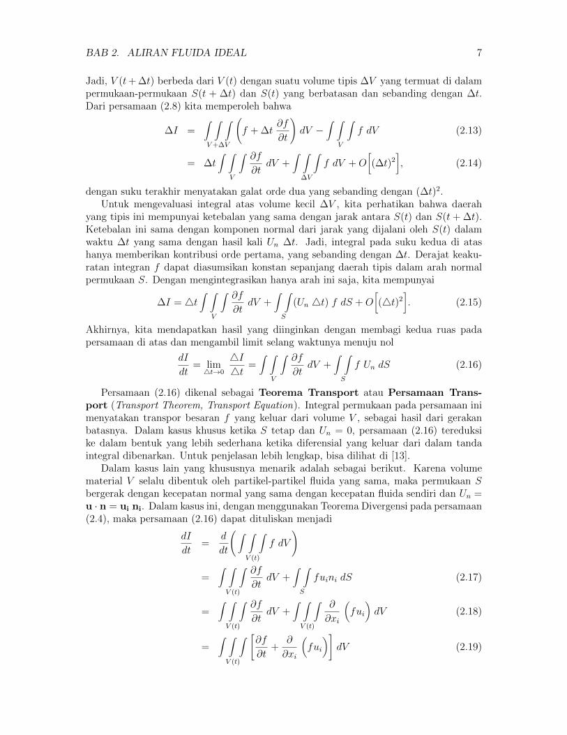
BAB 2. ALIRAN FLUIDA IDEAL 7
Jadi, V (t+ ∆t) berbeda dari V (t) dengan suatu volume tipis ∆V yang termuat di dalampermukaan-permukaan S(t + ∆t) dan S(t) yang berbatasan dan sebanding dengan ∆t.Dari persamaan (2.8) kita memperoleh bahwa
∆I =∫ ∫ ∫
V+∆V
(f + ∆t
∂f
∂t
)dV −
∫ ∫ ∫
V
f dV (2.13)
= ∆t∫ ∫ ∫
V
∂f
∂tdV +
∫ ∫ ∫
∆V
f dV +O[(∆t)2
], (2.14)
dengan suku terakhir menyatakan galat orde dua yang sebanding dengan (∆t)2.Untuk mengevaluasi integral atas volume kecil ∆V , kita perhatikan bahwa daerah
yang tipis ini mempunyai ketebalan yang sama dengan jarak antara S(t) dan S(t + ∆t).Ketebalan ini sama dengan komponen normal dari jarak yang dijalani oleh S(t) dalamwaktu ∆t yang sama dengan hasil kali Un ∆t. Jadi, integral pada suku kedua di atashanya memberikan kontribusi orde pertama, yang sebanding dengan ∆t. Derajat keaku-ratan integran f dapat diasumsikan konstan sepanjang daerah tipis dalam arah normalpermukaan S. Dengan mengintegrasikan hanya arah ini saja, kita mempunyai
∆I = 4t∫ ∫ ∫
V
∂f
∂tdV +
∫ ∫
S
(Un 4t) f dS +O[(4t)2
]. (2.15)
Akhirnya, kita mendapatkan hasil yang diinginkan dengan membagi kedua ruas padapersamaan di atas dan mengambil limit selang waktunya menuju nol
dI
dt= lim4t→0
4I4t =
∫ ∫ ∫
V
∂f
∂tdV +
∫ ∫
S
f Un dS (2.16)
Persamaan (2.16) dikenal sebagai Teorema Transport atau Persamaan Trans-port (Transport Theorem, Transport Equation). Integral permukaan pada persamaan inimenyatakan transpor besaran f yang keluar dari volume V , sebagai hasil dari gerakanbatasnya. Dalam kasus khusus ketika S tetap dan Un = 0, persamaan (2.16) tereduksike dalam bentuk yang lebih sederhana ketika diferensial yang keluar dari dalam tandaintegral dibenarkan. Untuk penjelasan lebih lengkap, bisa dilihat di [13].
Dalam kasus lain yang khususnya menarik adalah sebagai berikut. Karena volumematerial V selalu dibentuk oleh partikel-partikel fluida yang sama, maka permukaan Sbergerak dengan kecepatan normal yang sama dengan kecepatan fluida sendiri dan Un =u · n = ui ni. Dalam kasus ini, dengan menggunakan Teorema Divergensi pada persamaan(2.4), maka persamaan (2.16) dapat dituliskan menjadi
dI
dt=
d
dt
(∫ ∫ ∫
V (t)
f dV
)
=∫ ∫ ∫
V (t)
∂f
∂tdV +
∫ ∫
S
fuini dS (2.17)
=∫ ∫ ∫
V (t)
∂f
∂tdV +
∫ ∫ ∫
V (t)
∂
∂xi
(fui
)dV (2.18)
=∫ ∫ ∫
V (t)
[∂f
∂t+
∂
∂xi
(fui
)]dV (2.19)

BAB 2. ALIRAN FLUIDA IDEAL 8
2.4 Persamaan Kontinuitas
Persamaan ini berkaitan erat dengan hukum kekekalan massa dan Teorema Transportkarena ia diturunkan dari kedua persamaan tersebut. Perhatikan kembali persamaan(2.2) yang menyatakan hukum kekekalan massa. Dengan memanfaatkan hasil TeoremaTransport pada persamaan (2.19) kita memperoleh
d
dt
(∫ ∫ ∫
V
ρ dV
)=∫ ∫ ∫
V
[∂ρ
∂t+
∂
∂xi
(ρ ui
)]dV = 0. (2.20)
Karena integral terakhir dievaluasi pada waktu sesaat yang tetap, perbedaan bahwa Vadalah volume material tidaklah perlu pada taraf/keadaan ini. Lebih jauh, volume terse-but dapat disusun oleh sembarang kelompok partikel-partikel fluida. Dengan demikian,integran di atas sama dengan nol pada seluruh fluida. Jadi, integral volume pada per-samaan (2.20) dapat diganti dengan suatu persamaan diferensial parsial yang menyatakanhukum kekekalan massa dalam bentuk sebagai berikut :
∂ρ
∂t+
∂
∂xi(ρ ui) = 0 (2.21)
Apabila dinyatakan dengan komponen kecepatan tiga dimensi, persamaan tersebut mem-punyai bentuk :
∂ρ
∂t+∂ρu
∂x+∂ρv
∂y+∂ρw
∂z= 0, (2.22)
atau bila ditulis dalam bentuk diferensial :
∂ρ
∂t+∇ · (ρ u) = 0 (2.23)
Persamaan penting inilah yang dikenal sebagai kondisi untuk hukum kekekalan massa ataupersamaan kontinuitas untuk suatu aliran fluida termampatkan. Persamaan (2.22)menggambarkan rata-rata perubahan rapat massa pada suatu titik tetap sebagai hasildari perubahan pada vektor kecepatan massa ρu. Dengan mengekspansi suku-suku yangmemuat hasil kali kerapatan dan komponen kecepatan, kita bisa menurunkan bentuk laindari persamaan kontinuitas.
∂ρ
∂t+ u
∂ρ
∂x+ ρ
∂u
∂x+ v
∂ρ
∂y+ ρ
∂v
∂y+ w
∂ρ
∂z+ ρ
∂w
∂z= 0 (2.24)
(∂ρ
∂t+ u
∂ρ
∂x+ v
∂ρ
∂y+ w
∂ρ
∂z
)+ ρ
(∂u
∂x+∂v
∂y+∂w
∂z
)= 0. (2.25)
Dengan menggunakan operator turunan material atau turunan total (lihat Apendiks A),persamaan (2.25) dapat dituliskan menjadi
Dρ
Dt+ ρ (∇ · u) = 0. (2.26)
Jika alirannya tunak (steady), yakni tidak bergantung waktu, maka∂ρ
∂t= 0 sehingga
persamaan kontinuitas menjadi ∇ · (ρ u) = 0. Dengan menggunakan asumsi bahwa air

BAB 2. ALIRAN FLUIDA IDEAL 9
adalah fluida yang tak termampatkan (incompressible), yakni mempunyai rapat massa ρyang konstan, maka persamaan kontinuitasnya (2.25) tereduksi menjadi
∂u
∂x+∂v
∂y+∂w
∂z= 0. (2.27)
Atau dalam bentuk vektor, yang bisa juga diturunkan dari persamaan (2.26), didapat
∇ · u = 0. (2.28)
Hubungan inilah yang dikenal sebagai kondisi tak termampatkan (condition of in-compressibility). Kondisi ini menyatakan fakta bahwa keseimbangan antara aliran yangkeluar (outflow) dan aliran yang masuk (inflow) untuk suatu elemen volume atau volumematerial adalah nol pada tiap saat.
2.5 Persamaan Euler
Berbeda dengan persamaan kontinuitas yang berkaitan dengan hukum kekekalan massa,persamaan ini berkaitan erat dengan hukum kekekalan momentum dan Teorema Transportkarena ia diturunkan dari kedua persamaan tersebut. Perhatikan kembali persamaan (2.6)yang menyatakan hukum kekekalan momentum. Dengan memanfaatkan hasil TeoremaTransport pada persamaan (2.19) kita memperoleh
∫ ∫ ∫
V
[∂ρui∂t
+∂
∂xj
(ρui uj
)]dV =
∫ ∫ ∫
V
(∂τij∂xj
+ Fi
)dV. (2.29)
Karena integral di atas sama-sama dilakukan atas volume yang sama, maka persamaan(2.29) haruslah dipenuhi untuk integrannya saja, yakni
∂
∂t(ρ ui) +
∂
∂xj
(ρ ui uj
)=∂τij∂xj
+ Fi. (2.30)
Selanjutnya, jika turunan hasil kali di ruas kiri dari persamaan ini diekspansi denganaturan rantai, maka kita peroleh
ui∂ρ
∂t+ ρ
∂ui∂t
+ uiuj∂ρ
∂xj+ ρuj
∂ui∂xj
+ ρui∂uj∂xj
=∂τij∂xj
+ Fi. (2.31)
Dengan asumsi bahwa fluida yang diamati adalah tak termampatkan (incompressible)dan mempunyai rapat massa ρ yang konstan serta dari hasil persamaan kontinuitas pada(2.28), kita sampai pada persamaan Euler∗, yang juga dikenal sebagai persamaanmomentum:
∂ui∂t
+ uj∂ui∂xj
=1
ρ
(∂τij∂xj
+ Fi
). (2.32)
Dengan menggunakan turunan material (lihat kembali Apendiks A), persamaan Eulerdapat dinyatakan menjadi
DuiDt
=1
ρ
(∇ · τi + Fi
). (2.33)
∗Euler, Leonhard (1707-83). Matematikawan Swiss dengan pengertian tenang yang memberikansumbangan dasar yang sangat berarti bagi banyak cabang matematika dan penerapannya: persamaandiferensial, deret tak hingga, analisis kompleks, mekanika dan hidrodinamika, serta kalkulus variasi; diajuga sangat berpengaruh dalam mempromosikan penggunaan dan pengertian analisis.[9]

BAB 2. ALIRAN FLUIDA IDEAL 10
2.6 Persamaan Bernoulli
Kita tinjau kembali persamaan (2.32). Dalam aliran yang tidak ada gesekan (friction-less flow), tidak terdapat tegangan geser dan tegangan normal hanyalah tekanan yangisotropik. Kita sepakati tegangan normal (normal stress) τ11, τ22, dan τ33 berarah positifjika mereka adalah tension. Karena kita telah mengasumsikan bahwa air adalah fluidayang tak kental (inviscid fluid), maka tensor tegangan τ hanya mempunyai komponen-komponen normal dari tekanan. Untuk penjelasan lebih lanjut, silakan lihat di [8, 10, 13].Lalu, kita bentuk menjadi
τ11 = τ22 = τ33 = − p, (2.34)
sehingga persamaan momentum menjadi
∂ui∂t
+ uj∂ui∂xj
=1
ρ
(∂p
∂xj+ Fi
), (2.35)
atau dalam notasi vektorDu
Dt=
1
ρ
(−∇p+ F
), (2.36)
dengan u = (u, v, w), F = (0, 0, −ρ g), dan p adalah tekanan. Jadi,
∂u
∂t+ (u · ∇) u = −∇
(p
ρ+ g z
). (2.37)
Dari identitas vektor, kita punya
u× (∇× u) = (u · ∇) u−∇(
1
2| u |2
). (2.38)
Apabila diasumsikan bahwa air adalah fluida yang tak berputar (irrotational)∗, yakni
∇ × u = 0, maka (u · ∇) u = ∇(
1
2| u |2
). Selain itu, karena asumsi ini, maka
vektor kecepatan u dapat dinyatakan sebagai gradien dari skalar potensial kecepatan,yakni u = ∇φ. (Untuk keterangan yang terperinci, silakan lihat di [3] dan [11]). Inidilakukan dengan tujuan untuk mempermudah kerja kita, karena kita berurusan denganbesaran skalar yang lebih mudah dianalisis daripada besaran vektor.
Dengan demikian,
∂∇φ∂t
+∇(
1
2| u |2
)= −∇
(p
ρ+ g z
), (2.39)
atau
∇(∂φ
∂t+
1
2| u |2 +
p
ρ+ g z
)= 0. (2.40)
∗Fluida irrotational di sini memaksudkan tidak adanya pusaran arus (eddy) atau pusaran air(whirlpool).

BAB 2. ALIRAN FLUIDA IDEAL 11
Apabila persamaan (2.40) diintegrasikan terhadap seluruh ruang kita mendapatkan per-samaan Bernoulli∗∗
∂φ
∂t+
1
2| u |2 +
p
ρ+ g z = konstan ≡ f(t). (2.41)
Bagan keterkaitan fluida ideal
∗∗Bernoulli, Daniel (1700-82). Ilmuwan kelahiran Belanda ini adalah anggota keluarga Swissterkenal yang terdiri atas sekitar 10 matematikawan (ayah, putra, paman, sepupu), dikenal baik karenakaryanya mengenai aliran fluida dan teori kinetik gas; persamaannya untuk aliran fluida pertama kaliditerbitkan pada 1783; dia juga menekuni bidang astronomi dan kemagnetan, serta ilmuwan pertamayang memecahkan persamaan Ricatti.[9]

Bab 3
Teori Pembangkit Gelombang Dua Di-mensi
Kita akan membandingkan dua teori pembangkit gelombang yang telah diselidiki dandibuat model matematisnya. Bagian yang pertama adalah teori yang disederhanakanyang berangkat dari ide dasar berkenaan volume air yang dipindahkan oleh pembangkitgelombang tipe ’flap’ pada sebuah tangki atau kolam air yang cukup panjang (towingtank). Kemudian, bagian yang kedua, akan diulas mengenai teori yang lebih terper-inci yang dihasilkan oleh pembangkit gelombang tipe ’flap’ di salah satu ujung towingtank tadi. Dari hasil kedua teori ini, kita akan mengamati perbandingan antara ampli-tudo gelombang yang dihasilkan H dengan besarnya simpangan maksimum pembangkitgelombang S (stroke).
Di dalam pembahasan tugas akhir ini, teori yang lebih terperinci tersebut didasarkanatas ’teori gelombang linear’ yang dibahas dan dikembangkan oleh Airy∗ sekitar 160 tahunyang lalu, dalam menganalisis perilaku gelombang air laut. [1]
3.1 Teori Pembangkit Gelombang yang
Disederhanakan
Di dalam air dangkal, teori sederhana untuk profil perambatan gelombang yang dihasilkanoleh suatu pembangkit gelombang pertama kali dikembangkan oleh Galvin pada tahun1964, yang bernalar bahwa air yang dipindahkan oleh suatu pembangkit gelombang se-harusnya sama dengan volume puncak dari bentuk gelombang yang merambat. Per-timbangkan sebuah pembangkit gelombang tipe flap yang ujung bawahnya terikat danmempunyai simpangan maksimum stroke S. Kedalaman air dalam towing tank adalah
h. Volume air yang dipindahkan oleh simpangan flap adalah1
2S h. Lihat Gambar 3.1.
Volume air dalam suatu puncak gelombang adalah∫ 1
2L
0
1
2H sin k x dx dengan k =
2π
Ladalah bilangan gelombang. Dengan demikian,
12L∫
0
1
2H sin (k x) dx =
∫ 12L
0
1
2H sin
(2 π
Lx
)dx (3.1)
∗Airy, Sir George Biddel (1801-92). Matematikawan dan fisikawan Inggris, yang menjadi as-tronom kerajaan (Astronomer Royal) selama 46 tahun; dia memberikan sumbangan pada teori-teoricahaya dan, tentulah, pada astronomi, tetapi juga pada gravitasi, kemagnetan dan suara, sebagaimanahalnya pada perambatan gelombang secara umum dan pada teori pasang-surut air pada khususnya. [9]
12

BAB 3. TEORI PEMBANGKIT GELOMBANG DUA DIMENSI 13
=H L
2π(3.2)
=H
k(3.3)
Dengan menyamakan kedua volume,
1
2S h =
H
k= H
L
2 π=H
2
(L
2
)2
π
dengan2
πadalah faktor yang menyatakan perbandingan antara luas daerah yang diben-
tuk oleh profil gelombang dengan persegipanjang yang melingkupinya (yang disebut juga
dengan istilah faktor luas.) Dari persamaan1
2S h =
H
k, kita bisa mengetahui besarnya
perbandingan ketinggian gelombang H dengan simpangan S, yaitu
H
S=
1
2k h.
Hubungan ini berlaku hanya untuk daerah air dangkal, yakni k h <1
10π.
Gambar 3.1: Skema pembangkit gelombang tipe flap.
3.2 Teori Pembangkit Gelombang Linear
Berdasarkan asumsi bahwa air adalah fluida yang tak termampatkan (incompressible),maka dari hasil di sub-bab 2.4, persamaan (2.28), kita telah mempunyai ∇·u = 0. Selainitu, asumsi lain yang digunakan adalah tidak adanya pusaran air (whirpool), dengan katalain, aliran air tak berputar (irrotational). Berdasarkan asumsi ini, dari penjelasan di sub-bab 2.6, kita telah mendapatkan u = ∇φ. Apabila kedua persamaan ini digabungkan,

BAB 3. TEORI PEMBANGKIT GELOMBANG DUA DIMENSI 14
maka kita peroleh ∇·∇φ = ∇2φ = 0. Persamaan ini dikenal dengan persamaan Laplace,∗
yang merupakan persamaan diferensial pengatur (governing differential equation) untukpotensial kecepatan φ. Dalam koordinat kartesius untuk dua dimensi — arah horizontal(sumbu x) dan arah vertikal (sumbu z) — persamaan Laplace dapat dituliskan sebagai
∇2φ =∂2φ
∂x2+∂2φ
∂z2= 0, (3.4)
dan persamaan ini berlaku pada daerah −h ≤ z ≤ η(x, t), 0 ≤ x ≤ ∞.Masalah nilai batas yang terkait di sini adalah persoalan nilai batas untuk peram-
batan gelombang dua dimensi dalam suatu fluida ideal. Kita akan memecahkan per-samaan tersebut dengan beberapa syarat batas yang sesuai dengan kondisi towing tank.Setidaknya, kita memiliki tiga buah kondisi syarat batas yang akan membantu kita untukmemecahkan persamaan penuntun di atas. Berikut ini adalah syarat batas yang berkaitandengan kondisi towing tank.
3.2.1 Syarat batas lateral di pembangkit gelombang(pseudo-boundary)
Misal fungsi yang menggambarkan pergeseran horizontal pada permukaan pembangkitgelombang adalah
F (x, z, t) = x− 1
2S(z) sin ω t = 0, (3.5)
maka dengan melakukan diferensial total pada F (x, z, t), kita peroleh
DF
Dt=∂F
∂t+∂F
∂x
dx
dt+∂F
∂z
dz
dt(3.6)
0 = −1
2ω S(z) cos ω t+ v − 1
2wdS(z)
dzsin ω t (3.7)
v − 1
2wdS(z)
dzsin ω t =
1
2ω S(z) cos ω t pada F (x, z, t) = 0 (3.8)
dengan v dan w masing-masing adalah komponen kecepatan pada arah x dan z. (Ingatbahwa u = (v,w) adalah vektor kecepatan dua dimensi.) Atau, persamaan ini juga dapatdituliskan sebagai
φx =1
2
(φz S
′(z) sin ω t+ ω S(z) cos ω t
). (3.9)
Untuk pergeseran S(z) yang cukup kecil dan kecepatan yang juga kecil, kita dapatmelinearkan persamaan tersebut dengan mengabaikan suku kedua di ruas kiri. Sepertiyang akan dilakukan pada permukaan bebas, akan lebih tepat apabila kita mengungkapkan
∗Laplace, Marquis Pierre Simon de (1749-1827). Matematika-fisikawan Perancis yang mem-berikan sumbangan pada studi mengenai celestial mekanika dan, pada khususnya, menjelaskan orbitplanet Yupiter dan Saturnus; dia mengembangkan ide dalam menggunakan fungsi potensial dan fungsiortogonal, serta memperkenalkan transformasi integralnya; dia juga memainkan peranan penting dalamperkembangan teori peluang.

BAB 3. TEORI PEMBANGKIT GELOMBANG DUA DIMENSI 15
syarat pada batas lateral yang bergerak dalam suku-suku yang dievaluasi di posisi rata-ratanya, yakni pada x = 0. Untuk melakukan hal ini, kita ekspansikan syarat tersebutdalam deret Taylor terpotong (lebih spesifik, deret Maclaurin terpotong).
(φx −
1
2ω S(z) cosω t
)∣∣∣∣∣x= 1
2S(z) sin ω t
=
(φx −
1
2ω S(z) cos ω t
)∣∣∣∣∣x=0
+1
2S(z) sin ω t
∂
∂x
(φx −
1
2ω S(z) cos ω t
)∣∣∣∣∣x=0
+ . . . . (3.10)
Jelaslah, hanya suku pertama dari ekspansi di atas yang linear terhadap φx dan S(z),sedangkan suku-suku yang lain dapat dibuang karena diasumsikan sangat kecil. Dengandemikian, syarat batas lateral akhir sebagai akibat dari proses linearisasi adalah per-samaan
u(0, z, t) = φx =1
2ω S(z) cos(ωt). (3.11)
3.2.2 Syarat batas di dasar towing tank (persyaratan kinematika)
Karena tidak ada aliran air yang menembus ke dasar towing tank, maka kecepatan fluidapada arah vertikal adalah sama dengan nol, yakni
φz =∂φ
∂z= 0, pada z = −h. (3.12)
3.2.3 Syarat batas di permukaan air
• Syarat batas kinematika permukaan bebas
Pada setiap batas, apakah ia bebas, seperti pada permukaan air, ataupun tidak be-bas (fixed), seperti pada dasar kolam, beberapa persyaratan fisis haruslah dipenuhi olehkecepatan fluida. Di bawah pengaruh gaya, batas ini bisa saja mengalami perubahanbentuk (deformasi). Semua persyaratan ini yang bekerja pada kinematika partikel airdisebut dengan syarat batas kinematika (kinematics boundary conditions). Pada setiappermukaan fluida atau perbatasan fluida (interface), jelaslah bahwa tidak akan terdapataliran yang melewati interface, jika tidak demikian, maka tak terdapat interface. Halseperti ini sangatlah jelas dalam kasus permukaan tetap kedap air (impermeable fixedsurface) seperti suatu lembar timbunan dinding laut (sheet pile seawall).[3]
Misalkan fungsi yang menggambarkan permukaan air adalah
G(x, z, t) = z − η (x, t) = 0, (3.13)
dengan η(x, t) adalah ketinggian gelombang, yakni jarak suatu titik pada permukaangelombang dari permukaan bebas rata-rata atau sering dikenal dengan istilah elevasi per-mukaan air. Maka, diferensial total persamaan di atas akan memberikan
DG
Dt=∂G
∂t+∂G
∂x
dx
dt+∂G
∂z
dz
dt(3.14)
0 = −∂η∂t
+
(− ∂η
∂x
)v + w (3.15)
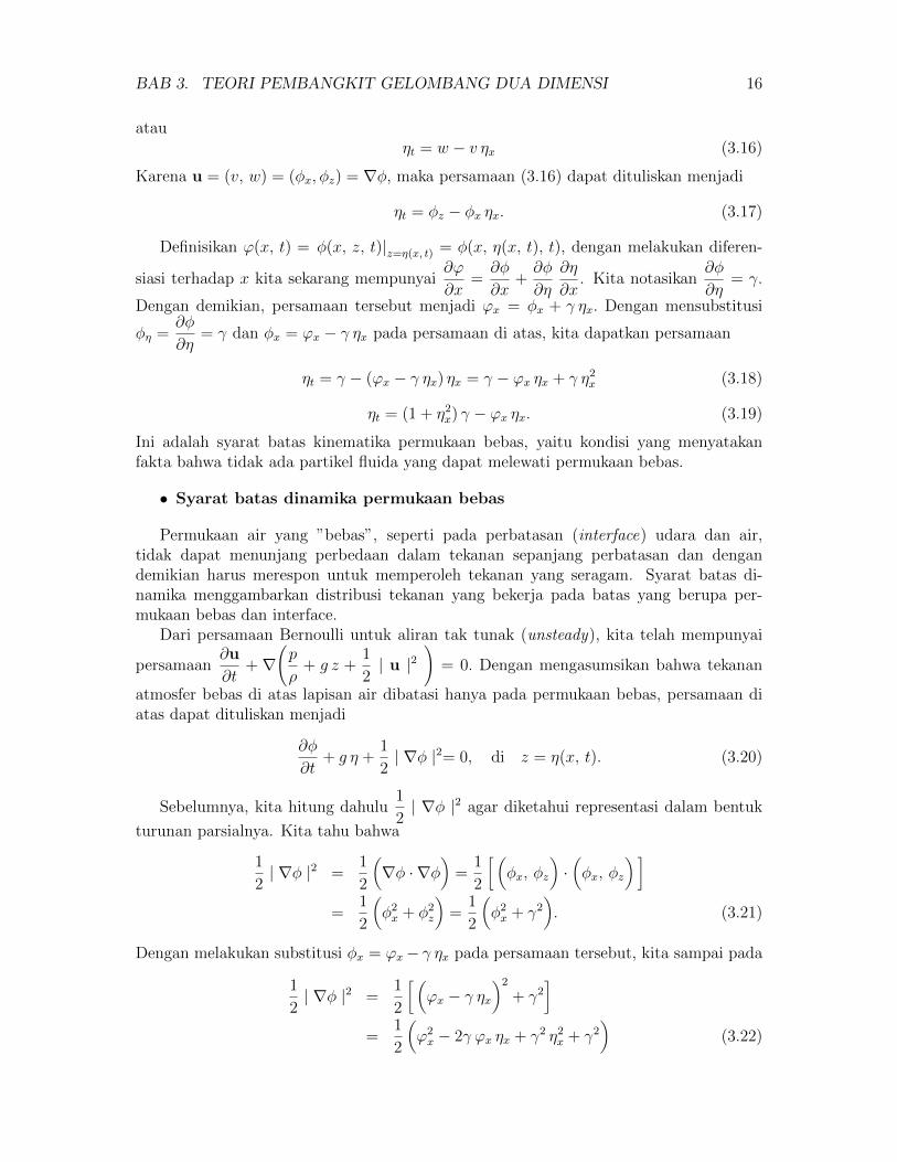
BAB 3. TEORI PEMBANGKIT GELOMBANG DUA DIMENSI 16
atauηt = w − v ηx (3.16)
Karena u = (v, w) = (φx, φz) = ∇φ, maka persamaan (3.16) dapat dituliskan menjadi
ηt = φz − φx ηx. (3.17)
Definisikan ϕ(x, t) = φ(x, z, t)|z=η(x, t) = φ(x, η(x, t), t), dengan melakukan diferen-
siasi terhadap x kita sekarang mempunyai∂ϕ
∂x=∂φ
∂x+∂φ
∂η
∂η
∂x. Kita notasikan
∂φ
∂η= γ.
Dengan demikian, persamaan tersebut menjadi ϕx = φx + γ ηx. Dengan mensubstitusi
φη =∂φ
∂η= γ dan φx = ϕx − γ ηx pada persamaan di atas, kita dapatkan persamaan
ηt = γ − (ϕx − γ ηx) ηx = γ − ϕx ηx + γ η2x (3.18)
ηt = (1 + η2x) γ − ϕx ηx. (3.19)
Ini adalah syarat batas kinematika permukaan bebas, yaitu kondisi yang menyatakanfakta bahwa tidak ada partikel fluida yang dapat melewati permukaan bebas.
• Syarat batas dinamika permukaan bebas
Permukaan air yang ”bebas”, seperti pada perbatasan (interface) udara dan air,tidak dapat menunjang perbedaan dalam tekanan sepanjang perbatasan dan dengandemikian harus merespon untuk memperoleh tekanan yang seragam. Syarat batas di-namika menggambarkan distribusi tekanan yang bekerja pada batas yang berupa per-mukaan bebas dan interface.
Dari persamaan Bernoulli untuk aliran tak tunak (unsteady), kita telah mempunyai
persamaan∂u
∂t+ ∇
(p
ρ+ g z +
1
2| u |2
)= 0. Dengan mengasumsikan bahwa tekanan
atmosfer bebas di atas lapisan air dibatasi hanya pada permukaan bebas, persamaan diatas dapat dituliskan menjadi
∂φ
∂t+ g η +
1
2| ∇φ |2= 0, di z = η(x, t). (3.20)
Sebelumnya, kita hitung dahulu1
2| ∇φ |2 agar diketahui representasi dalam bentuk
turunan parsialnya. Kita tahu bahwa
1
2| ∇φ |2 =
1
2
(∇φ · ∇φ
)=
1
2
[ (φx, φz
)·(φx, φz
) ]
=1
2
(φ2x + φ2
z
)=
1
2
(φ2x + γ2
). (3.21)
Dengan melakukan substitusi φx = ϕx− γ ηx pada persamaan tersebut, kita sampai pada
1
2| ∇φ |2 =
1
2
[ (ϕx − γ ηx
)2
+ γ2]
=1
2
(ϕ2x − 2γ ϕx ηx + γ2 η2
x + γ2)
(3.22)

BAB 3. TEORI PEMBANGKIT GELOMBANG DUA DIMENSI 17
Jadi,1
2| ∇φ |2=
1
2ϕ2x − γ ϕx ηx +
1
2
(1 + η2
x
)γ2.
Dari ϕ(x, t) = φ(x, η(x, t), t), diferensiasi parsial terhadap t memberikan∂ϕ
∂t=∂φ
∂t+
∂φ
∂η
∂η
∂t=⇒ ϕt = φt + γ ηt =⇒ φt = ϕt − γ ηt.
Dengan demikian, substitusi pada persamaan Bernoulli (3.20) akan menghasilkan
ϕt − γ ηt +1
2ϕ2x − γ ϕx ηx +
1
2
(1 + η2
x
)γ2 + g η = 0. (3.23)
Untuk memperoleh bentuk yang lebih sederhana, kita substitusi ηt =(
1 + η2x
)γ − ϕx ηx
yang telah diperoleh dari syarat batas kinematika. Akibatnya,
ϕt − γ[ (
1 + η2x
)γ − ϕx ηx
]+
1
2ϕ2x − γ ϕx ηx +
1
2
(1 + η2
x
)γ2 + g η = 0, (3.24)
ϕt −(
1 + η2x
)γ2 + ϕx ηx γ +
1
2ϕ2x − γ ϕx ηx +
1
2
(1 + η2
x
)γ2 + g η = 0, (3.25)
ϕt −1
2
(1 + η2
x
)γ2 +
1
2ϕ2x + g η = 0. (3.26)
Akhirnya diperoleh, ϕt =1
2
(1 + η2
x
)γ2 − 1
2ϕ2x − g η. Persamaan inilah yang dikenal
dengan syarat batas dinamika permukaan bebas.
Gambar 3.2: Skema pembangkit gelombang dengan persamaan pengatur dan syarat-syarat batasnya.
Untuk air dangkal, kita lebih tertarik untuk mempelajari dan menggunakan bentukterlinearisasi dari syarat batas kinematika dan syarat batas dinamika permukaan bebas

BAB 3. TEORI PEMBANGKIT GELOMBANG DUA DIMENSI 18
agar lebih memudahkan dalam menyelesaikan persamaan diferensial pengatur dengansyarat-syarat batas yang telah ditentukan.
Tinjau kembali persamaan (3.16) sebagai syarat batas kinematika permukaan bebas,
∂η
∂t= (w)|z=η −
∂η
∂x(v)|z=η (3.27)
atau∂η
∂t=
(∂φ
∂z
)∣∣∣∣∣z=η
− ∂η
∂x
(∂φ
∂x
)∣∣∣∣∣z=η
(3.28)
Dengan mengabaikan suku-suku non-linear-nya, kita miliki bentuk yang lebih sederhanadari syarat batas kinematika, yakni
(∂φ
∂z
)∣∣∣∣∣z=0
=∂η
∂t. (3.29)
Dengan cara serupa, kita juga mempunyai bentuk yang lebih sederhana dari syaratbatas dinamika permukaan bebas, yakni
(∂φ
∂t
)∣∣∣∣∣z=0
= −g η. (3.30)
Skema pembangkit gelombang dengan governing equation dan beberapa syarat batasdapat dilihat pada Gambar 3.2.
3.3 Solusi Governing Differential Equation
Berikut ini adalah solusi umum potensial kecepatan
φ(x, z, t) = Ap cosh kp (h+ z) sin (kp x− ω t) + (Ax+B)
+C e−ks x cos ks (h+ z) cos ω t. (3.31)
Untuk permasalahan pembangkit gelombang, koefisien A di atas haruslah sama dengannol karena tidak ada aliran seragam yang mungkin melalui pembangkit gelombang dankoefisien B di atas juga dapat diset menjadi nol juga tanpa mempengaruhi medan ke-cepatan. Suku-suku sisanya haruslah memenuhi dua syarat batas permukaan bebas yangterlinearisasi. Biasanya akan lebih bermanfaat apabila menggabungkan kedua syarat batastersebut menjadi bentuk yang lebih sederhana.Dengan menurunkan φ terhadap t, kita peroleh
∂φ
∂t= −ω Ap cosh kp (h+ z) cos (kp x− ω t)
−ω C e−ks x cos ks (h+ z) sinω t. (3.32)
Turunan kedua φ terhadap t menghasilkan
∂2φ
∂t2= −ω2Ap cosh kp (h+ z) sin (kp x− ω t)−ω2C e−ks x cos ks (h+ z) cos ω t
= −ω2 φ. (3.33)
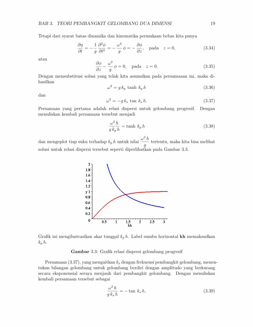
BAB 3. TEORI PEMBANGKIT GELOMBANG DUA DIMENSI 19
Tetapi dari syarat batas dinamika dan kinematika permukaan bebas kita punya
∂η
∂t= − 1
g
∂2φ
∂t2= − ω
2
gφ = − ∂φ
∂z, pada z = 0, (3.34)
atau∂φ
∂z− ω2
gφ = 0, pada z = 0. (3.35)
Dengan mensubstitusi solusi yang telah kita asumsikan pada persamaaan ini, maka di-hasilkan
ω2 = g kp tanh kp h (3.36)
danω2 = −g ks tan ks h. (3.37)
Persamaan yang pertama adalah relasi dispersi untuk gelombang progresif. Denganmenuliskan kembali persamaan tersebut menjadi
ω2 h
g kp h= tanh kp h (3.38)
dan mengeplot tiap suku terhadap kp h untuk nilaiω2 h
gtertentu, maka kita bisa melihat
solusi untuk relasi dispersi tersebut seperti diperlihatkan pada Gambar 3.3.
Grafik ini mengilustrasikan akar tunggal kp h. Label sumbu horizontal kh memaksudkankp h.
Gambar 3.3: Grafik relasi dispersi gelombang progresif
Persamaan (3.37), yang mengaitkan ks dengan frekuensi pembangkit gelombang, menen-tukan bilangan gelombang untuk gelombang berdiri dengan amplitudo yang berkurangsecara eksponensial seraya menjauh dari pembangkit gelombang. Dengan menuliskankembali persamaan tersebut sebagai
ω2 h
g ks h= − tan ks h, (3.39)

BAB 3. TEORI PEMBANGKIT GELOMBANG DUA DIMENSI 20
maka dengan mengeplot grafiknya kita bisa melihat bahwa ia mempunyai tak hinggabanyaknya penyelesaian. Penyelesaian persamaan ini dapat dilihat dalam bentuk grafikrelasi dispersi, seperti tampak pada Gambar 3.4.
Gambar 3.4: Grafik relasi dispersi gelombang berdiri
Grafik ini mengilustrasikan terdapat tak hingga banyaknya akar majemuk ks(n)h. Labelsumbu horizontal kh memaksudkan ks h.
Setiap penyelesaian akan dinyatakan dengan ks(n), dengan n bilangan asli. Bentukakhir dari potensial kecepatan adalah
φ(x, z, t) = Ap cosh kp (h+ z) sin (kp x− ω t)
+∞∑
n=1
Cn e−ks(n)x cos ks(n) (h+ z) cos ω t. (3.40)
Suku pertama menyatakan gelombang progresif yang dihasilkan oleh pembangkit gelom-bang, sedangkan suku deret menyatakan gelombang berdiri yang semakin meluruh serayamenjauh dari pembangkit gelombang.
Untuk memperoleh solusi gelombang yang lengkap, kita harus menentukan Ap dan Cn.Nilai-nilai ini diperoleh dengan bantuan syarat batas lateral di pembangkit gelombang,yakni
u(0, z, t) =
(∂φ
∂x
)∣∣∣∣∣x=0
=1
2ω S(z) cos ω t (3.41)
Dengan menurunkan potensial kecepatan terhadap x dan mengevaluasinya di x = 0, kitamemperoleh
1
2ω S(z) cos ω t = Ap kp cosh kp (h+ z) cos ω t
−∞∑
n=1
Cn ks(n) cos ks(n) (h+ z) cos ω t, (3.42)
atau1
2ω S(z) = Ap kp cosh kp (h+ z)−
∞∑
n=1
Cn ks(n) cos ks(n) (h+ z). (3.43)

BAB 3. TEORI PEMBANGKIT GELOMBANG DUA DIMENSI 21
Sekarang kita mempunyai sebuah fungsi z yang sama dengan suatu deret fungsi-fungsitrigonometri dari z di ruas kanan, situasi yang mirip dengan deret Fourier. Kita punya
fakta bahwa himpunan fungsi-fungsi{
cosh kp (h + z), cos [ks(n) (h + z)]}∞
n=1memben-
tuk suatu deret harmonik lengkap fungsi-fungsi ortogonal, dan sembarang fungsi kontinudapat diekspansi dalam suku-suku deret tersebut.
Dengan demikian, untuk mencari Ap, kalikan persamaan di atas dengan cosh kp (h+z)dan diintegrasikan terhadap z dari −h sampai 0. Kita sekarang mempunyai
0∫
−h
1
2ω S(z) cosh kp (h+ z) dz =
0∫
−hAp kp cosh k2
p (h+ z) dz
−0∫
−h
∞∑
n=1
Cn ks(n) cos ks(n) (h+ z) cosh kp (h+ z) dz. (3.44)
Dengan menggunakan sifat keortogonalan, suku terakhir akan sama dengan nol, dan aki-batnya
Ap =12ω∫ 0−h S(z) cosh kp (h+ z) dz
kp∫ 0−h cosh k2
p (h+ z) dz(3.45)
Untuk pembangkit gelombang tipe flap, fungsi simpangan S dapat dinyatakan secaraspesifik sebagai
S(z) = S
(1 +
z
h
). (3.46)
Dengan menggunakan kalkulus sederhana kita bisa menyatakan koefisien Ap tanpa meng-gunakan integral, yaitu
Ap =2ω S
k2p h
kp h sinh kp h− cosh kp h+ 1
sinh 2 kp h+ 2 kp h(3.47)
Dengan cara yang serupa, kita bisa mendapatkan koefisien C(n) dengan mengalikanpersamaan (3.43) dengan cos [ks(n) (h+ z)] dan mengintegrasikannya terhadap z dari −hsampai dengan 0 (sepanjang kedalaman). Kita dapatkan
Cn =−1
2ω∫ 0−h S(z) cos ks(n) (h+ z) dz
ks(n)∫ 0−h cos2 [ks(n) (h+ z)] dz
(3.48)
atau, dengan melakukan sedikit proses integrasi kita sampai pada hasil berikut :
Cn =−2ω S
[ks(n)]2 h
[ks(n)h] sin [ks(n)h] + cos [ks(n)h]
sin [2 ks(n)h] + 2 ks(n)h. (3.49)
Tinggi gelombang untuk gelombang progresif ditentukan dengan mengevaluasi η cukupjauh dari pembangkit gelombang.
η = −1
g
(∂φ
∂t
)∣∣∣∣∣z=0
=Apgω cosh kp h cos (kp x− ω t)
=H
2cos (kp x− ω t) x� h (3.50)

BAB 3. TEORI PEMBANGKIT GELOMBANG DUA DIMENSI 22
Dengan mensubstitusi nilai Ap yang telah diperoleh, kita bisa mendapatkan perbandingantinggi gelombang H dengan besarnya stroke S, yaitu
H
S= 4
(sinh kp h
kp h
) (kp h sinh kp h− cosh kp h+ 1
sinh 2 kp h+ 2 kp h
). (3.51)
Plot grafik perbandingan H dan S, baik untuk teori yang disederhanakan (air dangkal)maupun yang lebih lengkap (teori pembangkit gelombang linear) dapat dilihat pada Gam-bar 3.5.
Gambar 3.5: Grafik perbandingan ketinggian gelombang H dengan simpangan S ter-hadap kedalaman relatif kp h.
Label sumbu horizontal kh memaksudkan kp h, sedangkan label sumbu vertikal H S
memaksudkanH
S.

Bab 4
Simulasi Numerik
Pada bab ini, akan dibahas beberapa hasil yang diperoleh dengan memilih nilai-nilai be-saran tertentu. Dengan bantuan perangkat lunak Maple V Release 5, kita bisa melihatanimasi gelombang monokromatik yang dihasilkan apabila pembangkit gelombang diger-akkan dengan simpangan tertentu.
4.1 Menghitung Bilangan Gelombang Progresif
Kita perhatikan kembali persamaan (3.36) yang menyatakan relasi dispersi gelombangprogresif :
ω2 = g kp tanh kp h. (4.1)
Untuk memperoleh nilai bilangan gelombang kp, kita tidak dapat menghitungnya secaraeksak, sehingga digunakan metode numerik untuk menyelesaikannya. Beberapa nilai yangdiberikan adalah frekuensi sudut monokromatik ω = 2 rad/detik, tetapan percepatangravitasi g = 9, 8 m/detik2, dan kedalaman towing tank h = 3 m. Dengan menggunakaniterasi Newton-Raphson, kita akan mencari nilai kp apabila diberikan tebakan awal p0
dengan mencari akar persamaan f(kp) = 0, dengan f(kp) = ω2 − g kp tanh kp h. Untukmengetahui lebih lengkap mengenai algoritma iterasi Newton-Raphson, dapat dilihat diApendiks B. Dengan memilih nilai-nilai galat δ = 10−9, ε = 10−9, dan kecil = 10−9
juga, serta iterasi maksimum = 5000, maka dengan menggunakan tebakan awal p0 = 0, 5kita memperoleh hasil kp = 0, 4624593666. Lihat grafiknya pada Gambar 3.3.
Untuk ω = 1, nilai bilangan gelombang progresif yang diperoleh adalah kp = 0, 1943823443.
4.2 Menghitung Bilangan Gelombang Berdiri
Kita perhatikan kembali persamaan (3.37) yang menyatakan relasi dispersi gelombangberdiri :
ω2 = −g ks tan ks h. (4.2)
Untuk memperoleh nilai bilangan gelombang ks, kita tidak dapat menghitungnya secaraeksak, sehingga digunakan metode numerik untuk menyelesaikannya. Beberapa nilai yangdiberikan adalah frekuensi sudut monokromatik ω = 2 rad/detik, tetapan percepatangravitasi g = 9, 8 m/detik2, dan kedalaman towing tank h = 3 m. Dengan menggu-nakan iterasi Newton-Raphson, kita akan mencari nilai ks apabila diberikan tebakan awalp0 dengan mencari akar persamaan g(ks) = 0, dengan g(ks) = ω2 + g ks tan ks h. Un-tuk mengetahui lebih lengkap mengenai algoritma iterasi Newton-Raphson, dapat dilihatkembali di Apendiks B. Nilai-nilai galat yang dipilih adalah δ = 10−5, ε = 10−5, dan
23

BAB 4. SIMULASI NUMERIK 24
kecil = 10−5 dengan menggunakan iterasi maksimum = 10000. Karena perpotongangrafik pada relasi dispersi menghasilkan tak hingga banyaknya titik potong, yakni nilai-nilai bilangan gelombang berdiri, maka digunakan tebakan awal yang bervariasi sesuaidengan kebutuhan, p0 = 1, 2, 3, · · · . Untuk keperluan, kita pilih beberapa bilangan gelom-bang tertentu saja yang berurutan. Akhirnya, kita memperoleh hasilks(1) = 0, 9061212307;ks(2) = 2, 028197863;ks(3) = 3, 097926261;ks(4) = 4, 156159228;ks(5) = 5, 209926525;ks(6) = 6, 261487236;ks(7) = 7, 311794624;ks(8) = 8, 361321437;ks(9) = 9, 410329031.Lihat kembali grafiknya pada Gambar 3.4.
Dengan cara yang serupa seperti di atas, yakni menggunakan tebakan awal yangbervariasi, maka untuk ω = 1 kita memperoleh beberapa nilai bilangan gelombang berdiriseperti berikut:ks(1) = 1, 013758189;ks(2) = 2, 078040121;ks(3) = 3, 130732073;ks(4) = 4, 180655871.
4.3 Profil Gelombang Monokromatik
4.3.1 Dua Profil Gelombang dengan Ketinggian H Berbeda
Perhatikan kembali persamaan (3.40), persamaan potensial kecepatan yang menggam-barkan gelombang air yang dihasilkan oleh pembangkit gelombang
φ(x, z, t) = Ap cosh kp (h+ z) sin (kp x− ω t)
+∞∑
n=1
Cn e−ks(n)x cos ks(n) (h+ z) cos ω t. (4.3)
Dengan menggunakan persamaan (3.47) dan persamaan (3.51), kita bisa menyatakankonstanta Ap dalam ω, H, kp, dan h, yakni :
Ap =ωH
2 kp sin kp h(4.4)
Dengan mensubstitusi nilai ω = 2, kp = 0, 4624593666, dan h = 3, maka :
• untuk H = 0, 5, kita punya Ap = 1, 099621133; dan
• untuk H = 0, 75, kita punya Ap = 1, 649431700.

BAB 4. SIMULASI NUMERIK 25
Untuk mendapatkan simpangan maksimum S, kita menggunakan persamaan (3.51),yakni
S =
(H kp h
4 sinh kp h
) (sinh 2 kp h+ 2 kp h
kp h sinh kp h− cosh kp h+ 1
). (4.5)
Dengan mensubstitusi kembali nilai-nilai yang telah kita punya, akibatnya :
• untuk H = 0, 5, kita peroleh S = 0, 2908632665; dan
• untuk H = 0, 75, kita peroleh S = 0, 4362948995.
Profil gerakan pembangkit gelombang ketika ia mencapai simpangan terjauh dapatdilihat pada Gambar 4.1.
Gambar 4.1: Simpangan terjauh flap yang menghasilkan dua profil gelombang denganketinggian berbeda.
Untuk mencari besarnya konstanta Cn sebagai koefisien gelombang berdiri, kita meng-gunakan persamaan (3.49), yaitu
Cn =−2ω S
[ks(n)]2 h
[ks(n)h] sin [ks(n)h] + cos [ks(n)h]
sin [2 ks(n)h] + 2 ks(n)h. (4.6)
Nilai-nilai ks(n) yang telah kita punyai adalah sebanyak 4 buah, karena untuk n yanglebih besar pengaruh konstanta Cn terhadap solusi gelombang relatif kecil sehingga dapatdiabaikan.
• Untuk S = 0, 2908632665, nilaiC1 = 0, 08013595964;C2 = 0, 00976252019;C3 = 0, 001714039296; danC4 = 0, 001110132786.

BAB 4. SIMULASI NUMERIK 26
• Untuk S = 0, 4362948995, nilaiC1 = 0, 1202039395;C2 = 0, 01464378027;C3 = 0, 002571058938; danC4 = 0, 001665199177.
Dengan menggunakan persamaan (3.30), yakni
η(x, t) = −1
g
(∂φ
∂t
)∣∣∣∣∣z=0
(4.7)
kita dapat mencari persamaan elevasi permukaan gelombang air yang terbentuk. Denganbantuan perangkat lunak komputer kita juga bisa menampilkan hasil plot permukaan.Hasil plot permukaan air dengan dua ketinggian yang berbeda diperlihatkan pada Gam-bar 4.2.
Gambar 4.2: Bentuk permukaan gelombang air (elevasi) yang dibentuk oleh dua gelom-bang dengan ketinggian yang berbeda.
4.3.2 Dua Profil Gelombang dengan Frekuensi Sudut ω Berbeda
Cara yang serupa seperti pada sub-bab sebelumnya diterapkan juga pada sub-bab ini.Kedalaman towing tank masih sama yaitu h = 3 m dan profil ketinggian gelombang yangdiinginkan adalah H = 0, 5 m. Namun, frekuensi sudut ω yang diberikan adalah masing-masing 2 dan 1. Dengan menggunakan iterasi Newton-Raphson terhadap relasi dispersigelombang progresif maupun gelombang berdiri, kita bisa mendapatkan nilai kp dan ks(n)untuk ω = 1. Hasil-hasilnya telah diperoleh pada sub-bab 4.1 dan 4.2. Untuk lebih jelas,hasilnya dicantumkan kembali pada sub-bab ini. Sebagai tambahan, dicantumkan juganilai-nilai konstanta potensial kecepatan yang berkaitan dengan nilai ω, yakni Ap dan Cn.
Berikut ini adalah hasil yang telah diperoleh dengan menggunakan bantuan perangkatlunak Maple V Release 5.
a. Untuk ω = 2
• Nilai bilangan gelombang progresif kp = 0, 4624593666.
• Nilai-nilai bilangan gelombang berdiriks(1) = 0, 9061212307; ks(2) = 2, 028197863;ks(3) = 3, 0979262610; ks(4) = 4, 156159228.

BAB 4. SIMULASI NUMERIK 27
• Nilai koefisien Ap = 1, 099621133
• Besar simpangan maksimum S = 0, 2908632665
• Nilai-nilai koefisien Cn adalahC1 = 0, 8013595964; C2 = 0, 009762520190;C3 = 0, 001714039296; C4 = 0, 001110132786.
b. Untuk ω = 1
• Nilai bilangan gelombang progresif kp = 0, 1943823443.
• Nilai-nilai bilangan gelombang berdiriks(1) = 1, 013758189; ks(2) = 2, 078040121;ks(3) = 3, 130732073; ks(4) = 4, 180655871.
• Nilai koefisien Ap = 2, 335633604
• Besar simpangan maksimum S = 1, 140576790
• Nilai-nilai koefisien Cn adalahC1 = 0, 2125853842; C2 = 0, 004369427564;C3 = 0, 007018430814; C4 = 0, 0005323318426.
Profil gerakan flap pada saat simpangan terjauh ditunjukkan pada Gambar 4.3.
Gambar 4.3: Simpangan terjauh flap yang menghasilkan dua profil gelombang denganfrekuensi sudut berbeda.
Profil gelombang yang dihasilkan evolusinya terhadap waktu dapat dilihat pada Gam-bar 4.4 sampai dengan Gambar 4.11.

BAB 4. SIMULASI NUMERIK 28
Gambar 4.4: Grafik permukaan gelombang air pada t = 3.
Gambar 4.5: Grafik permukaan gelombang air pada t = 5.
Gambar 4.6: Grafik permukaan gelombang air pada t = 10.
Gambar 4.7: Grafik permukaan gelombang air pada t = 15.
Gambar 4.8: Grafik permukaan gelombang air pada t = 17.

BAB 4. SIMULASI NUMERIK 29
Gambar 4.9: Grafik permukaan gelombang air pada t = 25.
Gambar 4.10: Grafik permukaan gelombang air pada t = 30.
Gambar 4.11: Grafik permukaan gelombang air pada t = 34.
Bab 5
Kesimpulan dan Saran
5.1 Kesimpulan
Berikut ini adalah beberapa kesimpulan yang diperoleh penulis setelah mengerjakan tugasakhir mengenai pembangkit gelombang ini:
a. Asumsi fluida ideal diperlukan untuk memodelkan permasalahan pembangkitangelombang.
b. Teori gelombang linear digunakan untuk memperoleh pernyelesaian dari governingdifferential equation yang dihasilkan pada pemodelan pada bagian (a).
c. Kaitan antara bilangan gelombang, ketinggian gelombang, dan simpangan pem-bangkit gelombang diperoleh melalui teori gelombang pada bagian (b).
d. Untuk air dangkal, teori yang disederhanakan dan teori gelombang linear mem-berikan hasil yang sama, sedangkan untuk air yang lebih dalam, kedua teori tersebutmemberikan hasil yang berbeda.
5.2 Saran
Berikut ini adalah beberapa saran yang dapat dikembangkan untuk bahan tugas akhirataupun penelitian berikutnya :
a. Teori gelombang yang digunakan bisa menggunakan teori gelombang non-linear danbisa diperluas menjadi teori pembangkit gelombang tiga dimensi.
b. Tipe gelombang yang dihasilkan bisa dikembangkan menjadi sembarang gelombangtak regular.
c. Penambahan pantai (beach) dapat digunakan untuk menggantikan domain yangsemi-infinite.
30

Apendiks A
Turunan Material
OperatorD
Dt=
∂
∂t+ u · ∇ (A.1)
dikenal sebagai turunan material, turunan total, turunan substansial, atau turunan La-
grange. Secara umum,D
Dtadalah suatu operator vektor. Akibatnya, komponen-komponen
D
Dtyang bekerja pada vektor tidaklah sama dengan yang bekerja pada komponen skalar
suatu vektor, kecuali dalam koordinat Kartesius. Operator turunan material dapat jugaditerapkan pada besaran skalar, seperti temperatur. Secara fisis, ini menyatakan peruba-han besaran tersebut terhadap waktu, dengan pengamat bergerak bersama fluida yangdiukur pada lokasi tertentu di ruang dan waktu instant ketika turunan tersebut dievaluasi.
Operator ini adalah turunan total terhadap waktu yang bekerja pada elemen fluida,yang dapat dilihat sebagai berikut. Misalkan ξ adalah koordinat ruang (spatial) yangmenggambarkan fluida pada keadaan (instant) awal yang tetap, t = 0, dan misalkan pulax adalah koordinat ruang yang memberikan lokasi pada saat t dari elemen fluida bahwapada saat ξ ketika t = 0. Tetapi x = x(ξ, t). Turunan terhadap waktu (Eulerian) adalah
∂
∂t=
∂
∂t
∣∣∣∣∣x tetap
, (A.2)
di mana yang berperan sebagai turunan Lagrangian adalah
D
Dt=
∂
∂t
∣∣∣∣∣ξ tetap
. (A.3)
Dengan menggunakan aturan rantai,
D
Dt=
∂
∂t
∣∣∣∣∣ξ tetap
=∂
∂t
∣∣∣∣∣x tetap
+∂xi∂t
∣∣∣∣∣ξ tetap
∂
∂t,
yang menghasilkan persamaan (A.1), karena∂x
∂t
∣∣∣∣∣ξ
= u.
Operator ini digunakan juga dalam persamaan Navier-Stokes yang menyatakan per-cepatan total suatu partikel sebagai
a =Du
Dt=∂u
∂t+
(u∂u
∂x+ v
∂u
∂y+ w
∂u
∂z
). (A.4)
31

APENDIKS A. TURUNAN MATERIAL 32
Di ruas kanan dari (A.4), suku pertama menyatakan percepatan lokal (local accel-eration) yang akan sama dengan 0 untuk aliran tunak (steady-state flow) dan sisanyamenyatakan percepatan konvektif (convective acceleration). Suku percepatan konvektifmenunjukkan bahwa aliran fluida mempunyai kecepatan yang berbeda pada posisi yangberbeda pula. Untuk penjelasan yang lebih lengkap, silakan lihat di [5, 8].
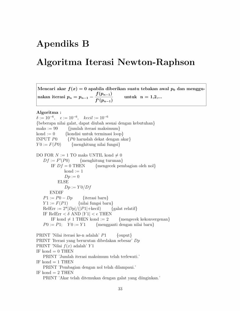
Apendiks B
Algoritma Iterasi Newton-Raphson
Mencari akar f(x) = 0 apabila diberikan suatu tebakan awal p0 dan menggu-
nakan iterasi pn = pn−1 −f(pn−1)
f ′(pn−1)untuk n = 1,2,...
Algoritma :δ := 10−6, ε := 10−6, kecil := 10−6
{beberapa nilai galat, dapat diubah sesuai dengan kebutuhan}maks := 99 {jumlah iterasi maksimum}kond := 0 {kondisi untuk terminasi loop}INPUT P0 {P0 haruslah dekat dengan akar}Y 0 := F (P0) {menghitung nilai fungsi}
DO FOR N := 1 TO maks UNTIL kond 6= 0Df := F ′(P0) {menghitung turunan}
IF Df = 0 THEN {mengecek pembagian oleh nol}kond := 1Dp := 0
ELSEDp := Y 0/Df
ENDIFP1 := P0−Dp {iterasi baru}Y 1 := F (P1) {nilai fungsi baru}RelErr := 2*|Dp|/(|P1|+kecil) {galat relatif}IF RelErr < δ AND |Y 1| < ε THEN
IF kond 6= 1 THEN kond := 2 {mengecek kekonvergenan}P0 := P1; Y 0 := Y 1 {mengganti dengan nilai baru}
PRINT ’Nilai iterasi ke-n adalah’ P1 {ouput}PRINT ’Iterasi yang berurutan dibedakan sebesar’ DpPRINT ’Nilai f(x) adalah’ Y 1IF kond = 0 THEN
PRINT ’Jumlah iterasi maksimum telah terlewati.’IF kond = 1 THEN
PRINT ’Pembagian dengan nol telah dilampaui.’IF kond = 2 THEN
PRINT ’Akar telah ditemukan dengan galat yang diinginkan.’
33

Apendiks C
Laboratorium Hidrodinamika di Dunia
Berikut ini adalah beberapa fasilitas laboratorium hidrodinamika yang ada di berbagainegara di penjuru dunia. Banyak dari antara mereka yang digunakan untuk ujicobakomersial dan pertahanan yang berkaitan dengan struktur kelautan. Untuk keteranganterperinci, bisa dilihat di [2] atau merujuk ke International Towing Tank Conference.
a. Institute of Marine Dynamics Towing Tank, St. John’s, Newfoundland,KanadaKolam Air DalamUkuran Kolam (Panjang, Lebar, dan Kedalaman): 200 m × 12 m × 7 mKecepatan Pembawa : 10 m/detikGelombang : Regular dan Tak regular; 1 mPembangkit gelombang : Tipe flap-gandaPantai : Memuat dasar berombak.
b. Offshore Model Basin, Escondido, California, Amerika SerikatUkuran Kolam : 90 m × 14,6 m × 4,6 mBagian yang dalam : Lubang melingkar 9 m dalamnyaKecepatan Pembawa : 6 m/detikGelombang : Regular dan Tak regular; 0,74 mPembangkit gelombang : Papan flap-tunggalPantai : Serutan logam
c. Offshore Technology Research Center, Texas A & M, College Station,Texas, Amerika SerikatUkuran Kolam : 45,7 m × 30,5 m × 5,8 mBagian yang dalam : 16,7 m lubang dengan lantai yang dapat disesuaikanPembangkit gelombang : Tipe flap dengan kendali engsel hidrolikKetinggian gelombang maksimum : 80 cmKisaran frekuensi : 0,5 – 4,0 detikPantai : Panel logam
d. David Taylor Research Center, Bethesda, Maryland, Amerika Serikat
• Maneuvering and Seakeeping Facilities (MASK)
Ukuran Kolam : 79,3 m × 73,2 m × 6,1 mPembangkit gelombang : Total sebanyak 21 pembangkit gelombang tipe pneumaticGelombang : Berarah banyak, regular dan tak regular; ketinggian maksimum 0,6m; dan panjang gelombang 0,9 – 12,2 m
34

APENDIKS C. LABORATORIUM HIDRODINAMIKA DI DUNIA 35
Pantai : Penyerap gelombangKecepatan pembawa : 7,7 m/detik
• Deep Water Basin
Ukuran Kolam : 846 m × 15,5 m × 6,7 mGelombang : Ketinggian maksimum 0,6 m dan panjang gelombang 1,5 – 12,2 mKecepatan pembawa : 10,2 m/detik
• High Speed Basin
Ukuran Kolam : 79,3 m × 73,2 m × 6,1 mGelombang : Ketinggian maksimum 0,6 m; dan panjang gelombang 0,9 – 12,2 mKecepatan pembawa : 35,8 – 51,2 m/detik
e. Maritime Research Institute, Belanda (MARIN)
• Seakeeping Basin
Ukuran Kolam : 100 m × 24,5 m × 2,5 mBagian yang dalam : Lubang sedalam 6 mGelombang : Regular dan tak regular; ketinggian maksimum 0,3 m; dan kisaranfrekuensi 0,7 – 3,0 detikKecepatan pembawa : 4,5 m/detik
•Wave and Current Basin
Ukuran Kolam : 60 m × 40 m × 1,2 mBagian yang dalam : Lubang sedalam 3 mGelombang : Regular dan tak regularKecepatan pembawa : 3 m/detikKisaran kecepatan : 0,1 – 0,6 m/detik
• Deep Water Towing Tank
Ukuran Kolam : 252 m × 10,5 m × 5,5 mKecepatan pembawa : 9 m/detik
• High Speed Towing Tank
Ukuran Kolam : 220 m × 4 m × 4 mPembangkit gelombang : Tipe flap hidrolikGelombang : Regular dan tak regular; ketinggian maksimum 0,4 m; dan kisaranperiode 0,3 – 5 detikPembawa : Kendali motor dan kendali jetKecepatan pembawa : 15 dan 30 m/detikPantai : Kisi-kisi berupa busur melingkar
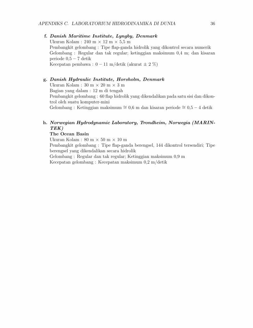
APENDIKS C. LABORATORIUM HIDRODINAMIKA DI DUNIA 36
f. Danish Maritime Institute, Lyngby, DenmarkUkuran Kolam : 240 m × 12 m × 5,5 mPembangkit gelombang : Tipe flap-ganda hidrolik yang dikontrol secara numerikGelombang : Regular dan tak regular; ketinggian maksimum 0,4 m; dan kisaranperiode 0,5 – 7 detikKecepatan pembawa : 0 – 11 m/detik (akurat ± 2 %)
g. Danish Hydraulic Institute, Horsholm, DenmarkUkuran Kolam : 30 m × 20 m × 3 mBagian yang dalam : 12 m di tengahPembangkit gelombang : 60 flap hidrolik yang dikendalikan pada satu sisi dan dikon-trol oleh suatu komputer-miniGelombang : Ketinggian maksimum ∼= 0,6 m dan kisaran periode ∼= 0,5 – 4 detik
h. Norwegian Hydrodynamic Laboratory, Trondheim, Norwegia (MARIN-TEK)The Ocean BasinUkuran Kolam : 80 m × 50 m × 10 mPembangkit gelombang : Tipe flap-ganda berengsel, 144 dikontrol tersendiri; Tipeberengsel yang dikendalikan secara hidrolikGelombang : Regular dan tak regular; Ketinggian maksimum 0,9 mKecepatan gelombang : Kecepatan maksimum 0,2 m/detik

Daftar Pustaka
[1] Azoury, P. H., Engineering Applications of Unsteady Fluid Flow, John Wiley &Sons, 1992. (ISBN 0 471 92968 9; 97/602; 620.1’064 AZO).
[2] Chakrabarti, S. K., Offshore Structure Modelling, World Scientific, 1994. (ISBN981-02-1513-4; 96/5715; 627.98 CHA)
[3] Dean, R. G., Dalrymple, R. A., Water Wave Mechanics for Engineers and Sci-entists, World Scientific, 1991. (ISBN 9810204205-9810204213; 627’.042-dc20)
[4] Dingemans, M. W. Water Wave Propagation Over Uneven Bottoms, Part 1 -Linear Wave Propagation, World Scientific, 1997. (ISBN 981-02-3393-9)
[5] Fowler, A. C., Mathematical Models in the Applied Sciences, Cambridge Univer-sity Press, 1997.
[6] Groesen, E. van, Lecture Notes Computational Fluid Dynamics, Research Work-shop, University of Twente, 1997.
[7] Hooft, J. P., Advanced Dynamics of Marine Structures, John Wiley & Sons, 1982.(ISBN 0-471-03000-7; 87/2262; 627’.042 HOO)
[8] Hughes, W. F., Brighton, J. A., Theory and Problems of Fluid Dynamics, 2nd
Edition, Schaum’s Outline Series, McGraw–Hill, Inc., 1991. (ISBN 0-07-112632-5;94/501; 532-05 HUG)
[9] Johnson, R. S., A Modern Introduction to the Mathematical Theory of WaterWaves, Cambridge University Press, 1997 (ISBN 0 521 59832 X)
[10] Keener, J. P., Principles of Applied Mathematics — Transformation and Approx-imation, Addison–Wesley Publishing Company, 1988.
[11] Landau, L. D., Lifshitz, E. M., Fluid Mechanics (Mekhanika Sploshnykh Sred),2nd English Edition, Volume 6 of Course of Theoretical Physics (TeoreticheskaiaFizika), Translated from the Russian by J. B. Sykes and W. H. Reid, PergamonPress, 1987.
[12] Mathews, J. H., Numerical Methods for Mathematics, Science, and Engineering,2nd Edition, Prentice Hall, 1992. (ISBN 0-13-624990-6)
[13] Newman, J. N., Marine Hydrodynamics, The MIT Press, 1977. (ISBN 0-262-14026-8)
[14] Ramamrutham, S., Fluid Mechanics, Hydraulics, and Fluid Machines, DhanpatRai & Sons, 1986. (90/522; 620.106 RAM)
37

DAFTAR PUSTAKA 38
[15] Round, G. F., Garg, V. K., Applications of Fluid Dynamics, Edward Arnold,1986. (ISBN 0-7131-3546-8; 87/1153; 620.1’064 ROU)
[16] Thomas, Jr. G. B., Finney, R. L., Calculus and Analytic Geometry, 9th Edi-tion, Addison–Wesley Publishing Company, 1996. (ISBN 0-201-40015-4; 515.15 THO;08119)
[17] Wiryanto, L. H., Diktat Kuliah MA-475 Komputasi Dinamika Fluida, JurusanMatematika, Fakultas Matematika dan Ilmu Pengetahuan Alam, Institut TeknologiBandung, 2000.