J. LOGIC PROGRAMMING 1988:5:231-242 231

A TECHNIQUE FOR TRANSLATING CLAUSAL SPECIFICATIONS OF NUMERICAL METHODS INTO EFFICIENT PROGRAMS

W. F. CLOCKSIN

D We describe a technique for translating numerical algorithms specified as clauses into dataflow graphs. The graphs have the property that common subexpressions are computed only once. The purpose of this technique is to convert high-complexity (exponential) solutions derived from elegant clausal specifications into very efficient computations having low (linear or log) complexity. The translation is not a program transformation, but a compi- lation of a term deduced from a goal clause. The effect of this translation is demonstrated for an assortment of numerical algorithms, including the fast Fourier transform, solution of matrix equations, and series approximation. a

1. INTRODUCTION

The application of logic programming to numerical methods has been neither widely explored nor appreciated. Apart from a paper [3] which illustrates some ideas in program transformation using numerical integration as an example, a paper [2] that investigates the parallel execution of communicating processes using a Dirichlet problem as a benchmark program, and a paper [4] showing that a Dirichlet problem may be solved in a declarative manner using constraints, there appears to have been little previous work focusing on logic-progr amming formulations of numerical methods. We shall attempt to redress this imbalance a little by presenting declara- tive formulations of some classical numerical methods, and describing an imple- mented compiler that translates term deduced from these formulations into very efficient dataflow graphs. Such graphs can be used as the program for a hypothetical dataflow computer.

Our method is a kind of partial computation. First, the problem is formulated using clauses, written here in a subset of PROLOG. Such a formulation, though

Address correspondence to Mr. W. F. Clocksin, Computer Laboratory, University of Cambridge, New Museum Site, Pembroke Street, Cambridge CB2 3QG, England.

Received 5 May 1987; accepted 15 October 1987.

THE JOURNAL OF LOGIC PROGRAMMING

GElsevier Science Publishing Co., Inc., 1988 52 Vanderbilt Ave., New York, NY 10017 0743-1066/88/$3.50

brought to you by COREView metadata, citation and similar papers at core.ac.uk

provided by Elsevier - Publisher Connector

232 W. F. CLOCKSIN

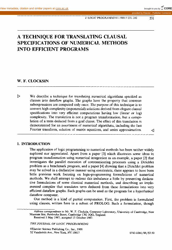
FIGURE 1. Pattern of subgoals for the goal f i b( 5, N 1. Multiple identical sub- goals are the standard characteristic of the naive definition of fib.

elegant, is unlikely to be efficient as the sole means by which solutions can be deduced. However, we use the clausal program to construct a term which, when compiled and executed later, yields the solution. The compiler itself is simply an algorithm for rewriting the term as a directed acyclic graph.

A simple example of the method, for illustrative purposes only, is the well-known naive double-recursive formulation of the Fibonacci sequence, where the goal f i b ( x, n 1 succeeds when the x th Fibonacci number can be computed by evaluat- ing term n. This can be written, without loss of generality, in PROLOG as follows:

fib(O,O).

fib(l,l).

fib(X,Fl+F2) :-

Nl is N-l, N2 is N-2,

fib(Nl,Fl), fib(N2,F21.

Satisfying the goal f i b ( 5, X 1 will instantiate X to the term depicted in tree form in Figure 1. The tree demonstrates the characteristic shortcoming of actually using such naive formulations in practice: the presence of many identical subgoals. On a sequential computer, repeated execution of an identical subgoal can be considered a waste of time; on a parallel computer, there are additional consequences such as congestion (wasteful occupancy of distribution bandwidth).

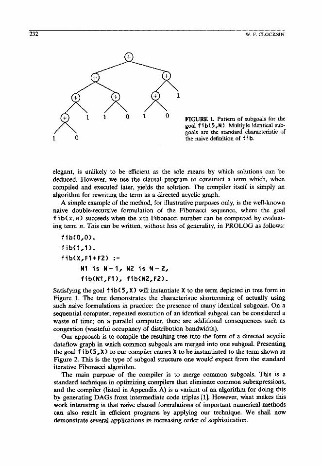
Our approach is to compile the resulting tree into the form of a directed acyclic dataflow graph in which common subgoals are merged into one subgoal. Presenting the goal f i b( 5,X 1 to our compiler causes X to be instantiated to the term shown in Figure 2. This is the type of subgoal structure one would expect from the standard iterative Fibonacci algorithm.

The main purpose of the compiler is to merge common subgoals. This is a standard technique in optimizing compilers that eliminate common subexpressions, and the compiler (listed in Appendix A) is a variant of an algorithm for doing this by generating DAGs from intermediate code triples [I]. However, what makes this work interesting is that naive clausal formulations of important numerical methods can also result in efficient programs by applying our technique. We shall now demonstrate several applications in increasing order of sophistication.

SPECIFICATIONS OF NUMERICAL METHODS 233

FIGURE 2. Pattern of subgoals resulting from applying the compiler described in this paper to the goal f i b ( 5, N 1. This pattern is character- istic of iterative algorithms with explicit use of state variables.

2. APPROXIMATION OF SERIES

The next example, like fib above, is a trivial example for illustrative purposes only. The exponential function may be approximated by calculating several terms of the

well-known series expansion

x2 x3 x4 ex=l+x+ 2!+5+ . r!+“‘*

The most naive clausal formulation of Equation (1) calculates each factorial and

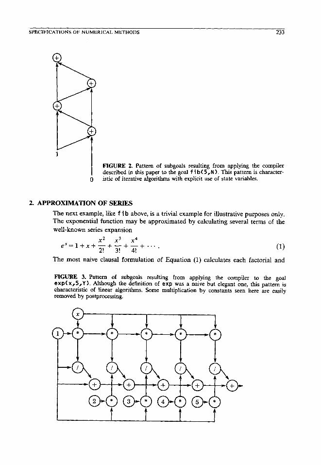
FIGURE 3. Pattern of subgoals resulting from applying the compiler to the goal exp(x,S,Y 1. Although the definition of exp was a naive but elegant one, this pattern is characteristic of linear algorithms. Some multiplication by constants seen here are easily removed by postprocessing.

234 W. F. CLOCKSIN

power from scratch for each term, and the following clauses do this. The goal exp( x, n, t 1 instantiates t to the tree which, when evaluated, yields the approxima- tion of ex to n terms:

exp(_,O,l>.

exp(X,N,XP/TF+S) :-

power(X,N,XP), fact(N,TF), Nl is N-l, exp(X,Nl,S).

power(X,O,l).

power(X,N,X*P) :- Nl is N-l, power(X,Nl,P).

fact(l,l>.

fact(N,N*F) :- Nl is N-l, fact(Nl,F).

It should be clear that any tree resulting from such a naive program is grossly unsuitable for efficient computation. However, presenting the goal exp ( x,5,X 1 to our compiler causes X to be instantiated to the tree shown in Figure 3. This is the type of subgoal structure one would expect from a more efficient algorithm; the number of operations is linear in the number of terms. Some redundant computa- tions can be observed in Figure 3, in particular the bottom row of multiplications. Such nodes are easily removed by postprocessing the dataflow graph using standard techniques. In this case, a postprocessing pass to fold constants suffices to produce the most efficient computation for approximating the exponential function accord- ing to Equation (1).

The primary disadvantage of our technique is readily apparent in this example. The compiler generates a term from a given goal. Thus, for the above example it is necessary to know-at compile time-the number of terms of Equation (1). For more serious applications this shortcoming is not always relevant. For many matrix and transform problems of the kind given next, the size of the problem (rank of the matrix, number of transform dimensions, order of the polynomial, etc.) is known at compile time, and it is worthwhile to apply our technique if the resulting program is to be executed more than once.

3. SOLUTION OF MATRIX EQUATIONS

The problem is to solve for the vector x in the matrix equation Ux = a, where U is an upper triangular matrix, and x is of length n. Each element x, of x is given by the following equation:

1

i

n

xi= ri,, ai- j=,+l = I x,u, / . (2) ’

A naive formulation of this equation calculates each x, independently, ignoring the possibility of performing backsubstitutions. Predicate solve is defined such that goal so lve( i, n, s) succeeds when s is the tree which, when evaluated, names the solution of the n-vector x,:

solve(I,N,(l/u(I,I))*(a(I)-S)) :-

J is I+l,

sum(J,N,I,S,N).

SPECIFICATIONS OF NUMERICAL METHODS 235

a3 b s x3

a2

F?

S o+

S x2

\

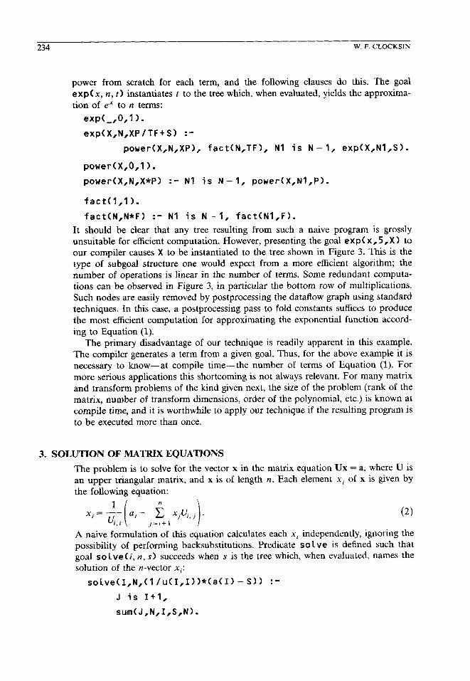
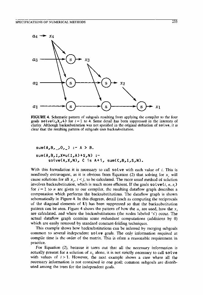
FIGURE 4. Schematic pattern of subgoals resulting from applying the compiler to the four goals so Lve( i,X,,4) for i = 1 to 4. Some detail has been suppressed in the interests of clarity. Although backsubstitution was not specified in the original definition of solve, it is clear that the resulting pattern of subgoals uses backsubstitution.

sum(A,B,_,O,_) :- A > B.

sum(A,B,I,X*u(I,A)+S,N) :- solve(A,X,N), C is A+l, sum(C,B,I,S,N).

With this formulation it is necessary to call solve with each value of i. This is needlessly extravagant, as it is obvious from Equation (2) that solving for xi will cause solutions for all xj, i <j, to be calculated. The more usual method of solution involves backsubstitution, which is much more efficient. If the goals so 1 ve ( i, n, si 1

for i = 1 to n are given to our compiler, the resulting dataflow graph describes a computation which performs the backsubstitutions. The dataflow graph is shown schematically in Figure 4. In this diagram, detail (such as computing the reciprocals of the diagonal elements of U) has been suppressed so that the backsubstitution pattern can be seen. Figure 4 shows the pattern of how the a, are used, how the xi are calculated, and where the backsubstitutions (the nodes labeled ‘s’) occur. The actual dataflow graph contains some redundant computations (additions by 0) which are easily removed by standard constant-folding techniques.

This example shows how backsubstitutions can be inferred by merging subgoals common to several independent so lve goals. The only information required at compile time is the order of the matrix. This is often a reasonable requirement in practice.

For Equation (2), because it turns out that all the necessary information is actually present for a solution of x1 alone, it is not strictly necessary to call so Lve with values of i > 1. However, the next example shows a case where all the necessary information is not contained in one goal; common subgoals are distrib- uted among the trees for the independent goals.

236 W. F. CLOCKSIN

4. THE FAST FOURIER TRANSFORM

An n-point discrete Fourier transform (DFT) algorithm can be specified in the following way. Let p(x) be a polynomial in x of degree n - 1, where n is 2” for some m:

p(x) = a,+ a,x + u2x* + . * * +a,_,xn-1.

We shall notate the polynomial p(x) of degree n - 1 in the following form, where the i,, it,. . . in_ I are called indices:

P[i,,i,,...,i,_,](x) = aio + ‘ilx + ui,x2 + * . ’ +“in_lx”-l~

For example,

P[I,S,&) = a, + u3x + aSx2 + u7x3.

This notation has a practical benefit that will become obvious later when describing the clausal formulation.

Letting c.& denote the ith power of the n th root of unity, we wish to compute all thep(o’),p(w’),..., p( d-l). The computation of a p( ok) proceeds by recursively decomposing a given polynomial into the sum of two polynomials according to the Danielson-Lanczos lemma:

P[i,,i, ,.,. in_l](ak) ‘P[i,,i, ,._, in_2)(W2k) + okP[il,i3 ,_,. i,_,](02k)-

Note that this amounts to recursively rewriting a polynomial having n indices into two polynomials each having the n/2 alternating indices of the original polynomial. The recursion terminates when only one index is encountered, in which case we rewrite this to an expression consisting of the indexed coefficient:

P[i]tWk) = ‘i.

4.1. Example: 8-point DFT

Let p(x) be a polynomial of degree 7 in x:

p(x) = a, + u,x + u*x* + u3x3 + $X4 + ugx5 + ugx6 + (1,x?

p(x) can be rewritten in the form

dx> =P[0,2,4,6](x2) + x~[l,3,6,7](x2>~

where

P[O,2,4,6)(x) = a, + u,x + u4x* + U6X3,

P[1,3,5,7](X) = a, + a3x + u5x2 + a,x3.

Letting oi denote the ith power of the 8th root of unity, we wish to compute the following: P(o’), ~(a’), ~(a*), p(03), p(w4), ~(0% p(J% and p(w7).

SPECIFICATIONS OF NUMERICAL METHODS 237

Now rewrite each polynomial in wi according to the above scheme (for simplicity we will not use the identities w4 = -CO’, w5 = -a’, w6 = - 02, and w’ = - w3):

I+“> =P [0,2,4,6]b") + o"P[l,3,5,71bo)9

PW =P [0,2,4,6]b2) + 01P[1,3,5,7j(w2)9

PM =P [0,2,4,6]b4) + w2P[1,3,5,7](w4)9

Pb3> =P [0,2,4,6]b6) + 03P[1,3,5,7](w6).

Pb”) =P (0,2,4,61b") + ~4P[1,3,5,7](~o)~

P(J) =P [0,2,4,6]b2) + w5P[l,3,5,7](w2)~

P(4 ‘P [0,2,4,6]b4) + w6P~1,3,5,7Jb4)~

Pb’) =P [0,2,4,6]tw6) + w7p[1,3,5,7,(06).

Proceeding with the next recursion,

P[0,2,4,6]b") =P[0,4]b") + w"P[2,6]bo)~

P[O,2,4,6]b*) =P[0,4]b4) + w2P[2,6]b4)~

P[0,2,4,6]b4) =P[0,4](oo) + 04P[2,6]bo),

P[0,2,4,6]tw6) =P[0,4]b4) + w6P[2,6](u4).

Next,

P[1,3,5,+“) =P[l,5](~“) + @“P[3,7](~o)~

P[1,3,5,7]b2) ‘P[1,5]b4) + ~*Pp,7]b4L

P[1,3,5,7](04) = Pp,51(~“) + ~4P[3,7]bo)9

P[1,3,5,7]W ‘P[l,5]b4) + W6P[3,7](W4b

Finally,

P[0,4]b0) = a,+ w”a4,

P~o,~~(w~) = a,+ w4a4;

P[l,5]b0) = a1 + o"a,>

P[l,5]b4) = a, + W4Q5i

P[3,7]h0) = a3 + w”a7,

P[3,7]b4) = a3 + w4a7.

238 W. F. CLOCKSIN

4.2. Naive Implementation of the DFT

We write a root of unity raised to a power k as the compound term w-k using an infix operator “+. We write a polynomial P(~~,~,,,,,~,_~~(w~) as the compound term p( Ci,, i,, . . . , i,l, w-k 1, so for example the polynomial p ,0,2,4,61( w6) is written as p( t0,2,4,6l,w-6).

As each recursive decomposition requires the even and odd indices, we first define the predicate alternate, such that the goal aLternate(L,Ll,LZ) succeeds when Ll is the set of odd indices in L, and L2 is the set of even indices in L. The procedure consists of the following two clauses:

alternate(Cl,Cl,Cl).

alternate(CA,B(Tl,CA(T13,CB~T21~ :- alternate(T,Tl,Ti?).

By inspection of their heads, these two clauses are mutually exclusive. Finally, we define the predicate eva 1. The goal eva I( P, X, N 1 succeeds when X is the expression which specifies the evaluation of polynomial P at a complex root of unity. To compute an n-point DFT, an eva 1 goal must be satisfied at each of the N powers of the N roots of unity. The eva 1 procedure consists of the following two clauses:

eval(p(CIl,V),a(I),_).

eval(p(L,V^P),Al +V^P*A2,N) :-

alternate(L,Ll,LZ),

PI is (P*2) mod N,

eval(p(Ll,V~Pl),Al,N),

eval(p(L2,V*Pl),Ai?,N).

The first clause specifies the base case for the recursion. The second clause is the recursive case, which composes the sum-and-product term (in its second argument), finds the alternating indices, multiplies the power, and recurs on the two decom- posed polynomials. These two clauses are mutually exclusive (the a 1 te rna te goal fails if its first argument is a one-element list).

As an example, the following goal evaluates the input polynomial at an 8th root of unity w6, which is one of eight goals required for an g-point DFT:

eval(p(C0 I 2 3 4 5 6 7l,w^6),X,8>. 11,111‘ X=a(O)+w^O*a(4)+w^4*(a(2)tw~O*a(6))

+w~6*(a(l)+w~O*a(5)+w^4*(a(3>+v^0*a(7~~~

Note that the identities w4 = -GO, o5 = -w’, etc. are not used, but it is a trivial matter to substitute these if it is ever considered necessary to reduce the number of different complex constants.

4.3. From DFT to FFT

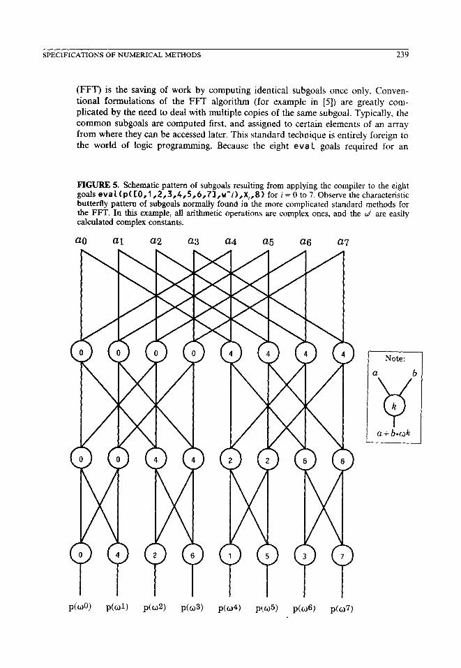
Although there are no shared subgoals in the above value of X, there are a number of identical subgoals shared among the trees for evaluation of the other seven 8th roots of unity required for the full transform. The key to the fast Fourier transform

SPECIFICATIONS OF NUMERICAL METHODS 241

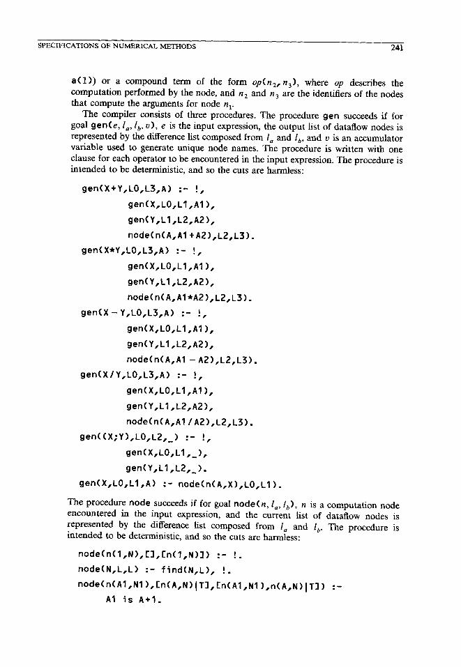
a ( 1)) or a compound term of the form op( n 2, n 3 1, where op describes the computation performed by the node, and nz and n3 are the identifiers of the nodes that compute the arguments for node n,.

The compiler consists of three procedures. The procedure gen succeeds if for goal gen ( e, I,, I,, u 1, e is the input expression, the output list of dataflow nodes is represented by the difference list composed from I, and I,, and u is an accumulator variable used to generate unique node names. The procedure is written with one clause for each operator to be encountered in the input expression. The procedure is intended to be deterministic, and so the cuts are harmless:

gen(X+Y,LO,L3,A) :- !,

gen(X,LO,Ll,Al),

gen(Y,Ll,L2,A2),

node(n(A,Al+A2),L2,L3).

gen(X*Y,LO,L3,A) :- !,

gen(X,LO,Ll,Al),

gen(Y,Ll,L2,A2),

node(n(A,Al*A2),L2,L3).

gen(X-Y,LO,L3,A) :- !,

gen(X,LO,Ll,Al),

gen(Y,Ll,L2,A2),

node(n(A,Al-A2),L2,L3).

gen(X/Y,LO,L3,A) :- !,

gen(X,LO,Ll,Al),

gen(Y,Ll,L2,A2),

node(n(A,Al/A2),L2,L3).

gen((X;Y),LO,L2,_) :- !,

gen(X,LO,Ll,_),

gen(Y,Ll,LZ,_).

gen(X,LO,Ll,A) :- node(n(A,X),LO,Ll).

The procedure node succeeds if for goal node(n, I,, I,), n is a computation node encountered in the input expression, and the current list of dataflow nodes is represented by the difference list composed from I, and I,. The procedure is intended to be deterministic, and so the cuts are harmless:

node(n(l,N>,CI,Cn(l,N~l~ :- !.

node(N,L,L) :- find(N,L), !.

node(n(Al,Nl ),Cn(A,N) (Tl,Cn(Al,Nl ),n(A,N) (TII :-

Al is A+l.

242 W. F. CLOCKSIN

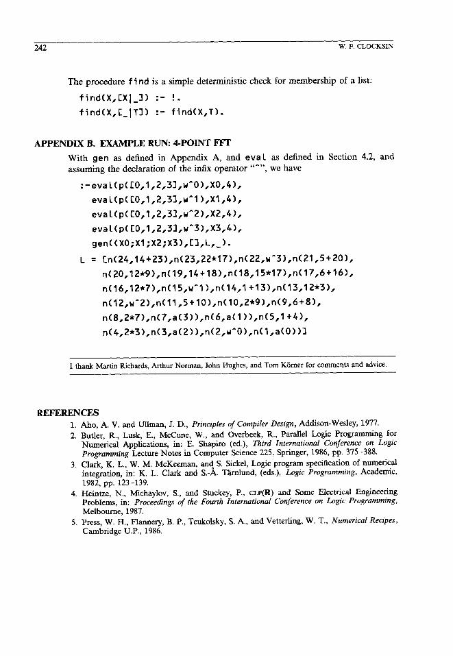
The procedure f i nd is a simple deterministic check for membership of a list:

find(X,CXI_l) :- !.

find(X,C_)Tl) :- find(X,T).

APPENDIX B. EXAMPLE RUN: 4-POINT FFT

With gen as defined in Appendix A, and eval as defined in Section 4.2, and assuming the declaration of the infix operator “““, we have

:-eval(p(C0,1,2,3l,w^O),XO,4~,

eval(p(C0,1,2,3l,w~l),X1,4),

eval(p(t0,1,2,31,wA2),X2,4),

eval(p(C0,1,2,33,w~3),X3,4),

gen((XO;Xl;XZ;X3),tl,L,_).

L = Cn(24,14+23),n(23,22*17),n(22,w~3~,n(21,5+201,

n(20,12*9),n(19,14+18)ln(18,15*17),n(17,6t16~,

n(16,12*7),n(15,w~l),n(14,ltl3~,n(13,12*3~,

n(12,w~2),n(11,5+10),n(lO,2*9),n(9,6+8),

n(8,2*7),n(7,a(3>),n(6,a(l)~,n(5,1+4>,

n(4,2*3>,n(3,a(2>),n(2,u~O~,n(l,a(O~~l

I thank Martin Richards, Arthur Norman, John Hughes, and Tom Kiimer for comments and advice.

REFERENCES

1.

2.

3.

4.

5.

Aho, A. V. and Ullman, J. D., Principles of Compiler Design, Addison-Wesley, 1977. Butler, R., Lusk, E., McCune, W., and Overbeek, R., Parallel Logic Programming for Numerical Applications, in: E. Shapiro (ed.), Third International Conference on Logic Programming Lecture Notes in Computer Science 225, Springer, 1986, pp. 375-388.

Clark, K. L., W. M. McKeeman, an{ S. Sickel, Logic program specification of numerical integration, in: K. L. Clark and S.-A. T&rnlund, (eds.), L.ogic Programming, Academic, 1982, pp. 123-139.

Heintze, N., Michaylov, S., and Stuckey, P., CLP(W) and Some Electrical Engineering Problems, in: Proceedings of the Fourth International Conference on Logic Programming, Melbourne, 1987.

Press, W. H., Plannery, B. P., Teukolsky, S. A., and Vetterhng, W. T., Numerical Recipes, Cambridge U.P., 1986.