a taste of categorical logic | tutorial...

A Taste of Categorical Logic — Tutorial Notes

Lars Birkedal ([email protected]) Ales Bizjak ([email protected])

October 12, 2014

Contents

1 Introduction 2

2 Higher-order predicate logic 2

3 A first set-theoretic model 4

4 Hyperdoctrine 84.1 Interpretation of higher-order logic in a hyperdoctrine . . . . . . . . . . . . . . . . 94.2 A class of Set-based hyperdoctrines . . . . . . . . . . . . . . . . . . . . . . . . . . . 144.3 Examples based on monoids . . . . . . . . . . . . . . . . . . . . . . . . . . . . . . . 164.4 BI-hyperdoctrines . . . . . . . . . . . . . . . . . . . . . . . . . . . . . . . . . . . . . 184.5 Guarded recursion for predicates . . . . . . . . . . . . . . . . . . . . . . . . . . . . 19

4.5.1 Application to the logic . . . . . . . . . . . . . . . . . . . . . . . . . . . . . 21

5 Complete ordered families of equivalences 235.1 U-based hyperdoctrine . . . . . . . . . . . . . . . . . . . . . . . . . . . . . . . . . . 25

6 Constructions on the category U 316.1 A typical recursive domain equation . . . . . . . . . . . . . . . . . . . . . . . . . . 326.2 Explicit construction of fixed points of locally contractive functors in U . . . . . . 36

7 Further Reading — the Topos of Trees 41

1

1 Introduction

We give a taste of categorical logic and present selected examples. The choice of examples isguided by the wish to prepare the reader for understanding current research papers on step-indexed models for modular reasoning about concurrent higher-order imperative programminglanguages.

These tutorial notes are supposed to serve as a companion when reading up on introductorycategory theory, e.g., as described in Awodey’s book [Awo10], and are aimed at graduate studentsin computer science.

The material described in Sections 5 and 6 has been formalized in the Coq proof assistantand there is an accompanying tutorial on the Coq formalization, called the ModuRes tutorial,available online at

http://cs.au.dk/~birke/modures/tutorial

The Coq ModuRes tutorial has been developed primarily by Filip Sieczkowski, with contributionsfrom Ales Bizjak, Yannick Zakowski, and Lars Birkedal.

We have followed the “design desiderata” listed below when writing these notes:

• keep it brief, with just enough different examples to appreciate the point of generalization;

• do not write an introduction to category theory; we may recall some definitions, but thereader should refer to one of the many good introductory books for an introduction

• use simple definitions rather than most general definitions; we use a bit of category theoryto understand the general picture needed for the examples, but refer to the literature formore general definitions and theorems

• selective examples, requiring no background beyond what an undergraduate computer sci-ence student learns, and aimed directly at supporting understanding of step-indexed modelsof modern programming languages

For a much more comprehensive and general treatment of categorical logic we recommend Jacobs’book [Jac99]. See also the retrospective paper by Pitts [Pit02] and Lawvere’s original papers,e.g., [Law69].

2 Higher-order predicate logic

In higher-order predicate logic we are concerned with sequents of the form Γ | Ξ ` ψ. Here Γ isa type context and specifices which free variables are allowed in Ξ and ψ. Ξ is the propositioncontext which is a lists of propositions. ψ is a proposition. The reading of Γ | Ξ ` ψ is that ψ(the conclusion) follows from the assumptions (or hypotheses) in Ξ. For example

x : N, y : N | odd(x), odd(y) ` even(x+ y) (1)

is a sequent expressing that the sum of two odd natural numbers is an even natural number.However that is not really the case. The sequent we wrote is just a piece of syntax and

the intuitive description we have given is suggested by the suggestive names we have used forpredicate symbols (odd, even), function symbols (+) and sorts (also called types) (N). To expressthe meaning of the sequent we need a model where the meaning of, for instance, odd(x) will bethat x is an odd natural number. We now make this precise.

To have a useful logic we need to start with some basic things; a signature.

2

http://cs.au.dk/~birke/modures/tutorial

Definition 2.1. A signature (T,F) for higher-order predicate logic consists of

• A set of base types (or sorts) T including a special type Prop of propositions.

• A set of typed function symbols F meaning that each F ∈ F has a type F : σ1, σ2, . . . , σn → σn+1for σ1, . . . , σn+1 ∈ T associated with it. We read σ1, . . . , σn as the type of arguments andσn+1 as the result type.

We sometimes call function symbols P with codomain Prop, i.e., P : σ1, σ2, . . . , σn → Prop

predicate symbols.

Example 2.2. Taking T = N, Prop and F = odd : N→ Prop, even : N→ Prop,+ : N,N→ N wehave that (T,F) is a signature.

Given a signature Σ = (T,F) we have a typed language of terms. This is simply typed lambdacalculus with base types in T and base constants in F and these are the terms whose propertieswe specify and prove in the logic. The typing rules are listed in Figure 1. The set of types C(T)

is inductively defined to be the least set containing T and closed under 1 (the unit type) product(×) and arrow (→). We write M [N/x] denote for capture-avoiding substitution of term N forfree variable x in M. We write M [N1/x1, N2/x2, . . . Nn/xn] for simultaneous capture-avoidingsubstitution of Ni for xi in M.

σ ∈ C(T)

x : σ ` x : σidentity

Γ `M : τ

Γ, x : σ `M : τweakening

Γ, x : σ, y : σ `M : τ

Γ, x : σ `M [x/y] : τcontraction

Γ, x : σ, y : σ ′, ∆ `M : τ

Γ, x : σ ′, y : σ,∆ `M [y/x, x/y] : τexchange

Γ `M1 : τ1 . . . Γ `Mn : τn

Γ ` F(M1, . . . ,Mn) : τn+1

function symbol

F : τ1, . . . , τn → τn+1 ∈ F

Γ `M : τ Γ ` N : σ

Γ ` 〈M,N〉 : τ× σpairing

Γ `M : τ× σΓ ` π1M : τ

proj-1Γ `M : τ× σΓ ` π2M : σ

proj-2Γ, x : σ `M : τ

Γ ` λx.M : σ→ τabs

Γ `M : τ→ σ Γ ` N : τ

Γ `MN : σapp

Γ ` 〈〉 : 1unit

Figure 1: Typing rules relative to a signature (T,F). Γ is a type context, i.e., a listx1 : σ1, x2 : σ2, . . . , xn : σn and when we write Γ, x : σ we assume that x does not occur in Γ .

Since we are dealing with higher-order logic there is no real distinction between propositionsand terms. However there are special connectives that only work for terms of type Prop, i.e.,propositions. These are

• ⊥ falsum

• > the true proposition

• ϕ∧ψ conjunction

• ϕ∨ψ disjunction

• ϕ⇒ ψ implication

• ∀x : σ,ϕ universal quantification over σ ∈ C(T))

3

• ∃x : σ,ϕ existential quantification over σ ∈ C(T))

The typing rules for these are listed in Figure 2. Capture avoiding substitution is extended inthe obvious way to these connectives.

Notice that we did not include an equality predicate. This is just for brevity. In higher-orderlogic equality can be defined as Leibniz equality, see, e.g., [Jac99]. (See the references in theintroduction for how equality can be modeled in hyperdoctrines using left adjoints to reindexingalong diagonals.)

Γ ` ⊥ : Propfalse

Γ ` > : Proptrue

Γ ` ϕ : Prop Γ ` ψ : Prop

Γ ` ϕ∧ψ : Propconj


Γ ` ϕ∨ψ : Propdisj


Γ ` ϕ⇒ ψ : Propimpl

Γ, x : σ ` ϕ : Prop

Γ ` ∀x : σ,ϕ : Propforall

Γ, x : σ ` ϕ : Prop

Γ ` ∃x : σ,ϕ : Propexists

Figure 2: Typing rules for logical connectives. Note that these are not introduction and elimi-nation rules for connectives. These merely state that some things are propositions, i.e., of typeProp

We can now describe sequents and provide basic rules of natural deduction. If ψ1, ψ2, . . . , ψnhave type Prop in context Γ we write Γ ` ψ1, ψ2, . . . , ψn and call Ξ = ψ1, . . . , ψn the propositionalcontext. Given Γ ` Ξ and Γ ` ϕ we have a new judgment Γ | Ξ ` ϕ. The rules for deriving theseare listed in Figure 3.

3 A first set-theoretic model

What we have described up to now is a system for deriving two judgments, Γ ` M : τ andΓ | Ξ ` ϕ. We now describe a first model where we give meaning to types, terms, propositionsand sequents.

We interpret the logic in the category Set of sets and functions. There are several things tointerpret.

• The signature (T,F).

• The types C(T)

• The terms of simply typed lambda calculus

• Logical connectives

• The sequent Γ | Ξ ` ψ

Interpretation of the signature For a signature (T,F) we pick interpretations. That is, foreach τ ∈ T we pick a set Xτ but for Prop we pick the two-element set of “truth-values” 2 = 0, 1.For each F : τ1, τ2, . . . , τn → τn+1 we pick a function f from Xτ1 × Xτ2 × · · · × Xτn to Xτn+1

.

4

We then have the following result which holds for any cartesian closed category, in particularSet.

Proposition 3.1. The interpretation of terms validates all the β and η rules, i.e., if Γ ` M ≡N : σ then JΓ `M : σK = JΓ `M : τK.

The β and η rules are standard computation rules for simply typed lambda calculus. Wedo not write them here explicitly and do not prove this proposition since it is a standard resultrelating simply typed lambda calculus and cartesian closed categories. But it is good exercise totry and prove it.

Exercise 3.1. Prove the proposition. Consider all the rules that generate the equality judgment≡ and prove for each that it is validate by the model. ♦

Interpretation of logical connectives Recall that the interpretation of Prop is 2, the twoelement set 0, 1. We take 1 to mean “true” and 0 to mean “false”. If we order 2 by postulatingthat 0 6 1 then 2 becomes a complete Boolean algebra which in particular means that it is acomplete Heyting algebra.

Exercise 3.2. Show that given any set X, the set of functions from X to 2, i.e., HomSet (X, 2) isa complete Heyting algebra for operations defined pointwise.

Moreover, check for any two sets X and Y and any function f : X → Y, HomSet (f, 2) is aHeyting algebra homomorphism. ♦

In higher-order logic propositions are just terms so they are interpreted in the same way.However instead of using the cartesian closed structure of the category Set we use the Heytingalgebra structure on HomSet (X, 2) to interpret logical connectives. We write >X, ⊥X, ∧X, ∨Xand ⇒X for Heyting algebra operations in HomSet (X, 2).

JΓ ` > : PropK = >JΓK

JΓ ` ⊥ : PropK = ⊥JΓK

JΓ ` ϕ∧ψ : PropK = (JΓ ` ϕ : PropK)∧JΓK (JΓ ` ψ : PropK)

JΓ ` ϕ∨ψ : PropK = (JΓ ` ϕ : PropK)∨JΓK (JΓ ` ψ : PropK)

JΓ ` ϕ⇒ ψ : PropK = (JΓ ` ϕ : PropK)⇒JΓK (JΓ ` ψ : PropK)

It only remains to interpret quantifiers ∀ and ∃. Recall the formation rules from Figure 2. Theinterpretation of Γ ` ∀x : σ,ϕ : Prop should be a function f : JΓK → 2 and we are given theinterpretation of Γ, x : σ ` ϕ : Prop, which is interpreted as a function g : JΓK× JσK→ 2. What we

need, then, is a function function ∀JσKJΓK

∀JσKJΓK : HomSet (JΓK× JσK , 2)→ HomSet (JΓK , 2) .

There are many such functions, but only two that have all the necessary properties. One foruniversal and one for existential quantification. In fact we can be more general. We define

∀YX, ∃YX : HomSet (X× Y, 2)→ HomSet (X, 2)

6

for any sets X and Y and ϕ : X× Y → 2 as

∀YX(ϕ) = λx.

1 if ∀y ∈ Y,ϕ(x, y) = 10 otherwise

= λx.

1 if x× Y ⊆ ϕ−1 [1]

0 otherwise

∃YX(ϕ) = λx.

1 if ∃y ∈ Y,ϕ(x, y) = 10 otherwise

= λx.

1 if x× Y ∩ϕ−1 [1] 6= ∅0 otherwise

To understand these definitions and to present them graphically a presentation of functionsfrom X → 2 as subsets of X is useful. Consider the problem of obtaining a subset of X given asubset of X×Y. One natural way to do this is to “project out” the second component, i.e., map asubset A ⊆ X×Y to π [A] = π(z) | z ∈ A where π : X×Y → X is the first projection. Observe thatthis gives rise to ∃YX. Geometrically, if we draw X on the horizontal axis and Y on the verticalaxis, A is a region on the graph. The image π [A] includes all x ∈ X such that the vertical line atx intersects A in at least one point.

We could instead choose to include only points x ∈ X such that the vertical line at x is asubset of A. This way, we would get exactly ∀YX(A).

To further see that these are not arbitrary definitions but in fact essentially unique show thefollowing.

Exercise 3.3. Let π∗X,Y = HomSet (π, 2) : HomSet (X, 2) → HomSet (X× Y, 2). Show that ∀YX and∃YX are monotone functions (i.e., functors) and that ∀YX is the right adjoint to π∗X,Y and ∃YX its leftadjoint.

Concretely the last part means to show for any ϕ : X→ 2 and ψ : X× Y → 2 that

π∗X,Y(ϕ) 6 ψ ⇐⇒ ϕ 6 ∀YX(ψ)

and

∃YX(ψ) 6 ϕ ⇐⇒ ψ 6 π∗X,Y(ϕ).

♦

Moreover, ∀YX and ∃YX have essentially the same definition for all X, i.e., they are natural in X.This is expressed as the commutativity of the diagram

HomSet (X′ × Y, 2) HomSet (X× Y, 2)

HomSet (X′, 2) HomSet (X, 2)

∀YX′

HomSet(s×idY ,2)

∀YX

HomSet(s,2)

for any s : X → X ′ (remember that the functor HomSet (−, 2) is contravariant) and analogouslyfor ∃.

This requirement that ∀YX and ∃YX are “natural” is often called the Beck-Chevalley condition.

Exercise 3.4. Show that ∃YX and ∀YX are natural in X. ♦

Using these adjoints we can finish the interpretation of propostions:

JΓ ` ∀x : σ,ϕ : PropK = ∀JσKJΓK (JΓ, x : σ ` ϕ : PropK)

JΓ ` ∃x : σ,ϕ : PropK = ∃JσKJΓK (JΓ, x : σ ` ϕ : PropK)

7

Given a sequence of terms ~M = M1,M2, . . . ,Mn of type ~σ = σ1, σ2, . . . , σn in context Γ wedefine

qΓ ` ~M : ~σ

yas the tupling of interpretations of individual terms.

Exercise 3.5. Show that given contexts Γ = y1 : σ1, . . . , ym : σm and ∆ = x1 : δ1, . . . , xn : δnwe have the following property of the interpretation for any N of type τ in context ∆ and anysequence of terms ~M of appropriate types

rΓ ` N

[~M/~x

]: τ

z= J∆ ` N : τK

qΓ ` ~M : ~δ

y

To show this proceed by induction on the typing derivation for N. You will need to use thenaturality of quantifiers. ♦

Remark 3.2. If you have done Exercise 3.5, you will have have notices that the perhaps mysteri-ous Beck-Chevalley condition is nothing but the requirement that the model respects substitution,i.e., that the interpretation of

(∀y : σ,ϕ) [M/x]

is equal to the interpretation of

∀y : σ, (ϕ [M/x])

for x 6= y.

4 Hyperdoctrine

Using the motivating example above we now define the concept of a hyperdoctrine, which willbe our general notion of a model of higher-order logic for which we prove soundness of theinterpretation defined above.

Definition 4.1. A hyperdoctrine is a cartesian closed category C together with an object Ω ∈ C

(called the generic object) and for each object X ∈ C a choice of a partial order on the setHomC (X,Ω) such that the conditions below hold. We write P for the contravariant functorHomC (−,Ω).

• P restricts to a contravariant functor Cop → Heyt, from C to the category of Heytingalgebras and Heyting algebra homomorphisms, i.e., for each X, P(X) is a Heyting algebraand for each f, P(f) is a Heyting algebra homomorphisms, in particular it is monotone.

• For any objects X, Y ∈ C and the projection π : X× Y → X there exist monotone functions1

∃YX and ∀YX such that ∃YX is a left adjoint to P(π) : P(X)→ P(X×Y) and ∀YX is its right adjoint.Moreover, these adjoints are natural in X, meaning that for any morphism s : X → X ′ thediagrams

P(X ′ × Y) P(X× Y)

P(X ′) P(X)

∀YX′

P(s×idY)

∀YX

P(s)

P(X ′ × Y) P(X× Y)

P(X ′) P(X)

∃YX′

P(s×idY)

∃YX

P(s)

commute.1We do not require them to be Heyting algebra homomorphisms.

8

Example 4.2. The category Set together with the object 2 for the generic object which wedescribed in Section 3 is a hyperdoctrine. See the discussion and exercises in Section 3 for thedefinitions of adjoints.

4.1 Interpretation of higher-order logic in a hyperdoctrine

The interpretation of higher-order logic in a general hyperdoctrine proceeds much the same asthe interpretation in Section 3.

First, we choose objects of C for base types and morphisms for function symbols. We must,of course, choose the interpretation of the type Prop to be Ω.

We then interpret the terms of simply typed lambda calculus using the cartesian closedstructure of C and the logical connectives using the fact that each hom-set is a Heyting algebra.The interpretation is spelled out in Figure 4.

Note that the interpretation itself requires no properties of the adjoints to P(π). However,to show that the interpretation is sound, i.e., that it validates all the rules in Figure 3, allthe requirements in the definition of a hyperdoctrine are essential. A crucial property of theinterpretation is that it maps substitution into composition in the following sense.

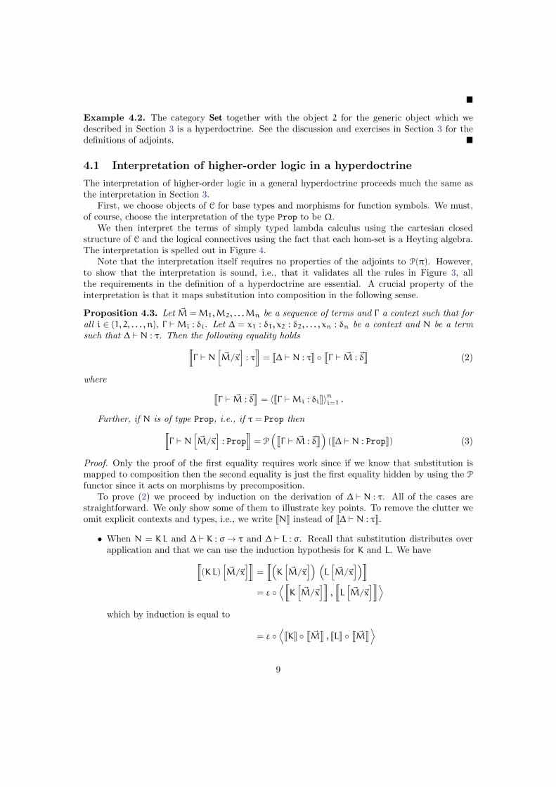
Proposition 4.3. Let ~M =M1,M2, . . .Mn be a sequence of terms and Γ a context such that forall i ∈ 1, 2, . . . , n, Γ `Mi : δi. Let ∆ = x1 : δ1, x2 : δ2, . . . , xn : δn be a context and N be a termsuch that ∆ ` N : τ. Then the following equality holds

rΓ ` N

[~M/~x

]: τ

z= J∆ ` N : τK

qΓ ` ~M : ~δ

y(2)

where

qΓ ` ~M : ~δ

y= 〈JΓ `Mi : δiK〉ni=1 .

Further, if N is of type Prop, i.e., if τ = Prop then

rΓ ` N

[~M/~x

]: Prop

z= P

(qΓ ` ~M : ~δ

y)(J∆ ` N : PropK) (3)

Proof. Only the proof of the first equality requires work since if we know that substitution ismapped to composition then the second equality is just the first equality hidden by using the P

functor since it acts on morphisms by precomposition.To prove (2) we proceed by induction on the derivation of ∆ ` N : τ. All of the cases are

straightforward. We only show some of them to illustrate key points. To remove the clutter weomit explicit contexts and types, i.e., we write JNK instead of J∆ ` N : τK.

• When N = KL and ∆ ` K : σ→ τ and ∆ ` L : σ. Recall that substitution distributes overapplication and that we can use the induction hypothesis for K and L. We have

r(KL)

[~M/~x

]z=

r(K[~M/~x

]) (L[~M/~x

])z= ε

⟨rK[~M/~x

]z,rL[~M/~x

]z⟩which by induction is equal to

= ε ⟨JKK

q~M

y, JLK

q~M

y⟩

9

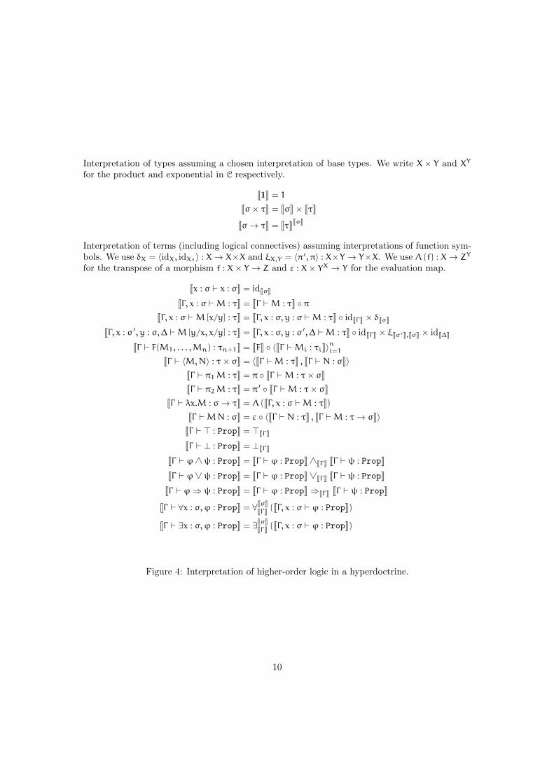
Interpretation of types assuming a chosen interpretation of base types. We write X × Y and XY

for the product and exponential in C respectively.

J1K = 1Jσ× τK = JσK× JτK

Jσ→ τK = JτKJσK

Interpretation of terms (including logical connectives) assuming interpretations of function sym-bols. We use δX = 〈idX, idX, 〉 : X→ X×X and ξX,Y = 〈π ′, π〉 : X×Y → Y×X. We use Λ (f) : X→ ZY

for the transpose of a morphism f : X× Y → Z and ε : X× YX → Y for the evaluation map.

Jx : σ ` x : σK = idJσK

JΓ, x : σ `M : τK = JΓ `M : τK πJΓ, x : σ `M [x/y] : τK = JΓ, x : σ, y : σ `M : τK idJΓK × δJσK

JΓ, x : σ ′, y : σ,∆ `M [y/x, x/y] : τK = JΓ, x : σ, y : σ ′, ∆ `M : τK idJΓK × ξJσ′K,JσK × idJ∆K

JΓ ` F(M1, . . . ,Mn) : τn+1K = JFK 〈JΓ `Mi : τiK〉ni=1JΓ ` 〈M,N〉 : τ× σK = 〈JΓ `M : τK , JΓ ` N : σK〉

JΓ ` π1M : τK = π JΓ `M : τ× σKJΓ ` π2M : τK = π ′ JΓ `M : τ× σK

JΓ ` λx.M : σ→ τK = Λ (JΓ, x : σ `M : τK)JΓ `MN : σK = ε 〈JΓ ` N : τK , JΓ `M : τ→ σK〉JΓ ` > : PropK = >JΓK

JΓ ` ⊥ : PropK = ⊥JΓK

JΓ ` ϕ∧ψ : PropK = JΓ ` ϕ : PropK ∧JΓK JΓ ` ψ : PropK

JΓ ` ϕ∨ψ : PropK = JΓ ` ϕ : PropK ∨JΓK JΓ ` ψ : PropK

JΓ ` ϕ⇒ ψ : PropK = JΓ ` ϕ : PropK⇒JΓK JΓ ` ψ : PropK

JΓ ` ∀x : σ,ϕ : PropK = ∀JσKJΓK (JΓ, x : σ ` ϕ : PropK)

JΓ ` ∃x : σ,ϕ : PropK = ∃JσKJΓK (JΓ, x : σ ` ϕ : PropK)

Figure 4: Interpretation of higher-order logic in a hyperdoctrine.

10

which by a simple property of products gives us

= ε 〈JKK , JLK〉 q~M

y

= JKLK q~M

y

• WhenN = λx.K and ∆ ` K : σ→ τ we first use the fact that when Γ `Mi : δi then Γ, y : σ `Mi : δiby a single application of weakening and we write π∗( ~M) for ~M in this extended context.So we have

r(λx.K)

[~M/~x

]z=

rλy.K

([π∗(~M)/~x, y/x

])z= Λ

(rK([π∗(~M)/~x, y/x

])z)= Λ

(JKK

rπ∗(~M), y

z)induction hypothesis for ~M,y

and since the interpretation no weakening is precomposition with the projection we have

= Λ(JKK

⟨q~M

y π, π ′

⟩)which by a simple property of products gives us

= Λ(JKK

(q~M

y× idJσK

))which by a simple property of exponential transposes finally gives us

= Λ (JKK) q~M

y= JNK

q~M

y.

Admittedly we are a bit sloppy with the bound variable x but to be more precise we wouldhave to define simultaneous subsitution precisely which is out of scope of this tutorial andwe have not skipped anything essential.

• When N = ϕ∧ψ we haver(ϕ∧ψ)

[~M/~x

]z=

r(ϕ[~M/~x

])∧(ψ[~M/~x

])z=

rϕ[~M/~x

]z∧

rψ[~M/~x

]zwhich by the induction hypothesis and the definition of P gives us

= JϕK q~M

y∧ JψK

q~M

y

= P(q

~My)

(JϕK)∧ P(q

~My)

(JψK)

and since by definition P is a Heyting algebra homomorphism it commutes with ∧ givingus

= P(q

~My)

(JϕK ∧ JψK)

and again using the definition of P but in the other direction

= (JϕK ∧ JψK) q~M

y

= Jϕ∧ψK q~M

y

which is conveniently exactly what we want. All the other binary connectives proceedin exactly the same way; use the fact that P is a Heyting algebra homomorphism andnaturality of Θ.

11

• When N = ∀x : σ,ϕ we haver(∀x : σ,ϕ)

[~M/~x

]z=

r∀y : σ,

(ϕ[

~π∗(M)/~x, y/x])z

the definition of the interpretation of ∀ gives us

= ∀(rϕ[π∗( ~M)/~x, y/x

]z)where we use π∗ for the same purpose as in the case for λ-abstraction. The inductionhypothesis for ϕ now gives us

= ∀(JϕK

qπ∗( ~M), y

y)and by the same reasoning as in the λ-abstraction case we get

= ∀(JϕK

(q~M

y× idJσK

)).

Using the definition of P we have

= ∀(P(q

~My× idJσK

)(JϕK)

).

Now we are in a situation where we can use the Beck-Chevalley condition to get

= P(q

~My)

(∀ (JϕK))

which by the same reasoning as in the last step of the previous case gives us

= ∀ (JϕK) q~M

y

= J∀x : σ,ϕK q~M

y.

These four cases cover the essential ideas in the proof. The other cases are all essentially thesame as one of the four cases covered.

Theorem 4.4 (Soundness). Let Θ = ϑ1, ϑ2, . . . , ϑn be a propositional context. If Γ | Θ ` ϕ isderivable using the rules in Figure 3 then

n∧i=1

JΓ ` ϑi : PropK 6 JΓ ` ϕ : PropK

in the Heyting algebra P (JΓK).In particular if Γ | − ` ϕ is derivable then JΓ ` ϕ : PropK = >.

Proof. The proof is, of course, by induction on the derivation Γ | Θ ` ϕ. Most of the casesare straightforward. We only show the cases for the universal quantifier where we also useProposition 4.3. In the proof we again omit explicit contexts to avoid clutter.

First, the introduction rule. We assume that the claim holds for Γ, x : σ | Θ ` ϕ and show thatit also holds for Γ | Θ ` ∀x : σ,ϕ.

By definition

J∀x : σ,ϕK = ∀JσKJΓK (JϕK)

12

and thus we need to show

n∧i=1

JΓ ` ϑi : PropK 6 ∀JσK

JΓK (JϕK) .

Since by definition ∀ is the right adjoint to P(π) this is equivalent to

P(π)

(n∧i=1

JΓ ` ϑi : PropK

)6 JϕK

where π : JΓK×JσK→ JΓK is of course the first projection. We cannot do much with the right side,so let us simplify the left-hand side. By definition P(π) is a Heyting algebra homomorphism soin particular it commutes with conjuction which gives us

P(π)

(n∧i=1

JΓ ` ϑi : PropK

)=

n∧i=1

P(π) (JΓ ` ϑi : PropK)

using the definition of P we get

=

n∧i=1

JΓ ` ϑi : PropK π.

Now recall the definition of the interpretation of terms, in particular the definition of the inter-pretation of weakening in Figure 4. It gives us that

JΓ ` ϑi : PropK π = JΓ, x : σ ` ϑi : PropK .

so we get

n∧i=1

JΓ ` ϑi : PropK π =

n∧i=1

JΓ, x : σ ` ϑi : PropK

By the induction hypothesis we have

n∧i=1

JΓ, x : σ ` ϑi : PropK 6 JϕK

which concludes the proof of the introduction rule for ∀.

Exercise 4.1. Where did we use the side-condition that x does not appear in Θ? ♦

For the elimination rule assume that Γ `M : σ and that the claim holds for Γ | Θ ` ∀x : σ,ϕ.We need to show it for Γ | Θ ` ϕ [M/x], so we need to show

n∧i=1

JΓ ` ϑi : PropK 6 JΓ ` ϕ [M/x] : PropK

From Proposition 4.3 (the second equality) we have

JΓ ` ϕ [M/x] : PropK = P(⟨

idJΓK, JΓ `M : σK⟩)

(JΓ, x : σ ` ϕ : PropK) . (4)

13

Since P(π) is left adjoint to ∀JσKJΓK we have in particular that

P(π) ∀JσKJΓK 6 idP(JΓ,x:σK)

which is the counit of the adjunction. Thus

JΓ, x : σ ` ϕ : PropK >(P(π) ∀JσK

JΓK

)(JΓ, x : σ ` ϕ : PropK)

whose right-hand side is, by definition of the interpretation of the universal quantifier, equal to

= P(π) (JΓ ` ∀x : σ,ϕ : PropK) ,

which by induction hypothesis and monotonicity of P(π) is greater than

> P(π)

(n∧i=1

JΓ ` ϑi : PropK

).

Further, since P is a contravariant functor we have

P(⟨

idJΓK, JΓ `M : σK⟩) P (π) = P

(π ⟨idJΓK, JΓ `M : σK

⟩)= P

(idJΓK

).

Thus combining the last two results with (4) we have

JΓ ` ϕ [M/x] : PropK > P(idJΓK

)( n∧i=1

JΓ ` ϑi : PropK

)=

n∧i=1

JΓ ` ϑi : PropK

concluding the proof.

4.2 A class of Set-based hyperdoctrines

To get other examples of Set-based hyperdoctrines, we can keep the base category Set and replacethe generic object 2 with a different complete Heyting algebra.

Definition 4.5. A complete Heyting algebra is a Heyting algebra that is complete as a lattice.

Exercise 4.2. Show that any complete Heyting algebra satisfies the infinite distributivity law

x∧∨i∈Iyi =

∨i∈I

(x∧ yi)

Hint: use your category theory lessons (left adjoints preserve. . . ). ♦

Exercise 4.3. Show that if H is a (complete) Heyting algebra and X any set then the set of allfunctions from X to (the underlying set of) H when ordered pointwise, i.e., ϕ 6HX ψ ⇐⇒ ∀x ∈X,ϕ(x) 6H ψ(x), is a (complete) Heyting algebra with operations also inherited pointwise fromH, e.g. (ϕ∧HX ψ)(x) = ϕ(x)∧H ψ(x). ♦

Theorem 4.6. Let H be a complete Heyting algebra. Then Set together with the functorHomSet (−, H) and the generic object H is a hyperdoctrine.

14

Proof. Clearly Set is a cartesian closed category and from Exercise 4.3 we know that HomSet (X,H)

is a complete Heyting algebra. To show that HomSet (−, H) is a functor into Heyt we need toestablish that for any function f, HomSet (f,H) is a Heyting algebra homomorphism. We usegreek letters ϕ,ψ, . . . for elements of HomSet (X,H).

Recall that the action of the hom-functor on morphisms is by precomposition: HomSet (f,H) (ϕ) =

ϕ f. We now show that for any f : X → Y, HomSet (f,H) preserves conjunction and leave theother operations as an exercise since the proof is essentially the same. Let ϕ,ψ ∈ HomSet (X,H)

and y ∈ Y then

HomSet (f,H) (ϕ∧HX ψ)(y) = ((ϕ∧HX ψ) f)(y) = ϕ(f(y))∧H ψ(f(y)) = ((ϕ f)∧HY (ψ f))(y).

As y was arbitrary we have HomSet (f,H) (ϕ∧HX ψ) = (ϕ f)∧HY (ψ f), as needed.Observe that we have not yet used completeness of H anywhere. We need completeness to

define adjoints ∀YX and ∃YX to HomSet (π,H) for π : X× Y → X which we do now.To understand the definitions of adjunctions recall that universal quantification is akin to an

infinite conjunction and existential quantification is akin to infinite disjunction. Let X and Y besets and ϕ ∈ HomSet (X× Y,H). Define

∃YX(ϕ) = λx.∨y∈Y

ϕ(x, y)

∀YX(ϕ) = λx.∧y∈Y

ϕ(x, y).

It is a straightforward exercise to show that ∃YX and ∀YX are monotone. We now show that ∃YX isleft adjoint to HomSet (π,H) and leave the proof that ∀YX is right adjoint as another exercise. Weshow the two implications separately.

Let ϕ ∈ HomSet (X× Y,H) and ψ ∈ HomSet (X,H). Assume that ∃YX(ϕ) 6 ψ. We are to showϕ 6 HomSet (π,H) (ψ) which reduces to showing for any x ∈ X and y ∈ Y that ϕ(x, y) 6 ψ(π(x, y))which further reduces to showing ϕ(x, y) 6 ψ(x).

Let x ∈ X and y ∈ Y. By assumption ∃YX(ϕ)(x) 6 ψ(x) which simplifies to∨y∈Y ϕ(x, y) 6 ψ(x).

By definition of supremum ϕ(x, y) 6∨y∈Y ϕ(x, y) so we get ϕ(x, y) 6 ψ(x) by transitivity.

Note that for this direction we only needed that∨y∈Y ϕ(x, y) is an upper bound of the set

ϕ(x, y) | y ∈ Y, not that it is the least upper bound. We need this last property for the otherdirection.

For the other direction let again ϕ ∈ HomSet (X× Y,H) and ψ ∈ HomSet (X,H). Assumethat ϕ 6 HomSet (π,ψ). We are to show ∃YX(ϕ) 6 ψ which reduces to showing for any x ∈ X,∨y∈Y ϕ(x, y) 6 ψ(x). Let x ∈ X. The assumption ϕ 6 HomSet (π,ψ) gives us that for any y ∈ Y,

ϕ(x, y) 6 ψ(x) which means that ψ(x) is the upper bound of the set ϕ(x, y) | y ∈ Y. But bydefinition of supremum,

∨y∈Y ϕ(x, y) is the least upper bound, so

∨y∈Y ϕ(x, y) 6 ψ(x).

Exercise 4.4. Show that ∀YX is the right adjoint to HomSet (π,H). ♦

What we are still missing is the Beck-Chevalley condition for ∃YX and ∀YX. Again, we showthis for ∃YX and leave the other as an exercise for the reader.

Let X and X ′ be sets and s : X→ X ′ a function. We need to show that ∃YXHomSet (s× idY , H) =HomSet (s,H) ∃YX′ . Let ϕ ∈ HomSet (X

′ × Y,H). Then(∃YX HomSet (s× idY , H)

)(ϕ) = ∃YX(ϕ (s× idY)) = λx.

∨y∈Y

ϕ(s(x), y)

and (HomSet (s,H) ∃YX′

)(ϕ) = ∃YX′(ϕ) s.

15

For any x ∈ X ′ we have (∃YX′(ϕ) s

)(x) = ∃YX′(ϕ)(s(x)) =

∨y∈Y

ϕ(s(x), y)

which means ∃YX′(ϕ) s = λx.∨y∈Y ϕ(s(x), y), which is exactly what we need it to be.

Exercise 4.5. Show that the Beck-Chevalley condition also holds for ∀YX. ♦

We now give some examples of complete Heyting algebras. We only give definitions and leavethe straightforward verifications of the axioms as an exercise

Exercise 4.6. Let P be a preordered set (i.e., a set with a reflexive and transitive relation 6).Show that the set of upwards closed subsets of P, P↑ (P)

P↑ (P) = A ⊆ P | ∀x ∈ A, ∀y ∈ P, x 6 y⇒ x ∈ A

is a complete Heyting algebra for the following operations

> = P ⊥ = ∅ A∨ B = A ∪ B A∧ B = A ∩ B∨i∈IAi =

⋃i∈IAi

∧i∈IAi =

⋂i∈IAi A⇒ B = x ∈ P | ∀y > x, y ∈ A⇒ y ∈ B

Concretely show that all these operations are well defined (that the sets defined are again upwardsclosed) and that they satisfy the axioms of a complete Heyting algebra.

Also show that the set of downwards closed subsets of P, P↓ (P) is a complete Heyting algebra(you only need to change the definition of one of the operations). ♦

4.3 Examples based on monoids

Another set of examples is useful in modeling various logics dealing with resources. We needsome definitions.

Definition 4.7. Let f, g : A B be two partial functions and a ∈ A. We write f(a) ' g(a)for Kleene equality meaning that if either of the sides is defined then both are and they areequal.

Definition 4.8. A partial commutative monoid M is a set M together with a partial function· :M×MM (multiplication) and an element 1 ∈M (the unit) such that the following axiomshold:

• for all m ∈M, m · 1 ' 1 ·m ' m (in particular 1 ·m and m · 1 are always defined)

• for m,n ∈M, m · n ' n ·m (commutativity)

• for `,m,n ∈M, ` · (m · n) ' (` ·m) · n.

We write a#b to say that a · b is defined.

16

Example 4.9. Let H be the set of finite partial maps from N to X where X is some set. It couldfor instance be the set of values of some programming language. Then H would be a model ofthe heap.

Define the operation · : H×H H as follows

f · g =

f ] g if dom (f) ∩ dom (g) = ∅undefined otherwise

where

(f ] g)(x) =

f(x) x ∈ dom (f)

g(x) x ∈ dom (g)

undefined otherwise

Then it is easy to see that H with · is a partial commutative monoid with the unit theeverywhere undefined function.

Given a partial commutative monoid M there is a canonical preorder associated with it thatarises from multiplication ·. It is called the extension order. Concretely, we define

m 6 n ⇐⇒ ∃k ∈M,m · k ' n

(note that associativity of · is used to show that 6 is transitive).

Example 4.10. For the example partial commutative monoid H above the extension order canequivalently be defined as

f 6 g ⇐⇒ dom (f) ⊆ dom (g)∧ ∀x ∈ dom (f) , f(x) ' g(x)

If we think of f and g as heaps then f 6 g if the heap g is derived from f by allocating some newlocations.

As we have seen in Exercise 4.6 given a preordered set P, the set of upwards closed subsets ofP is a complete Heyting algebra. It turns out that given a partial commutative monoid and itsderived preorder we can lift the multiplication of the monoid to multiplication of upwards closedsubsets, giving rise to a (complete) BI-algebra.

Definition 4.11. A (complete) BI-algebra H is a (complete) Heyting algebra with an additionalconstant I and two binary operations ? and →? such that the following axioms hold

• ? is monotone: for any h, h ′, g, g ′, if h 6 h ′ and g 6 g ′ then h ? g 6 h ′ ? g ′.

• I is the unit for ?.

• ? is commutative and associative

• for any h, h ′, h ′′ ∈ H, h ? h ′ 6 h ′′ ⇐⇒ h 6 h ′ →?h ′′ (→? is right adjoint to ?).

Note in contrast to the operations of a (complete) Heyting algebra, which are uniquely de-termined by the order relation (why?), there can be (potentially) many different definitions of ?,→? and I (although →? is determined by ?).

17

Exercise 4.7. Any (complete) Heyting algebra is trivially a (complete) BI algebra. What canwe choose for operations ?, I and →?? ♦

Exercise 4.8. Show that if H is a (complete) BI-algebra and X is any set, then the set offunctions from X to H is another (complete) BI-algebra with operations defined pointwise. ♦

Of course, we want nontrivial examples. Partial commutative monoids give rise to such.

Example 4.12. LetM be a partial commutative monoid. Then the set of upwards closed subsetsof M (with respect to the extension order) is a complete BI-algebra.

We already know that it is a complete Heyting algebra. We need to define I, ? and →?. Theoperation ? is a pointwise lifting of the operation · of the monoid in the sense

A ? B = m · n | m ∈ A,n ∈ B,m · n defined .

The unit I is the whole monoid M.Recalling that the order on P↑ (M) is subset inclusion it is clear that ? is monotone. To see

that M is the unit for ? we prove two inclusions. Let A ∈ P↑ (M). We wish to show A ?M = A.Suppose m ∈ A. Since 1 ∈ M and m · 1 ' m clearly, m ∈ A ?M. Conversely, suppose

m ∈ A ?M. By definition there exists a ∈ A and n ∈M, such that m ' a ·n. This means (recallthe definition of the extension order) that m > a. Since A is upwards closed by definition anda ∈ A, it must be that m ∈ A as well.

Showing M ? A = A is analogous. The fact that it is commutative and associative likewisefollows easily.

Exercise 4.9. Show that ? is commutative and associative. ♦

Finally, the operation →? is defined as

A→?B = m ∈M | ∀a ∈ A,m · a ∈ B

Exercise 4.10. Show that A →?B is well defined (i.e., upwards closed) and that it is the rightadjoint to ?. ♦

4.4 BI-hyperdoctrines

Definition 4.13. A BI-hyperdoctrine is a hyperdoctrine (C,Ω) such that P restricts to a functorinto the category of BI-algebras and BI-algebra homomorphisms.

Example 4.14. Let H be a complete BI-algebra. Then Set together with the hom-functorHomSet (−, H) is a BI-hyperdoctrine.

Since a complete BI-algebra is in particular a complete Heyting algebra, we know that thehom-functor forms a hyperdoctrine. From Exercise 4.8 we know that for each X, HomSet (X,H)

is a BI-algebra. It remains to show that for any function f, HomSet (f,H) is a BI-algebra homo-morphism. This is straightforward and we leave it as an exercise for the reader.

BI-hyperdoctrines can be used to model higher-order separation logic. See [BBTS07] fordetails of how this is done.

A canonical example of a BI-hyperdoctrine is the hyperdoctrine arising from the partialcommutative monoid of heaps from Example 4.9. Predicates are modeled as upwards closed sets

18

of heaps and observe that for predicates P and Q the predicate P ?Q contains those heaps thatcan be split into two disjoint heaps; a heap satisfying P and a heap satisfying Q.

More generally, we can take a partial commutative monoid that represents abstract resourcesand build a model of higher-order separation logic. Then for predicates P and Q the predicateP ?Q will contain resources which can be split into resources satisfying P and resources satisfyingQ. But the separation does not have to be as literal as with heaps, that is, the splitting doesnot have to represent actual splitting of the heap but only some fiction of separation, dependingon what the monoid of resources is.

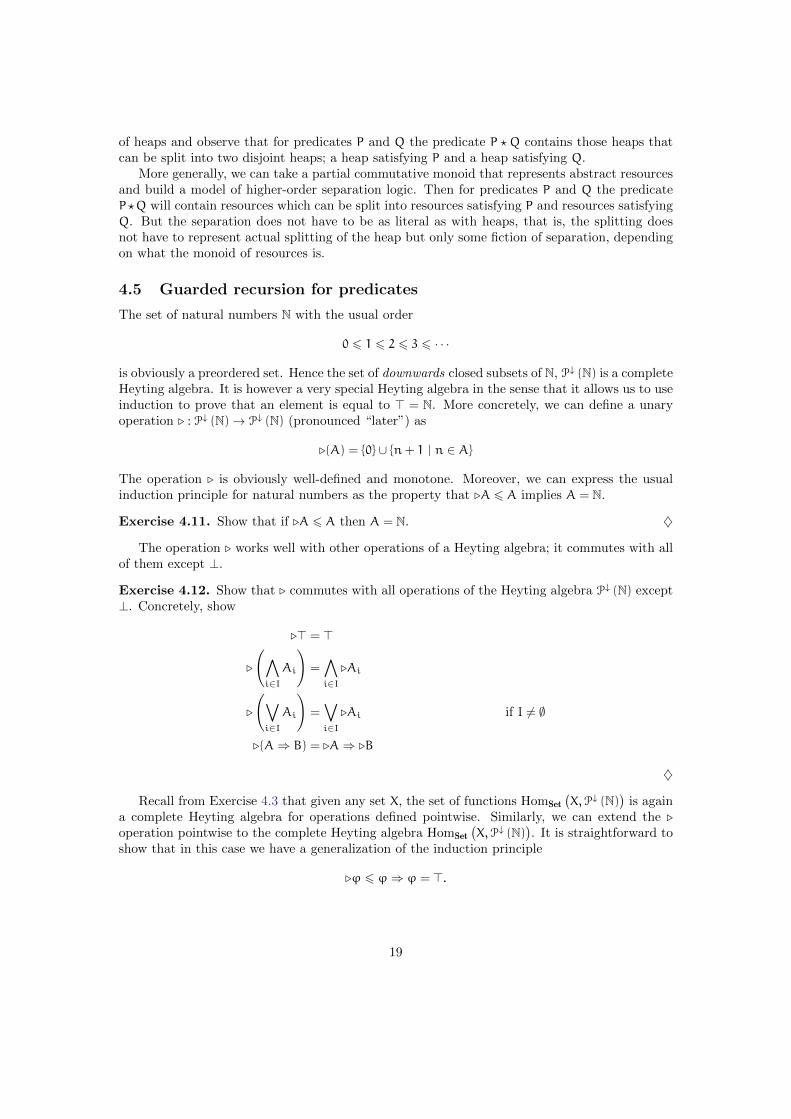
4.5 Guarded recursion for predicates

The set of natural numbers N with the usual order

0 6 1 6 2 6 3 6 · · ·

is obviously a preordered set. Hence the set of downwards closed subsets of N, P↓ (N) is a completeHeyting algebra. It is however a very special Heyting algebra in the sense that it allows us to useinduction to prove that an element is equal to > = N. More concretely, we can define a unaryoperation . : P↓ (N)→ P↓ (N) (pronounced “later”) as

.(A) = 0 ∪ n+ 1 | n ∈ A

The operation . is obviously well-defined and monotone. Moreover, we can express the usualinduction principle for natural numbers as the property that .A 6 A implies A = N.

Exercise 4.11. Show that if .A 6 A then A = N. ♦

The operation . works well with other operations of a Heyting algebra; it commutes with allof them except ⊥.

Exercise 4.12. Show that . commutes with all operations of the Heyting algebra P↓ (N) except⊥. Concretely, show

.> = >

.

(∧i∈IAi

)=∧i∈I

.Ai

.

(∨i∈IAi

)=∨i∈I

.Ai if I 6= ∅

.(A⇒ B) = .A⇒ .B

♦

Recall from Exercise 4.3 that given any set X, the set of functions HomSet

(X,P↓ (N)

)is again

a complete Heyting algebra for operations defined pointwise. Similarly, we can extend the .

operation pointwise to the complete Heyting algebra HomSet

(X,P↓ (N)

). It is straightforward to

show that in this case we have a generalization of the induction principle

.ϕ 6 ϕ⇒ ϕ = >.

19

Exercise 4.13. Show that if .ϕ 6 ϕ then ϕ is the top element of HomSet

(X,P↓ (N)

).

Moreover, show that . on HomSet

(X,P↓ (N)

)also commutes with the same Heyting algebra

operations as . on P↓ (N).Finally, show that if f : X→ Y is any function then for any ϕ ∈ HomSet

(Y,P↓ (N)

)we have

.(HomSet

(f,P↓ (N)

)(ϕ))= HomSet

(f,P↓ (N)

)(.(ϕ))

which means that all the Heyting algebra morphisms HomSet

(f,P↓ (N)

)also preserve the opera-

tion .. ♦

All of these are straightforward to show directly from the definitions of all the operations butit is good practice to show some of them to get used to the definitions.

The reason for introducing the . operation is that we can use it to show existence of certainguarded recursively defined predicates. To show this, we need some auxiliary definitions. Untilthe end of this section we are working in some complete Heyting algebra H = HomSet

(X,P↓ (N)

)for some set X.

Definition 4.15. Let ϕ,ψ ∈ H. For n ∈ N we define bϕcn ∈ H as

bϕcn (x) = k ∈ ϕ(x) | k < n

and we write ϕn=ψ for

bϕcn = bψcn .

Note that for any ψ,ϕ ∈ H we have ϕ0=ψ and that ϕ

n+1= ψ⇒ ϕ

n=ψ and finally that if ∀n,ϕ n

=ψ

then ψ = ϕ.We say that a function Φ : H → H is non-expansive if for any ϕ,ψ ∈ H and any n ∈ N we

have

ϕn=ψ⇒ Φ(ϕ)

n=Φ(ψ)

and we say that it is contractive if for any ϕ,ψ ∈ H and any n ∈ N we have

ϕn=ψ⇒ Φ(ϕ)

n+1= Φ(ψ).

We can now put . to good use.

Exercise 4.14. Show that . is contractive. Show that composition (either way) of a contractiveand non-expansive function is contractive. Conclude that if Φ is a non-expansive function on Hthen Φ . and . Φ are contractive. ♦

Finally the property we were looking for.

Proposition 4.16. If Φ : H→ H is a contractive function then it has a unique fixed point, i.e.,there is a unique ϕ ∈ H such that Φ(ϕ) = ϕ.

We will prove a more general theorem later (Theorem 5.10) so we skip the proof at this point.However, uniqueness is easy to show and is a good exercise.

Exercise 4.15. Show that if Φ : H → H is contractive then the fixed point (if it exists) mustnecessarily be unique.

Hint: Use contractiveness of Φ together with the fact that if bϕcn = bψcn for all n ∈ N thenϕ = ψ. ♦

20

4.5.1 Application to the logic

Suppose that we extend the basic higher-order logic with an operation . on propositions. Con-cretely, we add the typing judgment

Γ ` ϕ : Prop

Γ ` .ϕ : Prop

together with the following introduction and elimination rules

Γ | Ξ ` ϕΓ | Ξ ` .ϕ

monoΓ | Ξ, .ϕ ` ϕΓ | Ξ ` ϕ

Lob

We can interpret this extended logic in the hyperdoctrine arising from the complete Heytingalgebra P↓ (N) by extending the basic interpretation with

JΓ ` .ϕ : PropK = . (JΓ ` ϕ : PropK) .

The properties of . from Exercise 4.13 then give us the following properties of the logic.Judgments

Γ | Ξ ` .(ϕ∧ψ)

Γ | Ξ ` .ϕ∧ .ψ

Γ | Ξ ` .ϕ∧ .ψ

Γ | Ξ ` .(ϕ∧ψ)

and if σ is inhabited, that is if there exists a term M such that − `M : σ then

Γ | Ξ ` .(∃x : σ,ϕ)Γ | Ξ ` ∃x : σ, .(ϕ)

Γ | Ξ ` ∃x : σ, .(ϕ)Γ | Ξ ` .(∃x : σ,ϕ)

and similar rules for all the other connectives except ⊥ are all valid in the model.Moreover, the property that for any function f, HomSet

(f,P↓ (N)

)preserves . gives us that

the rules

Γ | Ξ ` . (ϕ [N/x])

Γ | Ξ ` (.ϕ) [N/x]

Γ | Ξ ` (.ϕ) [N/x]

Γ | Ξ ` . (ϕ [N/x])

are valid, i.e., that . commutes with substitution. This is a property that must hold for theconnective to be useful since we use substitution constantly in reasoning, most of the timeimplicitly. For instance every time we instantiate a universally quantified formula or when weprove an existential, we use substitution.

Exercise 4.16. Show that the rules we listed are valid. ♦

Finally, we would like show that we have fixed points of guarded recursively defined predicates.More precisely, suppose the typing judgment Γ, p : Propτ ` ϕ : Propτ is valid and that p in ϕ onlyoccurs under a . (or not at all). Then we would like there to exist a unique term µp.ϕ of typePropτ in context Γ , i.e.,

Γ ` µp.ϕ : Propτ

such that the following sequents hold

Γ, x : τ | (ϕ [µp.ϕ/p]) x ` (µp.ϕ) x Γ | (µp.ϕ) x ` (ϕ [µp.ϕ/p]) x. (5)

21

Observe that this implies

Γ | − ` ∀x : τ, (ϕ [µp.ϕ/p]) x⇔ (µp.ϕ) x

Recall that when interpreting higher-order logic in the hyperdoctrine HomSet

(−,P↓ (N)

)the term

ϕ is interpreted as

JΓ, p : Propτ ` ϕ : PropτK : JΓK×H→ H

where H = JτK→ JPropK = JτK→ P↓ (N). Suppose that for each γ ∈ JΓK the function Φγ : H→ H

defined as

Φγ(h) = JΓ, p : Propτ ` ϕ : PropτK (γ, h)

were contractive. Then we could appeal to Proposition 4.16 applied to Φγ so that for each γ ∈ Γwe would get a unique element hγ ∈ H, such that Φγ(h) = hγ, or, in other words, we would geta function from Γ to H, mapping γ to hγ. Define

JΓ ` µp.ϕ : PropτK

to be this function. We then have

JΓ ` µp.ϕ : PropτK = hγ = JΓ, p : Propτ ` ϕ : PropτK (γ, hγ)= JΓ, p : Propτ ` ϕ : PropτK (γ, JΓ ` µp.ϕ : PropτK)= JΓ ` ϕ [µp.ϕ/p] : PropτK

The last equality following from Proposition 4.3. Observe that this is exactly what we need tovalidate the rules (5).

However not all interpretations where the free variable p appears under a . will be contractive.The reason for this is that can choose interpretations of base constants from the signature to bearbitrarily bad and a single use of . will not make these non-expansive. The problem comes fromthe fact that we are using a Set-based hyperdoctrine and so interpretations of terms (includingbasic function symbols) can be any functions. If we instead used a category where we had ameaningful notion of non-expansiveness and contractiveness and all morphisms would be non-expansive by definition, then perhaps every term with a free variable p guarded by a . would becontractive and thus define a fixed point.

Example 4.17. Consider a signature with a single function symbol of type F : Prop→ Prop andthe interpretation in the hyperdoctrine HomSet

(−,P↓ (N)

)where we choose to interpret F as

JFK = λA.

.(A) if A 6= N∅ if A = N

Exercise 4.17. Show that JFK is not non-expansive and that JFK . and JFK . are also notnon-expansive. Show also that JFK . and . JFK have no fixed-points. ♦

This example (together with the exercise) shows that even though p appears under a . in

p : Prop ` F (.(p)) : Prop

the interpretation of p : Prop ` F (.(p)) : Prop has no fixed points and so we are not justified inadding them to the logic.

This brings us to the next topic, namely the definition of a category in which all morphismsare suitably non-expansive.

22

5 Complete ordered families of equivalences

Ordered families of equivalences (o.f.e.’s) are sets equipped with a family of equivalence relationsthat approximate the actual equality on the set X. These relations must satisfy some basiccoherence conditions.

Definition 5.1 (o.f.e.). An ordered family of equivalences is a pair(X,(n=)∞n=0

)where X is a

set and for each n, the binary relationn= is an equivalence relation on X such that the relations

n= satisfy the following conditions

• 0= is the total relation on X, i.e., everything is equal at stage 0.

• for any n ∈ N,n+1= ⊆ n

= (monotonicity)

• for any x, x ′ ∈ X, if ∀n ∈ N, x n= x ′ then x = x ′.

We say that an o.f.e.(X,(n=)∞n=0

)is inhabited if there exists an element x ∈ X.

Example 5.2. A canonical example of an o.f.e. is a set of strings (finite and infinite) over somealphabet. The strings x, x ′ are n-equal, x

n= x ′ if they agree for the first n characters.

Example 5.3. The set P↓ (N) together with the relationsn= from Definition 4.15 is an o.f.e.

Remark 5.4. If you are familiar with metric spaces observe that o.f.e.’s are but a differentpresentation of bisected 1-bounded ultrametric spaces.

Definition 5.5 (Cauchy sequences and limits). Let(X,(n=)∞n=0

)be an o.f.e. and xn

∞n=0 be a

sequence of elements of X. Then xn∞n=0 is a Cauchy sequence if

∀k ∈ N, ∃j ∈ N, ∀n > j, xjk= xn

or in words, the elements of the chain get arbitrarily close.An element x ∈ X is the limit of the sequence xn

∞n=0 if

∀k ∈ N, ∃j ∈ N, ∀n > j, x k= xn.

A sequence may or may not have a limit. If it has we say that the sequence converges. The limitis necessarily unique in this case (Exercise 5.1) and we write limn→∞ xn for it.

Remark 5.6. These are the usual Cauchy sequence and limit definitions for metric spacesspecialized to o.f.e.’s.

Exercise 5.1. Show that limits are unique. That is, suppose that x and y are limits of xn∞n=0.

Show x = y. ♦

One would perhaps intuitively expect that every Cauchy sequence has a limit. This is notthe case in general.

Exercise 5.2. Show that if the alphabet Σ contains at least one letter then the set of finitestrings over Σ admits a Cauchy sequence without a limit. The equivalence relation

n= relates

strings that have the first n characters equal.Hint: Pick σ ∈ Σ and consider the sequence xn = σn (i.e., xn is n σ’s). ♦

23

We are interested in spaces which do have the property that every Cauchy sequence hasa limit. These are called complete. Completeness allows us to have fixed points of suitablecontractive functions which we define below.

Definition 5.7 (c.o.f.e.). A complete ordered family of equivalences is an ordered family of

equivalences(X,(n=)∞n=0

)such that every Cauchy sequence in X has a limit in X.

Example 5.8. A canonical example of a c.o.f.e. is the set of infinite strings over an alphabet.The relation

n= relates streams that agree on at least the first n elements.

Exercise 5.3. Show the claims made in Example 5.8.Show that P↓ (N) with relations from Definition 4.15 is a c.o.f.e. (We show a more general

result later in Proposition 5.12.) ♦

To have a category we also need morphisms between (complete) ordered families of equiva-lences.

Definition 5.9. Let(X,(n=X

)∞n=0

)and

(Y,(n=Y

)∞n=0

)be two ordered families of equivalences

and f a function from the set X to the set Y. The function f is

• non-expansive if for any x, x ′ ∈ X, and any n ∈ N,

xn=Xx ′ ⇒ f(x)

n=Yf(x ′)

• contractive if for any x, x ′ ∈ X, and any n ∈ N,

xn=Xx ′ ⇒ f(x)

n+1=Yf(x ′)

Exercise 5.4. Show that non-expansive functions preserve limits, i.e., show that if f is a non-expansive function and xn

∞n=0 is a converging sequence, then so is f(xn)

∞n=0 and that

f(

limn→∞ xn

)= limn→∞ f(xn).

♦

The reason for introducing complete ordered families of equivalences, as opposed to justo.f.e.’s, is that any contractive function on a inhabited c.o.f.e. has a unique fixed point.

Theorem 5.10 (Banach’s fixed point theorem). Let(X,(n=)∞n=0

)be a an inhabited c.o.f.e. and

f : X→ X a contractive function. Then f has a unique fixed point.

Proof. First we show uniqueness. Suppose x and y are fixed points of f, i.e. f(x) = x and f(y) = y.

By definition of c.o.f.e.’s we have x0=y. From contractiveness we then get f(x)

1= f(y) and so x

1=y.

Thus by induction we have ∀n, x n=y. Hence by another property in the definition of c.o.f.e.’s wehave x = y.

To show existence, we take any x0 ∈ X (note that this exists since by assumption X isinhabited). We then define xn+1 = f(xn) and claim that xn

n= xn+m for any n and m which

we prove by induction on n. For n = 0 this is trivial. For the inductive step we have, bycontractiveness of f

xn+1 = f(xn)n+1= f(xn+m) = xn+m+1,

24

as required. This means that the sequence xn∞n=0 is Cauchy. Now we use completeness to

conclude that xn∞n=0 has a limit, which we claim is the fixed point of f. Let x = limn→∞ xn.

We have (using Exercise 5.4)

f(x) = f(

limn→∞ xn

)= limn→∞ f(xn) = lim

n→∞ xn+1 = limn→∞ xn = x

concluding the proof.

Definition 5.11 (The category U). The category U of complete ordered families of equiva-lences has as objects complete ordered families of equivalences and as morphisms non-expansivefunctions.

From now on, we often use the underlying set X to denote a (complete) o.f.e.(X,(n=X

)∞n=0

),

leaving the family of equivalence relations implicit.

Exercise 5.5. Show that U is indeed a category. Concretely, show that composition of non-expansive morphisms is non-expansive and that the identity function is non-expansive. ♦

Exercise 5.6. Show that if f is contractive and g is non-expansive, then f g and g f arecontractive. ♦

Exercise 5.7. Show that the Set is a coreflective subcategory of U. Concretely, this meansthat there is an inclusion functor ∆ : Set → U which maps a set X to a c.o.f.e. with equivalencerelation

n= being the equality on X for n > 0 and the total relation for 0.

Show that the functor ∆ is full and faithful and that it has a right adjoint, the forgetfulfunctor F : U→ Set that “forgets” the equivalence relations.

Further, show that the only contractive functions from any c.o.f.e. to ∆(Y) are constant. ♦

The last part of the exercise is one of the reasons why we can define fixed points of guardedrecursive predicates in the U hyperdoctrine which we describe below but not in a Set-basedhyperdoctrine from Section 4.5.

If we wish to find a fixed point of a function f from a set X to a set Y we really have nothingto go on. What the o.f.e.’s give us is the ability to get closer and closer to a fixed point, if f iswell-behaved. What the c.o.f.e.’s additionally give us is that the “thing” we get closer and closerto is in fact an element of the o.f.e.

5.1 U-based hyperdoctrine

We now wish to imitate the Set-based hyperdoctrine arising from a preordered set P; the hyper-doctrine with P = HomSet

(−,P↑ (P)

)but in a way that would allow us also to model . in the

logic. We can express this in a nice way by combining P↓ (N) with P↑ (P) into uniform predicatesUPred (P).

Let P be a preordered set. We define UPred (P) ⊆ P (N× P) as

UPred (P) = A ∈ P (N× P) | ∀n ∈ N, p ∈ P, (n, p) ∈ A⇒ ∀m 6 n,∀q > p, (m,q) ∈ A

i.e., they are sets downwards closed in the natural numbers and upwards closed in the order onP.

Observe that UPred (P) is nothing else than P↑ (Nop × P) where the order on the productis component-wise and Nop are the naturals with the reverse of the usual order relation, i.e.,1 > 2 > 3 > · · · . This immediately gives us that UPred (P) is a complete Heyting algebra(Exercise 4.6).

25

Proposition 5.12. For any preorder P, UPred (P) is a c.o.f.e. with relationn= defined as

An=B ⇐⇒ bAcn = bBcn

where

bAcn = (m,a) | (m,a) ∈ A∧m < n

Proof. First we need to show that the specified data satisfies the requirements of an o.f.e. It

is obvious that all the relations are equivalence relations and that0= is the total relation on

UPred (P). Regarding monotonicity, suppose An+1= B. We need to show bAcn = bBcn and we do

this by showing that they are included in one another. Since the two inclusions are completelysymmetric we only show one.

Let (k, a) ∈ bAcn. By definition (k, a) ∈ A and k < n which clearly implies that (k, a) ∈bAcn+1. The assumption A

n+1= B gives us (k, a) ∈ bBcn+1 but since k < n we also have (k, a) ∈

bBcn concluding the proof of inclusion.

To show that the intersection of all relationsn= is the identity relation suppose A

n=B for

all n. We again show that A and B are equal by showing two inclusions which are completelysymmetric so it suffices to show only one.

Suppose (m,a) ∈ A. By definition (m,a) ∈ bAcm+1, so from the assumption (m,a) ∈ bBcm+1

and thus (m,a) ∈ B, showing that A ⊆ B.We are left with showing completeness. Suppose An

∞n=0 is a Cauchy sequence. Recall

that this means that for each n ∈ N there exists an Nn, such that for any j > Nn, ANn

n=Aj.

Because of the monotonicity of the relationsn= we can assume without loss of generality that

N1 6 N2 6 N3 6 · · · .Define A =

(m,a) | (m,a) ∈ ANm+1

. We claim that A is the limit of An

∞n=0.

First we show that A is in fact an element of UPred (P). Take (m,a) ∈ A and n 6 m andb > a. We need to show (n, b) ∈ A. By definition this means showing (n, b) ∈ ANn+1

. Recallthat Nn+1 6 Nm+1 by assumption and from the definition of the numbers Nk we have

ANn+1

n+1= ANm+1

which again by definition means⌊ANn+1

⌋n+1

=⌊ANm+1

⌋n+1

. But note that by the fact thatANm+1

is an element of UPred (P) we have (n, b) ∈ ANm+1and from this we have

(n, b) ∈⌊ANm+1

⌋n+1

=⌊ANn+1

⌋n+1⊆ ANn+1

showing that (n, b) ∈ ANn+1.

Exercise 5.8. Using similar reasoning show that An=ANn

. ♦

The only thing left to show is that A is in fact the limit of UPred (P). Let n ∈ N and k > Nn.We have

Akn=ANn

n=A.

Thus for each n ∈ N there exists a Nn such that for every k > Nn, Akn=A, i.e., A is the limit of

the sequence An∞n=0.

26

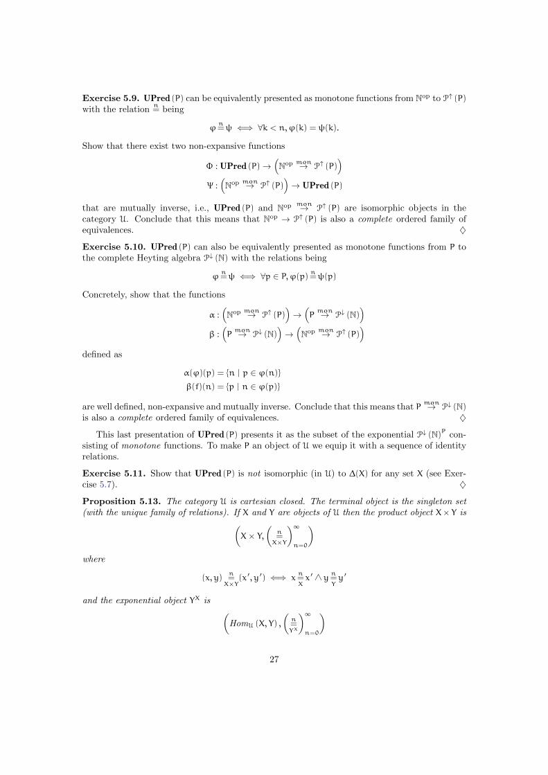
Exercise 5.9. UPred (P) can be equivalently presented as monotone functions from Nop to P↑ (P)

with the relationn= being

ϕn=ψ ⇐⇒ ∀k < n,ϕ(k) = ψ(k).

Show that there exist two non-expansive functions

Φ : UPred (P)→(Nop mon→ P↑ (P)

)Ψ :(Nop mon→ P↑ (P)

)→ UPred (P)

that are mutually inverse, i.e., UPred (P) and Nop mon→ P↑ (P) are isomorphic objects in thecategory U. Conclude that this means that Nop → P↑ (P) is also a complete ordered family ofequivalences. ♦

Exercise 5.10. UPred (P) can also be equivalently presented as monotone functions from P tothe complete Heyting algebra P↓ (N) with the relations being

ϕn=ψ ⇐⇒ ∀p ∈ P,ϕ(p) n=ψ(p)

Concretely, show that the functions

α :(Nop mon→ P↑ (P)

)→(Pmon→ P↓ (N)

)β :(Pmon→ P↓ (N)

)→(Nop mon→ P↑ (P)

)defined as

α(ϕ)(p) = n | p ∈ ϕ(n)β(f)(n) = p | n ∈ ϕ(p)

are well defined, non-expansive and mutually inverse. Conclude that this means that Pmon→ P↓ (N)

is also a complete ordered family of equivalences. ♦

This last presentation of UPred (P) presents it as the subset of the exponential P↓ (N)P con-sisting of monotone functions. To make P an object of U we equip it with a sequence of identityrelations.

Exercise 5.11. Show that UPred (P) is not isomorphic (in U) to ∆(X) for any set X (see Exer-cise 5.7). ♦

Proposition 5.13. The category U is cartesian closed. The terminal object is the singleton set(with the unique family of relations). If X and Y are objects of U then the product object X× Y is(

X× Y,(

n=X×Y

)∞n=0

)where

(x, y)n=X×Y

(x ′, y ′) ⇐⇒ xn=Xx ′ ∧ y

n=Yy ′

and the exponential object YX is (HomU (X, Y) ,

(n=YX

)∞n=0

)

27

where

fn=YXg ⇐⇒ ∀x ∈ X, f(x) n=

Yg(x).

is the exponential object.

Note that the underlying set of the exponential YX consists of the non-expansive functionsfrom the underlying set of X to the underlying set of Y.

Exercise 5.12. Prove Proposition 5.13. ♦

Proposition 5.14. Let Y be an object of U and P a preordered set. Then HomU (Y,UPred (P))is a complete Heyting algebra for operations defined pointwise.

Proof. Since UPred (P) is a complete Heyting algebra we know from Exercise 4.3 that the set ofall functions from the set X to UPred (P) is a complete Heyting algebra for operations definedpointwise. Thus we know that the operations satisfy all the axioms of a complete Heyting algebra,if they are well-defined. That is, if all operations preserve non-expansiveness of functions. Thisis what we need to check.

We only show it for ⇒. The other cases follow exactly the same pattern.Recall that the definition of ⇒ in UPred (P) is

A⇒ B = (n, p) | ∀k 6 n,∀q > p, (k, q) ∈ A⇒ (k, q) ∈ B .

We first show that if An=A ′ and B

n=B ′ then A ⇒ B

n=A ′ ⇒ B ′ by showing two inclusions. The

two directions are symmetric so we only consider one.Let (m,p) ∈ bA⇒ Bcn. By definition m < n and (m,p) ∈ A ⇒ B and we need to show

(m,p) ∈ bA ′ ⇒ B ′cn. Since we know that m < n it suffices to show (m,p) ∈ A ′ ⇒ B ′ and for

this take k 6 m and q > p and assume (k, q) ∈ A ′. Observe that k < n and since An=A ′ we

have (k, q) ∈ A which implies (k, q) ∈ B which implies, using the fact that Bn=B ′ and k < n that

(k, q) ∈ B ′.Suppose now that f, g : X→ UPred (P) are non-expansive and x, x ′ ∈ X such that x

n= x ′. Then

by definition of operations we have

(f⇒ g)(x) = (f(x)⇒ g(x))n=(f(x ′)⇒ g(x ′)) = (f⇒ g)(x ′)

where we used the fact that⇒ is “non-expansive” in UPred (P) (shown above) and non-expansivenessof f and g to get

n= in the middle.

Recall the motivation for going to the category U; we wanted to be able to talk about guardedrecursive functions in general. Similarly to the Heyting algebra P↓ (N) there is an operation . onUPred (P) defined as

.(A) = (0, p) | p ∈ P ∪ (n+ 1, p) | (n, p) ∈ A .

Exercise 5.13. Show that . is contractive. ♦

This . can be extended pointwise to the complete Heyting algebra HomU (Y,UPred (P)) forany c.o.f.e. Y and is also contractive (when HomU (Y,UPred (P)) is equipped with the metricdefined in Proposition 5.13).

28

Proposition 5.15. Let M be a partial commutative monoid. The complete Heyting algebraUPred (M) arising from the extension order on M is a complete BI-algebra for the followingoperations

I = N×MA ? B = (n, a · b) | (n, a) ∈ A, (n, b) ∈ B, a#b

A→?B = (n, a) | ∀m 6 n,∀b#a, (m,b) ∈ A⇒ (m,a · b) ∈ B

Exercise 5.14. Prove Proposition 5.15. ♦

With Propositions 5.13, 5.14 and 5.15 we have shown the following.

Theorem 5.16. Let M be a partial commutative monoid. The category U together with thegeneric object UPred (M) is a BI-hyperdoctrine.

We can generalize this construction further, replacing UPred (M) by any other c.o.f.e. whoseunderlying set is a complete BI-algebra with a ..

Definition 5.17. A Lob BI-algebra is a c.o.f.e.(H,(n=)∞n=0

)whose underlying set H is a

complete BI-algebra H with a monotone and contractive operation . : H→ H satisfying h 6 .(h)

(monotonicity) and whenever .(h) 6 h then h = > (Lob rule).Further, the BI-algebra operations have to be non-expansive. For instance if I is any index

set and for each i ∈ I, ain=bi, then we require∧

i∈Iain=∧i∈Ibi∨

i∈Iain=∨i∈Ibi

to hold.Additionally, . is required to satisfy the following equalities

.> = >

.

(∧i∈IAi

)=∧i∈I

.Ai

.

(∨i∈IAi

)=∨i∈I

.Ai if I 6= ∅

.(A⇒ B) = .A⇒ .B

.(A ? B) = .(A) ? .(B)

.(A→?B) = .(A)→? . (B)

Remark 5.18. In the definition of a Lob BI-algebra we included the requirements that aresatisfied by all the examples we consider below. However, it is not clear whether all of therequirements are necessary for applications of the logic or whether they could be weakened (forinstance, whether we should require .(A ? B) = .(A) ? .(B) or not).

Example 5.19. If M is a partial commutative monoid then UPred (M) is a Lob BI-algebra.

29

We then have the following theorem. The proof is much the same as the proof of Proposi-tion 5.14. The requirement that the BI-algebra operations are non-expansive implies that theoperations defined pointwise will preserve non-expansiveness of functions.

Theorem 5.20. Let H be a Lob BI-algebra. Then HomU (−, H) is a BI-hyperdoctrine for oper-ations defined pointwise that also validates rules involving . from Section 4.5.1.

Recall again the motivation for introducing c.o.f.e.’s from Section 4.5 and Example 4.17. Ifwe used a Set-based hyperdoctrines we could choose to interpret the signature in such a waythat even though we guarded free variables using a ., we would have no fixed points since theinterpretations of function symbols were arbitrary functions.

However in a U-based hyperdoctrine we must interpret all function symbols as non-expansivefunctions since these are the only morphisms in U. We thus have the following theorem andcorollary for the hyperdoctrine HomU (−, H) for a Lob BI-algebra H.

Theorem 5.21. Assume ϕ satisfies Γ, p : Propτ, ∆ ` ϕ : σ and suppose further that all free oc-currences of p in ϕ occur under a .. Then for each γ ∈ JΓK and δ ∈ J∆K,

JΓ, p : Propτ, ∆ ` ϕ : σK (γ,−, δ) : JPropτK→ JσK

is contractive.

Proof. We proceed by induction on the typing derivation Γ, p : Propτ, ∆ ` ϕ : σ and show someselected rules.

• Suppose the last rule used was

Γ, p : Propτ, ∆ ` ϕ : Prop

Γ, p : Propτ, ∆ ` .ϕ : Prop.

Then by definition, the interpretation JΓ, p : Propτ, ∆ ` ϕ : PropK (γ,−, δ) is non-expansivefor each γ and δ (this is because it is interpreted as a morphism in U). By definition, theinterpretation

JΓ, p : Propτ, ∆ ` .ϕ : PropK = . JΓ, p : Propτ, ∆ ` ϕ : PropK

and so

JΓ, p : Propτ, ∆ ` .ϕ : PropK (γ,−, δ) = . JΓ, p : Propτ, ∆ ` ϕ : PropK (γ,−, δ).

Exercises 5.13 and 5.6 then give us that JΓ, p : Propτ, ∆ ` .ϕ : PropK (γ,−, δ) is contractive.Note that we have not used the induction hypothesis here and in fact we could not since pmight not be guarded anymore when we go under a ..

• Suppose that the last rule used was the function symbol rule. For simplicity assume thatF has only two arguments so that the last rule used was

Γ, p : Propτ, ∆ `M1 : τ1 Γ, p : Propτ, ∆ `M2 : τ2

Γ, p : Propτ, ∆ ` F(M1,M2) : σ

To reduce clutter we write JM1K and JM2K for the interpretations of the typing judgmentsof M1 and M2. By definition we have

JΓ, p : Propτ, ∆ ` F(M1,M2) : σK = JFK 〈JM1K , JM2K〉 .

30

Since JFK is a morphism in U it is non-expansive. The induction hypothesis gives us thatJM1K (γ,−, δ) and JM2K (γ,−, δ) are contractive. It is easy to see that then 〈JM1K , JM2K〉 (γ,−, δ)is also contractive which gives us that JΓ, p : Propτ, ∆ ` F(M1,M2) : σK (δ,−, γ) is also con-tractive (Exercise 5.6).

• Suppose the last rule used was the conjunction rule

Γ, p : Propτ, ∆ ` ϕ : Prop Γ, p : Propτ, ∆ ` ψ : Prop

Γ, p : Propτ, ∆ ` ϕ∧ψ : Prop

By definition,

JΓ, p : Propτ, ∆ ` ϕ∧ψ : PropK = JϕK ∧ JψK

and recall that the definitions of Heyting algebra operations on HomU (X,H) are pointwise.Therefore JϕK∧JψK = ∧H〈JϕK , JψK〉 where on the right-hand side ∧H is the conjunction ofthe BI-algebra H. Using the induction hypothesis we have that JϕK (γ,−, δ) and JψK (γ,−, δ)are contractive. By assumption thatH is a Lob BI-algebra we have that ∧H is non-expansivegiving us, using Exercise 5.6 that JΓ, p : Propτ, ∆ ` ϕ∧ψ : PropK (γ,−, δ) is contractive.

The other cases are similar.

Corollary 5.22. Assume ϕ satisfies Γ, p : Propτ ` ϕ : Propτ and suppose further that all freeoccurrences of p in ϕ occur under a .. Then for each γ ∈ JΓK there exists a unique hγ ∈ JPropτKsuch that

JΓ, p : Propτ ` ϕ : PropτK (γ, hγ) = hγ

and further, this assignment is non-expansive, i.e., if γn=γ ′ then hγ

n=hγ′ .

Proof. Existence and uniqueness of fixed points follows from Theorem 5.10 and the fact thatUPred (M)JτK is always inhabited, since UPred (M) is.

Non-expansiveness follows from non-expansivness of JΓ, p : Propτ ` ϕ : PropτK and the factthat if two sequences are pointwise n-equal, so are their respective limits (see the constructionof fixed points in Theorem 5.10).

Using these results we can safely add fixed points of guarded recursively defined predicatesas in Section 4.5 to the logic and moreover, we can add rules stating uniqueness of such fixedpoints (up to equivalence ⇐⇒ ).

6 Constructions on the category U

The . is useful when we wish to construct fixed points of predicates, i.e., functions with codomainsome Lob BI-algebra. For models of pure separation logic and guarded recursion we can useuniform predicates as shown above. Pure separation logic provides us with a way to reasonabout programs that manipulate dynamically allocated mutable state by allowing us to assertfull ownership over resources. In general, however, we also wish to specify and reason aboutshared ownership over resources. This is useful for modeling type systems for references, wherethe type of a reference cell is an invariant that is shared among all parts of the program, orfor modeling program logics that combine ideas from separation logic with rely-guarantee stylereasoning, see, e.g., [BRS+11] and the references therein. In these cases, the basic idea is that

31

propositions are indexed over “worlds”, which, loosely speaking, contain a description of thoseinvariants that have been established until now. In general, an invariant can be any kind ofproperty, so invariants are propositions. A world can be understood as a finite map from naturalnumbers to invariants. We then have that propositions are indexed over worlds which containpropositions and hence the space of propositions must satisfy a recursive equation of roughly thefollowing form:

Prop = (N fin Prop)→ UPred (M) .

For cardinality reasons, this kind of recursive domain equation does not have a solution in Set.In this section we show that a solution to this kind of recursive domain equation can be found inthe category U and, moreover, that the resulting recursively defined space will in fact give riseto a BI-hyperdoctrine that also models guarded recursively defined predicates.

To express the equation precisely in U we will make use of the I functor :

Definition 6.1. The functor I is a functor on U defined as

I(X,(n=)∞n=0

)=(X,(n≡)∞n=0

)I (f) = f

where0≡ is the total relation and x

n+1≡ x ′ iff xn= x ′

Exercise 6.1. Show that the functor I is well-defined. ♦

Definition 6.2. The category Uop has as objects complete ordered families of equivalences anda morphism from X to Y is a morphism from Y to X in U.

Definition 6.3. A functor F : Uop × U → U is locally non-expansive if for all objects X, X ′, Y,and Y ′ in U and f, f ′ ∈ HomU (X,X ′) and g, g ′ ∈ HomU (Y ′, Y) we have

fn= f ′ ∧ g

n= g ′ ⇒ F(f, g)

n= F(f ′, g ′).

It is locally contractive if the stronger implication

fn= f ′ ∧ g

n= g ′ ⇒ F(f, g)

n+1= F(f ′, g ′).

holds. Note that the equalities are equalities on function spaces.

Proposition 6.4. If F is a locally non-expansive functor then I F and F (Iop × I) are locallycontractive. Here, the functor F (Iop × I) works as

(F (Iop × I))(X, Y) = F (Iop (X),I (Y))

on objects and analogously on morphisms and Iop: Uop → Uop is just I working on Uop (i.e., itsdefinition is the same).

Exercise 6.2. Show Proposition 6.4. ♦

6.1 A typical recursive domain equation

We now consider the typical recursive domain equation mentioned above.

Let X be a c.o.f.e. We write N fin X for the set of finite partial maps from N to X (no

requirement of non-expansiveness).

32

Proposition 6.5. If X is a c.o.f.e. then the space N fin X is a c.o.f.e. when equipped with the

following equivalence relations

fn=g ⇐⇒ n = 0∨

(dom (f) = dom (g)∧ ∀x ∈ dom (f) , f(x)

n=g(x)

).

Exercise 6.3. Prove Proposition 6.5. The only non-trivial thing to check is completeness. Forthis, first show that for any Cauchy sequence fn

∞n=0 there is an n, such that for any k > n,

dom (fk) = dom (fn). Then the proof is similar to the proof that the set of non-expansivefunctions between c.o.f.e.’s is again complete. ♦

We order the space N fin X by extension ordering, i.e.,

f 6 g ⇐⇒ dom (f) ⊆ dom (g)∧ ∀n ∈ dom (f) , f(n) = g(n).

Note that this is the same order that we used for ordering the monoid of heaps in Example 4.9.

Theorem 6.6. Let H be a Lob BI-algebra and X a c.o.f.e. Suppose that the limits in H respectthe order on H, i.e., given two converging sequences an

∞n=0 and bn

∞n=0 such that for all n,

an 6 bn we also have limn→∞ an 6 limn→∞ bn.

Then the set of monotone and non-expansive functions from N fin to H with the metric

inherited from the space HomU

(N fin X,H

)is again a Lob BI-algebra.

Proof. We know that the set of non-expansive functions with operations defined pointwise isagain a Lob BI-algebra, but that does not immediately imply that the set of monotone andnon-expansive functions is as well.

It is easy to see that limits of Cauchy sequences exists using the fact that limits in H preserveorder. Exercise!

It is a standard fact that monotone functions from a preordered set into a complete Heytingalgebra again form a complete Heyting algebra for pointwise order and the operations defined asfollows

(f⇒ g)(x) =∧y>x

(f(y)⇒ g(y))

(∧i∈Ifi

)(x) =

∧i∈I

(fi(x))

(∨i∈Ifi

)(x) =

∨i∈I

(fi(x)) .

We first need to check that the operations are well defined. It is easy to see that given monotonefunctions as input the operations produces monotone functions as output. It is also easy to seethat

∧and

∨preserve non-expansiveness. However proving non-expansiveness of f ⇒ g is not

so straightforward.Suppose x

n= x ′. The case when n = 0 is not interesting so assume n > 0. We need to show

that ∧y>x

(f(y)⇒ g(y))n=∧y′>x′

(f(y ′)⇒ g(y ′)).

By the definition of the equality relation on N fin X we have that dom (x)dom (x ′) and that for

each k ∈ dom (x) , x(k)n= x ′(k). By the definition of the order relation on N fin

X we have that ify > x then dom (y) ⊇ dom (x) and for each k ∈ dom (x), x(k) = y(k) and similarly for x ′. Thus ify > x and y ′ > x ′ then ∀k ∈ dom (x) = dom (x ′) , y(k)

n=y ′(k). Thus for each y > x there exists a

y ′ > x ′, such that yn=y ′ and conversely, for each y ′ > x ′ there exists a y > x, such that y

n=y ′.

33

Exercise 6.4. Let I and J be two index sets and n ∈ N. Suppose that for each i ∈ I there existsa j ∈ J, such that ai

n=bj and conversely that for each j ∈ J there exists an i ∈ I, such that ai

n=bj.

Show that in this case ∧i∈Iain=∧j∈Jbj.

Hint: Consider the extended index set K = I t J, the disjoint union of I and J. Define elementsa ′k and b ′k such that for each k ∈ K, a ′k

n=b ′k and so that∧

k∈Ka ′k =

∧i∈Iai

∧k∈K

b ′k =∧j∈Jbj.

Then use that∧

is non-expansive. ♦

Remark 6.7. Theorem 6.6 considers monotone functions on some particular c.o.f.e. Of course,this can be generalized to monotone functions on any suitable preordered c.o.f.e., see [BST10].

Now we know that the operations are well-defined. Next we need to show that they satisfythe Heyting algebra axioms.

Exercise 6.5. Show that operations so defined satisfy the Heyting algebra axioms. ♦

We also need to establish that the operations are non-expansive. Recall that equality on thefunction space is defined pointwise. We only consider the implication, the other operations aresimilar.

Suppose fn= f ′ and g

n=g ′. We then have that for each y, (f(y) ⇒ g(y))

n=(f ′(y) ⇒ g ′(y)) and

from this it is easy to see that (f⇒ g)n=(f ′ ⇒ g ′) by non-expansiveness of

∧.

It is easy to see that we can extend the operation . pointwise, i.e.,

.(f) = . f.

Exercise 6.6. Show that the . defined this way satisfies all the requirements. ♦

The BI-algebra operations are defined as follows

(f ? g)(x) = f(x) ? g(x) (f→?g)(x) =∧y>x

(f(y)→?g(y)).

We can show in the same way as for ∧ and ⇒ that they are well-defined and satisfy the correctaxioms.

Given any partial commutative monoid we have, using Theorem 6.6, that the functor

F : Uop → U

F(X) = (N fin X)

mon→n.e.

UPred (M)

is well-defined.The space of propositions will be derived from this functor. However in general this functor

does not have a fixed-point; we need to make it locally-contractive by composing with the functorI. Using Theorem 6.9 (described in the next subsection) we have that G =I F has a unique

34

fixed point which we call PreProp. That is, G(PreProp) ∼= PreProp in U. Concretely, we have anon-expansive bijection ι with a non-expansive inverse

ι : G(PreProp)→ PreProp.

Since PreProp is a c.o.f.e. we can use Theorem 6.6 to show that the space

Prop = F(PreProp) = (N fin PreProp)

mon→n.e.

UPred (M)

is a Lob BI-algebra. Hence the hyperdoctrine HomU (−,Prop) is a BI-hyperdoctrine that alsomodels the . operation and fixed points of guarded recursive predicates (Theorem 5.20).

Summary As a summary, we present the explicit model of propositions in the hyperdoctrineHomU (−,Prop) (we include equality, although we have not considered that earlier). Recall thata proposition in context Γ ` ϕ : Prop is interpreted as a non-expansive function from JΓK to Prop.Omitting : Prop from the syntax, we have:

JΓ `M =τ NKγw =(n, r) | JΓ `M : τKγ

n+1= JΓ ` N : τKγ

JΓ ` >Kγw = N×M

JΓ ` ϕ∧ψKγw = JΓ ` ϕKγw ∩ JΓ ` ψKγw

JΓ ` ⊥Kγw = ∅

JΓ ` ϕ∨ψKγw = JΓ ` ϕKγw ∪ JΓ ` ψKγw

JΓ ` ϕ⇒ ψKγw = ∀w ′ > w, ∀n ′ 6 n,∀r ′ > r, (n ′, r ′) ∈ JΓ ` ϕKγw′ ⇒ (n ′, r ′) ∈ JΓ ` ψKγw

′

JΓ ` ∀x : σ,ϕKγw =⋂d∈JσK

JΓ, x : σ ` ϕK(γ,d)w

JΓ ` ∃x : σ,ϕKγw =⋃d∈JσK

JΓ, x : σ ` ϕK(γ,d)w

JΓ ` .ϕKγw = (0, r) | r ∈M ∪ (n+ 1, r) | (n, r) ∈ JΓ ` ϕKγw

JΓ ` IKγw = N×M

JΓ ` ϕ ?ψKγw = (n, r) | ∃r1, r2, r = r1 · r2 ∧ (n, r1) ∈ JΓ ` ϕKγw∧ (n, r2) ∈ JΓ ` ψKγw

JΓ ` ϕ→?ψKγw = (n, r) | ∀w ′ > w, ∀n ′ 6 n,∀r ′#r.(n ′, r ′) ∈ JΓ ` ϕKγw′ ∧ (n ′, r · r ′) ∈ JΓ ` ψKγw

′

In particular note that the “resources” r are not used in the interpretation of equality.Moreover, when p occurs under a . in ϕ, then we have a recursively defined predicate:

JΓ ` µp.ϕ : PropτKγ = fix (λx : JPropτK . JΓ, p : Propτ ` ϕ : PropτK(γ,x))

Here fix yields the fixed point of the contractive function, see Corollary 5.22.Finally, we can have a new logical connective for expressing invariants. Syntactically

Γ `M : N Γ ` ϕ : Prop

Γ ` ϕ M : Prop

where N is a base type, which we interpret by the natural numbers (formally, as the object ∆(N)in U).

35

Then we definerΓ ` ϕ M

z

γw =

(n, r) | w(JΓ `MKγ)

n+1= ι(JΓ ` ϕKγ)

.

Let us unfold the definition to see what it means and to see that it makes sense. First, givenγ ∈ JΓK we have

JΓ `MKγ ∈ JNK = ∆(N)

JΓ ` ϕKγ ∈ JPropK = Prop = F(PreProp)

and we wish to haverΓ ` ϕ M : Prop

z

γ∈ JPropK = Prop = (N fin

PreProp)mon→n.e.

UPred (M) .

Thus given w ∈ N fin PreProp we wish to have

rΓ ` ϕ M : Prop

z

γw ∈ UPred (M) .

Now since the underlying set of ∆(N) is N we have w(JΓ `MKγ) ∈ PreProp. Recall theisomorphism ι :I (F(PreProp)) → PreProp. Since the underlying set of I (F(PreProp)) is thesame as the underlying set of F(PreProp) we can apply ι to JΓ ` ϕKγ to get

ι(JΓ ` ϕKγ

)∈ PreProp

We then compare for n-equality in the space PreProp.

Now what the definition is supposed to express is that if (n, r) is inrΓ ` ϕ M : Prop

z

γw for

some world w, then the invariant for region M in world w is approximately ϕ, where approxi-mately is expressed using n-equality and means, intuitively, that ϕ cannot be distinguished fromthe invariant for M in w for n steps. The use of the isomorphism ι is necessary only because wedo not have a solution of the domain equation up to equality, but only up to an isomorphism.

Observe also that therΓ ` ϕ M : Prop

z

γw is oblivious to resources (to r ∈M).

Exercise 6.7. Check that the interpretation ofrΓ ` ϕ M : Prop

zis well defined. Concretely,

check thatrΓ ` ϕ M : Prop

zis non-expansive and that for each γ ∈ Γ , the function

rΓ ` ϕ M : Prop

z

γ

is an element of F(PreProp) which means that it is non-expansive and monotone in the world wand actually maps into UPred (M). ♦

6.2 Explicit construction of fixed points of locally contractive functorsin U

In this subsection, we present an elementary construction of the fixed point of a locally contractivefunctor in the category of complete ordered families of equivalences. This fixed point theoremis originally due to America and Rutten [AR89]. In [BST10] one can find a category-theoreticgeneralization, which shows how to obtain fixed points of locally contractive funtors on categoriesenriched in U. It is not necessary to understand the proof in this subsection to understand therest of the material in these notes.

36

Definition 6.8. A fixed point of a locally contractive functor F is an object X ∈ U, such thatF(X,X) ∼= X.

Theorem 6.9. Every locally contractive functor F such that F(1, 1) is inhabited has a uniquefixed point. The fixed point is unique among inhabited c.o.f.e.’s.

If in addition F(∅, ∅) is inhabited then the fixed point of F is unique.

Proof. We first construct a solution. Then show uniqueness.Define a sequence of spaces Fn ∈ U by induction as follows:

F0 = (∗, (=)∞n=0)Fn+1 = F(Fn, Fn)

together with projections pn : Fn+1 → Fn and embeddings en : Fn → Fn+1

p0 = the unique map to F0

pn+1 = F(en, pn)

e0 = any map from F0 to F1

en+1 = F(pn, en)

Note that e0 exists because by assumption F(1, 1) is inhabited and constant functions are non-expansive.

Later we will need the fact that ek and pk are indeed embeddings and projections, i.e., that

∀k, pk ek = idFk . (6)

which we show by induction. The base case is trivial. For the inductive case we have

pk+1 ek+1 = F(ek, pk) F(pk, ek) = F(pk ek, pk ek) = F (idFk , idFk) = idFk+1.

Projection followed by an embedding does not equal the identity function, but it does getcloser with increasing k. More precisely, we have

∀k, ek pkk= idFk+1

(7)

The base case is trivial, since everything is equal at step 0. For the inductive step we have

ek+1 pk+1 = F(pk, ek) F(ek, pk) = F(ek pk, ek pk)k+1= idFk+2

the last equation holding by the induction hypothesis and contractiveness of F. This is the placewhere local contractiveness of F is used.

It will be convenient later to use compositions of embeddings e`k : Fk → F` and projectionsp`k : F` → Fk which we define as

pkk = idFk

pk+`+1k = pk+`k pk+`

ekk = idFk

ek+`+1k = ek+` ek+`k

Exercise 6.8. Show that for any ` > k,

p`k e`k = idFk . (8)

♦

37

Hint: Use (6).We claim that

X =

x ∈∏n∈N

Fn

∣∣∣ ∀k, pk (xk+1) = xk

is a fixed point of F, i.e., that F(X,X) ∼= X. The equality on X is defined as

xn=X x

′ ⇐⇒ ∀k, xkn=Fk x

′k

wheren=Fk denotes n-th equivalence relation on the set Fk.

It is easy to see that(X,(n=)∞n=0

)is indeed an object of U. In fact, it is also inhabited, for

instance (en0 (∗))∞n=0 is an element of X which is easy to see using (8).

To construct an isomorphism between X and F(X,X) we will need auxiliary embeddings ιn :

Fn → X and projections πn : X→ Fn defined as follows

πn(x) = xn (ιn(y))k =

pnk (y) if n > k

ekn(y) if k > n

Using (8) it is easy to see that ιn is well defined for any n and since pk and ek are non-expansive,so are pnk and ekn and consequently also ιn (see definition of equality on X).

Using these we can define morphism α : X → F(X,X) and β : F(X,X) → X and show themmutually inverse. They are defined as follows

β(z)n =

∗ if n = 0

F(ιm, πm)(z) if n = m+ 1

and

α(x) = limk→∞ F (πk, ιk) (xk+1)

We first need to make sure that these are good definitions, i.e., that they do indeed definemorphism in U between X and F(X,X). First we consider β. To be well-defined it has to actuallymap into X and be non-expansive. To see that it maps into X we proceed by induction. The basecase is trivial since F1 is a single-element space. For the inductive case we have

pn+1 (β(z)n+2) = pn+1 (F(ιn+1, πn+1)(z)) = F(en, pn) (F(ιn+1, πn+1)(z))

= F (ιn+1 en, pn πn+1) (z) = F(ιn, πn)(z) = β(z)n+1

where we have used the fact, which is easily checked, that ιn+1 en = ιn and pn πn+1 = πn.The fact that β is non-expansive follows directly from the fact that F(ιm, πm) is non-expansive

for all m, since F is a functor mapping into U.To see that α is well-defined we have to first show that the limit used in its definition actually

exists. Recall that we are working with c.o.f.e.’s so we only need to check that the sequenceF (πk, ιk) (xk+1)

∞k=0 is a Cauchy chain for x ∈ X.

We will show thatF (πk, ιk) (xk+1)

k+1= F (πk+`, ιk+`) (xk+`+1)

for any ` with the equality being the equality in F(X,X).We proceed by induction on ` with the base case being trivial by construction.

38

F (πk, ιk) (xk+1) = F (πk, ιk) (pk+1xk+2)

= F (πk, ιk) (F (ek, pk) (xk+2))

= F (ek πk, ιk pk) (xk+2)

and from (7) we have

ek(πk(y)) = ek(pk(πk+1(y)))k= πk+1(y)

since πk = pk πk+1 and

ιk(pk(y)) = ιk+1(ek(pk(y)))k= ιk+1(y)

since ιk+1 ek = ιk. Combining these together with the fact that F is contractive we have

F (ek πk, ιk pk) (xk+2)k+1= F (πk+1, ιk+1) (xk+2)

and using the induction hypothesis for ` we get

F (πk+1, ιk+1) (xk+2)k+1= F (πk+1+`, ιk+1+`) (xk+2+`) = F (πk+`+1, ιk+`+1) (xk+1+`+1)

concluding the proof.We have thus established that the sequence used in the definition of α is a Cauchy chain,

hence it has a limit by completeness.

Exercise 6.9. It is a good exercise to show that α is non-expansive or more generally, that giventwo Cauchy-chain that are pointwise n-equal, then the limits are also n-equal. That is, given two

Cauchy-chains an∞n=0 and bn

∞n=0 such that ∀n, an

k= bn, then limn→∞ an k

= limn→∞ bn. ♦

Thus we have α and β, two non-expansive maps. Now we need to show that they are inverses.We first consider α β.

(α β)(z) = limk→∞ F(πk, ιk) (F(ιk, πk)(z)) = lim

k→∞ F(ιk πk, ιk πk)(z)We wish to show that the limit is z. To that end we show that ιk πk

k= idX. Let x ∈ X. We have

for ` > k

ιk(πk(x))` =

x` if ` 6 k

e`k(xk) if k 6 `

so clearly ιk(πk(x))`k= x` for ` 6 k. For k 6 ` we have

ιk(πk(x))` = e`k(xk) = e

`k(p

`k(x`))

k= x`

where we have used

Exercise 6.10. Show that for any ` > k, e`k p`kk= idF` . ♦

39

Hint: Use induction and (7).Since F is contractive we have shown that z is the limit of limk→∞ F(ιk πk, ιk πk)(z) and so

α(β(z)) = z.To show β(α(x)) = x we proceed as follows

β(α(x))n+1 = F(ιn, πn)

(limk→∞ F (πk, ιk) (xk+1)

)and since non-expansive functions preserve limits we get

limk→∞ F(ιn, πn) (F (πk, ιk) (xk+1)) = lim

k→∞ F(πk ιn, πn ιk) (xk+1)Exercise 6.11. For k > n we have πk ιn = ekn and πn ιk = pkn and additionally F(ekn, p

kn) =

pk+1n+1. ♦

Using the result of the last exercise we get

limk→∞ F(πk ιn, πn ιk) (xk+1) = lim

k→∞pkn+1(xk+1) = limk→∞ xn+1 = xn+1

concluding the proof that β α = idX.Now to show uniqueness (up to isomorphism) suppose Y is another inhabited solution, i.e.,

γ : F(Y, Y) ∼= Y. We need to show there is an isomorphism between X and Y and we proceedsimilarly as we did in the construction of an isomorphisms between F(X,X) and X.

Define embedding projection pairs ξn : Y → Fn and ζn : Fn → Y by induction as

ξ0 = the unique map to F0

ξn+1 = F(ζn, ξn) γ−1ζ0 = the unique map such that γ F(ξ0, ζ0) e0 = ζ0

ζn+1 = γ F(ξn, ζn)

Then define ε : Y → X as ε(y)n = ξn(y) and δ : X→ Y as δ(x) = limk→∞ ζk(πk(x)).Exercise 6.12. Show that ζ0 is well-defined, that is, that there is a unique map ζ0 : F0 → Y,such that γ F(ξ0, ζ0) e0 = ζ0. Hint: define a contractive function on HomU (F0, Y) using therequired property. ♦

Exercise 6.13. Show that for all n we have pn ξn+1 = ξn and ζn+1 en = ζn. Further, showthat ξn ζn = idFn . Using these show that for n > k we have ξn ζk = enk . ♦

Exercise 6.14. Show that ε and δ are well-defined, non-expansive and mutually inverse. Addi-tionally show that γ F(ε, δ) = δ β. For the last part notice that ε = limn→∞ ιn ξn by usingthe fact that limn→∞ ιn πn = idX. Then use the fact that F, being locally contractive, preserveslimits on hom-sets. ♦

Exercise 6.15. Find an example of a locally contractive functor that has two fixed points, aninhabited one and ∅. ♦

40

7 Further Reading — the Topos of Trees

The first hyperdoctrine we considered in these notes was the one for the set-theoretic model ofhigher-order logic, namely Set with 2 as the generic object. One of the particular propertiesof this hyperdoctrine is that HomSet (X, 2) is naturally isomorphic to subobjects of X. In otherwords, 2 is a subobject classifier in Set. A topos is a cartesian closed category with a subobjectclassifier.

The category U is a full subcategory of the topos of trees S, which is the category of presheavesover the natural numbers. The I functor extends to S and one can also find solutions to recursivedomain equations in S. See [BMSS12] for a discussion of that and also for an application to a“synthetic” step-indexed model of a programming language with dynamically allocated refer-ences. In [SB14], S is used as the ambient logic in which a model of a program logic called iCAPis defined. We emphasize, however, that the model of iCAP can also be given more explicitlyusing the approach detailed in the previous section.

References

[AR89] P. America and J. J. M. M. Rutten. Solving reflexive domain equations in a categoryof complete metric spaces. J. Comput. Syst. Sci., 39(3):343–375, 1989.

[Awo10] S. Awodey. Category Theory. Oxford Logic Guides. Oxford University Press, 2010.

[BBTS07] Bodil Biering, Lars Birkedal, and Noah Torp-Smith. Bi-hyperdoctrines, higher-orderseparation logic, and abstraction. ACM Trans. Program. Lang. Syst., 29(5), August2007.

[BMSS12] L. Birkedal, R. Møgelberg, J. Schwinghammer, and K. Støvring. First steps in syn-thetic guarded domain theory: step-indexing in the topos of trees. Logical Methods inComputer Science, 8(4), October 2012.

[BRS+11] L. Birkedal, B. Reus, J. Schwinghammer, K. Støvring, J. Thamsborg, and H. Yang.Step-indexed kripke models over recursive worlds. In Thomas Ball and Mooly Sagiv,editors, Proceedings of the 38th ACM SIGPLAN-SIGACT Symposium on Principlesof Programming Languages, POPL 2011, Austin, TX, USA, January 26-28, 2011,pages 119–132. ACM, 2011.

[BST10] L. Birkedal, K. Støvring, and J. Thamsborg. The category-theoretic solution of re-cursive metric-space equations. Theor. Comput. Sci., 411(47):4102–4122, 2010.

[Jac99] B. Jacobs. Categorical Logic and Type Theory, volume 141 of Studies in Logic and theFoundations of Mathematics. North-Holland Publishing Co., Amsterdam, 1999.

[Law69] F.W. Lawvere. Adjointness in foundations. Dialectica, 23(3/4):281–296, 1969.

[Pit02] A. M. Pitts. Tripos theory in retrospect. Math. Structures Comput. Sci., 12(3):265–279, 2002.

[SB14] K. Svendsen and L. Birkedal. Impredicative Concurrent Abstract Predicates. InProceedings of ESOP, 2014.

41

a taste of categorical logic | tutorial...

Documents