A Tale of Two Platforms: Dealer Intermediation in the European Sovereign Bond Market

_______________

Peter DUNNE Harald HAU Michael MOORE 2010/64/FIN

A Tale of Two Platforms: Dealer Intermediation in the

European Sovereign Bond Market

Peter Dunne*

Harald Hau**

Michael Moore***

August 13, 2010

We thank Euro MTS for their generous access to the data. We also thank KX-Systems, Palo Alto, and their European partner, First Derivatives, for providing their database software Kdb. We are also grateful for comments from Christine Parlour, Thierry Foucault, Maurice Roche, Mardi Dungey, and the participants of the 3rd Annual Central Bank Workshop on the Microstructrure of Financial Markets as well as at seminars at Brandeis and Ryerson Universities.

* Research Department, Centra l Bank of Ireland, Dame Street, Dublin 2, Ireland. Ph: (+353)1 224 6331 Email: peter.dunne@centralbank.ie

** Associate Professor of Finance at INSEAD, Boulevard de Constance, 77305 Fontainebleau,

France and CEPR. Ph: +33 (0) 1 60 72 44 84 Email: harald.hau@insead.edu *** Professor at School of Management and Economics, Queens University, Belfast, BT7 1NN,

Northern Ireland, United Kingdom. Ph: (+44) 28 9097 3208 Email: m.moore@qub.ac .uk

A working paper in the INSEAD Working Paper Series is intended as a means whereby a facultyresearcher's thoughts and findings may be communicated to interested readers. The paper should be considered preliminary in nature and may require revision. Printed at INSEAD, Fontainebleau, France. Kindly do not reproduce or circulate without permission.

Abstract European sovereign bond trading occurs in a highly liquid inter-dealer market and a parallel dealer-customer market in which buy-side financial institutions request quotes from primary dealers. Synchronized price data from both market segments allow us to compare market quality. We find that customer transactions (i) are on average priced very favorably relative to the best inter-dealer quotes, (ii) feature a relatively high price dispersion at any given moment, and (iii) show less average quality deterioration under higher market volatility and bond maturity than the best inter-dealer quotes. We develop a simple dynamic model of dealer intermediation across markets that can account for these findings. The dealers’ inventory management concerns are shown to be an important determinant of customer transaction quality both in the model and in the data.

Keywords: Dealer Intermediation; Spread Determination; Adverse Selection; Market Segmentation.

1 Introduction

The European sovereign bond market is the world’s largest market for debt securities. The inter-dealer

segment of the market comes close to an ‘ideal market’ with high liquidity in many bond issues. Price

transparency is also high as inter-dealer trading occurs through centralized modern electronic trading

systems and its price data are widely disseminated.1 Transaction spreads are therefore generally

small in the inter-dealer market in spite of volume-based user fees for the trading platform. But, as

with many other markets, wholesale customers do not have direct access to the inter-dealer trading

platform. Instead, smaller banks and other financial institutions request quotes from the primary

dealers. Do the favorable market conditions in the inter-dealer market translate into favorable trading

conditions in the customer segment of the bond market? In particular, we ask the following three

questions:

1. Does dealer intermediation impose considerable average costs on clients?

2. What determines the quality of customer quotes and their dispersion?

3. How does customer quote quality vary with market conditions and interest rate risk proxied by

bond maturity?

To obtain insights into these three issues, this paper uses new data combining inter-dealer price data

from the largest European bond trading platform MTS with customer price data from the BondVision

customer quote request system, which is also owned by MTS. For simplicity, we refer to the inter-

dealer segment of the bond market as the B2B market and the customer segment as the B2C market.

Electronic recording of all accepted B2C quotes allows a direct comparison of customer prices to the

prevailing inter-dealer prices on both the ask and bid side of the market.

Studies of customer price quality are rather rare even though most investors do not have direct

access to an inter-dealer market. Recently, work on retail prices in the U.S. municipal bond market has

aroused considerable interest (Harris and Piwowar (2006), Green et al. (2007)). This over-the-counter

market lacks the price transparency of the European bond market and liquidity is dispersed over a

large number of bonds. Dealer intermediation in the U.S. municipal bond market results in a large

retail price dispersion and very unfavorable retail prices for many small investors. Green et al. (2007)

1The interdealer segment is characterized by both pre- and post-trade transparency. There is virtually instant visibility

of best quotes and recent transactions from the MTS B2B platform on Bloomberg and Reuters screens. In November

2004 the entire range of MTS data was made available in real time to a wide variety of market participants.

explain the retail price dispersion in the U.S. bond market by reference to dealer price discrimination

against uninformed small retail customers.2

Our B2C data on European sovereign bonds concerns larger financial investors with access to

the electronic quote request system. It is important to emphasize that our B2C market is a market

between dealers and sophisticated financial customers rather than a ‘retail’ market in which private

households transact.3 This makes it less plausible that any price differences between the B2B and B2C

transactions amount to ‘trading errors’. At the same time, lack of market access to the inter-dealer

market and the fragmentation of the B2C market into bilateral dealer-customer relationships give

rise to serious regulatory concerns about market quality in the customer segment of the market. This

paper addresses some of these concerns by comparing market outcomes in the B2C and B2B segments.

1.1 Empirical Findings

To measure market quality in the B2C segment, we introduce the notion of cross-market spread. This

measures the price difference between a B2C transaction and the best prevailing B2B quote at the

same moment in time and is defined positive if the comparison is in favor of the B2C price. Based on

this relative market quality measure, we can highlight the following findings:

1. B2C transactions occur at very favorable prices in the European bond market. The cross-

market spread as a measure of B2C price quality is on average positive, which shows that B2C

transactions occur at prices that are average are more favorable than the best simultaneous

quote in the inter-dealer (B2B) segment of the market.

2. We find evidence for large transaction price dispersion of the cross-market spread. Its dispersion

measured for the 340 bonds by the difference between the (average of the) 25 percent best and

worst trades is 4.56 cents on the ask side and 5.13 cents on the bid side. This is large relative

to an average inter-dealer (B2B) spread of approximately 4.31 cents.

3. The inter-dealer (B2B) spread is increasing in market volatility, while the cross-market spread

is either constant (bid side) or even decreasing (ask side) in volatility. The spread deterioration

of the B2B market under higher volatility is therefore not fully passed on to the B2C segment of

2Evidence that higher post-trade transparency lowers trading costs is found for the corporate bond market in a variety

of studies (Bessembinder et al. (2006), Edwards et al. (2007), Goldstein et al. (2007)).3 In this respect the B2C market in Euro-area sovereign bonds is more akin to how institutional block orders execute

in equity dealer markets (Reiss and Werner (1996), Bernhardt et al. (2005)).

2

the market. More interest-sensitive, long-run bonds generally have lower cross-market spreads

and therefore more favorable B2C transaction prices.

The lower average transaction costs in the B2C segment relative to the B2B segment seem sur-

prising at first. However, dealers face volume-based trading fees when using the inter-dealer trading

platform. Unlike the B2B segment, MTS (the trading service provider faces) considerable competition

in the B2C segment (for example, from free voice brokerage) and may charge no fee or much smaller

fees here. Unfortunately, the secrecy surrounding the B2B fee structure does not allow a more detailed

discussion here. But we can certainly say that the average transaction spreads in the B2C segment

are very modest. The beneficial role of market transparency in the U.S. corporate bond market has

been highlighted by Bessembinder, Maxwell and Venkataraman (2006) and Bessembinder and Maxwell

(2008). Our evidence for the European sovereign bond market suggests that high market transparency

in the B2B segment may have beneficial externalities for the market quality in the B2C market. We

also highlight that the high average quality of B2C transactions extends to the less liquid bond issues,

which do not feature a benchmark status. Such findings can contribute to the ongoing policy debate

about the benefits of post-trade transparency.4

A second important feature of the data concerns the high degree of B2C price dispersion relative to

the best inter-dealer quote. Such price dispersion is difficult to reconcile with a perfectly competitive

setting between dealers and customers. We argue in this paper that dealer inventory management

concerns are important for explaining the B2C price behavior. Under inventory constraints, dealers

find it optimal to quote inventory-contingent B2C prices, provided that their dealer-client relationship

grants them some degree of market power. Inventory dispersion among dealers can thus explain the

observed cross sectional B2C price dispersion. We also explore whether customer heterogeneity or

varying degrees of quote competition can account for the B2C quote dispersion. While corresponding

proxies show some price influence, they do not seem to invalidate the role of inventory effects as an

important determinant of B2C quote quality.

The volatility and particularly the maturity dependence of B2C market quality provides additional

insights into the market structure. Such evidence is relatively easy to explain under dealer market

power. A dealer’s monopolistic pricing power is counterbalanced by an adverse selection effect if

the volatility of customer demand increases or a long maturity bond is traded. A fully competitive

4The Committee of European Securities Regulators (CESR) reviewed the level of market transparency in the bond

markets. In its report CESR concluded that additional post-trade information would be beneficial to the market. See

CESR/09-348, ‘Transparency of corporate bond, structured finance product and credit derivatives markets,’ July 10,

2009.

3

inter-dealer market should fully reflect increased adverse selection risk through higher B2B spreads,

while B2C spreads buffer higher adverse selection risk through diminished dealer price mark-ups and

intermediation profits. Higher volatility therefore reduces dealer rents from market making. This

latter aspect can explain why the cross-market spread increases in volatility (at least on the ask side)

and in bond maturity.

1.2 Theoretical Discussion and Related Work

To structure the discussion, we develop a new dynamic market model of dealer intermediation across

markets. The model characterizes the dealers’ optimal customer quotes for sequentially arriving cus-

tomers. Dealers face inventory constraints and use the B2B market to rebalance. The B2B spread is

determined under perfect competition. Dealers provide each other with limit orders that reflect their

reservation price for buying (bid price) or selling (ask price) one unit of the asset. No trading profits

are earned in the B2B segment of the market; its sole purpose is to facilitate inventory management.

In contrast, the B2C relationship is characterized by monopolistic quote setting under uncertainty

about the customer’s reservation price. The distribution of customer reservation prices and the ex-

ogenous arrival rates of potential customers fully determine the pricing power of dealers in the B2C

market. In particular, customer arrival is not influenced by a dealer’s price-setting behavior. This

set-up eliminates all strategic dealer interaction with respect to B2C pricing, but captures the role of

B2C market power in a simple and tractable manner. The dynamic setting allows us to study how

increased levels of price volatility and adverse selection erode a dealer’s market power and generate

very favorable B2C quotes relative to the B2B benchmark spreads.

Our model allows a new perspective on the joint determination of B2B and B2C spreads. Previous

research has compared market outcomes under different types of market structure. Biais (1993), for

example, contrasts the ‘centralized’ (B2B) market structure with a ‘fragmented’ market analogous

to our B2C market. By contrast, our framework models the interaction between a centralized B2B

market and a fragmented inter-dealer structure.

Empirically, the role of inventory effects is best examined using individual dealer inventory data.

Unfortunately, dealer inventory data are rarely available in multi-dealer markets. Here, our new theo-

retical framework is useful. While we cannot infer individual dealer imbalances, aggregate imbalances

of all dealers can be indirectly inferred from the limit order book of the inter-dealer market. According

to our model of dealer intermediation, the best B2B ask quotes are provided by dealers with positive

inventory imbalances and the best B2B bid quotes come from dealers with negative imbalances. The

4

difference in market depth at the best ask and bid quote measures therefore aggregate dealer imbal-

ances. Under inventory contingent customer pricing, such differences in B2B market depth should be

related to the average quality of B2C trade at the opposite side of the market. Positive imbalances

deteriorate the average B2C bid side quote and negative imbalances deteriorate the B2C ask side

quote. We test if these model predictions are confirmed by the data and find strong empirical support

for inventory effects determining customer transaction quality.

The early microstructure literature on dealer behavior has recognized the importance of both

adverse selection (Glosten and Milgrom (1985), Kyle (1985)) and inventory management concerns

(Stoll (1978), Amihud and Mendelson (1980)) for quote determination. Subsequent work integrated

both aspects into dynamic models with a (single) value optimizing dealer (O’Hara and Oldfield (1986),

Madhavan and Smidt (1993)). In Madhavan and Smidt (1993), a ‘specialist’ sets quotes to trade with

informed and liquidity traders and simultaneously faces inventory costs. A single market serves the

purpose of both customer intermediation and inventory management. Also, Hendershott and Menkveld

(2010) use a dynamic inventory management model by a single dealer to relate inventory positions to

short-run price pressure effects.

Our theoretical set-up is also dynamic, but differs in other respects. First, modern electronic

markets do not have a monopolistic specialist, but typically feature many dealers. The inter-dealer

spread should therefore be determined competitively. Secondly, customer intermediation and inventory

management do not need to take place in the same market, but may occur in separate market segments.

The electronic inter-dealer platform in the European sovereign bond market, for example, is not

accessible to customers who have to interact directly with dealers. Inversely, B2B transactions do not

occur via the B2C platform. Generally, dealer-client relationships may give dealers some degree of

market power in the B2C market. The competitive inter-dealer market, on the other hand, serves

as a trading venue to mediate inventory imbalances from dealer-client transactions. Both aspects

are captured in our model and provide a better fit with the institutional aspects of the European

government bond market than previous theoretical frameworks.5

The following section provides an overview of the European sovereign bond market and establishes

stylized facts about the behavior of customer spreads relative to inter-dealer spreads. Section 3 presents

a model of intermediation under inventory constraints and B2C-B2B segmentation. Section 4 develops

the empirical implications. We define aggregate dealer inventory imbalances, discuss their role for the

5For a survey of the recent microstructure literature, we refer to Biais, Glosten and Spatt (2005) and Madhavan

(2000).

5

average B2C transaction quality on either side of the market, and test the respective predictions.

Section 5 discusses limitations and possible extensions of the analysis. Conclusions follow in section

6.

2 Overview of the European Sovereign Bond Market

2.1 Market Structure

The European sovereign bond market is the world’s largest market for debt securities.6 With an

outstanding aggregate value of approximately €4,395.9 billion in 2006, it exceeds the size of the U.S.

sovereign bond market with an aggregate value of roughly U.S.$4,413.5 billion (around €3 trillion, at

the time). The European market has as many issuers as countries and the outstanding value differs

greatly across issuers. Table 1 provides an overview of the outstanding value by issuing country. The

largest issuer is the Italian treasury with an outstanding sovereign debt of €1,213 billions 7 in 2005,

followed by Germany and France.8

The market participants can be grouped into primary dealers, other dealers, and customers. Cus-

tomers are typically other financial institutions, like smaller banks or investment funds. Dealers have

access to electronic inter-dealer platforms, of which the most important is MTS. MTS has different

shares of the inter-dealer market in different countries. Its largest market share is in Portugal and Italy,

where it has close to 100 percent. In the case of Italy, the dominant position of MTS is explained by

market regulation which stipulates that for monitoring purposes, all inter-dealer trades have to occur

on the MTS platform. In other countries MTS has a lower market share, as shown in the last column

of Table 1. But overall, approximately half of all inter-dealer trades are transacted through MTS.

Trading in the MTS inter-dealer platform is similar in operation to any electronic limit order book

market. It is dedicated to inter-dealer trading and customers do not have access. We therefore refer

to MTS trades as B2B transactions. MTS dealers are mostly so-called ‘primary dealers,’ that is, they

face two-sided quoting obligations in exchange for privileged consideration when it comes to new bond

issues. Primary dealers are usually allowed a maximum spread size in long maturity bonds of 7 basis

points. However, this seems quite large when compared to the average inside spread of approximately

3 basis points.

6This was certainly true during the span of the data we analyze. The relative importance of the U.S. and Euro-zone

markets has oscillated back and forth since then.7Table 1 only includes debt with a maturity in excess of 1.5 years. Italy also issues a substantial volume of short-dated

securities.8For more institutional background, see also Dunne et al. (2006, 2007).

6

Trading in the dealer-customer segment of the market has traditionally been conducted ‘over-the-

counter’ by individual dealers in bilateral phone contact with their customers. The B2C segment has

remained opaque while the inter-dealer segment is very transparent in terms of pre- and post-trade

information. Over-the-counter (OTC) trading in the B2C segment has been declining but according

to interviews with participants it remains a significant fraction of all B2C transactions and it increases

in times of market stress (Dunne, Moore, and Portes, (2006)).9 At the time of our study, various

B2C trading platforms coexisted. The Eurex platform has not long been established and did not

have a large share of the market. Also, Bloomberg’s BBT platform was mostly a repository for limit

orders and expressions of interest in awkwardly sized or very small orders. TradeWeb and BondVision

customers were now able to submit simultaneously ‘requests-for-quotes’(RFQs) from a small number

of dealers who could potentially supply instant responses that could be accepted electronically. It was

widely understood that TradeWeb had a slightly larger share of the B2C market in Euro-denominated

bonds than BondVision. However, BondVision was operated by MTS in parallel with the inter-dealer

platform and thus it was easier to compile consistent and accurate time-stamped data from the two

segments by using BondVision data. Despite its being a small fraction of all customer-dealer trading

in Euro-denominated bonds, we believe that BondVision provides a representative sample of the B2C

segment in terms of the quality of pricing.

On BondVision dealers are not required to provide quotes when requested, nor are customers

obliged to accept any submitted quote. An important feature of the BondVision platform is that the

identity of customers is revealed on request submission. Also, while dealers know when there is a

request from multiple dealers they do not know who the other dealers are and they are only informed

about their performance in auctions if they provided the second-best quote. The customer option to

transact on any dealer quote expires after 90 seconds but for most accepted quotes transactions occur

within the first 30 seconds. Customers may have trading relationships with more than one of the

9Even in the case of OTC trading, customers usually have access to pre-trade information from their dealer via elec-

tronic means. In early versions of electronic access, dedicated screens had to be installed to access pre-trade information

from specific dealers. The fixed costs associated with these arrangements meant that customers chose a sub-set of the

available platforms and competition was driven more by the quality of the electronic equipment available to customers

and the costs associated with switching from one platform to another rather than the competitiveness of pricing for

individual deals. This situation afforded a large degree of market power to those dealers who were the earliest developers

and adopters of quality communications technology. The effects of switching costs is examined by Foucault and Menkveld

(2008). This structure changed with the adoption of internet-based communications technology, which enabled larger

customers to subscribe to more information feeds and brought dealers into direct competition with each other on a deal-

by-deal basis. The structure again changed markedly in more recent years when even more integrated and actionable

systems were set up by TradeWeb, MTS (BondVision), Eurex and to some extent Bloomberg (called Bloomberg Bond

Trader or BBT).

7

many registered dealers who provide prices on request on the BondVision platform.10 The degree of

competition matters for the quality of pricing and we document this.

2.2 MTS and BondVision Data

We explore a new data set that combines both inter-dealer (B2B) and dealer-customer data (B2C). The

B2B data are sourced from the MTS inter-dealer electronic platform while the dealer-to-customer data

come from the BondVision request-for-quote system.11 The BondVision system is also owned by MTS.

The data cover the last three quarters of 2005. There are reliably time stamped and trade initiation is

electronically signed in both markets. In the case of the B2B market we obtained observations about

the state of the limit order book at a per second frequency and we were also provided with transaction

data on an event basis. Our empirical analysis involves a comparison of the quotes made to customers

on the BondVision platform with the prevailing quotes made between dealers on the B2B platform at

the exact time of the customer requests for quotes.

The total volume12 traded for the last three quarters of 2005 in the B2C BondVision platform was

€240.22 billion spread over 45,504 trades or just over €2 billion per day. Volume in the B2B segment

was €1,369 billion spread over 188,782 trades. Volume in the B2B was therefore about 5.7 times B2C

volumes. The smaller B2C volume may largely reflect the fact that a significant proportion of B2C

activity occurs in the OTC market or on other electronic platforms, such as Tradeweb and Bloomberg

Bond Trader (BBT). Despite the fragmentation of the market the BondVision platform represents a

significant proportion of B2C electronic requests for quote (RFQ) trading. This is particularly true

for Italian issues, where conversations with dealers suggest that a particularly high proportion of B2C

trading occurs on BondVision. Given the strong market position of MTS in the Italian B2C segment,

it is natural to focus much of our empirical analysis on Italian bonds.

Table 2 provides summary statistics on the B2B and B2C segment of the Italian and non-Italian

bonds for the last three quarters of 2005. Over this period 72 (268) different Italian (non-Italian) bonds

were traded on both MTS and BondVision. Our sample consists of 105,469 (83,313) Italian (non-

Italian) bond B2B trades and 28,245 (17,259) Italian (non-Italian) bond B2C trades. The majority

10For example, there are 35 dealers authorized to trade Italian bonds.11The MTS B2B platform operates on a country-specific basis as well as at a pan-Euro-area level where only the

Euro-benchmark bonds are traded. This introduces the possibility of fragmentation since some bonds can be traded

on both platforms. However the analysis by DeJong et al. (2004) did not find any significant fragmentation from this

source and in our analysis we do not distinguish between trading or quoting that takes place simultaneously on parallel

MTS platforms.12We have excluded very short dated (<1.5 years to maturity) securities from our data set because of the impracticality

of calculating statistics and regression coefficients for bonds that mature within our sample time period.

8

of trades in each case concern so-called benchmark bonds. The term ‘benchmark’ bond is defined

by MTS and refers to bonds of particularly high liquidity. It is not the same as ‘on-the run’ bonds

in U.S. Treasury market.13 Indeed, there are typically multiple benchmarks bonds at each stage of

maturity and even within the maturity bucket of a single country. We also group the bonds into three

different maturity groups. Short-medium bonds have a maturity of 1.5 to 7.5 years, long bonds of 7.5

to 13.5 years and very long bonds feature maturities beyond 13.5 years. Each maturity group from

the same issuer represents bonds that are presumably close substitutes so that they can be pooled for

the purpose of our transaction cost analysis.

The liquidity is high in most bonds and relatively constant over the nine months of the sample.

High liquidity at the inside spread justifies why we ignore market depth as an additional measure of

B2B market quality. There is virtually no difference between the quoted and transacted spread as the

available liquidity at the inside spread almost always exceeds any market order size.

2.3 Transaction and Quote Quality in the B2C Market

The unique feature of our data is that they combine inter-dealer and dealer-customer price data. It

is therefore straightforward to access the competitiveness of the B2C segment by comparing the B2C

trades to the best B2B quote at the same side of the market. We distinguish B2C trades that occur at

the ask and compare them to the best B2B ask price prevailing at the same moment in time. Similarly,

B2C trades at the bid side of the market are compared to the best available contemporaneous B2B

bid price. We refer to this price difference as cross-market spread, defined as

Cross-Market Spread (Ask) = Best B2B Ask Price −B2C Ask Price

Cross-Market Spread (Bid) = B2C Bid Price − Best B2B Bid Price.

How favorable are B2C transaction prices in BondVision relative to the best B2B quote on the same

side of the market in the MTS inter-dealer platform?

Table 3 addresses this question for the total sample of 340 bonds. It Reports is the cross-market

spread for ask side trades and (separately) bid side trades for bonds in the four liquidity groups. The

four liquidity categories are a two by two classification by Italian/non-Italian and benchmark/non-

benchmark bonds. We separate out Italian bonds because of their overall prominence in MTS’s B2B

13 In terms of the number of trades per month, we detected only a slight ‘on-the-run’ effect for the most recently issued

bond. This contrasts with the pronounced ‘on-the-run’ liquidity effects observed by Barclay et al. (2006) in the U.S.

Treasury market. For additional work on the liquidity in the U.S. Treasury market see Fleming and Remolona (1999)

and Brandt and Kavajecz (2004).

9

and B2C trading platforms, as is clear from Tables 1 and 2. The cross-market spreads for each liquidity

category are grouped into quartiles, where Q(1) denotes the 25 percent lowest (best) cross-market

spreads and Q(4) represents the 25 percent highest (worst) spreads from the customer perspective.

We report the quartile mean as well as the overall mean. The mean of the observations within each

quartile is a smoother measure of spread variation compared to the quartile limits. We found that the

quartile limit was afflicted by tick size clustering and was therefore frenquently relatively insensitive

to differences in the spread distribution.

The insight from Table 3 is that B2C spreads are surprisingly favorable. The mean cross-market

spread is positive for Italian and non-Italian bonds, benchmark and non-benchmark bonds, is both bid

and ask side transactions. Even the mean of the 25 percent worst B2C transactions on the ask side

shows a slightly positive cross-market spread. These trades even occur on terms (on average) more

favorable than the best B2B ask quote. On the bid side, B2C trades are slightly less favorable. The

25 percent worst trades show an average transaction price outside the B2B spread. The cross-market

spread is somewhat smaller for Italian benchmark bonds compared to the other three categories. But

the overall finding is similar across all four groups. B2C transactions occur on average at or inside

the B2B spread. At the same time, the dispersion of the cross-market spread is substantial. It ranges

from an average of 4.80 (4.75) cents for the 25 percent best B2C ask (bid) side trades to 0.24 (−0.38)

cents for the 25 worst B2C ask (bid) side trades.

One may suspect that any comparison between quoted B2B prices and executed B2C prices intro-

duces a selection bias, resulting in the positive cross-market spreads. B2C quotes might be executed

when they are particularly favorable relative to the B2B quotes. But this ‘execution’ bias can be easily

examined by comparing non-executed B2C quotes to the simultaneous B2B quotes. The B2C data on

RFQs reveal that 32 percent of Italian RFQs resulted in non-execution of the received best quotes by

customers. While non-executed B2C prices are less favorable than their executed counterpart, they

still tend to be very good relative to the corresponding B2B quotes. Thus, for the entire sample of

RFQs we found that 47 percent of executed B2C bids were better than the prevailing B2B bids at

the times of B2C execution and that this declined only slightly for non-executed best B2C bids, to

39 percent. On the ask side the proportion of more favorable prices available in the B2C market fell

from 80 percent for executed to 74 percent for non-executed.14 A more plausible explanation for the

14Additonal tables based on non-executed B2C quotes by country and maturity are available in an earlier version of

this paper and from the authors upon request. The same information compared at the times of quote requests and at

the times of acceptance of executed quotes is available. There are only very slight differences in the results for the two

alternative choices of when to observe the difference between the two markets.

10

positive cross-market spread is the higher volume-based order processing costs charged by MTS for

B2B transactions relative to B2C transactions.15

The right-hand side of panels A and B report the distribution of B2B spreads recorded at the

time when B2C trades occur. On the ask side, the average B2B half-spread is 1.98 cents (≈ 1.98

basis points) and can be compared to the average cross-market spread of 1.99 cents (≈ 1.99 basis

points). This implies that ask side B2C trades occur on average at the midpoint of the B2B spread.

On the bid side, B2C trades are slightly less favorable, but still extremely ‘low cost.’ B2C trades are

centered around a price level between the B2B midprice and the best B2B bid price, as the comparison

between the average cross-market spread of 1.49 cents and the B2B half-spread of 2.33 cents reveals.

Our findings here contrast with Vitale (1998) who studies the U.K. gilt market and reports that

customer transactions are substantially more costly than inter-dealer trades. However, unlike the

European sovereign bond market, the ‘opaque’ inter-dealer market in U.K. gilts features low market

transparency, which is likely to impair customer price discovery.

A second insight concerns the maturity dependence of the cross-market spread. Table 4 tabulates

cross-market spreads for 171 benchmark bonds (Italian and non-Italian) classified by three maturity

groups. Long-run and very long-run bonds, with their high interest rate risk show relatively more

favorable cross-market spreads. The overall mean for the cross-market spread increases along the

maturity both dimension on the ask and bid side. A clue as to why this is the case is provided

by the summary statistics on the B2B spreads. These increase noticeably in maturity in the same

magnitude as the cross-market spreads decrease. This suggests that interest rate risk (associated with

maturity) widens the B2B spread. Since the B2C spread is measured relative to the B2B spread as

cross-market spread, it shows a relative improvement in bond maturity. This also shows that B2C

quotes in BondVision are not as sensitive to the interest rate risk as to the B2B quotes in the MTS

inter-dealer platform.16

Table 5 explores the volatility dependence of the spread determination for 13 highly liquid Italian

bonds. We measure volatility as hourly realized volatility measured over return intervals of two

minutes. Four different volatility levels are distinguished. ‘Low’ volatility periods are those with

15MTS competes for B2C trades with similar platforms and also with ‘free’ B2C voice brokerage. As a consequence,

MTS cannot charge high order processing fees, unlike its B2B trades. Unfortunately, we were not able to obtain reliable

data on the fee structure of MTS as this varies by dealer.16 It is useful to compare European inter-dealer spreads with typical spreads on the BrokerTec platform for U.S.

Treasuries. Table 2 of Fleming and Mizrach (2008) reports inter-dealer half spreads that are easy to convert into cents.

They are approximately 0.4 cents at the short, 0.75 cents at the long, and 1.5 cents at the very long maturity. The

corresponding numbers in Table 3 for the European sovereign bond market are approximately 0.4, 1.5, and 5.0. In other

words, European spreads are comparable at the short end but much higher for long maturities.

11

hourly realized volatility in the lowest 10 percent quantile. ‘Medium’ volatility captures volatility

levels ranging from the 10 percent quantile to the 90 percent quantile. From the 90 percent to the

95 percent quantile we have the ‘high’ volatility range and beyond the 95 percent quantile we refer to

‘very high’ volatility. Table 5 reports quantile means of the cross-market spreads and B2B spreads for

each volatility level as well as the overall mean. The average cross-market spread is positive for each

of the four volatility levels for both ask and bid side trades. It increases in volatility on the ask side

and is almost constant on the bid side of the market. Ask side B2C trades improve (relative to the

best B2B quote) in volatility and on the bid side they do not deteriorate as volatility increases. This

finding contrasts with the behavior of the B2B spread itself. B2B spreads show a pronounced increase

in volatility on both the ask and bid side. The increase in the average B2B spread from the lowest to

the highest volatility category is 35 percent on the ask side and 12 percent on the bid. A preliminary

conclusion is that B2B spreads have the expected positive volatility sensitivity, while the B2C spread

is apparently less sensitive to volatility.

Table 6 considers the relation between the cross-market and B2B spreads and inventory imbalance.

We measure inventory imbalance using the (limit order) quantities at the best prices on either side

of the B2B market prevailing at each B2C transaction. Imbalance are calculated across the 13 most

liquid Italian bonds in the sample as the difference between the amount offered at the best ask price

and the amount at the best bid price. Imbalance at each B2C bid and each B2C ask side trade are then

grouped into four quantiles, which are labeled ‘very negative’, ‘negative’, ‘positive,’ or ‘very positive,’

respectively. Table 5 reports quantile means of the cross-market spread for each imbalance quantile

as well as the overall mean. In general, on the ask side the cross-market spread becomes larger as

the imbalance becomes more positive. The mean cross-market spread on the ask side is 1.35 cents

for ‘very negative’ B2B limit order book imbalances and improves to 1.52 cents if those imbalances

become ‘very positive.’ The opposite is true for the bid side, where the same change in the imbalance

measure deteriorates the average cross-market spread from 0.87 to 0.66 cents. Over the same imbalance

range, the change in B2B spreads is just marginal. This dependence of the cross-market spread on the

imbalance in the B2B limit order book is indicative that inventory effects are important for explaining

price dispersion of B2C trades. The model developed in the next section explores the determinants

of B2C trade quality in a structural framework. The model is then tested empirically in a framework

that controls for the trade size and the number of competing dealers. The statistics regarding these

control variables are given in Table 7.

We note that a large fraction of all RFQs are from four dealers (about 80 percent for the ask side

12

and around 85 percent for the bid side). There is a relatively larger average cross-market spread for

RFQs from more than one competing dealer and this is even more apparent in the regression results

we present later. Even so, there is on average a positive cross-market spread even for RFQs from a

single dealer. It is clear that we must control for this obvious source of variation in the cross-market

spread and we note that this is not a feature that is explicitly covered by our theory. The mean

(median) B2C buy transaction size is €3.896 (1.0) million. The mean (median) sell transaction size

is €3.604 (0.60) million. Regardless of the sub-sample considered in Table 7 we note that the median

trade size is always between €0.5 million and €2 million. While this indicates a reasonably small trade

size compared with the median trade size in the B2B (€10 million) there is a lot of dispersion of this

variable, with the 75th percentile being around €10 million the liquid long Italian benchmark bonds

and roughly €20 million for the full sample. There is little consistent relationship between trade size

and the number of competing dealers. Our theory does not attempt to model the variable pricing that

could relate to customer attributes, such as their degree of informedness. However, it is likely that

trade size would on average proxy for such attributes.

3 A Model of Cross-Market Intermediation

Microstructure models of dealer intermediation have incorporated adverse selection and inventory

management concerns. We combine inventory management concerns with adverse selection risk in

client transactions in a dynamic setting. The adverse selection risk is captured by time varying

customer reservation prices, which are observed by dealers only with a one-period delay. Inventory

management concerns are embodied simply as binding constraints on dealer inventory positions. For

simplicity, dealer inventories cannot exceed these exogenous thresholds.

Most importantly, our model captures important institutional aspects of the European bond mar-

ket. First, clients are excluded from participation in the B2B market and have to transact directly

with a dealer. This creates a dual market structure with a B2B and B2C segment, where dealer in-

termediation occurs across markets of different competitiveness. Dealers possess an exogenous degree

of market power in their dealer-client relationships. This degree of market power is predetermined

through a given distribution of customer reservation prices and an exogenous customer arrival rate.

Strategic competition between dealers is thus eliminated from the B2C market.17 Second, the B2B

segment only serves as a trading venue to intermediate dealer inventory imbalances stemming from

17This assumption only becomes plausible if the dealership market features a large number of dealers. We will assume

this to be the case throughout the paper.

13

transactions in the B2C segment. Price determination here is competitive and transactions occur at

the reservation price of the dealer supplying liquidity. For a highly transparent, multi-dealer mar-

ket this assumption is appropriate relative to a setting with a single market specialist considered by

Madhavan and Smidt (1993).

The model set-up is simple but nevertheless produces a range of results. It allows us to (i) char-

acterize the optimal inventory-dependent quote behavior of dealers in the B2C market, (ii) determine

the competitive inter-dealer spread in the B2B market, (iii) compare the cross-market spread and

the inter-dealer spread for different levels of market volatility, and (iv) show how aggregate dealer

imbalances influence the quote behavior in the B2C segment of the market. The following section

spells out the model assumptions in more detail.

3.1 Assumptions

Dealers face a stochastic environment in which potential customers arrive sequentially with uncertain

reservation prices.

Assumption 1: Customer Flows

Customer requests for buy and sell quotes arrive each period with a constant probability

q. Let Ra and Rb denote the customer reservation price such that the customer buys if

Ra > ba and sells if Rb < bb, where the requested ask and bid prices (ba,bb) are set oneperiod ahead. Reservation prices have a uniform distribution with density d over the

interval [xt+1, xt+1 + 1d ] and [xt+1 −

1d , xt+1] for the ask and the bid, respectively. The

mid-price xt+1 is a stochastic martingale process known to all dealers only at time t + 1.

For simplicity we choose ∆xt+1 = xt+1 − xt ∈ {− ,+ } with corresponding probabilities

(12 ,12). All transactions concern a quantity of one unit.

Assumption 1 characterizes the competitive situation of each dealer in the B2C market segment.

More unfavorable client quotes reduce (linearly) the chance of customer acceptance. A customer may

then either not undertake a transaction or seek a more favorable offer from another dealer. The

reservation price assumption implicitly grants dealers a certain degree of monopolistic market power

that depends on the distribution of reservation prices governed by the parameter d. A large d increases

the monopolistic rents a dealer can earn from the dealer-client relationship. The exogenous distribution

of customer reservation prices excludes any strategic interaction between dealers, whereby the pricing

14

behavior of a single dealer alters the customer demand for another dealer. Each dealer is assumed to

be atomistic. We also assume that the parameter d is constant and does not depend on the volatility

of the mid-price process. In principle, the parameter d could also differ on the ask and the bid side of

the market. This would give rise to asymmetric market power on the ask and bid side and allow for

a richer asymmetric distribution of B2C quote behavior. For simplicity, we focus on the symmetric

case.

A second important aspect concerns the information structure. It is assumed that dealers quote

optimal ask and bid prices for period t+1 based on knowledge of the mid-price xt, but not yet based

on the new realization xt+1. Hence dealer-quoted customer prices incorporate demand shocks only

with a one-period delay. This subjects dealers to an adverse selection problem that widens spreads.

The adverse selection risk increases in the volatility 2 of the midprice process xt.

It is useful to denote standardized ask and bid quotes by a = ba− xt and b = bb− xt, respectively.18

Standardized quotes represent the quoted dealer prices relative to the current expected midprice

xt = E(xt+1). We also define cumulative density functions for the acceptance of a dealer quote as

F a (Ra ≥ ba) = F a (Ra − xt+1 ≥ ba− xt+1 = a−∆xt+1) = 1− ad+ d∆xt+1

F b(Rb ≤ bb) = F b(Rb − xt+1 ≤ bb− xt+1 = b−∆xt+1) = 1 + bd− d∆xt+1,

respectively. A higher dealer ask price a, for example, reduces the quote acceptance linearly. The

term d∆xt+1 captures changes in the acceptance probability resulting from the exogenous evolution

of the reservation price distribution.

For the purpose of inventory management, dealers can resort to an inter-dealer market with a

spread S = bA− bB > 0.

Assumption 2: Competitive Inter-Dealer Market

Dealers have access to the inter-dealer market and can buy inventory at an ask price bAand sell at price bB. The inter-dealer prices are cointegrated with the price process xt withbA = xt+

S2 and

bB = xt− S2 .We refer to standardized inter-dealer prices as A =

bA−xt = S2

and B = bB − xt = −S2 , respectively and assume

S2 ∈ [0,

1d ]. The ask and bid (limit order)

prices A and B are set competitively (i.e. equal a dealer’s reservation price) by a large

number of dealers distributed across all inventory levels. Inter-dealer transactions require

order processing costs of τ per transaction for liquidity providers.19

18Hereafter, the expression ‘standardized quotes’ means the deviation of the quote from the prevailing B2B mid-price.19MTS charges dealers a fee for executed limit orders proportional to trading volume. This brokerage fee may decrease

15

The inter-dealer market allows dealers to manage their inventory and respect their inventory

constraints. Excessive long or short inventory positions can be reversed or at least stabilized at

prices B and A, respectively. The inter-dealer spread reflects all public dealer information about

the price xt. An important aspect of the analysis is to develop the (endogenous) equilibrium spread

S under a competitive inter-dealer market structure. A competitive market structure implies that

identical dealers with identical inventory levels compete away all rents from liquidity provision in the

inter-dealer market. Hence, perfect inter-dealer competition makes dealers indifferent to whether their

limit order is executed or not. This indifference implies that inter-dealer transactions do not modify

the value functions of the dealers.20

Assumption 3: Dealer Objectives and Inventory Constraints

A dealer sets optimal retail quotes (ba,bb) for the ask and bid price in order to maximizethe expected payoff under an inventory constraint that limits her inventory level to the

three values I = 1, 0,−1. She is required to liquidate any inventory above 1 or below −1

immediately in the inter-dealer market. Let 0 < β < 1 denote the dealer’s discount factor.

In order to limit the number of state variables we allow for only three inventory levels. This

choice greatly facilitates the exposition.21 Inventory constraints embody the idea that dealers work

within managerially pre-set position limits during the course of trading. Considering endogenously

determined trading limits might be interesting, but any given limit is unlikely to change over the

microstructure horizon we are considering here. Direct empirical evidence about the role of inventory

constraints in dealer markets mostly relates to equity markets (Hansch, Naik and Viswanathan (1998),

Reiss and Werner (1998)).

We summarize the sequence of trading in Figure 1. It is assumed that all payoffs come at the

end of the period and are therefore discounted. We also note that the optimal B2C quotes generally

depend on inventory level as well as on the known state xt of the lagged price. The following sections

characterize a dealer’s value function and optimal quote behavior.

in a dealer’s overall MTS trading volume, but details on volume discounts were not disclosed to us. We assume for

simplicity a fee structure that is constant for each unit of executed limit order supply.20This aspect simplifies the analysis considerably. In a first step we solve for the optimal quote behavior of the dealers

under an exogenous B2B spread. A second step consists of deriving the endogenous inter-dealer spread.21 It is possible to generalize the model to more inventory states at the cost of a more cumbersome exposition. On the

other hand, all analytical insights are preserved under the most parsimonious structure of only three inventory states.

16

3.2 A Dealer’s Value Function

We denote a dealer’s value function for the present value of all future expected payoffs by V (s, xt).

The state variable s = 1, 0,−1 represents one of the three possible inventory values. Furthermore, let

pstst+1 denote the transition probability of state st in period t to state st+1 in period t+ 1. For three

states, a total of nine transition probabilities characterize the transition matrix

M =

⎡⎢⎢⎢⎣p12 + p11 p10 0

p01 p00 p0−1

0 p−10 p−1−1 + p−1−2

⎤⎥⎥⎥⎦ .The matrix element p12 + p11 in the first row and column arises from two possible events. Starting

from a maximum inventory of 1, the dealer remains in that state if she does not conduct any trades

in the B2C market: we denote this probability as p11. Alternatively, the dealer might acquire an

additional unit if her bid quote is accepted by a customer. In this case, the dealer would exceed the

maximum inventory level of 1 and has to off-set the excess inventory immediately in the B2B market

with a sell transaction. We denote this probability by p12. The symmetric case arises under a negative

inventory level of −1, where we distinguish as p−1−2 the probability of a dealer selling an additional

unit with the obligation to acquire immediately one unit in the B2B market.

The transition probabilities depend on the standardized state-dependent ask quotes a(s) and bid

quotes b(s). We can now characterize the value function for the three inventory states as

V(s, xt) =

⎡⎢⎢⎢⎣V (1, xt)

V (0, xt)

V (−1, xt)

⎤⎥⎥⎥⎦ = max{a(s),b(s)}βEthM V (s, xt+1) + eΛi (1)

where Et represents the expectation operator, and eΛ denotes the period payoff given byeΛ =

⎡⎢⎢⎢⎣eΛ(1)eΛ(0)eΛ(−1)

⎤⎥⎥⎥⎦ =⎡⎢⎢⎢⎣

h bB −bb(1)i p12 + ba(1)p10 + rxt

−bb(0)p01 + ba(0)p0−1−bb(−1)p−10 + hba(−1)− bAi p−1−2 − rxt

⎤⎥⎥⎥⎦ .The payoff in state s = 1 includes the profit bB−bb(1) if a dealer’s bid quote is executed (which occurswith probability p12) and the expected profit ba(1)p10 if the ask quote is accepted by a customer.Analogous explanations apply to the other two states. The terms rxt and −rxt capture the interest

revenue and cost in the two states with positive or negative bond inventories, respectively.22

22For the interest rate r we assume 1/(1 + r) = β. The rate of interest equals the rate of time preference. This

assumption assures that the value function takes on its simple linear form expressed in proposition 1.

17

The optimal quote policy can be characterized in terms of the standardized quotes (a(s), b(s)) and

so does not depend on the level of xt. Quotes need to be optimal relative to any given level of the

distribution of customer reservation prices. In other words, dealers make their profit based on the

spread; profit is not contingent on any particular price level of the underlying asset. The expected

profit from a given spread should be the same independently of whether the bond price is €90 or

€110. As a consequence, for a zero inventory level, the value function has to be independent of the

price level, that is V (0, xt+1) = V (0, xt) = V (0) = V . For a positive or negative inventory level the

value function is linear in the process xt. Here, a higher price level for the price process implies that

a positive inventory level has a correspondingly higher value function. An analogous remark can be

made with respect to a negative inventory. The value difference corresponds to the expected future

sales value given by ∆xt+1 for a positive inventory and −∆xt+1 for a negative inventory. We conclude

that the value functions are fully characterized by two parameter values V and ∇ as summarized in

the following proposition:

Proposition 1: Value Function Linearity

The value function of the dealer is linear in price and concave in inventory levels:

V (1, xt+1) = V (1, xt) +∆xt+1 = V −∇+ xt+1

V (0, xt+1) = V (0, xt) = V

V (−1, xt+1) = V (−1, xt)−∆xt+1 = V −∇− xt+1

, (2)

where V and ∇ are two positive parameters.23

Proof: See online Technical Appendix A.24

The value function is the discounted expected cash flow from being a dealer, i.e. of intertemporal

intermediation in the B2C market and (occasionally) using the B2B market for inventory management.

For the states s = 1 and s = −1 the value function V (s, xt+1) accounts for the momentary value of the

inventory given by xt+1 and −xt+1, respectively. We can also show that V (−1, 0) = V (1, 0) < V (0, 0).

This is intuitive, as the dealer is in a more favorable position with a zero inventory than with either

extreme inventory state. A dealer with no inventory owns the two-way option of being able to absorb

both ask and bid transactions in the customer segment without having to resort to the inter-dealer

23A neccessary condition for existence is the usual transversality condition which requires that the present value of the

future payoff be bounded.24http://www.haraldhau.com or http://www.qub-efrg.com/faculty-directory/6/michael-moore/

18

market. In the extreme inventory states, the dealer owns a one-way option. For example, with a

positive inventory, a customer sell cannot be internalized and the dealer is forced into the B2B market:

this reduces the value function. The parameter ∇ characterizes the concavity of the value function

with respect to the inventory level. It embodies a dealer’s value loss due to inventory constraints.

3.3 Optimal B2C Quotes

The first order conditions are obtained by differentiating the value function (1) with respect to the

bid and ask prices (ba(s),bb(s)) for each inventory state s. The first order conditions do not depend onthe price process xt. The standardized quotes (a(s), b(s)) can be characterized only in terms of the

inter-dealer spread S, the parameter ∇, and the density parameter d for the distribution of reservation

prices.

For example, increasing the quoted ask price a(1) in state s = 1 marginally by ∂a has two opposite

effects. It increases the expected profit on prospective sell transactions that have a likelihood of

qF a (Ra − xt+1 ≥ a(1)−∆xt+1) = q (1− a(1)d+ d∆xt+1) for the current period. This implies an

expected profit increase of q [1− a(1)d] ∂a. But a higher selling price also reduces the number of

expected buyers by (qd) ∂a and the value of each transaction is given by a (1)+∇. The marginal gain

and loss are equalized for

q [a (1) +∇] d = q (1− a(1)d) ,

which implies, for the optimal ask quote,

a(1) =1

2d− 12∇.

Similar expressions are obtained for the two other inventory states and for the optimal bid quotes,

which we summarize in proposition 2:

Proposition 2: Optimal B2C Quotes

For every given inter-dealer spread 0 < S < 2d and inventory state s, there exists a unique

optimal ask and bid quote (a(s), b(s)) given by⎡⎢⎢⎢⎣a (−1)

a (0)

a (1)

⎤⎥⎥⎥⎦ =⎡⎢⎢⎢⎣

12d

12d

12d

⎤⎥⎥⎥⎦+ 12⎡⎢⎢⎢⎣

S2

∇

−∇

⎤⎥⎥⎥⎦ and

⎡⎢⎢⎢⎣b (−1)

b (0)

b (1)

⎤⎥⎥⎥⎦ =⎡⎢⎢⎢⎣− 12d

− 12d

− 12d

⎤⎥⎥⎥⎦+ 12⎡⎢⎢⎢⎣∇

−∇

−S2

⎤⎥⎥⎥⎦ (3)

which depend linearly on the concavity parameter ∇ and the inter-dealer spread S. The

value function of a dealer follows as the perpetuity value of her future expected payoffs Λ0

19

and the expected adverse selection losses Φ. Formally,

V(s, 0) =

⎡⎢⎢⎢⎣V −∇

V

V −∇

⎤⎥⎥⎥⎦ = (I− βM)−1 (Λ0 +Φ) . (4)

The concavity parameter ∇ > 0 is monotonically increasing in S and monotonically de-

creasing in the volatility 2 of the mid-price process xt.

Proof: See online Technical Appendix B.25

Equation (4) implicitly defines the concavity parameter ∇ as a function of the inter-dealer half-

spread S2 . A particular parameter combination (S2 ,∇) corresponds to optimal B2C quotes. This

equilibrium schedule is graphed in Figure 2 as the B2C equilibrium schedule in a space spanned by

S2 and ∇. The concavity parameter ∇ monotonically increases in the B2B half-spread

S2 . Intuitively,

higher inter-dealer spreads render inventory imbalances more costly as rebalancing occurs at less

favorable transaction prices. An increase in ∇ affects the optimal quotes differently, according to a

dealer’s inventory state. The optimal B2C quotes a (1) and b (−1) become more favorable as dealers

seek to substitute B2C trades for more costly B2B trades, while B2C quotes under balanced inventories

a (0) and b (0) deteriorate.

The next section develops the equilibrium condition for the inter-dealer market.

3.4 Competitive B2B Spreads

A competitive market structure for inter-dealer quotes implies that identical dealers with identical

inventory levels compete away all rents in the B2B segment. Inter-dealer competition makes dealers

indifferent to whether their limit order is executed or not. Hence, inter-dealer transactions do not

modify the value functions of the dealers. The first-order conditions developed in proposition 2 remain

valid, even if we allow dealers to engage in B2B liquidity supply through an electronic limit order

market.

Dealers with extreme inventories have a value function that is lower by ∇ > 0. Dealers with a

negative inventory position of −1 gain ∇ by increasing their inventory level to zero and dealers with

a positive inventory position also gain ∇ by decreasing their inventory to zero. Hence, dealers with

a short inventory position will provide the most competitive inter-dealer bid B while dealers with a

25http:// www.haraldhau.com or http://www.qub-efrg.com/faculty-directory/6/michael-moore/

20

positive inventory submit the most competitive inter-dealer ask A. The competitive spread is therefore

determined by the two dealers with extreme positions who make a gross gain ∇ by moving to a zero

inventory position.

Limit order submission in the inter-dealer market also amounts to writing a trading option that

other dealers can execute. In particular, we assume that a dealer with an inventory position dete-

riorating from −1 to −2 following a customer buy order immediately needs to rebalance to −1 by

resorting to a market buy order in the inter-dealer market. Under assumption 1, the distribution

of the customer reservation prices is assumed to move up or down by . For example, a rise in the

mid-price (∆xt+1 = > 0) increases customer demand at the ask. The area of the reservation price

distribution that leads to the customer acceptance of a dealer quote at the ask increases by d because

the reservation price distribution is uniform. This probability change is multiplied by the probability

q of customer arrival to produce an upward demand shift of qd. Similarly, sales at the bid to a dealer

with inventory 1 fall by the same amount. Analogous remarks can be made for a fall in the mid-price

process.

The customer demand increase at the ask price, a(−1), for a dealer with inventory −1 spills over

into the B2B market. Similarly, the customer sales decrease at the bid, b(1), faced by a dealer with

inventory 1 is also passed on to the B2B market. The B2B market order flow is therefore correlated

with ∆xt+1. Hence, the limit order submitting dealer in the B2B market is exposed to an adverse

selection problem. She faces a systematically higher execution probability at the ask price A if the

customer moves toward a higher valuation, and a lower execution probability for limit orders at the bid

price B. The following proposition characterizes the expected adverse selection loss and the competitive

B2B half-spread S2 .

Proposition 3 : Competitive B2B Quotes

The expected adverse selection loss due to executed limit order at both ask and bid is

given by

L = LA = LB =2 2

1d −

S2

> 0.26

Under quote competition in the B2B market, the competitive ask and bid prices are given

26Recall that the properties of the uniform distribution require that the denominator be positive.

21

by

A = max(L−∇+ τ , 0) = S2

B = min(−L+∇− τ , 0) = −S2

, (5)

respectively, where τ represents the order processing costs of the liquidity provider and ∇

denotes the concavity parameter of the dealers’ value function.

Proof: See online Technical Appendix C.27

An interesting feature of Proposition 3 is that the expected adverse selection loss of an executed

limit order does not depend on the distribution of inventories across the dealers. This seems counter-

intuitive at first. A larger number of limit order submitting trader, for example, reduces the likelihood

of execution for any given limit order. However, what matters for the adverse selection loss of executed

trades is not the likelihood of execution itself, but the probability of adverse mid-price movement

conditional on execution. The latter is not contingent on the distribution of dealers across the inventory

states. Not surprisingly, the loss function is increasing in the variance 2 of the market process xt. It is

also increasing in the density d of reservation prices, because the more concentrated this distribution

becomes, the greater the shift in demand induced by any given price change. Finally, the expected

adverse selection loss is increasing in the inter-dealer spread. Note that dealers adjust their B2C

quotes a(−1) and b(1) to a widening B2B spread S. If B2C execution occurs nevertheless, then it is

highly correlated with the directional change ∆xt of the reservation price distribution, which implies

a high adverse selection risk for the liquidity suppliers in the B2B segment.

The equilibrium condition expressed in the second part of proposition 3 is straightforward. A

dealer with a positive inventory submits a sell limit order at the B2B ask with price A. Her expected

adverse selection loss conditional on execution is L, but she gains ∇ by moving to a zero inventory if

execution occurs. Under the competitive market assumption 2, her expected conditional profit is zero,

hence A+∇−L− τ = 0, where τ represents the order processing costs. An analogous remark applies

at the bid price B. We also note that for the B2B quotes given by equation (5), dealers in inventory

states s = ±1 do not find it optimal to submit market orders, as the cost S2 exceeds their benefit ∇ of

rebalancing. Only dealers who run against the inventory limits at ±2 place market orders.

Proposition 3 shows that the B2B spread is given by the difference between the adverse selection

loss L and the benefit of moving to a zero inventory. The inter-dealer quote spread is therefore

negatively related to the benefit of moving to a zero inventory position and positively to the adverse

27http://www.qub-efrg.com/faculty-directory/6/michael-moore/

22

selection loss of quote submission. As with the B2C locus, we can graph the B2B locus in the (S2 ,∇)

space. It is the parabola illustrated in Figure 2 with the label B2B. Its intercept and turning point

are derived in online Technical Appendix D.28

For a low B2B spread S, an increase in the B2B spread comes with a decrease in the concavity

parameter ∇. Intuitively, the most competitive B2B quote is provided on the ask side by dealers

with positive inventory and on the bid side by dealers with negative inventory. A successful B2B

transaction moves the dealer in both cases to the zero inventory state and the associated value gain is

given by ∇. Under competitive B2B bidding, a higher value gain from rebalancing implies a lower B2B

spread. Hence the negative link between S and ∇ at low levels of volatility. As the equilibrium spread

S becomes large, the expected adverse selection loss L increases non-linearly. If liquidity supplying

dealers are still earn a zero expected profit, the benefit of reverting to a zero inventory given by ∇ has

to increase as S increases. The steepness of the loss function in S eventually dominates and implies a

positive relationship between S and ∇.

3.5 Existence and Stability of the Equilibrium

The previous sections derive separately the equilibrium relationship for the B2B and B2C markets in

the (S2 ,∇) space. It is shown that the optimal quotes in the B2C market depend on the spread S

in the B2B market. Inversely, the equilibrium spread in the B2B market depends on the concavity

parameter ∇ of the value function under optimal B2C quote setting. This market interdependence

requires that we solve the model for the joint equilibrium in both markets. The joint equilibrium

solution is illustrated in Figure 2 as the intersection of the B2B and B2C graphs. Figure 2 highlights

that there could be up to two equilibria. We label the equilibrium where both S2 and ∇ are high as ZU ,

in contrast to the equilibrium ZL with low values of S2 and∇. It is straightforward to identify ZU as the

unstable equilibrium. Assume two dealers with opposite inventory positions deviate from equilibrium

ZU to ZL by quoting the much narrower inter-dealer spread SL. Since the effective inter-dealer spread

is determined by the most competitive quote, their quoted spread SL becomes the new reference point

for the customer segment of the market. Hence, all customer quotes in the B2C market also adjust

to the new equilibrium ZL, whereby the previous equilibrium is identified as unstable. Note that the

equilibrium ZL cannot be destabilized by the reverse process of two dealers quoting higher spreads.

Their B2B quotes would stand no chance of being executed. Hence these non-competitive quotes are

irrelevant and cannot trigger any adjustment in the B2C segment of the market. We can therefore

28http://www.haraldhau.com or http://www.qub-efrg.com/faculty-directory/6/michael-moore/

23

conclude that ZL is the only stable equilibrium and discard ZU .

Proposition 4: Equilibrium Existence and Stability

Under assumptions (1) to (3) and market volatility 2 below some threshold 2, there

exists a single stable equilibrium pair (S2 ,∇) for the B2B spread S and the convexity of

the dealer value function ∇, such that (i) dealers make optimal customer quotes as stated

in proposition 2, and (ii) these quotes imply a value function with convexity ∇ so that S

is the competitive B2B spread as stated in proposition 3.

Proof: See online Technical Appendix D.29

The uniqueness of the stable equilibrium ZL allows us to undertake comparative statics with respect

to the price volatility 2. Note that the price volatility is directly tied to the information asymmetry

between customer and dealer and the degree of adverse selection under quote provision. The axis

intercepts in Figure 2 show that a volatility increase (higher 2) pushes the B2B locus upwards and

the B2C locus to the right. The B2B spread unambiguously increases. The same is true for an increase

in the order processing costs τ , which also shifts the B2B schedule upwards. Again, the inter-dealer

spread S increases as the higher cost of liquidity provision in the B2B market is incorporated into the

inter-dealer spread.

It is also instructive to consider two boundary cases. First, for zero volatility, the B2C schedule

passes through the origin, while the intercept for the B2B curve is at the level τ . In the absence

of any adverse selection, the inter-dealer spread reaches its minimum at a level that is less than the

order processing cost because the dealer is still partly compensated by an option value of inventory

holding ∇, which remains positive. For zero order processing costs (τ = 0), the competitive inter-

dealer spread becomes zero. Second, consider a high level of price volatility given by 2 = 14d2

. At

this level of volatility the B2C equilibrium schedule degenerates to a single point (1d , 0) without any

possible intersection with the B2B locus. We conclude that at very high levels of volatility, the adverse

selection effect does not allow for a market equilibrium. The market equilibrium can only exist for a

volatility of the process xt below a critical threshold so that the B2B and B2C schedules still intersect.

The derivation of the joint equilibrium implicitly assumes that there are, at any period, dealers with

inventory positions 1 and −1, who maintain the inside B2B spread S. This assumption is generally

fulfilled in a large market with many dealers. However, for dealership markets with only a few dealers29http://www.haraldhau.com or http://www.qub-efrg.com/faculty-directory/6/michael-moore/

24

this might be more problematic. In that case the positive probability of having to rebalance at a wider

inter-dealer spread has to be incorporated into the model.

4 Empirical Implications

4.1 A Linearized Model Solution

It is straightforward, though tedious, to solve equations for the B2B and B2C spreads. A more

informative representation is obtained by a simple linearization of the model.

Proposition 5: Linear Equilibrium Approximation

A linear approximation to the joint market equilibrium implies inventory-dependent op-

timal B2C quotes that are linearly dependent on market volatility V ol = 2 according

to

a(−1) = γ1c + γ1v × V ol b(−1) = −γ3ca(0) = γ2c b(0) = −γ2ca(1) = γ3c b(1) = −γ1c − γ1v × V ol

(6)

and a B2B half-spread given by

12S =

12 (A−B) = γ4c + γ4v × V ol , (7)

where the parameters fulfill γ1c > γ2c > γ3c > 0; γ2c > γ4c > 0 and γ4v > γ1v > 0.

Proof: See online Technical Appendix E.30

The B2C spread shows a volatility dependence that differs across inventory states. The most

unfavorable ask side quote a(−1) increases in volatility and the most unfavorable bid side quote b(1)

decreases in volatility. The volatility dependence in these two inventory states reflects the volatility

dependence of the B2B spread. In both inventory states it is possible that the dealer has to resort to

the B2B market if the respective B2C quotes are executed. To avoid trading losses, the B2C quotes

deteriorate in volatility. But the volatility dependence of the B2B spread is nevertheless much stronger

than for the B2C quotes a(−1) and b(1) as γ4v > γ1v. The four B2C quotes a(0) > a(1) > b(−1) > b(0)

are constant in volatility under the linear approximation. Intuitively, the market power of the dealer

implies a monopolistic B2C quote with a constant price mark-up determined by the distribution of30http://www.haraldhau.com or http://www.qub-efrg.com/faculty-directory/6/michael-moore/

25

reservation prices. The mark-up largely absorbs the adverse selection effect under increasing volatility

except for the outside quotes a(−1) and b(1), which have to account for the probability of rebalancing

in the B2B market. The competitive nature of the B2B market, on the other hand, fully reflects the

adverse selection effect and therefore features a strong volatility dependence. The finding of a strong

volatility dependence in the B2B spread and a weak volatility dependence in the B2C spread implies

the following:

Corollary 1: Volatility Dependence of the Cross-Market Spread

Higher volatility improves the quality of the average B2C trade (a, b) relative to the B2B

spreads (A,B) as measured by the average cross-market spreads, a − A and −b + B,

respectively. The average cross-market spread decreases in volatility both on the ask and

bid sides of the market.

Proof: See online Technical Appendix E.31

4.2 Evidence on the Volatility Dependence of Spread

This section applies regression analysis to test for the negative volatility dependence of the cross-

market spread predicted in Corollary 1. A linear regression is proposed as follows:

Cross-Market Spread (Ask) = A− a = μa0 + μav × V ol + ηa

Cross-Market Spread (Bid) = b−B = μb0 + μbv × V ol + ηb

,

where ηa and ηb are i.i.d. processes, μa0, μav, μb0 and μbv are parameters. Corollary 1 implies

parameter estimates μav = μbv > 0.

A potential problem with this regression is simultaneity bias. For example, relatively high realiza-

tions of the best B2B ask quote A change the cross-market spread on the ask side positively. But this

simultaneously increases the volatility measure based on variations of the mid-priceMidP = 12(A+B).

An instrumental variable approach is needed to eliminate this simultaneity bias in the regression.

Lagged volatility is fortunately a very good instrument for the contemporaneous volatility measure

and it is therefore used in the regression. We also include fixed effects for each bond to control for

heterogeneity across bonds.

In Table 8, columns (1) and (3) present the regression results for the cross-market spread. Panel

A reports the regression results for the ask side and panel B for the bid side of the market. The31http://www.haraldhau.com or http://www.qub-efrg.com/faculty-directory/6/michael-moore/

26

analysis here focuses on the Italian bonds because of the high market coverage of our B2C data for

this segment. In each case we run a regression for the full sample of all 13 liquid Italian government

bonds and the subsample of six most liquid long-dated Italian government bonds. The six long-dated

bonds form a particularly homogenous subsample in terms of coupon rates, maturity, and liquidity

characteristics, and at the same time represent a large share of the overall bond transactions in Italian

long-dated bonds. Before we consider effects covered by our theory it is interesting to note that our

control variables give significant results. The cross-market spread is significantly negatively related to

the log of B2C transaction size in all cases. This is consistent with the view that large-sized trades are

more likely to be from informed customers and that such adverse selection risk is priced. Alternatively,

larger trades may pose greater challenges in terms of inventory management and therefore encounter

less favorable B2C execution. However, this finding is difficult to reconcile with the hypothesis of dealer

discrimination across customer sophistication as long as smaller trade size proxies for less customer

sophistication.

Competition effects are controlled for by the use of separate intercepts for RFQs from a single dealer

and RFQs from more than one dealer; in all cases, these indicate that competition improves pricing for

the customer. The regression results of most relevance to the theoretical model are consistent with the

model (and with the findings in Table 5). The cross-market spread on the ask side is almost constant

in volatility and increasing on the bid side. The increase on the bid side is statistically significant at

the 1 percent level for both the full sample and the subsample of long maturity bonds. The behavior

of the bid side spread is therefore fully consistent with the model prediction. For the ask side, we

cannot confirm that the predicted cross-market spread increases in volatility. On the other hand we

do not find any negative volatility effect, either. Hence, there is no volatility premium on the B2C ask

side relative to the best B2B quotes.

The B2B spreads in Table 8, columns (5) and (7), show, as expected, a highly significant positive

volatility dependence. The volatility dependence in the full sample is stronger on the bid side than

the ask side with coefficients 0.590 and 0.277, respectively. The more positive volatility dependence

for the B2B spread on the bid side may explain algebraically why we find a more positive volatility

dependence for the cross-market spread on the bid side as well. The asymmetry in the spread behavior

between the ask and bid side needs to be explained by forces outside the current model framework,

and we do this later in Section 5.1. Next, we look at the central issue of inventory imbalances and

their role in the determination of the B2C quotes.

27

4.3 Aggregate Inventory Imbalances and B2C Trades

An important feature of the model is that the B2C quotes depend on the inventory state of the dealer.

Unfortunately, such inventory data are not directly available. However, inventory imbalances also

induce dealers to submit the most competitive B2B quotes. The relative depth of the best B2B quotes

indicate the distribution of inventory imbalances within the dealer population. We can therefore infer

the aggregate inventory imbalances from the B2B market and verify empirically whether inventory

imbalances have the predicted role for the B2C quotes. For example, a large depth in the B2B market

at the inside ask quote indicates willingness of many traders to sell and this should occur under

undesirable positive inventory, namely the state s = 1 for many dealers.

To obtain an empirical counterpart to inventory imbalances, consider that n dealers compete in

the B2B market for liquidity supply. Their distribution over the three inventory states s = −1, 0, 1 is

denoted by n(−1), n(0) and n(1), respectively. We define the imbalance toward positive inventory as

Imb =n(1)− n(−1)n(1) + n(−1) ,

where −1 ≤ Imb ≤ 1. Since each of the dealers in states s = −1 and s = 1 submits a unit quantity

of liquidity at the best B2B bid and ask price, respectively, we can directly measure the variable Imb

without observing dealer-specific inventory states.

We can express the (conditional) probability distribution of traders over the three inventory states

as a function of the variable Imb. The share of traders with a balanced inventory can be defined as

ct =n(0)

n(1) + n(0) + n(−1)

and the expected share as E(ct) = c. The number of dealers with unbalanced inventories follows simply

as n(1) + n(−1) = (1− ct)n. The probability of a particular trader to be in state s is given by

p(s) = p(s, Imb, c) =

⎧⎪⎪⎪⎪⎨⎪⎪⎪⎪⎩Ehn(1)n

i= 1−c

2 (1 + Imb) for s = 1

Ehn(0)n

i= c for s = 0

Ehn(−1)n

i= 1−c

2 (1− Imb) for s = −1

. (8)

A high value for imbalances Imb therefore implies a relatively higher expected probability that a

representative dealer is in inventory state s = 1 and a lower expected probability that he is in state

s = −1.

An attractive feature of the aggregate imbalance variable Imb is its observability in the B2B order

book data. According to our model, each dealer with a positive inventory submits an ask quote A

28

in the B2B market at the best inside quote. The total liquidity available at the best ask is therefore

proportional to the number of dealers with inventory s = 1. The same holds for dealers in state s = −1,

who are the liquidity suppliers at the best B2B bid. We can therefore measure aggregate inventory

imbalances as

Imb =Q(Ask)−Q(Bid)

Q(Bid) +Q(Ask)

where Q(.) denotes the limit order book liquidity at the best ask or bid, respectively.

The average B2C quotes (a, b) depend on the distribution of inventory states p(s). Formally, we

have

a =X

s=−1,0,1p(s)a(s)g(a(s)) and b =

Xs=−1,0,1

p(s)b(s)g(b(s)),

where p(s) represents the probability of inventory state s. The functions g(a(s)) = 1 − a(s)d and

g(b(s)) = 1 + b(s)d denote the probabilities that customer quotes a(s) and b(s) are accepted. A

positive inventory imbalance implies that relatively more dealers are in state s = 1 and this implies

in turn that more customers receive favorable ask quotes a(1) and unfavorable bid quotes b(1). The

expected B2C ask and bid transaction prices (a, b) should therefore decrease in the inventory imbalance

Imb.

Figure 3, panel A plots the average cross-market spread A− a on the ask side as a function of the

inventory imbalance and the volatility. The corresponding cross-market spread b−B on the bid side

is featured in panel B. As before, higher volatility increases this spread because of the higher volatility

sensitivity of the B2B spread S. Moreover, Figure 3 also reveals the dependence of the cross-market

spread on the inventory imbalance. A more positive aggregate inventory imbalance, namely more

dealers in state s = 1 relative to s = −1, comes with a lower average ask quote a and therefore a

higher cross-market spread on the ask side. On the bid side, the cross-market spread decreases in the

imbalance statistic, as depicted in panel B. Intuitively, a positive imbalance comes with a tilt of the

probability distribution of dealer states toward s = 1, as described in equation (8). This implies that

relatively more dealers quote B2C prices a(1) or b(1) relative to a(−1) or b(−1). Hence the average

cross-market spread improves on the ask side and deteriorates on the bid side. The dependence of the

cross-market spread on both volatility and the inventory imbalance is summarized as follows:

29

Proposition 6: Transaction Spreads under Dealer Inventory Imbalances

The cross-market spreads on the ask and bid side can be linearly approximated by

Cross-Market Spread (Ask) = A− a = μa0 + μav × V ol + μaI × Imb+ η

Cross-Market Spread (Bid) = b−B = μb0 + μbv × V ol + μbI × Imb+ η,

where we expect for the coefficients μav = μbv > 0 and μaI = −μbI > 0.

Proof: See online Technical Appendix E.32

Previous work has found evidence for inventory effects on prices in equity and future markets.

Hasbrouck and Sofianos (1993), for example, find evidence that inventory shocks influence the quote

behavior of NYSE specialists. Manaster and Mann (1996) confirm inventory price effects in futures

trading and Lyons (1997) for a single FX dealer. The following section takes up this issue for the

European sovereign bond market.

4.4 Evidence on the Role of Aggregate Dealer Imbalances

Extending the previous regression on the nexus between volatility and spreads to inventory imbalances

is straightforward. Price outliers in the inter-dealer market tend to influence both the B2B half-spread

and the volatility measurement in the same period. To avoid this simultaneity bias, we use again an

instrumental variable approach based on lagged rather than contemporaneous volatility.

In Table 8, columns (2) and (4) we present the regression results for the inventory dependence

of the cross-market spread once again including controls for competition and transaction size. The

control variables do not require further discussion as they do not change much from the case that

excluded the imbalance variable. Panel A reports the regression results for the ask side and panel B

for the bid side. In each case we run a regression for the full sample of all 13 liquid Italian government

bonds and the subsample of six very liquid long-dated Italian government bonds. The estimation

coefficients have the signs predicted in proposition 6 and are therefore consistent with the numerical

results depicted in Figure 3. The point estimates for the volatility dependence of the spread are very

similar to those in columns (1) and (3). The imbalance measure is almost orthogonal to the volatility

measure and its inclusion in the regression is without consequence for the spread-volatility nexus.33

The imbalance measure itself is statistically highly significant with t-statistics always above 7 in

absolute value. For the ask side we find a positive effect on the cross-market spread and for the bid32http://www.haraldhau.com or http://www.qub-efrg.com/faculty-directory/6/michael-moore/33The correlation between imbalances and volatility for the long-dated bonds is miniscule at 0.0076.

30

side a negative coefficient as predicted by proposition 6. The intuition is simple. A large number of

dealers with positive inventory will tend to increase the liquidity available at the best ask relative to

the best bid and therefore generate a positive realization for the imbalance measure. But a positive

inventory imbalance by the majority of traders will also imply that the average B2C quote is very

favorable on the ask side and very unfavorable on the bid side . As a consequence, the cross-market

spread should ceteris paribus be high on the ask side and low on the bid side of the market, as depicted

in Figure 3.

Finally, we highlight that the point estimates, in absolute value, for imbalances between 0.313 and

0.477 are also economically significant. To see this, assume that inventory imbalances move over half

the maximal range from −0.5 to 0.5. The coefficient estimates then represent the corresponding change

in the B2C price quality in cents. Such an inventory-related price change is large considering that, as

Table 5 shows, the B2B half-spreads are on average only 1.40 cents on the ask side and 1.68 cents on

the bid side whenever B2C trades occur. Inventory imbalances proxied by liquidity imbalances in the

B2B market therefore explain economically significant variations in B2C transaction price quality.

5 Extensions and Limitations of the Analysis

Our simple dynamic market intermediation problem of optimal B2B and B2C price setting already

gives rise to a relatively rich model in the case of only three inventory states. Here we point out some

possible extensions.

A first generalization is to extend the number of inventory states from 3 to 2n + 1. Since every

inventory state comes with separate first-order conditions for the B2B and B2C segment, we would

have to solve 4n+2 equations. Instead of a single convexity parameter ∇, we would have to solve for

a set of n value function parameters. But we do not see that this increased complexity renders any

new qualitative insights into the dynamics intermediation problem.

A second more interesting extension consists of allowing for asymmetry of the reservation price

distribution on the ask and bid side. Summary statistics in Tables 3-6 show somewhat more favorable

cross-market spreads on the ask than on the bid side. One straightforward explaination could be

more dense distribution of customer reservation prices on the ask side. The model can capture this by

distinguishing the ask side distribution of reservation prices by a parameter da from the corresponding

bid side parameter db with da > db. This symmetry-breaking assumption implies that first order

conditions on the ask and bid side are no longer mirror images and the value function is no longer

symmetric in inventory imbalances. We rather obtain separate convexity parameters ∇a and ∇b

31

influencing ask and bid side quotes differently. While this is still rather tractable and can capture bid-

and ask-side asymmetry, the fundamental insights of the models are not altered.

A still more desirable extension would be the introduction of dealer competition for customer

quotes. But such an extension unfortunately poses fundamental challenges. Simple Bertrand price

competition in a dealer duopoly already eliminates all pricing setting power for the dealers. Such a

fully competitive setting would be at odds with the evidence for inventory effects in section 4.4. In

order to moderate price competition and retain some pricing power for dealers, additional assumptions

are needed. A lack of common knowledge about the state variable xt, for example, could reduce the

full rent dissipation under Bertrand competition. A duopoly situation involving traders with different

beliefs about xt may justify deviations from fully competitive price setting. While a richer duopolistic

situation can still be modelled, its equilibrium outcome would also depend on the inventory state

of each of the two dealers. Random matching of trader types would require us to keep track of the

entire distribution of trader types, which greatly complicates the dynamic optimization problem. It

is therefore technically difficult to introduce inter-dealer competition for customer quotes into our

framework. But we may access the consequences of more inter-dealer competition on an intuitive

level: It should diminish the B2C price mark-ups and therefore favor customers. At the same time,

market breakdown (due to adverse selection) should occur at lower levels of mid-price volatility. This

suggests an interesting trade-off between competitiveness in the B2C market and the robustness of

the market structure with respect to high volatility and adverse selection.

6 Conclusions

Microstructure research has typically framed a dealer’s intermediation problem within a single market

that enables both liquidity provision and inventory rebalancing. The segmented market structure of

the European bond market separates both functions. Liquidity provision for customers occurs through

requests for quote systems like BondVision, while electronic inter-dealer platforms like MTS primarily

serve dealers’ rebalancing needs. Customers generally do not have direct market access to the inter-

dealer platform. The dealer is therefore an ‘interface’ between a centralized B2B market and a group

of potential customers.

This paper examines transaction quality in such a segmented market structure. Synchronized price

data from both market segments allow us to compare B2C transactions to the prevailing B2B quotes.

The price difference between the B2C price and the best B2B quote is referred to as the cross-market

spread. The size of this cross-market spread is an important measure of market quality for market

32

outsiders, namely hundreds of buy-side institutions that access the market indirectly through primary

dealers. Our analysis provides an informative benchmark on how inexpensive market intermediation

is under a structure of high inter-dealer market transparency.

Three stylized findings emerge from the analysis: First, the cross-market spread is frequently

positive. Customer transactions are therefore (on average) very favorably priced. Positive average

cross-market spreads may be a consequence of higher order processing costs in the inter-dealer market

compared to the B2C segment. Second, the price dispersion of the cross-market spread is found to

be large. The price difference between the 25 percent best and the 25 percent worst B2C trades on

either the bid or the ask side of the market exceeds the average B2B spread. Third, B2B and B2C

prices feature different sensitivities with respect to adverse selection risk proxied by market volatility

and bond maturity. As expected, B2B spreads increase in midprice volatility. But the same volatility

dependence is not found for the cross-market spread. Cross-market spreads are constant or even

increasing in volatility and are particularly high for long maturity bonds. Hence, B2C prices become

relatively more favorable as adverse selection risk becomes more severe.

The recent literature has argued that price dispersion in dealer-customer transactions may reflect

price discrimination between informed and uninformed investors. Dealers may for example earn infor-

mational rents on illiquid municipal bonds that are difficult for a retail investor to price. High price

transparency of B2B quotes in European sovereign bonds, and a sophisticated institutional buy side,

make such an explanation very implausible for European bond prices. We argue instead that the B2C

price dispersion is driven by dealers’ inventory management concerns. Under inventory constraints,

dealers find it optional to provide B2C price mark-ups or discounts if their dealer-client relationship

grants them some degree of market power. Inventory dispersion can thus generate cross-sectional B2C

price dispersion.

We develop a dynamic model of dealer intermediation across the two market segments to explain

the stylized facts. We show that dealer market power can explain the volatility puzzle for the cross-

market spreads. Quote behavior in the competitive B2B segment is very sensitive to the adverse

selection risk that comes with higher volatility. Optimal B2C price quotation, by contrast, is strongly

inventory dependent, but less sensitive to changes in adverse selection risk. Intuitively, monopolistic

mark-ups in the customer segment can partly absorb increasing adverse selection losses in customer

transactions. Customer trades therefore become relatively more competitive compared to inter-dealer

trades on the same side of the market as volatility increases or longer maturities are traded.

An additional empirical prediction of our model framework is the inventory dependence of the

33

B2C quote behavior. Do dealer inventory effects influence B2C trade quality? Inventory data are

generally not available in multi-dealer markets like the European bond market. But we have access

to the limit order book in the inter-dealer trading platform MTS and can use this information to

infer the aggregate state of the dealer inventory. Optimal inventory management through this B2B

segment implies that dealers with a positive inventory imbalance tend to submit limit orders at the

best ask and dealers with a negative inventory post liquidity at the best bid. The relative depth of the

limit order book at the best bid relative to the best ask therefore proxies for the aggregate inventory

imbalance among all dealers. We show that the inferred measure of inventory imbalances is indeed

a strong predictor of B2C trade quality. A positive inventory imbalance decreases customer trade

costs on the ask side and increases customer trade costs on the bid side. The dealer inventory effect

is both statistically and economically significant for the quality of B2C transactions. The inventory

management concerns of primary dealers can explain an economically significant proportion of the

high quality dispersion of customer trades.

34

References

[1] Amihud; Y. and H. Mendelson. “Dealership Markets: Market Making with Inventory”. Journal

of Financial Economics, 8 (1980), 31-53.

[2] Biais, B.; L. Glosten; and C. Spatt. “Market Microstructure: A Survey of Microfoundations,

Empirical Results, and Policy Implications”. Journal of Financial Markets, 8 (2005), 217-264.

[3] Barclay, M. J.; T. Hendershott; and K. Kotz. “Automation versus Intermediation: Evidence from

Treasuries Going Off the Run”. Journal of Finance, 61, 5 (2006), 2395-2414.

[4] Bernhardt, D.; V. Dvoracek; E. Hughson; and I. Werner. “Why Do Larger Orders Receive Dis-

counts on the London Stock Exchange?” Review of Financial Studies, 18 (2005), 1343-1368.

[5] Bessembinder, H.; and W. Maxwell. “Markets: Transparency and the Corporate Bond Market.”

Journal of Economic Perspectives, 22, 2 (2008), 217-234.

[6] Bessembinder, H.; W. Maxwell; and K. Venkataraman. “Market Transparency, Liquidity Exter-

nalities, and Institutional Trading Costs in Corporate Bonds.” Journal of Financial Economics,

82, 2 (2006), 251-288.

[7] Biais, B. “Price Formation and Equilibrium Liquidity in Fragmented and Centralized Markets.”

Journal of Finance, 48 (1993), 157-185.

[8] Brandt, M. W.; and K. A. Kavajecz. “Price Discovery In The U.S. Treasury Market: The Impact

of Orderflow and Liquidity on the Yield Curve.” Journal of Finance, 59, 6 (2004), 2623-2654.

[9] DeJong, F.; Y. Chung; and B. Rindi. “Trading European Sovereign Bonds: The Microstructure

of the MTS trading platforms, European Central Bank.” Working Paper No. 432 (2005).

[10] Dunne, P. G.; M. Moore; and R. Portes. “European Government Bond Markets: Transparency,

Liquidity, Efficiency; City of London.” Corporation Monograph commissioned from CEPR,

http://www.cityoflondon.gov.uk/economicresearch (2006).

[11] Dunne, P. G.; M. Moore; and R. Portes. “Benchmark Status in Fixed-Income Asset Markets.”

Journal of Business Finance and Accounting, 34, 9-10 (2007), 1615—1634.

[12] Edwards, A. K.; L. Harris; and M. Piwowar. “Corporate Bond Market Transaction Costs and

Transparency.” Journal of Finance, 62, 3 (2007), 1421-1451.

35

[13] Fleming, M. J.; and E. M. Remolona. “Price Formation and Liquidity in the U.S. Treasury

Market: The Response to Public Information.” Journal of Finance, 54, 5 (1999), 1901-1915.

[14] Fleming, M. J.; and B. Mizrach. “The Microstructure of a U.S. Treasury ECN: The BrokerTec

Platform.” Mimeo, http://snde.rutgers.edu/wp/[48]-WP_brokertec.pdf (2008).

[15] Foucault, T. and A. J. Menkveld. “Competition for Order Flow and Smart Order Routing Sys-

tems.” Journal of Finance, 63, 1 (2008), 119-158.

[16] Goldstein, M.; E. Hotchkiss; and E. Sirri. “Transparency and Liquidity: A Controlled Experiment

on Corporate Bonds”, Review of Financial Studies, 20 (2007), 235-273.

[17] Glosten, L.; and P. Milgrom. “Bid, Ask, and Transaction Prices in a Specialist Market with

Heterogeneously Informed Traders” Journal of Financial Economics, 14, 1 (1985), 71-100.

[18] Green, R.; B. Hollifield; and N. Schurhoff. “Financial Intermediation and the Costs of Trading in

an Opaque Market.” Review of Financial Studies, 20, 2 (2007), 275-314.

[19] Hansch, O.; Naik, N.; and S. Viswanathan. “Do Inventories Matter in Dealership Markets? Evi-

dence from the London Stock Exchange.” Journal of Finance, 53, 5 (1998), 1623-56.

[20] Harris, L.; and M. Piwowar. “Secondary Trading Costs in the Municipal Bond Market Preview.”

Journal of Finance, 61, 3 (2006), 1361-1397.

[21] Hasbrouck, J.; and G. Sofianos. “The Trades of Market Makers: An Empirical Analysis of NYSE

Specialists” Journal of Finance, 48 (1993), 1565-1594.

[22] Hendershott, T.; and A. Menkveld. “Price Pressures.” SSRN working paper (2010).

[23] Kyle, A.. “Continuous Auctions and Insider Trading.” Econometrica, 53, 6 (1985), 1315-1335.

[24] Lyons, R. K.. “A Simultaneous Trade Model of the Foreign Exchange Hot Potato.” Journal of

International Economics, 42 (1997), 275-98.

[25] Madhavan, A.; and S. Smidt. “An Analysis of Changes in Specialist Inventories and Quotations”

Journal of Finance, 48, 5 (1993), 1595-1628.

[26] Madhavan, A.. “Market Microstructure.” Journal of Financial Markets, 3 (2000), 2005-258.

[27] Manaster, S.; and S. Mann. “Life in the Pits: Competitive Market Making and Inventory Control.”

Review of Financial Studies, 9 (1996), 953-976.

36

[28] O’Hara, M., and G. Oldfield. “The Microeconomics of Market Making.” Journal of Financial and

Quantitative Analysis, 21, 4 (1986), 361-376.

[29] Reiss, P.C.; and I. Werner. “Transaction Costs in Dealer Markets: Evidence from The London

Stock Exchange.” Lo, A., ed.. In The Industrial Organization and Regulation of the Securities

Industry, University of Chicago Press (1996) 125-176.

[30] Reiss, P.C.; and I. Werner. “Does Risk Sharing Motivate Interdealer Trading?” Journal of Fi-

nance, 53, 5 (1998), 1657-1703.

[31] Stoll, H.. “The Supply of Dealer Services in Securities Markets.” Journal of Finance, 33 (1978),

1133-1151.

[32] Vitale, P.. “Two months in the life of several gilt-edged market makers on the London Stock

Exchange.” Journal of International Financial Markets, Institutions and Money, 8 (1998), 413—

432.

37

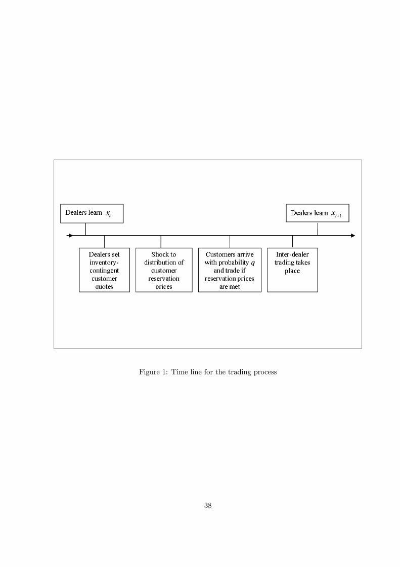
Figure 1: Time line for the trading process

38

Figure 2: The B2C schedule characterizes the inventory concavity parameter∇ for optimal B2C quotesunder any B2B spread S. The B2B schedule defines the competitive B2B spread S for dealers who

have ∇ as their inventory concavity parameter. The two intersections fulfill the equilibrium conditionsin both the B2B and B2C market. Of the two equilibria, only one, ZL, is stable.

39

Figure 3: For the ask side (panel A) and the bid side (panel B) we plot vertically the average cross-

market spread as a function of volatility ( 2) and the aggregate inventory imbalance (Imb). The red

area marks the region for which the average B2C spread is more favorable than the B2B spread. The

order processing cost parameter is chosen as τ = 0.5; the probability of customer arrival is q = 0.5;

the discount rate β = 0.99; the density of the customer price reservation distribution d is set at 1.

40

Table 1: European Sovereign Bond Market by Country and MTS Sample Size

The size of the European government bond market in terms of bond value outstanding is described by country for 2005. Only government bonds with a maturity above 1.5 years are considered.

The MTS data sample of the B2B market extends over the last three quarters of 2005. The coverage ratio reports the ratio of MTS trading volume divided by the value outstanding in eachmarket. For the Italian market the coverage ratio corresponds to a 100 percent market share since MTS benefits from a legal monopoly in B2B trading. Assuming that the volume to valueratio for Italy applies to all countries, we estimate the percentage market share of MTS in each country (with 100 percent as the upper boundary). Transaction volumes are stated in billions of

Euros. European sovereign bonds with a maturity of less than 1.5 years amount to an additional 800 billion Euros.

European Sovereign Bonds MTS Sample of B2B Market Coverage Ratios(2005) (2005q2 to 2005q4)

Country Value Outstanding Bonds Volume Trades Volume/Value MTS Market Share

Austria 121.9 14 27.28 2, 903 0.223 34.6

Belgium 250.9 19 103.16 10, 649 0.411 63.6

France 780.9 60 114.82 14, 285 0.147 22.8

Germany 603.1 65 125.19 17, 141 0.208 32.1

Greece 148.7 22 101.30 12, 127 0.681 100.0

Ireland 31.3 5 10.39 1177 0.332 51.4

Italy 990.5 72 640.07 105, 465 0.646 100.0

Netherlands 200.4 24 47.41 3, 767 0.237 36.6

Portugal 82.7 17 114.39 12, 424 1.383 100.0

Spain 286.0 42 85.04 8, 727 0.297 46.0

All 3, 557.9 340 1, 369.05 188, 665 0.391 60.8

41

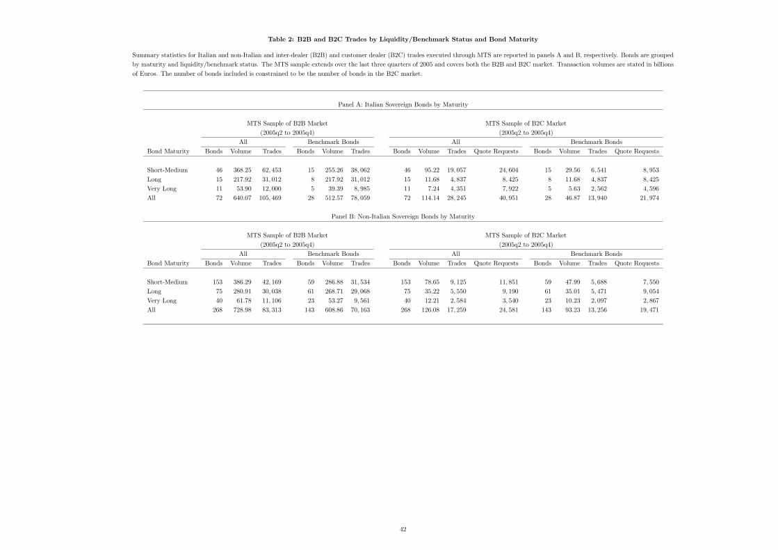
Table 2: B2B and B2C Trades by Liquidity/Benchmark Status and Bond Maturity

Summary statistics for Italian and non-Italian and inter-dealer (B2B) and customer dealer (B2C) trades executed through MTS are reported in panels A and B, respectively. Bonds are groupedby maturity and liquidity/benchmark status. The MTS sample extends over the last three quarters of 2005 and covers both the B2B and B2C market. Transaction volumes are stated in billions

of Euros. The number of bonds included is constrained to be the number of bonds in the B2C market.

Panel A: Italian Sovereign Bonds by Maturity

MTS Sample of B2B Market MTS Sample of B2C Market(2005q2 to 2005q4) (2005q2 to 2005q4)

All Benchmark Bonds All Benchmark Bonds

Bond Maturity Bonds Volume Trades Bonds Volume Trades Bonds Volume Trades Quote Requests Bonds Volume Trades Quote Requests

Short-Medium 46 368.25 62, 453 15 255.26 38, 062 46 95.22 19, 057 24, 604 15 29.56 6, 541 8, 953

Long 15 217.92 31, 012 8 217.92 31, 012 15 11.68 4, 837 8, 425 8 11.68 4, 837 8, 425

Very Long 11 53.90 12, 000 5 39.39 8, 985 11 7.24 4, 351 7, 922 5 5.63 2, 562 4, 596

All 72 640.07 105, 469 28 512.57 78, 059 72 114.14 28, 245 40, 951 28 46.87 13, 940 21, 974

Panel B: Non-Italian Sovereign Bonds by Maturity

MTS Sample of B2B Market MTS Sample of B2C Market

(2005q2 to 2005q4) (2005q2 to 2005q4)All Benchmark Bonds All Benchmark Bonds

Bond Maturity Bonds Volume Trades Bonds Volume Trades Bonds Volume Trades Quote Requests Bonds Volume Trades Quote Requests

Short-Medium 153 386.29 42, 169 59 286.88 31, 534 153 78.65 9, 125 11, 851 59 47.99 5, 688 7, 550

Long 75 280.91 30, 038 61 268.71 29, 068 75 35.22 5, 550 9, 190 61 35.01 5, 471 9, 054

Very Long 40 61.78 11, 106 23 53.27 9, 561 40 12.21 2, 584 3, 540 23 10.23 2, 097 2, 867

All 268 728.98 83, 313 143 608.86 70, 163 268 126.08 17, 259 24, 581 143 93.23 13, 256 19, 471

42

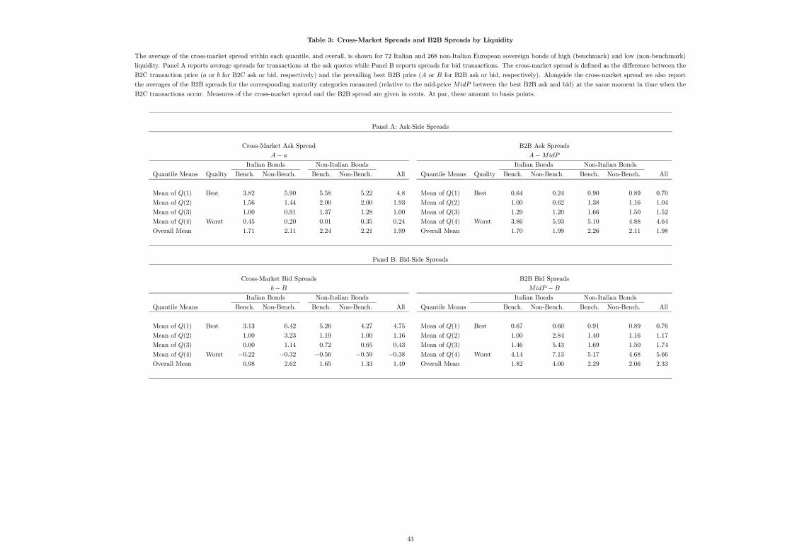
Table 3: Cross-Market Spreads and B2B Spreads by Liquidity

The average of the cross-market spread within each quantile, and overall, is shown for 72 Italian and 268 non-Italian European sovereign bonds of high (benchmark) and low (non-benchmark)liquidity. Panel A reports average spreads for transactions at the ask quotes while Panel B reports spreads for bid transactions. The cross-market spread is defined as the difference between the

B2C transaction price (a or b for B2C ask or bid, respectively) and the prevailing best B2B price (A or B for B2B ask or bid, respectively). Alongside the cross-market spread we also reportthe averages of the B2B spreads for the corresponding maturity categories measured (relative to the mid-price MidP between the best B2B ask and bid) at the same moment in time when the

B2C transactions occur. Measures of the cross-market spread and the B2B spread are given in cents. At par, these amount to basis points.

Panel A: Ask-Side Spreads

Cross-Market Ask Spread B2B Ask SpreadsA− a A−MidP

Italian Bonds Non-Italian Bonds Italian Bonds Non-Italian BondsQuantile Means Quality Bench. Non-Bench. Bench. Non-Bench. All Quantile Means Quality Bench. Non-Bench. Bench. Non-Bench. All

Mean of Q(1) Best 3.82 5.90 5.58 5.22 4.8 Mean of Q(1) Best 0.64 0.24 0.90 0.89 0.70

Mean of Q(2) 1.56 1.44 2.00 2.00 1.93 Mean of Q(2) 1.00 0.62 1.38 1.16 1.04

Mean of Q(3) 1.00 0.91 1.37 1.28 1.00 Mean of Q(3) 1.29 1.20 1.66 1.50 1.52

Mean of Q(4) Worst 0.45 0.20 0.01 0.35 0.24 Mean of Q(4) Worst 3.86 5.93 5.10 4.88 4.64

Overall Mean 1.71 2.11 2.24 2.21 1.99 Overall Mean 1.70 1.99 2.26 2.11 1.98

Panel B: Bid-Side Spreads

Cross-Market Bid Spreads B2B Bid Spreadsb−B MidP −B

Italian Bonds Non-Italian Bonds Italian Bonds Non-Italian Bonds

Quantile Means Bench. Non-Bench. Bench. Non-Bench. All Quantile Means Bench. Non-Bench. Bench. Non-Bench. All

Mean of Q(1) Best 3.13 6.42 5.26 4.27 4.75 Mean of Q(1) Best 0.67 0.60 0.91 0.89 0.76

Mean of Q(2) 1.00 3.23 1.19 1.00 1.16 Mean of Q(2) 1.00 2.84 1.40 1.16 1.17

Mean of Q(3) 0.00 1.14 0.72 0.65 0.43 Mean of Q(3) 1.46 5.43 1.69 1.50 1.74

Mean of Q(4) Worst −0.22 −0.32 −0.56 −0.59 −0.38 Mean of Q(4) Worst 4.14 7.13 5.17 4.68 5.66

Overall Mean 0.98 2.62 1.65 1.33 1.49 Overall Mean 1.82 4.00 2.29 2.06 2.33

43

Table 4: Cross-Market Spreads and B2B Spreads by Bond Maturity

The average of the cross-market spread within each quantile, and overall, is shown for each of the three main maturity categories of all 171 (Italian and non-Italian) benchmark bonds. Panel Areports average spreads for transactions at the ask quotes while Panel B reports spreads for bid transactions. The cross-market spread is defined as the difference between the B2C transaction

price (a or b for B2C ask or bid, respectively) and the prevailing best B2B price (A or B for B2B ask or bid, respectively). Alongside the cross-market spread we also report the averages of theB2B spreads for the corresponding maturity categories measured (relative to the mid-price MidP between the best B2B ask and bid) at the same moment in time when the B2C transactions

occur. Measures of the cross-market spread and the B2B spread are given in cents. At par, these amount to basis points.

Panel A: Ask-Side Spreads

Cross-Market Ask Spread B2B Ask SpreadsA− a A−MidP

Bond Maturity Bond MaturityQuantile Means Quality Short-Medium Long Very Long All Quantile Means Quality Short-Medium Long Very Long All

Mean of Q(1) Best 2.21 3.26 9.40 4.64 Mean of Q(1) Best 0.52 0.96 2.53 0.76

Mean of Q(2) 1.16 2.00 5.20 1.94 Mean of Q(2) 0.99 1.39 4.68 1.06

Mean of Q(3) 1.00 1.17 3.35 1.00 Mean of Q(3) 1.00 1.50 6.02 1.53

Mean of Q(4) Worst 0.46 0.39 -0.19 0.24 Mean of Q(4) Worst 1.54 2.23 8.28 4.48

Overall Mean 1.21 1.71 4.44 1.95 Overall Mean 1.01 1.52 5.38 1.96

Panel B: Bid-Side Spreads

Cross-Market Bid Spreads B2B Bid Spreadsb−B MidP −B

Bond Maturity Bond Maturity

Quantile Means Short-Medium Long Very Long All Quantile Means Short-Medium Long Very Long All

Mean of Q(1) Best 1.23 2.51 9.10 4.17 Mean of Q(1) Best 0.49 0.95 2.25 0.78

Mean of Q(2) 0.54 1.00 4.10 1.00 Mean of Q(2) 0.97 1.36 4.33 1.14

Mean of Q(3) 0.00 0.46 2.36 0.32 Mean of Q(3) 1.00 1.50 5.72 1.61

Mean of Q(4) Worst −0.25 −0.36 −0.11 −0.37 Mean of Q(4) Worst 1.51 2.37 8.18 4.60

Overall Mean 0.38 0.90 3.86 1.28 Overall Mean 0.99 1.55 5.12 2.03

44

Table 5: Cross-Market Spreads and B2B Spreads by Volatility

The average of the cross-market spread within each quantile, and overall, is shown for the ‘Low,’ ‘Medium,’ ‘High,’ and ‘Very-High’ volatility levels for the 13 liquid Italian bonds (eight long andfive very long benchmark bonds). Panel A reports average spreads for transactions at the ask quotes while Panel B reports those at the bid. The cross-market spread is defined as the difference

between the B2C transaction price (a or b for B2C ask or bid, respectively) and the prevailing best B2B price (A or B for B2B ask or bid, respectively). Volatility is measured as hourly ‘realizedvolatility’ based on observations of an equal weighted average of mid-prices of the six very liquid long Italian bonds taken at one minute intervals. ‘Low’ volatility is defined as volatility lying

below the 10th percentile of observed realized volatilities, ‘Medium’ is realized volatility between the 10th and 90th percentiles, ‘High’ is between the 90th and the 95th percentiles, and ‘VeryHigh’ volatility corresponds to levels above the 95th percentile. Alongside the cross-market spread we also report the averages of the B2B spreads (relative to the mid-price MidP between thebest B2B ask and bid) for the corresponding groups measured at the same moment in time when the B2C transactions occur. Measures of the cross-market spread and the B2B spread are given

in cents. At par, these amount to basis points.

Panel A: Ask-Side Spreads

Cross-Market Ask Spread B2B Ask Spreads

A− a A−MidP

Volatility Level Volatility LevelQuantile Means Quality Low Medium High Very High All Quantile Means Small Medium High Very High All

Mean of Q(1) Best 3.24 3.36 3.79 4.18 3.41 Mean of Q(1) Best 0.26 0.31 0.36 0.37 0.31

Mean of Q(2) 1.15 1.28 1.53 1.75 1.30 Mean of Q(2) 0.60 0.70 0.78 0.85 0.70

Mean of Q(3) 1.00 1.00 1.00 1.00 1.00 Mean of Q(3) 1.19 1.24 1.51 1.56 1.26

Mean of Q(4) Worst 0.11 0.12 0.00 −0.02 0.11 Mean of Q(4) Worst 3.22 3.24 4.00 4.39 3.34

Overall Mean 1.37 1.44 1.58 1.74 1.45 Overall Mean 1.32 1.37 1.66 1.78 1.40

Panel B: Bid-Side Spreads

Cross-Market Bid Spreads B2B Bid Spreadsb−B MidP −B

Volatility Level Volatility Level

Quantile Means Low Medium High Very High All Quantile Means Low Medium High Very High All

Mean of Q(1) Best 3.09 2.93 2.84 3.27 2.96 Mean of Q(1) Best 0.35 0.35 0.36 0.38 0.35

Mean of Q(2) 0.81 0.76 1.00 0.91 0.78 Mean of Q(2) 0.86 0.88 0.96 1.03 0.88

Mean of Q(3) 0.00 0.00 0.03 0.00 0.00 Mean of Q(3) 1.56 1.48 1.61 1.83 1.51

Mean of Q(4) Worst −0.37 −0.37 −0.40 −0.56 −0.38 Mean of Q(4) Worst 4.29 3.89 4.33 4.67 3.98

Overall Mean 0.88 0.83 0.87 0.91 0.84 Overall Mean 1.76 1.65 1.81 1.97 1.68

45

Table 6: Cross-Market Spreads by Imbalance

The average of the cross-market spread within each quantile, and overall, is shown by quantiles of the inventory imbalance proxy. Imbalance is measured as the difference between the B2Bliquidity at the best ask and the best bid across all 13 liquid Italian government bonds (eight long and five very long benchmark bonds) at the moment when a B2C transaction takes place. We

form four quantiles for the imbalance measure denoted as ‘Very Negative,’ ‘Negative,’ ‘Positive,’ and ‘Very Positive.’ Panel A reports average spreads for transactions at the ask quotes whilePanel B reports those at the bid. The cross-market spread is defined as the difference between the B2C transaction price (a or b for B2C ask or bid, respectively) and the prevailing best B2B

price (A or B for B2B ask or bid, respectively). Imbalance is measured as the difference between best limit order quantities relative to their sum across all 13 bonds. Alongside the cross-marketspread we also report the averages of the B2B spreads (relative to the mid-price MidP between the best B2B ask and bid) for the corresponding groups measured at the same moment in timewhen the B2C transactions occurred. Measures of the cross-market spread and the B2B spread are given in cents. At par, these amount to basis points.

Panel A: Ask-Side Spreads

Cross-Market Ask Spread B2B Ask Spreads

A− a A−MidP

Imbalance Level Imbalance LevelQuantile Means Quality Very Negative Negative Positive Very Positive All Quantile Means Very Negative Negative Positive Very Positive All

Mean of Q(1) Best 3.23 3.39 3.41 3.58 3.41 Mean of Q(1) Best 0.29 0.30 0.32 0.32 0.31

Mean of Q(2) 1.22 1.36 1.29 1.34 1.30 Mean of Q(2) 0.70 0.68 0.69 0.72 0.70

Mean of Q(3) 1.00 1.00 1.00 1.00 1.00 Mean of Q(3) 1.25 1.27 1.28 1.23 1.26

Mean of Q(4) Worst 0.06 0.19 0.13 0.17 0.11 Mean of Q(4) Worst 3.18 3.33 3.48 3.36 3.34

Overall Mean 1.35 1.49 1.46 1.52 1.45 Overall Mean 1.35 1.39 1.44 1.40 1.40

Panel B: Bid-Side Spreads

Cross-Market Bid Spreads B2B Bid Spreadsb−B MidP −B

Imbalance Level Imbalance LevelQuantile Means Very Negative Negative Positive Very Positive All Quantile Means Very Negative Negative Positive Very Positive All

Mean of Q(1) Best 2.97 3.29 3.03 2.54 2.96 Mean of Q(1) Best 0.36 0.36 0.34 0.34 0.35

Mean of Q(2) 0.86 0.94 0.80 0.53 0.78 Mean of Q(2) 0.89 0.90 0.87 0.87 0.88

Mean of Q(3) 0.00 0.00 0.00 0.00 0.00 Mean of Q(3) 1.46 1.62 1.58 1.39 1.51

Mean of Q(4) Worst −0.36 −0.35 −0.37 −0.45 −0.38 Mean of Q(4) Worst 3.78 4.49 4.07 3.60 3.98

Overall Mean 0.87 0.97 0.87 0.66 0.84 Overall Mean 1.62 1.84 1.71 1.55 1.68

46

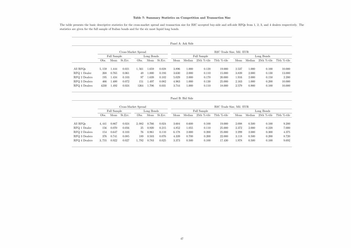
Table 7: Summary Statistics on Competition and Transaction Size

The table presents the basic descriptive statistics for the cross-market spread and transaction size for B2C accepted buy-side and sell-side RFQs from 1, 2, 3, and 4 dealers respectively. Thestatistics are given for the full sample of Italian bonds and for the six most liquid long bonds.

Panel A: Ask Side

Cross-Market Spread B2C Trade Size, Mil. EURFull Sample Long Bonds Full Sample Long Bonds

Obs. Mean St.Err. Obs. Mean St.Err. Mean Median 25th %-tile 75th %-tile Mean Median 25th %-tile 75th %-tile

All RFQs 5, 159 1.444 0.021 1, 561 1.659 0.028 3.896 1.000 0.120 19.000 2.537 1.000 0.100 10.000

RFQ 1 Dealer 268 0.765 0.061 49 1.000 0.193 3.630 2.000 0.110 15.000 3.839 2.000 0.130 13.000

RFQ 2 Dealers 195 1.434 0.103 97 1.639 0.102 5.029 2.000 0.170 20.000 1.916 2.000 0.150 2.200

RFQ 3 Dealers 466 1.400 0.072 151 1.497 0.082 4.963 1.000 0.130 25.000 2.163 1.000 0.200 10.000

RFQ 4 Dealers 4230 1.492 0.024 1264 1.706 0.031 3.744 1.000 0.110 18.000 2.579 0.900 0.100 10.000

Panel B: Bid Side

Cross-Market Spread B2C Trade Size, Mil. EURFull Sample Long Bonds Full Sample Long Bonds

Obs. Mean St.Err. Obs. Mean St.Err. Mean Median 25th %-tile 75th %-tile Mean Median 25th %-tile 75th %-tile

All RFQs 4, 441 0.867 0.024 2, 082 0.766 0.024 3.604 0.600 0.100 19.000 2.098 0.500 0.100 9.200

RFQ 1 Dealer 156 0.070 0.056 25 0.920 0.215 4.852 1.055 0.110 25.000 2.372 2.000 0.220 7.000

RFQ 2 Dealers 154 0.647 0.103 76 0.961 0.110 6.178 2.000 0.200 25.000 2.299 2.000 0.300 4.375

RFQ 3 Dealers 376 0.741 0.085 189 0.503 0.076 4.339 0.700 0.200 22.000 3.118 0.500 0.200 8.720

RFQ 4 Dealers 3, 755 0.922 0.027 1, 792 0.783 0.025 3.373 0.500 0.100 17.430 1.978 0.500 0.100 9.692

47

Table 8: Cross-Market Spread and B2B Spread Estimation

Reported are instrumental variable estimates of the relation between the spreads, volatility, and imbalance controlling for competition and order size where applicable. The dependent variablesare the cross-market spread and the B2B spread respectively for ask-side and bid-side B2C activity. The competition control is in the form of separate dummies for requests for quotes from

one dealer and more than one dealer respectively. Order size enters as the log of B2C quantity. The explanatory variables are realized volatility and imbalance at the best quotes in the B2Bmarket prevailing at the time of the B2C request for quotes. Volatility is measured by the log-realized volatility of the mid-price returns over one-minute intervals computed for every full hour.

Imbalance (Imb) is measured as the difference between the B2B liquidity at the best ask and the best bid for the benchmark Italian long bond at the moment when a B2C transaction takesplace in any given bond. Results are provided for the full-sample of liquid Italian bonds and for the sub-sample containing the six very liquid long bonds. In all cases we include bond-specificfixed effects to control for spread differences across bonds. The ask-side results are presented in Panel A and the bid-side results are presented in Panel B. The IV regression uses a constant

and volatility lagged by one hour as instruments. The t-statistics presented are based on standard errors that have been adjusted for heteroscedasticity. Spreads are expressed in cents. At par,these amount to basis points. Even-numbered regressions include the imbalance variable. The tests for equality of the constants for competition/no-competition in regressions (1) to (4) is notdecisively rejected for the ask-side but is easily rejected on the bid-Side. The F-test statistics (significance) are as follows. Ask-Side(Regression 1): 1.97 (0.14), Ask-Side(Regression 2): 1.84

(0.16), Ask-side(Regression 3): 1.77 (0.17), Ask-Side(Regression 4): 1.81 (0.16), Bid-Side(Regression 1): 3.21 (0.04), Bid-Side(Regression 2): 2.64 (0.07), Bid-Side(Regression 3): 7.61 (0.00),Bid-Side(Regression 4): 6.82 (0.001). Regressions (5) to (8) refer to the B2B bid-ask spread. In these regressions there is no role for the competition dummies and the NO COMP coefficient is

simply the regression constant.

48

.

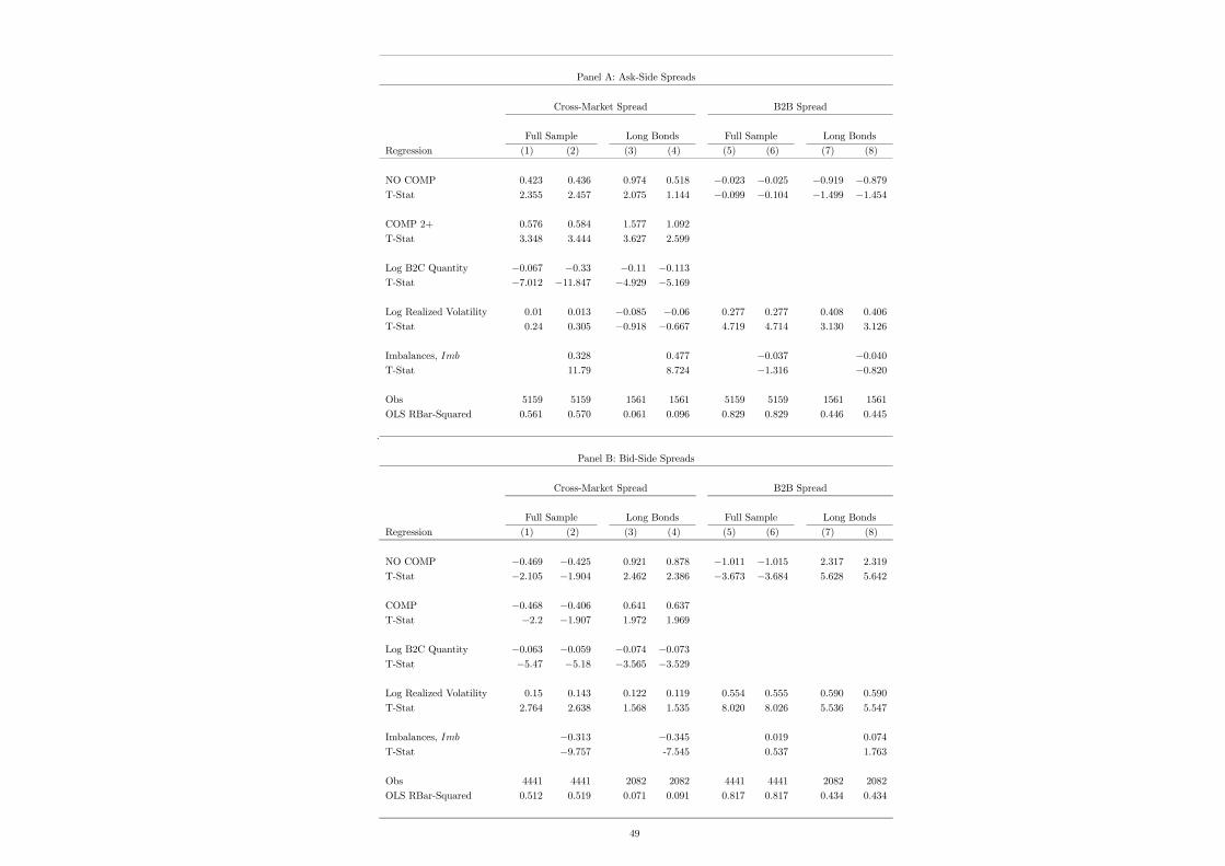
Panel A: Ask-Side Spreads

Cross-Market Spread B2B Spread

Full Sample Long Bonds Full Sample Long BondsRegression (1) (2) (3) (4) (5) (6) (7) (8)

NO COMP 0.423 0.436 0.974 0.518 −0.023 −0.025 −0.919 −0.879T-Stat 2.355 2.457 2.075 1.144 −0.099 −0.104 −1.499 −1.454

COMP 2+ 0.576 0.584 1.577 1.092

T-Stat 3.348 3.444 3.627 2.599

Log B2C Quantity −0.067 −0.33 −0.11 −0.113T-Stat −7.012 −11.847 −4.929 −5.169

Log Realized Volatility 0.01 0.013 −0.085 −0.06 0.277 0.277 0.408 0.406

T-Stat 0.24 0.305 −0.918 −0.667 4.719 4.714 3.130 3.126

Imbalances, Imb 0.328 0.477 −0.037 −0.040T-Stat 11.79 8.724 −1.316 −0.820

Obs 5159 5159 1561 1561 5159 5159 1561 1561

OLS RBar-Squared 0.561 0.570 0.061 0.096 0.829 0.829 0.446 0.445

Panel B: Bid-Side Spreads

Cross-Market Spread B2B Spread

Full Sample Long Bonds Full Sample Long Bonds

Regression (1) (2) (3) (4) (5) (6) (7) (8)

NO COMP −0.469 −0.425 0.921 0.878 −1.011 −1.015 2.317 2.319

T-Stat −2.105 −1.904 2.462 2.386 −3.673 −3.684 5.628 5.642

COMP −0.468 −0.406 0.641 0.637

T-Stat −2.2 −1.907 1.972 1.969

Log B2C Quantity −0.063 −0.059 −0.074 −0.073T-Stat −5.47 −5.18 −3.565 −3.529

Log Realized Volatility 0.15 0.143 0.122 0.119 0.554 0.555 0.590 0.590

T-Stat 2.764 2.638 1.568 1.535 8.020 8.026 5.536 5.547

Imbalances, Imb −0.313 −0.345 0.019 0.074

T-Stat −9.757 -7.545 0.537 1.763

Obs 4441 4441 2082 2082 4441 4441 2082 2082

OLS RBar-Squared 0.512 0.519 0.071 0.091 0.817 0.817 0.434 0.434

49