No. 06‐13 

 A Tale of Tails:  

An Empirical Analysis of Loss Distribution Models for Estimating Operational Risk Capital 

Kabir Dutta and Jason Perry  Abstract: Operational risk is being recognized as an important risk component for financial institutions as evinced  by  the  large  sums  of  capital  that  are  allocated  to mitigate  this  risk.  Therefore,  risk measurement is of paramount concern for the purposes of capital allocation, hedging, and new product  development  for  risk  mitigation.  We  perform  a  comprehensive  evaluation  of commonly used methods  and  introduce new  techniques  to measure  this  risk with  respect  to various criteria. We find that our newly introduced techniques perform consistently better than the other models we tested.   Keywords: exploratory data analysis, operational risk, g‐and‐h distribution, goodness‐of‐fit, skewness‐kurtosis, risk measurement, extreme value theory, peaks‐over‐threshold method, generalized Pareto distribution. 

JEL Codes: G10, G20, G21, G32, D81  This paper was substantially completed while Kabir Dutta was a Senior Economist and Jason Perry was a Financial Economist,  both  with  the  Federal  Reserve  Bank  of  Boston.    Their  current email  addresses  are  kabir.dutta.wg97@wharton.upenn.edu and jason6@stanfordalumni.org, respectively.  This paper, which may be revised, is available on the web site of the Federal Reserve Bank of Boston at http://www.bos.frb.org/economic/wp/index.htm.   The views expressed in this paper do not necessarily reflect the views of the Federal Reserve Bank of Boston or the Federal Reserve System.  We are extremely grateful to Ricki Sears and Christine Jaw for their research support. Without their valuable help, this work would not have been possible. We thank Patrick de Fontnouvelle and Eric Rosengren for their comments on  earlier  drafts  of  the  paper; David Hoaglin  for  his  advice  on modeling  the  g‐and‐h  distribution;  and  Valérie Chavez‐Demoulin, Paul Embrechts, and Johanna Nešlehová for their valuable help in our understanding of Extreme Value Theory. We would also  like to thank Stacy Coleman, Peggy Gilligan, Mark Levonian, Robin Lumsdaine, Jim Mahoney, and Scott Ulman for their comments.   This version: April 2007 (first version: July 2006) 

1

Executive Summary

Institutions face many modeling choices as they attempt to measure operational risk exposure.

One of the most significant choices is which technique to use for modeling the severity (dollar

value) of operational losses. There are many techniques being used in practice, and for

policy makers an important question is whether institutions using different severity modeling

techniques can arrive at very different (and inconsistent) estimates of their exposure. Our

results suggest that they can: We find that using different models for the same institution can

result in materially different capital estimates. We also find that some of these models can be

readily dismissed on either statistical or logical grounds. This leaves us with a more limited

range of techniques that are potentially suitable for modeling operational loss severity. Most

importantly, we find that there are some techniques that yield consistent and plausible results

across the different institutions that we consider in spite of each institution having different

data characteristics. This last finding is important for several reasons. First, it suggests that

operational risk can be modeled and that there is indeed some regularity in loss data across

institutions. Second, it lays out the hope that while preserving the AMA’s flexibility, we can

still develop a benchmark model for use by both institutions and supervisors.

In order to understand the inherent nature and exposure of operational risk that a financial

institution faces, we conducted an experiment to comparatively analyze various approaches

that could be used to measure operational risk using financial institutions’ internal loss data

collected under the 2004 Loss Data Collection Exercise (LDCE). The quality of the data

varied across institutions. In order to ensure a meaningful analysis, we used data from

seven institutions that reported a sufficient number of losses (at least one thousand total loss

events) and whose data was also consistent and coherent relative to the other institutions.

These seven institutions adequately covered various business types and asset sizes for financial

institutions.

We used the Loss Distribution Approach (LDA) to measure operational risk at the en-

terprise level as well at the Basel business line and event type levels. Measuring risk at the

(aggregated) enterprise level is advantageous because there are more data available; however,

the disadvantage is that dissimilar losses are grouped together. By estimating operational

risk at the business line and event type levels as well, we are able to present the estimates

in a more balanced fashion. The LDA has three essential components-a distribution of the

annual number of losses (frequency), a distribution of the dollar amount of losses (severity),

2

and an aggregate loss distribution that combines the two.

Before we selected the severity models for our experiment, we performed an analysis to

understand the structure of the data. Based on this analysis we found that in order for a

model to be successful in fitting all of the various types of data, one would need to use a model

that is flexible enough in its structure. Although it is quite clear that some of the commonly

used simple techniques may not model all of the data well, nevertheless we included these

techniques in our analysis in order to compare their performance relative to more flexible

approaches.

To model the severity distribution, we used three different techniques: parametric distri-

bution fitting, a method of Extreme Value Theory (EVT), and capital estimation based on

non-parametric empirical sampling. In parametric distribution fitting, the data are assumed

to follow some specific parametric model, and the parameters are chosen (estimated) such that

the model fits the underlying distribution of the data in some optimal way. EVT is a branch

of statistics concerned with the study of extreme phenomena such as large operational losses.

Empirical sampling (sometimes called historical simulation) entails drawing at random from

the actual data. We considered the following one- and two-parameter distributions to model

the loss severity: exponential, gamma, generalized Pareto, loglogistic, truncated lognormal,

and Weibull. Many of these distributions were reported as used by financial institutions in the

Quantitative Impact Study 4 (QIS-4) submissions. We also used four-parameter distributions

such as the Generalized Beta Distribution of Second Kind (GB2) and the g-and-h distribu-

tion, which have the property that many different distributions can be generated from these

distributions for specific values of their parameters. Modeling with the g-and-h and GB2 is

also considered parametric distribution fitting, but each of these distributions has its own

estimation procedure.

We measured operational risk capital as the 99.9% percentile level of the simulated capital

estimates for aggregate loss distributions using one million trials because the 99.9% level is

what is currently proposed under the Basel II accord.1 To equally compare institutions and

preserve anonymity, we scaled the capital estimates by the asset size or gross income of

each institution. We evaluated severity distributions or methods according to five different

performance measures listed in order of importance:

1. Good Fit - Statistically, how well does the method fit the data?

2. Realistic - If a method fits well in a statistical sense, does it generate a loss distribution

1Details can be found at http://www.federalreserve.gov/boarddocs/press/bcreg/2006/20060330/default.htm.

3

with a realistic capital estimate?

3. Well-Specified - Are the characteristics of the fitted data similar to the loss data andlogically consistent?

4. Flexible - How well is the method able to reasonably accommodate a wide variety ofempirical loss data?

5. Simple - Is the method easy to apply in practice, and is it easy to generate randomnumbers for the purposes of loss simulation?

We regard any technique that is rejected as a poor statistical fit for most institutions to

be an inferior technique for fitting operational risk data. If this condition were relaxed, a

large variation in the capital estimates could be generated. We are not aware of any research

work in the area of operational risk that has addressed this issue. Goodness-of-fit tests are

important because they provide an objective means of ruling out some modeling techniques

which if used could potentially contribute to cross-institution dispersion in capital results.

The exponential, gamma, and Weibull distributions are rejected as good fits to the loss

data for virtually all institutions at the enterprise, business line, and event type levels. The

statistical fit of each distribution other than g-and-h was tested using the formal statistical

tests noted earlier. For the g-and-h we compared its Quantile-Quantile (Q-Q) plot to the

Q-Q plots of other distributions to assess its goodness-of-fit. In all situations we found that

the g-and-h distribution fit as well as other distributions on the Q-Q plot that were accepted

as a good fit using one or more of the formal statistical methods described earlier. No other

distribution we used could be accepted as a good fit for every institution at the enterprise

level. The GB2, loglogistic, truncated lognormal, and generalized Pareto had a reasonable

fit for most institutions. We also could find a reasonable statistical fit using the EVT POT

method for most of the institutions. However good fit does not necessarily mean a distribution

would yield a reasonable capital estimate. This gives rise to the question of how good the

method is in terms of modeling the extreme events. Here, we observed that even when many

distributions fit the data they resulted in unrealistic capital estimates (sometimes more than

100% of the asset size), primarily due to their inability to model the extremely high losses

accurately.

With respect to the capital estimates at the enterprise level, only the g-and-h distribution

and the method of empirical sampling resulted in realistic and consistent capital estimates

4

across all of the seven institutions.2 Although empirical sampling yields consistent capital

estimates, these estimates are likely to understate capital if the actual data do not contain

enough extreme events.

Our most important finding is that the g-and-h distribution results in a meaningful op-

erational risk measure in that it fits the data and results in consistently reasonable capital

estimates. Many researchers have conjectured that one may not be able to find a single distri-

bution that will fit both the body and the tail of the data to model operational loss severity;

however, our results regarding the g-and-h distribution imply that at least one single distribu-

tion can indeed model operational loss severity without trimming or truncating the data in an

arbitrary or subjective manner. The median capital/asset ratio for the g-and-h distribution

at the enterprise level was 0.79%, and the median capital/gross income was 16.79%. Further-

more, the g-and-h distribution yielded the most realistic and least varying capital estimates

across institutions at the enterprise, business line, and event type levels. Our observations

are of a similar nature at the business line and the event type level. Also we observed much

more similarity in the capital estimates using the g-and-h distribution by event types than by

business lines. We observed that for three out of seven institutions in our sample enterprise

level capital estimates were very close to the sum of capital estimates at the event type levels.

For the other four institutions the number was not significantly different. We would like to

think that a business line’s operational risks are nothing more than a portfolio of risk events.

Therefore, this portfolio will vary among the institutions depending on the type of business

and risk control they are involved in. We aggregated business line (and event types) capital

estimates for the g-and-h distribution in two different ways: assuming zero correlation (in-

dependence) and comonotonicity (random variables have perfect positive dependence3). We

observed that the difference between these two numbers are much smaller than we expected.

We will explore the issue of dependence and its impact on capital estimates further in our

subsequent research. Also, the diversification benefit using comonotonicity at the enterprise

level was not unreasonably high for the g-and-h distribution. The diversification benefit is

much smaller for the summation of capital estimates from event types than from business

lines.

2We consider a meaningful capital estimate as a capital/asset ratio less than 3%. Our conclusions will notbe different even if we raise this ratio to 10%. In some cases, capital estimates may be unreasonably low, yetstill fall into our definition of “reasonable.”

3Random variables are comonotonic if they have as their copula the Frechet upper bound (see McNeil etal. (2005) for a more technical discussion of comonotonicity).

5

However, many of the other distributions we used resulted in significant variation across

institutions, with unrealistically high capital estimates in situations where they were otherwise

found to be a good fit to the data with respect to some statistical test.4 This is an important

finding because it implies that even when an institution constrains itself to using techniques

with good statistical fits, capital estimates across these techniques can vary greatly. This issue

is especially of concern for the EVT POT approach and the power law variant, which gave

the most unreasonable capital estimates with the most variation of all of the methods across

the enterprise, business line, and event type levels. This method fit well in some statistical

sense but gave reasonable estimates for just two of the seven institutions at the enterprise

level. Also, the capital estimates for these institutions are highly sensitive to the threshold

choice. The lognormal and loglogistic distributions fit the data in many cases at the business

line and event type levels in addition to providing realistic capital estimates.

In summary, we found that applying different models to the same institution yielded vastly

different capital estimates. We also found that in many cases, applying the same model to

different institutions yielded very inconsistent and unreasonable estimates across institutions

even when statistical goodness-of-fit was satisfied. This raises two primary questions regarding

the models that only imply realistic estimates in a few situations: (1) Are these models even

measuring risk properly for the cases when they do yield reasonable exposure estimates, or

are some reasonable estimates expected from any model simply due to chance? (2) If an

institution measures its exposure with one of these models and finds its risk estimate to be

reasonable today, how reasonable will this estimate be over time?

It is unlikely that the results we obtained from the g-and-h distribution are a matter of

chance because we observed that the g-and-h capital estimates are consistently reasonable

across institutions. In contrast, we could not make the same conclusion for the other tech-

niques particularly for EVT and its power law variants. For the cases where these techniques

did result in reasonable capital estimates, additional verification using future data will help

to justify their appropriateness in measuring the risk. Furthermore, with limited data the

second question would more appropriately be addressed in future research.

The g-and-h distribution was found to perform the best overall according to our five

performance measures. We do not think that the g-and-h is the only distribution that will be

able to model operational loss data. We hope that researchers and practitioners will view our

4Most of these distributions, including the approach of EVT, were found to have resulted in a meaningfulcapital estimate in at most two to three out of the seven instances. By unrealistically high we mean that thecapital-to-assets ratio exceeds 50%.

6

research as a framework where we experimented with many different methods and techniques

along with a rigorous analysis of the data. The challenge of the operational risk loss data

should motivate us to find new models that describe the characteristics of the data rather

than limit the data so that it matches the characteristics of the model. Also, future research

should explore models that address the two fundamental questions raised above. We hope

this analysis will not only be useful for estimating capital for operational risk, but also for

encouraging risk mitigation and hedging through new product development. Some researchers

have argued that operational risk can be highly diversifiable. Thus, there is a strong argument

for pooling the risk. An accurate, coherent, and robust risk measurement technique can aid

in that direction.

1

1 Introduction

It is important to understand what you can do before you learn to measure how

well you seem to have done it. – John W. Tukey

Operational risk is gaining significant attention due to sizable operational losses that finan-

cial institutions have faced in recent years.5 Froot (2003) observed that operational risk can

trigger illiquidity and systemic risk in the financial system. As institutions are hedging their

market and credit risk through asset securitization and other means, their exposure to opera-

tional risk is becoming a larger share of their total risk exposure. Only very recently financial

institutions have begun estimating their operational risk exposure with greater quantitative

precision. The Basel II capital accord will require that many large financial institutions use

an Advanced Measurement Approach (AMA) to model their operational risk exposure.

In some countries outside the United States, financial institutions will have the option of

choosing to use an AMA to estimate operational risk capital or apply a simpler approach such

as the Basic Indicator or the Standardized Approaches. Under the Basic Indicator Approach

for estimating operational risk, capital is computed as 15% of enterprise-level gross income.6

Under the Standardized Approach, capital is computed as a fixed percentage of gross income

at each business line and then summed to achieve a capital estimate at the enterprise level.

This fixed percentage known as beta takes values of 12%, 15%, or 18% depending on the

business line.

Unlike the modeling of market and credit risk, the measurement of operational risk faces

the challenge of limited data availability. Furthermore, due to the sensitive nature of opera-

tional loss data, institutions are not likely to freely share their loss data. Only recently has

the measurement of operational risk moved towards a data-driven Loss Distribution Approach

(LDA).7 Therefore, many financial institutions have begun collecting operational loss data as

they are trying to move towards an LDA to measure their operational risk. In the market

and credit risk areas, the strengths and weaknesses of risk measurement models have been

continuously tested. For example, Buhler et al. (1999) have performed an extensive com-

5In this paper we use the Basel Committee (2003) definition of operational risk: “the risk of loss resultingfrom inadequate or failed internal processes, people and systems, or from external events.”

6Gross income is calculated as the sum of net interest income and total non-interest income minus insuranceand reinsurance underwriting income and income from other insurance and reinsurance.

7In the Standardized and Basic Indicator approaches, each loss event is not directly used to measure theoperational risk.

2

parison of interest rate models. These studies have exemplified the need for a comparative

analysis of various models. Even though the measurement of operational risk is still evolving,

comparing various measurement methods with respect to some basic criteria will aid in our

basic understanding of this risk.

Several researchers have experimented with operational loss data over the past few years.

Moscadelli (2004) and de Fontnouvelle et al. (2004) are two examples. Our study differs

in that we primarily focus on understanding how to appropriately measure operational risk

rather than assessing whether certain techniques can be used for a particular institution. We

attempt to find which measurement techniques may be considered appropriate measures of

operational risk. The measurement of operational risk typically results in a capital estimate

that institutions hold as reserves for potential operational losses. Froot (2003) describes

capital as “collateral on call.” From this point of view, the capital calculation must capture

the inherent operational risk of the institution. When sufficiently available, the internal loss

data of an institution are prime indicators for this risk.

In order to understand the quantitative characteristics of institutions’ internal operational

loss data, we conduct an analysis using data from the 2004 Loss Data Collection Exercise

(LDCE).8 Our analysis is carried out using LDCE data at the enterprise level as well as at

the Basel-defined business line and event type levels for seven institutions that reported loss

data totaling at least 1,000 observations of $10,000 or more. These three different levels are

essentially three different units of measurement of risks. We will discuss later why we chose

to use these three units of measurement. Specifically, at each level (enterprise, business line,

and event type) we attempt to address the following questions:

• Which commonly used techniques do not fit the loss data statistically?

• Which techniques fit the loss data statistically and also result in meaningful capitalestimates?

• Are there models that can be considered appropriate operational risk measures?

• How do the capital estimates vary with respect to the model assumptions across differentinstitutions classified by asset size, income, and other criteria?

• Which goodness-of-fit criteria are most appropriately used for operational loss data?

8The LDCE of 2004 was a joint effort of US banking regulatory agencies to collect operational risk data.The bank supervisors include the Federal Reserve System, the Office of the Controller of Currency, the FederalDeposit Insurance Corporation, and the Office of Thrift Supervision.

3

In order to address these questions, we adopt a rigorous analytical approach that is consis-

tently applied across institutions. First, we perform some exploratory data analyses suggested

by Tukey (1977a) to understand the structure of the data before deciding on a modeling

technique. The various modeling techniques we consider use simple parametric distributions,

generalized parametric distributions, extreme value theory, and empirical (historical) sam-

pling. Although our exploratory data analysis suggests that some of these models are not

supported by the structure of the data, we use them nevertheless for the purpose of compar-

ative analysis. Second, we use various goodness-of-fit tests to ensure that the data fit the

model. Among those models that fit the data, we compare them with respect to additional

performance measures.

In Section 2 we describe the LDCE data, discuss our sample selection procedure, and

perform an exploratory data analysis. Models for loss severity are presented in Section 3,

and the methodology used to compare these models is presented in Section 4. Finally, capital

estimates and other results are compared in Section 5, and the paper is concluded in Section

6.

2 Data

In 2004, US banking regulatory agencies conducted two related studies: the Quantitative

Impact Study 4 (QIS-4) and the Loss Data Collection Exercise (LDCE). Participation was

voluntary and limited to institutions with a US presence. One component of QIS-4 was a

questionnaire aimed at eliciting institutions’ methods for measuring operational risk and their

operational risk capital estimates based on this method. The internal operational loss data

used to compute these capital estimates were submitted under LDCE. There were twenty-

three institutions that participated in LDCE, and twenty of these institutions also submitted

information under QIS-4.9

Prior to 2004 there were two other LDCEs. The 2004 LDCE was different in that no stan-

dard time period was required for the loss submissions, and there was no specified minimum

loss threshold that institutions had to adhere to. Furthermore, institutions were requested

to define mappings from their internally-defined business lines and event types to the ones

9For a summary of results the LDCE as well as the Operational Risk portion of QIS-4, see Results ofthe 2004 Loss Data Collection Exercise for Operational Risk (2004). For a broader summary of the QIS-4results, see Summary Findings of the Fourth Quantitative Impact Study 2006 which can be found online athttp://www.federalreserve.gov/boarddocs/press/bcreg/2006/20060224/.

4

defined by Basel II. Basel II categorization was useful because it helped to bring uniformity

in data classification across institutions. The loss records include loss dates, loss amounts,

insurance recoveries, and codes for the legal entity for which the losses were incurred.

Internal business line losses were mapped to the eight Basel-defined business lines and an

“Other” category.10 Throughout this paper these Basel-defined business lines and event types

will be referred to with BL and ET number codes. See Table 1 for these definitions. Section

Table 1: Business Line and Event Type CodesThis table presents the eight Basel business lines and seven basel event types that were used in this study.Each business line and event type number is matched with its description.

2.1 describes the characteristics of the data. Section 2.2 explains how these challenges can be

surmounted with appropriate data selection and modeling assumptions.

2.1 Characteristics of the Data

Institutions that collect and analyze operational loss data for the purpose of estimating capital

face a variety of challenges. This section highlights the essential features and characteristics of

the LDCE data. There are two types of reporting biases that are present in the LDCE data.

The first type of bias is related to structural changes in reporting quality. When institutions

first began collecting operational loss data, their systems and processes were not completely

solidified. Hence, the first few years of data typically have far fewer losses reported than

later years. In addition, the earlier systems for collecting these data may have been more

likely to identify larger losses than smaller losses. Therefore, the structural reporting bias

may potentially affect loss frequency as well as severity.

10Some institutions reported losses in the “Other” category when these losses were not classified accordingto the Basel II categories. The largest losses for some institutions were reported under this special category.

5

The second type of reporting bias is caused by inaccurate time-stamping of losses, which

results in temporal clustering of losses. For many institutions, a disproportionate number of

losses occurred on the last day of the month, the last day of the quarter, or the last day of the

year. The non-stationarity of the loss data over time periods of less than one year constrains

the types of frequency estimation that one can perform.

Loss severities in the LDCE data set tend to fall disproportionately on dollar amounts

that are multiples of $10,000. Also, there tend to be more loss severities of $100,000 than

$90,000 and $1,000,000 than $900,000. There are two possible reasons for this. First, some

loss severities may be rounded to the nearest dollar value multiple of $10,000 or $100,000 (if

the loss is large enough). Second, some event types such as lawsuits may only generate losses

in multiples of $100,000.

Less than one-third of the participating institutions reported losses prior to 2000. A little

less than half of the institutions reported losses for three or fewer years. Even though an

institution may have reported losses for a given year, the number of losses in the first few years

was typically much lower than the number of reported losses in later years. Classifying the

loss data into business line or event type buckets further reduces the number of observations

and increases the difficulty of modeling them. With limited data, the more granular the unit

of measure, the more difficult it may be to obtain precise capital estimates.11

The loss threshold is defined as the minimum amount that a loss must equal in order

to be reported in the institution’s data set. Some institutions have different loss thresholds

for each business line. For the LDCE data, thresholds ranged from $0 to $20,000 at an

institution-wide level, but thresholds exceeded $20,000 for certain institutions’ business lines.

Only seventeen institutions used a consistent threshold for the entire organization. There

were six institutions that used a threshold of $0, and nine institutions had a threshold of

$10,000 or more. Different loss thresholds are not a data problem, but simply a characteristic

of the data that must be handled accordingly.

As part of the LDCE questionnaire, institutions were asked whether their data could be

considered fully comprehensive in that all losses above their chosen threshold were complete

for all business lines in recent years. Only ten institutions indicated that their data were fully

comprehensive, seven indicated that their data were partially comprehensive, and the rest

provided no information regarding comprehensiveness. Besides the issue of data completeness,

institutions differed in the degree to which reporting biases and rounding of losses affected

11It should be noted, however, that many institutions only engage in a few business lines.

6

their data.

2.2 Data Selection and Descriptive Statistics

Many of the data challenges discussed in Section 2.1 can be overcome with appropriate sample

selection procedures. Although there were twenty-three institutions that submitted data

under LDCE, the data set used in this analysis only includes seven institutions that submitted

at least 1,000 total loss events. Out of the institutions with fewer than 1,000 loss events, the

institution with the median number of losses submitted less than 200 losses under LDCE.

With so few observations for the institutions excluded from our analysis, calculating capital

estimates based solely on internal data would not have been very meaningful. Subdividing

these losses by business line or event type would further reduce the number of losses available

for estimation. Thus, we reasoned it necessary to constrain the analysis to institutions with

more than 1,000 total losses.

In addition to excluding institutions with too few observations, we also removed years of

data that were deemed to be incomplete or non-representative of an institution’s loss history.

For example, suppose that a hypothetical institution submitted six years of data with the

following loss frequencies in each year: 15, 8, 104, 95, 120, and 79. In this case, we would

have removed the first two years of data due to a perceived structural change in reporting

quality. If this structural reporting problem were not addressed, estimated loss frequencies

and severities would be biased as previously mentioned.

Due to the inaccurate time-stamping of losses, we cannot estimate loss frequency based

on daily or even monthly losses. Instead we only consider the average annual frequency of

losses as an appropriate measure of annual loss frequency. This idea will be further expanded

upon in Section 4. In order to address the issue of threshold consistency across institutions,

we applied the same $10,000 threshold to all seven institutions.12 Besides these adjustments

to the LDCE data, no other modifications were made.

Table 2 reports the combined frequency and dollar value of annual losses of all twenty-

three institutions in the LDCE. All but one of the institutions in the sample reported losses

in 2003, and more than half of these institutions reported losses for at least four years. The

shortest data series was one year. Table 3 shows the aggregate number and dollar value of

losses for the LDCE institutions. Four of the twenty-three institutions reported more than

12In some situations the threshold was higher than $10,000. In these cases we accounted for the higherthreshold in our models.

7

Table 2: LDCE Loss Data by YearAs reported in the 2004 Loss Data Collection Exercise, this table presents a summary by year of loss data(for losses of $10000 or more) submitted by all 23 participating institutions.

∗∗ 2004 reflects only a partial year as institutions were asked to submit data through June 30, or September30, 2004.

Table 3: LDCE Loss Counts and ComprehensivenessThis table presents summary totals for the data received in the 2004 Loss Data Collection Exercise.

∗ An institution’s data are considered fully comprehensive if the institution indicated that the loss dataabove its internal threshold were complete for all business lines for recent years. An institution’s data areconsidered partially comprehensive if the institution indicated that the percentage of losses reported wasless than 100% for one or more business lines.

8

2500 total losses of at least $10,000 each. The aggregate dollar value of all losses in the sample

(above the $10,000 threshold) is almost $26 billion. Table 3 also provides the institutions’ own

assessments regarding the completeness of the data they submitted. Ten of the twenty-three

institutions claimed that their data were fully comprehensive. Although we have raised many

issues about the LDCE data as a whole, the data we selected for our sample are fairly robust

and a good representation of operational loss data.

One can argue that internal loss data should be carefully selected to reflect the current

business environment of the institution. Some of the less recent loss data may not be appro-

priate as an institution’s operating environment might have changed. Hence, we made sure

in our selection process that the data we used are still relevant for the institutions in terms

of their business and operating environment.

2.3 Exploratory Data Analysis

As noted earlier before we embarked on choosing a distribution to model the severity of the

loss data, we wanted to understand the structure and characteristics of the data. We believe

that this is an important step in the process of modeling because no research so far has

demonstrated that operational loss severity data follow some particular distribution. Tukey

(1977a) argued that before we can probabilistically express the shape of the data we must

perform a careful Exploratory Data Analysis (EDA). Badrinath and Chatterjee (1988) used

EDA to study equity market data. Using some of the methods Tukey suggested, we analyzed

the characteristics of the data. Additionally, we have used some of the EDA techniques

suggested in Hoaglin (1985a). Typically, the EDA method can assess the homogeneity of the

data by the use of quantiles.

We experimented with many different techniques suggested in Tukey (1977a) and Hoaglin

(1985a), but for the sake of brevity we only present two of the most easily visualized char-

acteristics of the data: skewness and kurtosis. Hoaglin (1985a) noted that the concepts of

skewness and kurtosis in statistical measurement is imprecise and is subject to method of

measurements. It is well known and reported that operational loss severity data is skewed

and heavy-tailed. However all these tail measurements are based on third and fourth moments

of the data or distributions, but in those analyses it is impossible to differentiate between

tail measures of two distributions that have infinite fourth moments. We measured skew-

ness and kurtosis (sometimes referred to as elongation) as relative measures, as suggested by

Hoaglin (1985a), rather than as absolute measures. In our analysis a distribution can have

9

a finite skewness or kurtosis value at different percentile levels of a distribution even when it

has an infinite third or fourth moment. We measure the skewness and kurtosis of our data

with respect to the skewness and kurtosis of the normal distribution. If the data {Xi}Ni=1 are

symmetric then

X0.5 −Xp = X1−p −X0.5,

where Xp, X1−p, and X0.5 are the 100pth percentile, 100(1 − p)th percentile, and the median

of the data respectively. This implies that for symmetric data such as data drawn from a

normal distribution, a plot of X0.5−Xp versus X1−p−X0.5 will be a straight line with a slope

of one. Any deviation from that will signify skewness in the data. In addition, if the data

are symmetric, the mid-summary of the data, as defined by midp = 12(Xp + X1−p), must be

equal to the median of the data for all percentiles p. A plot of midp versus 1− p is useful in

determining whether there is systematic skewness in the data.13

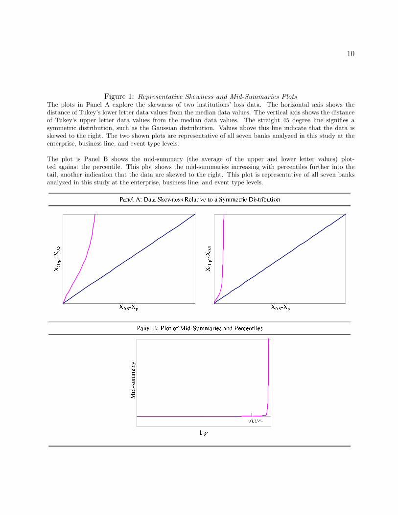
We observed that the loss severity data exhibit a high degree of unsystematic skewness.

The shapes of the skewness are very similar for all institutions at the enterprise, business

line, and event type levels. The top and bottom panels of Figure 1 are representative plots of

skewness and mid-summaries respectively. The upper panel of the figure shows that the data

are highly skewed relative to the normal distribution, which is represented by the straight

line in the figure. The bottom panel reveals that the data are less symmetric in the tail of

the distribution.

For a normal random variable Y with mean µ and standard deviation σ, Y = µ + σZ,

where Z is a standard normal variate. Hence, (Yp−Y1−p)

2Zp= σ where Yp and Y1−p are the 100pth

and 100(1 − p)th percentiles of Y , and Zp is the 100pth percentile of Z. One can define the

pseudosigma (or p-sigma) of the data {Xi}Ni=1 as (Xp−X1−p)

2Zpfor each percentile p. From the

definition it is clear that the pseudosigma is a measure of tail thickness with respect to the tail

thickness of the normal distribution. If the data are normally distributed, the pseudosigma

will be constant across p and equal to σ. When the kurtosis of the data exceeds that of the

normal distribution, p-sigma will increase for increasing values of p.

In Figure 2 we plot ln(p-sigma) versus Z2 as suggested in Hoaglin (1985a) to present the

figure in a more compact form. Even though we observed some similarity in terms of kurtosis

among the loss data in our sample, unlike skewness, there is no definite emerging pattern. The

figure illustrates a mixture of varieties of tail thickness that we observed in our data at the

13Systematic skewness is defined as skewness that does not change sharply with varying percentiles. It willbe affected by the extreme values in the data.

10

Figure 1: Representative Skewness and Mid-Summaries PlotsThe plots in Panel A explore the skewness of two institutions’ loss data. The horizontal axis shows thedistance of Tukey’s lower letter data values from the median data values. The vertical axis shows the distanceof Tukey’s upper letter data values from the median data values. The straight 45 degree line signifies asymmetric distribution, such as the Gaussian distribution. Values above this line indicate that the data isskewed to the right. The two shown plots are representative of all seven banks analyzed in this study at theenterprise, business line, and event type levels.

The plot is Panel B shows the mid-summary (the average of the upper and lower letter values) plot-ted against the percentile. This plot shows the mid-summaries increasing with percentiles further into thetail, another indication that the data are skewed to the right. This plot is representative of all seven banksanalyzed in this study at the enterprise, business line, and event type levels.

11

Figure 2: Plots for Several Institutions’ Tail StructuresThese plots explore the kurtosis of bank data at the enterprise, business line, and event type levels. The plotsshow the natural log of the pseudosigma versus Z2. If the data are normally distributed, the pseudosigma willbe constant across p and equal to σ. When the kurtosis of the data exceeds that of the normal distribution,p-sigma will increase for increasing values of p. The shown plots are representative of the various curve shapesthat occurred at the enterprise, business line, and event type levels.

12

enterprise, business line and event type levels. A horizontal line indicates neutral elongation

in the tail. A positive slope indicates that the kurtosis of the data is greater than that of the

normal distribution. A sharp increase in the slope indicates a non-smooth and unsystematic

heavy tail with increasing values of Z2. As one can see from the figures, the upper tail

is highly elongated (thick) relative to the body of the distribution. In the extreme end of

the tail, the p-sigma flattens out. Some flattening happens earlier than others as evident in

Figure 2(d), which shows an event type with very few data points and more homogeneity in

the losses. Typically one (enterprise, business line, or event type) that has more data and has

two adjacent losses that are of disproportionately different magnitude will have flattening at

higher percentile level. Based on this analysis we infer that in order to fit our loss data we

need a distribution with a flexible tail structure that can significantly vary across different

percentiles. In the subsequent sections of our analysis we compare the tail structure of many

different distributions and their ability to model the tail of the observed data.

3 Selected Models

A loss event Li (also known as the loss severity) is an incident for which an entity suffers

damages that can be measured with a monetary value. An aggregate loss over a specified

period of time can be expressed as the sum

S =N∑

i=1

Li, (1)

where N is a random variable that represents the frequency of losses that occur over the

period. We assume that the Li are independent and identically distributed, and each Li

is independent from N . The distribution of the Li is called the severity distribution, the

distribution of N over each period is called the frequency distribution, and the distribution

of S is called the aggregate loss distribution. This framework is also known as the Loss

Distribution Approach (LDA). The risk exposure can be measured as a quantile of S.14 The

sum S is an N-fold convolution of the Li.

Given the characteristics and challenges of the data, we can resolve many issues by using

an LDA approach. The sum S can be calculated either by fast Fourier transform as suggested

14Basel II will require that the quantile be set to 99.9%. Therefore, throughout the analysis we report ourrisk measure at this level.

13

in Klugman et al. (2004), by Monte Carlo simulation, or by an analytical approximation. We

have used the simulation method, which will be described in Section 4. The LDA has been

exhaustively studied by actuaries, mathematicians, and statisticians well before the concept

of operational risk came into existence.15

Based on the QIS-4 submissions, we observe that financial institutions use a wide variety

of severity distributions for their operational risk data.16 Five of the seven institutions in our

analysis reported using some variant of EVT, and all but one institution reported modeling

loss frequency with the Poisson distribution. Five of the institutions supplemented their

model with external data (three of them directly and two indirectly using scenario analysis).

There are potentially many different alternatives for the choice of severity and frequency

distributions. Our goal is to understand if there exists any inherent structure in the loss data

that is consistent across institutions. In other words, is there some technique or distribution

that is flexible and robust enough to adequately model the operational loss severity for every

institution?

The modeling techniques presented in the following sections are focused on the loss severity

distribution as opposed to the frequency distribution. Based on the exploratory data analysis,

it is quite clear that some of the commonly used simple parametric distributions will not model

the data well. However, we include some of these distributions to compare their performance

to flexible general class distributions, which accommodate a wider variety of underlying data.

In Section 3.1 we describe some of the basic parametric distributions that are typically fitted

to operational loss severity data. We expand upon these distributions in Section 3.2 where

we motivate the use of the g-and-h distribution and the GB2 distribution as flexible models

of operational loss severity. This flexibility can be visualized with skewness-kurtosis plots

presented in Section 3.3. Finally, Section 3.4 explains how extreme value theory can be used

to model loss severity.

3.1 Parametric Distributions

One of the oldest approaches to building a model for loss distributions is to fit parametric

distributions to the loss severity and frequency data. The parameters can be estimated using a

variety of techniques such as maximum likelihood, method of moments, or quantile estimation.

15Klugman et al. (2004) is a good source for various loss models.16In addition, many of the institutions have experimented with several different methods before arriving at

the ultimate model submitted under QIS-4.

14

In our analysis we have separated continuous parametric distributions into two classes: (1)

Simple parametric distributions are those that typically have one to three parameters; and

(2) Generalized parametric distributions typically have three or more parameters and nest a

large variety of simple parametric distributions. Most continuous distributions take either all

real numbers or all positive real numbers as their domain. Some distributions such as the beta

or the uniform have a bounded support. The support of the distribution is important because

losses can never take negative values.17 Hence, it is typical to only consider distributions with

positive support.

For the purposes of fitting loss distributions to the LDCE data, we have used the following

simple parametric distributions presented in Table 4. Appendix A provides some technical

Table 4: Selected Simple Parametric Distributions

Distribution Density Function f(x)a Number of Parameters

Exponential 1λ exp

(−xλ

)I[0,∞)(x) One

Weibull κλ

(xλ

)κ−1 exp−(x/λ)κI[0,∞)(x) Two

Gamma 1λαΓ(α)x

α−1 exp(−x/λ)I[0,∞)(x) Two

Truncated Lognormalb 1xσ√

2πexp

[−

(ln x−µ

σ√

2

)2]

11−F (a)I(a,∞)(x) Two

Loglogistic η(x−α)η−1

[1+(x−α)η]2 I(α,∞)(x) Two

Generalized Paretoc 1β

(1 + ξ

β x)− 1

ξ−1

I[0,∞)(x) TwoaThe indicator function IS(x) = 1 if x ∈ S and 0 otherwise. For example, I[0,∞)(x) = 1 for x ≥ 0 and 0 otherwise.bWhere a is the lower truncation point of the data. F(a) is the CDF of X at the truncation point, a.cThis is the case for ξ 6= 0.

details regarding these distributions. Each of these distributions has two parameters except

the exponential, which has one parameter. They were chosen because of their simplicity and

applicability to other areas of economics and finance. Distributions such as the exponential,

Weibull, and gamma are unlikely to fit heavy-tailed data, but provide a nice comparison to

the heavier-tailed distributions such as the generalized Pareto or the loglogistic. All of these

distributions have positive real numbers as their domain.

We also consider the following generalized distributions: the generalized beta distribution

17Losses are typically treated as positive values for modeling purposes even though they result in a reductionof firm value.

15

of the second kind (GB2) and the g-and-h distribution. Each of these distributions has four

parameters. The GB2 takes positive real numbers as its domain; however, the g-and-h takes

all real numbers as its domain.18 Both of these distributions nest a large family of simple

distributions, which allows the GB2 and the g-and-h more flexibility in fitting the data relative

to the simple distributions.

3.2 General Class Distribution Models

At this moment, we can neither appeal to mathematical theory nor economic reasoning to

arrive at the ideal severity distribution. One approach to finding an appropriate severity

distribution is to experiment with many different distributions with the hope that some

distributions will yield sensible results. Many severity distributions have been tested over a

considerable period of time. It is practically impossible to experiment with every possible

parametric distribution that we know of. An alternative way to conduct such an exhaustive

search could be to fit general class distributions to the loss data with the hope that these

distributions are flexible enough to conform to the underlying data in a reasonable way.

A general class distribution is a distribution that has many parameters (typically four

or more) from which many other distributions can be derived or approximated as special

cases. The four parameters typically represent or indicate the following: location (such as the

mean or median), scale (such as the standard deviation or volatility), skewness, and kurtosis.

These parameters can have a wide range of values and therefore can assume the values for

the location, scale, skewness, and kurtosis of many different distributions. Furthermore,

because general class distributions nest a wide array of other parametric distributions, they

are very powerful distributions used to model loss severity data. A poor fit for a general

class distribution automatically rules out the possibility of a good fit with any of its nested

distributions. In our experiments we have chosen two such general class distributions: the

g-and-h and the GB2 distributions. The motivation to use these two particular general class

distributions is that they have been applied to other areas of economics and finance.

18It is only a minor shortcoming that the g-and-h distribution takes negative values. One can force randomnumbers drawn from the g-and-h to be positive using a rejection sampling method.

16

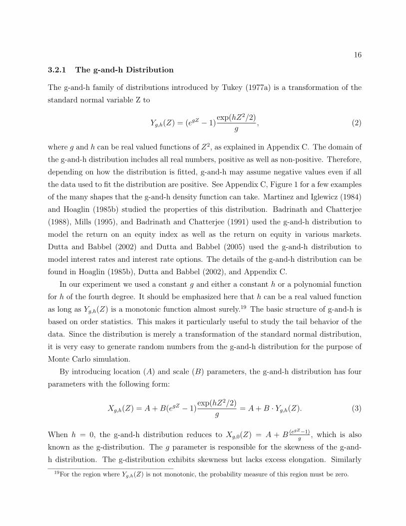
3.2.1 The g-and-h Distribution

The g-and-h family of distributions introduced by Tukey (1977a) is a transformation of the

standard normal variable Z to

Yg,h(Z) = (egZ − 1)exp(hZ2/2)

g, (2)

where g and h can be real valued functions of Z2, as explained in Appendix C. The domain of

the g-and-h distribution includes all real numbers, positive as well as non-positive. Therefore,

depending on how the distribution is fitted, g-and-h may assume negative values even if all

the data used to fit the distribution are positive. See Appendix C, Figure 1 for a few examples

of the many shapes that the g-and-h density function can take. Martinez and Iglewicz (1984)

and Hoaglin (1985b) studied the properties of this distribution. Badrinath and Chatterjee

(1988), Mills (1995), and Badrinath and Chatterjee (1991) used the g-and-h distribution to

model the return on an equity index as well as the return on equity in various markets.

Dutta and Babbel (2002) and Dutta and Babbel (2005) used the g-and-h distribution to

model interest rates and interest rate options. The details of the g-and-h distribution can be

found in Hoaglin (1985b), Dutta and Babbel (2002), and Appendix C.

In our experiment we used a constant g and either a constant h or a polynomial function

for h of the fourth degree. It should be emphasized here that h can be a real valued function

as long as Yg,h(Z) is a monotonic function almost surely.19 The basic structure of g-and-h is

based on order statistics. This makes it particularly useful to study the tail behavior of the

data. Since the distribution is merely a transformation of the standard normal distribution,

it is very easy to generate random numbers from the g-and-h distribution for the purpose of

Monte Carlo simulation.

By introducing location (A) and scale (B) parameters, the g-and-h distribution has four

parameters with the following form:

Xg,h(Z) = A + B(egZ − 1)exp(hZ2/2)

g= A + B · Yg,h(Z). (3)

When h = 0, the g-and-h distribution reduces to Xg,0(Z) = A + B (egZ−1)g

, which is also

known as the g-distribution. The g parameter is responsible for the skewness of the g-and-

h distribution. The g-distribution exhibits skewness but lacks excess elongation. Similarly

19For the region where Yg,h(Z) is not monotonic, the probability measure of this region must be zero.

17

when g = 0, the g-and-h distribution reduces to

X0,h(Z) = A + BZ exp(hZ2/2) = A + B · Y0,h(Z),

which is also known as the h-distribution. The h parameter in the g-and-h distribution is

responsible for the kurtosis. The h-distribution can model heavy tails (kurtosis), but lacks

skewness. The moments for the g-and-h distribution can be found in Appendix D.

Martinez and Iglewicz (1984) have shown that the g-and-h distribution can approximate a

wide variety of distributions by choosing the appropriate values of A, B, g, and h. The power

of this distribution is essentially in its ability to approximate probabilistically the shapes of

many different data and distributions. The g-and-h distribution is a natural outcome of the

exploratory data analysis we used in Section 2.3. The method and techniques we used in

exploratory data analysis are in fact building blocks towards modeling the data with the g-

and-h distribution. All of the distributions that were reported by financial institutions under

QIS-4 can be approximated by the g-and-h distribution to a very high degree. The generalized

Pareto distribution (GPD), which is used to model the tail of a distribution in extreme value

theory, can also be approximated by the g-and-h distribution to a very high degree.

Typically, a quantile-based method given in Hoaglin (1985b) is used for the estimation of

the parameters of the g-and-h distribution. Compared to commonly used estimation methods

such as the method of moments and maximum likelihood estimation (MLE), quantile-based

methods can potentially be more accurate for fitting the tails of a distribution. Furthermore,

the transformational structure of the standard normal distribution given in (3) above, makes

the g-and-h particularly suitable for quantile-based fitting. In addition to introducing the

g-and-h distribution, we study another flexible four-parameter distribution for the purpose of

comparison.

3.2.2 The GB2 Distribution

The Generalized Beta Distribution of the Second Kind (GB2) is a four-parameter distribution

that approximates many important one- and two-parameter distributions including all of

the distributions described in Appendix A as well as the Burr type 3, Burr type 12, log-

Cauchy, and chi-square distributions. Bookstabber and McDonald (1987) show many of the

distributions that can be derived from GB2 as special cases of the parameter values. The

GB2, like the g-and-h distribution, can accommodate a wide variety of tail-thicknesses and

18

permits skewness as well. Many of the important properties and applications of the GB2

distribution can be found in McDonald (1996) and McDonald and Xu (1995). Bookstabber

and McDonald (1987) and Dutta and Babbel (2005) have explored the possibility of modeling

equity and interest rates respectively using GB2. The density function for GB2 is defined as

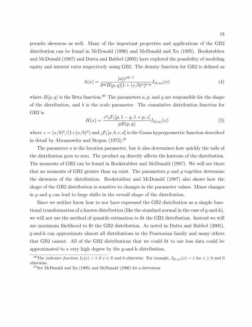
h(x) =|a|xap−1

bapB(p, q)[1 + (x/b)a]p+qI(0,∞)(x) (4)

where B(p, q) is the Beta function.20 The parameters a, p, and q are responsible for the shape

of the distribution, and b is the scale parameter. The cumulative distribution function for

GB2 is

H(x) =zp

2F1[p, 1− q, 1 + p, z]

pB(p, q)I(0,∞)(x) (5)

where z = (x/b)a/(1+(x/b)a) and 2F1[a, b, c, d] is the Gauss hypergeometric function described

in detail by Abramowitz and Stegun (1972).21

The parameter a is the location parameter, but it also determines how quickly the tails of

the distribution goes to zero. The product aq directly affects the kurtosis of the distribution.

The moments of GB2 can be found in Bookstabber and McDonald (1987). We will see there

that no moments of GB2 greater than aq exist. The parameters p and q together determine

the skewness of the distribution. Bookstabber and McDonald (1987) also shows how the

shape of the GB2 distribution is sensitive to changes in the parameter values. Minor changes

in p and q can lead to large shifts in the overall shape of the distribution.

Since we neither know how to nor have expressed the GB2 distribution as a simple func-

tional transformation of a known distribution (like the standard normal in the case of g-and-h),

we will not use the method of quantile estimation to fit the GB2 distribution. Instead we will

use maximum likelihood to fit the GB2 distribution. As noted in Dutta and Babbel (2005),

g-and-h can approximate almost all distributions in the Pearsonian family and many others

that GB2 cannot. All of the GB2 distributions that we could fit to our loss data could be

approximated to a very high degree by the g-and-h distribution.

20The indicator function IS(x) = 1 if x ∈ S and 0 otherwise. For example, I[0,∞)(x) = 1 for x ≥ 0 and 0otherwise.

21See McDonald and Xu (1995) and McDonald (1996) for a derivation.

19

3.3 Skewness-Kurtosis Analysis

In addition to characterizing distributions by the number of parameters, distributions can be

somewhat ordered by assessing the heaviness of their tails. In the context of a loss distribu-

tion, the tail corresponds to that part of the distribution that lies above a high threshold.

A heavy-tailed distribution is one in which the likelihood of drawing a large loss is high.22

Another way of stating this is that operational losses are dominated by low frequency, but

high-severity events. There are formal statistical notions of heavy-tailed. For example, distri-

butions that are classified as subexponential (such as the lognormal) or dominatedly varying

may be considered heavy-tailed.23 To simplify things we will classify institutions’ loss severi-

ties as light-tailed if the exponential, gamma, or Weibull distributions reasonably fit the loss

data. If the loglogistic, lognormal, or g-and-h (with a positive h parameter) distributions fit

the data reasonably well, we will describe the loss severities as heavy-tailed.24

A distribution can also be characterized by its moments. The first two moments are the

mean and variance, which characterize the location and scale of a distribution. The third mo-

ment, the skewness, measures the asymmetry in the distribution. Skewness can take positive

or negative values, and a positive skewness implies that the upper tail of the distribution is

more pronounced than the lower tail. Kurtosis, the fourth moment, characterizes both the

heaviness of the tails and the peakedness of the distribution.25 Kurtosis is always positive,

and distributions with a kurtosis above three (the kurtosis for the normal distribution) are

referred to as leptokurtic.

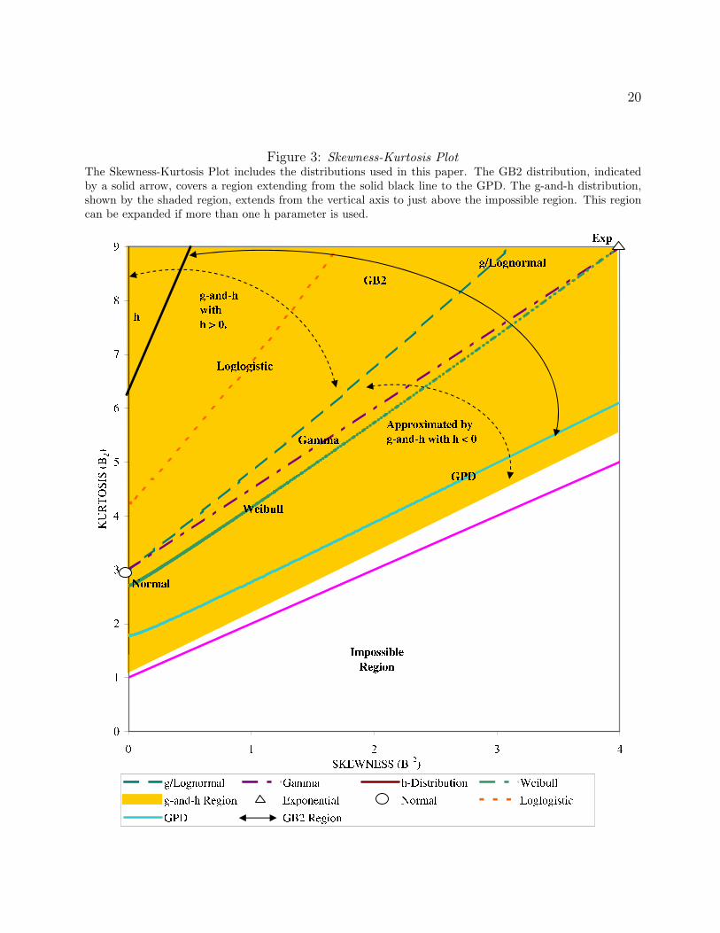
One way of visualizing the flexibility of a distribution is by rendering its skewness-kurtosis

plot. The plot shows the locus of skewness-kurtosis pairs that the distribution can take by

varying its parameter values. This plot can be a point, curve, or two-dimensional surface

depending upon whether the skewness or kurtosis are functions of zero, one, or many param-

eters. The plots for a variety of distributions are presented in Figure 3 where the skewness

is squared to show only positive values. The normal and exponential distributions are repre-

sented as points on the graph because their skewness and kurtosis can only take one value each

no matter what its parameter values are. The GB2 and g-and-h distributions are represented

22What constitutes a “high likelihood” is somewhat arbitrary.23For precise properties of heavy-tailed distributions, see Embrechts et al. (1997).24The GB2 and the GPD distributions can be heavy-tailed or light-tailed depending upon the parameter

values. With certain tail parameter values, the GPD can have a non-existent mean implying a very heavytail. For other tail parameter values, the GPD can be lighter-tailed than the gamma or Weibull. The g-and-hdistribution can be light-tailed with a negative h.

25For a discussion of the intuitive interpretation of kurtosis see Ruppert (1987).

20

Figure 3: Skewness-Kurtosis PlotThe Skewness-Kurtosis Plot includes the distributions used in this paper. The GB2 distribution, indicatedby a solid arrow, covers a region extending from the solid black line to the GPD. The g-and-h distribution,shown by the shaded region, extends from the vertical axis to just above the impossible region. This regioncan be expanded if more than one h parameter is used.

21

as skewness-kurtosis surfaces. These distributions are the most flexible in the sense that they

span a large set of possible skewness-kurtosis values. The loglogistic, lognormal, Weibull,

GPD, and gamma distributions have one-dimensional skewness-kurtosis curves.26 In some

sense, the lognormal curve forms an envelope where skewness-kurtosis plots above this enve-

lope represent heavy-tailed distributions and plots below this envelope represent light-tailed

distributions. In this graphical sense the Weibull, gamma, and exponential distributions

would be classified as light-tailed.

The skewness-kurtosis plot is particularly useful in illustrating the relationship among

distributions. For example, the exponential distribution is a special case of the Weibull

distribution, and therefore the exponential is represented as a single point lying on the Weibull

skewness-kurtosis curve. Furthermore, the loglogistic curve is completely contained within the

g-and-h skewness-kurtosis surface. In this sense one could say that the g-and-h distribution

is a parent distribution of the loglogistic. If a distribution fits the data, then its parent

distribution will fit the data at least as well. Because general class distributions such as

the g-and-h and GB2 span a larger area on the skewness-kurtosis plot, they provide more

flexibility in modeling a wide variety of skewness and kurtosis.27

3.4 Extreme Value Theory for Modeling Loss Severity

A loss distribution can be divided into two pieces: the body and the tail. Losses below a

certain threshold τ are from the body of the distribution, and losses above the threshold are

from the tail. For the sake of computing operational risk capital, the tail of the loss severity

distribution is of paramount concern because the extreme losses are the ones that effectively

drive capital. Quite naturally, this leads to the subject of extreme value theory (EVT), a

branch of statistics concerned with the study of extreme phenomena - rare events that lie in

the tail of a probability distribution.

There are two general ways to view the loss database for EVT purposes. In the first case

the losses can be broken into several non-overlapping periods of fixed duration (blocks), and

the points of interest are the largest observations from each period. These largest observations

are referred to as block maxima. In the second case the losses are treated as though they were

incurred over one time period, and the losses of interest are those losses above a specified

26Although the plots may appear to be straight lines in the figure, many of them are in fact non-linearcurves. One would see this clearly if the plot were on a larger scale.

27Using multiple parameters for h, one can cover the entire skewness-kurtosis region.

22

threshold. This is referred to as the peaks over threshold (POT) approach. Typically the

POT approach to EVT is preferred when the data have no clear seasonality. This is the case

with operational risk data, and hence, we will use this approach in the analysis. See Appendix

B for a technical discussion of the EVT theorems.

The Pickands-Balkema-de Haan theorem describes the limit distribution of scaled excess

losses over a sufficiently high threshold. Under certain regularity conditions, this limit distri-

bution will always be a generalized Pareto distribution (GPD). So applying the POT method

entails choosing a sufficiently high threshold to divide the distribution into a body and tail

and fitting GPD to the excess losses in the tail. The body of the distribution is sometimes

fitted with another parametric distribution such as the lognormal, but it can also be modeled

with the empirical distribution.

4 Methodology

In the previous section we discussed techniques for modeling the severity of operational losses.

This section describes the methodology we use to assess the performance of these techniques.

For each technique we describe in detail the method of estimation. Then, we discuss the

following four types of goodness-of-fit tests used to assess the statistical fit of distributions:

Pearson’s chi-square test, the Kolmogorov-Smirnov (K-S) test, the Anderson-Darling (A-D)

test, and the Quantile-Quantile (Q-Q) plot. Finally, we present our procedure to estimate

capital. We measure the performance of our modeling approaches with respect to these five

dimensions listed in order of importance:28

1. Good Fit - Statistically, how well does the method fit the data?

2. Realistic - If a method fits well in a statistical sense, does it generate a loss distributionwith a realistic capital estimate?

3. Well-Specified - Are the characteristics of the fitted data similar to the loss data andlogically consistent?

4. Flexible - How well is the method able to reasonably accommodate a wide variety ofempirical loss data?

5. Simple - Is the method easy to apply in practice, and is it easy to generate randomnumbers for the purposes of loss simulation?

28Our experiment included every distribution reported in QIS-4.

23

In addition, we characterize a distribution or method in terms of coherence, consistency,

and robustness. These are discussed later in Section 5.5.

As we described earlier, the techniques for estimating loss severities for the institutions

in our data set can be broken into four categories: simple parametric distribution fitting,

generalized parametric distribution fitting, non-parametric fitting, and the application of

EVT. Non-parametric fitting involves modeling the data in the absence of any theoretical

parametric constraints.29 In this analysis, the non-parametric method we consider is simply

assuming that the empirical loss distribution is a near substitute for the actual loss distribu-

tion. Hence, simulations based on this method involve drawing random observations directly

from the historical loss data. The application of EVT that we consider (the peaks over thresh-

old approach) entails separating the loss severity distribution into a body and tail and fitting

the generalized Pareto distribution to the data in the tail.

The frequency distribution plays an equally important role in the estimation of capital.

Unfortunately, because most institutions have fewer than four years of data, and the loss oc-

currence dates are not accurately recorded, frequency modeling is highly limited. As discussed

above, our frequency estimates are only based upon loss arrivals at the annual level to avoid

seasonal variation due to inaccurate time-stamping of losses. Due to the annual reporting

and other regulatory requirements, the time stamping on an annual basis is generally found

to be more accurate than on a daily, weekly, or a monthly basis.

In this analysis we only consider the method of using a parametric distribution for fre-

quency. The two most important discrete parametric distributions for modeling the frequency

of operational losses are the Poisson and negative binomial distributions. From QIS-4 sub-

missions, we observe that there is near unanimity in terms of the use of Poisson distribution

as the frequency distribution. The Poisson distribution has one parameter, which is equal

to both the mean and variance of the frequency. The negative binomial distribution is a

two-parameter alternative to the Poisson that allows for differences in the mean and variance

of frequency with mean less than the variance; however, we did not have enough data to

estimate the parameters of the negative binomial distribution.30 Therefore, we chose to use

the Poisson distribution with its parameter value equal to the average number of losses per

year.

To simplify matters, we make the following assumptions throughout the paper:

29Neural networks and kernel estimation are two examples of this technique.30We typically had loss data for two to three years. Estimating two parameters using just a few data points

(in most cases two or three) would not be appropriate.

24

1. All frequency random variables are independent from one another (at the business lineand event type level).

2. All severity random variables are independent.31

3. Frequency is independent from loss severity.

4. Frequency is distributed Poisson with constant mean frequency equal to the averagenumber of losses per year for the particular institution, business line, or event type.

5. Loss severities are identically distributed.

The dependence structure in operational loss data is not currently clear. Hence Assumption

(1) is appropriate given the current state of research. Assumptions (1) - (3) imply that losses

follow a multivariate compound Poisson process.32 In the following sections, we describe in

detail each of the four methods for loss severity modeling. For each of these methods, we

experimented with loss data at the enterprise level, as well as at the Basel business line and

event type levels.

4.1 Unit of Measurement

We conducted our study using three different units of measurement:33

1. Enterprise level.

2. Business line level (determined by the institutions which included many Basel-definedbusiness lines).

3. Event type level (determined by the institutions which included many Basel-definedevent types).

Grouping the data into business lines and event types enables us to study similar data.

Many institutions recorded their losses in just a few business lines or event types. We find

that most of the institutions have only three business lines or two event types with more than

300 data points. A few institutions even had only one business line or event type in which

more than 200 losses were recorded. Also, many institutions often record their largest losses

31This assumption is relaxed in Section 5.4.2 when we explore different dependency structures.32See McNeil et al. (2005) for a discussion of the properties of multivariate Poisson processes.33We could further refine the unit of measurement by breaking losses down by event types within each

business line, but data scarcity have precluded any meaningful data analysis.

25

in one unit, such as the “Other” business line category or the Clients, Products & Business

Practices event type (ET4).

If most losses are concentrated in only a few categories, then any measurement based on

aggregation of the measurements at the business line or event type level would be close to

that of the enterprise level. We find this to be true for data that are comprised of mostly low

severity/high frequency losses in one or two units and high severity/low frequency losses in

not more than one unit. In these cases, the tail determined by extreme events is essentially

coming from very few business lines or event types.

This gives rise to an important question: will a measurement at the enterprise level be

different from aggregating business line or event type measurements under any dependence

structure? We will analyze this question later under two extreme conditions, independence

(zero correlation) and comonotonicity (random variables have perfect positive dependence),

and compare it to the measurement at the enterprise level.

4.2 Methods of Estimation

Two different methods were used to estimate the parameters of the severity distributions.

Maximum Likelihood Estimation (MLE) was used in all cases excluding the g-and-h distri-

bution, for which we used the method of quantile estimation as suggested by Hoaglin (1985b)

and Tukey (1977a). The MLE assigns equal weight to all the data used to fit the distributions.

In contrast, the method of quantiles estimation can place more weight on the data in the tails

of the distribution. Quantile-based methods are not appropriate for all distributions, but are

especially suited for transform distributions such as the g-and-h. Alternatively, we could have

used a numerical MLE method to estimate the g-and-h parameters; however, as discussed

in Rayner and MacGillivray (2002) this MLE method has shortcomings when applied to the

g-and-h distribution. Appendix C describes the estimation procedure for the g-and-h distri-

bution, and Appendix D contains the formulas for computing the general moments of the

g-and-h.

The g-and-h distribution can potentially take negative values even though loss amounts

could never be recorded as negative numbers.34 For all of the institutions that we fitted using

g-and-h, at most 6% of the distribution in the lower tail was found to be negative, and many

34The g-and-h is fitted to the exceedances: losses minus the loss threshold. Hence, a negative value for theexceedance is equivalent to drawing a loss below the threshold.

26

of them had only 0.7% negative.35 We corrected this by using a rejection sampling method

in the simulation for the loss distribution where we replaced negative draws with positive

draws. In order to test the impact of the negativity, we ran the simulation with and without

the rejection sampling method. We observed insignificant changes in the capital estimates

for all of the institutions. Hence, this drawback had no practical significance. The g-and-h

transformation must also be monotonic. In high quantiles one may need to use rejection

sampling to force observations into an area where the distribution is well defined.

The $10,000 threshold for losses must be incorporated into the estimation. In most cases

this can be accomplished by subtracting $10,000 from each data point and then adding the

threshold back in at a later point. This was the approach we took for all distributions

except for the lognormal for which the truncated lognormal PDF was used in the maximum

likelihood estimation.36 After performing the parameter estimation we measured the model’s

goodness-of-fit.

4.3 Comparison of Goodness-of-Fit Tests

One can attempt to fit any particular parametric distribution to data; however, only certain

distributions will have a “good” fit. There are two ways of assessing this goodness-of-fit:

using graphical methods and using formal statistical goodness-of-fit tests. Graphs such as a

Quantile-Quantile (Q-Q) plot or a normalized Probability-Probability (P-P) plot can help an

individual determine whether a fit is very poor, but may not reveal whether a fit is “good”

in the formal sense of statistical fit.

Goodness-of-fit tests fall into a variety of standard categories: chi-square tests (such as

Pearson’s chi-square test), tests based on the empirical distribution function (such as the

Kolmogorov-Smirnov, Anderson-Darling, and Cramer-von Mises tests), tests based on regres-

sion or correlation (such as the Shapiro-Wilk test), and tests based on the third and fourth

sample moments (such as the rectangle test).37 Due to their popularity for assessing the fit of

35In three occasions at the business line and event type levels, we found situations in which approximately10% of the distribution was negative. In these particular cases there were considerably fewer observationsrelative to others. In addition, the dollar value of losses in the lower tail is insignificant relative to the capitalestimates. Therefore, substituting zero values for these draws will not change the capital estimates.

36For two of the seven institutions (and a handful of the business line and event types), the maximumlikelihood estimates of the truncated lognormal parameters implied that an extremely small fraction of thedistribution lies above the point of truncation. In these cases the truncation point was adjusted upwards untilthe first point where the parameter estimates implied a reasonable underlying distribution.

37For a review and comparison of goodness-of-fit tests, see D’Agostino and Stephens (1986).

27

a distribution to operational loss data, the Pearson’s chi-square test, the Kolmogorov-Smirnov

(K-S) test, the Anderson-Darling (A-D) test, and the Q-Q plot are the only goodness-of-fit

tests that will be used in this analysis. Appendix E provides a description of these four tests.

Although the chi-square test is very flexible, it has low power relative to many other

goodness-of-fit tests. The chi-square test results will still be presented due to the test’s pop-

ularity. The K-S test is also a relatively low power test, but it is very simple to compute and

is one of the most popular empirical distribution function (EDF) test statistics. The main

disadvantage of the K-S test for our purposes is that the test puts more weight on the center

of the distribution than on the tails. The tail fit of the distribution is of paramount impor-

tance because the capital estimate is mainly driven by the tail behavior of the distribution.

Therefore, we should be more concerned with the goodness-of-fit in the tail than in the body.

The A-D test is superior to the K-S in this regard because the A-D test puts more weight on

the tail of the distribution.

When testing the goodness-of-fit of a distribution to data, it is important to use the

correct critical values for the test statistic. When the null distribution has one or more shape

parameters (parameters other than just location and scale), the critical values of the test

statistic will depend on the values of these shape parameters as well as the number of sample

observations. Thus, it is important to compute critical values by simulating the values of the

test statistic. This is the approach we take for all of the K-S and A-D tests in this paper.38

For a comparison of goodness-of-fit tests along with extensive power studies, see D’Agostino

and Stephens (1986) and Gan and Koehler (1990).

A Q-Q plot is a visual representation of fit. A seemingly good fit on the Q-Q plot may

not always translate to a good statistical fit. However, if distribution A has a better fit than

distribution B on the Q-Q plot, and distribution B has not been rejected as a poor fit by a

formal statistical test, then using a transitivity argument, distribution A can be considered

to be at least as good a fit according to some formal test as well.

38To compute the A-D and K-S, we follow the method outlined in D’Agostino and Stephens (1986) for anEDF test with unknown parameters. A vector of size n is simulated from the estimated sample parameters,where n is the sample size. The parameters are then re-estimated and the test statistic is computed from thissample. These simulations are repeated 50,000 times and the critical value is taken at the 5% significancelevel.

28

4.4 Capital Estimation Techniques

For each of the methods presented below, the capital estimate is computed as the 99.9%

quantile of the simulated loss distribution. We used MATLAB exclusively to generate the

pseudo-random numbers for the simulations. The following sections below describe the sim-

ulation procedure in detail.

4.4.1 Parametric

Once the parameter estimates have been obtained, one can simulate from the estimated loss

distribution to obtain a capital estimate in the following way. For each simulated year, draw

a frequency N from the Poisson distribution. Draw N loss severities from the estimated

parametric distribution. Sum these N losses to get the total annual loss. Finally, these steps

are repeated one million times. For the g-and-h distribution it is possible to draw losses below

the loss threshold. We used rejection sampling to correct this issue.39

4.4.2 Extreme Value Theory

To estimate capital for the EVT technique, we use the following simulation method. Choose a

threshold τ to divide the distribution into body and tail. Fit the GPD to excess losses above

τ using MLE. For each simulated year, draw a frequency N from the Poisson distribution.

Multiply N by the fraction of the data in the body to get NL and the fraction of the data

in the tail to get NH . Draw NL loss severities (with replacement) from the data in the body

(empirical sampling). Draw NH loss severities from the estimated GPD in the tail. Sum all

NH and NL losses together to get the total annual loss. Finally, these steps are repeated one

million times.

One of the most difficult problems in the practical application of EVT is choosing the

appropriate threshold for where the tail begins. Not only are estimates of ξ highly sensitive

to the threshold choice, capital estimates are even more sensitive. As the threshold is raised,

it is expected that the data are better approximated by the GPD. However, there will be

fewer observations available. In this case the bias of the estimate is low, but the variance in

the estimate of ξ is high. Conversely, when the threshold is reduced, the bias in the estimate

of ξ is high, but the variance of this estimate is low. There is no unique technique that can

39Rejection sampling can be used to correct this problem. If the distribution below the threshold has alarge mass, rejection sampling will be inefficient. In our case this mass is typically small - below 5%.

29

be used to deduce the appropriate threshold; however, each of the following methods could

be considered:

1. Graphical methods (Hill plots, mean excess plots, etc)

2. Bias-variance bootstrap methods

3. Ad hoc methods

4. Goodness-of-fit

Method (1) involves creating several plots of the data and using heuristics to choose the

appropriate threshold. Two important plots are the Hill plot, which displays an estimate

of ξ for different exceedance levels, and the mean excess plot, which graphs the conditional

mean of the data above different thresholds. One problem with using graphical methods is

that the choice of threshold is still somewhat arbitrary. There may be multiple thresholds

that satisfy the heuristic decisions embedded in the graphical methods. Some researchers

have suggested using a technique to find the threshold that yields an optimal bias-variance

tradeoff. Method (2) involves using bootstrap simulations to numerically compute the optimal

threshold taking into account this bias-variance tradeoff. See Danielsson et al. (2001) for

details on this bootstrap method.

Method (3) refers to the use of an ad hoc objective criterion for choosing the threshold.

One such criterion would be to choose the threshold such that 40 observations are in the tail

of the distribution. Another possibility would be to choose the threshold such that 15% of

the observations in the data set are in the tail. Although EVT suggests that once a high

enough threshold is chosen that the GPD will theoretically fit the data in the tail, this does

not guarantee that the GPD will pass any formal statistical goodness-of-fit test. Method (4)

entails choosing the threshold such that the GPD fits the data in the tail better than any

other threshold. Clearly there may be many thresholds for which the GPD fit is “good.”

Hence, this method also suffers from the problem of a multiplicity of possible thresholds. We

attempted to apply each of these four threshold selection methods in our EVT models. A

discussion regarding our findings with these methods will follow in Section 5.1.

4.4.3 Empirical Sampling

One approach to estimating capital is to avoid fitting any parametric distributions to the loss

data and instead simply simulate losses from the “empirical distribution.” For this approach

30

we use the following simulation method. For each simulated year, draw a frequency N from

the Poisson distribution. Draw N loss severities (with replacement) using the original pooled

loss severity data. Sum these N losses to get the total annual loss. Finally, these steps are

repeated one million times.

The empirical sampling capital estimates can be used as baselines of comparison because

there is no underlying parametric model that needs to be justified. Also, if the empirical

distribution accurately represents the underlying loss severity distribution, then the capital

estimation via empirical sampling will yield a reasonable approximation for capital. Since

capital estimation is dependent on the sample drawn, a biased estimate may occur. If the

empirical distribution contains too few tail events, then the capital estimate will be biased

downwards. Conversely, if tail events are over-represented, then the capital estimate will be

biased upwards.

5 Results

In this section we present the results of the comparative analysis at the enterprise, business

line, and event type levels. In order to protect the anonymity of the institutions in our sample,

institutions are simply labelled with a letter from A to G. In certain cases we only present

summary tables regarding these institutions to further maintain anonymity. In addition,

all capital estimates are presented as percentages of the institutions’ total assets and gross

income. This not only serves to anonymize the results, but also allows one to make better

comparisons among the institutions, which vary substantially in terms of asset size. We

simulated the capitals for every loss distribution method irrespective of whether we found a

good fit in order to determine the sensitivity of the capital estimate to the various methods.

Throughout the analysis we will refer to some capital estimates as reasonable or unreason-

able. We will define “reasonable” as a capital estimate that falls below 3.0% of the asset size

(a little over half the tier 1 capital requirement) so that there is room for model estimation

error.40 We understand our choice is arbitrary. However, the conclusion of our paper will not

be very different even if we raise the threshold to 10.0%, which is equivalent to more than

twenty times the median unadjusted AMA capital reported by the financial institutions under

QIS-4 submissions and more than the entire tier-1 capital requirement. In some cases, capital

40This number is roughly about eight times the median unadjusted AMA capital reported by the financialinstitutions under QIS-4 submissions. Tier 1 capital is regulatory core capital that includes equity capitaland disclosed reserves.

31

estimates may be unreasonably low, yet still fall into our definition of “reasonable.” These

are typically the institutions that did not experience many large losses. These institutions

may supplement their data with external data and scenario analyses.

It is more difficult to determine a reasonableness standard for these capital estimates as

a percentage of gross income relative to ones based on total asset size. This is because gross

income tends to vary much more than assets across time. Although enterprise level gross

income figures are publicly reported, business line gross income figures are generally not;

how gross income is appropriately allocated to the business lines is subject to interpretation.

Hence, enterprise level gross income figures are better denominators than business line gross

income figures for assessing reasonableness of capital estimates across institutions. For ex-

ample, a business line may incur a large loss thus reducing its gross income to zero. In this

case its capital estimate (as a percentage of gross income) would approach infinity no matter

which method is chosen.

The results are first reported at the enterprise level and then by business line and event

type. Finally, we compare our estimates based on the performance measures described in

Section 4.

5.1 Enterprise Level

The results at the enterprise level are reported with EVT first, then with parametric distri-

bution approaches, and then with empirical sampling. The capital estimates at the enterprise

level are reported as percentages of total assets as well as enterprise level gross income. We

will discuss the characteristics of the models we tested in the context of our enterprise level

results. Most of these characteristics also translate to the business line and event type lev-

els. In the business and event type result sections we will only discuss those results that are

particular to those levels.

5.1.1 Extreme Value Theory

Embrechts et al. (1997) cautions practitioners of EVT that EVT is designed to estimate

extremal events under very precise conditions. If these conditions are not satisfied, the the-

ory can lead to incorrect estimates of the likelihood of extreme events. Also, even if these

assumptions are satisfied, the POT appraoch is appropriate for sufficiently high thresholds.

Whether a threshold is sufficiently high depends upon the underlying distribution of the data

32

generating process. With these caveats stated up front, we summarize our EVT findings at

the enterprise level.

Because threshold selection is critical to capital estimation under EVT, we simulated cap-

ital for a variety of thresholds. We began by estimating the GPD parameters with thresholds

set at 10 exceedances through 1000 exceedances in increments of 10. For each threshold

(number of exceedances) we estimated capital based on the simulation method presented in

Section 4. We found that institutions’ capital estimates are highly sensitive to the threshold

choice. There is an exponential relationship between the GPD estimate of ξ and the estimated

capital. For example, it can be shown that the 99.9% capital estimate is proportional to

τ +β

ξ[(.001/q)−ξ − 1],

where q is the proportion of total observations exceeding the threshold τ . Whenever ξ is

above one, the GPD has an infinite mean, which implies an extremely large capital estimate.

Figure 4 plots the GPD maximum likelihood estimates for ξ over the range of thresholds

for six institutions. Capital estimates for the three institutions in the top panel of Figure

4 are reasonable for some thresholds, whereas capital estimates for the three institutions in

the bottom panel are very high for essentially all thresholds due to ξ being greater than one.

Figure 4 reveals the important result that for the three institutions in the bottom panel, our

EVT method will yield implausibly high capital estimates for virtually all thresholds when the

GPD is estimated at the enterprise level. Because of the importance of threshold selection on

capital estimation, we experimented with all four of the threshold selection methods discussed

in Section 4.4.

The first threshold selection method we used was to choose the appropriate threshold

based on the Hill plots and mean excess plots for each institution. For over half of the

institutions, the mean excess plots are not properly defined because the estimated values of ξ

are infinite. An alternative is to use the median excess plots. We found that these graphical

methods could be used to justify a variety of thresholds that would imply both low as well

as high capital estimates. For each institution a range of thresholds would be acceptable

under the graphical methods, but there is no objective method available that can be used to

distinguish among these thresholds consistently across institutions. In an attempt to avoid

this subjectivity, we looked to the other methods.

We implemented the Danielsson et al. (2001) bootstrap method for its ability to objectively

33

Figure 4: GPD Estimates of ξ Versus Number of Exceedances for Six InstitutionsThe top figure shows institutions which may have reasonable capital estimates since ξ estimates from EVT arenot always above one. The bottom figure shows three institutions for which we would not expect reasonablecapital estimates at any threshold since ξ estimates are consistently greater than one.

34

choose the threshold based on a bias-variance trade-off. We simulated 10,000 bootstraps to

derive the threshold for all of the institutions in our sample. For most institutions, the

bootstrap implied thresholds that were not supported as reasonable choices according to

the graphical methods. In addition, for some institutions the bootstrap optimal threshold

included either the entire sample of data or very few observations. The capital estimates

based on the bootstrap thresholds were also unreasonably high.

After estimating the parameters of the GPD using maximum likelihood for each thresh-

old, we performed the K-S and A-D goodness-of-fit tests. We initially expected that these

goodness-of-fit tests could be used to narrow down the choice of threshold. In theory, one

could choose the threshold with the lowest test statistic value or more appropriately, the

highest p-value.41 However, the null hypothesis that the data fit the GPD is not rejected for

almost all of the thresholds up to 1,000 exceedances. Thus, using goodness-of-fit measures

to choose the threshold is not appropriate with this particular data set because one cannot

distinguish a good fit from a better fit in this way.

As an objective alternative to these threshold selection methods, we decided to choose the

threshold based on an ad hoc percentage of the number of losses above $10,000. Specifically,

two thresholds were selected: one with GPD fitted to 5% of the losses and one with GPD fitted

to 10% of the losses.42 Because every institution in the sample has at least 1000 losses at the

enterprise level, there were at least 50 and 100 exceedances used for the maximum likelihood

estimation at these two threshold levels. The EVT capital estimates at the enterprise level are

presented in Table 5 along with the estimates for the other models. Only summary results are

presented in order to preserve the anonymity of the institutions in our sample. The results

clearly indicate significant variation in capital estimates across institutions even when the

model has passed statistical goodness-of-fit tests. It is also apparent from the table that the

EVT results yield some of the highest estimates relative to the other models.

It should be noted that we are not suggesting any specific threshold selection method.

For certain specific institutions we found that many different threshold selection methods

41A low p-value implies that the distribution is a poor fit to the data. A high p-value may imply a goodfit, but it could also imply that there is not enough data to determine whether or not the fit is statisticallygood.

42We could have chosen a fixed number of exceedances instead of a fixed percentage of total observations.We chose the latter because we feel it provides more consistency across institutions. For example, if one chose100 exceedances for each institution, the tail would represent more extreme events for an institution with50,000 observations relative to one with only 1000 observations. The conclusions we make based on the 5%and 10% thresholds are the same regardless of which thresholds are actually applied consistently across theinstitutions (provided there are enough observations to fit the GPD).

35

Table 5: Capital at the Enterprise Level as a Percentage of Total Assets and Gross IncomeThis table presents a summary of the 99.9% capital estimates as a percentage of total assets (Panels A and B)and as a percentage of gross income (Panels C and D). The capital estimates were simulated from one milliontrials. Panels A and C present the first, second and third quartiles, which were calculated across each model.These statistics include both capital estimates that statistically fit and do not fit. Panels B and D present afrequency distribution of banks whose capital estimates fit according to one or more of the following goodness-of-fit tests: Kolmogorov-Smirnoff, Chi-Square, and Anderson-Darling. The fit for the g-and-h distributionwas only tested using Q-Q plots. No goodness-of-fit tests were performed for the empirical distribution. Byconstruction, the empirical distribution would fit the data. All empirical estimates are included in thesecounts. The total number that fit is also presented above Panel A.

36

could all yield reasonable capital estimates over a range of thresholds. But for a comparative

analysis of EVT across seven different institutions, we prefer to use a method that can be

consistently applied to each of these institutions in an objective manner.

The most surprising result of this analysis is that for over half of the institutions, the EVT

POT approach yielded an infinite mean for the tail of the distribution and unreasonable capital

estimates regardless of the threshold selected. Neslehova et al. (2006) provide some possible

explanations for these infinite mean models. The authors state that data contamination is a

major concern. When the basic assumptions of the EVT framework are not satisfied (such

as iid data), estimates of ξ can be incorrect. Data contamination may be unavoidable with

real data, so operational risk measurement techniques should do a reasonable job of coping

with contamination.

Although one could easily blame the data for being contaminated, another potential issue

is that even if all of the EVT assumptions are satisfied, estimates of ξ can be incorrect if

convergence of the GPD to the tail of the distribution requires a significantly large number

of observations. McNeil and Saladin (1997) perform a Monte Carlo study to determine how

large the sample size should be in order for there to be low parameter estimation error. They

simulate from the lognormal, loggamma, Student’s t, and Pareto distributions and find that

the heavier the tail of the distribution, the sample size and threshold must be increased.

In many of their simulations, the sample size should be above 2000 observations for the

estimation bias to be tolerable.

Mignola and Ugoccioni (2005) also perform Monte Carlo simulations to assess the per-

formance of the EVT POT method given a variety of underlying loss severity distributions.

They find that the rate of convergence of the tail parameter ξ in reasonably large samples

can be very poor when the lognormal and loggamma distributions are used as the underlying

distributions. In these cases ξ was significantly overestimated. Given the results of these

two simulation papers and the fact that operational loss severity distributions are sometimes

severely heavy-tailed, it is not unreasonable to expect that capital estimates using the EVT

POT approach will yield over-inflated estimates in samples of under 100,000 observations.

Diebold et al. (1998) and Embrechts et al. (1997) present some of the theoretical pitfalls

associated with EVT estimation.

One could argue that large operational losses follow a power law, also known as Zipf’s Law.

In this specification the tail of the CDF can be written as 1−G(x) ∼ x−1/ξ.43 This is similar

43This is equivalent to assuming that G(x) lies in the maximum domain of attraction (MDA) of the Frechet

37

to using the EVT POT approach for estimating capital. It is mathematically convenient to

assume this specification because the high quantiles of the aggregate loss distribution can be

well approximated by the largest order statistic as shown by Bocker and Kluppelberg (2005).

A capital estimate can be calculated without simulation using the following formula

Capital = τ · (1000 ·N)ξ, (6)

where τ is the dollar threshold used to fit the power law to the tail, N is the number of losses

exceeding τ , and ξ is an estimate of the tail parameter. As a corollary to our EVT analysis,

we attempted to estimate capital using this method as well.

Our results are almost completely identical to the EVT results. We used the Hill estimator

to estimate ξ and chose the threshold to be 5% and 10% just as we did for the EVT analysis.

Table 6 reports the capital estimates as a percentage of total assets for the power law analysis

without reporting details about the fit of the model. The capital estimates are unreasonably

Table 6: Power Law Capital Estimates at the Enterprise Level as a Percentage of Total AssetsPanel A presents ξ for each bank, computed using the Hill estimator, with 5 and 10 percent of the data inthe tail. Panel B presents summary statistics for capital estimates at the 99.9% level for each institution as apercentage of total assets. These capital estimates were not simulated, but instead calculated using the powerlaw approximation method described in the paper. No goodness-of-fit tests are presented in this table.

large due to the high tail estimates for ξ. We also estimated capital according to the number of

exceedances above the threshold τ . We started with 10 and incremented the exceedances up by

10 until all of the data were included. The results indicate large differences in capital estimates

distribution, and the slowly varying function L(x) in Appendix B.1 converges to a constant.

38

depending upon which threshold is chosen. While reasonable results for some institutions

occur at some thresholds, for other institutions no reasonable capital estimates could be

found because the Hill estimator always exceeded one. For other institutions virtually no

reasonable capital estimates could be found because the Hill estimator for ξ always exceeded

one. Even if one could show that the power law fits large operational losses (which is unlikely),

this method yields very unreasonable capital estimates.

5.1.2 Parametric Distribution Fitting with Maximum Likelihood

Table 7 presents the goodness-of-fit results for all models at the enterprise level. The shaded

Table 7: Goodness-of-Fit at the Enterprise LevelThis table presents a summary of the goodness-of-fit tests performed and capital estimates at the 99.9% levelfor each institution as a percentage of total assets. These capital estimates were simulated from one milliontrials. The numbers in parentheses indicate those tests that were not rejected at the 5% significance levelunder the following goodness-of-fit tests: (1) Kolmogorov-Smirnoff (2) Chi-Square (3) Anderson-Darling. (4)The fit for the g-and-h distribution was only tested using Q-Q plots. In all cases this model appears to fit justas well or better than any of the other models tested according to the Q-Q plots. (5) No goodness-of-fit testswere performed for the empirical distribution. By its very nature, the empirical distribution would fit the data.

Those models that fit one or more of the goodness-of-fit tests and had a capital estimate of up to 3%of assets are highlighted in gray.

regions in the table signify models that fit according to at least one goodness-of-fit test and

yielded reasonable capital estimates. The exponential distribution is rejected as a good fit

under all of the statistical tests. In fact, this distribution has the worst fit of any of the

distributions we tested. Because the exponential distribution has only one parameter, one

would not expect this distribution to fit the data well. The fits for the two-parameter gamma

and Weibull distributions are virtually as bad as the fit for the exponential at the enterprise

39

level. In addition, the capital estimates for these three distributions are low compared to the

estimates from the other methods.

The GPD, a two-parameter distribution, was fit to the entire data set, unlike the EVT

method for which GPD was only used to fit the tail. Hence, fitting GPD to the full data set is

equivalent to our EVT methodology with the threshold equal to $10,000 for all institutions.

The goodness-of-fit results for the GPD are mixed. For some institutions GPD was not

rejected under any of the tests, and for others GPD was rejected under all tests. Similar

test results were found for the loglogistic, a two-parameter distribution. The GB2, a four-

parameter general class distribution, fit well for all but two institutions according to either

the K-S or A-D tests. This is not surprising given that it is a general class distribution, and

its skewness-kurtosis plot covers a wide area.

Table 5 illustrates the capital estimates for each method by institution. The top of the

table shows frequencies for the number of institutions modeled in this study and for those

that statistically fit. Panels A and B illustrate summary statistics for capital as a percentage

of assets, whereas Panels C and D present the same information as a percentage of gross

income.44

The capital estimates for GB2, GPD, and loglogistic are unreasonable for almost all of the

institutions. The same is true for EVT using the 5% and 10% thresholds. For the truncated

lognormal, the capital estimates are comparatively smaller, but three of the institutions had

unreasonable capital estimates. Of all of the methods we applied to the loss data, the EVT

approach yielded the largest capital estimates. For three of the institutions, the EVT 5%

capital estimate was larger than the total asset size of the institution. Choosing slightly

different thresholds for each institution yields capital estimates several times the total asset

size.

5.1.3 The g-and-h Distribution

For the g-and-h distribution we used a Quantile-Quantile (Q-Q) plot to measure its goodness-

of-fit. For g-and-h this is the most appropriate test given its special structure. We made an

attempt to fit the g-and-h distribution with only one h parameter. However, for two of the

seven institutions, we found a better fit on the Q-Q plot using four h parameters instead

of one h relative to the plots for the other distributions. For these institutions we used the

44In order to maintain the anonymity of the institutions, we cannot present the complete estimates byinstitution.

40

polynomial function for h with four parameters as discussed in Appendix C.45

We observe a good fit for all of the institutions fitted with the g-and-h distribution using

the Q-Q plot as a goodness-of-fit metric as described in Section 4.3.46 Figure 5 shows the

Q-Q plot for Bank F, which compares the fit of the g-and-h distribution with the fits of other

distributions. The other distributions on the plot were statistically good fits according to

either the K-S or A-D test with the exception of the exponential distribution, which is only

presented as an example of a poor-fitting distribution. This Q-Q plot is fairly representative

of the plots for the other institutions, business lines, and event types. The plot clearly shows

that the g-and-h distribution fits just as well as the other distributions; however, the g-and-h

has a much better fit in the tail.47 Most of the other distributions for which we observed a

good fit under any of the formal statistical tests showed a good fit for the lower percentiles

(the body of the distribution) according to the Q-Q plot, but did not perform as well as the

g-and-h distribution did in the upper tail above the 99th percentile. As we noted earlier, it is

difficult to apply conventional statistical goodness-of-fit tests, such as the K-S and A-D tests,

to the g-and-h distribution. However, Figure 5 clearly shows that the g-and-h distribution

fits better than some of the distributions that were found to be a good fit under the K-S,

A-D, and Chi-square tests. Therefore, the g-and-h distribution can also be considered a good

fit in these cases.

Figure 6 illustrates the Q-Q plot for Bank C. In contrast to the previous Q-Q plot, Figure

6 shows that the g-and-h fit is distinctly better than the fit for the other distributions. This

Q-Q plot is different than the one for Bank F because formal statistical tests rejected the fit

of all distributions (other than g-and-h). This atypical situation occurs in rare cases. What

is interesting about the figure is that the g-and-h plot appears to be on the 45 degree line

across all quantiles of the data. In this situation we say that the g-and-h distribution has the

best fit of all the models.

Each model, other than the g-and-h, that could be statistically accepted as a good fit

45Out of about 58 different units that we could model using g-and-h distribution, including business line andevent type, we used four h parameters to fit the g-and-h distribution in only five units. In all those situations,the data set had more than several thousands losses. We did not incrementally increase the number of hparameters. It will be a good process to increase the parameters for h incrementally in fitting g-and-h. Wefeel in those cases where we used four parameters of h to model the tail, fewer parameters could have beenused.

46A formal goodness-of-fit test for the g-and-h distribution would be computationally complex so we havenot included it here. Given the good fit of the g-and-h on the Q-Q plot, we believe that a formal test wouldnot change the results of this analysis.

47Most of the tail points lie on the 45 degree line except for the very last data point.

41

Figure 5: Q-Q Plot for Bank FThese plots show the Q-Q plots for enterprise level expected losses versus observed losses for models that fitaccording to goodness-of-fit tests. The exponential distribution is also shown as an example of a poor fittingmodel and does not fall within the range of some plots. The first plot covers the body of the distributionfrom the 0th percentile to the 85th percentile (body). The second plot (to the right of the first plot) coversthe 85th percentile to the 97th percentile (lower tail). The third plot covers the 97th percentile to the 99.3thpercentile (upper tail), and the final plot covers all points from the 99.3th percentile to the 100th (extremeupper tail). Please note that the scales of the Q-Q plots differ.

42

Figure 6: Q-Q Plot for Bank CThese plots show the Q-Q plots for enterprise level expected losses versus observed losses for models that fitaccording to goodness-of-fit tests. The exponential distribution is also shown as an example of a poor fittingmodel and does not fall within the range of some plots. The first plot covers the body of the distributionfrom the 0th percentile to the 85th percentile (body). The second plot (to the right of the first plot) coversthe 85th percentile to the 97th percentile (lower tail). The third plot covers the 97th percentile to the 99.8th

percentile (upper tail), and the final plot covers all points from the 99.8th percentile to the 100th (extremeupper tail). Please note that the scales of the Q-Q plots differ.

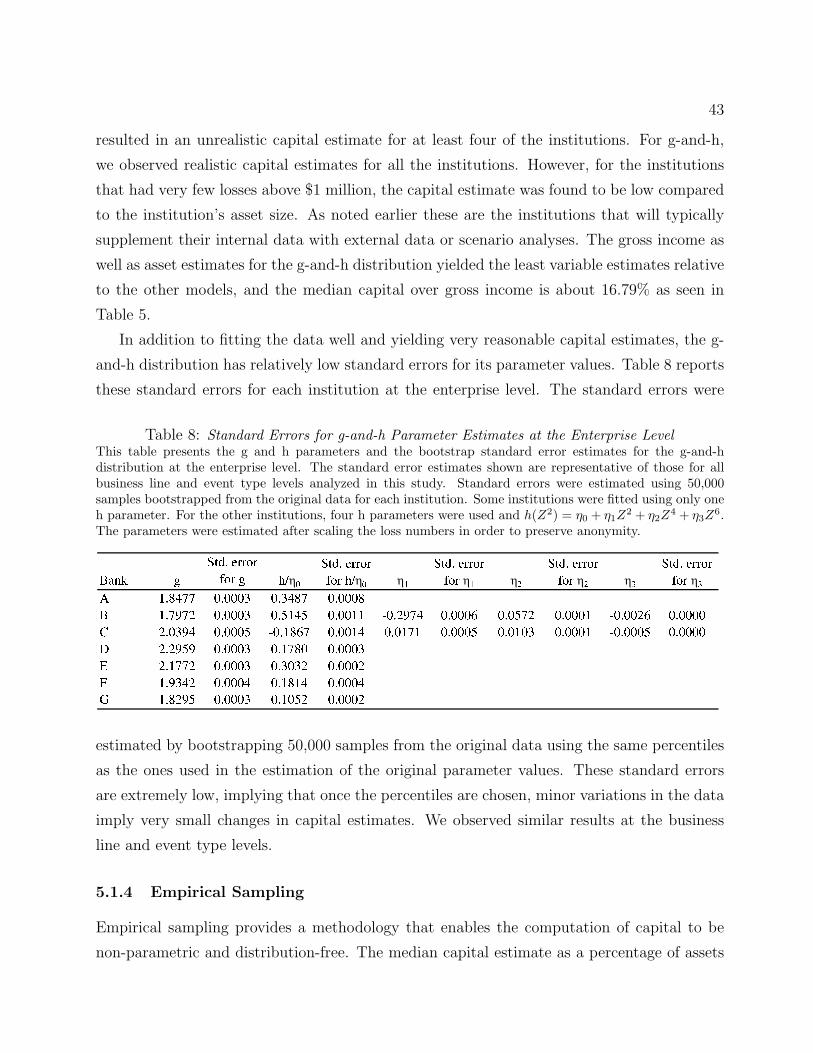
43

resulted in an unrealistic capital estimate for at least four of the institutions. For g-and-h,

we observed realistic capital estimates for all the institutions. However, for the institutions

that had very few losses above $1 million, the capital estimate was found to be low compared

to the institution’s asset size. As noted earlier these are the institutions that will typically

supplement their internal data with external data or scenario analyses. The gross income as

well as asset estimates for the g-and-h distribution yielded the least variable estimates relative

to the other models, and the median capital over gross income is about 16.79% as seen in

Table 5.

In addition to fitting the data well and yielding very reasonable capital estimates, the g-

and-h distribution has relatively low standard errors for its parameter values. Table 8 reports

these standard errors for each institution at the enterprise level. The standard errors were

Table 8: Standard Errors for g-and-h Parameter Estimates at the Enterprise LevelThis table presents the g and h parameters and the bootstrap standard error estimates for the g-and-hdistribution at the enterprise level. The standard error estimates shown are representative of those for allbusiness line and event type levels analyzed in this study. Standard errors were estimated using 50,000samples bootstrapped from the original data for each institution. Some institutions were fitted using only oneh parameter. For the other institutions, four h parameters were used and h(Z2) = η0 + η1Z

2 + η2Z4 + η3Z

6.The parameters were estimated after scaling the loss numbers in order to preserve anonymity.

estimated by bootstrapping 50,000 samples from the original data using the same percentiles

as the ones used in the estimation of the original parameter values. These standard errors

are extremely low, implying that once the percentiles are chosen, minor variations in the data

imply very small changes in capital estimates. We observed similar results at the business

line and event type levels.

5.1.4 Empirical Sampling

Empirical sampling provides a methodology that enables the computation of capital to be

non-parametric and distribution-free. The median capital estimate as a percentage of assets

44

under this method is about 0.27%. For some of the institutions, these estimates are close to

the g-and-h capital estimates. The g-and-h estimates are higher than the empirical sampling

estimates for four of the seven institutions. No goodness-of-fit tests were performed for the

empirical sampling method because the fit is appropriate by construction.

A primary disadvantage of using this method is that its capital estimates can be easily

biased. It may underestimate capital because it assumes that a future loss cannot be greater

than the largest loss over the sample period. In addition, smaller institutions are less likely to

have extreme tail events, which may also lead to underestimating capital. On the other hand,

the empirical sampling method may overestimate capital when there is an extremely large loss

in the sample. Of all of the methods tested in our analysis, the empirical sampling method

and the g-and-h distribution provided the most reasonable capital estimates; however, the

range and standard deviation in these estimates across institutions is higher for the empirical

sampling method relative to the g-and-h. As shown in Table 5, the 25th percentile and the

median of the empirical estimates are roughly one-half and one-third of the g-and-h estimates,

respectively. On the other hand, the 75th percentile of the empirical estimates is greater than

that of the g-and-h. The empirical sampling method’s dependence on the sample and time

period chosen is a drawback that cannot be understated.

5.2 Business Line Level

Table 9 illustrates the capital estimates by business line for each institution presented as

percentages of business line gross income (as reported under LDCE). Since capital is com-

puted as a fixed percentage of gross income at each business line under the Standardized

Approach, we chose to report the capital here as a percentage of business line gross income

for the purpose of comparison. We do not report capital as a percentage of assets in order to

save space. Although we have modeled every business line with a sufficient number of losses

(and the “Other” category), only BL2, BL3, BL4, and BL6 are presented for anonymity

purposes. Many distributions reported under “Generally Yielded Unreasonable Capital Es-

timates” appear to have better performance than they had at the enterprise level, but all of

these distributions have very poor performance at many of the business lines including those

not reported here (BL1, BL5, BL7, BL8, and the “Other” business line). We did not compute

capital estimates for GB2 at the business line level because simulating capital for the GB2

was computationally intensive. For business lines with 20 or fewer observations, we did not

perform any distribution fitting because of the imprecision in the parameter estimation and

45

the instability of maximum likelihood estimates. We also required at least 15 observations for

fitting the GPD under the EVT POT approach. For example, the 5% EVT model required

at least 300 observations at the business line level in order to have at least 15 observations in

the tail. We required at least 100 observations for fitting the g-and-h. Consequently, many

institutions did not have a sufficient number of losses to model all of the distributions. For

instance, we were only able to model three institutions for business lines 2 and 4 using g-and-h

and EVT.

The comparative results at the business line level are similar to what we found at the

enterprise level. Therefore, in this section we only report observations that are distinct from

those at the enterprise level. The exponential, gamma, and Weibull distributions have lower

capital estimates than the estimates for the heavier-tailed distributions (GPD, loglogistic,

and g-and-h). Furthermore, the exponential, gamma, and Weibull were all rejected as good

fits for almost all of the institution’s business lines despite the paucity of the data. It appears

as though the GPD, loglogistic, lognormal, and EVT models fit well, but the Q-Q plots by

business line show much more variation and poorer fits than at the enterprise level (given the

smaller sample sizes). The Q-Q plots in Section 5.1 are fairly typical of what we observed at

the business line level.

The capital estimates for the g-and-h distributions yielded reasonable capital estimates for

all the business lines.48 The lognormal distribution also yielded reasonable capital estimates

for many business lines. Excluding the exponential, gamma, and Weibull distributions, the

empirical sampling method yielded much lower capital estimates than the other approaches.

The median capital estimates for empirical sampling are at most one-third those of g-and-h.

The one exception was for the “Other” business line (not shown on Table 9) for which many

large losses are recorded, causing empirical capital estimates to be unreasonably high. In that

category empirical sampling often resulted in a capital estimate fifteen times more than that

of g-and-h. GPD, loglogistic, and EVT all gave some very unreasonable capital estimates.

Some of these capital estimates are several orders of magnitude more than 1000% of business

line gross income.49 The EVT method yielded the highest median capital estimates for all

business lines other than BL2 and BL6.

Table 10 shows the sum of the business line capital estimates as a percentage of total assets

and total gross income. This is almost equivalent to an enterprise-level capital calculation

48As noted earlier we modeled only those business lines that recorded at least 100 losses.49In terms of enterprise asset size, these estimates are several orders of magnitude more than 100% of

enterprise assets.

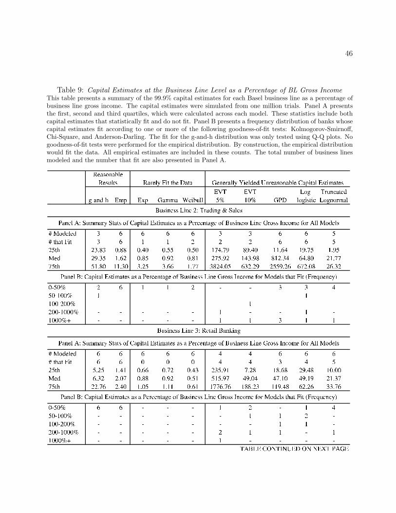
46

Table 9: Capital Estimates at the Business Line Level as a Percentage of BL Gross IncomeThis table presents a summary of the 99.9% capital estimates for each Basel business line as a percentage ofbusiness line gross income. The capital estimates were simulated from one million trials. Panel A presentsthe first, second and third quartiles, which were calculated across each model. These statistics include bothcapital estimates that statistically fit and do not fit. Panel B presents a frequency distribution of banks whosecapital estimates fit according to one or more of the following goodness-of-fit tests: Kolmogorov-Smirnoff,Chi-Square, and Anderson-Darling. The fit for the g-and-h distribution was only tested using Q-Q plots. Nogoodness-of-fit tests were performed for the empirical distribution. By construction, the empirical distributionwould fit the data. All empirical estimates are included in these counts. The total number of business linesmodeled and the number that fit are also presented in Panel A.

47

48

Table 10: Summed BL Capital Estimates as a Percentage of Total Assets and Gross IncomeThis table presents a summary of the 99.9% capital estimates summed across Basel business lines toenterprise level as a percentage of total assets (Panels A and B) and as a percentage of gross income (PanelsC and D). Panels A and C present the first, second and third quartiles, which were calculated across eachmodel. Panels B and D present a frequency distribution of all models. Panels A-D include all modelsregardless of statistical fit. The capital estimates were simulated from one million trials. For the empiricalmodel, all business lines were estimated. For the g-and-h distribution, business lines with 100 or moreobservations were estimated. Some business lines were combined in order to estimate capital using g-and-hand EVT. For all other business lines that could not be estimated due to limited data and for non-Baselbusiness lines, estimates from the empirical model were substituted.

Including empirical estimates may have biased these results causing some to appear extreme.

49

assuming perfect positive dependence (comonotonicity) across the business lines for each

institution.50 This is obviously an unrealistic assumption, but we computed the summed

estimates in order to make some simple comparisons with the enterprise level capital computed

earlier. For business lines where there were no estimates due to limited data, we substituted

the capital estimates for empirical sampling. Although in the table the maximum bucket for

capital as a percentage of assets is 100%+, many of the estimates for EVT and distributions

other than g-and-h were several orders of magnitude above 100%.

The median capital estimates (by total assets and gross income) in Table 10 are higher

than the estimates in Table 5. For example, the median g-and-h capital estimate by total

assets in Table 10 is almost twice the estimate as the one in Table 5. The smaller enterprise

level estimates are somewhat due to a diversification benefit across the business lines. Similar

to what we observe in Table 5, in Table 10 EVT resulted in unreasonable capital estimates

for institutions that experienced large operational losses.

5.3 Event Type Level

The advantage of fitting models at the event type level is that the loss processes are somewhat

more homogenous. Event types can be viewed as risk factors for operational risk. We did

not compute capital estimates for GB2 at the event type level because simulating capital

for the GB2 was computationally intensive. As can be seen in Table 11, the event type

capital estimates across institutions for the g-and-h distribution are more homogenous than

the estimates by business line presented in Table 9.

Although we have modeled every event type, we have not included ET1, ET5, and event

type “Other” in order to preserve the anonymity of the institutions. We modeled every event

type (including the “Other” category) with a sufficient number of losses, as explained in Sec-

tion 5.2. Similar to the business line level, many event types could not be modeled. While

many distributions reported under “Generally Yielded Unreasonable Capital Estimates” ap-

pear to have better performance at the event type level than the enterprise level, all these

distributions have very poor performance at many of the event types including those not

reported in the table.

Some of the simple parametric distributions that did not result in realistic capital estimates

at the enterprise level did result in reasonable estimates for some event types for many of the

50The sum of the VaRs for each business line is typically not an upper bound because VaR is not subadditiveas shown in Artzner et al. (1999).

50

Table 11: Capital Estimates at the Event Type Level as a Percentage of Total AssetsThis table presents a summary of the 99.9% capital estimates for each Basel event type as a percentage of totalassets. The capital estimates were simulated from one million trials. Panel A presents the first, second andthird quartiles, which were calculated across each model. These statistics include both capital estimates thatstatistically fit and do not fit. Panel B presents a frequency distribution of banks whose capital estimatesfit according to one or more of the following goodness-of-fit tests: Kolmogorov-Smirnoff, Chi-Square, andAnderson-Darling. The fit for the g-and-h distribution was only tested using Q-Q plots. No goodness-of-fittests were performed for the empirical distribution. By construction, the empirical distribution would fit thedata. All empirical estimates are included in these counts. The total number of event types modeled and thenumber that fit are also presented in Panel A.

51

52

institutions. This is because many large losses that were observed at the enterprise level are

concentrated in one or two event types, while other event types had recorded high frequency

low severity losses. For example, the truncated lognormal, loglogistic, and GPD appear to

yield reasonable capital estimates for some event types. EVT 5% seems to yield reasonable

capital estimates for ET2 and EVT 10% seems to do so for ET2 and ET3. We were surprised

that the EVT capital estimates for ET4 and “Other” event types were unreasonably high in

spite of there being more homogeneity at the event type level. This provides some evidence

that the poor EVT performance may be the result of non-convergence as opposed to data

contamination. Other than the observations just mentioned, the results at the event type

level are similar to the business line and enterprise levels, particularly the observations with

respect to empirical sampling. In the case of event types, the median capital estimates for

empirical sampling was always significantly lower than those of the g-and-h.

For completeness we present the aggregated capital estimates by event type in Table 12.

As with the business line results, although in the table the maximum bucket for capital as a

percentage of assets is 100%+, many of the estimates for EVT and distributions other than

g-and-h were several orders of magnitude above 100%.

We observed that for three out of seven institutions in our sample, the enterprise level

capital estimates were very close to the sum of capital estimates of their event type levels.

For the other four institutions the number was not significantly different.

53

Table 12: Summed ET Capital Estimates as a Percentage of Total Assets and Gross IncomeThis table presents a summary of the 99.9% capital estimates summed across Basel event types to enterpriselevel as a percentage of total assets (Panels A and B) and as a percentage of gross income (Panels C andD). Panels A and C present the first, second and third quartiles, which were calculated across each model.Panels B and D present a frequency distribution of all models. Panels A-D include all models regardlessof statistical fit. The capital estimates were simulated from one million trials. For the empirical model, allevent types were estimated. For the g-and-h distribution, event types with 100 or more observations wereestimated. Some event types were combined in order to estimate using g-and-h and EVT. For all other eventtypes that could not be estimated due to limited data and for non-Basel event types, estimates from theempirical model were substituted.

Including empirical estimates may have biased these results causing some to appear extreme.

54

5.4 Comparison of Methods Based on Performance Measures

In Section 4 we stated that the performance of the modeling techniques we implemented

were to be measured with respect to these five dimensions: good fit, realistic, well-specified,

flexible, and simple. Much of the analysis in Section 5 has focused on goodness-of-fit as well

as whether the capital estimates calculated from the model are realistic. We will summarize

these main points first before moving on to the other three performance measures.

5.4.1 Good Fit

Many different approaches to modeling operational risk are currently being used, which is

why we chose to test so many different techniques in this study. If a model does not fit the

data, then the model is estimating a risk exposure that is not indicated by the data. This

is why we feel that testing goodness-of-fit is a necessary condition for any model being used

before capital is calculated.

We found that the three thin-tailed distributions (exponential, gamma, and Weibull)

are rejected as a good fit to the data for virtually all institutions at all levels of analysis.

Other than the g-and-h distribution, all other models had trouble fitting the data for some

institutions at the enterprise, business line, and event type levels. For some distributions

that passed the statistical goodness-of-fit tests, the Q-Q plots indicated that the fit was much

better in the body than in the tail of the distribution. Because the tail of the distribution

drives the capital estimate, the tail-fit of a distribution may be more critical than the fit of

the body.51

5.4.2 Realistic

Our two high-level observations regarding how realistic the capital estimates are: (1) We find

that for certain models, there is substantial variation in capital estimates across institutions;

and (2) For every institution we find that there is substantial variation in capital estimates

across models. The previous statements are true even limiting the models to those that fit

the data. These observations imply that problems more often arise due to the choice of the

models rather than the data. We also find that both the g-and-h distribution and the em-

pirical sampling method yielded reasonable capital estimates across all institutions; however,

51It is not clearly defined where the tail of a distribution begins. Clearly, a method that fits the tail as wellas the body is preferred to a method that only fits the tail.

55

as stated earlier, the empirical sampling method may be biased towards extremely low or ex-

tremely high capital estimates depending on the data sample. We have discussed the g-and-h

capital estimates were the least variable across institutions. Using g-and-h distribution as the

severity distribution, we also found the averages for the aggregate loss distribution were rea-

sonable.52 In contrast, EVT produced the highest and most variable capital estimates across

institutions. Many of the EVT estimates were several orders of magnitude larger than the

g-and-h estimates.53 These estimates also varied significantly with the choice of tail threshold.

Under the new Basel Accord, the AMA allows institutions significant flexibility in choosing

a model to estimate operational risk. While this has many benefits, it should be made clear

that the choice of model in some sense determines the risk that is estimated, and in turn

the capital that is held by the institution. Table 13 ranks the models for each institution

according to the capital estimate at the enterprise level as a percentage of total assets.

The Weibull distribution is always ranked as yielding the lowest capital estimate for all

institutions. The exponential and gamma distributions yield the next lowest estimates. One

can clearly see that the light-tailed distributions are clustered on the left of the table, and

the heavy-tailed distributions lie on the right of the table (including EVT, which is fit with

the GPD). At the center of the table lies the g-and-h distribution, which gave the most

reasonable capital estimates consistently. For certain parameters, the g-and-h distribution

can produce heavy tails, like those of the distributions on the right hand side of the table, yet

g-and-h results in a different tail shape than those models when fitted to the data. Typically

the capital estimates from the distributions on the right hand side of the table resulted in

unrealistically large capital estimates. If one limits models to those that yield realistic capital

estimates and have good statistical fits, then the choice of models is confined to the shaded

region of Table 13.54

We should stress here that the light-tailed distributions rarely fit the data. The heavy-

tailed distributions such as the GB2, GPD, lognormal, and loglogistic sometimes fit the data,

but gave unreasonable capital estimates compared to either the g-and-h or the empirical

sampling method. The distributions on the far right and far left side of Table 13 do not fit

52The 25th percentile, median, and 75th percentile of the averages across all institutions were 0.05%, 0.06%,and 0.09% of enterprise assets, respectively. We also observed reasonable estimates for the averages at thebusiness line and event type levels.

53In fact, some of the GPD and lognormal estimates exceeded 100,000%. In more than one case the EVTestimates exceeded 1,000,000%.

54The shaded region of the Table 13 will not change even if we raise the limit for “realistic” capital to be10% of assets.

56

Table 13: Capital Estimation Ranking of Loss Severity Modeling TechniquesThis table presents the relative rankings of capital estimates at the 99.9% level for each institution as apercentage of total assets. The capital estimates are simulated from one million trials. Models are orderedby the median rank across all banks. Capital models were ranked 1 to 11 for each bank with a ranking of 1for the model with the smallest capital-to-assets ratio. Some of the listed models were not a good fit for thedata, and all models were ranked regardless of how well they fit the data. The fit for the g-and-h distributionwas only tested using Q-Q plots. In all cases this model appears to fit just as well or better than any of theother models tested according to the Q-Q plots. No goodness-of-fit tests were performed for the empiricaldistribution. By construction, the empirical distribution would fit the data. The other models were tested atthe 5% significance level under the following goodness-of-fit tests: (1) Kolmogorov-Smirnoff (2) Chi-Square(3) Anderson-Darling. For each model, the sample statistics mean, median, and standard deviation werecalculated.

Those models that fit one or more of the goodness-of-fit tests and had a capital estimate of up to 3% of assetsare highlighted in gray.

57

the upper tail of the data well as illustrated on the Q-Q plots in Figures 5 and 6.

Capital estimates are primarily determined by the shape of the distribution’s tail. Figure

7 illustrates the tail shape of several distributions for four representative institutions. The

plots show 1−F (x) versus a loss amount x, where F (x) is the CDF of X. This function must

always be decreasing and asymptotic to the horizontal axis. The faster the function converges

to this axis, the thinner the tail. The g-and-h distributions in the figure have thinner tails

relative to the other distributions. Because the g-and-h distribution yields reasonable capital

estimates compared to the other distributions, one can infer that the g-and-h tail reflects the

tail structure of the data. It appears from the Q-Q plot in Figure 6 that the distributions other

than g-and-h have underestimated the extreme tail of the data. Yet the other distributions

gave capital estimates at least seven times that of the g-and-h. This can only be explained

by comparing the extreme tail structures of these distributions as represented in Figure 7.

Figure 8 shows the same information as Figure 7, but on a log-log scale. On a log-log

scale it is easier to see the similarities and differences among various tail shapes; however,

the tails of each distribution appear closer together than in Figure 7. One gets a better sense

of the the differences in capital estimates by looking at Figure 7. Some of the plots on a

log-log scale may appear to be straight lines; however, different levels of magnification reveal

curvature implying that none of these distributions follow a power law.

Although the region for the empirical method is shaded on Table 13, indicating a good

fit and realistic capital estimates, the inherent biasedness and inaccuracies of the empirical

method, which were discussed earlier, should be taken into account. As mentioned in Sections

5.2 and 5.3, the observations based on Table 13 also apply to business lines and event types.

In order to understand the dependence structure within business lines and event types

we used the g-and-h distribution to aggregate unit level capital estimates under two different

assumptions: independence (zero correlation) and comonotonicity (random variables have

perfect positive dependence55).56 Table 14 shows the difference between the capital estimates

under these two assumptions.

As we reported earlier, many institutions did not record more than 100 losses in some

business lines or event types. We could not model any of these units using g-and-h. In these

situations, we combined unit losses and computed the capital. If there were still an insufficient

55Random variables are comonotonic if they have as their copula the Frechet upper bound (see McNeil etal. (2005) for a more technical discussion of comonotonicity).

56We limit this analysis to the g-and-h because it was the only distribution that fit and resulted in reasonablecapital estimate across all business lines and event types.

58

Figure 7: Tail Shapes for Various DistributionsThese graphs show the tails for some of the models used in this paper for four representative institutions. Thehorizontal axis gives the loss amount X as a percentage of the institution’s assets. The vertical axis shows oneminus the cumulative distribution function (CDF) of X. Among the institutions and models shown, the EVTmodels have the fattest tails and the g-and-h distribution has the thinnest. Please note that the thinnest-tailed models (exponential, gamma and Weibull) are not shown. These plots also show that the tail thicknessvaries across institutions and across distributions.

59

Figure 8: Tail Shapes for Various Distributions on a Logarithmic ScaleThese graphs show the tails for some of the models used in this paper for four representative institutions.The horizontal axis gives the natural log of the loss amount X as a percentage of the institution’s assets. Thevertical axis shows the natural log of one minus the cumulative distribution function (CDF) of X. Amongthe institutions and models shown, the EVT models have the fattest tails and the g-and-h distribution hasthe thinnest. Please note that the thinnest-tailed models (exponential, gamma and Weibull) are not shown.These plots also show that the tail thickness varies across institutions and across distributions.

60

Table 14: Difference Between Aggregate Capital Estimates of g-and-h (as a Percentage of EnterpriseAssets) Under Comonotonic and Independence StructuresThis table shows the difference between the 99.9% capital estimates (as a percentage of enterprise assets) cal-culated under two dependence assumptions: comonotonicity (perfect positive dependence) and independence(zero correlation). Only business lines and event types with 100 or more observations were estimated usingg-and-h. For some business lines and event types that had less than 100 observations, business lines or eventtypes could be combined to create a larger dataset. In the other cases, estimates from the empirical modelwere substituted. The mean, median, standard deviation, and interquartile statistics were calculated acrossall institutions. Only the g-and-h distribution is shown since all other models produced some unrealisticcapital estimates.

Including empirical estimates may have biased these results causing them to appear unrealistic or extreme.

61

number of losses after combining these, we substituted empirical sampling estimates.

The difference between the capital estimates using comonotonicity and independence are

much smaller than we expected. The difference is much smaller for event types than business

lines. If dependence were to exist, it may be more prevalent among business lines than at

the event type levels. This supports our previous suggestion (see section 4.1) that exposure

is often more diversified across business lines than it is across event types. Another reason

could be that we did not have enough data to conclude if dependence exists at different

units of measurement. Also, the diversification benefit using comonotonicity at the enterprise

level was not unreasonably high for the g-and-h distribution. The diversification benefit for

the g-and-h distribution using comonotonicity is much smaller for the summation of capital

estimates from event types than from business lines.57

5.4.3 Well-Specified

In addition to appropriate statistical fit and reasonableness, techniques should be well-

specified. For example, the g-and-h distribution can assume negative values whereas loss

data must be positive. This misspecification, however, can be remedied by appropriate re-

jection sampling to ensure that all simulated losses are positive.58 In addition, if multiple h

parameters are used in fitting the g-and-h (or the estimated h parameter is negative), there

is sometimes an implicit upper bound on the loss severity. This does not pose a problem as

long as the range of losses is sufficiently large, which is what we encountered for our g-and-h

fits.59

Of all the techniques we tested, the EVT POT approach yielded some of the worst specified

loss severities. For over half of the institutions (at the enterprise level), EVT implies infinite

expected loss. For a few institutions, this result holds no matter how large one makes the tail

of the distribution. This implausible result is what leads to such large capital estimates for

EVT. We initially expected to see much better results using EVT as it is a well-researched

method particularly designed to handle high severity data such as flood and other catastrophic

losses. For the institutions where we observed very high values (extreme) for losses, EVT

57We define the diversification benefit as the percent change of the business line or event type summedcapital over enterprise capital. The median diversification benefit was calculated across all banks for businesslines and event types. They are 97.8% and 51.2%, respectively.

58The area of the distribution below zero is typically so small that capital estimates are not greatly affectedonce rejection sampling is performed.

59For each institution we made sure that the range extended beyond the 99.99% of the severity distribution.

62

resulted in a unrealistically high capital estimates. On the other hand where EVT yielded

somewhat reasonable capital estimates (only in two out of seven cases), these estimates varied

significantly with the choice of tail threshold. As noted earlier, we are unaware of a method

that can identify a unique tail threshold in a completely objective manner. Furthermore, at

the enterprise level for the two cases for which EVT gave reasonable capital estimates, the

lognormal also gave reasonable estimates.

5.4.4 Flexible

We observed that the LDCE data exhibit a wide variety of skewness and kurtosis across

institutions, business lines, and event types. Therefore, it is important that a technique be

flexible enough to accommodate many different types of data. Although the lognormal and

loglogistic distributions are flexible enough to accommodate many types of heavy-tailed data,

they are nowhere near as flexible as the g-and-h and GB2 distributions in terms of their ability

to embody certain skewness-kurtosis points. The g-and-h distribution is the most flexible in

that it embodies the largest set of skewness-kurtosis points and contains as a special case the

same possible combinations of skewness of kurtosis as every other parametric distribution used

in this analysis. Its ability to fit the data well for every institution at every level lends more

evidence to the flexibility of the distribution. We believe that it is not just the flexibility of

the g-and-h that yields reasonable capital estimates, but that the g-and-h has a more natural

tail structure as explained in Section 5.4.2.

5.4.5 Simple

The simplest technique that we implemented is the empirical sampling method because no

estimation is required. This approach yields realistic capital estimates, is flexible, and fits

the data by construction. The biggest drawback to using the empirical sampling method is

that it is not well-specified. If an institution has very few large losses, the empirical sampling

method will yield capital estimates that are biased downwards. In contrast, one very large

loss could skew the capital estimate to an unreasonably high value. The advantage of using

a parametric distribution to fit the data is that the gaps between the losses (and above the

losses) are filled in.

Next in terms of simplicity is fitting the Weibull, exponential, gamma, GPD, or loglogis-

tic. These distributions are simple to estimate, and most statistical software packages have

63

prepackaged simulation algorithms for each of these distributions. The truncated lognor-

mal, GB2, g-and-h, and EVT methods are the most difficult to implement. EVT requires

some additional exploratory data analysis for threshold selection; however, simulation is quite

easy. Fitting the truncated lognormal can also require threshold selection because the MLE

parameter estimates may appear unrealistic for some thresholds thus leading to simulation

problems.

Of all of the parametric distributions we used to fit the data, the GB2 was the most

difficult to simulate from. If one wishes to use the inverse CDF of the GB2 to generate pseudo-

random numbers, one must do so numerically. The GB2 CDF incorporates a hypergeometric

function. Hence, there is no known closed-form solution for the inverse CDF. Additionally,

it takes significant time to simulate capital from the GB2. This is why there are no capital

estimates reported at the business line or event type levels. Furthermore, we found that in

certain cases MLE convergence was very sensitive to the starting values of the optimization.

Although the g-and-h distribution is flexible, fits the LDCE data well in both a statistical

and realistic sense, and can be made well-specified to fit loss data, it is not the simplest method

to use and can have possible challenges. It is relatively difficult to apply formal statistical

goodness-of-fit tests to the g-and-h distribution. Unlike MLE, for which a unique estimation

of parameters can be obtained with one set of data (setting aside the issue of multiple local

optima), the quantile estimation used to estimate the parameters of the g-and-h distribution

can result in different parameter estimates depending upon the quantiles chosen. To improve

the fit we use an iterative procedure to eventually determine a set of optimal percentiles

by assessing the Q-Q plot with each fit, until we find a fit as good as at least one other

distribution, which has not been rejected under a formal statistical goodness-of-fit test (see

Section 4.3).60

5.5 Summary of Performance Measures

Out of all the performance measures we considered, a statistical good fit is the most important

one. If a method does not fit the data then the risk measure based on the method is not

60We do not know of any method that has shown how to choose the quantiles. Choosing the optimalquantiles can be very challenging. As stated earlier, we started with Tukey’s quantiles and iteratively improvedthe fit by changing the quantiles. We are working on building an algorithm, based on an unpublished paperby Hoaglin and Tukey, that will find the optimal quantile. In our experiment, when we found two differentfits for the g-and-h that were as good as at least one other distribution which has not been rejected under aformal goodness-of-fit test, the capital estimates for these two g-and-h fits are not very different from eachother.

64

indicated by the data. As discussed in Section 4.3, we have been open to a wide variety

of methods for testing goodness-of-fit, even though each method has different strengths and

weaknesses. Given the nature of operational risk, it is particularly important to fit all high

severity/low frequency data. While there may be many methods that fit low severity, high

frequency data, it can be a challenge to fit a data set that includes high severity data, at each

unit of measurement (enterprise, business lines, or event types). We found all the heavy-tailed

distributions and methods we experimented with (EVT, GPD, loglogistic, lognormal, GB2)

fit the data at different units of measurement. However good fit does not necessarily mean a

distribution would yield a reasonable capital estimate.

This gives rise to the question of how good the method is in terms of modeling the tail.

Here, we observed that even when many distributions fit the data they resulted in unrealistic

capital estimates (sometimes more than 100% of the asset size), primarily due to their inflex-

ible tail shapes, which prevent them from fitting the tail accurately. Using g-and-h’s quantile

fitting we found a way to model the tail better than many other distributions or methods. In

many of the cases, the g-and-h distribution resulted in realistic capital estimates, even when

g-and-h was found to have an infinite kurtosis (h>0.25). However, in those cases many other

different distributions or methods with an infinite kurtosis resulted in an unrealistically high

capital estimate. In this context we observe that the EVT was particularly poor in fitting

the (extreme) tail, even though the theory is designed for extreme tail modeling.

Our definition of “reasonable” isolates extremely high capital estimates, but ignores ex-

tremely low capital estimates. For that reason, the empirical sampling capital estimates were

categorized as reasonable even when they resulted in very low capital estimates in many cases,

especially at many business lines and event types level. The capital estimate from empirical

sampling was sometimes found to be similar to what was obtained from the Weibull distri-

bution, but the Weibull distribution was rejected for its poor fit. Empirical sampling fits the

data by construction, so unlike the Weibull distribution, the empirical samples can never be

rejected for poor fit.

In terms of flexibility, we observed that the g-and-h and GB2 have the greatest flexibility,

as shown in Figure 3. It is not necessarily true that if two distributions have same number

of parameters they will have the same type of flexible structure. For example, the g-and-h

(with one h parameter) and GB2 both have four parameters, yet in some situations g-and-h

resulted in a much better fit and yielded reasonable capital estimate while GB2 did not.

Flexibility is often associated with the complexities in modeling. It was very difficult to

65

generate random numbers from GB2. Its complexity prevented us from being able to model

GB2 at the business line and event type level.

Well-specification and simplicity are other two criteria we used to measure the perfor-

mance. Well-specification is another important measure of the performance of a model. For

example, if the g-and-h distribution resulted in a negative support of more than 10%, it

would have been a poorly specified model. The tails of those distributions which resulted in

an unrealistic capital estimate are not well-specified. Passing a goodness-of-fit test does not

guarantee that the model is well-specified.

We view simplicity as an added advantage and not a necessary condition for a method to

be good. The qualification of simplicity may be a trade-off with accurate risk measurement.

The g-and-h distribution may not be simple to model and can have many challenges, most

importantly, adjusting the quantiles to fit the data. Insisting on simplicity may result in an

inaccurate and meaningless risk measure. Exponential distribution, for example, is simple

to implement but did not result in a good fit. Therefore the risk measure (capital estimate)

derived using this distribution would not have been indicated by the data. Empirical sampling

is another example of simplicity. We discussed many possible drawbacks of this approach

earlier.

In our performance measures, we did not include a very important measure, the perfor-

mance in out of sample. This was primarily due to (1) the focus of this research was to find

the methods that work in the sample, and (2) to test out of sample performance one would

need several years of data that many institutions do not currently have. We are in the process

of testing the out of sample performance of those methods that we found promising in this

analysis using data of those institutions that recorded the losses for many years. For the

g-and-h distribution, we tested the out of sample performance indirectly in some cases. For

two events or business lines that experienced similar losses, we found similar parameters and

capital estimates. Also, the standard error of the parameters presented in Table 8 shows that

parameter estimates are stable. As noted earlier, we had similar observations at the business

lines and at the event type levels.

A method that has performed well in some business lines or event types may not necessar-

ily reflect the strength of the method. In that context it is important to know how coherent,

consistent, and robust the method is with respect to its performance. A method is deemed

consistent if it statistically fits and yields a realistic capital estimate throughout a particular

unit. We find that for BL6, EVT 10% was consistent. For ET2, EVT 5% and 10% were

66

consistent, and for ET6 and ET7, loglogistic was consistent. We find that the g-and-h distri-

bution is consistent across all business lines and event types that had a sufficient number of

losses to be modeled. We would like to have a model that is consistent across many different

business lines or event types.

We would call a method coherent if it results in a capital commensurate with the loss sizes.

For example, if a business line or event type experienced many large losses, the capital should

reflect that. In that sense many of the distributions, except for the g-and-h, are incoherent

because they yielded an extremely large or disproportionately small capital estimate.61

The idea of robustness of a method is very similar to the idea of coherence, which we

defined above. Small standard errors in the estimates of parameter values indicate that a

method is robust. As we noted earlier, we computed the standard errors for the parameter

estimates of the g-and-h distribution and found them to be very low. Because some distribu-

tions did not fulfill other performance measures, we did not compute their standard errors.

It is possible for a distribution that yielded unreasonable capital estimates to be robust.

6 Conclusion

The methods and techniques of operational risk measurement are still developing. Many

different techniques being tested by researchers are centered around EVT. In many of those

cases we observe that the attempts are made to fit a distribution or apply a method with-

out understanding the characteristics of the loss data or the limitation of the models. Our

research is distinctly different from others because prior to experimenting with models, we

studied the characteristics of the data using the methods of Exploratory Data Analysis (EDA)

suggested by Tukey (1977a). To determine the appropriateness of various models, we needed

to understand the structure of the data. The results from EDA suggest that the data are

highly skewed and abnormally elongated (heavy-tailed), as others observed. However, we also

found that the data across institutions and unit levels display wide differences in the shape

of elongation. Using EDA we could measure and model various shapes.

Another significant aspect of our work is that we compared different methods analytically

with respect to the five different performance measures. Out of all the measures that we

61A different, but important definition of coherence is given by Artzner et al. (1999). We have not mathe-matically verified the subadditivity property for g-and-h, but in all cases we have observed empirically thatenterprise level capital is less than or equal to the sum of the capitals from business lines or event types. Theproperties of monotonicity, positive homogeneity and translation invariance in the definition could be verified.

67

considered, we view goodness-of-fit as the most important criterion. If this condition were

relaxed, a large variation in the capital estimates could be generated. Our analysis is less

concerned with whether specific models will imply reasonable exposure estimates for partic-

ular institutions, business lines, or event types, even though that is one of the byproducts

of our analysis. Instead, we ask whether there are any models that yield meaningful esti-

mates of the risk implied by institutions’ internal loss data.62 In this sense, methods that

are based on trimming (ignoring) the data will be an example of a poorly specified method.

Another example of a poorly specified method is to truncate the fitted severity distribution

by a threshold (unless the threshold is of such a high magnitude, typically the size of the en-

terprise asset, that the truncated severity distribution fits all of the data.). Many researchers

and practitioners, such as Chernobai and Rachev (2006) and Neslehova et al. (2006), discuss

different problems of operational loss data, such as outliers and data contamination. We

observe many of their conclusions are model specific and originating from their inability to

match some model or distributional characteristics to the characteristics of operational losses.

We view this as a limitation of a model rather than of the data.

We observed that some loss severity modeling techniques can lead to very different, incon-

sistent, and unrealistic estimates across institutions. This is especially true for the EVT POT

approach and the power law variant, which gave the most unreasonable capital estimates (in

many situations several orders more than the value of an institution’s assets) with the most

variation of capital estimates for all of the methods across the enterprise, business line, and

event type levels. These methods fit under some statistical goodness-of-fit measure, but only

yielded reasonable estimates for two of the seven institutions at the enterprise level and very

few at the business line and event type levels. This shows that their tail structure overesti-

mated the losses and thereby was not well-specified.63 Also, the capital estimates for these

institutions are highly sensitive to the threshold choice. Wherever we observed that EVT and

its power law variant yielded a reasonable capital estimates, many other distributions such

as lognormal or loglogistic also yielded similar results. We did not observe any advantage for

using EVT over the lognormal or loglogistic distributions because of the sensitivity of EVT

to threshold choice. Many researchers justified their use of EVT in modeling operational loss

62Our analysis is only concerned with measuring risk based on institutions’ internal data. Therefore, welimited our analysis to institutions that had a sufficient number of internal losses. Institutions may incorporateexternal data, scenario analysis, or other factors into their operational risk models. Furthermore, the methodwe described here is not dependent on whether data is internal, but rather on the framework of LDA.

63The results are very similar at the business line and the event type level. Our conclusion on EVT and itspower law variant would not be different no matter what tail threshold choices were made.

68

severity because in theory it can model extremely large losses. In our experiment we found

that EVT often did not work for data where we observed many large losses.64

A general consensus we observed in such papers as Chernobai and Rachev (2006) is that it

may not be possible to find a single loss distribution that fits both low severity/high frequency

and high severity/low frequency losses. Those researchers believe that such distributions will

essentially result in a distribution (or an aggregated loss distribution) with an infinite mean.

Our most important finding is that the g-and-h distribution resulted in a realistic capital

estimate for each unit of measure and did not result in a severity or loss distribution with

an infinite mean.65 Our results imply that at least one single distribution (the g-and-h

distribution) can indeed model the entire operational loss severity. The g-and-h distribution

yielded the most realistic and least variable capital estimates across institutions (at all levels),

and the standard errors of the parameter estimates are low. Hoaglin (1985b) has shown that

the g-and-h can approximate the skewness and kurtosis of almost any distribution to a very

high degree. This also implies its flexibility in modeling various shapes of skewness and

kurtosis.66 We believe that this characteristic of g-and-h and Tukey’s estimation technique

are key reasons for the results we observed in our experiment. The idea of data contamination

or outliers may be an issue for EVT and other distributions but not an issue for g-and-h.

Since g-and-h is the only distribution that resulted in a reasonable capital estimate across

all institutions and all levels within an institution, we can make meaningful comparisons for

the estimates across various levels and institutions for the g-and-h distribution only. The

median capital-to-assets ratio for the g-and-h distribution at the enterprise level was 0.79%,

and the median capital-to-gross income was 16.79%. Also we observed much more similarity in

the capital estimates using the g-and-h distribution by event types than by business lines. We

64Although we have not reported it here, we also conducted a few experiments modeling loss data usingloglogistic, lognormal, and EVT and its power law variant by ignoring disproportionately large losses tounderstand how these distributions work with relatively homogeneous data. Even in those cases, EVT andits power law variant did not result in meaningful capital estimates, whereas distributions such as loglogisticyielded better results. We neither believe nor are suggesting that ignoring large losses is a meaningful wayto model operational loss severity. This experiment was purely to understand the limitations of the modelssuch as EVT. Also, data at the business line and the event type level were much more homogeneous thanat the enterprise level. EVT and its power law variant performed poorly in those situations as well. We didnot observe any difference in the capital estimates even when we truncated the severity distribution at a highthreshold, such as equal to the size of the institution’s assets.

65We used the estimation technique based on order statistics suggested by Tukey. However we found thata set of percentile points different from those suggested by Tukey fits the data much better.

66GB2 distribution also shows a great deal of flexibility in terms of skewness and kurtosis as noted in theskewness-kurtosis diagram. However, we found it was very difficult to implement GB2, and in many situationsit yielded unreasonable capital estimates.

69

would like to think that a business line’s operational risks are nothing more than a portfolio

of risk events. Therefore, this portfolio will vary among the institutions depending on the

type of business and risk control they are involved in. As we have discussed in Section 5.4.2,

we aggregated business line (and event types) capital estimates for the g-and-h distribution

in two different ways: assuming zero correlation (independence) and comonotonicity (simple

sum of individual numbers). We observed that the differences between these two numbers are

much smaller than we expected. We will explore the issue of dependence and its impact on

capital estimates further in our subsequent research. Also, the diversification benefit of using

comonotonicity at the enterprise level was not unreasonably high for the g-and-h distribution.

The diversification benefit is much smaller for the summation of capital estimates from event

types than from business lines.

Empirical sampling yields capital estimates that appear too small for certain institutions

at the enterprise level, business line and event type, and yields capital estimates that are

unreasonably high for some business lines and event types for which high severity losses were

disproportionately more prevalent than low severity losses. Because empirical sampling limits

the simulated losses to the largest loss in the sample, smaller institutions whose data sets lack

large losses could estimate low exposures based on empirical sampling. The lognormal and

loglogistic distributions fit the data in some cases at the business line and event type levels

in addition to providing realistic capital estimates. In fact, in terms of performance on the

whole, we would rank these two distributions next to g-and-h. In contrast, some thin-tailed

distributions such as the exponential, Weibull, and gamma do not fit the data and imply

capital estimates that are too small.

In summary, we found that applying different models to the same institution yielded

vastly different capital estimates.67 We also found that in several cases, applying the same

model to different institutions yielded very inconsistent and unreasonable estimates across

institutions even when statistical goodness-of-fit tests were satisfied. In those situations we

observed poor tail fitting. This raises two primary questions regarding the models that imply

realistic estimates only in a few situations: (1) Are these models even measuring risk properly

for the cases when they do yield reasonable exposure estimates, or do models generate some

reasonable estimates simply due to chance? (2) If an institution measures its exposure with

one of these models and finds its risk estimate to be reasonable today, how reasonable will

67As we described earlier, if we limit our choices to “good fit” and “realistic” criteria, then the number ofchoices gets greatly reduced.

70

this estimate be over time?

It is unlikely that the results we obtained from the g-and-h distribution are a matter of

chance because we observed that the g-and-h capital estimates are consistently reasonable

across institutions and at different units of measurement. In contrast, we could not make the

same conclusion for the other techniques particularly for EVT and its power law variants.

For the cases in which these techniques resulted in reasonable capital estimates, additional

verification using future data would help to justify their appropriateness in measuring the risk.

Furthermore, with limited data the second question would be more appropriately addressed

in future research.

The most important conclusion of our research is that the operational risk loss data can

be modeled in the loss distribution framework without trimming or truncating the data in

an arbitrary or subjective manner. Also, we could indeed measure the risk at the 99.9% level

of confidence at every unit level of our analysis and none of the severity or loss distributions

resulted in an infinite mean. We clearly believe the problem of operational risk measurement

is essentially a measurement and modeling of the tail structure. A distribution or method

that is unable to model a variety of tail shapes is not expected to perform well in modeling

the operational loss data. Our results clearly confirmed this. We do not think that the g-

and-h is the only distribution that will be able to model operational loss data. We hope that

researchers and practitioners will view our research as a framework where we experimented

with many different methods and techniques along with a rigorous analysis of the data. As

we stated earlier, we did not stumble upon g-and-h by accident. It was Tukey’s EDA that

led us to this distribution. The challenge of the operational loss data should motivate us to

find new models that describe the characteristics of the data rather than limit the data so

that it matches the characteristics of a model.

We also hope our analysis will not only be useful for estimating capital for operational

risk, but also for encouraging risk mitigation and hedging through new product development.

An accurate, coherent, and robust risk measurement technique can aid in that direction.

On the other hand, poor operational risk measurement can have very significant adverse

consequences. As Froot (2003) observed, “Hopefully we do not need a large operational risk

event as a wake up call.”

71

A Selected Loss Severity Distributions

The following exposition provides the basic characteristics of the simple parametric distri-

butions used throughout the analysis. The indicator function IS(x) = 1 if x ∈ S and 0

otherwise. For example, I[0,∞)(x) = 1 for x ≥ 0 and 0 otherwise.

A.1 Exponential Distribution

If the random variable X has an exponential distribution, then the pdf of X is

h(x) =1

λexp

(−x

λ

)I[0,∞)(x) (7)

where the scale parameter λ > 0. The exponential distribution is a one-parameter distribution

used to model processes with a constant time to failure (or arrival) per unit of time. The

distribution is memoryless in that P(X > s + t|X > t) = P(X > s) for all s, t ≥ 0.

A.2 Weibull Distribution

Given the implausibility of a constant time to failure for certain processes, the exponential

distribution is not always appropriate. If X has a Weibull distribution, its pdf is defined as

h(x) =κ

λ

(x

λ

)κ−1

exp−(x/λ)κI[0,∞)(x) (8)

where λ, κ > 0. The two-parameter Weibull distribution is more flexible than the exponential

distribution because it can be used to model failure rates that increase (κ > 1), decrease

(κ < 1) or remain constant over time (κ = 1). When κ = 1 the distribution is the exponential

distribution.

A.3 Gamma Distribution

If X has the gamma distribution, then the pdf of X is

h(x) =1

λαΓ(α)xα−1 exp(−x/λ)I[0,∞)(x) (9)

where α and λ are positive, and Γ(α) =∫∞

0tα−1e−tdt denotes the gamma function. It can be

shown that if {Xn} are a sequence of independent exponentially distributed random variables

72

with common parameter λ, then Y =∑n

i=1 Xi is distributed gamma with α = n and common

parameter λ. The exponential distribution is a special case of the gamma distribution for

α = 1. The chi-square distribution with k degrees of freedom is also a special case of the

gamma distribution for α = 2k and λ = 2.

A.4 Lognormal Distribution

If Y is a normally distributed random variable, then X = eY has the lognormal distribution

with pdf

h(x) =1

xσ√

2πexp

[−

(ln x− µ

σ√

2

)2]

I(0,∞)(x) (10)

where µ ∈ R is the mean and σ > 0 is the standard deviation of ln X. This is sometimes

denoted X ∼ LN(µ, σ). An important property of lognormally distributed random variables

is that if {Xn} are a sequence of independent lognormally distributed random variables where

each Xi ∼ LN(µ, σ2i ), then

Y =n∏

i=1

Xi ∼ LN

(µ,

n∑i=1

σ2i

).

This is important because if certain loss types can be thought of as the product of many

independent losses, then the lognormal distribution may be appropriate to model these losses.

A.5 Loglogistic Distribution

The loglogistic distribution, also referred to as the Fisk distribution, has the following pdf for

a random variable X:

h(x) =η(x− α)η−1

[1 + (x− α)η]2I(α,∞)(x). (11)

In this form, η functions as the shape parameter and α is a location parameter. It is possible

to add a scale parameter, but in this form its value is set to unity. A random variable has a

loglogistic distribution if the logarithm of the random variable is logistically distributed.

A.6 Generalized Pareto Distribution

The Generalized Pareto Distribution (GPD) arises naturally from extreme value theory and

is discussed in detail in Appendix B.2.

73

B Extreme Value Theory

There are two general ways in which to view the loss database for EVT purposes. In the

first case the losses can be broken into several non-overlapping periods of fixed duration

(blocks), with the points of interest being the largest observations from each period. These

largest observations are referred to as block maxima. In the second case the losses are treated

as though they were incurred over one time period, and the losses of interest are those

losses above a specified threshold. This is referred to as the peaks over threshold (POT)

approach. For each of these two methods there is a corresponding theorem regarding the

limiting distribution of the losses of interest: (1) The Fisher-Tippett theorem is concerned

with the limit distribution of “normalized” block maxima68; and (2) The Pickands-Balkema-

de Haan theorem describes the limit distribution of scaled excess losses over a sufficiently

high threshold. These ideas are formalized in Sections B.1 and B.2 below.

B.1 The Fisher-Tippett Theorem

Let {Xn} be a sequence of i.i.d. random variables each with distribution function G(x), and

define Mn = max(X1, . . . , Xn). For the purposes of operational risk, Mn can be thought of

as the largest loss in a given period of time. We say that G(x) lies in the maximum domain

of attraction (MDA) of H(z) if there exist centering and normalizing constants µn ∈ R and

σn > 0 and a distribution function H(z) such that

Zn =Mn − µn

σn

d→ H(z).

68The origins of the theorem can be traced to Fisher and Tippett (1928) and Gnedenko (1943).

74

The Fisher-Tippett theorem formally states that if G(x) lies in the MDA of Hξ(z), then Hξ(z)

must be one of the following three distributions:

Gumbel : Hξ(z) = exp{−e−z} z ∈ R,

Frechet : Hξ(z) =

{0 z ≤ 0,

exp{−z−α} z > 0,

Weibull : Hξ(z) =

{exp{−(−z)α} z ≤ 0,

1 z > 0,

where α > 0.69 In other words, if properly-normalized block maxima converge to some

distribution, then that distribution will be either the Gumbel, Weibull, or Frechet distribution.

Which of these three distributions G(x) lies in the MDA of depends upon the tail behavior

of G(x):

• If G(x) lies in the MDA of the Weibull distribution, then G(x) has a finite right endpoint

or bounded upper support.70 Examples include the uniform and beta distributions.

• If G(x) lies in the MDA of the Frechet distribution, then the tail of G(x) declines by a

power law.71 Examples include fat-tailed distributions such as the Pareto, Cauchy, and

loggamma distributions.

• If G(x) lies in the MDA of the Gumbel distribution, then the tail of G(x) declines at an

exponential rate. Examples include thin-tailed distributions such as the exponential,

Weibull, normal, lognormal, and gamma distributions.

69See Embrechts et al. (1997) for an extensive exposition of the Fisher-Tippett theorem and many otherstatistical results related to EVT.

70The right endpoint of a distribution function is defined as xU = sup{x ∈ R : G(x) < 1}.71Formally, G(x) lies in the MDA of the Frechet distribution iff 1−G(x) = x−αL(x) for some slowly varying

function L(x) and α > 0. A positive function L(x) on (0,∞) is slowly varying if

limt→∞

L(tx)L(t)

= 1,

where x > 0. See Feller (1968) for an explanation of regularly varying and slowly varying functions.

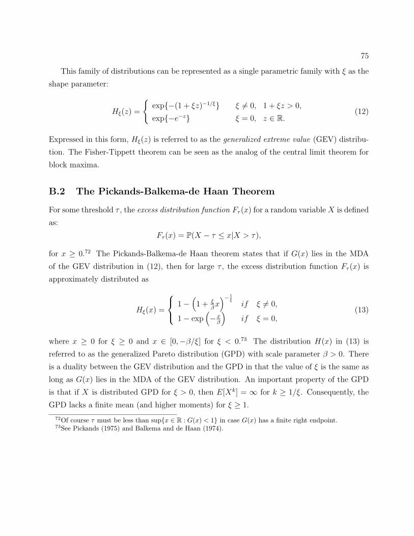
75

This family of distributions can be represented as a single parametric family with ξ as the

shape parameter:

Hξ(z) =

{exp{−(1 + ξz)−1/ξ} ξ 6= 0, 1 + ξz > 0,

exp{−e−z} ξ = 0, z ∈ R.(12)

Expressed in this form, Hξ(z) is referred to as the generalized extreme value (GEV) distribu-

tion. The Fisher-Tippett theorem can be seen as the analog of the central limit theorem for

block maxima.

B.2 The Pickands-Balkema-de Haan Theorem

For some threshold τ , the excess distribution function Fτ (x) for a random variable X is defined

as:

Fτ (x) = P(X − τ ≤ x|X > τ),

for x ≥ 0.72 The Pickands-Balkema-de Haan theorem states that if G(x) lies in the MDA

of the GEV distribution in (12), then for large τ , the excess distribution function Fτ (x) is

approximately distributed as

Hξ(x) =

1−(1 + ξ

βx)− 1

ξif ξ 6= 0,

1− exp(−x

β

)if ξ = 0,

(13)

where x ≥ 0 for ξ ≥ 0 and x ∈ [0,−β/ξ] for ξ < 0.73 The distribution H(x) in (13) is

referred to as the generalized Pareto distribution (GPD) with scale parameter β > 0. There

is a duality between the GEV distribution and the GPD in that the value of ξ is the same as

long as G(x) lies in the MDA of the GEV distribution. An important property of the GPD

is that if X is distributed GPD for ξ > 0, then E[Xk] = ∞ for k ≥ 1/ξ. Consequently, the

GPD lacks a finite mean (and higher moments) for ξ ≥ 1.

72Of course τ must be less than sup{x ∈ R : G(x) < 1} in case G(x) has a finite right endpoint.73See Pickands (1975) and Balkema and de Haan (1974).

76

C Parameter Estimation for the g-and-h Distribution

The g-and-h distribution is a strictly increasing transformation of the standard normal Z

defined by

Xg,h(Z) = A + B(egZ − 1)exp(hZ2/2)

g(14)

where A, B, g, and h ≥ 0 are the four parameters of the distribution. When A = 0, then

X−g,h(Z) = −Xg,h(−Z) implying that a change in the sign of g only changes the direction

of the skewness, but not its magnitude. Hoaglin (1985b) and Dutta and Babbel (2002) give

derivations of several other important properties of the g-and-h distribution. The following

summarizes the method we used to estimate the parameters. For a detailed description and

derivation of the estimation method see Hoaglin (1985b). See Figure 1 for some possible

shapes the g-and-h probability density function can take.

Defining Xp and Zp as the 100pth percentiles of the g-distribution and standard normal

distribution respectively, then

gp = −(

1

Zp

)ln

(X1−p −X0.5

X0.5 −Xp

)

where X0.5, the median of the data, is equal to A. Because there are many different gp

depending on the percentile p, Hoaglin (1985b) suggest choosing g equal to the median of the

gp. We follow that approach in this regard. It can be shown that

lng(Xp −X1−p)

(egZp − e−gZp)= ln(B) + h(Z2

p/2). (15)

Given that operational risk data are positively skewed and heavy-tailed to the right, it is

more appropriate to express the left-hand side of (15) using the upper half spread (UHS) as

defined in Hoaglin (1985b):

UHS =g(X1−p −X0.5)

(e−gZp − 1).

Conversely, if the data are negatively skewed and heavy-tailed to the left, then it is more

appropriate to use the lower half spread (LHS):

LHS =g(X0.5 −Xp)

(1− egZp).

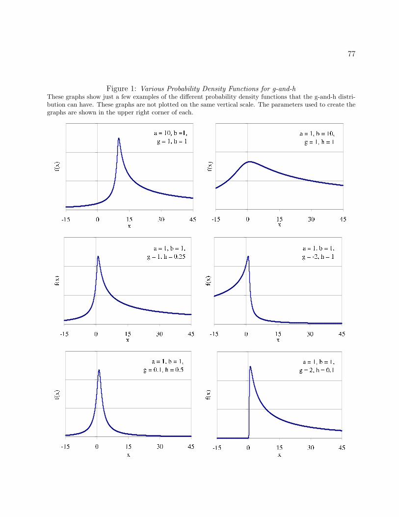
77

Figure 1: Various Probability Density Functions for g-and-hThese graphs show just a few examples of the different probability density functions that the g-and-h distri-bution can have. These graphs are not plotted on the same vertical scale. The parameters used to create thegraphs are shown in the upper right corner of each.

78

So once A and g are determined, the values of B and h can be found from an OLS regression

of ln(UHS) on Z2p/2. The exponentiated value of the intercept is the estimate of B, and the

coefficient of the regression is an estimate of h.

There are infrequent times when the transformation expressed in (14) does not permit the

g-and-h distribution to fit the data well. In these cases the g and/or h parameters can be

expressed as polynomial functions of Z2p . A more general form of the g-and-h transformation

is

Xg,h(Z) = A + B(eg(Z2)Z − 1)exp(h(Z2)Z2/2)

g(Z)(16)

where g(Z2) and h(Z2) are polynomials in Z2. For example, g(Z2) = γ0 +γ1Z2 +γ2Z

4 +γ3Z6

and h(Z2) = η0 + η1Z2 + η2Z

4 + η3Z6. In our models we only generalized the h parameter

and kept a constant g. In this case the distribution has four h parameters for a total of

seven distribution parameters.74 One could in principle add higher-order terms beyond Z6;

however, there is typically no gain in fit.

Our initial goal was to fit the g-and-h distribution using only one parameter for g and h

as in (14). In less than ten percent of the cases we had to augment the g-and-h specification

with additional h parameters. We found that in all cases, one g parameter was sufficient

to model the data. When the estimated value of h is negative, the g-and-h distribution is

platykurtic, and for a certain range of values of Z the transformation in (14) ceases to be

increasing. Therefore, when h is negative, (14) can only have a density function for a finite

range of the data. As h becomes a larger negative number, the range over which the density

is defined shrinks. In fact, whenever more than one h parameter is used in the polynomial

as in (16), there is a concern that h(Z2) will become decreasing for a certain range of Z2.

Again, the density will not be defined for all values of the data.

The parameters are typically estimated using the percentiles suggested by Tukey in

Hoaglin (1985b). If n is the number of observations, then one needs log2 n percentile points

to estimate the parameters. Tukey’s percentiles are typically the starting point for the esti-

mation procedure. We chose to use fourteen percentiles for all institutions at the enterprise,

business line, and event type levels. These percentiles usually need to be adjusted to achieve

a better fit of the g-and-h distribution to the data. The optimal spacing of the percentiles

depends upon the correlation that exists among the order statistics. When the correlation is

high, fewer percentiles may be needed, and the percentiles can be spaced further apart. Typi-

74In our analysis only in five instances (two at the enterprise level, one at the business line level, and twoat the event type level) out of over 50 total units did we use more than one h parameter.

79

cally, more percentiles are needed to model the tail than to model the body of the distribution

given that the correlation in the order statistics is low in the tail.

D General Moments for the g-and-h Distribution

If g 6= 0, the general formula for the nth moment of the g-and-h distribution with no location

and scale parameters is:

E(Y n) =1

gn√

1− nh

n∑i=0

(−1)i

(n

i

)exp

([(n− i)g]2

2(1− nh)

). (17)

With the location and scale parameters, A and B respectively, the nth moment becomes

E(Y n) =n∑

i=0

(n

i

)An−iBi

∑ir=0 (−1)r

(ir

)exp

([(i−r)g]2

2(1−ih)

)

gi√

1− ih. (18)

The moment is defined for 0 ≤ h < 1n. For h < 0, special treatment may be required because

the monotonicity of Ygh fails for z2 < − 1h. For h ≥ 1

n, this equation produces an imaginary

number for the moment. The following sections below give brief derivations of the mean,

variance, skewness, and kurtosis for the g-and-h-distribution.75

D.1 Mean

The mean is equal to the first moment, E(Y ). Using equation (18), if 0 ≤ h < 1 the mean

for the first moment with scale and location parameters is:

µ = A + B

exp

(g2

2(1−h)

)− 1

g√

1− h

.

For the simple case of A = 0 and B = 1, the mean of the g-and-h distribution is

µ =exp

(g2

2(1−h)

)− 1

g√

1− h.

75These derivations were provided by Ricki Sears.

80

For simplicity, the results below show derivations of the higher moments only for this simple

case when A = 0 and B = 1.

D.2 Variance

Using the generic formula for the moments, the second moment of the simple g-and-h distri-

bution is

E(Y 2) =1

g2√

1− 2h

2∑i=0

(−1)i

(2

i

)exp

([(2− i)g]2

2(1− 2h)

).

We expand out the summation to get the second raw moment:

E(Y 2) =1

g2√

1− 2h

[exp

(2g2

(1− 2h)

)− 2 exp

(g2

2(1− 2h)

)+ 1

].

The second moment about the mean, σ2 = E[(X − µ)2] defined for 0 ≤ h < 12, can be

simplified to

σ2 =1

g2√

1− 2h

[exp

(2g2

(1− 2h)

)− 2 exp

(g2

2(1− 2h)

)+ 1

]−

[exp[ g2

2(1−h)]− 1

g√

1− h

]2

.

D.3 Skewness

The third moment for the g-and-h distribution is

E(Y 3) =1

g3√

1− 3h

3∑i=0

(−1)i

(3

i

)exp

([(3− i)g]2

2(1− 3h)

).

Again, summing the terms yields

E(Y 3) =exp

(9g2

2(1−3h)

)− 3 exp

(4g2

2(1−3h)

)+ 3 exp

(g2

2(1−3h)

)− 1

g3√

1− 3h

for the third raw moment. Skewness is sometimes written as a squared quantity (β1) so that

it is always positive:

β1 =µ′3

2

µ′23 ,

81

where µ′n ≡ E[(Y − µ)n] is the nth moment about the mean. After much simplification, the

skewness for 0 ≤ h < 13

can be written as

β1 =

[2

(exp( g2

2(1−h))− 1

√1− h

)3

− 3

(exp( g2

2(1−h))− 1

√1− h

)(exp( 2g2

(1−2h))− 2 exp( g2

2(1−2h)) + 1

√1− 2h

)+

(exp( 9g2

2(1−3h))− 3 exp( 4g2

2(1−3h)) + 3 exp( g2

2(1−3h))− 1

√1− 3h

)]2/

[1√

1− 2h

(exp

(2g2

(1− 2h)

)− 2 exp

(g2

2(1− 2h)

)+ 1

)−

(exp[ g2

2(1−h)]− 1

√1− h

)2]3

.

D.4 Kurtosis

The fourth raw moment can be simplified to

E(Y 4) =exp

(16g2

2(1−4h)

)− 4 exp

(9g2

2(1−4h)

)+ 6 exp

(4g2

2(1−4h)

)− 4 exp

(g2

2(1−4h)

)+ 1

g4√

1− 4h

Kurtosis defined as

β2 =µ′4µ′2

2 ,

can be expressed in a “simplified” form for 0 ≤ h < 14:

β2 =

[− 3

(exp( g2

2(1−h))− 1

√1− h

)4

+ 6

(exp( g2

2(1−h))− 1

√1− h

)2(exp( 2g2

1−2h)− 2 exp( g2

2(1−2h)) + 1

√1− 2h

)−

4

(exp( g2

2(1−h))− 1

√1− h

)(exp( 9g2

2(1−3h))− 3 exp( 4g2

2(1−3h)) + 3 exp( g2

2(1−3h))− 1

√1− 3h

)+

(exp( 16g2

2(1−4h))− 4 exp( 9g2

2(1−4h)) + 6 exp( 4g2

2(1−4h))− 4 exp( g2

2(1−4h)) + 1

√1− 4h

)]/

[(exp( 2g2

1−2h)− 2 exp( g2

2(1−2h)) + 1

√1− 2h

)−

(exp( g2

2(1−h))− 1

√1− h

)2]2

E Goodness-of-Fit Tests

This section describes the four goodness-of-fit tests used throughout the paper.

82

E.1 Pearson’s Chi-Square Test

In Pearson’s chi-square test, the null distribution is divided into cells, and the test is based

on comparing the observed cell counts to the expected cell counts under the null hypothesis.

Chi-square tests are the most flexible goodness-of-fit tests because they can be applied to both

continuous and discrete distributions and situations with univariate and multivariate data.

Despite this flexibility, chi-square tests have three major shortcomings: (1) Since distributions

are divided into cells (as in the case of continuous distributions), some information about the

distribution is discarded, which may cause the chi-square test to be less powerful than other

goodness-of-fit tests; (2) The test is sensitive to the choice of the number of cells used and

the size of each cell; and (3) The sample size should be large enough so that the expected cell

frequency in each cell exceeds four.

Mann and Wald (1942) and Cohen and Sackrowitz (1975) proved that Pearson’s test

statistic is unbiased when the cells are chosen to have equal probabilities under the null.

Mann and Wald also discuss what the optimal number of cells should be, given that the cells

are chosen to be equiprobable. A modification of their optimal cell choice based on Schorr

(1974) is to set the number of cells equal to 2n(2/5), where n is the sample size. This is the

approach followed in this analysis.

E.2 The Kolmogorov-Smirnov Test

The K-S test is a non-parametric supremum test based on the empirical cumulative distri-

bution function (CDF). The test statistic D is constructed by computing the largest vertical

distance between Hn(x), the empirical CDF, and H(x), the expected CDF under the null:

D = supx|Hn(x)−H(x)|.

Although the K-S test statistic is simple to compute, it has some important drawbacks: (1)

It can only be used for continuous distributions; (2) It is more sensitive to deviations in the

center of the distribution than in the tails; and (3) If the null distribution contains shape

parameters, the critical value of the K-S statistic would need to be simulated.

83

E.3 The Anderson-Darling Test

Another important statistic based on the empirical distribution function is the A-D test

statistic, which is a member of the quadratic Cramer-von Mises family. Formally, the test

statistic A2 is defined by

A2 = n

∫ ∞

−∞

(Hn(x)−H(x))2

H(x)(1−H(x))dH(x).

Like the K-S test, the A-D test can only be used for continuous distributions. However, unlike

the K-S test, the A-D test gives more weight to tail observations. The main disadvantage

of using the A-D test is that different critical values must be used for each null distribution.

This also works as an advantage because the A-D test is generally more powerful than the

K-S test due to its sensitivity to the null distribution.

E.4 The Quantile-Quantile Plot

The Q-Q plot depicts the (mis)match between the observed values in the data and the esti-

mated value given by the hypothesized fitted distribution. If the data were in fact generated

from the hypothesized distribution, then the points of the graph should lie on the 45 degree

line. Although a Q-Q plot is not a formal statistical goodness-of-fit test, it is just as important

a tool in determining fit. A Q-Q plot can provide clues as to which observations do not fit

the hypothesized distribution well. For example, a Q-Q plot can detect variations in location,

scale, asymmetry, and the presence of outliers among data sets. It may be the best method

for assessing the tail-fit of a distribution.

One of the primary advantages of a Q-Q plot is that it can be used to graphically compare

the fit of many different distributions. For example, two different distributions may fit the

data well according to a K-S or A-D test, but one of these distributions may be a superior fit

according to the Q-Q plots (although one cannot say anything about the statistical significance

between these two). A second advantage is that given a small sample size, a Q-Q plot may

be a more appropriate measure of fit than any formal statistical test. The reason for this is

that as the sample size shrinks, formal statistical tests become more likely to fail to reject

the fit of a distribution. Therefore, a Q-Q plot may be able to reveal a poor fit even when

the fit is not rejected by a formal statistical test.

84

References

Abramowitz, Milton and Irene A. Stegun, Handbook of Mathematical Functions, NewYork, NY: Dover Publications, 1972.

Artzner, Philippe, Freddy Delbaen, Jean-Marc Eber, and David Heath, “CoherentMeasures of Risk,” Mathematical Finance, 1999, 9, 203–228.

Badrinath, S. G. and Sangit Chatterjee, “On Measuring Skewness and Elongation inCommon Stock Return Distributions: The Case of the Market Index,” The Journal ofBusiness, 1988, 61 (4), 451–472.

and , “A Data-Analytic Look at Skewness and Elongation in Common-Stock-ReturnDistributions,” The Journal of Business & Economic Statistics, 1991, 9 (9), 223–233.

Balkema, A.A. and L. de Haan, “Residual Life Time at Great Age,” The Annals ofProbability, 1974, 2 (5), 792–804.

Basel Committee, “Sound Practices for the Management and Supervision of OperationalRisk,” 2003. Bank for International Settlements.

Bocker, Claus and Claudia Kluppelberg, “Operational VaR: A Closed-Form Approxi-mation,” 2005. Unpublished Working Paper.

Bookstabber, Richard M. and James B. McDonald, “A General Distribution for De-scribing Security Price Returns,” The Journal of Business, 1987, 60 (3), 401–424.

Buhler, Wolfgang, Marliese Uhrig-Homburg, Ulrich Walter, and Thomas Weber,“An Empirical Comparison of Forward-Rate and Spot-Rate Models for Valuing Interest-Rate Options,” The Journal of Finance, 1999, 45 (1), 269–305.

Chernobai, Anna and Svetlozar Rachev, “Applying Robust Methods to OperationalRisk Modeling,” The Journal of Operational Risk, 2006, 1, 27–41.

Cohen, A. and H. B. Sackrowitz, “Unbiasedness of the Chi-Square, Likelihood Ratio,and Other Goodness of Fit Tests for the Equal Cell Case,” Annals of Statistics, 1975, 4,959–964.

D’Agostino, Ralph B. and Michael A. Stephens, Goodness-of-Fit Techniques, NewYork, NY: Marcel Dekker, Inc., 1986.

Danielsson, J., Lawrence de Haan, L. Peng, and Casper G. de Vries, “Using aBootstrap Method to Choose the Sample Fraction in Tail Index Estimation,” Journal ofMultivariate Analysis, 2001, 76, 226–248.

de Fontnouvelle, Patrick, John S. Jordan, and Eric S. Rosengren, “Implicationsof Alternative Operational Risk Modeling Techniques,” 2004. NBER Working Paper No.W11103.

85

Diebold, Francis X., Til Schuermann, and John D. Stroughair, “Pitfalls and Op-portunities in the Use of Extreme Value Theory in Risk Management,” in A.P.N. Refenes,J.D. Moody, and A.N. Burgess, eds., Advances in Computational Finance, Amsterdam,Netherlands: Kluwer Academic Publishers, 1998, pp. 3–12. Reprinted in Journal of RiskFinance, 1 (Winter 2000), 30-36.

Dutta, Kabir K. and David F. Babbel, “On Measuring Skewness and Kurtosis in ShortRate Distributions: The Case of the US Dollar London Inter Bank Offer Rates,” 2002.Wharton Financial Institutions Center Working Paper.

and , “Extracting Probabilistic Information from the Prices of Interest Rate Options:Tests of Distributional Assumptions,” The Journal of Business, 2005, 78 (3), 841–870.

Embrechts, Paul, Claudia Kluppelberg, and Thomas Mikosch, Modeling ExtremalEvents for Insurance and Finance, Berlin, Germany: Springer-Verlag, 1997.

Federal Reserve System, Office of the Comptroller of the Currency, Office ofThrift Supervision, and Federal Deposit Insurance Corporation, Results of the2004 Loss Data Collection Exercise for Operational Risk, May 2004.

Feller, William, An Introduction to Probability Theory and Its Applications Volume II, NewYork, NY: John Wiley & Sons, Inc., 1968.

Fisher, Ronald A. and Leonard H.C. Tippett, “Limiting Forms of the Frquency Dis-tribution of the Largest or Smallest Member of a Sample,” Proceedings of the CambridgePhilosophical Society, 1928, 24, 180–190.

Froot, Kenneth A., “Bank Capital and Risk Management: Operational Risks in Context,”2003. Presentation at the Federal Reserve Bank of Boston.

Gan, F. F. and K. J. Koehler, “Goodness-of-Fit Tests Based on P-P Probability Plots,”Technometrics, 1990, 32 (3), 289–303.

Gnedenko, Par B., “Sur la Distribution Limite du Terme Maximum D’Une Serie Aleatoire,”Proceedings of the Cambridge Philosophical Society, 1943, 44 (3), 423–453.

Hoaglin, David C., “Using Quantiles to Study Shape,” in David C. Hoaglin, FrederickMosteller, and John W. Tukey, eds., Exploring Data Tables, Trends, and Shapes, NewYork, NY: John Wiley & Sons, Inc., 1985a, pp. 417–460.

, “Summarizing Shape Numerically: The g-and-h Distributions,” in David C. Hoaglin,Frederick Mosteller, and John W. Tukey, eds., Exploring Data Tables, Trends, and Shapes,New York, NY: John Wiley & Sons, Inc., 1985b, pp. 461–513.

Klugman, Stuart A., Harry H. Panjer, and Gordon E. Willmot, Loss Models: FromData to Decisions, second ed., New York, NY: John Wiley & Sons, Inc., 2004.

86

Mann, H. B. and A. Wald, “On the Choice of the Number of Class Intervals in theApplication of the Chi-Square Test,” Annals of Mathematical Statistics, 1942, 13, 306–317.

Martinez, Jorge and Boris Iglewicz, “Some Properties of the Tukey g and h Family ofDistributions,” Communications in Statistics - Theory and Methods, 1984, 13 (3), 353–369.

McDonald, James B., “Probability Distributions for Financial Models,” in G.S. Maddalaand C.R. Rao, eds., Handbook of Statistics Volume 14: Statistical Methods in Finance,Amsterdam, Netherlands: Elsevier Science, 1996, pp. 427–461.

and Yexiao J. Xu, “A Generalization of the Beta Distribution with Applications,” TheJournal of Econometrics, 1995, 66, 133–152.

McNeil, Alexander J. and Thomas Saladin, “The Peaks Over Thresholds Method forEstimating High Quantiles of Loss Distributions,” 1997. Proceedings of the 28th Interna-tional ASTIN Colloquium.

, Rudiger Frey, and Paul Embrechts, Quantitative Risk Management: Concepts, Tech-niques and Tools, Princeton, NJ: Princeton University Press, 2005.

Mignola, Giulio and Roberto Ugoccioni, “Tests of Extreme Value Theory Applied toOperational Risk Data,” 2005. Unpublished Working Paper.

Mills, Terence C., “Modelling Skewness and Kurtosis in the London Stock Exchange FT-SEIndex Return Distributions,” The Statistician, 1995, 44 (3), 323–332.

Moscadelli, Marco, “The Modelling of Operational Risk: Experience with the Analysis ofthe Data Collected by the Basel Committee,” 2004. Temi di discussione Working Paper.

Neslehova, Johanna, Paul Embrechts, and Valerie Chavez-Demoulin, “Infinite MeanModels and the LDA for Operational Risk,” The Journal of Operational Risk, 2006, 1, 3–25.

Pickands, James III, “Statistical Inference Using Extreme Order Statistics,” The Annalsof Statistics, 1975, 3 (1), 119–131.

Rayner, G. D. and H. L. MacGillivray, “Numerical Maximum Likelihood Estimationfor the g-and-h and Generalized g-and-h Distributions,” Statistics and Computing, 2002,12, 57–75.

Ruppert, David, “What is Kurtosis?: An Influence Function Approach,” The AmericanStatistician, 1987, 41 (1), 1–5.

Schorr, B., “On the Choice of the Class Intervals in the Application of the Chi-Square Test,”Math. Operations Forsch. u. Statist., 1974, 5, 357–377.

Tukey, John W., Exploratory Data Analysis, Reading, MA: Addison-Wesley, 1977a.