a tableau system for linear-time temporal logic - … · culi, the tableau calculi, which seem to...

A Tableau System for Linear-TIME Temporal Logic

Peter H. Schmitt and Jean Goubault-Larrecq* **

Institut f/Jr Logik, Komplexit/it und Deduktionssysteme Universits Karlsruhe, D-76128 Karlsruhe

Abs t rac t . We present a sound, complete and terminating tableau system for the propositional logic of linear-TIME with only [] and ~ as temporal operators.

1 I n t r o d u c t i o n

Deduction calculi for propositional linear-TIME temporal logic and their reali- sation in theorem proving programs play an important part in verification and analysis of systems. We are concerned here with one particular class of calculi, the tableau calculi, which seem to be most popular in this area and also well adapted to the task. As a first introduction to this method we refer to the overview paper [Wo185]. A more recent tableau calculus is treated at length in the book [MP95] and has also been implemented in the STeP System: see [MAB+94] and [BBC+96]. One drawback of all calculi for linear-TIME temporal logic proposed so far, as compared to calculi in classical propositional logic, is the fact that termination of the procedure cannot be determined locally. In [Wo185] e.g. a loop-check has to be performed during the expansion of the tableau to detect recurring node labels. The tableau system in IMP95] depends crucially on the global concept of maximal strongly connected subgraphs of the tableau. Both approaches neces- sitate the use of involved data structures and algorithms in an implementation, which limits the efficiency of the resulting theorem proving system. In this paper, we present a calculus that terminates when no further expansion rule is applicable, which is guaranteed to happen. The formulas we consider in this paper only use D and ~ as temporal operators, and the next-time operator @ is not included. This fragment, let us call it LTLo, is less expressive than full l inear-TIME time logic, LTL. An extension of the calculus to full LTL is in preparation. But the restricted temporal language also deserves attention, if only for the reason that the satisfiability problem for LTLo is merely NP-complete [SC85], while it is PSPACE-complete for LTL. It may therefore be advantageous to submit problems that happen to belong to

* Research funded by the HCM grant 7532.7-06 from the European Union. ** On leave from Bull Corporate Research Center, rue Jean Jaurbs, F-78340 Les Clayes

sous Bois.

131

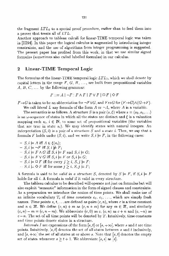
the fragment LTLo to a special proof procedure, rather than to feed them into a prover that treats all of LTL . Another approach to tableau calculi for linear-TIME temporal logic was taken in [HI94]. In this paper the logical calculus is augmented by introducing integer constraints, and the use of algorithms from integer programming is suggested. The present paper has profited from this work, in that we use similar signed formulas (sometimes also called labelled formulas) in our calculus.

2 L i n e a r - T I M E T e m p o r a l L o g i c

The formulas of the linear-TIME temporal logic LTLo, which we shall denote by capital letters in the range F, G, H, . . . , are built from propositional variables A, B, C, . . . by the following grammar:

F ::=AI FIFAFIFVFIOFI F

F ~ G is taken to be an abbreviation for -~FVG, and F ~ G for (F--+G)A(G--~F). We call literal L any formula of the form A or -~A, where A is a variable. The semantics is as follows. A structure S is a pair (s, ~) where s : (so, s l , . . . )

is an w-sequence of states in which all the states are distinct and ~ is a valuation mapping each si, i E IN, to some set of propositional variables (the variables that are true in state si). We may identify states with natural integers. An interpretation (S, i) is a pair of a structure S and a state i. Then, we say that a formula F holds under (S, i), and we write S, i ~ F, in the following cases:

- s , i A ifr A

- S , i ~ - , F i f f S , i ~ : F ; - S , i ~ F A G i f f S , i ~ F a n d S , i ~ G ; - S , i ~ F V G i f f S , i ~ F o r S , i ~ G ; - S, i ~ [] F iff for every j >__ i, S , j ~ F ; - S , i ~ O F i f f f o r s o m e j ~ i , S , j ~ F ;

A formula is said to be valid in a structure S, denoted by S ~ F, if S, i ~ F holds for all i. A formula is valid if it valid in every structure.

The tableau calculus to be described will operate not just on formulas but will also exploit "semantic" information in the form of signed clauses and constraints. As a preparation we introduce the notion of time points. We shall make Use of an infinite vocabulary Tc of time constants co, cl, . . , which are simply fresh names. Time points s, t, . . . are defined as pairs (c, n), where c is a time constant and n E 2Z. We define (c, n) + m as (c,n + m) for any m E ~ , and similarly (c, n) - m = (e, n - m). We abbreviate (c, 0) as c, (c, n) as c + n and (c, - n ) as c - n. The set of all t ime points wilt be denoted by T. Intuitively, t ime constants and time points denote states in a structure.

Intervals I are expressions of the form [s, t] or Is, +c<~[, where s and t are time points. Intuitively, [s, t] denotes the set of all states between s and t inclusively, and [s, +oo[ the set of all states at or above s. Note that [s, t] denotes the empty set of states whenever s _> t + 1. We abbreviate Is, s] as Is].

132

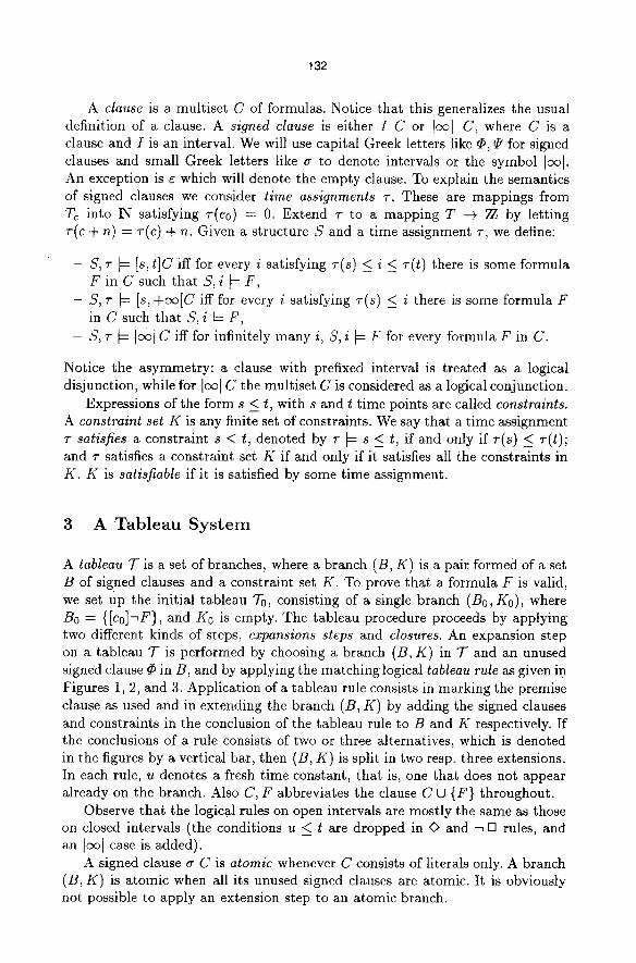
A clause is a multiset C of formulas. Notice that this generalizes the usual definition of a clause. A signed clause is either I C or [oo[ C, where C is a clause and I is an interval. We will use capital Greek letters like 4, ~ for signed clauses and small Greek letters like g to denote intervals or the symbol leo[. An exception is ~ which will denote the empty clause. To explain the semantics of signed clauses we consider time assignments 7". These are mappings from Tc into lN satisfying r(e0) = 0. Extend r to a mapping T -+ ~ by letting r(c + n) = ~-(c) + n. Given a structure S and a time assignment r, we define:

- S, v ~ Is, tiC iff for every i satisfying r(s) < i _< r(t) there is some formula F in C such that S , i ~ F ,

- S, r ~ [s, + ~ [ C iff for every i satisfying r(s) _< i there is some formula F in C such that S, i ~ F,

- S, r ~ [oo[ C iff for infinitely many i, S, i ~ F for every formula F in C.

Notice the asymmetry: a clause with prefixed interval is treated as a logical disjunction, while for Ioo I C the multiset C is considered as a logical conjunction.

Expressions of the form s < t, with s and t time points are called constraints. A constraint set K is any finite set of constraints. We say that a time assignment r satisfies a constraint s < t, denoted by r ~ s < t, if and only if r(s) < r( t) ; and r satisfies a constraint set K if and only if it satisfies all the constraints in K. K is satisfiable if it is satisfied by some time assignment.

3 A T a b l e a u S y s t e m

A tableau T is a set of branches, where a branch (B, K) is a pair formed of a set B of signed clauses and a constraint set K. To prove that a formula F is valid, we set up the initial tableau To, consisting of a single branch (B0, K0), where B0 = {[c0]~F}, and K0 is empty. The tableau procedure proceeds by applying two different kinds of steps~ expansions steps and closures. An expansion step on a tableau T is performed by choosing a branch (B, K) in T and an unused signed clause r in B, and by applying the matching logical tableau rule as given in Figures 1, 2, and 3. Application of a tableau rule consists in marking the premise clause as used and in extending the branch (B, K) by adding the signed clauses and constraints in the conclusion of the tableau rule to B and K respectively. If the conclusions of a rule consists of two or three alternatives, which is denoted in the figures by a vertical bar, then (B, K) is split in two resp. three extensions. In each rule, u denotes a fresh time constant, that is, one that does not appear already on the branch. Also C, F abbreviates the clause C U {F} throughout.

Observe that the logical rules on open intervals are mostly the same as those on closed intervals (the conditions u < t are dropped in ~ and -~ [] rules, and an ]oo[ case is added).

A signed clause cr C is atomic whenever C consists of literals only. A branch (B, K) is atomic when all its unused signed clauses are atomic. It is obviously not possible to apply an extension step to an atomic branch.

133

Extending the initial tableau ({[c0]-,F}, O) may be viewed as a systematic search for a counter-model of F. Each branch may then be looked at as a partial counter-model. It will be shown below that if a tableau is reached with all its branches unsatisfiable, then [c0]-,F is also unsatisfiable and thus F is valid.

A branch (B, K) is satisfiable if there is a structure S and a time assignment r such that S , r ~ C for each signed clause C in B and r(s) <_ r(t) for all constraints s < t in K.

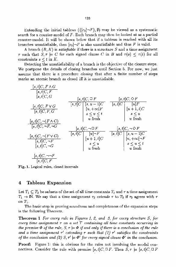
Detecting t-he unsatisfiability of a branch is the objective of the closure steps. We postpone the details of closing branches until Section 5. For now, we just assume that there is a procedure closing that after a finite number of steps marks an atomic branch as closed iff it is unsatisfiable.

[s, t]C, F ^ G [s, t] C, F Is, t] c, c

[s, t]C, F V G [s, t]C, F, G

Is, t ic, -,(F ^ a) [s, t]C, -,F,-,a

[s, t]c, -X F v a) [s, t]C, -,F Is,tic, ~a

[s,t]C,--,-,F [s, t]C, F

[s, t]C, D F [s, t]C, O F [s, t ic [s, u - 1 ]C

[u, + ~ [ F s < u < t

u fresh

[s, t]C [u]F [u + 1, t ic

s < u u fresh

[s, tiC, --, [] F [s,t]C,--,OF [s, t]C [u]~F

[u + 1, t ]c s < u

u fresh

[s, t]C [s, u - 1]C [u, + o o b F s < u < t

u fresh

Fig. 1. Logical miles, closed intervals

4 Tableau Expansion

Let T1 C_ T2 be subsets of the set of all t ime constants Tc and r a time assignment T1 -+ ]IN. We say that a time assignment ~-2 extends v to 2"2 if v2 agrees with v on TI.

The basic step in proving soundness and completeness of the expansion steps is the following Theorem.

T h e o r e m 1 For every rule in Figures 1, 2, and 3, for every structure S, for every time assignment v on a set T containing all time constants occurring in the premise ~ of the rule, S, r ~ q~ if and only if there is a conclusion of the rule and a time assignment v ~ extending r such that (1) r ~ satisfies the constraints of the conclusion and (2) S, v I ~ qY for every signed clause qY in the conclusion.

P r o o f : Figure 1: this is obvious for the rules not involving the modal con- nectives. Consider the rule with premise [s, t]C, n F. Then S, r ~ [s,t]C, [] F

134

[s, +co[C, F A G [s, +co[C, F [s, +co[C, a

[s, +oo[C, F v G [s, +oo[C, F, G

[.% +co[c, -,(F ^ c) [~, +co[c,-,F, -~a

[s, +oo[C, --,(F v C) [s, +oc[C, - ,F [~, +co[C, 7 0

[s, +co[C, ~ = F [s, +co[C, F

[s, +at[C, [] F [~--7 +oo[c I Is,. - i ] c

I [u, + o e [ f

s < u u fresh

[s, +co[C, -, O F

[s, +co[C, 0 F [s, +co[C [u]F

[u + 1, +co[C s < u

u fresh [s, +oo[C, -, [] F

IcoIF

[s, +oo[C [s, u - 1 ] C [,~, +co[-~F

s<~tL

u f resh

[s, +oo[C [u]-~F [u + 1, +co[C

s < u

u fresh

loci , F

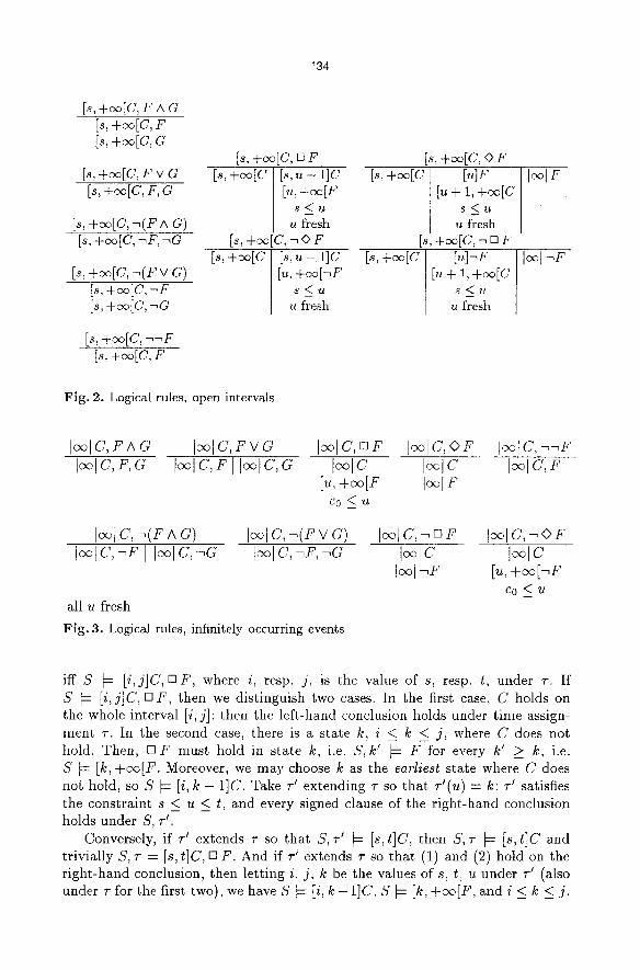
Fig. 2. Logical rules, open intervals

I~IC, F A g I~IC, F,G

IooIC, F v G Iool c, F I IoolC, a

I~IC, DF I~lC, OF I ~ I O , ~ F IoolC IoolC

[u, + �9149 tool F Co<U

Iool C,-,(F A C) Iool C,-,F I Iool c,--.c

Ioot c, - . (F v G) !ool C, ~F, -~C

Iool c, u

all u fresh

Fig. 3. Logical rules, infinitely occurring events

IoolC Io~lO Iool-~F [u, +oc[--,F

c o < u

iff S D [i,j]C, [] F, where i, resp. j , is the value of s, resp. t, under r . If S D [i,j]C, DF, then we dist inguish two cases. In the first case, C holds on the whole interval [i, j]: then the left-hand conclusion holds under t ime assignment r . In the second case, there is a s tate k, i < k < j, where C does not hold. Then, [] F must hold in s ta te k, i.e. S , k ~ ~ F - f o r every k' _> k, i.e. S ~ [k, + � 9 Moreover, we may choose k as the earliest state where C does not hold, so S ~ [i, k - 1]C. Take r ' extending r SO tha t T'(U) = k: r' satisfies the constraint s < u < t, and every signed clause of the r ight-hand conclusion holds under S, r ' .

Conversely, if r ' extends r so tha t S,r ' D [s,t]C, then S , r ~ [s,t]C and tr ivial ly S , r ~ [s,t]C, OF. And if r' extends r so tha t (1) and (2) hold on the r ight-hand conclusion, then let t ing i, j , k be the values of s, t, u under r ' (also under r for the first two), we have S D [i, k - 1]C, S ~ [k, + � 9 and i < k < j .

135

In particular, we have S ~ [i, k - 1]C and S ~ [k, j] [] F, so S ~ [i, j]C, [] F, so the premise holds under v.

Consider now the rule with premise [s, tiC, OF. If [i, j]C, OF holds, then either [i,j]C holds (left conclusion), or there is a state k in [i,j] where C does not hold. In the latter case, choose k the latest such k. Then [k + 1, j]C holds, and O F holds in staite k. In particular, there is a state k' > k such that F holds in state k'. Moreover, since [k + 1 , j ]C holds and k' _> k, in particular [ k ' + 1 , j ]C holds. And i < k' also holds, so (1) and (2) are verified on the right-hand conclusion if we take 7-' extending 7- by mapping u to k' (not k).

Conversely, if [i,j]C holds (left conclusion), then [i , j]C,r holds too (premise). And if [k', k']F and [ k ' + 1,j]C hold with i < k' (right conclusion), then [i, k'] e F on the one hand and [k'+l,j]C on the other hand, so [i,j]C, r

The cases of [s,t]C,-, n F and [s, t]C, ~ OF are similar.

Figure 2. The cases are similar, except that in the [s, +oc[C, OF case, where we assume that [i, +c~[C, O F , there might not be any latest k _> i such that C does not hold. This justifies the third possible conclusion: in that case, there is an infinite sequence k0 < kl < . . . of states such that k0 > i and C does not hold at k0, or kl, or . . . ; therefore O F must hold at k0, and at kl, and . . . ; so there are states k' o >_ ko, k i >_ k l , . . . , where F holds. This sequence k~, kl, . . . , must be infinite, otherwise it would be bounded from above, hence k0, kl, . . . , would also be bounded from above, which is impossible. So there is an infinitely increasing subsequence of states k' < k' < at which F holds, i.e. Ioc]F

( T 0 ( 7 1 �9 . .

holds. Conversely, if ]oc] F holds, there is a sequence k0 < kl < . . . of states at which F holds; then for every j _> i, there exists a kp such that kp __ j , at which F holds, so [i, + o c [ O F holds, and therefore [i, +oc[C, O F holds, i.e. the premise holds. The case of the rule of premise [s, +co[C,- , [] F is similar.

Figure 3. The case of the rule with premise loci C, FAG is obvious (remember that clauses under the loci sign are taken conjunctively).

As regards loci C, F V G, it holds if and only if there is a sequence k of states k0 < kl < �9 �9 at which C and F V G hold. Consider the subsequence M of states at which C and F hold, and the subsequence k" of states at which C and G hold. Every state in k belongs to k' or k", so k' or k" must be infinite. If k' is infinite, then the left conclusion loci C, F holds, and if k" is infinite, the right conclusion holds. Conversely, ioo1 C, F or leo] C, G clearly implies ]e~ I C, F V G.

Look at the rule with premise leo] C, [] F. If it holds, then there is a sequence k0 < kl < . . . of states at which both C and [] F hold. In particular, loci C and [k0, +oc [ F hold: we let r ' extend r by mapping u to k0, then the conclusion holds. Conversely, if Ioc I C and [k, +oo[F both hold, then let k0 < kl < . . . be the sequence of states at which C holds. The subsequence of these states that are _> k is an infinite sequence at which C A [] F holds, so the premise holds.

Consider now the rule with premise loci C,<>F. If it holds, then there is a sequence k0 < kl < . . . of states at which both C and O F hold. So on the one hand loci C holds, and on the other there are states k~ > k0, k~ _> kl, . . . , at which F holds. If k~, k[, . . . , were bounded from above, so would be k0, kl, . . . ; so we can extract an infinite increasing subsequence k' < k' < of states at

( 7 0 ( 7 1 �9 . .

!36

which F holds. Tha t is, Ioo] F holds. Conversely, if both [oo I C and I~1F hold, then let k0 < kl < . . . be an infinite sequence of states at which C holds. At each kp, C holds and there is also a later state at which F holds, so O F holds at kp. Therefore the premise Iool c, <> F holds.

The other rules of Figure 3 are similar. []

T h e o r e m 2 Applying the rules in Figures 1, 2, 3 terminates.

P r o o f : Define the following complexity measure: IAI = 1 for variables A, IF A al = IFval = IF I + Ial +2, I-~FI = I D f l = I O F I = IFI + J-; I[~, t ] f l , . . . , F,,I = I[~, +oo[&,..., F,,I = Ilool & , . . . , F,~I = I & l + . . . + IF,~I. ~f B is a branch of a tableau, then ]B I is the natural ordinal sum of the will where r ranges over the signed clauses on B (i.e., we compare branches by a multiset ordering). Then every conclusion of a rule is smaller that its premise, so that branches decrease by application of each rule. []

Assume that a procedure closing is given that takes as input atomic tableau branches (B, K) and returns the answer closed iff (B, K) is not satisfiable. We call a tableau T closed when all it branches are atomic and the procedure closing returns closed for all branches in T.

T h e o r e m 3 A formula F from LTLo is valid iff from the initial tableau {([c0]--~F, 0)} a closed tableau can be reached by successive applications of expansion steps.

P r o o f i Given a structure S and a time assignment v we say that S, r satisfies a tableau 7" if there is one branch (B, K) in 7- with S, 7" ~ (B, K). Let To , . . .7~ be a sequence of tableaux, with To the initial tableau for F, 7i+1 is obtained from 7~ by one extension step for all 0 _< i < k and 7~ is closed. We claim that F is valid. By definition and the assumptions on the procedure closing 7-k is not satisfiable. Using Theorem 1 repeatedly we conclude that To is not satisfiable, which is just another way of saying that F is valid. Assume on the other hand that F is valid, thus the initial tableau To is not satisfiable. By Theorem 2, we know that by a finite number of expansion steps we will reach an atomic tableau 7~. Repeated application of Theorem 1, now used in the reverse direction, shows that Tk is not satisfiable. By the assumption on closing this implies that 7~ is indeed closed. []

Observe also that all rules are invertible, so that F is in fact valid iff a closed tableau can be reached by any maximal sequence of expansion steps: we don' t have to backtrack on the choice of the expansion rule.

5 Closing Branches

Any procedure for closing atomic branches that satisfies the requirement set forth above Theorem 3 can be used together with the expansion rules to yield a complete and sound method to prove validity of formulas in LTLo. In the next subsection we propose a procedure based on the resolution calculus.

137

5.1 Closing by Resolution

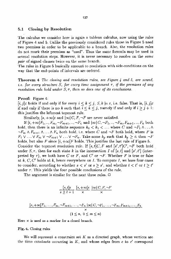
The calculus we consider here is again a tableau calculus, now using the rules of Figure 4 and 5. Unlike the previously considered rules those in Figure 5 need two premises in order to be applicable to a branch. Also, the resolution rules do not mark their premises as "used". Thus the same formula may be used in several resolution steps. However, it is never necessary to resolve on the same pair of signed clauses twice on the same branch. The rules in Figure 5 basically amount to resolution with side-conditions on the way that the end-points of intervals are ordered.

T h e o r e m 4 The closing and resolution rules, see Figure 4 and 5, are sound, i.e. for every structure S, for every time assignment v, if the premises of any resolution rule hold under S, "r, then so does one of its conclusions.

P r o o f i Figure 4: [i, j]r holds if and only if for every i < k < j , S, k ~ r i.e. false. Tha t is, [i, j]r if and only if there is no k such that i < k < j, namely if and only if i > j + 1: this justifies the teftmost topmost rule.

Similarly, [s, +o0[r and tocl C, F , - - F are never satisfied. If [i, +oc[F1, .., Fro,-'Fro+l,.., -,Fn and Iocl C, --F1, .., --F,~, Fro+l, .., F~ both

hold, then there is an infinite sequence k0 < kl < . . . where C and -~F1 A . . . A -'Fro A Fm+l A . . . A Fn both hold, i.e. where C and -~F both hold, where F is F1 V . . . V Fm V -'Fm+l V . . . V -~Fn. Take some kp such that kp ~ i: then -~F holds, but also F since [i, + c c [ F holds. This justifies the last rule of Figure 5. Consider the topmost resolution rule. If [s , t]C,F and [s',t ']C',-~F both hold under S, r , then for each state k in the intersection I of [s, t] and [s', t'] (inter- preted by r) , we both have C or F, and C ~ or --F. Whether F is true or false at k, C, C ~ holds at k, hence everywhere on I. To compute I, we have four cases to consider, according to whether s < s ~ or s > s ~, and whether t < t ~ or t > t ~ under r . This yields the four possible conclusions of the rule.

The argument is similar for the next three rules. []

[s, t]~ [~, +oo[~ Iool c, F, -,F s > _ t + l x x

[s, +oo[F1,. . . , F,~,--Fm+l,...,--F,~ ]co I C,- ,F1, . . . , -,F,~, Fro+l, . . . , F,~ X

( l < n , 0 < r e < n )

Here • is used as a marker for a closed branch.

Fig. 4. Closing rules

We will represent a constraint set K as a directed graph, whose vertices are the time constants occurring in /4, and whose edges from c to d correspond

138

Is, t]C, F Is', t']c', ~ f

s <_ s' - l , t <_ t' - l s ' <_ s, t < t ' - l s <_ s' - l , t' < t s ' <_ s, t ' <_ t [s', t]C, C' [s, t]C; C' [s', t']C, C z- [s, t']C, C'

[s, t ]C , F [s, t ]C , ~ F [s, +oo[C, F Is', + o o [ c ' , - F [~', +oo[c' , F [r +oo[c', . F

s < s ' - I s ' <_ s s < s ' - l [ s' < s s <_ s ' - i s ' < s [s( t ]c , c ' [~, t]c, c ' r- , - , , Is , t ] c , c I[s,t]c,c Is , + o o [ c , c ' [ , , + ~ c , c '

Fig. 5. Resolution rules

exactly to constraints (e < c ~ + n) in K, and are labeled by n. We may actuailly impose t, hat there is at most one edge from c to d by merging c " >c' and e " ~c' into c ~ >d, with n" = min(n ,n 0. The weight of a path co ~~ ~1> ...~k-~Ck, k > 0 in this graph is no + nl + . . . + nk-1; it is a cycle if and only if k > 0 and ck = co. We have:

L e m m a 1. Let K be a well-formed constraint set, where "well-formed" means that, for every vertex c, there is a path from co to c of non-positive weight.

K is satisfiable if and only if it has no cycle of strictly negative weight.

P r o o f : This is mostly well-known [Be158, Pra77]. []

Checking satisfiability of K amounts to checking whether there is a cycle with negative weight in K: this is checkable in polynomial time by Floyd's or Ford's shortest path algorithm (see [McH90], Chapter 3); there are even efficient incre- mental algorithms to do this [AIMSN90]. It is easy to check that any constraint set produced by the tableau rules from the initial tableau To is well-formed. Finally we introduce the constraint rule which declares a branch (B, K) "closed" (put the marker x on it) if K is unsatisfiable.

T h e o r e m 5 The resolution, closure and constraint rules are complete, i.e. given any unsatisfiable atomic branch (B, K) , there is a finite tableau starting from (B, K) and produced using these rules, whose branches are all closed.

P r o o f : The proof is by contraposition. Starting fi'om (B, K), apply all resolution and closing rules until a saturated tableau T is reached, i.e. on each branch every rule that is applicable has been applied. T can be reached in finitely many steps. Assume that there is an open branch (B', K ' ) in T. We then claim that (B', K') has a model. Since B C_ B' and K C K' , this is a contradiction.

First, because the set of constraints K ' is satisfiable, let 7- be a mapping from time constants to integers satisfying it, and let N be the highest integer in the range of r. Let also I~] C1, . . . , ]c~l C,~ be the signed clauses with sign [~] in B'. We build a structure (S, ~) on which B* will hold.

For every i such that 0 < i < N, let: S; = { [s , t ]C C B' I T(s ) < i < r ( t ) } U { [s ,+oo[C e B' I ~-(s ) < i }

and let S~ be the clauses in Si without signs: N = { C I I C E Si for some interval I}

139

Si is closed under the rules of Figure 5, hence S~ is closed under the usual propositional resolution rule. By the completeness of propositional resolution:

- either S~ contains the empty clause, and Si then contains some clause Is, t]c or [s, + ~ [ e ; since B ~ is open, the second case is impossible; in the first case, and since B ~ is saturated, K t must contain the constraint s > t + 1, which contradicts our assumption that j _< i < k, where j = v(s) and k = r(t);

- or S~ does not contain the empty clause, so S~ then has a model: let ~ map i to the set of propositional variables that are true under this model.

For every j E IN, for every 1 < i < n, we build 4(N ~- jn + i) as follows. Let Ti be the set of all clauses of the form [s, +cx~[C in B', and T~ be the set of the corresponding C's. Again, Ti is closed under the rules of Figure 5, hence T{ is closed under the propositional resolution rule, and cannot contain the empty clause. Let Ci be written as L i l , . . . , Lin~. Let then T~ I be T[ union the ni unit clauses Lil, . . . , Li,u. Let T{ I~ be the closure of T[ ~ under propositional resolution. Since T~ ~ is already closed under this rule and by the closure rules from Figure 4, resolution among the units Lil, . . . , Li,~, does not occur, and the only possible resolution steps take as one parent clause C,-~L~kl,...,-~Likj in T{ and resolve it, maybe repeatedly, with complementary units Li from Lil, . . . , Li,~,. The empty clause could enter T "~ only if a clause in T{ consisted exclusively of complements of literals in Lil, �9 �9 �9 Li,~. But in this case the bot tommost closing rule of Figure 4 would close branch B ~, which contradicts our assumption. T[ ~ is therefore a resolution-closed set of clauses without the empty clause. Again by the completeness of propositional resolution, T{ ~ has a model: let ~ map N + jn + i to the set of propositional variables that are true under this model.

Consider any clause of the form [s, t]C in B'. We have lN, ~ ~ [s, t]C. Indeed, for every i such that s < i < t (modulo r) , in particular 0 < i < N, and [s, t]C is in Si, so C E S~, so by construction ~(i) makes C true.

Consider any clause I~] Ci, 1 < i < n. By construction, every literal of Ci is true under ~ at state N + jn + i (they are the clauses that we have added to Ti t to yield T['). So IN, ~, g + jn + i ~ Ci, hence IN, ~ ~ I~1Ci.

Finally, consider any clause [s, +c~[C in B ~. For every i such that s < i < N, C holds at state i: the argument is as for clauses of the form [s, tiC. For every state N + j n + i , j > 0, 1 < i < n, by construction ~(N+jn+i) is a propositional model of T{ ~, hence of T[. Therefore C holds at state N + jn + i. To sum up, C holds at every state ~ s, hence IN, ~ ~ [s, +oz[C. []

5 . 2 R e f i n e m e n t s o f R e s o l u t i o n

Because the proof of Theorem 5 rests on the completeness of propositional resolution in a rather simple way, it is tempting to use standard refinements of resolution [CL73].

Consider for instance ordered resolution, see [FLTZ93]. Unfortunately this does not preserve completeness; and the same is true for hyper-resolution or

140

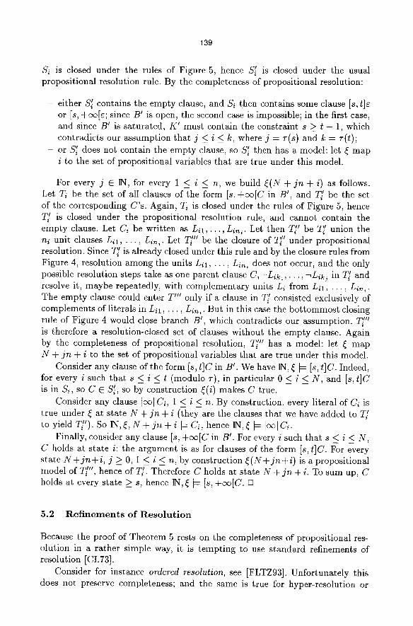
linear resolution. This may be repaired by introducing a new sign Ioolc,, and transform loci Ci with Ci = L i l , . . . , Li,~, into the ni unit signed clauses:

Io lc, Lil

Ioolc, Lin,

We then close branches by using the resolution rules of Figure 5, the additional resolution rules of Figure 6 and the closing rules of Figure 7, which replace those of Figure 4. Semantically, leOIc~ C, where C is a set of literals, means that the disjunction (not the conjunction!) of literals in C holds at all infinitely many time points N + jn + i, j > O, of the proof of Theorem 5; at all these time points, the conjunction of literals in Ci holds.

[s, +oo[C,F [s, +oc[C,-nF Ioo1 , C,~F IC~lci C',-,F IOClc, C', F _l lc, c ' , F I lo, C, C' Ioolc, C, C' Io%, c, c'

Fig. 6. Additional resolution rules

Fig. 7. Closing rules (bis)

s > t + l x x

T h e o r e m 6 For any complete refinement of resolution (ordered, hyper- resolution, linear resolution, etc.), the rules of Figures 5, 6 and 7 used according to the given refinement are complete.

Proof i Analogously to proof for Theorem 5. []

6 F u r t h e r I m p r o v e m e n t s

We present further improvements of our calculus that preserve correctness and completeness, but prove to be very effective in an actual implementation, see Section 8. Let us first mention the simplification rules in Figure 8. The conclusion part of these rules is empty. So their application amounts to the deletion of their premise, which, as can be easily observed, will not contribute to the closure of a branch. They may be used either with the calculus of Subsections 5.1, or 5.2.

[s, tiC, F, -~F [s, +oo[C, F, -~F loot e

Fig. 8. Simplification rules

Another shortcut in the application of the expansion rules of Figures 1, 2, and 3 is the case when the premise consists of just one formula, i.e. C = r

141

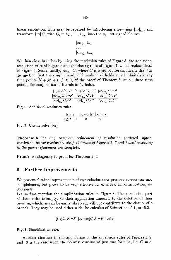
which allows us to omit any parts of the conclusion referring to C. Thus:

[s, + ~ [ e , [] F [s, +oo[~ F [s, +oo[e Is, u - lie [u, +co[F

[u, +co[F is replaced by s<_u s < u

u fresh u fresh

Assume you wish to prove a formula of the form F A G. Then, it is enough to prove F and G separately, and this is what a tableau system for classical logic would do. However, here this would be transformed into [c0]-~F V -~G, and further into [c0]-~F,-~G. But when the current interval contains only one point, it is usually better to transform it into [c0]-~F and [c0]-~G. We may therefore add the following case decomposition rule:

[ s ] F 1 , . . . , F ,

[S]Fll...l[s]F~

Using this rule eagerly amounts to use it right after the rules with premise [s, t]C, F V G or [s, t]C, -~( F A G) when s = t.

[s]F A G [s]F V G [s]-~(F A G) [s]'~(F V G) [ s ] ~ F [s]S [s]Fl[s]a [s]--Fl[s]-,a [s]-.F [s]F [s]a [s]-,a

[s]n F [s]O F [s]-.I::lF [s]-.O F [s, +oo[F [u]F [u]-~F Is, +oo[-.F

s < u s < u u fresh u fresh

Fig. 9. Logical rules, single time points

Specializing the rules of Figure 1 to use the case decomposition rule eagerly yields new rules. Then, notice that if we start from [c0]F, where F is the formula to prove, then all signed clauses of the form [siC that we shall ever need are such that C contains exactly one formula. This yields the rules of Figure 9. Here we do not need to include the case decomposition rule explicitly.

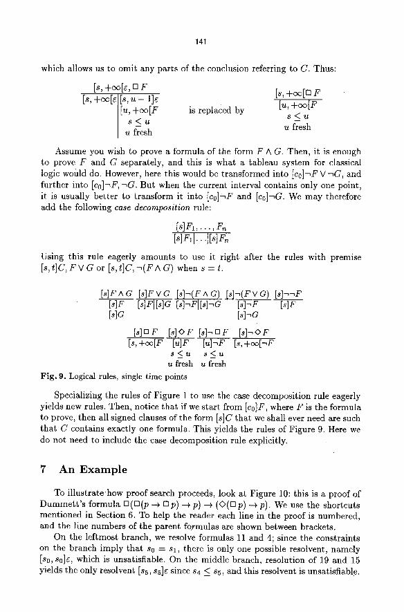
7 An Example

To i l lustratehow proof search proceeds, look at Figure 10: this is a proof of Dummett ' s formula D([:](p-+ [] p) --+ p) --+ (O(Q p) -+ p). We use the shortcuts mentioned in Section 6. To help the reader each line in the proof is numbered, and the line numbers of the parent formulas are shown between brackets.

On the leftmost branch, we resolve formulas 11 and 4; since the constraints on the branch imply that so = sl, there is only one possible resolvent, namely [so, s0]e, which is unsatisfiable. On the middle branch, resolution of 19 and 15 yields the only resolvent [sh, sh]e since s4 ~ sh, and this resolvent is unsatisfiable.

142

I [su,so]~(~D(~D(-~PvDP) v P)V~ODPV P)

I �9 211] Is0, s~ D(~ D(~p v D ~) v p) 311] [s~ s~ [] P 411] [s0, so]~P

I (~[2] so < s~ < so

I 7f3i [~,. ,4 D p 813] so < s..,

I 9[7] [s~, +c~[P t0171 s~<s~<~2

1 [] 1115] [% +oo[P 15[~1 [s~, +oo[P 23151 To~iP,

] as] I Si < S4 ]

12[n,4] [s0,s0]e 17114] [s4,s4]P 24[23] I [~176 P 13112] s o > s o + l i81141 [s~,s4]-,nP 25[23] ]o~]-~P x

26[25,9] x 19[I8] [s3,ss]-~P 20118] s4 _< s~

I 21119,15] [~, ~& 22121] ~5 _> ~s + 1 •

~ P

Fig. 10. Example, Dummet t ' s formula

8 Experimental Results

We have i m p l e m e n t e d this sys tem in the H i m M L byte-coded interpreter , an i m p l e m e n t a t i o n of S t anda rd ML with fast set and m a p operat ions . The rules of Figure 9 were used, and we always ma in t a in formulas in negat ion no rma l form.

Our expans ion s t r a t egy is to expand a current goal until it has become a tomic , in which case we focus on ano the r non -a tomic signed fo rmula on the current branch as new goal; when the b ranch becomes a tomic , we call the resolut ion rules. We also accumula t e cons t ra in t s along the way, using the g raph s t ruc ture of L e m m a 1 and declare the b ranch closed whenever the current set of cons t ra in ts becomes unsatisf iable. Finally, the fo rmula tha t we select in the current goal clause is the first n o n - m o d a l fo rmula t ha t we find in it, or the first m o d a l fo rmula (n F or O F ) if there are no non -modM formulas left in the goal.

We have used posi t ive hyper-resolut ion, where (non-uni t ) clauses to resolve are chosen so t ha t one of t h e m is a posi t ive clause, i.e. does not conta in any negated a tom; if there are uni t clauses, we resolve pr ior i tar i ly on them, whether they are posi t ive or negat ive. Th is also means tha t we have used the closing rules

143

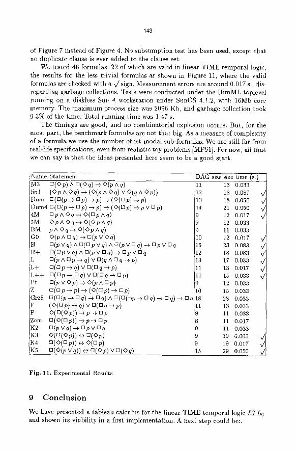
of Figure 7 instead of Figure 4. No subsumption test has been used, except that no duplicate clause is ever added to the clause set.

We tested 46 formulas, 22 of which are valid in linear-TIME temporal logic, the results for the less trivial formulas ar shown in Figure 11, where the valid formulas are checked with a x/sign. Measurement errors are around 0.017 s., dis- regarding garbage collections. Tests were conducted under the HimML toplevel running on a diskless Sun 4 workstation under SunOS 4.1.2, with 16Mb core memory. The maximum process size was 2096 Kb, and garbage collection took 9.3% of the time. Total running time was 1.47 s.

The timings are good, and no combinatorial explosion occurs. But, for the most part, the benchmark formulas are not that big. As a measure of complexity of a formula we use the number of ist modal sub-formulas. We are still far from real-life specifications, even from realistic toy problems [MP91]. For now, all that we can say is that the ideas presented here seem to be a good start.

game Statement DAG size size time (s.) M3 linl Dum Dum4 !4M 5M BM !co H H+ L L+ L++ Pt Z

Grz5 F P Zero K2 K3 K4 K5

a(op) ^ D(Oq) -+ O(p^ q) (op ̂ Oq) . (o0 ^ oq) v O(q ̂ or)) D(m(p ~ []p) -+p) -+ (o(D p) -+p) D ( D ( p . = p ) . p) ~ (O(D p ) . p v [] p) D p A Oq--+ O ( D p A q ) Op n Oq-+ O(Op A q) pA Oq-4- O(OpAq) o(p^ aq) -+ D(p v Oq) =(p v q) ̂ =(Dp vq) ̂ [](pv aq) ~ []p v =q D(Dp v q) ̂ a(pV aq) + apV Oq ~3(p A E] p -.--~ q) V [3(q A [3 q -+ p) [-n([] p __+ q) V n(~j q ~ p)

[]([] p . D q) v D(~q -~ D p) D(p v Op) ~ o(p ̂ ~p) [](~v-+p) ~ (o(op) -+ Dp) D(n(p -.+ f3q) --+ nq) A [~(D("~p -~ [3q) -+ Dq) -+ nq (o(• p) --+ q) v [](e q-+ p) o(o(ov)) -+p-~ []p [](o(op)) .p-+ np EJ(p V q) --~ FJ p V r~ q o(~(op)) ++ ~(op) D(o(~ p)) ++ O(Dp) D(o(p v q)) ++ D(op) v D(Oq)

11 13 0.033 12 18 0.067 V ~ 180.050 V

21 0.050 V 9 12 0.017 V 9 12 0.033 9 11 0.033 10 12 0.017 ~/ 15 23 0.083 x/ 12 18 0.083 x/ 13 17 0.033 ~/ 11 13 0.017 x/ 11 15 0.033 ~/ 9 12 0,033 I0 15 0.033 18 28 0.033 11 13 0.033 9 11 0.033 8 11 0.017 9 11 0.033 o 19 0.033 V 9 19 0.017 ~/ 15 20 0.050 ~/

Fig. 11. Experimental Results

9 C o n c l u s i o n

We have presented a tableau calculus for the linear-TIME temporal logic L T L o and shown its viability in a first implementation. A next step could be:.

144

To extend the present approach to full l inear-TIME temporal logic; this is under way and looks promising.

- To improve branch closure. Is it possible to adapt Floyd's or Ford's graph algorithm, which just detects negative cycles, to directly check the satisfiability of an atomic branch (B, K)? Is it possible to replace the resolution principle, which is known not to perform very well on propositional logic, by a variant of the Davis-Putnam-procedure, or a variant of BDD-based satisfiability algorithms?

References

[AIMSN90]

[BBC+96]

[Be158]

[CL73]

[FLTZ93]

[HI94]

[MAB+94]

[McH90] IMP91]

IMP95]

[Pra77]

[scss]

[Wo185]

G. Ausiello, G. F. Italiano, A. Marchetti Spaccamela, and U. Nanni. In- cremental algorithms for minimal length paths. In Proc. 1st ACM-SIAM Symposium on Discrete Algorithms, pages 12-21, 1990. N. Bjr A. Browne, E. Chang, M. Col6n, A. Kapur, Z. Manna, H. Sipma, and T. Uribe. STEP: Deductive-algorithmic verification of reactive and real-time systems. In Proc. 8 *h CAV Conference, 1996. R. Bellman. On a routing problem. Quarterly of Applied Mathematics, 16(1):87-90, 1958. C.-L. Chang and R. C.-T. Lee. Symbolic Logic and Mechanical Theorem Proving. Computer Science Classics. Academic Press, 1973. C. Fermfiller, A. Leitsch, T Tammet, and N. Zamov. Resolution Methods for the Decision Problem, volume 679 of LNCS. Springer-Verlag, 1993. R. Hs and O. Ibens. Improving temporal logic tableaux using integer constraints. In Proc. Int. Conf. on Temporal Logic, Bonn, volume 827 of LNCS, pages 535 - 539. Springer Verlag, 1994. Z. Manna, A. Anuchitanukul, N. Bjcrner, A. Browne, E. Chang, M. Col6n, L. De Alfaro, H. Devarajan, H. Sipma, and T. Uribe. STEP: The Stanford Temporal Prover. CS-report, Computer Science Dept., Stanford, 1994. J. A. McHugh. Algorithmic Graph Theory. Prentice-Hall Intn., 1990. Z. Manna and A. Pnueli. The Temporal Logic of Reactive and Concurrent Systems. Springer-Verlag, 1991. Z. Manna and A. Pnueli. Temporal Verification of Reactive Systems: Safety. Springer-Verlag, 1995. V. R. Pratt. Two easy theories whose combination is hard. Technical report, M.I.T., September 1977. A. P. Sistla and E. M. Clarke. The complexity of propositional linear temporal logics. J. ACM, 32(3):733-749, July 1985. P. Wolper. The tableau method for temporal logic: An overview. Logique et Analyse, 28 ~ annie, 110-111:119-136, 1985.

a tableau system for linear-time temporal logic - … · culi, the tableau calculi, which seem to...

Documents